Embed Size (px)
Citation preview

Machine Learning Methods for Product QualityMonitoring in Electric Resistance Welding
Zur Erlangung des akademischen Grades einesDOKTORS DER INGENIEURWISSENSCHAFTEN (Dr. -Ing.)
von der KIT-Fakultät für Maschinenbau desKarlsruher Instituts für Technologie (KIT)
angenommeneDISSERTATION
von
M.Sc. Baifan Zhou
Tag der mündlichen Prüfung: 26 April 2021Hauptreferent: apl. Prof. Dr.-Ing. Ralf MikutKorreferent: Prof. Dr.-Ing. habil. Volker Schulze


Kurzfassung
Elektrisches Widerstandsschweißen (Englisch: Electric Resistance Weld-ing, ERW) ist eine Gruppe von vollautomatisierten Fertigungsprozessen,bei denen metallische Werkstoffe durch Wärme verbunden werden, dievon elektrischem Strom und Widerstand erzeugt wird. Eine genaueQualitätsüberwachung von ERW kann oft nur teilweise mit destruktivenMethoden durchgeführt werden. Es besteht ein großes industriellesund wirtschaftliches Potenzial, datengetriebene Ansätze für die Qualitäts-überwachung in ERW zu entwickeln, um die Wartungskosten zu senkenund die Qualitätskontrolle zu verbessern. Datengetriebene Ansätze wiemaschinelles Lernen (ML) haben aufgrund der enormen Menge verfügbarerDaten, die von Technologien der Industrie 4.0 bereitgestellt werden, vielAufmerksamkeit auf sich gezogen. Datengetriebene Ansätze ermöglicheneine zerstörungsfreie, umfassende und präzise Qualitätsüberwachung, wenneine bestimmte Menge präziser Daten verfügbar ist. Dies kann eineumfassende Online-Qualitätsüberwachung ermöglichen, die ansonsten mitherkömmlichen empirischen Methoden äußerst schwierig ist.
Es gibt jedoch noch viele Herausforderungen bei der Adoption solcherAnsätze in der Fertigungsindustrie. Zu diesen Herausforderungen gehören:effiziente Datensammlung, die das Wissen von erforderlichen Datenmengenund relevanten Sensoren für erfolgreiches maschinelles Lernen verlangt;das anspruchsvolle Verstehen von komplexen Prozessen und facettenreichenDaten; eine geschickte Selektion geeigneter ML-Methoden und die Integra-tion von Domänenwissen für die prädiktive Qualitätsüberwachung mit in-homogenen Datenstrukturen, usw.
i

Abstract
Bestehende ML-Lösungen für ERW liefern keine systematische Vorge-hensweise für die Methodenauswahl. Jeder Prozess der ML-Entwicklungerfordert ein umfassendes Prozess- und Datenverständnis und ist auf einbestimmtes Szenario zugeschnitten, das schwer zu verallgemeinern ist.Es existieren semantische Lösungen für das Prozess- und Datenverständ-nis und Datenmanagement. Diese betrachten die Datenanalyse als eineisolierte Phase. Sie liefern keine Systemlösungen für das Prozess- undDatenverständnis, die Datenaufbereitung und die ML-Verbesserung, diekonfigurierbare und verallgemeinerbare Lösungen für maschinelles Lernenermöglichen.
Diese Arbeit versucht, die obengenannten Herausforderungen zuadressieren, indem ein Framework für maschinelles Lernen für ERWvorgeschlagen wird, und demonstriert fünf industrielle Anwendungsfälle,die das Framework anwenden und validieren. Das Framework überprüft dieFragen und Datenspezifitäten, schlägt eine simulationsunterstützte Datener-fassung vor und erörtert Methoden des maschinellen Lernens, die in zweiGruppen unterteilt sind: Feature Engineering und Feature Learning. DasFramework basiert auf semantischen Technologien, die eine standardisierteProzess- und Datenbeschreibung, eine Ontologie-bewusste Datenaufberei-tung sowie halbautomatisierte und Nutzer-konfigurierbare ML-Lösungenermöglichen. Diese Arbeit demonstriert außerdem die Übertragbarkeit desFrameworks auf einen hochpräzisen Laserprozess.
Diese Arbeit ist ein Beginn des Wegs zur intelligenten Fertigung vonERW, der mit dem Trend der vierten industriellen Revolution korre-spondiert.
ii

Abstract
Electric Resistance Welding (ERW) is a group of fully automated manu-facturing processes that join metal materials through heat, which is gener-ated due to electric current and resistance. Precise quality monitoring ofERW can often be performed only partially by using destructive methods.There is huge industrial and economical potential to develop data-drivenapproaches for quality monitoring in ERW, to reduce maintenance cost andimprove quality control. Data-driven approaches, such as Machine Learning(ML), have attracted much attention due to the enormous amount of avail-able data provided by technologies of Industry 4.0. Data-driven approachesallow non-destructive, all-covering and precise quality monitoring if a cer-tain amount of precise data are collected. This can enable large-scale andonline quality monitoring that are otherwise extremely difficult through tra-ditional empirical methods.
However, there remain many challenges of adoption of such approachesin manufacturing industry. These challenges include: adequate data collec-tion which requires knowledge of necessary data amount and relevant sen-sors for successful machine learning; understanding of sophisticated processand multi-faceted data and efficient data management; selection of machinelearning methods and integration of domain knowledge for predictive qual-ity monitoring with inhomogeneous data structures, etc.
Existing ML solutions for ERW do not provide systematic approaches formethod selection. Each process of ML development requires extensive pro-cess and data understanding and is tailored to a specific scenario, thus diffi-cult to generalise. There exist semantic solutions for process understanding,
iii

Abstract
data understanding and management. These solutions consider data analysisas several isolated stages. They do not provide system solutions for processand data understanding, data preparation, and ML enhancement that allowsconfigurable and generalisable machine learning solutions.
This work strives to address these challenges by proposing a frameworkof machine learning for ERW and demonstrates five industrial use cases thatapply and evaluate the framework. The framework revisits the questionsand data particularities, suggests simulation-aided data collection, discussesmachine learning methods organised in two groups, feature engineering andfeature learning, and relies on semantic technologies to allow standardisedprocess and data understanding, ontology-aware data preparation, and semi-automated and user-configurable machine learning solutions.
Furthermore, this work also applies the same framework on another man-ufacturing process with a use case: the high-precision laser process, todemonstrate the transferability of the framework.
This work starts the journey towards a more intelligent manufacturing,which will merge to the grand trend of the Fourth Industrial Revolution
iv

Acknowledgment
Firstly I greatly appreciate Prof. Ralf Mikut for recommending and provid-ing me the opportunity to do PhD study at the Institute for Automation andApplied Informatics (IAI) at Karlsruhe Institute of Technology (KIT), forhis guidance through the entire time of my PhD study, the encouragementduring my trough time, the patience and sympathy to help me overcomepredicaments, the support for solving many data science problems, the ad-vice for academic development, correcting and reviewing my dissertation,and many more.
My deep gratitude to Prof. Volker Schulze for being the seconder reviewerand his valuable comments on this work.
My special thanks to Dr. Tim Pychynski, my supervisor at Bosch, forhiring me to conduct research at Corporate Research Center at Robert BoschGmbH, for his inspirational ideas, the constructive discussions on the study,the constant support in helping me with organisational as well as technicalissues at Bosch. I want to thank Robert Bosch GmbH for providing me theposition and all resources necessary for the study.
I express my sincere and deep gratitude to Prof. Evgeny Kharlamov forhis initiative of collaboration, enlightening discussions, valuable lessons inscientific writing, and the opening of a new world of semantic technologiesto me.
I am deeply grateful to Dr. Dmitriy Mikhaylov for providing me the topicand data of high-precision laser processes. We had really efficient and pro-ductive join work.
v

Abstract
Dr. Yulia Svetashova also deserves my deep gratitude, for providing methe support of semantic technologies, designing and conducting user studiestogether, and pointing to me learning resources of ontologies. We had greatexperience in developing the topic of semantic machine learning step-by-step to broader and very promising research directions.
Prof. Markus Reischl provided great support for statistic estimation withsmall sample size. I thank him sincerely for his excellent derivation of for-mulas and patient explanation.
I would like to thank the students that I have supervised or collaboratedfor their great support: Alexander Schif, Anusha Achutan, Seongsu Byeon,Carolin Diemer, Barun Mazumdar, Xinyuan Ge, and Fu Xing Long.
My appreciation to my group leader, Dr. Friedhelm Günter for the discus-sions during my presentations and the support in organisational issues.
Many thanks to my colleagues at Bosch and at IAI for the comments andideas during my presentation discussions.
Foremost I want to thank my family. I thank my mother and father fortheir support and precious education about life attitude, views, and personaldevelopment.
Leonberg, 21 September 2020 Baifan Zhou
vi

Contents
Symbols and Acronyms . . . . . . . . . . . . . . . . . . . . . . xi
1 Introduction . . . . . . . . . . . . . . . . . . . . . . . . . . . . 11.1 Background and Motivation . . . . . . . . . . . . . . . . . 11.2 Electric Resistance Welding . . . . . . . . . . . . . . . . . 5
1.2.1 Description of Electric Resistance Welding Process . 51.2.2 State-of-the-art of Process Development, Quality
Monitoring, and Maintenance in ERW . . . . . . . . 61.2.3 Typical Difficulties in Electric Resistance Welding . 9
1.3 Introduction to Machine Learning and Ontology . . . . . . . 111.3.1 Feature Engineering + Classic Machine Learning . . 141.3.2 Feature Learning + Neural Networks (Deep Learning) 151.3.3 Introduction to Ontology . . . . . . . . . . . . . . . 16
1.4 Machine Learning in Manufacturing . . . . . . . . . . . . . 191.4.1 Overview of Machine Learning in Manufacturing . . 191.4.2 Machine Learning in Condition Monitoring . . . . . 201.4.3 Machine Learning in Metal Welding . . . . . . . . . 211.4.4 Previous Studies of Machine Learning in Electric
Resistance Welding . . . . . . . . . . . . . . . . . 221.5 Open Questions . . . . . . . . . . . . . . . . . . . . . . . . 251.6 Objectives and Thesis Outline . . . . . . . . . . . . . . . . 28
2 A Framework of Machine Learning in Electric Resis-tance Welding . . . . . . . . . . . . . . . . . . . . . . . . . . . 31
vii

Contents
2.1 Question Definition Revisited . . . . . . . . . . . . . . . . . 312.1.1 Quality Indicators of Different Fidelity Levels and
Accessibility . . . . . . . . . . . . . . . . . . . . . 322.1.2 Multi-levels of Temporal Structures in Data . . . . . 342.1.3 Insufficient Data Problem and Three Data Challenges 372.1.4 Multi-fidelity Data Model and Application Questions 40
2.2 Data Collection: Data Acquisition and Evaluation . . . . . . 432.2.1 Overview: Simulation-supported Interactive Data
Acquisition and Analysis . . . . . . . . . . . . . . . 442.2.2 Similarity Analysis between Datasets . . . . . . . . 452.2.3 Inverse Modelling of the Simulation Model . . . . . 482.2.4 Data Amount and Feature Sets Analysis . . . . . . . 492.2.5 Evaluation of Datasets . . . . . . . . . . . . . . . . 50
2.3 Data Preparation: Ontology-supported Data Understandingand Integration . . . . . . . . . . . . . . . . . . . . . . . . 562.3.1 Ontology-supported Process & Data Understanding . 582.3.2 Ontology-supported Data Integration . . . . . . . . 642.3.3 Linkage to Machine Learning Ontology . . . . . . . 68
2.4 Data Preprocessing and ML Modelling . . . . . . . . . . . . 692.4.1 Data Preprocessing: Handling Data with Hierarchi-
cal Temporal Structures . . . . . . . . . . . . . . . 712.4.2 Data Preprocessing: Domain Knowledge Integrated
Feature Engineering . . . . . . . . . . . . . . . . . 742.4.3 Data Preprocessing: Feature Reduction . . . . . . . 802.4.4 Data Preprocessing: Normalisation . . . . . . . . . 812.4.5 ML Modelling: Classic Machine Learning Method
Selection . . . . . . . . . . . . . . . . . . . . . . . 822.4.6 Data Preprocessing and ML Modelling: Ontology-
enhanced Machine Learning for FE-CML . . . . . . 822.4.7 Data Preprocessing and ML Modelling: Hierarchi-
cal Feature Learning . . . . . . . . . . . . . . . . . 89
viii

Contents
2.4.8 Evaluation: Discussion of Performance Metrics . . . 90
3 Implementation . . . . . . . . . . . . . . . . . . . . . . . . . . 933.1 Implementation with Python . . . . . . . . . . . . . . . . . 933.2 Implementation with SciXMiner . . . . . . . . . . . . . . . 99
4 Use Cases . . . . . . . . . . . . . . . . . . . . . . . . . . . . . 1034.1 Spot Diameter Estimation and Guidance for Simulation
Data Collection . . . . . . . . . . . . . . . . . . . . . . . . 1034.1.1 Question Definition . . . . . . . . . . . . . . . . . . 1044.1.2 Data Description . . . . . . . . . . . . . . . . . . . 1054.1.3 Experiment Settings . . . . . . . . . . . . . . . . . 1064.1.4 Results and Discussion . . . . . . . . . . . . . . . . 1084.1.5 Conclusion and Outlook . . . . . . . . . . . . . . . 110
4.2 Evaluation of Production Datasets . . . . . . . . . . . . . . 1144.2.1 Question Definition . . . . . . . . . . . . . . . . . . 1144.2.2 Data Description . . . . . . . . . . . . . . . . . . . 1154.2.3 Experiment Settings . . . . . . . . . . . . . . . . . 1174.2.4 Results and Discussion . . . . . . . . . . . . . . . . 1184.2.5 Conclusion and Outlook . . . . . . . . . . . . . . . 123
4.3 Quality Prediction with Feature Engineering and FeatureLearning . . . . . . . . . . . . . . . . . . . . . . . . . . . . 1244.3.1 Question Definition . . . . . . . . . . . . . . . . . . 1244.3.2 Data Description . . . . . . . . . . . . . . . . . . . 1254.3.3 Experiment Settings . . . . . . . . . . . . . . . . . 1264.3.4 Results and Discussion . . . . . . . . . . . . . . . . 1334.3.5 Conclusion and Outlook . . . . . . . . . . . . . . . 137
4.4 A Closer Study on Feature Engineering and Feature Evalu-ation . . . . . . . . . . . . . . . . . . . . . . . . . . . . . . 1394.4.1 Question Definition . . . . . . . . . . . . . . . . . . 1394.4.2 Data Description . . . . . . . . . . . . . . . . . . . 139
ix

Contents
4.4.3 Experiment Settings . . . . . . . . . . . . . . . . . 1404.4.4 Results and Discussion . . . . . . . . . . . . . . . . 1464.4.5 Conclusion and Outlook . . . . . . . . . . . . . . . 154
4.5 Transferability of Models between Datasets . . . . . . . . . 1564.5.1 Question Definition . . . . . . . . . . . . . . . . . . 1564.5.2 Data Description . . . . . . . . . . . . . . . . . . . 1574.5.3 Experiment Settings . . . . . . . . . . . . . . . . . 1574.5.4 Results and Discussion . . . . . . . . . . . . . . . . 1594.5.5 Conclusion and Outlook . . . . . . . . . . . . . . . 162
4.6 Transferability to Another Application: Laser Welding . . . 1644.6.1 Question Definition . . . . . . . . . . . . . . . . . . 1654.6.2 Data Description . . . . . . . . . . . . . . . . . . . 1674.6.3 Experiment Settings . . . . . . . . . . . . . . . . . 1674.6.4 Results and Discussion . . . . . . . . . . . . . . . . 1694.6.5 Conclusion and Outlook . . . . . . . . . . . . . . . 172
5 Conclusion and Outlook . . . . . . . . . . . . . . . . . . . . 175
A Appendix . . . . . . . . . . . . . . . . . . . . . . . . . . . . . 181A.1 List of Figures and Tables . . . . . . . . . . . . . . . . . . . 181A.2 List of Open Questions and Application Questions . . . . . 189A.3 Following Use Case 4.2: Dataset Evaluation of Additional
Welding Machines . . . . . . . . . . . . . . . . . . . . . . 192A.4 Determination of Minimal Number of Data Tuples for Sta-
tistical Estimation . . . . . . . . . . . . . . . . . . . . . . . 193
x

Symbols and Acronyms
# Number ofa Value variable of a data tuple in raw dataANN Artificial Neutral NetworksANOVA ANalysis Of VArianceAQ Application Questionb Value variable of a data tuple in the trendBN Bayesian NetworkBRNN Bidirectional Recurrent Neural NetworksC ClassificationCART Classification And Regression Treesχ2
n−1 Random variable with chi-square distribution ofn−1 degree of freedom
CM Condition MonitoringCNN Convolutional Neural NetworksCp Indicator of process capabilityCpk Adjusted Cp for non-centred distributionCPS Cyber-Physical Systemscsv Comma separated valuesD DiameterDKFE Domain Knowledge based Feature EngineeringDL Deep LearningDM Data MiningDNN Deep Neural NetworksDT Decision Trees
xi

Symbols and Acronyms
Dtr Training datasetDtrx Training and validation dataset, also referred to as
trainingx dataDtst Test datasetDval Validation datasetEpitt Pitting potentialERW Electric Resistance WeldingExpR Linear Regression with Exponential termsF ForceFE Feature EngineeringFeatSetprod Feature Set of productionFEM Finite Element MethodFL Feature LearningFN False NegativeFP False PositiveFS Feature SelectionFSW Friction Stir Welding{Ft} Single features describing the temporal structures
of dataFuzzyNN Fuzzy Neural NetworksFX Cumulative distribution function of a random vari-
able X
GA Genetic AlgorithmGMAW Gas Metal Arc WeldingGRNN General Regression Neural Networksh HeightHopfieldNN Hopfield Neural NetworksHS Hot-StakingI CurrentIoT Internet of ThingsIQR Interquartile Range
xii

Symbols and Acronyms
k One time step of any temporal structure featuresKELM Kernel Extreme Learning MachinekNN K-Nearest NeighboursLab LaboratoryLDA Linear Discriminant Analysislen Length of time seriesLogisticR Logistic RegressionLogR Linear Regression with Logarithmic termsLR Linear RegressionLSTM Long Short-Term MemoryLTL Lower Tolerance LimitLVQ Linear Vector QuantisationM5 One type of decision tree learner for regression
taskmax MaximumMD Mahalanobis Discriminationmin MinimumML Machine LearningMLP Multilayer Perceptronmnpo Minimum positionµ Mean valuemxpo Maximum positionn Number of data tuples in a datasetnBest N Best features selectionNDC Dress CountNEC Electrode CountNWC Wear CountO Optimisationo Value variable of a data tuple of outliersOECD Organisation for Economic Cooperation and De-
velopment
xiii

Symbols and Acronyms
OEM Original Equipment ManufacturesOQ Open QuestionOWL Ontology Web LanguageP, ProgNo Welding program numberPCA Principle Component AnalysisPolyR Polynomial RegressionProd ProductionProg Welding programPSO Particle Swarm OptimizationQ1 First quartileQ3 Third quartileQDA Quadratic Discriminant AnalysisQI Quality IndicatorQIest Estimated value of a Quality IndicatorQItrue Ground-truth of a Quality IndicatorQMM Quality Monitoring in ManufacturingQ-Value One type of quality indicator for weldingR Regressionrdf Resource description frameworkrdfs Resource description framework schemarms Root mean squaredRNN Recurrent Neural NetworksRSW Resistance Spot WeldingSAE Stacked Auto-EncoderSAM Scanning Acoustic MicroscopySAW Submerged Arc WeldingSBFS Sequential Backwards Floating SelectionSBS Sequential Backwards SelectionSF Single FeaturesSFFS Sequential Forwards Floating SelectionSFS Sequential Forwards Selection
xiv
Symbols and Acronyms
σ , std Standard deviation of a random variableSim SimulationSOM Self-Organising MapsSPC Statistic Process ControlsT,n Estimated standard deviation for a random vari-
able. n data tuples used for the estimationSVM Support Vector MachinesSWRL Semantic Web Rule Languagesz Number of time series featurestn−1 Random variable with t-distribution of n−1 degree
of freedomt TimeT TemperatureTN True NegativeTP True PositivetP Sliding window length, including only points of
program P
tr TrainingTS Time SeriesTSFE Time Series Feature EngineeringTSS Tensile Shear Strengthtst TestU VoltageUTL Upper Tolerance Limitval Validationx Value of a random variableX Random variablexsd XML schema definitionxT,n Estimated mean value for a random variable. n data
tuples are used for the estimation
xv


1 Introduction
1.1 Background and Motivation
Manufacturing industry has long been playing an important role in eco-nomic growth and employment in Germany and worldwide. The term man-ufacturing can be generally understood as transformation of material inputs
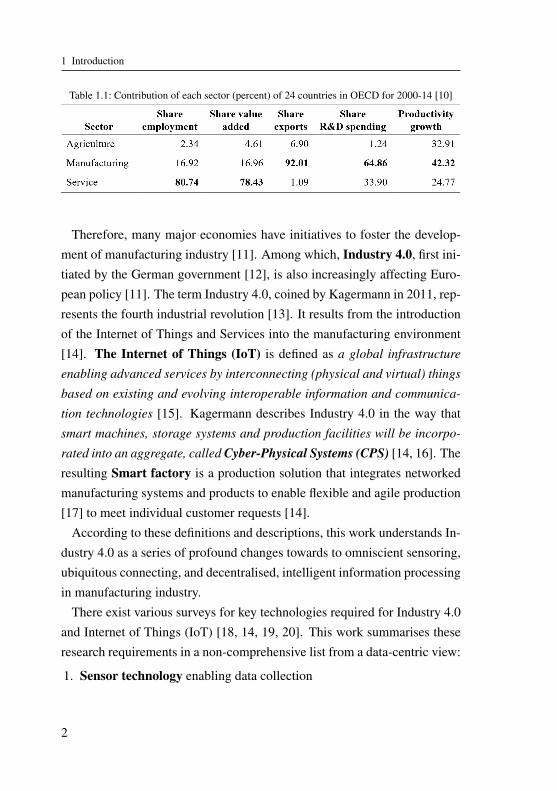
and immaterial inputs into new products [1, 2]. It is the main contributor toinnovation, exports and productivity growth [3]. In 2017, manufacturingindustry contributes to about 30% economic growth in Germany and world-wide (Figure 1.1), over 90% to export, 65% to innovation, and 40% to pro-ductivity growth in the 24 countries (Table 1.1). Manufacturing is especiallyimportant for Germany, as Germany is one of the leading export countriesin the world [4]. Productivity describes the rate at which goods and servicesare produced [5, 6], and is important to a country’s living-standard [5] andeconomic well-being [7].
Figure 1.1: GDP by sectors in Germany and worldwide [8, 9]
1
1 Introduction
Table 1.1: Contribution of each sector (percent) of 24 countries in OECD for 2000-14 [10]
Therefore, many major economies have initiatives to foster the develop-ment of manufacturing industry [11]. Among which, Industry 4.0, first ini-tiated by the German government [12], is also increasingly affecting Euro-pean policy [11]. The term Industry 4.0, coined by Kagermann in 2011, rep-resents the fourth industrial revolution [13]. It results from the introductionof the Internet of Things and Services into the manufacturing environment[14]. The Internet of Things (IoT) is defined as a global infrastructure
enabling advanced services by interconnecting (physical and virtual) things
based on existing and evolving interoperable information and communica-
tion technologies [15]. Kagermann describes Industry 4.0 in the way thatsmart machines, storage systems and production facilities will be incorpo-
rated into an aggregate, called Cyber-Physical Systems (CPS) [14, 16]. Theresulting Smart factory is a production solution that integrates networkedmanufacturing systems and products to enable flexible and agile production[17] to meet individual customer requests [14].
According to these definitions and descriptions, this work understands In-dustry 4.0 as a series of profound changes towards to omniscient sensoring,ubiquitous connecting, and decentralised, intelligent information processingin manufacturing industry.
There exist various surveys for key technologies required for Industry 4.0and Internet of Things (IoT) [18, 14, 19, 20]. This work summarises theseresearch requirements in a non-comprehensive list from a data-centric view:
1. Sensor technology enabling data collection
2
1.1 Background and Motivation
2. Communication technology facilitating data exchange between devices
3. Computational technology providing sufficient computational powerand intelligent data processing algorithms
4. Actuator technology meaningfully transforming data into machine ac-tion
Machine Learning, categorised into computational technology, is one ofthe key technologies of Industry 4.0 [21, 11, 22]. Machine learning providesintelligent data processing algorithms. In manufacturing, it has created newintelligent tools for automatic information extraction and knowledge discov-ery [23, 24], which are important for practices like root cause identificationor decision-making [25]. A big data problem arises because an unprece-dented amount of data are collected in manufacturing industry nowadays[26]. The resulting "4Vs" requirements need to be addressed: Volume, Ve-
locity, Variety, Veracity (Authenticity) [27, 28].In an Industrial 4.0 scenario, voluminous data are collected through in-
terconnected devices, which by themselves possess a certain degree of pro-cessing power. The large amount of data are stored in a central or distributeddatabase, and then centrally or distributedly processed by some intelligentalgorithms, to extract organised information and systematic rules, whichculminate as "knowledge" learned from the data, enabling machine guidedprocess optimisation, namely machine learning. The key differences be-tween the human guided process optimisation and machine guided processoptimisation lies thereupon, that the machine guided process optimisationis not explicitly programmed, and requires no or little manual effort in de-signing all the optimisation parameters and even procedures. Instead, theprocess of optimisation, or learning in another word, happens in an at leastpartially automatic way. Yet, no machine learning method is able to builda technologically meaningful information processing from an unstructureddataset on its own. Each application domain needs to be analysed and thenappropriate machine learning processes can be designed.
3

1 Introduction
Electric Resistance Welding (ERW), widely applied in automotive pro-duction, is a typical automatic manufacturing process with inhomogeneousdata structures as well as statistical and systematic dynamics [29]. Qual-ity monitoring is to estimate or predict the quality characterised by somecategorical or numerical values. It is an essential task in ERW as well asin manufacturing (Other tasks include process development and optimisa-tion, etc.). There exists huge industrial and economic potential to developdata-driven approaches, especially machine learning approaches, for qualitymonitoring in ERW, to reduce maintenance cost and improve quality con-trol. Machine learning approaches are non-destructive and can potentiallymonitor the quality of all welding processes. Recently many ML-tools [30]have become available thanks to extensive research in this area.
The central question of this thesis is to identify challenges of developingmachine learning approaches for quality monitoring in ERW and to exploresolutions to them.
The rest of this chapter is organised as follows. Section 1.2 introduces theelectric resistance welding process and summarises the typical difficultiesin this field. Section 1.3 gives a short overview of machine learning andontology background knowledge necessary for this work. Section 1.4 takesa glance at recent development of machine learning in manufacturing to seeif there exist similar challenges and solutions in other manufacturing fields,and narrows the scope step by step from manufacturing in general, to condi-tion monitoring, metal welding technology, and electric resistance welding.Section 1.5 derives the open questions in the field of machine learning in
electric resistance welding by translating the difficulties in Section 1.2 andpartially adapting the challenges in previous studies in Section 1.4. Sec-tion 1.6 decomposes the central question into sub-objectives and lists theorganisation of the thesis.
4

1.2 Electric Resistance Welding
(a) (b)Figure 1.2: (a) RSW as an example of ERW. The current I flows through the welding zone
and results in a spot-form connection [29](b) Measuring the welding spot diameter by tearing the welded worksheetsapart [29].
1.2 Electric Resistance Welding
This section first gives a short description of the ERW process [31] (Section1.2.1), then introduces state-of-the-art of process development, monitoringand maintenance in ERW (Section 1.2.2), and at the end summarises thetypical difficulties (Section 1.2.3).
1.2.1 Description of Electric Resistance Welding Process
Electric resistance welding (ERW) is a group of welding processes with
pressure in which the heat necessary for welding is produced by resistance
to an electrical current flowing through the welding zone [32]. The weldingzone is between the electrodes (Figure 1.2), including the small volume ofworksheets and their contacting surface. After the welding process, a con-nection will be formed in the contact areas. The connection can have theform of e.g. spots (Resistance Spot Welding, RSW) or wire-hook joint (HotStaking, HS).
In industrial practice, ERW is ubiquitously applied. The wide applicationof the ERW is the result of numerous advantages of ERW, including mini-mal deformation of the welded products, excellent chemical and mechanicalproperties of the welding areas, time- and energy-efficiency, high degree of
5

1 Introduction
automation, etc. However, there still exist many difficulties in ERW (Section1.2.3).
1.2.2 State-of-the-art of Process Development, QualityMonitoring, and Maintenance in ERW
To understand the central question of quality monitoring in ERW, it is neces-sary to understand a general process pipeline in ERW (Figure 1.3). The rawproducts, such as chassis for RSW and electric motors for HS, are trans-formed into products by a welding process. The welding process is con-trolled by a welding control, normally an adaptive control, which forces theactual process variables, such as process curves of current, voltage, to followpredefined values or profiles named as setpoints or reference curves. Thewelding control also constantly collects measurement data from the process,and compares these measurements with the references stored in the adaptivecontrol, to give estimations of quality indicators. Quality indicators describequality, which is the degree to which a set of inherent characteristics fulfils
Figure 1.3: A general process pipeline for electric resistance welding. Thick arrows indicatematerial and energy flow. Thin arrows indicate information flow.
6

1.2 Electric Resistance Welding
requirements [33]. The references of quality indicators are obtained in pro-cess development, where a certain number of manufacturing operations arecarried out without the adaptive control. Some of these operations, whosequality indicators are estimated as good, are selected for determining thereferences.
Quality monitoring assesses various quality indicators. Some quality in-dicators are measured (QImeas), including e.g. welding spot diameter forRSW [34, 35] or tensile shear strength (TSS) for both RSW and HS. Forthese two, relatively precise measurements can only be obtained throughdestructive methods (Figure 1.2b). In automotive industry, this means tear-ing the welded chassis apart. There also exist non-destructive methods tomeasure them, like ultrasonic and X-ray tests in RSW, but these methodsalso cause problems in terms of costs and facilities [36, 37], and are there-fore only used for random samples [38]. Since the measured quality indi-cators are very costly, some empirical quality indicators (QIemp) are devel-oped, which are estimated through comparing references and measurements.Their expected behaviour is to be stable around a setpoint pre-defined by thewelding program. The empirical quality indicators can reflect the measuredquality indicators in most cases, but their correspondence is not perfect.
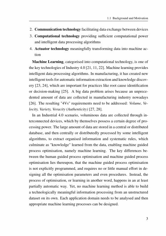
Measured quality indicators QImeas and the estimated empirical valueQIemp both are assumed to follow Gaussian distribution (Figure 1.4). Theseempirical quality indicators are monitored according to principles of Statis-
tical Process Control (SPC) [39]. A process is capable if it adheres to the
tolerance specifications defined with respect to the evaluated quality char-
acteristics [40], quantified by process capability indices, such as those inEquation (1.1). In the equation, UT L and LT L represent upper tolerance
limit and lower tolerance limit (determined by experiments or empiricallyby process development engineers), respectively. µ and σ stand for themean and standard deviation (estimated from samples) of the quality indi-cators to be characterised. These indices evaluate the probability that thequality indicators lie in the tolerance limits, compared to a baseline of 6σ
7
1 Introduction
Figure 1.4: Two-dimensional Gaussian distribution (6σ area is drawn within an eclipse)of measured quality indicators QImeas and empirical quality indicators QIemp.UT Lmeas and LT Lmeas stand for the upper tolerance limit and lower tolerance limitof the QImeas; UT Lemp and LT Lemp stand for the estimated upper tolerance limitand lower tolerance limit for QIemp. The intersection area of the rectangle withthick dashed lines is the area of True Positive (TP), where the QIemp as well as theQImeas lie within the respective tolerance bands. The other areas are False Positive(FP), False Negative (FN), and True Negative (TN) (Table 1.2). In the figure onlythe TP/FP/TN/FN for exceeding the UTL are drawn.
(a probability of 99.73%). The bigger Cp,Cpk are, the more probable thequality indicators lie in the tolerance limits.
Cp =UT L−LT L
6σ
Cpk =min(UT L− µ, µ−LT L)
3σ
(1.1)
There exist four cases of whether QIemp deviates from QImeas, representedby a confusion matrix (Table 1.2). False Negative (FN) means a productof good quality is estimated to be of poor quality, which is a waste of pro-duction. False Positive (FP) means a product of poor quality is estimatedto be of good quality, which is undetected quality failure. FP is normallymuch worse than FN, because FN is merely a waste of time and resource,but quality failure in e.g. vehicles could cause severe accidents.
Process maintenance in ERW include regular maintenance and main-tenance in case of quality failure. The former one is needed because the
8

1.2 Electric Resistance Welding
Table 1.2: Confusion matrix of estimated value and predicted value
electrodes directly touching the parts wear due to e.g. oxidation, materialsticking, etc. Common regular maintenance can be e.g. Dressing [41], thatis to remove a thin surface layer of the electrodes to restore the surface con-dition, or that the electrodes will be changed when dressing is not workinganymore. The regular maintenance is currently performed with a fixed pe-riod. In case a quality failure is detected by the adaptive control, the wholeproduction line will be stopped and necessary manual interference is needed,causing enormous economic loss.
1.2.3 Typical Difficulties in Electric Resistance Welding
To achieve successful quality monitoring in ERW, many questions and dif-ficulties need to be solved. This work summarises these difficulties in twoaspects.
A priori knowledge problems are problems of limited domain knowledge.
• Empirically understood process. There exist many effects that are limitedlyand empirically understood, e.g. contact resistance between electrodes andworksheets, strong electric-magnetic interferences, and empirical qualityindicators. Their mechanism and influence on quality can therefore notthoroughly described with domain knowledge.
• Systematic variance. The systematic variance is caused by systematicchange of welding conditions, e.g. the wearing effect of electrodes through
9

1 Introduction
time, system and environmental temperature change. The mechanism ofhow these changes influence welding is limitedly understood.
• Unknown discrepancy between process development and deployment. Thereferences of quality indicators are obtained in process development, but theconditions are often different to real production conditions. This discrep-ancy may cause a discrepancy between the quality of process deploymentand the quality of process development.
Data problems are problems of lacking of data.
• Partial coverage of quality monitoring. Measured quality indicators re-quire destructive methods like tearing the welded products apart, or non-destructive methods like X-ray or ultrasonic test. These methods are onlycarried out sample-wise on the products and data of measured qualityindicators are mostly unavailable. A full-coverage quality monitoring isneeded.
• Expensive data acquisition. Both destructive methods that destroy the prod-ucts and non-destructive methods that require extra X-ray or ultrasonicequipment are extremely expensive. Moreover, extra sensor measurementsthat can potentially improve quality monitoring are also costly and there-fore not available in production.
• Data variety. Data collected from multiple sources have various differ-ences. Production data are generated by multiple versions of productionsystems due to user individualisation. Laboratory or simulation data of-ten contain more sensor measurements and are stored with various formats,variable names, sampling frequency, etc.
• Statistic variance. The statistic variance is the result of multiple uncon-trollable variables, e.g. different properties of raw products that are manu-factured by different suppliers in multiple production batches, despite thatthey are nominally identical.
10

1.3 Introduction to Machine Learning and Ontology
To address or partially solve these difficulties, this thesis suggests usingMachine Learning, which is a data-driven approach, limiting the cost, andhas great modelling power for complicated problems. Only after properlytranslating the difficulties in ERW and manufacturing to questions in ma-chine learning (Section 1.5), it becomes possible to develop machine learn-ing approaches.
1.3 Introduction to Machine Learning andOntology
The term machine learning (ML) was coined by Samuel in 1952 [42].From a handful of engineering practices and statistics, machine learninghas developed into a broad discipline both rich in applications and theory[43]. There exist different definitions or descriptions for machine learn-ing and data mining [44, 45, 46]. One common understanding of machinelearning (ML) is using statistical theory in building mathematical models
to enable computers to make inference from data without being explicitly
programmed [46, 47]. This seems to emphasise the modelling aspect men-tioned in the definition of data mining, the complete process of data collec-
tion, preparation, preprocessing, modelling and interpretation [48]. Sincemodelling would be not possible or meaningful without the other steps, es-pecially in manufacturing, data mining and machine learning in this workare treated as having the same meaning. In the following text, only the termmachine learning will be used. Machine learning, in a higher view, is a pro-
cess of extracting information and learning knowledge from data, to support
decision-making, and in the long-term to form knowledge and wisdom (Fig-ure 1.5) [48, 49].
11

1 Introduction
Figure 1.5: Pyramid of data mining: extracting information from data, learning knowledgefrom information, and achieving wisdom with knowledge [49]
The pre-requisite of successful machine learning practice is a good ques-tion definition in the specific domain and a meaningful transformation ofthe question into mathematical representation [48] (question definition inmachine learning). Figure 1.6 shows a typical workflow of machine learn-ing. The question can be defined before or after data collection.
Data collection is the process of collecting raw data. This process couldbe measuring of some physical quantities manually, or by sensors, cameras,etc. Raw data are collected in various formats, e.g. csv files, txt files, SQLdatabases.
Data preparation is the process of merging different sources of data intoone uniform format, possibly also changing their naming, to facilitate vi-sualisation or analysis. Until this step, the statistic properties of data areunchanged.
Data preprocessing and modelling are two deeply intertwined steps.Data preprocessing is to change the representation of data so that it can beused by the subsequent machine learning algorithms. Common data prepro-cessing procedures are feature extraction, selection, normalisation, etc. Thestatistic properties of data will be changed in this step. Modelling is to usemachine learning algorithms, ranging from classic machine learning meth-
12

1.3 Introduction to Machine Learning and Ontology
Figure 1.6: A typical machine learning workflow [44, 50, 51]. The question can be definedbefore or after data collection.
ods to complicated neural networks, to extract statistic regularities from theinput data and make predictions.
Interpretation of results is to combine the results delivered by data anal-ysis and problem-specific domain knowledge and its mathematical formu-lation, to evaluate and visualise the meanings of the results to supportdecision-making.
Significant effort of machine learning flows into data preprocessing so thatthe resulting data representation or features [52] can facilitate effective ma-chine learning modelling [53, 54]. The choice of feature extraction meth-ods, which can be categorised into two groups, feature engineering (Section1.3.1) and feature learning (Section 1.3.2), greatly impact the choice of thesubsequent machine learning algorithms.
From this point of view, machine learning approaches can be largely di-vided into two groups [51]:
13

1 Introduction
• feature engineering + classic machine learning algorithms;• feature learning + neural networks, or more commonly known as deep
learning.
It is important to note that there exists no clear boundary between the twogroups in a mathematical or even sometimes methodological sense. Yetthese two groups follow two different philosophies. The former empha-sises on integration of domain knowledge in feature engineering and inter-pretability of the extracted features, ML algorithms and results. Instead,the latter strives to minimise the effort to use domain knowledge for fea-ture extraction, and to build rather general machine learning algorithms fordifferent purposes.
1.3.1 Feature Engineering + Classic Machine Learning
Feature Engineering (FE) is the process of transforming features throughdomain expert knowledge [51] or mathematics so that machine learning al-gorithms work. The choice of data representation is crucial to the perfor-mance of machine learning algorithms that are applied on the data. Featureengineering integrates human ingenuity and prior knowledge to compensatethat some machine learning models are not effective and delicate enough tocapture the subtle discriminative information lying in the data [52].
Common feature engineering methods include:• Generating new single features from raw single features using unary
or binary operations [55], e.g. logarithmic, reciprocal, sine/cosine,correlation features, etc.;
• Extracting single features from data with temporal or spatial struc-tures, e.g. segmenting [56], subsampling [57, 58], calculating statisticproperties like maximum, variance [59], filtering [60], transformingto frequency domain [61, 62] or time-frequency domain [62], etc.;
• Reducing the raw features to a lower dimensional space, e.g. Prin-cipal Component Analysis (PCA) [63], Linear Discriminant Analysis(LDA) [64], etc.
14

1.3 Introduction to Machine Learning and Ontology
After feature engineering, even very simple machine learning algorithmscan deliver good results. These simple algorithms can be Linear Regression(LR), Polynomial Regression (PolyR) [45], k-Nearest Neighbours (kNN)methods [65], etc. The advantage of the pipeline of feature engineering +classic machine learning is that the models are more transparent and un-derstandable than feature learning. Which features are more important andhow they influence the model quality is easily interpretable from the modelresults.
1.3.2 Feature Learning + Neural Networks (DeepLearning)
According to [52], Feature Learning (FL), or representation learning,refers to an algorithm that can learn to identify and disentangle the under-
lying explanatory factors hidden in the observed milieu of low-level sensory
data. Feature learning was initiated to avoid labour intensive and domain-specific feature engineering. The advantage of feature learning is that thelearning algorithms become less dependent on feature engineering so thatnovel applications could be developed faster.
The current feature learning study has developed into two parallel ap-proaches: probabilistic graphical models and neural networks (or deeplearning) [52]. The former approach attempts to recover latent randomvariables describing a distribution, while the latter one uses a computationalgraph to extract abstract features from the data. There exists no formal def-inition for the term deep learning, but various literature [52, 66, 67, 68, 69]shares the view that Deep Learning (DL) is a group of machine learning
algorithms for multiple layers (or levels) of non-linear information process-
ing to learn hierarchical representations (or abstractions) of data, mainly
with neural networks. Some authors thinks the hierarchical feature learn-
ing is the most important characteristic for deep learning [70]. Others thinkmore than one hidden layer is required [71]. For simplicity and clearance,
15

1 Introduction
this work refers to deep learning as neural networks with more than one
hidden layer for hierarchical feature learning, i.e. deep learning has at leasttwo hidden layers, one input layer, and one output layer. Artificial neu-ral networks with fewer than two hidden layers, or that do not possess thecharacteristic of hierarchical feature learning, are categorised into classicmachine learning.
A basic type of deep learning is Deep Neural Networks (DNN), which isMLP with at least two hidden layers [72]. There exist other types of neuralnetworks designed for specific data structures, e.g. Convolutional NeuralNetworks (CNN) [73] for data with temporal or spatial structures, RecurrentNeural Networks (RNN) [74] or Bidirectional Recurrent Neural Networks(BRNN) [75], and Long Short-Term Memory (LSTM) [76] for data withtemporal structures, etc.
1.3.3 Introduction to Ontology
An ontology [77, 78] is a shared conceptualisation of a domain of interestwritten in a formal language. The ontological modelling in this work followsthe description logic of OWL 2 [79], which is built upon the World WideWeb Consortium’s (W3C) XML standard for objects called the ResourceDescription Framework (RDF) [80] and compatible with RDF Schema(RDFS) [81].
Ontology and its related semantic technologies, represent semantics (mean-ing) and associations between data [82]. Semantic technologies have re-cently gained a considerable attention in industry for a wide range of ap-plications and automation tasks such as modelling of industrial assets [83]and industrial analytical tasks [84], integration [85, 86, 87, 88] and query-ing [89] of production data, and for process monitoring [90] and equipmentdiagnostics [91].
16

1.3 Introduction to Machine Learning and Ontology
Figure 1.7: (a) An example of ontology. (b) Different types of ontologies [92].
All entities, including physical objects and abstract concepts are describedwith rdfs:Class1 (blue rounded squares in Figure 1.7a). Data are modelledwith rdfs:Literal and connected by owl:DatatypeProperty (black squares inFigure 1.7a) to rdfs:Class, described with xsd:<schema>. The prefixes indi-cate their following namespace.
Each formula in ontology states that one complex class is a subclass ofanother class, or a property is a subproperty of another property. Complexclasses are composed from the atomic classes and properties using logicalAND, OR, and Negation, as well as universal and existential quantifiers.Reasoning over ontologies allows to compute logical entailments.
Figure 1.7a illustrates a simple ontology. The default namespace here isManufacturing Ontology, for which the prefix is mo:, or simply a colon :.In the ontology, three classes and one datatype property are defined. Theseclasses are connected with two types of predicates, rdfs:subClassOf, indicat-ing a hierarchy of categories. It can be serialised in Manchester Syntax [77]:
Class: mo:ElectricResistanceWeldingProcess
SubClassOf: core:ManufacturingProcess
and owl:ObjectProperty, indicating a non-hierarchical relationship:
ObjectProperty: mo:hasOperation
Domain: mo:ElectricResistanceWeldingProcess
Range: mo:ElectricResistanceWeldingOperation
The owl:DatatypeProperty is a property connected to a feature in data:
1 Note there exists no space after the colon in the representation of ontologies.
17

1 Introduction
Figure 1.8: An example of ontology templates. By providing values for the variables in thetemplate (middle row in the figure), an ontology can be instantiated (lower row).
DataProperty: mo:hasOperationID
Domain: mo:ElectricResistanceWeldingOperation
Range: xsd:string
The predicates of object properties and data properties can also be groupedhierarchically using rdfs:subPropertyOf.
Ontologies are of different types (Figure 1.7b). An Upper Ontology is todescribe a general and cross-domain ontology, e.g. a Manufacturing Ontol-
ogy. A Domain Ontology contains terms that are fundamental concepts ofa domain of interest, e.g. a Electric Resistance Welding Ontology and theyare subclasses of the upper ontology. A Task Ontology includes fundamentalconcepts of a task, e.g. a Machine Learning Ontology for machine learninganalysis in this work. An Application Ontology is a specialised ontologyfocusing on a specific domain and task, e.g. a Quality Monitoring Ontology
of using machine learning for welding quality monitoring.Ontology templates are a language and tools for creating OWL ontol-
ogy models with parametrised ontologies by providing values for eachvariable [93]. Figure 1.8 gives an example for creating a small ontologythat contains Welding Operation, which belongs to WeldingProcess and hasWeldingOperationID. The user needs to select the super class Operation,specifies its class name, and chooses its belonging WeldingProcess (thisclass is created beforehand). Then the ontology for welding (domain ontol-ogy) is created from the template (upper ontology), and serialised as OWL
18

1.4 Machine Learning in Manufacturing
axioms. Templates guarantee good quality and consistency of the createdontology, as well as the relative simplicity of the ontology creation process.
1.4 Machine Learning in Manufacturing
This section first takes a glance at machine learning in manufacturing ingeneral, and then narrows the scope to condition monitoring, other metalwelding processes, and finally ERW.
1.4.1 Overview of Machine Learning in Manufacturing
In recent years, machine learning in manufacturing has been increasinglydrawing attention [94, 24, 95]. It is developed and applied in various sub-fields in the broad and comprehensive realms of manufacturing industry, in-cluding plant-wide optimisation, sustainable production, agile supply chain[26], and product lifecycle management [28], etc., to achieve goals [94] likecost estimation, quality monitoring and improvement, fault diagnosis, con-dition monitoring, process optimisation, etc.
The challenges of machine learning in manufacturing [94] include• acquisition of relevant data [95];• big data problems like handling high-dimensional and voluminous
data;• skewed distribution of failure types;• selection of suitable machine learning algorithm;• interpretation of the results;• adaptability to changing environment, conditions or problems.
Solutions to address these problems include:• Data lakes [96] were proposed to store unstructured raw data;• Data warehouse [97] for integrated data;• Various descriptions or solutions on big data problems were proposed
in [27, 28];• Machine learning-algorithms were organised to different groups ac-
cording to nature of defined question and data structure [94].
19

1 Introduction
All these challenges also exist in machine learning in ERW. The solutionsto address them were also adapted to ERW in this thesis. Details see Section1.5 and 1.6.
1.4.2 Machine Learning in Condition Monitoring
Condition monitoring is a sub-discipline in manufacturing, referred to asactivity intended to assess the characteristics of the physical actual state of
an item [98]. Condition monitoring is frequently performed for predictivemaintenance, which is defined as condition-based maintenance carried out
following a forecast derived from repeated analysis and evaluation of the
degradation of the item [98].Condition monitoring and the subsequent predictive maintenance can be
performed for two types of purposes. Machine health monitoring [99]means to maintain the healthy state of an equipment, while quality moni-toring is to ensure the product quality within acceptable limits.
The challenges in condition monitoring include using meta-informationand sensor measurements for
• feature extraction, including feature fusion, dimension reduction [62],feature learning [99], etc.;
• fault detection and state classification, for machine health, e.g. windturbine [100], bearing [62], line insulators [101], and for product[102] in e.g. plastic injection moulding [103];
• estimation (regression) of a machine health indicator or quality indi-cator, e.g. tool wear [104].
Solutions are feature engineering and classic machine learning models,e.g. random forests [105], support vector machines [106], fuzzy logic [107],Bayesian networks [107], and feature learning with Deep Learning algo-rithms, e.g. stacked auto-encoder [108], Deep Neural Networks [109].
The same challenges also exist in quality monitoring in ERW. Many of theproposed ML methods can also be used, but the challenge of selection of
20
1.4 Machine Learning in Manufacturing
suitable machine learning algorithm needs to be solved. This thesis will ad-dress quality monitoring for welding in detail in the following two sections.
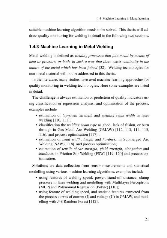
1.4.3 Machine Learning in Metal Welding
Metal welding is defined as welding processes that join metal by means of
heat or pressure, or both, in such a way that there exists continuity in the
nature of the metal which has been joined [32]. Welding technologies fornon-metal material will not be addressed in this thesis.
In the literature, many studies have used machine learning approaches forquality monitoring in welding technologies. Here some examples are listedin detail.
The challenge is always estimation or prediction of quality indicators us-ing classification or regression analysis, and optimisation of the process,examples include
• estimation of lap-shear strength and welding seam width in laserwelding [110, 111];
• classification the welding seam type as good, lack of fusion, or burnthrough in Gas Metal Arc Welding (GMAW) [112, 113, 114, 115,116], and process optimisation [117] ;
• estimation of bead width, height and hardness in Submerged ArcWelding (SAW) [118], and process optimisation;
• estimation of tensile shear strength, yield strength, elongation andhardness, in Friction Stir Welding (FSW) [119, 120] and process op-timisation.
Solutions are data collection from sensor measurements and statisticalmodelling using various machine learning algorithms, examples include
• using features of welding speed, power, stand-off distance, clamppressure in laser welding and modelling with Multilayer Perceptrons(MLP) and Polynomial Regression (PolyR) [110];
• using feature of welding speed, and statistic features extracted fromthe process curves of current (I) and voltage (U) in GMAW, and mod-elling with J48 Random Forest [112];
21

1 Introduction
• using features of voltage, current, welding speed, nozzle-to-plate dis-tance in SAW, evaluating with analysis of variance, and then mod-elling with polynomial regression [118];
• using features of tool rotation speed, profile, feed speed, and hardnessin FSW, and modelling with Multilayer Perceptrons [119].
It is also worthy to notice that all these studies have collected data fromlaboratory experiments. Due to high cost of data collection their dataamount are relatively small, e.g. 14 in [118] and 26 in [110].
1.4.4 Previous Studies of Machine Learning in ElectricResistance Welding
Many previous studies have adopted the approach of machine learning to
predict quality indicators in ERW based on the historically recorded data.The most studied process is Resistance Spot Welding (RSW). No literatureabout machine learning in Hot-Staking (HS) is found. This section willreview the previous studies from the following perspectives and summarisethe detailed information in Table 1.3 and 1.4.
Question Definition. The previous studies have defined the question eitheras Classification (C) - that is to predict the category of quality: good, bad,and sometimes the concrete failure types - or Regression (R) - that is toassess a numerical value of the quality. Each welding operation is treatedas an independent event. The quality indicators to be classified or predictedare usually spot diameter (D), spot height (h), Tensile Shear Strength (TSS),spatter, failure load (load). Special quality indicators include gaps [121],pitting potential (Epitt ) [122], and penetration [36]. Some works also studiedOptimisation (O) of the process.
Data Collection. It is worthy to note that almost all of the previous studieshave collected data from laboratory experiments, or from welding machinesfor production but under experimental settings, except for [123], which usedaccumulated production data. In fact, there exist at least three data sources
22

1.4 Machine Learning in Manufacturing
throughout process pipeline of development, monitoring and maintenance:simulation, laboratory, and production data. The dataset size, i.e. numberof welding spots, ranges from 10 to around 3000. For a summary of theprevious two aspects see Table 1.3.
Data Preprocessing and Modelling. In the input features, Single features(SF) are recorded as constants for a welding process, including electrodeforce (F), welding current (I), welding time (t), sheet thickness (thickness),sheet coating (coating), pressure. Some features are recorded as Time se-ries (TS), including dynamic resistance (Re), electrode force (F), weldingcurrent (I), electrode displacement (s), welding voltage (U), ultrasonic oscil-logram, power. Besides the two common types, [127] used images collectedfrom Scanning Acoustic Microscopy (SAM).
Most of these studies have extracted geometric features or statistic featuresbased on or inspired by domain knowledge, denoted as domain knowledgebased feature engineering (DKFE), but the usage of domain knowledge formachine learning and interpretation is still limited. The methods for TimeSeries Feature Engineering (TSFE) include subsampling, segmentations,histogram, and transition points. Some studies extracted geometric featureslike slopes, lengths of slopes, signal drops from a peak to the followingvalley, or statistic features (stats), e.g. maximum (max), minimum (min),maximum position (mxpo), mean, standard deviation (std), range, root meansquared (rms), because these features are considered meaningful also fromthe ERW process perspective. A special method named as scale-space fil-tering [149] is used in [142] for times series segmentation. Some worksapplied a further step of Feature Engineering (FE) on raw single featuresand time series extracted features, using PCA, polynomial feature genera-tion, discretisation, radar chart, Chernoff face. Feature Selection (FS) areperformed in [135], [136], [139], applied methods including analysis ofvariance (ANOVA), power of the test, Sequential Forward Selection (SFS),Sequential Backward Selection (SBS), Sequential Forward Floating selec-
23

1 Introduction
Table 1.3: An overview of related works of machine learning in ERW, Part 1. All studies arecarried out with laboratory data source on RSW except for [123]. Explanations foracronyms see Section 1.4.4 or Table of Acronyms and Symbols.
Citation Year Author Question #Data[38] 2000 Cho R: TSS 50[124] 2000 Li R: D 170[125] 2001 Lee R: TSS 80[126] 2002 Cho R: D,TSS 60[127] 2003 Lee C: D 390[128] 2004 Cho C: TSS 10[56] 2004 Junno C: D 192[129] 2004 Laurinen C: D 192[57] 2004 Park C: TSS, h 78[130] 2004 Podržaj C: spatter 30[131] 2005 Haapalainen C: TSS 3879[132] 2006 Tseng R, O: load 25[121] 2007 Hamedi R, O: gaps 39[133] 2007 Koskimaki C: TSS 3879[134] 2007 Martin C: D 438[135] 2008 El-Banna C: D 1270[136] 2008 Haapalainen C: TSS 3879[137] 2009 Martin R: TSS 242[36] 2010 El Ouafi R: h, penetration, D 54[122] 2010 Martin R: Epitt 242[138] 2012 Li R: D 145[139] 2013 Panchakshari R, O: D, TSS, load 25[140] 2014 Afshari R: D 54[141] 2015 Yu C: TSS, spatter 473[58] 2015 Zhang C: TSS, D 200[142] 2016 Boersch R: D 3241[143] 2016 Pashazadeh R, O: D, h 48[144] 2016 Wan C,R: D, load 60[145] 2017 Summerville R: D 126[146] 2017 Summerville R: TSS 170[147] 2017 Sun C: TSS 67[148] 2017 Zhang C: TSS 120[123] 2018 Kim R: D 3344
24

1.5 Open Questions
tion (SFFS), Sequential Backward Floating Selection (SBFS) and N-BestFeatures Selection (nBest).
Most of the subsequent machine learning models are classical ma-chine learning methods like Linear Regression (LR), Polynomial Regression(PolyR), k-nearest neighbours (kNN), Bayesian Network (BN), DecisionTrees (DT), Genetic Algorithm (GA), Support Vector Machines (SVM), etc.The Artificial Neutral Networks (ANN) used in previous studies, includeFuzzy Neural Networks (FuzzyNN), Self-organising Maps (SOM), GeneralRegression Neural Networks (GRNN), Hopfield Neural Networks (Hop-fieldNN), and Multilayer-Perceptrons. Since these networks either havefewer than two hidden layers, or do not demonstrate the characteristic of hi-erarchical feature learning (see Section 1.3), this thesis subsumes them intothe category of classic machine learning. A summary of data preprocessingand machine learning modelling see Table 1.4.
1.5 Open Questions
After viewing typical difficulties in ERW (Section 1.2.3), challenges andsolutions of machine learning in manufacturing and in ERW (Section 1.4),this thesis summarises Open Questions (OQ) below.
• OQ 1. Insufficient data problem. In order to build a all-covering qual-ity monitoring system, data collection is crucial. Data collected fromproduction however often lack the most important quality indicator,e.g. the diameters, due to expensive measuring methods. Data col-lected from laboratory experiments can have the quality indicators,but the amount is limited compared to production data, and cannotfully cover the various production conditions exhaustively. Further-more, some important features such as temperature, force, displace-ment, are only available in laboratory. Previous studies have very lim-ited addressed the insufficient data problem. The questions remain
25
1 Introduction
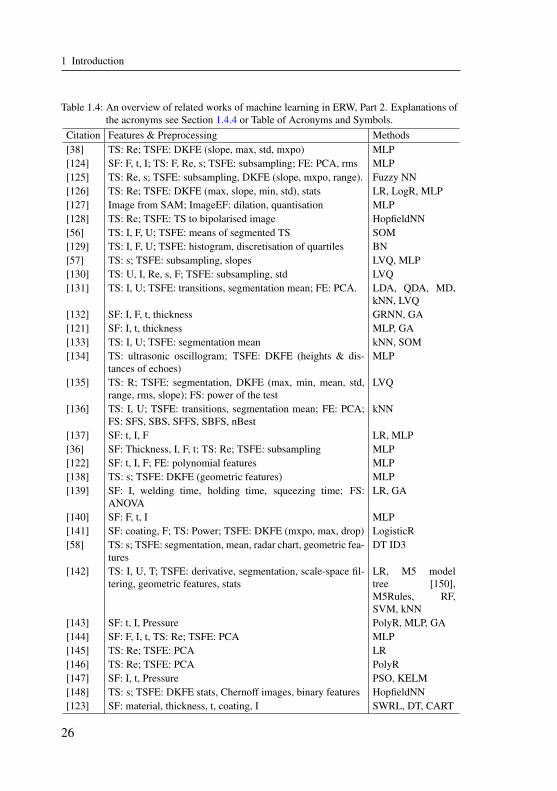
Table 1.4: An overview of related works of machine learning in ERW, Part 2. Explanations ofthe acronyms see Section 1.4.4 or Table of Acronyms and Symbols.
Citation Features & Preprocessing Methods[38] TS: Re; TSFE: DKFE (slope, max, std, mxpo) MLP[124] SF: F, t, I; TS: F, Re, s; TSFE: subsampling; FE: PCA, rms MLP[125] TS: Re, s; TSFE: subsampling, DKFE (slope, mxpo, range). Fuzzy NN[126] TS: Re; TSFE: DKFE (max, slope, min, std), stats LR, LogR, MLP[127] Image from SAM; ImageEF: dilation, quantisation MLP[128] TS: Re; TSFE: TS to bipolarised image HopfieldNN[56] TS: I, F, U; TSFE: means of segmented TS SOM[129] TS: I, F, U; TSFE: histogram, discretisation of quartiles BN[57] TS: s; TSFE: subsampling, slopes LVQ, MLP[130] TS: U, I, Re, s, F; TSFE: subsampling, std LVQ[131] TS: I, U; TSFE: transitions, segmentation mean; FE: PCA. LDA, QDA, MD,
kNN, LVQ[132] SF: I, F, t, thickness GRNN, GA[121] SF: I, t, thickness MLP, GA[133] TS: I, U; TSFE: segmentation mean kNN, SOM[134] TS: ultrasonic oscillogram; TSFE: DKFE (heights & dis-
tances of echoes)MLP
[135] TS: R; TSFE: segmentation, DKFE (max, min, mean, std,range, rms, slope); FS: power of the test
LVQ
[136] TS: I, U; TSFE: transitions, segmentation mean; FE: PCA;FS: SFS, SBS, SFFS, SBFS, nBest
kNN
[137] SF: t, I, F LR, MLP[36] SF: Thickness, I, F, t; TS: Re; TSFE: subsampling MLP[122] SF: t, I, F; FE: polynomial features MLP[138] TS: s; TSFE: DKFE (geometric features) MLP[139] SF: I, welding time, holding time, squeezing time; FS:
ANOVALR, GA
[140] SF: F, t, I MLP[141] SF: coating, F; TS: Power; TSFE: DKFE (mxpo, max, drop) LogisticR[58] TS: s; TSFE: segmentation, mean, radar chart, geometric fea-
turesDT ID3
[142] TS: I, U, T; TSFE: derivative, segmentation, scale-space fil-tering, geometric features, stats
LR, M5 modeltree [150],M5Rules, RF,SVM, kNN
[143] SF: t, I, Pressure PolyR, MLP, GA[144] SF: F, I, t, TS: Re; TSFE: PCA MLP[145] TS: Re; TSFE: PCA LR[146] TS: Re; TSFE: PCA PolyR[147] SF: I, t, Pressure PSO, KELM[148] TS: s; TSFE: DKFE stats, Chernoff images, binary features HopfieldNN[123] SF: material, thickness, t, coating, I SWRL, DT, CART
26

1.5 Open Questions
whether the available data amount is sufficient, and whether furtherfeatures are necessary to be collected from production.
• OQ 2. Standardised process description, data description and man-
agement. Machine learning projects in manufacturing involve multi-ple parties with distinct knowledge background, e.g. process experts,measurement experts, data scientists, managers. A standardised pro-cess description is needed to ease the communication between theseexperts. Based on the process description, the data also requires to bemodelled in a standardised way, to facilitate the data management ofdifferent data sources and processes.
• OQ 3. Dataset evaluation for identifying conspicuity. Large vol-umes of data are generated from manufacturing processes like elec-tric resistance welding. It is very desired to gain a quick overviewof the data collected from all welding machines, to evaluate the col-lected datasets and identify which welding machine, which weldingprogram or which dress cycle are conspicuous and may be subject torisks of quality failures.
• OQ 4. Quality monitoring with temporal structure and probabilistic
estimation. Previous studies estimated quality monitoring as sin-gle values for each welding operation independently. In fact, thesewelding operations comprise a welding process with temporal struc-tures caused by the continuous wearing effect of the electrodes. Theestimation of quality indicators should be a probabilistic distribution.
• OQ 5. Evaluation and selection of machine learning methods. Vari-ous machine learning methods have been experimented for ERW andManufacturing. Yet it remains unclear, when and how to use whichmethods, and how to evaluate the machine learning models.
• OQ 6. Integration of domain knowledge problem. Previous studieshave used domain knowledge to some degree in feature engineering,
27

1 Introduction
but there exists still improvement space for more systematic discus-sions of the role of domain knowledge in machine learning, such aswhat is the best role of domain knowledge in machine learning, howthe influence of domain knowledge can be intensified, etc.
• OQ 7. Concept drift monitoring. When the production condi-tions change during the production process, the developed methodsfor quality monitoring could fail, because the data under the changedconditions differs for the data collected for model training. A mech-anism is needed to detect the data drift and adapt the model accord-ingly.
• OQ 8. Transfer of developed ML approaches to other datasets and
processes. As mentioned in Section 1.1, there exists no machinelearning method that can perform technologically meaningful infor-mation processing from unstructured datasets. Manufacturing datasetswith different structures can be generated frequently from differentdata sources, i.e. operation conditions, machines, plants. Little workhas been done in ERW to make machine learning methods scalable todifferent sources, versions of datasets, and to different manufacturingprocesses.
1.6 Objectives and Thesis Outline
The aim of the Ph.D. study is to study and develop effective and gener-alisable machine learning frameworks, for quality monitoring in electricalresistance welding, i.e. assessment and prediction of the quality indicators.In an attempt to achieve this central goal, this work has the following sub-objectives.
• Discussing the central goal of quality monitoring and studying the particu-larities of data of electrical resistance welding in depth;
28

1.6 Objectives and Thesis Outline
• Exploring, developing and organising the machine learning methods andother methods for handling and modelling the data;
• Implementing software for ML analysis and data handling;
• Applying, validating and demonstrating the methods on industrial datasetsin use cases.
This work is organised as follows. Chapter 2 proposes a ML frame-work that attempts a comprehensive coverage for collecting, understanding,preparing, preprocessing, and modelling the data in ERW and elaboratesthe methodological details. The framework is a result of deep intertwin-ing of ML methods, domain knowledge of ERW, and semantic technolo-gies. Chapter 3 describes one implementation of the methodologies in thiswork on two programming platforms, Python and SciXMiner (MATLAB).Chapter 4 selects six industrial use cases to demonstrate and validate theapplication of methodologies, to evaluate their performances and test theirtransferability. Chapter 5 summarises the thesis, lists the contribution, con-cludes the work and previews the outlook.
29


2 A Framework of MachineLearning in Electric ResistanceWelding
In developing methodologies of machine learning in ERW, it often revealsthat the development of new algorithms are not the most urgent tasks. Ma-chine learning approaches are not able to retrieve meaningful information tosupport decision making from unstructured and not-understood datasets. Itis not trivial to use and adapt the existent algorithms in the field of ERW aswell as manufacturing. This work will therefore focus more on identificationof a suitable framework that makes the machine learning approach effectivefor the datasets we have understood once, and scalable for other datasetswith similar structures. This work will go across the boundaries of data sci-ence, understanding data characteristics of ERW from a combined view ofdata science, domain knowledge of engineering, and semantic technologies,revealing some aspects that are limitedly discussed in previous studies.
2.1 Question Definition Revisited
This section discusses questions resulting from data characteristics in ERWas well as in manufacturing. The questions are addressed in the proceduresof machine learning workflow (Section 1.3): data collection, data prepara-tion, data preprocessing and machine learning modelling.
31

2 A Framework of Machine Learning in Electric Resistance Welding
Figure 2.1: Quality indicators of different levels. “Dec” stands for decision. The asterisk in-dicates data-driven methods for estimating quality indicators, which is the centralgoal of this thesis, that can be seen as online analysers. The optimal target (labels)of machine learning analysis are usually QI1 to QI3.
2.1.1 Quality Indicators of Different Fidelity Levels andAccessibility
The central question of the thesis is to estimate quality indicators. Vari-ous quality indicators have been discussed in the literature [151, 152, 153],but they have not been systematically organised or are not applicable toERW [154, 155, 156, 157]. This thesis groups them into different levels ac-cording to their fidelity and accessibility. Figure 2.1 illustrates these levelsbased on the workflow of quality control.
After a welding process, the welded part will go through a series of qualitycontrol gates. At each gate, a rejection decision can be made according tothe corresponding judgement based on the respective quality indicators.
• QI1 is the “final” quality indicator of a product, the optimal label to bepredicted in machine learning. This can be e.g. the lifespan of a productbefore quality failure. However, QI1 is usually unavailable, unless ex-
32

2.1 Question Definition Revisited
tremely huge effort is spent on measuring this indicator, e.g. collectingvoluminous historical usage data from customers.
• QI2 and QI3 stand for quality indicators that can only be measured of-fline, i.e. after the production process, and are therefore only measuredsample-wise due to cost reasons. QI3 are those measured using non-destructive methods, e.g. ultrasonic test results or X-ray test results, QI2are those that can only be measured using destructive methods, e.g. spotdiameters in RSW, tensile shear strength in RSW and HS. Since QI2 isalready relatively precise and much more available than QI1, QI2 is es-tablished as a standard quality indicator [32, 34]. QI2 and QI3 are alsousual target (labels) for ML prediction.
• QI4 are the quality indicators that can also be measured online in pro-duction, but require extra equipment, which are usually even more ex-pensive than the welding machines themselves. An example would bethe contact resistance between the welded wire and hook (called as theGDG-resistance [31]) in Hot-staking (HS).
• QI5 and QI6 are quality indicators that can be measured or calculated on-line by the machine software systems. QI6 indicates the direct measuredphysical quantities, e.g. current, resistance, force, etc. QI6 is replacedby QI5, if QI5 exists. QI5 represents the calculated quality indicators de-veloped with process know-how. QI5 functions as online analyser duringthe production process. Examples of QI5 include the Q-Value, spatter oc-curring time, the process stability factor in the Bosch Rexroth weldingsystem [31].
The goal of all data-driven methods can be seen as to build an offline oronline analyser to estimate an improved QI5 quality indicator, to save QI1to Q4 as a long-term goal. This thesis treads the starting steps towards thelong-term goal by proposing the framework (Chapter 2), studying QI5 that
33

2 A Framework of Machine Learning in Electric Resistance Welding
0 500 1000 1500 2000
Number of welding operations
0.6
0.8
1
1.2
1.4
1.6
Q-V
alu
e
540 560 580 600 620
Number of welding operations
0.6
0.8
1
1.2
1.4
1.6
Q-V
alu
e
Prog1
Prog2
(a) (b)Figure 2.2: (a) Q-Value along number of welding operations for an example welding machine.
The red rectangle indicates the area for a closer look in (b).(b) Welding operations performed with different welding programs often possessdifferent dynamics, e.g. the mean of Q-Values are different
replaces QI2 with simulation data (Use Case 4.1), and forecasting qualityindicators (Use Case 4.3), etc.
2.1.2 Multi-levels of Temporal Structures in Data
Previous studies have treated each welding operation independently (Sec-tion 1.4.4). If we closely examine the data, e.g. Figure 2.2 showing theQ-Value along the number of welding operations for an example weldingmachine, we can see clearly that the data has relatively strong periodicity,which indicates the data very likely have temporal dependencies. With theexample dataset of RSW, this section elaborates the multi-levels of temporalstructures in data, which is an intrinsic result of the structure of productionprocesses.
The first time level is the welding time level during a single welding op-eration, which usually takes several hundreds of milliseconds (Figure 2.3a).From each welding operation, data of single features and process curves arerecorded (Figure 2.3b). The consecutive welding operations constitute thesecond time level, the welding operation level. All process curves on thewelding time level for one single welding operation (including e.g. the pro-cess curves in Figure 2.3a) are aggregated onto one time step on the welding
34

2.1 Question Definition Revisited
operation level (Figure 2.3b). These operations are controlled by the adap-tive control system and are operated according to welding programs. Acloser look at a small area reveals that the welding programs of the opera-tions are arranged with specific orders prescribed by the production schedule(Figure 2.2b). These operations with each welding program form the weld-ing program level. As the welding process goes on, the electrode wears.Since there exists no available feature that reflects the wearing effect in aphysically meaningful way, the wearing effect is quantified using the singlefeature WearCount (Figure 2.5).
Table 2.1: Correspondence table of temporal structure features (Ft ) and time levels
Ft Symbols Time levelTimeStamp t Welding time levelWearCount NWC Welding operation levelDressCount NDC Dress cycle level
ElectrodeCount NEC Electrode cycle levelProgramNumber ProgNo Welding program level
MachineID - Machine level
A regular welding process can include welding, dressing, and short-circuitmeasurements before and after dressing (Figure 2.4). A complete dressing-welding-dressing procedure forms a Dress Cycle. The wearing effect repeatsin each dress cycle. The consecutive dress cycles form the dress cycle level.According to the domain expert, the periodicity of the Q-Value is caused bythe wearing effect. The Q-Values in Figure 2.2 begin with small values ateach start of dress cycle, rises as the electrode wears, and normally reachesstable conditions at the end of the dress cycle. After a certain number ofdress cycles, the electrode needs to be changed (for RSW the electrode capis changed). The welding dynamics is thus influenced by the new electrode.All operations welded by one electrode constitute an Electrode Cycle. Theconsecutive electrode cycles comprise the electrode cycle level. Note thatfor some manufacturing processes, some levels are optional. For example,the dress cycle level does not exist for HS, since in HS the electrode will be
35

2 A Framework of Machine Learning in Electric Resistance Welding
directly changed instead of being dressed. Table 2.1 lists the correspondencebetween temporal structure features (Ft ) and time levels.
Until here, the time levels of a single welding machine are explained. Astep further to see the multiple machines organised in production lines re-veals two typical structures of production lines. Figure 2.6 schematically il-lustrates a production line for RSW with a sequential structure, while Figure2.7 schematically illustrates a production line for Hot-staking with a parallelstructure. These organisations of welding machines constitute the machinelevel. Depending on the structures of production lines, the collected datapoints need to be organised with different temporal structures.
Other time-levels, including the level of car bodies, production batches ofcar bodies and machines, suppliers of the car bodies and machines, are alsoimportant, but this information is currently not available in the data studiedby this work. They will not be addressed in this work.
Further levels above the production lines are the levels of plant locations,and different original equipment manufacturers (OEM). These levels are nolonger temporal levels and are normally treated independently.
0 100 200 300 4000.5
0.6
0.7
0.8
0.9
1
0
0.2
0.4
0.6
0.8
1
Reference Resistance(t)Example Resistance(t)Reference Current(t)Example Current(t)
Res
ista
nce
Cur
rent
Time (ms)
(a) (b)Figure 2.3: (a) Examples of process curves. The adaptive control will try to force the process
curves follow the reference curves defined by the welding program. Left y-axis:Resistance (anonymised), right y-axis: Current (anonymised), x-axis: Samples(b) Consecutive welding operations constitute the welding operation level. Data ofsingle features on the welding operation level and process curves on the weldingtime level (Section 2.1.2) are recorded by the machine software system.
36

2.1 Question Definition Revisited
Figure 2.4: Schematic illustration of a welding process from the perspective of one machine,including maintenance of a welding machine in RSW. NWC stands for WearCount,NDC stands for DressCount. Before and after each dressing operation, short-circuitmeasurements (optional) are performed to monitor the electrode status. The ma-chine is responsible for several designated spots on each chassis part (marked withblue circles).
In data analysis, a data instance is an atomic object. Depending on the timelevel of analysis, a data instance can be a welding operation, an electrodedress cycle, a welding program, a welding machine, etc.
2.1.3 Insufficient Data Problem and Three DataChallenges
As mentioned in Section 1.2.3 and 1.4, data acquisition is difficult in man-ufacturing in general as well as in ERW, especially the labelled data (QI1-QI3). Most of the previous studies have mentioned that their data werecollected from laboratory experiments. The laboratory data and the modelstrained on them are different than that of the real production, as the weldingconditions (such as cooling time and wearing effect) are usually different.Apart from the labelled data amount problem, other difficulties exist formachine learning in ERW. This work summarises these difficulties as threeData Challenges.
37
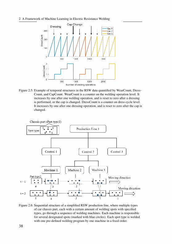
2 A Framework of Machine Learning in Electric Resistance Welding
Figure 2.5: Example of temporal structures in the RSW data quantified by WearCount, Dress-Count, and CapCount. WearCount is a counter on the welding operation level. Itincreases by one after one welding operation, and is reset to zero after a dressingis performed, or the cap is changed. DressCount is a counter on dress cycle level.It increases by one after one dressing operation, and is reset to zero after the cap ischanged.
Figure 2.6: Sequential structure of a simplified RSW production line, where multiple typesof car chassis part, each with a certain amount of welding spots with specifiedtypes, go through a sequence of welding machines. Each machine is responsiblefor several designated spots (marked with blue circles). Each spot type is weldedwith one pre-defined welding program by one machine in a fixed order.
38

2.1 Question Definition Revisited
Figure 2.7: Parallel structure of a simplified hot-staking production line, where several elec-tric motors are welded by several welding machines simultaneously, and thesewelding machines can be controlled by one welding controls system.
Challenge 1 is the limit on labelled data amount, which results from thedifficulty in collecting labelled data in production or in the laboratory.
Challenge 2 is the limit on features. Additional sensors, e.g. electrodedisplacement, or extra measurements, such as actual worksheet thickness ormaterial properties, may be necessary for reliable quality prediction in man-ufacturing processes. However, more sensors mean higher costs, changeof equipment design, larger installation space, increased risks of expensivemachine stops caused by sensor failures, etc. The installation of some sen-sors are even physically infeasible. When deciding whether to install anextra sensor, its benefit needs to outweigh the disadvantages. It is there-fore important to understand which sensors or measurements (or features indata science) are necessary and to quantify their benefit to justify the highercosts.
Challenge 3 is the limit on coverage of relevant situations. Quality fail-ures are very unusual in manufacturing data, because the welding quality isgood under normal conditions. Moreover, quality failures may be of differ-
39

2 A Framework of Machine Learning in Electric Resistance Welding
ent types, making it even more difficult to collect sufficient data for reliablequality prediction.
These three data challenges can be interpreted as concrete questions:
• Questions to Challenge 1: How much labelled data should be collected?• Questions to Challenge 2: Which sensors should be installed? Which
precision level should the measurements have?• Questions to Challenge 3: What production conditions are meaningful to
study? Are they covered in the available data?
The methods to address the three Data Challenges are proposed in Sec-tion 2.2.4.
2.1.4 Multi-fidelity Data Model and Application Questions
Manufacturing data are collected from three typical sources, the productionplants at OEMs, the laboratories for process development, and simulationin research centre for a better understanding of the process. In compari-son to literature, where almost only laboratory data are analysed and thedifferent data sources are not separately addressed, this work proposes themulti-fidelity data model (Figure 2.8) to cover these three data sources. Thissection will discuss the three sources in aspects of data properties and pos-sible application questions. The three data sources have different properties(Table 2.2), and therefore can be potentially combined to compensate theirrespective disadvantages.
Properties of the three data sources. The ultimate goal of any processmonitoring, development or diagnostics is to improve the actual productionprocess and produced goods. The production data (prod) collected fromplants are the most realistic data. Yet the disadvantages are obvious. Pro-duction data are provided as is. As a by-product of the produced goods,they can be constantly collected but their conditions (normally) cannot bespecified or designed. The available features from production are limited tothe already implemented sensors. The cost to collect labels from production
40
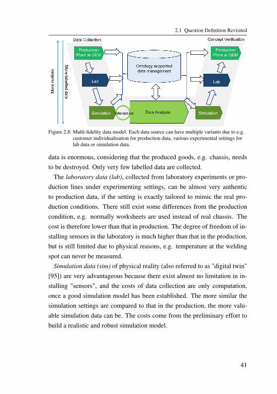
2.1 Question Definition Revisited
Figure 2.8: Multi-fidelity data model. Each data source can have multiple variants due to e.g.customer individualisation for production data, various experimental settings forlab data or simulation data.
data is enormous, considering that the produced goods, e.g. chassis, needsto be destroyed. Only very few labelled data are collected.
The laboratory data (lab), collected from laboratory experiments or pro-duction lines under experimenting settings, can be almost very authenticto production data, if the setting is exactly tailored to mimic the real pro-duction conditions. There still exist some differences from the productioncondition, e.g. normally worksheets are used instead of real chassis. Thecost is therefore lower than that in production. The degree of freedom of in-stalling sensors in the laboratory is much higher than that in the production,but is still limited due to physical reasons, e.g. temperature at the weldingspot can never be measured.
Simulation data (sim) of physical reality (also referred to as "digital twin"[95]) are very advantageous because there exist almost no limitation in in-stalling "sensors", and the costs of data collection are only computation,once a good simulation model has been established. The more similar thesimulation settings are compared to that in the production, the more valu-able simulation data can be. The costs come from the preliminary effort tobuild a realistic and robust simulation model.
41

2 A Framework of Machine Learning in Electric Resistance Welding
Table 2.2: Properties of three data sourcesData source Veracity Degree of freedom Cost
Production (unlabelled) High Low LowProduction (labelled) High Low High
Laboratory Relatively high Medium MediumSimulation Relatively high High Medium
Application questions. Based on the properties of different data sources inthe multi-fidelity data model, many concrete Application Questions (AQ) areworthy to study. For some of them, this work will give concrete use casesin Chapter 4. For the others, this work will only limitedly address themand leave them for future research. An overview of addressed AQs, theircorresponding Open Questions (Section 1.5) and their use cases (Chapter 4)is listed in Table 2.3. These AQs categorised below in two groups:
Analysis of one data source, including:• AQ 1. Dataset evaluation to quickly gain an overview of datasets, for the
purpose of identifying conspicuous welding machines, welding programs,dress cycles, outliers from huge datasets collected from various weldingmachines, and pointing out interesting datasets for further investigation.
• AQ 2. Data amount analysis to assess minimal necessary data amountfor effective quality monitoring with machine learning for guiding datacollection and saving costs.
• AQ 3. Feature evaluation to evaluate importance and benefits of featurescollected from sensors or measurements or generated in data preprocess-ing, for understanding process, analysing root causes of failures, guidingdata collection, etc.
• AQ 4. Classification and regression analysis for estimating the value ofcurrent quality indicators using data-driven methods.
• AQ 5. Classification and regression analysis for predicting the value offuture quality indicators with historical data.
42

2.2 Data Collection: Data Acquisition and Evaluation
• AQ 6. Process parameter optimisation using algorithms such as Bayesianoptimisation and reinforcement learning, which are usually built upon theclassification / regression models for AQ4 and AQ5.
• AQ 7. Semi-supervised learning for predicting partially labelled data, e.g.using a large amount of unlabelled production data to train an auto-encoderand then using a small amount of labelled data to train a decoder.
Analysis across data sources, including:• AQ 8. Similarity analysis between datasets to determine how similar or
dissimilar two datasets are, for determining the fidelity of a data sourceand guiding data collection. E.g., similarity analysis between simulationdataset and laboratory dataset can reveal whether the simulation scenariois designed sufficiently realistic as the laboratory data so as to determinewhether simulation data can be used for process understanding, etc.
• AQ 9. Interactive data acquisition and analysis by analysing a data sourcewith fewer data to guide collection of another data source with more dataamount, for example, analysing the laboratory data to help with designingsimulation scenarios, then determining similarity between the two datasets,then designing new simulation scenarios.
• AQ 10. Transferability of models trained on one dataset to other datasets,or trained on one data source (typically with more data and lower costs,e.g. simulation data) to other data sources (typically with less data amountand higher costs, e.g. production data).
2.2 Data Collection: Data Acquisition andEvaluation
This work addresses the data collection topic with the following aspects:(2.2.1) simulation-supported interactive data acquisition and analysis; (2.2.2)data similarity analysis; (2.2.3) inverse modelling of simulation model;
43

2 A Framework of Machine Learning in Electric Resistance Welding
Table 2.3: Overview of application questions (AQ), their corresponding open questions (OQ)(Section 1.5), method sections (M), and use cases (Chapter 4). Some method sec-tions are partially evaluated and their use cases are not presented in this thesis dueto space limit.
AQ OQ Methods Use case
AQ2, AQ3, AQ4 OQ1, OQ5 M2.1.1, M2.1.2, M2.1.3, M2.2.4,M2.4.2, M2.4.5, M2.4.8 Use Case 4.1
AQ1 OQ3, OQ4 M2.2.5 Use Case 4.2AQ3, AQ5 OQ4, OQ5, OQ6 M2.1.1, M2.1.2, M2.4.1, M2.4.2, M2.4.7 Use Case 4.3
AQ3, AQ5 OQ4, OQ5, OQ6 M2.1.1, M2.1.2, M2.2.4, M2.4.1,M2.4.2, M2.4.5, M2.4.3, Use Case 4.4
AQ5, AQ10 OQ4, OQ8 M2.1.1, M2.4.5 Use Case 4.5AQ2, AQ6 OQ1, OQ5, OQ8 M2.1.3, M2.2.3, M2.2.4 Use Case 4.6
- OQ2 M2.3.1, M2.3.2 -- OQ5, OQ6, OQ8 M2.3.3, M2.4.6 -
(2.2.4) determining necessary data amount for ML modelling; (2.2.5) iden-tifying conspicuous data areas for a further analysis.
2.2.1 Overview: Simulation-supported Interactive DataAcquisition and Analysis
The interactive data acquisition and analysis relies on generating data ofuser-defined scenarios by physics-based simulation with a verified FiniteElement Method (FEM) model [158].
Simulation-supported data collection. The FEM simulation models me-chanical effects (elastic-plastic deformation and thermal expansion), ther-mal effects (temperature changes and heat transfer) and electrical effects(change of electric current density and electric potential field). Non-linearchanges of material and contact properties, such as electrical and thermalcontact conductivity, are also taken into account. Strong interactions be-tween all three fields result in very dynamic process behaviour and requirea multi-field coupled simulation. The FEM models should be verified usingdata from laboratory tests or production lines under controlled conditions.An established simulation model has four advantages:
44

2.2 Data Collection: Data Acquisition and Evaluation
• Each simulation run produces one labelled data point. Running a lot ofsimulations can thus offer a large amount of labelled data.
• There is little limit for obtaining features measured by sensors that arecostly or difficult to install in the laboratory or production.
• By designing the simulation scenarios astutely, rare situations in produc-tion can be studied in detail.
• There are no precision issues of sensor measurements that are present inthe laboratory or in production.
The main effort of the FEM simulation lies in two points: (1) gatheringrelevant information as simulation inputs, such as worksheet and electrodegeometries, temperature-dependent material data, contact properties, etc.;(2) setting up a parametric Finite Element Model in an automated simula-tion loop, including simulation preparation and data extraction, using com-mercial and open source tools, such as Python, software packages for FiniteElement Method, etc.
Interactive data analysis and collection. The simulation supported datacollection follow the six steps iteratively (Figure 2.9).
1. Data collection from laboratory or production.2. Initial simulation scenario definition.3. Data collection from simulation.4. Similarity analysis between simulation data and laboratory/production
data.5. Data amount and feature evaluation.6. New simulation scenario definition.
2.2.2 Similarity Analysis between Datasets
Dataset similarity analysis is to answer the question of how similar twodatasets are. A deep understanding of this topic requires rigorous mathe-matical deduction. In the literature, various methods have been proposed,
45

2 A Framework of Machine Learning in Electric Resistance Welding
Figure 2.9: Simulation-supported interactive data analysis and collection
e.g. similarity measures for one-dimensional datasets [159], an effective sta-tistical evaluation of genomic dataset similarity [160], measuring similaritybetween homogeneous datasets for distributed data mining [161], similarityof condensed data models (e.g. for check data anonymisation) across high-dimensional datasets [162]. However, similarity comparison methods forERW or manufacturing have been limitedly discussed in the literature. Nomethod can be directly applied.
This work suggests some practical concepts and methods for similarityanalysis of ERW datasets, for which there exist many important applicationexamples: (1) comparing simulation data with laboratory/production datato test veracity of simulation data; (2) comparing the dataset collected formodel development with another dataset collected for model deploymentto test model deployability; (3) comparing datasets collected from differentmachines, production lines, welding conditions to test transferability. If thesimulation model is realistic enough, then it can be used to generate morelabelled data, for providing engineering insights, or substitute the costly labdata or production data. The pre-requisite for similarity analysis is that thetwo datasets should share a common subset that contains the same featuresrepresenting the same physical meanings. The term dataset similarity canbe divided into two aspects:
• Mechanism, whether the change of features in two datasets follow thesame patterns.
46

2.2 Data Collection: Data Acquisition and Evaluation
• Distribution, whether the data points in two datasets have similar valuedistributions and lie in similar operating areas, defined by statistic proper-ties e.g. amplitudes, changing range, etc.
Mechanism similarity analysis. The analysis of mechanism similarity hastwo levels. The first level is to identify whether the features in two datasetsfollow the same correlation patterns, i.e. whether the correlation relation-ships between features of two datasets are similar (Figure 2.10a). The sec-ond level is to figure out whether the causality patterns of two datasets aresimilar (Figure 2.10b).
Figure 2.10: Correlation pattern is generated by drawing lines between pairs of featureswhose correlation coefficients are greater than a defined threshold.
The correlation pattern [163, 164] is to calculate correlation matrix usinge.g. Pearson coefficient [165]. the causality pattern is to calculate pair-wisetransfer entropy matrix [166, 163].
Distribution similarity analysis. The analysis of distribution is to comparethe statistic properties of the two datasets, including mean, median, standarddeviation, range, maximum, minimum, ratio between important features se-lected using domain knowledge, etc.
47
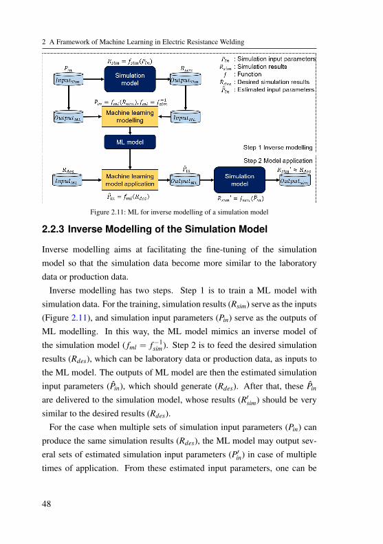
2 A Framework of Machine Learning in Electric Resistance Welding
Figure 2.11: ML for inverse modelling of a simulation model
2.2.3 Inverse Modelling of the Simulation Model
Inverse modelling aims at facilitating the fine-tuning of the simulationmodel so that the simulation data become more similar to the laboratorydata or production data.
Inverse modelling has two steps. Step 1 is to train a ML model withsimulation data. For the training, simulation results (Rsim) serve as the inputs(Figure 2.11), and simulation input parameters (Pin) serve as the outputs ofML modelling. In this way, the ML model mimics an inverse model ofthe simulation model ( fml = f−1
sim). Step 2 is to feed the desired simulationresults (Rdes), which can be laboratory data or production data, as inputs tothe ML model. The outputs of ML model are then the estimated simulationinput parameters (Pin), which should generate (Rdes). After that, these Pin
are delivered to the simulation model, whose results (R′sim) should be verysimilar to the desired results (Rdes).
For the case when multiple sets of simulation input parameters (Pin) canproduce the same simulation results (Rdes), the ML model may output sev-eral sets of estimated simulation input parameters (P′in) in case of multipletimes of application. From these estimated input parameters, one can be
48

2.2 Data Collection: Data Acquisition and Evaluation
chosen based on manual preferences, or some performance metrics, likehigher similarity, less simulation time, etc.
2.2.4 Data Amount and Feature Sets Analysis
This section aims at addressing the three data challenges in Section 2.1.3.The approaches centre on training machine learning models with differentdata subsets and comparing their performance.
Analysis of training data numbers. Data can be split into several subsetsof different training data numbers for answering the question: How muchlabelled data should be collected (Data Challenge 1). A series of train-ing subsets is built by randomly selecting a different number of data pointsfrom the training dataset, and the larger training subsets always contain thesmaller ones. To allow direct comparison of the testing results, the testdataset always contains the same data points. ML models are trained withthese subsets of different training data numbers, and tested on the same testset (Table 2.4).
Table 2.4: Data splitting to subsets of different training data size. Dtr1 stands for training set1, Dtr,all stands for training set with all data, and Dtst stands for test set, whereDtr1 ⊂ Dtr2 ⊂ Dtr3 ⊂ ...⊂ Dtr,all .
Training data Dtr1 Dtr2 Dtr3 ... Dtr,all
Test data Dtst Dtst Dtst ... Dtst
Analysis of feature sets. Data can be split into several subsets of differentfeatures for answering the question: Which features are important (DataChallenge 2). All available features, i.e. time series features as well as singlefeatures, are divided into four subsets (Table 2.5). The feature importanceis evaluated by comparing the performance of ML models trained with thefour different feature subsets.
Analysis of noisy sets. Data can be augmented with additional noise toanswer the question: Which precision level should the sensors have (DataChallenge 2)? Adding noise to the aforementioned non-noisy subsets of
49

2 A Framework of Machine Learning in Electric Resistance Welding
Table 2.5: Data splitting into four subsets of different features
Feature set DescriptionFeatSetprod Features that are always available in production.FeatSetlablow FeatSetprod + features available in laboratory with relatively low cost.FeatSetlabhigh FeatSetlablow + features available in laboratory with higher cost.
FeatSetallFeatSetlabhigh + other features in simulation that are difficult or extremelycostly to realise in reality.
different training data and feature sets results in a series of subsets withnoise. The way of adding noise and the noise levels can be determinedcollectively with process and measurement experts for single features andtime series.
• For time series, the noise should be added for every single sample point.• For single features, the noise should be added for each feature.
To address questions regarding Challenge 3 requires particular simulationscenarios defined by the process experts, which can be hardly achieved bypure data analysis using existent data.
2.2.5 Evaluation of Datasets
The manufacturing industry produces a huge volume of data. Consideringthe number of cars produced every day, each car body with 3000 - 6000welding spots, the amount of data generated even only from one plant ofone OEM is enormous. It is impossible to analyse all data in detail in MLdevelopment as well as in application. Some methods are needed to eval-uate the data and select the most interesting areas, where quality failuresare more likely to happen, or where the behaviour of quality indicators isunstable. If any data area is deemed to constitute an abstract “dataset”,identification of interesting data areas is to perform dataset evaluation, oranomalous dataset detection. This is to evaluate the already collected data,and is therefore an offline analysis. Dataset evaluation targets on analysing alarge dataset in these aspects: information summarisation and visualisation,
50
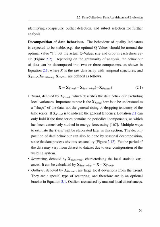
2.2 Data Collection: Data Acquisition and Evaluation
identifying conspicuity, outlier detection, and subset selection for furtheranalysis.
Decomposition of data behaviour. The behaviour of quality indicatorsis expected to be stable, e.g. the optimal Q-Values should be around theoptimal value “1”, but the actual Q-Values rise and drop in each dress cy-cle (Figure 2.2). Depending on the granularity of analysis, the behaviourof data can be decomposed into two or three components, as shown inEquation 2.1, where X is the raw data array with temporal structures, andXTrend ,XScattering,XOutlier are defined as follows.
X = XTrend +XScattering(+XOutlier) (2.1)
• Trend, denoted by XTrend , which describes the data behaviour excludinglocal variances. Important to note is the XTrend here is to be understood asa “shape” of the data, not the general rising or dropping tendency of thetime series. If XTrend is to indicate the general tendency, Equation 2.1 canonly hold if the time series contains no periodical components, as whichhas been extensively studied in energy forecasting [167]. Multiple waysto estimate the Trend will be elaborated later in this section. The decom-position of data behaviour can also be done by seasonal decomposition,since the data possess obvious seasonality (Figure 2.12). Yet the period ofthe data may vary from dataset to dataset due to user configuration of thewelding system.
• Scattering, denoted by XScattering, characterising the local statistic vari-ances. It can be calculated by XScattering = X−XTrend .
• Outliers, denoted by XOutlier, are large local deviations from the Trend.They are a special type of scattering, and therefore are in an optionalbracket in Equation 2.1. Outliers are caused by unusual local disturbances.
51

2 A Framework of Machine Learning in Electric Resistance Welding
0 100 200 300 400 500
Number of welding operations
0.8
0.9
1
1.1
1.2
1.3
1.4
1.5Q
-Val
ue
0
0.2
0.4
0.6
0.8
1
Sca
tterin
g
Q-ValueTrendScattering
Figure 2.12: Q-Values, Trend, and Scattering across multiple dress cycles. The Trend of Q-Values usually resets to a low level at the start of each dress cycle, rises as weareffect intensifies, and reaches a stable level at the end of each dress cycle. Thepattern of Scattering of Q-Values is not distinctively visible.
Detection of outliers. Outliers can be detected using a statistic methodsimilar to the Interquartile Range rule [168]. X [k] ∈ XOutlier if:
X [k]≤ Q1−1.5× IQR | X [k]≥ Q3 +1.5× IQR (2.2)
where k indicates a time step of any temporal structure feature listed inTable 2.1, Q1 stands for the first quartile, Q3 stands for the third quartile,and IQR = Q3−Q1. The calculation of quartiles depends on the method ofTrend estimation (explained later in paragraphs of estimation of Trend).
This work also proposes an adjusted method for outlier detection, to takeinto account the “shape” of the data:
X [k]≤ XTrend [k]−2× IQR | X [k]≥ XTrend [k]+2× IQR (2.3)
in which XTrend [k] is used instead of Q1 or Q3, and therefore the coefficientof IQR is adjusted to 2 since XTrend [k] can be seen as approximately Q3−Q1.
52

2.2 Data Collection: Data Acquisition and Evaluation
Estimation of Trend. Three types of methods are to estimate the Trend.
• Local Trend, which is obtained by using an acausal sliding window tocalculate the moving average (median) of data points belonging to thesame welding program (Equation 2.4, 2.5). The sliding window has alength of tP, where P means only the points that belong to the program P
are included in the window, and XP denotes the sub-time-series of X thatbelong to the same Prog. The calculation can be acausal because this is anoffline analysis. Median filter is less sensitive to local outliers comparedto mean filter. If the local trend is used for outlier detection, the quartilescan be calculated within the sliding window.
XTrend [k] =1
tP +1
k+tP/2
∑i=k−tP/2
(XP[i]) (2.4)
XTrend [k] = median(XP[k− tP/2], ...,XP[k+ tP/2]) (2.5)
If the sliding window approaches the start or end of a dress cycle, the win-dow should be shortened, only to include the data points within the samedress cycle, because the data behaviour of end of the previous dress cyclediffers from the start of the next dress cycle significantly. This can be ob-served from data and reasoned from the wearing effect of electrodes usingdomain knowledge. It should be noticed, the selection of window lengthtP is not trivial. Especially in case where a welding machine performsmany welding programs, or where a dress cycle is very short because ofe.g. manual interference, the data points belonging to the same weldingprogram in one dress cycle become very few, the estimation of the Trendusing very few points becomes unreliable. Appendix A.4 derives the min-imal number of data points (often referred to as data tuples in this work toavoid confusion) required for a reliable estimation.
53

2 A Framework of Machine Learning in Electric Resistance Welding
• Global Trend is an average (or median) of all Trends across all dress cy-cles (or electrode cycles). For the k-th point, the global trend XTrend [k] iscalculated as the mean value (or median value) (Equation 2.6, 2.7) of alldata points with the same WearCount (NWCi) as the k-th point (denoted asNWCi = NWCk ). The calculation should be also performed for each weld-ing program separately. The calculation of Q1 and Q3 can use the globaldata when the global trend is used for outlier detection.
XTrend [k] =1N
N
∑i(XP[i]), f or all i where NWCi = NWCk (2.6)
XTrend [k] = median(XP[i]), f or all i where NWCi = NWCk (2.7)
N denotes the number of all points XP[i] whose NWCi = NWCk . This calcu-lation method assumes that the Trends of all dress cycles (or electrode cy-cles) should be the same, as the different dress cycles (or electrode cycles)should be nominally identical, according to domain knowledge. This ispartially correct, since the data behaviour in different dress cycles is some-how similar for some welding machines (Figure 2.2 and Figure 4.15), butmore different for some other welding machines with change of produc-tion plan (Figure 4.20).
• ML Model Trend is to use the model prediction of the target quality indi-cator as the Trend. The ML models can be linear or non-linear, and shouldonly take the temporal structure features ({Ft}) as inputs (Equation 2.8,2.9). Two examples are:
XTrend = LR({Ft}) (2.8)
XTrend = MLP({Ft}). (2.9)
Overall metrics and discrepancy metrics. The three components of databehaviour can be quantified and reduced to six metrics.
54
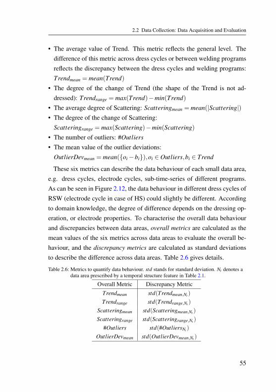
2.2 Data Collection: Data Acquisition and Evaluation
• The average value of Trend. This metric reflects the general level. Thedifference of this metric across dress cycles or between welding programsreflects the discrepancy between the dress cycles and welding programs:Trendmean = mean(Trend)
• The degree of the change of Trend (the shape of the Trend is not ad-dressed): Trendrange = max(Trend)−min(Trend)
• The average degree of Scattering: Scatteringmean = mean(|Scattering|)• The degree of the change of Scattering:
Scatteringrange = max(Scattering)−min(Scattering)
• The number of outliers: #Outliers
• The mean value of the outlier deviations:OutlierDevmean = mean({oi−bi}),oi ∈ Outliers,bi ∈ Trend
These six metrics can describe the data behaviour of each small data area,e.g. dress cycles, electrode cycles, sub-time-series of different programs.As can be seen in Figure 2.12, the data behaviour in different dress cycles ofRSW (electrode cycle in case of HS) could slightly be different. Accordingto domain knowledge, the degree of difference depends on the dressing op-eration, or electrode properties. To characterise the overall data behaviourand discrepancies between data areas, overall metrics are calculated as themean values of the six metrics across data areas to evaluate the overall be-haviour, and the discrepancy metrics are calculated as standard deviationsto describe the difference across data areas. Table 2.6 gives details.
Table 2.6: Metrics to quantify data behaviour. std stands for standard deviation. Nt denotes adata area prescribed by a temporal structure feature in Table 2.1.
Overall Metric Discrepancy Metric
Trendmean std(Trendmean,Nt )
Trendrange std(Trendrange,Nt )
Scatteringmean std(Scatteringmean,Nt )
Scatteringrange std(Scatteringrange,Nt )
#Outliers std(#OutliersNt )
OutlierDevmean std(OutlierDevmean,Nt )
55

2 A Framework of Machine Learning in Electric Resistance Welding
2.3 Data Preparation: Ontology-supported DataUnderstanding and Integration
In order to perform data preparation in a way that can facilitate the subse-quent machine learning, this work suggests to rely on semantic technolo-gies, including ontologies, templates, reasoning, etc. The methodologiesin this section were developed in cooperation with Yulia Svetashova. Theauthor’s contribution is conceptualisation, co-design of the ontologies (in-cluding the upper ontology, manufacturing templates, ML ontology, MLtemplates, ML pipeline ontology), and design of mechanism for retrievinginformation from ontologies for data preprocessing and ML modelling. Re-lated publications include: [169, 170, 171, 172, 173]
Process and data understanding. Successful and efficient data preparationrequires necessary understanding of process and deep insights of data. Dif-ferent types of manufacturing processes often involve complex physical orengineering domain knowledge. However, to gain understanding of processand data is often laborious and fallible for data scientists. The commu-nication between data scientists, domain experts and measurement expertscan be time-consuming and error-prone due to their asymmetric knowledgebackground and vocabulary discrepancy.
This work relies on semantic technologies to describe the process and datawith knowledge graphs. After a minimal training of knowledge of seman-tic technologies, process experts, measurement experts and data scientistscan work together to encode knowledge (Figure 2.13) in domain ontolo-gies by filling in fields of Manufacturing Templates, based on an upper on-tology (named as Core Ontology, or shortly core) for manufacturing. Thecore models the discrete manufacturing process [174] as entities connectedto each atomic operation that produces a product, and allows extension tovarious specific domain ontologies for many variants of welding processes.After that, they can use the ontologies as a “lingua franca” for process and
56

2.3 Data Preparation: Ontology-supported Data Understanding and Integration
Figure 2.13: Overview of ontology-supported machine learning development, where theCore ontology is an upper ontology, ML ontology is a task ontology, and theML pipeline ontology is an application ontology (Figure 1.7).
data understanding. The domain ontologies constrain the process and datadescription with formal language in a pre-defined way, so that the descrip-tion becomes unambiguous, high-quality, easy to understand, and machineprocessable.
Data integration. For the same manufacturing process, data collected fromdifferent conditions and sources (Section 2.1.4) can have discrepancies dueto software versioning, individualisation for customers or specific engineer-ing solutions. Data collected from different processes can have much com-monness from the view of data science, e.g. similar mathematical structuresor semantic patterns.
By annotating data with uniformly defined structures and feature namesfrom ontologies, data collected from different conditions, sources or evendifferent processes with similarity can be integrated into a Uniform Data
Format. This simplifies the subsequent data analysis practice.
ML generalisability. Extensibility of machine learning approaches is verydesired in manufacturing industry. There exist numerous types of manu-facturing processes and their variants. If some groups of processes canbe abstracted to common knowledge structures, so that machine learning
57
2 A Framework of Machine Learning in Electric Resistance Welding
approaches developed on one process can be extended to other processeswith acceptable amount of adaptation effort, progress of Industry 4.0 can belargely accelerated.
This is possible with semantic technologies. After semantic annotation,different datasets can be integrated into one Uniform Data Format (UDF).The features in UDF are connected to common terms in core. The terms incore are then linked to ML Pipeline Ontologies, which encode the knowl-edge of some pre-designed ML Pipelines. By doing so, ML developmentis facilitated significantly. A set of efficient ML pipelines needs to be de-veloped beforehand, and then these pipelines can be configured, and gen-eralised to other datasets through data preparation. This saves effort andcostly greatly, compared to developing individual ML pipelines for a vari-ety of similar work for each dataset with even slight discrepancy.
This section introduces the mechanism of ontologies for Knowledge En-
coding and Data Integration. ML Generalisability will be elaborated in Sec-tion 2.4.
2.3.1 Ontology-supported Process & Data Understanding
In the following, the upper ontology, manufacturing templates and domainontologies will be introduced.
Upper ontology: core. To provide a common knowledge architecture thatshould be general for manufacturing processes, the upper ontology is de-veloped. Manufacturing processes can be largely divided into discrete pro-cesses and continuous processes [174], among which discrete processes arecomprised of single operations, each producing a distinct, countable item,e.g. a welding spot on a car-body. Products of such manufacturing are easilyidentifiable and differ greatly from continuous processes where the productsare undifferentiated, e.g. salt, oil, petrol. This thesis only discusses discreteprocesses, for they are more relevant to electric resistance welding.
58

2.3 Data Preparation: Ontology-supported Data Understanding and Integration
In discrete manufacturing processes, there exist the following entities orconcepts:
• Physical entities and their organisation: machines, machine parts, produc-tion lines, raw products, resulting products, product parts, sensors, etc.
• Processes: manufacturing processes, maintenance processes, and sequen-ces of operations that comprise these processes.
• Software entities: manufacturing software such as control systems, func-tional modules of software, pre-designed programs for manufacturing,etc.
• Data or concepts to describe these entities and processes:
– Descriptive parameters of the physical entities, e.g. nominal and actualmeasured geometry, material, surface and interaction properties of themachines, machine parts, products, product parts, etc.
– Descriptive parameters of the processes, e.g. operation count, mainte-nance count, etc.
– Prescriptive parameters of the processes, e.g. reference curves or set-points of sensor measurements, control status, monitoring status, etc.
– Actual measurements of the processes or products, e.g. actual sensormeasurements, quality indicators, etc.
– Calculations or soft sensors of the software system, e.g. statistics ofsensor measurements, etc.
This work develops an upper ontology core to encode the general manu-facturing knowledge. It is an OWL 2 ontology and can be expressed in theDescription Logics S(D). Currently, it has 1170 axioms, which define 95classes, 70 object properties and 122 datatype properties. Of course, the core
allows further extension.The main part of core is visualised in Figure 2.14, where the classes are
represented by rounded blue squares, object properties by black arrows, do-main of object properties by starts of the arrows, and range of object prop-erties by the ends of the arrows. This is an operation-centric view, intuitive
59

2 A Framework of Machine Learning in Electric Resistance Welding
Figure 2.14: Schematic illustration of the upper ontology core, serving as a common knowl-edge architecture of manufacturing. Labels of object properties are omitted forsimplicity.
to process experts and convenient for data analysis, for manufacturing dataare often organised with operations as basic units. As is in Figure 2.14 il-lustrated, an operation is the atomic process that takes raw product in andproduces a product, e.g. a RSW operation takes worksheets in and producesa welding nugget. Operations have quality indicators. Some of them areproduct properties, e.g. nugget diameter, and others are operation status,e.g. Q-Value. Processes are sequences of operations.
The operations are performed by machines, which have machine parts.Machines are controlled by software systems. Software systems have func-tional modules. Functional modules can be measurement modules that con-nect sensor measurements, modelled by observation collection reusing partof sosa:Observation, or control modules that stores the control status andpre-designed programs, etc. Programs prescribe the reference curves forsensor measurement curves, and setpoints for other status or single-valuedmeasurements in adaptive control.
Manufacturing templates. Built on the Reasonable Ontology Templates(OTTR) framework [93], manufacturing templates are fragments of knowl-edge encoded in parametrised ontologies. By providing values (arguments)for each parameter, even non-ontologists can easily instantiate templates toconsistent ontologies as instances of templates, which are then serialised as
60

2.3 Data Preparation: Ontology-supported Data Understanding and Integration
OWL axioms. The manufacturing templates contain 30 templates and areconnected to core. Templates use the same prefix core:.
Figure 2.15 schematically illustrates the physical entity templates, whererdfs:subClassOf is represented by blue arrows, data type properties by dashedblack arrows, rdfs:Literals by black squares, and the rest follows the samestyle of Figure 2.14. The physical entity templates can be used to create sub-classes like core:Machine, core:MachinePart, and core:RawProduct. To createa class using this template, the user needs to first select a super class, e.g.core:Machine, and fills in fields of the template, like Name: RSWMachine,and Performs operation: RSWOperation. After this, a series of classes andproperties will be automatically created for RSWMachine, including manydescriptive parameters, such as material, geometry and surface condition.Each of them represents an “Form” [175], or super class and its proper-ties. For example, core:Material is a super class of all materials. It canhave the name (core:hasName) xsd:"Steel", and many material propertiesmodelled with rdfs:Class. One example is core:EModulus, which has value(core:hasEModulusValue), and unit (core:hasEModulusUnit).
The class Interaction is used to model interaction properties betweenphysical entities. For example, between the two worksheets of RSW, therecould exist adhesive; between any two contacting physical entities, the con-
Figure 2.15: Schematic illustration of the templates of physical entity, its properties, andsubclasses, including machine, machine part, raw product and product part.
61

2 A Framework of Machine Learning in Electric Resistance Welding
Figure 2.16: Schematic illustration of (a) the templates of observation collection. (b) thetemplates of quality indicator.
tact properties like thermal or electric conductivity need to be described forsimulation data.
Figure 2.16a schematically illustrates the observation collection templatefor creating classes of process curves (e.g. current curve, voltage curve),which include sequences of measurements (observations) with value, unit,and ordered with time stamps. The welding process is comprised of severalstages, e.g. in RSW there exist initial, start, welding, cooling stages. Inadaptive control mode, the process curves have reference curves (ideal curveprofiles). The observation has measurement contexts like the measuringsensor, or the operator who performed the measurement, etc.
Figure 2.16b demonstrates the template mechanism in datatype propertylevel. The example here is NuggetDiameter, which is the product propertyof the RSW process. The user needs to select a super class (product prop-erty), give a name, select the more general property, link it to the product,and check if it is a quality indicator. The datatype properties of a qualityindicator will then be created to the nugget diameter with the corresponding
62

2.3 Data Preparation: Ontology-supported Data Understanding and Integration
internationalised resource identifiers (IRI) changed, e.g. hasQualityIndica-
torUnit is changed to hasNuggetDiameterUnit.
Domain ontologies. With help of templates and core, domain ontologiescan be easily created. Figure 2.17a is an illustration of the domain ontol-ogy for resistance spot welding rsw. All classes are subclasses of classes incore. Their object properties and datatype properties “inherit” that of core
and templates. The rsw is also operation-centric, where an RSWOperation
takes chassis part in and produces welding spot. The chassis part consistsof worksheet top and worksheet bottom. These two worksheets have sheet-sheet-interaction, where their interaction properties, like adhesive, contactthermal conductivity, etc., are modelled. The welding spot has an importantproduct property, the spot diameter, which is a subclass of quality indicator.
Figure 2.17: Schematic illustration of the domain ontology rsw. Labels of object propertiesare omitted for simplicity.
63

2 A Framework of Machine Learning in Electric Resistance Welding
As is illustrated in Figure 2.17, the RSWOperation is performed by anRSWMachine, which has machine parts of welding gun, welding shaft topand bottom, welding cap top and bottom, etc. The welding caps have systemcomponent status of WearCount and DressCount, which are operation countand maintenance count. The welding machine is controlled by the softwaresystem WeldingControl, which has three functional modules. Measurement-
Module collects the process curves, ControlModule performs adaptive con-trol and stores welding programs, prescribing the reference curves and set-points and the MonitorModule that monitors the welding operation and cal-culates operation status like Q-Value and ProcessStabilityFactor, which areboth quality indicators.
Figure 2.17b is an illustration of the domain ontology for hot-staking hs.It is very similar to rsw when the domain knowledge is represented usingthe common architecture core and templates.
After ontology construction, the domain experts, measurement experts,and data scientists can talk using the visualised ontologies. Since they allhave understanding of the upper ontology core, it becomes very easy forthem to discuss the detailed entities, concepts and data in each welding pro-cess. They can continue to expand the ontologies using templates when newaspects of process or new data need to be considered. This greatly sim-plifies process and data understanding and facilitates the machine learningdevelopment process.
2.3.2 Ontology-supported Data Integration
The constructed ontologies do not only serve as a means for understanding,but also for data integration. This section elaborates the issues and solutionsof data integration.
Variety of data. Following the same physical laws and engineering prin-ciples, the three sources in the multi-fidelity data model (Section 2.1.4) are
64

2.3 Data Preparation: Ontology-supported Data Understanding and Integration
very similar in nature, but can be very different in format. The effort to unifythe data formats is non-trivial because of the variety of data:
• Variety in physical storage level: they are collected from different loca-tions, and stored in storage devices.
• Variety in measurement technology level:
– They can have different features because different sensors are in-stalled. For example, in simulation there exist a lot more (virtual)sensors than in lab data or production data.
– The same features may have differences in physical meanings. E.g.,the sensors may be installed at different positions. Reasons could bethat simulations do not model the complete machine so that some vir-tual sensors in simulation need to be adjusted to realise their similarfunctionality.
– Sensor signals can be collected with different measuring frequenciesdue to e.g. different measuring devices.
• Variety in data level:
– Semantic difference: features representing the same or similar physicalmeanings usually have different variable names. Reasons could be thereexist multiple versions of the same control system, or simulation datafollow another naming convention, etc.
– Format difference: The data can be stored in different formats, includ-ing SQL databases, xlsx (Excel) tables, json files, xml files, and furthercustom defined formats.
Raw data formats. Depending on the software system of welding pro-cesses, raw data formats are very different. They are recorded by differentdevices, sometimes partially merged in the software system. All of them arerecorded with time stamps (in normal cases). The main categories include:
65

2 A Framework of Machine Learning in Electric Resistance Welding
• SQL databases, which are essentially tables with data instances (of weld-ing operations) in rows and features in columns [176]. For example, RSWproduction data contain four protocols stored in SQL databases.
– main protocol: with data recorded by the welding software systems.Each row records a welding operation, columns are features includingavailable welding quality, control information, system component sta-tus;
– error protocol: with minor errors relevant to possible quality deteriora-tion or inefficiency;
– failure protocol: with more severe quality failures;– change protocol: with recorded manual interference by operators;
• Excel, csv, and txt files, which are still SQL-like relational databases.Examples are: feedback curves database with sensor data of resistance,pulse width modulation, force, etc., measured per millisecond during thewelding process; and meta settings database with general configurationsof welding sheet material, geometry, adhesive, etc.
• JavaScript Object Notation (JSON) is human-readable text to store andtransmit data objects consisting of attribute-value pairs and serialisablevalues [177]. JSON is used for e.g. storing data collected from multiplecontrol, measurement and analysing systems of Hot-Staking.
• Extensible Markup Language (XML) [178], which is a both human-readable and machine-readable. This is used for e.g. online changingwelding control configuration.
• Output database (ODB) files generated by simulation (e.g. using Abaqus).These files are mainly the output of simulation data source, and need tobe post-processed and extracted to other formats.
• RUI files, a special format used by Bosch Rexroth for storing processfeedback curves and reference curves.
Feature types and unified file formats. A manufacturing process or an op-eration can be described by many features. A Data Tuple (DT) [50] is usedto indicate a single data instance that contains all features fully describingthe instance. The common types of formats of these features are listed be-low.
66

2.3 Data Preparation: Ontology-supported Data Understanding and Integration
1. Quality indicators: product quality indicators or operation quality
indicators, whose estimation is the central task of quality monitoring.2. Identifiers: features to identify data tuples, e.g. unique IDs for each
manufacturing operation.3. Single numeric features: single numbers for describing a welding
operation, corresponding to the ratio scale in level of measure [179],e.g. actual welding time, temporal structure features (Section 2.1.2),measurements statistics of feedback curves.
4. Single categorical features: these are distinct classifications and donot involve a quantitative value or order, corresponding to the nomi-
nal scale [179], such as failure types, program numbers, etc.5. Time series: sequences of numeric values with temporal structure,
e.g. the force measurement continuously collected by sensors.6. Other types of data formats, e.g. images, videos, log-files.
Among which data of Type 1 should always be present, otherwise thetask of process monitoring has no target feature; then data of at least oneof Types 3–6 should be present, serving as the input features of ML model;data of Type 2 is needed to provide correspondence between data items ofthe Types 3–6 and between them and the ones of Type 1.
The Unified File Formats is a series of formats with pre-defined struc-tures, and should allow transformation between each other. For example:(1) csv files with Type 1-4 stored in one big csv table and Type 5-6 storedin many csv tables in subfolders; (2) mat files with all types stored in MAT-LAB structures; (3) JSON files with all types stored in nested attribute-valuepairs; and many other file formats.
Uniform data format. After data are transformed into unified file formats,their feature names need to be changed to unified feature names. This is es-sential for allowing any algorithms of data visualisation, data preprocessingor ML modelling in the subsequent steps to access the features in a uniformmanner.
67

2 A Framework of Machine Learning in Electric Resistance Welding
The domain experts or measurement experts can inspect the raw featurenames, then map them to the domain feature names (datatype properties) ofthe domain ontologies created by themselves, generating the raw-to-domainmapping (Raw-to-DO). These domain feature names are then simplified tounified feature names by dropping repeating terms like "has", "Value(s)",resulting in a table with the example illustrated in Table 2.7. This tablemaps the raw feature names from different datasets to the system of unifiedfeature names. The resulting data with unified feature names in unified fileformats are named as Uniform Data Format (UDF) in this work.
2.3.3 Linkage to Machine Learning Ontology
The next step is to connect the domain feature names with terms in ma-chine learning ontologies, so that data analysis algorithms can access thesefeatures through the machine learning feature groups. This is achieved byfirst mapping the domain feature names (in domain ontologies) to core fea-ture names (Table 2.8), which are then mapped to feature groups in machinelearning ontology ml (DO-to-Core-to-FG, or DO-to-FG) (Section 2.4.6).
The DO-to-FG mapping allows the subsequent data visualisation or analy-sis to operate only with ML feature groups, without tailoring to specific fea-tures or formats in different raw data, which greatly increases the reusabilityof scripts of data visualisation and ML pipelines. Furthermore, the mappingcan also be configured by the users (domain experts, measurement experts,data scientists, etc.). With a set of scripts established beforehand, these users
Table 2.7: The raw-to-domain mapping that maps raw feature names to terms in domain on-tology rsw and the unified feature names.
Raw variable name Domain feature name Unified feature name
SimulationID rsw:hasRSWOperationID RSWOperationID
welding_diameter_top_max rsw:hasNuggetDiameterValue NuggetDiameter
Cap_wear rsw:hasCapWearStatusValue WearCount
EPOT_ShaftTop rsw:hasCurveVoltageValues CurveVoltage
TotalResistance rsw:hasCurveResistanceValues CurveResistance
68

2.4 Data Preprocessing and ML Modelling
can directly perform data visualisation or data analysis without diving deepinto the scripts, which largely facilitates the accessibility and generalisabil-ity of ML pipelines.
2.4 Data Preprocessing and ML Modelling: MLDevelopment for Quality Monitoring in ERW
Data preprocessing and ML modelling are deeply interdependent and can beseen as the core activity of ML-based quality monitoring in ERW. To addressthe OQ 5, Evaluation and Selection of ML Methods, literature attempted tocategorise machine learning methods into different groups (Section 1.4.1).Similar to this approach, this work organises a wide range of suitable MLmethods into the machine learning pipelines illustrated in Figure 2.18. Thisschema is adapted from the pipeline by Fayyad [44] and Mikut [48].
In the workflow, questions need first to be defined and raw data should beprepared to Uniform Data Format (UDF). After that, the data are analysedin two steps: preprocessing and ML modelling. The results are interpreted,evaluated, and visualised, based on which decisions are made and a bestML model is selected. The ML model is deployed in industrial applicationand should be constantly monitored to cope with concept drift. During themodel deployment and monitoring, data are continuously collected, and newquestions are defined. These steps form a closed loop, and many of themare iterative between each other, depicted by double-headed arrows.
Table 2.8: Example of the DO-to-FG mapping that maps domain feature names in rsw to MLfeature groups in ml
Domain feature name Core feature name ML feature group
rsw:hasRSWOperationId core:hasOperationID ml:Identifier
rsw:hasNuggetDiameterValue core:hasQualityIndicatorValue ml:QualityIndicator
rsw:hasCapWearStatusValue core:hasToolWearingStatusValue ml:SingleFeature
rsw:hasCurveVoltageValues core:hasObservationCollectionValues ml:TimeSeries
rsw:hasCurveResistanceValues core:hasObservationCollectionValues ml:TimeSeries
69

2 A Framework of Machine Learning in Electric Resistance Welding
Figure 2.18: Workflow of ontology-supported machine learning pipelines adapted from [44]and [48]. Ontologies are optional for both data preparation and ML pipeline ofFE.
The methods of ML-based data analysis are organised into two types ofML pipelines [51], including Feature Engineering (FE) and Feature Learn-ing (FL, or representation learning). Two traditional ML pipelines are
Feature Engineering (FE) - Classic Machine Learning (CML)Feature Learning (FL) - Neural Networks (NN)
Moreover, these four components are not mutually exclusive. Instead,they can also be combined as FE-NN and FL-CML.
The outputs of machine learning methods can have the following formats:categorical values (for classification problems), numerical values (for re-gression problems), time series (for regression with temporal structures,e.g. forecasting), images (for regression with spatial structures, e.g. im-age de-noising, repairing, generation, etc.), etc. These outputs need to beinterpreted using domain knowledge. Only after this step, the results can beused to support decision-making.
The following subsections will dive deep into particularities of data pre-processing and ML modelling for quality monitoring in ERW.
70

2.4 Data Preprocessing and ML Modelling
2.4.1 Data Preprocessing: Handling Data withHierarchical Temporal Structures
Hierarchical feature extraction. There exist several time levels in the hi-erarchical time structures (Figure 2.19). Features extracted from the timeseries on the welding time level are vectors containing compressed informa-tion from the time series. These time series extracted features are on thewelding operation level, i.e. each welding operation corresponds to a setof time series extracted features. The time series extracted features can beconcatenated with other features of the welding operation level, e.g. singlefeatures, and the consecutive concatenated features form another time serieson the welding operation level. These concatenated features can be furtherextracted to features on the same time level or on the next time level, e.g.welding program level or dress cycle level. The final achieved level dependson the desired granularity of time levels.
In the FE pipelines (Figure 2.18), different types of features in UDF areprocessed by corresponding feature engineering algorithms. They are thenconcatenated for further feature engineering. This procedure can continueto repeat in a cascading manner. Similarly, in the FL pipelines, differenttypes of features in UDF are preprocessed to adapt their format (e.g. ma-
Figure 2.19: An example of hierarchical feature extraction on single features and processcurves (time series). Feature extraction can be performed with feature engineer-ing or feature learning, resulting in two types of ML pipelines in Figure 2.18
71

2 A Framework of Machine Learning in Electric Resistance Welding
trix dimension) for corresponding feature learning neural networks. Theyare then concatenated and can go through further preprocessing and featurelearning. This procedure can continue to repeat in a cascading manner.
At the end, the extracted features (or latent variables) can be modelled byfurther neural networks or classic ML methods after feature reduction, forsolving classification or regression tasks.
Data reshaping to accentuate short-time dependency. For predictingquality of the future welding operations (typically one time step in the fu-ture, i.e. the next welding operation), the input features, extracted featuresor latent features need to be reshaped to small time snippets of a certainlook-back length.
If the consecutive welding operations are assumed independent, the look-back length should be one and the output feature will be at the same timestep as the input features. Since the temporal dependency of welding opera-tions is assumed in this work, the look-back length will be normally greaterthan one.
The look-back length cannot be infinite or varying. This is because, onthe one hand, most machine learning algorithms require the input featuresto have a fixed length, and on the other hand, the data just before the nextoperation are assumed to be more influential for the next operation. There-fore, only a certain number of welding operations before the next weldingoperation will be taken into account for predicting the quality of the nextoperation.
Figure 2.20: An example of data reshaping to handle data of hierarchical temporal structures
72

2.4 Data Preprocessing and ML Modelling
In this way, the data are reshaped to accentuate short-time dependency(Figure 2.20). The extracted features are represented by N×s matrix, whereN is the number of data tuples in the dataset to be preprocessed and s is thenumber of features. The matrix will be folded to a three dimensional matrixwith the extra dimension l for the number of previous welding operationsto be considered. If the subsequent machine learning algorithm is a classicmachine learning method that can only handle data in flat table format (con-sisting of rows and columns based on relational models [176], often can bequeried with SQL), the 3D matrix will be flattened to a flat table and fedinto classic machine learning methods. If the subsequent machine learningalgorithm is a method that can handle temporal structure, e.g. RNN, the 3Dmatrix will be directly fed into the ML method.
Data splitting according to temporal structures. Data splitting also needsto take the temporal structures of data into consideration. The data are splitinto training, validation and test set according to some complete units ofa time level. Figure 2.21 illustrates data splitting of Q-Value according tocomplete dress cycles. According to domain knowledge, the applicationscenario will only be to test the developed machine learning methods oncomplete dress cycles. It is therefore more meaningful to split the data also
0 500 1000 1500 2000
Number of welding operations
0.8
1
1.2
1.4
1.6
Q-v
alu
e
training
validation
test
Figure 2.21: Example of data splitting rounded to complete dress cycles
73

2 A Framework of Machine Learning in Electric Resistance Welding
in this way, to test the generalisability of the methods on complete dresscycles.
There exists an issue about data overlapping. For example, a dataset issplit into trainingx set (including training and validation data) and test setaccording to the output variable QI (Figure 2.22). Quality prediction ofthe first operation in the test dataset (QIi+1) would need its input featuresof previous l time steps (from Inputsi−l+1 to Inputsi), among which l− 1data tuples overlap with the input features (from Inputsi−l to Inputsi−1) forquality prediction of the last operation in the trainingx dataset (QIi).
It is arguable whether this issue of data overlapping would cause informa-tion leakage since the input features of different time steps possess differenttemporal meanings for predicting the output. This work will strictly avoiddata overlapping, resulting that the first l output in the test dataset cannot bepredicted, as is the same case for the trainingx dataset. The data overlap-ping between training dataset and validation dataset is not critical since theinformation of validation dataset is used anyway for model selection.
2.4.2 Data Preprocessing: Domain Knowledge IntegratedFeature Engineering
FE on TS: Unifying time series lengths. The Time Series (TS) in UDFneed to be unified to the same length before further processing. Possiblemethods [180] include Truncation, Padding, and Resampling.
• Truncation is to cut all time series to the same length, often the minimallength in the dataset. This causes loss of information.
• Padding is to elongate the time series to the same length, often the maxi-mal length in the dataset, with different values that are physically mean-ingful. For example, current, voltage and pulse width modulation canbe padded with zero, since after welding they are de facto zero, whileresistance should be padded with the last value, for resistance is the in-trinsic property of matter and does not disappear after welding. This does
74

2.4 Data Preprocessing and ML Modelling
Figu
re2.
22:D
ata
over
lapp
ing
issu
ebe
caus
eof
data
resh
apin
g:Q
ualit
ypr
edic
tion
ofth
efir
stop
erat
ion
inth
ete
stda
tase
t(Q
I i+1)
wou
ldne
edits
inpu
tfea
ture
sof
prev
ious
ltim
est
eps
(fro
mIn
puts
i−l+
1to
Inpu
tsi)
,am
ong
whi
chl−
1da
tatu
ples
over
lap
with
the
inpu
tfea
ture
s(f
rom
Inpu
tsi−
lto
Inpu
tsi−
1)fo
rqua
lity
pred
ictio
nof
the
last
oper
atio
nin
the
trai
ning
xda
tase
t(Q
I i).T
hegr
eyar
eais
the
area
with
the
issu
eof
data
over
lapp
ing.
75

2 A Framework of Machine Learning in Electric Resistance Welding
not cause information loss, and is the most physically meaningful, butpadding will create artificial information if e.g. the subsequent data pre-processing is PCA (See the sudden jumps of the principle components inFigure 2.23a after padding).
• Resampling is to scale the time series to the same length. This preservesall information and does not create artefacts, but it will destroy some pat-terns in data. For example, the time point between the initial stage andstart stage in the raw data will be always at t0 ms. After resampling, thistime point for time series of different lengths will be moved to differentplaces.
FE on TS: Feature extraction. After unifying the lengths, various featureextraction strategies can be adopted [56, 57, 58, 125, 135, 141], dependingon the application scenario. Some are discussed below:
• Statistics: eight statistic features of minimum [135], maximum [38], min-imum position, maximum position [125], mean [135], median, standarddeviation [135], and length (welding time [139]) are the most basic de-sign. A minimal understanding of domain knowledge is required.
Figure 2.23: (a) Artefacts in principle components caused by padding current curve with zero.(b) Example of domain knowledge integrated feature extraction for resistancecurve [38, 135, 36, 125]
76

2.4 Data Preprocessing and ML Modelling
• Domain knowledge integrated feature extraction: as Figure 2.23b illus-trates, features like slope (slope = (max−min)/(mxpo−mnpo) [126]),drop, end value, root mean square, skewness, etc., can be of interest, de-pending on the domain knowledge and application scenario.
• Segmentation [180]: time series can be divided into segments according tothe welding stages. Feature extraction can be performed on each segmentto provide more detailed information.
• Principle component analysis (PCA) [181]: time series can be aggregatedto several principle components and to preserve the desired variance levelby selecting the number of components. With PCA, the original timeseries can be reconstructed from the components. This is especially de-sired for application of e.g. optimisation of future process curves whichrequires inverse calculation of the optimal time series.
The feature extracted from time series using feature engineering will bereferred to as Time Series Features Engineered (TSFE) in this work.
FE on SF: Processing temporal structure features. Strategies for featureengineering on single features are designed based on the meaning of featuresin domain knowledge, changing the representations of the raw features. Theextracted features are denoted as Engineered Single Features (EngSF). Oneproven strategy [170] is to generate new features based the temporal struc-ture features to highlight some temporal relationships. Three examples arelisted:
• WearDiff is calculated as the difference between WearCount of two con-secutive data tuples, characterising the degree of change of wearing effect.The value is normally ONE if the data are continuous; if some data tuplesare missing, the value will be other numbers that correctly describe thewearing effect; and the value will be a large negative value after eachfresh dressing.
• NewDress will be ONE after each dressing, and ZERO for other weldingoperations.
77

2 A Framework of Machine Learning in Electric Resistance Welding
• NewCap will be ONE after each Cap Change, and ZERO for other weld-ing operations.
One advantage of these features is that before the next welding operationhappens, the WearCount, DressCount, and CapCount of the next operationare already known, since they are artificially designed incremental features.The EngSF based on them are therefore also known. These features corre-sponding to the next welding operation can therefore be used for forecastingquality of future welding operations.
FE on SF: Encoding categorical features. Categorical features are fea-tures with non-numerical values (e.g. material type is steel or aluminium)or features whose values are numerical but they can not be treated as ordinalnumbers (e.g. failure type I, II). Most machine learning algorithms can onlydeal with numerical values (except for a few exceptions, such as RandomForests). The categorical features therefore need to be first encoded as nu-merical features. Common methods include Ordinal Encoding and One-Hot
Encoding [182].
• Ordinal Encoding is to simply transform the categorical feature to a seriesof integers. For example, steel can be encoded as 1, aluminium as 2,copper as 3, etc. The advantage is its simplicity, while the disadvantageis the misrepresentation of relationships between the encoded values, e.g.aluminium (2) is not twice “big” as steel (1).
• One-Hot Encoding is to encode categorical features as a “switch” betweenmodels. For example, steel can be encoded as a vector [1, 0, 0], aluminiumas [0, 1, 0], and copper as [0, 0, 1]. The advantage is that there exists nomisrepresentation of relationships between the encoded values. The dis-advantage is the length of the vector is determined by the possible valuesof the feature. The consequence is, e.g. a model trained on a dataset withthree material types cannot be transferred to another dataset with four ma-terial types, if the newly added feature value has not been foreseen in theencoding.
78

2.4 Data Preprocessing and ML Modelling
These two methods all have their disadvantages, and are not suitable forencoding the feature “Welding program" (Prog1, Prog2, etc.), which is avery important feature in welding. According to domain knowledge andobserving from Figure 2.2b, Q-Values with different welding programshave different behaviours, but this work does not consider Program Number(ProgNo) as a good feature for machine learning modelling. The same valueof ProgNo would have different meanings for different welding machinesin case of using raw values of ProgNo for modelling, and the number offeatures may change in case of One-Hot Encoding. Therefore, this workcreates another type of features to incorporate the information of ProgNoimplicitly, avoiding using the feature ProgNo (Figure 2.24).
Further FE: Incorporating welding program information. Firstly, allsingle features that form time series on the welding operation level will bedecomposed into sub-time series, each only belonging to one ProgNo. Sec-ondly, the aforementioned EngSF are extracted separately from each sub-time series. We give a name to this group of features: Engineered Single
Features considering ProgNo, (EngSF_Prog). For example, WearDiff_Prog
is calculated as the difference between consecutive WearCounts that belongto the same ProgNo. NewDress_Prog and NewCap_Prog are calculated sim-ilarly.
Figure 2.24: Example for generating EngF_Prog with data of Welding Machine 1, modifiedfrom [170]. Each dot indicates a welding spot and its data. Purple dots belongto Welding Program 1 and yellow dots belong to Welding Program 2. All singlefeatures that form time series on the welding operation level are decomposedinto sub-time series, each only belonging to one ProgNo. The Engineered Fea-tures considering ProgNo (EngF_Prog) are extracted separately from each sub-time series.
79

2 A Framework of Machine Learning in Electric Resistance Welding
Moreover, the following features are also created to incorporate the infor-mation of welding program implicitly.
• RawSF_Prog indicates the features generated by decomposing the raw
single features of the data points belonging to the same ProgNo.• TSFE_Prog indicates the features generated by decomposing the time se-
ries features engineered of the data points belonging to the same ProgNo.
EngSF_Prog, RawSF_Prog, and TSFE_Prog are grouped under the nameEngineered Features considering ProgNo (EngF_Prog).
Other feature engineering strategies on welding operation level are pos-sible, depending on the domain knowledge and application scenarios, e.g.creating polynomial features (I2), interaction features (I×U), exponentialfeatures (et ), logarithmic features (ln(F)), etc.
2.4.3 Data Preprocessing: Feature Reduction
Feature reduction is crucial for applying classic ML methods on manufac-turing data for many reasons: (1) Too many features can lead to over com-plex machine learning models, which tend to overfitting; (2) Sometimes thenumber of features even exceed the number of data tuples when data col-lection is costly; (3) Too many features also lead to long computation time,which is not desired in an industrial application; (4) Not all features containnecessary information of building a successful model; (5) Many featuresin manufacturing data contain information redundancy, e.g. resistance canbe derived from current and voltage, and high collinearity between inputfeatures are therefore prevalent.
This work suggests using step-wise forward feature selection [48] (SFFS)for feature reduction in ML pipelines of FE-CML, which is efficient and ef-fective. Other feature selection methods, e.g. recursive feature elimination,univariate F-Test, normally yield worse performance than SFFS in experi-menting. Highly correlated features will cause problems in feature selection
80

2.4 Data Preprocessing and ML Modelling
and regression. Step-wise forward feature selection is relatively insensitiveto high collinearity problem.
For ML pipelines of FL-NN, feature reduction is automatically handledby neural networks.
2.4.4 Data Preprocessing: Normalisation
Normalisation is necessary to make data analysis scale-independent, espe-cially important for calculation of distance (dissimilarity) or for ML meth-ods that assume a zero-average, e.g. MLP. Normalisation methods used inthis work include:
• Min-Max normalisation [183] (also called One-Zero normalisation) is toscale the data into a range of (0,1) (Equation 2.10, where xn is the nor-malised data).
xn =x−xmin
xmax−xmin(2.10)
• Z-score normalisation [183] (also called standard-score normalisation) as-sumes the data conform to a Gaussian distribution and sets the mean valueof data to zero and standard deviation to 1 (Equation 2.11), where µx isthe mean value of xn and σx is the standard deviation.
xn =x−µx
σx(2.11)
For input features of ML models, normalisation should always be per-formed. For output features, if their scale is fixed to a level, sometimes it’spossible or even better to not perform normalisation. For example, whenmape is used as the performance metric, z-score normalisation would turnmany target values to zero and mape becomes inapplicable. In this case,mape should be calculated after “de-normalisation", that is to rescale theprediction results back to the original scale of the prepared data. The nor-malisation parameters (e.g. xmin, xmax, µx, σx) are learned from the trainingdata, when the data are split into training data and test data), or from the
81

2 A Framework of Machine Learning in Electric Resistance Welding
trainingx data (including the training data and the validation data), when thedata are split into training data, validation data and test data.
2.4.5 ML Modelling: Classic Machine Learning MethodSelection
Classic machine learning methods require the input features to be reshapedto a flat table-like data format (consisting of columns and rows similar to aSQL relational table), and normally assume these input features are indepen-dent from each other. Linear regression (LR) is suggested to begin with forsolving every problem, according to the principle of Ockham’s razor [184].The performance of LR models provides a first estimation of problem com-plexity. Polynomial regression (PolyR) is suggested to be tested after lin-ear regression, for it provides insights into degree of data non-linearity andfeature importance when interpreted with domain knowledge. Multi-layer
perception (MLP) with one hidden layer is recommended for data with rel-atively high complexity or high non-linearity. K-nearest neighbour (kNN)is recommended for small datasets and locally linear data.
If classic methods do not yield satisfactory performance, testing featurelearning methods becomes more interesting (Section 2.4.7).
2.4.6 Data Preprocessing and ML Modelling:Ontology-enhanced Machine Learning for FE-CML
Semantic technologies like ontologies and ontology templates allow con-structing semi-automated and configurable machine learning solutions. Thepre-requisites are: (1) ML solutions comprised of modularised machinelearning components, and (2) a set of ontological models, including a pre-designed (and extensible) ML ontology, ML templates, and ad hoc designedML pipeline ontologies (Figure 2.13). The intuition is to parametrise MLsolutions with ontological models. In particular, the ML ontology prescribesthe allowed solution space for constructing ML pipelines; ML templates are
82

2.4 Data Preprocessing and ML Modelling
the parametrised ontology fragments to instantiate modularised ML com-ponents; and ML pipeline ontologies encode knowledge of concrete MLsolutions for specific questions. With these ontological models, users likedata scientists, engineers and process experts, can configure, extend andconstruct ML pipelines without diving into details of ML scripts. Instead,based on a set of pre-designed ML solutions, the users only need to adaptML solutions to new datasets by annotating raw data with domain ontologyterms or feature groups for the new dataset; and configure or design newML solutions by constructing ML pipeline ontologies using ML templates.This thesis discusses ontology-enhanced Feature Engineering-Classic Ma-chine Learning (FE-CML) solutions. Ontology-enhanced ML solutions forFL-NN awaits future research.
ML ontology. Following the same principles of process description usingontologies, ML knowledge is encoded beforehand into formal language inthe ML Ontology, (ml, Figure 2.13). ML Ontology is a Task Ontology (Fig-ure 1.7b), which prescribes the general knowledge of the task of machinelearning analysis, such as the general workflow of ML pipelines, featuregroups, their applicable processing algorithms, resulting processed features,and ML algorithms. ML Ontology will be combined with ML templates
to create ML pipeline ontologies (application ontology in Figure 1.7b) forspecific application scenarios.
Figure 2.25 schematically illustrates ml for describing a general work-flow of ML pipelines in Figure 2.18, in which the visualisation techniquesfollow that of Figure 2.14. An ML pipeline starts from the prepared data(modelled in feature prepared layer), goes through a series of data prepro-cessing steps (feature processing layer and feature processed layer) and fi-nally reaches the ML modelling steps, including specifying the input andoutput features (ML feature layer), choosing ML modelling algorithms (ML
modelling layer), resulting in ML models (ML model layer). The prepareddata are annotated with FeatureGroup in feature prepared layer, which can
83

2 A Framework of Machine Learning in Electric Resistance Welding
be reasoned from the DO-to-FG mapping (Table 2.8) and allows manualconfiguration. Feature processing algorithms are linked to suitable/allowedinput Feature Groups and output Feature Processed Groups. The featureprocessing and ML modelling can be better understood with examples ofML templates in the following text.
ML templates. Figure 2.26a illustrates ontology-supported feature pro-cessing with the example of the algorithm: GetTSStats. To instantiate theGetTSStats into an ML pipeline ontology, the user needs to select the su-per class, give a name, and choose the input feature group from a list ofallowed feature types encoded in ml. If FG-TimeSeries is chosen, it meansall its subclass features (e.g. time series of current, voltage, resistance) willbe processed by GetTSStats. The output from FPG-TSStats are reasonedfrom ml, and all subclass names (i.e. feature names) are also reasoned usinga pre-defined naming convention. More fine-granular manual configurationon feature level and naming is also allowed.
Figure 2.26b schematically illustrates some example templates of featureprocessing algorithms for FG-Wear, FG-Count, FG-SingleFeature and theirresulting feature processed groups. Apart from feature engineering to gen-erate WearDiff, NewDress and NewCap introduced in Section 2.4.2, some
Figure 2.25: Schematic illustration of part of the machine learning ontology ml.
84
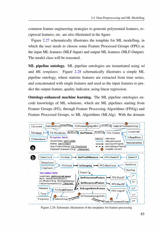
2.4 Data Preprocessing and ML Modelling
common feature engineering strategies to generate polynomial features, re-ciprocal features, etc. are also illustrated in the figure.
Figure 2.27 schematically illustrates the template for ML modelling, inwhich the user needs to choose some Feature Processed Groups (FPG) asthe input ML features (MLF-Input) and output ML features (MLF-Output).The model class will be reasoned.
ML pipeline ontology. ML pipeline ontologies are instantiated using ml
and ML templates. Figure 2.28 schematically illustrates a simple MLpipeline ontology, where statistic features are extracted from time series,and concatenated with single features and used as the input features to pre-dict the output feature, quality indicator, using linear regression.
Ontology-enhanced machine learning. The ML pipeline ontologies en-code knowledge of ML solutions, which are ML pipelines starting fromFeature Groups (FG), through Feature Processing Algorithms (FPAlg) andFeature Processed Groups, to ML Algorithms (MLAlg). With the domain
Figure 2.26: Schematic illustration of the templates for feature processing
85

2 A Framework of Machine Learning in Electric Resistance Welding
Figure 2.27: Schematic illustration of the template for ML modelling.
ontology, the core ontology, the ML ontology and an ML pipeline ontology,three mappings (Figure 2.13) can be inferred via e.g. SPARQL queries: Do-main feature names to Feature Group mapping (DO-to-FG), Feature Groupto Feature Processing Algorithm to Feature Processed Group mapping (FG-FPAlg-FPG), and Feature Processed Group to ML Feature to ML Algo-rithm mapping (FPG-MLF-MLAlg). Figure 2.29 illustrates the completeontology-enhanced ML pipeline with the simple example pipeline in Fig-ure 2.28 in the following steps:
1. The raw feature names are retrieved from raw data and features are re-named to domain feature names using the Raw-to-DO mapping (Sec-tion 2.3.2);
2. All features are assigned with FG based on the DO-to-FG mapping (Sec-tion 2.3.3);
3. Based on the FG-FPAlg-FPG mapping, the corresponding FPAlg for eachFG is retrieved. All FPAlg are connected with ML script modules to
Figure 2.28: Schematic illustration of an example ML pipeline ontology.
86

2.4 Data Preprocessing and ML Modelling
Figu
re2.
29:A
nex
ampl
eof
onto
logy
-enh
ance
dM
Lpi
pelin
eof
FE-L
R,m
odifi
edfr
om[1
70]
87

2 A Framework of Machine Learning in Electric Resistance Welding
process the features. The processed features are annotated with FPG. Forexample, the GetTSStats is retrieved for FG-TimeSeries. Thus, the MLmodule GetTSStats processes all time series features and generate thetime series statistic features, like VoltageMean, ResistanceMinimum, etc.The time series statistic features are annotated with FPG-TSStats;
4. Feature processing can have multiple sub-steps, where the newly gen-erated features are further processed by FPAlgs to output new FPGs.In the example, the time series statistic features (annotated with FPG-
TSStats) are concatenated with the unchanged single features (anno-tated with FPG-SFMaintained). The OperationID (annotated with FG-
Identifier) is used for finding the correspondence between them so thatthey can be correctly concatenated.
5. According to the FPG-MLF-MLAlg mapping, some FPGs are selectedas the input for ML modelling, and some other FPGs (also FGs are possi-ble) as output. In the example, the concatenated features (annotated withFPG-SFConcatenated) are selected as MLF-Input and the NuggetDiame-ter (annotated with FG-QualityIndicator) as the MLF-Output;
6. The MLAlg trains a model on the input and output data pairs. In theexample, linear regression is used to take in the concatenated features topredict the diameter, and generate a LRModel.
The execution of the described pipeline is possible due to the knowledgeencoding with ontologies for 1) domain knowledge, 2) ML feature process-ing strategies and 3) classic ML algorithms and order of their application.Semantic enhancement enables users to start with the initial (Raw-to-DO)mapping and execute these ML pipelines with small adjustments and adap-tations to new datasets and new questions. The generated four mappingsduring data preparation, data preprocessing and ML modelling can also beused to inspect the resulting models and the underlying data, to explain thefeature importance and to interpret the best model.
88

2.4 Data Preprocessing and ML Modelling
2.4.7 Data Preprocessing and ML Modelling: HierarchicalFeature Learning
An alternative ML pipeline to the hierarchical feature engineering intro-duced in Section 2.4.2 is hierarchical feature learning. The general schemais already illustrated in Figure 2.18. Preprocessing is required to make thedata suitable for feature learning, e.g. align the data matrices dimensionsby reshaping, padding, truncation, etc. Feature learning (FL) for singlefeatures can be performed with MLP. FL for time series (sequences withtemporal dependencies) can be performed with RNN, FL for images (ma-trices with spatial dependencies) can be performed with CNN, and FL forfeatures with temporal and spatial structures (e.g. videos) can be performedwith a combination of RNN-CNN. After the initial feature learning on dif-ferent feature types, the resulting latent features can often be concatenatedfor further feature learning. After all feature learning layers, some neuralnetwork layers are followed to perform ML modelling. Note that there ex-ists no clear boundaries between feature learning and ML modelling. Thisseparated description is only of philosophical meaning.
Figure 2.30 illustrates an example of the ML pipeline of FL-NN for pre-dicting the Q-Value of future welding operations. Process curves padded tolength k form time series on the welding time level. A total number of sz ofthese curves of l previous welding operations are first reshaped and fed intoa time distributed LSTM (it is a RNN) network for feature learning. The re-sulting Time Series Features Learned (TSFL) are on the welding operation
Figure 2.30: An example of hierarchical feature learning pipeline with LSTM (Use Case 4.3).PaddedTS: time series padded to the same length. RawSF: raw single features.TD(MLP): time distributed MLP. TSFL: time series features learned.
89

2 A Framework of Machine Learning in Electric Resistance Welding
level, and are concatenated with the raw single features. The concatenatedfeatures form time series on the welding operation level, and are fed intoa time distributed MLP network for a further step of feature learning. Theresulting features are latent features that contain compressed information ofthe previous l welding operations. A further LSTM network is followed toaggregate the latent features to predict the Q-Value. The complete neuralnetwork is trained together using back-propagation.
2.4.8 Evaluation: Discussion of Performance Metrics
Prediction accuracy of ML models is the classic performance metric inthe ML community. However, to ensure that ML approaches have a goodchance to be widely adopted in manufacturing industry, not only predictionaccuracy is important, but also many other performance metrics that influ-ence the adoptability of ML approaches.
Prediction accuracy. In this work, prediction accuracy is defined in thefollowing way:
• rmse (or mse) [137, 142] stands for root mean squared error (or meansquared error) between the target values and estimations. The disadvan-tages of rmse are that it is scale-dependent [185], and not particularlyintuitive for domain experts, compared to other measures.
• mae stands for mean absolute error between the target values and estima-tions. It is less sensitive to outliers, compared to rmse.
• mape stands for mean absolute percentage error. It is scale-independentand intuitive for domain experts. The disadvantage is this becomes inap-plicable when there exists zeros in target values.
• Correlation Coefficient (or another similar metric, the coefficient of deter-mination R2) [186] is good for judging the ability of ML models to predictthe general trend of the training data.
• The most intuitive measures for process experts are perhaps User-Defined
Errors (UDE) [142]. These are more suitable for helping to set the safety
90

2.4 Data Preprocessing and ML Modelling
factor, thus closer to the goal of minimising product failures. Two com-mon UDEs are Error Within 5%, which means the percentage of predic-tions with relative errors smaller than 5% of the target value (In welding5% error is fairly good performance). Error Within 10% is likewise.
Adoptability metrics. Machine learning in manufacturing has more re-quirements than prediction accuracy. Many other factors, e.g. the time andeffort for development of ML approaches, data collection, and implementa-tion, should also be taken into consideration. This work suggests using thefollowing performance dimensions for a more comprehensive evaluation ofadoptability of ML approaches.
• Domain understanding reflects the effort and time for data scientists orengineers to understand the domain to enable successful ML approaches.This can be measured by questionnaires or time spent for understanding.
• Feature understanding measures the time required for detailed under-standing of features for successful data preprocessing. This can be mea-sured by questionnaires of cognitive difficulty or time spent for under-standing.
• Data preparation measures how efficient or generalisable the merging andintegration of data from different sources are. This can be measured byquestionnaires or time spent for adapting developed ML pipelines for newdatasets.
• Hyper-parameter tuning measures the effort required for tuning hyper-parameters of ML models. This can be measured by questionnaires, num-ber of tuning experiments, or time spent for tuning.
• Required training data amount indicates the minimal data amount neces-sary for training a machine learning model with acceptable performance.This is especially critical, as the data collection in manufacturing can bevery time-consuming and expensive. This can be directly measured bythe number of necessary training data tuples, or by time spent on datacollection.
91

2 A Framework of Machine Learning in Electric Resistance Welding
• Average training time and test time measures the mean value of trainingtime of ML models, including data preprocessing. Training time influ-ences the time delay resulted from model adaptation when new Trends aredetected in the data so that existing models are no longer successful. Testtime determines whether the approach is suitable for online implementa-tion in hardware. This is measured by time with description of computinghardware.
• Model explainability measures whether the selected features, ML modeland prediction results are easy to understand, especially for non-ML-experts. This can be measured by questionnaires or time spend for modelexplanation.
92

3 Implementation
This chapter concisely describes the implementation of the proposed frame-work in Chapter 2. The framework is implemented with two programmingplatforms: (3.1) Python [187] language, including various libraries for ma-chine learning like scikit-learn [188], tensorflow [189], and keras [190];(3.2) the SciXMiner [191] data analysis toolbox based on MATLAB [192].
3.1 Implementation with Python
Data collection is done by process experts in production, measurement ex-perts in laboratory, or simulation engineers. This work implements the MLpipeline from data preparation, through data preprocessing, and ML mod-elling (Figure 3.1).
Data preparation. This step is the process of extract-transform-load.
Extract. Various Bosch internal tools were used to extract data from raw for-mats of SQL database, RUI files, control backup files etc., and store them intext/csv, mat (MATLAB format) or json formats. For all three data sources(production, lab, simulation), the extracted data have two major groups. Ifthe data are stored in text/csv format, these two groups are: (1) A set of re-lational tables of single features, with each row corresponding to one weld-ing operation, and each column corresponding to one feature; (2) A largenumber of relational tables. In each table, the process curves (time series)corresponding to one welding operation are stored. In case of json or mat,the two groups are stored in lists of dictionaries or structures, in which eachfield is a single feature or time series feature.
93

3 Implementation
Figure 3.1: Architecture of implementation scripts. The three modules in Data Preprocessingare called in Feature Processing. The three modules in ML Modelling are called inML Modelling.
Transform. Data need to be transformed to Uniform Data Format with sevenprocedures: combining headers and values, splitting, sorting, matching,padding, merging, and feature renaming. Some procedures are not manda-tory under certain circumstances.
• Combining headers and values. It is necessary in the case when headersand values are stored separately, e.g. text/csv data or prjz data.
• Splitting. A dataset is normally comprised of data of dozens of weldingmachines. In most analysis, these welding machines are analysed inde-
94
3.1 Implementation with Python
pendently. Therefore, the big dataset needs to be split into smaller sets,with each only containing data of one welding machine.
• Sorting. Welding operations are sorted using the logical-temporal orderof WearCount-DressCount-CapCount. Time stamps are not always reli-able, because manual interference of operations will cause time stampsrenewed. CapCount is missing for some datasets and therefore an ad hocCapCount needs to be added.
• Matching. The various features types (Section 2.3.2) of data are normallystored in different files. Sometimes there exist no Identifiers to find thecorrespondence between data, especially for the two groups, single fea-tures and time series. Due to software settings of the welding control, thetime stamps of data entries are not perfectly aligned. After various testing,this work suggests to use WearCount, DressCount as the logical-temporalorder to match data. These two features exist in files of both groups.Note these two features cannot identify data entries uniquely, because theWearCount-DressCount combination will repeat when a new electrode
cycle begins. CapCount is missing for some datasets, and therefore itcannot be used for matching. A dynamic matching algorithm is needed:(1) narrowing down the search area using time stamps, allowing e.g. oneday tolerance as the search area; (2) finding the matching WearCount-
DressCount combination within the search area for the two groups.• Padding with NaN. For single features without values, NaN (not a num-
ber) is filled. For time series with different lengths, NaN is padded tonormalise the lengths. The NaN-padding avoids errors caused by dimen-sion inconsistency.
• Merging. Now the correspondence between different feature types ispresent, and dimension inconsistency is eliminated. Data can be mergedinto a single dictionary and stored in numpy array or pickle. Data can alsobe logically merged by adding Identifiers in all files and storing them ina pre-designed manner. A typical style for text/csv format is (similar tomerge SQL table): (1) All single features are stored in one relational table,
95

3 Implementation
adding one column for the identifier. Some feature values need to be repli-cated. For example, the meta configurations of all welding programs werestored separately in a small relational table, with each row correspond-ing to one welding program. It will be repeatedly filled into the mergedsingle feature table of welding operations, since each welding programis executed by a large number of welding operations. (2) All time seriesfeatures are stored in a series of relational tables in a sub-folder, with alltime series files named as the identifier.
• Feature renaming. All feature names will be changed to the Unified
feature names using the Raw-to-DO mapping (raw to domain ontologyterms) to simplify the subsequent scripts.
Load. Data in UDF can be easily loaded by reading the json or pickle filesor reading the text/csv files using pandas.
ML modules. Uniform data format allows the subsequent scripts to bestandardised and repeatedly used. This work implements frequently usedfunctions in seven modules. Modularisation of ML scripts are essential forreadability and ontology-enhanced ML pipelines.
• ModuleTimeSeriesFeatureExtraction is written in three levels:
– (1) The TS feature extraction for a welding operation. The inputis a 2D-matrix with shape [len,sz], where k is the TS length afterdimension-normalisation and sz is the number of TS features. Theexact algorithm can be various: statistic features, geometrical features,segmentation, PCA features, etc.
– (2) The corresponding feature name generation function for (1).– (3) The TS feature extraction for a dataset. It takes a 3D-matrix with
shape [n,len,sz] as input, where n is the number of data tuples in thedataset. The output is a 2D-matrix of shape [n,sts], where sts is thenumber of extracted time series features. Different algorithms writtenin (1) can be used as plug-in in (3). New algorithms in level (1) canalso be easily added.
96

3.1 Implementation with Python
• ModuleFeatureSelection implements a stepwise forward linear regressionalgorithm using Dynamic Programming. In each iteration, it selects onebest feature using wrapper method from the appointed dataset, and deliverthe rest sub-dataset into the next iteration, and solve the sub-problem re-peatedly. The return is an array of the order of selected features and thecorresponding feature scores evaluated using correlation coefficient.
• ModuleNormalisation implements Z-score normalisation and Min-Max
normalisation, and provides functions of fit, transform, inverse-transform
for single feature and fitts for time series.• ModuleMLPPipeline implements all functions for a complete MLP
pipeline, including loading data, normalisation, denormalisation, con-structing MLP architectures according to input, training and testing themodels, hyper-parameter tuning, performance evaluation and saving re-sults.
• ModulePerformanceMetric implements the metrics of prediction accuracydiscussed in Section 2.4.8.
• ModuleVisualisation implements frequent visualisation functions in mat-
plotlib and bokeh, e.g. line-plot and scatter-plot along welding operationsor WearCount for quality indicators, row-wise independent heatmaps fordataset evaluation.
• ModuleOntologyCommunication implements the mechanism of MLpipeline communicating with ontologies. Details please see the next para-graph.
Information retrieval from ontologies. Ontology-enhanced ML pipelinesneed to communicate with the ontologies to retrieve information encoded inML pipeline ontology. This is realised by sending SPARQL queries to queryontologies. These scripts are capsuled in the ModuleOntologyCommunica-
tion.
97

3 Implementation
• Load graph. The ontologies serialised in Turtle [193] can either be loadedinto memory from a URL using the rdflib package, or be queried onlineusing the stardog package.
• Query. All encoded information are retrieved using queries. For example,to retrieve the stored ML pipeline ontology, a querySELECT * WHERE ?s a :MLPipeline. is sent to the loaded graph. Thereturn will be processed to extract the label of the class or the string ofliteral. The return of the example is the label of the ML pipeline stored inthe graph: [’MLPipeline’]. Further examples include:(1) SELECT ?FG WHERE:FeaturePreparedLayer :hasMemberFG ?FG
with the return: [’QualityIndicator1’, ’SFGroup1’, ’TSGroup2’]
(2) SELECT ?FPAlg WHERE:SingleFeatureGroup1 :hasFPAlg ?FPAlg
with the return: [’Maintain’].
Exploratory data analysis. In this step the data are visualised, con-spicuities are examined, and benchmarks can be calculated.
• Visualisation. There exist two important types of visualisation. (1) Threefeatures, WearCount, DressCount, and CapCount, are visualised usingline-plot with matplotlib or bokeh. The left y-axis will be WearCount andthe right y-axis will be DressCount and CapCount. The x-axis can be timestamps or number of welding operations. With this visualisation, it is easyto obtain an overview of all dress cycles and electrode cycles. Incompletecycles are obvious. (2) Any single feature of interest can be visualisedusing line-plot or scatter-plot. Conspicuities can be detected. A typicalexample is the Q-Value, as discussed in detail in Use Case 4.2.
• Conspicuity and Benchmark. For calculation of trends or benchmarks, themost efficient solution is to use nested dictionaries to store the calculatedvalues, e.g. the trend value of WM1, Prog1, Cap2, Dress2, Wear120 isstored in trend[’WM1’][’Prog1’][’CapDress202’][’Wear120’].
Data preprocessing. It includes cleaning, dimension-normalisation, featureextraction, normalisation.
98

3.2 Implementation with SciXMiner
• Cleaning is to delete features (columns) or data entries (rows) with NaN
that exceed a threshold.• Dimension-normalisation for time series is to make the TS lengths equal
by truncation (deletion), padding (with physically meaningful values, seeSection 2.4.2) or resampling (using e.g. numpy.interp).
• Feature extraction includes various feature engineering strategies imple-mented in ML modules, or feature learning, discussed together in MLmodelling.
• Normalisation is implemented using ModuleNormalisation for Z-score
normalisation and Min-Max normalisation.
ML modelling. All modelling is implemented in four levels.
• ML architecture construction: For classic ML, this level is simply to usea function written in established packages, e.g. scikit-learn. For featurelearning, this level constructs the designated network architecture and re-turns the constructed architecture.
• Training and test: This level capsules one round of training and test ina function. It takes preprocessed data and ML architecture as input, andoutputs the ML prediction results for both training and test data.
• Performance evaluation: This level takes the prediction results as input,and uses the ModulePerformanceMetric to calculate all performance met-rics and returns a DataFrame of performance summary.
• Saving results: This level takes the prediction results and performancesummary as input, saves all these results, and visualises the predictionresults using line-plot and scatter-plot in ModuleVisualisation.
3.2 Implementation with SciXMiner
ML pipeline with SciXMiner. A ML pipeline in MATLAB can execute aseries of ML experiments that are designed to achieve one goal. For exam-ple, the same scripts run on a series of datasets with different training sub-
99
3 Implementation
sets/feature subsets to analyse the influence of training data amount/featuresets on model performance. The architecture of ML pipeline scripts is or-ganised in three levels: a batch file, experiment instances, and several scriptcomponents.
Batch file. In this file, the project directory and script directory are specifiedfor SciXMiner to find data and scripts.
Experiment instance. After specification of directories, a series of experi-ment instances are executed. For each there exist (1) a prjz file (SciXMinerproject), (2) a configuration script and (3) a master script.
• Prjz file. This is the SciXMiner project that stores the data. The prjz file issimilar to a MATLAB structure, which has fields and values. The valuescan be a single string or float, or matrices, or nested structures.
• Configuration script. In this script the number of CPU cores are specifiedto help the system allocate computing resource. A new directory for thecurrent experiment instance is created with a unique name, by e.g. usingthe current time in the folder name. A directory (usually the project direc-tory) needs to be assigned to a variable, working directory. The workingdirectory is important for execution of script components.
• Master script. This script has two parts. (1) Part I prescribes the hyper-parameters, the target output feature, and creates sub-directories for sub-experiments of e.g. cross-validation. (2) Part II contains all script compo-nents from data preprocessing, ML modelling, to saving results. The MLalgorithms coded in SciXMiner can only access global variable names-pace, i.e. cannot process data passed into a function internally. Therefore,all script components are directly executed in global variable namespace.
Script components. These are modularised components with different func-tionalities for data preprocessing and ML modelling. In particular, thereexist the following types of components:
100

3.2 Implementation with SciXMiner
• Creating project backup. Since all script components are executed inglobal variable namespace, a backup of the project data needs to be cre-ated before any experiments. The backup includes single features (d_org),single feature names (dorgbez), time series (d_orgs), time series featurenames (bez_code), output class encodings (code_alle), output class fea-ture names (var_bez), and output class terms (zgf_y_bez).
• Data preprocessing. These components include data splitting into trainingand test sets, deletion of irrelevant features, feature extraction (sometimesthis can be omitted if the features are already extracted by Python scripts),univariate or multivariate feature selection. If wrapper method is adopted,the feature selection is coupled with ML modelling.
• ML modelling. These components include ML model configuration usingthe hyper-parameters prescribed by the master script, or selected fromthe hyper-parameter list in case of sub-experiments for hyper-parameterselection. After that, the model training and testing are executed.
• Visualisation and saving results. These components include visualisationof prediction results in line-plot or scatter plot, performance evaluation,and saving all these results in the sub-directory for the current experimentinstance.
• Restoring project backup. When all components are executed, the projectdata need to be restored from the backup, so that the next experimentinstance can be executed.
• Hyper-parameter selection. This component is to visualise and evaluateall performance after all sub-experiments are executed. It is needed whenthe goal of the experiments is to find the best hyper-parameters.
101

4 Use Cases
This chapter will demonstrate use cases, validating the methods proposedin Chapter 2 on data collected from simulation, laboratory and production.Relevant rows of the overview table (Table 2.3) are separately displayedagain for each use case.
4.1 Spot Diameter Estimation and Guidance forSimulation Data Collection
Overview: This use case studies estimation of welding quality for resis-tance spot welding process. The target feature of the ML models is thewelding nugget diameter. The data are collected from a validated FiniteElement Method (FEM) simulation model [158]. This is a supervised re-gression problem. Since the classification of welding quality into good/badcategories depends on specific welding configurations, the study of regres-sion is more general than classification, and can provide more insights toprocess experts. Besides, the classification can still be made after regres-sion.
Strategies of data preprocessing are extracting statistic features from timeseries and feature selection. The ML methods are three classic methods:polynomial regression, “shallow” multi-layer perceptron (with only one hid-den layer), k-nearest neighbours. Analysis of the influence of feature setsand amount of training data on prediction accuracy is conducted to gain in-sights for preparing costly data collection from laboratory and production.
103

4 Use Cases
The related publication is [29]. An overview of the corresponding applica-tion questions, open questions and methods is listed in Table 4.1.
Table 4.1: Overview of application questions (AQ), open questions (OQ) and methods (M)
AQ OQ MethodsAQ2, AQ3, AQ4 OQ1, OQ5 M2.1.1, M2.1.2, M2.1.3,
M2.2.4, M2.4.2, M2.4.5,M2.4.8
4.1.1 Question Definition
An enormous amount of data is generated every day in automatic manu-facturing. Yet the acquired data do not always contain relevant information(e.g. labels) and thus are sometimes not suitable for data analysis [94]. In re-sistance spot welding, the level 2 quality indicators (QI2, see Section 2.1.1),such as weld nugget diameter data, are often scarce and can only partiallycover quality monitoring. Moreover, additional sensor data, such as weldingforce and temperature, are not always available because of sensor installa-tion cost and accessibility.
Machine learning enables data-driven methods for more reliable and all-covering quality monitoring for RSW, by replacing QI2 with QI5 generatedby ML models. In most cases, the more data are used for training, the higherthe chance is to obtain accurate models. However, the cost of data collectionin manufacturing is extremely high. It would be optimal to gain some in-sights of the RSW process before starting a costly data collection plan fromlaboratory or production, so that data collection can have some references.Interesting questions include, e.g. how many data are necessary for success-ful machine learning modelling? What features are more informative?
This section uses physics-based simulation data generated with a verifiedFinite Element Method (FEM) model [158] to address the insufficient dataproblem and the three data challenges (Section 2.1.3). Concretely, three
questions regarding the first two data challenges in collecting costly labelleddata will be studied:
104

4.1 Spot Diameter Estimation and Guidance for Simulation Data Collection
• Q1: How many labelled data to collect first? (Challenge 1)• Q2: Which sensors should be installed first? (Challenge 2)• Q3: Which precision level should the sensors and measurements of weld-
ing spot diameters have? (Challenge 2)
4.1.2 Data Description
Simulation scenario. The most normal conditions in production, i.e. onlyrandom variation without spatter or other disturbances, are selected as thesimulation scenario for the data studied in this use case. This simple sce-nario consists of one welding machine, one type of worksheet pair withidentical nominal sheet thickness and material, and three welding programsfor three different target spot diameters (Figure 4.1). A total of 13,952 weld-ing spots with diameter measurements are simulated, which contain 14 elec-trode cycles.
The FEM simulation models mechanical effects (elastic-plastic deforma-tion and thermal expansion of chassis parts), thermal effects (temperaturechange and heat transfer) and electrical effects (electric current density andelectric potential field), taking into account non-linear changes of materialand contact properties (such as electrical and thermal contact conductivity).Strong interactions between all three fields result in a very dynamic processbehaviour and a multi-field coupled simulation.
Features. For each weld spot, there are two types of data:
• Time series (or process curves): In total, 20 time series were simulated,including two types.
– Process input curves are input time series of the FEM simulation model,such as electric current (I), and force applied on the electrode (F).
– Process feedback curves are output time series of the FEM model, suchas voltage (U), resistance (R) , displacement (s) of the electrode, tem-perature (T ) of certain measuring positions, etc.
• Single features: They are nominal and measured geometry or materialproperties of the caps and worksheets, the number of spots welded, posi-
105

4 Use Cases
tions of the welding spots, temporal structure features (Section 2.1.2), etc.There exist up to 235 single features in the simulation dataset.
ProgNo : 1 ProgNo : 2 ProgNo : 3
0
1
Dia
me
ter
(no
rma
lize
d)
(a) (b)
Figure 4.1: (a) Process curves for the three welding programs. ProgNo indicates the pro-gram number. The welding programs prescribe the way the welding process isperformed, by specifying the process curves and some additional welding parame-ters [29].(b) Boxplot of the diameters for the three welding programs [29].
4.1.3 Experiment Settings
The approach for exploring answers to the three questions centres on train-ing machine learning models with different data subsets and comparing theirperformance.
Data splitting according to temporal structure. As mentioned in Section2.4.1, data splitting should be performed according to some complete unitsof a time level. In this study, the electrode cycle level will be used as com-plete time units. Data generated with 9 electrode caps (7973 data points)are used for training and selecting hyper-parameters, denoted as “trainingxdata”. Data from the remaining 5 electrode caps (5979 data points) are usedfor testing.
Data splitting into subsets of different training data numbers. ML mod-els are trained with different number of data tuples to study how the number
106

4.1 Spot Diameter Estimation and Guidance for Simulation Data Collection
of training data influence the model performance (Section 2.2.4), for an-swering Question 1 in Section 4.1.1. The trainingx dataset is split into sevensubsets (Table 4.2), with the condition that the larger subsets always containthe smaller subsets to avoid the random effect of data on model performance,e.g. D2 contains all data in D1, D3 contains all data in D2.
Table 4.2: Data splitting into seven subsets of different training data number
Dataset name D1 D2 D3 D4 D5 D6 Dall
#Trainingx data 100 250 500 1000 2000 5000 7973
#Test data 5979 5979 5979 5979 5979 5979 5979
Data splitting into subsets of different feature sets. For answering Ques-tion 2, ML models are trained with different feature subsets to investigatethe influence of each feature subset on the performance (Table 4.3). As in-troduced in Section 2.2.4, the features are split into Feature Set available inproduction, in the lab with low cost, in the lab with high cost, and all featuresin simulation. The feature set splitting is applied to each of the seven subsetsof training data number, resulting in a total of 28 subsets (7×4 = 28).
Table 4.3: Data splitting into four subsets of different features
Feature set FeatSetprod FeatSetlablow FeatSetlabhigh FeatSetall
#Features 15SF, 4TS 16SF, 10TS 29SF, 14TS 235SF, 20TS
Generating additional noisy datasets. For answer Question 3, noise isadded to the 28 subsets, resulting in an additional set of 28 noisy datasets.The noise levels are a best engineering guess derived from discussions withprocess experts and measurement experts (Table 4.4). In total, 7×4×2= 56subsets are used to train and test machine learning models and compare theirperformance.
Feature engineering and selection. The feature engineering strategies ap-plied to the time series are extracting 8 statistic features, including min-
107

4 Use Cases
Table 4.4: Data splitting into four subsets of different features
Features Added noise
Sensor data (time series and singlefeatures)
Gaussian noise with 2% standard deviation forevery single sample point
Diameter measurements Gaussian noise with 0.1 mm standard deviation
imum, maximum, minimum position, maximum position, mean, median,standard deviation, and length.
These extracted features combined with all other single features are thenevaluated and selected using step-wise forward selection (Section 2.4.3),starting with the evaluation of each single feature, and incrementally addingmore features. The features resulting in models with the best regression ac-curacy (RMSE) for the prediction of spot diameters are selected. Resultsshow that in most cases, the model performance increases as the number ofselected features increases. For some models the performance does not in-crease any more from about 10 features. For some models the performancedoes not improve any more up to 20 selected features. To make the com-parison fair and reduce computation time, all models are trained with 20selected features.
ML methods and hyper-parameter tuning. Three machine learning meth-ods, polynomial regression, neural networks and k-nearest neighbours arestudied. The hyper-parameters are chosen with 5-fold cross validationwith the largest trainingx data (training set of Dall with 7973 training datapoints) and the Feature Set of Production (FeatSetprod). The resulting hyper-parameters are shown in Table 4.5.
4.1.4 Results and Discussion
Figure 4.2 illustrates the performance on test set of best polynomial models(Polynomial1) trained on non-noisy subsets of different training data num-ber and feature sets, evaluated with four performance metrics.
108

4.1 Spot Diameter Estimation and Guidance for Simulation Data Collection
Table 4.5: ML models and hyper-parameters selected through 5-fold cross validation. Notethat some polynomial models with higher degree than 1 do not show statisticallysignificant improvement than first order polynomial models. According to theprinciple of Ockham’s razor, polynomial order of 1 is selected.
Machine learning model Hyper-parameter Value
Multivariate polynomial regression Polynomial order 1
Multi-layer perceptron (one hidden layer) #Neurons in the hidden layer 16
K-nearest neighbours k (#Neighbours) 3
Feature sets. Comparing models trained on different feature sets reveals,as expected, when more features are available for training, the models alsohave better performance in testing in most cases: Pall > Plabhigh > Plablow >
Pprod (P indicates performance).
Training data number. Comparing models trained on different trainingdata subsets shows that, when the training data number is greater than 250,the performance improves insignificantly as the training data number furtherincreases.
Performance metrics. Comparing the performance represented by differ-ent metrics, it can be seen that RMSE, Correlation Coefficient and ErrorWithin 5% have similar trends. This is also the case for the multi-layer per-ceptron models (Figure 4.3) and k-nearest neighbour models (Figure 4.4).Error Within 10% cannot differentiate the models trained with different datanumber and feature sets, since they always show very good results. There-fore, only Error Within 5% will be compared in the following discussions.
ML methods. Comparing models trained using different machine learn-ing methods can be made by comparing Figure 4.2c, Figure 4.3, and 4.4,or in Figure 4.5. These figures reveal that the performance of the mod-els built with three machine learning methods is: Polynomial ≈ MLP >KNN. Figure 4.3 shows that MLP16 tends to overfit for the FeatSetlablow
and FeatSetlabhigh. In this regard, Polynomial1 is more advantageous.
109

4 Use Cases
100 250 500 1000 2000 50007973
Training data number
0.06
0.08
0.1
0.12
RM
SE
(m
m)
Production
LabLowCost
LabHighCost
All
100 250 500 1000 2000 50007973
Training data number
0.97
0.98
0.99
1
Co
rre
lation
Coeff
icie
nt
Production
LabLowCost
LabHighCost
All
(a) (b)
100 250 500 1000 2000 50007973
Training data number
0.85
0.9
0.95
1
Err
or
Within
5 P
erc
ent
Production
LabLowCost
LabHighCost
All
100 250 500 1000 2000 50007973
Training data number
0.99
0.995
1
Err
or
Within
10
Pe
rcen
t
Production
LabLowCost
LabHighCost
All
(c) (d)Figure 4.2: Comparison of performance on test set of Polynomial1 models trained on non-
noisy subsets of different training data number and feature sets [29]. Note thatin (d) Error Within 10% cannot differentiate the models, since all models areextremely good and have more than 99% predictions with less than 10% errors.
Noise in data. Comparing models trained with non-noisy data and noisydata can be made by contrasting Figure 4.2 c and Figure 4.6. The compari-son suggests the performance deteriorates strongly with noisy data. Gener-ally speaking, the difference between models trained on these three featuresubsets, FeatSetprod , FeatSetlablow, and FeatSetlabhigh is insignificant.
4.1.5 Conclusion and Outlook
Conclusion. Simulation data can provide a large amount of economicallygenerated labelled data, and features that would be otherwise unavailable.
110

4.1 Spot Diameter Estimation and Guidance for Simulation Data Collection
100 250 500 1000 2000 50007973
Training data number
0.85
0.9
0.95
1
Err
or
Within
5 P
erc
en
t
Production
LabLowCost
LabHighCost
All
100 250 500 1000 2000 50007973
Training data number
0.85
0.9
0.95
1
Err
or
Within
5 P
erc
en
t
Production
LabLowCost
LabHighCost
All
Figure 4.3: Testing results MLP16 onnon-noisy datasets [29]
Figure 4.4: Testing results KNN3 on non-noisydatasets [29]
100 250 500 1000 2000 50007973
Training data number
0.85
0.9
0.95
1
Err
or
Within
5 P
erc
ent
Polynomial1
MLP16
KNN3
100 250 500 1000 2000 50007973
Training data number
0.85
0.9
0.95
1
Err
or
Within
5 P
erc
ent
Production
LabLowCost
LabHighCost
All
Figure 4.5: Testing models trained onnon-noisy Production Set [29]
Figure 4.6: Testing Polynomial1 on noisydatasets [29]
These data contain no or low measurement error. As a result, it is possibleto guide the collection of costly data from production or laboratory withthe insights gained from analysing simulation data. Reviewing the startingpoint of the three questions, the following insights can be interpreted fromthe analysis results.
• Answer to Question 1: Starting with a collection of 250 labeled datapoints.
• Answer to Question 2: Features available in Production can already beuseful.
• Answer to Question 3: Measurement uncertainty can lead to significantdeterioration of the prediction performance. In our case, precision betterthan Gaussian errors of 2% standard deviation for sensors and 0.1mm
111

4 Use Cases
standard deviation for diameter measurements, respectively, is recom-mended.
It is important to note that the conclusions regarding the necessary num-ber of data points and features are highly dependent on the dataset, and thesimulation scenario from which the data are collected. It is therefore safe tosay that the results can be generalised over the simulated situations. Theycan serve as a first guidance for data collection, but should NOT be assumedas valid in general. Since the selected simulation scenario of one weldingmachine and three welding programs is a simple scenario, these conclusionsmay not hold for other scenarios or for complex production data. The opti-mal data collection plan may vary depending on the complexity of the actualsituations compared to the simulated situation.
Outlook. In future research, several topics can be explored for combiningthe simulated data and laboratory or production data.
• The first option is to use laboratory data or production data to furtherimprove and fine-tune the simulation model so that realistic physical ef-fects and authentic variance of influencing factors can be rebuilt in thesimulation. This realistic simulation data can be used for further dataanalysis.
• A further step is to apply the model trained on simulated data on labora-tory or production data to see the generalisability of the models.
• A third option is to transfer learning, i.e. to pre-train a model on simu-lated data, then to fine-tune the model on laboratory data or productiondata, and to see how much improvement in performance can be gained.
• The improved simulation model and generated data can be used for pro-duction condition evaluation before a real production process begins, sothat the influence of welding parameters changes, such as welding gunproperties, material properties, distance between the worksheets, can besystematically evaluated.
112
4.1 Spot Diameter Estimation and Guidance for Simulation Data Collection
• Alternative feature extraction methods (such as features based on do-main knowledge or Principal Component Analysis) can be analysed toevaluate the difference of prediction accuracy using different feature ex-traction methods.
• As actual production conditions may change due to a change in supplier,new engineering design, etc., it is always questionable to what extent amodel trained on historic or lab data can be deployed on production datain the future, which constitutes a general problem in manufacturing. Thisissue of concept drift remains an open question.
This use case strives to gain insights from data analysis for guidance ofdata collection. The iterative process data-collection → data analysis →data-analysis guided data collection→ data analysis is an attempt to com-bine data collection and analysis (Figure 2.9). A similar practice would beparticularly necessary in fields where limits on the amount of labelled data,features, and covering situations is a problem of interest.
113

4 Use Cases
4.2 Evaluation of Production Datasets
Overview: This use case demonstrates using multiple metrics and vi-sual analytics techniques to gain a quick overview of large manufacturingdatasets, including categorical features (ProgramNumber), numerical fea-tures (Q-Value), features with multi-level temporal structures (time series,WearCount, DressCount, etc., Section 2.1.2). In this example, the data arecollected from various welding machines and their Q-Value behaviour isinspected for each machine. Similar practices can be done for other units(e.g. chassis part types, worksheet thickness combination types STC), andother quality indicators (e.g. process stability factor, spatter occurring time).Visual analytics is used to identify conspicuous welding machines, weld-ing programs, or dress cycles that are subject to risks of quality failures.Visual analytics refers to methods and practice of information visualisa-tion for analytical reasoning [194], and has found a wide range of applica-tions [195, 196]. An overview of the corresponding application questions,open questions and methods is listed in Table 4.6.
Table 4.6: Overview of application questions (AQ), open questions (OQ) and methods (M)
AQ OQ MethodsAQ1 OQ3, OQ4 M2.2.5
4.2.1 Question Definition
ERW processes produce a large volume of data. It is therefore very de-sired for process experts to gain a quick overview of the data collected fromall welding machines, to identify which welding machine, which weldingprogram or which dress cycle are conspicuous and may subject to risks ofquality failures. These conspicuities include deviation from the expectedbehaviour, large scattering or outliers (Section 2.2.5).
The users can choose any single feature as the criteria, e.g. Process Stabil-
ity Factor, Resistance Mean. Among these, Q-Value is especially important,
114

4.2 Evaluation of Production Datasets
and will be used as the criteria in this use case for identifying conspicuities.Q-Value, developed by Bosch Rexroth through engineering know-how andlong-time experience, is calculated after each welding operation, based onstatistic features (e.g. mean, maximum) from sensor data. The optimalQ-Value is one and any value that deviates from one indicates quality dete-rioration or inefficiency.
In dataset evaluation, an overview of the general information (e.g. #weld-ing operations, #welding programs), and the behaviour of Q-Value shouldbe presented to the users (e.g. process experts, data scientists), to iden-tify potential problematic welding machines. These problems should thenbe attributed to specific welding programs or dress cycles, to narrow downthe search realm for root causes of problems. Appropriate visualisation ofthe general information and Q-Value behaviour should be illustrated in ancondensed and intuitive way to enable comprehensive evaluation of datasets(i.e. welding machines in this use case) and conspicuity (outliers in somecases).
In this use case, the general information of a sample welding produc-tion line is summarised in heatmaps by using the metrics proposed in Sec-tion 2.2.5. The heatmaps then serve as a guidance to identify potentiallyproblematic welding machines, welding programs or dress cycles. Illus-tration of the Q-Values of the area after narrowing down confirms that thelocated data snippet is indeed subject to risks of quality failure.
4.2.2 Data Description
The sample dataset has two welding production lines, which consist of 22welding machines, responsible for 195 unique welding programs (weldingspot types), including 263 fields, 53.2 million records and 1.4 billion itemsin total. In the use case, a data tuple (Section 2.3.2) corresponds to a weldingoperation, and contains Single Features and Time Series.
115

4 Use Cases
num_capdress
37
38
37
106
102
97
10
10
19
10
32
44
911
11
19
11
32
43
10
num_cap
77
74
77
11
21
23
12
21
22
22
num_prog
12
12
12
32
37
38
22
42
68
22
24
26
82
WM_A
WM_B
WM_C
WM_D
WM_E
WM_F
WM_G
WM_HWM_I
WM_J
WM_K
WM_L
WM_M
WM_N
WM_O
WM_P
WM_K
WM_R
WM_S
WM_T
num_data
6597
6601
6597
17600
20550
20108
1998
1998
3996
1998
5839
7836
1998
1998
1998
3996
1998
5839
7836
1998
outliersdev_m
ean
0.264
0.581
0.145
0.208
0.2
0.184
0.202
0.221
00
0.172
00.21
0.158
00.297
0.112
00.276
0.0986
outliers_n
um
12
22
31
764
13
20
070
02
57
06
20
382
scattering_range
0.429
0.804
0.415
0.541
0.394
0.435
0.44
0.384
0.406
0.191
0.504
0.353
0.381
0.574
0.462
0.552
0.206
0.543
0.563
0.247
scattering_mean
0.0306
0.03
0.0261
0.031
0.02920.02580.02370.02330.03410.01840.02780.02830.03140.03310.05360.03580.02210.04050.03980.0262
trend_range
0.411
0.388
0.202
0.438
0.458
0.396
0.396
0.454
0.41
0.223
0.503
0.426
0.41
0.443
0.397
0.44
0.288
0.681
0.4
0.271
WM_A
WM_B
WM_C
WM_D
WM_E
WM_F
WM_G
WM_HWM_I
WM_J
WM_K
WM_L
WM_M
WM_N
WM_O
WM_P
WM_K
WM_R
WM_S
WM_T
trend_mean
1.09
1.11
1.09
1.09
1.08
1.09
1.09
1.08
1.17
1.09
1.08
1.1
1.12
1.06
1.16
1.18
1.1
1.17
1.05
1.02
b a
Figure4.7:(a)G
eneralinformation
ofallwelding
machines.
(b)Overview
ofdatasetmetrics
inthe
time
levelofwelding
machine.T
hecolourm
apis
asm
oothcontinuum
throughyellow
(con-spicuously
largevalues),purple
(middle
values),andblue
(smallvalues,thus
with
de-emphasised
text)hues.
116

4.2 Evaluation of Production Datasets
4.2.3 Experiment Settings
The information in different protocols, databases, and files are transformedinto the Uniform Data Format (UDF) (Section 2.3) before evaluation.
Firstly, a general information overview will be given to the 22 weldingmachines, including #welding operations, #welding programs, #electrodecaps and #dress cycles.
Secondly, the six overall metrics of trend, scattering and outliers of Q-Value (Table 2.6) of these 22 welding machines will be visualised byheatmaps, using colour contrast to help the users to identify conspicuityquickly. Moreover, the discrepancy metrics with respect to welding pro-grams and dress cycles (and electrode caps for welding machines with manyelectrode cap changes) will be illustrated also by heatmaps, to give usersfurther information of whether there exist obvious discrepancies betweenwelding programs or dress cycles. This use case adopts the global trend inSection 2.2.5 for calculation of the metrics, assuming that the data behaviourof Q-Values should be independent from DressCount. The assumption isbased on the domain knowledge that nominally welding quality in differentdress cycles should be the same.
After that, the users dive into specific welding machines where the datasetmetrics are conspicuous, which indicate these machines may be subject torisks of quality failures. The six overall metrics of trend, scattering andoutliers of Q-Value (Table 2.6) are then visualised by heatmaps for eachwelding program, each dress cycle, and electrode cap. Thus the users cannarrow down the search area to specific welding programs or dress cycles.The colours in the heatmaps adopt the “plasma” colour map [197], witha pleasant smooth continuum through yellow (conspicuously large values),purple (middle values), and blue (small values) hues. In the next step, theQ-Values, trend, scattering and outliers of noticeable welding programs arevisualised using scatter plots and line plots. Two types of such Q-Valueplots exist (both types of such plots are overlapped with line plot of trend):
117

4 Use Cases
(1) scatter plot of Q-Value along welding operations, which is suitable foridentifying conspicuous dress cycles, and (2) scatter plot of Q-Value overWearCount, which is suitable when there exist too many data tuples.
4.2.4 Results and Discussion
The visualisation results show that WMB, WMI , and WMR are conspicuousand will be discussed in this section. WMO and WMT are also conspicuousand are discussed in Appendix A.3 due to space limit.
General information overview. An overview of the production line datais illustrated in a heatmap in Figure 4.7a. Note each row is an indepen-dent heatmap with its own colour scale. The bottom row “num_data” sum-marises the #data tuples, with each data tuple corresponding to a weldingoperation. The row “num_prog” indicates #welding programs of each weld-ing machine. Welding programs are designed for different worksheet com-binations and spot positions on the chassis. Different welding programstherefore have distinctive dynamics. The number of welding programs cantherefore be used as an indicator for data complexity. It can be observed thatthe number of data tuples correlate with the number of welding programs.This is caused by the settings of data collection, that 999 data tuples werecollected from each welding program. The row “num_cap” is #electrodecaps in the dataset. The row “num_capdress” is #dress cycles in the dataset.In summary, the most complex datasets are collected from WMA (WeldingMachine A), WMB, WMC, WMD, WME , and WMF .
Metrics on the welding machine level. The six Overall Metrics of allwelding machines are illustrated in Figure 4.7b. These six metrics frombottom to top are mean values of the trend Trendmean (“trend_mean”),range of the trend Trendrange (“trend_range”), mean values of the scatteringScatteringmean (“scattering_mean”), range of the scattering Scatteringrange
(“scattering_range”), #outliers (“outliers_num”), and mean values of theoutlier deviation OutlierDevmean (“outliersdev_mean”).
118

4.2 Evaluation of Production Datasets
outliersdev_mean_capdress_std 0.093 0.0923 0 0.0797 0 0.118 0 0.0429
outliers_num_capdress_std 0.32 0.85 0 1.96 0 0.729 0 15
scattering_range_capdress_std 0.0738 0.0497 0.057 0.0602 0.0845 0.0866 0.0833 0.0466
scattering_mean_capdress_std 0.0528 0.00273 0.00741 0.00524 0.0111 0.00416 0.00677 0.00758
trend_range_capdress_std 0.0791 0.0563 0.0332 0.0607 0.104 0.0398 0.0711 0.0773
trend_mean_capdress_std 0.0242 0.0143 0.0134 0.00696 0.0616 0.00744 0.0479 0.052
outliersdev_mean_prog_std 0.242 0.078 0 0.0818 0 0.129 0 0.00188
outliers_num_prog_std 0.416 6.56 0 18.6 0 2.6 0 31
scattering_range_prog_std 0.216 0.0863 0.0777 0.132 0.00118 0.0966 0.058 0.00833
scattering_mean_prog_std 0.0123 0.00987 0.00873 0.0123 0.00482 0.00645 0.00728 0.00725
trend_range_prog_std 0.0832 0.0809 0.133 0.116 0.0373 0.0598 0.0919 0.0147
trend_mean_prog_std 0.0629 0.034 0.0593 0.0531 0.0331 0.0472 0.0669 0.00177
WM_B
WM_FWM_I
WM_K
WM_O
WM_P
WM_R
WM_T
WM_B
WM_FWM_I
WM_K
WM_O
WM_P
WM_R
WM_Ta b
Figure 4.8: Discrepancy metrics of conspicuous welding machines. Yellow: conspicuouslylarge values, purple: middle values, blue: small values with de-emphasised text.
It can be observed that WMB, WMF , WMI , WMK , WMO, WMP, WMR
and WMT have high values in some metrics and may be subject to risksof quality failure. In particular, WMB has a high level of Scatteringrange
and OutlierDevmean. WMF , WMK , WMN , and WMT have a high level of#Outliers, indicating large local deviation, which could be caused by prob-lematic chassis parts or unstable process settings. WMI , WMO, WMP andWMR have a high level of Trendmean (recall that the optimal Q-Value is 1),indicating more energy was spend on welding than the optimal setting, be-cause Q-Value is positively correlated to energy input, according to domainknowledge. WMO has a high level of Scatteringmean, indicating complexQ-Value behaviour, which could be caused by unstable process settings orcontrol behaviour. WMR has a high level of Trendrange, indicating a rela-tively large trend variation, which could be caused by strong wearing effects.
The six Discrepancy Metrics with respect to electrode dress cyclesand welding programs are illustrated in Figure 4.8. The bottom row“trend_mean_capdress_std” in Figure 4.8a is the standard deviation of theTrendmean calculated for each electrode cap, reflecting the discrepancyof Trendmean across different dress cycles. The other metrics are de-fined similarly, to reflect the discrepancies of Trendrange, Scatteringmean,Scatteringrange, Outliersnum, OutliersDevmean across dress cycles. Thesemetrics together reflect the discrepancies of Q-Value behaviour across dresscycles. Metrics to reflect discrepancies of Q-Value behaviour across weld-ing programs are defined similarly and visualised in Figure 4.8b.
119

4 Use Cases
outliersdev_mean 0 0 0 nan nan nan 0.57 0 0 0 0.593 0
outliers_num 0 0 0 nan nan nan 1 0 0 0 1 0
scattering_range 0.328 0.348 0.213 nan nan nan 0.75 0.312 0.215 0.15 0.76 0.23
scattering_mean 0.0261 0.041 0.0231 nan nan nan 0.0341 0.0382 0.0166 0.0193 0.0567 0.0435
trend_range 0.195 0.153 0.1 nan nan nan 0.161 0.235 0.0517 0.0249 0.04 0.271
trend_mean 1.05 1.22 1.09 nan nan nan 1.11 1.18 1.01 1.06 1.13 1.16
prog1
prog2
prog3
prog4
prog5
prog6
prog7
prog8
prog9
prog1
0pro
g11
prog1
2
num_data 887 887 887 60 60 60 999 999 999 254 255 254
Figure 4.9: Overall metrics of WMB. Yellow: conspicuously large values, purple: middlevalues, blue: small values, thus with de-emphasised text. For Prog4, Prog5 andProg6 there exist not enough data tuples to estimate the trend (see paragraph ofEstimation of Trend in Section 2.2.5).
Identifying conspicuity of Welding Machine B. WMB has the highest levelof Scatteringrange and OutlierDevmean, while a very low Scatteringmean. Re-call that outliers are a special type of scattering with large deviations (Sec-tion 2.2.5). WMB therefore may have actually low level of scattering, butthe high Scatteringrange is caused by the two outliers. Figure 4.8 showsthe discrepancies of Scatteringrange between welding programs are morepronounced than that between dress cycles, and supports this postulation.Diving into the metrics of WMB in Figure 4.9, it can be seen that there existonly two outliers in Prog7 and Prog11, whose Scatteringrange are very high.To interpret from the domain view, WMB should be working in a relativelystable condition. The two local outliers should be attributed to anomalouschassis part or welding spots, not the welding machine. Note that for Prog4,Prog5, and Prog6 there exist so few data tuples (60 for each) that a reliableestimation of trend is not possible (see paragraph of Estimation of Trendin Section 2.2.5). The metrics for these three programs are therefore notcalculated and shown as nan (not a number). In a later machine learninganalysis, the dynamics of these programs will more be extrapolated fromother welding programs.
120

4.2 Evaluation of Production Datasets
1000 2000 3000 4000 5000 6000
Number of Welding Operations
0.0
0.5
1.0
1.5
Q-V
alu
e
0 1000 2000 3000 4000 5000 6000
Number of Welding Operations
Trend Q-Value Scattering Outlier
a b
Prog7 Prog11
Figure 4.10: Q-Value along welding operations of WMB for Prog7 (a) and Prog11 (b). Notein (a) the trend is missing for some points at the beginning due to too few datatuples, and therefore is replaced by a straight line.
After narrowing down the search area for conspicuity on Prog7 and Prog11,the Q-Value along welding operations can be visualised and presented to theusers in Figure 4.10. It is quite clear that WMB is relatively stable exceptfor the two outliers at the starting dress cycles. The postulation is finallyconfirmed. Note that the data tuples in Figure 4.10b are much sparser thanthat in Figure 4.10a because Prog11 has only 255 data tuples in the collecteddataset. In Figure 4.10a there also exists a small area of the starting dresscycles, where there are no scattering plotted. The reason is also too few datatuples for a reliable estimation of the trend.
Identifying conspicuity of Welding Machine I. WMI has a high levelof Trendmean (Figure 4.7b). A closer view on the metrics of WMI (Fig-ure 4.11a) reveals that the high levels concentrate on Prog1 and Prog5. Afternarrowing down the search area on Prog1 and Prog5, the Q-Value plots ofthese two programs in Figure 4.11b and Figure 4.11c show that almost all Q-Values of these two programs are above one (the optimal value), which could
Trend Q-Value Scattering OutlierProg1 Prog5
b c
outliersdev_mean 0 0 0 0
outliers_num 0 0 0 0
scattering_range 0.406 0.203 0.239 0.318
scattering_mean 0.0407 0.0257 0.0253 0.0448
trend_range 0.339 0.144 0.089 0.41
trend_mean 1.22 1.14 1.08 1.22
prog1 prog2 prog4 prog5
num_data 999 999 999 999
aFigure 4.11: Metrics and scatter plots of Q-Values of WMI . Yellow: conspicuously large
values, purple: middle values, blue: small values, thus with de-emphasised text.
121

4 Use Cases
indicate energy inefficiency or higher security assurance, since the more en-ergy flows into welding, the stronger the connection will likely be. Amongwhich, some Q-Values are exceptionally high in the middle dress cycles, af-ter a very short dress cycle, which indicates that the electrode cap is changedbefore the WearCount reaches the normal dress cycle length (around 220).
Identifying conspicuity of Welding Machine R. WMR has a high level of
outliersdev_mean 0 0 0 0 0 0
outliers_num 0 0 0 0 0 0
scattering_range 0.299 0.428 0.476 0.372 0.358 0.339
scattering_mean 0.0364 0.0359 0.0558 0.0424 0.0372 0.0348
trend_range 0.354 0.324 0.534 0.562 0.528 0.482
trend_mean 1.12 1.11 1.19 1.24 1.08 1.25
prog1
prog2
prog3
prog6
prog7
prog8
num_data 999 999 999 948 947 947
Figure 4.13: Metrics of WMR. Yellow: con-spicuously large values, purple:middle values, blue: small values,thus with de-emphasised text.
Trendmean and the highestTrendrange. The overall metricswith respect to welding programsin Figure 4.13 reveal these highTrendrange concentrate on Prog3,Prog6 and Prog7. Besides, Prog3also has a relatively high level ofScatteringmean and Scatteringrange.The scatter plots of Q-Values overWearCount in Figure 4.12 confirmthis. The Q-Values are almost al-ways above one for these threewelding programs, indicating inef-ficiency. Especially at the later stages of the dress cycles, the trend of Q-Values fluctuates and the scattering increases significantly for Prog3 (Fig-ure 4.12a). The trend of Q-Values rises constantly for Prog6 and Prog7(Figure 4.12b and Figure 4.12c), increasingly deviating from the optimalvalue of one, which could be caused by relatively strong wearing effects.
Trend Q-Value Scattering Outlier
a b
Prog3
c
Prog6 Prog7
Figure 4.12: Q-Values over WearCount of WMR
122

4.2 Evaluation of Production Datasets
4.2.5 Conclusion and Outlook
The conspicuous welding machines, welding programs and dress cycles areidentified through metrics and visualisations. Although there exist no abso-lute criteria for formally defining conspicuities, it is still possible to narrowdown the search to areas of interests and help the users to gain insights andevaluate the datasets with help of the metrics and illustrations. A directionfor future study can be to figure out the root causes responsible for theseconspicuities.
Because the global trend is adopted, there exist not enough data for esti-mation of trend of some welding programs, causing missing values of trendvalues (e.g. WMB). The global trend assumes the data behaviour are inde-pendent from DressCount, which is the optimal situation, but in actual datasome conspicuities are concentrated on specific dress cycles (e.g. WMT ).Adopting the local trend or ML model trend may obviate these problemsby assuming data behaviour can be different in different dress cycles. Thisremains as a direction for future study.
WMG and WMI are selected for a further step analysis in this thesis. Theirdata are complete, and trend estimations are also complete. Their complex-ity range from low (WMG with 2 welding programs) to moderate (WMI with4 welding programs). Their Trendrange and Scatteringmean are moderate.WMG reflects a rather normal welding condition. It is thus suitable to testthe performance of developed ML pipelines on normal welding conditions.WMI has a high level Trendmean. It is thus suitable to test the ML pipelineson a slightly more complex condition. Besides, these two welding machinesare also of special interest in a research project in our group. WMR, with 6welding programs, has a high level of Trendmean and the highest TrendRange.Its data are complete and the estimation of trend is also complete. WMR istherefore optimal for case study with relatively high complexity.
In the following sections, WMG, WMI , and WMR will be referred to asWM1 (Welding Machine 1), WM2 and WM3 for simplicity.
123

4 Use Cases
4.3 Quality Prediction with Feature Engineeringand Feature Learning
Overview: This use case studies predicting (or forecasting) quality of re-sistance spot welding. The target output of the ML models in this use caseis the quality indicator, Q-Value of a future welding operation. Regres-sion will be studied instead of classification for the same reason as in UseCase 4.1. The studied data are collected from WM1 (or WMG) and WM2(WMI) in Use Case 4.2, since their data are complete and representative(Section 4.2.5). Two types of machine learning methods are compared togain insights into suitability of ML methods: feature engineering and fea-ture learning. The following publications are based on/related to this usecase: [169], [170], [171]. An overview of the corresponding applicationquestions, open questions and methods is listed in Table 4.7.
Table 4.7: Overview of application questions (AQ), open questions (OQ) and methods (M)
AQ OQ MethodsAQ3, AQ5 OQ4, OQ5, OQ6 M2.1.1, M2.1.2, M2.4.1, M2.4.2,
M2.4.7
4.3.1 Question Definition
Previous studies have focused on estimating the welding quality after thewelding operation (Section 1.4.4). Predictive quality monitoring with MLfor ERW has been little discussed. This section demonstrates machinelearning (ML) methods for predicting the welding quality, Q-Value, (Sec-tion 2.1.1) before the actual welding process happens (Figure 4.14). Fig-ure 4.14 illustrates the envisioned workflow of welding with the predictionfunction incorporated in the welding system. If the quality of the next weld-ing operation is predicted to be inadequate (largely deviating from the op-timal value of 1), necessary measures can be undertaken to prevent qualityfailures, e.g. performing electrode dressing, or adapting the reference curves
124

4.3 Quality Prediction with Feature Engineering and Feature Learning
Figure 4.14: Envisioned welding workflow with quality prediction. The welded spots betweenthe worksheets are shown on the worksheets for illustration purpose [170].
in the welding control. Two types of ML methods categorised as Feature
Engineering (FE) or Feature Learning (FL) are developed and compared toanalyse what ML methods are suitable for ERW (Section 2.4).
The formal representation of the defined question is to find a functionbetween the available information and the Q-Value of the next welding op-eration Qk+1, shown in Equation 4.1, where X1, ...,Xk−1,Xk are data tuples(including single features and time series) of welding operations from timestep 1 to step k, and SF∗k+1 are known features of the next welding operation(e.g. welding program).
Qk+1 = f (X1, ...,Xk−1,Xk,SF∗k+1). (4.1)
In the following text, the subscripts 1, ...,k−1,k,k+1 will be replaced by1, ..., pre2, pre1,next1 for a better understanding:
Qnext1 = f (X1, ...,Xpre2,Xpre1,SF∗next1) (4.2)
4.3.2 Data Description
Two example datasets collected from WM1 (or WMG) and WM2 (WMI) inUse Case 4.2 are studied in this use case (Table 4.8). The prepared data con-tain 164 Single Features and 4 effective Time Series (Section 2.3.2). Fourreference process curves (time series) are excluded from the analysis since
125

4 Use Cases
0 500 1000 1500 2000
Number of welding operations
0.6
0.8
1
1.2
1.4
1.6
Q-V
alue
1460 1480 1500 1520 1540 1560 1580
Number of welding operations
0.6
0.8
1
1.2
1.4
1.6
Q-V
alue
Prog1Prog2Prog4Prog5
(a) (b)Figure 4.15: (a) Q-Value along number of welding operations for Welding Machine 2 (par-
tially shown). The red rectangle indicates the area for a closer look in (b).(b) Welding operations with different welding programs are performed for spotsof different welding positions on the car part, thus often possessing differentdynamics, e.g. the means of Q-Values are different [170].
in this use case the reference curves for the same program are always thesame, and their information are therefore represented by the welding pro-grams.
The behaviour of Q-Value is illustrated in Figure 2.2 for WM1 and Fig-ure 4.15 for WM2, with x-axis being number of welding operations. Thisstrong periodicity of Q-Values confirm that the example datasets have tem-poral dependencies described in Section 2.1.2.
4.3.3 Experiment Settings
FE- and FL- based ML pipelines of two different feature settings give fourpipelines, and two complexity levels of each pipeline result in eight MLmodels in total (Table 4.11).
Table 4.8: Two example datasets for prediction of the next Q-Value. Prog: welding programs.DT: data tuples. tr : training set, val: validation set, tst: test set.
Dataset Welding machine #Prog #DT #DTtr #DTval #DTtst
Dataset 1 Welding Machine 1 2 1998 1598 200 200Dataset 2 Welding Machine 2 4 3996 3127 448 421
126

4.3 Quality Prediction with Feature Engineering and Feature Learning
Four pipelines. The two basic pipelines are: FE-LR and FL-LSTM (Figure4.16). Apart from the two classic pipelines, it is also very interesting to seewhat would be the effect if these two pipelines are mixed up, resulting intwo more pipelines: FE-LSTM and FL-LR.
Data splitting. The data splitting in this use case follows a classic way, thatis to split the dataset into training, validation, and test set in a ratio of 0.8 :0.1 : 0.1, without considering the temporal structures.
ML pipeline of feature engineering in two steps. The ML pipelines offeature engineering are FE-LR or FE-LSTM. Experiments with two com-plexity levels, namely the Base version and the Full version, are designedto test feature engineering on time series or both on single features and timeseries.
Base is to perform only FE on time series, represented by the pipelineshown in Figure 4.17a after dropping the optional boxes. Padded time se-ries features (Padded TS) are raw time series processed by length normal-isation using padding. The padded TS on the welding time level are thenprocessed by feature engineering to be reduced to time series features engi-neered (TSFE) on the welding operation level. The TSFE, the same as thatin Use Case 4.1, include 8 statistic features of minimum, maximum, min-imum position, maximum position, mean, median, standard deviation, andlength, serving as supplementary information to the ProcessCurveMeans inRawSF. Note that the reference curves of the same welding program arenormally identical (unless they are manually changed by process experts),so that no TSFE are generated from them to avoid redundancy. The in-formation of welding programs is captured in Full. RawSF and TSFE are
Figure 4.16: Machine learning pipeline of feature engineering and feature learning127

4 Use Cases
concatenated and reshaped. After that, they can directly be fed into LSTM,or fed into LR after flattening and feature selection.
Full is to perform further FE on time series and single features, repre-sented by the pipeline shown in Figure 4.17a with the optional boxes. Theraw single features go through feature engineering, resulting in engineeredsingle features (EngSF) (Section 2.4.2). The RawSF, EngSF and TSFE areconcatenated and further processed by Advanced feature engineering with
respect to ProgNo (Section 2.4.2), resulting in engineered features consid-ering program number (EngF_Prog). After that, they are reshaped for mod-elling, and follow the same procedures of Base.
ML pipeline of feature learning in two steps. The ML pipelines of fea-ture learning are FL-LR or FL-LSTM. Two steps of experiments are to testfeature learning on time series or both on single features and time series.
In the Base pipelines FL is only performed on time series, representedby the pipeline shown in Figure 4.17b after dropping the optional boxes.The padded TS are first reshaped, and then processed by a time distributedLSTM network to automatically “learn” important features, resulting intime series features learned (TSFL), thus reducing time series on the weld-ing time level to TSFL on the welding operation level. Program numbers(ProgNo) are one-hot encoded to incorporate information of welding pro-grams (strictly speaking, this is also a kind of feature engineering), in con-trast to feature engineering’s decomposition of time series with ProgNo.(The pros and cons will be discussed in the discussion section.) After that,RawSF are reshaped and concatenated with TSFL. They can directly be fedto a further LSTM network for modelling, or be flattened and fed into LR.
In the Full pipelines further FL is performed on time series and singlefeatures, represented by the pipeline shown in Figure 4.17b with the optionalboxes. The only difference from Base is that an extra time distributed MLPis added after the concatenation layer, resulting in learned single features
128

4.3 Quality Prediction with Feature Engineering and Feature Learning
Figu
re4.
17:M
Lpi
pelin
eof
feat
ure
engi
neer
ing
(a)[
170]
and
ML
pipe
line
offe
atur
ele
arni
ng(b
).B
oxes
with
“Opt
iona
l”in
dica
teop
tiona
lpr
oced
ures
test
edin
Exp
erim
entF
ull.
129
4 Use Cases
(LSF) and another time series features learned (TSFL∗). The optional timedistributed MLP provides the possibility to “learn” feature from RawSF.
The feature learning part of neural networks can be seen as a Encoder,transforming information of the input features into some abstract represen-tations. While the modelling part can be seen as a Decoder, which takesthe Readout from the Encoder and performs the information aggregation tooutput features.
Feature reduction and model alignment for comparison. Feature engi-neering generates a large number of features. From each of the 4 actualprocess curves, 8 features are extracted (4× 8 = 32). Adding the RawSF,the number of features amounts to 164+32= 196 before reshaping for Base
(Figure 4.17a). For Full, EngSF adds 3 more features, and EngF_Prog dou-bles the feature number. The number of features amount to ((164+ 32+3)×2 = 398) before reshaping.
For FE-LR, suppose the look-back length l is 10, for Base a total of 1960(196× 10) features are generated after flattening, while for Full 3980 fea-tures. The large amount of features need to be reduced before modelling.This study adopts a wrapper method with step-wise forward feature selec-
tion (Section 2.4.3) to reduce the feature number for LR modelling, sinceother methods (e.g. F-Test, recursive feature elimination) yield worse per-formance in experiments. For FE-LSTM, the feature reduction is alreadyperformed by neural networks.
Feature learning handles the issue of excessive features by adjusting thenumber of neurons. To make these approaches more comparable, the num-ber of neurons in some layers should be aligned with the feature engineeringapproaches. The number of ReadOut features from time distributed LSTMnetwork is therefore set (Figure 4.17b) to 8 for each time series, amountingto 32 in total (corresponding to the number of TSFE). To not constrain theflexibility of network architecture, the ReadOut is realised by adding a lin-ear layer after the time distributed LSTM network. Similarly, the number
130

4.3 Quality Prediction with Feature Engineering and Feature Learning
1 2 3 4 5 6 7 8 9 10 11 12 13 14 15 16 17 18 19 20
#Selected features
1
2
3
4
5
6
7
8
9
10
look
-bac
k le
ngth
1.6
1.7
1.8
1.9
2
2.1
50 100 150 200 250 300Number of Neurons
1.4
1.6
1.8
2.0
2.2
2.4
2.6
2.8
3.0
map
e
trainingvalidationtest
(a) (b)
Figure 4.18: (a) Hyper-parameter tuning by evaluating mape on validation set of WM1 forLR. Blue: low mape. Yellow: middle mape. Red: high mape.(b) Hyper-parameter tuning by evaluating mape on validation set of WM1 forLSTM. Performance on three all sets are illustrated for monitoring [170].
of neurons of the time distributed MLP in Full also aligns with the featurenumber after FE in Full, amounting to 398.
Performance metric and data normalisation. This study uses the perfor-mance metric mape (Section 2.4.8), as it is scale-independent and intuitiveto the domain experts.
Z-score normalisation (Section 2.4.4) is applied to the input features be-fore modelling. The parameters for normalisation, including mean valuesand standard deviations, are learned from the training and validation set andapplied to all input data.
No normalisation is applied to the output feature, the Q-Value, becausethe scale of Q-Value is fixed to a level (the optimal value is one).
ML model training and hyper-parameter selection. Eight ML modelsare trained on the training set and the hyper-parameters are selected basedon the performance evaluated on the validation set.
(1) For the pipeline FE-LR, the model is the simplest: linear regression.Two hyper-parameters are to be selected for LR, the #selected features (ω)
fed into LR and look-back length (l) for data reshaping (Table 4.10). Thesetwo hyper-parameters are similar in the sense, that as they increase, the data
131

4 Use Cases
Table 4.9: Hyper-parameters that are fixed once chosen
Hyper-parameter Value ReasonLook-back length 10 Kept the same as FE-LR
Optimiser Adeldelta Fast convergenceData shuffling True Better performance
Memory Stateless Better performanceEarly-stopping Save the best model Better performance
amount provided to the ML model will increase and therefore the modelperformance evaluated on the training set should always increase.
These two features are selected with LR and then fixed for other FEpipelines, for several reasons. 1) To make a fair comparison, the data amountdelivered to the model should remain the same, so that the performance dif-ference is indeed caused by the quality of features or models, not the dataamount. 2) In industrial application, it is desired to find suitable hyper-parameters that provide relatively good performance, avoid overfitting, andideally make the model insensitive to the hyper-parameters.
A grid search is performed to find these two hyper-parameters. It canbe clearly seen from Figure 4.18a that after around 12 of selected featuresand a look-back length of 5, the performance of models trained on Dataset1 reaches a plateau (or basin in sense of mape). The models trained onDataset 2 show similar characteristics. At the end, ω = 20 and l = 10 areselected because they are in a relatively large and insensitive area of the twohyper-parameters.
(2) For FE-LSTM, there exist many hyper-parameters. Most of them needonly to be tested once because these will normally deliver better perfor-mance than their alternatives. A series of experiments are conducted andthese hyper-parameters are then fixed as shown in Table 4.9.
Other hyper-parameters include #layers of the Decoder LSTM and #neu-rons in each layer. They are tuned using limited grid search (varying onewhile fixing others), and the results (Figure 4.18b) show model performanceis relatively insensitive to the hyper-parameters, as the difference between
132

4.3 Quality Prediction with Feature Engineering and Feature Learning
Table 4.10: Hyper-parameter selection of ML methods
Methods Hyper-parameters Selection methodFE-LR #Selected features , look-back length Grid search
FE-LSTM #Layers of Decoder LSTM, #neurons and Table 4.9 LimitedFL-LR #Layers of FL LSTM, #neurons and Table 4.9 grid
FL-LSTM #Layers of FL and Decoder LSTM, #neurons and Table 4.9 search
the worst performance and the best performance is about 0.3% mape (forvalidation data). After experimenting, models with two layers of LSTMhave almost the same performance as models with one layer. Therefore, onelayer of LSTM is selected according to the principle of Ockham’s razor.
(3) For FL-LR, the look-back length is the same as FE pipelines for a faircomparison. Other hyper-parameters include #layers of feature learning(Encoder) LSTM and #neurons in each layer. They are selected with thebest performance on the validation sets. Through limited grid search it turnsout the models are also relatively insensitive to the number of neurons. Thesame as FE-LSTM, one layer of LSTM is good enough to be selected.
(4) For FL-LSTM, the look-back length and optimiser are the same as thatfor FL-LR. Other hyper-parameters include #layers of FL LSTM, #layersof Decoder LSTM, and #neurons in each layer. They are selected with thesame practice as that for FL-LR.
4.3.4 Results and Discussion
After hyper-parameter selection, the ML models are trained again with thetraining and validation sets (trainingx sets), then tested on the test set. Thetwo levels of complexity (Base and Full) and four pipelines result in eightbest models. Two benchmarks are used as the baselines comparison for
133

4 Use Cases
model performance, which is Benchmark 2 (Qnext = Qpre1) and Benchmark3 (Qnext = Qpre1_Prog). 1
Comparison of prediction accuracy. The model performance and featuresettings are listed in Table 4.11. The simple benchmarks are already goodfor Welding Machine 1, perhaps for its lower complexity with only 2 weld-ing programs, while much worse for Welding Machine 2 with 4 weldingprograms. It can be seen that the results of the eight models are alwaysbetter than the benchmarks. The best models in Full are always better thanthat in Base, as expected. This means high level of feature engineering andfeature learning brings improvement. In general, the performance of the FEpipelines and FL pipelines are very good and comparable, indicating ade-quate feature engineering and effective feature learning.
Table 4.11: Model performance tested on test sets
Data preprocessing andfeature setting
Modelling mape(WM1)
mape(WM2)
Benchmark2: Qnext = Qpre1 3.19% 7.74%Benchmark3: Qnext = Qpre1_Prog 2.51% 2.51%
BaseFE RawSF, TSFE
LR 2.38% 2.50%LSTM 2.35% 2.27%
FL RawSF, TSFLLR 2.14% 2.11%
LSTM 2.72% 2.37%
FullFE RawSF, TSFE,
EngSF, EngF_ProgLR 1.61% 2.10%
LSTM 2.04% 1.94%
FL LSF, TSFL∗LR 2.01% 1.94%
LSTM 2.45% 2.30%
The best model for Welding Machine 1 is FE-LR (1.61%), while for Weld-ing Machine 2 FE-LSTM and FL-LR are equally good (1.94%). FE-LRoutperforms FE-LSTM for Welding Machine 1, and for Welding Machine 2the other way around. By comparing FE-LR and FE-LSTM, the reason canbe postulated that Welding Machine 1 has less complex data than Welding
1 Benchmark 1 is Qnext = mean(Qpre1,Qpre2, ...,Qpre10), established for reference. It is alwaysworse than Benchmark 2 and 3. Therefore, only Benchmark 2 and 3 are used for performancecomparison.
134

4.3 Quality Prediction with Feature Engineering and Feature Learning
0 250 500 750 1000 1250 1500 1750 2000Number of Welding Operations
0.6
0.8
1.0
1.2
1.4
1.6
Q-V
alu
e
targetestimated trainingestimated test
0.6 0.8 1.0 1.2 1.4 1.6Target
0.6
0.8
1.0
1.2
1.4
1.6
Estim
atio
n
trainingtest
(a) all data of WM1 (b)
3650 3700 3750 3800 3850 3900 3950Number of Welding Operations
0.6
0.8
1.0
1.2
1.4
1.6
Q-V
alu
e
targetestimated test
0.6 0.8 1.0 1.2 1.4 1.6Target
0.6
0.8
1.0
1.2
1.4
1.6
Estim
atio
n
trainingtest
(c) test set area of WM2 (d)
Figure 4.19: Results of the best FE model for WM1 in line plot (a) and scatter plot (b). Re-sults of the best FL model for WM2 in line plot (c) (closer zoom into the test setarea) and scatter plot (d) [170]
Machine 2. The most complicated model FL-LSTM is however not the best.The reason may be that the data are still too simple for FL-LSTM to demon-strate its power, as neural networks are known for its capacity of capturingvery complicated data [198].
The best prediction results are illustrated in Figure 4.19 with line plots andscatter plots. It can be seen from Figure 4.19a that the model predictions forWM1 follow the target trend very closely. Figure 4.19b shows the estimationfor targets with high values in training data are not good, but these targets areactually outliers in Figure 4.19a. This indicates that the model is insensitiveto outliers. Figure 4.19c zooms into the test set area of WM2, and showsthat the predictions match the target exceptionally well.
135

4 Use Cases
Table 4.12: More comprehensive evaluation. 1: on NVIDIA Titan V, 2: on AMD EPYC 7801.
Domainunderstanding
Featureunderstanding
Datapreparation
Hyper-parametertuning
Meantraining time
Model ex-plainability
FL 8 meetings 2 meetings less general 250 experiments about 355s1 mediocreFE 8 meetings 10 meetings less general 200 experiments about 15s2 good
The FE-LR can provide insights by interpreting what features are selected.The resulted models show the most important features are the Qpre1_Prog,WearDiff, Imean, Rstd . These indicate (1) the previous spot with the sameprogram number contain important information for predicting the quality ofthe next welding operation; (2) wearing effect has large impact for quality;(3) average value of current and standard deviation of resistance contain themost important information of quality.
Besides, from results of hyper-parameter tuning for FE-LR (Figure 4.18),it can be interpreted that the quality of next spot is truly dependent on pre-vious 1 to 4 spots, as mape decreases until a look-back of 5. The number offeatures should be better more than 12, indicating the quality is influencedby multiple factors.
Comparison of adoptability metrics. The prediction accuracy of the FLand FE pipelines are comparable. Yet for adoption and deployment in indus-try, not only prediction accuracy is important, but also many other adoptabil-ity metrics. Table 4.12 summarises these metrics. To evaluate these metrics,an ideal way is to strictly design and conduct experiments of developingand deploying ML pipelines across numerous use cases and analyse the col-lected statistics. This is however not realistic in most cases, not only becausethat any companies would not have abundant ML projects to economicallytest and evaluate, but also for huge discrepancies between different projectsto be compared. However, this does not prevent obtaining insights beforenumerous use cases are conducted.
Number of meetings between data scientists and domain experts (averagedto about one hour each) is used for evaluating effort of domain understand-ing and feature understanding, and the number of experiments for evalu-
136

4.3 Quality Prediction with Feature Engineering and Feature Learning
ating hyper-parameter tuning. Training time is an average value for eachrun of model training, including data pre-processing. Clearly, in these met-rics some aspects are quite subjective, but in practice it gives a reasonableestimation of adoptability for ML pipelines in an industrial setting.
Domain understanding for data scientists takes the same time for FL andFE. After that, 2 more meetings about the detailed meaning of features wereneeded, and then FL was possible. While for FE, 10 meetings were spenton understanding the details of features.
For data preparation, both FL and FE needed to pull data from differentdatasets with discrepancies in naming and formats. Effort was needed to usedifferent versions of scripts to extract data from SQL database, Excel table,text files, RUI-files (for time series), etc. Thus the effort was the same andscripts were rather less generalisable.
Hyper-parameter tuning for FL was arduous. For each LSTM and eachdataset, 10 hyper-parameters with about 250 experiments needed to be deter-mined. Considering the time for each model training, the hyper-parametertuning for FL easily exceeded several hours. While for FE, the training timewas much faster, and the tuning was quite handy even for grid search.
In terms of model explainability, there was not much to interpret from FLmodels, because their neurons were abstractions of features, lacking phys-ical meanings. In contrast, the FE models indeed could provide some in-sights.
4.3.5 Conclusion and Outlook
Conclusion. This use case compares the performance of eight models fromML pipelines following two feature extraction philosophies, in terms of pre-diction accuracy, time and effort expense for domain and data understand-ing, hyper-parameter tuning and training time, and model explainability.The ML pipelines of feature engineering and feature learning are compa-rable in terms of prediction accuracy, but relatively different in terms of
137

4 Use Cases
other performance metrics of adoptability (Table 4.12). These adoptabilitymetrics are especially important for industrial deployment.
Outlook. In future research, the two ML pipelines can be evaluated morethoroughly on other datasets and other scenarios. Both two pipelines canbe enhanced with semantic technologies to improve their adoptability. Thefeature engineering pipeline will be studied thoroughly more in direction offeature evaluation and selection in Use Case 4.4, to provide more insightsfor the welding domain from a data-driven perspective.
138

4.4 A Closer Study on Feature Engineering and Feature Evaluation
4.4 A Closer Study on Feature Engineering andFeature Evaluation
Overview: The same as in Use Case 4.3, this use case studies predicting (orforecasting) quality of resistance spot welding. The difference is that thisstudy focuses on feature engineering, feature evaluation and interpretation.The goal is to gain insights from these features. The studied data are col-lected from WM1 (or WMG) and WM3 (WMR) in Use Case 4.2, since theyare complete and representative datasets of low complexity and high com-plexity (Section 4.2.5). The studied ML methods are feature engineeringwith three classic methods: linear regression, multi-layer perceptron (withone hidden layer), and support vector machine. An overview of the cor-responding application questions, open questions and methods is listed inTable 4.13.
Table 4.13: Overview of application questions (AQ), open questions (OQ) and methods (M)
AQ OQ MethodsAQ3, AQ5 OQ4, OQ5,
OQ6M2.1.1, M2.1.2, M2.2.4, M2.4.1,
M2.4.2, M2.4.5, M2.4.7
4.4.1 Question Definition
The same question in Use Case 4.3 is studied, to predict Q-Value of the nextwelding operation. The special emphasis is to experiment on four featureengineering strategies (two of them are already introduced in Use Case 4.3)to analyse the influence of features on model performance. This is alsoan attempt to integrate domain knowledge in machine learning modelling,combining views from data science and manufacturing domain.
4.4.2 Data Description
An overview of the datasets collected from WM1 and WM3 are given inTable 4.14. The data contain 164 Single Features and 8 Time Series (Section
139

4 Use Cases
0 500 1000 1500 2000
Number of welding operations
0.6
0.8
1
1.2
1.4
1.6
Q-V
alue
550 600 650
Number of welding operations
0.6
0.8
1
1.2
1.4
1.6
Q-V
alue
Prog1Prog2Prog3Prog6Prog7Prog8
(a) (b)
Figure 4.20: (a) Q-Value along number of welding operations for WM3 (partially shown).The irregular trends of Q-Value indicate complex production conditions. The redrectangle indicates the area for a closer look in (b).(b) Welding operations performed with different welding programs. Note thatthere exists a change of production arrangement. Before the 618th welding op-eration, only three welding programs were performed (Prog6, 7 and 8). Afterthat three MORE welding programs were performed (Prog1, 2 and 3) due to achange of production plan. Possibly a new chassis part is welded. The change isa typical situation in manufacturing.
2.3.2). The reference process curves are not excluded this time since thedata of WM3 are collected from a period with changed production schedule(Figure 4.20b). The behaviour of quality indicator Q-Value is illustratedin Figure 2.2 for WM1 and Figure 4.20 for WM3. This strong periodicityof Q-Values indicate that the example datasets very likely have temporaldependencies described in Section 2.1.2.
Table 4.14: Two example datasets for prediction of the next Q-Value
Dataset Welding machine #Prog #DT #DTtr #DTval #DTtst
Dataset 1 WM1 2 1998 1456 219 323Dataset 3 WM3 6 5839 4474 602 763
4.4.3 Experiment Settings
The data analysis in this use case follows the branch of feature engineeringand classic machine learning modelling introduced in Section 2.4. The im-plementation in the use case is illustrated in the upper part of Figure 4.16.
140

4.4 A Closer Study on Feature Engineering and Feature Evaluation
After data preparation, hierarchical feature extraction will be performed onthe two time levels using feature engineering. These engineered featuresthen will be reshaped to accentuate short-time dependency. The reshapinglook-back length adopts the same one (10) as in Use Case 4.3. Twentyfeatures will be selected and fed into three classic machine learning meth-ods. After hyper-parameter selection based on the model performance onthe validation data, the best model of each method will be retrained usingall training data and validation data (trainingx set). In the end, the modelswill be compared and the results will be interpreted with deep involvementof engineering know-how.
Data splitting according to temporal structure. In this use case, the datasplitting points are chosen at complete units of dress cycle levels. Thedatasets are first split into to training, validation, and test in a 0.8 : 0.1 :0.1 ratio, and then rounded to complete electrode dress cycles. It is alsoimportant to note that the validation data and test data should contain atleast one complete dress cycle to ensure that they cover the wearing effectthrough a full dress cycle. Details of data tuple numbers are illustrated inFigure 4.21 and Table 4.14.
0 500 1000 1500 2000
Number of welding operations
0.8
1
1.2
1.4
1.6
Q-v
alu
e
training
validation
test
0 1000 2000 3000 4000 5000 6000
Number of welding operations
0.8
1
1.2
1.4
1.6
Q-v
alu
e
training
validation
test
(a) WM1 (b) WM3Figure 4.21: Example of data splitting rounded to complete dress cycles. Note that the data of
WM3 is much more complicated than that of WM1. Especially at the beginningcycles, complicated dressing operations were performed. This is caused by thechange of production arrangement (Figure 4.20)
141

4 Use Cases
Four settings of feature engineering. Feature engineering is performed onboth time series features and single features. Four settings of feature en-gineering are designed. From Setting 0 to Setting 3, the degree of featureengineering deepens, to study whether and to which degree feature engineer-ing can increase model prediction power. The feature engineering followsthe strategies introduced in Section 2.4.2.• Setting 0, no feature engineering. Only the raw single features will be
used in machine learning modelling. Note that the ProcessCurveMeans
in the raw single features already provide some information of the timeseries. A total of 1640 (164× 10) features are generated before featureselection.
• Setting 1 (almost equal to Base of FE pipeline in Section 4.3), only per-forming feature engineering on time series. Additional four referencecurves are added in analysis. Ten features are extracted from each timeseries (explained in the next paragraph). A total of 2440 ((164+8×10)×10) features are generated before feature selection.
• Setting 2, performing feature engineering on time series and single fea-tures. The time series features engineered (TSFE), raw single features(RawSF) and engineered single features (EngSF) will be concatenated formachine learning modelling. A total of 2470 ((164+ 3+ 8× 10)× 10)features are generated before feature selection.
• Setting 3 (almost equal to Full of FE pipeline in Section 4.3), performinga further step of feature engineering on time series and single features. Atotal of 4940 ((164+ 3+ 8× 10)× 2× 10) features are generated beforefeature selection.
Feature engineering on time series. Different from the strategies in UseCase 4.3, this use case deepens the degree of domain knowledge integration.According to domain knowledge, the time series contain an initial stage anda welding stage, pre-determined by the adaptive control. After referring tovarious literature, ten TSFE are designed, extracted from the welding stage
142
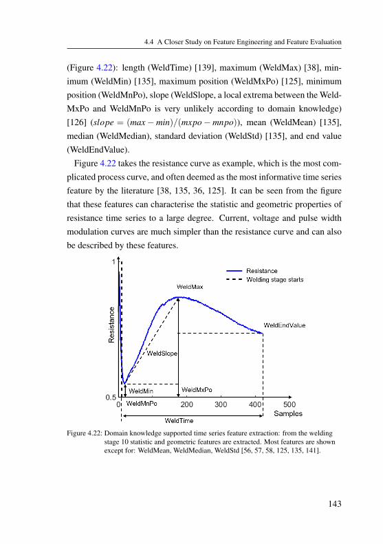
4.4 A Closer Study on Feature Engineering and Feature Evaluation
(Figure 4.22): length (WeldTime) [139], maximum (WeldMax) [38], min-imum (WeldMin) [135], maximum position (WeldMxPo) [125], minimumposition (WeldMnPo), slope (WeldSlope, a local extrema between the Weld-MxPo and WeldMnPo is very unlikely according to domain knowledge)[126] (slope = (max−min)/(mxpo−mnpo)), mean (WeldMean) [135],median (WeldMedian), standard deviation (WeldStd) [135], and end value(WeldEndValue).
Figure 4.22 takes the resistance curve as example, which is the most com-plicated process curve, and often deemed as the most informative time seriesfeature by the literature [38, 135, 36, 125]. It can be seen from the figurethat these features can characterise the statistic and geometric properties ofresistance time series to a large degree. Current, voltage and pulse widthmodulation curves are much simpler than the resistance curve and can alsobe described by these features.
Figure 4.22: Domain knowledge supported time series feature extraction: from the weldingstage 10 statistic and geometric features are extracted. Most features are shownexcept for: WeldMean, WeldMedian, WeldStd [56, 57, 58, 125, 135, 141].
143

4 Use Cases
Feature selection. The number of features grow enormously because offeature engineering. After feature extraction from time series, 80 TSFE aregenerated. After reshaping, 2470 features are generated for Setting 2 and4940 for Setting 3. These features need to be reduced before modelling.Feature selection is optimal as it preserves the features for interpretation(the other option is feature aggregation, which loses the meanings of thefeatures). The multivariate wrapper method, step-wise forward feature se-
lection [50] is applied with LR. Experiments have confirmed that featuresselected by MLP and SVR are almost the same as that by LR, because thenumber of selected features is set to 20, which allows the selected featurescover a larger range of relevant information than what is normally needed.Therefore, the same features selected by LR are also used for modellingwith MLP and SVR, to reduce the computational time.
Figure 4.23: Reducing features by feature selection. SF: single features. TS: time series.
Performance metric. This study adopts the performance metric mape (Sec-tion 2.4.8), as it is scale-independent and intuitive to the domain experts.
Normalisation. Z-score normalisation (Section 2.4.4) is applied to the inputfeatures before feeding them into modelling. The parameters for normali-sation, including mean values and standard deviations, will be learned fromthe training and validation set and applied to all input data. No normalisa-tion is applied to the output feature, the Q-Value, for the scale of Q-Value isfixed to a level (the setpoint is 1).
ML model training. Three representative classical ML methods, linearregression (LR), multi-layer perceptron with one hidden layer (MLP), andsupport vector regression (SVR) are studied. They are trained on the training
144

4.4 A Closer Study on Feature Engineering and Feature Evaluation
Table 4.15: Hyper-parameter selection of ML methods
Methods Hyper-parameters Selection method
LR #Selected features, features, look-back length Limited grid search
MLP#Selected features, features, look-back length Kept the same as LR
#Neurons, activation function Limited grid search
SVR#Selected features, features, look-back length Kept the same as LR
Kernel type, regularisation factor, degree Limited grid search
set, and their hyper-parameters are selected based on the performance on thevalidation set.
Hyper-parameter selection for LR. Two hyper-parameters are to be se-lected for linear regression, the number of selected features (ω) and look-
back length (l). Apart from the study in Use Case 4.3, additional limitedgrid search is done for the four settings. The results in Figure 4.24 illustratethe model performance evaluated on validation set of WM1 and WM3. Themodels become insensitive to the hyper-parameters after more than approx-imately 20 features are selected and when the length of look-back windowis longer than about 10. To note in Setting 3, where the EngF_Prog is used,the effective look-back time step is look-back length × number of welding
program (l×#Prog). The performance of Setting 0 and Setting 1 for WM1is more sensitive to hyper-parameters.
Hyper-parameter selection for MLP and SVR. The same feature sets de-termined by LR are used for MLP and SVR. Other hyper-parameters areselected using limited grid search. MLP has two hyper-parameters, #neu-rons in the hidden layer and the activation function. SVR has three hyper-parameters, kernel type, regularisation factor, and degree in case of polyno-mial kernel types (Table 4.15).
145

4 Use Cases
(a) (b)
(c) (d)Figure 4.24: Hyper-parameter selection with limited grid search based on performance of
validation set of WM1 for #selected features ω (a) and look-back length l (b).The performance reaches a basin in the area where ω ≈ 20 and l ≈ 10 featuresare selected. The same for WM3 in (c) and (d).
4.4.4 Results and Discussion
The models are trained again with the selected hyper-parameters on thecombined set of training data and validation data (trainingx set), and testedon the test sets. The model performance is compared and percentage im-provements are calculated with respect to Setting 0 and the best benchmark(Benchmark 3) for WM1 (Table 4.16) and WM3 (Table 4.17). The predic-tion results on WM1 are illustrated in Figure 4.25.
Interpretation of prediction results. Based on the Table 4.16 and Ta-ble 4.17, it is easy to conclude that the model performance increases as thedegree of feature engineering deepens. The performance of Setting 0 and
146

4.4 A Closer Study on Feature Engineering and Feature Evaluation
Table 4.16: LR performance on test set of WM1. Imprv. w.r.t.: improvement with respect to.
Feature settings or benchmarks mape(LR)
Imprv.w.r.t.
Setting 0
Imprv. w.r.t.Bench-mark3
Benchmark3 Qnext1 = Qpre1_Prog 2.69% -0.75% -
Setting 0 RawSF 2.67% - 0.74%
Setting 1 RawSF, TSFE 2.55% 4.49% 5.20%
Setting 2 RawSF, TSFE, EngSF 2.10% 21.35% 21.93%
Setting 3 RawSF, TSFE, EngSF, EngF_Prog 1.92% 28.09% 28.62%
Table 4.17: LR performance on test set of WM3. Imprv. w.r.t.: improvement with respect to.
Feature settings or benchmarks mape(LR)
Imprv.w.r.t.
Setting 0
Imprv. w.r.t.Bench-mark3
Benchmark 3 Qnext1 = Qpre1_Prog 5.17% -7.48% -
Setting 0 RawSF 4.81% - 6.69%
Setting 1 RawSF, TSFE 4.55% 5.41% 11.99%
Setting 2 RawSF, TSFE, EngSF 4.19% 12.89% 18.96%
Setting 3 RawSF, TSFE, EngSF, EngF_Prog 3.40% 29.31% 34.24%
Setting 1 on WM1 shows slight improvement compared to Benchmark 3.The performance of Setting 0 and Setting 1 on dataset of WM3 shows moreimprovement with respect to Benchmark 3, because the Q-Value behaviourof WM3 (Figure 2.2d) is much more complicated.
The performance improvement of Setting 1 compared to Setting 0 is in-significant, but consistent (Figure 4.24), which implies the features in theRawSF that contain time series information (the ProcessCurveMeans) al-ready provide valuable information. A significant improvement begins withSetting 2, which indicates the feature engineering strategies on the weldingoperation level are meaningful. The performance difference between Set-ting 2 and Setting 3 analysed on dataset of WM1 is rather small, but that ondataset of WM3 is evident.
147

4 Use Cases
A further inspection on the two datasets reveals that the welding programsof WM1 are always arranged in a fixed interlaced order (Figure 2.2b), i.e.the ProgNo always repeat the same pattern: Prog1, Prog2, Prog1, Prog2,..., but the welding programs of WM3 are not arranged in a fixed order. Achange of production arrangement happened in the 618th welding opera-tion (Figure 2.2d), before which the production arrangement was comprisedof three welding programs. After the 618th welding operation, three ex-tra welding programs were added to the production arrangement, which istypical in manufacturing industry since the production arrangement couldchange at any time in agile manufacturing. This explains why Setting 3, inwhich the welding program information is specially handled, has a signifi-cant improvement on dataset of WM3, but an insignificant improvement ondataset of WM1.
Interpretation of prediction visualisations. Figure 4.25 illustrates the vi-sualisation of the target values and estimated values of WM1. It can beseen that the Setting 0 and Setting 1 learned a general rising trend of thebehaviour of Q-Values. However, the dynamics of behaviour of Q-Valuesare more complex than a simple rising trend. The Q-Value trend first risesthen declines slightly, and remains stable at the end. These dynamics arebetter learned by more complicated feature settings.
Besides, although most of the Q-Values are predicted with small errors,there exist quite a few outliers that have an apparent different behaviourthan the "normal" Q-Values. These outliers seem to be random, and cannotbe explained with the trained models.
The complex dynamics of Q-Value behaviours implicate that the weldingquality is not solely influenced by the assumedly linear wearing effect. Ac-cording to domain knowledge, other influential factors include the statisticand stochastic variance caused by dressing, the chassis to be welded, etc.
Interpretation of hyper-parameter tuning results. Reviewing the hyper-parameter results (Figure 4.24b), the selection of look-back length imply
148

4.4 A Closer Study on Feature Engineering and Feature Evaluation
1700 1750 1800 1850 1900 1950
Number of welding operations
0.8
1
1.2
1.4
Q-v
alu
e
target
estimated training
estimated test
1700 1750 1800 1850 1900 1950
Number of welding operations
0.8
1
1.2
1.4
Q-v
alu
e
target
estimated training
estimated test
(a) Setting 0 (b) Setting 1
1700 1750 1800 1850 1900 1950
Number of welding operations
0.8
1
1.2
1.4
Q-v
alu
e
target
estimated training
estimated test
1700 1750 1800 1850 1900 1950
Number of welding operations
0.8
1
1.2
1.4
Q-v
alu
e
target
estimated training
estimated test
(c) Setting 2 (d) Setting 3
Figure 4.25: Prediction results zoomed into test set area of LR models on WM1.
that the hypothesis holds, that there exist temporal dependencies betweenwelding spots, since the performance of the models improves as the look-back length increases. That is to say, the Q-Value of the next welding spotis indeed dependent on the previous welding operations. Figure 4.24 alsoreveals that the improvements along degree of feature engineering is notrandom but systematic, although some times small.
Feature interpretation of WM1 with engineering knowledge. Table 4.18lists the 5 most important features with a order of descending importance forSetting 0, Setting 1, Setting 2 and Setting 3 on dataset of WM1, respectively.
149

4 Use Cases
Table 4.18: The most important 5 features selected from feature settings in the analysis ofdataset of WM1, listed in ranking of descending importance. Note that the scoreis evaluated on a multivariate basis, i.e. the importance of ω-th feature is thecombined score of the 1st to ω-th feature. The correlation coefficient between themodel estimation and target value is chosen as the feature score for an intuitivecomparison.The prefixes RawSF, TSFE, EngSF, EngF_Prog indicate the feature source, thesuffixes indicate the time stamp of the features, and the stems indicate the phys-ical meanings, e.g. Q for Q-Value, R for resistance, I for current, I2_Mean forProcessCurveMeans of current, I_WeldMin for the minimum extracted from thewelding stage.
# Setting 0 Score Setting 1 Score
1 RawSF_Q_pre2 0.72 RawSF_Q_pre2 0.72
2 RawSF_I2_Mean_pre1 0.78 RawSF_I2_Mean_pre1 0.78
3 RawSF_WearCount_next1 0.79 RawSF_WearCount_next1 0.79
4 RawSF_Q_pre9 0.81 TSFE_I_WeldMin_pre3 0.81
5 RawSF_Q_pre3 0.82 TSFE_R_WeldStd_pre8 0.82
# Setting 2 Score Setting 3 Score
1 RawSF_Q_pre2 0.72 EngF_Prog_Q_pre1 0.72
2 EngSF_NewDress_next1 0.80 EngF_Prog_WearDiff_next1 0.86
3 RawSF_I2_Mean_pre1 0.84 EngF_Prog_I2_Mean_pre1 0.87
4 TSFE_R_WeldStd_pre1 0.86 TSFE_R_WeldStd_pre1 0.88
5 RawSF_I_Mean_pre3 0.87 EngF_Prog_Q_pre2 0.88
The Q-Value of the previous second welding spot (RawSF_Q_pre2) is se-lected as the most important feature in three settings. Since the ProgNoalways repeat the same pattern: Prog1, Prog2, Prog1, Prog2, ..., the fea-ture RawSF_Q_pre2 is therefore equal to EngF_Prog_Q_pre1. EngF_Prog-_Q_pre1 is namely the Q-Value of the previous spot welded with the samewelding program as the next welding spot (this feature is identical to Bench-mark 3). This means the quality of welding usually does not have abruptchanges.
Moreover, the features RawSF_WearCount_next1, EngSF_NewDress_next1, EngF_Prog_WearDiff_next1 are selected, which means the wear-
150

4.4 A Closer Study on Feature Engineering and Feature Evaluation
ing effect has strong influence on the welding quality, and therefore qualityprediction should always consider features characterising the wearing effect.
The features RawSF_I2_Mean_pre1, TSFE_R_WeldStd_pre1, TSFE_I_-WeldMin_pre3, RawSF_I_ Mean_pre3 are selected, which means the timeseries features extracted from the welding stage indeed contain some infor-mation for predicting the next spot quality. Note that these features are ofprevious first or third spots, which are not welded with the same ProgNoas the next spot. This indicates that the information provided by historicalspots that are not welded with the same ProgNo as the next spot are also im-portant. The reason may be that the wearing effect during these temporallyadjacent welding operations has influence on the next welding quality.
In Setting 0 and 1, the selected features of relatively early operations, likeRawSF_Q_pre9, TSFE_R_WeldStd_pre8, are questionable, because theirinfluence should not be greater than temporally more adjacent features. Se-lection of these questionable features is avoided in Setting 2 and Setting 3,which feature engineering is more complex.
Feature interpretation of WM3 with engineering knowledge. As forWM3 (Table 4.19), the selected features are different. The most obviousdifference is that RawSF_Q_pre2 is no longer selected as the most im-portant feature. As mentioned in Section 4.4.4, a change of arrangementof welding programs happened in the 618th welding operation. For thesame reason, no EngSF is selected in the most important features, sinceEngSFs do not incorporate information of welding programs. Although thefeature RawSF_WearCount_next1 can also describe the dependency of Q-Value on wearing effect to some degree, as it is selected through Setting 0to 2, the performance of models trained on Setting 3 demonstrates a signifi-cant improvement (Table 4.17). This highlights the advantage of the featureEngF_Prog_Q_pre1 in Setting 3.
Many TSFEs extracted from reference curves are selected as more impor-tant than those from actual process curves. Reference curves are prescribed
151

4 Use Cases
Table 4.19: The most important 5 features selected from feature settings in the analysis ofdataset of WM3, listed in ranking of descending importance. Feature scores aresimilar to Table 4.18.The prefixes RawSF, TSFE, EngSF, EngF_Prog indicate the feature source, thesuffixes indicate the time stamp of the features, and the stems indicate the physi-cal meanings, e.g. Q for Q-Value, I2_Mean for ProcessCurveMeans of current, Rfor resistance, RefU_WeldEndValue for the end value extracted from the weldingstage of the reference curve of voltage, I_WeldMin for the minimum extractedfrom the welding stage, RefPWM for the reference curve of the Pulse Width Mod-ulation
# Setting 0 Score Setting 1 Score
1 RawSF_WearCount_next1 0.75 RawSF_WearCount_next1 0.75
2 RawSF_Time_pre2 0.81 TSFE_RefU_WeldEndValue_pre2 0.85
3 RawSF_I2_Mean_pre2 0.85 TSFE_RefR_WeldMax_pre1 0.88
4 RawSF_R_Mean_pre1 0.86 TSFE_I_WeldMin_pre3 0.90
5 RawSF_Power_Mean_pre10 0.87 TSFE_R_WeldMax_pre1 0.90
# Setting 2 Score Setting 3 Score
1 RawSF_WearCount_next1 0.75 EngF_Prog_Q_pre1 0.79
2 TSFE_RefU_WeldEndValue_pre2 0.85 EngF_Prog_WearDiff_next1 0.91
3 TSFE_RefR_WeldMax_pre1 0.88 TSFE_RefR_WeldSlope_pre2 0.92
4 TSFE_I_WeldMin_pre3 0.90 RawSF_WearCount_next1 0.93
5 TSFE_R_WeldMax_pre1 0.90 TSFE_RefPWM_WeldMean_pre4 0.93
by the welding programs, and are therefore always identical for a specificprogram. This implicates that the next spot quality is also dependent on thewelding programs performed on the previous spots, rather than the corre-sponding actual process curves. This phenomenon is not evident for WM1,since its welding program arrangement is fixed. Similar to the case of WM1,complex feature engineering avoids selection of questionable features likeRawSF_Power_Mean_pre10.
Interpretation of results of MLP and SVR models. Table 4.20 and 4.21list the results of MLP and SVR models trained with the features determinedby LR models and their hyper-parameters selected using limited grid search.
152

4.4 A Closer Study on Feature Engineering and Feature Evaluation
Table 4.20: MLP and SVR models evaluated on test set of WM1. “rbf": Radial-Basis-Function.
Featuresettings
mape(MLP)
Activationfunction
#Neurons mape(SVR)
Kerneltype
Regularisationfactor
Setting 0 2.27% tanh 5 2.25% rbf 8.17
Setting 1 2.42% tanh 25 1.94% rbf 10.19
Setting 2 2.03% tanh 50 2.08% rbf 6.15
Setting 3 1.92% tanh 53 1.87% rbf 8.17
Table 4.20 and 4.21 demonstrate that performance can indeed be improvedby non-linear models. This indicates that there exist non-linearity and inter-action between the selected features, which cannot be described using theLR models.
The performance of MLP models are usually better than LR models. Theperformance gain becomes significant for complicated datasets (WM3) withthe highest degree of feature engineering (Setting 3). Conspicuous is that theSetting 1 model performance is worse than that of Setting 0 for both weldingmachines (Note that the number of selected features are the same for allsettings. Only the available features before feature selection are different.).This indicates the time series features engineered may cause overfitting insome cases.
A closer look at the results of LR and MLP models on the test set ofWM3 for two example welding programs with Setting 3 is illustrated inFigure 4.26. It reveals that although the different welding programs havevery different behaviour of Q-values, both LR and MLP models are able to
Table 4.21: MLP and SVR models evaluated on test set of WM3. “rbf": Radial-Basis-Function.
Featuresettings
mape(MLP)
Activationfunction
#Neurons mape(SVR)
Kerneltype
Regularisationfactor
Setting 0 3.87% tanh 50 4.02% rbf 19.02
Setting 1 4.07% tanh 47 4.49% rbf 21.29
Setting 2 3.57% logistic 60 4.32% rbf 14.79
Setting 3 2.97% tanh 44 3.34% rbf 16.00
153

4 Use Cases
860 880 900 920 940 960
Number of welding operations (only for Prog1)
0.6
0.8
1
1.2
1.4
1.6
Q-v
alu
e
target
estimated test LR
estimated test MLP
860 880 900 920 940 960
Number of welding operations (only for Prog3)
0.6
0.8
1
1.2
1.4
1.6
Q-v
alu
e
target
estimated test LR
estimated test MLP
(a) Setting 3 Prog 1 (b) Setting 3 Prog 3
Figure 4.26: Examples of prediction results on test set of WM3 illustrated for two weldingprograms, with the model of MLP with the Setting 3 of feature engineering, 20features selected, and a look-back length of 10.
capture the different dynamics. From the figure the performance of the twomodels are not easy to differentiate. This indicates the importance of thenumerical performance metric in Table 4.17 and 4.21.
The performance of SVR models are on par with the LR models. Alsoconspicuous is that the performance of SVR models does not always im-prove as the degree of feature engineering increases. A further investigationof SVR models reveals that the performance of them fluctuates irregularlyquite a few (up to 1.2% mape) as the regularisation factor changes, whichmeans SVR models often fall into local optimums. Some SVR models per-form well on training and validation sets but perform badly on test sets,which indicates a tendency of overfitting.
4.4.5 Conclusion and Outlook
Conclusion. This use case studies the ML pipelines of feature engineeringwith more domain knowledge integration than that in Use Case 4.3, the de-gree of which is intensified through four feature settings. In the area of the
154

4.4 A Closer Study on Feature Engineering and Feature Evaluation
selected two hyper-parameters, the machine learning method is insensitiveto the hyper-parameters, number of features and look-back length, which isdesired for industrial application. Furthermore, the results and selected fea-tures are extensively interpreted to provide more insights to the domain per-spective. A blind training of ML models would select questionable and lessrobust features. Through domain knowledge-supported feature engineering,visualisation of prediction results and interpretation of selected features, theexplainable ML pipelines of feature engineering can avoid this, enabling arelatively transparent understanding of machine learning modelling.
Outlook. In future work, the following directions are valuable from bothindustrial and academic points of view:
• Testing the proposed approach on more datasets to verify the generalis-ability.
• Exploring other feature extraction strategies on complex welding ma-chines.
• Investigating other machine learning methods, e.g. other types of arti-ficial neural networks, especially recurrent neural networks, which aresuitable for processing data with temporal structures.
• Predicting the Q-Value of the next welding spot as a probabilistic distri-bution, by using e.g. quantile regression [199]. Before the next weldingactually happens, the next Q-Value can in fact not be deterministicallypredicted. The prediction of the next Q-Value in this work is actually aprediction of the mean value. A better way is probabilistic forecasting.
• Using the prediction results as a basis for process optimisation. Afterthe next spot quality is predicted, there exist several possible measuresto undertake, e.g. flexible dressing, adaptation of the reference curves,or switching to non-adaptive control mode.
155

4 Use Cases
4.5 Transferability of Models between Datasets
Overview: Once ML models are developed for some datasets, it is desiredand necessary to transfer these models to other datasets. This section studieswhether the ML model trained on one dataset can be transferred to datasetscollected from other welding machines. The feature settings and models arethe same as in Use Case 4.4. The target output of the ML models is thesame: Q-Value of future welding operations. The studied data are collectedfrom WM1 (or WMG), WM2 (WMI), and WM3 (WMR) in Use Case 4.2.An overview of the corresponding application questions, open questions andmethods is listed in Table 4.22.
Table 4.22: Overview of application questions (AQ), open questions (OQ) and methods (M)
AQ OQ MethodsAQ5, AQ10 OQ4, OQ8 M2.1.1, M2.4.5
4.5.1 Question Definition
This use case studies the transferability between models trained on differentdatasets, e.g. whether it is possible to train ML models on the dataset ofone welding machine and apply them on another welding machine (Figure4.27). The transferability is very desired in industrial scenarios, becausethere exist many advantages if a model trained on the dataset of one machinecan be transferred to another new machine, without change or with smalladaptation:
Figure 4.27: The simple workflow of model transfer. D1: Dataset 1. D2: Dataset 2.
• The cost of extra data collection on the new welding machine can beobviated or at least reduced;
156

4.5 Transferability of Models between Datasets
• The cost of new model development, or old model adaptation, for thenew welding machine can be saved;
• The time, in which the new machine performs manufacturing tasks butits product quality is not fully covered by data-driven monitoring, can beminimised.
ML models of Setting 3 introduced in Use Case 4.4 provide good predic-tion accuracy and are explainable. Their transferability will be investigated.
4.5.2 Data Description
Apart from the two datasets described in Section 4.4, the dataset collectedfrom WM2 is also studied. The three datasets are summarised again forreaders’ convenience in Table 4.23. Their Q-Values are illustrated in Fig-ure 2.2 for WM1, Figure 4.15 for WM2, and Figure 4.20 for WM3.
Table 4.23: Example datasets for studying model transferability
Dataset Welding machine #Prog #DT #DTtr #DTval #DTtst
Dataset 1 WM1 2 1998 1456 219 323Dataset 2 WM2 4 3996 3127 448 421Dataset 3 WM3 6 5839 4474 602 763
4.5.3 Experiment Settings
This section first introduces a preliminary experiment and the problem re-vealed by this experiment. Then it explains the solution to the problem andthe experiment settings to implement the solution.
Data splitting according to temporal structure. The data splitting strat-egy is exactly the same as in Use Case 4.4. Since after the hyper-parameterselection, the ML models need to be trained again using training and valida-tion sets, the training and validation dataset can be deemed as the “trainingdataset” in a more general sense, and will be referred to as the “trainingxset” (Dtrx).
157
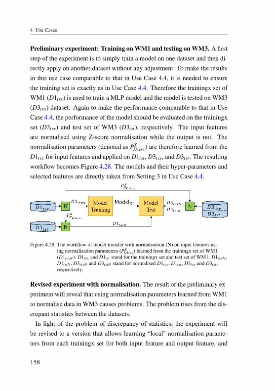
4 Use Cases
Preliminary experiment: Training on WM1 and testing on WM3. A firststep of the experiment is to simply train a model on one dataset and then di-rectly apply on another dataset without any adjustment. To make the resultsin this use case comparable to that in Use Case 4.4, it is needed to ensurethe training set is exactly as in Use Case 4.4. Therefore the trainingx set ofWM1 (D1trx) is used to train a MLP model and the model is tested on WM3(D3trx) dataset. Again to make the performance comparable to that in UseCase 4.4, the performance of the model should be evaluated on the trainingxset (D3trx) and test set of WM3 (D3tst ), respectively. The input featuresare normalised using Z-score normalisation while the output is not. Thenormalisation parameters (denoted as PX
D1trx) are therefore learned from theD1trx for input features and applied on D1tst , D3trx, and D3tst . The resultingworkflow becomes Figure 4.28. The models and their hyper-parameters andselected features are directly taken from Setting 3 in Use Case 4.4.
Figure 4.28: The workflow of model transfer with normalisation (N) on input features us-ing normalisation parameters (PX
D1trx) learned from the trainingx set of WM1(D1trxN ). D1trx and D1tst stand for the trainingx set and test set of WM1. D1trxN ,D1tstN , D3trxN and D3tstN stand for normalised D1trx, D1tst , D3trx and D3tst ,respectively.
Revised experiment with normalisation. The result of the preliminary ex-periment will reveal that using normalisation parameters learned from WM1to normalise data in WM3 causes problems. The problem rises from the dis-crepant statistics between the datasets.
In light of the problem of discrepancy of statistics, the experiment willbe revised to a version that allows learning “local" normalisation parame-ters from each trainingx set for both input feature and output feature, and
158

4.5 Transferability of Models between Datasets
Figure 4.29: Normalisation parameters learned from each trainingx set and applied to train-ingx set and test set before model transfer. The results are better than that inFigure 4.28, and therefore the model transfer is tested on WM2 and WM3.
applying the learned normalisation parameters on the trainingx set and itscorresponding test set, respectively, as shown in Figure 4.29. Before test-ing the models on WM2 and WM3, the normalisation parameters will belearned from trainingx set of WM2 and applied to trainingx set and test setof WM2. The same workflow repeats for models trained on trainingx set ofWM3 and tested on WM1 and WM2.
4.5.4 Results and Discussion
Preliminary experiment and the revealed problem. The results of thepreliminary experiment are listed in Table 4.24 and illustrated in Figure4.30.
Table 4.24: Performance of the model trained on D1trx (trainingx set of WM1) and testedon D1tst and D3tst (test set of WM1 and WM3) in the preliminary experiment.Normalisation parameters are only learned from D1trx. The blue texts indicate thetraining set and test set are collected from the same welding machine.
TrainingMethod
mape of model testingset D1trx D1tst D3trx D3tst
Row1 D1trx MLP 1.92% 1.81% 10.3% 10.0%
Table 4.21 shows that the model transfer results on WM3 are significantlyworse than that of WM1, on which the model is trained. Comparing the (a)and (b) in Figure 4.30, it can be seen clearly that there exists a discrepancyof mean value when testing the model.
159

4 Use Cases
Since normalisation is only performed on input features, not on output (Q-Value), it is natural to hypothesise that the mean value of Q-Values of WM1is different from that of WM2. A simple calculation gives that the meanvalue of Q-Value in D1trx is 1.09, and that in D2trx is 1.17 (anonymised).This confirms the hypothesis. Furthermore, the statistics, e.g. mean valuesand standard deviations, of input features in WM1 also differ from that inWM3. The experiment of directly transferring a model trained on WM1to WM3 reveals the problem caused by the difference of statistics betweendatasets. To improve the results, normalisation parameters should be learned“locally” from the dataset to be transferred to.
0 500 1000 1500 2000
Number of welding operations
0.6
0.8
1
1.2
1.4
1.6
Q-V
alue
target training test
0 1000 2000 3000 4000 5000 6000
Number of welding operations
0.6
0.8
1
1.2
1.4
1.6Q
-Val
ue
target training test
(a) (b)Figure 4.30: (a) Results of the MLP model trained on and tested on WM1. It is the complete
version of Figure 4.25d.(b) Results of the MLP model trained on the trainingx set of WM1 and tested onWM3.
Revised experiments. The results of the revised experiment are listed inTable 4.25. Each row lists the performance of the models trained on thedataset in the “Training set” column and tested on several datasets. The bluetexts indicate the case when the data are trained and tested on the datasetscollected from the same welding machine.
In particular, Row 1 and Row 2 list performance of ML models trained onD1trx and tested on D1, D3, and D2 with the methods LR and MLP. Row3 and Row 4 list performance of ML models trained on D3trx and tested onD1, D3, and D2 with the methods LR and MLP. Note that to evaluate the
160

4.5 Transferability of Models between Datasets
performance of model transfer to WM2, the performance of models trainedon D2 and tested on D2 is needed, and is added in Row 5. Comparing Row1 in Table 4.24 and Row 2 in Table 4.25 reveals that learning normalisationparameters from each dataset improves the performance slightly, from about10% mape to 8% or 9%.
However, in general the performance of models transferring is not good.The performance of Benchmark 3 for WM1, WM2, and WM3 is 2.69%,2.67%, and 5.17%. All performance of model transfer is worse than that.By comparing the model performance in each column, it shows that themodel performance deteriorates significantly when testing on the datasetscollected from other welding machines. In particular, looking at Column1 and Column 2, it reveals that the model performance trained on D1 andtesting on D1 is about 2% mape, but the mape is more than 5% when themodel is trained on D2trx. The same phenomena repeat when looking atColumn 3 and Column 4. The added Row 5 further confirms this.
Figure 4.31 illustrates the prediction results of MLP and LR modelstrained on D1trx and tested on D3 and D2. It reveals although the problemof mean shift is eliminated by learning “local” normalisation parameters,the discrepant dynamics in behaviours of Q-Values still cause problems formodel transfer. On one hand, the Q-Values of WM3 have a larger range
Table 4.25: Performance of the model trained on D1trx (trainingx set of WM1) or D3trx (train-ingx set of WM3) and tested on D1tst , D2tst , and D3tst (test set of WM1, WM2and WM3) in the revised experiment. Normalisation parameters are learned fromeach trainingx set. The blue texts indicate the training and test set are collectedfrom the same Welding Machine.
mape of model testingTraining Method Col1 Col2 Col3 Col4 Col5 Col6
set D1trx D1tst D3trx D3tst D2trx D2tst
Row1 D1trx LR 1.93% 1.92% 9.11% 8.65% 5.71% 4.53%Row2 D1trx MLP 1.93% 2.03% 8.93% 8.40% 5.64% 4.36%Row3 D3trx LR 6.00% 6.05% 3.02% 3.40% 3.95% 3.49%Row4 D3trx MLP 5.36% 5.38% 2.72% 3.10% 3.90% 3.56%Row5 D2trx LR - - - - 2.25% 2.07%
161

4 Use Cases
than that of WM1 and have more complex dynamics (WM3 has 6 weldingprograms). The models trained on D1trx are not capable to cope with thecomplexity. On the other hand, the models trained on D3trx are too complexfor transferring to WM1. By comparing Figure 4.30 and Figure 4.31c andd, it reveals that the predicted Q-Values are “chunkier” than they shouldbe, because the Q-Values of WM3 are “chunkier” than that of WM1 in theillustrated shape.
4.5.5 Conclusion and Outlook
Conclusion. In summary, transferring a model by simply training the modelon one dataset and applying on another is not sufficient. Normalisation of
0 1000 2000 3000 4000 5000 6000
Number of welding operations
0.4
0.6
0.8
1
1.2
1.4
1.6
Q-V
alue
target training test
0 1000 2000 3000 4000 5000 6000
Number of welding operations
0.4
0.6
0.8
1
1.2
1.4
1.6
Q-V
alue
target training test
(a) (b)
0 500 1000 1500 2000
Number of welding operations
0.6
0.8
1
1.2
1.4
1.6
Q-V
alue
target training test
0 500 1000 1500 2000
Number of welding operations
0.6
0.8
1
1.2
1.4
1.6
Q-V
alue
target training test
(c) (d)Figure 4.31: The results of the MLP model (a) or LR model (b) trained on D1trx and tested
on D3. The results of the MLP model (c) or LR model (d) trained on D3trx andtested on D1.
162

4.5 Transferability of Models between Datasets
the new dataset with the learned parameters brings a slight improvement butalso does not provide satisfactory results. Transferring a model trained withmore complex data to simpler data is more promising than the other wayaround.
Outlook. In future work, the following directions can potentially improvethe model transfer performance:• In this use case, learning “local” normalisation parameters has used a large
amount of data, which does not reduce the effort and cost of data collec-tion. In the future, less data should be used to learn the normalisationparameters, and a dynamic approach for adjusting the normalisation pa-rameters can be investigated, so that learning “local” normalisation pa-rameters indeed becomes practical.
• To adopt a transfer learning approach to fine-tune ML models on newdatasets and studying the necessary data amount for fine-tuning.
• To develop an active learning approach to constantly adjusting ML modelson new datasets. This could also handle the OQ7 concept drift problem.
• To train a Master Model on a large dataset collected from a group of weld-ing machines and fine-tuning the master model to tailor to specific weldingmachines. The Master Model should be trained on a very complex dataset,as the results indicate transferring from a model trained from complex datato simpler data is more promising than the other way around.
163

4 Use Cases
4.6 Transferability to Another Application:Laser Welding
Overview: This use case tests the transferability of the proposed frameworkand approaches to another quite different welding process, laser welding.The methods in this use case are however not limited to laser welding, butalso apply to other laser processes, e.g. high-precision laser machining andsurface treatment. This use case study is accomplished in cooperation withDmitriy Mikhaylov. The author’s contribution is conceptualisation, design,and implementation of ML methods of Neural Networks. The followingpublications are based on/related to this use case: [200], [201]. An overviewof the corresponding application questions, open questions and methods islisted in Table 4.26.
Table 4.26: Overview of application questions (AQ), open questions (OQ) and methods (M)
Application Question Open Question Methods
AQ2, AQ6 OQ1, OQ5, OQ8 M2.1.3, M2.2.3, M2.2.4
The target output of the machine learning models is the input laser ampli-tude matrix to an optic system for achieving the desired output laser ampli-tude distribution. This is a supervised multivariate regression problem. Theresults of ML models are tested in laboratory experiments to validate themethods and compared to conventional non-ML benchmarks.
In addition, an analysis of the influence of amount of training data onprediction accuracy is conducted to gain insights for preparing costly datacollection from laboratory or production.
The data for model development are collected in a laboratory setting. Thetested machine learning methods are linear regression and convolutionalneural networks.
164

4.6 Transferability to Another Application: Laser Welding
4.6.1 Question Definition
Liquid crystal on silicon phase-only spatial light modulator (LCoS-SLM) isa type of optical device often used to generate beam splitter patterns (de-noted as a matrix A) for parallelised high-precision laser processes. The ac-curacy of laser power amplitude distribution of these processes is essentialfor many laser applications, e.g. multifocal fluorescence microscopy [202,203, 204], two-photon polymerisation [205] or high-precision laser materialprocessing.
In application, the laser light from the laser source (Figure 4.32) is ex-panded to a broader single laser beam by the beam expander, then trans-formed to a set of beams by the spatial light modulator, and goes through aseries of optical devices and reaches the workpiece. The output laser ampli-tude distribution can be measured by a camera if an extra beam attenuatoris installed to scale down the laser amplitude. The measured amplitude dis-tribution can be described by a matrix Ameas. An ideal optical system willoutput the desired amplitude distribution (Ades) so that Ameas = Ades, whilein reality the Ameas normally differs from Ades to some degree.
In order to achieve an Ameas more close to Ades, a phase hologram (φ )needs to be generated and fed into the SLM. Many algorithms [206] (knownas phase retrieval algorithms) attempted to calculate the phase hologramφ from an input amplitude distribution matrix (Ain), by iterative or non-iterative methods. Among which, the weighting Iterative Fourier Transform
algorithm (IFTA) is a most commonly used method because it has fewerconstraints and enables fast implementation and calculation [207, 208]. Tra-ditionally, the Ain is directly set to Ades and ideally Ameas should be equal toAdes.
However, the actual Ameas deviates from Ades to a certain degree, becauseIFTA assumes an ideal optical setup, differing from the real experimentalsystem. To overcome this small deviation, an extended IFTA with a closedcamera feedback loop (referred to as Camera-IFTA) was proposed [209],
165

4 Use Cases
Figure 4.32: Schematic illustration of an application of the liquid crystal on silicon phase-only spatial light modulator (LCoS-SLM). φ indicates the phase hologram cal-culated by Iterative Fourier Transformation Algorithm (IFTA). An extra beamattenuator is needed for scaling down the laser amplitude to measure the outputamplitude distribution (Ameas) using a camera. The figure is modified from [201].
achieving higher accuracy, but increasing the computational time signifi-cantly.
To achieve both high accuracy and fast computation, this section proposesnovel approaches of ML-aided phase retrieval algorithms to combineIFTA, camera feedback, and machine learning algorithms.
The basic idea is to extend the standard IFTA with an ML model for com-puting the phase hologram, so that the ML-aided IFTA can achieve higheraccuracy than IFTA, and with much less time than the Camera-IFTA. TheML model is pre-trained using a dataset with Ameas as the input data andAin as the output data (Ain = fml(Ameas)), so that the ML model can beseen as an inverse model of the optical system ( fml = f−1
optics). The op-tical system includes IFTA, SLM and the subsequent optical setups untilthe camera in Figure 4.32. After that, the desired distribution Ades is in-put to the ML model to estimate the output of the ML model, which is anestimated input of the optical system Ain that should have Ades as output,i.e. Ain = fml(Ades)⇒ Ades = foptics(Ain). The extended ML-aided IFTApipeline is illustrated in Figure 4.33.
166
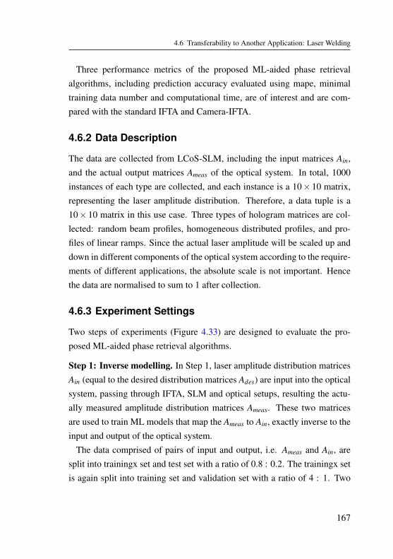
4.6 Transferability to Another Application: Laser Welding
Three performance metrics of the proposed ML-aided phase retrievalalgorithms, including prediction accuracy evaluated using mape, minimaltraining data number and computational time, are of interest and are com-pared with the standard IFTA and Camera-IFTA.
4.6.2 Data Description
The data are collected from LCoS-SLM, including the input matrices Ain,and the actual output matrices Ameas of the optical system. In total, 1000instances of each type are collected, and each instance is a 10× 10 matrix,representing the laser amplitude distribution. Therefore, a data tuple is a10× 10 matrix in this use case. Three types of hologram matrices are col-lected: random beam profiles, homogeneous distributed profiles, and pro-files of linear ramps. Since the actual laser amplitude will be scaled up anddown in different components of the optical system according to the require-ments of different applications, the absolute scale is not important. Hencethe data are normalised to sum to 1 after collection.
4.6.3 Experiment Settings
Two steps of experiments (Figure 4.33) are designed to evaluate the pro-posed ML-aided phase retrieval algorithms.
Step 1: Inverse modelling. In Step 1, laser amplitude distribution matricesAin (equal to the desired distribution matrices Ades) are input into the opticalsystem, passing through IFTA, SLM and optical setups, resulting the actu-ally measured amplitude distribution matrices Ameas. These two matricesare used to train ML models that map the Ameas to Ain, exactly inverse to theinput and output of the optical system.
The data comprised of pairs of input and output, i.e. Ameas and Ain, aresplit into trainingx set and test set with a ratio of 0.8 : 0.2. The trainingx setis again split into training set and validation set with a ratio of 4 : 1. Two
167

4 Use Cases
Figure 4.33: Extended ML-aided IFTA with 2 steps: inverse modelling and model application.The figure is modified from [201].
types of ML models, regularised Linear Regression (LR) and ConvolutionalNeural Networks (CNN) are trained.
The CNN models are first trained on the training set. The hyper-parametersof CNN models are selected based on the performance on the validation set.A series of architectures, including different layers, number of layers andnumber of neurons, were experimented using limited grid search (varyingone while fixing other hyper-parameters). In particular, using C denot-ing the Conv2d layer, D denoting the Dense layer, the tested architecturesinclude: C, CC, CCC, CCCC, CD, CCD, and CDC. Among which, twoarchitectures, CC and CD, prevail in performance and are selected. Thebest CC network selected based on the performance of validation set isConv256-Conv1 with filter sizes of (6,6) and (4,4) for each layer. The bestCD network is Conv320-Dense100 with a filter size of (6,6) in the Conv2dlayer. All activation functions are ReLU (rectified linear units). The “Adam”optimiser is adopted, and loss function is mape.
After that, CC and CD with the best hyper-parameters and LR are trainedagain with the trainingx set (combining training and validation set) andtested on the test set (200 matrices), and evaluated with mape and maxape(maximal absolute percentage error).
168

4.6 Transferability to Another Application: Laser Welding
Table 4.27: Data splitting to seven subsets of different training data number
Dataset name D1 D2 D3 D4 D5 D6 Dall
#Trainingx data 10 50 101 150 200 400 800
#Test data 200 200 200 200 200 200 200
Step 2: Model application. In Step 2, the ML models are applied and theresults are validated in an experimental setting. In particular, the desireddistribution matrices Ades of the test set (200 matrices) are used as inputto the ML models (in contrast to Step 1 where Ades is used as output) toestimate the input distribution of optical systems Ain, that should have Ades
as output.Then the estimated distribution matrices Ain are input into the optical sys-
tem in the laboratory to generate the output, measured as A′meas. These A′meas
are compared with Ades using mape and maxape to quantify the performanceof ML models in experimental validation.
Data splitting into subsets of different training data numbers. To ad-dress the open question how many minimal data are necessary, the trainingdata set is split into a series of subsets of different numbers of data tuples(Table 4.27), similar to Use Case 4.1. All three selected ML models, LR,CC and CD are trained with each subset of training data and evaluated interms of prediction accuracy and experimental validation.
4.6.4 Results and Discussion
The performance in model application (Step 2) of the best ML-aided IFTA,whose ML models are trained with 800 trainingx set, are validated with thetest set (200 matrices) and compared with two benchmarks in Table 4.28.Note that the IFTA calculation in each phase retrieval algorithm has internalerrors. Thus the error of any IFTA-based phase retrieval algorithm cannotbe lower than the IFTA calculation error. This error is also listed in Row 1 inTable 4.28 for reference. The two benchmarks are standard IFTA (referred
169

4 Use Cases
to as IFTA) and extended IFTA with a closed camera feedback loop (referredto as Camera-IFTA).
Table 4.28 reveals that the ML-aided phase retrieval algorithms have sig-nificantly better performance compared to the standard IFTA. Especially theLR-aided IFTA and CC-aided IFTA can even approximate the performanceof Camera-IFTA.
The mape is the mean absolute error calculated by comparing the A′meas
and Ades. Since each A′meas is a 10× 10 matrix, the comparison of eachmatrix has a mape. The average values of mape (µ) of the 200 test datatuples for each method are listed in Column 2, while the standard deviationof mape (σ ) are listed in Column 3. Similarly, the maxape is the maximalabsolute error of the comparison between A′meas and Ades. Its average valuesand standard deviations are listed in Column 4 and Column 5.
Table 4.28: Performance comparison of ML-aided IFTA with the best ML models
Method mape (%) maxape (%)µ σ µ σ
IFTA calculation 1.11 0.37 5.06 1.99IFTA 7.14 0.35 24.7 1.92
Camera-IFTA 1.93 0.31 7.80 2.33LR-aided IFTA 2.36 0.40 8.46 1.66CC-aided IFTA 2.46 0.29 8.99 1.95CD-aided IFTA 3.59 0.47 13.00 2.50
A further analysis of necessary training data number for ML models isillustrated in Figure 4.34. The two figures on the left side are the results ofmodel prediction accuracy in Step 1 of Figure 4.33, and on the right side arethe results of model application accuracy in Step 2.
Figure 4.34 gives the relationship between method performance and num-ber of data tuples used for model training and validation. Sub-figures ofboth prediction performance (left column) and experimental validation per-formance (right column) indicate that LR and CC are much better than CDwhen training data number < 400. After that their performance becomescomparable. LR and CC are quite close in performance when training data
170

4.6 Transferability to Another Application: Laser Welding
0
10
20
30m
apeP(%)
0
10
20
30
mapeE(%)
7.14 %
LR CC CD IFTA Benchmark
10
50
101
150
200
400
800
Training data number
0
25
50
75
100
maxa
peP(%)
10
50
101
150
200
400
800
Training data number
0
25
50
75
100
maxa
peE(%)
24.7 %
Figure 4.34: ML models for prediction and experimental validation compared to IFTA. Thefigure is modified from [201].
number≥ 150. CC can still achieve relatively good performance when train-ing data number is only 101, while LR needs the training data number to beat least 150, because the Theory of Equation requires the number of equa-tions > number of variables.
In summary, the ML-aided IFTA need at least 150, 101, 400 training datatuples for the ML model of LR, CC, and CD respectively, to achieve sig-nificantly improvement compared to standard IFTA. This is summarised inTable 4.29.
Table 4.29 evaluates the ML-aided methods considering minimal num-ber of training data, and computational time. The standard IFTA takes 40seconds for each hologram computation with relatively large errors. TheCamera-IFTA takes 280 seconds for each hologram computation with sig-nificantly better performance, serving as benchmark for the proposed ML-aided methods. The LR-aided IFTA needs at least 150 training data, re-quiring about 270 seconds for data collection and neglectable training time.
171

4 Use Cases
Once the LR model is trained, no further data collection time and trainingtime is needed. After that, the computation of each hologram takes 40 sec-onds, since the method is based on IFTA. This means the LR-aided IFTAbecomes more efficient from the computation of the 2nd hologram (270s +40s × 2 = 350s) than the Camera-IFTA (280s × 2 = 560s), while achievinga comparably good performance as Camera-IFTA. Similarly, the CC-aidedIFTA saves time already from the 1st hologram (182s + 40s = 222s < 280s)than Camera-IFTA, and CD-aided IFTA saves time from the 4th hologram(720s + 40s× 4 = 880s, better than that of Camera-IFTA 280s× 4 = 1120s).
Table 4.29: Evaluation of ML-aided methods considering time
Method Minimal#trainingx
data
Minimal datacollection
time
Trainingtime
Hologramcomputation
time
#Data from whichML method saves
time
IFTA - - - 40s -
Camera-IFTA - - - 280s Benchmark
LR-aided IFTA 150 270s <1s 40s 2
CC-aided IFTA 101 182s 5s 40s 1
CD-aided IFTA 400 720s 38s 40s 4
4.6.5 Conclusion and Outlook
Conclusion. This use case has studied improving phase retrieval algorithmin laser beam splitting application by extending the standard IFTA with MLmodels. The performance of the ML models is validated both from MLperspective with training and test, and from domain perspective with labo-ratory experiments. To further improve the adoptability and efficiency, theinfluence of training data number on model performance is studied. All MLmethods have shown comparable performance and improvement in compu-tation time, compared to the state-of-the-art phase retrieval algorithm, theCamera-IFTA, given that sufficient training data are provided. ML-aidedIFTA has better comprehensive performance if several holograms need to
172

4.6 Transferability to Another Application: Laser Welding
be calculated. Especially CC-aided IFTA surpasses Camera-IFTA in termsof efficiency for even the calculation of the first hologram.
Outlook. In the studied use case the input and output of the optical sys-tem are required to be dense matrices. In industrial application, sometimessparse matrices are used. In this case, the three proposed ML methods, LR,CC and CD, become not suitable anymore. The sparse matrices have twocomplexity levels. The simpler version is when the number of laser spots inthe input amplitude matrix Ain equals the number of laser spots in the outputmatrix Ameas. In this case, the spatial information of the laser spots can beprovided as features for ML modelling. The more complex version is whenthe number of laser spots in the input matrix Ain does not equal that in theoutput matrix Ameas. This case may be handled by padding the matrix withthe shorter length. These questions remain as future research direction.
173


5 Conclusion and Outlook
Aiming on studying and developing effective and generalisable machinelearning frameworks for quality monitoring in electrical resistance welding(Section 1.6), this work goes beyond the boundaries of data science, com-bining perspective of machine learning, domain knowledge and semantictechnologies. This chapter first summarises the study concisely, then makesseveral conclusions, and finally previews future research.
Summary. Firstly, this work reviews (Chapter 1) state-of-the-art of machinelearning methods for product quality monitoring in electric resistance weld-ing (ERW) and summarises open questions in this field. To address theseopen questions, this work proposes a framework of ML methods (Chap-ter 2), which expands the angle from traditional machine learning to deepintegration of domain knowledge and to semantic technologies such as on-tologies and templates. Then, a concise description of some technical pointsfor implementation of the framework (Chapter 3) is given. After that, thiswork demonstrates six industrial use cases (Chapter 4) to exemplify andevaluate some methods in the framework.
Contribution. The major contribution of this work is a framework of ma-chine learning in ERW that pursues a comprehensive coverage on topics ofquality monitoring in ERW. In particular, it includes the following contribu-tions.
1. Revealing many domain aspects and data particularities in ERW thatare little discussed in the literature (Section 2.1), including: (1) qual-ity indicators subsumed into six fidelity levels and accessibility; (2)
175

5 Conclusion and Outlook
the multi-levels of temporal structures in data; (3) insufficient dataproblem summarised into three data challenges; (4) a comprehensivelist of application questions related to three data sources: production,lab, and simulation;
2. A novel simulation-supported data collection regime for ERW (Sec-tion 2.2), including: (1) procedures and methods of interactive dataacquisition and analysis; (2) datasets similarity analysis; (3) inversemodelling of simulation model; (4) data amount and feature sets anal-ysis; (5) datasets evaluation;
3. A new ontology-supported data preparation scheme for ERW (Sec-tion 2.3), including: (1) convenient domain ontology construction byusers based on upper ontology and templates for process and data un-derstanding; (2) ontology-aware data integration to the Uniform Data
Format to unify the data from different sources, versions, and pro-cesses; (3) a mechanism to link the Uniform Data Format to machinelearning;
4. A systematic approach for selecting suitable ML methods and con-structing ML pipelines for ERW (Section 2.4), including: (1) a noveldata preprocessing design to handle the temporal structures by spe-cial data splitting, reshaping, and hierarchical feature extraction; (2)several feature engineering strategies with deep integration of do-main knowledge; (3) discussion of feature selection, normalisationand classic machine learning methods; (4) ontology-enabled ML en-hancement that allows semi-automated and user-configurable ma-chine learning pipeline construction; (5) a special design of neuralnetworks for hierarchical feature learning; (6) discussion of perfor-mance metrics, such as prediction accuracy and several adoptabilitymetrics;
176

5 Conclusion and Outlook
5. Successful validation of the proposed ML framework with five in-dustrial use cases of ERW, including: (1) simulation-supported dataanalysis and collection (Section 4.1), (2) visualisation and evaluationof a large amount of production data to detect conspicuous weldingmachines and welding programs for further analysis (Section 4.2),(3) regression analysis to predict the next quality for comparing twoschool of ML pipelines: feature engineering - classic ML and fea-ture learning - neural networks (Section 4.3), (4) regression analysiswith deep integration of domain knowledge and gaining insights fromfeature evaluation (Section 4.4); (5) transferability analysis of MLmodels trained with data of one machine to data of other machines(Section 4.5).
6. Successful demonstration of the transferability of the proposed MLframework with an industrial use case of high-precision laser pro-cesses (Section 4.6);
7. The implementation of the proposed ML framework with two pro-gramming platforms, Python and SciXMiner (MATLAB) (Chapter 3),including six ML modules and ML pipeline components of datapreparation, data preprocessing and ML modelling.
Conclusion. From the review of state-of-the-art and open questions, it canbe seen that the difficulties of efficient machine learning in ERW, as wellas in manufacturing, are not development of novel and complex ML algo-rithms. Instead, a system solution is needed that covers multi-faceted topicsfrom data collection, through data management, and to ML development.
This work proposes a framework of ML in ERW for quality monitoring,aiming at establishing a system solution to cover these broad topics, whichnaturally is not confined to the application of quality monitoring in ERW butalso applicable to other questions of similar mathematical nature in discretemanufacturing. The target-oriented approach results in an interdisciplinary
177

5 Conclusion and Outlook
framework that combines three perspectives: data science, manufacturingtechnologies, and semantic technologies. This work designs the architectureof the framework and provides theoretical corner stones as well as evalua-tion use cases in the five aforementioned topics: question definition, datacollection, data preparation, data preprocessing and ML modelling.
Nevertheless, much work remains to be done to further evaluate and im-prove the proposed framework. This work starts the journey towards moreintelligent manufacturing, which merges to the grand trend of the FourthIndustrial Revolution (Industry 4.0).
Outlook. For the following topics, this work has only proposed theoreti-cal approaches. They need to be further evaluated and validated: similarityanalysis between datasets to support data collection and evaluation, inversemodelling of simulation models, ontology-supported process & data under-standing, ontology-supported data integration, ontology-enhanced machinelearning for feature engineering - classic machine learning.
The theories in the following aspects need to be further developed andcompleted: addressing the third data challenge of limit on coverage of rel-evant situations, a more general semantic framework for knowledge encod-ing and data modelling in discrete manufacturing, a better combined use ofmultiple data sources in the multi-fidelity data model, quality monitoringwith probabilistic estimation, concept drift monitoring, ontology-enhancedmachine learning for feature learning - neural networks.
The ML framework proposed by this work awaits further study in otherprocesses of discrete manufacturing and process manufacturing [174] to ex-plore the transferability, e.g. hardening [210], machining [211, 212], wherefactors like system input parameters (e.g. force, speed), system componentstatus (e.g. tool wear), and system feedbacks (e.g. temperature, stress) areextensively studied for quality analysis. In summary, a deep intertwiningof domain knowledge, machine learning, and semantic technologies is ex-
178

5 Conclusion and Outlook
pected as the general manner for many other research realms in Industry4.0.
179


A Appendix
A.1 List of Figures and Tables
181

List of Figures
1.1 GDP by sectors in Germany and worldwide . . . . . . . . . . . 11.2 Resistance spot welding and measuring the spot quality using
destructive methods . . . . . . . . . . . . . . . . . . . . . . . . 51.3 A general process pipeline for electric resistance welding . . . . 61.4 Two-dimensional Gaussian distribution of QImeas and QIemp. . . 81.5 Pyramid of data mining . . . . . . . . . . . . . . . . . . . . . . 121.6 A typical machine learning workflow . . . . . . . . . . . . . . . 131.7 Ontology and its types . . . . . . . . . . . . . . . . . . . . . . 171.8 An example of ontology templates . . . . . . . . . . . . . . . . 18
2.1 Quality indicators of different levels . . . . . . . . . . . . . . . 322.2 Q-Value along number of welding operations . . . . . . . . . . 342.3 Examples of process curves and consecutive welding operations 362.4 Schematic illustration of a welding process from the perspective
of one machine . . . . . . . . . . . . . . . . . . . . . . . . . . 372.5 Temporal structures in the data . . . . . . . . . . . . . . . . . . 382.6 Sequential structure of a simplified RSW production line . . . . 382.7 Parallel structure of a simplified hot-staking production line . . . 392.8 Multi-fidelity data model . . . . . . . . . . . . . . . . . . . . . 412.9 Simulation-supported interactive data analysis and collection . . 462.10 Correlation and causality pattern of a dataset . . . . . . . . . . . 472.11 ML for inverse modelling of a simulation model . . . . . . . . . 482.12 Q-Values, Trend, and Scattering across multiple dress cycles . . 522.13 Overview of ontology-supported machine learning development 572.14 Schematic illustration of the upper ontology core . . . . . . . . 60
182

List of Figures
2.15 Schematic illustration of the templates of physical entity, itsproperties, and subclasses, including machine, machine part,raw product and product part. . . . . . . . . . . . . . . . . . . . 61
2.16 Schematic illustration of the templates of observation collectionand quality indicator . . . . . . . . . . . . . . . . . . . . . . . 62
2.17 Schematic illustration of the domain ontology rsw . . . . . . . . 632.18 Workflow of ontology supported machine learning pipelines . . 702.19 Hierarchical feature extraction . . . . . . . . . . . . . . . . . . 712.20 An example of data reshaping to handle data of hierarchical
temporal structures . . . . . . . . . . . . . . . . . . . . . . . . 722.21 Example of data splitting rounded to complete dress cycles . . . 732.22 Data overlapping issue because of data reshaping . . . . . . . . 752.23 Feature engineering on welding time level . . . . . . . . . . . . 762.24 Example for generating EngF_Prog with data of WM1 . . . . . 792.25 Schematic illustration of part of the machine learning ontology
ml. . . . . . . . . . . . . . . . . . . . . . . . . . . . . . . . . . 842.26 Schematic illustration of the templates for feature processing . . 852.27 Schematic illustration of the template for ML modelling. . . . . 862.28 Schematic illustration of an example ML pipeline ontology. . . . 862.29 An example of ontology-enhanced ML pipeline of FE-LR . . . . 872.30 An example of hierarchical feature learning pipeline with LSTM 89
3.1 Architecture of implementation scripts . . . . . . . . . . . . . . 94
4.1 Line-plot of process curves and boxplot of diameters . . . . . . 1064.2 Model performance of Polynomial1 trained on non-noisy subsets 1104.3 Testing results MLP16 on non-noisy datasets . . . . . . . . . . 1114.4 Testing results KNN3 on non-noisy datasets [29] . . . . . . . . 1114.5 Testing models trained on non-noisy Production Set . . . . . . . 1114.6 Testing Polynomial1 on noisy datasets [29] . . . . . . . . . . . 1114.7 Overview of dataset metrics in the time level of welding machine 116
183
List of Figures
4.8 Discrepancy metrics of conspicuous welding machines. . . . . . 1194.9 Overall metrics of WMB . . . . . . . . . . . . . . . . . . . . . 1204.10 Q-Value along welding operations of WMB . . . . . . . . . . . 1214.11 Metrics and scatter plots of Q-Values of WMI . . . . . . . . . . 1214.13 Metrics of WMR. . . . . . . . . . . . . . . . . . . . . . . . . . 1224.12 Q-Values over WearCount of WMR . . . . . . . . . . . . . . . . 1224.14 Envisioned welding workflow with quality prediction . . . . . . 1254.15 Q-Value along number of welding operations for WM2 . . . . . 1264.16 Machine learning pipeline of feature engineering and feature
learning . . . . . . . . . . . . . . . . . . . . . . . . . . . . . . 1274.17 ML pipeline of feature engineering and feature learning . . . . . 1294.18 Hyper-parameter selection on Welding Machine 1 . . . . . . . . 1314.19 Results of the best FE and FL models . . . . . . . . . . . . . . 1354.20 Q-Value along number of welding operations for WM3 . . . . . 1404.21 Example of data splitting rounded to complete dress cycles . . . 1414.22 Domain knowledge supported time series feature extraction . . . 1434.23 Reducing features by feature selection . . . . . . . . . . . . . . 1444.24 Hyper-parameter selection with limited grid search on WM1
and WM3 . . . . . . . . . . . . . . . . . . . . . . . . . . . . . 1464.25 Prediction results zoomed into test set area of LR models on
WM1. . . . . . . . . . . . . . . . . . . . . . . . . . . . . . . . 1494.26 Examples of prediction results on test set of WM3 . . . . . . . . 1544.27 The simple workflow of model transfer . . . . . . . . . . . . . . 1564.28 Workflow of preliminary experiment for model transfer . . . . . 1584.29 Revised workflow for model transfer . . . . . . . . . . . . . . . 1594.30 Results of the MLP model trained on the trainingx set of WM1 . 1604.31 The results of the model trained on WM1 and tested on WM3
and vice versa . . . . . . . . . . . . . . . . . . . . . . . . . . . 1624.32 Schematic illustration of an application of the liquid crystal on
silicon phase-only spatial light modulator (LCoS-SLM) . . . . . 1664.33 Extended ML-aided IFTA with 2 steps . . . . . . . . . . . . . . 168
184

List of Figures
4.34 ML models for prediction (P) and experimental (E) validationcompared to IFTA . . . . . . . . . . . . . . . . . . . . . . . . . 171
A.1 Metrics and scatter-plots of Q-Values of WMO . . . . . . . . . 192A.2 Metrics with respect to welding programs and cap dresses of
WMT . . . . . . . . . . . . . . . . . . . . . . . . . . . . . . . 193A.3 Q-Values along welding operation and over WearCount of WMT 193
185

List of Tables
1.1 Contribution of each sector (percent) of 24 countries in OECDfor 2000-14 . . . . . . . . . . . . . . . . . . . . . . . . . . . . 2
1.2 Confusion matrix of estimated value and predicted value . . . . 91.3 An overview of related works of machine learning in ERW, Part 1 241.4 An overview of related works of machine learning in ERW, Part 2 26
2.1 Correspondence table of temporal structure features (Ft ) andtime levels . . . . . . . . . . . . . . . . . . . . . . . . . . . . . 35
2.2 Properties of three data sources . . . . . . . . . . . . . . . . . . 422.3 Overview of all AQs, OQs, methods and use cases. . . . . . . . 442.4 Data splitting to subsets of different training data size . . . . . . 492.5 Data splitting into four subsets of different features . . . . . . . 502.6 Metrics to quantify data behaviour . . . . . . . . . . . . . . . . 552.7 The raw-to-domain mapping that maps raw feature names to
terms in domain ontology rsw and the unified feature names. . . 682.8 Example of the DO-to-FG mapping that maps domain feature
names in rsw to ML feature groups in ml . . . . . . . . . . . . . 69
4.1 Overview of application questions (AQ), open questions (OQ)and methods (M) . . . . . . . . . . . . . . . . . . . . . . . . . 104
4.2 Data splitting into seven subsets of different training data number 1074.3 Data splitting into four subsets of different features . . . . . . . 1074.4 Data splitting into four subsets of different features . . . . . . . 1084.5 ML models and hyper-parameters selected through 5-fold cross
validation . . . . . . . . . . . . . . . . . . . . . . . . . . . . . 109
186

List of Tables
4.6 Overview of application questions (AQ), open questions (OQ)and methods (M) . . . . . . . . . . . . . . . . . . . . . . . . . 114
4.7 Overview of application questions (AQ), open questions (OQ)and methods (M) . . . . . . . . . . . . . . . . . . . . . . . . . 124
4.8 Two example datasets for prediction of the next Q-Value . . . . 1264.9 Hyper-parameters that are fixed once chosen . . . . . . . . . . . 1324.10 Hyper-parameter selection of ML methods . . . . . . . . . . . . 1334.11 Model performance tested on test sets . . . . . . . . . . . . . . 1344.12 More comprehensive evaluation of ML pipelines . . . . . . . . 1364.13 Overview of application questions (AQ), open questions (OQ)
and methods (M) . . . . . . . . . . . . . . . . . . . . . . . . . 1394.14 Two example datasets for prediction of the next Q-Value . . . . 1404.15 Hyper-parameter selection of ML methods . . . . . . . . . . . . 1454.16 LR performance on test set of WM1. Imprv. w.r.t.: improve-
ment with respect to. . . . . . . . . . . . . . . . . . . . . . . . 1474.17 LR performance on test set of WM3. Imprv. w.r.t.: improve-
ment with respect to. . . . . . . . . . . . . . . . . . . . . . . . 1474.18 Feature evaluation for WM1 . . . . . . . . . . . . . . . . . . . 1504.19 Feature evaluation for WM2 . . . . . . . . . . . . . . . . . . . 1524.20 MLP and SVR models evaluated on test set of WM1 . . . . . . 1534.21 MLP and SVR models evaluated on test set of WM3 . . . . . . 1534.22 Overview of application questions (AQ), open questions (OQ)
and methods (M) . . . . . . . . . . . . . . . . . . . . . . . . . 1564.23 Example datasets for studying model transferability . . . . . . . 1574.24 Transfer of model trained on WM1 and tested on Wm1 and WM31594.25 Performance of the model trained on the trainingx set of WM1
or WM3 . . . . . . . . . . . . . . . . . . . . . . . . . . . . . . 1614.26 Overview of application questions (AQ), open questions (OQ)
and methods (M) . . . . . . . . . . . . . . . . . . . . . . . . . 1644.27 Data splitting to seven subsets of different training data number . 169
187

List of Tables
4.28 Performance comparison of ML-aided IFTA with the best MLmodels . . . . . . . . . . . . . . . . . . . . . . . . . . . . . . . 170
4.29 Evaluation of ML-aided methods considering time . . . . . . . 172
188

A.2 List of Open Questions and Application Questions
A.2 List of Open Questions and ApplicationQuestions
189

List of Open Questions
Open Question 1 Insufficient data problem. . . . . . . . . . . . . . 25Open Question 2 Standardised process description, data description
and management. . . . . . . . . . . . . . . . . . . . . . . . . . . 27Open Question 3 Dataset evaluation for identifying conspicuity. . . . 27Open Question 4 Quality monitoring with temporal structure and
probabilistic estimation. . . . . . . . . . . . . . . . . . . . . . . . 27Open Question 5 Evaluation and selection of machine learning
methods. . . . . . . . . . . . . . . . . . . . . . . . . . . . . . . . 27Open Question 6 Integration of domain knowledge problem. . . . . 27Open Question 7 Concept drift monitoring. . . . . . . . . . . . . . 28Open Question 8 Transfer of developed ML approaches to other
datasets and processes. . . . . . . . . . . . . . . . . . . . . . . . 28
190

List of Application Questions
Application Question 1 Dataset evaluation . . . . . . . . . . . . . . 42Application Question 2 Data amount analysis . . . . . . . . . . . . 42Application Question 3 Feature evaluation . . . . . . . . . . . . . . 42Application Question 4 Classification and regression analysis for
estimating . . . . . . . . . . . . . . . . . . . . . . . . . . . . . . 42Application Question 5 Classification and regression analysis for
predicting . . . . . . . . . . . . . . . . . . . . . . . . . . . . . . 42Application Question 6 Process parameter optimisation . . . . . . . 43Application Question 7 Semi-supervised learning . . . . . . . . . . 43Application Question 8 Similarity analysis . . . . . . . . . . . . . . 43Application Question 9 Interactive data acquisition and analysis . . 43Application Question 10 Transferability . . . . . . . . . . . . . . . . 43
191

List of Application Questions
A.3 Following Use Case 4.2: Dataset Evaluationof Additional Welding Machines
Identifying conspicuity of Welding Machine O. WMO has a high level ofTrendmean and the highest Scatteringmean (Figure 4.7b). The overall metricsof WMO in Figure A.1a reveals that the Prog2 has a higher Trendmean andProg1 has a higher Scatteringmean. These two welding programs are bothconspicuous in some way. The scatter-plots of Q-Value over WearCount forthese two programs in Figure A.1b and Figure A.1c show that Q-Values ofWMO indeed have some conspicuous behaviour. The Q-Values of Prog1diverge into two groups in the later phases of dress cycles. One group fallsback to the optimal value of one, while the other group continues to rise. TheQ-Values of Prog2 have a discernible phase of rising in the middle phasesof dress cycles and reach a stable plateau in the later phases of dress cycles,deviating from the optimal value of one significantly.outliersdev_mean 0 0
outliers_num 0 0
scattering_range 0.452 0.45
scattering_mean 0.0584 0.0488
trend_range 0.309 0.384
trend_mean 1.13 1.19
prog1 prog2
num_data 999 999
a b c
Trend Q-Value Scattering OutlierProg1 Prog2
Figure A.1: Metrics and scatter-plots of Q-Values of WMO
Identifying conspicuity of Welding Machine T. WMT has the most #Outliers
(Figure 4.7b) and the discrepancy metrics show the differences are more at-tributed to welding programs than dress cycles (Figure 4.8). The overallmetrics with respect to welding programs in Figure A.2a reveals that almostall these outliers are from Prog27. The overall metrics with respect to dresscycles in Figure A.2b further reveals that most of these outliers concentrateon one dress cycle (cap1 dress0). After narrowing down the search area,the scatter-plots of the Q-Values along welding operation (Figure A.3a) and
192

A.4 Determination of Minimal Number of Data Tuples for Statistical Estimation
outliersdev_mean 0.102 0.0981
outliers_num 10 72
scattering_range 0.23 0.247
scattering_mean 0.019 0.0335
trend_range 0.241 0.271
trend_mean 1.02 1.03
prog2
6pro
g27
num_data 999 999
outliersdev_mean 0 0.0895 0.0903 0 0.102 0 0.0831 0.0899 0.101 0.0931
outliers_num 0 3 4 0 52 0 2 6 3 12
scattering_range 0.135 0.177 0.174 0.0344 0.2 0.136 0.149 0.146 0.212 0.17
scattering_mean 0.0194 0.0246 0.0259 0.015 0.0442 0.0205 0.0201 0.0227 0.0263 0.0299
trend_range 0.065 0.271 0.271 0.09 0.271 0.271 0.271 0.271 0.271 0.269
trend_mean 1.04 1.02 1.02 0.852 1.02 1.02 1.02 1.02 1.02 1.02
cap0_d
ress13
cap0_d
ress14
cap0_d
ress15
cap0_d
ress16
cap1_d
ress0
cap1_d
ress1
cap1_d
ress2
cap1_d
ress3
cap1_d
ress4
cap1_d
ress5
num_data 132 234 234 6 234 234 234 234 234 222
Figure A.2: Metrics with respect to welding programs and cap dresses of WMT
over WearCount (Figure A.3b) further confirm that almost all outliers are ofProg27 in one dress cycle, where the actual Q-Values systematically deviatefrom the estimated trend.
Trend Q-Value Scattering Outlier
a b
Prog27 Prog27
Figure A.3: Q-Values along welding operation and over WearCount of WMT
A.4 Determination of Minimal Number of DataTuples for Statistical Estimation
This section derives the minimal number of data tuples for estimation ofmean value and standard deviation of an (assumedly) Gaussian distributedrandom variable X . This section is written with great support from Prof.Markus Reischl.
193

List of Application Questions
Estimation of Mean. Suppose the estimated mean value is estimated withn data tuples, expressed as xT,n, and it cannot deviate from the true mean
value µ by 10%. The probability of |xT,n− µ| ≤ 0.1µ should be greaterthan or equal 95%. This is expressed in the following inequation:
P(0.9µ ≤ xT,n ≤ 1.1µ)≥ 95% (A.1)
Inside the probability parenthesis of the left hand side of the inequation itis also an inequation. A µ can be deducted from all sides in the ineuqationin the parenthesis, and thus the inequation can be changed to:
P(0.9µ−µ ≤ xT,n−µ ≤ 1.1µ−µ)≥ 95% (A.2)
This can be further changed by multiplying√
n/σ in all sides inside theparenthesis and it becomes:
P(−0.1µ
σ
√n≤
xT,n−µ
σ
√n≤ 0.1µ
σ
√n)≥ 95% (A.3)
Since x is assumed to be Gaussian distributed, and xT,n is the estimatedmean value of x with small sample size, then (xT,n− µ)/σ should be nor-mal distributed, and
√n(xT,n− µ)/σ should be t-distributed 1 [213, 214].
√n(xT,n−µ)/σ can therefore be replaced with tn−1, indicating t-distributed
random variable with n−1 degree of freedom. Thus the inequation can beexpressed as:
P(−0.1µ
σ
√n≤ tn−1 ≤ 0.1
µ
σ
√n)≥ 95% (A.4)
1 Student’s t-distribution refers to any continuous probability distributions that often arises forestimating the mean of a normally-distributed population whose sample size is small and thepopulation’s standard deviation is unknown
194

A.4 Determination of Minimal Number of Data Tuples for Statistical Estimation
To estimate the value of the probability, µ and σ will be replaced withestimated values, i.e. xT,n and sT,n, respectively.
P(−0.1xT,n
sT,n
√n≤ tn−1 ≤ 0.1
xT,n
sT,n
√n)≥ 95% (A.5)
Using FX (x) as the cumulative distribution function of the random variableX , the inequation becomes:
FX (0.1xT,n
sT,n
√n)−FX (−0.1
xT,n
sT,n
√n)≥ 95% (A.6)
This is not analytically solvable, but can be solved numerically with tablesof cumulative distribution function of t-distribution.
Estimation of Standard Deviation. Suppose the estimated standard de-viation is estimated with n data tuples, expressed as sT,n, and it cannotdeviate from the true standard deviation σ by 10%. The probability of|sT,n−σ | ≤ 0.1σ should be greater than or equal 95%. This is expressed inthe following inequation:
P(0.9σ ≤ sT,n ≤ 1.1σ)≥ 95% (A.7)
All sides in the inequation in the parenthesis are strictly greater than 0.Thus, they can be squared, and the inequation still holds:
P(0.81σ2 ≤ s2
T,n ≤ 1.21σ2)≥ 95% (A.8)
All sides in the inequation in the parenthesis can be multiplied by a posi-tive number (n−1)/(σ2) (n > 1), and the inequation is changed to:
P(0.81σ2 (n−1)
σ2 ≤ s2T,n
(n−1)σ2 ≤ 1.21σ
2 (n−1)σ2 )≥ 95% (A.9)
195

List of Application Questions
The σ2 in the numerator and denominator cancel themselves and the in-equation becomes:
P(0.81(n−1)≤ (n−1)s2
T,n
σ2 ≤ 1.21(n−1))≥ 95% (A.10)
Since X is Gaussian distributed, thus (n− 1)s2T,n/(σ
2) is chi-square dis-tributed with n− 1 degree of freedom [214]. The inequation can be ex-pressed by
P(0.81(n−1)≤ χ2n−1 ≤ 1.21(n−1))≥ 95% (A.11)
Using FX (x) as the cumulative distribution function of the random variableX , the inequation becomes:
FX (1.21(n−1))−FX (0.81(n−1))≥ 95% (A.12)
This ineuqation is not analytically solvable, but can be solved numericallywith tables of cumulative distribution function of chi-square distribution.
196

Bibliography
[1] Department of Economic and Social Affairs, Statistics Division: International
Standard Industrial Classification of All Economic Activities (ISIC), Rev.4.
United Nations (2008)
[2] European Commission: NACE: Statistical Classification of Economic Activ-
ities in the European Community. European Commission (2011)
[3] Manyika, J., Sinclair, J., Dobbs, R., Strube, G., Rassey, L., Mischke, J.,
Remes, J., Roxburgh, C., George, K., O’Halloran, D., Ramaswamy, S.: Man-
ufacturing the Future: The Next Era of Global Growth and Innovation. Tech.
rep., McKinsey Global Institute (2012)
[4] Dillinger, J.: The World’s 20 Largest Exporting Countries. Online (2019).
URL https://www.worldatlas.com/articles/exports-by-country-20-largest-ex
porting-countries.html. Accessed 11 September 2019
[5] Mankiw, N.G.: Principles of Economics. Cengage Learning, Boston (2014)
[6] Oxford Learner’s Dictionaries, Word Entry: Productivity. Online.
URL https://www.oxfordlearnersdictionaries.com/definition/english/producti
vity?q=productivity. Accessed 19 September 2019
[7] Saari, S.: Production and Productivity as Sources of Well-Being. Manage-
ment Information Development Oy 25 (2011)
[8] statista: Germany Share of GDP by Sectors in 2018. URL
https://www.statista.com/statistics/295519/germany-share-of-economic-
sectors-in-gross-domestic-product/. Accessed 2 April 2019
[9] CIA: The World Factbook (Sector Composition) (2019). URL https://www.ci
a.gov/library/publications/resources/the-world-factbook/fields/214.html. Ac-
cessed 18 December 2019
197
Bibliography
[10] Santacreu, A.M., Zhu, H.: Manufacturing and Service Sector Roles in the
Evolution of Innovation and Productivity. Economic Synopses 2, 1–3 (2018)
[11] Thoben, K.D., Wiesner, S., Wuest, T.: Industrie 4.0 and Smart
Manufacturing–A Review of Research Issues and Application Examples. Int.
J. Autom. Technol 11(1), 4–16 (2017)
[12] BMBF: Industrie 4.0. URL https://www.bmbf.de/de/zukunfts-projekt-indust
rie-4-0-848.html. Accessed 11 September 2019
[13] Kagermann, H., Lukas, W.D., Wahlster, W.: Industrie 4.0: Mit dem Internet
der Dinge auf dem Weg zur 4. Industriellen Revolution. VDI Nachrichten
13(1), 2–3 (2011)
[14] Kagermann, H.: Recommendations for Implementing the Strategic Initiative
INDUSTRIE 4.0. Tech. rep., acatech–National Academy of Science and En-
gineering, Frankfurt, DE (2013)
[15] ITU: Recommendation ITU-T Y.2060: Overview of the Internet of Things.
Standard, International Telecommunication Union, Geneva, CH (2012)
[16] NSF: NSF 11-516: Cyber-Physical Systems (CPS). Tech. rep., National Sci-
ence Foundation, Virginia, USA (2010)
[17] Wang, S., Wan, J., Zhang, D., Li, D., Zhang, C.: Towards Smart Factory
for Industry 4.0: A Self-Organized Multi-Agent System with Big Data Based
Feedback and Coordination. Computer Networks 101, 158–168 (2016)
[18] Hermann, M., Pentek, T., Otto, B.: Design Principles for Industrie 4.0 Scenar-
ios. In: 49th Hawaii International Conference on System Sciences (HICSS),
pp. 3928–3937. IEEE (2016)
[19] Lasi, H., Fettke, P., Kemper, H.G., Feld, T., Hoffmann, M.: Industry 4.0.
Business & Information Systems Engineering 6(4), 239–242 (2014)
[20] Mueller, E., Chen, X.L., Riedel, R.: Challenges and Requirements for the Ap-
plication of Industry 4.0: A Special Insight with the Usage of Cyber-Physical
System. Chinese Journal of Mechanical Engineering 30(5), 1050 (2017)
198

Bibliography
[21] Rüßmann, M., Lorenz, M., Gerbert, P., Waldner, M., Justus, J., Engel, P.,
Harnisch, M.: Industry 4.0: The Future of Productivity and Growth in Man-
ufacturing Industries. Tech. rep., Boston Consulting Group, Boston, USA
(2015)
[22] Zhang, Y., Ren, S., Liu, Y., Si, S.: A Big Data Analytics Architecture for
Cleaner Manufacturing and Maintenance Processes of Complex Products.
Journal of Cleaner Production 142, 626–641 (2017)
[23] Wang, K.: Applying Data Mining to Manufacturing: The Nature and Impli-
cations. Journal of Intelligent Manufacturing 18(4), 487–495 (2007)
[24] Nagorny, K., Lima-Monteiro, P., Barata, J., Colombo, A.W.: Big Data Anal-
ysis in Smart Manufacturing: A Review. International Journal of Communi-
cations, Network and System Sciences 10(03), 31 (2017)
[25] Zhu, S., Kong, L., Chen, L.: Data Mining of Sensor Monitoring Time Series
and Knowledge Discovery. In: 2nd International Conference on Artificial
Intelligence, Management Science and Electronic Commerce (AIMSEC), pp.
2914–2917. Zhengzhou, China (2011)
[26] Chand, S., Davis, J.: What is Smart Manufacturing. Time Magazine Wrapper
7, 28–33 (2010)
[27] Mikut, R.: Big Data & Automatisierung. at-Automatisierungstechnik 64(7),
503–506 (2016)
[28] Woo, J., Shin, S.J., Seo, W., Meilanitasari, P.: Developing a Big Data Analyt-
ics Platform for Manufacturing Systems: Architecture, Method, and Imple-
mentation. The International Journal of Advanced Manufacturing Technology
99(9-12), 2193–2217 (2018)
[29] Zhou, B., Pychynski, T., Reischl, M., Mikut, R.: Comparison of Machine
Learning Approaches for Time-Series-Based Quality Monitoring of Resis-
tance Spot Welding (RSW). Archives of Data Science, Series A (Online First)
5(1), 1–27 (2018)
[30] Bartschat, A., Reischl, M., Mikut, R.: Data Mining Tools. Wiley Interdisci-
plinary Reviews: Data Mining and Knowledge Discovery 9(4), e1309 (2019)
199

Bibliography
[31] Zhou, B., Pychynski, T.: Internal Report: Process Description of Electric
Resistance Welding. Tech. rep., Robert Bosch GmbH, Renningen, DE (2018)
[32] DIN: EN14610: 2005-02: Schweißen und verwandte Prozesse-Begriffe für
Metallschweißprozesse. Standard, Beuth Verlag GmbH, Berlin, DE (2004)
[33] DIN: EN ISO 9001:2015: Qualitätsmanagementsysteme - Anforderungen.
Standard, Beuth Verlag GmbH, Berlin, DE (2008)
[34] ISO: 14327:2004: Resistance Welding – Procedures for Determining the
Weldability Lobe for Resistance Spot, Projection and Seam Welding. Stan-
dard, International Organization for Standardization, Geneva, CH (2004)
[35] DVS: 2902–3: Widerstandspunktschweißen von Stählen bis 3 mm
Einzeldicke – Konstruktion und Berechnung. Standard, Deutscher Verband
für Schweißen und verwandte Verfahren e. V., Düsseldorf, DE (2016)
[36] El Ouafi, A., Bélanger, R., Méthot, J.F.: An On-line ANN-Based Approach
for Quality Estimation in Resistance Spot Welding. Advanced Materials Re-
search 112, 141–148 (2010)
[37] Zhang, Y., Chen, G., Lin, Z.: Study on Weld Quality Control of Resistance
Spot Welding Using a Neuro-Fuzzy Algorithm. In: International Conference
on Knowledge-Based and Intelligent Information and Engineering Systems,
pp. 544–550. Springer, Berlin/Heidelberg, Wellington, New Zealand (2004)
[38] Cho, Y., Rhee, S.: New Technology for Measuring Dynamic Resistance and
Estimating Strength in Resistance Spot Welding. Measurement Science and
Technology 11(8), 1173 (2000)
[39] DIN: Begriffe der Qualitätssicherung und Statistik. Standard, Beuth Verlag
GmbH, Berlin, DE (1989)
[40] Gamweger, J.: Design for Six Sigma: Kundenorientierte Produkte und
Prozesse fehlerfrei entwickeln. Carl Hanser Verlag, Munich (2009)
[41] Rexroth: Operation Instructions: Weld Timer with Medium-Frequency In-
verter. User Manual, Rexroth Bosch Group (2019). URL http://spotweldinc.
com/PDFs/Bosch/1070080028_06.pdf. Accessed 18 December 2019
200

Bibliography
[42] Samuel, A.L.: Some Studies on Machine Learning Using the Game of Check-
ers. IBM Journal of Research and Development 3, 211–229 (1959)
[43] Mitchell, T.M.: The Discipline of Machine Learning, vol. 9. Carnegie Mel-
lon University, School of Computer Science, Machine Learning Department,
Pittsburgh (2006)
[44] Fayyad, U., Piatetsky-Shapiro, G., Smyth, P.: From Data Mining to Knowl-
edge Discovery in Databases. AI Magazine 17(3), 37–37 (1996)
[45] Bishop, C.M.: Pattern Recognition and Machine Learning. Springer,
Berlin/Heidelberg (2006)
[46] Alpaydin, E.: Introduction to Machine Learning. MIT Press, Massachusetts
(2009)
[47] Samuel, A.L.: Some Studies in Machine Learning Using the Game of Check-
ers. IBM Journal of Research and Development 44(1.2), 206–226 (2000)
[48] Mikut, R.: Data Mining in der Medizin und Medizintechnik, vol. 22. KIT
Scientific Publishing, Karlsruhe (2008)
[49] Frické, M.: The Knowledge Pyramid: A Critique of the DIKW Hierarchy.
Journal of Information Science 35(2), 131–142 (2009)
[50] Mikut, R., Reischl, M., Burmeister, O., Loose, T.: Data Mining in Medical
Time Series. Biomedizinische Technik 51(5/6), 288–293 (2006)
[51] LaCasse, P.M., Otieno, W., Maturana, F.P.: A Survey of Feature Set Reduc-
tion Approaches for Predictive Analytics Models in the Connected Manufac-
turing Enterprise. Applied Sciences 9(5), 843 (2019)
[52] Bengio, Y., Courville, A., Vincent, P.: Representation Learning: A Review
and New Perspectives. IEEE Transactions on Pattern Analysis and Machine
Intelligence 35(8), 1798–1828 (2013)
[53] Pyle, D.: Data Preparation for Data Mining. Morgan Kaufmann Publishers,
San Francisco (1999)
[54] Ramírez-Gallego, S., Krawczyk, B., García, S., Wozniak, M., Herrera, F.: A
Survey on Data Preprocessing for Data Stream Mining: Current Status and
Future Directions. Neurocomputing 239, 39–57 (2017)
201

Bibliography
[55] Zöller, M.A., Huber, M.F.: Survey on Automated Machine Learning. ArXiv
Preprint ArXiv:1904.12054 (2019)
[56] Junno, H., Laurinen, P., Tuovinen, L., Röning, J.: Studying the Quality of
Resistance Spot Welding Joints Using Self-Organising Maps. In: In: Fourth
International ICSC Symposium on Engineering of Intelligent Systems (EIS),
pp. 705–711. Madeira, Portugal (2004)
[57] Park, Y.J., Cho, H.: Quality Evaluation by Classification of Electrode Force
Patterns in the Resistance Spot Welding Process Using Neural Networks. Pro-
ceedings of the Institution of Mechanical Engineers, Part B: Journal of Engi-
neering Manufacture 218(11), 1513–1524 (2004)
[58] Zhang, H., Hou, Y., Zhang, J., Qi, X., Wang, F.: A New Method for Non-
destructive Quality Evaluation of the Resistance Spot Welding Based on the
Radar Chart Method and the Decision Tree Classifier. International Journal
of Advanced Manufacturing Technology 78(5-8), 841–851 (2015)
[59] Zhang, H., Wang, F., Xi, T., Zhao, J., Wang, L., Gao, W.: A Novel Quality
Evaluation Method for Resistance Spot Welding Based on the Electrode Dis-
placement Signal and the Chernoff Faces Technique. Mechanical Systems
and Signal Processing 62-63, 431 – 443 (2015)
[60] Jain, R., Kasturi, R., Schunck, B.G.: Machine Vision, vol. 5. McGraw-Hill
New York (1995)
[61] Hamilton, J.D.: Time Series Analysis, vol. 2. Princeton University Press,
New Jersey (1994)
[62] Guo, L., Gao, H., Huang, H., He, X., Li, S.: Multifeatures Fusion and Non-
linear Dimension Reduction for Intelligent Bearing Condition Monitoring.
Shock and Vibration 2016 (2016)
[63] Jolliffe, I.T., Cadima, J.: Principal Component Analysis: A Review and
Recent Developments. Philosophical Transactions of the Royal Society
A: Mathematical, Physical and Engineering Sciences 374(2065), 20150202
(2016)
[64] Martínez, A.M.: PCA Versus LDA. IEEE Transactions on Pattern Analysis
and Machine Intelligence 23(2) (2001)
202

Bibliography
[65] Altman, N.S.: An Introduction to Kernel and Nearest-Neighbor Nonparamet-
ric Regression. The American Statistician 46(3), 175–185 (1992)
[66] Deng, L., Yu, D., et al.: Deep Learning: Methods and Applications. Founda-
tions and Trends in Signal Processing 7(3–4), 197–387 (2014)
[67] Schmidhuber, J.: Deep Learning in Neural Networks: An Overview. Neural
Networks 61, 85–117 (2015)
[68] LeCun, Y., Bengio, Y., Hinton, G.: Deep Learning. Nature 521(7553), 436
(2015)
[69] Goodfellow, I., Bengio, Y., Courville, A.: Deep Learning. MIT Press, Mas-
sachusetts (2016)
[70] Amaratunga, Thimira: How ‘Deep’ Should It Be to Be Called Deep Learn-
ing? Online (2017). URL https://towardsdatascience.com/how-deep-should-
it-be-to-be-called-deep-learning-a7b1a6ab5610. Accessed 16 September
2019
[71] Nicholson, Chris: A Beginner’s Guide to Neural Networks and Deep Learn-
ing. Online. URL https://skymind.ai/wiki/neural-network. Accessed 16
September 2019
[72] Hinton, G., Deng, L., Yu, D., Dahl, G., Mohamed, A.R., Jaitly, N., Senior,
A., Vanhoucke, V., Nguyen, P., Kingsbury, B., et al.: Deep Neural Networks
for Acoustic Modeling in Speech Recognition. IEEE Signal Processing Mag-
azine 29(6), 82–97 (2012)
[73] LeCun, Y., Haffner, P., Bottou, L., Bengio, Y.: Object Recognition with
Gradient-Based Learning. In: Shape, Contour and Grouping in Computer
Vision, pp. 319–345. Springer, Berlin/Heidelberg (1999)
[74] Lipton, Z.C., Berkowitz, J., Elkan, C.: A Critical Review of Recurrent Neural
Networks for Sequence Learning. ArXiv Preprint ArXiv:1506.00019 (2015)
[75] Schuster, M., Paliwal, K.K.: Bidirectional Recurrent Neural Networks. IEEE
Transactions on Signal Processing 45(11), 2673–2681 (1997)
[76] Hochreiter, S., Schmidhuber, J.: Long Short-Term Memory. Neural Compu-
tation 9(8), 1735–1780 (1997)
203

Bibliography
[77] Hitzler, P., et al.: OWL 2 Web Ontology Language Primer. W3C Recommen-
dation 27(1), 123 (2009)
[78] Baader, F., Calvanese, D., McGuinness, D., et al.: The Description Logic
Handbook: Theory, Implementation and Applications. Cambridge University
Press, Cambridge (2003)
[79] Motik, B., Grau, B.C., Horrocks, I., Wu, Z., Fokoue, A., Lutz, C., et al.: OWL
2 Web Ontology Language Profiles. W3C Recommendation 27, 61 (2009)
[80] W3C, et al.: OWL 2 Web Ontology Language Document Overview (2012).
URL https://www.w3.org/TR/owl2-overview/. Accessed 27 July 2020
[81] McGuinness, D.L., Van Harmelen, F., et al.: OWL Web Ontology Language
Overview. W3C Recommendation 10(10), 2004 (2004)
[82] Polikoff, I., Allemang, D.: Semantic Technology. URL https://lists.oasis-op
en.org/archives/regrep-semantic/200402/pdf00000.pdf. Accessed 7 January
2021
[83] Kharlamov, E., Grau, B.C., Jiménez-Ruiz, E., Lamparter, S., Mehdi, G.,
Ringsquandl, M., Nenov, Y., Grimm, S., Roshchin, M., Horrocks, I.: Cap-
turing Industrial Information Models With Ontologies and Constraints. In:
Proceedings of the 15th International Semantic Web Conference, pp. 325–
343. Springer, Berlin/Heidelberg, Kobe, Japan (2016)
[84] Kharlamov, E., Kotidis, Y., Mailis, T., Neuenstadt, C., Nikolaou, C., Özçep,
Ö.L., Svingos, C., Zheleznyakov, D., Ioannidis, Y.E., Lamparter, S., Möller,
R., Waaler, A.: An Ontology-Mediated Analytics-Aware Approach to Sup-
port Monitoring and Diagnostics of Static and Streaming Data. Journal of
Web Semantics 56, 30–55 (2019)
[85] Kharlamov, E., Hovland, D., Skjæveland, M.G., Bilidas, D., Jiménez-Ruiz,
E., Xiao, G., Soylu, A., Lanti, D., Rezk, M., Zheleznyakov, D., Giese, M.,
Lie, H., Ioannidis, Y.E., Kotidis, Y., Koubarakis, M., Waaler, A.: Ontology
Based Data Access in Statoil. Journal of Web Semantics 44, 3–36 (2017)
[86] Kharlamov, E., Mailis, T., Mehdi, G., Neuenstadt, C., Özçep, Ö.L., Roshchin,
M., Solomakhina, N., Soylu, A., Svingos, C., Brandt, S., Giese, M., Ioannidis,
204
Bibliography
Y.E., Lamparter, S., Möller, R., Kotidis, Y., Waaler, A.: Semantic Access to
Streaming and Static Data at Siemens. Journal of Web Semantics 44, 54–74
(2017)
[87] Horrocks, I., Giese, M., Kharlamov, E., Waaler, A.: Using Semantic Tech-
nology to Tame the Data Variety Challenge. IEEE Internet Computing 20(6),
62–66 (2016)
[88] Kalaycı, E.G., González, I.G., Lösch, F., Xiao, G., ul Mehdi, A., Kharlamov,
E., Calvanese, D.: Semantic Integration of Bosch Manufacturing Data Using
Virtual Knowledge Graphs. In: Proceedings of the 19th International Se-
mantic Web Conference, pp. 464–481. Springer, Berlin/Heidelberg, Athens,
Greece (2020)
[89] Soylu, A., Kharlamov, E., Zheleznyakov, D., Jiménez-Ruiz, E., Giese, M.,
Skjæveland, M.G., Hovland, D., Schlatte, R., Brandt, S., Lie, H., Horrocks, I.:
Optiquevqs: A Visual Query System Over Ontologies for Industry. Semantic
Web 9(5), 627–660 (2018)
[90] Ringsquandl, M., Kharlamov, E., Stepanova, D., Hildebrandt, M., Lamparter,
S., Lepratti, R., Horrocks, I., Kröger, P.: Event-Enhanced Learning for KG
Completion. In: Proceedings of the 15th Extended Semantic Web Confer-
ence, pp. 541–559. Springer (2018)
[91] Kharlamov, E., Mehdi, G., Savkovic, O., Xiao, G., Kalayci, E.G., Roshchin,
M.: Semantically-Enhanced Rule-Based Diagnostics for Industrial Internet
of Things: The SDRL Language and Case Study for Siemens Trains and
Turbines. Journal of Web Semantics 56, 11–29 (2019)
[92] Obitko, M.: Translations Between Ontologies in Multi-Agent Systems. Ph.D.
thesis, Faculty of Electrical Engineering, Czech Technical University in
Prague (2007)
[93] Skjæveland, M.G., Lupp, D.P., et al.: Practical Ontology Pattern Instantiation,
Discovery, and Maintenance With Reasonable Ontology Templates. In: Pro-
ceedings of the 17th International Semantic Web Conference, pp. 477–494.
Springer, Monterey, USA (2018)
205

Bibliography
[94] Wuest, T., Weimer, D., Irgens, C., Thoben, K.D.: Machine Learning in Man-
ufacturing: Advantages, Challenges, and Applications. Production & Manu-
facturing Research 4(1), 23–45 (2016)
[95] Tao, F., Cheng, J., Qi, Q., Zhang, M., Zhang, H., Sui, F.: Digital Twin-Driven
Product Design, Manufacturing and Service with Big Data. The International
Journal of Advanced Manufacturing Technology 94(9), 3563–3576 (2018)
[96] Fang, H.: Managing Data Lakes in Big Data Era: What’s a Data Lake and
Why Has It Became Popular in Data Management Ecosystem. In: 2015 IEEE
International Conference on Cyber Technology in Automation, Control, and
Intelligent Systems (CYBER), pp. 820–824. IEEE, Shenyang, China (2015)
[97] Hernandez-Matias, J., Vizan, A., Perez-Garcia, J., Rios, J.: An Integrated
Modelling Framework to Support Manufacturing System Diagnosis for Con-
tinuous Improvement. Robotics and Computer-Integrated Manufacturing
24(2), 187–199 (2008)
[98] DIN: EN 13306:2017: Maintenance-Maintenance Terminology. Standard,
Beuth Verlag GmbH, Berlin, DE (2018)
[99] Zhao, R., Yan, R., Chen, Z., Mao, K., Wang, P., Gao, R.X.: Deep Learning
and Its Applications to Machine Health Monitoring. Mechanical Systems and
Signal Processing 115, 213–237 (2019)
[100] Kusiak, A., Verma, A.: A Data-Mining Approach to Monitoring Wind Tur-
bines. IEEE Transactions on Sustainable Energy 3(1), 150–157 (2012)
[101] Potnuru, S.P., Bhima, P.R.: Image Processing and Machine Learning Ap-
plied for Condition Monitoring of 11-kV Power Distribution Line Insulators
Using Curvelet and LTP Features. In: 2017 IEEE International Conference
on Power, Control, Signals and Instrumentation Engineering (ICPCSI), pp.
3012–3017. Chennai, India (2017)
[102] Wuest, T., Irgens, C., Thoben, K.D.: An Approach to Monitoring Quality in
Manufacturing Using Supervised Machine Learning on Product State Data.
Journal of Intelligent Manufacturing 25(5), 1167–1180 (2014)
206

Bibliography
[103] Ribeiro, B.: Support Vector Machines for Quality Monitoring in a Plastic
Injection Molding Process. IEEE Transactions on Systems, Man, and Cyber-
netics, Part C (Applications and Reviews) 35(3), 401–410 (2005)
[104] Wang, J., Xie, J., Zhao, R., Zhang, L., Duan, L.: Multisensory Fusion Based
Virtual Tool Wear Sensing for Ubiquitous Manufacturing. Robotics and
Computer-Integrated Manufacturing 45, 47–58 (2017)
[105] Wang, D.: K-Nearest Neighbors Based Methods for Identification of Differ-
ent Gear Crack Levels Under Different Motor Speeds and Loads: Revisited.
Mechanical Systems and Signal Processing 70, 201–208 (2016)
[106] Widodo, A., Yang, B.S.: Support Vector Machine in Machine Condition
Monitoring and Fault Diagnosis. Mechanical Systems and Signal Process-
ing 21(6), 2560–2574 (2007)
[107] Baraldi, P., Podofillini, L., Mkrtchyan, L., Zio, E., Dang, V.N.: Comparing the
Treatment of Uncertainty in Bayesian Networks and Fuzzy Expert Systems
Used for a Human Reliability Analysis Application. Reliability Engineering
& System Safety 138, 176–193 (2015)
[108] Jia, F., Lei, Y., Lin, J., Zhou, X., Lu, N.: Deep Neural Networks: A Promising
Tool for Fault Characteristic Mining and Intelligent Diagnosis of Rotating
Machinery with Massive Data. Mechanical Systems and Signal Processing
72, 303–315 (2016)
[109] Sun, J., Yan, C., Wen, J.: Intelligent Bearing Fault Diagnosis Method Com-
bining Compressed Data Acquisition and Deep Learning. IEEE Transactions
on Instrumentation and Measurement 67(1), 185–195 (2018)
[110] Acherjee, B., Mondal, S., Tudu, B., Misra, D.: Application of Artificial Neu-
ral Network for Predicting Weld Quality in Laser Transmission Welding of
Thermoplastics. Applied Soft Computing 11(2), 2548–2555 (2011)
[111] Huang, W., Kovacevic, R.: A Neural Network and Multiple Regression
Method for the Characterization of the Depth of Weld Penetration in Laser
Welding Based on Acoustic Signatures. Journal of Intelligent Manufacturing
22(2), 131–143 (2011)
207

Bibliography
[112] Sumesh, A., Rameshkumar, K., Mohandas, K., Babu, R.S.: Use of Machine
Learning Algorithms for Weld Quality Monitoring Using Acoustic Signature.
Procedia Computer Science 50, 316–322 (2015)
[113] Aktepe, A., Öncel, Ç., Ersöz, S.: An Artificial Neural Network Model on
Welding Process Control of 155 mm Artillery Ammunition. In: 6th Inter-
national Advanced Technologies Symposium (IATS’11), pp. 16–18. Elazıg,
Turkey (2011)
[114] Bhattacharya, S., Pal, K., Pal, S.K.: Multi-Sensor Based Prediction of Metal
Deposition in Pulsed Gas Metal Arc Welding Using Various Soft Computing
Models. Applied Soft Computing 12(1), 498–505 (2012)
[115] Aviles-Viñas, J.F., Rios-Cabrera, R., Lopez-Juarez, I.: On-line Learning of
Welding Bead Geometry in Industrial Robots. The International Journal of
Advanced Manufacturing Technology 83(1), 217–231 (2016)
[116] Yao, P., Xue, J., Zhou, K.: Study on the Wire Feed Speed Prediction of
Double-Wire-Pulsed MIG Welding Based on Support Vector Machine Re-
gression. The International Journal of Advanced Manufacturing Technology
79(9), 2107–2116 (2015)
[117] Romero-Hdz, J., Saha, B., Toledo-Ramirez, G., Lopez-Juarez, I.: A Rein-
forcement Learning Based Approach for Welding Sequence Optimization. In:
Transactions on Intelligent Welding Manufacturing, pp. 33–45. Springer, Sin-
gapore, Singapore (2018)
[118] Vedrtnam, A., Singh, G., Kumar, A.: Optimizing Submerged Arc Welding
Using Response Surface Methodology, Regression Analysis, and Genetic Al-
gorithm. Defence Technology 14(3), 204–212 (2018)
[119] Dhas, J.E.R., Dhas, S.J.H.: A Review on Optimization of Welding Process.
Procedia Engineering 38, 544–554 (2012)
[120] Fleming, P., Lammlein, D., Wilkes, D., Fleming, K., Bloodworth, T., Cook,
G., Strauss, A., DeLapp, D., Lienert, T., Bement, M., et al.: In-Process Gap
Detection in Friction Stir Welding. Sensor Review 28(1), 62–67 (2008)
208

Bibliography
[121] Hamedi, M., Shariatpanahi, M., Mansourzadeh, A.: Optimizing Spot Weld-
ing Parameters in a Sheet Metal Assembly by Neural Networks and Genetic
Algorithm. Proceedings of the Institution of Mechanical Engineers, Part B:
Journal of Engineering Manufacture 221(7), 1175–1184 (2007)
[122] Martín, T., De Tiedra, P., López, M.: Artificial Neural Networks for Pitting
Potential Prediction of Resistance Spot Welding Joints of AISI 304 Austenitic
Stainless Steel. Corrosion Science 52(7), 2397–2402 (2010)
[123] Kim, K.Y., Ahmed, F.: Semantic Weldability Prediction with RSW Quality
Dataset and Knowledge Construction. Advanced Engineering Informatics 38,
41–53 (2018)
[124] Li, W., Hu, S.J., Ni, J.: On-line Quality Estimation in Resistance Spot Weld-
ing. Journal of Manufacturing Science and Engineering 122(3), 511–512
(2000)
[125] Lee, S.R., Choo, Y.J., Lee, T.Y., Kim, M.H., Choi, S.K.: A Quality Assur-
ance Technique for Resistance Spot Welding Using a Neuro-Fuzzy Algo-
rithm. Journal of Manufacturing Systems 20(5), 320–328 (2001)
[126] Cho, Y., Rhee, S.: Primary Circuit Dynamic Resistance Monitoring and Its
Application to Quality Estimation During Resistance Spot Welding. Welding
Journal 81(6), 104–111 (2002)
[127] Lee, H.T., Wang, M., Maev, R., Maeva, E.: A Study on Using Scanning
Acoustic Microscopy and Neural Network Techniques to Evaluate the Qual-
ity of Resistance Spot Welding. International Journal of Advanced Manufac-
turing Technology 22(9-10), 727–732 (2003)
[128] Cho, Y., Rhee, S.: Quality Estimation of Resistance Spot Welding by Using
Pattern Recognition with Neural Networks. IEEE Transactions on Instrumen-
tation and Measurement 53(2), 330–334 (2004)
[129] Laurinen, P., Junno, H., Tuovinen, L., Röning, J.: Studying the Quality of
Resistance Spot Welding Joints Using Bayesian Networks. In: Proceedings
of the Artificial Intelligence and Applications, pp. 705–711. Toulouse, France
(2004)
209

Bibliography
[130] Podržaj, P., Polajnar, I., Diaci, J., Kariž, Z.: Expulsion Detection System for
Resistance Spot Welding Based on a Neural Network. Measurement Science
and Technology 15(3), 592 (2004)
[131] Haapalainen, E., Laurinen, P., Junno, H., Tuovinen, L., Röning, J.: Meth-
ods for Classifying Spot Welding Processes: A Comparative Study of Per-
formance. In: International Conference on Industrial, Engineering and
Other Applications of Applied Intelligent Systems, pp. 412–421. Springer,
Berlin/Heidelberg, Bari, Italy (2005)
[132] Tseng, H.Y.: Welding Parameters Optimization for Economic Design Using
Neural Approximation and Genetic Algorithm. International Journal of Ad-
vanced Manufacturing Technology 27(9-10), 897–901 (2006)
[133] Koskimaki, H.J., Laurinen, P., Haapalainen, E., Tuovinen, L., Roning, J.:
Application of the Extended k nn Method to Resistance Spot Welding Process
Identification and the Benefits of Process Information. IEEE Transactions on
Industrial Electronics 54(5), 2823–2830 (2007)
[134] Martín, Ó., López, M., Martin, F.: Artificial Neural Networks for Quality
Control by Ultrasonic Testing in Resistance Spot Welding. Journal of Mate-
rials Processing Technology 183(2-3), 226–233 (2007)
[135] El-Banna, M., Filev, D., Chinnam, R.B.: Online Qualitative Nugget Classifi-
cation by Using a Linear Vector Quantization Neural Network for Resistance
Spot Welding. The International Journal of Advanced Manufacturing Tech-
nology 36(3-4), 237–248 (2008)
[136] Haapalainen, E., Laurinen, P., Junno, H., Tuovinen, L., Röning, J.: Feature
Selection for Identification of Spot Welding Processes. In: Informatics in
Control Automation and Robotics, pp. 69–79. Springer, Berlin/Heidelberg
(2008)
[137] Martín, O., Tiedra, P.D., López, M., San-Juan, M., García, C., Martín, F.,
Blanco, Y.: Quality Prediction of Resistance Spot Welding Joints of 304
Austenitic Stainless Steel. Materials and Design 30(1), 68–77 (2009)
210

Bibliography
[138] Li, Y., Zhao, W., Xue, H., Ding, J.: Defect Recognition of Resistance Spot
Welding Based on Artificial Neural Network. Advances in Intelligent and
Soft Computing 115(2), 423–430 (2012)
[139] Panchakshari, A.S., Kadam, M.S.: Optimization of the Process Parameters in
Resistance Spot Welding Using Genetic Algorithm. International Journal of
Multidisciplinary Science and Engineering 4(3), 1438–1442 (2013)
[140] Afshari, D., Sedighi, M., Karimi, M.R., Barsoum, Z.: Prediction of the
Nugget Size in Resistance Spot Welding with a Combination of a Finite-
Element Analysis and an Artificial Neural Network. Materiali in Tehnologije
48(1), 33–38 (2014)
[141] Yu, J.: Quality Estimation of Resistance Spot Weld Based on Logistic Regres-
sion Analysis of Welding Power Signal. International Journal of Precision
Engineering and Manufacturing 16(13), 2655–2663 (2015)
[142] Boersch, I., Füssel, U., Gresch, C., Großmann, C., Hoffmann, B.: Data Min-
ing in Resistance Spot Welding. The International Journal of Advanced Man-
ufacturing Technology 99(5-8), 1085–1099 (2018)
[143] Pashazadeh, H., Gheisari, Y., Hamedi, M.: Statistical Modeling and Opti-
mization of Resistance Spot Welding Process Parameters Using Neural Net-
works and Multi-Objective Genetic Algorithm. Journal of Intelligent Manu-
facturing 27(3), 549–559 (2016)
[144] Wan, X., Wang, Y., Zhao, D.: Quality Monitoring Based on Dynamic Re-
sistance and Principal Component Analysis in Small Scale Resistance Spot
Welding Process. The International Journal of Advanced Manufacturing
Technology 86(9-12), 3443–3451 (2016)
[145] Summerville, C., Adams, D., Compston, P., Doolan, M.: Nugget Diameter
in Resistance Spot Welding: A Comparison Between a Dynamic Resistance
Based Approach and Ultrasound C-Scan. Procedia Engineering 183, 257–263
(2017)
[146] Summerville, C.D.E., Adams, D., Compston, P., Doolan, M.: Process Moni-
toring of Resistance Spot Welding Using the Dynamic Resistance Signature.
Welding Journal 11, 403–412 (2017)
211

Bibliography
[147] Sun, H., Yang, J., Wang, L.: Resistance Spot Welding Quality Identification
with Particle Swarm Optimization and a Kernel Extreme Learning Machine
Model. The International Journal of Advanced Manufacturing Technology
91(5-8), 1879–1887 (2017)
[148] Zhang, H., Hou, Y., Zhao, J., Wang, L., Xi, T., Li, Y.: Automatic Welding
Quality Classification for the Spot Welding Based on the Hopfield Associa-
tive Memory Neural Network and Chernoff Face Description of the Electrode
Displacement Signal Features. Mechanical Systems and Signal Processing
85, 1035 – 1043 (2017)
[149] Witkin, A.P.: Scale-Space Filtering. In: Readings in Computer Vision, pp.
329–332. Morgan Kaufmann, San Francisco, USA (1987)
[150] Holmes, G., Hall, M., Prank, E.: Generating Rule Sets From Model Trees. In:
Australasian Joint Conference on Artificial Intelligence, pp. 1–12. Sydney,
Australia (1999)
[151] BokTech-Team: Quality Control Process (2020). URL https://www.boktech.
cc/learn/detail/8.html. Accessed 29 October 2020
[152] Prístavka, M., Kotorová, M., Savov, R.: Quality Control in Production Pro-
cesses. Acta Technologica Agriculturae 19(3), 77–83 (2016)
[153] Rahani, A., Al-Ashraf, M.: Production Flow Analysis Through Value Stream
Mapping: A Lean Manufacturing Process Case Study. Procedia Engineering
41, 1727–1734 (2012)
[154] Franceschini, F., Galetto, M., Maisano, D.: Classification of Performance and
Quality Indicators in Manufacturing. International Journal of Services and
Operations Management 2(3), 294–311 (2006)
[155] Effendi, M., Razali, M., Rohana, A., Adi, S.: A Study on the Development of
Key Performance Indicators (Kpis) at an Aerospace Manufacturing Company.
The International Journal of Advanced Manufacturing Technology 2, 1–17
(2008)
[156] Roriz, C., Nunes, E., Sousa, S.: Application of Lean Production Principles
and Tools for Quality Improvement of Production Processes in a Carton Com-
pany. Procedia Manufacturing 11, 1069–1076 (2017)
212

Bibliography
[157] Schnell, J., Reinhart, G.: Quality Management for Battery Production: A
Quality Gate Concept. Procedia CIRP 57, 568–573 (2016)
[158] Schif, A.: Examination of Machine Learning Methods for the Evaluation of
Resistance Spot Welds Based on Simulated Process Scenarios. Master’s the-
sis, University of Stuttgart (2017)
[159] Gonzalez-Abril, L., Gavilan, J.M., Velasco Morente, F.: Three Similarity
Measures between One-Dimensional DataSets. Revista Colombiana de Es-
tadística 37(1), 79–94 (2014)
[160] D. Chikina, M., G. Troyanskaya, O.: An Effective Statistical Evaluation of
Chipseq Dataset Similarity. Bioinformatics 28(5), 607–613 (2012)
[161] Parthasarathy, S., Ogihara, M.: Exploiting Dataset Similarity for Distributed
Mining. In: International Parallel and Distributed Processing Symposium, pp.
399–406. Springer, Berlin/Heidelberg, Cancun, Mexico (2000)
[162] Sequeira, K., Zaki, M.J.: Exploring Similarities Across High-Dimensional
Datasets. In: Research and Trends in Data Mining Technologies and Appli-
cations, pp. 53–84. IGI Global, Pennsylvania (2007)
[163] Zhou, B., Chioua, M., Bauer, M., Schlake, J.C., Thornhill, N.F.: Improving
Root Cause Analysis by Detecting and Removing Transient Changes in Os-
cillatory Time Series with Application to a 1, 3-Butadiene Process. Industrial
& Engineering Chemistry Research 58(26), 11234–11250 (2019)
[164] Kühnert, C., Gröll, L., Heizmann, M., Reischl, M., Mikut, R.: Metho-
den zur Datengetriebenen Formulierung und Visualisierung von Kausalität-
shypothesen. at-Automatisierungstechnik Methoden und Anwendungen der
Steuerungs-, Regelungs-und Informationstechnik 60(10), 630–640 (2012)
[165] Pearson, K.: Notes on Regression and Inheritance in the Case of Two Par-
ents. In: Proceedings of the Royal Society of London, vol. 58, pp. 240–242.
London, UK (1895)
[166] Schreiber, T.: Measuring Information Transfer. Physical Review Letters
85(2), 461 (2000)
213

Bibliography
[167] González Ordiano, J.Á., Waczowicz, S., Hagenmeyer, V., Mikut, R.: Energy
Forecasting Tools and Services. Wiley Interdisciplinary Reviews: Data Min-
ing and Knowledge Discovery 8(2), e1235 (2018)
[168] Tukey, J.W.: Exploratory Data Analysis: Past, Present and Future. Princeton
University Press Princeton, Department of Statistics, New Jersey (1993)
[169] Svetashova, Y., Zhou, B., Pychynski, T., Schmidt, S., Sure-Vetter, Y., Mikut,
R., Kharlamov, E.: Ontology-Enhanced Machine Learning Pipeline: A Bosch
Use Case of Welding Quality Monitoring. In: Proceedings of the 19th Interna-
tional Semantic Web Conference, pp. 531–550. Springer, Berlin/Heidelberg,
Athens, Greece (2020)
[170] Zhou, B., Svetashova, Y., Byeon, S., Pychynski, T., Mikut, R., Kharlamov,
E.: Predicting Quality of Automated Welding with Machine Learning and Se-
mantics: a Bosch Case Study. In: Proceedings of the 29th ACM International
Conference on Information & Knowledge Management, pp. 2933–2940. As-
sociation for Computing Machinery, Galway, Ireland (2020)
[171] Zhou, B., Svetashova, Y., Pychynski, T., Kharlamov, E.: SemFE: Facili-
tating ML Pipeline Development with Semantics. In: Proceedings of the
29th ACM International Conference on Information & Knowledge Manage-
ment, pp. 3489–3492. Association for Computing Machinery, Galway, Ire-
land (2020)
[172] Svetashova, Y., Zhou, B., Pychynski, T., Kharlamov, E.: SemML: Reusable
ML for Condition Monitoring in Discrete Manufacturing. In: Proceedings of
the 19th International Semantic Web Conference, vol. 2721, p. 214. Athens,
Greece (2020)
[173] Svetashova, Y., Zhou, B., Pychynski, T., Kharlamov, E.: Semantic ML
for Manufacturing Monitoring at Bosch. In: Proceedings of the 19th In-
ternational Semantic Web Conference. Springer, Berlin/Heidelberg, Athens,
Greece (2020)
[174] Ocampo-Martinez, C., et al.: Energy Efficiency in Discrete-Manufacturing
Systems: Insights, Trends, and Control Strategies. Journal of Manufacturing
Systems 52, 131–145 (2019)
214

Bibliography
[175] Ross, D.: Plato’s Theory of Ideas. Cambridge University Press, Cambridge
(1953)
[176] Codd, E.F.: A Relational Model of Data for Large Shared Data Banks. In:
Software Pioneers, pp. 263–294. Springer, Berlin/Heidelberg (2002)
[177] ECMA, E.: 404: The JSON Data Interchange Format. ECMA (European
Association for Standardizing Information and Communication Systems),
Geneva, Switzerland (2013)
[178] W3C, et al.: Extensible Markup Language (XML) 1.0 (Fifth Edition) (2008).
URL https://www.w3.org/TR/xml/. Accessed 29 July 2020
[179] Kirch, W.: Level of Measurement. Encyclopedia of Public Health 2, 851–852
(2008)
[180] Chatfield, C., Xing, H.: The Analysis of Time Series: An Introduction With
R. CRC press, Florida (2019)
[181] Barnett, T., Preisendorfer, R.: Origins and Levels of Monthly and Seasonal
Forecast Skill for United States Surface Air Temperatures Determined by
Canonical Correlation Analysis. Monthly Weather Review 115(9), 1825–
1850 (1987)
[182] Brownlee, J.: Deep Learning With Python: Develop Deep Learning Models
on Theano and Tensorflow Using Keras. Machine Learning Mastery, Vermont
Victoria (2016)
[183] Freedman, D., Pisani, R., Purves, R.: Statistics. New York: WW Norton
(1998)
[184] Schaffer, J.: What Not to Multiply Without Necessity. Australasian Journal
of Philosophy 93(4), 644–664 (2015)
[185] Hyndman, R.J., Koehler, A.B.: Another Look At Measures of Forecast Accu-
racy. International Journal of Forecasting 22(4), 679–688 (2006)
[186] Muhammad, N., Manurung, Y.H.P.: Design Parameters Selection and Opti-
mization of Weld Zone Development in Resistance Spot Welding. Proceed-
ings of World Academy of Science, Engineering and Technology 2012(71),
1220 (2012)
215

Bibliography
[187] Rossum, G.: Python Reference Manual. Tech. rep., Centre for Mathematics
and Computer Science, Amsterdam, The Netherlands (1995)
[188] Pedregosa, F., Varoquaux, G., Gramfort, A., Michel, V., Thirion, B., Grisel,
O., Blondel, M., Prettenhofer, P., Weiss, R., Dubourg, V., Vanderplas, J., Pas-
sos, A., Cournapeau, D., Brucher, M., Perrot, M., Duchesnay, E.: Scikit-
Learn: Machine Learning in Python. Journal of Machine Learning Research
12, 2825–2830 (2011)
[189] Abadi, M., Agarwal, A., Barham, P., Brevdo, E., Chen, Z., Citro, C., Corrado,
G.S., Davis, A., Dean, J., Devin, M., et al.: TensorFlow: Large-Scale Ma-
chine Learning on Heterogeneous Systems. arXiv preprint arXiv:1603.04467
(2016)
[190] Chollet, F., et al.: Keras. https://keras.io (2015). Accessed 7 January 2021
[191] Mikut, R., Bartschat, A., Doneit, W., Ordiano, J.Á.G., Schott, B., Stegmaier,
J., Waczowicz, S., Reischl, M.: The MATLAB Toolbox SciXMiner: User’s
Manual and Programmer’s Guide. ArXiv:1704.03298 (2017)
[192] The Mathworks, Inc., Natick, Massachusetts: MATLAB Version
9.5.0.944444 (R2018b) (2018)
[193] RDF 1.1 Turtle - Terse RDF Triple Language (2014). URL https://www.w3.
org/TR/turtle/. Accessed 27 July 2020
[194] Wong, P.C., Thomas, J.: Visual analytics. IEEE Computer Graphics and
Applications 24(5), 20–21 (2004)
[195] Feller, D.J., Burgermaster, M., Levine, M.E., Smaldone, A., Davidson, P.G.,
Albers, D.J., Mamykina, L.: A Visual Analytics Approach for Pattern-
Recognition in Patient-Generated Data. Journal of the American Medical
Informatics Association 25(10), 1366–1374 (2018)
[196] Canossa, A., Nguyen, T.H.D., El-Nasr, M.S.: G-Player: Exploratory Visual
Analytics for Accessible Knowledge Discovery. In: Proceedings of the First
International Joint Conference of DiGRA/FDG, pp. 1–16. Digital Games Re-
search Association, Dundee, Scotland (2016)
216

Bibliography
[197] Hunter, J.D.: Matplotlib: A 2D Graphics Environment. Computing in Science
& Engineering 9(3), 90–95 (2007)
[198] Han, Y., et al.: Production Capacity Analysis and Energy Saving of Complex
Chemical Processes Using LSTM Based on Attention Mechanism. Applied
Thermal Engineering 160, 114072 (2019)
[199] Ordiano, J.Á.G., Gröll, L., Mikut, R., Hagenmeyer, V.: Probabilistic Energy
Forecasting Using the Nearest Neighbors Quantile Filter and Quantile Re-
gression. International Journal of Forecasting 36(2), 310–323 (2020)
[200] Mikhaylov, D., Zhou, B., Kiedrowski, T., Mikut, R., Lasagni, A.F.: ML
Aided Phase Retrieval Algorithm for Beam Splitting With an LCoS-SLM.
In: Laser Resonators, Microresonators, and Beam Control XXI, vol. 10904,
p. 109041M. International Society for Optics and Photonics, San Francisco,
USA (2019)
[201] Mikhaylov, D., Zhou, B., Kiedrowski, T., Mikut, R., Lasagni, A.F.: High Ac-
curacy Beam Splitting Using SLM Combined With ML Algorithms. Optics
and Lasers in Engineering 121, 227–235 (2019)
[202] Bewersdorf, J., Pick, R., Hell, S.W.: Multifocal Multiphoton Microscopy.
Optics Letters 23(9), 655–657 (1998)
[203] Shao, Y., Qin, W., Liu, H., Qu, J., Peng, X., Niu, H., Gao, B.: Multifocal Mul-
tiphoton Microscopy Based on a Spatial Light Modulator. Applied Physics B
107(3), 653–657 (2012)
[204] Coelho, S., Poland, S., Krstajic, N., Li, D., Monypenny, J., Walker, R., Tyn-
dall, D., Ng, T., Henderson, R., Ameer-Beg, S.: Multifocal Multiphoton Mi-
croscopy with Adaptive Optical Correction. In: Multiphoton Microscopy in
the Biomedical Sciences XIII, vol. 8588, p. 858817. International Society for
Optics and Photonics, Bellingham, USA (2013)
[205] Obata, K., Koch, J., Hinze, U., Chichkov, B.N.: Multi-Focus Two-Photon
Polymerization Technique Based on Individually Controlled Phase Modula-
tion. Optics Express 18(16), 17193–17200 (2010)
[206] Romero, L.A., Dickey, F.M.: Theory of Optimal Beam Splitting by Phase
Gratings. I. One-Dimensional Gratings. JOSA A 24(8), 2280–2295 (2007)
217

Bibliography
[207] Gerchberg, R.W.: A Practical Algorithm for the Determination of Phase from
Image and Diffraction Plane Pictures. Optik 35, 237–246 (1972)
[208] Fienup, J.: Iterative Method Applied to Image Reconstruction and to
Computer-Generated Holograms. Optical Engineering 19(3), 193297 (1980)
[209] Matsumoto, N., Okazaki, S., Fukushi, Y., Takamoto, H., Inoue, T., Terakawa,
S.: An Adaptive Approach for Uniform Scanning in Multifocal Multiphoton
Microscopy with a Spatial Light Modulator. Optics Express 22(1), 633–645
(2014)
[210] Mühl, F., Damon, J., Dietrich, S., Schulze, V.: Simulation of Induction Hard-
ening: Simulative Sensitivity Analysis With Respect to Material Parameters
and the Surface Layer State. Computational Materials Science 184, 109916
(2020)
[211] Zanger, F., Boev, N., Schulze, V.: Surface Quality After Broaching With Vari-
able Cutting Thickness. Procedia CIRP 13, 114–119 (2014)
[212] Dehen, S., Segebade, E., Gerstenmeyer, M., Zanger, F., Schulze, V.: Milling
Parameter and Tool Wear Dependent Surface Quality in Micro-Milling of
Brass. Procedia CIRP 87, 95–100 (2020)
[213] Pearson, E.S., Gosset, W.S., Plackett, R., Barnard, G.A.: Student: A Sta-
tistical Biography of William Sealy Gosset. Oxford University Press, USA
(1990)
[214] Hartung, J., Knapp, G., Sinha, B.K.: Statistical Meta-Analysis with Applica-
tions, vol. 738. John Wiley & Sons, New Jersey (2011)
218


