Simulations in Matlab/Simulink

XMUT315 Control Systems Engineering

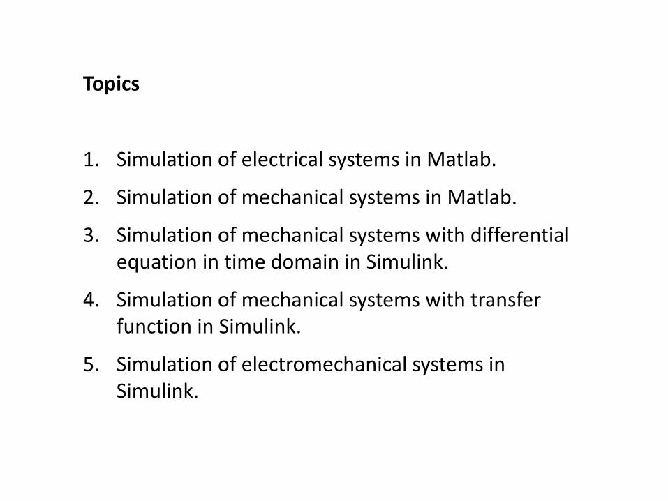
Topics

1. Simulation of electrical systems in Matlab.

2. Simulation of mechanical systems in Matlab.

3. Simulation of mechanical systems with differential equation in time domain in Simulink.

4. Simulation of mechanical systems with transfer function in Simulink.

5. Simulation of electromechanical systems in Simulink.

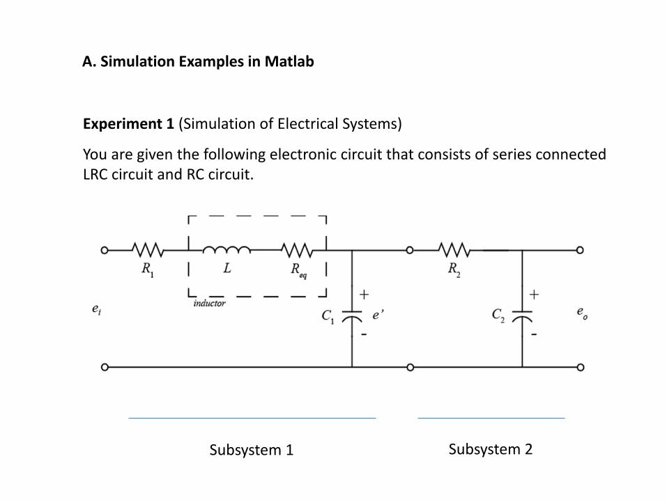
Experiment 1 (Simulation of Electrical Systems)

You are given the following electronic circuit that consists of series connected LRC circuit and RC circuit.

Subsystem 1 Subsystem 2

A. Simulation Examples in Matlab

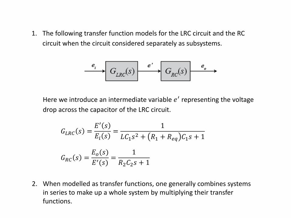
1. The following transfer function models for the LRC circuit and the RC

circuit when the circuit considered separately as subsystems.

Here we introduce an intermediate variable 𝑒′ representing the voltage

drop across the capacitor of the LRC circuit.

𝐺𝐿𝑅𝐶 𝑠 =𝐸′ 𝑠

𝐸𝑖 𝑠=

1

𝐿𝐶1𝑠2 + 𝑅1 + 𝑅𝑒𝑞 𝐶1𝑠 + 1

𝐺𝑅𝐶 𝑠 =𝐸𝑜(𝑠)

𝐸′(𝑠)=

1

𝑅2𝐶2𝑠 + 1

2. When modelled as transfer functions, one generally combines systems in series to make up a whole system by multiplying their transfer functions.

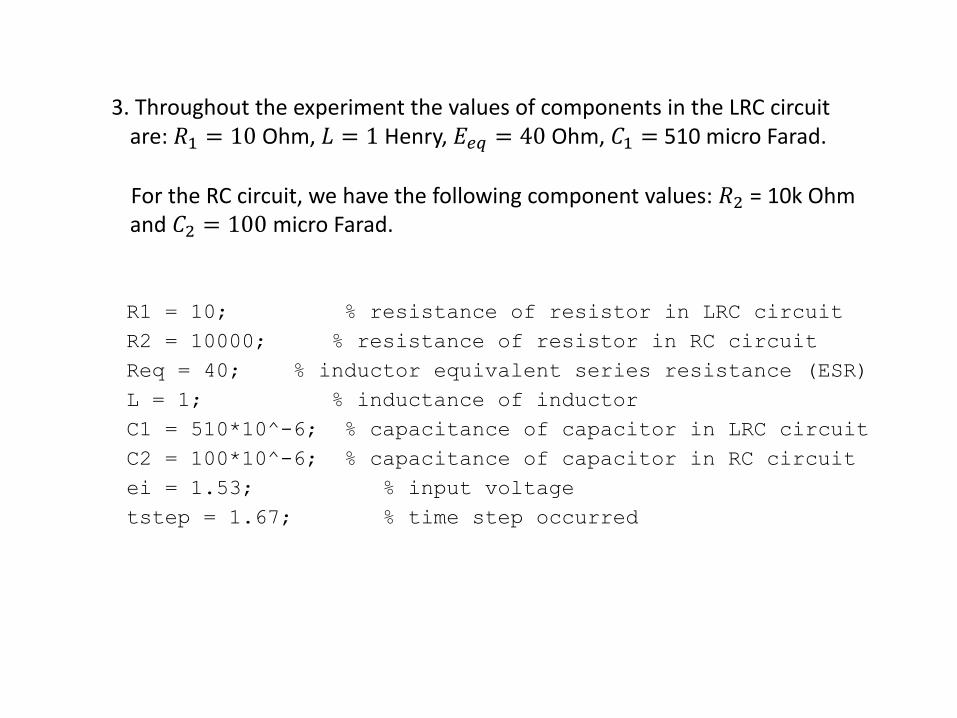
3. Throughout the experiment the values of components in the LRC circuit are: 𝑅1 = 10 Ohm, 𝐿 = 1 Henry, 𝐸𝑒𝑞 = 40 Ohm, 𝐶1 = 510 micro Farad.

For the RC circuit, we have the following component values: 𝑅2 = 10k Ohm and 𝐶2 = 100 micro Farad.

R1 = 10; % resistance of resistor in LRC circuit

R2 = 10000; % resistance of resistor in RC circuit

Req = 40; % inductor equivalent series resistance (ESR)

L = 1; % inductance of inductor

C1 = 510*10^-6; % capacitance of capacitor in LRC circuit

C2 = 100*10^-6; % capacitance of capacitor in RC circuit

ei = 1.53; % input voltage

tstep = 1.67; % time step occurred

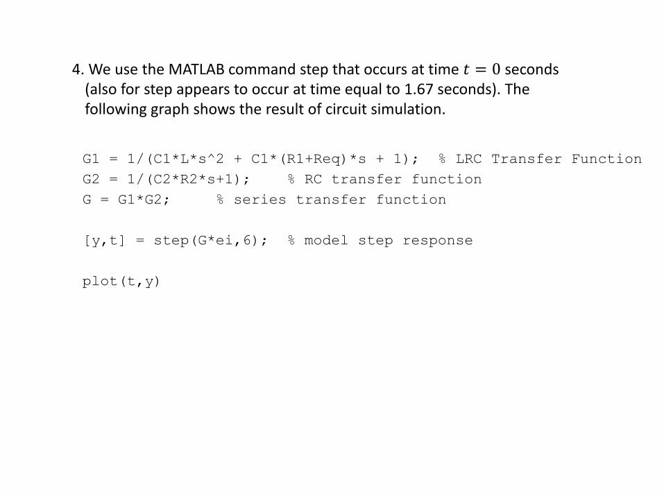
4. We use the MATLAB command step that occurs at time 𝑡 = 0 seconds (also for step appears to occur at time equal to 1.67 seconds). The following graph shows the result of circuit simulation.

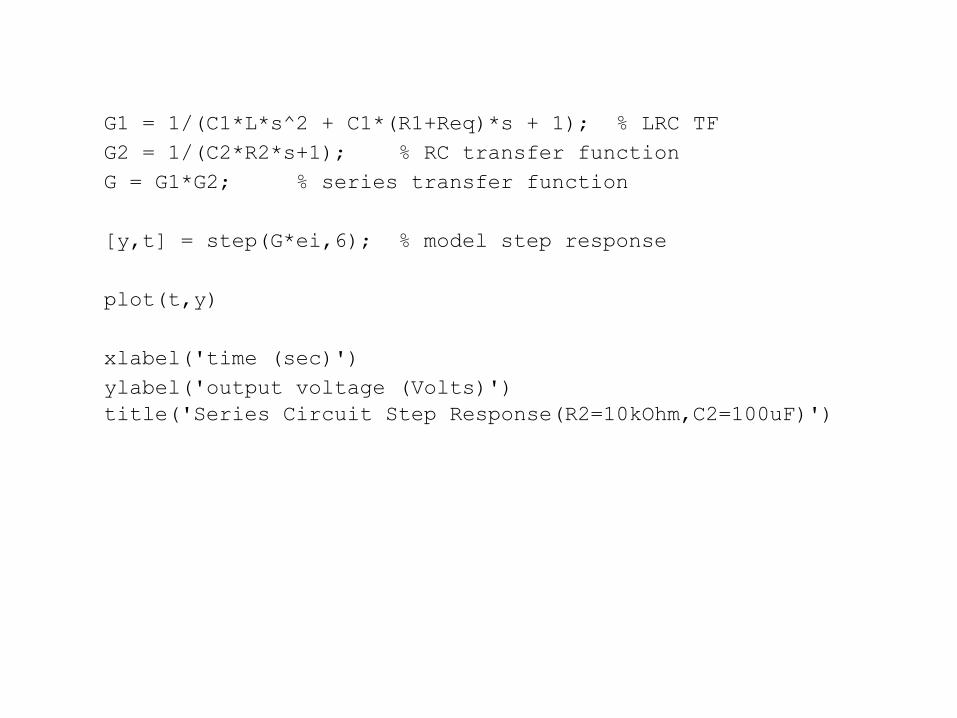
G1 = 1/(C1*L*s^2 + C1*(R1+Req)*s + 1); % LRC Transfer Function

G2 = 1/(C2*R2*s+1); % RC transfer function

G = G1*G2; % series transfer function

[y,t] = step(G*ei,6); % model step response

plot(t,y)

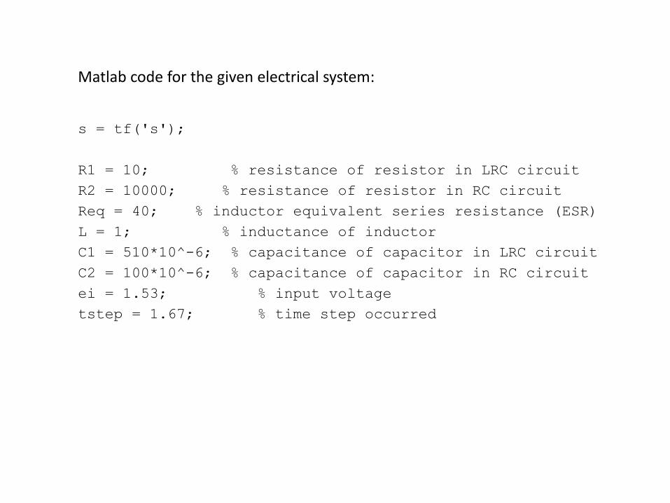
Matlab code for the given electrical system:

s = tf('s');

R1 = 10; % resistance of resistor in LRC circuit

R2 = 10000; % resistance of resistor in RC circuit

Req = 40; % inductor equivalent series resistance (ESR)

L = 1; % inductance of inductor

C1 = 510*10^-6; % capacitance of capacitor in LRC circuit

C2 = 100*10^-6; % capacitance of capacitor in RC circuit

ei = 1.53; % input voltage

tstep = 1.67; % time step occurred

G1 = 1/(C1*L*s^2 + C1*(R1+Req)*s + 1); % LRC TF

G2 = 1/(C2*R2*s+1); % RC transfer function

G = G1*G2; % series transfer function

[y,t] = step(G*ei,6); % model step response

plot(t,y)

xlabel('time (sec)')

ylabel('output voltage (Volts)')

title('Series Circuit Step Response(R2=10kOhm,C2=100uF)')

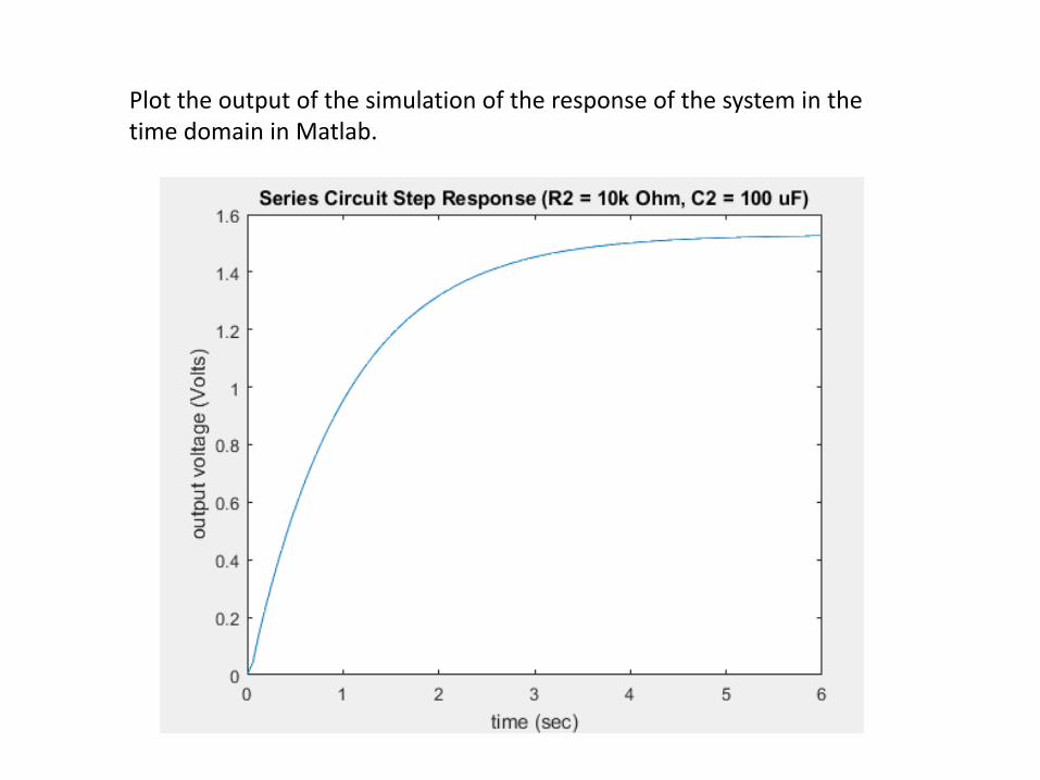
Plot the output of the simulation of the response of the system in the time domain in Matlab.

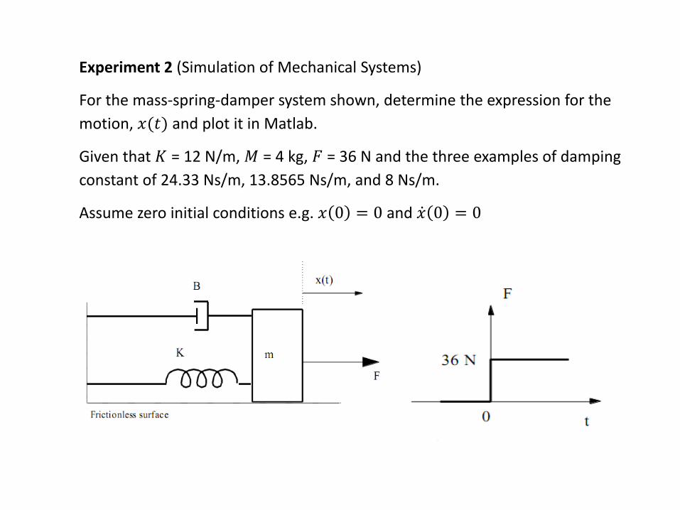
Experiment 2 (Simulation of Mechanical Systems)

For the mass-spring-damper system shown, determine the expression for the

motion, 𝑥(𝑡) and plot it in Matlab.

Given that 𝐾 = 12 N/m, 𝑀 = 4 kg, 𝐹 = 36 N and the three examples of damping

constant of 24.33 Ns/m, 13.8565 Ns/m, and 8 Ns/m.

Assume zero initial conditions e.g. 𝑥 0 = 0 and ሶ𝑥 0 = 0

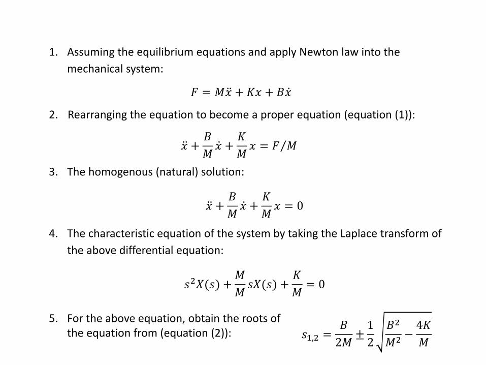
1. Assuming the equilibrium equations and apply Newton law into the

mechanical system:

𝐹 = 𝑀 ሷ𝑥 + 𝐾𝑥 + 𝐵 ሶ𝑥

2. Rearranging the equation to become a proper equation (equation (1)):

ሷ𝑥 +𝐵

𝑀ሶ𝑥 +

𝐾

𝑀𝑥 = Τ𝐹 𝑀

3. The homogenous (natural) solution:

ሷ𝑥 +𝐵

𝑀ሶ𝑥 +

𝐾

𝑀𝑥 = 0

4. The characteristic equation of the system by taking the Laplace transform of

the above differential equation:

𝑠2𝑋(𝑠) +𝑀

𝑀𝑠𝑋(𝑠) +

𝐾

𝑀= 0

𝑠1,2 =𝐵

2𝑀±1

2

𝐵2

𝑀2−4𝐾

𝑀

5. For the above equation, obtain the roots of the equation from (equation (2)):

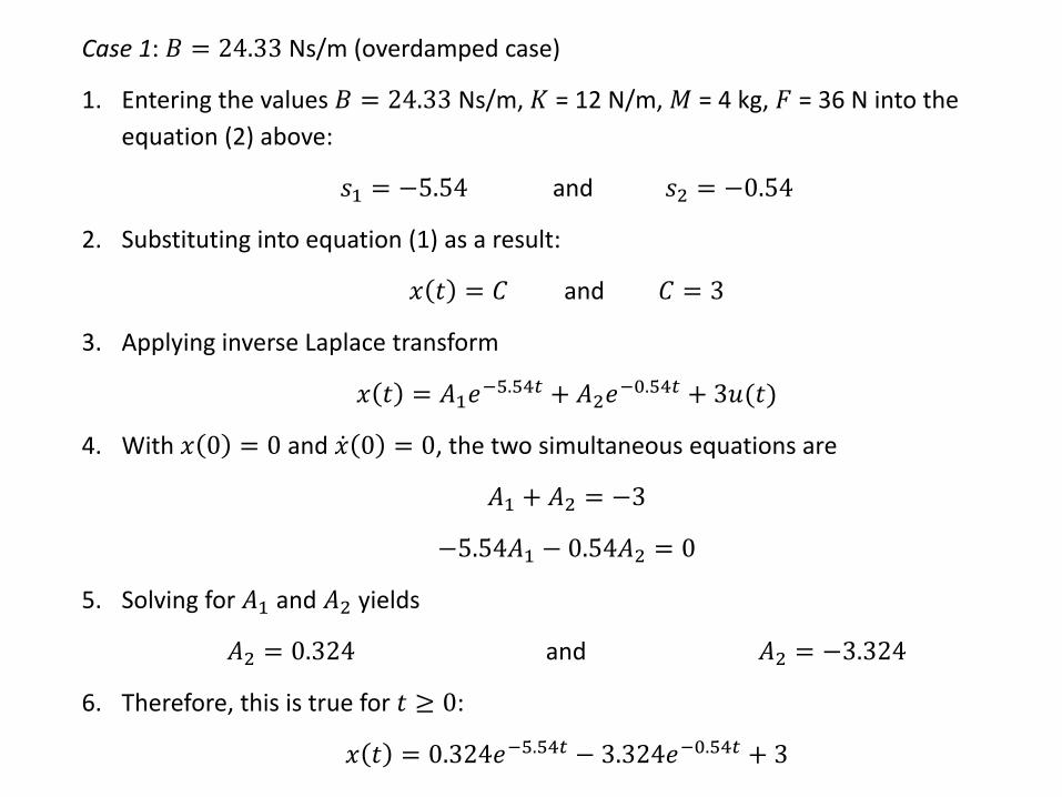
Case 1: 𝐵 = 24.33 Ns/m (overdamped case)

1. Entering the values 𝐵 = 24.33 Ns/m, 𝐾 = 12 N/m, 𝑀 = 4 kg, 𝐹 = 36 N into the

equation (2) above:

𝑠1 = −5.54 and 𝑠2 = −0.54

2. Substituting into equation (1) as a result:

𝑥 𝑡 = 𝐶 and 𝐶 = 3

3. Applying inverse Laplace transform

𝑥 𝑡 = 𝐴1𝑒−5.54𝑡 + 𝐴2𝑒

−0.54𝑡 + 3𝑢(𝑡)

4. With 𝑥 0 = 0 and ሶ𝑥 0 = 0, the two simultaneous equations are

𝐴1 + 𝐴2 = −3

−5.54𝐴1 − 0.54𝐴2 = 0

5. Solving for 𝐴1 and 𝐴2 yields

𝐴2 = 0.324 and 𝐴2 = −3.324

6. Therefore, this is true for 𝑡 ≥ 0:

𝑥 𝑡 = 0.324𝑒−5.54𝑡 − 3.324𝑒−0.54𝑡 + 3

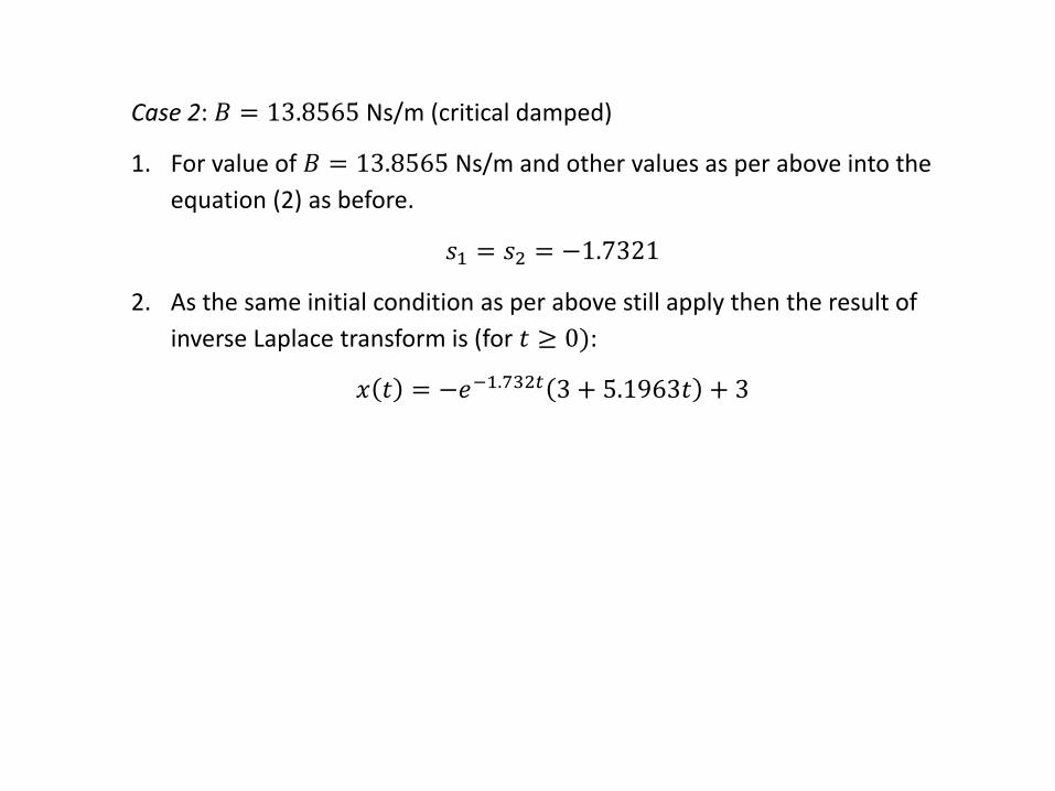
Case 2: 𝐵 = 13.8565 Ns/m (critical damped)

1. For value of 𝐵 = 13.8565 Ns/m and other values as per above into the

equation (2) as before.

𝑠1 = 𝑠2 = −1.7321

2. As the same initial condition as per above still apply then the result of

inverse Laplace transform is (for 𝑡 ≥ 0):

𝑥 𝑡 = −𝑒−1.732𝑡 3 + 5.1963𝑡 + 3

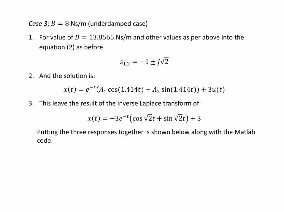
Case 3: 𝐵 = 8 Ns/m (underdamped case)

1. For value of 𝐵 = 13.8565 Ns/m and other values as per above into the

equation (2) as before.

𝑠1.2 = −1 ± 𝑗 2

2. And the solution is:

𝑥 𝑡 = 𝑒−𝑡 𝐴1 cos(1.414𝑡) + 𝐴2 sin(1.414𝑡) + 3𝑢(𝑡)

3. This leave the result of the inverse Laplace transform of:

𝑥 𝑡 = −3𝑒−𝑡 cos 2𝑡 + sin 2𝑡 + 3

Putting the three responses together is shown below along with the Matlabcode.

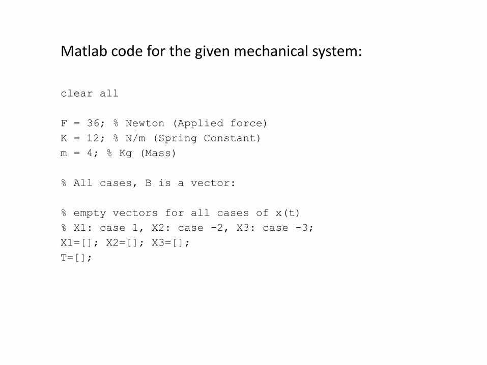
Matlab code for the given mechanical system:

clear all

F = 36; % Newton (Applied force)

K = 12; % N/m (Spring Constant)

m = 4; % Kg (Mass)

% All cases, B is a vector:

% empty vectors for all cases of x(t)

% X1: case 1, X2: case -2, X3: case -3;

X1=[]; X2=[]; X3=[];

T=[];

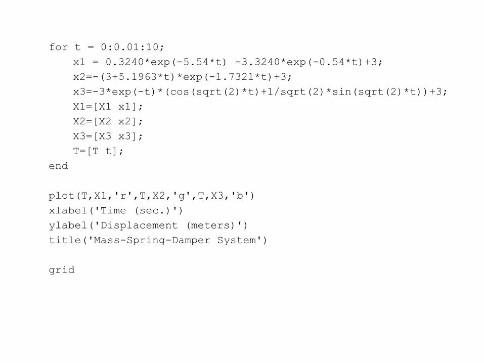
for t = 0:0.01:10;

x1 = 0.3240*exp(-5.54*t) -3.3240*exp(-0.54*t)+3;

x2=-(3+5.1963*t)*exp(-1.7321*t)+3;

x3=-3*exp(-t)*(cos(sqrt(2)*t)+1/sqrt(2)*sin(sqrt(2)*t))+3;

X1=[X1 x1];

X2=[X2 x2];

X3=[X3 x3];

T=[T t];

end

plot(T,X1,'r',T,X2,'g',T,X3,'b')

xlabel('Time (sec.)')

ylabel('Displacement (meters)')

title('Mass-Spring-Damper System')

grid

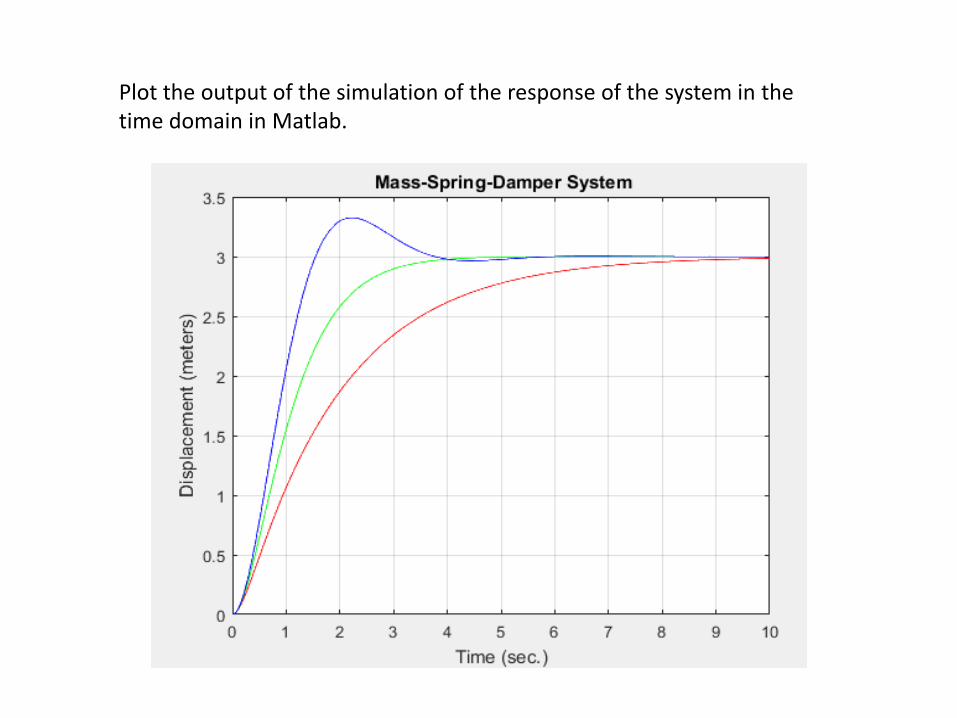
Plot the output of the simulation of the response of the system in the time domain in Matlab.

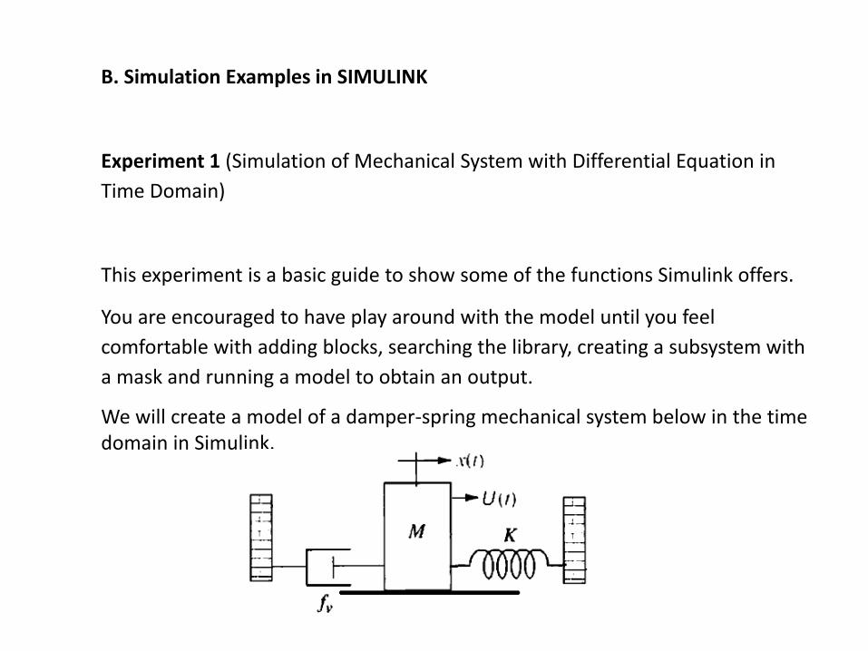
Experiment 1 (Simulation of Mechanical System with Differential Equation in

Time Domain)

This experiment is a basic guide to show some of the functions Simulink offers.

You are encouraged to have play around with the model until you feel

comfortable with adding blocks, searching the library, creating a subsystem with

a mask and running a model to obtain an output.

We will create a model of a damper-spring mechanical system below in the time domain in Simulink.

B. Simulation Examples in SIMULINK

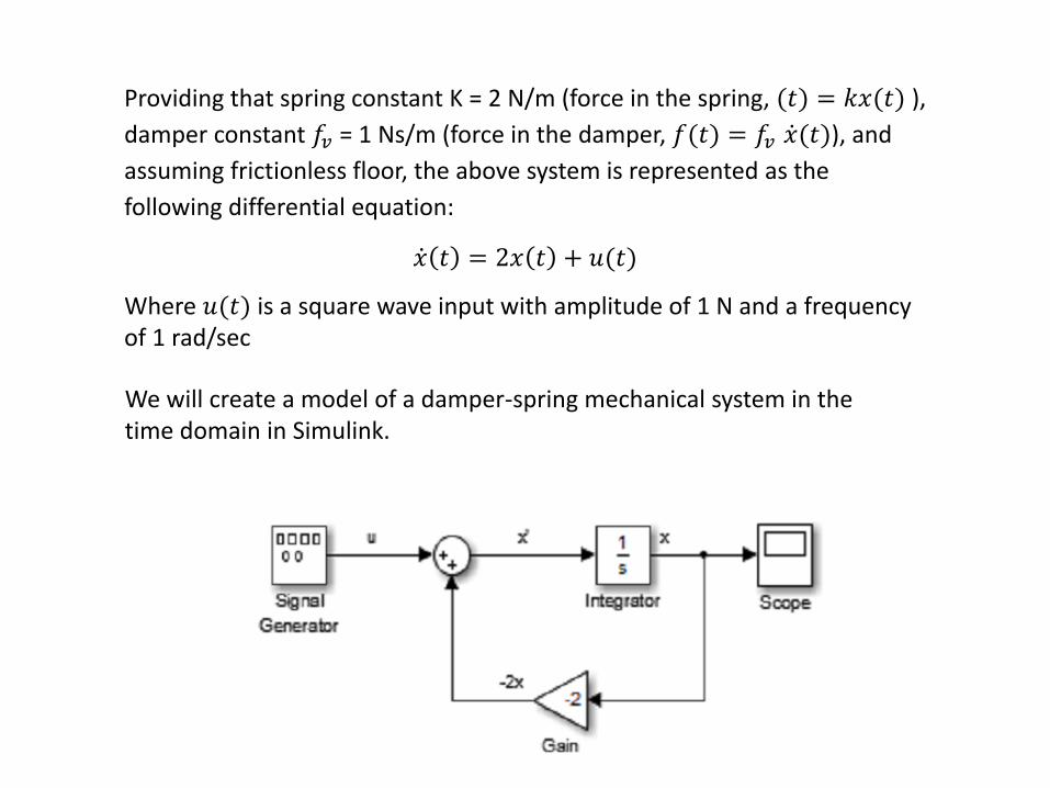
We will create a model of a damper-spring mechanical system in the time domain in Simulink.

Providing that spring constant K = 2 N/m (force in the spring, (𝑡) = 𝑘𝑥(𝑡) ),

damper constant 𝑓𝑣 = 1 Ns/m (force in the damper, 𝑓(𝑡) = 𝑓𝑣 ሶ𝑥(𝑡)), and

assuming frictionless floor, the above system is represented as the

following differential equation:

ሶ𝑥 𝑡 = 2𝑥 𝑡 + 𝑢(𝑡)

Where 𝑢(𝑡) is a square wave input with amplitude of 1 N and a frequency of 1 rad/sec

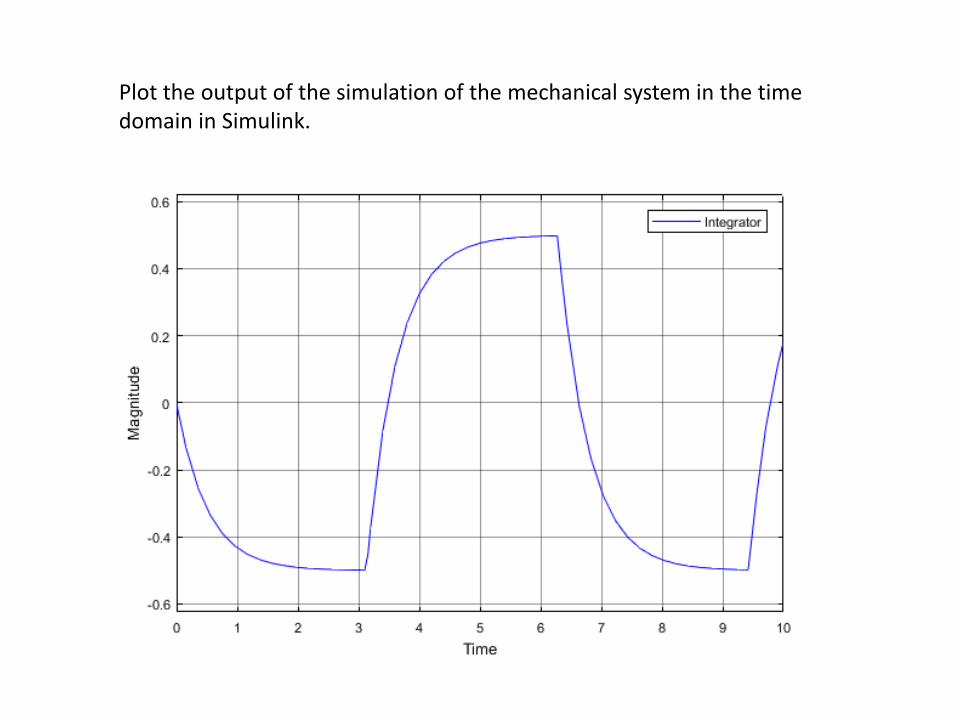
Plot the output of the simulation of the mechanical system in the time domain in Simulink.

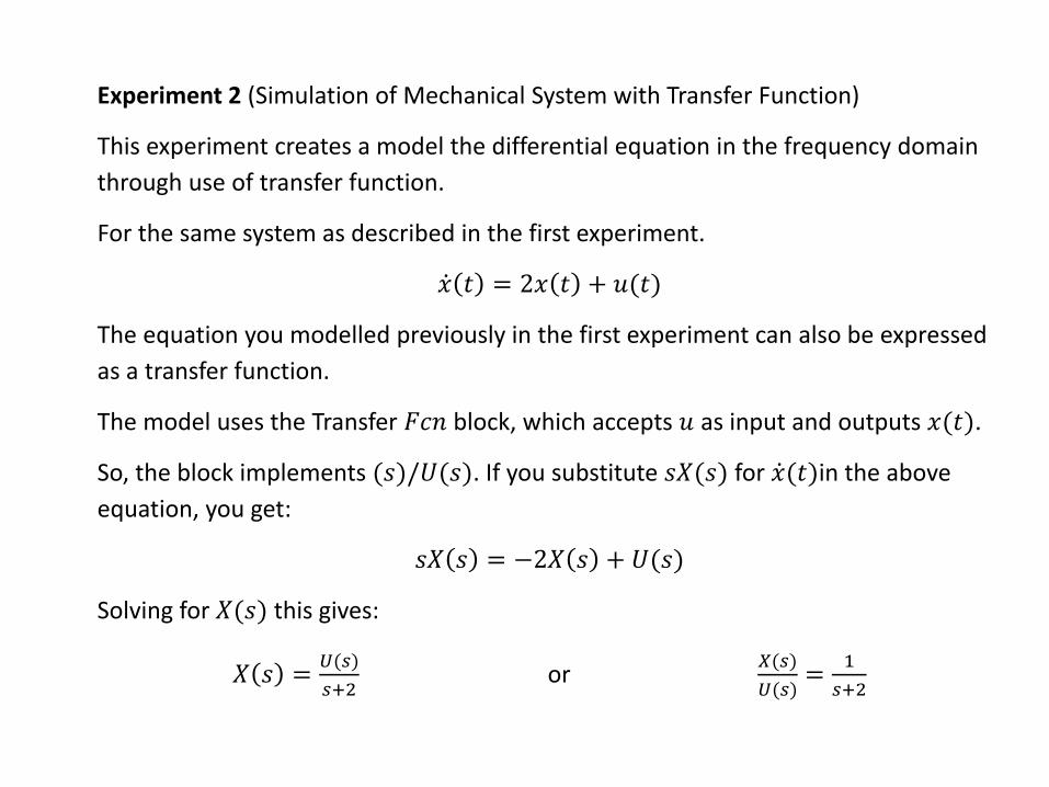
Experiment 2 (Simulation of Mechanical System with Transfer Function)

This experiment creates a model the differential equation in the frequency domain

through use of transfer function.

For the same system as described in the first experiment.

ሶ𝑥 𝑡 = 2𝑥 𝑡 + 𝑢(𝑡)

The equation you modelled previously in the first experiment can also be expressed

as a transfer function.

The model uses the Transfer 𝐹𝑐𝑛 block, which accepts 𝑢 as input and outputs 𝑥(𝑡).

So, the block implements (𝑠)/𝑈(𝑠). If you substitute 𝑠𝑋(𝑠) for ሶ𝑥(𝑡)in the above

equation, you get:

𝑠𝑋 𝑠 = −2𝑋 𝑠 + 𝑈(𝑠)

Solving for 𝑋(𝑠) this gives:

𝑋 𝑠 =𝑈(𝑠)

𝑠+2or

𝑋(𝑠)

𝑈(𝑠)=

1

𝑠+2

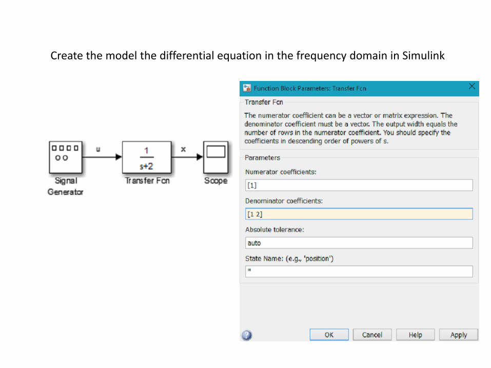
Create the model the differential equation in the frequency domain in Simulink

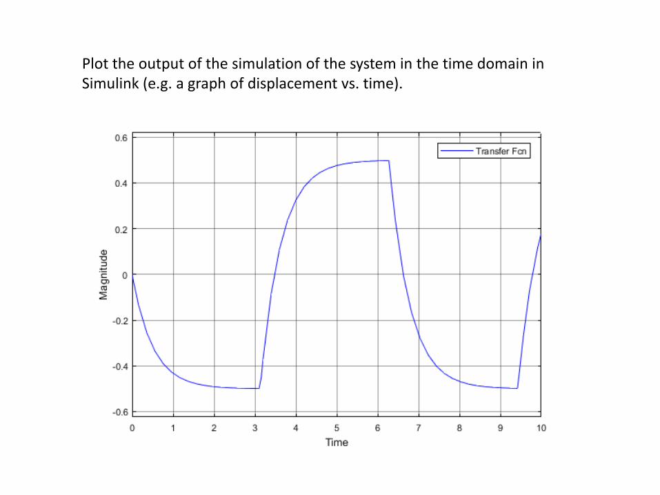
Plot the output of the simulation of the system in the time domain in Simulink (e.g. a graph of displacement vs. time).

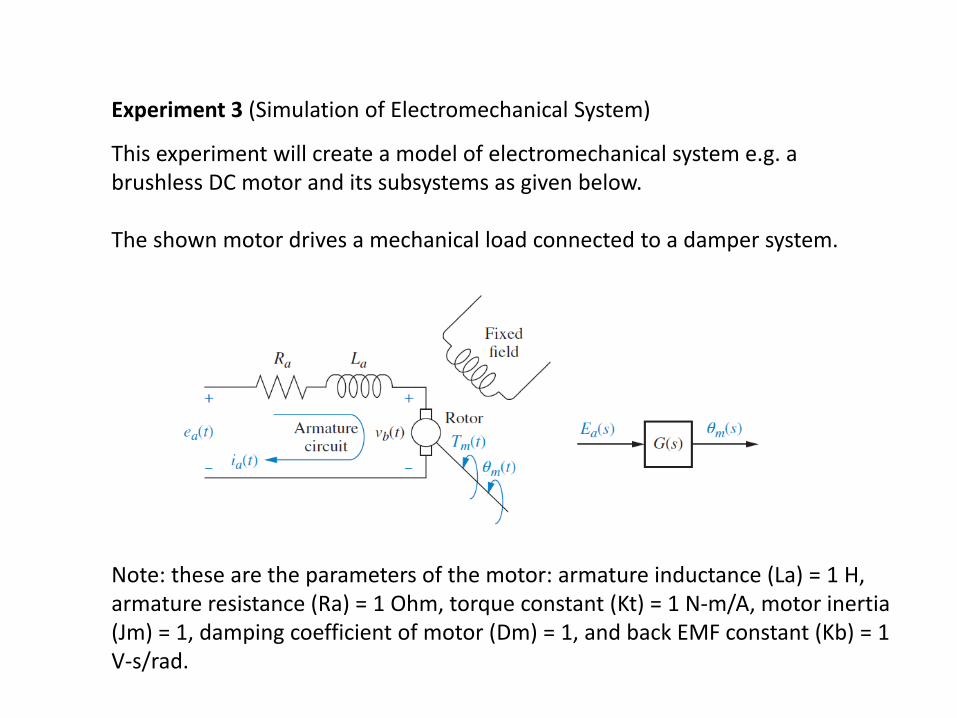
Experiment 3 (Simulation of Electromechanical System)

This experiment will create a model of electromechanical system e.g. a brushless DC motor and its subsystems as given below.

The shown motor drives a mechanical load connected to a damper system.

Note: these are the parameters of the motor: armature inductance (La) = 1 H, armature resistance (Ra) = 1 Ohm, torque constant (Kt) = 1 N-m/A, motor inertia (Jm) = 1, damping coefficient of motor (Dm) = 1, and back EMF constant (Kb) = 1 V-s/rad.

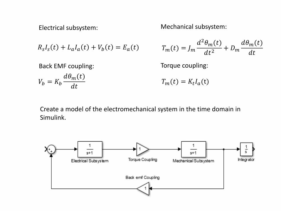
Create a model of the electromechanical system in the time domain in Simulink.

𝑇𝑚(𝑡) = 𝐽𝑚𝑑2𝜃𝑚(𝑡)

𝑑𝑡2+ 𝐷𝑚

𝑑𝜃𝑚(𝑡)

𝑑𝑡

𝑇𝑚(𝑡) = 𝐾𝑡𝐼𝑎(t)

𝑅𝑠𝐼𝑠 𝑡 + 𝐿𝑎𝐼𝑎 𝑡 + 𝑉𝑏 𝑡 = 𝐸𝑎(𝑡)

𝑉𝑏 = 𝐾𝑏𝑑𝜃𝑚(𝑡)

𝑑𝑡

Electrical subsystem: Mechanical subsystem:

Torque coupling:Back EMF coupling:

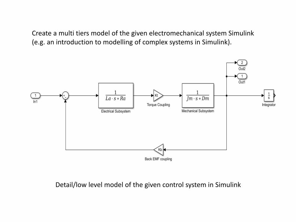
Create a multi tiers model of the given electromechanical system Simulink (e.g. an introduction to modelling of complex systems in Simulink).

Detail/low level model of the given control system in Simulink

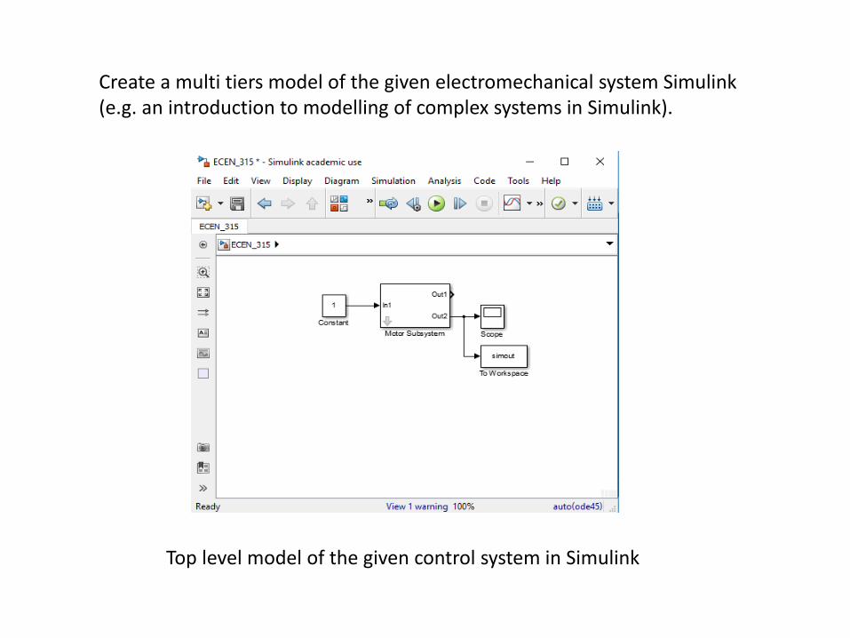
Create a multi tiers model of the given electromechanical system Simulink (e.g. an introduction to modelling of complex systems in Simulink).

Top level model of the given control system in Simulink

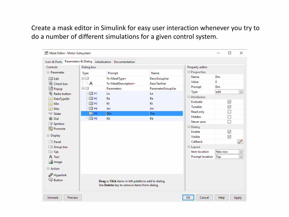
Create a mask editor in Simulink for easy user interaction whenever you try to do a number of different simulations for a given control system.

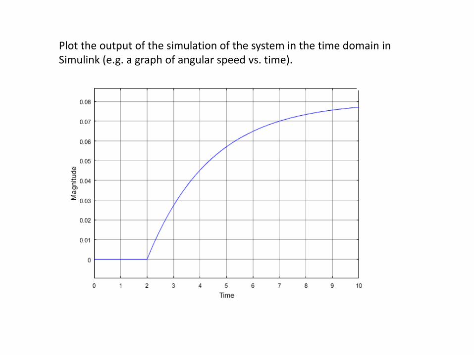
Plot the output of the simulation of the system in the time domain in Simulink (e.g. a graph of angular speed vs. time).