Embed Size (px)
Citation preview
MANAGERIAL ECONOMICS
VENKATESHWARAOPEN UNIVERSITY
www.vou.ac.in
VENKATESHWARAOPEN UNIVERSITY
www.vou.ac.in
MANAGERIAL ECONOMICS
MBA[MBA-203]
MANAGERIAL ECONOM
ICS
13 MM
MANAGERIAL ECONOMICS
MBA
[MBA-203]
Authors:D.N. Dwivedi, Professor of Economics, Maharaja Agrsen Institute of Management Studies, DelhiUnits (1-9, 11-13)Dr. Suman Lata, Lecturer, Ginni Devi Modi Girls College, Modinagar, GhaziabadUnit (10)Aditi Sharma, Freelance AuthorUnit (14)
All rights reserved. No part of this publication which is material protected by this copyright noticemay be reproduced or transmitted or utilized or stored in any form or by any means now known orhereinafter invented, electronic, digital or mechanical, including photocopying, scanning, recordingor by any information storage or retrieval system, without prior written permission from the Publisher.
Information contained in this book has been published by VIKAS® Publishing House Pvt. Ltd. and hasbeen obtained by its Authors from sources believed to be reliable and are correct to the best of theirknowledge. However, the Publisher and its Authors shall in no event be liable for any errors, omissionsor damages arising out of use of this information and specifically disclaim any implied warranties ormerchantability or fitness for any particular use.
Vikas® is the registered trademark of Vikas® Publishing House Pvt. Ltd.
VIKAS® PUBLISHING HOUSE PVT LTDE-28, Sector-8, Noida - 201301 (UP)Phone: 0120-4078900 Fax: 0120-4078999Regd. Office: A-27, 2nd Floor, Mohan Co-operative Industrial Estate, New Delhi 1100 44Website: www.vikaspublishing.com Email: [email protected]
BOARD OF STUDIES
Prof Lalit Kumar SagarVice Chancellor
Dr. S. Raman IyerDirectorDirectorate of Distance Education
SUBJECT EXPERT
Dr. S. Raman IyerDr. Richa AgarwalDr. Anand KumarDr. Babar Ali KhanDr. Adil Hakeem Khan
Programme DirectorAssistant ProfessorAssistant ProfessorProfessor in CommerceProfessor in Management
CO-ORDINATOR
Mr. Tauha KhanRegistrar
SYLLABI-BOOK MAPPING TABLEManagerial Economics
BLOCK I : BASICS OF MANAGERIAL DEVELOPMENTUnit-1: Economics: Introduction – Meaning, nature and scope ofManagerial Economics – General Foundations of managerialEconomics – Economic Approach – Working of Economic system- Circular flow activities - Economics & Business Decisions -Relationship between Economic theory and Managerial Economics.Unit-2: Business Decisions: Role of managerial Economics in Decisionmaking – Decision making under Risk and Uncertainty - Concepts ofOpportunity cost, - Production possibility curve – IncrementalConcepts - Cardinal and Ordinal approaches to consumer BehaviourTime Value of Money –Unit-3: Consumer Behaviour: Marginalism – Equilibrium and Equi-marginalism and their role in business decision making. – Equi-Marginal principles – Utility analysis – Total and Marginal Utility –Law of diminishing marginal utility – Marshallian approach andIndifference curve analysis.Unit-4: Demand analysis: Meaning, Functions - Determinants ofdemand-Law of Demand – Demand Estimation and Forecasting -Applications of demand in analysis - Elasticity of Demand: Types,Measures and Role in Business Decisions.
BLOCK II: PERSONAL AND SUPPLY MANAGEMENTUnit-5: Supply Analysis: Determinants of supply- Elasticity of Supply-Measures and Significance - Derivations of market demand – DemandEstimation and Fore casting- Demand and Supply equilibrium – GiffenParadoxUnit-6: Production Functions: Managerial uses of production function- Cobb-Douglas and other production functions - Isoquants – Shortrun and long run production function – Theory of production –Empirical estimations of production functions.Unit-7: Forms of Markets: Meaning and Characteristics - MarketEquilibrium: Practical Importance, Market Equilibrium and Changesin Market Equilibrium. Pricing Functions: Market Structures - Pricingand output decisions under different competitive conditions: MonopolyMonopolistic completion and OligopolyUnit-8: Strategic Behaviour of the firms and Game Theory - NashEquilibrium: Implications – Prisoner’s Dilemma: Types of strategy– Price and Non price competition – Relation to the firm behaviour.
BLOCK III: COST AND BREAK FROM POINTUnit-9: Cost and Return: Cost function and cost output relationship– Economics and Diseconomies of scale - Cost control and costreduction- Cost Behaviour and Business Decision- Relevant costsfor decision-making- Traditional and Modern theory of Cost.Unit-10: New Product Penetrative Decision and Skimming the creamPricing- Government control over pricing - Concept of Profit- Typesand Theories of Profit by Knight (Uncertainty), Schumpeter
Unit 1: Basics of ManagerialEconomics
(Pages 1-15)Unit 2: Decision Making and
Business Decisions(Pages 16-27)
Unit 3: Consumer Behaviour(Pages 28-44)
Unit 4: Demand Analysis(Pages 45-66)
Unit 5: Supply Analysis(Pages 67-80)
Unit 6: Production Functions(Pages 81-105)
Unit 7: Forms of Markets(Pages 106-135)
Unit 8: Strategic Behaviour ofthe Firms and Game Theory
(Pages 136-146)
Unit 9: Cost and Return(Pages 147-168)
Unit 10: Penetration andSkimming Strategies
(Pages 169-189)Unit 11: Profit and Investment
Analysis(Pages 190-208)
(Innovation), Clark (Dynamic) and Hawley (Risk) - Profit maximization– Cost volume profit analysis – Risk and Return Relationship.Unit-11: Profit and Investment Analysis: Meaning – Measurement ofprofit – Theories of Pricing- Profit planning and forecasting- Profitand Wealth maximization – Cost volume profit analysis – Investmentanalysis and Evaluation: IRR, NPV and APV techniques.
BLOCK IV: MACRO ECONOMICS AND REGULATIONSUnit-12: Macro-economic Factors: Nature, Importance ; EconomicGrowth and Development - Business cycle – Phases and BusinessDecision- Inflation - Factors causing Inflation and Deflation - Controlmeasures – Balance of payment Trend and its implications in managerialdecision.Unit-13: National Income: Introduction Meaning – Theories – Methodsof Measurement - Sectoral and Population distributions – Per capitaIncome: Definition – Calculations – Uses – Limitations – GDP – GNP- Recent developments in Indian Economy.Unit-14: Economic Regulations of Business: Introduction – Antitrusttheory and Regulations – The structure – Conduct – Performanceparadigm – Concentration: Overview – Measuring concentration –Regulation of Externalities.
Unit 12: Macro-Economic Factors(Pages 209-232)
Unit 13: National Income(Pages 233-255)
Unit 14: Economic Regulations ofBusiness
(Pages 256-273)
INTRODUCTION
BLOCK I: BASICS OF MANAGERIAL DEVELOPMENTUNIT 1 BASICS OF MANAGERIAL ECONOMICS 1-15
1.0 Introduction1.1 Objectives1.2 Economics: Introduction1.3 Meaning and Nature of Managerial Economics
1.3.1 Scope of Managerial Economics1.4 General Foundations of Managerial Economics
1.4.1 Economic Approach1.4.2 Working of Economic System and Circular Flow of Activities
1.5 Economics and Business Decisions1.5.1 Relationship between Economic Theory and Managerial Economics
1.6 Answers to Check Your Progress Questions1.7 Summary1.8 Key Words1.9 Self Assessment Questions and Exercises
1.10 Further ReadingsUNIT 2 DECISION MAKING AND BUSINESS DECISIONS 16-27
2.0 Introduction2.1 Objectives2.2 Role of Managerial Economics in Decision Making
2.2.1 Decision Making Under Risk and Uncertainity2.3 Business Decision Rules
2.3.1 Concepts of Opportunity Cost2.3.2 Production Possibility Curve2.3.3 Incremental Concepts2.3.4 Cardinal and Ordinal Approaches to Consumer Behaviour2.3.5 Time Value of Money
2.4 Answers to Check Your Progress Questions2.5 Summary2.6 Key Words2.7 Self Assessment Questions and Exercises2.8 Further Readings
UNIT 3 CONSUMER BEHAVIOUR 28-443.0 Introduction3.1 Objectives3.2 Marginalism, Equilibrium and Equi-Marginalism and their Role in
Business Decision Making3.2.1 Equi-Marginal Principles
3.3 Utility Analysis3.3.1 Total and Marginal Utility
CONTENTS
3.4 Cardinal Utility Approach or the Marshallian Approach3.4.1 Law of Diminshing Marginal Utility
3.5 Ordinal Utility Approach or the Hicks Approach3.5.1 Indifference Curve Analysis
3.6 Answers to Check Your Progress Questions3.7 Summary3.8 Key Words3.9 Self Assessment Questions and Exercises
3.10 Further ReadingsUNIT 4 DEMAND ANALYSIS 45-66
4.0 Introduction4.1 Unit Objectives4.2 Meaning, Functions and Applications of Demand Analysis
4.2.1 Law of Demand4.2.2 Determinants of Demand4.2.3 Demand Estimation and Forecasting
4.3 Elasticity of Demand: Types and Measures4.3.1 Price Elasticity of Demand4.3.2 Cross Elasticity of Demand4.3.3 Income Elasticity of Demand4.3.4 Advertisement or Promotional Elasticity
4.4 Answers to Check Your Progress Questions4.5 Summary4.6 Key Words4.7 Self Assessment Questions and Exercises4.8 Further Readings
BLOCK II: PERSONAL AND SUPPLY MANAGEMENTUNIT 5 SUPPLY ANALYSIS 67-80
5.0 Introduction5.1 Objectives5.2 The Law of Supply and Determinants of Supply
5.2.1 Elasticity of Supply: Measures and Significance5.2.2 Derivations of Market Demand5.2.3 Demand Estimation and Forecasting
5.3 Demand Supply Equilibrium5.4 Giffen Paradox5.5 Answers to Check Your Progress Questions5.6 Summary5.7 Key Words5.8 Self Assessment Questions and Exercises5.9 Further Readings
UNIT 6 PRODUCTION FUNCTIONS 81-1056.0 Introduction6.1 Objectives6.2 Production Functions: Short-Run and Long-Run Production Function6.3 Theory of Production and Managerial Uses of Production Function
6.3.1 Short-Run Laws of Production
6.3.2 Isoquants6.3.3 Long-Run Laws of Production
6.4 Cobb-Douglas and Other Production Functions: Empirical Estimation6.5 Answers to Check Your Progress Questions6.6 Summary6.7 Key Words6.8 Self Assessment Questions and Exercises6.9 Further Readings
UNIT 7 FORMS OF MARKETS 106-1357.0 Introduction7.1 Unit Objectives7.2 Meaning and Characteristics of Markets
7.2.1 Market Equilibirum and Changes in Market Equilibrium7.2.2 Market Equilibrium: Practical Importance
7.3 Pricing Functions under Different Market Structures7.3.1 Market Structures and Pricing Decisions
7.4 Price and Output Decisions under Different Competitive Conditions7.4.1 Monopoly7.4.2 Monopolistic Competition7.4.3 Oligopoly
7.5 Answers to Check Your Progress Questions7.6 Summary7.7 Key Words7.8 Self Assessment Questions and Exercises7.9 Further Readings
UNIT 8 STRATEGIC BEHAVIOUR OF THE FIRMSAND GAME THEORY 136-146
8.0 Introduction8.1 Unit Objectives8.2 Strategic Behaviour of the Firms: Price and Non-Price Competition8.3 Game Theory: Types of Strategy and Relation to the Firm’s Behaviour
8.3.1 Prisoner’s Dilemma8.3.2 Application of Game Theory to Oligopolistic Startegy8.3.3 Nash Equilibirum and Implications
8.4 Answers to Check Your Progress Questions8.5 Summary8.6 Key Words8.7 Self Assessment Questions and Exercises8.8 Further Readings
BLOCK III: COST AND BREAK FROM POINTUNIT 9 COST AND RETURN 147-168
9.0 Introduction9.1 Objectives9.2 Relavant Costs for Decision-Making9.3 Traditional Theory of Cost: Cost Function and Cost Output Relationship
9.3.1 Short-Run Cost-Output Relations
9.3.2 Long-Run Cost-Output Relations9.3.3 Economies and Diseconomies of Scale
9.4 Modern Theory of Cost9.5 Cost Control and Cost reduction9.6 Cost Behaviour and Business Decision9.7 Answers to Check Your Progress Questions9.8 Summary9.9 Key Words
9.10 Self Assessment Questions and Exercises9.11 Further Readings
UNIT 10 PENETRATION AND SKIMMING STRATEGIES 169-18910.0 Introduction10.1 Objectives10.2 Concept of Profit
10.2.1 Types of Profit10.3 Theory of Profit
10.3.1 Dynamic Theory of Profit10.3.2 Innovation Theory of Profit10.3.3 Uncertainty – Bearing Theory of Profit10.3.4 Risk Bearing Theory of Profit
10.4 Cost Volume Profit Analysis10.4.1 Total Contribution Margin10.4.2 Basic Assumptions of Cost Volume Profit Analysis
10.5 Pricing of a New Product10.6 Answers To Check Your Progress10.7 Summary10.8 Key Words10.9 Self Assessment Questions and Exercises
10.10 Further ReadingsUNIT 11 PROFIT AND INVESTMENT ANALYSIS 190-208
11.0 Introduction11.1 Objectives11.2 Meaning and Measurement of Profit11.3 Theories of Pricing
11.3.1 Cost-Plus Pricing11.3.2 Multiple Product Pricing11.3.3 Pricing in the Life-Cycle of a Product11.3.4 Transfer Pricing11.3.5 Peak Load Pricing
11.4 Profit Planning and Forecasting11.4.1 Profit and Wealth Maximization11.4.2 Cost Volume Profit Analysis
11.5 Investment Analysis and Evaluation11.5.1 Internal Rate of Return (IRR)11.5.2 Net Present Value (NPV)11.5.3 Adjusted Present Value (APV)
11.6 Answers to Check Your Progress Questions11.7 Summary11.8 Key Words
11.9 Self Assessment Questions and Exercises11.10 Further Readings
BLOCK IV: MACRO ECONOMICS AND REGULATIONSUNIT 12 MACRO-ECONOMIC FACTORS 209-232
12.0 Introduction12.1 Objectives12.2 Meaning and Nature of Macro-Economic Factors
12.2.1 Importance of Macro-Economic Factors12.3 Economic Growth and Development12.4 Business Cycle: Phases and Business Decisions12.5 Inflation
12.5.1 Factors Causing Inflation12.5.2 Factors Causing Deflation12.5.3 Control Measures
12.6 Balance of Payment Trend and Its Implications on Managerial Decisions12.7 Answers to Check Your Progress Questions12.8 Summary12.9 Key Words
12.10 Self Assessment Questions and Exercises12.11 Further Readings
UNIT 13 NATIONAL INCOME 233-25513.0 Introduction13.1 Objectives13.2 Introduction to National Income
13.2.1 Methods of Measurement13.3 Theory of National Income Determination
13.3.1 Two-Sector Model13.3.2 Three-Sector Model13.3.3 Four-Sector Model
13.4 Sectoral and Population distributions13.5 Per Capita Income: Definition, and Calculations
13.5.1 GDP and GNP13.5.2 Uses and Limitations13.5.3 Recent Developments in Indian Economy
13.6 Answers to Check Your Progress Questions13.7 Summary13.8 Key Words13.9 Self Assessment Questions and Exercises
13.10 Further ReadingsUNIT 14 ECONOMIC REGULATIONS OF BUSINESS 256-273
14.0 Introduction14.1 Objectives14.2 Antitrust Theory and Regulations
14.2.1 Antitrust Theory14.2.2 Activities of Business which Require the Use of Antitrust Laws
14.3 The Structure – Conduct – Performance Paradigm14.3.1 Elements of the Paradigm14.3.2 Criticisms of the SCP Paradigm
14.4 Concentration: Overview and Measurement14.4.1 Measuring Industrial Concentration14.4.2 Monopoly Vs Concentration of Economic Power
14.5 Regulation of Externalities14.6 Answers to Check Your Progress Questions14.7 Summary14.8 Key Words14.9 Self Assessment Questions and Exercises
14.10 Further Readings
Introduction
NOTES
Self-InstructionalMaterial
INTRODUCTION
The natural curiosity of a student who begins to study a subject is to know itsnature and scope. Such as it is, a student of economics would like to know ‘Whatis economics’ and ‘What is its subject matter’. Surprisingly, there is no preciseanswer to these questions. Attempts made by economists over the past 300 yearsto define economics have not yielded a precise and universally acceptable definitionof economics. Economists right from Adam Smith—the ‘father of economics’—down to modern economists have defined economics differently, depending ontheir own perception of the subject matter of economics of their era. Thus,economics is fundamentally the study of choice-making behaviour of the people.The choice-making behaviour of the people is studied in a systematic or scientificmanner. This gives economics the status of a social science.
However, the scope of economics, as it is known today, has expandedvastly in the post-World War II period. Modern economics is now divided intotwo major branches: Microeconomics and Macroeconomics. Microeconomics isconcerned with the microscopic study of the various elements of the economicsystem and not with the system as a whole. As Lerner has put it, ‘Microeconomicsconsists of looking at the economy through a microscope, as it were, to see howthe millions of cells in body economic—the individuals or households as consumersand the individuals or firms as producers—play their part in the working of thewhole economic organism.’ Macroeconomics is a relatively new branch ofeconomics. Macroeconomics is the study of the nature, relationship and behaviourof aggregates and average of economic variables. Therefore, the technique andprocess of business decision-making has of late changed tremendously.
The basic functions of business managers is to take appropriate decisionson business matters, to manage and organize resources, and to make optimum useof available resources with the objective of achieving the business goals. In today’sworld, business decision-making has become an extremely complex task due tothe ever-growing complexity of the business world and the business environment.It is in this context that modern economics—howsoever defined—contributes agreat deal towards business decision-making and performance of managerial dutiesand responsibilities. Just as biology contributes to the medical profession and physicsto engineering, economics contributes to the managerial profession.
This book, Managerial Economics has been divided into fourteen units.The book has been written in keeping with the self-instructional mode or the SIMformat wherein each Unit begins with an Introduction to the topic, followed by anoutline of the Objectives. The detailed content is then presented in a simple andorganized manner, interspersed with Check Your Progress questions to test thestudent’s understanding of the topics covered. A Summary along with a list of KeyWords, set of Self-Assessment Questions and Exercises and Further Readings isprovided at the end of each Unit for effective recapitulation.
Basics of ManagerialEconomics
NOTES
Self-InstructionalMaterial 1
BLOCK - I
BASICS OF MANAGERIAL DEVELOPMENT
UNIT 1 BASICS OF MANAGERIALECONOMICS
Structure
1.0 Introduction1.1 Objectives1.2 Economics: Introduction1.3 Meaning and Nature of Managerial Economics
1.3.1 Scope of Managerial Economics1.4 General Foundations of Managerial Economics
1.4.1 Economic Approach1.4.2 Working of Economic System and Circular Flow of Activities
1.5 Economics and Business Decisions1.5.1 Relationship between Economic Theory and Managerial Economics
1.6 Answers to Check Your Progress Questions1.7 Summary1.8 Key Words1.9 Self Assessment Questions and Exercises
1.10 Further Readings
1.0 INTRODUCTION
Managerial Economics has emerged as a separate branch of economics. Theemergence of managerial economics can be attributed to at least three factors:(i) growing complexity of the business environment and decision-making process;(ii) increasing application of economic logic, concepts, theories and tools ofeconomic analysis in the process of business decision-making; and (iii) rapidincrease in demand for professionally trained managerial manpower with goodknowledge of economics. The growing complexity of the business world can beattributed to rapid growth of large scale industries, increasing number of businessfirms, quick innovation and introduction of new products, globalization and growthof multinational corporations, merger and acquisition of business firms, and large-scale diversification of business activities. These factors have contributed a greatdeal to the inter-firm, inter-industry and inter-country business rivalry andcompetition, enhancing uncertainty and risk in the business world.
Business decision-making in this kind of complex business environment hasbecome a very complex affair. There was a time when family training, personalexperience and business acumen were sufficient to make good business decisions
Basics of ManagerialEconomics
NOTES
Self-Instructional2 Material
and run an organization successfully. In today’s business world, however, personalexperience, knowledge and family training are no longer sufficient to meet themanagerial challenges of the modern business world, though one can find a numberof reputed businessmen with no management training.
Before we proceed to discuss the nature and scope of managerial economics,let us first know “what economics is about”.
1.1 OBJECTIVES
After going through this unit, you will be able to:
Prepare an introduction to economics
Discuss the meaning, nature and scope of economics
Explain the general foundations of managerial economics
Analyse the relationship between economics and business decisions
1.2 ECONOMICS: INTRODUCTION
Economists of different generations have defined economics in different waysaccording to their perception and subject matter of economics. For example,according to Adam Smith (1976), the “father of economics”, economics is “aninquiry into the nature and causes of the wealth of nations”. According to AlfredMarshall, (1922), an eminent economist of the neo-classical era, “Economics isthe study of mankind in the ordinary business of life; it examines that part of individualand social actions which is most closely connected with the attainment and withthe use of the material requisites of well-being.”
Economics can, thus be defined as a social science that studies economicbehaviour of the people, the individuals, households, firms, and the government.Economic behaviour is essentially economizing behaviour. Economizingbehaviour is the effort of the people to derive maximum gain from the use of theirlimited resources—land, labour, capital, time and knowledge, etc., which havealternative uses. Technically, the term ‘economizing’ means deriving maximum gainsfrom a given cost and alternatively minimizing cost for a given gain. This iseconomizing behaviour—a natural behaviour.
Why do People Economize? People tend to adopt economizing behaviourbecause of the following facts of economic life of human beings.
1. Human wants, desires and aspirations are endless. Human wants areendless is the sense that they go on increasing with the availability of newkinds of goods and services and increase in ability to pay.
2. Resources available to the people are scarce. Resources (labour, land,capital, time and knowledge, etc.) available to the people at any point ontime are scarce and limited; though they have alternative uses.
Basics of ManagerialEconomics
NOTES
Self-InstructionalMaterial 3
3. People are by nature economizers. Attempt to economize is a naturalbehaviour of the people. For example, if metro service is easily available,one would not like to hire a taxi, and if a pizza is available at 50 in collegecanteen and for 100 in a nearby restaurant, students would prefer to eatpizza in the canteen. This is economizing behaviour.
In order to maximize their gains, people allocate their resources betweentheir competing wants in such a way that their total gain is maximized. Thus,economics as a social science studies how people allocate their limitedresources to their alternative uses with the objective of deriving maximumpossible gains from the use of their resources. For analysing economic behaviourof the people, economists use certain specific concepts, logic, tools of analysisand maximization techniques. The ultimate result of this kind of analysis is theformulation of economic theories.
Microeconomics and Macroeconomics
Economics as a social science has two major branches—microeconomics andmacroeconomics. Microeconomics is the study of the economizing behaviour ofthe individual economic entities—individuals, households, firms, industries andfactory owners. For example, microeconomics studies how individuals andhouseholds with limited income decide ‘what to consume’ and ‘how much toconsume’ so that their total utility is maximized. In other words, microeconomicsstudies how individual consumers make choice of goods and services they want toconsume and how they allocate their limited income between the goods and servicesof their choice to maximize their total economic welfare.
Macroeconomics, on the other hand, studies the economic phenomena atthe national aggregate level. Specifically, macroeconomics is the study of workingand performance of the economy as a whole. It studies what factors and forcesdetermine the level of national output or national income, rate of economic growth,employment, price level, and economic welfare. Besides, macroeconomics studieshow government of a country formulates its macroeconomic policies—taxationand public expenditure policies (the fiscal policy), monetary policy, price policy,employment policy, foreign trade policy, etc., to resolve the problems of the country.
1.3 MEANING AND NATURE OF MANAGERIALECONOMICS
Managerial economics can be defined as the study of economic theories, logic,concepts and tools of economic analysis applied in the process of businessdecision-making. In general practice, economic theories and techniques ofeconomic analysis are applied to diagnose the business problems and to evaluatealternative options and opportunities open to the firm for finding an optimum solutionto the problems.
Basics of ManagerialEconomics
NOTES
Self-Instructional4 Material
Managerial economics is an integration of economic science with decisionmaking process of business management. The integration of economic sciencewith management has become inevitable because application of economic theoriesand analytical tools make significant contribution to managerial decision-making.
As we know, the basic managerial functions are planning, organizing, staffing,leading and controlling business related factors. The ultimate objective of thesemanagerial functions is to ensure maximum return from the utilization of firm’sresources. To this end, managers have to take decisions at each stage their functionsin view of business issues and implement decisions effectively to achieve the goalsof the organization. As we will see later, almost all managerial decision issuesinvolve economic analysis and analytical techniques. Therefore, economic theoriesand analytical tools are applied as a means to find solution to the business issue.This is how economics gets integrated to managerial functions and gives emergenceof managerial economics. The integration of economic theories and concepts withquantitative methods creates managerial economics.
Some other definitions of managerial economics are given below:
According to Spencer and Siegelman:
“The integration of economic theory with business practice for the purposeof facilitating decision-making and forward planning by management”.
According to McGutgan and Moyer:
“Managerial economics is the application of economic theory andmethodology to decision-making problems faced by both public and privateinstitutions”.
In the words of TJ. Webster, ”Managerial economics is the synthesis ofmicroeconomic theory and quantitative methods to find optimal solutions tomanagerial decision-making problems.”
In the words of Hirschey and Pappas, ”Managerial economics applieseconomic theory and methods to business and administrative decision making”
According to Mansfield, ”Managerial economics provides a link betweeneconomic theory and decision sciences in the analysis of managerial decisionmaking.”
Brigham and Poppas believe that managerial economics is “the applicationof economic theory and methodology to business administration practice.”
Hague on the other hand, considers managerial economics as “a fundamentalacademic subject which seeks to understand and to analyse the problems ofbusiness decision-making.”
It may be added at the end that economic science has a very wideperspective. All economic theories are neither applicable nor are applied to businessdecision-making. Most business management issues are of internal nature and asignificant part of microeconomics deals with internal decision-making issues of
Basics of ManagerialEconomics
NOTES
Self-InstructionalMaterial 5
the business firms—what to produce, how to produce, how much to produce,and what price to charge, etc. That is why most microeconomic theories andanalytical tools are generally applied to managerial decision-making. Therefore,managerial economics is treated as applied microeconomics. Macroeconomicsdeals with environmental issues—how is the economic condition of the country;what is the likely trend; what are government’s economic policies; how governmentpolicies might affect business environment of the country; what kind of businesspolicy will be required, and so on.
1.3.1 Scope of Managerial Economics
The scope of managerial economics is comprised of economic concepts, theoriesand tools of analysis that can be applied in the process of business decision makingto analyse business problems, to evaluate business options, to assess the businessprospects, with the purpose of finding appropriate solution to business problemsand formulating business policies for future. As noted above, economic sciencehas two major branches, viz., microeconomics and macroeconomics. BothMicroeconomics and Macroeconomics are applied to business analysis andbusiness decision making depending on the nature of the issue to be examined.Managerial decision issues can be divided broadly under two broad categories:(a) Internal managerial issues and (b) External environmental issues.
Microeconomic Theories Applied to Internal Issues
Internal managerial issues refer to decision-making issues arising in themanagement of the firm. Internal managerial issues include problems that arise inoperating the business organization. All such managerial issues fall within the purviewand the control of the managers. Some of the basic internal management issuescan be listed as follows.
What to produce—choice of the business
How much to produce—determining the size of the firm
How to produce choice of efficient and affordable technology
How to price the product—determining the price of the product
How to promote sale of the product
How to face price competition from the competing firms
How to enlarge the scale of production—planning new investment
How to manage profit and capital.
The microeconomic theories and tools of analysis that provide a logicalbasis and ways and means to find a reasonable solution to business problemsconstitute the microeconomic scope of managerial economics. The mainmicroeconomic theories that fall within the scope of managerial economics arefollowing: Theory of Consumer Demand, Theory of Production, Theory of Cost,Theory of Price Determination and Theory of Capital and Investment Decisions.
Basics of ManagerialEconomics
NOTES
Self-Instructional6 Material
Macroeconomics Applied to Business Decision
Macroeconomics is the study of economic conditions of the economy as a wholewhereas a firm is a small unit of the economy. As such, macroeconomic theoriesare not directly applicable to managerial decisions. However, business managers,while making business decisions, cannot assume the economic conditions of thecountry to remain the same for ever. As a matter of fact, economic conditions ofthe country keep changing. Changing economic conditions change the economicenvironment of the country, and thereby business environment and businessprospect. And, as management experts Weihrich and Koontz point out, “...managers cannot perform their task well unless they have an understanding of,and are responsive to the many elements of the external environment—economic,technological, social, political, and ethical factors that affect their areas ofoperations.” Therefore, while making business decisions, managers have to takeinto account the economic environment of the country. The factors which, in general,determine the economic environment of a country are (i) the general trend in nationalincome (GDP), saving and investment, prices, employment, etc., (ii) the structureand role of the financial institutions, (iii) the level and trend in foreign trade,(iv) economic policies of the government, (v) socio-economic organizations liketrade unions, consumer associations, and (vi) political environment.
It is far beyond the powers of a single firm, howsoever large it may be, todetermine the course of economic, political and social conditions of the country.But the environmental factors have a far reaching bearing on the functioning andperformance of the business firms. Therefore, it is essential for business decision-makers to take in view the present and future economic environment of the country.It is essential because business decisions taken ignoring the environmental factorsmay not only fail to produce the result but may also cause heavy losses.
Macroeconomic Factors
The major macroeconomic environmental factors that figure in business decisions,especially those related to forward planning and formulation of strategy, may bedescribed under the following three categories: Trend in the Economy, InternationalEconomic Conditions and Government Policies.
1.4 GENERAL FOUNDATIONS OF MANAGERIALECONOMICS
Managerial economics is defined as science which deals with the application theoryof economics in managerial practice. It is the study of allocation of resourcesavailable to an enterprise. In simple words, Managerial economics is economicsapplied in decision-making.
1.4.1 Economic Approach
What is a Positive and a Normative Science? A positive science studies thephenomena as they actually are or as they actually happen. It does not involve any
Basics of ManagerialEconomics
NOTES
Self-InstructionalMaterial 7
value judgement on whether what happens is good or bad, desirable orundesirable. A normative science, on the other hand, involves value judgementon whether what happens is socially desirable or undesirable, and if undesirable,how it can be made desirable. As J.N. Keynes puts it, “…a positive science is abody of systematized knowledge concerning what is [and] a normative orregulatory science is a body of systematized knowledge relating to criteria ofwhat ought to be and is concerned therefore with ideal as distinguished fromactual.” Friedman has defined ‘positive science’ more elaborately and clearly. Inhis own words, “The ultimate goal of a positive science is the development of a‘theory’ or ‘hypothesis’ that yields valid and meaningful (i.e., not truistic) predictionsabout phenomena not yet observed.” Judged against these definitions of positiveand normative science, economics as a social science deals with both positiveand normative economic questions: ‘what is’ and ‘what ought to be’. Thus,economics is both a positive and a normative science. Let us look at positiveand normative character of economic science in some detail.
Economics as a Positive Science
Economics as a positive science seeks to analyze systematically and explaineconomic phenomena as they actually happen; find common characteristics ofeconomic events; brings out the ‘cause and effect’ relationship between the economicvariables, if any; and generalizes this relationship in the form of a theoreticalproposition. One of the main purposes of economic studies is ‘to provide a systemof generalization’ in the form of economic theories that can be used to makepredictions about the future course of related events. It means that economics hasa positive character. Economics explains the economic behaviour of individualdecision-makers under given conditions; their response to change in economicconditions; and it brings out the relationship between the change in economicconditions and economic decision of the people.
Economics as a Normative Science
Economics as a normative science is concerned with ideal economic situation,not with what actually happens. Its objective is to examine ‘what actuallyhappens’ from moral and ethical points of view and to judge whether ‘whathappens’ is socially desirable. It examines also whether economic phenomenalike production, consumption, distribution, prices, etc. are socially desirableor undesirable. Desirability and undesirability of economic happenings aredetermined on the basis of socially determined values. Thus, normativeeconomics involves value judgement and values are drawn from the moraland ethical values and political aspirations of the society. In simple words,normative side of economics deals with such normative questions as ‘whatought to be?’ and whether ‘what happens’ is good or bad from society’s pointof view? It not, then how to correct it.
Basics of ManagerialEconomics
NOTES
Self-Instructional8 Material
1.4.2 Working of Economic System and Circular Flow of Activities
If you look around, you find people busy in some kind of economic activity. Farmers,firms and factories are busy in producing goods and services; buyers and sellers inthe shops are busy in buying goods; some persons are busy in ferrying the peoplefrom one place to another; some persons are busy in offices in finalizing their dealsand recording the transactions; and so on. All these people are performing somekind of economic activity. Any activity that produces goods and services isproductive activity and any activity that creates goods and services of value iscalled economic activity. The basic objective behind all economic activities is tomake income, the source of livelihood.
An important feature of economic activities is that they are interrelatedand interdependent in the sense that producers produce what consumers want toconsume and consumers can consume only what producers produce and theyproduce only as much as consumers are willing to consume. Similarly, sellers cansell only what buyers are willing to buy and buyers can buy only what is offered forsale; and so on. This interrelatedness and interdependence of economic activitiesare carried out in a self-operated system. Given this brief description of people’sinterrelated and interdependent, we may now attempt to define economy.
An economy is a social organism in which people act, interact,cooperate and compete in the process of production and consumption tomake their living. An economy is constituted of interrelated and interdependenteconomic activities of the economic players. Economic players include individuals,households, firms, farms, factories, financial institutions and government. Theseeconomic players participate in economic organism in different ways. Individualsand households use their resources (land, labour, capital and skill) either themselvesto produce goods and services, or sell services of their resources to other producers(firms, farms, factories and the government) to make their living. Producers hirethe resources to produce goods and services which they sell in market at a profit.Financial institutions, e.g., banks, financial corporations, mutual funds, insurancecompanies, collect savings from the households and make it available to theproducers on interest. Obviously, people of a society are constantly busy in somekind of these economic activities—production of commodities, buying and selling,transporting men and materials, saving and investing, borrowing and lending, andso on.
Government is an important institution in the modern economy. Thegovernment performs both non-economic (administrative) and economic functions.It taxes people’s income and hires factors of production and produces certaingoods and services for the people. In addition, it intervenes with the economicactivities of the people, as it controls, regulates and guides their economic activitieswith the purpose of achieving certain social and economic goals. The level ofintervention and participation of the government in overall economic activities ofthe people determines the nature of economic system, i.e., whether an economy is
Basics of ManagerialEconomics
NOTES
Self-InstructionalMaterial 9
a capitalist or free enterprise economy, a socialist or command economy or amixed economy. The basic features of these kinds of economic systems arediscussed below.
How an Economy Works
Working of a modern economy is extremely complex. Millions of personsparticipate and contribute to its working in different ways and different capacities—as producers, traders, workers, financiers, and consumers. Thousands of goodsand services are produced and consumed and millions of persons are engaged inproduction and distributions of a single commodity. All those who are involved ineconomic activities act and interact with different interests and motivations. Thevarious forms and nature of cross-section interdependence and interrelatednessof their economic activities add to the complexity of the economic system. Topresent a complete picture of economic system showing the role of each individualparticipation in respect of each commodity is an extremely difficult task, ratherimpossible. However, we present below working of an economy in a simplifiedmodel.
A Simple Model of an Economy
A simple model of the economy consists of two sectors: (i) households, and(ii) business firms. The households and business firms are, in fact, the two maindecision makers in an economy. The functions and the roles of these economicunits in the model economy are described below.
The households play two major roles in the economic system: (i) householdssupply all the factors of production, viz., land, labour and capital, to the firmswhich constitute the production sector, and (ii) they consume all the goods andservices produced by the business firms.
Business firms include all firms, farms, factories and shops engaged inproduction and distribution of goods and services. Business firms perform twofunctions: (i) they hire factors of production from the households and transformthem into final goods and services, and (ii) they supply all the goods and servicesto the households, the consumers.
Interaction between the Households and Firms
The functions and the mode of interaction between the two kinds of economicentities and working of the economic system are exhibited in Fig. 1.1. Householdsand firms interact in two ways: (i) as sellers and buyers of inputs, and (ii) as buyersand sellers of output. The sale and purchase of inputs creates factor marketwhere factor prices are determined, and sale and purchase of final goods andservices creates product market where product prices are determined.
As Fig. 1.1 shows, factors of production (land, labour, capital, etc.) flowfrom the households to the factor market. The interaction between households
Basics of ManagerialEconomics
NOTES
Self-Instructional10 Material
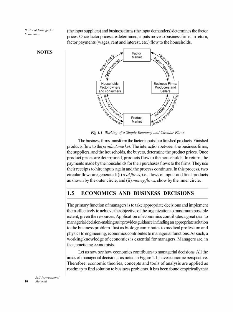
(the input suppliers) and business firms (the input demanders) determines the factorprices. Once factor prices are determined, inputs move to business firms. In return,factor payments (wages, rent and interest, etc.) flow to the households.
Fig 1.1 Working of a Simple Economy and Circular Flows
The business firms transform the factor inputs into finished products. Finishedproducts flow to the product market. The interaction between the business firms,the suppliers, and the households, the buyers, determine the product prices. Onceproduct prices are determined, products flow to the households. In return, thepayments made by the households for their purchases flows to the firms. They usetheir receipts to hire inputs again and the process continues. In this process, twocircular flows are generated: (i) real flows, i.e., flows of inputs and final productsas shown by the outer circle, and (ii) money flows, show by the inner circle.
1.5 ECONOMICS AND BUSINESS DECISIONS
The primary function of managers is to take appropriate decisions and implementthem effectively to achieve the objective of the organization to maximum possibleextent, given the resources. Application of economics contributes a great deal tomanagerial decision-making as it provides guidance in finding an appropriate solutionto the business problem. Just as biology contributes to medical profession andphysics to engineering, economics contributes to managerial functions. As such, aworking knowledge of economics is essential for managers. Managers are, infact, practicing economists.
Let us now see how economics contributes to managerial decisions. All theareas of managerial decisions, as noted in Figure 1.1, have economic perspective.Therefore, economic theories, concepts and tools of analysis are applied asroadmap to find solution to business problems. It has been found empirically that

Basics of ManagerialEconomics
NOTES
Self-InstructionalMaterial 11
application of economic theories and tools of analysis makes significant contributionto the process of business decision making in many ways.
According to Baumol, a Nobel laureate in economics, economic theorycontributes to business decision making in three important ways.
First, ‘one of the most important things which the economic theory cancontribute to management science’ is providing framework for building analyticalmodels which can help recognize the structure of managerial problem, determinethe important factors to be managed, and eliminate the minor factors that mightobstruct decision making.
Secondly, economics provides ‘a set of analytical methods’ which may notbe directly applicable to analyse specific business problems but they do widen thescope of business analysis and enhance the analytical capability of the businessanalyst in understanding the nature of the business problems.
Thirdly, various economic terms are used in common parlance, which arenot applicable to business analysis and decision making. Economic theory offersclarity to various economic concepts used in business analysis, which enables themanagers to avoid conceptual pitfalls. For example, in general sense, ‘demand’means quantity demanded at a point of time. But, in economic sense, ‘demand’means the quantity people are willing to buy at a given price and they have abilityand willingness to pay.
Apart from providing analytical models and methods and conceptual clarity,economics contributes to business decision in many other ways also. Most businessconditions are taken under the condition of risk and uncertainty. Risk anduncertainty arise in business because of continuous change in business conditionsand environment, and unpredictable market behaviour. Economics provides models,tools and technique to predict the future course of market conditions, ways andmeans to assess the risk and, thereby, helps in business decision making.
It is because of these important contributions of economics to businessdecision making that economics has been integrated with managerial decisions.Managerial decision making without applying economic logic, theory and analyticaltools may not offer a reasonable solution.
1.5.1 Relationship between Economic Theory and ManagerialEconomics
We have noted above that application of theories to the process of businessdecision-making contributes a great deal in arriving at appropriate businessdecisions. In this section, we highlight the gap between the theoretical world andthe real world and see how managerial economics bridges this gap.
Theory vs. Practice
It is widely known that there exists a gap between theory and practice in all walksof life, more so in the world of economic theory and behaviour. A theory which
Basics of ManagerialEconomics
NOTES
Self-Instructional12 Material
appears logically sound may not be directly applicable in practice. For example, ifthere is a constant relationship between inputs and outputs, it may be theoreticallyconcluded that if inputs are doubled, output will be doubled and if inputs aretrebled, output will be trebled. This theoretical conclusion may not hold in practice.This gap between theory and practice has been very well illustrated in the form ofa story by a classical economist, J.M. Clark. He writes:
‘There is a story of a man who thought of getting the economy of large scaleproduction in plowing, and built a plow three times as long, three times as wide,and three times as deep as an ordinary plow and harnessed six horses [three timesthe usual number] to pull it, instead of two. To his surprise, the plow refused tobudge, and to his greater surprise it finally took fifty horses to move the refractorymachine… [and] the fifty could not pull together as well as two’.
The gist of the story is that managers—assuming they have abundantresources—may increase the size of their capital and labour, but may not obtainthe expected results. Most probably the man in Clark’s story did not get theexpected result because he was either not aware of or he ignored or could notmeasure the resistance of the soil to a huge plow. This incident clearly shows thegap between theory and practice.
Economic theories are, no doubt, hypothetical in nature but not awayfrom reality. Economic theories are, in fact, a caricature of reality under certainspecified conditions. In their abstract form, however, they do look divorced fromreality. Besides, abstract economic theories cannot be straightaway applied toreal life problems. This should, however, not mean that economic models andtheories do not serve any useful purpose. ‘Microeconomic theory facilitates theunderstanding of what would be a hopelessly complicated confusion of billions offacts by constructing simplified models of behaviour, which are sufficiently similarto the actual phenomenon and thereby help in understanding them’. Nevertheless,it cannot be denied that there is apparently a gap between economic theory andpractice. This gap arises mainly due to the inevitable gap between the abstractworld of economic models and the real world.
How Managerial Economics Fills the Gap
There is undeniably a gap between economic theory and the real economic world.Therefore, economic theories do not offer a custom-made or readymade solutionto business problems. However, economic theories do provide a framework forlogical economic model-building and systematic analysis of economic issues. Theneed for such a framework arises because the real economic world is too complexto permit considering every bit of relevant facts that influence economic decisions.In the words of Keynes, ‘The objective of [economic] analysis is not to provide amachine, or method of blind manipulation, which will furnish an infallible answer,but to provide ourselves with an organized and orderly method of thinking outparticular problem…’. In the opinion of Boulding, the objective of economic analysis
Basics of ManagerialEconomics
NOTES
Self-InstructionalMaterial 13
is to present the ‘map’ of reality rather than a perfect picture of it. In fact, economicanalysis equips us with a road map; it guides us to the destination, but does notcarry us there. This is how managerial economics bridges the gap betweeneconomics and business decision-making. As an example, managerial economicscan also be compared with medical science. Just as the knowledge of medicalscience helps in diagnosing the disease and prescribing an appropriate medicine,managerial economics helps in analyzing the business problems and in arriving atan appropriate decision.
Let us now see how managerial economics bridges this gap. On one side,there is the complex business world and, on the other, are abstract economictheories. ‘The big gap between the problems of logic that intrigue economic theoristsand the problems of policy that plague practical management needs to be bridgedin order to give executive access to the practical contributions that economic thinkingcan make to top management policies’. Managerial decision-makers deal with thecomplex, rather chaotic, business conditions of the real world and have to find theway to their destination, i.e., achieving the goal that they set for themselves.Managerial economics applies economic logic and analytical tools to sift wheatfrom the chaff. Economic logic and tools of analysis guide business managers inthe following ways.
(i) Identifying their problems in achieving their goal,
(ii) Collecting the relevant data and related facts,
(iii) Processing and analyzing the facts,
(iv) Drawing relevant conclusions,
(v) Determining and evaluating the alternative means to achieve the goal, and
(vi) Taking a decision.
Without application of economic logic and tools of analysis, businessdecisions are most likely to be irrational and arbitrary, which may often provecounter-productive.
Check Your Progress
1. Name the two branches of economics.
2. What is the ultimate objective of the managerial functions?
3. State the main sectors comprising a simple model of an economy.
1.6 ANSWERS TO CHECK YOUR PROGRESSQUESTIONS
1. The two branches of economics are microeconomics and macroeconomics.
2. The ultimate objective of the managerial functions is to ensure maximumreturn from the utilization of firm’s resources.
Basics of ManagerialEconomics
NOTES
Self-Instructional14 Material
3. A simple model of the economy consists of two main sectors: (i) householdsand (ii) business firms.
1.7 SUMMARY
The emergence of managerial economics can be attributed to at least threefactors: (i) growing complexity of the business environment and decision-making process; (ii) increasing application of economic logic, concepts,theories and tools of economic analysis in the process of business decision-making; and (iii) rapid increase in demand for professionally trainedmanagerial manpower with good knowledge of economics.
Economists of different generations have defined economics in different waysaccording to their perception and subject matter of economics.
Economics can, thus be defined as a social science that studies economicbehaviour of the people, the individuals, households, firms, and thegovernment.
Internal managerial issues refer to decision-making issues arising in themanagement of the firm. Internal managerial issues include problems thatarise in operating the business organization.
Economics has two major branches—microeconomics andmacroeconomics. The main economic theories and tools of analysis of bothmicroeconomics and macroeconomics constitute the subject matter ofmanagerial economics.
Working of a modern economy is extremely complex. Millions of personsparticipate and contribute to its working in different ways and differentcapacities—as producers, traders, workers, financiers, and consumers.
The primary function of managers is to take appropriate decisions andimplement them effectively to achieve the objective of the organization tomaximum possible extent, given the resources.
It is because of these important contributions of economics to businessdecision making that economics has been integrated with managerialdecisions. Managerial decision making without applying economic logic,theory and analytical tools may not offer a reasonable solution.
1.8 KEY WORDS
Microeconomics: It is the study of the economizing behavior of theindividual economic entities—individuals, households, firms, industries andfactory owners.
Basics of ManagerialEconomics
NOTES
Self-InstructionalMaterial 15
Managerial economics: It can be defined as the study of economictheories, logic, concepts and tools of economic analysis applied in the processof business decision-making.
1.9 SELF ASSESSMENT QUESTIONS ANDEXERCISES
Short Answer Questions
1. Prepare an introduction to economics.
2. What is the subject matter of microeconomics and macroeconomics?
3. Write a short note on the scope of managerial economics.
Long Answer Questions
1. Discuss the general foundations of managerial economics.
2. Explain the working of a simple economy.
3. Analyse the relationship between economics and business decisions.
1.10 FURTHER READINGS
Dwivedi, D. N. 2015. Principles of Economics, Eight Edition. New Delhi: VikasPublishing House.
Weil. David N. 2004. Economic Growth. London: Addison Wesley.
Thomas, Christopher R. and Maurice S. Charles. 2005. Managerial Economics:Concepts and Applications, Eighth Edition. New Delhi: Tata McGraw-Hill Publishing Company Limited.
Mankiw, Gregory N. 2002. Principles of Economics, Second Edition. India:Thomson Press.
Websites
https://blogs.economictimes.indiatimes.com/et-commentary/heres-how-indias-widening-income-distribution-can-be-redressed/
https://www.livemint.com/Opinion/WmpSjQAvPGeVzxqpgXYvtK/The-dangers-of-Indias-Billionaire-Raj.html
Decision Making andBusiness Decisions
NOTES
Self-Instructional16 Material
UNIT 2 DECISION MAKING ANDBUSINESS DECISIONS
Structure2.0 Introduction2.1 Objectives2.2 Role of Managerial Economics in Decision Making
2.2.1 Decision Making Under Risk and Uncertainity2.3 Business Decision Rules
2.3.1 Concepts of Opportunity Cost2.3.2 Production Possibility Curve2.3.3 Incremental Concepts2.3.4 Cardinal and Ordinal Approaches to Consumer Behaviour2.3.5 Time Value of Money
2.4 Answers to Check Your Progress Questions2.5 Summary2.6 Key Words2.7 Self Assessment Questions and Exercises2.8 Further Readings
2.0 INTRODUCTION
Managerial decisions are taken at different levels of sophistication. While somebusiness decisions require only ‘rule-of-thumb’ technique, others involve the useof sophisticated techniques. The ‘rule-of-thumb’ technique, evolved out of thetraditional business management practices, is used where routine type of businessdecisions are involved. Sophisticated techniques of business decision-making areused where business decisions involve the problem of handling complex businessissues. There are certain fundamental economic concepts which are used—explicityor implicity, consciously or unconsciously, deliberately or otherwise—in businessdecisions of complex nature. This unit presents a brief explanation of some majoreconomic concepts and their use in business decision-making.
2.1 OBJECTIVES
After going through this unit, you will be able to: Explain the role of managerial economies in decision making Define opportunity cost Describe production possibility curve with the help of a diagram Discuss the cardinal and ordinal approaches to consumer behaviour State the time value of money
Decision Making andBusiness Decisions
NOTES
Self-InstructionalMaterial 17
2.2 ROLE OF MANAGERIAL ECONOMICS INDECISION MAKING
Managerial economics, also known as business economics, lays emphasis onapplying economic theory directly to business organizations. The application ofeconomic theory using statistical methods assists business organizations in takingdecisions and deciding on a strategy related to pricing, operations, risk, investmentsand production. The entire objective of managerial economics is to enhance theefficiency of decision-making in enterprises to enhance profit.
Pricing: Managerial economics helps business organizations in determiningthe pricing strategies and suitable pricing levels for their products and services.
Elastic Vs. Inelastic Goods: Economists can decide price sensitivity ofproducts using a price elasticity analysis. This will ensure that it becomeseasy to take decisions related to marketing and pricing of goods.
Operations and Production: Quantitative methods are used by managerialto analyze production and operational efficiency by means of scheduleoptimization, economies of scale and resource analyses.
Investments: Many managerial economic tools and analysis models areused to assist in making investing decisions both for corporations as well asindividual investors. These tools are used to make stock market investingdecisions and decisions on capital investments for a business.
Risk: Uncertainty exits in every business and managerial economics canhelp reduce risk through uncertainty model analysis and decision-theoryanalysis. Statistical probability theory is largely used to provide potentialscenarios for business enterprises while making decisions.
2.2.1 Decision Making Under Risk and Uncertainity
The concept of risk and uncertainty can be better explained and understood incontrast to the concept of certainty. Certainty is the state of perfect knowledgeabout the market conditions. In the state of certainty, there is only one rate ofreturn on the investment and that rate is known to the investors. That is, in the stateof certainty, the investors are fully aware of the outcome of their investmentdecisions. For example, if you deposit your savings in ‘fixed deposit’ bearing 10%interest, you know for certain that the return on your investment in time deposit is10%, and FDR can be converted into cash any day. Or, if you buy governmentbonds, treasury bills, etc. bearing an interest of 11%, you know for sure that thereturn on your investment is 11% per annum, your principal remaining safe. Ineither case, you are sure that there is little or no possibility of the bank or thegovernment defaulting on interest payment or on refunding the money. This iscalled the state of certainty.
Decision Making andBusiness Decisions
NOTES
Self-Instructional18 Material
In reality, however, there is a vast area of investment avenues in which theoutcome of investment decisions is not precisely known. The investors do notknow precisely or cannot predict accurately the possible return on their investment.
Meaning of Risk
In common parlance, risk means a low probability of an expected outcome. Frombusiness decision-making point of view, risk refers to a situation in which a businessdecision is expected to yield more than one outcome and the probability of eachoutcome is known to the decision makers or it can be reliably estimated.
There are two approaches to estimating probabilities of outcomes of abusiness decision, viz., (i) a priori approach, i.e., the approach based on deductivelogic or intuition and (ii) posteriori approach, i.e., estimating the probabilitystatistically on the basis of the past data. In case of a priori probability, we knowthat when a coin is tossed, the probabilities of ‘head’ or ‘tail’ are 50:50, and whena dice is thrown, each side has 1/6 chance to be on the top. The posterioriassumes that the probability of an event in the past will hold in future also. Theprobability of outcomes of a decision can be estimated statistically by way of‘standard deviation’ and ‘coefficient of variation’.
Meaning of Uncertainty
Uncertainty refers to a situation in which there is more than one outcome ofa business decision and the probability of no outcome is known nor can it bereliably estimated. The unpredictability of outcome may be due to lack of reliablemarket information, inadequate past experience, and high volatility of the marketconditions. For the purpose of decision-making, the uncertainty is classified as:
(a) complete ignorance, and(b) partial ignorance.
In case of complete ignorance, investment decisions are taken by theinvestor using their own judgement or using any of the rational criteria. What criterionhe chooses depends on his attitude towards risk. The investor’s attitude towardsrisk may be that of
(i) a risk averter,(ii) a risk neutral or(iii) a risk seeker or risk lover.
In case of partial ignorance, on the other hand, there is some knowledgeabout the future market conditions; some information can be obtained from theexperts in the field, and some probability estimates can be made. The availableinformation may be incomplete and unreliable. Under this condition, the decision-makers use their subjective judgement to assign an a priori probability to theoutcome or the pay-off of each possible action such that the sum of suchprobability distribution is always equal to one. This is called subjectiveprobability distribution.
Decision Making andBusiness Decisions
NOTES
Self-InstructionalMaterial 19
2.3 BUSINESS DECISION RULES
Let us go through the various economic concepts which assist in making businessdecision rules.
2.3.1 Concepts of Opportunity Cost
The opportunity cost is essentially opportunity lost because of scarcity of resources.The concept of opportunity cost is related to the alternative uses of scarce resources.As noted earlier, resources, both natural and man-made, are scarce in relation todemand for them to satisfy the ever growing human needs. Resources, thoughscarce, have alternative uses. The scarcity and the alternative uses of theresources give rise to the concept of opportunity cost.
In the context of a business firm, resources available to a business unit—beit an individual firm, a joint stock corporation or a multinational—are limited. Butthe limited resources available to a firm can be put to alternative uses.
The difference between actual earning and its opportunity cost is calledeconomic gain or economic profit. The concept of opportunity cost assumes agreat significance where economic gain is neither insignificant nor very large becausethen it requires a careful evaluation of the two alternative options.
The applicability of the opportunity cost concept is not limited to decisionson the use of financial resources. The concept can be applied to all other kinds ofissues involved in business decisions, especially where there are at least twoalternative options involving costs and benefits. For example, suppose a firm hasto take a decision on whether to fire an efficient labour officer (for treating labourunkindly) in settlement of a dispute with the labour union or to allow the matter tobe taken to the labour court. If the firm decides to fire the labour officer, then theloss of an efficient and reliable labour officer is the opportunity cost of buyingpeace with the labour union. If the firm decides to retain the labour officer, comewhatever may, then the cost of prolonged litigation, the cost arising out of a possiblelabour strike and the consequent reduction in output are the opportunity costs ofretaining the labour officer. Given the two options, the firm will have to evaluatethe cost and benefit of each option and take a decision accordingly.
2.3.2 Production Possibility Curve
Societies cannot have all that they want because resources are scarce andtechnology is given. In reality, however, both human and non-human resourcesavailable to a country keep increasing over time and technology becoming moreand more efficient and productive. Availability of human resources increases dueto a natural process of increase in population, and non-human resources (especiallycapital goods and raw materials) increase due to creative nature of human beings.Non-human resources have been increasing due to human efforts to create moreand better of capital goods, to discover new kinds and sources of raw materials,
Decision Making andBusiness Decisions
NOTES
Self-Instructional20 Material
and to create a new and more efficient technique of production. Such factorsbring about a change in production possibilities and production possibilitiesfrontier of an economy.
To begin with, we will assume a static model with the followingassumptions: (i) a country’s resources consists of only labour and capital;(ii) availability of labour and capital is given; (iii) the country produces only twogoods—food and clothing; and (iv) production technology for the goods is given.
The Production Possibilities Frontier
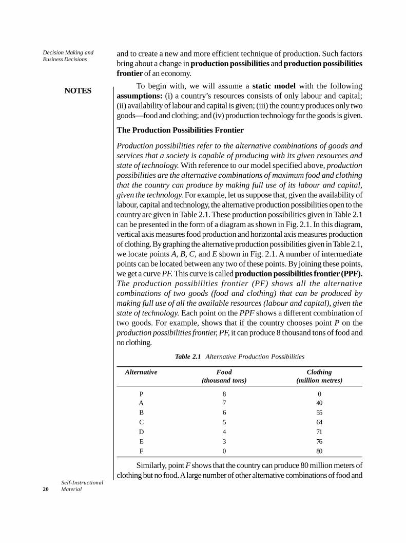
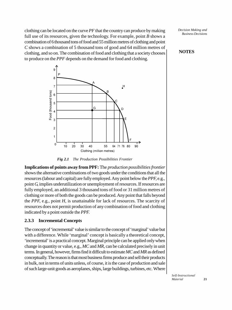
Production possibilities refer to the alternative combinations of goods andservices that a society is capable of producing with its given resources andstate of technology. With reference to our model specified above, productionpossibilities are the alternative combinations of maximum food and clothingthat the country can produce by making full use of its labour and capital,given the technology. For example, let us suppose that, given the availability oflabour, capital and technology, the alternative production possibilities open to thecountry are given in Table 2.1. These production possibilities given in Table 2.1can be presented in the form of a diagram as shown in Fig. 2.1. In this diagram,vertical axis measures food production and horizontal axis measures productionof clothing. By graphing the alternative production possibilities given in Table 2.1,we locate points A, B, C, and E shown in Fig. 2.1. A number of intermediatepoints can be located between any two of these points. By joining these points,we get a curve PF. This curve is called production possibilities frontier (PPF).The production possibilities frontier (PF) shows all the alternativecombinations of two goods (food and clothing) that can be produced bymaking full use of all the available resources (labour and capital), given thestate of technology. Each point on the PPF shows a different combination oftwo goods. For example, shows that if the country chooses point P on theproduction possibilities frontier, PF, it can produce 8 thousand tons of food andno clothing.
Table 2.1 Alternative Production Possibilities
Alternative Food Clothing(thousand tons) (million metres)
P 8 0A 7 40B 6 55C 5 64D 4 71E 3 76F 0 80
Similarly, point F shows that the country can produce 80 million meters ofclothing but no food. A large number of other alternative combinations of food and
Decision Making andBusiness Decisions
NOTES
Self-InstructionalMaterial 21
clothing can be located on the curve PF that the country can produce by makingfull use of its resources, given the technology. For example, point B shows acombination of 6 thousand tons of food and 55 million metres of clothing and pointC shows a combination of 5 thousand tons of good and 64 million metres ofclothing, and so on. The combination of food and clothing that a society choosesto produce on the PPF depends on the demand for food and clothing.
Fig 2.1 The Production Possibilities Frontier
Implications of points away from PPF: The production possibilities frontiershows the alternative combinations of two goods under the conditions that all theresources (labour and capital) are fully employed. Any point below the PPF, e.g.,point G, implies underutilization or unemployment of resources. If resources arefully employed, an additional 3 thousand tons of food or 31 million metres ofclothing or more of both the goods can be produced. Any point that falls beyondthe PPF, e.g., point H, is unattainable for lack of resources. The scarcity ofresources does not permit production of any combination of food and clothingindicated by a point outside the PPF.
2.3.3 Incremental Concepts
The concept of ‘incremental’ value is similar to the concept of ‘marginal’ value butwith a difference. While ‘marginal’ concept is basically a theoretical concept,‘incremental’ is a practical concept. Marginal principle can be applied only whenchange in quantity or value, e.g., MC and MR, can be calculated precisely in unitterms. In general, however, firms find it difficult to estimate MC and MR as definedconceptually. The reason is that most business firms produce and sell their productsin bulk, not in terms of units unless, of course, it is the case of production and saleof such large-unit goods as aeroplanes, ships, large buildings, turbines, etc. Where
Decision Making andBusiness Decisions
NOTES
Self-Instructional22 Material
production and sale activities are carried out in bulk and where both fixed andvariable costs are subject to change, business managers use the incrementalprinciple in their business decisions.
The incremental principle is applied to business decisions which involvebulk production and a large increase in total cost and total revenue. Such anincrease in total cost and total revenue is called ‘incremental cost’ and ‘incrementalrevenue’ respectively, related to ‘incremental output’.
Let us first explain the concept of incremental cost. Conceptually,incremental costs can be defined as the costs that arise due to a business decision.Thus, an increase in the total cost of production due to a business decision isincremental cost.
The incremental revenue, on the other hand, is the increase in revenuedue to a business decision, e.g., a decision to increase production and sale of thefirm’s product. When a business decision is successfully implemented, it doesresult in a significant increase in its total revenue. The increase in the total revenueresulting from a business decision is called incremental revenue.
Incremental Reasoning in Business Decision
The use of the incremental concept in business decisions is called incrementalreasoning. The incremental reasoning is used for accepting or rejecting a businessproposition or option.
It may be added at the end, by way of comparison, that the marginalconcept (especially when defined and measured by calculus) is used in economicanalysis where a high degree of precision is involved, whereas the incrementalconcept is used where large values, especially of cost and revenue are involved.Besides, incremental concept and reasoning are used in business decisions morefrequently than the marginal concept. There are at least two reasons for this.First, marginal concept used in business analysis is generally associated with one(marginal) unit of output produced or sold whereas most business decisions involvelarge quantities and values. Second, the precise calculation of marginal change(defined in terms of the first derivative of a function) is neither practicable nornecessary in real life business decisions. However, marginal concept is of greatsignificance in theoretical analysis.
2.3.4 Cardinal and Ordinal Approaches to Consumer Behaviour
Consumers demand a commodity because they derive or expect to derive utilityfrom the consumption of that commodity. The expected utility from a commodityis the basis of demand for it. Though ‘utility’ is a term of common usage, it has aspecific meaning and use in the analysis of consumer demand. We will, therefore,describe in this section the meaning of utility, the related concepts and the lawassociated with utility.
Decision Making andBusiness Decisions
NOTES
Self-InstructionalMaterial 23
Meaning of Utility
The concept of utility can be looked upon from two angles—from the productangle and from the consumer’s angle. From the product angle, utility is the want-satisfying property of a commodity. From consumer’s angle, utility is thepsychological feeling of satisfaction, pleasure, happiness or well-being, whicha consumer derives from the consumption, possession or the use of acommodity.
There is a subtle difference between the two concepts which must be bornein mind. The concept of a want-satisfying property of a commodity is ‘absolute’ inthe sense that this property is ingrained in the commodity irrespective of whetherone needs it or not. For example, a pen has its own utility irrespective of whethera person is literate or illiterate. Another important attribute of the ‘absolute’ conceptof utility is that it is ‘ethically neutral’ because a commodity may satisfy a frivolousor socially immoral need, e.g., alcohol, drugs, porn-CDs, etc.
On the other hand, from a consumer’s point of view, utility is a post-consumption phenomenon as one derives satisfaction from a commodity only whenone consumes or uses it. Utility in the sense of satisfaction is a ‘subjective’ or‘relative’ concept because (i) a commodity need not be useful for all—cigarettesdo not have any utility for non-smokers, and meat has no utility for strict vegetarians;(ii) utility of a commodity varies from person to person and from time to time; and(iii) a commodity need not have the same utility for the same consumer at differentpoints of times, at different levels of consumption and for different moods of aconsumer. In consumer analysis, only the ‘subjective’ concept of utility is used.
Having explained the concept of utility, we now turn to some quantitativeconcepts related to utility used in utility analysis, viz. total utility and marginalutility.
The cardinal and ordinal concepts of utility arise out of question whether‘utility is measureable’. Let us now look into the origin of the two concepts ofutility and their use in the analysis of demand.
Cardinal Utility
Some early psychological experiments on an individual’s responses to variousstimuli led neo-classical economists to believe that utility is measurable and cardinallyquantifiable. According to neo-classical economists, utility can be measured interms of money. That is, utility of a unit of a commdity for a person is equal to theamount of money he is willing to pay for it. This belief gave rise to the concept ofcardinal utility. It implies that utility can be assigned a cardinal number like 1, 2, 3,etc. Neo-classical economists built up the theory of consumption on the assumptionthat utility is cardinally measurable. They coined and used a term ‘util’ meaning‘units of utility’. In their measure of utility, they assumed (i) that one ‘util’ equalsone unit of money, and (ii) that utility of money remains constant.
Decision Making andBusiness Decisions
NOTES
Self-Instructional24 Material
It has, however, been realized over time that absolute or cardinalmeasurement of utility is not possible. Difficulties in measuring utility have provedto be insurmountable.
Ordinal Utility
The modern economists have discarded the concept of cardinal utility and haveinstead employed the concept of ordinal utility for analyzing consumer behaviour.The concept of ordinal utility is based on the fact that it may not be possible forconsumers to express the utility of a commodity in absolute or quantitative terms,but it is always possible for a consumer to tell introspectively whether a commodityis more or less or equally useful compared to another. For example, a consumermay not be able to say that ice cream gives 5 utils and chocolate gives 10 utils. Buthe or she can always specify whether chocolate gives more or less utility than icecream. This assumption forms the basis of the ordinal theory of consumer behaviour.
While neo-classical economists maintained that cardinal measurement ofutility is practically possible and is meaningful in consumer analysis, moderneconomists maintain that utility being a psychological phenomenon is inherentlyimmeasurable, theoretically, conceptually as well as quantitatively. They also maintainthat the concept of ordinal utility is a feasible concept and it meets the conceptualrequirement of analyzing consumer behaviour in the absence of any cardinal measuresof utility.
Two Approaches to the Consumer Demand Analysis
Based on cardinal and ordinal concepts of utility, there are two approaches to theanalysis of consumer behaviour.
(i) Cardinal Utility Approach, attributed to Alfred Marshall and his followers,is also called the Neo-classical Approach.
(ii) Ordinal Utility Approach, pioneered by J.R. Hicks, a Nobel laureate,and R.G.D. Allen, is also called the Indifference Curve Analysis.The two approaches are not in conflict with one another. In fact, they
represent two levels of sophistication in the analysis of consumer behaviour. Boththe approaches are important for assessing and analyzing consumer demand for acommodity—be it for thoretical purpose or for business decision-making,depending on the level of sophistication required.
2.3.5 Time Value of Money
All business decisions are taken with a certain time perspective. The timeperspective refers to the duration of time period extending from the relevant pastand foreseeable future taken in view while taking a business decision. Relevantpast refers to the period of past experience and trends which are relevant forbusiness decisions with long-run implications. All business decisions do not have
Decision Making andBusiness Decisions
NOTES
Self-InstructionalMaterial 25
the same time perspective. Some have short-run outcome or pay-off and, therefore,involve short-run time perspective. For example, a decision to buy explosivematerials for manufacturing crackers involves short-run demand prospects. Similarly,a decision regarding building inventories of finished product involves a short-runtime perspective. There are, however, a large number of business decisions whichhave long-run repercussions, e.g., investment in plant, building, machinery, land,spending on labour welfare activities, expansion of the scale of production,introduction of a new product, advertisement, bribing a government officer andinvestment abroad. The decision about such business issues, for example, thedecision regarding the introduction of a new product may not be profitable in theshort-run but may prove very profitable in the long-run.
The business decision-makers must assess and determine the time perspectiveof business propositions well in advance and make decisions accordingly.Determination of time perspective is of great significance especially whereprojections are involved. The decision-makers must decide on an appropriatefuture period for projecting the value of a variable. Otherwise, projections mayprove meaningless from analysis point of view and decisions based thereon mayresult in poor pay-offs. For example, in a business decision regarding theestablishment of a Management Institute, projecting a short-run demand and takinga short-run time perspective will be unwise, and in buying explosive materials formanufacturing crackers for Deepawali, a long-run time perspective is unwise.
Check Your Progress
1. Define opportunity cost.2. Name the two approaches used to analyse consumer behaviour.
2.4 ANSWERS TO CHECK YOUR PROGRESSQUESTIONS
1. Opportunity cost is a term in economics that refers to the value of what youhave to give up in order to choose something else.
2. The two approaches used to analyse consumer behavior are the following: Cardinal utility approach Ordinal utility approach
2.5 SUMMARY
Managerial decisions are taken at different levels of sophistication. Whilesome business decisions require only ‘rule-of-thumb’ technique, some othersinvolve the use of sophisticated techniques.
Decision Making andBusiness Decisions
NOTES
Self-Instructional26 Material
Certainty is the state of perfect knowledge about the market conditions. Inthe state of certainty, there is only one rate of return on the investment andthat rate is known to the investors.
From business decision-making point of view, risk refers to a situation inwhich a business decision is expected to yield more than one outcome andthe probability of each outcome is known to the decision makers or it canbe reliably estimated.
Uncertainty refers to a situation in which there is more than one outcome ofa business decision and the probability of no outcome is known nor can itbe reliably estimated.
The scarcity and the alternative uses of the resources give rise to the conceptof opportunity cost.
The difference between actual earning and its opportunity cost is calledeconomic gain or economic profit. The concept of opportunity cost assumesa great significance where economic gain is neither insignificant nor verylarge because then it requires a careful evaluation of the two alternativeoptions.
Production possibilities refer to the alternative combinations of goods andservices that a society is capable of producing with its given resources andstate of technology.
The incremental revenue is the increase in revenue due to a business decision,e.g., a decision to increase production and sale of the firm’s product.
Consumers demand a commodity because they derive or expect to deriveutility from the consumption of that commodity. The expected utility from acommodity is the basis of demand for it.
From consumer’s angle, utility is the psychological feeling of satisfaction,pleasure, happiness or well-being, which a consumer derives from theconsumption, possession or the use of a commodity.
The cardinal and ordinal concepts of utility arise out of question whether‘utility is measureable’.
All business decisions are taken with a certain time perspective. The timeperspective refers to the duration of time period extending from the relevantpast and foreseeable future taken in view while taking a business decision.
The business decision-makers must assess and determine the time perspectiveof business propositions well in advance and make decisions accordingly.
2.6 KEY WORDS
Risk: It means a low probability of an expected outcome.
Decision Making andBusiness Decisions
NOTES
Self-InstructionalMaterial 27
Uncertainty: It refers to a situation in which there is more than one outcomeof a business decision and the probability of no outcome is known nor canit be reliably estimated.
Incremental costs: These are costs that arise due to a business decision.
2.7 SELF ASSESSMENT QUESTIONS ANDEXERCISES
Short Answer Questions
1. What is the significance of opportunity cost?2. Define economic profit.3. Write a short note on the time value of money.
Long Answer Questions
1. What is the role of managerial economics in decision making?2. Explain the production possibilities frontier with the help of an example.3. Describe the two approaches used to analyse consumer behaviour.
2.8 FURTHER READINGS
Dwivedi, D. N. 2015. Principles of Economics, Eight Edition. New Delhi: VikasPublishing House.
Weil. David N. 2004. Economic Growth. London: Addison Wesley.Thomas, Christopher R. and Maurice S. Charles. 2005. Managerial Economics:
Concepts and Applications, Eighth Edition. New Delhi: Tata McGraw-Hill Publishing Company Limited.
Mankiw, Gregory N. 2002. Principles of Economics, Second Edition. India:Thomson Press.
Websites
https://blogs.economictimes.indiatimes.com/et-commentary/heres-how-indias-widening-income-distribution-can-be-redressed/
https://www.livemint.com/Opinion/WmpSjQAvPGeVzxqpgXYvtK/The-dangers-of-Indias-Billionaire-Raj.html
Consumer Behaviour
NOTES
Self-Instructional28 Material
UNIT 3 CONSUMER BEHAVIOUR
Structure3.0 Introduction3.1 Objectives3.2 Marginalism, Equilibrium and Equi-Marginalism and their Role in
Business Decision Making3.2.1 Equi-Marginal Principles
3.3 Utility Analysis3.3.1 Total and Marginal Utility
3.4 Cardinal Utility Approach or the Marshallian Approach3.4.1 Law of Diminshing Marginal Utility
3.5 Ordinal Utility Approach or the Hicks Approach3.5.1 Indifference Curve Analysis
3.6 Answers to Check Your Progress Questions3.7 Summary3.8 Key Words3.9 Self Assessment Questions and Exercises
3.10 Further Readings
3.0 INTRODUCTION
Consumer demand is the basis of all productive activities. Just as ‘necessity is themother of invention’, demand is the mother of production. Increasing demandfor a product offers high business prospects for it in future and decreasing demandfor a product diminishes its business prospect. For example, increasing demandfor computers, cars, mobile phones etc., in India has enlarged the business prospectfor both domestic and foreign companies selling these goods. On the other hand,declining demand for black and white TV sets and manual typewriters is forcingtheir companies to switch over to modern substitutes or else go out of business. Itis, therefore, essential for business managers to have a clear understanding of thefollowing aspects of demand for their products:
(i) What is the basis of demand for a commodity?(ii) What are the determinants of demand?(iii) How do the buyers decide the quantity of a product to be purchased?(iv) How do the buyers respond to change in product prices, their incomes and
prices of the related goods?(v) How can the total or market demand for a product be assessed and
forecasted?These questions are answered by the analysis of consumer behaviour.
The study of consumer behaviour gives rise to the Theory of Consumer Demand.In this unit, you will study about the concept of marginalism, equilibrium and
Consumer Behaviour
NOTES
Self-InstructionalMaterial 29
equi-marginalism and their role in business decision-making, utility analysis, cardinaland ordinal utility approaches and the properties of an indifference curve.
3.1 OBJECTIVES
After going through this unit, you will be able to: Define marginalism and equilibrium State the equi-marginal principle Discuss total and marginal utility Explain the Marshallian approach Describe the properties of indifference curve
3.2 MARGINALISM, EQUILIBRIUM AND EQUI-MARGINALISM AND THEIR ROLE INBUSINESS DECISION MAKING
The concept of ‘marginal’ value is widely used in economic analysis, for examplemarginal utility in consumer analysis, marginal productivity in productionanalysis and marginal revenue and marginal cost in pricing theory. Marginalityconcept assumes special significance where maximization or minimization problemis involved, for example, maximization of a consumer’s utility, maximization of afirm’s profit, minimization of cost, etc. The term ‘marginal’ refers to the change(increase or decrease) in total quantity or value due to a one-unit change in itsdeterminant. For example, given the factor prices, the total cost of production ofa commodity depends on the number of units produced. In this case, ‘marginalcost’ (MC) can be defined as the rise in total cost as a result of producing oneadditional unit of a commodity. The marginal cost (MC) can be worked out asfollows.
Marginal cost (MC) = TCn – TCn – 1
where TCn = total cost of producing n units and TCn – 1 = total cost of producingn – 1 units.
For example, suppose total cost (TC) of producing 100 units of a commodityis ̀ 2500. When production is increased to 101 units TC increases to ̀ 2550. Inthis case, TCn = `2550, TCn – 1 = `2500 (where n = 101 and n – 1 = 100).
Then MC = TCn – TCn – 1
= `2550 – `2500 = `50Similarly, MR can be defined as the change in TR due to the sale of one
additional unit of a product. It can also be defined as:Marginal revenue (MR) = TRn – TRn – 1
Consumer Behaviour
NOTES
Self-Instructional30 Material
where TRn = total revenue from the sale of n units and TRn – 1 = total revenue fromthe sale of n – 1 units.
Alternatively, if TC and TR are given in the form of functions, then MC andMR are defined as the first derivatives of the TC and TR functions, respectively.Suppose TC and TR functions are given as
TC = f(Q)and TR = f(Q)
Then the first derivative is calculated through calculus as follows.
TCMCQ
and TRMRQ
If TC and TR are given in the form of curves, then MC and MR are definedin terms of the slopes of the TR and TC curves. Marginal value derived from afunction in the form of its first derivative is not the same as defined in terms of aunit. More on this aspect of the ‘marginal’ concept will follow in a subsequentsection.The decision rule: Suppose a profit-maximizing firm is faced with a problem—how much to produce so that profit is maximized. One simple decision rule underthe marginal principle is that a business activity (production and sale) must becarried out so long as its MR > MC. As regards profit maximizing output,economists use the marginality principle to set a necessary condition for profitmaximizing output. The necessary condition for profit maximizing output is thatMC must be equal to MR. That is, profit is maximum where
MR = MCIn simple words, the profit of a firm is maximized at that level of output and
sale where the cost of producing one additional unit equals the revenue from thesale of that unit of output.
The application of the marginal principle for profit maximization has certainserious limitations which must be borne in mind.
One, it can be applied only where the management has the TC and TR datafor each and every unit of output or where the management is fully aware of thecost of producing one additional unit and the price expected to be received fromthe sale of that unit.
Two, the concept of ‘marginal’ value, when used in cost analysis, reducesthe value of MC to the change in variable cost only. Therefore, marginal analysiscan be applied to a situation in which only the variable cost changes.
3.2.1 Equi-marginal Principles
The equi-marginal principle was originally associated with consumption theoryand the law is called ‘the law of equi-marginal utility’. The law of equi-marginal
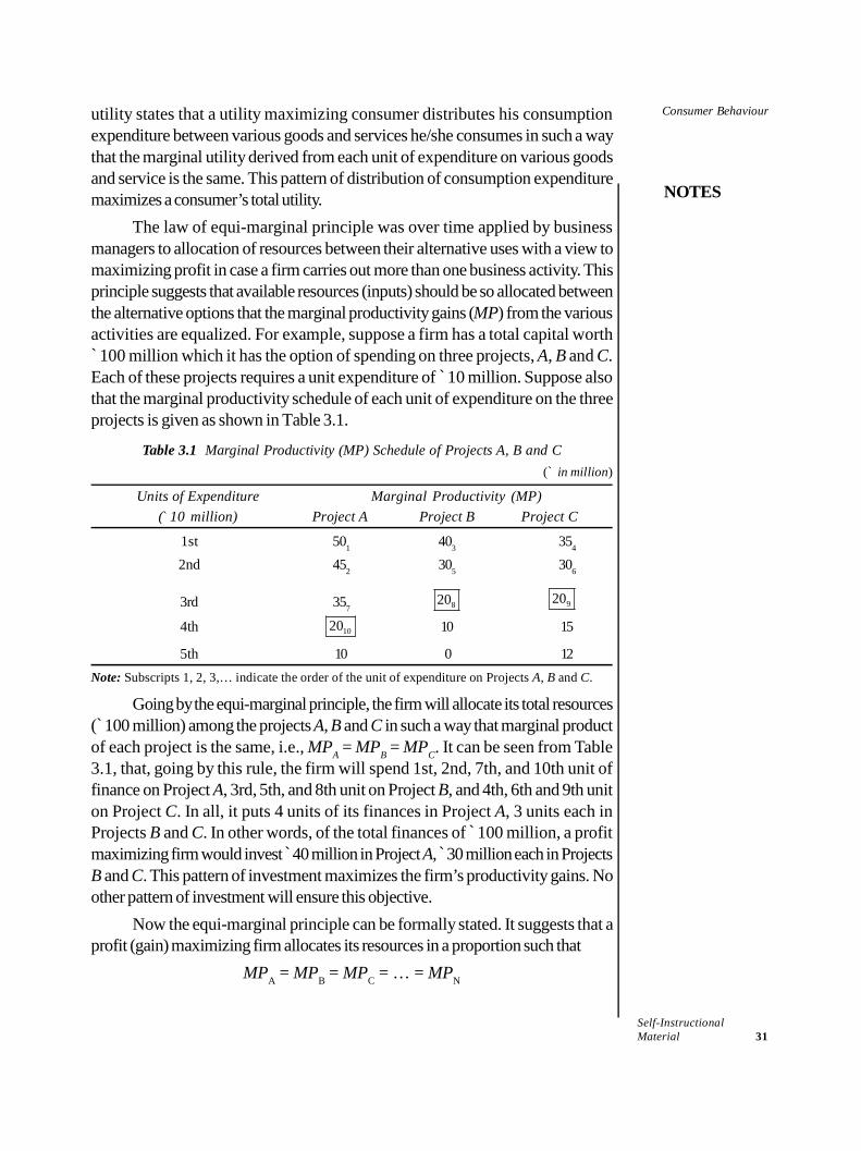
Consumer Behaviour
NOTES
Self-InstructionalMaterial 31
utility states that a utility maximizing consumer distributes his consumptionexpenditure between various goods and services he/she consumes in such a waythat the marginal utility derived from each unit of expenditure on various goodsand service is the same. This pattern of distribution of consumption expendituremaximizes a consumer’s total utility.
The law of equi-marginal principle was over time applied by businessmanagers to allocation of resources between their alternative uses with a view tomaximizing profit in case a firm carries out more than one business activity. Thisprinciple suggests that available resources (inputs) should be so allocated betweenthe alternative options that the marginal productivity gains (MP) from the variousactivities are equalized. For example, suppose a firm has a total capital worth`100 million which it has the option of spending on three projects, A, B and C.Each of these projects requires a unit expenditure of ̀ 10 million. Suppose alsothat the marginal productivity schedule of each unit of expenditure on the threeprojects is given as shown in Table 3.1.
Table 3.1 Marginal Productivity (MP) Schedule of Projects A, B and C(` in million)
Units of Expenditure Marginal Productivity (MP)(`10 million) Project A Project B Project C
1st 501 403 354
2nd 452 305 306
3rd 357 820 920
4th 1020 10 15
5th 10 0 12Note: Subscripts 1, 2, 3,… indicate the order of the unit of expenditure on Projects A, B and C.
Going by the equi-marginal principle, the firm will allocate its total resources(`100 million) among the projects A, B and C in such a way that marginal productof each project is the same, i.e., MPA = MPB = MPC. It can be seen from Table3.1, that, going by this rule, the firm will spend 1st, 2nd, 7th, and 10th unit offinance on Project A, 3rd, 5th, and 8th unit on Project B, and 4th, 6th and 9th uniton Project C. In all, it puts 4 units of its finances in Project A, 3 units each inProjects B and C. In other words, of the total finances of ̀ 100 million, a profitmaximizing firm would invest ̀ 40 million in Project A,`30 million each in ProjectsB and C. This pattern of investment maximizes the firm’s productivity gains. Noother pattern of investment will ensure this objective.
Now the equi-marginal principle can be formally stated. It suggests that aprofit (gain) maximizing firm allocates its resources in a proportion such that
MPA = MPB = MPC = … = MPN
Consumer Behaviour
NOTES
Self-Instructional32 Material
If cost of project (COP) varies from project to project, then resources areso allocated that MP per unit of COP is the same. That is, resources are allocatedin such proportions that
A
A
MPCOP =
B
B
MPCOP =
C
C
MPCOP = ... =
N
N
MPCOP
The equi-marginal principle can be applied only where (i) firms have limitedinvestible resources, (ii) resources have alternative uses, and (iii) the investmentin various alternative uses is subject to diminishing marginal productivity or returns.
3.3 UTILITY ANALYSIS
Let us go through the various economic terms associated with utility analysis.
3.3.1 Total and Marginal Utility
Assuming that utility is measurable and additive, total utility may be defined as thesum of the utility derived by a consumer from the various units of a good or servicehe consumes at a point or over a period of time. Suppose a consumer consumesfour units of a commodity, X, at a time and derives utility from the successive unitsof consumption as u1, u2, u3 and u4. His total utility (Ux) from commodity X can bemeasured then as follows.
Ux = u1 + u2 + u3 + u4
If a consumer consumes a large number of commodities, say, n number ofcommodities, his total utility, TUn, is the sum of the total utility derived from eachcommodity. For instance, if the consumption goods are X, Y and Z and their totalrespective utilities are Ux, Uy and Uz, then
TUn = Ux + Uy + Uz
Marginal Utility
Marginal utility is another very important concept used in economic analysis.Marginal utility can be defined as the utility derived from the marginal or oneadditional unit consumed. It may also be defined as the addition to the total utilityresulting from the consumption of one additional unit. Marginal Utility (MU) thusrefers to the change in the Total Utility (i.e.,TU) obtained from the consumptionof an additional unit of a commodity, say X. It may be expressed as
MUx = x
x
TUQ
where TUx = total utility, and Qx = change in quantity consumed by one unit.Another way of expressing marginal utility (MU), when the number of units
consumed is n, can be as follows.MU of nth unit = TUn – TUn–1
Consumer Behaviour
NOTES
Self-InstructionalMaterial 33
3.4 CARDINAL UTILITY APPROACH OR THEMARSHALLIAN APPROACH
In the preceding unit, you were briefly introduced to the concept of cardinal utilityand ordinal utility approaches to consumer behaviour. In this section, you willstudy the cardinal utility approach also known as the Marshallian approach indetail with the help of tables and figures.
The central theme of the consumption theory – be it based on ordinal utilityor cardinal utility approach – is the utility maximizing behaviour of the consumer.The fundamental postulate of the consumption theory is that all the consumers—individuals and households—aim at utility maximization and all their decisionsand actions as consumers are directed towards utility maximization. The specificquestions that the consumption theory seeks to answer are:
(i) how does a consumer decide the optimum quantity of a commodity that heor she chooses to consume, i.e., how does a consumer attain his/herequilibrium in respect to each commodity?
(ii) how does he or she allocate his/her disposable income between variouscommodities of consumption so that his/her total utility is maximized?The theory of consumer behaviour based on the cardinal utility approach
seeks to answer the above questions on the basis of the following assumptions.
Assumptions
(i) Maximization of satisfaction: Every rational consumer intends tomaximize his/her satisfaction from his/her given money income.
(ii) Rationality: It is assumed that the consumer is a rational being in the sensethat he or she satisfies his/her wants in the order of their preference. That is,he or she buys that commodity first which is expected to yield the highestutility and the last which is likely to the least utility.
(iii) Limited money income: The consumer has a limited money income tospend on the goods and services he or she chooses to consume. Limitednessof income, along with utility maximization objective makes the choicebetween goods inevitable.
(iv) Utility is cardinally measurable: The cardinalists have assumed that utilityis cardinally measurable and that utility of one unit of a commodity equalsthe units of money a consumer is prepared to pay for it, i.e., 1 util = 1 unitof money.
(v) Diminishing marginal utility: The consumption of a commodity is subjectto the law of diminishing marginal utility. That is, it is assumed that the utilitygained from the successive units of a commodity consumed decreases as aperson consumes them. This is an axiom of the theory of consumer behaviour.
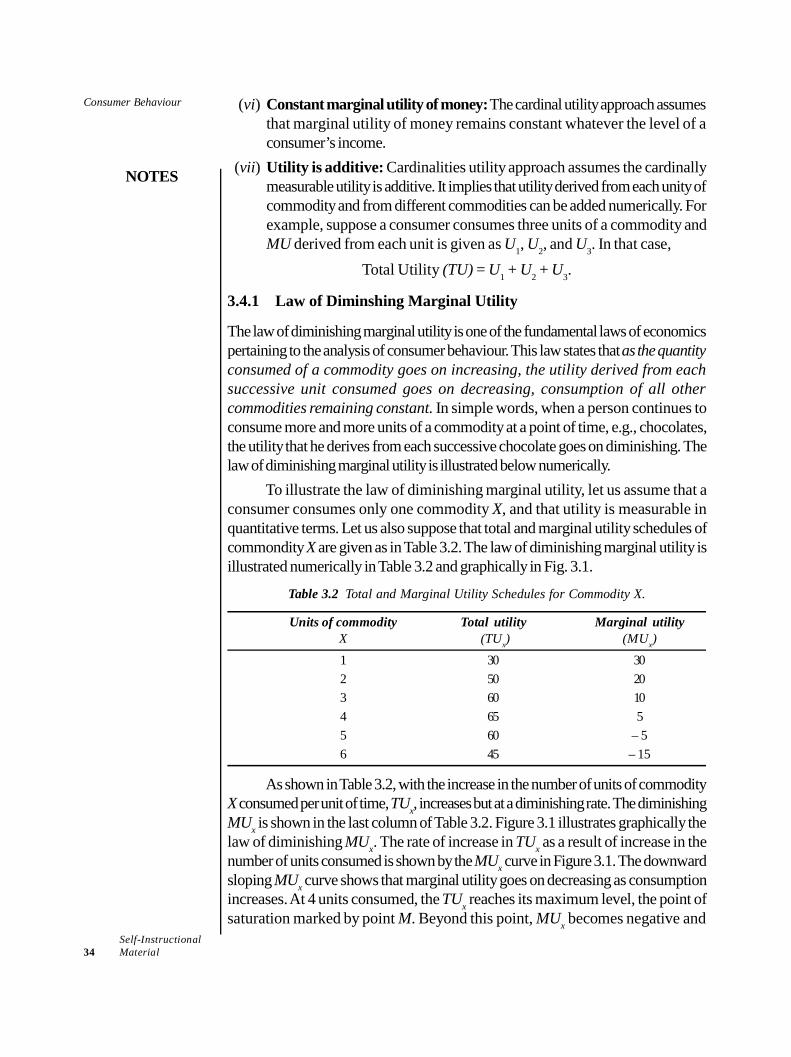
Consumer Behaviour
NOTES
Self-Instructional34 Material
(vi) Constant marginal utility of money: The cardinal utility approach assumesthat marginal utility of money remains constant whatever the level of aconsumer’s income.
(vii) Utility is additive: Cardinalities utility approach assumes the cardinallymeasurable utility is additive. It implies that utility derived from each unity ofcommodity and from different commodities can be added numerically. Forexample, suppose a consumer consumes three units of a commodity andMU derived from each unit is given as U1, U2, and U3. In that case,
Total Utility (TU) = U1 + U2 + U3.
3.4.1 Law of Diminshing Marginal Utility
The law of diminishing marginal utility is one of the fundamental laws of economicspertaining to the analysis of consumer behaviour. This law states that as the quantityconsumed of a commodity goes on increasing, the utility derived from eachsuccessive unit consumed goes on decreasing, consumption of all othercommodities remaining constant. In simple words, when a person continues toconsume more and more units of a commodity at a point of time, e.g., chocolates,the utility that he derives from each successive chocolate goes on diminishing. Thelaw of diminishing marginal utility is illustrated below numerically.
To illustrate the law of diminishing marginal utility, let us assume that aconsumer consumes only one commodity X, and that utility is measurable inquantitative terms. Let us also suppose that total and marginal utility schedules ofcommondity X are given as in Table 3.2. The law of diminishing marginal utility isillustrated numerically in Table 3.2 and graphically in Fig. 3.1.
Table 3.2 Total and Marginal Utility Schedules for Commodity X.
Units of commodity Total utility Marginal utilityX (TUx) (MUx)1 30 302 50 203 60 104 65 55 60 – 56 45 – 15
As shown in Table 3.2, with the increase in the number of units of commodityX consumed per unit of time, TUx, increases but at a diminishing rate. The diminishingMUx is shown in the last column of Table 3.2. Figure 3.1 illustrates graphically thelaw of diminishing MUx. The rate of increase in TUx as a result of increase in thenumber of units consumed is shown by the MUx curve in Figure 3.1. The downwardsloping MUx curve shows that marginal utility goes on decreasing as consumptionincreases. At 4 units consumed, the TUx reaches its maximum level, the point ofsaturation marked by point M. Beyond this point, MUx becomes negative and
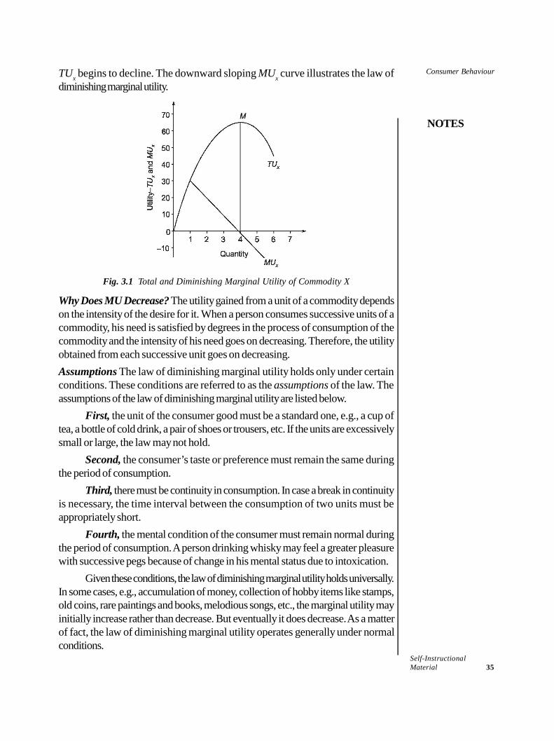
Consumer Behaviour
NOTES
Self-InstructionalMaterial 35
TUx begins to decline. The downward sloping MUx curve illustrates the law ofdiminishing marginal utility.
Fig. 3.1 Total and Diminishing Marginal Utility of Commodity X
Why Does MU Decrease? The utility gained from a unit of a commodity dependson the intensity of the desire for it. When a person consumes successive units of acommodity, his need is satisfied by degrees in the process of consumption of thecommodity and the intensity of his need goes on decreasing. Therefore, the utilityobtained from each successive unit goes on decreasing.Assumptions The law of diminishing marginal utility holds only under certainconditions. These conditions are referred to as the assumptions of the law. Theassumptions of the law of diminishing marginal utility are listed below.
First, the unit of the consumer good must be a standard one, e.g., a cup oftea, a bottle of cold drink, a pair of shoes or trousers, etc. If the units are excessivelysmall or large, the law may not hold.
Second, the consumer’s taste or preference must remain the same duringthe period of consumption.
Third, there must be continuity in consumption. In case a break in continuityis necessary, the time interval between the consumption of two units must beappropriately short.
Fourth, the mental condition of the consumer must remain normal duringthe period of consumption. A person drinking whisky may feel a greater pleasurewith successive pegs because of change in his mental status due to intoxication.
Given these conditions, the law of diminishing marginal utility holds universally.In some cases, e.g., accumulation of money, collection of hobby items like stamps,old coins, rare paintings and books, melodious songs, etc., the marginal utility mayinitially increase rather than decrease. But eventually it does decrease. As a matterof fact, the law of diminishing marginal utility operates generally under normalconditions.
Consumer Behaviour
NOTES
Self-Instructional36 Material
It concluded that as price deceases, demand increases. This inverserelationship between demand and price gives rise to demand curve.
3.5 ORDINAL UTILITY APPROACH OR THEHICKS APPROACH
In the preceding section, we have discussed the consumer behaviour based oncardinal utility approach. In this section, we proceed to discuss consumerbehaviour on the basis of ordinal utility approach. The cardinal utility approachis based on the assumption that utility is cardinally or numerically measurable whileordinal utility approach is based on the assumption that utility is measurable onlyordinally, not cardinally or numerically. In other words, utility can be expressedonly comparatively. For example, a consumer consuming two googs, X and Y, canexpress his feeling of utility as utility of X is ‘higher than’ or ‘lower than’ that of Y.Although the concept of ‘ordinal utility’ was evolved much earlier, the analysis ofconsumer behaviour based on ordinal utility concept was developed by J.R. Hicksand R.G.D. Allen in 1934. The ordinal utility approach is also known as Hicks-Allen Approach. However, the basic theory of consumer behaviour was developedby J. R. Hicks. In order to analyse consumer behaviour, Hicks used a new tool ofanalysis called Indifference curve. In this section, we will discuss consumerbehaviour following the ordinal utility approach. We will first explain the ‘indifferencecurve’, the tool of analysis and then proceed to analyse consumer behaviour throughthe indifference curve.
Assumptions of Ordinal Utility Theory
1. Rationality: The consumer is assumed to be a rational being. Rationalitymeans that a consumer aims at maximizing his total satisfaction given hisincome and prices of the goods and services he consumes and his decisionsare consistent with this objective.
2. Ordinal utility: Indifference curve analysis is based on the assumptionthat utility is only ordinally expressible. That is, the consumer is only able toexpress the order of his preference for different baskets of goods.
3. Transitivity and consistency of choice: Consumer’s choices are assumedto be transitive. Transitivity of choice means that if a consumer prefers Ato B and B to C, he must prefer A to C. Or, if he treats A = B and B = C, hemust treat A = C. Consistency of choice means transitivity of choice over aperiod of time. For example, it means that if a consumer prefers A to B inone period, he does not prefer B to A in another period or even treat themas equal.
4. Nonsatiety: It is also assumed that the consumer has not reached the pointof saturation in case of any commodity. Therefore, a consumer always prefersa larger quantity of all the goods.
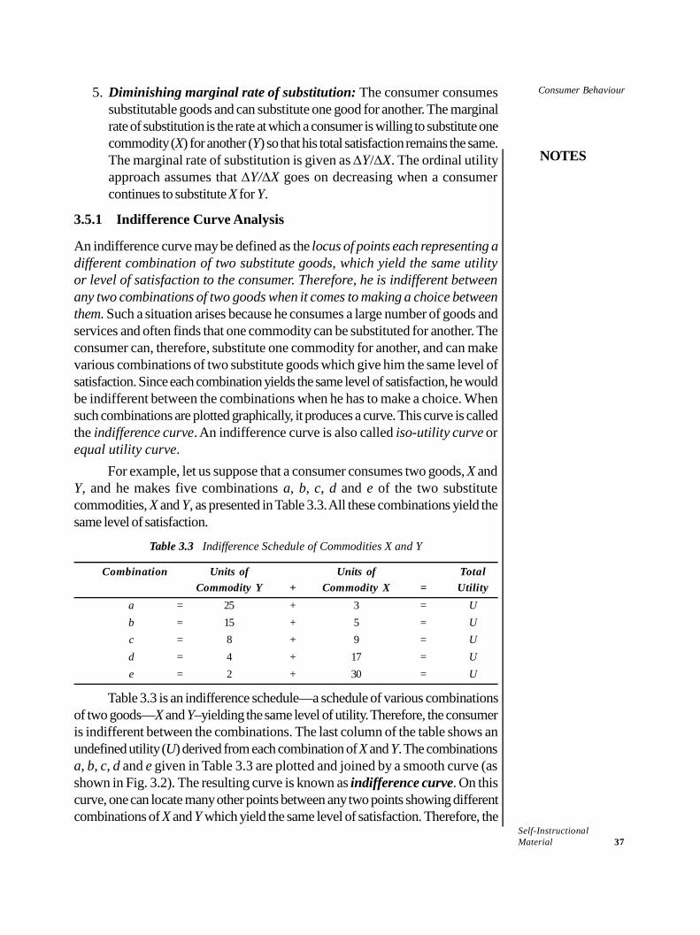
Consumer Behaviour
NOTES
Self-InstructionalMaterial 37
5. Diminishing marginal rate of substitution: The consumer consumessubstitutable goods and can substitute one good for another. The marginalrate of substitution is the rate at which a consumer is willing to substitute onecommodity (X) for another (Y) so that his total satisfaction remains the same.The marginal rate of substitution is given as Y/X. The ordinal utilityapproach assumes that Y/X goes on decreasing when a consumercontinues to substitute X for Y.
3.5.1 Indifference Curve Analysis
An indifference curve may be defined as the locus of points each representing adifferent combination of two substitute goods, which yield the same utilityor level of satisfaction to the consumer. Therefore, he is indifferent betweenany two combinations of two goods when it comes to making a choice betweenthem. Such a situation arises because he consumes a large number of goods andservices and often finds that one commodity can be substituted for another. Theconsumer can, therefore, substitute one commodity for another, and can makevarious combinations of two substitute goods which give him the same level ofsatisfaction. Since each combination yields the same level of satisfaction, he wouldbe indifferent between the combinations when he has to make a choice. Whensuch combinations are plotted graphically, it produces a curve. This curve is calledthe indifference curve. An indifference curve is also called iso-utility curve orequal utility curve.
For example, let us suppose that a consumer consumes two goods, X andY, and he makes five combinations a, b, c, d and e of the two substitutecommodities, X and Y, as presented in Table 3.3. All these combinations yield thesame level of satisfaction.
Table 3.3 Indifference Schedule of Commodities X and Y
Combination Units of Units of TotalCommodity Y + Commodity X = Utility
a = 25 + 3 = Ub = 15 + 5 = Uc = 8 + 9 = Ud = 4 + 17 = Ue = 2 + 30 = U
Table 3.3 is an indifference schedule—a schedule of various combinationsof two goods—X and Y–yielding the same level of utility. Therefore, the consumeris indifferent between the combinations. The last column of the table shows anundefined utility (U) derived from each combination of X and Y. The combinationsa, b, c, d and e given in Table 3.3 are plotted and joined by a smooth curve (asshown in Fig. 3.2). The resulting curve is known as indifference curve. On thiscurve, one can locate many other points between any two points showing differentcombinations of X and Y which yield the same level of satisfaction. Therefore, the
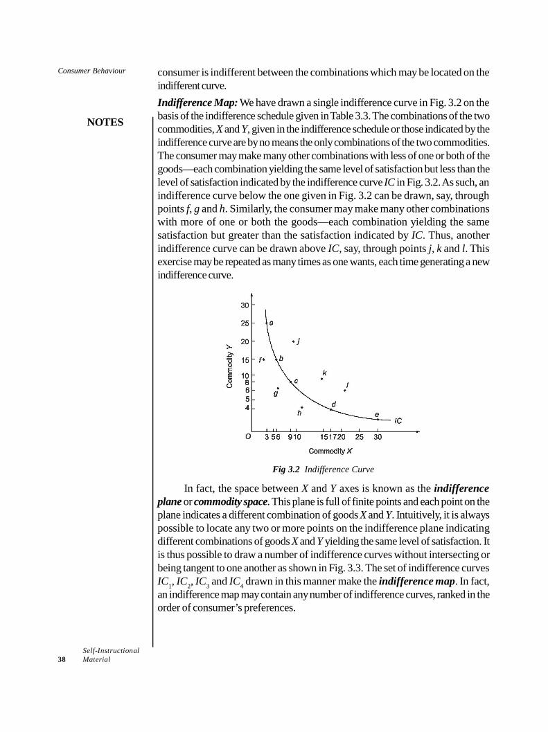
Consumer Behaviour
NOTES
Self-Instructional38 Material
consumer is indifferent between the combinations which may be located on theindifferent curve.Indifference Map: We have drawn a single indifference curve in Fig. 3.2 on thebasis of the indifference schedule given in Table 3.3. The combinations of the twocommodities, X and Y, given in the indifference schedule or those indicated by theindifference curve are by no means the only combinations of the two commodities.The consumer may make many other combinations with less of one or both of thegoods—each combination yielding the same level of satisfaction but less than thelevel of satisfaction indicated by the indifference curve IC in Fig. 3.2. As such, anindifference curve below the one given in Fig. 3.2 can be drawn, say, throughpoints f, g and h. Similarly, the consumer may make many other combinationswith more of one or both the goods—each combination yielding the samesatisfaction but greater than the satisfaction indicated by IC. Thus, anotherindifference curve can be drawn above IC, say, through points j, k and l. Thisexercise may be repeated as many times as one wants, each time generating a newindifference curve.
Fig 3.2 Indifference Curve
In fact, the space between X and Y axes is known as the indifferenceplane or commodity space. This plane is full of finite points and each point on theplane indicates a different combination of goods X and Y. Intuitively, it is alwayspossible to locate any two or more points on the indifference plane indicatingdifferent combinations of goods X and Y yielding the same level of satisfaction. Itis thus possible to draw a number of indifference curves without intersecting orbeing tangent to one another as shown in Fig. 3.3. The set of indifference curvesIC1, IC2, IC3 and IC4 drawn in this manner make the indifference map. In fact,an indifference map may contain any number of indifference curves, ranked in theorder of consumer’s preferences.
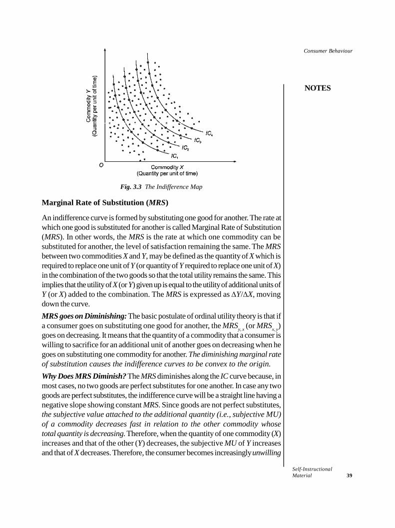
Consumer Behaviour
NOTES
Self-InstructionalMaterial 39
Fig. 3.3 The Indifference Map
Marginal Rate of Substitution (MRS)
An indifference curve is formed by substituting one good for another. The rate atwhich one good is substituted for another is called Marginal Rate of Substitution(MRS). In other words, the MRS is the rate at which one commodity can besubstituted for another, the level of satisfaction remaining the same. The MRSbetween two commodities X and Y, may be defined as the quantity of X which isrequired to replace one unit of Y (or quantity of Y required to replace one unit of X)in the combination of the two goods so that the total utility remains the same. Thisimplies that the utility of X (or Y) given up is equal to the utility of additional units ofY (or X) added to the combination. The MRS is expressed as Y/X, movingdown the curve.MRS goes on Diminishing: The basic postulate of ordinal utility theory is that ifa consumer goes on substituting one good for another, the MRSy, x (or MRSx, y)goes on decreasing. It means that the quantity of a commodity that a consumer iswilling to sacrifice for an additional unit of another goes on decreasing when hegoes on substituting one commodity for another. The diminishing marginal rateof substitution causes the indifference curves to be convex to the origin.Why Does MRS Diminish? The MRS diminishes along the IC curve because, inmost cases, no two goods are perfect substitutes for one another. In case any twogoods are perfect substitutes, the indifference curve will be a straight line having anegative slope showing constant MRS. Since goods are not perfect substitutes,the subjective value attached to the additional quantity (i.e., subjective MU)of a commodity decreases fast in relation to the other commodity whosetotal quantity is decreasing. Therefore, when the quantity of one commodity (X)increases and that of the other (Y) decreases, the subjective MU of Y increasesand that of X decreases. Therefore, the consumer becomes increasingly unwilling
Consumer Behaviour
NOTES
Self-Instructional40 Material
to sacrifice more units of Y for one unit of X. But, if he is required to sacrificeadditional units of Y, he will demand increasing units of X to maintain the level of hissatisfaction. As a result, the MRS decreases.
Properties of Indifference Curve
Indifference curves have the following four basic properties:1. Indifference curves slope downward to right;2. Indifference curves of imperfect substitutes are convex to the origin;3. Indifference curves do not intersect nor are they tangent to one another;4. Upper indifference curves indicate a higher level of satisfaction.
These properties of indifference curves, in fact, reveal the consumer’sbehaviour, his choices and preferences. They are, therefore, very important in themodern theory of consumer behaviour. Let us now look at their implications.1. Indifference Curves Slope Downward to Right. In the words of Hicks,“... so long as each commodity has a positive marginal utility, the indifferencecurve must slope downward to the right”, as shown in Fig. 3.3. The negative slopeof an indifference curve implies two requisits: (a) that the two commodities can besubstituted for each other; and (b) that if the quantity of one commodity decreases,qunatity of the other commodity must so increase that the consumer stays at thesame level of satisfaction. The conditions make the indifference curve slopedownward to the right. In case two goods are perfect substitutes, then the changein the combination of two goods produces an indifference line, not a curve.2. Indifference Curves are Convex to Origin. Indifference curves are not onlynegatively sloped, but are also convex to the origin as shown in Fig 3.3. Theconvexity of the indifference curves is caused by two factors:
(i) the two commodities are imperfect substitutes for one another, and(ii) the marginal rate of substitution (MRS) between the two goods decreases
as a consumer moves along an indifference curve.The postulate of diminishing MRS, is based on the fact that if a consumer
substitutes one commodity (X) for another (Y), his willingness to sacrifice moreunits of Y for one additional unit of X decreases, as quantity of Y decreases. Thereare two reasons for diminishing MRS: (i) two commodities are not, in general,perfect substitutes for one another, and (ii) MU of a commodity increases as itsquantity decreases and vice versa, and, therefore, more and more units of theother commodity are needed to keep the total utility constant.3. Indifference Curves Neither Intersect Nor are Tangent with One Another.If two indifference curves intersect or are tangent with one another, it will yieldtwo impossible conclusions: (i) that two equal combinations of two goods yieldtwo different levels of satisfaction, and (ii) that two different combinations—onebeing larger than the other–yield the same level of satisfaction. Such conditions
Consumer Behaviour
NOTES
Self-InstructionalMaterial 41
are impossible if the consumer’s subjective valuation of a commodity is greaterthan zero.4. Upper Indifference Curves Represent a Higher Level of Satisfactionthan the Lower Ones. An indifference curve placed above and to the right ofanother represents a higher level of satisfaction than the lower one. The reason isthat an upper indifference curve contains all along its length a larger quantity of oneor both the goods than the lower indifference curve. And a larger basket ofcommodities is supposed to yield a greater satisfaction than the smaller one,provided MU of goods is greater than zero.
Budgetary Constraints on Consumer’s Choice: Limited Income and Prices
Given the indifference map, a utility maximizing consumer would like to reach thehighest possible indifference curve on his indifference map. But the consumer hastwo strong constraints: (i) he has a limited income, and (ii) he has to pay a pricefor the goods. Given the prices, the limitedness of income acts as a constraint onhow high a consumer can ride on his indifference map. This is known asbudgetary constraint. In a two-commodity model, the budgetary constraintmay be expressed through a budget equation as
Px . Qx + Py . Qy = M
where Px and Py are prices of goods X and Y respectively; Qx and Qy are theirrespective quantities; and M is the consumer’s money income.
The budget equation states that the total expenditure of the consumer ongoods X and Y cannot exceed his total income, M. The quantities of X and Y thata consumer can buy, given his income (M) and prices, Px and Py, can be easilyobtained from the budget equation, as shown below.
Qx = MPx
– PPy
xQy
and Qy = MPy
– PPx
yQx
Now, Qx or Qy may be alternatively assigned any positive numerical valueand the corresponding values of Qy and Qx may be obtained. When the values ofQx and Qy are plotted on the X and Y axes, we get a line with a negative slope,which is called the budget line or price line.
The budget line shows the alternative options of commodity combinationsavailable to the consumer given his income and the prices of X and Y.
Shifts in the Budget Line
The budget line is drawn on the basis of the budget equation, given as M = Px . Qx+ Py . Qy. Any change in the parameters of the budget equation, viz., M, Px and Py,make the budget line shift upward or downward or swivel left or right and up ordown. If consumer’s income (M) increases, prices remaining constant, the budget
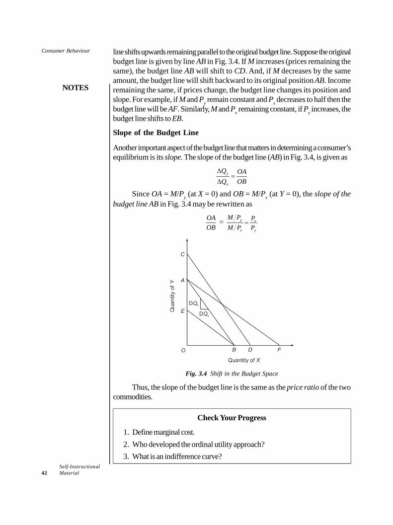
Consumer Behaviour
NOTES
Self-Instructional42 Material
line shifts upwards remaining parallel to the original budget line. Suppose the originalbudget line is given by line AB in Fig. 3.4. If M increases (prices remaining thesame), the budget line AB will shift to CD. And, if M decreases by the sameamount, the budget line will shift backward to its original position AB. Incomeremaining the same, if prices change, the budget line changes its position andslope. For example, if M and Py remain constant and Px decreases to half then thebudget line will be AF. Similarly, M and Px remaining constant, if Py increases, thebudget line shifts to EB.
Slope of the Budget Line
Another important aspect of the budget line that matters in determining a consumer’sequilibrium is its slope. The slope of the budget line (AB) in Fig. 3.4, is given as
y
x
Q OAQ OB
Since OA = M/Py (at X = 0) and OB = M/Px (at Y = 0), the slope of thebudget line AB in Fig. 3.4 may be rewritten as
OAOB
= y x
x y
M P PM P P
Fig. 3.4 Shift in the Budget Space
Thus, the slope of the budget line is the same as the price ratio of the twocommodities.
Check Your Progress
1. Define marginal cost.2. Who developed the ordinal utility approach?3. What is an indifference curve?
Consumer Behaviour
NOTES
Self-InstructionalMaterial 43
3.6 ANSWERS TO CHECK YOUR PROGRESSQUESTIONS
1. Marginal cost (MC) can be defined as the rise in total cost as a result ofproducing one additional unit of a commodity.
2. The ordinal utility approach was developed by J.R. Hicks and R.G.D. Allenin 1934. The ordinal utility approach is also known as Hicks-Allen Approach.
3. An indifference curve may be defined as the locus of points each representinga different combination of two substitute goods, which yield the same utilityor level of satisfaction to the consumer.
3.7 SUMMARY
Consumer demand is the basis of all productive activities. Just as ‘necessityis the mother of invention’, demand is the mother of production.
The concept of ‘marginal’ value is widely used in economic analysis, forexample marginal utility in consumer analysis, marginal productivity inproduction analysis and marginal revenue and marginal cost in pricing theory.
The law of equi-marginal principle was over time applied by businessmanagers to allocation of resources between their alternative uses with aview to maximizing profit in case a firm carries out more than one businessactivity.
Marginal utility can be defined as the utility derived from the marginal or oneadditional unit consumed. It may also be defined as the addition to the totalutility resulting from the consumption of one additional unit.
The central theme of the consumption theory – be it based on ordinal utilityor cardinal utility approach – is the utility maximizing behaviour of theconsumer.
The law of diminishing marginal utility states that as the quantity consumedof a commodity goes on increasing, the utility derived from each successiveunit consumed goes on decreasing, consumption of all other commoditiesremaining constant.
An indifference curve may be defined as the locus of points each representinga different combination of two substitute goods, which yield the same utilityor level of satisfaction to the consumer.
An indifference curve is formed by substituting one good for another. Therate at which one good is substituted for another is called Marginal Rate ofSubstitution (MRS).
Consumer Behaviour
NOTES
Self-Instructional44 Material
3.8 KEY WORDS
Marginal Rate of Substitution (MRS): It is defined as the rate at whichone good is substituted for another.
Budget line: It shows all the combinations of two commodities that aconsumer can afford at given market prices and within the particular incomelevel.
3.9 SELF ASSESSMENT QUESTIONS ANDEXERCISES
Short Answer Questions
1. State the limitations of the application of the marginal principle for profitmaximization.
2. Write a short note on the cardinal utility approach or the Marshallianapproach.
3. What are the assumptions of the ordinal utility approach?
Long Answer Questions
1. Explain the equi-marginal principle.2. Discuss the law of diminishing marginal utility.3. Describe the properties of an indifference curve.
3.10 FURTHER READINGS
Dwivedi, D. N. 2015. Principles of Economics, Eight Edition. New Delhi: VikasPublishing House.
Weil. David N. 2004. Economic Growth. London: Addison Wesley.Thomas, Christopher R. and Maurice S. Charles. 2005. Managerial Economics:
Concepts and Applications, Eighth Edition. New Delhi: Tata McGraw-Hill Publishing Company Limited.
Mankiw, Gregory N. 2002. Principles of Economics, Second Edition. India:Thomson Press.
Websites
https://blogs.economictimes.indiatimes.com/et-commentary/heres-how-indias-widening-income-distribution-can-be-redressed/
https://www.livemint.com/Opinion/WmpSjQAvPGeVzxqpgXYvtK/The-dangers-of-Indias-Billionaire-Raj.html
Demand Analysis
NOTES
Self-InstructionalMaterial 45
UNIT 4 DEMAND ANALYSIS
Structure
4.0 Introduction4.1 Unit Objectives4.2 Meaning, Functions and Applications of Demand Analysis
4.2.1 Law of Demand4.2.2 Determinants of Demand4.2.3 Demand Estimation and Forecasting
4.3 Elasticity of Demand: Types and Measures4.3.1 Price Elasticity of Demand4.3.2 Cross Elasticity of Demand4.3.3 Income Elasticity of Demand4.3.4 Advertisement or Promotional Elasticity
4.4 Answers to Check Your Progress Questions4.5 Summary4.6 Key Words4.7 Self Assessment Questions and Exercises4.8 Further Readings
4.0 INTRODUCTION
Demand is an economic term alluding to a consumer’s desire and willingness topay a price for a particular good/service. Keeping all other factors constant, anincrease in the price of a good or service will decrease demand and vice versa. Thisunit will introduce you to the concept of demand which includes the determinantsof demand, law of demand, demand estimation and demand forecasting, applicationof demand in analysis, types and measures of elasticity of demand their role inbusiness decisions.
4.1 UNIT OBJECTIVES
After going through this unit, you will be able to:
Discuss the function and application of demand analysis
Define the law of demand
List the determinants of demand
Explain demand estimation and forecasting
Describe the types and measures of elasticity of demand
Demand Analysis
NOTES
Self-Instructional46 Material
4.2 MEANING, FUNCTIONS AND APPLICATIONSOF DEMAND ANALYSIS
The accomplishment of any business enterprise generally depends on sales andsales is governed by market demand behaviour. Market demand analysis is one ofthe fundamental necessities for the existence of any business enterprise. Analysisof market demand for a product/service is essential for the management in orderto take decisions regarding production, cost allocation, product pricing, advertising,inventory holdings and other factors. How much the business enterprise must workhard to produce largely depends upon the demand for its product. If demand failsto fulfill the number of items produced, then the two must be balanced by creatinga new demand through better advertisement and publicity. In case, the futuredemand for the product is likely to be more, the more the inventories that the firmshould hold. If the demand for the product is high, a higher price can be charged,with other things remaining the same.
Demand analysis has two significant applications in managerial decision-making:
Forecasting Demand
Manipulating Demand
Market demand analysis assists the manager to take decisions regarding:(a) sales forecasting with a sound basis and greater accuracy: (b) guidelines fordemand manipulation through advertising and sales promotion programmes;(c) production planning and product improvement: (d) pricing policy;(e) determination of sales quotas and performance appraisal of personnel in thesales department; and (f) size of market for a given product and matching marketshare.
4.2.1 Law of Demand
The term ‘demand’ refers to the quantity demanded of a commodity per unit oftime at a given price. It implies also a desire backed by ability and willingness topay. A mere desire of a person to purchase a commodity is not his demand. Hemust possess adequate resources and must be willing to spend his resources tobuy the commodity. Besides, the quantity demanded has always a reference to‘a price’ and ‘a unity of time’. The quantity demanded referred to ‘per unit of time’makes it a flow concept. Apparently there may be some problems in applying thisflow concept to the demand for durable consumer goods like house, car,refrigerators, etc. But this apparent difficulty may be resolved by considering thefact that the total service of a durable good is not consumed at one point of time
Demand Analysis
NOTES
Self-InstructionalMaterial 47
and its utility is not exhausted in a single use. The service of a durable good isconsumed over time. At a time, only a part of its service is consumed. Therefore,the demand for the services of durable consumer goods may also be visualised asa demand per unit of time. However, this problem does not arise when the conceptof demand is applied to total demand for a consumer durable. Thus, the demandfor consumer goods also is a flow concept.
The quantity of a commodity that an individual or a household consumesper unit of time is determined by a number of factors including price of thecommodity, price of its substitutes and complements, consumer’s income, his/herwealthholding, taste and preference, expectations about future income and price,demonstration effect, etc. In the short run, however, all factors other than price ofthe commodity are assumed to remain constant. In the short run, therefore, thelaw of demand is linked to the price of the commodity.
Let it be emphasized that price of a commodity is the most importantdeterminant of its demand, and the only determinant in the short run when all otherdeterminants of demand are assumed to remain constant. The relationship betweenprice and demand is expressed by the law of demand. The law of demand statesthat quantity of a product demanded per unit of time increases when its pricefalls, and decreases when its price increases, other factors remaining constant.The assumption ‘other factors remaining constant’ implies that income of theconsumers, prices of the substitutes and complementary goods, consumers’ tasteand preference, and number of consumers, remain unchanged.
The law of demand can be illustrated through a demand schedule. A demandschedule is a series of quantities which consumers would like to buy per unit oftime at different prices. To illustrate the law of demand, an imaginary demandschedule for tea is given in Table 4.1. It shows seven alternative prices and thecorresponding quantities (number of cups of tea) demand per day. Each price hasa unique quantity demanded, associated with it. As price per cup of tea decreases,daily demand for tea increases, in accordance with the law of demand.
The Demand Curve
The law of demand can also be presented through a curve called demand curve.A demand curve is a locus of points showing various alterative price-quantitycombinations. It shows the quantities of a commodity that consumers or userswould buy at different prices per unit of time under the assumptions of the law ofdemand. An individual’s demand curve for tea as given in Fig. 4.1 can be obtainedby plotting the data given in Table 4.1.
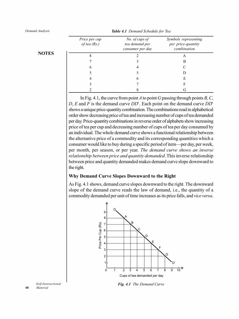
Demand Analysis
NOTES
Self-Instructional48 Material
Table 4.1 Demand Schedule for Tea
Price per cup No. of cups of Symbols representingof tea (Rs.) tea demand per per price-quantity
consumer per day combination
8 2 A
7 3 B
6 4 C
5 5 D
4 6 E
3 7 F
2 8 G
In Fig. 4.1, the curve from point A to point G passing through points B, C,D, E and F is the demand curve DD. Each point on the demand curve DDshows a unique price-quantity combination. The combinations read in alphabeticalorder show decreasing price of tea and increasing number of cups of tea demandedper day. Price-quantity combinations in reverse order of alphabets show increasingprice of tea per cup and decreasing number of cups of tea per day consumed byan individual. The whole demand curve shows a functional relationship betweenthe alternative price of a commodity and its corresponding quantities which aconsumer would like to buy during a specific period of item—per day, per week,per month, per season, or per year. The demand curve shows an inverserelationship between price and quantity demanded. This inverse relationshipbetween price and quantity demanded makes demand curve slope downward tothe right.
Why Demand Curve Slopes Downward to the Right
As Fig. 4.1 shows, demand curve slopes downward to the right. The downwardslope of the demand curve reads the law of demand, i.e., the quantity of acommodity demanded per unit of time increases as its price falls, and vice versa.
Fig. 4.1 The Demand Curve
Demand Analysis
NOTES
Self-InstructionalMaterial 49
The reasons behind the law of demand, i.e., inverse relationship between priceand quantity demanded are following.
(i) Substitution Effect
When the price of a commodity falls it becomes relatively cheaper if price of allother related goods, particularly of substitutes, remain constant or, in other words,substitute goods become relatively costlier. Since consumers substitute cheapergoods for costlier ones, demand for the relatively cheaper commodity increases.The increase in demand on account of this factor is known as substitution effect.
(ii) Income Effect
As a result of fall in the price of a commodity, the real income of its consumerincrease at least in terms of this commodity. In other words, his/her purchasingpower increases since he is required to pay less for the same quantity. The increasein real income (or purchasing power) encourages demand for the commodity withreduced price. The increase in demand on account of increase in real income isknown as income effect.
It should however be noted that the income effect is negative in case of inferiorgoods. In case price of an inferior good accounting for a considerable proportionof the total consumption expenditure falls substantially, consumers’ real incomeincreases: they become relatively richer. Consequently, they substitute the superiorgood for the inferior ones, i.e., they reduce the consumption of inferior goods.Thus, the income effect on the demand for inferior goods becomes negative.
(iii) Diminishing Marginal Utility
Diminishing marginal utility is also responsible for increase in demand for acommodity when its price falls. When a person buys a commodity, he exchangeshis money income with the commodity in order to maximise is satisfaction. Hecontinues to buy goods and services so long as marginal utility of money (MU
m) is
less then marginal utility of the commodity (MUc). Given the price of a commodity,
he adjusts his purchase so that MUc = MU
m. This proposition holds good under
both Marshallian assumption of constant MUm and Hicksian assumption of
diminishing MUm. Under Marshallian approach, MU
m remaining constant, MU
c =
Pc and a utility maximising consumer reaches his equilibrium where
MUm = P
c = MU
c
When price falls, (MUm = P
c) MU
c. Thus, equilibrium condition is disturbed. To
regain his equilibrium condition, i.e., MUm = P
c = MU
c, he purchases more of the
commodity. For, when the stock of a commodity increases, its MU decreases andonce again MU
m = MU
c. That is why demand for a commodity increases when its
price decreases.
Demand Analysis
NOTES
Self-Instructional50 Material
Exceptions to the Law of Demand
The law of demand does not apply to the following cases:
(a) Expectations regarding future price. When consumers expect acontinuous increase in the price of a durable commodity, they buy more ofit despite increase in its price. They do so with a view to avoiding the pinchof still higher price in future. Similarly, when consumers anticipate aconsiderable decrease in the price in future, they postpone their purchasesand wait for the price to fall to the expected level rather than buy thecommodity when its price initially falls. Such decisions of the consumers arecontrary to the law of demand.
(b) Status goods. The law does not apply to the commodities which serve asa ‘status symbol’, enhance social prestige or display wealth and richness,e.g., gold, precious stones, rare paintings and antiques, etc. Rich peoplebuy such goods mainly because their prices are high.
(c) Giffen goods. An exception to this law is also the classic case of Giffengoods named after Robert Giffen (1837–1910).
4.2.2 Determinants of Demand
Market demand for a product depends on a number of factors, calleddeterminants of demand. The knowledge of the determinants of market demandfor a product and the nature of relationship between the demand and its determinantsproves very helpful in analyzing and estimating demand for the product. It may benoted at the very outset that a host of factors determine the market demand for aproduct.
In general, however, following are the factors that determine the marketdemand for a product:
1. Price of the Product?: The price of a product is one of the most importantdeterminants of its demand in the long-run and the only determinant in the short-run. The price of a product and its quantity demanded are inversely related. Theprice of a product is one of the most important determinants of its demand in thelong-run and the only determinant in the short-run. The price of a product and itsquantity demanded are inversely related. The law of demand states that the quantitydemanded of a product which its consumers/users would like to buy per unit oftime, increases when its price falls and decreases when its price increases, otherfactors remaining constant. The assumption ‘other factors remaining constant’implies that factors other than price remain constant, particularly income of theconsumers, prices of the substitutes and complementary goods, consumer’s tasteand preferences, and number of consumers, remain unchanged. Other factorsremaining constnat, price is the main determinant of market demand especially inshort run.
Demand Analysis
NOTES
Self-InstructionalMaterial 51
2. Price of the Related Goods: The demand for a commodity is also affected bythe changes in the prices of its related goods. Related goods are classified undertwo categories: (i) substitutes, and (ii) complementary goods.
(i) Substitutes. Two commodities are deemed to be substitutes for one anotherif they satisfy the same want and change in the price of one changes the demandfor its substitute in the same direction. That is, increase in the price of a goodincreases demand for its substitutes.
(ii) Complements. A commodity is considered to be a complement for anotherwhen it complements the use of the other. In case of complements, the use of thetwo goods goes together. For example, petrol is a complement to cars, butter andjam to bread, milk and sugar to tea and coffee, electricity to computer, chair totable, etc. In economic sense, two goods are termed as complementary to oneanother if an increase in the price of one causes a decrease in demand for theother. By definition, there is an inverse relation between the demand for a goodand the price of its complement.
3. Consumer’s Income: Income is the basic determinant of quantity of a productdemanded as it determines the purchasing power of the consumer. That is whypeople with higher current disposable incomes spend a larger amount on consumergoods and services than those with lower income. Income-demand relationship isof a more varied nature than that between demand and its other determinants.While other determinants of demand, e.g., product’s own price and the price of itssubstitutes are more significant in the short-run, income as a determinant of demandis equally important in both short-run and long-run.
The relationship between the demand for a commodity, say X, and thehousehold income (Y), assuming all other factors to remain constant, is expressedby a demand function such as
Dx = f(Y), D
x/Y > 0
Before we proceed to discuss income-demand relationships, it will be usefulto note that consumer goods of different nature have different relationships withincomes of different categories of consumers. The managers need, therefore, tobe fully aware of the goods they are dealing with and their relationship with theincome of consumers, particularly in regard to the assessment of both existing andprospective demand for a product.
For the purpose of income-demand analysis, consumer goods and servicesmay be grouped under four broad categories, viz. (a) essential consumer goods,(b) inferior goods, (c) normal goods, and (d) luxury or prestige goods. Let us nowlook into the relationship between income and the different goods. This relationshipis presented through Engel curves.
(a) Essential consumer goods (ECG). The goods and services in this categoryare called ‘basic needs’ and are consumed by all persons of a society, e.g.,foodgrains, salt, vegetable oils, matches, cooking fuel, minimum clothing and
Demand Analysis
NOTES
Self-Instructional52 Material
housing. Quantity demanded of this category of goods increases with increase inconsumer’s income but only upto a certain limit, even though the total expendituremay increase in accordance with the quality of goods consumed, other factorsremaining the same.
(b) Inferior goods (IG). Inferior and superior goods are widely known to bothconsumers and sellers. For instance, every consumer knows that millet is inferiorto wheat and rice; bidi (indigenous cigarette) is inferior to cigarette, cotton clothesare inferior to silk clothes, kerosene is inferior to cooking gas; bike is inferior tocar; non-AC car is inferior to AC-car, and so on and so forth. In economic sense,however, a commodity is deemed to be inferior if its demand decreases withthe increase in consumer’s income beyond a certain level of income.
(c) Normal goods (NG). Technically, normal goods are those that are demandedin increasing quantities as consumers’ income rises. Clothing, house, furniture, andautomobiles are some of the important examples of this category of goods. Demandfor normal goods increases rapidly with the increase in the consumer’s income butslows down with further increases in income.
(d) Luxury and prestige goods (LG). What is and what is not a luxury good isa matter of consumer’s perception of the need for a commodity. Conceptually,however, all such goods that add to the pleasure and prestige of the consumerwithout enhancing his earning capacity or efficiency fall in the category of luxurygoods. Demand for such goods arises beyond a certain level of consumer’s income,i.e., consumption of luxury goods at a certain level high level of income. Producersof such items, while assessing the demand for their product, should consider theincome change in the richer section of the society, and not merely the per capitaincome.
4. Consumer’s Taste and Preference: Consumer’s taste and preference playan important role in determining the demand for a product. Taste and preferencegenerally depend on life-style, social customs, religious values attached to acommodity, habit of the people, the general levels of living of the society, and ageand sex of the consumers. Change in these factors changes consumers’ taste andpreferences. As a result, consumers reduce or give up the consumption of somegoods and add new ones to their consumption pattern.
This piece of information is useful for the manufacturers of goods and servicessubject to frequent changes in fashion and style, at least in two ways: (i) they canmake quick profits by designing new models of their product and popularisingthem through advertisement, and (ii) they can plan production better and can evenavoid over-production if they keep an eye on the changing fashions.
5. Advertisement Expenditure: Products are advertised with the objective ofpromoting sales of the product. Advertisement helps in increasing demand for theproduct in at least four ways: (a) by informing the potential consumers about theavailability of the product; (b) by showing its superiority over the rival product;(c) by influencing consumers’ choice against the rival products; and (d) by setting
Demand Analysis
NOTES
Self-InstructionalMaterial 53
new fashions and changing tastes. The impact of such effects shifts the demandupward to the right. In other words, other factors remaining the same, as expenditureon advertisement increases, volume of sales increases to an extent.
6. Consumers’ Expectations: Consumers’ expectations regarding the futureprices, income, and supply position of goods, etc. play an important role indetermining the demand for goods and services in the short-run. If consumersexpect a high rise in the price of a storable commodity, they would buy more of itat its high current price with a view to avoiding the pinch of a high price rise infuture. On the contrary, if consumers expect a fall in the price of certain goods,they postpone their purchase of such goods with a view to taking advantage oflower prices in future, mainly in the case of non-essential goods. This behaviour ofconsumers reduces the current demand for goods whose prices are expected todecrease in the future.
7. Demonstration and Snob Effect: When new commodities or new models ofexisting ones appear in the market, rich people buy them first. But once newcommodities are in vogue, many households buy them not because they have agenuine need for them but because their neighbours have bought these goods. Thepurchases made by the latter category of the buyers arise out of such feelings asjealousy, competition and equality in the peer group, social inferiority and the desireto raise their social status. Purchases made on account of these factors are theresult of what economists call ‘Demonstration effect’ or the ‘Bandwagon effect’.These factors have a positive effect on demand. On the contrary, when a commoditybecomes the thing of common use, some people, mostly rich, decrease or give upthe consumption of such goods. This is known as the ‘Snob effect’. It has a negativeeffect on the demand for the related goods.
8. Consumer-Credit Facility: Availability of credit to the consumers from thesellers, banks, relations and friends, or from other sources, enduces the consumersto buy more than what they would buy in the absence of credit facility. That is whyconsumers who can borrow more can consume more than those who cannotborrow. Credit facility mostly affects the demand for durable goods, particularlythose which require bulk payment at the time of purchase.
9. Population of the Country: The total domestic demand for a product ofmass consumption depends also on the size of the population. Given the price, percapita income, tastes and preferences etc., the larger the population, the larger thedemand for a product. With an increase (or decrease) in the size of population andwith the employment percentage remaining the same, demand for the producttends to increase (or decrease). The global perception that India offers the largestmarket in the world is based on the fact that she has the second largest population– albeit with a low purchasing power – in the world.
10. Distribution of National Income: The level of national income is the basicdeterminant of the market demand for a product—the higher the national income,the higher the demand for all normal goods and services. Apart from its level, the
Demand Analysis
NOTES
Self-Instructional54 Material
distribution pattern of national income is also an important determinant of the overalldemand for a product. If national income is unevenly distributed, i.e., if a majorityof the population belongs to the lower income groups, market demand for essentialgoods, including inferior ones, will be the largest whereas the demand for othergoods will be relatively lower.
4.2.3 Demand Estimation and Forecasting
The business world is characterized by risk and uncertainty and, therefore, mostbusiness decisions are made under the condition of risk and uncertainty. One wayto reduce the adverse effects of risk and uncertainty is to acquire knowledgeabout the future demand prospects for the product. The information regarding thefuture demand for the product is obtained by demand forecasting. Demandforecasting is predicting the future demand for firm’s product. A reliable forecastof the future demand for the product helps a great deal in the following areas ofbusiness management.
Determining the production target,
Planning and scheduling production,
Acquiring inputs (labour, raw material and capital),
Making provision for finances,
Formulating pricing strategy,
Planning advertisement.
Steps in Demand Forecasting
The demand can be forecast reliably only when forecast is made systematicallyand scientifically and when it is fairly reliable. The following steps are generallytaken to make systematic demand forecasting.
(i) Specifying the objective
(ii) Determining the time perspective
(iii) Making choice of method for demand forecasting
(iv) Collection of data and data adjustment
(v) Estimation and interpretation of results
Methods of Demand Forecasting: An Overview
There are various methods of demand forecasting. As pointed out above, thechoice of method for forecasting demand depends on the purpose and kind ofdemand forecasting and availability of required data. The various methods ofdemand forecasting are listed below.
1. Survey Methods
(i) Consumer Survey – direct interview
(ii) Opinion Poll Methods
Demand Analysis
NOTES
Self-InstructionalMaterial 55
2. Statistical Methods
(i) Trend Projection
(ii) Barometric Methods
(iii) Econometric Methods
All these methods have different kinds of sub-methods.
4.3 ELASTICITY OF DEMAND: TYPES ANDMEASURES
In general terms, the elasticity of demand is defined as the degree ofresponsiveness of demand for a product to change in its determinants. The measureof the degree of responsiveness of demand to change in its determinants gives themeasure of the extent of relationship between the demand for a product and anyof its determinants. In technical terms, the measure of elasticity of demand is calledelasticity coefficient measured by the following formula:
Ed =
Percentage Change in Quantity Demanded of Product
Percentage Change in Demand Determinant Factor
X
Y
For instance, suppose a determinant of demand for a product changes by10 percent and, as a result, demand changes by 15 percent. In that case, theelasticity coefficient equals 15/10 = 1.5.
The general formula for measuring the elasticity of demand can be expressedas follows.
Ed =
/
/
Q Q Q Y
Y Y F Q …(4.1)
where Q = quantity demanded initially; Q = change in demand, Y = the originalvalue of demand determinant factor; and Y = change in the determinant factor.
Let us now discuss the elasticity of demand with reference to its differentdeterminants.
4.3.1 Price Elasticity of Demand
Price elasticity of demand is generally defined as the responsiveness orsensitiveness of demand for a commodity to the changes in its price. Moreprecisely, elasticity of demand is the percentage change in demand due toone per cent change in the price of the commodity. A formal definition of priceelasticity of demand (e
p) is given as
ep =
Percentage change in quantity demanded
Percentage change in price
Demand Analysis
NOTES
Self-Instructional56 Material
A general formula for calculating coefficient of price elasticity, as given inEq. (4.1), is given as follows:
ep =
Q P Q P
Q P Q P
= Q P
P Q …(4.2)
where Q = original quantity demanded, P = original price, Q = change in quantitydemanded and P = change in price.
It is important to note here that a minus sign (–) is generally inserted in theformula before the fraction in order to make the elasticity coefficient a non-negativevalue.
The price elasticity can be measured between any two points on a demandcurve (called arc elasticity) or at a point (called point elasticity).
Measuring Price Elasticity from a Demand Function
The price elasticity of demand for a product can be measured directly from thedemand function. In this section, we describe the method of measuring priceelasticity of demand for a product from the demand function—both linear andnon-linear. It may be noted here that if a demand function is given, arc elasticitycan be measured simply by assuming two prices and working out P and Q. Wewill, therefore, confine ourselves here to point elasticity of demand with respect toprice.
Measuring Price Elasticity from a Linear Demand Function
Suppose that a linear demand function is given as
Q = 100 – 5P
Given the demand function, point elasticity can be measured for any price.For example, suppose one has to measure elasticity at P = 10. Point elasticity ismeasured as
ep =
Q P
P Q
The term Q/P in the elasticity formula gives the slope of the demandcurve. The slope of the demand curve can be found by differentiating the demandfunction. Thus
(100 5 )5
Q P
P P
Having obtained the slope of the demand curve as Q/P = –5, ep at P =
10 can be calculated as follows. At price P = 10, Q = 100 – 5(10) = 50. Bysubstituting these values into the elasticity formula,
Demand Analysis
NOTES
Self-InstructionalMaterial 57
ep =
Q P
P Q
we get, ep = (– 5)
10
50 = –1
Similarly, at P = 8, Q = 100 – 5(8) = 60 and
ep = – 5 (8/60) = – 40/60 = – 0.67
And at P = 15, Q = 100 – 5(15) = – 25, and
ep = – 5(15/25) = – 75/25 = – 3
Measuring Price Elasticity from a Non-linear Demand Function
Suppose a non-linear demand function of multiplicative form is given as follows
Q = aP–b
and we want to compute the price elasticity of demand. The formula for computingthe price elasticity is the same, i.e.,
ep =
Q P
P Q …(4.3)
What one needs to compute the price-elasticity coefficient is to find first thevalue of the first term, Q/P, i.e., the slope of the demand curve. The slope canbe obtained by differentiating the demand function, Thus,
slope of demand curve = Q
P = – baP–b-1 …(4.4)
By substituting Eq. (4.4) in Eq. (4.3), ep can be expressed as
ep = – baP–b–1 P
Q
= bbaP
Q …(4.5)
Since Q = aP–b, by substitution, we get
ep =
b
b
baP
aP = – b …(4.6)
Equation (4.6) shows that when a demand function is of a multiplicative orpower form, price elasticity coefficient equals the power of the variable P. Thismeans that price elasticity in the case of a multiplicative demand functionremains constant all along the demand curve regardless of a change in price.
Determinants of Price Elasticity of Demand
We have noted above that price-elasticity of demand for a product may varybetween zero and infinity. However, price-elasticity of demand, at a given price,varies from product to product depending on the following factors.
Demand Analysis
NOTES
Self-Instructional58 Material
1. Availability of Substitutes. The higher the degree of closeness of thesubstitutes, the greater the elasticity of demand for the commodity. On the otherhand, sugar and salt do not have close substitutes and hence their price-elasticityis lower.
2. Nature of Commodity. Demand for luxury goods (e.g., high-price refrigerators,TV sets, cars, decoration items, etc.) is more elastic than the demand for necessitiesand comforts because consumption of luxury goods can be dispensed with orpostponed when their prices rise. On the other hand, consumption of necessarygoods, (e.g., sugar, clothes, vegetables) cannot be postponed and hence theirdemand is inelastic. Comforts have more elastic demand than necessities and lesselastic than luxuries. Demand for durable goods is more elastic than that for non-durable goods, because when the price of the former increases, people either getthe old one repaired instead of replacing it or buy a ‘second hand’.
3. Weightage in the Total Consumption. If proportion of income spent on acommodity is large, its demand will be more elastic. On the contrary, if theproportion of income spent on a commodity is small, its demand is less price-elastic.
4. Time Factor in Adjustment of Consumption Pattern. Price-elasticity ofdemand depends also on the time consumers need to adjust their consumptionpattern to a new price: the longer the time available, the greater the price-elasticity.
5. Range of Commodity Use. The range of uses of a commodity also influencesthe price-elasticity of its demand. The wider the range of the uses of a product, thehigher the elasticity of demand for the decrease in price.
6. Proportion of Market Supplied. The elasticity of market demand also dependson the proportion of the market supplied at the ruling price. If less than half ofthe market is supplied at the ruling price, price-elasticity of demand will be higherthan 1 and if more than half of the market is supplied, e < 1.
Application of Price Elasticity
Having explained the concept and measurement of elasticity, we discuss now theapplication of price elasticity of demand with respect to (a) manoeuvring price tomaximize sales revenue and (b) determination of optimal price for profitmaximization.
1. Manoeuvring of Price. Price manoeuvring means changing price of the productto achieve business objective. The concept of elasticity of demand plays a crucialrole in business-decisions regarding manoeuvring of prices for the benefit of thefirm. For instance, when cost of production is increasing, the firm would want topass the rising cost on to the consumer by raising the price. Firms may decide tochange the price even without any change in the cost of production. But, whetherraising price following the rise in cost or otherwise proves beneficial or not dependson at least two factors:
(a) The price-elasticity of demand for the product, i.e., how high or low is theproportionate change in its demand in response to a certain percentagechange in its price; and
Demand Analysis
NOTES
Self-InstructionalMaterial 59
(b) Price-elasticity of demand for its substitute, because when the price of aproduct increases, the demand for its substitutes increases automaticallyeven if their prices remain unchanged.
Raising the price will be beneficial only if (i) demand for a product is lesselastic; and (ii) demand for its substitute is much less elastic. Although mostbusinessmen are intuitively aware of the elasticity of demand of the goods theymake, the use of precise estimates of elasticity of demand will add precision totheir business decisions.
2. Determination of Optimum Price. Another and a rather very importantapplication of price elasticity is that it can be used, at least theoretically, to determinethe optimum price with the objective of profit maximization for a firm facingdownward sloping demand curve. How optimum price, i.e., profit maximizingprice, can be determined by using the price elasticity is explained below. Thenecessary condition for profit maximization is given as MR – MC. That is, profit ismaximized at the level of price and output at which
MR = MC …(4.7)
As has been shown
MR = P [l + (1/ep)] …(4.8)
By substituting Eq. (4.8) for MR in Eq. (4.7), the profit maximizing conditioncan be expressed as
P [l + (1/ep)] = MC …(4.9)
The optimal price can be worked out from Eq. (4.9) as follows.
P = MC / [l + (l/ep)] …(4.10)
Given the Eq. (4.10). if point elasticity of demand curve and marginal cost(MC) of a firm are known, the optimal price can be easily determined. For example,suppose point elasticity of demand at point on demand curve is estimated as e
p =
_ 2 and firm’s MC = 50. In that case, optimal price can be worked out as follows.
P = 50 / [1+ (1/–2)]
= 100
It may thus be concluded that the concept of price elasticity of demand canbe used to manipulate the price to maximize the revenue of the firm given thedemand function and to find the optimal price for profit maximization.
Some Problems on Price Elasticity of Demand
Problem: 1
A cinema charges 8 per ticket for evening screenings and sells 250 tickets anight on average. They estimate that the price elasticity of demand for tickets is(-) 1.6.
Calculate the expected number of tickets sold if they reduce the ticket price to 7.
Demand Analysis
NOTES
Self-Instructional60 Material
Answer:
Price elasticity of demand = % change in Qty Demanded / % change inPrice % change in price = 12.5%
If Price elasticity of demand = (-) 1.6 then ticket sales will rise by 1.6 ×12.5% = 20%
20% of 250 is 50 extra tickets
Expected tickets sold rises to 300
Problem: 2
A mall raises the price of car parking from 3 per day to 5 per day and findsthat usage of car parks contracts from 1,200 cars a day to 900 cars per day.
Calculate the price elasticity of demand for this price change and calculatewhether total revenue from the car park rises or falls.
Answer:
% change in price = (+) 66.7%
% change in demand = (-) 25%
Price elasticity of demand = -25/66.7
= 0.375 (i.e. demand is price inelastic)
Total revenue:
@£3 per day – revenue = £3 × 1,200 = £3,600
@ £5 per day – revenue = £5 × 900 = £4,500
Revenue rises when Price elasticity of demand <1 and a business raisestheir average selling price.
4.3.2 Cross Elasticity of Demand
The cross-elasticity is the measure of responsiveness of demand for a commodityto the changes in the price of its substitutes and complementary goods. For instance,cross-elasticity of demand for tea is the percentage change in its quantity demandeddue to the change in the price of its substitute, coffee. The formula for measuringcross-elasticity of demand is the same as that of the price elasticity with a difference.For example, cross-elasticity of demand for tea (e
t, c) can be measured by the
formula given below.
et, c
= Percentage change in demand for tea ( )
Percentage change in price of coffee ( )t
c
Q
P
The cross-elasticity of demand for tea with respect price of coffee can beexpressed technically as follows.
= .c t
t c
P Q
Q P …(4.11)
Similarly, cross-elasticity of demand for coffee with respect to change in the priceof tea is measured as follows.
Demand Analysis
NOTES
Self-InstructionalMaterial 61
ec, t
= .t c
c t
P Q
Q P …(4.12)
The same formula is used to measure the cross-elasticity of demand for agood with respect to a change in the price of its complementary goods. Electricityto electrical gadgets, petrol to automobiles, butter to bread, sugar to tea and coffee,are the examples of complementary goods.
It is important to note that when two goods are substitutes for one another,their demand has positive cross-elasticity because increase in the price of onegood increases the demand for its substitute. And, the demand for complementarygoods has negative cross-elasticity, because increase in the price of a complementarygood decreases the demand for the main good.
Uses of Cross Elasticity
The concept of cross-elasticity has both theoretical and practical uses.
Theoretically, an important use of cross-elasticity is to define substitute goods.If cross-elasticity between any two goods is positive, the two goods may beconsidered as substitutes of one another. Also, the greater the cross-elasticity, thecloser the substitute. Similarly, if cross-elasticity of demand for two related goodsis negative, the two may be considered as complementary of one another: thehigher the negative cross-elasticity, the higher the degree of complementarity.
Practically, the concept of cross-elasticity is of vital importance in pricing decisions,i.e., in changing prices of products having substitutes and complementary goods.If cross-elasticity in response to the price of substitutes is greater than one, itwould be inadvisable to increase the price; rather, reducing the price may provebeneficial. In case of complementary goods also, reducing the price may be helpfulin maintaining the demand in case the price of the complementary good is rising.Besides, if accurate measures of cross-elasticities are available, the firm can forecastthe demand for its product and can adopt necessary safeguards against fluctuatingprices of substitutes and complements.
4.3.3 Income Elasticity of Demand
Apart from the price of a product and its substitutes, consumer’s income is anotherbasic determinant of demand for a product. As noted earlier, the relationship betweenquantity demanded and consumers income is of positive nature, unlike the negativeprice-demand relationship. The demand for most goods and services increases withincrease in consumer’s income and vice versa. The responsiveness of demand tothe changes in income is known as income-elasticity of demand.
Income-elasticity of demand for a product, say X, (i.e., ey) may be measured as:
ey=
% change in demand for product
% change in consumer’s incomeq
q
XX Y
X YY
ey =
q
q
XY
X Y …(4.13)
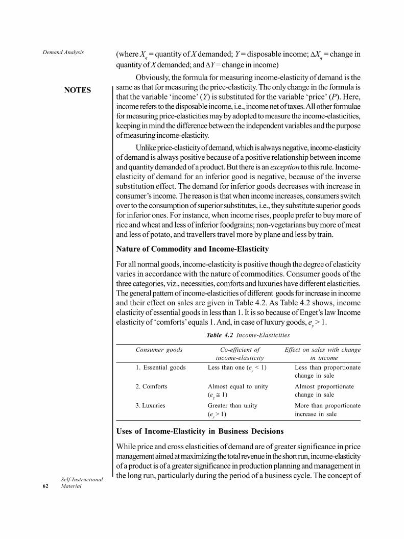
Demand Analysis
NOTES
Self-Instructional62 Material
(where Xq = quantity of X demanded; Y = disposable income; X
q = change in
quantity of X demanded; and Y = change in income)
Obviously, the formula for measuring income-elasticity of demand is thesame as that for measuring the price-elasticity. The only change in the formula isthat the variable ‘income’ (Y) is substituted for the variable ‘price’ (P). Here,income refers to the disposable income, i.e., income net of taxes. All other formulaefor measuring price-elasticities may by adopted to measure the income-elasticities,keeping in mind the difference between the independent variables and the purposeof measuring income-elasticity.
Unlike price-elasticity of demand, which is always negative, income-elasticityof demand is always positive because of a positive relationship between incomeand quantity demanded of a product. But there is an exception to this rule. Income-elasticity of demand for an inferior good is negative, because of the inversesubstitution effect. The demand for inferior goods decreases with increase inconsumer’s income. The reason is that when income increases, consumers switchover to the consumption of superior substitutes, i.e., they substitute superior goodsfor inferior ones. For instance, when income rises, people prefer to buy more ofrice and wheat and less of inferior foodgrains; non-vegetarians buy more of meatand less of potato, and travellers travel more by plane and less by train.
Nature of Commodity and Income-Elasticity
For all normal goods, income-elasticity is positive though the degree of elasticityvaries in accordance with the nature of commodities. Consumer goods of thethree categories, viz., necessities, comforts and luxuries have different elasticities.The general pattern of income-elasticities of different goods for increase in incomeand their effect on sales are given in Table 4.2. As Table 4.2 shows, incomeelasticity of essential goods in less than 1. It is so because of Enget’s law Incomeelasticity of ‘comforts’ equals 1. And, in case of luxury goods, e
y > 1.
Table 4.2 Income-Elasticities
Consumer goods Co-efficient of Effect on sales with changeincome-elasticity in income
1. Essential goods Less than one (ey < 1) Less than proportionate
change in sale
2. Comforts Almost equal to unity Almost proportionate(e
y 1) change in sale
3. Luxuries Greater than unity More than proportionate(e
y > 1) increase in sale
Uses of Income-Elasticity in Business Decisions
While price and cross elasticities of demand are of greater significance in pricemanagement aimed at maximizing the total revenue in the short run, income-elasticityof a product is of a greater significance in production planning and management inthe long run, particularly during the period of a business cycle. The concept of
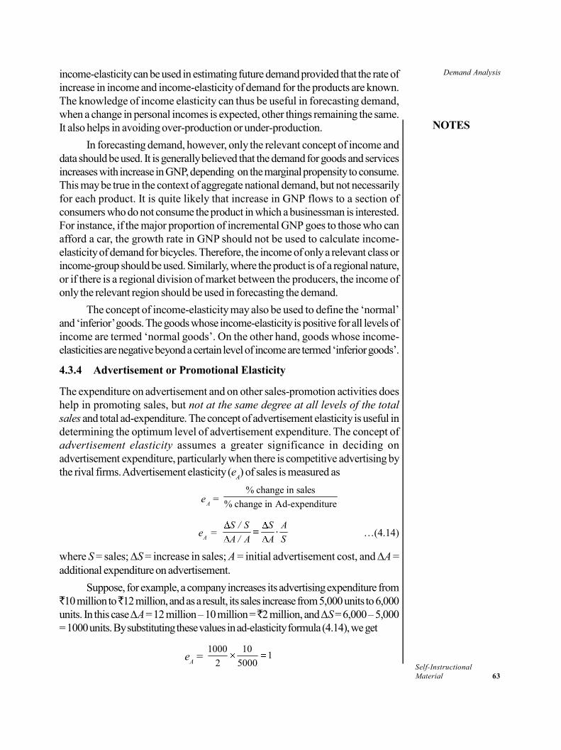
Demand Analysis
NOTES
Self-InstructionalMaterial 63
income-elasticity can be used in estimating future demand provided that the rate ofincrease in income and income-elasticity of demand for the products are known.The knowledge of income elasticity can thus be useful in forecasting demand,when a change in personal incomes is expected, other things remaining the same.It also helps in avoiding over-production or under-production.
In forecasting demand, however, only the relevant concept of income anddata should be used. It is generally believed that the demand for goods and servicesincreases with increase in GNP, depending on the marginal propensity to consume.This may be true in the context of aggregate national demand, but not necessarilyfor each product. It is quite likely that increase in GNP flows to a section ofconsumers who do not consume the product in which a businessman is interested.For instance, if the major proportion of incremental GNP goes to those who canafford a car, the growth rate in GNP should not be used to calculate income-elasticity of demand for bicycles. Therefore, the income of only a relevant class orincome-group should be used. Similarly, where the product is of a regional nature,or if there is a regional division of market between the producers, the income ofonly the relevant region should be used in forecasting the demand.
The concept of income-elasticity may also be used to define the ‘normal’and ‘inferior’ goods. The goods whose income-elasticity is positive for all levels ofincome are termed ‘normal goods’. On the other hand, goods whose income-elasticities are negative beyond a certain level of income are termed ‘inferior goods’.
4.3.4 Advertisement or Promotional Elasticity
The expenditure on advertisement and on other sales-promotion activities doeshelp in promoting sales, but not at the same degree at all levels of the totalsales and total ad-expenditure. The concept of advertisement elasticity is useful indetermining the optimum level of advertisement expenditure. The concept ofadvertisement elasticity assumes a greater significance in deciding onadvertisement expenditure, particularly when there is competitive advertising bythe rival firms. Advertisement elasticity (e
A) of sales is measured as
eA
= % change in sales
% change in Ad-expenditure
eA =
S / S S A
A / A A S…(4.14)
where S = sales; S = increase in sales; A = initial advertisement cost, and A =additional expenditure on advertisement.
Suppose, for example, a company increases its advertising expenditure from10 million to 12 million, and as a result, its sales increase from 5,000 units to 6,000
units. In this case A = 12 million – 10 million = 2 million, and S = 6,000 – 5,000= 1000 units. By substituting these values in ad-elasticity formula (4.14), we get
eA =
1000 101
2 5000
Demand Analysis
NOTES
Self-Instructional64 Material
It means that a one per cent increase in ad-expenditure increases sales by1 per cent.
Interpretation of Advertisement Elasticity: The advertisement elasticityof sales varies between e
A = 0 and e
A = depending on the nature of the product,
the level of market supplied, the trend in consumers’ income, the compatitive strengthof the competitors, etc. The interpretation of some measures of advertising elasticityis given below.
Elasticities Interpretation
eA = 0 Sales do not respond to the advertisement expenditure.
eA > 0 but < 1 Increase in total sales is less than proportionate to the
increase in advertisement expenditure.
eA = 1 Sales increase in proportion to the increase in advertisement
expenditure.
eA > 1 Sales increase at a higher rate than the rate of increase of
advertisement expenditure.
Determinants of Advertisement Elasticity
Some important factors that determine the level of ad-elasticity are the following.
(i) The level of total sales
(ii) Advertisement by rival firms
(iii) Cumulative effect of past advertisement
(iv) Other factors
Check Your Progress
1. What is a demand curve?
2. State the factors that determine the market demand for a product.
4.4 ANSWERS TO CHECK YOUR PROGRESSQUESTIONS
1. A demand curve is a locus of points showing various alterative price-quantitycombinations.
2. The factors that determine the market demand for a product are the following:
Price of the product,
Price of the related goods—substitutes, complements and supplements,
Level of consumers’ income,
Consumers’ taste and preferences,
Advertisement of the product,
Demand Analysis
NOTES
Self-InstructionalMaterial 65
Consumers’ expectations about future price and supply position,
Demonstration effect and ‘bandwagon effect’,
Consumer-credit facility,
Population of the country (for the goods of mass consumption),
Distribution pattern of national income, etc.
4.5 SUMMARY
The term ‘demand’ refers to the quantity demanded of a commodity perunit of time at a given price. It implies also a desire backed by ability andwillingness to pay.
The relationship between price and demand is expressed by the law ofdemand. The law of demand states that quantity of a product demandedper unit of time increases when its price falls, and decreases when its priceincreases, other factors remaining constant.
The law of demand can also be presented through a curve called demandcurve. A demand curve is a locus of points showing various alterative price-quantity combinations.
Diminishing marginal utility is also responsible for increase in demand for acommodity when its price falls. When a person buys a commodity, heexchanges his money income with the commodity in order to maximize issatisfaction.
Market demand for a product depends on a number of factors, calleddeterminants of demand. The knowledge of the determinants of marketdemand for a product and the nature of relationship between the demandand its determinants proves very helpful in analyzing and estimating demandfor the product.
The information regarding the future demand for the product is obtained bydemand forecasting. Demand forecasting is predicting the future demandfor firm’s product.
There are various methods of demand forecasting. The choice of methodfor forecasting demand depends on the purpose and kind of demandforecasting and availability of required data.
In general terms, the elasticity of demand is defined as the degree ofresponsiveness of demand for a product to change in its determinants. Themeasure of the degree of responsiveness of demand to change in itsdeterminants gives the measure of the extent of relationship between thedemand for a product and any of its determinants. There are various sub-types including price, income, cross and advertising elasticity of demand.
Demand Analysis
NOTES
Self-Instructional66 Material
4.6 KEY WORDS
Income effect: The increase in demand on account of increase in realincome is known as income effect.
Elasticity of demand: It is defined as the degree of responsiveness ofdemand for a product to change in its determinants.
4.7 SELF ASSESSMENT QUESTIONS ANDEXERCISES
Short Answer Questions
1. State the law of demand.
2. What are the exceptions to the law of demand?
3. Write a short note on diminishing marginal utility.
4. Define demand forecasting.
5. Briefly mention the methods of demand forecasting.
Long Answer Questions
1. Discuss the application of demand analysis.
2. Explain the application of price elasticity of demand.
3. Explain income elasticity of demand.
4. What is cross elasticity of demand? Mention its uses.
4.8 FURTHER READINGS
Dwivedi, D. N. 2015. Principles of Economics, Eight Edition. New Delhi: VikasPublishing House.
Weil. David N. 2004. Economic Growth. London: Addison Wesley.
Thomas, Christopher R. and Maurice S. Charles. 2005. Managerial Economics:Concepts and Applications, Eighth Edition. New Delhi: Tata McGraw-Hill Publishing Company Limited.
Mankiw, Gregory N. 2002. Principles of Economics, Second Edition. India:Thomson Press.
Websites
https://blogs.economictimes.indiatimes.com/et-commentary/heres-how-indias-widening-income-distribution-can-be-redressed/
https://www.livemint.com/Opinion/WmpSjQAvPGeVzxqpgXYvtK/The-dangers-of-Indias-Billionaire-Raj.html
Supply Analysis
NOTES
Self-InstructionalMaterial 67
BLOCK - IIPERSONAL AND SUPPLY MANAGEMENT
UNIT 5 SUPPLY ANALYSIS
Structure5.0 Introduction5.1 Objectives5.2 The Law of Supply and Determinants of Supply
5.2.1 Elasticity of Supply: Measures and Significance5.2.2 Derivations of Market Demand5.2.3 Demand Estimation and Forecasting
5.3 Demand Supply Equilibrium5.4 Giffen Paradox5.5 Answers to Check Your Progress Questions5.6 Summary5.7 Key Words5.8 Self Assessment Questions and Exercises5.9 Further Readings
5.0 INTRODUCTION
Supply and demand are economic terms which occupy a significant place in theanalysis of market economy. In the previous unit, you studied about demand analysisand this unit will introduce you supply analysis. This unit will introduce you to thelaw of supply, the measures of elasticities of supply, derivation of market demand,demand supply equilibrium and finally, the Giffen paradox.
5.1 OBJECTIVES
After going through this unit, you will be able to: State the law of supply Discuss the measures of elasticities of supply Explain the derivation of market demand Describe the demand supply equilibrium Define the Giffen paradox
Supply Analysis
NOTES
Self-Instructional68 Material
5.2 THE LAW OF SUPPLY AND DETERMINANTSOF SUPPLY
In the previous unit, we discussed the law of demand. In this section, we turn tothe other side of the market and to discuss the law of supply, specifically the law ofmarket supply. Market supply means the quantity of a commodity which all itsproducers or sellers offer to sell at a given price, per unit of time. Market supply,like market demand, is the sum of supplies of a commodity made by all individualfirms.
The law of supply can be stated as the supply of a product increaseswith the increase in its price and decreases with decrease in its price,other things remaining constant. It implies that the supply of a commodity andits price are positively related. This relationship holds under the assumption that“other things remaining the same”. “Other things” include cost of production, changein technology, price of related goods (substitutes and complements), and weatherand climate in case of agricultural products.
The Supply Factors
In reality, the supply of a commodity depends on its price, cost of production andproduction technology. In other words, supply of a product X is the function of itsprice (Px), cost of production (Cx) and technology of its production (Tx). In itsfunctional form
Qx = f (Px, Cx, Tx)
In simple theory of supply, however, the law of supply is expressed generallyin terms of price-quantity relationship supply function is expressed as
Qx = f (Px) ...(5.1)
The Supply Schedule
The supply schedule is a tabular presentation of the supply function. In fact, asupply schedule is a table showing alternative prices of a commodity and thecorresponding quantity that suppliers are willing to offer for sale. Table 5.1 presentsa hypothetical supply schedule of shirts per month.
Table 5.1 Supply Schedule for Shirts
Price (in `) 100 200 300 400 600 800
Supply(Shirts in ‘000) 10 40 55 70 75 80
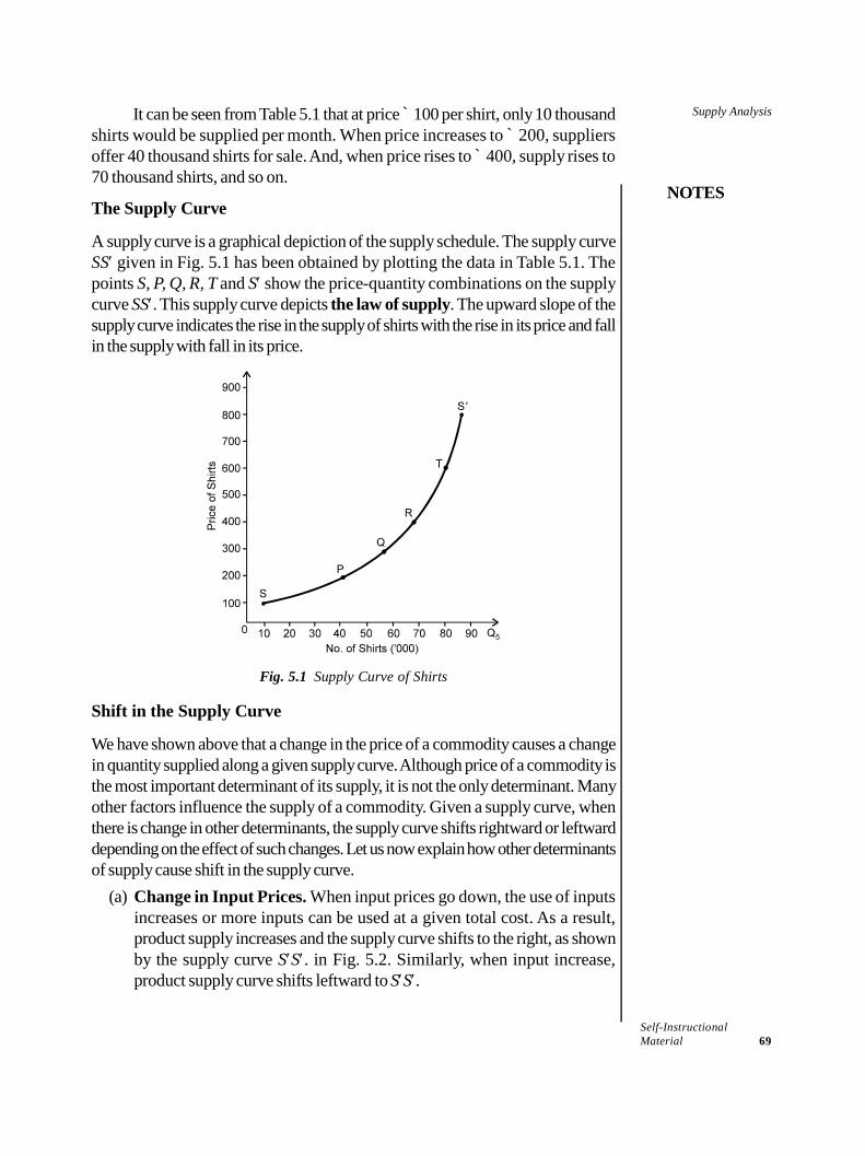
Supply Analysis
NOTES
Self-InstructionalMaterial 69
It can be seen from Table 5.1 that at price ̀ 100 per shirt, only 10 thousandshirts would be supplied per month. When price increases to ̀ 200, suppliersoffer 40 thousand shirts for sale. And, when price rises to ̀ 400, supply rises to70 thousand shirts, and so on.
The Supply Curve
A supply curve is a graphical depiction of the supply schedule. The supply curveSS given in Fig. 5.1 has been obtained by plotting the data in Table 5.1. Thepoints S, P, Q, R, T and S show the price-quantity combinations on the supplycurve SS. This supply curve depicts the law of supply. The upward slope of thesupply curve indicates the rise in the supply of shirts with the rise in its price and fallin the supply with fall in its price.
Fig. 5.1 Supply Curve of Shirts
Shift in the Supply Curve
We have shown above that a change in the price of a commodity causes a changein quantity supplied along a given supply curve. Although price of a commodity isthe most important determinant of its supply, it is not the only determinant. Manyother factors influence the supply of a commodity. Given a supply curve, whenthere is change in other determinants, the supply curve shifts rightward or leftwarddepending on the effect of such changes. Let us now explain how other determinantsof supply cause shift in the supply curve.
(a) Change in Input Prices. When input prices go down, the use of inputsincreases or more inputs can be used at a given total cost. As a result,product supply increases and the supply curve shifts to the right, as shownby the supply curve SS. in Fig. 5.2. Similarly, when input increase,product supply curve shifts leftward to SS.
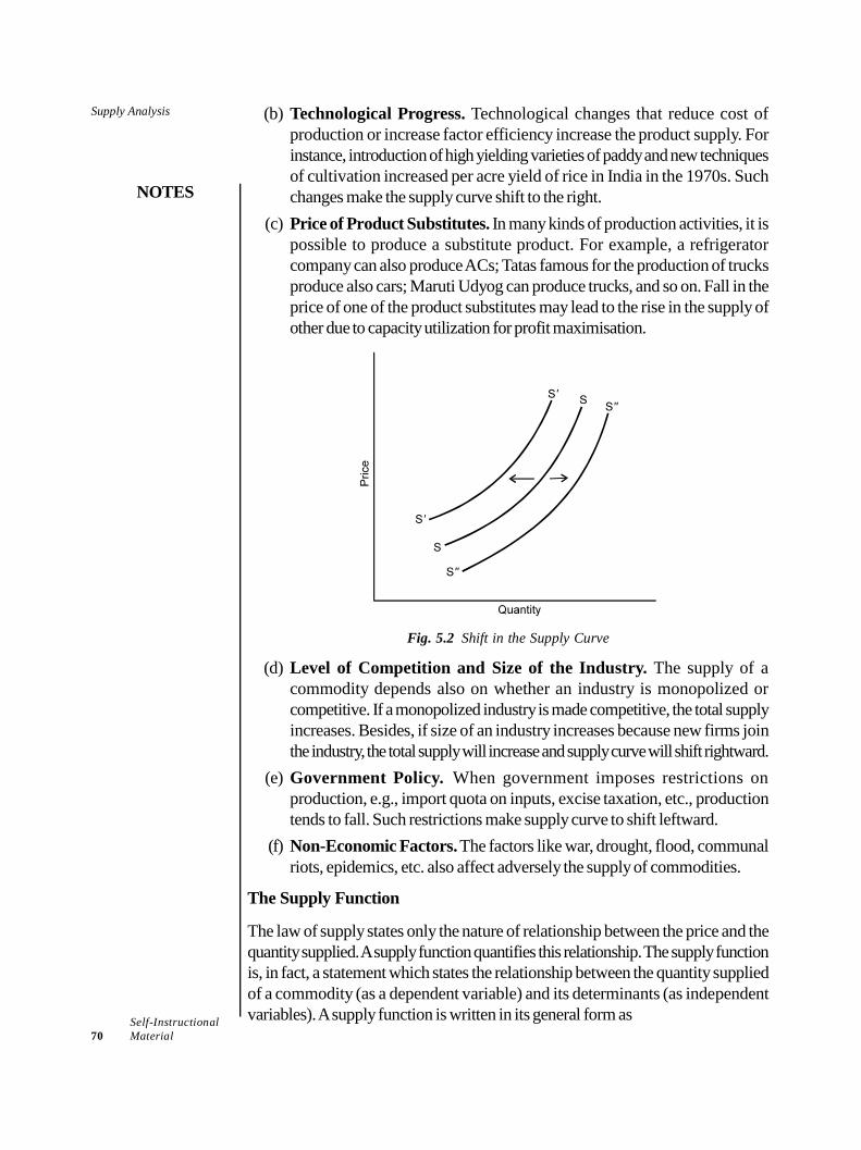
Supply Analysis
NOTES
Self-Instructional70 Material
(b) Technological Progress. Technological changes that reduce cost ofproduction or increase factor efficiency increase the product supply. Forinstance, introduction of high yielding varieties of paddy and new techniquesof cultivation increased per acre yield of rice in India in the 1970s. Suchchanges make the supply curve shift to the right.
(c) Price of Product Substitutes. In many kinds of production activities, it ispossible to produce a substitute product. For example, a refrigeratorcompany can also produce ACs; Tatas famous for the production of trucksproduce also cars; Maruti Udyog can produce trucks, and so on. Fall in theprice of one of the product substitutes may lead to the rise in the supply ofother due to capacity utilization for profit maximisation.
Fig. 5.2 Shift in the Supply Curve
(d) Level of Competition and Size of the Industry. The supply of acommodity depends also on whether an industry is monopolized orcompetitive. If a monopolized industry is made competitive, the total supplyincreases. Besides, if size of an industry increases because new firms jointhe industry, the total supply will increase and supply curve will shift rightward.
(e) Government Policy. When government imposes restrictions onproduction, e.g., import quota on inputs, excise taxation, etc., productiontends to fall. Such restrictions make supply curve to shift leftward.
(f) Non-Economic Factors. The factors like war, drought, flood, communalriots, epidemics, etc. also affect adversely the supply of commodities.
The Supply Function
The law of supply states only the nature of relationship between the price and thequantity supplied. A supply function quantifies this relationship. The supply functionis, in fact, a statement which states the relationship between the quantity suppliedof a commodity (as a dependent variable) and its determinants (as independentvariables). A supply function is written in its general form as
Supply Analysis
NOTES
Self-InstructionalMaterial 71
Qx = sPx ...(5.2)
where Qx = quantity supplied of commodity X, s = Qx/Px, and Px = price.Given the supply function (5.2), a supply schedule can be generated by
substituting numerical values for Px and assuming s = 10. For example, if Px = 2,Qx = 10 × 2 = 20 and if Px = 5, Qx = 10 × 5 = 50 and so on. By plotting the supplyschedule, a supply curve can be obtained. (For procedure, refer to the section ondemand function).
5.2.1 Elasticity of Supply: Measures and Significance
Like the law of demand, the law of supply states only the nature of relationshipbetween the change in the price of a commodity and the quantity supplied thereof.The law does not quantity the relationship. The quantitative relationship is measuredby the price elasticity of supply.
The price elasticity of supply is the measure of responsiveness of the quantitysupplied of a good to the changes in its market price. The coefficient of priceelasticity of supply (ep) is the measure of percentage change in the quantity suppliedof a product due to a given percentage change in its price. The formula of supplyelasticity is given as
ep =%
% change in quantity supplied ( )
change in price ( )Q
P
ep =
Q QP P
QP
PQ
Note that the formula for measuring the price elasticity of supply is the sameas for the price elasticity of demand, without a minus sign. Given the formula, priceelasticity of supply can be easily measured.
Determinants of the Price Elasticity of Supply
The price elasticity of the supply depends on the following factors:
Time Period. Time period is the most important factor in determining the elasticityof the supply curve. In a very short period, the supply of most goods is fixed andinelastic. In the short run, the supply tends to remain inelastic. In the long run, thesupply of all the products gains its maximum elasticity because of increase inand expansion of firms, new investments, improvement in technology, and a greateravailability of inputs.
It is important to note here that short and long periods are not fixed in termsof days, months or years. It varies depending on the nature of the product. Forexample, for the supply of perishable commodities like milk and fish in a city, aweek’s time may be a short period. For agricultural products, 6 months may be ashort period. But in regard to the local supply of petroleum products in India, aperiod of five years or even more may be regarded as a short period.
Supply Analysis
NOTES
Self-Instructional72 Material
Law of Diminishing Returns. The other factor that determines the elasticity ofsupply is the Law of Diminishing Returns. We will discuss this law later in detailwhen we take up the laws of production. Here, it suffices to say that if the law ofdiminishing returns come in force at an early level of production, cost increasesrapidly. As a result, supply tends to becomes less and less elastic.
5.2.2 Derivations of Market Demand
Market demand can be defined as the sum of individual demands for a product ata price per unit of time. We may recall that the quantity demanded of a commodityby an individual per unit of time, at a given price, is known as ‘individual demand’for that commodity. The aggregate of individual demands for a product iscalled market demand for the product. In other words, the sum of quantitydemand by all the consumers/users of a commodity per unit of time at a givenprice, all other things remaining the same, is called ‘market demand’ for that product.
For example, suppose there are only three consumers—A, B and C—of acommodity X which has a fixed price. Consumers A, B and C consume 100 units,200 units and 300 units respectively, of commodity X monthly. Therefore, themonthly market demand for commodity X equals 100 + 200 + 300 = 600 units.
Derivation of Market Demand Curve
If individual demand schedules or individual demand functions are known, themarket demand schedule and market demand curve can easily be derived. Themarket demand curve can be derived by adding up (i) the individual demandschedules, and (ii) the individual demand functions. In this section, we illustratethe derivation of market demand curve by using these two methods.
Derivation of Market Demand Curve from Individual Demand Schedules
Suppose again that there are three consumers (A, B and C) of a commodity X andtheir monthly demand schedules for the commodity are given in Table 5.2. Thetable shows the quantity demanded of commodity X individually by the threeconsumers at different prices of commodity X. The last column shows the marketdemand, i.e., the sum of individual demands for commodity X. The market demandshows the total quantity of commodity X demanded per month by the threeconsumers at different prices.
Given the individual and market demand schedules, the market demandcurve can be obtained by plotting the market demand against the respective prices.This is illustrated in Fig. 5.3 by the curve DM.
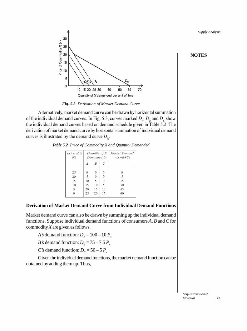
Supply Analysis
NOTES
Self-InstructionalMaterial 73
Fig. 5.3 Derivation of Market Demand Curve
Table 5.2 Price of Commodity X and Quantity Demanded
Derivation of Market Demand Curve from Individual Demand Functions
Market demand curve can also be drawn by summing up the individual demandfunctions. Suppose individual demand functions of consumers A, B and C forcommodity X are given as follows.
A’s demand function: DA = 100 – 10 Px
B’s demand function: DB = 75 – 7.5 Px
C’s demand function: DC = 50 – 5 Px
Given the individual demand functions, the market demand function can beobtained by adding them up. Thus,
Supply Analysis
NOTES
Self-Instructional74 Material
Market Demand function:
DM = (100 – 10 Px) + (75 – 7.5 Px) + (50 – 5 Px)
DM = 225 – 22.5 Px
This market demand function can be converted into a market demandschedule by assigning numerical values to Px. The market demand curve can thenbe drawn by plotting the demand schedule.
5.2.3 Demand Estimation and Forecasting
We have already discussed this concept in Unit 4, let us revise the concept herebriefly. Demand forecasting and estimation is used by business enterprises to obtainvaluable information about the markets in which they operate and the markets inwhich they plan to launch their products. Forecasting and estimation are termswhose usage is synonymous—that basically mean predicting what will happen inthe future. If business enterprises do not use demand forecasting and estimation,then they might enter markets which are not worthy of the products produced bythem.
The fundamental objective of demand forecasting and estimation is to analysethe business’s potential demand. This will facilitate managers to make accuratedecisions about pricing, business growth and market potential. We can understandthis with the help of an example. For instance, if the market demand for pasta isextremely high in a city but there are few competitors, then the business managerscan price pasta slightly higher than if the demand was less. Established businessesuse the tool of demand forecasting and estimation if they wish to venture into anew market. If the demand for their product is currently low, but will increase inthe future, they will wait to enter the market.
5.3 DEMAND SUPPLY EQUILIBRIUM
In this section, we will explain how demand and supply strike a balance, howmarket attains equilibrium, and how equilibrium price is determined in a free market.A Free Market is one in which market forces of demand and supply are free totake their own course: there is no outside control on price, demand and supply.
The Concept of Equilibrium
In a general sense, the term equilibrium means the “state of rest”. It indicates thecondition where forces working in opposite direction are in balance. In the contextof the market analysis, equilibrium refers to a state of market in which thequantity demanded of a commodity equals the quantity supplied of thecommodity. The equality of demand and supply produces an equilibrium price.
The equilibrium price is the price at which quantity demanded of acommodity over a period of time equals its quantity supplied over that period. In
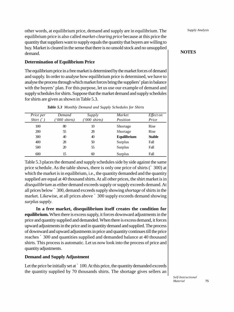
Supply Analysis
NOTES
Self-InstructionalMaterial 75
other words, at equilibrium price, demand and supply are in equilibrium. Theequilibrium price is also called market-clearing price because at this price thequantity that suppliers want to supply equals the quantity that buyers are willing tobuy. Market is cleared in the sense that there is no unsold stock and no unsupplieddemand.
Determination of Equilibrium Price
The equilibrium price in a free market is determined by the market forces of demandand supply. In order to analyse how equilibrium price is determined, we have toanalyse the process through which market forces bring the suppliers’ plan in balancewith the buyers’ plan. For this purpose, let us use our example of demand andsupply schedules for shirts. Suppose that the market demand and supply schedulesfor shirts are given as shown in Table 5.3.
Table 5.3 Monthly Demand and Supply Schedules for Shirts
Price per Demand Supply Market Effect onShirt (`) (‘000 shirts) (‘000 shirts) Position Price
100 80 10 Shortage Rise200 55 28 Shortage Rise300 40 40 Equilibrium Stable400 28 50 Surplus Fall500 20 55 Surplus Fall
600 15 60 Surplus Fall
Table 5.3 places the demand and supply schedules side by side against the sameprice schedule. As the table shows, there is only one price of shirts (` 300) atwhich the market is in equilibrium, i.e., the quantity demanded and the quantitysupplied are equal at 40 thousand shirts. At all other prices, the shirt market is indisequilibrium as either demand exceeds supply or supply exceeds demand. Atall prices below ̀ 300, demand exceeds supply showing shortage of shirts in themarket. Likewise, at all prices above ̀ 300 supply exceeds demand showingsurplus supply.
In a free market, disequilibrium itself creates the condition forequilibrium. When there is excess supply, it forces downward adjustments in theprice and quantity supplied and demanded. When there is excess demand, it forcesupward adjustments in the price and in quantity demand and supplied. The processof downward and upward adjustments in price and quantity continues till the pricereaches ` 300 and quantities supplied and demanded balance at 40 thousandshirts. This process is automatic. Let us now look into the process of price andquantity adjustments.
Demand and Supply Adjustment
Let the price be initially set at ̀ 100. At this price, the quantity demanded exceedsthe quantity supplied by 70 thousands shirts. The shortage gives sellers an
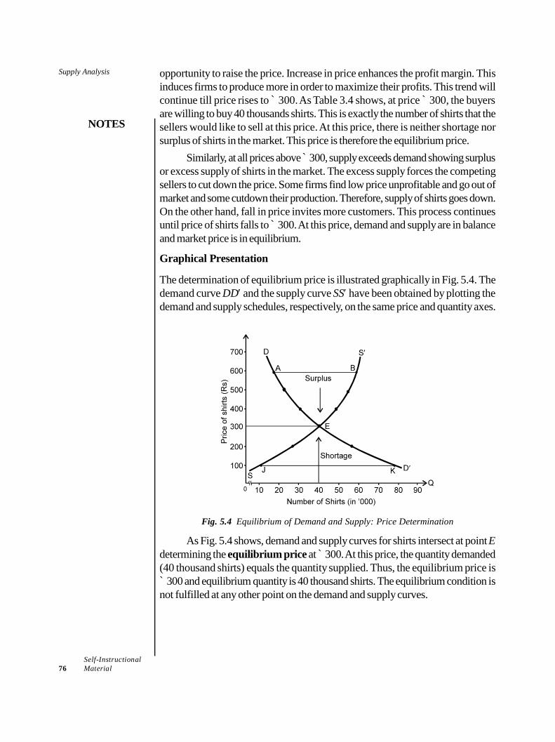
Supply Analysis
NOTES
Self-Instructional76 Material
opportunity to raise the price. Increase in price enhances the profit margin. Thisinduces firms to produce more in order to maximize their profits. This trend willcontinue till price rises to ̀ 300. As Table 3.4 shows, at price ̀ 300, the buyersare willing to buy 40 thousands shirts. This is exactly the number of shirts that thesellers would like to sell at this price. At this price, there is neither shortage norsurplus of shirts in the market. This price is therefore the equilibrium price.
Similarly, at all prices above ̀ 300, supply exceeds demand showing surplusor excess supply of shirts in the market. The excess supply forces the competingsellers to cut down the price. Some firms find low price unprofitable and go out ofmarket and some cutdown their production. Therefore, supply of shirts goes down.On the other hand, fall in price invites more customers. This process continuesuntil price of shirts falls to ̀ 300. At this price, demand and supply are in balanceand market price is in equilibrium.
Graphical Presentation
The determination of equilibrium price is illustrated graphically in Fig. 5.4. Thedemand curve DD and the supply curve SS have been obtained by plotting thedemand and supply schedules, respectively, on the same price and quantity axes.
Fig. 5.4 Equilibrium of Demand and Supply: Price Determination
As Fig. 5.4 shows, demand and supply curves for shirts intersect at point Edetermining the equilibrium price at ̀ 300. At this price, the quantity demanded(40 thousand shirts) equals the quantity supplied. Thus, the equilibrium price is` 300 and equilibrium quantity is 40 thousand shirts. The equilibrium condition isnot fulfilled at any other point on the demand and supply curves.
Supply Analysis
NOTES
Self-InstructionalMaterial 77
Algebra of Demand-Supply Equilibrium
In the previous section, we have seen graphically how the equilibrium of demandand supply is determined at the point of intersection of the demand and supplycurves. If demand and supply functions are known, the equilibrium quantity andequilibrium price can also be determined algebraically. In this section, we assumelinear demand and supply functions for a commodity X to show the determinationof equilibrium price and quantity.
Let the demand function for commodity X be given as
Qd = 150 – 5Px
and supply function asQs = 10Px
We know that the equilibrium of demand and supply takes place wherethe quantity supplied equals the quantity demanded, i.e., where
Qs = Qd ...(5.3)
By substituting supply and demand functions into Eq. 5.3, we get
10Px = 150 – 5Px ...(5.4)
Given the Eq. (5.4) the equilibrium price can be worked out as follows:
10Px = 150 – 5Px ...(5.5)or 10Px + 5Px = 150
15Px = 150Px = 10
Thus, at equilibrium, Px = 10. That is, the equilibrium price is ̀ 10.Given the equilibrium price Px = 10, the equilibrium quantity supplied and
the quantity demanded can be easily worked out. Equilibrium supply equals 10(Px) = 10 (10) = 100. Similarly, equilibrium demand equals 150 – 5Px = 150 – 5(10) = 100.
The algebraic determination of equilibrium price and quantity can also bedemonstrated graphically. It is shown in Fig. 5.5. The demand curve DD hasbeen drawn using the demand function Qd = 150 – 5Px and the supply curve SSusing the supply function Qs = 10Px.
The demand and the supply curves intersect at point P. A perpendiculardrawn from point P to the quantity axis determines the equilibrium quantity at 100units and a line drawn from point P to the price axis determines the equilibriumprice at ̀ 10. At this price, the quantity demanded equals the quantity supplied at100 units (Fig. 5.5).
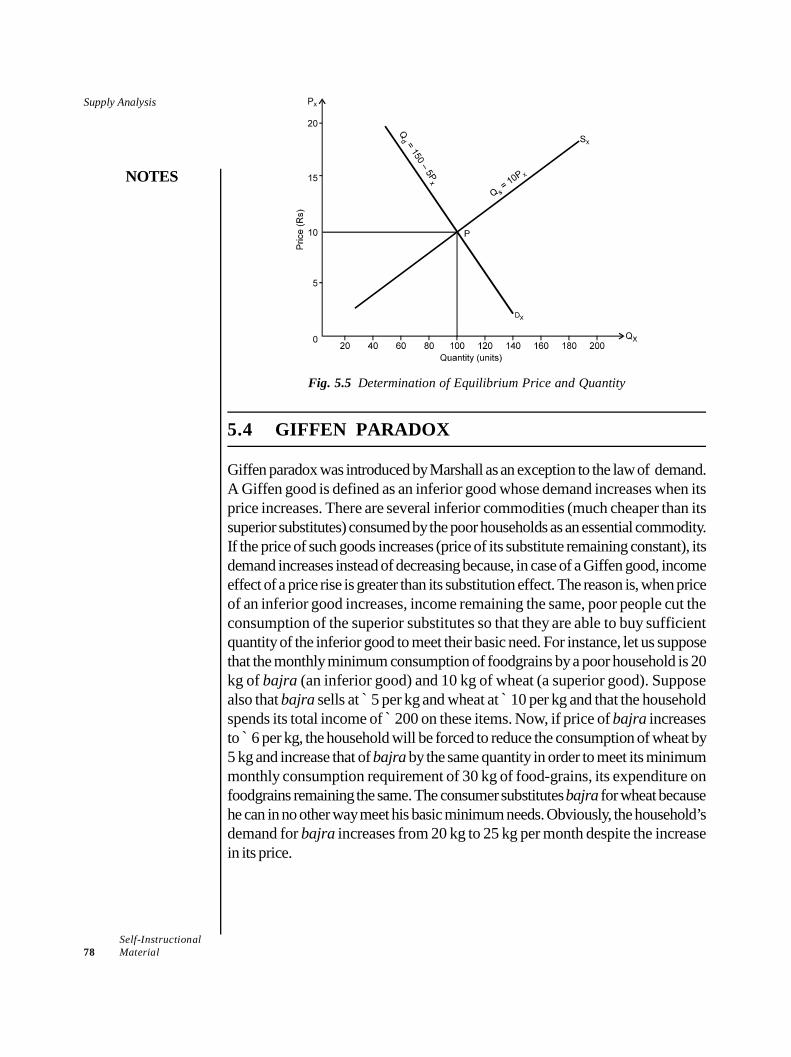
Supply Analysis
NOTES
Self-Instructional78 Material
Fig. 5.5 Determination of Equilibrium Price and Quantity
5.4 GIFFEN PARADOX
Giffen paradox was introduced by Marshall as an exception to the law of demand.A Giffen good is defined as an inferior good whose demand increases when itsprice increases. There are several inferior commodities (much cheaper than itssuperior substitutes) consumed by the poor households as an essential commodity.If the price of such goods increases (price of its substitute remaining constant), itsdemand increases instead of decreasing because, in case of a Giffen good, incomeeffect of a price rise is greater than its substitution effect. The reason is, when priceof an inferior good increases, income remaining the same, poor people cut theconsumption of the superior substitutes so that they are able to buy sufficientquantity of the inferior good to meet their basic need. For instance, let us supposethat the monthly minimum consumption of foodgrains by a poor household is 20kg of bajra (an inferior good) and 10 kg of wheat (a superior good). Supposealso that bajra sells at ̀ 5 per kg and wheat at ̀ 10 per kg and that the householdspends its total income of ̀ 200 on these items. Now, if price of bajra increasesto ̀ 6 per kg, the household will be forced to reduce the consumption of wheat by5 kg and increase that of bajra by the same quantity in order to meet its minimummonthly consumption requirement of 30 kg of food-grains, its expenditure onfoodgrains remaining the same. The consumer substitutes bajra for wheat becausehe can in no other way meet his basic minimum needs. Obviously, the household’sdemand for bajra increases from 20 kg to 25 kg per month despite the increasein its price.
Supply Analysis
NOTES
Self-InstructionalMaterial 79
Check Your Progress
1. What is a supply schedule?2. Define a free market.
5.5 ANSWERS TO CHECK YOUR PROGRESSQUESTIONS
1. The supply schedule is a tabular presentation of the supply function. In fact,a supply schedule is a table showing alternative prices of a commodity andthe corresponding quantity that suppliers are willing to offer for sale.
2. A free market is one in which market forces of demand and supply are freeto take their own course: there is no outside control on price, demand andsupply.
5.6 SUMMARY
The law of supply can be stated as the supply of a product increases withthe increase in its price and decreases with decrease in its price, other thingsremaining constant.
The supply schedule is a tabular presentation of the supply function. In fact,a supply schedule is a table showing alternative prices of a commodity andthe corresponding quantity that suppliers are willing to offer for sale.
Technological changes that reduce cost of production or increase factorefficiency increase the product supply.
The law of supply states only the nature of relationship between the priceand the quantity supplied. A supply function quantifies this relationship.
Like the law of demand, the law of supply states only the nature of relationshipbetween the change in the price of a commodity and the quantity suppliedthereof.
Market demand can be defined as the sum of individual demands for aproduct at a price per unit of time.
In a general sense, the term equilibrium means the “state of rest”. It indicatesthe condition where forces working in opposite direction are in balance.
In a free market, disequilibrium itself creates the condition for equilibrium. Giffen paradox was introduced by Marshall as an exception to the law of
demand. A Giffen good is defined as an inferior good whose demandincreases when its price increases.
Supply Analysis
NOTES
Self-Instructional80 Material
5.7 KEY WORDS
Price elasticity of supply: It is the measure of responsiveness of thequantity supplied of a good to the changes in its market price.
Market demand: It can be defined as the sum of individual demands fora product at a price per unit of time.
Giffen good: It is defined as an inferior good whose demand increaseswhen its price increases.
5.8 SELF ASSESSMENT QUESTIONS ANDEXERCISES
Short Answer Questions
1. State the law of supply.2. Write a short note on the supply function.3. What are the determinants of price elasticity of supply?4. Write a short note on the Giffen paradox.
Long Answer Questions
1. Explain the supply curve with the help of diagrams.2. Discuss the derivation of market demand curve.3. Describe the determination of equilibrium price.
5.9 FURTHER READINGS
Dwivedi, D. N. 2015. Principles of Economics, Eight Edition. New Delhi: VikasPublishing House.
Weil. David N. 2004. Economic Growth. London: Addison Wesley.Thomas, Christopher R. and Maurice S. Charles. 2005. Managerial Economics:
Concepts and Applications, Eighth Edition. New Delhi: Tata McGraw-Hill Publishing Company Limited.
Mankiw, Gregory N. 2002. Principles of Economics, Second Edition. India:Thomson Press.
Websites
https://blogs.economictimes.indiatimes.com/et-commentary/heres-how-indias-widening-income-distribution-can-be-redressed/
https://www.livemint.com/Opinion/WmpSjQAvPGeVzxqpgXYvtK/The-dangers-of-Indias-Billionaire-Raj.html
Production Functions
NOTES
Self-InstructionalMaterial 81
UNIT 6 PRODUCTION FUNCTIONS
Structure6.0 Introduction6.1 Objectives6.2 Production Functions: Short-Run and Long-Run Production Function6.3 Theory of Production and Managerial Uses of Production Function
6.3.1 Short-Run Laws of Production6.3.2 Isoquants6.3.3 Long-Run Laws of Production
6.4 Cobb-Douglas and Other Production Functions: Empirical Estimation6.5 Answers to Check Your Progress Questions6.6 Summary6.7 Key Words6.8 Self Assessment Questions and Exercises6.9 Further Readings
6.0 INTRODUCTION
Once business firms take decision on ‘what to produce’ the major issues that ariseare ‘how to produce’ and ‘how much to produce’. These issues arise becauseachieving optimum efficiency in production and minimizing cost for a givenproduction is one of the prime concerns of the business managers. In fact, the verysurvival of a firm in a competitive market depends on their ability to produce at acompetitive cost. Therefore, managers of business firms endeavour to minimizethe production cost of a given output or, in other words, maximize the output froma given quantity of inputs. In their effort to minimize the cost of production, thefundamental questions that managers are faced with are:
(i) How can production be optimized with given resources?(ii) How does output respond to change in quantity of inputs?(iii) How does technology matter in reducing the cost of production?(iv) How can the least-cost combination of inputs be achieved?(v) Given the technology, what happens to the rate of return when more plants
are added to the firm?
Production Functions
NOTES
Self-Instructional82 Material
This unit presents a detailed discussion on the theory of production and itsmanagerial uses. In addition, the unit also deals with the application of isoquants,long-run and short-run laws of production, Cobb-Douglas function and otherproduction functions.
6.1 OBJECTIVES
After going through this unit, you will be able to: Explain the short-run and long-run production function Describe the theory of production Identify the uses of production function Define isoquants State Cobb-Douglas and other production functions
6.2 PRODUCTION FUNCTIONS: SHORT-RUN ANDLONG-RUN PRODUCTION FUNCTION
This section presents a brief discussion on the basic concepts and terminologyused in the analysis of the theory of production.
Meaning of Production
In general sense of the term, ‘production’ means transforming inputs (labour, capital,raw materials, time, etc.) into an output with value added. This concept ofproduction is however limited to only ‘manufacturing’. In economic sense, theterm ‘production’ means a process by which resources (men, material, time, etc.)are transformed into a different and more useful commodity or service. In otherwords, a process by which men, material, capital and time are converted intovalue added products is called production.
Input and Output
An input is a good or service that goes into the process of production. In thewords of Baumol, “An input is simply anything which the firm buys for use in itsproduction or other processes.” An output is any good or service that comes outof production process.
The term ‘inputs’ needs some more explanations. Production process requiresa wide variety of inputs, depending on the nature of product. But, economistsclassified inputs as (i) labour, (ii) capital, (iii) land, (iv) raw materials and(v) entrepreneurship. Technology and time are also treated as inputs in the modernconcept of production.
Production Functions
NOTES
Self-InstructionalMaterial 83
Fixed and Variable Inputs
Inputs are classified as(i) fixed inputs, and(ii) variable inputs.
Fixed and variable inputs are defined in economic sense and also in technicalsense. The two concepts of input are explained below in economic as well as intechnical sense.
Fixed Inputs In economic sense, a fixed input is one whose supply isinelastic in the short-run. Therefore, all of its users together cannot buy more of itin the short-run. In technical sense, a fixed factor is one that remains fixed (orconstant) for a certain level of output.
Variable Input A variable input is defined as one whose supply in theshort-run is elastic, e.g., labour and raw material, etc. All the users of such factorscan employ a larger quantity in the short-run as well as in the long-run. Technically,a variable input is one that changes with the change in output. In the long-run, allinputs are variable.
Short-run and Long-run
Production of a good involves timer. The reference to time period involved inproduction process is another important concept used in production analysis. Thetwo reference periods are short-run and long-run. The short-run refers to aperiod of time in which the supply of certain inputs (e.g., plant, building, machinery,etc.) is fixed or is inelastic and are used in a fixed quantity. In the short-run, therefore,production of a commodity can be increased by increasing the use of only variableinputs like labour and raw materials.
On the other hand, long-run refers to a period of time in which the supplyof all the inputs is elastic, but not enough to permit a change in technology. That is,in the long-run, all the inputs are variable. Therefore, in the long-run, production ofa commodity can be increased by employing more of both variable and fixedinputs.
It is important to note that ‘short-run’ and ‘long-run’ are economists’ jargon.They do not refer to any specific time period. While in some industries short-runmay be a matter of few weeks or few months, in some others (e.g., in housing,shipping, flying, electricity and power industries), it may mean three or more years.
The economists use another term, i.e., very long-run which refers to aperiod in which the technology of production is also subject to change or can beimproved. In the very long-run, the production function also changes. Thetechnological advances result in a larger output from a given quantity of inputs perunit of time.
Production Functions
NOTES
Self-Instructional84 Material
Production Function
Production function is a mathematical presentation of input-output relationship.More specifically, a production function states the technological relationship betweeninputs and output in the form of an equation, a table or a graph. In its general form,it specifies the inputs required for the production of a commodity or service. In itsspecific form, it states the extent of quantitative relationships between inputs andoutput. Besides, the production function represents the technology of a firm or ofan industry. For example, suppose production of a product, say X, depends onlabour (L) and capital (K), then production function is expressed in equation formas
Qx = f (L, K)
A real-life production function is generally very complex. It includes a widerange of inputs, viz., (i) land and building; (ii) labour including manual labour,engineering staff and production manager, (iii) capital, (iv) raw material, (v) time,and (vi) technology. All these variables enter the actual production function of afirm. The long-run production function is generally expressed as
Q = f(LB, L, K, M, T, t)
where LB = land and building L = labour, K = capital, M = raw materials,T = technology and t = time.
The economists have however reduced the number of variable inputs usedin a production function to only two, viz., labour (L) and capital (K) , for thesake of convenience and simplicity in the analysis of input-output relations. It haslogical reasoning also. A production function with two variable inputs, K and L, isexpressed as
Q = f(K, L)
The reasons for excluding other inputs are following.Land and building (LB), as inputs, are constant for the economy as a
whole, and hence they do not enter into the aggregate production function. However,land and building are not a constant variable for an individual firm or industry. Inthe case of individual firms, land and building are lumped with ‘capital’.
Production Functions
NOTES
Self-InstructionalMaterial 85
So is the case, generally, with time and space. Also, technology (T) ofproduction remains constant over a period of time. That is why, in most productionfunctions, only labour and capital are included.
We will illustrate the tabular and graphic forms of a production functionwhen we move on to explain the laws of production. Here, let us illustrate themathematical form of a production function. It is this form of production functionthat is most commonly used in production analysis.
QC = f (K, L) …(6.1)
where QC = the quantity of coal produced per time unit; K = capital; andL = labour.
The production function (6.1) implies that quantity of coal produced dependson the quantity of capital (K) and labour (L) employed to produce coal. Increasingcoal production will require increasing K and L. Whether the firm can increaseboth K and L or only L depends on the time period it takes into account forincreasing production, i.e., whether the firm considers a short-run or a long-run.
By definition, as noted above, short-run is a period in which supply of capitalis inelastic. In the short-run, therefore, the firm can increase coal production byincreasing only labour since the supply of capital in the short run is fixed. Long-run is a period during which supply of both labour and capital becomes elastic,i.e., it increases over time. In the long-run, therefore, the firm can employ more ofboth capital and labour. Accordingly, there are two kinds of production functions:
(i) Short-run production function; and(ii) Long-run production function.
The two kinds of production functions are described here breifly.
Q = f(L,), where indicates constant capital. …(6.2)An estimated short-run production function may take any of the following
forms depending on input-output relationship.(a) Linear function: Q = a + bL(b) Quadratic function: Q = a + bL – cL2;(c) Cubic function: a + bL + cL2 – dL3; or(d) Power function: Q = aLb (b > 1).
Production Functions
NOTES
Self-Instructional86 Material
(ii) Long-run Production Function: In the long-term production function, bothK and L are treated as variable factors and the function takes the following form.
Q = f (K, L)
Q = AKaLb …(6.3)
(where K = Capital, L = Labour, and A, a and b are parameters, and b = 1 – a)Production function (6.3) gives the general form of Cobb-Douglas
production function. The numerical values of parameters A, a and b, can beestimated by using actual factory data on production, capital and labour.
6.3 THEORY OF PRODUCTION ANDMANAGERIAL USES OF PRODUCTIONFUNCTION
Let us now discuss the significant aspects of the theory of production.
6.3.1 Short-Run Laws of Production
The laws of production state the relationship between output and input. In theshort-run, input-output relations are studied with one variable input (labour), otherinputs (especially, capital) held constant. The laws of production under theseconditions are called the ‘Laws of Variable Proportions’ or the ‘Laws of Returnsto a Variable Input’. In this section, we explain the ‘laws of returns to a variableinput’.
The Law of Diminishing Returns to a Variable Input
The Law of Diminishing Returns. The law of diminishing returns states thatwhen more and more units of a variable input are used with a given quantityof fixed inputs, the total output may initially increase at increasing rate andthen may be at a constant rate, but it will eventually increase at diminishingrates. That is, the marginal increase in total output decreases eventually whenadditional units of a variable factor are used, given quantity of fixed factors.Assumptions. The law of diminishing returns is based on the following assumptions:
(i) labour is the only variable input, capital remaining constant;(ii) labour is homogeneous;
Production Functions
NOTES
Self-InstructionalMaterial 87
(iii) the state of technology is given; and(iv) input prices are given.
To illustrate the law of diminishing returns, let us assume (i) that a firm (say,the coal mining firm in our earlier example) has a set of mining machinery as itscapital (K) fixed in the short-run, and (ii) that it can employ only more mine-workers to increase its coal production. Thus, the short-run production functionfor the firm will take the following form.
Qc = f(L), K constant
Now let us suppose that labour and production data of the coal mining firmare given as in cols. (1) and (2) of Table 6.2. When regression technique is appliedto estimate the production function, it produces an empirical production functionas given below.
Qc = – L3 + 15L2 + 10L …(6.4)
Given the production function (6.4), we may assign different numerical valuesto L in the function and work out a series of Qc, i.e., the quantity of coal that can beproduced with different number of workers. For example, if L = 5, then bysubstitution, we get
Qc = – 53 + 15 × 52 + 10 × 5 = – 125 + 375 + 50 = 300
What we need now is to analyse the input-output relationship with theobjective of taking production decision. To this end, we need is to work outmarginal productivity of labour (MPL) to find the trend in the contribution of themarginal labour and average productivity of labour (APL) to find the averagecontribution of labour.
Marginal Productivity of Labour (MPL) can be obtained by differentiatingthe production function (6.4). Thus,
MPLQL
= – 3L2 + 30L + 10 …(6.5)
By substituting numerical value for labour (L) in Eq. (6.5), MPL can beobtained at different levels of labour employment. However, this method can beused only where labour is perfectly divisible and L 0. Since, in our example,each unit of L = 1, calculus method cannot be used.
Alternatively, where labour can be increased by a minimum of one unit,MPL can be obtained as
MPL = TPL – TPL–1
The MPL worked out by this method is presented in Col. 3 of Table 6.1.
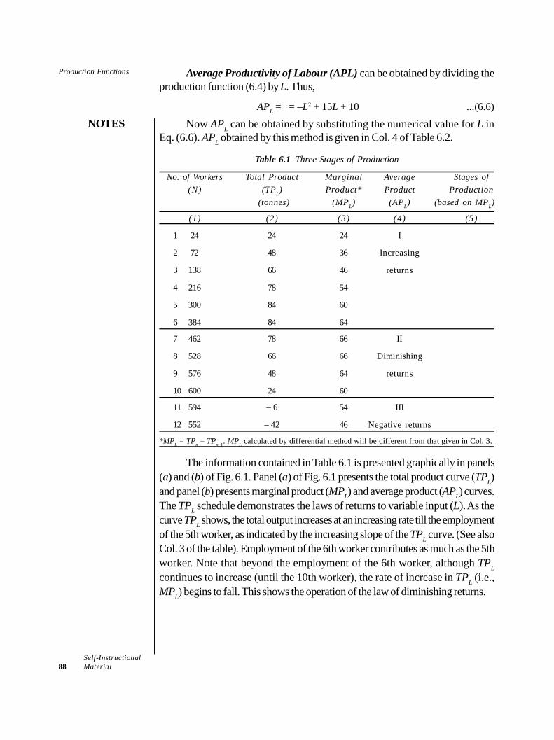
Production Functions
NOTES
Self-Instructional88 Material
Average Productivity of Labour (APL) can be obtained by dividing theproduction function (6.4) by L. Thus,
APL = = –L2 + 15L + 10 ...(6.6)
Now APL can be obtained by substituting the numerical value for L inEq. (6.6). APL obtained by this method is given in Col. 4 of Table 6.2.
Table 6.1 Three Stages of Production
No. of Workers Total Product Marginal Average Stages of(N) (TPL) Product* Product Production
(tonnes) (MPL) (APL) (based on MPL)
(1) (2) (3) (4) (5)
1 24 24 24 I
2 72 48 36 Increasing
3 138 66 46 returns
4 216 78 54
5 300 84 60
6 384 84 64
7 462 78 66 II
8 528 66 66 Diminishing
9 576 48 64 returns
10 600 24 60
11 594 – 6 54 III
12 552 – 42 46 Negative returns
*MPL = TPn – TPn–1. MPL calculated by differential method will be different from that given in Col. 3.
The information contained in Table 6.1 is presented graphically in panels(a) and (b) of Fig. 6.1. Panel (a) of Fig. 6.1 presents the total product curve (TPL)and panel (b) presents marginal product (MPL) and average product (APL) curves.The TPL schedule demonstrates the laws of returns to variable input (L). As thecurve TPL shows, the total output increases at an increasing rate till the employmentof the 5th worker, as indicated by the increasing slope of the TPL curve. (See alsoCol. 3 of the table). Employment of the 6th worker contributes as much as the 5thworker. Note that beyond the employment of the 6th worker, although TPLcontinues to increase (until the 10th worker), the rate of increase in TPL (i.e.,MPL) begins to fall. This shows the operation of the law of diminishing returns.
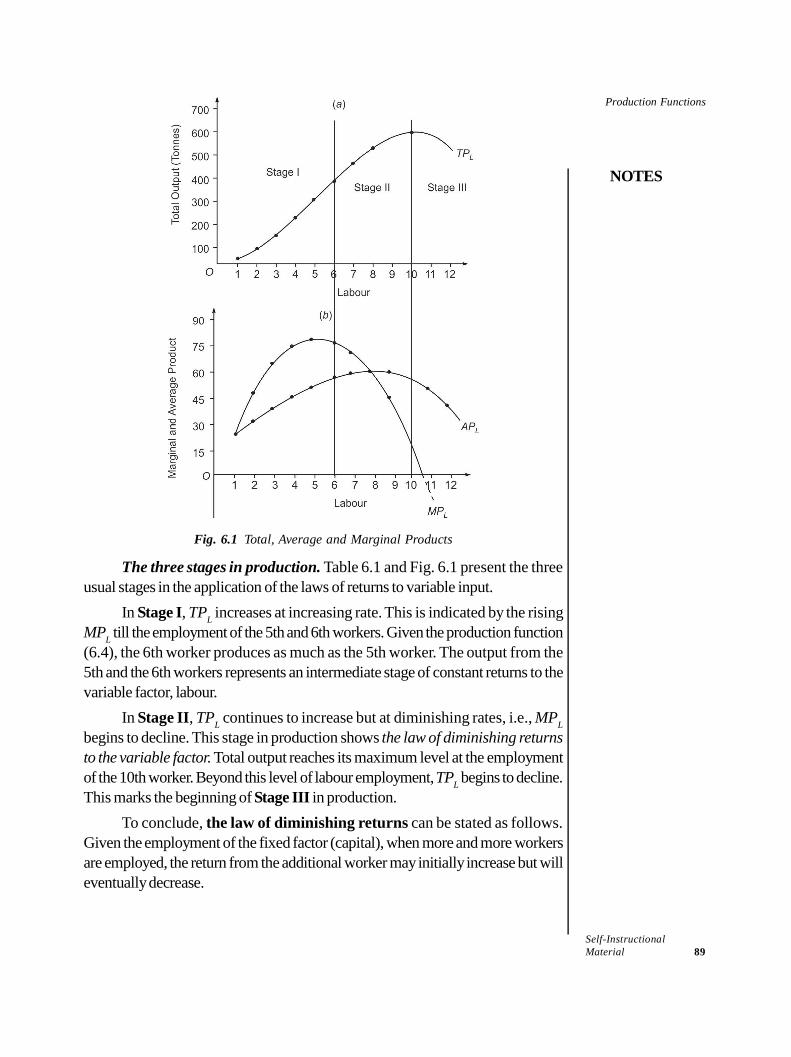
Production Functions
NOTES
Self-InstructionalMaterial 89
Fig. 6.1 Total, Average and Marginal Products
The three stages in production. Table 6.1 and Fig. 6.1 present the threeusual stages in the application of the laws of returns to variable input.
In Stage I, TPL increases at increasing rate. This is indicated by the risingMPL till the employment of the 5th and 6th workers. Given the production function(6.4), the 6th worker produces as much as the 5th worker. The output from the5th and the 6th workers represents an intermediate stage of constant returns to thevariable factor, labour.
In Stage II, TPL continues to increase but at diminishing rates, i.e., MPLbegins to decline. This stage in production shows the law of diminishing returnsto the variable factor. Total output reaches its maximum level at the employmentof the 10th worker. Beyond this level of labour employment, TPL begins to decline.This marks the beginning of Stage III in production.
To conclude, the law of diminishing returns can be stated as follows.Given the employment of the fixed factor (capital), when more and more workersare employed, the return from the additional worker may initially increase but willeventually decrease.
Production Functions
NOTES
Self-Instructional90 Material
Factors Behind the Laws of Returns. As shown in Fig. 6.1, the marginalproductivity of labour (MPL) increases is Stage I, whereas it decreases in StageII. In other words, in Stage I, Law of Increasing Returns to variable input is inoperation and in Stage II, the law of Diminishing Returns is in application. Thereasons which underly the application of the laws of returns in Stages I and II maybe described as follows.
One of the important factors causing increasing returns to a variable factoris the indivisibility of fixed factor (capital). The size of a capital is given and,given the technoloyg, it requires an optimum number of labour. If labour is lessthan optimum number, capital cannot be divided to suit the number of workers.Therefore, if labour is less than its optimum number, capital remains underutilized.Let us suppose that optimum capital-labour combination is 1:6. If capital isindivisible and less than 6 workers are employed, then capital would remainunderutilized. When more and more workers are added, utilization of capitalincreases. As a result, productivity of capital increases. This gives increasing returnsto variable input, labour.
The second and the most important reason for increase in labour productivityis the division of labour, i.e., assigning works to labour according to their skill.This becomes possible with the employment of additional labour. Devision of labouraccording to their skill and specialization increases productivity of labour.
Thus increase in productivity of both the factors, capital and labour, increasesthe output at increasing rate.
Once the optimum capital-labour ratio is reached, employment of additionallabour amounts to underutilization of labour. So the productivity of marginal labourdecreases. Also, with increasing number of workers, capital remaining the same,capital-labour ratio goes on decreasing. As a result, productivity of labour beginsto decline. This marks the beginning of the second stage—the stage of decreasingreturns.
Application of the Law of Diminishing Returns
The law of diminishing returns to the variable input is an empirical law, frequentlyobserved in various production activities. This law, however, may not applyuniformally to all kinds of productive activities since it is not as true as the law ofgravitation. In some productive activities, the law of diminishing returns may operatequickly, in some its operation may take a little longer time and in some others, itmay not appear at all. This law has been found to operate in agricultural productionmore regularly than in industrial production. The reason is, in agriculture, naturalfactors play a predominant role whereas man-made factors play the major role inindustrial production. Despite the limitations of the law, if increasing units of aninput are applied to the fixed factors, the marginal returns to the variable inputdecrease eventually.
Production Functions
NOTES
Self-InstructionalMaterial 91
The Law of Diminishing Returns and Business Decisions. The law ofdiminishing returns as presented graphically has a relevance to the businessdecisions. The graph can help in identifying the rational and irrational stages ofoperations. It can also tell the business managers the number of workers (or othervariable inputs) to apply to a given fixed input so that, given all other factors,output is maximum. As Fig. 6.1 exhibits, capital is presumably underutilized inStage I. So a firm operating in Stage I is required to increase labour, and a firmoperating in Stage III is required to reduce labour, with a view to maximizing itstotal production. From the firm’s point of view, setting an output target in Stages Iand III is irrational because setting output target in stage I means underutilizationof capital and setting output target in Stage III means accepting negative productivityof labour. The only meaningful and rational stage from the firm’s point of view isStage II in which the firm can find answer to the question ‘how many workers toemploy’ to maximize production, given the labour productivity. Figure 6.1 showsthat the firm should employ a minimum of 7 workers and a maximum of 10 workerseven if labour is available free of cost. This means that the firm has a limitedchoice—ranging from 7 to 10 workers. How many workers to employ against thefixed capital and how much to produce can be answered, only when the price oflabour, i.e., wage rate, and product price are known. This question is answeredbelow.
Optimum Employment of Labour
It may be recalled from Fig. 6.1 that an output maximizing coal-mining firm wouldlike to employ 10 workers since at this level of employment, the output is maximum.The firm can, however, employ 10 workers only if workers are available free ofcost. But labour is not available free of cost—the firm is required to pay wages tothe workers. The objective of the firm to maximize profit, not output. Therefore,the question arises as to how many workers would the firm employ—10 or less ormore than 10—to maximize its profit. A simple answer to this question is that thenumber of workers to be employed depends on the output that maximizes thefirm’s profit, given the product price and the wage rate. This point can be provedas follows.
Pprofit is maximum whereMC = MR
The same rule can be applied to determine the optium level of employment,with some modification, of course. In our example here, since labour is the onlyvariable input, marginal cost (MC) equals marginal wages (MW), i.e., MC = MW.
As regards MR, in case of factor employment, the concept of MarginalRevenue Productivity (MRP) is used. The marginal revenue productivity is thevalue of product resulting from the marginal unit of variable input (labour). In specific
Production Functions
NOTES
Self-Instructional92 Material
terms, marginal revenue productivity (MRP) equals marginal physical productivity(MPL) of labour multiplied by the price (P) of the product, i.e.,
MRP = MPL Χ P
6.3.2 Isoquants
In the preceding section, we have discussed the short-term laws of production,i.e., technological relationship between inputs and output assuming labour to bethe only variable input, capital held constant. In this section, we proceed to discussthe long-term laws of production, i.e., the nature of relationship between inputsand output under the condition that both the inputs, capital and labour, are variablefactors. In the long-run, supply of both the inputs is supposed to be elastic and,therefore, firms can use larger quantities of both labour and capital. With largeremployment of capital labour, the scale of production increases. The nature ofchanging relationship between changing scale of inputs and output is refered to thelaws of returns to scale. The laws of returns to scale are generally explainedthrough the production function and isoquant curve technique. The most commonand simple tool of analysis is isoquant curve technique. We will, therefore, firstintroduce and elaborate on this tool of analysis. The laws of return to scale willthen be explained through isoquant curve technique. The laws of returns to scalethrough production function will be explained in the next section.
Isoquant: The Tool of Analyses
The term ‘isoquant’ has been derived from the Greek word iso meaning ‘equal’and Latin word quantus meaning ‘quantity’. The ‘isoquant curve’ is, therefore,also known as ‘Equal Product Curve’ or ‘Production Indifference Curve’. Anisoquant curve can be defined as the locus of points representing variouscombinations of two inputs—capital and labour—yielding the same output.An ‘isoquant curve’ is analogous to an ‘indifference curve’, with two points ofdistinction: (a) an indifference curve is made of two consumer goods while anisoquant curve is constructed of two producer goods (labour and capital), and(b) an indifference curve represents an unmeasured level of satisfaction whereasan isoquant represents the quantity of output of a commodity.
Isoquant curves are drawn on the basis of the following assumptions:(i) there are only two inputs, viz., labour (L) and capital (K), to produce
a commodity X;(ii) both L and K and product X are perfectly divisible;(iii) the two inputs—L and K—can substitute each other but at a diminishing
rate as they are imperfect substitutes; and(iv) the technology of production is given.
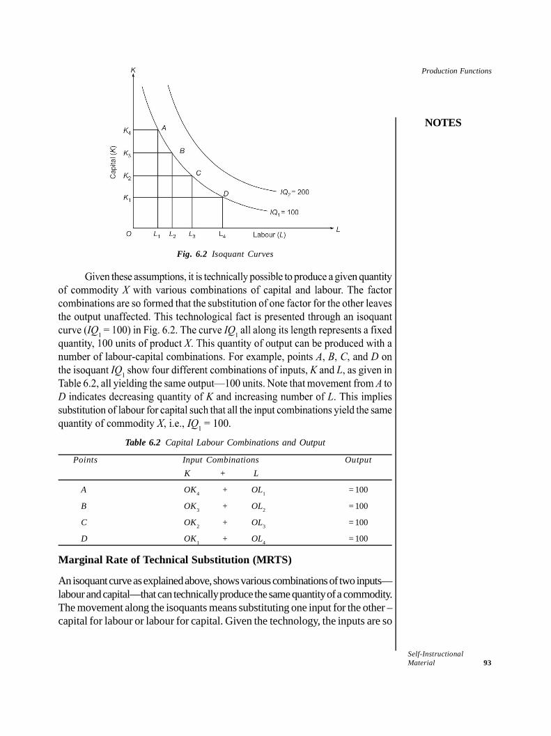
Production Functions
NOTES
Self-InstructionalMaterial 93
Fig. 6.2 Isoquant Curves
Table 6.2 Capital Labour Combinations and Output
Points Input Combinations OutputK + L
A OK4 + OL1 = 100
B OK3 + OL2 = 100
C OK2 + OL3 = 100
D OK1 + OL4 = 100
Marginal Rate of Technical Substitution (MRTS)
An isoquant curve as explained above, shows various combinations of two inputs—labour and capital—that can technically produce the same quantity of a commodity.The movement along the isoquants means substituting one input for the other –capital for labour or labour for capital. Given the technology, the inputs are so
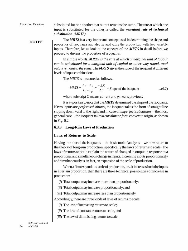
Production Functions
NOTES
Self-Instructional94 Material
substituted for one another that output remains the same. The rate at which oneinput is substituted for the other is called the marginal rate of technicalsubstitution (MRTS).
In simple words, MRTS is the rate at which a marginal unit of labourcan be substituted for a marginal unit of capital or other way round, totaloutput remaining the same. The MRTS gives the slope of the isoquant at differentlevels of input combinations.
The MRTS is measured as follows.
c p
c p
K K KMRTSL L L
= Slope of the isoquant …(6.7)
where subscript C means current and p means previous.It is important to note that the MRTS determined the shape of the isoquants.
If two inputs are perfect substitutes, the isoquant takes the form of straight linesloping downward to the right and in case of imperfect substitutes—the mostgeneral case—the isoquant takes a curvilinear form convex to origin, as shownin Fig. 6.2.
6.3.3 Long-Run Laws of Production
Laws of Returns to Scale
Having introduced the isoquants—the basic tool of analysis—we now return tothe theory of long-run production, specifically the laws of returns to scale. Thelaws of returns to scale explain the nature of changed in output in response to aproportional and simultaneous change in inputs. Increasing inputs proportionatelyand simultaneously is, in fact, an expansion of the scale of production.
When a firm expands its scale of production, i.e., it increases both the inputsin a certain proportion, then there are three technical possibilities of increase inproduction:
(i) Total output may increase more than proportionately;(ii) Total output may increase proportionately; and(iii) Total output may increase less than proportionately.
Accordingly, there are three kinds of laws of returns to scale:(i) The law of increasing returns to scale;(ii) The law of constant returns to scale, and(iii) The law of diminishing returns to scale.
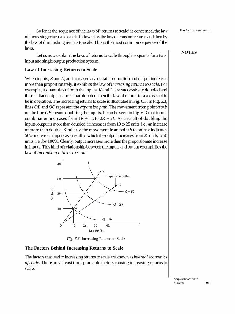
Production Functions
NOTES
Self-InstructionalMaterial 95
So far as the sequence of the laws of ‘returns to scale’ is concerned, the lawof increasing returns to scale is followed by the law of constant returns and then bythe law of diminishing returns to scale. This is the most common sequence of thelaws.
Let us now explain the laws of returns to scale through isoquants for a two-input and single output production system.
Law of Increasing Returns to Scale
When inputs, K and L, are increased at a certain proportion and output increasesmore than proportionately, it exhibits the law of increasing returns to scale. Forexample, if quantities of both the inputs, K and L, are successively doubled andthe resultant output is more than doubled, then the law of returns to scale is said tobe in operation. The increasing returns to scale is illustrated in Fig. 6.3. In Fig. 6.3,lines OB and OC represent the expansion path. The movement from point a to bon the line OB means doubling the inputs. It can be seen in Fig. 6.3 that input-combination increases from 1K + 1L to 2K + 2L. As a result of doubling theinputs, output is more than doubled: it increases from 10 to 25 units, i.e., an increaseof more than double. Similarly, the movement from point b to point c indicates50% increase in inputs as a result of which the output increases from 25 units to 50units, i.e., by 100%. Clearly, output increases more than the proportionate increasein inputs. This kind of relationship between the inputs and output exemplifies thelaw of increasing returns to scale.
Fig. 6.3 Increasing Returns to Scale
The Factors Behind Increasing Returns to Scale
The factors that lead to increasing returns to scale are known as internal economicsof scale. There are at least three plausible factors causing increasing returns toscale.
Production Functions
NOTES
Self-Instructional96 Material
(i) Technical and managerial indivisibilities. Certain inputs, particularlymechanical equipments and managers, used in the process of production areavailable in a given size. Such inputs cannot be divided into parts to suit small scaleof production. For example, half a turbine cannot be used and one-third or a partof a composite harvester and earth-movers cannot be used to produce the relevantproduct.
In regard to managerial manpower, if scale of production is small, managersremain under-employed because half of a production manager cannot be employed,if part-time employment is not acceptable to the manager. Because of indivisibilityof machinery and managers, given the state of technology, they have to beemployed in a minimum quantity even if scale of production is much less than thecapacity output. Therefore, when scale of production is expanded by increasingall the inputs, the productivity of indivisible factors increases exponentially becauseof technological advantage. This results in increasing returns to scale.(ii) Higher degree of specialization. Another factor causing increasing returnsto scale is higher degree of specialization of both labour and machinery, whichbecomes possible with increase in scale of production. The use of specializedlabour suitable to a particular job and of a composite machinery increasesproductivity of both labour and capital per unit of inputs. Their cumulative effectscontribute to the increasing returns to scale. Besides, employment of specializedmanagerial personnel, e.g., administrative manager, production managers salesmanager and personnel manager, contributes a great deal in increasing production.(iii) Dimensional relations. Increasing returns to scale is also a matter ofdimensional relations. For example, when the length and breadth of a room (15 ×10 = 150 sq. ft.) are doubled, then the size of the room is more than doubled: itincreases to 30 × 20 = 600 sq. ft. When diameter of a pipe is doubled, the flowof water is more than doubled. In accordance with this dimensional relationship,when the labour and capital are doubled, the output is more than doubled and soon.
Law of Constant Returns to Scale
When the increase in output is proportionate to the increase in inputs, it exhibitsconstant returns to scale. For example, if quantities of both the inputs, K and L,are doubled and output is also doubled, then the returns to scale are said to beconstant. Constant returns to scale are illustrated in Fig. 6.4. The lines OA and OBare ‘expansion paths’ indicating two hypothetical techniques of production withoptimum capital-labour ratio. The isoquants marked Q = 10, Q = 20 and Q = 30indicate the three different levels of output. In the figure, the movement from pointsa to b indicates doubling both the inputs—increasing capital from 1K to 2K andlabour from 1L to 2L. When inputs are doubled, output is also doubled, i.e.,output increases from 10 to 20.
Production Functions
NOTES
Self-InstructionalMaterial 97
Fig. 6.4 Constant Returns to Scale
Similarly, the movement from point b to c indicates a 50 per cent increase inboth labour and capital. This increase in inputs results in an increase of output from20 to 30 units, i.e., a 50 per cent increase in output. In simple words, a 50 per centincrease in inputs leads to a 50 per cent increase in output. This relationship betweena proportionate change in inputs and the same proportional change in outputs maybe summed up as follows.
1K + 1L 102K + 2L 203K + 3L 30
This kind of relationship between inputs and output exhibits constant returnsto scale.
The constant returns to scale are attributed to the limits of the economiesof scale. With expansion in the scale of production, economies arise from suchfactors as indivisibility of fixed factors, greater possibility of specialization of capitaland labour, use of more efficient techniques of production, etc. But there is a limitto the economies of scale. When economies of scale reach their limits anddiseconomies are yet to begin, returns to scale become constant. The constantreturns to scale take place also where factors of production are perfectly divisibleand where technology is such that capital-labour ratio is fixed. When the factors ofproduction are perfectly divisible, the production function is homogeneous of degree1 showing constant returns to scale.
Decreasing Returns to Scale
The firms are faced with decreasing returns to scale when a certain proportionateincrease in inputs, K and L, leads to a less than proportionate increase in output.For example, when inputs are doubled and output is less than doubled, thendecreasing returns to scale is in operation. The decreasing returns to scale isillustrated in Fig. 6.5. As the figure shows, when the inputs K and L are doubled,
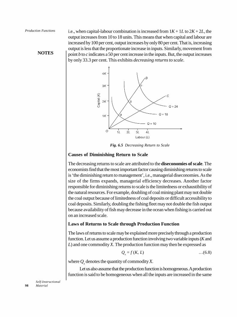
Production Functions
NOTES
Self-Instructional98 Material
i.e., when capital-labour combination is increased from 1K + 1L to 2K + 2L, theoutput increases from 10 to 18 units. This means that when capital and labour areincreased by 100 per cent, output increases by only 80 per cent. That is, increasingoutput is less that the proportionate increase in inputs. Similarly, movement frompoint b to c indicates a 50 per cent increase in the inputs. But, the output increasesby only 33.3 per cent. This exhibits decreasing returns to scale.
Fig. 6.5 Decreasing Return to Scale
Causes of Diminishing Return to Scale
The decreasing returns to scale are attributed to the diseconomies of scale. Theeconomists find that the most important factor causing diminishing returns to scaleis ‘the diminishing return to management’, i.e., managerial diseconomies. As thesize of the firms expands, managerial efficiency decreases. Another factorresponsible for diminishing returns to scale is the limitedness or exhaustibility ofthe natural resources. For example, doubling of coal mining plant may not doublethe coal output because of limitedness of coal deposits or difficult accessibility tocoal deposits. Similarly, doubling the fishing fleet may not double the fish outputbecause availability of fish may decrease in the ocean when fishing is carried outon an increased scale.
Laws of Returns to Scale through Production Function
The laws of returns to scale may be explained more precisely through a productionfunction. Let us assume a production function involving two variable inputs (K andL) and one commodity X. The production function may then be expressed as
Qx = f (K, L) …(6.8)
where Qx denotes the quantity of commodity X.Let us also assume that the production function is homogeneous. A production
function is said to be homogeneous when all the inputs are increased in the same
Production Functions
NOTES
Self-InstructionalMaterial 99
proportion and the proportion can be factored out. And, if all the inputs are increasedby a certain proportion (say, k) and output increases in the same proportion (k),then production is said to be homogeneous of degree 1. This kind of productionfunction may be expressed as follows.
kQx = f (kK, kL) …(6.9)
or = k (K, L)
A homogeneous production function of degree 1, as given in Eq. (6.9),implies constant returns to scale. Eq. (6.9) shows that increase in inputs, K andL, by a multiple of k, increases output, Qx by the same multiple (k). This meansconstant returns to scale.
The constant returns to scale may not be applicable at all the levels of increasein inputs. Increasing inputs K and L in the same proportion may result in increasingor diminishing returns to scale. In other words, it is quite likely that if all the inputsare increased by a certain proportion, output may increase more or less thanproportionately. For example, if all the inputs are doubled, the output may increaseby less than or more than double. Then the production function may be expressedas
hQx = f (kK, kL) …(6.10)
where h denotes h-times increase in Qx, as a result of k-times increase in inputs,K and L. The proportion h may be greater than k, equal to k, or less than k.Accordingly, it reveals the three laws of returns to scale:
(i) If h = k, production function reveals constant returns to scale.(ii) If h > k, it reveals increasing returns to scale.(iii) If h < k, it reveals decreasing returns to scale.
6.4 COBB-DOUGLAS AND OTHER PRODUCTIONFUNCTIONS: EMPIRICAL ESTIMATION
Cobb-Douglas Production Function—The Multiplicative Power Function
In the preceding section, the laws of returns to scale have been illustrated througha normal and a power function. In this section, we show the application of themost widely used production functions – the multiplicative power function. Themost popular production function of this category is ‘Cobb-Douglas ProductionFunction of the form
Q = AKa Lb …(6.11)
where A is a positive constant; a and b are positive fractions; and b = 1 – a.The Cobb-Douglas production function is often used in its following form.
Q = AKa L1–a …(6.12)
Production Functions
NOTES
Self-Instructional100 Material
Properties of Cobb-Douglas Production Function. A power function of thiskind has several important properties.
First, the multiplicative form of the power function can be changed into itslog-linear form as
log Q = log A + a log K + b log L …(6.13)
In its logarithmic form, the function becomes simple to handle and can beempirically estimated using linear regression analysis.
Secondly, power functions are homogeneous and the degree of homogeneityis given by the sum of the exponents a and b. If a + b = 1, then the productionfunction is homogeneous of degree 1 and implies constant returns to scale.
Thirdly, parameters a and b represent the elasticity co-efficient of outputfor inputs K and L, respectively. The output elasticity co-efficient () in respect ofcapital may be defined as proportional change in output as a result of a givenchange in K, keeping L constant. Thus,
k =Q Q Q KK K K Q
…(6.14)
By differentiating the production function Q = AKaLb with respect to K andsubstituting the result in Eq. (6.14), we can find the elasticity co-efficient. Weknow that
QK
= a AKa–1 Lb
By substituting the values for Q and Q/K, we get
k = a AKa–1 Lba b
KAK L
= a …(6.15)
Thus, output-elasticity coefficient for K is ‘a’. The same procedure may beadopted to show that b is the elasticity co-efficient of output for L.
Fourthly, constants a and b represent the relative share of inputs, K andL, in total output Q. The share of K in Q is given by
Q KK
Similarly, the share of L in Q is given by
Q LL
The relative share of K inQ an e obtained as11 .a b
a b
Q a AK L KK aL Q AK L
Similarly, it can be shown that b gives the relative share of L in Q.
Production Functions
NOTES
Self-InstructionalMaterial 101
Finally, Cobb-Douglas production function in its general form,Q = Ka L1–a implies that at zero cost, there will be zero production.
Some Input-Output Relationships
Some of the concepts used in production analysis can be easily derived from theCobb-Douglas production function as shown below.
(i) Average Product (AP) of L and K:APL = A (K/L)1–a
APK = A (L/K)1
(ii) Marginal Product of L and K:
MPL = a.A (K/L) a = a (Q/L)
MPK = (a – 1) A (L/K) a = (1 – a) Q/K
(iii)Marginal Rate of Technical Substitution:
, 1L
L kK
MP a KMRTSMP a L
CES Production Function
In addition to the Cobb-Douglas production function, there are several other formsof production function, viz., ‘constant elasticity substitution’ (CES), ‘variableelasticity of substitution’ (VES), Leontief-type, and linear-type. Of these, theconstant elasticity substitution (CES) production function is more widely used,apart from Cobb-Douglas production function. We will, therefore, discuss theCES production function briefly.
The CES production function is expressed asQ = A[K– + (1 – )L–]–1/ ... (6.16)
or Q = A[L– + (1 – )K–]–1/
(A > 0, 0 < < 1, and > – 1)
where L = labour, K = capital, and A, and are the three parameters.An important property of the CES production function is that it is
homogeneous of degree 1. This can be proved by increasing both the inputs,K and L, by a constant factor and finding the final outcome. Let us suppose thatinputs K and L are increased by a constant factor m. Then the production functiongiven in Eq. (6.16) can be written as follows.
Q = A[(mK)– + (1 – ) (mL)–]–1/
= A[m– {K– + (1 – )L–}]–1/
= (m–)–1/ A[K–+ (1 –) L–]–1/ ...(6.17)
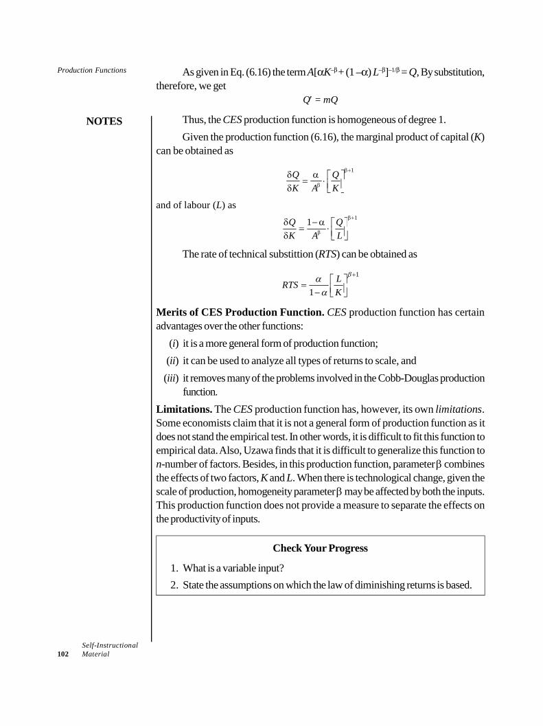
Production Functions
NOTES
Self-Instructional102 Material
As given in Eq. (6.16) the term A[K–+ (1 –) L–]–1/ = Q, By substitution,therefore, we get
Q = mQ
Thus, the CES production function is homogeneous of degree 1.Given the production function (6.16), the marginal product of capital (K)
can be obtained as1Q Q
K A K
and of labour (L) as11Q Q
K A L
The rate of technical substittion (RTS) can be obtained as
1
1LRTSK
Merits of CES Production Function. CES production function has certainadvantages over the other functions:
(i) it is a more general form of production function;(ii) it can be used to analyze all types of returns to scale, and(iii) it removes many of the problems involved in the Cobb-Douglas production
function.Limitations. The CES production function has, however, its own limitations.Some economists claim that it is not a general form of production function as itdoes not stand the empirical test. In other words, it is difficult to fit this function toempirical data. Also, Uzawa finds that it is difficult to generalize this function ton-number of factors. Besides, in this production function, parameter combinesthe effects of two factors, K and L. When there is technological change, given thescale of production, homogeneity parameter may be affected by both the inputs.This production function does not provide a measure to separate the effects onthe productivity of inputs.
Check Your Progress
1. What is a variable input?2. State the assumptions on which the law of diminishing returns is based.
Production Functions
NOTES
Self-InstructionalMaterial 103
6.5 ANSWERS TO CHECK YOUR PROGRESSQUESTIONS
1. A variable input is defined as one whose supply in the short-run is elastic,e.g., labour and raw material, etc. All the users of such factors can employa larger quantity in the short-run as well as in the long-run.
2. The law of diminishing returns is based on the following assumptions:(i) labour is the only variable input, capital remaining constant;(ii) labour is homogeneous;(iii) the state of technology is given; and(iv) input prices are given.
6.6 SUMMARY
Once business firms take decision on ‘what to produce’ the major issuesthat arise are ‘how to produce’ and ‘how much to produce’. These issuesarise because achieving optimum efficiency in production and minimizingcost for a given production is one of the prime concerns of the businessmanagers.
In general sense of the term, ‘production’ means transforming inputs (labour,capital, raw materials, time, etc.) into an output with value added. Thisconcept of production is however limited to only ‘manufacturing’.
In economic sense, production process may take a variety of forms otherthan manufacturing.
Inputs are classified aso fixed inputs, ando variable inputs.
Production function is a mathematical presentation of input-outputrelationship. More specifically, a production function states the technologicalrelationship between inputs and output in the form of an equation, a table ora graph. In its general form, it specifies the inputs required for the productionof a commodity or service.
There are two kinds of production functions:(i) Short-run production function; and(ii) Long-run production function
The marginal revenue productivity is the value of product resulting from themarginal unit of variable input (labour).
Production Functions
NOTES
Self-Instructional104 Material
The term ‘isoquant’ has been derived from the Greek word iso meaning‘equal’ and Latin word quantus meaning ‘quantity’. The ‘isoquant curve’is, therefore, also known as ‘Equal Product Curve’ or ‘ProductionIndifference Curve’.
In simple words, MRTS is the rate at which a marginal unit of labour canbe substituted for a marginal unit of capital or other way round, total outputremaining the same.
The factors that lead to increasing returns to scale are known as internaleconomics of scale. There are at least three plausible factors causingincreasing returns to scale.
The decreasing returns to scale are attributed to the diseconomies of scale.The economists find that the most important factor causing diminishing returnsto scale is ‘the diminishing return to management’, i.e., managerialdiseconomies.
In addition to the Cobb-Douglas production function, there are severalother forms of production function, viz., ‘constant elasticity substitution’(CES), ‘variable elasticity of substitution’ (VES), Leontief-type, and linear-type.
6.7 KEY WORDS
An isoquant curve: It can be defined as the locus of points representingvarious combinations of two inputs—capital and labour—yielding the sameoutput.
Marginal rate of technical substitution (MRTS): It is the rate at whicha marginal unit of labour can be substituted for a marginal unit of capital orother way round, total output remaining the same.
6.8 SELF ASSESSMENT QUESTIONS ANDEXERCISES
Short Answer Questions
1. What is the significance of the production function in economics?2. Write a short note on the short-run and long-run production function.3. Briefly mention the use of isoquant curves.4. What is the Cobb-Douglas production function?
Long Answer Questions
1. Describe the theory of production and its managerial uses.
Production Functions
NOTES
Self-InstructionalMaterial 105
2. Discuss the application of the law of diminishing returns.3. Explain the three kinds of laws of returns to scale.
6.9 FURTHER READINGS
Dwivedi, D. N. 2015. Principles of Economics, Eight Edition. New Delhi: VikasPublishing House.
Weil. David N. 2004. Economic Growth. London: Addison Wesley.Thomas, Christopher R. and Maurice S. Charles. 2005. Managerial Economics:
Concepts and Applications, Eighth Edition. New Delhi: Tata McGraw-Hill Publishing Company Limited.
Mankiw, Gregory N. 2002. Principles of Economics, Second Edition. India:Thomson Press.
Websites
https://blogs.economictimes.indiatimes.com/et-commentary/heres-how-indias-widening-income-distribution-can-be-redressed/
https://www.livemint.com/Opinion/WmpSjQAvPGeVzxqpgXYvtK/The-dangers-of-Indias-Billionaire-Raj.html
Forms of Markets
NOTES
Self-Instructional106 Material
UNIT 7 FORMS OF MARKETS
Structure7.0 Introduction7.1 Unit Objectives7.2 Meaning and Characteristics of Markets
7.2.1 Market Equilibirum and Changes in Market Equilibrium7.2.2 Market Equilibrium: Practical Importance
7.3 Pricing Functions under Different Market Structures7.3.1 Market Structures and Pricing Decisions
7.4 Price and Output Decisions under Different Competitive Conditions7.4.1 Monopoly7.4.2 Monopolistic Competition7.4.3 Oligopoly
7.5 Answers to Check Your Progress Questions7.6 Summary7.7 Key Words7.8 Self Assessment Questions and Exercises7.9 Further Readings
7.0 INTRODUCTION
Knowing input-output relations and output-cost relations is not the objective ofbusiness firms. Profit maximization is the objective of business firms, as assumedin traditional theory of firm. Profit is maximized when TR – TC is maximized. SinceTR = P × Q, where P = price, and Q = quantity sold, given the cost-outputrelation, the main task for profit maximization is to find the profit maximizing price.This takes us to the theory of price determination. The theory or model of pricedetermination developed by economic pundits is based on the market conditions.Market conditions are determined by the number of firms in an industry and thenature and degree of competition among the firms. The number of firms and degreeof inter-firm competition determine the market structure of the industry. Theeconomists have proposed different kinds of theoretical models for pricedetermination on the basis of the nature and the characteristics of the market.Market conditions provide the playing field of the business firms.
In this unit, you will study about the meaning and characteristics ofmarketstructure, price determination by demand and supply functions and pricing andoutput decisions under monopoly, monopolistic competition and oligopoly.
7.1 UNIT OBJECTIVES
After going through this unit, you will be able to: Identify the characteristics of the market structure
Forms of Markets
NOTES
Self-InstructionalMaterial 107
Evaluate price determination by demand and supply functions Discuss pricing and output decisions under monopoly, monopolistic
competition and oligopoly
7.2 MEANING AND CHARACTERISTICS OFMARKETS
In general usage, the term ‘market’ means a place or locality where goods andservices are bought and sold, e.g., Connaught Place market, Chandani Chowkmarket, Karol Bagh Market, etc. The term ‘market’ is also used with reference toa product, e.g., wheat market, vegetable market (Sabji mandi), gold market, stockmarket, etc.
In economics, the word ‘market’ is used in a rather abstract sense. Themarket means a system by which sellers and buyers of a commodity interact tosettle its price and the quantity to be bought and sold. According to Samuelsonand Nordhaus, “A market is a mechanism by which buyers and sellers interact todetermine the price and quantity of a good or service”. Market for a commodityconsists of the buyers and sellers who interact to settle its price and quantity to betransacted. The sellers and buyers may be individuals, firms, factories, dealersand agents.Some important aspects of the market concept are the following ones:
(i) A market need not be situated in a particular place or locality. Thegeographical area of a market depends on how far and wide are the buyersand sellers scattered. It may be as small as a fish market in a corner of a cityor as large as the entire world, e.g., the global markets for arms, cars,electronic goods, aeroplanes, computers, oil, medicines, etc.
(ii) Buyers and sellers need not come into personal contact with each other.The transactions can be carried out through postal services ortelecommunication system—telephone, fax, agents, or e-mail etc. Peopledo buy many goods and services without ever meeting the supplier.
(iii) The word ‘market’ may refer to a commodity or service (e.g., fruit market,car market, share market, money market, paper market, labour market,etc.) or to a geographical area, Bombay market, Indian market, Asianmarket, or the world market.
(iv) The economists distinguish between markets also on the basis of (a) natureof goods and services, e.g., factor market, input market and output market;(b) number of firms and degree of competition, e.g., perfectly competitivemarket (very large number of firms), monopolistic market (many firms withdifferentiated products); oligopolistic market, and so on.
Forms of Markets
NOTES
Self-Instructional108 Material
The Market System: An Overview
Market system refers to the process by which buyers and sellers of a productinteract to settle the price of the product and carry out the sale-purchase transactions.The market system works on the basis of a basic market principle. The marketprinciple is based on the fundamental laws of demand and supply. Buyerscreate the demand and sellers create the supply of the product. Demand andsupply work as two opposite market forces. The working of the market systemis governed by the fundamental laws of demand and supply. The laws of demandand supply play a crucial role in determining the price of a product and the size ofthe market—total demand and total supply. A clear understanding of how marketswork is essential for business decisions on production and future planning. Asnoted above, market system works on the basis of two market forces—demandand supply. The demand and supply forces represent two sides of the markets,viz., (i) Demand side, and (ii) Supply side. The demand and supply sides workon the laws of demand and supply, respectively.
7.2.1 Market Equilibirum and Changes in Market Equilibrium
In this section, we explain how demand and supply interact to strike a balance,how market attains equilibrium, and how equilibrium price is determined in afree market. A free market is one in which market forces of demand and supplyare free to take their own course and there is no outside control on price, demandand supply.
The Concept of Market Equilibrium
In physical sense, the term equilibrium means the ‘state of rest’. In general sense,it means that forces working in opposite directions are in balance. In the contextof market analysis, equilibrium refers to a state of market in which quantitydemanded of a commodity equals the quantity supplied of the commodity.The equality of demand and supply produces an equilibrium price. The equilibriumprice is the price at which quantity demanded of a commodity equals its quantitysupplied. That is, at equilibrium price, demand and supply are in equilibrium.Equilibrium price is also called market-clearing price. Market is cleared in thesense that there is no unsold stock and no unsupplied demand.
Determination of Market Price
Equilibrium price of a commodity in a free market is determined by the marketforces of demand and supply. In order to analyse how equilibrium price isdetermined, we need to integrate the demand and supply curves. For this purpose,let us use our earlier example of shirts. Let us suppose that the weekly marketdemand and supply schedules for shirts in Delhi are given as shown in Table 7.1.
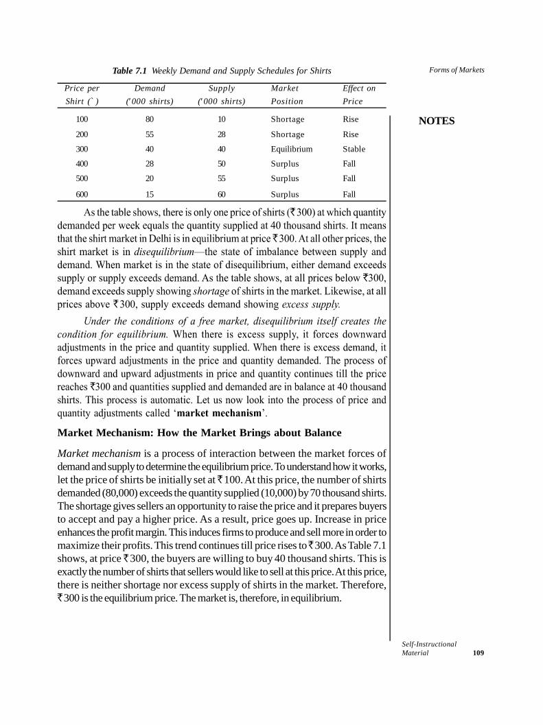
Forms of Markets
NOTES
Self-InstructionalMaterial 109
Table 7.1 Weekly Demand and Supply Schedules for Shirts
Price per Demand Supply Market Effect onShirt (`) (000 shirts) (000 shirts) Position Price
100 80 10 Shortage Rise
200 55 28 Shortage Rise
300 40 40 Equilibrium Stable
400 28 50 Surplus Fall
500 20 55 Surplus Fall
600 15 60 Surplus Fall
Market Mechanism: How the Market Brings about Balance
Market mechanism is a process of interaction between the market forces ofdemand and supply to determine the equilibrium price. To understand how it works,let the price of shirts be initially set at 100. At this price, the number of shirtsdemanded (80,000) exceeds the quantity supplied (10,000) by 70 thousand shirts.The shortage gives sellers an opportunity to raise the price and it prepares buyersto accept and pay a higher price. As a result, price goes up. Increase in priceenhances the profit margin. This induces firms to produce and sell more in order tomaximize their profits. This trend continues till price rises to 300. As Table 7.1shows, at price 300, the buyers are willing to buy 40 thousand shirts. This isexactly the number of shirts that sellers would like to sell at this price. At this price,there is neither shortage nor excess supply of shirts in the market. Therefore,
300 is the equilibrium price. The market is, therefore, in equilibrium.
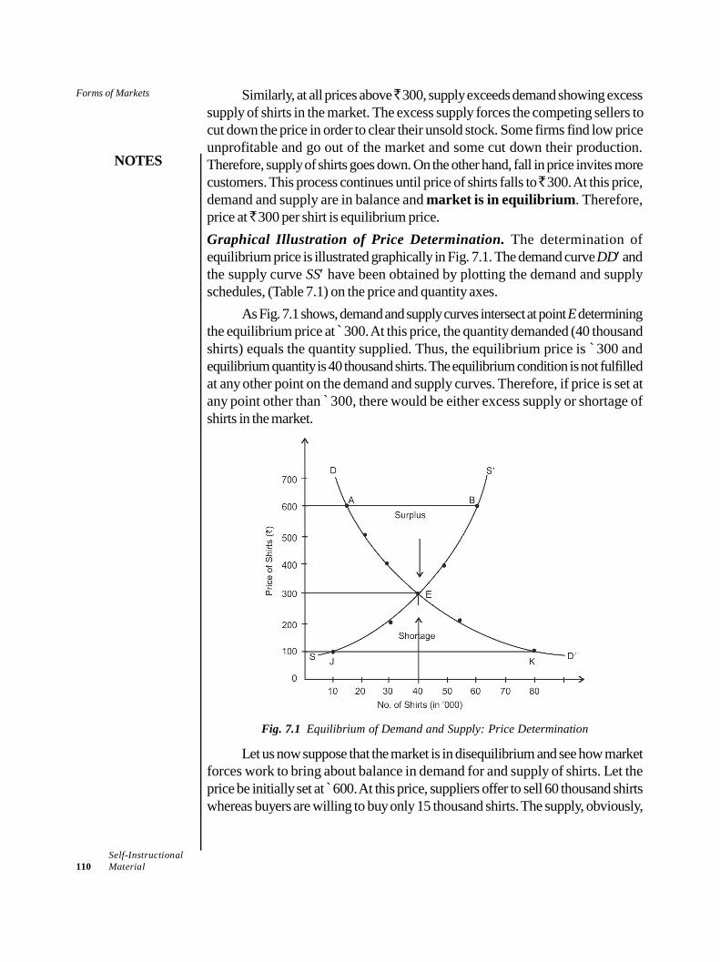
Forms of Markets
NOTES
Self-Instructional110 Material
Similarly, at all prices above 300, supply exceeds demand showing excesssupply of shirts in the market. The excess supply forces the competing sellers tocut down the price in order to clear their unsold stock. Some firms find low priceunprofitable and go out of the market and some cut down their production.Therefore, supply of shirts goes down. On the other hand, fall in price invites morecustomers. This process continues until price of shirts falls to 300. At this price,demand and supply are in balance and market is in equilibrium. Therefore,price at 300 per shirt is equilibrium price.Graphical Illustration of Price Determination. The determination ofequilibrium price is illustrated graphically in Fig. 7.1. The demand curve DDandthe supply curve SS have been obtained by plotting the demand and supplyschedules, (Table 7.1) on the price and quantity axes.
As Fig. 7.1 shows, demand and supply curves intersect at point E determiningthe equilibrium price at ̀ 300. At this price, the quantity demanded (40 thousandshirts) equals the quantity supplied. Thus, the equilibrium price is `300 andequilibrium quantity is 40 thousand shirts. The equilibrium condition is not fulfilledat any other point on the demand and supply curves. Therefore, if price is set atany point other than ̀ 300, there would be either excess supply or shortage ofshirts in the market.
Fig. 7.1 Equilibrium of Demand and Supply: Price Determination
Let us now suppose that the market is in disequilibrium and see how marketforces work to bring about balance in demand for and supply of shirts. Let theprice be initially set at ̀ 600. At this price, suppliers offer to sell 60 thousand shirtswhereas buyers are willing to buy only 15 thousand shirts. The supply, obviously,
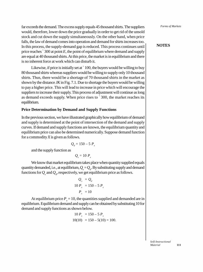
Forms of Markets
NOTES
Self-InstructionalMaterial 111
far exceeds the demand. The excess supply equals 45 thousand shirts. The supplierswould, therefore, lower down the price gradually in order to get rid of the unsoldstock and cut down the supply simultaneously. On the other hand, when pricefalls, the law of demand comes into operation and demand for shirts increases too.In this process, the supply-demand gap is reduced. This process continues untilprice reaches ̀ 300 at point E, the point of equilibrium where demand and supplyare equal at 40 thousand shirts. At this price, the market is in equilibrium and thereis no inherent force at work which can disturb it.
Likewise, if price is initially set at ̀ 100, the buyers would be willing to buy80 thousand shirts whereas suppliers would be willing to supply only 10 thousandshirts. Thus, there would be a shortage of 70 thousand shirts in the market asshown by the distance JK in Fig. 7.1. Due to shortage the buyers would be willingto pay a higher price. This will lead to increase in price which will encourage thesuppliers to increase their supply. This process of adjustment will continue as longas demand exceeds supply. When price rises to `300, the market reaches itsequilibrium.
Price Determination by Demand and Supply Functions
In the previous section, we have illustrated graphically how equilibrium of demandand supply is determined at the point of intersection of the demand and supplycurves. If demand and supply functions are known, the equilibrium quantity andequilibrium price can also be determined numerically. Suppose demand functionfor a commodity X is given as follows.
Qd = 150 – 5 Px
and the supply function asQs = 10 Px
We know that market equilibrium takes place when quantity supplied equalsquantity demanded, i.e., at equilibrium, Qs = Qd. By substituting supply and demandfunctions for Qs and Qd, respectively, we get equilibrium price as follows.
Q s = Qd
10 Px = 150 – 5 Px
Px = 10
At equilibrium price Px = 10, the quantities supplied and demanded are inequilibrium. Equilibrium demand and supply can be obtained by substituting 10 fordemand and supply functions as shown below.
10 Px = 150 – 5 Px
10(10) = 150 – 5(10) = 100.
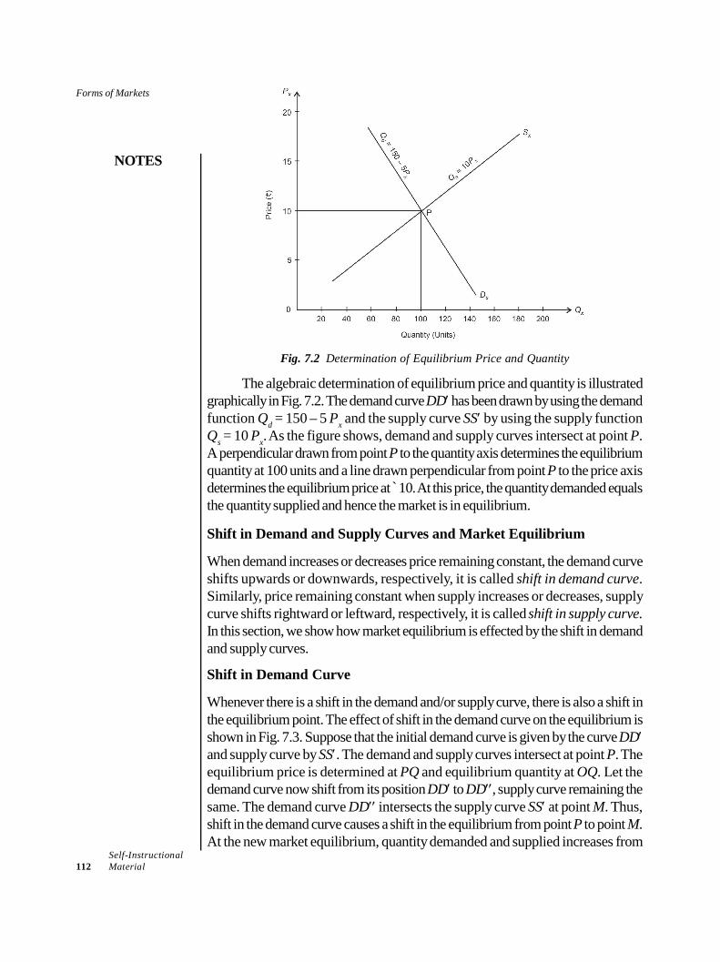
Forms of Markets
NOTES
Self-Instructional112 Material
Fig. 7.2 Determination of Equilibrium Price and Quantity
The algebraic determination of equilibrium price and quantity is illustratedgraphically in Fig. 7.2. The demand curve DDhas been drawn by using the demandfunction Qd = 150 – 5 Px and the supply curve SS by using the supply functionQs = 10 Px. As the figure shows, demand and supply curves intersect at point P.A perpendicular drawn from point P to the quantity axis determines the equilibriumquantity at 100 units and a line drawn perpendicular from point P to the price axisdetermines the equilibrium price at ̀ 10. At this price, the quantity demanded equalsthe quantity supplied and hence the market is in equilibrium.
Shift in Demand and Supply Curves and Market Equilibrium
When demand increases or decreases price remaining constant, the demand curveshifts upwards or downwards, respectively, it is called shift in demand curve.Similarly, price remaining constant when supply increases or decreases, supplycurve shifts rightward or leftward, respectively, it is called shift in supply curve.In this section, we show how market equilibrium is effected by the shift in demandand supply curves.
Shift in Demand Curve
Whenever there is a shift in the demand and/or supply curve, there is also a shift inthe equilibrium point. The effect of shift in the demand curve on the equilibrium isshown in Fig. 7.3. Suppose that the initial demand curve is given by the curve DDand supply curve by SS. The demand and supply curves intersect at point P. Theequilibrium price is determined at PQ and equilibrium quantity at OQ. Let thedemand curve now shift from its position DD to DD, supply curve remaining thesame. The demand curve DD intersects the supply curve SS at point M. Thus,shift in the demand curve causes a shift in the equilibrium from point P to point M.At the new market equilibrium, quantity demanded and supplied increases from
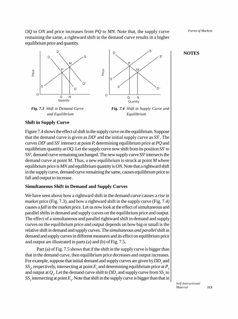
Forms of Markets
NOTES
Self-InstructionalMaterial 113
OQ to ON and price increases from PQ to MN. Note that, the supply curveremaining the same, a rightward shift in the demand curve results in a higherequilibrium price and quantity.
Fig. 7.3 Shift in Demand Curve Fig. 7.4 Shift in Supply Curve andand Equilibrium Equilibrium
Shift in Supply Curve
Figure 7.4 shows the effect of shift in the supply curve on the equilibrium. Supposethat the demand curve is given as DD and the initial supply curve as SS. Thecurves DD and SS intersect at point P, determining equilibrium price at PQ andequilibrium quantity at OQ. Let the supply curve now shift from its position SS toSS², demand curve remaining unchanged. The new supply curve SS² intersects thedemand curve at point M. Thus, a new equilibrium is struck at point M whereequilibrium price is MN and equilibrium quantity is ON. Note that a rightward shiftin the supply curve, demand curve remaining the same, causes equilibrium price tofall and output to increase.
Simultaneous Shift in Demand and Supply Curves
We have seen above how a rightward shift in the demand curve causes a rise inmarket price (Fig. 7.3), and how a rightward shift in the supply curve (Fig. 7.4)causes a fall in the market price. Let us now look at the effect of simultaneous andparallel shifts in demand and supply curves on the equilibrium price and output.The effect of a simultaneous and parallel rightward shift in demand and supplycurves on the equilibrium price and output depends on how big or small is therelative shift in demand and supply curves. The simultaneous and parallel shift indemand and supply curves in different measures and its effect on equilibrium priceand output are illustrated in parts (a) and (b) of Fig. 7.5.
Part (a) of Fig. 7.5 shows that if the shift in the supply curve is bigger thanthat in the demand curve, then equilibrium price decreases and output increases.For example, suppose that initial demand and supply curves are given by DD1 andSS1, respectively, intersecting at point E1 and determining equilibrium price at P1and output at Q1. Let the demand curve shift to DD2 and supply curve from SS1 toSS3 intersecting at point E3. Note that shift in the supply curve is bigger than that in
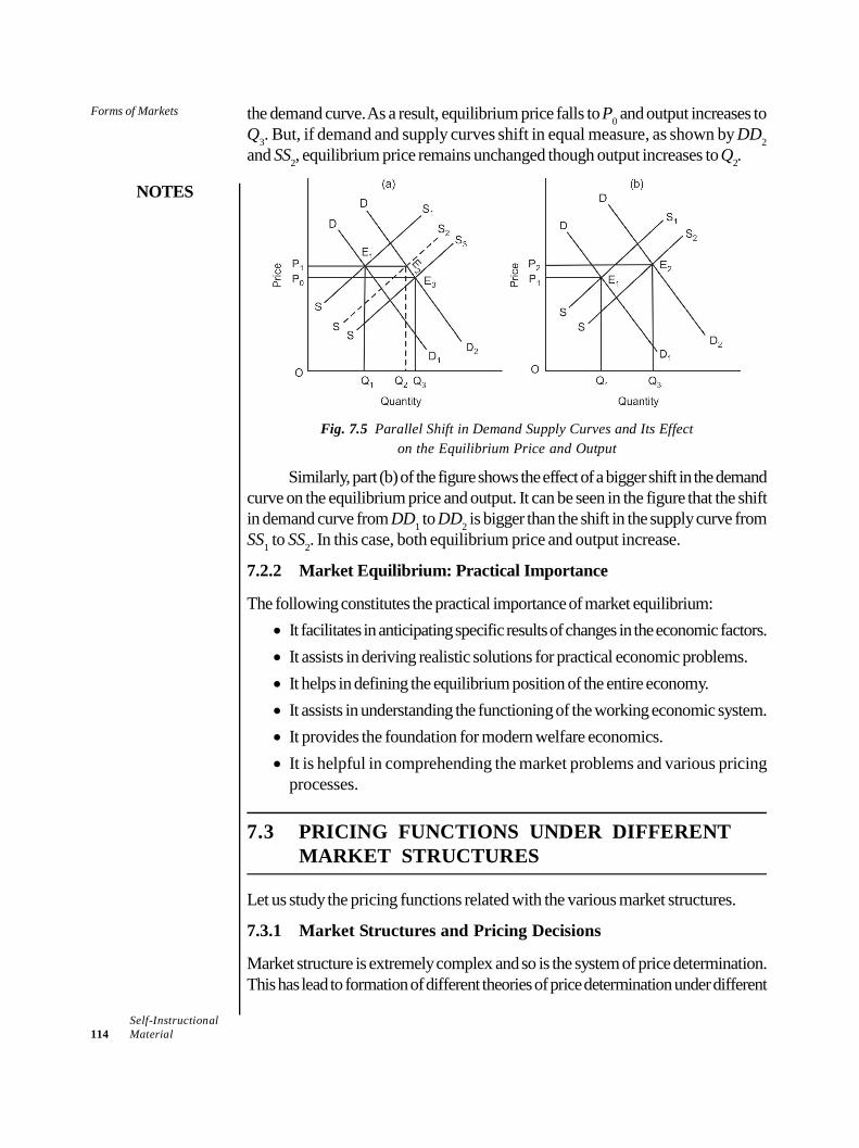
Forms of Markets
NOTES
Self-Instructional114 Material
the demand curve. As a result, equilibrium price falls to P0 and output increases toQ3. But, if demand and supply curves shift in equal measure, as shown by DD2and SS2, equilibrium price remains unchanged though output increases to Q2.
Fig. 7.5 Parallel Shift in Demand Supply Curves and Its Effecton the Equilibrium Price and Output
Similarly, part (b) of the figure shows the effect of a bigger shift in the demandcurve on the equilibrium price and output. It can be seen in the figure that the shiftin demand curve from DD1 to DD2 is bigger than the shift in the supply curve fromSS1 to SS2. In this case, both equilibrium price and output increase.
7.2.2 Market Equilibrium: Practical Importance
The following constitutes the practical importance of market equilibrium: It facilitates in anticipating specific results of changes in the economic factors. It assists in deriving realistic solutions for practical economic problems. It helps in defining the equilibrium position of the entire economy. It assists in understanding the functioning of the working economic system. It provides the foundation for modern welfare economics. It is helpful in comprehending the market problems and various pricing
processes.
7.3 PRICING FUNCTIONS UNDER DIFFERENTMARKET STRUCTURES
Let us study the pricing functions related with the various market structures.
7.3.1 Market Structures and Pricing Decisions
Market structure is extremely complex and so is the system of price determination.This has lead to formation of different theories of price determination under different
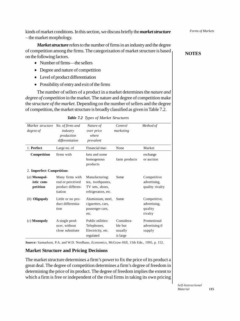
Forms of Markets
NOTES
Self-InstructionalMaterial 115
kinds of market conditions. In this section, we discuss briefly the market structure– the market morphology.
Market structure refers to the number of firms in an industry and the degreeof competition among the firms. The categorization of market structure is basedon the following factors.
Number of firms—the sellers Degree and nature of competition Level of product differentiation Possibility of entry and exit of the firmsThe number of sellers of a product in a market determines the nature and
degree of competition in the market. The nature and degree of competition makethe structure of the market. Depending on the number of sellers and the degreeof competition, the market structure is broadly classified as given in Table 7.2.
Table 7.2 Types of Market Structures
Market structure No. of firms and Nature of Control Method ofdegree of industry over price marketing
production wheredifferentiation prevalent
1. Perfect Large no. of Financial mar- None Market
Competition firms with kets and some exchangehomogenous farm products or auctionproducts
2. Imperfect Competition:
(a) Monopol- Many firms with Manufacturing: Some Competitiveistic com- real or perceived tea, toothpastes, advertising,petition product differen- TV sets, shoes, quality rivalry
tiation refrigerators, etc.
(b) Oligopoly Little or no pro- Aluminium, steel, Some Competitive,duct differentia- cigarettes, cars, advertising,tion passenger cars, quality
etc. rivalry
(c) Monopoly A single prod- Public utilities: Considera- Promotionalucer, without Telephones, ble but advertising ifclose substitute Electricity, etc. usually supply
regulated is large
Source: Samuelson, P.A. and W.D. Nordhaus, Economics, McGraw-Hill, 15th Edn., 1995, p. 152.
Market Structure and Pricing Decisions
The market structure determines a firm’s power to fix the price of its product agreat deal. The degree of competition determines a firm’s degree of freedom indetermining the price of its product. The degree of freedom implies the extent towhich a firm is free or independent of the rival firms in taking its own pricing
Forms of Markets
NOTES
Self-Instructional116 Material
decisions. Depending on the market structure, the degree of competition variesbetween zero and one. And, a firm’s discretion or the degree of freedom in settingthe price for its product varies between one and none in the reverse order of thedegree of competition. As a matter of rule, the higher the degree of competition,the lower the firm’s degree of freedom in pricing decision and control overthe price of its own product and vice versa. Let us now see how the degree ofcompetition affects pricing decisions in different kinds of market structures.
Under perfect competition, a large number of firms compete against eachother for selling their product. Therefore, the degree of competition under perfectcompetition is close to one, i.e., the market is highly competitive. Consequently,firm’s discretion in determining the price of its product is close to none. In fact, inperfectly competitive market, price is determined by the market forces of demandand supply and a firm has to accept the price determined by the market forces. Ifa firm uses its discretion to fix the price of its product above or below its marketlevel, it loses its revenue and profit in either case. For, if it fixes the price of itsproduct above the ruling price, it will not be able to sell its product, and if it cutsthe price down below its market level, it will not be able to cover its average cost.In a perfectly competitive market, therefore, firms have little or no choice in respectto price determination.
In case of a monopoly, the degree of competition is close to nil. Anuncontrolled monopoly firm has full freedom to determine the price of its product.A monopoly, in the true sense of the term, is free to fix any price for its product, ofcourse, under certain constraints, viz., (i) the objective of the firm, and (ii) demandconditions.
The theory of pricing provides different models of how price is determinedin different kinds of market structures. The characteristics of different kinds of
Forms of Markets
NOTES
Self-InstructionalMaterial 117
market structures and price determination in each type of market has been discussedin a theoretical framework in the subsequent section since most markets in moderntimes are either digopolistic or monopolistically competitive. It implies that mostfirms have some monopoly power.
Check Your Progress
1. What do you understand by the term ‘market clearing price’?2. What are the factors which determine the categorization of market structure?
7.4 PRICE AND OUTPUT DECISIONS UNDERDIFFERENT COMPETITIVE CONDITIONS
Let us study the pricing and output decisions under different competitive conditionsnamely, monopoly, monopolistic competition and oligopoly.
7.4.1 Monopoly
Let us begin with the theory of price and output determination in another kind ofrare market – monopoly. In modern times, most monopolies are established orgoverned by the government. Price in government monopolies and governmentgoverned monopolies are determined under social considerations, not under marketconditions. In this section, however, we discuss price and output determinationunder the conditions of private monopolies. Let us first look at definition of monopolyand factors that lead to emergence of private monopolies.Definition of MonopolyThe term pure monopoly means an absolute power of a firm to produce and sella product that has no close substitute. In other words, a monopolized market isone in which there is only one seller of a product having no close substitute. Thecross elasticity of demand for a monopoly product is either zero or negative. Amonopolized industry is a single-firm industry. Firm and industry are identicalin a monopoly setting. In a monopolized industry, equilibrium of the monopoly firmsignifies the equilibrium of the industry.
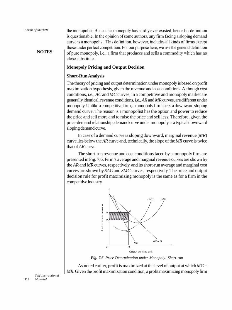
Forms of Markets
NOTES
Self-Instructional118 Material
Monopoly Pricing and Output Decision
Short-Run AnalysisThe theory of pricing and output determination under monopoly is based on profitmaximization hypothesis, given the revenue and cost conditions. Although costconditions, i.e., AC and MC curves, in a competitive and monopoly market aregenerally identical, revenue conditions, i.e., AR and MR curves, are different undermonopoly. Unlike a competitive firm, a monopoly firm faces a downward slopingdemand curve. The reason is a monopolist has the option and power to reducethe price and sell more and to raise the price and sell less. Therefore, given theprice-demand relationship, demand curve under monopoly is a typical downwardsloping demand curve.
In case of a demand curve is sloping downward, marginal revenue (MR)curve lies below the AR curve and, technically, the slope of the MR curve is twicethat of AR curve.
The short-run revenue and cost conditions faced by a monopoly firm arepresented in Fig. 7.6. Firm’s average and marginal revenue curves are shown bythe AR and MR curves, respectively, and its short-run average and marginal costcurves are shown by SAC and SMC curves, respectively. The price and outputdecision rule for profit maximizing monopoly is the same as for a firm in thecompetitive industry.
Fig. 7.6 Price Determination under Monopoly: Short-run
As noted earlier, profit is maximized at the level of output at which MC =MR. Given the profit maximization condition, a profit maximizing monopoly firm
Forms of Markets
NOTES
Self-InstructionalMaterial 119
chooses a price-output combination at which MR = SMC. Given the monopolyfirm’s cost and revenue curves in Fig. 7.6, its MR and SMC intersect at point N.An ordinate drawn from point N to X-axis, determines the profit maximizing outputat OQ. The ordinate NQ extended to the demand curve (AR = D) gives the profitmaximizing price PQ. It means that given the demand curve, the output OQ can besold per time unit at only one price, i.e., PQ (= OP1). Thus, the determination ofequilibrium output simultaneously determines the equilibrium price for the monopolyfirm. Once price is fixed, the unit and total profits are also simultaneously determined.Hence, the monopoly firm is in a state of equilibrium.
At output OQ and price PQ, the monopoly firm maximizes its unit and totalprofits. Its per unit monopoly or economic profit (i.e., AR – SAC) equals PQ –MQ = PM. Its total profit, = OQ × PM. Since OQ = P2M, = P2M × PM =area P1PMP2 as shown by the shaded rectangle. Since cost and revenue conditionsare not expected to change in the short-run, the equilibrium of the monopoly firmwill remain stable.
Determination of Monopoly Price and Output: Algebraic Solution
The determination of price and output by a monopoly firm in the short-run isillustrated above graphically (see Fig. 7.6). Here, we present an algebraic solutionto the problem of determination of equilibrium price and output under monopoly.
Suppose demand and total cost functions for a monopoly firm are given asfollows.Demand function : Q = 100 – 0.2 P …(7.1.1)Price function : P = 500 – 5Q ...(7.1.2)Cost function : TC = 50 + 20Q + Q2 ...(7.2)
Given the demand and cost functions, the problem before the monopolyfirm is to find the profit maximizing output and price. The problem can be solvedas follows.
We know that profit is maximum at output at which MR = MC. So the firststep is to find MR and MC from the demand function and cost function, respectively.We have noted earlier that MR and MC are the first derivation of TR and TCfunctions, respectively. TC function is given, but TR function is not. So, let us findTR function first. We know that
TR = P.Q
Since P = 500 – 5Q, by substitution, we getTR = (500 – 5Q) QTR = 500Q – 5Q2 ...(7.3)
Given the TR function (7.3), MR can be obtained by differentiating the TRfunction.
Forms of Markets
NOTES
Self-Instructional120 Material
MR = TRQ
= 500 – 10Q
Likewise, MC can be obtained by differentiating the TC function (7.2).
MC = TRQ
= 20 + 2Q
Now that MR and MC function are known, profit maximizing output can beeasily obtained. Recall that profit is maximum where MR = MC. As given above,
MR = 500 – 10Qand MC = 20 + 2Q
By equalizing the MR and MC functions, we get profit maximizing output(Q) as follows.
MR = MC500 – 10Q = 20 + 2Q
480 = 12QQ = 40
The output Q = 40 is the profit maximizing output.Now profit maximizing price can be obtained by substituting 40 for Q in the
price function (7.1.2). Thus, P = 500 – 5 (40) = 300. Profit maximizing price is`300.
Given the TR and TC functions, the total profit () can be obtained asfollows.
= TR – TCBy substitution, we get
= 500Q – 5Q2 – (50 + 20Q + Q2)
= 500Q – 5Q2 – 50 – 20Q – Q2
By substituting profit maximizing output (40) for Q, we get = 500(40) – 5(40)(40) – 50 – 20(40) – (40 ×
40) = 20,000 – 8,000 – 50 – 800 – 1600 = 9,550
Thus, total maximum profit comes to ̀ 9,550.
Does a Monopoly Firm Always Earn Abnormal Profit?
There is no certainty that a monopoly firm will always earn an economic or abnormalprofit. Whether a monopoly firm earns abnormal profit or normal profit or incursloss depends on:
(i) its cost and revenue conditions;
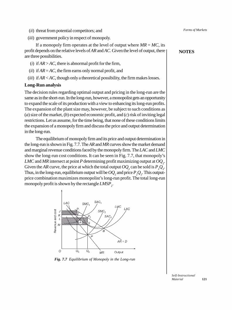
Forms of Markets
NOTES
Self-InstructionalMaterial 121
(ii) threat from potential competitors; and(iii) government policy in respect of monopoly.
If a monopoly firm operates at the level of output where MR = MC, itsprofit depends on the relative levels of AR and AC. Given the level of output, thereare three possibilities.
(i) if AR > AC, there is abnormal profit for the firm,(ii) if AR = AC, the firm earns only normal profit, and(iii) if AR < AC, though only a theoretical possibility, the firm makes losses.
Long-Run analysisThe decision rules regarding optimal output and pricing in the long-run are thesame as in the short-run. In the long-run, however, a monopolist gets an opportunityto expand the scale of its production with a view to enhancing its long-run profits.The expansion of the plant size may, however, be subject to such conditions as(a) size of the market, (b) expected economic profit, and (c) risk of inviting legalrestrictions. Let us assume, for the time being, that none of these conditions limitsthe expansion of a monopoly firm and discuss the price and output determinationin the long-run.
The equilibrium of monopoly firm and its price and output determination inthe long-run is shown in Fig. 7.7. The AR and MR curves show the market demandand marginal revenue conditions faced by the monopoly firm. The LAC and LMCshow the long-run cost conditions. It can be seen in Fig. 7.7, that monopoly’sLMC and MR intersect at point P determining profit maximizing output at OQ2.Given the AR curve, the price at which the total output OQ2 can be sold is P2Q2.Thus, in the long-run, equilibrium output will be OQ2 and price P2Q2. This output-price combination maximizes monopolist’s long-run profit. The total long-runmonopoly profit is shown by the rectangle LMSP2.
Fig. 7.7 Equilibrium of Monopoly in the Long-run
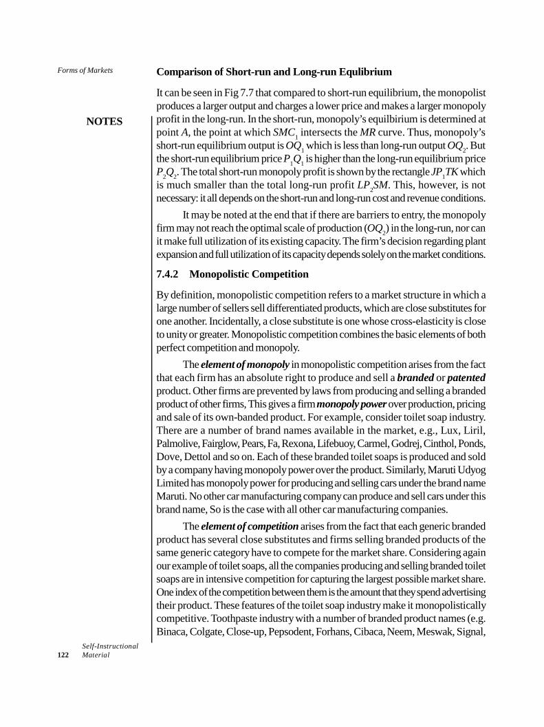
Forms of Markets
NOTES
Self-Instructional122 Material
Comparison of Short-run and Long-run Equlibrium
It can be seen in Fig 7.7 that compared to short-run equilibrium, the monopolistproduces a larger output and charges a lower price and makes a larger monopolyprofit in the long-run. In the short-run, monopoly’s equilbirium is determined atpoint A, the point at which SMC1 intersects the MR curve. Thus, monopoly’sshort-run equilibrium output is OQ1 which is less than long-run output OQ2. Butthe short-run equilibrium price P1Q1 is higher than the long-run equilibrium priceP2Q2. The total short-run monopoly profit is shown by the rectangle JP1TK whichis much smaller than the total long-run profit LP2SM. This, however, is notnecessary: it all depends on the short-run and long-run cost and revenue conditions.
It may be noted at the end that if there are barriers to entry, the monopolyfirm may not reach the optimal scale of production (OQ2) in the long-run, nor canit make full utilization of its existing capacity. The firm’s decision regarding plantexpansion and full utilization of its capacity depends solely on the market conditions.
7.4.2 Monopolistic Competition
By definition, monopolistic competition refers to a market structure in which alarge number of sellers sell differentiated products, which are close substitutes forone another. Incidentally, a close substitute is one whose cross-elasticity is closeto unity or greater. Monopolistic competition combines the basic elements of bothperfect competition and monopoly.
The element of monopoly in monopolistic competition arises from the factthat each firm has an absolute right to produce and sell a branded or patentedproduct. Other firms are prevented by laws from producing and selling a brandedproduct of other firms, This gives a firm monopoly power over production, pricingand sale of its own-banded product. For example, consider toilet soap industry.There are a number of brand names available in the market, e.g., Lux, Liril,Palmolive, Fairglow, Pears, Fa, Rexona, Lifebuoy, Carmel, Godrej, Cinthol, Ponds,Dove, Dettol and so on. Each of these branded toilet soaps is produced and soldby a company having monopoly power over the product. Similarly, Maruti UdyogLimited has monopoly power for producing and selling cars under the brand nameMaruti. No other car manufacturing company can produce and sell cars under thisbrand name, So is the case with all other car manufacturing companies.
The element of competition arises from the fact that each generic brandedproduct has several close substitutes and firms selling branded products of thesame generic category have to compete for the market share. Considering againour example of toilet soaps, all the companies producing and selling branded toiletsoaps are in intensive competition for capturing the largest possible market share.One index of the competition between them is the amount that they spend advertisingtheir product. These features of the toilet soap industry make it monopolisticallycompetitive. Toothpaste industry with a number of branded product names (e.g.Binaca, Colgate, Close-up, Pepsodent, Forhans, Cibaca, Neem, Meswak, Signal,
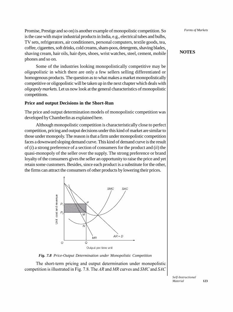
Forms of Markets
NOTES
Self-InstructionalMaterial 123
Promise, Prestige and so on) is another example of monopolistic competition. Sois the case with major industrial products in India, e.g., electrical tubes and bulbs,TV sets, refrigerators, air conditioners, personal computers, textile goods, tea,coffee, cigarettes, soft drinks, cold creams, sham-poos, detergents, shaving blades,shaving cream, hair oils, hair dyes, shoes, wrist watches, steel, cement, mobilephones and so on.
Some of the industries looking monopolistically competitive may beoligopolistic in which there are only a few sellers selling differentiated orhomogenous products. The question as to what makes a market monopolisticallycompetitive or oligopolistic will be taken up in the next chapter which deals witholigopoly markets. Let us now look at the general characteristics of monopolisticcompetitions.
Price and output Decisions in the Short-Run
The price and output determination models of monopolistic competition wasdeveloped by Chamberlin as explained here.
Although monopolistic competition is characteristically close to perfectcompetition, pricing and output decisions under this kind of market are similar tothose under monopoly. The reason is that a firm under monopolistic competitionfaces a downward sloping demand curve. This kind of demand curve is the resultof (i) a strong preference of a section of consumers for the product and (ii) thequasi-monopoly of the seller over the supply. The strong preference or brandloyalty of the consumers gives the seller an opportunity to raise the price and yetretain some customers. Besides, since each product is a substitute for the other,the firms can attract the consumers of other products by lowering their prices.
Fig. 7.8 Price-Output Determination under Monopolistic Competition
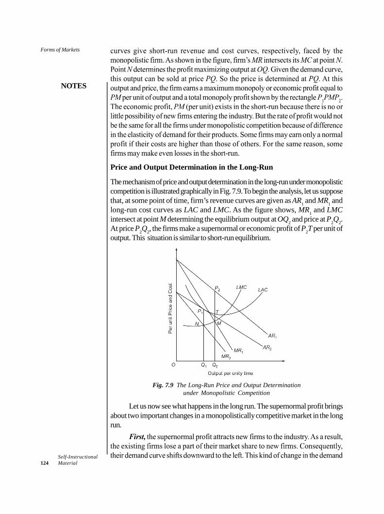
Forms of Markets
NOTES
Self-Instructional124 Material
Price and Output Determination in the Long-Run
The mechanism of price and output determination in the long-run under monopolisticcompetition is illustrated graphically in Fig. 7.9. To begin the analysis, let us supposethat, at some point of time, firm’s revenue curves are given as AR1 and MR1 andlong-run cost curves as LAC and LMC. As the figure shows, MR1 and LMCintersect at point M determining the equilibrium output at OQ2 and price at P2Q2.At price P2Q2, the firms make a supernormal or economic profit of P2T per unit ofoutput. This situation is similar to short-run equilibrium.
Fig. 7.9 The Long-Run Price and Output Determinationunder Monopolistic Competition
Let us now see what happens in the long run. The supernormal profit bringsabout two important changes in a monopolistically competitive market in the longrun.
Forms of Markets
NOTES
Self-InstructionalMaterial 125
Second, the increasing number of firms intensifies the price competitionbetween them. Price competition increases because losing firms try to regain orretain their market share by cutting down the price of their product. And, newfirms in order to penetrate the market set comparatively low prices for their product.The price competition increases the slope of the firms’ demand curve or, in otherwords, it makes the demand curve more elastic. Note that AR2 has a greater slopethan AR1 and MR2 has a greater slope than MR1.
The ultimate picture of price and output determination under monopolisticcompetition is shown at point P1 in Fig. 7.9. As the figure shows, LMC intersectsMR2 at point N where firm’s long-run equilibrium output is determined at OQ1 andprice at P1Q1. Note that price at P1Q1 equals the LAC at the point of tangency. Itmeans that under monopolistic competition, firms make only normal profit in thelong-run. Once all the firms reach this stage, there is no attraction (i.e., supernormal profit) for the new firms to enter the industry, nor is there any reason for theexisting firms to quit the industry. This signifies the long-run equilibrium of theindustry.
7.4.3 Oligopoly
Oligopoly is defined as a market structure in which there are a few sellers sellinghomogeneous or differentiated products. In case oligopoly firms sell ahomogeneous product, it is called pure or homogeneous oligopoly. For example,industries producing bread, cement, steel, petrol, cooking gas, chemicals, aluminiumand sugar are industries characterized by homogeneous oligopoly. And, wherefirms of an oligopoly industry sell differentiated products, it is called differentiatedor heterogeneous oligopoly. Automobiles, television sets, soaps and detergents,refrigerators, soft drinks, computers, cigarettes, etc. are some examples of industriescharacterized by differentiated or heterogeneous oligopoly.
Be it pure or differentiated, “Oligopoly is the most prevalent form of marketorganization in the manufacturing sector of the industrial nations…”. In non-industrialnations like India also, a majority of big and small industries have acquired thefeatures of oligopoly market. The market share of 4 to 10 firms in 84 big and smallindustries of India is given in Table 7.3.
Table 7.3 Distribution of Industries by Market Share
Market share (%) No. of industries
1 – 24.9 8
25 – 49.9 11
50 – 74.9 15
75 – 100 50Total 84
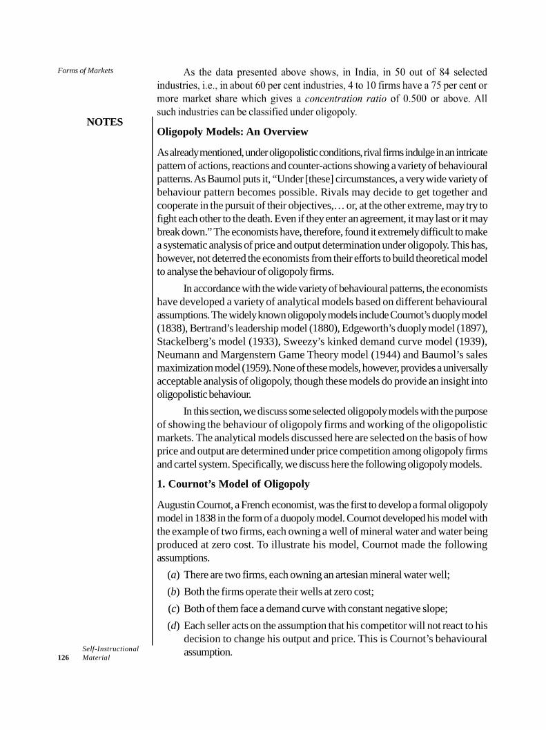
Forms of Markets
NOTES
Self-Instructional126 Material
Oligopoly Models: An Overview
As already mentioned, under oligopolistic conditions, rival firms indulge in an intricatepattern of actions, reactions and counter-actions showing a variety of behaviouralpatterns. As Baumol puts it, “Under [these] circumstances, a very wide variety ofbehaviour pattern becomes possible. Rivals may decide to get together andcooperate in the pursuit of their objectives,… or, at the other extreme, may try tofight each other to the death. Even if they enter an agreement, it may last or it maybreak down.” The economists have, therefore, found it extremely difficult to makea systematic analysis of price and output determination under oligopoly. This has,however, not deterred the economists from their efforts to build theoretical modelto analyse the behaviour of oligopoly firms.
In accordance with the wide variety of behavioural patterns, the economistshave developed a variety of analytical models based on different behaviouralassumptions. The widely known oligopoly models include Cournot’s duoply model(1838), Bertrand’s leadership model (1880), Edgeworth’s duoply model (1897),Stackelberg’s model (1933), Sweezy’s kinked demand curve model (1939),Neumann and Margenstern Game Theory model (1944) and Baumol’s salesmaximization model (1959). None of these models, however, provides a universallyacceptable analysis of oligopoly, though these models do provide an insight intooligopolistic behaviour.
In this section, we discuss some selected oligopoly models with the purposeof showing the behaviour of oligopoly firms and working of the oligopolisticmarkets. The analytical models discussed here are selected on the basis of howprice and output are determined under price competition among oligopoly firmsand cartel system. Specifically, we discuss here the following oligopoly models.
1. Cournot’s Model of Oligopoly
Augustin Cournot, a French economist, was the first to develop a formal oligopolymodel in 1838 in the form of a duopoly model. Cournot developed his model withthe example of two firms, each owning a well of mineral water and water beingproduced at zero cost. To illustrate his model, Cournot made the followingassumptions.
(a) There are two firms, each owning an artesian mineral water well;(b) Both the firms operate their wells at zero cost;(c) Both of them face a demand curve with constant negative slope;(d) Each seller acts on the assumption that his competitor will not react to his
decision to change his output and price. This is Cournot’s behaviouralassumption.
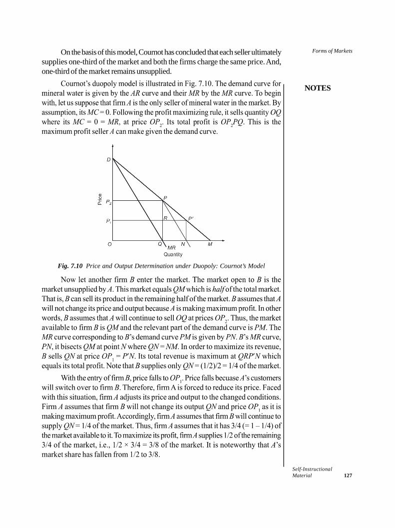
Forms of Markets
NOTES
Self-InstructionalMaterial 127
On the basis of this model, Cournot has concluded that each seller ultimatelysupplies one-third of the market and both the firms charge the same price. And,one-third of the market remains unsupplied.
Fig. 7.10 Price and Output Determination under Duopoly: Cournot’s Model
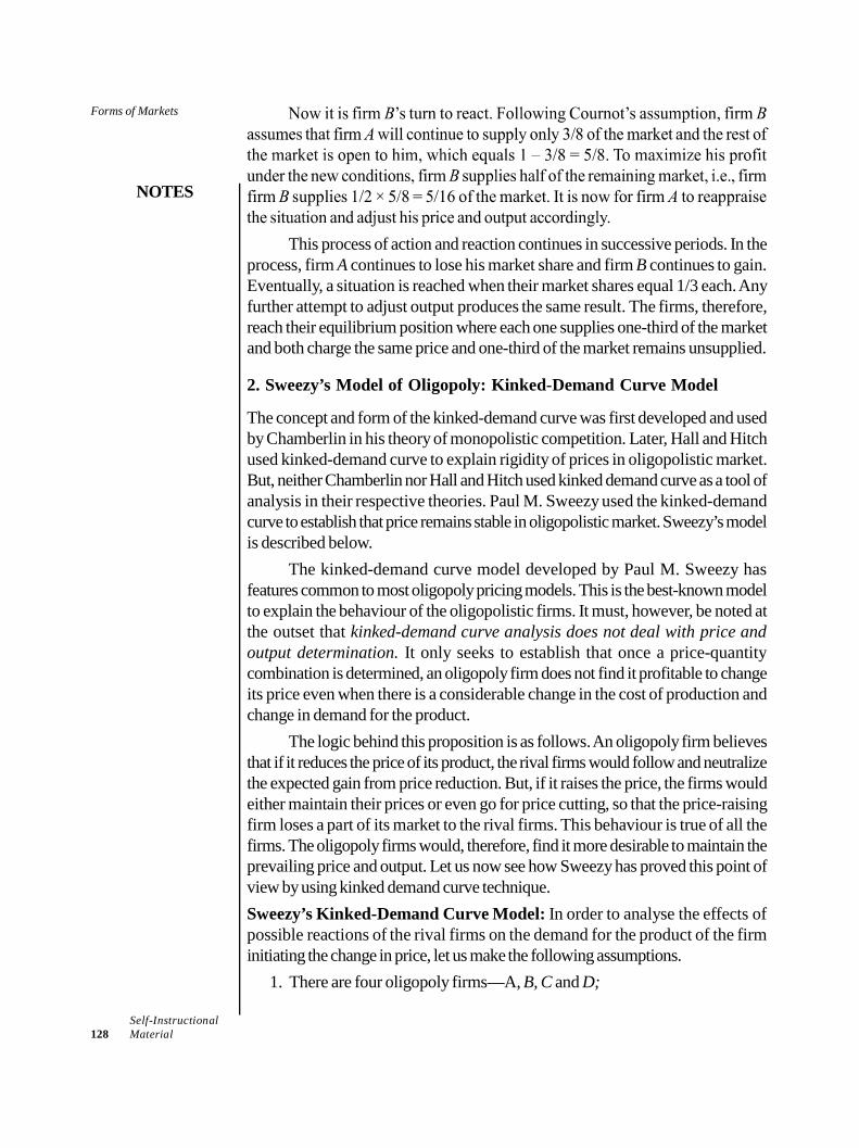
Forms of Markets
NOTES
Self-Instructional128 Material
This process of action and reaction continues in successive periods. In theprocess, firm A continues to lose his market share and firm B continues to gain.Eventually, a situation is reached when their market shares equal 1/3 each. Anyfurther attempt to adjust output produces the same result. The firms, therefore,reach their equilibrium position where each one supplies one-third of the marketand both charge the same price and one-third of the market remains unsupplied.
2. Sweezy’s Model of Oligopoly: Kinked-Demand Curve Model
The concept and form of the kinked-demand curve was first developed and usedby Chamberlin in his theory of monopolistic competition. Later, Hall and Hitchused kinked-demand curve to explain rigidity of prices in oligopolistic market.But, neither Chamberlin nor Hall and Hitch used kinked demand curve as a tool ofanalysis in their respective theories. Paul M. Sweezy used the kinked-demandcurve to establish that price remains stable in oligopolistic market. Sweezy’s modelis described below.
The kinked-demand curve model developed by Paul M. Sweezy hasfeatures common to most oligopoly pricing models. This is the best-known modelto explain the behaviour of the oligopolistic firms. It must, however, be noted atthe outset that kinked-demand curve analysis does not deal with price andoutput determination. It only seeks to establish that once a price-quantitycombination is determined, an oligopoly firm does not find it profitable to changeits price even when there is a considerable change in the cost of production andchange in demand for the product.
The logic behind this proposition is as follows. An oligopoly firm believesthat if it reduces the price of its product, the rival firms would follow and neutralizethe expected gain from price reduction. But, if it raises the price, the firms wouldeither maintain their prices or even go for price cutting, so that the price-raisingfirm loses a part of its market to the rival firms. This behaviour is true of all thefirms. The oligopoly firms would, therefore, find it more desirable to maintain theprevailing price and output. Let us now see how Sweezy has proved this point ofview by using kinked demand curve technique.Sweezy’s Kinked-Demand Curve Model: In order to analyse the effects ofpossible reactions of the rival firms on the demand for the product of the firminitiating the change in price, let us make the following assumptions.
1. There are four oligopoly firms—A, B, C and D;
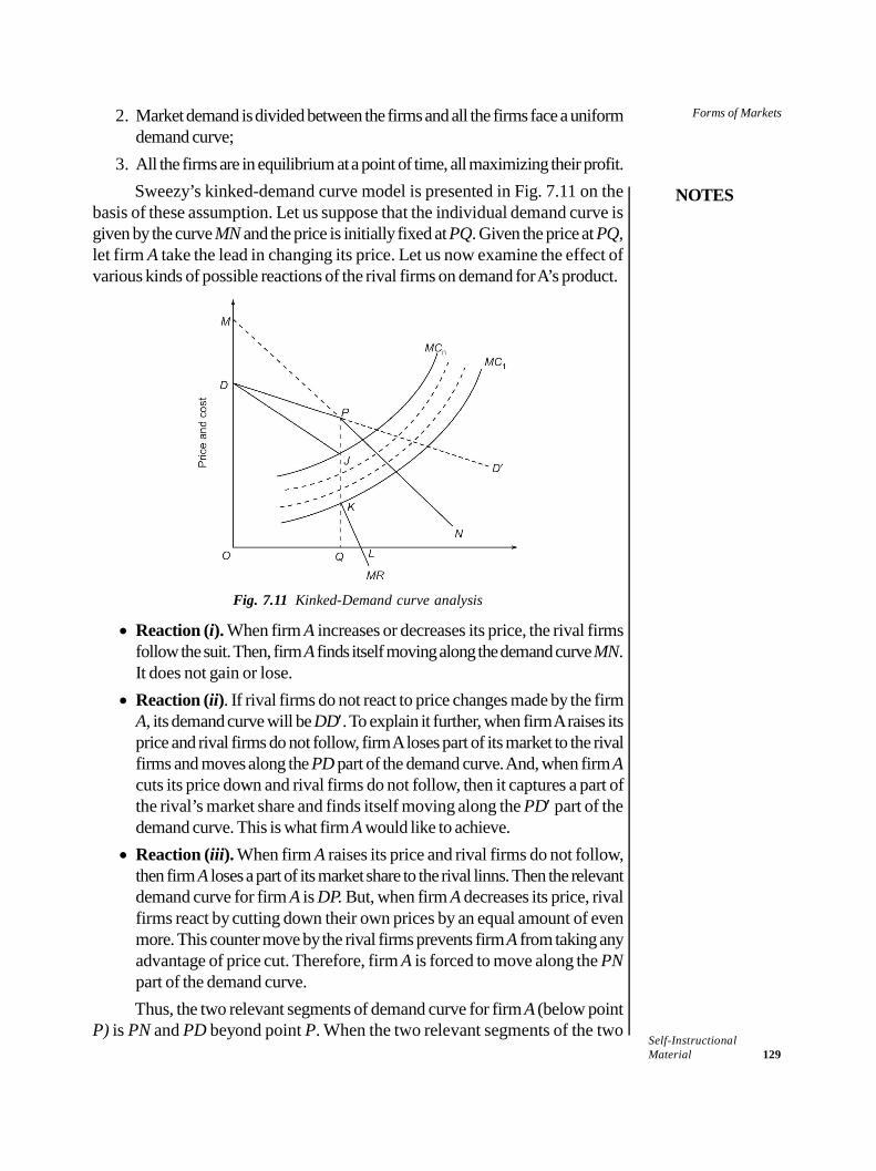
Forms of Markets
NOTES
Self-InstructionalMaterial 129
2. Market demand is divided between the firms and all the firms face a uniformdemand curve;
3. All the firms are in equilibrium at a point of time, all maximizing their profit.Sweezy’s kinked-demand curve model is presented in Fig. 7.11 on the
basis of these assumption. Let us suppose that the individual demand curve isgiven by the curve MN and the price is initially fixed at PQ. Given the price at PQ,let firm A take the lead in changing its price. Let us now examine the effect ofvarious kinds of possible reactions of the rival firms on demand for A’s product.
Fig. 7.11 Kinked-Demand curve analysis
Reaction (i). When firm A increases or decreases its price, the rival firmsfollow the suit. Then, firm A finds itself moving along the demand curve MN.It does not gain or lose.
Reaction (ii). If rival firms do not react to price changes made by the firmA, its demand curve will be DD. To explain it further, when firm A raises itsprice and rival firms do not follow, firm A loses part of its market to the rivalfirms and moves along the PD part of the demand curve. And, when firm Acuts its price down and rival firms do not follow, then it captures a part ofthe rival’s market share and finds itself moving along the PD part of thedemand curve. This is what firm A would like to achieve.
Reaction (iii). When firm A raises its price and rival firms do not follow,then firm A loses a part of its market share to the rival linns. Then the relevantdemand curve for firm A is DP. But, when firm A decreases its price, rivalfirms react by cutting down their own prices by an equal amount of evenmore. This counter move by the rival firms prevents firm A from taking anyadvantage of price cut. Therefore, firm A is forced to move along the PNpart of the demand curve.Thus, the two relevant segments of demand curve for firm A (below point
P) is PN and PD beyond point P. When the two relevant segments of the two
Forms of Markets
NOTES
Self-Instructional130 Material
demand curves (MN and DD) are put together, the demand curve for A’s producttakes the form of the curve DPN. The demand curve DPN has a kink at point P.It is, therefore, called a kinked-demand curve.
Now let us see why price gets stabilized at PQ even when there is change incost curves. Suppose MC curve of the firms is given as MC1 which intersects MRat point K, Point K satisfies the necessary condition for profit maximization (MR =MC). Therefore, oligopoly firms are in equilibrium at output OQ and they aremaking maximum profit at price PQ. Now, if MC curve shifts upwards to MCn ortoany level between points J and K, their profit would not be affected becauseprofit maximization condition remains undistributed. Therefore, they have nomotivation for increasing or decreasing their price. It is always beneficial for themto stick to the price PQ and output OQ. Thus, both price and output are stable.This is how price gets stabilized under oligopoly. The oligopoly firms would go forchanging their price and output only if MC rises beyond point J or falls belowpoint K (in Fig. 7.11)
To conclude, the basic point that Sweezy’s model establishes is the rigidityof price in oligopolistic market. As shown in Fig. 7.11, once price is determined inoligopoly, it remains rigidly fixed because profit maximizing firms’ have no incentiveto change price even if MC curve shifts upwards or downwards within the rangebetween points J and K. Therefore, price remains constant over a period of time.
3. Collusive Models of Oligopoly
The oligopoly models discussed in the previous sections are based on theassumption that the oligopoly firms act independently; they are in competitionwith one another; and there is no collusion or any kind of agreement between thefirms. The oligopoly models of this category are called non-collusive models. Inreality, however, oligopoly firms are found to be in some kind of collusion oragreement—open or secret, explicit or tacit, written or unwritten, and legal orillegal—with one another for at least three major reasons.
First, collusion eliminates or reduces the degree of competition betweenthe firms and gives them some monopolistic powers in their price and outputdecisions.
Secondly, collusion reduces the degree of uncertainty surrounding theoligopoly firms and ensure profit maximization.
Thirdly, collusion creates some kind of barriers to the entry of new firms.
Forms of Markets
NOTES
Self-InstructionalMaterial 131
The models that deal with the collusive oligopolies are called collusiveoligopoly models. Collusion between firms may take many forms depending ontheir relative strength and objective of collusion, and on whether collusion is legalor illegal. There are, however, two major forms of collusion between the oligopolyfirms: (i) cartel, i.e., firms’ association and (ii) price leadership agreements.
On the basis of these forms of collusion between oligopoly firms, collusiveoligopoly models are classified as:
1. Cartel models, and2. Price leadership models.
In this section, we will discuss these two types of oligopoly collusive models.
4. Price and Output Determination under Cartel Models
Cartel Models of Collusion. A cartel is a formal collusion of the oligopoly firmsin an industry with a purpose. A general purpose of cartels is to centralize certainareas of managerial decisions and functions of individual firms of the industry, witha view to promoting common benefits. Under cartel system, “the firms jointlyestablish a cartel organization to make price and output decisions, to establishproduction quotas for each firm and to supervise market activation of the firms inthe industry”. Cartels are formed with the purpose of (i) eliminating uncertainty inbusiness, and (ii) restraining harmful interfirm competition.
Although a cartel performs a variety of functions for its members, the twoimportant functions of cartels are following.
1. Fixing price for joint profit maximization, and2. Market sharing between its members.
5. Price Leadership Models
Price leadership is an informal position of a firm in most oligopolisticindustries. Price leadership may emerge spontaneously due to technical reasonsor out of a tacit or explicit agreement between the firms to assign a leadership roleto one of them. The spontaneous price leadership may be the result of such technicalreasons as size, efficiency, economies of scale or firm’s ability to forecast marketconditions accurately or a combination of these factors. The most typical case ofprice leadership is the leading role played by the dominant firm, i.e., the largest
Forms of Markets
NOTES
Self-Instructional132 Material
firm in the industry. The dominant firm takes lead in determining the price and inmaking price changes and the smaller ones follow.
Sometimes, price leadership is barometric by a firm whose decisions andactions serve as a barometer for the decisions and actions taken by other firms.Inthe barometric price leadership one of the firms, not necessarily the dominantone, takes the lead generally in announcing a change in price, particularly whensuch a change is due but is not effected due to uncertainty in the market.
The price leadership is found under both product homogeneity and productdifferentiation. There may be, however, price differences commensurate withproduct differentiation. Price differentials may also exist on account of costdifferentials.
Another important aspect of price leadership is that it often serves as ameans to price discipline and price stabilization. Achievement of this objectiveestablishes an ‘effective price leadership’. Such a leadership can, however, existand work effectively only under the following conditions.
(i) There is a small number of firms in oligopoly;(ii) Entry to the industry is restricted;(iii) Products are, by and large, homogeneous;(iv) Demand for industry is inelastic or has very low elasticity, and(v) Firms have almost similar cost curves.
Price Leadership Models: Given the conditions for effective working of priceleadership, the economists have envisaged the following kinds of price leadershipmodels.
1. Price leadership by low cost firm,2. Price leadership by dominant firm, and3. Price leadership by barometeric firm.
Check Your Progress
3. Where does the element of monopoly in monopolistic competition arisesfrom?
4. Define oligopoly.5. What is barometric price leadership?
7.5 ANSWERS TO CHECK YOUR PROGRESSQUESTIONS
1. Market-clearing price is also known as the equilibrium price. It implies thatthe market is cleared in the sense that there is no unsold stock and nounsupplied demand.
Forms of Markets
NOTES
Self-InstructionalMaterial 133
2. The factors which determine the categorization of market structure are thefollowing: Number of firms—the sellers Degree and nature of competition Level of product differentiation Possibility of entry and exit of the firms
3. The element of monopoly in monopolistic competition arises from the factthe each firm has an absolute right to produce and sell a branded or patentedproduct.
4. Oligopoly is defined as a market structure in which there are a few sellersselling homogeneous or differentiated products.
5. In the barometric price leadership one of the firms, not necessarily thedominant one, takes the lead generally in announcing a change in price,particularly when such a change is die but is not affected due to uncertaintyin the market.
7.6 SUMMARY
In economics, the word ‘market’ is used in a rather abstract sense. Themarket means a system by which sellers and buyers of a commodity interactto settle its price and the quantity to be bought and sold.
Market system refers to the process by which buyers and sellers of a productinteract to settle the price of the product and carry out the sale-purchasetransactions. The market system works on the basis of a basic marketprinciple.
In the context of market analysis, equilibrium refers to a state of market inwhich quantity demanded of a commodity equals the quantity supplied ofthe commodity. The equality of demand and supply produces an equilibriumprice.
Equilibrium price of a commodity in a free market is determined by themarket forces of demand and supply. In order to analyze how equilibriumprice is determined, we need to integrate the demand and supply curves.
Market mechanism is a process of interaction between the market forces ofdemand and supply to determine the equilibrium price.
Market structure refers to the number of firms in an industry and the degreeof competition among the firms.
The market structure determines a firm’s power to fix the price of its producta great deal. The degree of competition determines a firm’s degree offreedom in determining the price of its product.
Forms of Markets
NOTES
Self-Instructional134 Material
The term pure monopoly means an absolute power of a firm to produceand sell a product that has no close substitute. In other words, a monopolizedmarket is one in which there is only one seller of a product having no closesubstitute.
The decision rules regarding optimal output and pricing in the long-run arethe same as in the short-run. In the long-run, however, a monopolist gets anopportunity to expand the scale of its production with a view to enhancingits long-run profits.
By definition, monopolistic competition refers to a market structure in whicha large number of sellers sell differentiated products, which are closesubstitutes for one another.
Oligopoly is defined as a market structure in which there are a few sellersselling homogeneous or differentiated products. In case oligopoly firms sella homogeneous product, it is called pure or homogeneous oligopoly.
7.7 KEY WORDS
Market mechanism: It is a process of interaction between the marketforces of demand and supply to determine the equilibrium price.
Market structure: It refers to the number of firms in an industry and thedegree of competition among the firms.
Monopoly: It means an absolute power of a firm to produce and sell aproduct that has no close substitute.
7.8 SELF ASSESSMENT QUESTIONS ANDEXERCISES
Short Answer Questions
1. Mention the various aspects of the market concept.2. How is the market price determined?3. State the practical importance of market equilibrium.4. Write a short note on the types of market structures.
Long-Answer Questions
1. Discuss shift in demand and supply curves.2. Explain pricing and output decisions under monopoly with the help of
diagrams.3. Evaluate the pricing and output decisions under monopolistic competition.4. Describe the various oligopoly models.
Forms of Markets
NOTES
Self-InstructionalMaterial 135
7.9 FURTHER READINGS
Dwivedi, D. N. 2015. Principles of Economics, Eight Edition. New Delhi: VikasPublishing House.
Weil. David N. 2004. Economic Growth. London: Addison Wesley.Thomas, Christopher R. and Maurice S. Charles. 2005. Managerial Economics:
Concepts and Applications, Eighth Edition. New Delhi: Tata McGraw-Hill Publishing Company Limited.
Mankiw, Gregory N. 2002. Principles of Economics, Second Edition. India:Thomson Press.
Websites
https://blogs.economictimes.indiatimes.com/et-commentary/heres-how-indias-widening-income-distribution-can-be-redressed/
https://www.livemint.com/Opinion/WmpSjQAvPGeVzxqpgXYvtK/The-dangers-of-Indias-Billionaire-Raj.html
Strategic Behaviour of theFirms and Game Theory
NOTES
Self-Instructional136 Material
UNIT 8 STRATEGIC BEHAVIOUROF THE FIRMS AND GAMETHEORY
Structure8.0 Introduction8.1 Unit Objectives8.2 Strategic Behaviour of the Firms: Price and Non-Price Competition8.3 Game Theory: Types of Strategy and Relation to the Firm’s Behaviour
8.3.1 Prisoner’s Dilemma8.3.2 Application of Game Theory to Oligopolistic Startegy8.3.3 Nash Equilibirum and Implications
8.4 Answers to Check Your Progress Questions8.5 Summary8.6 Key Words8.7 Self Assessment Questions and Exercises8.8 Further Readings
8.0 INTRODUCTION
Several mathematicians and economists have made numerous attempts to findreasonable explanation to strategic behaviour of firms. The first most importantcontribution to this field was made by a mathematician John von Neumann and aneconomist Oskar Morgenstern in 1944. Their contribution was in the form ofgame theory. The game theory brings out the strategy used by the oligopoly firmsto determine the best possible action to maximize their predetermined objective.Although many other economists have contributed to game theory, Martin Shubikis regarded as the ‘most prominent proponent of the game theory approach’. Amore recent and in-depth work on the game theory and its application of economicsand management problems can be found in the work of Prajit K. Dutta.
In this unit, you will study about the strategic behaviour of the firms, theapplication of the game theory to oligopolistic strategy, prisoner’s dilemma, Nashequilibrium and its implications.
8.1 UNIT OBJECTIVES
After going through this unit, you will be able to: Analyse the strategic behaviour of the firms Discuss the game theory Explain the prisoner’s dilemma
Strategic Behaviour of theFirms and Game Theory
NOTES
Self-InstructionalMaterial 137
Evaluate the application of game theory to oligopolistic strategy State the use of the Nash equilibrium technique
8.2 STRATEGIC BEHAVIOUR OF THE FIRMS:PRICE AND NON-PRICE COMPETITION
We have already discussed the non-price competition strategies in relation tomonopolistic competition and oligopoly in Unit 7. Let us revisit some of the basicconcepts before moving on to learning about game theory and its application.Price competition is the competition that lays focus on the issue of price as moreand attempts to stay ahead of the the price of the competitors existing in themarket.
Non-price competition is the competition that lays emphases on the factorsother than the price of the product. The main objective is to differentiate from theproducts that are available as alternatives in the market. Non- price competitioncan be compared and contrasted with price competition, that is, where a businessenterprise tries to make a distinction of its product or service from competingproducts on the basis of a low price.
Business enterprises engage in non-price competition, despite the additionalcosts involved because it is generally more profitable than selling for a lower priceand evades the hazard of a price war. Although a non-price competition strategycan be utilized by any business enterprise, yet it is most commonly used underoligopolies and monopolistic competition because these firms can be extremelycompetitive.
The business enterprise can also distinguish its product offering on the basisof quality of service, extensive distribution, customer focus, or any other sustainablecompetitive advantage other than price. The objective is to try to persuadeconsumers that they should purchase these products, not only because they arecheaper but also as they are better than those made by competitors in one way orthe other. Non-price competition characteristically involves promotionalexpenditures (such as advertising, selling staff, the locations convenience, salespromotions, coupons, special orders, or free gifts), marketing research, newproduct development, and brand management costs. Business enterprises willcertainly engage in non-price competition because it is generally more profitablethan selling for a lower price and evades the hazard of a price war. For instance,branded goods often sell more items than do their local counterparts, due topromotion and publicity despite being more expensive. Non-price competitionmay also promote innovation as business enterprise try to distinguish their product.
A non-price competition strategy can be used by any business enterprise.However, it is most common among oligopolies and monopolistic competitionbecause these firms can be extremely competitive.
Strategic Behaviour of theFirms and Game Theory
NOTES
Self-Instructional138 Material
8.3 GAME THEORY: TYPES OF STRATEGY ANDRELATION TO THE FIRM’S BEHAVIOUR
Before we proceed to discuss the game theory, it is helpful to understand themeaning and purpose of the game theory and some basic terms and tools used inthe analysis and application of game theory.1. The Game Theory: In all kinds of games there are two teams. In all games,the objective of the players of each team is to win the game. To win the game,players make their play-strategy and take action in anticipation of possible reactionsof the opposite team and plan their own counter action. This concept of strategicplay has been applied by von Neumann and Morgenstern to strategic play ofoligopoly firms. As a player, each firm formulates its strategic play and estimatesits effects on its objective, called pay-off. The pay-off may be positive, negativeor zero-sum for a firm taking strategic action. Accordingly, if a strategic actiontaken by a firm may yield some gains to the firm and counteraction by the rival firmneutralises the gain, it is a zero-sum game. If both the firms—action-taking firmand rival firms—gain from the strategic action taken by a firm, it is a positive-sumgame. And, if both the firms, action-taking firm and rival firms, make losses fromthe strategic action taken by a firm, it is a negative-sum game.2. Interdependence: The game theory has been formulated on the basis of arealistic assumption of interdependence of oligopoly firms. It implies that decision-making of the firms under oligopoly is interdependent. That is, while taking abusiness decision – be it price determination, advertising, introduction of a newproduct or brand, setting-up a new production unit, or any other issue – oligopolyfirms take into account the possible action and reaction of the rival firms. This kindof behaviour of the oligopoly firms shows their interdependence.3. Strategy: The term ‘strategy’ means the course of action to be taken by theoligopoly firms with the purpose of gaining most from an action under the conditionof unknown reaction of the rival firms. For example, suppose there are two firms– A and B. Firm A plans to cut down the price of its product. But Firm A is not sureof the possible reaction of the rival Firm B. There are two possible reactions of therival Firm B: (i) it may cut down its own price, and (ii) it may not cut down theprice. The price cutting firm A will assess its gain and losses under these conditionsand chose the best option. This is the strategy of the price cutting firm.4. Pay-off Matrix: The ‘pay-off matrix’ is tabular recording of gains and lossesof a firm taking an action under different kinds of anticipated reactions of the rivalfirms. Recall the above example of two firms, A and B. Firm A estimates its gainsand losses in terms of increase in the sales of its product under the followingconditions:
(i) Estimated increase in its sales when Firm A does not reduce its price;
Strategic Behaviour of theFirms and Game Theory
NOTES
Self-InstructionalMaterial 139
(ii) Estimated increase in its sales when Firm A reduces its price and Firm Bdoes not react;
(iii) Estimated increase in its sales when Firm A reduces its price and Firms Balso cuts down the price of its product; and
(iv) Estimated change in its sales when Firm A does not cut down its price butFirm B does cut down its price. When all these estimates are recorded in a cross-sectional tabular form, it
produces a pay-off matrix.5. Dominant Strategy: As noted above, strategy means the course of actionplanned by an oligopoly firm with the purpose of gaining most from its action. Thepay-off of the strategy may be high or it may be low depending on the counteractiontaken by the rival firm. A strategic action that yields the best outcome whatever thereaction of the rival firms is called dominant strategy. In the context of gametheory, dominant strategy can be defined as the strategy that gives the bestpayoff no matter what counteraction is taken by the rival firm.
Having looked at the ‘basics’ of the game theory, we proceed now to discussthe game theory and its application to business decision-making. In game theory,the decision-making problem of the oligopoly firms is best exemplified by, whatgame theorists call, the prisoners’ dilemma. We begin our discussion with theconcept of prisoners’ dilemma – an example of dilemma faced by the oligopolyfirms in decision-making.
8.3.1 Prisoner’s Dilemma
The nature of the decision-making problems faced by the oligopoly firms isexemplified in game theory by prisoner’s dilemma. To illustrate prisoners’dilemma, let us suppose that two persons, A and B, are partners in illegal activities.They are arrested under the suspicion of being involved in cricket match-fixing.They are lodged in separate jails with no possibility of communication betweenthemselves. They are interrogated by CBI officials under the following conditionsdisclosed to each of them in isolation.
1. If you confess your involvement in match fixing, you will get a 5-yearimprisonment.
2. If you deny your involvement and your partner denies too, you will be setfree for lack of evidence.
3. If you confess and your partner does not confess and you turn approver,then you get 2-year imprisonment and the other person will get 10-yearimprisonment.
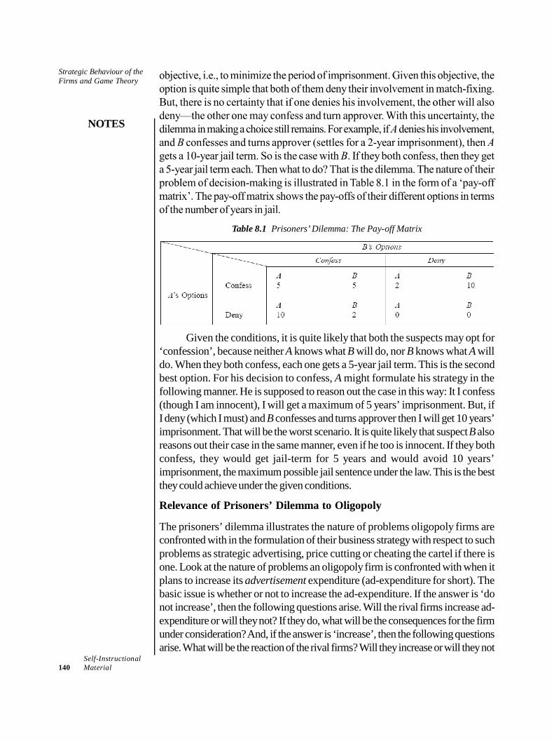
Strategic Behaviour of theFirms and Game Theory
NOTES
Self-Instructional140 Material
Table 8.1 Prisoners’ Dilemma: The Pay-off Matrix
Given the conditions, it is quite likely that both the suspects may opt for‘confession’, because neither A knows what B will do, nor B knows what A willdo. When they both confess, each one gets a 5-year jail term. This is the secondbest option. For his decision to confess, A might formulate his strategy in thefollowing manner. He is supposed to reason out the case in this way: It I confess(though I am innocent), I will get a maximum of 5 years’ imprisonment. But, ifI deny (which I must) and B confesses and turns approver then I will get 10 years’imprisonment. That will be the worst scenario. It is quite likely that suspect B alsoreasons out their case in the same manner, even if he too is innocent. If they bothconfess, they would get jail-term for 5 years and would avoid 10 years’imprisonment, the maximum possible jail sentence under the law. This is the bestthey could achieve under the given conditions.
Relevance of Prisoners’ Dilemma to Oligopoly
The prisoners’ dilemma illustrates the nature of problems oligopoly firms areconfronted with in the formulation of their business strategy with respect to suchproblems as strategic advertising, price cutting or cheating the cartel if there isone. Look at the nature of problems an oligopoly firm is confronted with when itplans to increase its advertisement expenditure (ad-expenditure for short). Thebasic issue is whether or not to increase the ad-expenditure. If the answer is ‘donot increase’, then the following questions arise. Will the rival firms increase ad-expenditure or will they not? If they do, what will be the consequences for the firmunder consideration? And, if the answer is ‘increase’, then the following questionsarise. What will be the reaction of the rival firms? Will they increase or will they not
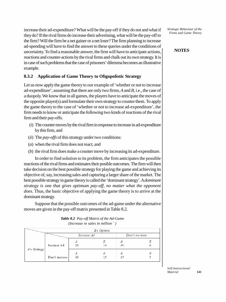
Strategic Behaviour of theFirms and Game Theory
NOTES
Self-InstructionalMaterial 141
increase their ad-expenditure? What will be the pay-off if they do not and what ifthey do? If the rival firms do increase their advertising, what will be the pay-off tothe firm? Will the firm be a net gainer or a net loser? The firm planning to increasead-spending will have to find the answer to these queries under the conditions ofuncertainty. To find a reasonable answer, the firm will have to anticipate actions,reactions and counter-actions by the rival firms and chalk out its own strategy. It isin case of such problems that the case of prisoners’ dilemma becomes an illustrativeexample.
8.3.2 Application of Game Theory to Oligopolistic Strategy
Let us now apply the game theory to our example of ‘whether or not to increasead-expenditure’, assuming that there are only two firms, A and B, i.e., the case ofa duopoly. We know that in all games, the players have to anticipate the moves ofthe opposite player(s) and formulate their own strategy to counter them. To applythe game theory to the case of ‘whether or not to increase ad-expenditure’, thefirm needs to know or anticipate the following two kinds of reactions of the rivalfirm and their pay-offs.
(i) The counter moves by the rival firm in response to increase in ad-expenditureby this firm, and
(ii) The pay-offs of this strategy under two conditions:(a) when the rival firm does not react, and(b) the rival firm does make a counter move by increasing its ad-expenditure.
In order to find solution to its problem, the firm anticipates the possiblereactions of the rival firms and estimates their posible outcomes. The firm will thentake decision on the best possible strategy for playing the game and achieving itsobjective of, say, increasing sales and capturing a larger share of the market. Thebest possible strategy in game theory is called the ‘dominant strategy’. A dominantstrategy is one that gives optimum pay-off, no matter what the opponentdoes. Thus, the basic objective of applying the game theory is to arrive at thedominant strategy.
Suppose that the possible outcomes of the ad-game under the alternativemoves are given in the pay-off matrix presented in Table 8.2.
Table 8.2 Pay-off Matrix of the Ad-Game(Increase in sales in million `)
Strategic Behaviour of theFirms and Game Theory
NOTES
Self-Instructional142 Material
As the matrix shows, if Firm A decides to increase its ad-expenditure, andFirm B counters A’s move by increasing its own ad-expenditure, A’s sales go upby ̀ 20 million and those of Firm B by ̀ 10 million. And, if Firm A increases itsadvertisement and B does not, then A’s sales increase by ̀ 30 million and there areno sales gain for Firm B. One can similarly find the pay-offs of the stategy ‘Don’tincrease’ in case of both firms. As shown in Table 8.2, if Firm A does not increaseits Ad-spending and Firm B does increase its Ad-spending, then A’s sales increasesby ̀ 10 million and of B by ̀ 15 million.
Given the pay-off matrix, the question arises: What strategy should Firm Achoose to optimize its gain from extra ad-expenditure, irrespective of counter-action by the rival Firm B. It is clear from the pay-off matrix that Firm A willchoose the strategy of increasing the ad-expenditure because, no matter whatFirm B does, its sales increase by at least `20 million. This is, therefore, thedominant strategy for Firm A. A better situation could be that when Firm Aincreases its expenditure on advertisement, Firm B does not. In that case, sales ofFirm A could increase by ̀ 30 million and sales of Firm B do not increase. Butthere is a greater possibility that Firm B will go for counter-advertising in anticiptionof losing a part of its market to Firm A in future. Therefore, a strategy based on theassumption that Firm B will not increase its ad-expenditure involves a great deal ofuncertainty. Under these conditions, the first option gives the dominant strategyfor Firm A.
8.3.3 Nash Equilibirum and Implications
In the preceding section, we have used a very simple example to illustrate theapplication of game theory to an oligopolistic market setting, with the followingsimplifying assumptions.
(i) The strategy formulation is a one-time affair,(ii) Only one firm initiates the competitive warfare and other firms only react to
action taken by one firm, and(iii) The there exists a dominant strategy—a strategy which gives an optimum
solution.
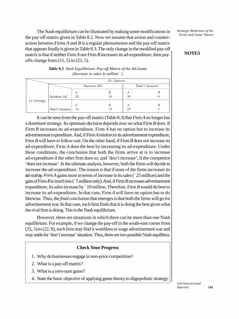
Strategic Behaviour of theFirms and Game Theory
NOTES
Self-InstructionalMaterial 143
The Nash equilibrium can be illustrated by making some modifications inthe pay-off matrix given in Table 8.2. Now we assume that action and counter-action between Firms A and B is a regular phenomenon and the pay-off matrixthat appears finally is given in Table 8.3. The only change in the modified pay-offmatrix is that if neither Firm A nor Firm B increases its ad-expenditure, then pay-offs change from (15, 5) to (25, 5).
Table 8.3 Nash Equilibrium: Pay-off Matrix of the Ad-Game(Increase in sales in million `)
It can be seen from the pay-off matrix (Table 8.3) that Firm A no longer hasa dominant strategy. Its optimum decision depends now on what Firm B does. IfFirm B increases its ad-expenditure, Firm A has no option but to increase itsadvertisement expenditure. And, if Firm A reinforces its advertisement expenditure,Firm B will have to follow suit. On the other hand, if Firm B does not increase itsad-expenditure, Firm A does the best by increasing its ad-expenditure. Underthese conditions, the conclusion that both the firms arrive at is to increasead-expenditure if the other firm does so, and ‘don’t increase’, if the competitor‘does not increase’. In the ultimate analysis, however, both the firms will decide toincrease the ad-expenditure. The reason is that if none of the firms increases itsad-outlay, Firm A gains more in terms of increase in its sales (`25 million) and thegain of Firm B is much less (`5 million only). And, if Firm B increases advertisementexpenditure, its sales increase by ̀ 10 million. Therefore, Firm B would do best toincrease its ad-expenditure. In that case, Firm A will have no option but to dolikewise. Thus, the final conclusion that emerges is that both the firms will go foradvertisement war. In that case, each firm finds that it is doing the best given whatthe rival firm is doing. This is the Nash equilibrium.
However, there are situations in which there can be more than one Nashequilibrium. For example, if we change the pay-off in the south-east corner from(25, 5) to (22, 8); each firm may find it worthless to wage advertisement war andmay settle for ‘don’t increase’ situation. Thus, there are two possible Nash equilibria.
Check Your Progress
1. Why do businesses engage in non-price competition?2. What is a pay-off matrix?3. What is a zero-sum game?4. State the basic objective of applying game theory to oligopolistic strategy.
Strategic Behaviour of theFirms and Game Theory
NOTES
Self-Instructional144 Material
8.4 ANSWERS TO CHECK YOUR PROGRESSQUESTIONS
1. Business enterprises engage in non-price competition, despite the additionalcosts involved because it is generally more profitable than selling for a lowerprice and evades the hazard of a price war.
2. The ‘pay-off matrix’ is tabular recording of gains and losses of a firm takingan action under different kinds of anticipated reactions of the rival firms.
3. If a strategic action taken by a firm may yield some gains to the firm andcounteraction by the rival firm neutralizes the gain, it is a zero-sum game.
4. The basic objective of applying game theory is to arrive at the dominantstrategy.
8.5 SUMMARY
Price competition is the competition that lays focus on the issue of price asmore and attempts to stay ahead of the price of the competitors existing inthe market.
Non-price competition is the competition that lays emphases on the factorsother than the price of the product. The main objective is to differentiatefrom the products that are available as alternatives in the market.
Business enterprises engage in non-price competition, despite the additionalcosts involved because it is generally more profitable than selling for a lowerprice and evades the hazard of a price war.
The pay-off may be positive, negative or zero-sum for a firm taking strategicaction. Accordingly, if a strategic action taken by a firm may yield somegains to the firm and counteraction by the rival firm neutralises the gain, it isa zero-sum game.
The game theory has been formulated on the basis of a realistic assumptionof interdependence of oligopoly firms. It implies that decision-making ofthe firms under oligopoly is interdependent.
The ‘pay-off matrix’ is tabular recording of gains and losses of a firm takingan action under different kinds of anticipated reactions of the rival firms.
The prisoners’ dilemma illustrates the nature of problems oligopoly firmsare confronted with in the formulation of their business strategy with respectto such problems as strategic advertising, price cutting or cheating the cartelif there is one.
Strategic Behaviour of theFirms and Game Theory
NOTES
Self-InstructionalMaterial 145
The Nash equilibrium technique seeks to establish that each firm does thebest it can, given the strategy of its competitors and a Nash equilibrium isone in which none of the players can improve their pay-off given the strategyof the other players.
8.6 KEY WORDS
Strategy: It is a general plan or set of plans intended to achieve something,especially over a long period.
Duopoly: It is the most basic form of oligopoly, a market dominated by asmall number of companies.
8.7 SELF ASSESSMENT QUESTIONS ANDEXERCISES
Short Answer Questions
1. What is a dominant strategy in the context of game theory?2. Give an example to illustrate the prisoner’s dilemma.3. Write a short note on the relevance of prisoner’s dilemma to oligopoly.
Long Answer Questions
1. Analyse the strategic behaviour of the firms.2. Discuss the application of game theory to oligopolistic strategy.3. Give examples to illustrate the use of the Nash equilibrium technique.
8.8 FURTHER READINGS
Dwivedi, D. N. 2015. Principles of Economics, Eight Edition. New Delhi: VikasPublishing House.
Weil. David N. 2004. Economic Growth. London: Addison Wesley.Thomas, Christopher R. and Maurice S. Charles. 2005. Managerial Economics:
Concepts and Applications, Eighth Edition. New Delhi: Tata McGraw-Hill Publishing Company Limited.
Mankiw, Gregory N. 2002. Principles of Economics, Second Edition. India:Thomson Press.
Strategic Behaviour of theFirms and Game Theory
NOTES
Self-Instructional146 Material
Websites
https://blogs.economictimes.indiatimes.com/et-commentary/heres-how-indias-widening-income-distribution-can-be-redressed/
https://www.livemint.com/Opinion/WmpSjQAvPGeVzxqpgXYvtK/The-dangers-of-Indias-Billionaire-Raj.html
Cost and Return
NOTES
Self-InstructionalMaterial 147
UNIT 9 COST AND RETURN
Structure9.0 Introduction9.1 Objectives9.2 Relavant Costs for Decision-Making9.3 Traditional Theory of Cost: Cost Function and Cost Output Relationship
9.3.1 Short-Run Cost-Output Relations9.3.2 Long-Run Cost-Output Relations9.3.3 Economies and Diseconomies of Scale
9.4 Modern Theory of Cost9.5 Cost Control and Cost reduction9.6 Cost Behaviour and Business Decision9.7 Answers to Check Your Progress Questions9.8 Summary9.9 Key Words
9.10 Self Assessment Questions and Exercises9.11 Further Readings
9.0 INTRODUCTION
The theory of cost provides conditions for minimizing the cost of production. Inaddition, analysis of cost of production is very important in almost all kinds ofbusiness decisions, especially those related to the weak points of productionmanagement; determining the output level for cost minimization; determining theprice of the product and dealers’ margin; and estimating and projecting the cost ofbusiness operation. Cost functions help in determining the relationship betweenoutputs and costs. In this unit, we will study the relevant costs for decision-makingand the traditional and modern theories of cost.
9.1 OBJECTIVES
After going through this unit, you will be able to: Discuss the relevant costs for decision-making Explain the traditional theory and modern theories of cost Describe the cost function and cost output relationship Discuss the concept of cost control, cost reduction, cost behaviour and
business decisions
Cost and Return
NOTES
Self-Instructional148 Material
9.2 RELAVANT COSTS FOR DECISION-MAKING
The cost concepts that are relevant to business operations and decisions can begrouped on the basis of their nature and purpose under two overlapping categories:(i) cost concepts used for accounting purposes, and (ii) analytical cost conceptsused in economic analysis of business activities. We will discuss some importantconcepts of the two categories. It is important to note here that this classificationof cost concepts is only a matter of analytical convenience.
Accounting Cost Concepts
1. Opportunity Cost and Actual Cost: Actual cost is all paid out costs of thebusiness firms to take the advantage of the best opportunity available to them. Theopportunity cost is the opportunity lost for lack of resources. An opportunity tomake income is lost because of scarcity of resources like land, labour, capital, etc.We know that resources available to any person, firm or society are scarce buthave alternative uses with different returns. Income maximizing resource ownersput their scarce resources to their most productive use and thus, they forego theincome expected from the second best use of the resources. Thus, the opportunitycost may be defined as the returns expected from the second best use of theresources foregone due to the scarcity of resources. The opportunity cost is alsocalled alternative cost. Had the resource available to a person, a firm or a societybeen unlimited, there would be no opportunity cost.2. Business Costs and Full Costs: Business costs include all the expenses thatare incurred to carry out a business. The concept of business costs is similar to theactual or real costs. Business costs “include all the payments and contractualobligations made by the firm together with the book cost of depreciation on plantand equipment.” Business costs are used for calculating business profits and lossesand for filing returns for income-tax and also for other legal purposes.
The concept of full cost, includes business costs, opportunity cost andnormal profit. The opportunity cost includes the foregone earning expected fromthe second best use of the resources, or the market rate of interest on the internalmoney capital and also the value of an entrepreneur’s own services that are notcharged for in the current business. Normal profit is a necessary minimum earningin addition to the opportunity cost, which a firm must receive to remain in itspresent occupation.3. Actual or Explicit Costs and Implicit or Imputed Costs: The Actual orExplicit costs are those which are actually incurred by the firm in payment forlabour, material, plant, building, machinery, equipment, travelling and transport,advertisement, etc. The total money expenses, recorded in the books of accountsare, for all practical purposes, the actual costs. Actual cost comes under theaccounting cost concept.
Cost and Return
NOTES
Self-InstructionalMaterial 149
In contrast to explicit costs, there are certain other costs that do not takethe form of cash outlays, nor do they appear in the accounting system. Such costsare known as implicit or imputed costs. Opportunity cost is an important exampleof implicit cost. For example, suppose an entrepreneur does not utilize his servicesin his own business and works as a manager in some other firm on a salary basis.If he sets up his own business, he foregoes his salary as manager. This loss ofsalary is the opportunity cost of income from his own business. This is an implicitcost of his own business. Thus, implicit wages, rent, and implicit interest are thewages, rent and interest that an owner’s labour, building and capital respectively,can earn from their second best use.
Implicit costs are not taken into account while calculating the loss or gainsof the business, but they form an important consideration in deciding whether ornot to retain a factor in its present use. The explicit and implicit costs togethermake the economic cost.4. Out-of-Pocket and Book Costs: The items of expenditure that involve cashpayments or cash transfers, both recurring and non-recurring, are known asout-of-pocket costs. All the explicit costs (e.g., wages, rent, interest, cost ofmaterials and maintenance, transport expenditure, electricity and telephoneexpenses, etc.) fall in this category. On the contrary, there are certain actual businesscosts that do not involve cash payments, but a provision is therefore made in thebooks of account and they are taken into account while finalizing the profit andloss accounts. Such expenses are known as book costs. In a way, these arepayments made by a firm to itself. Depreciation allowances and unpaid interest onthe owner’s own funds are the example of book costs.
Analytical Cost Concepts
The analytical cost concepts refers to the different cost concepts that are used inanalysing the cost-output relationship with increase in inputs and output and alsothe cost concepts that figure in analysing the effect of expansion of production onthe society as a whole.1. Fixed and Variable Costs. Fixed costs are those that remain fixed in amountfor a certain quantity of output. Fixed cost does not vary with variation in theoutput between zero and a certain level of output. In other words, costs that donot vary or remain constant for a certain level of output are treated as fixed costs.The fixed costs include (i) depreciation of machinery, building and other fixedassets, (ii) costs of managerial and administrative staff, (iii) maintenance of land,etc. The concept of fixed cost is associated with the short-run.
Variable costs are those which vary with the variation in the total output.Variable costs include cost of raw material, running cost of fixed capital, such asfuel, repairs, routine maintenance expenditure, direct labour charges associatedwith the level of output, and the costs of all other inputs that vary with output.2. Total, Average and Marginal Costs. Total cost (TC) refers to the totaloutlays of money expenditure, both explicit and implicit, on the resources used to
Cost and Return
NOTES
Self-Instructional150 Material
produce a given level of output. It includes both fixed and variable costs. The totalcost for a given output is measured as
TC = Total fixed cost + Total variable cost
Average cost (AC) is of statistical nature—it is not actual cost. It is obtainedby dividing the total cost (TC) by the total output (Q), i.e.,
AC = T CQ
Marginal cost (MC) is defined as the addition to the total cost on accountof producing one additional unit of the product. Or, marginal cost is the cost of themarginal unit produced. Marginal cost is calculated as TCn – TCn–1 where n is thenumber of units produced. Using cost function, MC is obtained as the first derivativeof the cot function.
MC = TCQ
Total, average and marginal cost concepts are used in the economic analysisof firm’s production and in pricing decisions. These cost concepts are discussed infurther detail in the following section.3. Short-Run and Long-Run Costs. Short-run and long-run cost concepts arerelated to variable and fixed costs, respectively, and often figure in economic analysiscost-output relationship.
Short-run refers to the time period during which scale of production remainsunchanged. The costs incurred in the short-run are called short-run costs. It includesboth the variable and the fixed costs. From analytical point of view, short-runcosts are those that vary with the variation in output in short-run, the size of thefirm remaining the same. Therefore, short-run costs are treated as variable costs.
Furthermore, long-run costs are by implication the costs that are incurredin the long-run. In the long run, however, even the fixed costs become variablecosts as the size of the firm or scale of production increases. Broadly speaking,‘the short-run costs are those associated with variables in the utilization of fixedplant or other facilities whereas long-run costs are associated with the changes inthe size and kind of plant.’4. Incremental Costs and Sunk Costs. Conceptually, incremental costs areclosely related to the concept of marginal cost but with a relatively widerconnotation. While marginal cost refers to the cost of the marginal unit (generallyone unit) of output, incremental cost refers to the total additional cost associatedwith the decisions to expand the output or to add a new variety of product, etc.
Cost and Return
NOTES
Self-InstructionalMaterial 151
5. Historical and Replacement Costs. Historical cost refers to the cost incurredin past on the acquisition of productive assets, e.g. land, building, machinery, etc.,whereas replacement cost refers to the expenditure made for replacing an oldasset. These concepts owe their significance to the unstable nature of input prices.Stable prices over time, other things given, keep historical and replacement costson par with each other. Instability in asset prices makes the two costs differ fromeach other.
As regards their application, historical cost of assets is used for accountingpurposes, in the assessment of the net worth of the firm whereas replacement costfigures in business decisions regarding the renovation of the plant.
Private costs are those which are actually incurred or provided for by anindividual or a firm on the purchase of goods and services from the market. For afirm, all the actual costs, both explicit and implicit, are private costs. Private costsare internalized costs that are incorporated in the firm’s total cost of production.
Check Your Progress
1. Define explicit costs.2. Under which category does the running cost and depreciation of the capital
assets come?
9.3 TRADITIONAL THEORY OF COST: COSTFUNCTION AND COST OUTPUTRELATIONSHIP
The theory of cost deals with how cost of production changes with change inoutput. In other words, the cost theory deals with cost-output relations. The basicprinciple of the cost-output relationship is that the total cost increases with increasein output. This simple statement of an observed fact is of little theoretical andpractical importance. What is important from a theoretical and managerial decision
Cost and Return
NOTES
Self-Instructional152 Material
point of view is the rate of increase in total cost with increase in output and thedirection of change in the average cost (AC) and the marginal cost (MC). Thedirection of change in AC and MC—whether AC and MC decrease or increaseor remain constant—depends on the nature of the cost function. A cost function isa symbolic statement of the technological relationship between the cost and output.The general form of the cost function is written as
TC = f(Q), with TC/Q > 0 …(9.1)
The actual form of cost function depends on whether the time frameworkchosen for cost analysis is short-run or long-run. It is important to recall here thatsome costs remain constant in the short-run while all costs are variable in the long-run. Thus, depending on whether cost analysis pertains to short-run or to long-run, there are two kinds of cost functions: (i) short-run cost functions, and(ii) long-run cost functions. Accordingly, the cost output relations are analyzed inshort-run and long-run framework.
9.3.1 Short-Run Cost-Output Relations
In this section, we will analyse the cost-output relations in the short-run. The long-run cost output relations discussed in the following section. Before we discuss theshort-run cost-output relations, let us first look at the cost concepts and thecomponents used to analyze the short-run cost-output relations.
The basic analytical cost concepts used in the analysis of cost behaviour areTotal, Average and Marginal costs. The total cost (TC) is defined as the actualcost that are incurred to produce a given quantity of output. The short-run TC iscomposed of two major elements: (i) total fixed cost (TFC), and (ii) total variablecost (TVC). That is, in the short-run,
TC = TFC + TVC ...(9.2)
As mentioned earlier, TFC (i.e., the cost of plant, building, etc.) remainsfixed in the short run, whereas TVC (the labour cost) varies with the variation inthe output.
For a given quantity of output (Q), the average cost (AC), average fixedcost (AFC) and average variable cot (VC) can be defined as follws.
AC =T C T FC TV C TFC TVCQ Q Q Q
= AFC + AVC
Thus, AFC =T FC
Q and AVC =TV C
Q
and AC = AFC + AVC ...(9.3)
Marginal cost (MC) can be defined as the change in the total cost due tochange in the total output by one unit, i.e.,
Cost and Return
NOTES
Self-InstructionalMaterial 153
MC = 1
1 1n n
n n
TC TCTCQ Q Q
...(9.4)
In case TC is expressed in functional form, MC is measured as the first derivative
of cost function, i.e., TCQ
.
MC = TVC. Now we turn to cost function and derivationof various cost curves.
Short-Run Cost Functions and Cost Curves
The cost-output relations are revealed by the cost function and are exhibited throughcost curves. The shape of the cost curves depends on the nature of the costfunction. Cost functions are derived from actual cost data of the firms. The natureof estimated cost function depends on the cost trend revealed by cost data. Giventhe cost data, cost functions may take a variety of forms, e.g., linear, quadratic orcubic, yielding different kinds of cost curves. The cost curves produced by linear,quadratic and cubic cost functions are illustrated below.1. Linear Cost Function. When total cost increases at a constant rate withincrease in production, it produces a linear cost function. A linear cost functiontakes the following form.
TC = a + bQ …(9.5)where TC = total cost, Q = quantity produced, a = TFC, and b = Change in TVCdue to change in Q.
Given the cost function [Eq. (9.5)] AC and MC can be obtaied as follows.
AC = TC a bQ aQ Q Q
+ b
and MC = TC bQ
Note that since ‘b’ is a constant coefficient, MC remains constant, throughoutin case of a linear cost function.
Note that, in case of a linear cost function, while MC remains constant, ACcontinues to decline with the increase in output. This is so simply because of thelogic of the linear cost function.2. Quadratic Cost Function. When TC increases at increasing rate with constantincrease in output (Q), the TC data produces a quadratic cost function expressedas
TC = a + bQ + Q2 ....(9.6)
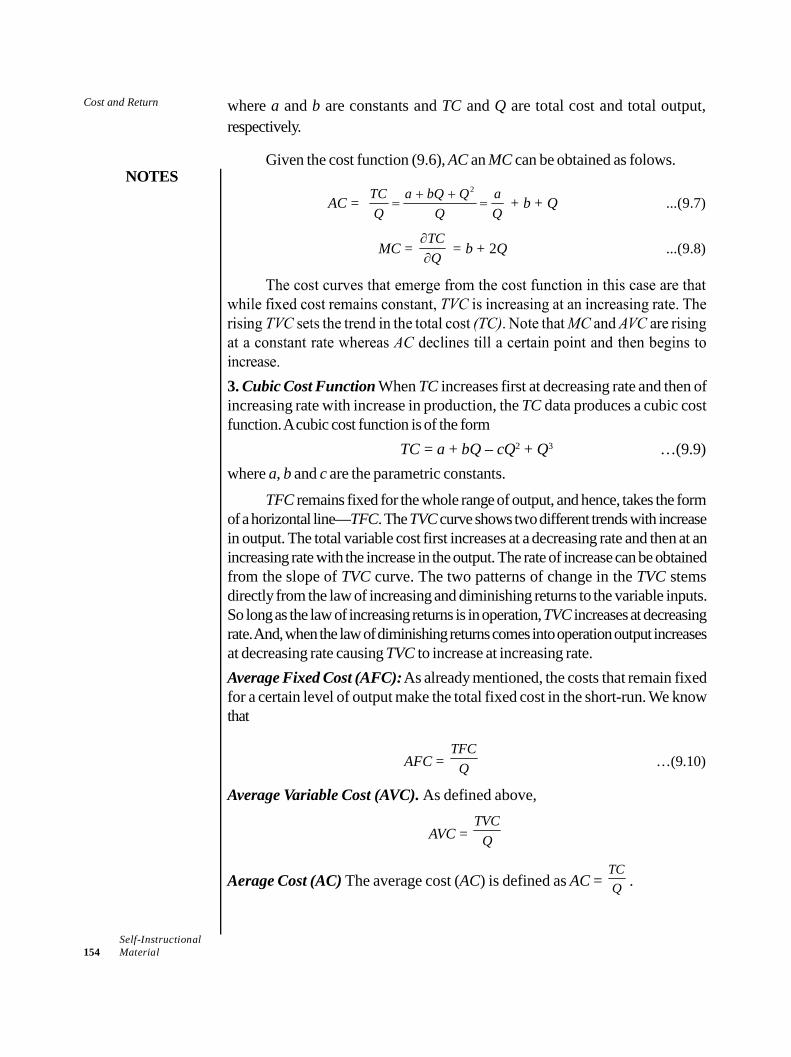
Cost and Return
NOTES
Self-Instructional154 Material
where a and b are constants and TC and Q are total cost and total output,respectively.
Given the cost function (9.6), AC an MC can be obtained as folows.
AC = 2TC a bQ Q a
Q Q Q
+ b + Q ...(9.7)
MC = TCQ
= b + 2Q ...(9.8)
3. Cubic Cost Function When TC increases first at decreasing rate and then ofincreasing rate with increase in production, the TC data produces a cubic costfunction. A cubic cost function is of the form
TC = a + bQ – cQ2 + Q3 …(9.9)where a, b and c are the parametric constants.
TFC remains fixed for the whole range of output, and hence, takes the formof a horizontal line—TFC. The TVC curve shows two different trends with increasein output. The total variable cost first increases at a decreasing rate and then at anincreasing rate with the increase in the output. The rate of increase can be obtainedfrom the slope of TVC curve. The two patterns of change in the TVC stemsdirectly from the law of increasing and diminishing returns to the variable inputs.So long as the law of increasing returns is in operation, TVC increases at decreasingrate. And, when the law of diminishing returns comes into operation output increasesat decreasing rate causing TVC to increase at increasing rate.Average Fixed Cost (AFC): As already mentioned, the costs that remain fixedfor a certain level of output make the total fixed cost in the short-run. We knowthat
AFC = TFC
Q …(9.10)
Average Variable Cost (AVC). As defined above,
AVC = TVC
Q
Aerage Cost (AC) The average cost (AC) is defined as AC = TCQ .
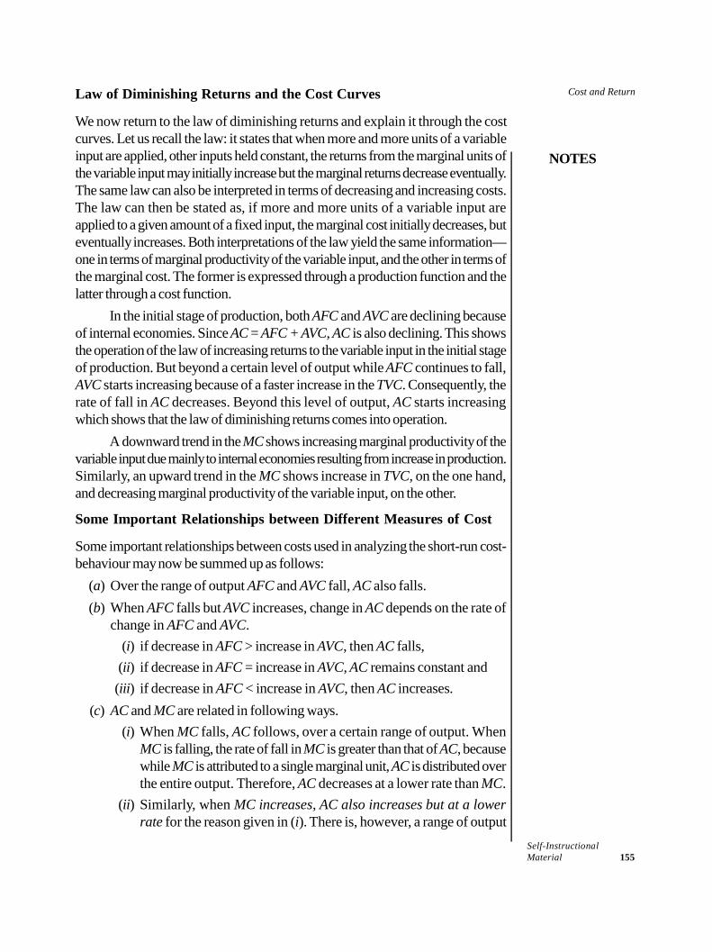
Cost and Return
NOTES
Self-InstructionalMaterial 155
Law of Diminishing Returns and the Cost Curves
We now return to the law of diminishing returns and explain it through the costcurves. Let us recall the law: it states that when more and more units of a variableinput are applied, other inputs held constant, the returns from the marginal units ofthe variable input may initially increase but the marginal returns decrease eventually.The same law can also be interpreted in terms of decreasing and increasing costs.The law can then be stated as, if more and more units of a variable input areapplied to a given amount of a fixed input, the marginal cost initially decreases, buteventually increases. Both interpretations of the law yield the same information—one in terms of marginal productivity of the variable input, and the other in terms ofthe marginal cost. The former is expressed through a production function and thelatter through a cost function.
In the initial stage of production, both AFC and AVC are declining becauseof internal economies. Since AC = AFC + AVC, AC is also declining. This showsthe operation of the law of increasing returns to the variable input in the initial stageof production. But beyond a certain level of output while AFC continues to fall,AVC starts increasing because of a faster increase in the TVC. Consequently, therate of fall in AC decreases. Beyond this level of output, AC starts increasingwhich shows that the law of diminishing returns comes into operation.
A downward trend in the MC shows increasing marginal productivity of thevariable input due mainly to internal economies resulting from increase in production.Similarly, an upward trend in the MC shows increase in TVC, on the one hand,and decreasing marginal productivity of the variable input, on the other.
Some Important Relationships between Different Measures of Cost
Some important relationships between costs used in analyzing the short-run cost-behaviour may now be summed up as follows:
(a) Over the range of output AFC and AVC fall, AC also falls.(b) When AFC falls but AVC increases, change in AC depends on the rate of
change in AFC and AVC.(i) if decrease in AFC > increase in AVC, then AC falls,(ii) if decrease in AFC = increase in AVC, AC remains constant and(iii) if decrease in AFC < increase in AVC, then AC increases.
(c) AC and MC are related in following ways.(i) When MC falls, AC follows, over a certain range of output. When
MC is falling, the rate of fall in MC is greater than that of AC, becausewhile MC is attributed to a single marginal unit, AC is distributed overthe entire output. Therefore, AC decreases at a lower rate than MC.
(ii) Similarly, when MC increases, AC also increases but at a lowerrate for the reason given in (i). There is, however, a range of output
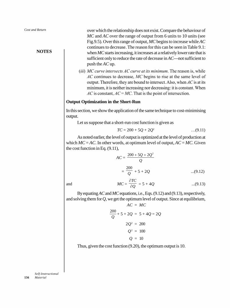
Cost and Return
NOTES
Self-Instructional156 Material
over which the relationship does not exist. Compare the behaviour ofMC and AC over the range of output from 6 units to 10 units (seeFig.9.5). Over this range of output, MC begins to increase while ACcontinues to decrease. The reason for this can be seen in Table 9.1:when MC starts increasing, it increases at a relatively lower rate that issufficient only to reduce the rate of decrease in AC—not sufficient topush the AC up.
Output Optimization in the Short-Run
In this section, we show the application of the same technique to cost-minimisingoutput.
Let us suppose that a short-run cost function is given asTC = 200 + 5Q + 2Q2 …(9.11)
As noted earlier, the level of output is optimized at the level of production atwhich MC = AC. In other words, at optimum level of output, AC = MC. Giventhe cost function in Eq. (9.11),
AC = 2200 5 2Q Q
Q
= 200Q + 5 + 2Q ...(9.12)
and MC = TCQ
= 5 + 4Q ...(9.13)
By equating AC and MC equations, i.e., Eqs. (9.12) and (9.13), respectively,and solving them for Q, we get the optimum level of output. Since at equilibrium,
AC = MC200Q
+ 5 + 2Q = 5 + 4Q = 2Q
2Q2 = 200
Q2 = 100
Q = 10
Thus, given the cost function (9.20), the optimum output is 10.
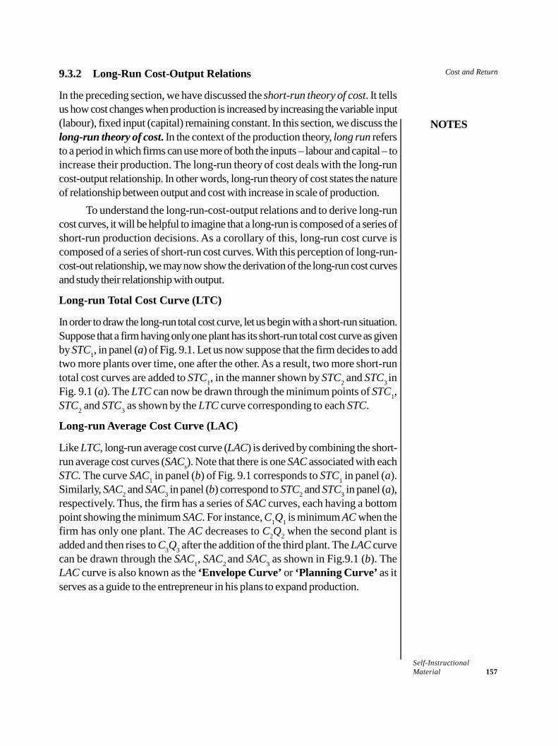
Cost and Return
NOTES
Self-InstructionalMaterial 157
9.3.2 Long-Run Cost-Output Relations
In the preceding section, we have discussed the short-run theory of cost. It tellsus how cost changes when production is increased by increasing the variable input(labour), fixed input (capital) remaining constant. In this section, we discuss thelong-run theory of cost. In the context of the production theory, long run refersto a period in which firms can use more of both the inputs – labour and capital – toincrease their production. The long-run theory of cost deals with the long-runcost-output relationship. In other words, long-run theory of cost states the natureof relationship between output and cost with increase in scale of production.
To understand the long-run-cost-output relations and to derive long-runcost curves, it will be helpful to imagine that a long-run is composed of a series ofshort-run production decisions. As a corollary of this, long-run cost curve iscomposed of a series of short-run cost curves. With this perception of long-run-cost-out relationship, we may now show the derivation of the long-run cost curvesand study their relationship with output.
Long-run Total Cost Curve (LTC)
In order to draw the long-run total cost curve, let us begin with a short-run situation.Suppose that a firm having only one plant has its short-run total cost curve as givenby STC1, in panel (a) of Fig. 9.1. Let us now suppose that the firm decides to addtwo more plants over time, one after the other. As a result, two more short-runtotal cost curves are added to STC1, in the manner shown by STC2 and STC3 inFig. 9.1 (a). The LTC can now be drawn through the minimum points of STC1,STC2 and STC3 as shown by the LTC curve corresponding to each STC.
Long-run Average Cost Curve (LAC)
Like LTC, long-run average cost curve (LAC) is derived by combining the short-run average cost curves (SACs). Note that there is one SAC associated with eachSTC. The curve SAC1 in panel (b) of Fig. 9.1 corresponds to STC1 in panel (a).Similarly, SAC2 and SAC3 in panel (b) correspond to STC2 and STC3 in panel (a),respectively. Thus, the firm has a series of SAC curves, each having a bottompoint showing the minimum SAC. For instance, C1Q1 is minimum AC when thefirm has only one plant. The AC decreases to C2Q2 when the second plant isadded and then rises to C3Q3 after the addition of the third plant. The LAC curvecan be drawn through the SAC1, SAC2 and SAC3 as shown in Fig.9.1 (b). TheLAC curve is also known as the ‘Envelope Curve’ or ‘Planning Curve’ as itserves as a guide to the entrepreneur in his plans to expand production.
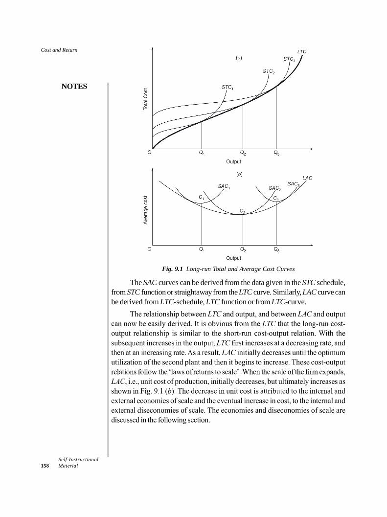
Cost and Return
NOTES
Self-Instructional158 Material
Fig. 9.1 Long-run Total and Average Cost Curves
The SAC curves can be derived from the data given in the STC schedule,from STC function or straightaway from the LTC curve. Similarly, LAC curve canbe derived from LTC-schedule, LTC function or from LTC-curve.
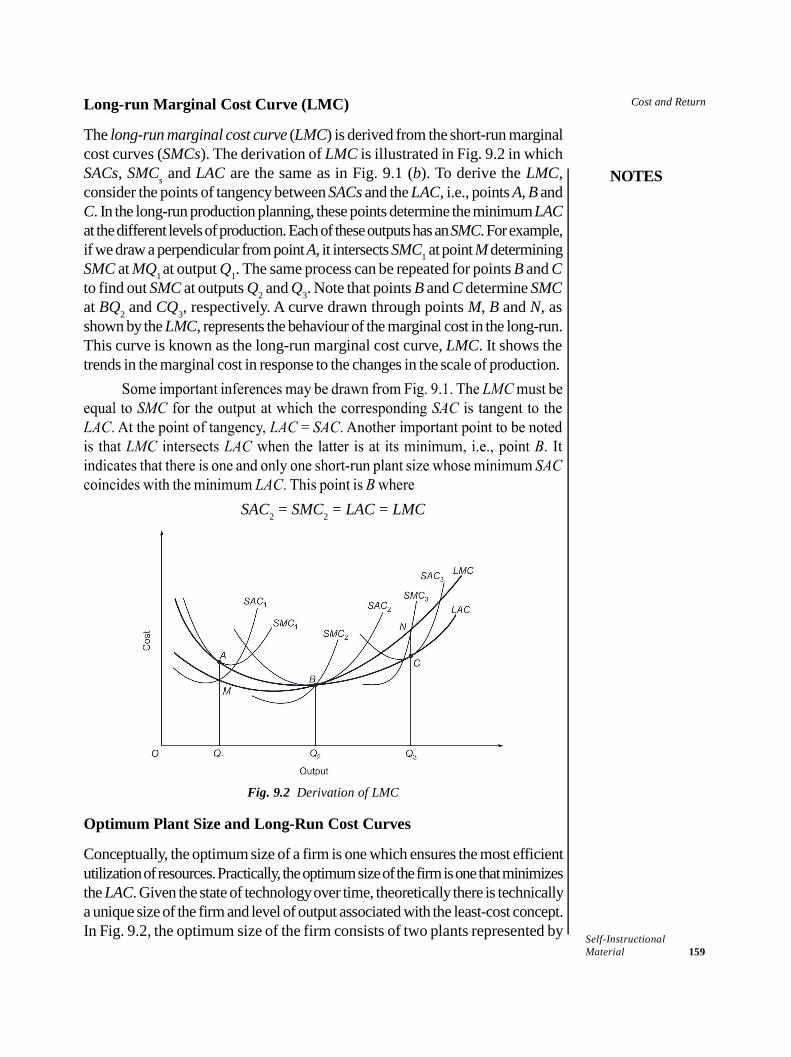
Cost and Return
NOTES
Self-InstructionalMaterial 159
Long-run Marginal Cost Curve (LMC)
The long-run marginal cost curve (LMC) is derived from the short-run marginalcost curves (SMCs). The derivation of LMC is illustrated in Fig. 9.2 in whichSACs, SMCs and LAC are the same as in Fig. 9.1 (b). To derive the LMC,consider the points of tangency between SACs and the LAC, i.e., points A, B andC. In the long-run production planning, these points determine the minimum LACat the different levels of production. Each of these outputs has an SMC. For example,if we draw a perpendicular from point A, it intersects SMC1 at point M determiningSMC at MQ1 at output Q1. The same process can be repeated for points B and Cto find out SMC at outputs Q2 and Q3. Note that points B and C determine SMCat BQ2 and CQ3, respectively. A curve drawn through points M, B and N, asshown by the LMC, represents the behaviour of the marginal cost in the long-run.This curve is known as the long-run marginal cost curve, LMC. It shows thetrends in the marginal cost in response to the changes in the scale of production.
SAC2 = SMC2 = LAC = LMC
Fig. 9.2 Derivation of LMC
Optimum Plant Size and Long-Run Cost Curves
Conceptually, the optimum size of a firm is one which ensures the most efficientutilization of resources. Practically, the optimum size of the firm is one that minimizesthe LAC. Given the state of technology over time, theoretically there is technicallya unique size of the firm and level of output associated with the least-cost concept.In Fig. 9.2, the optimum size of the firm consists of two plants represented by
Cost and Return
NOTES
Self-Instructional160 Material
SAC1 and SAC2. The two plants together produce OQ2 units of a product atminimum long-run average cost (LAC) of BQ2. The downtrend in the LAC indicatesthat until output reaches the level of OQ2, the firm is of less than optimal size.Similarly, expansion of the firm beyond production capacity OQ2, causes a rise inSMC and, therefore, in LAC. It follows that given the technology, a firm aiming tominimize its average cost over time must choose a plant that gives minimum LACwhere SAC = SMC = LAC = LMC. This size of plant assures the most efficientutilization of the resources. Any change in output level—increase or decrease—will make the firm enter the area of inoptimality.
9.3.3 Economies and Diseconomies of Scale
While optimization of output in the long run is an important concern of businessfirms, cost minimization is an equally import decision area. Cost of productiondepends not only on internal factor – the productivity of inputs – but also onmany external factors – the factors that arise out of the firm. Since we areconcerned in this unit with the theory of cost, in this section we give a detailedanalysis of internal and external economies and diseconomies of scale and howthey determine the trend in cost of production. To begin with, let us have look atthe trend of long-run average cost curve (LAC).
As shown in Fig. 9.1(b), LAC decreases with the expansion of productionscale up to OQ2 and then it begins to rise. Decrease in LAC is caused by theeconomies of scale and increase in LAC is caused by diseconomies of scale.Economies of scale result in cost saving and diseconomies lead to rise in cost.Economies and diseconomies of scale determine also the returns to scale.Increasing returns to scale operate till economies of scale are greater than thediseconomies of scale, and returns to scale decrease when diseconomies aregreater than the economies of scale. When economies and diseconomies are inbalance, returns to scale are constant. In this section, we briefly discuss the variouskinds of economies and diseconomies of scale and their effect on cost of production.
Economies of Scale
The economies of scale are classified as(a) Internal or Real Economies, and(b) External or Pecuniary Economies.
A. Internal Economies
Internal economies, also called ‘real economies’, are those that arise within thefirm with addition of new production plants. This means that internal economiesare available exclusively to the expanding firm. Internal economies may be classifiedunder the following categories.
(i) Economies in production;(ii) Economies in marketing;
Cost and Return
NOTES
Self-InstructionalMaterial 161
(iii) Managerial economies, and(iv) Economies in transport and storage.
(i) Economies in Production Economies in production arise from two sources:(a) technological advantages, and (b) advantages of division of labour based onspecialization and skill of labour.(ii) Economies in Purchase of Inputs Economies in input purchases arise fromthe large-scale purchase of raw materials and other material inputs and large-scale selling of the firm’s own products. As to economies in the purchase of inputs,the large-size firms normally make bulk purchases of their inputs. The large scalepurchase entitles the firm for certain discounts in input prices and other concessionsthat are not available on small purchases. As such, the growing firms gain economieson the cost of their material inputs.
(iv) Economies in Transport and Storage Economies in transportation andstorage costs arise from fuller utilization of transport and storage facilities.Transportation costs are incurred both on production and sales sides. Similarly,storage costs are incurred on both raw materials and finished products. The large-size firms may acquire their own means of transport and they can, thereby, reducethe unit cost of transportation, at least to the extent of profit margin of the transportcompanies. Besides, own transport facility prevents delays in transporting goods.Some large-scale firms have their own railway tracks from the nearest railwaypoint to the factory, and thus they reduce the cost of transporting goods in andout. For example, Bombay Port Trust has its own railway tracks, oil companieshave their own fleet of tankers. Similarly, large-scale firms can create their owngodowns in various centres of product distribution and can save on cost of storage.
B. External or Pecuniary Economies of Scale
External economies are those that arise outside the firm and accrue to the expandingfirms. External economies appear in the form of money saving on inputs, called
Cost and Return
NOTES
Self-Instructional162 Material
pecuniary economies. Pecuniary economies accrue to the large-size firms in theform of discounts and concessions on (i) large scale purchase of raw material,(ii) large scale acquisition of external finance, particularly from the commercialbanks; (iii) massive advertisement campaigns; (iv) large scale hiring of means oftransport and warehouses, etc. These benefits are available to all the firms of anindustry but large scale firms benefit more than small firms.
Diseconomies of Scale
The economics of scale have their own limits, i.e., scale economies exist only up toa certain level of production scale. The expansion of scale of production beyondthat limit creates condition for diseconomies of scale. Diseconomies of scale aredisadvantages that arise due to the expansion of production scale beyond its optimumlevel and lead to rise in the cost of production. Like economies, diseconomiesmay be internal and external. Let us describe the nature of internal and externaldiseconomies in some detail.1. Internal Diseconomies. Internal diseconomies are those that are exclusiveand internal to a firm as they arise within the firm. Like everything else, economiesof scale have a limit too. This limit is reached when the advantages of division oflabour and managerial staff have been fully exploited; excess capacity of plant,warehouses, transport and communication systems, etc., is fully used; and economyin advertisement cost tapers off. Although some economies may still exist,diseconomies begin to outweigh the economies and the costs begin to rise.Managerial Inefficiency. Diseconomies begin to appear first at the managementlevel. Managerial inefficiencies arise, among other things, from the expansion ofscale itself. With fast expansion of the production scale, personal contacts andcommunications between (i) owners and managers, (ii) managers and labour, and(iii) between the managers of different departments or sections get rapidly reduced.The lack of fast or quick communication causes delays in decision-making affectingproduction adversely.
Secondly, close control and supervision is replaced by remote controlmanagement. With the increase in managerial personnel, decision-making becomescomplex and delays in decision-making become inevitable.
Thirdly, implementation of whatever decisions are taken is delayed due tocoordination problem in large scale organisations.
Finally, with the expansion of the scale of production, management isprofessionalized beyond a point. As a result, the owner’s objective function ofprofit maximization is gradually replaced by managers’ utility function, like jobsecurity and high salary, standard or reasonable profit target, satisfying functions.All these lead to laxity in management and, hence to a rise in the cost of production.
Labour Inefficiency: Increasing number of labour leads to a loss of control overlabour management. This affects labour productivity adversely. Besides, increase
Cost and Return
NOTES
Self-InstructionalMaterial 163
in the number of workers encourages labour union activities that cause loss ofoutput per unit of time and hence, rise in the cost of production.
2. External Diseconomies. External diseconomies are the disadvantages thatarise outside the firm, especially in the input markets, due to natural constraints,specially in agriculture and extractive industries. With the expansion of the firm,particularly when all the firms of the industry are expanding, the discounts andconcessions that are available on bulk purchases of inputs and concessional financecome to an end. More than that, increasing demand for inputs puts pressure onthe input markets and input prices begin to rise causing a rise in the cost of production.These are pecuniary diseconomies.
On the production side, the law of diminishing returns to scale come intoforce due to excessive use of fixed factors, more so in agriculture and extractiveindustries. For example, excessive use of cultivable land turns it into barren land;pumping out water on a large scale for irrigation causes the water table to godown resulting in rise in cost of irrigation; extraction of minerals on a large scaleexhausts the mineral deposits on upper levels and mining further deep causes risein cost of production; extensive fishing reduces the availability of fish and the catch,even when fishing boats and nets are increased. These kinds of diseconomiesmake the LAC move upward.
9.4 MODERN THEORY OF COST
Up till now have learnt about the traditional theory of costs, in this section we willlearn the modern theory of cost. Unlike the traditional theory of cost, the moderntheory does not agree to the U-shape of the cost curve. As per the modern theory,the short run cost curve has a saucer-type shape and the long-run average costcurve is either L-shaped or inverse J-shaped. This is because of the existence ofbuilt- in- reserve capacity which imparts flexibility and enables the plant to producelarger output without adding to the costs.
Short-Run Cost Curves
The SAVC, SMC and the AFC has a saucer shape. Further the AVC is saucer-shaped because the reserve capacity is maintained by the firm and the AFC isdownward slopping even as the output expands. The SAC curve has a U-shapeeven in the modern version.
Long-Run Cost Curves
The long-run Average cost curve is not U-shaped in the modern theory, in fact it isL-shaped of inverse J-Shaped. This can be understood through the returns toscale. The traditional theory assumed a U shaped Long-run cost curve because ofthe assumption that after the optimal level of output, the diseconomies of scaleovertake the economies of scale. As per the modern theory, the long run averagecosts includes basically production and managerial costs of which the average
Cost and Return
NOTES
Self-Instructional164 Material
production costs continue to fall even at large scales while the managerial costsper unit of output may rise only gradually and at large scales of output.
9.5 COST CONTROL AND COST REDUCTION
The primary aim of business firms is to produce more products at the least possiblecost. Profit maximization becomes essential in such conditions. The cost accountingsystems have gained prominence because the success of the firms depends ontheir ability to reduce costs while selling more products. Cost control, essentially,deals with the cost-effective ways of operations. This majorly involves the avoidanceor elimination of wastages in the current operations.
The primary aim of business firms is to produce more products at the leastpossible cost. Profit maximization becomes essential in such conditions. The costaccounting systems have gained prominence because the success of the firmsdepends on their ability to reduce costs while selling more products. Cost control,essentially, deals with the cost-effective ways of operations. This majorly involvesthe avoidance or elimination of wastages in the current operations.The advantages of cost control are:
The profit margins increase along with it becoming the top competition forothers
It is the necessary condition for ensuring efficient productivity The competitive prices will ensure that the sales are stable and employment
of the workforce It reduces the costs involved in producing products thereby reducing its
overall costs Without cost control, it is very much possible that the firm’s profits start to
decrease even with an increase in the volume of salesThere are mainly two types of standards of cost control and reduction:
External: This includes the company adjudging its performance in comparisonto its competitions. This is done through measuring cost ratios.
Internal: These are standards used by the companies to identify places wherecosts can be reduced. Some of the tools under these standards are:
o Budgetary control: This is nothing but a plan of action for a givenperiod of time in numerical terms. The organizational activities are notonly forecasting but carried forward based on the anticipated revenuesand expenses.
o Standard costing: This refers to the assigning and use of certain setstandard costs based on which actual costs are computed. Thedifferences in such comparisons are then corrected to minimizewastage.
Cost and Return
NOTES
Self-InstructionalMaterial 165
9.6 COST BEHAVIOUR AND BUSINESS DECISION
Cost behaviour primarily refers to the phenomenon of studying the pattern in whichcosts change in relation to volume and activity. The categorization of cost behaviouris done on the basis of:
Costs which change with the activity or volume Costs which remain constant throughout Costs which fall somewhere in the middleAs you can understand, these types of costs are total costs, fixed costs and
variable costs. We have already seen how these affect output and productionearlier in the unit, now let’s see why studying costs are important in businessdecisions.
The correct forecasting or estimation of costs is crucial as it assists themanagers ensure that their planning is accurate. Based on this planning, organizingactivities are undertaken which ultimately reflects on the business performance.Several researchers stress on the importance of studying cost behaviour as it iscrucial to making financial decisions in the present, as well as planning and decision-making in the future. Further, the significance of cost behaviour to business decisioncan be understood by the fact that any half-baked knowledge will result in thecompany incurring serious losses. Proper study of cost behaviour is helpful inensuring the operating margins are kept under control and that the wastages areidentified and eliminated.
Check Your Progress
3. What is quadratic cost function?4. What does the operation of the law of increasing returns to variable inputs
in the initial stage of production means in terms of costs?5. Name the curve whose shape remains a U-type in the modern theory of
cost.
9.7 ANSWERS TO CHECK YOUR PROGRESSQUESTIONS
1. Explicit costs are those which area actually incurred by the firm in paymentfor labour, material, plant, building, machinery, equipment, travelling andtransport, etc.
2. The running cost and depreciation of the capital assets are included in theshort-run or variable costs.
Cost and Return
NOTES
Self-Instructional166 Material
3. When the total cost increase at increasing rate with constant increase inoutput, the TC data produces a quadratic cost function.
4. In the initial stages of production, both AFC and AVC are declining becauseof internal economies. Since AC=AFC+AVC, AC is also declining. Thisshows the operation of the law of increasing returns to the variable input inthe initial stage of production.
5. In the modern theory of cost, the SAC curve has the same U-shape.
9.8 SUMMARY
The cost concepts that are relevant to business operations and decisionscan be grouped on the basis of their nature and purpose under twooverlapping categories: (i) cost concepts used for accounting, and (ii)analytical cost concepts used in economic analysis of business activities.
Accounting cost concepts include opportunity cost and actual cost; businesscosts and full costs; explicit and implicit cost; and out-of-pocket and bookcosts.
Analytical cost concepts are: fixed and variable costs; total, average andmarginal costs; short-run and long-run costs; incremental costs and sunkcosts and historical and replacement costs.
The theory of cost deals with how cots of production changes with changein output. The basic principle of the cost-output relationship is that the totalcost increases with increase in output.
The short-run total cost is composed of two major elements (i)total fixedcost and, (ii) total variable cost. That is, in the short-run, TC=TFC+TVC
Long-run cost curve is composed of a series of short-run curves. Decrease in LAC is caused by diseconomies of scale. Economies of scale
result in cost saving and diseconomies of scale determine also the returns toscale. Dieconomies of scale are disadvantages that arises due to theexpansion of production scale beyond its optimum level and lead to rise inthe cost of production.
Unlike the traditional theory of cost, the modern theory does not agree tothe U-shape of the cost curve. As per the modern theory, the short run costcurve has a saucer-type shape and the long-run average cost curve is eitherL-shaped or inverse J-shaped. This is because of the existence of built- in-reserve capacity which imparts flexibility and enables the plant to producelarger output without adding to the costs.
The primary aim of business firms is to produce more products at the leastpossible cost. Profit maximization becomes essential in such conditions.The cost accounting systems have gained prominence because the success
Cost and Return
NOTES
Self-InstructionalMaterial 167
of the firms depends on their ability to reduce costs while selling moreproducts. Cost control, essentially, deals with the cost-effective ways ofoperations. This majorly involves the avoidance or elimination of wastagesin the current operations.
Cost behaviour primarily refers to the phenomenon of studying the patternin which costs change in relation to volume and activity. The correctforecasting or estimation of costs is crucial as it assists the managers ensurethat their planning is accurate. Based on this planning, organizing activitiesare undertaken which ultimately reflects on the business performance.
9.9 KEY WORDS
Analytical cost concepts: It refers to the different cost concepts that areused in analysing the cost-output relationship with increase in inputs andoutput and also the cost concepts that figure in analysing the effect ofexpansion of production on the society as a whole.
Short-run: It refers to the time period during which scale of productionremains unchanged.
Long-run: It refers to those costs that are incurred to increase the scale ofproduction in the long-run.
Total cost: It is defined as the actual cost that are incurred to produce agiven quantity of output.Marginal cost: It is defined as the change in the total cost due to change inthe total output by one unit.
9.10 SELF ASSESSMENT QUESTIONS ANDEXERCISES
Short Answer Questions
1. Differentiate between business costs and full costs.2. What are incremental costs?3. Explain social costs.4. Write a short note on cost control and reduction.5. What is the modern theory of cost?
Long Answer Questions
1. Explain the accounting and analytical cost concepts relevant to decision-making.
Cost and Return
NOTES
Self-Instructional168 Material
2. Describe the cost curves produced by linear, quadratic and cubic costfunctions.
3. Mention some of the important relationships between difference measuresof cost.
4. Examine long-run cost-output relations.5. Discuss the economies and diseconomies of scale.
9.11 FURTHER READINGS
Dwivedi, D. N. 2015. Principles of Economics, Eight Edition. New Delhi: VikasPublishing House.
Weil. David N. 2004. Economic Growth. London: Addison Wesley.Thomas, Christopher R. and Maurice S. Charles. 2005. Managerial Economics:
Concepts and Applications, Eighth Edition. New Delhi: Tata McGraw-Hill Publishing Company Limited.
Mankiw, Gregory N. 2002. Principles of Economics, Second Edition. India:Thomson Press.
Websites
https://blogs.economictimes.indiatimes.com/et-commentary/heres-how-indias-widening-income-distribution-can-be-redressed/
https://www.livemint.com/Opinion/WmpSjQAvPGeVzxqpgXYvtK/The-dangers-of-Indias-Billionaire-Raj.html
Penetration andSkimming Strategies
NOTES
Self-InstructionalMaterial 169
UNIT 10 PENETRATION ANDSKIMMING STRATEGIES
Structure
10.0 Introduction10.1 Objectives10.2 Concept of Profit
10.2.1 Types of Profit10.3 Theory of Profit
10.3.1 Dynamic Theory of Profit10.3.2 Innovation Theory of Profit10.3.3 Uncertainty – Bearing Theory of Profit10.3.4 Risk Bearing Theory of Profit
10.4 Cost Volume Profit Analysis10.4.1 Total Contribution Margin10.4.2 Basic Assumptions of Cost Volume Profit Analysis
10.5 Pricing of a New Product10.6 Answers To Check Your Progress10.7 Summary10.8 Key Words10.9 Self Assessment Questions and Exercises
10.10 Further Readings
10.0 INTRODUCTION
In ordinary language, profit is the surplus of income over expenses of productionaccording to a businessman. Profit is the fourth component of factor pricing. It isthe amount left with the entrepreneur after he has made all other payments rent toland, wage to labour and interest on capital. Therefore profit can be called asremuneration to the entrepreneur for his service in the production process. Nodoubt profits are associated with entrepreneur and functions. In this unit, you willstudy about the concept of profit, types and theories of profit and cost volumeprofit analysis.
10.1 OBJECTIVES
After going through this unit, you will be able to:
Interpret the concept of profit
Name the types of profit
Discuss the theories of profit
Penetration andSkimming Strategies
NOTES
Self-Instructional170 Material
Describe cost volume profit analysis
Explain pricing of new product
10.2 CONCEPT OF PROFIT
In general, profit is the difference between coast and the price of the commodity.In more technical terms, profit implies a positive residual of an entrepreneur afterdeducting the total cost from the total revenue. It is worth mentioning that profitsare defined as residual income left after the payment of the contractual rewards toother factors of production. The entrepreneur while engaging other factors ofproduction enters into contract with them. He, thus, pays wages to the workers,rent on the land employed, and interest on the loans taken at the rate already fixedby contracts. In fact, the entrepreneur makes payment to these factors much inadvance of the realization of the value of the output produced after sale of theproduct. What is left after paying the contractual rewards of other factors employedis the profit of entrepreneur. Thus, profits are non-contractual income, therefore,they may be positive or negative, whereas the contractual income of other factorssuch as wage, rent, interest are always positive and never negative.
The term profit has been differently defined by different economists. Somedefinitions are as follows:
According to Ulmer: “Profit may be defined the difference between firm’stotal revenue and its total cost.”
According to Pearce: “Profit is the difference between the revenue generatedfrom the sale of output and the full opportunity coast of factors used in theproduction of that output.”
According to Prof. J.B. Clark, “Profit arises due to disequilibrium of demandand supply.”
According to Prof. Hawley, “Profit of an enterprises is not reward ofmanagement or co-ordination but at the risk and responsibilities that heunder table.”
F.H. Knight– “Profit is the reward not for risk bearing but for uncertaintybearing.”
10.2.1 Types of Profit
Let us now study the types of profit.
1. Gross Profit
Gross profit refers to that part of the income of a businessman which is availableto him after all payment to the contractually hired factors and other current
Penetration andSkimming Strategies
NOTES
Self-InstructionalMaterial 171
obligations like taxes and depreciation charges. In other words, the differencebetween total revenue of entrepreneur and total explicit costs is called gross profit.Thus,
Gross profit = Total Revenue – Explicit cost
For instance, the total revenue of business man is 25,000. He pays 6000 as wage, 5000 as interest and 2000 by the way of rent. Therefore, his
total explicit cost will be 13000 (6000 + 5000 + 2000).
Gross profit includes many constituents. The main constituents of gross profitare depreciation and replacement of capital, monopoly gains, and rewards forother factors supplied by the entrepreneur and so on.
2. Net Profit
Pure profit is the amount that is available to the entrepreneur for assuming riskinseparable from all business in anticipation of demand. In simple words, pureprofit can be calculated by deducting the implicit costs comprising rent ofentrepreneur’s land, interest on entrepreneur’s capital, wage for entrepreneur’slabour and so forth from gross profit. Symbolically, we can write it as: NP =GP – IC.
Net profit = Gross profit – Implicit Cost
Pure/Net Profit = Total Revenue – Explicit costs – Implicit Cost
Or
Net profit = Total Revenue – Total Cost
Difference between Net Profit and Gross Profit
The difference between gross profit and net profit is based on certainarguments which are given as the following:
Wider: Gross profit is wider as compared to net profit. In fact, net profit isa part of gross profit.
Costs: Gross profit includes the explicit cost while net profit includes implicitcosts.
Perfect competition: Under the condition of perfect competition, net profitcan be obtained but a part of net profit is earned.
Loss: Actual loss can be calculated from gross profit, but in the case of netprofits this not possible.
Long period: In a long period, net profit is not available but only a part ofgross profit is earned.
Penetration andSkimming Strategies
NOTES
Self-Instructional172 Material
10.3 THEORY OF PROFIT
Profit is the reward for the enterprise. No doubt profit is associated with theentrepreneur and his function but the economists from time to time have expresseddiverse and conflicting views about the nature, origin and role of profit. Till today,there is no complete agreement among economists about the nature and origin ofprofits.
Some economists have held the view that the function of the entrepreneur isto organize and coordinate other factors of production. According to them, theentrepreneur earns profit for his performing function. As per this view, enterpriseis a special type of labour and profit is a special form of wage. Others havedescribed the entrepreneur as performing the joint and inseparable functions ofresponsibility (ultimate risk bearing) and control (decision making). The entrepreneurearns profit because he takes a risk of incurring losses when his price and outputpolicies prove to be incorrect in view of the future business movements. Thus,Hawley ascribed it to the entrepreneurs risk taking ability. Schumpeter has assignedto the entrepreneur the role of an innovator and profits as a reward for introducinginnovations. F.H. Knight has emphasised uncertainty in the economy as a factorwhich give rise to profits and bearing of uncertainty is the task assigned to theentrepreneur. Thus, profit is an income which arises out of change, uncertainty andfriction inherent in a dynamic world.
Some economists have described profit as a non-functional income. Theearly classical economists regarded profit as accruing to the capitalists whosupplied capital and owned the business. They did not distinguish betweeninterest and profit. J.M. Keynes expressed the view that profits resulted fromthe favourable movements of general price level. J. Robinson, E.H. Chamberlinand M. Kalecki have associated profit with the imperfect competition andmonopoly. According to them, greater the degree of imperfection or in otherwords greater the degree of monopoly power, the greater the profits made bythe entrepreneur.
This profit has been associated by Knight with uncertainty, by Schumpeterwith innovations, by Hawley with risk bearing and by Joan Robinson andChamberlin with the degree of monopoly power. As a matter of fact, profits arisefrom all these sources.
“Profit may come to units as a result of monopoly or monopsony, as areward for innovation, as reward for correct estimate of uncertain factors, eitherparticular to the industry or general to the whole economy.”
Penetration andSkimming Strategies
NOTES
Self-InstructionalMaterial 173
10.3.1 Dynamic Theory of Profit
Professor J.B. Clark propounded his dynamic theory of profit in 1900. Accordingto him, profit is defined as the difference between price and cost of productionof a commodity. He argued that in a stationary state where no changes inconditions of demand and supply are taking place, the prices paid to the factorson the basis of their marginal productivity would exhaust the total value ofproduction and profit would accrue to the entrepreneur. Profits accrue whenselling prices of the goods exceed their cost of production. If there is no changeeither in the condition of demand or in the condition of supply, competitiveequilibrium will persist and, therefore, no profits will be earned by the entrepreneur.On the contrary, if due to change in either demand or supply, price exceeds costof production, profit will arise. If due to these changes, price falls below the costof production, negative profits, that is, losses will accrue to the entrepreneur. Itis evident that changes disturb the equilibrium and thereby give rise to profits. Inother words, profits arise due to disequilibrium caused by the changes in demandand supply conditions.
It should be noted that due to disequilibrium profits arise from unanticipatedchanges in demand or cost conditions. If the changes could be foreseen in advance,then suitable adjustments can be made according to the anticipated changes sothat forces of competition do not drive profits to zero.
Now the question is; what changes occur in the economy and give riseto profits? J.B. Clark mentioned five changes that occur in the dynamiceconomy and which give rise to profits. These five changes are mentioned asthe following:
Increase in population.
Changes in the quantity and quality of human wants
Changes in methods or techniques of production
Changes in the amount of capital
Changes in the forms of business organization
These changes are constantly taking place and bring about divergencebetween price and cost and thereby give rise to profits— positive and negative. Ifthe demand for a commodity increases due to increase in population or increase inthe income of the people or due to the increase in consumer’s preference for thecommodity, the price of the commodity will rise, and if the cost remains the same,profits would accrue to the entrepreneurs producing the commodity. On the otherhand, cost of production may go down as a result of the adoption of a new techniqueof production, or as a result of low cost of the raw material, and if prices remainsconstant or do not fall to the same extent, then profit would arise.
Penetration andSkimming Strategies
NOTES
Self-Instructional174 Material
Apart from the five changes, there are other changes also which take placein the economy. All the changes which takes place and as a result of which profitsarise in a dynamic economy may be classified into two types– (i) innovations and(ii) exogenous changes.
(i) Innovation represents changes which are introduced by individualentrepreneurs themselves. The entrepreneur earns large profits fromintroducing innovations such as a new product, a new and cheaper methodof production, a new method of marketing the product, a new way ofadvertisement. The innovational changes may either reduce the cost orincrease the demand for the product and thereby bring profits into existence.New innovations are being continuously introduced by entrepreneurs andprofits continue to arise out of them.
(ii) Exogenous changes refer to those changes which are external to the firmsor industries in an economy. These changes affect all firms in an industryor sometimes all the industries in the economy. Examples of exogenouschanges include outbreak of wars, periods of inflation and sometimesbusiness depression and falling prices, changes in the monetary and fiscalpolicies of government affecting favourably or unfavourably, changes intechnology of production, changes in tastes and preferences of theconsumers, changes in income and spending habits of the people, changesin the availability of substitute products, alteration in the legislative andlegal environment affecting the industries, and changes in preferencesbetween income and leisure. All these changes affect the cost or demandof the products and give rise to profits— positive and negative as thecase may be. For instance, during war when prices of goods mount up,and costs lag behind, the entrepreneurs make a lot of profits. Similarly,when inflation takes place due to the increase demand for goods causedby rising incomes, increasing population and expansion in the moneysupply, huge profits accrue to the firms.
10.3.2 Innovation Theory of Profit
The innovation theory of profit is propounded by Professor J.A. Schumpeter.It has been held by J.A. Schumpeter that the main function of the entrepreneuris to introduce innovation in the economy and profits are the reward which heearns for performing his functions. According to him, “Profits arise due to theintroduction of innovations in the production process or the sale of outputproduced.” Innovations refer to those measures which either curtail the costof production or lead to an increase in demand of the product. In the firstcase, innovations are included in the form of introduction of a new machinery,new and cheaper technique or process of production, exploitation of new
Penetration andSkimming Strategies
NOTES
Self-InstructionalMaterial 175
source of raw material, a new and better method of organising the firm and soforth. In the second case, innovations are those which change the demand orutility function thereby increasing demand. In the second case, innovations areincluded in the form of introduction of a new product, a new variety or designof the product, a new and superior method of advertising, discovery of newmarkets and so forth.
If an innovation proves successful, that is, if it achieves its aim of eitherreducing the cost of production or enhancing the demand for the product, it willgive rise to profit. Profits emerge due to successful innovation whereby either thecost of production falls below the prevailing price of the product or the entrepreneuris able to sell more units at a better price than before; consequently, the entrepreneurearns profit very wisely.
It is here worth mentioning that profits brought about by a particularinnovation are only temporary in nature and tend to fade as the competitors of theindustry might imitate that innovation. Hence, as long as the entrepreneur enjoys amonopoly position in the market, he will earn profits. However, when his innovativemeasure is imitated by the competitors then his profits will start declining gradually.Now, the entrepreneur will further strive to incorporate some new innovations sothat he may remain ahead of others. In a competitive and progressive economy,the entrepreneur always continues to introduce new innovations and, thus, earningprofits.
Criticism: The innovation theory of profit is subject to the following limitations:
Schumpeter has not given importance to the element of uncertainty. As longas there is no uncertainty, profits will be equal to wages.
Schumpeter has overseen the risk taking ability of the entrepreneur.
Schumpeter calls economic profits a temporary surplus. In the long run,innovations get reduced and so there will be no profits.
10.3.3 Uncertainty – Bearing Theory of Profit
Professor F.H. Knight in his classic work, “Risk, uncertainty and Profit” propoundedthe theory of profit. According to him, “Profit is the reward not for risk bearing butfor uncertainty bearing.” He accepts that the dynamic changes and risk bearingare all important elements of profit. As the future is uncertain and unpredictable,any entrepreneur who probes in the darkness does so only with a view to earnsome profit.
Knight has greatly developed the theory of profits based on uncertainty. Hehas distinguished between risk and uncertainty on the one hand and predictableand unpredictable changes on the other hand. According to him, dynamic changesgive rise to profits.
Penetration andSkimming Strategies
NOTES
Self-Instructional176 Material
If there were no changes or if the changes were foreseen and predictable,there would have been no uncertainty about future and no profits. If the futureconditions become completely predictable, then competition would certainly adjustthings to the ideal state where all prices would equal costs and profit would notemerge. It is the divergence of the actual conditions from those which are expectedand on the basis of which business arrangements have been made that give rise touncertainty and profit.
Entrepreneurs have to make estimates of the future conditions regardingdemand for the product and other factors which affect price and cost. In view oftheir estimates and anticipations, they make contract with the suppliers of factorsof production in advance at fixed rates of remuneration. They realize the value ofthe output produced and sold in the markets. It is to be noted that between thetime of contracts and the sale of the output, many changes may take place whichcan upset anticipation for good or worse and thereby give rise to profits— positiveand negative.
If the conditions prevailing at the time of the sale of output could be knownand predicted when the entrepreneurs enter into contractual relationships with thefactors of production about their rates of remuneration, there would have been nouncertainty and, therefore, no profits. Thus, uncertainty leads to complete ignoranceabout the future conditions of demand and supply.
We, thus, see that profit is a residual and non-contractual income whichaccrues to the entrepreneurs because of the fact of uncertainty. It is theentrepreneur who bears uncertainty and earns profit as a reward for that bearingthat hazard.
Now the question is what are changes causing uncertainty? There are twotypes of changes which take place and are responsible for uncertainty. The firsttype of change refers to the innovations (for example, introduction of a new productor a new cheaper method of production). The second type is changes in the tasteand fashions of the people, changes in the government policies and laws especiallytaxation, wages and labour policies and laws, movement of prices as a result ofinflation and depression. All these changes cause uncertainty and bring profitseither positive or negative into existence.
Due to the changes there are continuously taking place in the economy, theentrepreneur has to face many risks. Professor F.H. Knight has drawn a distinctionbetween insurable risk and non-insurable risk. The entrepreneur faces risk of fire,theft, accident and from other factors which may cause him huge losses. But thesekinds of risks—fire, theft and accident can be insured against by paying a fixedpremium. Insurance premium is included in the cost of production. Thus, nouncertainty arises due to insurable risks as far as the individual entrepreneur is
Penetration andSkimming Strategies
NOTES
Self-InstructionalMaterial 177
concerned and, therefore, they cannot give rise to profit.
Only those risks can be insured the probability of whose occurrence can becalculated. But there are many risks which cannot be insured and, therefore, theyhave to be borne by the entrepreneurs. These non-insurable risks relate to theoutcomes of the price output decisions to be taken by the entrepreneurs.
Criticism
The main shortcomings of the theory are mentioned as the following:
Knight’s theory is based on unrealistic assumptions. It considers thatuncertainty is the root cause for restricting the supply of the entrepreneur.There are so many other factors, i.e., lack of knowledge and others, whichare equally responsible for the same.
Knight’s theory is criticised on the ground that it is a vague theory of profitdetermination. In the present times, MNCs have assumed such greatimportance that they have succeeded in bringing an element of certainty intheir profit.
Knight’s theory of profit in incomplete. This theory gives no place to otherfunctions of the entrepreneur namely, management, coordination and soforth.
In joint stock companies, the entrepreneurial functions are divided amongthe shareholders, managers and directors. The theory is not clear as to whobears uncertainty.
10.3.4 Risk Bearing Theory of Profit
The risk theory of profit was propounded by F.B. Hawley who regarded risktaking ability as the main function of the entrepreneur. Profit is the residual incomewhich the entrepreneur receives because he assumes risks. The entrepreneurexposes his business to risk and receives in turn a reward in the form of profitsbecause the task of risk-taking is irksome. Profit is ‘an excess of payment abovethe actuarial value of the risk. No entrepreneur will be willing to undertake risks ifhe gets only the normal return. Therefore, the reward for risk taking must behigher than the actual value of the risk. In Hawley’s words, ‘The profit of anundertaking, of the residue of the product after the claims of land, capital andlabour (furnished by others or by the undertaker himself) are satisfied, is not thereward of management or coordination, but of risks and responsibilities that theundertaken subjects himself to.’
According to Hawley, the entrepreneur can avoid certain risk for a fixedpayment to the insurance company. But he cannot get rid of all risks by means ofinsurance, for if he is able to do so, he would cease to be an entrepreneur and
Penetration andSkimming Strategies
NOTES
Self-Instructional178 Material
would earn only wages of management and no profit.
However, when the entrepreneur transfers his risk to the insurance company,he abdicates his risk-taking function to the latter which receives the profit. Thereward of the insurance company is not the premium it receives, but the differencebetween that premium and the loss it eventually suffers. So profit is the reward ofrisk taking, especially of ‘wisely selected’ risks. It is to be noted that not allentrepreneurs are capable of taking risks. Those who remain in business are ableto earn an excess of payment above the actuarial value of the risk.
Its criticisms
Like other theories, the risk theory of profit has also been criticised on the followinggrounds:
Meaning of risk is unclear: Hawley does not clarify the meaning ofrisk.
Profits due to the entrepreneurial ability: Risk taking is not only anentrepreneurial function which leads to the emergence of profits. Profitsalso accrue due to the organizational and coordinating ability of theentrepreneurs.
Profits are the reward of avoiding risks: According to Carver, thoseentrepreneurs who are able to avoid risks earn profits. Hence, profits arisenot because risks are undertaken but because they are avoided by ableentrepreneurs.
Amount of profit not related to size of risk: The quantum of profit isany way not related to the size of the risk undertaken. If it were so, everyentrepreneur would involve himself into huge risks in order to earn largerprofits.
Incomplete theory: There is little empirical evidence to prove thatentrepreneurs earn more in risky enterprises. Hawley’s risk theory is alsoan incomplete theory profit.
10.4 COST VOLUME PROFIT ANALYSIS
The success of a business as measured in term of profit depends upon its sales.The volume of sales must be sufficient to cover all costs and allow a satisfactorymargin for net income. When the proportion of the fixed costs in a business becomeslarge in relation to total costs, then volume becomes an extremely important factorin achieving profitability. For example a business with only variable costs wouldbe able to report net income at any level of sales as long as price exceeds the
Penetration andSkimming Strategies
NOTES
Self-InstructionalMaterial 179
variable cost rates. However, a business with only fixed costs cannot accrue profituntil the contribution from sales is equal to the amount of fixed expenses. Therefore,a minimum level of sales is absolutely essential in a business that incurs fixedexpenses.
It is essential to know that change in volume can have a profound impact onthe profits of a business. Cost volume profit analysis has been developed as amanagement tool to enable analysis of the following variables:
(i) Price
(ii) Quantity
(iii) Variable cost
(iv) Fixed cost
The local point of the cost-volume profit analysis is on the effect that changesin volume have on fixed and variable costs. Volume may be regarded as the numberof units sold. Typically, the theory of cost-volume-profit analysis is explained interm of units. However, using units as the measure of volume for completing break–even point or target income point requires that the business sells only a singleproduct. Since all business from a practical viewpoint sell multiple products, thepractical use of cost volume profit analysis requires that volume should be measuredin term of sales.
Cost volume profit analysis for a single product business
The primary objective of the management in using cost volume profit analysis is todetermine the target income point and not the break-even point. The break-eventpoint is simply the quantity of sales that achieve net zero income. It is that level ofsales where total sales equals total expenses. The break-event point may becomputed as follows:
B.E.P. (in units) = –
F
S V
Where F = Fixed cost
S = Selling price (per unit)
V = Variable cost (per unit)
Let F = 20,000, S = 10, V = 6
B.E.P. = 20,000 20,000
500010 – 6 4
Units
B.E.P. in rupees
1 –
FVS
20,0006
1–10
20,0004
10
20,000 10
4 = 50,000 Units
Penetration andSkimming Strategies
NOTES
Self-Instructional180 Material
Cost volume profit analysis for multiple products
For a business selling multiple products, it is necessary to use the monetary valueof sales as the measure of volume. The cost volume profit analysis for a multipleproduct business can be calculated as follows:
–
I FS
I V
Where, S = Sales Volume
F = Fixed Cost
V = Variable cost (percentage)
This equation may be used to complete the value level of sales required toattain a desired level of income. For example, assume that a company’s variablecost percentage is 80 and fixed cost is 10,000. Furthermore, assume thatmanagement has set a profit goal of 50,000. What must be the value of volume ofsales in order to attain the 50,000 profit objective?
50,000 10,000 60,000
1– 1 – .8 .2
I F
V 3,00,000
Graphical Illustration of Cost-Volume Profit Analysis
Since the fundamental relationship of cost volume profit analysis is basicallymathematical in nature, the elements of cost volume profit analysis can be illustratedgraphically. The general procedure is to plot the revenue and cost functions on thesame graph. In order to illustrate the cost volume profit graphically, the followingdata has been assumed:
P = 10; V = 6; F = 20,000
For purpose of preparing the graph assume different levels increasing activityby increments of 1,000 units.
We can explain cost-volume profit analysis with the help of Figure 10.1.
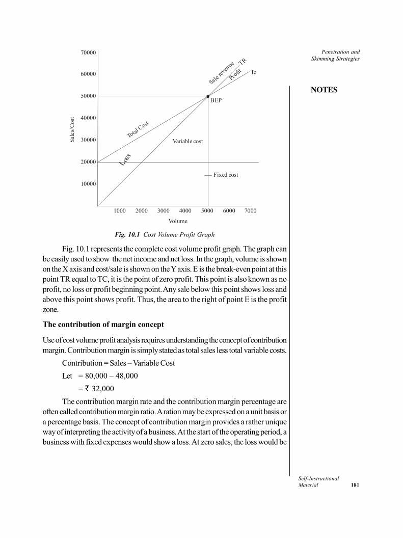
Penetration andSkimming Strategies
NOTES
Self-InstructionalMaterial 181
1000 2000 3000 4000 5000 6000 7000
10000
20000
30000
40000
50000
60000
70000
Volume
Sale
s/C
ost
Loss
Total Cost
Sale rev
enue
Profit
Variable cost
Fixed cost
BEP
TcTR
Fig. 10.1 Cost Volume Profit Graph
Fig. 10.1 represents the complete cost volume profit graph. The graph canbe easily used to show the net income and net loss. In the graph, volume is shownon the X axis and cost/sale is shown on the Y axis. E is the break-even point at thispoint TR equal to TC, it is the point of zero profit. This point is also known as noprofit, no loss or profit beginning point. Any sale below this point shows loss andabove this point shows profit. Thus, the area to the right of point E is the profitzone.
The contribution of margin concept
Use of cost volume profit analysis requires understanding the concept of contributionmargin. Contribution margin is simply stated as total sales less total variable costs.
Contribution = Sales – Variable Cost
Let = 80,000 – 48,000
= 32,000
The contribution margin rate and the contribution margin percentage areoften called contribution margin ratio. A ration may be expressed on a unit basis ora percentage basis. The concept of contribution margin provides a rather uniqueway of interpreting the activity of a business. At the start of the operating period, abusiness with fixed expenses would show a loss. At zero sales, the loss would be
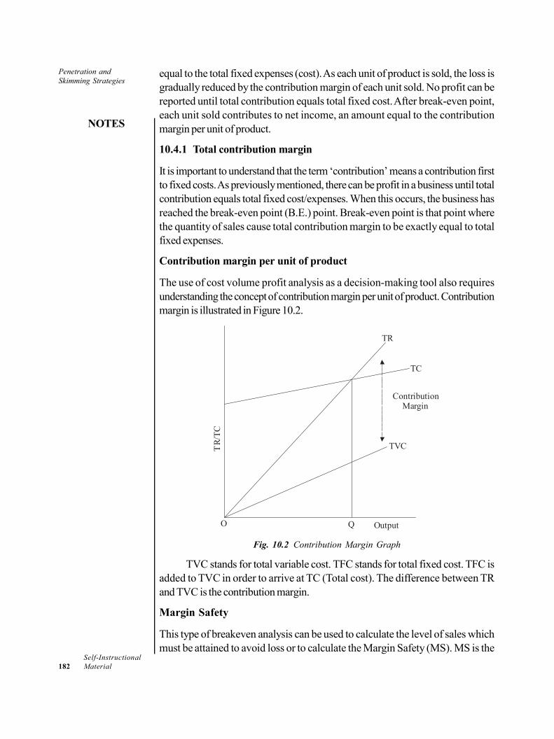
Penetration andSkimming Strategies
NOTES
Self-Instructional182 Material
equal to the total fixed expenses (cost). As each unit of product is sold, the loss isgradually reduced by the contribution margin of each unit sold. No profit can bereported until total contribution equals total fixed cost. After break-even point,each unit sold contributes to net income, an amount equal to the contributionmargin per unit of product.
10.4.1 Total contribution margin
It is important to understand that the term ‘contribution’ means a contribution firstto fixed costs. As previously mentioned, there can be profit in a business until totalcontribution equals total fixed cost/expenses. When this occurs, the business hasreached the break-even point (B.E.) point. Break-even point is that point wherethe quantity of sales cause total contribution margin to be exactly equal to totalfixed expenses.
Contribution margin per unit of product
The use of cost volume profit analysis as a decision-making tool also requiresunderstanding the concept of contribution margin per unit of product. Contributionmargin is illustrated in Figure 10.2.
TC
TR
ContributionMargin
TVC
OutputQO
TR
/TC
Fig. 10.2 Contribution Margin Graph
TVC stands for total variable cost. TFC stands for total fixed cost. TFC isadded to TVC in order to arrive at TC (Total cost). The difference between TRand TVC is the contribution margin.
Margin Safety
This type of breakeven analysis can be used to calculate the level of sales whichmust be attained to avoid loss or to calculate the Margin Safety (MS). MS is the
Penetration andSkimming Strategies
NOTES
Self-InstructionalMaterial 183
difference between the firm’s actual level of sales and sales at the BEP point. It isexpressed as the following:
MS = Actual sales revenue – B.E. Sales
However, firms calculate the MS in terms of ration as
MS Ratio = MS
Actual Sales
The MS is an indicator of the strength of a firm. If margin is large, it showsthat the firm can make profit even if it has to face difficulties. On the other hand, ifthe margin is small, a small reduction in sales can lead to loss. MS is nil at the BEPoint because actual sales volume is equal to the cost.
10.4.2 Basic Assumptions of Cost Volume Profit Analysis
Cost volume profit analysis may be used as a profit planning tool and therebyit is useful in decision making. However, effective use of cost volume profitanalysis for planning purposes requires understanding of certain basicassumptions. Unless the following assumptions are substantially met, any attemptto use cost volume profit analysis in a real world situation may prove to beinaccurate and misleading.
The basic assumptions underlying the cost volume profit analysis can besummarized as follows:
Within a relevant range of volume, the variables namely, price, quantity,fixed costs and variable costs are subject to managerial control.
Price and the variable cost rate are constant within the relevant range ofactivity.
This assumption simply means that variable costs and revenue are assumedto vary early with changes in volume. Stated differently, changes in volumehave no effect on price, the variable cost rate and fixed costs.
In a company selling multiple products, the sales mix ratio remains constantwith changes in total sales.
In a company that uses absorption costing unless sales equals production,there exists no unique break-even point. When direct costing is used, noproblems arise where production varies from sales. In direct costing, fixedmanufacturing overhead is treated as a period charge.
Cost volume profit analysis is a powerful analytical tool. It can be effectivelyused in different kinds of decisions. Cost volume profit analysis is based on thetheory of cost behaviour and as such it is imperative that the management has agood understanding of the cost behaviour.
Penetration andSkimming Strategies
NOTES
Self-Instructional184 Material
10.5 PRICING OF A NEW PRODUCT
A new product may simply be either another brand name added to the existingones or an altogether new product. Pricing a new brand for which there are severalsubstitutes available in the market is not as big a problem as pricing a new productfor which close substitutes are not available. In case of the former (where thereare several substitutes available in the market), the market provides adequateinformation regarding cost, demand and availability of market and so forth. In thiscase, pricing depends on the nature of the market. In pricing a new product withoutclose substitutes, however, problems arise due to lack of information; hence, thereis some degree of uncertainty.
Thus, the pricing policy in respect of new products depends on whether ornot close substitutes are available. Depending on whether or not close substitutesare available in pricing a new product, generally two kinds of pricing policies areavailable: (i) Penetration Price Policy and (ii) Skimming Price Policy.
1. Penetration Price Policy: In contrast to the skimming price policy, thepenetration price policy involves a reserve strategy. This pricing policy is generallyadopted in the case of new products for which substitutes are available. Thispolicy requires fixing a lower initial price designed to penetrate the market asquickly as possible and is intended to maximize the profits in the long run. Therefore,the firm pursuing the penetration price policy sets a low price of the product in theinitial stage. As the product slowly becomes popular in the market, its price isgradually increased. The success of the penetration price policy requires theexistence of the following conditions:
(i) The short run demand for the product should have elasticity greater thanunity e
p > 1. It helps in capturing the market at lower prices.
(ii) Economics of large scale production are available to the firm with the increasein sales. Otherwise, increase in production would result in increase in costswhich might reduce the competitiveness of the price.
(iii) The product should have a high cross elasticity in relation to rival productsfor the initial lower price to be effective.
(iv) The potential market for the product is fairly large and has a good deal offuture prospects.
(v) The product by nature should be such that it can be easily accepted andadopted by the consumers.
2. Skimming Price Policy: The skimming price policy is adopted where closesubstitutes of a new product are not available. This pricing strategy is intended toskim the cream of the market, i.e., consumer’s surplus, by setting a high initial
Penetration andSkimming Strategies
NOTES
Self-InstructionalMaterial 185
price, three or four times the ex-factory price, and a subsequent lowering of pricesin a series of reduction especially in case of consumer durables. The initial highprice would generally be accompanied by heavy sales promoting expenditure.This policy succeeds due to the following reasons:
(i) In the initial stage of the introduction of products, demand is relatively inelasticbecause of consumers design for distinctiveness by the consumption of anew product.
(ii) Cross elasticity is usually very low for lack of a close substitute.
(iii) Step by step price cut help skimming consumers surplus available at thelower segment of demand curve.
(iv) High initial prices are helpful in recouping the development costs.
The post skimming strategy includes the decisions regarding the time andsize of price reduction. The appropriate occasion for price reduction is the time ofsaturation of the top level demand or when a strong competition is apprehended.As regards the rate of price reduction, when the product is on its way to losing itsdistinctiveness, the price cut should be appropriately larger. But if the product hasretained its exclusiveness, a series of small price reductions would be moreappropriate.
The choice between the two strategic price policies depends on the followingaspects:
(i) The rate of market growth
(ii) The rate of erosion of distinctiveness, and
(iii) The cost structure of the producers
If the rate of the market growth is slow for such reasons as lack of information,consumers’ hesitation and other factors then the penetration price policy would beunsuitable. The reason is that a low price will not imply sale of more number ofunits. If the pioneer product is likely to lose its distinctiveness at a faster rate thenthe skimming price policy would be unsuitable. It should be followed when thelead time i.e., the period of distinctiveness is fairly long. If its cost structure showsincreasing return overtime; penetration pricing policy would be more suitable, sinceit enables the producer to reduce the cost and prevents potential competitors fromentering the market in the short run.
Government Control over Pricing
General price controls—controls on prices of many goods—are often imposedwhen the public becomes alarmed that inflation is out of control.
In India, price control has been one of the major instruments used by thegovernment for accomplishing economic goals and for the implementation of Five
Penetration andSkimming Strategies
NOTES
Self-Instructional186 Material
Year Plans.
Why is price control required?
The price mechanism in a free enterprise economy leads to an optimum allocationof resources subject to certain assumptions.
The imposition of the price control mechanism in the context of the Indianeconomy needs to consider the following aspects:
(i) It is vital to analyse the choice of products within the framework of economicjustification for imposing price controls on them.
(ii) It is necessary to evaluate the impact of price control mechanism on theflow of investment resources especially on those products that are subjectto price control.
Check Your Progress
1. State one difference between gross profit and net profit.
2. Mention the five changes which according to J.B. Clark give rise to profitsin a dynamic economy.
3. Who propounded the innovation theory of profit?
10.6 ANSWERS TO CHECK YOUR PROGRESS
1. Actual loss can be calculated from gross profit, but in the case of net profitsthis is not possible.
2. The five changes which according to J.B. Clark give rise to profits in adynamic economy are the following:
Increase in population.
Changes in the quantity and quality of human wants
Changes in methods or techniques of production
Changes in the amount of capital
Changes in the forms of business organization
3. The innovation theory of profit is propounded by Professor J.A. Schumpeter.
10.7 SUMMARY
In ordinary language, profit is the surplus of income over expenses ofproduction according to a businessman. Profit is the fourth component offactor pricing.
Penetration andSkimming Strategies
NOTES
Self-InstructionalMaterial 187
In general, profit is the difference between coast and the price of thecommodity. In more technical terms, profit implies a positive residual of anentrepreneur after deducting the total cost from the total revenue.
Profits are non-contractual income, therefore, they may be positive ornegative, whereas the contractual income of other factors such as wage,rent, interest are always positive and never negative.
Gross profit refers to that part of the income of a businessman which isavailable to him after all payment to the contractually hired factors and othercurrent obligations like taxes and depreciation charges.
Pure profit is the amount that is available to the entrepreneur for assumingrisk inseparable from all business in anticipation of demand.
Profit is the reward for the enterprise. No doubt profit is associated withthe entrepreneur and his function but the economists from time to time haveexpressed diverse and conflicting views about the nature, origin and role ofprofit.
J.M. Keynes expressed the view that profits resulted from the favourablemovements of general price level. J. Robinson, E.H. Chamberlin and M.Kalecki have associated profit with the imperfect competition and monopoly.
Professor J.B. Clark propounded his dynamic theory of profit in 1900.According to him, profit is defined as the difference between price and costof production of a commodity.
It should be noted that due to disequilibrium profits arise from unanticipatedchanges in demand or cost conditions. If the changes could be foreseen inadvance, then suitable adjustments can be made according to the anticipatedchanges so that forces of competition do not drive profits to zero.
The innovation theory of profit is propounded by Professor J.A. Schumpeter.It has been held by J.A. Schumpeter that the main function of the entrepreneuris to introduce innovation in the economy and profits are the reward whichhe earns for performing his functions.
Professor F.H. Knight in his classic work, “Risk, uncertainty and Profit”propounded the theory of profit. According to him, “Profit is the reward notfor risk bearing but for uncertainty bearing.” He accepts that the dynamicchanges and risk bearing are all important elements of profit. As the future isuncertain and unpredictable, any entrepreneur who probes in the darknessdoes so only with a view to earn some profit.
The risk theory of profit was propounded by F.B. Hawley who regardedrisk taking ability as the main function of the entrepreneur. Profit is the residualincome which the entrepreneur receives because he assumes risks.
Penetration andSkimming Strategies
NOTES
Self-Instructional188 Material
The success of a business as measured in term of profit depends upon itssales. The volume of sales must be sufficient to cover all costs and allow asatisfactory margin for net income.
The primary objective of the management in using cost volume profit analysisis to determine the target income point and not the break-even point. Thebreak-event point is simply the quantity of sales that achieve net zero income.
Break-even point is that point where the quantity of sales cause totalcontribution margin to be exactly equal to total fixed expenses.
Cost volume profit analysis may be used as a profit planning tool and therebyit is useful in decision making. However, effective use of cost volume profitanalysis for planning purposes requires understanding of certain basicassumptions.
A new product may simply be either another brand name added to theexisting ones or an altogether new product. Pricing a new brand for whichthere are several substitutes available in the market is not as big a problemas pricing a new product for which close substitutes are not available.
Depending on whether or not close substitutes are available in pricing anew product, generally two kinds of pricing policies are available: (i)Penetration Price Policy and (ii) Skimming Price Policy.
10.8 KEY WORDS
Gross profit: It is the difference between total revenue of entrepreneurand total explicit costs.
Break-even point: It is the production level where total revenues equalstotal expenses.
10.9 SELF ASSESSMENT QUESTIONS ANDEXERCISES
Short Answer Questions
1. Define profit.
2. Write a short note on the types of profit.
3. What are the criticisms raised against the uncertainty – bearing theory ofprofit?
4. Mention the major tenets of the risk theory of profit.
5. What is margin safety? How is it calculated?
Penetration andSkimming Strategies
NOTES
Self-InstructionalMaterial 189
Long Answer Questions
1. Discuss the Innovation theory propounded by J.A. Schumpeter.
2. Explain the Dynamic theory of profit.
3. Analyse the use of Cost volume profit analysis as a decision-making tool.
4. Describe the pricing policies adopted for launching new products in themarket.
10.10 FURTHER READINGS
Dwivedi, D. N. 2015. Principles of Economics, Eight Edition. New Delhi: VikasPublishing House.
Weil. David N. 2004. Economic Growth. London: Addison Wesley.
Thomas, Christopher R. and Maurice S. Charles. 2005. Managerial Economics:Concepts and Applications, Eighth Edition. New Delhi: Tata McGraw-Hill Publishing Company Limited.
Mankiw, Gregory N. 2002. Principles of Economics, Second Edition. India:Thomson Press.
Websites
https://blogs.economictimes.indiatimes.com/et-commentary/heres-how-indias-widening-income-distribution-can-be-redressed/
https://www.livemint.com/Opinion/WmpSjQAvPGeVzxqpgXYvtK/The-dangers-of-Indias-Billionaire-Raj.html
Profit and Investment Analysis
NOTES
Self-Instructional190 Material
UNIT 11 PROFIT AND INVESTMENTANALYSIS
Structure11.0 Introduction11.1 Objectives11.2 Meaning and Measurement of Profit11.3 Theories of Pricing
11.3.1 Cost-Plus Pricing11.3.2 Multiple Product Pricing11.3.3 Pricing in the Life-Cycle of a Product11.3.4 Transfer Pricing11.3.5 Peak Load Pricing
11.4 Profit Planning and Forecasting11.4.1 Profit and Wealth Maximization11.4.2 Cost Volume Profit Analysis
11.5 Investment Analysis and Evaluation11.5.1 Internal Rate of Return (IRR)11.5.2 Net Present Value (NPV)11.5.3 Adjusted Present Value (APV)
11.6 Answers to Check Your Progress Questions11.7 Summary11.8 Key Words11.9 Self Assessment Questions and Exercises
11.10 Further Readings
11.0 INTRODUCTION
The first and foremost responsibility of business managers is to achieve the objectiveof the firm they manages. Therefore, all their managerial decisions, policies, strategyand functions are directed towards the attainment of the objective of the firm. Aquestion that arises here is: What is the objective of business firms? The quickanswer to this question is ‘making maximum profit, of course!’ However, economistsdo not agree with this answer. According to Baumol, a Nobel laureate in Economicsand an authority on business economics, ‘It is most frequently assumed in economicanalysis that the firm is trying to maximize its total profit. However, there is noreason to believe that all business firms pursue the same objective’. ‘In fact, it iscommon experience when interviewing executives to find that they will agree toevery plausible goal about which they are asked. The say they want to maximizesales and also to maximize profits; that they wish ... to minimize cost; and so on’.In this unit, we will concentrate on the profit maximizing objective of the businessfirms. We will also explain how firms formulate their strategic pricing policy anddetermine the price of their product. Finally, we will also discuss the investmentrelated tools which are employed by companies for achieving good returns.
Profit and Investment Analysis
NOTES
Self-InstructionalMaterial 191
11.1 OBJECTIVES
After going through this unit, you will be able to: Describe the meaning and measurement of profit Discuss the different theories of pricing Explain the profit and wealth maximization objective of firms Recall some tools of investment analysis and evaluation
11.2 MEANING AND MEASUREMENT OF PROFIT
Profit means different things to different people. “The word ‘profit’ has differentmeaning to businessmen, accountants, tax collectors, workers and economistsand it is often used in a loose polemical sense that buries its real significance…” Ina general sense, ‘profit’ is regarded as income accruing to entrepreneurs, in thesame sense as wages accrue to the labour; rent accrues to the owners of rentableassets; and interest accrues to the moneylenders. To a layman, profit means allincome that flows to the investors. To an accountant, ‘profit’ means the excess ofrevenue over all paid-out costs including both manufacturing and overheadexpenses, also known as ‘accounting profit’. It is more or less the same as ‘netprofit’. For all practical purposes, profit means accounting profit plus non-allowableexpenses. Profit figures published by the business firms are profits conforming toaccounting concept of profit. Economist’s concept of profit is of ‘pure profit’, alsocalled ‘economic profit’ or ‘just profit’. Pure profit is a return over and above theopportunity cost, i.e., the income which a businessman might expect from thesecond best alternative use of his resources. The accounting and economic conceptsof profit are discussed below in detail.
Accounting Profit vs. Economic Profit
The two important concepts of profit that figure in business decisions are ‘economicprofit’ and ‘accounting profit’. From conceptual clarity point of view, it is useful tounderstand the difference between the two concepts of profit. As already mentioned,in accounting sense, profit is surplus of total revenue over and above all paid-outcosts, including both manufacturing and overhead expenses. Accounting profitmay be calculated as follows.
Accounting profit = TR – (W + R + I + M)
where TR = total revenue, W = wages and salaries, R = rent, I = interest,and M = cost of materials.
Obviously, while calculating accounting profit, only explicit or book costs,i.e., the costs recorded in the books of accounts, are considered.
Profit and Investment Analysis
NOTES
Self-Instructional192 Material
It should also be noted that economic or pure profit makes provision alsofor (a) insurable risks, (b) depreciation, and (c) necessary minimum payment toshareholders to prevent them from withdrawing their capital. Pure profit may thusbe defined as ‘a residual left after all contractual costs have been met, includingthe transfer costs of management, insurable risks, depreciation and payments toshareholders sufficient to maintain investment at its current level’. Thus,
Pure profit = Total revenue – (explicit costs + implicit costs)
Alternatively, pure profit may be defined as follows.
11.3 THEORIES OF PRICING
Up till now we have discussed the conventional theories of price determinationunder the conditions of different market structures, under the postulate that firms’objective is to maximize profit. The alternative theories of firm offered by the nextgeneration of economists have built their theories assuming different objectives offirms. A section of economists has built game theory and have shown its applicationto business decision-making. As noted in previous units, all these theories andstrategic models have their own deficiencies and problems in application becauseof increasing complexity of the business world. The other economists haverecognized the complexity of business world and have explained how firmsformulate their strategic pricing policy and determine the price of their product.We begin our discussion by explaining the cost-plus pricing method of productpricing.
Profit and Investment Analysis
NOTES
Self-InstructionalMaterial 193
11.3.1 Cost-Plus Pricing
Cost-plus pricing is also known as ‘mark-up pricing’, ‘average cost pricing’and ‘full cost pricing’. The cost-plus pricing is the most common method ofpricing used by the manufacturing firms. The general practice under this method isto add a ‘fair’ percentage of profit margin to the average variable cost (AVC). Theformula for setting the price is given as
P = AVC + AVC (m) …(11.1)where AVC = average variable cost, and m = mark-up percentage, and AVC (m) =gross profit margin (GPM).
The mark-up percentage (m) is fixed so as to cover average fixed cost(AFC) and a net profit margin (NPM). Thus,
AVC (m) = AFC + NPM …(11.2)
The general procedure followed by the firms for arriving at AVC and pricefixation may be summarized as follows.
The first step in price fixation is to estimate the average variable cost. Forthis, the firm has to ascertain the volume of its output for a given period of time,usually one accounting or fiscal year. To ascertain the output, the firm uses figuresof its ‘planned’ or ‘budgeted’ output or takes into account its normal level ofproduction. If the firm is in a position to compute its optimum level of output or thecapacity output, the same is used as standard output in computing the averagecost.
The next step is to compute the total variable cost (TVC) of the ‘standardoutput.’ The TVC includes direct cost, i.e., the cost of labour and raw material,and other variable costs e.g., electricity and transportation cost, etc. These costsadded together give the total variable cost. The ‘Average Variable Cost’ (AVC)is then obtained by dividing the total variable cost (TVC) by the ‘standard output’(Q), i.e.,
AVC = TVC
Q
After AVC is obtained, a ‘mark-up’ in the form of some percentage of AVCis added to it as profit margin and the price is fixed. While determining the mark-up, firms always take into account ‘what the market will bear’ and the degree ofcompetition in the market.
11.3.2 Multiple Product Pricing
Most microeconomic models of price determination are based on the assumptionthat a firm produces a single, homogeneous product. In actual practice, however,production of a single homogeneous product by a firm is an exception rather thana rule. Almost all firms have more than one product in their line of production.Even the most specialized firms produce a commodity in multiple models, styles
Profit and Investment Analysis
NOTES
Self-Instructional194 Material
and sizes, each so much differentiated from the other that every model or size ofthe product may be considered a different product. For example, the variousmodels of refrigerators, TV sets, cell phones, computers and car models etc.produced by the same company may be treated as different products for at leastpricing purpose. The various models are so differentiated that consumers viewthem as different products and, in some cases, as close substitutes for each other.It is for this reason that each model or product has different AR and MR curvesand that one product of the firm competes against the other product. The pricingunder these conditions is known as multi-product pricing or product-line pricing.
The major problem in pricing multiple products is that each product has aseparate demand curve. But, since all the products are produced under oneestablishment by interchangeable production facilities, they have only one jointand one inseparable marginal cost curve (MC). That is, while revenue curves, ARand MR, are separate for each product, cost curves, AC and MC, are inseparable.Therefore, the marginal rule of pricing cannot be applied straightaway to fix theprice of each product separately. The problem, however, has been provided witha solution by E.W. Clemens. The solution is similar to the technique employed toillustrate third degree price discrimination under profit maximization assumption.As a discriminating monopoly tries to maximize its revenue in all its markets, sodoes a multi-product firm in respect of each of its products.
11.3.3 Pricing in the Life-Cycle of a Product
The life-cycle of a product is generally divided into five stages: (i) Introduction orinitial stage, (ii) Growth, (iii) Maturity, (iv) Saturation, and (v) Decline. Theintroduction phase is the period taken to introduce the product to the market.The total sale during this period is limited to the quantity put on the market for trialwith considerable advertisement. The sales during this period remain almostconstant. Growth is the stage, after a successful trial, during which the productgains popularity among the consumers and sales increase at an increasing rate asa result of cumulative effect of advertisement over the initial stage. Maturity is thestage in which sales continue to increase but at a lower rate and the total saleeventually becomes constant. During the saturation period the total salesaturates—there is no considerable increase or decrease in the sales. After thesaturation stage, comes the stage of decline in which total sales begin to declinefor such reasons as (i) increase in the availability of substitutes, and (ii) the loss ofdistinctiveness of the product.
The pricing strategy varies from stage to stage over the life-cycle of aproduct, depending on the market conditions. From the pricing strategy point ofview, growth and maturity stages may be treated likewise.
11.3.4 Transfer Pricing
Large size firms often divide their production process into different product divisionsor their subsidiaries. Also, growing firms add new divisions or departments to the
Profit and Investment Analysis
NOTES
Self-InstructionalMaterial 195
existing ones. The firms then transfer some of their production activities to otherdivisions. The goods and services produced by the new divisions are used by theparent organization. In other words, the parent division buys the product of itssubsidiaries. Such firms face the problem of determining an appropriate price forthe product transferred from one division or subsidiary to the parent body. Thisproblem becomes much more difficult when each division has a separate profitfunction to maximize. Pricing of intra-firm ‘transfer product’ is referred to as ‘transferpricing’. One of the most systematic treatments of the transfer pricing techniquehas been provided by Hirshleifer. We will discuss here briefly his technique oftransfer pricing.
To begin with, let us suppose that a refrigerator company established adecade ago used to produce and sell refrigerators fitted with compressors boughtfrom a compressor manufacturing company. Now the refrigerator company decidesto set up its own subsidiary to manufacture compressors. Now the problem forthe company is how to price the product of its subsidiary under the followingconditions.
(i) Both parent and subsidiary companies have their own profit functions tomaximize, and
(ii) The refrigerator company has the option of using all the compressorsproduced by its subsidiary and/or to sell the compressors in a competitivemarket and its demand is given by a straight horizontal line.
Given these condition of the model, transfer pricing is discussed under twoconditions.
(i) The parent company uses the entire output of its subsidiary and there is noexternal market for the compressors, and
(ii) There does exist a competitive market for the compressor and refrigeratorcompany sells also in the open market.
11.3.5 Peak Load Pricing
There are certain non-storable products, e.g., electricity, telephones, transportand security services, etc., which are demanded in varying measures during theday as well as night. For example, consumption of electricity reaches its peak inday time. It is called ‘peak-load’ time. It reaches its bottom in the night. This iscalled ‘off-peak’ time. Electricity consumption peaks in daytime because all businessestablishments, offices and factories come into operation. Electricity consumptiondecreases during nights because most business establishments are closed andhousehold consumption falls to its basic minimum. In Delhi, demand for electricitypeaks during summers due to use of ACs and coolers, and it declines to its minimumlevel during winters. Similarly, consumption of telephone services is at its peak atday time and at its bottom at nights. Another example of ‘peak’ and ‘off-peak’demand is of railway and air services. During festivals, summer holidays, ‘Pooja’vacations, etc., the demand for railway and air travel services rises to its peak.
Profit and Investment Analysis
NOTES
Self-Instructional196 Material
Check Your Progress
1. Define pure profit.2. Mention some of the other names for cost-plus pricing.3. Why does the total sales begin to decline in the last stage of the life-cycle
of a product?
11.4 PROFIT PLANNING AND FORECASTING
Profit forecasting is essential for profit planning in any organization. The projectiveof earnings in the future after taking in to account different factors like costingpolicies, pricing policies, depreciation policies, etc., is known as profit forecasting.This profit estimation is advantageous to the firm for making different projectionsrelated to costs, profits and sales volume.
Some researches have suggested different approaches to profit forecasting.As per Joel Deal, profit forecasting can be done through the following threeapproaches: (1) break-even analysis; (2) spot projection which includes projectionfor the specified future period; and environmental analysis which is analysis relatedto the factors in the economic environment which are beyond the scope of theenterprises.
Several elements of business have an impact on the profits of the businessfirms. These elements are known to have some type of pattern or the other. Elementslike rate of output, material costs, wages, efficiency work in a pattern at thecompany, industry and national levels. They are interdependent and have a bearingon each other. If these patterns are studied in a proper manner, these can be usedto improving the chances of the firms to earn profits and in fact help them find therelation between specific profit making variables. Profit planning and forecastingaims to decode this functional relationship so as to work for the profit maximizationof the firms.
11.4.1 Profit and Wealth Maximization
The conventional economic theory assumes profit maximization as the onlyobjective of business firms—profit measured as TR–TC.Profit maximization asthe objective of business firms has a long history in economic literature. It formsthe basis of conventional price theory. Profit maximization is regarded as the most
Profit and Investment Analysis
NOTES
Self-InstructionalMaterial 197
reasonable and analytically the most ‘productive’ business objective. The strengthof this assumption lies in the fact that this assumption ‘has never been unambiguouslydisproved’.
Besides, profit maximization assumption has a greater predictive power. Ithelps in predicting the behaviour of business firms in the real world and also thebehaviour of price and output under different market conditions. No otherhypothesis explains and predicts the behaviour of firms better than the profitmaximization assumption. Nevertheless, the profit maximization has beenquestioned strongly by some modern economists. This created a controversy onobjectives of business firms. The controversy has been discussed below in detail.
Controversy on Profit Maximization: Theory vs. Practice
As discussed above, the conventional theory of firm assumes profit maximizationas the sole objective of the business firms. Some modern economists, however,refute the profit maximization assumption because, in their opinion, it is practicallynon-achievable. Their own findings reveal that business firms, especially bigcorporations, pursue several other objectives, rather than profit maximization.However, some modern economists have strongly defended the profit maximizationobjective. This has created a controversy on the profit maximization objective ofthe business firms. In this section, we discuss briefly the arguments against and forprofit maximization objective.
Arguments against Profit-Maximization Objective
(i) The first argument against the profit maximization objective is based onthe dichotomy between the ownership and management of business firms.It is argued that, in modern times, due to rapid growth of large businesscorporations, management of business firms has got separated from theownership. The separation of management from ownership gives managersan opportunity and also the discretion to set firm’s goals other than profitmaximization. The researches conducted by the economists reveal that, inpractice, business managers pursue such objectives as: (a) maximizationof sales revenue, (b) maximization of the value of the firm, i.e., the networth of the firm, (c) maximization of managerial utility function,(d) maximization of firm’s growth rate, (e) making a target profit,(f) retaining and increasing market share, and so on.
(ii) Another argument against profit maximization objective is that traditionaltheory of firm assumes managers to have full and perfect knowledge ofmarket conditions and of the possible future development in businessenvironment of firm. The firm is thus supposed to be fully aware of its demandand cost conditions in both short and long runs. Briefly speaking underprofit maximization objective, a complete certainty about the marketconditions is assumed. Some modern economists question the validity ofthis assumption. They argue that the firms do not possess the perfect
Profit and Investment Analysis
NOTES
Self-Instructional198 Material
knowledge of their costs, revenue and future business environment. Theyoperate in the world of uncertainty. Most price and output decisions arebased on probabilities.Besides, it is further argued that the equi-marginal principle of profit
maximization, i.e., equalizing MC and MR, has been claimed to be ignored in thedecision-making process of the firms. Empirical studies of the pricing behaviour ofthe firms have shown that the marginal rule of pricing does not stand the test ofempirical verification. Hall and Hitch have found, in their study of pricing practicesof 38 UK firms, that the firms do not pursue the objective of profit maximizationand that they do not use the marginal principle of equalizing MR and MC in theirprice and output decisions. According to them, most firms aim at long-run profitmaximization. In the short-run, they set the price of their product on the basis ofaverage cost principle, so as to cover AC = AVC + AFC (where AC = Averagecost, AVC = Average variable cost, AFC = Average fixed cost) and a normalmargin of profit (usually 10 per cent).
In a similar study, Gordon has found (i) that there is a marked deviationin the real business conditions from the assumptions of the traditional theory, and(ii) that pricing practices were notably different from the marginal theory of pricing.Gordon has concluded that the real business world is much more complex thanthe one postulated by the theorists. Because of the extreme complexity of the realbusiness world and ever-changing conditions, the past experience of the businessfirms is of little use in forecasting demand, price and costs. The firms are notaware of their MR and MC. The average-cost-principle of pricing is widely usedby the firms. Findings of many other studies of the pricing practices lend supportto the view that there is little link between pricing theory and pricing practices.
The Defence of Profit Maximization
The arguments against profit-maximization objectives have been strongly rejectedby other economists. They argued strongly that pricing theory does have relevanceto the actual pricing policy of the business firms. A section of economists hasstrongly defended the profit maximization objective and ‘marginal principle’ ofpricing and output decisions.
The conventional economic theorists defend the profit maximizationhypothesis on the following grounds.
1. Profit is indispensable for firm’s survival. The survival of all the profit-oriented firms in the long run depends on their ability to make a reasonableprofit depending on the business conditions and the level of competition.What profit is reasonable may be a matter of opinion. But, making profit isa necessary condition for the survival of the firm. Once the firms begin tomake profit, they try to maximize it.
Profit and Investment Analysis
NOTES
Self-InstructionalMaterial 199
2. Achieving other objectives depends on firm’s ability to make profit.Many other objectives of business firms have been cited in economicliterature, e.g., maximization of managerial utility function, maximization oflong-run growth, maximization of sales revenue, satisfying all the concernedparties, increasing and retaining market share, etc. The achievement of suchalternative objectives depends wholly or at least partly on the primaryobjective of making profit.
3. Evidence against profit maximization objective is not conclusive.Profit maximization is a time-honoured objective of business firms. Althoughthis objective has been questioned by many researchers, some economistshave argued that the evidence against it is not conclusive or unambiguous.
4. Profit maximization objective has a greater predicting power.Compared to other business objectives, profit maximization objective hasbeen found to provide a much more powerful basis for predicting certainaspects of firms’ behaviour. As Friedman has argued, the validity of theprofit maximization objective cannot be judged by a priori logic or by askingbusiness executives, as some economists have done. In his opinion, ultimatetest of its validity lies in its ability to predict the business behaviour and thebusiness trends.
5. Profit is a more reliable measure of a firm’s efficiency. Though notperfect, profit is the most quick and reliable measure of the efficiency of afirm. It is also the source of internal finance. Profit as a source of internalfinance assumes a much greater significance when financial market is highlyvolatile. The recent trend shows a growing dependence on the internal financein the industrially advanced countries. In fact, in developed countries,internal sources of finance contribute more than three-fourths of thetotal finance.
6. Finally, according to Milton Friedman, whatever one may say about firms’motivations, if one judges their motivations by their managerial acts, profitmaximization appears to be a more valid business objective.
11.4.2 Cost Volume Profit Analysis
The theory of cost guides both the analysts and the firms to find the nature ofchange in cost of production with change in output. Also, it provides conditions fordetermining cost minimizing output. However, despite its high analytical value, costtheory does not provide answer to certain basic questions pertaining to businessdecisions of new firms. Some such questions are: (i) given the product price andcost, what is the minimum output to recover the total cost? (ii) what is the output atwhich total cost (TC) and total revenue (TR) break-even? and (iii) if anticipatedTR and TC functions produce non-linear curves, what output would maximize the
Profit and Investment Analysis
NOTES
Self-Instructional200 Material
profit? The economists have developed a new technique, in addition to costanalysis, that can be used to find answer to these questions. The technique isknown as Break-Even analysis known also as Profit Contribution Analysisand Cost-Volume Profit Analysis.
Meaning of Break-even Analysis
The break-even analysis is an important analytical technique used to study therelationship between the total costs, total revenue and total profit and loss overthe whole range of stipulated output. The break-even analysis is a technique ofhaving a preview of profit prospects and a tool of profit planning. It integrates thecost and revenue estimates to ascertain the profits and losses associated withdifferent levels of output.
The relationship between cost and output and between price and outputmay be linear or non-linear in nature.
11.5 INVESTMENT ANALYSIS AND EVALUATION
Investment is an activity of spending resources (money, labour and time) oncreating assets that can generate income over a long period of time or whichenhances the returns on the existing assets. In a broader sense of the term,investments that generate returns over a number of years can be classified underfollowing categories.
1. Investment in Financial Assets including bank deposits, deposits withcompanies, contribution to provident fund (in excess of compulsorydeduction), shares and debentures, government bonds and treasury bills,purchase of NSC, buying units, personal lending, etc.
2. Investment in Physical Assets including purchase of land, building,machinery, plants, etc.
3. Investment in Human Capital including expenditure on skill formationthrough education and training that increases productivity and earningcapacity of a person.
4. Miscellaneous Investment including expenditure on replacement ofdepreciated and obsolete machinery, product diversification, R&D,installation of safety measures for employees, pollution control for publichealth and safety, and meeting legal requirements.
Investment Decisions under Certainty
In this section, we discuss the methods of investment decisions under the conditionof certainty. In the context of investment, certainty means that investors havecomplete knowledge about the market conditions, especially the investmentopportunities, cost of capital and the expected returns on the investment.
Profit and Investment Analysis
NOTES
Self-InstructionalMaterial 201
Specifically, certainty means that there is only one outcome of investment and it isknown and assured to the investor. For example, money put in fixed deposit in abank yields an assured return with full certainty.
(i) Pay-back (or pay-out) period;(ii) Net discounted present value, and(iii) Internal rate of return or marginal efficiency of capital.
These criteria are equally applicable to a variety of investment decisionsregarding new investments and those pertaining to replacement, scrapping, andwidening or deeping of capital. Incidentally, from analysis point of view, there is nostructural difference between decisions on new investment and those onreplacement.
11.5.1 Internal Rate of Return (IRR)
120 million(1 + )r = ̀ 100 million
= (1 + r) 100 = 120
and r = 0.20
The IRR of this project is 0.20 or 20 per cent. No other value of r canequate the NPV of the project with its cost.
The IRR or MEI is defined as ‘the rate of interest or return which rendersthe discounted present value of its expected future marginal yields exactlyequal to the investment cost of project’. In other words, ‘IRR is the rate ofreturn (r) at which the discounted present value of receipts and expenditures areequal’. The IRR of a project yielding a stream of returns over n years and involvingdifferent investment costs can be obtained by using the formula given in Eq. (11.3).
1 1(1 ) (1 )
n nn n
n nj j
R Cr r
...(11.3)
or1 1(1 ) (1 )
n nn n
n nj j
R Cr r
= 0 ...(11.4)
Profit and Investment Analysis
NOTES
Self-Instructional202 Material
11.5.2 Net Present Value (NPV)
The Concept of Present Value: The Time Value of Money. The concept ofthe present value of money is very well reflected in the proverb ‘a bird in the handis worth two in the bush’. In general, money received today is valued more thanmoney receivable tomorrow. Cash in hand is valued more because it gives(i) liquidity and (ii) an opportunity to invest it and earn return (interest) on it. Thisis called the time value of money. The concept of the time value of money is veryoften applied to investment decisions. Generally, there is a time-lag betweeninvestment and its returns. When an investment is made today, it begins to yieldreturns at some future date. The time gap between the investment and the firstreturn from the investment is called ‘time lag’. During the time lag, the investorloses interest on the expected incomes. This implies that a rupee received today isworth more than a rupee receivable at some future date. Or conversely, a rupeeexpected one year hence is worth less than a rupee today. In the context of thetime value of money, the present value of a future income is lower than its value ifreceived today.
The concept of present value of money can be explained through an example.Suppose that a sum of `100 held in cash today is deposited in a bank at 10per cent rate of interest. After one year, ̀ 100 today will increase to ̀ 110. Theamount (principal + interest) is worked out as follows.
Amount = 100 + 100 (10/100)
= 100 + 10 = 110
It follows that ̀ 110 expected one year hence is worth only ̀ 100 today.This means that ̀ 100 is the present value of ̀ 110 to be earned after a period ofone year at the interest rate of 10 per cent. The present value (PV) of `110 can beobtained as follows.
PV of `110 = 110
(1 0.1) = 100
The present value of a future income may thus be defined as its valuediscounted at the current rate of interest. Alternatively, the present value of anamount expected at a future date is the amount of money which must be investedtoday to get that amount in future.The Formula for Computing Present Value. Suppose that an amount X0 isinvested for a period of one year at a compounding interest rate. At the end of theyear, the total receipt, say X1 can be expressed as
Profit and Investment Analysis
NOTES
Self-InstructionalMaterial 203
X1 = (X0 + r X0) = X0 (1 + r) …(11.5)
Equation (11.5) shows that X0 increases at the rate of (1 + r) to take thevalue X1 after one year. It implies that if X1 is discounted at the same rate ofinterest, it gives its present value (PV). The formula for computing the presentvalue is given below.
PV of X1– = 11
1(1 ) 1
X Xr r
…(11.6)
In Eq. (11.6), 1/(1 + r) is the discount rate for one year. Given the rate ofinterest (i.e., the numerical value for r), any income receivable after one year canbe discounted to its present value. For example, the present value of an income of`500 expected after one year at 10 per cent interest per annum (where r = 0.10),can be calclated as
PV = 500 11 0.10
= 454.55
It means that, at 10 per cent interest rate, the present value of ̀ 500 expectedafter one year is ̀ 454.55. Given the formule in Eq. (11.6), the discount rate (d2)for an income receivable after 2 years will be 1/(1 + r)2, and for an income receivableafter 3 years, d3 = 1/(1 + r)3 and so on. The formula for discount rate for the nthyar is given as
dn = 1
(1 )nr ...(11.7)
The present value (PV) formula of an amount receivable in the nth yar isgiven as
PV = 1
(1 )n nXr
...(11.8)
or PV = (1 )n
nX
r
Present Value of an Income Stream. The formula for calculating the total presentvalue (TPV) of a stream of annual return (R) over n year is given as
TPV = 31 22 3 ...
(1 ) (1 ) (1 ) (1 )n
n
R RR Rr r r r
...(11.9a)
= 1
1(1 )
n
n nj
Rr
or = 1 (1 )
nn
nj
Rr ...(11.9b)
Net Present Value and Investment Decision. Having noted the concept ofpresent value (PV) and the method of calculating PV of a future income, let usnow see how investment decisions are taken on the basis of present value. In fact,
Profit and Investment Analysis
NOTES
Self-Instructional204 Material
present value (PV) adjusted for the cost of investment provides the basis ofinvestment decisions. The PV adjusted for its cost is called ‘Net Present Value’.The investment decision—accepting or rejecting a project—is taken on the basisof net present value. The net present value (NPV) may be defined as the differencebetween the present value (PV) of an income stream and the cost of investment(C), i.e.,
NV = PV – C
or = 1
1(1 )
n
n nj
R Cr
...(11.10)
where C is the total cost of investment without any recurring expenditure.The investment decision rules can be specified as follows.
(i) If NPV > 0, the project is acceptable;(ii) If NPV = 0, the project is accepted or rejected on non-economic
considerations;(iii) If NPV < 0, the project is rejected.
If investment is a recurring expenditure, the total present cost (TPC) for nyears can be calculated in the same manner as present value of an income streamis calulated, i.e.,
TPC = 1 (1 )
nn
nj
Cr ...(11.11)
And then, NPV = 1 1(1 ) (1 )
n nn n
n nj j
R Cr r
= 1 (1 )
nn n
nj
R Cr
...(11.12)
The investment decision rule in this case is the same as given above. If theNPV is positive (i.e., NPV > 0), the project is profitable and acceptable. The firmcan borrow any amount at the existing interest rate (r) and invest in it. When achoice between two projects has to be made, the one with higher NPV would bechosen.
11.5.3 Adjusted Present Value (APV)
The Adjusted Present Value can be defined as the Net Present Value (NPV) orinvestment adjusted for the interest and tax advantages of leveraging debt providedthat equity is the only source of financing.
Amongst the many ways in which a company finances its projects, a companybring into use the unleveraged shareholders’ equity alone as an investment sourcefor the projects. In such situations, the unleveraged cash flows from theshareholder’s equity is utilized to repays associated debts. The company in suchcircumstances becomes entitled to significant tax deductions on the interest
Profit and Investment Analysis
NOTES
Self-InstructionalMaterial 205
component of these payments. The tax deductions received here is advantageousfor the companies to the limit of project’s ultimate profitability, as they increase theproject’s bottom line. Adjusted present values is used in such situations to analysea project’s profitability. This measure reflects the project orinvestment’s NPV adjusted for the tax benefits from interest obligations onoutstanding debts associated with the project or investment.
Any project which is using the un-leveraged equity cash flows as a sourceof finance and is receiving tax deductions for it can be assessed for profitabilityusing APV measures.
Check Your Progress
4. List some of the objectives of business firms which are dependent whollyor at least partly on the primary objective of making profit.
5. What is the Net Present Value (NPV)?
11.6 ANSWERS TO CHECK YOUR PROGRESSQUESTIONS
1. Pure profit is a return over and above the opportunity cost, i.e., the incomewhich a businessman might expect from the second best alternative use ofhis resources.
2. Cost-plus pricing is also known as ‘mark-up pricing’, ‘average cost pricing’and ‘full cost pricing’.
3. The total sales begin to decline in the last stage of the life-cycle of a productfor such reasons as (i) increase in the availability of substitutes, and (ii) theloss of distinctiveness of the product.
4. Some of the objectives of business firms which are dependent wholly oratleast partly on the primary objective of making profit are maximization ofmanagerial utility function, maximization.
5. The net present value (NPV) is defined as the difference between the presentvalue (PV) of an income stream and the cost of investment.
11.7 SUMMARY
Pure profit is a return over and above the opportunity cost, i.e., the incomewhich a businessman might expect from the second best alternative use ofhis resources.
The accounting profit may be calculated as follows: Accounting profit= TR-(W+ R+ I + M), while calculating accounting profit, only explicit or book
Profit and Investment Analysis
NOTES
Self-Instructional206 Material
costs, i.e., the costs recorded in the book of accounts are considered.Economic profit also takes into account the implicit and imputed costs.
Cost-plus pricing is also known as ‘mark-up pricing’, ‘average cost pricing’and ‘full cost pricing’. The cost-plus pricing is the most common method ofpricing used by the manufacturing firms. The general practice under thismethod is to add a ‘fair’ percentage of profit1 margin to the average variablecost (AVC).
Most microeconomic models of price determination are based on theassumption that a firm produces a single, homogeneous product. In actualpractice, however, production of a single homogeneous product by a firmis an exception rather than a rule. It is for this reason that each model orproduct has different AR and MR curves and that one product of the firmcompetes against the other product. The pricing under these conditions isknown as multi-product pricing or product-line pricing.
The life-cycle of a product is generally divided into five stages: (i) Introductionor initial stage, (ii) Growth, (iii) Maturity, (iv) Saturation, and (v) Decline.The pricing strategy varies from stage to stage over the life-cycle of aproduct, depending on the market conditions.
Pricing of intra-firm ‘transfer product’ is referred to as ‘transfer pricing’. There are certain non-storable products, e.g., electricity, telephones,
transport and security services, etc., which are demanded in varying measuresduring the day as well as night. The pricing of such products is known aspeak load pricing.
Profit forecasting means projection of future earnings after considering allthe factors affecting the size of business profits, such as firm’s pricing policies,costing policies, depreciation policy, and so on.
Profit maximization is regarded as the most reasonable and analytically themost ‘productive’ business objective.
The break-even analysis is an important analytical technique used to studythe relationship between the total costs, total revenue and total profit andloss over the whole range of stipulated output.
The IRR or MEI is defined as the rate of interest or return which rendersthe discounted present value of its expected future marginal yields exactlyequal to the investment cost of project.
The concept of present value of an amount expected at a future date is theamount of money which must be invested today to get that amount in future.
Adjusted present value is the net present value or investment adjusted forthe interest and tax advantages of leveraging debt provided that equity isthe only source of financing.
Profit and Investment Analysis
NOTES
Self-InstructionalMaterial 207
11.8 KEY WORDS
Pure Profit: It is a return over and above the opportunity cost. Cost-Plus Pricing: It is a the most common method of pricing used by the
manufacturing firms which includes adding a fair percentage of profit marginto the average variable cost.
Break-Even Analysis: It refers to the technique which integrates the costand revenue estimates to ascertain the profits and losses associated withdifferent levels of output.
Investment: It is an activity of spending resources on creating assets thatcan generate income over a long period of time or which enhances thereturns on the existing assets.
11.9 SELF ASSESSMENT QUESTIONS ANDEXERCISES
Short Answer Questions
1. Differentiate between accounting and economic profit.2. What is the general procedure followed by the firms for arriving at AVC
and price fixation?3. List the five stages of a life-cycle of a product.4. What is cost volume profit analysis?
Long Answer Questions
1. Describe the different theory of pricing.2. Discuss the arguments for and against profit maximization objective.3. Explain the tools of NPV, APV and IRR.
11.10 FURTHER READINGS
Dwivedi, D. N. 2015. Principles of Economics, Eight Edition. New Delhi: VikasPublishing House.
Weil. David N. 2004. Economic Growth. London: Addison Wesley.Thomas, Christopher R. and Maurice S. Charles. 2005. Managerial Economics:
Concepts and Applications, Eighth Edition. New Delhi: Tata McGraw-Hill Publishing Company Limited.
Mankiw, Gregory N. 2002. Principles of Economics, Second Edition. India:Thomson Press.
Profit and Investment Analysis
NOTES
Self-Instructional208 Material
Websites
https://blogs.economictimes.indiatimes.com/et-commentary/heres-how-indias-widening-income-distribution-can-be-redressed/
https://www.livemint.com/Opinion/WmpSjQAvPGeVzxqpgXYvtK/The-dangers-of-Indias-Billionaire-Raj.html
Macro-Economic Factors
NOTES
Self-InstructionalMaterial 209
UNIT 12 MACRO-ECONOMICFACTORS
Structure12.0 Introduction12.1 Objectives12.2 Meaning and Nature of Macro-Economic Factors
12.2.1 Importance of Macro-Economic Factors12.3 Economic Growth and Development12.4 Business Cycle: Phases and Business Decisions12.5 Inflation
12.5.1 Factors Causing Inflation12.5.2 Factors Causing Deflation12.5.3 Control Measures
12.6 Balance of Payment Trend and Its Implications on Managerial Decisions12.7 Answers to Check Your Progress Questions12.8 Summary12.9 Key Words
12.10 Self Assessment Questions and Exercises12.11 Further Readings
12.0 INTRODUCTION
The subject matter of managerial microeconomics consists of theories of demandand supply, theory of production, cost-output relationships, market mechanism,theory of price determination under different kinds of market structure, pricingprinciples and prices, and capital budgeting and investment decisions. Managerialdecisions on these issues, except on consumers’ demand, fall within the purviewof the decision powers of the managers. Most micro level managerial decisionsare made generally with short-run perspective assuming that the business environmentof the economy would continue to remain the same and changes therein, if any, arepredictable and can be taken into account while making business decisions.
However, managerial decision-making, especially in case of large and mediumscale business corporations, does not remain always confined to short-run andinternal microeconomic issues. In case of large and medium scale business firms,managerial decisions are taken with a long-run perspective of economic conditionsand business environment of the country.
Changing economic conditions and business environment have significantimpact on the business decisions. As a result, business decisions on internal mattersare likely to be affected by the deteriorating economic environment of the country.Macroeconomics is the study of the factors that determine the economic
Macro-Economic Factors
NOTES
Self-Instructional210 Material
environment of the country and business prospects. Therefore, macroeconomicsconstitute a subject matter of managerial economics.
In this unit, you will study about the meaning, nature and importance ofmacro-economic factors, economic growth and development, business cycle,factors causing inflation and deflation and finally, balance of payment trend and itsimplications on managerial decisions.
12.1 OBJECTIVES
After going through this unit, you will be able to: Discuss the meaning, nature and importance of macro-economic factors Analyse economic growth and development Explain the phases of business cycles Identify the factors causing inflation and deflation Describe balance of payment trend and its implication on managerial
decisions
12.2 MEANING AND NATURE OF MACRO-ECONOMIC FACTORS
Macroeconomics is essentially the study of the behaviour and performanceof the economy as a whole. More importantly, it studies the relationship andinteraction between the ‘factors and forces’ that determine the level andgrowth of national output and employment, general price level, and thebalance of payments positions of an economy. This definition too should betreated only as a working definition of macroeconomics.
To comprehend better the subject matter of macroeconomics, let uslook at the kinds of questions that macroeconomics seeks to answer.
What determines the levels of economic activities, national income, totaloutput, the general price level, and the overall employment in a country?
How is the equilibrium level of national income determined? How product and monetary markets interact to bring about a general
equilibrium in the economy? What causes fluctuations in the national output and employment? What determines the general level of prices in a country? What determines the level of foreign trade and trade balance? What causes disequilibrium in the balance of payments of a country?
Macro-Economic Factors
NOTES
Self-InstructionalMaterial 211
How do the monetary and fiscal policies of the government affect theeconomy?
What economic policies can steer the economy on the path of growth?These are some major theoretical questions that macroeconomics seeks to
answer.Besides, there are various areas and kinds of business decisions which have
a long-run perspective and long-run financial implications, e.g., business decisionsrelated to setting up a new production unit like Reliance planning to set up a newpower plant in Uttar Pradesh; innovation and introduction of a new product likeTatas planning to launch a low-price car; adopting a new production technology,setting up a new industry or retail chains or shopping malls; going for franchise ofa multinational company; and so on. All such business decisions have to be takenin view of the long-term perspective of business environment of the country. Businessenvironment of a country is constituted of economic, social and political environmentof the country. Therefore, business decision-makers have to take into account theeconomic, social and political environment of the country. For example,establishment of Special Economic Zones (SEZs) and the problem of landacquisition for SEZs has created both social and political problems—social problembecause farmers lose the source of their livelihood and this often leads to theirresistance and loss of human lives as it happened in Singrur and Nandigram ofWest Bengal; political problem because this issue has to be resolved at the politicallevel. The social and political issues fall outside the purview of the macroeconomicaspects of managerial decisions. However, macroeconomic aspects of businessenvironment are very much a part of managerial economics. The need for thestudy of economic aspects of business environment extends the scope of managerialeconomics to include also the study of macroeconomics.
Nature of Macroeconomics
The nature of a subject is determined on the basis of whether the subject has apurely positive (theoretical) or normative (policy) orientation or both. A positivescience has theoretical orientation in the sense that it aims at formulation of theoriesand laws. And a science having normative orientation aims at setting norms forfinding solution to practical problems and provides policy guidelines.Macroeconomics has both positive (theoretical) and policy orientations.
Macroeconomics as a positive science has theoretical orientation. As apositive science, it uses macroeconomic models to explain the behaviour ofmacroeconomic variables—national income, aggregate consumption, savingsand investment, price level, and employment. This results in formulation ofmacroeconomic theories. An important aspect of macroeconomic theories is thatthey provide a framework and analytical models to analyze the macroeconomicphenomena. The theories of income determination, consumption, investment,
Macro-Economic Factors
NOTES
Self-Instructional212 Material
employment, price-level determination, product and money market equilibrium,exchange rate and balance-of-payments constitute the main body of themacroeconomic theories.
Macroeconomics as a policy or normative science provides guidelines forthe formulation of economic policies. And also, it studies the working ofmacroeconomic policies of the government and investigates into the effects ofpublic policies on the economy. It provides a framework for policy evaluation andguidelines for the formulation of appropriate macroeconomic policies. In fact, theultimate aim of macroeconomic studies is to formulate macroeconomic policiesfor macroeconomic management. It is perhaps for this reason that some economistsconsider macroeconomics as a purely policy science. According to someeconomists, “Macroeconomics is first and foremost a policy science”. In fact, itanalyzes the various macro aspects of the economy with the aim of providing thebase and logic for policy formulation with the objective of controlling and guidingthe economy on the path of stable growth of output and employment. Thus,macroeconomics as a policy science provides a framework and instruments formanaging the economy and guiding it on the path of growth and stability.
12.2.1 Importance of Macro-Economic Factors
The importance of macroeconomics can be viewed from two angles: (i) how itcontributes to government’s economic policy formulation for the management ofthe economy, and (ii) how it guides business managers for taking appropriatebusiness decisions and business planning. It has been proved over time thatmacroeconomics has contributed a great deal to both these areas. In this section,we discuss briefly how macroeconomics contributes to these two areas.
Application of Macroeconomic Management
In modern times, most countries are confronted with three major macroeconomicproblems: (i) problems in achieving a sustainable growth rate, (ii) problem ofunemployment, and (iii) problem of inflation. Given these problems, the basiceconomic functions of the government are (i) ensuring a sustainable economicgrowth rate; (ii) ensuring full employment, (iii) ensuring price stability.Macroeconomic problems of the country have to be resolved effectively as theeconomic fate of the country and its people depends on its economic strength.Macroeconomics contributes a great deal in formulating economic policies toachieve these ends.
Both developed and developing countries are constantly confronted withsome or the other kind of macroeconomic problems, e.g., recession anddepression, stagflation, balance-of-payment deficits, outflow of capital,mounting debt burden or a country falling into debt trap, and so on. Theseproblems have to be solved if eventual economic collapse like the Great Depression
Macro-Economic Factors
NOTES
Self-InstructionalMaterial 213
of 1930s has to be averted. Even if economic catastrophes of this magnitude donot take place, macroeconomic problems like recession, unemployment, inflationand increasing external debt burden need to be solved because they have serioussocio-political implications for the country in general and the government inparticular.
12.3 ECONOMIC GROWTH AND DEVELOPMENT
The overall economic trend in a country is the most important element of its businessenvironment. A growing economy with a considerably high and sustained growthrate in its GDP over a long period of time provides a promising business prospectand builds business confidence.
Meaning of Economic Growth
In general, economic growth means continuous increase in GDP or GNP over aperiod of time at a reasonably high rate. In real sense of the term, however, economicgrowth means a sustained increase in per capita national output or net nationalproduct over a long period of time. It implies that the rate of increase in totaloutput must be greater than the rate of population growth. Economic growth impliesa considerable and sustained increase in per capita income with or without increasein population.
Another qualification of economic growth is that the national output shouldbe composed of such goods and services which satisfy the maximum wants of themaximum number of people. Besides, for economic growth to be genuine, theincrease in output must be sustained over a long period of time. A short-run increasefollowed by a similar decrease in the output does not mean economic growth.Also seasonal, occasional and cyclical increases in output do not satisfy theconditions of sustained economic growth.
Determinants of Economic Growth
There are five most important determinants of economic growth of a country, viz.,(i) Human resources and its quality,(ii) Natural resources of the country,(iii) The rate of capital formation,(iv) Technological development, and(v) Political and Social environment.
The first four factors are considered as the “four wheels” of economic growth.The social and political factors make the fifth factor. Let us now see how thesefactors contribute to economic growth of a country.
Macro-Economic Factors
NOTES
Self-Instructional214 Material
1. Human Resource and its Quality
Human resource of a country is the most crucial factor in its economic growth.Human resource is comprised of the available labour force and its quality. Qualityof labour force depends on the level of its education, training, skills, and its inventiveand innovative abilities. Quantity and quality of manpower are both equallyimportant. However, an excees supply of unskilled labour force, as is the case inmost LDCs including India, is of little consequence. On the other hand, scarcity ofskilled labour in the US is proving a serious constraint to its economic growth. Thelabour force along with its skill is the source of all goods and services.
Apart from quantity and quality, an appropriate combination of labour withdifferent skills is also very important in making optimum use of human resources.
2. Natural Resources
Natural resources of a country include the area of usable land, and resources onthe land surface and underground. Land surface resources include sources ofnatural water (rivers and lakes), forests, landscape, etc. Underground resourcesinclude oil and natural gas and minerals. Favourable climatic and environmentalconditions add to the natural resources endowments of a country. The countrieswith rich natural resource endowments have a much larger growth potential thanthose lacking natural resources.
However, natural resources are passive factors of growth. The exploitationand use of natural resources depends on the quality of manpower, availability ofcapital and technology. The countries endowed with rich natural resources and ahighly skilled and motivated manpower can do miracles in economic growth.
3. Capital Formation
Capital is defined as man-made means of production. In practual sense of theterm, capital includes machinery, plant and building, means of transport andcommunication, electricity plants, and social overheads like roads, railways,schools, colleges, hospitals, etc. Creating or acquiring man-made means ofproduction is known as capital formation or capital accumulation. Capitalformation enhances the availability of capital per worker. A high capital/labourratio enhances the productivity of labour. In other words. With a high rate ofcapital formation, a larger quantity of goods and services are produced per unit oftime. This means a high growth rate.
Capital formation requires saving men and material resources from their usein consumer goods and transforming them into producer goods. In economic jargon,capital formation means sacrificing current consumption and saving incomes to beinvested in capital goods (machinery, plant, building and equipment etc.). In general,the countries with a high rate of saving and investment have a higher rate of economicgrowth. Also, as the rate of saving and investment increases, the rate of economicgrowth increases too.
Macro-Economic Factors
NOTES
Self-InstructionalMaterial 215
4. Technological Development
Technology used in production is the fourth vital determinant of economic growth.Technology refers to scientific methods and techniques of production. In effect,technology means the nature and kind of machinery and technical equipment usedwith a given amount of labour. Capital-labour ratio is a broad measure oftechnology. Technological development means improving the technique ofproduction through research and innovations. It results in a larger output from agiven number of labour, materials and time. Invention of steam engines and railways,telephones and wireless, electricity, airplanes and computers are a few examplesof technological developments over the past two centuries. Historical evidenceshows that countries which achieved technological development at a rapid pacehave made big strides in the field of economic growth. Economically backwardcountries which are unable to make technological development on their own haveto import technology from other countries. Countries using inefficient technologyhave evidently grown at a slower pace.
5. Social and Political Factors
Social and political systems, organizations, institutions, social values, etc., alsoplay an important role in the development process of an economy. Social factorslike customs, traditions, beliefs, institutions, social (communal) harmony, and attitudetowards the material life and well-being, determine, to a considerable extent, thepace of economic growth. A society of illiterate and ignorant people living withsuperstitions and unscientific beliefs resists modern ways of life and rationalorganization of society. Such a society finds it very difficult to achieve a high growthrate.
The form of government and its economic roles and policies matter to agreat extent in determining the level and the rate of economic growth of a country.A government that plays a promotional role, provides adequate and efficientindustrial infrastructure, builds an efficient system of public utilities (health andeducation system), invests in industries in which private investment is inadequateand removes weaknesses of the market system—helps economic growth. On theother hand, a government that throttles business and, thereby, activities through itsrestrictive economic policies, controls and regulations—as did the Indian governmentprior to the 1991 reforms through its licence, permit, quota raj—encouragesinefficiency and malallocation of resources and restrains economic growth.
12.4 BUSINESS CYCLE: PHASES AND BUSINESSDECISIONS
Business cycles, i.e., repeated phases of economic booms and slumps are essentiallya perpetual feature of the economic environment of a country. Business cyclesinfluence business prospects tremendously and set the trend for future business.
Macro-Economic Factors
NOTES
Self-Instructional216 Material
The period of prosperity opens up new and larger oppor tunities for investment,employment and production, and thereby promotes business. On the contrary,the period of depression reduces business opportunities. A profit maximizingentrepreneur must, therefore, analyze and take in view the economic environmentof the period prior to making decisions, particularly those pertaining to forwardplanning.
Phases of Business Cycles
Business cycles refer to the periodic booms and slumps in economic activities,generally compared to ‘ebb and flow’. The ups and downs in the economy arereflected by the fluctuations in aggregate economic magnitudes, including totalproduction, investment, employment, prices, wages, bank credits, etc. The upwardand downward movements in these magnitudes show different phases of businesscycles. Basically, there are only two phases in a cycle, viz., prosperity anddepression. However, considering the intermediate stages between prosperityand depression, the various phases of trade cycle are enumerated as follows:
(i) Expansion of economic activities,(ii) Peak of boom or prosperity,(iii) Recession, the downtrend,(iv) Trough, the bottom of depression, and(v) Recovery and expansion.
The five phases of the business cycle are presented in Fig. 12.1. The steadygrowth line shows the growth of the economy when there are no business cycles.The various phases of business cycles are shown by the line of cycle which movesup and down the steady growth line. The line of cycle moving above the steadygrowth line marks the beginning of the period of ‘expansion’ or prosperity’ in theeconomy. The expansion phase is characterized by increase in output,employment, investment, aggregate demand, sales, profits, bank credits, wholesaleand retail prices, per capita output and a rise in standard of living. However,growth rate eventually slows down and reaches its peak. The phase of recessionbegins when the downward slide in the growth rate becomes rapid and steady.Output, employment, prices, etc., register a rapid decline, though the realizedgrowth rate may still remain above the steady growth line. So long as growth rateexceeds or equals the expected steady growth rate, the economy enjoys the periodof prosperity—high or low. But, when the growth rate falls below the steadygrowth rate, it marks the beginning of depression in the economy. When depressioncontinues and hits the bottom, it marks a period of trough. After the period oftrough, the economy begins to recuperate and treads on the path of recovery. Theprocess is continuous.
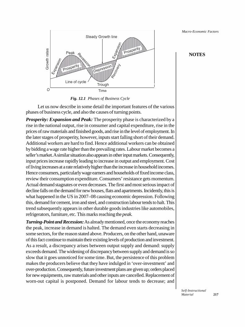
Macro-Economic Factors
NOTES
Self-InstructionalMaterial 217
Fig. 12.1 Phases of Business Cycle
Let us now describe in some detail the important features of the variousphases of business cycle, and also the causes of turning points.Prosperity: Expansion and Peak: The prosperity phase is characterized by arise in the national output, rise in consumer and capital expenditure, rise in theprices of raw materials and finished goods, and rise in the level of employment. Inthe later stages of prosperity, however, inputs start falling short of their demand.Additional workers are hard to find. Hence additional workers can be obtainedby bidding a wage rate higher than the prevailing rates. Labour market becomes aseller’s market. A similar situation also appears in other input markets. Consequently,input prices increase rapidly leading to increase in output and employment. Costof living increases at a rate relatively higher than the increase in household incomes.Hence consumers, particularly wage earners and households of fixed income class,review their consumption expenditure. Consumers’ resistance gets momentum.Actual demand stagnates or even decreases. The first and most serious impact ofdecline falls on the demand for new houses, flats and apartments. Incidently, this iswhat happened in the US in 2007–08 causing economic depression. Followingthis, demand for cement, iron and steel, and construction labour tends to halt. Thistrend subsequently appears in other durable goods industries like automobiles,refrigerators, furniture, etc. This marks reaching the peak.Turning-Point and Recession: As already mentioned, once the economy reachesthe peak, increase in demand is halted. The demand even starts decreasing insome sectors, for the reason stated above. Producers, on the other hand, unawareof this fact continue to maintain their existing levels of production and investment.As a result, a discrepancy arises between output supply and demand: supplyexceeds demand. The widening of discrepancy between supply and demand is soslow that it goes unnoticed for some time. But, the persistence of this problemmakes the producers believe that they have indulged in ‘over-investment’ andover-production. Consequently, future investment plans are given up; orders placedfor new equipments, raw materials and other inputs are cancelled. Replacement ofworn-out capital is postponed. Demand for labour tends to decrease; and
Macro-Economic Factors
NOTES
Self-Instructional218 Material
temporary and casual workers are laid off in a bid to bring demand and supply inbalance. The cancellation of orders for inputs by the producers of consumer goodscreates a chain-reaction in the input market. Producers of capital goods and rawmaterials cancel their orders for their input. This is the turning point and thebeginning of recession.
Since demand for inputs has decreased, input prices, e.g., wages, interest,etc., show a gradual decline leading to a simultaneous decrease in the incomes ofwage and interest earners. This ultimately causes demand recession. On the otherhand, producers lower their price in order to get rid of their inventories and also tomeet their financial obligations. Consumers, is their turn, expect a further decreasein price, and hence, postpone their purchases. As a result, the discrepancy betweendemand and supply continues to grow. When this process gathers speed, it takesthe form of irreversible recession. Investments start declining. The decline ininvestment leads to decline in employment, income and consumption. Wheninvestments continue to decline, production and employment continue to declinecausing in further decline in demand for both consumer and capital goods.Borrowings for investment decreases; bank credit shrinks; stock prices decrease;unemployment increases even though there is a fall in wage rates. At this stage, theprocess of recession is complete. When growth rate falls below the steady growthline, the economy enters the phase of depression.Depression and Trough. During the phase of depression, economic activitiesslide down their normal level. The growth rate becomes negative. The level ofnational income and expenditure declines rapidly. Prices of consumer and capitalgoods decline steadily. Workers lose their jobs. Debtors find it difficult to pay offtheir debts. Demand for bank credit reaches a low ebb and banks experiencemounting of their cash balances. Investment in stock becomes less profitable andless attractive. At the depth of depression, all economic activities touch the bottomand the phase of trough is reached. Even the expenditure on maintenance isdeferred in view of excess production capacity. Weaker firms are eliminated fromthe industries. At this point, the process of depression is complete.How is the Process Reversed? The basic factor that reverses the recessionarytrend is the limit to which an economy can shrink. When the economy hits thebottom and stays there for some time, it marks the end of pessimism and beginningof optimism. This reverses the process. The process of reversal generally beginsin the labour market. The widespread unemployment forces workers to work atwages less than the prevailing rates. The producers anticipating better future try tomaintain their capital stock and offer jobs to some workers here and there. Theydo so also because they begin to take an optimistic view of the situation due to thehalt in decrease in price in the trough phase. Consumers on their part expecting nofurther decline in price begin to resume their postponed consumption and hencedemand picks up, though gradually. Bankers having accumulated excess liquidity(idle cash reserve) try to salvage their financial position by lowering the lendingrate and by investing their funds in securities and bonds, even if rate of return isvery low. Consequently, investment picks up and employment gradually increases.
Macro-Economic Factors
NOTES
Self-InstructionalMaterial 219
Following this recovery in production and wage income, demand for both consumerand capital goods starts picking up. Since banks have accumulated excess cashreserves, bank credit becomes easily available and at a lower rate. For all thesereasons economic activities get accelerated. Due to increase in income andconsumption, the process of multiplier gives further impetus to the economicactivities, and the phase of recovery gets underway, depending on the speed ofrecovery.The Phase of Recovery. As the recovery gathers momentum, some firms planaddi-tional investment; some undertake renovation programmes; and someundertake both. These activities generate construction activities in both consumerand capital goods sectors. Individuals who had postponed their plans to constructhouses undertake this task now, lest cost of construction should mount. As a result,more and more employment is generated in the construction sector. As employmentincreases despite wage rates moving upward, the total wage incomes increase ata rate higher than the employment rate. Wage income rises and so does theconsumption expenditure. Businessmen realizing a quick return with high profitability,speed up the production machinery.
Over a period, as factors of production become more fully employed, wagesand other input prices move upward rapidly, though not uniformly. Investors,therefore, select the best of the alternative investment opportunities. As prices,wages and other factor prices increase, a number of related developments beginto take place. Businessmen start increasing their inventories, consumers start buyingmore and more of durable goods and variety items. With this process catching up,the economy enters the phase of expansion and prosperity. The cycle is thuscomplete.
12.5 INFLATION
Inflation means generally an unduely high and persistent rise in the general level ofprices over a period of time. However, there is no universally acceptable definitionof inflation. The definition of inflation has been changing over time depending onthe perception of the economists. For example, according to Pigou, a neo-classicaleconomist, “Inflation exists when money income is expanding more than inproportion to increase in earning activity.” To Coulborn, inflation is a situation of“too much money chasing too few goods”. Modern economists have tried to defineinflation more meaningfully. According to Ackley, “Inflation is a persistent andappreciable rise in the general level or average of prices.” Harry G. Johnson definesinflation as “a sustained rise in prices.” According to Samuelson, “Inflation denotesa rise in the general level of prices.” Bronfenbrenner and Holzman have suggesteda number of alternative definitions of inflation which are mostly modified versionsof earlier definitions. Their alternative definitions make things more fuzzy ratherthan adding clarity to inflation.
Macro-Economic Factors
NOTES
Self-Instructional220 Material
However, economists seem to agree that inflation means a ‘persistent’and ‘appreciable’ increase in the general level of prices. The terms like‘persistent’, ‘appreciable’, ‘sustained’, ‘considerable’, ‘continuing’ and ‘prolonged’are not precisely defined. In practice, however, the term ‘persistent’ implies thatthe price rise exhibits a secular trend or continues to rise over a period of one totwo years, and does not respond to anti-inflationary policies. The term‘appreciable’ is more ambiguous because it does not specify as to what rate ofincrease in the price level is to be considered as ‘appreciable’ or ‘considerable’. Itvaries from country to country and from time to time. For example, in India, a 7–8% annual inflation in 1970s and 1980s was not so appreciable but a 6% inflationApril–May 2007 and 7–8% in 2013 had become highly problematic—a matterof great concern for both the government and the RBI.
Annual consumer inflation in India declined to 3.69 percent in August of2018 from 4.17 percent in July and below market expectations of 3.86 percent. Itis the lowest inflation rate since October of 2017, mainly due to a sharp slowdownin food cost.
Methods of Measuring Inflation
There are two common methods of measuring inflation: (i) by computing changein Price Index Numbers (PIN), and (ii) by comparing the change in GNP Deflator.The two methods are explained here briefly.
Wholesale PINs Method
The formula used for measuring the rate of inflation through the changes in thePINs is given below.
Rate of inflation = 1
1
100t t
t
PIN PINPIN
where PINt is the wholesale price index number for the year selected for measuringinflation and PINt–1 is the PIN in the preceding year.
GNP Deflator Method
The GNP deflator method uses the ratio of nominal GNP in a year to the realGNP of that year. The GNP deflator is defined as follows:
GNP deflator = Nominal
Real GNP
GNP
where Nominal GNP is GNP at current prices and Real GNP is GNP atconstant prices.
12.5.1 Factors Causing Inflation
The modern theories of inflation follows the theory of price determination. That is,the general price is determined by aggregate demand for and aggregate supply
Macro-Economic Factors
NOTES
Self-InstructionalMaterial 221
of goods and services and the variation in the aggregate price level is caused bythe level of shift in the aggregate demand and aggregate supply curves. The moderntheory of inflation is, in fact, a synthesis of classical and Keynesian theories ofinflation. The modern analysis of inflation shows that inflation is caused by one orboth of demand and supply-side factors. The factors which operate on the demandside are called demand-pull factors, and those operating on the supply-side arecalled cost-push factors. Accordingly, there are two kinds of inflation:
(i) Demand-pull inflation and (ii) Cost push inflation. The two kinds ofinflation are discussed here briefly. However, a section of economists argues thatdemand-pull and cost-push factors interact to cause inflation. The theory of inflationbased on interaction of demand-pull and cost-push factors has been discussedsubsequently.
Demand-Pull Inflation
The demand-pull inflation occurs when the aggregate demand increases at a muchhigher rate than the aggregate supply. In other words, demand-pull inflation occurswhen, given the aggregate supply, aggregate demand increases substantially. Increasein aggregate demand may be caused by (a) monetary factors, i.e., increase inmoney supply and/or (b) real factors, i.e., increase in demand for real output. Letus now see how monetary and real factors cause inflation.(a) Increase in Money Supply and Demand-Pull Inflation: One importantreason for demand-pull inflation is increase in money supply in excess of increasein potential output. Whether increase in money supply in excess of increase inoutput is the only cause of inflation is a controversial issue. But the fact is thatmonetary expansion in excess of increase in the level of output is one of the mostimportant factors causing demand-pull inflation.(b) Real-Factor Demand-Pull Inflation: Real-Factor demand-pull inflationcan be caused by any or many of the following real factors.
(i) Increase in the government expenditure without change in tax revenue;(ii) Cut in tax rates without change in the government expenditure;(iii) Increase in investment;(iv) Increase in consumer demand;(v) Increase in exports given imports; and(vi) Decrease in imports given the exports.
The first four factors straightaway increase the level of disposable income.Increase in aggregate income increases aggregate demand causing demand-pullinflation. For example, suppose that the government increases its spending financedthrough borrowings abroad. The rise in the government spending generatesadditional demand and, therefore, aggregate demand increases. Since there is, byassumption, full employment, additional resources can be acquired only by biddinga higher price. This pushes the prices up without increase in the output. Therefore,
Macro-Economic Factors
NOTES
Self-Instructional222 Material
the transaction demand for money increases. In order to meet the additionaltransaction demand for money, people sell their financial assets—bonds andsecurities. Consequently, bond and security prices go down and the rate of interestgoes up. In the product market, prices increase to such an extent that the additionalgovernment spending is absorbed by the price rise. This is how other real factorsalso cause inflation.
Cost-Push Inflation
There are instances of inflation which could not be fully explained by the demand-side factors. The 1958-recession in the Western countries is a famous instance.During the period of recession, the aggregate demand had declined. Yet there wasno decrease in the general price level. Instead, it tended to rise. In recent times, itis a common experience that prices generally do not decrease during the period ofrecession. Furthermore, even when there is stagnation in the economy and there isno inflationary pressure, the general price level generally continues to increase. Itimplies a situation of stagflation. The investigation into this kind of phenomenon,particularly for the 1958-puzzle, had led to the emergence of supply-side theoriesof inflation, popularly known as cost-push theory and supply-shock theory ofinflation.
Cost-push inflation is generally caused by monopolistic groups of thesociety, like labour unions and firms in monopolistic and oligopolistic market setting.Strong labour unions often succeed in forcing money wages to go up causingprices to go up. This kind of rise in price level is called wage-push inflation.Also, firms enjoying monopoly power have also been found using their monopolypower to raise prices which in turn leads to rise in the general price level. Themonopolistic and oligopoly firms push their profit margin up causing a rise in thegeneral price level. This kind of inflation is called profit-push inflation. Anotherkind of cost-push inflation is said to be caused by supply shocks, i.e., decrease inthe aggregate supply. This is called supply shock inflation. Minimum-wagelegislation and administered prices are other supply side factors which not onlykeep price level up but also create conditions for increase in the prices. In thissection, we will discuss briefly these kinds of cost-push inflation.(i) Wage-Push Inflation: Wage-push inflation is attributed to the exercise ofmonopolistic power by the labour unions to get their money wages enhancedmore than the competitive labour market conditions would permit. Organized andpowerful labour unions exercise their monopoly power and force their employersto increase their money wages above the competitive level without matchingincrease in labour productivity. Increase in money wages causes an equal increasein the cost of production. The increase in cost of production forces the firms toincrease the price. This trend causes the aggregate supply curve to shift backward.A backward shift in the aggregate supply causes an upward movement in the pricelevel.
Macro-Economic Factors
NOTES
Self-InstructionalMaterial 223
However, every rise in the money wages is not always inflationary. The risein money wages due to the following factors is not said to be inflationary.
(i) Increase in wage rate due to increase in productivity,(ii) Rise in wage rates due to inflation,(iii) Wage rise where unionized wage bill is very small, and(iv) Wage rise due to shortage of labour supply.
(ii) Profit-Push Inflation: In contrast to wage-push inflation, profit-push inflationis caused by the use of monopoly power by the monopolistic and oligopolisticfirms to enhance their profit margin which results in the rise in price and inflation.Today, monopolistic competition and oligopolies characterize the real marketsituation all over the world. The monopolies, monopolistically competitive firmsand oligopolies tend to increase their price to increase their profit margin, given themarket conditions, of course. Therefore, a profit-push type of inflation is certainlya theoretical possibility.
Profit-wage Spiral: It may be added here that wage-push and profit-push inflation go hand in hand, whichever may be the leading cause. Labourunions may be the first to force wage rate to go up but firms raise the price leveloften more than proportionately. Or else, monopolistic firms may be the first topush the product price up forcing labour unions to demand a higher wage rate. Itthen has its repercussions on the money wages. Higher prices and profits inducedemand for higher wages. The powerful labour unions force their employers toraise their wages. Following the wage hike, firms raise the product prices. Whenthis process gets going, it takes the form of ‘profit-wage spiral’.(iii) Supply-Shock Inflation: Supply shock is generally caused by unexpecteddecline in the supply of major consumer goods or key industrial inputs. For example,vegetable and foodgrain prices shot up in India by more than 100 per cent in thelast quarter of 2013, making a big election issue in 2014. Prices of some keyindustrial inputs like, coal, steel, cement, oil, basic chemicals, etc., go up becauseof short supply caused by labour strikes, natural calamities, etc. Also, rise in theprice may be caused by supply bottlenecks in the domestic economy or internationalevents (generally wars) causing bottlenecks in the movement of internationallytraded goods and causing thereby shortage of supply and rise in imported industrialinputs.
12.5.2 Factors Causing Deflation
Deflation is caused by a decline in demand. When the demand is less then thebusiness enterprises are forced to lower the prices of products which can lead tostiff competition. Deflated is also caused by technology changes, such as moreefficient computer chips. Deflation can also be caused by exchange rates. Let usgo through some of the factors which cause deflation:
Macro-Economic Factors
NOTES
Self-Instructional224 Material
1. Change in Structure of Capital MarketsWhen a similar kind of product/service is being sold in the market by differententerprises then the price of that product is likely to be lower in the market due tostiff competition. Time and again, the capital structure of the economy will transformand enterprises will have easier access to debt and equity markets, which can beutilized to fund new business enterprises or improve productivity.2. Increased ProductivityThe introduction of innovative measures and new processes assists in increasingefficiency, which ultimately leads to lower prices. It is to be noted that someinnovations have an impact only affect the productivity of certain industries; othersmay have a profound effect on the entire economy.3. Decrease in Currency SupplyAs the currency supply decreases, prices will decrease so that people can affordgoods.4. Austerity MeasuresDeflation can be the outcome of decreased governmental, business, or consumerspending, which implies that the government spending cuts can lead to periods ofsignificant deflation.5. Deflationary SpiralOnce depression comes into the picture, it becomes difficult to control its aftereffects on the economy of a country. Firstly, when consumers begin reducing theirspending amount, the profits of business houses decrease. This implies thatbusinesses have to lessen wages and reduce their own purchases.
12.5.3 Control Measures
Economists agree that inflation beyond a moderate rate is bad and can often provedisastrous and, therefore, it must be kept under control. The various policymeasures generally adopted for controlling inflation can be classified as follows.
(i) monetary policy measures,(ii) fiscal policy measures,(iii) price and wage control measures, and(iv) indexation.
These measures of controlling inflation are discussed here briefly.
Monetary Measures
Monetary measures which are generally used to control inflation include (i) bankrate policy, (ii) variable reserve ratio and (iii) open market operation.(i) Bank Rate Policy: The bank rate as a measure of inflation control works intwo ways. One, during the period of inflation, the central bank raises the bankrate. This increases the cost of borrowing which reduces commercial banks’
Macro-Economic Factors
NOTES
Self-InstructionalMaterial 225
borrowing from the central bank. This reduces banks’ ability to create credit throughthe process of credit creation. As a result, flow of money from the commercialbanks to the public gets reduced. Therefore, inflation is controlled to the extent itis caused by the bank credit. Two, bank rate sets the trend for the general marketrate of interest, particularly in the short-term money market. When bank rate isincreased with a view to controlling money supply and, thereby, inflation, commercialbanks increase their lending rates and other market rates follow suit. In general,the cost of borrowing goes up. This slows down the monetary flows to the society.
This method, however, does not work effectively, if (i) commercial bankshave excess liquidity, (ii) they have alternative sources of creating reserves,(iii) they are free not to raise their lending rates following the increase in the bankrate, and (iv) future expectations regarding the market prospects is optimistic.(ii) Variable Reserve Ratio: Commercial banks are required to maintain acertain proportion of their total demand and time deposits in the form of cashreserves, called cash reserve ratio (CRR). The cash reserve ratio (CRR) isgenerally determined and imposed by the central bank which it uses as a weaponto control money supply. To control inflation, the central bank raises the CRR.When central bank raises the CRR, it reduces the lending capacity of the commercialbanks. As a result, flow of money from the commercial banks to the publicdecreases. In the process, it halts the rise in prices to the extent it is caused by thebanks credits to the public. This measure of controlling inflation has the samelimitations as the bank rate policy.(iii) Open Market Operations: Open market operations refer to sale andpurchase of the government securities and bonds by the central bank. To controlinflation, central bank sells the government securities to the public through theauthorized commercial banks. The sale of government bonds through the banksresults in the transfer of a part of bank deposits to central bank account. Thisreduces credit creation capacity of the commercial banks. Therefore, money supplywith public is reduced by a multiple of sale proceeds of the treasury bills. As aresult, inflation is controlled to the extent money supply with public decreases.
Fiscal Measures
Fiscal measures to control inflation include taxation, government expenditureand public borrowings. Keynesian economists, also called ‘fiscalists’, argue thatdemand-pull inflation is caused by excess of aggregate demand over aggregatesupply. The excess demand is the result of increase in expenditure by the households,firms and the government, particularly by excessive spending by government. Excessdemand, be it due to household or government expenditure, can be effectivelycontrolled by fiscal measures. Therefore, fiscal policy measures are a more powerfuland effective weapon to control demand-pull inflation.
In case government expenditure is the cause of excess demand, it can becontrolled straightaway by cutting down public expenditure. A cut in publicexpenditure reduces government demand for goods and services and also the
Macro-Economic Factors
NOTES
Self-Instructional226 Material
private income and consumption expenditure arising out of government expendituremultiplier. Therefore, the excess demand decreases more than a given cut in publicexpenditure. And, in case excess demand is caused by rise in private expenditure,increasing income tax rate is a more appropriate measure to control inflation.Taxation of incomes reduces the disposable income of the people and therebyconsumer demand.
In case of a very high rate of persistent inflation, the government may adoptboth the measures simultaneously. It should cut down its own spending, on theone hand, and increase the rate of income taxation, on the other. This kind ofpolicy is known as a policy of surplus budgeting, i.e., the government shouldspend less than its tax revenue.
Price and Wage Control
In case monetary and fiscal measures prove ineffective in controlling inflation,direct control measures are adopted to control inflation. Direct measures consistmainly of price and wage controls. The price and wage controls go together becauseprice-push and cost-push inflation go hand in hand whatever may be the cause ofinitial inflation.
Under price control method, a maximum retail price of goods and servicesis fixed. Price control may be general, applicable to all goods and services or itmay be partial, confined to only scarce and essential goods and services. Theprimary objective of price control is to prevent the price rise of scarce goods andto ration the use of the commodity. Whether price control works effectively andefficiently is also a controversial matter. It is a general experience that price controlslead to black-marketing of goods and unfair distribution of scarce goods andservices, especially where administrative machinery is corrupt and inefficient.
Wage control is used where inflation is of cost-push or of wage pushnature. Under this method, rise in wage rate is prevented directly by imposing aceiling on the wage incomes in both private and public sectors. Often ‘wage-freeze’ is applied to control inflation. In case trade unions are powerful and oppose‘wage-freeze’ effectively, government uses a weaker method called ‘jawboning’.A more sensible and effective method of containing wage-push inflation is knownas ‘wage guideposts’— a plan of action against inflation prepared by commonconsent and mutual agreement between the representatives of the government,trade unions and the businessmen, for a disciplined and controlled upwardmovement in the wages and prices. Under this scheme, wage and price rise aremonitored by a board of the representatives. However, this method does notwork for long, especially when prices continue to rise. Friedman comments,“Guideposts and pleas for voluntary compliance are a halfway [measure] whoseonly merit is that they can more readily be abandoned than legally imposed controls.They are not an alternative to other effective measures to stem inflation, but atmost a smoke-screen to conceal lack of action.”
Macro-Economic Factors
NOTES
Self-InstructionalMaterial 227
Indexation
It should be clear from the foregoing discussion that inflation is an intractableproblem. Controlling inflation involves the risk of aggravating unemploymentproblem. However, as discussed above, a high rate of inflation affects differentsections of the society in different ways. Economists argue that if controlling inflationis not advisable, its adverse effects on different sections of society can be minimizedby a method called indexation. They suggest indexation of prices, wages andcontractual obligations with a view to compensating those who lose their realincomes due to inflation. According to Samuelson and Nordhaus, “Indexing is amechanism by which wages, prices and contracts are partially or whollycompensated for changes in the general price level.” Thus, indexation is not amethod of controlling inflation. It is a method of adjusting monetary incomes so asto minimize the undue gains and losses in real incomes of the different sections ofthe society due to inflation. Its main objective is to manage social discontent and tomake inflation easier to live with.
Indexation of wages is most important and a common practice in manycountries where wage contracts are long-term contracts and inflation continues topersist. In such cases, compensating workers for the loss of their real income dueto inflation becomes unavoidable. Two systems are adopted in general: one is totie wages to cost-of-living index (CPI) and second is to make a periodic schedulingof wage rise after CPI goes up by a certain percentage point. For instance, in theUSA, wages are linked to cost-of-living index and cost-of-living adjustment(COLA) with inflation is made automatically. Here, wages increase automaticallyfollowing the increase in the cost-of-living index. In India, wage compensationtakes the form of ‘dearness allowance’, i.e., compensation for loss of purchasingpower of the nominal wages due to inflation. Dearness allowance to the publicsector employees in India is linked to consumer price index (CPI) and dearnessallowance is granted after every eight percentage point increase in the CPI.
Although economists strongly recommend indexing of wages, debts, taxes,and all other long-term contractual payments, the governments doubt the feasibilityand practicability of indexation method for three reasons. First, adjustment inindexation is impracticable in case of frequent supply shocks of great amplitude.Second, economy being a complex system with interlinked and interrelated prices,a reasonable indexing of all prices to the satisfaction of all concerned is an extremelydifficult task. Third, the government finds indexation politically undesirable becauseit does not control inflation, it rather creates a base for its perpetuation.
12.6 BALANCE OF PAYMENT TREND AND ITSIMPLICATIONS ON MANAGERIAL DECISIONS
The BOP of a country is a systematic accounting of all economic transactionsbetween the residents of the country and the residents of the rest of the world over
Macro-Economic Factors
NOTES
Self-Instructional228 Material
a period of time, usually a year. In simple words, the BOP of a country is anaccount of all international receipts and payments for the accounting year. Theaccounting year may be a calendar year or a financial year. In India, the BOP isprepared for every financial year, although it is also prepared and reported on aquarterly basis.
Although the definition of BOP is quite clear, some terms used in the definitionneed some clarification.
The term ‘systematic accounting’ does not refer to any particular system.But the system generally adopted is double entry book-keeping system. Underthis system, both receipts and payments of an economic transaction—sale andpurchase—are recorded in one entry. We know that each economic transactioninvolves two flows—inflow and outflow. What comes in, i.e., inflow, is treated asa debit item and what goes out, i.e., the outflow, is treated as a credit item.Under double entry book-keeping system, the values of debit and credit items arerecorded simultaneously. For example, in case of exports, goods and services goout of the country and payments received come to the country. What goes out(export) is recorded as a credit item and what comes in (payments received), as adebit item. Both the value of exports and the payments received are recorded inthe same accounting entry of the transaction. Similarly, in the case of imports, thevalue of imports of goods and services is recorded as a debit item and paymentsfor imports are recorded as a credit item. Both the value of imports and thepayments made are recorded in the same accounting entry. This is the doubleentry book-keeping system.
‘Economic transactions’ include all such transactions that involve the transferof money (foreign exchange) along with the right of ownership of the transactedgoods, money, and assets. Specifically, exports and imports of goods and services,foreign investment, and borrowing from and lending to a foreign country, are alleconomic transactions. It is important to note here that while in some transactions,there is a physical transfer of goods, services, assets, and money along with thetransfer of ownership, in others, no physical transfer is required. For example, if aUS resident imports garments from India, they have to be transferred physicallyalong their ownership. But if a US multinational corporation operating in Indiareinvests its profits in India, there is no physical transfer, i.e., transfer of money.
The term ‘resident’ refers to the nationality of the persons or organizationscarrying out the transaction, not their physical presence in their own country. Forexample, foreign tourists, diplomats, military personnel, migrant labour and branchesof companies in a country are treated as residents of their own nation, not asresidents of the country in which they are physically present.
Purpose of Balance of Payments
The purpose of preparing balance of payments (BOP) is similar to that of thebalance sheet of business firms. We know that all business firms prepare their
Macro-Economic Factors
NOTES
Self-InstructionalMaterial 229
annual (or periodic) balance sheet of their transactions with the rest of society withthe purpose of taking stock of their profit and loss and their assets and liabilities.Likewise, all nations having economic transactions with the rest of the world preparetheir periodic BOP accounts just to take stock of their receipts and payments, andtheir assets and liabilities resulting from their international economic transactions.However, the purpose of BOP goes far beyond this limited purpose as it revealsthe overall implications of international economic transactions for the economy ofa country. The BOP accounts serve the following purposes.
First, the international economic transactions of a country—its exports,imports, and foreign investments—and inflows and outflows of incomes (e.g.,remittances) have a serious impact on the levels of its consumption and the stockof capital. The change in the levels of consumption and of capital accumulationaffects the national income of the country and its economic growth over time.
Therefore, in order to find out the impact of the monetary inflows and outflowsof on the economy, a country has to prepare its balance of payments.
Second, in case a country has a large and persistent trade deficit, and capitalinflows are not sufficient to make up the trade deficit, it faces a serious foreignpayment problem. A country having a large and persistent trade deficit has toborrow from abroad to settle its payments. When the country makes a largeborrowing from abroad over a long period of time, it tends to fall into internationalindebtedness. This can have serious adverse repercussions for the of the economyof the country. This is what had happend in India in 1990–91.
Third, the balance of payments provides useful data for analysing a country’sweaknesses and strengths with respect to foreign trade and its gains and lossesfrom international transactions. The balance of payments contains data on exportsand imports, capital inflows and outflows, borrowings and lendings, and foreignexchange reserves for successive years. By analysing the data one can find outwhether the economic condition of a country in relation to the world economy isimproving or deteriorating. If it is deteriorating, the government will have to formulateappropriate corrective policy measures and implement them on time. ‘One of thebasic problems of international economic policy is to find effective means of restoringexternal balance to the country whose balance of payments is seriously in surplusor in deficit.’ The balance of payments provides useful data and guidelines for theformulation a suitable foreign trade and exchange rate policy.
Specific Uses of BOP for a Business Manager
A study evaluating the country’s balance of payments can help the businessmanager in deciding whether he can borrow/raise funds in a particular countryor invest his funds there.
A proper analysis of balance of payments data can disclose trends in factorsthat underlie the value of the country’s currency in a foreign market.
Macro-Economic Factors
NOTES
Self-Instructional230 Material
Check Your Progress
1. Define inflation.2. What is the main objective of indexation?3. What is gross domestic product?
12.7 ANSWERS TO CHECK YOUR PROGRESSQUESTIONS
1. Inflation means generally an unduly high and persistent rise in the generallevel of prices over a period of time.
2. The main objective of indexation is to manage social discontent and tomake inflation easier to live with.
3. Gross Domestic Product (GDP) is defined as the total market value of allfinal goods and services produced within a country in a given period.
12.8 SUMMARY
The subject matter of managerial microeconomics consists of theories ofdemand and supply, theory of production, cost-output relationships, marketmechanism, theory of price determination under different kinds of marketstructure, pricing principles and prices, and capital budgeting and investmentdecisions.
Macroeconomics as a positive science has theoretical orientation. As apositive science, it uses macroeconomic models to explain the behaviour ofmacroeconomic variables—national income, aggregate consumption, savingsand investment, price level, and employment.
The importance of macroeconomics can be viewed from two angles:(i) how it contributes to government’s economic policy formulation forthe management of the economy, and (ii) how it guides business managersfor taking appropriate business decisions and business planning.
Both developed and developing countries are constantly confronted withsome or the other kind of macroeconomic problems, e.g., recession anddepression, stagflation, balance-of-payment deficits, outflow of capital,mounting debt burden or a country falling into debt trap, and so on.
The overall economic trend in a country is the most important element of itsbusiness environment. A growing economy with a considerably high andsustained growth rate in its GDP over a long period of time provides apromising business prospect and builds business confidence.
Macro-Economic Factors
NOTES
Self-InstructionalMaterial 231
Business cycles refer to the periodic booms and slumps in eco-nomicactivities, generally compared to ‘ebb and flow’.
Inflation means generally an unduly high and persistent rise in the generallevel of prices over a period of time. However, there is no universallyacceptable definition of inflation.
The modern theories of inflation follow the theory of price determination.That is, the general price is determined by aggregate demand for andaggregate supply of goods and services and the variation in the aggregateprice level is caused by the level of shift in the aggregate demand andaggregate supply curves.
Deflation is caused by a drop in demand. Fewer shoppers mean businesseshave to lower prices, which can turn into a bidding war. It is also caused bytechnology changes, such as more efficient computer chips. Deflation canalso be caused by exchange rates.
Monetary measures which are generally used to control inflation include(i) bank rate policy, (ii) variable reserve ratio and (iii) open market operation.
Fiscal measures to control inflation include taxation, government expenditureand public borrowings.
Indexation of wages is most important and a common practice in manycountries where wage contracts are long-term contracts and inflationcontinues to persist.
The BOP of a country is a systematic accounting of all economic transactionsbetween the residents of the country and the residents of the rest of theworld over a period of time, usually a year.
12.9 KEY WORDS
Stagflation: It is a condition of slow economic growth and relatively highunemployment, or economic stagnation, accompanied by rising prices, orinflation.
Capital formation: It is the process of creating or acquiring man-mademeans of production.
12.10 SELF ASSESSMENT QUESTIONS ANDEXERCISES
Short Answer Questions
1. Write a short note on the nature of macroeconomics.2. What is the importance of macro-economic factors?
Macro-Economic Factors
NOTES
Self-Instructional232 Material
3. How is economic growth defined?4. What are the methods of measuring inflation?
Long Answer Questions
1. Discuss the determinants of economic growth.2. Describe the phases of business cycles.3. Explain the factors causing inflation.4. Evaluate the measures adopted for controlling inflation.5. ‘BOP of a country is an account of all international receipts and payments
for the accounting year.’ Elucidate the statement.
12.11 FURTHER READINGS
Dwivedi, D. N. 2015. Principles of Economics, Eight Edition. New Delhi: VikasPublishing House.
Weil. David N. 2004. Economic Growth. London: Addison Wesley.Thomas, Christopher R. and Maurice S. Charles. 2005. Managerial Economics:
Concepts and Applications, Eighth Edition. New Delhi: Tata McGraw-Hill Publishing Company Limited.
Mankiw, Gregory N. 2002. Principles of Economics, Second Edition. India:Thomson Press.
Websites
https://blogs.economictimes.indiatimes.com/et-commentary/heres-how-indias-widening-income-distribution-can-be-redressed/
https://www.livemint.com/Opinion/WmpSjQAvPGeVzxqpgXYvtK/The-dangers-of-Indias-Billionaire-Raj.html
National Income
NOTES
Self-InstructionalMaterial 233
UNIT 13 NATIONAL INCOME
Structure13.0 Introduction13.1 Objectives13.2 Introduction to National Income
13.2.1 Methods of Measurement13.3 Theory of National Income Determination
13.3.1 Two-Sector Model13.3.2 Three-Sector Model13.3.3 Four-Sector Model
13.4 Sectoral and Population distributions13.5 Per Capita Income: Definition, and Calculations
13.5.1 GDP and GNP13.5.2 Uses and Limitations13.5.3 Recent Developments in Indian Economy
13.6 Answers to Check Your Progress Questions13.7 Summary13.8 Key Words13.9 Self Assessment Questions and Exercises
13.10 Further Readings
13.0 INTRODUCTION
National income is the final outcome of the economic activities of the people of thenation. National income is the most important macroeconomic variable. The levelof national income of a country determines its economic strength to sustain theeconomic, political, social and international problems. It determines the level ofemployment, per capita income, aggregate demand and supply of goods andservices, and the level of production. What is more important form the view pointof business management is the fact that change in national income determines thebusiness environment of the country. Business environment matters a great deal inmaking business decisions. We begin our discussion by defining the term ‘nationalincome’ and some basic concepts related to national income measurement.
13.1 OBJECTIVES
After going through this unit, you will be able to: Discuss the concept of national income Describe the methods of measurement of national income Explain the theory of national income determination Discuss the sectoral and population distributions
National Income
NOTES
Self-Instructional234 Material
Examine the concept, uses and limitation of per capita income Recall the recent developments in the Indian Economy
13.2 INTRODUCTION TO NATIONAL INCOME
National income can be defined as the sum of money value of all final goodsand services produced in a country over a period of one year. Some termsused in the definition of national income need to be clarified. The term ‘moneyvalue’ means the value estimated at the current price of the goods and services. Asregards the term ‘final goods and services’, productive activities create many goodsand services. While some goods and services are final, some are used again in theprocess of production, and some take the form of capital. In all cases, whilemeasuring national income only final goods and services are taken into account.
National income can be defined also as the sum of all factors incomes.Factors of production, viz., land, labour, capital and entrepreneurship, are used toproduce goods and services. Use of factors of production generates factor incomesin the form of rent, wages, interest and profit. These factor incomes constitute thenational income of a country. The sum of all these factor-incomes gives the estimateof national income.
National Income: Some Basic Concepts
Measuring national income is an extremely complex and complicated task as itinvolves both conceptual and practical problems. Therefore, before we discussthe methods of estimating national income, it is useful to understand the conceptsused in estimating national income. In this section, we take the view of someconcepts used in estimation of national income.
1. Gross Domestic Product (GDP). Gross domestic product (GDP) is themeasure of the total market value of all final goods and services producedin the domestic economy during a period of one year plus income earnedby the foreigners in the country minus income earned by countrymen fromabroad.
2. Gross National Product (GNP). GNP is the measure of the total marketvalue of all final goods and services produced in the domestic economyduring a period of one year plus incomes earned abroad by the citizensminus income earned by the foreigners in the country.
3. Economic and Non-economic Products. In estimating national incomeonly economic products are included. Goods and services that are producedto be sold at market price and goods and services that are produced by thegovernment and public organizations1 are treated as economic products.Thus, economic products include both marketable and non-marketablegoods. And, non-economic products include services rendered to self, to
National Income
NOTES
Self-InstructionalMaterial 235
family, to relations and to neighbours. Non-economic products are notincluded in national income.
4. Intermediate and Final Products. Products (goods and services) thatare used in the process of further production are considered to beintermediate product and products that are consumed by the finalconsumers are considered to be final products. The same product may bean intermediate or a final product. For examples, when wheat produced byfarmers are consumed by themselves, it is treated as final good, but whenit is sold to bread companies, it is treated as intermediate product. Likewise,when services provided by the government, e.g., transport, telephonic, postal,railway services, etc. are used by the consumers, they are treated as finalgoods and when used in the process of production, then these services aretreated as intermediate goods. In estimating national income, only finalproducts are taken into account.
5. Transfer Payments. Payments made by the people to other people,organizations or to the government without any equal transfer in return aretreated as transfer payment. For example, gifts paid to relatives and friends,donations given to social organization, and taxes paid to governmentauthorities, etc., are transfer payments. Such payments are not taken intoaccount in national income estimates.
National Income as Money Flow
We have defined national income from the angle of product flows. The same canbe defined in terms of money flows. While economic activities generate flow ofgoods and services, on the one hand, they generate money flows, on the other, inthe form of factor payments—wages, interest, rent, profits, and earnings of self-employed. Thus, national income may also be estimated by adding the factor earningsand adjusting the sum for indirect taxes and subsidies. The national income thusobtained is known as national income at factor cost. It is related to moneyincome flows.
The concept of national income refers to the income of the society as awhole. It differs fundamentally from the concept of private income. Conceptually,national income refers to the money value of the entire volume of final goods andservices resulting from all economic activities of the country. This is not true ofprivate income. Also from the calculation point of view, there are certain receiptsof money or of services and goods that are not ordinarily included in private incomesbut are included in the national incomes, and vice versa. National income includes,for example, employer’s contribution to the social security and welfare funds forthe benefit of employees, profits of public enterprises and services of owner occupiedhouses. But it excludes the interest on warloans, social security benefits andpensions. These items are, however, included in the private incomes. The nationalincome is, therefore, not merely an aggregation of the private incomes.
National Income
NOTES
Self-Instructional236 Material
13.2.1 Methods of Measurement
National income of a country is created by its people participating in differentkinds of economic activities and producing goods and services. For measuringnational income, an economy is viewed from three different angles.
1. The national economy is considered as an aggregate of productive unitsof different sectors such as agriculture, mining, manufacturing, trade andcommerce, services, etc.
2. The whole national economy is viewed as a combination of individualsand households owning different kinds of factors of production whichthey use themselves or sell factor-services to make their livelihood.
3. The national economy may also be viewed as a collection of consuming,saving and investing units (individuals, households, firms and government).
Following these notions of a national economy, national income may be measuredby three different corresponding methods:
1. Net product method—when the entire national economy is considered asan aggregate of producing units;
2. Factor-income method—when national economy is considered ascombination of factor-owners and users;
3. Expenditure method—when national economy is viewed as a collectionof spending units.The procedures which are followed in measuring the national income in a
closed economy—an economy which has no economic transactions with the restof the world—are briefly described here. The measurement of national income inan open economy and adjustment with regard to income from abroad will bediscussed subsequently.
Net Output or Value Added Method
The net output method is also called the value added method. In its standardform, this method consists of three stages: “(i) estimating the gross value of domesticoutput in the various branches of production; (ii) determining the cost of materialand services used and also the depreciation of physical assets; and (iii) deductingthese costs and depreciation from gross value to obtain the net value of domesticoutput...”. The net value of domestic product thus obtained is often called thevalue added or income product which is equal to the sum of wages, salaries,supplementary labour incomes, interest, profits, and net rent paid or accrued. Letus now describe the stages (i) and (ii) in some detail.(a) Measuring Gross Value. For measuring the gross value of domestic product,output is classified under various categories on the basis of the nature of activitiesfrom which they originate. The output classification varies from country to countrydepending on (i) the nature of domestic activities; (ii) their significance in aggregateeconomic activities, and (iii) availability of requisite data. For example, in the US,
National Income
NOTES
Self-InstructionalMaterial 237
about seventy-one divisions and subdivisions are used to classify the national output;in Canada and the Netherlands, classification ranges from a dozen to a score; andin Russia, only half a dozen divisions are used. According to the CSO publication,fifteen sub-categories are currently used in India.
After the output is classified under the various categories, the value of grossoutput is computed in two alternative ways: (i) by multiplying the output of eachcategory of sector by its respective market price and adding them together or(ii) by collective data about the gross sales and changes in inventories from theaccount of the manufacturing enterprises and computing the value of GDP on thebasis thereof. If there are gaps in data, some estimates are made thereof and gapsare filled.(b) Estimating Cost of Production. The next step in calculating the net nationalproduct is to estimate the cost of production including depreciation. Estimatingcost of production is, however, a relatively more complicated and difficult taskbecause of non-availability of adequate and requisite data. Much more difficult isthe task of estimating depreciation since it involves both conceptual and statisticalproblems. For this reason, many countries adopt factor-income method forestimating their national income.
However, countries adopting net-product method find some ways and meansto calculate the deductible cost. The costs are estimated either in absolute terms(where input data are adequately available) or as an overall ratio of input to thetotal output. The general practice in estimating depreciation is to follow the usualbusiness practice of depreciation accounting. Traditionally, depreciation is estimatedat some percentage of capital, permissible under the tax-laws. In some estimatesof national income, the estimators deviate from the traditional practice and estimatedepreciation as some ratio of the current output of final goods.
Following a suitable method, deductible costs including depreciation areestimated for each sector. The cost estimates are then deducted from the sectoralgross output to obtain the net sectoral products. The net sectoral products arethen added together. The total thus obtained is taken to be the measure of netnational product or national income by net product method.
Factor-Income Method
This method is also known as income method and factor-share method. Underthis method, the national income is calculated by adding up all the “incomes accruingto the basic factors of production used in producing the national product”. Factorsof production are conventionally classified as land, labour, capital and organization.Accordingly, the national income equals the sum of the corresponding factorearnings. Thus,
National income = Rent + Wages + Interest + ProfitHowever, in a modern economy, it is conceptually very difficult to make a
distinction between earnings from land and capital, on the one hand, and between
National Income
NOTES
Self-Instructional238 Material
the earnings from ordinary labour and entrepreneurial functions, on the other. Forthe purpose of estimating national income, therefore, factors of production arebroadly grouped as labour and capital. Accordingly, national income is supposedto originate from two primary factors, viz., labour and capital. In some activities,however, labour and capital are jointly supplied and it is difficult to separate thelabour and capital contents from the total earnings of the supplier. Such incomesare termed as mixed incomes. Thus, the total factor-incomes are grouped underthree categories; (i) labour incomes, (ii) capital incomes and (iii) mixed incomes.(a) Labour Incomes. Labour incomes included in the national income have threecomponents: (a) wages and salaries paid to the residents of the country includingbonus and commission, and social security payments; (b) supplementary labourincomes including employer’s contribution to social security and employee’s welfarefunds, and direct pension payments to retired employees;4 (c) supplementary labourincomes in kind, e.g., free health and education, food and clothing, andaccommodation, etc. Compensations in kind (food and clothes) to domesticservants and such other free-of-cost services provided to the employees areincluded in labour income. War bonuses, pensions, service grants are not includedin labour income as they are regarded as ‘transfer payments’. Certain othercategories of income, e.g., incomes from incidental jobs, gratuities, tips, etc., areignored for lack of data.(b) Capital Incomes. According to Studenski, capital incomes include thefollowing kinds of earnings:
(a) dividends excluding inter-corporate dividends;(b) undistributed before-tax-profits of corporations;(c) interest on bonds, mortgages, and saving deposits (excluding interests on
war bonds, and on consumer-credit);(d) interest earned by insurance companies and credited to the insurance policy
reserves;(e) net interest paid out by commercial banks;( f) net rents from land, buildings, etc., including imputed net rents on owner-
occupied dwellings;(g) royalties and(h) profits of government enterprises.
The data for the first two items are obtained mostly from the firms’ books ofaccounts submitted for taxation purposes. But the definition of profit for nationalaccounting purposes differs from that employed by taxation authorities. Someadjustments in income tax data therefore, become, necessary. The data adjustmentsgenerally pertain to (i) excessive allowance of depreciation made by the firms;(ii) elimination of capital gains and losses since these items do not reflect the
National Income
NOTES
Self-InstructionalMaterial 239
changes in current income and (iii) elimination of under or over-valuation ofinventories on book-value.(c) Mixed Income. Mixed incomes include earnings from (a) farming enterprises,(b) sole proprietorship (not included under profit or capital income) and (c) otherprofessions, e.g., legal and medical practices, consultancy services, trading andtransporting, etc. This category also includes the incomes of those who earn theirliving through various sources as wages, rent on own property, interest on owncapital, etc.
All the three kinds of incomes, viz., labour incomes, capital incomes andmixed incomes, added together give the measure of national income by factor-income method.
Expenditure Method
The expenditure method, also known as final product method, measures nationalincome at the final expenditure stages. In estimating the total national expenditure,any one of the two following methods are used: (i) all the money expenditures atmarket price are computed and added up together and (ii) the value of all theproducts finally disposed off are computed and added up, to arrive at the totalnational expenditure. The items of expenditure which are taken into account underthe first method are (a) private consumption expenditure; (b) direct tax payments;(c) payments to the non-profit-making institutions and charitable organizationslike schools, hospitals, orphanages, etc. and (d) private savings. Under the secondmethod, the following items are considered: (a) private consumer goods andservices, (b) private investment goods, (c) public goods and services and (d) netinvestment abroad. The second method is more extensively used because the datarequired in this method can be collected with greater ease and accuracy.Treatment of Net Income from Abroad. We have so far discussed methods ofmeasuring national income of a ‘closed economy’. But most economies are openin the sense that they carry out foreign trade in goods and services and financialtransactions with the rest of the world. In the process, some nations make netincome through foreign trade while some lose their income to foreigners. The netearnings or losses from foreign trade change the national income. In measuring thenational income, therefore, the net result of external transactions is adjusted to thetotal. Net incomes from abroad are added to, and net losses from the foreigntransactions are deducted from the total national income arrived at through any ofthe above three methods.
Briefly speaking, all exports of merchandise and of services like shipping,insurance, banking, tourism, and gifts are added to the national income. And, allthe imports of the corresponding items are deducted from the value of nationaloutput to arrive at the approximate measure of national income. To this is addedthe net income from foreign investment. These adjustments for internationaltransactions are based on the international balance of payments of the nations.
National Income
NOTES
Self-Instructional240 Material
13.3 THEORY OF NATIONAL INCOMEDETERMINATION
In the preceding section, we have discussed the methods of estimating nationalincome. The method of estimating income does not reveal how the level of nationalincome is determined. In this section, we proceed to discuss the theory of nationalincome determination. The theory of national income determination explains howequilibrium level of national income is determined. This theory was propoundedby a British economist, John Maynard Keynes, in 1936 in his book The GeneralTheory of Employment, Interest and Money. The Keynesian theory of incomedetermination has been discussed in this chapter. For sake of analytical convenience,the Keynesian theory of income determination is presented in the framework ofthree models:
1. Two-sector model: households and business sector,2. Three-sector model: households, business and government sectors, and3. Four-sector model: households, business, government and foreign sectors.
The fundamental principle of the Keynesian theory of national incomedetermination is that the national income is determined by aggregate demandand aggregate supply and equilibrium level of national income is determined atthe level where aggregate demand equals aggregate supply. The Keynesian theoryof income determination has been discussed in this unit under the above threemodels. We begin our discussion on the theory of income determination with two-sector model.
13.3.1 Two-Sector Model
First, there are only two sectors in the economy: households and firms. Householdsown the factors of production and they sell their factor services or provide them tothe firms to earn their living in the form of factor payments—wages, rent, interestand profits. Also, households are the consumers of all final goods and services.The firms, on the other hand, hire factor services from the households and producegoods and services which they sell to the households.
Secondly, there is no government. Or, if government is there, it does notperform any economic function; it does not tax, it does not spend and it does notconsume.
Thirdly, the economy is a closed one: there is no foreign trade. It impliesthat there is no outflow or inflow of goods and services to and from foreign countries.
Fourthly, there are no corporate savings or undistributed (or retained)corporate profits, i.e., the total corporate profit is distributed as dividends.
Finally, prices of all goods and services, supply of labour and capital, andthe state of production technology are given and remain constant.

National Income
NOTES
Self-InstructionalMaterial 241
As noted above, according to Keyens, national income of a country isdetermined by two factors: (i) aggregate demand (AD) and (ii) aggregate supply(AS) of goods and services. And, the equilibrium level of national income isdetermined where AD equals AS. Before we illustrate graphically the determinationof national income, let us explain the concepts of aggregate demand and aggregatesupply.
Aggregate Supply
The aggregate supply (AS) refers to the total value of goods and services producedand supplied in an economy per unit of time. Aggregate supply includes bothconsumer goods and producer goods. The goods and services produced per timeunit multiplied by their respective (constant) prices give the total value of the nationaloutput. This is the aggregate supply in terms of money value.Aggregate Supply Schedule. The Keynesian aggregate supply schedule oraggregate supply curve is drawn on the assumption that total income is alwaysspent – no part of it is retained or withheld. By Keynesian assumption, totalexpenditure is always equal to the total income. If income increases, expenditureincreases by the same amount. This relationship between income and expenditureis shown by a 45° line. This line is also called aggregate supply schedule. In theKeynesian theory of income determination, aggregate income equals consumption(C) plus savings (S). Therefore, AS schedule is generally named as C + S schedule.The aggregate supply (AS) curve is also sometimes called ‘aggregate expenditure’(AE) curve.
Aggregate Demand
The aggregate demand is an ex-post concept. It implies effective demand whichequals actual expenditure. The aggregate effective demand is equal to the aggregateexpenditure made by the society per unit of time. Aggregate demand (AD) consistsof two components:
(i) aggregate demand for consumer goods (C) and(ii) aggregate demand for capital goods (I).
Thus, AD = C + I ...(13.1)
Aggregate Demand Schedule
The aggregate demand AD schedule is also called C + I schedule. In the Keynesianframework, investment (I) is assumed to remain constant in the short-run. But,consumption (C) is treated to be a constant function of income (Y). Pending detaileddiscussion on the consumption function till the next section, let us let us note herethat the Keynesian consumption function is given as
C = a + bY ...(13.2)where a denotes a constant denoting C when Y = 0 and b denotes a constant ratioof income consumed, i.e., b =C/Y.
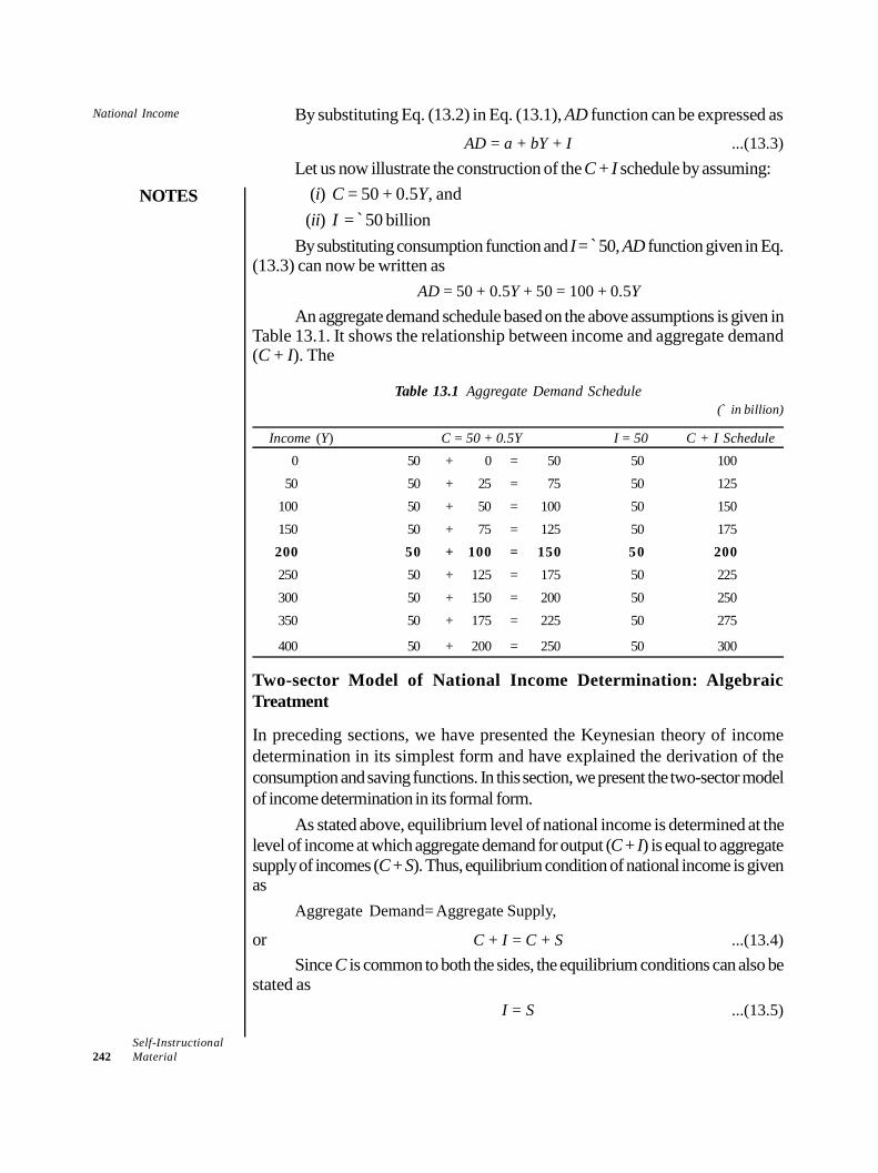
National Income
NOTES
Self-Instructional242 Material
By substituting Eq. (13.2) in Eq. (13.1), AD function can be expressed asAD = a + bY + I ...(13.3)
Let us now illustrate the construction of the C + I schedule by assuming:(i) C = 50 + 0.5Y, and
(ii) I = ̀ 50 billionBy substituting consumption function and I = ̀ 50, AD function given in Eq.
(13.3) can now be written asAD = 50 + 0.5Y + 50 = 100 + 0.5Y
An aggregate demand schedule based on the above assumptions is given inTable 13.1. It shows the relationship between income and aggregate demand(C + I). The
Table 13.1 Aggregate Demand Schedule(` in billion)
Income (Y) C = 50 + 0.5Y I = 50 C + I Schedule0 50 + 0 = 50 50 100
50 50 + 25 = 75 50 125100 50 + 50 = 100 50 150150 50 + 75 = 125 50 175200 50 + 100 = 150 50 200250 50 + 125 = 175 50 225300 50 + 150 = 200 50 250350 50 + 175 = 225 50 275
400 50 + 200 = 250 50 300
Two-sector Model of National Income Determination: AlgebraicTreatment
In preceding sections, we have presented the Keynesian theory of incomedetermination in its simplest form and have explained the derivation of theconsumption and saving functions. In this section, we present the two-sector modelof income determination in its formal form.
As stated above, equilibrium level of national income is determined at thelevel of income at which aggregate demand for output (C + I) is equal to aggregatesupply of incomes (C + S). Thus, equilibrium condition of national income is givenas
Aggregate Demand= Aggregate Supply,
or C + I = C + S ...(13.4)Since C is common to both the sides, the equilibrium conditions can also be
stated asI = S ...(13.5)
National Income
NOTES
Self-InstructionalMaterial 243
Given these conditions of equilibrium, there are two alternative ways toshow the determination of national income:
(i) by using aggregate demand (C + I) and aggregate supply (C + S)schedules, and
(ii) by using only saving (S) and investment (I) schedules.The two approaches are known as income-expenditure approach and
saving-investment approach, respectively.
13.3.2 Three-Sector Model
We have explained above income determination in a simple, two-sector economy.A real economy, however, also contains two other major sectors, viz., thegovernment sector and the foreign sector. In this section, we explain incomedetermination in a three-sector model including household, business andgovernment sectors. The four-sector model including three domestic sectors andthe foreign sector will be discussed in the next section.
Let us assume an economy consisting of three sectors, viz., households,firms and government. Inclusion of the government into the model brings in twovariables:
(i) government expenditures, and (ii) taxation. While governmnetexpedntiures are injections to the income stream, taxation is withdrawal fromthe income stream. Government expenditure adds to the aggregate demand, andtaxation, on the other hand, reduces the aggregate demand. How the level ofnational income is affected by the inclusion of government expenditure and taxationinto the model is discussed below.
To begin with, let us incorporate government sector into our two-sectormodel, assuming that the government follows a balanced budget policy, i.e.,government expenditure (G) equals the amount of taxes (T), and both G and Tare exogenously determined. Let us now redefine the parameters of the aggregatedemand and aggregate supply for the three-sector model.
Aggregate demand (AD) in the three-sector model can be expressed asAD = C + I + G
and aggregate supply (AS) asAS = C + S + T
The equilibrium of national income is determined whereAS = AD
Thus, at equilibrium, Y = C + S + T = C + I + GSince S = I and T = G, at equilibrium, Y = C + I + G ...(13.6)
In Eq. (13.6), C = a + bYd where Yd is disposable income, i.e., Yd = Y – Tand
T = lump-sum tax
National Income
NOTES
Self-Instructional244 Material
By substituting consumption function a + bYd for C in Eq. (13.6) and Y – T forYd in the resulting equation, the quilibrium equation can be written as
Y = a + b(Y – T) + I + G ...(13.7)
Solving for Y, we get equilibrium level of national income asY = a + bY – bT + I + G
Y(1 – b) = a – bT + I + G
Y = 1 ( )
1a bT I G
b
...(13.8)
Alternatively, the equilibrium condition of national income can be derivedby saving-investment approach as follows. Consider the equilibrium conditiongiven as
C + S + T = C + I + G
Since C on each side gets cancelled out, equilibrium equation can be rewrittenas
S + T = I + G
13.3.3 Four-Sector Model
We have been concerned so far with the theory of income determination in a‘closed economy’, i.e., on economy without foreign trade. In this section, we willdiscuss income determination in an ‘open economy’. An open economy is onewhich carries out economic transactions with the rest of the world—mainly foreigntrade. Inclusion of foreign trade makes the model a complete, four-sector model.In foreign trade, exports are injections and imports are outflows from the circularflows of incomes. In the national income analysis, however, only trade balances(X – M) is taken into account. That is, only X – M is incorporated in the four-sector model of income determination. Injections increase the level of income andwithdrawals decrease it. Therefore, if X > M, there is net injection and nationalincome increases, and if X < M, there is a net withdrawal which causes nationalincome to decrease.
To begin the analysis of income determination with foreign sector, let us firstspecify the export and import functions.
Export Function
Exports of a country depend on such factors as: (i) prices of domestic goods inrelation to prices of goods in importing countries; (ii) tariffs and trade policies ofimporting countries; (iii) export subsidies; (iv) income elasticity for imports in theimporting countries, and (v) level of imports by the domestic economy, etc.
The factors other than (i) and (iii) are beyond the control of the economyand hence are not included among the policy variables. For the sake of simplicity,therefore, it is assumed that exports (X) are determined by the factors operating
National Income
NOTES
Self-InstructionalMaterial 245
outside the economy. In the income determination model, therefore, X is treatedas an autonomous variable and assumed to be given as.
Import Function
Imports of a country, like its exports, are determined by (i) import prices in relationto domestic prices; (ii) the level of domestic tariffs; (iii) domestic trade policy;(iv) income-elasticity of imports; (v) the level of incomes and (vi) the level ofexports.
For analytical purpose, however, a simplifying assumption is made thatimports (M) depend on the level of domestic income (Y) and on the marginalpropensity to import (MPM). Under this assumption, import function is expressedas
M = M + gy ...(13.9)where M = autonomous imports, g = M/Y = MPM (assumed to be constant).
Having specified the X and M functions, we may now specify the four-sectormodel of income determination as given below.
Y = C + I + G + (X – M) ...(13.10)where C = a + bYd
I IG G
These variables are constant
X X
Yd = Y – TM = M + gY
By incorporating these variables and functions in Eq. (13.10), the equilibriumequaiton can be written as
Y = ( ) ( )a b Y T I G X M gY
=1 ( )
1a bT I G X M
b g
...(13.11)
The term 1/(1 – b + g) in Eq. (13.11) is the foreign trade multiple, on theassumption that consumption and imports are both a linear function of domesticincome. This can be proved as follows. Let exports (X) increase by X, whileother variables remain constant. The equilibrium level of national income can thenbe written as follows.
Y + Y = 1 ( )
1a bT I G X M X
b g
...(13.12)
or Y + Y = 1 1( )
1 1a bT I G X M X
b g b g
National Income
NOTES
Self-Instructional246 Material
By subtracting Y from both sides, we get
Y = 1
1X
b g
...(13.13)
By rearranging Eq. (13.13), we get foreign trade multiplier (Y/X) as
= 1
1YX b g
...(13.14)
Equation (13.14) can be alternatively written as
= 1
1 ( )YX b g
...(13.15)
where b is MPC and g is MPM (marginal propensity to import).Eq. (13.15) reveals that if b = g, then foreign trade multiplier will be equal
to unity.
Check Your Progress
1. What are non-economic products?2. Define expenditure method of determining national income.3. State the fundamental principle of the Keynesian theory of national income.
13.4 SECTORAL AND POPULATIONDISTRIBUTIONS
There are basically three sectors into which the Indian economy is classified:Agriculture and allied, Industry and Services.The agriculture sector comprises the following:
Agriculture (agriculture proper & livestock) Forestry and logging Fishing and related activities
The industry sector comprises the following: Manufacturing (both registered and unregistered) Electricity Gas Water supply Construction
The services sector comprises the following: Trade Repair
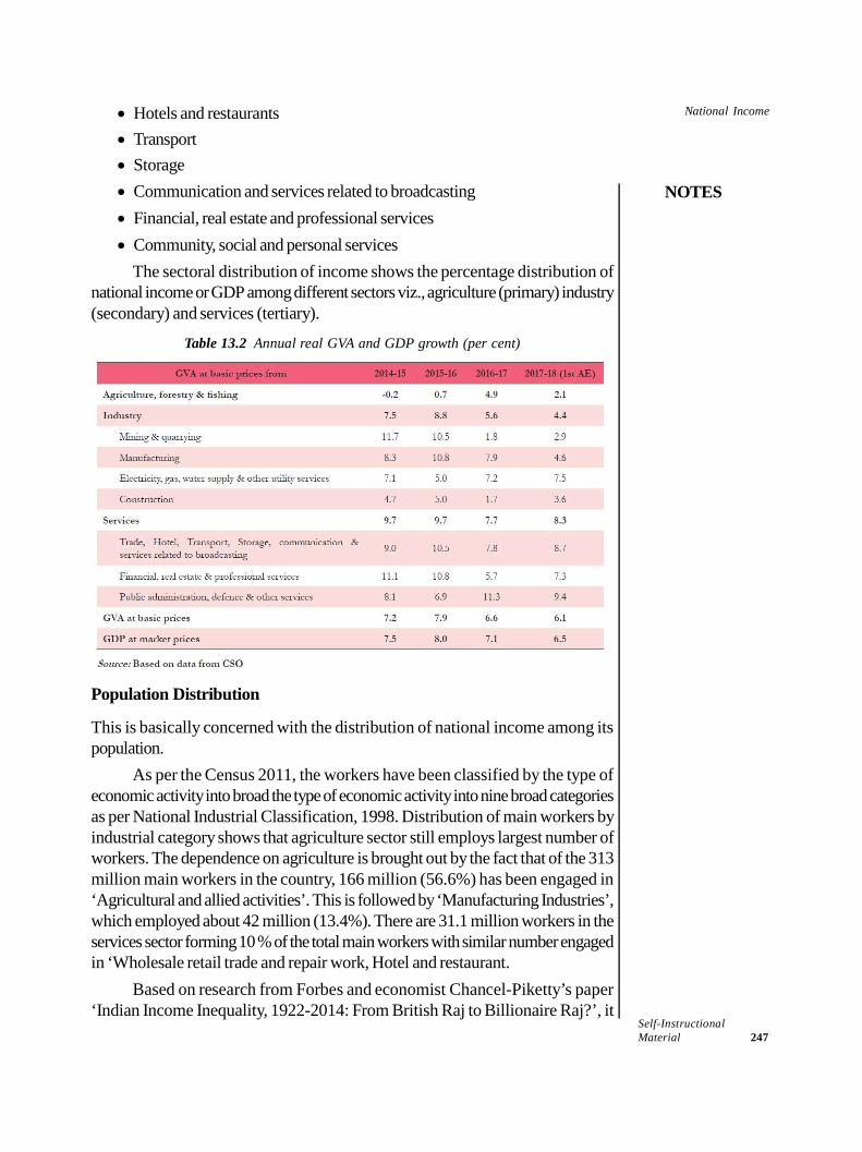
National Income
NOTES
Self-InstructionalMaterial 247
Hotels and restaurants Transport Storage Communication and services related to broadcasting Financial, real estate and professional services Community, social and personal services
The sectoral distribution of income shows the percentage distribution ofnational income or GDP among different sectors viz., agriculture (primary) industry(secondary) and services (tertiary).
Table 13.2 Annual real GVA and GDP growth (per cent)
Population Distribution
This is basically concerned with the distribution of national income among itspopulation.
As per the Census 2011, the workers have been classified by the type ofeconomic activity into broad the type of economic activity into nine broad categoriesas per National Industrial Classification, 1998. Distribution of main workers byindustrial category shows that agriculture sector still employs largest number ofworkers. The dependence on agriculture is brought out by the fact that of the 313million main workers in the country, 166 million (56.6%) has been engaged in‘Agricultural and allied activities’. This is followed by ‘Manufacturing Industries’,which employed about 42 million (13.4%). There are 31.1 million workers in theservices sector forming 10 % of the total main workers with similar number engagedin ‘Wholesale retail trade and repair work, Hotel and restaurant.
Based on research from Forbes and economist Chancel-Piketty’s paper‘Indian Income Inequality, 1922-2014: From British Raj to Billionaire Raj?’, it
National Income
NOTES
Self-Instructional248 Material
has been observed that from a share of 6% of national income in 1982-83, theshare going to the top 1% reached nearly 22% in 2013-14, of which nearly 9%went to the top 0.1%, nearly 4% to the top 0.01%, and almost 2% to the top0.001%. Clearly, income concentration had increased rapidly since the early 1980s.The remaining 90% of the population suffered significant declines in income share.
The middle 40% of the national income distribution possessed 46% of totalincome in 1982-83, declining to 30% in 2013-14. The bottom 50% of thepopulation worsened from nearly 24% in 1982-83 to 15% in 2013-14.
13.5 PER CAPITA INCOME: DEFINITION, ANDCALCULATIONS
Per capita income or average income measures the average income earned perperson in a given area (city, region, country, etc.) in a specified year. It is calculatedby dividing the area’s total income by its total population.
Per capita income is national income/total population.Per capita income is often used to measure an area’s average income. This
is used to compare the wealth of one population with those of others. Per capitaincome is often used to measure a country’s standard of living. It is usually expressedin terms of a commonly used international currency such as the Euro or UnitedStates dollar, and is useful because it is widely known, is easily calculable fromreadily available gross domestic product (GDP) and population estimates, andproduces a useful statistic for comparison of wealth between sovereign territories.This helps to ascertain a country’s development status. It is one of the three measuresfor calculating the Human Development Index of a country.
13.5.1 GDP and GNP
We have briefly discussed these concepts earlier in the unit.
Gross National Product (GNP)
Of the various measures of national income used in national income analysis, GNPis the most important and widely used measure of national income. It is the mostcomprehensive measure of the national productive activities in an open economy.The GNP is defined as the value of all final goods and services producedduring a specific period, usually one year, plus incomes earned abroad by thenationals minus incomes earned locally by the foreigners. The GNP so definedis identical to the concept of gross national income (GNI). Thus, GNP = GNI.The difference between the two is only of procedural nature. While GNP is estimatedon the basis of product-flows, GNI is estimated on the basis of money incomeflows, (i.e., wages, profits, rent, interest, etc.).
National Income
NOTES
Self-InstructionalMaterial 249
Gross Domestic Product (GDP)
The Gross Domestic Product (GDP) is defined as the market value of all finalgoods and services produced in the domestic economy during a period of oneyear, plus income earned locally by the foreigners minus incomes earned abroadby the nationals. The concept of GDP is similar to that of GNP with a significantprocedural difference. In case of GNP, incomes earned by the nationals in foreigncountries are added and incomes earned locally by the foreigners are deductedfrom the market value of domestically produced goods and services. But, in caseof GDP, the process is reversed—incomes earned locally by foreigners are addedand incomes earned abroad by the nationals are deducted from the total value ofdomestically produced goods and services.
Net National Product (NNP)
NNP is defined as GNP less depreciation, i.e.,NNP = GNP – Depreciation
Depreciation is that part of total productive assets which is used to replace thecapital worn out in the process of creating GNP. Briefly speaking, in the processof producing goods and services (including capital goods), a part of total stock ofcapital is used up. ‘Depreciation’ is the term used to denote the worn out or usedup capital in the process of production. An estimated value of depreciation isdeducted from the GNP to arrive at NNP.
The NNP, as defined above, gives the measure of net output available forconsumption and investment by the society (including consumers, producers andthe government). NNP is the real measure of the national income. NNP = NNI(net national income). In other words, NNP is the same as the national income atfactor cost. It should be noted that NNP is measured at market prices includingdirect taxes. Indirect taxes are, however, not a part of actual cost of production.Therefore, to obtain real national income, indirect taxes are deducted from theNNP. Thus, NNP less indirect taxes = National Income.
Some Accounting Definitions
(a) Accounting Identities at Market PriceGNP GNI (Gross National Income)GDP GNP less net income from abroadNNP GNP less depreciationNDP (Net Domestic Product) NNP less net income from abroad
(b) Some Accounting Indentities at Factor CostGNP at factor cost GNP at market price less net indirect taxesNNP at factor cost NNP at market price less net indirect taxes
National Income
NOTES
Self-Instructional250 Material
NDP at factor cost NNP at market price less net income from abroadNDP at factor cost NDP at market price less net indirect taxesNDP at factor cost GDP at market price less depreciation
13.5.2 Uses and Limitations
In this section, we will discuss the uses and limitations of per capita income.
Uses of Per Capita Income
Per capita income is a great measure of ascertaining the financial stability of two ormore regions through the comparison of the different incomes. In fact, regionalincome data is mostly calculated through per capita income because it gives anaccurate picture of the average level of income of the population of the particulararea. The per capita income related comparisons can be used for economic stability,investment and aid related appeals in the international community.
Wealth and Stability: Per capita income is the ratio of the amount of theregion’s income divided by the population of the region. This indicates thatif this ratio rises then the population of the region on an average is morestable and comfortable than in the past. Similarly, if this ratio decreases thenit shows that the income levels of the region has been on the decline. Thisfollows the assumption that the inflation remains the same.
Aid: There are a lot of governmental level aid-related agency which providefinancial assistance to member countries in need. Since the per capita incomeshowcases the prosperity of the region, it will help these agencies guagewhich regions are in need of assistance. For example, if the income of countryA is higher than country B, and the price of rice is higher in country A thanin country B, then the population of country B are just as prosperous as thepopulation in country A. However, if the per capita incomes are same inboth countries A and B and the price of rise is higher in country A, then theincreased cost will be an issue. This can be dealt with through financialassistance to the financial worse of country which is country A in this case.
Limitations of Per Capita Income
The increase in the per capita incomes are due to increase in prices and notphysical outputs and this is why it is not really a credible source ofmeasurement.
Since per capita income is an average, then the national data will cover upthe regional variations that might arise in terms of income, employment, andoutput of the population per head.
Per capita income, as mentioned before, is an average. This means thateven if the average income increases there are chances that the inequalitieswithin the population grows, where the income of one section keeps onincreasing while the other section’s becomes stagnant or lower in comparison.
National Income
NOTES
Self-InstructionalMaterial 251
The per capita income is an economic measure therefore, it might show theincrease of incomes but does not reveal the cost at which it is achieved. Forexample, it might be possible that in order to increase production workinghours might have been increased for labour which affects the actual prosperityof the population in qualitative terms.
Certain indicators of prosperity for example, improvements in life expectancy,health care or education is not reflected through economic measurementslike GDP.
13.5.3 Recent Developments in Indian Economy
As per the Economic Survey 2017-18: A series of major reforms undertaken over the past year will allow real
GDP growth to reach 6.75 percent this fiscal and will rise to 7.0 to 7.5percent in 2018-19, thereby re-instating India as the world’s fastest growingmajor economy.
Due to the launch of transformational Goods and Services Tax (GST) reformon July 1, 2017, resolution of the long-festering Twin Balance Sheet (TBS)problem by sending the major stressed companies for resolution under thenew Indian Bankruptcy Code, implementing a major recapitalization packageto strengthen the public sector banks, further liberalization of FDI and theexport uplift from the global recovery, the economy began to accelerate inthe second half of the year and can clock 6.75 percent growth this year.
India can be rated as among the best performing economies in the world asthe average growth during last three years is around 4 percentage pointshigher than global growth and nearly 3 percentage points higher than that ofEmerging Market and Developing Economies.
The GDP growth has averaged 7.3 per cent for the period from 2014-15to 2017-18, which is the highest among the major economies of the world.That this growth has been achieved in a milieu of lower inflation, improvedcurrent account balance and notable reduction in the fiscal deficit to GDPratio makes it all the more creditable.
The agenda for the next year consequently remains full: stabilizing the GST,completing the TBS actions, privatizing Air India, and staving off threats tomacro-economic stability. The TBS actions, noteworthy for cracking thelong-standing “exit” problem, need complementary reforms to shrink unviablebanks and allow greater private sector participation.
Three areas of policy focus stand out: Employment: finding good jobs forthe young and burgeoning workforce, especially for women. Education:creating an educated and healthy labor force. Agriculture: raising farmproductivity while strengthening agricultural resilience. Above all, India mustcontinue improving the climate for rapid economic growth on the strengthof the only two truly sustainable engines—private investment and exports.
National Income
NOTES
Self-Instructional252 Material
As per Budget 2018-19: Budget 2018-19 reflects the Government’s firm commitment to substantially
boost investment in Agriculture, Social Sector, Digital Payments,Infrastructure and Employment Generation on the one hand andsimultaneously stick to the path of fiscal rectitude by aiming for a reductionof FD by 0.2% of GDP over RE 2017-18.
Various economic reforms were undertaken in the year which include:implementation of the Goods and Service Tax, announcement of bankrecapitalization, push to infrastructure development by giving infrastructurestatus to affordable housing, higher allocation of funds for highwayconstruction and greater focus on coastal connectivity.
Other sectoral initiatives undertaken include: measures to revive theconstruction sector and promotion of exports in textile and apparel industry.Apart from these, the measures that were taken by the Government in theprevious years to boost manufacturing, employment generation, improvingease of doing business and transparency via schemes such as Make-in-India, Skill India, direct benefit transfer and measures for financial inclusionwere also taken forward in 2017-18.
Check Your Progress
4. What are the components of industry sector?5. Name the tool which is used as one of the three measures for calculating
the HDI of a country.6. Define NDP at factor cost as an accounting identity.
13.6 ANSWERS TO CHECK YOUR PROGRESSQUESTIONS
1. Non-economic products include services rendered to self, to family, torelations and to neighbours. Non-economic products are not included innational income.
2. The expenditure method of national income calculation in which the nationalincome is calculated at the final expenditure stages.
3. The fundamental principle of the Keynesian theory of national incomedetermination is that the national income is determined by aggregate demandand aggregate supply and equilibrium level of national income is determinedat the level where aggregate demand equals aggregate supply.
4. The industry sector comprises the following: manufacturing, electricity, gas,water supply and construction.
National Income
NOTES
Self-InstructionalMaterial 253
5. Per capita income is the tool which is used as one the three measures forcalculating the HDI of a country.
6. NDP at factor cost is equal to NDP at market price less net income fromabroad.
13.7 SUMMARY
National income is defined as the money value of all final gods and servicesproduced over a period of one year. Alternatively, national income is alsodefined as the sum of factors income (wages, rent, interest and profit)generated over a period of one year.
National income is measured in terms of (i) Gross Domestic Product (GDP),and (ii) Gross National Product (GNP).
GDP is the measure of the total market value of all final goods and servicesproduced in the domestic economy during a period of one year plus incomeearned by the foreigners in the country minus income earned by countrymenfrom abroad.
GNP is the measure of the total market value of all final goods and servicesproduced in the domestic economy during a period of one year plus incomesearned abroad by the citizens minus income earned by the foreigners in thecountry.
Three methods are used to measure the national income: (i) Net product orValue Added Method, (ii) Factor-income method, and (iii) Expendituremethod.
Under Net Product or value-added method, national income is estimated inthree stages: estimating gross value of domestic output, (ii) estimating costof production, and estimating depreciation of capital. National income isworked out by deducting cost of production and depreciation from thegross value.
Under factor income method, national income is estimated by adding up allfactor incomes. Thus, National Income = Rent + Wages + Interest + Profits.In general, national income is estimated by working out and adding up labourincome, capital income and mixed income.
Under expenditure method, national income is estimated by adding up (i)private consumption expenditure, (ii) direct tax payments, (iii) payments asdonation, and private savings.
Theory of national income determination was formulated by J. M. Keynes.According to Keynes, the equilibrium level of national demand is determinedby aggregate demand for and aggregate supply (AS) of goods and services.
National Income
NOTES
Self-Instructional254 Material
Aggregate demand (AD) refers to the total expenditure made by the peopleof country including households, government, and foreigners. Aggregatesupply (AS) refers the total supply of consumer goods and services andcapital goods (machinery, equipments, etc.).
Keynesian theory of income determination is explained under three models:(i) two-sector model including only two sectors – households and firms;(ii) three- sector model including households, firmsand government; and(iii) four-sector model including households, firms, government and foreignsector.
Sectoral distribution of income is simply the distribution of income amongstthe three sectors of the economy. Population distribution of income reflectsthe manner in which income is distributed amongst the population of thecountry.
Per capita income or average income measures the average income earnedper person in a given are (city, region, country, etc.) in a specified year. It iscalculated by dividing the area’s total income by its total population.
13.8 KEY WORDS
National income: It is defined as the sum of money value of all final goodsand services produced in a country over a period of one year.
Theory of national income determination: It refers to the theory whichexplains how equilibrium level of national income is determined.
Aggregate supply: It refers to the total value of goods and servicesproduced and supplied in an economy per unit of time.
Aggregate demand: It is an ex-post concept which implies effectivedemand which equals actual expenditure.
Per capita income: It measures the average income earned per person ina given area in a specified year.
13.9 SELF ASSESSMENT QUESTIONS ANDEXERCISES
Short Answer Questions
1. Define intermediate and final products.2. What is the difference between national income and private income?3. List the varied types of income included in the factor income method.4. Write a short note on sectoral and population distribution of income.5. What are the limitations and uses of per capita income?
National Income
NOTES
Self-InstructionalMaterial 255
Long Answer Questions
1. Explain the different methods of measurement of national income.2. Examine, in detail, the Keynesian theory of income determination through
different models.3. Describe the concept of GDP, GNP and NNP.
13.10 FURTHER READINGS
Dwivedi, D. N. 2015. Principles of Economics, Eight Edition. New Delhi: VikasPublishing House.
Weil. David N. 2004. Economic Growth. London: Addison Wesley.Thomas, Christopher R. and Maurice S. Charles. 2005. Managerial Economics:
Concepts and Applications, Eighth Edition. New Delhi: Tata McGraw-Hill Publishing Company Limited.
Mankiw, Gregory N. 2002. Principles of Economics, Second Edition. India:Thomson Press.
Websites
https://blogs.economictimes.indiatimes.com/et-commentary/heres-how-indias-widening-income-distribution-can-be-redressed/
https://www.livemint.com/Opinion/WmpSjQAvPGeVzxqpgXYvtK/The-dangers-of-Indias-Billionaire-Raj.html
Economic Regulationsof Business
NOTES
Self-Instructional256 Material
UNIT 14 ECONOMIC REGULATIONSOF BUSINESS
Structure14.0 Introduction14.1 Objectives14.2 Antitrust Theory and Regulations
14.2.1 Antitrust Theory14.2.2 Activities of Business which Require the Use of Antitrust Laws
14.3 The Structure – Conduct – Performance Paradigm14.3.1 Elements of the Paradigm14.3.2 Criticisms of the SCP Paradigm
14.4 Concentration: Overview and Measurement14.4.1 Measuring Industrial Concentration14.4.2 Monopoly Vs Concentration of Economic Power
14.5 Regulation of Externalities14.6 Answers to Check Your Progress Questions14.7 Summary14.8 Key Words14.9 Self Assessment Questions and Exercises
14.10 Further Readings
14.0 INTRODUCTION
The economic framework within which the firm functions plays a crucial role in itsefforts to thrive, grow and beat its competitors. Since business is fundamentally aneconomic activity, the economic environment, both within the country as well asbeyond its national frontiers will have a definite influence on its fortunes. It isinconceivable that there could be any institution, bodies or persons who are insulatedfrom the effects of the economic environs. Business has to deal with a vast numberof governmental bodies, rules, regulations, and guidelines relating to its statutoryresponsibilities, the capital market, sources of finance including stock marketoptions, venture capital, offshore funds, disinvestment options, bank funding andso on. In this unit, we will study the concept of economic regulations of business.
14.1 OBJECTIVES
After going through this unit, you will be able to: Discuss the antithrust theory and regulations Describe the structure-conduct-performance paradigm Explain the concept of concentration and its measurement Examine externalities and its regulations in managerial economics
Economic Regulationsof Business
NOTES
Self-InstructionalMaterial 257
14.2 ANTITRUST THEORY AND REGULATIONS
Antitrust laws are often mentioned as ‘competition laws’. These are laws establishedby the governments to protect the consumers from predacious practices of business.The laws ensure existence of impartial competition in economy which is basedopen-market. They have developed as the markets have evolved and are in keepingwith the recent trends. They safeguard the markets and the consumers fromprospective monopolies which will become a cause of commotions to theproductivity and competitive flow.
14.2.1 Antitrust Theory
The classical viewpoint on competition maintained that particular agreements andpractices of business may result in unreasoned restriction over people’s freedomin business attempting to earn a livelihood. Restrictions were adjudged asacceptable or unacceptable by courts as fresh incidents came to light with thechanges in the business environment. Therefore, the courts established exactclassifications of agreement, explicit articles, towards foul play of their code onfair economic practices, and courts did not scheme for a central notion of marketpower. Initial theorists of the field like Adam Smith had precluded power ofmonopoly on such grounds. He was of the view that any form of monopoly practicedin the market has similar impact as that of a secret in business or the producers. Itdoes not matter how the producers monopolise the market, they could undersupply or sell their products more than the actual price and increase their profits.
In his book The Wealth of Nations, Adam Smith observed problems relatedto cartel, but he did not preach any legal methods to curtail them, he observed:‘People of the same trade seldom meet together, even for merriment and diversion,but the conversation ends in a conspiracy against the public, or in some contrivanceto raise prices. It is impossible indeed to prevent such meetings, by any law whicheither could be executed, or would be consistent with liberty and justice. Butthough the law cannot hinder people of the same trade from sometimes assemblingtogether, it ought to do nothing to facilitate such assemblies; much less to renderthem necessary.’ At the same time, Smith overruled the mere presence of any kindof corporations whether big, dominating or foul.
Large corporations had become an integral part of market economy towardsthe middle of the nineteenth century. During this time John Stuart Mill submitted hisapproach in his book treatise On Liberty published in 1859. In his approach, Millregarded business as a social activity and thought all traders have to consider theinterest of others and entire society. Producers supply good as well as bad qualitygoods and this leaves the buyers to find other alternatives. He preached the doctrineof Free Trade; this was not on the same lines as individual liberty which had beenemphasized earlier. All types of restrictions are restrains and these are not goodfor the trade.
Economic Regulationsof Business
NOTES
Self-Instructional258 Material
The Neo-classical view point was a shift from the views of Mill and it focusedon model of competition which was based free markets and services provided inmarkets which were free from competition provided maximum social good.According to this model, firms were allowed to enter the market without restrictionsand freely compete with firms functioning in the market. The economists felt that inthe absence of competition, markets function with greater efficiency. This model iscompletely contrasting with monopolies and cartels. Conventional economistscompletely agreed that there was no such thing as perfection in competition hencethe objective is always to attain a state of competition which is workable andprovided maximum efficiency. After both these contradictory theories, theeconomists and lawyers connected with the Chicago University advocated anapproach which worked towards establishing laws for competition.
Robert Bork was not much in favour of decisions taken by court on antitrustlaws and he voiced his opinions in his book The Antitrust Paradox. There areviews of Harvard Professor Philip Areeda who was keen for the court to adoptmore forceful laws and policies over antitrust.
14.2.2 Activities of Business which Require the use of Antitrust Laws
There are numerous debatable activities of business on which the Antitrust lawsare used, these include:
Allocation of Market: Suppose company B functions in eastern part ofthe city and company C functions in western parts of the city so they wouldcontinue to function in their specified areas. This will give kind of monopolyto both in their respective areas as cost of setting up a new company is veryhigh hence no new company will provide competition.
Bid Rigging: In this scenario three corporations join hands and form acartel. In this they equally permit all members to have an equal share and donot try to encroach over others share, thus they do not compete againsteach other. There is no competition in the market.Bid rigging further have three sub-types:
(i) Bid Suppression: Participants abstain to bid against each other bywithdrawing from the bid so that the decided bidder can win
(ii) Complementary Bidding: This type is also called courtesy bidding,this takes place in situations where the applicants purposely submitmuch higher bids and allow the decided bidder to quote less andaccommodate all the demands of the buyer. These are most prone torigging and are developed to provide a false picture for the buyerabout the market environment.
(iii) Bid Rotation: As the word suggests in this type the participants winthe biddings in rotation and follow a cycle so each gets to win.
Price Fixing: Company A and B are the sole producers of a product. Theproducts are completely identical and consumers have no preference other
Economic Regulationsof Business
NOTES
Self-InstructionalMaterial 259
than the price of the product. Both the companies sell their products at thesame price so that they can avoid the conflict because of price. Selling theproduct at the same price helps in maintaining the margin and results in thecustomers paying more for the product which they could have got at alower price.
Monopolies: The formulation of antitrust laws occurred in order to avoidmonopolies. Among the most prominent legal cases of antitrust was ofMicrosoft Corporation, it was charged with undertaking actions whichencouraged its monopoly in market and were against the competitive normsof the market. The corporation was compelling its users to install their webbrowsers for the operating system of Windows.Controllers have to make sure that monopolies are prevented from cultivating
an environment which is obviously competitive and market share should be earnedwith the help of business expertise and new inventions. Earning market share byillegal means is considered wrong.
Following are some of the arrangements which lead to monopolising marketshare in an illegal manner and are subjective to action by law:
Exclusive Supply Agreements: This happens in case a supplier is stoppedfrom retailing to any other buyer other than the ones mentioned in the contract.These type of agreements kills all the competition from the market andhelps in establishing monopoly.
Securing the Sale of Two Products: In cases where a producer has astrong monopoly over a product in the market and desires to acquiremonopoly over a second product, the producer in order to acquire monopolyon the second product ties the sale of strong product with the new one andcompels the buyers to purchase the new product as well even if it is notneeded by them. This compelling is against the antitrust laws.
Predacious Pricing: Though this practice of establishing monopoly is noteasy to bring out in the open and, the firm may keep prices low for a longtime and maintain the market share so that it can overcome the losses in thelong run.
Rebuff Deals: Companies who have monopoly over the market are ableto decide the firms with whom they wish to have business dealings. Ininstances where they use their dominance to curtail competition they areliable for violating the antitrust laws.
Mergers and Acquisitions: The antitrust laws cover the sphere of all themergers and new businesses which are acquired. There are divided intothree types:
(i) Horizontal Mergers: Here the two companies which are rivals sharethe same product line and markets to become one single firm.
Economic Regulationsof Business
NOTES
Self-Instructional260 Material
(ii) Vertical Mergers: These are mergers which are undertaken whentwo companies at different levels of the production of same productmerge their operations.
(iii) Conglomerate Mergers: These are mergers where betweencompanies operating in different industries for synergy, productextension and market extension benefits.
Competition Laws in India
India was among the first developing countries to have a competition law in theform of the Monopolies and Restrictive Trade Practices (MRTP) Act, 1969. TheMRTP Act was designed to check concentration of economic power, prohibitrestrictive or unfair trade practices and control of monopolies. Then came 1991,which has proved to be a watershed in the history of India’s economicdevelopment. The new India required new rules. Hence, the need for a newcompetition law. Accordingly, the Competition Act was passed in 2002 andamended in 2007. The Competition Commission of India (CCI) was establishedon March 1, 2009 as an autonomous body comprising of a Chairperson and sixmembers. An appellate body Competition Appellate Tribunal was also set up inMay 2009 with final appeal lying to the Supreme Court of India. Subsequently,the MRTP Act was repealed, MRTP Commission established under that act wasabolished and its pending cases were transferred to the CCI. Sections 5 & 6relating to Merger & Acquisition were notified in June, 2011.
The Competition Act, 2002, as amended by the Competition (Amendment)Act, 2007, follows the philosophy of modern competition laws. The Act prohibitsanti-competitive agreements, abuse of dominant position by enterprises andregulates combinations (acquisition, acquiring of control and M&A), which causesor likely to cause an appreciable adverse effect on competition within India. Thesectors that have been covered are as diverse as infrastructure, finance,entertainment, IT, telecom, civil aviation, energy, insurance, travel, automobilemanufacturing, real estate and pharmaceuticals etc.
14.3 THE STRUCTURE – CONDUCT –PERFORMANCE PARADIGM
Structure-Conduct-Performance (SCP) framework suggests a connecting affiliationamong the market’s structure (S), the conduct (C) of various firms of that marketand their performance (P) in the economy. The paradigm was initially suggestedby E. Mason during the 1930s and was further developed in 1950s by J Bain. Theneo-classical theory of firm formed the basis of the paradigm and since then it hasbeen the focal point if all the industrial organization studies.
The systematic framework which is used to create a relationship betweenthe structure of the market, conduct of the market and performance of the market
Economic Regulationsof Business
NOTES
Self-InstructionalMaterial 261
is called Structure, Conduct and Performance paradigm (SCP). As mentionedearlier, in 1959 American Economist Joe S Bain Jr developed the framework andhe had included the SCP in his book Industrial Organization. The paradigmcreated by him was of the structure, conduct, and performance in connection tothe industry and was different from firms and industries owned by individuals. Itsuggested and verified blockades to access as a determining factor of industryperformance. Market concentration had been examined in connection to powerof the market and rate of profit.
Since it was developed, in the field of economics and all fields of businessmanagement and controlling the SCP paradigm is regarded as mainstay of thetheory of industrial organization. It offers the starting point for analysing variousmarkets and industries. The paradigm helped a lot of researches and academicsof economics to base their work on the foundation of SCP, even Americanacademic Michael E. Porter built his works on competition, theories on economicsand business strategy on the principles of the paradigm.
On the reasoning of the paradigm it can be understood that performance ofindustries (that are working towards social good) are dependent on the conductof the firms functioning in the confines of the specific industry and they are furtherdependent on the market structure.
14.3.1 Elements of the Paradigm
Let’s look at each of the elements of the paradigm in this section.Structure: It involves the fixed aspects which remain considerably same withpassing time and result in impacting the behaviour of both suppliers and consumersor either one of them. The system where the market is unable to follow a conditionof perfect competition is dependent on extent of factors such as concentration ofsupply and demand both respectively, product differentiation and barriers in enteringthe market. Furthermore, the product’s nature and the technology used formanufacturing the product would also play a significant role in determining thestructure of the market.
Conduct: This refers to the behaviour of the consumers and retailers, theirbehaviour with each other as well as between themselves have an impact. Thebehaviour of the firms is based on their strategy which is decided after researchingaspects like investment, development, levels of advertisement and collusions.
Performance: The third element of the paradigm is performance which isevaluated on the basis of the comparison drawn from the outcomes of all the firmsof the industry in terms of the level of efficiency and diverse ratios are employed toevaluate the varied levels of profitability. The varied levels taken under considerationare level of pricing, quality of the product, distribution of resources, levels ofefficiency during production and many more.
The markets are made up of retailers and consumers; the ever-changingbehaviour of both the constituents has an impact on the markets. The dynamism of
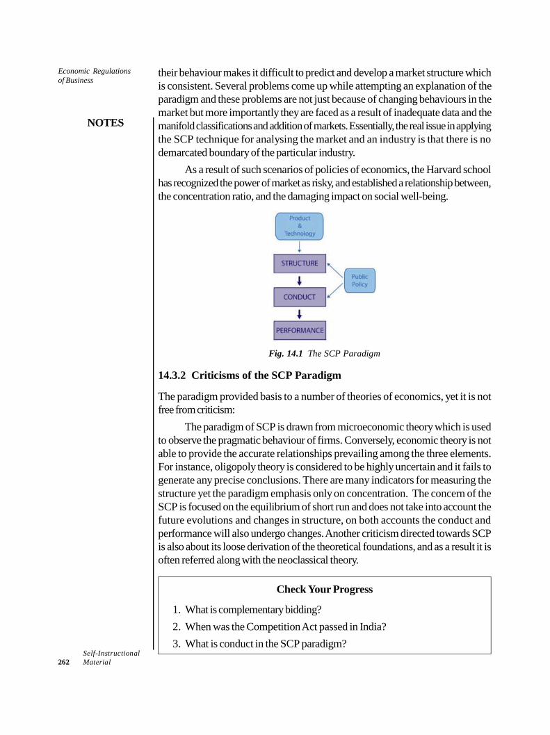
Economic Regulationsof Business
NOTES
Self-Instructional262 Material
their behaviour makes it difficult to predict and develop a market structure whichis consistent. Several problems come up while attempting an explanation of theparadigm and these problems are not just because of changing behaviours in themarket but more importantly they are faced as a result of inadequate data and themanifold classifications and addition of markets. Essentially, the real issue in applyingthe SCP technique for analysing the market and an industry is that there is nodemarcated boundary of the particular industry.
As a result of such scenarios of policies of economics, the Harvard schoolhas recognized the power of market as risky, and established a relationship between,the concentration ratio, and the damaging impact on social well-being.
Fig. 14.1 The SCP Paradigm
14.3.2 Criticisms of the SCP Paradigm
The paradigm provided basis to a number of theories of economics, yet it is notfree from criticism:
The paradigm of SCP is drawn from microeconomic theory which is usedto observe the pragmatic behaviour of firms. Conversely, economic theory is notable to provide the accurate relationships prevailing among the three elements.For instance, oligopoly theory is considered to be highly uncertain and it fails togenerate any precise conclusions. There are many indicators for measuring thestructure yet the paradigm emphasis only on concentration. The concern of theSCP is focused on the equilibrium of short run and does not take into account thefuture evolutions and changes in structure, on both accounts the conduct andperformance will also undergo changes. Another criticism directed towards SCPis also about its loose derivation of the theoretical foundations, and as a result it isoften referred along with the neoclassical theory.
Check Your Progress
1. What is complementary bidding?2. When was the Competition Act passed in India?3. What is conduct in the SCP paradigm?
Economic Regulationsof Business
NOTES
Self-InstructionalMaterial 263
14.4 CONCENTRATION: OVERVIEW ANDMEASUREMENT
Economic concentration has several denotations in the industrial structure and isoften applied to various ‘indexes of concentration’ in order to understand thedistinctive features of the structure in industries. According to the economic theory,concentration is a vital factor as it determines the behaviour of the market and alsoaffects its outcome. All other things being equal, when few big firms are responsiblefor supplying chunk of the market demand it is highly possible for monopolies tobe established in comparison to when large firms do not supply the bulk demand.Therefore, in the clarification of business policy, the features of an industry articulatedin the concentration index are expected to have an essential role. This connectionwith extent of monopoly has encouraged several pragmatic studies to be coveringthe aspect of measurement of concentration.
Industrial concentration refers to retailer concentration. It means that themarket is dominated by few large firms and they control manufacturing and sellingof products. Two factors affect the extent of industrial concentration, one factor isquantity of firms active in a particular market, and the other factor is percentage ofthe share of the market demand fulfilled by the firm. In case the number of firms inthe market is low then the share of the firms would be large and these big firmswould also have larger control on the overall supply. This being the case then thescenario would be referred as high quantity of retailer/industrial concentration.The market power of each firm decides the extent of its quantity industrialconcentration. The capability of a firm or retailer to affect the product’s cost in themarket is referred to as market power. Market power of a firm is zero in a marketsituation with perfect competition, thus even the industrial concentration is zero.Industrial concentration is highest in a market where monopolistic practices arefollowed.
14.4.1 Measuring Industrial Concentration
Keeping a measurement of industrial concentration is essential as it clearly indicatesthe nature of the market. When there are more number of firms, the market has thecharacter of perfect competition and less number of firms will automatically increasethe measurement of the concentration. Another reason for keeping a track on theextent of concentration is for highlighting the percentage of concentration. Forinstance, if the Concentration Ratio (CR) is 54.2 percent it clearly points out thatproduction of five firms is above fifty percent in a particular industry.
The ways of measuring industrial concentration has two classifications namelyabsolute and relative.
Economic Regulationsof Business
NOTES
Self-Instructional264 Material
Absolute Measures of Concentration
The fundamental fact of this classification is that the number of firms is absolute interms of manufacturing, service or capital in the industry. There are twomeasurements for this:
(i) The Concentration Ratio (CR): This ratio measures the share ofmanufacturing, sales and employment of three or five largest firms. In theillustration the analysis of the manufacturing is taken. The share of ten firmsis taken into account; assume there are forty firms in total. Total manufacturingof five largest firms is as given below:
Firm 1 manufactures 10,000 PartsFirm 2 manufactures 12,000 PartsFirm 3 manufactures 9,000 PartsFirm 4 manufactures 15,000 PartsFirm 5 manufactures 14,000 PartsTotal Production of the five biggest firms – 60,000 PartsTotal Production in Industry—1,10,000
Concentration Ratio of the Five firms – (60,000/1,10, 000) × 100= 54.54%Thus the five firms have an industrial concentration of 54.54%
(ii) The Herfindahl Index: This is another absolute measure for industrialconcentration, it is also referred to as Herfindahl–Hirschman Index, HHI,or even as HHI-score. It gives the measure of magnitude of firms incomparison to others in the industry and also indicates the quantity ofcompetition between the firms. It takes its name from its creators Orris C.Herfindahl and Albert O. Hirschman, both are renowned economists andthe index is often used cases of in competition law.In this all firms existing in the industry are taken into account. H-index isexplained below:Assume,
n = Number of firms in the industry.x = Absolute amount of firm manufacturing.T = Total manufacturing of the industry.
As stated above the H index takes into account all firms of the industrywhile calculating. The index value is zero to one. In case the industry hasmore firms of similar size then the index value is taken as zero. On the otherhand, in case industry has one firm then the value is one. The H-index hasbeen explained in the following illustration, assume an industry has fourfirms totally and each firm manufactures 500, 350, 300, and 200 partsrespectively. This makes the value of T as 1350 that means share of each
Economic Regulationsof Business
NOTES
Self-InstructionalMaterial 265
firm in total manufacturing is [x1/T] 2 that makes the share of each firm as0.372, 0.262, 0.222 and 0.152 as a result, the value of H index is 0.275.Since this is very close to zero, hence it is clear that concentration levels arelow in the industry. The index helps in showing the extent of concentrationfor all periods.
Relative Measures of Concentration
The inequality of firms is focused in this measure. This implies that markets whichare constituted with firms of uneven proportions have uneven productions as well.The approximate industrial concentration may be measured by using the LorenzCurve. The Lorenz curve provides the representation of wealth distribution withthe help of a graph. In 1905, Max O. Lorenz developed this curve to representthe disparity in the distribution of wealth. In mathematics it is referred as Gini-coefficient.
Gini Concentration Ratio is the statistical measure centered on Lorenz Curve.The value of Gini coefficient is 0 to1 in a Gini coefficient of inequality. In situationswhere all the firms are of same size then the line representing equality and LorenzCurve will be similar. The value of Gini co-efficient will be zero in such a situation.Increased inequality will result in increasing the value of the Gini coefficient.
14.4.1 Monopoly Vs Concentration of Economic Power
A firm’s control over production and distribution of a product is referred to asmonopoly. Monopolistic environment may be created in large as well as smallscale industries. On the other hand, concentration of economic power refers tocentrally controlling essential economic activities such as availability of capital,employment and manufacturing in a major industry or agriculture etc.
The concentration of economic power in India is achieved by promotingmonopoly. In fact, it is the means to acquire power and then promote monopolisticactivities so that the power can be maintained. The aim of all modern economies isto diffuse concentration of economic power as it hampers social justice.
14.5 REGULATION OF EXTERNALITIES
In business, once capital has been sourced, the investors need to determine howmuch capital will be needed to produce a given output. This is revealed throughthe capital output ratio. Capital output ratio is the ratio of capital to output over aperiod of time. In order to calculate this ratio, we need to know the total outputproduced by a country. But it is known that the production, consumption andinvestment decisions relating to the output are bound to lead to consequences thatare not directly exposed or experienced? These indirect and unseen outcomesmay exist and can become problematic when they create large problems. Theseproblems or side effects are referred to by the economists as externalities.
Economic Regulationsof Business
NOTES
Self-Instructional266 Material
Externalities are one of the reasons that government intervention is particularlyrequired in economic affairs of the state. Also, this is why there is a differencebetween the private returns of a commodity (to the owners of factors of production)and the costs of the commodity to a society as a whole. Environmental pollution isa good example of an externality. Additionally, externalities are not always negative.For example, a company may be funding a research conducted by its Researchand Development Department, but the findings of the research will have positiveeffects on the society as a whole. Externalities help the government in determiningfactors such as taxation, grant of subsidies, permits and licenses.
An externalityexists when the actions or decisions of one person or groupimpose a cost, or bestow a benefit on some second or third parties. Externalitiesare sometimes called spillovers or neighbourhood effects. Inefficient decisionsresult when decision makers fail to consider social costs and benefits.
The presence of externalities is a significant phenomenon in modern life.Examples are everywhere: air, water, land, sight, and sound pollution; trafficcongestion; automobile accidents; abandoned housing; nuclear accidents; andpassive smoking are only a few of them. Because there are so many externalitiesthat affect the environment, the study of externalities is a major concern ofenvironmental economics.
Externalities are costs and benefits of economic activity that do not enterinto the firm’s own calculations of costs or revenues. Thus, in the absence of somesort of non-market correction (usually government action), they lead to inefficientallocation of resources.
External costs and benefits are at the core of the common resource problem.A new producer creates higher costs for all previous entrants, or all producersimpose external costs on the general population. In either case, in the absence ofregulation, taxes, or property rights for environmental quality, external costs arenot borne by the producers who cause them. It is obvious then that the prices oftheir products do not reflect the social costs of production. Thus, more of theseresource-depleting or -polluting goods and services are produced and consumedthan would be the case if prices reflected external costs. Hence, societies pollutemore than their people would choose if markets reflected all social costs.
In a market with competitive producers, the supply curve represents privatemarginal costs. But, if this is a polluting industry, the external costs would make thesocial marginal cost, SMC, higher. If these costs were reflected in the market, theprice would jump higher and demand, and therefore, output would be reduced.As less of the offending product would be grown or manufactured, there would beless environmental degradation.
Polluters impose costs on others. If these external costs are reflected in thefirms’ costs, the social marginal cost curve, SMC, would prevail; the market pricewould increase; and output will reduce. But, because the firms do not bear these
Economic Regulationsof Business
NOTES
Self-InstructionalMaterial 267
costs, their private marginal cost curve, is lower. So, more Q1 of the pollutingproduct is produced and consumed.
Types of Externalities
(I) Detrimental (negative) externalities: Detrimental externalities impose costson other outside firms, but do not cost the firm anything. Beneficial externalitiescreate benefits outside the firm, but provide no revenue to the firm.
A typical example of a detrimental externality is the pollution. It can beexplained as follows:
A firm’s production process may send smoke into the air. The firm sustainsno cost to ‘use’ the air in this way. It actually is cheaper for the firm to do sothan to make the effort and pay the expense to clean up its exhaust.
The surrounding area, however, sustains the cost of enduring and cleaningup after the effects of the firm’s smoke. Therefore, there is a cost of thispollution, but it is not paid by the polluting firm; it is imposed on someoneelse (neighbours).
Social and private costs: The social cost of the polluting firm’s production is thesum of its internal costs (private costs, which the market imposes on the firm) andthe external social costs imposed on others by its pollution.
One way or another, society at large has to pay the full social cost in orderfor the firm’s production to occur. The market provides no reliable way toforce the firm to pay anything, but the private cost portion of total socialcost, because there are no private property rights to the air.
The cost of the detrimental externality is not necessarily imposed by themarket upon the firm’s customers, either. They, too, may benefit from thefirm’s lower costs.
If the total social cost could be imposed upon the firm, its cost would behigher and its cost curves would rise. The result would be lower output, ata higher price, reflecting the true social cost of the output.
(II) Beneficial (positive) externalities: Beneficial or positive externalities arepositive effects upon others due to private economic activity. For example,a flowerfarm exists for the purpose of making profit by growing and selling flowers.However, it also is a very attractive thing to see and smell, and so, producespositive externalities for its neighbours and passersby.
The market does not provide the firm (flower farm) any way to collect theextra value to society of the beneficial externality, even though the firm isresponsible for producing it.
If the firm could collect the value of the beneficial externalities it produces,its perceived demand and marginal revenue would increase, and it wouldproduce more.
Economic Regulationsof Business
NOTES
Self-Instructional268 Material
Remedies for Externalities
The market provides no remedy for the misallocation of resources caused byexternalities. Therefore, non-market means have to be found. The most commonone is government action.
Government regulation: In many areas, state and central governmentapply regulations that force some firms to ‘internalize’ negative externalities.Significant examples are anti-pollution laws that require firms to pay thecosts of remedying negative pollution externalities.
Taxation: Government also can impose a tax upon firms creating negativeexternalities. The tax collections then are used to reimburse those who actuallydo pay these external costs. The problems in such an arrangement includeaccurately measuring the social cost involved; how to see to it that thosewho really do pay the external costs are the ones who get compensated.
Subsidy: In the case of positive externalities, government can subsidizefirms that produce them, thus providing the firms with revenue fully reflectingthe social benefit that they produce.
Taxes on Negative Externality
Because pollution imposes costs on the general public, the social marginal cost ofthe pollution (SMC) exceeds the private marginal cost (PMC) of making the goodby the good’s external marginal cost (EMC). The private marginal cost is themarginal cost to the producers of the good. The social cost is the cost to everyone,including the public and the producer. In this case, we have the following equation:
SMC = PMC + EMC; andSMC > PMC when EMC > 0
Assuming there are no positive externalities, the demand curve reflects boththe social marginal benefit (SMB) and the private marginal benefit (PMB) frommaking the good (SMB = PMB).
In the absence of a tax, the free market will produce the good, and sell themfor at a price where PMC = PMB. But because SMC = PMC + EMC, thesocially optimal level of production is where SMC = MB.
An optimal tax would equal the good’s external marginal cost (Tax = EMC).This makes the SMC curve in effect the industry’s PMC curve.
Subsidy for Positive Externalities
Because the good creates benefits for more than just its buyers pay, its socialmarginal benefits (SMB) exceed its private marginal benefits (PMB) by its externalmarginal benefit (EMB). So, we have the following equation:
SMB = PMB + EMB; andSMB > PMB; andEMB > 0
Economic Regulationsof Business
NOTES
Self-InstructionalMaterial 269
We assume there are no negative externalities in this figure. So, the supplycurve reflects both the private and social marginal cost of making the good(PMC = SMC).
In the absence of a tax, the free market will produce the good, and sell themat a price where PMC = PMB. But because SMB > PMB, the socially optimallevel of production is where where SMB = MC.
The socially optimal subsidy is equal to the good’s external marginal benefit(subsidy = EMB).
Pollution as an Externality
In this section, we will restrict our study to learn about pollution as an externality.The government regulation of pollution illustrates some of the principles we
have been talking about. Pollution is a negative externality. Because of transactioncosts, it is too difficult for people to, by themselves, bargain with firms for theoptimal level of pollution.
Two solutions have emerged:1. Taxing polluters: One solution has been proposed to tax polluters.
Emission charges are common in Europe. Water polluters have to paya waste disposal tax there is also an emission charge on gasoline. Thesocial cost includes the private cost plus the cost of pollution emittedby cars. An emission tax equal to the difference between the socialand private marginal cost will result in the optimal level of driving.
2. Limiting the amount of pollution: The second solution is limitingthe amount of pollution. In place of a tax, the government can regulateand limit the amount of pollution allowed.
However, if the same limit is imposed on all individuals, we are not takinginto consideration that the needs of driving vary from individual to individual.Regarding the preceding example of driving, some people have a greater demandfor driving than others. Similarly, some people drive cleaner cars than others.
The Optimal Level of Pollution
What level of pollution should a regulatory agency allow? Pollution is costly. It is asubject of controversy as to how costly it is. But let us pretend that we are all-knowing and have precise figures on pollution’s cost. Similarly, it is costly to getrid of pollution. Let us also suppose that we know these costs. How then do wedecide what is the correct level of pollution? There are two costs society faces:
Total cost = Total pollution cost + Total pollution abatement costThe socially optimal level of pollution minimizes the sum of these two costs.
We can use marginal analysis to assist us. Let Q be the quantity of pollution allowed.The marginal cost of increasing Q by one unit is the bad that occurs. Total pollutioncosts go up. New Delhi gets smoggier. More fish die from acid rain. More people
Economic Regulationsof Business
NOTES
Self-Instructional270 Material
have a higher risk of getting sick. The marginal benefit of increasing Q by one unitis the reduction in pollution abatement costs. Q should be increased as long asMB>MC. At the optimal Q, MB = MC. Because the cheapest ways to reducepollution will be used first, the subsequent units of pollution will cost more to cleanup. Similarly, the marginal cost of pollution will increase. This means the higherthe level of pollution; the costlier a given addition is in terms of the damage thatit does.
Check Your Progress
4. Name the factors which affect the extent of industrial concentration.5. What is HHI?6. Mention some of the other names for externalities.7. What represents private marginal costs in a market with competitive
producers?
14.6 ANSWERS TO CHECK YOUR PROGRESSQUESTIONS
1. Complementary bidding is also called courtesy bidding, this takes place insituations where the applicants purposely submit much higher bids and allowthe decided bidder to quote less and accommodate all the demands of thebuyer. These are most prone to rigging and are developed to provide afalse picture for the buyer about the market environment.
2. The Competition Act was passed in 2002 and amended in 2007.3. Conduct in the SCP paradigm refers to the behaviour of the consumers and
retailers, their behaviour with each other as well as between themselveshave an impact. The behaviour of the firms is based on their strategy whichis decided after researching aspects like investment, development, levels ofadvertisement and collusions.
4. Two factors affect the extent of industrial concentration, one factor is quantityof firms active in a particular market, and the other factor is percentage ofthe share of the market demand fulfilled by the firm.
5. Herfindahl–Hirschman Index, HHI, or even as HHI-score is an absolutemeasure of concentration which gives the measure of magnitude of firms incomparison to others in the industry and also indicates the quantity ofcompetition between the firms.
6. Externalities are sometimes called spillovers or neighbourhood effects.7. In a market with competitive producers, the supply curve represents private
marginal costs.
Economic Regulationsof Business
NOTES
Self-InstructionalMaterial 271
14.7 SUMMARY
The economic framework within which the firm functions plays a crucialrole in its efforts to thrive, grow and beat its competitors. Since business isfundamentally an economic activity, the economic environment, both withinthe country as well as beyond its national frontiers will have a definite influenceon its fortunes.
Business has to deal with a vast number of governmental bodies, rules,regulations, and guidelines relating to its statutory responsibilities, the capitalmarket, sources of finance including stock market options, venture capital,offshore funds, disinvestment options, bank funding and so on.
Antitrust laws are often mentioned as ‘competition laws’. These are lawsestablished by the governments to protect the consumers from predaciouspractices of business. The laws ensure existence of impartial competition ineconomy which is based open-market. They have developed as the marketshave evolved and are in keeping with the recent trends.
There are numerous debatable activities of business on which theAntitrust laws are used: allocation of market, bid rigging, price fixing,monopolies, etc.
India was among the first developing countries to have a competition law inthe form of the Monopolies and Restrictive Trade Practices (MRTP) Act,1969. The MRTP Act was designed to check concentration of economicpower, prohibit restrictive or unfair trade practices and control ofmonopolies.
The year 1991 proved to be a watershed in the history of India’s economicdevelopment. The new India required new rules. Hence, the need for anew competition law. Accordingly, the Competition Act was passed in 2002and amended in 2007.
The Competition Act, 2002, as amended by the Competition (Amendment)Act, 2007, follows the philosophy of modern competition laws. The Actprohibits anti-competitive agreements, abuse of dominant position byenterprises and regulates combinations (acquisition, acquiring of control andM&A), which causes or likely to cause an appreciable adverse effect oncompetition within India.
Structure-Conduct-Performance (SCP) framework suggests a connectingaffiliation among the market’s structure (S), the conduct (C) of various firmsof that market and their performance (P) in the economy. The paradigmwas initially suggested by E. Mason during the 1930s and was furtherdeveloped in 1950s by J Bain. The neo-classical theory of firm formed thebasis of the paradigm and since then it has been the focal point if all theindustrial organization studies.
Economic Regulationsof Business
NOTES
Self-Instructional272 Material
Economic concentration has several denotations in the industrial structureand is often applied to various ‘indexes of concentration’ in order tounderstand the distinctive features of the structure in industries. Accordingto the economic theory, concentration is a vital factor as it determines thebehaviour of the market and also affects its outcome.
A firm’s control over production and distribution of a product is referred toas monopoly. Monopolistic environment may be created in large as well assmall scale industries. On the other hand, concentration of economic powerrefers to centrally controlling essential economic activities such as availabilityof capital, employment and manufacturing in a major industry or agricultureetc.
Externalities are costs and benefits of economic activity that do not enterinto the firm’s own calculations of costs or revenues. Thus, in the absenceof some sort of non-market correction (usually government action), theylead to inefficient allocation of resources.
Remedies for Externalities include: government regulations, taxation andsubsidies.
14.8 KEY WORDS
Antitrust laws: Also known as ‘competition laws’, these are lawsestablished by the governments to protect the consumers from predaciouspractices of business.
Structure-Conduct-Performance (SCP) framework: It suggests aconnecting affiliation among the market’s structure (S), the conduct (C) ofvarious firms of that market and their performance (P) in the economy.
Externality: An economic effect that results from an economic choice butis not reflected in market price
14.9 SELF ASSESSMENT QUESTIONS ANDEXERCISES
Short Answer Questions
1. Give a brief introduction to the development of Antitrust theory.2. Write a short note on competition laws in India.3. What are the criticisms against the SCP paradigm?4. What is the difference between monopoly and concentration of economic
power?5. Mention the solutions to pollution as an externality.
Economic Regulationsof Business
NOTES
Self-InstructionalMaterial 273
Long Answer Questions
1. What are the activities of business which require the use of anti-trust laws?2. Explain the elements of the SCP paradigm.3. Describe the absolute and relative measures of industrial concentration.4. Discuss the types of and remedies for externalities.
14.10 FURTHER READINGS
Dwivedi, D. N. 2015. Principles of Economics, Eight Edition. New Delhi: VikasPublishing House.
Weil. David N. 2004. Economic Growth. London: Addison Wesley.Thomas, Christopher R. and Maurice S. Charles. 2005. Managerial Economics:
Concepts and Applications, Eighth Edition. New Delhi: Tata McGraw-Hill Publishing Company Limited.
Mankiw, Gregory N. 2002. Principles of Economics, Second Edition. India:Thomson Press.
Websites
https://blogs.economictimes.indiatimes.com/et-commentary/heres-how-indias-widening-income-distribution-can-be-redressed/
https://www.livemint.com/Opinion/WmpSjQAvPGeVzxqpgXYvtK/The-dangers-of-Indias-Billionaire-Raj.html

MANAGERIAL ECONOMICS
VENKATESHWARAOPEN UNIVERSITY
www.vou.ac.in
VENKATESHWARAOPEN UNIVERSITY
www.vou.ac.in
MANAGERIAL ECONOMICS
MBA[MBA-203]
MANAGERIAL ECONOM
ICS13 MM


