Embed Size (px)
Citation preview
Brigham Young University Brigham Young University
BYU ScholarsArchive BYU ScholarsArchive
Theses and Dissertations
2021-02-09
Mean Square Displacement for a Discrete Centroid Model of Cell Mean Square Displacement for a Discrete Centroid Model of Cell
Motion and a Mathematical Analysis of Focal Adhesion Lifetimes Motion and a Mathematical Analysis of Focal Adhesion Lifetimes
and Their Effect on Cell Motility and Their Effect on Cell Motility
Mary Ellen Furner Rosen Brigham Young University
Follow this and additional works at: https://scholarsarchive.byu.edu/etd
Part of the Physical Sciences and Mathematics Commons
BYU ScholarsArchive Citation BYU ScholarsArchive Citation Rosen, Mary Ellen Furner, "Mean Square Displacement for a Discrete Centroid Model of Cell Motion and a Mathematical Analysis of Focal Adhesion Lifetimes and Their Effect on Cell Motility" (2021). Theses and Dissertations. 8780. https://scholarsarchive.byu.edu/etd/8780
This Dissertation is brought to you for free and open access by BYU ScholarsArchive. It has been accepted for inclusion in Theses and Dissertations by an authorized administrator of BYU ScholarsArchive. For more information, please contact [email protected].

Mean Square Displacement for a Discrete Centroid Model of Cell Motion and
A Mathematical Analysis of Focal Adhesion Lifetimes
and Their Effect on Cell Motility
Mary Ellen Furner Rosen
A dissertation submitted to the faculty ofBrigham Young University
in partial fulfillment of the requirements for the degree of
Doctor of Philosophy
John Dallon, ChairEmily Evans
Christopher GrantKening Lu
Benjamin Webb
Department of Mathematics
Brigham Young University
Copyright © 2021 Mary Ellen Furner Rosen
All Rights Reserved

abstract
Mean Square Displacement for a Discrete Centroid Model of Cell Motion andA Mathematical Analysis of Focal Adhesion Lifetimes
and Their Effect on Cell Motility
Mary Ellen Furner RosenDepartment of Mathematics, BYU
Doctor of Philosophy
One of the characteristics that distinguishes living things from non-living things is motil-ity. On the cellular level, the motility or non-motility of different types of cells can be lifebuilding, life-saving or life-threatening. A thorough study of cell motion is needed to helpunderstand the underlying mechanisms of motion in order to be able to inhibit or promotecell motion [1]. We introduce a discrete centroid model of cell motion in the context of ageneralized random walk. We find an approximation for the theoretical mean square dis-placement (MSD) that uses a subset of the state space to estimate the MSD for the entirespace. We give some intuition as to why this is an unexpectedly good estimate. A lower andupper bound for the MSD is also given. We extend the centroid model to an ODE model anduse it to analyze the distribution of focal adhesion (FA) lifetimes gathered from experimentaldata. We found that in all but one case a unimodal, non-symmetric gamma distribution isa good match for the experimental data. We use a detach-rate function in the ODE modelto determine how long a FA will persist before it detaches. A detach-rate function thatis dependent on both force and time produces distributions with a best fit gamma curvethat closely matches the data. Using the data gathered from the matching simulations, wecalculate both the cell speed and mean FA lifetime and compare them. Where available, wealso compare this relationship to that of the experimental data and find that the simulationreasonably matches it in most cases. In both the simulations and experimental data, thecell speed and mean FA lifetime are related, with longer mean lifetimes being indicative ofslower speeds. We suspect that one of the main predictors of cell speed for migrating cellsis the distribution of the FA lifetimes.
Keywords: cell motion, focal adhesions, biology, dynamical systems, stochastic process, ran-dom walk, generalized random walk, mean square displacement, gamma distribution, detach-rate function

Acknowledgments
Thanks to my husband and my children and their spouses for all of their encouragement
and support. Thanks to my parents for instilling in me a love of learning. Thanks to my
advisor, John Dallon, for being patient and guiding me through the process. Finally, thanks
to God who helped me every step of the way. “I can do all things through Christ which
strengtheneth me.” (Philippians 4:13)

Contents
Contents iv
List of Tables vi
List of Figures viii
1 Introduction to Cell Motion 1
2 Mean Square Displacement for a Discrete Centroid Model of Cell Motion 2
2.1 Introduction to the Mean Square Displacement . . . . . . . . . . . . . . . . 3
2.2 Random Walks . . . . . . . . . . . . . . . . . . . . . . . . . . . . . . . . . . 6
2.3 Finding an Estimate for the Theoretical MSD for a Specific Generalized Ran-
dom Walk . . . . . . . . . . . . . . . . . . . . . . . . . . . . . . . . . . . . . 8
2.4 Lower Bound . . . . . . . . . . . . . . . . . . . . . . . . . . . . . . . . . . . 19
2.5 Upper Bound . . . . . . . . . . . . . . . . . . . . . . . . . . . . . . . . . . . 22
2.6 MSD as a Function of Tau . . . . . . . . . . . . . . . . . . . . . . . . . . . . 27
2.7 Discussion . . . . . . . . . . . . . . . . . . . . . . . . . . . . . . . . . . . . . 28
3 A Mathematical Analysis of Focal Adhesion Lifetimes and Their Effect on
Cell Motility 29
3.1 FA Lifetimes are Gamma Distributed . . . . . . . . . . . . . . . . . . . . . . 29
3.2 Mathematical Model of Cell Motion Mimics FA Lifetime Distributions . . . . 36
3.3 Focal Adhesion Lifetime Regulates Cell Speed . . . . . . . . . . . . . . . . . 47
3.4 Discussion . . . . . . . . . . . . . . . . . . . . . . . . . . . . . . . . . . . . . 49
4 Conclusion 51
A Units and Parameters 53
iv

B Resulting Distributions from Different Detach-Rate Functions 55
C Model Artifacts 59
D Code 61
D.1 Experimental MSD Code . . . . . . . . . . . . . . . . . . . . . . . . . . . . . 61
D.2 ODE Model Code . . . . . . . . . . . . . . . . . . . . . . . . . . . . . . . . . 68
Bibliography 83
v

List of Tables
2.1 Centroid Model (n=2) for j ≥ 1. The projected state is the state space
considering only the indicated number of attached FAs at event j. . . . . . . 11
2.2 Centroid Model (n=5). The superscripts are an event counter, and the sub-
script on η for an attach event is the kth outreach and for a detach event is
the outreach order in the creation story of the sequential configuration. *The
starred values are only valid for sequential attachments. (For the purposes
of finding an estimate for the MSD, the probabilities on the table are for the
entire state space even though the random variables for a detach event are
only valid for a sequential configuration.) . . . . . . . . . . . . . . . . . . . . 15
3.1 Different cell types with their associated FA lifetime statistics. The double
horizontal lines split the table into three categories: raw data and estimated
raw data, histogram data, and central tendency and/or dispersion statistics
only. *IQR is interquartile range. . . . . . . . . . . . . . . . . . . . . . . . . 30
3.2 This table finds the Kullback-Leibler Divergence (KL-Divergence) between the
experimental data and different standard distributions for several cell types.
For the Astrocytes, the first line is information for the leader cells and the
second line is for the follower cells. The term N.A. indicates that the KL Di-
vergence is not available because the support of the experimental distribution
is not a subset of the comparing distribution, and the KL Divergence cannot
be computed in this case. . . . . . . . . . . . . . . . . . . . . . . . . . . . . . 35
3.3 The detach-rate function for the simulation is r(t, f) = h(t) · g(f). Different
functions for h(t) and g(f) are given with the resulting distributions. Both
F and T are force and time thresholds, respectively, when the nature of h
and g changes. Both c and a are constants. The total number of FAs for the
simulation is 10 with 5 attached on average. . . . . . . . . . . . . . . . . . . 39
vi

3.4 Different cell types with the parameters used in Equation 3.1. The double
horizontal line splits the table into two categories: Raw data and estimated
raw data, and histogram data. The average speed was computed by taking
the average of the distance traveled in each time increment and dividing it by
the time increment. Speed was computed by taking the distance between the
centroid at the beginning of the simulation and the end of the simulation and
dividing it by the total time. *MSD is measured in µm2, and the speeds in
µm/min. **wound assay . . . . . . . . . . . . . . . . . . . . . . . . . . . . . 43
B.1 Distributions for different detach-rate functions, r(t, f) = h(t)·g(f), are shown
in the above Tables. Distributions for the FA lengths are also shown in the
first three tables. . . . . . . . . . . . . . . . . . . . . . . . . . . . . . . . . . 58
vii

List of Figures
2.1 This figure from Dallon, et.al. [2] depicts the way the cell is being modeled
mathematically. The cell is a center location (nucleus) with attached springs.
The other ends of the springs correspond to the different FAs that are attached
to the extracellular matrix at “x”. . . . . . . . . . . . . . . . . . . . . . . . . 9
2.2 Visualization of Centroid Model (n=2). The left column shows the three
possible initial conditions: No attached FAs, one attached FA and 2 attached
FAs (in any configuration). The arrows point to possible transitions. Distance
is measured vertically. The open dots indicate a detached adhesion site and a
black dot represents an attached adhesion site. An“x” indicates the centroid.
When the centroid is in the same position as a dot, then it is indicated to the
right of the dot. . . . . . . . . . . . . . . . . . . . . . . . . . . . . . . . . . 12
2.3 For the left panel, the experimental MSD (Equation 2.2 with τ = 1) is com-
puted from a simulated trajectory with 10,000,000 events and is marked with
a red “x” for different values of FAs. It is compared to the estimated theoret-
ical MSD found in Equation 2.11, given by the solid lines. The highest graph
is for r = 1/3, the middle for r = 1, and the lowest for r = 10. The right
panel shows the relative error between the experimental and theoretical MSD
for different values of r. For this simulation and all reported simulations the
angle of outreach is from -30 to 30 degrees, and the length of outreach is from
0 to 10. Generating more data will smooth out the curves. . . . . . . . . . . 19
2.4 The experimental MSD computed from Equation 2.2 with τ = 1 (red x’s)
compared against Equation 2.11, the estimated theoretical MSD (black line),
and the lower bound for the MSD (blue line) found in Equation 2.15. For this
graph, a trajectory of 10,000 events was used for the experimental MSD with
r=1. . . . . . . . . . . . . . . . . . . . . . . . . . . . . . . . . . . . . . . . . 21
viii
2.5 This shows the maximum displacement for a given number of total FAs that
are all attached. Each line is composed of asterisks that represent cj+1 − cj
where cj is the location of the centroid with the initial FA attached at 0 and
all other FAs located further and further from 0 as described in the text. The
value cj+1 is the location of the centroid after 0 detaches. The change from
dark to light is indicative of an increase in the number of FAs. Notice that
the darkest horizontal line is at 1/2 (n=2), the next darkest horizontal line is
at 2/3 (n=3) and so on. Notice that more iterations are required to reach the
steady state as the number of attached FAs increases. . . . . . . . . . . . . . 24
2.6 Upper bound for the experimental MSD. A trajectory of 100,000 events with
r = 1 was used to compute the experimental MSD defined in Equation 2.2 . 26
2.7 This figure visualizes the difference between the theoretical MSD vs. tau (as-
suming the process is the sum of iids) and the model’s MSD vs. tau (which
is not a sum of iids). The lines represents the relationship between tau and
the experimental MSD. The “x” uses the estimated theoretical MSD (Equa-
tion 2.11) and expectation (Equation 2.5) to compute the MSD in Equation 2.4
for different values of tau. As the line changes from red to blue, the number
of total FAs increases from 2 to 10. There were 1,000,000 events with r=10. . 27
2.8 This figure visualizes the relative difference between the experimental MSD
and the right side of Equation 2.4 for different values of τ , or the relative
difference between the “x’s” and lines in Fig. 2.7. As the line changes from
red to blue, the number of total FAs increases from 2 to 10. The magnitude
of error being greater for two FAs could be explained by larger regions of ran-
dom variable overlap and limited state choices, creating greater dependency.
Parameters are per Figure 2.7. . . . . . . . . . . . . . . . . . . . . . . . . . 28
3.1 Available FA lifetimes raw data histogram and gamma fit for keratinocytes
from Stehbens et al. [3] . . . . . . . . . . . . . . . . . . . . . . . . . . . . . . 31
ix

3.2 FA lifetimes raw data histogram and gamma fit for mouse embryonic fibrob-
lasts from Cleghorn et al. [4] . . . . . . . . . . . . . . . . . . . . . . . . . . . 32
3.3 FA lifetimes raw data histogram and gamma fit for fibroblasts from Berginski
et al. [5] . . . . . . . . . . . . . . . . . . . . . . . . . . . . . . . . . . . . . . 32
3.4 FA lifetimes raw data histogram and gamma fit for cancer cells from Astro et
al. [6] . . . . . . . . . . . . . . . . . . . . . . . . . . . . . . . . . . . . . . . 33
3.5 FA lifetimes raw data histogram and gamma fit for cancer cells from Pascalis
et al. [7] for both the leader cells (left panel) and follower cells (right panel). 33
3.6 FA lifetimes extracted from a histogram and gamma fit for cancer cells from
Stricker et al. [8] . . . . . . . . . . . . . . . . . . . . . . . . . . . . . . . . . 34
3.7 A comparison of best fit distributions to the Cleghorn et al. [4] data. The
data was normalized and the ”fitdist” MATLAB function was used to find
the best fit for each type of distribution except the uniform distribution as
discussed in the text. . . . . . . . . . . . . . . . . . . . . . . . . . . . . . . . 36
3.8 In this figure the effect of changing T in the detach-rate function is shown.
The red line is the gamma curve fit for the Cleghorn et al. [4] data for both
panels. The other curves show how the nature of the curve changes as the
value of T changes. For smaller values of T , the uptick of the curve starts
sooner, as seen in the right panel magnification of the curve near the origin.
The values of T start at 8.5 for the first uptick curve and increase to 12.5 for
the last uptick curve. . . . . . . . . . . . . . . . . . . . . . . . . . . . . . . 41
3.9 In this figure, the effect of changing F in the detach-rate function is shown.
The red line is the gamma curve fit for the Cleghorn et al. [4] data. Smaller
values of F in Equation 3.3 produce a higher amplitude curve as seen in the
solid black line. The amplitude decreases and the tail elongates as the value
of F increases. The value of F increases from 5.077 for the tallest curve to
5.877 for the shortest curve. . . . . . . . . . . . . . . . . . . . . . . . . . . . 42
x

3.10 These are distributions of the FA lifetimes generated by the model when sim-
ulating data for Stehbens et al. [3] (a), Cleghorn et al. [4] (b), Berginski et al.
[5] (c), Astro et al. [6] (d), Pascalis et al. [7] (e) (leader cells), and Spanjaard
et al. [9] (f). The parameters for the detach-rate function are taken from
Table 3.4 and produce the best fit gamma curves that match those of the
experimental data. The uptick at the beginning of some of the distributions
appears to be an artifact of the model and is explained in Appendix C. . . . 45
3.11 Experimental data gamma curves are matched by the mathematical model.
The parameters used for the detach-rate function in the model are found in
Table 3.4. The simulation was run for 4500 minutes with 40 total FAs for the
cell with an average of 30 FAs attached over the duration of the simulation. . 45
3.12 This figure shows how the average number of attached FAs changes the lifetime
distribution. The total number of FAs is 100. The different colors are the
averaged number of attached FAs. The values for the parameters for T and
F are those listed on Table 3.4 for the mouse embryonic fibroblasts [4]. . . . 46
3.13 This figure shows a better fit for the astrocyte follower cells data found in
[7]. The parameters for the followers cells are per Table 3.4, but the average
number of attached FAs was increased from 30 to 38 out of 40. . . . . . . . . 46
xi

3.14 This figure shows how the lifetime distribution changes if the average number
of attached FAs remains constant, but the total number of FAs changes. For
the left panel, the average number of attached FAs is 30 for every simulation.
The different colored curves are gamma fits for the simulations, varying the
total number of FAs. The values for the parameters for T and F are those
listed on Table 3.4 for the mouse embryonic fibroblasts [4]. The black dotted
line in the right panel is the average gamma fit of 20 simulations using the
same parameter values that were used in the left figure. The error bars are the
standard deviation of the 20 simulations. There are 40 total FAs with an av-
erage of 30 attached FAs for each simulation. The red line is the experimental
data gamma fit. . . . . . . . . . . . . . . . . . . . . . . . . . . . . . . . . . . 47
3.15 This figure compares the cell speed with the mean FA lifetime of both the
simulations and the experimental data. The asterisks represent information
taken from the simulations using the model. The triangles are experimental
data. When the asterisk and triangle agree in color, then the asterisk data
comes from the simulation that has the best fit gamma curve that closely
matches the best fit experimental gamma curve for the control cells. Except
for the Meenderink et al. [6] data (red), the experimental and simulated data
are reasonably close, although the actual speeds tend to be faster. When the
means don’t align, it may be due to the fact that the experiment to find the
speed was conducted on different cells than the experiment to find the FA
lifetimes. For the Pascalis et al. [7] data, the FA lifetime mean and the speed
were given for the follower and leader cells combined. Notice how that triangle
fits between the simulations for the leader and follower cells. The squares are
simulations where the time parameter T is changed as per Figure 3.8 and
the pluses are simulations where the force parameter F is changed as per
Figure 3.9. . . . . . . . . . . . . . . . . . . . . . . . . . . . . . . . . . . . . 48
xii

C.1 This figure shows the distribution from the simulation that produced a gamma
fit that best matched the Meenderink experimental gamma fit. Notice the
spike at the beginning of the distribution. The redline is the best fit gamma
curve to the simulation, and the blue vertical line is the minimum data value
from the experimental data. This spike is an artifact of the model, and dis-
appears when the length of outreach is smaller. For this simulation, there are
40 total FAs with 30 attached on average. The outreach is from 1 to 10. . . . 60
C.2 This figure shows the distribution from the simulation using the Meenderink
parameters from Table 3.4 with 40 total attachments and 30 attachments on
average. The outreach is from 1 to 6. Notice the absence of the spike at the
beginning. . . . . . . . . . . . . . . . . . . . . . . . . . . . . . . . . . . . . . 60
xiii

Chapter 1. Introduction to Cell Motion
One of the characteristics that distinguishes living things from non-living things is motility.
On the cellular level, the motility or non-motility of different types of cells can be life-
building, life-saving or life-threatening. An example of life-building is embryogenesis when
cells must move and differentiate in order for the embryo to grow and develop [10]. Consider
the urgency for white blood cells to move to a new location in order to fight pathogens, or
for fibroblasts to migrate to an area to facilitate wound healing - both examples of life-saving
cell motion. The break off of a cancer cell from a group and movement to another location,
metastasis, with the consequent formation of new tumors is an example of life-threatening
cell motion. A thorough study of cell motion is needed to help understand the underlying
mechanisms of motion in order to be able to inhibit or promote cell motion [1].
Cells are classified into three categories: prokaryotes, archaebacteria and eukaryotes.
Prokaryotic cells include bacteria and cyanobacteria and lack a distinct nucleus. Archaebac-
teria “old” bacteria) include many extremophile bacteria, and until recently were included
in the prokaryote group [11]. Eukaryotic cells make up higher life forms and have a distinct
nucleus [12]. There are differences in motility between these types of cells.
Prokaryotes can move across surfaces or through fluids by“swimming, swarming, gliding,
twitching or floating” [13]. Some of the mechanisms for motion in prokaryotes are surface
appendages, such as flagella, pili (which are hairlike structures that pull the cell), and large
cell surface Gli proteins connected to the cytoskeleton that move Mycoplasma mobile in a
centipede-like motion. Some prokaryotes such as Listeria monocytogenes and Shigella flexneri
use polar polymerization of the actin filaments in a host eukaryotic cell to push them within
and between cells [13]. Many bacteria and archaea use non-active transport such as buoyancy
from gas vesicles [14] to move the cell vertically in the water column.
Eukaryotes mostly exhibit ciliary or flagellar motion and amoeboid motion [15]. The main
mechanism of active transport for amoeboid cell motion is the creation and dismantling of
1

structures, called focal adhesions (FAs), which were first described in a paper in 1978 [16],
and is unique to eukaryotes. The cell interacts with the extracellular matrix (ECM) through
these integrin-based FAs, both on a mechanical and chemical level, thus giving the cell
polarity and a mechanism to move [17]. (This type of motion need not happen on a surface,
but can also happen in three dimensions [18],[19].) As the actin filaments at the leading edge
of a cell increase, they form a protruding lamellipodia where the integrin-mediated nascent
adhesions begin to form and attach to the ECM. These nascent adhesions either dismantle
quickly, called adhesion turnover, or attach to the cytoskeleton and mature, forming a full
FA complex which eventually dismantles at the back end of the cell in order to facilitate
forward motion [5]. The process of motion, then, is the protrusion of the leading edge, the
creation and attachment of adhesions at the leading edge and the disassembly and release
of adhesions from the tail, and finally the contraction of the cell in the forward direction
[20]. While there is non-FA amoeboid motion, FA structures are the most common and will
be the main topic of cell motion study for this paper. In general, any motion where the
cell gains traction by exerting forces at localized regions fits in the theoretical framework
discussed here. (For a more thorough discussion of experimental and theoretical ideas of
non-FA amoeboid motion, see Paluch et al. [21].)
In Chapter 2, we introduce the mean square displacement (MSD) in the context of a
mathematical model for amoeboid cell motion. We find an estimate for the theoretical MSD
that closely matches the experimental MSD. We then find an upper and lower bound for the
experimental MSD.
In Chapter 3, we do some statistical analysis of experimental data for different cell types,
in particular, data on FA lifetimes. We look at the different distributions of FA lifetimes and
use a mathematical model to further analyze the mechanics and statistics behind the FA
lifetimes. Using the simulated and experimental data, we look at the relationship between
the speed of the cell and the mean FA lifetime for the different cell types.
2

Chapter 2. Mean Square Displacement for
a Discrete Centroid Model of Cell
Motion
2.1 Introduction to the Mean Square Displacement
The mean square displacement (MSD) is a statistical measure of the average distance a
particle travels over time. It can be thought of as a measure of overall drift. For instance, if
a particle has a lot of motion within a small radius, its displacement over time may not be a
good measure of overall motion, whereas the MSD will capture that. If the data available is
a sufficiently long time trajectory for a single particle, then the time averaged MSD, MN(τ),
at lag time τ is commonly defined and calculated as follows:
MN(τ) =1
N − τ + 1
N−τ∑i=0
|X(i+ τ)−X(i)|2, τ = 1, 2, . . . , N − 1, N (2.1)
where N is the time length of the particle trajectory and X is the location of a particle at
a given time [22]. Thus, the MSD acts on a discrete time stochastic process and can be
extended to a continuous time stochastic process by means of the definition of the second
moment in the continuous case [23].
The advantages of the Equation 2.1 definition is that for small values of τ , there are
many displacements, and the MSD is well averaged. The disadvantage is that it complicates
any theoretical calculations when τ > 1 because there is overlap between the displacements,
and successive displacements are not independent.
If the definition is restricted, so that no overlap is allowed between displacements then
the time averaged MSD is defined as
3

MN(τ) =1
b(N/τ)c
b(N/τ)c−1∑i=0
|X((i+ 1)τ)−X(iτ)|2, τ = 1, 2, . . . , N − 1, N (2.2)
where b c denotes the integer part. This allows displacements to be uncorrelated for
theoretical calculations, but if τ is large, it is a poor statistical measure due to fewer sample
points. In the subsequent theoretical sections of this paper, this is the definition that will be
used for the MSD, since our calculations assume there is independence between successive
displacements.
If multiple particles of the same type are being tracked over a short period of time then
the ensemble averaged MSD (EAMSD) at time τ is defined as:
EAMSD = MP (τ) =1
P
P∑i=1
(|X i(τ)−X i(0)|)2
where P is the number of particles and X i(τ) is the location of the i-th particle at time
τ , and X i(0) is the referenced position for the i-th particle. When both types of data are
available and the system is ergodic (the time average and ensemble average are equivalent for
large time) [24], then a simultaneous time and ensemble average is sometimes used, where
a time average MSD is computed for each particle and then the average is computed over
all of the time MSDs. This is especially helpful when lag times are long and improves the
statistics [25].
In the year 1905, Einstein published his Annus Mirabilis (“extraordinary year”) papers,
the second of which contained his research and results on Brownian motion [26]. From
his work on the diffusion equation in one dimension he was able to find a linear, time
dependent relationship between the MSD and the diffusion coefficient D, which is a measure
of the rate that a particle can move through a fluid that is in thermal equilibrium. The
relationship is given by MN(τ) = 2Dτ in one dimension and is extended to MN(τ) = 2dDτ
for a d-dimensional system. It was a landmark paper and established the value of statistical
4

mechanics in research. The relationship for MSD was further extended to the viscosity of
a purely viscous fluid at thermal equilibrium by research simultaneously developed by both
Einstein and Sutherland, although Sutherland’s contributions were only recognized recently
[27]. The relationship between the diffusion coefficient and the viscosity, η, of a fluid is given
by the Stokes-Einstein-Sutherland relation D = kBT/(6πηRp) where kB is Boltzmann’s
constant, T is the absolute temperature, and Rp is the radius of a particle, and the particle
experiences Stokes drag [26] [28]. Thus, MN(τ) = 2dτkBT/(6πηRp).
Further research has shown that the MSD can be used to determine features of the local
rheology of non-Newtonian viscoelastic fluids. Thus, the complex shear modulus [25], the
dynamic moduli [29], and the creep compliance [30] for these fluids can be found using the
MSD. A power law tau dependence between the MSD and tau given by MN(τ) = Aτα is
indicative that a particle is moving by nondiffusive transport when α 6= 1. It also describes
diffusion through a viscoelastic medium [31] [32]. The MSD scaling exponent, α, has values
0 ≤ α ≤ 2 for physical processes. When α < 1 the process is considered subdiffusive, and for
α > 1, it is superdiffusive. When the MSD exhibits the relationship MN(τ) = 4Dτ + (V τ)2
with V being velocity, the particle exhibits directed motion with diffusive behavior. These
different relationships indicate that the MSD, along with the diffusion coefficient, are helpful
in revealing the mode of transport, but not all of the mechanisms driving the transport [33].
For living cells, the Stokes-Einstein-Sutherland relation and other equations derived to
explain diffusive processes cannot immediately be applied, since living cells use thermal
energy and active transport. Under certain conditions, such as active transport inhibition,
they are still relevant and can provide information about transport. The time dependent
power law is also a useful tool in understanding motion in living cells. Single and two-particle
tracking of particles inside a cell have been done on a large number of cell types to find the
MSD and hence the MSD scaling exponent [33]. For living cells, if the scaling exponent
is in the subdiffusive range, then it may be indicative of a dense intracellular environment
and/or there may be numerous reactions and obstacles inside the cell [34]. If the scaling
5

exponent is in the superdiffusive range, then active transport is present [35]. It was also
found when tracking whole cells that there is an inverse relationship between the MSD and
the stiffness of a cell [36]. This relationship was seen in cancerous cells when the stiffness
of the cell decreased as the cell increased in metastatic potential [37]. So, in some cases
the MSD can give information on specific behaviors, but in general it is only a good first
indicator of transport type and mechanics in living cells [33].
In this paper we will first discuss the MSD for a simple random walk. We then discuss
calculating the MSD for a specific generalized random walk, a mathematical model for cell
motion. A good estimate for the MSD was found as well as an upper and lower bound for
the MSD for this model. We then compare and contrast numerical results found for the
simple random walk and our generalized random walk.
2.2 Random Walks
A random walk or drunkard’s walk was first referred to in 1905 in the journal Nature in a
discussion between Pearson and Rayleigh, demonstrating the theorem, “the most likely place
to find a drunken walker is somewhere near his starting point [38].” Since that time, random
walk theory has been studied extensively, impacting many important fields, such as random
processes, random noise, stochastic equations and spectral analysis. For a more thorough
discussion of random walks in biology, see “Random Walk Models in Biology”, by Codling,
et.al. [39].
A simple random walk refers to a stochastic process that is the equivalent of a succession of
random steps in some space or on some grid. In one dimension on an integer grid, the walker
starts at some point and with some probability p jumps +1 and with some probability q jumps
−1 and with probability 1− p− q stays in the same place. One feature of a random walk is
that the jumps are independent. The process is Markov, since if X(t) represent the location
at time t where t is a non-negative integer, then P(X(t + 1) = j | X(0), X(1), . . . , X(t)) =
P(X(t + 1) = j | X(t)) [40]. Also note that a random walk is both time homogeneous
6

(P(X(t) = j | X(0) = a) = P(X(s + t) = j | X(s) = a)) and space homogeneous (P(X(t) =
j | X(0) = a) = P(X(t) = j+b | X(0) = a+b)) [40]. Since the process is space homogeneous,
we can assume that X(0) = 0, for our purposes. These properties of simple random walks
then give that E[(X(t + τ) − X(t))2] = E[(X(τ) − X(0))2] = E[X(τ)2]. Since Var(X) =
E[X2]− (E[X])2, then E[(X(τ)−X(0))2] = Var[X(τ)]+(E[X(τ)])2. Each X(t) is the sum of
random, independent, identically distributed variables (iids), so Var[(X(τ)] = τVar[X(1)]
and E[X(τ)] = τE[X(1)]. This with the fact that E[X(1)] = p − q and Var[X(1)] =
p+ q − (p− q)2 gives the following relationship:
MSD = E[(X(t+ τ)−X(t))2] = E[(X(τ)−X(0))2]
= τVar[X(1)] + (τE[X(1)])2 =
τ [p+ q − (p− q)2] + τ 2(p− q)2.
The MSD for a simple random walk is a quadratic function in τ . If there is no bias, p = q,
then the MSD is linear and indicative of a diffusive process.
For a two dimensional grid let the probabilities for walking right, left, up, down, and
resting be p, q, u, d, and 1 − p − q − u − d respectively. Per the method in the above
paragraph, E[X(τ)2 +Y (τ)2] = τ [p+ q+u+ d− (p− q)2− (u− d)2] + τ 2[(p− q)2 + (u− d)2],
giving a similar quadratic formula for two dimensions. This process can be extended to any
finite dimension.
Consider the case where the walker steps randomly from the position at time t to a
new location with probability p determined by a step vector y taken from the distribution
ρ or remains in the same location with probability 1 − p. Thus at the new time if the
walker moves, the new location will move from X(t) to X(t) + y. The random variable, X
is a discrete-time continuous-space random Markov jump process. By the same reasoning
as above E[X(1)] = p∫
y ρ(dy), and E[X2(1)] = p∫
y2 ρ(dy). Thus the mean squared
displacement is τ [p∫
y2 ρ(dy)− (p∫
y ρ(dy))2] + τ 2(p∫
y ρ(dy))2.
7

In general, in a normed vector space, for any finite dimension, the theoretical MSD can
be computed as follows
MSD = E[‖X(t+ τ)−X(t)‖2]. (2.3)
If, in addition, X is the sum of iids and the process is space and time invariant, then
MSD = E[‖X(t+ τ)−X(t)‖2] = E[‖X(τ)−X(0)‖2]
= τ · trace(Cov(X(1))) + τ 2 · ‖E[X(1)]‖2 . (2.4)
2.3 Finding an Estimate for the Theoretical MSD for a Spe-
cific Generalized Random Walk
In a paper by John Dallon, et.al. [2], the authors introduce a mathematical model of in-
dividual cell migration. The model specifies discrete focal adhesion (FA) attachment sites
with random switching terms for each site. The random switching terms determine if a FA
is attached or detached. The time a FA remains attached or detached is taken from a given
probability distribution. A detached site is reattached at a distance from the present cell
center. The distance is taken from a given probability distribution. Forces exerted on the
center of the cell by the different FAs are determined by Hooke’s Law. Using Newton’s
second law of motion, and ignoring the acceleration due to the low Reynolds number, all
of these forces together with the drag force which involves velocity are summed to produce
a differential equation model that has the feature of different FAs attaching and detaching
randomly and tracks the movement of the cell over time. See Figure 2.1. (This differential
equation model will be explained in further detail in Chapter 3.)
In a further paper [41], the differential equation model from [2] is approximated heuristi-
cally by a problem that tracks the centroid of the cell, cj. This new problem was motivated
by informally considering the limit of the differential equation model as the cell spring con-
8

Figure 2.1: This figure from Dallon, et.al. [2] depicts the way the cell is being modeledmathematically. The cell is a center location (nucleus) with attached springs. The otherends of the springs correspond to the different FAs that are attached to the extracellularmatrix at “x”.
stants become very large. In this limit, the cell nucleus jumps from centroid to centroid. Let
j denote the number of binding events (attach or detach events) that have occurred and n
the number of FAs. The equation describing cj is
0 =n∑i=1
αi(cj − vji )ψ
ji
where vji is the location of the ith attachment site at stage j, αi is the spring constant for
the ith attachment and ψji is either 1 if the ith attachment site is attached at event j or
0 if the ith attachment site is detached at event j. Analysis of the centroid model by the
authors produced an explicit formula for Eρ[cj+1 − cj]. It is given by the following:
Eρ[cj+1 − cj] =
(1 +
n∑k=1
(rk−1(1− r)(n−1k−1
)+ rk
(nk
))r(n− k)
(k + r(n− k))(k + 1)
)Eν [η]
2(1 + r)n−1(2.5)
where ρ is a probability measure on the Borel sets of the state space which satisfies certain
conditions, n ∈ N is the number of adhesion sites, r > 0 is the scaling factor that relates
detaching to attaching, ν is a probability measure on the Borel sets of R2, and η is a ν-
distributed random vector describing the outreach from the centroid to find the location of
an attaching FA. It is noted that the MSD of the centroid in this setting changes the meaning
9

of τ from a time shift to an event shift. We work to determine a similar formula for the
MSD of one event shift (τ = 1), i.e. Eρ[‖cj+1 − cj‖2].
Case: n = 1
Consider n = 1 with |ψj| = 0 where |ψj| is the number of attached sites at time j, and
compute cj+1 − cj. (If the initial configuration has no attachments, it is assumed that the
centroid has an initial location.) In this case, the difference cj+1− cj would be the outreach
from the centroid on the next step, ηj+1. For |ψj| = 1, the only possibility for the next event
would be going from one attachment to no attachments. (We assume that if all the FAs
detach, then the location of the centroid does not move.) In this case the centroid does not
move, so cj+1 − cj = 0. Those two cases then give the only possible values for the random
variables, cj+1 − cj, in the stochastic process when n = 1.
Case: n = 2
For n = 2, cj+1 − cj (for any j ≥ 1) can be computed for all scenarios of FA attach-
ments/detachments. See Table 2.1. A visualization for n = 2 can be found in Figure 2.2.
Note that the open dots indicate a detached adhesion site and a black dot represents an
attached adhesion site. An “x” indicates the centroid.
Thus, for the two simple cases of n = 1 and n = 2 the MSD can be computed by sub-
stituting the values of the random variables and associated probabilities into Equation 2.3
with τ = 1 and isEν [‖η‖2]
2and
Eν [‖η‖2]2(1 + r)
(1 +
r
2
), respectively.
Case: n > 2
When n > 2, we only consider cases that begin with no attached FAs to eliminate problems
with the initial conditions. In order to find a good estimate for the theoretical MSD, we
considered two features of the model:
(i) Only one event happens at a time.
10

(ii) The probability that a single FA (focal adhesion) remains attached for a long period
of time is small.
These two features imply that the probability that the FAs will be fairly close together
is greater than the probability that they will be far apart. If we assume that all FAs for
any k ≤ n, where n, is the total number of FAs, are sequential attachments then the FAs
will be clustered together. By sequential attachments, we mean that for any k ≤ n, the k
attachments are sequential if they are in a configuration that can be arrived at by starting
with a centroid and no attachments and then attaching one FA at a random outreach (ν-
distributed) from the centroid. Then the new centroid location is computed and another
FA attaches at a random outreach. Each new FA attaches in this same way until k are
attached. The FAs are also considered sequential if they are in the configuration described
above whether or not they arrived in that manner. In other words, FAs are in a sequential
configuration if they have a sequential creation story. Assuming sequential attachments
makes it possible to compute the displacement of the centroid when a detach event occurs.
Probability of |ψj| |ψj+1| Possibilities cj+1 − cj Probability ofProjected State Attach/Detach
π0 =1
2(1 + r)0 1
(21
)ηj+1 rp0 = 1
2
π1 = 12
1 2(11
) ηj+1
2rp1 =
r
1 + r
1 0(11
)0 p1 =
1
1 + r
π2 =r
2(1 + r)2 1
(21
)±ηj
2p2 = 1
2
Table 2.1: Centroid Model (n=2) for j ≥ 1. The projected state is the state space consideringonly the indicated number of attached FAs at event j.
The values for cj+1 − cj are computed for n = 5 as shown in Table 2.2. The values for
an attach event are valid for any configuration in the state space, but the ones for a detach
event are only valid if the configuration is a sequential attachment. For the purposes of
finding an estimate for the MSD, we assign the full probabilities of the state space to both
11

Figure 2.2: Visualization of Centroid Model (n=2). The left column shows the three possibleinitial conditions: No attached FAs, one attached FA and 2 attached FAs (in any configura-tion). The arrows point to possible transitions. Distance is measured vertically. The opendots indicate a detached adhesion site and a black dot represents an attached adhesion site.An“x” indicates the centroid. When the centroid is in the same position as a dot, then it isindicated to the right of the dot.
12

attach and detach events, even though the random variable for the detach events is only for
a sequential configuration.
In general, for n total FAs
cj+1 − cj =ηj+1k
k(2.6)
when going from |ψj| = k − 1 to |ψj+1| = k attached sites with 1 ≤ k ≤ n, where the
superscripts are an event counter, and the subscript on η for an attach event is the kth
outreach and for a detach event is the outreach order in the creation story of the sequential
configuration.
In order to understand cj+1−cj when the event j+1 is a detachment, we use the example
of n = 5 total FAs, and at event j there are 3 attachments in a sequential configuration,
and at event j + 1 there are 2 attachments. (See the fourth row of Table 2.2). At event j,
let vj1,vj2 and vj3 be the location of each of the FAs in the creation story of the sequential
configuration. The computation of cj+1−cj is not dependent on the location of the centroid
at the outreach for vj1, so we locate it at the origin. The location for vj1,vj2 and vj3 is ηj1, η
j1+ηj2
and2ηj
1+ηj2
2+ηj3, respectively. Computation of the centroid at event j yields cj =
6ηj1+3ηj
2+2ηj3
6.
If the first FA detaches, then cj+1 =4ηj
1+3ηj2+2ηj
3
4, and cj+1− cj = 1
2
(ηj2
2+
ηj3
3
). If the second
FA detaches, then cj+1 =4ηj
1+ηj2+2ηj
3
4, and cj+1 − cj = 1
2
(− ηj
2
2+
ηj3
3
). If the third FA
detaches, then cj+1 =2ηj
1+ηj2
2, and cj+1 − cj = −ηj
3
3.
In general, when going from |ψj| = k to |ψj+1| = k − 1 attached sites with 2 ≤ k ≤ n
there are(k1
)possibilities for cj+1 − cj. For ` = 0 to k − 2, the `th possibility is
1
k − 1
k−(`+2)∑i=0
ηjk−ik − i
−`ηj`+1
(`+ 1). (2.7)
The last possibility is
− ηjkk. (2.8)
Thus, there are a total of(k1
)possibilities. Each of these possibilities corresponds to a
13

particular site in the creation story detaching.
If we consider the value of cj+1 − cj for each configuration, where the number of at-
tachments is known as is the nature of the next event (attach or detach), and consider the
possible values of that difference as random variables which depend only on the distribution
ν, then we can determine expectations. By using Equations 2.6, 2.7 and 2.8, we can deter-
mine expectations with respect to ν that contribute to an MSD estimate of the full state
space.
Configuration attach:
We find Eν [‖cj+1 − cj‖ 2] for any number of attachments, k, with the next event being an
attachment by using Equation 2.6. Thus, for |ψj| = k − 1 and |ψj+1| = k and 1 ≤ k < n
then
Eν[ ∥∥cj+1 − cj
∥∥2 ] =Eν [‖ηj+1‖2]
k2=
Eν [‖η‖2]k2
(2.9)
where the norm is defined in terms of the inner product.
Configuration detach (assuming sequential configuration):
Similarly, we find Eν [∥∥cj+1 − cj
∥∥2] for any number of attachments, k, with the next event
being an detachment using Equations 2.7 and 2.8.
We use an example from Table 2.2. Consider the entries in the table on the third row
corresponding to |ψj| = 3 and |ψj+1| = 2, under the heading cj+1 − cj. There are three
possibilities. Examining the first,1
2
(ηj22
+ηj33
), we compute the norm squared and then
take the expectation. The norm squared gives
∥∥∥∥∥1
2
(ηj22
+ηj33
)∥∥∥∥∥2
=1
22
(‖η2
j‖2
22+
ηj2 • ηj3
2 · 3+
ηj3 • ηj2
2 · 3+‖η3
j‖2
32
).
14

Probability of |ψj| |ψj+1| Possibilities cj+1 − cj Probability ofProjected State Attach/Detach
π0 = 12(1+r)4
0 1(51
)ηj+11 rp0 = 1
5
π1 = 1 2(41
) ηj+12
2rp1 = r
1+4r1+4r
2(1+r)41 0
(11
)0 p1 = 1
1+4r
π2 = 2 3(31
) ηj+13
3rp2 = r
2+3r
2r(3r+2)2(1+r)4
2 1(21
)±ηj2
2p2 = 1
2+3r
π3 = 3 4(21
) ηj+14
4rp3 = r
3+2r
2r2(2r+3)2(1+r)4
3 2(31
)12(ηj22
+ηj33
)∗ p3 = 13+2r
12(−ηj2
2+
ηj33
)*
−ηj33∗
π4 = 4 5(11
) ηj+15
5rp4 = r
4+r
r3(r+4)2(1+r)4
4 3(41
)13(ηj22
+ηj33
+ηj44
)* p4 = 14+r
13(−ηj2
2+
ηj33
+ηj44
)*
13(−2ηj3
3+
ηj44
)*
−ηj44∗
π5 = 5 4(51
)14(ηj22
+ηj33
+ηj44
+ηj55
)∗ p5 = 15
r4
2(1+r)414(−ηj2
2+
ηj33
+ηj44
+ηj55
)∗
14(−2ηj3
3+
ηj44
+ηj55
)∗
14(−3ηj4
4+
ηj55
)*
−ηj55∗
Table 2.2: Centroid Model (n=5). The superscripts are an event counter, and the subscripton η for an attach event is the kth outreach and for a detach event is the outreach orderin the creation story of the sequential configuration. *The starred values are only validfor sequential attachments. (For the purposes of finding an estimate for the MSD, theprobabilities on the table are for the entire state space even though the random variables fora detach event are only valid for a sequential configuration.)
15

Given two independent random variables X and Y, then E(X •Y) = E(X) •E(Y). Since
the η are independent if they have different subscripts, then
Eν[ ∥∥∥∥∥1
2
(ηj22
+ηj33
)∥∥∥∥∥2 ]
=1
22
(Eν [‖η‖2]
22+‖Eν [η]‖2
3+
Eν [‖η‖2]32
).
Similarly, the expectations for the other two possibilities are
Eν[ ∥∥∥∥∥1
2
(− ηj2
2+
ηj33
)∥∥∥∥∥2 ]
=1
22
(Eν [‖η‖2]
22− ‖Eν [η]‖2
3+
Eν [‖η‖2]32
)and
Eν [‖η‖2]32
.
Thus for |ψj| = 3 and |ψj+1| = 2, by summing up these three equally probable possibili-
ties, then
Eν[ ∥∥cj+1 − cj
∥∥2 ] =1
22
(2Eν [‖η‖2]
22+
6Eν [‖η‖2]32
)=
1
22
(Eν [‖η‖2]
2+
2Eν [‖η‖2]3
).
In general, for |ψj| = k and |ψj+1| = k − 1, with 2 ≤ k ≤ n (cj+1 − cj = 0 when k = 1),
then
Eν[ ∥∥cj+1 − cj
∥∥2 ] =1
(k − 1)2
k−1∑i=1
iEν [‖η‖2]i+ 1
. (2.10)
Using the expectations found in Equations 2.9 and 2.10, we derive an estimate for the
MSD with respect to the initial distribution ρ (as described in [41]) where ρ is a distribution
on the Borel sets of the possible cell states, B(X), where
X :=
{((ψ1, . . . , ψn), (v1, . . . ,vn), c) ∈ {0, 1}n × (R2)n × R2 :
n∑i=1
ψi(vi − c) = 0
}.
16

(We give X the product topology with the discrete topology on {0, 1} and the standard
topology on R.) We put a further restriction on ρ, such that the probabilities of a projection
of X onto the number of attachments |ψ| associated with any given configuration is consistent
with the steady state distribution. This is given by the equation
ρ(((ψ1, . . . , ψn)× (R2)n × R2) ∩X) = π|ψ|
for every (ψ1, . . . , ψn) ∈ {0, 1}n with π|ψ| being the probability of the projected steady state.
This steady state was computed in Dallon, et al. [41] and is shown in Equation 2.12.
Thus, for n > 1 adhesion sites the estimated theoretical MSD with respect to the initial
distribution, ρ, that is compatible with the projected steady state found in [41], assuming
only a sequential configuration for a detach event with a full state space probability for all
events, is given by
Eρ[∥∥cj+1 − cj
∥∥2] ≈Eν [‖η‖2]
2(1 + r)n−1
(1 +
n−1∑k=1
(n− 1
k
)rk
(k + 1)2+
(n− 1
k
)rk
(k + 1)(k2)
k∑i=1
i
i+ 1
). (2.11)
To find this estimate for the MSD, Equation 2.9 is multiplied by
πk =rk−1
(n−1k−1
)2(1 + r)n−1k
[k + (n− k)r
](2.12)
(the probability of being in the projected state of k attachments for any configuration for
0 < k ≤ n with π0 = 1/(2(1 + r)n−1)) and by rpk (the probability of going from k to k + 1
attachments) with
pk =1
k + (n− k)r(2.13)
[41] and by the number of possibilities n − k, for 0 ≤ k ≤ n − 1. Summing these products
over k gives the first two terms in Equation 2.11 withEν [‖η‖2]
2(1 + r)n−1being factored out from all
17

terms. (The first term (“1”) is when k = 0.) Likewise multiplying Equation 2.10 by πk and
pk (the probability of going from k to k−1 attachments) and summing over all k (1 ≤ k ≤ n),
with an appropriate change of indices yields the third term in 2.11. In summary, the first
term is for the attachment event when k = 0, the second term is for all other attachment
events and the third term is for the detachment events.
Some numerical simulations were conducted to see how closely this formula compares to
the experimental MSD (for the full state space - not just sequential attachments), where
we assume that τ = 1. For 10,000,000 simulations and fixed r, the MSD was computed
and compared to the number of FAs. The graph of the estimated theoretical MSD from
Equation 2.11 was also computed for fixed r and number of FAs and was juxtaposed on the
same graph, (see Figure 2.3). As seen from the graph, Equation 2.11, is a good estimate for
the MSD.
The numerical simulation to determine the experimental MSD begins with the location
of the FAs in a circle equally spaced around the origin at a random distance from 0 to 10
with all FAs attached. It proceeds as follows:
1. Generate a number from the standard uniform distribution.
2. If this number is less than r∗p∗(number of detached FAs) where p = 1/(|ψ|+(n−|ψ|)r),
then the event is an attachment. Using MATLAB’s random number generator, a random
detached FA is selected and its length and angle of outreach is chosen from a random
distribution, and it is attached at the chosen length and angle from the present centroid.
3. If #2 is not true, then the event is a detachment. A random attached FA is selected and
detached.
4. The new location of the centroid is computed.
5. The location of the centroid is not recorded until a preset amount of events have happened.
(This is done to“wash out” the initial conditions.)
18

6. The simulation continues until the specified number of events has happened.
7. The data file of the centroid locations at each event is then used to compute the MSD
using Equation 2.2 with τ = 1.
(a) (b)
Figure 2.3: For the left panel, the experimental MSD (Equation 2.2 with τ = 1) is computedfrom a simulated trajectory with 10,000,000 events and is marked with a red “x” for differentvalues of FAs. It is compared to the estimated theoretical MSD found in Equation 2.11, givenby the solid lines. The highest graph is for r = 1/3, the middle for r = 1, and the lowest forr = 10. The right panel shows the relative error between the experimental and theoreticalMSD for different values of r. For this simulation and all reported simulations the angle ofoutreach is from -30 to 30 degrees, and the length of outreach is from 0 to 10. Generatingmore data will smooth out the curves.
2.4 Lower Bound
In order to find a lower bound for the experimental MSD, given n total FAs, we used the
random variable values found in Equations 2.6, 2.7, 2.8, and for values that are unknown
we use 0. For random variable values from Equations 2.7 and 2.8 (a detach event) we
used the probability of being in a sequential configuration when the creation story and the
actual history coincide (given n total FAs, we start with no attachments, then the next
event is adding an attachment, the next event is adding an attachment, and so on, up to k
attachments, and then detaching a FA). The probability of starting with no attachments is
19
π0. The probability of attaching one FA is rp0 multiplied by the number of possibilities of
FAs to attach, which is n. The probability of attaching another FA is rp1 multiplied by the
number of possibilities, n−1. We continue until we attach the kth FA, which has probability
rpk−1(k − 1). Multiplying all of these probabilities together and then multiplying by pk(k)
(the probability of being in the state of k attachments and detaching one of them) gives the
probability of being in this particular sequential configuration of k attachments and then
detaching one of the FAs. Thus, given n FAs, the probability of being in this particular
sequential state of k attachments and then detaching one of them is
P dk (r) = π0(rp0n)(rp1(n− 1)) . . . (rpk−1(n− (k − 1)))(pkk)
= π0krkp0p1 . . . pk
(n!
(n− k)!
)=
1
2(1 + r)n−1
(r
nr
)(r
1 + (n− 1)r
). . .(
r
(k − 1) + (n− (k − 1))r
)(k
k + (n− k)r
)(n!
(n− k)!
)(2.14)
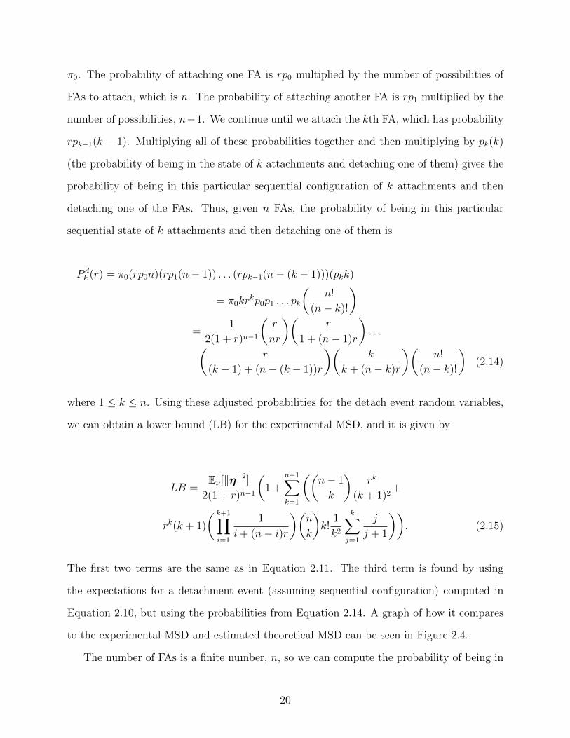
where 1 ≤ k ≤ n. Using these adjusted probabilities for the detach event random variables,
we can obtain a lower bound (LB) for the experimental MSD, and it is given by
LB =Eν [‖η‖2]
2(1 + r)n−1
(1 +
n−1∑k=1
((n− 1
k
)rk
(k + 1)2+
rk(k + 1)
( k+1∏i=1
1
i+ (n− i)r
)(n
k
)k!
1
k2
k∑j=1
j
j + 1
)). (2.15)
The first two terms are the same as in Equation 2.11. The third term is found by using
the expectations for a detachment event (assuming sequential configuration) computed in
Equation 2.10, but using the probabilities from Equation 2.14. A graph of how it compares
to the experimental MSD and estimated theoretical MSD can be seen in Figure 2.4.
The number of FAs is a finite number, n, so we can compute the probability of being in
20

Figure 2.4: The experimental MSD computed from Equation 2.2 with τ = 1 (red x’s)compared against Equation 2.11, the estimated theoretical MSD (black line), and the lowerbound for the MSD (blue line) found in Equation 2.15. For this graph, a trajectory of 10,000events was used for the experimental MSD with r=1.
the state of any number of attachments and then detaching. This is computed by summing
over all 1 ≤ k ≤ n the product πkpkk and using the values given in Equations 2.12 and 2.13.
The sum is given by
n∑k=1
πkpkk =n∑k=1
(rk−1
(n−1k−1
)2(1 + r)n−1k
[k + (n− k)r
])( 1
k + (n− k)r
)k
=1
2(1 + r)n−1
n∑k=1
(n− 1
k − 1
)rk−1 =
1
2(1 + r)n−1· (1 + r)n−1 =
1
2
with the next to last inequality being valid because of the binomial theorem. Similarly, the
probability of being in a state of any number of attachments and attaching is also 1/2. Thus
over a long enough simulation, on average, the probability of being in a state of any number
of attachments and then detaching, and the probability of being in a state of any number of
attachments and then attaching both approach 1/2.
For each k, 1 ≤ k ≤ n, limr→∞
P dk (r) = 0. The total probability of being in this particular
sequential configuration for any number of attachments and then detaching is the sum over
all k of P dk , so as r increases sufficiently, the probability,
n∑k=1
P dk decreases (approaching 0).
So as r becomes large, the total probability of a detach event is dominated by detachments
21

that are not of this particular sequential configuration. For k = 1, limr→0
P dk (r) = .5, but for
2 ≤ k ≤ n, limr→0
P dk (r) = 0. Again, the total probability of being in this particular sequential
configuration for any number of attachments and then detaching is the sum over all k of
P dk , so as r decreases sufficiently, the probability
n∑k=1
P dk increases (approaching .5). So as
r becomes small, the probability of this particular sequential configuration dominates the
total probability for a detach event.
This helped us better understand why Equation 2.11 is such a good estimate for the
experimental MSD. Heuristically, as r decreases sufficiently, the number of attachments
decreases, and the sequential probability increases, implying that the random variable (RV)
values, cj+1−cj, being used for a detachment event (Equations 2.7 and 2.8) are closer to the
actual values of the RVs. As r increases sufficiently, the number of attachments on average
approaches the total number of FAs. Because of our assumption that the initial condition
has no attachments, FAs quickly attach (r is large) until most are attached and the system
stays in a highly attached state. Because the majority of attachments happened quickly they
will be close to a sequential configuration. Thus the RVs being used for a detachment event
(Equations 2.7 and 2.8) are still a good estimate for the MSD. For the “middle” values of r,
the estimate is not as good, but is still adequate.
2.5 Upper Bound
To postulate on the maximum value for ‖cj+1 − cj‖, when event j + 1 is a detachment, we
start with our initial condition assumption of no attachments but position the centroid at
the origin. Assume the first FA, v1, attaches at the origin. For simplicity and to obtain a
maximum combined outreach, we assume all incremental outreaches occur in one dimension
in the positive direction. The next FA, v2, attaches at a maximum outreach, ηmax, from
the origin. Let each subsequent outreach be at a maximum outreach from the previously
attached FA until all n FAs are attached, the location of the ith FA given by vi, with v1 = 0
and vn = ηmax(n − 1). (This is a maximum outreach scenario that is more than the actual
22

model, since the outreach in the model for each new attaching FA is from the centroid.) By
fixing v1 at 0 for all events up through j, and allowing vd to detach (vd ∈ {vi|1 ≤ i ≤ n})
for the event j + 1 (j > n) we can find an upper bound for any ‖cj+1 − cj‖.
∥∥cj+1 − cj∥∥ =
∑ni=1 vi − vdn− 1
−∑n
i=1 vin
=
∑ni=2 vi − nvdn(n− 1)
≤ ηmax(n− 1)(n− 1)
n(n− 1)=ηmax(n− 1)
n(2.16)
where the values after the inequality come from taking the max value for all vi and taking
the minimum value of 0 for vd.
In general, for k attachments (1 ≤ k ≤ n) we find an upper bound for the displacement
by using the upper bound configuration found in Equation 2.16, i.e. all nonzero FAs are
ηmax(n− 1) units away from the origin. So for j > n
∥∥cj+1 − cj∥∥ ≤ ηmax(n− 1)(k − 1)
k − 1− ηmax(n− 1)(k − 1)
k=
ηmax(n− 1)
k. (2.17)
We now show that the maximum displacement bound found in Equation 2.16 can be
achieved in the limit. Following the process described in the previous paragraph but with
the constraints of the model, assume initially that for any given value of n, the total number
of FAs, there are no attachments and the centroid is at 0. The first event is a FA that
attaches at 0. At the next event a FA attaches at a maximum outreach distance, ηmax,
from 0 and the new centroid is computed. (Again, for simplicity and to obtain a maximum
combined outreach, we assume all incremental outreaches occur in one dimension in the
positive direction.) At the next event, another FA attaches at a maximum outreach distance,
ηmax from that centroid. The process is continued until all of the FAs are attached. Then the
FA that is closest to zero, but not at zero, detaches and reattaches at a distance of ηmax from
the current centroid. Numerical simulations were done of this process with ηmax = 1. At
each step, the simulation computed the location of the centroid and subtracted it from the
23

location the centroid would be if the FA at zero was dropped. The results of this difference
are shown in Figure 2.5. The numerical simulations indicate that a steady state for each
value of n is achieved, so we analytically show how to find the steady state.
Figure 2.5: This shows the maximum displacement for a given number of total FAs thatare all attached. Each line is composed of asterisks that represent cj+1 − cj where cj is thelocation of the centroid with the initial FA attached at 0 and all other FAs located furtherand further from 0 as described in the text. The value cj+1 is the location of the centroidafter 0 detaches. The change from dark to light is indicative of an increase in the numberof FAs. Notice that the darkest horizontal line is at 1/2 (n=2), the next darkest horizontalline is at 2/3 (n=3) and so on. Notice that more iterations are required to reach the steadystate as the number of attached FAs increases.
Given n FAs, there is a linear recurrence relation for the location of the next FA, given
the location of the previous n− 1 FAs, given by
xt =(xt−1 + xt−2 + . . .+ xt−n+2 + x1)
n− 1+ ηmax
where each xi is the location of a FA and t ≥ n. Furthermore,
xt =(xt−1 + xt−2 + . . .+ xt−n+2)
n− 1+ ηmax (2.18)
since x1 = 0.
The steady state of this equation is found by setting all values of x to x∗ and solving for
24

x∗. The steady state is then x∗ = ηmax(n− 1). In order to find if this is an attracting steady
state, let yt = xt − x∗, and Equation 2.18 becomes
yt =(yt−1 + yt−2 + . . .+ yt−n+2)
n− 1. (2.19)
The characteristic equation for this recurrence relation is
(n− 1)λn−2 = λn−3 + . . .+ λ+ 1. (2.20)
For ease of computation consider the equivalent system
(k + 1)λk = λk−1 + . . . λ+ 1
where k + 1 = n− 1. Thus the characteristic polynomial is λk − λk−1
k+1− . . .− λ
k+1− 1
k+1.
By Descartes’ rule of signs, we know that the polynomial has exactly one positive real
root. Since one and negative one are not roots of the polynomial, the upper and lower bound
theorem for real roots of polynomials says that all of the real roots lie between negative one
and one. In particular, the unique positive root, call it ζ, must be between 0 and 1, i.e. 0 <
ζ < 1. Further analysis shows that xk− xk−1
k+1−. . .− x
k+1− 1k+1
< 0 or xk ≤ xk−1
k+1+. . .+ x
k+1+ 1k+1
for all values of 0 ≤ x < ζ and xk− xk−1
k+1− . . .− x
k+1− 1
k+1≥ 0 for x ≥ ζ. Let z0 be a complex
root of the characteristic polynomial, then zk0 −zk−10
k+1− . . .− z0
k+1− 1
k+1= 0. Using the triangle
inequality, then |z0|k ≤ |z0|k−1
k+1+ . . .+ |z0|
k+1+ 1
k+1. This implies that 0 < |z0| < ζ < 1. Since z0
was arbitrary, then all of the complex roots of the characteristic polynomial have modulus
less than one. Therefore, all roots of the characteristic polynomial lie within the unit circle
in the complex plane, showing that the steady state, x∗ = ηmax(n− 1) is attracting, and the
system will converge to it, since it is the only steady state. As the system approaches the
steady state, then the displacement is maximal, and by extending to higher dimensions, is
25

Figure 2.6: Upper bound for the experimental MSD. A trajectory of 100,000 events withr = 1 was used to compute the experimental MSD defined in Equation 2.2
given by,
limj→∞
∥∥cj+1 − cj∥∥ =
ηmax(n− 1)(n− 1)
n− 1− ηmax(n− 1)(n− 1)
n=ηmax(n− 1)
n(2.21)
for n total FAs, which is the value seen in our numerical simulations and in Equation 2.16.
Since the upper bound of the displacement found in Equation 2.16 can be obtained in
the limit (Equation 2.21), we now use the results found in Equations 2.16 and 2.17 to find
an upper bound for the MSD. We partition the state space into three parts: {F ak }, {F d
k }
and {F dk }. Each F a
k , 0 ≤ k ≤ n − 1, represents arriving to a state of k attachments from
any configuration and then attaching. Each F dk , 1 ≤ k ≤ n represents arriving to the state
of k attachments from a sequential configuration and then detaching. Each F dk , 1 ≤ k ≤ n,
represents arriving to a state of k attachments from a non-sequential configuration and then
detaching. We use the known values and associated probabilities for F ak , and we use the RV
values in Equations 2.7 and 2.8 with probabilities from 2.14 for F dk in the computation of
the MSD upper bound. We use the results from Equation 2.17, as a RV upper bound for
the event of arriving at k attachments from a non-sequential configuration. For the upper
bound for the probabilities in this case, we use kπkpk − π0krkp0p1 . . . pk(
n!(n−k)!
)(sequential
probability from 2.14 subtracted from the probability of being in a state of k attachments
and then detaching). The resultant upper bound can be seen in Figure 2.6. For {F dk }, since
26
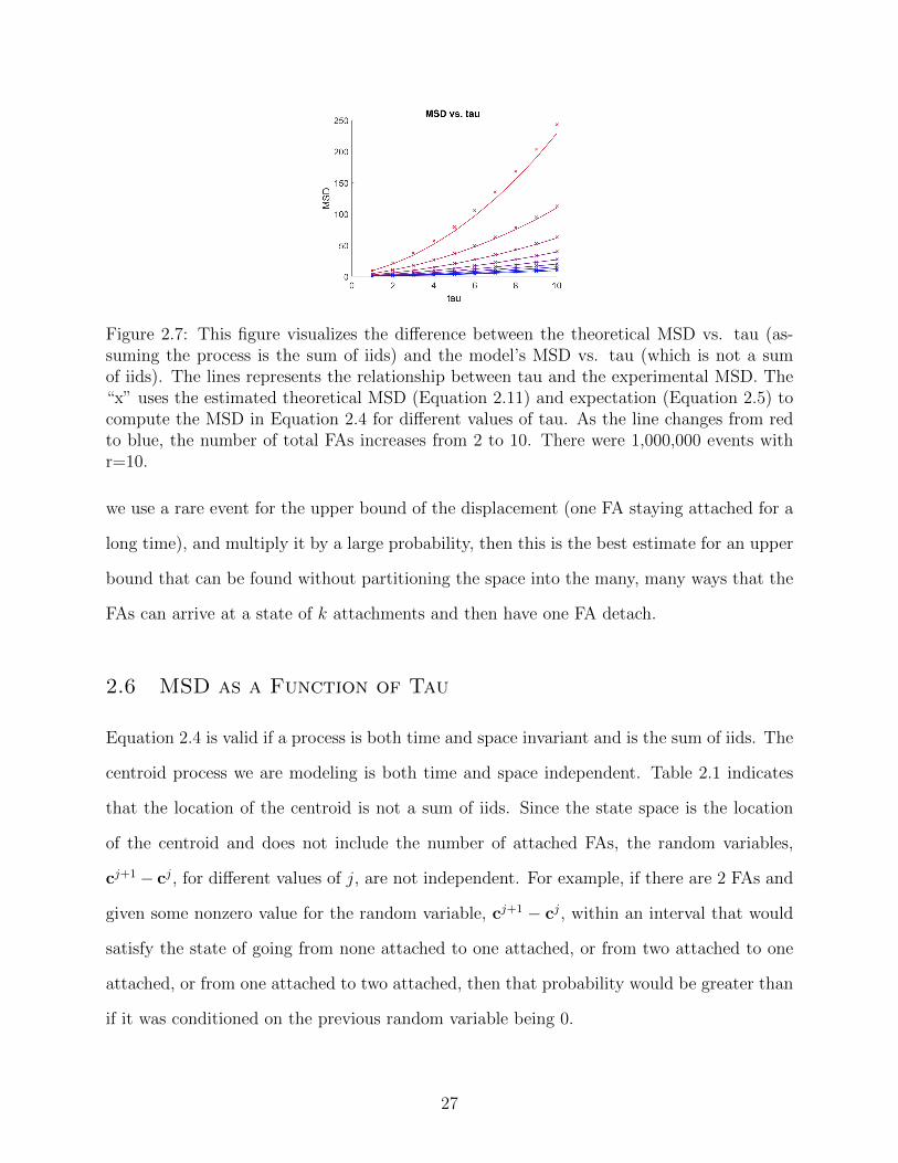
Figure 2.7: This figure visualizes the difference between the theoretical MSD vs. tau (as-suming the process is the sum of iids) and the model’s MSD vs. tau (which is not a sumof iids). The lines represents the relationship between tau and the experimental MSD. The“x” uses the estimated theoretical MSD (Equation 2.11) and expectation (Equation 2.5) tocompute the MSD in Equation 2.4 for different values of tau. As the line changes from redto blue, the number of total FAs increases from 2 to 10. There were 1,000,000 events withr=10.
we use a rare event for the upper bound of the displacement (one FA staying attached for a
long time), and multiply it by a large probability, then this is the best estimate for an upper
bound that can be found without partitioning the space into the many, many ways that the
FAs can arrive at a state of k attachments and then have one FA detach.
2.6 MSD as a Function of Tau
Equation 2.4 is valid if a process is both time and space invariant and is the sum of iids. The
centroid process we are modeling is both time and space independent. Table 2.1 indicates
that the location of the centroid is not a sum of iids. Since the state space is the location
of the centroid and does not include the number of attached FAs, the random variables,
cj+1− cj, for different values of j, are not independent. For example, if there are 2 FAs and
given some nonzero value for the random variable, cj+1 − cj, within an interval that would
satisfy the state of going from none attached to one attached, or from two attached to one
attached, or from one attached to two attached, then that probability would be greater than
if it was conditioned on the previous random variable being 0.
27

Figure 2.8: This figure visualizes the relative difference between the experimental MSD andthe right side of Equation 2.4 for different values of τ , or the relative difference betweenthe “x’s” and lines in Fig. 2.7. As the line changes from red to blue, the number of totalFAs increases from 2 to 10. The magnitude of error being greater for two FAs could beexplained by larger regions of random variable overlap and limited state choices, creatinggreater dependency. Parameters are per Figure 2.7.
Numerical simulations were conducted to see how closely Equation 2.4 relates the exper-
imental MSD to the variance and expectation when Equations 2.11 and 2.5 are used in the
computation of the variance and expectation, given by
MSD = τ(Eρ[∥∥cj+1 − cj
∥∥2]− ∥∥Eρ[cj+1 − cj]∥∥2) + τ 2
∥∥Eρ[cj+1 − cj]∥∥2
= τEρ[∥∥cj+1 − cj
∥∥2] + (τ 2 − τ)∥∥Eρ[cj+1 − cj]
∥∥2 .Figure 2.7 uses this computation of the MSD versus τ . The relative error between the two
computations are show in Figure 2.8.
2.7 Discussion
MSD is a measure of the overall drift of a particle and can be a useful tool for understanding
cell motion. We introduced a mathematical model for cell motion and discussed it in the
context of a generalized random walk and a centroid model. We were able to find a good
estimate for the theoretical MSD of the centroid model by introducing the concept of a se-
quential configuration. We found the displacement of the centroid after an attach event for
28

all configurations and the displacement after a detach event when in a sequential configura-
tion. Using the displacement for sequential configurations to approximate all detach events,
we found an approximation for the MSD with a delay of one event. To further quantify
the experimental MSD, we found a lower and upper bound for the experimental MSD. We
surmised that the estimate for the theoretical MSD had a small relative error because the
FA configuration frequently is in a sequential configuration or close to it.
Chapter 3. A Mathematical Analysis of Fo-
cal Adhesion Lifetimes and Their Ef-
fect on Cell Motility
In the introduction we emphasized the importance of cell motion and gave examples of how
it can be life-building, life-saving or life-threatening. In this chapter we study FA lifetime
distributions obtained from experimental data, relating it to cell motility. We first study the
experimental FA lifetime distributions, showing that the gamma distribution is a good fit.
We reintroduce the math model described in the previous chapter, supplying more details
and introducing a detach-rate function that determines the lifetimes of the FAs. By changing
certain parameters, the math model can produce a distribution that has a best fit gamma
curve matching those of different data sets. We finally discuss the correlation between the
cell speed and the mean FA lifetime in both the experimental and simulated data.
3.1 FA Lifetimes are Gamma Distributed
We first studied the data from various research groups to determine the distribution of FA
lifetimes. Table 3.1 shows the statistical information for mean, standard deviation, median
and interquartile range (IQR) for the control cells as recorded in the papers.
Stehbens et al. [3] tracked the FAs in cells expressing paxillin-mCherry. In the study
they used a wound assay where a monolayer of epithelial cells, grown on fibronectin coated
29

Cell TypeFA Lifetime (min)
Median/IQR*FA Lifetime (min)
Mean/SDComments
HaCaTKeratinocyte [3]
∼ 24.6/13.7 ∼ 27.2/9.7 Calculated from raw data.
Mouse EmbryonicFibroblasts [4]
∼ 23/16 ∼ 26/11.8 Calculated from raw data.
NIH 3T3Fibroblasts [5]
∼ 30/18 ∼ 37.1/20.1 Calculated from raw data.
MDA-231Human
Breast Cancer Cells [6]∼ 25/22 ∼ 27.8/15.3
Calculated from raw datathat was estimated fromgiven figures.
Astrocytes [7]∼ 24/16∼ 70/60
∼ 23/15.4∼ 75/42.7
Estimated from a dot plot.First entry is for leader cells,and the second entryis for followers.
ProstateCarcinoma Cells [9]
∼ 9.6/12.1 Estimated from a histogram.
U2OSOsteosarcoma
Epithelial Cells [8]∼ 51/20
Mean and standard deviationwere given. Histogramwas also included.
Mouse EmbryonicFibroblasts [42]
∼ 34.3/19.2 Estimated from a histogram
Astrocytes [43] ∼ 40/20Estimated from a boxand whisker plot
HEK293Embryonic Kidney [44]
Cells∼ 13 Estimated from a figure.
HT-1080 [45]Fibrosarcoma
∼ 22 Estimated from a figure.
Motile Fibroblasts [46] ∼ 15/8 Estimated from a boxand whisker plot.
Table 3.1: Different cell types with their associated FA lifetime statistics. The doublehorizontal lines split the table into three categories: raw data and estimated raw data,histogram data, and central tendency and/or dispersion statistics only. *IQR is interquartilerange.
30

Figure 3.1: Available FA lifetimes raw data histogram and gamma fit for keratinocytes fromStehbens et al. [3]
cover sheet, is scraped with a razor blade to remove half the cells [47]. They emphasized
caution when using fully computerized image analysis with some of the pitfalls being an
incomplete understanding of the algorithm, input errors if the images are not clear, the need
for optimization of parameters and the possibility of coding errors. Figure 3.1 shows the
distribution of a subset of their published data with a gamma curve fit to the data. (We
used the “histfit” function from MATLAB to find the best fit gamma curve.) They mentioned
in their paper that a Poisson distribution was a better fit than a normal distribution. We
found the gamma curve to be a good fit as well. Although, the Poisson curve was a possible
fit for this set of data, it was not a good fit for the rest of the data sets. We found that the
gamma curve was a better fit for all of the other raw data that was collected.
Cleghorn et al. [4] tracked the FAs with GFP-paxillin. In this study double arrestin
knockout mouse embryonic fibroblasts are plated on fibronectin or poly-D-lysine coated
slides. We received the raw data for the WT cells and found the gamma curve to be a much
better fit than the Poisson for this data set. See Figure 3.2.
Berginski et al. [5] introduced a fully computerized image analysis. They analyzed the
focal adhesions of migrating NIH 3T3 fibroblasts plated on fibronectin. The advantage of
this type of analysis is it allowed them to track a large volume of FAs (103 − 104 adhesions
31

Figure 3.2: FA lifetimes raw data histogram and gamma fit for mouse embryonic fibroblastsfrom Cleghorn et al. [4]
Figure 3.3: FA lifetimes raw data histogram and gamma fit for fibroblasts from Berginski etal. [5]
per cell), but it does have some drawbacks. They had a large amount of FAs with very short
lifetimes, so they set a minimum lifetime of 20 minutes for their analysis. It is unknown, but
seems unlikely, that these very short lived attachments have any impact on cell migration.
By only counting the FA lifetimes that were greater than 20 minutes, a gamma curve loosely
modeled the data as seen in Figure 3.3, but an exponential curve was a better fit when all
of the data was included.
Astro et al. [6] provided figures that showed raw data. They tracked the FAs with
mCherry-Zyxin as a marker in the free migration of MDA-231 breast cancer cells plated
32

Figure 3.4: FA lifetimes raw data histogram and gamma fit for cancer cells from Astro et al.[6]
Figure 3.5: FA lifetimes raw data histogram and gamma fit for cancer cells from Pascalis etal. [7] for both the leader cells (left panel) and follower cells (right panel).
on fibronectin. We estimated the FA lifetime data from the control cells (siLuc, GFP, and
GFP-WT) shown in the figures, combined all the data and again found the gamma curve to
be a good fit. See Figure 3.4.
Pascalis et al. [7] also provided figures that showed raw data. They used a wound
migration assay by plating astrocytes and used a pipette to scratch the monolayer. We
estimated the FA lifetime data from the control cell figures for both the leader and follower
cells. The gamma curve was a reasonable fit for both as seen in Figures 3.5, but not as tight
as some of the other fits, probably due to the inaccuracy of the estimates.
For Spanjaard et al. [9], Stricker et al. [8] and Meenderick et al. [42], we were not
33

Figure 3.6: FA lifetimes extracted from a histogram and gamma fit for cancer cells fromStricker et al. [8]
able to obtain raw data and therefore extracted data from the histograms represented in
the papers. In the case of Spanjaard, where cells from a human prostate cancer cell line
were plated on collagen coated plates and induced to migrate with HGF, the data looked
exponential, but the coarseness of the data would mask a unimodal gamma distribution.
Since the exponential distribution is a special case of the gamma, we were still able to fit
the data with a gamma distribution. The gamma fit in all of these cases was not as tight
as seen in the raw data fits, but the gamma fit is still consistent with the data. See a
representative distribution that was taken from the data in Stricker et al. in Figure 3.6.
In the Stricker study, human osteosarcoma cells are plated on polyacrylamide substrates
so force measurements are possible. Whereas in Meenderick, a wound assay is used where
mouse embryonic fibroblasts are grown on fibronectin covered plates and a pipette is used
to make a scratch wound.
To further quantify the validity of a gamma fit, we calculated the Kullback-Leibler diver-
gence (KL divergence), using the experimental distribution and comparable uniform, normal,
Poisson, and gamma distributions for the different cell types. For the uniform distribution,
we matched the smallest interval containing the support of the experimental distribution.
For the other distributions, we used the MATLAB “histfit” function to find the best fit. The
34

KL divergence comes from information theory and measures the relative entropy between
two distributions. It is defined to be
DKL(P ||Q) =N∑i=1
P (xi) · (logP (xi)− logQ(xi))
with P being a distribution and Q being a comparing distribution and N is the number
of values for the random variable [48]. It measures how much information is lost when
estimating one distribution with another distribution. For our computation of DKL, P is
the experimental distribution and Q, the comparing distributions. Our results are found in
Table 3.2. The results show that the minimum divergence for all cell types is found when
comparing the experimental distribution to the gamma distribution. Figure 3.7 gives a visual
representation of the fitted distributions compared to the actual Cleghorn, et al. [4] data.
Cell Type Uniform Normal Poisson Gamma
HaCaTKeratinocyte [3]
.9603 .2995 .9044 .2449
Mouse EmbryonicFibroblasts [4]
.8361 .2831 1.3933 .1878
NIH 3T3Fibroblasts [5]
2.66 .6072 N.A. .3323
MDA-231Human
Breast Cancer Cells [6].6279 .2331 2.7911 .1833
Astrocytes [7]1.88422.7752
.80081.2551
N.A.N.A.
.63491.1730
U2OSOsteosarcoma
Epithelial Cells [8]2.3965 1.7917 3.7287 1.7604
Table 3.2: This table finds the Kullback-Leibler Divergence (KL-Divergence) between theexperimental data and different standard distributions for several cell types. For the Astro-cytes, the first line is information for the leader cells and the second line is for the followercells. The term N.A. indicates that the KL Divergence is not available because the supportof the experimental distribution is not a subset of the comparing distribution, and the KLDivergence cannot be computed in this case.
In summary, for the 9 data sets that we obtained, where there was enough information
35

Figure 3.7: A comparison of best fit distributions to the Cleghorn et al. [4] data. The datawas normalized and the ”fitdist” MATLAB function was used to find the best fit for eachtype of distribution except the uniform distribution as discussed in the text.
given to reconstruct a distribution for the FA lifetimes, it was found that the gamma dis-
tribution was the best fit. The most common shape for the distribution was a unimodal
non-symmetric curve. Gamma distributions have been used to model seismic inter-event
times [49], avalanche inter-event times for certain material properties [50], and actual wait
times at a bus stop [51]. The gamma distribution seems a reasonable fit for FA lifetimes as
well.
3.2 Mathematical Model of Cell Motion Mimics FA Lifetime
Distributions
3.2.1 The Model. In a paper by John Dallon et al. [2], the authors introduce a mathe-
matical model of individual cell migration. This model was described briefly in the previous
chapter with an emphasis on the centroid model, so we re-describe it here in more detail.
The model specifies discrete focal adhesion (FA) attachment sites with random switching
terms for each site. The random switching terms determine if a FA is attached or detached.
The time a FA remains attached or detached is taken from a given probability distribution.
A detached site is reattached at a distance from the present cell center. The distance is taken
36

from a given probability distribution. Forces exerted on the center of the cell by the different
FAs are determined by Hooke’s Law. Using Newton’s second law of motion, and ignoring
the acceleration due to the low Reynolds number, all of these forces together with the drag
force, which involves velocity, are summed to produce a differential equation model that has
the feature of different FAs attaching and detaching randomly and tracks the movement of
the cell over time. The equation of motion for the cell location is given by
µx′ = −n∑j=1
αj(‖x− vj‖ − `j)x− vj‖x− vj‖
Ψj(t).
The drag coefficient, µ = .101 g/h, is found using Stoke’s Law and calculating the drag on a
3 micron diameter sphere, the nucleus, through water. The spring constant α = .206 nN/µm
for all FAs, resulting in a force on average of .8 nN from each FA. (When simulating the
Cleghorn, et. al [4] data, see Figure 3.11, a FA is, on average, approximately 4 µm from
the centroid. Then by Hooke’s Law, each FA exerts a force of .806 nN on the centroid.
Fibroblasts have been reported to exert forces of 2.2 nN per focal adhesion [52].) The total
number of FAs is given by n. The location of the center of the cell is x, with the location of
the jth FA given by vj. The length of the spring at rest is `j, and is 0 for our simulations.
The function Ψj(t) determines if the jth FA is attached or detached at time t, being 1 or 0
respectively. The visualization of this model can be seen in Figure 2.1.
Initially we used the Gillespie Algorithm [53] to determine when a FA detaches. This al-
gorithm was first developed to simulate stochastic chemical kinetics. It determines what time
a reaction will occur, and which molecule will be affected. This algorithm saves computer
time since it does not have to check at every time increment if a reaction has happened and
only needs to evaluate when a reaction occurs. It seemed a good fit for our model since the
reaction time for our model would be the lifetime of a FA, and the affected molecule would
be the affected FA. Unfortunately, the assumption for this algorithm is that the chemical
reactions are a Markov process, implying that the inter-event times are exponential. Since
37

the experimental data shows that the FA lifetimes distributions are not exponential then we
had to look for a different algorithm to track the motion of the cell.
For our algorithm, we use a detach-rate function to determine when a FA detaches.
Initially, all FAs are attached equally spaced around the origin, so the centroid begins at the
origin. The simulation proceeds as follows:
1. At each time increment, ∆t, the ODE is solved, and it is checked to see if an event occurs.
2. The order of the FAs is randomized and each detached FA is checked to see if its detached
time has expired. If the time has expired for a FA, then an event has occurred and the
FA reattaches at a random direction and outreach (r, θ) from the present location of the
centroid. (For our simulation the outreach was directed, with theta ranging from −π/3
to π/3.)
3. If there is no attachment event, then a uniform random number is generated and the first
FA from the new ordering is selected. If this random number is less than the value of a
given detach-rate function (which is a function of the non-dimensionalized force from the
given FA and/or time) times ∆t, then an event has occurred and that FA detaches and
is assigned a number from an exponential distribution with a given mean. This is the
amount of time the FA will remain detached.
4. If an event does not happen, then time is incremented by another ∆t and the process
repeats itself continuing until a preset amount of time has expired.
The ODE was solved using Sundials ODE Solver [54].
38

Function of Time Function of Force ResultingDistributions
h(t) = c g1(f) ={.1 0 ≤ f ≤ F
(x− F ) + .1 f > F
Exponential
g2(f) = (f − F )2 Exponential
g3(f) = a · f Exponential
g4(f) = c Exponentialh(t) = t g1 Gamma
g2 Exponentialg3 Gammag4 Gamma
h(t) = t2 g1 Gammag2 Gammag3 Normalg4 Gamma
h(t) =
{0 0 ≤ t ≤ T
ln (t− (T − 1)) t > T
g1 Gamma
g2 Exponentialg3 Gammag4 Gamma
Table 3.3: The detach-rate function for the simulation is r(t, f) = h(t) · g(f). Differentfunctions for h(t) and g(f) are given with the resulting distributions. Both F and T areforce and time thresholds, respectively, when the nature of h and g changes. Both c and aare constants. The total number of FAs for the simulation is 10 with 5 attached on average.
39

In order to manipulate the distribution for the FA lifetimes, we considered different pos-
sibilities for the detach-rate function which determines when an attached FA will detach. We
constructed this function as a product of a time-dependent function and a force-dependent
function. We first set the time-dependent function to a constant, so that the rate function
only depended on force and not on time. We tried different possibilities for the force-
dependent function: (1) A piece-wise linear function that is a small constant until it reaches
a force threshold at which point it increases linearly, (2) A parabolic function that has its
vertex at a positive force threshold on the x-axis, (3) A constant function, and (4) An in-
creasing linear function. For all of the cases, the simulation distributions for the FA lifetimes
best fit an exponential distribution instead of the gamma distribution seen in the experi-
mental data. We next made the time-dependent function an increasing linear function, and
tried the above options for the force-dependent function. We found that the piece-wise linear
force function was the best match for the gamma function found in the experimental data,
but also noted that the mean was too small and the tail too short to match the experimental
data. We then defined the time-dependent function as a parabola with vertex at the origin,
pointing up. Again, the best gamma distribution match came from the piece-wise linear
force-dependent function with similar problems for the mean and tail. We found that a
piece-wise logarithmic function for the time-dependent function slowed the rise of the curve
and extended the tail. The product of this time-dependent function along with the piece-
wise force-dependent function created a detach-rate function that produced data that best
matched the experimental data. Thus the detach-rate function that produced the best FA
lifetime data match was
r(t, f) = h(t) · g(f) (3.1)
where the time-dependent function, h(t), is defined as
h(t) =
0 0 ≤ t ≤ T
ln (t− (T − 1)) t > T
(3.2)
40
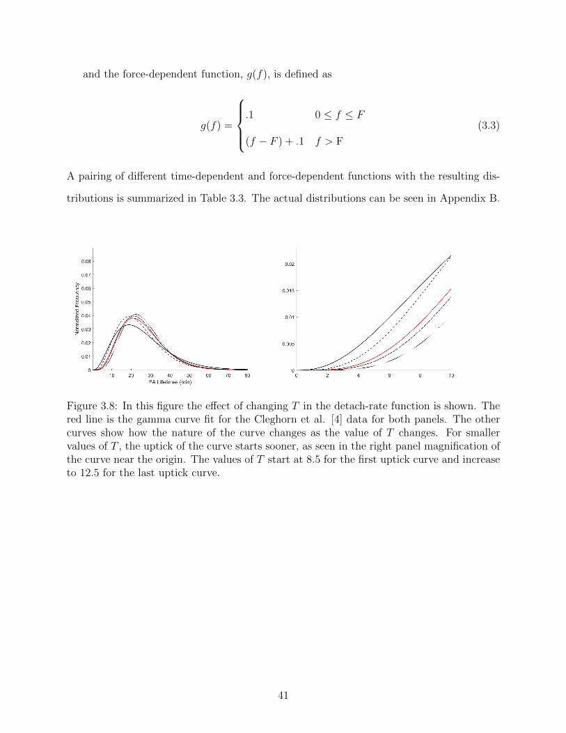
and the force-dependent function, g(f), is defined as
g(f) =
.1 0 ≤ f ≤ F
(f − F ) + .1 f > F
(3.3)
A pairing of different time-dependent and force-dependent functions with the resulting dis-
tributions is summarized in Table 3.3. The actual distributions can be seen in Appendix B.
Figure 3.8: In this figure the effect of changing T in the detach-rate function is shown. Thered line is the gamma curve fit for the Cleghorn et al. [4] data for both panels. The othercurves show how the nature of the curve changes as the value of T changes. For smallervalues of T , the uptick of the curve starts sooner, as seen in the right panel magnification ofthe curve near the origin. The values of T start at 8.5 for the first uptick curve and increaseto 12.5 for the last uptick curve.
41

Figure 3.9: In this figure, the effect of changing F in the detach-rate function is shown.The red line is the gamma curve fit for the Cleghorn et al. [4] data. Smaller values of F inEquation 3.3 produce a higher amplitude curve as seen in the solid black line. The amplitudedecreases and the tail elongates as the value of F increases. The value of F increases from5.077 for the tallest curve to 5.877 for the shortest curve.
42

Cell TypeTime (T)
and Force (F)Threshold
MSD*/Ave. Speed/
Speed
ExperimentalSpeed (µm/min)
HaCaTKeratinocyte [3]
T = 14.2F = 5.44
.74/.36/.33.2-.25 average
(min .05, max .35) [55]Mouse Embryonic
Fibroblasts [4]T = 10.5F = 5.477
.80/.37/.33.16, .19** [56]
.57 [57]NIH 3T3
Fibroblasts [5]T = 13.4F = 6.14
.41/.25/.22.31-.5** [58].1, .24 [59]
MDA-231Human
Breast Cancer Cells [6]
T = 7.25F = 5.634
.63/.31/.27 .42 [6]
Astrocytes [7]
LeaderT = 8
F = 5.57FollowerT = 10F = 50
.76/.35/.31
.13/.13/.11.18 [7]
ProstateCarcinoma Cells [9]
T = .16F = 3.61
2.24/.58/.5 .5-1 [9]
U2OSOsteosarcoma
Epithelial Cells [8]
T = 20F = 7
.26/.19/.17 .24** [60]
Mouse EmbryonicFibroblasts [42]
T = 9F = 6.05
.45/.26/.22 1.52 [42]
Table 3.4: Different cell types with the parameters used in Equation 3.1. The double hor-izontal line splits the table into two categories: Raw data and estimated raw data, andhistogram data. The average speed was computed by taking the average of the distancetraveled in each time increment and dividing it by the time increment. Speed was computedby taking the distance between the centroid at the beginning of the simulation and the endof the simulation and dividing it by the total time. *MSD is measured in µm2, and thespeeds in µm/min. **wound assay
43
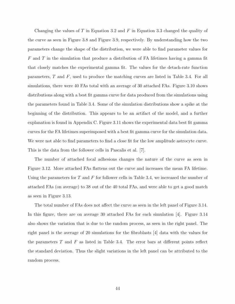
Changing the values of T in Equation 3.2 and F in Equation 3.3 changed the quality of
the curve as seen in Figure 3.8 and Figure 3.9, respectively. By understanding how the two
parameters change the shape of the distribution, we were able to find parameter values for
F and T in the simulation that produce a distribution of FA lifetimes having a gamma fit
that closely matches the experimental gamma fit. The values for the detach-rate function
parameters, T and F , used to produce the matching curves are listed in Table 3.4. For all
simulations, there were 40 FAs total with an average of 30 attached FAs. Figure 3.10 shows
distributions along with a best fit gamma curve for data produced from the simulations using
the parameters found in Table 3.4. Some of the simulation distributions show a spike at the
beginning of the distribution. This appears to be an artifact of the model, and a further
explanation is found in Appendix C. Figure 3.11 shows the experimental data best fit gamma
curves for the FA lifetimes superimposed with a best fit gamma curve for the simulation data.
We were not able to find parameters to find a close fit for the low amplitude astrocyte curve.
This is the data from the follower cells in Pascalis et al. [7].
The number of attached focal adhesions changes the nature of the curve as seen in
Figure 3.12. More attached FAs flattens out the curve and increases the mean FA lifetime.
Using the parameters for T and F for follower cells in Table 3.4, we increased the number of
attached FAs (on average) to 38 out of the 40 total FAs, and were able to get a good match
as seen in Figure 3.13.
The total number of FAs does not affect the curve as seen in the left panel of Figure 3.14.
In this figure, there are on average 30 attached FAs for each simulation [4]. Figure 3.14
also shows the variation that is due to the random process, as seen in the right panel. The
right panel is the average of 20 simulations for the fibroblasts [4] data with the values for
the parameters T and F as listed in Table 3.4. The error bars at different points reflect
the standard deviation. Thus the slight variations in the left panel can be attributed to the
random process.
44
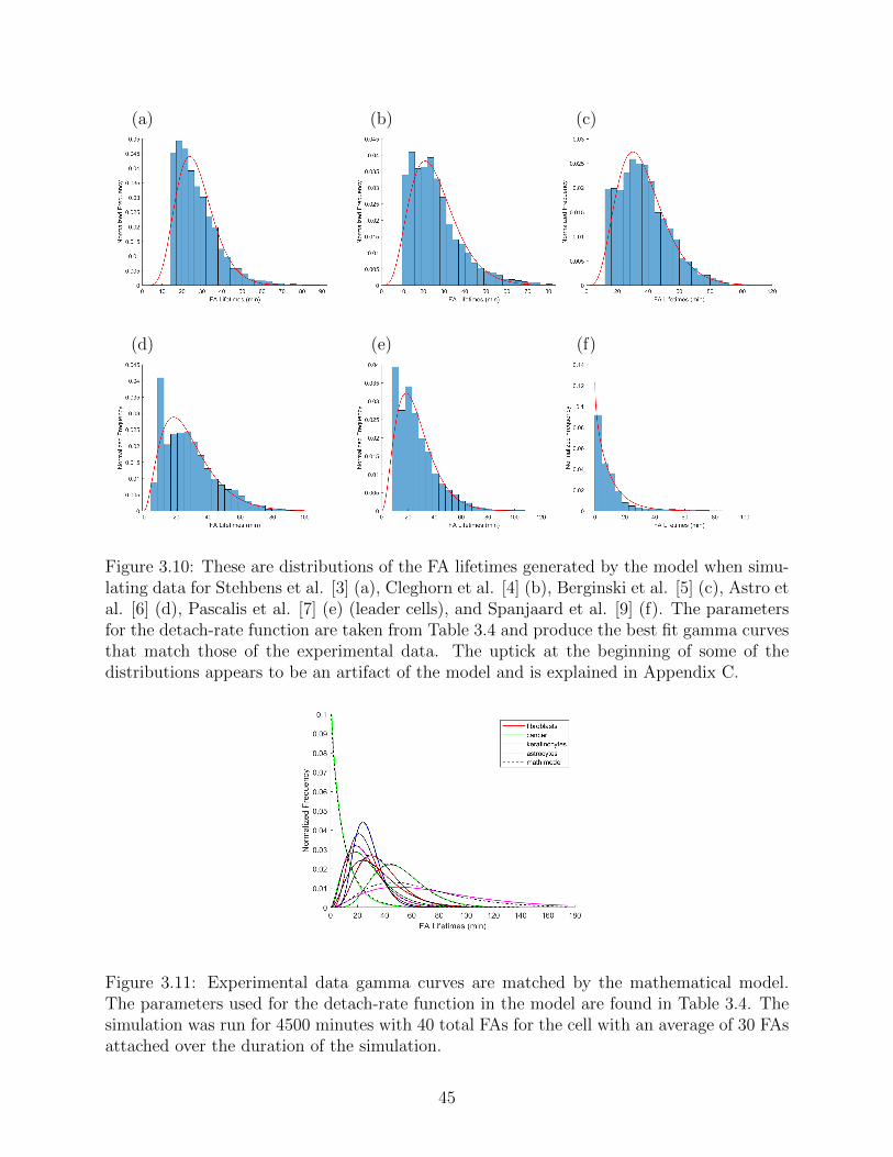
(a) (b) (c)
(d) (e) (f)
Figure 3.10: These are distributions of the FA lifetimes generated by the model when simu-lating data for Stehbens et al. [3] (a), Cleghorn et al. [4] (b), Berginski et al. [5] (c), Astro etal. [6] (d), Pascalis et al. [7] (e) (leader cells), and Spanjaard et al. [9] (f). The parametersfor the detach-rate function are taken from Table 3.4 and produce the best fit gamma curvesthat match those of the experimental data. The uptick at the beginning of some of thedistributions appears to be an artifact of the model and is explained in Appendix C.
Figure 3.11: Experimental data gamma curves are matched by the mathematical model.The parameters used for the detach-rate function in the model are found in Table 3.4. Thesimulation was run for 4500 minutes with 40 total FAs for the cell with an average of 30 FAsattached over the duration of the simulation.
45

Figure 3.12: This figure shows how the average number of attached FAs changes the lifetimedistribution. The total number of FAs is 100. The different colors are the averaged numberof attached FAs. The values for the parameters for T and F are those listed on Table 3.4for the mouse embryonic fibroblasts [4].
Figure 3.13: This figure shows a better fit for the astrocyte follower cells data found in [7].The parameters for the followers cells are per Table 3.4, but the average number of attachedFAs was increased from 30 to 38 out of 40.
46
Figure 3.14: This figure shows how the lifetime distribution changes if the average numberof attached FAs remains constant, but the total number of FAs changes. For the left panel,the average number of attached FAs is 30 for every simulation. The different colored curvesare gamma fits for the simulations, varying the total number of FAs. The values for theparameters for T and F are those listed on Table 3.4 for the mouse embryonic fibroblasts[4]. The black dotted line in the right panel is the average gamma fit of 20 simulations usingthe same parameter values that were used in the left figure. The error bars are the standarddeviation of the 20 simulations. There are 40 total FAs with an average of 30 attached FAsfor each simulation. The red line is the experimental data gamma fit.
3.3 Focal Adhesion Lifetime Regulates Cell Speed
Cell speed is correlated to the mean FA lifetime as can be seen in figure 3.15. Five of the
papers we collected data from reported both the FA lifetime and cell speeds and the results
are shown as triangles in figure 3.15. It is not always clear whether the data comes from the
same experiment. For the best analysis, the focal adhesion data and the cell motion data
would come from the same cell. The Meenderink et al. [42] experimental data is shifted
away from the other data but still shows the same tendency - that the cell speed decreases
with increasing FA lifetime.
Our simulations shows the same tendency (asterisks in figure 3.15). We plotted the speed
of cells from simulations where the parameters of the FA detach-rate function produced the
matching best fit gamma curves to the data (asterisks with the same color as the trian-
gles). The match between the simulations and the actual data is close in most cases. The
Meenderink et al. [42] experimental data was significantly different from the simulation. By
47

Figure 3.15: This figure compares the cell speed with the mean FA lifetime of both thesimulations and the experimental data. The asterisks represent information taken from thesimulations using the model. The triangles are experimental data. When the asterisk andtriangle agree in color, then the asterisk data comes from the simulation that has the bestfit gamma curve that closely matches the best fit experimental gamma curve for the controlcells. Except for the Meenderink et al. [6] data (red), the experimental and simulated dataare reasonably close, although the actual speeds tend to be faster. When the means don’talign, it may be due to the fact that the experiment to find the speed was conducted ondifferent cells than the experiment to find the FA lifetimes. For the Pascalis et al. [7] data,the FA lifetime mean and the speed were given for the follower and leader cells combined.Notice how that triangle fits between the simulations for the leader and follower cells. Thesquares are simulations where the time parameter T is changed as per Figure 3.8 and thepluses are simulations where the force parameter F is changed as per Figure 3.9.
48

changing the parameters in the model (including outreach length, average number of attach-
ments, and outreach angle) to increase the cell speed we could match the control cell data
point, but the FA lifetime distribution for the simulation did not match that of the data.
3.4 Discussion
We studied the distributions of FA lifetimes from different raw data sets received from
researchers as well as data sets estimated from figures and histograms from research papers.
We found that all the data could be modeled with a gamma distribution. In fact, all but
one data set was a unimodal, non-symmetric curve.
Using a mathematical model we were able to create distributions whose gamma curves
closely matched the best fit gamma curves for the experimental FA lifetime data. In order
to replicate the data we had to assume both a time (meaning the time from first attaching)
and force dependency in the detach-rate function for the FAs. The force dependency was
expected. As more force is exerted on a FA it is natural to assume the cell reinforces the FA
so it will persist, while FAs that have little or no force are not contributing to cell motion
and can be disassembled. Yet when the FA is located in the back of the cell it will inhibit
forward cell motion and thus should be dismantled regardless of the forces exerted on it. In
fact, cells are known to leave pieces behind as they move forward [61, 62], as if FAs which
are not fully dismantled are left behind as the membrane is ripped away. A simple method
for the cell to accomplish this regulation of FAs would be for the cell to track the age of the
FAs. New ones would have a lower rate of detachment and older ones would have a higher
rate. Thus we hypothesize that FA’s detachment rate is both time and force dependent. It
is possible that the reason for the time dependency in our model is an artifact of the model
since the forces are Hookean, i.e., when the FA first attaches it immediately exerts a force
since the spring is stretched. We do not believe this is the case, though, for two reasons.
The first reason is that a more realistic force function might have a time component (new
FAs cannot exert or support large forces), but this is mathematically the same, in terms of
49

the detach-rate function, as what we are modeling and would produce similar FA lifetime
distributions. The difference would be in the forces on the cell and the cell’s motion and
position if the time dependency was in the forces generated and not just the detach rate.
The second reason is force measurements show that the largest forces exerted by a cell are at
the front and back of a polarized cell [63, 64, 65]. Thus there are FAs at the front of the cell
with significant forces. Of the time dependencies we tried, only the logarithmic dependency
fit the data well, suggesting the time contribution initially inhibits FA detachment with its
effect slowly diminishing.
The simulations’ suggestion that the detach-rate function depends both on force and
time means the cell has some mechanism to determine how long a FA has been attached. It
may be as simple as once a focal adhesion is attached there is a minimum time necessary
to disassemble it. From Table 3.4 it would seem this would be somewhere between 7 and
20 minutes for the cell data we examined. Yet for the prostate cancer cells, which moved
significantly faster than the majority of the other cells, the minimum time to disassemble
the FA seems to be an order of magnitude smaller. This suggests new ways to control and
investigate cell migration.
An alternate mechanism which we did not investigate would be for the detach rate to be
space (relative to the front and back of the the cell) and force dependent. Thus FAs in the
front of the cell would be less likely to release and the FAs in the back of the cell would be
more likely to release.
Finally, we observed a correlation between the mean lifetime of FAs and the speed of
cells. The data indicates that the longer the mean lifetime the slower the cells move. This
is consistent with previous theoretical work where a mathematical model (similar to the
one used here but with a fixed distribution for the FA lifetime) showed that cell speed was
determined by mean FA lifetime [2]. Modifying the model by adding a FA detach-rate
function and not prescribing the FA lifetime distribution, we were able to replicate similar
data to the experimental data with regards to mean FA lifetime and cell speed.
50

It seems clear that FA dynamics are fundamental to cell migration. We suspect that one
of the main predictors of cell speed for migrating cells is the distribution of the FA lifetimes.
To better understand this relationship more study and data regarding the dynamics of FAs
and how it influences cell motion is needed. By learning to manipulate the cell to change
these distributions we can gain better control of cell migration.
Chapter 4. Conclusion
In the first chapter we described different types of cell motion and made a case for the
importance of a thorough study of cell motion. Such a study is needed to help understand
the underlying mechanisms of motion in order to be able to inhibit or promote cell motion
[1].
In the second chapter, we found an approximation to the mean square displacement for a
generalized random walk. The generalized random walk is a discrete-time jump process which
approximates a force based model for cell motion. The key to finding the approximation
was to find the mean square displacement for a subset of the state space and use it as
an approximation for the entire state space. We gave some intuition as to why this is an
unexpectedly good approximation. A lower bound and upper bound for the mean squared
displacement were also given. We showed that, although the upper bound is far from the
computed mean squared displacement, in rare cases the large displacements are approached.
In the third chapter, by analyzing the distributions of focal adhesion (FA) lifetimes from
different cell types, we found that a gamma distribution best matched the experimental
distributions. In all but one case, it was a unimodal, non-symmetric gamma distribution. We
used a mathematical model of cell motion to help understand the mechanics and data behind
the FA lifetime distributions. The model uses a detach-rate function to determine how long
a FA will persist before it detaches. The detach-rate function that produced distributions
with a best fit gamma curve that closely matched that of the data was both force and time
51

dependent. Using the data gathered from the matching simulations, we calculated both the
cell speed and mean FA lifetime and compared them. Where available, we also compared
this relationship to that of the experimental data and found that the simulation reasonably
matches it in most cases. In both the simulations and experimental data, the cell speed and
mean FA lifetime are related, with longer mean lifetimes being indicative of slower speeds.
We suspect that one of the main predictors of cell speed for migrating cells is the distribution
of the FA lifetimes.
For immediate further research, we hope to find the relationship between the speed of
the cell and the standard deviation of the experimental data distribution and compare it to
that same relationship using data gathered from the mathematical model. In addition, we
found a relationship between the cell speed and the spring coefficient in preliminary studies,
and plan to explore that further. Looking to the future, we plan to model the focal adhesion
dynamics on a molecular scale.
52

Appendix A. Units and Parameters
(i) Stoke’s Law
Fd = 6πηRv
Fd is the force of viscosity on a small sphere moving through a viscous fluid. It is
measured in nanonewtons or 10−9 N, where newtons are measured inkg ·m
s2. The
variable η is the dynamic viscosity that is measured in Pa·s which translates to kg/m·s.
In water, η = 10−3 kg/(m · s
). The radius of the sphere is R, measured in microns,
µm, or 10−6 m. The flow velocity, v, is measured in microns per second.
Dallon et al. [2] states 6πηR is equal to .101 g/h. They assume a cell of diameter of 3
microns with the viscosity being that of water. To find the origin of this number, we
use these paramaters in Stoke’s Law.
Fd = 6π · 10−3kg
m · s· 1.5µm
= 6π · 10−3kg
m · s· 1000g
1kg· 3600s
1hr· 10−6 · 1.5m
= .10178760197g
h≈ .101
g
h
(ii) Hooke’s Law
The force (F) needed to extend or compress a spring by some distance X is proportional
to that distance.
F = αX
53
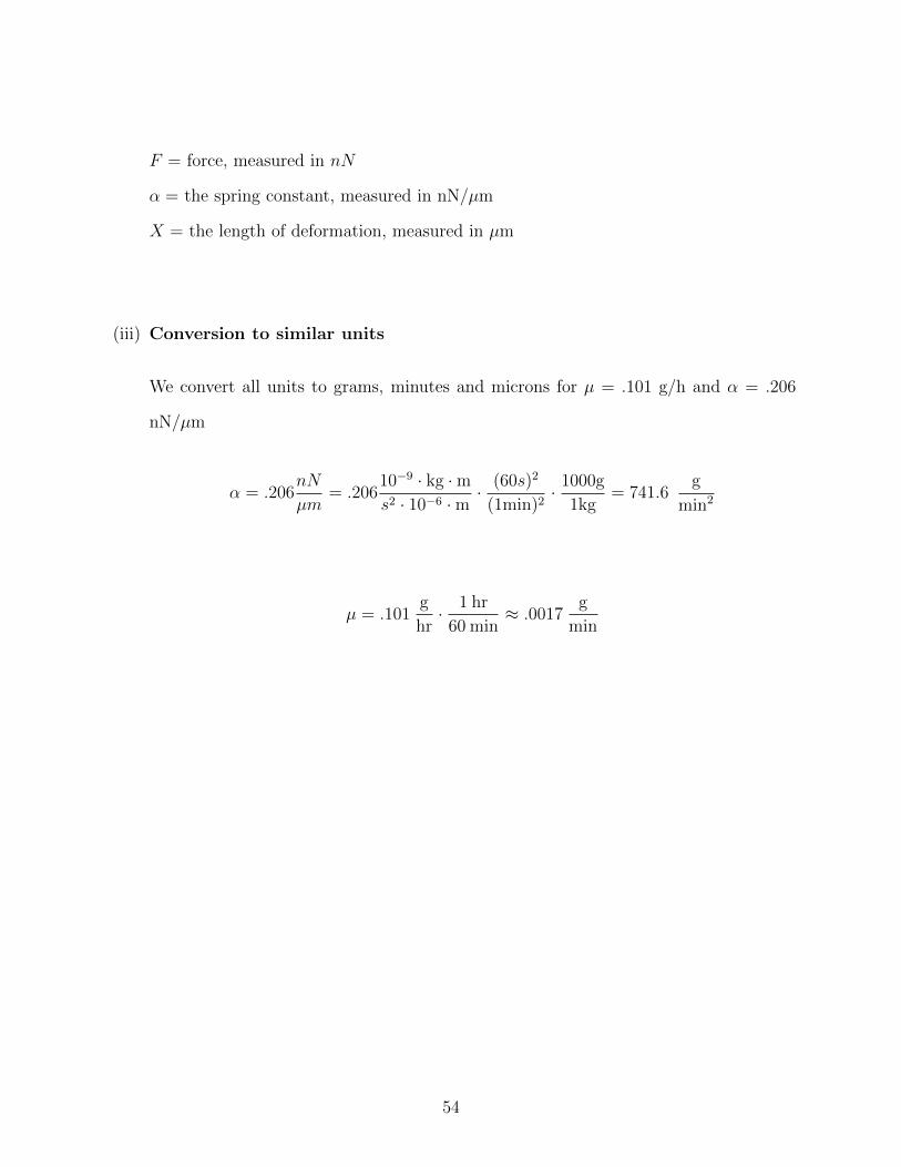
F = force, measured in nN
α = the spring constant, measured in nN/µm
X = the length of deformation, measured in µm
(iii) Conversion to similar units
We convert all units to grams, minutes and microns for µ = .101 g/h and α = .206
nN/µm
α = .206nN
µm= .206
10−9 · kg ·ms2 · 10−6 ·m
· (60s)2
(1min)2· 1000g
1kg= 741.6
g
min2
µ = .101g
hr· 1 hr
60 min≈ .0017
g
min
54

Appendix B. Resulting Distributions from
Different Detach-Rate Functions
In the following tables, we show the simulation-produced FA lifetime distributions for dif-
ferent detach-rate functions, r(t, f) = h(t) · g(f). We tried different functions for both the
time component, h(t), and force component, g(f).
Distributions for the Detach-Rate Function r(t, f ) = h(t) · g(f )Function of Time and Force Attach Times FA Lengths
h(t) = c
g(f) =
{.1 0 ≤ f ≤ F
(f − F ) + .1 f > F
g(f) = (f − F )2
g(f) = c
g(f) = a · f
55

Function of Time and Force Attach Times FA Lengthsh(t) = t
g(f) =
{.1 0 ≤ f ≤ F
(f − F ) + .1 f > F
g(f) = (f − F )2
g(f) = c
g(f) = a · f
Function of Time and Force Attach Times FA Lengthsh(t) = t2
g(f) =
{.1 0 ≤ f ≤ F
(f − F ) + .1 f > F
g(f) = (f − F )2
g(f) = c
g(f) = a · f
56

Function of Time and Force Attach Timesh(t) = c
g(f) = (f − 5)2
g(f) = (f − 10)2
h(t) = (t− 2)2
g(f) =
{.1 0 ≤ f ≤ F
(f − F ) + .1 f > F
g(f) = a · f
h(t) = (t− 4)2
g(f) ={.1 0 ≤ f ≤ F
(f − F ) + .1 F > F
g(f) = a · f
57

Function of Time and Force Attach Times
h(t) =
{0 0 ≤ t ≤ T
ln (t− (T − 1)) t > T
g(f) =
{.1 0 ≤ f ≤ F
(f − F ) + .1 f > F
g(f) = (f − F )2
g(f) = a
g(f) = a · f
Table B.1: Distributions for different detach-rate functions, r(t, f) = h(t) · g(f), are shownin the above Tables. Distributions for the FA lengths are also shown in the first three tables.
58

Appendix C. Model Artifacts
Some of the simulated distributions had histograms that had a spike at the beginning of the
distribution. We ran 10 simulations for the Astro, et al. [6] data each with the parameters
for T and F as found in Table 3.4, and found that about two-thirds of them had this
anomaly. The Meenderink et al., [42] data also showed this spike as seen in Figure C.1.
This spike disappears if the length of outreach is reduced. The explanation is that the
Hookean forces will be greater when a FA of longer length attaches, and since the detach-rate
function is dependent on force as described in Equation 3.3, there is a greater likelihood of a
quick detachment. Figure C.2 shows the distribution and gamma fit using the Meenderink
parameters listed in Table 3.4, but with an outreach from 1 to 6 as opposed to the original
simulation with outreach from 1 to 10. Notice that there is no spike.
59

Figure C.1: This figure shows the distribution from the simulation that produced a gammafit that best matched the Meenderink experimental gamma fit. Notice the spike at thebeginning of the distribution. The redline is the best fit gamma curve to the simulation, andthe blue vertical line is the minimum data value from the experimental data. This spike isan artifact of the model, and disappears when the length of outreach is smaller. For thissimulation, there are 40 total FAs with 30 attached on average. The outreach is from 1 to10.
Figure C.2: This figure shows the distribution from the simulation using the Meenderinkparameters from Table 3.4 with 40 total attachments and 30 attachments on average. Theoutreach is from 1 to 6. Notice the absence of the spike at the beginning.
60

Appendix D. Code
D.1 Experimental MSD Code
D.1.1 Main Code.
%%This program computes experimental MSD using the time measure of MSD and plots
%it versus my formula. It plots nint versus the MSD.
global average_length;
global icounter;
Relative_error = figure;
MSD_vs_r = figure;
iterationend = 30;
MSD = zeros(1, iterationend);
%nint = zeros(1,iterationend+1);
nintvector = zeros(1, iterationend);
MSD_formula = zeros(1, iterationend);
for m = 1:3
if m == 1
r = 10;
elseif m == 2
r = 1;
elseif m == 3
r = 1 / 3;
end
for j = 1:iterationend
nint = j;
nintvector(j) = j;
%nint=10;
counter = 10000000;
min_length = 0;
max_length = 10;
61

angle = 60;
tau = 1;
average_length = 0;
icounter = 0;
final_data = zeros(counter, 2);
[x, y, site_state, cx, cy] = Initialize(min_length, max_length, nint, angle);
for i = 1:50
[cx, cy] = Compute_Centroid(x, y, nint, site_state, cx, cy);
[x, y, site_state] = Update_Integrins(x, y, nint, site_state,
min_length, max_length, angle, cx, cy, r);
end
for k = 1:counter
[cx, cy] = Compute_Centroid(x, y, nint, site_state, cx, cy);
[x, y, site_state] = Update_Integrins(x, y, nint, site_state,
min_length, max_length, angle, cx, cy, r);
final_data(k, :) = [cx, cy];
end
[MSD(j)] = Compute_MSD(tau, counter, final_data);
%figure(MSD_vs_r);
%hold on;
%plot(r, MSD,’*’, ’Color’, ’r’, ’LineWidth’, 1.5, ’DisplayName’,
’Experimental MSD’)
%xlabel(’"r"’);
%set(gca, ’FontSize’, 14);
%ylabel(’MSD’);
%set(gca, ’FontSize’, 14);
%title(’MSD vs. "r"’);
%set(gca,’FontSize’, 18);
sum1 = 0;
if nint == 1
62

MSD_formula(j) = (1 / (2 * 3 * (max_length - min_length)))
* (max_length ^ 3 - min_length ^ 3);
%MSD_formula(j) = (max_length+min_length)^2/(8);
else
for ii = 1:nint - 1
sigma = 0;
for jj = 1:ii
sigma = sigma + jj / (jj + 1);
end
sum1 = nchoosek(nint - 1, ii) * (r ^ ii / ((ii + 1) ^ 2))
* (1 + (sigma * (ii + 1)) / (ii ^ 2)) + sum1;
end
%MSD_formula(j) =
(max_length + min_length)^2*(1+sum1)/(8*(1+r)^(nint-1));
MSD_formula(j) = (1 / (3 * (max_length - min_length)))
* (max_length ^ 3 - min_length ^ 3) * (1 + sum1)
/ (2 * (1 + r) ^ (nint - 1));
end
%pause;
%plot(r, MSD_formula,’*’, ’Color’, ’b’, ’LineWidth’, 1.5,
’DisplayName’, ’Formula MSD’)
%legend
%average_length/icounter
end
figure(MSD_vs_r);
hold on;
plot(nintvector, MSD, ’x’, ’Color’, ’r’, ’LineWidth’, 1.5,
’DisplayName’, ’Experimental MSD’)
xlabel(’Number of FAs’);
set(gca, ’FontSize’, 14);
ylabel(’MSD’);
set(gca, ’FontSize’, 14);
title({’MSD vs. Number of FAs’; ’’});
63

set(gca, ’FontSize’, 18);
plot(nintvector, MSD_formula, ’-’, ’Color’, ’b’, ’LineWidth’, 1.5,
’DisplayName’, ’Formula MSD’)
legend(’Experimental MSD’, ’Theoretical MSD’);
figure(Relative_error);
hold on;
difference = abs(MSD_formula - MSD) ./ MSD_formula;
xlabel(’Number of FAs’);
set(gca, ’FontSize’, 14);
ylabel(’Relative Error’);
set(gca, ’FontSize’, 14);
title({’Relative Error between the’; ’Experimental and Theoretical MSD’; ’’});
set(gca, ’FontSize’, 18);
if m == 1
plot(nintvector, difference, ’-’, ’Color’, ’r’, ’Linewidth’, 1.5);
elseif m == 2
plot(nintvector, difference, ’-’, ’Color’, ’b’, ’Linewidth’, 1.5);
elseif m == 3
plot(nintvector, difference, ’-’, ’Color’, ’g’, ’Linewidth’, 1.5);
legend(’r=10’, ’r=1’, ’r=1/3’);
end
end
% graphname = (’C:\Users\mefro\Experimental MSD vs Formula\Compare_MSD_varying_nint’);
% saveas(figure(MSD_vs_r), graphname);
% graphname = (’C:\Users\mefro\Experimental MSD vs Formula\Relative_Error’);
% saveas(figure(Relative_error), graphname);
D.1.2 Initialize Integrins.
%This program is a function that initializes the center and i-sites in the
%centroid model. Input is the minimum and maximum outreach length, the
%number of integrins (nint), and the angle in degrees on either side of zero for the
64

%outreach (angle). All integrins are initialized as attached.
function[x, y, site_state, cx, cy] =
Initialize(min_length, max_length, nint, angle)
cx = 0;
cy = 0;
x = zeros(1, nint);
y = zeros(1, nint);
site_state = zeros(1, nint);
for i = 1:nint
%length = min_length + (max_length-min_length)*rand;
length = (min_length + max_length) / 2;
theta = 360 / nint * i * pi / 180;
%theta=0;
%length=(min_length + max_length)/2;
x(i) = length * cos(theta);
y(i) = length * sin(theta);
site_state(i) = 1;
end
end
D.1.3 Update Integrins.
%This program is a function that updates the integrins. It determines what
%kind of event happened, and changes the status of an attached or detached site.
%Inputs for the function are: The x and y coordinates of the i-sites (x,y),
%the number of integrins (nint), the site status vector (site_state),
%minimum and max length of outreach, angle of outreach, location of the
%centroid, (c) and the value of "r" as described in "Cell Speed is
%Independent of Force ...", by Dallon, et. al.
function[x, y, site_state] = Update_Integrins(x, y, nint, site_state,
min_length, max_length, angle, cx, cy, r)
global average_length;
65

global icounter;
psi = sum(site_state);
p = 1 / (psi + (nint - psi) * r);
random = rand;
numdet = nint - psi;
if random < r * p * (numdet)
temp = randi([1 numdet], 1, 1);
idx = find(site_state == 0, temp, ’first’);
which_integrin = idx(end);
site_state(which_integrin) = 1;
length = min_length + (max_length - min_length) * rand;
theta = - angle * pi / 180 + 2 * angle * rand * pi / 180;
x(which_integrin) = length * cos(theta) + cx;
y(which_integrin) = length * sin(theta) + cy;
else
temp2 = randi([1 psi], 1, 1);
idx = find(site_state == 1, temp2, ’first’);
which_integrin = idx(end);
site_state(which_integrin) = 0;
end
end
D.1.4 Compute Centroid.
%This program is a function that computes the centroid. Input given is the
%i-site location (x,y), the number of integrins (nint), and the site status
%(site_state) which equals one if attached and 0 if not attached.
function[cx, cy] = Compute_Centroid(x, y, nint, site_state, cx, cy)
sumx = 0;
sumy = 0;
psi = 0;
for i = 1:nint
66

if site_state(i) == 1
sumx = sumx + x(i);
sumy = sumy + y(i);
psi = psi + 1;
end
end
if psi == 0
cx = cx;
cy = cy;
else
cx = sumx / psi;
cy = sumy / psi;
end
D.1.5 Compute MSD.
%This program is a function that computes the MSD, given data from the
%centroid model. Input is the number tau, or lag time between points to be
%compared. The variable counter is how many centroids were computed. Also,
%"c" is the location of the centroid
function[MSD] = Compute_MSD(tau, counter, final_data)
n = 0;
sum_msd = 0;
for i = 1:tau:((counter - mod(counter, tau)) - tau)
%for i=1:counter-tau
n = n + 1;
ss(n, 1) = (final_data(i + tau, 1) - final_data(i, 1));
ss(n, 2) = (final_data(i + tau, 2) - final_data(i, 2));
tt(n) = (final_data(i + tau, 1) - final_data(i, 1)) ^ 2 +
(final_data(i + tau, 2) - final_data(i, 2)) ^ 2;
sum_msd = tt(n) + sum_msd;
end
67

MSD = sum_msd / n;
MSD_STD = std(tt);
VAR = sum(var(ss));
EXP = mean(ss);
norm_squared = dot(EXP, EXP);
clear tt;
D.2 ODE Model Code
//Units are microns and minutes and grams.
#include <cmath>
#include <iostream>
#include <cstdlib>
#include <fstream>
#include <vector>
#include <algorithm>
#include "randomc.h"
#include "cellclass.h"
#include "stocc.h"
#include <cvode/cvode.h>
#include <sunlinsol/sunlinsol_spgmr.h>
#include <nvector/nvector_serial.h>
#include <sundials/sundials_types.h>
int check_flag(void *flagvalue, char *funcname, int opt);
int move_nodes(double t, N_Vector cc, N_Vector fval, void *f_data);
unsigned
const num_of_integrins = 40; //number of integrins
double min_length = 1;
double max_length = 10;
unsigned
const realizations = 10;
unsigned
68

const output_counter = 20; //frequency of data collection
int psi[num_of_integrins];
double attach_times[num_of_integrins];
double detach_times[num_of_integrins];
double detach_times_hold[num_of_integrins];
double theta; //random angle to find new integrin site
double radius; //random radius of length between min_length and max_length
int v[num_of_integrins]; //shuffle vector
double alpha[num_of_integrins]; //spring constants
double s1[num_of_integrins], s2[num_of_integrins]; //location of integrins
int length[num_of_integrins]; // length of each spring at rest
double intpart; //integer part of a floating point
int mm; //dummy variable for argument to load up length, spring constant and sites
double tt, ff; //dummy variables for time and force function
int seed = (unsigned int) time(NULL);
//StochasticLib1 rg1(seed); //Poisson number generator
CRandomMersenne rg(seed); //library containing uniform number generator
double mu = .101 / 60; //.101 g/hr, changed to g/min
void load_length(int mm);
void load_attach_times(int mm, double current_time);
void load_detach_times(int mm, double one_over_lambda);
void load_alpha(int mm);
void load_sites(int mm);
double force_mag[num_of_integrins];
double length_of_FAs[num_of_integrins];
double function_of_force_and_time(double ff, double tt);
//describes relation between forces and speed of detachment
double one_over_lambda = 8.; //mean of exponential
using namespace std;
static
const double pi = 3.14159265358979323846264338327950288419716939937510;
69
string filenames(int i, string file)
{
string num = to_string(i);
file += num;
file += ".dat";
return file;
}
int
main()
{
int flag;
int nnmax = 2;
double rtol = 1e-6;
double atol = 1e-6;
double tstart = 0;
double deltat;
double tempend;
ofstream myfile;
ofstream attach_times_file;
ofstream detach_times_file;
ofstream cell_center;
ofstream lengths_of_FA;
load_alpha(num_of_integrins);
load_length(num_of_integrins);
for (int k = 0; k < realizations; k++)
{
myfile.open(filenames(k, "naive_algorithm_data"));
attach_times_file.open(filenames(k, "naive_algorithm_attach_times"));
detach_times_file.open(filenames(k, "naive_algorithm_detach_times"));
70

cell_center.open(filenames(k, "naive_algorithm_cell_center"));
lengths_of_FA.open(filenames(k, "naive_algorithm_lengths"));
load_sites(num_of_integrins);
load_attach_times(num_of_integrins, tstart);
load_detach_times(num_of_integrins, one_over_lambda);
v[0] = 0;
for (int i = 1; i < num_of_integrins; i++)
{
v[i] = v[i - 1] + 1;
}
int jj = 1;
for (int i = 0; i < num_of_integrins; i++)
{
psi[i] = 1;
}
void *kmem;
kmem = NULL;
N_Vector sc;
SUNLinearSolver LS;
sc = N_VNew_Serial(nnmax);
N_VConst_Serial(0., sc);
/*Call KINCreate / KINMalloc to initialize KINSOL :
nvSpec is the nvSpec pointer used in the serial version
A pointer to KINSOL problem memory is returned and stored in kmem . */
kmem = CVodeCreate(CV_BDF); // for stiff problems
// kmem = CVodeCreate(CV_ADAMS,CV_FUNCTIONAL); // for non stiff problems
if (check_flag((void*) kmem, " CVodeCreate ", 0)) return (1);
flag = CVodeInit(kmem, move_nodes, tstart, sc);
71

if (check_flag((void*) kmem, " CVodeInit ", 0)) return (1);
int maxstep = 1e5;
flag = CVodeSetMaxNumSteps(kmem, maxstep);
if (check_flag(&flag, "CVodeSetMaxNumSteps", 1)) return (1);
int ord = 5;
flag = CVodeSetMaxOrd(kmem, ord);
if (check_flag(&flag, "CVodeSetMaxOrd", 1)) return (1);
flag = CVodeSStolerances(kmem, rtol, atol);
if (check_flag(&flag, "CVodeSStolerances", 1)) return (1);
const int mmax = 5; //dimension of krylov space
LS = SUNLinSol_SPGMR(sc, PREC_NONE, mmax);
flag = CVodeSetLinearSolver(kmem, LS, NULL);
if (check_flag(&flag, "CVSpgmr", 1)) return (1);
double tend = 4500;
double tret = 0;
myfile << tstart << " " << NV_Ith_S(sc, 0) << " " << NV_Ith_S(sc, 1)
<< " " << "0" << "\n";
//myfiletimes << tstart << "\n";
cell_center << tstart << " " << NV_Ith_S(sc, 0) << " " << NV_Ith_S(sc, 1) << "\n";
for (int i = 0; i < num_of_integrins; i++)
{
myfile << tstart << " " << s1[i] << " " << s2[i] << " " << psi[i] << "\n";
}
deltat = .1;
tempend = tstart + deltat; //solve ODE at increments of deltat and output to a file
double total_attached;
double total_detached;
total_attached = 0;
72

total_detached = 0;
double count_events;
count_events = 0;
while (tempend <= tend)
{
for (int i = 0; i < num_of_integrins - 1; i++)
{
int j = i + rand() % (num_of_integrins - i);
std::swap(v[i], v[j]);
}
for (int i = 0; i < num_of_integrins; i++)
{
length_of_FAs[i] = sqrt(pow(NV_Ith_S(sc, 0) - s1[i], 2)
+ pow(NV_Ith_S(sc, 1) - s2[i], 2));
force_mag[i] = alpha[i] *length_of_FAs[i];
}
double test_number = rg.Random();
int ii = 0;
while (ii < num_of_integrins)
{
if (psi[v[ii]] == 0 && detach_times[v[ii]] <= 0)
{
detach_times_file << detach_times_hold[v[ii]] << "\n";
for (int ss = 0; ss < num_of_integrins; ss++)
{
if (psi[ss] == 1)
{
lengths_of_FA << length_of_FAs[ss] << "\n";
73

}
}
psi[v[ii]] = 1;
attach_times[v[ii]] = tempend;
theta = rg.Random() *(2 *pi / 3) - pi / 3;
radius = rg.Random() *(max_length - min_length) + min_length;
s1[v[ii]] = NV_Ith_S(sc, 0) + radius* cos(theta);
s2[v[ii]] = NV_Ith_S(sc, 1) + radius* sin(theta);
for (int q = 0; q < num_of_integrins; q++)
{
total_attached = total_attached + psi[q];
}
count_events = count_events + 1;
ii = num_of_integrins;
}
else
{
if (psi[v[ii]] == 1 && test_number <= function_of_force_and_time(
force_mag[v[ii]] / alpha[v[ii]], tempend - attach_times[v[ii]]) *deltat)
{
for (int ss = 0; ss < num_of_integrins; ss++)
{
if (psi[ss] == 1)
{
lengths_of_FA << length_of_FAs[ss] << "\n";
}
}
psi[v[ii]] = 0;
detach_times[v[ii]] = -one_over_lambda* log(rg.Random());
74

detach_times_hold[v[ii]] = detach_times[v[ii]];
attach_times_file << tempend - attach_times[v[ii]] << "\n";
for (int q = 0; q < num_of_integrins; q++)
{
total_attached = total_attached + psi[q];
}
count_events = count_events + 1;
ii = num_of_integrins;
}
}
ii = ii + 1;
}
flag = CVodeReInit(kmem, tempend - deltat, sc);
if (check_flag((void*) kmem, " CVodeInit ", 0)) return (1);
int maxstep = 1e5;
flag = CVodeSetMaxNumSteps(kmem, maxstep);
if (check_flag(&flag, "CVodeSetMaxNumSteps", 1)) return (1);
int ord = 5;
flag = CVodeSetMaxOrd(kmem, ord);
if (check_flag(&flag, "CVodeSetMaxOrd", 1)) return (1);
flag = CVodeSStolerances(kmem, rtol, atol);
if (check_flag(&flag, "CVodeSStolerances", 1)) return (1);
const int mmax = 5; //dimension of krylov space
flag = CVode(kmem, tempend, sc, &tret, CV_NORMAL);
/*Call KINSol and print output concentration profile */
75

if (check_flag(&flag, "CVode", 1)) return (1);
if (jj % output_counter == 0)
{
myfile << tempend << " " << NV_Ith_S(sc, 0) << " "
<< NV_Ith_S(sc, 1) << " " << "0" << "\n";
cell_center << tempend << " " << NV_Ith_S(sc, 0)
<< " " << NV_Ith_S(sc, 1) << "\n";
for (int i = 0; i < num_of_integrins; i++)
{
myfile << tempend << " " << s1[i] << " " << s2[i] << " " << psi[i] << "\n";
}
}
tempend = tempend + deltat;
jj = jj + 1;
for (int i = 0; i < num_of_integrins; i++)
{
detach_times[i] = detach_times[i] - deltat;
}
}
total_attached = total_attached / count_events;
cout << "average number of attached FAs " << total_attached << "\n";
cout << "number of events is " << count_events << "\n";
CVodeFree(&kmem);
myfile.close();
attach_times_file.close();
detach_times_file.close();
cell_center.close();
lengths_of_FA.close();
76

}
return 0;
}
// defines the nonlinear system using springs i.e. F(x) = k(|x|-l)x/|x| + F
//assumes we can neglect acceleration
int move_nodes(double t, N_Vector cc, N_Vector fval, void *f_data)
{
int nn = NV_LENGTH_S(cc);
double u[nn];
double savf[nn];
double a[num_of_integrins]; //1st coordinate of the center minus each node
double b[num_of_integrins]; //2nd coordinate of the center minus each node
double distance[num_of_integrins]; //distance from center to nodes
double force_magnitude[num_of_integrins]; //magnitude of force on each node
for (int i = 0; i < nn; i++) // initialize the arrays since we only use part of them
{
u[i] = 0;
savf[i] = 0;
}
for (int i = 0; i < nn; i++)
{
u[i] = NV_Ith_S(cc, i);
}
for (int i = 0; i < num_of_integrins; i++)
{
77

a[i] = u[0] - s1[i];
b[i] = u[1] - s2[i];
distance[i] = sqrt(pow(a[i], 2) + pow(b[i], 2));
force_magnitude[i] = alpha[i] *(distance[i] - length[i]);
savf[0] = (-1 / mu) *(alpha[i]) *(u[0] - s1[i]) *psi[i] + savf[0];
savf[1] = (-1 / mu) *(alpha[i]) *(u[1] - s2[i]) *psi[i] + savf[1];
}
for (int i = 0; i < nn; i++)
{
NV_Ith_S(fval, i) = savf[i];
}
return (0);
}
void load_sites(int mm) //loads up the integrin sites
{
for (int i = 0; i < mm; i++)
{
double fractpart = modf(360 / num_of_integrins, &intpart);
s1[i] = (max_length + min_length) / 2* cos(intpart *pi / 180 *i);
s2[i] = (max_length + min_length) / 2* sin(intpart *pi / 180 *i);
}
}
void load_alpha(int mm)
{
//loads up the spring constants
for (int i = 0; i < mm; i++)
78

{
alpha[i] = 741.6;
}
}
void load_length(int mm)
{
//loads up resting length of spring
for (int i = 0; i < mm; i++)
{
length[i] = 0;
}
}
void load_attach_times(int mm, double current_time)
{
//initializes times to 0
for (int i = 0; i < mm; i++)
{
attach_times[i] = current_time;
}
}
void load_detach_times(int mm, double one_over_lambda)
{
//initializes detach times
for (int i = 1; i < mm; i++)
{
detach_times[i] = -one_over_lambda* log(rg.Random());
detach_times_hold[i] = detach_times[i];
}
}
79

double function_of_force_and_time(double x, double t)
{
//specifies the relation between attachment forces, time and speed of detachment
double f;
// f=(t-4)*(t-4);
// f=1.;
// f=t;
double starttime = 7.25;
if (t < starttime)
{
f = 0;
}
else
{
f = log(t - (starttime - 1));
}
// f=t*t;
double g;
double constant = 1.;
double upper_threshold = 5.634;
double y;
if (x <= upper_threshold)
{
g = .1;
}
else
{
g = constant *(x - upper_threshold) + .1;
}
// g=(x-5)*(x-5);
// g=(x-constant*max_length)*(x-constant*max_length);
80

// g=2;
// g=x*2;
y = g * f;
return y;
}
/*
*Check function return value ...
*opt == 0 means SUNDIALS function allocates memory so check if
*returned NULL pointer *opt == 1 means SUNDIALS function returns a flag so check
if * flag >= 0 *opt == 2 means function allocates memory so check if returned
*NULL pointer
*/
int check_flag(void *flagvalue, char *funcname, int opt)
{
int *errflag;
/*Check if SUNDIALS function returned NULL pointer - no memory allocated */
if (opt == 0 && flagvalue == NULL)
{
fprintf(stderr,
"\n SUNDIALS_ERROR : %s() failed - returned NULL pointer \n\n",
funcname);
return (1);
}
/*Check if flag < 0 */
else if (opt == 1)
{
errflag = (int*) flagvalue;
if (*errflag < 0)
{
fprintf(stderr,
"\n SUNDIALS_ERROR : %s() failed with flag = %d \n\n",
81

funcname, *errflag);
return (1);
}
}
/*Check if function returned NULL pointer - no memory allocated */
else if (opt == 2 && flagvalue == NULL)
{
fprintf(stderr,
"\n MEMORY_ERROR : %s() failed - returned NULL pointer \n\n", funcname);
return (1);
}
return (0);
}
82

Bibliography
[1] Mark S. Bretscher. How Animal Cells Move. Scientific American, 257(6):72–93, 1987.Publisher: Scientific American, a division of Nature America, Inc.
[2] J. C. Dallon, Matthew Scott, and W. V. Smith. A force based model of individualcell migration with discrete attachment sites and random switching terms. Journal ofBiomechanical Engineering, 135(7):71008, July 2013.
[3] Samantha J. Stehbens and Torsten Wittmann. Chapter 18 - Analysis of focal adhesionturnover: A quantitative live-cell imaging example. In Jennifer C. Waters and TorstenWittman, editors, Methods in Cell Biology, volume 123 of Quantitative Imaging in CellBiology, pages 335–346. Academic Press, January 2014.
[4] Whitney M. Cleghorn, Kevin M. Branch, Seunghyi Kook, Christopher Arnette, NadaBulus, Roy Zent, Irina Kaverina, Eugenia V. Gurevich, Alissa M. Weaver, andVsevolod V. Gurevich. Arrestins regulate cell spreading and motility via focal adhesiondynamics. Molecular Biology of the Cell, 26(4):622–635, December 2014.
[5] Mathew E. Berginski, Eric A. Vitriol, Klaus M. Hahn, and Shawn M. Gomez. High-Resolution Quantification of Focal Adhesion Spatiotemporal Dynamics in Living Cells.PLOS ONE, 6(7):e22025, July 2011.
[6] Veronica Astro, Diletta Tonoli, Sara Chiaretti, Sabrina Badanai, Kristyna Sala, MarinoZerial, and Ivan de Curtis. Liprin-α1 and ERC1 control cell edge dynamics by promotingfocal adhesion turnover. Scientific Reports, 6:33653, September 2016.
[7] Chiara De Pascalis, Carlos Perez-Gonzalez, Shailaja Seetharaman, Batiste Boeda,Benoit Vianay, Mithila Burute, Cecile Leduc, Nicolas Borghi, Xavier Trepat, and San-drine Etienne-Manneville. Intermediate filaments control collective migration by re-stricting traction forces and sustaining cell–cell contacts. The Journal of Cell Biology,217(9):3031–3044, September 2018.
[8] Jonathan Stricker, Yvonne Beckham, Michael W. Davidson, and Margaret L. Gardel.Myosin II-Mediated Focal Adhesion Maturation Is Tension Insensitive. PLOS ONE,8(7):e70652, July 2013.
[9] Emma Spanjaard, Ihor Smal, Nicos Angelopoulos, Ingrid Verlaan, Alexandre Matov,Erik Meijering, Lodewyk Wessels, Hans Bos, and Johan de Rooij. Quantitative imagingof focal adhesion dynamics and their regulation by HGF and Rap1 signaling. Experi-mental Cell Research, 330(2):382–397, January 2015.
[10] Douglas A. Lauffenburger and Alan F. Horwitz. Cell Migration: A Physically IntegratedMolecular Process. Cell, 84(3):359–369, February 1996. Publisher: Elsevier.
[11] Carl R. Woese. A New Biology for a New Century. Microbiology and Molecular Biol-ogy Reviews, 68(2):173–186, June 2004. Publisher: American Society for MicrobiologySection: Review.
83

[12] Gerald Bergtrom. What We Know and How Found Out. Cell and Molecular Biology4e: - All Versions, January 2020.
[13] Ken F. Jarrell and Mark J. McBride. The surprisingly diverse ways that prokaryotesmove. Nature Reviews Microbiology, 6(6):466–476, June 2008. Number: 6 Publisher:Nature Publishing Group.
[14] Felicitas Pfeifer. Gas Vesicles of Archaea and Bacteria. In Jessup M. Shively, editor,Complex Intracellular Structures in Prokaryotes, Microbiology Monographs, pages 115–140. Springer, Berlin, Heidelberg, 2006.
[15] P. Cappuccinelli. The movement of eukaryotic cells. In P. Cappuccinelli, editor, Motilityof Living Cells, pages 59–74. Springer Netherlands, Dordrecht, 1980.
[16] J. P. Heath and G. A. Dunn. Cell to substratum contacts of chick fibroblasts andtheir relation to the microfilament system. A correlated interference-reflexion and high-voltage electron-microscope study. Journal of Cell Science, 29(1):197–212, February1978. Publisher: The Company of Biologists Ltd Section: Journal Articles.
[17] Benjamin Geiger, Joachim P. Spatz, and Alexander D. Bershadsky. Environmentalsensing through focal adhesions. Nature Reviews Molecular Cell Biology, 10(1):21–33,January 2009. Number: 1 Publisher: Nature Publishing Group.
[18] Kristopher E. Kubow and Alan Rick Horwitz. Reducing background fluorescence revealsadhesions in 3D matrices. Nature Cell Biology, 13(1):3–5, January 2011. Number: 1Publisher: Nature Publishing Group.
[19] Sarah Gierke and Torsten Wittmann. EB1-Recruited Microtubule +TIP ComplexesCoordinate Protrusion Dynamics during 3D Epithelial Remodeling. Current Biology,22(9):753–762, May 2012.
[20] Revathi Ananthakrishnan and Allen Ehrlicher. The Forces Behind Cell Movement.International Journal of Biological Sciences, 3(5):303–317, June 2007.
[21] Ewa K. Paluch, Irene M. Aspalter, and Michael Sixt. Focal Adhesion–Independent CellMigration. Annual Review of Cell and Developmental Biology, 32(1):469–490, 2016.eprint: https://doi.org/10.1146/annurev-cellbio-111315-125341.
[22] Grzegorz Sikora, Marek Teuerle, Agnieszka Wy lomanska, and Denis Grebenkov. Sta-tistical properties of the anomalous scaling exponent estimator based on time-averagedmean-square displacement. Physical Review E, 96(2):022132, August 2017.
[23] Vincent Tejedor, Olivier Benichou, Raphael Voituriez, Ralf Jungmann, Friedrich Sim-mel, Christine Selhuber-Unkel, Lene B. Oddershede, and Ralf Metzler. QuantitativeAnalysis of Single Particle Trajectories: Mean Maximal Excursion Method. BiophysicalJournal, 98(7):1364, April 2010. Publisher: The Biophysical Society.
84

[24] Adi Rebenshtok and Eli Barkai. Distribution of Time-Averaged Observables for WeakErgodicity Breaking. Physical Review Letters, 99(21):210601, November 2007. arXiv:0707.3865.
[25] T. G. Mason, K. Ganesan, J. H. van Zanten, D. Wirtz, and S. C. Kuo. Particle TrackingMicrorheology of Complex Fluids. Physical Review Letters, 79(17):3282–3285, October1997.
[26] A. Einstein. Uber die von der molekularkinetischen Theorie der Warme geforderteBewegung von in ruhenden Flussigkeiten suspendierten Teilchen. Annalen der Physik,322(8):549–560, 1905.
[27] Todd M. Squires and John F. Brady. A simple paradigm for active and nonlinearmicrorheology. Physics of Fluids, 17(7):073101, July 2005.
[28] William Sutherland. LXXV. A dynamical theory of diffusion for non-electrolytes and themolecular mass of albumin. The London, Edinburgh, and Dublin Philosophical Magazineand Journal of Science, 9(54):781–785, June 1905.
[29] Bivash R. Dasgupta, Shang-You Tee, John C. Crocker, B. J. Frisken, and D. A. Weitz.Microrheology of polyethylene oxide using diffusing wave spectroscopy and single scat-tering. Physical Review E, 65(5):051505, May 2002.
[30] Jingyuan Xu, Virgile Viasnoff, and D. Wirtz. Compliance of actin filament networksmeasured by particle-tracking microrheology and diffusing wave spectroscopy. Rheolog-ica Acta, 37(4):387–398, August 1998.
[31] Michael J. Saxton and Ken Jacobson. SINGLE-PARTICLE TRACKING:Applicationsto Membrane Dynamics. Annual Review of Biophysics and Biomolecular Structure,26(1):373–399, 1997. eprint: https://doi.org/10.1146/annurev.biophys.26.1.373.
[32] Daphne Weihs, Thomas G. Mason, and Michael A. Teitell. Bio-Microrheology: A Fron-tier in Microrheology. Biophysical Journal, 91(11):4296–4305, December 2006.
[33] Naama Gal, Diana Lechtman-Goldstein, and Daphne Weihs. Particle tracking in livingcells: a review of the mean square displacement method and beyond. Rheologica Acta,52(5):425–443, May 2013.
[34] Stas Burov, Jae-Hyung Jeon, Ralf Metzler, and Eli Barkai. Single particle trackingin systems showing anomalous diffusion: the role of weak ergodicity breaking. Phys-ical Chemistry Chemical Physics, 13(5):1800–1812, 2011. Publisher: Royal Society ofChemistry.
[35] Julia F. Reverey, Jae-Hyung Jeon, Han Bao, Matthias Leippe, Ralf Metzler, and Chris-tine Selhuber-Unkel. Superdiffusion dominates intracellular particle motion in the super-crowded cytoplasm of pathogenic Acanthamoeba castellanii. Scientific Reports, 5(1):1–14, June 2015. Number: 1 Publisher: Nature Publishing Group.
85

[36] Brenton D. Hoffman, Gladys Massiera, Kathleen M. Van Citters, and John C. Crocker.The consensus mechanics of cultured mammalian cells. Proceedings of the NationalAcademy of Sciences, 103(27):10259–10264, July 2006. Publisher: National Academyof Sciences Section: Biological Sciences.
[37] Naama Gal and Daphne Weihs. Intracellular Mechanics and Activity of Breast CancerCells Correlate with Metastatic Potential. Cell Biochemistry and Biophysics, 63(3):199–209, July 2012.
[38] Karl Pearson. The Problem of the Random Walk. Nature, 72(1867):342–342, August1905. Number: 1867 Publisher: Nature Publishing Group.
[39] Codling Edward A, Plank Michael J, and Benhamou Simon. Random walk models inbiology. Journal of The Royal Society Interface, 5(25):813–834, August 2008.
[40] Geoffrey R. Grimmett and David R. Stirzaker. Probability and Random Processes. OUPOxford, May 2001.
[41] J. C. Dallon, E. J. Evans, Christopher P. Grant, and W. V. Smith. Cell speed isindependent of force in a mathematical model of amoeboidal cell motion with randomswitching terms. Mathematical Biosciences, 246(1):1–7, November 2013.
[42] Leslie M. Meenderink, Larisa M. Ryzhova, Dominique M. Donato, Daniel F. Gochberg,Irina Kaverina, and Steven K. Hanks. P130Cas Src-Binding and Substrate DomainsHave Distinct Roles in Sustaining Focal Adhesion Disassembly and Promoting CellMigration. PLOS ONE, 5(10):e13412, October 2010.
[43] Bertille Bance, Shailaja Seetharaman, Cecile Leduc, Batiste Boeda, and SandrineEtienne-Manneville. Microtubule acetylation but not detyrosination promotes focaladhesion dynamics and astrocyte migration. Journal of Cell Science, 132(7), April2019.
[44] Claudia Schafer, Grzegorz Rymarczyk, Lai Ding, Michael T. Kirber, and Victoria M.Bolotina. Role of Molecular Determinants of Store-operated Ca2+ Entry (Orai1, Phos-pholipase A2 Group 6, and STIM1) in Focal Adhesion Formation and Cell Migration.Journal of Biological Chemistry, 287(48):40745–40757, November 2012.
[45] Jeanne M. Bristow, Theresa A. Reno, Minji Jo, Steven L. Gonias, and Richard L.Klemke. Dynamic phosphorylation of tyrosine 665 in pseudopodium-enriched atypicalkinase 1 (PEAK1) is essential for the regulation of cell migration and focal adhesionturnover. The Journal of Biological Chemistry, 288(1):123–131, January 2013.
[46] J. Srivastava, G. Barreiro, S. Groscurth, A. R. Gingras, B. T. Goult, D. R. Critchley,M. J. S. Kelly, M. P. Jacobson, and D. L. Barber. Structural model and functional signif-icance of pH-dependent talin–actin binding for focal adhesion remodeling. Proceedingsof the National Academy of Sciences, 105(38):14436–14441, September 2008.
86

[47] Samantha Stehbens, Hayley Pemble, Lyndsay Murrow, and Torsten Wittmann. Imagingintracellular protein dynamics by spinning disk confocal microscopy. In Methods inEnzymology, volume 504, pages 293–313. Elsevier, 2012.
[48] David J. C. MacKay. Information Theory, Inference and Learning Algorithms. Cam-bridge University Press, September 2003. Google-Books-ID: AKuMj4PN EMC.
[49] Laxman Bokati, Aaron Velasco, and Vladik Kreinovich. Why Gamma Distribution ofSeismic Inter-Event Times: A Theoretical Explanation. Departmental Technical Reports(CS), December 2019.
[50] Pinaki Kumar, Evangelos Korkolis, Roberto Benzi, Dmitry Denisov, Andre Niemeijer,Peter Schall, Federico Toschi, and Jeannot Trampert. On interevent time distributions ofavalanche dynamics. Scientific Reports, 10(1):626, January 2020. Number: 1 Publisher:Nature Publishing Group.
[51] Stephen A Arhin, Adam Gatiba, Melissa Anderson, Babin Manandhar, and MelkamsewRibbisso. Acceptable Wait Time Models at Transit Bus Stops. Engineering, Technologyand Applied Science Research, 9(4):7, 2019.
[52] Patrick W Oakes, Shiladitya Banerjee, M Cristina Marchetti, and Margaret L Gardel.Geometry regulates traction stresses in adherent cells. Biophysical Journal, 107(4):825–833, 2014.
[53] Daniel T. Gillespie. Stochastic simulation of chemical kinetics. Annual Review of Phys-ical Chemistry, 58:35–55, 2007.
[54] SUNDIALS: SUite of Nonlinear and DIfferential/ALgebraic Equation Solvers, January2016.
[55] Praveen Kumar, Karen S Lyle, Sarah Gierke, Alexandre Matov, Gaudenz Danuser, andTorsten Wittmann. Gsk3β phosphorylation modulates clasp–microtubule associationand lamella microtubule attachment. Journal of Cell Biology, 184(6):895–908, 2009.
[56] Luis Vidali, Feng Chen, Gregor Cicchetti, Yasutaka Ohta, and David J Kwiatkowski.Rac1 null mouse embryonic fibroblasts are motile and respond to pdgf. Biological Chem-istry, 272:30688–92, 2006.
[57] Chun-Min Lo, Denis B Buxton, Gregory CH Chua, Micah Dembo, Robert S Adel-stein, and Yu-Li Wang. Nonmuscle myosin iib is involved in the guidance of fibroblastmigration. Molecular Biology of the Cell, 15(3):982–989, 2004.
[58] Chen Zhang, Sogol Hekmatfar, Anand Ramanathan, and Nancy W Karuri. Pegylatedhuman plasma fibronectin is proteolytically stable, supports cell adhesion, cell migra-tion, focal adhesion assembly, and fibronectin fibrillogenesis. Biotechnology Progress,29(2):493–504, 2013.
87

[59] Shoeb Ahmed, Hyun-kwan Yang, Ali E Ozcam, Kirill Efimenko, Michael C Weiger, JanGenzer, and Jason M Haugh. Poly (vinylmethylsiloxane) elastomer networks as func-tional materials for cell adhesion and migration studies. Biomacromolecules, 12(4):1265–1271, 2011.
[60] Claudia Conte, Michelle A Baird, Michael W Davidson, and Eric R Griffis. Spindly isrequired for rapid migration of human cells. Biology Open, 7(5), 2018.
[61] J. B. L. Bard and E. D. Hay. The behaviour of fibroblasts from the developing aviancornea. morphology and movement in situ and in vitro. Journal of Cell Biology, 67:400–418, 1975.
[62] Paul W. Kriebel, Valarie A. Barr, Erin C. Rericha, Guofeng Zhang, and Carole A. Par-ent. Collective cell migration requires vesicular trafficking for chemoattractant deliveryat the trailing edge. Journal of Cell Biology, 183:949–961, 2008.
[63] KK Parker, AL Brock, C Brangwynne, RJ Mannix, N Wang, E Ostuni, NA Geisse,JC Adams, GM Whitesides, and DE Ingber. Directional control of lamellipodia ex-tension by constraining cell shape and orienting cell tractional forces. Faseb Journal,16(10), August 2002.
[64] Maria L. Lombardi, David A. Knecht, Micah Dembo, and Juliet Lee. Traction force mi-croscopy in dictyostelium reveals distinct roles for myosin ii motor and actin-crosslinkingactivity in polarized cell movement. Journal of Cell Science, 120(9):1624–1634, May2007.
[65] J Hui and SW Pang. Dynamic tracking of osteoblastic cell traction force during guidedmigration. Cellular and Molecular Bioengineering, 11(1):11–23, 2018.
88


