arX

iv:a

stro

-ph/

0506

741

v1

29 J

un 2

005

Measurement of Pressure Dependent

Fluorescence Yield of Air: Calibration Factor

for UHECR Detectors

J.W. Belz, a G.W. Burt, b Z. Cao, b F.Y. Chang c C.C. Chen c

C.W. Chen c P. Chen, d C. Field, d J. Findlay, b

P. Huntemeyer, b,∗ M.A. Huang c W-Y.P. Hwang c R. Iverson, d

B.F Jones, b C.C.H. Jui, b M. Kirn a G.-L. Lin c E.C. Loh, b

M.M. Maestas, b N. Manago, b K. Martens, b J.N. Matthews, b

J.S.T. Ng, d A. Odian, d K. Reil, d J.D. Smith, b R. Snow, b

P. Sokolsky, b R.W. Springer, b J.R. Thomas, b S.B. Thomas, b

G.B. Thomson, e D. Walz, d and A. Zech e

The FLASH Collaboration

aUniversity of Montana, Department of Physics and Astronomy, Missoula,MT 59812, USA.

bUniversity of Utah, Department of Physics and High Energy AstrophysicsInstitute, Salt Lake City, UT 84112, USA

cCenter for Cosmology and Particle Astrophysics, Department of Physics,National Taiwan University, 1 Roosevelt Road , Section 4, Taipei 106-17, Taiwan

dStanford Linear Accelerator Center, 2575 Sand Hill Road, Menlo Park,CA 94025, USA

eRutgers — The State University of New Jersey, Department of Physics andAstronomy, Piscataway, NJ 08854, USA

Preprint submitted to Elsevier Science 20 December 2005

Abstract

In a test experiment at the Final Focus Test Beam of the Stanford Linear Accel-erator Center, the fluorescence yield of 28.5 GeV electrons in air and nitrogen wasmeasured. The measured photon yields between 300 and 400 nm at 1 atm and 29◦Care

Y (760 Torr)air = 4.42 ± 0.73 and Y (760 Torr)N2 = 29.2 ± 4.8

photons per electron per meter. Assuming that the fluorescence yield is proportionalto the energy deposition of a charged particle traveling through air, good agreementwith measurements at lower particle energies is observed.

Key words:Nitrogen fluorescence, Air fluorescence, Extensive air shower, Ultrahigh-energycosmic raysPACS: 95.55.Vj, 96.40.Pq, 96.40.De, 32.50.+d

1 Introduction

Measuring the energy spectrum of Ultra High Energy Cosmic Rays (UHECR)is the goal of several past, present, and future experiments using the air fluores-cence technique. It is of special interest to measure the spectrum in the rangeof 1020 eV and establish whether it is suppressed as predicted by the GZKmechanism [1]. The published results of the two, at that time largest, exper-iments collecting UHECR data disagree [2]. One of those detectors, the HighResolution Fly’s Eye (HiRes) utilizes air fluorescence to detect cosmic rays andto determine their energy. The other experiment, the Akeno Giant Air ShowerArray (AGASA), a ground array of scintillation counters in Japan, used theparticle sampling technique. The energy dependent HiRes flux measurementis systematically smaller than that of AGASA and is consistent with a GZKsuppression. One systematic uncertainty in the case of the fluorescence tech-nique is the uncertainty of the measured fluorescence yield of charged particlesin air itself. A more precise study of the yield would be valuable in seekingthe cause for the apparent discrepancies between the techniques.

There are a number of previous fluorescence yield experiments. In his the-sis from 1967 Bunner summarized the existing data and quoted uncertaintiesof around 30% on the reported fluorescence efficiencies [3]. Bunner’s work

∗ Corresponding author. E-mail address: petra@cosmic.utah.edu

2

served as the standard reference for fluorescence technique based cosmic rayexperiments into the nineties. In a more recent experiment [4], Kakimoto et

al. measured the total fluorescence yield between 300 and 400 nm with an un-certainty of >10% and the yield at three pronounced lines - 337 nm, 357 nm,and 391 nm. The newest measurements using a 90Sr β source published byNagano et al. [5,6], determined the total fluorescence yield between 300 nmand 406 nm with a systematic uncertainty of 13.2% as the sum of the yieldsof 15 wave bands which were measured separately using narrow band filters.An improvement in the present level of accuracy and confidence is necessary,from measurements not subject to the same set of systematic uncertainties,especially since other systematics, like the atmospheric uncertainty, which de-pends on variable pressure profile, transparency, scattering, etc., are expectedto be reduced significantly in the near future.

New experiments using the fluorescence technique are beginning to take data,are in construction, or are being planned. These include the hybrid detectorsof the Pierre Auger Observatory [7], and of the Telescope Array (TA) [8],or the space-based fluorescence detectors EUSO [9] and OWL [10]. Theseexperiments are designed to increase the detection aperture and statisticsin the ultra high energy region. The hybrid detectors should also help toresolve the disagreements between the particle sampling technique and thefluorescence technique. Independent measurements of the fluorescence yield ofcharged particles in air as presented in this paper, and refinements proposedto follow this work, will complete the picture.

The test experiment presented in this paper, T-461, was conducted at theStanford Linear Accelerator Center (SLAC) to study the feasibility of a largerfluorescence experiment, FLASH 1 . Both experiments have since been installedin SLAC’s Final Focus Test Beam (FFTB) tunnel. FLASH aims to measure thenet fluorescence yield as well as the yields of the individual spectral lines witha systematic uncertainty of less than 10%. Measurements with mono-energeticelectrons, and separately with electron-positron showers downstream of thickmaterials, are used to measure the fluorescence yield down to an electronenergy of 100 keV[11]. T-461 used only the mono-energetic beam approachand was designed to measure the total fluorescence yield between 300 and400 nm using a UV bandpass filter as installed in the HiRes experiment. Inthe following Section, the experimental setup of T-461 will be described indetail. In Section 3, the selection of good quality data is described. This isfollowed by a brief description of the calibration of the experimental setup inSection 4. The fluorescence yield measured in air and nitrogen is presented inSection 5 along with a list of the systematic errors which were studied. In thelast Section, the T-461 results are compared with previous measurements andimprovements are discussed for the full scale fluorescence experiment FLASH.

1 FLuorescence in Air from SHowers

3

2 Experimental setup

The experiment T-461 was carried out in the Final Focus Fest Beam at SLAC.It was installed in an air gap of the beam pipe, approximately 35 cm long,downstream of the dump magnets. The beam is focused effectively at infinityin this region, so that the bremsstrahlung from the beam windows and thinexperimental equipment in this region continues along the electron beam tothe dump. In addition, since the thickness of the material in the beam washeld below 1% of a radiation length, multiple scattering of beam particles intodownstream collimators is negligible.

A beam spot size of about 2×1 mm was generated in this region, with in-tensities between 109 and 2 ×1010 e−/pulse. Between 108 and 109 electronsper pulse, the intensity is below the sensitivity of the beam position moni-tors and feedback becomes inoperative. Nonetheless, intensities as low as 108

were delivered for 24 hours during T-461. However, the beam current measur-ing toroidal ferrite-core current transformer registered intensity variations of≈ 30% during this period. The toroid was calibrated using charge-injectionon a one-turn winding. The accuracy was determined to be 10% for beamcharges below 109 e− by cross comparison with a high-accuracy toroid duringa subsequent FLASH run. 2

The thin target installed in FFTB during T-461 was a 1.6 liter air-filled cylin-der, coaxial with the beam. The vessel had thin beam windows and radialports to allow light to reach shielded photomultiplier tubes (PMTs) as shownin Figure 1. The inside of the vessel was black-anodized and baffled to suppressall but direct light from the beam. The fluorescence light was detected in twoindependent radial tubes. In each, the optical aperture was defined by a slitnear the beam axis, measured to be 1 cm parallel, and 1.7 cm perpendicularto it. In each tube, light passed through a series of circular apertures forminga baffle. At the far end of the 42.9 cm long baffle, the PMTs were protectedfrom scattered background radiation by using dielectric mirrors to reflect thefluorescence light through 900 into the detector. There, the PMTs were en-cased in a lead vault. As can be seen in Figure 1, a UV band pass filter fromthe High Resolution Fly’s Eye (HiRes) experiment was installed between thedielectric mirror and PMT. The PMTs, Philips (now Photonis) XP3062/FL,are also the type used in the HiRes experiment. The optical unit includingthe mirror, UV filter, and PMT was calibrated at the University of Utah afterT-461 data taking was completed.

To monitor the stability of the PMT response in-situ, ultraviolet LEDs wereinstalled on arms opposite the detector arms. The LEDs were fired between

2 Details of the calibration of the high-accuracy toroid is the subject of a futurepublication.

4

Fig. 1. The experimental setup showing one of two orthogonal optical pathwaysthrough baffled channels, and 45 degree reflection to a photomultiplier tube (PMT).The values are given in inches [mm].

beam pulses emitting light across the fluorescence cylinder. To measure beaminduced backgrounds in the PMTs, optically hooded — “blind” — PMTs weremounted beside the “live” tubes. Signals of the blind tubes were collectedcontinuously along with the signals of the live tubes and normalized to thelive signals by collecting data while the fluorescence chamber was filled witha non-fluorescing gas.

The gas system allowed the flow of a premixed gas with a pressure in the vesselbetween 3 and 760 Torr. The pressure was set manually, but monitored bycomputer during data taking. Data for dry air and pure nitrogen were collectedwith flowing gas. Data for various air-nitrogen mixtures were collected withoutflowing the gas through the chamber.

During T-461, a CAMAC based DAQ system was used to collect the data.Pulse amplitudes from the PMTs and the beam toroid signal were recordedusing LRS 2249W ADCs from Lecroy. PMT high voltage, pressure and tem-perature were digitized with the Smart Analog Module, a 32-channel moduleused to digitize analog signals.

3 Data taking and event selection

Altogether about 1 million events were recorded with a mean high voltage of1186 V supplied to the PMTs. The voltage was constrained to better thanhalf a volt over the entire run period.

Throughout the data taking, a special trigger, about once every 52 beam

5

Fig. 2. Pedestal subtracted response of the south signal PMT to the LED. a) Thesouth PMT response versus the run number. The dashed lines represent the dataquality preselection cut. b) The projection of the response onto the signal axis.

pulses, was used to measure ADC pedestals. The pedestal values were foundto be stable around 45 and 47 counts for the north and south signal PMTs,respectively. From each beam event the nearest pedestal measurement wassubtracted.

The PMT response was tracked throughout the data taking with ultravioletLEDs. As for the pedestal events, LED events were also taken once every52 beam events. The response of the south PMT to the LED was very sta-ble (around 2%) during the experiment as seen in Figure 2a. Similar to thepedestal subtraction scheme, each beam induced event was assigned the closestLED reading.

In order to remove poor quality data and data with unstable detector response,the LED data of the south PMT were fitted to a Gaussian, see Figure 2b. Beamdata during time periods where LED events were outside of ±6σ of the fittedmean were removed from the data set. The ±6σ band is represented by twodashed lines in Figure 2a. Less than 1.5% of the data were excluded by thisrequirement (see Table 1).

Figure 3 shows that the north PMT’s response was unstable, probably due toa HV connector problem. While the north PMT data were used to check thedata quality, because of such wide systematic wandering, the north PMT wasnot used in the final result. The pedestal subtracted LED signals were usedto correct for gain changes shown in Figures 2 and 3 by the formulas,

Scd = (S − Spd) ×〈SLED〉

SLED − Spd

(1)

6

Cut Efficiency (%)

LED requirement 98.6

PMT correlation 98.5

Beam distribution 84.7

Linearity cut 41.9

Air 15.8

Mixtures 13.7

N2 (flowing) 2.6

Table 1Efficiency of the main preselection requirements imposed on the T-461 data. SeeSection 3 for details.

and

Ncd = (N − Npd) ×〈NLED〉

NLED − Npd

. (2)

Here, Scd and Ncd are the stability corrected and pedestal subtracted southand north PMT signals, S and N are the raw ADC readouts from the PMTs,Spd and Npd are the signals of the assigned pedestal events, 〈SLED〉 and 〈NLED〉are the fitted means of the pedestal subtracted LED distributions shown forthe signal PMTs by horizontal lines in Figure 2a and 3, and SLED and NLED

are the signals of the closest LED events. The mean for all the LED eventscollected by the south signal PMT is 〈SLED〉 = 1011 counts. The mean of〈NLED〉 = 765 counts was calculated only from the longest period of northPMT gain stability which occurred between runs 504 and 947.

After the PMT signals had been corrected for LED response the signal sizewas required to correlate well between the two signal PMTs. In Figure 4a thecorrected signal, Ncd, of the north PMT is plotted versus the corrected sig-nal, Scd, of the south PMT. A strong correlation for most of the data is quiteapparent. The data were fitted to the linear function Ncd = kScd, k being thecorrelation factor of the two signals. Then the axes were rotated so that thefitted line was the ordinate of a new plot. The new abscissa is calculated ac-cording to the formula x = Ncd cos θ − Scd sin θ, where k = tan θ. The rotateddistribution was then projected onto the new abscissa. The resulting distribu-tion is shown in Figure 4b. All events beyond ±85.0 ADC counts were removedfrom the data sample. The upper and lower lines in Figure 4a represent the170 ADC counts acceptance band. The fraction of events remaining after thiscut is listed in Table 1.

During the two weeks of data collection, data were recorded at beam charges

7

Fig. 3. Pedestal subtracted response of the north signal PMT to the LED. Thex-axis is the run number and the y-axis is the pedestal subtracted LED signal.

Fig. 4. Signal PMT correlation. a) The x-axis is the background subtracted andgain corrected south PMT signal and the y-axis is the background subtracted andgain corrected north PMT signal. Air, N2, and air-N2 mixture events are shown.The dashed lines correspond to the PMT correlation cut, see Table 1. b) Projectionof the rotated distribution showing the correlation between Ncd and Scd wherex = Ncd cos θ − Scd sin θ. See text for details.

between 108 and 1010 e− per bunch. For each data part, the target beamcharge was specified, and the charge of each bunch was measured with a toroidinstalled up-stream of the thin target vessel. Figure 5 shows example distri-butions of measured beam charges for four runs. As can be seen, some of thedistributions, especially those with low beam intensity, have long tails possiblyindicating poor beam quality. To remove the corresponding events from thedata sample, the beam charge distribution of each run was fitted to a Gaussiancurve and events lying outside of 2σ were cut. The selection efficiency of this

8

Fig. 5. The beam charge distributions of four typical data runs as measured by anupstream toroid during T-461.

requirement is also listed in Table 1.

In order to investigate possible background due to reflected Cherenkov light orother sources, some data were collected while the gas chamber was filled withethylene, a non-fluorescing gas. The same range of pressures were investigatedas for air and nitrogen. The corrected signals, Ncd and Scd, of both PMTsfor the ethylene data runs are plotted versus pressure in Figure 6. The figureshows that Scd and Ncd do not depend on the pressure, indicating negligiblelight background. The larger signal values for each signal tube at the lowestpressure probably indicate the presence of a trace amount of air.

During the entire experiment, the beam related background was measured bytwo “blind” PMTs positioned next to the “signal” PMTs. Figure 7 shows thatthe blind PMT signal increases with the beam charge. Using the ethylene datathe blind PMT data was normalized to the signal PMT data. The pedestal

9

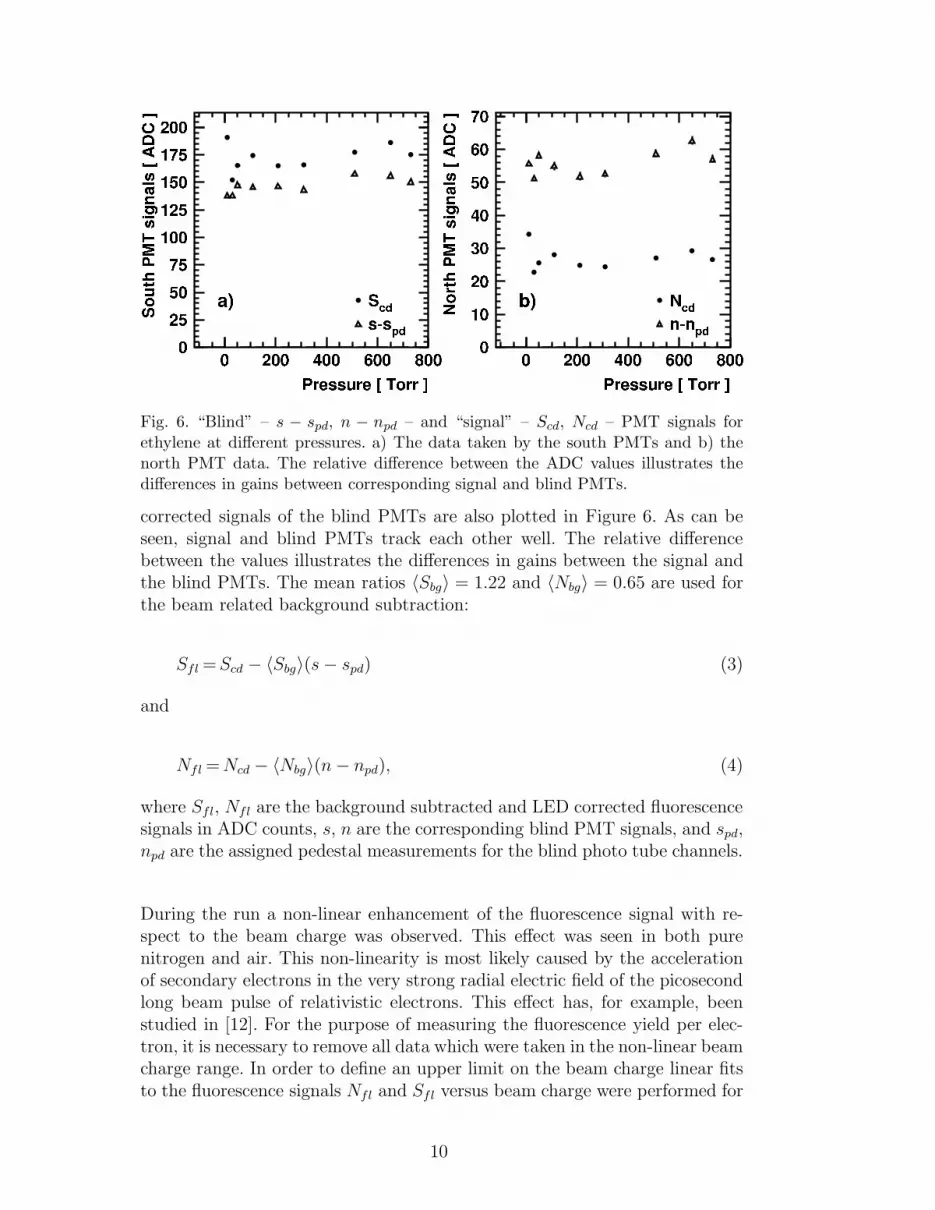
Fig. 6. “Blind” – s − spd, n − npd – and “signal” – Scd, Ncd – PMT signals forethylene at different pressures. a) The data taken by the south PMTs and b) thenorth PMT data. The relative difference between the ADC values illustrates thedifferences in gains between corresponding signal and blind PMTs.

corrected signals of the blind PMTs are also plotted in Figure 6. As can beseen, signal and blind PMTs track each other well. The relative differencebetween the values illustrates the differences in gains between the signal andthe blind PMTs. The mean ratios 〈Sbg〉 = 1.22 and 〈Nbg〉 = 0.65 are used forthe beam related background subtraction:

Sfl =Scd − 〈Sbg〉(s − spd) (3)

and

Nfl = Ncd − 〈Nbg〉(n − npd), (4)

where Sfl, Nfl are the background subtracted and LED corrected fluorescencesignals in ADC counts, s, n are the corresponding blind PMT signals, and spd,npd are the assigned pedestal measurements for the blind photo tube channels.

During the run a non-linear enhancement of the fluorescence signal with re-spect to the beam charge was observed. This effect was seen in both purenitrogen and air. This non-linearity is most likely caused by the accelerationof secondary electrons in the very strong radial electric field of the picosecondlong beam pulse of relativistic electrons. This effect has, for example, beenstudied in [12]. For the purpose of measuring the fluorescence yield per elec-tron, it is necessary to remove all data which were taken in the non-linear beamcharge range. In order to define an upper limit on the beam charge linear fitsto the fluorescence signals Nfl and Sfl versus beam charge were performed for

10

Fig. 7. The south background PMT signal versus the number of beam electrons perbunch.

Fig. 8. Stability corrected and background subtracted signal versus the number ofelectrons per beam pulse for two selected pressure regions for air.

varying beam charge ranges. Based on the quality of the fits an upper limit of1 × 109e− per beam pulse was chosen and all the data taken at higher beamcharges were removed from the data sample. Two example fits with an appliedbeam charge limit of 1 × 109 e− per pulse are shown in Figure 8.

The final fraction of events remaining after all cuts for air, nitrogen andnitrogen-air mixtures are listed in Table 1. In the case of nitrogen, only datawhich were collected when the gas was flowing through the chamber were con-sidered. This ensured that potential impurities from small leaks of ambientair in the chamber were negligible. The fluorescence yield Y per electron permeter in air and nitrogen was then determined based on these preselected datasamples as will be described in the following sections.

11

4 Calibration and Geometrical Acceptance

Before the fluorescence yield can be calculated, the detectors and the DAQsystem need to be calibrated and the geometrical acceptance of the detectors,as they were mounted on the thin target chamber, must be determined.

The fluorescence yield then can be calculated as

Y =1

Ne−·Sfl · C

RD · G, (5)

where Sfl is the background subtracted and LED corrected fluorescence signalin ADC counts, C is the calibration factor converting ADC counts into pC,Ne− is the number of electrons in a beam pulse, G is the effective geometricalacceptance in m−1, and RD is the photon flux responsivity of the detectorassembly in pC m2/γ.

As mentioned in the last section only the south signal PMT was used for thefinal result. The calibration constant C for its DAQ channel was measured tobe 1/3.48 pC/ADC counts.

The south detector assembly was calibrated after T-461 data taking was com-pleted. As can be seen in Figure 1, the PMT was mounted in a brass housingalong with a HiRes filter and a mirror. The complete unit was calibrated ina standard HiRes calibration setup at the University of Utah. A schematicof the calibration setup is shown in Figure 9. It consisted of a 100 W high-pressure mercury arc lamp, a monochromator, a light guide and a diffuseras the light source, a 1.8 m light path in a baffled foam tube, and a standwith a calibrated silicon photo diode installed next to the south PMT unit.The diffuser, the baffled light path, the Si photo diode and the PMT unitwere enclosed completely in a dark box. The south signal PMT detector unitand the silicon photo diode were aligned so that they were directly facingthe diffuser. During calibration the monochromator scanned the wavelengthregion between 260 nm and 420 nm in 1 nm steps. After several monochro-mator scans were recorded, the PMT and photo diode were swapped. In thismanner light emitted by the mercury lamp was collected by the PMT assem-bly and the diode. The current output of each detector was measured by apico ampere meter. From the calibration curve of the wavelength dependentresponsivity of the silicon photo diode in units of A/(W/cm2), and the mea-sured size of the entrance pupil of the T-461 detector assembly, its responsivitycould be calculated in units of A/(W/cm2). In order to calculate the spectrumweighted photon flux responsivity RD of the detector the wavelength depen-dent responsivity was folded with the normalized fluorescence spectrum of airand nitrogen at 760 Torr as reported in Tables 1 and 2 of reference [6]. The

12

Fig. 9. The detector calibration setup.

fluorescence photon flux responsivity between 300 and 400 nm was found tobe RD = 1.47 × 10−6pC · m2/γ for air and RD = 1.66 × 10−6pC · m2/γ fornitrogen.

The geometrical acceptance G′ was calculated as

G′ =W

4 · π · (D − L) · D(6)

where D is the distance from the beam axis to the detector unit’s aperture, Lis the distance from the beam axis to the slit, and W is the slit width definingthe beam length seen by the detector. D, L, and W were measured for thesouth signal PMT arm and based on the measured numbers G′ was calculatedto be 1/213.8 m−1. A small fraction of the energy deposited by the beam inthe gas was outside the transverse aperture of the optical slit (± 0.85 cm).This was evaluated from the Monte Carlo simulations of the process, leadingto a correction of 7% and an effective geometrical acceptance of

G = G′ · l, (7)

where l is ∼ 93% with a very small pressure dependence.

13

5 Resulting Fluorescence Yield

Figure 10 shows the calculated yield in units of γ

e−mversus the measured

pressure in Torr for air and nitrogen at 29◦ C. For air, the curve plateausat about 4.4 γ

e−m, while the N2 curve continues to climb with pressure and

reaches a yield approaching seven times that at 800 Torr. Figure 11 shows themeasured pressure dependent yield of four different air-N2 mixtures framedby the N2 and air yield curves. Inspired by the fluorescence yield studiesin previous publications [3,5,6], where fits were performed to the measuredpressure (p) dependent yields of individual spectral lines, the function

Y (p) =C

1

p′+ 1

p

(8)

was fitted to the air and N2 yield curves using the log likelihood method withC and p′ as freely variable parameters. In the case of an individual spectralline, p′ is the reference pressure specific to the line and C is the product

C =dE

dx·

1

RThν· Φ0. (9)

Here dE/dx is the energy deposited by an electron traveling through the gastarget, R is the specific gas constant, T is the temperature, hν is the photon’senergy, and Φ0 is the fluorescence efficiency of the corresponding spectral linein the absence of collisional quenching [3,5,6]. The values for p′ derived fromthe fits are 8.9 ±0.8 Torr for air and 103±10 Torr for nitrogen. The functions,Y (p), resulting from the fits were then used to calculate the yields in air andnitrogen at 1 atm:

Y (760 Torr)air = 4.42 ± 0.73γ

e−m

and

Y (760 Torr)N2 = 29.2 ± 4.8γ

e−m.

The sources contributing to the overall uncertainty are summarized in ta-ble 2. The total uncertainty is 16.6%. The statistical uncertainty contributesless than 1% to the total uncertainty. The largest systematic uncertainty isassociated with the detector calibration (10.5%). This accounts for the trans-fer uncertainty from the calibration setup in Utah to SLAC, the radiometer

14

Fig. 10. The fluorescence yield curves for air (left plot) and N2 (right plot) asmeasured by the south PMT. The x-axis is the pressure measured in Torr, and they-axis is the resulting fluorescence yield between 300 and 400 nm in photons perelectron per meter ( γ

e−m).

Fig. 11. The fluorescence yield curves of air and N2 and various air-N2 mixtures. Thex-axis is the pressure measured in Torr, and the y-axis is the resulting fluorescenceyield between 300 and 400 nm in γ

e−m.

calibration uncertainty of the silicon photo diode, in addition to statistical,environmental, geometrical, and other systematic uncertainties derived froma series of calibration measurements. The uncertainties of the fluorescencespectrum in air and nitrogen quoted in Table 1 and 2 of reference [6] werealso taken into account. The second largest contribution of 10% to the totaluncertainty is from the beam charge measurement. It was estimated based onsystematic studies comparing simultaneous measurements of the two differenttoroids used during T-461 and FLASH (E-165). The uncertainty of the effec-tive geometrical acceptance, G, of 7% is due to a conservative estimate of the

15

Relative error at 760 Torr Air and N2

Statistics <<1%

Systematics

Detector calibration RD 10.5%

Beam Toroid Calibration Ne− 10%

Geometrical Acceptance G 7%

Linearity cut Sfl/Ne− 3%

ADC calibration C 2%

Background subtraction 〈Sbg〉 1%

Total Y 16.6%

Table 2Summary of statistical and systematic uncertainties in the measurement of the totalfluorescence yield, Y , in air and pure nitrogen at 760 Torr at 29◦ C.

uncertainties on the measured slit widths and the measured distances to thebeam line. A potential systematic effect from the linearity cut described inSection 3 was also investigated. The linearity requirement was varied betweenNe− < 0.5 · 109 and Ne− < 1.1 · 109 electrons per bunch resulting in differencesof the measured yield in air and nitrogen of up to 3%. The uncertainty ofthe ADC calibration of the south PMT DAQ channel contributes 2% to theoverall uncertainty. The smallest systematic uncertainty of 1% is associatedwith the background subtraction.

6 Fluorescence Decay Time

The strong saturation of the fluorescence yield in the pressure range up toatmospheric (Fig. 10) is caused by collisional de-excitation of the nitrogenmolecules. This statistical process enforces exponential decay times on theexcited states. The basic formalism is the same as in the previous section andin terms of decay lifetimes, τ , may be given as τ = τ0/(1 + p/p′). Here p′ isthe same as in eq. 8 and τ0 is the decay time in the absence of collisions, forexample at very low pressure.

Most of the wavelengths in this study are transitions in the second positivebands, and may be expected to have similar decay properties. The 1N tran-sition at 391 nm may be different, but accounts for a small fraction of thelight at our pressures. In this experiment, decay effects are averaged over thedetected wavelengths.

16

Fig. 12. Pulse profiles from the photomultiplier for air pressures of 5 and 748 Torr.

An overall dependence of the decay time on pressure was indeed observed. Asa way of studying it, photomultiplier pulse profiles were recorded at variousgas pressures, using a digital oscilloscope. Typically 16 pulses were averaged.The dependence of decay time on pressure was very obvious, as is illustratedby the pulses shown in Fig. 12 for air at 5 and 748 Torr.

In order to process the data, the small effect of beam induced backgroundin the PMT was removed. As described in Section 3, this was accomplishedby using pulse shapes recorded while the test vessel was filled with ethylene,corresponding to that part of the signal not from the gas fluorescence. Suit-ably normalized to the correct beam intensity, this was subtracted, sample bysample, from the fluorescence pulse profiles. The effect was noticeable onlybelow 30 Torr, and especially in air which gives smaller signals.

The next step was to record the PMT intrinsic pulse shape, which was mea-

17

sured using an Sr90 source to make picosecond long pulses of Cherenkov light inthe tube face. For computational purposes, this shape was parametrized by awell fitting asymmetric probability distribution, Pearson IV [13]. (Other func-tions would have fitted almost as well.) The intrinsic shape was then foldedwith hypothetical light pulses which turned on instantly (corresponding tothe SLAC picosecond electron pulse length) but decayed exponentially. Thefolding was repeated for a range of decay times of the light, and, for eachcase, the width of the folded pulse at half maximum (FWHM) was taken tocharacterize the pulse shape.

Using this calibration, the measured FWHM values of the actual data pulseprofiles were transformed to the light decay times. Values for air and nitrogenare shown in Fig. 13. The nitrogen data below 30 Torr were excluded because ofuncertainty about the effect of a small air leak in the system. Uncertainties ateach point were estimated for the FWHM measurements and the backgroundsubtraction, and scaled, after fitting, so that χ2 was equal to the number ofdegrees of freedom. Fitting to the functional form above allows us to obtain thevalues for decay times at “zero pressure” (i.e. in the absence of collisional de-excitation) of 32.0±2.2 ns for air and 26.1±1.2 ns for nitrogen. At atmosphericpressure, the values found are 0.41 ± 0.01 ns for air, and 2.20 ± 0.06 ns fornitrogen. The values for p’ are 9.9 ± 0.7 Torr for air and 70 ± 4 for nitrogen.The nitrogen value is significantly lower than that obtained from the yieldcurve. This may be related to our assumption that all the emission lines can betreated by a single average parameter. Differences between them would distortthe decay time and yield fits differently, especially given the extrapolationbelow 30 Torr. In future work we intend to measure the lines separately.

In the case of nitrogen, numerous measurements of the “zero pressure” decaylifetimes have been reported for various wavelength bands, mostly after excita-tion by proton beams. Results, summarized by Dotchin et al. [14], show valuesin the range 34 to 48 ns. A measurement at 10−6 Torr observed 58 ns [15].Recently, however, Nagano and collaborators [5], using electrons to excite thenitrogen, report lower values. They give values in six wavelength bands, ap-proximately covering the spectral range of our data. To allow a comparisonbetween the two experiments, we have weighted the decay time for each ofNagano’s wavebands by its relative intensity and taken a weighted average.Their average value for nitrogen is then 27.4 ± 1.4 ns. A similar average oftheir results for air is 30.5± 2 ns. Our life time measurements agree well withNagano and collaborators, but not with the earlier proton beam experiments.

18

Fig. 13. Decay time vs. pressure: a) air; b) nitrogen.

7 Conclusion and Discussion

Figure 14 shows the total fluorescence yield between 300 and 400 nm perelectron in air at 760 Torr and 290C calculated in this paper as well as theyields reported by Kakimoto [4] and Nagano [6]. The yields are plotted versusthe energy of the electrons injected in a thin air target and together with twodE/dx curves. The line shows the energy loss of electrons in air as calculatedbased on reference [16], while the dashed line represents the energy deposit ofan electron in a 1 cm thick slab of air as calculated by GEANT 3 [17]. Theconversion from dE/dx to fluorescence yield was found by performing a χ2 fitof the energy deposit to the various measurements. As can be seen, there isgood agreement over four decades in electron energy. The overall uncertainty

19

Fig. 14. Comparison of the results from Nagano et al.[6], Kakimoto et al.[4], andT-461.

of the T-461 result of 16.6% is dominated by systematic effects. Those willbe reduced in future fluorescence measurements at SLAC by improvements inthe calibration of the light detectors and beam toroid. Among other things, itis planned to derive an end-to-end calibration of the thin target chamber fromfirst principles using Rayleigh scattering of a nitrogen laser beam of knownenergy sent through the chamber. The experimental program will also besupplemented with a spectrally resolved measurement of the fluorescence lightyield between 290 and 440 nm and an energy dependent yield measurementin which the electron beam is injected in an air-like target material of variablethicknesses to produce confined electromagnetic showers at various showerdepths.

8 Acknowledgments

We are indebted to the SLAC accelerator operations staff for their expertisein meeting the unusual beam requirements, and to personnel of the Experi-mental Facilities Department for very professional assistance in preparationand installation of the equipment. We also gratefully acknowledge the manycontributions from the technical staffs of our home institutions. This work wassupported in part by the U.S. Department of Energy under contract number

20

DE-AC02-76SF00515 as well as by the National Science Foundation underawards NSF PHY-0245428, NSF PHY-0305516, NSF PHY-0307098, and NSFPHY-0400053.

References

[1] K. Greisen, Phys. Rev. .Lett. 16 (1966) 748;V. A. Kuzmin, G. T. Zatsepin, Pisma Zh. Eksp. Teor. Fiz. 4 (1966) 114 [JETPLett. 4, 78].

[2] R. Abbasi et al., Phys. Rev. Lett. 92 (2004) 151101;M. Takeda et al., Astrophys. J. 522 (1999), 225;M. Takeda et al., Phys. Rev. Lett. 81 (1998), 1163.

[3] A. N. Bunner, Ph. D. thesis (Cornell University) (1967).

[4] F. Kakimoto, E. C. Loh, M. Nagano, H. Okuno, M. Teshima, S. Ueno, Nucl.Instrum. Meth., A 372 (1996) 527.

[5] M. Nagano, K. Kobayakawa, N. Sakaki, and K. Ando, Astropart. Phys. 20

(2003) 293.

[6] M. Nagano, K. Kobayakawa, N. Sakaki, and K. Ando, Astropart. Phys. 22

(2004) 235.

[7] S. Argiro, Eur. Phys. J. C 33 (2004) S947;J. Abraham et al., Nucl. Instrum. Meth. A 523 (2004) 50;A. Etchegoyen, Astrophys. Space Sci. 290 (2004) 379;M. Kleifges, Nucl. Instrum. Meth. A 518 (2004) 180;D. V. Camin, Nucl. Instrum. Meth. A 518 (2004) 172.

[8] M. Fukushima, Institute for Cosmic Ray Research Mid-term (2004-2009)Maintenance Plan Proposal Book “Cosmic Ray Telescope Project”, TokyoUniversity (2002);F. Kakimoto et al., Prepared for 28th International Cosmic Ray Conferences(ICRC 2003), Tsukuba, Japan, 31 Jul - 7 Aug 2003.

[9] L. Scarsi et al., Prepared for 27th International Cosmic Ray Conferences (ICRC2001), Hamburg, Germany, 7 Aug - 15 Aug 2001, Proceedings, 839.

[10] L. Scarsi, Prepared for 26th International Cosmic Ray Conference (ICRC 1999),Salt Lake City, Utah, 17-25 Aug 1999, Proceedings Vol. 2, 384;J. Linsley, Prepared for 26th International Cosmic Ray Conference (ICRC1999), Salt Lake City, Utah, 17-25 Aug 1999, Proceedings Vol. 2, 423.

[11] J. Belz et. al., “Fluorescence in Air from Showers (FLASH)”, E-165 Proposal(2002), [http://www.slac.stanford.edu/grp/rd/epac/Proposal/index.html].

[12] J. S. T. Ng, et al., Phys. Rev. Lett. 87, 244801 (2001) [arXiv:physics/0110015].

21

[13] J.A. Greenwood and H.O. Hartley, Guide to Tables in Mathematical Statistics,Princeton University Press, 1962.

[14] L.W. Dotchin, E.L. Chupp and D.J. Pegg, Journal Chem. Phys. 59 (1973) 3960;L.L. Nicholls and W.E. Wilson, Applied Optics 7 (1968) 167.

[15] M.A. Plum et al., Nucl. Instr.and Meth. A 492 (2002), 74.

[16] S. M. Seltzer and M. J. Berger, Int. J. Appl. Radiat. Isot., 33, 1189 (1982);R. M. Sternheimer, Berger and Seltzer, Atomic Data and Nuclear Data Tables30, 261 (1984).

[17] R. Brun et al., GEANT3 User’s Guide, CERN DD/EE/84-1, Sept 1987, RevisedVersion.

22