Embed Size (px)
Citation preview

EUROPEAN ORGANIZATION FOR NUCLEAR RESEARCH
CERN-EP/98-12
26th of January, 1998
MEASUREMENT OF THE SPECTRAL FUNCTIONS OF
AXIAL-VECTOR HADRONIC � DECAYS AND
DETERMINATION OF �s(M2� )
The ALEPH Collaboration1
Abstract
An analysis based on 124 000 selected � pairs recorded by the ALEPH detector
at LEP provides the vector (V ) and axial-vector (A) spectral functions of hadronic
� decays together with their total widths. This allows the evaluation of finite energy
chiral sum rules that are weighted integrals over the (V �A) spectral functions. In
addition, a precise measurement of �s along with a determination of nonperturbative
contributions at the � mass scale is performed. The experimentally and theoretically
most robust determination of �s(M2� ) is obtained from the (V + A) fit that yields
�s(M2� ) = 0:334� 0:022 giving �s(M
2Z) = 0:1202� 0:0027 after the extrapolation to
the mass of the Z boson. The approach of the Operator Product Expansion (OPE)
is tested experimentally studying the evolution of the � hadronic widths to masses
smaller than the � mass.
(Submitted to The European Physical Journal C)
1See next pages for the list of authors.

The ALEPH Collaboration
R. Barate, D. Buskulic, D. Decamp, P. Ghez, C. Goy, J.-P. Lees, A. Lucotte, E. Merle, M.-N. Minard,J.-Y. Nief, B. Pietrzyk
Laboratoire de Physique des Particules (LAPP), IN2P3-CNRS, 74019 Annecy-le-Vieux Cedex, France
R. Alemany, G. Boix, M.P. Casado, M. Chmeissani, J.M. Crespo, M. Del�no, E. Fernandez,M. Fernandez-Bosman, Ll. Garrido,15 E. Graug�es, A. Juste, M. Martinez, G. Merino, R. Miquel,Ll.M. Mir, I.C. Park, A. Pascual, J.A. Perlas, I. Riu, F. Sanchez
Institut de F�isica d'Altes Energies, Universitat Aut�onoma de Barcelona, 08193 Bellaterra (Barcelona),Spain7
A. Colaleo, D. Creanza, M. de Palma, G. Gelao, G. Iaselli, G. Maggi, M. Maggi, S. Nuzzo, A. Ranieri,G. Raso, F. Ruggieri, G. Selvaggi, L. Silvestris, P. Tempesta, A. Tricomi,3 G. Zito
Dipartimento di Fisica, INFN Sezione di Bari, 70126 Bari, Italy
X. Huang, J. Lin, Q. Ouyang, T. Wang, Y. Xie, R. Xu, S. Xue, J. Zhang, L. Zhang, W. Zhao
Institute of High-Energy Physics, Academia Sinica, Beijing, The People's Republic of China8
D. Abbaneo, U. Becker, P. Bright-Thomas, D. Casper, M. Cattaneo, V. Ciulli, G. Dissertori,H. Drevermann, R.W. Forty, M. Frank, R. Hagelberg, J.B. Hansen, J. Harvey, P. Janot, B. Jost,I. Lehraus, P. Mato, A. Minten, L. Moneta,21 A. Pacheco, J.-F. Pusztaszeri,23 F. Ranjard, L. Rolandi,D. Rousseau, D. Schlatter, M. Schmitt,25 O. Schneider, W. Tejessy, F. Teubert, I.R. Tomalin,H. Wachsmuth, A. Wagner20
European Laboratory for Particle Physics (CERN), 1211 Geneva 23, Switzerland
Z. Ajaltouni, F. Badaud, G. Chazelle, O. Deschamps, A. Falvard, C. Ferdi, P. Gay, C. Guicheney,P. Henrard, J. Jousset, B. Michel, S. Monteil, J-C. Montret, D. Pallin, P. Perret, F. Podlyski, J. Proriol,P. RosnetLaboratoire de Physique Corpusculaire, Universit�e Blaise Pascal, IN2P3-CNRS, Clermont-Ferrand,63177 Aubi�ere, France
J.D. Hansen, J.R. Hansen, P.H. Hansen, B.S. Nilsson, B. Rensch, A. W�a�an�anen
Niels Bohr Institute, 2100 Copenhagen, Denmark9
G. Daskalakis, A. Kyriakis, C. Markou, E. Simopoulou, I. Siotis, A. Vayaki
Nuclear Research Center Demokritos (NRCD), Athens, Greece
A. Blondel, G. Bonneaud, J.-C. Brient, P. Bourdon, A. Roug�e, M. Rumpf, A. Valassi,6 M. Verderi,H. VideauLaboratoire de Physique Nucl�eaire et des Hautes Energies, Ecole Polytechnique, IN2P3-CNRS, 91128Palaiseau Cedex, France
E. Focardi, G. Parrini, K. Zachariadou
Dipartimento di Fisica, Universit�a di Firenze, INFN Sezione di Firenze, 50125 Firenze, Italy
M. Corden, C. Georgiopoulos, D.E. Ja�e
Supercomputer Computations Research Institute, Florida State University, Tallahassee, FL 32306-4052, USA 13;14
A. Antonelli, G. Bencivenni, G. Bologna,4 F. Bossi, P. Campana, G. Capon, F. Cerutti, V. Chiarella,G. Felici, P. Laurelli, G. Mannocchi,5 F. Murtas, G.P. Murtas, L. Passalacqua, M. Pepe-Altarelli
Laboratori Nazionali dell'INFN (LNF-INFN), 00044 Frascati, Italy

L. Curtis, A.W. Halley, J.G. Lynch, P. Negus, V. O'Shea, C. Raine, J.M. Scarr, K. Smith, P. Teixeira-Dias,A.S. Thompson, E. Thomson
Department of Physics and Astronomy, University of Glasgow, Glasgow G12 8QQ,United Kingdom10
O. Buchm�uller, S. Dhamotharan, C. Geweniger, G. Graefe, P. Hanke, G. Hansper, V. Hepp, E.E. Kluge,A. Putzer, J. Sommer, K. Tittel, S. Werner, M. Wunsch
Institut f�ur Hochenergiephysik, Universit�at Heidelberg, 69120 Heidelberg, Fed. Rep. of Germany16
R. Beuselinck, D.M. Binnie, W. Cameron, P.J. Dornan,2 M. Girone, S. Goodsir, E.B. Martin, N. Marinelli,A. Moutoussi, J. Nash, J.K. Sedgbeer, P. Spagnolo, M.D. Williams
Department of Physics, Imperial College, London SW7 2BZ, United Kingdom10
V.M. Ghete, P. Girtler, E. Kneringer, D. Kuhn, G. Rudolph
Institut f�ur Experimentalphysik, Universit�at Innsbruck, 6020 Innsbruck, Austria18
A.P. Betteridge, C.K. Bowdery, P.G. Buck, P. Colrain, G. Crawford, A.J. Finch, F. Foster, G. Hughes,R.W.L. Jones, M.I. Williams
Department of Physics, University of Lancaster, Lancaster LA1 4YB, United Kingdom10
I. Giehl, A.M. Greene, C. Ho�mann, K. Jakobs, K. Kleinknecht, G. Quast, B. Renk, E. Rohne,H.-G. Sander, P. van Gemmeren, C. Zeitnitz
Institut f�ur Physik, Universit�at Mainz, 55099 Mainz, Fed. Rep. of Germany16
J.J. Aubert, C. Benchouk, A. Bonissent, G. Bujosa, J. Carr,2 P. Coyle, F. Etienne, O. Leroy, F. Motsch,P. Payre, M. Talby, A. Sadouki, M. Thulasidas, K. Trabelsi
Centre de Physique des Particules, Facult�e des Sciences de Luminy, IN2P3-CNRS, 13288 Marseille,France
M. Aleppo, M. Antonelli, F. Ragusa
Dipartimento di Fisica, Universit�a di Milano e INFN Sezione di Milano, 20133 Milano, Italy
R. Berlich, W. Blum, V. B�uscher, H. Dietl, G. Ganis, H. Kroha, G. L�utjens, C. Mannert, W. M�anner,H.-G. Moser, S. Schael, R. Settles, H. Seywerd, H. Stenzel, W. Wiedenmann, G. Wolf
Max-Planck-Institut f�ur Physik, Werner-Heisenberg-Institut, 80805M�unchen, Fed. Rep. of Germany16
J. Boucrot, O. Callot, S. Chen, A. Cordier, M. Davier, L. Du ot, J.-F. Grivaz, Ph. Heusse, A. H�ocker,A. Jacholkowska, D.W. Kim,12 F. Le Diberder, J. Lefran�cois, A.-M. Lutz, M.-H. Schune, E. Tourne�er,J.-J. Veillet, I. Videau, D. Zerwas
Laboratoire de l'Acc�el�erateur Lin�eaire, Universit�e de Paris-Sud, IN2P3-CNRS, 91405 Orsay Cedex,France
P. Azzurri, G. Bagliesi,2 G. Batignani, S. Bettarini, T. Boccali, C. Bozzi, G. Calderini, M. Carpinelli,M.A. Ciocci, R. Dell'Orso, R. Fantechi, I. Ferrante, L. Fo�a,1 F. Forti, A. Giassi, M.A. Giorgi, A. Gregorio,F. Ligabue, A. Lusiani, P.S. Marrocchesi, A. Messineo, F. Palla, G. Rizzo, G. Sanguinetti, A. Sciab�a,R. Tenchini, G. Tonelli,19 C. Vannini, A. Venturi, P.G. Verdini
Dipartimento di Fisica dell'Universit�a, INFN Sezione di Pisa, e Scuola Normale Superiore, 56010 Pisa,Italy
G.A. Blair, L.M. Bryant, J.T. Chambers, M.G. Green, T. Medcalf, P. Perrodo, J.A. Strong,J.H. von Wimmersperg-Toeller
Department of Physics, Royal Holloway & Bedford New College, University of London, Surrey TW20OEX, United Kingdom10
D.R. Botterill, R.W. Cli�t, T.R. Edgecock, S. Haywood, P.R. Norton, J.C. Thompson, A.E. Wright
Particle Physics Dept., Rutherford Appleton Laboratory, Chilton, Didcot, Oxon OX11 OQX, UnitedKingdom10
B. Bloch-Devaux, P. Colas, S. Emery, W. Kozanecki, E. Lan�con,2 M.-C. Lemaire, E. Locci, P. Perez,J. Rander, J.-F. Renardy, A. Roussarie, J.-P. Schuller, J. Schwindling, A. Trabelsi, B. Vallage
CEA, DAPNIA/Service de Physique des Particules, CE-Saclay, 91191 Gif-sur-Yvette Cedex, France17

S.N. Black, J.H. Dann, R.P. Johnson, H.Y. Kim, N. Konstantinidis, A.M. Litke, M.A. McNeil, G. Taylor
Institute for Particle Physics, University of California at Santa Cruz, Santa Cruz, CA 95064, USA22
C.N. Booth, C.A.J. Brew, S. Cartwright, F. Combley, M.S. Kelly, M. Lehto, J. Reeve, L.F. Thompson
Department of Physics, University of She�eld, She�eld S3 7RH, United Kingdom10
K. A�holderbach, A. B�ohrer, S. Brandt, G. Cowan, C. Grupen, P. Saraiva, L. Smolik, F. Stephan
Fachbereich Physik, Universit�at Siegen, 57068 Siegen, Fed. Rep. of Germany16
M. Apollonio, L. Bosisio, R. Della Marina, G. Giannini, B. Gobbo, G. Musolino
Dipartimento di Fisica, Universit�a di Trieste e INFN Sezione di Trieste, 34127 Trieste, Italy
J. Rothberg, S. Wasserbaech
Experimental Elementary Particle Physics, University of Washington, WA 98195 Seattle, U.S.A.
S.R. Armstrong, E. Charles, P. Elmer, D.P.S. Ferguson, Y. Gao, S. Gonz�alez, T.C. Greening, O.J. Hayes,H. Hu, S. Jin, P.A. McNamara III, J.M. Nachtman,24 J. Nielsen, W. Orejudos, Y.B. Pan, Y. Saadi,I.J. Scott, J. Walsh, Sau Lan Wu, X. Wu, G. Zobernig
Department of Physics, University of Wisconsin, Madison, WI 53706, USA11
1Now at CERN, 1211 Geneva 23, Switzerland.2Also at CERN, 1211 Geneva 23, Switzerland.3Also at Dipartimento di Fisica, INFN, Sezione di Catania, Catania, Italy.4Also Istituto di Fisica Generale, Universit�a di Torino, Torino, Italy.5Also Istituto di Cosmo-Geo�sica del C.N.R., Torino, Italy.6Supported by the Commission of the European Communities, contract ERBCHBICT941234.7Supported by CICYT, Spain.8Supported by the National Science Foundation of China.9Supported by the Danish Natural Science Research Council.
10Supported by the UK Particle Physics and Astronomy Research Council.11Supported by the US Department of Energy, grant DE-FG0295-ER40896.12Permanent address: Kangnung National University, Kangnung, Korea.13Supported by the US Department of Energy, contract DE-FG05-92ER40742.14Supported by the US Department of Energy, contract DE-FC05-85ER250000.15Permanent address: Universitat de Barcelona, 08208 Barcelona, Spain.16Supported by the Bundesministerium f�ur Bildung, Wissenschaft, Forschung und Technologie, Fed.
Rep. of Germany.17Supported by the Direction des Sciences de la Mati�ere, C.E.A.18Supported by Fonds zur F�orderung der wissenschaftlichen Forschung, Austria.19Also at Istituto di Matematica e Fisica, Universit�a di Sassari, Sassari, Italy.20Now at Schweizerischer Bankverein, Basel, Switzerland.21Now at University of Geneva, 1211 Geneva 4, Switzerland.22Supported by the US Department of Energy, grant DE-FG03-92ER40689.23Now at School of Operations Research and Industrial Engineering, Cornell University, Ithaca, NY
14853-3801, U.S.A.24Now at University of California at Los Angeles (UCLA), Los Angeles, CA 90024, U.S.A.25Now at Harvard University, Cambridge, MA 02138, U.S.A.

Contents
1 Introduction 3
2 Spectral Functions 4
3 The ALEPH Detector 5
4 The Measurement Procedure 6
4.1 Systematic Errors . . . . . . . . . . . . . . . . . . . . . . . . . . . . . . . . 7
4.2 Invariant Mass Spectra and Spectral Functions . . . . . . . . . . . . . . . . 8
4.3 The Total Vector Spectral Function . . . . . . . . . . . . . . . . . . . . . . 9
4.4 Axial-Vector Spectral Functions . . . . . . . . . . . . . . . . . . . . . . . . 10
4.4.1 The inclusive � axial-vector spectral function . . . . . . . . . . . . . 11
4.5 The (v1 � a1) Spectral Functions . . . . . . . . . . . . . . . . . . . . . . . 12
5 Chiral Sum Rules 15
6 The Measurement of �s(M2
�) 17
6.1 Theoretical Prediction for R� . . . . . . . . . . . . . . . . . . . . . . . . . 176.2 Perturbative Prediction . . . . . . . . . . . . . . . . . . . . . . . . . . . . . 18
6.3 Nonperturbative Contributions . . . . . . . . . . . . . . . . . . . . . . . . 196.4 Spectral Moments . . . . . . . . . . . . . . . . . . . . . . . . . . . . . . . . 206.5 Measurement of R� and the Moments . . . . . . . . . . . . . . . . . . . . . 21
6.6 The Fits to the Data and the Theoretical Uncertainties . . . . . . . . . . . 266.7 Results of the Fits . . . . . . . . . . . . . . . . . . . . . . . . . . . . . . . 29
6.8 Test of the Running of �s(s) at low Energies . . . . . . . . . . . . . . . . . 336.8.1 Running using a hypothetical � mass . . . . . . . . . . . . . . . . . 336.8.2 Running via the integration range . . . . . . . . . . . . . . . . . . . 36
6.8.3 Systematic uncertainties from the OPE approach . . . . . . . . . . 386.8.4 Direct test of the nonperturbative prediction . . . . . . . . . . . . . 38
7 Conclusions 40
Appendix 41
References 41
1

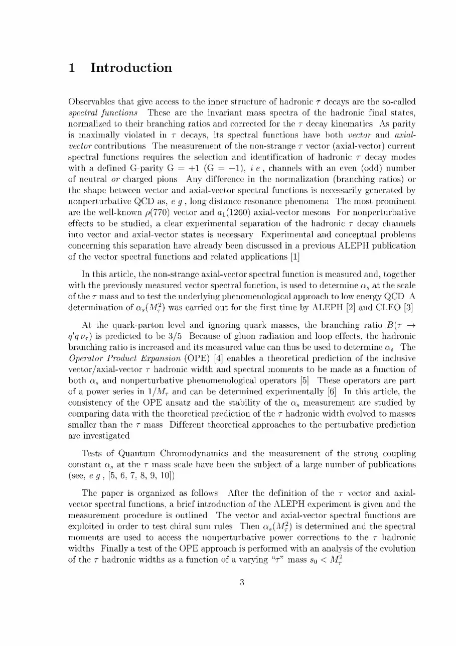
1 Introduction
Observables that give access to the inner structure of hadronic � decays are the so-called
spectral functions. These are the invariant mass spectra of the hadronic final states,
normalized to their branching ratios and corrected for the � decay kinematics. As parity
is maximally violated in � decays, its spectral functions have both vector and axial-
vector contributions. The measurement of the non-strange � vector (axial-vector) current
spectral functions requires the selection and identification of hadronic � decay modes
with a defined G-parity G = +1 (G = �1), i.e., channels with an even (odd) number
of neutral or charged pions. Any difference in the normalization (branching ratios) or
the shape between vector and axial-vector spectral functions is necessarily generated by
nonperturbative QCD as, e.g., long distance resonance phenomena. The most prominent
are the well-known �(770) vector and a1(1260) axial-vector mesons. For nonperturbative
effects to be studied, a clear experimental separation of the hadronic � decay channels
into vector and axial-vector states is necessary. Experimental and conceptual problems
concerning this separation have already been discussed in a previous ALEPH publicationof the vector spectral functions and related applications [1].
In this article, the non-strange axial-vector spectral function is measured and, together
with the previously measured vector spectral function, is used to determine �s at the scaleof the � mass and to test the underlying phenomenological approach to low energy QCD. Adetermination of �s(M
2� ) was carried out for the first time by ALEPH [2] and CLEO [3].
At the quark-parton level and ignoring quark masses, the branching ratio B(� !q0�q �� ) is predicted to be 3/5. Because of gluon radiation and loop effects, the hadronicbranching ratio is increased and its measured value can thus be used to determine �s. The
Operator Product Expansion (OPE) [4] enables a theoretical prediction of the inclusivevector/axial-vector � hadronic width and spectral moments to be made as a function of
both �s and nonperturbative phenomenological operators [5]. These operators are partof a power series in 1=M� and can be determined experimentally [6]. In this article, the
consistency of the OPE ansatz and the stability of the �s measurement are studied by
comparing data with the theoretical prediction of the � hadronic width evolved to massessmaller than the � mass. Different theoretical approaches to the perturbative prediction
are investigated.
Tests of Quantum Chromodynamics and the measurement of the strong coupling
constant �s at the � mass scale have been the subject of a large number of publications(see, e.g., [5, 6, 7, 8, 9, 10]).
The paper is organized as follows. After the definition of the � vector and axial-vector spectral functions, a brief introduction of the ALEPH experiment is given and the
measurement procedure is outlined. The vector and axial-vector spectral functions areexploited in order to test chiral sum rules. Then �s(M
2� ) is determined and the spectral
moments are used to access the nonperturbative power corrections to the � hadronic
widths. Finally a test of the OPE approach is performed with an analysis of the evolutionof the � hadronic widths as a function of a varying \�" mass s0 < M2
� .
3

2 Spectral Functions
The spectral function v1 (a1, a0), where the subscript refers to the spin J of the hadronic
system, is here defined for a non-strange vector (axial-vector) hadronic � decay channel
V � �� (A� �� ). Subsequently throughout this article the notation V=A will be used
to mean vector and axial-vector, respectively. The spectral function is obtained by
dividing the normalized invariant mass-squared distribution (1=NV=A)(dNV=A=ds) for a
given hadronic massps by the appropriate kinematic factor
v1(s)=a1(s) � M2�
6 jVudj2 SEWB(�� ! V �=A� �� )
B(�� ! e� ��e�� )
� dNV=A
NV=A ds
24 1� s
M2�
!2 1 +
2s
M2�
!35�1
; (1)
a0(s) � M2�
6 jVudj2 SEWB(�� ! �� �� )
B(�� ! e� ��e�� )
dNA
NA ds
1� s
M2�
!�2; (2)
where jVudj = 0:9752 � 0:0007 [11] denotes the CKM weak mixing matrix element andSEW = 1:0194 � 0:0040 accounts for electroweak radiative corrections [12] (see also the
discussion in Ref. [16]). Due to the conserved vector current, there is no J = 0 contributionto the vector spectral function, while the only contribution to a0 is assumed to be from thepion pole. It is connected via PCAC to the pion decay constant, a0; �(s) = 4�2f 2� �(s�m2
�).
The spectral functions are normalized by the ratio of the vector/axial-vector branchingfraction B(�� ! V �=A� �� ) to the branching fraction of the massless leptonic, i.e.,
electron, channel
B(�� ! e� ��e�� ) = (17:794� 0:045)% ; (3)
where the value includes the improvement in accuracy provided by the universalityassumption of leptonic currents together with the measurements B(�� ! e� ��e�� ) =
(17:83 � 0:08)% [11], B(�� ! �� ����� ) = (17:30 � 0:09)% [13, 14] and the � lifetime
�� = (290:0 � 1:2) fs [15]. The � mass of M� = 1776:96+0:31�0:27 MeV=c2 is taken from the
BES measurement [17].
Using unitarity and analyticity, the spectral functions of hadronic � decays are
connected to the imaginary part of the two-point correlation (or hadronic vacuumpolarization) functions [5, 8] ���
ij;U(q) � iRd4x eiqxh0jT (U�
ij(x)U�ij(0)
y)j0i = (�g��q2 +q�q�) �
(1)ij;U(q
2) +q�q� �(0)ij;U(q
2) of vector (U�ij � V �
ij = �qj �qi) or axial-vector (U
�ij � A�
ij =�qj
� 5qi) colour-singlet quark currents in corresponding quantum states and for time-
like momenta-squared q2 > 0. Lorentz decomposition is used to separate the correlation
function into its J = 1 and J = 0 parts. Thus, using the definition (1), one identifies fornon-strange quark currents
Im�(1)
�ud;V=A(s) =1
2�v1=a1(s) ; Im�
(0)�ud;A(s) =
1
2�a0(s) ; (4)
which provide the basis for comparing theory with data.
4
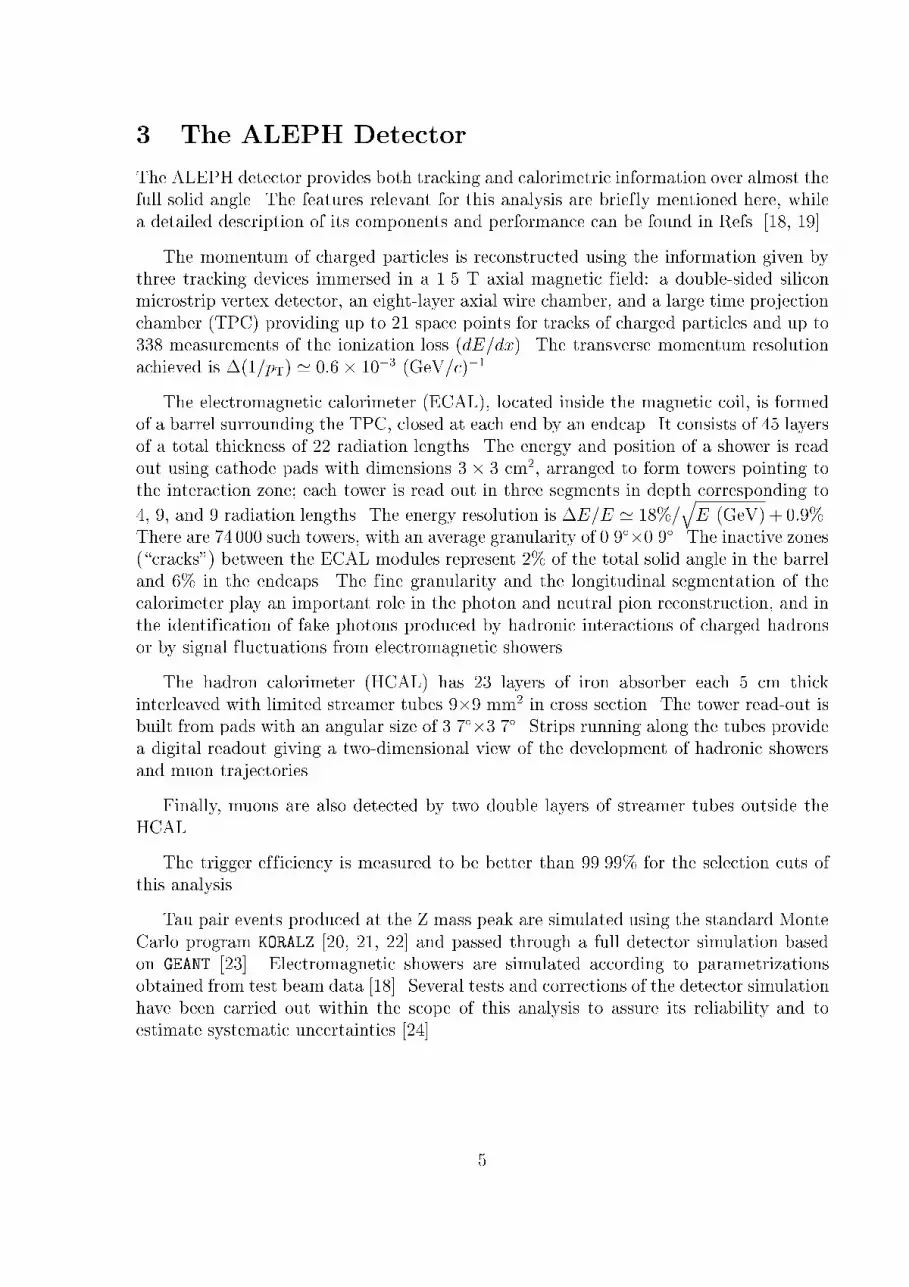
3 The ALEPH Detector
The ALEPH detector provides both tracking and calorimetric information over almost the
full solid angle. The features relevant for this analysis are briefly mentioned here, while
a detailed description of its components and performance can be found in Refs. [18, 19].
The momentum of charged particles is reconstructed using the information given by
three tracking devices immersed in a 1.5 T axial magnetic field: a double-sided silicon
microstrip vertex detector, an eight-layer axial wire chamber, and a large time projection
chamber (TPC) providing up to 21 space points for tracks of charged particles and up to
338 measurements of the ionization loss (dE/dx). The transverse momentum resolution
achieved is �(1=pT) ' 0:6� 10�3 (GeV=c)�1.
The electromagnetic calorimeter (ECAL), located inside the magnetic coil, is formed
of a barrel surrounding the TPC, closed at each end by an endcap. It consists of 45 layers
of a total thickness of 22 radiation lengths. The energy and position of a shower is read
out using cathode pads with dimensions 3� 3 cm2, arranged to form towers pointing to
the interaction zone; each tower is read out in three segments in depth corresponding to
4, 9, and 9 radiation lengths. The energy resolution is �E=E ' 18%=qE (GeV)+ 0:9%.
There are 74 000 such towers, with an average granularity of 0.9��0.9�. The inactive zones(\cracks") between the ECAL modules represent 2% of the total solid angle in the barrel
and 6% in the endcaps. The fine granularity and the longitudinal segmentation of thecalorimeter play an important role in the photon and neutral pion reconstruction, and in
the identification of fake photons produced by hadronic interactions of charged hadronsor by signal fluctuations from electromagnetic showers.
The hadron calorimeter (HCAL) has 23 layers of iron absorber each 5 cm thick
interleaved with limited streamer tubes 9�9 mm2 in cross section. The tower read-out isbuilt from pads with an angular size of 3.7��3.7�. Strips running along the tubes providea digital readout giving a two-dimensional view of the development of hadronic showers
and muon trajectories.
Finally, muons are also detected by two double layers of streamer tubes outside the
HCAL.
The trigger efficiency is measured to be better than 99.99% for the selection cuts ofthis analysis.
Tau pair events produced at the Z mass peak are simulated using the standard Monte
Carlo program KORALZ [20, 21, 22] and passed through a full detector simulation based
on GEANT [23]. Electromagnetic showers are simulated according to parametrizationsobtained from test beam data [18]. Several tests and corrections of the detector simulation
have been carried out within the scope of this analysis to assure its reliability and toestimate systematic uncertainties [24].
5

4 The Measurement Procedure
The measurement of the spectral functions defined in Eq. (1) requires the determination of
the physical invariant mass-squared distribution. The details of the analysis are reported
in [1]. In the following, a brief outline of the important steps of the measurement procedure
is given:
Tau pairs originating from Z0 decays are detected utilizing their characteristic
collinear jet signature and the low multiplicity of their decays. Using the data from
1991{1994, a total of 124 358 � pairs is selected corresponding to a detection efficiency
of (78:84 � 0:13)%. The overall non-� background contribution in the hadronic modes
amounts to (0:6�0:2)%. Details about the ALEPH � pair selection are given in [25, 13, 26].
Charged particles (electrons, muons and hadrons) are identified employing a
maximum likelihood method to combine different and essentially uncorrelated information
measured for each individual track. Discriminating variables used are the specific
ionization loss, dE=dx, the transverse and longitudinal shower profile of the energy
deposition in the ECAL, the average width of hadronic showers and the number of hits inthe HCAL and the muon chambers. The procedure and the discriminating variables usedin this analysis are described in [27, 13]. The momentum calibration of charged tracks is
performed using e+e�! �+�� events and using the invariant mass measurement of well-known, narrow resonances at low and intermediate energies. The resulting calibrationuncertainty amounts to less than 0.1%.
Photons are reconstructed by collecting associated energetic electromagneticcalorimeter (ECAL) towers, forming a cluster. To distinguish genuine photons from fakephotons a likelihood method is applied using ECAL information, e.g., the fraction of
energy in the ECAL stacks, the transverse size of the shower or the distance betweenthe barycentre of the cluster and the closest charged track. The energy calibration is
performed using electrons originating from Bhabha, � and two-photon events. A relativecalibration uncertainty of about 1.5% at low energy, 1% at intermediate energies and 0.5%
at high energy is obtained.
The �0 f inder uses a �0-mass constraint fit to attribute two reconstructed photonsto the corresponding �0 decay. At higher �0 energy, the opening angle betweenthe boosted photons tends to become smaller than the calorimeter resolution so that
the two electromagnetic showers are often merged in one cluster. The transverse
energy distribution in the ECAL nevertheless allows the computation of energy-weightedmoments providing a measure of the two-photon invariant mass. Remaining photons are
considered as originating from a �0 where the second photon has been lost.
The classification of the inclusive hadronic � decay channels is performed according
to Ref. [26] on the basis of the number of reconstructed charged and neutral pions.
The exclusive channels listed in Table 1 are obtained by subtracting the � and non-� background and the strange contribution from the inclusive measurements using the
Monte Carlo simulation. In order to extract the physical invariant mass spectra from themeasured ones they need to be unfolded from the effects of measurement distortion.
6

The unfolding method used here is based on the regularized inversion of the detector
response matrix, obtained from the Monte Carlo simulation, using the Singular Value
Decomposition technique. The regularization function applied minimizes the average
curvature of the distribution. The optimal choice of the regularization strength is found
by means of the Monte Carlo simulation where the true distribution is known. Details
about the method are published in Ref. [28].
4.1 Systematic Errors
The study of systematic errors affecting the measurement is subdivided into several
classes according to their origin, viz., the photon and �0 reconstruction, the charged
track measurement, the unfolding procedure and additional sources. Since an unfolding
procedure based upon a detector response matrix from the Monte Carlo simulation is
used, the reliability of the simulation has to be subjected to detailed studies [1, 26].
In order to check the photon reconstruction in the ECAL, the influence of calibrationand resolution uncertainties is studied as well as possible variations on the reference
distributions of a likelihood procedure used to veto fake photon candidates. The energydistribution of fake photons and the photon detection efficiency, both at threshold energies(Ethresh
= 300 MeV) and in the neighbourhood of charged tracks, are also investigated.
Similarly, the effects of momentum calibration and resolution uncertainties in thereconstruction of charged tracks are checked, accompanied by tests of the reconstruction
efficiency of highly collimated multi-prong events, and the simulation of secondary nuclearinteractions.
In addition, systematic errors introduced by the unfolding procedure are tested bycomparing known, true distributions to their corresponding unfolded ones and by varyingthe regularization conditions.
Finally, systematic errors due to the limitedMonte Carlo statistics and to uncertaintiesin the branching ratios are added.
In order to illustrate the importance of these systematic uncertainties, one may perform
an integration over the spectral functions with some given kernel, characteristic of a given
physical problem. The integration error is then obtained by Gaussian error propagationtaking into account the correlations. Using moderately s-dependent integration kernels,
the integration error is dominated by normalization uncertainties, i.e., the errors on the
contributing � branching ratios. However, the error on an integration with a strongly
s-dependent weighting kernel enhancing the low energy parts of the spectral functions
is dominated by systematics (mainly due to the fake photon rejection and the photonefficiency correction at threshold), while the central energy region (0.6 { 1.4 GeV2=c4) isstatistically limited. When enhancing the higher part of the spectrum, the integration
error is equally dominated by uncertainties due to the unfolding process, and by limiteddata and Monte Carlo statistics.
7

4.2 Invariant Mass Spectra and Spectral Functions
The above measurement procedure provides the physical invariant mass spectra of the
measured � decay modes including their bin-to-bin covariance matrices obtained, after
the unfolding of the spectra, from the statistical errors and the study of systematic
uncertainties.
Vector BR (in %) Axial-Vector BR (in %)
���0 �� 25.34� 0.19 �� �� 11.23� 0.16
��3�0 �� 1.18� 0.14 ��2�0 �� 9.23� 0.172���+�0 �� 2.42� 0.09 2���+ �� 9.15� 0.15
��5�0 �� ��4�0 �� 0.03� 0.03(1)
2���+3�0 ��
)0.04 � 0.02(1) 2���+2�0 �� 0.10� 0.02
3��2�+�0 �� 3��2�+ �� 0.07� 0.01
! �� ��(2) 1.93� 0.10 ! ���0 ��
(2) 0.39� 0.11
� ���0 ��(3) 0.17� 0.03 � 2���+ �� 0.04� 0.01
{ { � ��2�0 �� 0.02� 0.01
K�K0 �� 0.19� 0.04 { {
K�K+�� �� 0.08� 0.08 K�K+�� �� 0.08� 0.08
K0 �K0�� �� 0.08� 0.08(1) K0 �K0�� �� 0.08� 0.08
K�K0�0 �� 0.05� 0.05 KK0�0 �� 0.05� 0.05
K�K�� �� 0.08� 0.08(1) K�K�� �� 0.08� 0.08(1)
Total Vector 31.58� 0.29 Total Axial-Vector 30.56� 0.30
1 The branching ratio is obtained using constraints from isospin symmetry (seetext and [1]).2 Through ! ! ���+�0, 88.8% of this channel is reconstructed in 2���+�0 ��and 2���+2�0 �� , respectively.3 Through � ! 2 , 39.3% of this channel is reconstructed in ��3�0 �� .
Table 1: Vector and axial-vector hadronic � decay modes with their contributing branching
fractions. The branching ratios shown are re�tted so that the compilation of all � decay
channels sums up to one. Further information about the branching ratios involving kaons
used is given in the Appendix.
The exclusive vector and axial-vector � decay channels are listed in Table 1. Unless
otherwise specified, their branching ratios are taken from ALEPH publications [26, 29]
applying small corrections taking into account new ALEPH results on branching fractionsof � decay modes involving kaons [30]: the latter are listed in the Appendix. In some cases,
additional information is taken from the Particle Data Group [11] as described in Ref. [1].The individual fractions have been refitted so that the sum of all hadronic and leptonic
branching ratios adds up to 100%, where the latter are derived from Eq. (3) assuming
universality of the lepton couplings. This normalization slightly modifies the values givenin the above references. The branching ratios of the subsequent meson decays are taken
from [11]. The two-, four- and, in part, the six-pion modes are exclusively reconstructed.Special care is taken with isospin-violating ! and � decays, and with kaon pair production.
8

τ– → (V–, I=1) ντparton model prediction
perturbative QCD (massless)
ππ0
π3π0, 3ππ0, 6π
ωπ (corr.), ηππ0 (corr.), KK0 (MC)
KK-bar π (MC)
KK-bar ππ (MC)
Mass2 (GeV/c2)2
υ1 ALEPH
0
0.5
1
1.5
2
2.5
0 0.5 1 1.5 2 2.5 3 3.5
Figure 1: Total vector spectral function. The shaded areas indicate the contributions from
the exclusive � vector channels, where the shapes of the contributions labeled \MC" are
taken from the Monte Carlo simulation. The lines show the predictions from the naive
parton model and from massless perturbative QCD using �s(M2Z) = 0:120.
4.3 The Total Vector Spectral Function
The complete inclusive � vector spectral function and its contributions are shown inFig. 1. The dashed line depicts the naive parton model prediction while the massless
QCD prediction [37] using �s(M2Z) = 0:120 (solid line) lies roughly 14% higher at M2
� .One observes that at s � M2
� the inclusive � vector spectral function is larger than the
QCD prediction, i.e., the asymptotic region is not reached.
The two- and four-pion final states are measured exclusively, while the six-pion state is
only partly measured. The total six-pion branching ratio has been determined in [1] usingisospin symmetry. However, one has to account for the fact that the six-pion channel is
contaminated by isospin-violating ��! � 2���+, � ��2�0 �� decays. These were reported
for the first time by the CLEO Collaboration [31].
The small fraction of the ! �� �� decay channel that is not reconstructed in the four-
9

pion final state is added using the simulation. Similarly, one corrects for � ���0 �� decay
modes other than � ! 2 which is classified in the h�3�0 �� final state, since the two
photon mass is inconsistent with the �0 mass so that each photon is reconstructed as a
�0.
The K�K0 �� mass distribution is taken entirely from the simulation. The K�K� modes
are conservatively assumed to be (50� 50)% vector and axial-vector. The corresponding
spectral functions are obtained from the Monte Carlo simulation. This is further discussed
in Ref. [1]. Taking both vector and axial-vector parts as (50 � 50)%, the vector part of
the total K�K�� branching ratio is estimated to be (0:08� 0:08)%.
The invariant mass spectra of the small contributions labeled \MC" in Figs. 1 and 5 are
taken from the Monte Carlo simulation accompanied by a channel-dependent systematic
error of up to 50% of the bin entry.
4.4 Axial-Vector Spectral Functions
Exclusively measured axial-vector modes are the three-pion final states, occurring in
both 2���+ �� and ��2�0 �� , and the five-pion modes 3��2�+ �� and 2���+2�0 �� . Thecorresponding invariant mass-squared spectra before unfolding are depicted for data andMonte Carlo simulation in Figs. 2 and 3. The small shoulder seen in the measured
2���+ �� spectrum around 0:3 GeV2 mass-squared (upper plot in Fig. 2) stems fromdecays where only two tracks are reconstructed and the invariant mass as a result is
underestimated. Due to incomplete ECAL energy collection, the measured ��2�0 ��distribution is slightly shifted to lower masses. These features are well reproduced bythe detector simulation.
For both three-pion decay modes, the � decay library TAUOLA1.5 is used as physicsinput for the detector simulation. It employs the K�uhn-Santamaria parametrization [38]based on a dominant large a�1 (1260) resonance, �a1(1260) = 0:4 GeV=c2, which decays
into ��(770)�0 ! ��2�0 or �0(770)�� ! 2���+ with interference between the two�� combinations. Scalar contributions to the three pion decay, e.g., �(1300) ! ��,
suppressed by the PCAC theorem and by angular momentum considerations, are neglectedin this model. However, the measurement of the spectral functions and in particular theunfolding procedure is essentially independent of the physics input into the simulation.
Figure 4 shows the unfolded 2���+ �� and ��2�0 �� mass spectra with reasonable
agreement in form and normalization (�2 = 41:4 per 59 degrees of freedom). In thefollowing both channels are assumed to have identical spectra so that it is appropriate
to use the weighted average of the distributions for the inclusive axial-vector spectralfunction2.
2The weighted average is calculated between two intrinsically correlated distributions. The averageddistribution k with bin entries ki; i = 1; : : : ; Nbin is defined to minimize �2 = (x(��+) �
k)C�1(��+)
(x(��+)�k)+(x(�00)�k)C�1(�00)
(x(�00)�k) ; where the indices denote the charges of the � final
states, x are the mass-squared distributions and C�1 the corresponding inverted covariance matrices. Theweighted average is then the solution of the system of linear equations x(��+)C
�1
(��+)+ x(�00)C
�1
(�00)=
k(C�1(��+)
+ C�1(�00)
) , and the covariance matrix of the average satisfies C�1k = C�1(��+)
+ C�1(�00)
.
10

DataMCMC –τ backgr.
τ– → 2π–π+ ντ
Eve
nts / 0.
05 (
GeV
/c2 )2
τ– → π–2π0 ντ
Mass2 (GeV/c2)2
ALEPH
0
200
400
600
800
1000
1200
0
200
400
600
800
1000
1200
0 0.5 1 1.5 2 2.5 3 3.5
1
10
10 2
1.5 2 2.5 3
1
10
10 2
1.5 2 2.5 3
Figure 2: Invariant mass-squared distributions of the decays ��! 2���+ �� and ��!��2�0 �� .
4.4.1 The inclusive � axial-vector spectral function
In complete analogy to the vector spectral function the inclusive axial-vector spectral
function is obtained by summing up the exclusive axial-vector spectral functions with the
addition of small unmeasured modes taken from the Monte Carlo simulation. The rightcolumn of Table 1 gives a compilation of the exclusive axial-vector branching ratios used:
{ The five-pion spectral functions are only measured in the 2���+2�0 �� and
3��2�+ �� final states. Using Pais' isospin classes [39], the branching fractionof ��4�0 �� can be bounded entirely using the 3��2�+ �� branching fraction:
B��4�0 � 3=4 � B5�� = 0:054%. Half of this upper limit is taken with an error
of 100%.
{ As in the vector case, the small fraction of the ! ���0 �� decay channel that is notaccounted for in the 2���+2�0 �� final state is added from the simulation.
11

τ– → 3π– 2π+ ντ ALEPH
Mass2 (GeV/c2)2
Eve
nts / 0.
1 (G
eV/c2 )2
τ– → 2π– π+ 2π0 ντ ALEPH
Mass2 (GeV/c2)2
Eve
nts / 0.
1 (G
eV/c2 )2
0
5
10
15
20
0 1 2 30
50
100
150
200
0 1 2 3
Figure 3: Invariant mass-squared distributions of the decays �� ! 3��2�+ �� and
�� ! 2���+2�0 �� . The points are the ALEPH data, the histograms represent the
simulation and the hatched areas are the expected � background distributions according
to the simulation.
{ Also considered are the axial-vector � (3�)� �� final states [31]. CLEO observed that
the dominant part of it issues from the ��! f1(1285)�� intermediate state, with
B(��! f1�� �� ) = (0:068� 0:030)%, measured in the f1 ! � �+�� and f1 ! � �0�0
decay modes [31]. Since the f1 meson is isoscalar, the branching ratios relate as
B(�� ! � 2���+ �� ) = 2 � B(�� ! � ��2�0 �� ). The distributions are takenfrom the ordinary six-pion phase space simulation accompanied by large systematicerrors.
{ The K�K� and K�K�� final states contribute with (50� 50)% to the inclusive axial-
vector spectral function, with full anticorrelation to the inclusive vector spectral
function. Both invariant mass distributions are taken from the simulation.
The total inclusive axial-vector spectral function is plotted in Fig. 5 together with the
naive parton model and the massless, perturbative QCD prediction. One observes that
the asymptotic region is apparently not reached at the � mass scale.
4.5 The (v1 � a1) Spectral Functions
For the total (v1 + a1) hadronic spectral function one does not have to distinguish the
current properties of the non-strange hadronic � decay channels. Hence the mixture of allcontributing non-strange final states is measured inclusively using the following procedure.
The two- and three-pion final states dominate and their exclusive measurements areadded with proper accounting for the correlations. The remaining contributing topologies
12

τ– → π–π+π– ντ
τ– → π– 2π0 ντ
Weighted average
Mass2 (GeV/c2)2
(1/N
) dN
/ 0.05
(G
eV/c2 )2
ALEPH
0
0.01
0.02
0.03
0.04
0.05
0.06
0 0.5 1 1.5 2 2.5 3 3.5
Figure 4: Unfolded (physical) invariant mass-squared spectra of the � �nal states 2���+ ��and ��2�0 �� and their weighted average.
τ– → (A–, I=1) ντ
parton model prediction
perturbative QCD (massless)
π2π0, 3π
π4π0, 3π2π0, 5π
KK-bar π (MC)
KK-bar ππ (MC)
Mass2 (GeV/c2)2
a1 ALEPH
0
0.2
0.4
0.6
0.8
1
1.2
0 0.5 1 1.5 2 2.5 3 3.5
Figure 5: Total inclusive � axial-vector current spectral function (without the pion pole).
The lines show the prediction from the naive parton model and from massless perturbative
QCD using �s(M2Z) = 0:120.
13

τ– → (V,A, I=1) ντparton model prediction
perturbative QCD (massless)
Mass2 (GeV/c2)2
υ1 + a1 ALEPH
0
0.5
1
1.5
2
2.5
0 0.5 1 1.5 2 2.5 3 3.5
Figure 6: Inclusively measured vector plus axial-vector (v1 + a1) spectral function and
predictions from the parton model and from massless perturbative QCD using �s(M2Z) =
0:120.
are treated inclusively, i.e., without separation of the vector and axial-vector decay modes.
This reduces the statistical uncertainty. The effect of the feedthrough between � final
states on the invariant mass spectrum is described by the Monte Carlo simulation and
thus corrected in the data unfolding. In this procedure the simulated mass distributions
are iteratively corrected using the exclusive vector/axial-vector unfolded mass spectra.
Another advantage of the inclusive (v1 + a1) measurement is that one does not have toseparate the vector/axial-vector currents of the K�K� and K�K�� modes. The (v1 + a1)
spectral function is depicted in Fig. 6. The improvement in precision in comparison to an
exclusive sum of Fig. 1 and Fig. 5 is obvious at higher mass-squared. One clearly sees the
oscillating behaviour of the spectral function but, unlike the vector/axial-vector spectral
functions, this does approximately reach the asymptotic limit predicted by perturbativeQCD at s!M2
� .
In the case of the (v1� a1) spectral function, uncertainties on the V=A separation are
reinforced due to their complete anticorrelation. In addition, anticorrelations given in
14

τ– → (V,A, I=1) ντ
parton model/perturbative QCD
Mass2 (GeV/c2)2
υ1 – a1 ALEPH
-1
-0.5
0
0.5
1
1.5
2
2.5
0 0.5 1 1.5 2 2.5 3 3.5
Figure 7: Inclusively measured vector minus axial-vector (v1 � a1) spectral function. In
the parton model as well as in perturbative QCD vector and axial-vector contributions are
degenerate.
Ref. [26] between � final states with adjacent numbers of pions increase the errors. The
(v1 � a1) spectral function is shown in Fig. 7. The oscillating behaviour of the respective
v1 and a1 spectral functions is emphasized and the asymptotic behaviour is clearly not
attained at M2� .
5 Chiral Sum Rules
The application of chiral symmetry leads to low energy sum rules involving the difference
of vector and axial-vector spectral functions by virtue of the optical theorem. These sum
rules are dispersion relations between real and absorptive parts of a two-point correlation
function that transforms symmetrically under SU(2)L�SU(2)R in the case of non-strange
15

currents. Corresponding integrals are:
1
4�2
s0!1Z0
ds1
s[v1(s)� a1(s)] = f 2�
hr2�i3� FA ; (5)
1
4�2
s0!1Z0
ds [v1(s)� a1(s)] = f 2� ; (6)
1
4�2
s0!1Z0
ds s [v1(s)� a1(s)] = 0 ; (7)
1
4�2
s0!1Z0
ds s lns
�2[v1(s)� a1(s)] = �4�f 2�
3�(m2
�� �m2�0) : (8)
Equation (5) is known as the Das-Mathur-Okubo (DMO) sum rule [32]. It relates the
given integral to the square of the pion decay constant f� = (92:4 � 0:3) MeV [11]obtained from the decays �� ! ����� and �� ! ����� , to the pion axial-vector form
factor FA for radiative decays �� ! `���` , and to the pion charge radius-squaredhr2�i = (0:439 � 0:008) fm2 obtained from a one parameter fit to space-like data [33].Eqs. (6) and (7) are the first and the second Weinberg sum rules (WSR) [34]. When
switching quark masses on, only the first WSR remains valid while the second WSR breaksdown due to contributions from the difference of non-conserved vector and axial-vectorcurrents of order m2
q=s, leading to a quadratic divergence of the integral. Equation (8)
represents the electromagnetic splitting of the pion masses [35]. Although apparentlycontaining an arbitrary renormalization scale �, the sum rule is actually independent of
� by virtue of the second WSR (7). Only for s0 values for which Eq. (7) has not reached
convergence does Eq. (8) maintains its � dependence.
The above integrals are calculated with variable upper integration bounds s0 � M2�
using the spectral functions and their respective covariance matrices in order to provide
a straightforward gaussian error propagation taking into account the strong bin-to-bin
correlations of the spectral functions. Also considered are the anticorrelations between v1and a1;0 due to the estimates of the vector/axial-vector parts of the final states K�K� andK�K�� and the � hadronic branching ratios.
The sum rules (5){(8) versus the upper integration bound s0 � M2� are plotted
in Figs. 8a{d. The horizontal band depicts the corresponding chiral predictions of theintegrals taken from Ref. [36]. One observes that only for the DMO sum rule (Fig. 8a), for
which contributions from higher mass-squares are suppressed, does the saturation withinthe one sigma error seem to occur at the � mass scale. The other sum rules (Fig. 8b{c)
are apparently not saturated at M2� (non-zero slope) as indicated by the non-vanishing
(v1 � a1) spectral function at the end of the � phase space (Fig. 7) and its oscillatorybehaviour. More quantitative studies of the sum rules can be found in Ref. [24].
16

(υ1 – a1)
chiral prediction
(a)
s0 (GeV2)
I(s 0)
0
0.01
0.02
0.03
0.04
0.05
0.06
0 0.5 1 1.5 2 2.5 3
(υ1 – a1)
chiral prediction
(b)
s0 (GeV2)
I(s 0)
(G
eV2 )
-0.005
0
0.005
0.01
0.015
0.02
0.025
0.03
0 0.5 1 1.5 2 2.5 3
(υ1 – a1)
chiral prediction
(c)
s0 (GeV2)
I(s 0)
(G
eV4 )
-0.015
-0.01
-0.005
0
0.005
0.01
0.015
0.02
0.025
0.03
0 0.5 1 1.5 2 2.5 3
(υ1 – a1), λ=150 MeV
chiral prediction
(d)
λ=250 MeV
s0 (GeV2)
I(s 0)
(G
eV4 )
-0.06
-0.04
-0.02
0
0.02
0.04
0.06
0.08
0.1
0.12
0 0.5 1 1.5 2 2.5 3
Figure 8: Sum rules corresponding to Eqs. (5){(8) (plots: a{d) versus the upper integrationbound s0.
6 The Measurement of �s(M2�)
The measurement of �s(M2� ) presented in this section adopts a method based on
a simultaneous fit of QCD parametrizations with perturbative and nonperturbativecomponents to the ratio R� defined as
R� =�(�� ! hadrons� �� )
�(�� ! e� ��e�� ); (9)
and to the spectral moments defined below (Section 6.4). It was proposed by F. Le
Diberder and A. Pich [6] and has been employed in previous analyses by the ALEPH [2]and CLEO [3] Collaborations.
6.1 Theoretical Prediction for R�
According to Eq. (4) the imaginary parts of the vector and axial-vector two-point
correlation functions �(J)
�ud;V=A(s), with the spin J of the hadronic system, are proportional
17

to the � hadronic spectral functions with corresponding quantum numbers. The non-
strange ratio R� can be written as an integral of these spectral functions over the invariant
mass-squared s of the final state hadrons [5]:
R� (s0) = 12�SEW
s0Z0
ds
s0
�1� s
s0
�2 ��1 + 2
s
s0
�Im�(1)(s+ i�) + Im�(0)(s+ i�)
�; (10)
where �(J) can be decomposed as �(J) = jVudj2��(J)ud;V +�
(J)ud;A
�. The correlation function
�(J) is analytic in the complex s plane everywhere except on the positive real axis where
singularities exist. Hence by Cauchy's theorem, the imaginary part of �(J) is proportional
to the discontinuity across the positive real axis.
The energy scale s0 for s0 = M2� is large enough that contributions from
nonperturbative effects be small. It is therefore assumed that one can use the Operator
Product Expansion (OPE) to organize perturbative and nonperturbative contributions
to R� (s0). The factor (1 � s=s0)2 suppresses the contribution from the region near the
positive real axis where �(J)(s) has a branch cut and OPE validity is restricted [40].
The theoretical prediction of the vector and axial-vector ratio R�;V=A can thus be
written as:
R�;V=A =3
2jVudj2SEW
0@1 + �(0) + �0EW + �
(2�mass)
ud;V=A +X
D=4;6;:::
�(D)
ud;V=A
1A ; (11)
with the residual non-logarithmic electroweak correction �0EW = 0:0010 [41], neglected in
the following, and the dimension D = 2 contribution �(2�mass)
ud;V=A from quark masses which
is lower than 0:1% for u; d quarks. The term �(0) is the purely perturbative contribution,while the �(D) are the OPE terms in powers of s
�D=20 :
�(D)
ud;V=A =X
dimO=D
Cud;V=A(s; �)hOud(�)iV=A(�s0)D=2
; (12)
where the parameter � separates the long-distance nonperturbative effects, absorbed intothe vacuum expectation elements hOud(�)i, from the short-distance effects which are
included in the Wilson coefficients Cud;V=A(s; �) [42].
6.2 Perturbative Prediction
The perturbative prediction adopted in this analysis follows in detail Ref. [7]. Theperturbative contribution is given in the chiral limit. Effects from quark masses havebeen calculated in Ref. [43] and are found to be well below 1% for the light quarks. Thus
the contributions from vector and axial-vector currents coincide to any given order of
perturbation theory and the results are flavour independent.
The perturbative contribution in Eq. (11) is then given by [7]
1 + �(0) =3X
n=0
KnA(n)(�s) ; (13)
18

with K0 = K1 = 1, K2 = 1:63982 and K3 = 6:37101 for three active flavours in the MS
scheme [37]. The coefficients Kn are known up to three-loop order �3s and for n � 2 they
depend on the renormalization scheme employed. The functions A(n)(�s) in Eq. (13) are
the contour integrals
A(n)(�s) =1
2�i
Ijsj=s0
ds
s
"1� 2
s
s0+ 2
�s
s0
�3��s
s0
�4# �s(�s)�
!n; (14)
where the contour runs counter clockwise around the circle from s0 + i� to s0 � i�. The
strong coupling constant in the vicinity of s0 can be expanded in powers of �s(s0), with
coefficients that are polynomials in ln(s=s0) [5]. The perturbative prediction becomes
then a function of the Kn coefficients and elementary integrals. Up to fourth order the
fixed-order perturbation theory (FOPT) expansion reads
1 + �(0)E = 1 +
�s(s0)
�+ 5:2023
�s(s0)
�
!2+ 26:366
�s(s0)
�
!3
+(K4 + 78:00)
�s(s0)
�
!4; (15)
with the unknown K4 coefficient.
Another approach to the solution of the contour integral (14) is to perform a directnumerical evaluation using the solution of the renormalization group equation (RGE) to
four-loops [44] as input for the running �s(�s) [7]. It provides a resummation of all knownhigher order logarithmic integrals and improves the convergence of the perturbative series.
While, for instance, the third order term in the expansion (15) contributes with 17% tothe total (truncated) perturbative prediction, the corresponding term of the numericalsolution amounts only to 6:6% (assuming �s(M
2� ) = 0:35). This numerical solution of
Eq. (13) will be referred as contour-improved fixed-order perturbation theory (FOPTCI)in the following.
Despite a number of arguments expressed in Ref. [7], the intrinsic ambiguity between
FOPT and FOPTCI is unresolvable at present. This is due to the truncation of theperturbative approximation of �(0) at finite order in �s. A conservative measure of thisambiguity is obtained from the deviation in R� found when cutting all additional orders
in �s (which is FOPT) and keeping them (FOPTCI), respectively. Both methods are
likewise considered in this analysis.
6.3 Nonperturbative Contributions
Following SVZ [4], the first contribution to R� (s0) beyond the D = 0 perturbative
expansion is the non-dynamical quark mass correction of dimension D = 2, i.e.,
corrections in powers of 1=s0. They have been calculated up to next-to-leading order�s [45].
The dimension D = 4 operators have dynamical contributions from the gluon
condensate h(�s=�)GGi and quark condensates muh0j�uuj0i, mdh0j �ddj0i of the light u; d
19
quarks. Remaining D = 4 operators are the running quark masses to the fourth power.
The contribution of the gluon condensate to R�;V=A vanishes in first order �s(s0). However,
there appear second order terms in the Wilson coefficients due to the logarithmic s
dependence of �s(s) which after performing the integral (10) becomes �2s(s0).
The contributions from dimension D = 6 operators are rather complex. The large
number of independent operators of the four-quark type occurring can be reduced by
means of the vacuum saturation approximation [4, 5] to leading order �s. The operators
are then expressed as products of scale dependent two-quark condensates of the type
�s(�)h�qiqi(�)ih�qjqj(�)i. Since the vacuum saturation approximation is a simplifying
assumption, possible deviations are accounted for by introducing an effective scale
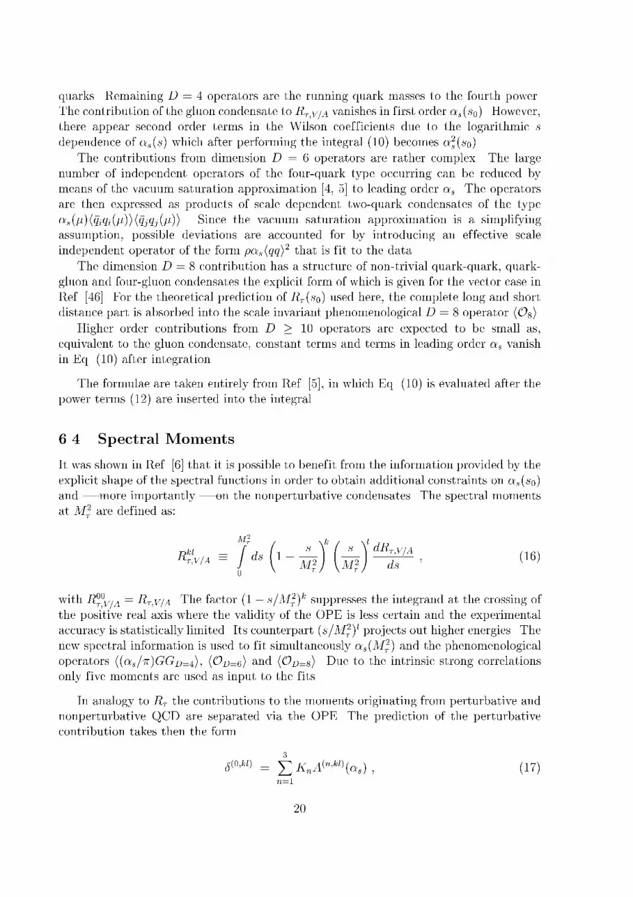
independent operator of the form ��sh�qqi2 that is fit to the data.The dimension D = 8 contribution has a structure of non-trivial quark-quark, quark-
gluon and four-gluon condensates the explicit form of which is given for the vector case in
Ref. [46]. For the theoretical prediction of R� (s0) used here, the complete long and short
distance part is absorbed into the scale invariant phenomenological D = 8 operator hO8i.Higher order contributions from D � 10 operators are expected to be small as,
equivalent to the gluon condensate, constant terms and terms in leading order �s vanish
in Eq. (10) after integration.
The formulae are taken entirely from Ref. [5], in which Eq. (10) is evaluated after thepower terms (12) are inserted into the integral.
6.4 Spectral Moments
It was shown in Ref. [6] that it is possible to benefit from the information provided by the
explicit shape of the spectral functions in order to obtain additional constraints on �s(s0)and | more importantly | on the nonperturbative condensates. The spectral momentsat M2
� are defined as:
Rkl�;V=A �
M2�Z
0
ds
1� s
M2�
!k s
M2�
!ldR�;V=A
ds; (16)
with R00�;V=A = R�;V=A. The factor (1� s=M2
� )k suppresses the integrand at the crossing of
the positive real axis where the validity of the OPE is less certain and the experimental
accuracy is statistically limited. Its counterpart (s=M2� )
l projects out higher energies. The
new spectral information is used to fit simultaneously �s(M2� ) and the phenomenological
operators h(�s=�)GGD=4i, hOD=6i and hOD=8i. Due to the intrinsic strong correlationsonly five moments are used as input to the fits.
In analogy to R� the contributions to the moments originating from perturbative andnonperturbative QCD are separated via the OPE. The prediction of the perturbative
contribution takes then the form
�(0;kl) =3X
n=1
KnA(n;kl)(�s) ; (17)
20

with contour integrals A(n;kl)(�s) [6] that are expanded up to �3s(s) (FOPT) or numerically
resolved for the running �s(�s) obtained from the RGE (FOPTCI).
In the chiral limit and neglecting the logarithmic s dependence of the Wilson
coefficients, the dimension D = 2; 4; 6; 8 nonperturbative contributions to the moments
read
�(D;kl)
ud;V=A = 8�2
0BBBBBB@
(D = 2) (D = 4) (D = 6) (D = 8) (k; l)1 0 �3 �2 (0; 0)1 1 �3 �5 (1; 0)0 �1 �1 3 (1; 1)0 0 1 1 (1; 2)0 0 0 �1 (1; 3)
1CCCCCCA
XdimO=D
C(�)hO(�)iMD
�
; (18)
where the matrix is defined by the choice of the coefficients for the moments k = 1,
l = 0; 1; 2; 3. It can be seen that with increasing weight l the low dimension operators
give no contributions.
For practical purpose it is more convenient to define moments that are normalized to
the corresponding R�;V=A in order to decouple the normalization from the shape of the �
spectral functions:
Dkl�;V=A �
Rkl�;V=A
R�;V=A
=
M2�Z
0
ds
1� s
M2�
!k s
M2�
!l1
NV=A
dNV=A
ds: (19)
There now exist two sets of experimentally almost uncorrelated observables | R�;V=A
and spectral moments | which provide independent constraints on �s(M2� ) and thus an
important test of consistency.
6.5 Measurement of R� and the Moments
The ratio of non-strange hadronic width and electronic branching ratio is calculated fromthe difference of the ratio of the total hadronic width and electronic branching ratio,
R� =1�B(�� ! e� ��e�� )� B(�� ! �� ����� )
B(�� ! e� ��e�� )=
1
B(�� ! e� ��e�� )� 1:9726
= 3:647� 0:014 ; (20)
obtained from the world average value (3), and the strange width ratio,
R�;S = 0:155� 0:008 ; (21)
taken from Ref. [47], yielding the result
R�;V+A = 3:492 � 0:016 : (22)
There is no advantage in including R�;S (or equivalently using R� ) in this analysis, because
the strange quark sector introduces another parameter, the strange quark mass, which
the additional data is used to fit [48]. Computing the ratio of the inclusive vector and
21
k=1,l=3
k=1,l=2
k=1,l=1 k=1,l=0
k=0,l=0
Mass2 (GeV/c2)2
Mom
ents / 0.
05 (
GeV
/c2)2
ALEPH
10-6
10-5
10-4
10-3
10-2
10-1
0 0.5 1 1.5 2 2.5 3 3.5
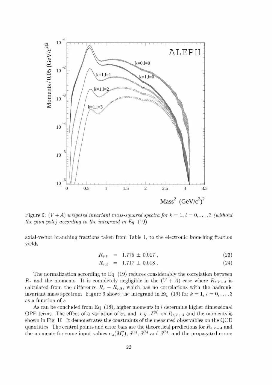
Figure 9: (V +A) weighted invariant mass-squared spectra for k = 1; l = 0; : : : ; 3 (without
the pion pole) according to the integrand in Eq. (19).
axial-vector branching fractions taken from Table 1, to the electronic branching fractionyields
R�;V = 1:775 � 0:017 ; (23)
R�;A = 1:717 � 0:018 : (24)
The normalization according to Eq. (19) reduces considerably the correlation between
R� and the moments. It is completely negligible in the (V + A) case where R�;V+A iscalculated from the difference R� � R�;S, which has no correlations with the hadronic
invariant mass spectrum. Figure 9 shows the integrand in Eq. (19) for k = 1; l = 0; : : : ; 3
as a function of s.
As can be concluded from Eq. (18), higher moments in l determine higher dimensional
OPE terms. The effect of a variation of �s and, e.g., �(8) on R�;V+A and the moments is
shown in Fig. 10. It demonstrates the constraints of the measured observables on the QCD
quantities. The central points and error bars are the theoretical predictions for R�;V+A and
the moments for some input values �s(M2� ), �
(4), �(6) and �(8), and the propagated errors
22
Rτ,V+A
3.4 3.45 3.5 3.55 3.6
D10,V+A
0.71 0.72 0.73
D11,V+A
0.15 0.155 0.16 0.165
D12,V+A
0.057 0.058 0.059 0.06
D13,V+A
0.025 0.026 0.027
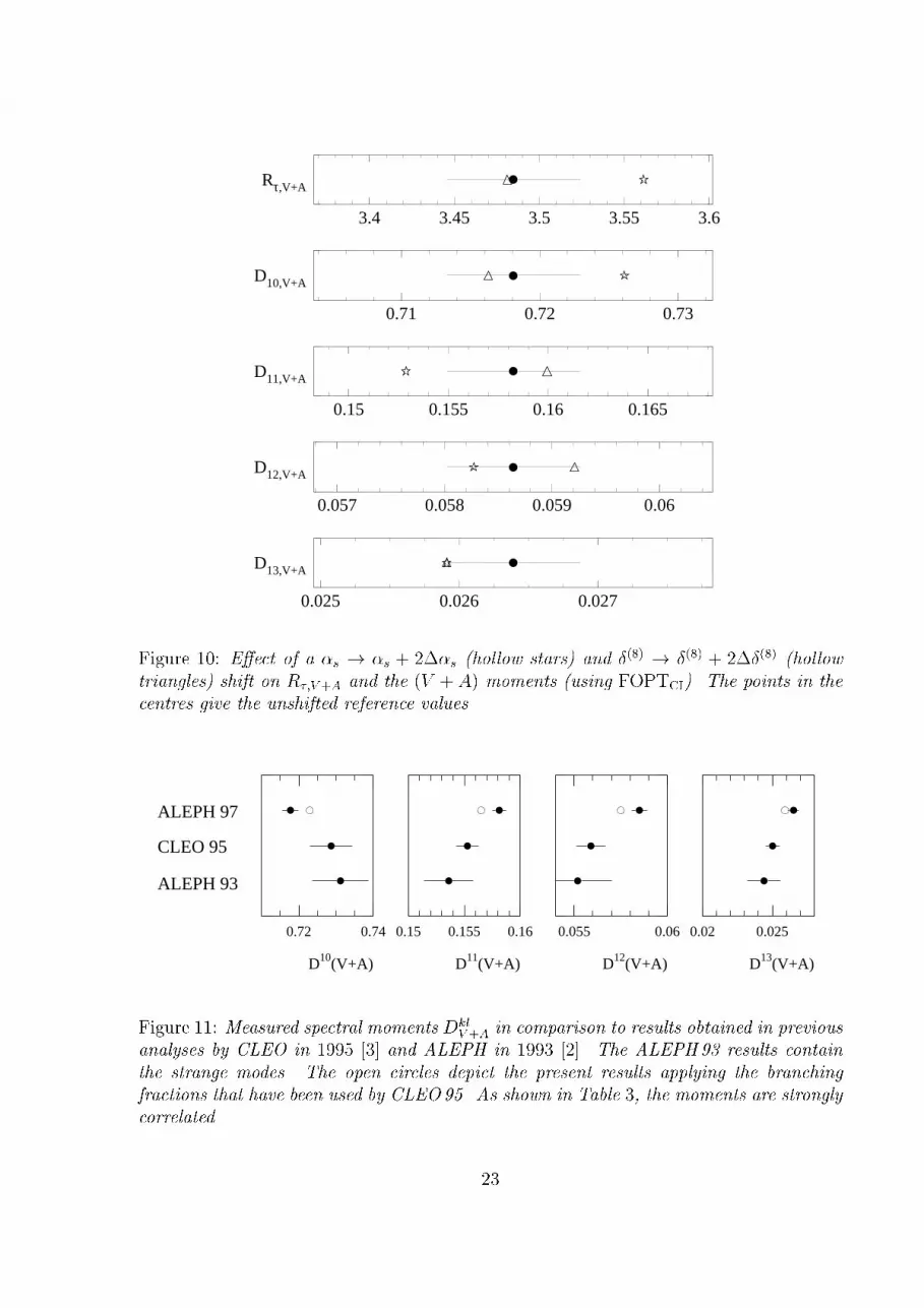
Figure 10: E�ect of a �s ! �s + 2��s (hollow stars) and �(8) ! �(8) + 2��(8) (hollow
triangles) shift on R�;V+A and the (V + A) moments (using FOPTCI). The points in the
centres give the unshifted reference values.
D10(V+A) D11(V+A) D12(V+A) D13(V+A)
ALEPH 97
CLEO 95
ALEPH 93
0.72 0.74 0.15 0.155 0.16 0.055 0.06 0.02 0.025
Figure 11: Measured spectral moments DklV+A in comparison to results obtained in previous
analyses by CLEO in 1995 [3] and ALEPH in 1993 [2]. The ALEPH93 results contain
the strange modes. The open circles depict the present results applying the branching
fractions that have been used by CLEO95. As shown in Table 3, the moments are stronglycorrelated.
23

ALEPH l = 0 l = 1 l = 2 l = 3
D1lV 0.7173 0.1687 0.0529 0.0225
�expD1lV 0.0035 0.0006 0.0007 0.0006
D1lA 0.7180 0.1472 0.0642 0.0306
�expD1lA 0.0040 0.0012 0.0007 0.0005
D1lV+A 0.7177 0.1581 0.0585 0.0265
�expD1lV+A 0.0022 0.0006 0.0004 0.0004
Table 2: Spectral Moments of vector (V ), axial-vector (A) and vector plus axial-vector
(V +A) inclusive � decays. The errors give the total experimental uncertainties including
statistical and systematic e�ects.
ALEPH D10�;V D11
�;V D12�;V D13
�;V
R�;V �0:56 0:33 0:58 0:56D10
�;V 1 �0:21 �0:87 �0:95D11
�;V { 1 0.63 0.39
D12�;V { { 1 0.96
D13�;V { { { 1
ALEPH D10�;A D11
�;A D12�;A D13
�;A
R�;A �0:52 0:24 0:48 0:56D10
�;A 1 �0:41 �0:81 �0:96D11
�;A { 1 0.83 0.51
D12�;A { { 1 0.90
D13�;A { { { 1
ALEPH D10�;V+A D11
�;V+A D12�;V+A D13
�;V+A
D10�;V+A 1 �0:30 �0:86 �0:96
D11�;V+A { 1 0.65 0.28
D12�;V+A { { 1 0.91
D13�;V+A { { { 1
Table 3: Experimental correlations between the moments Dkl�;V=A=V+A. There are no
correlations between R�;V+A and the corresponding moments.
of one standard deviation (�). The stars depict the shift when changing �s ! �s+2��s,
while the triangles show what happens when shifting �(8) ! �(8) + 2��(8). One observes
that �s(M2� ) is primarily determined from R�;V+A and the first moments D10
V+A, D11V+A.
On the other hand, D12V+A and D13
V+A constrain the high dimensional nonperturbativepower terms, while their effect on �s(M
2� ) is weak.
The measured values of the moments for V , A and the (V +A) spectral functions are
given in Table 2 and their correlation matrices in Table 3. The correlations between the
moments are computed analytically from the contraction of the derivatives of two involvedmoments with the covariance matrices of the respective normalized invariant mass-squaredspectra. In all cases, the negative sign between the k = 1; l = 0 and the k = 1; l � 1
moments is understood to be due to the � and the �, a1 peaks which determine the major
part of the k = 1; l = 0 moments. They are much less important for higher moments
24

Error source D10�;V+A D11
�;V+A D12�;V+A D13
�;V+A
Statistical error 0.10 0.12 0.18 0.35
Fake photons 0.08 0.09 0.10 0.21
ECAL energy calibration 0.03 0.06 0.08 0.20
ECAL energy resolution 0.07 0.08 0.17 0.35
Photon and �0 reconstruction 0.10 0.09 0.12 0.31
TPC momentum calibration 0.04 0.03 0.04 0.06
TPC momentum resolution 0.02 0.01 0.02 0.05
Unfolding 0.06 0.08 0.22 0.36
MC statistics 0.05 0.06 0.11 0.33
Branching ratios 0.24 0.32 0.58 0.95Non-� background 0.02 0.01 0.08 0.23
MC distributions 0.05 0.04 0.17 0.30
Total 0.31 0.39 0.72 1.31
Table 4: Relative experimental errors (in %) in the (V + A) moments.
as one can see in Fig. 9 and consequently the amount of negative correlation increases
with l = 1; 2; 3. This also explains the large and increasing positive correlations between
the k = 1; l � 1 moments, in which, with growing l, the high energy tail becomes moreimportant than the low energy peaks. The individual contributions to the total errors are
listed in Table 4 for the (V +A) case. One clearly sees the dominance from the hadronic
branching ratio uncertainties which is also the only relevant error contributing to R�;V=A.
The new measurement of the (V + A) spectral moments can be compared topublications which are already available from ALEPH and CLEO (Fig. 11). The
previous ALEPH measurements contain the Cabibbo suppressed final states so that the
comparisons to CLEO and to this analysis must be done with care. One observes a shift of
the first moment k = 1; l = 0 to lower values and, corresponding to their anti-correlations,larger values for the k = 1; l � 1 moments in the new analysis when compared to theformer ones. This is partially explained by the different � branching ratios used (see open
circles in Fig. 11) and the consideration of K�K, K�K� and K�K�� contributions in this
measurement.
25

6.6 The Fits to the Data and the Theoretical Uncertainties
The combined fits to the measured V , A and (V + A) ratios R� and moments adjust
the parameters �s(M2� ), h(�s=�)GGi, hO6iV=A and hO8iV=A of the OPE in the theoretical
predictions (11) and (16) of the above quantities.
These predictions are subject to uncertainties which do not differ qualitatively for
either R�;V=A or the moments. However, quantitatively, one expects larger effects, e.g.,
from uncertainties in the perturbative series, on R�;V=A or lower moments (l ' 0; 1). The
translation from theoretical errors on the perturbative predictions of R�;V=A to �s(M2� )
can be derived from Eqs. (11,13,15). One obtains (setting K4 = 50 and �s(M2� ) = 0:35)
��s(M2� )
�R�;V=A
�(0:88 (FOPTCI)
0:56 (FOPT)
and ��s(M2� )=�R�;V+A � 0:44 (0:28) for FOPTCI (FOPT).
The uncertainties entering the theoretical predictions are estimated below. The errors
used and their impact on R�;V=A and �s(M2� ) are explicitly given in Table 5, while the total
theoretical errors on R�;V+A and the moments are presented in Table 6. The correlationmatrix of the theoretical errors between R�;V+A and the moments is given in Table 7.
{ Physical constants. The relevant physical constants are
(a) the CKM matrix element jVudj,(b) the electroweak radiative correction factor SEW,
(c) the light quark masses mu; md,
(d) the quark condensates.
Errors from the light quark masses are negligible while the others, in particular�SEW, must be taken into account (see Table 5). For the quark condensates which
contribute to dimension D = 4, the PCAC relation,
(mu +md)h0j�uu+ �ddj0i ' �2f 2�m2� ; (25)
is used with the value for f� given in Section 5. A theoretical uncertainty of 10%for the above relation is assumed.
{ Perturbative series. The errors in the truncated perturbative expansion originatemainly from the unknown higher order expansion coefficient K4. The authors of
Ref. [49] advocate the principle of minimal sensitivity (PMS) [50], which allows
the computation of a renormalization scheme (RS) with optimal convergence, i.e.,
with minimal dependence on higher order corrections. The difference between anobservable calculated using the PMS and the MS schemes can be used to providean estimate of the missing terms accumulated in K4. The procedure results in
K4 ' 36. In Ref. [51] an experimental estimate of K4 is performed using the a
priori freedom of the choice of the renormalization scale � to increase the sensitivity
26

of the perturbative series on K4. This yields K4 = 27� 5. Motivated by the above
and the expectation that the perturbative series for �(0) should have a constant sign
behaviour with increasing coefficients [52], K4 is chosen to be 50� 50.
Another important point is the renormalization scale (�) dependence of the
prediction expressed in the RGE which governs the running of �s. Formally,
the integrals (14) in Eq. (13) also obey the RGE [7]. In a truncated series the
renormalization scale dependence remains and is therefore an intrinsic uncertainty
of the theoretical prediction. In order to estimate its size, � is varied from M� to
� = 1:1 GeV and � = 2:5 GeV [7]. When changing the � scale, the coefficients Kn
of the perturbative expansion, as well as �s, are reexpressed according to the RGE.
In addition to the renormalization scale dependence, the arbitrariness of the
choice of the renormalization scheme leaves an ambiguity. Again an estimate of its
associated uncertainty is obtained by changing the RS from MS to the PMS scheme.
This transformation induces a reduction of �s(M2� ) of approximately 0.010 [54],
which is taken as the corresponding uncertainty.
{ Nonperturbative operators. The OPE power terms of dimensions D = 4; 6; 8
have no theoretical errors since they are free varying parameters of the fits and aretherefore determined experimentally. Contributions from higher orders have notbeen calculated yet. However they can only contribute indirectly via a logarithmic
dependence on s to R� . The operators of dimension D = 10 are then suppressedby (�s=�)
2=M10� � 4 � 10�5, and thus neglected in this analysis. Also neglected is
any non-standard dimension D = 2 term (except for the quark masses). Such termsare not generated by a dynamical QCD action and are therefore absent in the SVZapproach. However they are not ruled out experimentally and are still controversial
theoretically [55]. No additional theoretical error is introduced to cover the possibleexistence of a �(0) � (�2=s) term from the first ultraviolet singularity (renormalon)
of the Borel resummed large-�0 approximation of the perturbative series [9]. Anysuch uncertainty is assumed to be taken into account by the error ascribed to K4.
In Refs. [56, 57, 58], R� has been calculated employing a renormalon resummation of�(0) in the large-�0 limit. The resummation is performed by evaluating the integral of the
Borel transform in the large-�0 limit, where infrared (IR) and ultraviolet (UV) singularities
appear in the Borel plane. The UV renormalons, situated outside the integration range,have alternating signs and can be resummed. However, the IR renormalons lie inside the
integration range on the positive axis and give rise to nonperturbative power contributionswhich are absorbed in the OPE. The authors of Ref. [59] developed a RS-invariant all-
orders renormalon resummation.
Figure 12 shows the results for �(0) using different methods to evaluate theperturbative series. The fixed-order PT corresponds to the Taylor expansion Eq. (15)
and the contour-improved prediction is Eq. (13) with a numerical evaluation of the A(n)
integrals. These procedures are applied here. The large-�0 limit resummed perturbativeprediction is taken from Ref. [57] and for the theoretical prediction of the RS-invariant
large-�0 resummed �(0) the formulae given in Ref. [59] are used. Both resummed
predictions are corrected for the first three, exactly known fixed-order coefficients. Also
27

�theoR�;V+A �theo�s(M2� ) �theo�s(M
2Z)Error source Value��theo
FOPTCI FOPT FOPTCI FOPT FOPTCI FOPT
SEW 1:0194 � 0:0040 0.014 0.006 0.004 0.0006 0.0004
Vud 0:9752 � 0:0007 0.005 0.002 0.001 0.0002 0.0001
K4 50� 50 0.027 0.057 0.012 0.007 0.0013 0.0007
R-scheme (RS) MS! PMS 0.022 0.035 0.010 0.010 0.0011 0.0011
R-scale � M� !M� � 0:7 0.011 0.051 0.005 0.014 0.0005 0.0015
Total errors 0.039 0.084 0.018 0.019 0.0019 0.0020
Table 5: Sources of theoretical uncertainties and their impacts on R�;V+A and �s(M2� ) for
�s(M2� )= 0:35 and evolved to �s(M
2Z). The origins of the di�erent errors are explained
in the text. The e�ects on R�;V=A are one-half of R�;V+A, while for V and A they are
degenerate.
ALEPH �theoR� �theoD10� �theoD11
� �theoD12� �theoD13
�
VFOPTCI0.019 0.0046 0.0038 0.0004 0.0003
AFOPTCI0.019 0.0046 0.0033 0.0005 0.0003
(V + A)FOPTCI0.039 0.0046 0.0035 0.0005 0.0003
(V + A)FOPT 0.084 0.0094 0.0042 0.0020 0.0010
Table 6: Total theoretical errors for the vector, axial-vector and (V + A) ratios R� and
the moments (�s(M2� ) = 0:35 assumed).
ALEPH R�;V+A D10�;V+A D11
�;V+A D12�;V+A D13
�;V+A
R�;V+A 1 0.91 �0:89 �0:65 �0:85D10
�;V+A { 1 �0:99 �0:63 �0:86D11
�;V+A { { 1 0.54 0.81
D12�;V+A { { { 1 0.89
D13�;V+A { { { { 1
Table 7: Correlations between R�;V+A and the moments from theoretical uncertainties
using FOPTCI.
28

Fixed-order PT (CI)Fixed-order PTRS-invariant large-β resummation (CI)Large-β resummation
Fit result (theo. error)
αs(Mτ)
δ(0)
2
0.15
0.2
0.25
0.3
0.35
0.28 0.3 0.32 0.34 0.36
Figure 12: Perturbative contribution �(0) to R�;V=A with di�erent approaches. \CI" means
contour-improved. The �xed-order PT curves are given for K4 = 50. Both large-�0resummations are corrected for the �rst three, exactly known �xed-order coe�cients. Also
shown is the result Eq. (26) of this analysis within its estimated theoretical uncertainty.
shown is the fit result of this analysis with its estimated theoretical uncertainty. Itcovers the whole range of perturbative approaches presented above within one standard
deviation.
6.7 Results of the Fits
The fit minimizes the �2 of the differences between measured and fitted quantitiescontracted with the inverse of the sum of the experimental and theoretical covariance
matrices taken from Tables 3 and 7.
The results are listed in Table 8. Table 9 gives the corresponding correlation
matrices between the fitted parameters. The limited number of observables and the
strong correlations between the spectral moments explain the large correlations observed,
especially between the fitted nonperturbative operators. The precision of �s(M2� ) obtained
with the two perturbative methods employed is comparable, however their central values
differ by about 0.02 as seen in Fig. 12. The di�erences between FOPTCI and FOPT for
the nonperturbative parameters are negligible compared to their errors so that only the
FOPTCI values are given. The �(2) term is the pure theoretical contribution from theknown masses of the light u; d quarks. No anomalous dimension D = 2 operator hasbeen fitted since empirically it is found to be degenerate to �s. The �(4) term receives
contributions from the quark and gluon condensates and the quartic light quark masses.
While the quark condensates and the quark masses are rather well known and are fixed
29

ALEPH Vector (V ) Axial-Vector (A) V + A
�s(M2� ) (FOPTCI) 0:340 � 0:016 � 0:017 0:349 � 0:015 � 0:017 0:345 � 0:007 � 0:017
�s(M2� ) (FOPT) 0:320 � 0:012 � 0:019 0:328 � 0:011 � 0:019 0:322 � 0:005 � 0:019
�(0) (FOPTCI) 0.198� 0.017 0.206� 0.018 0.202� 0.013
�(0) (FOPT) 0.197� 0.025 0.206� 0.026 0.200� 0.022
�(2) �(0.3� 0.3)�10�3 �(0.6� 0.3)�10�3 �(0.4� 0.2)�10�3
�(4) (0.6� 0.8)�10�3 (�5.7� 0.9)�10�3 �(2.5� 0.8)�10�3
�(6) 0.029� 0.004 �0.029� 0.004 0.001� 0.004
�(8) �0.009� 0.001 0.008� 0.001 �0.001� 0.001
Total �NP 0.020� 0.004 �0.027� 0.004 �0.003� 0.004
�2=d.o.f. 0.1/1 0.1/1 0.2/1
Table 8: Fit results of �s(M2� ) and the OPE nonperturbative contributions from vector,
axial-vector and (V +A) combined �ts using the corresponding ratios R� and the spectral
moments as input parameters. Where two errors are given they denote experimental (�rst
number) and theoretical uncertainties (second number). The di�erences between FOPTCI
and FOPT for the nonperturbative parameters are negligible compared to their errors. The
�(2) term is the pure theoretical prediction. The quark condensates in the �(4) term are
�xed to their theoretical values, Eq. (25), and only the gluon condensate is varied as a free
parameter. The total nonperturbative contribution is the sum �NP = �(4) + : : :+ �(8).
ALEPH hGGiV �(6)
V �(8)
V hGGiA �(6)
A �(8)
A hGGiV +A �(6)
V+A �(8)
V+A
�s(M2� ) �0:24 �0:18 �0:11 �0:47 0:38 �0:38 0:14 �0:01 0:13
hGGiV=A=V +A 1 0:78 0:82 1 �0:85 0:90 1 �0:68 0:78
�(6)
V=A=V+A { 1 0:98 { 1 �0:98 { 1 �0:95
�(8)
V=A=V+A { { 1 { { 1 { { 1
Table 9: Correlation matrices according to the �ts presented in Table 8 for vector (left
table), axial-vector (middle) and (V + A) (right table) using FOPTCI. As the gluon
condensate contributes only insigni�cantly to �(4), the correlations to the total �(4) term
are tiny.
30

-9
-8
-7
-6
-5
-4
-3
-2
-1
0
0 0.5 1 1.5 2 2.5 3 3.5 4
→ e+e– data (Narison 95) ←
← R
τ,V – Rτ,A (A
LEP
H 95) →
←
→Fit (υ
1+a1)
(ALEPH 93)
δ (6)(A) = (–11/7) δ (6)(V) (BNP 92)
combined fit Rτ, υ1, a1(ALEPH 97)
(6)
(6)
δV (in %)
δ A
(in
%)
Figure 13: Nonperturbative contributions �(6)
V=A to R�;V=A. The ellipse depicts the new
ALEPH result. The strong correlations of about 90% between �(6)V and �
(6)A are found in an
additional �t in which R�;V and R�;A and moments are combined. See Section 6.8.3 for adiscussion of the precision shown here. The references are: \ALEPH 93" [2], \ALEPH95" [26], \Narison 95" [60] and \BNP 92" [5].
theoretically by Eq. (25), the gluon condensate is adjusted in the fit.
One notices a remarkable agreement within statistical errors between the �s(M2� )
values using vector and axial-vector data. The results can be compared to the one obtained
in the previous ALEPH analysis [2] where, applying FOPTCI, the strong coupling was
measured to be �s(M2� ) = 0:330�0:046 using the much smaller data set of 8500 � decays.
The total nonperturbative power contribution to R�;V+A is compatible with zerowithin an uncertainty of 0.4%, that is much smaller than the error arising from the
perturbative term. The advantage of separating the vector and axial-vector channels and
comparing to the inclusive (V +A) fit becomes obvious in the adjustment of the leading
nonperturbative contributions of dimension D = 6 and D = 8, which cancel in theinclusive sum. This cancellation of the nonperturbative terms increases the con�dence onthe �s(M
2� ) determination from the inclusive (V +A) observables. The gluon condensate
is fixed by the first l = 0; 1 moments which receive lowest order contributions while it is
suppressed in R� by (�s=�)2. Taking the value obtained in the (V + A) inclusive fit and
31

RτV+A and Dkl,V+A
Rτ,V+A
Dkl,V+A
Rτ,V and Dkl,V
Rτ,A and Dkl,A
αs(Mτ)
ALEPH
0.28 0.3 0.32 0.34 0.36 0.38 0.4 0.42 0.44
Figure 14: Results for �s(M2� ) using R�;V+A only, the moments Dkl
V+A only and the
combined information from vector and axial-vector � decays using FOPTCI. The
measurements are strongly correlated due to the dominant theoretical errors.
adding as systematic uncertainties half of the difference between the vector and axial-vector fits as well as the FOPTCI and FOPT results, the gluon condensate is found to be
h(�s=�)GGi = (0:001�0:015) GeV4. An interesting observation is the alternating sign inboth vector and axial-vector cases between the �(6) and �(8) terms. This is connected withthe special form of the shape of R�;V (s0) (R�;A(s0)) as a function of a varying \� mass"
s0 � M2� , as will be discussed in the following section. Figure 13 shows the measured
�(6)A versus �
(6)V in comparison with other estimations of both experimental and theoretical
origin.
In order to check the consistency of the different approaches one can use either the
normalization, i.e., the ratio R� obtained from the hadronic branching ratios, or the
explicit form of the spectral functions, i.e., the spectral moments. The value of �s(M2� )
can then be determined using variables coming from only one of these inputs. This is
done for the (V +A) case for which contributions from nonperturbative terms are small,
so that the effect of additional theoretical assumptions are minimized. The results of
these fits using FOPTCI are shown in Fig. 14.
As mentioned in the introduction, there exists no constraining prescription which
allows a resolution of the ambiguity between FOPTCI and FOPT. The final result on�s(M
2� ) is thus the average of the two values given in Table 8, with half of their difference
added as theoretical error. The evolution of the �s(M2� ) measurement from the inclusive
(V +A) observables based on the Runge-Kutta integration of the differential equation to
32

N3LO [61, 44, 63] yields
�s(M2� ) = 0:334� 0:007exp � 0:021theo
�s(M2Z) = 0:1202� 0:0008exp � 0:0024theo � 0:0010evol
(26)
The first error accounts for the experimental uncertainty, the second number gives the
uncertainty of the theoretical prediction of R� and the spectral moments as well as the
ambiguity of the theoretical approaches employed, and the last error stands for possible
ambiguities in the evolution due to uncertainties in the matching scales of the quark
thresholds [63]. Effects associated with the truncation of the RGE at O(�5s) are small:the new N3LO order [44] gives a tiny contribution of �s(M
2Z)3�loop��s(M
2Z)4�loop = 0:0003.
The results Eq. (26) are obtained using the world average value for the leptonic
branching ratio (3). Employing only ALEPH measurements [13, 62] one obtains B(�� !e� ��e�� ) = (17:785 � 0:069)% resulting in �s(M
2� ) = 0:335 � 0:011exp � 0:021theo. The
evolution to the Z boson mass yields �s(M2Z) = 0:1204�0:0013exp�0:0024theo�0:0010evol.
One can express the value of �s(M2� ) in terms of the MS renormalization scale �MS at
four loop level. For the result (26) with three active flavours one has
�(3)
MS= (370� 13exp � 38theo) MeV : (27)
6.8 Test of the Running of �s(s) at low Energies
The analysis presented in the preceeding section indicates that the framework of theperturbative expansion and the OPE approach, used for the theoretical prediction of
the measured quantities, describes data phenomenologically. The exclusive measurementof the vector and axial-vector spectral functions allows further investigations of QCD
phenomena at low energies up to the � mass.
6.8.1 Running using a hypothetical � mass
Using the spectral functions, one can simulate the physics of a hypothetical � lepton
with a massps0 smaller than M� through Eq. (10). Assuming quark-hadron duality,
the evolution of R� (s0) provides a direct test of the running of �s(s0), governed by theRGE �-function. On the other hand, it is a test of the validity of the OPE approach in
� decays. The studies performed in this section employ only FOPTCI. Results obtainedwith FOPT are similar and differ only in the central �s(M
2� ) value.
The functional dependence of R�;V+A(s0) is plotted in Fig. 15 together with thetheoretical prediction using the results of Table 8. The spread due to uncertainties
are shown as bands. In the (V + A) case, the experimental errors are diminished by
normalizing R�;V+A(s0 = M2� ) to Eq. (22). The correlations between two adjacent bins
s1 < s2 are large as the only new information is provided by the small mass difference
33

3.2
3.4
3.6
3.8
4
4.2
0.5 1 1.5 2 2.5 3
Data (exp. err.)
Theory (theo. err.)
s0 (GeV2)
Rτ,
V+
A(s
0)
ALEPH
Figure 15: The ratio R�;V+A versus the square \� mass" s0. The curves are plotted as
error bands to emphasize their strong point-to-point correlations in s0. Also shown is the
theoretical prediction using FOPTCI and the results for R�;V+A and the nonperturbative
terms from Table 8. The theoretical errors are taken from Table 5.
0.3
0.4
0.5
0.6
1 1.25 1.5 1.75 2 2.25 2.5 2.75 3
Data (exp. errors only)
RGE Evolution (nf=3)
RGE Evolution (nf=2)
s0 (GeV2)
α s(s 0)
ALEPH
Figure 16: The running of �s(s0) obtained from the �t of the theoretical prediction to
R�;V+A(s0). The shaded band shows the data including experimental errors. The curves
give the four-loop RGE evolution for two and three avours.
34

1.5
1.6
1.7
1.8
1.9
2
2.1
2.2
2.3
2.4
0.75 1 1.25 1.5 1.75 2 2.25 2.5 2.75 3
V
A
Data (exp. err.)
Theory (theo. err.)
s0 (GeV2)
Rτ,
V/A
(s0)
ALEPH
Figure 17: The ratios R�;V and R�;A versus the square \� mass" s0 for data and the
theoretical prediction using the results of Table 8.
between the two bins and the slightly different weight function. They are reinforced by
the original experimental and theoretical correlations. Below 1 GeV2 the error of thetheoretical prediction of R�;V+A(s0) starts to blow up due to the increasing uncertaintyfrom the unknown K4 perturbative term; errors of the nonperturbative contributions are
not contained in the theoretical error band. Figure 16 shows the plot corresponding toFig. 15, translated into the running of �s(s0), i.e., the experimental value for �s(s0) has
been individually determined at every s0 from the comparison of data and theory. Also
plotted is the four-loop RGE evolution using two and three quark flavours.
Figure 17 gives the vector and axial-vector ratios R�;V=A as a function of s0 together
with the corresponding theoretical predictions using as input the fitted parameters of
Table 8. By construction data and theory converge at M2� , but the observed agreement
is much less stable than in the (V + A) case. As a consequence one might question the
reliability of the OPE approach at the scale M2� for vector or axial-vector only. On the
other hand, the agreement of the �s(M2� ) values for V and A (see Table 8) may indicate
that within the achieved precision, nonperturbative contributions are well absorbed bythe dimension D = 6; 8 power terms. Nevertheless, the deviation between data and
theory observed implies that the values of the fitted parameters should depend on the
spectral moments used, i.e., of the specific shape of the weighting function inserted in the
integral (16). These systematic uncertainties are quantified in Section 6.8.3.
35

The experimental fact that the nonperturbative contributions cancel over the whole
range 1:2 GeV2 � s0 � M2� leads to confidence that the �s determination from the
inclusive (V + A) data is robust.
6.8.2 Running via the integration range
Another definition of the evolution of R� (s0), which will be denoted ~R� (s0), is obtained
by varying only the integration range of Eq. (10) for s0 < M2� whilst keeping s0 = M2
� in
the integrand. This evolution technique differs intrinsically from the one applied in the
previous section by the choice of the weight function under the integral. It was originally
proposed in Ref. [6] and has been applied to data in Ref. [64]. The integrals A(n)(�s) used
in Eq. (13) to calculate the contribution from perturbation theory become
~A(n)(�s) =1
2�i
Ijsj=s0
ds
s
"2(s0 � s)
M2�
� 2(s30 � s3)
M6�
+s40 � s4
M8�
# �s(�s)
�
!n: (28)
In contrast to Eq. (12), in which the relative importance of the dimensional OPEterms increases when decreasing s0, here the nonperturbative contribution remains
constant, i.e., a series in powers of M�D� [6]. This property amplifies the sensitivity
of the observable to the perturbative part assuming validity of the OPE expansion
down to s0. However, for integration ranges s0 < M2� the above defined integrand
does not suppress the correlation function on the real axis and as a consequence theOPE might not be well behaved [4, 5]. Figure 18 shows the data distribution (with
error band) of ~R�;V+A(s0) together with the various theoretical predictions (upper plot)and the ratios of data and theory (lower plot). The experimental errors were again
diminished by normalizing ~R�;V+A(s0 =M2� ) to Eq. (22). The theoretical errors are given
representatively for the FOPTCI prediction. Included in the theoretical errors is an s0-independent error of 0.4% for the nonperturbative prediction. The RS-invariant and RS-
dependent large-�0 resummation results are obtained using the formulae given in Refs. [59]and [57], respectively. The adjusted �s(M
2� ) values which fit the theoretical predictions
of ~R�;V+A(M2� ) to the data are: 0.345 (0.322) for the FOPTCI (FOPT) approach, see
Table 8, and 0.349 (0.302) for the RS-invariant (RS-dependent3) large-�0 resummation.One notices the improved convergence of the contour-improved perturbation theories
compared to the FOPT expansion that blows up at s0 < 0:5 GeV2 (Fig. 18). All
theoretical approaches with a contour-improved calculation of the complex integral have
a similar shape and differ only in the total normalization, i.e., �s(M2� ). Using the known
FOPT expansion coefficients up to order �3s and adding the coefficients obtained from
the large-�0 resummation [57] gives qualitatively a similar curve as the truncated FOPTexpansion result, again with a different normalization [64].
The good agreement of FOPTCI for s0 > 0:8 GeV2 observed in Fig. 15 can beunderstood to be due to the additional dependence of the nonperturbative contributionson s0. The shortcomings of the perturbative prediction at small energy is covered by
3The value of 0.302 for the large-�0 resummation differs from Fig. 12 since the latter has been correctedfor the first three exactly known �xed-order coefficients. The corrected value reads �s(M
2� ) = 0:313.
36

1
1.5
2
2.5
3
3.5
Data
Fixed-order PT (CI)
Fixed-order PT
RS-invariant large-β resum. (CI)
Large-β resum. (CI)
~ Rτ,
V+
A(s
0)
ALEPH
0.9
1
1.1
0.2 0.7 1.2 1.7 2.2 2.7 3.2
s0 (GeV2)
The
ory / D
ata
Figure 18: ~R�;V+A versus the integration range s0. The hollow points depict the data
distribution, while the shaded band shows the FOPTCI prediction with theoretical errors.
The solid line gives the FOPT expansion Eq. (15). Represented by the dashed line is
the RS-invariant, improved large-�0 resummation technique of Ref. [59] and the dotted
line gives the large-�0 resummation of Refs. [57]. The lower plot shows the ratio of the
theoretical predictions to the data where the dotted horizontal band shows the uncertainties
on the data points.
37

V A V+A
��s(M2� ) 0.022 0.012 0.004
��(6) 0.016 0.008 0.002
��(8) 0.004 0.003 0.001
Table 10: Systematic uncertainties due to deviations from the OPE parametrization of
Ref. [5].
the additional nonperturbative degrees of freedom. The latter are not operational for~R�;V+A(s0), although the s0 behaviour postulated by the OPE is still assumed down to
the smallest s0 values.
6.8.3 Systematic uncertainties from the OPE approach
The tests of the running of R�;V=A(s0) performed in the previous sections revealedinconsistencies between data and theory for the vector and axial-vector cases. Deviations
from the SVZ approach within the parametrization of Ref. [5] introduce systematicuncertainties into the determination of �s and the non-perturbative power corrections.The amount of those effects can be evaluated by varying the fit procedure used to
determine Table 8. Fitting directly the R�;V=A=V+A curves shown in Figs. 15 and 17, forenergies between 0:8 GeV2 � s0 � M2
� for (V + A) and 1:9 GeV2 � s0 �M2� for V=A, to
the OPE improves the agreement between data and theory in these limited energy intervals
while it becomes worse at lower s0. Table 10 gives the systematic uncertainties due tothe deviations of the adjusted parameters from the results of Table 8. The uncertainties
on the vector and axial-vector nonperturbative contributions found here are much largerthan the experimental and theoretical errors of the fit values (Table 8). After addingthese systematic uncertainties, the total nonperturbative contributions become
�NP;V = 0:020� 0:017 ; (29)
�NP;A = �0:027� 0:009 ; (30)
�NP;V+A = �0:003� 0:005 : (31)
The good agreement between data and theory found for the running of R�;V+A(s0)
(Fig. 15) contributes negligible uncertainties to the (V + A) fit errors of Table 8.
6.8.4 Direct test of the nonperturbative prediction
To test whether the D = 6 and D = 8 terms of the OPE represent genuine
nonperturbative contributions arising in R�;V (s0) and R�;A(s0), one can use R�;V�A(s0)
which is independent of the perturbative contribution to all orders in perturbation theory.
Figure 19 shows R�;V�A versus the hypothetical � massps0. There is a positive remnant
of about two standard deviations at M2� and the range of validity for the OPE, the latter
shown by the dashed line in Fig. 19, has become smaller. The disagreement between dataand theory at energies below 2:5 GeV2 may be due to an intrinsic problem of the SVZ
38
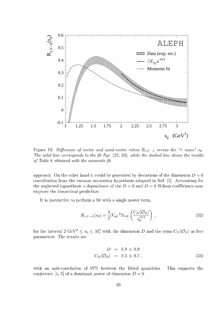
-0.1
0
0.1
0.2
0.3
0.4
0.5
0.6
1 1.25 1.5 1.75 2 2.25 2.5 2.75 3
Data (exp. err.)
∼ CD s–D/2
Moments fit
s0 (GeV2)
Rτ,
V–A
(s0)
ALEPH
Figure 19: Di�erence of vector and axial-vector ratios R�;V�A versus the \� mass" s0.
The solid line corresponds to the �t Eqs. (32, 33), while the dashed line shows the results
of Table 8 obtained with the moments �t.
approach. On the other hand it could be generated by deviations of the dimension D = 6contribution from the vacuum saturation hypothesis adopted in Ref. [5]. Accounting forthe neglected logarithmic s dependence of the D = 6 and D = 8 Wilson coefficients may
improve the theoretical prediction.
It is instructive to perform a fit with a single power term,
R�;V�A(s0) =3
2jVudj2SEW
CDhODisD=20
!; (32)
for the interval 2 GeV2 � s0 � M2� with the dimension D and the term CDhODi as free
parameters. The results are
D = 6:9 � 0:9
CDhODi = 2:3 � 0:7 ; (33)
with an anti-correlation of 97% between the fitted quantities. This supports the
conjecture [4, 5] of a dominant power of dimension D = 6.
39

7 Conclusions
Measurements are presented of the non-strange � vector and axial-vector current hadronic
spectral functions as well as their inclusive sum and difference. The distributions and
corresponding error matrices can be obtained as postscript and data files from the ALEPH
publication server on the WWW4.
The separation of vector and axial-vector spectral functions allows to test chiral sum
rules up to the � mass.
The spectral functions and measurements of the ratios R�;V=A=V+A of the vector and
axial-vector hadronic widths and the electronic width are exploited in order to obtain a
precise determination of the strong coupling constant �s(M2� ). Since QCD is applied at
a low energy scale, nonperturbative effects are accounted for by the use of the Operator
Product Expansion (OPE), with coefficients which can be fitted simultaneously with
�s(M2� ).
The best and most robust determination of �s(M2� ) is obtained from the inclusive
(V + A) fit. Using the world averages for the � leptonic branching ratios and the
� lifetime to obtain R� yields �s(M2� ) = 0:334 � 0:007 � 0:021, where the first error
accounts for experimental and the second for theoretical uncertainties. The result isthe mean value of those obtained using �xed-order perturbation theory (FOPT) and
contour-improved FOPT. Evolving the above value from the � to the Z mass scale gives�s(M
2Z) = 0:1202� 0:0008� 0:0024� 0:0010, where the last number gives the evolution
uncertainty. The total nonperturbative contribution to R�;V+A is found to be compatiblewith zero. However, the same fit using the exclusive vector and axial-vector ratio R�;V=A
and moments revealed that the nonperturbative contributions, in particular of dimension
D = 6, are large, but almost exactly cancel out in the inclusive sum.
The spectral function measurement allows the possibility to derive R� as a functionof a variable \� mass" s0 � M2
� , taking advantage of the universal nature of the
measured spectral functions. This provides a direct test of the running of �s(s0) whichgoverns the evolution of the theoretical prediction to values smaller than the � mass.
Excellent agreement between the measured R�;V+A(s0) and theory is found for the range
of 0:8 GeV2 � s0 � M2� , below which R�;V+A(s0) starts to diverge due to the influence of
the � peak and the pion pole.
The evolution of the nonperturbative contributions as a function of s0 can be accesseddirectly by considering R�;V�A(s0) in which perturbative contributions cancel. The fit of
one operator with variable dimension to R�;V�A(s0) yields D = 6:9 � 0:9, in agreement
with the assumption of a dominant D = 6 contribution made in the SVZ approach.
4http://alephwww.cern.ch/ALPUB/paper/paper.html
40

Acknowledgments
We gratefully acknowledge our colleagues from the accelerator divisions for the successful
operation of LEP. We are indebted to the engineers and technicians in all our institutions
for their contribution to the excellent performance of ALEPH. Those of us from non-member
countries thank CERN for its hospitality.
We are indebted to G. Altarelli, M. Beneke, S. Eidelman, G. Grunberg, S. Narison,
P. Nason, M. Neubert, P.A. R�aczka, A. Vainshtein, for a useful and very interesting one-day-long
discussion. Comments from A. Kataev are also acknowledged. Special thanks to C.J. Maxwell,
S. Menke, A. Pich and D.G. Tonge for the continuous theoretical and technical support.
Appendix
Table 1 lists the vector and axial-vector � final states and the corresponding branching
ratios. The following modes containing kaons are used as input into the sum of all �
branching ratios normalized to one and for the experimental subtraction of the Cabibbo
suppressed modes. The numbers are mainly taken from Refs. [47, 11]. Some are obtained
from isospin considerations (see Section 4):
B(��!K� �� ) = (0.69� 0.03)%
B(��!K� �� ) = (1.27� 0.09)%B(��!K� 2�0 �� ) = (0.09� 0.02)%B(��!K��+�� �� ) = (0.23� 0.05)%
B(��!K0���0 �� ) = (0.35� 0.08)%B(��!K����+�0 �� ) = (0.07� 0.05)%
B(��!K�K0 �� ) = (0.19� 0.04)%B(��!K�K+�� �� ) = (0.16� 0.03)%B(��!K0 �K0�� �� ) = (0.16� 0.03)%
B(��!K�K0�0 �� ) = (0.10� 0.05)%B(��!K�K�� �� ) = 0.16% (estimated)
References
[1] R. Barate et al. (ALEPH Collaboration), Z. Phys. C76 (1997) 15
[2] D. Buskulic et al. (ALEPH Collaboration), Phys. Lett. B307 (1993) 209
[3] T. Coan et al. (CLEO Collaboration), Phys. Lett. B356 (1995) 580
[4] M.A. Shifman, A.L. Vainshtein and V.I. Zakharov, Nucl. Phys. B147 (1979) 385,
448, 519
[5] E. Braaten, S. Narison and A. Pich, Nucl. Phys. B373 (1992) 581
[6] F. Le Diberder and A. Pich, Phys. Lett. B289 (1992) 165
[7] F. Le Diberder and A. Pich, Phys. Lett. B286 (1992) 147
41

[8] A. Pich, Nucl. Phys. B39 (Proc. Suppl.) (1995) 326
[9] G. Altarelli, P. Nason and G. Ridolfi, Z. Phys. C68 (1995) 257
[10] S. Narison, Nucl. Phys. B40 (Proc. Suppl.) (1995) 47; P.A. R�aczka and A. Szymacha,
Z. Phys. C70 (1996) 125
[11] R.M. Barnett et al. (Particle Data Group) Phys. Rev. D54 (1996) 1
[12] W. Marciano and A. Sirlin, Phys. Rev. Lett. 61 (1988) 1815; Phys. Rev. Lett. 61
(1986) 1815
[13] D. Buskulic et al. (ALEPH Collaboration), Z. Phys. C70 (1996) 561
[14] A. Anastassov et al. (CLEO Collaboration), Phys. Rev. D55 (1997) 2559;
P. Abreu et al. (DELPHI Collaboration), Phys. Lett. B355 (1995) 415;
R. Akers et al. (OPAL Collaboration), Phys. Lett. B369 (1996) 163; Z. Phys. C67
(1995) 543
[15] D. Buskulic et al. (ALEPH Collaboration), Report CERN PPE/97-090 (1997);R. Balest et al. (CLEO Collaboration), Phys. Lett. 388 (1996) 402;
P. Abreu, (DELPHI Collaboration), Phys. Lett. B365 (1996) 448;M. Acciarri et al. (L3 Collaboration), Phys. Lett. B389 (1996) 187;R. Akers, (OPAL Collaboration), Phys. Lett. B374 (1996) 341
[16] R. Alemany, M. Davier and A. H�ocker, Report LAL 97-02 (1997)
[17] J.Z. Bai et al. (BES Collaboration), Phys. Rev. D53 (1996) 20
[18] D. Decamp et al. (ALEPH Collaboration), Nucl. Inst. Meth. A294 (1990) 121
[19] D. Buskulic et al. (ALEPH Collaboration), Nucl. Inst. Meth. A360 (1995) 481
[20] S. Jadach, J.H. K�uhn and Z. W�as, Comp. Phys. Comm. 64 (1991) 275
[21] S. Jadach, B.F.L. Ward and Z. W�as, Comp. Phys. Comm. 79 (1994) 503
[22] S. Jadach et al., Comp. Phys. Comm. 76 (1993) 361
[23] R. Brun et al., GEANT3.15, Report CERN DD/EE/84-1 (1984)
[24] A. H�ocker, \Measurement of the � spectral functions and applications to QCD",
Thesis, Report LAL 97-18, Orsay, France (1997)
[25] D. Buskulic et al. (ALEPH Collaboration), Z. Phys. C62 (1994) 539
[26] D. Buskulic et al. (ALEPH Collaboration), Z. Phys. C70 (1996) 579
[27] D. Decamp et al. (ALEPH Collaboration), Z. Phys. C54 (1992) 211
[28] A. H�ocker and V. Kartvelishvili, Nucl. Inst. Meth. A372 (1996) 469
42

[29] D. Buskulic et al. (ALEPH Collaboration), Z. Phys. C74 (1997) 263
[30] P.L. Campana, Nucl. Phys. B55 C (Proc. Suppl.) (1997) 161
[31] V. Shelkov, Nucl. Phys. B55 C (Proc. Suppl.) (1997) 195
[32] T. Das, V.S. Mathur and S. Okubo, Phys. Rev. Lett. 19 (1967) 895
[33] S.R. Amendolia et al. (NA7 Collaboration), Nucl. Phys. B277 (1986) 168
[34] S. Weinberg, Phys. Rev. Lett. 18 (1967) 507.
[35] T. Das, G.S. Guralnik, V.S. Mathur, F.E. Low and J.E. Young, Phys. Rev. Lett. 18
(1967) 759
[36] J.F. Donoghue and E. Golowich, Phys. Rev. D49 (1994) 1513
[37] L.R. Surguladze and M.A. Samuel, Phys. Rev. Lett. 66 (1991) 560;
S.G. Gorishny, A.L. Kataev and S.A. Larin, Phys. Lett. B259 (1991) 144
[38] J.H. K�uhn and A. Santamaria, Z. Phys. C48 (1990) 445
[39] A. Pais, Ann. Phys. 9 (1960) 548
[40] E. Braaten, Phys. Rev. Lett./ 60 (1988) 1606
[41] E. Braaten and C.S. Li, Phys. Rev. D42 (1990) 3888
[42] K.G. Wilson, Phys. Rev. 179 (1969) 1499
[43] K.G. Chetyrkin and A. Kwiatkowski, Z. Phys. C59 (1993) 525
[44] S.A. Larin, T. van Ritbergen and J.A.M. Vermaseren, Phys. Lett. B400 (1997) 379
[45] C. Becchi, S. Narison, E. de Rafael and F.J. Yndurain, Z. Phys. C8 (1981) 335;
D.J. Broadhurst, Phys. Lett. B101 (1981) 423;S.C. Generalis, J. Phys. G15 (1989) L225
[46] D.J. Broadhurst and S.C. Generalis, Phys. Lett. 165 (1985) 175
[47] M. Davier, Nucl. Phys. B55 C (Proc. Suppl.) (1997) 395
[48] S. Chen (ALEPH Collaboration), Talk given at the High-Energy Physics
International Euroconference on Quantum Chromodynamics (QCD 97), Montpellier,France 1997
[49] A.L. Kataev, V.V. Starshenko, Mod. Phys. Lett. A10 (1995) 235; Nucl. Phys. B39
(Proc. Suppl.) (1995) 312
[50] P.M. Stevenson, Phys. Rev. D23 (1981) 2916
[51] F. Le Diberder, Nucl. Phys. B39 (Proc. Suppl.) (1995) 318
43

[52] A.L. Kataev, private communication (1997)
[53] G. Grunberg, Phys. Lett. B95 (1980) 70; Phys. Rev. D29 (1984) 2315
[54] P.A. R�aczka, Report DTP/97/50 (1997)
[55] G. Grunberg, Report CPTH-PC510-0597 (1997)
[56] M. Beneke and V.M. Braun, Phys. Lett. B348 (1995) 513; P. Ball, M. Beneke and
V.M. Braun, Nucl. Phys. B452 (1995) 563.
[57] M. Neubert, Report CERN-TH-7524-94 (1994); Nucl. Phys. B463 (1996) 511
[58] C.N. Lovett-Turner and C.J. Maxwell, Nucl. Phys. B452 (1995) 188
[59] C.J. Maxwell and D.G. Tonge, Nucl. Phys. B481 (1996); Report DTP-97-30 (1997)
[60] S. Narison, Phys. Lett. B361 (1995) 121
[61] W. Bernreuther, W. Wetzel, Nucl. Phys. B197 (1982) 228;W. Wetzel, Nucl. Phys. B196 (1982) 259;W. Bernreuther, Talk given at the Workshop on QCD at LEP, Aachen, Germany
1994, PITHA-94-31 (1994)
[62] R. Barate et al. (ALEPH Collaboration), Report CERN PPE/97-090 (1997)
[63] G. Rodrigo, A. Pich, A. Santamaria, FTUV-97-80 (1997)
[64] M. Girone and M. Neubert, Phys. Rev. Lett. 76 (1996) 3061
44


![Michel parameters and [tau] neutrino helicity from decay correlations in Z--\u003e[tau]+[tau]](https://img.pdfslide.net/doc/110x75/6350c359f55d98549a09e91e/michel-parameters-and-tau-neutrino-helicity-from-decay-correlations-in-z-u003etautau.jpg)


![Upper Limits on the Branching Ratios Tau-]Mu-Gamma and Tau-]E-Gamma](https://img.pdfslide.net/doc/110x75/63619cb540b666b8ec0dfe62/upper-limits-on-the-branching-ratios-tau-mu-gamma-and-tau-e-gamma.jpg)


