Embed Size (px)
Citation preview

Tennessee State University
Collage of Engineering, Technology and Computer Science
Department of Civil & Environmental Engineering
CVEN 3121 - Mechanics of Materials Laboratory
Laboratory Manual
Dr. Omar J. Al-Khatib
Dr. Farouk Mishu
June 3, 2008
ii
Table of Contents
1. MECHANICS OF MATERIALS LABORTORY OBJECTIVES ...............................1
2. DATA SHEETS ..............................................................................................................1
3. LABORATORY REPORT FORMAT ..........................................................................1
Objective of Lab Reports: ....................................................................................................1
Laboratory Report Sections: ................................................................................................1
1. Cover Page ...................................................................................................................1
2. Abstract ........................................................................................................................3
3. Grading Table ...............................................................................................................4
4. Table of Content ...........................................................................................................4
5. Introduction & Objective ..............................................................................................4
6. Theoretical Background ................................................................................................5
7. Materials & Apparatus ..................................................................................................5
8. Procedure .....................................................................................................................5
9. Experimental Date ........................................................................................................5
10. Calculations & Evaluation of Data ................................................................................6
11. Results and Discussion .................................................................................................6
12. Conclusion ...................................................................................................................6
13. Important Notes ............................................................................................................6
14. Laboratory Report Grading Criteria ..............................................................................7
15. References ....................................................................................................................7
Lab 1: Least Squares Regression .........................................................................................8
Lab 1: Least Squares Regression (MS Excel) ................................................................... 12
Lab 2: Vernier Caliper & Micrometer ............................................................................... 18
Lab 3: Tensile Test of Brittle and Ductile Metals (Clockhouse Machine)......................... 36
Lab 4: Flexure in Wood ...................................................................................................... 48
Lab 5: Tensile Test of Brittle and Ductile Metals (INSTRON) ......................................... 56
Lab 6: Tension Test Using the Universal Testing Machine ............................................... 67
Lab 7: Torsion Test of Ductile and Brittle Materials ......................................................... 78
Lab 8: Truss Test and Analysis .......................................................................................... 87
Basic Conversion Table ....................................................................................................... 94
References & Bibliography ................................................................................................. 95

iii
Preface
The Mechanics of materials Laboratory Manual is written to describe the experiments in Mechanics of Material Lab course (CVEN 3121). Each experiment procedure is explained thoroughly along with related background. The experiments are selected to apply some concepts from mechanics of materials such as analysis of materials properties based on tension, bending, and torsion. Some complementary topics are also presented such as using of measuring tools like vernier calipers and micrometers. The use of these tools will help students to understand how to measure objects precisely, which is a crucial skill in lab. Experimental data analysis techniques, such linear regression, are also presented to help student to determine mathematical models based on data obtained. The authors devoted considerable attention to laboratory report development and associated technical writing. These issues are one of the important objectives of CVEN-3121 and believed to be a crucial communication skills need to be developed. Data Sheet is developed for each experiment to help student learn how to manage experimental data obtained and make it handy during calculations. The data sheet provides tables listing parameters and variable needed to be measured or obtained through experimental work. In addition, Post-Lab Assignments are given to enhance student understanding of concepts being applied practically. Part of this manual is developed based on information obtained from books referenced at the last section of the manual. A sincere appreciation and credit should be given to authors of these books. Students are encouraged to check these resources for more information or interest in any topic.
1
1. MECHANICS OF MATERIALS LABORTORY OBJECTIVES
A- To apply mechanics of materials theory on real specimens and learn the practical testing procedures and concepts.
B- Demonstrate an understanding of tension, and compression forces and the resulting strains and deflections.
C- To demonstrate the relationship between stress and strain and application of Hooke’s law. D- Demonstrate an understanding of beams stresses, shear forces, and bending moments. E- Demonstrate an understanding of torsion and deformations resulting from torsion. F- To learn and improve laboratory report documents and technical writing which include:
1) Experimental objectives and procedures. 2) Presentation of results in an organized and clear manner. 3) Draw graphs and figures to summarize key findings.
2. DATA SHEETS
The experimental data obtained during laboratory work should be organized in a data sheet. This data sheet is required for all each experiment report and should be signed by the instructor before leaving the lab. The template data sheet is included as the last page in each experiment section in the lab manual. Remember that you are very unlikely to write a good report with bad or incomplete data. 3. LABORATORY REPORT FORMAT Objective of Lab Reports:
The primary objective of an experiment report is to inform others (engineers, instructors, etc.) about the testing procedure and the results being collected. The report should be well organized and written so that someone who is not familiar with the particular experiment or test set-up can understand the following:
1- The objective and aim of the experiment. 2- What procedures were followed and assumption being made. 3- What data was collected and type of materials tested. 4- What analysis was completed along with the necessary calculations? 5- Which conclusions were made and recommendations established.
Laboratory Report Sections:
The format of each section of the laboratory report will be described next. The format should be followed exactly as described below to avoid losing points.
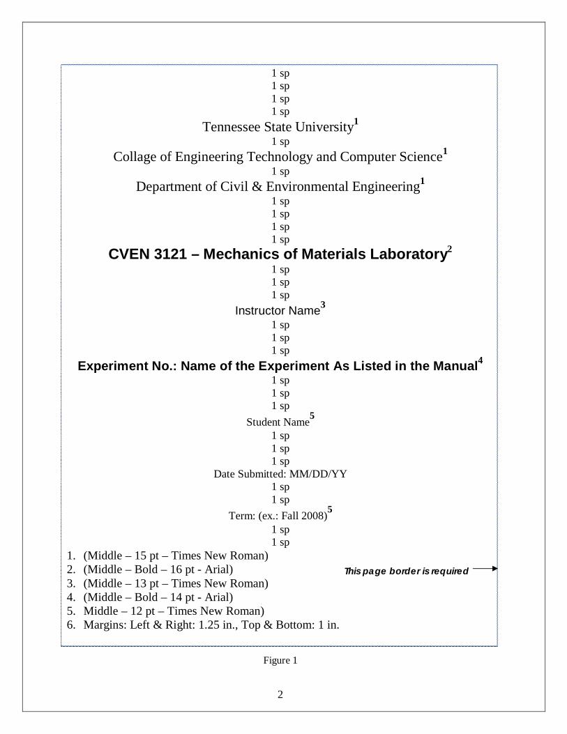
1. Cover Page
The cover page should include the name of the experiment, group name, group members, course number, date of the lab and date of report submittal and other relative information. A sample of required cover page with specific format is presented in Figure 1 next page.
2
This page border is required
1 sp 1 sp 1 sp 1 sp
Tennessee State University1 1 sp
Collage of Engineering Technology and Computer Science1 1 sp
Department of Civil & Environmental Engineering1 1 sp 1 sp 1 sp 1 sp
CVEN 3121 – Mechanics of Materials Laboratory2
1 sp 1 sp 1 sp
Instructor Name3
1 sp 1 sp 1 sp
Experiment No.: Name of the Experiment As Listed in the Manual4 1 sp 1 sp 1 sp
Student Name5 1 sp 1 sp 1 sp
Date Submitted: MM/DD/YY 1 sp 1 sp
Term: (ex.: Fall 2008)5 1 sp 1 sp
1. (Middle – 15 pt – Times New Roman) 2. (Middle – Bold – 16 pt - Arial) 3. (Middle – 13 pt – Times New Roman) 4. (Middle – Bold – 14 pt - Arial) 5. Middle – 12 pt – Times New Roman) 6. Margins: Left & Right: 1.25 in., Top & Bottom: 1 in.
Figure 1
3
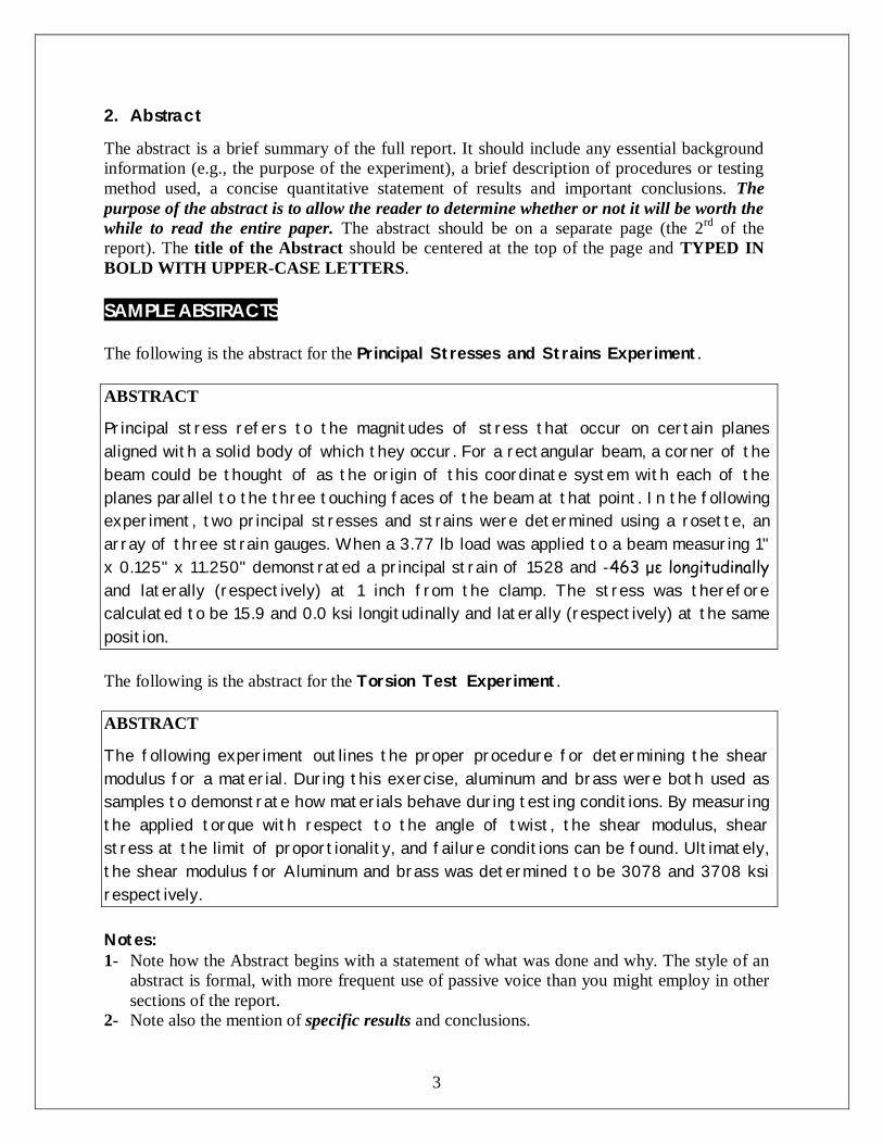
2. Abstract The abstract is a brief summary of the full report. It should include any essential background information (e.g., the purpose of the experiment), a brief description of procedures or testing method used, a concise quantitative statement of results and important conclusions. The purpose of the abstract is to allow the reader to determine whether or not it will be worth the while to read the entire paper. The abstract should be on a separate page (the 2rd of the report). The title of the Abstract should be centered at the top of the page and TYPED IN BOLD WITH UPPER-CASE LETTERS. SAMPLE ABSTRACTS The following is the abstract for the Principal Stresses and Strains Experiment. ABSTRACT
Principal stress refers to the magnitudes of stress that occur on certain planes aligned with a solid body of which they occur. For a rectangular beam, a corner of the beam could be thought of as the origin of this coordinate system with each of the planes parallel to the three touching faces of the beam at that point. In the following experiment, two principal stresses and strains were determined using a rosette, an array of three strain gauges. When a 3.77 lb load was applied to a beam measuring 1" x 0.125" x 11.250" demonstrated a principal strain of 1528 and -463 με longitudinally and laterally (respectively) at 1 inch from the clamp. The stress was therefore calculated to be 15.9 and 0.0 ksi longitudinally and laterally (respectively) at the same position. The following is the abstract for the Torsion Test Experiment. ABSTRACT
The following experiment outlines the proper procedure for determining the shear modulus for a material. During this exercise, aluminum and brass were both used as samples to demonstrate how materials behave during testing conditions. By measuring the applied torque with respect to the angle of twist, the shear modulus, shear stress at the limit of proportionality, and failure conditions can be found. Ultimately, the shear modulus for Aluminum and brass was determined to be 3078 and 3708 ksi respectively. Notes: 1- Note how the Abstract begins with a statement of what was done and why. The style of an
abstract is formal, with more frequent use of passive voice than you might employ in other sections of the report.
2- Note also the mention of specific results and conclusions.
4
Points of Weakness: 1- Omits critical findings. 2- Refers reader to figures or tables in the report. 3- Relies on vague language. 4- Write introduction context and detail theoretical background. 5- Omits the experiment summary or brief description.
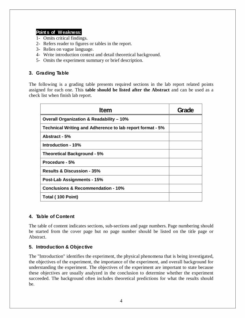
3. Grading Table
The following is a grading table presents required sections in the lab report related points assigned for each one. This table should be listed after the Abstract and can be used as a check list when finish lab report.
Item Grade Overall Organization & Readability – 10%
Technical Writing and Adherence to lab report format - 5%
Abstract - 5%
Introduction - 10%
Theoretical Background - 5%
Procedure - 5%
Results & Discussion - 35%
Post-Lab Assignments - 15%
Conclusions & Recommendation - 10%
Total ( 100 Point)
4. Table of Content The table of content indicates sections, sub-sections and page numbers. Page numbering should be started from the cover page but no page number should be listed on the title page or Abstract. 5. Introduction & Objective The "Introduction" identifies the experiment, the physical phenomena that is being investigated, the objectives of the experiment, the importance of the experiment, and overall background for understanding the experiment. The objectives of the experiment are important to state because these objectives are usually analyzed in the conclusion to determine whether the experiment succeeded. The background often includes theoretical predictions for what the results should be.
5
Points of Weakness:
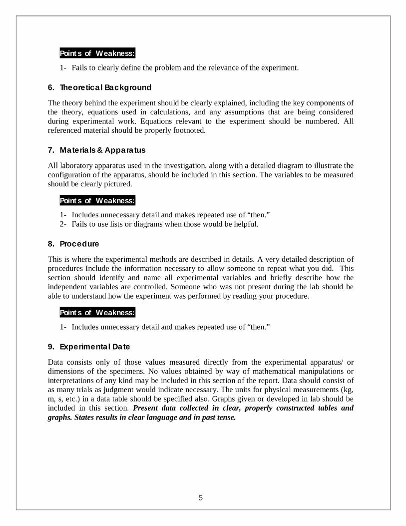
1- Fails to clearly define the problem and the relevance of the experiment. 6. Theoretical Background The theory behind the experiment should be clearly explained, including the key components of the theory, equations used in calculations, and any assumptions that are being considered during experimental work. Equations relevant to the experiment should be numbered. All referenced material should be properly footnoted. 7. Materials & Apparatus All laboratory apparatus used in the investigation, along with a detailed diagram to illustrate the configuration of the apparatus, should be included in this section. The variables to be measured should be clearly pictured.
Points of Weakness:
1- Includes unnecessary detail and makes repeated use of “then.” 2- Fails to use lists or diagrams when those would be helpful.
8. Procedure This is where the experimental methods are described in details. A very detailed description of procedures Include the information necessary to allow someone to repeat what you did. This section should identify and name all experimental variables and briefly describe how the independent variables are controlled. Someone who was not present during the lab should be able to understand how the experiment was performed by reading your procedure.
Points of Weakness:
1- Includes unnecessary detail and makes repeated use of “then.” 9. Experimental Date Data consists only of those values measured directly from the experimental apparatus/ or dimensions of the specimens. No values obtained by way of mathematical manipulations or interpretations of any kind may be included in this section of the report. Data should consist of as many trials as judgment would indicate necessary. The units for physical measurements (kg, m, s, etc.) in a data table should be specified also. Graphs given or developed in lab should be included in this section. Present data collected in clear, properly constructed tables and graphs. States results in clear language and in past tense.
6
10. Calculations & Evaluation of Data This section should include all graphs, analysis of graphs, and post laboratory calculations (hand calculations). State each formula, and if necessary, identify the symbols used in the formula. Be certain that your final calculated values are expressed to the correct number of significant figures. A description of the mathematical methods used to analyze the data is required.
Points of Weakness:
1- Fails to summarize overall results. 2- Fails to present data in formats that reveal critical relationships (trends, cause/effect,
etc.) 3- Fails to identify units of measurement.
11. Results and Discussion In discussing the results, you should not only analyze the results, but also discuss the implications of those results. Moreover, pay attention to the errors that existed in the experiment, both where they originated and what their significance is for interpreting the reliability of conclusions. One important way to present numerical results is to show them in graphs. POST-LAB QUESTIONS:
Post-lab questions are assigned with each experiment and intended to give an idea about the minimum issues or experiment aspects need to be discussed in the “Results and Discussions” section. The questions should be answered within the context of the experiment discussion in a paragraph writing style and not as a short answer format. In another word, do not limit the discussion to the post-lab questions only, discuss and analyze the experiment beyond the post-lab questions and based on the of materials taught in the course of Mechanics of Materials. 12. Conclusion In longer laboratory reports, a "Conclusion" section often appears. Whereas the "Results and Discussion" section has discussed the results individually, the "Conclusion" section discusses the results in the context of the entire experiment. Usually, the objectives mentioned in the "Introduction" are examined to determine whether the experiment succeeded. If the objectives were not met, you should analyze why the results were not as predicted. Note that in shorter reports or in reports where "Discussion" is a separate section from "Results," you often do not have a "Conclusion" section. 13. Important Notes 1- Avoid using personal pronouns (e.g. I, we, our, you, me, my…etc) in lab report.
2- Make sure to write clearly. Ask when you read it loud to yourself or a friend, does it make
sense? Don't forget to use the spell-checker in your word processor.
7
3- Check to be sure you addressed all the questions included in the lab exercise. 4- Do not use reports from previous semesters. Lab materials will be improved each semester. 5- Past tense should be used to describe what you did in lab. Present tense should be used for
statements of fact and chemical properties. For example: "The melting point of unknown 3319801 was measured to be 109ºC. The melting point of acetanilide is 114ºC."
6- Avoid using the first person and any statements of how you "felt" about an experiment,
whether it was "easy," or the supposition that you "learned a lot" from the lab. 14. Laboratory Report Grading Criteria The Lab Reports will be graded using the following guidelines:
1- Overall Organization & Readability – 10% 2- Technical writing and adherence to lab report format– 5% 3- Abstract – 5% 4- Introduction – 10% 5- Theoretical Background 5% 6- Procedures – 5% 7- Results & Discussion – 50% (30% on communication, 20% on technical merit). 8- Conclusions & Recommendations – 10% (7% on communication, 3% on
technical merit).
15. References Citations in the text should be in brackets and contain author(s) and year, e.g.: [Smith 2002], [Jobes and Mayton 2006], [Mayton et al. 2005]. The References section should list the references in alphabetical order by author.
8
Lab 1: Least Squares Regression
Lab 1-A: The Least Squares Regression - Introduction Introduction to linear regression
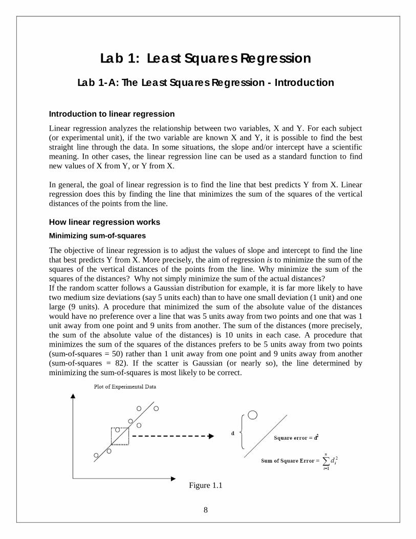
Linear regression analyzes the relationship between two variables, X and Y. For each subject (or experimental unit), if the two variable are known X and Y, it is possible to find the best straight line through the data. In some situations, the slope and/or intercept have a scientific meaning. In other cases, the linear regression line can be used as a standard function to find new values of X from Y, or Y from X. In general, the goal of linear regression is to find the line that best predicts Y from X. Linear regression does this by finding the line that minimizes the sum of the squares of the vertical distances of the points from the line. How linear regression works
Minimizing sum-of-squares
The objective of linear regression is to adjust the values of slope and intercept to find the line that best predicts Y from X. More precisely, the aim of regression is to minimize the sum of the squares of the vertical distances of the points from the line. Why minimize the sum of the squares of the distances? Why not simply minimize the sum of the actual distances? If the random scatter follows a Gaussian distribution for example, it is far more likely to have two medium size deviations (say 5 units each) than to have one small deviation (1 unit) and one large (9 units). A procedure that minimized the sum of the absolute value of the distances would have no preference over a line that was 5 units away from two points and one that was 1 unit away from one point and 9 units from another. The sum of the distances (more precisely, the sum of the absolute value of the distances) is 10 units in each case. A procedure that minimizes the sum of the squares of the distances prefers to be 5 units away from two points (sum-of-squares = 50) rather than 1 unit away from one point and 9 units away from another (sum-of-squares = 82). If the scatter is Gaussian (or nearly so), the line determined by minimizing the sum-of-squares is most likely to be correct.
Figure 1.1
9
The simplest example of a least square approximation is fitting a straight line to a set of paired data: (x1, y1), (x2, y2), ……, (xn, yn). The mathematical expression for the straight line is
y = ao + a1x + e (1.1)
where ao and a1 are coefficients representing the intercept and the slope, respectively, and e is the error (represented as d in Figure 1,1), or residual, which represents how far each point fat from the predicted line (the model), which can be be represented by rearranging Equation (1.1) as
e = y - ao - a1x (1.2)
Thus, the error, or residual, is the discrepancy between the true value of y and the approximate value (represented by d in Figure 1.1), ao + a1x, predicted by the linear equation. Regression analysis is based on minimizing the sum of the squares of the residuals between the measured y value and the calculated with linear model.
n
iioieli
n
imeasuredi
n
iir xaayyyeS
1
21
2mod,
1,
1
2 )()( (1.3)
To determine values for a0 and a1 in Equation 1.3 at minimum (to minimize the sum of the squares), Equation 1.3 is differentiated with respect to each coefficient and then set equal to zero as follows
)(2 1
0ioi
r xaayaS
(1.4)
iioir xxaay
aS )(2 1
1
(1.5)
then )(20 1 ioi xaay (1.6)
iioi xxaay )(20 1 (1.7)
rearranging ii xaay 100 (1.8)
2
10 a0 iiii xxaxy (1.9)
Note that 00 naa , therefore the equations can be expressed as a set of two simultaneous linear equations with two unknown (a0 and a1):
ii yaxna 10 (1.10)
10
iiii xyaxax 12
0 (1.11)
These are called the normal equations. They can be solved simultaneously for a1 and a0 as
221
ii
iiii
xxn
yxyxna (1.12)
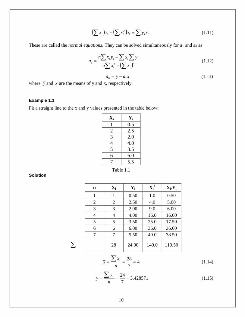
xaya 10 (1.13) where y and x are the means of y and x, respectively. Example 1.1
Fit a straight line to the x and y values presented in the table below:
Xi Yi 1 0.5 2 2.5 3 2.0 4 4.0 5 3.5 6 6.0 7 5.5
Table 1.1 Solution
n Xi Yi Xi2 Xi.Yi
1 1 0.50 1.0 0.50 2 2 2.50 4.0 5.00 3 3 2.00 9.0 6.00 4 4 4.00 16.0 16.00 5 5 3.50 25.0 17.50 6 6 6.00 36.0 36.00 7 7 5.50 49.0 38.50
28 24.00 140.0 119.50
4728
n
xx i (1.14)
428571.3724
n
yy i (1.15)

11
Using Equations (1.12) and (1.13),
83928.0)28()140(7
)24(28)5.119(721
a
071428.083928.0428571.30 a
Therefore, the least-squares fit is:
y = 0.071428 – 0.83928 x
12
Lab 1: Least Squares Regression
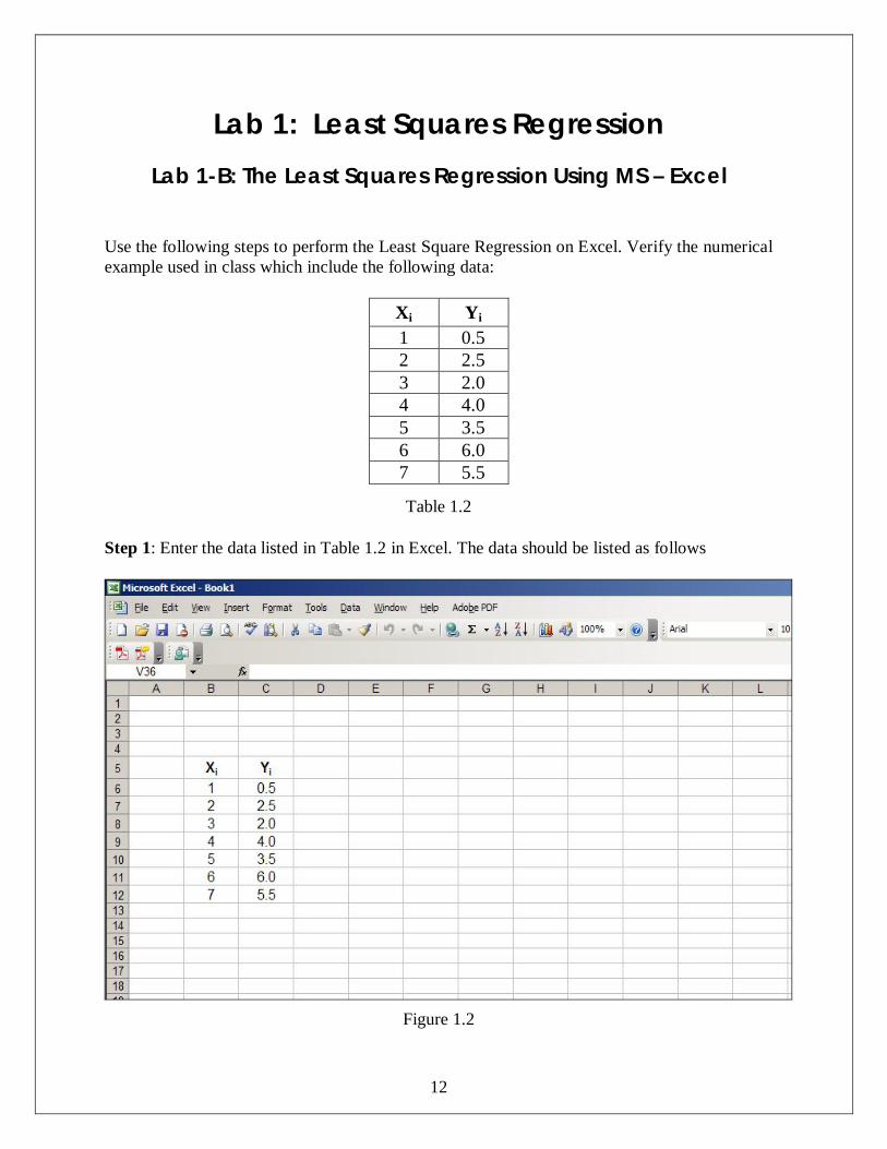
Lab 1-B: The Least Squares Regression Using MS – Excel
Use the following steps to perform the Least Square Regression on Excel. Verify the numerical example used in class which include the following data:
Xi Yi 1 0.5 2 2.5 3 2.0 4 4.0 5 3.5 6 6.0 7 5.5
Table 1.2
Step 1: Enter the data listed in Table 1.2 in Excel. The data should be listed as follows
Figure 1.2
13
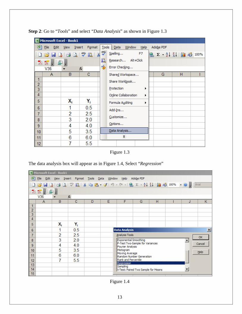
Step 2: Go to “Tools” and select “Data Analysis” as shown in Figure 1.3
Figure 1.3
The data analysis box will appear as in Figure 1.4, Select “Regression”
Figure 1.4
14
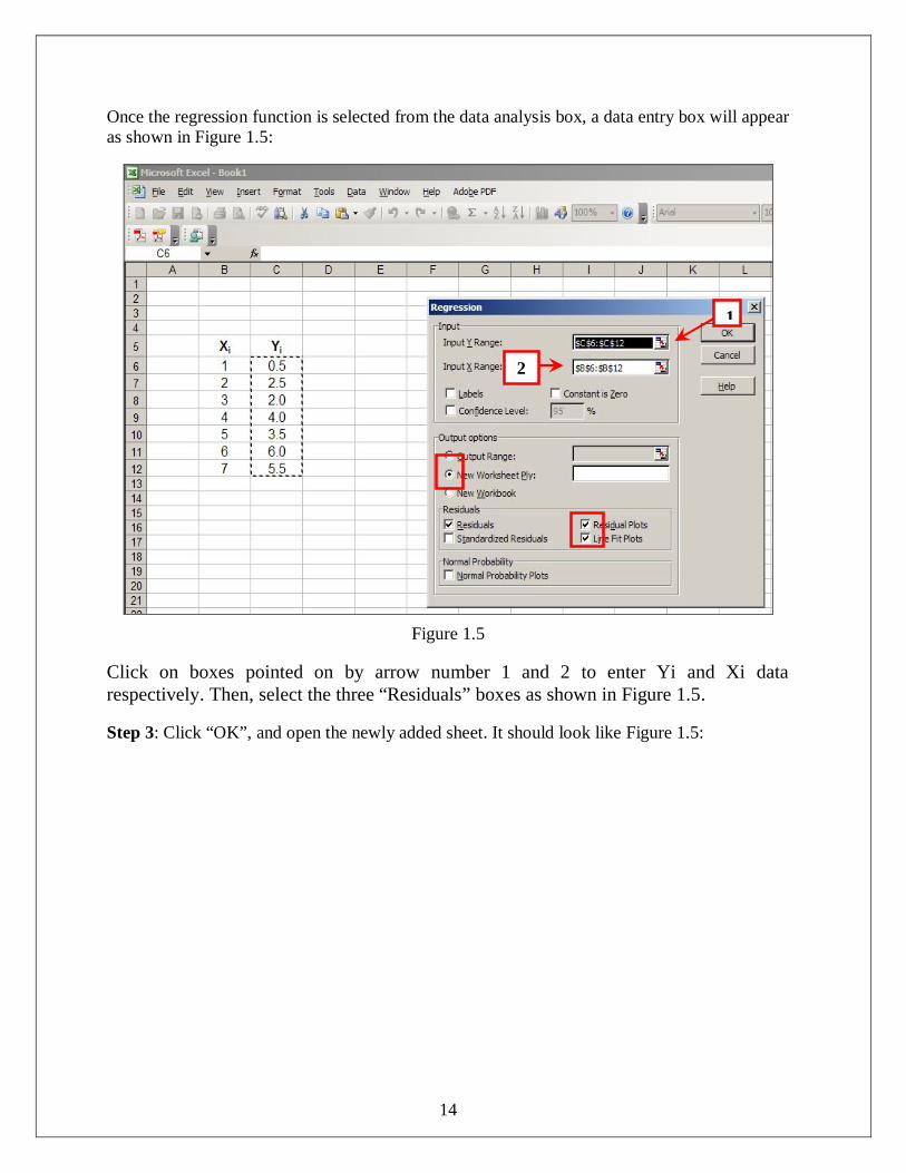
Once the regression function is selected from the data analysis box, a data entry box will appear as shown in Figure 1.5:
Figure 1.5
Click on boxes pointed on by arrow number 1 and 2 to enter Yi and Xi data respectively. Then, select the three “Residuals” boxes as shown in Figure 1.5. Step 3: Click “OK”, and open the newly added sheet. It should look like Figure 1.5:
1
2
15
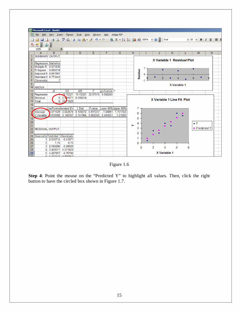
Figure 1.6
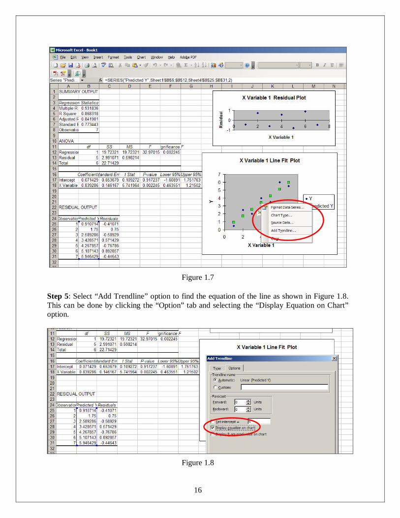
Step 4: Point the mouse on the “Predicted Y” to highlight all values. Then, click the right button to have the circled box shown in Figure 1.7.
16
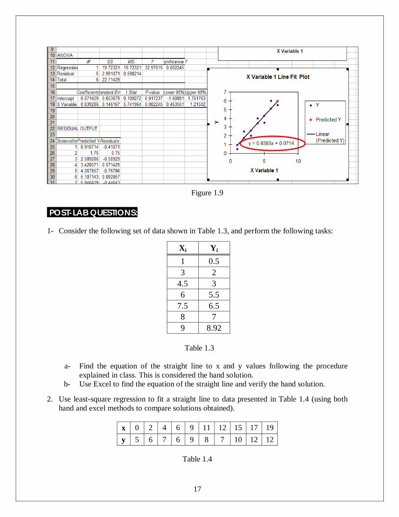
Figure 1.7 Step 5: Select “Add Trendline” option to find the equation of the line as shown in Figure 1.8. This can be done by clicking the “Option” tab and selecting the “Display Equation on Chart” option.
Figure 1.8
17
Figure 1.9 POST-LAB QUESTIONS: 1- Consider the following set of data shown in Table 1.3, and perform the following tasks:
Xi Yi 1 0.5 3 2
4.5 3 6 5.5
7.5 6.5 8 7 9 8.92
Table 1.3
a- Find the equation of the straight line to x and y values following the procedure explained in class. This is considered the hand solution.
b- Use Excel to find the equation of the straight line and verify the hand solution. 2. Use least-square regression to fit a straight line to data presented in Table 1.4 (using both
hand and excel methods to compare solutions obtained).
x 0 2 4 6 9 11 12 15 17 19 y 5 6 7 6 9 8 7 10 12 12
Table 1.4
18
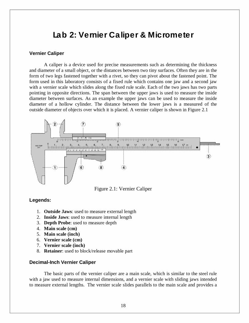
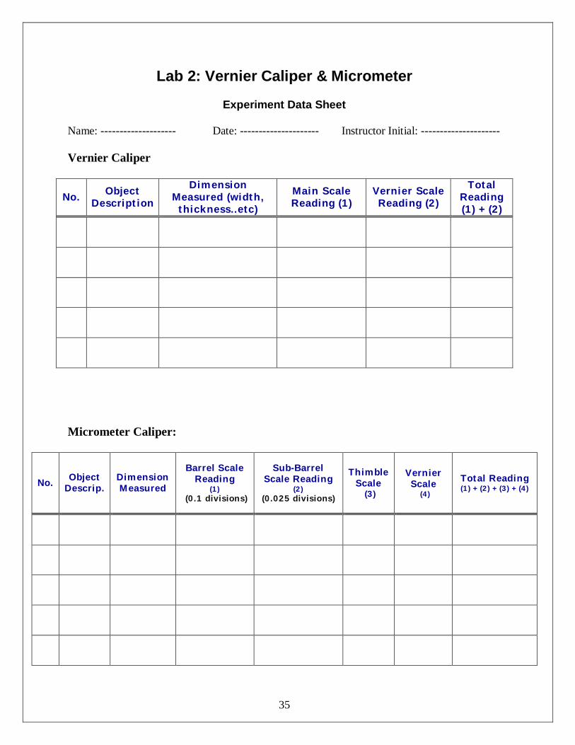
Lab 2: Vernier Caliper & Micrometer Vernier Caliper
A caliper is a device used for precise measurements such as determining the thickness and diameter of a small object, or the distances between two tiny surfaces. Often they are in the form of two legs fastened together with a rivet, so they can pivot about the fastened point. The form used in this laboratory consists of a fixed rule which contains one jaw and a second jaw with a vernier scale which slides along the fixed rule scale. Each of the two jaws has two parts pointing in opposite directions. The span between the upper jaws is used to measure the inside diameter between surfaces. As an example the upper jaws can be used to measure the inside diameter of a hollow cylinder. The distance between the lower jaws is a measured of the outside diameter of objects over which it is placed. A vernier caliper is shown in Figure 2.1
Figure 2.1: Vernier Caliper
Legends:
1. Outside Jaws: used to measure external length 2. Inside Jaws: used to measure internal length 3. Depth Probe: used to measure depth 4. Main scale (cm) 5. Main scale (inch) 6. Vernier scale (cm) 7. Vernier scale (inch) 8. Retainer: used to block/release movable part
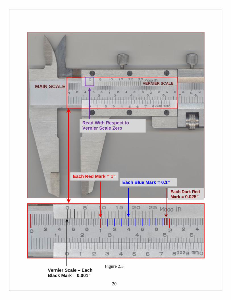
Decimal-Inch Vernier Caliper
The basic parts of the vernier caliper are a main scale, which is similar to the steel rule with a jaw used to measure internal dimensions, and a vernier scale with sliding jaws intended to measure external lengths. The vernier scale slides parallels to the main scale and provides a
19
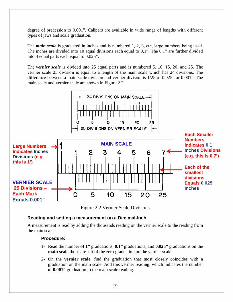
degree of precession to 0.001”. Calipers are available in wide range of lengths with different types of jaws and scale graduation.
The main scale is graduated in inches and is numbered 1, 2, 3, etc, large numbers being used. The inches are divided into 10 equal divisions each equal to 0.1”. The 0.1” are further divided into 4 equal parts each equal to 0.025”.
The vernier scale is divided into 25 equal parts and is numbered 5, 10, 15, 20, and 25. The vernier scale 25 division is equal to a length of the main scale which has 24 divisions. The difference between a main scale division and vernier division is 1/25 of 0.025” or 0.001”. The main scale and vernier scale are shown in Figure 2.2
Figure 2.2 Vernier Scale Divisions
Reading and setting a measurement on a Decimal-Inch
A measurement is read by adding the thousands reading on the vernier scale to the reading from the main scale.
Procedure:
1- Read the number of 1” graduations, 0.1” graduations, and 0.025” graduations on the main scale those are left of the zero graduation on the vernier scale.
2- On the vernier scale, find the graduation that most closely coincides with a graduation on the main scale. Add this vernier reading, which indicates the number of 0.001” graduation to the main scale reading.
MAIN SCALE
VERNIER SCALE 25 Divisions – Each Mark Equals 0.001”
Large Numbers Indicates Inches Divisions (e.g. this is 1’)
Each Smaller Numbers Indicates 0.1 Inches Divisions (e.g. this is 0.7’)
Each of the smallest divisions Equals 0.025 Inches
20
Figure 2.3
MAIN SCALE VERNIER SCALE
Each Red Mark = 1” Each Blue Mark = 0.1”
Each Dark Red Mark = 0.025”
Vernier Scale – Each Black Mark = 0.001”
Read With Respect to Vernier Scale Zero Zero
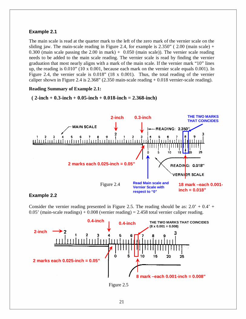
21
Example 2.1 The main scale is read at the quarter mark to the left of the zero mark of the vernier scale on the sliding jaw. The main-scale reading in Figure 2.4, for example is 2.350” ( 2.00 (main scale) + 0.300 (main scale passing the 2.00 in mark) + 0.050 (main scale)). The vernier scale reading needs to be added to the main scale reading. The vernier scale is read by finding the vernier graduation that most nearly aligns with a mark of the main scale. If the vernier mark “10” lines up, the reading is 0.010” (10 x 0.001, because each mark on the vernier scale equals 0.001). In Figure 2.4, the vernier scale is 0.018” (18 x 0.001). Thus, the total reading of the vernier caliper shown in Figure 2.4 is 2.368” (2.350 main-scale reading + 0.018 vernier-scale reading).
Reading Summary of Example 2.1:
( 2-inch + 0.3-inch + 0.05-inch + 0.018-inch = 2.368-inch)
Figure 2.4
Example 2.2 Consider the vernier reading presented in Figure 2.5. The reading should be as: 2.0’ + 0.4’ + 0.05’ (main-scale readings) + 0.008 (vernier reading) = 2.458 total vernier caliper reading.
Figure 2.5
THE TWO MARKS THAT COINCIDES
THE TWO MARKS THAT COINCIDES (8 x 0.001 = 0.008)
Read Main scale and Vernier Scale with respect to “0”
2-inch 0.3-inch
2 marks each 0.025-inch = 0.05”
18 mark –each 0.001-inch = 0.018”
2-inch
0.4-inch 0.4-inch
2 marks each 0.025-inch = 0.05”
8 mark –each 0.001-inch = 0.008”
22
Example 2.3 Read the vernier scale partial image presented in Figure 2.6. The vernier scale shown in Figure 2.6 is read as follows: - Main scale reading: 3-inch + 0.6-inch + 0.075-inch = 3.675-inch - Vernier scale: 0.02-inch - Total Reading (Main Scale + Vernier Scale): 3.695-inch
Figure 2.6
3-inch 0.6-inch
3 marks (between 6 and 0) each 0.025-inch = 0.075-inch
Mark coincides at 20 (20 x 0.001” = 0.02”)
Vernier Scale
Main Scale
23
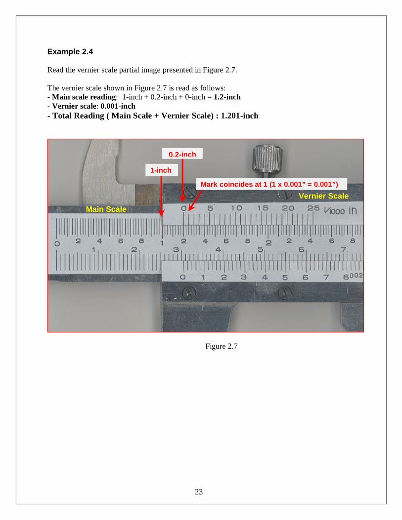
Example 2.4 Read the vernier scale partial image presented in Figure 2.7. The vernier scale shown in Figure 2.7 is read as follows: - Main scale reading: 1-inch + 0.2-inch + 0-inch = 1.2-inch - Vernier scale: 0.001-inch - Total Reading ( Main Scale + Vernier Scale) : 1.201-inch
Figure 2.7
1-inch
0.2-inch
Mark coincides at 1 (1 x 0.001” = 0.001”) Vernier Scale
Main Scale
24
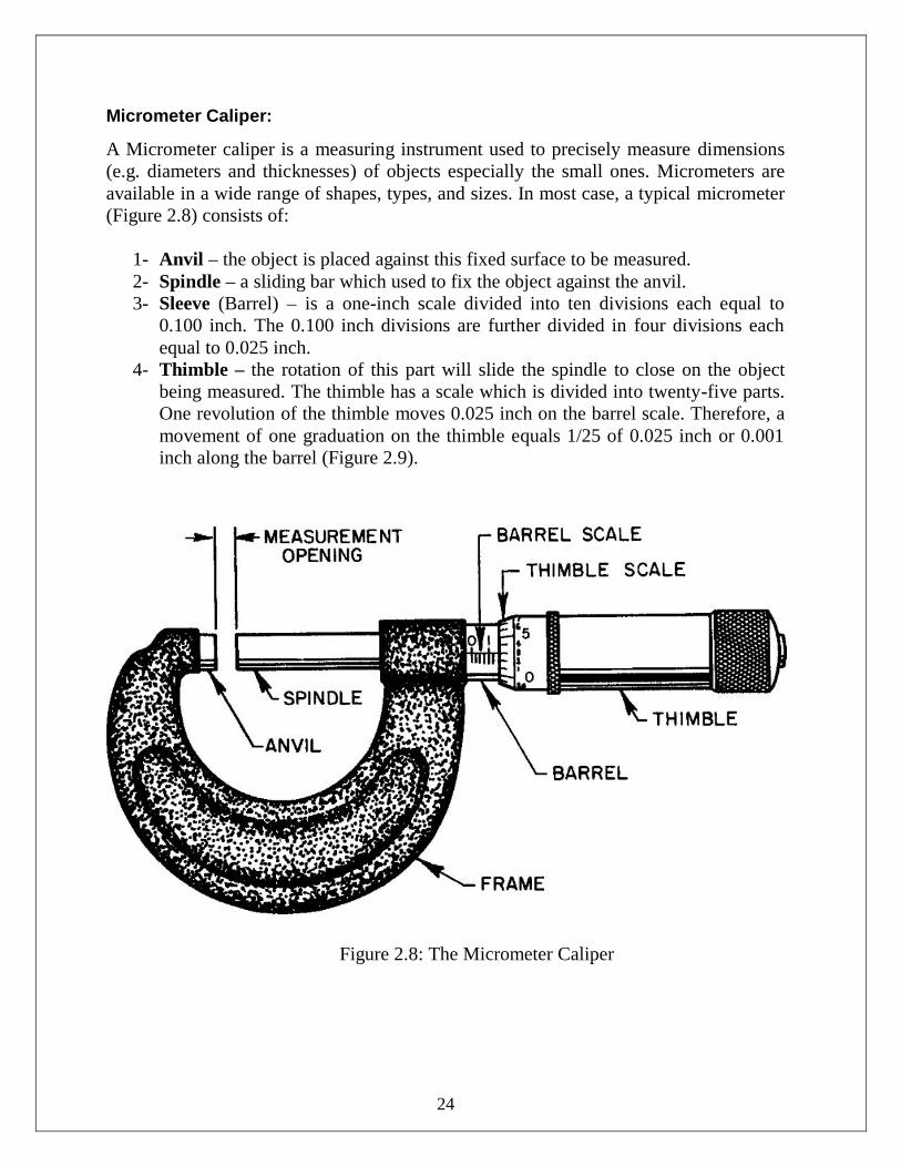
Micrometer Caliper:
A Micrometer caliper is a measuring instrument used to precisely measure dimensions (e.g. diameters and thicknesses) of objects especially the small ones. Micrometers are available in a wide range of shapes, types, and sizes. In most case, a typical micrometer (Figure 2.8) consists of:
1- Anvil – the object is placed against this fixed surface to be measured. 2- Spindle – a sliding bar which used to fix the object against the anvil. 3- Sleeve (Barrel) – is a one-inch scale divided into ten divisions each equal to
0.100 inch. The 0.100 inch divisions are further divided in four divisions each equal to 0.025 inch.
4- Thimble – the rotation of this part will slide the spindle to close on the object being measured. The thimble has a scale which is divided into twenty-five parts. One revolution of the thimble moves 0.025 inch on the barrel scale. Therefore, a movement of one graduation on the thimble equals 1/25 of 0.025 inch or 0.001 inch along the barrel (Figure 2.9).
Figure 2.8: The Micrometer Caliper
25
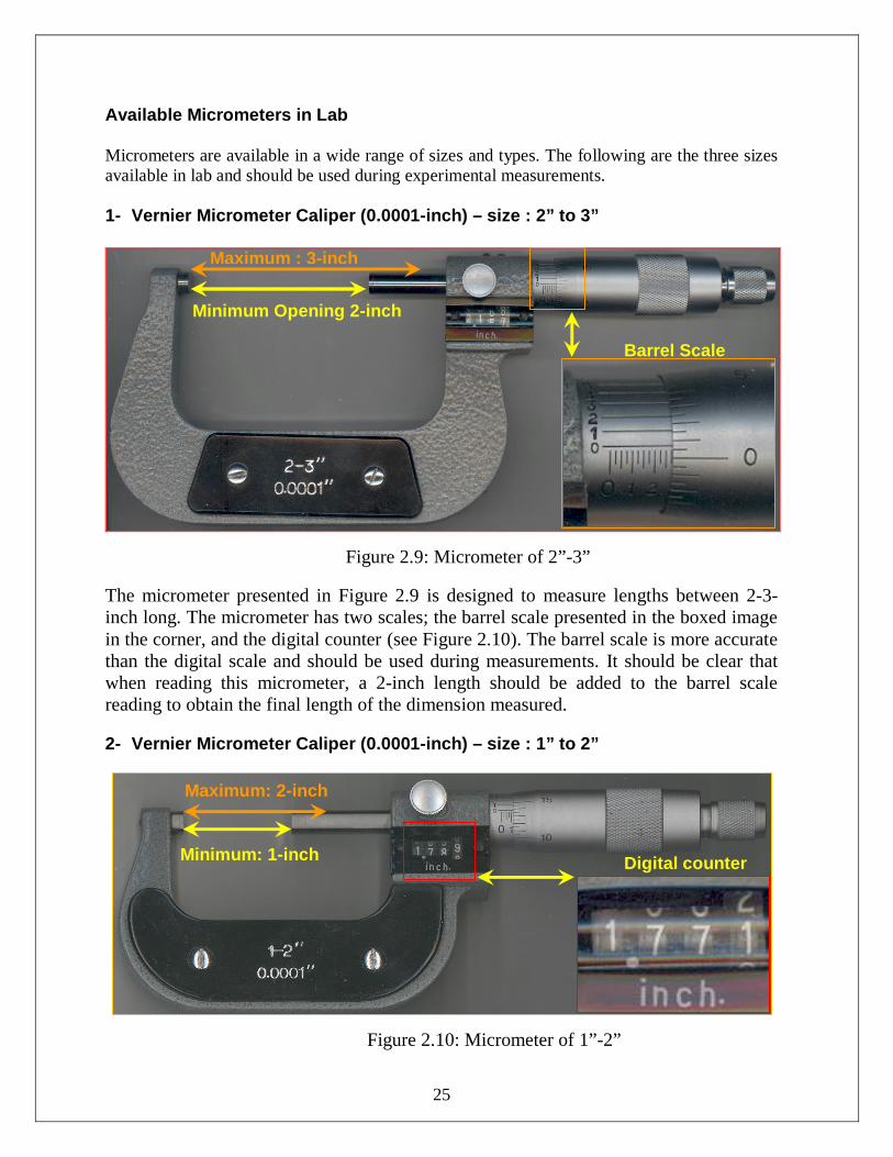
Available Micrometers in Lab Micrometers are available in a wide range of sizes and types. The following are the three sizes available in lab and should be used during experimental measurements. 1- Vernier Micrometer Caliper (0.0001-inch) – size : 2” to 3”
Figure 2.9: Micrometer of 2”-3”
The micrometer presented in Figure 2.9 is designed to measure lengths between 2-3-inch long. The micrometer has two scales; the barrel scale presented in the boxed image in the corner, and the digital counter (see Figure 2.10). The barrel scale is more accurate than the digital scale and should be used during measurements. It should be clear that when reading this micrometer, a 2-inch length should be added to the barrel scale reading to obtain the final length of the dimension measured.
2- Vernier Micrometer Caliper (0.0001-inch) – size : 1” to 2”
Figure 2.10: Micrometer of 1”-2”
Minimum Opening 2-inch
Maximum : 3-inch
Barrel Scale
Digital counter
Minimum: 1-inch
Maximum: 2-inch
26
The 1-2” micrometer works the same way as the 2-3” micrometer except that the minimum length can be measured is 1” and the maximum is 2”. The boxed picture in the corner shows the digital counter of the micrometer. The barrel scale is always preferred to be used over the digital counter.
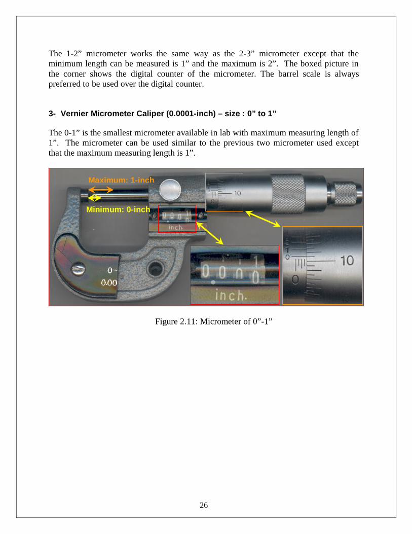
3- Vernier Micrometer Caliper (0.0001-inch) – size : 0” to 1”
The 0-1” is the smallest micrometer available in lab with maximum measuring length of 1”. The micrometer can be used similar to the previous two micrometer used except that the maximum measuring length is 1”.
Figure 2.11: Micrometer of 0”-1”
Minimum: 0-inch
Maximum: 1-inch
27
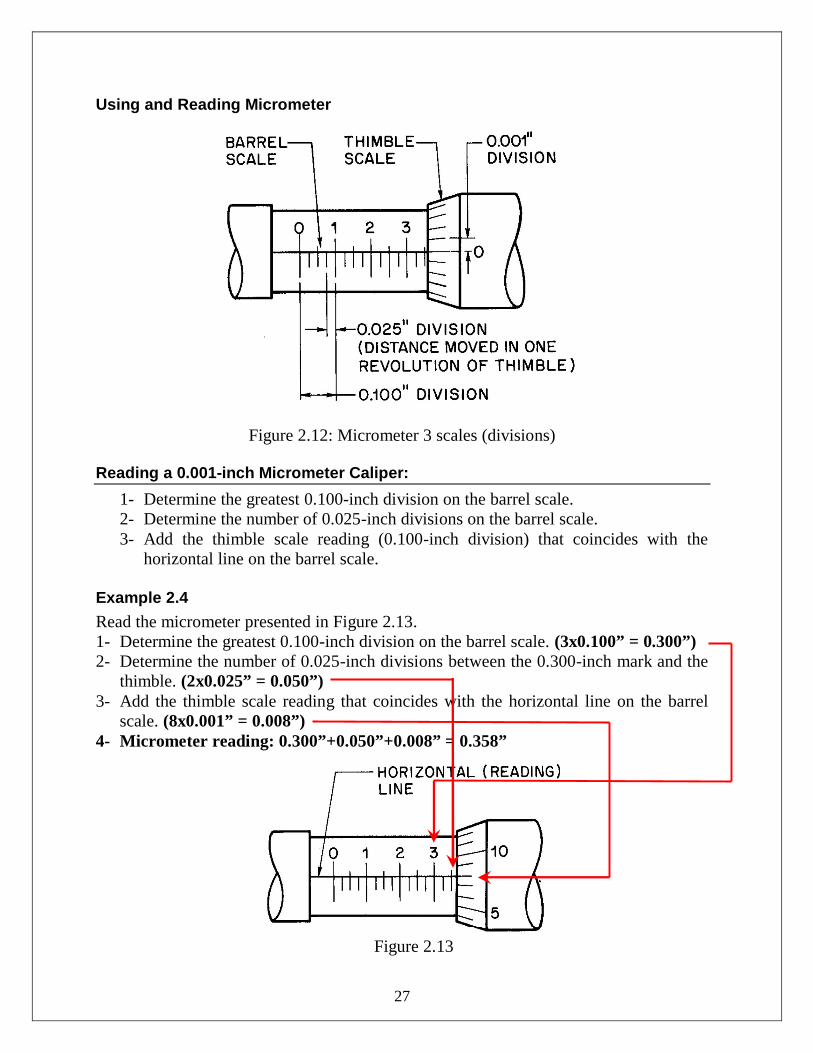
Using and Reading Micrometer
Figure 2.12: Micrometer 3 scales (divisions)
Reading a 0.001-inch Micrometer Caliper:
1- Determine the greatest 0.100-inch division on the barrel scale. 2- Determine the number of 0.025-inch divisions on the barrel scale. 3- Add the thimble scale reading (0.100-inch division) that coincides with the
horizontal line on the barrel scale. Example 2.4
Read the micrometer presented in Figure 2.13. 1- Determine the greatest 0.100-inch division on the barrel scale. (3x0.100” = 0.300”) 2- Determine the number of 0.025-inch divisions between the 0.300-inch mark and the
thimble. (2x0.025” = 0.050”) 3- Add the thimble scale reading that coincides with the horizontal line on the barrel
scale. (8x0.001” = 0.008”) 4- Micrometer reading: 0.300”+0.050”+0.008” = 0.358”
Figure 2.13
28
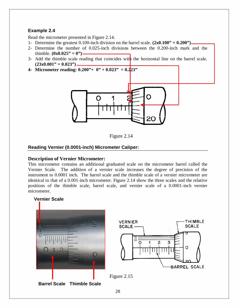
Example 2.4
Read the micrometer presented in Figure 2.14. 1- Determine the greatest 0.100-inch division on the barrel scale. (2x0.100” = 0.200”) 2- Determine the number of 0.025-inch divisions between the 0.200-inch mark and the
thimble. (0x0.025” = 0”) 3- Add the thimble scale reading that coincides with the horizontal line on the barrel scale.
(23x0.001” = 0.023”) 4- Micrometer reading: 0.200”+ 0” + 0.023” = 0.223”
Figure 2.14
Reading Vernier (0.0001-inch) Micrometer Caliper:
Description of Vernier Micrometer: This micrometer contains an additional graduated scale on the micrometer barrel called the Vernier Scale. The addition of a vernier scale increases the degree of precision of the instrument to 0.0001 inch. The barrel scale and the thimble scale of a vernier micrometer are identical to that of a 0.001-inch micrometer. Figure 2.14 show the three scales and the relative positions of the thimble scale, barrel scale, and vernier scale of a 0.0001-inch vernier micrometer.
Figure 2.15
Vernier Scale
Barrel Scale Thimble Scale
29
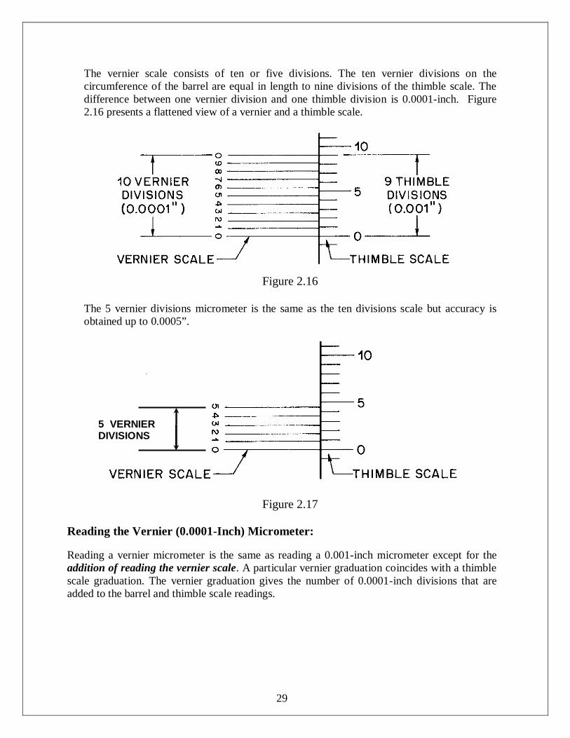
The vernier scale consists of ten or five divisions. The ten vernier divisions on the circumference of the barrel are equal in length to nine divisions of the thimble scale. The difference between one vernier division and one thimble division is 0.0001-inch. Figure 2.16 presents a flattened view of a vernier and a thimble scale.
Figure 2.16 The 5 vernier divisions micrometer is the same as the ten divisions scale but accuracy is obtained up to 0.0005”.
Figure 2.17
Reading the Vernier (0.0001-Inch) Micrometer: Reading a vernier micrometer is the same as reading a 0.001-inch micrometer except for the addition of reading the vernier scale. A particular vernier graduation coincides with a thimble scale graduation. The vernier graduation gives the number of 0.0001-inch divisions that are added to the barrel and thimble scale readings.
5 VERNIER DIVISIONS
30
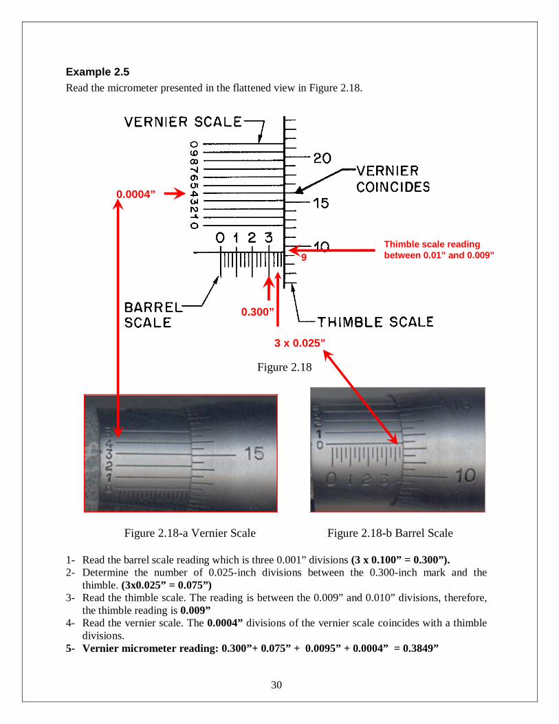
Example 2.5
Read the micrometer presented in the flattened view in Figure 2.18.
Figure 2.18
Figure 2.18-a Vernier Scale Figure 2.18-b Barrel Scale
1- Read the barrel scale reading which is three 0.001” divisions (3 x 0.100” = 0.300”). 2- Determine the number of 0.025-inch divisions between the 0.300-inch mark and the
thimble. (3x0.025” = 0.075”) 3- Read the thimble scale. The reading is between the 0.009” and 0.010” divisions, therefore,
the thimble reading is 0.009” 4- Read the vernier scale. The 0.0004” divisions of the vernier scale coincides with a thimble
divisions. 5- Vernier micrometer reading: 0.300”+ 0.075” + 0.0095” + 0.0004” = 0.3849”
0.300”
3 x 0.025”
9 Thimble scale reading between 0.01” and 0.009”
0.0004”
31
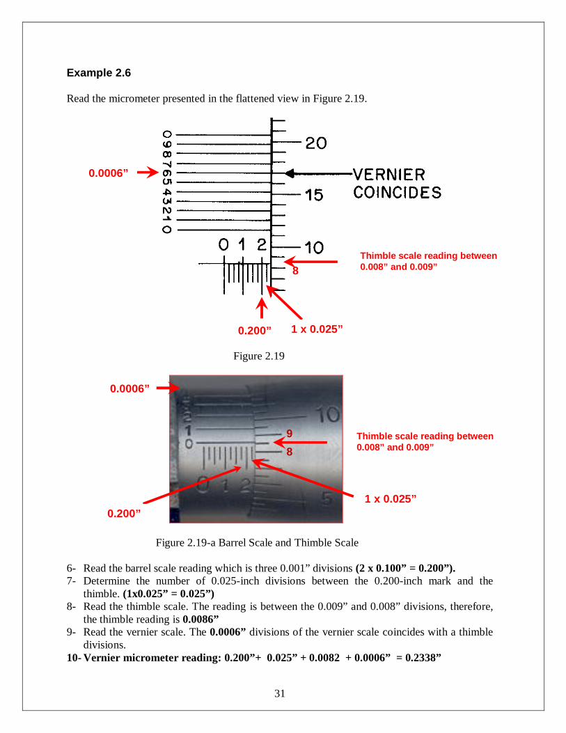
Example 2.6 Read the micrometer presented in the flattened view in Figure 2.19.
Figure 2.19
Figure 2.19-a Barrel Scale and Thimble Scale
6- Read the barrel scale reading which is three 0.001” divisions (2 x 0.100” = 0.200”). 7- Determine the number of 0.025-inch divisions between the 0.200-inch mark and the
thimble. (1x0.025” = 0.025”) 8- Read the thimble scale. The reading is between the 0.009” and 0.008” divisions, therefore,
the thimble reading is 0.0086” 9- Read the vernier scale. The 0.0006” divisions of the vernier scale coincides with a thimble
divisions. 10- Vernier micrometer reading: 0.200”+ 0.025” + 0.0082 + 0.0006” = 0.2338”
0.200” 1 x 0.025”
Thimble scale reading between 0.008” and 0.009”
0.0006”
8
0.200”
8 9
1 x 0.025”
Thimble scale reading between 0.008” and 0.009”
0.0006”
32
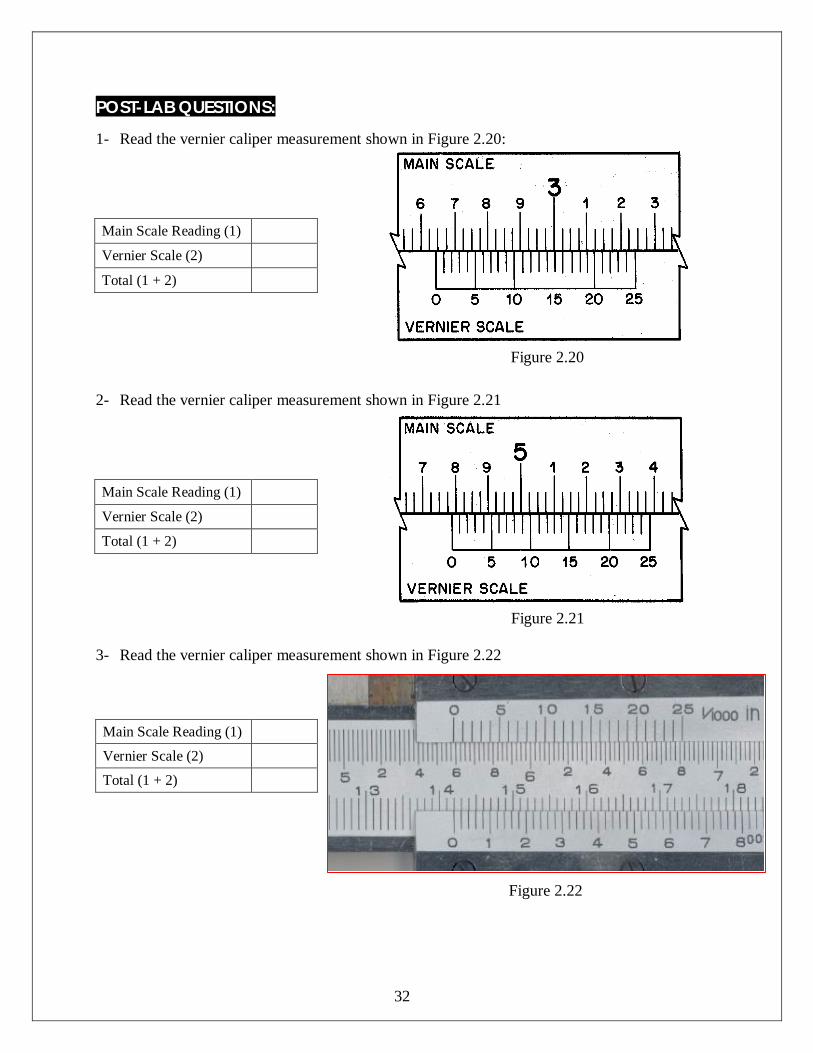
POST-LAB QUESTIONS: 1- Read the vernier caliper measurement shown in Figure 2.20:
Main Scale Reading (1)
Vernier Scale (2)
Total (1 + 2)
Figure 2.20 2- Read the vernier caliper measurement shown in Figure 2.21
Main Scale Reading (1)
Vernier Scale (2)
Total (1 + 2)
Figure 2.21 3- Read the vernier caliper measurement shown in Figure 2.22
Main Scale Reading (1)
Vernier Scale (2)
Total (1 + 2)
Figure 2.22
33
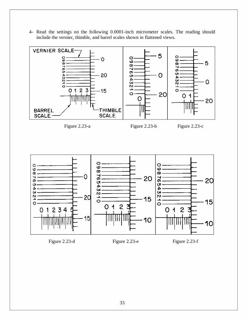
4- Read the settings on the following 0.0001-inch micrometer scales. The reading should include the vernier, thimble, and barrel scales shown in flattened views.
Figure 2.23-a Figure 2.23-b Figure 2.23-c
Figure 2.23-d Figure 2.23-e Figure 2.23-f
34
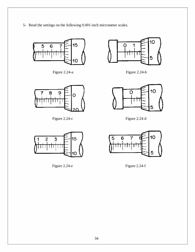
5- Read the settings on the following 0.001-inch micrometer scales.
Figure 2.24-a Figure 2.24-b
Figure 2.24-c Figure 2.24-d
Figure 2.24-e Figure 2.24-f
35
Lab 2: Vernier Caliper & Micrometer
Experiment Data Sheet
Name: -------------------- Date: --------------------- Instructor Initial: ---------------------
Vernier Caliper
No. Object Description
Dimension Measured (width, thickness..etc)
Main Scale Reading (1)
Vernier Scale Reading (2)
Total Reading (1) + (2)
Micrometer Caliper:
No. Object Descrip.
Dimension Measured
Barrel Scale Reading
(1) (0.1 divisions)
Sub-Barrel Scale Reading
(2) (0.025 divisions)
Thimble Scale (3)
Vernier Scale (4)
Total Reading (1) + (2) + (3) + (4)
36
Lab 3: Tensile Test of Brittle and Ductile Metals (Clockhouse Machine)
Objective
The aim of tensile test experiment of brittle and ductile metals is to discuses the basic concept of stress and strain. Experimental methods will be used to show the relationship between stress and strain and determine the mechanical properties for specific materials which include: 1. Proportional Limit 2. Modulus of Elasticity 3. Ductility 4. Percent Elongation 5. Ultimate Strength 6. Yield Points (Upper and Lower) Introduction
The strength of a material depends on its ability to sustain a load without undue deformation or failure. This property is inherent in the materials itself and must be determined by experiment. One of the most important tests to perform in this regard is the tension test. Although many important mechanical properties of a material can be determined from this test, it is used primarily to determine the relationship between the average normal stress and average normal strain in many engineering materials such as metals, ceramics, polymers, and composites.
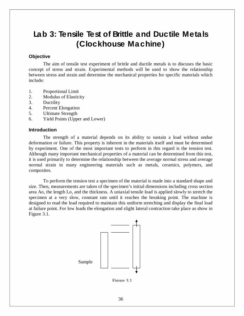
To perform the tension test a specimen of the material is made into a standard shape and size. Then, measurements are taken of the specimen’s initial dimensions including cross section area Ao, the length Lo, and the thickness. A uniaxial tensile load is applied slowly to stretch the specimen at a very slow, constant rate until it reaches the breaking point. The machine is designed to read the load required to maintain this uniform stretching and display the final load at failure point. For low loads the elongation and slight lateral contraction take place as show in Figure 3.1.
Sample
Figure 3.1
37
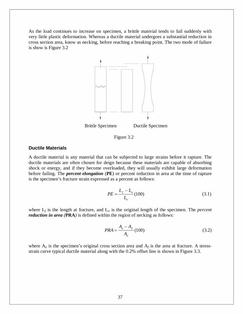
As the load continues to increase on specimen, a brittle material tends to fail suddenly with very little plastic deformation. Whereas a ductile material undergoes a substantial reduction in cross section area, know as necking, before reaching a breaking point. The two mode of failure is show is Figure 3.2
Figure 3.2
Ductile Materials A ductile material is any material that can be subjected to large strains before it rapture. The ductile materials are often chosen for deign because these materials are capable of absorbing shock or energy, and if they become overloaded, they will usually exhibit large deformation before failing. The percent elongation (PE) or percent reduction in area at the time of rapture is the specimen’s fracture strain expressed as a percent as follows:
)100(o
of
LLL
PE
(3.1)
where Lf is the length at fracture, and Lo is the original length of the specimen. The percent reduction in area (PRA) is defined within the region of necking as follows:
)100(o
fo
AAA
PRA
(3.2)
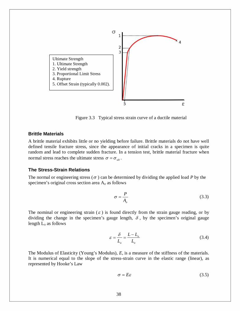
where Ao is the specimen’s original cross section area and Af is the area at fracture. A stress-strain curve typical ductile material along with the 0.2% offset line is shown in Figure 3.3.
Brittle Specimen Ductile Specimen
38
Figure 3.3 Typical stress strain curve of a ductile material Brittle Materials
A brittle material exhibits little or no yielding before failure. Brittle materials do not have well defined tensile fracture stress, since the appearance of initial cracks in a specimen is quite random and lead to complete sudden fracture. In a tension test, brittle material fracture when normal stress reaches the ultimate stress ult . The Stress-Strain Relations
The normal or engineering stress ( ) can be determined by dividing the applied load P by the specimen’s original cross section area Ao as follows
oA
P (3.3)
The nominal or engineering strain ( ) is found directly from the strain gauge reading, or by dividing the change in the specimen’s gauge length, , by the specimen’s original gauge length Lo as follows
o
o
o LLL
L
(3.4)
The Modulus of Elasticity (Young’s Modulus), E, is a measure of the stiffness of the materials. It is numerical equal to the slope of the stress-strain curve in the elastic range (linear), as represented by Hooke’s Law E (3.5)
Ultimate Strength 1. Ultimate Strength 2. Yield strength 3. Proportional Limit Stress 4. Rupture 5. Offset Strain (typically 0.002).
39
Brittle materials such as concrete and carbon fiber do not have a yield point, and do not strain-harden which means that the ultimate strength and breaking strength are the same. A stress-strain curve for a typical brittle material is shown in the Figure 3.4.
Figure 3.4 Typical stress strain curve of a brittle material
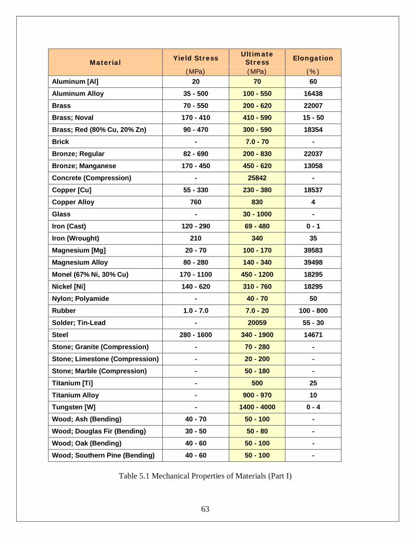
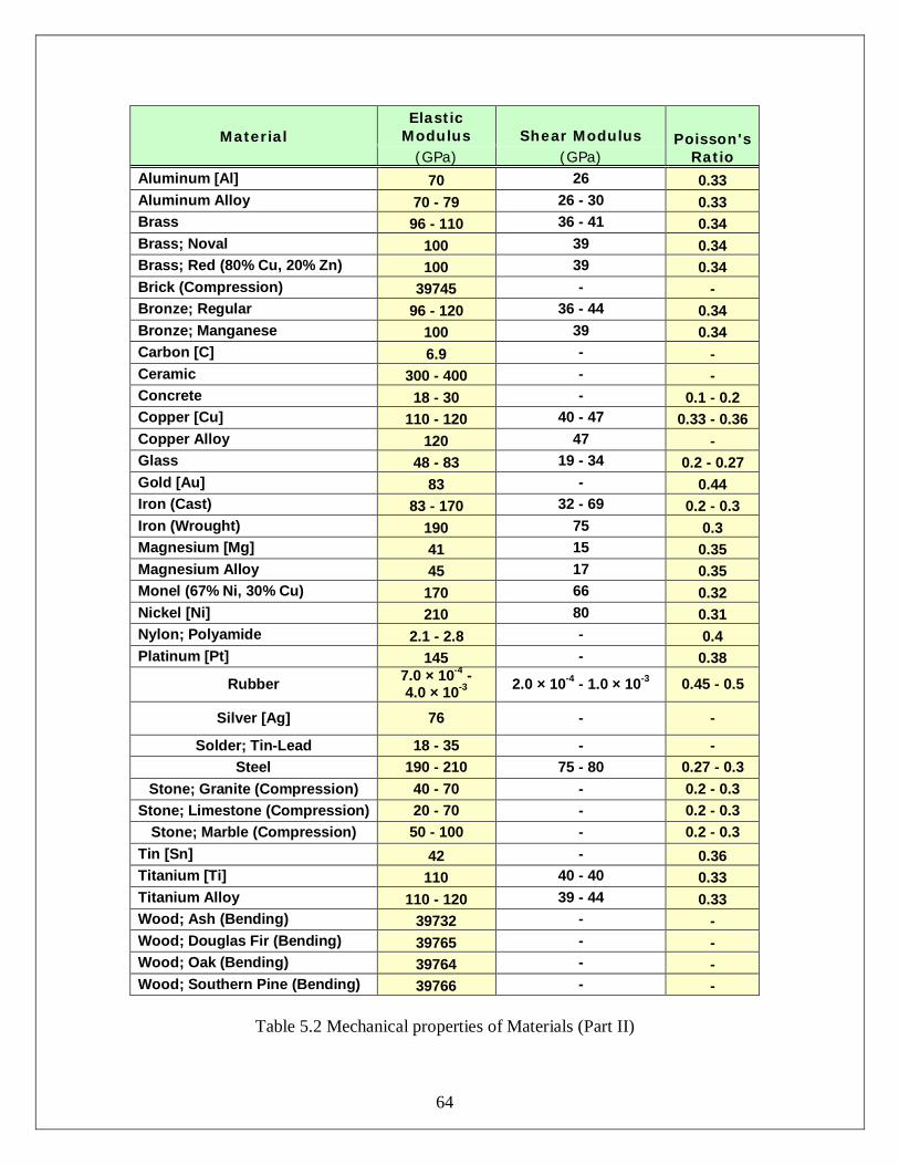
Some typical tensile strengths of some materials are listed in Tables 3.1 and 3.2:
Table 3.1
Ultimate Strength Rupture
40
Table 3.2
Procedure for the Clockhouse Machine: BEFORE YOU BEGIN THE EXERIMENT: Measure all specimens with micrometer or calipers before testing
Turn panel switch on, on the back of the digital control unit. Allow 15 minutes for warm-
up.
All letters in parenthesis ( ) are referring to controls shown in Figure 3.5 and Figure 3.6.
41
Figure 3.5 Control Panel of Clockhouse Machine
(A) (B)
(C)
Control Panel
42
Figure 3.6 Clockhouse Tension Machine
Top Jaw
Bottom Jaw
Rapid Up
Rapid Down
Top Jaw Handle (K)
Lower Jaw Handle (J)
(D) (E) (F) (G)
(H)
(I) Lower part of the machine
43
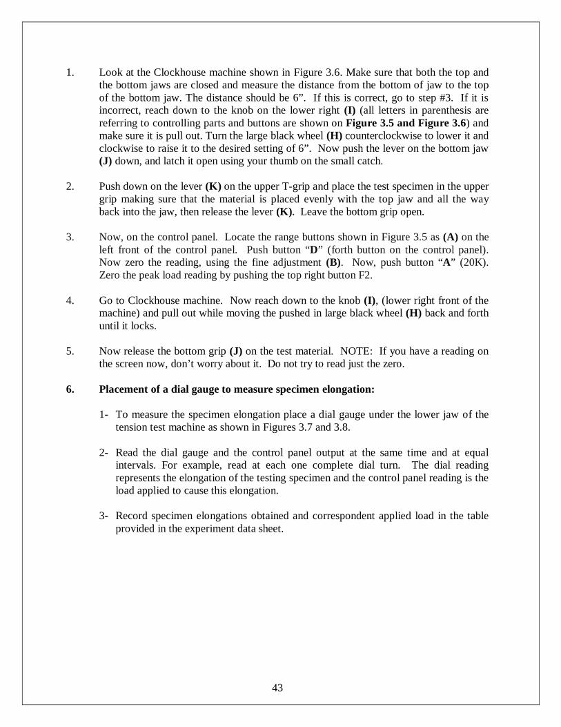
1. Look at the Clockhouse machine shown in Figure 3.6. Make sure that both the top and the bottom jaws are closed and measure the distance from the bottom of jaw to the top of the bottom jaw. The distance should be 6”. If this is correct, go to step #3. If it is incorrect, reach down to the knob on the lower right (I) (all letters in parenthesis are referring to controlling parts and buttons are shown on Figure 3.5 and Figure 3.6) and make sure it is pull out. Turn the large black wheel (H) counterclockwise to lower it and clockwise to raise it to the desired setting of 6”. Now push the lever on the bottom jaw (J) down, and latch it open using your thumb on the small catch.
2. Push down on the lever (K) on the upper T-grip and place the test specimen in the upper
grip making sure that the material is placed evenly with the top jaw and all the way back into the jaw, then release the lever (K). Leave the bottom grip open.
3. Now, on the control panel. Locate the range buttons shown in Figure 3.5 as (A) on the
left front of the control panel. Push button “D” (forth button on the control panel). Now zero the reading, using the fine adjustment (B). Now, push button “A” (20K). Zero the peak load reading by pushing the top right button F2.
4. Go to Clockhouse machine. Now reach down to the knob (I), (lower right front of the machine) and pull out while moving the pushed in large black wheel (H) back and forth until it locks.
5. Now release the bottom grip (J) on the test material. NOTE: If you have a reading on
the screen now, don’t worry about it. Do not try to read just the zero.
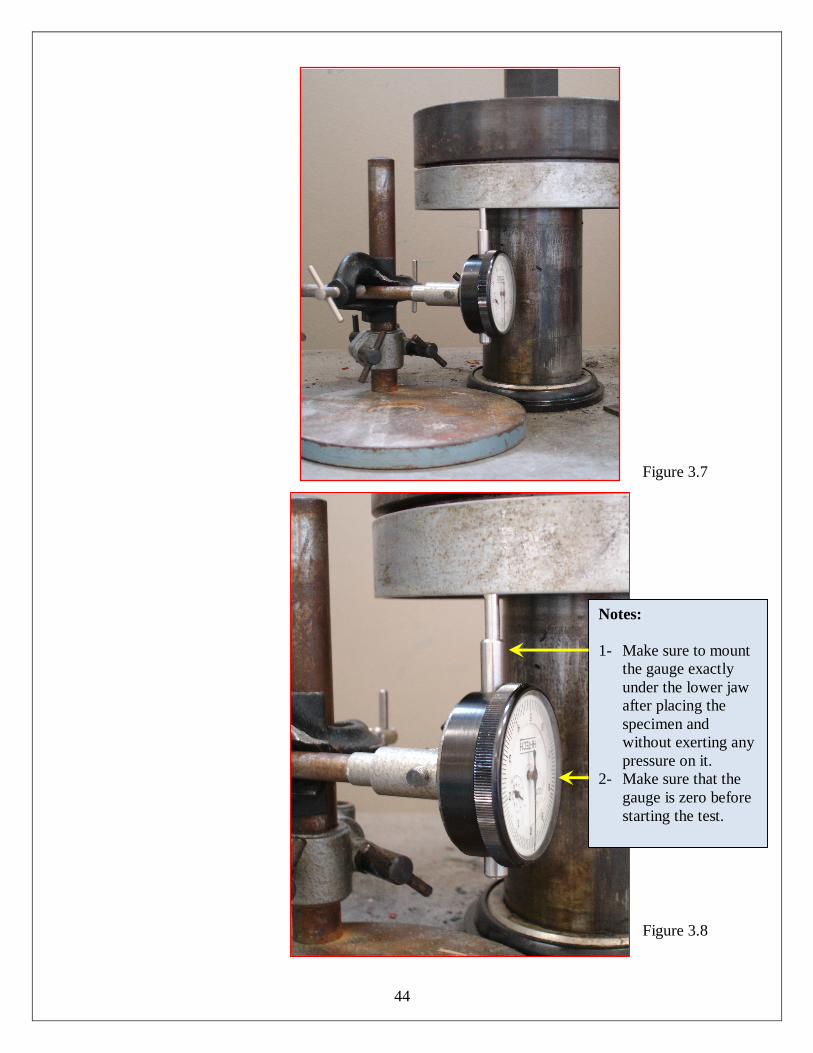
6. Placement of a dial gauge to measure specimen elongation: 1- To measure the specimen elongation place a dial gauge under the lower jaw of the
tension test machine as shown in Figures 3.7 and 3.8.
2- Read the dial gauge and the control panel output at the same time and at equal intervals. For example, read at each one complete dial turn. The dial reading represents the elongation of the testing specimen and the control panel reading is the load applied to cause this elongation.
3- Record specimen elongations obtained and correspondent applied load in the table
provided in the experiment data sheet.
44
Figure 3.7
Figure 3.8
Notes: 1- Make sure to mount
the gauge exactly under the lower jaw after placing the specimen and without exerting any pressure on it.
2- Make sure that the gauge is zero before starting the test.
45
7. Before you begin the test, turn the feed control (D) on the control column to the desired feed rate. The dial is calibrated in MM/MIN. One full turn equals 1 mm travel per minute. For most material, .5 – 1 MM/MIN is sufficient.
8. Note the lower set of three buttons (Figure 3.6) on the control column that say stop (E),
up (F) and down (G).
NOTE: All readings in the tension mode are negative.
9. Watch the reading on the control panel. When the peak reading has been reached the yield point of the material has also been reached, even though the specimen has not broken. In a short time, the reading will begin to reverse before breaking the material.
NOTE: The peak load reading will remain until cleared by pushing button (C)
10. Stop the machine by pushing button (F) on the control column. Graphs: Plot stress-
strain diagrams for all specimens up to failure using one graph for each type of metal. Show all quantities that can be determined from the diagrams on the same graph.
POST-LAB QUESTIONS:
1- Calculate: PE, PRA, stress, strain, and modulus of elasticity for all specimens.
2- Determine the type of metal used for the test based on the comparison between results obtained experimentally and values given in METALS HANDBOOK or your texts on strength of materials/or use tables listed above.
3- What is the ultimate strength and how can be determined?
4- Determine the type of materials being tested – Is it brittle or ductile
46
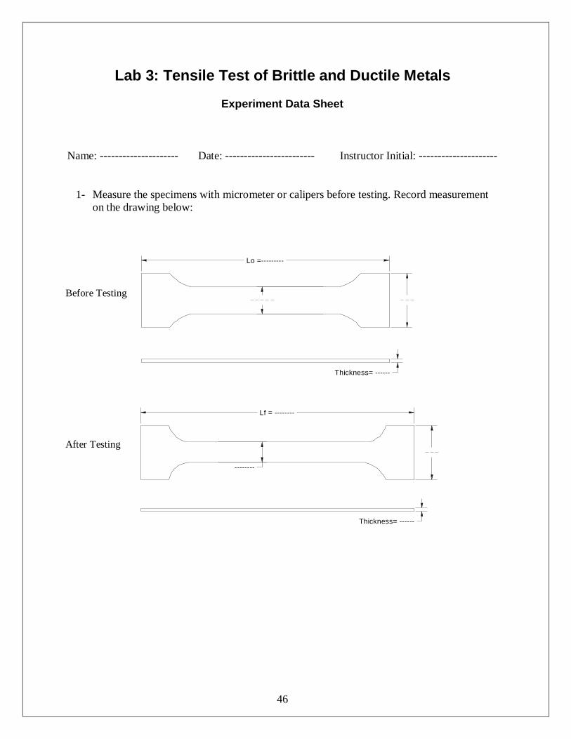
Lab 3: Tensile Test of Brittle and Ductile Metals
Experiment Data Sheet
Name: --------------------- Date: ------------------------ Instructor Initial: ---------------------
1- Measure the specimens with micrometer or calipers before testing. Record measurement
on the drawing below:
Lo =---------
Thickness= ------
Lf = --------
Thickness= ------
--------
Before Testing
After Testing
47
Lab 3: Tensile Test of Brittle and Ductile Metals
Experiment Data Sheet
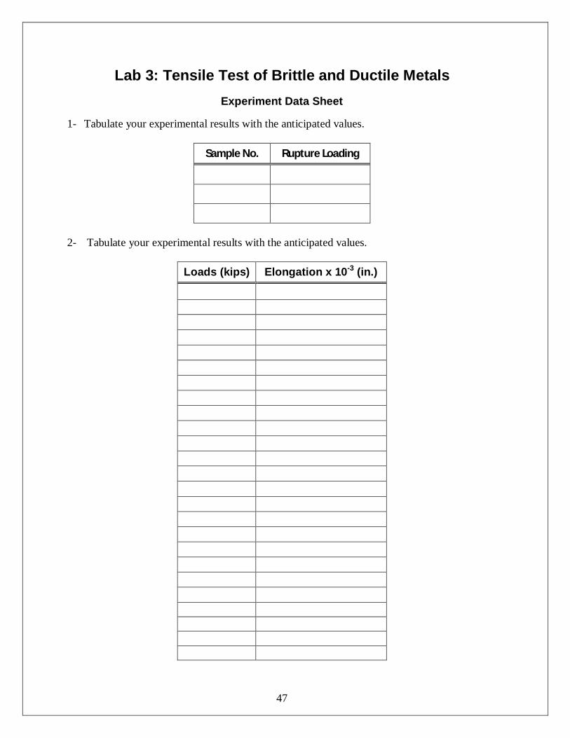
1- Tabulate your experimental results with the anticipated values.
Sample No. Rupture Loading
2- Tabulate your experimental results with the anticipated values.
Loads (kips) Elongation x 10-3 (in.)
48
Lab 4: Flexure in Wood (Universal Testing Machine)
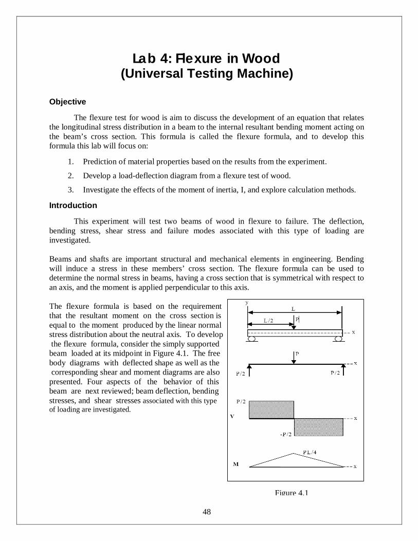
Objective
The flexure test for wood is aim to discuss the development of an equation that relates the longitudinal stress distribution in a beam to the internal resultant bending moment acting on the beam’s cross section. This formula is called the flexure formula, and to develop this formula this lab will focus on:
1. Prediction of material properties based on the results from the experiment.
2. Develop a load-deflection diagram from a flexure test of wood.
3. Investigate the effects of the moment of inertia, I, and explore calculation methods. Introduction
This experiment will test two beams of wood in flexure to failure. The deflection,
bending stress, shear stress and failure modes associated with this type of loading are investigated.
Beams and shafts are important structural and mechanical elements in engineering. Bending will induce a stress in these members’ cross section. The flexure formula can be used to determine the normal stress in beams, having a cross section that is symmetrical with respect to an axis, and the moment is applied perpendicular to this axis. The flexure formula is based on the requirement that the resultant moment on the cross section is equal to the moment produced by the linear normal stress distribution about the neutral axis. To develop the flexure formula, consider the simply supported beam loaded at its midpoint in Figure 4.1. The free body diagrams with deflected shape as well as the corresponding shear and moment diagrams are also presented. Four aspects of the behavior of this beam are next reviewed; beam deflection, bending stresses, and shear stresses associated with this type of loading are investigated.
Figure 4.1
49
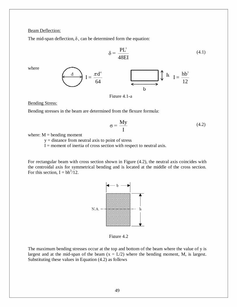
Beam Deflection:
The mid-span deflection, δ , can be determined form the equation:
3PLδ =
48EI (4.1)
where
4dI =
64
3hbI = 12
Bending Stress:
Bending stresses in the beam are determined from the flexure formula:
Myσ = I
(4.2)
where: M = bending moment y = distance from neutral axis to point of stress I = moment of inertia of cross section with respect to neutral axis. For rectangular beam with cross section shown in Figure (4.2), the neutral axis coincides with the centroidal axis for symmetrical bending and is located at the middle of the cross section. For this section, I = bh3/12.
The maximum bending stresses occur at the top and bottom of the beam where the value of y is largest and at the mid-span of the beam (x = L/2) where the bending moment, M, is largest. Substituting these values in Equation (4.2) as follows
Figure 4.2
Figure 4.1-a
50
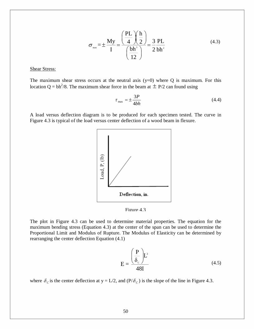
3max 2
PL hMy 3 PL4 2=
bhI 2 bh12
(4.3)
Shear Stress: The maximum shear stress occurs at the neutral axis (y=0) where Q is maximum. For this location Q = bh2/8. The maximum shear force in the beam at P/2 can found using
bhP
43
max (4.4)
A load versus deflection diagram is to be produced for each specimen tested. The curve in Figure 4.3 is typical of the load versus center deflection of a wood beam in flexure. The plot in Figure 4.3 can be used to determine material properties. The equation for the maximum bending stress (Equation 4.3) at the center of the span can be used to determine the Proportional Limit and Modulus of Rupture. The Modulus of Elasticity can be determined by rearranging the center deflection Equation (4.1)
C
3P Lδ
E = 48I
(4.5)
where C is the center deflection at y = L/2, and (P/ C ) is the slope of the line in Figure 4.3.
Figure 4.3
51
The modulus of rupture is the maximum stress obtained using
Mcσ = I
(4.6)
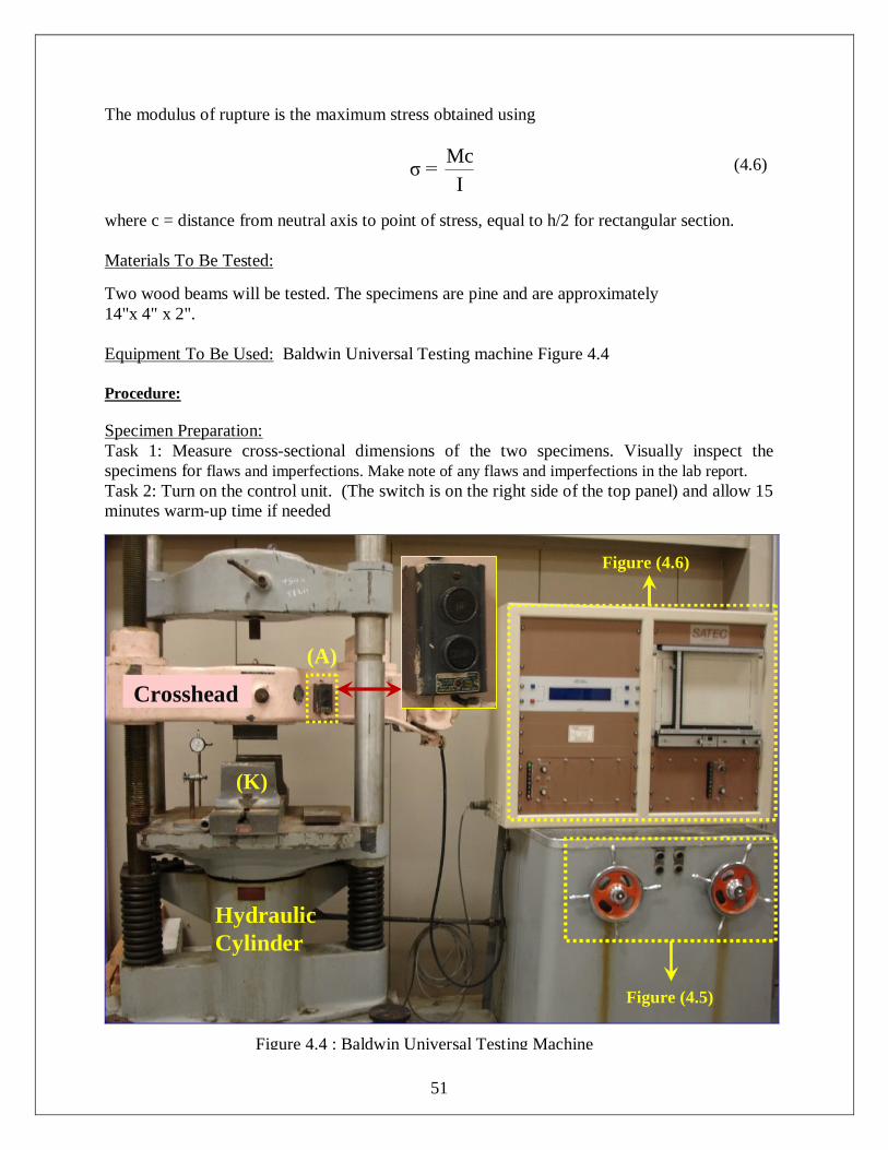
where c = distance from neutral axis to point of stress, equal to h/2 for rectangular section. Materials To Be Tested: Two wood beams will be tested. The specimens are pine and are approximately 14"x 4" x 2". Equipment To Be Used: Baldwin Universal Testing machine Figure 4.4 Procedure: Specimen Preparation: Task 1: Measure cross-sectional dimensions of the two specimens. Visually inspect the specimens for flaws and imperfections. Make note of any flaws and imperfections in the lab report. Task 2: Turn on the control unit. (The switch is on the right side of the top panel) and allow 15 minutes warm-up time if needed
Figure 4.4 : Baldwin Universal Testing Machine
Hydraulic Cylinder
(K)
Crosshead (A)
Figure (4.5)
Figure (4.6)
52
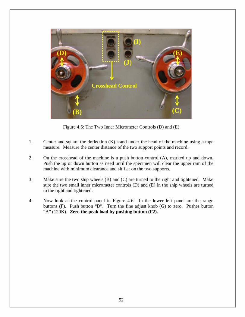
Figure 4.5: The Two Inner Micrometer Controls (D) and (E)
1. Center and square the deflection (K) stand under the head of the machine using a tape
measure. Measure the center distance of the two support points and record.
2. On the crosshead of the machine is a push button control (A), marked up and down. Push the up or down button as need until the specimen will clear the upper ram of the machine with minimum clearance and sit flat on the two supports.
3. Make sure the two ship wheels (B) and (C) are turned to the right and tightened. Make
sure the two small inner micrometer controls (D) and (E) in the ship wheels are turned to the right and tightened.
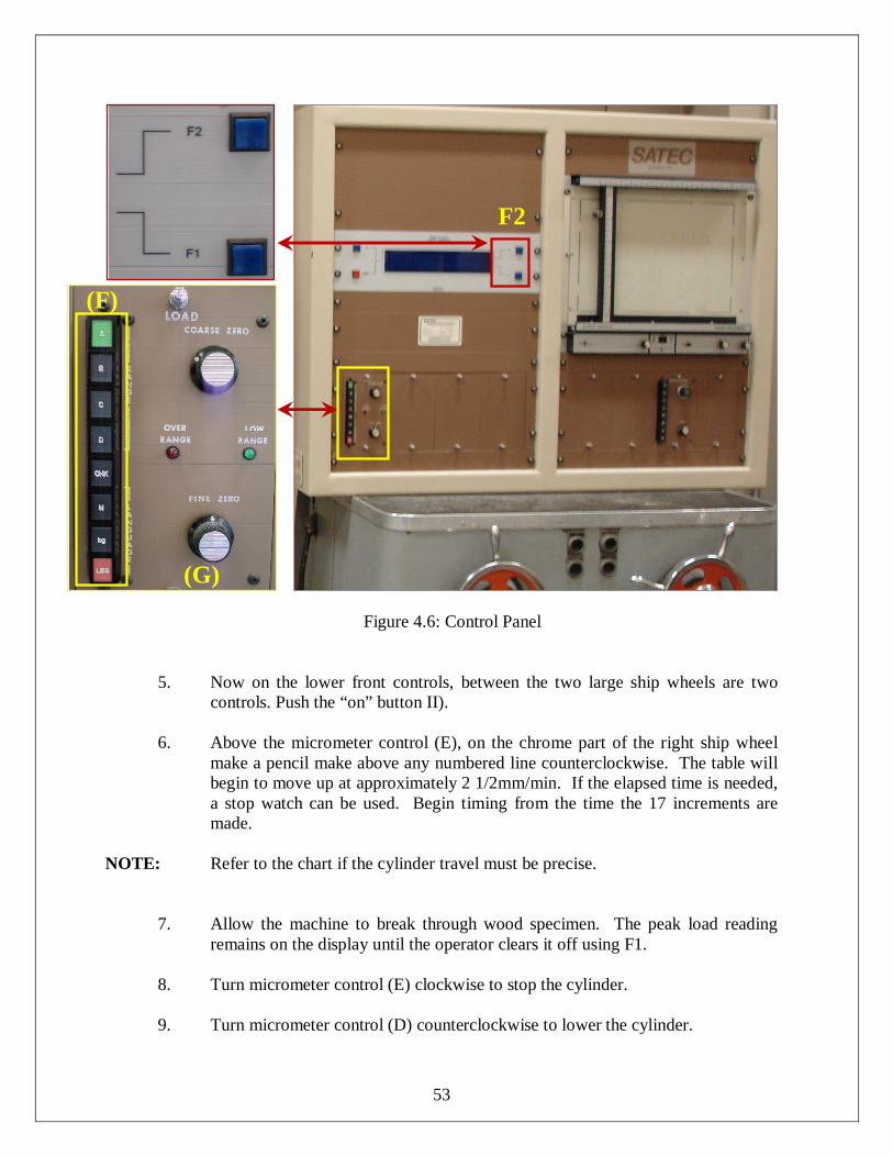
4. Now look at the control panel in Figure 4.6. In the lower left panel are the range
buttons (F). Push button “D”. Turn the fine adjust knob (G) to zero. Pushes button “A” (120K). Zero the peak load by pushing button (F2).
(E) (D) (I)
(J)
Crosshead Control
(C) (B)
53
Figure 4.6: Control Panel
5. Now on the lower front controls, between the two large ship wheels are two controls. Push the “on” button II).
6. Above the micrometer control (E), on the chrome part of the right ship wheel make a pencil make above any numbered line counterclockwise. The table will begin to move up at approximately 2 1/2mm/min. If the elapsed time is needed, a stop watch can be used. Begin timing from the time the 17 increments are made.
NOTE: Refer to the chart if the cylinder travel must be precise.
7. Allow the machine to break through wood specimen. The peak load reading remains on the display until the operator clears it off using F1.
8. Turn micrometer control (E) clockwise to stop the cylinder.
9. Turn micrometer control (D) counterclockwise to lower the cylinder.
F2
(G)
(F)
54
10. Now return control (D) to the off position (clockwise).
11. Turn machine off by pushing button (J). The above test should be repeated with another specimen, this time placing it on the edge instead of the flat. Observe the difference the load required to break the specimen. Post-lab Questions: 1. Determine the following properties for each wood specimen.
a. Proportional Limit of specimen b. Maximum shear stress in the specimen at failure c. Maximum bending stress in the specimen at failure d. Modulus of Elasticity
2. Discuss the results, possible sources of error and other conclusions relevant to TASK 1.
3. Plot applied load P versus the deflection obtained.
4. Is there any difference between the stresses measured at the top of the beam and at the same
location (at the same section) on the bottom of the beam? If so, explain
55
Lab 4: Flexure in Wood
Experiment Data Sheet
1- Tabulate your experimental results with the anticipated values.
Sample No. Loading
2- Tabulate your experimental results with the anticipated values.
Loads (kips) deflection (in.)
56
Lab 5: Tensile Test of Brittle and Ductile Metals (INSTRON)
Objective
The tensile test for brittle and ductile metals experiment is aim to discuss the basic concept of stress and strain. The experiment will show the relationship between stress and strain using experimental methods and determine the mechanical properties for specific materials which include: 7. Proportional Limit 8. Modulus of Elasticity 9. Ductility 10. Percent Elongation 11. Ultimate Strength 12. Yield Points (Upper and Lower) Introduction
A materials test involves subjecting a specimen of a material to forces, compressive (crushing), tensile (pulling), deflectional (bending), or torsional (twisting). In conjunction with accessories to your system, you can also test for other properties, such as frictional and peel resistance, and do tests under varying environmental conditions, such as temperature and pressure. The system automatically measures the forces applied to the material and the resulting behavior of the material, and will calculate many of the physical properties of the material, such as strength, brittleness, ductility, etc.
The strength of a material depends on its ability to sustain a load without undue deformation or failure. This property is inherent in the materials itself and must be determined by experiment. One of the most important tests to perform in this regard is the tension test. Although many important mechanical properties of a material can be determined from this test, it is used primarily to determine the relationship between the average normal stress and average normal strain in many engineering materials such as metals, ceramics, polymers, and composites.
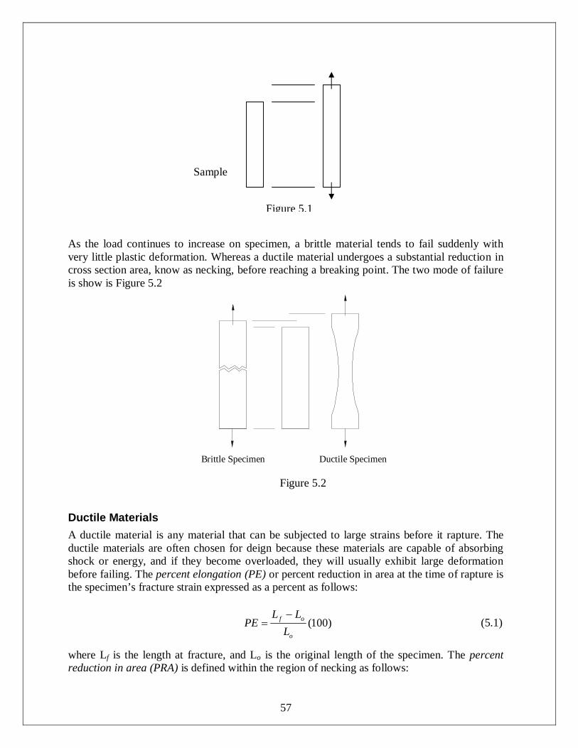
To perform the tension test a specimen of the material is made into a standard shape and size. Then, measurements are taken of the specimen’s initial dimensions including cross section area Ao, the length Lo, and the thickness. A uniaxial tensile load is applied slowly to stretch the specimen at a very slow, constant rate until it reaches the breaking point. The machine is designed to read the load required to maintain this uniform stretching and display the final load at failure point. For low loads the elongation and slight lateral contraction take place as show in Figure 5.1.
57
As the load continues to increase on specimen, a brittle material tends to fail suddenly with very little plastic deformation. Whereas a ductile material undergoes a substantial reduction in cross section area, know as necking, before reaching a breaking point. The two mode of failure is show is Figure 5.2
Figure 5.2 Ductile Materials
A ductile material is any material that can be subjected to large strains before it rapture. The ductile materials are often chosen for deign because these materials are capable of absorbing shock or energy, and if they become overloaded, they will usually exhibit large deformation before failing. The percent elongation (PE) or percent reduction in area at the time of rapture is the specimen’s fracture strain expressed as a percent as follows:
)100(o
of
LLL
PE
(5.1)
where Lf is the length at fracture, and Lo is the original length of the specimen. The percent reduction in area (PRA) is defined within the region of necking as follows:
Sample
Brittle Specimen Ductile Specimen
Figure 5.1
58
)100(o
fo
AAA
PRA
(5.2)
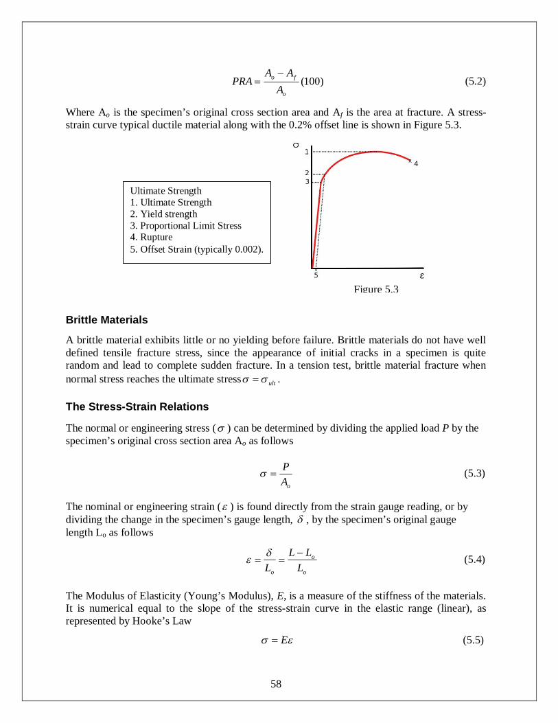
Where Ao is the specimen’s original cross section area and Af is the area at fracture. A stress-strain curve typical ductile material along with the 0.2% offset line is shown in Figure 5.3.
Brittle Materials
A brittle material exhibits little or no yielding before failure. Brittle materials do not have well defined tensile fracture stress, since the appearance of initial cracks in a specimen is quite random and lead to complete sudden fracture. In a tension test, brittle material fracture when normal stress reaches the ultimate stress ult . The Stress-Strain Relations The normal or engineering stress ( ) can be determined by dividing the applied load P by the specimen’s original cross section area Ao as follows
oA
P (5.3)
The nominal or engineering strain ( ) is found directly from the strain gauge reading, or by dividing the change in the specimen’s gauge length, , by the specimen’s original gauge length Lo as follows
o
o
o LLL
L
(5.4)
The Modulus of Elasticity (Young’s Modulus), E, is a measure of the stiffness of the materials. It is numerical equal to the slope of the stress-strain curve in the elastic range (linear), as represented by Hooke’s Law
E (5.5)
Figure 5.3
Ultimate Strength 1. Ultimate Strength 2. Yield strength 3. Proportional Limit Stress 4. Rupture 5. Offset Strain (typically 0.002).
59
Brittle materials such as concrete and carbon fiber do not have a yield point, and do not strain-harden which means that the ultimate strength and breaking strength are the same. A stress-strain curve for a typical brittle material is shown in the Figure 5.4.
Figure 5.4 Stress vs. Strain curve typical of a brittle material Typical tensile strengths of some materials are listed in Tables 5.1 and 5.2 on page 62. Procedure:
1. Obtain the desired materials specimen for testing.
2. Measure the specimen initial dimensions indicated in the data sheet using a vernier caliper
or a micrometer. The length of the specimen should be measured before (Lo) and after (L) the test.
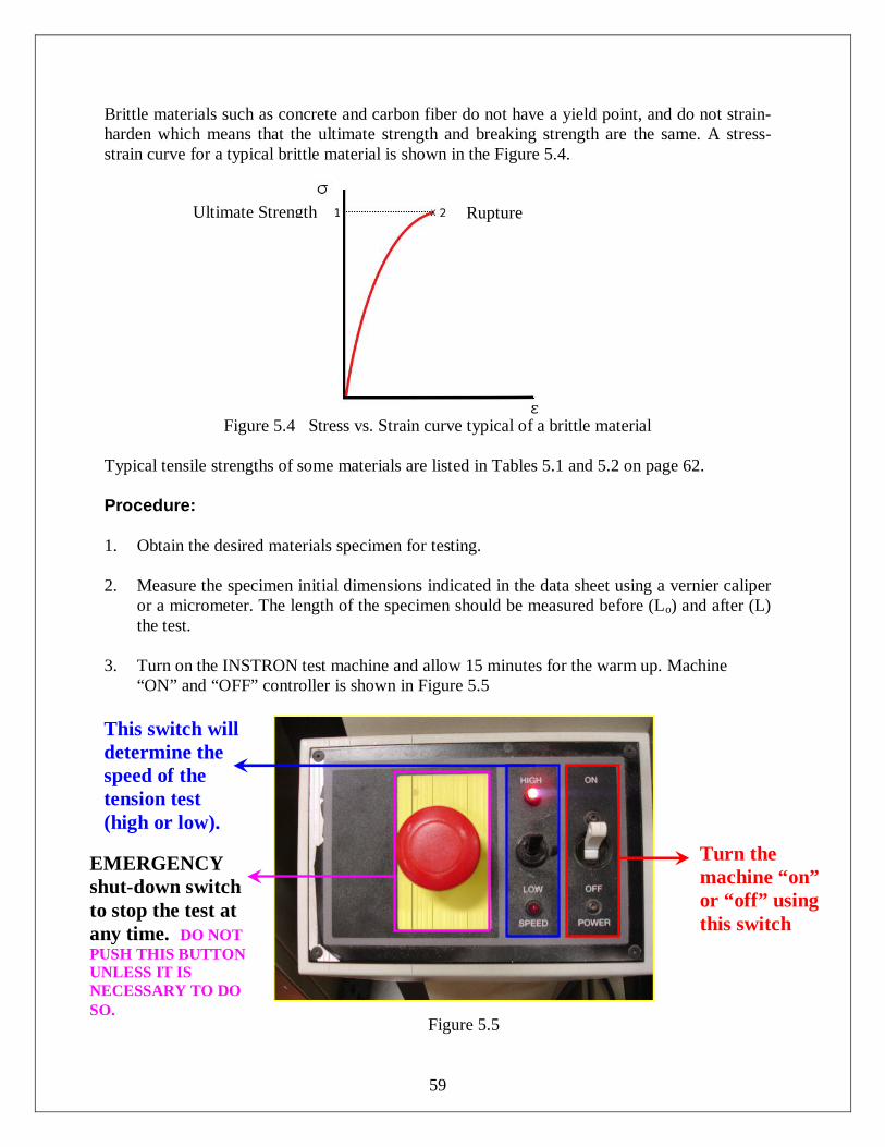
3. Turn on the INSTRON test machine and allow 15 minutes for the warm up. Machine
“ON” and “OFF” controller is shown in Figure 5.5
Figure 5.5
Ultimate Strength Rupture
Turn the machine “on” or “off” using this switch
This switch will determine the speed of the tension test (high or low).
EMERGENCY shut-down switch to stop the test at any time. DO NOT PUSH THIS BUTTON UNLESS IT IS NECESSARY TO DO SO.
60
4. Turn on the computer attached to the INSTRON test machine.
5. Launch the “Marlin” program on the computer, which will interface with the INSTRON machine for the test.
6. In the Marlin program, select “Tenslite” from the main menu.
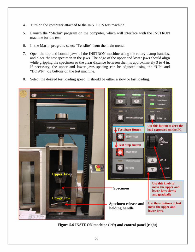
7. Open the top and bottom jaws of the INSTRON machine using the rotary clamp handles,
and place the test specimen in the jaws. The edge of the upper and lower jaws should align while gripping the specimen so the clear distance between them is approximately 3 to 4 in. If necessary, the upper and lower jaws spacing can be adjusted using the “UP” and “DOWN” jog buttons on the test machine.
8. Select the desired test loading speed; it should be either a slow or fast loading.
Figure 5.6 INSTRON machine (left) and control panel (right)
Specimen
Specimen release and holding handle
Upper Jaw
Lower Jaw
Use this button to zero the load expressed on the PC Test Start Button
Test Stop Button
Use these buttons to fast move the upper and lower jaws.
Use this knob to move the upper and lower jaws slowly and gradually
61
9. Press the “Balance Load” button using the computer program (or press the “1” button on the INSTRON machine.
10. Press the “Reset GL” button on the INSTRON machine.
11. Begin the test by pressing the “START TEST” button using the computer program.
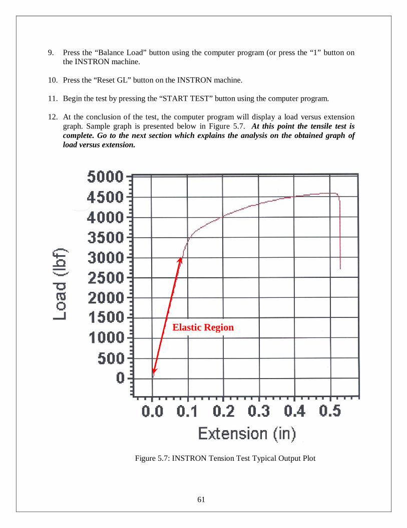
12. At the conclusion of the test, the computer program will display a load versus extension
graph. Sample graph is presented below in Figure 5.7. At this point the tensile test is complete. Go to the next section which explains the analysis on the obtained graph of load versus extension.
Figure 5.7: INSTRON Tension Test Typical Output Plot
Elastic Region
62
Procedure to obtain stresses and construct stress strain graph:
1. After the completion of the tensile test, a plot of load versus extension will be printed by the computer running the test.
2. Read loads applied and the corresponding extension value. It is recommended to use MS Office Excel to list these values. The more values obtained, the more accurate the stress strain graph constructed.
3. Show sample calculations for all tabulated results including stress and strain.
4. IMPORTANT: use linear regression to find the best fit on the stress vs. strain plot for the elastic (linear) region only (the linear region of typical stress vs. strain is shown in Figure 5.5). What is the slope of this relation represents?
5. Calculate the stress and strain for each value obtained using Equations 5.3 and 5.4.
6. Plot the stress versus strain plot using value calculated in step number 3.
7. Answer Post-Lab question using the graph obtained in step number 4.
Conversion Factors: 1 Pa =106 megapascal (MPa) 1 MPa = 0.001 gigapascals (GPa)
63
Material Yield Stress Ultimate
Stress Elongation
(MPa) (MPa) (%) Aluminum [Al] 20 70 60
Aluminum Alloy 35 - 500 100 - 550 16438
Brass 70 - 550 200 - 620 22007
Brass; Noval 170 - 410 410 - 590 15 - 50
Brass; Red (80% Cu, 20% Zn) 90 - 470 300 - 590 18354
Brick - 7.0 - 70 -
Bronze; Regular 82 - 690 200 - 830 22037
Bronze; Manganese 170 - 450 450 - 620 13058
Concrete (Compression) - 25842 -
Copper [Cu] 55 - 330 230 - 380 18537
Copper Alloy 760 830 4
Glass - 30 - 1000 -
Iron (Cast) 120 - 290 69 - 480 0 - 1
Iron (Wrought) 210 340 35
Magnesium [Mg] 20 - 70 100 - 170 39583
Magnesium Alloy 80 - 280 140 - 340 39498
Monel (67% Ni, 30% Cu) 170 - 1100 450 - 1200 18295
Nickel [Ni] 140 - 620 310 - 760 18295
Nylon; Polyamide - 40 - 70 50
Rubber 1.0 - 7.0 7.0 - 20 100 - 800
Solder; Tin-Lead - 20059 55 - 30
Steel 280 - 1600 340 - 1900 14671
Stone; Granite (Compression) - 70 - 280 -
Stone; Limestone (Compression) - 20 - 200 -
Stone; Marble (Compression) - 50 - 180 -
Titanium [Ti] - 500 25
Titanium Alloy - 900 - 970 10
Tungsten [W] - 1400 - 4000 0 - 4
Wood; Ash (Bending) 40 - 70 50 - 100 -
Wood; Douglas Fir (Bending) 30 - 50 50 - 80 -
Wood; Oak (Bending) 40 - 60 50 - 100 -
Wood; Southern Pine (Bending) 40 - 60 50 - 100 -
Table 5.1 Mechanical Properties of Materials (Part I)
64
Material Elastic
Modulus Shear Modulus Poisson's Ratio (GPa) (GPa)
Aluminum [Al] 70 26 0.33 Aluminum Alloy 70 - 79 26 - 30 0.33 Brass 96 - 110 36 - 41 0.34 Brass; Noval 100 39 0.34 Brass; Red (80% Cu, 20% Zn) 100 39 0.34 Brick (Compression) 39745 - - Bronze; Regular 96 - 120 36 - 44 0.34 Bronze; Manganese 100 39 0.34 Carbon [C] 6.9 - - Ceramic 300 - 400 - - Concrete 18 - 30 - 0.1 - 0.2 Copper [Cu] 110 - 120 40 - 47 0.33 - 0.36 Copper Alloy 120 47 - Glass 48 - 83 19 - 34 0.2 - 0.27 Gold [Au] 83 - 0.44 Iron (Cast) 83 - 170 32 - 69 0.2 - 0.3 Iron (Wrought) 190 75 0.3 Magnesium [Mg] 41 15 0.35 Magnesium Alloy 45 17 0.35 Monel (67% Ni, 30% Cu) 170 66 0.32 Nickel [Ni] 210 80 0.31 Nylon; Polyamide 2.1 - 2.8 - 0.4 Platinum [Pt] 145 - 0.38
Rubber 7.0 × 10⁻⁴ - 4.0 × 10⁻³ 2.0 × 10⁻⁴ - 1.0 × 10⁻³ 0.45 - 0.5
Silver [Ag] 76 - -
Solder; Tin-Lead 18 - 35 - - Steel 190 - 210 75 - 80 0.27 - 0.3
Stone; Granite (Compression) 40 - 70 - 0.2 - 0.3 Stone; Limestone (Compression) 20 - 70 - 0.2 - 0.3
Stone; Marble (Compression) 50 - 100 - 0.2 - 0.3 Tin [Sn] 42 - 0.36 Titanium [Ti] 110 40 - 40 0.33 Titanium Alloy 110 - 120 39 - 44 0.33 Wood; Ash (Bending) 39732 - - Wood; Douglas Fir (Bending) 39765 - - Wood; Oak (Bending) 39764 - - Wood; Southern Pine (Bending) 39766 - -
Table 5.2 Mechanical properties of Materials (Part II)
65
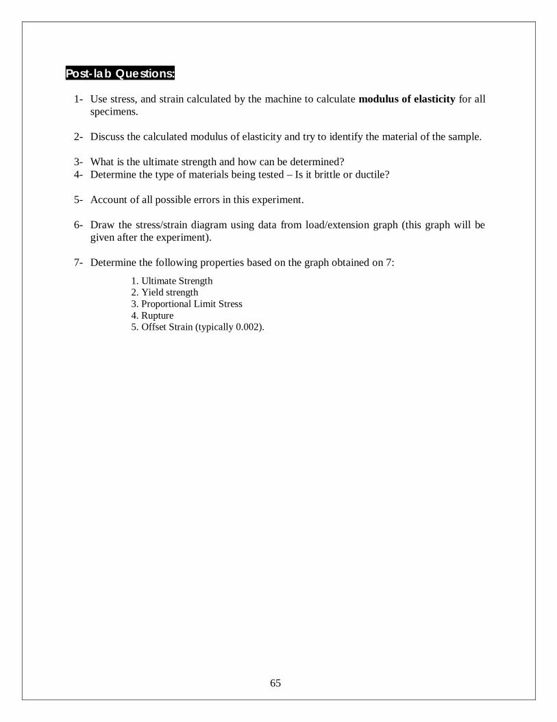
Post-lab Questions:
1- Use stress, and strain calculated by the machine to calculate modulus of elasticity for all specimens.
2- Discuss the calculated modulus of elasticity and try to identify the material of the sample.
3- What is the ultimate strength and how can be determined? 4- Determine the type of materials being tested – Is it brittle or ductile?
5- Account of all possible errors in this experiment.
6- Draw the stress/strain diagram using data from load/extension graph (this graph will be
given after the experiment).
7- Determine the following properties based on the graph obtained on 7:
1. Ultimate Strength 2. Yield strength 3. Proportional Limit Stress 4. Rupture 5. Offset Strain (typically 0.002).
66
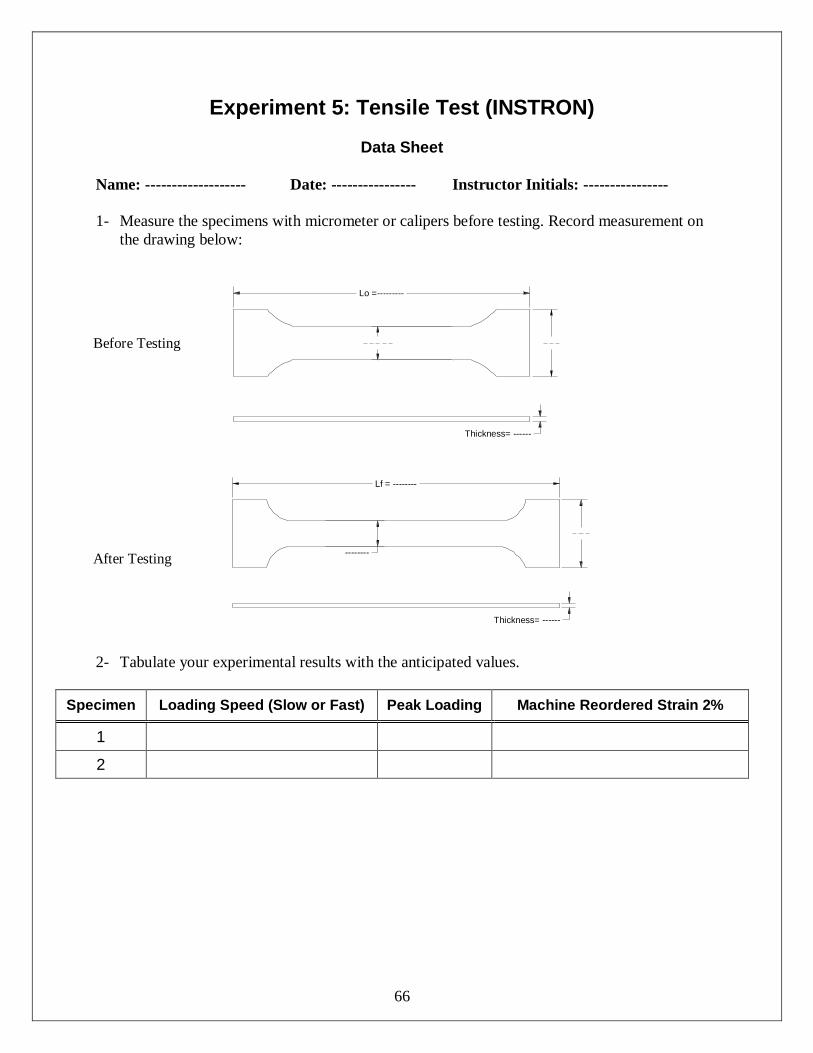
Experiment 5: Tensile Test (INSTRON)
Data Sheet Name: ------------------- Date: ---------------- Instructor Initials: ---------------- 1- Measure the specimens with micrometer or calipers before testing. Record measurement on
the drawing below:
Lo =---------
Thickness= ------
Lf = --------
Thickness= ------
--------
2- Tabulate your experimental results with the anticipated values.
Specimen Loading Speed (Slow or Fast) Peak Loading Machine Reordered Strain 2%
1
2
Before Testing
After Testing
67
Lab 6: Tension Test Using the Universal Testing Machine
Objective
The objective of this experiment is to evaluate the strength of metals and alloys using the tensile test. The experiment will show the relationship between stress and strain using experimental methods and determine the mechanical properties for specific materials which include:
13. Proportional Limit 14. Modulus of Elasticity 15. Ductility 16. Percent Elongation 17. Ultimate Strength 18. Yield Points (Upper and Lower)
Introduction
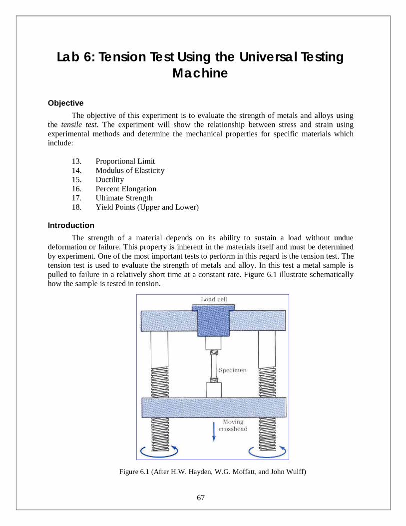
The strength of a material depends on its ability to sustain a load without undue deformation or failure. This property is inherent in the materials itself and must be determined by experiment. One of the most important tests to perform in this regard is the tension test. The tension test is used to evaluate the strength of metals and alloy. In this test a metal sample is pulled to failure in a relatively short time at a constant rate. Figure 6.1 illustrate schematically how the sample is tested in tension.
Figure 6.1 (After H.W. Hayden, W.G. Moffatt, and John Wulff)
68
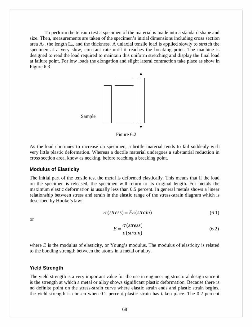
To perform the tension test a specimen of the material is made into a standard shape and size. Then, measurements are taken of the specimen’s initial dimensions including cross section area Ao, the length Lo, and the thickness. A uniaxial tensile load is applied slowly to stretch the specimen at a very slow, constant rate until it reaches the breaking point. The machine is designed to read the load required to maintain this uniform stretching and display the final load at failure point. For low loads the elongation and slight lateral contraction take place as show in Figure 6.3.
As the load continues to increase on specimen, a brittle material tends to fail suddenly with very little plastic deformation. Whereas a ductile material undergoes a substantial reduction in cross section area, know as necking, before reaching a breaking point. Modulus of Elasticity
The initial part of the tensile test the metal is deformed elastically. This means that if the load on the specimen is released, the specimen will return to its original length. For metals the maximum elastic deformation is usually less than 0.5 percent. In general metals shows a linear relationship between stress and strain in the elastic range of the stress-strain diagram which is described by Hooke’s law: )()( strainEstress (6.1) or
)()(
strainstressE
(6.2)
where E is the modulus of elasticity, or Young’s modulus. The modulus of elasticity is related to the bonding strength between the atoms in a metal or alloy. Yield Strength
The yield strength is a very important value for the use in engineering structural design since it is the strength at which a metal or alloy shows significant plastic deformation. Because there is no definite point on the stress-strain curve where elastic strain ends and plastic strain begins, the yield strength is chosen when 0.2 percent plastic strain has taken place. The 0.2 percent
Sample
Figure 6.2
69
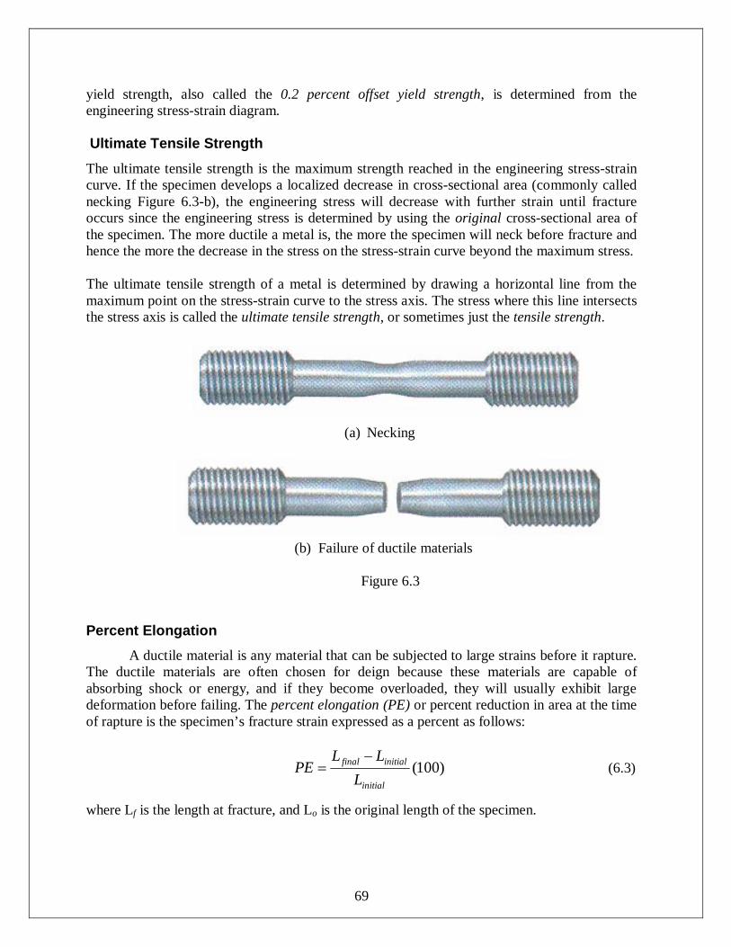
yield strength, also called the 0.2 percent offset yield strength, is determined from the engineering stress-strain diagram. Ultimate Tensile Strength
The ultimate tensile strength is the maximum strength reached in the engineering stress-strain curve. If the specimen develops a localized decrease in cross-sectional area (commonly called necking Figure 6.3-b), the engineering stress will decrease with further strain until fracture occurs since the engineering stress is determined by using the original cross-sectional area of the specimen. The more ductile a metal is, the more the specimen will neck before fracture and hence the more the decrease in the stress on the stress-strain curve beyond the maximum stress. The ultimate tensile strength of a metal is determined by drawing a horizontal line from the maximum point on the stress-strain curve to the stress axis. The stress where this line intersects the stress axis is called the ultimate tensile strength, or sometimes just the tensile strength.
(a) Necking
(b) Failure of ductile materials
Figure 6.3
Percent Elongation
A ductile material is any material that can be subjected to large strains before it rapture. The ductile materials are often chosen for deign because these materials are capable of absorbing shock or energy, and if they become overloaded, they will usually exhibit large deformation before failing. The percent elongation (PE) or percent reduction in area at the time of rapture is the specimen’s fracture strain expressed as a percent as follows:
)100(initial
initialfinal
LLL
PE
(6.3)
where Lf is the length at fracture, and Lo is the original length of the specimen.
70
The percent elongation at fracture is of engineering importance not only as a measure of ductility but also as an index of the quality of the metal. If the porosity or inclusions are present in the metal or if damage due to overheating the metal has occurred, the percent elongation of the specimen tested may be decreased below normal. The percent reduction in area (PRA) is defined within the region of necking as follows:
)100(o
fo
AAA
PRA
(6.4)
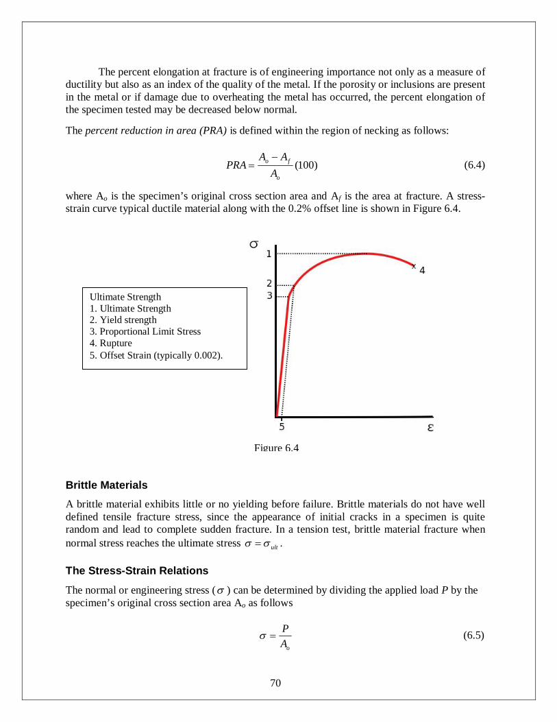
where Ao is the specimen’s original cross section area and Af is the area at fracture. A stress-strain curve typical ductile material along with the 0.2% offset line is shown in Figure 6.4. Brittle Materials
A brittle material exhibits little or no yielding before failure. Brittle materials do not have well defined tensile fracture stress, since the appearance of initial cracks in a specimen is quite random and lead to complete sudden fracture. In a tension test, brittle material fracture when normal stress reaches the ultimate stress ult . The Stress-Strain Relations
The normal or engineering stress ( ) can be determined by dividing the applied load P by the specimen’s original cross section area Ao as follows
oA
P (6.5)
Figure 6.4
Ultimate Strength 1. Ultimate Strength 2. Yield strength 3. Proportional Limit Stress 4. Rupture 5. Offset Strain (typically 0.002).
71
The nominal or engineering strain ( ) is found directly from the strain gauge reading, or by dividing the change in the specimen’s gauge length, , by the specimen’s original gauge length Lo as follows
o
o
o LLL
L
(6.6)
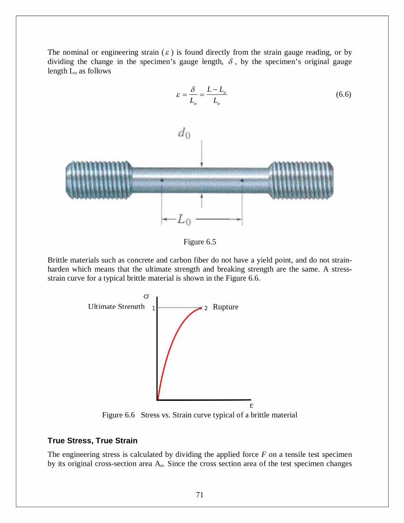
Figure 6.5
Brittle materials such as concrete and carbon fiber do not have a yield point, and do not strain-harden which means that the ultimate strength and breaking strength are the same. A stress-strain curve for a typical brittle material is shown in the Figure 6.6.
Figure 6.6 Stress vs. Strain curve typical of a brittle material True Stress, True Strain
The engineering stress is calculated by dividing the applied force F on a tensile test specimen by its original cross-section area Ao. Since the cross section area of the test specimen changes
Ultimate Strength Rupture
72
continuously during a tensile test, the engineering stress calculated is not precise. During the tensile test and after necking of the sample occurs, the engineering stress decreases as the strain increases, leading to a maximum engineering stress in the engineering stress-strain curve. Thus, once necking begins during the tensile test, the true stress is higher than the engineering stress. The true stress and true strain can be defined by the following: True Stress = F (average uniaxial force on the test sample) / Af (instantaneous minimum cross-sectional area of sample)
True strain = ln (Li/Lo)
where Lo is the original gage length of the sample and Li is the instantaneous extended gage length during the test.
Tension Test Procedure Using Universal Testing Machine: Note: Operating the universal testing machine for a tensile test should be exactly as indicated in Experiment 4 (Flexure in Wood). However, a few extra steps should be performed to carry a the tension test 1- Obtain the required testing specimens materials.
2- Measure the specimen dimensions indicated in the experiment data sheet using a vernier
caliper or a micrometer.
3- Turn on the Baldwin Universal Testing Machine and allow 15 minutes to warm up.
4- Set the measurement range of the machine to the 120K setting.
5- Install the test specimen into the test machine by threading the ends into the jaws on the testing machine. See Figure 6.7.
6- Use the manual “UP” and “DOWN” buttons to position the crosshead such that the
specimen no longer has any lose or play, but is not yet under tension.
7- If necessary, use the reset button (F2) on the control panel to zero any load reading displaced in the control panel (see Experiment 4).
8- Place a dial indicator (gauge) to measure specimen elongation under the crosshead as
shown in Figure 6.7.
9- Press the “START” button on the control panel.
10- During the course of the test, read the extension from the dial gauge and record the corresponding applied from the control panel at equal interval ( a 0.02” for example) of

73
extension. (Two students should perform this step – one should read the dial gauge and ask the other student at the same time to read the load displayed at the machine control panel).
11- After the specimen breaks, press the “STOP” button on the control panel.
12- Use vernier caliper to measure the final length of specimen between the threads.
13- Plot recorded load versus extension measured by the dial gauge.
14- Use the plot obtained in Step 13 to construct the stress versus strain plot.
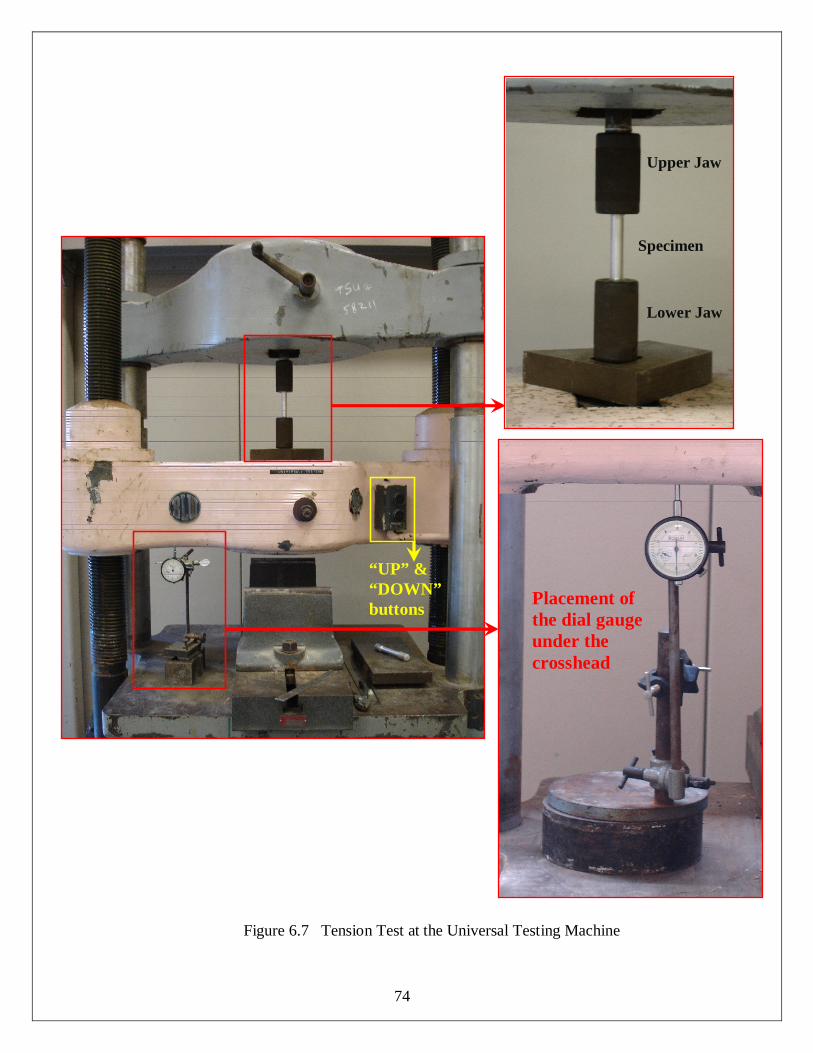
74
Figure 6.7 Tension Test at the Universal Testing Machine
Crosshead
Upper Jaw
Lower Jaw
Specimen
Placement of the dial gauge under the crosshead
“UP” & “DOWN” buttons
75
Post-lab Questions 1- Tabulate your experimental results with the anticipated values.
2- Calculate: PE, PRA, Stress, Strain, and modulus of elasticity for all specimens.
3- Comment on the calculated modulus of elasticity.
4- Calculate true stress and true strain.
5- What is the ultimate strength and how can be determined?
6- Determine the type of materials being tested – Is it brittle or ductile?
7- Account of all possible errors in this experiment.
8- Record instantaneous extension and corresponding load. This data will be used to draw
stress-strain curve for these specimens.
9- Show the following properties on the stress/strain graph obtained:
1. Ultimate Strength 2. Yield strength 3. Proportional Limit Stress 4. Rupture 5. Offset Strain (typically 0.002).
Lab Report Notes:
1. Show hand calculations to receive full credit.
2. Use Excel to report final results only and graphs.
3. Answer all above questions within the context of the “Results and Discussion” Section.
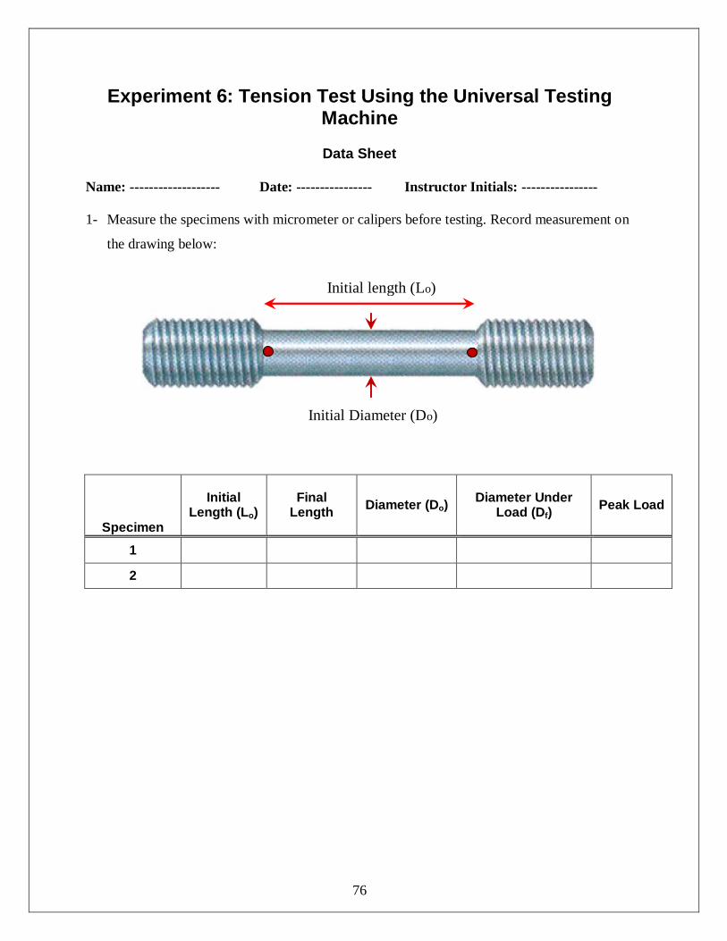
76
Experiment 6: Tension Test Using the Universal Testing Machine
Data Sheet
Name: ------------------- Date: ---------------- Instructor Initials: ---------------- 1- Measure the specimens with micrometer or calipers before testing. Record measurement on
the drawing below:
Specimen
Initial Length (Lo)
Final Length Diameter (Do) Diameter Under
Load (Df) Peak Load
1
2
Initial Diameter (Do)
Initial length (Lo)

77
2- Tabulate your experimental results with the anticipated values.
Loads (kips) Elongation (in.)
78
Lab 7: Torsion Test of Ductile and Brittle Materials
Objective 1. To learn the method of conducting a torsion test and to determine the characteristics and
behavior of ductile and brittle materials under torsion. 2. To find the strength of the materials to resist twisting forces, and to find its general
properties which include:
1. Shearing proportional limit 2. Yield strength at given offset 3. Shearing modulus of rupture 4. Modulus of rigidity 5. Probable tensile strength
Specimen Dimensions:
1” CRS STEEL BAR, 10”, 15” AND 20” LONG ¾” CRS STEEL BAR, 10”, 15, AND 20” LONG
Introduction
Torsion tests aim to measure the shear modulus (G) of a material. Although torsion testing is not common, it is a useful experiment and an important partner for tensile testing in determining the mechanical properties of a material.
Torque is a moment that tends to twist a member about its longitudinal axis. Its effect is of primary concern in the design of axles or drive shafts used in vehicles and machinery.
There are two kinds of torsion experiments: torque control and angular speed control. Torque control experiments apply a uniformly increasing torque to the specimen and the amount of strain is measured as an angle through which the specimen has turned. Angular speed control turns the specimen at a specific angular speed while the torque is measured. Angular speed control is the type of experiment will be considered in this lab, thus the directly measured quantity in this experiment will be torque. Consider the circular shaft which is shown in Figure 7.1. If the shaft is fixed at one end and a torque T is applied to other end, the shaft will twist, with its free end rotating through and angle called the angle of twist. A longitudinal line on the surface of the bar, such as line nn, will rotate through a small angle, , with respect to the position nn'. Because of this rotation, a rectangular element
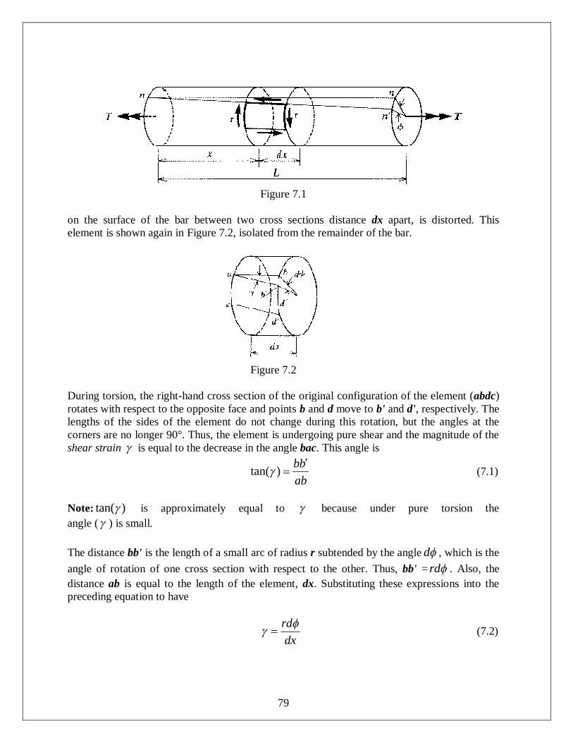
79
Figure 7.1
on the surface of the bar between two cross sections distance dx apart, is distorted. This element is shown again in Figure 7.2, isolated from the remainder of the bar.
Figure 7.2
During torsion, the right-hand cross section of the original configuration of the element (abdc) rotates with respect to the opposite face and points b and d move to b' and d', respectively. The lengths of the sides of the element do not change during this rotation, but the angles at the corners are no longer 90°. Thus, the element is undergoing pure shear and the magnitude of the shear strain is equal to the decrease in the angle bac. This angle is
abbb
)tan( (7.1)
Note: )tan( is approximately equal to because under pure torsion the angle ( ) is small. The distance bb' is the length of a small arc of radius r subtended by the angle d , which is the angle of rotation of one cross section with respect to the other. Thus, bb' = rd . Also, the distance ab is equal to the length of the element, dx. Substituting these expressions into the preceding equation to have
dx
rd (7.2)
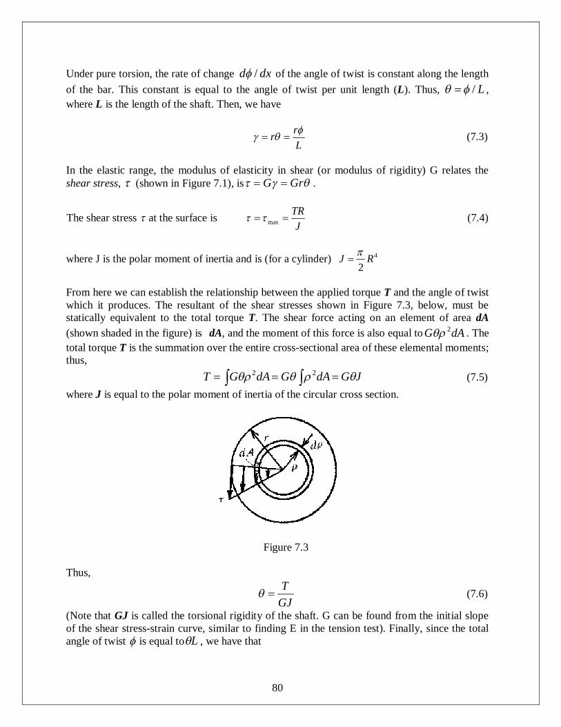
80
Under pure torsion, the rate of change dxd / of the angle of twist is constant along the length of the bar. This constant is equal to the angle of twist per unit length (L). Thus, L/ , where L is the length of the shaft. Then, we have
rrL (7.3)
In the elastic range, the modulus of elasticity in shear (or modulus of rigidity) G relates the shear stress, (shown in Figure 7.1), is GrG .
The shear stress at the surface is maxTRJ
(7.4)
where J is the polar moment of inertia and is (for a cylinder) 4
2J R
From here we can establish the relationship between the applied torque T and the angle of twist which it produces. The resultant of the shear stresses shown in Figure 7.3, below, must be statically equivalent to the total torque T. The shear force acting on an element of area dA (shown shaded in the figure) is dA, and the moment of this force is also equal to dAG 2 . The total torque T is the summation over the entire cross-sectional area of these elemental moments; thus, JGdAGdAGT 22 (7.5) where J is equal to the polar moment of inertia of the circular cross section.
Figure 7.3 Thus,
GJT
(7.6)
(Note that GJ is called the torsional rigidity of the shaft. G can be found from the initial slope of the shear stress-strain curve, similar to finding E in the tension test). Finally, since the total angle of twist is equal to L , we have that
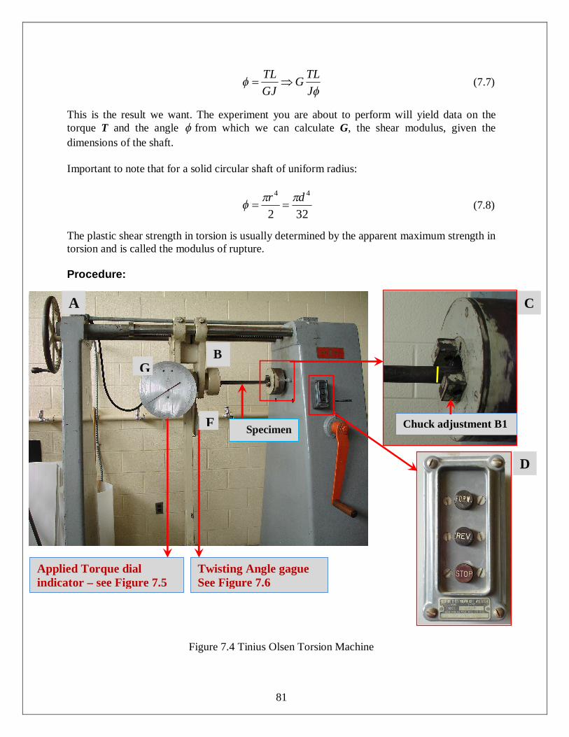
81
JTLG
GJTL
(7.7)
This is the result we want. The experiment you are about to perform will yield data on the torque T and the angle from which we can calculate G, the shear modulus, given the dimensions of the shaft.
Important to note that for a solid circular shaft of uniform radius:
322
44 dr (7.8)
The plastic shear strength in torsion is usually determined by the apparent maximum strength in torsion and is called the modulus of rupture.
Procedure:
Figure 7.4 Tinius Olsen Torsion Machine
Chuck adjustment B1 Specimen
Applied Torque dial indicator – see Figure 7.5
C
D
A
B
Twisting Angle gague See Figure 7.6
G
F
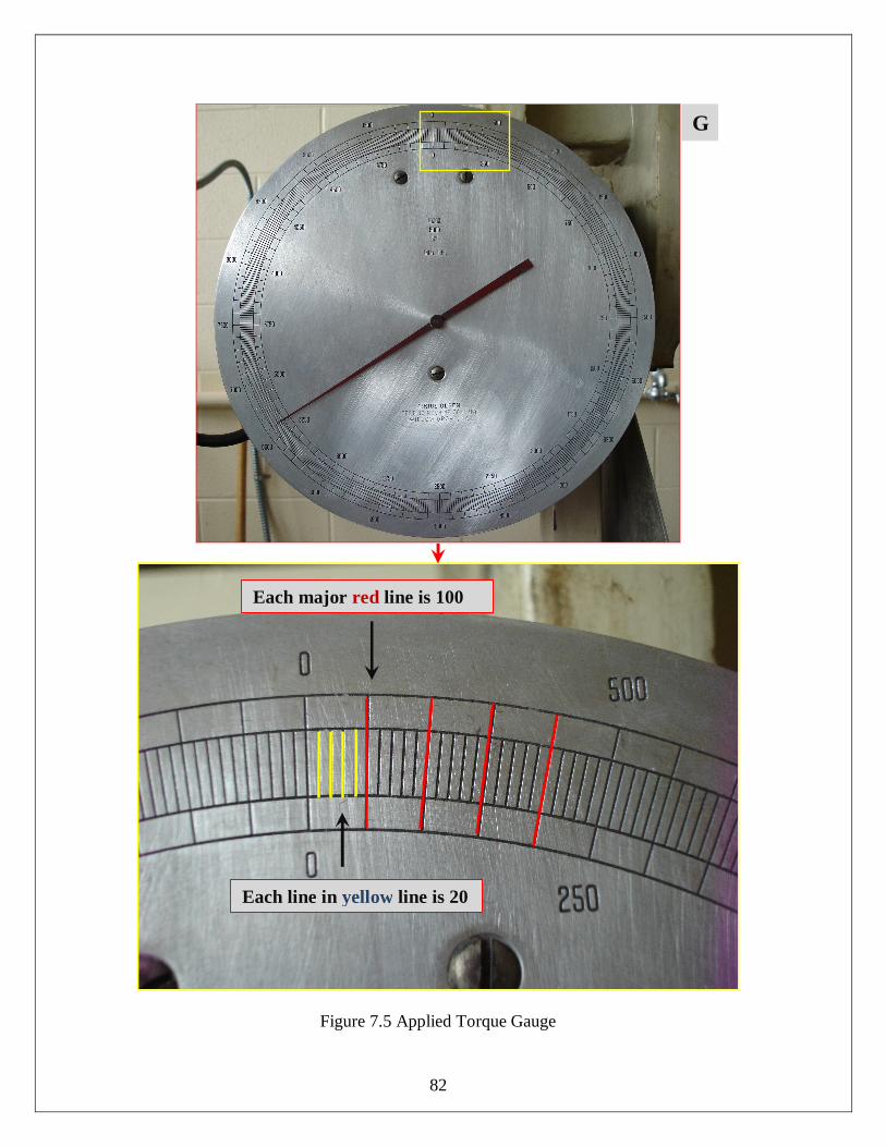
82
Figure 7.5 Applied Torque Gauge
Each major red line is 100
Each line in yellow line is 20
G
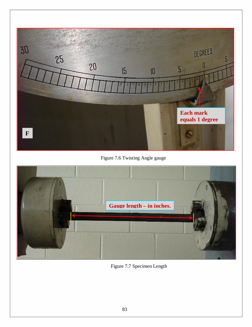
83
Figure 7.6 Twisting Angle gauge
Figure 7.7 Specimen Length
Each mark equals 1 degree
F
Gauge length – in inches.
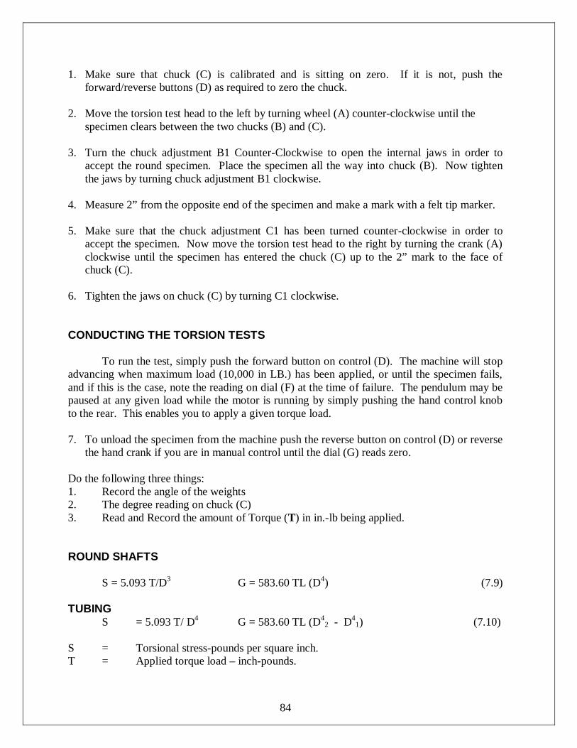
84
1. Make sure that chuck (C) is calibrated and is sitting on zero. If it is not, push the forward/reverse buttons (D) as required to zero the chuck.
2. Move the torsion test head to the left by turning wheel (A) counter-clockwise until the
specimen clears between the two chucks (B) and (C). 3. Turn the chuck adjustment B1 Counter-Clockwise to open the internal jaws in order to
accept the round specimen. Place the specimen all the way into chuck (B). Now tighten the jaws by turning chuck adjustment B1 clockwise.
4. Measure 2” from the opposite end of the specimen and make a mark with a felt tip marker. 5. Make sure that the chuck adjustment C1 has been turned counter-clockwise in order to
accept the specimen. Now move the torsion test head to the right by turning the crank (A) clockwise until the specimen has entered the chuck (C) up to the 2” mark to the face of chuck (C).
6. Tighten the jaws on chuck (C) by turning C1 clockwise. CONDUCTING THE TORSION TESTS To run the test, simply push the forward button on control (D). The machine will stop advancing when maximum load (10,000 in LB.) has been applied, or until the specimen fails, and if this is the case, note the reading on dial (F) at the time of failure. The pendulum may be paused at any given load while the motor is running by simply pushing the hand control knob to the rear. This enables you to apply a given torque load. 7. To unload the specimen from the machine push the reverse button on control (D) or reverse
the hand crank if you are in manual control until the dial (G) reads zero. Do the following three things: 1. Record the angle of the weights 2. The degree reading on chuck (C) 3. Read and Record the amount of Torque (T) in in.-lb being applied. ROUND SHAFTS
S = 5.093 T/D3 G = 583.60 TL (D4) (7.9) TUBING
S = 5.093 T/ D4 G = 583.60 TL (D42 - D4
1) (7.10) S = Torsional stress-pounds per square inch. T = Applied torque load – inch-pounds.
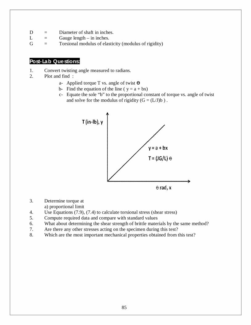
85
D = Diameter of shaft in inches. L = Gauge length – in inches. G = Torsional modulus of elasticity (modulus of rigidity) Post-Lab Questions: 1. Convert twisting angle measured to radians. 2. Plot and find :
a- Applied torque T vs. angle of twist ө b- Find the equation of the line ( y = a + bx) c- Equate the sole “b” to the proportional constant of torque vs. angle of twist
and solve for the modulus of rigidity (G = (L/J)b ) .
3. Determine torque at a) proportional limit
4. Use Equations (7.9), (7.4) to calculate torsional stress (shear stress) 5. Compute required data and compare with standard values 6. What about determining the shear strength of brittle materials by the same method? 7. Are there any other stresses acting on the specimen during this test? 8. Which are the most important mechanical properties obtained from this test?
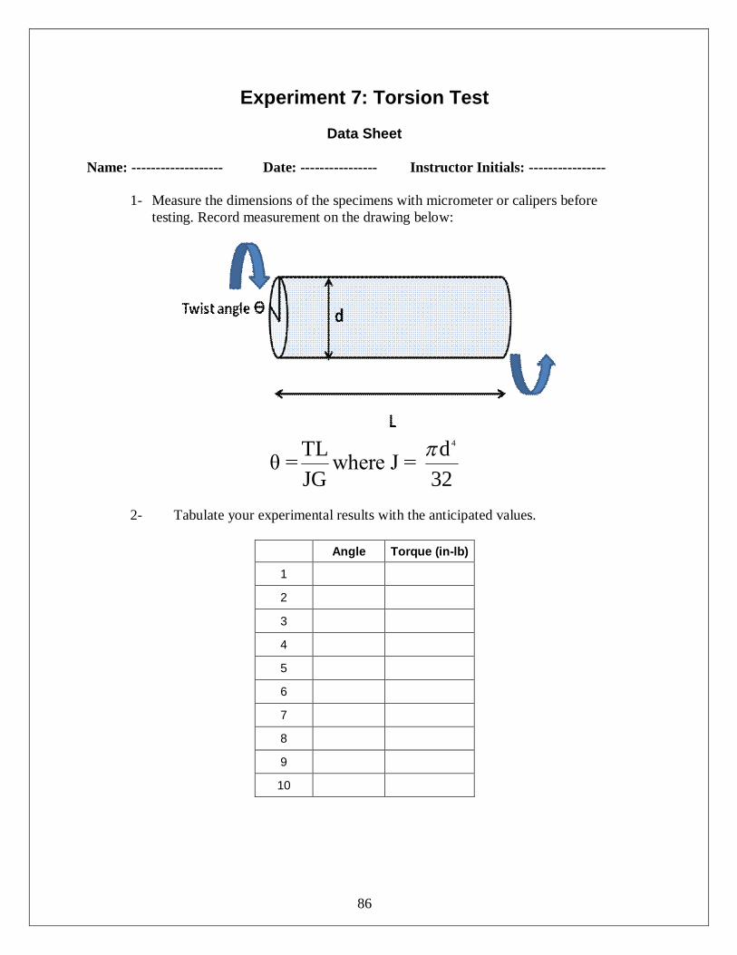
86
Experiment 7: Torsion Test
Data Sheet Name: ------------------- Date: ---------------- Instructor Initials: ----------------
1- Measure the dimensions of the specimens with micrometer or calipers before testing. Record measurement on the drawing below:
4TL dθ = where J =
JG 32
2- Tabulate your experimental results with the anticipated values.
Angle Torque (in-lb)
1
2
3
4
5
6
7
8
9
10
87
Lab 8: Truss Test and Analysis
Objective The objective of this lab is to learn the static analysis of truss using the method of joints and method of sections. In addition, to determine the external support forces as well as the forces acting on each of the members for given external loads. Introduction
An Italian architect, Andrea Palladio (1518-1580), is believed to develop the first trusses. His extensive writings on architectural include detailed description and drawings of several wooden trusses quite similar to those in use today. A truss can be defined as a structure formed by a group of members arranged in the shape of one or more triangles. Because the members are assumed to be connected with frictionless pins, the triangle is the only stable shape. Truss members are assumed to carry only axial forces, either in tension or compression, since no moment can be transferred through a frictionless pin joints. The truss members act in the direct stress, therefore they carry load efficiently and often have relatively small cross sections. A truss is completely analyzed when the magnitude and sense (tension or compression) of all bar forces and reactions are determined. To compute the reactions of a determinate truss, the entire structure should be treated as a rigid body, then apply the equations of static equilibrium together with any condition equations that may exist. The analysis used to evaluate the bar forces is based on the following assumptions:
1- Truss members are connected together with frictionless pins (Pins connections are used for very few trusses erected today, and no pins are frictionless. A heavy bolted or welded joint is a far cry from a frictionless pin.)
2- Truss members are straight. (If they are not straight, the axial forces would cause them
to have bending moments.)
3- Loads are applied only to joints. Truss Structural Elements Figure 8.1 shows a typical short-span roof truss, used for the dual tasks or providing for gable-form, pitched roof surfaces and the direct support of a flat, horizontal ceiling surface. The common elements of truss are as follow
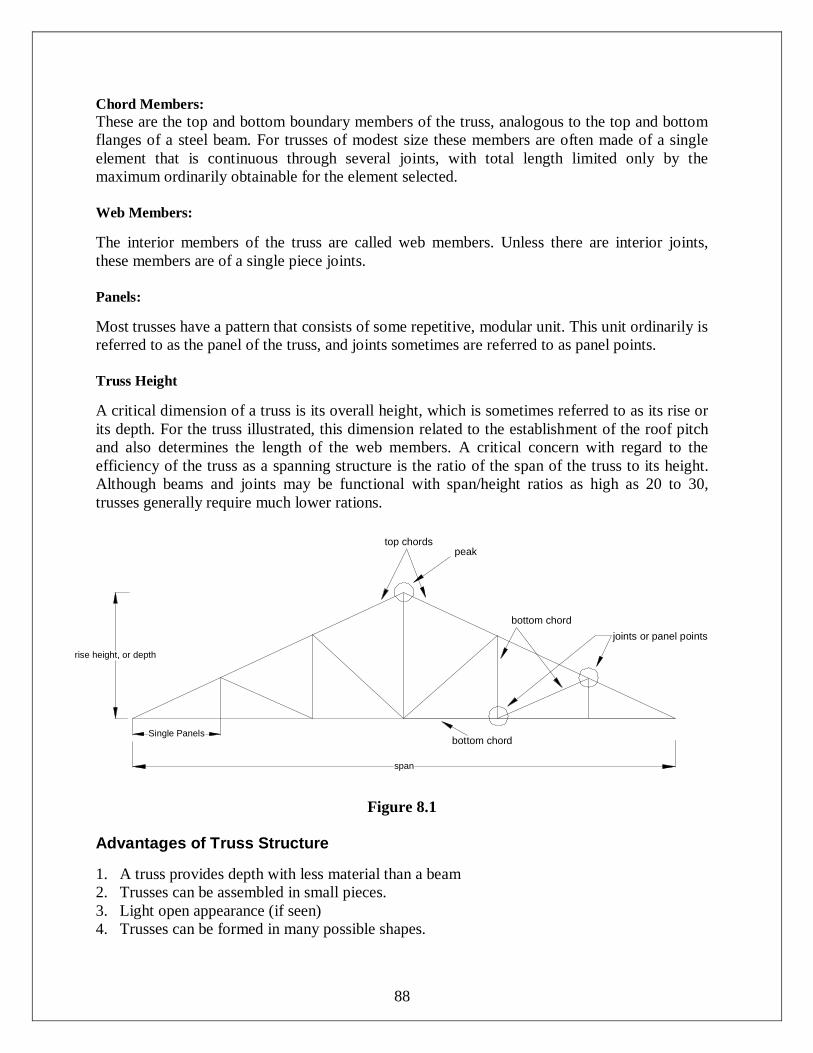
88
Single Panels
rise height, or depth
span
top chordspeak
joints or panel points
bottom chord
bottom chord
Chord Members: These are the top and bottom boundary members of the truss, analogous to the top and bottom flanges of a steel beam. For trusses of modest size these members are often made of a single element that is continuous through several joints, with total length limited only by the maximum ordinarily obtainable for the element selected. Web Members: The interior members of the truss are called web members. Unless there are interior joints, these members are of a single piece joints. Panels: Most trusses have a pattern that consists of some repetitive, modular unit. This unit ordinarily is referred to as the panel of the truss, and joints sometimes are referred to as panel points. Truss Height A critical dimension of a truss is its overall height, which is sometimes referred to as its rise or its depth. For the truss illustrated, this dimension related to the establishment of the roof pitch and also determines the length of the web members. A critical concern with regard to the efficiency of the truss as a spanning structure is the ratio of the span of the truss to its height. Although beams and joints may be functional with span/height ratios as high as 20 to 30, trusses generally require much lower rations.
Figure 8.1
Advantages of Truss Structure 1. A truss provides depth with less material than a beam 2. Trusses can be assembled in small pieces. 3. Light open appearance (if seen) 4. Trusses can be formed in many possible shapes.
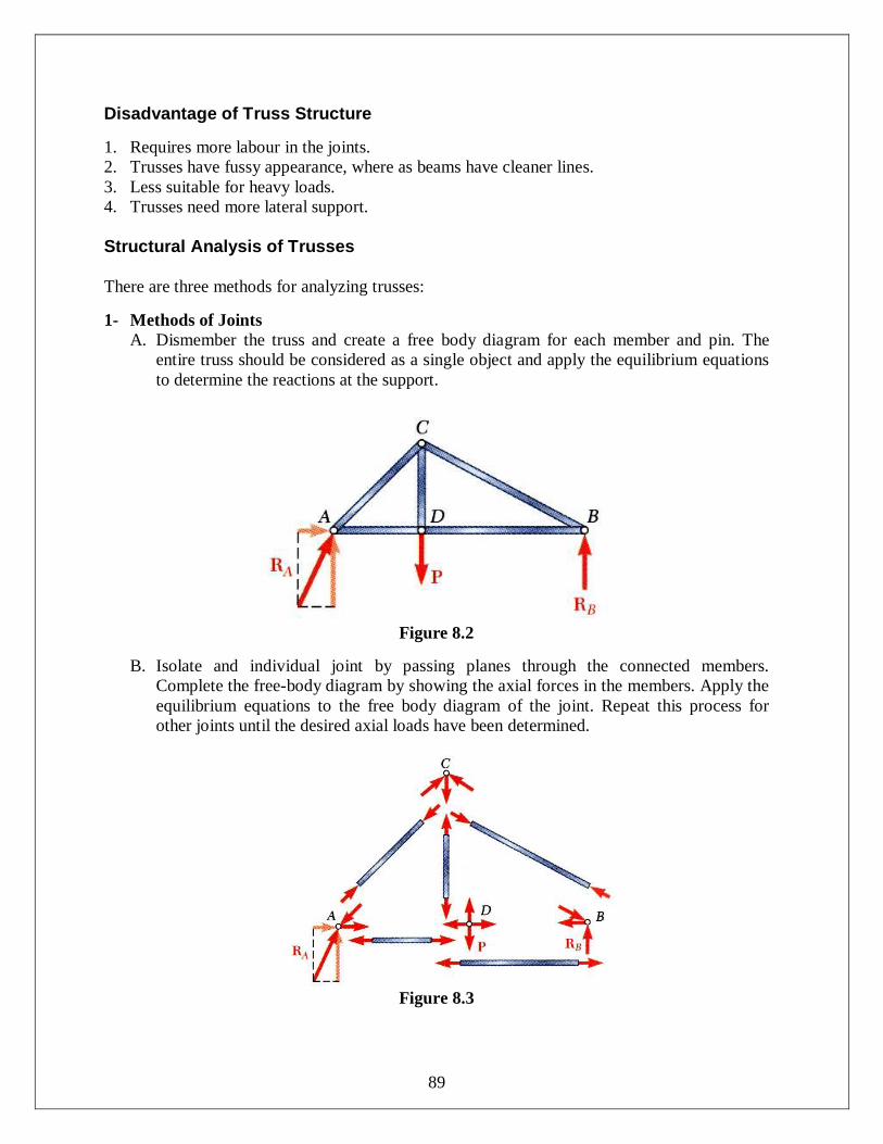
89
Disadvantage of Truss Structure 1. Requires more labour in the joints. 2. Trusses have fussy appearance, where as beams have cleaner lines. 3. Less suitable for heavy loads. 4. Trusses need more lateral support. Structural Analysis of Trusses There are three methods for analyzing trusses: 1- Methods of Joints
A. Dismember the truss and create a free body diagram for each member and pin. The entire truss should be considered as a single object and apply the equilibrium equations to determine the reactions at the support.
Figure 8.2
B. Isolate and individual joint by passing planes through the connected members. Complete the free-body diagram by showing the axial forces in the members. Apply the equilibrium equations to the free body diagram of the joint. Repeat this process for other joints until the desired axial loads have been determined.
Figure 8.3
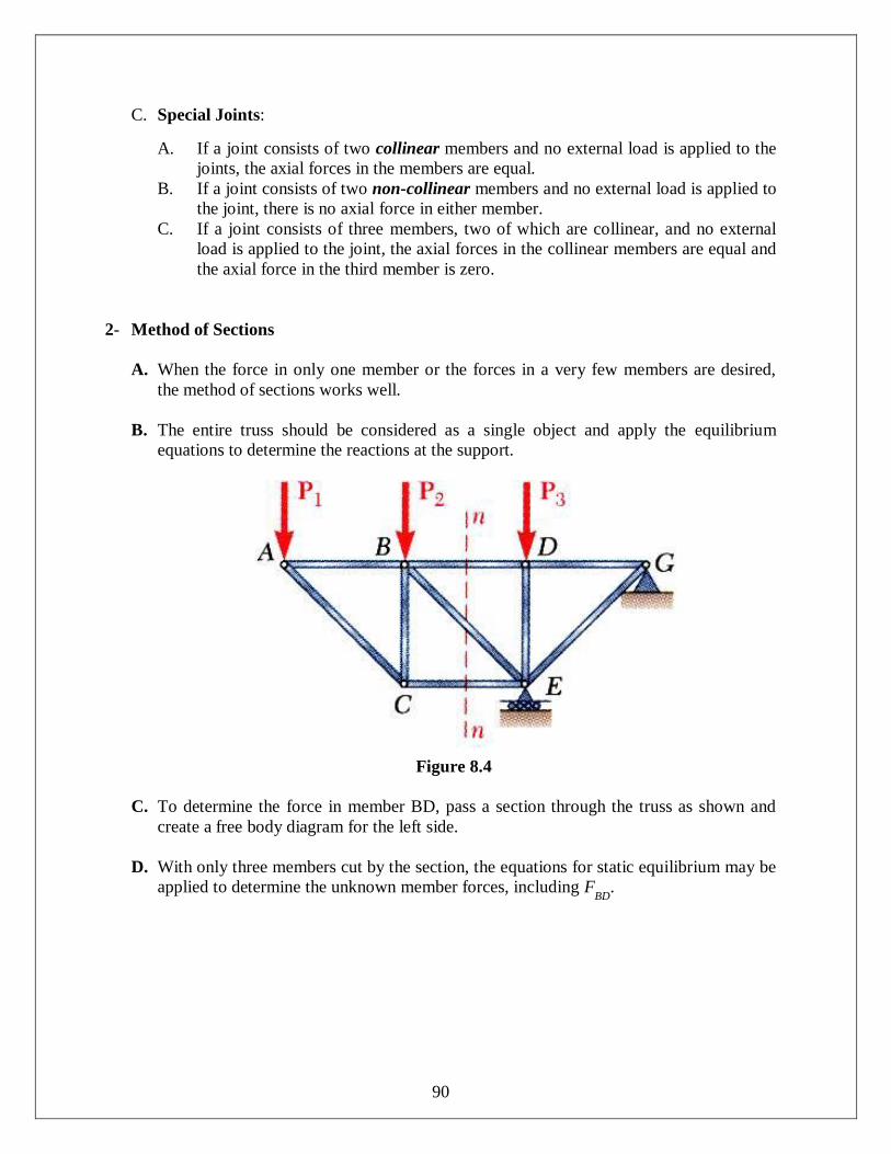
90
C. Special Joints: A. If a joint consists of two collinear members and no external load is applied to the
joints, the axial forces in the members are equal. B. If a joint consists of two non-collinear members and no external load is applied to
the joint, there is no axial force in either member. C. If a joint consists of three members, two of which are collinear, and no external
load is applied to the joint, the axial forces in the collinear members are equal and the axial force in the third member is zero.
2- Method of Sections
A. When the force in only one member or the forces in a very few members are desired, the method of sections works well.
B. The entire truss should be considered as a single object and apply the equilibrium equations to determine the reactions at the support.
Figure 8.4
C. To determine the force in member BD, pass a section through the truss as shown and
create a free body diagram for the left side.
D. With only three members cut by the section, the equations for static equilibrium may be applied to determine the unknown member forces, including FBD.
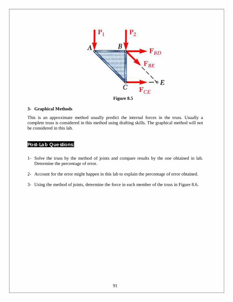
91
Figure 8.5
3- Graphical Methods This is an approximate method usually predict the internal forces in the truss. Usually a complete truss is considered in this method using drafting skills. The graphical method will not be considered in this lab.
Post-Lab Questions: 1- Solve the truss by the method of joints and compare results by the one obtained in lab.
Determine the percentage of error. 2- Account for the error might happen in this lab to explain the percentage of error obtained. 3- Using the method of joints, determine the force in each member of the truss in Figure 8.6.
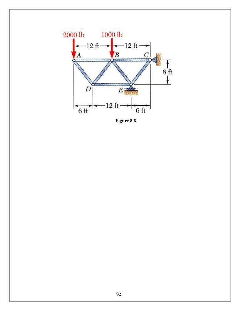
92
Figure 8.6
93
Experiment 8: Truss Test
Data Sheet Name: ------------------- Date: ---------------- Instructor Initials: ---------------- 1- Draw the truss in this experiment and measure necessary dimensions. (height, span, etc)
2- Tabulate your experimental results with the anticipated values.
Load Applied Left
Reaction Dial
Right Reaction Dial
Truss 1
Truss 2
Truss 3
Truss 4
Truss 5
Truss 6
5 10 25 30
94
Basic Conversion Table
Length
Imperial Metric 1 inch [in] 2.54 cm
1 foot [ft] 12 in 0.3048 m 1 yard [yd] 3 ft 0.9144 m
1 mile 1760 yd 1.6093 km
1 millimeter [mm] 0.03937 in
1 centimeter [cm] 10 mm 0.3937 in 1 metre [m] 100 cm 1.0936 yd
1 kilometer [km] 1000 m 0.6214 mile
Area
1 sq inch [in2] 6.4516 cm2 1 sq foot [ft2] 144 in2 0.0929 m2 1 sq yd [yd2] 9 ft2 0.8361 m2
1 acre 4840 yd2 4046.9 m2 1 sq mile [mile2] 640 acres 2.59 km2
1 sq cm [cm2] 100 mm2 0.1550 in2 1 sq m [m2] 10,000 cm2 1.1960 yd2
1 hectare [ha] 10,000 m2 2.4711 acres
1 sq km [km2] 100 ha 0.3861 mile2
95
References & Bibliography
1. Popowski, John D., Mathematical Tools for machine Technology, 1982, Breton Publisher, Chalifornia.
2. Hibbeler, R.C., Mechanics of Materials, prentice Hall, 2004, New Jersey 3. Smith, William F., Principal of Materials Science and Engineering, McGraw-Hill,
1990. 4. Egor P. Popov. Engineering Mechanics of Solids. Prentice Hall: Englewood Cliffs, New
Jersey, 1990. 5. Sokolnikoff, I.S., Specht, R.D. Mathematical Theory of Elasticity. McGraw-Hill Co.,
1946. 6. Timoshenko, S.P., Gere, J.M. Mechanics of Materials. D. Van Nostrand Co., 1972.