Metapopulations Study with Subjective Biotic and Abiotic Processes

Metapopulations Study with Subjective Biotic and Abiotic Processes

Karine F. Magnago1, Rodney C. Bassanezi2

1 IMECC, UNICAMP{[email protected]}2 DMA IMECC, UNICAMP

{[email protected]}Caixa Postal 6065, 13081- 970, Campinas, SP, Brazil

Telephone number (19) 3788 5933 – 3788 5950

Keywords: coupled populations; fuzzy rules-based systems; migration.

I. INTRODUCTION

The blowflies of the family calliphoridae are object of studies due to their importance in the biological and medical-veterinary contexts [1, 2]. In the biological context, several species are important as pollinator, decomposer and food source for some animals [3]. In the medical-veterinarian context, they are able to frequent rural, wild and urban environment, visiting dejections and carcasses and transmitting pathogens [1,4, 5]. Some species cause human and animal myiasis [6]. They are also important forensic indicators [7].

A deterministic mathematical model dependent of the density, for two coupled populations by migration of the same species, was proposed by Godoy and applied to species of blowflies of the family calliphoridae [8].

As there aren’t absolutely predictable environments and as the organisms don't respond to the environmental incentives in a homogeneous way, Godoy incorporated a probabilistic dimension to the model allowing the aleatory flotation of essential parameters for the population growth analysis [8].

Another option to work with the inherent subjectivity to the population variation process is the use of the fuzzy set theory. In this way we introduced fecundity, survival and migration like fuzzy variables in the Godoy deterministic model. This allowed the flotation of those parameters that describe the biological phenomenon [10].

On the other hand, several authors have been showing interest for the space distribution of populations in habitat broken into fragments in discrete patches [11, 12].

In this work, we propose a discrete model for the metapopulation and subpopulations study of a blowfly species. It is applied to a native species (Lucilia eximia) and an introduced species (Chrysomya albiceps), both of the family calliphoridae. The mathematical model is a linear deterministic model whose coefficients are estimated using fuzzy rules-based systems. The simplicity of the model implies a careful fuzzy modeling of the parameters: fecundity, survival and migration rates.

II. MATHEMATICAL MODEL

We consider the population of a unique species in a habitat broken into fragments in p interlinked patches. Each patch is enclosure by hostile environment. The interaction among neighboring patches occurs for the migration. The figure 1 A illustrates a closed or periodic configuration, while the figure 1 B illustrates a configuration that where extreme patches don’t interact directly.

Fig. 1 A. Periodic space distribution of the patches; B. The patches 1 e p don’t interact directly.

We denote the subpopulation density in the patch j and in the generation t by (non-overlapping generations). The metapopulation density is the sum of all the subpopulation densities.

We assume that the carry capacity of the metapopulation density is 1 and the carry capacities

of the subpopulation densities are k1, k2, ,kp such that .

We also assumed that, in each generation, the population goes through a local dynamics process followed by a migratory process.

In the migration absence, we express the local dynamics as , j = 1, 2, , p;

particularly, to blowfly species, we use such that ½ indicate that half of the

population is constituted of adult females; and are fecundity and survival in the patch j, respectively.

In this work, we use experimental data obtained by Godoy; the fecundity was estimated by the count of eggs number by female and the survival measuring the number of emergent adults in each colony [8].

The migration happens once in each generation and it is of short duration in relation to the scale of time used in the model (time between two serial generations). Consequently we consider the null mortality during the migration.

The migration can happen in a preferential direction – Unilateral Migration (we assume that this direction coincides with the ordination of the patches) or in the two possible directions – Bilateral Migration. The Unilateral Migration reflects sceneries in which external forces, as winds, have fundamental influence in the migratory process. Mathematically, we write:

,

(1)

such that , j = 1, 2, , p, is the individuals' fraction that migrates of a patch for the following. The Bilateral Migration allows that individuals of a patch migrate for the closer two neighboring patches; we write:

.

(2)

If the saturation of a subpopulation happened after the local dynamics, we suppose this patch doesn't receive individuals of the neighboring patches in this generation. If it happened after the migration, we suppose that the individuals' excess that entered in the patch comes back to the origin patch proportional the amount that left.

The fecundity , the survival and the migration rate were considered linguistic variables and were estimated through a fuzzy rules-based system.

III. FUZZY RULES-BASED SYSTEM

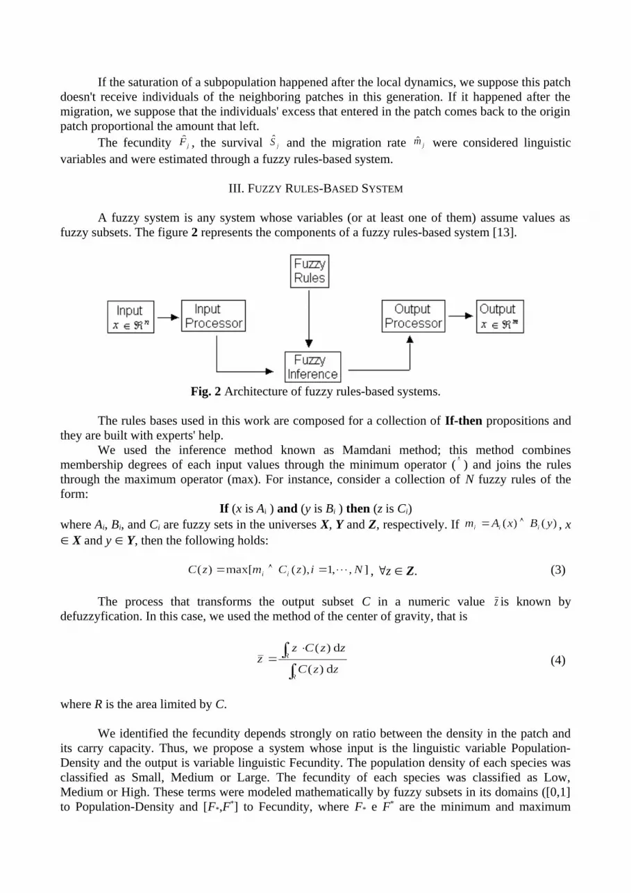
A fuzzy system is any system whose variables (or at least one of them) assume values as fuzzy subsets. The figure 2 represents the components of a fuzzy rules-based system [13].

Fig. 2 Architecture of fuzzy rules-based systems.

The rules bases used in this work are composed for a collection of If-then propositions and they are built with experts' help.

We used the inference method known as Mamdani method; this method combines membership degrees of each input values through the minimum operator ( ) and joins the rules through the maximum operator (max). For instance, consider a collection of N fuzzy rules of the form:

If (x is Ai ) and (y is Bi ) then (z is Ci)where Ai, Bi, and Ci are fuzzy sets in the universes X, Y and Z, respectively. If , x X and y Y, then the following holds:

, z Z. (3)

The process that transforms the output subset C in a numeric value is known by defuzzyfication. In this case, we used the method of the center of gravity, that is

(4)

where R is the area limited by C.

We identified the fecundity depends strongly on ratio between the density in the patch and its carry capacity. Thus, we propose a system whose input is the linguistic variable Population-Density and the output is variable linguistic Fecundity. The population density of each species was classified as Small, Medium or Large. The fecundity of each species was classified as Low, Medium or High. These terms were modeled mathematically by fuzzy subsets in its domains ([0,1] to Population-Density and [F*,F*] to Fecundity, where F* e F* are the minimum and maximum

fecundities of the species, respectively). The figures 3 A and 3 D illustrate the modeling of the input and output variables of the species Lucilia eximia, respectively.

0 0.2 0.4 0.6 0.8 1

0

0.2

0.4

0.6

0.8

1

Population-Density

Deg

ree

of m

embe

rshi

p

Small Medium Large

A

0 0.2 0.4 0.6 0.8 1

0

0.2

0.4

0.6

0.8

1

Abiotic-Conditions

Deg

ree

of m

embe

rshi

p

Bad Medium Good

B

0 0.2 0.4 0.6 0.8 1

0

0.2

0.4

0.6

0.8

1

Environment

Deg

ree

of m

embe

rshi

p

Hostile Indifferent Favourable

C

4.5 5 5.5 6 6.5 7

0

0.2

0.4

0.6

0.8

1

Fecundity

Deg

ree

of m

embe

rshi

p

Low Medium High

D

Fig. 3 A. Population density; B. Abiotic Conditions; C. Environment; D. Fecundity (Lucilia eximia).

In this case, we use the following rules base.

Fuzzy rules base:1. If Population-Density is Small) then (Fecundity is High)2. If (Population-Density is Medium) then (Fecundity is Medium)3. If (Population-Density is Large) then (Fecundity is Low)

The survival and migration rates depend on an evaluation of the environment in the patch, at the considered instant. This evaluation of the environment depends on population density and abiotic conditions. Then we have more three fuzzy rules-based systems.

The first proposed system considers the input variables Population-Density and Abiotic-Condition to estimate the output variable Environment. The figures 3 A, 3 B and 3 C illustrate the fuzzy modeling of these variables in their domains. We use the following rules base.

Fuzzy rules base:1. If (Population-Density is Small) and (Abiotic-Conditions are Bad) then (Environment is

Hostile)2. If (Population-Density is Medium) and (Abiotic-Conditions are Bad) then (Environment

is Hostile)3. If (Population-Density is Large) and (Abiotic-Conditions are Bad) then (Environment is

Hostile)

4. If (Population-Density is Small) and (Abiotic-Conditions are Medium) then (Environment is Indifferent)

5. If (Population-Density is Medium) and (Abiotic-Conditions are Medium) then (Environment is Indifferent)

6. If (Population-Density is Large) and (Abiotic-Conditions are Medium) then (Environment is Hostile)

7. If (Population-Density is Small) and (Abiotic-Conditions are Good) then (Environment is Favorable)

8. If (Population-Density is Medium) and (Abiotic-Conditions are Good) then (Environment is Indifferent)

9. If (Population-Density is Large) and (Abiotic-Conditions are Good) then (Environment is Indifferent)

The second proposed system considers the input variable Environment to estimate the output variable Survival. The figure 4 A illustrates the fuzzy modeling of the survival rate in its domain ([0,S*] where S* is the maximum survival rate of the species). We use the following rules base.

Fuzzy rules base:1. If (Environment is Hostile) then (Survival is Low)2. If (Environment is Indifferent) then (Survival is Medium)3. If (Environment is Favorable) then (Survival is High)

The last proposed system considers the input variable Environment to estimate the output variable Migration. The figure 4 B illustrates the fuzzy modeling of the migration rate in its domain ([0,1]). We use the following rules base.

Fuzzy rules base:1. If (Environment is Hostile) then (Migration is High)2. If (Environment is Indifferent) then (Migration is Medium)3. If (Environment is Favorable) then (Migration is Low)

0 0.1 0.2 0.3 0.4 0.5 0.6 0.7 0.8 0.9

0

0.2

0.4

0.6

0.8

1

Survival

Deg

ree

of m

embe

rshi

p

Low Medium High

A

0 0.1 0.2 0.3 0.4 0.5 0.6 0.7 0.8 0.9 1

0

0.2

0.4

0.6

0.8

1

Migration

Deg

ree

of m

embe

rshi

p

Low Medium High

B

m*

2/ F* 2/ F*

Fig. 4 A. Survival (Lucilia eximia); B. Migration (Lucilia eximia).

We obtained some values used as references in the fuzzy modeling of the survival and migration rates (2/F* and 2/F*; m*).

Considering an isolated population whose density is calculated by the equation

, it is easy to observe that the survival value so that the population density remains in

equilibrium is .Considering a population that doesn't receive individuals by migration, but that loses a

fraction m of its individuals at each generation, we can determine a threshold value

such that if , we have local extinction.

IV. RESULTS AND DISCUSSIONS

We made simulations for two species of blowflies: a native species (Lucilia eximia) and an introduced species (Chrysomya albiceps) because they present differences in the dynamic behavior observed by the biologists. While the introduced species present a stable cycle of two points, characterized by the oscillation between two representative values of the population size, the native species exhibit a stable equilibrium whose biological meaning is the stabilization of the population size in a unique value [8].

We used the equations (1) and (2) and calculated, in each iteration, the parameters , and using Toolbox Fuzzy of MATLAB version 6.0.

A. Periodic space distribution of the patches

This subsection is destined to the presentation of results considering the periodic space distribution of the patches.

When we assumed that the carry capacities, the initial densities and the abiotic conditions are equal in all the patches, we obtain the same stability results for the subpopulations, independent of simulate species and chosen migration type. This can be observed in the figures 5 A, 6 A, 7 A and 8 A.

In the simulations for the species Lucilia eximia, we observed that the subpopulation density is stabilized in a unique equilibrium value for each subpopulation (figures 5, 6, 10 A, C, E and 11 A, C, E). For isolated populations of this species, we also observed this behavior.

90 92 94 96 98 1000.1383

0.1383

0.1383

0.1383

0.1383

0.1383 A. Average Abiotic-Conditions [0.5; 0.5; 0.5; 0.5; 0.5]

Generation

90 92 94 96 98 1000.6

0.62

0.64

0.66

0.68

0.7

0.72

Generation

Met

apop

ulat

ion

Den

sity

D

A B C

90 92 94 96 98 1000.09

0.1

0.11

0.12

0.13

0.14

0.15

Generation

B. Abiotic-Conditions [0.18; 0.58; 0.98; 0.58; 0.18]

P 1P 2P 3P 4P 5

90 92 94 96 98 1000.13

0.135

0.14

0.145

0.15

0.155

0.16

Generation

C. Random Abiotic-Conditions [0.9501; 0.2311; 0.6068; 0.4860; 0.8913]

P 1P 2P 3P 4P 5

Patches 1, 2, 3, 4 e 5

njt n

jt

njt

Lucilia eximia -- Unilateral Migration

Fig. 5 Simulations for five subpopulations of the species Lucilia eximia using unilateral migration and periodic space distribution, with the same carry capacities (0.2) and the same initial densities (0.1); A. Subpopulation density considering the same abiotic conditions (Medium: 0.5); B. Subpopulation density considering the abiotic conditions [0.18; 0.58; 0.98; 0.58; 0.18] (Bad, Medium, Good, Medium, Bad); C. Subpopulation density considering the random abiotic conditions [0.9501; 0.2311; 0.6068; 0.4860; 0.8913] (Good; Bad, Medium, Medium, Good); D. Metapopulations density.

In the figure 5 B, we observe that the largest equilibrium value corresponds to the patch of better abiotic conditions (patch 3); as the migration is unilateral, the patch 4 obtained a superior equilibrium value to the patch 2 in spite of them to have the same abiotic conditions. This result points out the influence of the migratory movements. In fact, since the second generation, the difference between the individuals' fractions that enter and that leave is negative in these two patches, and the larger loss happens in the patch 2. Similar result is observed for the patches 1 and 5 that also have the same abiotic conditions.

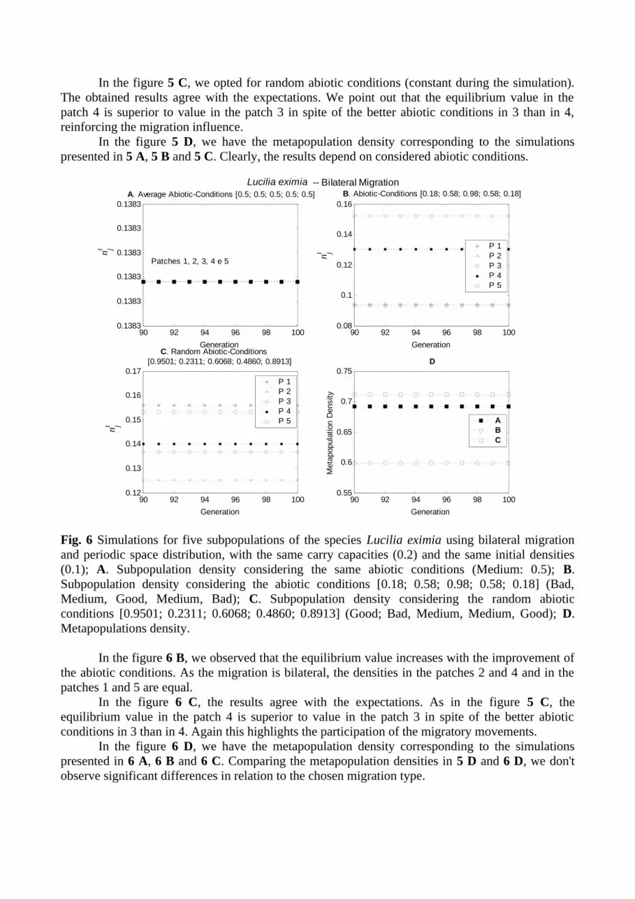
In the figure 5 C, we opted for random abiotic conditions (constant during the simulation). The obtained results agree with the expectations. We point out that the equilibrium value in the patch 4 is superior to value in the patch 3 in spite of the better abiotic conditions in 3 than in 4, reinforcing the migration influence.

In the figure 5 D, we have the metapopulation density corresponding to the simulations presented in 5 A, 5 B and 5 C. Clearly, the results depend on considered abiotic conditions.

90 92 94 96 98 1000.1383

0.1383

0.1383

0.1383

0.1383

0.1383

Generation

A. Average Abiotic-Conditions [0.5; 0.5; 0.5; 0.5; 0.5]

90 92 94 96 98 1000.55

0.6

0.65

0.7

0.75

Generation

Met

apop

ulat

ion

Den

sity

D

A B C

90 92 94 96 98 1000.08

0.1

0.12

0.14

0.16

Generation


P 1P 2P 3P 4P 5

90 92 94 96 98 1000.12

0.13

0.14

0.15

0.16

0.17

Generation


P 1P 2P 3P 4P 5

njt

njt

njt

Patches 1, 2, 3, 4 e 5

Lucilia eximia -- Bilateral Migration

Fig. 6 Simulations for five subpopulations of the species Lucilia eximia using bilateral migration and periodic space distribution, with the same carry capacities (0.2) and the same initial densities (0.1); A. Subpopulation density considering the same abiotic conditions (Medium: 0.5); B. Subpopulation density considering the abiotic conditions [0.18; 0.58; 0.98; 0.58; 0.18] (Bad, Medium, Good, Medium, Bad); C. Subpopulation density considering the random abiotic conditions [0.9501; 0.2311; 0.6068; 0.4860; 0.8913] (Good; Bad, Medium, Medium, Good); D. Metapopulations density.

In the figure 6 B, we observed that the equilibrium value increases with the improvement of the abiotic conditions. As the migration is bilateral, the densities in the patches 2 and 4 and in the patches 1 and 5 are equal.

In the figure 6 C, the results agree with the expectations. As in the figure 5 C, the equilibrium value in the patch 4 is superior to value in the patch 3 in spite of the better abiotic conditions in 3 than in 4. Again this highlights the participation of the migratory movements.

In the figure 6 D, we have the metapopulation density corresponding to the simulations presented in 6 A, 6 B and 6 C. Comparing the metapopulation densities in 5 D and 6 D, we don't observe significant differences in relation to the chosen migration type.

In the simulations for the species Chrysomya albiceps, we observe three possible situations: the subpopulation density reaches a unique equilibrium value or it evolves for a stable 2-cycle or it evolves for a stable 4-cycle (less common). In the case of isolated populations of this species, most of the simulations resulted in 2-cycles. Some subpopulations evolve for an equilibrium value since the abiotic conditions are in a restricted interval.

90 92 94 96 98 1000.16

0.17

0.18

0.19

0.2

0.21

Generation


90 92 94 96 98 1000.8

0.85

0.9

0.95

1

Generation

Met

apop

ulat

ion

Den

sity

D

A B C

90 92 94 96 98 1000.17

0.175

0.18

0.185

0.19

0.195

Generation


P 1P 2P 3P 4P 5

90 92 94 96 98 1000.16

0.17

0.18

0.19

0.2

0.21

Generation


P 1P 2P 3P 4P 5

Patches 1, 2, 3, 4 e 5

njt

njt

njt

Chrysomya albiceps -- Unilateral Migration

Fig. 7 Simulations for five subpopulations of the species Chrysomya albiceps using unilateral migration and periodic space distribution, with the same carry capacities (0.2) and the same initial densities (0.1); A. Subpopulation density considering the same abiotic conditions (Medium: 0.5); B. Subpopulation density considering the abiotic conditions [0.18; 0.58; 0.98; 0.58; 0.18] (Bad, Medium, Good, Medium, Bad); C. Subpopulation density considering the random abiotic conditions [0.9501; 0.2311; 0.6068; 0.4860; 0.8913] (Good; Bad, Medium, Medium, Good); D. Metapopulations density.

In the figure 7 B, the subpopulations of Chrysomya albiceps evolve for equilibrium points; in this case, the interesting result is that isolated populations simulations with the same initial conditions result 2-cycle solutions.

In the figure 7 C, the results agree with the expectations.In the figure 7 D, we have the metapopulations corresponding to the simulations presented

in 7 A, 7 B and 7 C. The maximum values of the two metapopulations that evolved for stable 2-cycles are very close, the same doesn't happen with the minimum values (simulations A and C).

90 92 94 96 98 1000.16

0.17

0.18

0.19

0.2

0.21

Generation


90 92 94 96 98 1000.8

0.85

0.9

0.95

1

Generation

Met

apop

ulat

ion

Den

sity

D

A B C

90 92 94 96 98 1000.16

0.17

0.18

0.19

0.2

0.21

Generation


P 1P 2P 3P 4P 5

90 92 94 96 98 1000.16

0.17

0.18

0.19

0.2

0.21

0.22

Generation


P 1P 2P 3P 4P 5

Patches 1, 2, 3, 4 e 5

njt

njt

njt

Chrysomia albiceps -- Bilateral Migration

Fig. 8 Simulations for five subpopulations of the species Chrysomya albiceps using bilateral migration and periodic space distribution, with the same carry capacities (0.2) and the same initial densities (0.1); A. Subpopulation density considering the same abiotic conditions (Medium: 0.5); B. Subpopulation density considering the abiotic conditions [0.18; 0.58; 0.98; 0.58; 0.18] (Bad, Medium, Good, Medium, Bad); C. Subpopulation density considering the random abiotic conditions [0.9501; 0.2311; 0.6068; 0.4860; 0.8913] (Good; Bad, Medium, Medium, Good); D. Metapopulations density.

In the figure 8 B, we obtain less surprising results than those obtained in the figure 7 B (same initial conditions, but unilateral migration). As the migration is bilateral, the densities in the patches 2 and 4 and in the patches 1 and 5 coincide.

In the figure 8 C, the results agree with the expectations.In the figure 8 D, we have the metapopulations corresponding to the simulations presented

in 8 A, 8 B and 8 C. After the stabilization, the maximum values of the metapopulation densities are very close, the same doesn't happen with the minimum values.

30 32 34 36 38 40 42 44 46 48 500

0.05

0.1

Generation

njt

A. Chrysomya albiceps -- Unilateral Migration

P1P2P3P4P5P6P7P8P9P10

30 32 34 36 38 40 42 44 46 48 500.6

0.65

0.7

0.75

0.8

Generation

Met

apop

ulat

ion

Den

sity

B

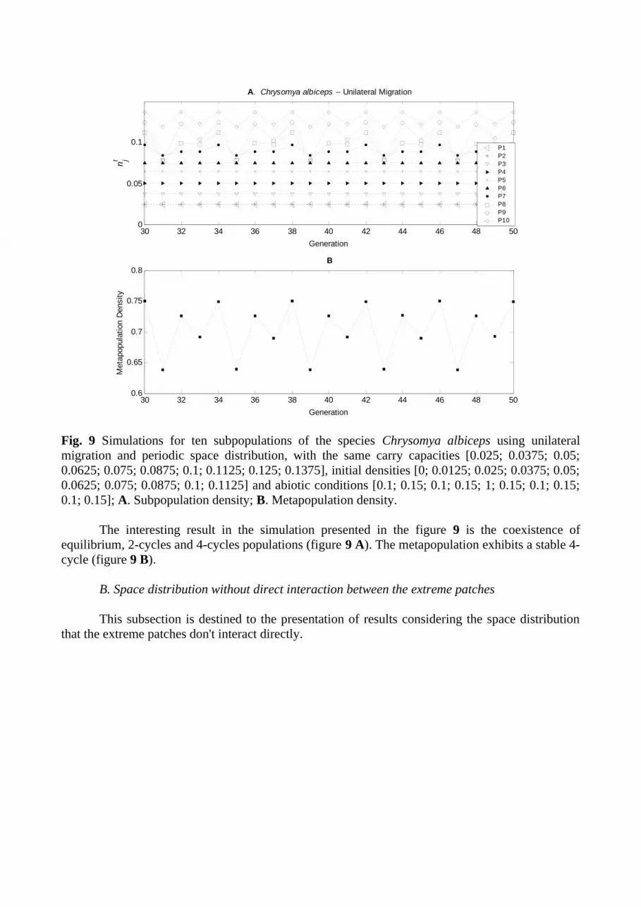
Fig. 9 Simulations for ten subpopulations of the species Chrysomya albiceps using unilateral migration and periodic space distribution, with the same carry capacities [0.025; 0.0375; 0.05; 0.0625; 0.075; 0.0875; 0.1; 0.1125; 0.125; 0.1375], initial densities [0; 0.0125; 0.025; 0.0375; 0.05; 0.0625; 0.075; 0.0875; 0.1; 0.1125] and abiotic conditions [0.1; 0.15; 0.1; 0.15; 1; 0.15; 0.1; 0.15; 0.1; 0.15]; A. Subpopulation density; B. Metapopulation density.

The interesting result in the simulation presented in the figure 9 is the coexistence of equilibrium, 2-cycles and 4-cycles populations (figure 9 A). The metapopulation exhibits a stable 4-cycle (figure 9 B).

B. Space distribution without direct interaction between the extreme patches

This subsection is destined to the presentation of results considering the space distribution that the extreme patches don't interact directly.

280 285 290 295 3000

0.05

0.1

0.15

0.2

280 285 290 295 3000

0.05

0.1

0.15

0.2

Generation

njt

280 285 290 295 3000

0.05

0.1

0.15

0.2 Chrysomya albiceps

280 285 290 295 3000

0.05

0.1

0.15

0.2

280 285 290 295 3000.05

0.1

0.15

0.2

0.25

20 40 60 80 100 1200

0.05

0.1

0.15

0.2 Lucilia eximia

Patch 5

Patches 1, 2, 3 and 4

P 2

P 3

P 4

P 5

njt

Patch 5


njt

njt

P 1

P 2 P 3

P 4

P 5

P 1 P 1

P 2

P 3,4,5

Generation

njt

Patch 5 n

jt

Unilateral Migration

A

C

E

B

D

F


Fig. 10 Simulations for five subpopulations of the species Lucilia eximia (A, C and E) and Chrysomya albiceps (B, D and F) using unilateral migration and space distribution without direct interaction between the patches 1 and 5, with the same carry capacities (0.2) and the same initial densities (0.1); A, B. Subpopulation density considering the same abiotic conditions (Bad: 0.1); C, D. Subpopulation density considering the same abiotic conditions (Medium: 0.5); E, F. Subpopulation density considering the same abiotic conditions (Good: 0.9).

In the figure 10, we consider unilateral migration and space distribution without direct interaction between the patches 1 and 5. Also the carry capacities (0.2) and the initial densities (0.1) are equal in all the five patches.

With bad abiotic conditions (0.1) in all the patches, we obtain the global extinction for the subpopulations of Lucilia eximia (figure 10 A). With the same abiotic conditions, the subpopulations of Chrysomya albiceps in the patches 1, 2, 3 and 4 also extinguished, just staying the subpopulation in the patch 5 exhibiting a stable 2-cycle (figure 10 B).

With medium abiotic conditions (0.5) in all the patches, the subpopulations of Lucilia eximia in the patches 1, 2, 3 and 4 extinguished but the subpopulation in the patch 5 was stabilized in a positive equilibrium point (figure 10 C). In the figure 10 D, we observed the subpopulation behavior of Chrysomya albiceps considering medium abiotic conditions. The patches 1 and 2 exhibit equilibrium while the other patches exhibit stable 2-cycles. If we repeated this simulation for isolated subpopulations, we would just have 2-cycle solutions.

With good abiotic conditions (0.9) in all the patches, the subpopulations of Lucilia eximia evolved for positive equilibria, and the values of these equilibria are increasing with the ordination of the patches (saturation in the patch 5 – figure 10 E). The subpopulations of Chrysomya albiceps also reached the equilibrium for good abiotic conditions, and it happened the saturation in the patches 3, 4 and 5 (figure 10 F).

20 40 60 80 100 1200

0.05

0.1 Lucilia eximia

280 285 290 295 3000.1383

0.1383

0.1383

0.1383

280 285 290 295 3000.1604

0.1604

0.1604

0.1604

Generation

njt

280 285 290 295 3000.175

0.18

0.185

0.19 Chrysomya albiceps

280 285 290 295 3000.16

0.18

0.2

0.22

280 285 290 295 3000.18

0.185

0.19

0.195

0.2

Generation

njt

njt

njt

njt

njt

Bilateral Migration

A

C

E

B

D

F

Patches 1, 2, 3, 4 and 5






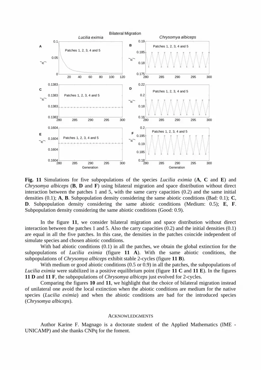
Fig. 11 Simulations for five subpopulations of the species Lucilia eximia (A, C and E) and Chrysomya albiceps (B, D and F) using bilateral migration and space distribution without direct interaction between the patches 1 and 5, with the same carry capacities (0.2) and the same initial densities (0.1); A, B. Subpopulation density considering the same abiotic conditions (Bad: 0.1); C, D. Subpopulation density considering the same abiotic conditions (Medium: 0.5); E, F. Subpopulation density considering the same abiotic conditions (Good: 0.9).

In the figure 11, we consider bilateral migration and space distribution without direct interaction between the patches 1 and 5. Also the carry capacities (0.2) and the initial densities (0.1) are equal in all the five patches. In this case, the densities in the patches coincide independent of simulate species and chosen abiotic conditions.

With bad abiotic conditions (0.1) in all the patches, we obtain the global extinction for the subpopulations of Lucilia eximia (figure 11 A). With the same abiotic conditions, the subpopulations of Chrysomya albiceps exhibit stable 2-cycles (figure 11 B).

With medium or good abiotic conditions (0.5 or 0.9) in all the patches, the subpopulations of Lucilia eximia were stabilized in a positive equilibrium point (figure 11 C and 11 E). In the figures 11 D and 11 F, the subpopulations of Chrysomya albiceps just evolved for 2-cycles.

Comparing the figures 10 and 11, we highlight that the choice of bilateral migration instead of unilateral one avoid the local extinction when the abiotic conditions are medium for the native species (Lucilia eximia) and when the abiotic conditions are bad for the introduced species (Chrysomya albiceps).

ACKNOWLEDGMENTS

Author Karine F. Magnago is a doctorate student of the Applied Mathematics (IME - UNICAMP) and she thanks CNPq for the foment.

REFERENCES

[1] HARWOOD, R. F.; JAMES, M. T. Entomology in human and animal health. New York, Macmillan Publishing Co., 1979.

[2] BOWMAN, D. D. Parasitology for veterinarians. Philadelphia, W. B. Saunders Company, 1995.

[3] NEVES, D. P. Parasitologia Humana. São Paulo, Atheneu, 2000.[4] GREENBERG, B. Flies and Disease. Ecology, Classification and Biotic Associations. V.

I, Princeton, Princeton University Press, 1971.[5] GREENBERG, B. Flies and Disease. Biology and Disease Transmission. V. II, Princeton,

Princeton University Press, 1973.[6] ZUMPT, F. Myiasis in man and animals in the Old World. London: Butterworths, 1965.[7] SMITH, K. G. V. A manual of forensic entomology. Oxford, University Printing House,

1986.[8] GODOY, W. A. C. Dinâmica determinística e estocástica em populações de dípteros

califorídeos: acoplamento por migração, extinção local e global. Tese de Livre Docência, Outubro, 2002. Instituto de Biociências de Botucatu, Universidade Estadual Paulista.

[9] ZADEH, L.A. V. Fuzzy Sets. Inform and Control, v.8, p.338-353, 1965.[10] CASTANHO, M. J. P.; MAGNAGO, K. F.; BASSANEZI, R. C. Abordagem Fuzzy na

Dinâmica de Populações de Dípteros Califorídeos. Biomatemática, v.XIII, p.55-65, 2003.[11] ROHDE, K.; ROHDE, P. P. Fuzzy Chaos: Reduced Chaos in the Combined Dynamics of

Several Independently Chaotic population. The American Naturalist. Chicago, v.158, n.5, p.553-556, November 2001.

[12] SILVA, J. A. L.; CASTRO, M. L. Sincronização e Caos em Metapopulações. Proceedings of Congresso Latino Americano de Biomatemática – X ALAB – V ELAEM (eds. R. C. Bassanezi and Geraldo L. Diniz). Campinas, 2001. p.18-29.

[13] PEDRYCZ, W.; GOMIDE, F. An introduction to fuzzy sets: analysis and design. Massachusetts, The MIT Press, 1998.

Documents

Metapopulations Study with Subjective Biotic and Abiotic Processes