method development of standard dilution analysis on

Kennesaw State University Kennesaw State University

DigitalCommons@Kennesaw State University DigitalCommons@Kennesaw State University

Master of Science in Chemical Sciences Theses Department of Chemistry and Biochemistry

Summer 7-27-2021

METHOD DEVELOPMENT OF STANDARD DILUTION ANALYSIS ON METHOD DEVELOPMENT OF STANDARD DILUTION ANALYSIS ON

MOLECULES AND DISSOLUTION STUDIES OF IBUPROFEN MOLECULES AND DISSOLUTION STUDIES OF IBUPROFEN

TABLETS ALONG WITH COMMON BEVERAGE CONSTITUENTS TABLETS ALONG WITH COMMON BEVERAGE CONSTITUENTS

Scott Richardson Kennesaw State University

Follow this and additional works at: https://digitalcommons.kennesaw.edu/mscs_etd

Part of the Analytical Chemistry Commons, and the Medicinal-Pharmaceutical Chemistry Commons

Recommended Citation Recommended Citation Richardson, Scott, "METHOD DEVELOPMENT OF STANDARD DILUTION ANALYSIS ON MOLECULES AND DISSOLUTION STUDIES OF IBUPROFEN TABLETS ALONG WITH COMMON BEVERAGE CONSTITUENTS" (2021). Master of Science in Chemical Sciences Theses. 44. https://digitalcommons.kennesaw.edu/mscs_etd/44

This Thesis is brought to you for free and open access by the Department of Chemistry and Biochemistry at DigitalCommons@Kennesaw State University. It has been accepted for inclusion in Master of Science in Chemical Sciences Theses by an authorized administrator of DigitalCommons@Kennesaw State University. For more information, please contact [email protected].

https://digitalcommons.kennesaw.edu/

https://digitalcommons.kennesaw.edu/mscs_etd

https://digitalcommons.kennesaw.edu/chem

https://digitalcommons.kennesaw.edu/mscs_etd?utm_source=digitalcommons.kennesaw.edu%2Fmscs_etd%2F44&utm_medium=PDF&utm_campaign=PDFCoverPages

http://network.bepress.com/hgg/discipline/132?utm_source=digitalcommons.kennesaw.edu%2Fmscs_etd%2F44&utm_medium=PDF&utm_campaign=PDFCoverPages

http://network.bepress.com/hgg/discipline/136?utm_source=digitalcommons.kennesaw.edu%2Fmscs_etd%2F44&utm_medium=PDF&utm_campaign=PDFCoverPages

https://digitalcommons.kennesaw.edu/mscs_etd/44?utm_source=digitalcommons.kennesaw.edu%2Fmscs_etd%2F44&utm_medium=PDF&utm_campaign=PDFCoverPages

mailto:[email protected]

METHOD DEVELOPMENT OF STANDARD DILUTION ANALYSIS ON

MOLECULES AND DISSOLUTION STUDIES OF IBUPROFEN TABLETS ALONG

WITH COMMON BEVERAGE CONSTITUENTS

by

Scott Irving Richardson III

Bachelor of Science in Chemistry

Kennesaw State University, 2018

_____________________________________________________________________

Submitted in Partial Fulfillment of the Requirements

For the Degree of Master of Science in the

Department of Chemistry and Biochemistry

Kennesaw State University

2021

iii

ACKNOWLEDGEMENTS

Throughout this incredible journey to achieve a Master of Science in the

Chemical Sciences in the area of Pharmaceutical Analytical Chemistry I realized that this

achievement is not solely my own.

I would like to thank my father and mother, John and Dione, whom have always

been there for me with their love and support through times of success, and more

importantly though times of failure where I learned my most important lessons.

I would like to thank my sister, Kellie, who started this academic journey before

me, providing me with her love and support, in which we have always challenged one

another to strive to be better.

I would like to thank my extended family, Freddy and Dan, for all the love and

encouragement they provided me especially at times when I thought I didn’t have the

energy to continue.

I would like to thank my father and mother in-law Michael and Camilla, my

sisters Margaret, Annie, and Cathy, and their spouses Dheeraj, Alice, and Sang who

accepted me into their family without hesitation and supported me through this trying

time.

I would like to thank my wife Dr. Elizabeth Dell Trippe whom has gone through

so much in her academic journey but took over all of our responsibilities so that I may

only concentrate on my research, provided me with endless love and support, and has

never given me the answer no matter how frustrated I have gotten so that I may have the

epiphanies necessary to develop a deeper understanding of my philosophy of science.

iv

I would like to thank my advisor, Dr. Marina Christina Koether, for a fantastic

research project with all the encouragement, guidance, support, and the freedom to follow

the directions I thought best so that I may make the necessary mistakes even if it meant

going down quite a few ‘Rabbit Holes’.

I would like to thank Dr. Chris Dockery for all the support he has provided to

myself and the other graduate students keeping us on track in our programs and

continually working to make a better life for graduate students here in the department of

chemistry and biochemistry.

I would like to thank Dr. Michael van Dyke for all the energy and support he has

provided to myself and the other graduate students especially all the input during our

practice thesis presentations that assisted us in greatly improving our presentation skills.

I would like to thank my fellow graduate students for every presentation,

conversation, and debate that assisted me in becoming a better chemist.

I would like to thank the undergraduate research assistants Jade Lugo and Ethan

Wagner for all the assistance they provided me in the experimental phase, but more

importantly by providing me with different perspectives of the research.

I would like to thank Ben Huck and Matthew Rosenberg for their support both

physically in the lab and with my mental health, Jacqueline Winters-Allen who is the best

administrator and logistics personnel I have ever encountered, and Ryan Beckett who is

an outstanding information technology administrator for whom this thesis would not be

completed without his assistance in locating and securing a workspace.

Lastly, I would like to thank the Department of Chemistry and Biochemistry and

the Mentor-Protégé program for the funding to complete my Research.

v

ABSTRACT

The United States Pharmacopeia sets the standards for the manufacturing, storage,

and analysis of medicinal formulations. One analysis, dissolution testing evaluates the

rate at which the medicinal formulation forms a solution to predict in vivo drug release.

Dissolution testing on ibuprofen tablets alone and in the presence of ascorbic acid or

caffeine was performed to mimic the administration using orange juice or caffeinated soft

drinks to assess their impact on the dissolution rate of ibuprofen. Results using the

external calibration method produced a dissolution rate of ibuprofen that decreased 4% in

the presence of ascorbic acid and increased 1% in the presence of caffeine. Figures of

merit using current calibration methods such as external calibration method, standard

addition method, and internal standard method via UV-Vis spectroscopy were performed

via the same instrument producing errors from 0.18% to 1.3%. The figures of merit were

then compared to a new method that combines the standard addition method and internal

standard method first developed in 2015 for elements called standard dilution analysis.

This high-risk, high reward attempt used the newly developed standard dilution analysis

on complex molecules and Ultra-High-Performance Liquid Chromatography and

produced errors from 11% to 15% that were attributed to pump pressure ripples. Biphenyl

was then employed to verify the method first using current calibration methods producing

errors from 3.4% to 14% and then compared to the standard dilution analysis that

produced errors from 0.010% to 17%. The figures of merit were achieved via current

calibration methods but due to variables involved with Ultra-High-Performance Liquid

Chromatography analysis and the variability of the instrumentation, the standard dilution

analysis method failed to be successful for the analysis of ibuprofen.

vi

TABLE OF CONTENTS

ACKNOWLEDGEMENTS..………………………………………………………………………iii

ABSTRACT..……………………………………………………………………………………….v

LIST OF ABBREVIATIONS.……………………………………………………………………viii

LIST OF FIGURES…………………………………………………………………….…………xii

LIST OF TABLES...……………………………………………………………………..………xvii

LIST OF EQUATIONS...…………………………………………………………………………xx

CHAPTER 1 – INTRODUCTION

1.10 History of Ibuprofen..….……………...…………………………………………1

1.11 Dissolution Testing..……………………………………………………………13

1.12 Calibration Methods.…………………………………………………………...20

1.13 Standard Dilution Analysis..……….……….…………….………….…………27

1.14 Figures of Merit..……………………………………………………………….29

1.15 Ultra-High-Performance Liquid Chromatography..……………………………31

1.16 Research Goals.…..……………………………………….……………………35

CHAPTER 2 – MATERIALS AND METHODS

2.10 Materials, Equipment, and Instrumentation Employed………………………...36

2.11 Dissolution Testing Medium.……………………………………..……………37

2.12 Mobile Phases..…………………………………………………………………39

2.13 Determination of Lambda Max.………………………………………………..40

2.14 Determination of LOD and LOQ.…………………………………………...…43

2.15 Determination of LOL..……………………………………………………...…44

2.16 UHPLC Pump Conditioning Analysis..………………………………...………46

2.17 Calibration Methods.……………………………………………………...……46

2.18 Instrumentation..……………………………………………..…………………56

2.19 Figures of Merit...………………………………………………………………58

vii

CHAPTER 3 – RESULTS AND DISCUSSION

3.10 Dissolution Testing of Ibuprofen Tablets………………………………………60

3.11 Determination of Lambda Max for Ibuprofen………………………………….70

3.12 Determination of the LOD and LOQ for Ibuprofen……………………………75

3.13 Separation of Ibuprofen and Benzoic Acid…………………………………….75

3.14 Determination of the LOL for Ibuprofen and Benzoic Acid…………………...78

3.15 Determination of the LDR for Ibuprofen and Benzoic Acid…………………...80

3.16 Quantification of Ibuprofen via Current Calibration Methods…………………80

3.17 Quantification of Ibuprofen via Standard Dilution Analysis…………………..83

3.18 UHPLC Pump Conditioning Analysis…………………………………………87

3.19 Determination of Lambda Max for Biphenyl and Naphthalene………………..90

3.20 Separation of Biphenyl and Naphthalene………………………………………92

3.21 Determination of the LOD and LOQ for Biphenyl and Naphthalene………….93

3.22 Determination of the LOL for Biphenyl and Naphthalene………………….….95

3.23 Determination of the LDR for Biphenyl and Naphthalene…………………….96

3.24 Quantification of Biphenyl via Current Calibration Methods.…………………96

3.25 Quantification of Biphenyl via Standard Dilution Analysis……………………98

3.26 Conclusions..………………………………………………………………….102

CHAPTER 4 – REFERENCES………………………………………………………………..…104

CHAPTER 5 – APPENDIX

5.10 UHPLC Startup and Conditioning…………………………………………….109

5.11 UHPLC Exporting Data for Excel.……………………………………………114

5.12 UHPLC PDF Report Creation….……………………………………………..116

5.13 UHPLC Shutdown…………………………………………………………….117

5.14 UHPLC Waste Transfer…...………………………………………………….118

5.15 UHPLC Sample Vial Reclamation….………………………………………..123

5.16 UHPLC Flushing…..………………………………………………………….124

5.17 UHPLC Batch File Creation…………………………………………………..144

5.18 UHPLC Manual Integration...………………………………………………...147

viii

LIST OF ABBREVIATIONS

oC Degrees in Celsius

�̅� Mean

µL Microliter

µm Micrometer

%w/w Percent Weight

%v/v Percent Volume

AA Ascorbic Acid

Abs Absorbance

ACE Angiotensin-Converting Enzyme

ADME Absorption, Distribution, Metabolism, and Excretion

API Active Pharmaceutical Ingredient

AU Absorbance Units

BA Benzoic Acid

BPH Biphenyl

C18 Octadecylsilane

CAF Caffeine

CIS Concentration of the Internal Standard

COX-1 Cyclooxygenase-1

COX-2 Cyclooxygenase-2

CRM Certified Reference Material

CS Concentration of the Standard

CUnk Concentration of the Unknown

ix

CV Coefficient of Variation

CYP2C19 Cytochrome P450 Subset 2C19



CYP3A4 Cytochrome P450 Subset 3A4

CYP450 Cytochrome P450

DI Deionized

ECM External Calibration Method

FOM Figures of Merit

fl. Fluid

g Gram

HPLC High Performance Liquid Chromatography

hrs. Hours

IBU Ibuprofen

ICP-OES Inductively Coupled Plasma – Optical Emission Spectroscopy

i.d. Inner Diameter

ISM Internal Standard Method

IS Internal Standard

kg. Kilogram

L Length or Liter

LC Liquid Chromatography

LDR Linear Dynamic Range

LOD Limit of Detection

x

LOL Limit of Linearity

LOQ Limit of Quantitation

M Molarity

mAU Milli Absorbance Units

Max Maximum

mg Milligram

Min Minimum

min Minute

mL Milliliter

mm Millimeter

MS Mass Spectroscopy

NAP Naphthalene

NF National Formulary

nm Nanometer

NSAIDs Nonsteroidal Anti-Inflammatory Drugs

oz. Ounce

PDVF Polyvinylidene Fluoride

PG Prostaglandin

PGG2 Prostaglandin G2

PGH2 Prostaglandin H2

pH Hydrogen Ion Concentration

ppm Parts Per Million

psi Pounds per Square Inch

xi

Q Unit Quantity

(R) Rectus

R2 Correlation Coefficient

Rec. Recovered

rpm Rotations Per Minute

RSD Relative Standard Deviation

Rtime Retention Time

(S) Sinister

SAM Standard Addition Method

SDA Standard Dilution Analysis

SIS Signal of the Internal Standard

SSRIs Selective Serotonin Reuptake Inhibitors

SUnk Signal of the Unknown

SX Standard Deviation

UHPLC Ultra-High-Performance Liquid Chromatography

USP United States Pharmacopeia

UTNB Uracil, Toluene, Naphthalene, and Biphenyl

UV-Vis Ultraviolet-Visible

VAL Valerophenone

xii

LIST OF FIGURES

Figure 1: The Structure of Ibuprofen

Figure 2: A High-Performance Liquid Chromatography System

Figure 3: Results for the Cary 50 Analysis of Ibuprofen in Unmodified Dissolution

Medium

Figure 4: Results for the Cary 50 Analysis Calibration Curve for Ibuprofen at 221nm in

Unmodified Dissolution Medium

Figure 5: Results for the CARY 50 Analysis of the Initial Dissolution Testing Profile for

Ibuprofen Using 900mL Per Vessel of Unmodified Dissolution Medium at

37oC with an Apparatus Speed of 50rpm Performed in Triplicate Using Six

200mg Ibuprofen Tablets Per Test

Figure 6: Results for the CARY 50 Analysis of the Triplicate Dissolution Testing Profiles

for Ibuprofen Using 900mL Per Vessel of Unmodified Dissolution Medium at

37oC with an Apparatus Speed of 50rpm Performed Each in Triplicate Using

Six 200mg Ibuprofen Tablets Per Test

Figure 7: Structure of Ascorbic Acid


Ascorbic Acid Modified Dissolution Medium

Figure 9: Results for the CARY 50 Analysis of the Triplicate Dissolution Testing Profile

for Ibuprofen Using 900mL Per Vessel of Ascorbic Acid Modified Dissolution

Medium at 37oC with an Apparatus Speed of 50rpm Performed Each in

Triplicate Using Six 200mg Ibuprofen Tablets Per Test

Figure 10: Structure of Caffeine

xiii


Caffeine Modified Dissolution Medium

Figure 12: Results for the CARY 50 Analysis of the Triplicate Dissolution Testing

Profile for Ibuprofen Using 900mL Per Vessel of Caffeine Modified

Dissolution Medium at 37oC with an Apparatus Speed of 50rpm Performed

Each in Triplicate Using Six 200mg Ibuprofen Tablets per Test

Figure 13: Results for the CARY 50 Analysis of the Triplicate Dissolution Testing

Profile of the Averaged Results for Ibuprofen Using 900mL Per Vessel Per

Test of Unmodified, Ascorbic Acid Modified, and Caffeine Modified

Dissolution Medium at 37oC with an Apparatus Speed of 50rpm Performed

Each in Triplicate Using Six 200mg Ibuprofen Tablets Per Test

Figure 14: Results for the Cary 50 Analysis of Ibuprofen, Ascorbic Acid, and Mixture in

Unmodified Dissolution Medium for Summative Effect Determination

Figure 15: Results for the Cary 50 Analysis of Ibuprofen, Caffeine, and Mixture in

Unmodified Dissolution Medium for Summative Effect Determination

Figure 16: Structure of Valerophenone

Figure 17: Structure of Benzoic Acid

Figure 18: Results for the Cary 50 Analysis of Ibuprofen and Benzoic Acid in Mobile

Phase A for the Determination of the Wavelengths to Monitor Using UHPLC

Analysis

Figure 19: Results for the UHPLC Separation of Ibuprofen and Benzoic Acid Using

Manual Integration

xiv

Figure 20: Results for the UHPLC Analysis Calibration Curve in Absorbance Units for

the Determination of the Limit of Linearity of Ibuprofen at 237nm in Mobile

Phase A


the Determination of the Limit of Linearity of Ibuprofen at 237nm in Mobile

Phase A


the Determination of the Limit of Linearity of Benzoic Acid at 241nm in

Mobile Phase A


the Determination of the Limit of Linearity of Benzoic Acid at 241nm in

Mobile Phase A

Figure 24: Results for the UHPLC External Calibration Method Analysis of Ibuprofen at

237nm in Mobile Phase A

Figure 25: Results for the UHPLC Standard Addition Method Analysis of Ibuprofen at


Figure 26: Results for the UHPLC Internal Standard Method Analysis of Ibuprofen at

237nm and Benzoic Acid at 241nm in Mobile Phase A

Figure 27: Results for the UHPLC Standard Dilution Analysis of Ibuprofen at 237nm and

Benzoic Acid at 241nm in Mobile Phase A


Benzoic Acid at 241nm in Mobile Phase A

xv


Benzoic Acid at 241nm in Mobile Phase A Increasing the Ibuprofen Unknown

Concentration by 20%


Benzoic Acid at 241nm in Mobile Phase A Decreasing the Ibuprofen

Unknown Concentration by 20%

Figure 31: Results for the UHPLC Pump Conditioning Analysis of Ibuprofen at 237nm in

Mobile Phase A

Figure 32: Results for the UHPLC Pump Conditioning Analysis of Benzoic Acid at


Figure 33: Results for the UHPLC Pump Conditioning Analysis for the Ratio of

Ibuprofen at 237nm and Benzoic Acid at 241nm in Mobile Phase A

Figure 34: Results for the UHPLC Pump Conditioning Analysis for the Rolling Ratio of


Figure 35: Structures of Biphenyl and Naphthalene

Figure 36: Results for the Cary 50 Analysis of Biphenyl and Naphthalene in Mobile

Phase B for the Determination of the Wavelengths to Monitor in UHPLC

Analysis

Figure 37: Results for the UHPLC Separation of Biphenyl and Naphthalene

Figure 38: Results for the UHPLC Analysis Calibration Curve for the Determination of

the Limit of Linearity of Biphenyl at 246nm in Mobile Phase B


the Limit of Linearity of Biphenyl at 246nm in Mobile Phase B

xvi


the Limit of Linearity of Naphthalene at 268nm in Mobile Phase B


the Limit of Linearity of Naphthalene at 268nm in Mobile Phase B

Figure 42: Results for the UHPLC External Calibration Method Analysis of Biphenyl at

246nm in Mobile Phase B

Figure 43: Results for the UHPLC Standard Addition Method Analysis of Biphenyl at

246nm in Mobile Phase B

Figure 44: Results for the UHPLC Internal Standard Method Analysis of Biphenyl at

246nm and Naphthalene at 268nm in Mobile Phase B

Figure 45: Results for the UHPLC Standard Dilution Analysis of Biphenyl at 246nm and

Naphthalene at 268nm in Mobile Phase B


Naphthalene at 268nm in Mobile Phase B


Naphthalene at 268nm in Mobile Phase B Increasing the Biphenyl Unknown



Naphthalene at 268nm in Mobile Phase B Decreasing the Biphenyl Unknown


xvii

LIST OF TABLES

Table 1: List of Chemicals

Table 2: List of Disposable Products

Table 3: List of Equipment

Table 4: List of Instrumentation

Table 5: Instrumental Techniques Employed in the Analysis of Ibuprofen

Table 6: Results for the CARY 50 Analysis of the Dissolution Testing Results of

Ibuprofen in Unmodified Dissolution Medium

Table 7: Results for the CARY 50 Analysis of the Dissolution Testing of Ibuprofen in




Table 9: Results for the Cary 50 Determination of Lambda Max for Ibuprofen, Ascorbic

Acid, and Mixture in Unmodified Dissolution Medium for Summative Effect

Determination

Table 10: Results for the Cary 50 Determination of Lambda Max for Ibuprofen, Caffeine,

and Mixture in Unmodified Dissolution Medium for Summative Effect

Determination

Table 11: Results for the Cary 50 Analysis of Ibuprofen and Benzoic Acid in Mobile

Phase A for the Determination of the Wavelengths to Monitor Using UHPLC

Analysis

Table 12: Results for the CARY 50 Determination of the Limit of Detection and Limit of

Quantitation for Ibuprofen

xviii

Table 13: USP Instrumental Parameters for the UHPLC Analysis of Ibuprofen Tablets

Table 14: USP Allowed Deviations for UHPLC Analysis

Table 15: Modified USP Parameters for the UHPLC Analysis of Ibuprofen

Table 16: Results for the UHPLC Separation of Ibuprofen and Benzoic Acid

Table 17: Results for the UHPLC Determination of the Linear Dynamic Range for


Table 18: Results for the UHPLC Quantification of Ibuprofen Using Current Calibration

Methods

Table 19: Results for the UHPLC Quantification of Ibuprofen Using Standard Dilution

Analysis

Table 20: Results for the UHPLC Pump Conditioning Analysis of Ibuprofen and Benzoic

Acid

Table 21: Instrumental Techniques Employed in the Analysis of Biphenyl

Table 22: Results for the Cary 50 Analysis of Biphenyl and Naphthalene in Mobile Phase

B for the Determination of the Wavelengths to Monitor in UHPLC Analysis

Table 23: Instrumental Parameters for the UHPLC Analysis of Biphenyl

Table 24: Results for the UHPLC Separation of Biphenyl and Naphthalene

Table 25: Results for the UHPLC Determination of the Limit of Detection and Limit of

Quantitation for Biphenyl and Naphthalene


Biphenyl at 246nm and Naphthalene at 268nm in Mobile Phase B

Table 27: Results for the UHPLC Quantification of Biphenyl Using Current Calibration

Methods

xix

Table 28: Results for the UHPLC Quantification of Biphenyl Using Standard Dilution

Analysis

xx

LIST OF EQUATIONS

Equation 1: 𝐴𝑠 = 𝑎𝑏𝐶𝑠

Equation 2: 𝐴𝑢 = 𝑎𝑏𝐶𝑢

Equation 3: 𝐶𝑢 = 𝐶𝑠 (𝐴𝑢

𝐴𝑠)

Equation 4: 𝑓1 = (∑ |𝑅𝑡−𝑇𝑡|𝑛𝑡=1

∑ 𝑅𝑡𝑛𝑡=1

) ∙ 100

Equation 5: 𝑓2 = 50 ∙ 𝑙𝑜𝑔 {[1 +1

𝑛∑ (𝑅𝑡 − 𝑇𝑡)

2𝑛𝑡=1 ]

−0.5

∙ 100}

Equation 6: 𝑦 = 𝑚𝑥 + 𝑏

Equation 7: 𝑘𝑆 =𝑆𝑆

𝐶𝑆

Equation 8: 𝐶𝐴 =𝑆𝐴

𝑘𝑆

Equation 9: 𝐶𝐴 =𝑆𝐴−𝑏

𝑘𝐴

Equation 10: 𝑦 =𝑆𝐴+𝑆−𝑆𝐴

𝐶𝑆𝑉𝑆𝑉𝐹

𝐶𝐴 + 𝑆𝐴

Equation 11: 𝐶𝐴 = |−𝑆𝐴


𝑆𝐴+𝑆−𝑆𝐴|

Equation 12: 𝐶𝐴 = |−𝑏

𝑚|

Equation 13: 𝑆𝐴 = 𝑘𝐴𝐶𝐴

Equation 14: 𝑆𝐼 = 𝑘𝐼𝐶𝐼

Equation 15: 𝑆𝐴

𝑆𝐼=

𝑘𝐴𝐶𝐴

𝑘𝐼𝐶𝐼


𝐶𝐴= 𝐾

𝑆𝐼

𝐶𝐼

Equation 17: 𝐾 =𝑆𝑆𝐶𝐼

𝑆𝐼𝐶𝑆


𝐶𝐴= 𝐾

𝑆𝐼

𝐶𝐼

Equation 19: 𝐶𝐴 =𝐶𝐼𝑆𝐴

𝐾𝑆𝐼

xxi

Equation 20: 𝐶𝐴 =(𝑆𝐴𝑆𝐼) −𝑏

𝑚


𝑆𝐼=

𝑚𝐴𝐶𝐴

𝑚𝐼𝐶𝐼=

𝑚𝐴(𝐶𝐴𝑠𝑡𝑑+𝐶𝐴

𝑠𝑎𝑚)

𝑚𝐼𝐶𝐼=

𝑚𝐴𝐶𝐴𝑠𝑎𝑚

𝑚𝐼𝐶𝐼+

𝑚𝐴𝐶𝐴𝑠𝑡𝑑

𝑚𝐼𝐶𝐼

Equation 22: 𝑆𝑙𝑜𝑝𝑒 =𝑚𝐴𝐶𝐴

𝑠𝑎𝑚

𝑚𝐼

Equation 23: 𝐼𝑛𝑡𝑒𝑟𝑐𝑒𝑝𝑡 =𝑚𝐴𝐶𝐴

𝑠𝑡𝑑

𝑚𝐼𝐶𝐼

Equation 24: 𝐶𝑜𝑛𝑠𝑡𝑎𝑛𝑡 =𝐶𝐴𝑠𝑡𝑑

𝐶𝐼

Equation 25: 𝐶𝐴𝑠𝑎𝑚 =

𝑚

𝑏×

𝐶𝐴𝑠𝑡𝑑

𝐶𝐼

Equation 26: �̅� =∑ 𝑥1𝑛𝑖=1

𝑛=

𝑥1+𝑥2+…+𝑥𝑛

𝑛

Equation 27: 𝑠 = √∑(𝑥−�̅�)2

𝑛−1

Equation 28: 𝑃𝑒𝑟𝑐𝑒𝑛𝑡 𝐸𝑟𝑟𝑜𝑟 =|𝑇ℎ𝑒𝑜𝑟𝑒𝑡𝑖𝑐𝑎𝑙−𝐸𝑥𝑝𝑒𝑟𝑖𝑚𝑒𝑛𝑡𝑎𝑙|

𝑇ℎ𝑒𝑜𝑟𝑒𝑡𝑖𝑐𝑎𝑙∙ 100

Equation 29: 𝑃𝑒𝑟𝑐𝑒𝑛𝑡 𝑅𝑒𝑙𝑎𝑡𝑖𝑣𝑒 𝑆𝑡𝑎𝑛𝑑𝑎𝑟𝑑 𝐷𝑒𝑣𝑖𝑎𝑡𝑖𝑜𝑛 =𝑠

�̅�∙ 100

Equation 30: 𝐿𝑖𝑚𝑖𝑡 𝑜𝑓 𝐷𝑒𝑡𝑒𝑐𝑡𝑖𝑜𝑛 =3𝑠

𝑚

Equation 31: 𝐿𝑖𝑚𝑖𝑡 𝑜𝑓 𝑄𝑢𝑎𝑛𝑡𝑖𝑓𝑖𝑐𝑎𝑡𝑖𝑜𝑛 =10𝑠

𝑚

Equation 32: 𝐿𝑖𝑛𝑒𝑎𝑟 𝐷𝑦𝑛𝑎𝑚𝑖𝑐 𝑅𝑎𝑛𝑔𝑒 = 𝑓𝑟𝑜𝑚 𝐿𝑖𝑚𝑖𝑡 𝑜𝑓 𝑄𝑢𝑎𝑛𝑡𝑖𝑓𝑖𝑐𝑎𝑡𝑖𝑜𝑛 𝑡𝑜 𝐿𝑖𝑚𝑖𝑡 𝑜𝑓 𝐿𝑖𝑛𝑒𝑎𝑟𝑖𝑡𝑦

1

CHAPTER 1 – INTRODUCTION

1.10 History of Ibuprofen

It is estimated that approximately 65% of human beings have turned to traditional

medicines that incorporate plants into their modern medical care. After many decades of

research on more than 150,000 plant species evidence has shown that plants display many

diverse biological activities including secondary metabolites such as tannins, metabolized

by the gut, that are used for the treatment of diarrhea, kidney and urinary issues, and

display anti-inflammatory activity. In the development of new drugs, plants have been the

primary source of substances that have provided novel compounds with pharmaceutical

applications that treat various types of health conditions and are responsible for a

considerable amount of the world’s prescription drugs.1

The first documented use of plants being employed for medicinal purposes was

etched onto stone tablets by the Assyrians in 4000B.C. in which they used willow leaves

for the relief of joint pain in which the Sumerians of 3500B.C. then continued the use to

reduce fevers, and then in 1300B.C. the Egyptians employed willow leaves in both the

relief of joint pain and the reduction of fever. In 605B.C. the Babylonians continued the

use of willow leaves but now employing them in the treatment of many different types of

pain. Greeks like Hippocrates in 400B.C. and Dioscorides in 100A.D. employed willow

leaves to reduce the pain of childbirth and reduce inflammation. The first clinical trial of

willow bark and willow powder was performed by Edward Stone in 1763 publishing a

letter on the benefits of the willow tree in the treatment of malaria, and in 1828 Johann

Buchner successfully extracted and purified the active pharmaceutical ingredient of

willow bark – Salicin.2,3

2

The structure of Salicin was finally resolved in 1838 by Raffaele Piria who then

oxidized salicyl alcohol into salicylic acid with H. Gerland being the first to prepare

salicylic acid in 1852. It was Charles von Gerhardt that first provided evidence of

salicylic acids functional groups and then developed acetylsalicylic acid in 1853 after

which Herman Kolbe and E. Lautemann developed an industrial scale production for

salicylic acid that ended the use of willow powder. Felix Hoffman then synthesized

acetylsalicylic acid in 1897 by acetylating the hydroxyl group of salicylic acid at the

ortho position producing a more stable structure and on March 6th, 1899, acetylsalicylic

acid was patented as Aspirin by the Bayer Company, and the first industrially produced

nonsteroidal anti-inflammatory drug was born. However, none of these societies knew

the mechanism of action until 1971 when John Vane blocked the biosynthesis of the pain

messenger prostaglandin thus proving the analgesic properties of Aspirin.2,3

When human beings are exposed to bacteria, microorganisms, irritants, toxins,

burns, or other trauma that causes cell injury, an evolutionary survival mechanism and

process of protection known as acute inflammation occurs that generates various local

and systemic effects which may produce a hot and painful red swelling of the damaged

area that may result in a loss of function in an attempt to restore homeostasis. If the acute

inflammation is excessive, or lasts beyond 2 to 6 weeks, it may become chronic causing

severe tissue damage, organ failure, and even death. Chronic inflammation can also be

caused by diseases such as Alzheimer’s, diabetes, and cancer to name just a few.

Inflammation is not a singular process, nor is it either on or off, but is modulated by

many factors in the cells environment. The total effects of acute inflammation are to

3

deliver inflammatory cells to the damaged tissue diluting the inciting agent and isolating

the damage from healthy tissue and blood so that healing may begin to occur.4,5

When John Vane blocked the biosynthesis of the pain messenger prostaglandin in

1971, he provided evidence that the mechanism of action of aspirin was the inhibition of

cyclooxygenase which decreased prostaglandin production. In 1988 the structure of

cyclooxygenase was clarified and the enzyme was cloned. However, aspirin caused many

issues such as gastric ulcers, fever, and inhibited blood clotting. The causes of these

issues were not identified until 1991 with the discovery of a second enzyme

cyclooxygenase-2.6

Arachidonic acid is a twenty-carbon omega-6 polyunsaturated fatty acid

embedded as a phospholipid ester in cell membranes that contains four double bonds in

cis position allowing for protein interaction due to its flexibility and may undergo non-

enzymatic reactions through autooxidation by reactive oxygen and nitrogen, or by way of

enzymatic reactions. There are a family of enzymes referred to as phospholipases that

assist in the release of arachidonic acid from membrane phospholipids referred to as

phospholipase A2 which releases arachidonic acid in one step through hydrolysis of the

phospholipid backbone and can travel through enzymatic pathways such as cytochrome

P450, anandamide, lipoxygenase, and cyclooxygenase producing eicosanoids such as

prostaglandins. When arachidonic acid is released from the phospholipid membrane

cyclooxygenase-1 and cyclooxygenase-2 converts arachidonic acid in two sequential

reactions. Arachidonic acid is oxidized to prostaglandin G2 (PGG2) followed by the

reduction of PGG2 to prostaglandin H2 (PGH2), which is then converted by multiple

4

synthases into five distinctly biologically active prostaglandins that act as secondary

messengers.7,8

Cyclooxygenase-1 is constitutively expressed in the cells and tissues,

gastrointestinal tract, kidneys, and cardiovascular system indicating that it is

developmentally regulated. Cyclooxygenase-1 stimulus regulates normal physiological

processes essential for homeostasis providing protection of gastrointestinal mucosa,

control of renal blood flow, autoimmune responses, pulmonary and central nervous

system functions and cardiovascular and reproductive diseases. Cyclooxygenase-2 is

located in the kidney and brain and is undetectable under normal physiological conditions

but is upregulated and detectable after induction by inflammatory stimuli.

Cyclooxygenase-1 in the gastrointestinal tract produce prostaglandins that exhibit

cytoprotective effects on the gastrointestinal mucosa by reducing gastric acid secretion in

the stomach increasing blood flow that stimulates the release of viscous mucus, and

inhibition may cause gastrointestinal toxicities and ulcerations. Cyclooxygenase-1 in the

vasculature produce prostaglandins that maintain the function of the kidneys by

regulating normal blood flow and vascular tone, and inhibition leads to decreased

glomerular filtration hindering the kidneys from filtering fluid and waste from the blood

causing kidney damage. Cyclooxygenase-1 in the cardiovascular system produce

prostaglandins that have pro-aggregatory effects that leads to platelet aggregation that

causes coagulation of the blood assisting in the formation of blood clots at the sites of

vascular injury, and inhibition decreases the regulation of vascular homeostasis

potentially increasing cardiovascular events.6,7,8

5

Nonsteroidal Anti-inflammatory Drugs (NSAIDs) are classified into four groups

according to their inhibitory activities with traditional NSAIDs, like aspirin, in group 1

having properties that inhibit both cyclooxygenase isoforms completely with little

selectivity and is referred to as a nonselective inhibitor. Aspirin is also a noncompetitive

and irreversible inhibitor binding to a separate location of cyclooxygenase thus changing

its form and inactivating it through covalent bonding with its active site. A low dose of

aspirin produces many desired effects with no systemic effects reducing platelet

aggregation, sensation of pain, and fever, however, high doses of aspirin are required to

induce anti-inflammatory activity which produces undesired effects that damage stomach

mucosa leading to ulceration of the stomach and toxicity of the kidneys.6,8

In the 1950’s aspirin was the most used over-the-counter drug in the treatment of

pain and the administration of aspirin for diseases such as rheumatoid arthritis was the

most popular, but only moderately effective compared to corticosteroids and opioids.

However, the use of corticosteroids at the dosage required could become toxic, and the

use of opioids came with a very high potential for addiction. Due to the adverse effects of

aspirin, corticosteroids, and opioids in the treatment of rheumatoid arthritis, Dr. Stewart

Adams began screening aspirin related salicylates and phthalates from 1952 to 1955

using acute skin inflammation induced in guinea pigs which became the standard for

testing the anti-inflammatory activity of compounds, but their activity was less than that

of aspirin. In 1956 he presented his objective of developing a ‘safer aspirin’ that would be

‘well tolerated by the gastrointestinal tract’ to the Boots Pure Drug Co. Ltd. by creating a

chemical synthetic program with the help of chemist Dr. John Nicolson in which they

would screen hundreds of compounds using anti-inflammatory, analgesic, and antipyretic

6

assays. The compounds consisted of phenoxyphenyl and phenylalkanoic acids in which

the phenoxyphenyl was unimpressive, however, the phenylalkanoic acids were further

investigated leading to the decision to begin the screening of phenylacetic acids and

phenylpropanoic acids.9

Luckily, assays such as the Randall-Selitto Inflamed Paw-Pressure Test for

analgesic activity and the Yeast-Fever Assay for antipyretic activity had been recently

developed and made it possible to screen for the necessary therapeutic requirements for

inflammation that controlled swelling, redness, heat and pain. This led to the selection of

two clinically active phenylacetic acid candidates, however, both produced a skin rash in

a significant number of patients and had to be dropped from consideration. Shortly after

another phenylacetic acid candidate, ibufenac, was screened using the acute skin

inflammation induced in guinea pigs and was found to be two to four times as potent as

aspirin producing anti-inflammatory and analgesic activity at approximately half the

dose. Ibufenac was eventually withdrawn from the market and further development due

to hepatotoxicity.9

Earlier studies of 4-propionic acids causing gastric ulcers in dogs were attributed

to a very high plasma half-life and that the main ulcerogenic action in rats was systemic.

Multiple studies were performed on the biodisposition of radiolabeled 4-substituted

phenylacetic acids compared to 4-phenylpropionic acids providing evidence that the

distribution of 4-phenylacetic acid in the body and accumulation in multiple organs were

much more extensive than that of 4-phenylpropionic acids. These findings led Dr. Adams

to the conclusion that phenylpropanoics with a long plasma half-life were higher in

toxicity, and that plasma half-life was directly related to the safety of NSAIDs. This new

7

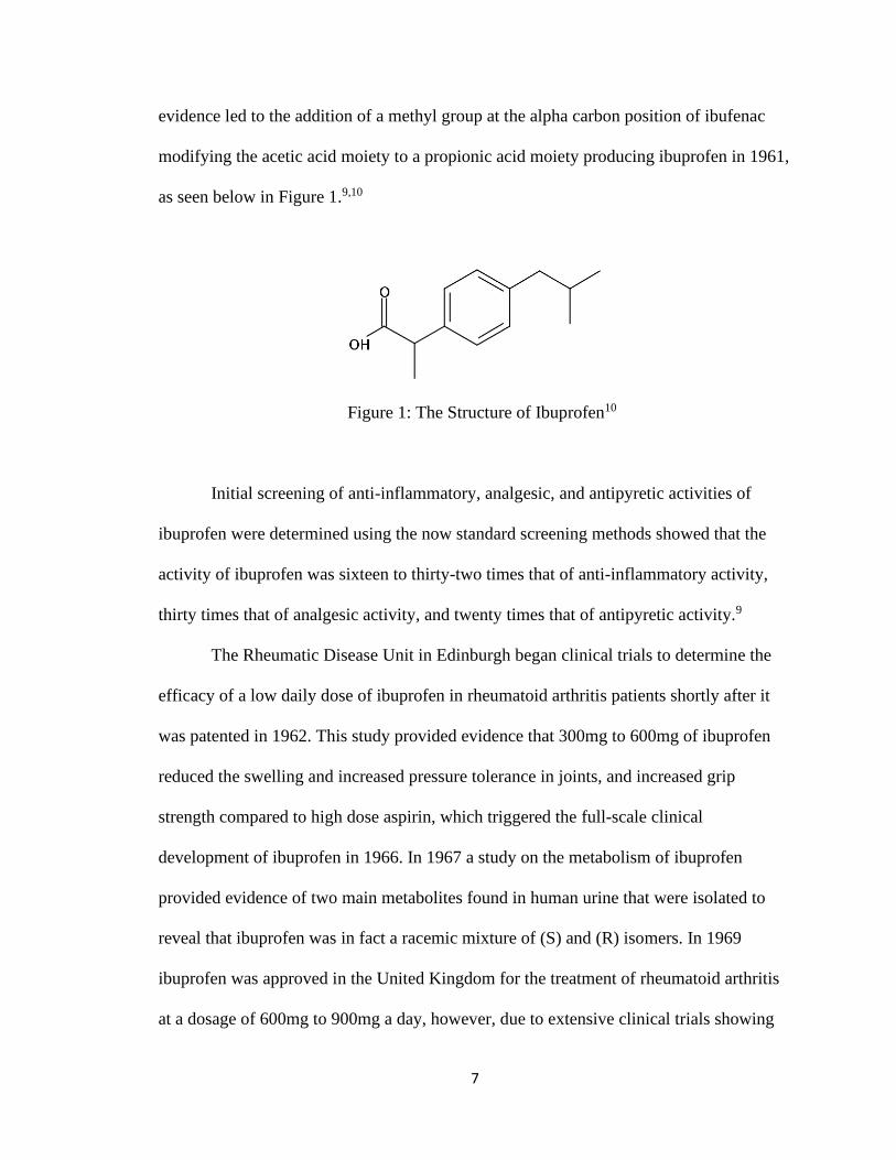
evidence led to the addition of a methyl group at the alpha carbon position of ibufenac

modifying the acetic acid moiety to a propionic acid moiety producing ibuprofen in 1961,

as seen below in Figure 1.9,10

Figure 1: The Structure of Ibuprofen10

Initial screening of anti-inflammatory, analgesic, and antipyretic activities of

ibuprofen were determined using the now standard screening methods showed that the

activity of ibuprofen was sixteen to thirty-two times that of anti-inflammatory activity,

thirty times that of analgesic activity, and twenty times that of antipyretic activity.9

The Rheumatic Disease Unit in Edinburgh began clinical trials to determine the

efficacy of a low daily dose of ibuprofen in rheumatoid arthritis patients shortly after it

was patented in 1962. This study provided evidence that 300mg to 600mg of ibuprofen

reduced the swelling and increased pressure tolerance in joints, and increased grip

strength compared to high dose aspirin, which triggered the full-scale clinical

development of ibuprofen in 1966. In 1967 a study on the metabolism of ibuprofen

provided evidence of two main metabolites found in human urine that were isolated to

reveal that ibuprofen was in fact a racemic mixture of (S) and (R) isomers. In 1969

ibuprofen was approved in the United Kingdom for the treatment of rheumatoid arthritis

at a dosage of 600mg to 900mg a day, however, due to extensive clinical trials showing

8

that ibuprofen was more effective and relatively safe at higher doses the recommended

daily dose was increased to 1200mg to 2400mg. Once it had been demonstrated that the

therapeutic effects of ibuprofen were greater than that of aspirin the examination of

ibuprofen’s effects on the gastrointestinal tract had to be evaluated. The most remarkable

study was performed using patients with a history of peptic ulcers that were administered

ibuprofen long-term in which approximately 10% displayed signs of gastric intolerance,

and another notable study on gastrointestinal blood loss found in patients administered

ibuprofen was noticeably less than that in patients administered aspirin. These studies

confirmed that ibuprofen was a viable replacement for aspirin in the treatment of

rheumatoid arthritis with greatly improved gastrointestinal tolerance.9

In 1976 Dr. Adams investigated the pharmacological differences and

contributions in the anti-inflammatory, analgesic, and anti-pyretic activities of

ibuprofen’s (S) and (R) isomers. Earlier studies had shown that other phenylpropanoic

acid compounds activity consisted essentially within the (S) configuration, and that the

ability of nonsteroidal anti-inflammatory drugs to inhibit prostaglandin synthesis in vitro

was quantitatively related to their activity in vivo.9 Dr. Adams found that in vitro the (S)

isomer was highly active and the (R) isomer had very little activity, however, an

inversion from the (R) to the (S) isomer occurred almost completely in vivo. The great

successes in the study of ibuprofen’s safety record prompted the Boots Co. Ltd. to apply

for non-prescription, over the counter, use in 1978 but was initially turned down in 1979

claiming it was on the grounds of safety. An outside research group brought in by the

Boots Co. Ltd. collected all the data from the 19,000 clinical trials and began new

investigations into the safety of ibuprofen. In 1982 they revised and resubmitted their

9

application, which was approved by the British government in 1983. Ibuprofen was

approved for over-the-counter use in the United States soon after in 1984.9

Since the discovery of cyclooxygenase-2 in 1991 there has been numerous

advances in the field of pharmacology most importantly in pharmacokinetics and

pharmacodynamics, which allowed for a closer look at the mechanism behind ibuprofen’s

two isomers. Studies of the pharmacokinetics of ibuprofen determined that the oral

administration of ibuprofen has a very short half-life (~3hrs.) and at therapeutic

concentrations for anti-inflammatory, analgesic, and anti-pyretic effect (~10-50mg/L) it is

almost completely bound to plasma proteins (>98%), which demonstrates ibuprofen’s

quick absorption (~2hrs.) in the body. Ibuprofen’s low volume of distribution (~0.1-

0.2L/Kg) is consistent with the extent of plasma protein binding that occurs and with the

ability to penetrate the central nervous system and accumulate at necessary peripheral

sites for its anti-inflammatory and analgesic activity. Ibuprofen’s (R) isomer undergoes

inversion (~65%) to the (S) isomer by way of an Acyl-CoA thioester that occurs

predominantly in the liver, and to a lesser extent the gut. Ibuprofen is primarily

metabolized in the liver by way of an oxidative metabolism via Cytochrome P450

(CYP450) in which both isomers are metabolized by a CYP450 subset CYP2C9 and to a

lesser extent the (R) isomer by the CYP450 subsets CYP2C8, CYP2C19, and CYP3A4.

Elimination of ibuprofen occurs within 24 hours through urinary excretion (99%) and

biliary excretion (1%) with a high rate of clearance (3-13L/hr.). Ibuprofen is classified as

a non-selective inhibitor like aspirin, however, unlike aspirin it is a competitive and

reversible inhibitor that binds to the active site of an enzyme preventing other substrates

from binding to the enzyme but can be overwhelmed by increasing concentrations of

10

another substrate thus allowing the enzyme to bind with the competing substrate or allow

the enzyme to resume its normal function. It was his early understanding into the

necessity of a phenylpropanoic acid with a short half-life that provided Dr. Adams with

the correct criteria for the selection of the proper drug candidate. He knew that the extent

of gastrointestinal intolerance was directly related to the drugs half-life, and that the

systemic accumulation of the drug was directly related to organ toxicity. It was these

pharmacological properties that made ibuprofen the most commonly used and most

frequently prescribed nonsteroidal anti-inflammatory drug on the market.9,11

Drug interaction and synergy is the alteration in the pharmacological effect of one

drug in the presence of another drug, food, drink, or environmental agent that occurs

through pharmacokinetic interactions that affect absorption, distribution, metabolism, and

excretion of the drug, or through pharmacodynamic interactions at the drugs site of

action. The pharmacological effect of each drug may increase, decrease, or it can produce

a completely new effect where these interactions may be beneficial or harmful. Many

drug interactions occur through multiple mechanisms that act together and are frequently

termed the “Mechanisms of Drug Interactions”.12

Interactions that occur during absorption may decrease the amount of drug

absorbed therefore decreasing the effectiveness of the drug or may increase the amount of

drug absorbed thus increasing the probability of adverse effects or drug toxicity.

Interactions that occur during distribution may affect the plasma protein binding of one

drug by competition for the site of action by a second drug thus displacing the first drug

activating it and increasing its concentration in plasma water that will not only affect the

volume of distribution of the first drug, but the volume of distribution of the second drug

11

as well. The freed drug molecules are metabolized causing the bound drug molecules to

become free allowing them to pass into solution to exert their pharmacological activity

after which they are metabolized and excreted. The first drug has been metabolized and

excreted prior to achieving stable blood plasma concentrations thus diminishing its

therapeutic effect. Interactions that occur during metabolism may affect one drug when a

second drug inhibits the metabolic enzymes used by the first drug and as the

administration of the first drug continues its concentration increases until adverse effects

or drug toxicity occurs, or the second drug may increase the formation of metabolic

enzymes used by the first drug thus decreasing its concentration and the effectiveness of

the first drug. Interactions that occur during excretion interferes with the liver’s biliary

excretion and the kidneys urinary excretion of most drugs. Interference with the blood

entering the renal arteries, renal tubules, or the disruption of the kidneys transport

systems will increase or decrease urinary excretion or the reabsorption of drug molecules.

Drug molecules are commonly conjugated making them water soluble allowing for

biliary excretion and metabolism by gut flora for reabsorption, however, if a second drug

has antibacterial activity the gut flora decreases thus reabsorption does not occur

decreasing the concentration and the effectiveness of the first drug. Interference with

transport proteins such as the bile salt export pump and solute carriers involved with the

hepatic extraction and biliary excretion of drug molecules may decrease or even inhibit

the flow of bile from the liver and affect renal extraction of drug molecules.12

Alcohol is absorbed into the bloodstream from the gastro-intestinal tract, the

target organ for most medication, and is referred to as ‘First-Pass’ metabolism in which

the liver’s enzyme alcohol dehydrogenase and CYP450 metabolizes a small portion to

12

form the toxic acetaldehyde, which is metabolized by aldehyde dehydrogenase to form

acetate. However, CYP450 plays a crucial role in alcohol-medication interactions and in

the presence of alcohol competition for the enzyme occurs and metabolism of the

medication is hindered. When alcohol and ibuprofen are administered concurrently

increasing concentrations of alcohol causes increasing dissolution of Ibuprofen, which

when in the gastrointestinal tract leads to competition for CYP450 decreasing the

metabolism and excretion of ibuprofen resulting in either overabsorption of ibuprofen

causing an adverse reaction or undissolved ibuprofen resulting in organ damage. Food

delays gastric emptying that frequently affects the rate of absorption of many drugs

including nonsteroidal anti-inflammatory drugs. When Gingko Biloba and ibuprofen are

administered concurrently the platelet-activating receptor antagonist, ginkgolide B,

affects coagulation mechanisms resulting in reduced clotting, which is associated with

prolonged bleeding times and subdural haematomas.11,12

Aspirin is widely used for its anti-inflammatory, analgesic, anti-pyretic, and anti-

platelet activity. When aspirin and ibuprofen are administered concurrently ibuprofen

competes for the binding site of COX-1 where aspirin may decrease ibuprofen’s serum

levels without affecting the serum levels of salicylate, and ibuprofen antagonizes

aspirin’s cardioprotective effect in platelets and increases gastrointestinal bleeding.

Selective serotonin reuptake inhibitors are administered for the treatment of depression

and increase the risk of gastrointestinal bleeding by 30%. When Selective Serotonin

Reuptake Inhibitors (SSRIs) and ibuprofen are administered concurrently serotonin from

the bloodstream is taken into platelets regulating the response to injury as it activates

platelet aggregation where SSRIs can block serotonin reuptake by platelets leading to

13

serotonin depletion and a 50-60% increase in gastrointestinal bleeding due to competition

for the CYP450 subset CYP2C9. Anticoagulants like warfarin are administered for the

treatment of blood clots in the legs and lungs. When warfarin and ibuprofen are

administered concurrently the clotting tendency of blood decreases due to competition for

the CYP450 subset CYP2C9 inhibiting the metabolism of warfarin and increasing its

concentration until an over-anticoagulation effect or drug toxicity occurs.

Antihypertensives like Angiotensin-Converting Enzyme (ACE) inhibitors are

administered for the treatment of high blood pressure and heart problems. When ACE

inhibitors and ibuprofen are administered concurrently an interference with the efficacy

of the ACE inhibitor occurs in the kidney’s where vasoconstriction and fluid retention

activate the renin-angiotensin system causing a significant increase in blood pressure due

to the decrease in the hypotensive effect of the ACE inhibitor.11,12

1.11 Dissolution Testing

The United States Pharmacopeia (USP) is a non-profit organization founded in

1820 with the goal of protecting and improving the health of all human beings by

developing a set of regulatory standards for the quality control and quality assurance in

the manufacturing and storage of human and animal drugs, over-the-counter medicines,

and food ingredients ensuring that each individual item has the identical identity,

strength, quality, purity, and consistency within a set tolerance. Each ingredient or

preparation has a USP Monograph associated with it that includes the name, description,

labelling requirements, packing and storage requirements, and specifications on testing

procedures, methodology, and acceptance criteria. Medicinal formulation Monographs

14

also include the strength, quality, and purity required to meet USP standards. One such

testing procedure is dissolution testing where the medicinal formulation is evaluated to

determine the rate and extent in which it forms a solution under a controlled condition,

which is then used to predict in vivo drug release profiles. The results of this testing

ensure that the bioavailability of the medicinal formulation is not hindered by dissolution,

but it does not definitively demonstrate sample bioavailability. However, failure in

dissolution testing is an accepted sign of substandard performance and further evaluations

must be performed.13,14,15,16

Each Monograph provides the requirements for dissolution medium, apparatus,

evaluation time, Certified Reference Material (CRM), sample solution, instrumental

conditions, and evaluation tolerances. The media is placed into a vessel where a motor

driven apparatus circulates it to simulate the environment of the gastro-intestinal tract.

The medicinal formulation is then placed into the vessel and left to dissolve over a

specific amount of time at body temperature. Samples of the solution are then drawn at

different increments of time and analyzed under specific instrumental conditions. The

quantitative data is then used to produce a Dissolution Profile and determine the

percentage, or concentration, of Active Pharmaceutical Ingredient (API) dissolved and

then compared to the evaluation tolerances provided in the Monograph.14

The dissolution testing system employs six vessels, each a cylindrical container

with a hemispherical bottom made from glass or other inert materials with volumes

ranging from 100mL to 4000mL, however, 900mL vessels are most common. The shape,

material, and manufacturing method play a crucial role in the precision of dissolution

testing. If there are dimensional variations in any of the six vessels employed it will

15

produce unreliable results, which can be resolved by employing injection molded glass

vessels. Dosage forms evaluated in glass vessels may stick to the walls, which can be

resolved by employing plastic vessels. There are many types of dissolution apparatus that

are employed each designed for a specific dosage form and agitation method. When

evaluating solid, beaded, or suspended dosage forms there are one of two apparatus that

the monograph will require. The Basket, Apparatus 1, is connected to a steel shaft and is

commonly designed as a cylinder consisting of a 40-mesh stainless steel screen

containing the dosage form rotated at a rate of 100rpm inside of a 900mL vessel.

Modifications to the basket such as 10-mesh to 100-mesh screens for use in 100mL to

4000mL vessels, varying basket dimensions, and changing the rotation rate to 50rpm or

75rpm are made depending on the dissolution performance desired for a specific dosage

form. The Paddle, Apparatus 2, is connected to a steel shaft and is commonly designed as

a hemispherical blade consisting of an inert material such as Teflon or stainless steel that

is fixed above the dosage form rotating at a rate of 50rpm, 75rpm, or 100rpm.

Modifications to the paddle such as reducing the dimensions producing a ‘mini-paddle’

for use in 200mL vessels are employed if very low concentration dosage forms are being

evaluated.17,18

The dissolution protocol checklist is performed beginning with referencing the

monograph for the solid dosage forms to be examined to determine the testing parameters

required. The apparatus is then selected, and any necessary modifications are performed.

Parameters such as medium composition, quantity dissolved specifications, and rate of

rotation are verified. The sampling method, sampling interval, and sampling analysis

protocols are then developed. The vessels are then inspected for any nicks, cracks, or

16

debris adhered to all surfaces assuring that they are transparent so that air bubbles in the

medium can be detected, and more precise observations can be performed during the

disintegration process. The bath temperature is then adjusted to 37oC. The vessels are

installed, and the bath level is verified to be above the surface of the vessel medium. The

medium is then prepared as per the individual monograph, degassed, and added to the

vessels. The syringes, cannulas, filters, and the sampling access to the vessels are

checked for any interferences that may hinder sampling or alter adsorption. Vessel

sampling access is then configured so that the solid dosage forms can be inserted, and

samples can be drawn efficiently.17

The solid dosage forms are dropped as close to the center of the vessel, the clutch

is engaged initiating paddle rotation, and the stopwatch started. Between each sampling

interval detailed observations are recorded for each vessel. Each sample drawn is secured

using airtight sample vials to assure no evaporation can occur. All samples are retained

until the instrumental analysis has been completed and all calculations have been

verified.17

Once all dissolution samples have been secured a spectrophotometric absorption

assay is performed as stated on the monograph for the API using a CRM standard, which

is commonly performed via Ultraviolet and visible absorption spectroscopy (UV-Vis).

Using Beer’s Law, the standard (s) of concentration (C) is analyzed within a cuvette of

thickness (b) with the molar absorptivity of the API (a) to determine the absorbance of

the standard (As), as seen below in Equation 1.14

𝐴𝑠 = 𝑎𝑏𝐶𝑠 (1)

17

The dissolution sample (u) of concentration (C) is then analyzed using a matching

cuvette (b) with the same molar absorptivity (a) to determine the absorbance of the

dissolution sample (Au), as seen below in Equation 2.14

𝐴𝑢 = 𝑎𝑏𝐶𝑢 (2)

The equations are then combined using the Beer’s Law relationship in which the

molar absorptivity (a) and cuvette thickness (b) are removed, and the equation rearranged

to produce Equation 3 below.14

𝐶𝑢 = 𝐶𝑠 (𝐴𝑢

𝐴𝑠) (3)

The ratio method is an acceptable method, however, omitting a CRM in lieu of a

calibration curve is permissible only if the API conforms to the Beer’s Law relationship.

When implementing a calibration curve preparation of standards ranging between 75% to

125% of the concentration required on the monograph for the assay of the API, after

which the analysis is performed using the spectrophotometric absorption assay required

in the monograph for the API.14

The tolerance, or the unit quantity (Q), of the labeled amount of API specified in

the monograph is the amount dissolved in the specified amount of time, which is

expressed as a percentage of the labeled content. The tolerance value is acceptable only if

the dissolution test conforms to each Stage (Sn) of the acceptance table for the specific

dosage form being evaluated. Immediate-release solid dosage forms in which six units

18

are evaluated are classified as Stage 1 (S1) in which each unit cannot be less than Q+5%.

If the test satisfies S1 then it has met the required tolerance and no further evaluation is

necessary, however, if the test does not meet S1 then the next stage of the evaluation must

be performed. The next stage, Stage 2 (S2), requires that six more units be evaluated after

which the average of the units from S1 and S2 is determined and must be equal to or

greater than Q with no one unit less than Q-15%. If the test satisfies S2 then the test has

met the required tolerance and no further evaluation is necessary, however, if the test

does not meet S2 then the next stage of the evaluation must be performed. The next stage,

Stage 3 (S3), requires that twelve more units be evaluated after which the average of the

units from S1, S2, and S3 is determined and must be equal to or greater than Q with no

two units less than Q-15%, and with no one unit less than Q-25%.14

The difference factor (𝑓1) and similarity factor (𝑓2) test (𝑓-Test) is performed

routinely to determine bioequivalence, or the expected biological equivalence, as to

obtain biowaivers to allow pharmaceutical companies to be exempt from being required

to perform timely and expensive bioequivalence studies. The 𝑓-Test is used to determine

the bioequivalence of two different preparations of dosage units, different formulations,

different strengths, different manufacturing methods, different compositions of

components, or to compare a newly manufactured dosage unit to a dosage unit that has

been stored for an extended period. The 𝑓-Test is also implemented to compare dosage

forms from an identical batch. To perform a dissolution profile comparison the

dissolution test is performed two separate times using twelve dosage units in each

dissolution test performed under identical conditions, methods, and sampling times to

produce two dissolution curves using no less than three dissolution measurements with no

19

one release value above 85%. The dissolution measurements should appropriately

represent the dissolution profile with measurements being as spread out as possible. If

mean data is to be used then the %CV must be no more than 20% for dissolution

measurements at or below 15 minutes, and no more than 10% for all other measurements.

The 𝑓1 test is the percent difference between the two dissolution profiles at individual

measurement times, which represents the relative error between the two dissolution

profiles. It is normalized and the acceptance value is based on a 10% average difference

between the two dissolution profiles. The 𝑓1 test profile is identical if it has a value of 0

and is considered not to be different if it has a value between 0 and 15. The 𝑓1 test is

calculated using the sum of the number of measurement time points (n), the dissolution

value of the reference batch at time t (Rt), and the dissolution value of the test batch at

time t (Tt), as seen below in Equation 4.19,20

𝑓1 = (∑ |𝑅𝑡−𝑇𝑡|𝑛𝑡=1

∑ 𝑅𝑡𝑛𝑡=1

) ∙ 100 (4)

The 𝑓2 test is the logarithmic reciprocal square root transformation of the sum or

the error squared, which represents the measurement of similarity in the percent

dissolution between the two dissolution profiles. The 𝑓2 test profile is identical if it has a

value of 100 and is considered not to be different if it has a value between 50 and 100.

The 𝑓2 test is calculated using the sum of the number of measurement time points (n), the

dissolution value of the reference batch at time t (Rt), and the dissolution value of the test

batch at time t (Tt), as seen below in Equation 5.19,20

20

𝑓2 = 50 ∙ 𝑙𝑜𝑔 {[1 +1

𝑛∑ (𝑅𝑡 − 𝑇𝑡)

2𝑛𝑡=1 ]

−0.5

∙ 100} (5)

The determination of the difference and similarity reflect the maximum and

minimum change between two dissolution profiles and is an excellent tool which allows

for the dissolution equivalence to be characterized in a simple approach.20

1.12 Calibration Methods

Quality assurance is responsible for the design of experimental procedures and the

gathering and analysis of experimental data, which continually assists in the improvement

of one another by determining and correcting systematic and random sources of error.

The two components of a quality assurance program are quality control and quality

assessment. The main purpose of quality control is to design specific protocols, methods,

and techniques in the attempt to bring the analytical method under statistical control. This

includes the collection, analysis, and identification of samples within a specific range of

precision and accuracy. The main purpose of quality assessment is to confirm that the

specific protocols, methods, and techniques developed by quality control have reached

the state of statistical control required by state or federal regulations. In a laboratory

setting it is the analytical chemist who performs the analysis and treats the raw data

determining whether the specific protocol, method, or technique has reached that state of

statistical control. The data the analytical chemist treats is commonly concentrations of

known or unknown samples, or analytes, determined by applying a calibration method

combined with a specific instrumental technique then reporting those quantities after

statistical analysis in terms of mean, standard deviation, relative standard deviation,

21

confidence interval, and variance to name a few. Calibration is the process employed in

which to assess and refine the accuracy and precision of analytical methods and

instrumental techniques. Each calibration method employs reference samples known as

standards that can range from two to as many as ten, which includes a ‘Blank’ that

contains the medium and matrix involved in the analysis but does not contain any of the

unknown analyte. There are two approaches each calibration method can utilize to

determine the concentration of unknown analyte. The ratio approach and the graphical

approach.21,22,23

The ratio approach assumes that there is a linear relationship between the

analytical signal produced by the instrumental technique and the concentration of known

standards to determine the concentration of the unknown analyte, however, this

assumption could be incorrect due to error in the preparation of the standard, noise from

the instrument, or a matrix containing solvent or other substances surrounding the

analyte. The graphical approach confirms this linear relationship by way of graphing the

signal versus the concentration and then applies regression analysis. Regression analysis

is a statistical tool that estimates the relationship between the signal (y) and the

concentration (x) of the standard by minimizing the distance from a best-fit line, or

trendline, to each datapoint on the graph in which the distance between them represents

the error in the slope (m) and the intercept (b) of the trendline, as seen below in Equation

6. 21,22,23

𝑦 = 𝑚𝑥 + 𝑏 (6)

22

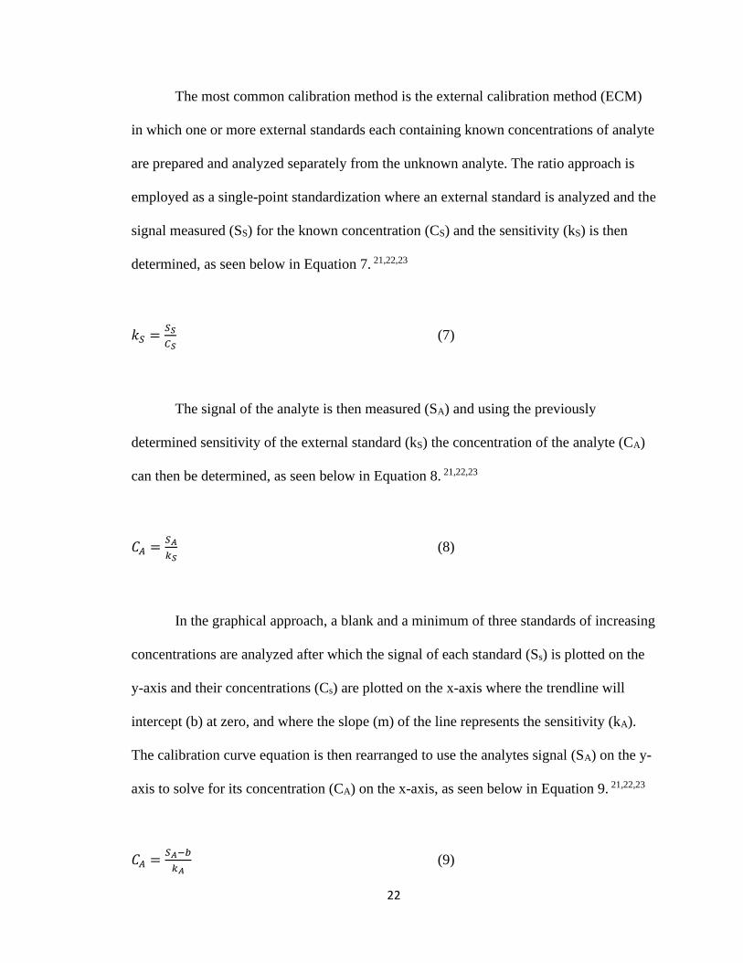
The most common calibration method is the external calibration method (ECM)

in which one or more external standards each containing known concentrations of analyte

are prepared and analyzed separately from the unknown analyte. The ratio approach is

employed as a single-point standardization where an external standard is analyzed and the

signal measured (SS) for the known concentration (CS) and the sensitivity (kS) is then

determined, as seen below in Equation 7. 21,22,23

𝑘𝑆 =𝑆𝑆

𝐶𝑆 (7)

The signal of the analyte is then measured (SA) and using the previously

determined sensitivity of the external standard (kS) the concentration of the analyte (CA)

can then be determined, as seen below in Equation 8. 21,22,23

𝐶𝐴 =𝑆𝐴

𝑘𝑆 (8)

In the graphical approach, a blank and a minimum of three standards of increasing

concentrations are analyzed after which the signal of each standard (Ss) is plotted on the

y-axis and their concentrations (Cs) are plotted on the x-axis where the trendline will

intercept (b) at zero, and where the slope (m) of the line represents the sensitivity (kA).

The calibration curve equation is then rearranged to use the analytes signal (SA) on the y-

axis to solve for its concentration (CA) on the x-axis, as seen below in Equation 9. 21,22,23

𝐶𝐴 =𝑆𝐴−𝑏

𝑘𝐴 (9)

23

However, if the matrix of the analyte is unknown than the ECM is not

implemented due to the matrix of the calibration method being much less complicated

than that of the analyte, which will then alter the signals sensitivity (kS). If there is error

in the preparation of one of the external standards the total error remains very small due

to the other external standards maintaining a linear relationship with the sensitivity (kA).

When the ECM cannot be implemented due to mismatched matrices between the standard

and the analyte it is commonplace to implement the standard addition method (SAM).

21,22,23

In the ratio approach, there are several ways to approach the SAM method. For

example, a constant volume of analyte (VA) is added to two volumetric flasks after which

a volume of external standard (VS) at a known concentration (CS) is added to one of the

volumetric flasks, referred to as a spike. Each are then topped with solvent to produce a

final volume (VF). The solutions are then analyzed producing one signal for the pure

analyte (SA) and one signal for the spiked analyte (SA+S), after which the concentration of

the unknown analyte (CA) can be determined, as seen below in Equations 10 and 11

beginning with Equation 6 and setting y to zero. 21,22,23

𝑦 =𝑆𝐴+𝑆−𝑆𝐴


𝐶𝐴 + 𝑆𝐴 (10)

𝐶𝐴 = |−𝑆𝐴


𝑆𝐴+𝑆−𝑆𝐴| (11)

24

In the graphical approach, the signal for the spiked analyte (SA+S) is plotted on the

y-axis and the concentration of spiked standard (CS) is plotted on the x-axis where the

trendline intercepts (b) on the y-axis, and the slope (m) of the line represents the

sensitivity. The calibration curve equation is then rearranged to solve for the x-intercept

by setting the y-axis to zero. Again, beginning with Equation 6, the concentration of

analyte can be determined using the absolute value, as seen below in Equation 12. 21,22,23

𝐶𝐴 = |−𝑏

𝑚| (12)

When there is a possibility of analyte loss during sample preparation such as

spillage or evaporation, instrumental drift due to variation in the radiation sources energy

or intensity, variation in sample injection volumes, or the necessity for improved

accuracy and precision, the internal standard method (ISM) is implemented. The ISM is

generally implemented using a single standard that employs a known concentration of a

compound that is similar in concentration, chemical properties, and within the same

wavelength excitation range as the analyte, referred to as the internal standard (IS), which

is added to the blank, standard, and analytes to be used in the instrumental analysis. Due

to the IS being added to the analyte during sample preparation the ratio of IS to the

analyte is constant. If there is any loss of analyte due to spillage or evaporation, then the

loss of IS will be proportional. This proportionality is also observed during the

instrumental analysis. If there is a variation in the radiation sources energy or intensity, or

injection volumes between analysis, then the IS response will be proportional. 21,22,23

25

In the ratio approach the signal of analyte measured (SA) is directly proportional

to the analyte concentration (CA) and sensitivity (kA), as seen below in Equation 13.

21,22,23

𝑆𝐴 = 𝑘𝐴𝐶𝐴 (13)

Similarly, the signal of IS measured (SI) is directly proportional to the IS

concentration (CI) and sensitivity (kI), as seen below in Equation 14. 21,22,23

𝑆𝐼 = 𝑘𝐼𝐶𝐼 (14)

Since the two signals are directly proportional Equation 8 and Equation 9 can then

be combined, as seen below in Equation 15. 21,22,23

𝑆𝐴

𝑆𝐼=

𝑘𝐴𝐶𝐴

𝑘𝐼𝐶𝐼 (15)

The sensitivity of the two signals will then be constant over a wide range of

conditions. If the signal of analyte increases due to change in temperature or flow rate,

then the signal of the IS increases proportionally, referred to as the relative response

factor (K), and the sensitivities can be combined and rearranged to produce the ISM

equation, as seen below in Equation 16. 21,22,23

𝑆𝐴

𝐶𝐴= 𝐾

𝑆𝐼

𝐶𝐼 (16)

26

The relative response factor (K) must be determined prior to analysis and is

determined by rearranging Equation 11. This is performed by analyzing a standard of

known concentration (CS) consisting of the same chemical species as the analyte to

determine its response (SS) in relation to the response of the IS (SI) at known

concentration (CI), as seen below in Equation 17. 21,22,23

𝐾 =𝑆𝑆𝐶𝐼

𝑆𝐼𝐶𝑆 (17)

The relative response factor (K) determined in Equation 17 is then used in the

analysis of the unknown concentration of analyte (CA) producing the measured signal

(SA) in relation to the measured signal of IS (SI) of known concentration (CI) using the

ISM equation, as seen below in Equation 18. 21,22,23

𝑆𝐴

𝐶𝐴= 𝐾

𝑆𝐼

𝐶𝐼 (18)

Lastly, the unknown concentration of analyte (CA) can be determined by

rearranging Equation 18, as seen below in Equation 19. 21,22,23

𝐶𝐴 =𝐶𝐼𝑆𝐴

𝐾𝑆𝐼 (19)

In the graphical approach, the IS concentration is held constant for all standards

and samples (analytes) The ratio of the standard signal (SS) to the IS signal (SI) is plotted

27

on the y-axis (𝑆𝑆

𝑆𝐼) and the standard concentration (CS) is plotted on the x-axis where the

trendline intercepts (b) on the y-axis and the slope (m) of the line represents the

sensitivity. The samples are analyzed subsequently and ratio of the analyte signal (SA) to

IS signal (SI) is calculated. Referring to Equation 6, the calibration curve equation is then

rearranged to solve for the analyte concentration (CA), as seen below in Equation 20.

21,22,23

𝐶𝐴 =(𝑆𝐴𝑆𝐼) −𝑏

𝑚 (20)

1.13 Standard Dilution Analysis

A new calibration method that combines both the SAM and ISM has been

evolving since 2015 called Standard Dilution Analysis (SDA), which corrects for matrix

effects and interferences caused by instrumental variations and non-spectral signal

fluctuations in analyte properties and positioning. Empirical evidence gathered from

current research shows that SDA produces more precise Figures of Merit than that of

ECM, SAM, and ISM when implemented individually. There are two requirements an

instrumental technique must meet prior to implementation of SDA. The Instrument must

have the ability to accept liquid samples and monitor a minimum of two wavelengths

simultaneously. As of today, SDA has only been performed in the analysis of elements

and small molecules such as hydrogen chloride, nitric acid, and ethanol. However, it has

not yet been attempted in both the analysis of larger molecules and employing Ultra

High-Performance Liquid Chromatography (UHPLC) as the analytical technique. The

28

SDA Calibration method is carried out by preparing a standard solution consisting of the

analyte (A) with an internal standard (I) that when analyzed produces a signal for the

analyte (SA) that originates from the sample (sam) and the standard (std), which is

monitored at one wavelength (λ1) while simultaneously monitoring the signal from the

internal standard (SI) at a second wavelength (λ2). Each signal is equal to the calibration

sensitivity (m) which is multiplied by the individual species concentrations (mACA) and

(mICI), as seen below in Equation 21.24,25,26,27

𝑆𝐴

𝑆𝐼=

𝑚𝐴𝐶𝐴

𝑚𝐼𝐶𝐼=

𝑚𝐴(𝐶𝐴𝑠𝑡𝑑+𝐶𝐴

𝑠𝑎𝑚)

𝑚𝐼𝐶𝐼=

𝑚𝐴𝐶𝐴𝑠𝑎𝑚

𝑚𝐼𝐶𝐼+

𝑚𝐴𝐶𝐴𝑠𝑡𝑑

𝑚𝐼𝐶𝐼 (21)

When the data is used to produce a calibration curve the ratio of analyte signal to

internal standard signal is plotted on the y-axis (𝑆𝐴

𝑆𝐼) versus the inverse of the internal

standard concentration (1

𝐶𝐼) on the x-axis, which produces the slope and intercept, as seen

below in Equation 22 and Equation 23, respectively.24

𝑆𝑙𝑜𝑝𝑒 =𝑚𝐴𝐶𝐴

𝑠𝑎𝑚

𝑚𝐼 (22)

𝐼𝑛𝑡𝑒𝑟𝑐𝑒𝑝𝑡 =𝑚𝐴𝐶𝐴

𝑠𝑡𝑑

𝑚𝐼𝐶𝐼 (23)

To prepare the solutions for SDA analysis the sample containing the unknown

analyte (A) is combined with the standard and the internal standard at a fixed ratio, as

seen below in Equation 24. 24

29


𝐶𝐼= 𝐶𝑜𝑛𝑠𝑡𝑎𝑛𝑡 (24)

If the amount of the sample continues to be constant during solution preparation,

then matrix effects do not occur and both the slope of the analyte and internal standard

(𝑚𝐴

𝑚𝐼) remains constant along with the intercept, and the concentration of the unknown

analyte (A) can be determined easily, as seen below in Equation 25. 24

𝐶𝐴𝑠𝑎𝑚 =

𝑆𝑙𝑜𝑝𝑒

𝐼𝑛𝑡𝑒𝑟𝑐𝑒𝑝𝑡×


𝐶𝐼 (25)

Since the standard solution contains a fixed ratio of analyte (A) to internal

standard (I) the concentration can be determined by the calibration plot. However, there

are three contributing factors that must be addressed prior to analysis: (1) Assuring that

the analyte (A) and internal standard (I) contain concentrations in the calibration curves

dynamic range, (2) The mixture contains no other contributing species, and (3) Spectral

interferences are measured beforehand, and the signals normalized. If these caveats

cannot be addressed, then SDA will fail.24

1.14 Figures of Merit

Upon completion of the instrumental analysis, method validation is performed to

determine the Figures of Merit (FOM). The analytical data is then used to calculate the

sample mean (�̅�) by summing all the samples (xn) then dividing the sample sum by the

number of samples (n), as seen below in Equation 26.14

30

�̅� =∑ 𝑥1𝑛𝑖=1

𝑛=

𝑥1+𝑥2+…+𝑥𝑛

𝑛 (26)

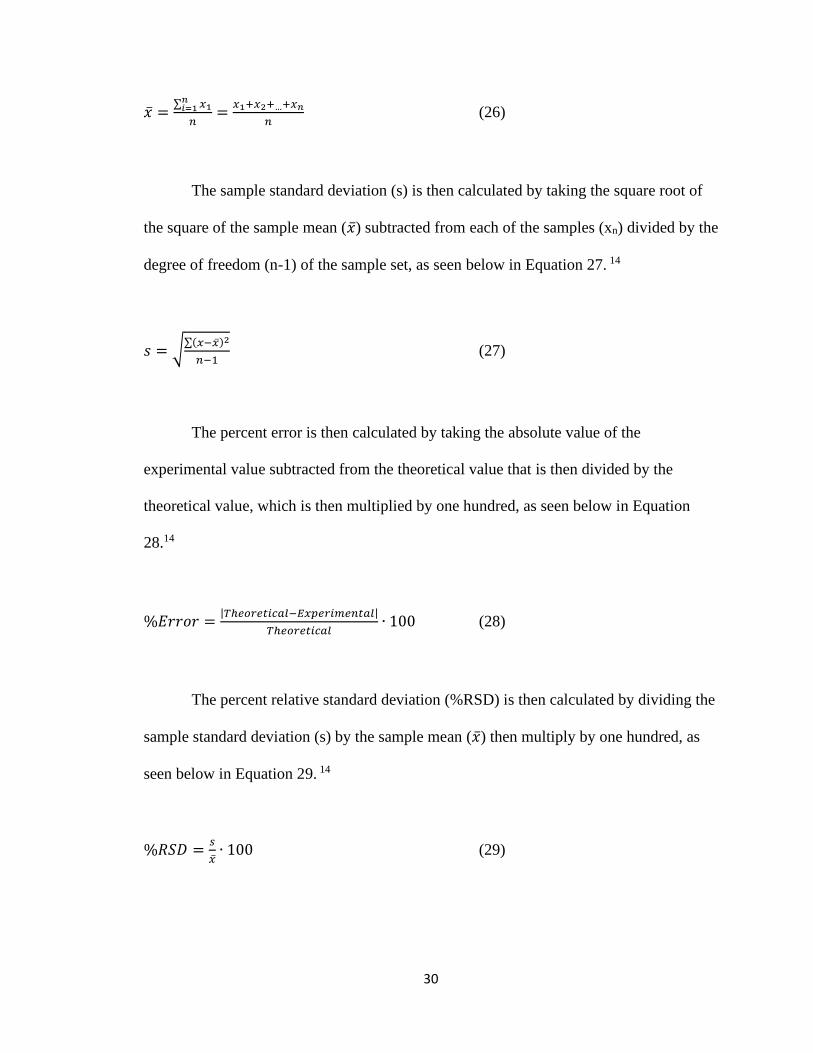
The sample standard deviation (s) is then calculated by taking the square root of

the square of the sample mean (�̅�) subtracted from each of the samples (xn) divided by the

degree of freedom (n-1) of the sample set, as seen below in Equation 27. 14

𝑠 = √∑(𝑥−�̅�)2

𝑛−1 (27)

The percent error is then calculated by taking the absolute value of the

experimental value subtracted from the theoretical value that is then divided by the

theoretical value, which is then multiplied by one hundred, as seen below in Equation

28.14

%𝐸𝑟𝑟𝑜𝑟 =|𝑇ℎ𝑒𝑜𝑟𝑒𝑡𝑖𝑐𝑎𝑙−𝐸𝑥𝑝𝑒𝑟𝑖𝑚𝑒𝑛𝑡𝑎𝑙|

𝑇ℎ𝑒𝑜𝑟𝑒𝑡𝑖𝑐𝑎𝑙∙ 100 (28)

The percent relative standard deviation (%RSD) is then calculated by dividing the

sample standard deviation (s) by the sample mean (�̅�) then multiply by one hundred, as

seen below in Equation 29. 14

%𝑅𝑆𝐷 =𝑠

�̅�∙ 100 (29)

31

The lowest concentration of analyte the instrumental technique can detect, or limit

of detection (LOD), is then determined by multiplying the sample standard deviation (s)

by three (3s) and then dividing it by the slope (m), as seen below in Equation 30.22

𝐿𝑂𝐷 =3𝑠

𝑚 (30)

The lowest concentration of analyte the instrumental technique can quantify, or

limit of quantitation (LOQ), is then determined by multiplying the sample standard

deviation (s) by ten (10s) and then dividing it by the slope (m), as seen below in Equation

31.22

𝐿𝑂𝑄 =10𝑠

𝑚 (31)

Lastly, from LOQ to the Limit of Linearity (LOL), the point at which the signal

ceases to maintain a linear relationship with the analyte concentration, is the Linear

Dynamic Range (LDR), or the range in which the signal maintains a linear relationship

with the concentration of analyte, as seen below in Equation 32.28

𝐿𝐷𝑅 = 𝑓𝑟𝑜𝑚 𝐿𝑂𝑄 𝑡𝑜 𝐿𝑂𝐿 (32)

1.15 Ultra-High-Performance Liquid Chromatography

Chromatography is the analytical technique that separates the complex

components of a chemical mixture between two phases. The stationary phase is a solid or

32

liquid that is fixed inside of a cylinder where the gas or liquid mobile phase moves the

chemical mixture across the stationary phase where analytes of the chemical mixture

having different strength affinities for the components in the stationary phase are retained

through a variety of mechanisms. The analytes return to the mobile phase at different

times thus separating each component in the chemical mixture.22

High-Performance Liquid Chromatography (HPLC) employs high pressure

pumps that push the liquid mobile phase at a set rate through a system of plumbing at a

maximum pressure of approximately 5,800psi and temperatures up to 40oC. The chemical

mixture is injected in volumes between 5-50µL into the flowing mobile phase by a

syringe or a prefilled ‘sample loop’. The stationary phase consists of many fine spherical

microporous silica particles between 3-5.0µm diameter containing large surface areas

with stationary phase coatings.22

There are two types of phases employed in liquid chromatography. The normal-

phase liquid chromatography is where the stationary phase is composed of a polar

packing material such as silica with hydroxyl groups and employs a less polar liquid

mobile phase where the more nonpolar components of the chemical mixture leave from

the column first. The reverse-phase liquid chromatography is where the stationary phase

is composed of a nonpolar entity such as octadecylsilane (C18) and employs a more polar

liquid mobile phase where the more polar components of the chemical mixture leave

from the column first.22

The analyte, in the process of partition chromatography, partitions between being

dissolved in the liquid mobile phase or the bonded stationary phase. The time the analyte

remains in the stationary phase is depends on the mobile phase strength. After the

33

analytes leave the column, they cross a detector which is most often a UV-Vis detector.

The results are sent to the instrument’s computer data station where the signal is

converted and displayed graphically as a chromatogram. A chromatogram is a graph that

displays the detector response as a function of the displacement of the molecules in the

chemical mixture over time. The display is a series of colored peaks representing the

signal response of the analytes in the chemical mixture. Finally, the mobile phase and

analytes enter a hazardous waste receptacle connected to the HPLC, as seen below in

Figure 2.22,29

Figure 2: A High-Performance Liquid Chromatography System30

Ultra-High-Performance Liquid Chromatography (UHPLC) functions under the

same principles as HPLC, however, it employs smaller inner diameter tubing, a

maximum pressure of approximately 19,000psi, temperatures as high as 65oC, injection

volumes between 2-20µL, and spherical microporous silica particles between 1.7-

5.0µm.29

34

There are many chromatography parameters that make up the chromatogram. The

retention time (tr) is the time it takes for the molecules in the chemical mixture to be

injected into the column and the time the molecules take to reach the detector. The

resolution (Rs) is the measure of the separation between two adjacent chromatographic

peaks where a higher value denotes a better separation, with 1.5 being required for

baseline separation. The capacity factor (k’) is the measure of the interaction, or

retention, of the molecules in a chemical mixture and the chromatographic column where

a value between 1 and 5 is optimal. The efficiency of a chromatographic peak measures

the dispersion of the molecules in the chemical mixture as it flows through the column.

The two parameters that make up column efficiency are theoretical plate number and

plate height. Theoretical plates are the division of equilibrations of the molecules in the

chemical mixture that are partitioned between the mobile phase and stationary phase. The

plate number (N) is the measure of the dispersion of the molecules in the chemical

mixture as it flows through the column, and the plate height (HETP) is the column length

required for one equilibration of the molecules in the chemical mixture. The tailing factor

(Tf) is a representation of the asymmetry in the chromatographic peak band shape. The

selectivity factor (α), or sensitivity, is the measure of a chromatographic systems ability

to differentiate between different molecules in the chemical mixture where the greater the

value the better separation between two peak apices.21,31

35

1.16 Research Goals

This research will evaluate the dissolution rate of 200mg ibuprofen tablets as per

the USP monograph in the presence of ascorbic acid or caffeine to mimic the

administration of the active pharmaceutical ingredient using orange juice and caffeinated

soft drinks, respectively. A comparative analysis of the figures of merit will be performed

for the external calibration method (ECM), the standard addition method (SAM), the

internal standard method (ISM), and the standard dilution analysis (SDA) method. The

empirical evidence gathered by the research will increase current knowledge of 1) the

effect of added beverage constituents on dissolution rates and 2) the utilization of SDA

by HPLC.

The standard dilution analysis (SDA) method has only been employed in the

analysis of colored dyes (Visible Spectroscopy)24, elements (ICP-OES)25,27, and ethanol

(Raman Spectroscopy)26. Superior figures of merit have been reported. Only UV-Vis

Spectroscopy, Raman Spectroscopy, and ICP-OES have been employed in the analyses to

date. SDA has not been employed in the analysis of other molecules nor has it been

employed via UHPLC as the analytical technique. This research is a high risk, high

reward first attempt employing SDA on UHPLC. Since SDA is the combination of SAM

and ISM, a large time commitment to one unknown sample occurs and this time

commitment increases due to the nature of chromatography. By utilizing an automated

UHPLC, with less than 2-minute chromatograms, this time commitment is shortened.

36

CHAPTER 2 – MATERIALS AND METHODS

2.10 Materials, Equipment, and Instrumentation Employed

The list of chemicals, disposable products, equipment, and instrumentation

employed in the research were tabulated for quick reference, as seen below in Table 1 to

Table 4, respectively.

Table 1: List of Chemicals

Table 2: List of Disposable Products

Chemical CAS Purity/Grade Physical State Mfg. Name Mfg. Location

Monobasic Potassium Phosphate 7778-77-0 Ultrapure Bioreagent Crystal, Solid J.T. Baker Phillipsburg, NJ

Sodium Hydroxide 1310-73-2 40% (w/w) Aqueous, Liquid VWR Chemicals Radnor, PA

L-Ascorbic Acid, ACS 50-81-7 ≥99% Powder, Solid Fisher Chemical Pittsburg, PA

Caffeine, USP/FCC 58-08-2 ≥98.5% Anhydrous, Solid Fisher Chemical Pittsburg, PA

Formic Acid 64-18-6 90% Aqueous, Liquid Fisher Chemical Pittsburg, PA

Methanol 67-56-1 LC/MS Grade Liquid Fisher Chemical Pittsburg, PA

Ammonium Hydroxide 1336-21-6 28-30% Aqueous, Liquid VWR Chemicals Radnor, PA

Acetonitrile 75-05-8 LC/MS Grade Liquid Fisher Chemical Pittsburg, PA

Water 7732-18-5 LC/MS Grade Liquid Fisher Chemical Pittsburg, PA

Ibuprofen, USP 15687-27-1 ≥97% Powder, Solid Spectrum Chemical New Brunswick, NJ

Benzoic Acid 65-85-0 99% Crystal, Solid Alfa Aesar Ward Hill, MA

Biphenyl 92-52-4 99.5% Crystal, Solid Eastman Kodak Rochester, NY

Naphthalene 91-20-3 99% Crystal, Solid Acros Organics Geel, Belgium

Item Model Volume/Size/Pore Material/Description Catalog Mfg. Name Mfg. Location

Membrane Filter Durapore 47mm x 0.45um Hydrophilic Polyvinylidene Fluoride HVLP04700 Merck Millipore Burlington, MA

Storage Bottle Nalgene 1L Narrow-Mouth High-Density Polyethylene Resin 2002-0032 Thermo Fisher Scientific Waltham, MA

Sample Test Tube Culture Tubes 16mm x 150mm Borosilicate Glass 14-961-31 Thermo Fisher Scientific Waltham, MA

Micropipette Tip Yellow Redi-Tip 1-200uL Polypropylene Resin 02-681-2 Thermo Fisher Scientific Waltham, MA

Micropipette Tip Blue Redi-Tip 100-1000uL Polypropylene Resin 02-681-4 Thermo Fisher Scientific Waltham, MA

LC Sample Vial Convienience Kit 2mL 12mm x 32mm Clear Glass 13-622-188 Thermo Fisher Scientific Waltham, MA

Syringe Luer-Lok 10mL Polypropylene Resin 309604 Becton, Dickinson & Co. Franklin Lakes, NJ

Filter Luer-Lok 25mm x 0.45um Nylon CH4525-NN Thermo Fisher Scientific Waltham, MA

Centrifuge Tube Falcon 15mL Polystyrene 352095 Corning Corning, NY

37

Table 3: List of Equipment

Table 4: List of Instrumentation

2.11 Dissolution Testing Medium

Unmodified Dissolution Medium

The parameters and medium used in the dissolution testing of ibuprofen tablets,

followed the USP35-NF30, and employed a pH 7.2 phosphate buffer. A 0.2M monobasic

potassium phosphate solution was prepared by adding 27.22g of monobasic potassium

phosphate to a 1L volumetric flask topped to the volumetric line with DI water. A 0.2M

sodium hydroxide stock was then prepared by adding 18.0mL of 40% (w/w) sodium

hydroxide to a 1L volumetric flask topped to the volumetric line with DI water. The

solutions were stirred by magnetic stir bars until homogeneous. This procedure was

performed two times for each dissolution test performed. The solids were measured using

Item Model/Series Description Model Number Mfg. Name Mfg. Location

Deionized Water System Picosystem 18MΩ cm-1

ASTM/CAP Type 1 Reagent Grade ET-11218 Hydro Atlanta, GA

Volumetric Pipettes Fisherbrand To Deliver ±0.003mL @ 20oC 13-650 Thermo Fisher Scientific Waltham, MA

Micropipettes Reference 10-100uL Single-Channel Variable-Volume 4910000042 Eppendorf Enfield, CT

Micropipettes Reference 100-1000uL Single-Channel Variable-Volume 22470302 Eppendorf Enfield, CT

Vision Classic 6 Dissolution Tester DS-00-0145

Easi-Lock USP Precision 1L Glass Vessels (Serialized) 74-104-101

USP PDVF 1L Spin-Paddles (Serialized) 74-105-201

Easi-Lock Vessel Covers 74-104-151

Easi-Lock Vessel Cover Plugs 74-107-006

Vision 1/8" Peek Manual Sampling Cannula Luer-Lok Adapter 74-104-201

Chromatography Column Hypersil Gold C18 100mm L x 4.6mm i.d. with 5um Particle Size 25005-104630 Shimadzu Columbia, MD

Dissolution Testing UnitTeledyne Hanson

ResearchChatsworth, CA

Instrument Model Description Model Number Mfg. Name Mfg. Location

Analytical Balance New Classic MF 0.0001g Readability AL204 Mettler-Toledo Greifensee, Switzerland

Analytical Balance Fisher Science Education 0.01g Readability ALF2002 Thermo Fisher Scientific Waltham, MA

Dual-Beam Monochromator

Full Spectrum Xenon Pulse Lamp

Dual Silicon Diode Detectors

Quartz Covered Optics

Communications Bus Unit CBM-20A

Solvent Delivery Unit LC-30AD

Solvent Degassing Unit DGU-20A5R

Automatic Sampling Unit SIL-30AC

Column Oven Unit CTO-20A

Multi-Wavelength Detector Unit SPD-30AM

Ultra-High-Performance

Liquid ChromatographyNexera X2 Shimadzu Columbia, MD

UV-Vis

SpectrophotometerVarian Cary 50 Probe Agilent Technologies Santa Clara, CA

38

an analytical balance with a 0.0001g readability and the volumes were measured using

volumetric pipettes.

To prepare the pH 7.2 phosphate buffer 750.0mL of 0.2M potassium phosphate

monobasic solution, 520.5mL of 0.2M sodium hydroxide solution, and 1729.5mL of DI

water was measured using a 1L graduated cylinder and then added to a 3L Erlenmeyer

flask and stirred for 15 minutes. Depending on the acidity or basicity of the phosphate

buffer the pH was measured and adjusted to 7.2 either using a 1.0M monobasic potassium

phosphate solution (prepared by adding 68.0430g of potassium phosphate monobasic to a

500mL volumetric flask topped to the volumetric line with DI water), or a 2.0M sodium

hydroxide solution (prepared by adding 90.1mL 40% w/w sodium hydroxide to a 500mL

volumetric flask topped to the volumetric line with DI water).

The phosphate buffer was then deaerated by heating above 41oC while stirring.

The deaerated phosphate buffer was then filtered through a 0.45µm PDVF 47mm

membrane filters using a 300mL Millipore 47mm glass vacuum filtration systems and

then stirred under vacuum for five minutes. Immediately after five minutes the medium

was placed into a 1L graduated cylinder and its mass was adjusted to 900g using a top-

loading balance with a readability of 0.01g. Each volume placed into the six dissolution

vessels was within ±1% of the required 900g. This procedure was performed twice

producing 6L of deaerated pH 7.2 phosphate buffer for the dissolution testing of

ibuprofen. Each dissolution test employed approximately 5400mL with approximately

600mL remaining for use as diluent in stock solutions and sample dilutions.

39

L-Ascorbic Acid Modified Dissolution Medium

To mimic the administration of ibuprofen tablets using 8 fl. oz. of orange juice

containing 82.0mg of L-ascorbic acid a modification to the pH 7.2 phosphate buffer was

performed prior to the deaeration procedure by adding 0.2460g of L-ascorbic acid to each

of the 3L Erlenmeyer flasks containing the pH 7.2 phosphate buffer and then stirred for

15 minutes. The pH was measured and adjusted to pH 7.2 then deaerated as previously

described.


To mimic the administration of ibuprofen tablets using 12 fl. oz. of caffeinated

soda containing 34.0mg of caffeine a modification to the pH 7.2 phosphate buffer was

performed prior to the deaeration procedure by adding 0.1020g of caffeine to each of the

3L Erlenmeyer flasks containing the pH 7.2 phosphate buffer then stirred for 15 minutes.

The pH was measured and adjusted to pH 7.2 then deaerated as previously described.

2.12 Mobile Phases

Ibuprofen and Benzoic Acid (Mobile Phase A)

A (40:60) 1% formic acid (v/v) in water at pH 2.5 and acetonitrile mobile phase

was prepared by transferring 11.1mL of formic acid to a 1L volumetric flask diluted with

LC/MS grade water. The pH was adjusted to pH 2.5 by transferring 0.5mL of ammonium

hydroxide to the 1L of 1% formic acid solution after which 400mL was transferred to a

1L graduated cylinder and 600mL of LC/MS grade acetonitrile was then transferred to

the 1L graduated cylinder. The (40:60) mixture of 1% formic acid in water at pH 2.5 and

acetonitrile was then transferred to a 1L Nalgene bottle.

40

Biphenyl and Naphthalene (Mobile Phase B)

A (30:70) water and acetonitrile mobile phase was prepared by transferring

300mL of LC/MS grade water and 700mL of LC/MS grade acetonitrile to a 1L graduated

cylinder. The (30:70) mixture of water and acetonitrile was then transferred to a 1L

Nalgene bottle.

2.13 Determination of the Lambda Max

Ibuprofen and L-Ascorbic Acid

Samples for the determination of the lambda max for ibuprofen and L-ascorbic

acid individually, and in a mixture were prepared by adding 0.1000g of ibuprofen to a

100mL volumetric flask topped to the volumetric line with unmodified dissolution

medium to produce a 1,000mg/L ibuprofen stock solution. All subsequent solutions from

this stock were topped to the volumetric line with unmodified dissolution medium. A

50mg/L ibuprofen sample was prepared by transferring 5.0mL of the 1,000mg/L

ibuprofen stock solution to a 100mL volumetric flask. A 1,000mg/L L-ascorbic acid

stock solution was prepared by adding 0.1000g of L-ascorbic acid to a 100mL volumetric

flask. A 50mg/L L-ascorbic acid sample was prepared by transferring 5.0mL of the

1,000mg/L L-ascorbic acid stock solution to a 100mL volumetric flask. A 50mg/L

ibuprofen and 50mg/L L-ascorbic acid sample mixture was prepared by adding 5.0mL of

the 1,000mg/L ibuprofen stock solution and 5.0mL of the 1,000mg/L L-ascorbic acid

stock solution to a 100mL volumetric flask.

41

Ibuprofen and Caffeine

Samples for the determination of the lambda max for ibuprofen and caffeine

individually, and in a mixture were prepared by adding 0.0200g of ibuprofen to a 50mL

volumetric flask topped to the volumetric line with unmodified dissolution medium to

produce a 0.40mg/L ibuprofen stock solution, and all subsequent solutions prepared from

this solution were topped to the volumetric line with unmodified dissolution medium. A

0.025mg/L ibuprofen sample was prepared by transferring 1.56mL of the 0.40mg/L

ibuprofen stock solution to a 25mL volumetric flask. A 0.40mg/L caffeine stock solution

was prepared by adding 0.0200g of caffeine to a 50mL volumetric flask. A 0.025mg/L

caffeine sample was prepared by transferring 1.56mL of the 0.40mg/L caffeine stock

solution to a 25mL volumetric flask. A 0.40mg/L ibuprofen and caffeine stock solution

was prepared by adding 0.2000g of ibuprofen and 0.2000g of caffeine to a 50mL

volumetric flask. A 0.025mg/L ibuprofen and caffeine sample mixture was prepared by

transferring 1.56mL of the 0.40mg/L ibuprofen and caffeine stock solution to a 25mL

volumetric flask.

Ibuprofen and Benzoic Acid

Samples for the determination of the lambda max for ibuprofen and benzoic acid

individually, and in a mixture were prepared by adding 0.1000g of ibuprofen to a 5mL

volumetric flask topped to the volumetric line with LC/MS grade methanol to produce a

20,000mg/L ibuprofen stock solution. A 1,000mg/L ibuprofen stock dilution was

prepared by transferring 0.50mL of the 20,000mg/L ibuprofen stock solution to a 10mL

volumetric flask topped to the volumetric line with the (40:60) 1% formic acid in water at

pH 2.5 and acetonitrile mobile phase. A 500mg/L ibuprofen sample was prepared by

42

transferring 0.25mL of the 20,000mg/L ibuprofen stock solution to a 10mL volumetric

flask topped to the volumetric line with the (40:60) 1% formic acid in water at pH 2.5 and

acetonitrile mobile phase. A 20,000mg/L benzoic acid stock solution was prepared by

adding 0.1000g of benzoic acid to a 5mL volumetric flask topped to the volumetric line

with LC/MS grade methanol. A 150mg/L benzoic acid stock dilution was prepared by

transferring 0.075mL of the 20,000mg/L benzoic acid stock solution to a 10mL


pH 2.5 and acetonitrile mobile phase. A 75mg/L benzoic acid sample was prepared by

transferring 0.038mL of the 20,000mg/L benzoic acid stock solution to a 10mL


pH 2.5 and acetonitrile mobile phase. A 500mg/L ibuprofen and 75mg/L benzoic acid

sample mixture was prepared by mixing 5mL of the 1,000mg/L ibuprofen stock dilution

with 5mL of the benzoic acid stock dilution together in a test tube.

Biphenyl and Naphthalene

Samples for the determination of the lambda max for biphenyl and naphthalene

individually, and in a mixture were prepared by adding 0.0100g of biphenyl to a 100mL

volumetric flask topped to the volumetric line with the (30:70) water and acetonitrile

mobile phase to produce a 100mg/L biphenyl stock solution. All subsequent solutions

were diluted to the volumetric line with the (30:70) water and acetonitrile mobile phase.

A 10mg/L biphenyl sample was prepared by transferring 1.0mL of the 100mg/L biphenyl

stock solution to a 10mL volumetric flask. A 100mg/L naphthalene stock solution was

prepared by adding 0.0100g of naphthalene to a 100mL volumetric flask. A 10mg/L

43

naphthalene sample was prepared by transferring 1.0mL of the 100mg/L naphthalene

stock solution to a 10mL volumetric flask. A 10mg/L biphenyl and naphthalene sample

mixture was prepared by transferring 1.0mL of the 100mg/L biphenyl stock solution and

1.0mL of the naphthalene stock solution to a 10mL flask.

2.14 Determination of the Limit of Detection and Limit of Quantitation

Ibuprofen

A 1,000mg/L ibuprofen stock solution was prepared by adding 0.1000g of

ibuprofen to a 100mL volumetric flask topped to the volumetric line with unmodified

dissolution medium. Ibuprofen samples from 2.0mg/L to 20mg/L in 2.0mg/L increments

along with a 1.0mg/L sample were prepared from the 1,000mg/L ibuprofen stock solution

using 100µL and 1000µL micropipettes to transfer to eleven 10mL volumetric flasks

topped to the volumetric line with unmodified dissolution medium.

Ibuprofen and L-Ascorbic Acid


ibuprofen to a 100mL volumetric flask topped to the volumetric line with L-ascorbic acid

modified dissolution medium. Ibuprofen samples from 2.0mg/L to 20mg/L in 2.0mg/L

increments along with a 1.0mg/L sample were prepared from the 1,000mg/L ibuprofen

stock solution using 100µL and 1000µL micropipettes to transfer to eleven 10mL

volumetric flasks topped to the volumetric line with L-ascorbic acid modified dissolution

medium.

44

Ibuprofen and Caffeine


ibuprofen to a 100mL volumetric flask topped to the volumetric line with caffeine

modified dissolution medium. Ibuprofen samples from 2.0mg/L to 20mg/L in 2.0mg/L

increments along with a 1.0mg/L sample were prepared from the 1,000mg/L ibuprofen

stock solution using 100µL and 1000µL micropipettes to transfer to eleven 10mL

volumetric flasks topped to the volumetric line with caffeine modified dissolution

medium.


A 100mg/L biphenyl and naphthalene stock solution was prepared by adding

0.1000g of biphenyl and 0.1000g of naphthalene to a 1L volumetric flask topped to the

volumetric line with LC/MS grade methanol. Biphenyl and naphthalene samples from

10mg/L to 100mg/L in 10mg/L increments were prepared from the 100mg/L biphenyl

and naphthalene stock solution using 100µL and 1000µL micropipettes to transfer to ten

LC sample vials.

2.15 Determination of the Limit of Linearity

Ibuprofen


ibuprofen to a 25mL volumetric flask topped to the volumetric line with LC/MS grade

methanol, and all subsequent solutions prepared were topped to the volumetric line with

LC/MS grade methanol. Ibuprofen samples from 10,000mg/L to 100,000mg/L in

45

10,000mg/L increments were prepared from the 100,000mg/L ibuprofen stock solution

using volumetric pipettes to transfer to 5mL volumetric flasks after which were then

transferred to ten LC sample vials. A 50,000mg/L ibuprofen stock solution was prepared

by adding 0.5000g of ibuprofen to a 10mL volumetric flask. Ibuprofen samples from

5,000mg/L to 30,000mg/L in 5,000mg/L increments were prepared from the 50,000mg/L

ibuprofen stock solution using volumetric pipettes to transfer to 5mL volumetric flasks

after which were then transferred to six LC sample vials.

Benzoic Acid

An 8,000mg/L benzoic acid stock solution was prepared by adding 0.2000g of

benzoic acid to a 25mL volumetric flask topped to the volumetric line with LC/MS grade

methanol. Benzoic acid samples from 500mg/L to 5,000mg/L in 500mg/L increments

were prepared from the 8,000mg/L benzoic acid stock solution using 100µL and 1000µL

micropipettes to transfer to 5mL volumetric flasks topped to the volumetric line with

LC/MS grade methanol after which were then transferred to ten LC sample vials.


A 1,200mg/L biphenyl and naphthalene stock solution was prepared by adding

0.1200g of biphenyl and 0.1200g of naphthalene to a 100mL volumetric flask topped to

the volumetric line with LC/MS grade methanol. Biphenyl and naphthalene samples from

100mg/L to 1,200mg/L in 100mg/L increments were prepared from the 1,200mg/L

biphenyl and naphthalene stock solution using 100µL and 1000µL micropipettes to

46

transfer the stock solution to twelve LC sample vials after which the samples were diluted

with LC/MS grade methanol.

2.16 UHPLC Pump Conditioning Analysis

Samples for the UHPLC conditioning analysis were prepared by adding 0.1500g

of ibuprofen and 0.1000g of benzoic acid to a 1L volumetric flask topped to the

volumetric line with (40:60) 1% formic acid in water at pH 2.5 and acetonitrile mobile

phase to produce a 150mg/L ibuprofen and 100mg/L benzoic acid stock solution using a

3mL transfer pipette to transfer the stock solution to sixty LC sample vials.

2.17 Calibration Methods

External Calibration Method

Ibuprofen


ibuprofen to a 100mL volumetric flask topped to the volumetric line with (40:60) 1%

formic acid in water at pH 2.5 and acetonitrile mobile phase. A 300mg/L ibuprofen stock

dilution was prepared by transferring 7.50mL of the 1,000mg/L ibuprofen stock solution

using volumetric pipettes to a 25mL volumetric flask topped to the volumetric line with

unmodified dissolution medium, and all subsequent dilutions were topped to the

volumetric line with unmodified dissolution medium. A 222mg/L ibuprofen ‘unknown’

was prepared by transferring 5.55mL of the 1,000mg/L ibuprofen stock solution using

volumetric pipettes to a 25mL volumetric flask after which 0.750mL was transferred

using a 1000µL micropipette to one LC sample vial. Ibuprofen standards from 150mg/L

47

to 300mg/L were prepared from the 300mg/L ibuprofen stock dilution using a 1000µL

micropipette to transfer the stock dilution to five LC sample vials after which the samples

were diluted.

Biphenyl

A 1,000mg/L biphenyl stock solution was prepared by adding 0.1000g of

biphenyl to a 100mL volumetric flask topped to the volumetric line with LC/MS grade

methanol, and all subsequent dilutions were topped to the volumetric line with LC/MS

grade methanol. A 100mg/L biphenyl ‘unknown’ was prepared by transferring 2.50mL of

the 1,000mg/L biphenyl stock solution using volumetric pipettes to a 25mL volumetric

flask. A 200mg/L biphenyl stock dilution was prepared by transferring 5.00mL of the

1,000mg/L biphenyl stock solution using volumetric pipettes to a 25mL volumetric flask.

Biphenyl standards from 20mg/L to 100mg/L were prepared from the 200mg/L biphenyl

stock dilution using a 1000µL micropipette to transfer the stock dilution to five LC

sample vials after which the samples were diluted.

Standard Addition Method

Ibuprofen


ibuprofen to a 100mL volumetric flask topped to the volumetric line with (40:60) 1%

formic acid in water at pH 2.5 and acetonitrile mobile phase. A 500mg/L ibuprofen stock

dilution was prepared by transferring 12.50mL of the 1,000mg/L ibuprofen stock solution

using volumetric pipettes to a 25mL volumetric flask topped to the volumetric line with

unmodified dissolution medium. A 222mg/L ibuprofen ‘unknown’ was prepared by

transferring 5.55mL of the 1,000mg/L ibuprofen stock solution using volumetric pipettes

48

to a 25mL volumetric flask after which 0.750mL was transferred using a 1000µL

micropipette to one LC sample vial diluted with 0.750mL of unmodified dissolution

medium. Ibuprofen standards from 50mg/L to 250mg/L were prepared from the 500mg/L

ibuprofen stock dilution using a 1000µL micropipette to transfer the stock dilution to five

LC sample vials after which 0.750mL of the 222mg/L ibuprofen ‘unknown’ was

transferred using a 1000µL micropipette to the five LC sample vials containing the

ibuprofen stock dilution. The five LC sample vials containing the 222mg/L ibuprofen

‘unknown’ and the 500mg/L ibuprofen stock dilution were then diluted with unmodified

dissolution medium.

Biphenyl



methanol. A 200mg/L biphenyl stock dilution was prepared by transferring 5.00mL of the

1,000mg/L biphenyl stock solution using volumetric pipettes to a 25mL volumetric flask

topped to the volumetric line with LC/MS grade methanol. A 100mg/L biphenyl

‘unknown’ was prepared by transferring 2.50mL of the 1,000mg/L biphenyl stock

solution using volumetric pipettes to a 25mL volumetric flask topped to the volumetric

line with LC/MS grade methanol after which 0.750mL was transferred using a 1000µL

micropipette to one LC sample vial diluted with 0.750mL of LC/MS grade methanol.

Biphenyl standards from 20mg/L to 100mg/L were prepared from the 200mg/L biphenyl

stock dilution using a 1000µL micropipette to transfer the stock dilution to five LC

sample vials after which 0.750mL of the 100mg/L biphenyl ‘unknown’ was transferred

49

using a 1000µL micropipette to the five LC sample vials containing the biphenyl stock

dilution. The five LC sample vials containing the 100mg/L biphenyl ‘unknown’, and the

200mg/L biphenyl stock dilution were then diluted with LC/MS grade methanol.

Internal Standard Method



ibuprofen to a 100mL volumetric flask topped to the volumetric line with LC/MS grade

methanol. A 1,000mg/L benzoic acid stock solution was prepared by adding 0.1000g of

benzoic acid to a 100mL volumetric flask topped to the volumetric line with LC/MS

grade methanol. A 222mg/L ibuprofen ‘unknown’ was prepared by transferring 5.55mL

of the 1,000mg/L ibuprofen stock solution using volumetric pipettes to a 25mL

volumetric flask topped to the line with unmodified dissolution medium. A 300mg/L

ibuprofen stock dilution was prepared by transferring 7.50mL of the 1,000mg/L

ibuprofen stock solution using volumetric pipettes to a 25mL volumetric flask topped to

the volumetric line with unmodified dissolution medium. A 150mg/L benzoic acid

internal standard dilution was prepared by transferring 3.75mL of the 1,000mg/L benzoic

acid stock solution using volumetric pipettes to a 25mL volumetric flask topped to the

volumetric line with unmodified dissolution medium. Ibuprofen standards from 50mg/L

to 150mg/L were prepared from the 300mg/L ibuprofen stock dilution using a 1000µL

micropipette to transfer the stock dilution to five LC sample vials after which 0.750mL of

the 150mg/L benzoic acid internal standard dilution was transferred using a 1000µL

micropipette to the five LC sample vials containing the 300mg/L ibuprofen stock dilution

and to a sixth LC sample vial after which 0.750mL of the 222mg/L ibuprofen ‘unknown’

50

dilution was transferred to the LC sample vial containing only the 150mg/L benzoic acid

internal standard. The five LC sample vials containing the 300mg/L ibuprofen stock

dilution and 150mg/L benzoic acid internal standard were then diluted with unmodified

dissolution medium.




methanol. A 1,000mg/L naphthalene stock solution was prepared by adding 0.1000g of

naphthalene to a 100mL volumetric flask topped to the volumetric line with LC/MS

grade methanol. A 100mg/L biphenyl ‘unknown’ was prepared by transferring 2.50mL of

the 1,000mg/L biphenyl stock solution using volumetric pipettes to a 25mL volumetric

flask topped to the line with LC/MS grade methanol. A 200mg/L biphenyl stock dilution

was prepared by transferring 5.00mL of the 1,000mg/L biphenyl stock solution using

volumetric pipettes to a 25mL volumetric flask topped to the volumetric line with LC/MS

grade methanol. A 100mg/L naphthalene internal standard dilution was prepared by

transferring 2.50mL of the 1,000mg/L naphthalene stock solution using volumetric

pipettes to a 25mL volumetric flask topped to the volumetric line with LC/MS grade

methanol. Biphenyl standards from 20mg/L to 100mg/L were prepared from the 200mg/L

biphenyl stock dilution using a 1000µL micropipette to transfer the stock dilution to five

LC sample vials after which 0.750mL of the 100mg/L naphthalene internal standard

dilution was transferred using a 1000µL micropipette to the five LC sample vials

containing the 200mg/L biphenyl stock dilution and to a sixth LC sample vial after which

51

0.750mL of the 100mg/L biphenyl ‘unknown’ dilution was transferred to the LC sample

vial containing only the 100mg/L naphthalene internal standard. The five LC sample

vials containing the 200mg/L biphenyl stock dilution and 100mg/L naphthalene internal

standard were then diluted with LC/MS grade methanol.

Standard Dilution Analysis Method


A 300mg/L ibuprofen standard, 100mg/L benzoic acid internal standard, and

222mg/L ibuprofen ‘unknown’ stock solution mixture was prepared by adding 0.5220g of

ibuprofen and 0.1000g of benzoic acid to a 1L volumetric flask topped to the volumetric

line with unmodified dissolution medium, and all subsequent solutions were diluted to

the volumetric line with unmodified dissolution medium. A 1,000mg/L ibuprofen

‘unknown’ stock solution was prepared by adding 0.1000g of ibuprofen to a 100mL

volumetric flask. A 222mg/L ibuprofen ‘unknown’ was prepared by transferring 2.22mL

of the 1,000mg/L ibuprofen ‘unknown’ stock solution using volumetric pipettes to a

10mL volumetric. The SDA samples were then prepared by transferring 0.750mL of the

300mg/L ibuprofen standard, 100mg/L benzoic acid internal standard, and 222mg/L

ibuprofen ‘unknown’ stock solution mixture using a 1000µL micropipette to transfer to

five LC sample vials which were then diluted using the 222mg/L ibuprofen ‘unknown’.

A 300mg/L ibuprofen standard, 75.0mg/L benzoic acid internal standard, and




52






300mg/L ibuprofen standard, 75.0mg/L benzoic acid internal standard, and 222mg/L


four LC sample vials which were then diluted using the 222mg/L ibuprofen ‘unknown’.
















53











A 1,250mg/L biphenyl standard, naphthalene internal standard, and biphenyl

‘unknown’ stock solution was prepared by adding 0.2500g of biphenyl and 0.1250g of


grade methanol, and all subsequent solutions were diluted to the volumetric line with

LC/MS grade methanol. A 1,250mg/L biphenyl ‘unknown’ stock solution was prepared

by adding 0.1250g of biphenyl to a 100mL volumetric flask. A 50.0mg/L biphenyl

standard, naphthalene internal standard, and biphenyl ‘unknown’ stock dilution was

prepared by transferring 1.0mL of the 1,250mg/L biphenyl standard, naphthalene internal

standard, and biphenyl ‘unknown’ stock solution using a volumetric pipette to a 25mL

volumetric. A 50.mg/L biphenyl ‘unknown’ stock dilution was prepared by transferring

1.0mL of the 1,250mg/L biphenyl ‘unknown’ stock solution using a volumetric pipette to

a 25mL volumetric. SDA samples were then prepared by transferring 0.500mL of the

54

50.0mg/L biphenyl standard, naphthalene internal standard, and biphenyl ‘unknown’

stock dilution using a 1000µL micropipette to transfer to ten LC sample vials which were

then diluted using the 50.0mg/L biphenyl ‘unknown’ stock dilution.

A 1,250mg/L biphenyl standard, naphthalene internal standard, and biphenyl

‘unknown’ stock solution was prepared by adding 0.2500g of biphenyl and 0.1250g of


grade methanol, and all subsequent solutions were diluted to the volumetric line with

LC/MS grade methanol. A 1,250mg/L biphenyl ‘unknown’ stock solution was prepared

by adding 0.1250g of biphenyl to a 100mL volumetric flask. A 50.0mg/L biphenyl

standard, naphthalene internal standard, and biphenyl ‘unknown’ stock dilution was

prepared by transferring 1.0mL of the 1,250mg/L biphenyl standard, naphthalene internal

standard, and biphenyl ‘unknown’ stock solution using a volumetric pipette to a 25mL

volumetric. A 50.mg/L biphenyl ‘unknown’ stock dilution was prepared by transferring

1.0mL of the 1,250mg/L biphenyl ‘unknown’ stock solution using a volumetric pipette to

a 25mL volumetric. SDA samples were then prepared by transferring 0.500mL of the

50.0mg/L biphenyl standard, naphthalene internal standard, and biphenyl ‘unknown’

stock dilution using a 1000µL micropipette to transfer to ten LC sample vials which were

then diluted using the 50.0mg/L biphenyl ‘unknown’ stock dilution.

A 1,250mg/L biphenyl standard and naphthalene internal standard, and

1,500mg/L biphenyl ‘unknown’ stock solution was prepared by adding 0.2750g of

biphenyl and 0.1250g of naphthalene to a 100mL volumetric flask topped to the

volumetric line with LC/MS grade methanol, and all subsequent solutions were diluted to

the volumetric line with LC/MS grade methanol. A 1,500mg/L biphenyl ‘unknown’ stock

55

solution was prepared by adding 0.1500g of biphenyl to a 100mL volumetric flask. A

50.0mg/L biphenyl standard and naphthalene internal standard, and 60.0mg/L biphenyl

‘unknown’ stock dilution was prepared by transferring 1.0mL of the 1,250mg/L biphenyl

standard and naphthalene internal standard, and 1,500mg/L biphenyl ‘unknown’ stock

solution using a volumetric pipette to a 25mL volumetric. A 60.mg/L biphenyl


‘unknown’ stock solution using a volumetric pipette to a 25mL volumetric. SDA samples

were then prepared by transferring 0.500mL of the 50.0mg/L biphenyl standard and

naphthalene internal standard, and 60.0mg/L biphenyl ‘unknown’ stock dilution using a

1000µL micropipette to transfer to ten LC sample vials which were then diluted using the

60.0mg/L biphenyl ‘unknown’ stock dilution.

A 1,250mg/L biphenyl standard and naphthalene internal standard, and

1,000mg/L biphenyl ‘unknown’ stock solution was prepared by adding 0.2250g of

biphenyl and 0.1250g of naphthalene to a 100mL volumetric flask topped to the

volumetric line with LC/MS grade methanol, and all subsequent solutions were diluted to

the volumetric line with LC/MS grade methanol. A 1,000mg/L biphenyl ‘unknown’ stock

solution was prepared by adding 0.1000g of biphenyl to a 100mL volumetric flask. A

50.0mg/L biphenyl standard and naphthalene internal standard, and 40.0mg/L biphenyl


standard and naphthalene internal standard, and 1,000mg/L biphenyl ‘unknown’ stock

solution using a volumetric pipette to a 25mL volumetric. A 40.mg/L biphenyl


‘unknown’ stock solution using a volumetric pipette to a 25mL volumetric. SDA samples

56

were then prepared by transferring 0.500mL of the 50.0mg/L biphenyl standard and

naphthalene internal standard, and 40.0mg/L biphenyl ‘unknown’ stock dilution using a

1000µL micropipette to transfer to ten LC sample vials which were then diluted using the

40.0mg/L biphenyl ‘unknown’ stock dilution.

2.18 Instrumentation

Agilent Cary 50 UV-Vis

Dissolution Testing Samples

The instrument was configured for an acquisition time of 1.0000 second, a Y

Mode of absorbance, and a Read Mode of 221nm for ibuprofen. A blank was prepared

using the appropriate dissolution medium to zero the instrument after which the blank

was analyzed five times. Each of the ten calibrators and samples were analyzed in

triplicate after which the external calibration method was used to determine the

concentration of the samples.

Lambda Max

The instrument was configured for an X Mode from 200nm to 300nm, a Y Mode

of absorbance, a dual Beam Mode, and a Baseline correction. The Scan Controls were

configured using an Average Time of 0.5000 seconds, a Data Interval of 0.50nm, and a

Scan Rate of 60.00nm/minute. A blank was prepared using the appropriate matrix to

measure a baseline correction after which each sample was analyzed to determine the

highest absorbance wavelengths.

57

Limit of Detection and Limit of Quantitation

The instrument was configured for an acquisition time of 1.0000 second, a Y

Mode of absorbance, and a Read Mode of 221nm for ibuprofen. A blank was prepared

using the appropriate dissolution medium to zero the instrument after which the blank

was analyzed seven times. Each of the ten calibrators were analyzed in triplicate and the

lowest concentration calibration was analyzed seven times.

Shimadzu Nexera X2 UHPLC/UV-Vis


A C18 100mm L x 4.6mm i.d. with a 5µm particle size Hypersil Gold reverse

phase column was employed in the separation of ibuprofen and benzoic acid with a

2.0mL/min flow rate, 10µL injection volume, and an oven temperature of 30.0oC. The

mobile phase was a (40:60) 1% formic acid (v/v) in water at pH 2.5 and acetonitrile. A

baseline correction was performed prior to all analyses. Ibuprofen was monitored at

237nm and benzoic acid was monitored at 241nm.


A C18 100mm L x 4.6mm i.d. with a 5µm particle size Hypersil Gold reverse

phase column was employed in the separation of biphenyl and naphthalene with a

2.0mL/min flow rate, 10µL injection volume, and an oven temperature of 40.0oC. The

mobile phase was a (30:70) water and acetonitrile. A baseline correction was performed

prior to all analyses. Biphenyl was monitored at 246nm, and naphthalene was monitored

at 268nm.

58

2.19 Figures of Merit

Limit of Detection and Limit of Quantitation

The limit of detection was determined by multiplying the standard deviation of

the seven analyses of the lowest concentration calibration by three then dividing it by the

slope of the calibration curve (Equation 30), and the limit of quantitation was determined

by multiplying the standard deviation of the seven analyses of the lowest concentration

calibration by ten then dividing it by the slope of the calibration curve (Equation 31).

External Calibration Method

The concentration of the unknown (CA) was determined by subtracting the

intercept (b) of the calibration curve from the signal of the unknown (SA), dividing it by

the slope (kA) of the calibration curve, and then multiplying by its dilution factor

(Equation 9).

Standard Addition Method

The concentration of the unknown (CA) was determined by taking the absolute

value of the negative intercept (-b) of the calibration curve divided by the slope (m) of the

calibration curve, and then multiplying by its dilution factor (Equation 12).

Internal Standard Method

The concentration of the unknown (CA) was determined by dividing the signal of

the unknown (SA) by the signal of the internal standard (SI) where the intercept (b) of the

59

calibration curve was then subtracted, which was then divided by the slope (m) of the

calibration curve, and then multiplying by its dilution factor (Equation 20).

Standard Dilution Analysis

The concentration of the unknown (𝐶𝐴𝑆𝑎𝑚) was determined by dividing the slope

(m) of the calibration curve by the intercept (b) of the calibration curve multiplied by the

concentration of the standard (𝐶𝐴𝑆𝑡𝑑) divided by the concentration of the internal standard

(CI) (Equation 25).

Percent Error

The percent error was calculated by taking the absolute value of the experimental

value subtracted from the theoretical value, divided by the theoretical value, and then

multiplied by one hundred (Equation 28).

Percent Relative Standard Deviation

The percent relative standard deviation was calculated by dividing the standard

deviation (s) of the analysis by the mean (�̅�) of the analysis, and then multiplied by one

hundred (Equation 29).

60

CHAPTER 3 – RESULTS AND DISCUSSION

3.10 Dissolution Testing of Ibuprofen Tablets

The dissolution testing of the 200mg ibuprofen tablets was performed as per the

USP35-NF30 monograph for ibuprofen tablets in which 900mL of unmodified

dissolution medium at 37oC was placed in each vessel using apparatus 2, the paddles, as

the agitating device. The six 200mg ibuprofen tablets were dropped into the vessels, the

paddles were engaged at 50rpm, and the timer started. The test was performed for one

hour and the samples were drawn from each vessel and secured every ten minutes. A UV-

Vis analysis was first performed on ibuprofen in unmodified dissolution medium to

validate ibuprofens documented lambda max of 221nm, as seen below in Figure 3.

Figure 3: Results for the Cary 50 Analysis of Ibuprofen in Unmodified

Dissolution Medium

The external calibration method was then performed via UV-Vis analysis at

221nm on each of the thirty-six ibuprofen dissolution samples and ibuprofen standards

61

from 2.0ppm to 12ppm to prepare a calibration curve, as seen below in Table 5 and

Figure 4.

Table 5: Instrumental Techniques Employed in the Analysis of Ibuprofen

Figure 4: Results for the Cary 50 Analysis Calibration Curve for Ibuprofen at

221nm in Unmodified Dissolution Medium

The calibration curve equation was then used to quantify the percent of dissolved

ibuprofen in each of the samples to produce a dissolution profile. It was observed that the

required tolerance (Q) of not less than 80% dissolved in one hour had been met within

Instrument Analytes Baseline Correction Analysis Wavelength (nm)

Cary 50 IBU / AA / CAF Dissolution Medium Dissolution Samples (ECM) 221

Cary 50 IBU / AA / Mixture Dissolution Medium Lambda Max (Scan) 200-300

Cary 50 IBU / CAF / Mixture Dissolution Medium Lambda Max (Scan) 200-300

Cary 50 IBU / BA / Mixture Mobile Phase A Lambda Max (Scan) 200-260

Cary 50 IBU / AA / CAF / BA Dissolution Medium LOD and LOQ 221

UHPLC IBU / BA Mobile Phase A LOL 237 (IBU) and 241 (BA)

UHPLC IBU Mobile Phase A ECM and SAM 237

UHPLC IBU / BA Mobile Phase A ISM 237 (IBU) and 241 (BA)

UHPLC IBU / BA Mobile Phase A SDA 237 (IBU) and 241 (BA)

62

thirty minutes thus reducing all subsequent dissolution tests to thirty minutes, as seen

below in Figure 5.

Figure 5: Results for the CARY 50 Analysis of the Initial Dissolution Testing

Profile for Ibuprofen Using 900mL Per Vessel of Unmodified

Dissolution Medium at 37oC with an Apparatus Speed of 50rpm

Performed in Triplicate Using Six 200mg Ibuprofen Tablets Per Test

Three separate dissolution tests of the 200mg ibuprofen tablets were then

performed. The tests were performed for thirty minutes, and the samples drawn from the

vessels and secured every ten minutes. The external calibration method was then

performed via UV-Vis Analysis at 221nm on each of the fifty-four ibuprofen dissolution

samples and the calibration curve equation used to quantify the percent of dissolved

ibuprofen in each of the samples to produce three dissolution profiles superimposed onto

one dissolution profile, as seen below in Figure 6.

63

Figure 6: Results for the CARY 50 Analysis of the Triplicate Dissolution

Testing Profiles for Ibuprofen Using 900mL Per Vessel of Unmodified

Dissolution Medium at 37oC with an Apparatus Speed of 50rpm

Performed Each in Triplicate Using Six 200mg Ibuprofen Tablets Per

Test

It was observed that the samples drawn at the ten-minute mark produced an error

between 4% and 10% with a 7% average and an 8.8% relative standard deviation, as seen

above in Figure 6 and below in Table 6.

Table 6: Results for the CARY 50 Analysis of the Dissolution Testing Results of

Ibuprofen in Unmodified Dissolution Medium

Time (min) % Dissolved (1) % Dissolved (2) % Dissolved (3) % Dissolved ( ) %RSD

10 84 ±4 83 ±6 80 ±10 82 ±7 8.8

20 98 ±2 96 ±4 97 ±3 97 ±3 2.8

30 99 ±2 97 ±3 97 ±2 99 ±2 2.4

×

64

The dissolution testing medium was then modified with ascorbic acid and three

separate dissolution tests of the 200mg ibuprofen tablets were then performed in

triplicate, seen below in Figure 7.

Figure 7: Structure of Ascorbic Acid35

The tests were performed for thirty minutes, and the samples drawn from the

vessels and secured every ten minutes. The external calibration method using ibuprofen

standards from 2.0ppm to 20ppm to prepare a calibration curve was then performed via

UV-Vis analysis at 221nm on each of the fifty-four ascorbic acid modified ibuprofen

dissolution samples, as seen below in Figure 8.


221nm in Ascorbic Acid Modified Dissolution Medium

65


ibuprofen in each of the ascorbic acid modified samples to produce three dissolution

profiles superimposed onto one dissolution profile, as seen below in Figure 9.


Testing Profile for Ibuprofen Using 900mL Per Vessel of Ascorbic

Acid Modified Dissolution Medium at 37oC with an Apparatus Speed

of 50rpm Performed Each in Triplicate Using Six 200mg Ibuprofen

Tablets Per Test

It was observed that the samples drawn at the ten-minute mark produced the same

error between 4% and 10% with the same 7% average but with a higher relative standard

deviation of 9.3%, as seen above in Figure 9 and below in Table 7.




10 80 ±4 84 ±5 72 ±10 79 ±7 9.3

20 92 ±2 97 ±2 90 ±3 93 ±2 2.5

30 93 ±2 100 ±4 92 ±3 95 ±3 2.8

×

66

The dissolution testing medium was then modified with caffeine and three

separate dissolution tests of the 200mg ibuprofen tablets were then performed in

triplicate, as seen below in Figure 10.

Figure 10: Structure of Caffeine33

The tests were performed for thirty minutes, and the samples drawn from the

vessels and secured every ten minutes. The external calibration method using ibuprofen

standards from 2.0ppm to 12ppm to prepare a calibration curve was then performed via

UV-Vis analysis at 221nm on each of the fifty-four-caffeine modified ibuprofen

dissolution samples, as seen below in Figure 11.


221nm in Caffeine Modified Dissolution Medium

67


ibuprofen in each of the caffeine modified samples to produce three dissolution profiles

superimposed onto one dissolution profile, as seen below in Figure 12.


Testing Profile for Ibuprofen Using 900mL Per Vessel of Caffeine

Modified Dissolution Medium at 37oC with an Apparatus Speed of

50rpm Performed Each in Triplicate Using Six 200mg Ibuprofen

Tablets per Test

It was observed that the samples drawn at the ten-minute mark produced the

lowest error between 5% and 8% with a lower average of 6% and a lower relative

standard deviation of 7.1%., as seen above in Figure 12 and below in Table 8.

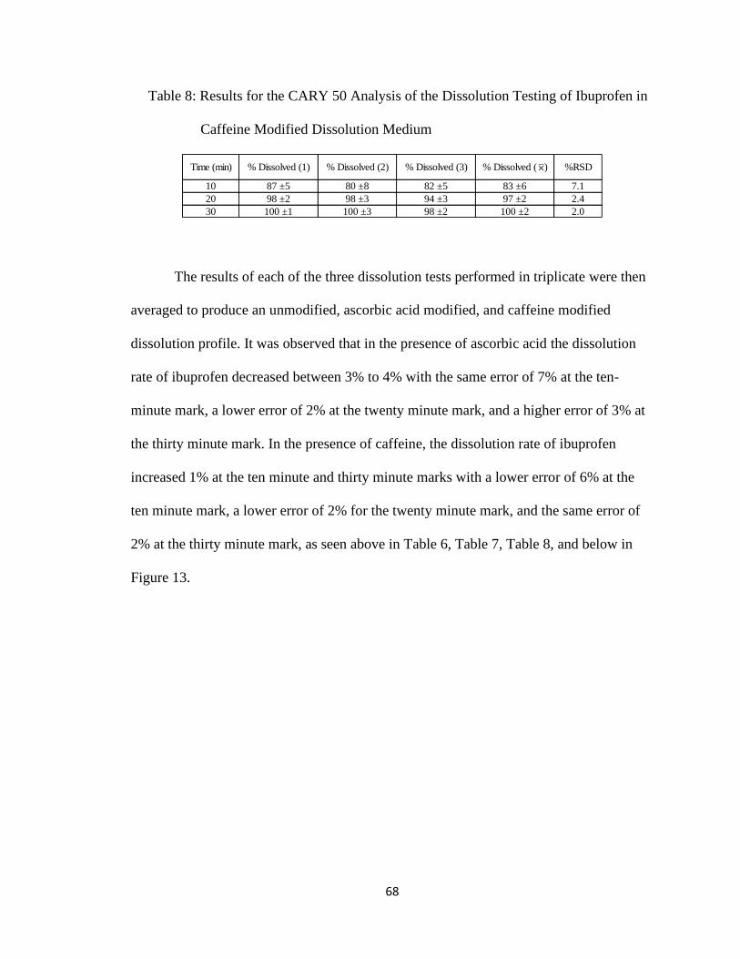
68



The results of each of the three dissolution tests performed in triplicate were then

averaged to produce an unmodified, ascorbic acid modified, and caffeine modified

dissolution profile. It was observed that in the presence of ascorbic acid the dissolution

rate of ibuprofen decreased between 3% to 4% with the same error of 7% at the ten-

minute mark, a lower error of 2% at the twenty minute mark, and a higher error of 3% at

the thirty minute mark. In the presence of caffeine, the dissolution rate of ibuprofen

increased 1% at the ten minute and thirty minute marks with a lower error of 6% at the

ten minute mark, a lower error of 2% for the twenty minute mark, and the same error of

2% at the thirty minute mark, as seen above in Table 6, Table 7, Table 8, and below in

Figure 13.


10 87 ±5 80 ±8 82 ±5 83 ±6 7.1

20 98 ±2 98 ±3 94 ±3 97 ±2 2.4

30 100 ±1 100 ±3 98 ±2 100 ±2 2.0

×

69


Testing Profile of the Averaged Results for Ibuprofen Using 900mL

Per Vessel Per Test of Unmodified, Ascorbic Acid Modified, and

Caffeine Modified Dissolution Medium at 37oC with an Apparatus

Speed of 50rpm Performed Each in Triplicate Using Six 200mg

Ibuprofen Tablets Per Test

The consistently high percent error and percent relative standard deviations for

the ten-minute mark were attributed to the varying times necessary for the coating,

consisting of pharmaceutical glaze, stearic acid, titanium dioxide, and sucrose, to open

up.34,35 The increased dissolution rate of ibuprofen in the presence of caffeine was

attributed to the ability of caffeine to increase the solubility of ibuprofen by ten-fold due

to eutectic physical interactions thus increasing its hygroscopicity which in turn increases

the dissolution rate and bioavailability of ibuprofen.36 The decreased dissolution rate of

ibuprofen seen with ascorbic acid is consistent with previous research that evaluated the

disintegration rates of immediate release pain medications in the presence of calcium

fortified orange juice in which the disintegration time of the 200mg ibuprofen tablets was

70

significantly decreased. The disintegration tests evaluated the rate of the breakdown of

the ibuprofen tablets into small fragments or granules directly affecting the dissolution

rate, or the rate at which the tablet fully dissolves into solution.14, 37

3.11 Determination of Lambda Max for Ibuprofen

The determination of the lambda max for ibuprofen both alone and in a mixture

with ascorbic acid was performed to verify that no summative effects occurred that would

require the separation of the components prior to measurement of ibuprofens signal by

the detector. It was observed that the phosphate buffer signal for ibuprofen and ascorbic

acid alone and in a mixture was 207.02nm, 201.51nm, and 206.07nm which is 0.0224

absorbance units lower in the mixture, respectively, and there was no summative effect

on the absorbance that occurred at ibuprofens lambda max of 221.93nm, 0.0281

absorbance units lower in the mixture, thus separation of the components was not

required to quantify ibuprofen in ascorbic acid modified dissolution medium, as seen

above in Table 5, and below in Figure 14 and Table 9.

71

Figure 14: Results for the Cary 50 Analysis of Ibuprofen, Ascorbic Acid, and

Mixture in Unmodified Dissolution Medium for Summative Effect

Determination

Table 9: Results for the Cary 50 Determination of Lambda Max for Ibuprofen,

Ascorbic Acid, and Mixture in Unmodified Dissolution Medium for

Summative Effect Determination

The determination of the lambda max for ibuprofen both alone and in a mixture

with caffeine was performed to verify that no summative effect on the absorbance of

wavelengths occurred that would require the separation of the components prior to

measurement of ibuprofens signal by the detector. It was observed that the phosphate

buffer signal for ibuprofen and caffeine alone and in a mixture was 203.97nm, 209.47nm,

and 211.98nm, respectively, and a summative effect on the absorbance of the phosphate

Copmpound λ (nm) Signal (Abs) Analysis (nm)

207.02 1.9070

221.93 2.0924

201.51 0.4986

260.06 0.9252

206.07 1.9294

221.93 2.0643

221

Ibuprofen

Ascorbic Acid

Mixture

72

buffer peak for ibuprofen at 203.97nm and caffeine at 209.47nm occurred producing a

new peak for the phosphate buffer in the mixture at 211.98nm. A second summative

effect on the absorbance occurred at the first isosbestic point where ibuprofens lambda

max of 222.97nm and the tailing edge of the phosphate buffer peak for caffeine occurred

concealing ibuprofens lambda max thus separation of the components via UHPLC was

required to quantify ibuprofen in caffeine modified dissolution medium, as seen above in

Table 5, and below in Figure 15 and Table 10.

Figure 15: Results for the Cary 50 Analysis of Ibuprofen, Caffeine, and Mixture

in Unmodified Dissolution Medium for Summative Effect

Determination

73

Table 10: Results for the Cary 50 Determination of Lambda Max for Ibuprofen,

Caffeine, and Mixture in Unmodified Dissolution Medium for

Summative Effect Determination

The selection of an internal standard was now necessary. The USP monograph for

ibuprofen tablets employs valerophenone as the internal standard, but in an attempt to

conserve resources valerophenone (Figure 16) was not selected.14

Figure 16: Structure of Valerophenone38

Benzoic acid was selected as the internal standard for the UHPLC/UV-Vis

analysis of ibuprofen since it was readily available, as seen below in Figure 17.

Figure 17: Structure of Benzoic Acid39

Copmpound λ (nm) Signal (Abs) Analysis (nm)

203.97 1.0784

222.97 1.0487

209.47 2.2133

274.00 1.1366

211.98 2.2264

273.53 1.0541

UHPLC

Separation is

Necessary due

to Summation

of Absorbances

Ibuprofen

Caffeine

Mixture

74

The determination of the lambda max for ibuprofen and benzoic acid was

performed to determine the wavelengths that would be monitored during the analysis of

ibuprofen. It was observed that the lambda max of ibuprofen and benzoic acid in mobile

phase A was 237.53nm and 240.98nm, respectively, after which the wavelengths selected

for analysis were 237nm and 241nm, respectively, as seen above in Table 5, and below in

Figure 18 and Table 11.

Figure 18: Results for the Cary 50 Analysis of Ibuprofen and Benzoic Acid in

Mobile Phase A for the Determination of the Wavelengths to Monitor

Using UHPLC Analysis

Table 11: Results for the Cary 50 Analysis of Ibuprofen and Benzoic Acid in

Mobile Phase A for the Determination of the Wavelengths to Monitor

Using UHPLC Analysis

Copmpound λ (nm) Signal (Abs) UHPLC (nm)

Ibuprofen 237.53 1.4507 237

Benzoic Acid 240.98 1.8782 241

Mixture 241.45 2.0084 NA

75

3.12 Determination of the LOD and LOQ for Ibuprofen

The Limit of Detection and Limit of Quantitation for ibuprofen in unmodified,

ascorbic acid modified, and caffeine modified dissolution medium was performed to

determine if the matrix components would shift the limit of detection and limit of

quantitation for ibuprofen. It was observed that in the presence of ascorbic acid the limit

of detection and limit of quantitation for ibuprofen decreased by 0.0340ppm and

0.116ppm, respectively, and in the presence of caffeine the limit of detection and limit of

quantitation for ibuprofen increased by 0.253ppm and 0.840ppm, respectively, which

confirmed the necessity for the UHPLC separation of the benzoic acid and matrix

components prior to quantification of ibuprofen, as seen above in Table 5, and below in

Table 12.

Table 12: Results for the CARY 50 Determination of the Limit of Detection and Limit of

Quantitation for Ibuprofen

3.13 Separation of Ibuprofen and Benzoic Acid

The USP monograph for ibuprofen tablets contains the UHPLC parameters for the

separation of ibuprofen and valerophenone, as seen below in Table 13.14

Matrix Slope (m) Std. Dev. (SX) R2 LOD (mg/L) LOQ (mg/L)

Unmodified 0.0438 0.00069 0.9999 0.047 0.16

Ascorbic Acid 0.0448 0.00020 0.9994 0.013 0.044

Caffeine 0.0339 0.0034 0.9974 0.30 1.0

76

Table 13: USP Instrumental Parameters for the UHPLC Analysis of Ibuprofen Tablets

However, if deviations must be made to the UHPLC parameters on the

monograph the USP provides a list of allowed deviations, as seen below in Table 14.14

Table 14: USP Allowed Deviations for UHPLC Analysis

The USP allowed deviations were employed to reduce the column length to

100mm, increase the injection volume to 10µL, and substitute the 1% chloroacetic acid

with 1% formic acid, as seen below in Table 15.

Table 15: Modified USP Parameters for the UHPLC Analysis of Ibuprofen

Once the deviations had been selected the UHPLC separation of benzoic acid and

ibuprofen was performed using automatic integration which contained many negative

peaks and ghost peaks, but once manual integration was employed the separation was

successful with retention times of 0.759min and 1.617min, respectively, and a total

runtime of 2.0min, as seen below in Figure 19.

Length (mm) Diameter (mm) Particle (um) Packing Flow (mL/min) Inj. (µL) Temp (oC) A (pH) B pH Adj. A:B

250 4.6 5.0 C18 2.0 5.0 30.0 3.0 ACN NH4OH 40:60

Column Parameters Chromatography Parameters

A

H2O and 1% C2H3ClO2

Column (L) Column (I.D.) Particle (Ld) Flow (mL/min) Temp (oC) Injection (µL) pH λmax (nm) Salt Level

±70%No Limit; Keep

Cons. Lin. Vel.-50% ±50% ±10

Satisfy Sys.

Conf. Req.±0.2 ±3 ±10%

Mobile Phase

One ±30% or

Abs. ±10%

Length (mm) Diameter (mm) Particle (um) Packing Flow (mL/min) Inj. (µL) Temp (oC) A (pH) B pH Adj. A:B

100 4.6 5.0 C18 2.0 10.0 30.0 3.0 ACN NH4OH 40:60


A

H2O and 1% CH2O2

77

Figure 19: Results for the UHPLC Separation of Ibuprofen and Benzoic Acid Using

Manual Integration

The separation of benzoic acid produced a low number of theoretical plates with a

high theoretical plate height and a low tailing factor indicative of a high dispersion of the

chromatographic band and column equilibrations with a slight tailing asymmetry

allowing for an easily resolved and reproducible peak. The separation of ibuprofen

produced a high number of theoretical plates with a low theoretical plate height, a low

tailing factor, with high resolution, and a selectivity factor greater than one indicative of a

low dispersion of the chromatographic band and column equilibrations with a slightly

higher tailing asymmetry than benzoic acid, and with excellent separation allowing for an

easily resolved and reproducible peak, as seen above in Figure 19 and below in Table 16.

Table 16: Results for the UHPLC Separation of Ibuprofen and Benzoic Acid

Compound Rtime k' N HETP Tailing Resolution α

Benzoic Acid 0.759 0.500 1421 70.363 1.099 0 0

Ibuprofen 1.617 1.132 5333 18.752 1.213 10.152 1.172

78

3.14 Determination of the LOL for Ibuprofen and Benzoic Acid

It was observed that ibuprofen became nonlinear at 40,000ppm and when a set of

lower concentration calibrations were analyzed it was observed that ibuprofen became

nonlinear at 15,000ppm, as seen above in Table 5, and below in Figure 20 and Figure 21.

Figure 20: Results for the UHPLC Analysis Calibration Curve in Absorbance

Units for the Determination of the Limit of Linearity of Ibuprofen at



Units for the Determination of the Limit of Linearity of Ibuprofen at


79

It was observed that benzoic acid became nonlinear at 1,500ppm, which was more

observable when the lower concentration standards were charted, as seen below in Figure

22 and Figure 23.


Units for the Determination of the Limit of Linearity of Benzoic Acid

at 241nm in Mobile Phase A


Units for the Determination of the Limit of Linearity of Benzoic Acid


80

3.15 Determination of the LDR for Ibuprofen and Benzoic Acid

It was determined that the LDR for ibuprofen and benzoic acid was 0.16ppm to

15,000ppm and 0.098ppm to 1,500ppm, respectively, as seen below in Table 17.



3.16 Quantification of Ibuprofen via Current Calibration Methods

A 200mg ibuprofen tablet fully dissolved in 900mL of dissolution medium had a

concentration of 222ppm. The external calibration method, standard addition method, and

internal standard method were performed to determine the concentrations of ibuprofen

and benzoic acid that would be compared to the standard dilution analysis method results.

The external calibration method employed a 222ppm ibuprofen ‘unknown’ that was

approximately in the middle of the ibuprofen standard range of 150ppm to 300ppm that

resulted in the lowest error of 0.18%, as seen above in Table 5 and below in Figure 24

and Table 25.

Compound LOD (mg/L) LOQ (mg/L) LOL (mg/L)

Ibuprofen 0.047 0.16 15,000

Benzoic Acid 0.029 0.098 1,500

81

Figure 24: Results for the UHPLC External Calibration Method Analysis of

Ibuprofen at 237nm in Mobile Phase A

Table 18: Results for the UHPLC Quantification of Ibuprofen Using Current Calibration

Methods

The standard addition method employed a 111ppm ibuprofen ‘unknown’ that was

approximately in the middle of the ibuprofen standard range of 50.0ppm to 250ppm that

resulted in the highest error of 1.3%, as seen above in Table 5 and Table 18, and below in

Figure 25.

Method IBU Std (mg/L) BA Int (mg/L) IBU Unk (mg/L) Rec (mg/L) Slope Intercept R2 Error (%)

ECM 300 NA 222 222.4 878.63 0 1.000 0.18

SAM 250 NA 111 112.5 948.46 103,679 0.9998 1.3

ISM 150 75.0 111 111.4 0.00160 0 1.000 0.38

82

Figure 25: Results for the UHPLC Standard Addition Method Analysis of

Ibuprofen at 237nm in Mobile Phase A

The internal standard method employed a 111ppm ibuprofen ‘unknown’ that was

approximately in the middle of the ibuprofen standard range of 50.0ppm to 150ppm with

a benzoic acid internal standard concentration of 75.0ppm that resulted in the second

lowest error of 0.38%, as seen above in Table 5 and Table 18 and below in Figure 26.

Figure 26: Results for the UHPLC Internal Standard Method Analysis of


83

3.17 Quantification of Ibuprofen via Standard Dilution Analysis

The standard dilution analysis method was then performed and employed a

222ppm ibuprofen ‘unknown’ that was approximately in the middle of the ibuprofen

standard range of 150ppm to 300ppm, selected due to the external calibration method

analysis producing the lowest error of 0.18%, with a benzoic acid internal standard

concentration of 100ppm. The standard dilution analysis produced an error of 11%, as

seen above in Table 5 and Table 18, and below in Figure 27 and Table 19.

Figure 27: Results for the UHPLC Standard Dilution Analysis of Ibuprofen at


Table 19: Results for the UHPLC Quantification of Ibuprofen Using Standard

Dilution Analysis

IBU Std (mg/L) BA Int (mg/L) IBU Unk (mg/L) Rec (mg/L) Slope Intercept R2 Error (%)

300 100 222 197.6 22.622 0.3432 0.9999 11

250 62.5 222 196.3 21.195 0.4319 0.9996 12

300 150 266 228.0 27.242 0.2389 0.9991 14

300 150 178 150.6 17.154 0.2278 0.9993 15

84

The standard dilution analysis method was performed a second time to evaluate

the concentrations employed in the first analysis. Only the diluted samples were

employed as per the initial publication of the standard dilution analysis method.24 The

ibuprofen ‘unknown’ was just above the middle of the ibuprofen standard concentration

range of 150ppm to 250ppm with a benzoic acid internal standard concentration of

62.5ppm producing an error of 12%. This confirmed that the undiluted samples can be

employed in the standard dilution analysis method, as seen above in Table 19 and below

in Figure 28.



The sensitivity of the standard dilution analysis method was then evaluated by

adjusting the ibuprofen ‘unknown’ by ±20%. The third standard dilution analysis

employed a 266ppm ibuprofen ‘unknown’ that was at the high end of the ibuprofen

standard range of 150ppm to 300ppm with a benzoic acid internal standard concentration

of 150ppm producing error of 14%, as seen above in Table 19 and below in Figure 29.

85


237nm and Benzoic Acid at 241nm in Mobile Phase A Increasing the

Ibuprofen Unknown Concentration by 20%

The fourth standard dilution analysis employed a 178pm ibuprofen ‘unknown’

that was slightly below the middle of the ibuprofen standard range of 150ppm to 300ppm

with a benzoic acid internal standard concentration of 150ppm producing an error of

15%, as seen above in Table 19 and below in Figure 30.

86


237nm and Benzoic Acid at 241nm in Mobile Phase A Decreasing the

Ibuprofen Unknown Concentration by 20%

The first and second standard dilution analyses were performed on the same day,

and the third and fourth standard dilution analyses were performed on the day after

producing good ruggedness with only a 1% difference between the percent error for both

analyses performed on the same days, as seen above in Table 19.

A baseline correction estimates the peak area irrespective of the background.

Translational and rotational effects can directly affect, or interfere, with the recovery of

an analyte depending on which calibration method is employed. Translational effects, or

baseline interference, are considered a constant bias and cannot be corrected using the

standard addition method or internal standard method but can be corrected applying a

baseline correction. Rotational effects, or matrix effect, are considered a proportional bias

and cannot be corrected using baseline correction but can be corrected using the standard

addition method or internal standard method. The standard dilution analysis is an

integration of standard addition method and internal standard method in which

87

translational and rotational effects should be corrected for and thus cannot be the cause of

the high error produced form the standard dilution analysis of ibuprofen.40

3.18 UHPLC Pump Conditioning Analysis

Sources such as leaks, incorrect compressibility values, faulty check valves,

impure solvents, air bubbles, and obstructed inline filters increase the inconsistency in

peak integration. Compressibility values of a mixture must be determined experimentally

beforehand as incorrect compressibility values greatly affect the accuracy and precision

of the flow rate. The increasing variability of peak integration that occurs causes an

inverse relationship between the relative standard deviation and the flow rate that

negatively affects the precision of the peak area. A UHPLC pump conditioning analysis

was performed using ibuprofen and benzoic acid to assess the effect pump pressure

ripples and back pressure have on the sensitivity of the integration and quantification of

the chromatographic peaks due to a fluctuating flow rate.41

Ibuprofen and benzoic acid were separated via UHPLC and the signal versus the

analysis number for each compound was charted. It was observed that ibuprofen and

benzoic acid did not produce a consistent signal around the mean signal value, much

variability occurred over 7 hours of 2-minute chromatograms, as seen below in Figure 31,

Figure 32, and Table 20.

88

Figure 31: Results for the UHPLC Pump Conditioning Analysis of Ibuprofen at


Figure 32: Results for the UHPLC Pump Conditioning Analysis of Benzoic Acid


Table 20: Results for the UHPLC Pump Conditioning Analysis of Ibuprofen and

Benzoic Acid

Compound Max Area Min Area Mean Area Max Ratio Min Ratio Mean Ratio Max Rolling Min Rolling Mean Rolling

Ibuprofen 166486 156652 162246

Benzoic Acid 814681 805729 8103244.939 4.9935.168 4.883 4.995 5.132

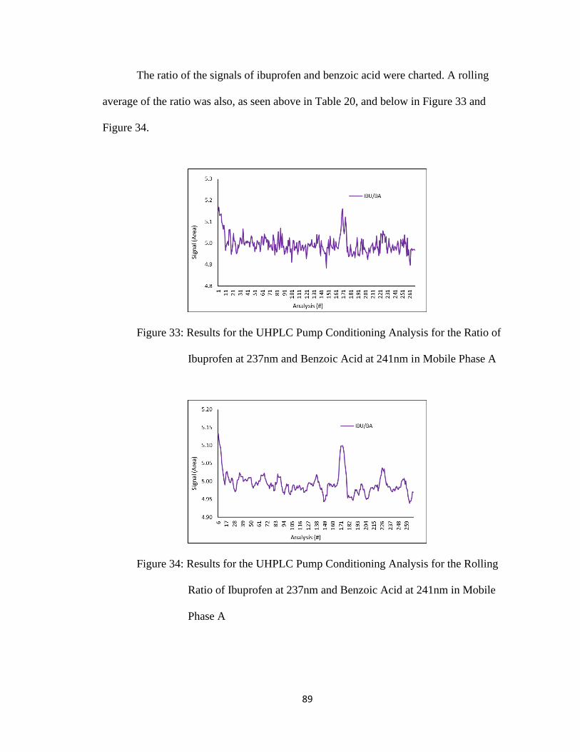
89

The ratio of the signals of ibuprofen and benzoic acid were charted. A rolling

average of the ratio was also, as seen above in Table 20, and below in Figure 33 and

Figure 34.

Figure 33: Results for the UHPLC Pump Conditioning Analysis for the Ratio of


Figure 34: Results for the UHPLC Pump Conditioning Analysis for the Rolling

Ratio of Ibuprofen at 237nm and Benzoic Acid at 241nm in Mobile

Phase A

90

3.19 Determination of Lambda Max for Biphenyl

In the development of an advanced instrumental undergraduate laboratory

experiment the chromatographic and UV-Vis responses of biphenyl and naphthalene

(Figure 35) were thoroughly investigated and documented. The lack of the standard

dilution analysis of ibuprofen to achieve an error lower than 11% led the research to

employ biphenyl and naphthalene in an attempt to produce a lower percent error.

Figure 35: Structures of Biphenyl and Naphthalene42,43

The determination of the lambda max for biphenyl and naphthalene was

performed to verify the previous wavelengths employed that would be monitored during

this analysis of biphenyl. It was observed that the lambda max of biphenyl and

naphthalene in mobile phase B was 248.52nm and 276.04nm, respectively. It was

observed that two summative effects on the absorbance occurred at isosbestic points with

the first at approximately 228nm and the second at approximately 270nm. It was

observed that naphthalene produced multiple peaks desirable for UHPLC analysis at

approximately 258nm, 268nm, 276nm, and 287nm. Due to the isosbestic summative

effect on the absorbance occurred at approximately 270nm the wavelengths selected for

biphenyl and naphthalene analysis were 246nm and 268nm, respectively, as seen below

in Table 21, Figure 36, and Table 22.

91

Table 21: Instrumental Techniques Employed in the Analysis of Biphenyl

Figure 36: Results for the Cary 50 Analysis of Biphenyl and Naphthalene in

Mobile Phase B for the Determination of the Wavelengths to Monitor

in UHPLC Analysis

Table 22: Results for the Cary 50 Analysis of Biphenyl and Naphthalene in Mobile Phase

B for the Determination of the Wavelengths to Monitor in UHPLC Analysis

Instrument Analytes Baseline Correction Analysis Wavelength (nm)

Cary 50 BPH / NAP / Mixture Mobile Phase B Lambda Max (Scan) 200-300

UHPLC BPH / NAP Mobile Phase B LOD and LOQ 246

UHPLC BPH / NAP Mobile Phase B LOL 246 (BPH) and 268 (NAP)

UHPLC BPH Mobile Phase B ECM and SAM 246

UHPLC BPH / NAP Mobile Phase B ISM 246 (BPH) and 268 (NAP)

UHPLC BPH / NAP Mobile Phase B SDA 246 (BPH) and 268 (NAP)

Copmpound λ (nm) Signal (Abs) UHPLC (nm)

206.95 1.6152

248.52 1.0427

216.53 2.0977

276.04 0.4785

222.97 2.2186

249.46 1.3701

Biphenyl

Naphthalene

Mixture NA

268

246

92

3.20 Separation of Biphenyl and Naphthalene

The UHPLC parameters for naphthalene and biphenyl were selected from the

previous UTNB experiment, as seen below in Table 23.

Table 23: Instrumental Parameters for the UHPLC Analysis of Biphenyl

The separation of naphthalene and biphenyl was performed using automatic

integration which contained two ghost peaks just above the baseline correction, but once

manual integration was employed to reject the two ghost peaks the separation was

successful with retention times of 1.182min and 1.379min, respectively, and a total

runtime of 2.0min, as seen below in Figure 37.

Figure 37: Results for the UHPLC Separation of Biphenyl and Naphthalene

The separation of naphthalene produced a low number of theoretical plates with a

high theoretical plate height and a low tailing factor indicative of a high dispersion of the

Length (mm) Diameter (mm) Particle (um) Packing Flow (mL/min) Inj. (µL) Temp (oC) A B A:B

100 4.6 5.0 C18 2.0 10.0 40.0 H2O ACN 30:70


93

chromatographic band and column equilibrations with a slight tailing asymmetry

allowing for an easily resolved and reproducible peak. The separation of biphenyl

produced a high number of theoretical plates with a low theoretical plate height, a low

tailing factor, with high resolution, and a selectivity factor greater than one indicative of a

low dispersion of the chromatographic band and column equilibrations with a slightly

lower tailing asymmetry than naphthalene, and with good separation allowing for an

easily resolved and reproducible peak, as seen below in Table 24.

Table 24: Results for the UHPLC Separation of Biphenyl and Naphthalene

3.21 Determination of the LOD and LOQ for Biphenyl and Naphthalene

The Limit of Detection and Limit of Quantitation for biphenyl and naphthalene

was performed to determine the lowest concentration of the linear dynamic range. It was

observed that the limit of detection and limit of quantitation for biphenyl was 0.15ppm

and 0.49ppm, respectfully, and naphthalene was 0.29ppm and 0.98ppm, respectfully, as

seen above in Table 21 and below in Table 25.

Table 25: Results for the UHPLC Determination of the Limit of Detection and Limit of

Quantitation for Biphenyl and Naphthalene

Compound Rtime k' N HETP Tailing Resolution α

Naphthalene 1.182 1.130 4295 23.281 1.234 0 0

Biphenyl 1.379 1.494 4985 20.456 1.211 2.615 1.313

Matrix Slope (m) Std. Dev. (SX) R2 LOD (mg/L) LOQ (mg/L)

Biphenyl 33199 1600 0.9999 0.15 0.49

Naphthalene 10851 1063 0.9998 0.29 0.98

94

It was observed that biphenyl became nonlinear at 400ppm, however, when only

the lower concentration calibrations were charted, it was observed that biphenyl became

nonlinear at 300ppm, as seen above in Table 21, and below in Figure 38 and Figure 39.

Figure 38: Results for the UHPLC Analysis Calibration Curve for the

Determination of the Limit of Linearity of Biphenyl at 246nm in

Mobile Phase B


Determination of the Limit of Linearity of Biphenyl at 246nm in

Mobile Phase B

95

3.22 Determination of the LOL for Biphenyl and Naphthalene

It was observed that naphthalene became nonlinear at 400ppm, which was more

observable when the lower concentration standards were charted, as seen below in Figure

40 and Figure 41.


Determination of the Limit of Linearity of Naphthalene at 268nm in

Mobile Phase B


Determination of the Limit of Linearity of Naphthalene at 268nm in

Mobile Phase B

96

3.23 Determination of the LDR for Biphenyl and Naphthalene

It was determined that the LDR for biphenyl and naphthalene was 0.49ppm to

300ppm and 0.98ppm to 400ppm, respectively, as seen below in Table 26.



3.24 Quantification of Biphenyl via Current Calibration Methods

The external calibration method, standard addition method, and internal standard

method were performed to compare to the standard dilution analysis method results. The

external calibration method employed a 50.0ppm biphenyl ‘unknown’ that resulted in the

second lowest error of 4.3%, as seen above in Table 21, and below in Figure 42 and

Table 27.

Figure 42: Results for the UHPLC External Calibration Method Analysis of

Biphenyl at 246nm in Mobile Phase B

Compound LOD (mg/L) LOQ (mg/L) LOL (mg/L)

Biphenyl 0.15 0.49 300

Naphthalene 0.29 0.98 400

97

Table 27: Results for the UHPLC Quantification of Biphenyl Using Current

Calibration Methods

The standard addition method employed a 50.0ppm biphenyl ‘unknown’ that

resulted in the highest error of 14%, as seen above in Table 21 and Table 27, and below

in Figure 43.

Figure 43: Results for the UHPLC Standard Addition Method Analysis of

Biphenyl at 246nm in Mobile Phase B

The internal standard method employed a 50.0ppm biphenyl ‘unknown’ and a

naphthalene internal standard concentration of 50.0ppm that resulted in the lowest error

of 3.4%, as seen above in Table 21 and Table 27, and below in Figure 44.

Method BPH Std (mg/L) NAP Int (mg/L) BPH Unk (mg/L) Rec (mg/L) Slope Intercept R2 Error (%)

ECM 100 NA 50.0 47.87 33,880 0 0.9999 4.3

SAM 100 NA 50.0 43.13 35,243 1,520,090 0.9994 14

ISM 100 50.0 50.0 48.32 0.0806 0 0.9999 3.4

98

Figure 44: Results for the UHPLC Internal Standard Method Analysis of


3.25 Quantification of Biphenyl via Standard Dilution Analysis

The standard dilution analysis method was then performed and employed a

50.0ppm biphenyl “unknown” and a naphthalene internal standard concentration of

50.0ppm that produced an error of 1.6%, as seen above in Table 21, and below in Figure

45 and Table 28.

Figure 45: Results for the UHPLC Standard Dilution Analysis of Biphenyl at


99

Table 28: Results for the UHPLC Quantification of Biphenyl Using Standard Dilution

Analysis

The standard dilution analysis method was performed a second time to evaluate

the concentrations employed in the first analysis, however, only employing the diluted

samples as per the initial publication of the method. The analysis employed a 50.0ppm

biphenyl ‘unknown’ with a naphthalene internal standard concentration of 35.7ppm that

produced the lowest error of 0.010% confirming for a second time that the undiluted

samples can be employed in the standard dilution analysis method, as seen above in

Table 20 and Table 28, and below in Figure 46.23

BPH Std (mg/L) NAP Int (mg/L) BPH Unk (mg/L) Rec. (mg/L) Slope Intercept R2 Error (%)

50.0 50.0 50.0 50.82 151.02 2.9716 0.9983 1.6

50.00 150.52 3.0106 0.9985 0.010

47.89 150.54 3.0599 0.9996 4.2

49.75 151.94 3.0540 0.9992 0.50

64.92 186.04 2.8655 0.9998 8.2

65.64 188.08 2.8653 0.9996 9.4

68.49 190.62 2.7831 0.9995 14

44.93 150.54 3.0599 0.9996 12

43.24 125.99 2.9138 0.9971 8.1

46.98 130.14 2.7704 0.9962 17

35.7 35.7

50.0

60.0

40.0

100



The sensitivity of the standard dilution analysis method was then evaluated by

adjusting the biphenyl ‘unknown’ by ±20%. The third standard dilution analysis

employed a 60.0ppm biphenyl ‘unknown’ with a naphthalene internal standard

concentration of 35.7ppm that produced an error of 8.2%, as seen above in Table 28 and

below in Figure 47.


246nm and Naphthalene at 268nm in Mobile Phase B Increasing the

Biphenyl Unknown Concentration by 20%

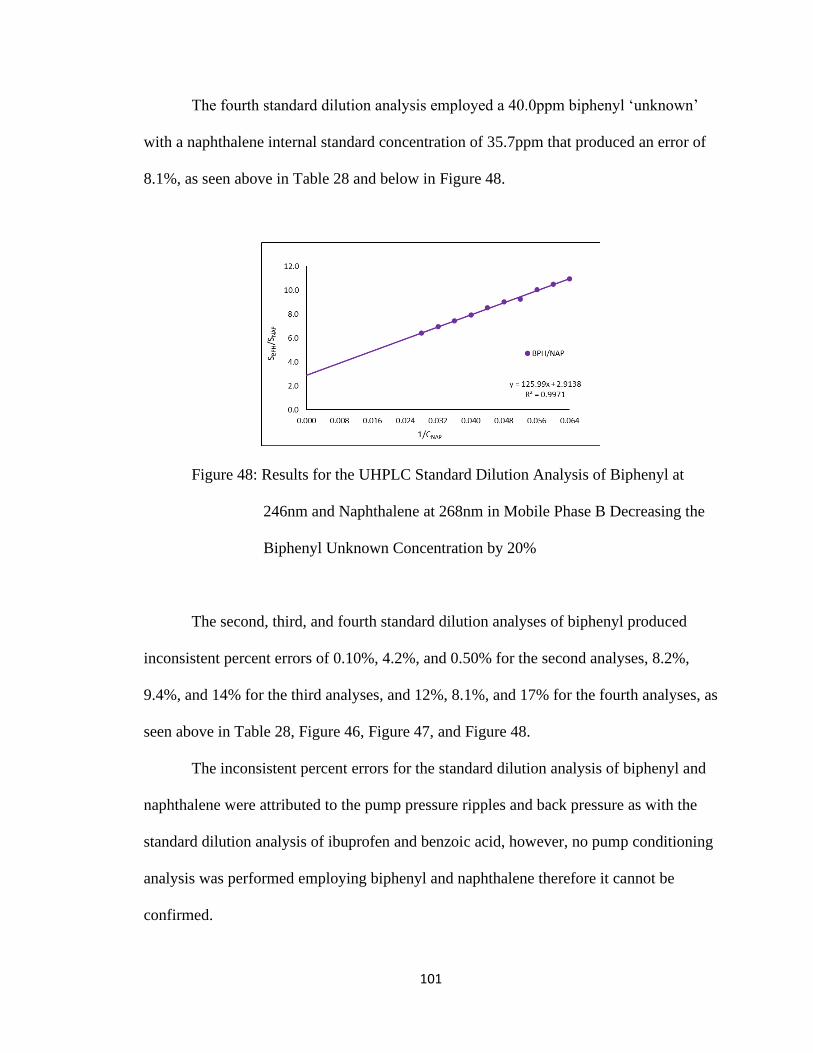
101

The fourth standard dilution analysis employed a 40.0ppm biphenyl ‘unknown’

with a naphthalene internal standard concentration of 35.7ppm that produced an error of

8.1%, as seen above in Table 28 and below in Figure 48.


246nm and Naphthalene at 268nm in Mobile Phase B Decreasing the

Biphenyl Unknown Concentration by 20%

The second, third, and fourth standard dilution analyses of biphenyl produced

inconsistent percent errors of 0.10%, 4.2%, and 0.50% for the second analyses, 8.2%,

9.4%, and 14% for the third analyses, and 12%, 8.1%, and 17% for the fourth analyses, as

seen above in Table 28, Figure 46, Figure 47, and Figure 48.

The inconsistent percent errors for the standard dilution analysis of biphenyl and

naphthalene were attributed to the pump pressure ripples and back pressure as with the

standard dilution analysis of ibuprofen and benzoic acid, however, no pump conditioning

analysis was performed employing biphenyl and naphthalene therefore it cannot be

confirmed.

102

3.26 Conclusions

The empirical evidence gathered in the dissolution testing of ibuprofen tablets

definitively established that ascorbic acid modified dissolution medium caused a decrease

in the dissolution rate of ibuprofen, however, due to the percent errors produced in the

dissolution testing of ibuprofen tablets in caffeine modified dissolution medium it cannot

be definitively asserted that caffeine increased the dissolution rate of ibuprofen.

The complete figures of merit were achieved for the external calibration method,

standard addition method, and internal standard method producing low percent errors for

ibuprofen with higher percent errors produced for biphenyl. The figures of merit were not

fully achieved in the standard dilution analysis of ibuprofen which produced high percent

errors, however, low but inconsistent percent errors were achieved for biphenyl.

The high percent errors produced in the standard dilution analysis of ibuprofen led

to the examination of the high pressure pumps employed in the UHPLC analyses to

evaluate the effect of pump pressure ripples on the flow rate that resulted in the

determination that there was disproportional variability in the response of ibuprofen and

benzoic acid that may have also affected the response of biphenyl and naphthalene but was

not confirmed through analysis.

In many high-risk high-reward research opportunities sometimes failures happen,

however, in reflection solutions to problems that arose during the experimental phase are

frequently illuminated providing the researcher with more appropriate directions to have

taken such as: 1) The validation of the UHPLC modules and related functions such as the

compressibility factor. 2) The validation of the internal standard valerophenone as per the

USP monograph for ibuprofen via UHPLC. 3) The validation of the original standard

103

dilution analysis experiment employing dyes. 4) Analyzing the dissolution samples

through the External Calibration Method on the UHPLC.

104

CHAPTER 4 – REFERENCES

1. Nunes, C. D.; Arantes, M. B.; Pereira, S. M. D.; da Cruz, L. L.; Passos, M. D.; de

Moraes, L. P.; Vieira, I. J. C.; de Oliveira, D. B., Plants as Sources of Anti-

Inflammatory Agents. Molecules 2020, 25 (16), 1-14.

2. Mahmud, S.; Rosen, N., History of NSAID Use in the Treatment of Headaches

Pre- and Post-industrial Revolution in the United States: The Rise and Fall of

Antipyrine, Salicylic Acid, and Acetanilide. Curr Pain Headache R 2019, 23 (1),

1-3.

3. Mahdi, J. G., Medicinal potential of willow: A chemical perspective of aspirin

discovery. J Saudi Chem Soc 2010, 14 (3), 317-322.

4. Scott, A.; Khan, K. M.; Cook, J. L.; Duronio, V., What is "Inflammation''? Are

we ready to move beyond Celsus? Brit J Sport Med 2004, 38 (3), 248-249.

5. Hurley, J. V., Inflammation - Micro-Circulatory Mechanisms and Control.

Microvasc Res 1980, 19 (2), 251-252.

6. Botting, R. M., Vane's discovery of the mechanism of action of aspirin changed

our understanding of its clinical pharmacology. Pharmacol Rep 2010, 62 (3), 518-

25.

7. Hanna, V. S.; Hafez, E. A. A., Synopsis of arachidonic acid metabolism: A

review. J Adv Res 2018, 11, 23-32.

8. Rao, P.; Knaus, E. E., Evolution of nonsteroidal anti-inflammatory drugs

(NSAIDs): cyclooxygenase (COX) inhibition and beyond. J Pharm Sci 2008, 11

(2), 81s-110s.

105

9. Rainsford, K. D., 2015. Ibuprofen: Discovery, Development and Therapeutics.

New Jersey: John Wiley and Sons, Inc., pp. 1-19.

10. Ibuprofen. CAS Registry Number 15687-27-1. https://scifinder.cas.org

11. Mazaleuskaya, L. L.; Theken, K. N.; Gong, L.; Thorn, C. F.; FitzGerald, G. A.;

Altman, R. B.; Klein, T. E., PharmGKB summary: ibuprofen pathways.

Pharmacogenet Genom 2015, 25 (2), 96-106.

12. Baxter, K., 2008. Stockley's Drug Interactions. 8th ed. London: Pharmaceutical

Press, pp.1-11.

13. United States Pharmacopeia. https://www.usp.org/

14. The United States Pharmacopeia 2012, 35th ed.; United States Pharmacopeial

Convention: Rockville, MD, pp. 258-1068.

15. Dokoumetzidis, A.; Macheras, P., A century of dissolution research: From Noyes

and Whitney to the Biopharmaceutics Classification System. Int J Pharmaceut

2006, 321 (1-2), 1-11.

16. Pezzini, B. R.; Issa, M. G.; Duque, M. D.; Ferraz, H. G., Applications of USP

apparatus 3 in assessing the in vitro release of solid oral dosage forms. Braz J

Pharm Sci 2015, 51 (2), 265-272.

17. Hanson, R.; Gray, V. Handbook of Dissolution Testing; Dissolution Technologies,

Inc.: Hockessin, Del., 2005; pp 1-143.

18. Liddell, M. R.; Deng, G.; Hauck, W. W.; Brown, W. E.; Wahab, S. Z.; Manning,

R. G., Evaluation of glass dissolution vessel dimensions and irregularities.

Dissolut Technol 2007, 14 (1), 28-33.

106

19. U.S. Department of Health and Human Services. Guidance for Industry:

Dissolution Testing of Immediate Release Solid Oral Dosage Forms; Food and

Drug Administration Center for Drug Evaluation and Research: Rockville, 1997;

pp 8-9.

20. Costa, P.; Manuel, J.; Lobo, S., Modeling and comparison of dissolution profiles.

Eur J Pharm Sci 2001, 13 (2), 123-133.

21. Harvey, D., 2008. Modern Analytical Chemistry, 2nd ed.; McGraw-Hill: San

Francisco, pp. 153-192.

22. Harris, D., 2010. Quantitative Chemical Analysis, 8th ed.; W.H. Freeman: New

York, pp. 68-112, 542-554, 1056-1058.

23. Robinson, J.; Skelly Frame, E.; Frame II, G., 2012. Undergraduate Instrumental

Analysis, Sixth Edition, 6th ed.; Taylor and Francis: Hoboken, pp. 52-110.

24. Jones, W. B.; Donati, G. L.; Calloway, C. P., Jr.; Jones, B. T., Standard dilution

analysis. Anal Chem 2015, 87 (4), 2321-2327.

25. Fortunato, F. M.; Bechlin, M. A.; Neto, J. A. G.; Virgilio, A.; Donati, G. L.;

Jones, B. T., Standard dilution analysis in flow system: Sodium determination by

flame atomic emission spectrometry. Microchem J 2016, 124, 662-667.

26. Fortunato, F. M.; Vieira, A. L.; Neto, J. A. G.; Donati, G. L.; Jones, B. T.,

Expanding the potentialities of standard dilution analysis: Determination of

ethanol in gasoline by Raman spectroscopy. Microchem J 2017, 133, 76-80.

107

27. Althoff, A. G.; Williams, C. B.; McSweeney, T.; Goncalves, D. A.; Donati, G. L.,

Microwave-Induced Plasma Optical Emission Spectrometry (MIP OES) and

Standard Dilution Analysis to Determine Trace Elements in Pharmaceutical

Samples. Appl Spectrosc 2017, 71 (12), 2692-2698.

28. Stauffer, M. T., The Many Faces of Calibration and Validation in Analytical

Methodology in the Present Day. In Calibration and Validation of Analytical

Methods - A Sampling of Current Approaches, 2018, 3-12.

29. Taleuzzaman, M.; Ali, S.; Gilani, S.J.; Imam, S.S.; Hafeez, A., Ultra Performance

Liquid Chromatography (UPLC) - A Review. Austin J Anal Pharm Chem. 2015; 2

(6), 1056-1058.

30. Waters Corporation, 2021. High-Performance Liquid Chromatography System.

https://www.waters.com.

31. CHROMAcademy. 2021. HPLC Chromatographic Parameters. [online]

Available at: https://www.chromacademy.com/.

32. L-ascorbic Acid. CAS Registry Number 50-81-7. https://scifinder.cas.org

33. Caffeine. CAS Registry Number 58-08-2. https://scifinder.cas.org

34. Advil Tablets. https://www.advil.com/our-products/advil-tablets/.

35. Rowe, R., Sheskey, P. and Owen, S., 2006. Handbook of pharmaceutical

excipients. 5th ed. London: Pharmaceutical Press, pp.649-784.

36. Nugrahani, I. and Kartini, K., Study of Physical Interaction Between Ibuprofen

and Caffeine and Its Influence on Solubility and Hygroscopicity of Ibuprofen. Int.

J. Pharm. Pharm. Sci., 2015. 7(11), pp.223-227.

108

37. Chuong, M. C.; Taglieri, C. A.; Crosby, S. J.; Ferullo, J. W.; Ng, P., Effect of

Beverages on the In Vitro Disintegration of Immediate-Release Pain Medications.

Dissolut Technol 2010, 17 (1), 31-37.

38. Valerophenone. CAS Registry Number 1009-14-9. https://scifinder.cas.org

39. Benzoic Acid. CAS Registry Number 65-85-0. https://scifinder.cas.org

40. Thompson, M.; Ellison, S. L. R., A review of interference effects and their

correction in chemical analysis with special reference to uncertainty. Accredit

Qual Assur 2005, 10 (3), 82-97.

41. Ahmad, I. A. H.; Hrovat, F.; Soliven, A.; Clarke, A.; Boswell, P.; Tarara, T.;

Blasko, A., A 14 Parameter Study of UHPLC's for Method Development Transfer

and Troubleshooting. Chromatographia 2017, 80 (8), 1143-1159.

42. Biphenyl. CAS Registry Number 92-52-4. https://scifinder.cas.org

43. Naphthalene. CAS Registry Number 91-20-3. https://scifinder.cas.org

109

CHAPTER 5 – APPENDIX

5.10 UHPLC Startup and Conditioning

1. Make a logbook entry consisting of the date, time, your full name, what you will

be using the UHPLC for, and your initials. Please remember to be precise in your

entry.

2. Remove, fold, and store the UHPLC cover in the second drawer beneath the

administration computer. Be careful not to disturb the 900mL glass bottles when

removing the cover.

3. Remove the cardboard, plastic tub cover, and plastic tub from the first drawer

beneath the administration computer as protection from solvents for the air vent

grating on the UHPLC.

4. Place the cardboard over the UHPLC air vent grating, cover the cardboard with

the plastic tub cover, and then place the plastic tub upside down. Place the 900mL

glass bottle on top of the upside-down plastic tub prior to refilling the solvents.

5. Replace the solvents in each 900mL glass bottle with the solvents being used in

the analysis.

a. Line A is for aqueous/polar solvents, or solvents that produce vapors, and

Line B is for organic/non-polar solvents.

b. Using a funnel, fill each 900mL glass bottle with the solvent to be used in

the analysis.

c. Assure all diffusers are pushed to the bottom of each 900mL glass bottles

then replace the bottle on the Velcro. This assures no movement of the

900mL glass bottles.

110

6. Assure the desired column is installed correctly prior to powering up the UHPLC.

a. If the installed column needs to be changed then contact Dr. Koether to

assist you with changing the column. DO NOT attempt to change the

column on your own.

7. Turn on the administration system and then turn on the PowerVar to power up the

UHPLC.

a. Each of the UHPLC system module lights will turn green if operating

correctly.

8. Launch the LabSolutions software and then connect the administration system to

the UHPLC.

a. LabSolutions → Instrument → Shimadzu UHPLC. The Login is ‘Admin’

and there is no password.

b. When the administration computer connects to the UHPLC controller you

will hear two dissimilar beeps. This launches the ‘Realtime Analysis’

window.

9. The ‘Shutdown Method File’ method file is loaded by default. This will be the

method file you reload before shutting down the UHPLC. The ‘Shutdown Method

File’ method file can be found in C:\LabSolutions\Data.

10. Select the ‘Mobile Phase Settings’ button in the lower left frame of the ‘Realtime

Analysis’ window.

a. Enter the name of the solvent in the ‘Composition’ textbox of each pump

and rinse line.

111

b. Enter the volume of the solvent in the ‘Capacity’ textbox of each pump

and rinse line.

c. Do not modify the ‘Alarm Levels’ that are set at 20%.

11. Prior to analysis both pumps and the autosampler must have the air purged from

them.

12. Open each right-side pump door by pressing inward until it clicks then let go to

open, and then open the left pump door by pulling outward with very little force.

a. Verify that the small bottles of 10% 2-propanol are filled to the red line. If

not lightly unscrew the lid and fill to the red line. Close the lid, replace the

bottle into the holding slot, and lightly close the left pump door.

b. Turn the pump handles counterclockwise until the first horizontal position

(9 O’clock).

c. Press the ‘Purge’ button on both pumps while observing the plastic tubing

for air bubbles and repeat the purge only if air bubbles remain.

d. When purging is complete slowly and gently turn the pump valve handles

clockwise until it is almost vertical and will not turn any further (11

O’clock).

e. Close the pump doors by pressing inward until it clicks then let go to

remain closed.

13. Purge the Autosampler by depressing the purge button on the front of the

Autosampler. This will take 20 minutes.

14. When the Autosampler has completed purging the UHPLC must be conditioned.

This will take a minimum of one hour.

112

15. Prior to conditioning the UHPLC a method file for your analysis must be created

and configured.

a. In the ‘Realtime Analysis’ window select File → New Method File after

which the new method file configuration window will appear with

multiple tabs. Only modify the tabs listed below.

b. ‘Data Acquisition’ Tab

i. ‘LC Program Time’ → ‘LC Stop Time’

1. Enter the analysis time for your sample.

a. Select ‘Apply to All Acquisition Time’

c. ‘Pump’ Tab

i. ‘Isocratic Flow’

1. Configured for the flow rate of each pump.

2. Maximum pressure limit for each pump is 10,000 psi.

ii. ‘Binary Gradient’ – Most commonly used.

1. Configured for the flow rate of both pumps.

2. Enter the percentage of Pump B being implemented.

a. Do not edit ‘Pump B Curve’ unless you know what

it does.

3. Maximum pressure limit for both pumps is 10,000 psi.

iii. ‘Compressibility Setting’

1. Select the check box to enter solvent settings.

2. ‘Pump A’

a. Aqueous/Polar solvent which produces vapors.

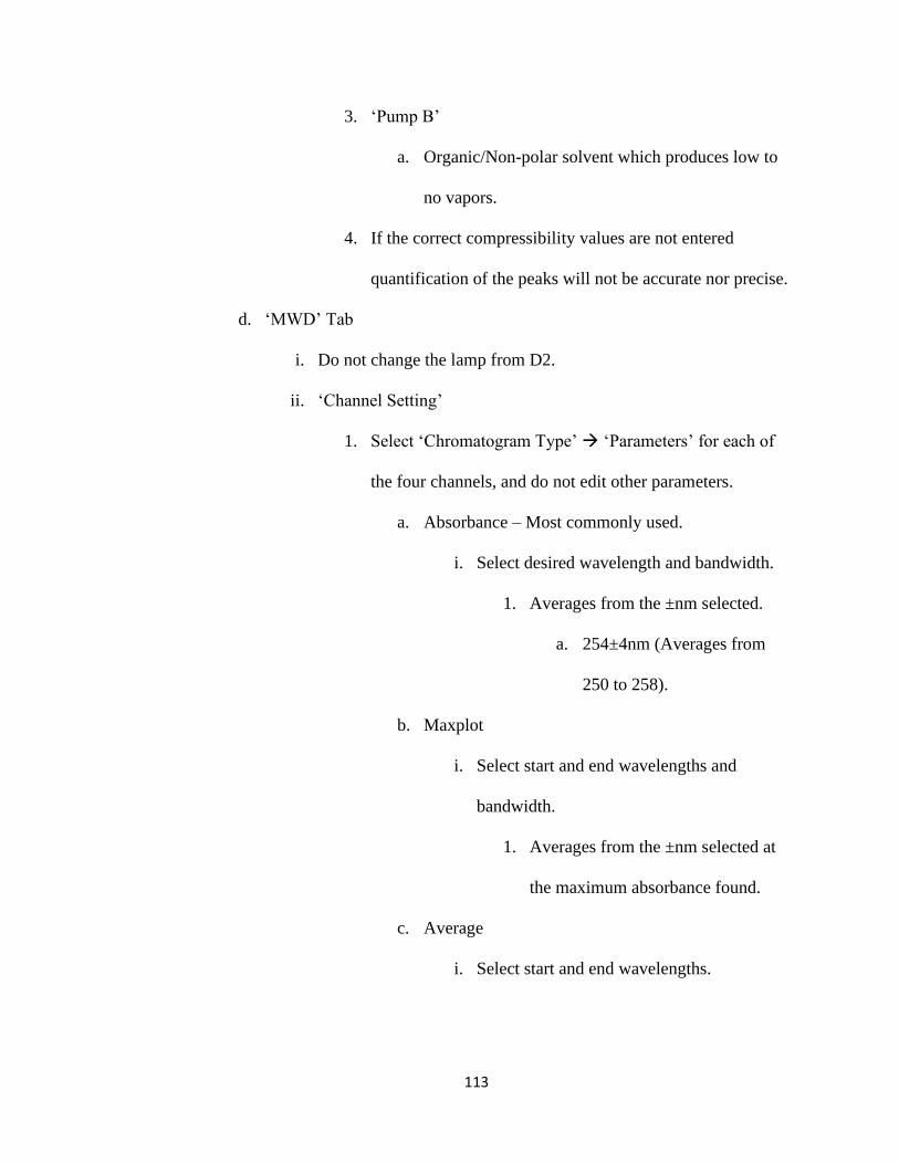
113

3. ‘Pump B’

a. Organic/Non-polar solvent which produces low to

no vapors.

4. If the correct compressibility values are not entered

quantification of the peaks will not be accurate nor precise.

d. ‘MWD’ Tab

i. Do not change the lamp from D2.

ii. ‘Channel Setting’

1. Select ‘Chromatogram Type’ → ‘Parameters’ for each of

the four channels, and do not edit other parameters.

a. Absorbance – Most commonly used.

i. Select desired wavelength and bandwidth.

1. Averages from the ±nm selected.

a. 254±4nm (Averages from

250 to 258).

b. Maxplot

i. Select start and end wavelengths and

bandwidth.

1. Averages from the ±nm selected at

the maximum absorbance found.

c. Average

i. Select start and end wavelengths.

114

1. Outputs chromatogram at the

average wavelength between start

and end wavelengths.

e. ‘Column Oven’ Tab

i. Set desired analysis temperature with the maximum temperature of

90oC with ‘Ready Check’ turned on.

16. After the parameters of your method file have been configured name your method

file in the top right textbox containing the word ‘untitled’. Select ‘Download and

Close’ at the bottom right to load your new method file.

17. Once you select ‘Download and Close’ save the method file in a directory you

create.

a. File → Save Method File As → C:\LabSolutions\Data\Your Folder Name.

18. On the bottom frame of the ‘Realtime Analysis’ window select ‘Oven On’ to turn

on the oven and select ‘Pump On’ to turn the pumps on using your flow rate.

Allow the UHPLC to condition for a minimum of two hours prior to starting your

analysis.

5.11 UHPLC Exporting Data for Excel

1. Navigate to the working data directory where the UHPLC data file (.lcd) resides.

2. Open the UHPLC data file (.lcd) in the ‘Postrun Analysis’ application by double

clicking on it.

3. Log into Lab Solutions to access the ‘Postrun Analysis’ application. There is no

password.

115

4. The ‘Postrun Analysis’ application will open with the UHPLC data file selected.

5. Verify it is the correct UHPLC data file before proceeding.

6. Select the ‘File’ icon on the menu toolbar.

7. Scroll down the ‘File’ menu to ‘Export Data’ and then select ‘Export Data as

ASCII’ and the export window will appear.

8. Select the radio button ‘Output File’ then select the desired parameters below for

export in the ‘Output Items’ text box then select the location to be saved.

a. Data File Properties – File and sample information.

b. Peak Table – All peak information from the chromatogram.

c. Identified Results – Quantitative information from the compound list.

d. Grouping Results – Quantitative information from the group list.

e. Status Trace – Status of pumps, degasser, sample cooler, oven temp, and

room temp.

f. Chromatogram – Retention time with absorbances for each wavelength

channel.

g. Slice Data – Multi-wavelength detector slice data for each wavelength

channel.

h. 3D Data – PDA data (if installed).

i. Fraction Data – Fraction collection information.

9. Select the folder icon for the ‘Output File’ and navigate to the working data

directory to save the file.

10. Name the file using the UHPLC data file (.lcd) name then click open. The

filename cannot have blank spaces.

116

11. Select the delimiter drop down and scroll to ‘Comma’ then click ‘Ok’ to close the

window and save the file.

12. Close the ‘Postrun Analysis’ application.

13. Insert a USB thumb drive into the front panel of the computer system connected

to the UHPLC instrument to copy the exported text file to the USB thumb drive.

14. When importing ‘Headers’ and ‘Comma’ are selected for the imported data to be

formatted correctly in excel.

5.12 UHPLC PDF Report Creation

1. Navigate to the working data directory where the UHPLC data file (.lcd) resides.

2. Open the UHPLC data file (.lcd) in the ‘Postrun Analysis’ application by double

clicking on it.

3. Log into Lab Solutions to access the ‘Postrun Analysis’ application.

4. The ‘Postrun Analysis’ application will open with the UHPLC data file selected.

5. Verify it is the correct UHPLC data file before proceeding.

6. Select the ‘File’ icon on the menu toolbar.

7. Scroll down the ‘File’ menu to ‘Data Report’ and then select ‘PDF Output’.

8. A window will open to save the ‘PDF Output’.

9. Select the folder location for the ‘PDF Output’ and name the file before saving.

10. Navigate to the saved file using windows explorer and verify its contents.

11. Close the ‘Postrun Analysis’ application.

12. Insert a USB thumb drive into the front panel of the computer system connected

to the UHPLC instrument to copy the PDF file for your own records.

117

5.13 UHPLC Shutdown

1. When your analysis is complete, navigate to the ‘Instrument’ menu item and

select shutdown.

a. The shutdown window will appear at which time you will select

‘Shutdown Method File’, if not already checked, and you may have to

navigate to C:\LabSolutions\Data to load the ‘Shutdown Method File.lcm’.

b. Select ‘Degassing Unit (LC Pump, Subcontroller) Off after Cooldown’, if

not already checked, and Select ‘Ok’.

c. Wait for the UHPLC lights to turn amber, then close the ‘Realtime

Analysis’ window by navigating to File → Exit.

118

d. You will hear two dissimilar beeps when communication to the UHPLC is

disconnected.

e. Turn off the UHPLC using the PowerVar switch, shutdown the computer,

and cover the UHPLC.

i. If the Computer displays a ‘Shutdown Error’ select ‘Shut Down

Anyway’.

2. Enter ‘Shutdown and Covered’ into the logbook prior to leaving.

5.14 UHPLC Waste Transfer

1. Transfer the UHPLC connected waste to the stand-alone waste when changing the

solvent system or when the level of solvent waste is four inches from the

containers plumbing connector.

2. The UHPLC connected waste is transferred to the stand-alone waste container.

119

3. Prior to moving the UHPLC connected waste out from the wall assure that you

unclip the plastic clips connected to the structure below the UHPLC assuring that

the inline plumbing connectors do not become disconnected.

a. Assure that the pump plumbing connector does not become disconnected.

4. Once the plumbing is free from the plastic clips move the UHPLC connected

waste out from the wall, even with the front of the UHPLC structure, and then

move the stand-alone waste next to the UHPLC connected waste.

a. To prepare the UHPLC connected waste for transfer to the stand-alone

waste the handle and lid of the UHPLC connected waste must be locked

into place using the clamp to the front and clamp to the rear of the handle.

120

i. Move the handle towards the rear clamp.

ii. Push on the front clamp to raise the teeth, move then handle

forward until it is under the teeth, and then lower the teeth until

they lock onto the handle.

iii. Use your left hand to push on the rear clamp to raise the teeth,

carefully move the handle towards the rear clamp until it is under

the teeth, and then lower the teeth until they lock onto the handle.

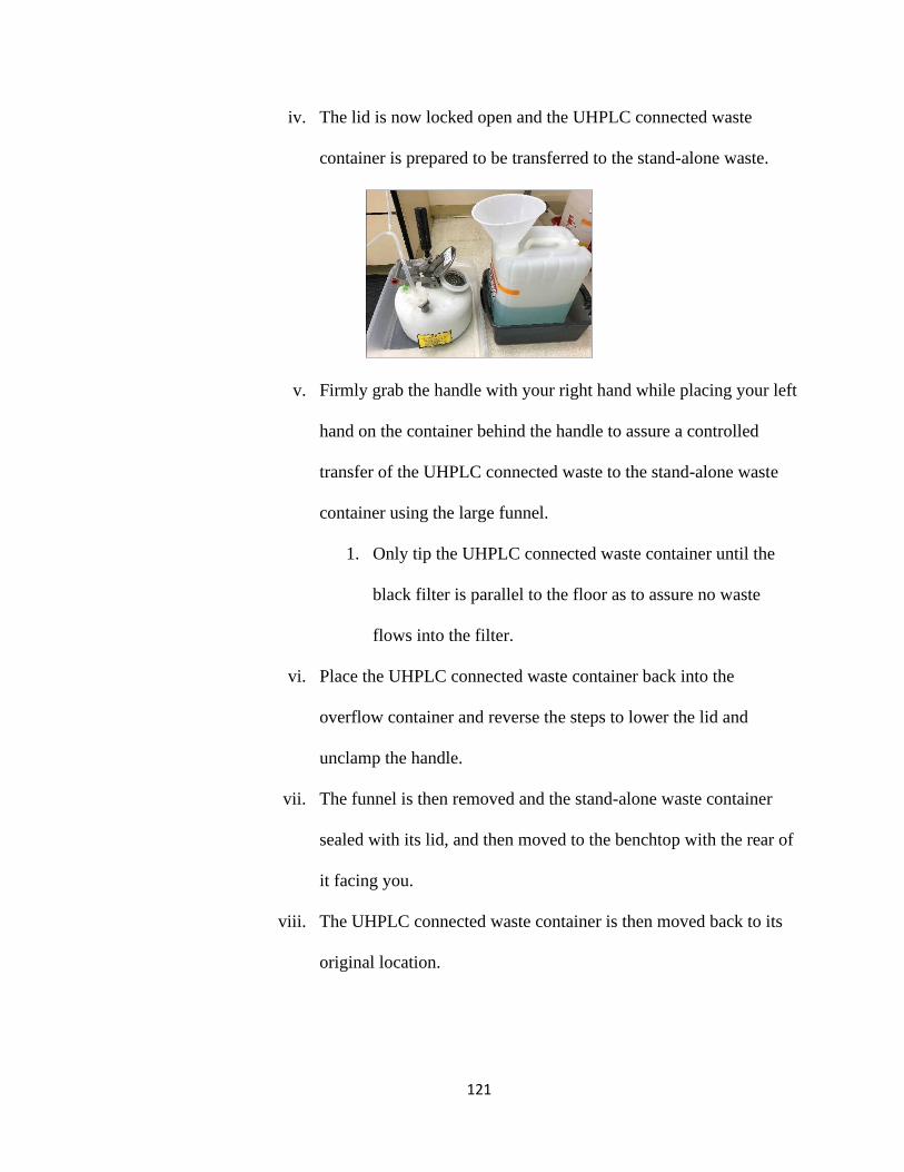
121

iv. The lid is now locked open and the UHPLC connected waste

container is prepared to be transferred to the stand-alone waste.

v. Firmly grab the handle with your right hand while placing your left

hand on the container behind the handle to assure a controlled

transfer of the UHPLC connected waste to the stand-alone waste

container using the large funnel.

1. Only tip the UHPLC connected waste container until the

black filter is parallel to the floor as to assure no waste

flows into the filter.

vi. Place the UHPLC connected waste container back into the

overflow container and reverse the steps to lower the lid and

unclamp the handle.

vii. The funnel is then removed and the stand-alone waste container

sealed with its lid, and then moved to the benchtop with the rear of

it facing you.

viii. The UHPLC connected waste container is then moved back to its

original location.

122

5. Correctly documenting the waste transfer.

a. Wait until the solvent in the stand-alone waste container has settled from

moving it.

i. Take a sharpie and in the center of the rear of the waste container

write your initials and the date, and then draw the solvent line to

the left and right of your initials and date.

ii. Place the stand-alone waste back into the overflow container, and

then move it back to its original location.

b. Log the transfer in the UHPLC logbook on the UHPLC administration

computer, and the stand-alone waste clipboard log.

c. Enter the solvent names and ratio along with the volume transferred in the

UHPLC connected waste clipboard log. Return the clipboard logs to their

proper waste containers.

123

5.15 UHPLC Sample Vial Reclamation

1. Diluent is employed in reclaiming LC sample vials due to the analyte being

miscible in it.

a. If the diluent is not within access, too expensive, or pH adjusted water

then determine another solvent the analyte is most miscible in to employ.

2. Once UHPLC analysis is completed immediately empty the LC sample vials. If

there are no saved caps then discard the punctured septa and retain the caps for

future use.

a. Rinse the LC sample vial caps with hot water, deionized water, and then

dry them.

i. If there are saved caps in a container then discard the caps and

septa.

3. Locate a beaker to hold all the LC sample vials in, but do not place them in the

beaker.

4. Fill the beaker with enough diluent to submerge half of the LC sample vials as the

diluent level will increase with every LC sample vial added.

5. Using a 3mL transfer pipette fill each LC sample vial with diluent from the

beaker, submerge the LC sample vials in the beaker by dropping them, and then

cover with parafilm. Assure no air bubbles are in the LC sample vials.

a. Let the LC sample vials soak overnight.

6. Decant the majority of diluent into a beaker and then transfer to a labelled plastic

bottle, preferably nalgene, for future use. This avoids spillage of the diluent while

performing step 7.

124

7. Take the LC sample vials from the beaker, empty the diluent from them, rinse

them with hot water, and then rinse them with deionized water.

8. The LC sample vials are placed standing upright in small beakers then dried in an

oven.

9. After the LC sample vials have cooled inspect them for solute that dried to the

vial walls.

a. If there is no solute visible store them in a labeled plastic container.

10. If solute has dried to the vial walls the process is repeated, however, a sonicator is

employed.

a. Place the LC sample vials into diluent as stated in step 5 but use an

erlenmeyer flask that can be partially submerged in the sonicator using a

ring stand and clamp.

b. Assure the erlenmeyer flask is firmly secured to the ring stand using the

clamp and submerge the erlenmeyer flask into the sonicator water just

below the clamp.

c. Sonicate for 30 minutes then repeat step 6 to step 9.

5.16 UHPLC Flushing

1. Prior to performing any analyses assure that the proper flushing solvent systems

are prepared.

a. Flushing the plumbing for salt buildup is performed if a buffer was

employed in the analyses.

125

i. The solvent system will be (90:10) LC grade water and methanol

and must be filtered using no larger than a 0.45uM filter.

1. The polar solvent reduces the lifetime of a high carbon load

column (C18), so the column is removed and replaced with

a coupling during this time.

a. The coupling is stored with guard screws at the

bottom of the column oven and the two wrenches

are found in the bottom drawer under the UHPLC.

ii. Runtime is 60 minutes of 2mL/min at 50% B with three 50uL

injections and external rinsing.

1. Each of the three 1L solvent bottles employed must have a

minimum of 200mL to assure the diffusers remain

submerged in solvent.

a. If the diffusers are not submerged the pumps will

draw air into the plumbing, which can cause

damage to the pumps.

2. The flush will consume 60mL of solvent each for Pump A

and Pump B, 1.5mL for Rinse 0, and 1.5mL for the LC

sample vial used for injections.

3. A minimum of 723mL of solvent must be prepared,

however, it is suggested to prepare 1L as the flush may

have to be extended due to heavy salt buildup in the

plumbing.

126

a. The 1L Pump A and Pump B bottles will have a

minimum of 260mL each, and the 1L Rinse 0 bottle

will have a minimum of 203mL.

iii. If the analysis was performed employing a buffer then proceed to

outline number 2.

b. Flushing the plumbing and column after any analysis is performed with no

buffer employed OR after “Flushing the plumbing for salt buildup”

i. The solvent system will be (75:15:10) LC grade water, methanol,

and acetonitrile and must be filtered using no larger than a 0.45uM

filter.

1. The more nonpolar solvent will not reduce the lifetime of a

high carbon load column (C18) and the column is not to be

removed or must be reinstalled after the previous flushing

with the coupling installed.

ii. Runtime is 60 minutes at 50% B with three 50uL injections and

external rinsing.

1. If the column installed is ≥100mm L x 4.6mm I.D. x 5.0uM

dp then 2mL/min.

a. Each of the three 1L solvent bottles employed must

have a minimum of 200mL to assure the diffusers

remain submerged in solvent.

127

i. If the diffusers are not submerged the pumps

will draw air into the plumbing, which can

cause damage to the pumps.

b. The flush will consume 60mL of solvent each for

Pump A and Pump B, 1.5mL for Rinse 0, and

1.5mL for the LC sample vial used for injections.

c. A minimum of 723mL of solvent must be prepared,

however, it is suggested to prepare 1L as the flush

may have to be extended due to heavy salt buildup

in the column.

i. The 1L Pump A and Pump B bottles will

have a minimum of 260mL each, and the 1L

Rinse 0 bottle will have a minimum of

203mL.

2. If the column installed is <100mm L x 4.6mm I.D. x 5.0uM

dp then 1mL/min.

a. Each of the three 1L solvent bottles employed must

have a minimum of 200mL to assure the diffusers

remain submerged in solvent.

i. If the diffusers are not submerged the pumps

will draw air into the plumbing, which can

cause damage to the pumps.

128

b. The flush will consume 30mL of solvent each for

Pump A and Pump B, 1.5mL for Rinse 0, and

1.5mL for the LC sample vial used for injections.

c. A minimum of 663mL of solvent must be prepared,

however, it is suggested to prepare 1L as the flush

may have to be extended due to heavy salt buildup

in the column.

i. The 1L Pump A and Pump B bottles will

have a minimum of 230mL each, and the 1L

Rinse 0 bottle will have a minimum of

203mL.

c. If the analysis was performed without employing a buffer then proceed to

outline number 3.

2. Flushing the plumbing for salt buildup.

a. Store the analysis solvent and load the flushing solvent.

i. Label and prime three 1L nalgene bottles to store the solvent

employed in analysis.

ii. Configure the cardboard, tub lid, and tub as per the ‘Startup and

Conditioning’ protocol.

iii. When the analysis employing a buffer has been completed stop

both pumps.

iv. Exchange the analysis solvents quickly and safely.

129

1. Remove the lid and diffuser from the 1L Pump A UHPLC

bottle and transfer the analysis solvent using a funnel to a

labelled and primed 1L nalgene bottle.

2. Label the 1L UHPLC bottle with the appropriate full names

of the flushing solvents and do not use abbreviations or

chemical formulas.

3. Transfer the flushing solvent using a funnel to the 1L Pump

A UHPLC bottle, insert the diffuser and secure the lid,

replace it in the appropriate location on the solvent rack,

and push the diffuser to the bottom of the bottle.

a. Repeat for the Pump B and Rinse 0 1L UHPLC

bottles.

v. Store the tub, tub lid, and cardboard in the drawer it was found in.

b. Removing the column and installing the coupling

i. Assure that you have the authorization to remove the column. If

you do not then contact Dr. Koether to assist you in this process as

cross threading any screws will render the column useless, and the

cost of a new column is from $800 to $2,000.

ii. Remove the UHPLC toolkit from the bottom drawer of below the

UHPLC.

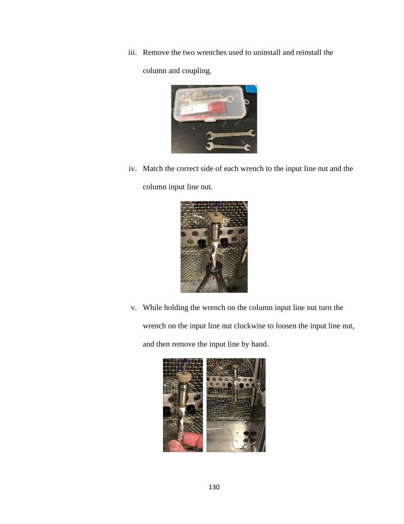
130

iii. Remove the two wrenches used to uninstall and reinstall the

column and coupling.

iv. Match the correct side of each wrench to the input line nut and the

column input line nut.

v. While holding the wrench on the column input line nut turn the

wrench on the input line nut clockwise to loosen the input line nut,

and then remove the input line by hand.

131

vi. Loosen the output line screw by turning it counter-clockwise one

turn.

1. While holding the plastic output line screw remove the

output line.

a. Remove the output line screw completely and place

it at the bottom of the oven unit.

132

vii. Remove the guard screws from the coupling and install them on

the column, and then store the column at the bottom of the oven

unit.

viii. Prepare the coupling by installing the plastic output line screw with

one turn clockwise.

ix. Place the output line into the screw holding it with the index finger

of the hand holding the coupling and then tighten the screw with

the other hand until it is snug, but do not overtighten.

133

x. Place the input line into the coupling and then tighten the screw by

turning it counter-clockwise until it is snug, but do not overtighten.

xi. Insert the coupling in the column mounting unit clamps.

xii. Match the correct side of each wrench to the input line nut and

coupling wrench location.

1. While holding the wrench on the coupling wrench location

turn the wrench on the input line nut counter-clockwise to

tighten the input line nut, but do not overtighten.

2. Close the oven doors and keep the toolkit wrenches

accessible until the flushing is complete and the column is

reinstalled.

134

c. Loading and Configuring the Flushing Method File

i. Select the ‘_UHPLC Flush’ project folder by selecting ‘File-

>Select Project (Folder)’ and navigate to

‘C:\LabSolutions\Data\_UHPLC Flush’ then click ‘OK’.

ii. Select ‘File->Open Method File’ and then select the ‘UHPLC

Flush.lcm’ method file.

iii. Assure the method file ‘Pump’ tab is configured for a flow rate of

2mL/min with 50% B, select ‘Download and Close’, and then

select ‘File-> Save Method File’.

iv. Fill a 1.5mL LC sample vial with the flushing solvent and then

load the sample vial into Tray 1 in vial location ‘1’.

d. Purging the Pumps and Autosampler.

i. Once the sample vial has been loaded the air from both pumps

must be purged.

1. Open each right-side pump door by pressing inward until it

clicks then let go to open, and then open the left pump door

by pulling outward with very little force.

a. Verify that the small bottles of 10% 2-propanol are

filled to the red line. If not lightly unscrew the lid

and fill to the red line. Close the lid, replace the

bottle into the holding slot, and lightly close the left

pump door.

135

b. Turn the pump handles counterclockwise until the

first horizontal position (9 O’clock).

c. Press the ‘Purge’ button on both pumps while

observing the clear plastic tubing for air bubbles

and repeat the purge only if air bubbles remain.

d. When purging is complete slowly and gently turn

the pump valve handles clockwise until it is almost

vertical and will not turn any further (11 O’clock).

2. Close the pump doors by pressing inward until it clicks

then let go to remain closed then start the pumps and set

your alarm for 1 hour.

ii. Press the purge button on the front of the Autosampler which will

take 20 minutes.

e. Loading and running the flush batch file.

i. Select ‘Main’ from the left pane and then select ‘Batch Editor.

1. Select ‘File->Open->Batch File’, navigate to

‘C:\LabSolutions\Data\_UHPLC Flush’, and then select

‘UHPLC 3 Injection Flush.lcb’ batch file.

ii. Select ‘Queue Batch Run’ from the left pane to start the batch file.

1. This will inject 50uL of the flush solvent three times as to

clean the inside of the autosampler needle where each

injection is followed by an external needle wash.

136

f. Reinstalling the column.

i. Once the Injections have been performed and one hour of flushing

has surpassed the pumps are shut off and the column reinstalled.

ii. Match the correct side of each wrench to the input line nut and

coupling wrench location.

iii. While holding the wrench on the coupling wrench location turn the

wrench on the input line nut clockwise to loosen the input line nut

then remove the input line by hand.

iv. Remove the output line from the plastic screw in the coupling by

turning the plastic screw one turn counter-clockwise and then

gently pull the output line from the screw.

137

v. Remove the output line screw by turning it counter-clockwise until

it is out, remove the guard screws from the column and reinstall

them in the coupling, and then store the coupling at the bottom of

the oven unit.

vi. Identify the column output by locating the flow direction arrow on

the column label as the column output is in the direction of the

flow arrow.

vii. Reinstall the output line by inserting the output line screw into the

column output and turn clockwise one turn.

138

viii. Place the output line into the screw holding it with the index finger

of the hand holding the coupling and then tighten the screw with

the other hand until it is snug, but do not overtighten.

ix. Reinstall the input line by inserting the input line nut into the

column input and tighten the input line nut by hand by turning the

input line nut counter-clockwise until it is snug then replace the

column back into the column mounting clamps.

x. Match the correct side of each wrench to the input line nut and the

column input line nut.

1. While holding the wrench on the column input line nut turn

the wrench on the input line nut counter-clockwise to

tighten it snugly, but do not overtighten.

139

2. If the input line nut is not tight enough small droplets of

mobile phase will leak from the column input line when the

pumps are turned on.

a. If this occurs shut the pumps off, verify that the

input line nut is not cross threaded, and then tighten

the input line nut using a little more force than what

was employed in the previous attempt.

b. This can be repeated to assure that the input line nut

is not overtightened.

xi. Store the wrenches in the toolkit and store the toolkit in the drawer

under the UHPLC.

xii. Now perform the flushing the column in outline number 3.

3. Flushing the plumbing and column after any analysis or after “Flushing the

plumbing for salt buildup”

a. When the analysis has been completed stop the flow by stopping the

pumps.

i. If the “Flushing the plumbing for salt buildup” was performed

replace the coupling with the column employed in the analysis that

employed a buffer.

b. Store the analysis solvent and load the flushing solvent.

140


employed in analysis.



iii. When the analysis employing a buffer has been completed stop

both pumps.

iv. Exchange the analysis solvents quickly and safely.


bottle and transfer the analysis solvent using a funnel to a



of the flushing solvents and do not use abbreviations or

chemical formulas.

3. Transfer the flushing solvent using a funnel to the 1L Pump




a. Repeat for the Pump B and Rinse 0 1L UHPLC

bottles.


141

c. Loading and Configuring the Flushing Method File

i. Select the ‘_UHPLC Flush’ project folder by selecting ‘File-

>Select Project (Folder)’ and navigate to

‘C:\LabSolutions\Data\_UHPLC Flush’ then click ‘OK’.

ii. Select ‘File->Open Method File’ and then select the ‘UHPLC

Flush.lcm’ method file.

iii. Assure the method file ‘Pump’ tab is configured for a flow rate of

2mL/min with 50% B, the ‘Oven’ tab is configured for 40oC, select

‘Download and Close’, and then select ‘File-> Save Method File’.

iv. Fill a 1.5mL LC sample vial with the flushing solvent and then

load the sample vial into Tray 1 in vial location ‘1’.

d. Purging the Pumps and Autosampler.

i. Once the sample vial has been loaded the air from both pumps

must be purged.

1. Open each right-side pump door by pressing inward until it

clicks then let go to open, and then open the left pump door

by pulling outward with very little force.

a. Verify that the small bottles of 10% 2-propanol are

filled to the red line. If not lightly unscrew the lid

and fill to the red line. Close the lid, replace the

bottle into the holding slot, and lightly close the left

pump door.

142

b. Turn the pump handles counterclockwise until the

first horizontal position (9 O’clock).

c. Press the ‘Purge’ button on both pumps while

observing the clear plastic tubing for air bubbles

and repeat the purge only if air bubbles remain.

d. When purging is complete slowly and gently turn

the pump valve handles clockwise until it is almost

vertical and will not turn any further (11 O’clock).

2. Close the pump doors by pressing inward until it clicks

then let go to remain closed then start the pumps, turn the

oven on, and set your alarm for 1 hour.

ii. Press the purge button on the front of the Autosampler which will

take 20 minutes.

e. Loading and running the flush batch file.

i. Select ‘Main’ from the left pane and then select ‘Batch Editor.

1. Select ‘File->Open->Batch File’, navigate to

‘C:\LabSolutions\Data\_UHPLC Flush’, and then select

‘UHPLC 3 Injection Flush.lcb’ batch file.

ii. Select ‘Queue Batch Run’ from the left pane to start the batch file.

1. This will inject 50uL of the flush solvent three times as to

clean the inside of the autosampler needle where each

injection is followed by an external needle wash.

143

f. Store the flushing solvent and load the analysis solvent.


employed in the flush.



iii. When the flushing has been completed stop both pumps.

iv. Exchange the flushing solvents quickly and safely.


bottle and transfer the flushing solvent using a funnel to a



of the analysis solvents and do not use abbreviations or

chemical formulas.

3. Transfer the analysis solvent using a funnel to the 1L Pump




a. Repeat for the Pump B (If Employed) and Rinse 0

1L UHPLC bottles.

i. If the one bottle method is employed in the

analysis using only Pump A then do not

remove the flushing solvent from the 1L

Pump B UHPLC bottle.

144


g. Shutdown and Cover the UHPLC

i. See the ‘Shutdown’ protocol.

5.17 UHPLC Batch File Creation

1. This protocol assumes that both standards and unknowns will be analyzed in the

same batch file.

2. Assure you have created and loaded the method file that will be employed in the

batch analysis from the ‘Startup and Conditioning’ protocol prior to creating a

batch file.

a. The batch file uses the currently loaded method file parameters for the

batch analysis.

i. If a baseline check is to be employed the method file must be

configured prior to the batch file creation.

3. Select ‘Main->Batch Editor->Wizard’ from the left pane and the ‘Batch Table

Wizard’ will appear.

4. Batch Table Wizard.

a. Assure the ‘Batch Table’ field appears as ‘New’ and the ‘Method File’ is

the method file that is currently loaded.

b. Select the desired injection volume and the number of ‘Sample Groups’ is

set to 1.

i. The UHPLC uses ‘Calibration Levels’ and not ‘Sample Groups’.

c. Assure ‘Standard and Unknown’ is selected, and then select ‘Next’.

145

i. All the parameters below can be modified when the wizard has

been completed.

5. Batch Table Wizard – Standard Sample.

a. Enter the standard ‘Sample Name’ with a ‘001’ and then select ‘Auto-

Increment’ if you would like the Sample Names to be in order of analysis.

b. Enter the ‘Sample ID’ with a ‘-0001’ and then select ‘Auto-Increment’ if

you would like the Sample IDs to be in order of analysis.

c. Enter the desired ‘Data File Name’ with a ‘001’ and then select ‘Auto-

Increment’ if you would like the ‘Data File Names’ to be in order of

analysis.

i. The ‘Create File Names’ automatically can be selected by

checking the box above the ‘Data File Name’ field.

d. Enter the ‘Number of Calibration Levels’, which can be up to ten.

e. Enter the amount of ‘Standard Sample Vials Per Level’, or how many of

identical concentrations of a specific standard is being employed.

f. Enter the amount of ‘Repetitions per Run’, or the number of times to

analyze each individual standard.

g. Assure the correct ‘Tray’ is selected.

i. The default tray is ‘Rack 1.5mL 105 Vials’.

h. Select the starting vial number for your standards, which should be ‘Vial

#1’.

i. The UHPLC will insert the ending ‘Vial #’ according to the

‘Number of Calibration Levels’ that was entered.

146

i. Select ‘Clear All Calibration Levels at the Beginning’ to initialize new set

of calibrations, and then select ‘Next’.

6. Batch Table Wizard – Unknown Sample.

a. Enter the unknown ‘Sample Name’ with a ‘001’ and then select ‘Auto-

Increment’ if you would like the Sample Names to be in order of analysis.

b. Enter the unknown ‘Sample ID’ with a ‘-0001’ and then select ‘Auto-

Increment’ if you would like the Sample IDs to be in order of analysis.

c. Enter the desired unknown ‘Data File Name’ with a ‘001’ and then select

‘Auto-Increment’ if you would like the ‘Data File Names’ to be in order of

analysis.

i. The ‘Create File Names’ automatically can be selected by

checking the box above the ‘Data File Name’ field.

d. Enter the amount of ‘Sample Vials in Each Group’, or the number of

unknown samples loaded into the autosampler rack.

e. Enter the amount of ‘Repetitions per Run’, or the number of times to

analyze each individual unknown sample.

f. The correct tray will be automatically selected from the configuration of

the standards.

g. The UHPLC will insert the beginning ‘Vial #’ according to the ‘Number

of Calibration Levels’ that was entered.

i. The UHPLC will insert the ending ‘Vial #’ according to the

‘Number of Unknown Samples in Each Group’ that was entered.

h. Select ‘Next’ twice.

147

7. Batch Table Wizard – Other Settings

a. If the method file was previously configured with a ‘Baseline Check’ then

select ‘Baseline Check’, but f it was not then just select next.

8. Batch Table Wizard – Save Batch File.

a. Navigate to the project folder using the blue folder icon at the top right of

the window, name the batch file, select open, and then select finish.

9. The initial batch file will be displayed.

a. Verify the ‘Vial #, Tray Name’ Sample Name’ Sample ID, Sample Type,

Method File Name, and Data File Name’.

b. If any field is incorrect then place the cursor in the column and row to be

edited and enter the new information.

10. Select ‘Queue Batch Run’ from the left pane to initiate the batch file analysis.

5.18 UHPLC Manual Integration

A basic understanding of the regulatory requirements is necessary prior to employing

manual integration.

1. An ‘Audit Trail’ must be established.

a. A backup of ALL original data files and manually integrated data files

must be retained for review.

i. A second person is required to review ALL original data files and

manually integrated data files to validate the use of manual

integration.

148

ii. If a run is to be discarded from quantitation the original data file

must be retained.

b. Regulatory documentation includes:

i. Initial, repeated, and reported results.

ii. Method employed (Standard Operating Procedures).

iii. Assay run identification.

iv. Analyst that is requesting and reasoning for the manual integration.

v. Manager who authorized the manual integration.

2. A justification and thorough explanation of the reasoning for the manual

integration is required.

a. Acceptable examples for inhibiting automatic integration functions.

i. Baseline perturbations caused by sample injection.

ii. USP impurity determinations.

1. The API peak is automatically integrated, but the impurity

peaks are manually integrated due to very low

concentrations.

iii. Analysis of metabolites or degradants that have very low

concentrations near the LOQ.

iv. Large amounts of noise and/or drift in the baseline.

1. This may be caused by a need for system maintenance, a

method that lacks robustness, or inadequate system

suitability requirements.

149

2. A common issue with manual integration is the

repositioning of the baseline correction so that it produces

inaccurate peak areas.

b. Multiple re-integrations that are not justified are called “Integrating into

Compliance”.

3. Standard operating procedures must be developed, validated, and adhered to.

a. Frequently developed for each compound or formulation that includes:

i. Guidelines on when and how to employ manual integration.

ii. Handling of extra peaks produced by excipients and impurities.

iii. Tolerances for analyst adjustments in the manual integration

parameters.

b. Once validated the manual integration parameters developed for the

standards MUST be employed with the unknown samples.

c. Developing standard operating procedures with a scientific rationale.

i. Perform an initial analysis on known standards and a prepared

sample using automatic integration to calculate the recovery.

ii. Evaluate each integration parameter by using the same known

standards and prepared sample by modifying each parameter below

to calculate the recovery.

1. Slope sensitivity.

2. Peak width.

3. Bunching factor.

4. Area reject.

150

5. Noise threshold.

6. Area threshold.

iii. Compare the recoveries to optimize the method of manual

integration.

4. Acceptable alternatives to consider before employing manual integration.

a. Adjusting automatic integration or ‘Manual Intervention’.

b. Optimization of the chromatographic method by modifying:

i. The solvent system and/or solvent system ratio.

ii. The flow rate and/or injection volume.

iii. The column type, length, inner diameter, and/or particle size.

iv. The column temperature.

5. The baseline correction and peak identification process.

a. The integration software initially establishes the baseline using the first

data point after which it redefines the baseline by averaging the input

signal.

i. If the integration software fails to establish a redefined baseline the

first data point is used for the initial baseline.

b. The integration software continues to monitor the input signal determining

a threshold for the baseline containing parameters for the noise threshold.

i. It is periodically reset to compensate for drift until the up-slope of

a peak is detected due to the data point being outside of the

baseline threshold.

151

6. Examples of manual integration techniques, as seen below in Figure 1.

a. Acceptable.

i. (1) Manual integration of the peak applying a justifiable baseline.

b. Unacceptable.

i. (2) Manual integration that shaves the peak producing less area.

ii. (3) Manual integration that enhances the peak producing more

area.

Figure 1: Data Integrity – Shaving and Enhancing Peaks2

7. Manual integration must be employed prior to performing regression analysis.

a. Performing regression analysis first will introduce bias when selecting to

employ manual integration and when selecting specific integration points.

152

The following protocol on manual integration utilizes the LabSolutions software

packaged with the Shimadzu Nexera X2 and will only employ the ‘Time Program Table’

displayed when the ‘Program’ command button is selected from the ‘Integration’ tab

found in the ‘Method View’ of the ‘Calibration Curve’ window located in the left pane of

the ‘Postrun Analysis’ or ‘Realtime Analysis’ windows after an analysis has been

performed. This protocol will employ the ‘Postrun Analysis’ feature of the LabSolutions

software and only manually integrate one peak of interest employing the integration

window used by the automatic integration algorithm. The instructions in this protocol

may be used to manually integrate more than one peak of interest if desired. A full list of

commands with definitions, setting ranges, and default settings can be found in the

‘Integration Time Program’ help file located in the ‘LabSolutions’ software.

1. Perform an analysis to generate the data files to be used in the manual integration.

a. Employ the standards and samples but do not perform regression analysis

and retain the original copies in a separate folder.

2. Determine the integration parameters to be employed.

a. Open the ‘LabSolutions’ software found on the windows desktop, navigate

to the ‘Postrun Analysis’ data analysis tool.

153

b. The ‘Postrun Analysis’ window will appear after which the ‘Main’ tab at

the top of the left windowpane is selected.

c. The ‘Calibration Curve’ icon in the left windowpane is then selected.

d. The ‘Calibration Curve’ window will then appear.

154

e. The project folder containing the method file employed in the analysis is

then selected.

i. A navigation window will appear to select the folder containing the

method file employed in the analysis after which click ‘OK’.

f. Once the project folder is selected open the method file used in the

analysis.

g. An empty calibration curve for the analysis associated with the method

file will appear in the upper left windowpane with the data files in the

upper right windowpane where each data file is displayed in the

‘Chromatogram View’ windowpane below it when selected.

155

h. The retention time of the peak of interest must be determined by

highlighting the data file in the ‘Data File’ windowpane and placing the

mouse cursor at the apex of the peak of interest in the ‘Chromatogram

View’.

i. There will be slightly varying retention times depending on the

concentration of the standard where the median retention time is

used.

156

1. The void volume peaks will not be retained in this protocol,

however, for the ‘LabSolutions’ software to automatically

perform the chromatographic calculations the void volume

times will have to be manually integrated.

i. Enter the median retention time in the ‘Compound Table’ by selecting

‘Edit’ from the ‘Method View’ windowpane.

i. Select ‘View’ to apply the changes and the ‘Calibration Curve’

windowpane will populate with the calibration curve for the

standards.

j. The negative peak from the analysis produced unacceptable integration

due to the addition of peak area to the peak of interest.

157

i. All the chromatograms from this analysis will also have additional

area so manual integration of the peak of interest is required.

k. To determine the integration window to be employed the highest

concentration standard data file is opened in read-only mode by double-

clicking the data file after which the chromatogram window for the data

file will appear.

i. The automatic integration points are denoted by an upward red

arrow to a downward red arrow. By left clicking on the channel

desired the channel peak will be highlighted as to differentiate

which set of arrows to observe the time window.

ii. Document the automatic integration time window for the peak of

interest then close the data file.

158

l. Enter ‘Edit’ mode, select the ‘Integration’ tab, and then select the

‘Program’ icon.

m. The ‘Integration Time Program’ window will then appear displaying the

highlighted data file from the ‘Data File’ windowpane.

3. Applying the integration parameters to the standards using the ‘Integration Time

Program’ window.

159

a. On row 1 assure the time is ‘0.000’ in the ‘Time (min)’ column then select

the open area of the ‘Command’ column and a dropdown list will appear

to select “Integration Off’.

b. On row 2 enter the starting time from the automatic integration in the

‘Time (min)’ column and then select the open area of the ‘Command’

column and a dropdown list will appear to select ‘Integration On’.

c. On row 3 enter the ending time from the automatic integration in the

‘Time (min)’ column and then select the open area of the ‘Command’

column and a dropdown list will appear to select ‘Integration Off’, select

‘Simulate’ to verify the integration, and then click ‘OK’.

d. Select ‘Copy to All Channels’ on the ‘Integration’ tab of the ‘Method

View’, select ‘Yes’ to copy to all channels, and then select ‘View’ to

apply the integration to all data files.

160

i. Applying the same time the automatic integration employed

maintains the baseline integration determined by the algorithm

without retaining the unwanted peaks.

e. Save the method file and close the ‘Calibration Curve’ window.

4. Applying the integration parameters to the samples.

a. Open the sample data file in the ‘Postrun Analysis’ window by double-

clicking on the data file.

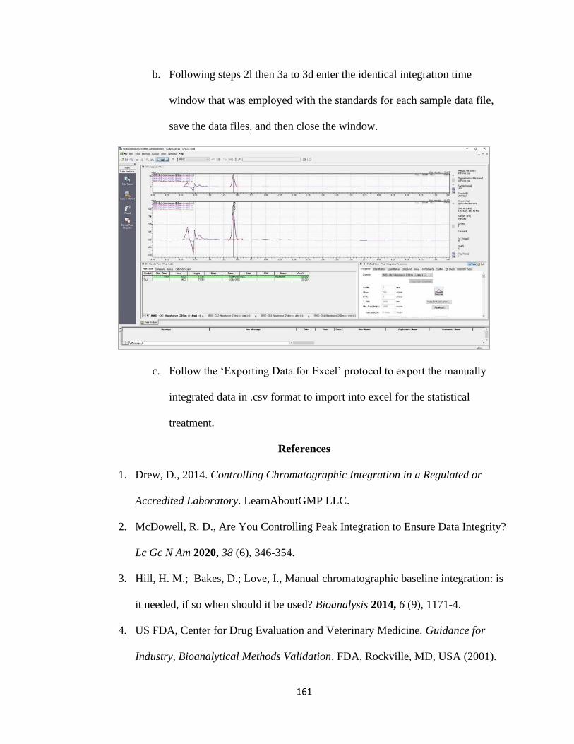
161

b. Following steps 2l then 3a to 3d enter the identical integration time

window that was employed with the standards for each sample data file,

save the data files, and then close the window.

c. Follow the ‘Exporting Data for Excel’ protocol to export the manually

integrated data in .csv format to import into excel for the statistical

treatment.

References

1. Drew, D., 2014. Controlling Chromatographic Integration in a Regulated or

Accredited Laboratory. LearnAboutGMP LLC.

2. McDowell, R. D., Are You Controlling Peak Integration to Ensure Data Integrity?

Lc Gc N Am 2020, 38 (6), 346-354.

3. Hill, H. M.; Bakes, D.; Love, I., Manual chromatographic baseline integration: is

it needed, if so when should it be used? Bioanalysis 2014, 6 (9), 1171-4.

4. US FDA, Center for Drug Evaluation and Veterinary Medicine. Guidance for

Industry, Bioanalytical Methods Validation. FDA, Rockville, MD, USA (2001).

Documents

method development of standard dilution analysis on