PUBLISHED BYMicrosoft PressA Division of Microsoft CorporationOne Microsoft WayRedmond, Washington 98052-6399

Copyright © 2004 by Craig Stinson and Mark Dodge

All rights reserved. No part of the contents of this book may be reproduced or transmitted in any formor by any means without the written permission of the publisher.

Library of Congress Cataloging-in-Publication DataStinson, Craig, 1943-

Microsoft Office Excel 2003 Inside Out / Craig Stinson, Mark Dodge.p. cm.

Includes index.ISBN 0-7356-1511-X1. Microsoft Excel (Computer file) 2. Business--Computer programs. 3. Electronic

spreadsheets. I. Dodge, Mark. II. Title.

HF5548.4.M523S753 2003005.369--dc21 2003052673

Printed and bound in the United States of America.

1 2 3 4 5 6 7 8 9 QWT 8 7 6 5 4 3

Distributed in Canada by H.B. Fenn and Company Ltd.

A CIP catalogue record for this book is available from the British Library.

Microsoft Press books are available through booksellers and distributors worldwide. For further informa-tion about international editions, contact your local Microsoft Corporation office or contact MicrosoftPress International directly at fax (425) 936-7329. Visit our Web site at www.microsoft.com/mspress.Send comments to mspinput@microsoft.com.

AutoSum, FrontPage, IntelliMouse, Microsoft, Microsoft Press, MS-DOS, PivotChart, PivotTable,SharePoint, Visual Basic, Windows, and Windows NT are either registered trademarks or trademarks ofMicrosoft Corporation in the United States and/or other countries. Other product and company namesmentioned herein may be the trademarks of their respective owners.

The example companies, organizations, products, domain names, e-mail addresses, logos, people, places,and events depicted herein are fictitious. No association with any real company, organization, product,domain name, e-mail address, logo, person, place, or event is intended or should be inferred.

Acquisitions Editor: Alex BlantonProject Editor: Sandra HaynesSeries Editor: Sandra Haynes

Body Part No. X09-69527

iii

Contents At A Glance

Contents at a Glance

Part 1Examining the Excel Environment

Chapter 1What’s New in Microsoft Office Excel 2003 . . . . . . . . . . . . . 3

Chapter 2Excel Fundamentals . . . . . . . . . . .13

Chapter 3Custom-Tailoring the Excel Workspace . . . . . . . . . . . . . . . . . .65

Part 2Building Worksheets

Chapter 4Worksheet Design Tips . . . . . . . . .93

Chapter 5How to Work a Worksheet . . . . . .101

Chapter 6How to Work a Workbook . . . . . .133

Part 3Formatting and Editing Worksheets

Chapter 7Worksheet Editing Techniques . . .147

Chapter 8Worksheet Formatting Techniques . . . . . . . . . . . . . . . . .195

Chapter 9Advanced Formatting and Editing Techniques . . . . . . . . . . .241

Part 4Adding Graphics and Printing

Chapter 10Creating Spiffy Graphics . . . . . . . 283

Chapter 11Printing and Presenting . . . . . . . 331

Part 5Creating Formulas and Performing Data Analysis

Chapter 12Building Formulas. . . . . . . . . . . . 351

Chapter 13Using Functions . . . . . . . . . . . . . 401

Chapter 14Everyday Functions . . . . . . . . . . 411

Chapter 15Formatting and Calculating Date and Time . . . . . . . . . . . . . . 435

Chapter 16Functions for Financial Analysis . . . . . . . . . . . . . . . . . . . 449

Chapter 17Functions for Analyzing Statistics . . . . . . . . . . . . . . . . . . 463

Chapter 18Performing What-If Analysis . . . . 493

Contents At A Glance

iv

Part 6Collaboration and the Internet

Chapter 19Collaborating with Excel . . . . . . .521

Chapter 20Transferring Files to and from Internet Sites . . . . . . . . . . .553

Part 7Integrating Excel with Other Applications

Chapter 21Linking and Embedding . . . . . . . .569

Chapter 22Using Hyperlinks . . . . . . . . . . . . .581

Chapter 23Using Excel Data in Word and PowerPoint Documents . . . . .589

Part 8Creating Charts

Chapter 24Basic Charting Techniques. . . . . .609

Chapter 25Enhancing the Appearance of Your Charts . . . . . . . . . . . . . . .623

Chapter 26Working with Chart Data . . . . . . .667

Chapter 27Advanced Charting Techniques . .683

Part 9Managing Databases and Lists

Chapter 28Managing Information in Lists. . . 701

Chapter 29Working with External Data . . . . 757

Chapter 30Analyzing Data with PivotTable Reports . . . . . . . . . . . . . . . . . . . 797

Part 10Automating Excel

Chapter 31Recording Macros . . . . . . . . . . . 841

Chapter 32Creating Custom Functions. . . . . 859

Chapter 33Debugging Macros and Custom Functions . . . . . . . . . . . 869

Part 11Appendixes

Appendix AInstalling Microsoft Excel . . . . . . 883

Appendix BUsing Speech and Handwriting Recognition . . . . . . . . . . . . . . . . 889

Appendix CKeyboard Shortcuts . . . . . . . . . . 903

Appendix DFunction Reference . . . . . . . . . . 921

v

Table of Contents

Table of Contents

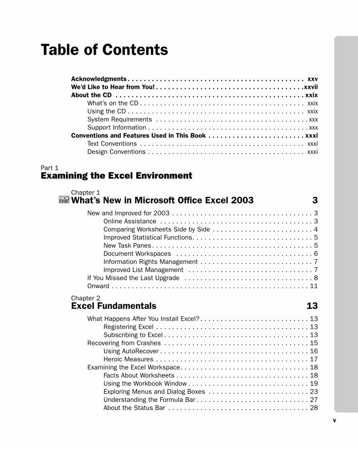
Acknowledgments . . . . . . . . . . . . . . . . . . . . . . . . . . . . . . . . . . . . . . . . . . . . xxvWe’d Like to Hear from You! . . . . . . . . . . . . . . . . . . . . . . . . . . . . . . . . . . . . .xxviiAbout the CD . . . . . . . . . . . . . . . . . . . . . . . . . . . . . . . . . . . . . . . . . . . . . . . xxix

What’s on the CD . . . . . . . . . . . . . . . . . . . . . . . . . . . . . . . . . . . . . . . . . xxixUsing the CD . . . . . . . . . . . . . . . . . . . . . . . . . . . . . . . . . . . . . . . . . . . . xxixSystem Requirements . . . . . . . . . . . . . . . . . . . . . . . . . . . . . . . . . . . . . . xxxSupport Information . . . . . . . . . . . . . . . . . . . . . . . . . . . . . . . . . . . . . . . . xxx

Conventions and Features Used in This Book . . . . . . . . . . . . . . . . . . . . . . . . xxxiText Conventions . . . . . . . . . . . . . . . . . . . . . . . . . . . . . . . . . . . . . . . . . xxxiDesign Conventions . . . . . . . . . . . . . . . . . . . . . . . . . . . . . . . . . . . . . . . xxxi

Part 1Examining the Excel Environment

Chapter 1What’s New in Microsoft Office Excel 2003 3

New and Improved for 2003 . . . . . . . . . . . . . . . . . . . . . . . . . . . . . . . . . . . 3Online Assistance . . . . . . . . . . . . . . . . . . . . . . . . . . . . . . . . . . . . . . 3Comparing Worksheets Side by Side . . . . . . . . . . . . . . . . . . . . . . . . . 4Improved Statistical Functions. . . . . . . . . . . . . . . . . . . . . . . . . . . . . . 5New Task Panes. . . . . . . . . . . . . . . . . . . . . . . . . . . . . . . . . . . . . . . . 5Document Workspaces . . . . . . . . . . . . . . . . . . . . . . . . . . . . . . . . . . 6Information Rights Management . . . . . . . . . . . . . . . . . . . . . . . . . . . . 7Improved List Management . . . . . . . . . . . . . . . . . . . . . . . . . . . . . . . 7

If You Missed the Last Upgrade . . . . . . . . . . . . . . . . . . . . . . . . . . . . . . . . 8Onward . . . . . . . . . . . . . . . . . . . . . . . . . . . . . . . . . . . . . . . . . . . . . . . . . 11

Chapter 2Excel Fundamentals 13

What Happens After You Install Excel? . . . . . . . . . . . . . . . . . . . . . . . . . . . 13Registering Excel . . . . . . . . . . . . . . . . . . . . . . . . . . . . . . . . . . . . . . 13Subscribing to Excel . . . . . . . . . . . . . . . . . . . . . . . . . . . . . . . . . . . . 13

Recovering from Crashes . . . . . . . . . . . . . . . . . . . . . . . . . . . . . . . . . . . . 15Using AutoRecover . . . . . . . . . . . . . . . . . . . . . . . . . . . . . . . . . . . . . 16Heroic Measures . . . . . . . . . . . . . . . . . . . . . . . . . . . . . . . . . . . . . . 17

Examining the Excel Workspace. . . . . . . . . . . . . . . . . . . . . . . . . . . . . . . . 18Facts About Worksheets . . . . . . . . . . . . . . . . . . . . . . . . . . . . . . . . . 18Using the Workbook Window . . . . . . . . . . . . . . . . . . . . . . . . . . . . . . 19Exploring Menus and Dialog Boxes . . . . . . . . . . . . . . . . . . . . . . . . . 23Understanding the Formula Bar . . . . . . . . . . . . . . . . . . . . . . . . . . . . 27About the Status Bar . . . . . . . . . . . . . . . . . . . . . . . . . . . . . . . . . . . 28

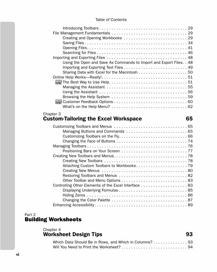
Table of Contents

vi

Introducing Toolbars . . . . . . . . . . . . . . . . . . . . . . . . . . . . . . . . . . . . 29File Management Fundamentals . . . . . . . . . . . . . . . . . . . . . . . . . . . . . . . 29

Creating and Opening Workbooks . . . . . . . . . . . . . . . . . . . . . . . . . . 29Saving Files . . . . . . . . . . . . . . . . . . . . . . . . . . . . . . . . . . . . . . . . . . 34Opening Files. . . . . . . . . . . . . . . . . . . . . . . . . . . . . . . . . . . . . . . . . 41Searching for Files . . . . . . . . . . . . . . . . . . . . . . . . . . . . . . . . . . . . . 46

Importing and Exporting Files . . . . . . . . . . . . . . . . . . . . . . . . . . . . . . . . . 48Using the Open and Save As Commands to Import and Export Files. . 48Importing and Exporting Text Files . . . . . . . . . . . . . . . . . . . . . . . . . . 49Sharing Data with Excel for the Macintosh . . . . . . . . . . . . . . . . . . . . 50

Online Help Works—Really!. . . . . . . . . . . . . . . . . . . . . . . . . . . . . . . . . . . 51The Best Way to Use Help. . . . . . . . . . . . . . . . . . . . . . . . . . . . . . . . 51Managing the Assistant . . . . . . . . . . . . . . . . . . . . . . . . . . . . . . . . . 55Using the Assistant . . . . . . . . . . . . . . . . . . . . . . . . . . . . . . . . . . . . 56Browsing the Help System . . . . . . . . . . . . . . . . . . . . . . . . . . . . . . . 59Customer Feedback Options . . . . . . . . . . . . . . . . . . . . . . . . . . . . . . 60What’s on the Help Menu? . . . . . . . . . . . . . . . . . . . . . . . . . . . . . . . 62

Chapter 3Custom-Tailoring the Excel Workspace 65

Customizing Toolbars and Menus . . . . . . . . . . . . . . . . . . . . . . . . . . . . . . 65Managing Buttons and Commands . . . . . . . . . . . . . . . . . . . . . . . . . 65Customizing Toolbars on the Fly. . . . . . . . . . . . . . . . . . . . . . . . . . . . 66Changing the Face of Buttons . . . . . . . . . . . . . . . . . . . . . . . . . . . . . 74

Managing Toolbars . . . . . . . . . . . . . . . . . . . . . . . . . . . . . . . . . . . . . . . . . 76Positioning Bars on Your Screen . . . . . . . . . . . . . . . . . . . . . . . . . . . 77

Creating New Toolbars and Menus. . . . . . . . . . . . . . . . . . . . . . . . . . . . . . 78Creating New Toolbars . . . . . . . . . . . . . . . . . . . . . . . . . . . . . . . . . . 78Attaching Custom Toolbars to Workbooks. . . . . . . . . . . . . . . . . . . . . 79Creating New Menus . . . . . . . . . . . . . . . . . . . . . . . . . . . . . . . . . . . 80Restoring Toolbars and Menus . . . . . . . . . . . . . . . . . . . . . . . . . . . . 82Other Toolbar and Menu Options . . . . . . . . . . . . . . . . . . . . . . . . . . . 83

Controlling Other Elements of the Excel Interface . . . . . . . . . . . . . . . . . . . 83Displaying Underlying Formulas . . . . . . . . . . . . . . . . . . . . . . . . . . . . 85Hiding Zeros . . . . . . . . . . . . . . . . . . . . . . . . . . . . . . . . . . . . . . . . . 86Changing the Color Palette . . . . . . . . . . . . . . . . . . . . . . . . . . . . . . . 87

Enhancing Accessibility. . . . . . . . . . . . . . . . . . . . . . . . . . . . . . . . . . . . . . 89

Part 2Building Worksheets

Chapter 4Worksheet Design Tips 93

Which Data Should Be in Rows, and Which in Columns? . . . . . . . . . . . . . . 93Will You Need to Print the Worksheet? . . . . . . . . . . . . . . . . . . . . . . . . . . . 94

vii

Table of Contents

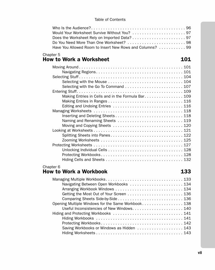
Who Is the Audience?. . . . . . . . . . . . . . . . . . . . . . . . . . . . . . . . . . . . . . . 96Would Your Worksheet Survive Without You? . . . . . . . . . . . . . . . . . . . . . . 97Does the Worksheet Rely on Imported Data? . . . . . . . . . . . . . . . . . . . . . . 97Do You Need More Than One Worksheet? . . . . . . . . . . . . . . . . . . . . . . . . 98Have You Allowed Room to Insert New Rows and Columns? . . . . . . . . . . . 99

Chapter 5How to Work a Worksheet 101

Moving Around . . . . . . . . . . . . . . . . . . . . . . . . . . . . . . . . . . . . . . . . . . . 101Navigating Regions. . . . . . . . . . . . . . . . . . . . . . . . . . . . . . . . . . . . 101

Selecting Stuff . . . . . . . . . . . . . . . . . . . . . . . . . . . . . . . . . . . . . . . . . . . 104Selecting with the Mouse . . . . . . . . . . . . . . . . . . . . . . . . . . . . . . . 104Selecting with the Go To Command . . . . . . . . . . . . . . . . . . . . . . . . 107

Entering Stuff. . . . . . . . . . . . . . . . . . . . . . . . . . . . . . . . . . . . . . . . . . . . 109Making Entries in Cells and in the Formula Bar . . . . . . . . . . . . . . . . 109Making Entries in Ranges . . . . . . . . . . . . . . . . . . . . . . . . . . . . . . . 116Editing and Undoing Entries . . . . . . . . . . . . . . . . . . . . . . . . . . . . . 116

Managing Worksheets . . . . . . . . . . . . . . . . . . . . . . . . . . . . . . . . . . . . . 118Inserting and Deleting Sheets . . . . . . . . . . . . . . . . . . . . . . . . . . . . 118Naming and Renaming Sheets . . . . . . . . . . . . . . . . . . . . . . . . . . . 119Moving and Copying Sheets . . . . . . . . . . . . . . . . . . . . . . . . . . . . . 120

Looking at Worksheets . . . . . . . . . . . . . . . . . . . . . . . . . . . . . . . . . . . . . 121Splitting Sheets into Panes . . . . . . . . . . . . . . . . . . . . . . . . . . . . . . 122Zooming Worksheets . . . . . . . . . . . . . . . . . . . . . . . . . . . . . . . . . . 125

Protecting Worksheets . . . . . . . . . . . . . . . . . . . . . . . . . . . . . . . . . . . . . 127Unlocking Individual Cells . . . . . . . . . . . . . . . . . . . . . . . . . . . . . . . 128Protecting Workbooks . . . . . . . . . . . . . . . . . . . . . . . . . . . . . . . . . . 128Hiding Cells and Sheets . . . . . . . . . . . . . . . . . . . . . . . . . . . . . . . . 132

Chapter 6How to Work a Workbook 133

Managing Multiple Workbooks. . . . . . . . . . . . . . . . . . . . . . . . . . . . . . . . 133Navigating Between Open Workbooks . . . . . . . . . . . . . . . . . . . . . . 134Arranging Workbook Windows . . . . . . . . . . . . . . . . . . . . . . . . . . . . 134Getting the Most Out of Your Screen . . . . . . . . . . . . . . . . . . . . . . . 136Comparing Sheets Side-by-Side . . . . . . . . . . . . . . . . . . . . . . . . . . . 136

Opening Multiple Windows for the Same Workbook . . . . . . . . . . . . . . . . . 138Useful Inconsistencies of New Windows. . . . . . . . . . . . . . . . . . . . . 140

Hiding and Protecting Workbooks . . . . . . . . . . . . . . . . . . . . . . . . . . . . . 141Hiding Workbooks . . . . . . . . . . . . . . . . . . . . . . . . . . . . . . . . . . . . 141Protecting Workbooks . . . . . . . . . . . . . . . . . . . . . . . . . . . . . . . . . . 142Saving Workbooks or Windows as Hidden . . . . . . . . . . . . . . . . . . . 143Hiding Worksheets . . . . . . . . . . . . . . . . . . . . . . . . . . . . . . . . . . . . 143

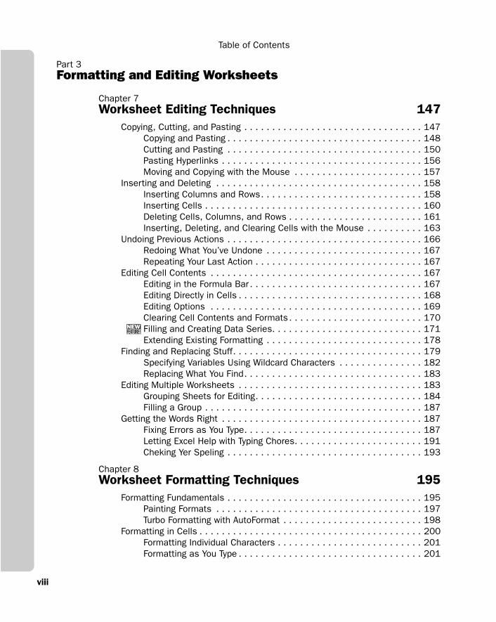
Table of Contents

viii

Part 3Formatting and Editing Worksheets

Chapter 7Worksheet Editing Techniques 147

Copying, Cutting, and Pasting . . . . . . . . . . . . . . . . . . . . . . . . . . . . . . . . 147Copying and Pasting . . . . . . . . . . . . . . . . . . . . . . . . . . . . . . . . . . . 148Cutting and Pasting . . . . . . . . . . . . . . . . . . . . . . . . . . . . . . . . . . . 150Pasting Hyperlinks . . . . . . . . . . . . . . . . . . . . . . . . . . . . . . . . . . . . 156Moving and Copying with the Mouse . . . . . . . . . . . . . . . . . . . . . . . 157

Inserting and Deleting . . . . . . . . . . . . . . . . . . . . . . . . . . . . . . . . . . . . . 158Inserting Columns and Rows. . . . . . . . . . . . . . . . . . . . . . . . . . . . . 158Inserting Cells . . . . . . . . . . . . . . . . . . . . . . . . . . . . . . . . . . . . . . . 160Deleting Cells, Columns, and Rows . . . . . . . . . . . . . . . . . . . . . . . . 161Inserting, Deleting, and Clearing Cells with the Mouse . . . . . . . . . . 163

Undoing Previous Actions . . . . . . . . . . . . . . . . . . . . . . . . . . . . . . . . . . . 166Redoing What You’ve Undone . . . . . . . . . . . . . . . . . . . . . . . . . . . . 167Repeating Your Last Action . . . . . . . . . . . . . . . . . . . . . . . . . . . . . . 167

Editing Cell Contents . . . . . . . . . . . . . . . . . . . . . . . . . . . . . . . . . . . . . . 167Editing in the Formula Bar . . . . . . . . . . . . . . . . . . . . . . . . . . . . . . . 167Editing Directly in Cells . . . . . . . . . . . . . . . . . . . . . . . . . . . . . . . . . 168Editing Options . . . . . . . . . . . . . . . . . . . . . . . . . . . . . . . . . . . . . . 169Clearing Cell Contents and Formats . . . . . . . . . . . . . . . . . . . . . . . . 170Filling and Creating Data Series. . . . . . . . . . . . . . . . . . . . . . . . . . . 171Extending Existing Formatting . . . . . . . . . . . . . . . . . . . . . . . . . . . . 178

Finding and Replacing Stuff. . . . . . . . . . . . . . . . . . . . . . . . . . . . . . . . . . 179Specifying Variables Using Wildcard Characters . . . . . . . . . . . . . . . 182Replacing What You Find. . . . . . . . . . . . . . . . . . . . . . . . . . . . . . . . 183

Editing Multiple Worksheets . . . . . . . . . . . . . . . . . . . . . . . . . . . . . . . . . 183Grouping Sheets for Editing. . . . . . . . . . . . . . . . . . . . . . . . . . . . . . 184Filling a Group . . . . . . . . . . . . . . . . . . . . . . . . . . . . . . . . . . . . . . . 187

Getting the Words Right . . . . . . . . . . . . . . . . . . . . . . . . . . . . . . . . . . . . 187Fixing Errors as You Type. . . . . . . . . . . . . . . . . . . . . . . . . . . . . . . . 187Letting Excel Help with Typing Chores. . . . . . . . . . . . . . . . . . . . . . . 191Cheking Yer Speling . . . . . . . . . . . . . . . . . . . . . . . . . . . . . . . . . . . 193

Chapter 8Worksheet Formatting Techniques 195

Formatting Fundamentals . . . . . . . . . . . . . . . . . . . . . . . . . . . . . . . . . . . 195Painting Formats . . . . . . . . . . . . . . . . . . . . . . . . . . . . . . . . . . . . . 197Turbo Formatting with AutoFormat . . . . . . . . . . . . . . . . . . . . . . . . . 198

Formatting in Cells . . . . . . . . . . . . . . . . . . . . . . . . . . . . . . . . . . . . . . . . 200Formatting Individual Characters . . . . . . . . . . . . . . . . . . . . . . . . . . 201Formatting as You Type . . . . . . . . . . . . . . . . . . . . . . . . . . . . . . . . . 201

ix

Table of Contents

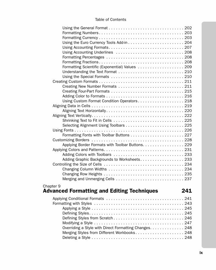
Using the General Format . . . . . . . . . . . . . . . . . . . . . . . . . . . . . . . 202Formatting Numbers . . . . . . . . . . . . . . . . . . . . . . . . . . . . . . . . . . . 203Formatting Currency . . . . . . . . . . . . . . . . . . . . . . . . . . . . . . . . . . . 203Using the Euro Currency Tools Add-in . . . . . . . . . . . . . . . . . . . . . . . 204Using Accounting Formats. . . . . . . . . . . . . . . . . . . . . . . . . . . . . . . 207Using Accounting Underlines . . . . . . . . . . . . . . . . . . . . . . . . . . . . 208Formatting Percentages . . . . . . . . . . . . . . . . . . . . . . . . . . . . . . . . 208Formatting Fractions . . . . . . . . . . . . . . . . . . . . . . . . . . . . . . . . . . . 208Formatting Scientific (Exponential) Values . . . . . . . . . . . . . . . . . . . 209Understanding the Text Format . . . . . . . . . . . . . . . . . . . . . . . . . . . 210Using the Special Formats . . . . . . . . . . . . . . . . . . . . . . . . . . . . . . 210

Creating Custom Formats . . . . . . . . . . . . . . . . . . . . . . . . . . . . . . . . . . . 211Creating New Number Formats . . . . . . . . . . . . . . . . . . . . . . . . . . . 211Creating Four-Part Formats . . . . . . . . . . . . . . . . . . . . . . . . . . . . . . 215Adding Color to Formats . . . . . . . . . . . . . . . . . . . . . . . . . . . . . . . . 216Using Custom Format Condition Operators . . . . . . . . . . . . . . . . . . . 218

Aligning Data in Cells . . . . . . . . . . . . . . . . . . . . . . . . . . . . . . . . . . . . . . 219Aligning Text Horizontally . . . . . . . . . . . . . . . . . . . . . . . . . . . . . . . . 220

Aligning Text Vertically. . . . . . . . . . . . . . . . . . . . . . . . . . . . . . . . . . . . . . 222Shrinking Text to Fit in Cells . . . . . . . . . . . . . . . . . . . . . . . . . . . . . 225Selecting Alignment Using Toolbars . . . . . . . . . . . . . . . . . . . . . . . . 225

Using Fonts . . . . . . . . . . . . . . . . . . . . . . . . . . . . . . . . . . . . . . . . . . . . . 226Formatting Fonts with Toolbar Buttons . . . . . . . . . . . . . . . . . . . . . . 227

Customizing Borders . . . . . . . . . . . . . . . . . . . . . . . . . . . . . . . . . . . . . . 228Applying Border Formats with Toolbar Buttons. . . . . . . . . . . . . . . . . 229

Applying Colors and Patterns. . . . . . . . . . . . . . . . . . . . . . . . . . . . . . . . . 231Adding Colors with Toolbars . . . . . . . . . . . . . . . . . . . . . . . . . . . . . 233Adding Graphic Backgrounds to Worksheets. . . . . . . . . . . . . . . . . . 233

Controlling the Size of Cells . . . . . . . . . . . . . . . . . . . . . . . . . . . . . . . . . 234Changing Column Widths . . . . . . . . . . . . . . . . . . . . . . . . . . . . . . . 234Changing Row Heights . . . . . . . . . . . . . . . . . . . . . . . . . . . . . . . . . 235Merging and Unmerging Cells . . . . . . . . . . . . . . . . . . . . . . . . . . . . 237

Chapter 9Advanced Formatting and Editing Techniques 241

Applying Conditional Formats . . . . . . . . . . . . . . . . . . . . . . . . . . . . . . . . 241Formatting with Styles . . . . . . . . . . . . . . . . . . . . . . . . . . . . . . . . . . . . . 243

Applying a Style . . . . . . . . . . . . . . . . . . . . . . . . . . . . . . . . . . . . . . 245Defining Styles. . . . . . . . . . . . . . . . . . . . . . . . . . . . . . . . . . . . . . . 245Defining Styles from Scratch . . . . . . . . . . . . . . . . . . . . . . . . . . . . . 246Modifying a Style . . . . . . . . . . . . . . . . . . . . . . . . . . . . . . . . . . . . . 247Overriding a Style with Direct Formatting Changes. . . . . . . . . . . . . . 248Merging Styles from Different Workbooks . . . . . . . . . . . . . . . . . . . . 248Deleting a Style . . . . . . . . . . . . . . . . . . . . . . . . . . . . . . . . . . . . . . 248

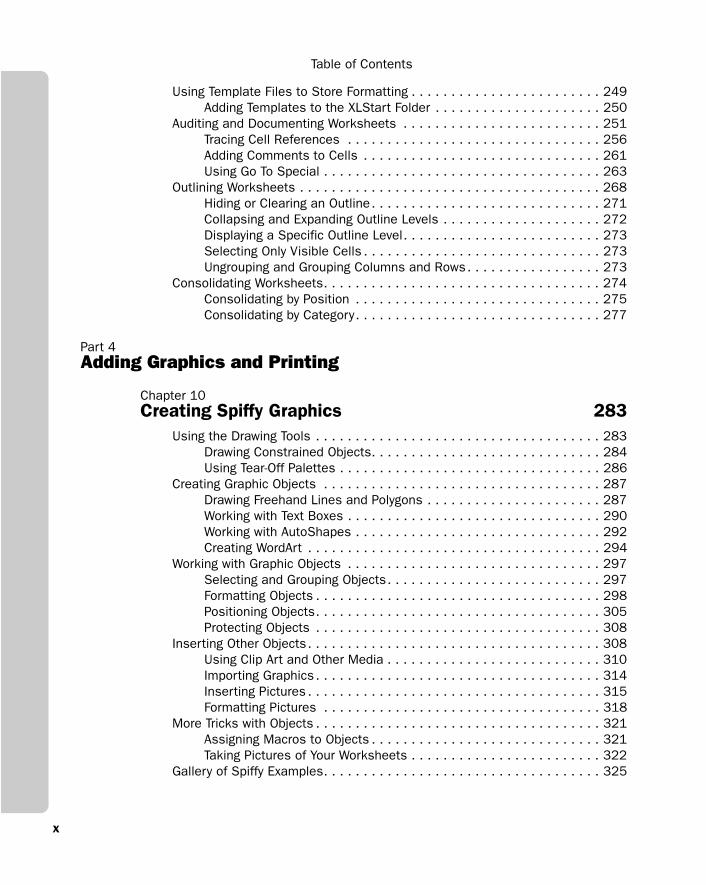
Table of Contents

x

Using Template Files to Store Formatting . . . . . . . . . . . . . . . . . . . . . . . . 249Adding Templates to the XLStart Folder . . . . . . . . . . . . . . . . . . . . . 250

Auditing and Documenting Worksheets . . . . . . . . . . . . . . . . . . . . . . . . . 251Tracing Cell References . . . . . . . . . . . . . . . . . . . . . . . . . . . . . . . . 256Adding Comments to Cells . . . . . . . . . . . . . . . . . . . . . . . . . . . . . . 261Using Go To Special . . . . . . . . . . . . . . . . . . . . . . . . . . . . . . . . . . . 263

Outlining Worksheets . . . . . . . . . . . . . . . . . . . . . . . . . . . . . . . . . . . . . . 268Hiding or Clearing an Outline. . . . . . . . . . . . . . . . . . . . . . . . . . . . . 271Collapsing and Expanding Outline Levels . . . . . . . . . . . . . . . . . . . . 272Displaying a Specific Outline Level. . . . . . . . . . . . . . . . . . . . . . . . . 273Selecting Only Visible Cells . . . . . . . . . . . . . . . . . . . . . . . . . . . . . . 273Ungrouping and Grouping Columns and Rows. . . . . . . . . . . . . . . . . 273

Consolidating Worksheets. . . . . . . . . . . . . . . . . . . . . . . . . . . . . . . . . . . 274Consolidating by Position . . . . . . . . . . . . . . . . . . . . . . . . . . . . . . . 275Consolidating by Category. . . . . . . . . . . . . . . . . . . . . . . . . . . . . . . 277

Part 4Adding Graphics and Printing

Chapter 10Creating Spiffy Graphics 283

Using the Drawing Tools . . . . . . . . . . . . . . . . . . . . . . . . . . . . . . . . . . . . 283Drawing Constrained Objects. . . . . . . . . . . . . . . . . . . . . . . . . . . . . 284Using Tear-Off Palettes . . . . . . . . . . . . . . . . . . . . . . . . . . . . . . . . . 286

Creating Graphic Objects . . . . . . . . . . . . . . . . . . . . . . . . . . . . . . . . . . . 287Drawing Freehand Lines and Polygons . . . . . . . . . . . . . . . . . . . . . . 287Working with Text Boxes . . . . . . . . . . . . . . . . . . . . . . . . . . . . . . . . 290Working with AutoShapes . . . . . . . . . . . . . . . . . . . . . . . . . . . . . . . 292Creating WordArt . . . . . . . . . . . . . . . . . . . . . . . . . . . . . . . . . . . . . 294

Working with Graphic Objects . . . . . . . . . . . . . . . . . . . . . . . . . . . . . . . . 297Selecting and Grouping Objects. . . . . . . . . . . . . . . . . . . . . . . . . . . 297Formatting Objects . . . . . . . . . . . . . . . . . . . . . . . . . . . . . . . . . . . . 298Positioning Objects. . . . . . . . . . . . . . . . . . . . . . . . . . . . . . . . . . . . 305Protecting Objects . . . . . . . . . . . . . . . . . . . . . . . . . . . . . . . . . . . . 308

Inserting Other Objects. . . . . . . . . . . . . . . . . . . . . . . . . . . . . . . . . . . . . 308Using Clip Art and Other Media . . . . . . . . . . . . . . . . . . . . . . . . . . . 310Importing Graphics . . . . . . . . . . . . . . . . . . . . . . . . . . . . . . . . . . . . 314Inserting Pictures . . . . . . . . . . . . . . . . . . . . . . . . . . . . . . . . . . . . . 315Formatting Pictures . . . . . . . . . . . . . . . . . . . . . . . . . . . . . . . . . . . 318

More Tricks with Objects . . . . . . . . . . . . . . . . . . . . . . . . . . . . . . . . . . . . 321Assigning Macros to Objects . . . . . . . . . . . . . . . . . . . . . . . . . . . . . 321Taking Pictures of Your Worksheets . . . . . . . . . . . . . . . . . . . . . . . . 322

Gallery of Spiffy Examples. . . . . . . . . . . . . . . . . . . . . . . . . . . . . . . . . . . 325

xi

Table of Contents

Chapter 11Printing and Presenting 331

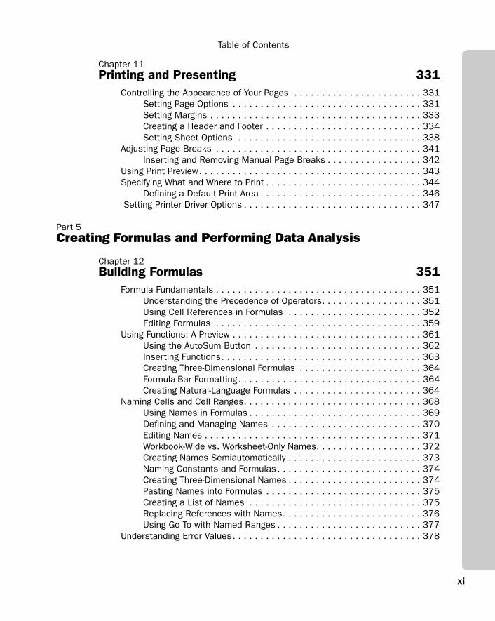
Controlling the Appearance of Your Pages . . . . . . . . . . . . . . . . . . . . . . . 331Setting Page Options . . . . . . . . . . . . . . . . . . . . . . . . . . . . . . . . . . 331Setting Margins . . . . . . . . . . . . . . . . . . . . . . . . . . . . . . . . . . . . . . 333Creating a Header and Footer . . . . . . . . . . . . . . . . . . . . . . . . . . . . 334Setting Sheet Options . . . . . . . . . . . . . . . . . . . . . . . . . . . . . . . . . 338

Adjusting Page Breaks . . . . . . . . . . . . . . . . . . . . . . . . . . . . . . . . . . . . . 341Inserting and Removing Manual Page Breaks . . . . . . . . . . . . . . . . . 342

Using Print Preview. . . . . . . . . . . . . . . . . . . . . . . . . . . . . . . . . . . . . . . . 343Specifying What and Where to Print . . . . . . . . . . . . . . . . . . . . . . . . . . . . 344

Defining a Default Print Area . . . . . . . . . . . . . . . . . . . . . . . . . . . . . 346 Setting Printer Driver Options . . . . . . . . . . . . . . . . . . . . . . . . . . . . . . . . 347

Part 5Creating Formulas and Performing Data Analysis

Chapter 12Building Formulas 351

Formula Fundamentals . . . . . . . . . . . . . . . . . . . . . . . . . . . . . . . . . . . . . 351Understanding the Precedence of Operators. . . . . . . . . . . . . . . . . . 351Using Cell References in Formulas . . . . . . . . . . . . . . . . . . . . . . . . 352Editing Formulas . . . . . . . . . . . . . . . . . . . . . . . . . . . . . . . . . . . . . 359

Using Functions: A Preview . . . . . . . . . . . . . . . . . . . . . . . . . . . . . . . . . . 361Using the AutoSum Button . . . . . . . . . . . . . . . . . . . . . . . . . . . . . . 362Inserting Functions. . . . . . . . . . . . . . . . . . . . . . . . . . . . . . . . . . . . 363Creating Three-Dimensional Formulas . . . . . . . . . . . . . . . . . . . . . . 364Formula-Bar Formatting. . . . . . . . . . . . . . . . . . . . . . . . . . . . . . . . . 364Creating Natural-Language Formulas . . . . . . . . . . . . . . . . . . . . . . . 364

Naming Cells and Cell Ranges. . . . . . . . . . . . . . . . . . . . . . . . . . . . . . . . 368Using Names in Formulas . . . . . . . . . . . . . . . . . . . . . . . . . . . . . . . 369Defining and Managing Names . . . . . . . . . . . . . . . . . . . . . . . . . . . 370Editing Names . . . . . . . . . . . . . . . . . . . . . . . . . . . . . . . . . . . . . . . 371Workbook-Wide vs. Worksheet-Only Names. . . . . . . . . . . . . . . . . . . 372Creating Names Semiautomatically . . . . . . . . . . . . . . . . . . . . . . . . 373Naming Constants and Formulas. . . . . . . . . . . . . . . . . . . . . . . . . . 374Creating Three-Dimensional Names . . . . . . . . . . . . . . . . . . . . . . . . 374Pasting Names into Formulas . . . . . . . . . . . . . . . . . . . . . . . . . . . . 375Creating a List of Names . . . . . . . . . . . . . . . . . . . . . . . . . . . . . . . 375Replacing References with Names. . . . . . . . . . . . . . . . . . . . . . . . . 376Using Go To with Named Ranges . . . . . . . . . . . . . . . . . . . . . . . . . . 377

Understanding Error Values. . . . . . . . . . . . . . . . . . . . . . . . . . . . . . . . . . 378

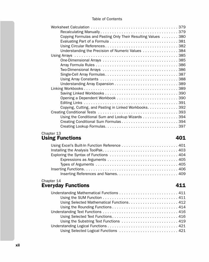
Table of Contents

xii

Worksheet Calculation . . . . . . . . . . . . . . . . . . . . . . . . . . . . . . . . . . . . . 379Recalculating Manually . . . . . . . . . . . . . . . . . . . . . . . . . . . . . . . . . 379Copying Formulas and Pasting Only Their Resulting Values . . . . . . . 380Evaluating Part of a Formula . . . . . . . . . . . . . . . . . . . . . . . . . . . . . 381Using Circular References. . . . . . . . . . . . . . . . . . . . . . . . . . . . . . . 382Understanding the Precision of Numeric Values . . . . . . . . . . . . . . . 384

Using Arrays . . . . . . . . . . . . . . . . . . . . . . . . . . . . . . . . . . . . . . . . . . . . 385One-Dimensional Arrays . . . . . . . . . . . . . . . . . . . . . . . . . . . . . . . . 385Array Formula Rules . . . . . . . . . . . . . . . . . . . . . . . . . . . . . . . . . . . 386Two-Dimensional Arrays . . . . . . . . . . . . . . . . . . . . . . . . . . . . . . . . 386Single-Cell Array Formulas. . . . . . . . . . . . . . . . . . . . . . . . . . . . . . . 387Using Array Constants . . . . . . . . . . . . . . . . . . . . . . . . . . . . . . . . . 388Understanding Array Expansion . . . . . . . . . . . . . . . . . . . . . . . . . . . 389

Linking Workbooks . . . . . . . . . . . . . . . . . . . . . . . . . . . . . . . . . . . . . . . . 389Saving Linked Workbooks . . . . . . . . . . . . . . . . . . . . . . . . . . . . . . . 390Opening a Dependent Workbook . . . . . . . . . . . . . . . . . . . . . . . . . . 390Editing Links . . . . . . . . . . . . . . . . . . . . . . . . . . . . . . . . . . . . . . . . 391Copying, Cutting, and Pasting in Linked Workbooks. . . . . . . . . . . . . 392

Creating Conditional Tests . . . . . . . . . . . . . . . . . . . . . . . . . . . . . . . . . . 393Using the Conditional Sum and Lookup Wizards . . . . . . . . . . . . . . . 394Creating Conditional Sum Formulas . . . . . . . . . . . . . . . . . . . . . . . . 394Creating Lookup Formulas. . . . . . . . . . . . . . . . . . . . . . . . . . . . . . . 397

Chapter 13Using Functions 401

Using Excel’s Built-In Function Reference . . . . . . . . . . . . . . . . . . . . . . . . 401Installing the Analysis ToolPak. . . . . . . . . . . . . . . . . . . . . . . . . . . . . . . . 403Exploring the Syntax of Functions . . . . . . . . . . . . . . . . . . . . . . . . . . . . . 404

Expressions as Arguments . . . . . . . . . . . . . . . . . . . . . . . . . . . . . . 405Types of Arguments . . . . . . . . . . . . . . . . . . . . . . . . . . . . . . . . . . . 405

Inserting Functions. . . . . . . . . . . . . . . . . . . . . . . . . . . . . . . . . . . . . . . . 406Inserting References and Names. . . . . . . . . . . . . . . . . . . . . . . . . . 409

Chapter 14Everyday Functions 411

Understanding Mathematical Functions . . . . . . . . . . . . . . . . . . . . . . . . . 411Using the SUM Function . . . . . . . . . . . . . . . . . . . . . . . . . . . . . . . . 411Using Selected Mathematical Functions. . . . . . . . . . . . . . . . . . . . . 412Using the Rounding Functions . . . . . . . . . . . . . . . . . . . . . . . . . . . . 414

Understanding Text Functions . . . . . . . . . . . . . . . . . . . . . . . . . . . . . . . . 416Using Selected Text Functions . . . . . . . . . . . . . . . . . . . . . . . . . . . . 416Using the Substring Text Functions . . . . . . . . . . . . . . . . . . . . . . . . 419

Understanding Logical Functions . . . . . . . . . . . . . . . . . . . . . . . . . . . . . . 421Using Selected Logical Functions . . . . . . . . . . . . . . . . . . . . . . . . . 421

xiii

Table of Contents

Understanding Information Functions. . . . . . . . . . . . . . . . . . . . . . . . . . . 424Using Selected Information Functions . . . . . . . . . . . . . . . . . . . . . . 424Using the IS Information Functions . . . . . . . . . . . . . . . . . . . . . . . . 425

Understanding Lookup and Reference Functions. . . . . . . . . . . . . . . . . . . 426Using Selected Lookup and Reference Functions . . . . . . . . . . . . . . 426

Chapter 15Formatting and Calculating Date and Time 435

Understanding How Excel Records Dates and Times . . . . . . . . . . . . . . . . 435Entering Dates and Times. . . . . . . . . . . . . . . . . . . . . . . . . . . . . . . . . . . 436

Entering a Series of Dates . . . . . . . . . . . . . . . . . . . . . . . . . . . . . . 437Formatting Dates and Times . . . . . . . . . . . . . . . . . . . . . . . . . . . . . . . . . 440

Creating Your Own Date and Time Formats . . . . . . . . . . . . . . . . . . . 441Calculating with Date and Time . . . . . . . . . . . . . . . . . . . . . . . . . . . . . . . 444Working with Date and Time Functions. . . . . . . . . . . . . . . . . . . . . . . . . . 445

Working with Specialized Date Functions . . . . . . . . . . . . . . . . . . . . 447

Chapter 16Functions for Financial Analysis 449

Calculating Investments . . . . . . . . . . . . . . . . . . . . . . . . . . . . . . . . . . . . 449The PV Function . . . . . . . . . . . . . . . . . . . . . . . . . . . . . . . . . . . . . . 450The NPV Function . . . . . . . . . . . . . . . . . . . . . . . . . . . . . . . . . . . . . 451The FV Function . . . . . . . . . . . . . . . . . . . . . . . . . . . . . . . . . . . . . . 451The PMT Function. . . . . . . . . . . . . . . . . . . . . . . . . . . . . . . . . . . . . 452The IPMT Function . . . . . . . . . . . . . . . . . . . . . . . . . . . . . . . . . . . . 453The PPMT Function. . . . . . . . . . . . . . . . . . . . . . . . . . . . . . . . . . . . 453The NPER Function . . . . . . . . . . . . . . . . . . . . . . . . . . . . . . . . . . . . 453The RATE Function . . . . . . . . . . . . . . . . . . . . . . . . . . . . . . . . . . . . 453The IRR Function . . . . . . . . . . . . . . . . . . . . . . . . . . . . . . . . . . . . . 454The MIRR Function . . . . . . . . . . . . . . . . . . . . . . . . . . . . . . . . . . . . 455

Calculating Depreciation . . . . . . . . . . . . . . . . . . . . . . . . . . . . . . . . . . . . 455The SLN Function . . . . . . . . . . . . . . . . . . . . . . . . . . . . . . . . . . . . . 455The DDB and DB Functions . . . . . . . . . . . . . . . . . . . . . . . . . . . . . . 456The VDB Function. . . . . . . . . . . . . . . . . . . . . . . . . . . . . . . . . . . . . 456The SYD Function. . . . . . . . . . . . . . . . . . . . . . . . . . . . . . . . . . . . . 457

Analyzing Securities . . . . . . . . . . . . . . . . . . . . . . . . . . . . . . . . . . . . . . . 457The DOLLARDE and DOLLARFR Functions. . . . . . . . . . . . . . . . . . . . 458The ACCRINT and ACCRINTM Functions . . . . . . . . . . . . . . . . . . . . . 459The INTRATE and RECEIVED Functions . . . . . . . . . . . . . . . . . . . . . . 459The PRICE, PRICEDISC, and PRICEMAT Functions . . . . . . . . . . . . . . 459The DISC Function . . . . . . . . . . . . . . . . . . . . . . . . . . . . . . . . . . . . 460The YIELD, YIELDDISC, and YIELDMAT Functions . . . . . . . . . . . . . . 460The TBILLEQ, TBILLPRICE, and TBILLYIELD Functions . . . . . . . . . . . 461The COUPDAYBS, COUPDAYS, COUPDAYSNC, COUPNCD,COUPNUM, and COUPPCD Functions . . . . . . . . . . . . . . . . . . . . . . . 461The DURATION and MDURATION Functions . . . . . . . . . . . . . . . . . . . 462

Table of Contents

xiv

Chapter 17Functions for Analyzing Statistics 463

Analyzing Distributions of Data . . . . . . . . . . . . . . . . . . . . . . . . . . . . . . . 464Using Built-In Statistical Functions. . . . . . . . . . . . . . . . . . . . . . . . . 464Using Functions That Analyze Rank and Percentile . . . . . . . . . . . . . 465Using Sample and Population Statistical Functions . . . . . . . . . . . . . 468

Understanding Linear and Exponential Regression . . . . . . . . . . . . . . . . . 469Calculating Linear Regression . . . . . . . . . . . . . . . . . . . . . . . . . . . . 470Calculating Exponential Regression . . . . . . . . . . . . . . . . . . . . . . . . 476

Using the Analysis Toolpak Data Analysis Tools . . . . . . . . . . . . . . . . . . . 477Using the Descriptive Statistics Tool . . . . . . . . . . . . . . . . . . . . . . . 477Creating Histograms. . . . . . . . . . . . . . . . . . . . . . . . . . . . . . . . . . . 479Using the Rank and Percentile Tool . . . . . . . . . . . . . . . . . . . . . . . . 482Generating Random Numbers . . . . . . . . . . . . . . . . . . . . . . . . . . . . 484Sampling a Population of Numbers . . . . . . . . . . . . . . . . . . . . . . . . 488Calculating Moving Averages . . . . . . . . . . . . . . . . . . . . . . . . . . . . . 489

Chapter 18Performing What-If Analysis 493

Using Data Tables . . . . . . . . . . . . . . . . . . . . . . . . . . . . . . . . . . . . . . . . 493Data Tables Based on One Input Variable. . . . . . . . . . . . . . . . . . . . 493Single-Variable Tables with More Than One Formula . . . . . . . . . . . . 495Data Tables Based on Two Input Variables . . . . . . . . . . . . . . . . . . . 495Editing Tables . . . . . . . . . . . . . . . . . . . . . . . . . . . . . . . . . . . . . . . 497

Using the Scenario Manager . . . . . . . . . . . . . . . . . . . . . . . . . . . . . . . . . 498Defining Scenarios . . . . . . . . . . . . . . . . . . . . . . . . . . . . . . . . . . . . 499Browsing Your Scenarios. . . . . . . . . . . . . . . . . . . . . . . . . . . . . . . . 501Adding, Editing, and Deleting Scenarios . . . . . . . . . . . . . . . . . . . . . 501Routing and Merging Scenarios . . . . . . . . . . . . . . . . . . . . . . . . . . . 502Creating Scenario Reports . . . . . . . . . . . . . . . . . . . . . . . . . . . . . . 504

Using the Goal Seek Command . . . . . . . . . . . . . . . . . . . . . . . . . . . . . . . 507Precision and Multiple Solutions . . . . . . . . . . . . . . . . . . . . . . . . . . 509

Using the Solver. . . . . . . . . . . . . . . . . . . . . . . . . . . . . . . . . . . . . . . . . . 509Stating the Objective . . . . . . . . . . . . . . . . . . . . . . . . . . . . . . . . . . 511Specifying Variable Cells . . . . . . . . . . . . . . . . . . . . . . . . . . . . . . . . 512Specifying Constraints . . . . . . . . . . . . . . . . . . . . . . . . . . . . . . . . . 512Saving and Reusing the Solver Parameters. . . . . . . . . . . . . . . . . . . 514Assigning the Solver Results to Named Scenarios . . . . . . . . . . . . . 515Other Solver Options . . . . . . . . . . . . . . . . . . . . . . . . . . . . . . . . . . 515Generating Reports . . . . . . . . . . . . . . . . . . . . . . . . . . . . . . . . . . . 517

xv

Table of Contents

Part 6Collaboration and the Internet

Chapter 19Collaborating with Excel 521

Saving and Retrieving Files on Remote Computers . . . . . . . . . . . . . . . . . 521Sharing Workbooks on a Network . . . . . . . . . . . . . . . . . . . . . . . . . . . . . 522

Using Advanced Sharing Options . . . . . . . . . . . . . . . . . . . . . . . . . . 525Tracking Changes . . . . . . . . . . . . . . . . . . . . . . . . . . . . . . . . . . . . . 526Reviewing Changes . . . . . . . . . . . . . . . . . . . . . . . . . . . . . . . . . . . 529Canceling the Shared Workbook Session . . . . . . . . . . . . . . . . . . . . 530

Combining Changes Made to Multiple Workbooks . . . . . . . . . . . . . . . . . . 530Merging Workbooks . . . . . . . . . . . . . . . . . . . . . . . . . . . . . . . . . . . 531

Distributing Workbooks and Worksheets by E-Mail . . . . . . . . . . . . . . . . . 532Sending an Entire Workbook as an E-Mail Attachment . . . . . . . . . . . 533Sending the Current Sheet as the Body of an E-Mail Message . . . . . 533Sending a Workbook for Review. . . . . . . . . . . . . . . . . . . . . . . . . . . 535Routing Workbooks to a Workgroup . . . . . . . . . . . . . . . . . . . . . . . . 536

Controlling Document Access with Information Rights Management . . . . . 538Protecting a Document with IRM . . . . . . . . . . . . . . . . . . . . . . . . . . 538Using a Protected Document . . . . . . . . . . . . . . . . . . . . . . . . . . . . . 541

Using a SharePoint Team Services Site . . . . . . . . . . . . . . . . . . . . . . . . . 541Downloading and Uploading Documents. . . . . . . . . . . . . . . . . . . . . 542Checking Documents In and Out . . . . . . . . . . . . . . . . . . . . . . . . . . 544Using the Shared Workspace Task Pane. . . . . . . . . . . . . . . . . . . . . 544Creating a New Document Workspace . . . . . . . . . . . . . . . . . . . . . . 548

Using Web Discussions . . . . . . . . . . . . . . . . . . . . . . . . . . . . . . . . . . . . 550

Chapter 20Transferring Files to and from Internet Sites 553

Working with FTP Sites . . . . . . . . . . . . . . . . . . . . . . . . . . . . . . . . . . . . . 553Adding a Site to Your My Places Bar . . . . . . . . . . . . . . . . . . . . . . . 555

Saving and Publishing Excel Files in HTML . . . . . . . . . . . . . . . . . . . . . . . 556Considering the Options . . . . . . . . . . . . . . . . . . . . . . . . . . . . . . . . 556Saving an Entire Workbook Without Interactivity . . . . . . . . . . . . . . . 561Publishing Without Interactivity . . . . . . . . . . . . . . . . . . . . . . . . . . . 562Publishing with Interactivity . . . . . . . . . . . . . . . . . . . . . . . . . . . . . . 563

Using the Interactive Web Components . . . . . . . . . . . . . . . . . . . . . . . . . 563

Table of Contents

xvi

Part 7Integrating Excel with Other Applications

Chapter 21Linking and Embedding 569

Embedding vs. Linking . . . . . . . . . . . . . . . . . . . . . . . . . . . . . . . . . . . . . 569Embedding vs. Static Pasting . . . . . . . . . . . . . . . . . . . . . . . . . . . . . . . . 570Embedding and Linking from the Clipboard. . . . . . . . . . . . . . . . . . . . . . . 571Embedding and Linking with the Object Command . . . . . . . . . . . . . . . . . 574Manipulating Embedded Objects . . . . . . . . . . . . . . . . . . . . . . . . . . . . . . 576Managing Links . . . . . . . . . . . . . . . . . . . . . . . . . . . . . . . . . . . . . . . . . . 577

Choosing Automatic or Manual Update . . . . . . . . . . . . . . . . . . . . . 578Updating on File Open . . . . . . . . . . . . . . . . . . . . . . . . . . . . . . . . . 578Fixing Broken Links . . . . . . . . . . . . . . . . . . . . . . . . . . . . . . . . . . . 579

Linking vs. Hyperlinking . . . . . . . . . . . . . . . . . . . . . . . . . . . . . . . . . . . . 579

Chapter 22Using Hyperlinks 581

Creating a Hyperlink in a Cell . . . . . . . . . . . . . . . . . . . . . . . . . . . . . . . . 582Turning Ordinary Text into a Hyperlink. . . . . . . . . . . . . . . . . . . . . . . 583Linking to a Web Site or Local File . . . . . . . . . . . . . . . . . . . . . . . . . 583Linking to a Location in the Current Document . . . . . . . . . . . . . . . . 585Linking to a New File . . . . . . . . . . . . . . . . . . . . . . . . . . . . . . . . . . 585Linking to an E-Mail Message . . . . . . . . . . . . . . . . . . . . . . . . . . . . 586

Assigning a Hyperlink to a Graphic, Toolbar Button, or Menu Command . . 587Editing, Removing, and Deleting a Hyperlink . . . . . . . . . . . . . . . . . . 587Formatting a Hyperlink . . . . . . . . . . . . . . . . . . . . . . . . . . . . . . . . . 588

Using the HYPERLINK Function . . . . . . . . . . . . . . . . . . . . . . . . . . . . . . . 588

Chapter 23Using Excel Data in Word and PowerPoint Documents 589

Using Excel Tables in Word Documents . . . . . . . . . . . . . . . . . . . . . . . . . 589Pasting an Excel Table from the Clipboard . . . . . . . . . . . . . . . . . . . 589Using Paste Special to Control the Format of Your Table . . . . . . . . . 591Using the Object Command. . . . . . . . . . . . . . . . . . . . . . . . . . . . . . 597

Using Excel Charts in Word Documents . . . . . . . . . . . . . . . . . . . . . . . . . 598Using Excel to Supply Mail-Merge Data to Word . . . . . . . . . . . . . . . . . . . 600Using Excel Data in PowerPoint . . . . . . . . . . . . . . . . . . . . . . . . . . . . . . . 603

Paste-Linking Excel Data into PowerPoint . . . . . . . . . . . . . . . . . . . . 605Using Excel Charts in PowerPoint. . . . . . . . . . . . . . . . . . . . . . . . . . 605

xvii

Table of Contents

Part 8Creating Charts

Chapter 24Basic Charting Techniques 609

Creating a New Chart . . . . . . . . . . . . . . . . . . . . . . . . . . . . . . . . . . . . . . 609Step 1: Choosing a Chart Type . . . . . . . . . . . . . . . . . . . . . . . . . . . 610Step 2: Specifying the Data to Plot . . . . . . . . . . . . . . . . . . . . . . . . 611Step 3: Choosing Chart Options . . . . . . . . . . . . . . . . . . . . . . . . . . 613Step 4: Telling Excel Where to Put Your Chart . . . . . . . . . . . . . . . . . 618

Creating Combination (Overlay) Charts . . . . . . . . . . . . . . . . . . . . . . . . . . 618Changing a Chart’s Size and Position . . . . . . . . . . . . . . . . . . . . . . . . . . . 618Plotting Hidden Cells . . . . . . . . . . . . . . . . . . . . . . . . . . . . . . . . . . . . . . 619Handling Missing Values . . . . . . . . . . . . . . . . . . . . . . . . . . . . . . . . . . . . 619Changing the Default Chart Type . . . . . . . . . . . . . . . . . . . . . . . . . . . . . . 620Printing Charts . . . . . . . . . . . . . . . . . . . . . . . . . . . . . . . . . . . . . . . . . . . 620Saving, Opening, and Protecting Charts . . . . . . . . . . . . . . . . . . . . . . . . . 621Working with Embedded Chart Objects. . . . . . . . . . . . . . . . . . . . . . . . . . 621

Chapter 25Enhancing the Appearance of Your Charts 623

Working with the Chart Menu and Chart Toolbar . . . . . . . . . . . . . . . . . . . 623Selecting Chart Elements . . . . . . . . . . . . . . . . . . . . . . . . . . . . . . . . . . . 625Copying Formats from One Chart to Another . . . . . . . . . . . . . . . . . . . . . . 625Adding a Customized Chart to the Chart Wizard Gallery. . . . . . . . . . . . . . 625Repositioning Chart Elements with the Mouse . . . . . . . . . . . . . . . . . . . . 626Moving and Resizing the Plot Area . . . . . . . . . . . . . . . . . . . . . . . . . . . . . 626Working with Titles . . . . . . . . . . . . . . . . . . . . . . . . . . . . . . . . . . . . . . . . 627

Creating a Two-Line Title . . . . . . . . . . . . . . . . . . . . . . . . . . . . . . . . 627Formatting a Title . . . . . . . . . . . . . . . . . . . . . . . . . . . . . . . . . . . . . 627Formatting Individual Characters in a Title . . . . . . . . . . . . . . . . . . . 630

Adding Text Annotations . . . . . . . . . . . . . . . . . . . . . . . . . . . . . . . . . . . . 631Working with Data Labels . . . . . . . . . . . . . . . . . . . . . . . . . . . . . . . . . . . 631

Label Positioning and Alignment Options . . . . . . . . . . . . . . . . . . . . 631Numeric Formatting Options for Data Labels. . . . . . . . . . . . . . . . . . 633Font and Patterns Options for Data Labels . . . . . . . . . . . . . . . . . . . 633Editing Data Labels . . . . . . . . . . . . . . . . . . . . . . . . . . . . . . . . . . . 633Positioning and Formatting Data Labels Individually . . . . . . . . . . . . 634Generating Useful Data Labels on XY (Scatter) Charts. . . . . . . . . . . 634

Working with Axes . . . . . . . . . . . . . . . . . . . . . . . . . . . . . . . . . . . . . . . . 636Specifying the Line Style, Color, and Weight . . . . . . . . . . . . . . . . . . 637Specifying the Position of Tick Marks and Tick-Mark Labels . . . . . . . 637Changing the Numeric Format Used by Tick-Mark Labels . . . . . . . . . 638Scaling Axes Manually . . . . . . . . . . . . . . . . . . . . . . . . . . . . . . . . . 639

Adding, Removing, and Formatting Gridlines . . . . . . . . . . . . . . . . . . . . . . 646

Table of Contents

xviii

Formatting Data Series and Markers . . . . . . . . . . . . . . . . . . . . . . . . . . . 647Assigning a Series to a Secondary Value Axis. . . . . . . . . . . . . . . . . 647Using Two or More Chart Types in the Same Chart . . . . . . . . . . . . . 647Changing the Series Order . . . . . . . . . . . . . . . . . . . . . . . . . . . . . . 648Toggling the Column/Row Orientation . . . . . . . . . . . . . . . . . . . . . . 649Changing Colors, Patterns, Fills, and Borders for Markers . . . . . . . . 649Adjusting Spacing in Two-Dimensional Column and Bar Charts . . . . . 650Adjusting Data Point Spacing in Three-Dimensional Charts . . . . . . . 652Adding Series Lines in Stacked Column and Bar Charts . . . . . . . . . 653Changing Shapes in Three-Dimensional Column and Bar Charts. . . . 653Smoothing the Lines in Line and XY (Scatter) Charts. . . . . . . . . . . . 654Changing Line and Marker Styles in Line, XY (Scatter), and Radar Charts . . . . . . . . . . . . . . . . . . . . . . . . . . . . . . . . . . . . 654Adding High-Low Lines and Up and Down Bars to Line Charts . . . . . 654Adding Drop Lines to Area and Line Charts. . . . . . . . . . . . . . . . . . . 655Exploding Pie Slices and Doughnut Bites . . . . . . . . . . . . . . . . . . . . 655Using Formatting and Split Options in Pie-Columnand Pie-Pie Charts . . . . . . . . . . . . . . . . . . . . . . . . . . . . . . . . . . . . 656Changing the Angle of the First Pie Slice or Doughnut Bite. . . . . . . . 657

Working with Data Tables . . . . . . . . . . . . . . . . . . . . . . . . . . . . . . . . . . . 657Formatting Background Areas . . . . . . . . . . . . . . . . . . . . . . . . . . . . . . . . 658

Filling an Area with a Color Gradient . . . . . . . . . . . . . . . . . . . . . . . 658Filling an Area with a Pattern . . . . . . . . . . . . . . . . . . . . . . . . . . . . . 659Filling an Area with a Texture or Picture . . . . . . . . . . . . . . . . . . . . . 660

Changing Three-Dimensional Viewing Angles . . . . . . . . . . . . . . . . . . . . . 664Adjusting the Elevation . . . . . . . . . . . . . . . . . . . . . . . . . . . . . . . . . 664Changing the Rotation . . . . . . . . . . . . . . . . . . . . . . . . . . . . . . . . . 664Changing the Height . . . . . . . . . . . . . . . . . . . . . . . . . . . . . . . . . . . 665Changing the Perspective . . . . . . . . . . . . . . . . . . . . . . . . . . . . . . . 665Changing the Axis Angle and Scale . . . . . . . . . . . . . . . . . . . . . . . . 665

Chapter 26Working with Chart Data 667

Adding Data. . . . . . . . . . . . . . . . . . . . . . . . . . . . . . . . . . . . . . . . . . . . . 667Using Copy and Paste. . . . . . . . . . . . . . . . . . . . . . . . . . . . . . . . . . 668Adding Series . . . . . . . . . . . . . . . . . . . . . . . . . . . . . . . . . . . . . . . 669

Using List Features to Create Expanding Charts . . . . . . . . . . . . . . . . . . . 670Removing Data. . . . . . . . . . . . . . . . . . . . . . . . . . . . . . . . . . . . . . . . . . . 671Changing or Replacing Data . . . . . . . . . . . . . . . . . . . . . . . . . . . . . . . . . 671Plotting or Marking Every nth Point . . . . . . . . . . . . . . . . . . . . . . . . . . . . 672Changing the Plot Order . . . . . . . . . . . . . . . . . . . . . . . . . . . . . . . . . . . . 675Using Multilevel Categories . . . . . . . . . . . . . . . . . . . . . . . . . . . . . . . . . . 675Adding Trend Lines . . . . . . . . . . . . . . . . . . . . . . . . . . . . . . . . . . . . . . . . 678Adding Error Bars . . . . . . . . . . . . . . . . . . . . . . . . . . . . . . . . . . . . . . . . . 679What-If Charting: Dragging Markers to Change Data . . . . . . . . . . . . . . . . 679

xix

Table of Contents

Chapter 27Advanced Charting Techniques 683

Using Named Ranges to Create Dynamic Charts. . . . . . . . . . . . . . . . . . . 683Plotting New Data Automatically . . . . . . . . . . . . . . . . . . . . . . . . . . 685Plotting Only the Most Recent Points . . . . . . . . . . . . . . . . . . . . . . . 686

Using Arrays to Create a Static Chart. . . . . . . . . . . . . . . . . . . . . . . . . . . 687Using Bubble Charts. . . . . . . . . . . . . . . . . . . . . . . . . . . . . . . . . . . . . . . 687Using Radar Charts . . . . . . . . . . . . . . . . . . . . . . . . . . . . . . . . . . . . . . . 689Creating Gannt Charts . . . . . . . . . . . . . . . . . . . . . . . . . . . . . . . . . . . . . 692Assorted Formatting Issues . . . . . . . . . . . . . . . . . . . . . . . . . . . . . . . . . 693

Tick-Mark Labels Without Axes . . . . . . . . . . . . . . . . . . . . . . . . . . . 694Tick-Mark Labels on the Plot Area . . . . . . . . . . . . . . . . . . . . . . . . . 694Formatting Selected Gridlines or Tick-Mark Labels . . . . . . . . . . . . . 695Staggered Tick-Mark Labels . . . . . . . . . . . . . . . . . . . . . . . . . . . . . 695Plotting Your Own Projection (Extrapolation) Line. . . . . . . . . . . . . . . 696

Part 9Managing Databases and Lists

Chapter 28Managing Information in Lists 701

Building and Maintaining a List . . . . . . . . . . . . . . . . . . . . . . . . . . . . . . . 701Using Label-Based Formulas in Calculated Columns . . . . . . . . . . . . 703Using (or Disabling) Other List-Building Aids . . . . . . . . . . . . . . . . . . 705Custom Lists . . . . . . . . . . . . . . . . . . . . . . . . . . . . . . . . . . . . . . . . 707

Working with List Objects . . . . . . . . . . . . . . . . . . . . . . . . . . . . . . . . . . . 707Publishing a List Object . . . . . . . . . . . . . . . . . . . . . . . . . . . . . . . . 709Toggling the Total Row . . . . . . . . . . . . . . . . . . . . . . . . . . . . . . . . . 717Resizing a List Object . . . . . . . . . . . . . . . . . . . . . . . . . . . . . . . . . . 718Inserting and Deleting Rows and Columns within a List Object. . . . . 718

Validating Data Entry . . . . . . . . . . . . . . . . . . . . . . . . . . . . . . . . . . . . . . 719Specifying Data Type and Acceptable Values. . . . . . . . . . . . . . . . . . 720Specifying an Input Message (Prompt) . . . . . . . . . . . . . . . . . . . . . . 721Specifying Error Alert Style and Message . . . . . . . . . . . . . . . . . . . . 721

Using Excel’s Form Command to Work with Lists. . . . . . . . . . . . . . . . . . . 721Adding Rows . . . . . . . . . . . . . . . . . . . . . . . . . . . . . . . . . . . . . . . . 722Finding Records . . . . . . . . . . . . . . . . . . . . . . . . . . . . . . . . . . . . . . 722

Sorting Lists and Other Ranges. . . . . . . . . . . . . . . . . . . . . . . . . . . . . . . 723Sorting on a Single Column. . . . . . . . . . . . . . . . . . . . . . . . . . . . . . 723Sorting on More than One Column. . . . . . . . . . . . . . . . . . . . . . . . . 724Sorting Only Part of a List . . . . . . . . . . . . . . . . . . . . . . . . . . . . . . . 725Sorting by Columns . . . . . . . . . . . . . . . . . . . . . . . . . . . . . . . . . . . 726Sorting Cells That Contain Formulas . . . . . . . . . . . . . . . . . . . . . . . 727Sorting Months, Weekdays, or Custom Lists. . . . . . . . . . . . . . . . . . 728Performing a Case-Sensitive Sort . . . . . . . . . . . . . . . . . . . . . . . . . 729

Table of Contents

xx

Filtering a List . . . . . . . . . . . . . . . . . . . . . . . . . . . . . . . . . . . . . . . . . . . 730Using the AutoFilter Command . . . . . . . . . . . . . . . . . . . . . . . . . . . 730Using the Advanced Filter Command . . . . . . . . . . . . . . . . . . . . . . . 734

Using Subtotals to Analyze a List. . . . . . . . . . . . . . . . . . . . . . . . . . . . . . 742Subtotaling on More Than One Column . . . . . . . . . . . . . . . . . . . . . 745Subtotaling with More Than One Aggregation Formula . . . . . . . . . . . 745Using Automatic Page Breaks . . . . . . . . . . . . . . . . . . . . . . . . . . . . 745Removing or Replacing Subtotals . . . . . . . . . . . . . . . . . . . . . . . . . 746Grouping by Date . . . . . . . . . . . . . . . . . . . . . . . . . . . . . . . . . . . . . 746Using the SUBTOTAL Function . . . . . . . . . . . . . . . . . . . . . . . . . . . . 746

Using Functions to Extract Details from a List. . . . . . . . . . . . . . . . . . . . . 747The Database Statistical Functions . . . . . . . . . . . . . . . . . . . . . . . . 747COUNTIF and SUMIF . . . . . . . . . . . . . . . . . . . . . . . . . . . . . . . . . . . 749COUNTBLANK . . . . . . . . . . . . . . . . . . . . . . . . . . . . . . . . . . . . . . . 750VLOOKUP and HLOOKUP. . . . . . . . . . . . . . . . . . . . . . . . . . . . . . . . 750MATCH and INDEX . . . . . . . . . . . . . . . . . . . . . . . . . . . . . . . . . . . . 752

Chapter 29Working with External Data 757

Using File, Open to Import External Data Files . . . . . . . . . . . . . . . . . . . . 757Opening Text Files . . . . . . . . . . . . . . . . . . . . . . . . . . . . . . . . . . . . 757Opening Microsoft Access Tables in Excel . . . . . . . . . . . . . . . . . . . 761Opening dBase Files. . . . . . . . . . . . . . . . . . . . . . . . . . . . . . . . . . . 762

Working with XML Files . . . . . . . . . . . . . . . . . . . . . . . . . . . . . . . . . . . . . 762Opening or Importing an XML List . . . . . . . . . . . . . . . . . . . . . . . . . 763Exporting an XML List . . . . . . . . . . . . . . . . . . . . . . . . . . . . . . . . . . 767

Using a Query to Retrieve External Data. . . . . . . . . . . . . . . . . . . . . . . . . 767Reusing an Existing Query. . . . . . . . . . . . . . . . . . . . . . . . . . . . . . . 767Creating a New Database Query . . . . . . . . . . . . . . . . . . . . . . . . . . 769Working Directly with Microsoft Query . . . . . . . . . . . . . . . . . . . . . . 779

Using a Web Query to Return Internet Data . . . . . . . . . . . . . . . . . . . . . . 791Using an Existing Web Query . . . . . . . . . . . . . . . . . . . . . . . . . . . . . 792Creating Your Own Web Query . . . . . . . . . . . . . . . . . . . . . . . . . . . . 793

Chapter 30Analyzing Data with PivotTable Reports 797

A Simple Example . . . . . . . . . . . . . . . . . . . . . . . . . . . . . . . . . . . . . . . . 797Creating a PivotTable . . . . . . . . . . . . . . . . . . . . . . . . . . . . . . . . . . . . . . 800

Starting the PivotTable And PivotChart Wizard. . . . . . . . . . . . . . . . . 800Step 1: Specifying the Type of Data Source . . . . . . . . . . . . . . . . . . 801Step 2: Indicating the Location of Your Source Data . . . . . . . . . . . . 801Step 3: Telling the Wizard Where to Put Your PivotTable . . . . . . . . . . 802Laying Out the PivotTable . . . . . . . . . . . . . . . . . . . . . . . . . . . . . . . 803

Pivoting a PivotTable . . . . . . . . . . . . . . . . . . . . . . . . . . . . . . . . . . . . . . . 804Using the Page Axis . . . . . . . . . . . . . . . . . . . . . . . . . . . . . . . . . . . 805

xxi

Table of Contents

Displaying Totals for a Field in the Page Area . . . . . . . . . . . . . . . . . 805Moving Page Fields to Separate Workbook Pages . . . . . . . . . . . . . . 806Selecting Items to Display on the Row and Column Axes . . . . . . . . . 806

Creating a PivotChart . . . . . . . . . . . . . . . . . . . . . . . . . . . . . . . . . . . . . . 806Refreshing a PivotTable. . . . . . . . . . . . . . . . . . . . . . . . . . . . . . . . . . . . . 808

Refreshing on File Open . . . . . . . . . . . . . . . . . . . . . . . . . . . . . . . . 808Selecting Elements of a PivotTable . . . . . . . . . . . . . . . . . . . . . . . . . . . . 808Formatting a PivotTable. . . . . . . . . . . . . . . . . . . . . . . . . . . . . . . . . . . . . 809

Using AutoFormat with PivotTables. . . . . . . . . . . . . . . . . . . . . . . . . 809Changing the Numeric Format for the Data Area . . . . . . . . . . . . . . . 809Changing the Way a PivotTable Displays Empty Cells . . . . . . . . . . . . 809Changing the Way a PivotTable Displays Error Values. . . . . . . . . . . . 810Merging Labels . . . . . . . . . . . . . . . . . . . . . . . . . . . . . . . . . . . . . . 810

Using Multiple Data Fields . . . . . . . . . . . . . . . . . . . . . . . . . . . . . . . . . . 811Renaming Fields and Items. . . . . . . . . . . . . . . . . . . . . . . . . . . . . . . . . . 812Sorting Items. . . . . . . . . . . . . . . . . . . . . . . . . . . . . . . . . . . . . . . . . . . . 812

Using AutoSort. . . . . . . . . . . . . . . . . . . . . . . . . . . . . . . . . . . . . . . 812Rearranging Items by Hand . . . . . . . . . . . . . . . . . . . . . . . . . . . . . . 813

Showing the Top or Bottom Items in a Field . . . . . . . . . . . . . . . . . . . . . . 814Hiding and Showing Inner Field Items . . . . . . . . . . . . . . . . . . . . . . . . . . 814Displaying the Details Behind a Data Value . . . . . . . . . . . . . . . . . . . . . . 815Grouping and Ungrouping Data . . . . . . . . . . . . . . . . . . . . . . . . . . . . . . . 816

Creating Ad Hoc Item Groupings . . . . . . . . . . . . . . . . . . . . . . . . . . 816Grouping Numeric Items . . . . . . . . . . . . . . . . . . . . . . . . . . . . . . . . 817Grouping Items in Date or Time Ranges . . . . . . . . . . . . . . . . . . . . . 818Removing Groups (Ungrouping) . . . . . . . . . . . . . . . . . . . . . . . . . . . 819

Using Grand Totals and Subtotals . . . . . . . . . . . . . . . . . . . . . . . . . . . . . 819Grand Totals . . . . . . . . . . . . . . . . . . . . . . . . . . . . . . . . . . . . . . . . 819Subtotals. . . . . . . . . . . . . . . . . . . . . . . . . . . . . . . . . . . . . . . . . . . 820Subtotals for Innermost Fields . . . . . . . . . . . . . . . . . . . . . . . . . . . 821

Changing a PivotTable’s Calculations . . . . . . . . . . . . . . . . . . . . . . . . . . . 821Using a Different Summary Function . . . . . . . . . . . . . . . . . . . . . . . 821Applying Multiple Summary Functions to the Same Field . . . . . . . . . 822Using Custom Calculations . . . . . . . . . . . . . . . . . . . . . . . . . . . . . . 822Using Calculated Fields and Items. . . . . . . . . . . . . . . . . . . . . . . . . 824

Referencing PivotTable Data from Worksheet Cells . . . . . . . . . . . . . . . . . 827Creating a PivotTable from External Data . . . . . . . . . . . . . . . . . . . . . . . . 827

Refreshing PivotTable Data from an External Source . . . . . . . . . . . . 829Using a PivotTable to Consolidate Ranges . . . . . . . . . . . . . . . . . . . . . . . 830Building a PivotTable from an Existing PivotTable. . . . . . . . . . . . . . . . . . . 835Printing PivotTables . . . . . . . . . . . . . . . . . . . . . . . . . . . . . . . . . . . . . . . 835

Using Row and Column Headings as Print Titles . . . . . . . . . . . . . . . 835Repeating Item Labels on Each Printed Page . . . . . . . . . . . . . . . . . 835Printing Each Outer Row Field Item on a New Page . . . . . . . . . . . . . 836

Using the PivotTable Web Component . . . . . . . . . . . . . . . . . . . . . . . . . . 836

Table of Contents

xxii

Part 10Automating Excel

Chapter 31Recording Macros 841

Using the Macro Recorder. . . . . . . . . . . . . . . . . . . . . . . . . . . . . . . . . . . 841Running a Macro Without Using a Keyboard Shortcut . . . . . . . . . . . 843

Behind the Scenes: The VBA Environment . . . . . . . . . . . . . . . . . . . . . . . 843Getting Help on VBA Keywords . . . . . . . . . . . . . . . . . . . . . . . . . . . 844Objects, Methods, and Properties . . . . . . . . . . . . . . . . . . . . . . . . . 845Manipulating an Object’s Properties Without Selecting the Object . . 849Naming Arguments to Methods . . . . . . . . . . . . . . . . . . . . . . . . . . . 850

Adding Code to an Existing Macro . . . . . . . . . . . . . . . . . . . . . . . . . . . . . 850Using Absolute and Relative References . . . . . . . . . . . . . . . . . . . . . . . . 853Macro Subroutines . . . . . . . . . . . . . . . . . . . . . . . . . . . . . . . . . . . . . . . . 855Using the Personal Macro Workbook . . . . . . . . . . . . . . . . . . . . . . . . . . . 856Going On from Here . . . . . . . . . . . . . . . . . . . . . . . . . . . . . . . . . . . . . . . 857

Chapter 32Creating Custom Functions 859

Using Custom Functions . . . . . . . . . . . . . . . . . . . . . . . . . . . . . . . . . . . . 861What’s Happening . . . . . . . . . . . . . . . . . . . . . . . . . . . . . . . . . . . . 862

Understanding Custom Function Rules. . . . . . . . . . . . . . . . . . . . . . . . . . 863Using VBA Keywords in Custom Functions . . . . . . . . . . . . . . . . . . . . . . . 863Documenting Macros and Custom Functions . . . . . . . . . . . . . . . . . . . . . 864Creating Custom Functions with Optional Arguments. . . . . . . . . . . . . . . . 865Making Your Custom Functions Available Anywhere . . . . . . . . . . . . . . . . . 867

Chapter 33Debugging Macros and Custom Functions 869

Using Design-Time Tools . . . . . . . . . . . . . . . . . . . . . . . . . . . . . . . . . . . . 869Catching Syntax Errors . . . . . . . . . . . . . . . . . . . . . . . . . . . . . . . . . 870Catching Misspelled Variable Names . . . . . . . . . . . . . . . . . . . . . . . 871Stepping Through Code. . . . . . . . . . . . . . . . . . . . . . . . . . . . . . . . . 872Setting Breakpoints with the Toggle Breakpoint Command. . . . . . . . 873Setting Conditional Breakpoints Using Debug.Assert. . . . . . . . . . . . 873Using the Watch Window to Monitor Variable Values and Object Properties . . . . . . . . . . . . . . . . . . . . . . . . . . . . . . . . . . 874Using the Immediate Window . . . . . . . . . . . . . . . . . . . . . . . . . . . . 875

Dealing with Run-Time Errors. . . . . . . . . . . . . . . . . . . . . . . . . . . . . . . . . 876

xxiii

Table of Contents

Part 11Appendixes

Appendix AInstalling Microsoft Excel 883

System Requirements . . . . . . . . . . . . . . . . . . . . . . . . . . . . . . . . . . . . . 883Additional Requirements and Recommendations . . . . . . . . . . . . . . 884

Installing Office . . . . . . . . . . . . . . . . . . . . . . . . . . . . . . . . . . . . . . . . . . 884Uninstalling Office . . . . . . . . . . . . . . . . . . . . . . . . . . . . . . . . . . . . . . . . 885Installing Additional Components. . . . . . . . . . . . . . . . . . . . . . . . . . . . . . 885

Installing International Features . . . . . . . . . . . . . . . . . . . . . . . . . . 886Using the On-Screen Keyboard . . . . . . . . . . . . . . . . . . . . . . . . . . . 886

Repairing Your Office Installation . . . . . . . . . . . . . . . . . . . . . . . . . . . . . . 887

Appendix BUsing Speech and Handwriting Recognition 889

Using the Language Bar . . . . . . . . . . . . . . . . . . . . . . . . . . . . . . . . . . . . 889Controlling the Language Bar . . . . . . . . . . . . . . . . . . . . . . . . . . . . 893

Using Speech Recognition . . . . . . . . . . . . . . . . . . . . . . . . . . . . . . . . . . 895Training Your Computer and Your Voice. . . . . . . . . . . . . . . . . . . . . . 895Issuing Verbal Commands. . . . . . . . . . . . . . . . . . . . . . . . . . . . . . . 896Using Your Voice to Input Text . . . . . . . . . . . . . . . . . . . . . . . . . . . . 896

Using Handwriting Recognition . . . . . . . . . . . . . . . . . . . . . . . . . . . . . . . 899

Appendix CKeyboard Shortcuts 903

Charts and Select Chart Elements. . . . . . . . . . . . . . . . . . . . . . . . . 904Data Forms . . . . . . . . . . . . . . . . . . . . . . . . . . . . . . . . . . . . . . . . . 904Dialog Box Edit Boxes. . . . . . . . . . . . . . . . . . . . . . . . . . . . . . . . . . 905Dialog Boxes . . . . . . . . . . . . . . . . . . . . . . . . . . . . . . . . . . . . . . . . 905Edit Data . . . . . . . . . . . . . . . . . . . . . . . . . . . . . . . . . . . . . . . . . . . 906Enter and Calculate Formulas . . . . . . . . . . . . . . . . . . . . . . . . . . . . 906Enter Data . . . . . . . . . . . . . . . . . . . . . . . . . . . . . . . . . . . . . . . . . . 907Enter Special Characters . . . . . . . . . . . . . . . . . . . . . . . . . . . . . . . 908Extend a Selection . . . . . . . . . . . . . . . . . . . . . . . . . . . . . . . . . . . . 908Filter Lists . . . . . . . . . . . . . . . . . . . . . . . . . . . . . . . . . . . . . . . . . . 909Format, Cells Dialog Box—Border Tab . . . . . . . . . . . . . . . . . . . . . . 909Format Data. . . . . . . . . . . . . . . . . . . . . . . . . . . . . . . . . . . . . . . . . 910Help . . . . . . . . . . . . . . . . . . . . . . . . . . . . . . . . . . . . . . . . . . . . . . 911Help Window . . . . . . . . . . . . . . . . . . . . . . . . . . . . . . . . . . . . . . . . 911Insert, Delete, and Copy Cells . . . . . . . . . . . . . . . . . . . . . . . . . . . . 912Languages. . . . . . . . . . . . . . . . . . . . . . . . . . . . . . . . . . . . . . . . . . 912Macros . . . . . . . . . . . . . . . . . . . . . . . . . . . . . . . . . . . . . . . . . . . . 912Menus and Toolbars . . . . . . . . . . . . . . . . . . . . . . . . . . . . . . . . . . . 912Move and Scroll—In End Mode . . . . . . . . . . . . . . . . . . . . . . . . . . . 913

Table of Contents

xxiv

Move and Scroll—Scroll Lock Activated . . . . . . . . . . . . . . . . . . . . . 913Move and Scroll—Worksheets. . . . . . . . . . . . . . . . . . . . . . . . . . . . 914Move Within a Selected Range . . . . . . . . . . . . . . . . . . . . . . . . . . . 914Open, Save As, and Insert Picture Dialog Boxes . . . . . . . . . . . . . . . 915PivotTable and PivotChart Wizard Layout Dialog Box . . . . . . . . . . . . 915PivotTable—Display and Hide Items . . . . . . . . . . . . . . . . . . . . . . . . 916PivotTable—Change the Layout . . . . . . . . . . . . . . . . . . . . . . . . . . . 916Print . . . . . . . . . . . . . . . . . . . . . . . . . . . . . . . . . . . . . . . . . . . . . . 916Print Preview . . . . . . . . . . . . . . . . . . . . . . . . . . . . . . . . . . . . . . . . 916Select Cells, Rows, Columns, and Objects . . . . . . . . . . . . . . . . . . . 917Select Cells with Special Characteristics . . . . . . . . . . . . . . . . . . . . 917Send E-Mail Messages . . . . . . . . . . . . . . . . . . . . . . . . . . . . . . . . . 918Show, Hide, and Outline Data . . . . . . . . . . . . . . . . . . . . . . . . . . . . 918Smart Tags . . . . . . . . . . . . . . . . . . . . . . . . . . . . . . . . . . . . . . . . . 919Speech Recognition and Text-To-Speech . . . . . . . . . . . . . . . . . . . . . 919Task Panes . . . . . . . . . . . . . . . . . . . . . . . . . . . . . . . . . . . . . . . . . 919Windows and Office Interface . . . . . . . . . . . . . . . . . . . . . . . . . . . . 920Worksheets . . . . . . . . . . . . . . . . . . . . . . . . . . . . . . . . . . . . . . . . . 920

Appendix DFunction Reference 921

Index of Troubleshooting Topics . . . . . . . . . . . . . . . . . . . . . . . . . . . . . . . . . . 969

Index . . . . . . . . . . . . . . . . . . . . . . . . . . . . . . . . . . . . . . . . . . . . . . . . . . . . . 971

xxv

Acknowledgments

Software books are not products of inspiration, but of perspiration. However, the work done by the authors is just the tip of the iceberg. Producing books like this requires a sort of “alter-nate sanity” on the part of all involved a combination of childlike curiosity, skepticism, stubbornness, and anger management skills for dealing with the idiosyncrasies of unfinished software and unruly authors. Our hats are off to Sandra Haynes, Kristen Weatherby, Bill Teel, Alex Blanton, Beth Fuller, Stephanie English, Jan Cocker, J.J. Andrews, Don Lesser, Mannie White, and Brenda Silva and the rest of nSight’s desktop team. Thanks to all for doing a great job. Musical thanks to guitar maestro Gary Moore for keeping the bar set higher than most other blues-rock mortals could possibly hope to leap.

Craig Stinson and Mark Dodge

xxvii

We’d Like to Hear from You!

Our goal at Microsoft Press is to create books that help you find the information you need to get the most out of your software.

The INSIDE OUT series was created with you in mind. As part of our ongoing effort to ensure that we’re creating books that meet your learning needs, we’d like to hear from you. Let us know what you think. Tell us what you like about this book and what we can do to make it better. When you write, please include the title and author of this book in your e-mail, as well as your name and contact information. We look forward to hearing from you!

How to Reach Us

E-mail: nsideout@microsoft.comMail: Inside Out Series Editor

Microsoft PressOne Microsoft WayRedmond, WA 98052

Note: Unfortunately, we can’t provide support for any software problems you might experience. Please go to http://support.microsoft.com for help with any software issues.

xxix

About the CD

The companion CD that ships with this book contains many tools and resources to help you get the most out of your Inside Out book.

What’s On the CDYour INSIDE OUT CD includes the following:

● Complete eBook. In this section you’ll find the electronic version of Microsoft Office Excel 2003 Inside Out. The eBook is in PDF format.

● Insider Extras. This section includes sample files referenced in the book. Copy these files to your hard disk and use them to follow along with the books examples or as a starting point for your own work.

● Microsoft Tools and Information. In this section you’ll resources, demos, and tools for the following applications: Excel, InfoPath, OneNote, and Publisher.

● Extending Excel. In this section you’ll find great information about third-party utili-ties and tools you use to further enhance your experience with Excel. A copy of a pro-gram named Spreadsheet Assistant is also included in this section. Details about how you might use this application are included in relevant sections of the book.

● Microsoft Computer Dictionary, Fifth Edition, eBook. Here you’ll find the full elec-tronic version of the Microsoft Computer Dictionary, Fifth Edition.

The companion CD provides detailed information about the files on this CD, and links to Microsoft and third-party sites on the Internet.

Note Please note that the links to third-party sites are not under the control of Microsoft Corporation and Microsoft is therefore not responsible for their content, nor should their inclusion on this CD be construed as an endorsement of the product or the site.

Using the CDTo use this companion CD, insert it into your CD-ROM drive. If AutoRun is not enabled on your computer, run the StartCD.exe in the root of the CD.

a08a61511x.fm Page xxix Friday, August 1, 2003 1:17 PM

About the CD

xxx

System RequirementsFollowing are the minimum system requirements necessary to run the CD:

● Microsoft Windows XP or later or Windows 2000 Professional with Service Pack 3or later

● 266-MHz or higher Pentium-compatible CPU

● 64 megabytes (MB) RAM

● 8X CD-ROM drive or faster

● Microsoft Windows–compatible sound card and speakers

● Microsoft Internet Explorer 5.01 or higher

● Microsoft Mouse or compatible pointing device

Note Individual add-in system requirements are specified on the CD. An Internet connec-tion is necessary to access the some of the hyperlinks. Connect time charges may apply.

Support InformationEvery effort has been made to ensure the accuracy of the book and the contents of this com-panion CD. For feedback on the book content or this companion CD, please contact us by using any of the addresses listed in the “We’d Like to Hear From You” section.

Microsoft Press provides corrections for books through the World Wide Web at http://www.microsoft.com/mspress/support/. To connect directly to the Microsoft Press Knowledge Base and enter a query regarding a question or issue that you may have, go to http://www.microsoft.com/mspress/support/search.htm.

For support information regarding Windows XP, you can connect to Microsoft Technical Support on the Web at http://support.microsoft.com/.

a08a61511x.fm Page xxx Friday, August 1, 2003 1:17 PM

xxxi

Conventions and FeaturesUsed in this Book

This book uses special text and design conventions to make it easier for you to find the infor-mation you need.

Text Conventions

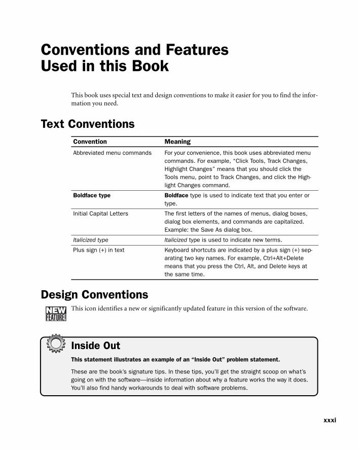
Design ConventionsThis icon identifies a new or significantly updated feature in this version of the software.

Inside OutThis statement illustrates an example of an “Inside Out” problem statement.

These are the book’s signature tips. In these tips, you’ll get the straight scoop on what’s going on with the software—inside information about why a feature works the way it does. You’ll also find handy workarounds to deal with software problems.

Convention Meaning

Abbreviated menu commands For your convenience, this book uses abbreviated menu commands. For example, “Click Tools, Track Changes, Highlight Changes” means that you should click the Tools menu, point to Track Changes, and click the High-light Changes command.

Boldface type Boldface type is used to indicate text that you enter or type.

Initial Capital Letters The first letters of the names of menus, dialog boxes, dialog box elements, and commands are capitalized. Example: the Save As dialog box.

Italicized type Italicized type is used to indicate new terms.

Plus sign (+) in text Keyboard shortcuts are indicated by a plus sign (+) sep-arating two key names. For example, Ctrl+Alt+Delete means that you press the Ctrl, Alt, and Delete keys at the same time.

xxxi

Front Matter Title

xxxii

Tip Tips provide helpful hints, timesaving tricks, or alternative procedures related to the task being discussed.

TroubleshootingThis statement illustrates an example of a “Troubleshooting” problem statement.

Look for these sidebars to find solutions to common problems you might encounter. Trou-bleshooting sidebars appear next to related information in the chapters. You can also use the Troubleshooting Topics index at the back of the book to look up problems by topic.

Cross-references point you to other locations in the book that offer additional information about the topic being discussed.

This icon indicates information or text found on the companion CD.

Caution Cautions identify potential problems that you should look out for when you’re completing a task or problems that you must address before you can complete a task.

Note Notes offer additional information related to the task being discussed.

SidebarsThe sidebars sprinkled throughout these chapters provide ancillary information on the topic being discussed. Go to sidebars to learn more about the technology or a feature.

Conventions and Features Used in this Book

xxxii

1

Part 1

Examining the Excel Environment

1 What’s New in Microsoft Office Excel 2003 3

2 Excel Fundamentals 13

3 Custom-Tailoring the Excel Workspace 65

3

Part 1: Examining the Excel Environment

Chapter 1

What’s New in MicrosoftOffice Excel 2003

New and Improved for 2003. . . . . . . . . . . .3If You Missed the Last Upgrade . . . . . . . . .8

Onward . . . . . . . . . . . . . . . . . . . . . . . . . . . 11

Sometimes new versions of software just don’t seem compelling enough for you to take the upgrade plunge. You wonder how many more big leaps can really be made in usability and functionality. Microsoft Excel has certainly evolved into a “mature” program. This release is more than just cosmetic, however; many of the new features are “under the hood,” and might not be apparent to the typical user. Foremost of the apparent enhancements: the new look of Microsoft Office that is, as Microsoft describes it, “more open and energetic.” In addition, new and improved task panes are available, including Help, Shared Workspace, and Research. And Tablet PC support now allows you to provide input directly into Office documents using a Tablet PC.

Microsoft Office Excel 2003 includes a few improvements to existing features and a few major new features that facilitate easier and more secure sharing of documents, efficient communi-cation and collaboration with others, more comprehensive and up-to-date online assistance, and enhanced programmability and extensibility. Here’s an overview of the new features you’ll find in Microsoft Office Excel 2003 and Microsoft Office 2003 Edition.

New and Improved for 2003First, we’ll highlight the new features in the 2003 release of Microsoft Office and Microsoft Excel, and later, we’ll summarize the features that are as good as new to you if you skipped the last upgrade.

Online AssistanceThe Microsoft Office help system is always changing, and this release is no exception. Web-based assistance is now a priority, with new commands such as Contact Us and Check For Updates offering direct connections to the Microsoft mother ship. Online help now automat-ically looks for additional help topics available from the Microsoft Web site, as shown in Fig-ure 1-1, making the Help system more complete and accurate than ever before. Online/offline integration is seamless—all you have to do is connect to the Internet and the Help sys-tem automatically avails itself of available online content.

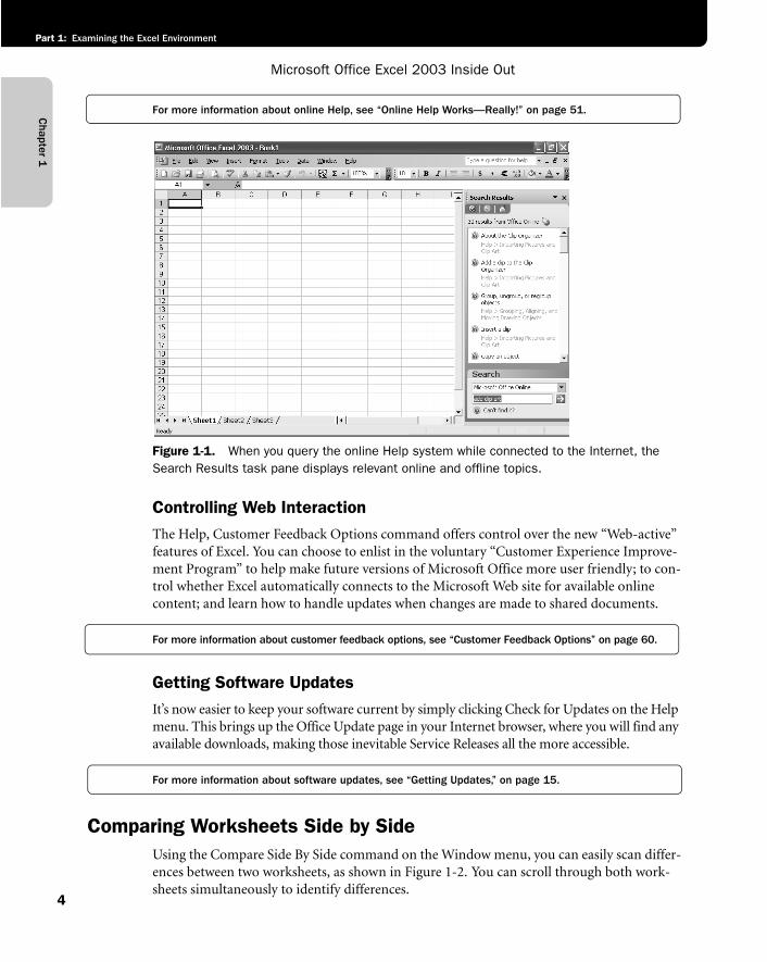
Chapter 1

Microsoft Office Excel 2003 Inside Out

Part 1: Examining the Excel Environment

4

For more information about online Help, see “Online Help Works—Really!” on page 51.

f01ie01

Figure 1-1. When you query the online Help system while connected to the Internet, the Search Results task pane displays relevant online and offline topics.

Controlling Web InteractionThe Help, Customer Feedback Options command offers control over the new “Web-active” features of Excel. You can choose to enlist in the voluntary “Customer Experience Improve-ment Program” to help make future versions of Microsoft Office more user friendly; to con-trol whether Excel automatically connects to the Microsoft Web site for available online content; and learn how to handle updates when changes are made to shared documents.

For more information about customer feedback options, see “Customer Feedback Options” on page 60.

Getting Software UpdatesIt’s now easier to keep your software current by simply clicking Check for Updates on the Help menu. This brings up the Office Update page in your Internet browser, where you will find any available downloads, making those inevitable Service Releases all the more accessible.

For more information about software updates, see “Getting Updates,” on page 15.

Comparing Worksheets Side by SideUsing the Compare Side By Side command on the Window menu, you can easily scan differ-ences between two worksheets, as shown in Figure 1-2. You can scroll through both work-sheets simultaneously to identify differences.

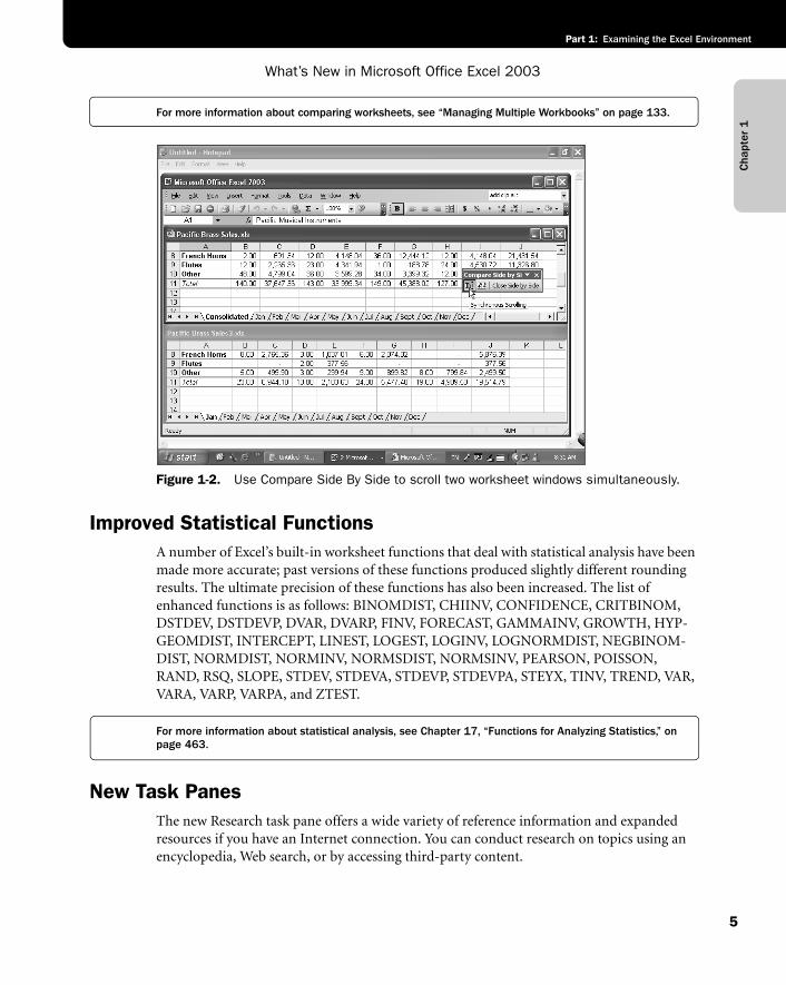
Cha

pter

1

What’s New in Microsoft Office Excel 2003

5

Part 1: Examining the Excel Environment

For more information about comparing worksheets, see “Managing Multiple Workbooks” on page 133.

f01ie02

Figure 1-2. Use Compare Side By Side to scroll two worksheet windows simultaneously.

Improved Statistical FunctionsA number of Excel’s built-in worksheet functions that deal with statistical analysis have been made more accurate; past versions of these functions produced slightly different rounding results. The ultimate precision of these functions has also been increased. The list of enhanced functions is as follows: BINOMDIST, CHIINV, CONFIDENCE, CRITBINOM, DSTDEV, DSTDEVP, DVAR, DVARP, FINV, FORECAST, GAMMAINV, GROWTH, HYP-GEOMDIST, INTERCEPT, LINEST, LOGEST, LOGINV, LOGNORMDIST, NEGBINOM-DIST, NORMDIST, NORMINV, NORMSDIST, NORMSINV, PEARSON, POISSON, RAND, RSQ, SLOPE, STDEV, STDEVA, STDEVP, STDEVPA, STEYX, TINV, TREND, VAR, VARA, VARP, VARPA, and ZTEST.

For more information about statistical analysis, see Chapter 17, “Functions for Analyzing Statistics,” on page 463.

New Task PanesThe new Research task pane offers a wide variety of reference information and expanded resources if you have an Internet connection. You can conduct research on topics using an encyclopedia, Web search, or by accessing third-party content.

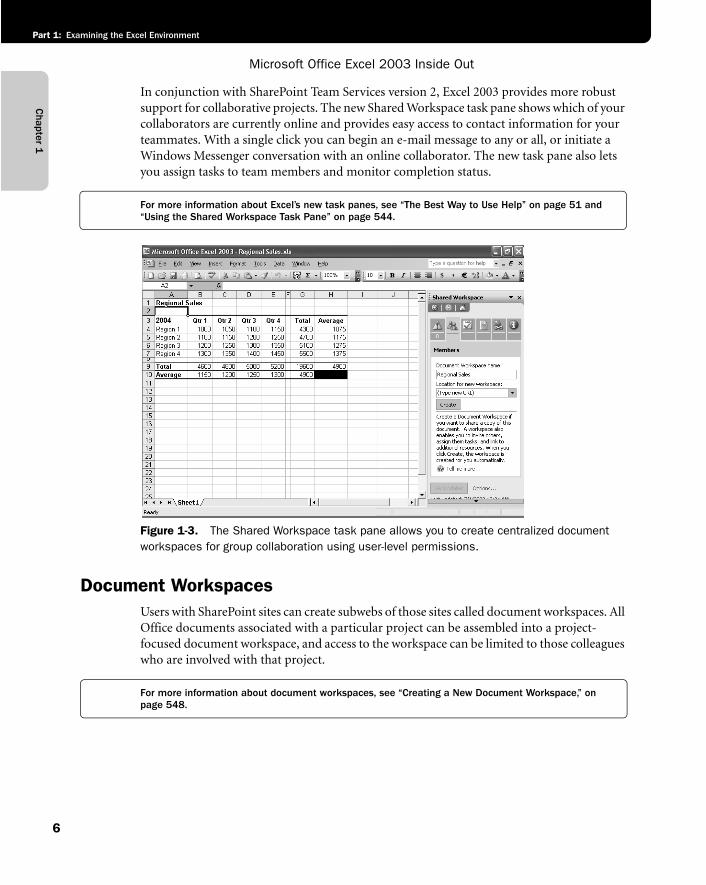
Chapter 1

Microsoft Office Excel 2003 Inside Out

Part 1: Examining the Excel Environment

6

In conjunction with SharePoint Team Services version 2, Excel 2003 provides more robust support for collaborative projects. The new Shared Workspace task pane shows which of your collaborators are currently online and provides easy access to contact information for your teammates. With a single click you can begin an e-mail message to any or all, or initiate a Windows Messenger conversation with an online collaborator. The new task pane also lets you assign tasks to team members and monitor completion status.

For more information about Excel’s new task panes, see “The Best Way to Use Help” on page 51 and “Using the Shared Workspace Task Pane” on page 544.

f01ie03

Figure 1-3. The Shared Workspace task pane allows you to create centralized document workspaces for group collaboration using user-level permissions.

Document WorkspacesUsers with SharePoint sites can create subwebs of those sites called document workspaces. All Office documents associated with a particular project can be assembled into a project-focused document workspace, and access to the workspace can be limited to those colleagues who are involved with that project.

For more information about document workspaces, see “Creating a New Document Workspace,” on page 548.

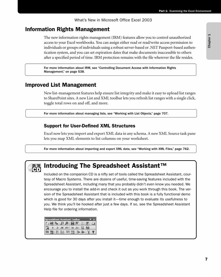
Cha

pter

1

What’s New in Microsoft Office Excel 2003

7

Part 1: Examining the Excel Environment

Information Rights ManagementThe new information rights management (IRM) features allow you to control unauthorized access to your Excel workbooks. You can assign either read or read/write access permission to individuals or groups of individuals using a robust server-based or .NET Passport-based authen-tication system, and you can set expiration dates that make documents inaccessible to others after a specified period of time. IRM protection remains with the file wherever the file resides.

For more information about IRM, see “Controlling Document Access with Information Rights Management,” on page 538.

Improved List ManagementNew list-management features help ensure list integrity and make it easy to upload list ranges to SharePoint sites. A new List and XML toolbar lets you refresh list ranges with a single click, toggle total rows on and off, and more.

For more information about managing lists, see “Working with List Objects,” page 707.

Support for User-Defined XML StructuresExcel now lets you import and export XML data in any schema. A new XML Source task pane lets you map XML elements to list columns on your worksheet.

For more information about importing and export XML data, see “Working with XML Files,” page 762.

Introducing The Spreadsheet Assistant™Included on the companion CD is a nifty set of tools called the Spreadsheet Assistant, cour-tesy of Macro Systems. There are dozens of useful, time-saving features included with the Spreadsheet Assistant, including many that you probably didn’t even know you needed. We encourage you to install the add-in and check it out as you work through this book. The ver-sion of the Spreadsheet Assistant that is included with this book is a fully functional demo which is good for 30 days after you install it—time enough to evaluate its usefulness to you. We think you’ll be hooked after just a few days. If so, see the Spreadsheet Assistant Help file for ordering information.

G01ie01

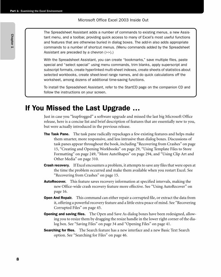
Chapter 1

Microsoft Office Excel 2003 Inside Out

Part 1: Examining the Excel Environment

8

The Spreadsheet Assistant adds a number of commands to existing menus, a new Assis-tant menu, and a toolbar, providing quick access to many of Excel’s most useful functions and features that are otherwise buried in dialog boxes. The add-in also adds appropriate commands to a number of shortcut menus. (Menu commands added by the Spreadsheet Assistant are preceded by a chevron (>>).)

With the Spreadsheet Assistant, you can create “bookmarks,” save multiple files, paste special and “select special” using menu commands, trim blanks, apply superscript and subscript formats, create hyperlinked multi-sheet indexes, create sheets of statistics about selected workbooks, create sheet-level range names, and do quick calculations off the worksheet, among dozens of additional time-saving functions.

To install the Spreadsheet Assistant, refer to the StartCD page on the companion CD and follow the instructions on your screen.

If You Missed the Last Upgrade …Just in case you “leapfrogged” a software upgrade and missed the last big Microsoft Office release, here is a concise list and brief description of features that are essentially new to you, but were actually introduced in the previous release.

The Task Pane. The task pane radically repackages a few existing features and helps make them smarter, more responsive, and less intrusive than dialog boxes. Discussions of task panes appear throughout the book, including “Recovering from Crashes” on page 15, “Creating and Opening Workbooks” on page 29, “Using Template Files to Store Formatting” on page 249, “More AutoShapes” on page 294, and “Using Clip Art and Other Media” on page 310.

Crash recovery. If Excel encounters a problem, it attempts to save any files that were open at the time the problem occurred and make them available when you restart Excel. See “Recovering from Crashes” on page 15.

AutoRecover. This feature saves recovery information at specified intervals, making the new Office-wide crash recovery feature more effective. See “Using AutoRecover” on page 16.

Open And Repair. This command can either repair a corrupted file, or extract the data from it, offering a powerful recovery feature and a little extra peace of mind. See “Recovering Corrupted Files” on page 45.

Opening and saving files. The Open and Save As dialog boxes have been redesigned, allow-ing you to resize them by dragging the resize handle in the lower right corner of the dia-log box. See “Saving Files” on page 34 and “Opening Files” on page 41.

Searching for files. The Search feature has a new interface and a new Basic Text Search option. See “Searching for Files” on page 46.

Cha

pter

1

What’s New in Microsoft Office Excel 2003

9

Part 1: Examining the Excel Environment

Smart Tags. These pop-up menus give you instant access to commands and actions that are relevant to the task at hand. For examples, see “Understanding Numeric Text Entries” on page 113, “Tracing Errors” on page 259, “Copying Formulas and Pasting Only Their Resulting Values” on page 380, and “Entering a Series of Dates” on page 437.

Color-coding sheet tabs. Sheet tabs can be colored, offering more organizational flexibility in your workbooks. See “Coloring Sheet Tabs” on page 120.

Inserting symbols. Excel now provides access to the complete character set of all fonts installed on your computer, allowing you to enter characters with diacritical marks, symbols, and other “hidden” characters beyond those visible on the keyboard. See “Entering Symbols” on page 115.

Password-protected cell ranges. These ranges provide access to specific areas of a protected worksheet and even specify individual permissions. See “Allowing Password Access to Specific Cell Ranges” on page 129.

Copying multiple items. The newly redesigned Collect And Copy feature lets you post twice as many items (24) to the Office Clipboard and uses the new Clipboard task pane. See “Collecting Multiple Items on the Clipboard” on page 148.

Finding and replacing. Find and replace formatting, and search the entire workbook, not just the current sheet. See “Finding and Replacing Stuff ” on page 179.

Cell formatting. In the Format Cells dialog box, the Number tab now offers Locale options, with more than 120 worldwide formats for phone numbers and postal codes. The Alignment tab allows text to be displayed right-to-left under certain conditions, and also features Right Indent and Distributed options. See “Using the Special Formats” on page 210 and “Aligning Data in Cells” on page 219.

Border drawing. A pencil-shaped tool can draw borders wherever you want them. See “Drawing Borders” on page 231.

Merge And Center. This button is now a toggle; unmerge cells by clicking Merge And Cen-ter again. See “Selecting Alignment Using Toolbars” on page 225.

The Evaluate Formula command. The Evaluate Formula command helps debug complex formulas by stepping you through each calculation and showing you the results. See “Auditing and Documenting Worksheets” on page 251.

The Formula Watch Window. If you need to keep an eye on remote cells as you make changes to other parts of a worksheet, the Formula Watch Window provides remote viewing of multiple cells on any open worksheet and provides dynamic data about each formula, including its location, its resulting value, and more. See “Watching Formulas” on page 255.

Text To Speech. Excel can now “read” the contents of cells to you as you visually check the original document, making auditing and proofreading chores a little easier. See “Hav-ing Excel Read Cells to You” on page 266.

The Trace Error button. Excel detects anomalies after editing a formula and displays a smart tag with a menu of pertinent actions. See “Tracing Errors” on page 259.

Chapter 1

Microsoft Office Excel 2003 Inside Out

Part 1: Examining the Excel Environment

10

Error Checking. This command quickly finds error values in the current worksheet. See “Checking for Errors” on page 252.

Picture formatting. The new Washout option creates images similar to watermarks; the new Compress option reduces the amount of disk space used by images. See “Format-ting Pictures” on page 318.

Using clip art. The Insert Clip Art button now displays a task pane, and the new Media Gal-lery represents a major overhaul of the old Clip Gallery. See “Using Clip Art and Other Media” on page 310.

Full-featured diagrams. You can now add full-featured, editable organizational charts, Venn diagrams, and other diagram types into your documents. See “Inserting Organization Charts” on page 315, and “Inserting Diagrams” on page 316.

AutoShape rotation. All two-dimensional objects now display a handle you can drag to rotate the object. See “Working with AutoShapes” on page 292.

Find Printer button. Search for any printer available on your network from the Print dialog box. See Chapter 11, “Printing and Presenting” on page 331.

No More Blank Page Printing. Excel now looks at the content of the current worksheet before sending it to the printer. See Chapter 11, “Printing and Presenting” on page 331.

Header Graphics. You can now add graphics to Headers and Footers. See Chapter 11, “Printing and Presenting” on page 331.

AutoSum. Now it is possible to enter other popular functions, including Average, Count, Max, or Min instead of just the SUM function. See “Using the AutoSum Button” on page 362.

The Function Wizard. This is a major step forward in usability and includes a function search feature that allows you to find the right function by entering a plain language description of what you’re trying to do. See “Inserting Functions” on page 363.

Function ScreenTips. Now when you enter or edit a function, Excel displays a pop-up box showing the function syntax. See “Using Excel’s Built-In Function Reference” on 401.

Workbook Review. A new command on the File, Send To menu provides an easy way to cir-culate workbooks for comments and edits by other members of your workgroup. See “Sending a Workbook for Review” on page 535.

Microsoft SharePoint Team Services. This is an Internet-based technology for team com-munications and collaboration. “Using a SharePoint Team Services Site” on page 541.

Web archives. In previous versions of Excel, saving an entire workbook to HTML generated a single HTM file in addition to (typically) a large folder full of supporting documents. The current version introduces an optional Web Archive format that encapsulates every-thing into a single file. See “Single-File Web Page or Web Page?” on page 560.

Cha

pter

1

What’s New in Microsoft Office Excel 2003

11

Part 1: Examining the Excel Environment

AutoRepublish. A new AutoRepublish option makes it easier than ever to keep Web pages up to date with Excel material. If you use this option, Excel updates an HTML copy of your file every time you save changes to the original. See “To Save or To Publish?” on page 560.

Accessing FTP Sites. If you regularly save files to or retrieve them from a particular FTP site, you can add that site to the My Places bar. The My Places bar is a navigational panel that appears at the left edge of Excel’s Open and Save As dialog boxes. See “Add-ing a Site to Your My Places Bar” on page 555.

My Places. Add any folder or FTP site to your My Places bar—the navigation panel on the left in the Save As and Open dialog boxes. See “Adding a Site to Your My Places Bar” on page 555.

Support for XML. Open and save Excel documents in Extensible Markup Language (XML) and create queries to XML source data. See “Working with XML Files” on page 762.

Editing hyperlinks. Hyperlinks used to be tricky to edit. Not any more. See the tip “Edit hyperlinks easily” on page 582.

Web queries. You can now create queries to retrieve data from Web sites, without knowing anything about HTML or how those Web sites are constructed. See “Using a Web Query to Return Internet Data” on page 791.

The PivotTable toolbar. This has been redesigned so that it no longer includes the names of fields in the current table. These now appear in a separate PivotTable Field List window that can be toggled in and out of view. See Chapter 30, “Analyzing Data with PivotTable Reports” on page 797.

PivotTable data reference. Any time you point to a PivotTable cell while building a formula outside the table, Excel creates the GETPIVOTDATA function for you. See Chapter 30, “Analyzing Data with PivotTable Reports” on page 797.

PivotTable properties. Users who build PivotTables from Online Analytical Processing (OLAP) data sources can take advantage of a new feature that allows annotation of Piv-otTable data with item properties. See Chapter 30, “Analyzing Data with PivotTable Reports” on page 797.

Voice recognition. It is now possible to use your own voice to issue commands, navigate, and dictate text into Excel and other Office programs. See Appendix B, “Using Speech and Handwriting Recognition” on page 889.

Handwriting input. If you have a drawing pad and stylus (and even if you don’t) you can now enter text directly into Excel and other Office programs using your own handwrit-ing. See Appendix B, “Using Speech and Handwriting Recognition” on page 889.

Onward …Taken together, the improvements made for the Microsoft Office System and Microsoft Excel represent a small but significant step in document sharing, communication, collaboration, assistance, programmability, and extensibility. And if you skipped the last upgrade, you’re poised for a giant leap forward in productivity. Read on!

13

Part 1: Examining the Excel Environment

Chapter 2

Excel FundamentalsWhat Happens After You Install Excel?. . .13Recovering from Crashes . . . . . . . . . . . . .15Examining the Excel Workspace . . . . . . . .18

File Management Fundamentals . . . . . . . 29Importing and Exporting Files . . . . . . . . . 48Online Help Works—Really! . . . . . . . . . . . 51

Before you can get the feel of the controls, you need to know where they are. This chapter tells you where to find Microsoft Excel’s tools and accessories.

What Happens After You Install Excel?OK, this is really basic, but we have a moral obligation to briefly mention it anyway. There are two principal ways to start Excel:

● In Microsoft Windows XP, click the Windows Start button, and click Microsoft Office Excel 2003 (or All Programs, Microsoft Office Excel 2003). In Microsoft Windows 9x, Windows Me, or Windows 2000, click the Windows Start button, point to Programs, and then click Microsoft Office Excel 2003.

● In Windows Explorer, double-click any Excel file or shortcut.

Registering ExcelWhen you start Excel for the first time, you will be asked to register, or “Activate,” the pro-gram. The easiest way to do this is by allowing Excel to register online, assuming that your computer is connected to the Internet. Online registration is fast and painless and a lot easier than taking a postcard to the mailbox. It is also highly recommended.

You may have qualms about any kind of owner registration, but with software, it’s really a good idea—trust us. When you register, you’ll automatically be in the loop for bug fixes (there will certainly be a Service Release [SR] or Service Pack [SP] available within a year or so), updates, and “special offers.” Maybe registering a garden tool, for example, is not worth the annoyance of “special offers,” but if you essentially got a new tool for free in a few months, you just might go for it. You won’t see too many upgrades for weed whackers, of course, but with software you can rely on getting an upgrade at some point.

Subscribing to ExcelThey say that this is the future of software—something lovingly referred to as “the subscrip-tion model.” It’s a way of purchasing software that has been available to big companies for years, but only now is the idea being floated to the general public.

Chapter 2

Microsoft Office Excel 2003 Inside Out

Part 1: Examining the Excel Environment

14

A major software application is a living thing—the moment one version is completed, teams of developers begin working on the next version, while other teams work on bug fixes for the version they just shipped. When you buy a box of software off the shelf, it’s not so much a fin-ished product as a work in progress. If you update your software semi-regularly, it becomes more like a magazine subscription than a weed whacker you buy once and throw away when it dies. So, the idea is, why not make software just like a subscription? You make smaller, more regular payments, and you get automatic, periodic updates. Subscription might make excel-lent sense for frequent updaters, depending, of course, on the fee.

If you purchased a standard shrink-wrapped retail version of Office or Excel, your product doesn’t “expire” at all. But you can still purchase a subscription, which will transform yours into a subscription installation. Once you subscribe, you can always buy more time, just like you can with magazine subscriptions. Helpfully, the Microsoft Office Activation Wizard will remind you within 60 days of your subscription’s expiration that it’s time to renew.

Why Are There So Many Bugs?There are probably not as many bugs as you think that actually affect your daily work. Such bugs are called “showstoppers.” Software almost never ships with showstoppers anymore; rigorous Beta-testing generally takes care of these problems. That said, all companies rou-tinely ship software that is riddled with bugs—it’s the way of the software marketing world. Microsoft and every other software company are equally guilty. But why?

As the battle for market share raged among application developers in the 1980s and 1990s, the mantra among developers was “Ship, ship, ship!” They raced to see how fast they could release the next version of their product for two main reasons.

First, all the other companies were moving at the same torrid pace, and everybody had to keep up. Applications lived or died because of feature checklists published in major com-puter magazines. If your product was in any way ill-represented in the published feature comparisons, your product was simply going to lose market share. If the new version of your program didn’t make it into, for example, the “Big Spreadsheet Showdown Issue,” you and your development group were in deep doo-doo.

Second, releasing an upgrade—that is, a new version of an existing program offered for sale rather than being free—represents a large infusion of income to software companies. This is where most of the money comes from for “mature” software products like Excel. Thus, the marketing folks would love to ship a new version every year, or even every six months!

But not only did their customers have a hard time justifying the purchase of upgrades every year or less, software development groups themselves had a hard time keeping that kind of pace. It takes time to develop ideas for new features, write the software code, integrate the new code with the existing code and make sure it doesn’t introduce major problems, and then to document, design, manufacture, market, and distribute the product. Plus, the more “mature” a program becomes, the more complex and unpredictable it becomes. Chaos the-ory starts to rear its ugly head. (Remember Jurassic Park?)

Excel Fundamentals

15

Part 1: Examining the Excel Environment

Cha

pter

2

One final but very important problem—technology may evolve, but these complex, bloated programs nonetheless had to remain compatible with “legacy” systems. This means not only that programs had to be able to recognize their own files even if they were created sev-eral versions ago, but also that commands and features that may have been rendered essentially obsolete had to be reconciled with new features. In some cases, this required continued support for old but often-used commands and keystroke shortcuts.

Completely debugging a program as complex as Excel could take years. Some think that it is impossible to absolutely eliminate all potential malfunctions in any program. Just as the FDA certifies that it’s OK for a certain small percentage of rat droppings to appear in hot dogs, software companies had to devise an acceptable threshold and severity of bugs that were acceptable to ship in a “finished” product. The good news is that these leftover bugs are usually so esoteric that most folks will never have to deal with them.

Getting UpdatesMicrosoft releases free updates called Service Releases (SRs), which begin to appear a year or so after the most recent version of Office is released. There will probably always be at least one SR for each new version of Office/Excel. SRs comprise good bits of software code that replace bad bits, circumvent errors, or otherwise intercept known problems. They are commonly called patches, a euphemism borrowed from the colorful lexicon of emergency tire repair. SRs might even activate new features that were “hidden” because they were only partially imple-mented when the software finally had to ship.

Service Releases are always free, but they are not very well advertised. If your computer is connected to the Internet, the easiest way to keep your software current is to click Check For Updates on the Help menu. This brings up the Office Update page in your Internet browser, where you can find links to any available patches.

The Microsoft Office Online link, also on the Help menu, connects you to a related Web location, a sort of central clearinghouse for templates, general assistance, news, and lesser patches that might be available for individual programs or add-ins. You should definitely check it out.

Recovering from CrashesIn the past, “crash recovery” largely involved an initial flurry of expletives, followed by a brisk walk around the office and perhaps a couple of aspirin. Excel provides something beyond comfort and sympathy for digital mishaps—an actual mechanism that attempts to tuck away open files before the program comes screeching to a halt. And it works pretty well. If Excel encounters a problem, it attempts to save any files that were open at the time the problem occurred, before bad things happen to them when the program crashes and burns. When you restart Excel, these files are then listed in the Document Recovery task pane that appears on the left side of the screen, as shown in Figure 2-1. If the file listed in the Document pane is marked “[Recovered],” Excel had some success in saving the file.

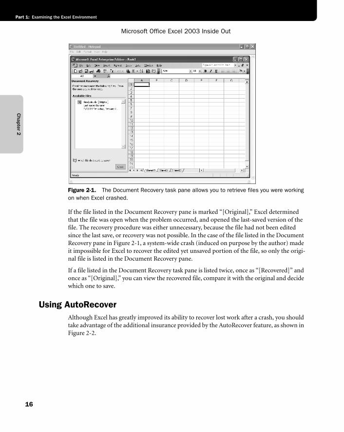
Chapter 2

Microsoft Office Excel 2003 Inside Out

Part 1: Examining the Excel Environment

16

02ie01

Figure 2-1. The Document Recovery task pane allows you to retrieve files you were working on when Excel crashed.

If the file listed in the Document Recovery pane is marked “[Original],” Excel determined that the file was open when the problem occurred, and opened the last-saved version of the file. The recovery procedure was either unnecessary, because the file had not been edited since the last save, or recovery was not possible. In the case of the file listed in the Document Recovery pane in Figure 2-1, a system-wide crash (induced on purpose by the author) made it impossible for Excel to recover the edited yet unsaved portion of the file, so only the origi-nal file is listed in the Document Recovery pane.

If a file listed in the Document Recovery task pane is listed twice, once as “[Recovered]” and once as “[Original],” you can view the recovered file, compare it with the original and decide which one to save.

Using AutoRecoverAlthough Excel has greatly improved its ability to recover lost work after a crash, you should take advantage of the additional insurance provided by the AutoRecover feature, as shown in Figure 2-2.

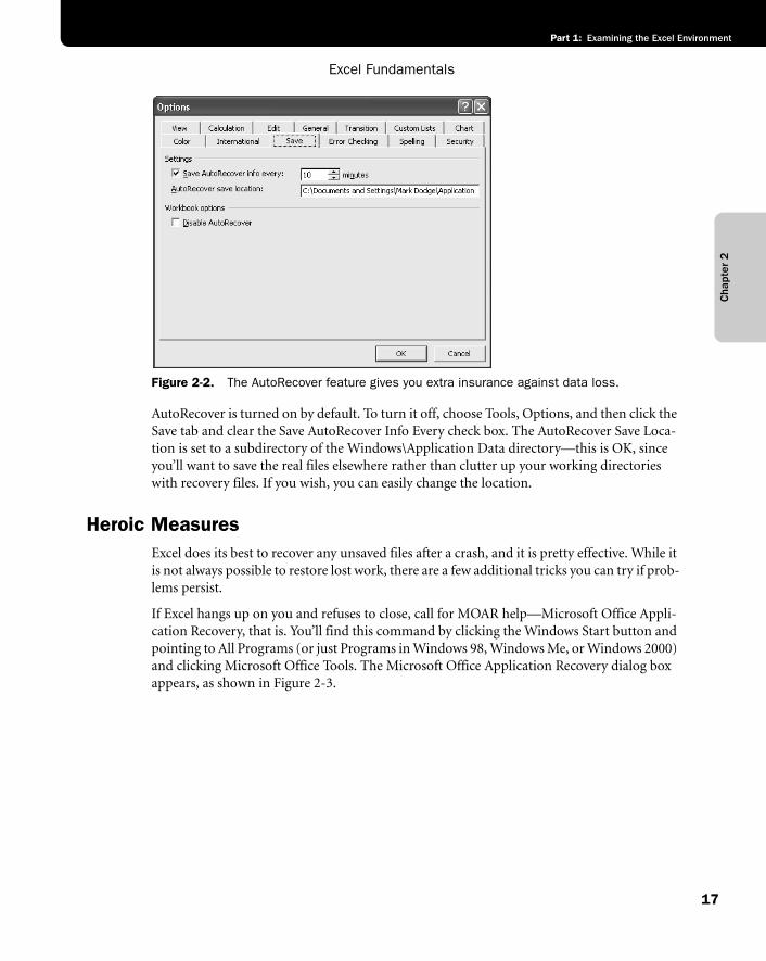
Excel Fundamentals

17

Part 1: Examining the Excel Environment

Cha

pter

2

f02ie02

Figure 2-2. The AutoRecover feature gives you extra insurance against data loss.

AutoRecover is turned on by default. To turn it off, choose Tools, Options, and then click the Save tab and clear the Save AutoRecover Info Every check box. The AutoRecover Save Loca-tion is set to a subdirectory of the Windows\Application Data directory—this is OK, since you’ll want to save the real files elsewhere rather than clutter up your working directories with recovery files. If you wish, you can easily change the location.

Heroic MeasuresExcel does its best to recover any unsaved files after a crash, and it is pretty effective. While it is not always possible to restore lost work, there are a few additional tricks you can try if prob-lems persist.

If Excel hangs up on you and refuses to close, call for MOAR help—Microsoft Office Appli-cation Recovery, that is. You’ll find this command by clicking the Windows Start button and pointing to All Programs (or just Programs in Windows 98, Windows Me, or Windows 2000) and clicking Microsoft Office Tools. The Microsoft Office Application Recovery dialog box appears, as shown in Figure 2-3.

Chapter 2

Microsoft Office Excel 2003 Inside Out

Part 1: Examining the Excel Environment

18

f02ie03

Figure 2-3. The Microsoft Office Application Recovery dialog box gives you a chance to save lost work if a crash occurs in Excel.

If Excel is still open but not responding, you can click the Recover Application button to try to recover the files that you were working on. If you just want to shut down the program, click the End Application button.

Examining the Excel WorkspaceThis section will take you on a tour of not only the dashboard of Excel, but also the trunk and the glove compartment. We might even slip on some gloves and take a peek under the floor mats.

Facts About WorksheetsHere are a few random tidbits of interesting information about the grid we call the worksheet.

● Column letters range from A through IV. (After column Z comes column AA, after AZ comes BA, and so on, up to IV.) Row numbers range from 1 through 65,536.

● The currently selected cell is referred to as the active cell. When you select a range of cells, only the cell in the upper-left corner is considered the active cell. The reference of the active cell appears at the left end of the Formula Bar in the Name box.

● The headings for the columns and rows containing selected cells are highlighted, mak-ing it easier to identify the location of selected cells.

● With 256 columns and 65,536 rows, your worksheet contains more than 16 million individual cells. Before you try to unravel the mysteries of the universe on a single worksheet, however, remember that the number of cells you can use at any one time is limited by the amount of memory your computer has. Although Excel allocates mem-ory only to cells containing data, you might have trouble actually using all the cells in one worksheet, no matter how much memory you have.

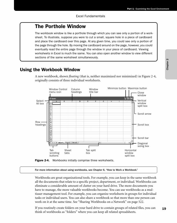
Excel Fundamentals

19

Part 1: Examining the Excel Environment

Cha

pter

2

The Porthole WindowThe workbook window is like a porthole through which you can see only a portion of a work-sheet. To illustrate, suppose you were to cut a small, square hole in a piece of cardboard and place the cardboard over this page. At any given time, you could see only a portion of the page through the hole. By moving the cardboard around on the page, however, you could eventually read the entire page through the window in your piece of cardboard. Viewing worksheets in Excel is much the same. You can also open another window to view different sections of the same worksheet simultaneously.

Using the Workbook WindowA new workbook, shown floating (that is, neither maximized nor minimized) in Figure 2-4, originally consists of three individual worksheets.

f02ie04

Figure 2-4. Workbooks initially comprise three worksheets.

For more information about using workbooks, see Chapter 6, “How to Work a Workbook.”

Workbooks are great organizational tools. For example, you can keep in the same workbook all the documents that relate to a specific project, department, or individual. Workbooks can eliminate a considerable amount of clutter on your hard drive. The more documents you have to manage, the more valuable workbooks become. You can use workbooks as a mul-tiuser management tool. For example, you can organize worksheets in groups for individual tasks or individual users. You can also share a workbook so that more than one person can work on it at the same time. See “Sharing Workbooks on a Network” on page 522.

If you routinely create folders on your hard drive to contain groups of related files, you can think of workbooks as “folders” where you can keep all related spreadsheets.

Rowheadings

SelectAll box

Tabscrollingbuttons

Sheettabs

Tab splitbox

Horizontalwindowsplit box

Diagonalsizing box

Scroll bar

Scroll box

Scroll arrow

Closewindow

Maximize buttonMinimize buttonWindowtitle bar

Window Controlmenu icon

Columnheadings

Verticalwindowsplit box

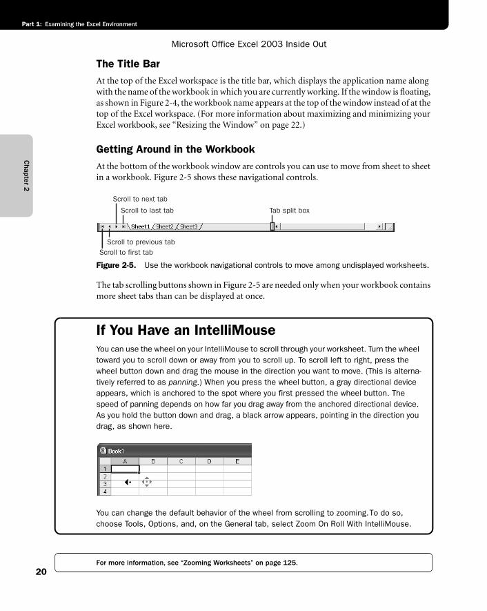
Chapter 2

Microsoft Office Excel 2003 Inside Out

Part 1: Examining the Excel Environment

20

The Title BarAt the top of the Excel workspace is the title bar, which displays the application name along with the name of the workbook in which you are currently working. If the window is floating, as shown in Figure 2-4, the workbook name appears at the top of the window instead of at the top of the Excel workspace. (For more information about maximizing and minimizing your Excel workbook, see “Resizing the Window” on page 22.)

Getting Around in the WorkbookAt the bottom of the workbook window are controls you can use to move from sheet to sheet in a workbook. Figure 2-5 shows these navigational controls.

f02ie05

Figure 2-5. Use the workbook navigational controls to move among undisplayed worksheets.

The tab scrolling buttons shown in Figure 2-5 are needed only when your workbook contains more sheet tabs than can be displayed at once.

If You Have an IntelliMouseYou can use the wheel on your IntelliMouse to scroll through your worksheet. Turn the wheel toward you to scroll down or away from you to scroll up. To scroll left to right, press the wheel button down and drag the mouse in the direction you want to move. (This is alterna-tively referred to as panning.) When you press the wheel button, a gray directional device appears, which is anchored to the spot where you first pressed the wheel button. The speed of panning depends on how far you drag away from the anchored directional device. As you hold the button down and drag, a black arrow appears, pointing in the direction you drag, as shown here.

g02ie01

You can change the default behavior of the wheel from scrolling to zooming. To do so, choose Tools, Options, and, on the General tab, select Zoom On Roll With IntelliMouse.

For more information, see “Zooming Worksheets” on page 125.

Scroll to last tab

Scroll to next tab

Scroll to first tabScroll to previous tab

Tab split box

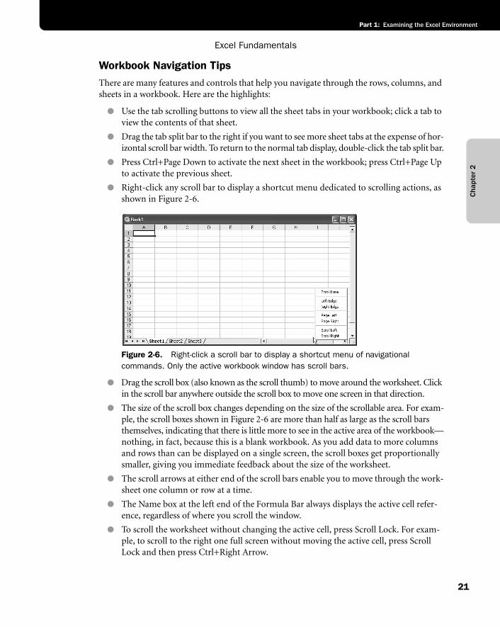
Excel Fundamentals

21

Part 1: Examining the Excel Environment

Cha

pter

2

Workbook Navigation TipsThere are many features and controls that help you navigate through the rows, columns, and sheets in a workbook. Here are the highlights:

● Use the tab scrolling buttons to view all the sheet tabs in your workbook; click a tab to view the contents of that sheet.

● Drag the tab split bar to the right if you want to see more sheet tabs at the expense of hor-izontal scroll bar width. To return to the normal tab display, double-click the tab split bar.

● Press Ctrl+Page Down to activate the next sheet in the workbook; press Ctrl+Page Up to activate the previous sheet.

● Right-click any scroll bar to display a shortcut menu dedicated to scrolling actions, as shown in Figure 2-6.

F02ie06

Figure 2-6. Right-click a scroll bar to display a shortcut menu of navigational commands. Only the active workbook window has scroll bars.

● Drag the scroll box (also known as the scroll thumb) to move around the worksheet. Click in the scroll bar anywhere outside the scroll box to move one screen in that direction.

● The size of the scroll box changes depending on the size of the scrollable area. For exam-ple, the scroll boxes shown in Figure 2-6 are more than half as large as the scroll bars themselves, indicating that there is little more to see in the active area of the workbook—nothing, in fact, because this is a blank workbook. As you add data to more columns and rows than can be displayed on a single screen, the scroll boxes get proportionally smaller, giving you immediate feedback about the size of the worksheet.

● The scroll arrows at either end of the scroll bars enable you to move through the work-sheet one column or row at a time.

● The Name box at the left end of the Formula Bar always displays the active cell refer-ence, regardless of where you scroll the window.

● To scroll the worksheet without changing the active cell, press Scroll Lock. For exam-ple, to scroll to the right one full screen without moving the active cell, press Scroll Lock and then press Ctrl+Right Arrow.

Chapter 2

Microsoft Office Excel 2003 Inside Out

Part 1: Examining the Excel Environment

22

What Is the Active Worksheet Area?The active area of a worksheet is simply the rectangular area that encompasses all of the data the worksheet contains. So if you have just three rows and columns of actual data in the top-left corner of the sheet, the active area would be A1:C3. If a stray character (even a space) happens to be in cell AB1299, the active area would be A1:AB1299. In a new, blank worksheet, however, Excel considers the default active area to be roughly what you can see on the screen, even before you enter any data.

Resizing the WindowAt the right end of the workbook window’s title bar are the Minimize, Maximize/Restore, and Close buttons. When your workbook window is maximized, the active window is displayed at full size in the Excel workspace.

After you maximize the window, a button with two small boxes—the Restore button—takes the place of the Maximize button. When you click the Restore button, the active window changes to a floating window.

When you click the Minimize button (the one with a small line at the bottom), the workbook collapses to what looks like a small title bar.

Minimizing workbooks is a handy way to reduce workspace clutter when you have several workbooks open at the same time. Click the Restore button on the menu bar to display the workbook at its former floating size, or click the Maximize button and the workbook fills the Excel workspace.

You can also drag the borders of a floating window to control its size. The smaller the win-dow, the less you see of the worksheet; however, because you can open multiple windows for the same workbook, you might find it more convenient to view different parts of the work-book, or even of an individual worksheet, side by side in two small windows rather than switch between sheets or scroll back and forth in one large window.

Tip See more rows on your screenThe Windows taskbar at the bottom of the screen can be set to automatically hide itself when not in use. In Windows XP, click the Start button, click Control Panel, click Appearance And Themes, and then click Taskbar And Start Menu. On the Taskbar tab, click Auto-hide the Taskbar. In Windows 98, Windows Me, or Windows 2000, click the Start button, point to Settings, and click Taskbar & Start Menu. On the Taskbar tab (in Windows XP) or Taskbar Options tab, click Auto Hide, then click OK. Now the taskbar stays hidden and pops up only when you move the mouse pointer to the bottom of the screen.

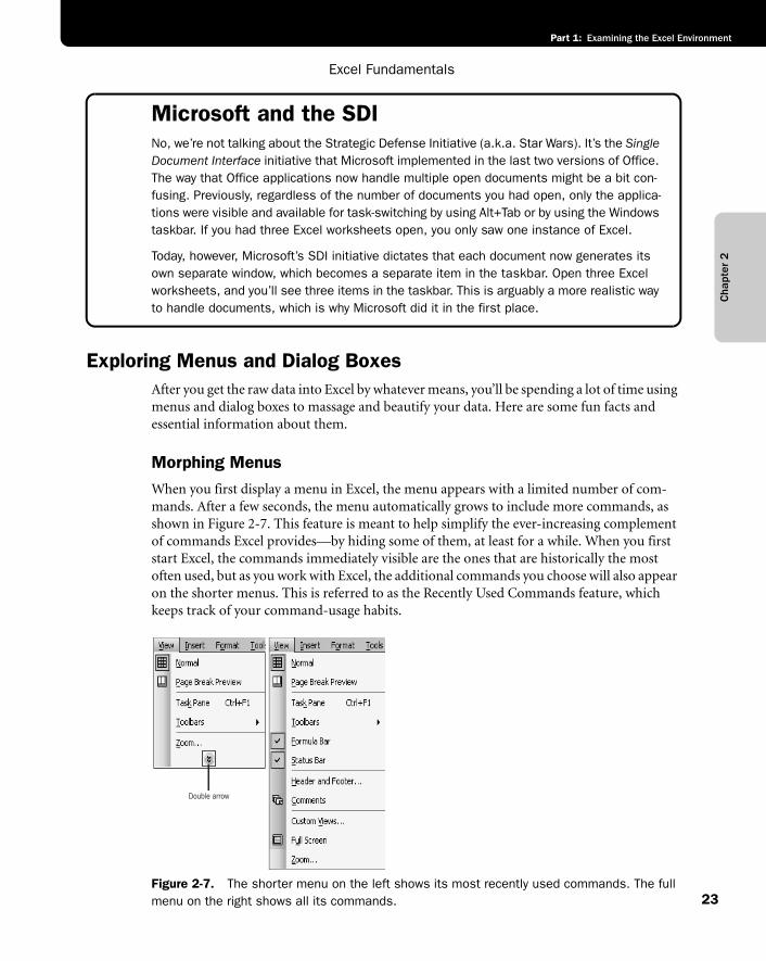
Excel Fundamentals

23

Part 1: Examining the Excel Environment

Cha

pter

2

Microsoft and the SDINo, we’re not talking about the Strategic Defense Initiative (a.k.a. Star Wars). It’s the SingleDocument Interface initiative that Microsoft implemented in the last two versions of Office. The way that Office applications now handle multiple open documents might be a bit con-fusing. Previously, regardless of the number of documents you had open, only the applica-tions were visible and available for task-switching by using Alt+Tab or by using the Windows taskbar. If you had three Excel worksheets open, you only saw one instance of Excel.

Today, however, Microsoft’s SDI initiative dictates that each document now generates its own separate window, which becomes a separate item in the taskbar. Open three Excel worksheets, and you’ll see three items in the taskbar. This is arguably a more realistic way to handle documents, which is why Microsoft did it in the first place.

Exploring Menus and Dialog BoxesAfter you get the raw data into Excel by whatever means, you’ll be spending a lot of time using menus and dialog boxes to massage and beautify your data. Here are some fun facts and essential information about them.

Morphing MenusWhen you first display a menu in Excel, the menu appears with a limited number of com-mands. After a few seconds, the menu automatically grows to include more commands, as shown in Figure 2-7. This feature is meant to help simplify the ever-increasing complement of commands Excel provides—by hiding some of them, at least for a while. When you first start Excel, the commands immediately visible are the ones that are historically the most often used, but as you work with Excel, the additional commands you choose will also appear on the shorter menus. This is referred to as the Recently Used Commands feature, which keeps track of your command-usage habits.

f02ie07

Figure 2-7. The shorter menu on the left shows its most recently used commands. The full menu on the right shows all its commands.

Double arrow

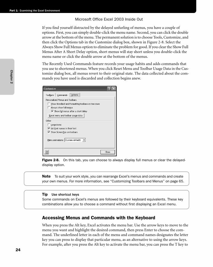
Chapter 2

Microsoft Office Excel 2003 Inside Out

Part 1: Examining the Excel Environment

24

If you find yourself distracted by the delayed unfurling of menus, you have a couple of options. First, you can simply double-click the menu name. Second, you can click the double arrow at the bottom of the menu. The permanent solution is to choose Tools, Customize, and then click the Options tab in the Customize dialog box, shown in Figure 2-8. Select the Always Show Full Menus option to eliminate the problem for good. If you clear the Show Full Menus After A Short Delay option, short menus will stay short unless you double-click the menu name or click the double arrow at the bottom of the menus.

The Recently Used Commands feature records your usage habits and adds commands that you use to shortened menus. When you click Reset Menu and Toolbar Usage Data in the Cus-tomize dialog box, all menus revert to their original state. The data collected about the com-mands you have used is discarded and collection begins anew.

f02ie08

Figure 2-8. On this tab, you can choose to always display full menus or clear the delayed-display option.

Note To suit your work style, you can rearrange Excel’s menus and commands and create your own menus. For more information, see “Customizing Toolbars and Menus” on page 65.

Tip Use shortcut keysSome commands on Excel’s menus are followed by their keyboard equivalents. These key combinations allow you to choose a command without first displaying an Excel menu.

Accessing Menus and Commands with the KeyboardWhen you press the Alt key, Excel activates the menu bar. Use the arrow keys to move to the menu you want and highlight the desired command, then press Enter to choose the com-mand. The underlined letter in each of the menu and command names designates the letter key you can press to display that particular menu, as an alternative to using the arrow keys. For example, after you press the Alt key to activate the menu bar, you can press the T key to

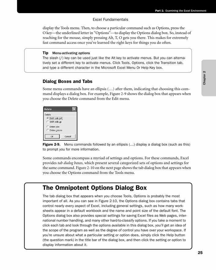
Excel Fundamentals

25

Part 1: Examining the Excel Environment

Cha

pter

2

display the Tools menu. Then, to choose a particular command such as Options, press the O key—the underlined letter in “Options”—to display the Options dialog box. So, instead of reaching for the mouse, simply pressing Alt, T, O gets you there. This makes for extremely fast command access once you’ve learned the right keys for things you do often.

Tip Menu-activating optionsThe slash (/) key can be used just like the Alt key to activate menus. But you can alterna-tively set a different key to activate menus. Click Tools, Options, click the Transition tab, and type a different character in the Microsoft Excel Menu Or Help Key box.

Dialog Boxes and TabsSome menu commands have an ellipsis (…) after them, indicating that choosing this com-mand displays a dialog box. For example, Figure 2-9 shows the dialog box that appears when you choose the Delete command from the Edit menu.

f02ie09

Figure 2-9. Menu commands followed by an ellipsis (…) display a dialog box (such as this) to prompt you for more information.

Some commands encompass a myriad of settings and options. For these commands, Excel provides tab dialog boxes, which present several categorized sets of options and settings for the same command. Figure 2-10 on the next page shows the tab dialog box that appears when you choose the Options command from the Tools menu.

The Omnipotent Options Dialog BoxThe tab dialog box that appears when you choose Tools, Options is probably the most important of all. As you can see in Figure 2-10, the Options dialog box contains tabs that control nearly every aspect of Excel, including general settings, such as how many work-sheets appear in a default workbook and the name and point size of the default font. The Options dialog box also provides special settings for saving Excel files as Web pages, inter-national number handling, and many other hard-to-classify options. If you take a moment to click each tab and look through the options available in this dialog box, you’ll get an idea of the scope of the program as well as the degree of control you have over your workspace. If you’re unsure about what a particular setting or option does, simply click the Help button (the question mark) in the title bar of the dialog box, and then click the setting or option to display information about it.

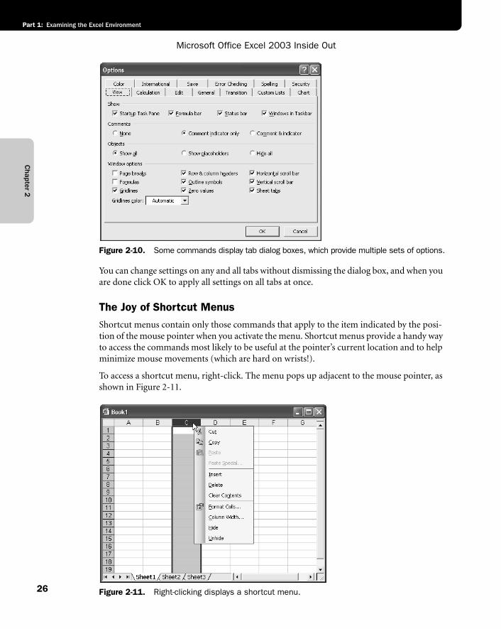
Chapter 2

Microsoft Office Excel 2003 Inside Out

Part 1: Examining the Excel Environment

26

f02ie10

Figure 2-10. Some commands display tab dialog boxes, which provide multiple sets of options.

You can change settings on any and all tabs without dismissing the dialog box, and when you are done click OK to apply all settings on all tabs at once.

The Joy of Shortcut MenusShortcut menus contain only those commands that apply to the item indicated by the posi-tion of the mouse pointer when you activate the menu. Shortcut menus provide a handy way to access the commands most likely to be useful at the pointer’s current location and to help minimize mouse movements (which are hard on wrists!).

To access a shortcut menu, right-click. The menu pops up adjacent to the mouse pointer, as shown in Figure 2-11.

f02ie11

Figure 2-11. Right-clicking displays a shortcut menu.

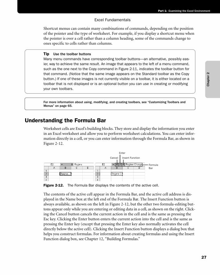
Excel Fundamentals

27

Part 1: Examining the Excel Environment

Cha

pter

2

Shortcut menus can contain many combinations of commands, depending on the position of the pointer and the type of worksheet. For example, if you display a shortcut menu when the pointer is over a cell rather than a column heading, some of the commands change to ones specific to cells rather than columns.

Tip Use the toolbar buttonsMany menu commands have corresponding toolbar buttons—an alternative, possibly eas-ier, way to achieve the same result. An image that appears to the left of a menu command, such as the one next to the Copy command in Figure 2-11, indicates the toolbar button for that command. (Notice that the same image appears on the Standard toolbar as the Copy button.) If one of these images is not currently visible on a toolbar, it is either located on a toolbar that is not displayed or is an optional button you can use in creating or modifying your own toolbars.

For more information about using, modifying, and creating toolbars, see “Customizing Toolbars and Menus” on page 65.

Understanding the Formula BarWorksheet cells are Excel’s building blocks. They store and display the information you enter in an Excel worksheet and allow you to perform worksheet calculations. You can enter infor-mation directly in a cell, or you can enter information through the Formula Bar, as shown in Figure 2-12.

f02ie12

Figure 2-12. The Formula Bar displays the contents of the active cell.

The contents of the active cell appear in the Formula Bar, and the active cell address is dis-played in the Name box at the left end of the Formula Bar. The Insert Function button is always available, as shown on the left in Figure 2-12, but the other two formula-editing but-tons appear only while you are entering or editing data in a cell, as shown on the right. Click-ing the Cancel button cancels the current action in the cell and is the same as pressing theEsc key. Clicking the Enter button enters the current action into the cell and is the same as pressing the Enter key (except that pressing the Enter key also normally activates the cell directly below the active cell). Clicking the Insert Function button displays a dialog box that helps you construct formulas. For information about creating formulas and using the Insert Function dialog box, see Chapter 12, “Building Formulas.”

Enter

FormulaBar

Insert FunctionCancel

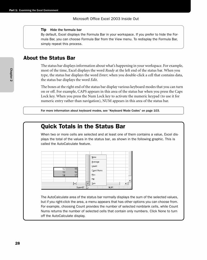
Chapter 2

Microsoft Office Excel 2003 Inside Out

Part 1: Examining the Excel Environment

28

Tip Hide the formula barBy default, Excel displays the Formula Bar in your workspace. If you prefer to hide the For-mula Bar, you can choose Formula Bar from the View menu. To redisplay the Formula Bar, simply repeat this process.

About the Status BarThe status bar displays information about what’s happening in your workspace. For example, most of the time, Excel displays the word Ready at the left end of the status bar. When you type, the status bar displays the word Enter; when you double-click a cell that contains data, the status bar displays the word Edit.

The boxes at the right end of the status bar display various keyboard modes that you can turn on or off. For example, CAPS appears in this area of the status bar when you press the Caps Lock key. When you press the Num Lock key to activate the numeric keypad (to use it for numeric entry rather than navigation), NUM appears in this area of the status bar.

For more information about keyboard modes, see “Keyboard Mode Codes” on page 103.

Quick Totals in the Status BarWhen two or more cells are selected and at least one of them contains a value, Excel dis-plays the total of the values in the status bar, as shown in the following graphic. This is called the AutoCalculate feature.

g02ie02

The AutoCalculate area of the status bar normally displays the sum of the selected values, but if you right-click the area, a menu appears that has other options you can choose from. For example, choosing Count provides the number of selected nonblank cells, while Count Nums returns the number of selected cells that contain only numbers. Click None to turn off the AutoCalculate display.

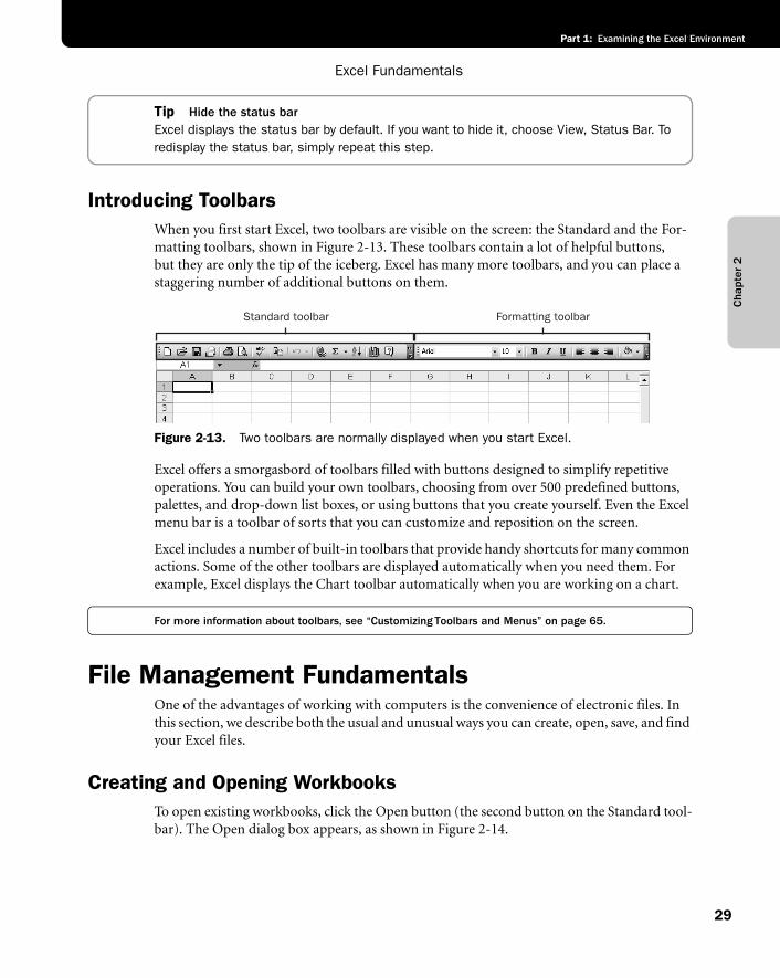
Excel Fundamentals

29

Part 1: Examining the Excel Environment

Cha

pter

2

Tip Hide the status barExcel displays the status bar by default. If you want to hide it, choose View, Status Bar. To redisplay the status bar, simply repeat this step.

Introducing ToolbarsWhen you first start Excel, two toolbars are visible on the screen: the Standard and the For-matting toolbars, shown in Figure 2-13. These toolbars contain a lot of helpful buttons, but they are only the tip of the iceberg. Excel has many more toolbars, and you can place a staggering number of additional buttons on them.

f02ie13

Figure 2-13. Two toolbars are normally displayed when you start Excel.

Excel offers a smorgasbord of toolbars filled with buttons designed to simplify repetitive operations. You can build your own toolbars, choosing from over 500 predefined buttons, palettes, and drop-down list boxes, or using buttons that you create yourself. Even the Excel menu bar is a toolbar of sorts that you can customize and reposition on the screen.

Excel includes a number of built-in toolbars that provide handy shortcuts for many common actions. Some of the other toolbars are displayed automatically when you need them. For example, Excel displays the Chart toolbar automatically when you are working on a chart.

For more information about toolbars, see “Customizing Toolbars and Menus” on page 65.

File Management FundamentalsOne of the advantages of working with computers is the convenience of electronic files. In this section, we describe both the usual and unusual ways you can create, open, save, and find your Excel files.

Creating and Opening WorkbooksTo open existing workbooks, click the Open button (the second button on the Standard tool-bar). The Open dialog box appears, as shown in Figure 2-14.

Standard toolbar Formatting toolbar

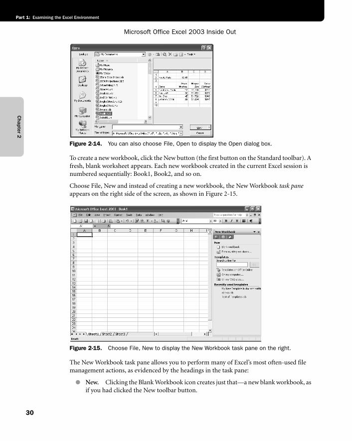
Chapter 2

Microsoft Office Excel 2003 Inside Out

Part 1: Examining the Excel Environment

30

f02ie14

Figure 2-14. You can also choose File, Open to display the Open dialog box.

To create a new workbook, click the New button (the first button on the Standard toolbar). A fresh, blank worksheet appears. Each new workbook created in the current Excel session is numbered sequentially: Book1, Book2, and so on.

Choose File, New and instead of creating a new workbook, the New Workbook task paneappears on the right side of the screen, as shown in Figure 2-15.

f02ie15

Figure 2-15. Choose File, New to display the New Workbook task pane on the right.

The New Workbook task pane allows you to perform many of Excel’s most often-used file management actions, as evidenced by the headings in the task pane:

● New. Clicking the Blank Workbook icon creates just that—a new blank workbook, as if you had clicked the New toolbar button.

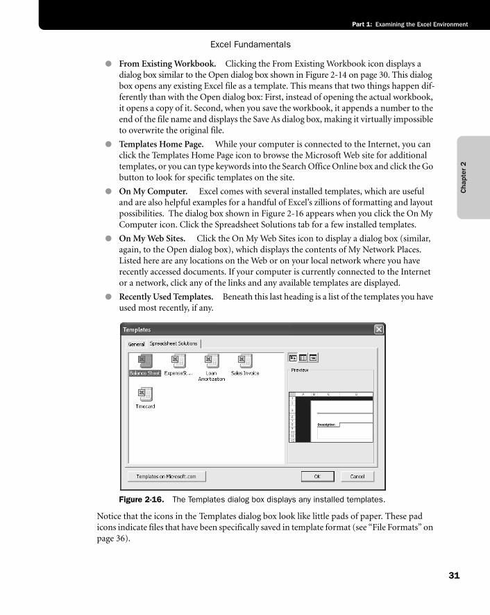
Excel Fundamentals

31

Part 1: Examining the Excel Environment

Cha

pter

2

● From Existing Workbook. Clicking the From Existing Workbook icon displays a dialog box similar to the Open dialog box shown in Figure 2-14 on page 30. This dialog box opens any existing Excel file as a template. This means that two things happen dif-ferently than with the Open dialog box: First, instead of opening the actual workbook, it opens a copy of it. Second, when you save the workbook, it appends a number to the end of the file name and displays the Save As dialog box, making it virtually impossible to overwrite the original file.

● Templates Home Page. While your computer is connected to the Internet, you can click the Templates Home Page icon to browse the Microsoft Web site for additional templates, or you can type keywords into the Search Office Online box and click the Go button to look for specific templates on the site.

● On My Computer. Excel comes with several installed templates, which are useful and are also helpful examples for a handful of Excel’s zillions of formatting and layout possibilities. The dialog box shown in Figure 2-16 appears when you click the On My Computer icon. Click the Spreadsheet Solutions tab for a few installed templates.

● On My Web Sites. Click the On My Web Sites icon to display a dialog box (similar, again, to the Open dialog box), which displays the contents of My Network Places. Listed here are any locations on the Web or on your local network where you have recently accessed documents. If your computer is currently connected to the Internet or a network, click any of the links and any available templates are displayed.

● Recently Used Templates. Beneath this last heading is a list of the templates you have used most recently, if any.

f02ie16 Figure 2-16. The Templates dialog box displays any installed templates.

Notice that the icons in the Templates dialog box look like little pads of paper. These pad icons indicate files that have been specifically saved in template format (see “File Formats” on page 36).

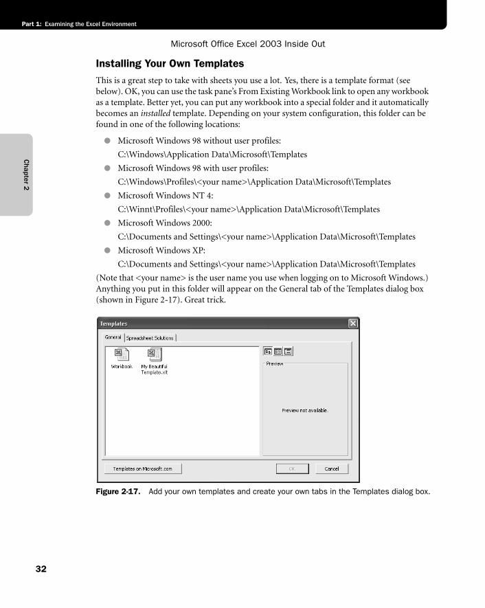
Chapter 2

Microsoft Office Excel 2003 Inside Out

Part 1: Examining the Excel Environment

32

Installing Your Own TemplatesThis is a great step to take with sheets you use a lot. Yes, there is a template format (see below). OK, you can use the task pane’s From Existing Workbook link to open any workbook as a template. Better yet, you can put any workbook into a special folder and it automatically becomes an installed template. Depending on your system configuration, this folder can be found in one of the following locations:

● Microsoft Windows 98 without user profiles:

C:\Windows\Application Data\Microsoft\Templates

● Microsoft Windows 98 with user profiles:

C:\Windows\Profiles\<your name>\Application Data\Microsoft\Templates

● Microsoft Windows NT 4:

C:\Winnt\Profiles\<your name>\Application Data\Microsoft\Templates

● Microsoft Windows 2000:

C:\Documents and Settings\<your name>\Application Data\Microsoft\Templates

● Microsoft Windows XP:

C:\Documents and Settings\<your name>\Application Data\Microsoft\Templates

(Note that <your name> is the user name you use when logging on to Microsoft Windows.) Anything you put in this folder will appear on the General tab of the Templates dialog box (shown in Figure 2-17). Great trick.

f02ie17

Figure 2-17. Add your own templates and create your own tabs in the Templates dialog box.

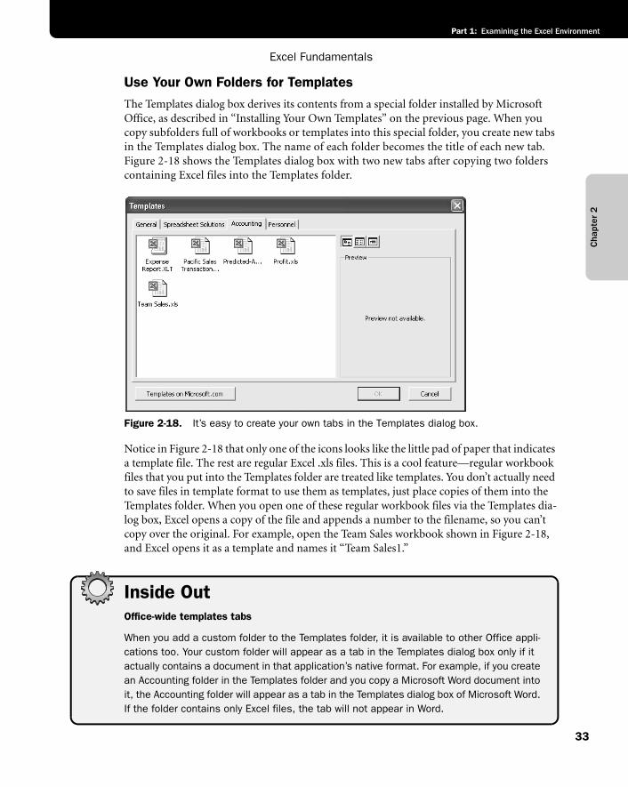
Excel Fundamentals

33

Part 1: Examining the Excel Environment

Cha

pter

2

Use Your Own Folders for TemplatesThe Templates dialog box derives its contents from a special folder installed by Microsoft Office, as described in “Installing Your Own Templates” on the previous page. When you copy subfolders full of workbooks or templates into this special folder, you create new tabs in the Templates dialog box. The name of each folder becomes the title of each new tab. Figure 2-18 shows the Templates dialog box with two new tabs after copying two folders containing Excel files into the Templates folder.

f02ie18

Figure 2-18. It’s easy to create your own tabs in the Templates dialog box.

Notice in Figure 2-18 that only one of the icons looks like the little pad of paper that indicates a template file. The rest are regular Excel .xls files. This is a cool feature—regular workbook files that you put into the Templates folder are treated like templates. You don’t actually need to save files in template format to use them as templates, just place copies of them into the Templates folder. When you open one of these regular workbook files via the Templates dia-log box, Excel opens a copy of the file and appends a number to the filename, so you can’t copy over the original. For example, open the Team Sales workbook shown in Figure 2-18, and Excel opens it as a template and names it “Team Sales1.”

Inside OutOffice-wide templates tabs

When you add a custom folder to the Templates folder, it is available to other Office appli-cations too. Your custom folder will appear as a tab in the Templates dialog box only if it actually contains a document in that application’s native format. For example, if you create an Accounting folder in the Templates folder and you copy a Microsoft Word document into it, the Accounting folder will appear as a tab in the Templates dialog box of Microsoft Word. If the folder contains only Excel files, the tab will not appear in Word.

Chapter 2

Microsoft Office Excel 2003 Inside Out

Part 1: Examining the Excel Environment

34

Changing the Default Book and SheetWant to design your own “blank” workbook? You can create two templates to do this—one that determines the format and content of all new workbooks (Book.xlt), and one that deter-mines the format and content of all individual sheets you insert using the Insert, Worksheet command (Sheet.xlt). These are special files that you create and save in a certain place:

C:\Documents and Settings<your name>\Application Data\Microsoft\Excel\XLStart

You save an .xlt file by choosing Save As from the File menu and selecting Template in the Save As Type drop-down list at the bottom of the Save As dialog box.

Note Any workbook that you place in the XLStart folder is opened automatically each time you start Excel (except workbooks named Book.xls or Sheet.xls).

These files override the standard appearance and content of new workbooks and new work-sheets. Even the default Book1 that appears every time you start Excel takes on the character-istics you supply in Book.xlt. If you want to revert to the original, simply remove the files from the XLStart folder.

Note that by using these files you can not only change the formatting, but you can also include text, graphics, formulas, custom toolbars, macros, and certain window and calcula-tion options. You can also determine the number and type of default sheets present in both new workbooks and inserted worksheets. That’s right, you can actually save the workbook Sheet.xlt with four worksheets. Then when you choose Insert, Worksheet you will actually be inserting four worksheets instead of just one. If you don’t want this to happen, simply delete additional sheets before saving Sheet.xlt.

Saving Files

For more information about saving workbooks as Web pages, see “Saving and Publishing Excel Files in HTML” in Chapter 20.

Arguably the most important yet boring function of any computer application is preserving data. But here in Inside-Out Land, we seek to expose the truth, however boring! In Excel, there are many ways that your files can be saved, including the Save, Save As, Save As Web Page, Save Workspace, Close, and Exit commands, and the easiest way to save—clicking the Save button on the Standard toolbar.

One other command that saves your workbooks is the Share Workbook command on the Tools menu. When you choose this command, your workbook is saved in shared mode. Besides saving the file, this command makes the workbook available to others on a network, who may open it and make changes of their own.

For more information, see “Sharing Workbooks on a Network” on page 522.

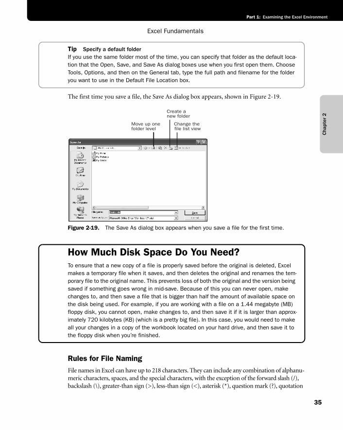
Excel Fundamentals

35

Part 1: Examining the Excel Environment

Cha

pter

2

Tip Specify a default folderIf you use the same folder most of the time, you can specify that folder as the default loca-tion that the Open, Save, and Save As dialog boxes use when you first open them. Choose Tools, Options, and then on the General tab, type the full path and filename for the folder you want to use in the Default File Location box.

The first time you save a file, the Save As dialog box appears, shown in Figure 2-19.

f02ie19

Figure 2-19. The Save As dialog box appears when you save a file for the first time.

How Much Disk Space Do You Need?To ensure that a new copy of a file is properly saved before the original is deleted, Excel makes a temporary file when it saves, and then deletes the original and renames the tem-porary file to the original name. This prevents loss of both the original and the version being saved if something goes wrong in mid-save. Because of this you can never open, make changes to, and then save a file that is bigger than half the amount of available space on the disk being used. For example, if you are working with a file on a 1.44 megabyte (MB) floppy disk, you cannot open, make changes to, and then save it if it is larger than approx-imately 720 kilobytes (KB) (which is a pretty big file). In this case, you would need to make all your changes in a copy of the workbook located on your hard drive, and then save it to the floppy disk when you’re finished.

Rules for File NamingFile names in Excel can have up to 218 characters. They can include any combination of alphanu-meric characters, spaces, and the special characters, with the exception of the forward slash (/), backslash (\), greater-than sign (>), less-than sign (<), asterisk (*), question mark (?), quotation

Move up one folder level

Change the file list view

Create anew folder

Chapter 2

Microsoft Office Excel 2003 Inside Out

Part 1: Examining the Excel Environment

36

mark (“), pipe symbol (|), colon (:), and semicolon (;). Although you can use any combination of uppercase and lowercase letters, keep in mind that Excel does not distinguish case in file names. For example, to Excel the names “MYFILE,” “MyFile,” and “myfile” are identical.

The familiar MS-DOS three-character file extension helps identify your Excel files, and it is added automatically when you save a file. Note, however, that file extensions may not appear with Windows file names depending on your settings. The following table lists some of Excel’s default extensions.

File FormatsIn addition to providing the file name and location, you can specify a different file format in the File, Save As dialog box. Click the arrow to the right of the Save As Type drop-down list box. The list expands to reveal all the formats in which you can save your files.

For more information about Excel’s export formats, see “Importing and Exporting Files” on page 48.

The default format is Microsoft Excel Workbook, and you’ll almost always use this option. If you want to export an Excel file to another program, however, you can use one of the other options to convert the file to a format that is readable by that program.

Document Types in Previous Versions of Excel In Microsoft Excel versions 5 through 11, worksheets, chart sheets, Excel 5 dialog sheets, and Excel 4 macro sheets are all contained in workbooks. In previous versions of Excel, worksheets, chart sheets, and macro sheets were saved separately. When you open one of these earlier sheet types in Excel 2003, it is automat-ically converted to an Excel 2003 workbook, which you can then choose to save in the current Excel format or keep in its original format. You can also combine sheets from a previous ver-sion of Excel into a single Excel 2003 workbook.

Excel 5 workbooks were compatible with Excel 95 and vice versa. This meant that you could save a workbook in Excel 95, and then open it in Excel 5 without problems. The last four versions of Excel share a somewhat different file format than the one shared by Excel 95 and Excel 5. To accommodate situations in which you must share files with others using different versions of Excel, The Files Of Type list in the Save As dialog box includes the special formats Microsoft Excel 5.0/95 Workbook and Microsoft Excel 97-Excel 2002 and 5.0/95 Workbook, the latter of which saves workbooks in these two formats simultaneously. Users of any of these versions of Excel can open a file saved in this format, but if someone using Excel 95 or Excel 5 saves changes to it, any features from Excel versions 2000 through 2003 and formatting are lost.

Document Type Extension

Add-in .XLA

Backup .XLK

Template .XLT

Workbook .XLS

Workspace .XLW

XML Spreadsheet .XML

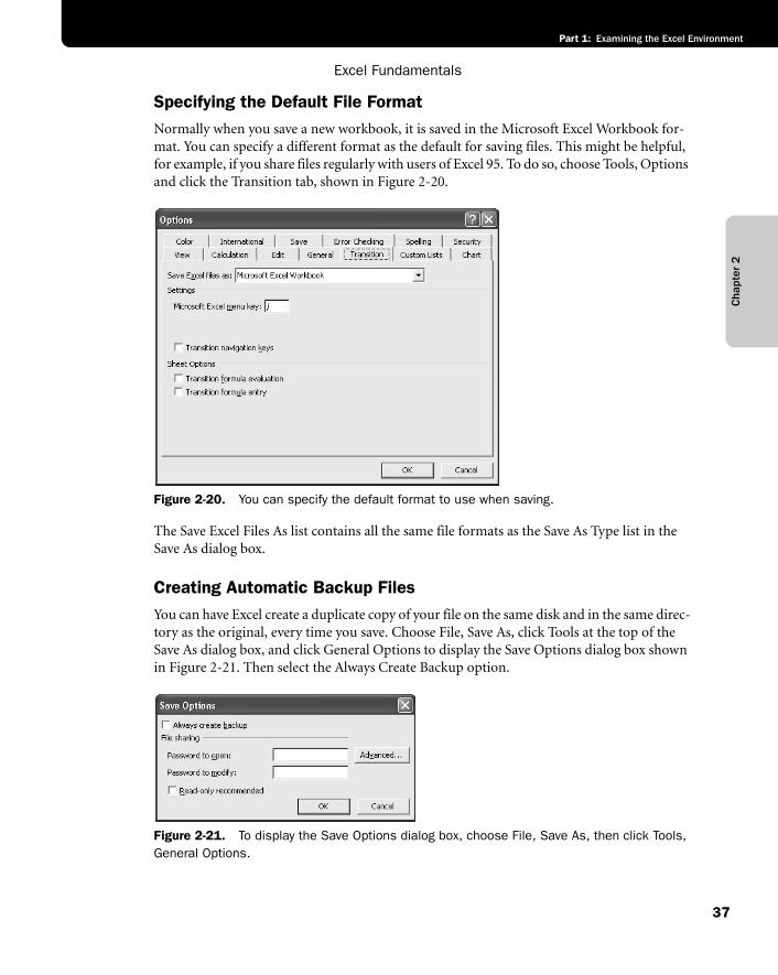
Excel Fundamentals

37

Part 1: Examining the Excel Environment

Cha

pter

2

Specifying the Default File FormatNormally when you save a new workbook, it is saved in the Microsoft Excel Workbook for-mat. You can specify a different format as the default for saving files. This might be helpful, for example, if you share files regularly with users of Excel 95. To do so, choose Tools, Options and click the Transition tab, shown in Figure 2-20.

f02ie20

Figure 2-20. You can specify the default format to use when saving.

The Save Excel Files As list contains all the same file formats as the Save As Type list in the Save As dialog box.

Creating Automatic Backup FilesYou can have Excel create a duplicate copy of your file on the same disk and in the same direc-tory as the original, every time you save. Choose File, Save As, click Tools at the top of the Save As dialog box, and click General Options to display the Save Options dialog box shown in Figure 2-21. Then select the Always Create Backup option.

f02ie21

Figure 2-21. To display the Save Options dialog box, choose File, Save As, then click Tools, General Options.

Chapter 2

Microsoft Office Excel 2003 Inside Out

Part 1: Examining the Excel Environment

38

The backup file is a duplicate file that carries the same name as your original, but the name is preceded by “Backup of” and has the file extension XLK.

Inside OutDon’t duplicate file names

Keep in mind that Excel always uses an XLK extension when creating backup files regard-less of the file type. Suppose you work with a workbook named Myfile.XLS as well as a tem-plate file on disk named Myfile.XLT, and you select the Always Create Backup option for both. Because only one Myfile.XLK can exist, the most recently saved file is saved as the XLK file and Excel overwrites the other file’s backup if one exists.

Protecting FilesYou can password-protect your files by using options in the Save Options dialog box shown in Figure 2-21 on the previous page. Choose from two types of passwords: Password To Open and Password To Modify. Passwords can have up to 15 characters and capitalization matters. Thus, if you assign the password Secret to a file, you can’t reopen that file by typing SECRETor secret. For added security, Excel does not display passwords on the screen when you type them to open a protected file.

● When you assign a Password To Open to a file and then you close it, Excel prompts you to supply that password before reopening the file.

● When you assign a Password To Modify, anyone can open the file as read-only, but they cannot open the original or save the file using the same name if they haven’t opened it using the password.

● A third protection option, the Read-Only Recommended option, augments the secu-rity that passwords provide. If less stringent security meets your needs, this option gently suggests that the user open the file as read-only.

Tip Create a better passwordAlthough Excel’s under-the-hood security measures have been tightened over the years, there are always people who delight in finding new and better ways to crack passwords. You can help by simply using better passwords. Make sure that your password is eight or more characters long—the longer the better—and try to use a healthy mix of capital and lower-case characters as well as numeric characters.

Adding Summary Information to FilesWhen you choose File, Properties, Excel displays a Properties dialog box that you use to record general information about the active workbook. The Properties dialog box is shown in Figure 2-22.

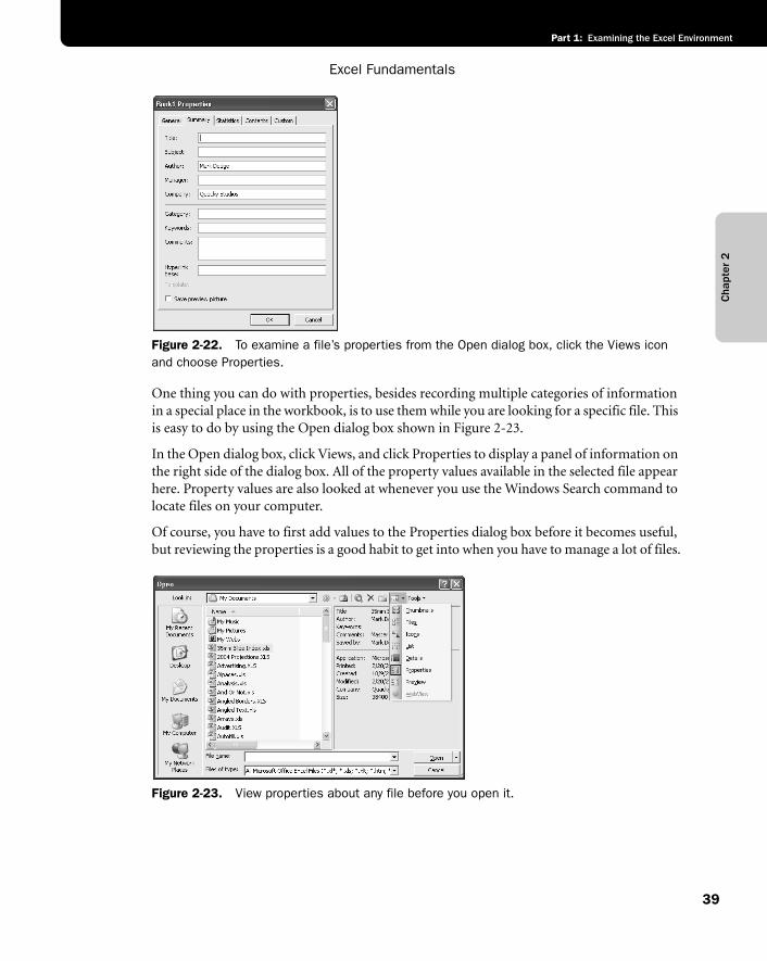
Excel Fundamentals

39

Part 1: Examining the Excel Environment

Cha

pter

2

f02ie22

Figure 2-22. To examine a file’s properties from the Open dialog box, click the Views icon and choose Properties.

One thing you can do with properties, besides recording multiple categories of information in a special place in the workbook, is to use them while you are looking for a specific file. This is easy to do by using the Open dialog box shown in Figure 2-23.

In the Open dialog box, click Views, and click Properties to display a panel of information on the right side of the dialog box. All of the property values available in the selected file appear here. Property values are also looked at whenever you use the Windows Search command to locate files on your computer.

Of course, you have to first add values to the Properties dialog box before it becomes useful, but reviewing the properties is a good habit to get into when you have to manage a lot of files.

f02ie23

Figure 2-23. View properties about any file before you open it.

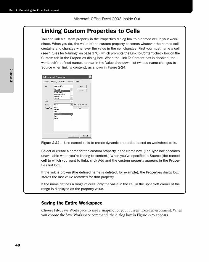
Chapter 2

Microsoft Office Excel 2003 Inside Out

Part 1: Examining the Excel Environment

40

Linking Custom Properties to CellsYou can link a custom property in the Properties dialog box to a named cell in your work-sheet. When you do, the value of the custom property becomes whatever the named cell contains and changes whenever the value in the cell changes. First you must name a cell (see “Rules for Naming” on page 370), which prompts the Link To Content check box on the Custom tab in the Properties dialog box. When the Link To Content box is checked, the workbook’s defined names appear in the Value drop-down list (whose name changes to Source when linking content), as shown in Figure 2-24.

f02ie24

Figure 2-24. Use named cells to create dynamic properties based on worksheet cells.

Select or create a name for the custom property in the Name box. (The Type box becomes unavailable when you’re linking to content.) When you’ve specified a Source (the named cell to which you want to link), click Add and the custom property appears in the Proper-ties list box.

If the link is broken (the defined name is deleted, for example), the Properties dialog box stores the last value recorded for that property.

If the name defines a range of cells, only the value in the cell in the upper-left corner of the range is displayed as the property value.

Saving the Entire WorkspaceChoose File, Save Workspace to save a snapshot of your current Excel environment. When you choose the Save Workspace command, the dialog box in Figure 2-25 appears.

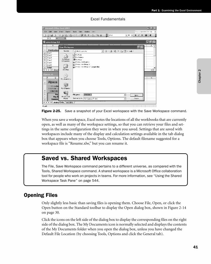
Excel Fundamentals

41

Part 1: Examining the Excel Environment

Cha

pter

2

f02ie25

Figure 2-25. Save a snapshot of your Excel workspace with the Save Workspace command.

When you save a workspace, Excel notes the locations of all the workbooks that are currently open, as well as many of the workspace settings, so that you can retrieve your files and set-tings in the same configuration they were in when you saved. Settings that are saved with workspaces include many of the display and calculation settings available in the tab dialog box that appears when you choose Tools, Options. The default filename suggested for a workspace file is “Resume.xlw,” but you can rename it.

Saved vs. Shared WorkspacesThe File, Save Workspace command pertains to a different universe, as compared with the Tools, Shared Workspace command. A shared workspace is a Microsoft Office collaboration tool for people who work on projects in teams. For more information, see “Using the Shared Workspace Task Pane” on page 544.

Opening FilesOnly slightly less basic than saving files is opening them. Choose File, Open, or click the Open button on the Standard toolbar to display the Open dialog box, shown in Figure 2-14 on page 30.

Click the icons on the left side of the dialog box to display the corresponding files on the right side of the dialog box. The My Documents icon is normally selected and displays the contents of the My Documents folder when you open the dialog box, unless you have changed the Default File Location (by choosing Tools, Options and click the General tab).

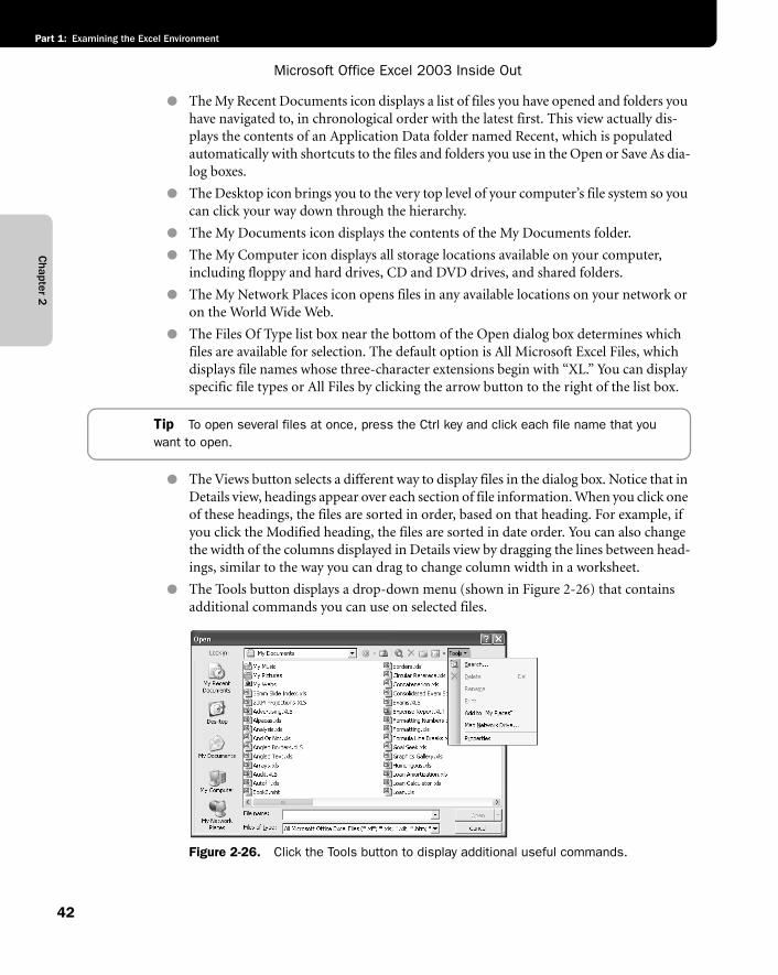
Chapter 2

Microsoft Office Excel 2003 Inside Out

Part 1: Examining the Excel Environment

42

● The My Recent Documents icon displays a list of files you have opened and folders you have navigated to, in chronological order with the latest first. This view actually dis-plays the contents of an Application Data folder named Recent, which is populated automatically with shortcuts to the files and folders you use in the Open or Save As dia-log boxes.

● The Desktop icon brings you to the very top level of your computer’s file system so you can click your way down through the hierarchy.

● The My Documents icon displays the contents of the My Documents folder.

● The My Computer icon displays all storage locations available on your computer, including floppy and hard drives, CD and DVD drives, and shared folders.

● The My Network Places icon opens files in any available locations on your network or on the World Wide Web.

● The Files Of Type list box near the bottom of the Open dialog box determines which files are available for selection. The default option is All Microsoft Excel Files, which displays file names whose three-character extensions begin with “XL.” You can display specific file types or All Files by clicking the arrow button to the right of the list box.

Tip To open several files at once, press the Ctrl key and click each file name that you want to open.

● The Views button selects a different way to display files in the dialog box. Notice that in Details view, headings appear over each section of file information. When you click one of these headings, the files are sorted in order, based on that heading. For example, if you click the Modified heading, the files are sorted in date order. You can also change the width of the columns displayed in Details view by dragging the lines between head-ings, similar to the way you can drag to change column width in a worksheet.

● The Tools button displays a drop-down menu (shown in Figure 2-26) that contains additional commands you can use on selected files.

f02ie26

Figure 2-26. Click the Tools button to display additional useful commands.

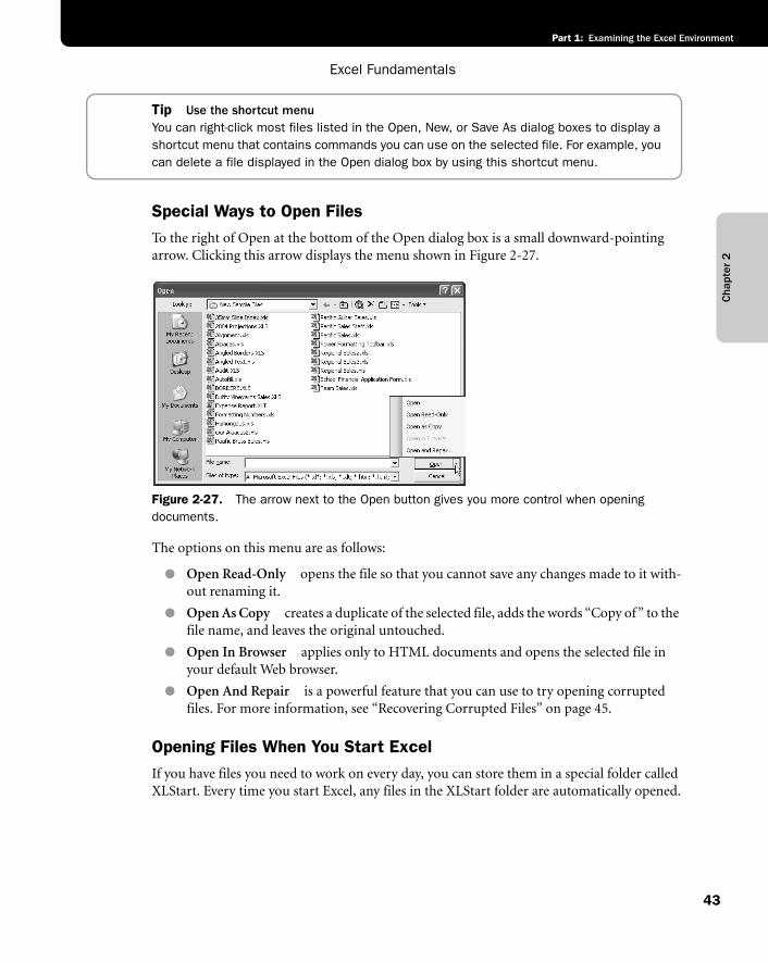
Excel Fundamentals

43

Part 1: Examining the Excel Environment

Cha

pter

2

Tip Use the shortcut menuYou can right-click most files listed in the Open, New, or Save As dialog boxes to display a shortcut menu that contains commands you can use on the selected file. For example, you can delete a file displayed in the Open dialog box by using this shortcut menu.

Special Ways to Open FilesTo the right of Open at the bottom of the Open dialog box is a small downward-pointing arrow. Clicking this arrow displays the menu shown in Figure 2-27.

f02ie27

Figure 2-27. The arrow next to the Open button gives you more control when opening documents.

The options on this menu are as follows:

● Open Read-Only opens the file so that you cannot save any changes made to it with-out renaming it.

● Open As Copy creates a duplicate of the selected file, adds the words “Copy of” to the file name, and leaves the original untouched.

● Open In Browser applies only to HTML documents and opens the selected file in your default Web browser.

● Open And Repair is a powerful feature that you can use to try opening corrupted files. For more information, see “Recovering Corrupted Files” on page 45.

Opening Files When You Start ExcelIf you have files you need to work on every day, you can store them in a special folder called XLStart. Every time you start Excel, any files in the XLStart folder are automatically opened.

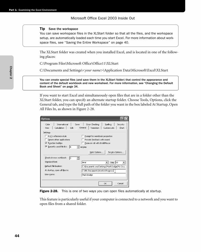
Chapter 2

Microsoft Office Excel 2003 Inside Out

Part 1: Examining the Excel Environment

44

Tip Save the workspaceYou can save workspace files in the XLStart folder so that all the files, and the workspace setup, are automatically loaded each time you start Excel. For more information about work-space files, see “Saving the Entire Workspace” on page 40.

The XLStart folder was created when you installed Excel, and is located in one of the follow-ing places:

C:\Program Files\Microsoft Office\Office11\XLStart

C:\Documents and Settings\<your name>\Application Data\Microsoft\Excel\XLStart

You can create special files (and save them in the XLStart folder) that control the appearance and content of the default workbook and new worksheet. For more information, see “Changing the Default Book and Sheet” on page 34.

If you want to start Excel and simultaneously open files that are in a folder other than the XLStart folder, you can specify an alternate startup folder. Choose Tools, Options, click the General tab, and type the full path of the folder you want in the box labeled At Startup, Open All Files In, as shown in Figure 2-28.

f02ie28

Figure 2-28. This is one of two ways you can open files automatically at startup.

This feature is particularly useful if your computer is connected to a network and you want to open files from a shared folder.

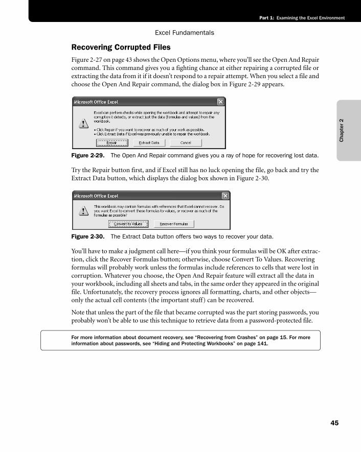
Excel Fundamentals

45

Part 1: Examining the Excel Environment

Cha

pter

2

Recovering Corrupted FilesFigure 2-27 on page 43 shows the Open Options menu, where you’ll see the Open And Repair command. This command gives you a fighting chance at either repairing a corrupted file or extracting the data from it if it doesn’t respond to a repair attempt. When you select a file and choose the Open And Repair command, the dialog box in Figure 2-29 appears.

f02ie29

Figure 2-29. The Open And Repair command gives you a ray of hope for recovering lost data.

Try the Repair button first, and if Excel still has no luck opening the file, go back and try the Extract Data button, which displays the dialog box shown in Figure 2-30.

f02ie30

Figure 2-30. The Extract Data button offers two ways to recover your data.

You’ll have to make a judgment call here—if you think your formulas will be OK after extrac-tion, click the Recover Formulas button; otherwise, choose Convert To Values. Recovering formulas will probably work unless the formulas include references to cells that were lost in corruption. Whatever you choose, the Open And Repair feature will extract all the data in your workbook, including all sheets and tabs, in the same order they appeared in the original file. Unfortunately, the recovery process ignores all formatting, charts, and other objects—only the actual cell contents (the important stuff) can be recovered.

Note that unless the part of the file that became corrupted was the part storing passwords, you probably won’t be able to use this technique to retrieve data from a password-protected file.

For more information about document recovery, see “Recovering from Crashes” on page 15. For more information about passwords, see “Hiding and Protecting Workbooks” on page 141.

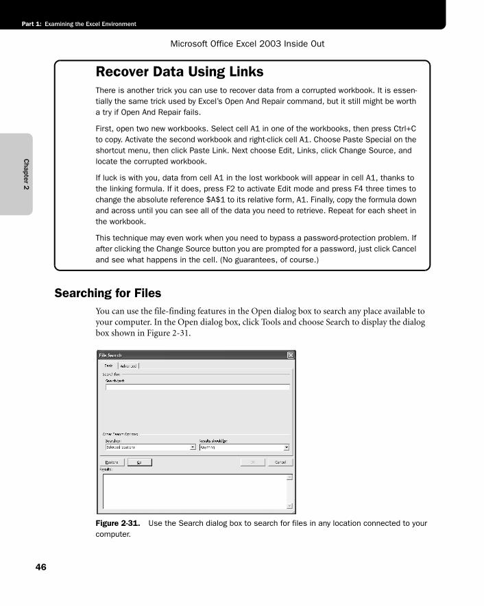
Chapter 2

Microsoft Office Excel 2003 Inside Out

Part 1: Examining the Excel Environment

46

Recover Data Using Links There is another trick you can use to recover data from a corrupted workbook. It is essen-tially the same trick used by Excel’s Open And Repair command, but it still might be worth a try if Open And Repair fails.

First, open two new workbooks. Select cell A1 in one of the workbooks, then press Ctrl+C to copy. Activate the second workbook and right-click cell A1. Choose Paste Special on the shortcut menu, then click Paste Link. Next choose Edit, Links, click Change Source, and locate the corrupted workbook.

If luck is with you, data from cell A1 in the lost workbook will appear in cell A1, thanks to the linking formula. If it does, press F2 to activate Edit mode and press F4 three times to change the absolute reference $A$1 to its relative form, A1. Finally, copy the formula down and across until you can see all of the data you need to retrieve. Repeat for each sheet in the workbook.

This technique may even work when you need to bypass a password-protection problem. If after clicking the Change Source button you are prompted for a password, just click Cancel and see what happens in the cell. (No guarantees, of course.)

Searching for FilesYou can use the file-finding features in the Open dialog box to search any place available to your computer. In the Open dialog box, click Tools and choose Search to display the dialog box shown in Figure 2-31.

f02ie31

Figure 2-31. Use the Search dialog box to search for files in any location connected to your computer.

Excel Fundamentals

47

Part 1: Examining the Excel Environment

Cha

pter

2

For more information about network issues, see “Sharing Workbooks on a Network” on page 522.

You can simply type something into the Search Text box and then click Search to start your search. However, we recommend that you first use the Other Search Options drop-down lists to narrow the search to certain locations and file types if you don’t have a lot of time to wait while every file on your hard drive is inspected. A list of links to found files appears at the bot-tom of the dialog box. Click OK, or double-click a link to close the Search dialog box and insert the file location into the File Name box in the Open dialog box.

Click the Advanced tab in the Search dialog box to add more criteria to narrow your search. Create one criterion at a time using the Search For options at the top of the dialog box, and add as many criteria as you want. Once you have specified Property, Condition, and Value, click Add to add your criteria to the list. You can add as many criteria as you need.

● The Property list includes most of the properties available in the Properties dialog box.

For more on the Properties dialog box, see “Adding Summary Information to Files” on page 38.

● The contents of the Condition box change depending on what you select in the Prop-erty box. For example, if you choose the Creation Date property, the list of conditions includes “on or after,” “today,” “last month,” and so on.

● You make entries in the Value box that are appropriate for the specified condition. For example, you’d enter a date in the Value box if the selected condition is Creation Date.

● Use And and Or to specify whether each criterion you add is “in addition to” or “instead of” the previous criterion. Some property types allow only one “And.” For example, if you attempt to add another Files Of Type criterion with And selected, a dia-log box informs you that a file type already appears in the criteria list and asks if you want to change it to an “Or” criteria.

● Remove any selected criteria by clicking Remove, or click Remove All to clear the crite-ria list.

● Click Search to begin; click Restore to clear the search results but leave the criteria intact.

● When you find the file you’re looking for, click OK to insert the location of the selected file into the File Name box in the Open dialog box.

● The next time you use the Search dialog box, the last search criteria you used is retained in case you want to use it again.

Tip Set a properties reminderTo help you get into the habit of entering properties to identify groups of files, you can have the Properties dialog box appear automatically each time you save a file for the first time. Choose Tools, Options, and click the General tab, and click the Prompt For Workbook Prop-erties option.

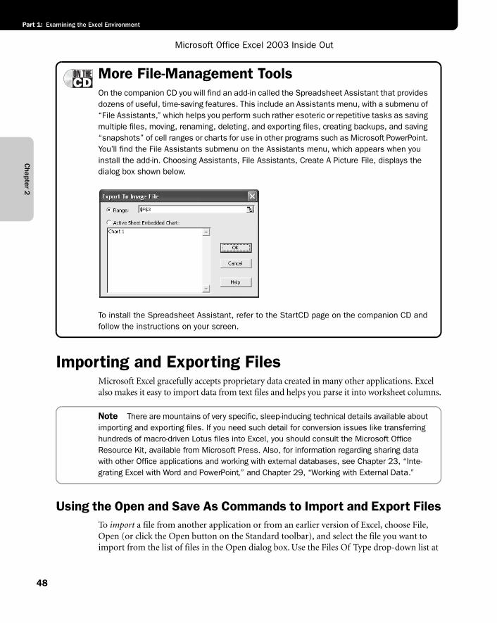
Chapter 2

Microsoft Office Excel 2003 Inside Out

Part 1: Examining the Excel Environment

48

More File-Management ToolsOn the companion CD you will find an add-in called the Spreadsheet Assistant that provides dozens of useful, time-saving features. This include an Assistants menu, with a submenu of “File Assistants,” which helps you perform such rather esoteric or repetitive tasks as saving multiple files, moving, renaming, deleting, and exporting files, creating backups, and saving “snapshots” of cell ranges or charts for use in other programs such as Microsoft PowerPoint. You’ll find the File Assistants submenu on the Assistants menu, which appears when you install the add-in. Choosing Assistants, File Assistants, Create A Picture File, displays the dialog box shown below.

g02ie04

To install the Spreadsheet Assistant, refer to the StartCD page on the companion CD and follow the instructions on your screen.

Importing and Exporting FilesMicrosoft Excel gracefully accepts proprietary data created in many other applications. Excel also makes it easy to import data from text files and helps you parse it into worksheet columns.

Note There are mountains of very specific, sleep-inducing technical details available about importing and exporting files. If you need such detail for conversion issues like transferring hundreds of macro-driven Lotus files into Excel, you should consult the Microsoft Office Resource Kit, available from Microsoft Press. Also, for information regarding sharing data with other Office applications and working with external databases, see Chapter 23, “Inte-grating Excel with Word and PowerPoint,” and Chapter 29, “Working with External Data.”

Using the Open and Save As Commands to Import and Export FilesTo import a file from another application or from an earlier version of Excel, choose File, Open (or click the Open button on the Standard toolbar), and select the file you want to import from the list of files in the Open dialog box. Use the Files Of Type drop-down list at

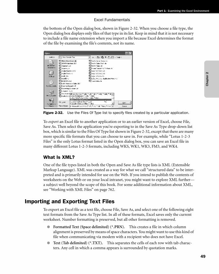
Excel Fundamentals

49

Part 1: Examining the Excel Environment

Cha

pter

2

the bottom of the Open dialog box, shown in Figure 2-32. When you choose a file type, the Open dialog box displays only files of that type in its list. Keep in mind that it is not necessary to include a file name extension when you import a file because Excel determines the format of the file by examining the file’s contents, not its name.

f02ie32

Figure 2-32. Use the Files Of Type list to specify files created by a particular application.

To export an Excel file to another application or to an earlier version of Excel, choose File, Save As. Then select the application you’re exporting to in the Save As Type drop-down list box, which is similar to the Files Of Type list shown in Figure 2-32, except that there are many more specific file formats that you can choose to save in. For example, while “Lotus 1-2-3 Files” is the only Lotus format listed in the Open dialog box, you can save an Excel file in many different Lotus 1-2-3 formats, including WKS, WK1, WK3, FM3, and WK4.

What Is XML?One of the file types listed in both the Open and Save As file type lists is XML (Extensible Markup Language). XML was created as a way for what we call “structured data” to be inter-preted and is primarily intended for use on the Web. If you intend to publish the contents of worksheets on the Web or on your local intranet, you might want to explore XML further—a subject well beyond the scope of this book. For some additional information about XML, see “Working with XML Files” on page 762.

Importing and Exporting Text FilesTo export an Excel file as a text file, choose File, Save As, and select one of the following eight text formats from the Save As Type list. In all of these formats, Excel saves only the current worksheet. Number formatting is preserved, but all other formatting is removed.

● Formatted Text (Space delimited) (*.PRN). This creates a file in which column alignment is preserved by means of space characters. You might want to use this kind of file when communicating via modem with a recipient who does not have Excel.

● Text (Tab delimited) (*.TXT). This separates the cells of each row with tab charac-ters. Any cell in which a comma appears is surrounded by quotation marks.

Chapter 2

Microsoft Office Excel 2003 Inside Out

Part 1: Examining the Excel Environment

50

● Unicode Text (*.TXT). This is a worldwide standard text format that stores each character as a unique number; Unicode defines a number for every character in every language and on any computer platform.

● CSV (Comma delimited) (*.CSV). This separates the cells of each row with commas. Comma-delimited text files are preferable to tab-delimited files for importing into database management programs. (Many database management programs can accept either form of text file, but some accept only .CSV files.) Also, many word processing applications can use .CSV files to store the information for mail merge operations.

● Text (Macintosh) (*.TXT). The Macintosh options use the Macintosh character set, so select one of these options if you intend to transfer your file to a Macintosh application.

● Text (MS-DOS) (*.TXT). The normal Text and .CSV options use the ANSI character set. You should select one of these options if you intend to import your text file into a Windows-based application, such as Microsoft Word for Windows.

● CSV (Macintosh) (*.CSV). The differences between the normal, Macintosh, and MS-DOS variants of each file type have to do only with characters that lie outside the normal 7-bit ASCII range.

● CSV (MS-DOS) (*.CSV). The MS-DOS options use the IBM PC extended character set. (You might see this also referred to as OEM text.) Select one of these options if you intend to import your text file into a non–Windows-based application.

Note Excel 2003 shares with its predecessors, Excel 2002, Excel 2000, and Excel 97, a file format that is incompatible with previous Excel versions. You can use the Save As com-mand, however, to export Excel 2002/2000/97 workbooks to any earlier version of Excel.

If you regularly share files with colleagues who use Excel 5 or Excel 7, you might want to take advantage of the Microsoft Excel 97-Excel 2003 and 5.0/95 Workbook format. This saves your work in a format that can be read in any of these Excel formats.

Sharing Data with Excel for the MacintoshMicrosoft Excel 98 and 2001 for the Macintosh both use the same file format as Excel 2003, 2002, 2000, and Excel 97. You can share files with Macintosh users by simply transferring files from one computer to the other.

To save an Excel 2002 file to share with someone using the Macintosh version of Excel 5, use the File, Save As command and choose the Microsoft Excel 5.0/95 Workbook option.

Keep the following points in mind:

● To import Macintosh files to your PC, you first need to transfer the file to your PC via a cable, modem, disk, network, or utility program, such as MacOpener. Simply choose File, Open and find the document you want.

● Exporting files from a Windows version of Excel to the Macintosh version is just as easy as importing Macintosh files. Transfer the file from the PC to Macintosh, and use the Open command to load the file just as you would load any other file.

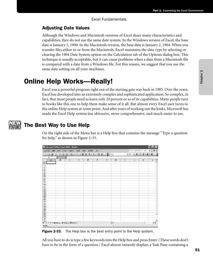
Excel Fundamentals

51

Part 1: Examining the Excel Environment

Cha

pter

2

Adjusting Date ValuesAlthough the Windows and Macintosh versions of Excel share many characteristics and capabilities, they do not use the same date system. In the Windows version of Excel, the base date is January 1, 1900. In the Macintosh version, the base date is January 2, 1904. When you transfer files either to or from the Macintosh, Excel maintains the date type by selecting or clearing the 1904 Date System option on the Calculation tab of the Options dialog box. This technique is usually acceptable, but it can cause problems when a date from a Macintosh file is compared with a date from a Windows file. For this reason, we suggest that you use the same date setting on all your machines.

Online Help Works—Really!Excel was a powerful program right out of the starting gate way back in 1985. Over the years, Excel has developed into an extremely complex and sophisticated application. So complex, in fact, that most people need to learn only 20 percent or so of its capabilities. Many people turn to books like this one to help them make sense of it all. But almost every Excel user turns to the online Help system at some point. And after years of working out the kinks, Microsoft has made the Excel Help system less obtrusive, more comprehensive, and much easier to use.

The Best Way to Use HelpOn the right side of the Menu bar is a Help box that contains the message “Type a question for help,” as shown in Figure 2-33.

f02ie33

Figure 2-33. The Help box is the best entry point to the Help system.

All you have to do is type a few keywords into the Help box and press Enter. (These words don’t have to be in the form of a question.) Excel almost instantly displays a Task Pane containing a

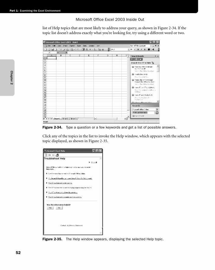
Chapter 2

Microsoft Office Excel 2003 Inside Out

Part 1: Examining the Excel Environment

52

list of Help topics that are most likely to address your query, as shown in Figure 2-34. If the topic list doesn’t address exactly what you’re looking for, try using a different word or two.

f02ie34

Figure 2-34. Type a question or a few keywords and get a list of possible answers.

Click any of the topics in the list to invoke the Help window, which appears with the selected topic displayed, as shown in Figure 2-35.

f02ie35

Figure 2-35. The Help window appears, displaying the selected Help topic.

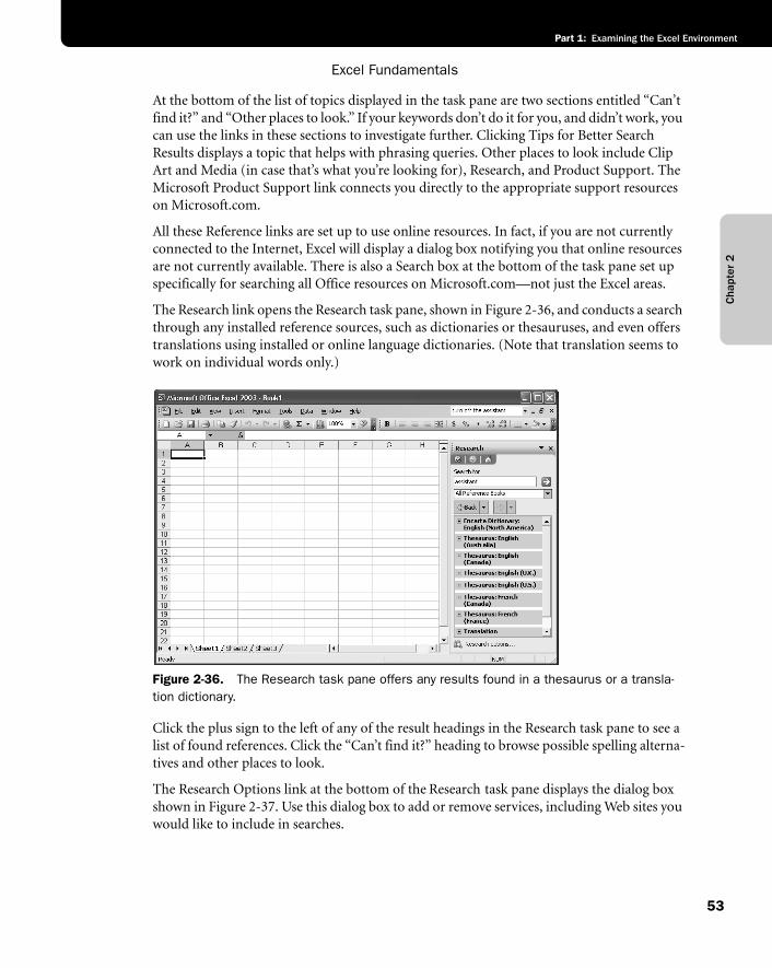
Excel Fundamentals

53

Part 1: Examining the Excel Environment

Cha

pter

2

At the bottom of the list of topics displayed in the task pane are two sections entitled “Can’t find it?” and “Other places to look.” If your keywords don’t do it for you, and didn’t work, you can use the links in these sections to investigate further. Clicking Tips for Better Search Results displays a topic that helps with phrasing queries. Other places to look include Clip Art and Media (in case that’s what you’re looking for), Research, and Product Support. The Microsoft Product Support link connects you directly to the appropriate support resources on Microsoft.com.

All these Reference links are set up to use online resources. In fact, if you are not currently connected to the Internet, Excel will display a dialog box notifying you that online resources are not currently available. There is also a Search box at the bottom of the task pane set up specifically for searching all Office resources on Microsoft.com—not just the Excel areas.

The Research link opens the Research task pane, shown in Figure 2-36, and conducts a search through any installed reference sources, such as dictionaries or thesauruses, and even offers translations using installed or online language dictionaries. (Note that translation seems to work on individual words only.)

f02ie36

Figure 2-36. The Research task pane offers any results found in a thesaurus or a transla-tion dictionary.

Click the plus sign to the left of any of the result headings in the Research task pane to see a list of found references. Click the “Can’t find it?” heading to browse possible spelling alterna-tives and other places to look.

The Research Options link at the bottom of the Research task pane displays the dialog box shown in Figure 2-37. Use this dialog box to add or remove services, including Web sites you would like to include in searches.

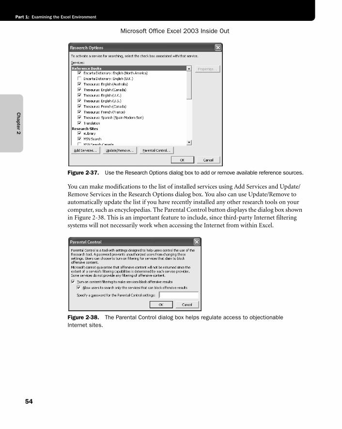
Chapter 2

Microsoft Office Excel 2003 Inside Out

Part 1: Examining the Excel Environment

54

f02ie37

Figure 2-37. Use the Research Options dialog box to add or remove available reference sources.

You can make modifications to the list of installed services using Add Services and Update/Remove Services in the Research Options dialog box. You also can use Update/Remove to automatically update the list if you have recently installed any other research tools on your computer, such as encyclopedias. The Parental Control button displays the dialog box shown in Figure 2-38. This is an important feature to include, since third-party Internet filtering systems will not necessarily work when accessing the Internet from within Excel.

f02ie38

Figure 2-38. The Parental Control dialog box helps regulate access to objectionable Internet sites.

Excel Fundamentals

55

Part 1: Examining the Excel Environment

Cha

pter

2

The Wizard Behind the CurtainThe Type a Question for Help box is a deceptively simple looking interface to a very sophis-ticated system. When you enter a question, Microsoft’s Answer Wizard technology works very quickly and usually returns a short list of relevant topics. The Type A Question For Help box accepts questions in full or partial sentences, using natural language, just as if you were talking to the Excel guru down the hall. Then, based on key words, order of words, and verbs used, the Ask A Question box returns a list of topics that is generated by a sophisti-cated system of probabilities.

Managing the AssistantIn the last few versions of Excel, we have witnessed the birth and adolescence of the previ-ously ubiquitous Office Assistant—whose default personality is the animated paper clip known as Clippit, but which can take on other personas, including our favorite, Rocky the dog. Previously, the Assistant was impossible to ignore and impossible to get rid of. Even if you turned off the Assistant, it would pop up from time to time depending on what you were doing. Our little friend has finally learned not to be heard or seen. Now you can remove the Assistant completely. Good news for many of us (although we still enjoy making Rocky the dog do little dances occasionally).

For more about choosing other Office Assistant characters, see “Selecting Office Assistant Options,” on page 57.

You’re Fired!In Excel 2003, the Office Assistant is not as pushy as it was in its younger days. Nevertheless, it’s still there and occasionally appears. If you would be happier if the Assistant never dark-ened your desktop again, choose Help, Show the Office Assistant (if it isn’t already visible). Click the Assistant and then click the Options button at the bottom of the balloon. The Office Assistant dialog box appears, as shown in Figure 2-39. On the Options tab, clear the Use the Office Assistant check box. When you do so, the rest of the options in the dialog box become unavailable.

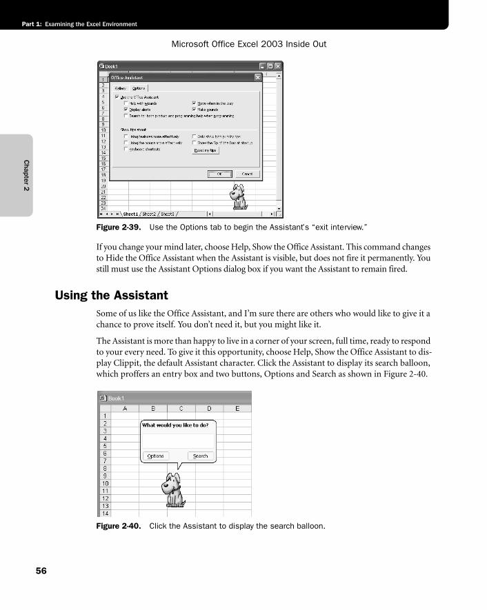
Chapter 2

Microsoft Office Excel 2003 Inside Out

Part 1: Examining the Excel Environment

56

f02ie39

Figure 2-39. Use the Options tab to begin the Assistant’s “exit interview.”

If you change your mind later, choose Help, Show the Office Assistant. This command changes to Hide the Office Assistant when the Assistant is visible, but does not fire it permanently. You still must use the Assistant Options dialog box if you want the Assistant to remain fired.

Using the AssistantSome of us like the Office Assistant, and I’m sure there are others who would like to give it a chance to prove itself. You don’t need it, but you might like it.

The Assistant is more than happy to live in a corner of your screen, full time, ready to respond to your every need. To give it this opportunity, choose Help, Show the Office Assistant to dis-play Clippit, the default Assistant character. Click the Assistant to display its search balloon, which proffers an entry box and two buttons, Options and Search as shown in Figure 2-40.

f02ie40

Figure 2-40. Click the Assistant to display the search balloon.

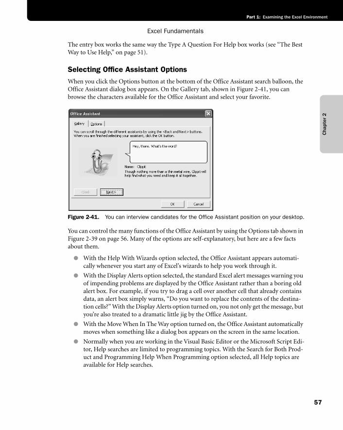
Excel Fundamentals

57

Part 1: Examining the Excel Environment

Cha

pter

2

The entry box works the same way the Type A Question For Help box works (see “The Best Way to Use Help,” on page 51).

Selecting Office Assistant OptionsWhen you click the Options button at the bottom of the Office Assistant search balloon, the Office Assistant dialog box appears. On the Gallery tab, shown in Figure 2-41, you can browse the characters available for the Office Assistant and select your favorite.

f02ie41

Figure 2-41. You can interview candidates for the Office Assistant position on your desktop.

You can control the many functions of the Office Assistant by using the Options tab shown in Figure 2-39 on page 56. Many of the options are self-explanatory, but here are a few facts about them.

● With the Help With Wizards option selected, the Office Assistant appears automati-cally whenever you start any of Excel’s wizards to help you work through it.

● With the Display Alerts option selected, the standard Excel alert messages warning you of impending problems are displayed by the Office Assistant rather than a boring old alert box. For example, if you try to drag a cell over another cell that already contains data, an alert box simply warns, “Do you want to replace the contents of the destina-tion cells?” With the Display Alerts option turned on, you not only get the message, but you’re also treated to a dramatic little jig by the Office Assistant.

● With the Move When In The Way option turned on, the Office Assistant automatically moves when something like a dialog box appears on the screen in the same location.

● Normally when you are working in the Visual Basic Editor or the Microsoft Script Edi-tor, Help searches are limited to programming topics. With the Search for Both Prod-uct and Programming Help When Programming option selected, all Help topics are available for Help searches.

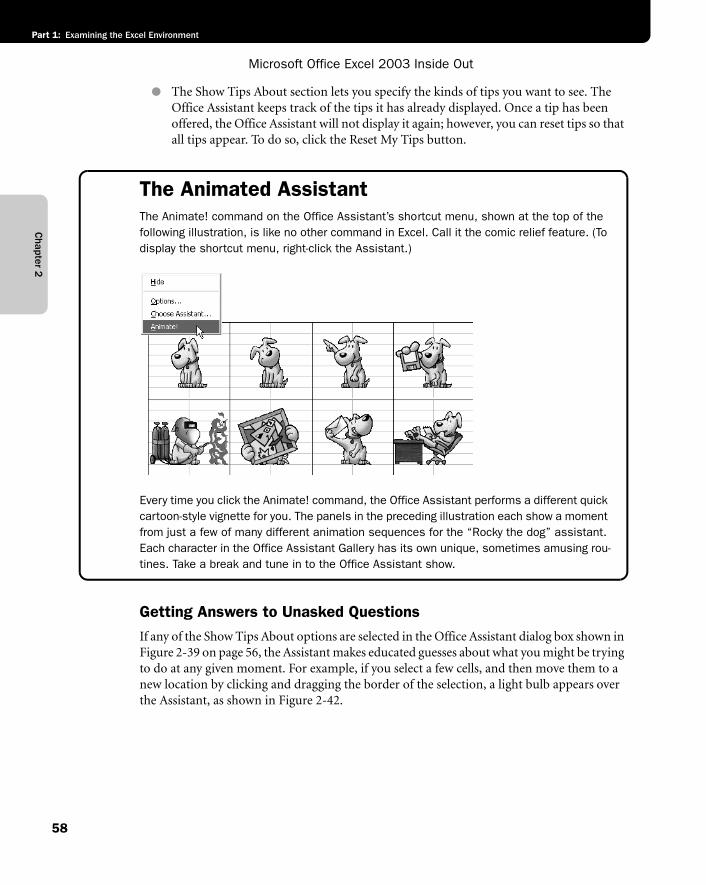
Chapter 2

Microsoft Office Excel 2003 Inside Out

Part 1: Examining the Excel Environment

58

● The Show Tips About section lets you specify the kinds of tips you want to see. The Office Assistant keeps track of the tips it has already displayed. Once a tip has been offered, the Office Assistant will not display it again; however, you can reset tips so that all tips appear. To do so, click the Reset My Tips button.

The Animated AssistantThe Animate! command on the Office Assistant’s shortcut menu, shown at the top of the following illustration, is like no other command in Excel. Call it the comic relief feature. (To display the shortcut menu, right-click the Assistant.)

g02ie03

Every time you click the Animate! command, the Office Assistant performs a different quick cartoon-style vignette for you. The panels in the preceding illustration each show a moment from just a few of many different animation sequences for the “Rocky the dog” assistant. Each character in the Office Assistant Gallery has its own unique, sometimes amusing rou-tines. Take a break and tune in to the Office Assistant show.

Getting Answers to Unasked QuestionsIf any of the Show Tips About options are selected in the Office Assistant dialog box shown in Figure 2-39 on page 56, the Assistant makes educated guesses about what you might be trying to do at any given moment. For example, if you select a few cells, and then move them to a new location by clicking and dragging the border of the selection, a light bulb appears over the Assistant, as shown in Figure 2-42.

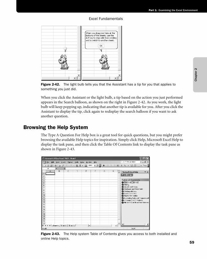
Excel Fundamentals

59

Part 1: Examining the Excel Environment

Cha

pter

2

f02ie42

Figure 2-42. The light bulb tells you that the Assistant has a tip for you that applies to something you just did.

When you click the Assistant or the light bulb, a tip based on the action you just performed appears in the Search balloon, as shown on the right in Figure 2-42. As you work, the light bulb will keep popping up, indicating that another tip is available for you. After you click the Assistant to display the tip, click again to redisplay the search balloon if you want to ask another question.

Browsing the Help SystemThe Type A Question For Help box is a great tool for quick questions, but you might prefer browsing the available Help topics for inspiration. Simply click Help, Microsoft Excel Help to display the task pane, and then click the Table Of Contents link to display the task pane as shown in Figure 2-43.

f02ie43

Figure 2-43. The Help system Table of Contents gives you access to both installed and online Help topics.

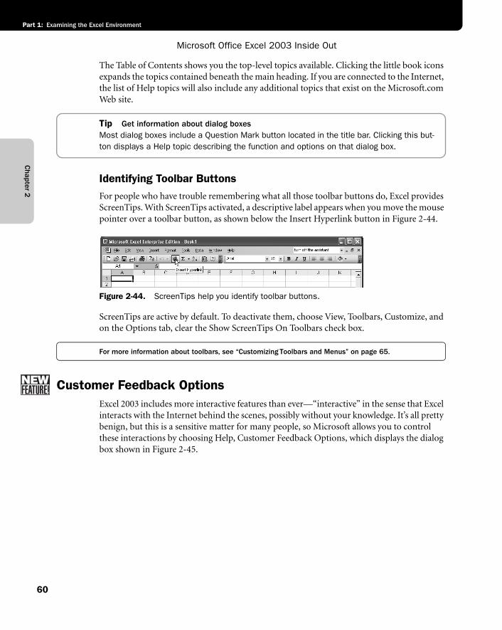
Chapter 2

Microsoft Office Excel 2003 Inside Out

Part 1: Examining the Excel Environment

60

The Table of Contents shows you the top-level topics available. Clicking the little book icons expands the topics contained beneath the main heading. If you are connected to the Internet, the list of Help topics will also include any additional topics that exist on the Microsoft.com Web site.

Tip Get information about dialog boxes Most dialog boxes include a Question Mark button located in the title bar. Clicking this but-ton displays a Help topic describing the function and options on that dialog box.

Identifying Toolbar ButtonsFor people who have trouble remembering what all those toolbar buttons do, Excel provides ScreenTips. With ScreenTips activated, a descriptive label appears when you move the mouse pointer over a toolbar button, as shown below the Insert Hyperlink button in Figure 2-44.

f02ie44

Figure 2-44. ScreenTips help you identify toolbar buttons.

ScreenTips are active by default. To deactivate them, choose View, Toolbars, Customize, and on the Options tab, clear the Show ScreenTips On Toolbars check box.

For more information about toolbars, see “Customizing Toolbars and Menus” on page 65.

Customer Feedback OptionsExcel 2003 includes more interactive features than ever—“interactive” in the sense that Excel interacts with the Internet behind the scenes, possibly without your knowledge. It’s all pretty benign, but this is a sensitive matter for many people, so Microsoft allows you to control these interactions by choosing Help, Customer Feedback Options, which displays the dialog box shown in Figure 2-45.

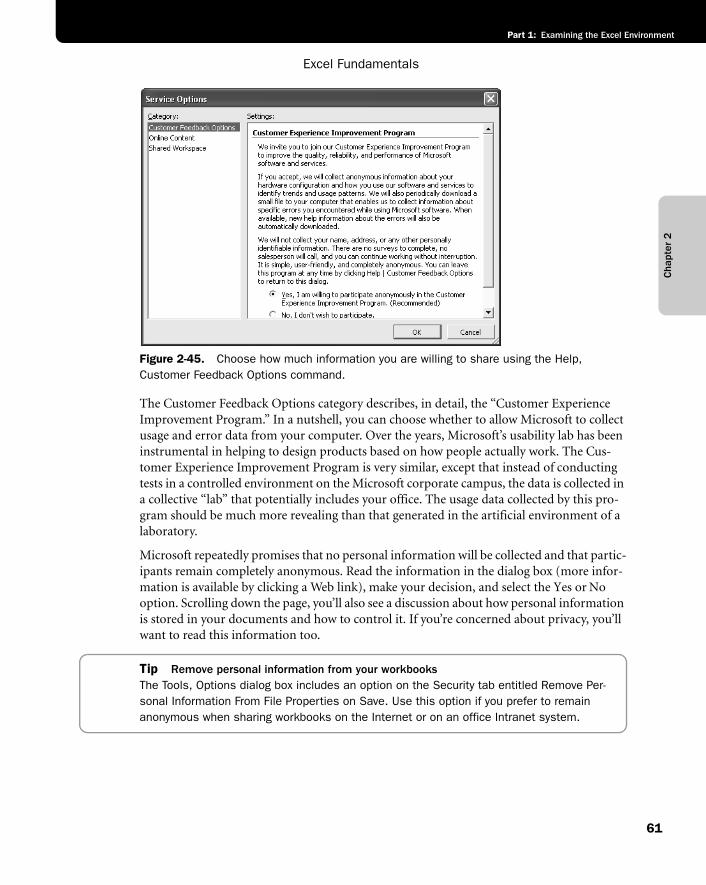
Excel Fundamentals

61

Part 1: Examining the Excel Environment

Cha

pter

2

F02ie45

Figure 2-45. Choose how much information you are willing to share using the Help, Customer Feedback Options command.

The Customer Feedback Options category describes, in detail, the “Customer Experience Improvement Program.” In a nutshell, you can choose whether to allow Microsoft to collect usage and error data from your computer. Over the years, Microsoft’s usability lab has been instrumental in helping to design products based on how people actually work. The Cus-tomer Experience Improvement Program is very similar, except that instead of conducting tests in a controlled environment on the Microsoft corporate campus, the data is collected in a collective “lab” that potentially includes your office. The usage data collected by this pro-gram should be much more revealing than that generated in the artificial environment of a laboratory.

Microsoft repeatedly promises that no personal information will be collected and that partic-ipants remain completely anonymous. Read the information in the dialog box (more infor-mation is available by clicking a Web link), make your decision, and select the Yes or No option. Scrolling down the page, you’ll also see a discussion about how personal information is stored in your documents and how to control it. If you’re concerned about privacy, you’ll want to read this information too.

Tip Remove personal information from your workbooksThe Tools, Options dialog box includes an option on the Security tab entitled Remove Per-sonal Information From File Properties on Save. Use this option if you prefer to remain anonymous when sharing workbooks on the Internet or on an office Intranet system.

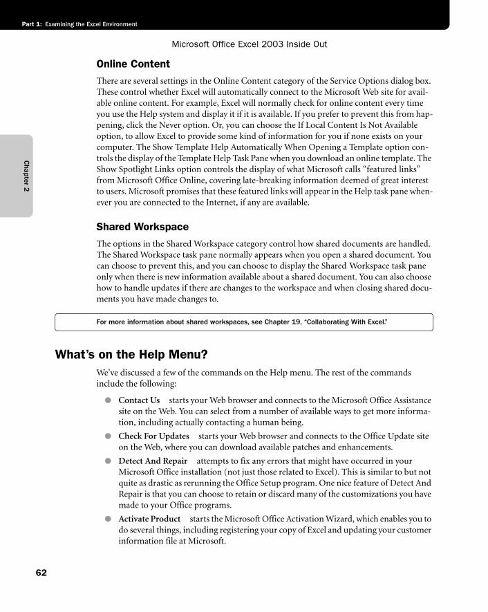
Chapter 2

Microsoft Office Excel 2003 Inside Out

Part 1: Examining the Excel Environment

62

Online Content There are several settings in the Online Content category of the Service Options dialog box. These control whether Excel will automatically connect to the Microsoft Web site for avail-able online content. For example, Excel will normally check for online content every time you use the Help system and display it if it is available. If you prefer to prevent this from hap-pening, click the Never option. Or, you can choose the If Local Content Is Not Available option, to allow Excel to provide some kind of information for you if none exists on your computer. The Show Template Help Automatically When Opening a Template option con-trols the display of the Template Help Task Pane when you download an online template. The Show Spotlight Links option controls the display of what Microsoft calls “featured links” from Microsoft Office Online, covering late-breaking information deemed of great interest to users. Microsoft promises that these featured links will appear in the Help task pane when-ever you are connected to the Internet, if any are available.

Shared WorkspaceThe options in the Shared Workspace category control how shared documents are handled. The Shared Workspace task pane normally appears when you open a shared document. You can choose to prevent this, and you can choose to display the Shared Workspace task pane only when there is new information available about a shared document. You can also choose how to handle updates if there are changes to the workspace and when closing shared docu-ments you have made changes to.

For more information about shared workspaces, see Chapter 19, “Collaborating With Excel.”

What’s on the Help Menu?We’ve discussed a few of the commands on the Help menu. The rest of the commands include the following:

● Contact Us starts your Web browser and connects to the Microsoft Office Assistance site on the Web. You can select from a number of available ways to get more informa-tion, including actually contacting a human being.

● Check For Updates starts your Web browser and connects to the Office Update site on the Web, where you can download available patches and enhancements.

● Detect And Repair attempts to fix any errors that might have occurred in your Microsoft Office installation (not just those related to Excel). This is similar to but not quite as drastic as rerunning the Office Setup program. One nice feature of Detect And Repair is that you can choose to retain or discard many of the customizations you have made to your Office programs.

● Activate Product starts the Microsoft Office Activation Wizard, which enables you to do several things, including registering your copy of Excel and updating your customer information file at Microsoft.

Excel Fundamentals

63

Part 1: Examining the Excel Environment

Cha

pter

2

● About Microsoft Excel displays information about the program and offers a couple of interesting services. For more information, see the sidebar “Before You Call Product Support” below.

For more information, see Chapter 3, “Custom-Tailoring the Excel Workspace.” For more information about repairing your Excel installation, see “Heroic Measures” on page 17.

Before You Call Product SupportWe encourage you to use Excel documentation, online Help, the Microsoft Excel Web site (http://www.microsoft.com/excel/), and especially this book to find answers to your ques-tions before you reach for the telephone. When you have exhausted these resources, it’s time to call Microsoft Product Support. But before you do, choose Help, About Microsoft Excel, and click the System Info button. Doing so displays a dialog box that lists your cur-rent system configuration, the applications running, display information, and much more. If you want, you can print the information in a report or save it as a file on disk. Then you can click Tech Support in the About Microsoft Excel dialog box to display a Help topic you can use to find telephone numbers for Microsoft Product Support Services around the world. When you talk to Product Support, having the System Info report at your fingertips will assist the representative in diagnosing your problem and will save you time. The other but-ton in the About Microsoft Excel dialog box is Disabled Items. Clicking this button opens a dialog box that lists any items that somehow got in the way of an Office program’s normal operation and were disabled. You also can try to start them up again by clicking Enable. If there is anything on this list, maybe that’s the problem. Or maybe it’s a symptom. In any case, the Disabled Items dialog box can provide good information to share with your Prod-uct Support representative.

65

Part 1: Examining the Excel Environment

Chapter 3

Custom-Tailoring the Excel Workspace

Customizing Toolbars and Menus . . . . . . .65Managing Toolbars . . . . . . . . . . . . . . . . . .76Creating New Toolbars and Menus . . . . . .78

Controlling Other Elements of the Excel Interface . . . . . . . . . . . . . . . . . . . . . 83Enhancing Accessibility . . . . . . . . . . . . . . 89

You needn’t settle for the way Microsoft Excel’s command and control systems are organized. There are a lot of ways to make them more comfortable for the way you work. This chapter tells you how to use Excel’s metaphorical six-way power seats and adjustable steering column, and even where they stuck that pesky hood release.

Customizing Toolbars and MenusDon’t you sometimes wish you could change the location of your car’s speedometer or some hard-to-reach, dashboard-mounted item? Excel’s “dashboard” is completely modular, so you can dismantle and reassemble it any way you like.

Managing Buttons and CommandsWhen you first start Excel, the Standard and Formatting toolbars are displayed in what the Excel developers refer to as the rafting configuration. This means that both toolbars share the same row, as shown in Figure 3-1.

You can change this so that each toolbar occupies its own row by choosing Customize from the Tools menu, and on the Options tab, selecting Show Standard And Formatting Toolbars On Two Rows. This way, your toolbars appear with all their default buttons visible, as shown in Figure 3-2. You can also use the command Show Buttons On Two Rows on the Toolbar Options shortcut menu shown in Figure 3-3.

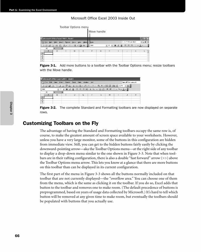
Microsoft Office Excel 2003 Inside Out

Part 1: Examining the Excel Environment

66

Chapter 3

f03ie01

Figure 3-1. Add more buttons to a toolbar with the Toolbar Options menu; resize toolbars with the Move handle.

f03ie02

Figure 3-2. The complete Standard and Formatting toolbars are now displayed on separate rows.

Customizing Toolbars on the FlyThe advantage of having the Standard and Formatting toolbars occupy the same row is, of course, to make the greatest amount of screen space available to your worksheets. However, unless you have a very large monitor, some of the buttons in this configuration are hidden from immediate view. Still, you can get to the hidden buttons fairly easily by clicking the downward-pointing arrow—aka the Toolbar Options menu—at the right side of any toolbar to display a drop-down menu similar to the one shown in Figure 3-3. Note that when tool-bars are in their rafting configuration, there is also a double “fast forward” arrow (>>) above the Toolbar Options menu arrow. This lets you know at a glance that there are more buttons on this toolbar than can be displayed in its current configuration.

The first part of the menu in Figure 3-3 shows all the buttons normally included on that toolbar that are not currently displayed—the “overflow area.” You can choose one of them from the menu, which is the same as clicking it on the toolbar. If you do so, Excel adds that button to the toolbar and removes one to make room. (The default precedence of buttons is preprogrammed, based on years of usage data collected by Microsoft.) It’s hard to tell which button will be removed at any given time to make room, but eventually the toolbars should be populated with buttons that you actually use.

Move handle

Toolbar Options menu

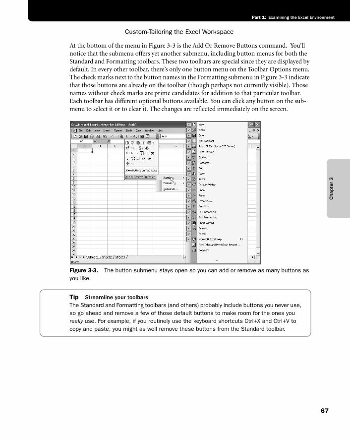
Custom-Tailoring the Excel Workspace

67

Part 1: Examining the Excel Environment

Cha

pter

3

At the bottom of the menu in Figure 3-3 is the Add Or Remove Buttons command. You’ll notice that the submenu offers yet another submenu, including button menus for both the Standard and Formatting toolbars. These two toolbars are special since they are displayed by default. In every other toolbar, there’s only one button menu on the Toolbar Options menu. The check marks next to the button names in the Formatting submenu in Figure 3-3 indicate that those buttons are already on the toolbar (though perhaps not currently visible). Those names without check marks are prime candidates for addition to that particular toolbar. Each toolbar has different optional buttons available. You can click any button on the sub-menu to select it or to clear it. The changes are reflected immediately on the screen.

f03ie03

Figure 3-3. The button submenu stays open so you can add or remove as many buttons as you like.

Tip Streamline your toolbarsThe Standard and Formatting toolbars (and others) probably include buttons you never use, so go ahead and remove a few of those default buttons to make room for the ones you really use. For example, if you routinely use the keyboard shortcuts Ctrl+X and Ctrl+V to copy and paste, you might as well remove these buttons from the Standard toolbar.

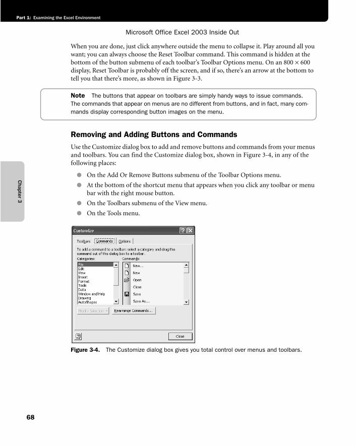
Microsoft Office Excel 2003 Inside Out

Part 1: Examining the Excel Environment

68

Chapter 3

When you are done, just click anywhere outside the menu to collapse it. Play around all you want; you can always choose the Reset Toolbar command. This command is hidden at the bottom of the button submenu of each toolbar’s Toolbar Options menu. On an 800 × 600 display, Reset Toolbar is probably off the screen, and if so, there’s an arrow at the bottom to tell you that there’s more, as shown in Figure 3-3.

Note The buttons that appear on toolbars are simply handy ways to issue commands. The commands that appear on menus are no different from buttons, and in fact, many com-mands display corresponding button images on the menu.

Removing and Adding Buttons and CommandsUse the Customize dialog box to add and remove buttons and commands from your menus and toolbars. You can find the Customize dialog box, shown in Figure 3-4, in any of the following places:

● On the Add Or Remove Buttons submenu of the Toolbar Options menu.

● At the bottom of the shortcut menu that appears when you click any toolbar or menu bar with the right mouse button.

● On the Toolbars submenu of the View menu.

● On the Tools menu.

f03ie04

Figure 3-4. The Customize dialog box gives you total control over menus and toolbars.

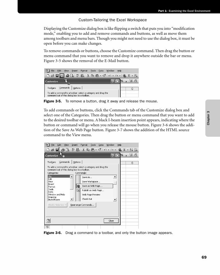
Custom-Tailoring the Excel Workspace

69

Part 1: Examining the Excel Environment

Cha

pter

3

Displaying the Customize dialog box is like flipping a switch that puts you into “modification mode,” enabling you to add and remove commands and buttons, as well as move them among toolbars and menu bars. Though you might not need to use the dialog box, it must be open before you can make changes.

To remove commands or buttons, choose the Customize command. Then drag the button or menu command that you want to remove and drop it anywhere outside the bar or menu. Figure 3-5 shows the removal of the E-Mail button.

f03ie01

Figure 3-5. To remove a button, drag it away and release the mouse.

To add commands or buttons, click the Commands tab of the Customize dialog box and select one of the Categories. Then drag the button or menu command that you want to add to the desired toolbar or menu. A black I-beam insertion point appears, indicating where the button or command will go when you release the mouse button. Figure 3-6 shows the addi-tion of the Save As Web Page button. Figure 3-7 shows the addition of the HTML source command to the View menu.

f03ie06

Figure 3-6. Drag a command to a toolbar, and only the button image appears.

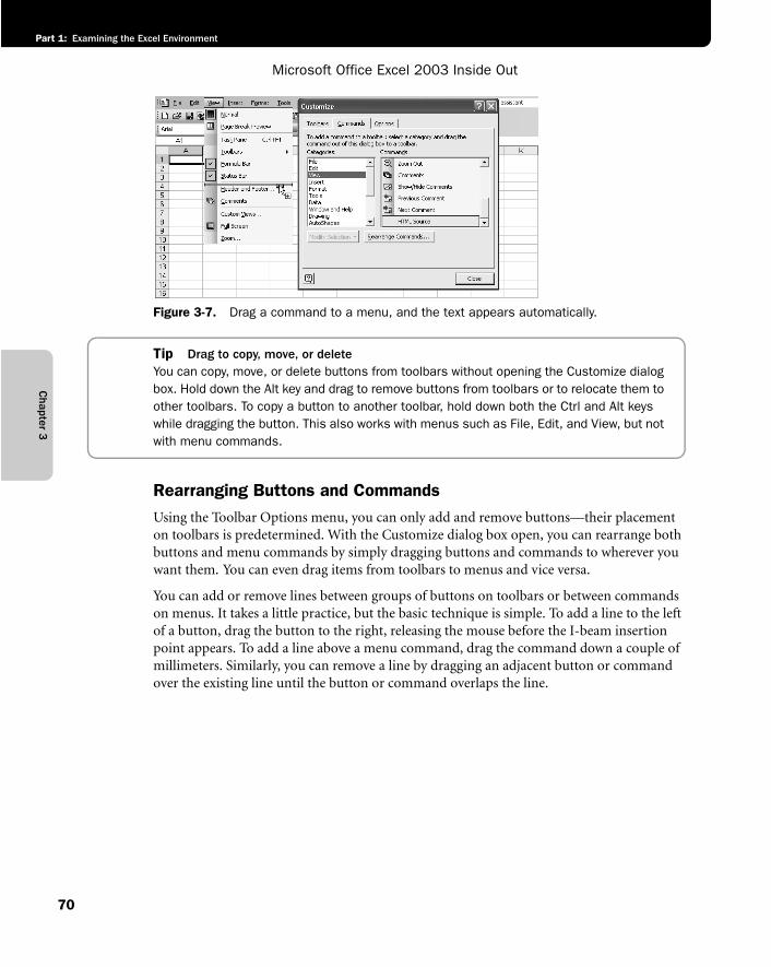
Microsoft Office Excel 2003 Inside Out

Part 1: Examining the Excel Environment

70

Chapter 3

f03ie07

Figure 3-7. Drag a command to a menu, and the text appears automatically.

Tip Drag to copy, move, or deleteYou can copy, move, or delete buttons from toolbars without opening the Customize dialog box. Hold down the Alt key and drag to remove buttons from toolbars or to relocate them to other toolbars. To copy a button to another toolbar, hold down both the Ctrl and Alt keys while dragging the button. This also works with menus such as File, Edit, and View, but not with menu commands.

Rearranging Buttons and Commands Using the Toolbar Options menu, you can only add and remove buttons—their placement on toolbars is predetermined. With the Customize dialog box open, you can rearrange both buttons and menu commands by simply dragging buttons and commands to wherever you want them. You can even drag items from toolbars to menus and vice versa.

You can add or remove lines between groups of buttons on toolbars or between commands on menus. It takes a little practice, but the basic technique is simple. To add a line to the left of a button, drag the button to the right, releasing the mouse before the I-beam insertion point appears. To add a line above a menu command, drag the command down a couple of millimeters. Similarly, you can remove a line by dragging an adjacent button or command over the existing line until the button or command overlaps the line.

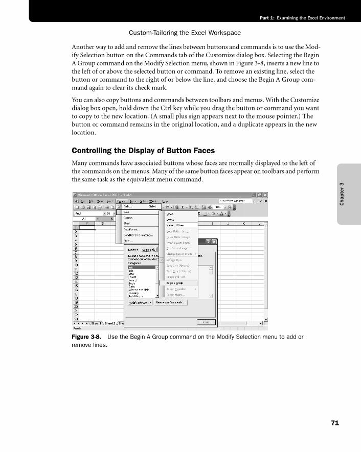
Custom-Tailoring the Excel Workspace

71

Part 1: Examining the Excel Environment

Cha

pter

3

Another way to add and remove the lines between buttons and commands is to use the Mod-ify Selection button on the Commands tab of the Customize dialog box. Selecting the Begin A Group command on the Modify Selection menu, shown in Figure 3-8, inserts a new line to the left of or above the selected button or command. To remove an existing line, select the button or command to the right of or below the line, and choose the Begin A Group com-mand again to clear its check mark.

You can also copy buttons and commands between toolbars and menus. With the Customize dialog box open, hold down the Ctrl key while you drag the button or command you want to copy to the new location. (A small plus sign appears next to the mouse pointer.) The button or command remains in the original location, and a duplicate appears in the new location.

Controlling the Display of Button Faces Many commands have associated buttons whose faces are normally displayed to the left of the commands on the menus. Many of the same button faces appear on toolbars and perform the same task as the equivalent menu command.

f03ie08

Figure 3-8. Use the Begin A Group command on the Modify Selection menu to add or remove lines.

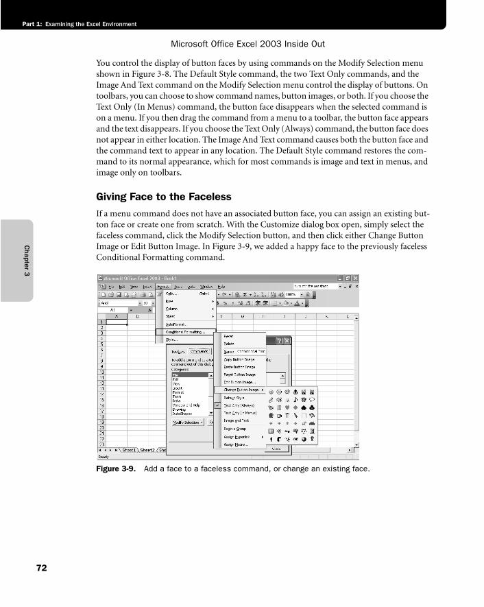
Microsoft Office Excel 2003 Inside Out

Part 1: Examining the Excel Environment

72

Chapter 3

You control the display of button faces by using commands on the Modify Selection menu shown in Figure 3-8. The Default Style command, the two Text Only commands, and the Image And Text command on the Modify Selection menu control the display of buttons. On toolbars, you can choose to show command names, button images, or both. If you choose the Text Only (In Menus) command, the button face disappears when the selected command is on a menu. If you then drag the command from a menu to a toolbar, the button face appears and the text disappears. If you choose the Text Only (Always) command, the button face does not appear in either location. The Image And Text command causes both the button face and the command text to appear in any location. The Default Style command restores the com-mand to its normal appearance, which for most commands is image and text in menus, and image only on toolbars.

Giving Face to the Faceless If a menu command does not have an associated button face, you can assign an existing but-ton face or create one from scratch. With the Customize dialog box open, simply select the faceless command, click the Modify Selection button, and then click either Change Button Image or Edit Button Image. In Figure 3-9, we added a happy face to the previously faceless Conditional Formatting command.

f03ie09

Figure 3-9. Add a face to a faceless command, or change an existing face.

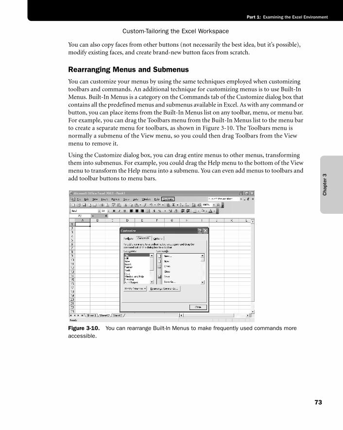
Custom-Tailoring the Excel Workspace

73

Part 1: Examining the Excel Environment

Cha

pter

3

You can also copy faces from other buttons (not necessarily the best idea, but it’s possible), modify existing faces, and create brand-new button faces from scratch.

Rearranging Menus and Submenus You can customize your menus by using the same techniques employed when customizing toolbars and commands. An additional technique for customizing menus is to use Built-In Menus. Built-In Menus is a category on the Commands tab of the Customize dialog box that contains all the predefined menus and submenus available in Excel. As with any command or button, you can place items from the Built-In Menus list on any toolbar, menu, or menu bar. For example, you can drag the Toolbars menu from the Built-In Menus list to the menu bar to create a separate menu for toolbars, as shown in Figure 3-10. The Toolbars menu is normally a submenu of the View menu, so you could then drag Toolbars from the View menu to remove it.

Using the Customize dialog box, you can drag entire menus to other menus, transforming them into submenus. For example, you could drag the Help menu to the bottom of the View menu to transform the Help menu into a submenu. You can even add menus to toolbars and add toolbar buttons to menu bars.

f03ie10

Figure 3-10. You can rearrange Built-In Menus to make frequently used commands more accessible.

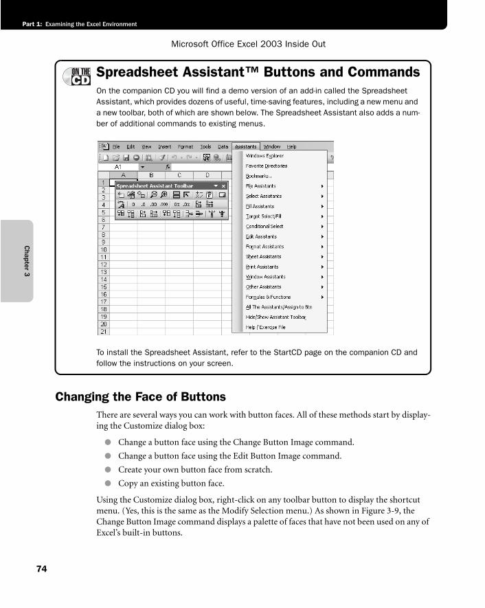
Microsoft Office Excel 2003 Inside Out

Part 1: Examining the Excel Environment

74

Chapter 3

Spreadsheet Assistant™ Buttons and CommandsOn the companion CD you will find a demo version of an add-in called the Spreadsheet Assistant, which provides dozens of useful, time-saving features, including a new menu and a new toolbar, both of which are shown below. The Spreadsheet Assistant also adds a num-ber of additional commands to existing menus.

G03ie01

To install the Spreadsheet Assistant, refer to the StartCD page on the companion CD and follow the instructions on your screen.

Changing the Face of ButtonsThere are several ways you can work with button faces. All of these methods start by display-ing the Customize dialog box:

● Change a button face using the Change Button Image command.

● Change a button face using the Edit Button Image command.

● Create your own button face from scratch.

● Copy an existing button face.

Using the Customize dialog box, right-click on any toolbar button to display the shortcut menu. (Yes, this is the same as the Modify Selection menu.) As shown in Figure 3-9, the Change Button Image command displays a palette of faces that have not been used on any of Excel’s built-in buttons.

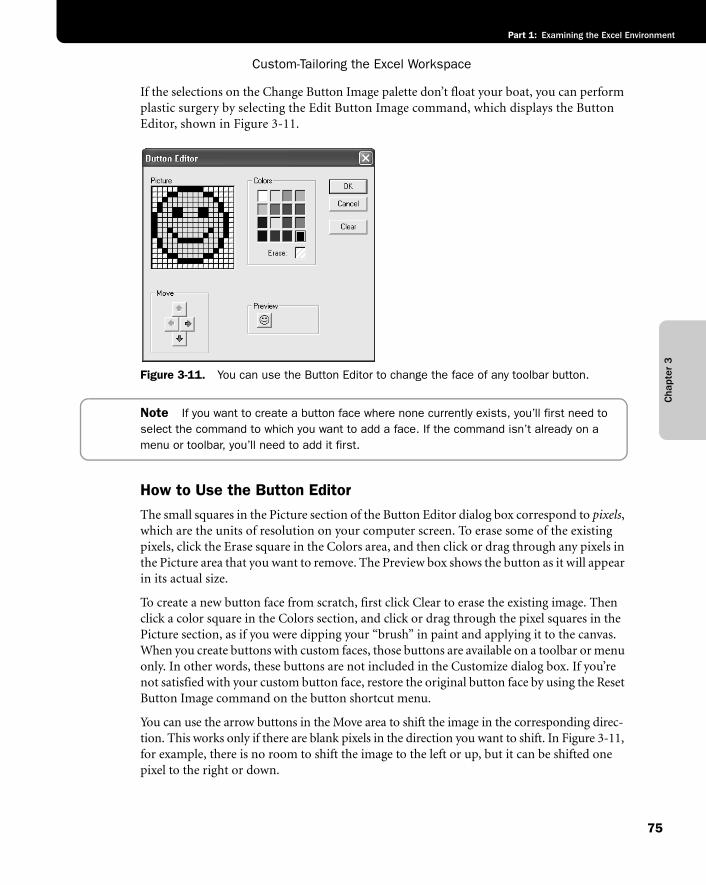
Custom-Tailoring the Excel Workspace

75

Part 1: Examining the Excel Environment

Cha

pter

3

If the selections on the Change Button Image palette don’t float your boat, you can perform plastic surgery by selecting the Edit Button Image command, which displays the Button Editor, shown in Figure 3-11.

f03ie11

Figure 3-11. You can use the Button Editor to change the face of any toolbar button.

Note If you want to create a button face where none currently exists, you’ll first need to select the command to which you want to add a face. If the command isn’t already on a menu or toolbar, you’ll need to add it first.

How to Use the Button EditorThe small squares in the Picture section of the Button Editor dialog box correspond to pixels,which are the units of resolution on your computer screen. To erase some of the existing pixels, click the Erase square in the Colors area, and then click or drag through any pixels in the Picture area that you want to remove. The Preview box shows the button as it will appear in its actual size.

To create a new button face from scratch, first click Clear to erase the existing image. Then click a color square in the Colors section, and click or drag through the pixel squares in the Picture section, as if you were dipping your “brush” in paint and applying it to the canvas. When you create buttons with custom faces, those buttons are available on a toolbar or menu only. In other words, these buttons are not included in the Customize dialog box. If you’re not satisfied with your custom button face, restore the original button face by using the Reset Button Image command on the button shortcut menu.

You can use the arrow buttons in the Move area to shift the image in the corresponding direc-tion. This works only if there are blank pixels in the direction you want to shift. In Figure 3-11, for example, there is no room to shift the image to the left or up, but it can be shifted one pixel to the right or down.

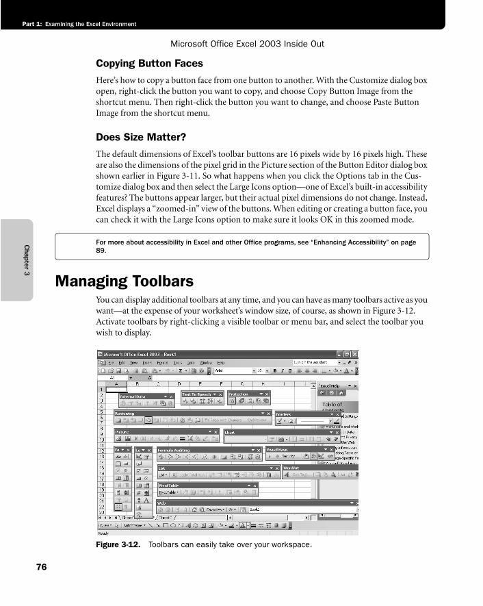
Microsoft Office Excel 2003 Inside Out

Part 1: Examining the Excel Environment

76

Chapter 3

Copying Button FacesHere’s how to copy a button face from one button to another. With the Customize dialog box open, right-click the button you want to copy, and choose Copy Button Image from the shortcut menu. Then right-click the button you want to change, and choose Paste Button Image from the shortcut menu.

Does Size Matter?The default dimensions of Excel’s toolbar buttons are 16 pixels wide by 16 pixels high. These are also the dimensions of the pixel grid in the Picture section of the Button Editor dialog box shown earlier in Figure 3-11. So what happens when you click the Options tab in the Cus-tomize dialog box and then select the Large Icons option—one of Excel’s built-in accessibility features? The buttons appear larger, but their actual pixel dimensions do not change. Instead, Excel displays a “zoomed-in” view of the buttons. When editing or creating a button face, you can check it with the Large Icons option to make sure it looks OK in this zoomed mode.

For more about accessibility in Excel and other Office programs, see “Enhancing Accessibility” on page 89.

Managing ToolbarsYou can display additional toolbars at any time, and you can have as many toolbars active as you want—at the expense of your worksheet’s window size, of course, as shown in Figure 3-12. Activate toolbars by right-clicking a visible toolbar or menu bar, and select the toolbar you wish to display.

f03ie12

Figure 3-12. Toolbars can easily take over your workspace.

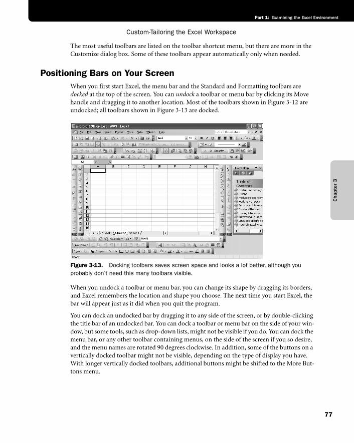
Custom-Tailoring the Excel Workspace

77

Part 1: Examining the Excel Environment

Cha

pter

3

The most useful toolbars are listed on the toolbar shortcut menu, but there are more in the Customize dialog box. Some of these toolbars appear automatically only when needed.

Positioning Bars on Your ScreenWhen you first start Excel, the menu bar and the Standard and Formatting toolbars are docked at the top of the screen. You can undock a toolbar or menu bar by clicking its Move handle and dragging it to another location. Most of the toolbars shown in Figure 3-12 are undocked; all toolbars shown in Figure 3-13 are docked.

f03ie13

Figure 3-13. Docking toolbars saves screen space and looks a lot better, although you probably don’t need this many toolbars visible.

When you undock a toolbar or menu bar, you can change its shape by dragging its borders, and Excel remembers the location and shape you choose. The next time you start Excel, the bar will appear just as it did when you quit the program.

You can dock an undocked bar by dragging it to any side of the screen, or by double-clicking the title bar of an undocked bar. You can dock a toolbar or menu bar on the side of your win-dow, but some tools, such as drop-down lists, might not be visible if you do. You can dock the menu bar, or any other toolbar containing menus, on the side of the screen if you so desire, and the menu names are rotated 90 degrees clockwise. In addition, some of the buttons on a vertically docked toolbar might not be visible, depending on the type of display you have. With longer vertically docked toolbars, additional buttons might be shifted to the More But-tons menu.

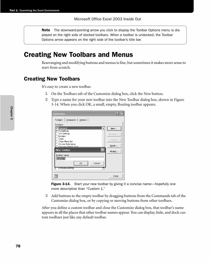
Microsoft Office Excel 2003 Inside Out

Part 1: Examining the Excel Environment

78

Chapter 3

Note The downward-pointing arrow you click to display the Toolbar Options menu is dis-played on the right side of docked toolbars. When a toolbar is undocked, the Toolbar Options arrow appears on the right side of the toolbar’s title bar.

Creating New Toolbars and MenusRearranging and modifying buttons and menus is fine, but sometimes it makes more sense to start from scratch.

Creating New ToolbarsIt’s easy to create a new toolbar.

1 On the Toolbars tab of the Customize dialog box, click the New button.

2 Type a name for your new toolbar into the New Toolbar dialog box, shown in Figure 3-14. When you click OK, a small, empty, floating toolbar appears.

f03ie14

Figure 3-14. Start your new toolbar by giving it a concise name—hopefully one more descriptive than “Custom 1.”

3 Add buttons to the empty toolbar by dragging buttons from the Commands tab of the Customize dialog box, or by copying or moving buttons from other toolbars.

After you define a custom toolbar and close the Customize dialog box, that toolbar’s name appears in all the places that other toolbar names appear. You can display, hide, and dock cus-tom toolbars just like any default toolbar.

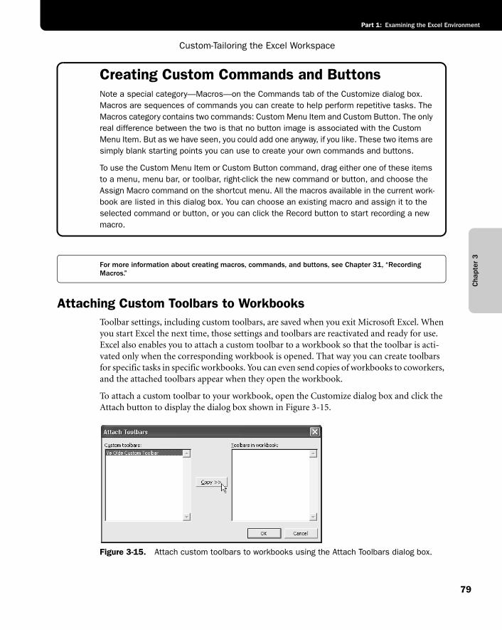
Custom-Tailoring the Excel Workspace

79

Part 1: Examining the Excel Environment

Cha

pter

3

Creating Custom Commands and ButtonsNote a special category—Macros—on the Commands tab of the Customize dialog box. Macros are sequences of commands you can create to help perform repetitive tasks. The Macros category contains two commands: Custom Menu Item and Custom Button. The only real difference between the two is that no button image is associated with the Custom Menu Item. But as we have seen, you could add one anyway, if you like. These two items are simply blank starting points you can use to create your own commands and buttons.

To use the Custom Menu Item or Custom Button command, drag either one of these items to a menu, menu bar, or toolbar, right-click the new command or button, and choose the Assign Macro command on the shortcut menu. All the macros available in the current work-book are listed in this dialog box. You can choose an existing macro and assign it to the selected command or button, or you can click the Record button to start recording a new macro.

For more information about creating macros, commands, and buttons, see Chapter 31, “Recording Macros.”

Attaching Custom Toolbars to WorkbooksToolbar settings, including custom toolbars, are saved when you exit Microsoft Excel. When you start Excel the next time, those settings and toolbars are reactivated and ready for use. Excel also enables you to attach a custom toolbar to a workbook so that the toolbar is acti-vated only when the corresponding workbook is opened. That way you can create toolbars for specific tasks in specific workbooks. You can even send copies of workbooks to coworkers, and the attached toolbars appear when they open the workbook.

To attach a custom toolbar to your workbook, open the Customize dialog box and click the Attach button to display the dialog box shown in Figure 3-15.

f03ie15

Figure 3-15. Attach custom toolbars to workbooks using the Attach Toolbars dialog box.

Microsoft Office Excel 2003 Inside Out

Part 1: Examining the Excel Environment

80

Chapter 3

Select the toolbar you want to attach to your workbook from the Custom Toolbars list. (Only custom toolbars can be attached to workbooks.) Click the Copy button to add the toolbar to the Toolbars In Workbook list on the right.

Tip Automatically activate a custom toolbarAfter you attach a custom toolbar to a workbook, you can delete the toolbar from the Cus-tomize dialog box. Simply select the toolbar on the Toolbars tab and click the Delete button. The toolbar will reappear only when you open the workbook to which it is attached, but the toolbar will remain available in the Customize dialog box even after the workbook is closed. You can use this functionality to save and distribute your custom toolbars.

To detach a custom toolbar from a workbook, you must use the Attach Toolbars dialog box again—except this time, select the toolbar in the Toolbars In Workbook list, and then click the Delete button. (The Copy button changes to Delete when you select an attached toolbar.) If you do not detach a toolbar in this way, it will reappear every time you open the workbook, even if you remove it from the Toolbars list.

Deleting Custom ToolbarsTo remove a custom toolbar, display the Customize dialog box and on the Toolbars tab, select the name of the custom toolbar and click the Delete button. Note the following:

● After you delete a toolbar, you cannot use the Undo command or button to restore it.

● You cannot remove any of Excel’s built-in toolbars.

Creating New MenusThe Categories list on the Commands tab of the Customize dialog box contains a category called New Menu. This is a unique category that contains only one item: New Menu. When you drag the New Menu item to a menu bar, a menu, or a toolbar, a blank menu named, sur-prisingly enough, New Menu, appears. “New Menu” probably isn’t a sufficiently descriptive name, so rename it by right-clicking New Menu and typing a name in the Name box, as shown in Figure 3-16. You can then populate the new menu with any commands, menus, or buttons you like. You can even put drop-down lists on menus.

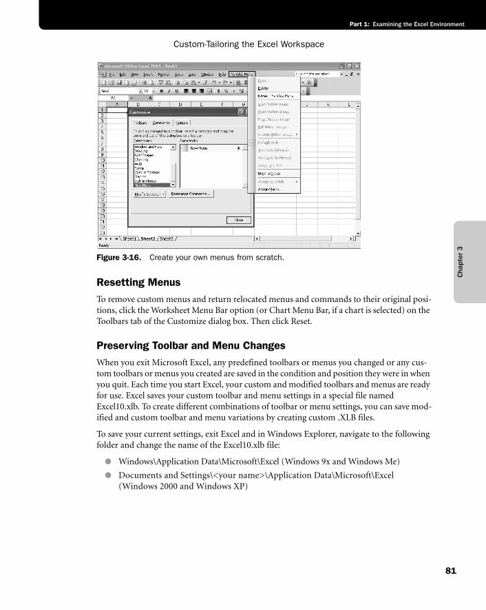
Custom-Tailoring the Excel Workspace

81

Part 1: Examining the Excel Environment

Cha

pter

3

f03ie16

Figure 3-16. Create your own menus from scratch.

Resetting MenusTo remove custom menus and return relocated menus and commands to their original posi-tions, click the Worksheet Menu Bar option (or Chart Menu Bar, if a chart is selected) on the Toolbars tab of the Customize dialog box. Then click Reset.

Preserving Toolbar and Menu ChangesWhen you exit Microsoft Excel, any predefined toolbars or menus you changed or any cus-tom toolbars or menus you created are saved in the condition and position they were in when you quit. Each time you start Excel, your custom and modified toolbars and menus are ready for use. Excel saves your custom toolbar and menu settings in a special file named Excel10.xlb. To create different combinations of toolbar or menu settings, you can save mod-ified and custom toolbar and menu variations by creating custom .XLB files.

To save your current settings, exit Excel and in Windows Explorer, navigate to the following folder and change the name of the Excel10.xlb file:

● Windows\Application Data\Microsoft\Excel (Windows 9x and Windows Me)

● Documents and Settings\<your name>\Application Data\Microsoft\Excel (Windows 2000 and Windows XP)

Microsoft Office Excel 2003 Inside Out

Part 1: Examining the Excel Environment

82

Chapter 3

Tip Recover file extensionsIf you don’t see file extensions in the Windows Explorer, choose Folder Options from the View menu (or the Tools menu in Windows 2000 and Windows XP), and on the View tab, clear the Hide File Extensions For Known File Types check box.

The settings that were active when you exited Excel are saved under the new filename, and any modifications you make during the next Excel session are saved in a fresh Excel10.xlb file. In this way, you can create any number of toolbar and menu configurations, which you can access by double-clicking the .XLB file.

Tip To totally reset all menus and toolbars and discard all personalization data, simply exit Excel and delete the Excel10.xlb file. Excel creates a new one the next time you start.

Restoring Toolbars and MenusNow that you’ve thoroughly scrambled your menus and toolbars, perhaps you’re having a bit of remorse. Don’t worry, it’s easy to get things back to normal.

● Restoring a toolbar. On the Toolbars tab of the Customize dialog box, select the name of the toolbar you want to restore from the Toolbars list, and then click the Reset button. Click OK to confirm the restoration.

● Restoring a menu. With the Customize dialog box open, right-click the menu you want to restore, and then choose the Reset command from the shortcut menu that appears.

● Restoring all menus. This resets all menus, submenus, and commands at the same time. Click the Toolbars tab in the Customize dialog box, and select the Worksheet Menu Bar option (or the Chart Menu Bar option, if a chart is currently active). Then click the Reset button. Click OK to confirm the restoration. Click Close when you are finished.

Restoring Personalized Toolbars and MenusThe preceding procedures reset toolbars and menus in terms of their inventory of commands and buttons, but they do not affect which commands and buttons are visible when personal-ization options are turned on. The Personalized Menus And Toolbars options are on the Options tab of the Customize dialog box.

When the Show Standard And Formatting Toolbars On Two Rows option is not selected, the toolbar equivalent of the “recently used commands” option is activated. Your usage habits, which are recorded by Excel as you work, partially determine which buttons are visible on the Standard and Formatting toolbars (or on any rafting toolbar), as well as which commands are visible on shortened menus. To discard this usage data and return all menu commands and toolbar buttons to their original places, click the Reset Menu and Toolbar Usage Data button.

Custom-Tailoring the Excel Workspace

83

Part 1: Examining the Excel Environment

Cha

pter

3

Other Toolbar and Menu OptionsThere just seems to be no end to the customization options you have at your command in Excel. Here are a few more that are quite helpful, and one that is kind of silly.

● If you want, you can enlarge all the toolbar buttons for easy selection and improved legibility. Simply select the Large Icons option on the Options tab of the Customize dialog box. Note, however, that magnifying the buttons reduces the number of buttons visible on a docked toolbar.

● When the Show ScreenTips On Toolbars option is selected, a small label appears when you move the mouse pointer over any toolbar button. (For more on ScreenTips, see “Show ScreenTips on the Toolbar” on page 89.)

● The Options tab in the Customize dialog box also contains a drop-down list labeled “Menu Animations.” This is one of the so-called visceral elements in Excel, along with sound feedback and animated row-and-column insertion and deletion (both of which are controlled by the Tools, Options command). You can select one of the four options in the Menu Animations list: Random, Unfold, Slide, and Fade (the default). When you click menus when animations are turned on, instead of simply appearing, they appear with a flourish! It’s kind of silly, yet oddly satisfying.

● You can click the Always Show Full Menus option to make all commands on all menus available at all times. This eliminates the need to either wait for shortened menus to unfurl, or to click the arrow at the bottom of a shortened menu to display it in its entirety.

● The List Font Names In Their Font option does just what it says and only applies to the Font drop-down list.

For more information about fonts and formatting, see Chapter 8, “Worksheet Formatting Techniques.”

Controlling Other Elements of the Excel InterfaceThere are three important tabs in the Options dialog box (shown in Figure 3-17): the View tab, the General tab, and the Color tab. You can use these tabs to control the way your docu-ments appear on screen.

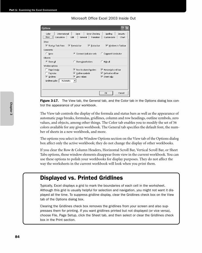
Microsoft Office Excel 2003 Inside Out

Part 1: Examining the Excel Environment

84

Chapter 3

f03ie17

Figure 3-17. The View tab, the General tab, and the Color tab in the Options dialog box con-trol the appearance of your workbook.

The View tab controls the display of the formula and status bars as well as the appearance of automatic page breaks, formulas, gridlines, column and row headings, outline symbols, zero values, and objects, among other things. The Color tab enables you to modify the set of 56 colors available for any given workbook. The General tab specifies the default font, the num-ber of sheets in a new workbook, and more.

The options you select in the Window Options section on the View tab of the Options dialog box affect only the active workbook; they do not change the display of other workbooks.

If you clear the Row & Column Headers, Horizontal Scroll Bar, Vertical Scroll Bar, or Sheet Tabs options, those window elements disappear from view in the current workbook. You can use these options to polish your workbooks for display purposes. They do not affect the way the worksheets in the current workbook will look when you print them.

Displayed vs. Printed GridlinesTypically, Excel displays a grid to mark the boundaries of each cell in the worksheet. Although this grid is usually helpful for selection and navigation, you might not want it dis-played all the time. To suppress gridline display, clear the Gridlines check box on the View tab of the Options dialog box.

Clearing the Gridlines check box removes the gridlines from your screen and also sup-presses them for printing. If you want gridlines printed but not displayed (or vice versa), choose File, Page Setup, click the Sheet tab, and then select or clear the Gridlines check box in the Print section.

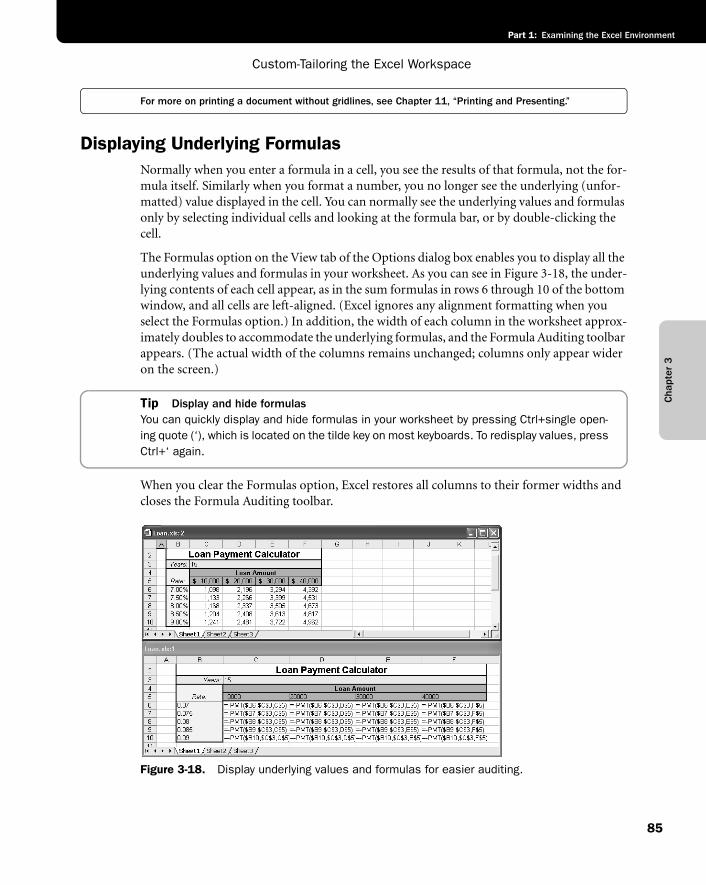
Custom-Tailoring the Excel Workspace

85

Part 1: Examining the Excel Environment

Cha

pter

3

For more on printing a document without gridlines, see Chapter 11, “Printing and Presenting.”

Displaying Underlying FormulasNormally when you enter a formula in a cell, you see the results of that formula, not the for-mula itself. Similarly when you format a number, you no longer see the underlying (unfor-matted) value displayed in the cell. You can normally see the underlying values and formulas only by selecting individual cells and looking at the formula bar, or by double-clicking the cell.

The Formulas option on the View tab of the Options dialog box enables you to display all the underlying values and formulas in your worksheet. As you can see in Figure 3-18, the under-lying contents of each cell appear, as in the sum formulas in rows 6 through 10 of the bottom window, and all cells are left-aligned. (Excel ignores any alignment formatting when you select the Formulas option.) In addition, the width of each column in the worksheet approx-imately doubles to accommodate the underlying formulas, and the Formula Auditing toolbar appears. (The actual width of the columns remains unchanged; columns only appear wider on the screen.)

Tip Display and hide formulasYou can quickly display and hide formulas in your worksheet by pressing Ctrl+single open-ing quote (‘), which is located on the tilde key on most keyboards. To redisplay values, press Ctrl+‘ again.

When you clear the Formulas option, Excel restores all columns to their former widths and closes the Formula Auditing toolbar.

f03ie18

Figure 3-18. Display underlying values and formulas for easier auditing.

Microsoft Office Excel 2003 Inside Out

Part 1: Examining the Excel Environment

86

Chapter 3

Tip Display each window differentlyIf you use the New Window command on the Window menu to create two or more windows in which to view the same workbook, you can use different display options in each window. For example, you can display formulas in one window and see the results of those formulas (the normal view) in another window.

The Formulas option is particularly helpful when you need to edit a large worksheet. You can see your formulas without having to activate each cell and view its contents in the Formula Bar. You can also use the Formulas option to document your work: After you select Formu-las, you can print your worksheet with the formulas displayed for archiving purposes.

Hiding ZerosNormally zeros are displayed on your worksheet. Sometimes, especially for presentation pur-poses, it is helpful to eliminate the clutter of excessive zero values on a worksheet. To hide zeros, clear the Zero Values option on the View tab of the Options dialog box. Any cells con-taining only zeros, or any formulas that result in zero, appear as blank cells on the sheet. The underlying entries are unaffected, of course. If you edit an entry or if the result of a formula changes so that the cell no longer contains a zero value, the value immediately becomes visible. If the Formulas option on the View tab is selected, clearing the Zero Values option has no effect on the display.

Caution If you hide zero values, be careful when editing your worksheet. What appears to be an empty cell might actually contain a formula.

Tip Changing the standard fontThe standard font is used not only for all text and numbers that you enter into a workbook, but it also determines the font used in row and column headings. In addition, the standard font is used as the font definition for the Normal style. You change the Standard Font option on the General tab of the Options dialog box, shown in Figure 3-19. The default standard font is 10-point Arial, but in Figure 3-19, the standard font was changed to 14-point Times New Roman, a good choice for high visibility, but a bad choice if you want to view many cells on the screen at one time. The new standard font will not become active until you quit and restart Excel. The next time you start Excel, all new workbooks you create are displayed with the new standard font. If you choose Style from the Format menu you’ll see that the Normal style now includes the new standard font.

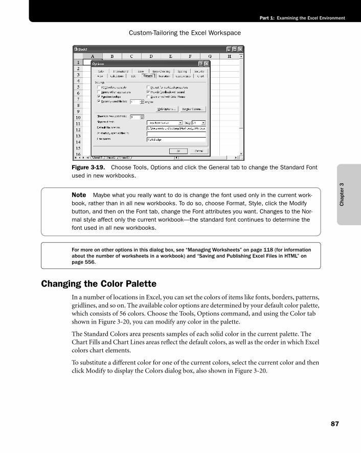
Custom-Tailoring the Excel Workspace

87

Part 1: Examining the Excel Environment

Cha

pter

3

f03ie19

Figure 3-19. Choose Tools, Options and click the General tab to change the Standard Font used in new workbooks.

Note Maybe what you really want to do is change the font used only in the current work-book, rather than in all new workbooks. To do so, choose Format, Style, click the Modify button, and then on the Font tab, change the Font attributes you want. Changes to the Nor-mal style affect only the current workbook—the standard font continues to determine the font used in all new workbooks.

For more on other options in this dialog box, see “Managing Worksheets” on page 118 (for information about the number of worksheets in a workbook) and “Saving and Publishing Excel Files in HTML” on page 556.

Changing the Color PaletteIn a number of locations in Excel, you can set the colors of items like fonts, borders, patterns, gridlines, and so on. The available color options are determined by your default color palette, which consists of 56 colors. Choose the Tools, Options command, and using the Color tab shown in Figure 3-20, you can modify any color in the palette.

The Standard Colors area presents samples of each solid color in the current palette. The Chart Fills and Chart Lines areas reflect the default colors, as well as the order in which Excel colors chart elements.

To substitute a different color for one of the current colors, select the current color and then click Modify to display the Colors dialog box, also shown in Figure 3-20.

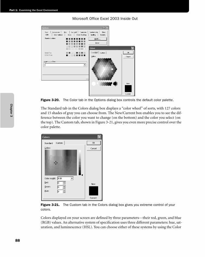
Microsoft Office Excel 2003 Inside Out

Part 1: Examining the Excel Environment

88

Chapter 3

f03ie20

Figure 3-20. The Color tab in the Options dialog box controls the default color palette.

The Standard tab in the Colors dialog box displays a “color wheel” of sorts, with 127 colors and 15 shades of gray you can choose from. The New/Current box enables you to see the dif-ference between the color you want to change (on the bottom) and the color you select (on the top). The Custom tab, shown in Figure 3-21, gives you even more precise control over the color palette.

f03ie21

Figure 3-21. The Custom tab in the Colors dialog box gives you extreme control of your colors.

Colors displayed on your screen are defined by three parameters—their red, green, and blue (RGB) values. An alternative system of specification uses three different parameters: hue, sat-uration, and luminescence (HSL). You can choose either of these systems by using the Color

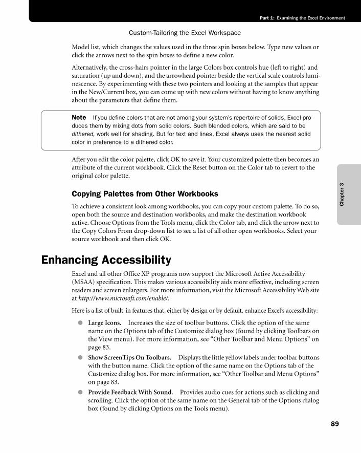
Custom-Tailoring the Excel Workspace

89

Part 1: Examining the Excel Environment

Cha

pter

3

Model list, which changes the values used in the three spin boxes below. Type new values or click the arrows next to the spin boxes to define a new color.

Alternatively, the cross-hairs pointer in the large Colors box controls hue (left to right) and saturation (up and down), and the arrowhead pointer beside the vertical scale controls lumi-nescence. By experimenting with these two pointers and looking at the samples that appear in the New/Current box, you can come up with new colors without having to know anything about the parameters that define them.

Note If you define colors that are not among your system’s repertoire of solids, Excel pro-duces them by mixing dots from solid colors. Such blended colors, which are said to be dithered, work well for shading. But for text and lines, Excel always uses the nearest solid color in preference to a dithered color.

After you edit the color palette, click OK to save it. Your customized palette then becomes an attribute of the current workbook. Click the Reset button on the Color tab to revert to the original color palette.

Copying Palettes from Other WorkbooksTo achieve a consistent look among workbooks, you can copy your custom palette. To do so, open both the source and destination workbooks, and make the destination workbook active. Choose Options from the Tools menu, click the Color tab, and click the arrow next to the Copy Colors From drop-down list to see a list of all other open workbooks. Select your source workbook and then click OK.

Enhancing AccessibilityExcel and all other Office XP programs now support the Microsoft Active Accessibility (MSAA) specification. This makes various accessibility aids more effective, including screen readers and screen enlargers. For more information, visit the Microsoft Accessibility Web site at http://www.microsoft.com/enable/.

Here is a list of built-in features that, either by design or by default, enhance Excel’s accessibility:

● Large Icons. Increases the size of toolbar buttons. Click the option of the same name on the Options tab of the Customize dialog box (found by clicking Toolbars on the View menu). For more information, see “Other Toolbar and Menu Options” on page 83.

● Show ScreenTips On Toolbars. Displays the little yellow labels under toolbar buttons with the button name. Click the option of the same name on the Options tab of the Customize dialog box. For more information, see “Other Toolbar and Menu Options” on page 83.

● Provide Feedback With Sound. Provides audio cues for actions such as clicking and scrolling. Click the option of the same name on the General tab of the Options dialog box (found by clicking Options on the Tools menu).

Microsoft Office Excel 2003 Inside Out

Part 1: Examining the Excel Environment

90

Chapter 3

● Function ToolTips. Displays yellow boxes with labels describing the syntax and argu-ments for functions entered or selected in the Formula bar or in cells. Click the option of the same name on the General tab of the Options dialog box. For more information, see Chapter 13, “Using Functions.”

● Provide Feedback With Animation. Adds visual cues for actions including menu display, scrolling, and inserting/deleting. Click the option of the same name on the Edit tab of the Options dialog box. For more information, see “Other Toolbar and Menu Options” on page 83.

● Enable AutoComplete For Cell Values. When entering data in a column, automati-cally inserts existing entries in the same column that match the current entry. This option saves keystrokes, for example, when repeatedly typing the same entry. Click the option of the same name on the General tab of the Options dialog box. For more infor-mation, see “Letting Excel Help with Typing Chores” on page 191.

● Gridlines Color. Changes the color of gridlines in your worksheet. Choose a color in the list box of the same name on the View tab of the Options dialog box.

● Colored Sheet Tabs. Makes it easier to find key sheets in a workbook, or color code to differentiate tabs. Choose Sheet on the Format menu and click Tab Color. For more information, see “Coloring Sheet Tabs” on page 120.

● Text To Speech. Reads the contents of cells to you. Point to Speech on the Tools menu, click Show Text To Speech Toolbar, and click the Speak Cells button. Or click the Speak On Enter button to have Excel vocalize what you just entered, to help increase accuracy. For more information, see “Having Excel Read Cells to You” on page 226.

● Keyboard Shortcuts. Gives you access to any command in Excel using the keyboard. For more information, see Appendix C, “Keyboard Shortcuts.”

● Scroll And Pan. If you have a Microsoft IntelliMouse, enables you to scroll through a worksheet by simply turning the wheel in the direction you want to scroll. If you press down on the wheel and drag the mouse, you can pan the worksheet in any direction.

● Zoom In. Enlarges the worksheet display up to 400 percent using the Zoom box on the Standard toolbar, or by holding down Ctrl and turning the wheel on a Microsoft IntelliMouse.

91

Part 2

Building Worksheets

4 Worksheet Design Tips 93

5 How to Work a Worksheet 101

6 How to Work a Workbook 133

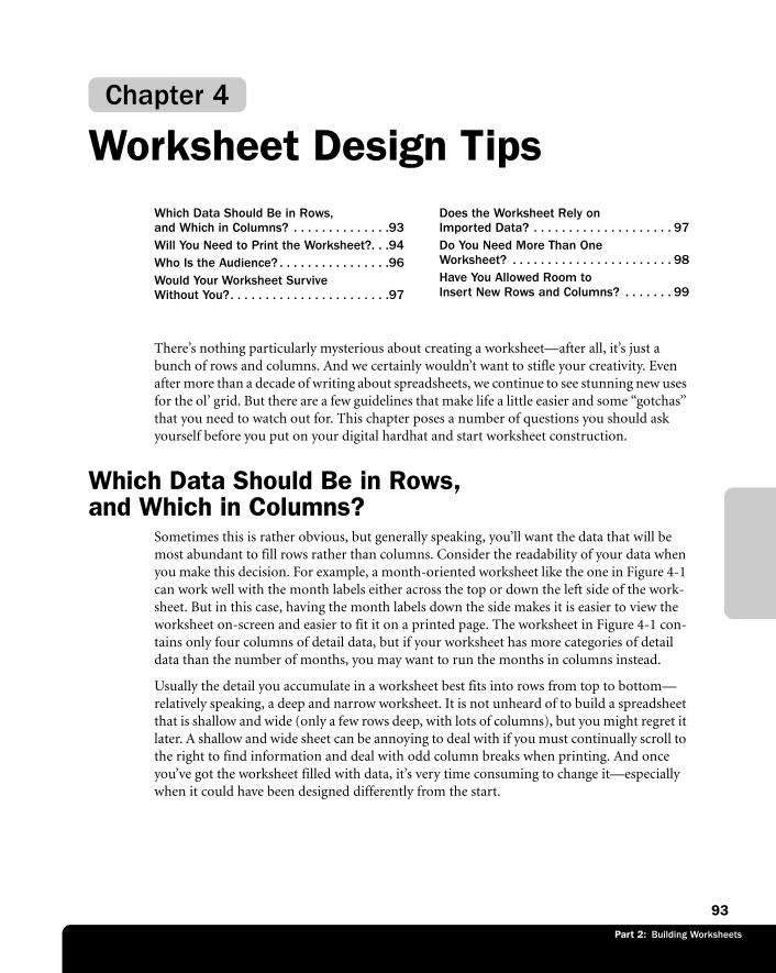
Part 2: Building Worksheets

93

Chapter 4

Worksheet Design TipsWhich Data Should Be in Rows, and Which in Columns? . . . . . . . . . . . . . .93Will You Need to Print the Worksheet?. . .94Who Is the Audience? . . . . . . . . . . . . . . . .96Would Your Worksheet Survive Without You?. . . . . . . . . . . . . . . . . . . . . . .97

Does the Worksheet Rely on Imported Data? . . . . . . . . . . . . . . . . . . . . 97Do You Need More Than One Worksheet? . . . . . . . . . . . . . . . . . . . . . . . 98Have You Allowed Room to Insert New Rows and Columns? . . . . . . . 99

There’s nothing particularly mysterious about creating a worksheet—after all, it’s just a bunch of rows and columns. And we certainly wouldn’t want to stifle your creativity. Even after more than a decade of writing about spreadsheets, we continue to see stunning new uses for the ol’ grid. But there are a few guidelines that make life a little easier and some “gotchas” that you need to watch out for. This chapter poses a number of questions you should ask yourself before you put on your digital hardhat and start worksheet construction.

Which Data Should Be in Rows, and Which in Columns?

Sometimes this is rather obvious, but generally speaking, you’ll want the data that will be most abundant to fill rows rather than columns. Consider the readability of your data when you make this decision. For example, a month-oriented worksheet like the one in Figure 4-1 can work well with the month labels either across the top or down the left side of the work-sheet. But in this case, having the month labels down the side makes it is easier to view the worksheet on-screen and easier to fit it on a printed page. The worksheet in Figure 4-1 con-tains only four columns of detail data, but if your worksheet has more categories of detail data than the number of months, you may want to run the months in columns instead.

Usually the detail you accumulate in a worksheet best fits into rows from top to bottom—relatively speaking, a deep and narrow worksheet. It is not unheard of to build a spreadsheet that is shallow and wide (only a few rows deep, with lots of columns), but you might regret it later. A shallow and wide sheet can be annoying to deal with if you must continually scroll to the right to find information and deal with odd column breaks when printing. And once you’ve got the worksheet filled with data, it’s very time consuming to change it—especially when it could have been designed differently from the start.

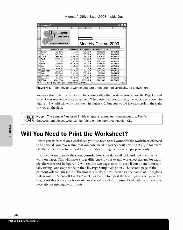
Part 2: Building Worksheets

Chapter 4

Microsoft Office Excel 2003 Inside Out

94

f04ie01

Figure 4-1. Monthly total worksheets are often oriented vertically, as shown here.

You may also prefer the worksheet to be long rather than wide so you can use the Page Up and Page Down keys to navigate on-screen. When oriented horizontally, the worksheet shown in Figure 4-1 would still work, as shown in Figure 4-2, but you would have to scroll to the right to view all the data.

Note The sample files used in this chapter’s examples, Humongous.xls, Pacific Sales.xls, and Alpacas.xls, can be found on the book’s companion CD.

Will You Need to Print the Worksheet?Before you start work on a worksheet, you also need to ask yourself if the worksheet will need to be printed. You may realize that you don’t need to worry about printing at all, if, for exam-ple, the worksheet is to be used for information storage or reference purposes only.

If you will want to print the sheet, consider how your data will look and how the sheet will work on paper. This will make a huge difference to your overall worksheet design. For exam-ple, the worksheet in Figure 4-2 will require two pages to print, even if you orient it horizon-tally (using Landscape mode in the File, Page Setup dialog box). The second page of the printout will contain some of the monthly totals, but you won’t see the names of the regions unless you use Microsoft Excel’s Print Titles feature to repeat the headings on each page. For large worksheets in either horizontal or vertical orientation, using Print Titles is an absolute necessity for intelligible printouts.

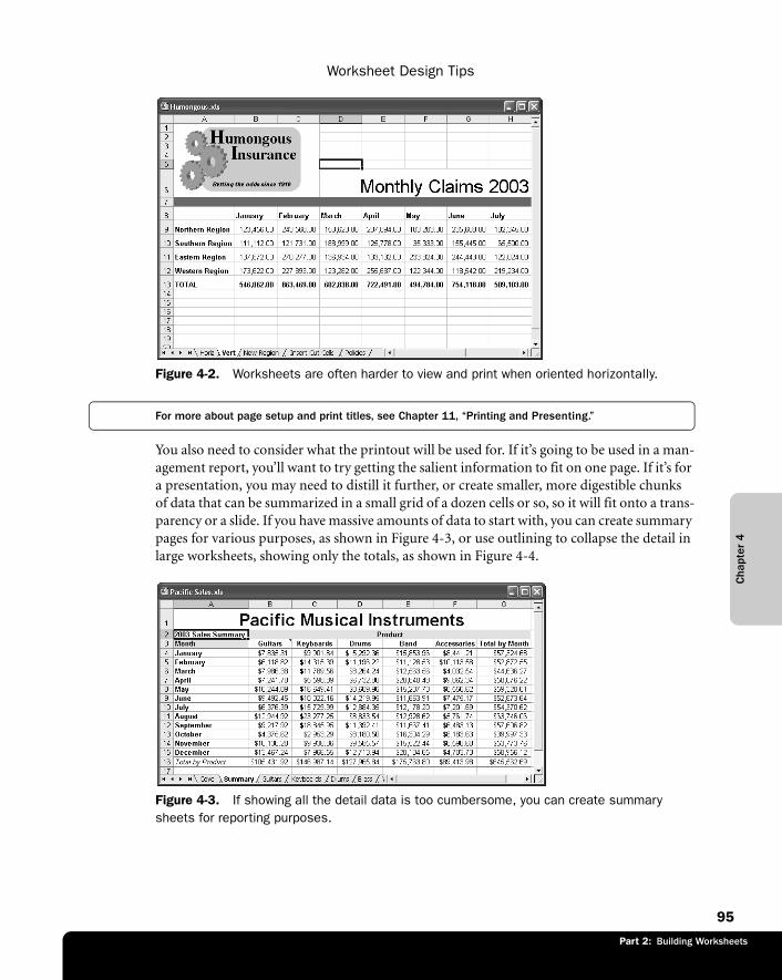
Part 2: Building Worksheets

Cha

pter

4

Worksheet Design Tips

95

f04ie02

Figure 4-2. Worksheets are often harder to view and print when oriented horizontally.

For more about page setup and print titles, see Chapter 11, “Printing and Presenting.”

You also need to consider what the printout will be used for. If it’s going to be used in a man-agement report, you’ll want to try getting the salient information to fit on one page. If it’s for a presentation, you may need to distill it further, or create smaller, more digestible chunks of data that can be summarized in a small grid of a dozen cells or so, so it will fit onto a trans-parency or a slide. If you have massive amounts of data to start with, you can create summary pages for various purposes, as shown in Figure 4-3, or use outlining to collapse the detail in large worksheets, showing only the totals, as shown in Figure 4-4.

f04ie03

Figure 4-3. If showing all the detail data is too cumbersome, you can create summary sheets for reporting purposes.

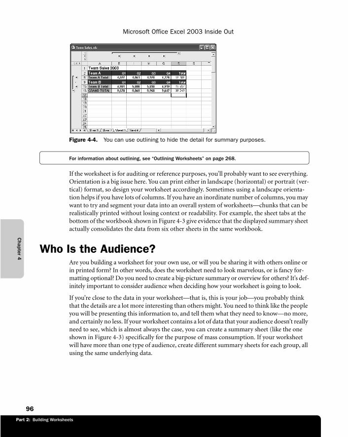
Part 2: Building Worksheets

Chapter 4

Microsoft Office Excel 2003 Inside Out

96

f04ie04

Figure 4-4. You can use outlining to hide the detail for summary purposes.

For information about outlining, see “Outlining Worksheets” on page 268.

If the worksheet is for auditing or reference purposes, you’ll probably want to see everything. Orientation is a big issue here. You can print either in landscape (horizontal) or portrait (ver-tical) format, so design your worksheet accordingly. Sometimes using a landscape orienta-tion helps if you have lots of columns. If you have an inordinate number of columns, you may want to try and segment your data into an overall system of worksheets—chunks that can be realistically printed without losing context or readability. For example, the sheet tabs at the bottom of the workbook shown in Figure 4-3 give evidence that the displayed summary sheet actually consolidates the data from six other sheets in the same workbook.

Who Is the Audience?Are you building a worksheet for your own use, or will you be sharing it with others online or in printed form? In other words, does the worksheet need to look marvelous, or is fancy for-matting optional? Do you need to create a big-picture summary or overview for others? It’s def-initely important to consider audience when deciding how your worksheet is going to look.

If you’re close to the data in your worksheet—that is, this is your job—you probably think that the details are a lot more interesting than others might. You need to think like the people you will be presenting this information to, and tell them what they need to know—no more, and certainly no less. If your worksheet contains a lot of data that your audience doesn’t really need to see, which is almost always the case, you can create a summary sheet (like the one shown in Figure 4-3) specifically for the purpose of mass consumption. If your worksheet will have more than one type of audience, create different summary sheets for each group, all using the same underlying data.

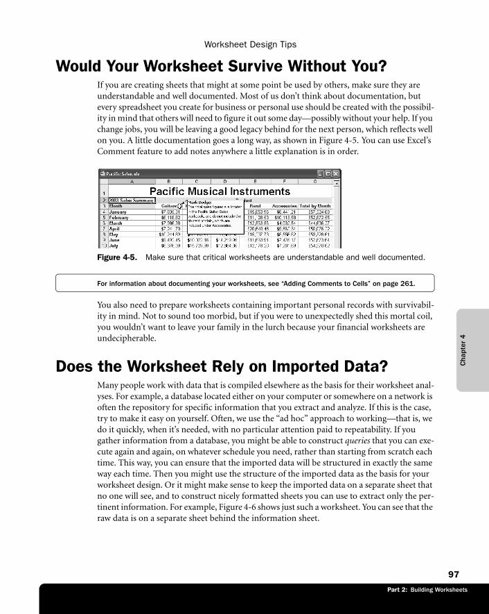
Part 2: Building Worksheets

Cha

pter

4

Worksheet Design Tips

97

Would Your Worksheet Survive Without You?If you are creating sheets that might at some point be used by others, make sure they are understandable and well documented. Most of us don’t think about documentation, but every spreadsheet you create for business or personal use should be created with the possibil-ity in mind that others will need to figure it out some day—possibly without your help. If you change jobs, you will be leaving a good legacy behind for the next person, which reflects well on you. A little documentation goes a long way, as shown in Figure 4-5. You can use Excel’s Comment feature to add notes anywhere a little explanation is in order.

f04ie05

Figure 4-5. Make sure that critical worksheets are understandable and well documented.

For information about documenting your worksheets, see “Adding Comments to Cells” on page 261.

You also need to prepare worksheets containing important personal records with survivabil-ity in mind. Not to sound too morbid, but if you were to unexpectedly shed this mortal coil, you wouldn’t want to leave your family in the lurch because your financial worksheets are undecipherable.

Does the Worksheet Rely on Imported Data?Many people work with data that is compiled elsewhere as the basis for their worksheet anal-yses. For example, a database located either on your computer or somewhere on a network is often the repository for specific information that you extract and analyze. If this is the case, try to make it easy on yourself. Often, we use the “ad hoc” approach to working—that is, we do it quickly, when it’s needed, with no particular attention paid to repeatability. If you gather information from a database, you might be able to construct queries that you can exe-cute again and again, on whatever schedule you need, rather than starting from scratch each time. This way, you can ensure that the imported data will be structured in exactly the same way each time. Then you might use the structure of the imported data as the basis for your worksheet design. Or it might make sense to keep the imported data on a separate sheet that no one will see, and to construct nicely formatted sheets you can use to extract only the per-tinent information. For example, Figure 4-6 shows just such a worksheet. You can see that the raw data is on a separate sheet behind the information sheet.

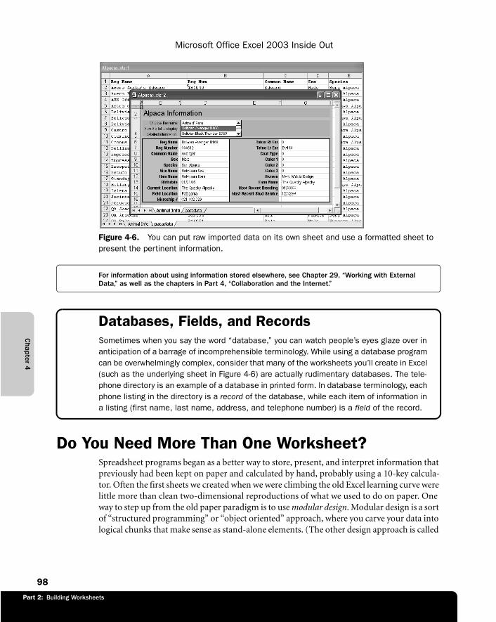
Part 2: Building Worksheets

Chapter 4

Microsoft Office Excel 2003 Inside Out

98

f04ie06

Figure 4-6. You can put raw imported data on its own sheet and use a formatted sheet to present the pertinent information.

For information about using information stored elsewhere, see Chapter 29, “Working with External Data,” as well as the chapters in Part 4, “Collaboration and the Internet.”

Databases, Fields, and RecordsSometimes when you say the word “database,” you can watch people’s eyes glaze over in anticipation of a barrage of incomprehensible terminology. While using a database program can be overwhelmingly complex, consider that many of the worksheets you’ll create in Excel (such as the underlying sheet in Figure 4-6) are actually rudimentary databases. The tele-phone directory is an example of a database in printed form. In database terminology, each phone listing in the directory is a record of the database, while each item of information in a listing (first name, last name, address, and telephone number) is a field of the record.

Do You Need More Than One Worksheet?Spreadsheet programs began as a better way to store, present, and interpret information that previously had been kept on paper and calculated by hand, probably using a 10-key calcula-tor. Often the first sheets we created when we were climbing the old Excel learning curve were little more than clean two-dimensional reproductions of what we used to do on paper. One way to step up from the old paper paradigm is to use modular design. Modular design is a sort of “structured programming” or “object oriented” approach, where you carve your data into logical chunks that make sense as stand-alone elements. (The other design approach is called

Part 2: Building Worksheets

Cha

pter

4

Worksheet Design Tips

99

hierarchical, which is organized for error identification and maximum readability.) Since there’s usually no need to keep detail data in any kind of presentable format, why bother? Concentrate your worksheet beautification program on the summary sheets and charts that you will share with others. Design a system of worksheets rather than trying to get everything on a single worksheet. Figure 4-6 shows a rudimentary example of modular design—that is, there is one sheet for data and another for a specific type of analysis. In a complex modular system, you might have dozens of sheets, each dedicated to a specific task.

Have You Allowed Room to Insert New Rows and Columns?

It’s critical to allow for expansion and editing after your worksheet is assembled. It’s generally a good idea to add a few extra rows and columns to the detail area and to keep totals sepa-rated from the detail data by a row or column or two, if possible. One of the most common editing actions you’ll perform is inserting new rows and columns. Excel has gotten a lot smarter about this over the years, making obsolete some of the rules of thumb that we old-timers have collected. But it’s still possible to mess up.

There’s a rather famous folkloric tale about an accounting person who inserted a row at the bottom of a range of cells but forgot to adjust the totals formulas and was fired because his numbers were $200,000 off. The moral: Edit worksheets carefully and audit yourself ruth-lessly, especially if your job is on the line.

Part 2: Building Worksheets

101

Chapter 5

How to Work a WorksheetMoving Around . . . . . . . . . . . . . . . . . . . 101Selecting Stuff. . . . . . . . . . . . . . . . . . . . 104Entering Stuff . . . . . . . . . . . . . . . . . . . . 109

Managing Worksheets . . . . . . . . . . . . . . 118Looking at Worksheets . . . . . . . . . . . . . 121Protecting Worksheets . . . . . . . . . . . . . . 127

The worksheet is Microsoft Excel’s playing field, where all your base hits, grand slams, errors, and wild pitches occur. This chapter discusses the “innings and outs” of using worksheets, including the quickest way to get from cell A1 to cell IV65536 (and anywhere between), the hidden methods of selecting, and the basics of editing.

You probably already know many of these techniques, but here we’ll present alternative methods. You might find that there is a better, or faster, way to do something you do fre-quently. If there’s one thing Excel has a lot of, it’s alternatives.

Moving AroundYou already know how to use scroll bars and the Page Up and Page Down keys. There are many other ways to get around, including some unique tricks you’ll find only in Excel.

Navigating RegionsA region is a range of cell entries bounded by blank cells or column and row headings. In Figure 5-1, the range A3:E7 is a region, as are the ranges G3:H7, A9:E10, and G9:H10. (Strictly speaking, cell A1 is also a region because there are no adjoining cells containing entries.) For example, cell E7 is within a region, even though it’s empty. The active area is a rectangle that encompasses all regions—that is, all the filled cells in the active worksheet.

The techniques used to navigate regions are especially helpful if you typically work with large tables of data. Getting to the bottom row of a 500-row table is easier when you don’t have to use the scroll bars. Read on to find out how.

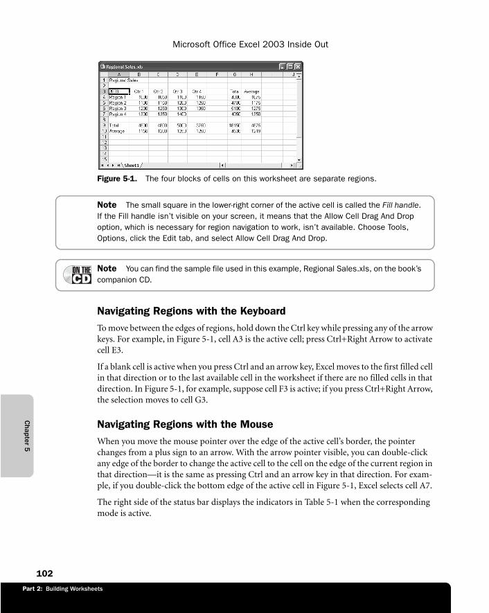
Part 2: Building Worksheets

Chapter 5

Microsoft Office Excel 2003 Inside Out

102

f05ie01

Figure 5-1. The four blocks of cells on this worksheet are separate regions.

Note The small square in the lower-right corner of the active cell is called the Fill handle.If the Fill handle isn’t visible on your screen, it means that the Allow Cell Drag And Drop option, which is necessary for region navigation to work, isn’t available. Choose Tools, Options, click the Edit tab, and select Allow Cell Drag And Drop.

Note You can find the sample file used in this example, Regional Sales.xls, on the book’s companion CD.

Navigating Regions with the KeyboardTo move between the edges of regions, hold down the Ctrl key while pressing any of the arrow keys. For example, in Figure 5-1, cell A3 is the active cell; press Ctrl+Right Arrow to activate cell E3.

If a blank cell is active when you press Ctrl and an arrow key, Excel moves to the first filled cell in that direction or to the last available cell in the worksheet if there are no filled cells in that direction. In Figure 5-1, for example, suppose cell F3 is active; if you press Ctrl+Right Arrow, the selection moves to cell G3.

Navigating Regions with the MouseWhen you move the mouse pointer over the edge of the active cell’s border, the pointer changes from a plus sign to an arrow. With the arrow pointer visible, you can double-click any edge of the border to change the active cell to the cell on the edge of the current region in that direction—it is the same as pressing Ctrl and an arrow key in that direction. For exam-ple, if you double-click the bottom edge of the active cell in Figure 5-1, Excel selects cell A7.

The right side of the status bar displays the indicators in Table 5-1 when the corresponding mode is active.

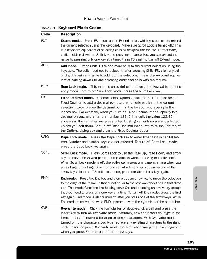
Part 2: Building Worksheets

Cha

pter

5

How to Work a Worksheet

103

Part 1: Part Title

Table 5-1. Keyboard Mode Codes

Code Description

EXT Extend mode. Press F8 to turn on the Extend mode, which you can use to extend the current selection using the keyboard. (Make sure Scroll Lock is turned off.) This is a keyboard equivalent of selecting cells by dragging the mouse. Furthermore, unlike holding down the Shift key and pressing an arrow key, you can extend the range by pressing only one key at a time. Press F8 again to turn off Extend mode.

ADD Add mode. Press Shift+F8 to add more cells to the current selection using the keyboard. The cells need not be adjacent; after pressing Shift+F8, click any cell or drag through any range to add it to the selection. This is the keyboard equiva-lent of holding down Ctrl and selecting additional cells with the mouse.

NUM Num Lock mode. This mode is on by default and locks the keypad in numeric-entry mode. To turn off Num Lock mode, press the Num Lock key.

FIX Fixed Decimal mode. Choose Tools, Options, click the Edit tab, and select Fixed Decimal to add a decimal point to the numeric entries in the current selection. Excel places the decimal point in the location you specify in the Places box. For example, when you turn on Fixed Decimal mode, specify two decimal places, and enter the number 12345 in a cell, the value 123.45 appears in the cell after you press Enter. Existing cell entries are not affected unless you edit them. To turn off Fixed Decimal mode, return to the Edit tab of the Options dialog box and clear the Fixed Decimal option.

CAPS Caps Lock mode. Press the Caps Lock key to enter typed text in capital let-ters. Number and symbol keys are not affected. To turn off Caps Lock mode, press the Caps Lock key again.

SCRL Scroll Lock mode. Press Scroll Lock to use the Page Up, Page Down, and arrow keys to move the viewed portion of the window without moving the active cell. When Scroll Lock mode is off, the active cell moves one page at a time when you press Page Up or Page Down, or one cell at a time when you press one of the arrow keys. To turn off Scroll Lock mode, press the Scroll Lock key again.

END End mode. Press the End key and then press an arrow key to move the selection to the edge of the region in that direction, or to the last worksheet cell in that direc-tion. This mode functions like holding down Ctrl and pressing an arrow key, except that you need to press only one key at a time. To turn off End mode, press the End key again. End mode is also turned off after you press one of the arrow keys. While End mode is active, the word END appears toward the right side of the status bar.

OVR Overwrite mode. Click the formula bar or double-click a cell and press the Insert key to turn on Overwrite mode. Normally, new characters you type in the formula bar are inserted between existing characters. With Overwrite mode turned on, the characters you type replace any existing characters to the right of the insertion point. Overwrite mode turns off when you press Insert again or when you press Enter or one of the arrow keys.

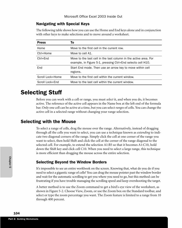
Part 2: Building Worksheets

Chapter 5

Microsoft Office Excel 2003 Inside Out

104

Navigating with Special KeysThe following table shows how you can use the Home and End keys alone and in conjunction with other keys to make selections and to move around a worksheet.

Selecting StuffBefore you can work with a cell or range, you must select it, and when you do, it becomes active. The reference of the active cell appears in the Name box at the left end of the formula bar. Only one cell can be active at a time, but you can select ranges of cells. You can change the active cell in a selected range without changing your range selection.

Selecting with the MouseTo select a range of cells, drag the mouse over the range. Alternatively, instead of dragging through all the cells you want to select, you can use a technique known as extending to indi-cate two diagonal corners of the range. Simply click the cell at one corner of the range you want to select, then hold Shift and click the cell at the corner of the range diagonal to the selected cell. For example, to extend the selection A1:B5 so that it becomes A1:C10, hold down the Shift key and click cell C10. When you need to select a large range, this technique is more efficient than dragging the mouse across the entire selection.

Selecting Beyond the Window BordersIt’s impossible to see an entire workbook on the screen. Knowing that, what do you do if you need to select a gigantic range of cells? You can drag the mouse pointer past the window border and wait for the automatic scrolling to get you where you need to go, but this method can be frustrating if you have trouble managing the scrolling speed and keep overshooting the target.

A better method is to use the Zoom command to get a bird’s-eye view of the worksheet, as shown in Figure 5-2. Choose View, Zoom, or use the Zoom box on the Standard toolbar, and select or type the zoom percentage you want. The Zoom feature is limited to a range from 10 through 400 percent.

Press To

Home Move to the first cell in the current row.

Ctrl+Home Move to cell A1.

Ctrl+End Move to the last cell in the last column in the active area. For example, in Figure 5-1, pressing Ctrl+End selects cell H10.

End Start End mode. Then use an arrow key to move within cell regions.

Scroll Lock+Home Move to the first cell within the current window.

Scroll Lock+End Move to the last cell within the current window.

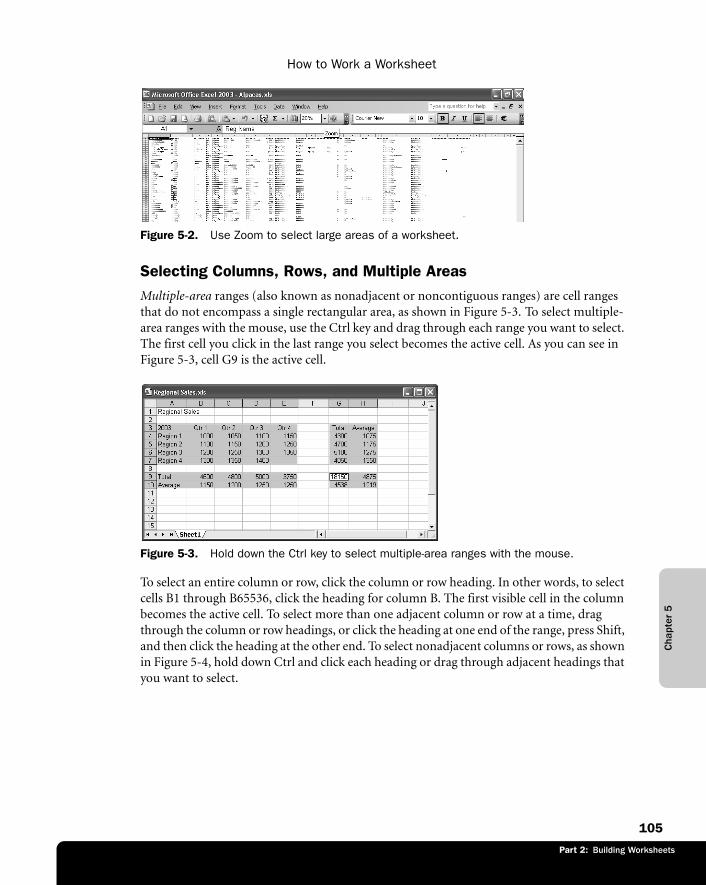
Part 2: Building Worksheets

Cha

pter

5

How to Work a Worksheet

105

Part 1: Part Title

f05ie02

Figure 5-2. Use Zoom to select large areas of a worksheet.

Selecting Columns, Rows, and Multiple AreasMultiple-area ranges (also known as nonadjacent or noncontiguous ranges) are cell ranges that do not encompass a single rectangular area, as shown in Figure 5-3. To select multiple-area ranges with the mouse, use the Ctrl key and drag through each range you want to select. The first cell you click in the last range you select becomes the active cell. As you can see in Figure 5-3, cell G9 is the active cell.

f05ie03

Figure 5-3. Hold down the Ctrl key to select multiple-area ranges with the mouse.

To select an entire column or row, click the column or row heading. In other words, to select cells B1 through B65536, click the heading for column B. The first visible cell in the column becomes the active cell. To select more than one adjacent column or row at a time, drag through the column or row headings, or click the heading at one end of the range, press Shift, and then click the heading at the other end. To select nonadjacent columns or rows, as shown in Figure 5-4, hold down Ctrl and click each heading or drag through adjacent headings that you want to select.

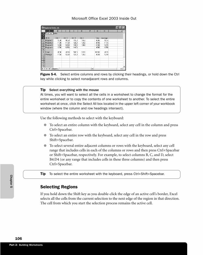
Part 2: Building Worksheets

Chapter 5

Microsoft Office Excel 2003 Inside Out

106

f05ie04

Figure 5-4. Select entire columns and rows by clicking their headings, or hold down the Ctrl key while clicking to select nonadjacent rows and columns.

Tip Select everything with the mouseAt times, you will want to select all the cells in a worksheet to change the format for the entire worksheet or to copy the contents of one worksheet to another. To select the entire worksheet at once, click the Select All box located in the upper left corner of your workbook window (where the column and row headings intersect).

Use the following methods to select with the keyboard:

● To select an entire column with the keyboard, select any cell in the column and press Ctrl+Spacebar.

● To select an entire row with the keyboard, select any cell in the row and press Shift+Spacebar.

● To select several entire adjacent columns or rows with the keyboard, select any cell range that includes cells in each of the columns or rows and then press Ctrl+Spacebar or Shift+Spacebar, respectively. For example, to select columns B, C, and D, select B4:D4 (or any range that includes cells in these three columns) and then press Ctrl+Spacebar.

Tip To select the entire worksheet with the keyboard, press Ctrl+Shift+Spacebar.

Selecting RegionsIf you hold down the Shift key as you double-click the edge of an active cell’s border, Excel selects all the cells from the current selection to the next edge of the region in that direction. The cell from which you start the selection process remains the active cell.

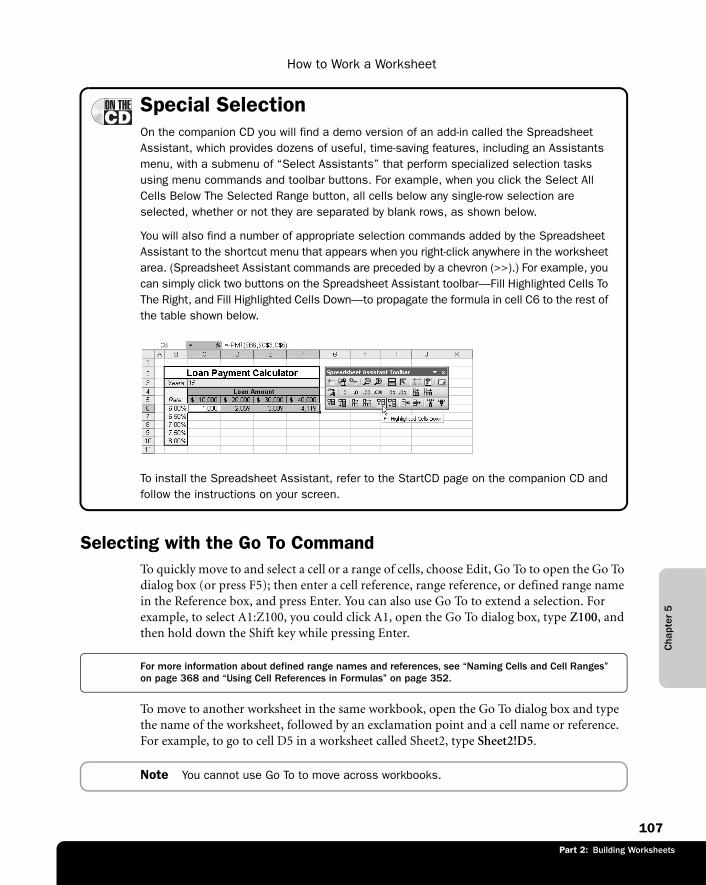
Part 2: Building Worksheets

Cha

pter

5

How to Work a Worksheet

107

Part 1: Part Title

Special SelectionOn the companion CD you will find a demo version of an add-in called the Spreadsheet Assistant, which provides dozens of useful, time-saving features, including an Assistants menu, with a submenu of “Select Assistants” that perform specialized selection tasks using menu commands and toolbar buttons. For example, when you click the Select All Cells Below The Selected Range button, all cells below any single-row selection are selected, whether or not they are separated by blank rows, as shown below.

You will also find a number of appropriate selection commands added by the Spreadsheet Assistant to the shortcut menu that appears when you right-click anywhere in the worksheet area. (Spreadsheet Assistant commands are preceded by a chevron (>>).) For example, you can simply click two buttons on the Spreadsheet Assistant toolbar—Fill Highlighted Cells To The Right, and Fill Highlighted Cells Down—to propagate the formula in cell C6 to the rest of the table shown below.

G05ie03

To install the Spreadsheet Assistant, refer to the StartCD page on the companion CD and follow the instructions on your screen.

Selecting with the Go To CommandTo quickly move to and select a cell or a range of cells, choose Edit, Go To to open the Go To dialog box (or press F5); then enter a cell reference, range reference, or defined range name in the Reference box, and press Enter. You can also use Go To to extend a selection. For example, to select A1:Z100, you could click A1, open the Go To dialog box, type Z100, and then hold down the Shift key while pressing Enter.

For more information about defined range names and references, see “Naming Cells and Cell Ranges” on page 368 and “Using Cell References in Formulas” on page 352.

To move to another worksheet in the same workbook, open the Go To dialog box and type the name of the worksheet, followed by an exclamation point and a cell name or reference. For example, to go to cell D5 in a worksheet called Sheet2, type Sheet2!D5.

Note You cannot use Go To to move across workbooks.

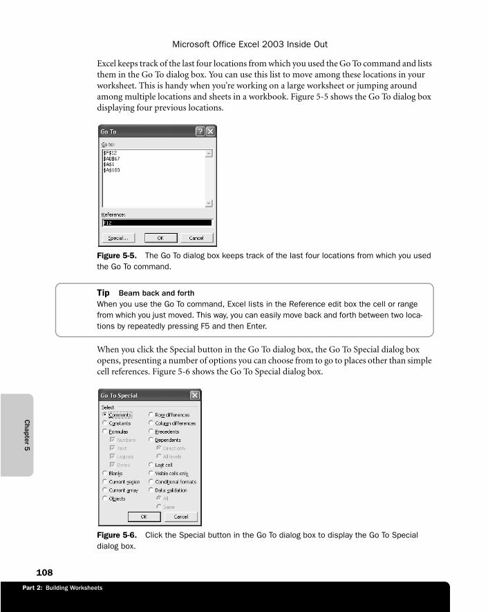
Part 2: Building Worksheets

Chapter 5

Microsoft Office Excel 2003 Inside Out

108

Excel keeps track of the last four locations from which you used the Go To command and lists them in the Go To dialog box. You can use this list to move among these locations in your worksheet. This is handy when you’re working on a large worksheet or jumping around among multiple locations and sheets in a workbook. Figure 5-5 shows the Go To dialog box displaying four previous locations.

f05ie05

Figure 5-5. The Go To dialog box keeps track of the last four locations from which you used the Go To command.

Tip Beam back and forthWhen you use the Go To command, Excel lists in the Reference edit box the cell or range from which you just moved. This way, you can easily move back and forth between two loca-tions by repeatedly pressing F5 and then Enter.

When you click the Special button in the Go To dialog box, the Go To Special dialog box opens, presenting a number of options you can choose from to go to places other than simple cell references. Figure 5-6 shows the Go To Special dialog box.

f05ie06

Figure 5-6. Click the Special button in the Go To dialog box to display the Go To Special dialog box.

Part 2: Building Worksheets

Cha

pter

5

How to Work a Worksheet

109

Part 1: Part Title

Entering StuffExcel accepts two basic types of cell entries: constants and formulas. Constants fall into three main categories: numeric values, text values (also called labels or strings), and date/time values. Excel also recognizes two special types of constants called logical values and error values.

For more on date values, see Chapter 15, “Formatting and Calculating Date and Time.”

Making Entries in Cells and in the Formula BarTo make an entry into a cell, just select the cell and start typing. As you type, the entry appears both in the formula bar and in the active cell. The flashing vertical bar in the active cell is called the insertion point.

After you finish typing, you must “lock in” the entry to store it permanently in the cell by pressing Enter. Pressing Enter normally causes the active cell to move down one row. You can change this so that when you press Enter, either the active cell doesn’t change or it moves to an adjacent cell in another direction. Choose Tools, Options, click the Edit tab, and either clear the Move Selection After Enter option or change the selection in the Direction list. You can also lock in an entry when you move the selection to a different cell by pressing Tab, Shift+Tab, Shift+Enter, or an arrow key, among other methods, after you type the entry, as shown in the following table.

When you begin typing an entry, three buttons appear on the formula bar: the Cancel but-ton, the Enter button, and the Insert Function button. When typing a formula where the entry begins with an equal sign (=), a plus sign (+), or a minus sign (–), a drop-down list of frequently used functions becomes available, as shown in Figure 5-7.

For more about editing formulas, see Chapter 12, “Building Formulas.”

Press To Activate

Enter The cell below the active cell, or whatever Direction is set for the Move Selection After Enter option on the Edit tab of the Options dialog box

Shift+Enter The cell above the active cell, or the opposite of the Direction set for the Move Selection After Enter option on the Edit tab of the Options dialog box

Tab The cell one column to the right of the active cell

Shift+Tab The cell one column to the left of the active cell

Arrow Key The adjacent cell in the direction of the arrow key that you press

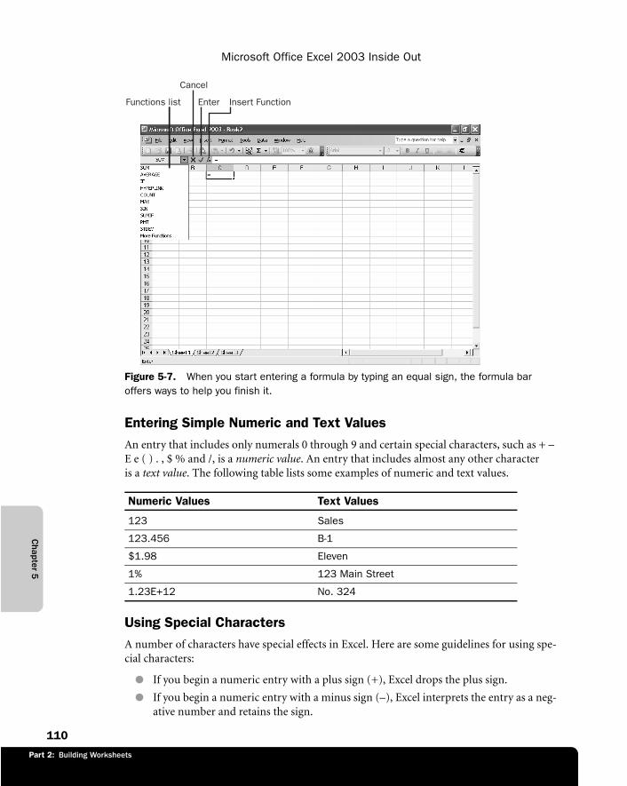
Part 2: Building Worksheets

Chapter 5

Microsoft Office Excel 2003 Inside Out

110

f05ie07

Figure 5-7. When you start entering a formula by typing an equal sign, the formula bar offers ways to help you finish it.

Entering Simple Numeric and Text ValuesAn entry that includes only numerals 0 through 9 and certain special characters, such as + – E e ( ) . , $ % and /, is a numeric value. An entry that includes almost any other character is a text value. The following table lists some examples of numeric and text values.

Using Special CharactersA number of characters have special effects in Excel. Here are some guidelines for using spe-cial characters:

● If you begin a numeric entry with a plus sign (+), Excel drops the plus sign.

● If you begin a numeric entry with a minus sign (–), Excel interprets the entry as a neg-ative number and retains the sign.

Cancel

Enter Insert FunctionFunctions list

Numeric Values Text Values

123 Sales

123.456 B-1

$1.98 Eleven

1% 123 Main Street

1.23E+12 No. 324

Part 2: Building Worksheets

Cha

pter

5

How to Work a Worksheet

111

Part 1: Part Title

● In a numeric entry, the characters E and e specify an exponent used in scientific nota-tion. For example, it interprets 1E6 as 1,000,000 (1 times 10 to the sixth power), which is displayed in Excel as 1.00E+06. To enter a negative exponential number, enter a minus sign before the exponent. For example, –1E6 (1 times 10 to the negative sixth power) equals –1,000,000, and is displayed in Excel as 1.00E-06.

● Excel interprets numeric constants enclosed in parentheses as negative numbers, which is a common accounting practice. For example, Excel interprets (100) as –100.

● You can use decimal points and commas as you normally would. When you enter num-bers that include commas as separators, however, the commas appear in the cell but not in the formula bar; this is the same as if you had applied one of Excel’s built-in Number formats. For example, if you enter 1,234.56, 1234.56 is displayed in the formula bar.

● If you begin a numeric entry with a dollar sign, Excel assigns a Currency format to the cell. For example, if you enter $123456, Excel displays $123,456 in the cell and 123456 in the formula bar. In this case, Excel adds the comma to the worksheet display because it’s part of the Currency format.

● If you end a numeric entry with a percent sign (%), Excel assigns a Percentage format to the cell. For example, if you enter 23%, Excel displays 23% in the formula bar and assigns a Percentage format to the cell, which also displays 23%.

● If you use a forward slash (/) in a numeric entry and the string cannot be interpreted as a date, Excel interprets the number as a fraction. For example, if you enter 11 5/8 (with a space between the number and the fraction), Excel assigns a Fraction format to the entry, meaning that the formula bar displays 11.625 and the cell displays 11 5/8.

Tip Enter numbers as fractionsTo make sure Excel does not interpret a fraction as a date, precede the fraction with a zero and a space. For example, to prevent Excel from interpreting the fraction 1/2 as January 2, type 0 1/2.

For more about Excel’s built-in Number formats, see “Formatting in Cells” on page 200. For more information about date and time formats, see “How Autofill Handles Dates and Times” on page 173.

Understanding the Difference Between Displayed Values and Underlying ValuesAlthough you can type 32,767 characters into a cell, a numeric cell entry can maintain pre-cision to only a maximum of 15 digits. This means that you can enter numbers longer than 15 digits into a cell, but Excel converts any digits after the fifteenth to zeros. If you are working with figures over 999 trillion, or decimals smaller than trillionths, perhaps you need to look into alternative solutions, such as a Cray supercomputer.

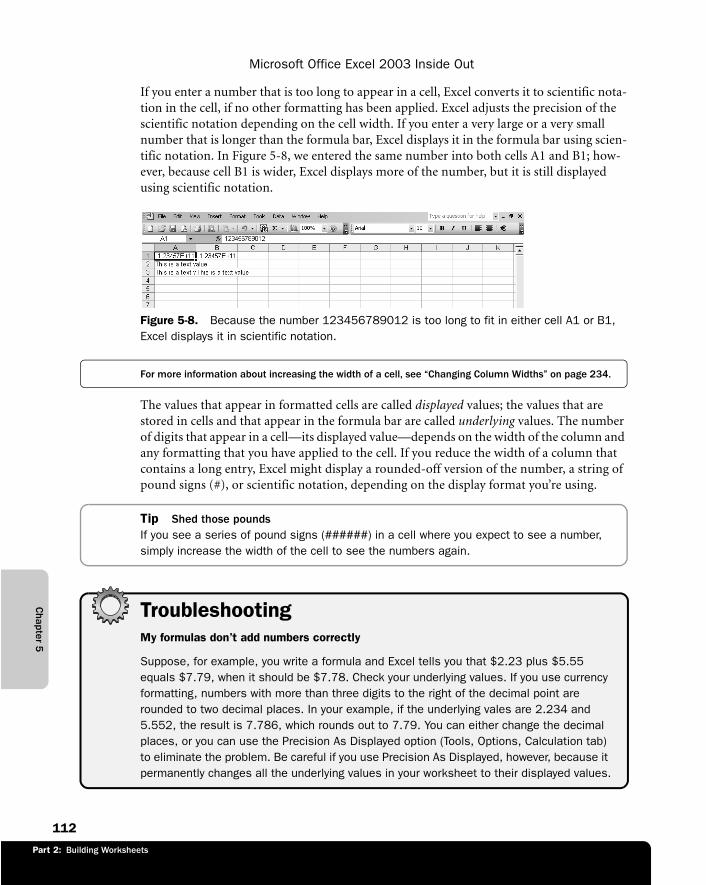
Part 2: Building Worksheets

Chapter 5

Microsoft Office Excel 2003 Inside Out

112

If you enter a number that is too long to appear in a cell, Excel converts it to scientific nota-tion in the cell, if no other formatting has been applied. Excel adjusts the precision of the scientific notation depending on the cell width. If you enter a very large or a very small number that is longer than the formula bar, Excel displays it in the formula bar using scien-tific notation. In Figure 5-8, we entered the same number into both cells A1 and B1; how-ever, because cell B1 is wider, Excel displays more of the number, but it is still displayed using scientific notation.

f05ie08

Figure 5-8. Because the number 123456789012 is too long to fit in either cell A1 or B1, Excel displays it in scientific notation.

For more information about increasing the width of a cell, see “Changing Column Widths” on page 234.

The values that appear in formatted cells are called displayed values; the values that are stored in cells and that appear in the formula bar are called underlying values. The number of digits that appear in a cell—its displayed value—depends on the width of the column and any formatting that you have applied to the cell. If you reduce the width of a column that contains a long entry, Excel might display a rounded-off version of the number, a string of pound signs (#), or scientific notation, depending on the display format you’re using.

Tip Shed those poundsIf you see a series of pound signs (######) in a cell where you expect to see a number, simply increase the width of the cell to see the numbers again.

TroubleshootingMy formulas don’t add numbers correctly

Suppose, for example, you write a formula and Excel tells you that $2.23 plus $5.55 equals $7.79, when it should be $7.78. Check your underlying values. If you use currency formatting, numbers with more than three digits to the right of the decimal point are rounded to two decimal places. In your example, if the underlying vales are 2.234 and 5.552, the result is 7.786, which rounds out to 7.79. You can either change the decimal places, or you can use the Precision As Displayed option (Tools, Options, Calculation tab) to eliminate the problem. Be careful if you use Precision As Displayed, however, because it permanently changes all the underlying values in your worksheet to their displayed values.

Part 2: Building Worksheets

Cha

pter

5

How to Work a Worksheet

113

Part 1: Part Title

Creating Long Text ValuesIf you enter text that is too long for Excel to display in a single cell, Excel overlaps the adjacent cells, but the text remains stored in the single cell. If you then type text in a cell that is over-lapped by another cell, the overlapping text appears truncated, as shown in cell B3 in Figure 5-8.

Tip Double-click and revealThe easiest way to eliminate overlapping text is to widen the column by double-clicking the column border in the heading. For example, in Figure 5-8, when you double-click the line between the A and the B in the column heading, the width of column A adjusts to accom-modate the longest entry in the column.

Using Word WrappingIf you have long text entries, word wrapping can make them easier to read. Word wrapping allows you to type long strings of text that wrap onto two or more lines within the same cell rather than overlapping adjacent cells. Select the cells where you want to use word wrapping, choose Format, Cells, click the Alignment tab, and select the Wrap Text box. To accommo-date the extra lines, Excel increases the height of the row.

For more about wrapping text, see “Wrapping Text in Cells” on page 221.

Understanding Numeric Text EntriesSometimes you might want to make an entry that contains special characters that Excel would not normally treat as plain text. For example, you might want +1 to appear in a cell. If you type +1, Excel interprets this as a numeric entry and drops the plus sign (as stated ear-lier). In addition, Excel normally ignores leading zeros in numbers, such as 01234. You can force Excel to accept special characters as text by using numeric text entries.

To enter a combination of text and numbers, such as G234, just type it. Because this entry includes nonnumeric characters, Excel interprets it as a text value. To create a text entry that consists entirely of numbers, you can precede the entry with a text alignment prefix character, such as an apostrophe. You can also enter it as a formula by typing an equal sign and enclosing the entry with quotation marks. For example, to enter the number 01234 as text so that the leading zero is dis-played, type either ‘01234 or =“01234” into a cell. Whereas numeric entries are normally right-aligned, a numeric text entry is left-aligned in the cell just like regular text, as shown in Figure 5-9.

Text-alignment prefix characters, like formula components, appear in the formula bar, but not in the cell. Table 5-2 lists all the text-alignment prefix characters.

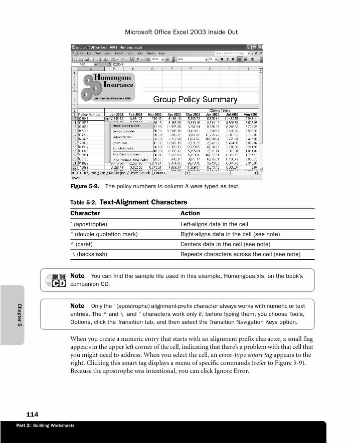
Part 2: Building Worksheets

Chapter 5

Microsoft Office Excel 2003 Inside Out

114

F05ie09

Figure 5-9. The policy numbers in column A were typed as text.

Note You can find the sample file used in this example, Humongous.xls, on the book’s companion CD.

Note Only the ’ (apostrophe) alignment-prefix character always works with numeric or text entries. The ^ and \ and “ characters work only if, before typing them, you choose Tools, Options, click the Transition tab, and then select the Transition Navigation Keys option.

When you create a numeric entry that starts with an alignment prefix character, a small flag appears in the upper left corner of the cell, indicating that there’s a problem with that cell that you might need to address. When you select the cell, an error-type smart tag appears to the right. Clicking this smart tag displays a menu of specific commands (refer to Figure 5-9). Because the apostrophe was intentional, you can click Ignore Error.

Table 5-2. Text-Alignment Characters

Character Action

’ (apostrophe) Left-aligns data in the cell

“ (double quotation mark) Right-aligns data in the cell (see note)

^ (caret) Centers data in the cell (see note)

\ (backslash) Repeats characters across the cell (see note)

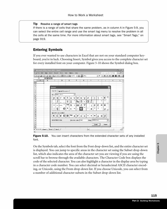
Part 2: Building Worksheets

Cha

pter

5

How to Work a Worksheet

115

Part 1: Part Title

Tip Resolve a range of smart tagsIf there is a range of cells that share the same problem, as in column A in Figure 5-9, you can select the entire cell range and use the smart tag menu to resolve the problem in all the cells at the same time. For more information about smart tags, see “Smart Tags,” on page 919.

Entering SymbolsIf you ever wanted to use characters in Excel that are not on your standard computer key-board, you’re in luck. Choosing Insert, Symbol gives you access to the complete character set for every installed font on your computer. Figure 5-10 shows the Symbol dialog box.

f05ie10

Figure 5-10. You can insert characters from the extended character sets of any installed font.

On the Symbols tab, select the font from the Font drop-down list, and the entire character set is displayed. You can jump to specific areas in the character set using the Subset drop-down list, which also indicates the area of the character set you are viewing if you are using the scroll bar to browse through the available characters. The Character Code box displays the code of the selected character. You can also highlight a character in the display area by typing in a character code number. You can select decimal or hexadecimal ASCII character encod-ing, or Unicode, using the From drop-down list. If you choose Unicode, you can select from a number of additional character subsets in the Subset drop-down list.

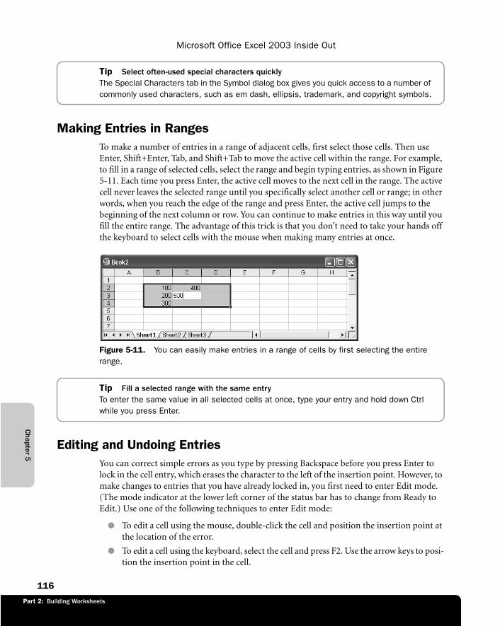
Part 2: Building Worksheets

Chapter 5

Microsoft Office Excel 2003 Inside Out

116

Tip Select often-used special characters quickly The Special Characters tab in the Symbol dialog box gives you quick access to a number of commonly used characters, such as em dash, ellipsis, trademark, and copyright symbols.

Making Entries in RangesTo make a number of entries in a range of adjacent cells, first select those cells. Then use Enter, Shift+Enter, Tab, and Shift+Tab to move the active cell within the range. For example, to fill in a range of selected cells, select the range and begin typing entries, as shown in Figure 5-11. Each time you press Enter, the active cell moves to the next cell in the range. The active cell never leaves the selected range until you specifically select another cell or range; in other words, when you reach the edge of the range and press Enter, the active cell jumps to the beginning of the next column or row. You can continue to make entries in this way until you fill the entire range. The advantage of this trick is that you don’t need to take your hands off the keyboard to select cells with the mouse when making many entries at once.

f05ie11

Figure 5-11. You can easily make entries in a range of cells by first selecting the entire range.

Tip Fill a selected range with the same entry To enter the same value in all selected cells at once, type your entry and hold down Ctrl while you press Enter.

Editing and Undoing EntriesYou can correct simple errors as you type by pressing Backspace before you press Enter to lock in the cell entry, which erases the character to the left of the insertion point. However, to make changes to entries that you have already locked in, you first need to enter Edit mode. (The mode indicator at the lower left corner of the status bar has to change from Ready to Edit.) Use one of the following techniques to enter Edit mode:

● To edit a cell using the mouse, double-click the cell and position the insertion point at the location of the error.

● To edit a cell using the keyboard, select the cell and press F2. Use the arrow keys to posi-tion the insertion point in the cell.

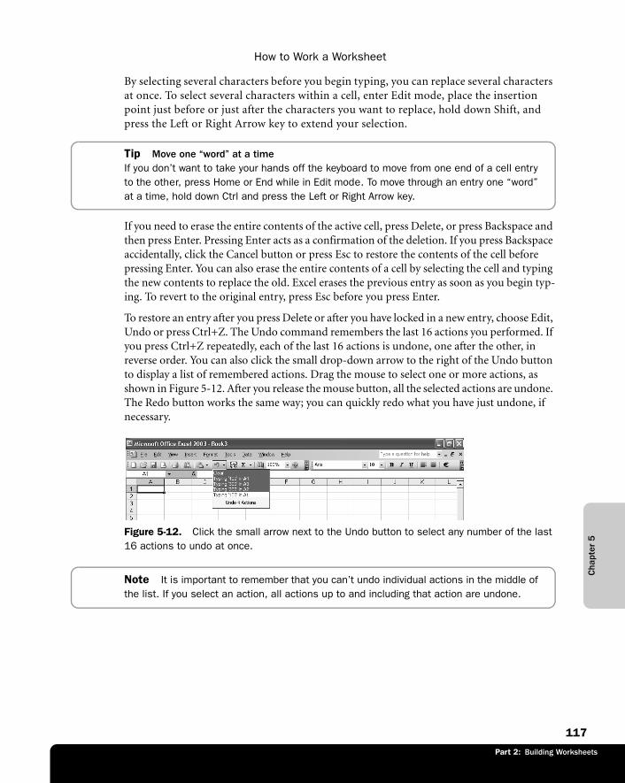
Part 2: Building Worksheets

Cha

pter

5

How to Work a Worksheet

117

Part 1: Part Title

By selecting several characters before you begin typing, you can replace several characters at once. To select several characters within a cell, enter Edit mode, place the insertion point just before or just after the characters you want to replace, hold down Shift, and press the Left or Right Arrow key to extend your selection.

Tip Move one “word” at a timeIf you don’t want to take your hands off the keyboard to move from one end of a cell entry to the other, press Home or End while in Edit mode. To move through an entry one “word” at a time, hold down Ctrl and press the Left or Right Arrow key.

If you need to erase the entire contents of the active cell, press Delete, or press Backspace and then press Enter. Pressing Enter acts as a confirmation of the deletion. If you press Backspace accidentally, click the Cancel button or press Esc to restore the contents of the cell before pressing Enter. You can also erase the entire contents of a cell by selecting the cell and typing the new contents to replace the old. Excel erases the previous entry as soon as you begin typ-ing. To revert to the original entry, press Esc before you press Enter.

To restore an entry after you press Delete or after you have locked in a new entry, choose Edit, Undo or press Ctrl+Z. The Undo command remembers the last 16 actions you performed. If you press Ctrl+Z repeatedly, each of the last 16 actions is undone, one after the other, in reverse order. You can also click the small drop-down arrow to the right of the Undo button to display a list of remembered actions. Drag the mouse to select one or more actions, as shown in Figure 5-12. After you release the mouse button, all the selected actions are undone. The Redo button works the same way; you can quickly redo what you have just undone, if necessary.

f05ie12

Figure 5-12. Click the small arrow next to the Undo button to select any number of the last 16 actions to undo at once.

Note It is important to remember that you can’t undo individual actions in the middle of the list. If you select an action, all actions up to and including that action are undone.

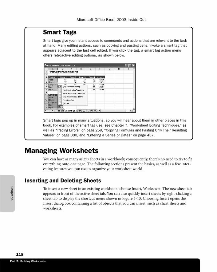
Part 2: Building Worksheets

Chapter 5

Microsoft Office Excel 2003 Inside Out

118

Smart TagsSmart tags give you instant access to commands and actions that are relevant to the task at hand. Many editing actions, such as copying and pasting cells, invoke a smart tag that appears adjacent to the last cell edited. If you click the tag, a smart tag action menu offers retroactive editing options, as shown below.

g05ie01

Smart tags pop up in many situations, so you will hear about them in other places in this book. For examples of smart tag use, see Chapter 7, “Worksheet Editing Techniques,” as well as “Tracing Errors” on page 259, “Copying Formulas and Pasting Only Their Resulting Values” on page 380, and “Entering a Series of Dates” on page 437.

Managing WorksheetsYou can have as many as 255 sheets in a workbook; consequently, there’s no need to try to fit everything onto one page. The following sections present the basics, as well as a few inter-esting features you can use to organize your worksheet world.

Inserting and Deleting SheetsTo insert a new sheet in an existing workbook, choose Insert, Worksheet. The new sheet tab appears in front of the active sheet tab. You can also quickly insert sheets by right-clicking a sheet tab to display the shortcut menu shown in Figure 5-13. Choosing Insert opens the Insert dialog box containing a list of objects that you can insert, such as chart sheets and worksheets.

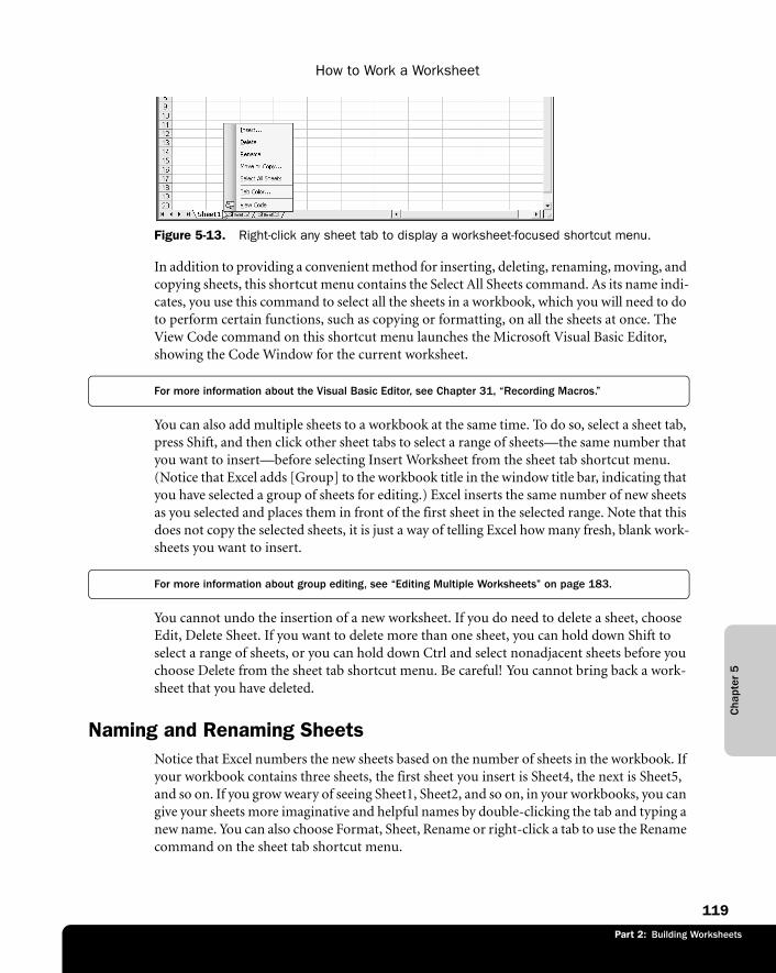
Part 2: Building Worksheets

Cha

pter

5

How to Work a Worksheet

119

Part 1: Part Title

f05ie13

Figure 5-13. Right-click any sheet tab to display a worksheet-focused shortcut menu.

In addition to providing a convenient method for inserting, deleting, renaming, moving, and copying sheets, this shortcut menu contains the Select All Sheets command. As its name indi-cates, you use this command to select all the sheets in a workbook, which you will need to do to perform certain functions, such as copying or formatting, on all the sheets at once. The View Code command on this shortcut menu launches the Microsoft Visual Basic Editor, showing the Code Window for the current worksheet.

For more information about the Visual Basic Editor, see Chapter 31, “Recording Macros.”

You can also add multiple sheets to a workbook at the same time. To do so, select a sheet tab, press Shift, and then click other sheet tabs to select a range of sheets—the same number that you want to insert—before selecting Insert Worksheet from the sheet tab shortcut menu. (Notice that Excel adds [Group] to the workbook title in the window title bar, indicating that you have selected a group of sheets for editing.) Excel inserts the same number of new sheets as you selected and places them in front of the first sheet in the selected range. Note that this does not copy the selected sheets, it is just a way of telling Excel how many fresh, blank work-sheets you want to insert.

For more information about group editing, see “Editing Multiple Worksheets” on page 183.

You cannot undo the insertion of a new worksheet. If you do need to delete a sheet, choose Edit, Delete Sheet. If you want to delete more than one sheet, you can hold down Shift to select a range of sheets, or you can hold down Ctrl and select nonadjacent sheets before you choose Delete from the sheet tab shortcut menu. Be careful! You cannot bring back a work-sheet that you have deleted.

Naming and Renaming SheetsNotice that Excel numbers the new sheets based on the number of sheets in the workbook. If your workbook contains three sheets, the first sheet you insert is Sheet4, the next is Sheet5, and so on. If you grow weary of seeing Sheet1, Sheet2, and so on, in your workbooks, you can give your sheets more imaginative and helpful names by double-clicking the tab and typing a new name. You can also choose Format, Sheet, Rename or right-click a tab to use the Rename command on the sheet tab shortcut menu.

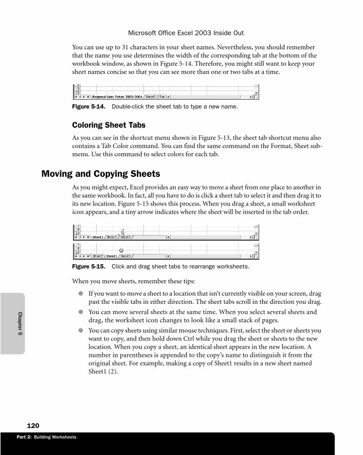
Part 2: Building Worksheets

Chapter 5

Microsoft Office Excel 2003 Inside Out

120

You can use up to 31 characters in your sheet names. Nevertheless, you should remember that the name you use determines the width of the corresponding tab at the bottom of the workbook window, as shown in Figure 5-14. Therefore, you might still want to keep your sheet names concise so that you can see more than one or two tabs at a time.

f05ie14

Figure 5-14. Double-click the sheet tab to type a new name.

Coloring Sheet TabsAs you can see in the shortcut menu shown in Figure 5-13, the sheet tab shortcut menu also contains a Tab Color command. You can find the same command on the Format, Sheet sub-menu. Use this command to select colors for each tab.

Moving and Copying SheetsAs you might expect, Excel provides an easy way to move a sheet from one place to another in the same workbook. In fact, all you have to do is click a sheet tab to select it and then drag it to its new location. Figure 5-15 shows this process. When you drag a sheet, a small worksheet icon appears, and a tiny arrow indicates where the sheet will be inserted in the tab order.

f05ie15

Figure 5-15. Click and drag sheet tabs to rearrange worksheets.

When you move sheets, remember these tips:

● If you want to move a sheet to a location that isn’t currently visible on your screen, drag past the visible tabs in either direction. The sheet tabs scroll in the direction you drag.

● You can move several sheets at the same time. When you select several sheets and drag, the worksheet icon changes to look like a small stack of pages.

● You can copy sheets using similar mouse techniques. First, select the sheet or sheets you want to copy, and then hold down Ctrl while you drag the sheet or sheets to the new location. When you copy a sheet, an identical sheet appears in the new location. A number in parentheses is appended to the copy’s name to distinguish it from the original sheet. For example, making a copy of Sheet1 results in a new sheet named Sheet1 (2).

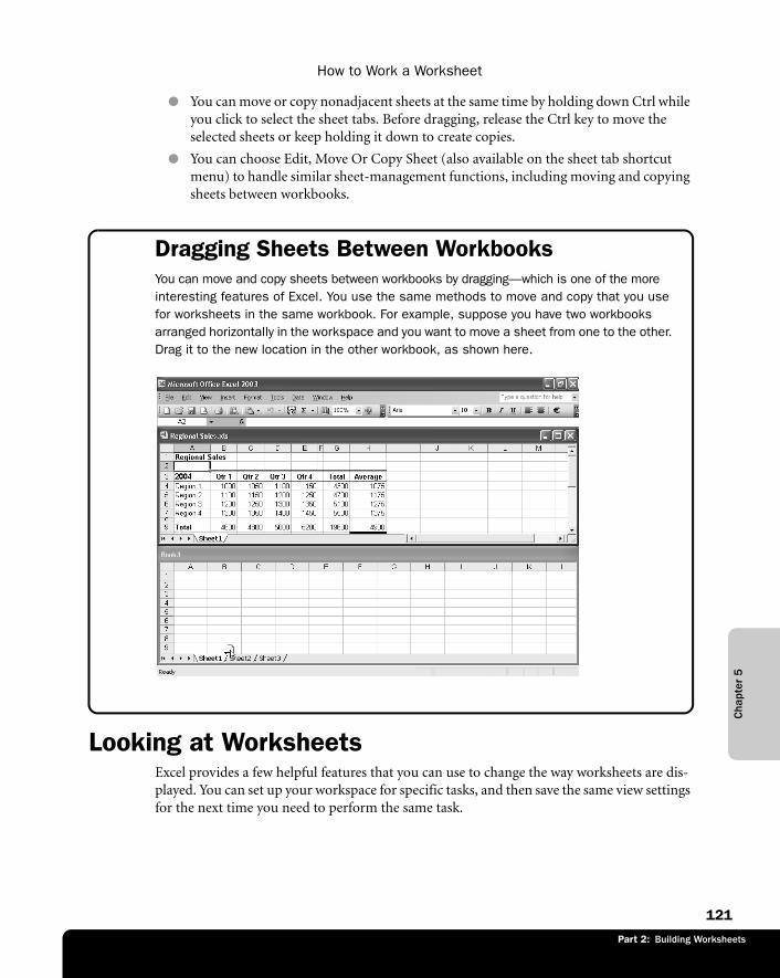
Part 2: Building Worksheets

Cha

pter

5

How to Work a Worksheet

121

Part 1: Part Title

● You can move or copy nonadjacent sheets at the same time by holding down Ctrl while you click to select the sheet tabs. Before dragging, release the Ctrl key to move the selected sheets or keep holding it down to create copies.

● You can choose Edit, Move Or Copy Sheet (also available on the sheet tab shortcut menu) to handle similar sheet-management functions, including moving and copying sheets between workbooks.

Dragging Sheets Between WorkbooksYou can move and copy sheets between workbooks by dragging—which is one of the more interesting features of Excel. You use the same methods to move and copy that you use for worksheets in the same workbook. For example, suppose you have two workbooks arranged horizontally in the workspace and you want to move a sheet from one to the other. Drag it to the new location in the other workbook, as shown here.

g05ie02

Looking at WorksheetsExcel provides a few helpful features that you can use to change the way worksheets are dis-played. You can set up your workspace for specific tasks, and then save the same view settings for the next time you need to perform the same task.

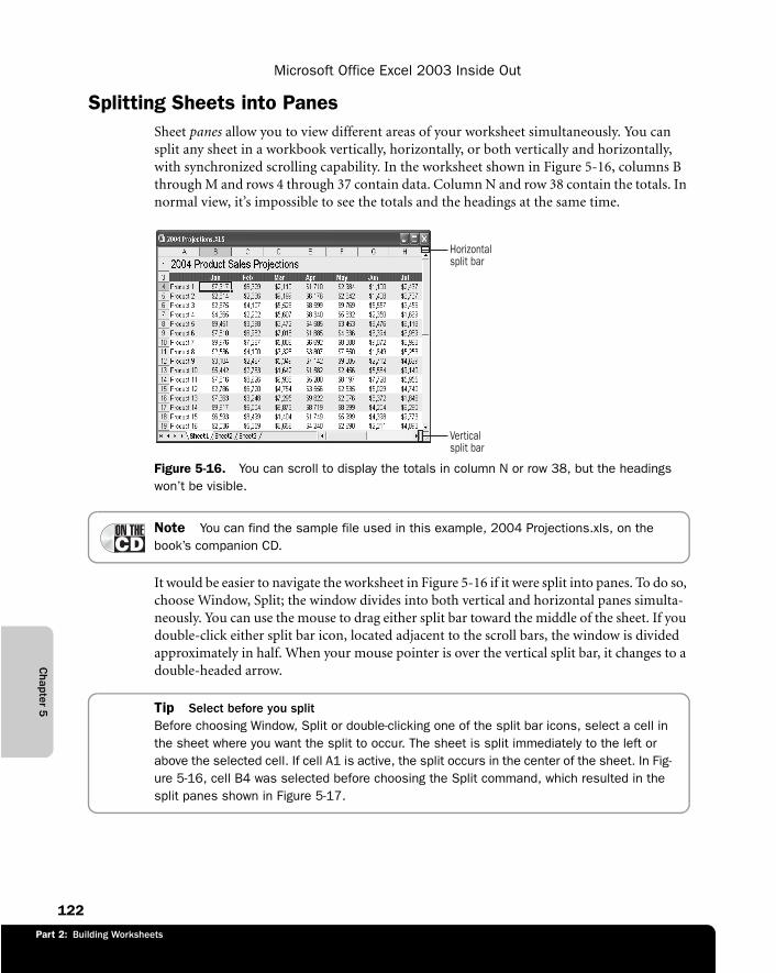
Part 2: Building Worksheets

Chapter 5

Microsoft Office Excel 2003 Inside Out

122

Splitting Sheets into PanesSheet panes allow you to view different areas of your worksheet simultaneously. You can split any sheet in a workbook vertically, horizontally, or both vertically and horizontally, with synchronized scrolling capability. In the worksheet shown in Figure 5-16, columns B through M and rows 4 through 37 contain data. Column N and row 38 contain the totals. In normal view, it’s impossible to see the totals and the headings at the same time.

f05ie16

Figure 5-16. You can scroll to display the totals in column N or row 38, but the headings won’t be visible.

Note You can find the sample file used in this example, 2004 Projections.xls, on the book’s companion CD.

It would be easier to navigate the worksheet in Figure 5-16 if it were split into panes. To do so, choose Window, Split; the window divides into both vertical and horizontal panes simulta-neously. You can use the mouse to drag either split bar toward the middle of the sheet. If you double-click either split bar icon, located adjacent to the scroll bars, the window is divided approximately in half. When your mouse pointer is over the vertical split bar, it changes to a double-headed arrow.

Tip Select before you splitBefore choosing Window, Split or double-clicking one of the split bar icons, select a cell in the sheet where you want the split to occur. The sheet is split immediately to the left or above the selected cell. If cell A1 is active, the split occurs in the center of the sheet. In Fig-ure 5-16, cell B4 was selected before choosing the Split command, which resulted in the split panes shown in Figure 5-17.

Horizontalsplit bar

Verticalsplit bar

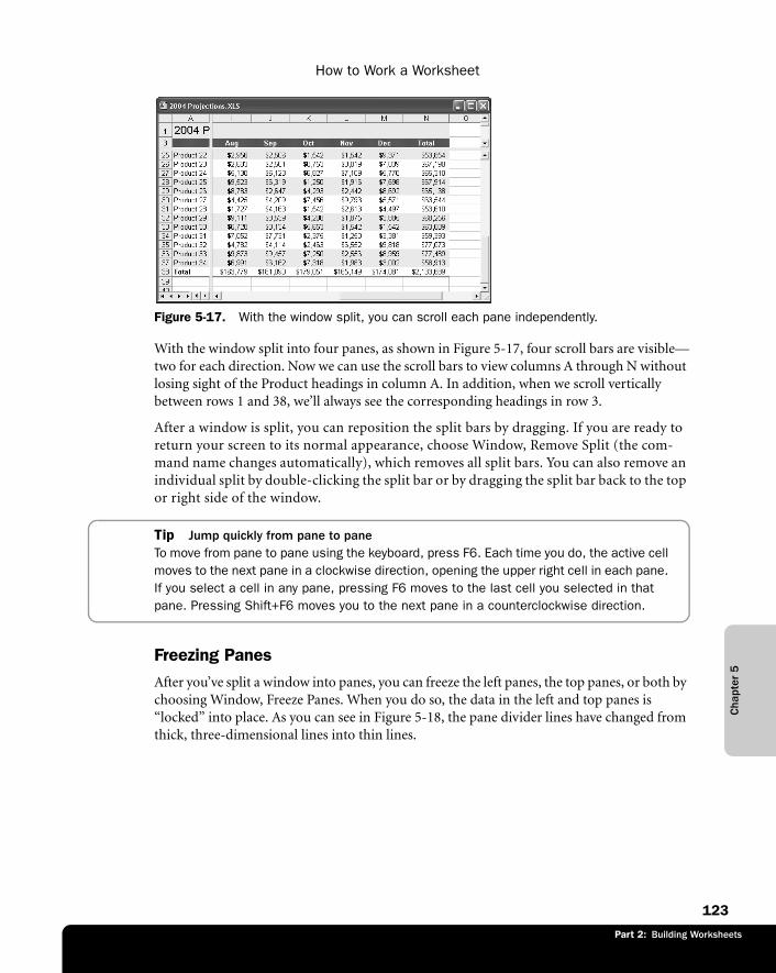
Part 2: Building Worksheets

Cha

pter

5

How to Work a Worksheet

123

Part 1: Part Title

f05ie17

Figure 5-17. With the window split, you can scroll each pane independently.

With the window split into four panes, as shown in Figure 5-17, four scroll bars are visible—two for each direction. Now we can use the scroll bars to view columns A through N without losing sight of the Product headings in column A. In addition, when we scroll vertically between rows 1 and 38, we’ll always see the corresponding headings in row 3.

After a window is split, you can reposition the split bars by dragging. If you are ready to return your screen to its normal appearance, choose Window, Remove Split (the com-mand name changes automatically), which removes all split bars. You can also remove an individual split by double-clicking the split bar or by dragging the split bar back to the top or right side of the window.

Tip Jump quickly from pane to paneTo move from pane to pane using the keyboard, press F6. Each time you do, the active cell moves to the next pane in a clockwise direction, opening the upper right cell in each pane. If you select a cell in any pane, pressing F6 moves to the last cell you selected in that pane. Pressing Shift+F6 moves you to the next pane in a counterclockwise direction.

Freezing PanesAfter you’ve split a window into panes, you can freeze the left panes, the top panes, or both by choosing Window, Freeze Panes. When you do so, the data in the left and top panes is “locked” into place. As you can see in Figure 5-18, the pane divider lines have changed from thick, three-dimensional lines into thin lines.

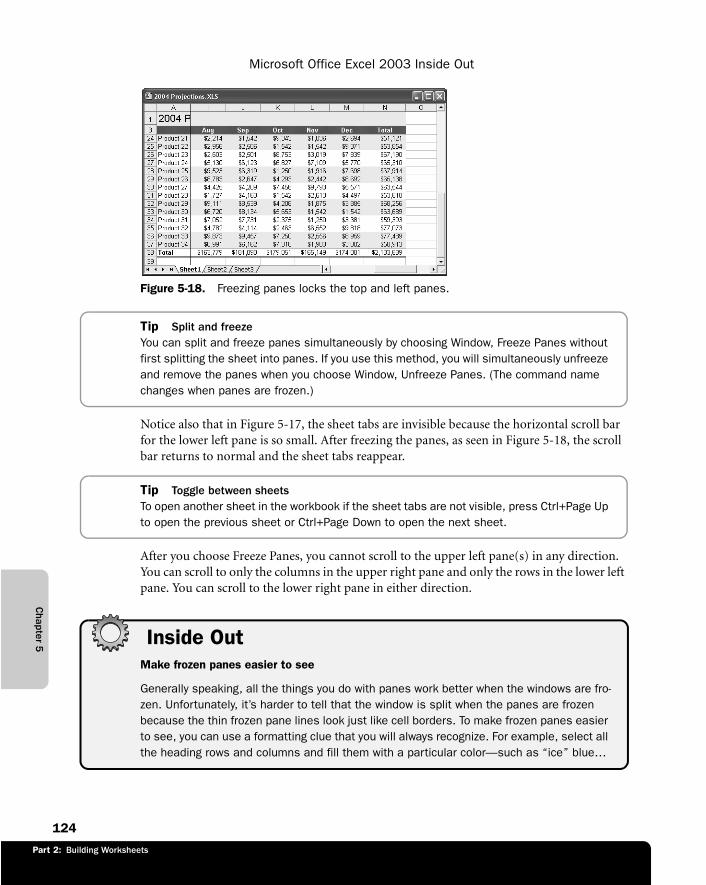
Part 2: Building Worksheets

Chapter 5

Microsoft Office Excel 2003 Inside Out

124

f05ie18

Figure 5-18. Freezing panes locks the top and left panes.

Tip Split and freezeYou can split and freeze panes simultaneously by choosing Window, Freeze Panes without first splitting the sheet into panes. If you use this method, you will simultaneously unfreeze and remove the panes when you choose Window, Unfreeze Panes. (The command name changes when panes are frozen.)

Notice also that in Figure 5-17, the sheet tabs are invisible because the horizontal scroll bar for the lower left pane is so small. After freezing the panes, as seen in Figure 5-18, the scroll bar returns to normal and the sheet tabs reappear.

Tip Toggle between sheetsTo open another sheet in the workbook if the sheet tabs are not visible, press Ctrl+Page Up to open the previous sheet or Ctrl+Page Down to open the next sheet.

After you choose Freeze Panes, you cannot scroll to the upper left pane(s) in any direction. You can scroll to only the columns in the upper right pane and only the rows in the lower left pane. You can scroll to the lower right pane in either direction.

Inside OutMake frozen panes easier to see

Generally speaking, all the things you do with panes work better when the windows are fro-zen. Unfortunately, it’s harder to tell that the window is split when the panes are frozen because the thin frozen pane lines look just like cell borders. To make frozen panes easier to see, you can use a formatting clue that you will always recognize. For example, select all the heading rows and columns and fill them with a particular color—such as “ice” blue…

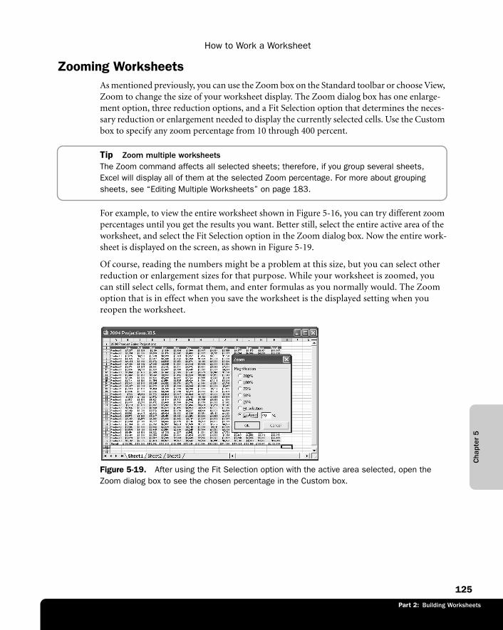
Part 2: Building Worksheets

Cha

pter

5

How to Work a Worksheet

125

Part 1: Part Title

Zooming WorksheetsAs mentioned previously, you can use the Zoom box on the Standard toolbar or choose View, Zoom to change the size of your worksheet display. The Zoom dialog box has one enlarge-ment option, three reduction options, and a Fit Selection option that determines the neces-sary reduction or enlargement needed to display the currently selected cells. Use the Custom box to specify any zoom percentage from 10 through 400 percent.

Tip Zoom multiple worksheetsThe Zoom command affects all selected sheets; therefore, if you group several sheets, Excel will display all of them at the selected Zoom percentage. For more about grouping sheets, see “Editing Multiple Worksheets” on page 183.

For example, to view the entire worksheet shown in Figure 5-16, you can try different zoom percentages until you get the results you want. Better still, select the entire active area of the worksheet, and select the Fit Selection option in the Zoom dialog box. Now the entire work-sheet is displayed on the screen, as shown in Figure 5-19.

Of course, reading the numbers might be a problem at this size, but you can select other reduction or enlargement sizes for that purpose. While your worksheet is zoomed, you can still select cells, format them, and enter formulas as you normally would. The Zoom option that is in effect when you save the worksheet is the displayed setting when you reopen the worksheet.

f05ie19

Figure 5-19. After using the Fit Selection option with the active area selected, open the Zoom dialog box to see the chosen percentage in the Custom box.

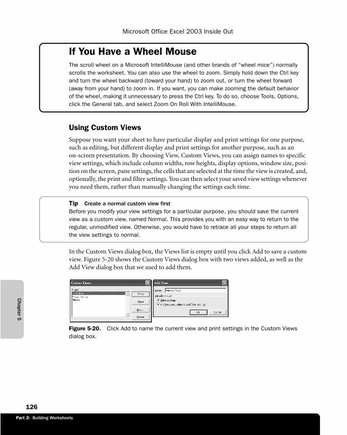
Part 2: Building Worksheets

Chapter 5

Microsoft Office Excel 2003 Inside Out

126

If You Have a Wheel MouseThe scroll wheel on a Microsoft IntelliMouse (and other brands of “wheel mice”) normally scrolls the worksheet. You can also use the wheel to zoom. Simply hold down the Ctrl key and turn the wheel backward (toward your hand) to zoom out, or turn the wheel forward (away from your hand) to zoom in. If you want, you can make zooming the default behavior of the wheel, making it unnecessary to press the Ctrl key. To do so, choose Tools, Options, click the General tab, and select Zoom On Roll With IntelliMouse.

Using Custom ViewsSuppose you want your sheet to have particular display and print settings for one purpose, such as editing, but different display and print settings for another purpose, such as an on-screen presentation. By choosing View, Custom Views, you can assign names to specific view settings, which include column widths, row heights, display options, window size, posi-tion on the screen, pane settings, the cells that are selected at the time the view is created, and, optionally, the print and filter settings. You can then select your saved view settings whenever you need them, rather than manually changing the settings each time.

Tip Create a normal custom view firstBefore you modify your view settings for a particular purpose, you should save the current view as a custom view, named Normal. This provides you with an easy way to return to the regular, unmodified view. Otherwise, you would have to retrace all your steps to return all the view settings to normal.

In the Custom Views dialog box, the Views list is empty until you click Add to save a custom view. Figure 5-20 shows the Custom Views dialog box with two views added, as well as the Add View dialog box that we used to add them.

f05ie20

Figure 5-20. Click Add to name the current view and print settings in the Custom Views dialog box.

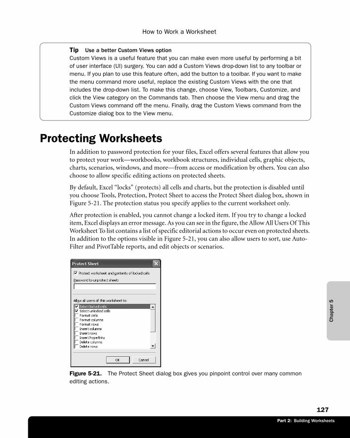
Part 2: Building Worksheets

Cha

pter

5

How to Work a Worksheet

127

Part 1: Part Title

Tip Use a better Custom Views optionCustom Views is a useful feature that you can make even more useful by performing a bit of user interface (UI) surgery. You can add a Custom Views drop-down list to any toolbar or menu. If you plan to use this feature often, add the button to a toolbar. If you want to make the menu command more useful, replace the existing Custom Views with the one that includes the drop-down list. To make this change, choose View, Toolbars, Customize, and click the View category on the Commands tab. Then choose the View menu and drag the Custom Views command off the menu. Finally, drag the Custom Views command from the Customize dialog box to the View menu.

Protecting WorksheetsIn addition to password protection for your files, Excel offers several features that allow you to protect your work—workbooks, workbook structures, individual cells, graphic objects, charts, scenarios, windows, and more—from access or modification by others. You can also choose to allow specific editing actions on protected sheets.

By default, Excel “locks” (protects) all cells and charts, but the protection is disabled until you choose Tools, Protection, Protect Sheet to access the Protect Sheet dialog box, shown in Figure 5-21. The protection status you specify applies to the current worksheet only.

After protection is enabled, you cannot change a locked item. If you try to change a locked item, Excel displays an error message. As you can see in the figure, the Allow All Users Of This Worksheet To list contains a list of specific editorial actions to occur even on protected sheets. In addition to the options visible in Figure 5-21, you can also allow users to sort, use Auto-Filter and PivotTable reports, and edit objects or scenarios.

f05ie21

Figure 5-21. The Protect Sheet dialog box gives you pinpoint control over many common editing actions.

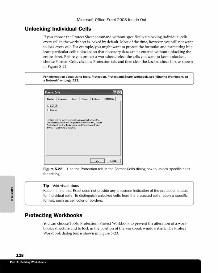
Part 2: Building Worksheets

Chapter 5

Microsoft Office Excel 2003 Inside Out

128

Unlocking Individual CellsIf you choose the Protect Sheet command without specifically unlocking individual cells, every cell in the worksheet is locked by default. Most of the time, however, you will not want to lock every cell. For example, you might want to protect the formulas and formatting but leave particular cells unlocked so that necessary data can be entered without unlocking the entire sheet. Before you protect a worksheet, select the cells you want to keep unlocked, choose Format, Cells, click the Protection tab, and then clear the Locked check box, as shown in Figure 5-22.

For information about using Tools, Protection, Protect and Share Workbook, see “Sharing Workbooks on a Network” on page 522.

f05ie22

Figure 5-22. Use the Protection tab in the Format Cells dialog box to unlock specific cells for editing.

Tip Add visual cluesKeep in mind that Excel does not provide any on-screen indication of the protection status for individual cells. To distinguish unlocked cells from the protected cells, apply a specific format, such as cell color or borders.

Protecting WorkbooksYou can choose Tools, Protection, Protect Workbook to prevent the alteration of a work-book’s structure and to lock in the position of the workbook window itself. The Protect Workbook dialog box is shown in Figure 5-23.

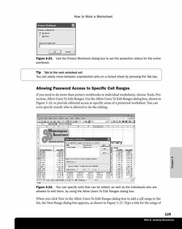
Part 2: Building Worksheets

Cha

pter

5

How to Work a Worksheet

129

Part 1: Part Title

f0523

Figure 5-23. Use the Protect Workbook dialog box to set the protection status for the entire workbook.

Tip Tab to the next unlocked cellYou can easily move between unprotected cells on a locked sheet by pressing the Tab key.

Allowing Password Access to Specific Cell RangesIf you need to do more than protect workbooks or individual worksheets, choose Tools, Pro-tection, Allow Users To Edit Ranges. Use the Allow Users To Edit Ranges dialog box, shown in Figure 5-24, to provide editorial access to specific areas of a protected worksheet. You can even specify exactly who is allowed to do the editing.

f05ie24

Figure 5-24. You can specify cells that can be edited, as well as the individuals who are allowed to edit them, by using the Allow Users To Edit Ranges dialog box.

When you click New in the Allow Users To Edit Ranges dialog box to add a cell range to the list, the New Range dialog box appears, as shown in Figure 5-25. Type a title for the range of

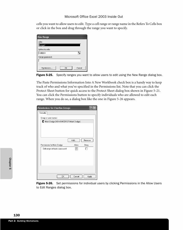
Part 2: Building Worksheets

Chapter 5

Microsoft Office Excel 2003 Inside Out

130

cells you want to allow users to edit. Type a cell range or range name in the Refers To Cells box or click in the box and drag through the range you want to specify.

f05ie25

Figure 5-25. Specify ranges you want to allow users to edit using the New Range dialog box.

The Paste Permissions Information Into A New Workbook check box is a handy way to keep track of who and what you’ve specified in the Permissions list. Note that you can click the Protect Sheet button for quick access to the Protect Sheet dialog box shown in Figure 5-21. You can click the Permissions button to specify individuals who are allowed to edit each range. When you do so, a dialog box like the one in Figure 5-26 appears.

f05ie26

Figure 5-26. Set permissions for individual users by clicking Permissions in the Allow Users to Edit Ranges dialog box.

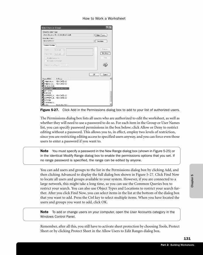
Part 2: Building Worksheets

Cha

pter

5

How to Work a Worksheet

131

Part 1: Part Title

f05ie27

Figure 5-27. Click Add in the Permissions dialog box to add to your list of authorized users.

The Permissions dialog box lists all users who are authorized to edit the worksheet, as well as whether they will need to use a password to do so. For each item in the Group or User Names list, you can specify password permissions in the box below; click Allow or Deny to restrict editing without a password. This allows you to, in effect, employ two levels of restriction, since you are restricting editing access to specified users anyway, and you can force even those users to enter a password if you want to.

Note You must specify a password in the New Range dialog box (shown in Figure 5-25) or in the identical Modify Range dialog box to enable the permissions options that you set. If no range password is specified, the range can be edited by anyone.

You can add users and groups to the list in the Permissions dialog box by clicking Add, and then clicking Advanced to display the full dialog box shown in Figure 5-27. Click Find Now to locate all users and groups available to your system. However, if you are connected to a large network, this might take a long time, so you can use the Common Queries box to restrict your search. You can also use Object Types and Locations to restrict your search fur-ther. After you click Find Now, you can select items in the list at the bottom of the dialog box that you want to add. Press the Ctrl key to select multiple items. When you have located the users and groups you want to add, click OK.

Note To add or change users on your computer, open the User Accounts category in the Windows Control Panel.

Remember, after all this, you still have to activate sheet protection by choosing Tools, Protect Sheet or by clicking Protect Sheet in the Allow Users to Edit Ranges dialog box.

Part 2: Building Worksheets

Chapter 5

Microsoft Office Excel 2003 Inside Out

132

For information about setting file-level permissions, see “Controlling Document Access with Information Rights Management,” on page 538. For information about Excel and networks, see “Sharing Workbooks on a Network” on page 522.

Hiding Cells and SheetsIn a protected sheet, if you applied the Hidden protection format to a cell that contains a for-mula (using the Protection tab in the Format Cells dialog box shown in Figure 5-22), the for-mula remains hidden in the formula bar even when you select that cell. Formulas in these cells are still functional, of course; they are hidden from view. In any case, the result of the formula is still visible.

For more information about hiding numbers, see “The Hidden Number Format” on page 218.

You can also hide entire worksheets within a workbook. Any data or calculations in a hidden worksheet are still available through references; the worksheet is simply hidden from view. To hide a worksheet, click the tab of the worksheet you want to hide and choose Format, Sheet, Hide. Unlike hiding cells, hiding a sheet happens immediately. After a sheet is hidden, the Unhide command is added to the Format, Sheet menu, allowing you to restore the hidden sheet. However, if you hide a sheet and then choose Tools, Protection, Protect Workbook, the Unhide command is no longer available, which helps keep the hidden sheet even better protected.

For more information about workbook protection, see “Hiding and Protecting Workbooks” on page 141.

Using PasswordsWhen you choose Protect Sheet, Protect Workbook, or Protect And Share Workbook, you can assign a password that must be used to disable the protection. You can use unique pass-words for each worksheet or workbook that you protect.

Caution Password protection in Excel is serious business. After you assign a password, there is no way to unprotect the sheet or workbook without it. Don’t forget your passwords! Remember, capitalization matters!

Part 2: Building Worksheets

133

Chapter 6

How to Work a WorkbookManaging Multiple Workbooks . . . . . . 133Opening Multiple Windows for the Same Workbook . . . . . . . . . . . . 138

Hiding and Protecting Workbooks . . . . . 141

In early versions of Microsoft Excel, worksheets, charts, and macro sheets were stored as sep-arate documents. Since Excel 5, however, all these types of data, and more, peacefully coexist in workbooks. You can keep as many sheets containing as many different types of data as you want in a workbook, you can have more than one workbook open at the same time, and you can have more than one window open for the same workbook. The only limitations to these capabilities are those imposed by your computer’s memory and system resources.

Managing Multiple WorkbooksThis chapter describes how to protect workbooks, how to use more than one workbook at a time, as well as how and why to split your view of a workbook into multiple win-dows. Generally, when you start Excel, a blank workbook opens with the provisional title Book1. The only exceptions occur when you start Excel by opening a workbook or when you have one or more Excel files stored in the XLStart directory so that they open automatically.

If you start Excel with Book1 visible and then open an existing Excel file, Book1 disappears unless you have edited it. You can open as many workbooks as you like until your computer runs out of memory.

For more on working with multiple windows, see “Opening Multiple Windows for the Same Workbook” on page 138. For more information about the XLStart directory, see “Opening Files When You Start Excel” on page 43.

c0661511x.fm Page 133 Friday, August 1, 2003 10:59 AM

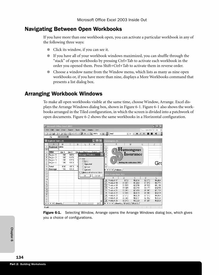
Part 2: Building Worksheets

Chapter 6

Microsoft Office Excel 2003 Inside Out

134

Navigating Between Open WorkbooksIf you have more than one workbook open, you can activate a particular workbook in any of the following three ways:

� Click its window, if you can see it.

� If you have all of your workbook windows maximized, you can shuffle through the “stack” of open workbooks by pressing Ctrl+Tab to activate each workbook in the order you opened them. Press Shift+Ctrl+Tab to activate them in reverse order.

� Choose a window name from the Window menu, which lists as many as nine open workbooks or, if you have more than nine, displays a More Workbooks command that presents a list dialog box.

Arranging Workbook WindowsTo make all open workbooks visible at the same time, choose Window, Arrange. Excel dis-plays the Arrange Windows dialog box, shown in Figure 6-1. Figure 6-1 also shows the work-books arranged in the Tiled configuration, in which the screen is divided into a patchwork of open documents. Figure 6-2 shows the same workbooks in a Horizontal configuration.

f06ie01

Figure 6-1. Selecting Window, Arrange opens the Arrange Windows dialog box, which gives you a choice of configurations.

c0661511x.fm Page 134 Friday, August 1, 2003 10:59 AM

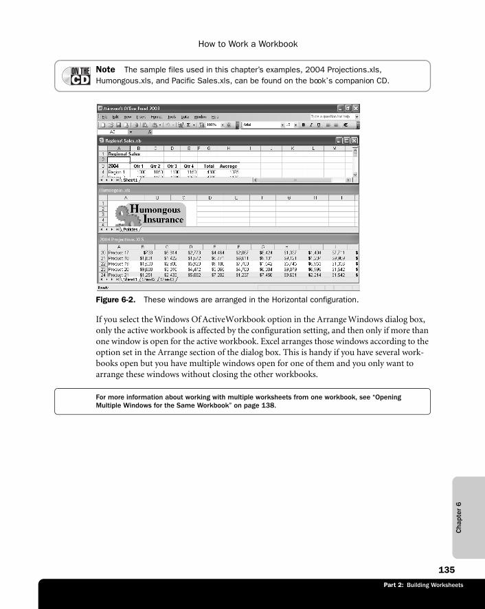
Part 2: Building Worksheets

Cha

pter

6

How to Work a Workbook

135

Part 1: Part Title

Note The sample files used in this chapter’s examples, 2004 Projections.xls, Humongous.xls, and Pacific Sales.xls, can be found on the book’s companion CD.

f06ie02

Figure 6-2. These windows are arranged in the Horizontal configuration.

If you select the Windows Of Active Workbook option in the Arrange Windows dialog box, only the active workbook is affected by the configuration setting, and then only if more than one window is open for the active workbook. Excel arranges those windows according to the option set in the Arrange section of the dialog box. This is handy if you have several work-books open but you have multiple windows open for one of them and you only want to arrange these windows without closing the other workbooks.

For more information about working with multiple worksheets from one workbook, see “Opening Multiple Windows for the Same Workbook” on page 138.

c0661511x.fm Page 135 Friday, August 1, 2003 10:59 AM

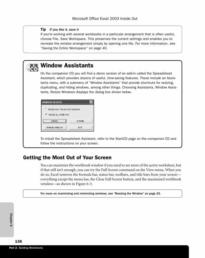
Part 2: Building Worksheets

Chapter 6

Microsoft Office Excel 2003 Inside Out

136

Tip If you like it, save itIf you’re working with several workbooks in a particular arrangement that is often useful, choose File, Save Workspace. This preserves the current settings and enables you torecreate the window arrangement simply by opening one file. For more information, see “Saving the Entire Workspace” on page 40.

Window AssistantsOn the companion CD you will find a demo version of an add-in called the Spreadsheet Assistant, which provides dozens of useful, time-saving features. These include an Assis-tants menu, with a submenu of “Window Assistants” that provide shortcuts for resizing, duplicating, and hiding windows, among other things. Choosing Assistants, Window Assis-tants, Resize Windows displays the dialog box shown below.

G06ie01

To install the Spreadsheet Assistant, refer to the StartCD page on the companion CD and follow the instructions on your screen.

Getting the Most Out of Your ScreenYou can maximize the workbook window if you need to see more of the active worksheet, but if that still isn’t enough, you can try the Full Screen command on the View menu. When you do so, Excel removes the formula bar, status bar, toolbars, and title bars from your screen—everything except the menu bar, the Close Full Screen button, and the maximized workbook window—as shown in Figure 6-3.

For more on maximizing and minimizing windows, see “Resizing the Window” on page 22.

c0661511x.fm Page 136 Friday, August 1, 2003 10:59 AM

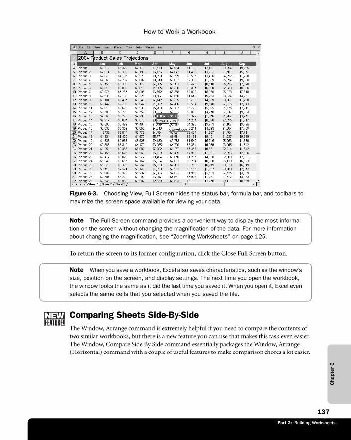
Part 2: Building Worksheets

Cha

pter

6

How to Work a Workbook

137

Part 1: Part Title

f06ie03

Figure 6-3. Choosing View, Full Screen hides the status bar, formula bar, and toolbars to maximize the screen space available for viewing your data.

Note The Full Screen command provides a convenient way to display the most informa-tion on the screen without changing the magnification of the data. For more information about changing the magnification, see “Zooming Worksheets” on page 125.

To return the screen to its former configuration, click the Close Full Screen button.

Note When you save a workbook, Excel also saves characteristics, such as the window’s size, position on the screen, and display settings. The next time you open the workbook, the window looks the same as it did the last time you saved it. When you open it, Excel even selects the same cells that you selected when you saved the file.

Comparing Sheets Side-By-SideThe Window, Arrange command is extremely helpful if you need to compare the contents of two similar workbooks, but there is a new feature you can use that makes this task even easier. The Window, Compare Side By Side command essentially packages the Window, Arrange (Horizontal) command with a couple of useful features to make comparison chores a lot easier.

c0661511x.fm Page 137 Friday, August 1, 2003 10:59 AM

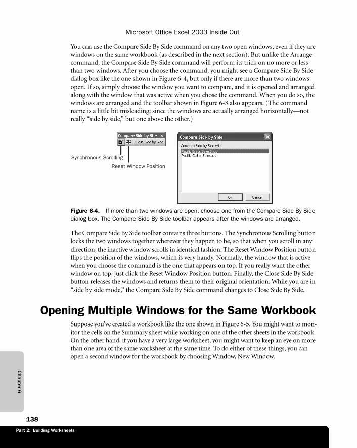
Part 2: Building Worksheets

Chapter 6

Microsoft Office Excel 2003 Inside Out

138

You can use the Compare Side By Side command on any two open windows, even if they are windows on the same workbook (as described in the next section). But unlike the Arrange command, the Compare Side By Side command will perform its trick on no more or less than two windows. After you choose the command, you might see a Compare Side By Side dialog box like the one shown in Figure 6-4, but only if there are more than two windows open. If so, simply choose the window you want to compare, and it is opened and arranged along with the window that was active when you chose the command. When you do so, the windows are arranged and the toolbar shown in Figure 6-3 also appears. (The command name is a little bit misleading; since the windows are actually arranged horizontally—not really “side by side,” but one above the other.)

f06ie04

Figure 6-4. If more than two windows are open, choose one from the Compare Side By Side dialog box. The Compare Side By Side toolbar appears after the windows are arranged.

The Compare Side By Side toolbar contains three buttons. The Synchronous Scrolling button locks the two windows together wherever they happen to be, so that when you scroll in any direction, the inactive window scrolls in identical fashion. The Reset Window Position button flips the position of the windows, which is very handy. Normally, the window that is active when you choose the command is the one that appears on top. If you really want the other window on top, just click the Reset Window Position button. Finally, the Close Side By Side button releases the windows and returns them to their original orientation. While you are in “side by side mode,” the Compare Side By Side command changes to Close Side By Side.

Opening Multiple Windows for the Same WorkbookSuppose you’ve created a workbook like the one shown in Figure 6-5. You might want to mon-itor the cells on the Summary sheet while working on one of the other sheets in the workbook. On the other hand, if you have a very large worksheet, you might want to keep an eye on more than one area of the same worksheet at the same time. To do either of these things, you can open a second window for the workbook by choosing Window, New Window.

Reset Window Position

Synchronous Scrolling

c0661511x.fm Page 138 Friday, August 1, 2003 10:59 AM

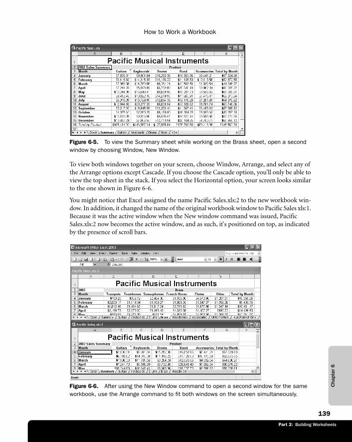
Part 2: Building Worksheets

Cha

pter

6

How to Work a Workbook

139

Part 1: Part Title

f06ie05

Figure 6-5. To view the Summary sheet while working on the Brass sheet, open a second window by choosing Window, New Window.

To view both windows together on your screen, choose Window, Arrange, and select any of the Arrange options except Cascade. If you choose the Cascade option, you’ll only be able to view the top sheet in the stack. If you select the Horizontal option, your screen looks similar to the one shown in Figure 6-6.

You might notice that Excel assigned the name Pacific Sales.xls:2 to the new workbook win-dow. In addition, it changed the name of the original workbook window to Pacific Sales xls:1. Because it was the active window when the New window command was issued, Pacific Sales.xls:2 now becomes the active window, and as such, it’s positioned on top, as indicated by the presence of scroll bars.

f06ie06

Figure 6-6. After using the New Window command to open a second window for the same workbook, use the Arrange command to fit both windows on the screen simultaneously.

c0661511x.fm Page 139 Friday, August 1, 2003 10:59 AM

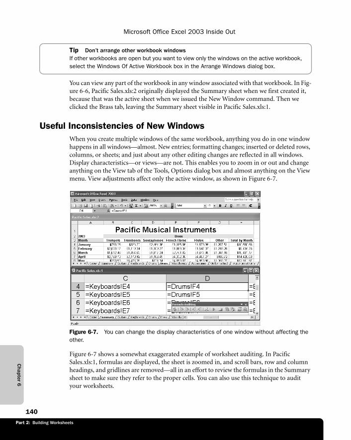
Part 2: Building Worksheets

Chapter 6

Microsoft Office Excel 2003 Inside Out

140

Tip Don’t arrange other workbook windows If other workbooks are open but you want to view only the windows on the active workbook, select the Windows Of Active Workbook box in the Arrange Windows dialog box.

You can view any part of the workbook in any window associated with that workbook. In Fig-ure 6-6, Pacific Sales.xls:2 originally displayed the Summary sheet when we first created it, because that was the active sheet when we issued the New Window command. Then we clicked the Brass tab, leaving the Summary sheet visible in Pacific Sales.xls:1.

Useful Inconsistencies of New WindowsWhen you create multiple windows of the same workbook, anything you do in one window happens in all windows—almost. New entries; formatting changes; inserted or deleted rows, columns, or sheets; and just about any other editing changes are reflected in all windows. Display characteristics—or views—are not. This enables you to zoom in or out and change anything on the View tab of the Tools, Options dialog box and almost anything on the View menu. View adjustments affect only the active window, as shown in Figure 6-7.

f06ie07

Figure 6-7. You can change the display characteristics of one window without affecting the other.

Figure 6-7 shows a somewhat exaggerated example of worksheet auditing. In Pacific Sales.xls:1, formulas are displayed, the sheet is zoomed in, and scroll bars, row and column headings, and gridlines are removed—all in an effort to review the formulas in the Summary sheet to make sure they refer to the proper cells. You can also use this technique to audit your worksheets.

c0661511x.fm Page 140 Friday, August 1, 2003 10:59 AM

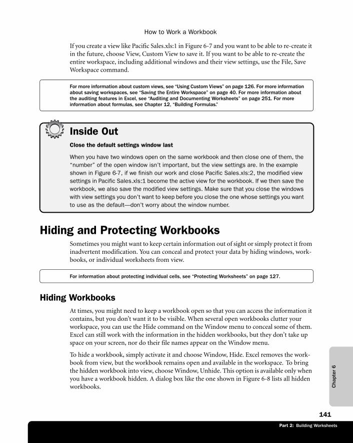
Part 2: Building Worksheets

Cha

pter

6

How to Work a Workbook

141

Part 1: Part Title

If you create a view like Pacific Sales.xls:1 in Figure 6-7 and you want to be able to re-create it in the future, choose View, Custom View to save it. If you want to be able to re-create the entire workspace, including additional windows and their view settings, use the File, Save Workspace command.

For more information about custom views, see “Using Custom Views” on page 126. For more information about saving workspaces, see “Saving the Entire Workspace” on page 40. For more information about the auditing features in Excel, see “Auditing and Documenting Worksheets” on page 251. For more information about formulas, see Chapter 12, “Building Formulas.”

Inside OutClose the default settings window last

When you have two windows open on the same workbook and then close one of them, the “number” of the open window isn’t important, but the view settings are. In the example shown in Figure 6-7, if we finish our work and close Pacific Sales.xls:2, the modified view settings in Pacific Sales.xls:1 become the active view for the workbook. If we then save the workbook, we also save the modified view settings. Make sure that you close the windows with view settings you don’t want to keep before you close the one whose settings you want to use as the default—don’t worry about the window number.

Hiding and Protecting WorkbooksSometimes you might want to keep certain information out of sight or simply protect it from inadvertent modification. You can conceal and protect your data by hiding windows, work-books, or individual worksheets from view.

For information about protecting individual cells, see “Protecting Worksheets” on page 127.

Hiding WorkbooksAt times, you might need to keep a workbook open so that you can access the information it contains, but you don’t want it to be visible. When several open workbooks clutter your workspace, you can use the Hide command on the Window menu to conceal some of them. Excel can still work with the information in the hidden workbooks, but they don’t take up space on your screen, nor do their file names appear on the Window menu.

To hide a workbook, simply activate it and choose Window, Hide. Excel removes the work-book from view, but the workbook remains open and available in the workspace. To bring the hidden workbook into view, choose Window, Unhide. This option is available only when you have a workbook hidden. A dialog box like the one shown in Figure 6-8 lists all hidden workbooks.

c0661511x.fm Page 141 Friday, August 1, 2003 10:59 AM

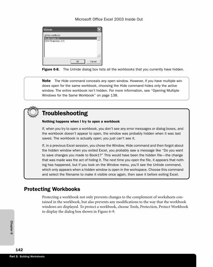
Part 2: Building Worksheets

Chapter 6

Microsoft Office Excel 2003 Inside Out

142

f06ie08

Figure 6-8. The Unhide dialog box lists all the workbooks that you currently have hidden.

Note The Hide command conceals any open window. However, if you have multiple win-dows open for the same workbook, choosing the Hide command hides only the active window. The entire workbook isn’t hidden. For more information, see “Opening Multiple Windows for the Same Workbook” on page 138.

TroubleshootingNothing happens when I try to open a workbook

If, when you try to open a workbook, you don’t see any error messages or dialog boxes, and the workbook doesn’t appear to open, the window was probably hidden when it was last saved. The workbook is actually open; you just can’t see it.

If, in a previous Excel session, you chose the Window, Hide command and then forgot about the hidden window when you exited Excel, you probably saw a message like “Do you want to save changes you made to Book1?” This would have been the hidden file—the change that was made was the act of hiding it. The next time you open the file, it appears that noth-ing has happened, but if you look on the Window menu, you’ll see the Unhide command, which only appears when a hidden window is open in the workspace. Choose this command and select the filename to make it visible once again, then save it before exiting Excel.

Protecting WorkbooksProtecting a workbook not only prevents changes to the complement of worksheets con-tained in the workbook, but also prevents any modifications to the way that the workbook windows are displayed. To protect a workbook, choose Tools, Protection, Protect Workbook to display the dialog box shown in Figure 6-9.

c0661511x.fm Page 142 Friday, August 1, 2003 10:59 AM

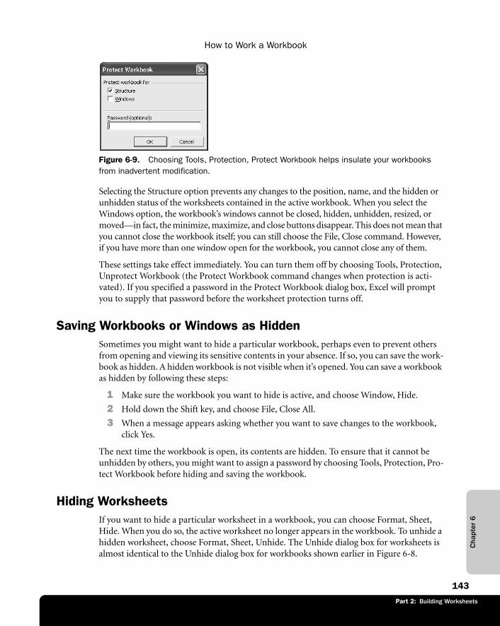
Part 2: Building Worksheets

Cha

pter

6

How to Work a Workbook

143

Part 1: Part Title

f06ie09

Figure 6-9. Choosing Tools, Protection, Protect Workbook helps insulate your workbooks from inadvertent modification.

Selecting the Structure option prevents any changes to the position, name, and the hidden or unhidden status of the worksheets contained in the active workbook. When you select the Windows option, the workbook’s windows cannot be closed, hidden, unhidden, resized, or moved—in fact, the minimize, maximize, and close buttons disappear. This does not mean that you cannot close the workbook itself; you can still choose the File, Close command. However, if you have more than one window open for the workbook, you cannot close any of them.

These settings take effect immediately. You can turn them off by choosing Tools, Protection, Unprotect Workbook (the Protect Workbook command changes when protection is acti-vated). If you specified a password in the Protect Workbook dialog box, Excel will prompt you to supply that password before the worksheet protection turns off.

Saving Workbooks or Windows as HiddenSometimes you might want to hide a particular workbook, perhaps even to prevent others from opening and viewing its sensitive contents in your absence. If so, you can save the work-book as hidden. A hidden workbook is not visible when it’s opened. You can save a workbook as hidden by following these steps:

1 Make sure the workbook you want to hide is active, and choose Window, Hide.

2 Hold down the Shift key, and choose File, Close All.

3 When a message appears asking whether you want to save changes to the workbook, click Yes.

The next time the workbook is open, its contents are hidden. To ensure that it cannot be unhidden by others, you might want to assign a password by choosing Tools, Protection, Pro-tect Workbook before hiding and saving the workbook.

Hiding WorksheetsIf you want to hide a particular worksheet in a workbook, you can choose Format, Sheet, Hide. When you do so, the active worksheet no longer appears in the workbook. To unhide a hidden worksheet, choose Format, Sheet, Unhide. The Unhide dialog box for worksheets is almost identical to the Unhide dialog box for workbooks shown earlier in Figure 6-8.

c0661511x.fm Page 143 Friday, August 1, 2003 10:59 AM

c0661511x.fm Page 144 Friday, August 1, 2003 10:59 AM

145

Part 3

Formatting and Editing Worksheets

7 Worksheet Editing Techniques 147

8 Worksheet Formatting Techniques 195

9 Advanced Formatting and Editing Techniques 241

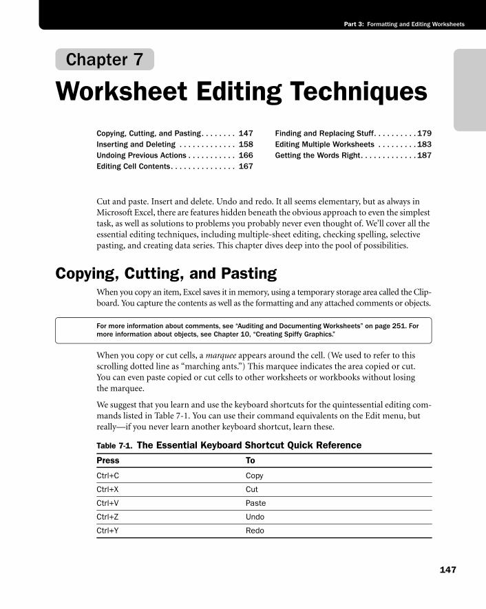
147

Part 3: Formatting and Editing Worksheets

Chapter 7

Worksheet Editing TechniquesCopying, Cutting, and Pasting. . . . . . . . 147Inserting and Deleting . . . . . . . . . . . . . 158Undoing Previous Actions . . . . . . . . . . . 166Editing Cell Contents. . . . . . . . . . . . . . . 167

Finding and Replacing Stuff. . . . . . . . . . 179Editing Multiple Worksheets . . . . . . . . . 183Getting the Words Right. . . . . . . . . . . . . 187

Cut and paste. Insert and delete. Undo and redo. It all seems elementary, but as always in Microsoft Excel, there are features hidden beneath the obvious approach to even the simplest task, as well as solutions to problems you probably never even thought of. We’ll cover all the essential editing techniques, including multiple-sheet editing, checking spelling, selective pasting, and creating data series. This chapter dives deep into the pool of possibilities.

Copying, Cutting, and PastingWhen you copy an item, Excel saves it in memory, using a temporary storage area called the Clip-board. You capture the contents as well as the formatting and any attached comments or objects.

For more information about comments, see “Auditing and Documenting Worksheets” on page 251. For more information about objects, see Chapter 10, “Creating Spiffy Graphics.”

When you copy or cut cells, a marquee appears around the cell. (We used to refer to this scrolling dotted line as “marching ants.”) This marquee indicates the area copied or cut. You can even paste copied or cut cells to other worksheets or workbooks without losing the marquee.

We suggest that you learn and use the keyboard shortcuts for the quintessential editing com-mands listed in Table 7-1. You can use their command equivalents on the Edit menu, but really—if you never learn another keyboard shortcut, learn these.

Table 7-1. The Essential Keyboard Shortcut Quick Reference

Press To

Ctrl+C Copy

Ctrl+X Cut

Ctrl+V Paste

Ctrl+Z Undo

Ctrl+Y Redo

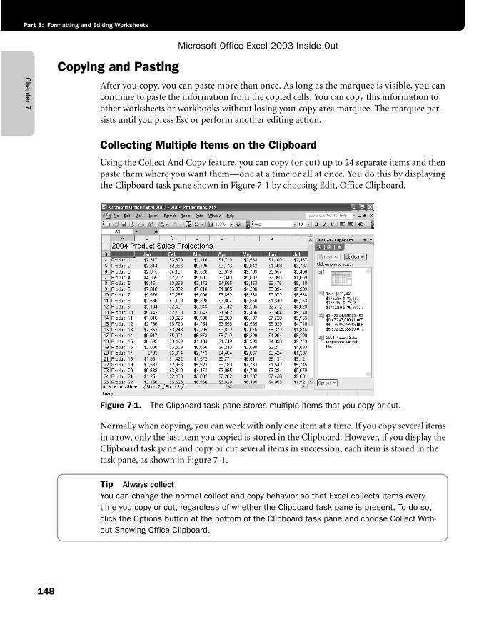
Chapter 7

Microsoft Office Excel 2003 Inside Out

Part 3: Formatting and Editing Worksheets

148

Copying and PastingAfter you copy, you can paste more than once. As long as the marquee is visible, you can continue to paste the information from the copied cells. You can copy this information to other worksheets or workbooks without losing your copy area marquee. The marquee per-sists until you press Esc or perform another editing action.

Collecting Multiple Items on the ClipboardUsing the Collect And Copy feature, you can copy (or cut) up to 24 separate items and then paste them where you want them—one at a time or all at once. You do this by displaying the Clipboard task pane shown in Figure 7-1 by choosing Edit, Office Clipboard.

f07ie01

Figure 7-1. The Clipboard task pane stores multiple items that you copy or cut.

Normally when copying, you can work with only one item at a time. If you copy several items in a row, only the last item you copied is stored in the Clipboard. However, if you display the Clipboard task pane and copy or cut several items in succession, each item is stored in the task pane, as shown in Figure 7-1.

Tip Always collectYou can change the normal collect and copy behavior so that Excel collects items every time you copy or cut, regardless of whether the Clipboard task pane is present. To do so, click the Options button at the bottom of the Clipboard task pane and choose Collect With-out Showing Office Clipboard.

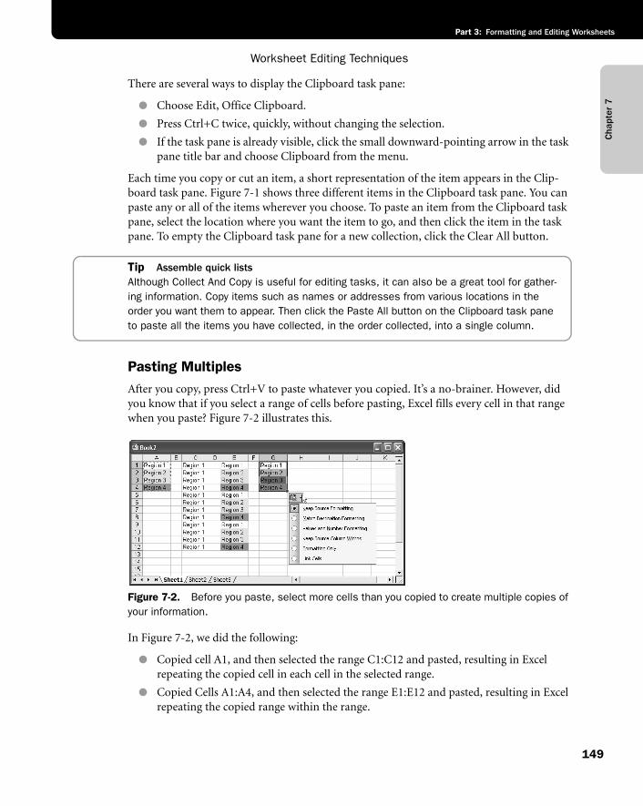
Cha

pter

7

Worksheet Editing Techniques

149

Part 3: Formatting and Editing Worksheets

There are several ways to display the Clipboard task pane:

● Choose Edit, Office Clipboard.

● Press Ctrl+C twice, quickly, without changing the selection.

● If the task pane is already visible, click the small downward-pointing arrow in the task pane title bar and choose Clipboard from the menu.

Each time you copy or cut an item, a short representation of the item appears in the Clip-board task pane. Figure 7-1 shows three different items in the Clipboard task pane. You can paste any or all of the items wherever you choose. To paste an item from the Clipboard task pane, select the location where you want the item to go, and then click the item in the task pane. To empty the Clipboard task pane for a new collection, click the Clear All button.

Tip Assemble quick listsAlthough Collect And Copy is useful for editing tasks, it can also be a great tool for gather-ing information. Copy items such as names or addresses from various locations in the order you want them to appear. Then click the Paste All button on the Clipboard task pane to paste all the items you have collected, in the order collected, into a single column.

Pasting MultiplesAfter you copy, press Ctrl+V to paste whatever you copied. It’s a no-brainer. However, did you know that if you select a range of cells before pasting, Excel fills every cell in that range when you paste? Figure 7-2 illustrates this.

f07ie02

Figure 7-2. Before you paste, select more cells than you copied to create multiple copies of your information.

In Figure 7-2, we did the following:

● Copied cell A1, and then selected the range C1:C12 and pasted, resulting in Excel repeating the copied cell in each cell in the selected range.

● Copied Cells A1:A4, and then selected the range E1:E12 and pasted, resulting in Excel repeating the copied range within the range.

Chapter 7

Microsoft Office Excel 2003 Inside Out

Part 3: Formatting and Editing Worksheets

150

● Copied cells A1:A4, and then selected cell G1 and pasted, resulting in an exact duplicate of the copied range.

Note If the selected paste range contains more cells than the copied range, Excel repeats the copied cells until it fills the destination. However, if the paste range is smaller than the copied range, Excel pastes the entire copied range anyway.

Using the Paste Options Smart TagNotice in Figure 7-2 that we clicked the Paste Options smart tag action menu that appears near the lower left corner of the pasted range. This smart tag appears whenever and wherever you paste, offering action options applicable after pasting—a sort of “Smart Paste Special.” The best part is that you can try each action in turn. Keep selecting Paste options until you like what you see, and then press Enter. The following describes each item on the Paste Options smart tag action menu:

For more information about using smart tags, see “Smart Tags” on page 919.

● Keep Source Formatting. Retains formatting. This is the default action. If the other options don’t work for you, you can always come back to this one before you press Enter.

● Match Destination Formatting. Copies formatted data into a differently formatted table without having to redo the formatting.

● Values And Number Formatting. Pastes values without losing number formats.

● Keep Source Column Widths. Retains column widths. This option is like choosing Keep Source Formatting with the added action of “pasting” the column width.

● Formatting Only. Leaves the contents of the cells alone and transfers the formatting. This works in the same way as the Format Painter button on the Standard toolbar.

● Link Cells. Instead of pasting the contents of the cut or copied cells, pastes a refer-ence to the source cells, ignoring the source formatting.

Cutting and PastingWhen you cut rather than copy cells, subsequent pasting places one copy in the selected des-tination, removes the copied cells from the Clipboard, and removes the marquee. Select the range you want to move, and press Ctrl+X, which places the marquee around the cut cells. When you press Ctrl+V to paste, Excel moves the cut cells to their new location and removes them from their original location.

When you cut and paste, the following rules apply:

● Excel clears both the contents and the formats of the cut range and transfers them to the cells in the paste range.

● Excel adjusts any formulas outside the cut area that refer to that cell.

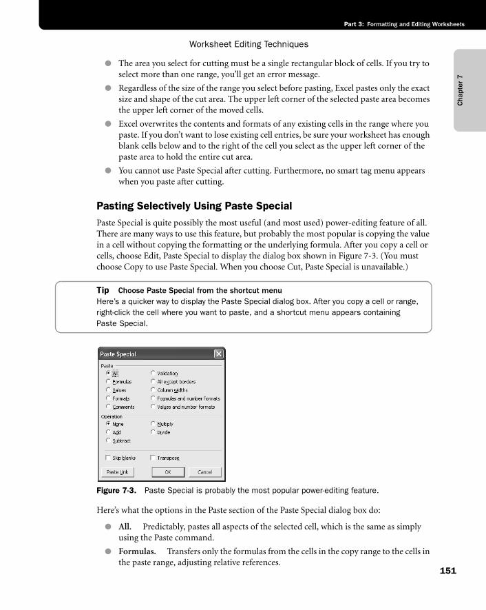
Cha

pter

7

Worksheet Editing Techniques

151

Part 3: Formatting and Editing Worksheets

● The area you select for cutting must be a single rectangular block of cells. If you try to select more than one range, you’ll get an error message.

● Regardless of the size of the range you select before pasting, Excel pastes only the exact size and shape of the cut area. The upper left corner of the selected paste area becomes the upper left corner of the moved cells.

● Excel overwrites the contents and formats of any existing cells in the range where you paste. If you don’t want to lose existing cell entries, be sure your worksheet has enough blank cells below and to the right of the cell you select as the upper left corner of the paste area to hold the entire cut area.

● You cannot use Paste Special after cutting. Furthermore, no smart tag menu appears when you paste after cutting.

Pasting Selectively Using Paste SpecialPaste Special is quite possibly the most useful (and most used) power-editing feature of all. There are many ways to use this feature, but probably the most popular is copying the value in a cell without copying the formatting or the underlying formula. After you copy a cell or cells, choose Edit, Paste Special to display the dialog box shown in Figure 7-3. (You must choose Copy to use Paste Special. When you choose Cut, Paste Special is unavailable.)

Tip Choose Paste Special from the shortcut menuHere’s a quicker way to display the Paste Special dialog box. After you copy a cell or range, right-click the cell where you want to paste, and a shortcut menu appears containing Paste Special.

f07ie03

Figure 7-3. Paste Special is probably the most popular power-editing feature.

Here’s what the options in the Paste section of the Paste Special dialog box do:

● All. Predictably, pastes all aspects of the selected cell, which is the same as simply using the Paste command.

● Formulas. Transfers only the formulas from the cells in the copy range to the cells in the paste range, adjusting relative references.

Chapter 7

Microsoft Office Excel 2003 Inside Out

Part 3: Formatting and Editing Worksheets

152

● Values. Pastes static text, numeric values, or only the displayed values resulting from formulas.

● Formats. Transfers only the formats in the copy range to the paste range.

Tip Quickly duplicate multiple formatsYou can quickly copy and paste formats from a single cell or from a range of cells using the Format Painter button on the Standard toolbar.

● Comments. Transfers only comments attached to selected cells.

● Validation. Pastes only the Data Validation settings that you have applied to the selected cells.

For more information about data validation, see “Validating Data Entry” on page 719.

● All Except Borders. Transfers data without disturbing the border formats you spent so much time applying.

● Column Widths. Transfers only column widths, which is handy when trying to make a sheet look consistent for presentation.

● Formulas And Number Formats. Transfers only formulas and number formats, which is handy when copying formulas to previously formatted areas. Usually, you’ll want the same number formats applied to formulas you copy, wherever they happen to go.

● Values And Number Formats. Transfers resulting values (but not the formulas) and number formats.

Tip Use the smart tag menuYou can apply a few common Paste Special options, including Values and Number Formatting, by clicking the smart tag action menu that appears after you paste, as shown in Figure 7-2.

Because the All option pastes the formulas, values, formats, and cell comments from the copy range into the paste range, it has the same effect as selecting Paste, making you wonder why Excel offers this option. That question brings us to our next topic—the Operation options.

Pasting Using Math OperatorsYou use the options in the Operation section of the Paste Special dialog box to mathemati-cally combine the contents of the copy area with the contents of the paste area. When you select any option other than None, Excel does not overwrite the destination cell or range with the copied data. Instead, it uses the specified operator to combine the copy and paste ranges.

For example, say we want to get a quick total of the Northern and Eastern regions in Figure 7-4. First we copied the Northern Region figures to column G, and then we copied the East-ern Region numbers in column D and chose Edit, Paste Special. We clicked the Values and Add options in the Paste Special dialog box, and after clicking OK, we saw the result shown at the bottom of Figure 7-4.

Cha

pter

7

Worksheet Editing Techniques

153

Part 3: Formatting and Editing Worksheets

f07ie04

Figure 7-4. We used the Values option of Paste Special to add the totals from column D to those in column G.

Note You can find the sample file used in this example, Humongous.xls, on the book’s companion CD.

The other options in the Operation section of the Paste Special dialog box combine the con-tents of the copy and paste ranges using the appropriate operators. Just remember that the Subtract option subtracts the copy range from the paste range, and the Divide option divides the contents of the paste range by the contents of the copy range. Also note that if the copy range contains text entries and you use Paste Special with an Operation option (other than None), nothing happens.

Choose the Values option when you use any Operation option. As long as the entries in the copy range are numbers, you can use All, but if the copy range contains formulas, you’ll get “interest-ing” results. As a rule, avoid using the Operation options if the paste range contains formulas.

Note Excel assigns the value 0 to blank spaces in the copy and paste ranges, regardless of which Operation option you select.

Chapter 7

Microsoft Office Excel 2003 Inside Out

Part 3: Formatting and Editing Worksheets

154

Pasting LinksThe Paste Link button in the Paste Special dialog box, shown in Figure 7-4, is a handy way to create references to cells or ranges. When you click the Paste link button, Excel enters an absolute reference to the copied cell in the new location. For example, if you copy cell A3, and then select cell B5, choose Edit, Paste Special, and click the Paste Link button, the formula =$A$3 is entered into cell B5.

If you copy a range of cells, the Paste Link button enters a similar formula for each cell in the copied range to the same sized range in the new location.

For more information about absolute references, see “Understanding Relative, Absolute, and Mixed References” on page 353.

Skipping Blank CellsThe Paste Special dialog box contains a Skip Blanks option that you use when you want Excel to ignore any blank cells in the copy range. Generally, if your copy range contains blank cells, Excel pastes those blank cells over the corresponding cells in the paste area. As a result, empty cells in the copy range overwrite the contents, formats, and comments in corresponding cells of the paste area. When you select Skip Blanks, however, the corresponding cells in the paste area are unaffected.

Transposing EntriesOne of the often-overlooked but extremely useful Paste Special features is the Transpose option, which helps you to reorient the contents of the copied range when you paste—that is, entries in rows appear in columns, and entries in columns appear in rows. For example, in Figure 7-5, we needed to use the column headings in Row 3 of the top sheet to create identical row headings in column A of the bottom sheet. Accomplishing this was as simple as copying cells B3:G3 in the top sheet, clicking cell A4 in the bottom sheet, and using Paste Special with Transpose selected.

Tip Transpose formulasIf you transpose cells containing formulas, Excel transposes the formulas and adjusts cell references. If you want the transposed formulas to continue to correctly refer to nontrans-posed cells, make sure the references in the formulas are absolute before you copy them. For more information on absolute cell references, see “Using Cell References in Formulas” on page 352.

Using Paste Special with ArraysAs with any other formula, you can convert the results of an array formula to a series of con-stant values by copying the entire array range and—without changing your selection—choosing Paste Special. If you select the Values option in the Paste Special dialog box, Excel overwrites the array formulas with their resulting constant values. Because the range now

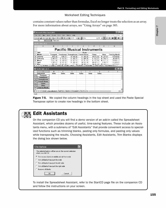
Cha

pter

7

Worksheet Editing Techniques

155

Part 3: Formatting and Editing Worksheets

contains constant values rather than formulas, Excel no longer treats the selection as an array. For more information about arrays, see “Using Arrays” on page 385.

f07ie05

Figure 7-5. We copied the column headings in the top sheet and used the Paste Special Transpose option to create row headings in the bottom sheet.

Edit AssistantsOn the companion CD you will find a demo version of an add-in called the Spreadsheet Assistant, which provides dozens of useful, time-saving features. These include an Assis-tants menu, with a submenu of “Edit Assistants” that provide convenient access to special-ized functions such as trimming blanks, pasting only formulas, and pasting only values while transposing the results. Choosing Assistants, Edit Assistants, Trim Blanks displays the dialog box shown below.

G07ie06sb

To install the Spreadsheet Assistant, refer to the StartCD page file on the companion CD and follow the instructions on your screen.

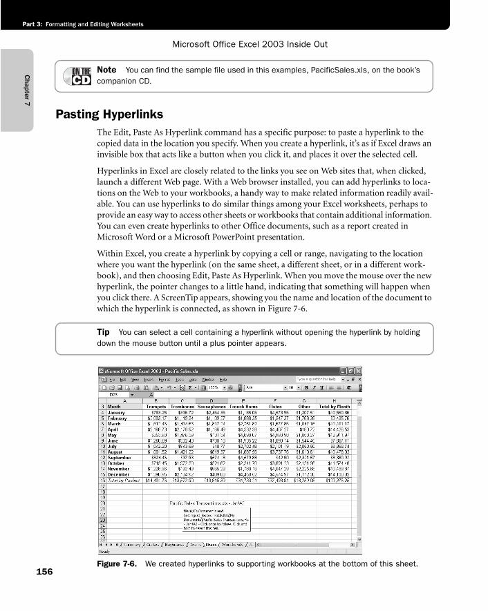
Chapter 7

Microsoft Office Excel 2003 Inside Out

Part 3: Formatting and Editing Worksheets

156

Note You can find the sample file used in this examples, PacificSales.xls, on the book’s companion CD.

Pasting HyperlinksThe Edit, Paste As Hyperlink command has a specific purpose: to paste a hyperlink to the copied data in the location you specify. When you create a hyperlink, it’s as if Excel draws an invisible box that acts like a button when you click it, and places it over the selected cell.

Hyperlinks in Excel are closely related to the links you see on Web sites that, when clicked, launch a different Web page. With a Web browser installed, you can add hyperlinks to loca-tions on the Web to your workbooks, a handy way to make related information readily avail-able. You can use hyperlinks to do similar things among your Excel worksheets, perhaps to provide an easy way to access other sheets or workbooks that contain additional information. You can even create hyperlinks to other Office documents, such as a report created in Microsoft Word or a Microsoft PowerPoint presentation.

Within Excel, you create a hyperlink by copying a cell or range, navigating to the location where you want the hyperlink (on the same sheet, a different sheet, or in a different work-book), and then choosing Edit, Paste As Hyperlink. When you move the mouse over the new hyperlink, the pointer changes to a little hand, indicating that something will happen when you click there. A ScreenTip appears, showing you the name and location of the document to which the hyperlink is connected, as shown in Figure 7-6.

Tip You can select a cell containing a hyperlink without opening the hyperlink by holding down the mouse button until a plus pointer appears.

f07ie06

Figure 7-6. We created hyperlinks to supporting workbooks at the bottom of this sheet.

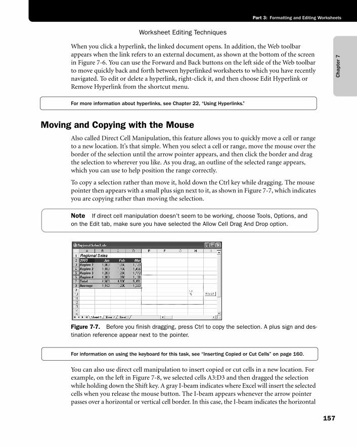
Cha

pter

7

Worksheet Editing Techniques

157

Part 3: Formatting and Editing Worksheets

When you click a hyperlink, the linked document opens. In addition, the Web toolbar appears when the link refers to an external document, as shown at the bottom of the screen in Figure 7-6. You can use the Forward and Back buttons on the left side of the Web toolbar to move quickly back and forth between hyperlinked worksheets to which you have recently navigated. To edit or delete a hyperlink, right-click it, and then choose Edit Hyperlink or Remove Hyperlink from the shortcut menu.

For more information about hyperlinks, see Chapter 22, “Using Hyperlinks.”

Moving and Copying with the MouseAlso called Direct Cell Manipulation, this feature allows you to quickly move a cell or range to a new location. It’s that simple. When you select a cell or range, move the mouse over the border of the selection until the arrow pointer appears, and then click the border and drag the selection to wherever you like. As you drag, an outline of the selected range appears, which you can use to help position the range correctly.

To copy a selection rather than move it, hold down the Ctrl key while dragging. The mouse pointer then appears with a small plus sign next to it, as shown in Figure 7-7, which indicates you are copying rather than moving the selection.

Note If direct cell manipulation doesn’t seem to be working, choose Tools, Options, and on the Edit tab, make sure you have selected the Allow Cell Drag And Drop option.

f07ie07

Figure 7-7. Before you finish dragging, press Ctrl to copy the selection. A plus sign and des-tination reference appear next to the pointer.

For information on using the keyboard for this task, see “Inserting Copied or Cut Cells” on page 160.

You can also use direct cell manipulation to insert copied or cut cells in a new location. For example, on the left in Figure 7-8, we selected cells A3:D3 and then dragged the selection while holding down the Shift key. A gray I-beam indicates where Excel will insert the selected cells when you release the mouse button. The I-beam appears whenever the arrow pointer passes over a horizontal or vertical cell border. In this case, the I-beam indicates the horizontal

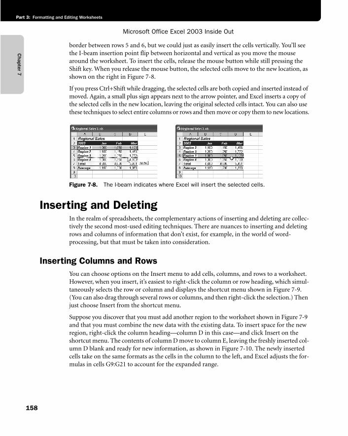
Chapter 7

Microsoft Office Excel 2003 Inside Out

Part 3: Formatting and Editing Worksheets

158

border between rows 5 and 6, but we could just as easily insert the cells vertically. You’ll see the I-beam insertion point flip between horizontal and vertical as you move the mouse around the worksheet. To insert the cells, release the mouse button while still pressing the Shift key. When you release the mouse button, the selected cells move to the new location, as shown on the right in Figure 7-8.

If you press Ctrl+Shift while dragging, the selected cells are both copied and inserted instead of moved. Again, a small plus sign appears next to the arrow pointer, and Excel inserts a copy of the selected cells in the new location, leaving the original selected cells intact. You can also use these techniques to select entire columns or rows and then move or copy them to new locations.

f07ie08

Figure 7-8. The I-beam indicates where Excel will insert the selected cells.

Inserting and DeletingIn the realm of spreadsheets, the complementary actions of inserting and deleting are collec-tively the second most-used editing techniques. There are nuances to inserting and deleting rows and columns of information that don’t exist, for example, in the world of word-processing, but that must be taken into consideration.

Inserting Columns and RowsYou can choose options on the Insert menu to add cells, columns, and rows to a worksheet. However, when you insert, it’s easiest to right-click the column or row heading, which simul-taneously selects the row or column and displays the shortcut menu shown in Figure 7-9. (You can also drag through several rows or columns, and then right-click the selection.) Then just choose Insert from the shortcut menu.

Suppose you discover that you must add another region to the worksheet shown in Figure 7-9 and that you must combine the new data with the existing data. To insert space for the new region, right-click the column heading—column D in this case—and click Insert on the shortcut menu. The contents of column D move to column E, leaving the freshly inserted col-umn D blank and ready for new information, as shown in Figure 7-10. The newly inserted cells take on the same formats as the cells in the column to the left, and Excel adjusts the for-mulas in cells G9:G21 to account for the expanded range.

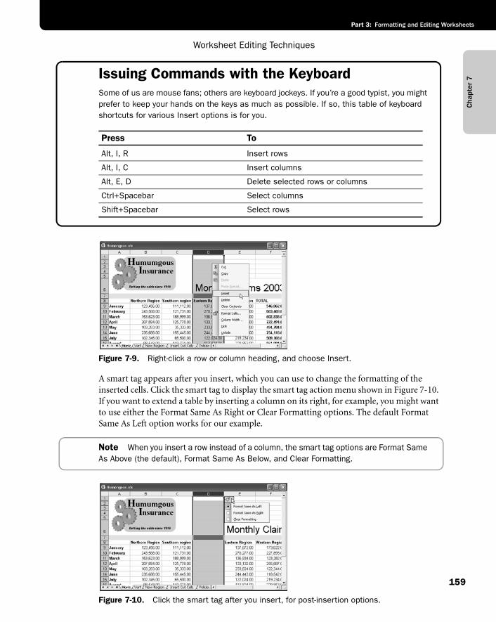
Cha

pter

7

Worksheet Editing Techniques

159

Part 3: Formatting and Editing Worksheets

Issuing Commands with the KeyboardSome of us are mouse fans; others are keyboard jockeys. If you’re a good typist, you might prefer to keep your hands on the keys as much as possible. If so, this table of keyboard shortcuts for various Insert options is for you.

f07ie09

Figure 7-9. Right-click a row or column heading, and choose Insert.

A smart tag appears after you insert, which you can use to change the formatting of the inserted cells. Click the smart tag to display the smart tag action menu shown in Figure 7-10. If you want to extend a table by inserting a column on its right, for example, you might want to use either the Format Same As Right or Clear Formatting options. The default Format Same As Left option works for our example.

Note When you insert a row instead of a column, the smart tag options are Format Same As Above (the default), Format Same As Below, and Clear Formatting.

f07ie10

Figure 7-10. Click the smart tag after you insert, for post-insertion options.

Press To

Alt, I, R Insert rows

Alt, I, C Insert columns

Alt, E, D Delete selected rows or columns

Ctrl+Spacebar Select columns

Shift+Spacebar Select rows

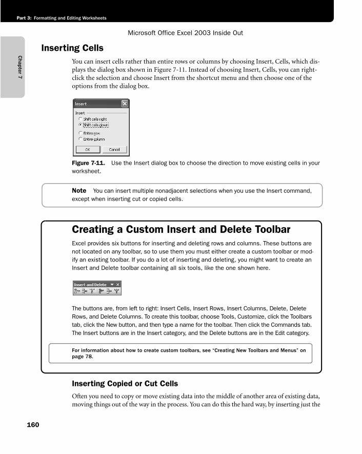
Chapter 7

Microsoft Office Excel 2003 Inside Out

Part 3: Formatting and Editing Worksheets

160

Inserting CellsYou can insert cells rather than entire rows or columns by choosing Insert, Cells, which dis-plays the dialog box shown in Figure 7-11. Instead of choosing Insert, Cells, you can right-click the selection and choose Insert from the shortcut menu and then choose one of the options from the dialog box.

f07ie11

Figure 7-11. Use the Insert dialog box to choose the direction to move existing cells in your worksheet.

Note You can insert multiple nonadjacent selections when you use the Insert command, except when inserting cut or copied cells.

Creating a Custom Insert and Delete ToolbarExcel provides six buttons for inserting and deleting rows and columns. These buttons are not located on any toolbar, so to use them you must either create a custom toolbar or mod-ify an existing toolbar. If you do a lot of inserting and deleting, you might want to create an Insert and Delete toolbar containing all six tools, like the one shown here.

g07ie02

The buttons are, from left to right: Insert Cells, Insert Rows, Insert Columns, Delete, Delete Rows, and Delete Columns. To create this toolbar, choose Tools, Customize, click the Toolbars tab, click the New button, and then type a name for the toolbar. Then click the Commands tab. The Insert buttons are in the Insert category, and the Delete buttons are in the Edit category.

For information about how to create custom toolbars, see “Creating New Toolbars and Menus” on page 78.

Inserting Copied or Cut CellsOften you need to copy or move existing data into the middle of another area of existing data, moving things out of the way in the process. You can do this the hard way, by inserting just the

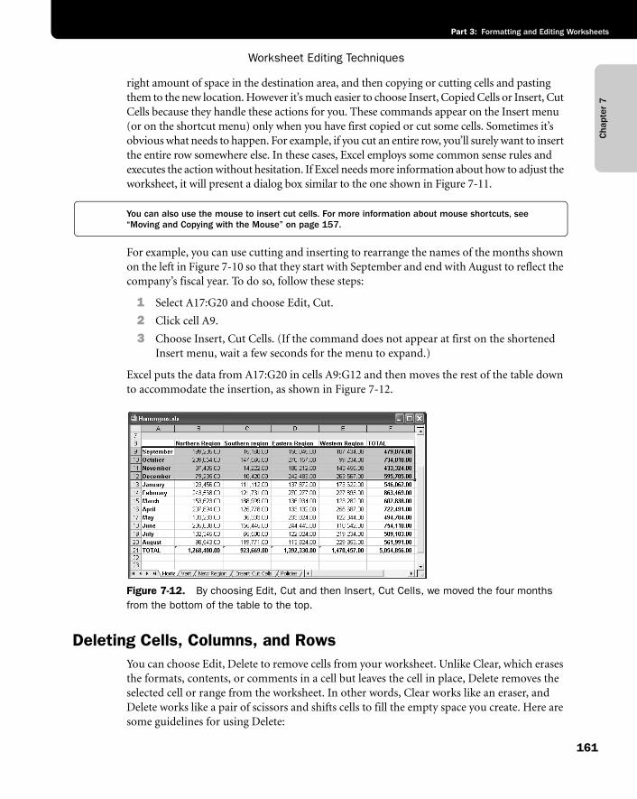
Cha

pter

7

Worksheet Editing Techniques

161

Part 3: Formatting and Editing Worksheets

right amount of space in the destination area, and then copying or cutting cells and pasting them to the new location. However it’s much easier to choose Insert, Copied Cells or Insert, Cut Cells because they handle these actions for you. These commands appear on the Insert menu (or on the shortcut menu) only when you have first copied or cut some cells. Sometimes it’s obvious what needs to happen. For example, if you cut an entire row, you’ll surely want to insert the entire row somewhere else. In these cases, Excel employs some common sense rules and executes the action without hesitation. If Excel needs more information about how to adjust the worksheet, it will present a dialog box similar to the one shown in Figure 7-11.

You can also use the mouse to insert cut cells. For more information about mouse shortcuts, see “Moving and Copying with the Mouse” on page 157.

For example, you can use cutting and inserting to rearrange the names of the months shown on the left in Figure 7-10 so that they start with September and end with August to reflect the company’s fiscal year. To do so, follow these steps:

1 Select A17:G20 and choose Edit, Cut.

2 Click cell A9.

3 Choose Insert, Cut Cells. (If the command does not appear at first on the shortened Insert menu, wait a few seconds for the menu to expand.)

Excel puts the data from A17:G20 in cells A9:G12 and then moves the rest of the table down to accommodate the insertion, as shown in Figure 7-12.

f07ie12

Figure 7-12. By choosing Edit, Cut and then Insert, Cut Cells, we moved the four months from the bottom of the table to the top.

Deleting Cells, Columns, and RowsYou can choose Edit, Delete to remove cells from your worksheet. Unlike Clear, which erases the formats, contents, or comments in a cell but leaves the cell in place, Delete removes the selected cell or range from the worksheet. In other words, Clear works like an eraser, and Delete works like a pair of scissors and shifts cells to fill the empty space you create. Here are some guidelines for using Delete:

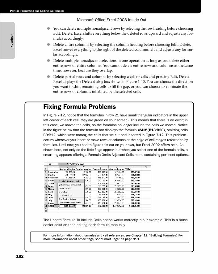
Chapter 7

Microsoft Office Excel 2003 Inside Out

Part 3: Formatting and Editing Worksheets

162

● You can delete multiple nonadjacent rows by selecting the row heading before choosing Edit, Delete. Excel shifts everything below the deleted rows upward and adjusts any for-mulas accordingly.

● Delete entire columns by selecting the column heading before choosing Edit, Delete. Excel moves everything to the right of the deleted columns left and adjusts any formu-las accordingly.

● Delete multiple nonadjacent selections in one operation as long as you delete either entire rows or entire columns. You cannot delete entire rows and columns at the same time, however, because they overlap.

● Delete partial rows and columns by selecting a cell or cells and pressing Edit, Delete. Excel displays the Delete dialog box shown in Figure 7-13. You can choose the direction you want to shift remaining cells to fill the gap, or you can choose to eliminate the entire rows or columns inhabited by the selected cells.

Fixing Formula ProblemsIn Figure 7-12, notice that the formulas in row 21 have small triangular indicators in the upper left corner of each cell (they are green on your screen). This means that there is an error; in this case, we moved the cells, so the formulas no longer include the cells we moved. Notice in the figure below that the formula bar displays the formula =SUM(B13:B20), omitting cells B9:B12, which were among the cells that we cut and inserted in Figure 7-12. This problem occurs whenever you insert or move rows or columns at the edge of cell ranges referred to by formulas. Until now, you had to figure this out on your own, but Excel 2002 offers help. As shown here, not only do the little flags appear, but when you select one of the formula cells, a smart tag appears offering a Formula Omits Adjacent Cells menu containing pertinent options.

g07ie03

The Update Formula To Include Cells option works correctly in our example. This is a much easier solution than editing each formula manually.

For more information about formulas and cell references, see Chapter 12, “Building Formulas.” For more information about smart tags, see “Smart Tags” on page 919.

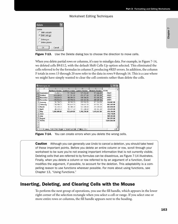
Cha

pter

7

Worksheet Editing Techniques

163

Part 3: Formatting and Editing Worksheets

f07ie13

Figure 7-13. Use the Delete dialog box to choose the direction to move cells.

When you delete partial rows or columns, it’s easy to misalign data. For example, in Figure 7-14, we deleted cells B9:E12, with the default Shift Cells Up option selected. This eliminated the cells referred to by the formulas in column F, producing #REF errors. In addition, the column F totals in rows 13 through 20 now refer to the data in rows 9 through 16. This is a case where we might have simply wanted to clear the cell contents rather than delete the cells.

f07ie14

Figure 7-14. You can create errors when you delete the wrong cells.

Caution Although you can generally use Undo to cancel a deletion, you should take heed of these important points. Before you delete an entire column or row, scroll through your worksheet to be sure you’re not erasing important information that is not currently visible. Deleting cells that are referred to by formulas can be disastrous, as Figure 7-14 illustrates. Finally, when you delete a column or row referred to by an argument of a function, Excel modifies the argument, if possible, to account for the deletion. This adaptability is a com-pelling reason to use functions wherever possible. For more about using functions, see Chapter 13, “Using Functions.”

Inserting, Deleting, and Clearing Cells with the MouseTo perform the next group of operations, you use the fill handle, which appears in the lower right corner of the selection rectangle when you select a cell or range. If you select one or more entire rows or columns, the fill handle appears next to the heading.

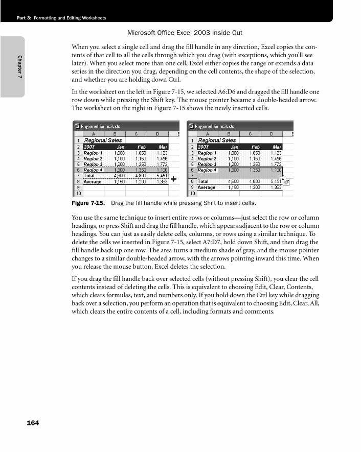
Chapter 7

Microsoft Office Excel 2003 Inside Out

Part 3: Formatting and Editing Worksheets

164

When you select a single cell and drag the fill handle in any direction, Excel copies the con-tents of that cell to all the cells through which you drag (with exceptions, which you’ll see later). When you select more than one cell, Excel either copies the range or extends a data series in the direction you drag, depending on the cell contents, the shape of the selection, and whether you are holding down Ctrl.

In the worksheet on the left in Figure 7-15, we selected A6:D6 and dragged the fill handle one row down while pressing the Shift key. The mouse pointer became a double-headed arrow. The worksheet on the right in Figure 7-15 shows the newly inserted cells.

f07ie15

Figure 7-15. Drag the fill handle while pressing Shift to insert cells.

You use the same technique to insert entire rows or columns—just select the row or column headings, or press Shift and drag the fill handle, which appears adjacent to the row or column headings. You can just as easily delete cells, columns, or rows using a similar technique. To delete the cells we inserted in Figure 7-15, select A7:D7, hold down Shift, and then drag the fill handle back up one row. The area turns a medium shade of gray, and the mouse pointer changes to a similar double-headed arrow, with the arrows pointing inward this time. When you release the mouse button, Excel deletes the selection.

If you drag the fill handle back over selected cells (without pressing Shift), you clear the cell contents instead of deleting the cells. This is equivalent to choosing Edit, Clear, Contents, which clears formulas, text, and numbers only. If you hold down the Ctrl key while dragging back over a selection, you perform an operation that is equivalent to choosing Edit, Clear, All, which clears the entire contents of a cell, including formats and comments.

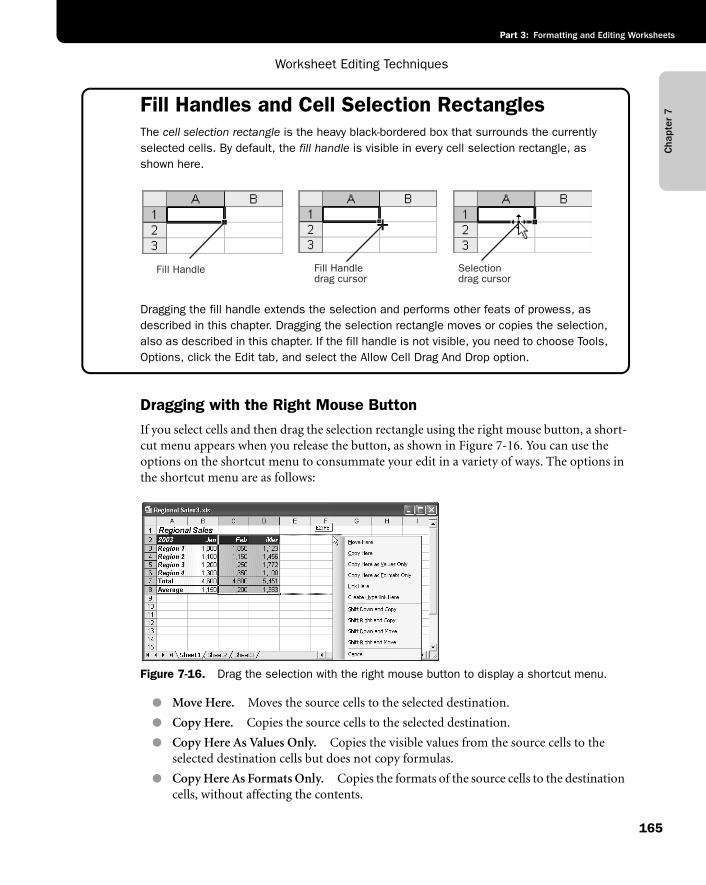
Cha

pter

7

Worksheet Editing Techniques

165

Part 3: Formatting and Editing Worksheets

Fill Handles and Cell Selection RectanglesThe cell selection rectangle is the heavy black-bordered box that surrounds the currently selected cells. By default, the fill handle is visible in every cell selection rectangle, as shown here.

g07ie04

Dragging the fill handle extends the selection and performs other feats of prowess, as described in this chapter. Dragging the selection rectangle moves or copies the selection, also as described in this chapter. If the fill handle is not visible, you need to choose Tools, Options, click the Edit tab, and select the Allow Cell Drag And Drop option.

Dragging with the Right Mouse ButtonIf you select cells and then drag the selection rectangle using the right mouse button, a short-cut menu appears when you release the button, as shown in Figure 7-16. You can use the options on the shortcut menu to consummate your edit in a variety of ways. The options in the shortcut menu are as follows:

f07ie16

Figure 7-16. Drag the selection with the right mouse button to display a shortcut menu.

● Move Here. Moves the source cells to the selected destination.

● Copy Here. Copies the source cells to the selected destination.

● Copy Here As Values Only. Copies the visible values from the source cells to the selected destination cells but does not copy formulas.

● Copy Here As Formats Only. Copies the formats of the source cells to the destination cells, without affecting the contents.

Fill Handle Fill Handledrag cursor

Selectiondrag cursor

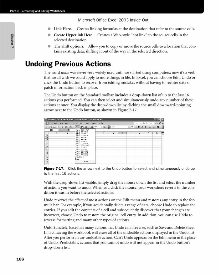
Chapter 7

Microsoft Office Excel 2003 Inside Out

Part 3: Formatting and Editing Worksheets

166

● Link Here. Creates linking formulas at the destination that refer to the source cells.

● Create Hyperlink Here. Creates a Web-style “hot link” to the source cells in the selected destination.

● The Shift options. Allow you to copy or move the source cells to a location that con-tains existing data, shifting it out of the way in the selected direction.

Undoing Previous ActionsThe word undo was never very widely used until we started using computers; now it’s a verb that we all wish we could apply to more things in life. In Excel, you can choose Edit, Undo or click the Undo button to recover from editing mistakes without having to reenter data or patch information back in place.

The Undo button on the Standard toolbar includes a drop-down list of up to the last 16 actions you performed. You can then select and simultaneously undo any number of these actions at once. You display the drop-down list by clicking the small downward-pointing arrow next to the Undo button, as shown in Figure 7-17.

f07ie17

Figure 7-17. Click the arrow next to the Undo button to select and simultaneously undo up to the last 16 actions.

With the drop-down list visible, simply drag the mouse down the list and select the number of actions you want to undo. When you click the mouse, your worksheet reverts to the con-dition it was in before the selected actions.

Undo reverses the effect of most actions on the Edit menu and restores any entry in the for-mula bar. For example, if you accidentally delete a range of data, choose Undo to replace the entries. If you edit the contents of a cell and subsequently discover that your changes are incorrect, choose Undo to restore the original cell entry. In addition, you can use Undo to reverse formatting and many other types of actions.

Unfortunately, Excel has many actions that Undo can’t reverse, such as Save and Delete Sheet. In fact, saving the workbook will erase all of the undoable actions displayed in the Undo list. After you perform an un-undoable action, Can’t Undo appears on the Edit menu in the place of Undo. Predictably, actions that you cannot undo will not appear in the Undo button’s drop-down list.

Cha

pter

7

Worksheet Editing Techniques

167

Part 3: Formatting and Editing Worksheets

Redoing What You’ve UndoneAfter you use Undo, you can then use Redo, which predictably reverses Undo. The Redo com-mand on the Edit menu and the Redo button on the Standard toolbar operate in the same manner, allowing you to redo the last action by clicking the button itself or to redo up to the last 16 actions at once. When you undo a number of actions using the Undo drop-down list, Excel transfers these actions to the Redo button’s drop-down list. If you then redo the same actions, Excel transfers them back to the Undo drop-down list.

You can take advantage of Undo and Redo to see the effects of an editing change in your worksheet. If you edit a cell that is referred to in several formulas, you can use Undo and Redo to get a “before and after” look at the results displayed by the formulas.

Repeating Your Last ActionEdit, Repeat and Edit, Redo share the same keyboard equivalent (Ctrl+Y), because you can do only one or the other at any given moment. Being able to repeat the last action is a great time-saver, and is particularly handy with repetitive chores. The phrase “last action” is the key to understanding the difference between the two faces of this command. The command name changes to reflect your most recent action. Redo is valid only if Undo was your last action. After you have redone all the “undos” (up to 16), you’re back to the “true” last action—that is, the last thing you did before you used Undo. For example, press Delete to clear the contents of a cell. When you choose the Edit menu, both Undo Clear and Repeat Clear appear there. If you choose Undo Clear and then choose the Edit menu again, Redo Clear replaces Repeat Clear. If you choose Redo Clear and then choose the Edit menu, Repeat Clear reappears.

Unlike Undo, Repeat works with most actions. The only exceptions are those actions that you can’t logically repeat. For example, if you save a file using File, Save, you can’t repeat the action. Whatever the case, Repeat reflects the last repeatable action.

Editing Cell ContentsYou can use the formula bar to edit the contents of a selected cell, or you can perform your editing “on location” in the cell itself. Excel also includes a few special features you can apply to tasks such as entering date sequences, which once used to involve editing each cell but are now semiautomatic, if you know where to find the “trigger.”

Editing in the Formula BarYou can also use Cut, Copy, Paste, and Clear to edit entries using the formula bar. Often, sim-ply reentering a value or formula is easier, but the Edit menu options are convenient when you’re working with a long, complex formula or label. These options work just as they do in a word-processing program such as Word when you’re working in the formula bar. For example, you can copy all or part of a formula from one cell to another. For example, suppose cell A10 contains the formula =IF(NPV(.15,A1:A9)>0,A11,A12), and you want to enter =NPV(.15,A1:A9) in cell B10.

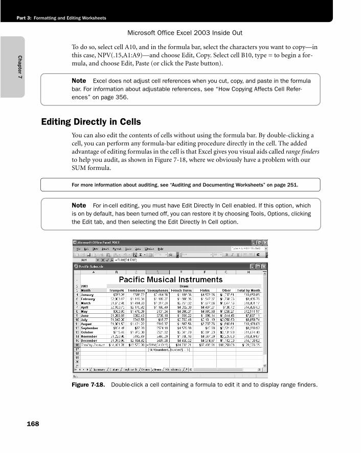
Chapter 7

Microsoft Office Excel 2003 Inside Out

Part 3: Formatting and Editing Worksheets

168

To do so, select cell A10, and in the formula bar, select the characters you want to copy—in this case, NPV(.15,A1:A9)—and choose Edit, Copy. Select cell B10, type = to begin a for-mula, and choose Edit, Paste (or click the Paste button).

Note Excel does not adjust cell references when you cut, copy, and paste in the formula bar. For information about adjustable references, see “How Copying Affects Cell Refer-ences” on page 356.

Editing Directly in CellsYou can also edit the contents of cells without using the formula bar. By double-clicking a cell, you can perform any formula-bar editing procedure directly in the cell. The added advantage of editing formulas in the cell is that Excel gives you visual aids called range findersto help you audit, as shown in Figure 7-18, where we obviously have a problem with our SUM formula.

For more information about auditing, see “Auditing and Documenting Worksheets” on page 251.

Note For in-cell editing, you must have Edit Directly In Cell enabled. If this option, which is on by default, has been turned off, you can restore it by choosing Tools, Options, clicking the Edit tab, and then selecting the Edit Directly In Cell option.

f07ie18

Figure 7-18. Double-click a cell containing a formula to edit it and to display range finders.

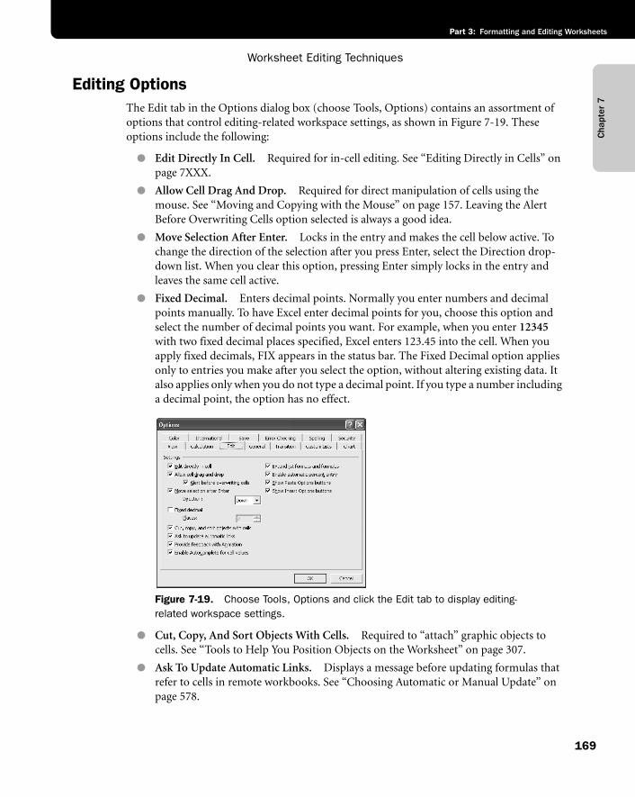
Cha

pter

7

Worksheet Editing Techniques

169

Part 3: Formatting and Editing Worksheets

Editing OptionsThe Edit tab in the Options dialog box (choose Tools, Options) contains an assortment of options that control editing-related workspace settings, as shown in Figure 7-19. These options include the following:

● Edit Directly In Cell. Required for in-cell editing. See “Editing Directly in Cells” on page 7XXX.

● Allow Cell Drag And Drop. Required for direct manipulation of cells using the mouse. See “Moving and Copying with the Mouse” on page 157. Leaving the Alert Before Overwriting Cells option selected is always a good idea.

● Move Selection After Enter. Locks in the entry and makes the cell below active. To change the direction of the selection after you press Enter, select the Direction drop-down list. When you clear this option, pressing Enter simply locks in the entry and leaves the same cell active.

● Fixed Decimal. Enters decimal points. Normally you enter numbers and decimal points manually. To have Excel enter decimal points for you, choose this option and select the number of decimal points you want. For example, when you enter 12345with two fixed decimal places specified, Excel enters 123.45 into the cell. When you apply fixed decimals, FIX appears in the status bar. The Fixed Decimal option applies only to entries you make after you select the option, without altering existing data. It also applies only when you do not type a decimal point. If you type a number including a decimal point, the option has no effect.

f07ie19 Figure 7-19. Choose Tools, Options and click the Edit tab to display editing-related workspace settings.

● Cut, Copy, And Sort Objects With Cells. Required to “attach” graphic objects to cells. See “Tools to Help You Position Objects on the Worksheet” on page 307.

● Ask To Update Automatic Links. Displays a message before updating formulas that refer to cells in remote workbooks. See “Choosing Automatic or Manual Update” on page 578.

Chapter 7

Microsoft Office Excel 2003 Inside Out

Part 3: Formatting and Editing Worksheets

170

● Provide Feedback With Animation. Animates the action. With this option selected, using the arrows on the scroll bars or inserting and deleting rows or columns will appear to roll in the direction of the action.

● Enable AutoComplete For Cell Values. Allows Excel to suggest cell entries by com-paring existing values it finds in the same column as you type. See “Letting Excel Help with Typing Chores” on page 191.

● Extend List Formats And Formulas. Allows Excel to apply formatting to new cells entered in a “list” or table, based on the formats of existing cells. See “Extending Exist-ing Formatting” on page 178.

● Enable Automatic Percent Entry. Helps you enter values in cells with the Percentage format. With this option selected, all entries less than 1 are multiplied by 100. With this option clear, all entries—including those greater than 1—are multiplied by 100.

● Show Paste Options Buttons/Show Insert Options Buttons. Shows the smart tag menu. Normally when you perform a paste or insert operation, a smart tag action menu appears, offering various specific actions you can perform after the fact. Clear this option to turn off these features.

Understanding Fixed and Floating DecimalsThe Fixed Decimal option on the Edit tab of the Options dialog box is handy when you need to enter long lists of numeric values. (It’s equivalent to the floating decimal feature avail-able on most ten-key calculators.) For example, if you’re performing a lengthy data-entry task such as entering multiple dollar values into a worksheet, select the Fixed Decimal option and choose 2 in the Places list box. Then just type numbers and press Enter, saving you an extra keystroke for the decimal point in each entry. If you’re entering a thousand val-ues, typing 295 instead of 2.95 eliminates 25 percent of the keystrokes you would other-wise have to perform. However, you need to be careful to enter trailing zeros or add a decimal point. For example, you would normally type 5 to enter a 5.00 value, but with two fixed decimals turned on, the same entry becomes 0.05, making it necessary to type either 500 or 5. to correctly locate the decimal point.

Clearing Cell Contents and FormatsYou can choose Edit, Clear to erase the contents of a cell or range, the format assigned to that cell or range, comments attached to a cell, or a chart. The Clear submenu offers the following four options:

● All. Erases the contents of the selected cells, any formats (other than column width and row height), and any comments attached to those cells.

● Formats. Removes the formats from the selected cells but leaves their contents and comments in place; the selected cells then revert to the General format and the Normal style.

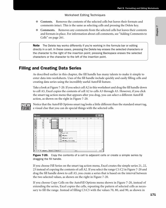
Cha

pter

7

Worksheet Editing Techniques

171

Part 3: Formatting and Editing Worksheets

● Contents. Removes the contents of the selected cells but leaves their formats and comments intact. This is the same as selecting cells and pressing the Delete key.

● Comments. Removes any comments from the selected cells but leaves their contents and formats in place. For information about cell comments, see “Adding Comments to Cells” on page 261.

Note The Delete key works differently if you’re working in the formula bar or editing directly in a cell. In these cases, pressing the Delete key erases the selected characters or the character to the right of the insertion point; pressing Backspace erases the selected characters or the character to the left of the insertion point.

Filling and Creating Data SeriesAs described earlier in this chapter, the fill handle has many talents to make it simple to enter data into worksheets. Uses of the fill handle include quickly and easily filling cells and creating data series using the incredibly useful AutoFill feature.

Take a look at Figure 7-20. If you select cell A2 in this worksheet and drag the fill handle down to cell A5, Excel copies the contents of cell A2 to cells A3 through A5. However, if you click the smart tag action menu that appears after you drag, you can select a different AutoFill action, as shown on the right in Figure 7-20.

Notice that the AutoFill Options smart tag looks a little different than the standard smart tag, a visual clue that you can do special things with the selected cells.

f07ie20

Figure 7-20. Copy the contents of a cell to adjacent cells or create a simple series by dragging the fill handle.

If you choose Fill Series on the smart tag action menu, Excel creates the simple series 21, 22, 23 instead of copying the contents of cell A2. If you select the range C1:C2 in Figure 7-20 and drag the fill handle down to cell A5, you create a series that is based on the interval between the two selected values, as shown on the right in Figure 7-20.

If you choose Copy Cells on the AutoFill Options menu shown in Figure 7-20, instead of extending the series, Excel copies the cells, repeating the pattern of selected cells as neces-sary to fill the range. Instead of filling C3:C5 with the values 70, 80, and 90, as shown in

Chapter 7

Microsoft Office Excel 2003 Inside Out

Part 3: Formatting and Editing Worksheets

172

Figure 7-20, choosing Copy Cells results in copying the values 50, 60, and 50 into the same range instead.

Tip Create decreasing seriesGenerally, when you create a series, you drag the fill handle down or to the right, and the values increase accordingly. You can also create a series of decreasing values, however, by simply dragging the fill handle either up or to the left. Enter the starting values in the cells at the bottom or to the right of the range you want to fill and then drag the fill handle back to the beginning of the range.

If you select a text value and drag the fill handle, Excel copies the text to the cells where you drag. If, however, the selection contains both text and numeric values, the AutoFill feature takes over and extends the numeric component while copying the text component. You can also extend dates in this way, using a number of date formats, including Qtr 1, Qtr 2, and so on. If you enter text that describes dates, even without numbers (such as months or days of the week), Excel treats the text as a series.

Inside OutFill series limited to 255 characters

Excel allows you to enter up to 32,767 characters in a cell. However, if you want to extend a series using Autofill, the selected source cells cannot contain more than 255 characters. If you try to extend a series from an entry of 256 characters or more, Excel simply copies the cells rather than extending the series. This is not really a bug, but a side effect of Excel’s column-width limitation of 255 characters. Besides, a 256-character entry is not going to be readable on the screen anyway. If you really need to create series out of humongous cell entries like this, perhaps a little worksheet redesign is in order. Otherwise, you’ll have to do it manually.

Figure 7-21 shows some examples of simple data series created by selecting single cells con-taining values and dragging the fill handle. The values in column A were typed, and the val-ues to the right of column A were extended using the fill handle. Figure 7-22 shows examples of creating data series using two selected values that, in effect, specify the interval to be used in creating the data series. We typed the values in columns A and B and extended the values to the right of column B using the fill handle. These two figures also show how AutoFill can create a series even when you mix text and numeric values in cells.

Tip Suppress AutoFillIf you hold down Ctrl while dragging the fill handle, you suppress AutoFill and copy the selected values to the adjacent cells. Conversely, Excel normally copies a single selected value, such as 100, to adjacent cells when you drag the fill handle. However, if you hold down Ctrl while dragging, Excel extends the series 100, 101, 102, and so on.

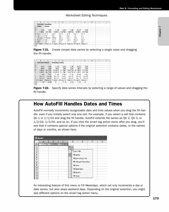
Cha

pter

7

Worksheet Editing Techniques

173

Part 3: Formatting and Editing Worksheets

f07ie21

Figure 7-21. Create simple data series by selecting a single value and dragging the fill handle.

f07ie22

Figure 7-22. Specify data series intervals by selecting a range of values and dragging the fill handle.

How AutoFill Handles Dates and TimesAutoFill normally increments recognizable date and time values when you drag the fill han-dle, even if you initially select only one cell. For example, if you select a cell that contains Qtr 1 or 1/1/04 and drag the fill handle, AutoFill extends the series as Qtr 2, Qtr 3, or 1/2/04, 1/3/04, and so on. If you click the smart tag action menu after you drag, you’ll see that it contains special options if the original selection contains dates, or the names of days or months, as shown here.

g07ie05

An interesting feature of this menu is Fill Weekdays, which not only increments a day or date series, but also skips weekend days. Depending on the original selection, you might see different options on the smart tag action menu.

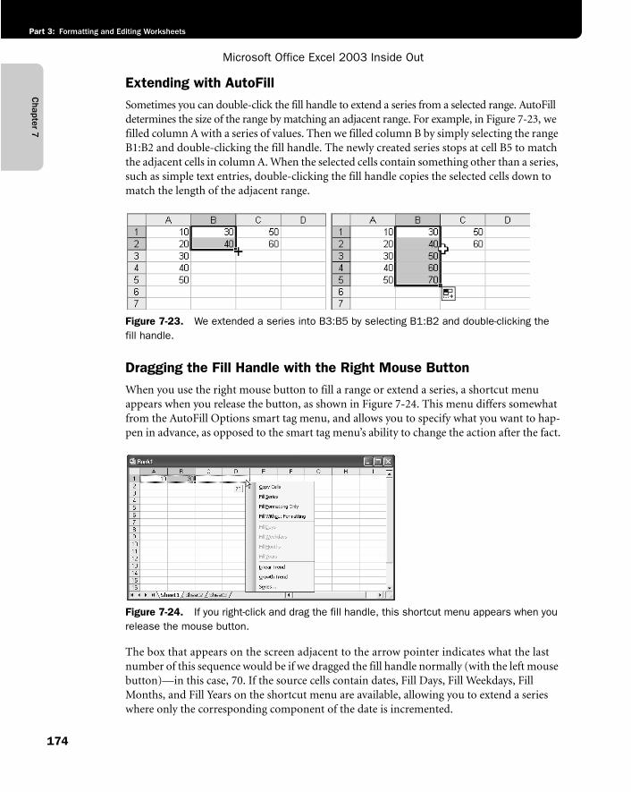
Chapter 7

Microsoft Office Excel 2003 Inside Out

Part 3: Formatting and Editing Worksheets

174

Extending with AutoFillSometimes you can double-click the fill handle to extend a series from a selected range. AutoFill determines the size of the range by matching an adjacent range. For example, in Figure 7-23, we filled column A with a series of values. Then we filled column B by simply selecting the range B1:B2 and double-clicking the fill handle. The newly created series stops at cell B5 to match the adjacent cells in column A. When the selected cells contain something other than a series, such as simple text entries, double-clicking the fill handle copies the selected cells down to match the length of the adjacent range.

f07ie23

Figure 7-23. We extended a series into B3:B5 by selecting B1:B2 and double-clicking the fill handle.

Dragging the Fill Handle with the Right Mouse ButtonWhen you use the right mouse button to fill a range or extend a series, a shortcut menu appears when you release the button, as shown in Figure 7-24. This menu differs somewhat from the AutoFill Options smart tag menu, and allows you to specify what you want to hap-pen in advance, as opposed to the smart tag menu’s ability to change the action after the fact.

f07ie24

Figure 7-24. If you right-click and drag the fill handle, this shortcut menu appears when you release the mouse button.

The box that appears on the screen adjacent to the arrow pointer indicates what the last number of this sequence would be if we dragged the fill handle normally (with the left mouse button)—in this case, 70. If the source cells contain dates, Fill Days, Fill Weekdays, Fill Months, and Fill Years on the shortcut menu are available, allowing you to extend a series where only the corresponding component of the date is incremented.

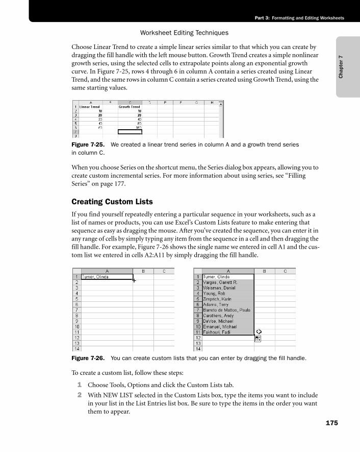
Cha

pter

7

Worksheet Editing Techniques

175

Part 3: Formatting and Editing Worksheets

Choose Linear Trend to create a simple linear series similar to that which you can create by dragging the fill handle with the left mouse button. Growth Trend creates a simple nonlinear growth series, using the selected cells to extrapolate points along an exponential growth curve. In Figure 7-25, rows 4 through 6 in column A contain a series created using Linear Trend, and the same rows in column C contain a series created using Growth Trend, using the same starting values.

f07ie25

Figure 7-25. We created a linear trend series in column A and a growth trend series in column C.

When you choose Series on the shortcut menu, the Series dialog box appears, allowing you to create custom incremental series. For more information about using series, see “Filling Series” on page 177.

Creating Custom ListsIf you find yourself repeatedly entering a particular sequence in your worksheets, such as a list of names or products, you can use Excel’s Custom Lists feature to make entering that sequence as easy as dragging the mouse. After you’ve created the sequence, you can enter it in any range of cells by simply typing any item from the sequence in a cell and then dragging the fill handle. For example, Figure 7-26 shows the single name we entered in cell A1 and the cus-tom list we entered in cells A2:A11 by simply dragging the fill handle.

f07ie26

Figure 7-26. You can create custom lists that you can enter by dragging the fill handle.

To create a custom list, follow these steps:

1 Choose Tools, Options and click the Custom Lists tab.

2 With NEW LIST selected in the Custom Lists box, type the items you want to include in your list in the List Entries list box. Be sure to type the items in the order you want them to appear.

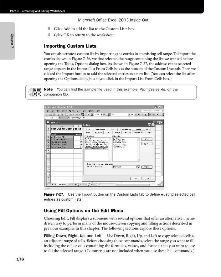
Chapter 7

Microsoft Office Excel 2003 Inside Out

Part 3: Formatting and Editing Worksheets

176

3 Click Add to add the list to the Custom Lists box.

4 Click OK to return to the worksheet.

Importing Custom ListsYou can also create a custom list by importing the entries in an existing cell range. To import the entries shown in Figure 7-26, we first selected the range containing the list we wanted before opening the Tools, Options dialog box. As shown in Figure 7-27, the address of the selected range appears in the Import List From Cells box at the bottom of the Custom Lists tab. Then we clicked the Import button to add the selected entries as a new list. (You can select the list after opening the Options dialog box if you click in the Import List From Cells box.)

Note You can find the sample file used in this example, PacificSales.xls, on the companion CD.

f07ie27

Figure 7-27. Use the Import button on the Custom Lists tab to define existing selected cell entries as custom lists.

Using Fill Options on the Edit MenuChoosing Edit, Fill displays a submenu with several options that offer an alternative, menu-driven way to perform many of the mouse-driven copying and filling actions described in previous examples in this chapter. The following sections explore these options.

Filling Down, Right, Up, and Left Use Down, Right, Up, and Left to copy selected cells to an adjacent range of cells. Before choosing these commands, select the range you want to fill, including the cell or cells containing the formulas, values, and formats that you want to use to fill the selected range. (Comments are not included when you use these Fill commands.)

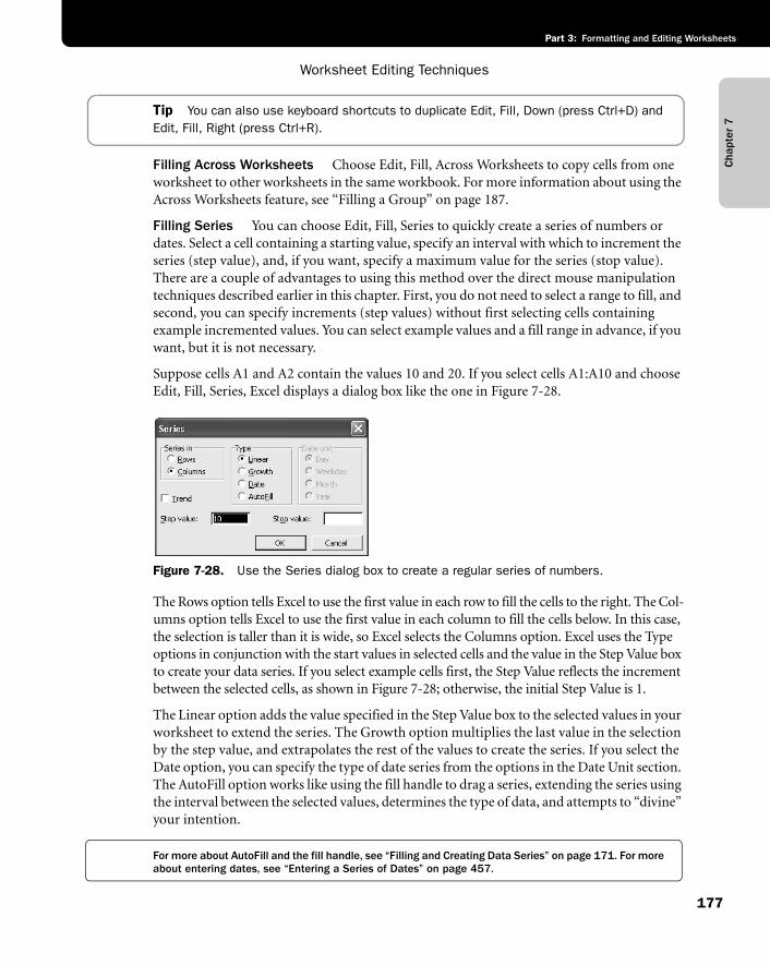
Cha

pter

7

Worksheet Editing Techniques

177

Part 3: Formatting and Editing Worksheets

Tip You can also use keyboard shortcuts to duplicate Edit, Fill, Down (press Ctrl+D) and Edit, Fill, Right (press Ctrl+R).

Filling Across Worksheets Choose Edit, Fill, Across Worksheets to copy cells from one worksheet to other worksheets in the same workbook. For more information about using the Across Worksheets feature, see “Filling a Group” on page 187.

Filling Series You can choose Edit, Fill, Series to quickly create a series of numbers or dates. Select a cell containing a starting value, specify an interval with which to increment the series (step value), and, if you want, specify a maximum value for the series (stop value). There are a couple of advantages to using this method over the direct mouse manipulation techniques described earlier in this chapter. First, you do not need to select a range to fill, and second, you can specify increments (step values) without first selecting cells containing example incremented values. You can select example values and a fill range in advance, if you want, but it is not necessary.

Suppose cells A1 and A2 contain the values 10 and 20. If you select cells A1:A10 and choose Edit, Fill, Series, Excel displays a dialog box like the one in Figure 7-28.

f07ie28

Figure 7-28. Use the Series dialog box to create a regular series of numbers.

The Rows option tells Excel to use the first value in each row to fill the cells to the right. The Col-umns option tells Excel to use the first value in each column to fill the cells below. In this case, the selection is taller than it is wide, so Excel selects the Columns option. Excel uses the Type options in conjunction with the start values in selected cells and the value in the Step Value box to create your data series. If you select example cells first, the Step Value reflects the increment between the selected cells, as shown in Figure 7-28; otherwise, the initial Step Value is 1.

The Linear option adds the value specified in the Step Value box to the selected values in your worksheet to extend the series. The Growth option multiplies the last value in the selection by the step value, and extrapolates the rest of the values to create the series. If you select the Date option, you can specify the type of date series from the options in the Date Unit section. The AutoFill option works like using the fill handle to drag a series, extending the series using the interval between the selected values, determines the type of data, and attempts to “divine” your intention.

For more about AutoFill and the fill handle, see “Filling and Creating Data Series” on page 171. For more about entering dates, see “Entering a Series of Dates” on page 457.

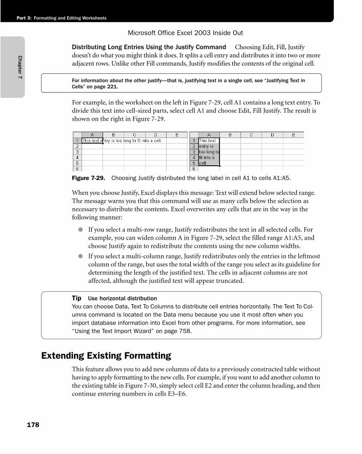
Chapter 7

Microsoft Office Excel 2003 Inside Out

Part 3: Formatting and Editing Worksheets

178

Distributing Long Entries Using the Justify Command Choosing Edit, Fill, Justify doesn’t do what you might think it does. It splits a cell entry and distributes it into two or more adjacent rows. Unlike other Fill commands, Justify modifies the contents of the original cell.

For information about the other justify—that is, justifying text in a single cell, see “Justifying Text in Cells” on page 221.

For example, in the worksheet on the left in Figure 7-29, cell A1 contains a long text entry. To divide this text into cell-sized parts, select cell A1 and choose Edit, Fill Justify. The result is shown on the right in Figure 7-29.

f07ie29

Figure 7-29. Choosing Justify distributed the long label in cell A1 to cells A1:A5.

When you choose Justify, Excel displays this message: Text will extend below selected range. The message warns you that this command will use as many cells below the selection as necessary to distribute the contents. Excel overwrites any cells that are in the way in the following manner:

● If you select a multi-row range, Justify redistributes the text in all selected cells. For example, you can widen column A in Figure 7-29, select the filled range A1:A5, and choose Justify again to redistribute the contents using the new column widths.

● If you select a multi-column range, Justify redistributes only the entries in the leftmost column of the range, but uses the total width of the range you select as its guideline for determining the length of the justified text. The cells in adjacent columns are not affected, although the justified text will appear truncated.

Tip Use horizontal distributionYou can choose Data, Text To Columns to distribute cell entries horizontally. The Text To Col-umns command is located on the Data menu because you use it most often when you import database information into Excel from other programs. For more information, see “Using the Text Import Wizard” on page 758.

Extending Existing FormattingThis feature allows you to add new columns of data to a previously constructed table without having to apply formatting to the new cells. For example, if you want to add another column to the existing table in Figure 7-30, simply select cell E2 and enter the column heading, and then continue entering numbers in cells E3–E6.

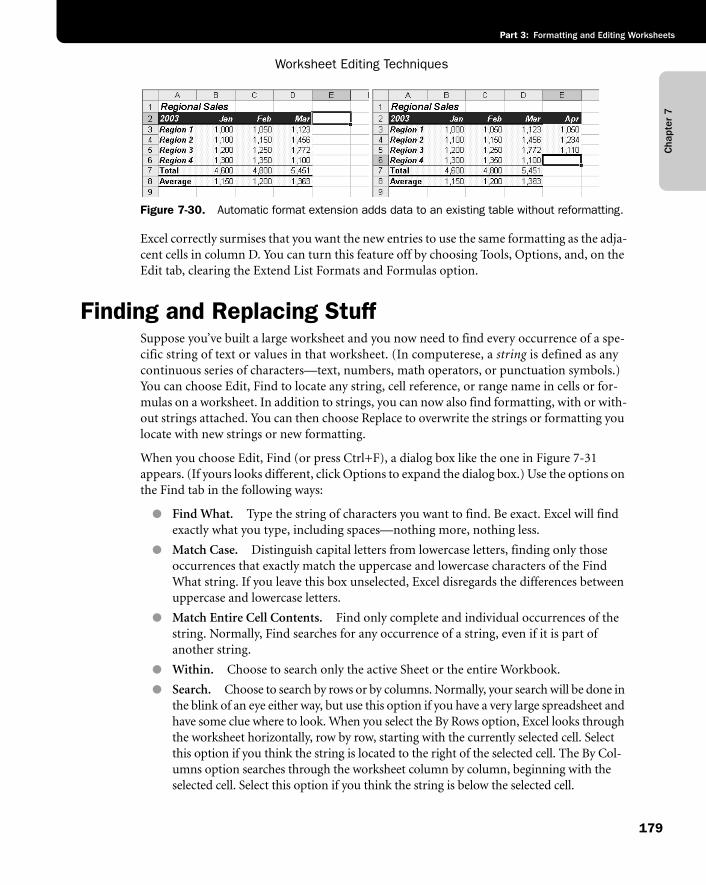
Cha

pter

7

Worksheet Editing Techniques

179

Part 3: Formatting and Editing Worksheets

f07ie30

Figure 7-30. Automatic format extension adds data to an existing table without reformatting.

Excel correctly surmises that you want the new entries to use the same formatting as the adja-cent cells in column D. You can turn this feature off by choosing Tools, Options, and, on the Edit tab, clearing the Extend List Formats and Formulas option.

Finding and Replacing StuffSuppose you’ve built a large worksheet and you now need to find every occurrence of a spe-cific string of text or values in that worksheet. (In computerese, a string is defined as any continuous series of characters—text, numbers, math operators, or punctuation symbols.) You can choose Edit, Find to locate any string, cell reference, or range name in cells or for-mulas on a worksheet. In addition to strings, you can now also find formatting, with or with-out strings attached. You can then choose Replace to overwrite the strings or formatting you locate with new strings or new formatting.

When you choose Edit, Find (or press Ctrl+F), a dialog box like the one in Figure 7-31 appears. (If yours looks different, click Options to expand the dialog box.) Use the options on the Find tab in the following ways:

● Find What. Type the string of characters you want to find. Be exact. Excel will find exactly what you type, including spaces—nothing more, nothing less.

● Match Case. Distinguish capital letters from lowercase letters, finding only those occurrences that exactly match the uppercase and lowercase characters of the Find What string. If you leave this box unselected, Excel disregards the differences between uppercase and lowercase letters.

● Match Entire Cell Contents. Find only complete and individual occurrences of the string. Normally, Find searches for any occurrence of a string, even if it is part of another string.

● Within. Choose to search only the active Sheet or the entire Workbook.

● Search. Choose to search by rows or by columns. Normally, your search will be done in the blink of an eye either way, but use this option if you have a very large spreadsheet and have some clue where to look. When you select the By Rows option, Excel looks through the worksheet horizontally, row by row, starting with the currently selected cell. Select this option if you think the string is located to the right of the selected cell. The By Col-umns option searches through the worksheet column by column, beginning with the selected cell. Select this option if you think the string is below the selected cell.

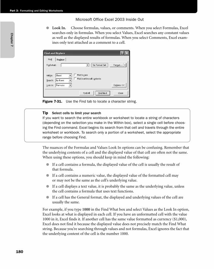
Chapter 7

Microsoft Office Excel 2003 Inside Out

Part 3: Formatting and Editing Worksheets

180

● Look In. Choose formulas, values, or comments. When you select Formulas, Excel searches only in formulas. When you select Values, Excel searches any constant values as well as the displayed results of formulas. When you select Comments, Excel exam-ines only text attached as a comment to a cell.

f07ie31

Figure 7-31. Use the Find tab to locate a character string.

Tip Select cells to limit your searchIf you want to search the entire workbook or worksheet to locate a string of characters (depending on the selection you make in the Within box), select a single cell before choos-ing the Find command. Excel begins its search from that cell and travels through the entire worksheet or workbook. To search only a portion of a worksheet, select the appropriate range before choosing Find.

The nuances of the Formulas and Values Look In options can be confusing. Remember that the underlying contents of a cell and the displayed value of that cell are often not the same. When using these options, you should keep in mind the following:

● If a cell contains a formula, the displayed value of the cell is usually the result of that formula.

● If a cell contains a numeric value, the displayed value of the formatted cell may or may not be the same as the cell’s underlying value.

● If a cell displays a text value, it is probably the same as the underlying value, unless the cell contains a formula that uses text functions.

● If a cell has the General format, the displayed and underlying values of the cell are usually the same.

For example, if you type 1000 in the Find What box and select Values as the Look In option, Excel looks at what is displayed in each cell. If you have an unformatted cell with the value 1000 in it, Excel finds it. If another cell has the same value formatted as currency ($1,000), Excel does not find it because the displayed value does not precisely match the Find What string. Because you’re searching through values and not formulas, Excel ignores the fact that the underlying content of the cell is the number 1000.

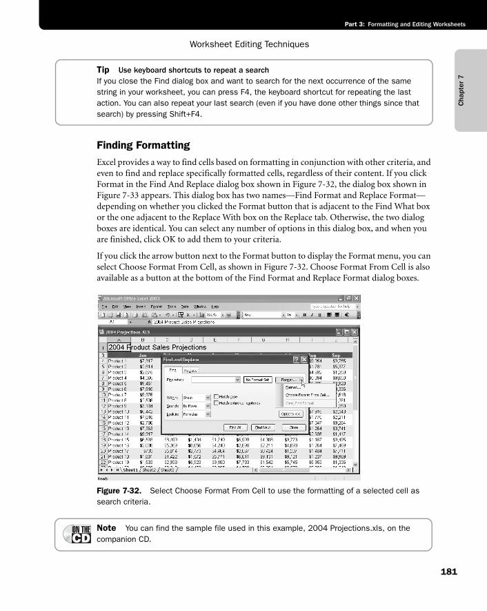
Cha

pter

7

Worksheet Editing Techniques

181

Part 3: Formatting and Editing Worksheets

Tip Use keyboard shortcuts to repeat a searchIf you close the Find dialog box and want to search for the next occurrence of the same string in your worksheet, you can press F4, the keyboard shortcut for repeating the last action. You can also repeat your last search (even if you have done other things since that search) by pressing Shift+F4.

Finding FormattingExcel provides a way to find cells based on formatting in conjunction with other criteria, and even to find and replace specifically formatted cells, regardless of their content. If you click Format in the Find And Replace dialog box shown in Figure 7-32, the dialog box shown in Figure 7-33 appears. This dialog box has two names—Find Format and Replace Format—depending on whether you clicked the Format button that is adjacent to the Find What box or the one adjacent to the Replace With box on the Replace tab. Otherwise, the two dialog boxes are identical. You can select any number of options in this dialog box, and when you are finished, click OK to add them to your criteria.

If you click the arrow button next to the Format button to display the Format menu, you can select Choose Format From Cell, as shown in Figure 7-32. Choose Format From Cell is also available as a button at the bottom of the Find Format and Replace Format dialog boxes.

f07ie32

Figure 7-32. Select Choose Format From Cell to use the formatting of a selected cell as search criteria.

Note You can find the sample file used in this example, 2004 Projections.xls, on the companion CD.

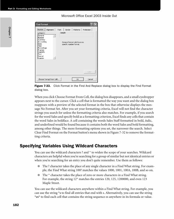
Chapter 7

Microsoft Office Excel 2003 Inside Out

Part 3: Formatting and Editing Worksheets

182

f07ie33

Figure 7-33. Click Format in the Find And Replace dialog box to display the Find Format dialog box.

When you click Choose Format From Cell, the dialog box disappears, and a small eyedropper appears next to the cursor. Click a cell that is formatted the way you want and the dialog box reappears with a preview of the selected format in the box that otherwise displays the mes-sage No Format Set. After you set your formatting criteria, Excel will not find the character strings you search for unless the formatting criteria also matches. For example, if you search for the word Sales and specify bold as a formatting criterion, Excel finds any cells that contain the word Sales in boldface. A cell containing the words Sales Staff formatted in bold, italic, and underlined would be found because it contains both the word Sales and bold formatting, among other things. The more formatting options you set, the narrower the search. Select Clear Find Format on the Format button’s menu shown in Figure 7-32 to remove the format-ting criteria.

Specifying Variables Using Wildcard CharactersYou can use the wildcard characters ? and * to widen the scope of your searches. Wildcard characters are helpful when you’re searching for a group of similar but not identical entries or when you’re searching for an entry you don’t quite remember. Use them as follows:

● The ? character takes the place of any single character in a Find What string. For exam-ple, the Find What string 100? matches the values 1000, 1001, 100A, 100B, and so on.

● The * character takes the place of zero or more characters in a Find What string. For example, the string 12* matches the entries 120, 125, 1200000, and even 123 Maple Street.

You can use the wildcard characters anywhere within a Find What string. For example, you can use the string *s to find all entries that end with s. Alternatively, you can use the string *es* to find each cell that contains the string sequence es anywhere in its formula or value.

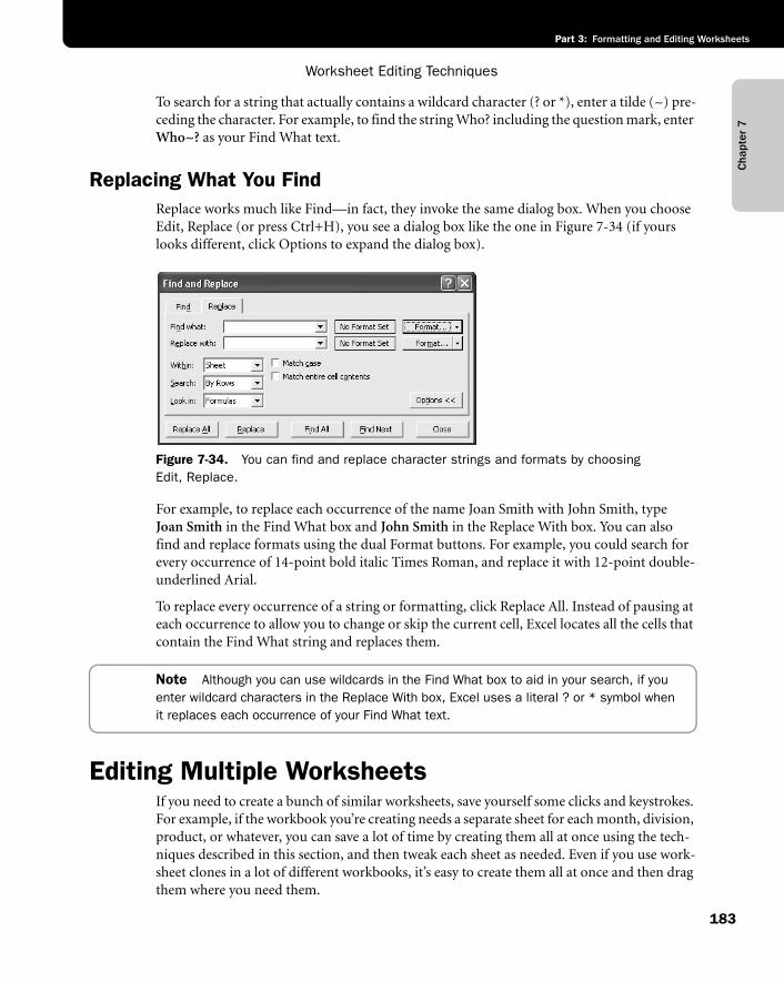
Cha

pter

7

Worksheet Editing Techniques

183

Part 3: Formatting and Editing Worksheets

To search for a string that actually contains a wildcard character (? or *), enter a tilde (~) pre-ceding the character. For example, to find the string Who? including the question mark, enter Who~? as your Find What text.

Replacing What You FindReplace works much like Find—in fact, they invoke the same dialog box. When you choose Edit, Replace (or press Ctrl+H), you see a dialog box like the one in Figure 7-34 (if yours looks different, click Options to expand the dialog box).

f07ie34

Figure 7-34. You can find and replace character strings and formats by choosing Edit, Replace.

For example, to replace each occurrence of the name Joan Smith with John Smith, typeJoan Smith in the Find What box and John Smith in the Replace With box. You can also find and replace formats using the dual Format buttons. For example, you could search for every occurrence of 14-point bold italic Times Roman, and replace it with 12-point double-underlined Arial.

To replace every occurrence of a string or formatting, click Replace All. Instead of pausing at each occurrence to allow you to change or skip the current cell, Excel locates all the cells that contain the Find What string and replaces them.

Note Although you can use wildcards in the Find What box to aid in your search, if you enter wildcard characters in the Replace With box, Excel uses a literal ? or * symbol when it replaces each occurrence of your Find What text.

Editing Multiple WorksheetsIf you need to create a bunch of similar worksheets, save yourself some clicks and keystrokes. For example, if the workbook you’re creating needs a separate sheet for each month, division, product, or whatever, you can save a lot of time by creating them all at once using the tech-niques described in this section, and then tweak each sheet as needed. Even if you use work-sheet clones in a lot of different workbooks, it’s easy to create them all at once and then drag them where you need them.

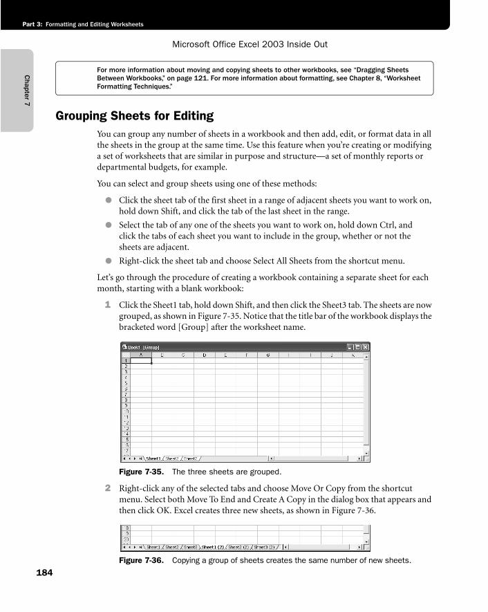
Chapter 7

Microsoft Office Excel 2003 Inside Out

Part 3: Formatting and Editing Worksheets

184

For more information about moving and copying sheets to other workbooks, see “Dragging Sheets Between Workbooks,” on page 121. For more information about formatting, see Chapter 8, “Worksheet Formatting Techniques.”

Grouping Sheets for EditingYou can group any number of sheets in a workbook and then add, edit, or format data in all the sheets in the group at the same time. Use this feature when you’re creating or modifying a set of worksheets that are similar in purpose and structure—a set of monthly reports or departmental budgets, for example.

You can select and group sheets using one of these methods:

● Click the sheet tab of the first sheet in a range of adjacent sheets you want to work on, hold down Shift, and click the tab of the last sheet in the range.

● Select the tab of any one of the sheets you want to work on, hold down Ctrl, and click the tabs of each sheet you want to include in the group, whether or not the sheets are adjacent.

● Right-click the sheet tab and choose Select All Sheets from the shortcut menu.

Let’s go through the procedure of creating a workbook containing a separate sheet for each month, starting with a blank workbook:

1 Click the Sheet1 tab, hold down Shift, and then click the Sheet3 tab. The sheets are now grouped, as shown in Figure 7-35. Notice that the title bar of the workbook displays the bracketed word [Group] after the worksheet name.

f07ie35

Figure 7-35. The three sheets are grouped.

2 Right-click any of the selected tabs and choose Move Or Copy from the shortcut menu. Select both Move To End and Create A Copy in the dialog box that appears and then click OK. Excel creates three new sheets, as shown in Figure 7-36.

f07ie36

Figure 7-36. Copying a group of sheets creates the same number of new sheets.

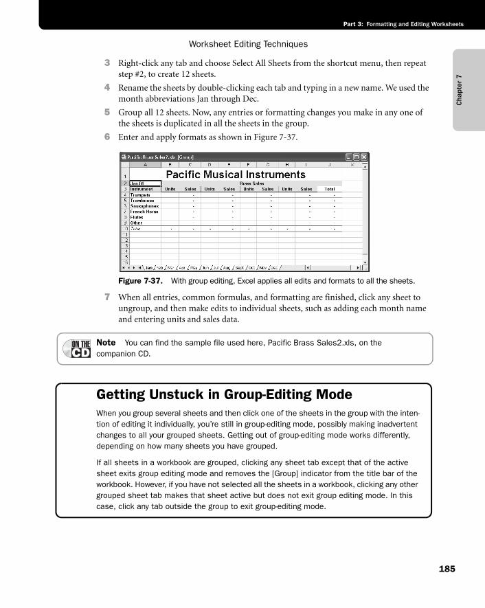
Cha

pter

7

Worksheet Editing Techniques

185

Part 3: Formatting and Editing Worksheets

3 Right-click any tab and choose Select All Sheets from the shortcut menu, then repeat step #2, to create 12 sheets.

4 Rename the sheets by double-clicking each tab and typing in a new name. We used the month abbreviations Jan through Dec.

5 Group all 12 sheets. Now, any entries or formatting changes you make in any one of the sheets is duplicated in all the sheets in the group.

6 Enter and apply formats as shown in Figure 7-37.

f07ie37

Figure 7-37. With group editing, Excel applies all edits and formats to all the sheets.

7 When all entries, common formulas, and formatting are finished, click any sheet to ungroup, and then make edits to individual sheets, such as adding each month name and entering units and sales data.

Note You can find the sample file used here, Pacific Brass Sales2.xls, on the companion CD.

Getting Unstuck in Group-Editing ModeWhen you group several sheets and then click one of the sheets in the group with the inten-tion of editing it individually, you’re still in group-editing mode, possibly making inadvertent changes to all your grouped sheets. Getting out of group-editing mode works differently, depending on how many sheets you have grouped.

If all sheets in a workbook are grouped, clicking any sheet tab except that of the active sheet exits group editing mode and removes the [Group] indicator from the title bar of the workbook. However, if you have not selected all the sheets in a workbook, clicking any other grouped sheet tab makes that sheet active but does not exit group editing mode. In this case, click any tab outside the group to exit group-editing mode.

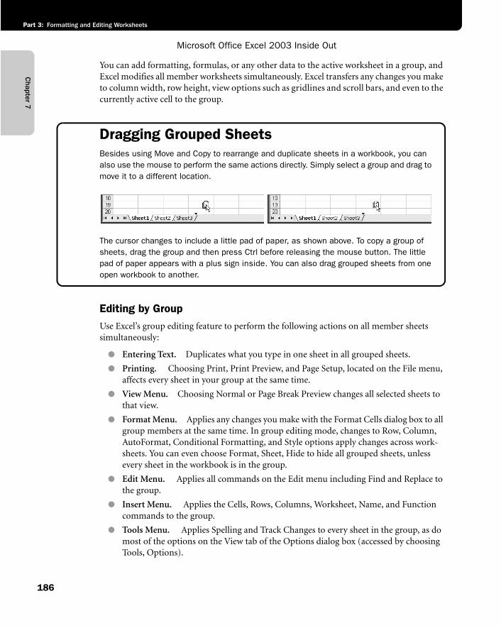
Chapter 7

Microsoft Office Excel 2003 Inside Out

Part 3: Formatting and Editing Worksheets

186

You can add formatting, formulas, or any other data to the active worksheet in a group, and Excel modifies all member worksheets simultaneously. Excel transfers any changes you make to column width, row height, view options such as gridlines and scroll bars, and even to the currently active cell to the group.

Dragging Grouped SheetsBesides using Move and Copy to rearrange and duplicate sheets in a workbook, you can also use the mouse to perform the same actions directly. Simply select a group and drag to move it to a different location.

g07ie06

The cursor changes to include a little pad of paper, as shown above. To copy a group of sheets, drag the group and then press Ctrl before releasing the mouse button. The little pad of paper appears with a plus sign inside. You can also drag grouped sheets from one open workbook to another.

Editing by GroupUse Excel’s group editing feature to perform the following actions on all member sheets simultaneously:

● Entering Text. Duplicates what you type in one sheet in all grouped sheets.

● Printing. Choosing Print, Print Preview, and Page Setup, located on the File menu, affects every sheet in your group at the same time.

● View Menu. Choosing Normal or Page Break Preview changes all selected sheets to that view.

● Format Menu. Applies any changes you make with the Format Cells dialog box to all group members at the same time. In group editing mode, changes to Row, Column, AutoFormat, Conditional Formatting, and Style options apply changes across work-sheets. You can even choose Format, Sheet, Hide to hide all grouped sheets, unless every sheet in the workbook is in the group.

● Edit Menu. Applies all commands on the Edit menu including Find and Replace to the group.

● Insert Menu. Applies the Cells, Rows, Columns, Worksheet, Name, and Function commands to the group.

● Tools Menu. Applies Spelling and Track Changes to every sheet in the group, as do most of the options on the View tab of the Options dialog box (accessed by choosing Tools, Options).

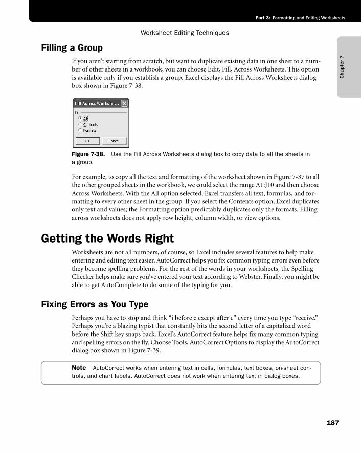
Cha

pter

7

Worksheet Editing Techniques

187

Part 3: Formatting and Editing Worksheets

Filling a GroupIf you aren’t starting from scratch, but want to duplicate existing data in one sheet to a num-ber of other sheets in a workbook, you can choose Edit, Fill, Across Worksheets. This option is available only if you establish a group. Excel displays the Fill Across Worksheets dialog box shown in Figure 7-38.

f07ie38

Figure 7-38. Use the Fill Across Worksheets dialog box to copy data to all the sheets ina group.

For example, to copy all the text and formatting of the worksheet shown in Figure 7-37 to all the other grouped sheets in the workbook, we could select the range A1:J10 and then choose Across Worksheets. With the All option selected, Excel transfers all text, formulas, and for-matting to every other sheet in the group. If you select the Contents option, Excel duplicates only text and values; the Formatting option predictably duplicates only the formats. Filling across worksheets does not apply row height, column width, or view options.

Getting the Words RightWorksheets are not all numbers, of course, so Excel includes several features to help make entering and editing text easier. AutoCorrect helps you fix common typing errors even before they become spelling problems. For the rest of the words in your worksheets, the Spelling Checker helps make sure you’ve entered your text according to Webster. Finally, you might be able to get AutoComplete to do some of the typing for you.

Fixing Errors as You TypePerhaps you have to stop and think “i before e except after c” every time you type “receive.” Perhaps you’re a blazing typist that constantly hits the second letter of a capitalized word before the Shift key snaps back. Excel’s AutoCorrect feature helps fix many common typing and spelling errors on the fly. Choose Tools, AutoCorrect Options to display the AutoCorrect dialog box shown in Figure 7-39.

Note AutoCorrect works when entering text in cells, formulas, text boxes, on-sheet con-trols, and chart labels. AutoCorrect does not work when entering text in dialog boxes.

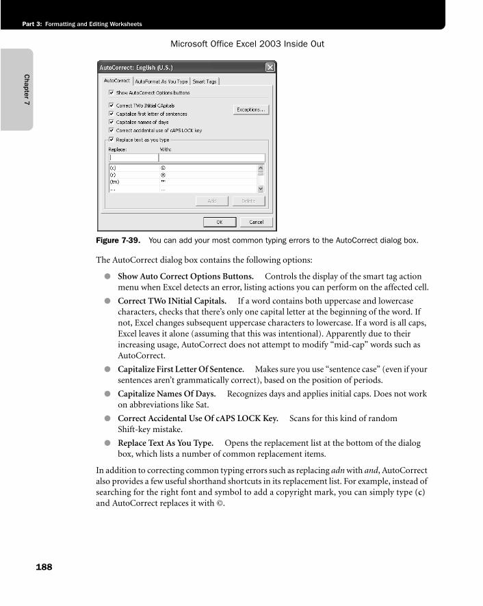
Chapter 7

Microsoft Office Excel 2003 Inside Out

Part 3: Formatting and Editing Worksheets

188

f07ie39

Figure 7-39. You can add your most common typing errors to the AutoCorrect dialog box.

The AutoCorrect dialog box contains the following options:

● Show Auto Correct Options Buttons. Controls the display of the smart tag action menu when Excel detects an error, listing actions you can perform on the affected cell.

● Correct TWo INitial Capitals. If a word contains both uppercase and lowercase characters, checks that there’s only one capital letter at the beginning of the word. If not, Excel changes subsequent uppercase characters to lowercase. If a word is all caps, Excel leaves it alone (assuming that this was intentional). Apparently due to their increasing usage, AutoCorrect does not attempt to modify “mid-cap” words such as AutoCorrect.

● Capitalize First Letter Of Sentence. Makes sure you use “sentence case” (even if your sentences aren’t grammatically correct), based on the position of periods.

● Capitalize Names Of Days. Recognizes days and applies initial caps. Does not work on abbreviations like Sat.

● Correct Accidental Use Of cAPS LOCK Key. Scans for this kind of random Shift-key mistake.

● Replace Text As You Type. Opens the replacement list at the bottom of the dialog box, which lists a number of common replacement items.

In addition to correcting common typing errors such as replacing adn with and, AutoCorrect also provides a few useful shorthand shortcuts in its replacement list. For example, instead of searching for the right font and symbol to add a copyright mark, you can simply type (c)and AutoCorrect replaces it with ©.

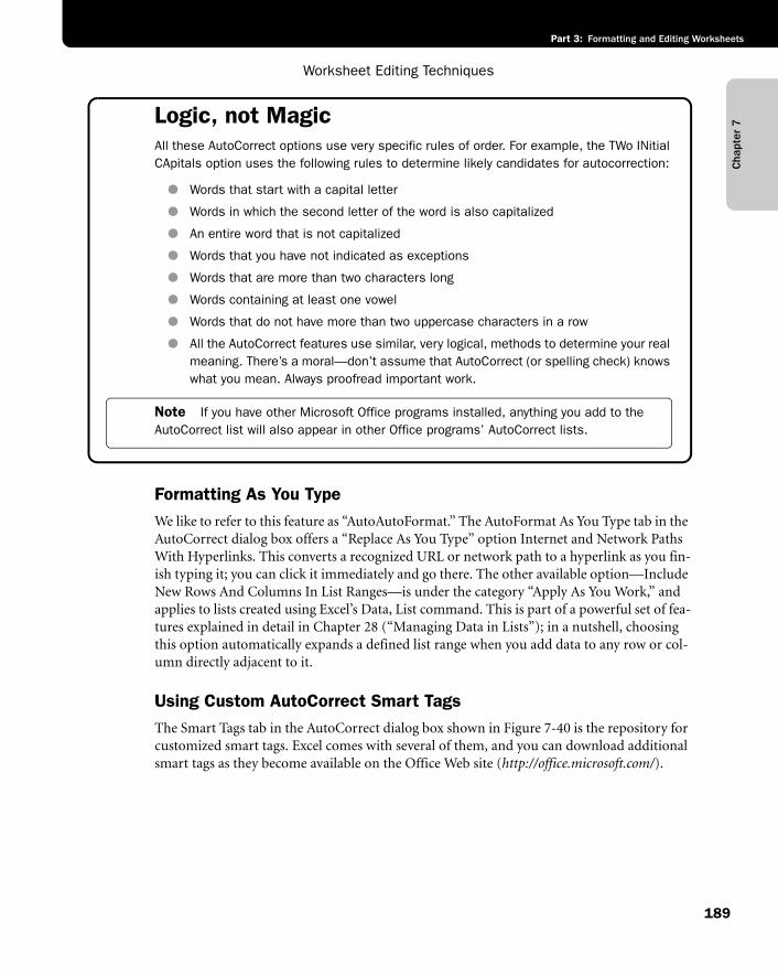
Cha

pter

7

Worksheet Editing Techniques

189

Part 3: Formatting and Editing Worksheets

Logic, not MagicAll these AutoCorrect options use very specific rules of order. For example, the TWo INitial CApitals option uses the following rules to determine likely candidates for autocorrection:

● Words that start with a capital letter

● Words in which the second letter of the word is also capitalized

● An entire word that is not capitalized

● Words that you have not indicated as exceptions

● Words that are more than two characters long

● Words containing at least one vowel

● Words that do not have more than two uppercase characters in a row

● All the AutoCorrect features use similar, very logical, methods to determine your real meaning. There’s a moral—don’t assume that AutoCorrect (or spelling check) knows what you mean. Always proofread important work.

Note If you have other Microsoft Office programs installed, anything you add to the AutoCorrect list will also appear in other Office programs’ AutoCorrect lists.

Formatting As You TypeWe like to refer to this feature as “AutoAutoFormat.” The AutoFormat As You Type tab in the AutoCorrect dialog box offers a “Replace As You Type” option Internet and Network Paths With Hyperlinks. This converts a recognized URL or network path to a hyperlink as you fin-ish typing it; you can click it immediately and go there. The other available option—Include New Rows And Columns In List Ranges—is under the category “Apply As You Work,” and applies to lists created using Excel’s Data, List command. This is part of a powerful set of fea-tures explained in detail in Chapter 28 (“Managing Data in Lists”); in a nutshell, choosing this option automatically expands a defined list range when you add data to any row or col-umn directly adjacent to it.

Using Custom AutoCorrect Smart TagsThe Smart Tags tab in the AutoCorrect dialog box shown in Figure 7-40 is the repository for customized smart tags. Excel comes with several of them, and you can download additional smart tags as they become available on the Office Web site (http://office.microsoft.com/).

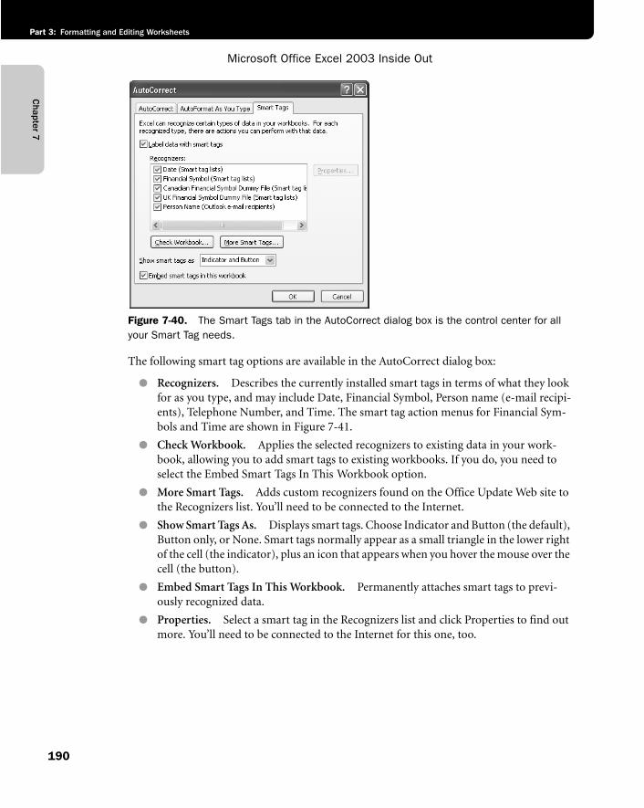
Chapter 7

Microsoft Office Excel 2003 Inside Out

Part 3: Formatting and Editing Worksheets

190

f07ie40

Figure 7-40. The Smart Tags tab in the AutoCorrect dialog box is the control center for all your Smart Tag needs.

The following smart tag options are available in the AutoCorrect dialog box:

● Recognizers. Describes the currently installed smart tags in terms of what they look for as you type, and may include Date, Financial Symbol, Person name (e-mail recipi-ents), Telephone Number, and Time. The smart tag action menus for Financial Sym-bols and Time are shown in Figure 7-41.

● Check Workbook. Applies the selected recognizers to existing data in your work-book, allowing you to add smart tags to existing workbooks. If you do, you need to select the Embed Smart Tags In This Workbook option.

● More Smart Tags. Adds custom recognizers found on the Office Update Web site to the Recognizers list. You’ll need to be connected to the Internet.

● Show Smart Tags As. Displays smart tags. Choose Indicator and Button (the default), Button only, or None. Smart tags normally appear as a small triangle in the lower right of the cell (the indicator), plus an icon that appears when you hover the mouse over the cell (the button).

● Embed Smart Tags In This Workbook. Permanently attaches smart tags to previ-ously recognized data.

● Properties. Select a smart tag in the Recognizers list and click Properties to find out more. You’ll need to be connected to the Internet for this one, too.

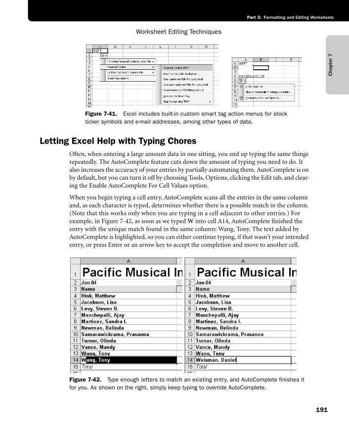
Cha

pter

7

Worksheet Editing Techniques

191

Part 3: Formatting and Editing Worksheets

f07ie41 Figure 7-41. Excel includes built-in custom smart tag action menus for stock ticker symbols and e-mail addresses, among other types of data.

Letting Excel Help with Typing ChoresOften, when entering a large amount data in one sitting, you end up typing the same things repeatedly. The AutoComplete feature cuts down the amount of typing you need to do. It also increases the accuracy of your entries by partially automating them. AutoComplete is on by default, but you can turn it off by choosing Tools, Options, clicking the Edit tab, and clear-ing the Enable AutoComplete For Cell Values option.

When you begin typing a cell entry, AutoComplete scans all the entries in the same column and, as each character is typed, determines whether there is a possible match in the column. (Note that this works only when you are typing in a cell adjacent to other entries.) For example, in Figure 7-42, as soon as we typed W into cell A14, AutoComplete finished the entry with the unique match found in the same column: Wang, Tony. The text added by AutoComplete is highlighted, so you can either continue typing, if that wasn’t your intended entry, or press Enter or an arrow key to accept the completion and move to another cell.

f07ie42

Figure 7-42. Type enough letters to match an existing entry, and AutoComplete finishes it for you. As shown on the right, simply keep typing to override AutoComplete.

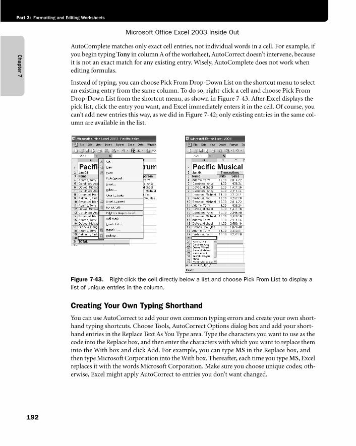
Chapter 7

Microsoft Office Excel 2003 Inside Out

Part 3: Formatting and Editing Worksheets

192

AutoComplete matches only exact cell entries, not individual words in a cell. For example, if you begin typing Tony in column A of the worksheet, AutoCorrect doesn’t intervene, because it is not an exact match for any existing entry. Wisely, AutoComplete does not work when editing formulas.

Instead of typing, you can choose Pick From Drop-Down List on the shortcut menu to select an existing entry from the same column. To do so, right-click a cell and choose Pick From Drop-Down List from the shortcut menu, as shown in Figure 7-43. After Excel displays the pick list, click the entry you want, and Excel immediately enters it in the cell. Of course, you can’t add new entries this way, as we did in Figure 7-42; only existing entries in the same col-umn are available in the list.

f07ie43

Figure 7-43. Right-click the cell directly below a list and choose Pick From List to display a list of unique entries in the column.

Creating Your Own Typing ShorthandYou can use AutoCorrect to add your own common typing errors and create your own short-hand typing shortcuts. Choose Tools, AutoCorrect Options dialog box and add your short-hand entries in the Replace Text As You Type area. Type the characters you want to use as the code into the Replace box, and then enter the characters with which you want to replace them into the With box and click Add. For example, you can type MS in the Replace box, and then type Microsoft Corporation into the With box. Thereafter, each time you type MS, Excel replaces it with the words Microsoft Corporation. Make sure you choose unique codes; oth-erwise, Excel might apply AutoCorrect to entries you don’t want changed.

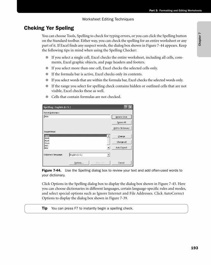
Cha

pter

7

Worksheet Editing Techniques

193

Part 3: Formatting and Editing Worksheets

Cheking Yer SpelingYou can choose Tools, Spelling to check for typing errors, or you can click the Spelling button on the Standard toolbar. Either way, you can check the spelling for an entire worksheet or any part of it. If Excel finds any suspect words, the dialog box shown in Figure 7-44 appears. Keep the following tips in mind when using the Spelling Checker:

● If you select a single cell, Excel checks the entire worksheet, including all cells, com-ments, Excel graphic objects, and page headers and footers.

● If you select more than one cell, Excel checks the selected cells only.

● If the formula bar is active, Excel checks only its contents.

● If you select words that are within the formula bar, Excel checks the selected words only.

● If the range you select for spelling check contains hidden or outlined cells that are not visible, Excel checks these as well.

● Cells that contain formulas are not checked.

f07ie44

Figure 7-44. Use the Spelling dialog box to review your text and add often-used words to your dictionary.

Click Options in the Spelling dialog box to display the dialog box shown in Figure 7-45. Here you can choose dictionaries in different languages, certain language-specific rules and modes, and select special options such as Ignore Internet and File Addresses. Click AutoCorrect Options to display the dialog box shown in Figure 7-39.

Tip You can press F7 to instantly begin a spelling check.

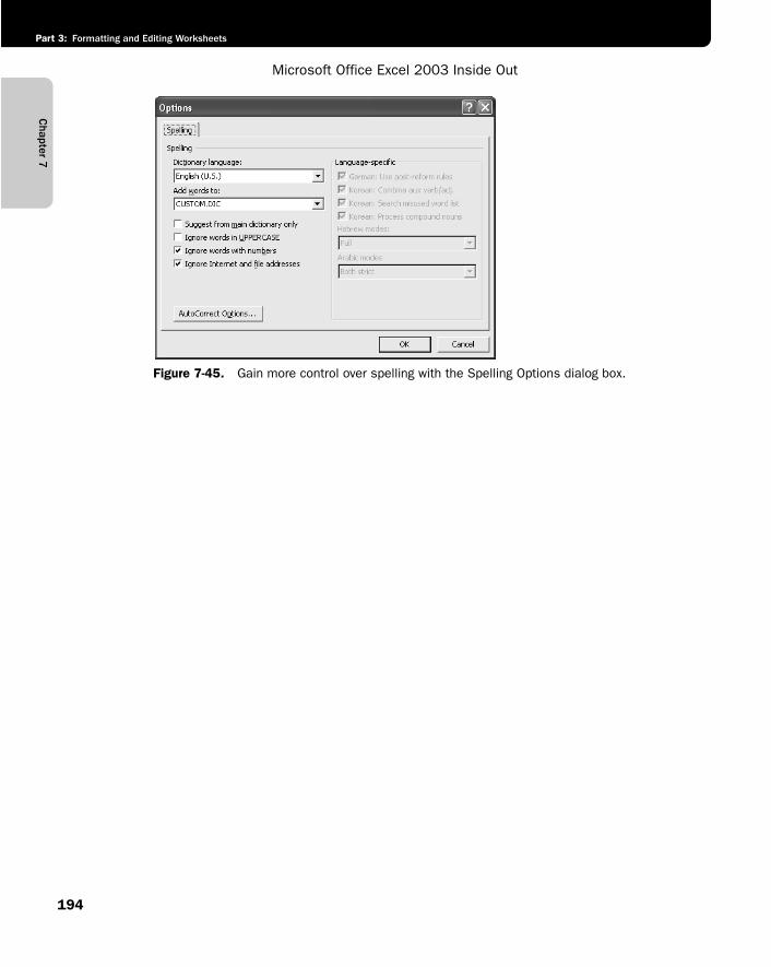
Chapter 7

Microsoft Office Excel 2003 Inside Out

Part 3: Formatting and Editing Worksheets

194

f07ie45

Figure 7-45. Gain more control over spelling with the Spelling Options dialog box.

195

Part 3: Formatting and Editing Worksheets

Chapter 8

Worksheet Formatting Techniques

Formatting Fundamentals . . . . . . . . . . 195Formatting in Cells . . . . . . . . . . . . . . . . 200Creating Custom Formats . . . . . . . . . . . 211Aligning Data in Cells . . . . . . . . . . . . . . 219Aligning Text Vertically . . . . . . . . . . . . . 222

Using Fonts. . . . . . . . . . . . . . . . . . . . . . . 226Customizing Borders . . . . . . . . . . . . . . . 228Applying Colors and Patterns. . . . . . . . . 231Controlling the Size of Cells . . . . . . . . . . 234

When creating a worksheet in Microsoft Excel, you probably don’t ask yourself the question: Why use formats? But we’ll answer it anyway. Compare Figure 8-1 to Figure 8-2 and we need say no more. Although the data is the same in both worksheets, the worksheet in Figure 8-2 takes advantage of the formatting features available in Excel and is therefore much easier to read and interpret. Proper use of formatting helps transform data into information; this chapter shows you how to do just that.

Note You can find the sample file used in this sample, Pacific Sales.xls, on the companion CD.

Formatting FundamentalsFormatting worksheets in Excel is easy: Just select the cell or range and choose the appropri-ate Format menu commands. The Format Cells command displays the dialog box shown in Figure 8-3, which controls most of the formatting features you can apply to your worksheets. You’ll examine the inner workings of the Format Cells dialog box throughout this chapter.

Tip To quickly access the Format Cells dialog box, press Ctrl+1.

When you select a category in the Category list, the formats and options available for that cat-egory type are displayed on the right side of the dialog box. The sample area at the top of the dialog box shows you how the selected format will affect the contents of the active cell.

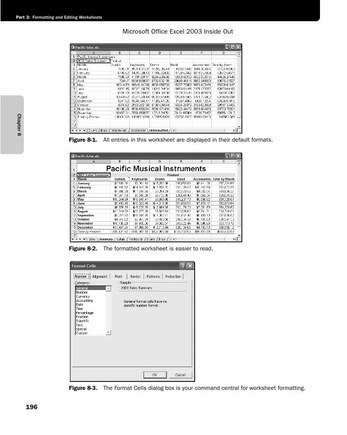
Chapter 8

Microsoft Office Excel 2003 Inside Out

Part 3: Formatting and Editing Worksheets

196

f08ie01

Figure 8-1. All entries in this worksheet are displayed in their default formats.

f08ie02

Figure 8-2. The formatted worksheet is easier to read.

f08ie03

Figure 8-3. The Format Cells dialog box is your command central for worksheet formatting.

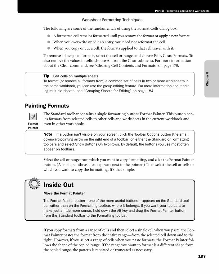
Cha

pter

8

Worksheet Formatting Techniques

197

Part 3: Formatting and Editing Worksheets

The following are some of the fundamentals of using the Format Cells dialog box:

● A formatted cell remains formatted until you remove the format or apply a new format.

● When you overwrite or edit an entry, you need not reformat the cell.

● When you copy or cut a cell, the formats applied to that cell travel with it.

To remove all assigned formats, select the cell or range, and choose Edit, Clear, Formats. To also remove the values in cells, choose All from the Clear submenu. For more information about the Clear command, see “Clearing Cell Contents and Formats” on page 170.

Tip Edit cells on multiple sheetsTo format (or remove all formats from) a common set of cells in two or more worksheets in the same workbook, you can use the group-editing feature. For more information about edit-ing multiple sheets, see “Grouping Sheets for Editing” on page 184.

Painting Formats

Format Painter

The Standard toolbar contains a single formatting button: Format Painter. This button cop-ies formats from selected cells to other cells and worksheets in the current workbook and even in other workbooks.

Note If a button isn’t visible on your screen, click the Toolbar Options button (the small downward-pointing arrow on the right end of a toolbar) on either the Standard or Formatting toolbars and select Show Buttons On Two Rows. By default, the buttons you use most often appear on toolbars.

Select the cell or range from which you want to copy formatting, and click the Format Painter button. (A small paintbrush icon appears next to the pointer.) Then select the cell or cells to which you want to copy the formatting. It’s that simple.

Inside OutMove the Format Painter

The Format Painter button—one of the more useful buttons—appears on the Standard tool-bar rather than on the Formatting toolbar, where it belongs. If you want your toolbars to make just a little more sense, hold down the Alt key and drag the Format Painter button from the Standard toolbar to the Formatting toolbar.

If you copy formats from a range of cells and then select a single cell when you paste, the For-mat Painter pastes the format from the entire range—from the selected cell down and to the right. However, if you select a range of cells when you paste formats, the Format Painter fol-lows the shape of the copied range. If the range you want to format is a different shape from the copied range, the pattern is repeated or truncated as necessary.

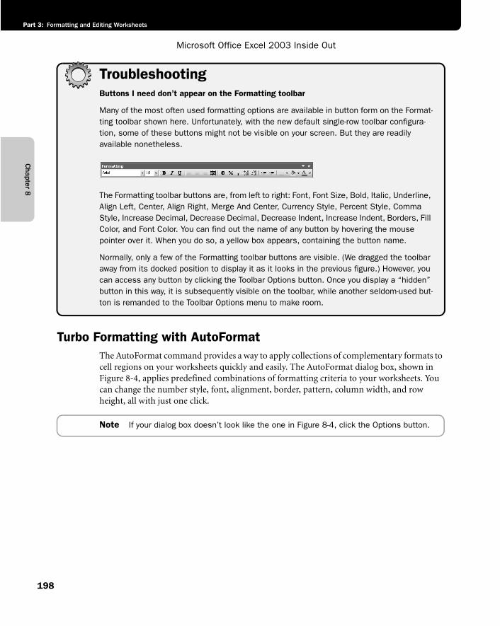
Chapter 8

Microsoft Office Excel 2003 Inside Out

Part 3: Formatting and Editing Worksheets

198

TroubleshootingButtons I need don’t appear on the Formatting toolbar

Many of the most often used formatting options are available in button form on the Format-ting toolbar shown here. Unfortunately, with the new default single-row toolbar configura-tion, some of these buttons might not be visible on your screen. But they are readily available nonetheless.

g08ie01

The Formatting toolbar buttons are, from left to right: Font, Font Size, Bold, Italic, Underline, Align Left, Center, Align Right, Merge And Center, Currency Style, Percent Style, Comma Style, Increase Decimal, Decrease Decimal, Decrease Indent, Increase Indent, Borders, Fill Color, and Font Color. You can find out the name of any button by hovering the mouse pointer over it. When you do so, a yellow box appears, containing the button name.

Normally, only a few of the Formatting toolbar buttons are visible. (We dragged the toolbar away from its docked position to display it as it looks in the previous figure.) However, you can access any button by clicking the Toolbar Options button. Once you display a “hidden” button in this way, it is subsequently visible on the toolbar, while another seldom-used but-ton is remanded to the Toolbar Options menu to make room.

Turbo Formatting with AutoFormatThe AutoFormat command provides a way to apply collections of complementary formats to cell regions on your worksheets quickly and easily. The AutoFormat dialog box, shown in Figure 8-4, applies predefined combinations of formatting criteria to your worksheets. You can change the number style, font, alignment, border, pattern, column width, and row height, all with just one click.

Note If your dialog box doesn’t look like the one in Figure 8-4, click the Options button.

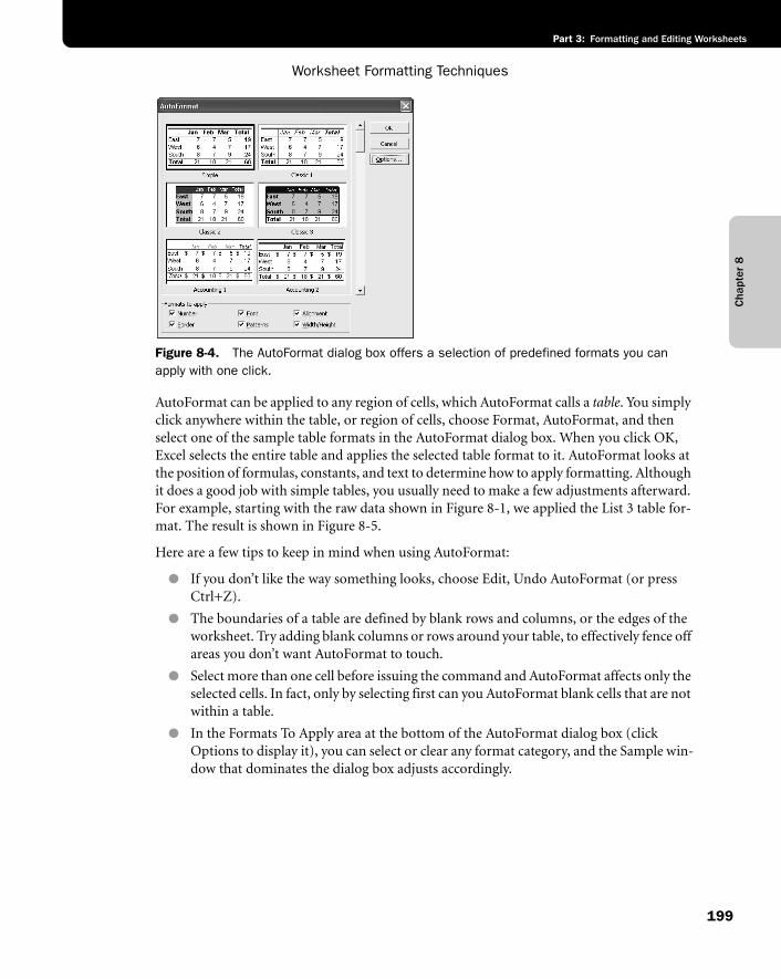
Cha

pter

8

Worksheet Formatting Techniques

199

Part 3: Formatting and Editing Worksheets

f08ie04

Figure 8-4. The AutoFormat dialog box offers a selection of predefined formats you can apply with one click.

AutoFormat can be applied to any region of cells, which AutoFormat calls a table. You simply click anywhere within the table, or region of cells, choose Format, AutoFormat, and then select one of the sample table formats in the AutoFormat dialog box. When you click OK, Excel selects the entire table and applies the selected table format to it. AutoFormat looks at the position of formulas, constants, and text to determine how to apply formatting. Although it does a good job with simple tables, you usually need to make a few adjustments afterward. For example, starting with the raw data shown in Figure 8-1, we applied the List 3 table for-mat. The result is shown in Figure 8-5.

Here are a few tips to keep in mind when using AutoFormat:

● If you don’t like the way something looks, choose Edit, Undo AutoFormat (or press Ctrl+Z).

● The boundaries of a table are defined by blank rows and columns, or the edges of the worksheet. Try adding blank columns or rows around your table, to effectively fence off areas you don’t want AutoFormat to touch.

● Select more than one cell before issuing the command and AutoFormat affects only the selected cells. In fact, only by selecting first can you AutoFormat blank cells that are not within a table.

● In the Formats To Apply area at the bottom of the AutoFormat dialog box (click Options to display it), you can select or clear any format category, and the Sample win-dow that dominates the dialog box adjusts accordingly.

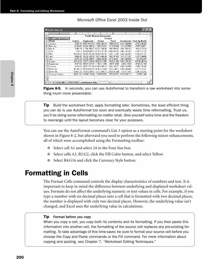
Chapter 8

Microsoft Office Excel 2003 Inside Out

Part 3: Formatting and Editing Worksheets

200

f08ie05

Figure 8-5. In seconds, you can use AutoFormat to transform a raw worksheet into some-thing much more presentable.

Tip Build the worksheet first; apply formatting later. Sometimes, the least efficient thing you can do is use AutoFormat too soon and eventually waste time reformatting. Trust us, you’ll be doing some reformatting no matter what. Give yourself extra time and the freedom to rearrange until the layout becomes clear for your purposes.

You can use the AutoFormat command’s List 3 option as a starting point for the worksheet shown in Figure 8-2, but afterward you need to perform the following minor enhancements, all of which were accomplished using the Formatting toolbar:

● Select cell A1 and select 24 in the Font Size box.

● Select cells A3, B2:G2, click the Fill Color button, and select Yellow.

● Select B4:G16 and click the Currency Style button.

Formatting in CellsThe Format Cells command controls the display characteristics of numbers and text. It is important to keep in mind the difference between underlying and displayed worksheet val-ues. Formats do not affect the underlying numeric or text values in cells. For example, if you type a number with six decimal places into a cell that is formatted with two decimal places, the number is displayed with only two decimal places. However, the underlying value isn’t changed, and Excel uses the underlying value in calculations.

Tip Format before you copyWhen you copy a cell, you copy both its contents and its formatting. If you then paste this information into another cell, the formatting of the source cell replaces any pre-existing for-matting. To take advantage of this time-saver, be sure to format your source cell before you choose the Copy and Paste commands or the Fill command. For more information about copying and pasting, see Chapter 7, “Worksheet Editing Techniques.”

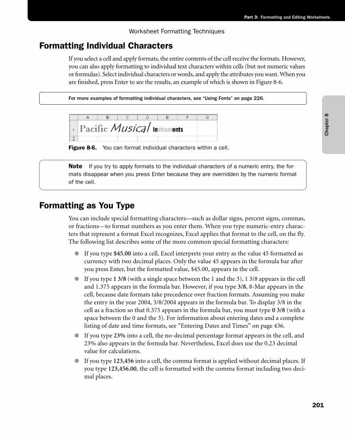
Cha

pter

8

Worksheet Formatting Techniques

201

Part 3: Formatting and Editing Worksheets

Formatting Individual CharactersIf you select a cell and apply formats, the entire contents of the cell receive the formats. However, you can also apply formatting to individual text characters within cells (but not numeric values or formulas). Select individual characters or words, and apply the attributes you want. When you are finished, press Enter to see the results, an example of which is shown in Figure 8-6.

For more examples of formatting individual characters, see “Using Fonts” on page 226.

f08ie06

Figure 8-6. You can format individual characters within a cell.

Note If you try to apply formats to the individual characters of a numeric entry, the for-mats disappear when you press Enter because they are overridden by the numeric format of the cell.

Formatting as You TypeYou can include special formatting characters—such as dollar signs, percent signs, commas, or fractions—to format numbers as you enter them. When you type numeric-entry charac-ters that represent a format Excel recognizes, Excel applies that format to the cell, on the fly. The following list describes some of the more common special formatting characters:

● If you type $45.00 into a cell, Excel interprets your entry as the value 45 formatted as currency with two decimal places. Only the value 45 appears in the formula bar after you press Enter, but the formatted value, $45.00, appears in the cell.

● If you type 1 3/8 (with a single space between the 1 and the 3), 1 3/8 appears in the cell and 1.375 appears in the formula bar. However, if you type 3/8, 8-Mar appears in the cell, because date formats take precedence over fraction formats. Assuming you make the entry in the year 2004, 3/8/2004 appears in the formula bar. To display 3/8 in the cell as a fraction so that 0.375 appears in the formula bar, you must type 0 3/8 (with a space between the 0 and the 3). For information about entering dates and a complete listing of date and time formats, see “Entering Dates and Times” on page 436.

● If you type 23% into a cell, the no-decimal percentage format appears in the cell, and 23% also appears in the formula bar. Nevertheless, Excel does use the 0.23 decimal value for calculations.

● If you type 123,456 into a cell, the comma format is applied without decimal places. If you type 123,456.00, the cell is formatted with the comma format including two deci-mal places.

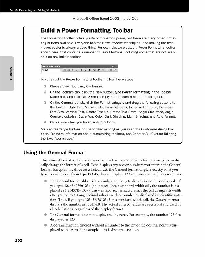
Chapter 8

Microsoft Office Excel 2003 Inside Out

Part 3: Formatting and Editing Worksheets

202

Build a Power Formatting ToolbarThe Formatting toolbar offers plenty of formatting power, but there are many other format-ting buttons available. Everyone has their own favorite techniques, and making the tech-niques easier is always a good thing. For example, we created a Power Formatting toolbar, shown here, that contains a number of useful buttons, including some that are not avail-able on any built-in toolbar.

g08ie02

To construct the Power Formatting toolbar, follow these steps:

1 Choose View, Toolbars, Customize.

2 On the Toolbars tab, click the New button, type Power Formatting in the Toolbar Name box, and click OK. A small empty bar appears next to the dialog box.

3 On the Commands tab, click the Format category and drag the following buttons to the toolbar: Style Box, Merge Cells, Unmerge Cells, Increase Font Size, Decrease Font Size, Vertical Text, Rotate Text Up, Rotate Text Down, Angle Clockwise, Angle Counterclockwise, Cycle Font Color, Dark Shading, Light Shading, and Auto Format.

4 Click Close when you finish adding buttons.

You can rearrange buttons on the toolbar as long as you keep the Customize dialog box open. For more information about customizing toolbars, see Chapter 3, “Custom-Tailoring the Excel Workspace.”

Using the General FormatThe General format is the first category in the Format Cells dialog box. Unless you specifi-cally change the format of a cell, Excel displays any text or numbers you enter in the General format. Except in the three cases listed next, the General format displays exactly what you type. For example, if you type 123.45, the cell displays 123.45. Here are the three exceptions:

● The General format abbreviates numbers too long to display in a cell. For example, if you type 12345678901234 (an integer) into a standard-width cell, the number is dis-played as 1.23457E+13. <<this was incorrect as stated, since the cell changes its width after you type>> Long decimal values are also rounded or displayed in scientific nota-tion. Thus, if you type 123456.7812345 in a standard-width cell, the General format displays the number as 123456.8. The actual entered values are preserved and used in all calculations, regardless of the display format.

● The General format does not display trailing zeros. For example, the number 123.0 is displayed as 123.

● A decimal fraction entered without a number to the left of the decimal point is dis-played with a zero. For example, .123 is displayed as 0.123.

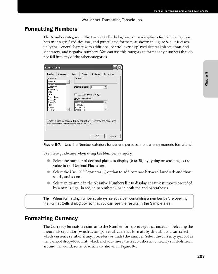
Cha

pter

8

Worksheet Formatting Techniques

203

Part 3: Formatting and Editing Worksheets

Formatting NumbersThe Number category in the Format Cells dialog box contains options for displaying num-bers in integer, fixed-decimal, and punctuated formats, as shown in Figure 8-7. It is essen-tially the General format with additional control over displayed decimal places, thousand separators, and negative numbers. You can use this category to format any numbers that do not fall into any of the other categories.

f08ie07

Figure 8-7. Use the Number category for general-purpose, noncurrency numeric formatting.

Use these guidelines when using the Number category:

● Select the number of decimal places to display (0 to 30) by typing or scrolling to the value in the Decimal Places box.

● Select the Use 1000 Separator (,) option to add commas between hundreds and thou-sands, and so on.

● Select an example in the Negative Numbers list to display negative numbers preceded by a minus sign, in red, in parentheses, or in both red and parentheses.

Tip When formatting numbers, always select a cell containing a number before opening the Format Cells dialog box so that you can see the results in the Sample area.

Formatting CurrencyThe Currency formats are similar to the Number formats except that instead of selecting the thousands separator (which accompanies all currency formats by default), you can select which currency symbol, if any, precedes (or trails) the number. Select the currency symbol in the Symbol drop-down list, which includes more than 250 different currency symbols from around the world, some of which are shown in Figure 8-8.

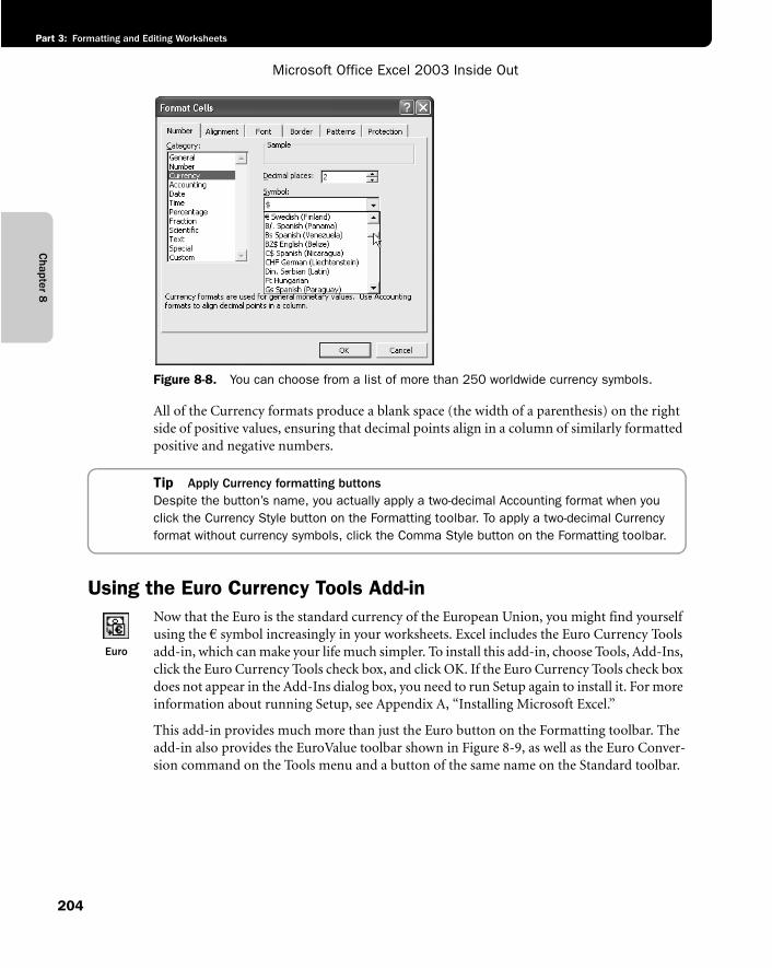
Chapter 8

Microsoft Office Excel 2003 Inside Out

Part 3: Formatting and Editing Worksheets

204

f08ie08

Figure 8-8. You can choose from a list of more than 250 worldwide currency symbols.

All of the Currency formats produce a blank space (the width of a parenthesis) on the right side of positive values, ensuring that decimal points align in a column of similarly formatted positive and negative numbers.

Tip Apply Currency formatting buttonsDespite the button’s name, you actually apply a two-decimal Accounting format when you click the Currency Style button on the Formatting toolbar. To apply a two-decimal Currency format without currency symbols, click the Comma Style button on the Formatting toolbar.

Using the Euro Currency Tools Add-in

Euro

Now that the Euro is the standard currency of the European Union, you might find yourself using the € symbol increasingly in your worksheets. Excel includes the Euro Currency Tools add-in, which can make your life much simpler. To install this add-in, choose Tools, Add-Ins, click the Euro Currency Tools check box, and click OK. If the Euro Currency Tools check box does not appear in the Add-Ins dialog box, you need to run Setup again to install it. For more information about running Setup, see Appendix A, “Installing Microsoft Excel.”

This add-in provides much more than just the Euro button on the Formatting toolbar. The add-in also provides the EuroValue toolbar shown in Figure 8-9, as well as the Euro Conver-sion command on the Tools menu and a button of the same name on the Standard toolbar.

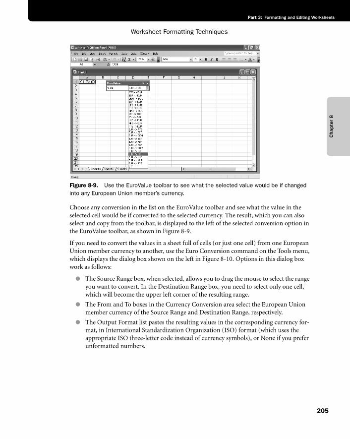
Cha

pter

8

Worksheet Formatting Techniques

205

Part 3: Formatting and Editing Worksheets

f08ie09

Figure 8-9. Use the EuroValue toolbar to see what the selected value would be if changed into any European Union member’s currency.

Choose any conversion in the list on the EuroValue toolbar and see what the value in the selected cell would be if converted to the selected currency. The result, which you can also select and copy from the toolbar, is displayed to the left of the selected conversion option in the EuroValue toolbar, as shown in Figure 8-9.

If you need to convert the values in a sheet full of cells (or just one cell) from one European Union member currency to another, use the Euro Conversion command on the Tools menu, which displays the dialog box shown on the left in Figure 8-10. Options in this dialog box work as follows:

● The Source Range box, when selected, allows you to drag the mouse to select the range you want to convert. In the Destination Range box, you need to select only one cell, which will become the upper left corner of the resulting range.

● The From and To boxes in the Currency Conversion area select the European Union member currency of the Source Range and Destination Range, respectively.

● The Output Format list pastes the resulting values in the corresponding currency for-mat, in International Standardization Organization (ISO) format (which uses the appropriate ISO three-letter code instead of currency symbols), or None if you prefer unformatted numbers.

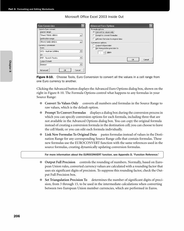
Chapter 8

Microsoft Office Excel 2003 Inside Out

Part 3: Formatting and Editing Worksheets

206

f08ie10

Figure 8-10. Choose Tools, Euro Conversion to convert all the values in a cell range from one Euro currency to another.

Clicking the Advanced button displays the Advanced Euro Options dialog box, shown on the right in Figure 8-10. The Formula Options control what happens to any formulas in your Source Range:

● Convert To Values Only converts all numbers and formulas in the Source Range to raw values, which is the default option.

● Prompt To Convert Formulas displays a dialog box during the conversion process in which you can specify conversion options for each formula, including three that are not available in the Advanced Options dialog box. You can copy the original formula instead of creating a conversion formula in the destination cell; you can choose to leave the cell blank; or you can edit each formula individually.

● Link New Formulas To Original Data pastes formulas instead of values in the Desti-nation Range for any corresponding Source Range cells that contain formulas. These new formulas use the EUROCONVERT function with the same references used in the source formulas, creating dynamically updating conversion formulas.

For more information about the EUROCONVERT function, see Appendix D, “Function Reference.”

● Output Full Precision controls the rounding of numbers. Normally, based on Euro-pean Union rules, converted currency values are calculated with a rounding factor that uses six significant digits of precision. To suppress this rounding factor, check the Out-put Full Precision box.

● Set Triangulation Precision To determines the number of significant digits of preci-sion, from 3 through 15, to be used in the intermediate calculations when converting between two European Union member currencies, which are performed in Euros.

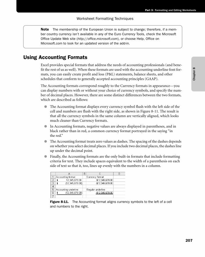
Cha

pter

8

Worksheet Formatting Techniques

207

Part 3: Formatting and Editing Worksheets

Note The membership of the European Union is subject to change; therefore, if a mem-ber country currency isn’t available in any of the Euro Currency Tools, check the Microsoft Office Update Web site (http://office.microsoft.com), or choose Help, Office on Microsoft.com to look for an updated version of the add-in.

Using Accounting FormatsExcel provides special formats that address the needs of accounting professionals (and bene-fit the rest of us as well). When these formats are used with the accounting underline font for-mats, you can easily create profit and loss (P&L) statements, balance sheets, and other schedules that conform to generally accepted accounting principles (GAAP).

The Accounting formats correspond roughly to the Currency formats in appearance—you can display numbers with or without your choice of currency symbols, and specify the num-ber of decimal places. However, there are some distinct differences between the two formats, which are described as follows:

● The Accounting format displays every currency symbol flush with the left side of the cell and numbers are flush with the right side, as shown in Figure 8-11. The result is that all the currency symbols in the same column are vertically aligned, which looks much cleaner than Currency formats.

● In Accounting formats, negative values are always displayed in parentheses, and in black rather than in red, a common currency format portrayed in the saying “in the red.”

● The Accounting format treats zero values as dashes. The spacing of the dashes depends on whether you select decimal places. If you include two decimal places, the dashes line up under the decimal point.

● Finally, the Accounting formats are the only built-in formats that include formatting criteria for text. They include spaces equivalent to the width of a parenthesis on each side of text so that it, too, lines up evenly with the numbers in a column.

f08ie11

Figure 8-11. The Accounting format aligns currency symbols to the left of a cell and numbers to the right.

Chapter 8

Microsoft Office Excel 2003 Inside Out

Part 3: Formatting and Editing Worksheets

208

Inside OutWhen AutoFormat applies accounting formats

AutoFormat generally does not change number formats except when you apply any one of the four Accounting AutoFormats. In this case, two different Accounting number formats are applied within the selected table (with and without currency symbols), according to GAAP.After you apply any of the Accounting AutoFormats, these number formats persist, even if you subsequently apply a non-Accounting AutoFormat, because none of the other AutoFor-mats affect number formatting.

Using Accounting Underlines The two Accounting underline formats on the Font tab of the Format Cells dialog box differ from their normal counterparts in two ways. First, accounting underlines are applied to the entire width of the cell (minus a parenthesis-size space on each side), whereas regular under-lines are applied only under the actual characters in a cell, as shown in Figure 8-11. If the cell contains a text entry that extends beyond the cell border, the accounting underlines stop at the cell border. Second, the Accounting underline formats appear near the bottom of cells, unlike normal underlines, which are applied much closer to the numbers or text in the cell, drawing annoying lines through commas and the descenders of letters like g and p.

For information about font formats, see “Using Fonts” on page 226.

Formatting PercentagesThe formats in the Percentage category of the Format Cells dialog box display numbers as percentages. The decimal point of the formatted number, in effect, moves two places to the right and a percent sign appears at the end of the number. For example, if you choose a per-centage format without decimal places, the entry 0.1234 will be displayed as 12%; if you select two decimal places, 0.1234 will be displayed as 12.34%.

Tip Apply Percentage formatting quicklyYou can also apply a Percentage format without decimals by clicking the Percent Style but-ton on the Formatting toolbar.

Formatting FractionsThe formats in the Fraction category, shown in Figure 8-12, display fractional numbers as actual fractions rather than as decimal values. As with all number formats, the underlying value does not change despite the displayed value of the fraction.

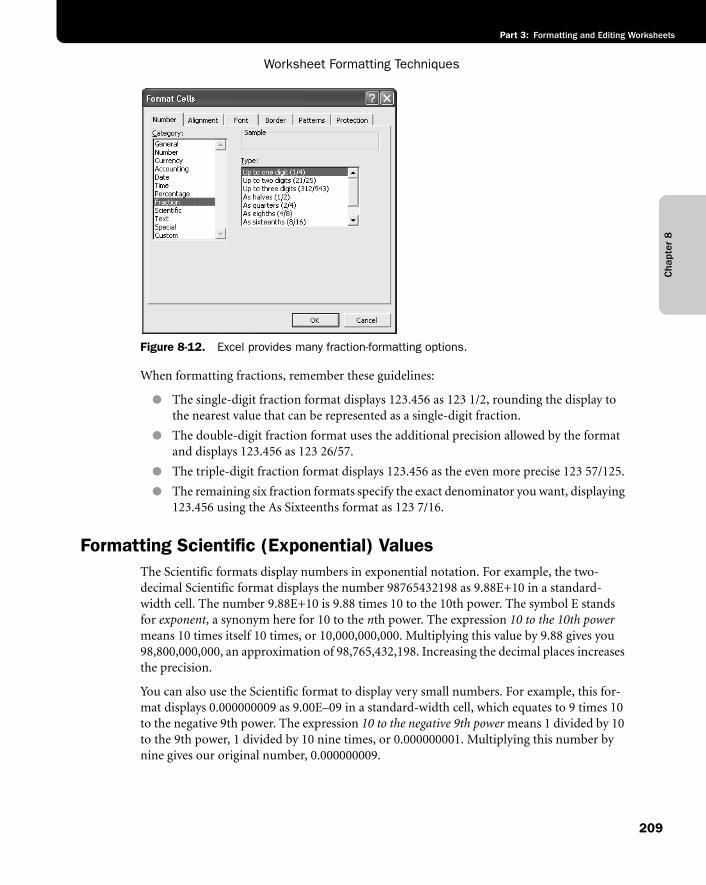
Cha

pter

8

Worksheet Formatting Techniques

209

Part 3: Formatting and Editing Worksheets

f08ie12

Figure 8-12. Excel provides many fraction-formatting options.

When formatting fractions, remember these guidelines:

● The single-digit fraction format displays 123.456 as 123 1/2, rounding the display to the nearest value that can be represented as a single-digit fraction.

● The double-digit fraction format uses the additional precision allowed by the format and displays 123.456 as 123 26/57.

● The triple-digit fraction format displays 123.456 as the even more precise 123 57/125.

● The remaining six fraction formats specify the exact denominator you want, displaying 123.456 using the As Sixteenths format as 123 7/16.

Formatting Scientific (Exponential) ValuesThe Scientific formats display numbers in exponential notation. For example, the two-decimal Scientific format displays the number 98765432198 as 9.88E+10 in a standard-width cell. The number 9.88E+10 is 9.88 times 10 to the 10th power. The symbol E stands for exponent, a synonym here for 10 to the nth power. The expression 10 to the 10th powermeans 10 times itself 10 times, or 10,000,000,000. Multiplying this value by 9.88 gives you 98,800,000,000, an approximation of 98,765,432,198. Increasing the decimal places increases the precision.

You can also use the Scientific format to display very small numbers. For example, this for-mat displays 0.000000009 as 9.00E–09 in a standard-width cell, which equates to 9 times 10 to the negative 9th power. The expression 10 to the negative 9th power means 1 divided by 10 to the 9th power, 1 divided by 10 nine times, or 0.000000001. Multiplying this number by nine gives our original number, 0.000000009.

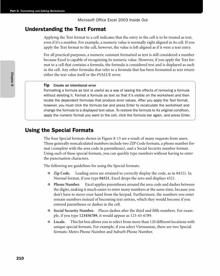
Chapter 8

Microsoft Office Excel 2003 Inside Out

Part 3: Formatting and Editing Worksheets

210

Understanding the Text FormatApplying the Text format to a cell indicates that the entry in the cell is to be treated as text, even if it’s a number. For example, a numeric value is normally right aligned in its cell. If you apply the Text format to the cell, however, the value is left aligned as if it were a text entry.

For all practical purposes, a numeric constant formatted as text is still considered a number because Excel is capable of recognizing its numeric value. However, if you apply the Text for-mat to a cell that contains a formula, the formula is considered text and is displayed as such in the cell. Any other formulas that refer to a formula that has been formatted as text return either the text value itself or the #VALUE error.

Tip Create an intentional errorFormatting a formula as text is useful as a way of seeing the effects of removing a formula without deleting it. Format a formula as text so that it’s visible on the worksheet and then locate the dependent formulas that produce error values. After you apply the Text format, however, you must click the formula bar and press Enter to recalculate the worksheet and change the formula to a displayed text value. To restore the formula to its original condition, apply the numeric format you want to the cell, click the formula bar again, and press Enter.

Using the Special FormatsThe four Special formats shown in Figure 8-13 are a result of many requests from users. These generally noncalculated numbers include two ZIP Code formats, a phone number for-mat (complete with the area code in parentheses), and a Social Security number format. Using each of these special formats, you can quickly type numbers without having to enter the punctuation characters.

The following are guidelines for using the Special formats:

● Zip Code. Leading zeros are retained to correctly display the code, as in 04321. In Normal format, if you type 04321, Excel drops the zero and displays 4321.

● Phone Number. Excel applies parentheses around the area code and dashes between the digits, making it much easier to enter many numbers at the same time, because you don’t have to move your hand from the keypad. Furthermore, the numbers you enter remain numbers instead of becoming text entries, which they would become if you entered parentheses or dashes in the cell.

● Social Security Number. Places dashes after the third and fifth numbers. For exam-ple, if you type 123456789, it would appear as 123-45-6789.

● Locale. This list box allows you to select from more than 120 different locations with unique special formats. For example, if you select Vietnamese, there are two Special formats: Metro Phone Number and Suburb Phone Number.

Cha

pter

8

Worksheet Formatting Techniques

211

Part 3: Formatting and Editing Worksheets

f08ie13 Figure 8-13. Excel provides several frequently requested formats in the Special category.

Creating Custom FormatsUse the Custom tab in the Format Cells dialog box, shown in Figure 8-14, to create custom number formats using special formatting codes. Excel adds new formats to the bottom of the list of formatting codes in the Type list, which also includes built-in formats. To delete a cus-tom format, select the format in the Format Cells dialog box and click Delete. You cannot delete built-in formats.

Creating New Number FormatsThe quickest way to start creating a custom format is to use one of the existing custom for-mats as a starting point for creating your own format. Here’s an easy way to build on an exist-ing format, as well as to see what the codes in the Type list mean:

1 Type a number and format it using the built-in format that most closely resembles the custom format you want to create. Leave this cell selected.

2 On the Number tab of the Format Cells dialog box, click the Custom category. The format you selected is highlighted in the Type list, representing the code equivalent of the format you want to modify.

3 Edit the contents of the Type box, using the codes listed in Table 8-1. The original for-mat isn’t affected, and the new format is added to the bottom of the Type list.

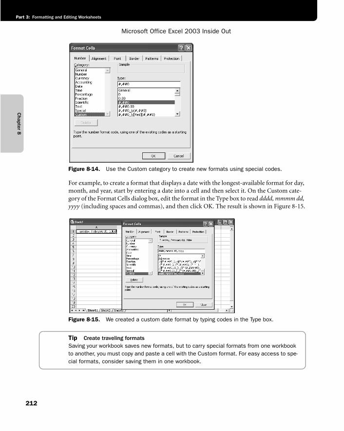
Chapter 8

Microsoft Office Excel 2003 Inside Out

Part 3: Formatting and Editing Worksheets

212

f08ie14

Figure 8-14. Use the Custom category to create new formats using special codes.

For example, to create a format that displays a date with the longest-available format for day, month, and year, start by entering a date into a cell and then select it. On the Custom cate-gory of the Format Cells dialog box, edit the format in the Type box to read dddd, mmmm dd, yyyy (including spaces and commas), and then click OK. The result is shown in Figure 8-15.

f08ie15

Figure 8-15. We created a custom date format by typing codes in the Type box.

Tip Create traveling formatsSaving your workbook saves new formats, but to carry special formats from one workbook to another, you must copy and paste a cell with the Custom format. For easy access to spe-cial formats, consider saving them in one workbook.

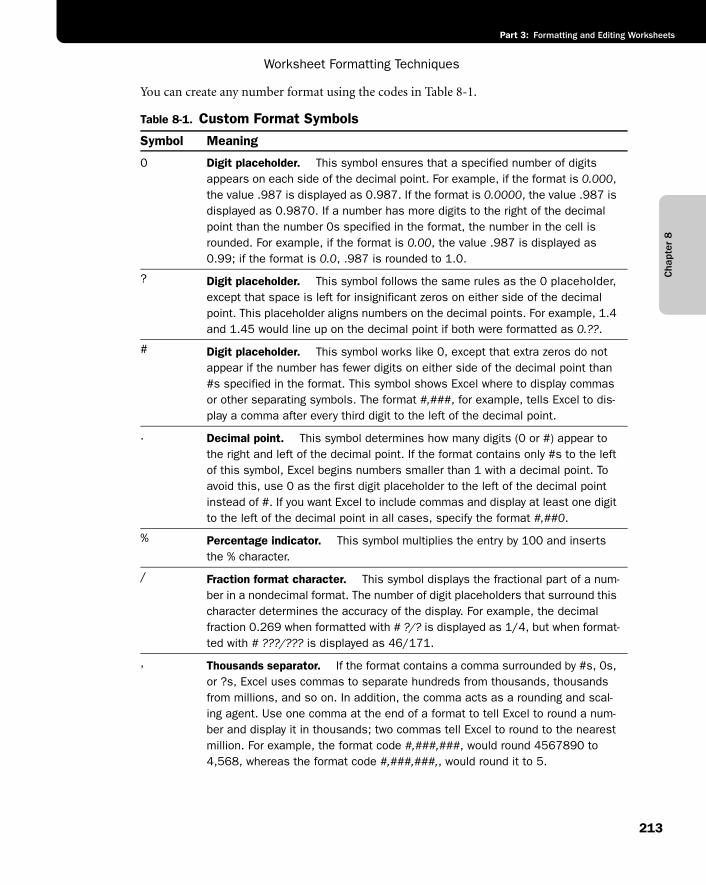
Cha

pter

8

Worksheet Formatting Techniques

213

Part 3: Formatting and Editing Worksheets

You can create any number format using the codes in Table 8-1.

Table 8-1. Custom Format Symbols

Symbol Meaning

0 Digit placeholder. This symbol ensures that a specified number of digits appears on each side of the decimal point. For example, if the format is 0.000,the value .987 is displayed as 0.987. If the format is 0.0000, the value .987 is displayed as 0.9870. If a number has more digits to the right of the decimal point than the number 0s specified in the format, the number in the cell is rounded. For example, if the format is 0.00, the value .987 is displayed as 0.99; if the format is 0.0, .987 is rounded to 1.0.

? Digit placeholder. This symbol follows the same rules as the 0 placeholder, except that space is left for insignificant zeros on either side of the decimal point. This placeholder aligns numbers on the decimal points. For example, 1.4 and 1.45 would line up on the decimal point if both were formatted as 0.??.

# Digit placeholder. This symbol works like 0, except that extra zeros do not appear if the number has fewer digits on either side of the decimal point than #s specified in the format. This symbol shows Excel where to display commas or other separating symbols. The format #,###, for example, tells Excel to dis-play a comma after every third digit to the left of the decimal point.

. Decimal point. This symbol determines how many digits (0 or #) appear to the right and left of the decimal point. If the format contains only #s to the left of this symbol, Excel begins numbers smaller than 1 with a decimal point. To avoid this, use 0 as the first digit placeholder to the left of the decimal point instead of #. If you want Excel to include commas and display at least one digit to the left of the decimal point in all cases, specify the format #,##0.

% Percentage indicator. This symbol multiplies the entry by 100 and inserts the % character.

/ Fraction format character. This symbol displays the fractional part of a num-ber in a nondecimal format. The number of digit placeholders that surround this character determines the accuracy of the display. For example, the decimal fraction 0.269 when formatted with # ?/? is displayed as 1/4, but when format-ted with # ???/??? is displayed as 46/171.

, Thousands separator. If the format contains a comma surrounded by #s, 0s, or ?s, Excel uses commas to separate hundreds from thousands, thousands from millions, and so on. In addition, the comma acts as a rounding and scal-ing agent. Use one comma at the end of a format to tell Excel to round a num-ber and display it in thousands; two commas tell Excel to round to the nearest million. For example, the format code #,###,###, would round 4567890 to 4,568, whereas the format code #,###,###,, would round it to 5.

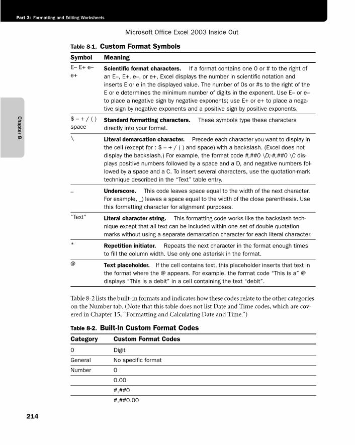
Chapter 8

Microsoft Office Excel 2003 Inside Out

Part 3: Formatting and Editing Worksheets

214

Table 8-2 lists the built-in formats and indicates how these codes relate to the other categories on the Number tab. (Note that this table does not list Date and Time codes, which are cov-ered in Chapter 15, “Formatting and Calculating Date and Time.”)

E– E+ e– e+

Scientific format characters. If a format contains one 0 or # to the right of an E–, E+, e–, or e+, Excel displays the number in scientific notation and inserts E or e in the displayed value. The number of 0s or #s to the right of the E or e determines the minimum number of digits in the exponent. Use E– or e– to place a negative sign by negative exponents; use E+ or e+ to place a nega-tive sign by negative exponents and a positive sign by positive exponents.

$ – + / ( ) space

Standard formatting characters. These symbols type these characters directly into your format.

\ Literal demarcation character. Precede each character you want to display in the cell (except for : $ – + / ( ) and space) with a backslash. (Excel does not display the backslash.) For example, the format code #,##0 \D;-#,##0 \C dis-plays positive numbers followed by a space and a D, and negative numbers fol-lowed by a space and a C. To insert several characters, use the quotation-mark technique described in the “Text” table entry.

_ Underscore. This code leaves space equal to the width of the next character. For example, _) leaves a space equal to the width of the close parenthesis. Use this formatting character for alignment purposes.

“Text” Literal character string. This formatting code works like the backslash tech-nique except that all text can be included within one set of double quotation marks without using a separate demarcation character for each literal character.

* Repetition initiator. Repeats the next character in the format enough times to fill the column width. Use only one asterisk in the format.

@ Text placeholder. If the cell contains text, this placeholder inserts that text in the format where the @ appears. For example, the format code “This is a” @ displays “This is a debit” in a cell containing the text “debit”.

Table 8-1. Custom Format Symbols

Symbol Meaning

Table 8-2. Built-In Custom Format Codes

Category Custom Format Codes

0 Digit

General No specific format

Number 0

0.00

#,##0

#,##0.00

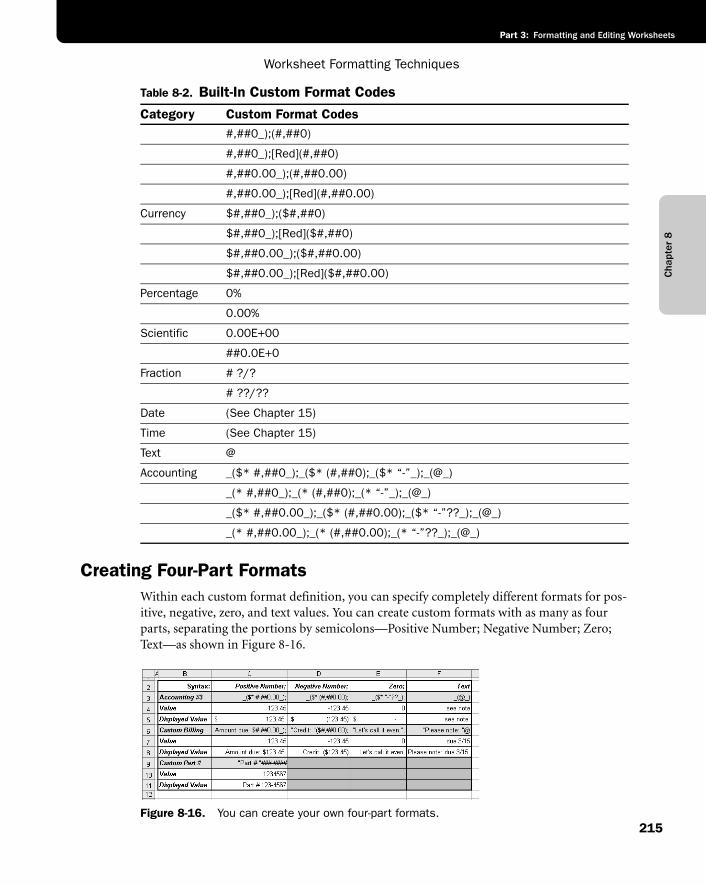
Cha

pter

8

Worksheet Formatting Techniques

215

Part 3: Formatting and Editing Worksheets

Creating Four-Part FormatsWithin each custom format definition, you can specify completely different formats for pos-itive, negative, zero, and text values. You can create custom formats with as many as four parts, separating the portions by semicolons—Positive Number; Negative Number; Zero; Text—as shown in Figure 8-16.

f08ie16

Figure 8-16. You can create your own four-part formats.

#,##0_);(#,##0)

#,##0_);[Red](#,##0)

#,##0.00_);(#,##0.00)

#,##0.00_);[Red](#,##0.00)

Currency $#,##0_);($#,##0)

$#,##0_);[Red]($#,##0)

$#,##0.00_);($#,##0.00)

$#,##0.00_);[Red]($#,##0.00)

Percentage 0%

0.00%

Scientific 0.00E+00

##0.0E+0

Fraction # ?/?

# ??/??

Date (See Chapter 15)

Time (See Chapter 15)

Text @

Accounting _($* #,##0_);_($* (#,##0);_($* “-”_);_(@_)

_(* #,##0_);_(* (#,##0);_(* “-”_);_(@_)

_($* #,##0.00_);_($* (#,##0.00);_($* “-”??_);_(@_)

_(* #,##0.00_);_(* (#,##0.00);_(* “-”??_);_(@_)

Table 8-2. Built-In Custom Format Codes

Category Custom Format Codes

Chapter 8

Microsoft Office Excel 2003 Inside Out

Part 3: Formatting and Editing Worksheets

216

Among the built-in formats, only the Accounting formats use all four parts, as shown in Figure 8-16, which shows the third Accounting format in Table 8-2. The following are some guidelines for creating multipart formats:

● If your custom format includes only one part, Excel applies that format to positive, negative, and zero values.

● If your custom format includes two parts, the first part applies to positive and zero val-ues; the second part applies to only negative values.

● If your custom format has three parts, the third part controls the display of zero values.

● The fourth and last element in a four-way format controls text-value formatting. Any formats with three or fewer elements have no effect on text entries.

Tip Hide zerosYou can suppress all zero values in a worksheet. Choose Tools, Options, and then click the View tab. Clear the Zero Values option in the Window Options area.

Adding Color to FormatsYou can also use the Number formats to change the color of selected cell entries. For example, you might use color to distinguish categories of information or to make totals stand out. You can even create formats that assign different colors to specific numeric ranges so that, for example, all values greater than or less than a specified value appear in a different color.

Create Custom Billing and Part Number FormatsSuppose you create a billing statement and you want to format the totals in the Amount Due col-umn so that they display differently depending on the value in each cell. You might create the Custom Billing format shown in Figure 8-16, which was created using the following code:

"Amount due: "$#,##0.00_);"Credit: "($#,##0.00);"Let's call it even. ";"Please note: "@

Suppose you’re creating an inventory worksheet and you want all the entries in a particular column to appear in the format Part # XXX-XXXX, shown as the Custom Part # format in Figure 8-16, which was created using the following code:

"Part # "###-####

Tip Use built-in conditional formattingYou can create codes that assign different colors based on the value in the cell, but there’s an easier way to do it that’s built into Excel: the Format, Conditional Formatting command. For more information, see “Applying Conditional Formats” on page 241.

Cha

pter

8

Worksheet Formatting Techniques

217

Part 3: Formatting and Editing Worksheets

To change the color of an entry, type the name of the new color, in brackets, in front of each segment of code. For example, if you want to apply blue Currency format with two decimal places, edit the $#,##0.00_);($#,##0.00) format as follows:

[Blue]$#,##0.00_);($#,##0.00)

When you apply this format to a worksheet, positive and zero values appear in blue; text and negative values appear as normal, in black. The following format displays positive values in blue, negative values in red, zero values in yellow, and text in green.

[Blue];[Red];[Yellow];[Green]

You can specify the following color names in your formats: Black, Blue, Cyan, Green, Magenta, Red, White, and Yellow. You can also specify a color as COLORn, where n is a num-ber in the range 1 through 16. Excel selects the corresponding color from your worksheet’s current 16-color palette. If that color is dithered (combines dots of two or more solid colors), Excel uses the nearest solid color.

Note If you define colors that are not among your system’s repertoire of solids, Excel pro-duces them by mixing dots from solid colors. Such blended colors, which are said to be dithered, work well for shading. But for text and lines, Excel always uses the nearest solid color in preference to a dithered color.

For more information about using custom format codes, see “Creating New Number Formats” on page 211.

TroubleshootingDecimal points in my currency formats don’t line up

Sometimes when you use currency formats with trailing characters, such as the French Canadian dollar (23.45 $), you want to use the GAAP practice of using currency symbols only at the top and bottom of a column of numbers. The numbers between should not dis-play any currency symbols, so how do you make all the decimal points line up properly?

You can create a custom format code to apply to the noncurrency format numbers in the middle of the column. An underscore character (_) in the format code tells Excel to leave a space that is equal in width to the character that follows it. For example, the code _$ leaves a space equal to the width of the dollar sign. Thus, the following code does the trick for you.

#,##0.00 _$;[Red]#,##0.00 _$

Make sure you add a space between the zeros and the underscores to properly line the numbers up with the built-in French Canadian dollar format.

Chapter 8

Microsoft Office Excel 2003 Inside Out

Part 3: Formatting and Editing Worksheets

218

Using Custom Format Condition OperatorsYou can create custom formats that are variable. To do so, you can add a condition operator to the first two parts of the standard four-part custom format. This, in effect, replaces the positive/negative formats with either/or formats. The third format becomes the default for-mat for values that don’t match the other two conditions, or the “else” format. You can use the conditional operators <, >, =, <=, >=, or <> with any number to define a format.

For example, suppose you are tracking accounts-receivable balances. To display accounts with a balance of more than $50,000 in blue, negative values in parentheses and in red, and all other values in the default color, create this format:

[Blue][>50000]$#,##0.00_);[Red][<0]($#,##0.00);$#,##0.00_)

Using these condition operators can also be a powerful aid if you need to scale numbers. For example, if your company produces a product that requires a few milliliters of a compound for each unit and you make thousands of units every day, you need to convert from milliliters to liters and kiloliters when you budget the use of this compound. Excel can make this con-version with the following numeric format:

[>999999]#,##0,,_m"kl";[>999]##,_k_m"L";#_k"ml"

The following table shows the effects of this format on various worksheet entries:

As you can see, using a combination of conditional formats, the thousands separator, and the proportional space indicator can improve both the readability and effectiveness of your worksheet, without increasing the number of formulas.

The Hidden Number FormatTo hide values in a worksheet, assign a null format to them. To create a null format, enter only the semicolon separator for that portion of the format. For example, to hide negative and zero values only, use this format:

$#,##0.00;;

Entry Display

72 72 ml

7286957 7 kl

7632 8 L

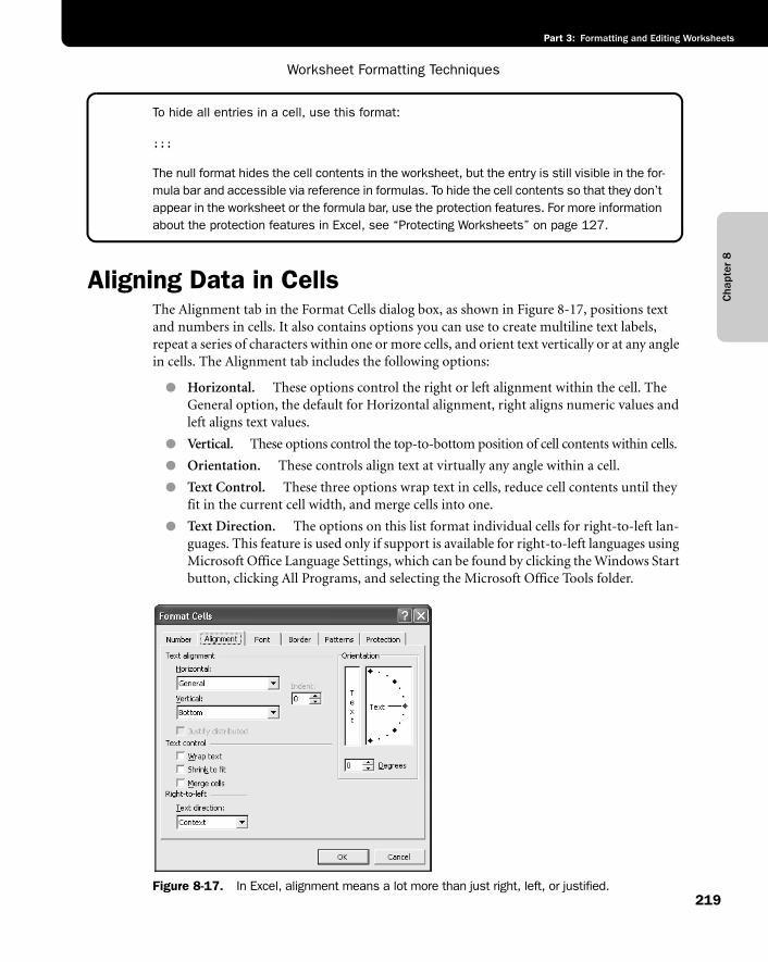
Cha

pter

8

Worksheet Formatting Techniques

219

Part 3: Formatting and Editing Worksheets

To hide all entries in a cell, use this format:

;;;

The null format hides the cell contents in the worksheet, but the entry is still visible in the for-mula bar and accessible via reference in formulas. To hide the cell contents so that they don’t appear in the worksheet or the formula bar, use the protection features. For more information about the protection features in Excel, see “Protecting Worksheets” on page 127.

Aligning Data in CellsThe Alignment tab in the Format Cells dialog box, as shown in Figure 8-17, positions text and numbers in cells. It also contains options you can use to create multiline text labels, repeat a series of characters within one or more cells, and orient text vertically or at any angle in cells. The Alignment tab includes the following options:

● Horizontal. These options control the right or left alignment within the cell. The General option, the default for Horizontal alignment, right aligns numeric values and left aligns text values.

● Vertical. These options control the top-to-bottom position of cell contents within cells.

● Orientation. These controls align text at virtually any angle within a cell.

● Text Control. These three options wrap text in cells, reduce cell contents until they fit in the current cell width, and merge cells into one.

● Text Direction. The options on this list format individual cells for right-to-left lan-guages. This feature is used only if support is available for right-to-left languages using Microsoft Office Language Settings, which can be found by clicking the Windows Start button, clicking All Programs, and selecting the Microsoft Office Tools folder.

f08ie17

Figure 8-17. In Excel, alignment means a lot more than just right, left, or justified.

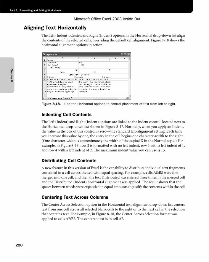
Chapter 8

Microsoft Office Excel 2003 Inside Out

Part 3: Formatting and Editing Worksheets

220

Aligning Text HorizontallyThe Left (Indent), Center, and Right (Indent) options in the Horizontal drop-down list align the contents of the selected cells, overriding the default cell alignment. Figure 8-18 shows the horizontal alignment options in action.

f08ie18

Figure 8-18. Use the Horizontal options to control placement of text from left to right.

Indenting Cell ContentsThe Left (Indent) and Right (Indent) options are linked to the Indent control, located next to the Horizontal drop-down list shown in Figure 8-17. Normally, when you apply an Indent, the value in the box of this control is zero—the standard left-alignment setting. Each time you increase this value by one, the entry in the cell begins one character-width to the right. (One character-width is approximately the width of the capital X in the Normal style.) For example, in Figure 8-18, row 2 is formatted with no left indent, row 3 with a left indent of 1, and row 4 with a left indent of 2. The maximum indent value you can use is 15.

Distributing Cell ContentsA new feature in this version of Excel is the capability to distribute individual text fragments contained in a cell across the cell with equal spacing. For example, cells A8:B8 were first merged into one cell, and then the text Distributed was entered three times in the merged cell and the Distributed (Indent) horizontal alignment was applied. The result shows that the spaces between words were expanded in equal amounts to justify the contents within the cell.

Centering Text Across ColumnsThe Center Across Selection option in the Horizontal text alignment drop-down list centers text from one cell across all selected blank cells to the right or to the next cell in the selection that contains text. For example, in Figure 8-18, the Center Across Selection format was applied to cells A7:B7. The centered text is in cell A7.

Cha

pter

8

Worksheet Formatting Techniques

221

Part 3: Formatting and Editing Worksheets

Tip Center without mergingAlthough the results might look similar, the Center Across Selection alignment option uses a different process than the Merge And Center button on the Formatting toolbar. When you use the Merge And Center button, the cells you select are merged—that is, they are replaced with a single cell, whereas when you use Center Across Selection, the text from the leftmost cell remains in its cell but is displayed across the entire range. For more infor-mation about merging cells, see “Merging and Unmerging Cells” on page 237.

Filling Cells with CharactersThe Fill option in the Horizontal alignment list repeats your cell entry to fill the width of the column. For example, in Figure 8-18, cells A9:B9 contain the single word Fill and a space, with the Fill option applied. Note that only the first cell in the range needs to contain text. Excel repeats the text to fill the range. Like the other Format commands, the Fill option affects only the appearance, not the underlying contents, of the cell.

Note Because the Fill option affects numeric values, as well as text, it can cause a number to look like something it isn’t. For example, if you apply the Fill option to a 10-character-wide cell that contains the number 3, the cell appears to contain the num-ber 3333333333.

Wrapping Text in CellsIf you enter a label that’s too wide for the active cell, Excel extends the label past the cell border and into adjacent cells—provided those cells are empty. If you select the Wrap Text option in the Text Control area of the Alignment tab, however, Excel displays your label entirely within the active cell. To accommodate the entire label, Excel increases the height of the row in which the cell is located and then wraps the text onto additional lines within the same cell. As shown in Figure 8-18, cell A10 contains a multiline label formatted with the Wrap Text option.

Inside OutAdjust row height manually

You can select the Wrap Text option with any alignment option. However, if you wrap text for-matted using the Orientation controls, the row height might not adjust to accommodate angled text in quite the way you expect. If you want to wrap angled text, it is best to adjust the row height manually to achieve the effect you want.

Justifying Text in CellsThe Alignment tab provides two Justify options—one in the Horizontal drop-down list and one in the Vertical drop-down list. The Horizontal Justify option wraps text in the active cell,

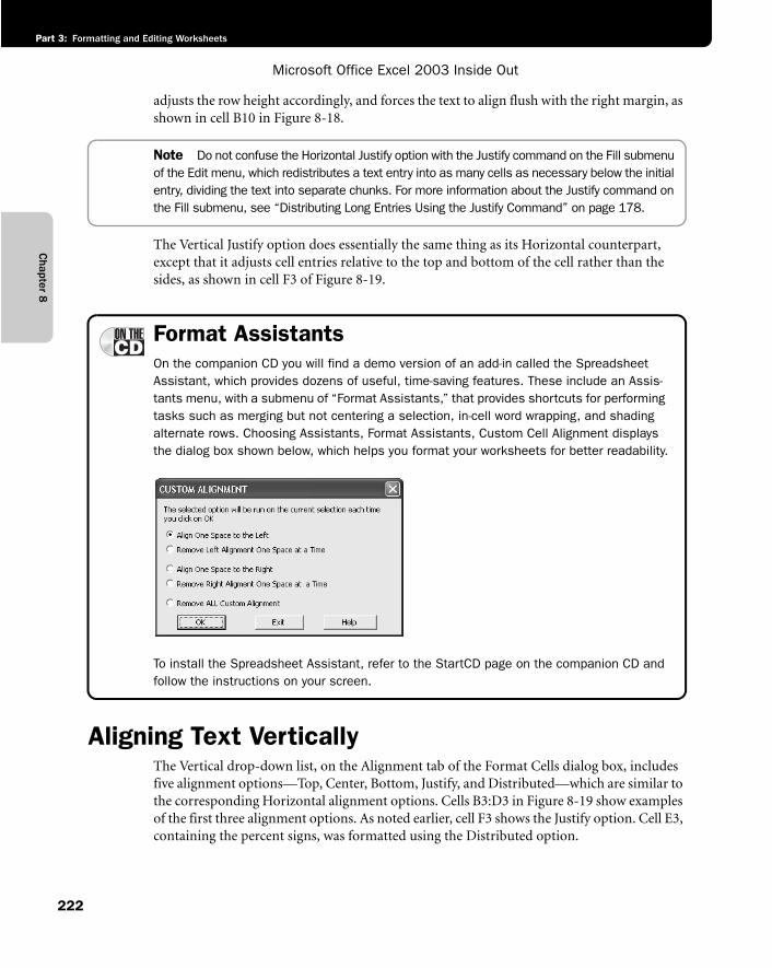
Chapter 8

Microsoft Office Excel 2003 Inside Out

Part 3: Formatting and Editing Worksheets

222

adjusts the row height accordingly, and forces the text to align flush with the right margin, as shown in cell B10 in Figure 8-18.

Note Do not confuse the Horizontal Justify option with the Justify command on the Fill submenu of the Edit menu, which redistributes a text entry into as many cells as necessary below the initial entry, dividing the text into separate chunks. For more information about the Justify command on the Fill submenu, see “Distributing Long Entries Using the Justify Command” on page 178.

The Vertical Justify option does essentially the same thing as its Horizontal counterpart, except that it adjusts cell entries relative to the top and bottom of the cell rather than the sides, as shown in cell F3 of Figure 8-19.

Format AssistantsOn the companion CD you will find a demo version of an add-in called the Spreadsheet Assistant, which provides dozens of useful, time-saving features. These include an Assis-tants menu, with a submenu of “Format Assistants,” that provides shortcuts for performing tasks such as merging but not centering a selection, in-cell word wrapping, and shading alternate rows. Choosing Assistants, Format Assistants, Custom Cell Alignment displays the dialog box shown below, which helps you format your worksheets for better readability.

G08ie05

To install the Spreadsheet Assistant, refer to the StartCD page on the companion CD and follow the instructions on your screen.

Aligning Text VerticallyThe Vertical drop-down list, on the Alignment tab of the Format Cells dialog box, includes five alignment options—Top, Center, Bottom, Justify, and Distributed—which are similar to the corresponding Horizontal alignment options. Cells B3:D3 in Figure 8-19 show examples of the first three alignment options. As noted earlier, cell F3 shows the Justify option. Cell E3, containing the percent signs, was formatted using the Distributed option.

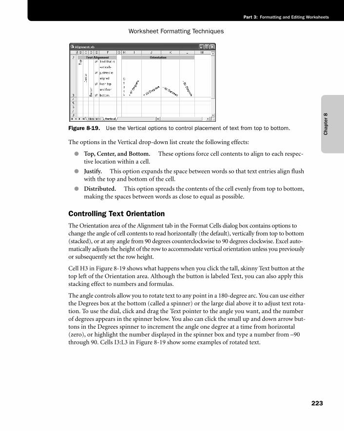
Cha

pter

8

Worksheet Formatting Techniques

223

Part 3: Formatting and Editing Worksheets

f08ie19

Figure 8-19. Use the Vertical options to control placement of text from top to bottom.

The options in the Vertical drop-down list create the following effects:

● Top, Center, and Bottom. These options force cell contents to align to each respec-tive location within a cell.

● Justify. This option expands the space between words so that text entries align flush with the top and bottom of the cell.

● Distributed. This option spreads the contents of the cell evenly from top to bottom, making the spaces between words as close to equal as possible.

Controlling Text OrientationThe Orientation area of the Alignment tab in the Format Cells dialog box contains options to change the angle of cell contents to read horizontally (the default), vertically from top to bottom (stacked), or at any angle from 90 degrees counterclockwise to 90 degrees clockwise. Excel auto-matically adjusts the height of the row to accommodate vertical orientation unless you previously or subsequently set the row height.

Cell H3 in Figure 8-19 shows what happens when you click the tall, skinny Text button at the top left of the Orientation area. Although the button is labeled Text, you can also apply this stacking effect to numbers and formulas.

The angle controls allow you to rotate text to any point in a 180-degree arc. You can use either the Degrees box at the bottom (called a spinner) or the large dial above it to adjust text rota-tion. To use the dial, click and drag the Text pointer to the angle you want, and the number of degrees appears in the spinner below. You also can click the small up and down arrow but-tons in the Degrees spinner to increment the angle one degree at a time from horizontal (zero), or highlight the number displayed in the spinner box and type a number from –90 through 90. Cells I3:L3 in Figure 8-19 show some examples of rotated text.

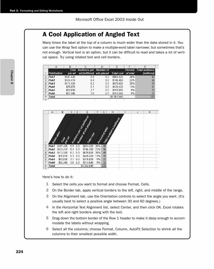
Chapter 8

Microsoft Office Excel 2003 Inside Out

Part 3: Formatting and Editing Worksheets

224

A Cool Application of Angled TextMany times the label at the top of a column is much wider than the data stored in it. You can use the Wrap Text option to make a multiple-word label narrower, but sometimes that’s not enough. Vertical text is an option, but it can be difficult to read and takes a lot of verti-cal space. Try using rotated text and cell borders.

g08ie03

Here’s how to do it:

1 Select the cells you want to format and choose Format, Cells.

2 On the Border tab, apply vertical borders to the left, right, and middle of the range.

3 On the Alignment tab, use the Orientation controls to select the angle you want. (It’s usually best to select a positive angle between 30 and 60 degrees.)

4 In the Horizontal Text Alignment list, select Center, and then click OK. Excel rotates the left and right borders along with the text.

5 Drag down the bottom border of the Row 1 header to make it deep enough to accom-modate the labels without wrapping.

6 Select all the columns; choose Format, Column, AutoFit Selection to shrink all the columns to their smallest possible width.

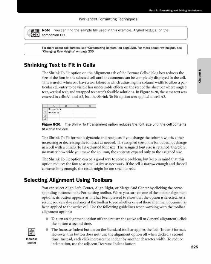
Cha

pter

8

Worksheet Formatting Techniques

225

Part 3: Formatting and Editing Worksheets

Note You can find the sample file used in this example, Angled Text.xls, on thecompanion CD.

For more about cell borders, see “Customizing Borders” on page 228. For more about row heights, see “Changing Row Heights” on page 235.

Shrinking Text to Fit in CellsThe Shrink To Fit option on the Alignment tab of the Format Cells dialog box reduces the size of the font in the selected cell until the contents can be completely displayed in the cell. This is useful when you have a worksheet in which adjusting the column width to allow a par-ticular cell entry to be visible has undesirable effects on the rest of the sheet, or where angled text, vertical text, and wrapped text aren’t feasible solutions. In Figure 8-20, the same text was entered in cells A1 and A2, but the Shrink To Fit option was applied to cell A2.

f08ie20

Figure 8-20. The Shrink To Fit alignment option reduces the font size until the cell contents fit within the cell.

The Shrink To Fit format is dynamic and readjusts if you change the column width, either increasing or decreasing the font size as needed. The assigned size of the font does not change in a cell with a Shrink To Fit-adjusted font size. The assigned font size is retained; therefore, no matter how wide you make the column, the contents expand only to the assigned size.

The Shrink To Fit option can be a good way to solve a problem, but keep in mind that this option reduces the font to as small a size as necessary. If the cell is narrow enough and the cell contents long enough, the result might be too small to read.

Selecting Alignment Using ToolbarsYou can select Align Left, Center, Align Right, or Merge And Center by clicking the corre-sponding buttons on the Formatting toolbar. When you turn on one of the toolbar alignment options, its button appears as if it has been pressed to show that the option is selected. As a result, you can always glance at the toolbar to see whether one of these alignment options has been applied to the active cell. Use the following guidelines when working with the toolbar alignment options:

● To turn an alignment option off (and return the active cell to General alignment), click the button a second time.

Increase Indent

● The Increase Indent button on the Standard toolbar applies the Left (Indent) format. However, this button does not turn the alignment option off when clicked a second time. Instead, each click increases the indent by another character width. To reduce indentation, use the adjacent Decrease Indent button.

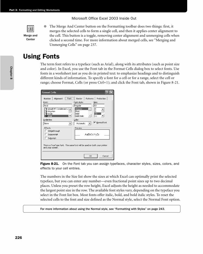
Chapter 8

Microsoft Office Excel 2003 Inside Out

Part 3: Formatting and Editing Worksheets

226

Merge and Center

● The Merge And Center button on the Formatting toolbar does two things: first, it merges the selected cells to form a single cell, and then it applies center alignment to the cell. This button is a toggle, removing center alignment and unmerging cells when clicked a second time. For more information about merged cells, see “Merging and Unmerging Cells” on page 237.

Using FontsThe term font refers to a typeface (such as Arial), along with its attributes (such as point size and color). In Excel, you use the Font tab in the Format Cells dialog box to select fonts. Use fonts in a worksheet just as you do in printed text: to emphasize headings and to distinguish different kinds of information. To specify a font for a cell or for a range, select the cell or range; choose Format, Cells (or press Ctrl+1); and click the Font tab, shown in Figure 8-21.

f08ie21

Figure 8-21. On the Font tab you can assign typefaces, character styles, sizes, colors, and effects to your cell entries.

The numbers in the Size list show the sizes at which Excel can optimally print the selected typeface, but you can enter any number—even fractional point sizes up to two decimal places. Unless you preset the row height, Excel adjusts the height as needed to accommodate the largest point size in the row. The available font styles vary, depending on the typeface you select in the Font list box. Most fonts offer italic, bold, and bold italic styles. To reset the selected cells to the font and size defined as the Normal style, select the Normal Font option.

For more information about using the Normal style, see “Formatting with Styles” on page 243.

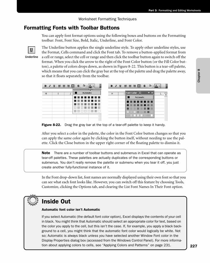
Cha

pter

8

Worksheet Formatting Techniques

227

Part 3: Formatting and Editing Worksheets

Formatting Fonts with Toolbar ButtonsYou can apply font format options using the following boxes and buttons on the Formatting toolbar: Font, Font Size, Bold, Italic, Underline, and Font Color.

Underline

The Underline button applies the single underline style. To apply other underline styles, use the Format, Cells command and click the Font tab. To remove a button-applied format from a cell or range, select the cell or range and then click the toolbar button again to switch off the format. When you click the arrow to the right of the Font Color button (or the Fill Color but-ton), a palette of colors drops down, as shown in Figure 8-22. This button is a tear-off palette, which means that you can click the gray bar at the top of the palette and drag the palette away, so that it floats separately from the toolbar.

f08ie22

Figure 8-22. Drag the gray bar at the top of a tear-off palette to keep it handy.

After you select a color in the palette, the color in the Font Color button changes so that you can apply the same color again by clicking the button itself, without needing to use the pal-ette. Click the Close button in the upper right corner of the floating palette to dismiss it.

Note There are a number of toolbar buttons and submenus in Excel that can operate as tear-off palettes. These palettes are actually duplicates of the corresponding buttons or submenus. You don’t really remove the palette or submenu when you tear it off, you just create another fully-functional instance of it.

In the Font drop-down list, font names are normally displayed using their own font so that you can see what each font looks like. However, you can switch off this feature by choosing Tools, Customize, clicking the Options tab, and clearing the List Font Names In Their Font option.

Inside OutAutomatic font color isn’t Automatic

If you select Automatic (the default font color option), Excel displays the contents of your cell in black. You might think that Automatic should select an appropriate color for text, based on the color you apply to the cell, but this isn’t the case. If, for example, you apply a black back-ground to a cell, you might think that the automatic font color would logically be white. Not so; Automatic is always black unless you have selected another Window Font color in the Display Properties dialog box (accessed from the Windows Control Panel). For more informa-tion about applying colors to cells, see “Applying Colors and Patterns” on page 231.

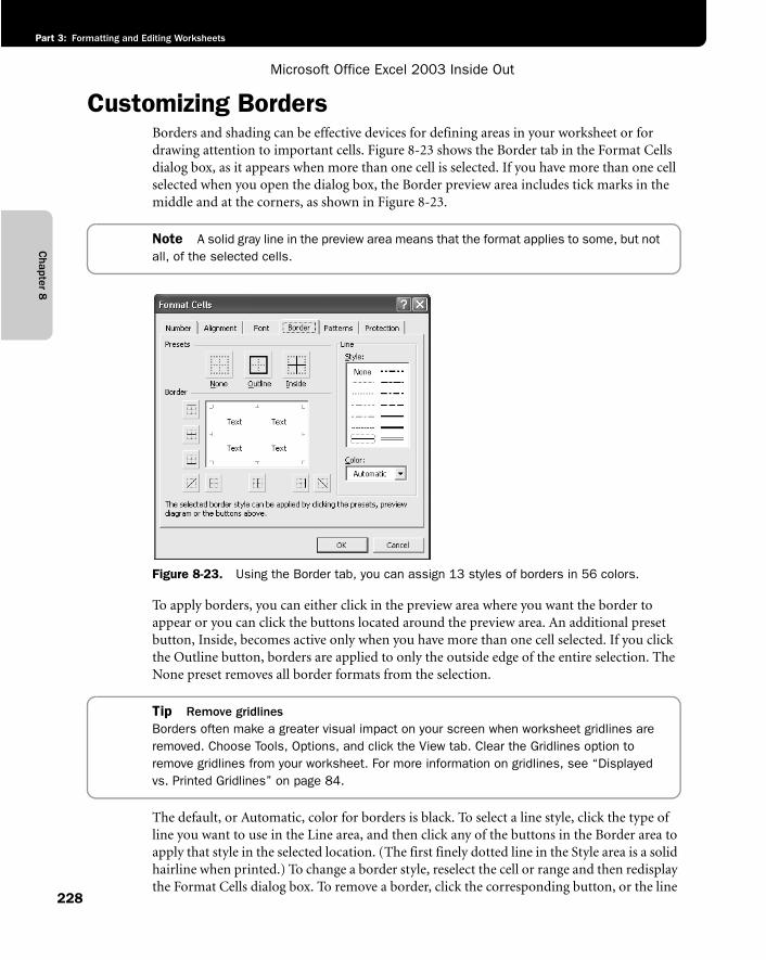
Chapter 8

Microsoft Office Excel 2003 Inside Out

Part 3: Formatting and Editing Worksheets

228

Customizing BordersBorders and shading can be effective devices for defining areas in your worksheet or for drawing attention to important cells. Figure 8-23 shows the Border tab in the Format Cells dialog box, as it appears when more than one cell is selected. If you have more than one cell selected when you open the dialog box, the Border preview area includes tick marks in the middle and at the corners, as shown in Figure 8-23.

Note A solid gray line in the preview area means that the format applies to some, but not all, of the selected cells.

f08ie23

Figure 8-23. Using the Border tab, you can assign 13 styles of borders in 56 colors.

To apply borders, you can either click in the preview area where you want the border to appear or you can click the buttons located around the preview area. An additional preset button, Inside, becomes active only when you have more than one cell selected. If you click the Outline button, borders are applied to only the outside edge of the entire selection. The None preset removes all border formats from the selection.

Tip Remove gridlinesBorders often make a greater visual impact on your screen when worksheet gridlines are removed. Choose Tools, Options, and click the View tab. Clear the Gridlines option to remove gridlines from your worksheet. For more information on gridlines, see “Displayed vs. Printed Gridlines” on page 84.

The default, or Automatic, color for borders is black. To select a line style, click the type of line you want to use in the Line area, and then click any of the buttons in the Border area to apply that style in the selected location. (The first finely dotted line in the Style area is a solid hairline when printed.) To change a border style, reselect the cell or range and then redisplay the Format Cells dialog box. To remove a border, click the corresponding button, or the line

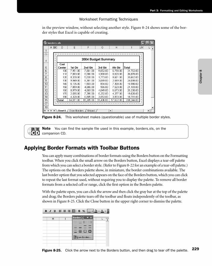
Cha

pter

8

Worksheet Formatting Techniques

229

Part 3: Formatting and Editing Worksheets

in the preview window, without selecting another style. Figure 8-24 shows some of the bor-der styles that Excel is capable of creating.

f08ie24

Figure 8-24. This worksheet makes (questionable) use of multiple border styles.

Note You can find the sample file used in this example, borders.xls, on the companion CD.

Applying Border Formats with Toolbar ButtonsYou can apply many combinations of border formats using the Borders button on the Formatting toolbar. When you click the small arrow on the Borders button, Excel displays a tear-off palette from which you can select a border style. (Refer to Figure 8-22 for an example of a tear-off palette.) The options on the Borders palette show, in miniature, the border combinations available. The last border option that you selected appears on the face of the Borders button, which you can click to repeat the last format used, without requiring you to display the palette. To remove all border formats from a selected cell or range, click the first option in the Borders palette.

With the palette open, you can click the arrow and then click the gray bar at the top of the palette and drag; the Borders palette tears off the toolbar and floats independently of the toolbar, as shown in Figure 8-25. Click the Close button in the upper right corner to dismiss the palette.

f08ie25

Figure 8-25. Click the arrow next to the Borders button, and then drag to tear off the palette.

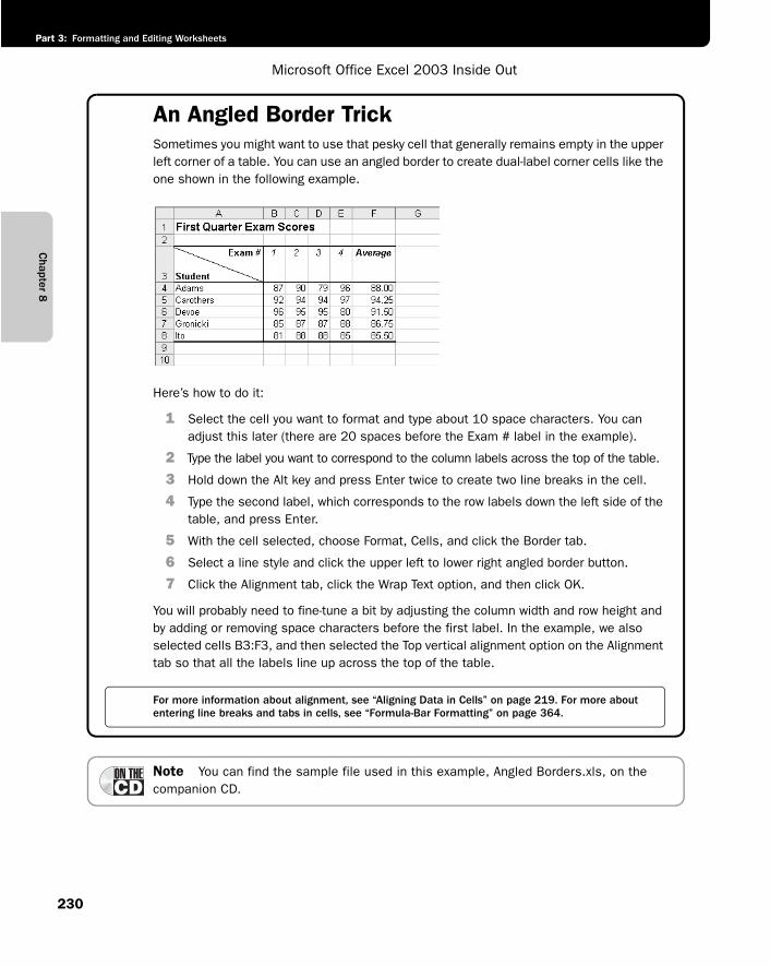
Chapter 8

Microsoft Office Excel 2003 Inside Out

Part 3: Formatting and Editing Worksheets

230

An Angled Border TrickSometimes you might want to use that pesky cell that generally remains empty in the upper left corner of a table. You can use an angled border to create dual-label corner cells like the one shown in the following example.

g08ie04

Here’s how to do it:

1 Select the cell you want to format and type about 10 space characters. You can adjust this later (there are 20 spaces before the Exam # label in the example).

2 Type the label you want to correspond to the column labels across the top of the table.

3 Hold down the Alt key and press Enter twice to create two line breaks in the cell.

4 Type the second label, which corresponds to the row labels down the left side of the table, and press Enter.

5 With the cell selected, choose Format, Cells, and click the Border tab.

6 Select a line style and click the upper left to lower right angled border button.

7 Click the Alignment tab, click the Wrap Text option, and then click OK.

You will probably need to fine-tune a bit by adjusting the column width and row height and by adding or removing space characters before the first label. In the example, we also selected cells B3:F3, and then selected the Top vertical alignment option on the Alignment tab so that all the labels line up across the top of the table.

For more information about alignment, see “Aligning Data in Cells” on page 219. For more about entering line breaks and tabs in cells, see “Formula-Bar Formatting” on page 364.

Note You can find the sample file used in this example, Angled Borders.xls, on the companion CD.

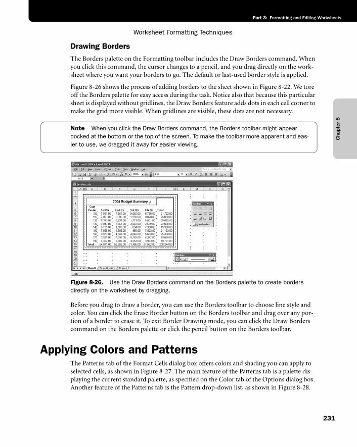
Cha

pter

8

Worksheet Formatting Techniques

231

Part 3: Formatting and Editing Worksheets

Drawing BordersThe Borders palette on the Formatting toolbar includes the Draw Borders command. When you click this command, the cursor changes to a pencil, and you drag directly on the work-sheet where you want your borders to go. The default or last-used border style is applied.

Figure 8-26 shows the process of adding borders to the sheet shown in Figure 8-22. We tore off the Borders palette for easy access during the task. Notice also that because this particular sheet is displayed without gridlines, the Draw Borders feature adds dots in each cell corner to make the grid more visible. When gridlines are visible, these dots are not necessary.

Note When you click the Draw Borders command, the Borders toolbar might appear docked at the bottom or the top of the screen. To make the toolbar more apparent and eas-ier to use, we dragged it away for easier viewing.

f08ie26

Figure 8-26. Use the Draw Borders command on the Borders palette to create borders directly on the worksheet by dragging.

Before you drag to draw a border, you can use the Borders toolbar to choose line style and color. You can click the Erase Border button on the Borders toolbar and drag over any por-tion of a border to erase it. To exit Border Drawing mode, you can click the Draw Borders command on the Borders palette or click the pencil button on the Borders toolbar.

Applying Colors and PatternsThe Patterns tab of the Format Cells dialog box offers colors and shading you can apply to selected cells, as shown in Figure 8-27. The main feature of the Patterns tab is a palette dis-playing the current standard palette, as specified on the Color tab of the Options dialog box. Another feature of the Patterns tab is the Pattern drop-down list, as shown in Figure 8-28.

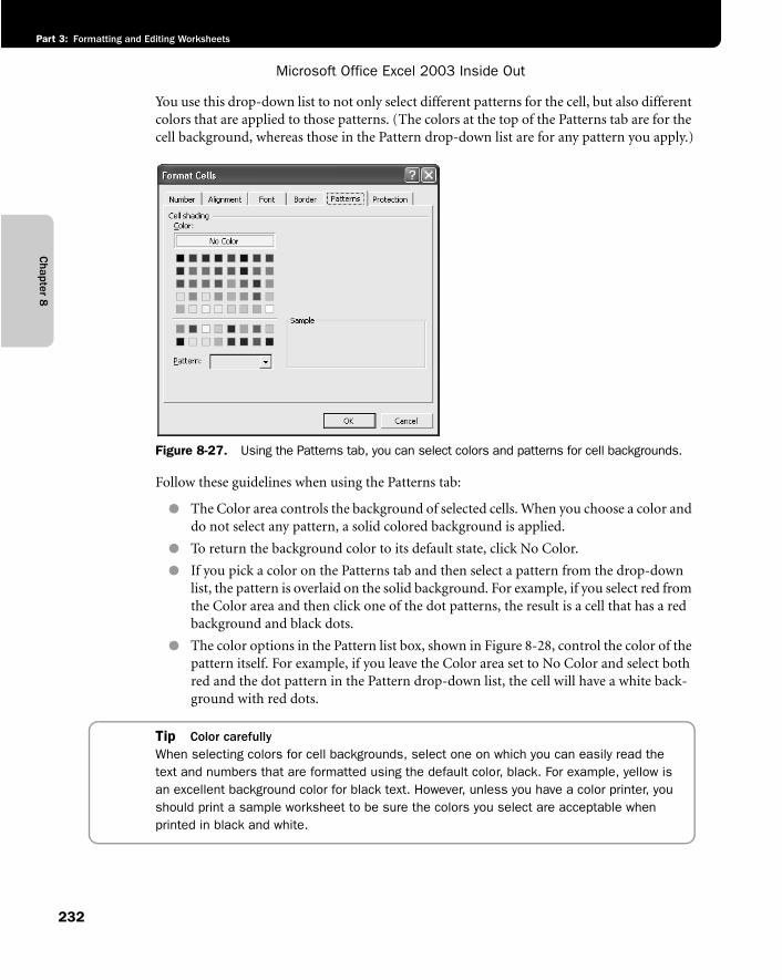
Chapter 8

Microsoft Office Excel 2003 Inside Out

Part 3: Formatting and Editing Worksheets

232

You use this drop-down list to not only select different patterns for the cell, but also different colors that are applied to those patterns. (The colors at the top of the Patterns tab are for the cell background, whereas those in the Pattern drop-down list are for any pattern you apply.)

f08ie27

Figure 8-27. Using the Patterns tab, you can select colors and patterns for cell backgrounds.

Follow these guidelines when using the Patterns tab:

● The Color area controls the background of selected cells. When you choose a color and do not select any pattern, a solid colored background is applied.

● To return the background color to its default state, click No Color.

● If you pick a color on the Patterns tab and then select a pattern from the drop-down list, the pattern is overlaid on the solid background. For example, if you select red from the Color area and then click one of the dot patterns, the result is a cell that has a red background and black dots.

● The color options in the Pattern list box, shown in Figure 8-28, control the color of the pattern itself. For example, if you leave the Color area set to No Color and select both red and the dot pattern in the Pattern drop-down list, the cell will have a white back-ground with red dots.

Tip Color carefullyWhen selecting colors for cell backgrounds, select one on which you can easily read the text and numbers that are formatted using the default color, black. For example, yellow is an excellent background color for black text. However, unless you have a color printer, you should print a sample worksheet to be sure the colors you select are acceptable when printed in black and white.

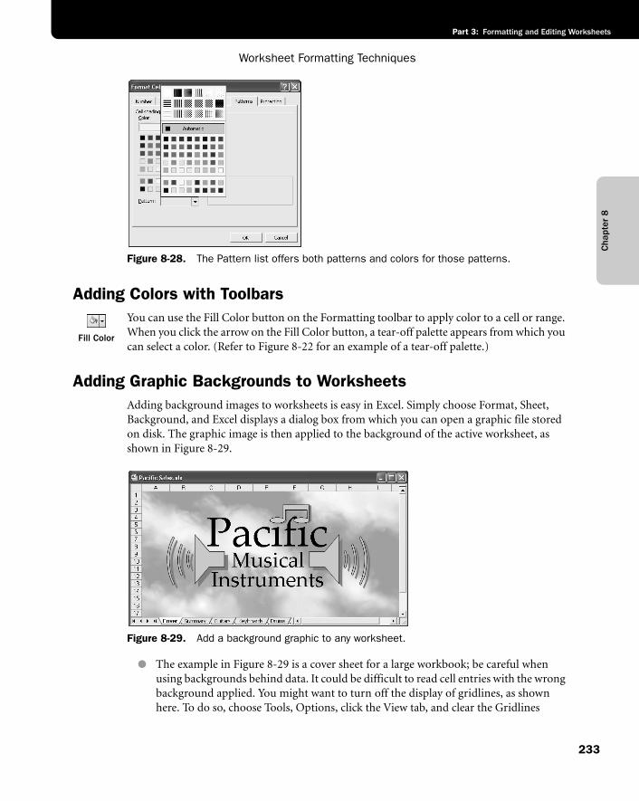
Cha

pter

8

Worksheet Formatting Techniques

233

Part 3: Formatting and Editing Worksheets

f08ie28

Figure 8-28. The Pattern list offers both patterns and colors for those patterns.

Adding Colors with Toolbars

Fill Color

You can use the Fill Color button on the Formatting toolbar to apply color to a cell or range. When you click the arrow on the Fill Color button, a tear-off palette appears from which you can select a color. (Refer to Figure 8-22 for an example of a tear-off palette.)

Adding Graphic Backgrounds to WorksheetsAdding background images to worksheets is easy in Excel. Simply choose Format, Sheet, Background, and Excel displays a dialog box from which you can open a graphic file stored on disk. The graphic image is then applied to the background of the active worksheet, as shown in Figure 8-29.

f08ie29

Figure 8-29. Add a background graphic to any worksheet.

● The example in Figure 8-29 is a cover sheet for a large workbook; be careful when using backgrounds behind data. It could be difficult to read cell entries with the wrong background applied. You might want to turn off the display of gridlines, as shown here. To do so, choose Tools, Options, click the View tab, and clear the Gridlines

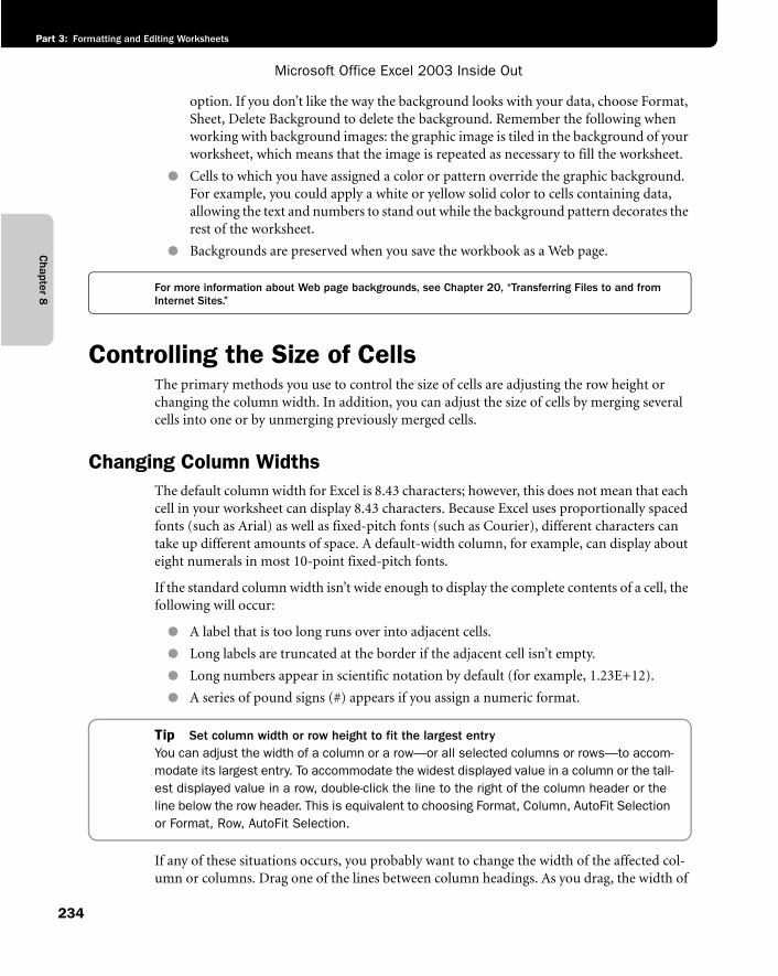
Chapter 8

Microsoft Office Excel 2003 Inside Out

Part 3: Formatting and Editing Worksheets

234

option. If you don’t like the way the background looks with your data, choose Format, Sheet, Delete Background to delete the background. Remember the following when working with background images: the graphic image is tiled in the background of your worksheet, which means that the image is repeated as necessary to fill the worksheet.

● Cells to which you have assigned a color or pattern override the graphic background. For example, you could apply a white or yellow solid color to cells containing data, allowing the text and numbers to stand out while the background pattern decorates the rest of the worksheet.

● Backgrounds are preserved when you save the workbook as a Web page.

For more information about Web page backgrounds, see Chapter 20, “Transferring Files to and from Internet Sites.”

Controlling the Size of CellsThe primary methods you use to control the size of cells are adjusting the row height or changing the column width. In addition, you can adjust the size of cells by merging several cells into one or by unmerging previously merged cells.

Changing Column WidthsThe default column width for Excel is 8.43 characters; however, this does not mean that each cell in your worksheet can display 8.43 characters. Because Excel uses proportionally spaced fonts (such as Arial) as well as fixed-pitch fonts (such as Courier), different characters can take up different amounts of space. A default-width column, for example, can display about eight numerals in most 10-point fixed-pitch fonts.

If the standard column width isn’t wide enough to display the complete contents of a cell, the following will occur:

● A label that is too long runs over into adjacent cells.

● Long labels are truncated at the border if the adjacent cell isn’t empty.

● Long numbers appear in scientific notation by default (for example, 1.23E+12).

● A series of pound signs (#) appears if you assign a numeric format.

Tip Set column width or row height to fit the largest entryYou can adjust the width of a column or a row—or all selected columns or rows—to accom-modate its largest entry. To accommodate the widest displayed value in a column or the tall-est displayed value in a row, double-click the line to the right of the column header or the line below the row header. This is equivalent to choosing Format, Column, AutoFit Selection or Format, Row, AutoFit Selection.

If any of these situations occurs, you probably want to change the width of the affected col-umn or columns. Drag one of the lines between column headings. As you drag, the width of

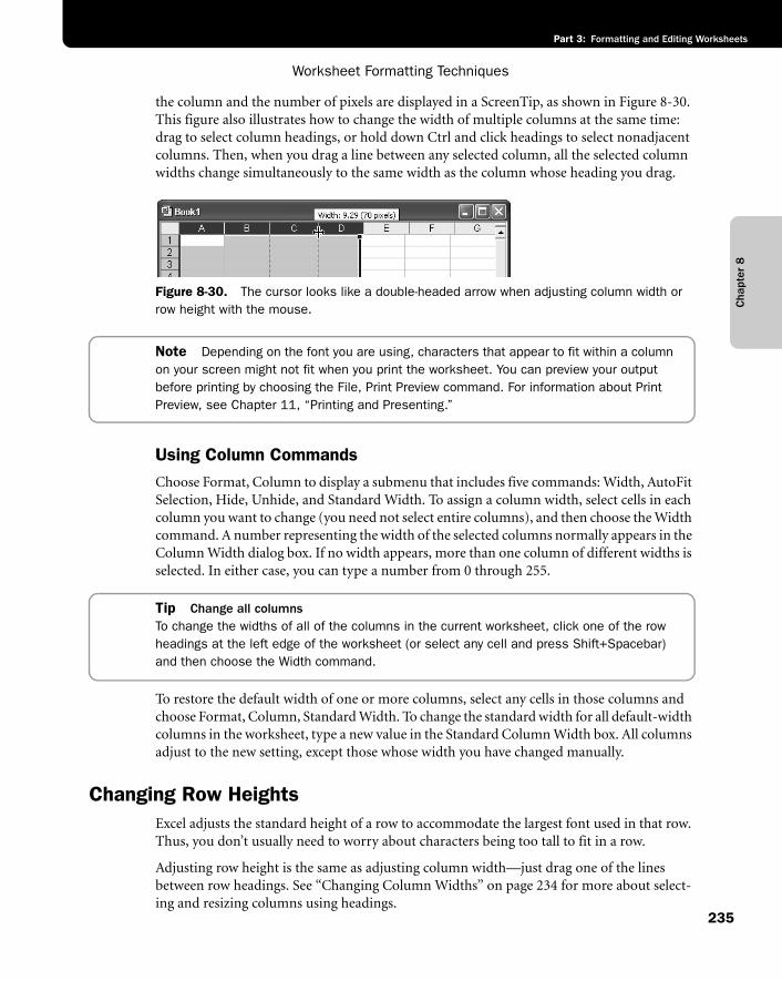
Cha

pter

8

Worksheet Formatting Techniques

235

Part 3: Formatting and Editing Worksheets

the column and the number of pixels are displayed in a ScreenTip, as shown in Figure 8-30. This figure also illustrates how to change the width of multiple columns at the same time: drag to select column headings, or hold down Ctrl and click headings to select nonadjacent columns. Then, when you drag a line between any selected column, all the selected column widths change simultaneously to the same width as the column whose heading you drag.

f08ie30

Figure 8-30. The cursor looks like a double-headed arrow when adjusting column width or row height with the mouse.

Note Depending on the font you are using, characters that appear to fit within a column on your screen might not fit when you print the worksheet. You can preview your output before printing by choosing the File, Print Preview command. For information about Print Preview, see Chapter 11, “Printing and Presenting.”

Using Column CommandsChoose Format, Column to display a submenu that includes five commands: Width, AutoFit Selection, Hide, Unhide, and Standard Width. To assign a column width, select cells in each column you want to change (you need not select entire columns), and then choose the Width command. A number representing the width of the selected columns normally appears in the Column Width dialog box. If no width appears, more than one column of different widths is selected. In either case, you can type a number from 0 through 255.

Tip Change all columnsTo change the widths of all of the columns in the current worksheet, click one of the row headings at the left edge of the worksheet (or select any cell and press Shift+Spacebar) and then choose the Width command.

To restore the default width of one or more columns, select any cells in those columns and choose Format, Column, Standard Width. To change the standard width for all default-width columns in the worksheet, type a new value in the Standard Column Width box. All columns adjust to the new setting, except those whose width you have changed manually.

Changing Row HeightsExcel adjusts the standard height of a row to accommodate the largest font used in that row. Thus, you don’t usually need to worry about characters being too tall to fit in a row.

Adjusting row height is the same as adjusting column width—just drag one of the lines between row headings. See “Changing Column Widths” on page 234 for more about select-ing and resizing columns using headings.

Chapter 8

Microsoft Office Excel 2003 Inside Out

Part 3: Formatting and Editing Worksheets

236

Using Row CommandsChoose Format, Row to display a submenu that includes four commands: Height, AutoFit, Hide, and Unhide. You can use the Height command to change the heights of several rows at the same time. Select at least one cell in each row you want to change and choose Format, Row, Height.

Tip Change all rowsTo change the heights of all the rows in the current worksheet, click one of the column headings at the top of the worksheet (or select any cell and press Ctrl+Spacebar), and then choose the Height command.

A number representing the height of the selected rows normally appears in the Row Height dialog box. If no height appears, more than one row of different heights is selected. In either case, you can type a number from 0 through 409.

To restore the default height of one or more rows, select any cells in those rows and choose Format, Row, AutoFit. Unlike column width, you cannot define a standard row height. The AutoFit command serves the same function, returning empty rows to the standard height needed to accommodate the default font and fitting row heights to accommodate the tallest entry. When you create or edit a multiline text entry using the Wrap Text or the Justify options on the Alignment tab of the Format Cells dialog box, Excel automatically adjusts the row height to accommodate it.

For more information, see “Wrapping Text in Cells” and “Justifying Text in Cells” on page 221.

Hiding a Column or RowIf you want to hide information within a worksheet, you can hide entire columns or rows. To hide a column, select any cell in the column you want to hide and choose Format, Column, Hide. Excel sets the width of the column to zero. You can also hide a column by dragging the line between the column headings to the left until you have narrowed the column to zero; or you can type 0 in the Column Width dialog box. When a column’s width is set to 0, Excel skips over the column when you move the active cell, and the column’s letter disappears from the top of the worksheet. For example, if you hide column C, the column heading line reads A, B, D, and so on.

To redisplay a column, drag to select the column headings on both sides of the hidden col-umn and choose Format, Column, Unhide.

You can hide and redisplay rows in a similar manner, using the mouse or the equivalent Row submenu on the Format menu. Note that the Hidden option on the Protection tab of the For-mat Cells dialog box hides only formulas in the formula bar.

For more information about protection options, see “Protecting Worksheets” on page 127.

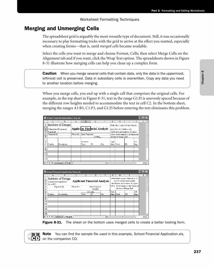
Cha

pter

8

Worksheet Formatting Techniques

237

Part 3: Formatting and Editing Worksheets

Merging and Unmerging CellsThe spreadsheet grid is arguably the most versatile type of document. Still, it was occasionally necessary to play formatting tricks with the grid to arrive at the effect you wanted, especially when creating forms—that is, until merged cells became available.

Select the cells you want to merge and choose Format, Cells; then select Merge Cells on the Alignment tab and if you want, click the Wrap Text option. The spreadsheets shown in Figure 8-31 illustrate how merging cells can help you clean up a complex form.

Caution When you merge several cells that contain data, only the data in the uppermost, leftmost cell is preserved. Data in subsidiary cells is overwritten. Copy any data you need to another location before merging.

When you merge cells, you end up with a single cell that comprises the original cells. For example, in the top sheet in Figure 8-31, text in the range G1:J5 is unevenly spaced because of the different row heights needed to accommodate the text in cell C2. In the bottom sheet, merging the ranges A1:B3, C1:F3, and G1:J5 before entering the text eliminates this problem.

f08ie31

Figure 8-31. The sheet on the bottom uses merged cells to create a better looking form.

Note You can find the sample file used in this example, School Financial Application.xls, on the companion CD.

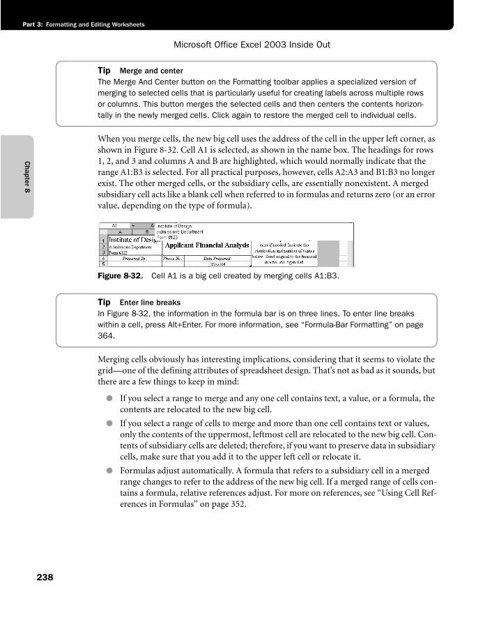
Chapter 8

Microsoft Office Excel 2003 Inside Out

Part 3: Formatting and Editing Worksheets

238

Tip Merge and centerThe Merge And Center button on the Formatting toolbar applies a specialized version of merging to selected cells that is particularly useful for creating labels across multiple rows or columns. This button merges the selected cells and then centers the contents horizon-tally in the newly merged cells. Click again to restore the merged cell to individual cells.

When you merge cells, the new big cell uses the address of the cell in the upper left corner, as shown in Figure 8-32. Cell A1 is selected, as shown in the name box. The headings for rows 1, 2, and 3 and columns A and B are highlighted, which would normally indicate that the range A1:B3 is selected. For all practical purposes, however, cells A2:A3 and B1:B3 no longer exist. The other merged cells, or the subsidiary cells, are essentially nonexistent. A merged subsidiary cell acts like a blank cell when referred to in formulas and returns zero (or an error value, depending on the type of formula).

f08ie32

Figure 8-32. Cell A1 is a big cell created by merging cells A1:B3.

Tip Enter line breaksIn Figure 8-32, the information in the formula bar is on three lines. To enter line breaks within a cell, press Alt+Enter. For more information, see “Formula-Bar Formatting” on page 364.

Merging cells obviously has interesting implications, considering that it seems to violate the grid—one of the defining attributes of spreadsheet design. That’s not as bad as it sounds, but there are a few things to keep in mind:

● If you select a range to merge and any one cell contains text, a value, or a formula, the contents are relocated to the new big cell.

● If you select a range of cells to merge and more than one cell contains text or values, only the contents of the uppermost, leftmost cell are relocated to the new big cell. Con-tents of subsidiary cells are deleted; therefore, if you want to preserve data in subsidiary cells, make sure that you add it to the upper left cell or relocate it.

● Formulas adjust automatically. A formula that refers to a subsidiary cell in a merged range changes to refer to the address of the new big cell. If a merged range of cells con-tains a formula, relative references adjust. For more on references, see “Using Cell Ref-erences in Formulas” on page 352.

Cha

pter

8

Worksheet Formatting Techniques

239

Part 3: Formatting and Editing Worksheets

● You can copy, delete, cut and paste, or click and drag big cells as you would any other cell. When you copy or move a big cell, it replaces the same number of cells at the des-tination. The original location of a cut or deleted big cell returns to individual cells.

● You can drag the Fill handle of a big cell as you can drag the Fill handle of regular cells. When you do so, the big cell is replicated, in both size and content, replacing all regular cells in its path. For more on using the Fill handle, see “Filling and Creating Data Series” on page 171.

● If you merge cells containing border formatting other than along any boundary of the selected range, border formats are erased.

● You can explode, or unmerge, a merged cell to return it to the original range of indi-vidual cells. To unmerge cells, select the big cell, choose Format, Cells, Alignment, and clear the Merge Cells option.

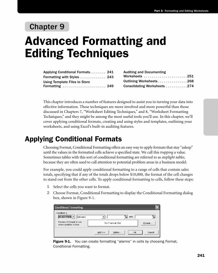
241

Part 3: Formatting and Editing Worksheets

Chapter 9

Advanced Formatting and Editing Techniques

Applying Conditional Formats . . . . . . . . 241Formatting with Styles . . . . . . . . . . . . . 243Using Template Files to Store Formatting . . . . . . . . . . . . . . . . . . . . . . 249

Auditing and Documenting Worksheets . . . . . . . . . . . . . . . . . . . . . . 251Outlining Worksheets . . . . . . . . . . . . . . . 268Consolidating Worksheets . . . . . . . . . . . 274

This chapter introduces a number of features designed to assist you in turning your data into effective information. These techniques are more involved and more powerful than those discussed in Chapters 7, “Worksheet Editing Techniques,” and 8, “Worksheet Formatting Techniques,” and they might be among the most useful tools you’ll use. In this chapter, we’ll cover applying conditional formats, creating and using styles and templates, outlining your worksheets, and using Excel’s built-in auditing features.

Applying Conditional FormatsChoosing Format, Conditional Formatting offers an easy way to apply formats that stay “asleep” until the values in the formatted cells achieve a specified state. We call this trapping a value. Sometimes tables with this sort of conditional formatting are referred to as stoplight tables,because they are often used to call attention to potential problem areas in a business model.

For example, you could apply conditional formatting to a range of cells that contain sales totals, specifying that if any of the totals drops below $10,000, the format of the cell changes to stand out from the other cells. To apply conditional formatting to cells, follow these steps:

1 Select the cells you want to format.

2 Choose Format, Conditional Formatting to display the Conditional Formatting dialog box, shown in Figure 9-1.

f09ie01

Figure 9-1. You can create formatting “alarms” in cells by choosing Format, Conditional Formatting.

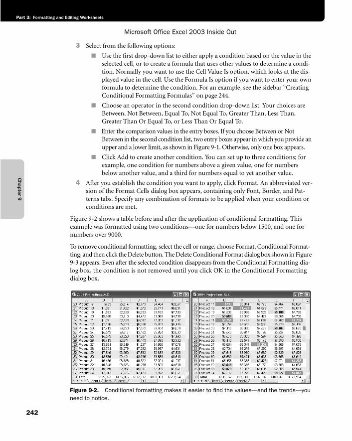
Chapter 9

Microsoft Office Excel 2003 Inside Out

Part 3: Formatting and Editing Worksheets

242

3 Select from the following options:

■ Use the first drop-down list to either apply a condition based on the value in the selected cell, or to create a formula that uses other values to determine a condi-tion. Normally you want to use the Cell Value Is option, which looks at the dis-played value in the cell. Use the Formula Is option if you want to enter your own formula to determine the condition. For an example, see the sidebar “Creating Conditional Formatting Formulas” on page 244.

■ Choose an operator in the second condition drop-down list. Your choices are Between, Not Between, Equal To, Not Equal To, Greater Than, Less Than, Greater Than Or Equal To, or Less Than Or Equal To.

■ Enter the comparison values in the entry boxes. If you choose Between or Not Between in the second condition list, two entry boxes appear in which you provide an upper and a lower limit, as shown in Figure 9-1. Otherwise, only one box appears.

■ Click Add to create another condition. You can set up to three conditions; for example, one condition for numbers above a given value, one for numbers below another value, and a third for numbers equal to yet another value.

4 After you establish the condition you want to apply, click Format. An abbreviated ver-sion of the Format Cells dialog box appears, containing only Font, Border, and Pat-terns tabs. Specify any combination of formats to be applied when your condition or conditions are met.

Figure 9-2 shows a table before and after the application of conditional formatting. This example was formatted using two conditions—one for numbers below 1500, and one for numbers over 9000.

To remove conditional formatting, select the cell or range, choose Format, Conditional Format-ting, and then click the Delete button. The Delete Conditional Format dialog box shown in Figure 9-3 appears. Even after the selected condition disappears from the Conditional Formatting dia-log box, the condition is not removed until you click OK in the Conditional Formatting dialog box.

f09ie02

Figure 9-2. Conditional formatting makes it easier to find the values—and the trends—you need to notice.

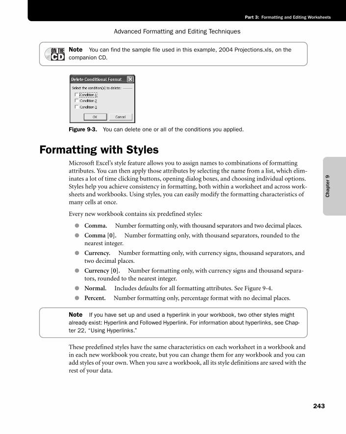
Cha

pter

9

Advanced Formatting and Editing Techniques

243

Part 3: Formatting and Editing Worksheets

Note You can find the sample file used in this example, 2004 Projections.xls, on the companion CD.

f09ie03

Figure 9-3. You can delete one or all of the conditions you applied.

Formatting with StylesMicrosoft Excel’s style feature allows you to assign names to combinations of formatting attributes. You can then apply those attributes by selecting the name from a list, which elim-inates a lot of time clicking buttons, opening dialog boxes, and choosing individual options. Styles help you achieve consistency in formatting, both within a worksheet and across work-sheets and workbooks. Using styles, you can easily modify the formatting characteristics of many cells at once.

Every new workbook contains six predefined styles:

● Comma. Number formatting only, with thousand separators and two decimal places.

● Comma [0]. Number formatting only, with thousand separators, rounded to the nearest integer.

● Currency. Number formatting only, with currency signs, thousand separators, and two decimal places.

● Currency [0]. Number formatting only, with currency signs and thousand separa-tors, rounded to the nearest integer.

● Normal. Includes defaults for all formatting attributes. See Figure 9-4.

● Percent. Number formatting only, percentage format with no decimal places.

Note If you have set up and used a hyperlink in your workbook, two other styles might already exist: Hyperlink and Followed Hyperlink. For information about hyperlinks, see Chap-ter 22, “Using Hyperlinks.”

These predefined styles have the same characteristics on each worksheet in a workbook and in each new workbook you create, but you can change them for any workbook and you can add styles of your own. When you save a workbook, all its style definitions are saved with the rest of your data.

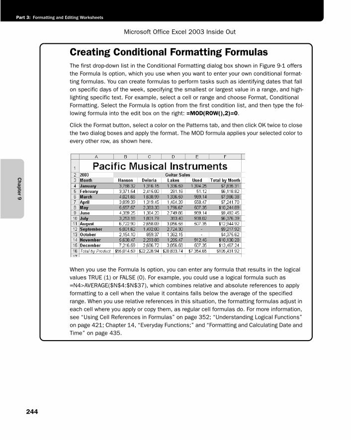
Chapter 9

Microsoft Office Excel 2003 Inside Out

Part 3: Formatting and Editing Worksheets

244

Creating Conditional Formatting FormulasThe first drop-down list in the Conditional Formatting dialog box shown in Figure 9-1 offers the Formula Is option, which you use when you want to enter your own conditional format-ting formulas. You can create formulas to perform tasks such as identifying dates that fall on specific days of the week, specifying the smallest or largest value in a range, and high-lighting specific text. For example, select a cell or range and choose Format, Conditional Formatting. Select the Formula Is option from the first condition list, and then type the fol-lowing formula into the edit box on the right: =MOD(ROW(),2)=0.

Click the Format button, select a color on the Patterns tab, and then click OK twice to close the two dialog boxes and apply the format. The MOD formula applies your selected color to every other row, as shown here.

g09ie01

When you use the Formula Is option, you can enter any formula that results in the logical values TRUE (1) or FALSE (0). For example, you could use a logical formula such as =N4>AVERAGE($N$4:$N$37), which combines relative and absolute references to apply formatting to a cell when the value it contains falls below the average of the specified range. When you use relative references in this situation, the formatting formulas adjust in each cell where you apply or copy them, as regular cell formulas do. For more information, see “Using Cell References in Formulas” on page 352; “Understanding Logical Functions” on page 421; Chapter 14, “Everyday Functions;” and “Formatting and Calculating Date and Time” on page 435.

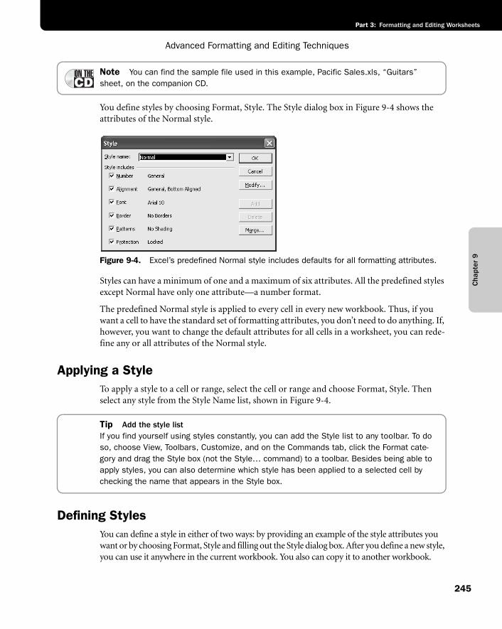
Cha

pter

9

Advanced Formatting and Editing Techniques

245

Part 3: Formatting and Editing Worksheets

Note You can find the sample file used in this example, Pacific Sales.xls, “Guitars” sheet, on the companion CD.

You define styles by choosing Format, Style. The Style dialog box in Figure 9-4 shows the attributes of the Normal style.

f09ie04

Figure 9-4. Excel’s predefined Normal style includes defaults for all formatting attributes.

Styles can have a minimum of one and a maximum of six attributes. All the predefined styles except Normal have only one attribute—a number format.

The predefined Normal style is applied to every cell in every new workbook. Thus, if you want a cell to have the standard set of formatting attributes, you don’t need to do anything. If, however, you want to change the default attributes for all cells in a worksheet, you can rede-fine any or all attributes of the Normal style.

Applying a StyleTo apply a style to a cell or range, select the cell or range and choose Format, Style. Then select any style from the Style Name list, shown in Figure 9-4.

Tip Add the style list If you find yourself using styles constantly, you can add the Style list to any toolbar. To do so, choose View, Toolbars, Customize, and on the Commands tab, click the Format cate-gory and drag the Style box (not the Style… command) to a toolbar. Besides being able to apply styles, you can also determine which style has been applied to a selected cell by checking the name that appears in the Style box.

Defining StylesYou can define a style in either of two ways: by providing an example of the style attributes you want or by choosing Format, Style and filling out the Style dialog box. After you define a new style, you can use it anywhere in the current workbook. You also can copy it to another workbook.

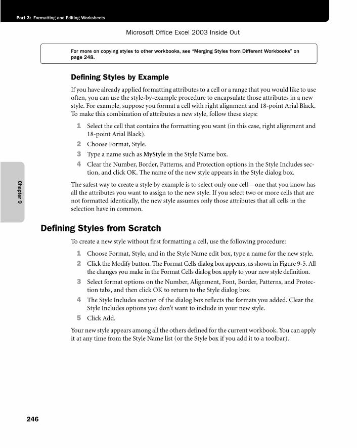
Chapter 9

Microsoft Office Excel 2003 Inside Out

Part 3: Formatting and Editing Worksheets

246

For more on copying styles to other workbooks, see “Merging Styles from Different Workbooks” on page 248.

Defining Styles by ExampleIf you have already applied formatting attributes to a cell or a range that you would like to use often, you can use the style-by-example procedure to encapsulate those attributes in a new style. For example, suppose you format a cell with right alignment and 18-point Arial Black. To make this combination of attributes a new style, follow these steps:

1 Select the cell that contains the formatting you want (in this case, right alignment and 18-point Arial Black).

2 Choose Format, Style.

3 Type a name such as MyStyle in the Style Name box.

4 Clear the Number, Border, Patterns, and Protection options in the Style Includes sec-tion, and click OK. The name of the new style appears in the Style dialog box.

The safest way to create a style by example is to select only one cell—one that you know has all the attributes you want to assign to the new style. If you select two or more cells that are not formatted identically, the new style assumes only those attributes that all cells in the selection have in common.

Defining Styles from ScratchTo create a new style without first formatting a cell, use the following procedure:

1 Choose Format, Style, and in the Style Name edit box, type a name for the new style.

2 Click the Modify button. The Format Cells dialog box appears, as shown in Figure 9-5. All the changes you make in the Format Cells dialog box apply to your new style definition.

3 Select format options on the Number, Alignment, Font, Border, Patterns, and Protec-tion tabs, and then click OK to return to the Style dialog box.

4 The Style Includes section of the dialog box reflects the formats you added. Clear the Style Includes options you don’t want to include in your new style.

5 Click Add.

Your new style appears among all the others defined for the current workbook. You can apply it at any time from the Style Name list (or the Style box if you add it to a toolbar).

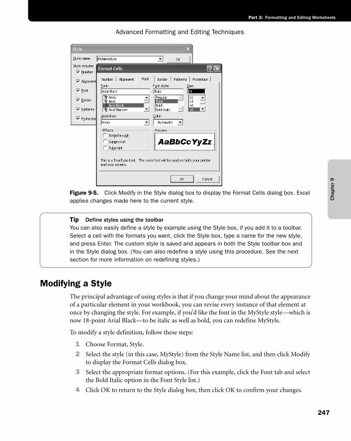
Cha

pter

9

Advanced Formatting and Editing Techniques

247

Part 3: Formatting and Editing Worksheets

f09ie05

Figure 9-5. Click Modify in the Style dialog box to display the Format Cells dialog box. Excel applies changes made here to the current style.

Tip Define styles using the toolbarYou can also easily define a style by example using the Style box, if you add it to a toolbar. Select a cell with the formats you want, click the Style box, type a name for the new style, and press Enter. The custom style is saved and appears in both the Style toolbar box and in the Style dialog box. (You can also redefine a style using this procedure. See the next section for more information on redefining styles.)

Modifying a StyleThe principal advantage of using styles is that if you change your mind about the appearance of a particular element in your workbook, you can revise every instance of that element at once by changing the style. For example, if you’d like the font in the MyStyle style—which is now 18-point Arial Black—to be italic as well as bold, you can redefine MyStyle.

To modify a style definition, follow these steps:

1 Choose Format, Style.

2 Select the style (in this case, MyStyle) from the Style Name list, and then click Modify to display the Format Cells dialog box.

3 Select the appropriate format options. (For this example, click the Font tab and select the Bold Italic option in the Font Style list.)

4 Click OK to return to the Style dialog box, then click OK to confirm your changes.

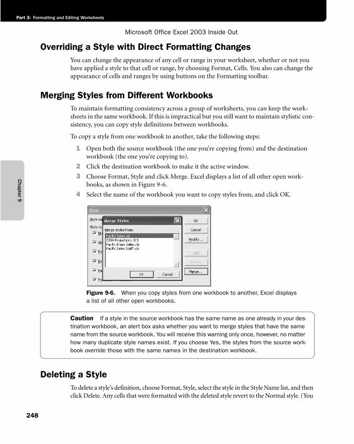
Chapter 9

Microsoft Office Excel 2003 Inside Out

Part 3: Formatting and Editing Worksheets

248

Overriding a Style with Direct Formatting ChangesYou can change the appearance of any cell or range in your worksheet, whether or not you have applied a style to that cell or range, by choosing Format, Cells. You also can change the appearance of cells and ranges by using buttons on the Formatting toolbar.

Merging Styles from Different WorkbooksTo maintain formatting consistency across a group of worksheets, you can keep the work-sheets in the same workbook. If this is impractical but you still want to maintain stylistic con-sistency, you can copy style definitions between workbooks.

To copy a style from one workbook to another, take the following steps:

1 Open both the source workbook (the one you’re copying from) and the destination workbook (the one you’re copying to).

2 Click the destination workbook to make it the active window.

3 Choose Format, Style and click Merge. Excel displays a list of all other open work-books, as shown in Figure 9-6.

4 Select the name of the workbook you want to copy styles from, and click OK.

f09ie06

Figure 9-6. When you copy styles from one workbook to another, Excel displays a list of all other open workbooks.

Caution If a style in the source workbook has the same name as one already in your des-tination workbook, an alert box asks whether you want to merge styles that have the same name from the source workbook. You will receive this warning only once, however, no matter how many duplicate style names exist. If you choose Yes, the styles from the source work-book override those with the same names in the destination workbook.

Deleting a StyleTo delete a style’s definition, choose Format, Style, select the style in the Style Name list, and then click Delete. Any cells that were formatted with the deleted style revert to the Normal style. (You

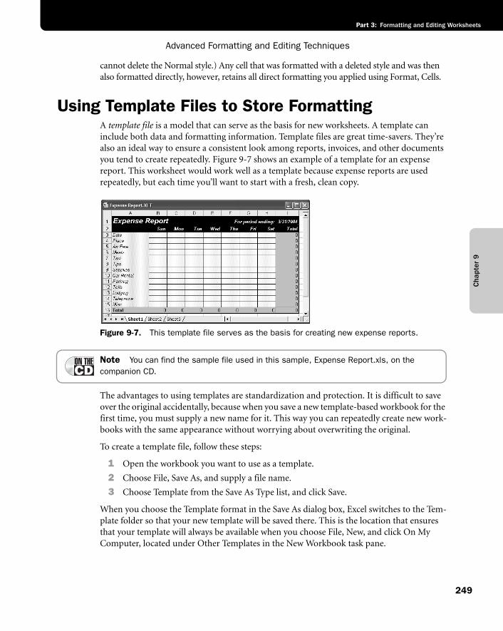
Cha

pter

9

Advanced Formatting and Editing Techniques

249

Part 3: Formatting and Editing Worksheets

cannot delete the Normal style.) Any cell that was formatted with a deleted style and was then also formatted directly, however, retains all direct formatting you applied using Format, Cells.

Using Template Files to Store FormattingA template file is a model that can serve as the basis for new worksheets. A template can include both data and formatting information. Template files are great time-savers. They’re also an ideal way to ensure a consistent look among reports, invoices, and other documents you tend to create repeatedly. Figure 9-7 shows an example of a template for an expense report. This worksheet would work well as a template because expense reports are used repeatedly, but each time you’ll want to start with a fresh, clean copy.

f09ie07

Figure 9-7. This template file serves as the basis for creating new expense reports.

Note You can find the sample file used in this sample, Expense Report.xls, on the companion CD.

The advantages to using templates are standardization and protection. It is difficult to save over the original accidentally, because when you save a new template-based workbook for the first time, you must supply a new name for it. This way you can repeatedly create new work-books with the same appearance without worrying about overwriting the original.

To create a template file, follow these steps:

1 Open the workbook you want to use as a template.

2 Choose File, Save As, and supply a file name.

3 Choose Template from the Save As Type list, and click Save.

When you choose the Template format in the Save As dialog box, Excel switches to the Tem-plate folder so that your new template will be saved there. This is the location that ensures that your template will always be available when you choose File, New, and click On My Computer, located under Other Templates in the New Workbook task pane.

Chapter 9

Microsoft Office Excel 2003 Inside Out

Part 3: Formatting and Editing Worksheets

250

Any Excel workbook can be used as a template, even if it was not saved in template format. When you installed Excel, a folder named Templates was installed on your hard disk in the following location.

C:\Documents and Settings\<your name>\Application Data\Microsoft\Templates (Windows 2000, XP)

Note In Windows 2000 and Windows XP, the Application Data folder is normally hidden. When you choose the Template format in the Save As dialog box, you can save template files there, but you won’t be able to see it in the Windows Explorer unless you change the view options. To do so, in the Windows Explorer choose Tools, Folder Options, and on the View tab, click Show Hidden Files And Folders.

Any workbook you move or copy to the Templates folder appears on the General tab of the Tem-plates dialog box and behaves like a template file. When you open a workbook that appears in the Templates dialog box, the original workbook does not open; instead, a fresh copy of the workbook is created. The copy is given a temporary name made up of the original file name plus a number. If the template file is named Expenses, for example, the working copy is named Expenses1.

Tip Show file extensionsYou can choose to display MS-DOS three-character extensions (such as XLT for template and XLS for regular workbook) so you can tell at a glance what format the file was saved in. To do so, open the Windows Explorer. On the Explorer’s Tools menu, choose Folder Options and clear the Hide File Extensions For Known File Types option on the View tab.

Inside OutThe New dialog box is dead, long live the task pane

When you choose File, New, the New dialog box is not displayed, as it had been up until Excel 2002. Now when you choose File, New, the New Workbook task pane appears on the right side of the workbook window, which is probably a step forward in usability. But it might confound you for a while until you get used to it. For example, if the New Workbook task pane is already open, choosing File, New seems to do nothing at all—especially if you’re expecting a dialog box to appear. What used to be called the New dialog box is now called the Templates dialog box, and you open it by clicking On My Computer in the New Workbook task pane under Other Templates.

Adding Templates to the XLStart FolderAny Excel files that you place in the XLStart folder are opened every time you start Excel, except for templates. When you place templates (with the XLT extension) in the XLStart folder, they are not opened; instead, they appear in the Templates dialog box when you click On My Computer in the New Workbook task pane.

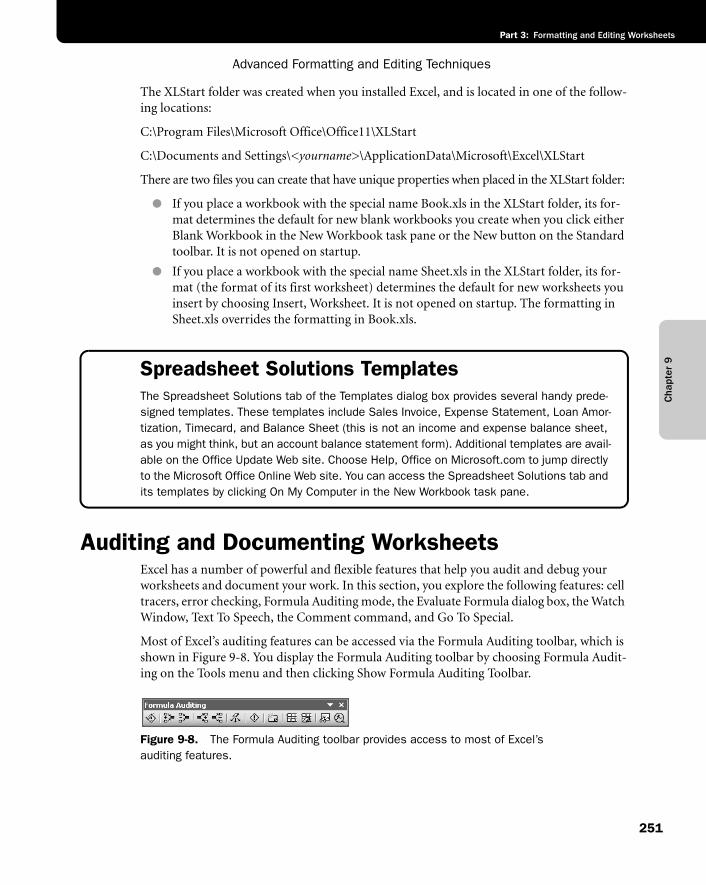
Cha

pter

9

Advanced Formatting and Editing Techniques

251

Part 3: Formatting and Editing Worksheets

The XLStart folder was created when you installed Excel, and is located in one of the follow-ing locations:

C:\Program Files\Microsoft Office\Office11\XLStart

C:\Documents and Settings\<yourname>\ApplicationData\Microsoft\Excel\XLStart

There are two files you can create that have unique properties when placed in the XLStart folder:

● If you place a workbook with the special name Book.xls in the XLStart folder, its for-mat determines the default for new blank workbooks you create when you click either Blank Workbook in the New Workbook task pane or the New button on the Standard toolbar. It is not opened on startup.

● If you place a workbook with the special name Sheet.xls in the XLStart folder, its for-mat (the format of its first worksheet) determines the default for new worksheets you insert by choosing Insert, Worksheet. It is not opened on startup. The formatting in Sheet.xls overrides the formatting in Book.xls.

Spreadsheet Solutions TemplatesThe Spreadsheet Solutions tab of the Templates dialog box provides several handy prede-signed templates. These templates include Sales Invoice, Expense Statement, Loan Amor-tization, Timecard, and Balance Sheet (this is not an income and expense balance sheet, as you might think, but an account balance statement form). Additional templates are avail-able on the Office Update Web site. Choose Help, Office on Microsoft.com to jump directly to the Microsoft Office Online Web site. You can access the Spreadsheet Solutions tab and its templates by clicking On My Computer in the New Workbook task pane.

Auditing and Documenting WorksheetsExcel has a number of powerful and flexible features that help you audit and debug your worksheets and document your work. In this section, you explore the following features: cell tracers, error checking, Formula Auditing mode, the Evaluate Formula dialog box, the Watch Window, Text To Speech, the Comment command, and Go To Special.

Most of Excel’s auditing features can be accessed via the Formula Auditing toolbar, which is shown in Figure 9-8. You display the Formula Auditing toolbar by choosing Formula Audit-ing on the Tools menu and then clicking Show Formula Auditing Toolbar.

f09ie08

Figure 9-8. The Formula Auditing toolbar provides access to most of Excel’s auditing features.

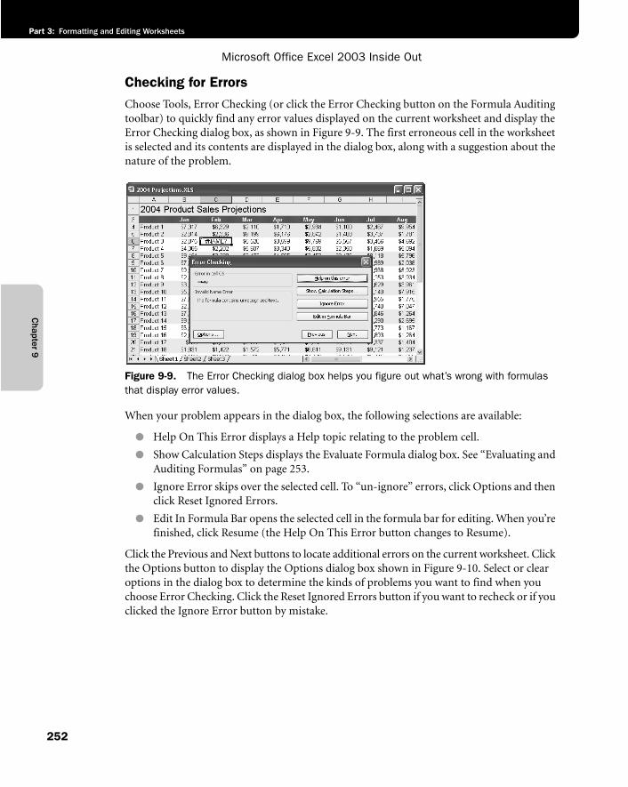
Chapter 9

Microsoft Office Excel 2003 Inside Out

Part 3: Formatting and Editing Worksheets

252

Checking for ErrorsChoose Tools, Error Checking (or click the Error Checking button on the Formula Auditing toolbar) to quickly find any error values displayed on the current worksheet and display the Error Checking dialog box, as shown in Figure 9-9. The first erroneous cell in the worksheet is selected and its contents are displayed in the dialog box, along with a suggestion about the nature of the problem.

f09ie09

Figure 9-9. The Error Checking dialog box helps you figure out what’s wrong with formulas that display error values.

When your problem appears in the dialog box, the following selections are available:

● Help On This Error displays a Help topic relating to the problem cell.

● Show Calculation Steps displays the Evaluate Formula dialog box. See “Evaluating and Auditing Formulas” on page 253.

● Ignore Error skips over the selected cell. To “un-ignore” errors, click Options and then click Reset Ignored Errors.

● Edit In Formula Bar opens the selected cell in the formula bar for editing. When you’re finished, click Resume (the Help On This Error button changes to Resume).

Click the Previous and Next buttons to locate additional errors on the current worksheet. Click the Options button to display the Options dialog box shown in Figure 9-10. Select or clear options in the dialog box to determine the kinds of problems you want to find when you choose Error Checking. Click the Reset Ignored Errors button if you want to recheck or if you clicked the Ignore Error button by mistake.

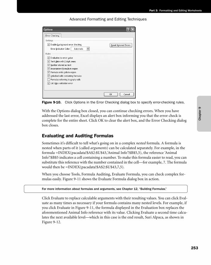
Cha

pter

9

Advanced Formatting and Editing Techniques

253

Part 3: Formatting and Editing Worksheets

f09ie10

Figure 9-10. Click Options in the Error Checking dialog box to specify error-checking rules.

With the Options dialog box closed, you can continue checking errors. When you have addressed the last error, Excel displays an alert box informing you that the error check is complete for the entire sheet. Click OK to clear the alert box, and the Error Checking dialog box closes.

Evaluating and Auditing FormulasSometimes it’s difficult to tell what’s going on in a complex nested formula. A formula is nested when parts of it (called arguments) can be calculated separately. For example, in the formula =INDEX(pacadata!$A$2:$U$43,‘Animal Info’!$B$5,5), the reference ‘Animal Info’!$B$5 indicates a cell containing a number. To make this formula easier to read, you can substitute this reference with the number contained in the cell—for example, 7. The formula would then be =INDEX(pacadata!$A$2:$U$43,7,5).

When you choose Tools, Formula Auditing, Evaluate Formula, you can check complex for-mulas easily. Figure 9-11 shows the Evaluate Formula dialog box in action.

For more information about formulas and arguments, see Chapter 12, “Building Formulas.”

Click Evaluate to replace calculable arguments with their resulting values. You can click Eval-uate as many times as necessary if your formula contains many nested levels. For example, if you click Evaluate in Figure 9-11, the formula displayed in the Evaluation box replaces the aforementioned Animal Info reference with its value. Clicking Evaluate a second time calcu-lates the next available level—which in this case is the end result, Suri Alpaca, as shown in Figure 9-12.

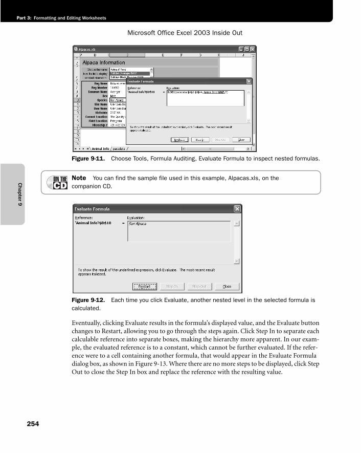
Chapter 9

Microsoft Office Excel 2003 Inside Out

Part 3: Formatting and Editing Worksheets

254

f09ie11

Figure 9-11. Choose Tools, Formula Auditing, Evaluate Formula to inspect nested formulas.

Note You can find the sample file used in this example, Alpacas.xls, on the companion CD.

f09ie12

Figure 9-12. Each time you click Evaluate, another nested level in the selected formula is calculated.

Eventually, clicking Evaluate results in the formula’s displayed value, and the Evaluate button changes to Restart, allowing you to go through the steps again. Click Step In to separate each calculable reference into separate boxes, making the hierarchy more apparent. In our exam-ple, the evaluated reference is to a constant, which cannot be further evaluated. If the refer-ence were to a cell containing another formula, that would appear in the Evaluate Formula dialog box, as shown in Figure 9-13. Where there are no more steps to be displayed, click Step Out to close the Step In box and replace the reference with the resulting value.

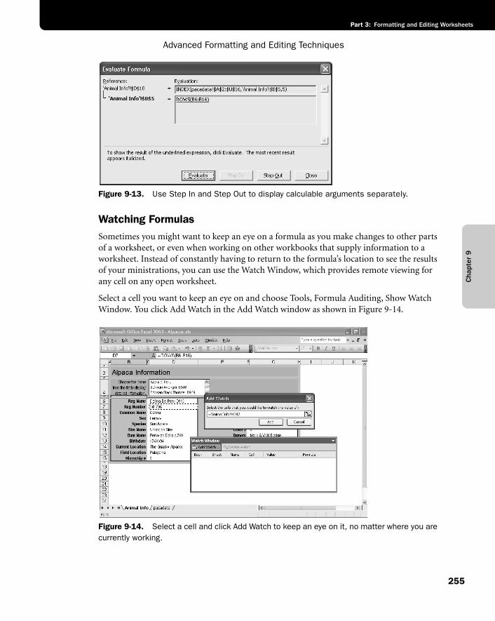
Cha

pter

9

Advanced Formatting and Editing Techniques

255

Part 3: Formatting and Editing Worksheets

f09ie13

Figure 9-13. Use Step In and Step Out to display calculable arguments separately.

Watching FormulasSometimes you might want to keep an eye on a formula as you make changes to other parts of a worksheet, or even when working on other workbooks that supply information to a worksheet. Instead of constantly having to return to the formula’s location to see the results of your ministrations, you can use the Watch Window, which provides remote viewing for any cell on any open worksheet.

Select a cell you want to keep an eye on and choose Tools, Formula Auditing, Show Watch Window. You click Add Watch in the Add Watch window as shown in Figure 9-14.

f09ie14

Figure 9-14. Select a cell and click Add Watch to keep an eye on it, no matter where you are currently working.

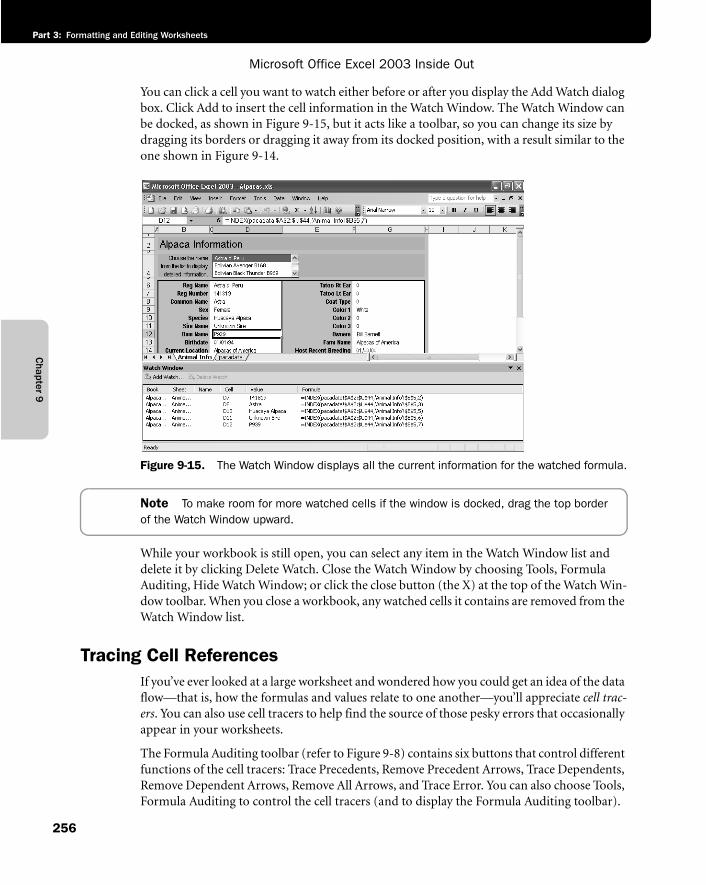
Chapter 9

Microsoft Office Excel 2003 Inside Out

Part 3: Formatting and Editing Worksheets

256

You can click a cell you want to watch either before or after you display the Add Watch dialog box. Click Add to insert the cell information in the Watch Window. The Watch Window can be docked, as shown in Figure 9-15, but it acts like a toolbar, so you can change its size by dragging its borders or dragging it away from its docked position, with a result similar to the one shown in Figure 9-14.

f09ie15

Figure 9-15. The Watch Window displays all the current information for the watched formula.

Note To make room for more watched cells if the window is docked, drag the top border of the Watch Window upward.

While your workbook is still open, you can select any item in the Watch Window list and delete it by clicking Delete Watch. Close the Watch Window by choosing Tools, Formula Auditing, Hide Watch Window; or click the close button (the X) at the top of the Watch Win-dow toolbar. When you close a workbook, any watched cells it contains are removed from the Watch Window list.

Tracing Cell ReferencesIf you’ve ever looked at a large worksheet and wondered how you could get an idea of the data flow—that is, how the formulas and values relate to one another—you’ll appreciate cell trac-ers. You can also use cell tracers to help find the source of those pesky errors that occasionally appear in your worksheets.

The Formula Auditing toolbar (refer to Figure 9-8) contains six buttons that control different functions of the cell tracers: Trace Precedents, Remove Precedent Arrows, Trace Dependents, Remove Dependent Arrows, Remove All Arrows, and Trace Error. You can also choose Tools, Formula Auditing to control the cell tracers (and to display the Formula Auditing toolbar).

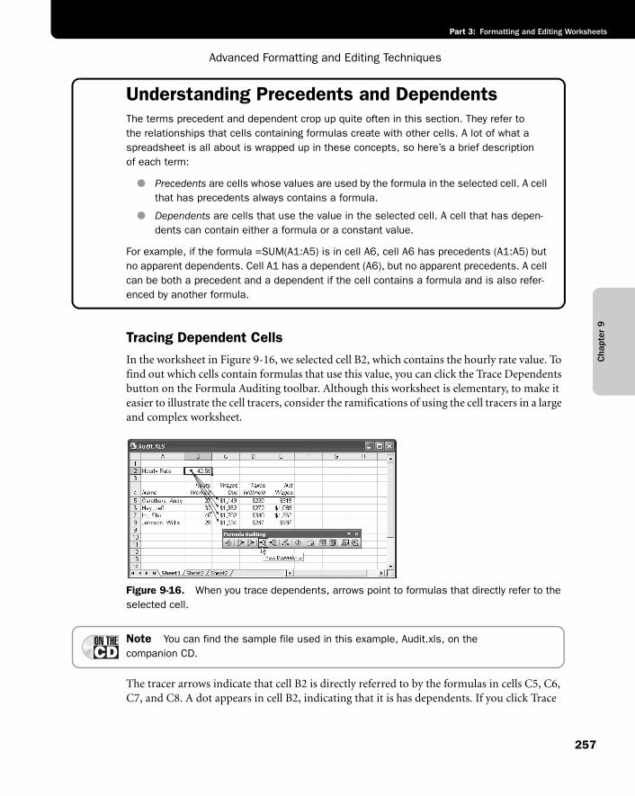
Cha

pter

9

Advanced Formatting and Editing Techniques

257

Part 3: Formatting and Editing Worksheets

Understanding Precedents and DependentsThe terms precedent and dependent crop up quite often in this section. They refer to the relationships that cells containing formulas create with other cells. A lot of what a spreadsheet is all about is wrapped up in these concepts, so here’s a brief description of each term:

● Precedents are cells whose values are used by the formula in the selected cell. A cell that has precedents always contains a formula.

● Dependents are cells that use the value in the selected cell. A cell that has depen-dents can contain either a formula or a constant value.

For example, if the formula =SUM(A1:A5) is in cell A6, cell A6 has precedents (A1:A5) but no apparent dependents. Cell A1 has a dependent (A6), but no apparent precedents. A cell can be both a precedent and a dependent if the cell contains a formula and is also refer-enced by another formula.

Tracing Dependent CellsIn the worksheet in Figure 9-16, we selected cell B2, which contains the hourly rate value. To find out which cells contain formulas that use this value, you can click the Trace Dependents button on the Formula Auditing toolbar. Although this worksheet is elementary, to make it easier to illustrate the cell tracers, consider the ramifications of using the cell tracers in a large and complex worksheet.

f09ie16

Figure 9-16. When you trace dependents, arrows point to formulas that directly refer to the selected cell.

Note You can find the sample file used in this example, Audit.xls, on the companion CD.

The tracer arrows indicate that cell B2 is directly referred to by the formulas in cells C5, C6, C7, and C8. A dot appears in cell B2, indicating that it is has dependents. If you click Trace

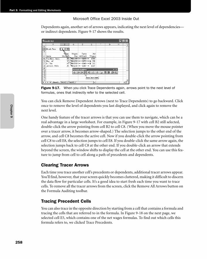
Chapter 9

Microsoft Office Excel 2003 Inside Out

Part 3: Formatting and Editing Worksheets

258

Dependents again, another set of arrows appears, indicating the next level of dependencies—or indirect dependents. Figure 9-17 shows the results.

f09ie17

Figure 9-17. When you click Trace Dependents again, arrows point to the next level of formulas, ones that indirectly refer to the selected cell.

You can click Remove Dependent Arrows (next to Trace Dependents) to go backward. Click once to remove the level of dependents you last displayed, and click again to remove the next level.

One handy feature of the tracer arrows is that you can use them to navigate, which can be a real advantage in a large worksheet. For example, in Figure 9-17 with cell B2 still selected, double-click the arrow pointing from cell B2 to cell C8. (When you move the mouse pointer over a tracer arrow, it becomes arrow-shaped.) The selection jumps to the other end of the arrow, and cell C8 becomes the active cell. Now if you double-click the arrow pointing from cell C8 to cell E8, the selection jumps to cell E8. If you double-click the same arrow again, the selection jumps back to cell C8 at the other end. If you double-click an arrow that extends beyond the screen, the window shifts to display the cell at the other end. You can use this fea-ture to jump from cell to cell along a path of precedents and dependents.

Clearing Tracer ArrowsEach time you trace another cell’s precedents or dependents, additional tracer arrows appear. You’ll find, however, that your screen quickly becomes cluttered, making it difficult to discern the data flow for particular cells. It’s a good idea to start fresh each time you want to trace cells. To remove all the tracer arrows from the screen, click the Remove All Arrows button on the Formula Auditing toolbar.

Tracing Precedent CellsYou can also trace in the opposite direction by starting from a cell that contains a formula and tracing the cells that are referred to in the formula. In Figure 9-18 on the next page, we selected cell E5, which contains one of the net wages formulas. To find out which cells this formula refers to, we clicked Trace Precedents.

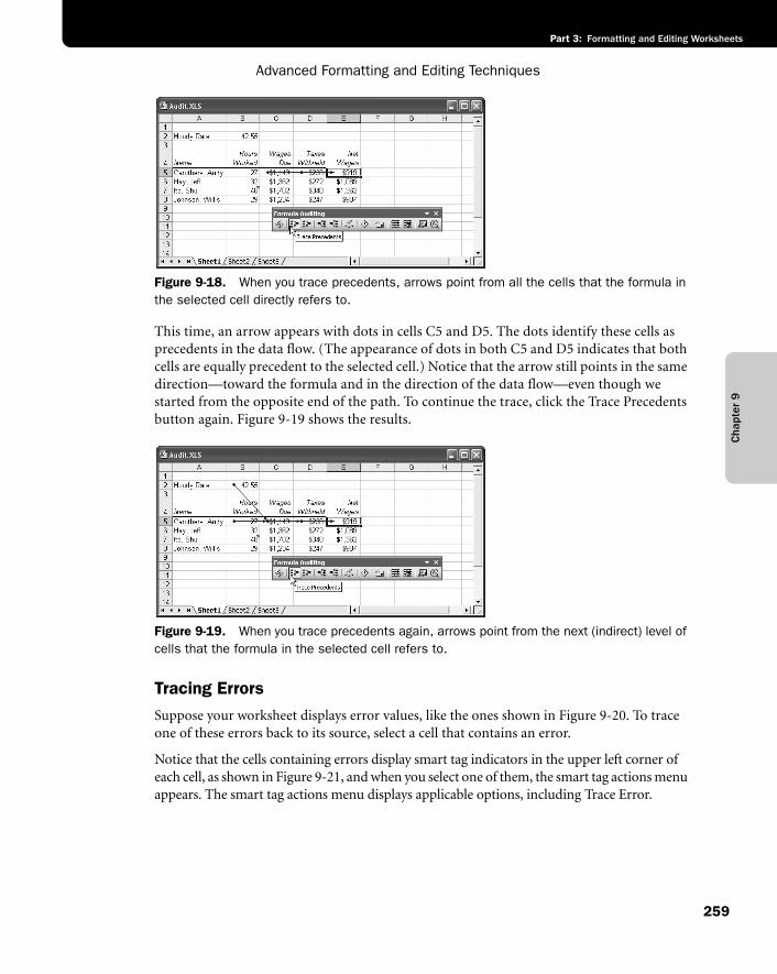
Cha

pter

9

Advanced Formatting and Editing Techniques

259

Part 3: Formatting and Editing Worksheets

f09ie18

Figure 9-18. When you trace precedents, arrows point from all the cells that the formula in the selected cell directly refers to.

This time, an arrow appears with dots in cells C5 and D5. The dots identify these cells as precedents in the data flow. (The appearance of dots in both C5 and D5 indicates that both cells are equally precedent to the selected cell.) Notice that the arrow still points in the same direction—toward the formula and in the direction of the data flow—even though we started from the opposite end of the path. To continue the trace, click the Trace Precedents button again. Figure 9-19 shows the results.

f09ie19

Figure 9-19. When you trace precedents again, arrows point from the next (indirect) level of cells that the formula in the selected cell refers to.

Tracing ErrorsSuppose your worksheet displays error values, like the ones shown in Figure 9-20. To trace one of these errors back to its source, select a cell that contains an error.

Notice that the cells containing errors display smart tag indicators in the upper left corner of each cell, as shown in Figure 9-21, and when you select one of them, the smart tag actions menu appears. The smart tag actions menu displays applicable options, including Trace Error.

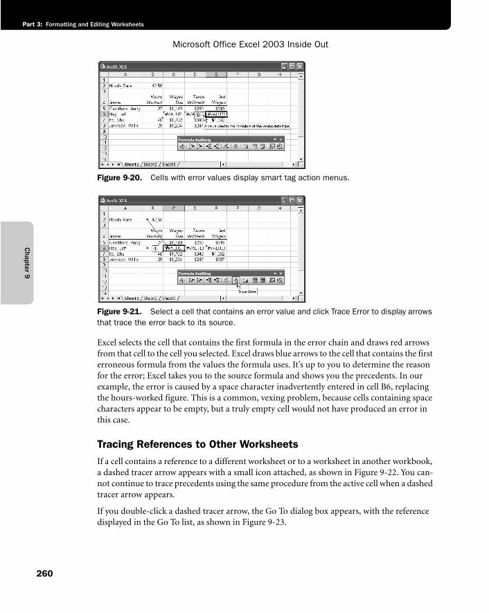
Chapter 9

Microsoft Office Excel 2003 Inside Out

Part 3: Formatting and Editing Worksheets

260

f09ie20

Figure 9-20. Cells with error values display smart tag action menus.

f09ie21

Figure 9-21. Select a cell that contains an error value and click Trace Error to display arrows that trace the error back to its source.

Excel selects the cell that contains the first formula in the error chain and draws red arrows from that cell to the cell you selected. Excel draws blue arrows to the cell that contains the first erroneous formula from the values the formula uses. It’s up to you to determine the reason for the error; Excel takes you to the source formula and shows you the precedents. In our example, the error is caused by a space character inadvertently entered in cell B6, replacing the hours-worked figure. This is a common, vexing problem, because cells containing space characters appear to be empty, but a truly empty cell would not have produced an error in this case.

Tracing References to Other WorksheetsIf a cell contains a reference to a different worksheet or to a worksheet in another workbook, a dashed tracer arrow appears with a small icon attached, as shown in Figure 9-22. You can-not continue to trace precedents using the same procedure from the active cell when a dashed tracer arrow appears.

If you double-click a dashed tracer arrow, the Go To dialog box appears, with the reference displayed in the Go To list, as shown in Figure 9-23.

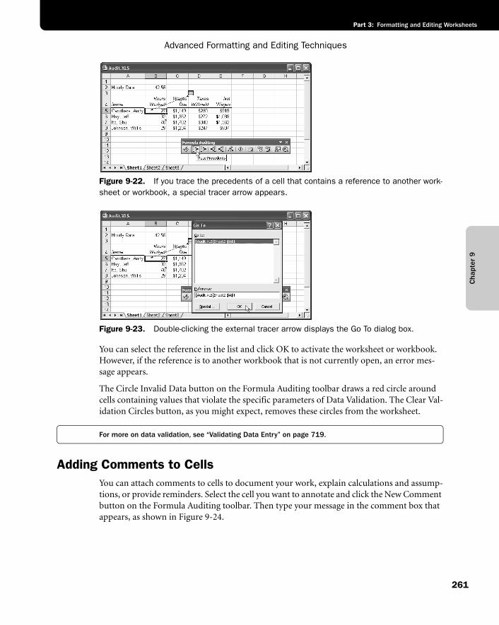
Cha

pter

9

Advanced Formatting and Editing Techniques

261

Part 3: Formatting and Editing Worksheets

f09ie22

Figure 9-22. If you trace the precedents of a cell that contains a reference to another work-sheet or workbook, a special tracer arrow appears.

f09ie23

Figure 9-23. Double-clicking the external tracer arrow displays the Go To dialog box.

You can select the reference in the list and click OK to activate the worksheet or workbook. However, if the reference is to another workbook that is not currently open, an error mes-sage appears.

The Circle Invalid Data button on the Formula Auditing toolbar draws a red circle around cells containing values that violate the specific parameters of Data Validation. The Clear Val-idation Circles button, as you might expect, removes these circles from the worksheet.

For more on data validation, see “Validating Data Entry” on page 719.

Adding Comments to CellsYou can attach comments to cells to document your work, explain calculations and assump-tions, or provide reminders. Select the cell you want to annotate and click the New Comment button on the Formula Auditing toolbar. Then type your message in the comment box that appears, as shown in Figure 9-24.

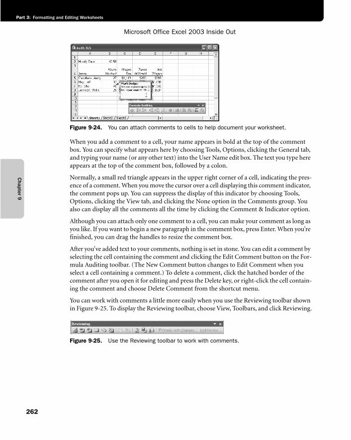
Chapter 9

Microsoft Office Excel 2003 Inside Out

Part 3: Formatting and Editing Worksheets

262

f09ie24

Figure 9-24. You can attach comments to cells to help document your worksheet.

When you add a comment to a cell, your name appears in bold at the top of the comment box. You can specify what appears here by choosing Tools, Options, clicking the General tab, and typing your name (or any other text) into the User Name edit box. The text you type here appears at the top of the comment box, followed by a colon.

Normally, a small red triangle appears in the upper right corner of a cell, indicating the pres-ence of a comment. When you move the cursor over a cell displaying this comment indicator, the comment pops up. You can suppress the display of this indicator by choosing Tools, Options, clicking the View tab, and clicking the None option in the Comments group. You also can display all the comments all the time by clicking the Comment & Indicator option.

Although you can attach only one comment to a cell, you can make your comment as long as you like. If you want to begin a new paragraph in the comment box, press Enter. When you’re finished, you can drag the handles to resize the comment box.

After you’ve added text to your comments, nothing is set in stone. You can edit a comment by selecting the cell containing the comment and clicking the Edit Comment button on the For-mula Auditing toolbar. (The New Comment button changes to Edit Comment when you select a cell containing a comment.) To delete a comment, click the hatched border of the comment after you open it for editing and press the Delete key, or right-click the cell contain-ing the comment and choose Delete Comment from the shortcut menu.

You can work with comments a little more easily when you use the Reviewing toolbar shown in Figure 9-25. To display the Reviewing toolbar, choose View, Toolbars, and click Reviewing.

f09ie25

Figure 9-25. Use the Reviewing toolbar to work with comments.

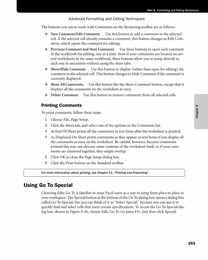
Cha

pter

9

Advanced Formatting and Editing Techniques

263

Part 3: Formatting and Editing Worksheets

The buttons you use to work with Comments on the Reviewing toolbar are as follows:

● New Comment/Edit Comment. Use this button to add a comment to the selected cell. If the selected cell already contains a comment, this button changes to Edit Com-ment, which opens the comment for editing.

● Previous Comment and Next Comment. Use these buttons to open each comment in the workbook for editing, one at a time. Even if your comments are located on sev-eral worksheets in the same workbook, these buttons allow you to jump directly to each one in succession without using the sheet tabs.

● Show/Hide Comment. Use this button to display (rather than open for editing) the comment in the selected cell. This button changes to Hide Comment if the comment is currently displayed.

● Show All Comments. Use this button like the Show Comment button, except that it displays all the comments on the worksheet at once.

● Delete Comment. Use this button to remove comments from all selected cells.

Printing CommentsTo print comments, follow these steps:

1 Choose File, Page Setup.

2 Click the Sheet tab, and select one of the options in the Comments list.

3 At End Of Sheet prints all the comments in text form after the worksheet is printed.

4 As Displayed On Sheet prints comments as they appear as text boxes if you display all the comments at once on the worksheet. Be careful, however, because comments printed this way can obscure some contents of the worksheet itself, or if your com-ments are clustered together, they might overlap.

5 Click OK to close the Page Setup dialog box.

6 Click the Print button on the Standard toolbar.

For more information about printing, see Chapter 11, “Printing and Presenting.”

Using Go To SpecialChoosing Edit, Go To is familiar to most Excel users as a way to jump from place to place in your workspace. The Special button at the bottom of the Go To dialog box opens a dialog box called Go To Special, but you can think of it as “Select Special,” because you can use it to quickly find and select cells that meet certain specifications. To access the Go To Special dia-log box, shown in Figure 9-26, choose Edit, Go To (or press F5), and then click Special.

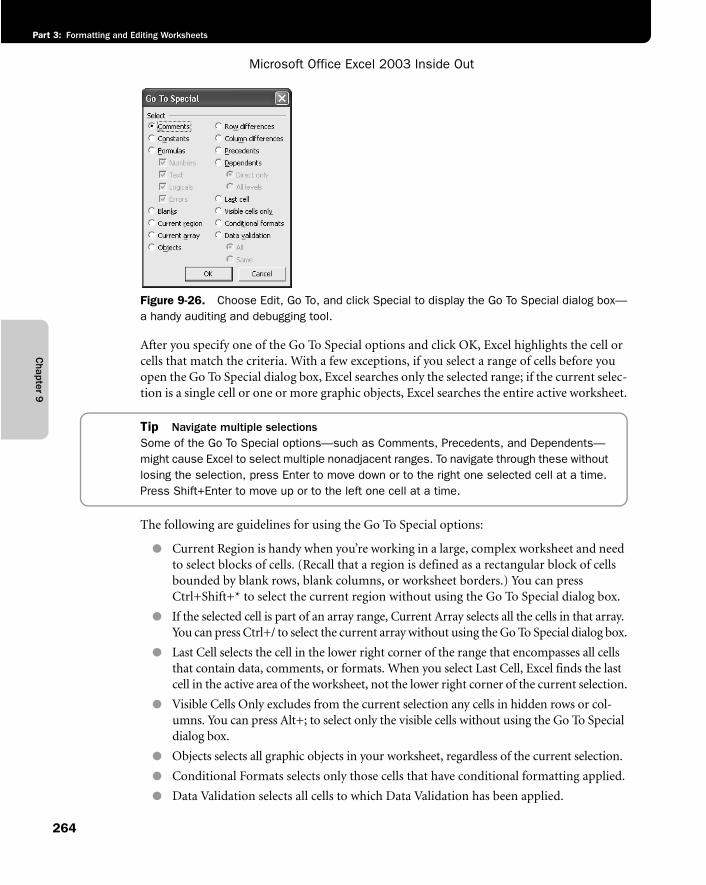
Chapter 9

Microsoft Office Excel 2003 Inside Out

Part 3: Formatting and Editing Worksheets

264

f09ie26

Figure 9-26. Choose Edit, Go To, and click Special to display the Go To Special dialog box—a handy auditing and debugging tool.

After you specify one of the Go To Special options and click OK, Excel highlights the cell or cells that match the criteria. With a few exceptions, if you select a range of cells before you open the Go To Special dialog box, Excel searches only the selected range; if the current selec-tion is a single cell or one or more graphic objects, Excel searches the entire active worksheet.

Tip Navigate multiple selectionsSome of the Go To Special options—such as Comments, Precedents, and Dependents—might cause Excel to select multiple nonadjacent ranges. To navigate through these without losing the selection, press Enter to move down or to the right one selected cell at a time. Press Shift+Enter to move up or to the left one cell at a time.

The following are guidelines for using the Go To Special options:

● Current Region is handy when you’re working in a large, complex worksheet and need to select blocks of cells. (Recall that a region is defined as a rectangular block of cells bounded by blank rows, blank columns, or worksheet borders.) You can press Ctrl+Shift+* to select the current region without using the Go To Special dialog box.

● If the selected cell is part of an array range, Current Array selects all the cells in that array. You can press Ctrl+/ to select the current array without using the Go To Special dialog box.

● Last Cell selects the cell in the lower right corner of the range that encompasses all cells that contain data, comments, or formats. When you select Last Cell, Excel finds the last cell in the active area of the worksheet, not the lower right corner of the current selection.

● Visible Cells Only excludes from the current selection any cells in hidden rows or col-umns. You can press Alt+; to select only the visible cells without using the Go To Special dialog box.

● Objects selects all graphic objects in your worksheet, regardless of the current selection.

● Conditional Formats selects only those cells that have conditional formatting applied.

● Data Validation selects all cells to which Data Validation has been applied.

Cha

pter

9

Advanced Formatting and Editing Techniques

265

Part 3: Formatting and Editing Worksheets

For more information about graphic objects, see Chapter 10, “Creating Spiffy Graphics.” For more information about conditional formatting, see “Applying Conditional Formats” on page 241. For more information about data validation, see “Validating Data Entry” on page 719.

Selecting Precedents and DependentsThe Precedents and Dependents options in the Go To Special dialog box allow you to find cells that are used by a formula or cells on which a formula depends. To use the Precedents and Dependents options, first select the cell whose precedents or dependents you want to select. When searching for precedents or dependents, Excel always searches the entire work-sheet. When you click the Precedents or Dependents option, Excel activates the Direct Only and All Levels options:

● Direct Only finds only those cells that directly refer to or that directly depend on the active cell.

● All Levels locates direct precedents and dependents plus those cells that are indirectly related to the active cell.

Tip Select precedents and dependents quicklyYou can also use these keyboard shortcuts to quickly select precedents and dependents of the active cell:

Ctrl+[ selects direct precedents.

Ctrl+Shift+{ selects all precedents.

Ctrl+] selects direct dependents.

Ctrl+Shift+} selects all dependents.

Selecting Row or Column DifferencesThe Row Differences and Column Differences options in the Go To Special dialog box com-pare the entries in a range of cells to spot potential inconsistencies. To use these debugging options, select the range before displaying the Go To Special dialog box. The position of the active cell in your selection determines which cell or cells Excel uses to make its comparisons. When searching for row differences, Excel compares the cells in the selection with the cells in the same column as the active cell. When searching for column differences, Excel compares the cells in the selection with the cells in the same row as the active cell.

Among other things, the Row Differences and Column Differences options look for differ-ences in references and select those cells that don’t conform to the comparison cell. They also verify that all the cells in the selected range contain the same type of entries. For example, if the comparison cell contains a SUM function, Excel flags any cells that contain a function, formula, or value other than SUM. If the comparison cell contains a constant text or numeric value, Excel flags any cells in the selected range that don’t exactly match the comparison value. The options, however, are not case-sensitive.

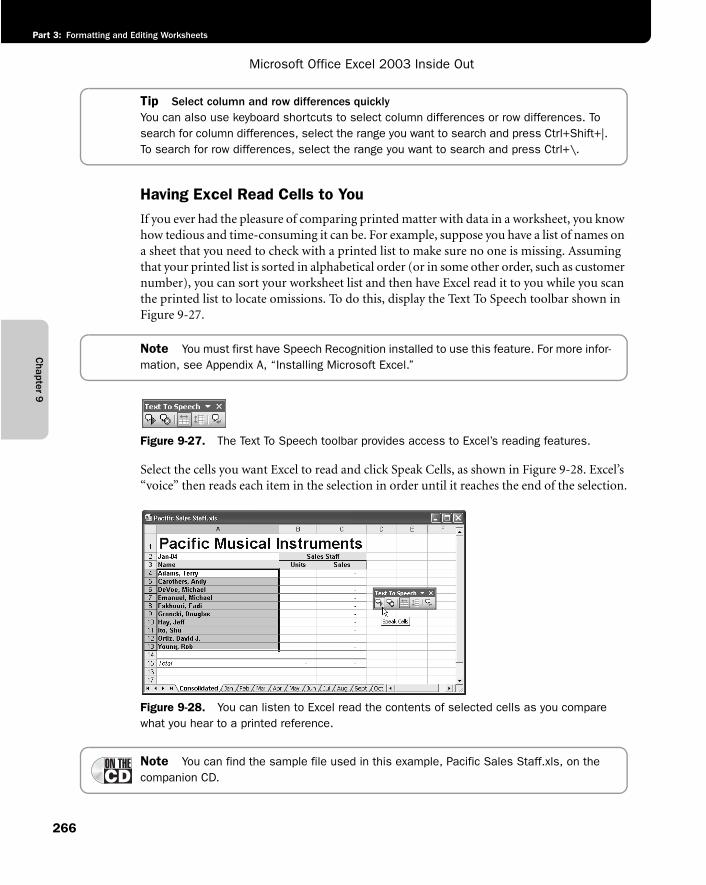
Chapter 9

Microsoft Office Excel 2003 Inside Out

Part 3: Formatting and Editing Worksheets

266

Tip Select column and row differences quicklyYou can also use keyboard shortcuts to select column differences or row differences. To search for column differences, select the range you want to search and press Ctrl+Shift+|. To search for row differences, select the range you want to search and press Ctrl+\.

Having Excel Read Cells to YouIf you ever had the pleasure of comparing printed matter with data in a worksheet, you know how tedious and time-consuming it can be. For example, suppose you have a list of names on a sheet that you need to check with a printed list to make sure no one is missing. Assuming that your printed list is sorted in alphabetical order (or in some other order, such as customer number), you can sort your worksheet list and then have Excel read it to you while you scan the printed list to locate omissions. To do this, display the Text To Speech toolbar shown in Figure 9-27.

Note You must first have Speech Recognition installed to use this feature. For more infor-mation, see Appendix A, “Installing Microsoft Excel.”

f09ie27

Figure 9-27. The Text To Speech toolbar provides access to Excel’s reading features.

Select the cells you want Excel to read and click Speak Cells, as shown in Figure 9-28. Excel’s “voice” then reads each item in the selection in order until it reaches the end of the selection.

f09ie28

Figure 9-28. You can listen to Excel read the contents of selected cells as you compare what you hear to a printed reference.

Note You can find the sample file used in this example, Pacific Sales Staff.xls, on the companion CD.

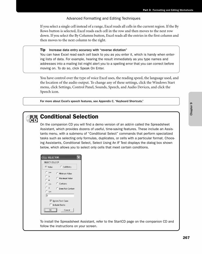
Cha

pter

9

Advanced Formatting and Editing Techniques

267

Part 3: Formatting and Editing Worksheets

If you select a single cell instead of a range, Excel reads all cells in the current region. If the By Rows button is selected, Excel reads each cell in the row and then moves to the next row down. If you select the By Columns button, Excel reads all the entries in the first column and then moves to the next column to the right.

Tip Increase data entry accuracy with “reverse dictation” You can have Excel read each cell back to you as you enter it, which is handy when enter-ing lists of data. For example, hearing the result immediately as you type names and addresses into a mailing list might alert you to a spelling error that you can correct before moving on. To do so, click Speak On Enter.

You have control over the type of voice Excel uses, the reading speed, the language used, and the location of the audio output. To change any of these settings, click the Windows Start menu, click Settings, Control Panel, Sounds, Speech, and Audio Devices, and click the Speech icon.

For more about Excel’s speech features, see Appendix C, “Keyboard Shortcuts.”

Conditional SelectionOn the companion CD you will find a demo version of an add-in called the Spreadsheet Assistant, which provides dozens of useful, time-saving features. These include an Assis-tants menu, with a submenu of “Conditional Select” commands that perform specialized tasks such as selecting only formulas, duplicates, or cells with a particular format. Choos-ing Assistants, Conditional Select, Select Using An IF Test displays the dialog box shown below, which allows you to select only cells that meet certain conditions.

G09ie03

To install the Spreadsheet Assistant, refer to the StartCD page on the companion CD and follow the instructions on your screen.

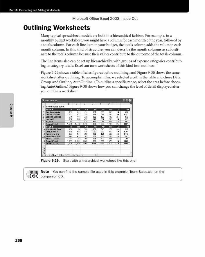
Chapter 9

Microsoft Office Excel 2003 Inside Out

Part 3: Formatting and Editing Worksheets

268

Outlining WorksheetsMany typical spreadsheet models are built in a hierarchical fashion. For example, in a monthly budget worksheet, you might have a column for each month of the year, followed by a totals column. For each line item in your budget, the totals column adds the values in each month column. In this kind of structure, you can describe the month columns as subordi-nate to the totals column because their values contribute to the outcome of the totals column.

The line items also can be set up hierarchically, with groups of expense categories contribut-ing to category totals. Excel can turn worksheets of this kind into outlines.

Figure 9-29 shows a table of sales figures before outlining, and Figure 9-30 shows the same worksheet after outlining. To accomplish this, we selected a cell in the table and chose Data, Group And Outline, AutoOutline. (To outline a specific range, select the area before choos-ing AutoOutline.) Figure 9-30 shows how you can change the level of detail displayed after you outline a worksheet.

f09ie29

Figure 9-29. Start with a hierarchical worksheet like this one.

Note You can find the sample file used in this example, Team Sales.xls, on the companion CD.

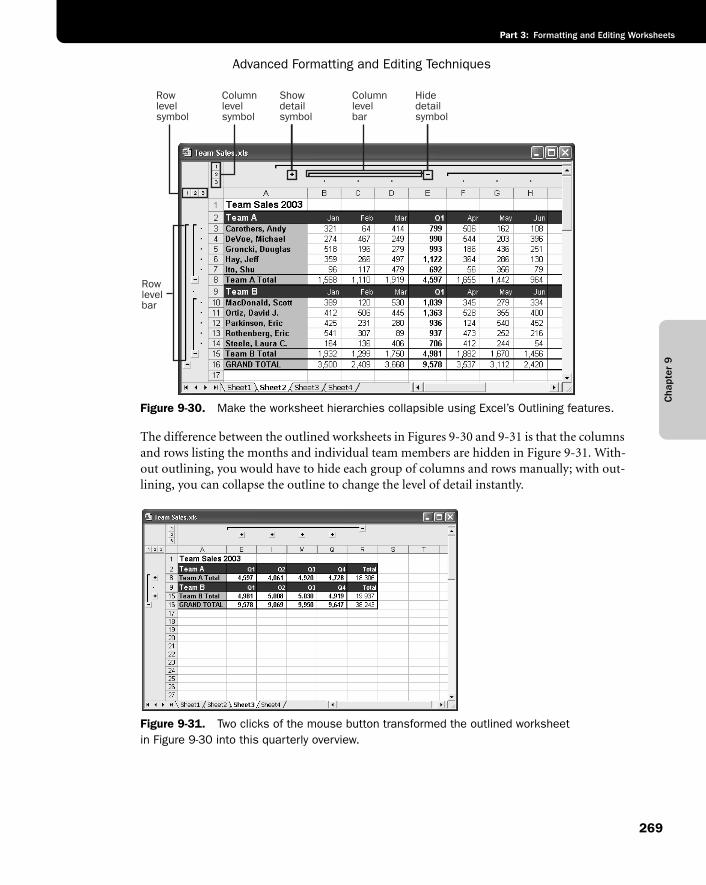
Cha

pter

9

Advanced Formatting and Editing Techniques

269

Part 3: Formatting and Editing Worksheets

f09ie30

Figure 9-30. Make the worksheet hierarchies collapsible using Excel’s Outlining features.

The difference between the outlined worksheets in Figures 9-30 and 9-31 is that the columns and rows listing the months and individual team members are hidden in Figure 9-31. With-out outlining, you would have to hide each group of columns and rows manually; with out-lining, you can collapse the outline to change the level of detail instantly.

f09ie31

Figure 9-31. Two clicks of the mouse button transformed the outlined worksheetin Figure 9-30 into this quarterly overview.

Rowlevel bar

Rowlevel symbol

Columnlevel symbol

Columnlevel bar

Hidedetailsymbol

Showdetailsymbol

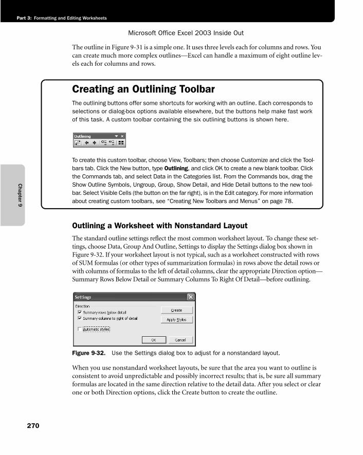
Chapter 9

Microsoft Office Excel 2003 Inside Out

Part 3: Formatting and Editing Worksheets

270

The outline in Figure 9-31 is a simple one. It uses three levels each for columns and rows. You can create much more complex outlines—Excel can handle a maximum of eight outline lev-els each for columns and rows.

Creating an Outlining ToolbarThe outlining buttons offer some shortcuts for working with an outline. Each corresponds to selections or dialog-box options available elsewhere, but the buttons help make fast work of this task. A custom toolbar containing the six outlining buttons is shown here.

g09ie02

To create this custom toolbar, choose View, Toolbars; then choose Customize and click the Tool-bars tab. Click the New button, type Outlining, and click OK to create a new blank toolbar. Click the Commands tab, and select Data in the Categories list. From the Commands box, drag the Show Outline Symbols, Ungroup, Group, Show Detail, and Hide Detail buttons to the new tool-bar. Select Visible Cells (the button on the far right), is in the Edit category. For more information about creating custom toolbars, see “Creating New Toolbars and Menus” on page 78.

Outlining a Worksheet with Nonstandard LayoutThe standard outline settings reflect the most common worksheet layout. To change these set-tings, choose Data, Group And Outline, Settings to display the Settings dialog box shown in Figure 9-32. If your worksheet layout is not typical, such as a worksheet constructed with rows of SUM formulas (or other types of summarization formulas) in rows above the detail rows or with columns of formulas to the left of detail columns, clear the appropriate Direction option—Summary Rows Below Detail or Summary Columns To Right Of Detail—before outlining.

f09ie32

Figure 9-32. Use the Settings dialog box to adjust for a nonstandard layout.

When you use nonstandard worksheet layouts, be sure that the area you want to outline is consistent to avoid unpredictable and possibly incorrect results; that is, be sure all summary formulas are located in the same direction relative to the detail data. After you select or clear one or both Direction options, click the Create button to create the outline.

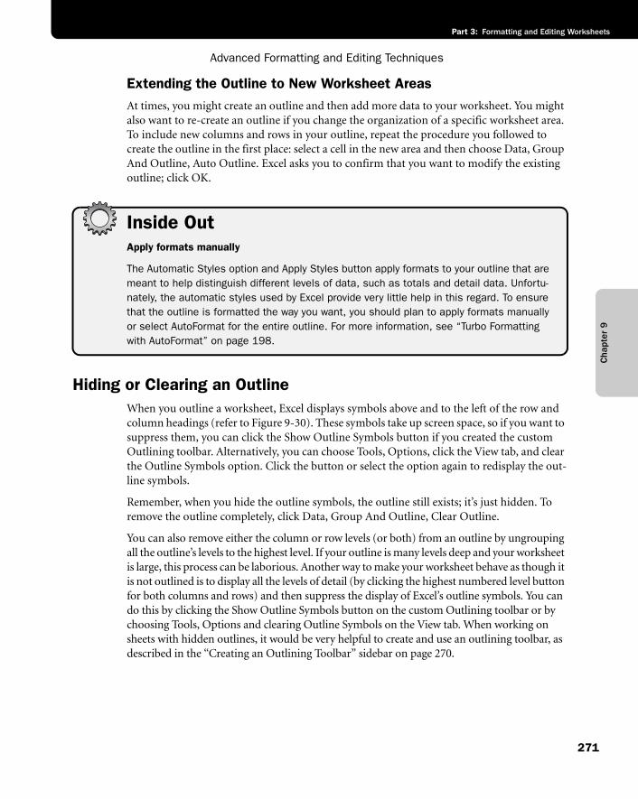
Cha

pter

9

Advanced Formatting and Editing Techniques

271

Part 3: Formatting and Editing Worksheets

Extending the Outline to New Worksheet AreasAt times, you might create an outline and then add more data to your worksheet. You might also want to re-create an outline if you change the organization of a specific worksheet area. To include new columns and rows in your outline, repeat the procedure you followed to create the outline in the first place: select a cell in the new area and then choose Data, Group And Outline, Auto Outline. Excel asks you to confirm that you want to modify the existing outline; click OK.

Inside OutApply formats manually

The Automatic Styles option and Apply Styles button apply formats to your outline that are meant to help distinguish different levels of data, such as totals and detail data. Unfortu-nately, the automatic styles used by Excel provide very little help in this regard. To ensure that the outline is formatted the way you want, you should plan to apply formats manually or select AutoFormat for the entire outline. For more information, see “Turbo Formatting with AutoFormat” on page 198.

Hiding or Clearing an OutlineWhen you outline a worksheet, Excel displays symbols above and to the left of the row and column headings (refer to Figure 9-30). These symbols take up screen space, so if you want to suppress them, you can click the Show Outline Symbols button if you created the custom Outlining toolbar. Alternatively, you can choose Tools, Options, click the View tab, and clear the Outline Symbols option. Click the button or select the option again to redisplay the out-line symbols.

Remember, when you hide the outline symbols, the outline still exists; it’s just hidden. To remove the outline completely, click Data, Group And Outline, Clear Outline.

You can also remove either the column or row levels (or both) from an outline by ungrouping all the outline’s levels to the highest level. If your outline is many levels deep and your worksheet is large, this process can be laborious. Another way to make your worksheet behave as though it is not outlined is to display all the levels of detail (by clicking the highest numbered level button for both columns and rows) and then suppress the display of Excel’s outline symbols. You can do this by clicking the Show Outline Symbols button on the custom Outlining toolbar or by choosing Tools, Options and clearing Outline Symbols on the View tab. When working on sheets with hidden outlines, it would be very helpful to create and use an outlining toolbar, as described in the “Creating an Outlining Toolbar” sidebar on page 270.

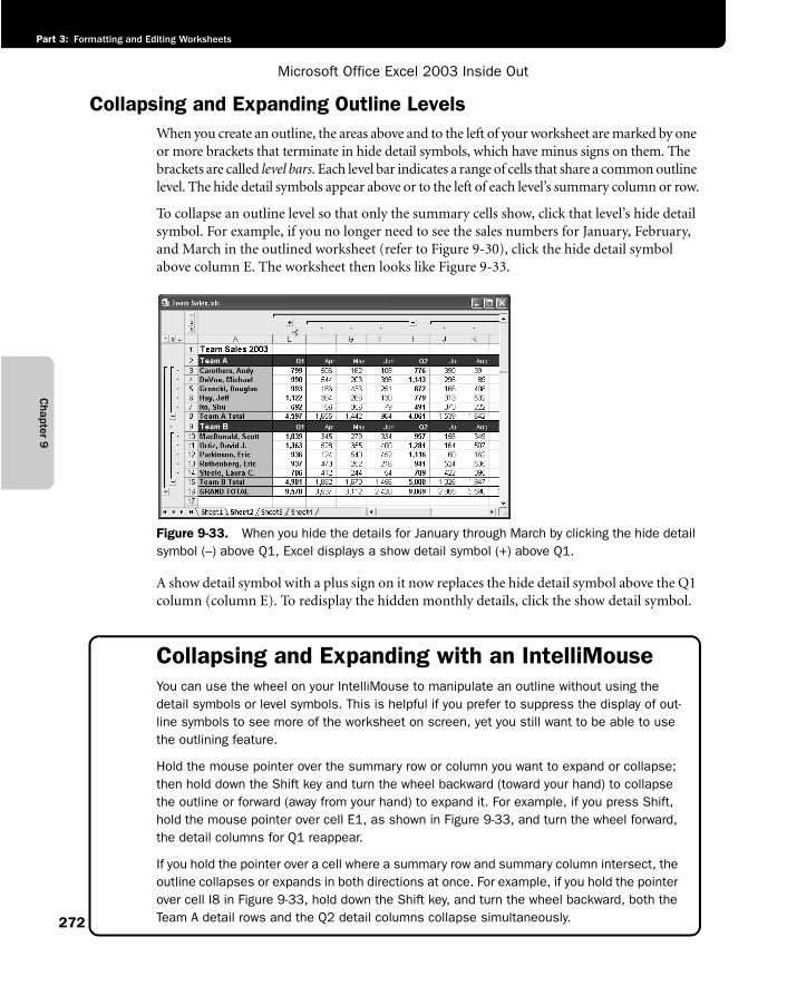
Chapter 9

Microsoft Office Excel 2003 Inside Out

Part 3: Formatting and Editing Worksheets

272

Collapsing and Expanding Outline LevelsWhen you create an outline, the areas above and to the left of your worksheet are marked by one or more brackets that terminate in hide detail symbols, which have minus signs on them. The brackets are called level bars. Each level bar indicates a range of cells that share a common outline level. The hide detail symbols appear above or to the left of each level’s summary column or row.

To collapse an outline level so that only the summary cells show, click that level’s hide detail symbol. For example, if you no longer need to see the sales numbers for January, February, and March in the outlined worksheet (refer to Figure 9-30), click the hide detail symbol above column E. The worksheet then looks like Figure 9-33.

f09ie33

Figure 9-33. When you hide the details for January through March by clicking the hide detail symbol (–) above Q1, Excel displays a show detail symbol (+) above Q1.

A show detail symbol with a plus sign on it now replaces the hide detail symbol above the Q1 column (column E). To redisplay the hidden monthly details, click the show detail symbol.

Collapsing and Expanding with an IntelliMouseYou can use the wheel on your IntelliMouse to manipulate an outline without using the detail symbols or level symbols. This is helpful if you prefer to suppress the display of out-line symbols to see more of the worksheet on screen, yet you still want to be able to use the outlining feature.

Hold the mouse pointer over the summary row or column you want to expand or collapse; then hold down the Shift key and turn the wheel backward (toward your hand) to collapse the outline or forward (away from your hand) to expand it. For example, if you press Shift, hold the mouse pointer over cell E1, as shown in Figure 9-33, and turn the wheel forward, the detail columns for Q1 reappear.

If you hold the pointer over a cell where a summary row and summary column intersect, the outline collapses or expands in both directions at once. For example, if you hold the pointer over cell I8 in Figure 9-33, hold down the Shift key, and turn the wheel backward, both the Team A detail rows and the Q2 detail columns collapse simultaneously.

Cha

pter

9

Advanced Formatting and Editing Techniques

273

Part 3: Formatting and Editing Worksheets

Displaying a Specific Outline LevelTo collapse each quarter so that only the quarterly totals and annual totals appear, you can click the hide detail symbols above Q1, Q2, Q3, and Q4. The level symbols—the squares with numerals at the upper left corner of the worksheet—provide an easier way, however. An out-line usually has two sets of level symbols, one for columns and one for rows. The column level symbols appear above the worksheet, and the row level symbols appear to the left of the worksheet.

You can use the level symbols to set an entire worksheet to a specific level of detail. The out-lined worksheet shown in Figure 9-30 has three levels each for both columns and rows. By clicking both of the number 2 level symbols in the upper left corner of the worksheet, you can transform the outline shown in Figure 9-30 to the one shown in Figure 9-31. By clicking the number 1 level symbols, you can further reduce the level of detail displayed by the worksheet so that only the grand total sales figure for the year in cell R16 is shown.

Selecting Only Visible CellsWhen you collapse part of an outline, Excel hides the columns or rows that you don’t want to see. In Figure 9-33, for example, the detail columns are hidden for Q1. Normally, if you select a range that includes hidden cells, those hidden cells are included in the selection. Whatever you do with these cells also happens to the hidden cells, so if you want to copy only the dis-played totals, using copy-and-paste gives you the entire table. By choosing Edit, Go To, click-ing the Special button, and selecting the Visible Cells Only option, you can restrict the selection to only the visible cells within a range.

The Select Visible Cells option is ideal for copying, charting, or performing calculations on only those cells that occupy a particular level of your outline. Select Visible Cells works the same way in worksheets that have not been outlined; it excludes any cells in hidden columns or rows from the current selection. This very handy option is available in button form, but you need to add it to a toolbar first, such as the one described in the “Creating an Outlining Toolbar” sidebar on page 270.

Ungrouping and Grouping Columns and RowsIf the default automatic outline doesn’t give you the structure you expect, you can adjust it by ungrouping or grouping particular columns or rows. You can easily change the hierarchy of outlined columns and rows by choosing Data, Group And Outline. Select the columns or rows you want to change and choose one of the options.

For example, you could select row 8 in the outlined worksheet shown in Figure 9-30 and choose Ungroup to change row 8 from level 2 to level 1. The outlining symbol to the left of the row moves to the left under the row level 1 button. To restore the row to its proper level, choose Group.

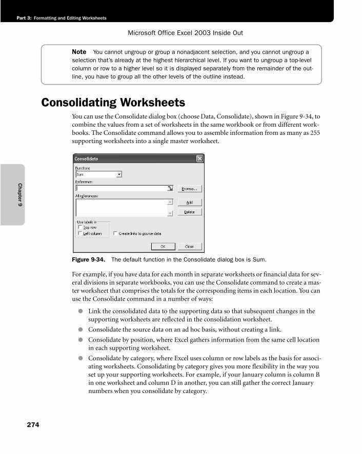
Chapter 9

Microsoft Office Excel 2003 Inside Out

Part 3: Formatting and Editing Worksheets

274

Note You cannot ungroup or group a nonadjacent selection, and you cannot ungroup a selection that’s already at the highest hierarchical level. If you want to ungroup a top-level column or row to a higher level so it is displayed separately from the remainder of the out-line, you have to group all the other levels of the outline instead.

Consolidating WorksheetsYou can use the Consolidate dialog box (choose Data, Consolidate), shown in Figure 9-34, to combine the values from a set of worksheets in the same workbook or from different work-books. The Consolidate command allows you to assemble information from as many as 255 supporting worksheets into a single master worksheet.

f09ie34

Figure 9-34. The default function in the Consolidate dialog box is Sum.

For example, if you have data for each month in separate worksheets or financial data for sev-eral divisions in separate workbooks, you can use the Consolidate command to create a mas-ter worksheet that comprises the totals for the corresponding items in each location. You can use the Consolidate command in a number of ways:

● Link the consolidated data to the supporting data so that subsequent changes in the supporting worksheets are reflected in the consolidation worksheet.

● Consolidate the source data on an ad hoc basis, without creating a link.

● Consolidate by position, where Excel gathers information from the same cell location in each supporting worksheet.

● Consolidate by category, where Excel uses column or row labels as the basis for associ-ating worksheets. Consolidating by category gives you more flexibility in the way you set up your supporting worksheets. For example, if your January column is column B in one worksheet and column D in another, you can still gather the correct January numbers when you consolidate by category.

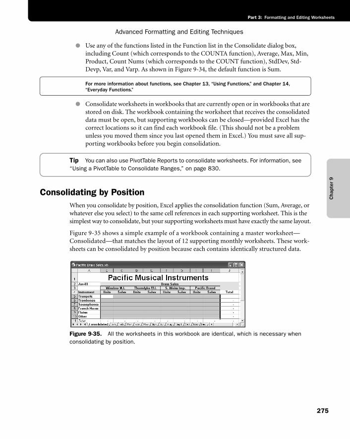
Cha

pter

9

Advanced Formatting and Editing Techniques

275

Part 3: Formatting and Editing Worksheets

● Use any of the functions listed in the Function list in the Consolidate dialog box, including Count (which corresponds to the COUNTA function), Average, Max, Min, Product, Count Nums (which corresponds to the COUNT function), StdDev, Std-Devp, Var, and Varp. As shown in Figure 9-34, the default function is Sum.

For more information about functions, see Chapter 13, “Using Functions,” and Chapter 14, “Everyday Functions.”

● Consolidate worksheets in workbooks that are currently open or in workbooks that are stored on disk. The workbook containing the worksheet that receives the consolidated data must be open, but supporting workbooks can be closed—provided Excel has the correct locations so it can find each workbook file. (This should not be a problem unless you moved them since you last opened them in Excel.) You must save all sup-porting workbooks before you begin consolidation.

Tip You can also use PivotTable Reports to consolidate worksheets. For information, see “Using a PivotTable to Consolidate Ranges,” on page 830.

Consolidating by PositionWhen you consolidate by position, Excel applies the consolidation function (Sum, Average, or whatever else you select) to the same cell references in each supporting worksheet. This is the simplest way to consolidate, but your supporting worksheets must have exactly the same layout.

Figure 9-35 shows a simple example of a workbook containing a master worksheet—Consolidated—that matches the layout of 12 supporting monthly worksheets. These work-sheets can be consolidated by position because each contains identically structured data.

f09ie35

Figure 9-35. All the worksheets in this workbook are identical, which is necessary when consolidating by position.

Chapter 9

Microsoft Office Excel 2003 Inside Out

Part 3: Formatting and Editing Worksheets

276

Note You can find the sample file used in this example, Pacific Brass Sales.xls, on the companion CD.

To consolidate the monthly worksheets in Figure 9-35 into the sheet named Consolidated, follow these steps:

1 Open the consolidation worksheet and select the block of cells that will receive the con-solidated data. In Figure 9-35, the destination area is the range B5:I10.

2 Choose Data, Consolidate.

3 Use the default Sum function in the Function list. Leave the options in the Use Labels In section and the Create Links To Source Data option unselected.

4 Select each source range with the mouse.

Tip Open supporting workbooksIf you are consolidating data in more than one workbook, you have to type references to the data ranges you want to consolidate in any workbooks that are not currently open. For this reason, make sure all supporting workbooks are open while you are building your consolidation sheet. Once you have the consolidation set up and the workbook is saved, supporting workbooks can stay closed during future consolidations. If you do have to type a reference, it must use the form [Filename]Sheetname!Reference. If the reference is in the same workbook, the file name (and its surrounding brackets) is unnecessary. If thesource range has been assigned a name, you can use this name in place of Reference (highly recommended).

If you use the mouse to select your source ranges, click the button on the right end of the Reference box to collapse the Consolidate dialog box and get it out of the way. Open worksheets by clicking their tabs. If a workbook is open but obscured by other workbooks on the screen, you can get to it by choosing its name from the Window menu. All these window maneuvers can be performed while you make your selections in the Consolidate dialog box; the dialog box remains active until you close it.

5 Click Add in the Consolidate dialog box. Excel transfers the reference from the Refer-ence edit box to the All References list. Figure 9-36 shows the completed dialog box. Repeat for each sheet you want to consolidate.

After you add the first range—$B$5:I$10 in the Jan sheet—Excel selects the same range in each sheet when you click its tab. Just click a sheet tab and then click Add to add references. Figure 9-37 shows the resulting consolidation.

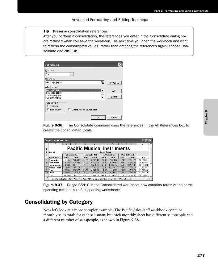
Cha

pter

9

Advanced Formatting and Editing Techniques

277

Part 3: Formatting and Editing Worksheets

Tip Preserve consolidation referencesAfter you perform a consolidation, the references you enter in the Consolidate dialog box are retained when you save the workbook. The next time you open the workbook and want to refresh the consolidated values, rather than entering the references again, choose Con-solidate and click OK.

f09ie36

Figure 9-36. The Consolidate command uses the references in the All References box to create the consolidated totals.

f09ie37

Figure 9-37. Range B5:I10 in the Consolidated worksheet now contains totals of the corre-sponding cells in the 12 supporting worksheets.

Consolidating by CategoryNow let’s look at a more complex example. The Pacific Sales Staff workbook contains monthly sales totals for each salesman, but each monthly sheet has different salespeople and a different number of salespeople, as shown in Figure 9-38.

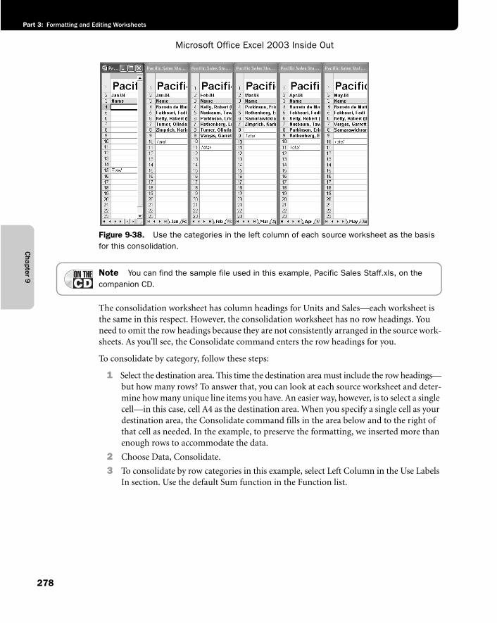
Chapter 9

Microsoft Office Excel 2003 Inside Out

Part 3: Formatting and Editing Worksheets

278

f09ie38

Figure 9-38. Use the categories in the left column of each source worksheet as the basis for this consolidation.

Note You can find the sample file used in this example, Pacific Sales Staff.xls, on the companion CD.

The consolidation worksheet has column headings for Units and Sales—each worksheet is the same in this respect. However, the consolidation worksheet has no row headings. You need to omit the row headings because they are not consistently arranged in the source work-sheets. As you’ll see, the Consolidate command enters the row headings for you.

To consolidate by category, follow these steps:

1 Select the destination area. This time the destination area must include the row headings—but how many rows? To answer that, you can look at each source worksheet and deter-mine how many unique line items you have. An easier way, however, is to select a single cell—in this case, cell A4 as the destination area. When you specify a single cell as your destination area, the Consolidate command fills in the area below and to the right of that cell as needed. In the example, to preserve the formatting, we inserted more than enough rows to accommodate the data.

2 Choose Data, Consolidate.

3 To consolidate by row categories in this example, select Left Column in the Use Labels In section. Use the default Sum function in the Function list.

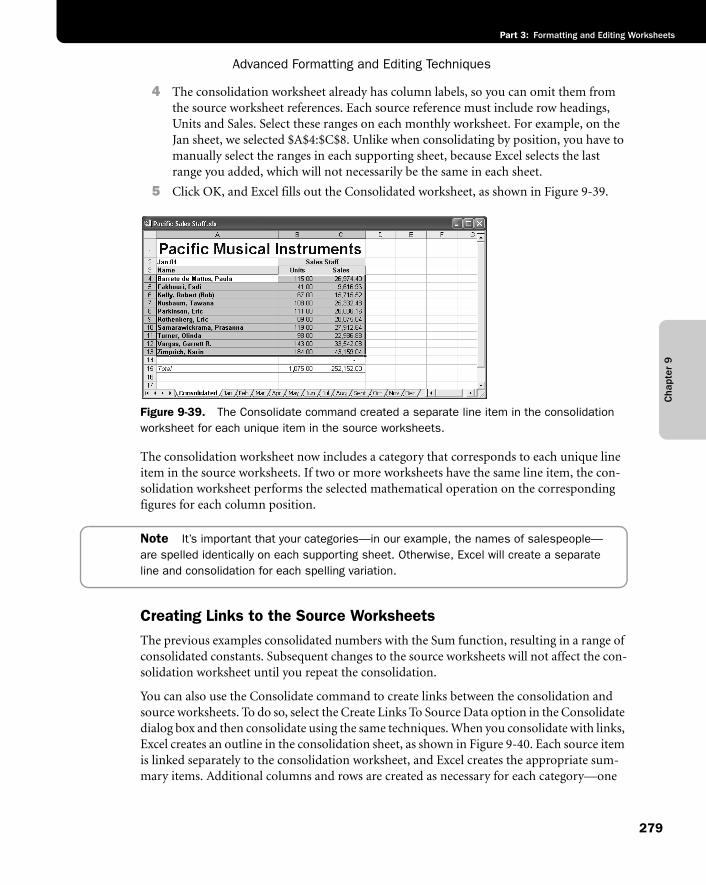
Cha

pter

9

Advanced Formatting and Editing Techniques

279

Part 3: Formatting and Editing Worksheets

4 The consolidation worksheet already has column labels, so you can omit them from the source worksheet references. Each source reference must include row headings, Units and Sales. Select these ranges on each monthly worksheet. For example, on the Jan sheet, we selected $A$4:$C$8. Unlike when consolidating by position, you have to manually select the ranges in each supporting sheet, because Excel selects the last range you added, which will not necessarily be the same in each sheet.

5 Click OK, and Excel fills out the Consolidated worksheet, as shown in Figure 9-39.

f09ie39

Figure 9-39. The Consolidate command created a separate line item in the consolidation worksheet for each unique item in the source worksheets.

The consolidation worksheet now includes a category that corresponds to each unique line item in the source worksheets. If two or more worksheets have the same line item, the con-solidation worksheet performs the selected mathematical operation on the corresponding figures for each column position.

Note It’s important that your categories—in our example, the names of salespeople—are spelled identically on each supporting sheet. Otherwise, Excel will create a separate line and consolidation for each spelling variation.

Creating Links to the Source WorksheetsThe previous examples consolidated numbers with the Sum function, resulting in a range of consolidated constants. Subsequent changes to the source worksheets will not affect the con-solidation worksheet until you repeat the consolidation.

You can also use the Consolidate command to create links between the consolidation and source worksheets. To do so, select the Create Links To Source Data option in the Consolidate dialog box and then consolidate using the same techniques. When you consolidate with links, Excel creates an outline in the consolidation sheet, as shown in Figure 9-40. Each source item is linked separately to the consolidation worksheet, and Excel creates the appropriate sum-mary items. Additional columns and rows are created as necessary for each category—one

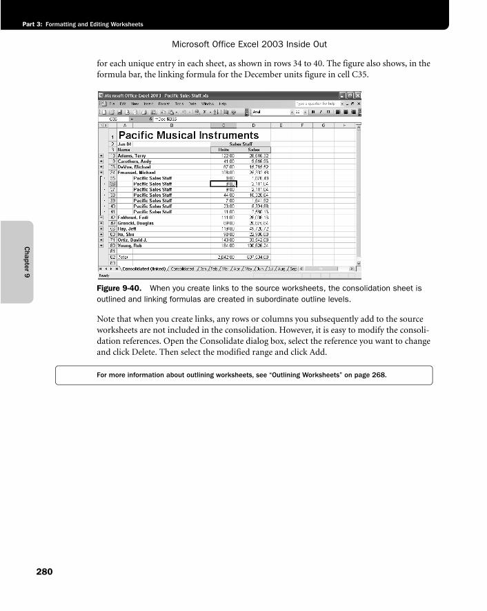
Chapter 9

Microsoft Office Excel 2003 Inside Out

Part 3: Formatting and Editing Worksheets

280

for each unique entry in each sheet, as shown in rows 34 to 40. The figure also shows, in the formula bar, the linking formula for the December units figure in cell C35.

f09ie40

Figure 9-40. When you create links to the source worksheets, the consolidation sheet is outlined and linking formulas are created in subordinate outline levels.

Note that when you create links, any rows or columns you subsequently add to the source worksheets are not included in the consolidation. However, it is easy to modify the consoli-dation references. Open the Consolidate dialog box, select the reference you want to change and click Delete. Then select the modified range and click Add.

For more information about outlining worksheets, see “Outlining Worksheets” on page 268.

281

Part 4

Adding Graphics and Printing

10 Creating Spiffy Graphics 283

11 Printing and Presenting 331

Part 4: Adding Graphics and Printing

283

Chapter 10

Creating Spiffy GraphicsUsing the Drawing Tools . . . . . . . . . . . . 283Creating Graphic Objects . . . . . . . . . . . 287Working with Graphic Objects. . . . . . . . 297

Inserting Other Objects . . . . . . . . . . . . . 308More Tricks with Objects . . . . . . . . . . . . 321Gallery of Spiffy Examples . . . . . . . . . . . 325

Microsoft Excel gives you the tools to create a variety of graphic objects—boxes, lines, circles, ovals, arcs, freeform polygons, text boxes, buttons, and a wide assortment of complex, pre-defined objects called AutoShapes. You can specify font, pattern, color, and line formats, and you can position objects in relation to the worksheet or to other objects. You can also take pictures of your worksheets and use them in other Excel documents or in documents created in other applications. If you already have graphics created in other applications, Excel imports those graphics as well.

Throughout this chapter, we add graphics to worksheets, but you can also add many of the same kinds of graphics to chart sheets. In addition, you can apply the techniques discussed in this chapter to a variety of graphic objects called controls that you create using Microsoft Excel Visual Basic for Applications (VBA).

For more information about Visual Basic for Applications, see Part 10, “Working with Visual Basic and Macros.”

Using the Drawing ToolsExcel’s drawing tool chest offers many of the powerful capabilities of dedicated illustration programs. You can use this tool chest to create smooth curves; linked objects using connec-tors; basic and not-so-basic shapes, such as three-dimensional boxes and lightning bolts; a variety of straight, curved, and multiheaded arrows; flow charts; stars, emblems, and ban-ners; and callouts. You create these graphic objects using the buttons and menus on the Drawing toolbar shown in Figure 10-1. The easiest way to display the Drawing toolbar is by right-clicking any displayed toolbar or the menu bar and choosing Drawing from the short-cut menu.

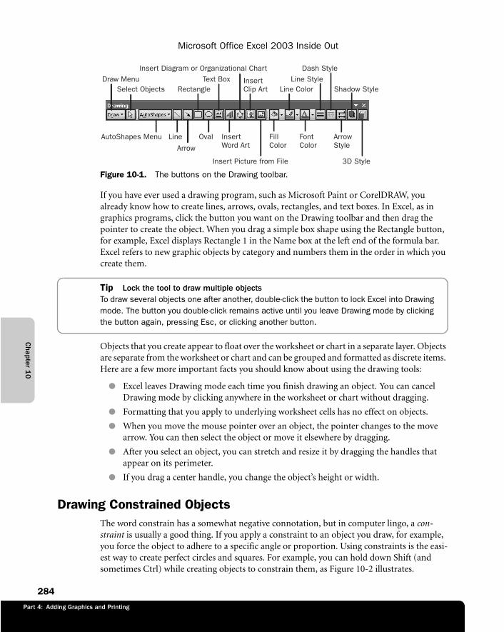
Chapter 1

0

Microsoft Office Excel 2003 Inside Out

284

Part 4: Adding Graphics and Printing

f10ie01

Figure 10-1. The buttons on the Drawing toolbar.

If you have ever used a drawing program, such as Microsoft Paint or CorelDRAW, you already know how to create lines, arrows, ovals, rectangles, and text boxes. In Excel, as in graphics programs, click the button you want on the Drawing toolbar and then drag the pointer to create the object. When you drag a simple box shape using the Rectangle button, for example, Excel displays Rectangle 1 in the Name box at the left end of the formula bar. Excel refers to new graphic objects by category and numbers them in the order in which you create them.

Tip Lock the tool to draw multiple objectsTo draw several objects one after another, double-click the button to lock Excel into Drawing mode. The button you double-click remains active until you leave Drawing mode by clicking the button again, pressing Esc, or clicking another button.

Objects that you create appear to float over the worksheet or chart in a separate layer. Objects are separate from the worksheet or chart and can be grouped and formatted as discrete items. Here are a few more important facts you should know about using the drawing tools:

● Excel leaves Drawing mode each time you finish drawing an object. You can cancel Drawing mode by clicking anywhere in the worksheet or chart without dragging.

● Formatting that you apply to underlying worksheet cells has no effect on objects.

● When you move the mouse pointer over an object, the pointer changes to the move arrow. You can then select the object or move it elsewhere by dragging.

● After you select an object, you can stretch and resize it by dragging the handles that appear on its perimeter.

● If you drag a center handle, you change the object’s height or width.

Drawing Constrained ObjectsThe word constrain has a somewhat negative connotation, but in computer lingo, a con-straint is usually a good thing. If you apply a constraint to an object you draw, for example, you force the object to adhere to a specific angle or proportion. Using constraints is the easi-est way to create perfect circles and squares. For example, you can hold down Shift (and sometimes Ctrl) while creating objects to constrain them, as Figure 10-2 illustrates.

Draw Menu

AutoShapes Menu

Select Objects RectangleText Box

Line

Arrow

Oval FillColor

FontColor

ArrowStyle

3D Style

InsertWord Art

Insert Picture from File

Line StyleShadow Style

Dash Style

InsertClip Art Line Color

Insert Diagram or Organizational Chart

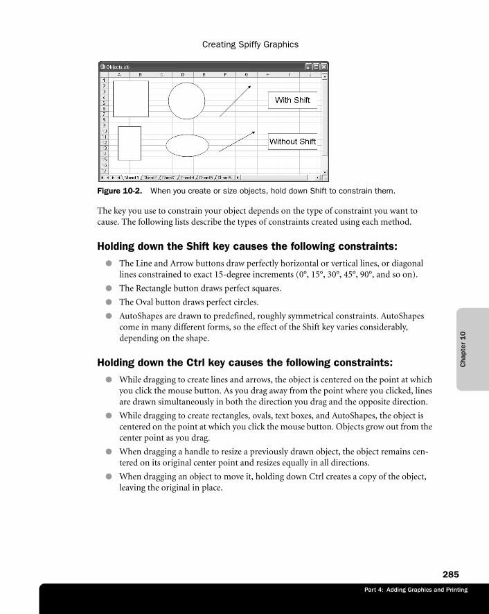
Cha

pter

10

Creating Spiffy Graphics

285

Part 3: Formatting and Editing Worksheets

Part 4: Adding Graphics and Printing

f10ie02

Figure 10-2. When you create or size objects, hold down Shift to constrain them.

The key you use to constrain your object depends on the type of constraint you want to cause. The following lists describe the types of constraints created using each method.

Holding down the Shift key causes the following constraints:● The Line and Arrow buttons draw perfectly horizontal or vertical lines, or diagonal

lines constrained to exact 15-degree increments (0°, 15°, 30°, 45°, 90°, and so on).

● The Rectangle button draws perfect squares.

● The Oval button draws perfect circles.

● AutoShapes are drawn to predefined, roughly symmetrical constraints. AutoShapes come in many different forms, so the effect of the Shift key varies considerably, depending on the shape.

Holding down the Ctrl key causes the following constraints:● While dragging to create lines and arrows, the object is centered on the point at which

you click the mouse button. As you drag away from the point where you clicked, lines are drawn simultaneously in both the direction you drag and the opposite direction.

● While dragging to create rectangles, ovals, text boxes, and AutoShapes, the object is centered on the point at which you click the mouse button. Objects grow out from the center point as you drag.

● When dragging a handle to resize a previously drawn object, the object remains cen-tered on its original center point and resizes equally in all directions.

● When dragging an object to move it, holding down Ctrl creates a copy of the object, leaving the original in place.

Chapter 1

0

Microsoft Office Excel 2003 Inside Out

286

Part 4: Adding Graphics and Printing

Holding down the Alt key causes the following constraint:● You can hold down Alt while creating objects to use the gridlines on a worksheet as a

drawing grid. The edges of your objects are then forced to follow the gridlines. If you use Shift and Alt together to draw a square or a circle aligned to the grid, Excel does its best, but the result might not be perfect. This is because the default height and width of the cells on a worksheet might not provide an ideal grid for perfect squares or circles.

Inside OutEnter “The Object Zone”

When you work with objects, it’s almost as if there’s another program with a transparent desktop that floats over the worksheet—as if the objects you draw are in another dimen-sion. In a sense, they are. What goes on in the grid of Excel has little to do with what goes on in the drawing layer we’ll call “The Object Zone,” although you do have opportunities to create interaction between object and worksheet using macros and formulas.

When you are working normally in cells, you can click on any graphic object to select it, and then click in the worksheet to select cells. You can hop back and forth, no problem. However, when you click the Select Objects button (the arrow) on the Drawing toolbar, you enter “The Object Zone,” where you cannot select a cell to save your life. This button is a toggle—you’re in “The Object Zone” until you click it again. This essentially locks out the worksheet so that you can toil in that phantom program to your heart’s content. This is handy when you are doing a lot of graphic work, because it makes it easier to select and work with objects without worrying about inadvertently clicking the sheet and exiting “The Object Zone.” If you forget that you’ve clicked the Select Objects button, you might experience a moment of panic, won-dering what happened, and worrying that perhaps Excel has crashed. Just look at the Select Object button, which stays highlighted. Click it again to leave “The Object Zone.”

Using Tear-Off PalettesMany of the submenus located on the Drawing toolbar are tear-off palettes. On the Draw menu, you can tear off the Order, Nudge, Align or Distribute, and Rotate or Flip submenus. Each sub-menu on the AutoShapes menu (except More AutoShapes, which is not a submenu) is a tear-off palette—in fact, you can tear off the entire AutoShapes menu itself, as shown in Figure 10-3. Click the selection bar (the three horizontal lines at the top of the menu) and drag it away. You can do the same with any menu or submenu that is displayed as a selection bar.

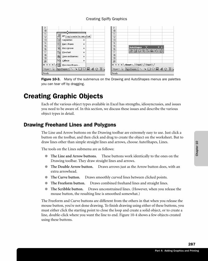
Cha

pter

10

Creating Spiffy Graphics

287

Part 3: Formatting and Editing Worksheets

Part 4: Adding Graphics and Printing

f10ie03

Figure 10-3. Many of the submenus on the Drawing and AutoShapes menus are palettes you can tear off by dragging.

Creating Graphic ObjectsEach of the various object types available in Excel has strengths, idiosyncrasies, and issues you need to be aware of. In this section, we discuss these issues and describe the various object types in detail.

Drawing Freehand Lines and PolygonsThe Line and Arrow buttons on the Drawing toolbar are extremely easy to use. Just click a button on the toolbar, and then click and drag to create the object on the worksheet. But to draw lines other than simple straight lines and arrows, choose AutoShapes, Lines.

The tools on the Lines submenu are as follows:

● The Line and Arrow buttons. These buttons work identically to the ones on the Drawing toolbar. They draw straight lines and arrows.

● The Double Arrow button. Draws arrows just as the Arrow button does, with an extra arrowhead.

● The Curve button. Draws smoothly curved lines between clicked points.

● The Freeform button. Draws combined freehand lines and straight lines.

● The Scribble button. Draws unconstrained lines. (However, when you release the mouse button, the resulting line is smoothed somewhat.)

The Freeform and Curve buttons are different from the others in that when you release the mouse button, you’re not done drawing. To finish drawing using either of these buttons, you must either click the starting point to close the loop and create a solid object, or to create a line, double-click where you want the line to end. Figure 10-4 shows a few objects created using these buttons.

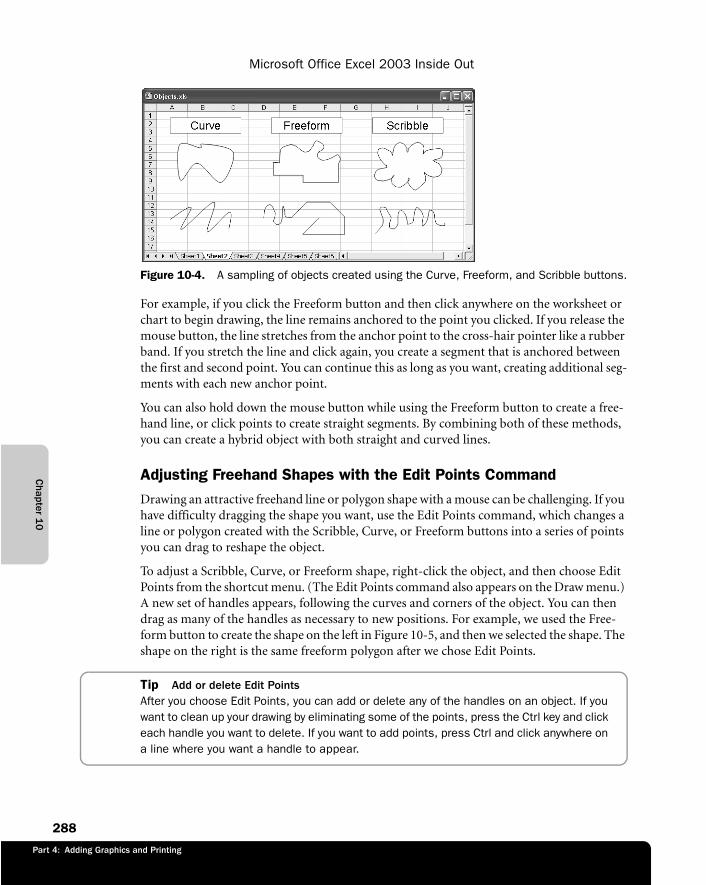
Chapter 1

0

Microsoft Office Excel 2003 Inside Out

288

Part 4: Adding Graphics and Printing

f10ie04

Figure 10-4. A sampling of objects created using the Curve, Freeform, and Scribble buttons.

For example, if you click the Freeform button and then click anywhere on the worksheet or chart to begin drawing, the line remains anchored to the point you clicked. If you release the mouse button, the line stretches from the anchor point to the cross-hair pointer like a rubber band. If you stretch the line and click again, you create a segment that is anchored between the first and second point. You can continue this as long as you want, creating additional seg-ments with each new anchor point.

You can also hold down the mouse button while using the Freeform button to create a free-hand line, or click points to create straight segments. By combining both of these methods, you can create a hybrid object with both straight and curved lines.

Adjusting Freehand Shapes with the Edit Points CommandDrawing an attractive freehand line or polygon shape with a mouse can be challenging. If you have difficulty dragging the shape you want, use the Edit Points command, which changes a line or polygon created with the Scribble, Curve, or Freeform buttons into a series of points you can drag to reshape the object.

To adjust a Scribble, Curve, or Freeform shape, right-click the object, and then choose Edit Points from the shortcut menu. (The Edit Points command also appears on the Draw menu.) A new set of handles appears, following the curves and corners of the object. You can then drag as many of the handles as necessary to new positions. For example, we used the Free-form button to create the shape on the left in Figure 10-5, and then we selected the shape. The shape on the right is the same freeform polygon after we chose Edit Points.

Tip Add or delete Edit PointsAfter you choose Edit Points, you can add or delete any of the handles on an object. If you want to clean up your drawing by eliminating some of the points, press the Ctrl key and click each handle you want to delete. If you want to add points, press Ctrl and click anywhere on a line where you want a handle to appear.

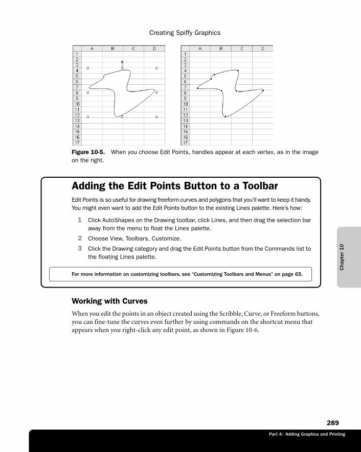
Cha

pter

10

Creating Spiffy Graphics

289

Part 3: Formatting and Editing Worksheets

Part 4: Adding Graphics and Printing

f10ie05

Figure 10-5. When you choose Edit Points, handles appear at each vertex, as in the image on the right.

Adding the Edit Points Button to a ToolbarEdit Points is so useful for drawing freeform curves and polygons that you’ll want to keep it handy. You might even want to add the Edit Points button to the existing Lines palette. Here’s how:

1 Click AutoShapes on the Drawing toolbar, click Lines, and then drag the selection bar away from the menu to float the Lines palette.

2 Choose View, Toolbars, Customize.

3 Click the Drawing category and drag the Edit Points button from the Commands list to the floating Lines palette.

For more information on customizing toolbars, see “Customizing Toolbars and Menus” on page 65.

Working with CurvesWhen you edit the points in an object created using the Scribble, Curve, or Freeform buttons, you can fine-tune the curves even further by using commands on the shortcut menu that appears when you right-click any edit point, as shown in Figure 10-6.

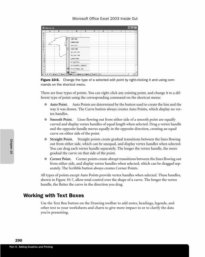
Chapter 1

0

Microsoft Office Excel 2003 Inside Out

290

Part 4: Adding Graphics and Printing

f10ie06

Figure 10-6. Change the type of a selected edit point by right-clicking it and using com-mands on the shortcut menu.

There are four types of points. You can right-click any existing point, and change it to a dif-ferent type of point using the corresponding command on the shortcut menu:

● Auto Point. Auto Points are determined by the button used to create the line and the way it was drawn. The Curve button always creates Auto Points, which display no ver-tex handles.

● Smooth Point. Lines flowing out from either side of a smooth point are equally curved and display vertex handles of equal length when selected. Drag a vertex handle and the opposite handle moves equally in the opposite direction, creating an equal curve on either side of the point.

● Straight Point. Straight points create gradual transitions between the lines flowing out from either side, which can be unequal, and display vertex handles when selected. You can drag each vertex handle separately. The longer the vertex handle, the more gradual the curve on that side of the point.

● Corner Point. Corner points create abrupt transitions between the lines flowing out from either side, and display vertex handles when selected, which can be dragged sep-arately. The Scribble button always creates Corner Points.

All types of points except Auto Points provide vertex handles when selected. These handles, shown in Figure 10-7, allow total control over the shape of a curve. The longer the vertex handle, the flatter the curve in the direction you drag.

Working with Text BoxesUse the Text Box button on the Drawing toolbar to add notes, headings, legends, and other text to your worksheets and charts to give more impact to or to clarify the data you’re presenting.

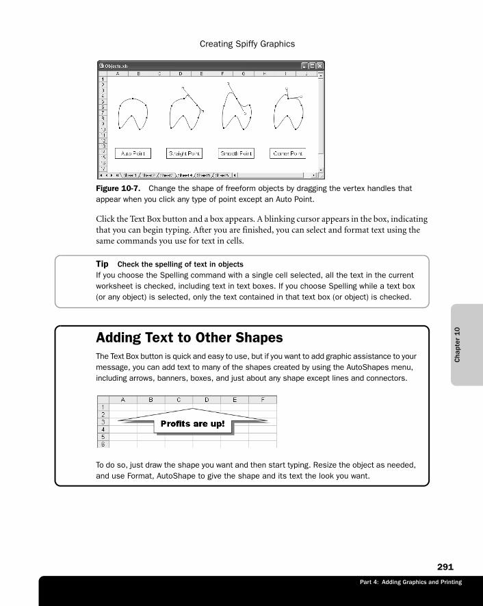
Cha

pter

10

Creating Spiffy Graphics

291

Part 3: Formatting and Editing Worksheets

Part 4: Adding Graphics and Printing

f10ie07

Figure 10-7. Change the shape of freeform objects by dragging the vertex handles that appear when you click any type of point except an Auto Point.

Click the Text Box button and a box appears. A blinking cursor appears in the box, indicating that you can begin typing. After you are finished, you can select and format text using the same commands you use for text in cells.

Tip Check the spelling of text in objectsIf you choose the Spelling command with a single cell selected, all the text in the current worksheet is checked, including text in text boxes. If you choose Spelling while a text box (or any object) is selected, only the text contained in that text box (or object) is checked.

Adding Text to Other ShapesThe Text Box button is quick and easy to use, but if you want to add graphic assistance to your message, you can add text to many of the shapes created by using the AutoShapes menu, including arrows, banners, boxes, and just about any shape except lines and connectors.

g10ie01

To do so, just draw the shape you want and then start typing. Resize the object as needed, and use Format, AutoShape to give the shape and its text the look you want.

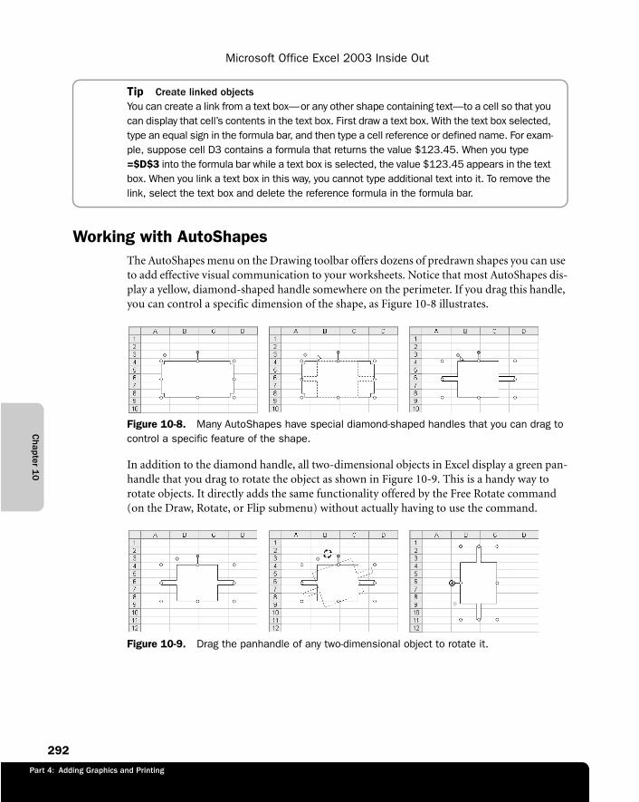
Chapter 1

0

Microsoft Office Excel 2003 Inside Out

292

Part 4: Adding Graphics and Printing

Tip Create linked objectsYou can create a link from a text box—or any other shape containing text—to a cell so that you can display that cell’s contents in the text box. First draw a text box. With the text box selected, type an equal sign in the formula bar, and then type a cell reference or defined name. For exam-ple, suppose cell D3 contains a formula that returns the value $123.45. When you type =$D$3 into the formula bar while a text box is selected, the value $123.45 appears in the text box. When you link a text box in this way, you cannot type additional text into it. To remove the link, select the text box and delete the reference formula in the formula bar.

Working with AutoShapesThe AutoShapes menu on the Drawing toolbar offers dozens of predrawn shapes you can use to add effective visual communication to your worksheets. Notice that most AutoShapes dis-play a yellow, diamond-shaped handle somewhere on the perimeter. If you drag this handle, you can control a specific dimension of the shape, as Figure 10-8 illustrates.

f10ie08

Figure 10-8. Many AutoShapes have special diamond-shaped handles that you can drag to control a specific feature of the shape.

In addition to the diamond handle, all two-dimensional objects in Excel display a green pan-handle that you drag to rotate the object as shown in Figure 10-9. This is a handy way to rotate objects. It directly adds the same functionality offered by the Free Rotate command (on the Draw, Rotate, or Flip submenu) without actually having to use the command.

f10ie09

Figure 10-9. Drag the panhandle of any two-dimensional object to rotate it.

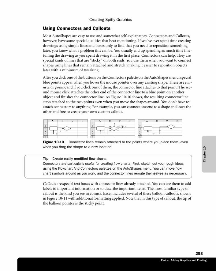
Cha

pter

10

Creating Spiffy Graphics

293

Part 3: Formatting and Editing Worksheets

Part 4: Adding Graphics and Printing

Using Connectors and CalloutsMost AutoShapes are easy to use and somewhat self-explanatory. Connectors and Callouts, however, have some special qualities that bear mentioning. If you’ve ever spent time creating drawings using simple lines and boxes only to find that you need to reposition something later, you know what a problem this can be. You usually end up spending as much time fine-tuning the drawing as you spent drawing it in the first place. Connectors can help. They are special kinds of lines that are “sticky” on both ends. You use them when you want to connect shapes using lines that remain attached and stretch, making it easier to reposition objects later with a minimum of tweaking.

After you click one of the buttons on the Connectors palette on the AutoShapes menu, special blue points appear when you hover the mouse pointer over any existing shape. These are con-nection points, and if you click one of them, the connector line attaches to that point. The sec-ond mouse click attaches the other end of the connector line to a blue point on another object and finishes the connector line. As Figure 10-10 shows, the resulting connector line stays attached to the two points even when you move the shapes around. You don’t have to attach connectors to anything. For example, you can connect one end to a shape and leave the other end free to create your own custom callout.

f10ie10

Figure 10-10. Connector lines remain attached to the points where you place them, even when you drag the shape to a new location.

Tip Create easily modified flow chartsConnectors are particularly useful for creating flow charts. First, sketch out your rough ideas using the Flowchart And Connectors palettes on the AutoShapes menu. You can move flow chart symbols around as you work, and the connector lines reroute themselves as necessary.

Callouts are special text boxes with connector lines already attached. You can use them to add labels to important information or to describe important items. The most familiar type of callout is the kind you see in comics. Excel includes several of these balloon callouts, shown in Figure 10-11 with additional formatting applied. Note that in this type of callout, the tip of the balloon pointer is the sticky point.

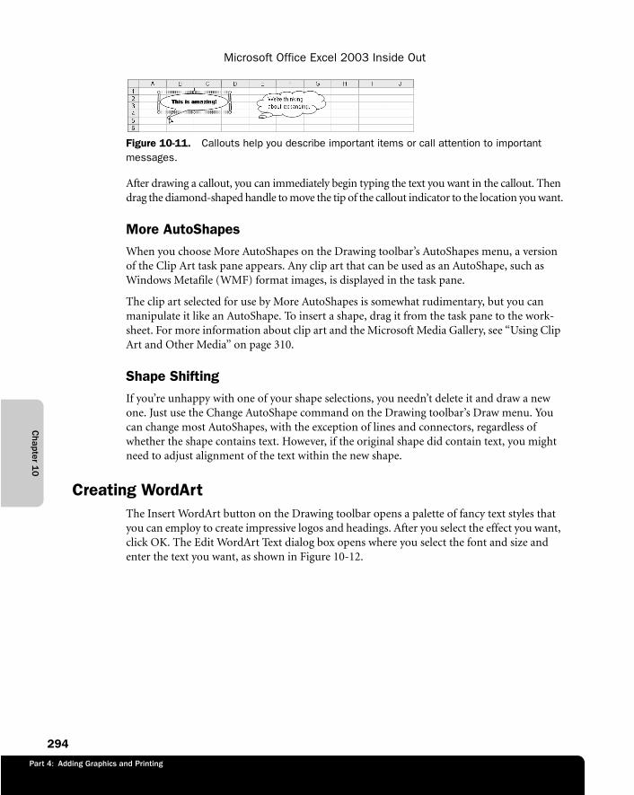
Chapter 1

0

Microsoft Office Excel 2003 Inside Out

294

Part 4: Adding Graphics and Printing

f10ie11

Figure 10-11. Callouts help you describe important items or call attention to important messages.

After drawing a callout, you can immediately begin typing the text you want in the callout. Then drag the diamond-shaped handle to move the tip of the callout indicator to the location you want.

More AutoShapesWhen you choose More AutoShapes on the Drawing toolbar’s AutoShapes menu, a version of the Clip Art task pane appears. Any clip art that can be used as an AutoShape, such as Windows Metafile (WMF) format images, is displayed in the task pane.

The clip art selected for use by More AutoShapes is somewhat rudimentary, but you can manipulate it like an AutoShape. To insert a shape, drag it from the task pane to the work-sheet. For more information about clip art and the Microsoft Media Gallery, see “Using Clip Art and Other Media” on page 310.

Shape ShiftingIf you’re unhappy with one of your shape selections, you needn’t delete it and draw a new one. Just use the Change AutoShape command on the Drawing toolbar’s Draw menu. You can change most AutoShapes, with the exception of lines and connectors, regardless of whether the shape contains text. However, if the original shape did contain text, you might need to adjust alignment of the text within the new shape.

Creating WordArtThe Insert WordArt button on the Drawing toolbar opens a palette of fancy text styles that you can employ to create impressive logos and headings. After you select the effect you want, click OK. The Edit WordArt Text dialog box opens where you select the font and size and enter the text you want, as shown in Figure 10-12.

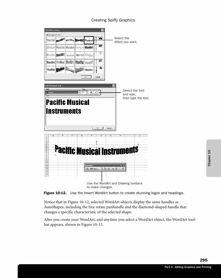
Cha

pter

10

Creating Spiffy Graphics

295

Part 3: Formatting and Editing Worksheets

Part 4: Adding Graphics and Printing

f10ie12

Figure 10-12. Use the Insert WordArt button to create stunning logos and headings.

Notice that in Figure 10-12, selected WordArt objects display the same handles as AutoShapes, including the free rotate panhandle and the diamond-shaped handle that changes a specific characteristic of the selected shape.

After you create your WordArt, and anytime you select a WordArt object, the WordArt tool-bar appears, shown in Figure 10-13.

Select the fontand size,then type the text.

Select the effect you want.

Use the WordArt and Drawing toolbars to make changes.

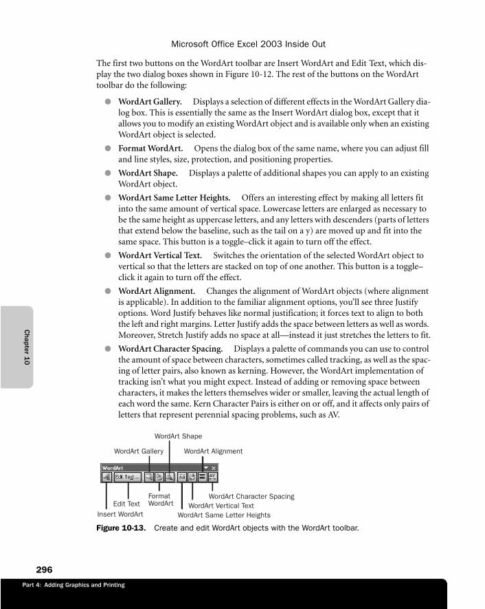
Chapter 1

0

Microsoft Office Excel 2003 Inside Out

296

Part 4: Adding Graphics and Printing

The first two buttons on the WordArt toolbar are Insert WordArt and Edit Text, which dis-play the two dialog boxes shown in Figure 10-12. The rest of the buttons on the WordArt toolbar do the following:

● WordArt Gallery. Displays a selection of different effects in the WordArt Gallery dia-log box. This is essentially the same as the Insert WordArt dialog box, except that it allows you to modify an existing WordArt object and is available only when an existing WordArt object is selected.

● Format WordArt. Opens the dialog box of the same name, where you can adjust fill and line styles, size, protection, and positioning properties.

● WordArt Shape. Displays a palette of additional shapes you can apply to an existing WordArt object.

● WordArt Same Letter Heights. Offers an interesting effect by making all letters fit into the same amount of vertical space. Lowercase letters are enlarged as necessary to be the same height as uppercase letters, and any letters with descenders (parts of letters that extend below the baseline, such as the tail on a y) are moved up and fit into the same space. This button is a toggle–click it again to turn off the effect.

● WordArt Vertical Text. Switches the orientation of the selected WordArt object to vertical so that the letters are stacked on top of one another. This button is a toggle–click it again to turn off the effect.

● WordArt Alignment. Changes the alignment of WordArt objects (where alignment is applicable). In addition to the familiar alignment options, you’ll see three Justify options. Word Justify behaves like normal justification; it forces text to align to both the left and right margins. Letter Justify adds the space between letters as well as words. Moreover, Stretch Justify adds no space at all—instead it just stretches the letters to fit.

● WordArt Character Spacing. Displays a palette of commands you can use to control the amount of space between characters, sometimes called tracking, as well as the spac-ing of letter pairs, also known as kerning. However, the WordArt implementation of tracking isn’t what you might expect. Instead of adding or removing space between characters, it makes the letters themselves wider or smaller, leaving the actual length of each word the same. Kern Character Pairs is either on or off, and it affects only pairs of letters that represent perennial spacing problems, such as AV.

f10ie13Figure 10-13. Create and edit WordArt objects with the WordArt toolbar.

WordArt Gallery

FormatWordArtEdit Text

Insert WordArt

WordArt Shape

WordArt Alignment

WordArt Character SpacingWordArt Vertical Text

WordArt Same Letter Heights

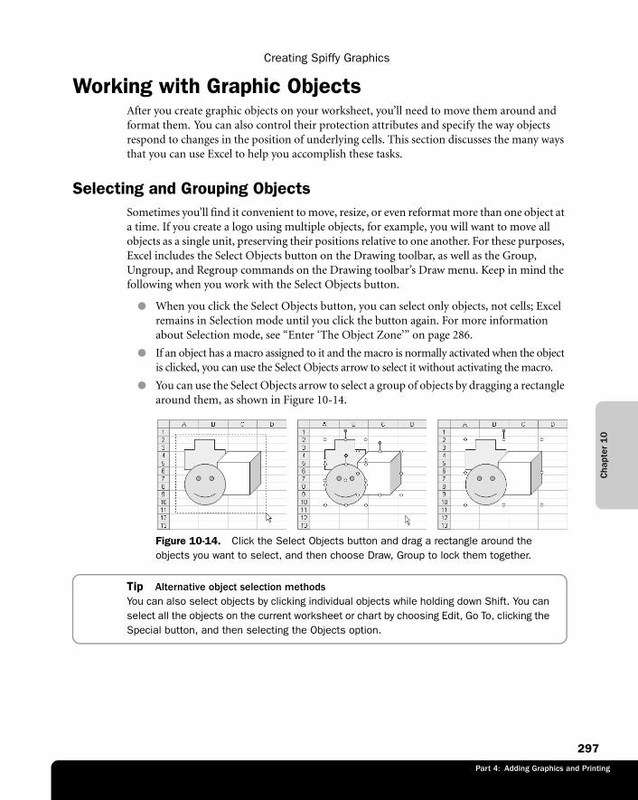
Cha

pter

10

Creating Spiffy Graphics

297

Part 3: Formatting and Editing Worksheets

Part 4: Adding Graphics and Printing

Working with Graphic ObjectsAfter you create graphic objects on your worksheet, you’ll need to move them around and format them. You can also control their protection attributes and specify the way objects respond to changes in the position of underlying cells. This section discusses the many ways that you can use Excel to help you accomplish these tasks.

Selecting and Grouping ObjectsSometimes you’ll find it convenient to move, resize, or even reformat more than one object at a time. If you create a logo using multiple objects, for example, you will want to move all objects as a single unit, preserving their positions relative to one another. For these purposes, Excel includes the Select Objects button on the Drawing toolbar, as well as the Group, Ungroup, and Regroup commands on the Drawing toolbar’s Draw menu. Keep in mind the following when you work with the Select Objects button.

● When you click the Select Objects button, you can select only objects, not cells; Excel remains in Selection mode until you click the button again. For more information about Selection mode, see “Enter ‘The Object Zone’” on page 286.

● If an object has a macro assigned to it and the macro is normally activated when the object is clicked, you can use the Select Objects arrow to select it without activating the macro.

● You can use the Select Objects arrow to select a group of objects by dragging a rectangle around them, as shown in Figure 10-14.

f10ie14

Figure 10-14. Click the Select Objects button and drag a rectangle around the objects you want to select, and then choose Draw, Group to lock them together.

Tip Alternative object selection methodsYou can also select objects by clicking individual objects while holding down Shift. You can select all the objects on the current worksheet or chart by choosing Edit, Go To, clicking the Special button, and then selecting the Objects option.

Chapter 1

0

Microsoft Office Excel 2003 Inside Out

298

Part 4: Adding Graphics and Printing

After you select a group of objects, you can lock them together using Group on the Drawing tool-bar’s Draw menu. The sets of handles around each selected object are then replaced by a single set of handles for the entire group, as shown in Figure 10-14. After the objects are grouped, you can manipulate the set of objects as a single object. You can resize, move, and apply formatting to them as a group. When you apply formatting, however, the separate objects might behave differ-ently, especially if you have grouped different kinds of objects with different formats. It’s best to apply formatting before you group objects together, unless the objects are similar.

To ungroup a set of objects, select the group and then click Draw, Ungroup. You can also apply Regroup to the objects you most recently ungrouped. For example, this is handy if you ungrouped a set of objects to make changes to one or more of them. Rather than selecting them again and choosing Group, just choose Regroup.

Tip Group and ungroup using the shortcut menuThe quickest way to group and ungroup objects is to right-click the selected objects and choose either Group or Ungroup from the shortcut menu that appears.

Selecting Objects That Contain TextUnlike other objects, when you click an object containing text, a gray border appears around it to indicate that it’s selected. You can then manipulate and format the box as you would any other object. When you double-click an object containing text, a flashing insertion point appears in the text area, giving you the opportunity to edit the text inside. If you want to move an object containing text while its text area is active, you must drag the gray border.

Formatting ObjectsYou can apply patterns, colors, and shading to objects using the command that appears at the top of the Format menu when an object is selected. The actual command name differs, depending on the type of object selected. For example, the command can be AutoShape, Text Box, or Picture when the corresponding object type is selected. If you choose any form of this command, or if you double-click the object (or the gray border of an object containing text), a dialog box similar to the one shown in Figure 10-15 appears.

Note The name of the first command on the Format menu varies depending on which object you have selected. Similarly, the name of the associated dialog box changes as well. For example, if a chart’s legend is selected, the command on the Format menu appears as Selected Legend and opens the Format Legend dialog box.

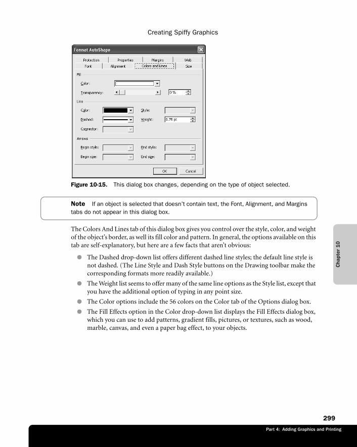
Cha

pter

10

Creating Spiffy Graphics

299

Part 3: Formatting and Editing Worksheets

Part 4: Adding Graphics and Printing

f10ie15

Figure 10-15. This dialog box changes, depending on the type of object selected.

Note If an object is selected that doesn’t contain text, the Font, Alignment, and Margins tabs do not appear in this dialog box.

The Colors And Lines tab of this dialog box gives you control over the style, color, and weight of the object’s border, as well its fill color and pattern. In general, the options available on this tab are self-explanatory, but here are a few facts that aren’t obvious:

● The Dashed drop-down list offers different dashed line styles; the default line style is not dashed. (The Line Style and Dash Style buttons on the Drawing toolbar make the corresponding formats more readily available.)

● The Weight list seems to offer many of the same line options as the Style list, except that you have the additional option of typing in any point size.

● The Color options include the 56 colors on the Color tab of the Options dialog box.

● The Fill Effects option in the Color drop-down list displays the Fill Effects dialog box, which you can use to add patterns, gradient fills, pictures, or textures, such as wood, marble, canvas, and even a paper bag effect, to your objects.

Chapter 1

0

Microsoft Office Excel 2003 Inside Out

300

Part 4: Adding Graphics and Printing

● If you apply a pattern using the Pattern tab in the Fill Effects dialog box, the color you select for the foreground is assigned to the pattern itself and is reflected in the sample pattern thumbnails displayed in the dialog box. The color you select for the back-ground is assigned to the white areas of the pattern.

TroubleshootingTextured and patterned fills don’t rotate

If you rotate an object formatted with either a textured or patterned fill effect, you’ll notice that the fill won’t rotate with the rest of the object. This is just the way these things work. To see what we’re talking about, double-click any 2-D object to open the Format AutoShape dialog box, and then choose Fill Effects from the Fill Color drop-down list. In the Fill Effects dialog box, select an option from either the Texture tab or the Pattern tab and click OK. Now try rotating the object using the panhandle, and you’ll notice that the pattern always remains oriented in the same direction. This may not be what you’re after, but it can also be a good thing. For example, if you create a number of objects on the same sheet using the same texture, they will seem to be little windows on a larger background pattern, which you can use as part of your design.

Changing Colors in the PaletteThe palette of colors available for use with objects is determined by the Color tab of the Tools, Options dialog box. To modify the palette, click the Color tab, select a color, click the Modify Color button, and pick a different color.

Adding TransparencyWhen you use the Transparency slider in either the Format Object or the Fill Effects dialog box, the worksheet and anything else that falls underneath the selected object shows through in the percentage you select. This option essentially turns off alternative fill color pixels, par-tially revealing whatever is behind it. Figure 10-16 shows two identical objects, but 50 percent transparency was applied to the one on the right.

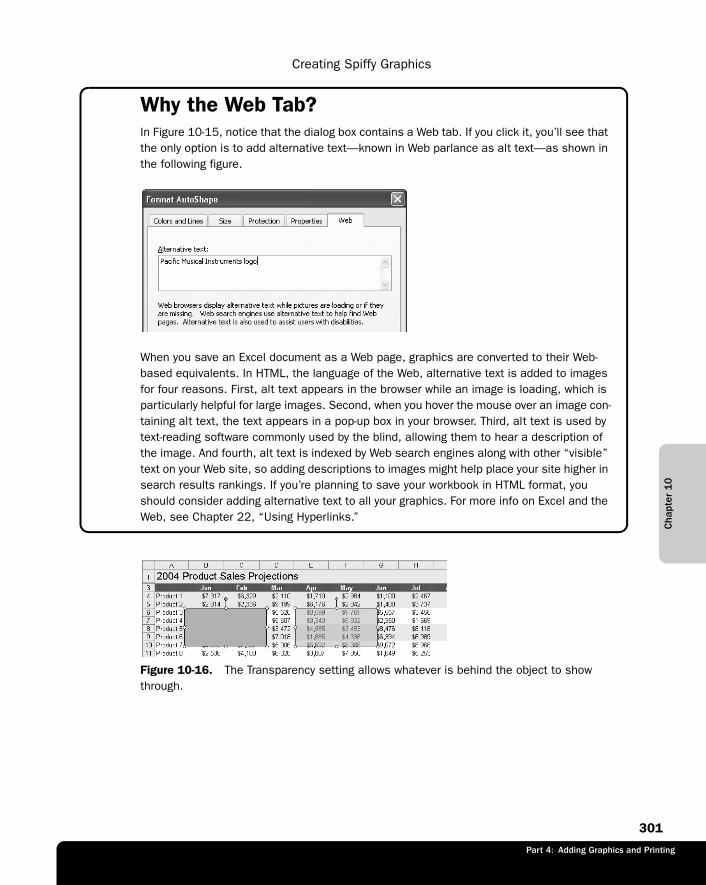
Cha

pter

10

Creating Spiffy Graphics

301

Part 3: Formatting and Editing Worksheets

Part 4: Adding Graphics and Printing

Why the Web Tab?In Figure 10-15, notice that the dialog box contains a Web tab. If you click it, you’ll see that the only option is to add alternative text—known in Web parlance as alt text—as shown in the following figure.

g10ie02

When you save an Excel document as a Web page, graphics are converted to their Web-based equivalents. In HTML, the language of the Web, alternative text is added to images for four reasons. First, alt text appears in the browser while an image is loading, which is particularly helpful for large images. Second, when you hover the mouse over an image con-taining alt text, the text appears in a pop-up box in your browser. Third, alt text is used by text-reading software commonly used by the blind, allowing them to hear a description of the image. And fourth, alt text is indexed by Web search engines along with other “visible” text on your Web site, so adding descriptions to images might help place your site higher in search results rankings. If you’re planning to save your workbook in HTML format, you should consider adding alternative text to all your graphics. For more info on Excel and the Web, see Chapter 22, “Using Hyperlinks.”

f10ie16

Figure 10-16. The Transparency setting allows whatever is behind the object to show through.

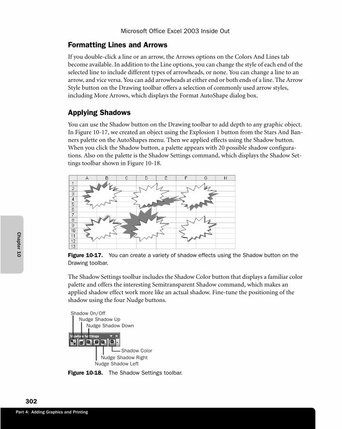
Chapter 1

0

Microsoft Office Excel 2003 Inside Out

302

Part 4: Adding Graphics and Printing

Formatting Lines and ArrowsIf you double-click a line or an arrow, the Arrows options on the Colors And Lines tab become available. In addition to the Line options, you can change the style of each end of the selected line to include different types of arrowheads, or none. You can change a line to an arrow, and vice versa. You can add arrowheads at either end or both ends of a line. The Arrow Style button on the Drawing toolbar offers a selection of commonly used arrow styles, including More Arrows, which displays the Format AutoShape dialog box.

Applying ShadowsYou can use the Shadow button on the Drawing toolbar to add depth to any graphic object. In Figure 10-17, we created an object using the Explosion 1 button from the Stars And Ban-ners palette on the AutoShapes menu. Then we applied effects using the Shadow button. When you click the Shadow button, a palette appears with 20 possible shadow configura-tions. Also on the palette is the Shadow Settings command, which displays the Shadow Set-tings toolbar shown in Figure 10-18.

f10ie17

Figure 10-17. You can create a variety of shadow effects using the Shadow button on the Drawing toolbar.

The Shadow Settings toolbar includes the Shadow Color button that displays a familiar color palette and offers the interesting Semitransparent Shadow command, which makes an applied shadow effect work more like an actual shadow. Fine-tune the positioning of the shadow using the four Nudge buttons.

f10ie18

Figure 10-18. The Shadow Settings toolbar.

Shadow ColorNudge Shadow Right

Nudge Shadow Left

Nudge Shadow DownNudge Shadow Up

Shadow On/Off

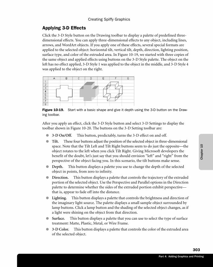
Cha

pter

10

Creating Spiffy Graphics

303

Part 3: Formatting and Editing Worksheets

Part 4: Adding Graphics and Printing

Applying 3-D EffectsClick the 3-D Style button on the Drawing toolbar to display a palette of predefined three-dimensional effects. You can apply three-dimensional effects to any object, including lines, arrows, and WordArt objects. If you apply one of these effects, several special formats are applied to the selected object: horizontal tilt, vertical tilt, depth, direction, lighting position, surface type, and color of the extruded area. In Figure 10-19, we started with three copies of the same object and applied effects using buttons on the 3-D Style palette. The object on the left has no effect applied, 3-D Style 1 was applied to the object in the middle, and 3-D Style 4 was applied to the object on the right.

f10ie19

Figure 10-19. Start with a basic shape and give it depth using the 3-D button on the Draw-ing toolbar.

After you apply an effect, click the 3-D Style button and select 3-D Settings to display the toolbar shown in Figure 10-20. The buttons on the 3-D Setting toolbar are:

● 3-D On/Off. This button, predictably, turns the 3-D effect on and off.

● Tilt. These four buttons adjust the position of the selected object in three-dimensional space. Note that the Tilt Left and Tilt Right buttons seem to do just the opposite—the object rotates to the left when you click Tilt Right. Giving Microsoft developers the benefit of the doubt, let’s just say that you should envision “left” and “right” from the perspective of the object facing you. In this scenario, the tilt buttons make sense.

● Depth. This button displays a palette you use to change the depth of the selected object in points, from zero to infinity.

● Direction. This button displays a palette that controls the trajectory of the extruded portion of the selected object. Use the Perspective and Parallel options in the Direction palette to determine whether the sides of the extruded portion exhibit perspective—that is, appear to fade off into the distance.

● Lighting. This button displays a palette that controls the brightness and direction of the imaginary light source. The palette displays a small sample object surrounded by lamp buttons. Click a lamp button and the shading of the selected object changes, as if a light were shining on the object from that direction.

● Surface. This button displays a palette that you can use to select the type of surface treatment: Matte, Plastic, Metal, or Wire Frame.

● 3-D Color. This button displays a palette that controls the color of the extruded area of the selected object.

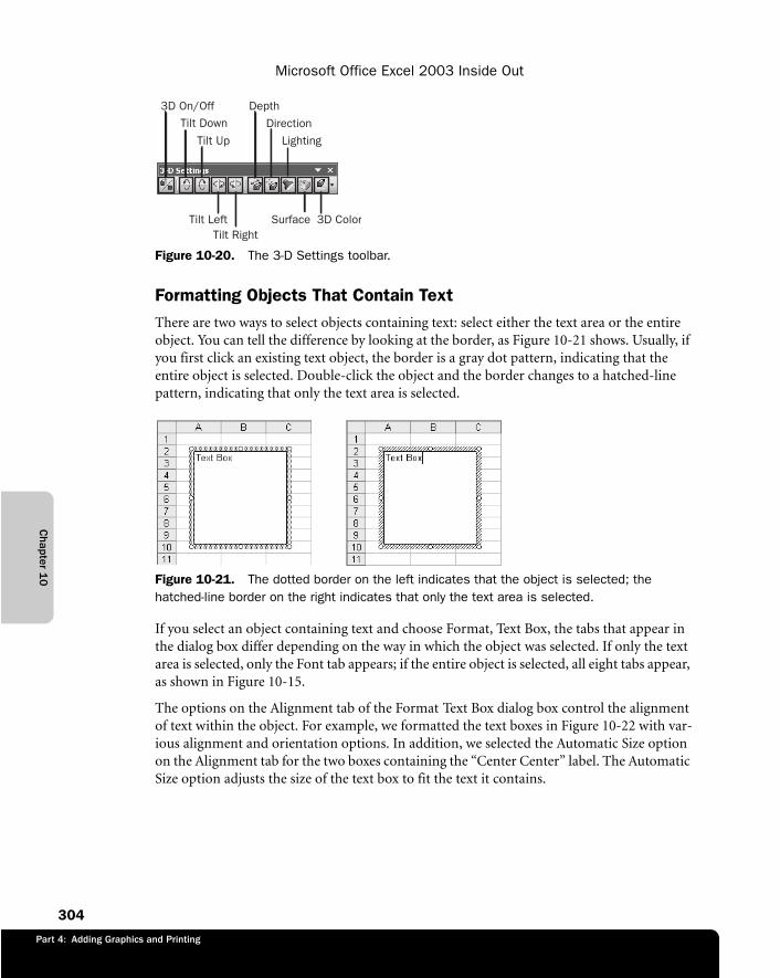
Chapter 1

0

Microsoft Office Excel 2003 Inside Out

304

Part 4: Adding Graphics and Printing

10ie20

Figure 10-20. The 3-D Settings toolbar.

Formatting Objects That Contain TextThere are two ways to select objects containing text: select either the text area or the entire object. You can tell the difference by looking at the border, as Figure 10-21 shows. Usually, if you first click an existing text object, the border is a gray dot pattern, indicating that the entire object is selected. Double-click the object and the border changes to a hatched-line pattern, indicating that only the text area is selected.

f10ie21

Figure 10-21. The dotted border on the left indicates that the object is selected; the hatched-line border on the right indicates that only the text area is selected.

If you select an object containing text and choose Format, Text Box, the tabs that appear in the dialog box differ depending on the way in which the object was selected. If only the text area is selected, only the Font tab appears; if the entire object is selected, all eight tabs appear, as shown in Figure 10-15.

The options on the Alignment tab of the Format Text Box dialog box control the alignment of text within the object. For example, we formatted the text boxes in Figure 10-22 with var-ious alignment and orientation options. In addition, we selected the Automatic Size option on the Alignment tab for the two boxes containing the “Center Center” label. The Automatic Size option adjusts the size of the text box to fit the text it contains.

Tilt Left Surface 3D ColorTilt Right

Tilt Up Lighting

Tilt Down Direction

3D On/Off Depth

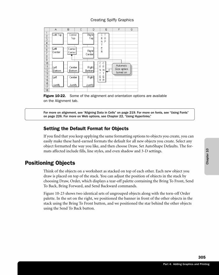
Cha

pter

10

Creating Spiffy Graphics

305

Part 3: Formatting and Editing Worksheets

Part 4: Adding Graphics and Printing

f10ie22

Figure 10-22. Some of the alignment and orientation options are available on the Alignment tab.

For more on alignment, see “Aligning Data in Cells” on page 219. For more on fonts, see “Using Fonts” on page 226. For more on Web options, see Chapter 22, “Using Hyperlinks.”

Setting the Default Format for ObjectsIf you find that you keep applying the same formatting options to objects you create, you can easily make these hard-earned formats the default for all new objects you create. Select any object formatted the way you like, and then choose Draw, Set AutoShape Defaults. The for-mats affected include fills, line styles, and even shadow and 3-D settings.

Positioning ObjectsThink of the objects on a worksheet as stacked on top of each other. Each new object you draw is placed on top of the stack. You can adjust the position of objects in the stack by choosing Draw, Order, which displays a tear-off palette containing the Bring To Front, Send To Back, Bring Forward, and Send Backward commands.

Figure 10-23 shows two identical sets of ungrouped objects along with the torn-off Order palette. In the set on the right, we positioned the banner in front of the other objects in the stack using the Bring To Front button, and we positioned the star behind the other objects using the Send To Back button.

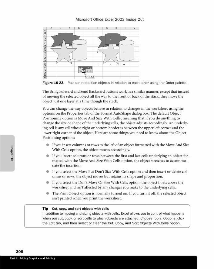
Chapter 1

0

Microsoft Office Excel 2003 Inside Out

306

Part 4: Adding Graphics and Printing

f10ie23

Figure 10-23. You can reposition objects in relation to each other using the Order palette.

The Bring Forward and Send Backward buttons work in a similar manner, except that instead of moving the selected object all the way to the front or back of the stack, they move the object just one layer at a time though the stack.

You can change the way objects behave in relation to changes in the worksheet using the options on the Properties tab of the Format AutoShape dialog box. The default Object Positioning option is Move And Size With Cells, meaning that if you do anything to change the size or shape of the underlying cells, the object adjusts accordingly. An underly-ing cell is any cell whose right or bottom border is between the upper left corner and the lower right corner of the object. Here are some things you need to know about the Object Positioning options:

● If you insert columns or rows to the left of an object formatted with the Move And Size With Cells option, the object moves accordingly.

● If you insert columns or rows between the first and last cells underlying an object for-matted with the Move And Size With Cells option, the object stretches to accommo-date the insertion.

● If you select the Move But Don’t Size With Cells option and then insert or delete col-umns or rows, the object moves but retains its shape and proportion.

● If you select the Don’t Move Or Size With Cells option, the object floats above the worksheet and isn’t affected by any changes you make to the underlying cells.

● The Print Object option is normally turned on. If you turn it off, the selected object isn’t printed when you print the worksheet.

Tip Cut, copy, and sort objects with cellsIn addition to moving and sizing objects with cells, Excel allows you to control what happens when you cut, copy, or sort cells to which objects are attached. Choose Tools, Options, click the Edit tab, and then select or clear the Cut, Copy, And Sort Objects With Cells option.

Cha

pter

10

Creating Spiffy Graphics

307

Part 3: Formatting and Editing Worksheets

Part 4: Adding Graphics and Printing

Tools to Help You Position Objects on the WorksheetIt’s great to be able to create cool graphics with Excel, but the free-floating nature of graphic objects sometimes makes it hard to maintain a semblance of order on your worksheet. The Draw menu contains several menus and tear-off palettes you can use to straighten things up. Here are some key points to remember about using these object positioning commands:

● To Grid, on the Snap submenu, uses the columns and rows of the worksheet to align objects. Pre-existing Objects don’t line up with the grid when you choose this com-mand, but as soon as you create or drag an object, it snaps to the nearest column and row borders.

● To Shape, on the Snap submenu, turns on the To Grid command when you choose it, activating its functionality. It adds to the spreadsheet grid virtual gridlines tangent to the edges of any existing objects, making it easy to align objects to one other. If you turn off the To Grid command, the To Shape command is turned off as well.

● Both the To Grid and To Shape commands, on the Snap submenu, are toggles—that is, you click once to turn them on and click again to turn them off.

● If you select an object and click any of the tools on the Nudge submenu, the object moves one pixel at a time in the direction you want.

● The Align Or Distribute submenu contains commands that operate only when two or more objects are selected, arranging the selected objects relative to each other.

Tip Nudge with the keyboardYou can also use the arrow keys on your keyboard—the functional equivalent of the Nudge buttons—to nudge objects one pixel at a time. If the To Grid command is turned on, press-ing an arrow key moves the selected object to the next gridline in that direction.

The Align Or Distribute submenu can be a great help when you are working with multiple objects. Suppose you have a number of objects that you want to be evenly spaced. You could start by using the Align Top command to line up one row of objects, and then choose Distrib-ute Horizontally to space them evenly. Then use the following Align Or Distribute com-mands to align objects.

● Align Left/Align Right. Lines up the left edges of all selected objects with the left edge of the leftmost object selected. Align Right works identically, but in the opposite direction.

● Align Center/Align Middle. Lines up the centers of objects along a vertical or middle axis and finds the average common centerline of all selected objects.

● Align Top/Align Bottom. Lines up the top edges of objects along a horizontal axis with the top edge of the topmost object. Align Bottom works identically with the bot-tom edges of selected objects.

● Distribute Horizontally and Distribute Vertically. Calculates the total amount of space between the selected objects and divides the space as equally as possible among them. The first and last objects (leftmost and rightmost, or top and bottom) do not move—all the objects in between are adjusted as necessary.

Chapter 1

0

Microsoft Office Excel 2003 Inside Out

308

Part 4: Adding Graphics and Printing

Protecting ObjectsYou can prevent objects from being selected, moved, formatted, or sized by choosing Format, AutoShape, clicking the Protection tab, and selecting the Locked option. You can also use the Lock Text option, which is visible only when a text box is selected, to protect the text contents of a text box. Newly drawn objects are assigned Locked protection. However, to turn on worksheet security and protection for both text boxes and new objects, you must also choose Tools, Protection, Protect Sheet. For more information about protection, see “Protecting Worksheets” on page 127.

Controlling the Display of ObjectsTo speed up the scrolling of your worksheet, choose Tools, Options and click the View tab. In the Objects area of the View tab, Show All is normally selected. Selecting the Show Placeholders option reduces text boxes, button objects, and embedded charts to simple patterns that indicate their locations on the worksheet. Show Placeholders increases your scrolling speed because Excel doesn’t have to redraw the objects every time you scroll to a new screen. You must turn on the Show All option before you print.

Hide All suppresses the display of objects entirely, increasing screen redraw speed even more. Although you cannot directly modify objects when Hide All is turned on, some actions still change them. If anything other than Don’t Move Or Size With Cells is selected on the Properties tab of the Format AutoShape dialog box, the object responds to adjustments made to the column width or row height of underlying cells.

Inserting Other ObjectsThe Object command on the Insert menu gives you direct access to other applications you can use to create objects. The difference between inserting a picture and inserting an object is that a picture is always static and cannot be directly edited or updated (although you can copy it to another program and edit it there), whereas an inserted object retains a connection to its source application. You can open an embedded object for editing by double-clicking it.

When you choose Insert, Object, a dialog box appears with two tabs—Create New and Create From File. The Create New tab, shown in Figure 10-24, turns on an application and then cre-ates the object directly in the selected application. You select an application in the Object Type list. The contents of this list box vary depending on the configuration of your system and the applications you have installed.

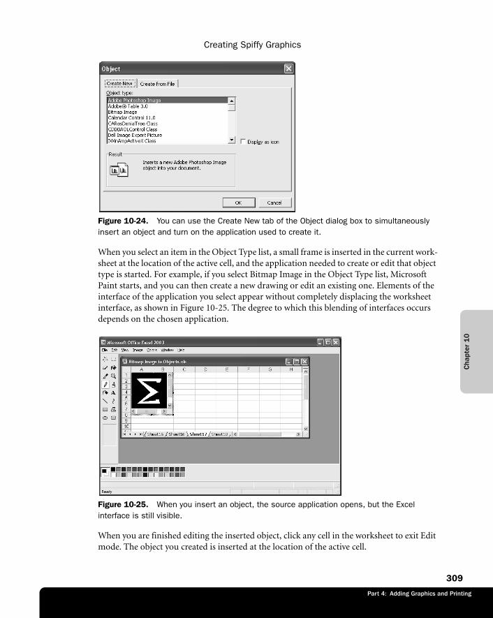
Cha

pter

10

Creating Spiffy Graphics

309

Part 3: Formatting and Editing Worksheets

Part 4: Adding Graphics and Printing

f10ie24

Figure 10-24. You can use the Create New tab of the Object dialog box to simultaneously insert an object and turn on the application used to create it.

When you select an item in the Object Type list, a small frame is inserted in the current work-sheet at the location of the active cell, and the application needed to create or edit that object type is started. For example, if you select Bitmap Image in the Object Type list, Microsoft Paint starts, and you can then create a new drawing or edit an existing one. Elements of the interface of the application you select appear without completely displacing the worksheet interface, as shown in Figure 10-25. The degree to which this blending of interfaces occurs depends on the chosen application.

f10ie25

Figure 10-25. When you insert an object, the source application opens, but the Excel interface is still visible.

When you are finished editing the inserted object, click any cell in the worksheet to exit Edit mode. The object you created is inserted at the location of the active cell.

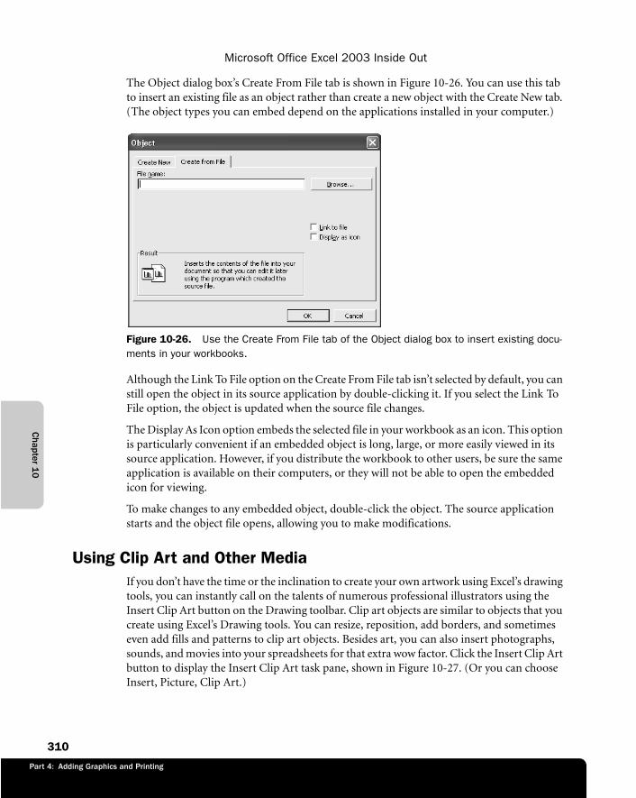
Chapter 1

0

Microsoft Office Excel 2003 Inside Out

310

Part 4: Adding Graphics and Printing

The Object dialog box’s Create From File tab is shown in Figure 10-26. You can use this tab to insert an existing file as an object rather than create a new object with the Create New tab. (The object types you can embed depend on the applications installed in your computer.)

f10ie26

Figure 10-26. Use the Create From File tab of the Object dialog box to insert existing docu-ments in your workbooks.

Although the Link To File option on the Create From File tab isn’t selected by default, you can still open the object in its source application by double-clicking it. If you select the Link To File option, the object is updated when the source file changes.

The Display As Icon option embeds the selected file in your workbook as an icon. This option is particularly convenient if an embedded object is long, large, or more easily viewed in its source application. However, if you distribute the workbook to other users, be sure the same application is available on their computers, or they will not be able to open the embedded icon for viewing.

To make changes to any embedded object, double-click the object. The source application starts and the object file opens, allowing you to make modifications.

Using Clip Art and Other MediaIf you don’t have the time or the inclination to create your own artwork using Excel’s drawing tools, you can instantly call on the talents of numerous professional illustrators using the Insert Clip Art button on the Drawing toolbar. Clip art objects are similar to objects that you create using Excel’s Drawing tools. You can resize, reposition, add borders, and sometimes even add fills and patterns to clip art objects. Besides art, you can also insert photographs, sounds, and movies into your spreadsheets for that extra wow factor. Click the Insert Clip Art button to display the Insert Clip Art task pane, shown in Figure 10-27. (Or you can choose Insert, Picture, Clip Art.)

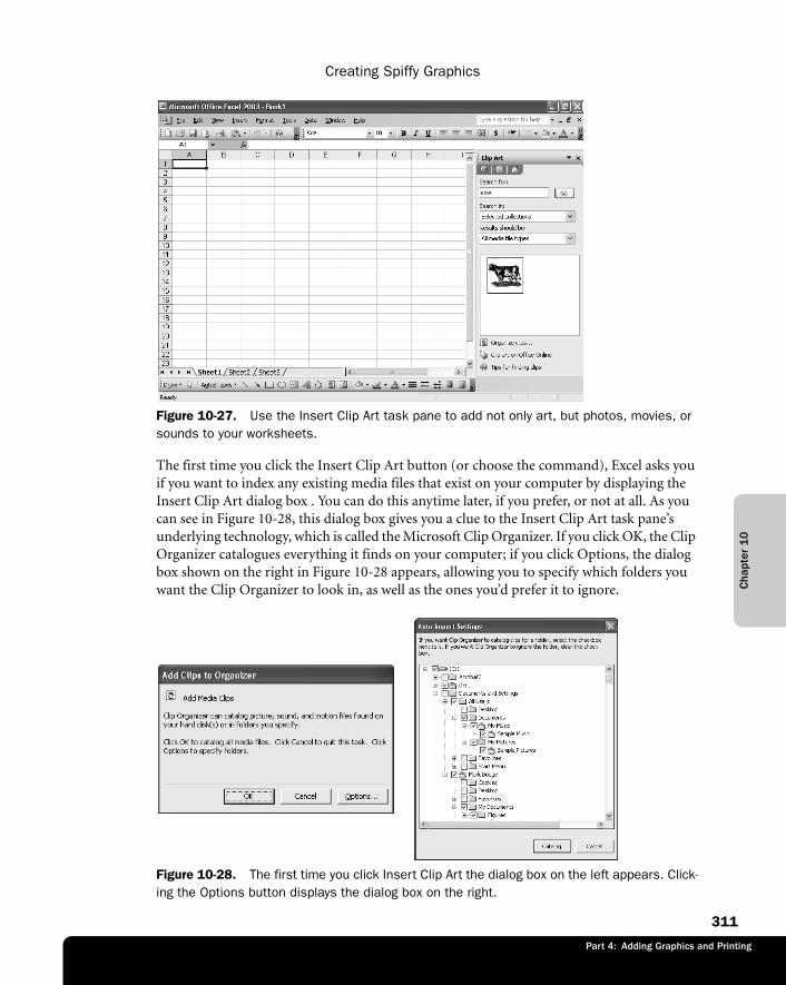
Cha

pter

10

Creating Spiffy Graphics

311

Part 3: Formatting and Editing Worksheets

Part 4: Adding Graphics and Printing

f10ie27

Figure 10-27. Use the Insert Clip Art task pane to add not only art, but photos, movies, or sounds to your worksheets.

The first time you click the Insert Clip Art button (or choose the command), Excel asks you if you want to index any existing media files that exist on your computer by displaying the Insert Clip Art dialog box . You can do this anytime later, if you prefer, or not at all. As you can see in Figure 10-28, this dialog box gives you a clue to the Insert Clip Art task pane’s underlying technology, which is called the Microsoft Clip Organizer. If you click OK, the Clip Organizer catalogues everything it finds on your computer; if you click Options, the dialog box shown on the right in Figure 10-28 appears, allowing you to specify which folders you want the Clip Organizer to look in, as well as the ones you’d prefer it to ignore.

f10ie28

Figure 10-28. The first time you click Insert Clip Art the dialog box on the left appears. Click-ing the Options button displays the dialog box on the right.

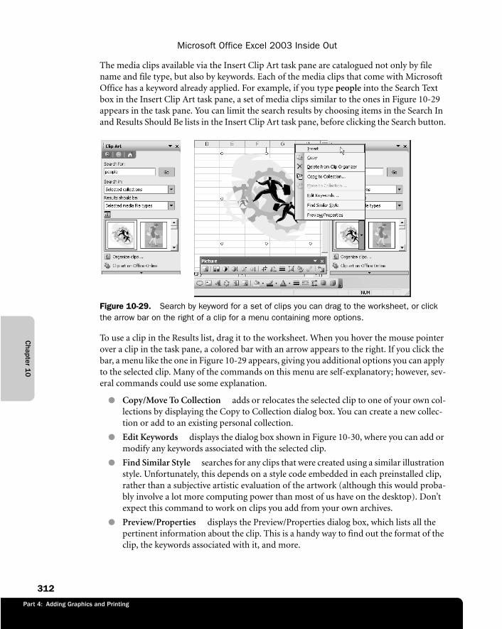
Chapter 1

0

Microsoft Office Excel 2003 Inside Out

312

Part 4: Adding Graphics and Printing

The media clips available via the Insert Clip Art task pane are catalogued not only by file name and file type, but also by keywords. Each of the media clips that come with Microsoft Office has a keyword already applied. For example, if you type people into the Search Text box in the Insert Clip Art task pane, a set of media clips similar to the ones in Figure 10-29 appears in the task pane. You can limit the search results by choosing items in the Search In and Results Should Be lists in the Insert Clip Art task pane, before clicking the Search button.

f10ie29

Figure 10-29. Search by keyword for a set of clips you can drag to the worksheet, or click the arrow bar on the right of a clip for a menu containing more options.

To use a clip in the Results list, drag it to the worksheet. When you hover the mouse pointer over a clip in the task pane, a colored bar with an arrow appears to the right. If you click the bar, a menu like the one in Figure 10-29 appears, giving you additional options you can apply to the selected clip. Many of the commands on this menu are self-explanatory; however, sev-eral commands could use some explanation.

● Copy/Move To Collection adds or relocates the selected clip to one of your own col-lections by displaying the Copy to Collection dialog box. You can create a new collec-tion or add to an existing personal collection.

● Edit Keywords displays the dialog box shown in Figure 10-30, where you can add or modify any keywords associated with the selected clip.

● Find Similar Style searches for any clips that were created using a similar illustration style. Unfortunately, this depends on a style code embedded in each preinstalled clip, rather than a subjective artistic evaluation of the artwork (although this would proba-bly involve a lot more computing power than most of us have on the desktop). Don’t expect this command to work on clips you add from your own archives.

● Preview/Properties displays the Preview/Properties dialog box, which lists all the pertinent information about the clip. This is a handy way to find out the format of the clip, the keywords associated with it, and more.

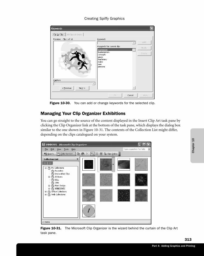
Cha

pter

10

Creating Spiffy Graphics

313

Part 3: Formatting and Editing Worksheets

Part 4: Adding Graphics and Printing

f10ie30 Figure 10-30. You can add or change keywords for the selected clip.

Managing Your Clip Organizer ExhibitionsYou can go straight to the source of the content displayed in the Insert Clip Art task pane by clicking the Clip Organizer link at the bottom of the task pane, which displays the dialog box similar to the one shown in Figure 10-31. The contents of the Collection List might differ, depending on the clips catalogued on your system.

f10ie31

Figure 10-31. The Microsoft Clip Organizer is the wizard behind the curtain of the Clip Art task pane.

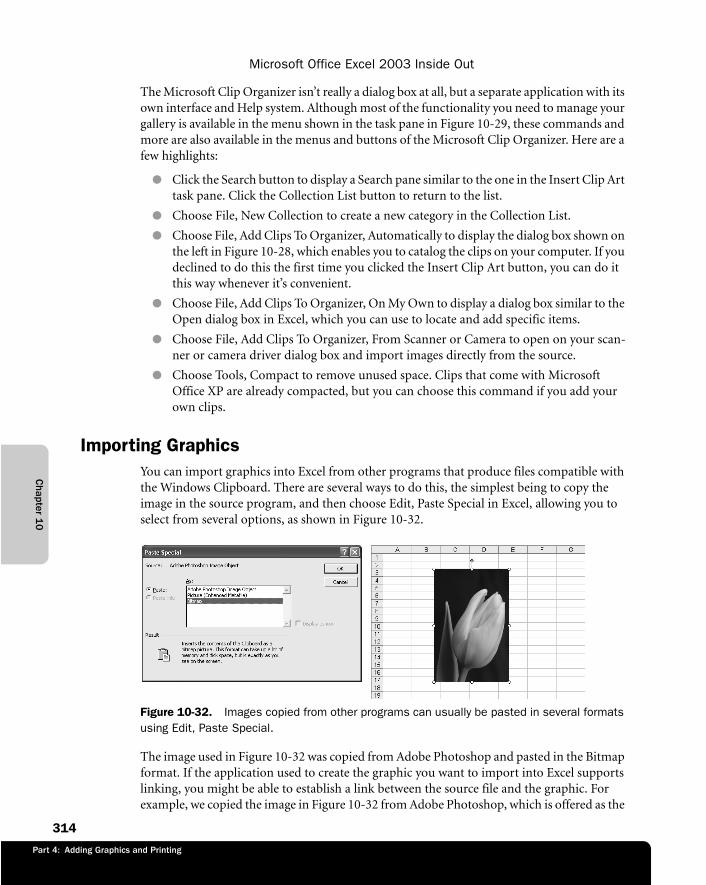
Chapter 1

0

Microsoft Office Excel 2003 Inside Out

314

Part 4: Adding Graphics and Printing

The Microsoft Clip Organizer isn’t really a dialog box at all, but a separate application with its own interface and Help system. Although most of the functionality you need to manage your gallery is available in the menu shown in the task pane in Figure 10-29, these commands and more are also available in the menus and buttons of the Microsoft Clip Organizer. Here are a few highlights:

● Click the Search button to display a Search pane similar to the one in the Insert Clip Art task pane. Click the Collection List button to return to the list.

● Choose File, New Collection to create a new category in the Collection List.

● Choose File, Add Clips To Organizer, Automatically to display the dialog box shown on the left in Figure 10-28, which enables you to catalog the clips on your computer. If you declined to do this the first time you clicked the Insert Clip Art button, you can do it this way whenever it’s convenient.

● Choose File, Add Clips To Organizer, On My Own to display a dialog box similar to the Open dialog box in Excel, which you can use to locate and add specific items.

● Choose File, Add Clips To Organizer, From Scanner or Camera to open on your scan-ner or camera driver dialog box and import images directly from the source.

● Choose Tools, Compact to remove unused space. Clips that come with Microsoft Office XP are already compacted, but you can choose this command if you add your own clips.

Importing GraphicsYou can import graphics into Excel from other programs that produce files compatible with the Windows Clipboard. There are several ways to do this, the simplest being to copy the image in the source program, and then choose Edit, Paste Special in Excel, allowing you to select from several options, as shown in Figure 10-32.

f10ie32

Figure 10-32. Images copied from other programs can usually be pasted in several formats using Edit, Paste Special.

The image used in Figure 10-32 was copied from Adobe Photoshop and pasted in the Bitmap format. If the application used to create the graphic you want to import into Excel supports linking, you might be able to establish a link between the source file and the graphic. For example, we copied the image in Figure 10-32 from Adobe Photoshop, which is offered as the

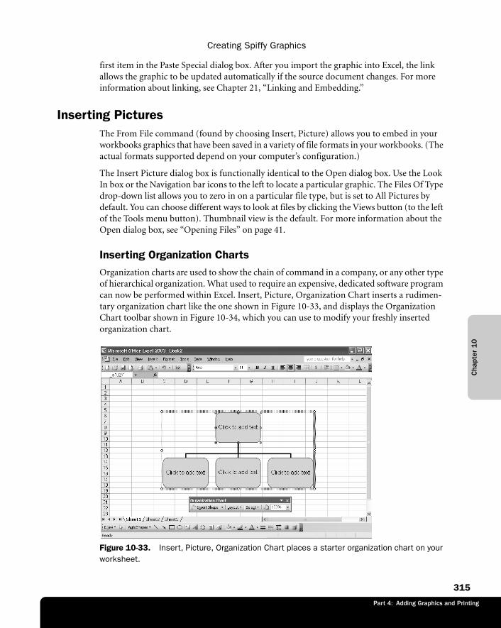
Cha

pter

10

Creating Spiffy Graphics

315

Part 3: Formatting and Editing Worksheets

Part 4: Adding Graphics and Printing

first item in the Paste Special dialog box. After you import the graphic into Excel, the link allows the graphic to be updated automatically if the source document changes. For more information about linking, see Chapter 21, “Linking and Embedding.”

Inserting PicturesThe From File command (found by choosing Insert, Picture) allows you to embed in your workbooks graphics that have been saved in a variety of file formats in your workbooks. (The actual formats supported depend on your computer’s configuration.)

The Insert Picture dialog box is functionally identical to the Open dialog box. Use the Look In box or the Navigation bar icons to the left to locate a particular graphic. The Files Of Type drop-down list allows you to zero in on a particular file type, but is set to All Pictures by default. You can choose different ways to look at files by clicking the Views button (to the left of the Tools menu button). Thumbnail view is the default. For more information about the Open dialog box, see “Opening Files” on page 41.

Inserting Organization ChartsOrganization charts are used to show the chain of command in a company, or any other type of hierarchical organization. What used to require an expensive, dedicated software program can now be performed within Excel. Insert, Picture, Organization Chart inserts a rudimen-tary organization chart like the one shown in Figure 10-33, and displays the Organization Chart toolbar shown in Figure 10-34, which you can use to modify your freshly inserted organization chart.

f10ie33

Figure 10-33. Insert, Picture, Organization Chart places a starter organization chart on your worksheet.

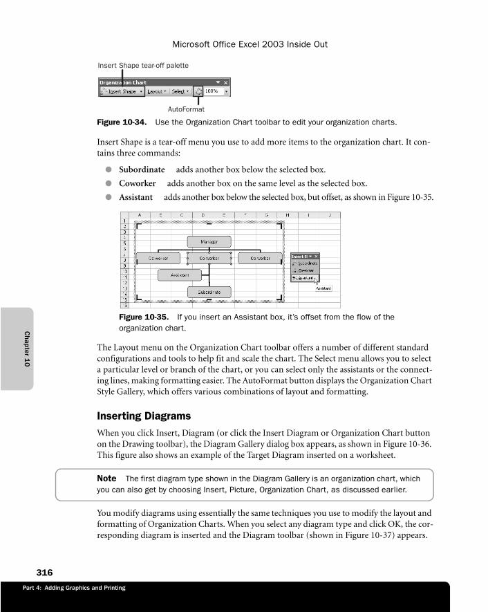
Chapter 1

0

Microsoft Office Excel 2003 Inside Out

316

Part 4: Adding Graphics and Printing

f10ie34

Figure 10-34. Use the Organization Chart toolbar to edit your organization charts.

Insert Shape is a tear-off menu you use to add more items to the organization chart. It con-tains three commands:

● Subordinate adds another box below the selected box.

● Coworker adds another box on the same level as the selected box.

● Assistant adds another box below the selected box, but offset, as shown in Figure 10-35.

f10ie35 Figure 10-35. If you insert an Assistant box, it’s offset from the flow of the organization chart.

The Layout menu on the Organization Chart toolbar offers a number of different standard configurations and tools to help fit and scale the chart. The Select menu allows you to select a particular level or branch of the chart, or you can select only the assistants or the connect-ing lines, making formatting easier. The AutoFormat button displays the Organization Chart Style Gallery, which offers various combinations of layout and formatting.

Inserting DiagramsWhen you click Insert, Diagram (or click the Insert Diagram or Organization Chart button on the Drawing toolbar), the Diagram Gallery dialog box appears, as shown in Figure 10-36. This figure also shows an example of the Target Diagram inserted on a worksheet.

Note The first diagram type shown in the Diagram Gallery is an organization chart, which you can also get by choosing Insert, Picture, Organization Chart, as discussed earlier.

You modify diagrams using essentially the same techniques you use to modify the layout and formatting of Organization Charts. When you select any diagram type and click OK, the cor-responding diagram is inserted and the Diagram toolbar (shown in Figure 10-37) appears.

Insert Shape tear-off palette

AutoFormat

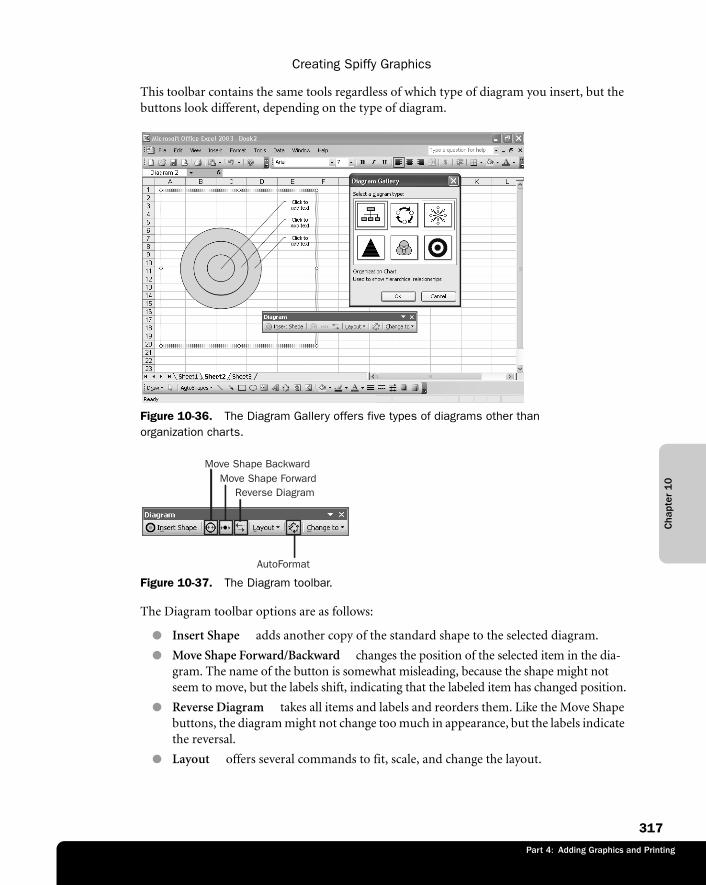
Cha

pter

10

Creating Spiffy Graphics

317

Part 3: Formatting and Editing Worksheets

Part 4: Adding Graphics and Printing

This toolbar contains the same tools regardless of which type of diagram you insert, but the buttons look different, depending on the type of diagram.

f10ie36

Figure 10-36. The Diagram Gallery offers five types of diagrams other than organization charts.

f10ie37

Figure 10-37. The Diagram toolbar.

The Diagram toolbar options are as follows:

● Insert Shape adds another copy of the standard shape to the selected diagram.

● Move Shape Forward/Backward changes the position of the selected item in the dia-gram. The name of the button is somewhat misleading, because the shape might not seem to move, but the labels shift, indicating that the labeled item has changed position.

● Reverse Diagram takes all items and labels and reorders them. Like the Move Shape buttons, the diagram might not change too much in appearance, but the labels indicate the reversal.

● Layout offers several commands to fit, scale, and change the layout.

AutoFormat

Reverse DiagramMove Shape Forward

Move Shape Backward

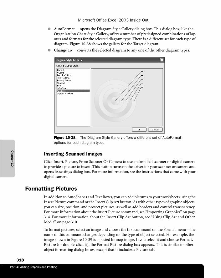
Chapter 1

0

Microsoft Office Excel 2003 Inside Out

318

Part 4: Adding Graphics and Printing

● AutoFormat opens the Diagram Style Gallery dialog box. This dialog box, like the Organization Chart Style Gallery, offers a number of predesigned combinations of lay-outs and formats for the selected diagram type. There is a different set for each type of diagram. Figure 10-38 shows the gallery for the Target diagram.

● Change To converts the selected diagram to any one of the other diagram types.

f10ie38 Figure 10-38. The Diagram Style Gallery offers a different set of AutoFormat options for each diagram type.

Inserting Scanned ImagesClick Insert, Picture, From Scanner Or Camera to use an installed scanner or digital camera to provide a picture to insert. This button turns on the driver for your scanner or camera and opens its settings dialog box. For more information, see the instructions that came with your digital camera.

Formatting PicturesIn addition to AutoShapes and Text Boxes, you can add pictures to your worksheets using the Insert Picture command or the Insert Clip Art button. As with other types of graphic objects, you can size, position, and protect pictures, as well as add borders and control transparency. For more information about the Insert Picture command, see “Importing Graphics” on page 314. For more information about the Insert Clip Art button, see “Using Clip Art and Other Media” on page 310.

To format pictures, select an image and choose the first command on the Format menu—the name of this command changes depending on the type of object selected. For example, the image shown in Figure 10-39 is a pasted bitmap image. If you select it and choose Format, Picture (or double-click it), the Format Picture dialog box appears. This is similar to other object formatting dialog boxes, except that it includes a Picture tab.

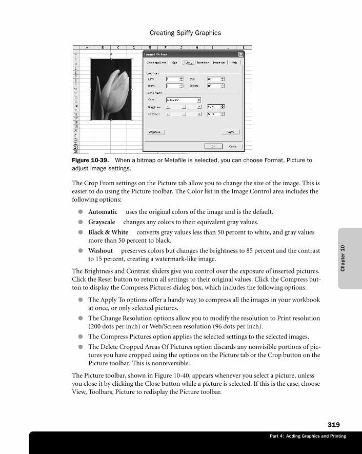
Cha

pter

10

Creating Spiffy Graphics

319

Part 3: Formatting and Editing Worksheets

Part 4: Adding Graphics and Printing

f10ie39

Figure 10-39. When a bitmap or Metafile is selected, you can choose Format, Picture to adjust image settings.

The Crop From settings on the Picture tab allow you to change the size of the image. This is easier to do using the Picture toolbar. The Color list in the Image Control area includes the following options:

● Automatic uses the original colors of the image and is the default.

● Grayscale changes any colors to their equivalent gray values.

● Black & White converts gray values less than 50 percent to white, and gray values more than 50 percent to black.

● Washout preserves colors but changes the brightness to 85 percent and the contrast to 15 percent, creating a watermark-like image.

The Brightness and Contrast sliders give you control over the exposure of inserted pictures. Click the Reset button to return all settings to their original values. Click the Compress but-ton to display the Compress Pictures dialog box, which includes the following options:

● The Apply To options offer a handy way to compress all the images in your workbook at once, or only selected pictures.

● The Change Resolution options allow you to modify the resolution to Print resolution (200 dots per inch) or Web/Screen resolution (96 dots per inch).

● The Compress Pictures option applies the selected settings to the selected images.

● The Delete Cropped Areas Of Pictures option discards any nonvisible portions of pic-tures you have cropped using the options on the Picture tab or the Crop button on the Picture toolbar. This is nonreversible.

The Picture toolbar, shown in Figure 10-40, appears whenever you select a picture, unless you close it by clicking the Close button while a picture is selected. If this is the case, choose View, Toolbars, Picture to redisplay the Picture toolbar.

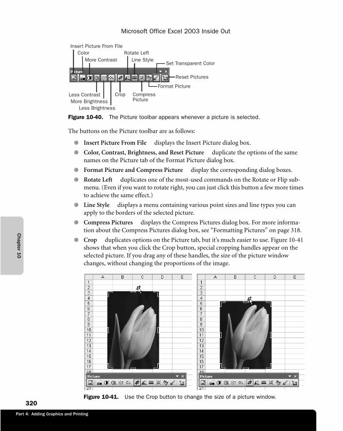
Chapter 1

0

Microsoft Office Excel 2003 Inside Out

320

Part 4: Adding Graphics and Printing

f10ie40

Figure 10-40. The Picture toolbar appears whenever a picture is selected.

The buttons on the Picture toolbar are as follows:

● Insert Picture From File displays the Insert Picture dialog box.

● Color, Contrast, Brightness, and Reset Picture duplicate the options of the same names on the Picture tab of the Format Picture dialog box.

● Format Picture and Compress Picture display the corresponding dialog boxes.

● Rotate Left duplicates one of the most-used commands on the Rotate or Flip sub-menu. (Even if you want to rotate right, you can just click this button a few more times to achieve the same effect.)

● Line Style displays a menu containing various point sizes and line types you can apply to the borders of the selected picture.

● Compress Pictures displays the Compress Pictures dialog box. For more informa-tion about the Compress Pictures dialog box, see “Formatting Pictures” on page 318.

● Crop duplicates options on the Picture tab, but it’s much easier to use. Figure 10-41 shows that when you click the Crop button, special cropping handles appear on the selected picture. If you drag any of these handles, the size of the picture window changes, without changing the proportions of the image.

f10ie41 Figure 10-41. Use the Crop button to change the size of a picture window.

Format Picture

Set Transparent Color

Reset Pictures

CompressPicture

Crop

Line StyleMore ContrastRotate LeftColor

Insert Picture From File

Less BrightnessMore Brightness

Less Contrast

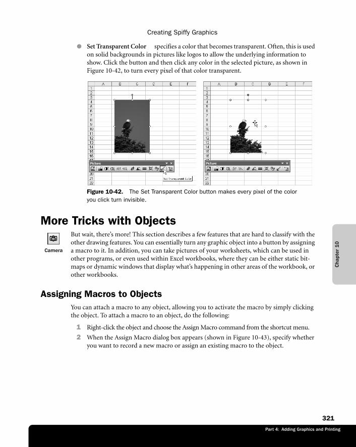
Cha

pter

10

Creating Spiffy Graphics

321

Part 3: Formatting and Editing Worksheets

Part 4: Adding Graphics and Printing

● Set Transparent Color specifies a color that becomes transparent. Often, this is used on solid backgrounds in pictures like logos to allow the underlying information to show. Click the button and then click any color in the selected picture, as shown in Figure 10-42, to turn every pixel of that color transparent.

f10ie42 Figure 10-42. The Set Transparent Color button makes every pixel of the color you click turn invisible.

More Tricks with Objects

Camera

But wait, there’s more! This section describes a few features that are hard to classify with the other drawing features. You can essentially turn any graphic object into a button by assigning a macro to it. In addition, you can take pictures of your worksheets, which can be used in other programs, or even used within Excel workbooks, where they can be either static bit-maps or dynamic windows that display what’s happening in other areas of the workbook, or other workbooks.

Assigning Macros to ObjectsYou can attach a macro to any object, allowing you to activate the macro by simply clicking the object. To attach a macro to an object, do the following:

1 Right-click the object and choose the Assign Macro command from the shortcut menu.

2 When the Assign Macro dialog box appears (shown in Figure 10-43), specify whether you want to record a new macro or assign an existing macro to the object.

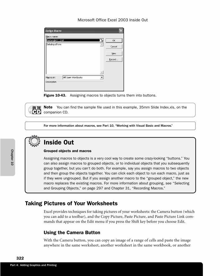
Chapter 1

0

Microsoft Office Excel 2003 Inside Out

322

Part 4: Adding Graphics and Printing

f10ie43

Figure 10-43. Assigning macros to objects turns them into buttons.

Note You can find the sample file used in this example, 35mm Slide Index.xls, on the companion CD.

For more information about macros, see Part 10, “Working with Visual Basic and Macros.”

Inside OutGrouped objects and macros

Assigning macros to objects is a very cool way to create some crazy-looking “buttons.” You can also assign macros to grouped objects, or to individual objects that you subsequently group together, but you can’t do both. For example, say you assign macros to two objects and then group the objects together. You can click each object to run each macro, just as if they were ungrouped. But if you assign another macro to the “grouped object,” the new macro replaces the existing macros. For more information about grouping, see “Selecting and Grouping Objects,” on page 297 and Chapter 31, “Recording Macros.”

Taking Pictures of Your WorksheetsExcel provides techniques for taking pictures of your worksheets: the Camera button (which you can add to a toolbar), and the Copy Picture, Paste Picture, and Paste Picture Link com-mands that appear on the Edit menu if you press the Shift key before you choose Edit.

Using the Camera ButtonWith the Camera button, you can copy an image of a range of cells and paste the image anywhere in the same worksheet, another worksheet in the same workbook, or another

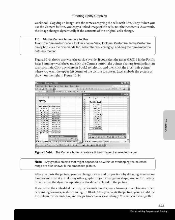
Cha

pter

10

Creating Spiffy Graphics

323

Part 3: Formatting and Editing Worksheets

Part 4: Adding Graphics and Printing

workbook. Copying an image isn’t the same as copying the cells with Edit, Copy. When you use the Camera button, you copy a linked image of the cells, not their contents. As a result, the image changes dynamically if the contents of the original cells change.

Tip Add the Camera button to a toolbarTo add the Camera button to a toolbar, choose View, Toolbars, Customize. In the Customize dialog box, click the Commands tab, select the Tools category, and drag the Camera button onto any toolbar.

Figure 10-44 shows two worksheets side by side. If you select the range G3:G16 in the Pacific Sales Summary worksheet and click the Camera button, the pointer changes from a plus sign to a cross hair. Click anywhere in Book2 to select it, and then click the cross-hair pointer where you want the upper left corner of the picture to appear. Excel embeds the picture as shown on the right in Figure 10-44.

f10ie44

Figure 10-44. The Camera button creates a linked image of a selected range.

Note Any graphic objects that might happen to be within or overlapping the selected range are also shown in the embedded picture.

After you paste the picture, you can change its size and proportions by dragging its selection handles and treat it just like any other graphic object. Changes in shape, size, or formatting do not affect the dynamic updating of the data displayed in the picture.

If you select the embedded picture, the formula bar displays a formula much like any other cell-linking formula, as shown in Figure 10-44. After you create the picture, you can edit the formula in the formula bar, and the picture changes accordingly. You can even change the

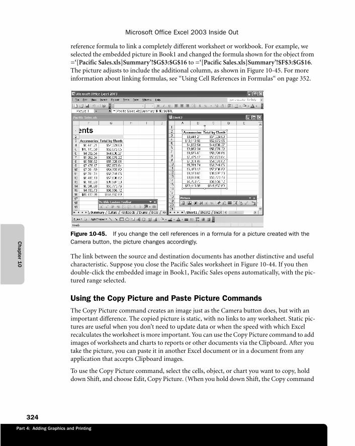
Chapter 1

0

Microsoft Office Excel 2003 Inside Out

324

Part 4: Adding Graphics and Printing

reference formula to link a completely different worksheet or workbook. For example, we selected the embedded picture in Book1 and changed the formula shown for the object from =‘[Pacific Sales.xls]Summary’!$G$3:$G$16 to =‘[Pacific Sales.xls]Summary’!$F$3:$G$16.The picture adjusts to include the additional column, as shown in Figure 10-45. For more information about linking formulas, see “Using Cell References in Formulas“ on page 352.

f10ie45

Figure 10-45. If you change the cell references in a formula for a picture created with the Camera button, the picture changes accordingly.

The link between the source and destination documents has another distinctive and useful characteristic. Suppose you close the Pacific Sales worksheet in Figure 10-44. If you then double-click the embedded image in Book1, Pacific Sales opens automatically, with the pic-tured range selected.

Using the Copy Picture and Paste Picture CommandsThe Copy Picture command creates an image just as the Camera button does, but with an important difference. The copied picture is static, with no links to any worksheet. Static pic-tures are useful when you don’t need to update data or when the speed with which Excel recalculates the worksheet is more important. You can use the Copy Picture command to add images of worksheets and charts to reports or other documents via the Clipboard. After you take the picture, you can paste it in another Excel document or in a document from any application that accepts Clipboard images.

To use the Copy Picture command, select the cells, object, or chart you want to copy, hold down Shift, and choose Edit, Copy Picture. (When you hold down Shift, the Copy command

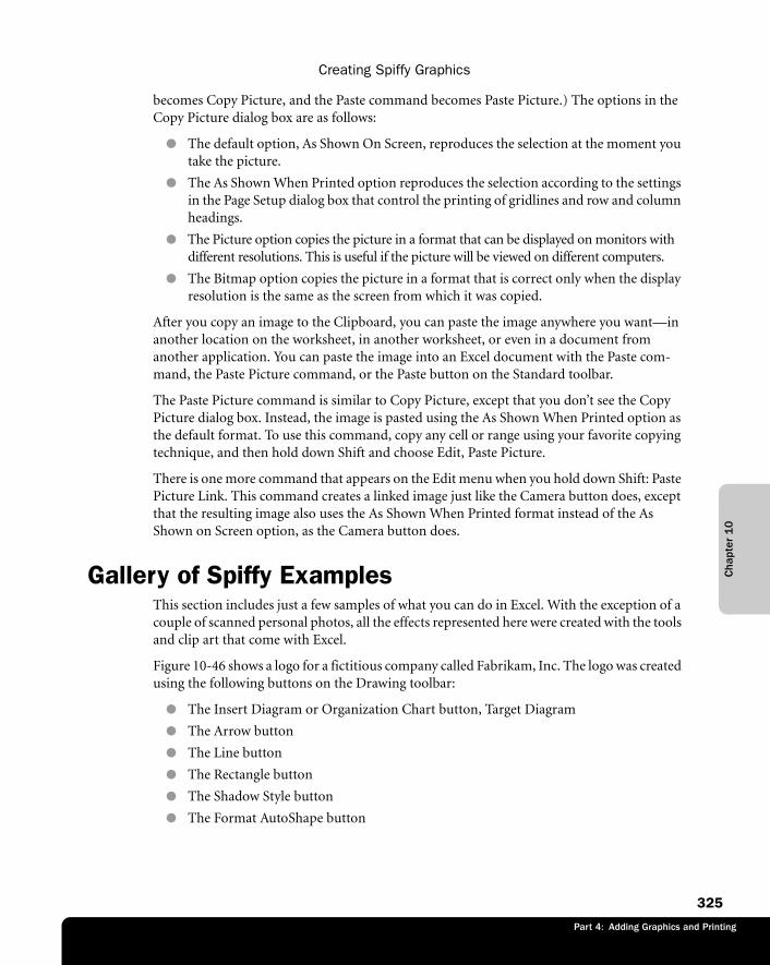
Cha

pter

10

Creating Spiffy Graphics

325

Part 3: Formatting and Editing Worksheets

Part 4: Adding Graphics and Printing

becomes Copy Picture, and the Paste command becomes Paste Picture.) The options in the Copy Picture dialog box are as follows:

● The default option, As Shown On Screen, reproduces the selection at the moment you take the picture.

● The As Shown When Printed option reproduces the selection according to the settings in the Page Setup dialog box that control the printing of gridlines and row and column headings.

● The Picture option copies the picture in a format that can be displayed on monitors with different resolutions. This is useful if the picture will be viewed on different computers.

● The Bitmap option copies the picture in a format that is correct only when the display resolution is the same as the screen from which it was copied.

After you copy an image to the Clipboard, you can paste the image anywhere you want—in another location on the worksheet, in another worksheet, or even in a document from another application. You can paste the image into an Excel document with the Paste com-mand, the Paste Picture command, or the Paste button on the Standard toolbar.

The Paste Picture command is similar to Copy Picture, except that you don’t see the Copy Picture dialog box. Instead, the image is pasted using the As Shown When Printed option as the default format. To use this command, copy any cell or range using your favorite copying technique, and then hold down Shift and choose Edit, Paste Picture.

There is one more command that appears on the Edit menu when you hold down Shift: Paste Picture Link. This command creates a linked image just like the Camera button does, except that the resulting image also uses the As Shown When Printed format instead of the As Shown on Screen option, as the Camera button does.

Gallery of Spiffy ExamplesThis section includes just a few samples of what you can do in Excel. With the exception of a couple of scanned personal photos, all the effects represented here were created with the tools and clip art that come with Excel.

Figure 10-46 shows a logo for a fictitious company called Fabrikam, Inc. The logo was created using the following buttons on the Drawing toolbar:

● The Insert Diagram or Organization Chart button, Target Diagram

● The Arrow button

● The Line button

● The Rectangle button

● The Shadow Style button

● The Format AutoShape button

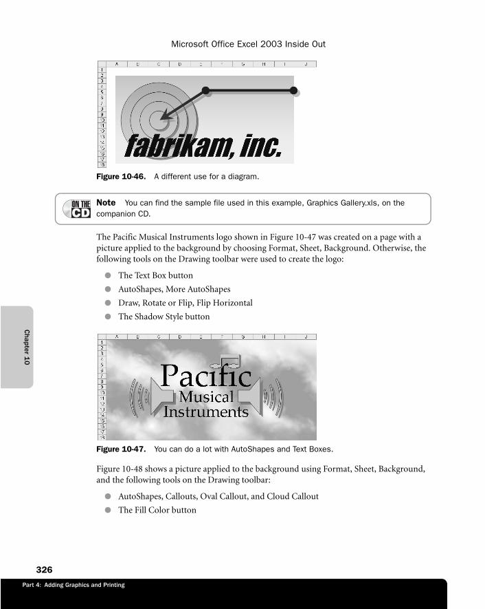
Chapter 1

0

Microsoft Office Excel 2003 Inside Out

326

Part 4: Adding Graphics and Printing

f10ie46

Figure 10-46. A different use for a diagram.

Note You can find the sample file used in this example, Graphics Gallery.xls, on the companion CD.

The Pacific Musical Instruments logo shown in Figure 10-47 was created on a page with a picture applied to the background by choosing Format, Sheet, Background. Otherwise, the following tools on the Drawing toolbar were used to create the logo:

● The Text Box button

● AutoShapes, More AutoShapes

● Draw, Rotate or Flip, Flip Horizontal

● The Shadow Style button

f10ie47

Figure 10-47. You can do a lot with AutoShapes and Text Boxes.

Figure 10-48 shows a picture applied to the background using Format, Sheet, Background, and the following tools on the Drawing toolbar:

● AutoShapes, Callouts, Oval Callout, and Cloud Callout

● The Fill Color button

Cha

pter

10

Creating Spiffy Graphics

327

Part 3: Formatting and Editing Worksheets

Part 4: Adding Graphics and Printing

f10ie48

Figure 10-48. Your friendly authors, mugging for the camera.

The Adventure Works worksheet in Figure 10-49 has an interesting argyle background created by first selecting A1:E4 and enlarging the cells by changing row heights and column widths. With the cell range still selected, we then chose Format, Cells, clicked the Border tab, and clicked both diag-onal border preset buttons. Then we clicked the Patterns tab and selected a fill color. The rest of the work was done with the following tools on the Drawing toolbar:

● The Insert Clip Art button

● The Rectangle button

● The WordArt button

● The Shadow Color button (click the Shadow Style button and select Shadow Settings)

● The Fill Color button’s Fill Effects command

f10ie49

Figure 10-49. You can use cell borders to create patterned backgrounds.

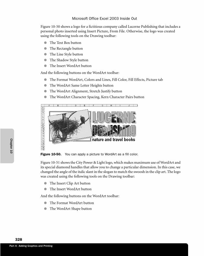
Chapter 1

0

Microsoft Office Excel 2003 Inside Out

328

Part 4: Adding Graphics and Printing

Figure 10-50 shows a logo for a fictitious company called Lucerne Publishing that includes a personal photo inserted using Insert Picture, From File. Otherwise, the logo was created using the following tools on the Drawing toolbar:

● The Text Box button

● The Rectangle button

● The Line Style button

● The Shadow Style button

● The Insert WordArt button

And the following buttons on the WordArt toolbar:

● The Format WordArt, Colors and Lines, Fill Color, Fill Effects, Picture tab

● The WordArt Same Letter Heights button

● The WordArt Alignment, Stretch Justify button

● The WordArt Character Spacing, Kern Character Pairs button

f10ie50

Figure 10-50. You can apply a picture to WordArt as a fill color.

Figure 10-51 shows the City Power & Light logo, which makes maximum use of WordArt and its special diamond handles that allow you to change a particular dimension. In this case, we changed the angle of the italic slant in the slogan to match the swoosh in the clip art. The logo was created using the following tools on the Drawing toolbar:

● The Insert Clip Art button

● The Insert WordArt button

And the following buttons on the WordArt toolbar:

● The Format WordArt button

● The WordArt Shape button

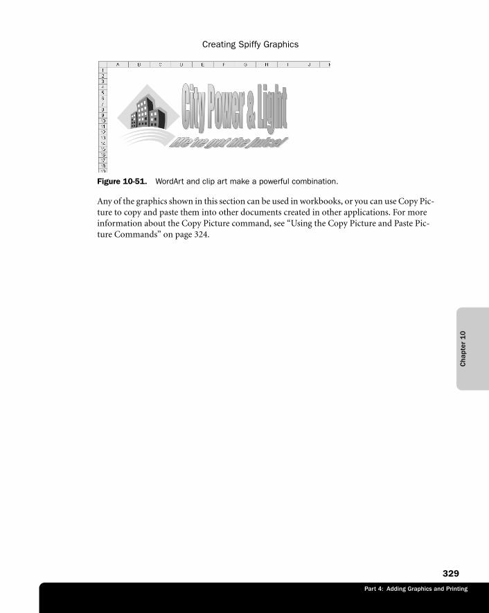
Cha

pter

10

Creating Spiffy Graphics

329

Part 3: Formatting and Editing Worksheets

Part 4: Adding Graphics and Printing

f10ie51

Figure 10-51. WordArt and clip art make a powerful combination.

Any of the graphics shown in this section can be used in workbooks, or you can use Copy Pic-ture to copy and paste them into other documents created in other applications. For more information about the Copy Picture command, see “Using the Copy Picture and Paste Pic-ture Commands” on page 324.

Part 4: Adding Graphics and Printing

331

Chapter 11

Printing and PresentingControlling the Appearance ofYour Pages . . . . . . . . . . . . . . . . . . . . . . 331Adjusting Page Breaks . . . . . . . . . . . . . 341

Using Print Preview . . . . . . . . . . . . . . . . 343Specifying What and Where to Print . . . 344Setting Printer Driver Options . . . . . . . . 347

Microsoft Excel makes it easy for you to produce polished, professional-looking reports. In this chapter, we explain how to define the layout of your printed pages, control page breaks, preview your pages for printing, and use the Report Manager. This chapter concentrates on printing worksheets, but with a few refinements, you can apply the procedures to printing charts.

For more information about printing charts, see Chapter 24, “Basic Charting Techniques.”

Controlling the Appearance of Your PagesTo set options affecting the appearance of your printed pages, choose File, Page Setup. The various tabs of the Page Setup dialog box let you set your printout’s orientation, scaling, mar-gins, headers and footers, and page numbering.

Setting Page OptionsThe Page tab in the Page Setup dialog box is the one you’ll use most often; it contains settings that control page orientation, scaling, paper size, print quality, and page numbering. Figure 11-1 shows the Page Setup dialog box, which you display by choosing File, Page Setup.

Printing Wide or TallOn the Page tab of the Page Setup dialog box, the Orientation setting determines whether Excel prints your worksheet vertically (using the Portrait setting) or horizontally (using the Landscape setting). When you select Portrait, pages have more room for rows but less room for columns. This setting is the default. Select Landscape if you have more columns but fewer rows on each page.

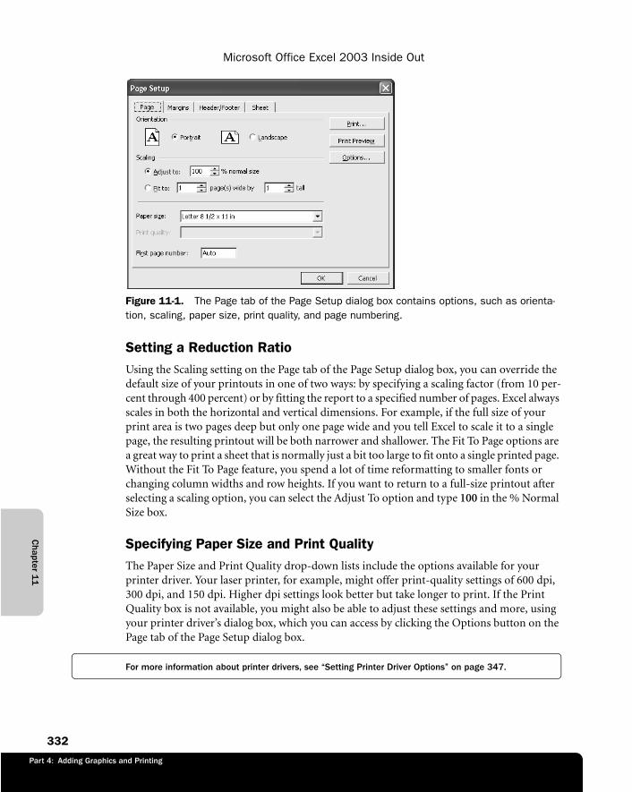
Part 4: Adding Graphics and Printing

Chapter 1

1

Microsoft Office Excel 2003 Inside Out

332

f11ie01

Figure 11-1. The Page tab of the Page Setup dialog box contains options, such as orienta-tion, scaling, paper size, print quality, and page numbering.

Setting a Reduction RatioUsing the Scaling setting on the Page tab of the Page Setup dialog box, you can override the default size of your printouts in one of two ways: by specifying a scaling factor (from 10 per-cent through 400 percent) or by fitting the report to a specified number of pages. Excel always scales in both the horizontal and vertical dimensions. For example, if the full size of your print area is two pages deep but only one page wide and you tell Excel to scale it to a single page, the resulting printout will be both narrower and shallower. The Fit To Page options are a great way to print a sheet that is normally just a bit too large to fit onto a single printed page. Without the Fit To Page feature, you spend a lot of time reformatting to smaller fonts or changing column widths and row heights. If you want to return to a full-size printout after selecting a scaling option, you can select the Adjust To option and type 100 in the % Normal Size box.

Specifying Paper Size and Print QualityThe Paper Size and Print Quality drop-down lists include the options available for your printer driver. Your laser printer, for example, might offer print-quality settings of 600 dpi, 300 dpi, and 150 dpi. Higher dpi settings look better but take longer to print. If the Print Quality box is not available, you might also be able to adjust these settings and more, using your printer driver’s dialog box, which you can access by clicking the Options button on the Page tab of the Page Setup dialog box.

For more information about printer drivers, see “Setting Printer Driver Options” on page 347.

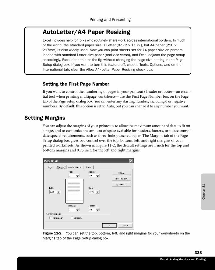
Part 4: Adding Graphics and Printing

Cha

pter

11

Printing and Presenting

333

AutoLetter/A4 Paper ResizingExcel includes help for folks who routinely share work across international borders. In much of the world, the standard paper size is Letter (8-1/2 × 11 in.), but A4 paper (210 × 297mm) is also widely used. Now you can print sheets set for A4 paper size on printers loaded with standard Letter size paper (and vice versa), and Excel adjusts the page setup accordingly. Excel does this on-the-fly, without changing the page size setting in the Page Setup dialog box. If you want to turn this feature off, choose Tools, Options, and on the International tab, clear the Allow A4/Letter Paper Resizing check box.

Setting the First Page NumberIf you want to control the numbering of pages in your printout’s header or footer—an essen-tial tool when printing multipage worksheets—use the First Page Number box on the Page tab of the Page Setup dialog box. You can enter any starting number, including 0 or negative numbers. By default, this option is set to Auto, but you can change it to any number you want.

Setting MarginsYou can adjust the margins of your printouts to allow the maximum amount of data to fit on a page, and to customize the amount of space available for headers, footers, or to accommo-date special requirements, such as three-hole-punched paper. The Margins tab of the Page Setup dialog box gives you control over the top, bottom, left, and right margins of your printed worksheets. As shown in Figure 11-2, the default settings are 1 inch for the top and bottom margins and 0.75 inch for the left and right margins.

f11ie02

Figure 11-2. You can set the top, bottom, left, and right margins for your worksheets on the Margins tab of the Page Setup dialog box.

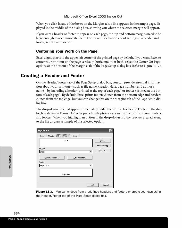
Part 4: Adding Graphics and Printing

Chapter 1

1

Microsoft Office Excel 2003 Inside Out

334

When you click in any of the boxes on the Margins tab, a line appears in the sample page, dis-played in the middle of the dialog box, showing you where the selected margin will appear.

If you want a header or footer to appear on each page, the top and bottom margins need to be large enough to accommodate them. For more information about setting up a header and footer, see the next section.

Centering Your Work on the PageExcel aligns sheets to the upper left corner of the printed page by default. If you want Excel to center your printout on the page vertically, horizontally, or both, select the Center On Page options at the bottom of the Margins tab of the Page Setup dialog box (refer to Figure 11-2).

Creating a Header and FooterOn the Header/Footer tab of the Page Setup dialog box, you can provide essential informa-tion about your printout—such as file name, creation date, page number, and author’s name—by including a header (printed at the top of each page) or footer (printed at the bot-tom of each page). By default, Excel prints footers .5 inch from the bottom edge and headers .5 inch from the top edge, but you can change this on the Margins tab of the Page Setup dia-log box.

The drop-down lists that appear immediately under the words Header and Footer in the dia-log box shown in Figure 11-3 offer predefined options you can use to customize your headers and footers. When you highlight an option in the drop-down list, the preview area adjacent to the list displays a sample of the selected option.

f11ie03

Figure 11-3. You can choose from predefined headers and footers or create your own using the Header/Footer tab of the Page Setup dialog box.

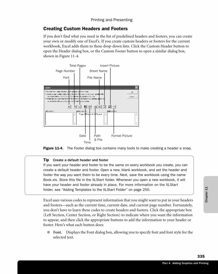
Part 4: Adding Graphics and Printing

Cha

pter

11

Printing and Presenting

335

Creating Custom Headers and FootersIf you don’t find what you need in the list of predefined headers and footers, you can create your own or modify one of Excel’s. If you create custom headers or footers for the current workbook, Excel adds them to these drop-down lists. Click the Custom Header button to open the Header dialog box, or the Custom Footer button to open a similar dialog box, shown in Figure 11-4.

f11ie04

Figure 11-4. The Footer dialog box contains many tools to make creating a header a snap.

Tip Create a default header and footerIf you want your header and footer to be the same on every workbook you create, you can create a default header and footer. Open a new, blank workbook, and set the header and footer the way you want them to be every time. Next, save the workbook using the name Book.xls. Store this file in the XLStart folder. Whenever you open a new workbook, it will have your header and footer already in place. For more information on the XLStart folder, see “Adding Templates to the XLStart Folder” on page 250.

Excel uses various codes to represent information that you might want to put in your headers and footers—such as the current time, current date, and current page number. Fortunately, you don’t have to learn these codes to create headers and footers. Click the appropriate box (Left Section, Center Section, or Right Section) to indicate where you want the information to appear, and then click the appropriate buttons to add the information to your header or footer. Here’s what each button does:

● Font. Displays the Font dialog box, allowing you to specify font and font style for the selected text.

Font

Page Number

Total Pages

Format Picture

File Name

Sheet Name

Insert Picture

Path & File

Date

Time

Part 4: Adding Graphics and Printing

Chapter 1

1

Microsoft Office Excel 2003 Inside Out

336

● Page Number. Inserts page number in the selected section.

● Total Pages. Inserts the total number of pages in the selected section; typically used in conjunction with the page number in a “Page X of Y” construction.

● Date. Inserts the date of printing in the selected section.

● Time. Inserts the time of printing in the selected section.

● Path & File. Inserts the folder path and file name of the workbook in the selected section.

● File Name. Inserts only the file name of the current workbook in the selected section.

● Sheet Name. Inserts the name of the current worksheet in the selected section.

● Insert Picture. Displays the Insert Picture dialog box, allowing you to add a picture to the selected section.

● Format Picture. Displays the Format Picture dialog box, allowing you to adjust set-tings of an inserted picture.

To specify text in your header or footer, click the appropriate edit box and type your text. To divide the text between two or more lines, press Enter at the end of each line. To include an ampersand in your text, type two ampersands.

Adding Pictures to Headers and FootersYou can add pictures to custom headers and footers using the Insert Picture and Format Picture buttons (refer to Figure 11-4). For example, you can insert pictures to add company logos or banners to your documents. Click the Insert Picture button to access the Insert Picture dialog box, which you use to locate the picture you want to use. When you insert the picture, Excel displays &[Picture] in the section box of the Header (or Footer) dialog box. (Unlike other header and footer codes, you can’t just type in this code—you have to use the Insert Picture button.)

After you insert the picture, click the Format Picture button to specify the size, brightness, and contrast of the picture and to rotate, scale, or crop the picture. (You can’t directly manip-ulate Header or Footer pictures—you must use the Format Picture button.) It might take some trial and error to obtain the result you want, adjusting the size of the picture as well as the top or bottom margins to accommodate it. Figure 11-5 shows a sample of a picture used in a header, displayed in Print Preview.

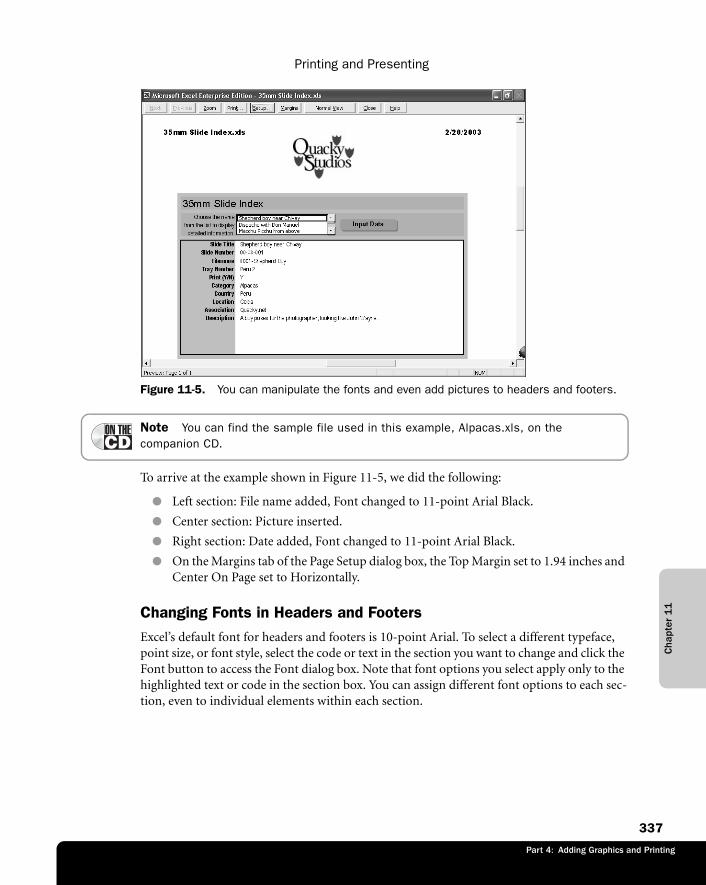
Part 4: Adding Graphics and Printing

Cha

pter

11

Printing and Presenting

337

f11ie05

Figure 11-5. You can manipulate the fonts and even add pictures to headers and footers.

Note You can find the sample file used in this example, Alpacas.xls, on the companion CD.

To arrive at the example shown in Figure 11-5, we did the following:

● Left section: File name added, Font changed to 11-point Arial Black.

● Center section: Picture inserted.

● Right section: Date added, Font changed to 11-point Arial Black.

● On the Margins tab of the Page Setup dialog box, the Top Margin set to 1.94 inches and Center On Page set to Horizontally.

Changing Fonts in Headers and FootersExcel’s default font for headers and footers is 10-point Arial. To select a different typeface, point size, or font style, select the code or text in the section you want to change and click the Font button to access the Font dialog box. Note that font options you select apply only to the highlighted text or code in the section box. You can assign different font options to each sec-tion, even to individual elements within each section.

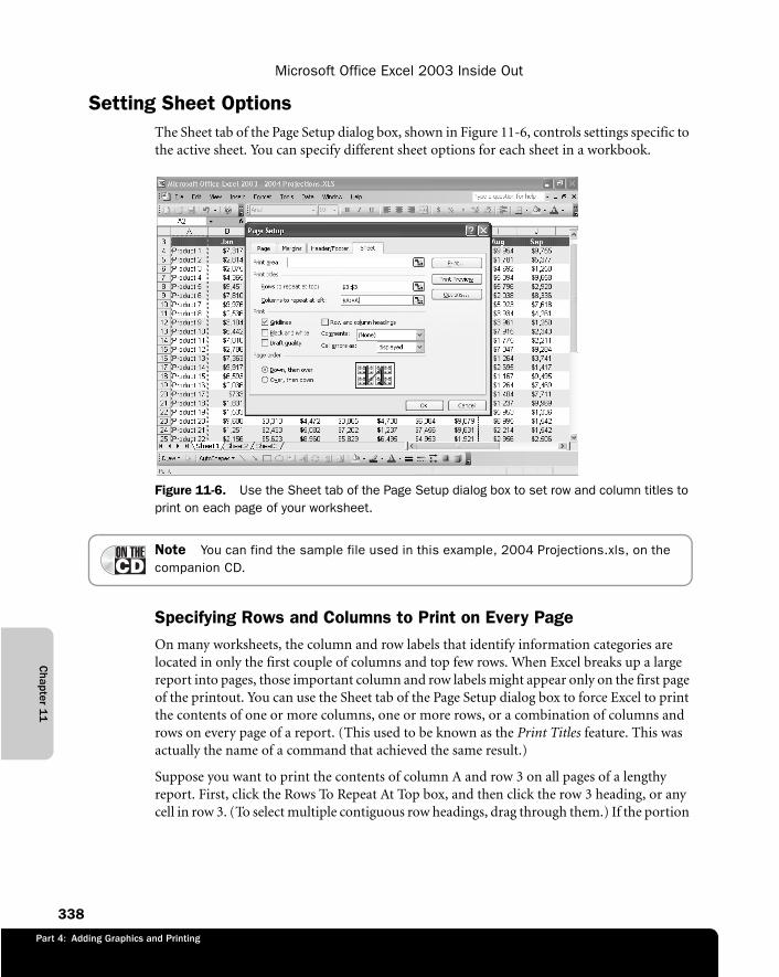
Part 4: Adding Graphics and Printing

Chapter 1

1

Microsoft Office Excel 2003 Inside Out

338

Setting Sheet OptionsThe Sheet tab of the Page Setup dialog box, shown in Figure 11-6, controls settings specific to the active sheet. You can specify different sheet options for each sheet in a workbook.

f11ie06

Figure 11-6. Use the Sheet tab of the Page Setup dialog box to set row and column titles to print on each page of your worksheet.

Note You can find the sample file used in this example, 2004 Projections.xls, on the companion CD.

Specifying Rows and Columns to Print on Every PageOn many worksheets, the column and row labels that identify information categories are located in only the first couple of columns and top few rows. When Excel breaks up a large report into pages, those important column and row labels might appear only on the first page of the printout. You can use the Sheet tab of the Page Setup dialog box to force Excel to print the contents of one or more columns, one or more rows, or a combination of columns and rows on every page of a report. (This used to be known as the Print Titles feature. This was actually the name of a command that achieved the same result.)

Suppose you want to print the contents of column A and row 3 on all pages of a lengthy report. First, click the Rows To Repeat At Top box, and then click the row 3 heading, or any cell in row 3. (To select multiple contiguous row headings, drag through them.) If the portion

Part 4: Adding Graphics and Printing

Cha

pter

11

Printing and Presenting

339

of the spreadsheet you want to select is not visible, click the button on the right side of the Rows To Repeat At Top box. The dialog box collapses to give you more room; to redisplay the full dialog box, click the button on the right side of the box. Click the Columns To Repeat At Left box, and then select the column A heading or any cell in column A. Figure 11-6 shows the result.

Note In some earlier versions of Excel, you had to be careful to exclude print title col-umns and rows from the print area—that is, the area of the worksheet that you were asking Excel to print. Otherwise, your titles would appear twice: once as titles and once as part of the print area. Recent versions of Excel are smart enough to recognize when print titles fall within the print area.

If you prefer to type your entries, you can enter the row numbers or column letters in the Rows To Repeat At Top box and the Columns To Repeat At Left box. To specify rows 3 and 4, for example, type 3:4. To specify column A, type A:A. Note that for a single row or column, you have to type the number or letter twice, separated by a colon. You can specify separate print titles for each worksheet in your workbook. Excel remembers the titles for each worksheet.

Note To remove print titles, you can go back to the Page Setup dialog box and delete the title specifications. However, you might find it quicker to use the Define Name dialog box. To use the Define Name dialog box, press Ctrl-F3 and delete the name Print_Titles.

Printing GridlinesBy default, Excel does not print gridlines, regardless of whether you have them displayed on your worksheet. If you want to print gridlines, select the Gridlines check box on the Sheet tab of the Page Setup dialog box.

Printing CommentsComments are annotations created by selecting Insert, Comment. To make sure the comments in your worksheet are included with your printout, select one of the Comments options on the Sheet tab of the Page Setup dialog box. If you select At End Of Sheet from the drop-down list, Excel adds a page to the end of the printout and prints all your notes together, starting on that new page. If you select As Displayed On Sheet, Excel prints the comments where they are located on a worksheet.

For more on creating comments, see “Adding Comments to Cells” on page 261.

Part 4: Adding Graphics and Printing

Chapter 1

1

Microsoft Office Excel 2003 Inside Out

340

Printing DraftsIf your printer offers a draft-quality mode, you can obtain a quicker, though less attractive, printout by selecting the Draft Quality option on the Sheet tab of the Page Setup dialog box. This option has no effect if your printer has no draft-quality mode and is most useful for dot matrix or other slow printers, or if your worksheet contains a lot of graphics.

Translating Screen Colors to Black and WhiteIf you’ve assigned colors and patterns to your worksheet but you want to see what it will look like when printed on a black-and-white printer, select the Black And White option on the Sheet tab of the Page Setup dialog box, which tells Excel to use only black and white when printing. If you are using a black and white printer, you probably won’t need to worry about this option, but if you seem to be having trouble, try selecting it.

Printing Row and Column HeadingsIf you select the Row And Column Headings option on the Sheet tab of the Page Setup dialog box, Excel prints row letters to the left of and column numbers on top of worksheet data. This option is handy when you’re using printouts to document the structure of a worksheet.

Setting the Printing Order of Large Print RangesWhen you print a large report, Excel breaks the report into page-size sections based on the current margin and page-size settings. If the print range is both too wide and too deep to fit on a single page, Excel normally works in “down, and then over” order. For example, suppose your print range measures 120 rows by 20 columns and Excel can fit 40 rows and 10 columns on a page. Excel prints the first 40 rows and first 10 columns on page 1, the second 40 rows and first 10 columns on page 2, and the third 40 rows and first 10 columns on page 3. On page 4, Excel prints the first 40 rows and second 10 columns, and so on. If you prefer to have Excel print each horizontal chunk before moving down to the next vertical chunk, select the Over, Then Down option on the Sheet tab of the Page Setup dialog box.

Print AssistantsOn the companion CD you will find a demo version of an add-in called the Spreadsheet Assistant, which provides dozens of useful, time-saving features, including an Assistants menu, with a submenu of “Print Assistants.” These commands provide helpful features such as copying print settings to other sheets, inserting page breaks based on cell entries, and setting or expanding the designated print area. Choosing Assistants, Print Assistants, Update Print Footer and Headers displays the dialog box shown below, which allows you to specify headers and footers for multiple sheets simultaneously.

Part 4: Adding Graphics and Printing

Cha

pter

11

Printing and Presenting

341

G11ie01sb

To install the Spreadsheet Assistant, refer to the StartCD page on the companion CD and follow the instructions on your screen.

Adjusting Page BreaksExcel makes it easy to adjust the positions of page breaks. You can do this by selecting View, Page Break Preview. The resulting preview is shown in Figure 11-7. You can move page breaks by drag-ging them with the mouse. You can even edit your worksheet while in Page Break Preview mode.

f11ie07

Figure 11-7. Page Break Preview shows default page breaks with dashed lines, which you can reposition by dragging with your mouse.

Using Page Break Preview allows you to see both the positions of your page breaks and the page numbers Excel will use when you print. Default page breaks—the ones that Excel

Part 4: Adding Graphics and Printing

Chapter 1

1

Microsoft Office Excel 2003 Inside Out

342

proposes to use if you don’t intervene—appear as dashed lines. If you’re not happy with the position of a default break, drag the line where you want it. Your page break then becomes a manual page break, and is displayed as a solid line. To return from Page Break Preview to Normal view, choose View, Normal.

Tip Lose the dashed linesAfter you set your page breaks, Excel displays them in Normal view as dashed lines. If you’d rather not see these lines, choose Tools, Options, click the View tab, and then clear the Page Breaks check box.

If you attempt to extend the dimensions of a page beyond the maximum width or depth according to the current page setup, Excel scales the sheet to make it fit and displays the Adjusted values in the Scaling options shown on the Page tab of the Page Setup dialog box.

If, after trying different page breaks, you want to revert to the automatic page breaks (dotted lines), drag the manual page breaks (solid lines) to the left past the row headers, or up past the column headers. Once you have removed all manual page breaks, the automatic breaks reappear in their default locations.

Inserting and Removing Manual Page BreaksSpreadsheet pagination can be problematic, given the fact that rows and columns of numbers often don’t fit into the 8-1/2 × 11 world of printing. This is why Excel provides yet another method you can use to manually adjust page breaks. To add a page break, select any cell of the row directly beneath or in the column directly to the right of where you want the break to occur, and then choose Insert, Page Break. If you select a cell where data appears both below and to the right, Excel applies page breaks both horizontally and vertically. To remove a break, position your mouse in the row below a horizontal break, or in the column to the right of a vertical break, and then choose Insert, Remove Page Break.

TroubleshootingMy manual page breaks don’t work

In the Page Setup dialog box, selecting the Fit To option on the Page tab can cause Excel to override manual page breaks. Fit To applies reduction sufficient to fit the entire print area into a specific number of pages. To derail this override, switch to the Adjust To option. This allows the worksheet to print according to your manual page breaks.

If you prefer the compressed Fit To “look” but still want to control page breaks, you can define the print area using multiple nonadjacent ranges—one range per page. Excel auto-matically prints each nonadjacent range as a separate page. Then you select the first range, hold down Ctrl, and select the next range. Select as many ranges (pages) as you want. Then choose File, Print Area, Set Print Area.

Part 4: Adding Graphics and Printing

Cha

pter

11

Printing and Presenting

343

Tip Remove all page breaksTo reset all the page breaks on a worksheet, click the header cell at the intersection of the row and column headers to select the entire sheet, and choose Insert, Reset All Page Breaks.

Using Print PreviewThe Print Preview feature gives you a glimpse of your worksheets the way they will look on paper. You can check the effect of page breaks, margins, and formatting before you needlessly waste paper with multiple test printouts. To access Print Preview, use one of the following methods:

● Choose File, Print Preview.

● Click the Print Preview button on the Standard toolbar.

● Shift-click the Print button on the Standard toolbar.

● Click Preview in the Print dialog box or Print Preview in the Page Setup dialog box.

If you’re not satisfied with the appearance of your worksheet, you can access most page layout settings from within Print Preview. Click the Setup button to display the Page Setup dialog box and change any page setting.

You can also change the margins and column widths without leaving Print Preview by click-ing the Margins button, as shown in Figure 11-8. To adjust a margin, drag a dotted line; to adjust a column’s width, drag the column handle. As you drag, the page-number indicator in the lower left corner of the screen changes to display the name and setting for the margin or the width of the selected column. To turn off the display of margin lines and column handles, click the Margins button again.

The following buttons help you to move around within Print Preview mode:

● You can move forward or backward a page at a time by clicking Next and Previous or by pressing Page Up and Page Down. Alternatively, to move more quickly through a long document, drag the scroll box. As you drag, Excel displays the current page number in the lower left corner of the Print Preview screen.

● Click Zoom to display the page in roughly 100 percent Zoom—the same size that you see in Normal view. Click Zoom to return to the normal Print Preview whole-page view. Alternatively, you don’t need to use Zoom at all. Click anywhere (except on a dis-played margin line) and the preview zooms in; click anywhere in zoomed mode and the preview returns to whole-page view.

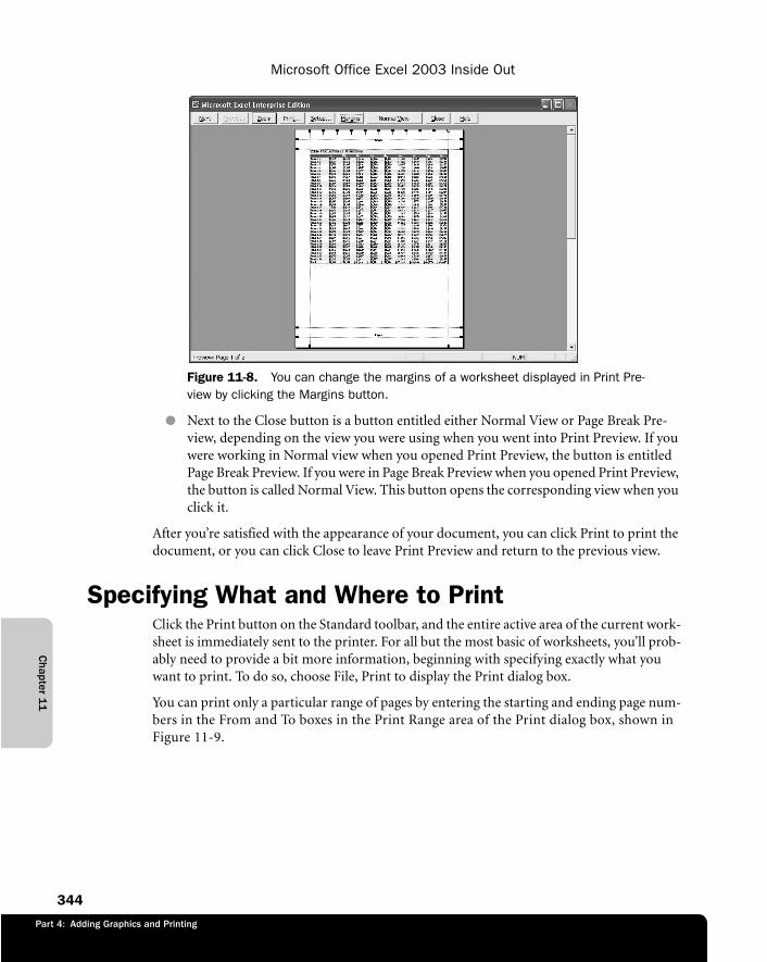
Part 4: Adding Graphics and Printing

Chapter 1

1

Microsoft Office Excel 2003 Inside Out

344

f11ie08

Figure 11-8. You can change the margins of a worksheet displayed in Print Pre-view by clicking the Margins button.

● Next to the Close button is a button entitled either Normal View or Page Break Pre-view, depending on the view you were using when you went into Print Preview. If you were working in Normal view when you opened Print Preview, the button is entitled Page Break Preview. If you were in Page Break Preview when you opened Print Preview, the button is called Normal View. This button opens the corresponding view when you click it.

After you’re satisfied with the appearance of your document, you can click Print to print the document, or you can click Close to leave Print Preview and return to the previous view.

Specifying What and Where to PrintClick the Print button on the Standard toolbar, and the entire active area of the current work-sheet is immediately sent to the printer. For all but the most basic of worksheets, you’ll prob-ably need to provide a bit more information, beginning with specifying exactly what you want to print. To do so, choose File, Print to display the Print dialog box.

You can print only a particular range of pages by entering the starting and ending page num-bers in the From and To boxes in the Print Range area of the Print dialog box, shown in Figure 11-9.

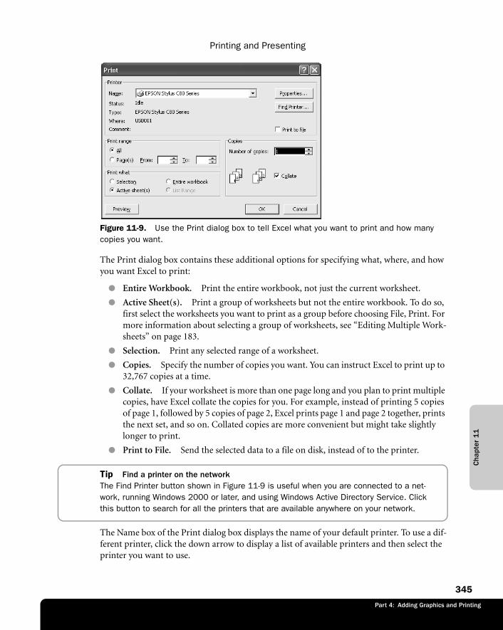
Part 4: Adding Graphics and Printing

Cha

pter

11

Printing and Presenting

345

f11ie09

Figure 11-9. Use the Print dialog box to tell Excel what you want to print and how many copies you want.

The Print dialog box contains these additional options for specifying what, where, and how you want Excel to print:

● Entire Workbook. Print the entire workbook, not just the current worksheet.

● Active Sheet(s). Print a group of worksheets but not the entire workbook. To do so, first select the worksheets you want to print as a group before choosing File, Print. For more information about selecting a group of worksheets, see “Editing Multiple Work-sheets” on page 183.

● Selection. Print any selected range of a worksheet.

● Copies. Specify the number of copies you want. You can instruct Excel to print up to 32,767 copies at a time.

● Collate. If your worksheet is more than one page long and you plan to print multiple copies, have Excel collate the copies for you. For example, instead of printing 5 copies of page 1, followed by 5 copies of page 2, Excel prints page 1 and page 2 together, prints the next set, and so on. Collated copies are more convenient but might take slightly longer to print.

● Print to File. Send the selected data to a file on disk, instead of to the printer.

Tip Find a printer on the networkThe Find Printer button shown in Figure 11-9 is useful when you are connected to a net-work, running Windows 2000 or later, and using Windows Active Directory Service. Click this button to search for all the printers that are available anywhere on your network.

The Name box of the Print dialog box displays the name of your default printer. To use a dif-ferent printer, click the down arrow to display a list of available printers and then select the printer you want to use.

Part 4: Adding Graphics and Printing

Chapter 1

1

Microsoft Office Excel 2003 Inside Out

346

Printing to a FileThe Print To File check box is in many ways an anachronism—a remnant of computing days of yore. It was often used to facilitate batch printing—that is, unattended printing of multi-ple files—back when print spooling was less widespread. You can still use Print To File if you want to print a document from a different computer on which Excel isn’t installed.

When you print to a file, Excel sends the same stream of data that would normally go straight to your printer into a file on your hard disk. This isn’t an Excel document file, but a printer document file. Excel saves all the necessary information from your document so that line and page breaks, spacing, and fonts (hopefully) remain the same. Unfortunately, your results can vary depending on the type of printer, the fonts you use, and the complexity of your document. For this reason, it’s advisable to test printer files before relying on them for critical work.

Here’s the key to making this process work: you have to use MS-DOS to send the file to your printer. In Windows XP, choose Start, All Programs, Accessories, Command Prompt. At the command prompt, type

copy <file name> lpt1: /b

This assumes that the printer file is located in the same directory where you are issuing the command. You can, of course, get around this assumption by specifying a full path name instead of just a file name.

Defining a Default Print AreaWhen using the Active Sheet(s) option in the Print dialog box, Excel checks to see whether you have assigned the range name Print_Area on each specified sheet. If you have, Excel prints only the range to which you’ve assigned the name. Otherwise, Excel prints the entire active area of the selected sheet(s). If you expect to print the same area of a given sheet repeat-edly, you can save yourself some steps by defining the print area. Here are the easiest ways to define the print area in Excel:

● Select the range you want to define and then choose File, Print Area, Set Print Area.

OR

● Choose File, Page Setup, and on the Sheet tab, enter the cell range you want to print in the Print Area box.

For more information about defining range names, see “Naming Cells and Cell Ranges” on page 368.

Part 4: Adding Graphics and Printing

Cha

pter

11

Printing and Presenting

347

Suppose you have a workbook that is crowded with data, but each sheet in the workbook includes only a small area of summary information that you need to print. You can define a unique print area on each sheet in a workbook. If you select two or more sheets and print using the Active Sheet(s) option, Excel prints only the area of each sheet where you have defined a print area and prints the entire active area of any selected sheets where you haven’t defined a print area.

Tip Take advantage of quick printingTo bypass the Print dialog box, click the Print button on the Standard toolbar or Shift-click the Print Preview button. Excel prints using the default Active Sheet(s) option.

Setting Printer Driver OptionsOccasionally while working in Excel, you might need to set options that only your printer driver provides. For example, you might need to switch from automatic to manual paper feed or from one paper tray to another. You can do this by choosing Start, Settings, Printers, right-clicking the appropriate printer, and then choosing Properties. You can also set many of these options from within Excel by clicking Properties in the Print dialog box (refer to Figure 11-9) to open a version of the printer driver dialog box for the selected printer.

349

Part 5

Creating Formulas and Performing Data Analysis

12 Building Formulas 351

13 Using Functions 401

14 Everyday Functions 411

15 Formatting and Calculating Date and Time 435

16 Functions for Financial Analysis 449

17 Functions for Analyzing Statistics 463

18 Performing What-If Analysis 493

351

Part 5: Creating Formulas and Performing Data Analysis

Chapter 12

Building FormulasFormula Fundamentals. . . . . . . . . . . . . 351Using Functions: A Preview . . . . . . . . . . 361Naming Cells and Cell Ranges . . . . . . . 368Understanding Error Values . . . . . . . . . 378

Worksheet Calculation . . . . . . . . . . . . . . 379Using Arrays . . . . . . . . . . . . . . . . . . . . . . 385Linking Workbooks . . . . . . . . . . . . . . . . 389Creating Conditional Tests . . . . . . . . . . . 393

Formulas are the heart and soul of a spreadsheet, and Microsoft Excel offers a rich environ-ment in which to build complex formulas. Armed with a few mathematical operators and rules for cell entry, you can turn a worksheet into a powerful calculator.

Formula FundamentalsAll formulas in Excel begin with an equal sign. The equal sign tells Excel that the succeeding characters constitute a formula. If you omit the equal sign, Excel might interpret the entry as text.

To see how formulas work, we’ll walk through some rudimentary ones. Begin by selecting blank cell A10. Then type =10+5 and press Enter. The value 15 appears in cell A10. Now select cell A10, and the formula bar displays the formula you just entered. What appears in the cell is the displayed value; what appears in the formula bar is the underlying value, which in this case is a formula.

Understanding the Precedence of OperatorsOperators are symbols that represent specific mathematical operations, including the plus sign (+), minus sign ( ), division sign (/), and multiplication sign (*). When performing these operations in a formula, Excel follows certain rules of precedence:

● Expressions within parentheses are processed first.

● Multiplication and division are performed before addition and subtraction.

● Consecutive operators with the same level of precedence are calculated from left to right.

Enter some formulas to see how these rules apply. Select an empty cell and type =4+12/6.Press Enter, and you see the value 6. Excel first divides 12 by 6 and then adds the result (2) to 4. If Excel used different precedence rules, the result would be different. For example, select another empty cell and type =(4+12)/6. Press Enter, and you see the value 2.666667. This demonstrates how you can change the order of precedence using parentheses. The formulas

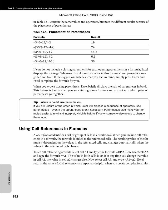
Chapter 1

2

Microsoft Office Excel 2003 Inside Out

Part 5: Creating Formulas and Performing Data Analysis

352

in Table 12-1 contain the same values and operators, but note the different results because of the placement of parentheses:

If you do not include a closing parenthesis for each opening parenthesis in a formula, Excel displays the message “Microsoft Excel found an error in this formula” and provides a sug-gested solution. If the suggestion matches what you had in mind, simply press Enter and Excel completes the formula for you.

When you type a closing parenthesis, Excel briefly displays the pair of parentheses in bold. This feature is handy when you are entering a long formula and are not sure which pairs of parentheses go together.

Tip When in doubt, use parenthesesIf you are unsure of the order in which Excel will process a sequence of operators, use parentheses—even if the parentheses aren’t necessary. Parentheses also make your for-mulas easier to read and interpret, which is helpful if you or someone else needs to change them later.

Using Cell References in FormulasA cell reference identifies a cell or group of cells in a workbook. When you include cell refer-ences in a formula, the formula is linked to the referenced cells. The resulting value of the for-mula is dependent on the values in the referenced cells and changes automatically when the values in the referenced cells change.

To see cell referencing at work, select cell A1 and type the formula =10*2. Now select cell A2, and type the formula =A1. The value in both cells is 20. If at any time you change the value in cell A1, the value in cell A2 changes also. Now select cell A3, and type =A1+A2. Excel returns the value 40. Cell references are especially helpful when you create complex formulas.

Table 12-1. Placement of Parentheses

Formula Result

=3*6+12/4-2 19

=(3*6)+12/(4-2) 24

=3*(6+12)/4-2 11.5

=(3*6+12)/4-2 5.5

=3*(6+12/(4-2)) 36

Cha

pter

12

Building Formulas

353

Part 5: Creating Formulas and Performing Data Analysis

Entering Cell References with the MouseYou can save time and increase accuracy when you enter cell references in a formula by select-ing them with the mouse. For example, to enter references to cells A9 and A10 in a formula in cell B10, do the following:

1 Select cell B10, and type an equal sign.

2 Click cell A9, and type a plus sign.

3 Click cell A10, and press Enter.

When you click each cell, a marquee surrounds the cell and a reference to the cell is inserted in cell B10. After you finish entering a formula, be sure to press Enter. If you do not press Enter and select another cell, Excel assumes that you want to include the cell reference in the formula.

The active cell does not have to be visible in the current window for you to enter a value in that cell. You can scroll through the worksheet without changing the active cell and click cells in remote areas of your worksheet, in other worksheets, or in other workbooks, as you build a formula. The formula bar displays the contents of the active cell, no matter which area of the worksheet is currently visible.

Tip Redisplay the active cellIf you scroll through your worksheet and the active cell is no longer visible, you can redis-play it by pressing Ctrl+Backspace.

Understanding Relative, Absolute, and Mixed ReferencesRelative references—the type we’ve used so far in the sample formulas—refer to cells by their position in relation to the cell that contains the formula, such as “the cell two rows above this cell.” Absolute references refer to cells by their fixed position in the worksheet, for example, the cell located at the intersection of column A and row 2. A mixed reference contains a rela-tive reference and an absolute reference, for example, the cell located in column A and two rows above this cell. Absolute and mixed references are important when you begin copying formulas from one location to another in your worksheet. When you copy and paste, relative references adjust automatically, while absolute references do not. For information about copying cell references, see “How Copying and Cutting Affect Cell References” on page 356.

A relative reference to cell A1, for example, looks like this: =A1. An absolute reference to cell A1 looks like this: =$A$1. You can combine relative and absolute references to cell A1 to cre-ate these mixed references: =$A1 or =A$1.

If the dollar sign precedes only the letter (A, for example), the column coordinate is absolute and the row is relative. If the dollar sign precedes only the number (1, for example), the col-umn coordinate is relative and the row is absolute.

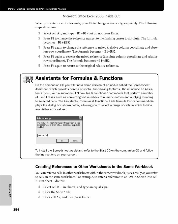
Chapter 1

2

Microsoft Office Excel 2003 Inside Out

Part 5: Creating Formulas and Performing Data Analysis

354

When you enter or edit a formula, press F4 to change reference types quickly. The following steps show how:

1 Select cell A1, and type =B1+B2 (but do not press Enter).

2 Press F4 to change the reference nearest to the flashing cursor to absolute. The formula becomes =B1+$B$2.

3 Press F4 again to change the reference to mixed (relative column coordinate and abso-lute row coordinate). The formula becomes =B1+B$2.

4 Press F4 again to reverse the mixed reference (absolute column coordinate and relative row coordinate). The formula becomes =B1+$B2.

5 Press F4 again to return to the original relative reference.

Assistants for Formulas & FunctionsOn the companion CD you will find a demo version of an add-in called the Spreadsheet Assistant, which provides dozens of useful, time-saving features. These include an Assis-tants menu, with a submenu of “Formulas & Functions” commands that perform a number of useful tasks such as converting text numbers to numeric entries and applying rounding to selected cells. The Assistants, Formulas & Functions, Hide Formula Errors command dis-plays the dialog box shown below, allowing you to select a range of cells in which to hide any visible error values.

G12ie03sb

To install the Spreadsheet Assistant, refer to the Start CD on the companion CD and follow the instructions on your screen.

Creating References to Other Worksheets in the Same WorkbookYou can refer to cells in other worksheets within the same workbook just as easily as you refer to cells in the same worksheet. For example, to enter a reference to cell A9 in Sheet2 into cell B10 in Sheet1, do this:

1 Select cell B10 in Sheet1, and type an equal sign.

2 Click the Sheet2 tab.

3 Click cell A9, and then press Enter.

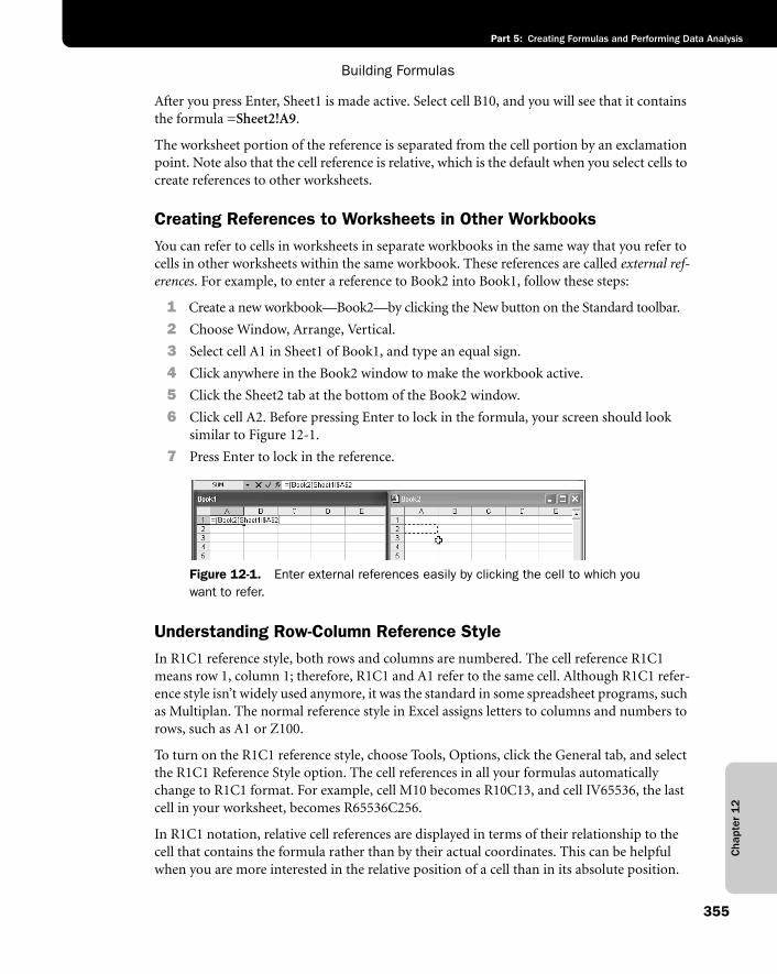
Cha

pter

12

Building Formulas

355

Part 5: Creating Formulas and Performing Data Analysis

After you press Enter, Sheet1 is made active. Select cell B10, and you will see that it contains the formula =Sheet2!A9.

The worksheet portion of the reference is separated from the cell portion by an exclamation point. Note also that the cell reference is relative, which is the default when you select cells to create references to other worksheets.

Creating References to Worksheets in Other WorkbooksYou can refer to cells in worksheets in separate workbooks in the same way that you refer to cells in other worksheets within the same workbook. These references are called external ref-erences. For example, to enter a reference to Book2 into Book1, follow these steps:

1 Create a new workbook—Book2—by clicking the New button on the Standard toolbar.

2 Choose Window, Arrange, Vertical.

3 Select cell A1 in Sheet1 of Book1, and type an equal sign.

4 Click anywhere in the Book2 window to make the workbook active.

5 Click the Sheet2 tab at the bottom of the Book2 window.

6 Click cell A2. Before pressing Enter to lock in the formula, your screen should look similar to Figure 12-1.

7 Press Enter to lock in the reference.

f12ie01

Figure 12-1. Enter external references easily by clicking the cell to which you want to refer.

Understanding Row-Column Reference StyleIn R1C1 reference style, both rows and columns are numbered. The cell reference R1C1 means row 1, column 1; therefore, R1C1 and A1 refer to the same cell. Although R1C1 refer-ence style isn’t widely used anymore, it was the standard in some spreadsheet programs, such as Multiplan. The normal reference style in Excel assigns letters to columns and numbers to rows, such as A1 or Z100.

To turn on the R1C1 reference style, choose Tools, Options, click the General tab, and select the R1C1 Reference Style option. The cell references in all your formulas automatically change to R1C1 format. For example, cell M10 becomes R10C13, and cell IV65536, the last cell in your worksheet, becomes R65536C256.

In R1C1 notation, relative cell references are displayed in terms of their relationship to the cell that contains the formula rather than by their actual coordinates. This can be helpful when you are more interested in the relative position of a cell than in its absolute position.

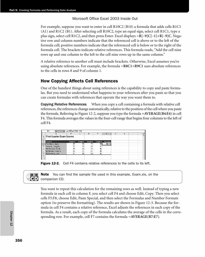
Chapter 1

2

Microsoft Office Excel 2003 Inside Out

Part 5: Creating Formulas and Performing Data Analysis

356

For example, suppose you want to enter in cell R10C2 (B10) a formula that adds cells R1C1 (A1) and R1C2 (B1). After selecting cell R10C2, type an equal sign, select cell R1C1, type a plus sign, select cell R1C2, and then press Enter. Excel displays =R[ 9]C[ 1]+R[ 9]C. Nega-tive row and column numbers indicate that the referenced cell is above or to the left of the formula cell; positive numbers indicate that the referenced cell is below or to the right of the formula cell. The brackets indicate relative references. This formula reads, “Add the cell nine rows up and one column to the left to the cell nine rows up in the same column.”

A relative reference to another cell must include brackets. Otherwise, Excel assumes you’re using absolute references. For example, the formula =R8C1+R9C1 uses absolute references to the cells in rows 8 and 9 of column 1.

How Copying Affects Cell ReferencesOne of the handiest things about using references is the capability to copy and paste formu-las. But you need to understand what happens to your references after you paste so that you can create formulas with references that operate the way you want them to.

Copying Relative References When you copy a cell containing a formula with relative cell references, the references change automatically, relative to the position of the cell where you paste the formula. Referring to Figure 12-2, suppose you type the formula =AVERAGE(B4:E4) in cell F4. This formula averages the values in the four-cell range that begins four columns to the left of cell F4.

f12ie02

Figure 12-2. Cell F4 contains relative references to the cells to its left.

Note You can find the sample file used in this example, Exam.xls, on thecompanion CD.

You want to repeat this calculation for the remaining rows as well. Instead of typing a new formula in each cell in column F, you select cell F4 and choose Edit, Copy. Then you select cells F5:F8, choose Edit, Paste Special, and then select the Formulas and Number Formats option (to preserve the formatting). The results are shown in Figure 12-3. Because the for-mula in cell F4 contains a relative reference, Excel adjusts the references in each copy of the formula. As a result, each copy of the formula calculates the average of the cells in the corre-sponding row. For example, cell F7 contains the formula =AVERAGE(B7:E7).

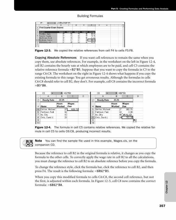
Cha

pter

12

Building Formulas

357

Part 5: Creating Formulas and Performing Data Analysis

f12ie03

Figure 12-3. We copied the relative references from cell F4 to cells F5:F8.

Copying Absolute References If you want cell references to remain the same when you copy them, use absolute references. For example, in the worksheet on the left in Figure 12-4, cell B2 contains the hourly rate at which employees are to be paid, and cell C5 contains the relative reference formula =B2*B5. Suppose that you want to copy the formula in C5 to the range C6:C8. The worksheet on the right in Figure 12-4 shows what happens if you copy the existing formula to this range: You get erroneous results. Although the formulas in cells C6:C8 should refer to cell B2, they don’t. For example, cell C8 contains the incorrect formula =B5*B8.

f12ie04

Figure 12-4. The formula in cell C5 contains relative references. We copied the relative for-mula in cell C5 to cells C6:C8, producing incorrect results.

Note You can find the sample file used in this example, Wages.xls, on thecompanion CD.

Because the reference to cell B2 in the original formula is relative, it changes as you copy the formula to the other cells. To correctly apply the wage rate in cell B2 to all the calculations, you must change the reference to cell B2 to an absolute reference before you copy the formula.

To change the reference style, click the formula bar, click the reference to cell B2, and then press F4. The result is the following formula: =$B$2*B5.

When you copy this modified formula to cells C6:C8, the second cell reference, but not the first, is adjusted within each formula. In Figure 12-5, cell C8 now contains the correct formula: =$B$2*B8.

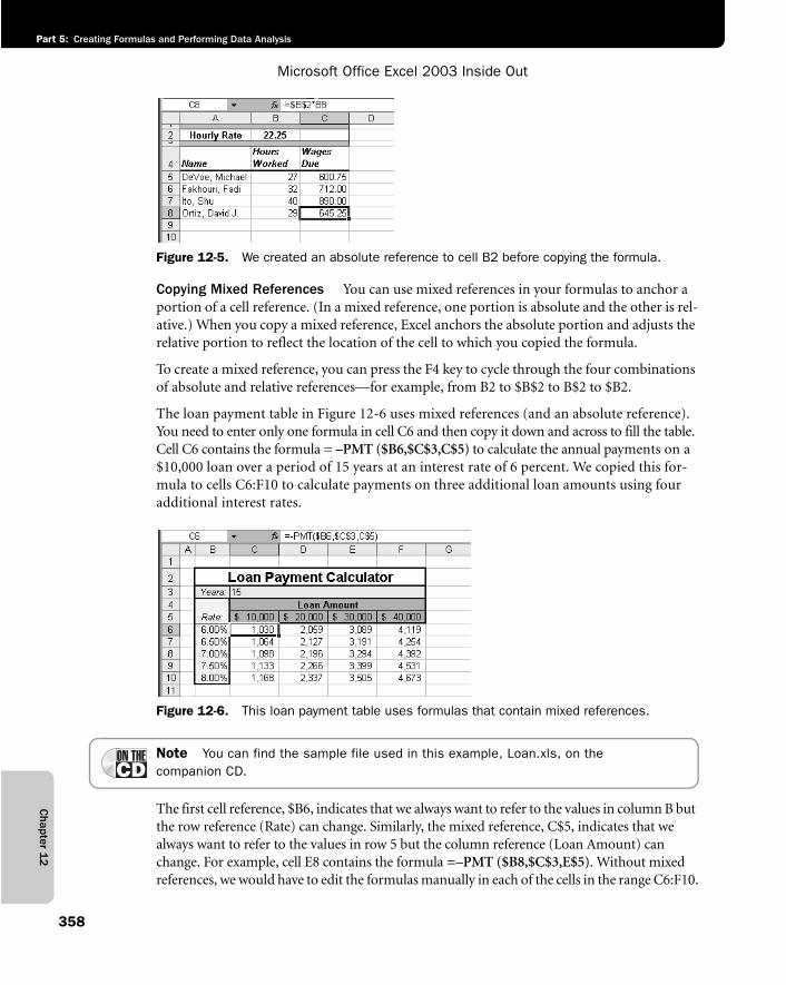
Chapter 1

2

Microsoft Office Excel 2003 Inside Out

Part 5: Creating Formulas and Performing Data Analysis

358

f12ie05

Figure 12-5. We created an absolute reference to cell B2 before copying the formula.

Copying Mixed References You can use mixed references in your formulas to anchor a portion of a cell reference. (In a mixed reference, one portion is absolute and the other is rel-ative.) When you copy a mixed reference, Excel anchors the absolute portion and adjusts the relative portion to reflect the location of the cell to which you copied the formula.

To create a mixed reference, you can press the F4 key to cycle through the four combinations of absolute and relative references—for example, from B2 to $B$2 to B$2 to $B2.

The loan payment table in Figure 12-6 uses mixed references (and an absolute reference). You need to enter only one formula in cell C6 and then copy it down and across to fill the table. Cell C6 contains the formula = –PMT ($B6,$C$3,C$5) to calculate the annual payments on a $10,000 loan over a period of 15 years at an interest rate of 6 percent. We copied this for-mula to cells C6:F10 to calculate payments on three additional loan amounts using four additional interest rates.

f12ie06

Figure 12-6. This loan payment table uses formulas that contain mixed references.

Note You can find the sample file used in this example, Loan.xls, on thecompanion CD.

The first cell reference, $B6, indicates that we always want to refer to the values in column B but the row reference (Rate) can change. Similarly, the mixed reference, C$5, indicates that we always want to refer to the values in row 5 but the column reference (Loan Amount) can change. For example, cell E8 contains the formula =–PMT ($B8,$C$3,E$5). Without mixed references, we would have to edit the formulas manually in each of the cells in the range C6:F10.

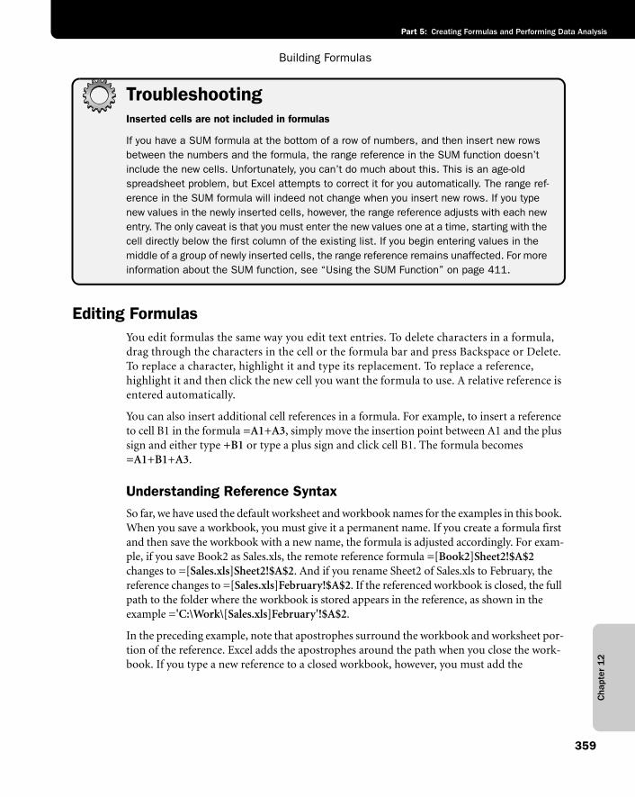
Cha

pter

12

Building Formulas

359

Part 5: Creating Formulas and Performing Data Analysis

TroubleshootingInserted cells are not included in formulas

If you have a SUM formula at the bottom of a row of numbers, and then insert new rows between the numbers and the formula, the range reference in the SUM function doesn’t include the new cells. Unfortunately, you can’t do much about this. This is an age-old spreadsheet problem, but Excel attempts to correct it for you automatically. The range ref-erence in the SUM formula will indeed not change when you insert new rows. If you type new values in the newly inserted cells, however, the range reference adjusts with each new entry. The only caveat is that you must enter the new values one at a time, starting with the cell directly below the first column of the existing list. If you begin entering values in the middle of a group of newly inserted cells, the range reference remains unaffected. For more information about the SUM function, see “Using the SUM Function” on page 411.

Editing FormulasYou edit formulas the same way you edit text entries. To delete characters in a formula, drag through the characters in the cell or the formula bar and press Backspace or Delete. To replace a character, highlight it and type its replacement. To replace a reference,highlight it and then click the new cell you want the formula to use. A relative reference is entered automatically.

You can also insert additional cell references in a formula. For example, to insert a reference to cell B1 in the formula =A1+A3, simply move the insertion point between A1 and the plus sign and either type +B1 or type a plus sign and click cell B1. The formula becomes =A1+B1+A3.

Understanding Reference SyntaxSo far, we have used the default worksheet and workbook names for the examples in this book. When you save a workbook, you must give it a permanent name. If you create a formula first and then save the workbook with a new name, the formula is adjusted accordingly. For exam-ple, if you save Book2 as Sales.xls, the remote reference formula =[Book2]Sheet2!$A$2changes to =[Sales.xls]Sheet2!$A$2. And if you rename Sheet2 of Sales.xls to February, the reference changes to =[Sales.xls]February!$A$2. If the referenced workbook is closed, the full path to the folder where the workbook is stored appears in the reference, as shown in the example ='C:\Work\[Sales.xls]February'!$A$2.

In the preceding example, note that apostrophes surround the workbook and worksheet por-tion of the reference. Excel adds the apostrophes around the path when you close the work-book. If you type a new reference to a closed workbook, however, you must add the

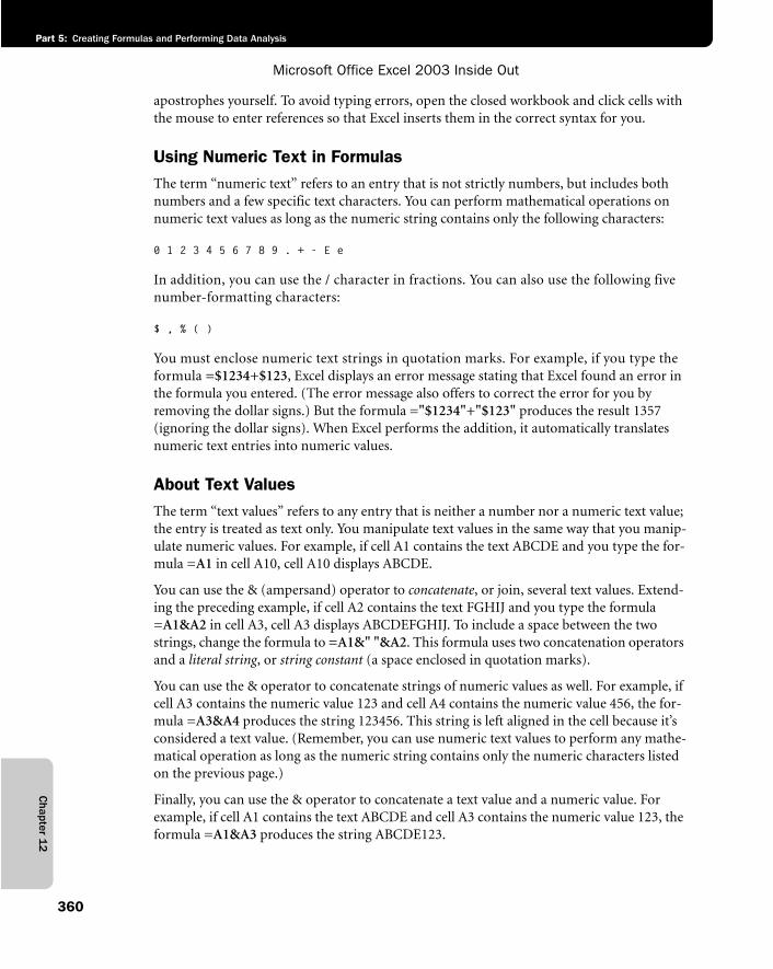
Chapter 1

2

Microsoft Office Excel 2003 Inside Out

Part 5: Creating Formulas and Performing Data Analysis

360

apostrophes yourself. To avoid typing errors, open the closed workbook and click cells with the mouse to enter references so that Excel inserts them in the correct syntax for you.

Using Numeric Text in FormulasThe term “numeric text” refers to an entry that is not strictly numbers, but includes both numbers and a few specific text characters. You can perform mathematical operations on numeric text values as long as the numeric string contains only the following characters:

0 1 2 3 4 5 6 7 8 9 . + - E e

In addition, you can use the / character in fractions. You can also use the following five number-formatting characters:

$ , % ( )

You must enclose numeric text strings in quotation marks. For example, if you type the formula =$1234+$123, Excel displays an error message stating that Excel found an error in the formula you entered. (The error message also offers to correct the error for you by removing the dollar signs.) But the formula ="$1234"+"$123" produces the result 1357 (ignoring the dollar signs). When Excel performs the addition, it automatically translates numeric text entries into numeric values.

About Text ValuesThe term “text values” refers to any entry that is neither a number nor a numeric text value; the entry is treated as text only. You manipulate text values in the same way that you manip-ulate numeric values. For example, if cell A1 contains the text ABCDE and you type the for-mula =A1 in cell A10, cell A10 displays ABCDE.

You can use the & (ampersand) operator to concatenate, or join, several text values. Extend-ing the preceding example, if cell A2 contains the text FGHIJ and you type the formula =A1&A2 in cell A3, cell A3 displays ABCDEFGHIJ. To include a space between the two strings, change the formula to =A1&" "&A2. This formula uses two concatenation operators and a literal string, or string constant (a space enclosed in quotation marks).

You can use the & operator to concatenate strings of numeric values as well. For example, if cell A3 contains the numeric value 123 and cell A4 contains the numeric value 456, the for-mula =A3&A4 produces the string 123456. This string is left aligned in the cell because it’s considered a text value. (Remember, you can use numeric text values to perform any mathe-matical operation as long as the numeric string contains only the numeric characters listed on the previous page.)

Finally, you can use the & operator to concatenate a text value and a numeric value. For example, if cell A1 contains the text ABCDE and cell A3 contains the numeric value 123, the formula =A1&A3 produces the string ABCDE123.

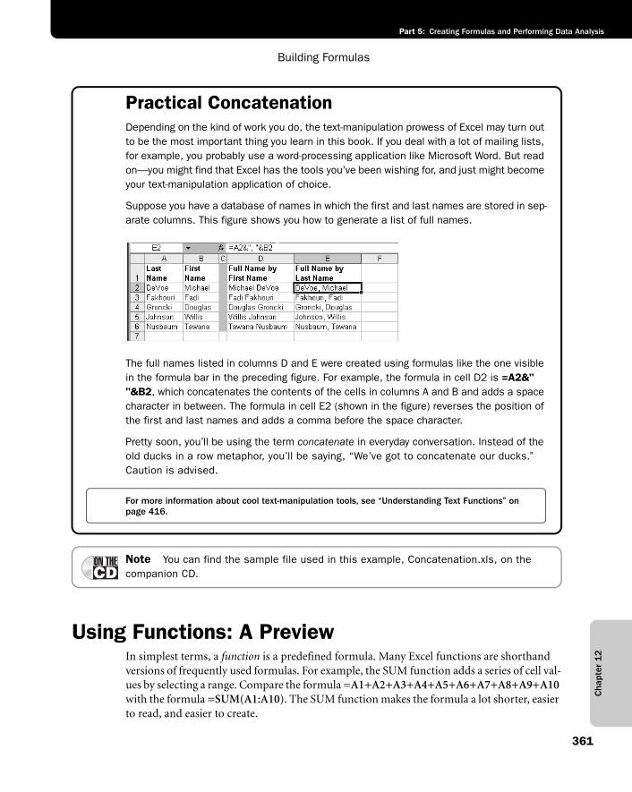
Cha

pter

12

Building Formulas

361

Part 5: Creating Formulas and Performing Data Analysis

Practical ConcatenationDepending on the kind of work you do, the text-manipulation prowess of Excel may turn out to be the most important thing you learn in this book. If you deal with a lot of mailing lists, for example, you probably use a word-processing application like Microsoft Word. But read on—you might find that Excel has the tools you’ve been wishing for, and just might become your text-manipulation application of choice.

Suppose you have a database of names in which the first and last names are stored in sep-arate columns. This figure shows you how to generate a list of full names.

g12ie01

The full names listed in columns D and E were created using formulas like the one visible in the formula bar in the preceding figure. For example, the formula in cell D2 is =A2&""&B2, which concatenates the contents of the cells in columns A and B and adds a space character in between. The formula in cell E2 (shown in the figure) reverses the position of the first and last names and adds a comma before the space character.

Pretty soon, you’ll be using the term concatenate in everyday conversation. Instead of the old ducks in a row metaphor, you’ll be saying, “We’ve got to concatenate our ducks.” Caution is advised.

For more information about cool text-manipulation tools, see “Understanding Text Functions” on page 416.

Note You can find the sample file used in this example, Concatenation.xls, on thecompanion CD.

Using Functions: A PreviewIn simplest terms, a function is a predefined formula. Many Excel functions are shorthand versions of frequently used formulas. For example, the SUM function adds a series of cell val-ues by selecting a range. Compare the formula =A1+A2+A3+A4+A5+A6+A7+A8+A9+A10with the formula =SUM(A1:A10). The SUM function makes the formula a lot shorter, easier to read, and easier to create.

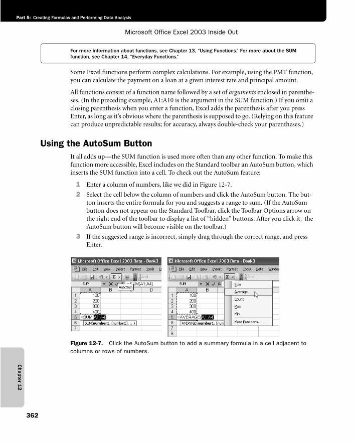
Chapter 1

2

Microsoft Office Excel 2003 Inside Out

Part 5: Creating Formulas and Performing Data Analysis

362

For more information about functions, see Chapter 13, “Using Functions.” For more about the SUM function, see Chapter 14, “Everyday Functions.”

Some Excel functions perform complex calculations. For example, using the PMT function, you can calculate the payment on a loan at a given interest rate and principal amount.

All functions consist of a function name followed by a set of arguments enclosed in parenthe-ses. (In the preceding example, A1:A10 is the argument in the SUM function.) If you omit a closing parenthesis when you enter a function, Excel adds the parenthesis after you press Enter, as long as it’s obvious where the parenthesis is supposed to go. (Relying on this feature can produce unpredictable results; for accuracy, always double-check your parentheses.)

Using the AutoSum ButtonIt all adds up—the SUM function is used more often than any other function. To make this function more accessible, Excel includes on the Standard toolbar an AutoSum button, which inserts the SUM function into a cell. To check out the AutoSum feature:

1 Enter a column of numbers, like we did in Figure 12-7.

2 Select the cell below the column of numbers and click the AutoSum button. The but-ton inserts the entire formula for you and suggests a range to sum. (If the AutoSum button does not appear on the Standard Toolbar, click the Toolbar Options arrow on the right end of the toolbar to display a list of “hidden” buttons. After you click it, the AutoSum button will become visible on the toolbar.)

3 If the suggested range is incorrect, simply drag through the correct range, and press Enter.

f12ie07

Figure 12-7. Click the AutoSum button to add a summary formula in a cell adjacent to columns or rows of numbers.

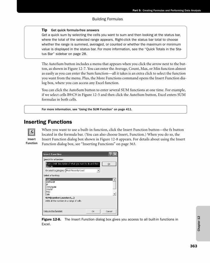
Cha

pter

12

Building Formulas

363

Part 5: Creating Formulas and Performing Data Analysis

Tip Get quick formula-free answersGet a quick sum by selecting the cells you want to sum and then looking at the status bar, where the total of the selected range appears. Right-click the status bar total to choose whether the range is summed, averaged, or counted or whether the maximum or minimum value is displayed in the status bar. For more information, see the “Quick Totals in the Sta-tus Bar” sidebar on page 28.

The AutoSum button includes a menu that appears when you click the arrow next to the but-ton, as shown in Figure 12-7. You can enter the Average, Count, Max, or Min function almost as easily as you can enter the Sum function—all it takes is an extra click to select the function you want from the menu. Plus, the More Functions command opens the Insert Function dia-log box, where you can access any Excel function.

You can click the AutoSum button to enter several SUM functions at one time. For example, if we select cells B9:C9 in Figure 12-5 and then click the AutoSum button, Excel enters SUM formulas in both cells.

For more information, see “Using the SUM Function” on page 411.

Inserting Functions

Insert Function

When you want to use a built-in function, click the Insert Function button—the fx button located in the formula bar. (You can also choose Insert, Function.) When you do so, the Insert Function dialog box shown in Figure 12-8 appears. For details about using the Insert Function dialog box, see “Inserting Functions” on page 363.

f12ie08

Figure 12-8. The Insert Function dialog box gives you access to all built-in functions in Excel.

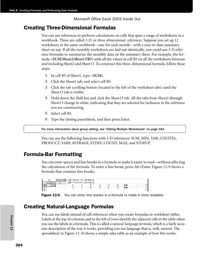
Chapter 1

2

Microsoft Office Excel 2003 Inside Out

Part 5: Creating Formulas and Performing Data Analysis

364

Creating Three-Dimensional FormulasYou can use references to perform calculations on cells that span a range of worksheets in a workbook. These are called 3-D, or three-dimensional, references. Suppose you set up 12 worksheets in the same workbook—one for each month—with a year-to-date summary sheet on top. If all the monthly worksheets are laid out identically, you could use 3-D refer-ence formulas to summarize the monthly data on the summary sheet. For example, the for-mula =SUM(Sheet2:Sheet13!B5) adds all the values in cell B5 on all the worksheets between and including Sheet2 and Sheet13. To construct this three-dimensional formula, follow these steps:

1 In cell B5 of Sheet1, type =SUM(.

2 Click the Sheet2 tab, and select cell B5.

3 Click the tab scrolling button (located to the left of the worksheet tabs) until the Sheet13 tab is visible.

4 Hold down the Shift key and click the Sheet13 tab. All the tabs from Sheet2 through Sheet13 change to white, indicating that they are selected for inclusion in the reference you are constructing.

5 Select cell B5.

6 Type the closing parenthesis, and then press Enter.

For more information about group editing, see “Editing Multiple Worksheets” on page 183.

You can use the following functions with 3-D references: SUM, MIN, VAR, COUNTA, PRODUCT, VARP, AVERAGE, STDEV, COUNT, MAX, and STDEVP.

Formula-Bar FormattingYou can enter spaces and line breaks in a formula to make it easier to read—without affecting the calculation of the formula. To enter a line break, press Alt+Enter. Figure 12-9 shows a formula that contains line breaks.

f12ie09

Figure 12-9. You can enter line breaks in a formula to make it more readable.

Creating Natural-Language FormulasYou can use labels instead of cell references when you create formulas in worksheet tables. Labels at the top of columns and to the left of rows identify the adjacent cells in the table when you use the labels in a formula. This is called a natural-language formula, which is a fairly accu-rate description of the way it works, providing you use language that is, well, natural. The spreadsheet in Figure 12-10 shows a simple sales table as an example of how this works.

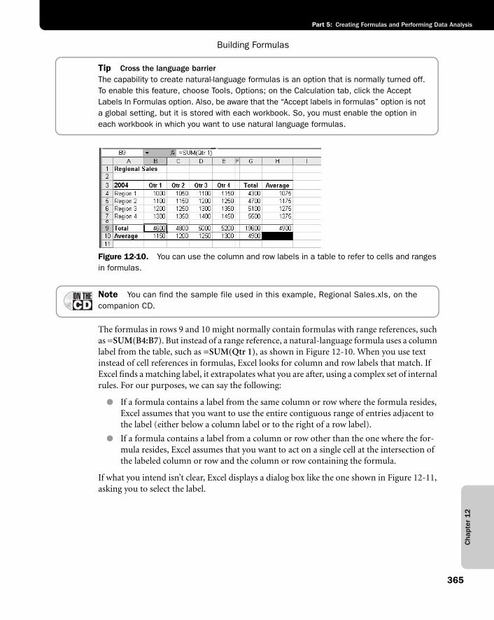
Cha

pter

12

Building Formulas

365

Part 5: Creating Formulas and Performing Data Analysis

Tip Cross the language barrierThe capability to create natural-language formulas is an option that is normally turned off. To enable this feature, choose Tools, Options; on the Calculation tab, click the Accept Labels In Formulas option. Also, be aware that the “Accept labels in formulas” option is not a global setting, but it is stored with each workbook. So, you must enable the option in each workbook in which you want to use natural language formulas.

f12ie10

Figure 12-10. You can use the column and row labels in a table to refer to cells and ranges in formulas.

Note You can find the sample file used in this example, Regional Sales.xls, on thecompanion CD.

The formulas in rows 9 and 10 might normally contain formulas with range references, such as =SUM(B4:B7). But instead of a range reference, a natural-language formula uses a column label from the table, such as =SUM(Qtr 1), as shown in Figure 12-10. When you use text instead of cell references in formulas, Excel looks for column and row labels that match. If Excel finds a matching label, it extrapolates what you are after, using a complex set of internal rules. For our purposes, we can say the following:

● If a formula contains a label from the same column or row where the formula resides, Excel assumes that you want to use the entire contiguous range of entries adjacent to the label (either below a column label or to the right of a row label).

● If a formula contains a label from a column or row other than the one where the for-mula resides, Excel assumes that you want to act on a single cell at the intersection of the labeled column or row and the column or row containing the formula.

If what you intend isn’t clear, Excel displays a dialog box like the one shown in Figure 12-11, asking you to select the label.

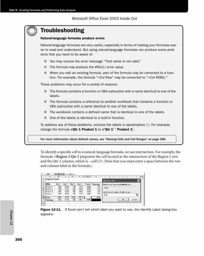
Chapter 1

2

Microsoft Office Excel 2003 Inside Out

Part 5: Creating Formulas and Performing Data Analysis

366

TroubleshootingNatural-language formulas produce errors

Natural-language formulas are very useful, especially in terms of making your formulas eas-ier to read and understand. But using natural-language formulas can produce some prob-lems that you need to be aware of.

● You may receive the error message “That name is not valid.”

● The formula may produce the #NULL! error value.

● When you edit an existing formula, part of the formula may be converted to a func-tion. For example, the formula "=Col Row" may be converted to "=Col ROW()."

These problems may occur for a variety of reasons:

● The formula contains a function or VBA subroutine with a name identical to one of the labels.

● The formula contains a reference to another workbook that contains a function or VBA subroutine with a name identical to one of the labels.

● The workbook contains a defined name that is identical to one of the labels.

● One of the labels is identical to a built-in function.

To address any of these problems, enclose the labels in apostrophes ('). For example, change the formula =Qtr 1 Product 1 to ='Qtr 1' ' Product 1'.

For more information about defined names, see “Naming Cells and Cell Ranges” on page 368.

To identify a specific cell in a natural-language formula, we use intersection. For example, the formula =Region 2 Qtr 2 pinpoints the cell located at the intersection of the Region 2 row and the Qtr 2 column, which is—cell C5. (Note that you must enter a space between the row and column label in the formula.)

f12ie11

Figure 12-11. If Excel can’t tell which label you want to use, the Identify Label dialog box appears.

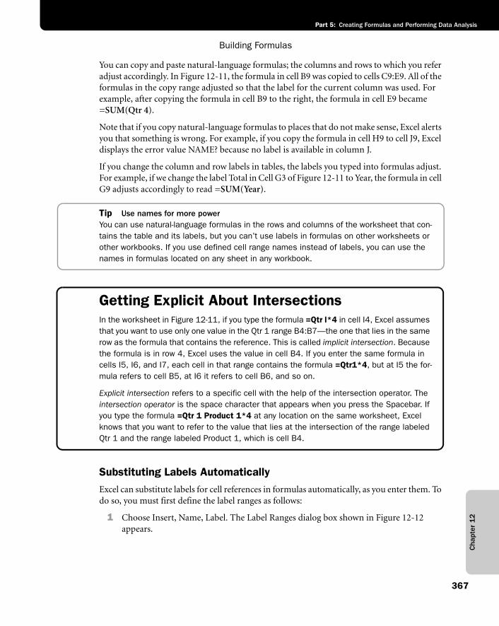
Cha

pter

12

Building Formulas

367

Part 5: Creating Formulas and Performing Data Analysis

You can copy and paste natural-language formulas; the columns and rows to which you refer adjust accordingly. In Figure 12-11, the formula in cell B9 was copied to cells C9:E9. All of the formulas in the copy range adjusted so that the label for the current column was used. For example, after copying the formula in cell B9 to the right, the formula in cell E9 became =SUM(Qtr 4).

Note that if you copy natural-language formulas to places that do not make sense, Excel alerts you that something is wrong. For example, if you copy the formula in cell H9 to cell J9, Excel displays the error value NAME? because no label is available in column J.

If you change the column and row labels in tables, the labels you typed into formulas adjust. For example, if we change the label Total in Cell G3 of Figure 12-11 to Year, the formula in cell G9 adjusts accordingly to read =SUM(Year).

Tip Use names for more powerYou can use natural-language formulas in the rows and columns of the worksheet that con-tains the table and its labels, but you can’t use labels in formulas on other worksheets or other workbooks. If you use defined cell range names instead of labels, you can use the names in formulas located on any sheet in any workbook.

Getting Explicit About IntersectionsIn the worksheet in Figure 12-11, if you type the formula =Qtr l*4 in cell I4, Excel assumes that you want to use only one value in the Qtr 1 range B4:B7—the one that lies in the same row as the formula that contains the reference. This is called implicit intersection. Because the formula is in row 4, Excel uses the value in cell B4. If you enter the same formula in cells I5, I6, and I7, each cell in that range contains the formula =Qtr1*4, but at I5 the for-mula refers to cell B5, at I6 it refers to cell B6, and so on.

Explicit intersection refers to a specific cell with the help of the intersection operator. The intersection operator is the space character that appears when you press the Spacebar. If you type the formula =Qtr 1 Product 1*4 at any location on the same worksheet, Excel knows that you want to refer to the value that lies at the intersection of the range labeled Qtr 1 and the range labeled Product 1, which is cell B4.

Substituting Labels AutomaticallyExcel can substitute labels for cell references in formulas automatically, as you enter them. To do so, you must first define the label ranges as follows:

1 Choose Insert, Name, Label. The Label Ranges dialog box shown in Figure 12-12 appears.

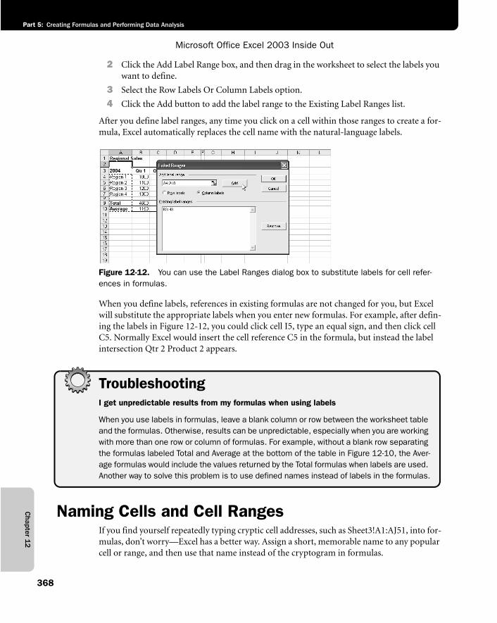
Chapter 1

2

Microsoft Office Excel 2003 Inside Out

Part 5: Creating Formulas and Performing Data Analysis

368

2 Click the Add Label Range box, and then drag in the worksheet to select the labels you want to define.

3 Select the Row Labels Or Column Labels option.

4 Click the Add button to add the label range to the Existing Label Ranges list.

After you define label ranges, any time you click on a cell within those ranges to create a for-mula, Excel automatically replaces the cell name with the natural-language labels.

f12ie12

Figure 12-12. You can use the Label Ranges dialog box to substitute labels for cell refer-ences in formulas.

When you define labels, references in existing formulas are not changed for you, but Excel will substitute the appropriate labels when you enter new formulas. For example, after defin-ing the labels in Figure 12-12, you could click cell I5, type an equal sign, and then click cell C5. Normally Excel would insert the cell reference C5 in the formula, but instead the label intersection Qtr 2 Product 2 appears.

TroubleshootingI get unpredictable results from my formulas when using labels

When you use labels in formulas, leave a blank column or row between the worksheet table and the formulas. Otherwise, results can be unpredictable, especially when you are working with more than one row or column of formulas. For example, without a blank row separating the formulas labeled Total and Average at the bottom of the table in Figure 12-10, the Aver-age formulas would include the values returned by the Total formulas when labels are used. Another way to solve this problem is to use defined names instead of labels in the formulas.

Naming Cells and Cell RangesIf you find yourself repeatedly typing cryptic cell addresses, such as Sheet3!A1:AJ51, into for-mulas, don’t worry—Excel has a better way. Assign a short, memorable name to any popular cell or range, and then use that name instead of the cryptogram in formulas.

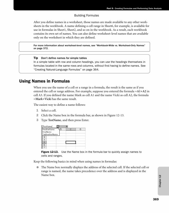
Cha

pter

12

Building Formulas

369

Part 5: Creating Formulas and Performing Data Analysis

After you define names in a worksheet, those names are made available to any other work-sheets in the workbook. A name defining a cell range in Sheet6, for example, is available for use in formulas in Sheet1, Sheet2, and so on in the workbook. As a result, each workbook contains its own set of names. You can also define worksheet-level names that are available only on the worksheet in which they are defined.

For more information about worksheet-level names, see “Workbook-Wide vs. Worksheet-Only Names” on page 372.

Tip Don’t define names for simple tablesIn a simple table with row and column headings, you can use the headings themselves in formulas located in the same rows and columns, without first having to define names. See “Creating Natural-Language Formulas” on page 364.

Using Names in FormulasWhen you use the name of a cell or a range in a formula, the result is the same as if you entered the cell or range address. For example, suppose you entered the formula =A1+A2 in cell A3. If you defined the name Mark as cell A1 and the name Vicki as cell A2, the formula =Mark+Vicki has the same result.

The easiest way to define a name follows:

1 Select a cell.

2 Click the Name box in the formula bar, as shown in Figure 12-13.

3 Type TestName, and then press Enter.

f12ie13

Figure 12-13. Use the Name box in the formula bar to quickly assign names to cells and ranges.

Keep the following basics in mind when using names in formulas:

● The Name box normally displays the address of the selected cell. If the selected cell or range is named, the name takes precedence over the address and is displayed in the Name box.

Chapter 1

2

Microsoft Office Excel 2003 Inside Out

Part 5: Creating Formulas and Performing Data Analysis

370

● When you define a name for a range of cells, the range name does not appear in the Name box unless the entire range is selected.

● When you click the Name box and select a name, the cell selection switches to the named cells.

● If you type a name that has already been defined into the Name box, Excel switches the selection instead of redefining the name.

● When you define a name, the address includes the worksheet name and the cell refer-ence is absolute. For example, when you define the name TestName for cell C5 in Sheet1, the actual name definition is recorded as Sheet1!$C$5.

For more information about absolute references, see “Understanding Relative, Absolute, and Mixed References” on page 353.

Defining and Managing NamesInstead of coming up with new names for cells and ranges, you can simply use existing text labels to create names. Choosing Insert, Name, Define, you can use text in adjacent cells to define cell and range names, as seen in Figure 12-14. You can choose this command also to redefine existing names.

Rules for NamingThe following rules apply when you name cells and ranges in Excel:

● All names must begin with a letter, a backslash (\), or an underscore (_).

● Numbers can be used.

● Spaces can’t be used.

● Excel translates blank spaces in labels to underscores in defined names.

● Symbols other than backslash and underscore can’t be used.

● Names that resemble cell references (for example, AB$5 or R1C7) can’t be used.

● Single letters, with the exception of the letters R and C, can be used as names.

A name can contain 255 characters, but if it contains more than 253 characters, you can’t select it from the Name box. Excel does not distinguish between uppercase and lowercase characters in names. For example, if you create the name Tax and then create the name TAX in the same workbook, the first name is overwritten by the second.

Tip Press Ctrl+F3 to display the Define Name dialog box instantly.

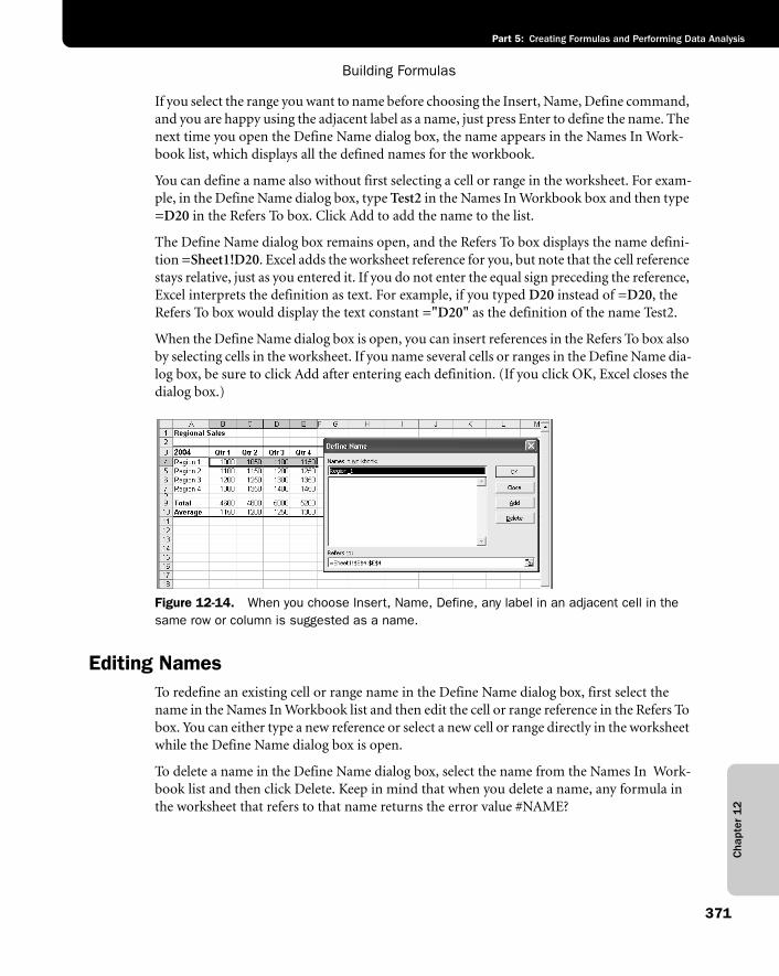
Cha

pter

12

Building Formulas

371

Part 5: Creating Formulas and Performing Data Analysis

If you select the range you want to name before choosing the Insert, Name, Define command, and you are happy using the adjacent label as a name, just press Enter to define the name. The next time you open the Define Name dialog box, the name appears in the Names In Work-book list, which displays all the defined names for the workbook.

You can define a name also without first selecting a cell or range in the worksheet. For exam-ple, in the Define Name dialog box, type Test2 in the Names In Workbook box and then type =D20 in the Refers To box. Click Add to add the name to the list.

The Define Name dialog box remains open, and the Refers To box displays the name defini-tion =Sheet1!D20. Excel adds the worksheet reference for you, but note that the cell reference stays relative, just as you entered it. If you do not enter the equal sign preceding the reference, Excel interprets the definition as text. For example, if you typed D20 instead of =D20, the Refers To box would display the text constant ="D20" as the definition of the name Test2.

When the Define Name dialog box is open, you can insert references in the Refers To box also by selecting cells in the worksheet. If you name several cells or ranges in the Define Name dia-log box, be sure to click Add after entering each definition. (If you click OK, Excel closes the dialog box.)

f12ie14

Figure 12-14. When you choose Insert, Name, Define, any label in an adjacent cell in the same row or column is suggested as a name.

Editing NamesTo redefine an existing cell or range name in the Define Name dialog box, first select the name in the Names In Workbook list and then edit the cell or range reference in the Refers To box. You can either type a new reference or select a new cell or range directly in the worksheet while the Define Name dialog box is open.

To delete a name in the Define Name dialog box, select the name from the Names In Work-book list and then click Delete. Keep in mind that when you delete a name, any formula in the worksheet that refers to that name returns the error value #NAME?

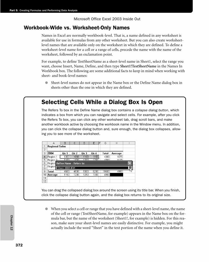
Chapter 1

2

Microsoft Office Excel 2003 Inside Out

Part 5: Creating Formulas and Performing Data Analysis

372

Workbook-Wide vs. Worksheet-Only NamesNames in Excel are normally workbook-level. That is, a name defined in any worksheet is available for use in formulas from any other worksheet. But you can also create worksheet-level names that are available only on the worksheet in which they are defined. To define a worksheet-level name for a cell or a range of cells, precede the name with the name of the worksheet, followed by an exclamation point.

For example, to define TestSheetName as a sheet-level name in Sheet1, select the range you want, choose Insert, Name, Define, and then type Sheet1!TestSheetName in the Names In Workbook box. The following are some additional facts to keep in mind when working with sheet- and book-level names:

● Sheet-level names do not appear in the Name box or the Define Name dialog box in sheets other than the one in which they are defined.

Selecting Cells While a Dialog Box Is OpenThe Refers To box in the Define Name dialog box contains a collapse dialog button, which indicates a box from which you can navigate and select cells. For example, after you click the Refers To box, you can click any other worksheet tab, drag scroll bars, and make another workbook active by choosing the workbook name in the Window menu. In addition, you can click the collapse dialog button and, sure enough, the dialog box collapses, allow-ing you to see more of the worksheet.

g12ie02

You can drag the collapsed dialog box around the screen using its title bar. When you finish, click the collapse dialog button again, and the dialog box returns to its original size.

● When you select a cell or range that you have defined with a sheet-level name, the name of the cell or range (TestSheetName, for example) appears in the Name box on the for-mula bar, but the name of the worksheet (Sheet1!, for example) is hidden. For this rea-son, make sure your sheet-level names are easily distinctive. For example, you might actually include the word “Sheet” in the text portion of the name when you define it.

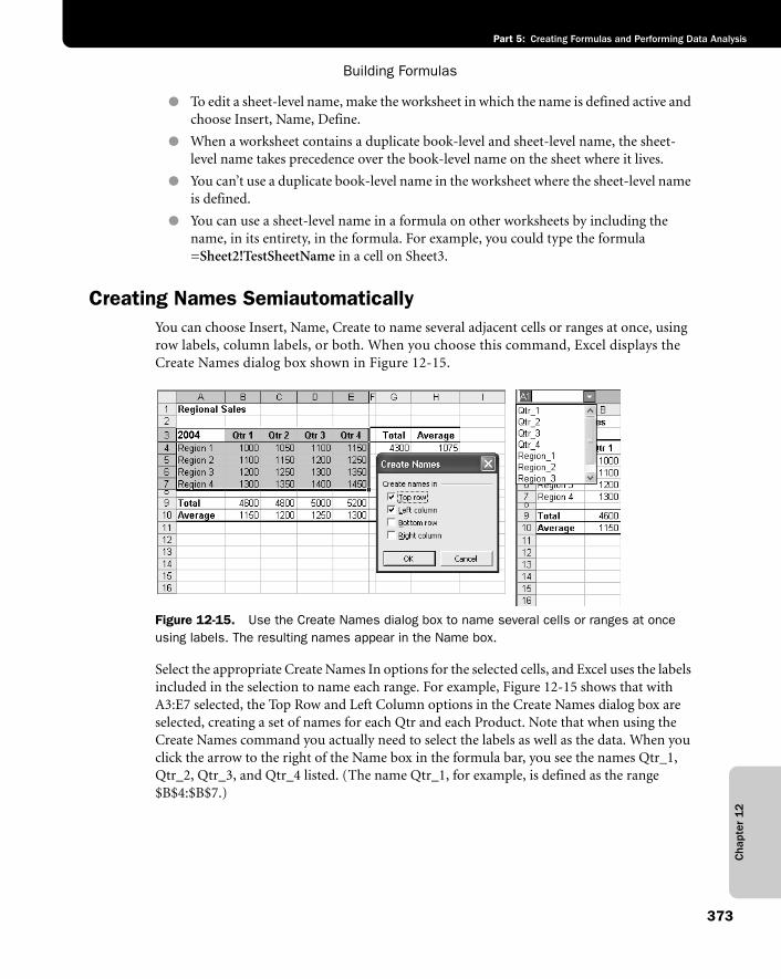
Cha

pter

12

Building Formulas

373

Part 5: Creating Formulas and Performing Data Analysis

● To edit a sheet-level name, make the worksheet in which the name is defined active and choose Insert, Name, Define.

● When a worksheet contains a duplicate book-level and sheet-level name, the sheet-level name takes precedence over the book-level name on the sheet where it lives.

● You can’t use a duplicate book-level name in the worksheet where the sheet-level name is defined.

● You can use a sheet-level name in a formula on other worksheets by including the name, in its entirety, in the formula. For example, you could type the formula =Sheet2!TestSheetName in a cell on Sheet3.

Creating Names SemiautomaticallyYou can choose Insert, Name, Create to name several adjacent cells or ranges at once, using row labels, column labels, or both. When you choose this command, Excel displays the Create Names dialog box shown in Figure 12-15.

f12ie15

Figure 12-15. Use the Create Names dialog box to name several cells or ranges at once using labels. The resulting names appear in the Name box.

Select the appropriate Create Names In options for the selected cells, and Excel uses the labels included in the selection to name each range. For example, Figure 12-15 shows that with A3:E7 selected, the Top Row and Left Column options in the Create Names dialog box are selected, creating a set of names for each Qtr and each Product. Note that when using the Create Names command you actually need to select the labels as well as the data. When you click the arrow to the right of the Name box in the formula bar, you see the names Qtr_1, Qtr_2, Qtr_3, and Qtr_4 listed. (The name Qtr_1, for example, is defined as the range $B$4:$B$7.)

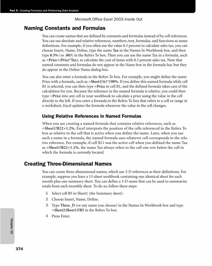
Chapter 1

2

Microsoft Office Excel 2003 Inside Out

Part 5: Creating Formulas and Performing Data Analysis

374

Naming Constants and FormulasYou can create names that are defined by constants and formulas instead of by cell references. You can use absolute and relative references, numbers, text, formulas, and functions as name definitions. For example, if you often use the value 8.3 percent to calculate sales tax, you can choose Insert, Name, Define, type the name Tax in the Names In Workbook box, and then type 8.3% (or .083) in the Refers To box. Then you can use the name Tax in a formula, such as =Price+(Price*Tax), to calculate the cost of items with 8.3 percent sales tax. Note that named constants and formulas do not appear in the Name box in the formula bar, but they do appear in the Define Name dialog box.

You can also enter a formula in the Refers To box. For example, you might define the name Price with a formula, such as =Sheet1!A1*190%. If you define this named formula while cell B1 is selected, you can then type =Price in cell B1, and the defined formula takes care of the calculation for you. Because the reference in the named formula is relative, you could then type =Price into any cell in your workbook to calculate a price using the value in the cell directly to the left. If you enter a formula in the Refers To box that refers to a cell or range in a worksheet, Excel updates the formula whenever the value in the cell changes.

Using Relative References in Named FormulasWhen you are creating a named formula that contains relative references, such as =Sheet1!B22+1.2%, Excel interprets the position of the cells referenced in the Refers To box as relative to the cell that is active when you define the name. Later, when you use such a name in a formula, the named formula uses whatever cell corresponds to the rela-tive reference. For example, if cell B21 was the active cell when you defined the name Tax as =Sheet1!B22+1.2%, the name Tax always refers to the cell one row below the cell in which the formula is currently located.

Creating Three-Dimensional NamesYou can create three-dimensional names, which use 3-D references as their definitions. For example, suppose you have a 13-sheet workbook containing one identical sheet for each month plus one summary sheet. You can define a 3-D name that can be used to summarize totals from each monthly sheet. To do so, follow these steps:

1 Select cell B5 in Sheet1 (the Summary sheet).

2 Choose Insert, Name, Define.

3 Type Three_D (or any name you choose) in the Names In Workbook box and type =Sheet2:Sheet13!B5 in the Refers To box.

4 Press Enter.

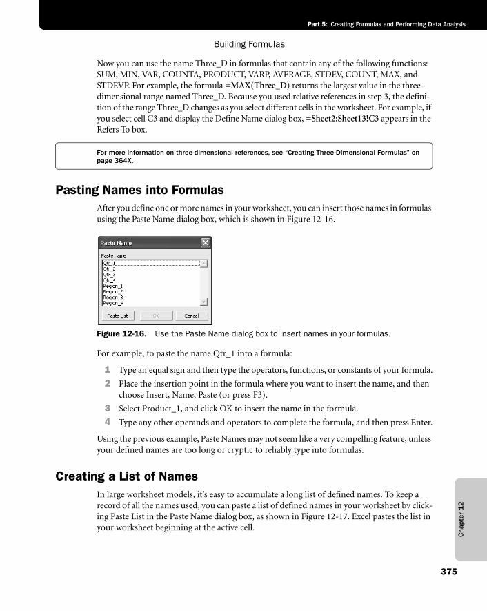
Cha

pter

12

Building Formulas

375

Part 5: Creating Formulas and Performing Data Analysis

Now you can use the name Three_D in formulas that contain any of the following functions: SUM, MIN, VAR, COUNTA, PRODUCT, VARP, AVERAGE, STDEV, COUNT, MAX, and STDEVP. For example, the formula =MAX(Three_D) returns the largest value in the three-dimensional range named Three_D. Because you used relative references in step 3, the defini-tion of the range Three_D changes as you select different cells in the worksheet. For example, if you select cell C3 and display the Define Name dialog box, =Sheet2:Sheet13!C3 appears in the Refers To box.

For more information on three-dimensional references, see “Creating Three-Dimensional Formulas” on page 364X.

Pasting Names into FormulasAfter you define one or more names in your worksheet, you can insert those names in formulas using the Paste Name dialog box, which is shown in Figure 12-16.

12ie16

Figure 12-16. Use the Paste Name dialog box to insert names in your formulas.

For example, to paste the name Qtr_1 into a formula:

1 Type an equal sign and then type the operators, functions, or constants of your formula.

2 Place the insertion point in the formula where you want to insert the name, and then choose Insert, Name, Paste (or press F3).

3 Select Product_1, and click OK to insert the name in the formula.

4 Type any other operands and operators to complete the formula, and then press Enter.

Using the previous example, Paste Names may not seem like a very compelling feature, unless your defined names are too long or cryptic to reliably type into formulas.

Creating a List of NamesIn large worksheet models, it’s easy to accumulate a long list of defined names. To keep a record of all the names used, you can paste a list of defined names in your worksheet by click-ing Paste List in the Paste Name dialog box, as shown in Figure 12-17. Excel pastes the list in your worksheet beginning at the active cell.

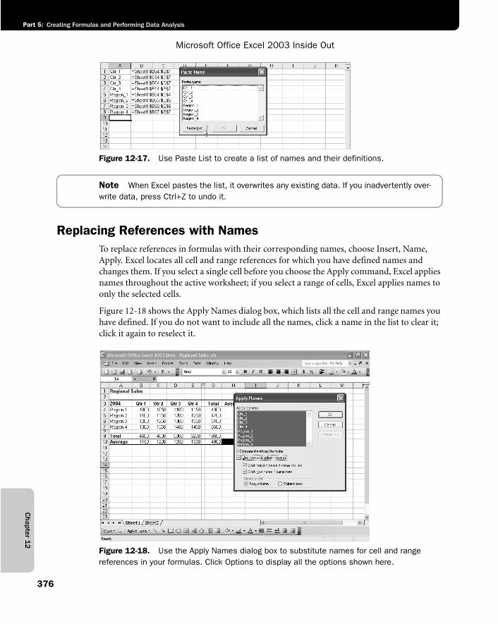
Chapter 1

2

Microsoft Office Excel 2003 Inside Out

Part 5: Creating Formulas and Performing Data Analysis

376

f12ie17

Figure 12-17. Use Paste List to create a list of names and their definitions.

Note When Excel pastes the list, it overwrites any existing data. If you inadvertently over-write data, press Ctrl+Z to undo it.

Replacing References with NamesTo replace references in formulas with their corresponding names, choose Insert, Name, Apply. Excel locates all cell and range references for which you have defined names and changes them. If you select a single cell before you choose the Apply command, Excel applies names throughout the active worksheet; if you select a range of cells, Excel applies names to only the selected cells.

Figure 12-18 shows the Apply Names dialog box, which lists all the cell and range names you have defined. If you do not want to include all the names, click a name in the list to clear it; click it again to reselect it.

f12ie18

Figure 12-18. Use the Apply Names dialog box to substitute names for cell and rangereferences in your formulas. Click Options to display all the options shown here.

Cha

pter

12

Building Formulas

377

Part 5: Creating Formulas and Performing Data Analysis

Excel normally does not apply the column or row name if either is superfluous. For example, Figure 12-18 shows a sheet after we applied names using the default options in the Apply Names dialog box. Cell I14 is selected, and the formula bar shows that it contains the formula =Region_2 Qtr_3, which before applying names contained the formula =D5. Because cell I14 isn’t in the same row or column as any of the defined ranges, both the row and column names are included in the new formula. Cell D14 contained the same formula, =D5. But because D14 is in the same column as the referenced cell, only the row name is needed thanks to implicit intersection, resulting in the formula =Region_2.

If you prefer to see both the column and row names even when they are not necessary, clear the Omit Column Name If Same Column option and the Omit Row Name If Same Row option.

For more information about implicit intersection, see the “Getting Explicit about Intersections” sidebar on page 367.

The Name Order options control the order in which row and column components appear. For example, using the Column Row option, the formula in cell I14 in Figure 12-18 would become =Qtr_3 Region_2.

Select the Ignore Relative/Absolute option to replace references with names regardless of the reference type. In general, leave this check box selected. Most name definitions use absolute references (the default when you define and create names), and most formulas use relative references (the default when you paste cell and range references in the formula bar). If you clear this option, absolute, relative, and mixed references are replaced with name definitions only if the definitions use the corresponding reference style.

The Use Row And Column Names option is necessary if you want to apply names in inter-section cases, as we have shown in the examples. If you define names for individual cells, however, you can clear Use Row and Column Names to apply names to only specific cell ref-erences in formulas.

Using Go To with Named RangesWhen you choose Edit, Go To (or press F5), range names appear in the Go To dialog box, as shown in Figure 12-19. Select a name, and click OK to jump to the range referred to. Note that names defined with constants or formulas do not appear in the Go To dialog box.

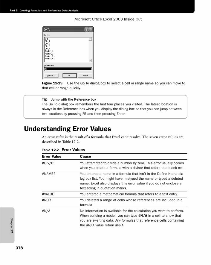
Chapter 1

2

Microsoft Office Excel 2003 Inside Out

Part 5: Creating Formulas and Performing Data Analysis

378

f12ie19

Figure 12-19. Use the Go To dialog box to select a cell or range name so you can move to that cell or range quickly.

Tip Jump with the Reference boxThe Go To dialog box remembers the last four places you visited. The latest location is always in the Reference box when you display the dialog box so that you can jump between two locations by pressing F5 and then pressing Enter.

Understanding Error ValuesAn error value is the result of a formula that Excel can’t resolve. The seven error values are described in Table 12-2.

Table 12-2. Error Values

Error Value Cause

#DIV/0! You attempted to divide a number by zero. This error usually occurs when you create a formula with a divisor that refers to a blank cell.

#NAME? You entered a name in a formula that isn’t in the Define Name dia-log box list. You might have mistyped the name or typed a deleted name. Excel also displays this error value if you do not enclose a text string in quotation marks.

#VALUE You entered a mathematical formula that refers to a text entry.

#REF! You deleted a range of cells whose references are included in a formula.

#N/A No information is available for the calculation you want to perform. When building a model, you can type #N/A in a cell to show that you are awaiting data. Any formulas that reference cells containing the #N/A value return #N/A.

Cha

pter

12

Building Formulas

379

Part 5: Creating Formulas and Performing Data Analysis

Worksheet CalculationExcel developers used to wear T-shirts emblazoned with the battle cry “Recalc or Die.” Rest assured that no developer has ever been harmed during the creation of any version of Excel. The deceptively simple process of calculation computes all formulas and then displays the results in the cells that contain them. When you change the values in the cells to which these formulas refer, Excel updates the values of the formulas as well. This updating process is called recalculation, and it affects only those cells containing references to cells that have changed.

By default, Excel recalculates whenever you make changes to a cell. If a large number of cells must be recalculated, the words Calculating Cells and a number appear at the left end of the status bar. The number indicates the percentage of recalculation that has been completed. You can interrupt the recalculation process simply by using commands or making cell entries; Excel pauses and then resumes recalculation when you are finished.

Recalculating ManuallyTo save time, particularly when you are making entries into a large workbook with many for-mulas, you can switch from automatic to manual recalculation; that is, Excel will recalculate only when you tell it to. To set manual recalculation, choose Tools, Options and then click the Calculation tab to display the options shown in Figure 12-20.

#NUM! You provided an invalid argument to a worksheet function. #NUM! can indicate also that the result of a formula is too large or too small to be represented in the worksheet.

#NULL! You included a space between two ranges in a formula to indicate an intersection, but the ranges have no common cells.

Table 12-2. Error Values

Error Value Cause

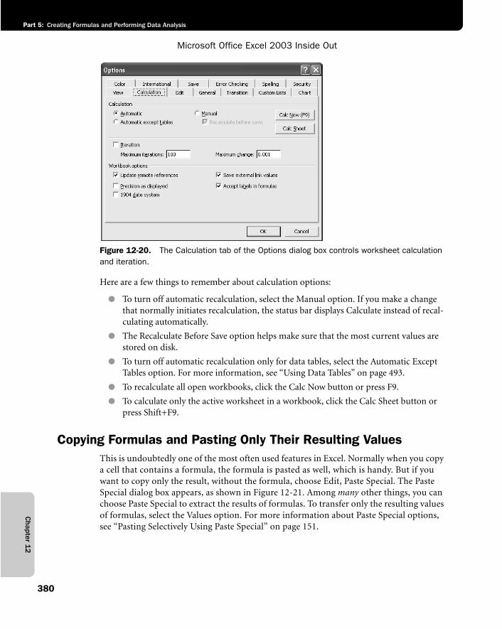
Chapter 1

2

Microsoft Office Excel 2003 Inside Out

Part 5: Creating Formulas and Performing Data Analysis

380

f12ie20

Figure 12-20. The Calculation tab of the Options dialog box controls worksheet calculation and iteration.

Here are a few things to remember about calculation options:

● To turn off automatic recalculation, select the Manual option. If you make a change that normally initiates recalculation, the status bar displays Calculate instead of recal-culating automatically.

● The Recalculate Before Save option helps make sure that the most current values are stored on disk.

● To turn off automatic recalculation only for data tables, select the Automatic Except Tables option. For more information, see “Using Data Tables” on page 493.

● To recalculate all open workbooks, click the Calc Now button or press F9.

● To calculate only the active worksheet in a workbook, click the Calc Sheet button or press Shift+F9.

Copying Formulas and Pasting Only Their Resulting ValuesThis is undoubtedly one of the most often used features in Excel. Normally when you copy a cell that contains a formula, the formula is pasted as well, which is handy. But if you want to copy only the result, without the formula, choose Edit, Paste Special. The Paste Special dialog box appears, as shown in Figure 12-21. Among many other things, you can choose Paste Special to extract the results of formulas. To transfer only the resulting values of formulas, select the Values option. For more information about Paste Special options, see “Pasting Selectively Using Paste Special” on page 151.

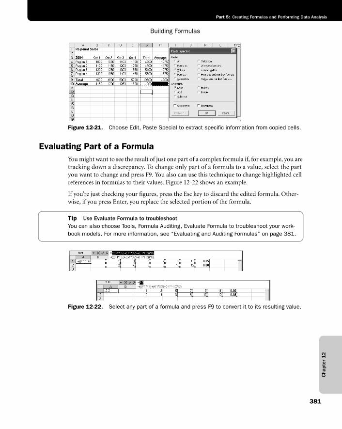
Cha

pter

12

Building Formulas

381

Part 5: Creating Formulas and Performing Data Analysis

f12ie21

Figure 12-21. Choose Edit, Paste Special to extract specific information from copied cells.

Evaluating Part of a FormulaYou might want to see the result of just one part of a complex formula if, for example, you are tracking down a discrepancy. To change only part of a formula to a value, select the part you want to change and press F9. You also can use this technique to change highlighted cell references in formulas to their values. Figure 12-22 shows an example.

If you’re just checking your figures, press the Esc key to discard the edited formula. Other-wise, if you press Enter, you replace the selected portion of the formula.

Tip Use Evaluate Formula to troubleshootYou can also choose Tools, Formula Auditing, Evaluate Formula to troubleshoot your work-book models. For more information, see “Evaluating and Auditing Formulas” on page 381.

f12ie22

Figure 12-22. Select any part of a formula and press F9 to convert it to its resulting value.

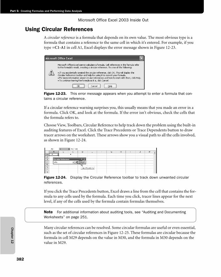
Chapter 1

2

Microsoft Office Excel 2003 Inside Out

Part 5: Creating Formulas and Performing Data Analysis

382

Using Circular ReferencesA circular reference is a formula that depends on its own value. The most obvious type is a formula that contains a reference to the same cell in which it’s entered. For example, if you type =C1-A1 in cell A1, Excel displays the error message shown in Figure 12-23.

f12ie23

Figure 12-23. This error message appears when you attempt to enter a formula that con-tains a circular reference.

If a circular reference warning surprises you, this usually means that you made an error in a formula. Click OK, and look at the formula. If the error isn’t obvious, check the cells that the formula refers to.

Choose View, Toolbars, Circular Reference to help track down the problem using the built-in auditing features of Excel. Click the Trace Precedents or Trace Dependents button to draw tracer arrows on the worksheet. These arrows show you a visual path to all the cells involved, as shown in Figure 12-24.

f12ie24

Figure 12-24. Display the Circular Reference toolbar to track down unwanted circularreferences.

If you click the Trace Precedents button, Excel draws a line from the cell that contains the for-mula to any cells used by the formula. Each time you click, tracer lines appear for the next level, if any of the cells used by the formula contain formulas themselves.

Note For additional information about auditing tools, see “Auditing and Documenting Worksheets” on page 251.

Many circular references can be resolved. Some circular formulas are useful or even essential, such as the set of circular references in Figure 12-25. These formulas are circular because the formula in cell M29 depends on the value in M30, and the formula in M30 depends on the value in M29.

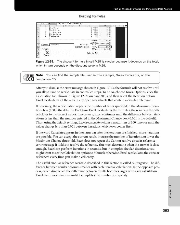
Cha

pter

12

Building Formulas

383

Part 5: Creating Formulas and Performing Data Analysis

f12ie25

Figure 12-25. The discount formula in cell M29 is circular because it depends on the total, which in turn depends on the discount value in M29.

Note You can find the sample file used in this example, Sales Invoice.xls, on thecompanion CD.

After you dismiss the error message shown in Figure 12-23, the formula will not resolve until you allow Excel to recalculate in controlled steps. To do so, choose Tools, Options, click the Calculation tab, shown in Figure 12-20 on page 380, and then select the Iteration option. Excel recalculates all the cells in any open worksheets that contain a circular reference.

If necessary, the recalculation repeats the number of times specified in the Maximum Itera-tions box (100 is the default). Each time Excel recalculates the formulas, the results in the cells get closer to the correct values. If necessary, Excel continues until the difference between iter-ations is less than the number entered in the Maximum Change box (0.001 is the default). Thus, using the default settings, Excel recalculates either a maximum of 100 times or until the values change less than 0.001 between iterations, whichever comes first.

If the word Calculate appears in the status bar after the iterations are finished, more iterations are possible. You can accept the current result, increase the number of iterations, or lower the Maximum Change threshold. Excel does not repeat the Cannot resolve circular reference error message if it fails to resolve the reference. You must determine when the answer is close enough. Excel can perform iterations in seconds, but in complex circular situations, you might want to set the Calculation option to Manual; otherwise, Excel recalculates the circular references every time you make a cell entry.

The useful circular reference scenario described in this section is called convergence: The dif-ference between results becomes smaller with each iterative calculation. In the opposite pro-cess, called divergence, the difference between results becomes larger with each calculation. Excel continues iterations until it completes the number you specify.

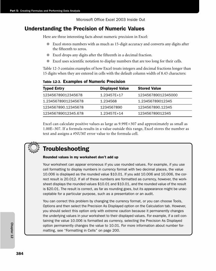
Chapter 1

2

Microsoft Office Excel 2003 Inside Out

Part 5: Creating Formulas and Performing Data Analysis

384

Understanding the Precision of Numeric ValuesHere are three interesting facts about numeric precision in Excel:

● Excel stores numbers with as much as 15-digit accuracy and converts any digits after the fifteenth to zeros.

● Excel drops any digits after the fifteenth in a decimal fraction.

● Excel uses scientific notation to display numbers that are too long for their cells.

Table 12-3 contains examples of how Excel treats integers and decimal fractions longer than 15 digits when they are entered in cells with the default column width of 8.43 characters:

Excel can calculate positive values as large as 9.99E+307 and approximately as small as 1.00E 307. If a formula results in a value outside this range, Excel stores the number as text and assigns a #NUM! error value to the formula cell.

TroubleshootingRounded values in my worksheet don’t add up

Your worksheet can appear erroneous if you use rounded values. For example, if you use cell formatting to display numbers in currency format with two decimal places, the value 10.006 is displayed as the rounded value $10.01. If you add 10.006 and 10.006, the cor-rect result is 20.012. If all of these numbers are formatted as currency, however, the work-sheet displays the rounded values $10.01 and $10.01, and the rounded value of the result is $20.01. The result is correct, as far as rounding goes, but its appearance might be unac-ceptable for a particular purpose, such as a presentation or an audit.

You can correct this problem by changing the currency format, or you can choose Tools, Options and then select the Precision As Displayed option on the Calculation tab. However, you should select this option only with extreme caution because it permanently changes the underlying values in your worksheet to their displayed values. For example, if a cell con-taining the value 10.006 is formatted as currency, selecting the Precision As Displayed option permanently changes the value to 10.01. For more information about number for-matting, see “Formatting in Cells” on page 200.

Table 12-3. Examples of Numeric Precision

Typed Entry Displayed Value Stored Value

123456789012345678 1.23457E+17 123456789012345000

1.23456789012345678 1.234568 1.23456789012345

1234567890.12345678 1234567890 1234567890.12345

123456789012345.678 1.23457E+14 123456789012345

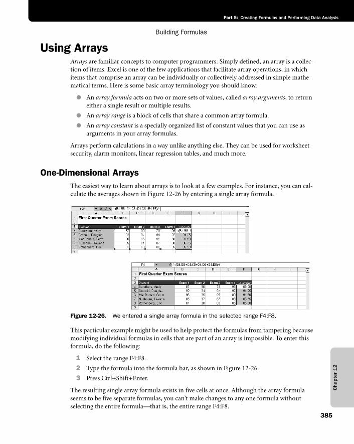
Cha

pter

12

Building Formulas

385

Part 5: Creating Formulas and Performing Data Analysis

Using ArraysArrays are familiar concepts to computer programmers. Simply defined, an array is a collec-tion of items. Excel is one of the few applications that facilitate array operations, in which items that comprise an array can be individually or collectively addressed in simple mathe-matical terms. Here is some basic array terminology you should know:

● An array formula acts on two or more sets of values, called array arguments, to return either a single result or multiple results.

● An array range is a block of cells that share a common array formula.

● An array constant is a specially organized list of constant values that you can use as arguments in your array formulas.

Arrays perform calculations in a way unlike anything else. They can be used for worksheet security, alarm monitors, linear regression tables, and much more.

One-Dimensional ArraysThe easiest way to learn about arrays is to look at a few examples. For instance, you can cal-culate the averages shown in Figure 12-26 by entering a single array formula.

f12ie26

Figure 12-26. We entered a single array formula in the selected range F4:F8.

This particular example might be used to help protect the formulas from tampering because modifying individual formulas in cells that are part of an array is impossible. To enter this formula, do the following:

1 Select the range F4:F8.

2 Type the formula into the formula bar, as shown in Figure 12-26.

3 Press Ctrl+Shift+Enter.

The resulting single array formula exists in five cells at once. Although the array formula seems to be five separate formulas, you can’t make changes to any one formula without selecting the entire formula—that is, the entire range F4:F8.

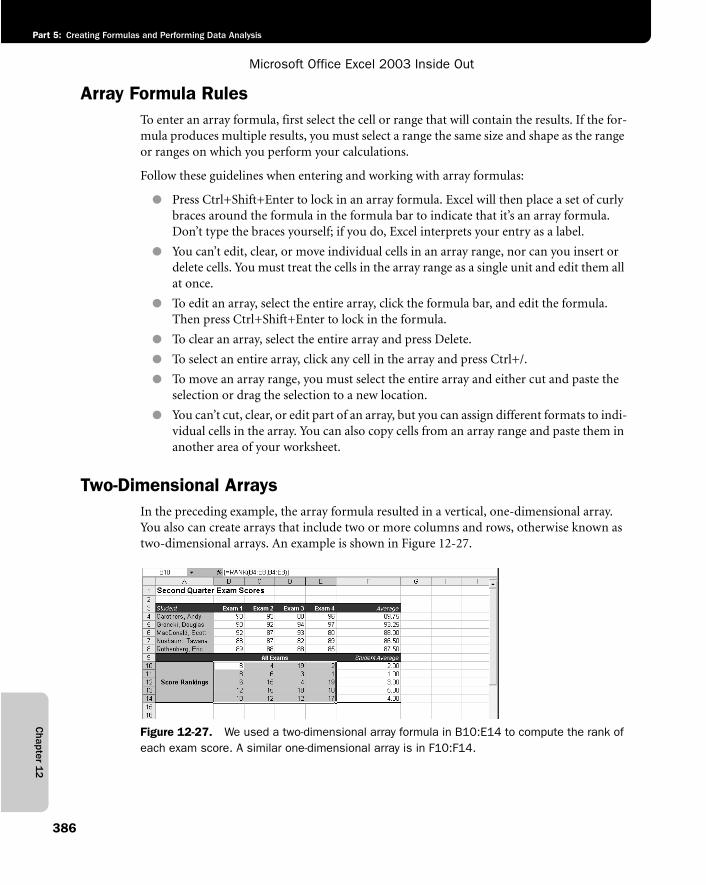
Chapter 1

2

Microsoft Office Excel 2003 Inside Out

Part 5: Creating Formulas and Performing Data Analysis

386

Array Formula RulesTo enter an array formula, first select the cell or range that will contain the results. If the for-mula produces multiple results, you must select a range the same size and shape as the range or ranges on which you perform your calculations.

Follow these guidelines when entering and working with array formulas:

● Press Ctrl+Shift+Enter to lock in an array formula. Excel will then place a set of curly braces around the formula in the formula bar to indicate that it’s an array formula. Don’t type the braces yourself; if you do, Excel interprets your entry as a label.

● You can’t edit, clear, or move individual cells in an array range, nor can you insert or delete cells. You must treat the cells in the array range as a single unit and edit them all at once.

● To edit an array, select the entire array, click the formula bar, and edit the formula. Then press Ctrl+Shift+Enter to lock in the formula.

● To clear an array, select the entire array and press Delete.

● To select an entire array, click any cell in the array and press Ctrl+/.

● To move an array range, you must select the entire array and either cut and paste the selection or drag the selection to a new location.

● You can’t cut, clear, or edit part of an array, but you can assign different formats to indi-vidual cells in the array. You can also copy cells from an array range and paste them in another area of your worksheet.

Two-Dimensional ArraysIn the preceding example, the array formula resulted in a vertical, one-dimensional array. You also can create arrays that include two or more columns and rows, otherwise known as two-dimensional arrays. An example is shown in Figure 12-27.

f12ie27

Figure 12-27. We used a two-dimensional array formula in B10:E14 to compute the rank of each exam score. A similar one-dimensional array is in F10:F14.

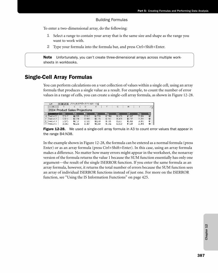
Cha

pter

12

Building Formulas

387

Part 5: Creating Formulas and Performing Data Analysis

To enter a two-dimensional array, do the following:

1 Select a range to contain your array that is the same size and shape as the range you want to work with.

2 Type your formula into the formula bar, and press Ctrl+Shift+Enter.

Note Unfortunately, you can’t create three-dimensional arrays across multiple work-sheets in workbooks.

Single-Cell Array FormulasYou can perform calculations on a vast collection of values within a single cell, using an array formula that produces a single value as a result. For example, to count the number of error values in a range of cells, you can create a single-cell array formula, as shown in Figure 12-28.

f12ie28

Figure 12-28. We used a single-cell array formula in A3 to count error values that appear in the range B4:N38.

In the example shown in Figure 12-28, the formula can be entered as a normal formula (press Enter) or as an array formula (press Ctrl+Shift+Enter). In this case, using an array formula makes a difference. No matter how many errors might appear in the worksheet, the nonarray version of the formula returns the value 1 because the SUM function essentially has only one argument—the result of the single ISERROR function. If you enter the same formula as an array formula, however, it returns the total number of errors because the SUM function sees an array of individual ISERROR functions instead of just one. For more on the ISERROR function, see “Using the IS Information Functions” on page 425.

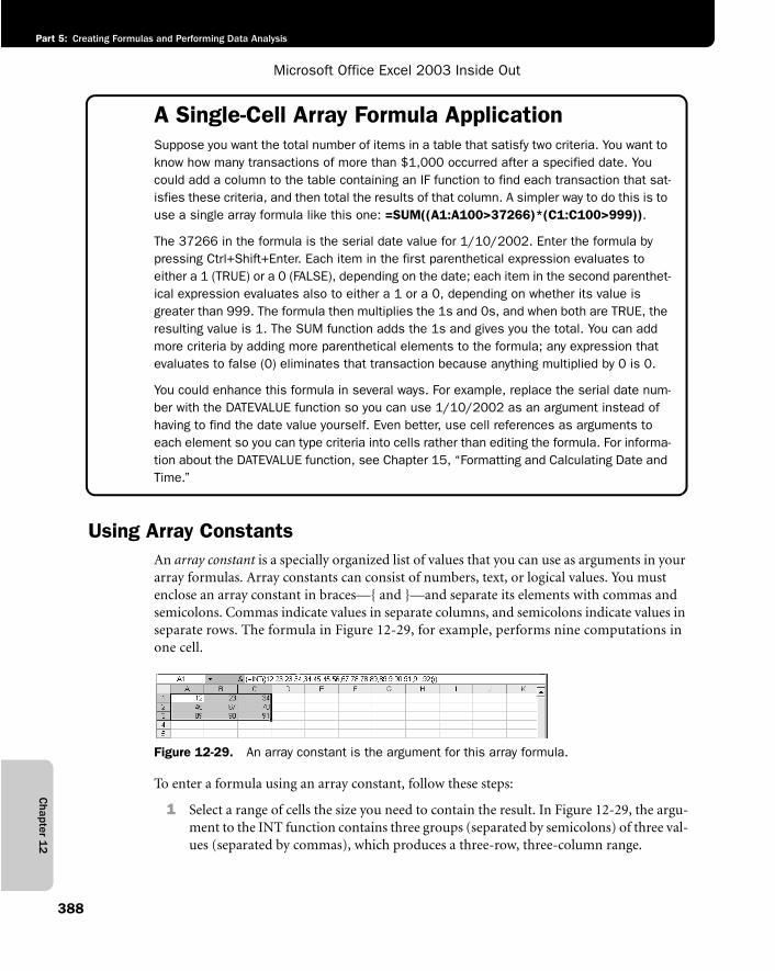
Chapter 1

2

Microsoft Office Excel 2003 Inside Out

Part 5: Creating Formulas and Performing Data Analysis

388

A Single-Cell Array Formula ApplicationSuppose you want the total number of items in a table that satisfy two criteria. You want to know how many transactions of more than $1,000 occurred after a specified date. You could add a column to the table containing an IF function to find each transaction that sat-isfies these criteria, and then total the results of that column. A simpler way to do this is to use a single array formula like this one: =SUM((A1:A100>37266)*(C1:C100>999)).

The 37266 in the formula is the serial date value for 1/10/2002. Enter the formula by pressing Ctrl+Shift+Enter. Each item in the first parenthetical expression evaluates to either a 1 (TRUE) or a 0 (FALSE), depending on the date; each item in the second parenthet-ical expression evaluates also to either a 1 or a 0, depending on whether its value is greater than 999. The formula then multiplies the 1s and 0s, and when both are TRUE, the resulting value is 1. The SUM function adds the 1s and gives you the total. You can add more criteria by adding more parenthetical elements to the formula; any expression that evaluates to false (0) eliminates that transaction because anything multiplied by 0 is 0.

You could enhance this formula in several ways. For example, replace the serial date num-ber with the DATEVALUE function so you can use 1/10/2002 as an argument instead of having to find the date value yourself. Even better, use cell references as arguments to each element so you can type criteria into cells rather than editing the formula. For informa-tion about the DATEVALUE function, see Chapter 15, “Formatting and Calculating Date and Time.”

Using Array ConstantsAn array constant is a specially organized list of values that you can use as arguments in your array formulas. Array constants can consist of numbers, text, or logical values. You must enclose an array constant in braces—{ and }—and separate its elements with commas and semicolons. Commas indicate values in separate columns, and semicolons indicate values in separate rows. The formula in Figure 12-29, for example, performs nine computations in one cell.

f12ie29

Figure 12-29. An array constant is the argument for this array formula.

To enter a formula using an array constant, follow these steps:

1 Select a range of cells the size you need to contain the result. In Figure 12-29, the argu-ment to the INT function contains three groups (separated by semicolons) of three val-ues (separated by commas), which produces a three-row, three-column range.

Cha

pter

12

Building Formulas

389

Part 5: Creating Formulas and Performing Data Analysis

2 Type the braces around the array argument, to indicate that the enclosed values make up an array constant. (Note that array arguments differ from array formulas, in which you cannot type the braces.)

3 Press Ctrl+Shift+Enter. The resulting array formula contains two sets of curly braces—one set encloses the array constant and the other encloses the entire array formula.

When entering array constants, remember that commas between array elements place those elements in separate columns, and semicolons between array elements place those elements in separate rows.

Understanding Array ExpansionWhen you use arrays as arguments in a formula, all your arrays should have the same dimen-sions. If the dimensions of your array arguments or array ranges do not match, Excel often expands the arguments. For example, to multiply all the values in cells A1:B5 by 10, you can use either of the following array formulas: { =A1:B5*10} or { ={ 1,2;3,4;5,6;7,8;9,10} *10}.

Note that these two formulas are not balanced; 10 values are on the left side of the mul-tiplication operator but only one is on the right. Excel expands the second argument to match the size and shape of the first. In the preceding example, the first formula is equivalent to { =A1:B5*{ 10,10;10,10;10,10;10,10;10,10} } and the second is equivalent to { ={ 1,2;3,4;5,6;7,8;9,10} *{ 10,10;10,10;10,10;10,10;10,10} }.

When you work with two or more sets of multivalue arrays, each set must have the same number of rows as the argument with the greatest number of rows and the same number of columns as the argument with the greatest number of columns.

Linking WorkbooksCreating dynamic links between workbooks with external reference formulas provides a number of advantages. For example, you could break a large, complex company budget model into more manageable departmental models. Then you could link all the departmen-tal workbooks (supporting workbooks) to a master budget workbook (a dependent work-book). In addition to creating more manageable and flexible models, linked workbooks can save recalculation time and memory.

This section discusses some special considerations to be aware of when working with work-books linked by external reference formulas. For more information about external refer-ences, see “Creating References to Other Worksheets in the Same Workbook” on page 354 and “Creating References to Worksheets in Other Workbooks” on page 355.

Chapter 1

2

Microsoft Office Excel 2003 Inside Out

Part 5: Creating Formulas and Performing Data Analysis

390

Saving Linked WorkbooksWhen you create a set of linked workbooks, you should save the supporting workbooks before you save the dependent workbooks. For example, suppose you are modeling your company’s 2004 budget in an unsaved workbook called Book1. When you save the work-book, you give it the name Budget 2004.

Now suppose that you have another active workbook in which you plan to enter actual (as opposed to budgeted) expenditures; you have already saved the workbook with the name Actual 2004. This workbook contains links to your Budget workbook and, therefore, is dependent on the Budget workbook for some of its information. When you first created these links, the Budget workbook was identified as Book1.

If you save Book1 as Budget 2004 while the Actual workbook is still open, all references to Book1 in the Actual workbook change automatically to Budget 2004. For example, if Actual contains the reference =[Book1]Sheet1!$A$1, the reference changes to ='[Budget 2004.xls]Sheet1'!$A$1.

If you try to close the dependent Actual 2004 workbook before you save the supporting Book1 (Budget) workbook, however, you see the warning “Save Actual 2004 with references to unsaved documents?” Click OK to save and close it. When you then save Book1 as Budget 2004, the references to Book1 in the Actual workbook are not updated because it’s not open; the formulas continue to reference Book1. When you reopen Actual 2004, Excel displays a message box notifying you that the workbook contains links to another workbook and prompts you to update the linked information. If you click Yes, Excel is, of course, unable to find Book1. You need to find the Actual 2004 workbook so that Excel can re-establish the links.

Opening a Dependent WorkbookWhen you save a workbook that contains dependent formulas, Excel stores the most recent results of those formulas. If you open and edit the supporting workbook after closing the dependent workbook, the values of edited cells in the supporting workbook might be differ-ent. When you open the dependent workbook again, it contains the old values of the external references in the dependent formulas, but Excel displays an alert box with the message “This document contains links to other data sources.” The alert box lets you tell Excel whether or not to read the current values from the closed workbook on the disk.

If you click Don’t Update, Excel opens the dependent workbook without updating any refer-ences to the supporting workbook. All dependent formulas retain their last saved values.

If you click Update, Excel searches for the supporting workbook. If it’s found, Excel reads the supporting values and updates the dependent formulas in the dependent workbook. Excel does not open the supporting workbook; it merely reads the appropriate values from it.

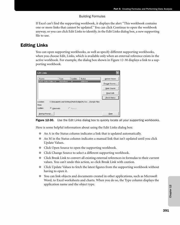
Cha

pter

12

Building Formulas

391

Part 5: Creating Formulas and Performing Data Analysis

If Excel can’t find the supporting workbook, it displays the alert “This workbook contains one or more links that cannot be updated.” You can click Continue to open the workbook anyway, or you can click Edit Links to identify, in the Edit Links dialog box, a new supporting file to use.

Editing LinksYou can open supporting workbooks, as well as specify different supporting workbooks, when you choose Edit, Links, which is available only when an external reference exists in the active workbook. For example, the dialog box shown in Figure 12-30 displays a link to a sup-porting workbook.

f12ie30

Figure 12-30. Use the Edit Links dialog box to quickly locate all your supporting workbooks.

Here is some helpful information about using the Edit Links dialog box:

● An A in the Status column indicates a link that is updated automatically.

● An M in the Status column indicates a manual link that isn’t updated until you click Update Values.

● Click Open Source to open the supporting workbook.

● Click Change Source to select a different supporting workbook.

● Click Break Link to convert all existing external references in formulas to their current values. You can’t undo this action, so click Break Link with caution.

● Click Update Values to fetch the latest figures from the supporting workbook without having to open it.

● You can link objects and documents created in other applications, such as Microsoft Word, to Excel worksheets and charts. When you do so, the Type column displays the application name and the object type.

Chapter 1

2

Microsoft Office Excel 2003 Inside Out

Part 5: Creating Formulas and Performing Data Analysis

392

Inside OutBe careful when moving documents

Normally you should be careful about moving documents to which you have created links in workbooks. This isn’t true, however, if you are using Windows XP, Windows 2000, or Windows NT. For example, if you create a link to text in a Word document and then change the name or location of that document, Excel still finds the source and updates the link—provided the source is stored on an NTFS (the Windows NT/2000/XP File System) volume. You can do this because NTFS maintains a change log, and Excel consults that log. (If you use Excel’s Hyperlinks, however, relocating or changing the source file breaks the link, even if the file is on an NTFS volume both before and after the change.) If you move the source document to a FAT32 (the MS-DOS/Windows File System) volume, however, Excel can’t find the document.

Copying, Cutting, and Pasting in Linked WorkbooksYou can use relative or absolute references to cells in other workbooks as you do in a single workbook. Relative and absolute references to cells in supporting workbooks respond to the Copy, Cut, and Paste commands and toolbar buttons in much the same way as references to cells in the same workbook do.

For example, suppose you create the formula =[Form2]Sheet1!F1 in cell A1 in Sheet1 of Form1 and then use Copy and Paste to copy this formula to cell B1. The formula in cell B1 becomes =[Form2]Sheet1!G1. The original formula changed when it was copied to cell B1 because the reference to cell F1 is relative. However, if the formula in cell A1 of Form1 con-tained an absolute reference, such as =[Form2]Sheet1!$F$1, the reference in the copied for-mula would not change.

Copying and Pasting between WorkbooksWhen you copy a dependent formula from one workbook to another and that formula includes a relative reference to a third workbook, the reference is adjusted to reflect the new position of the formula. For example, suppose that cell A1 in Form1 contains the formula =[Form2]Sheet1!A1. If you copy and paste that formula into cell B5 in Form3, the result is the formula =[Form2]Sheet1!B5. The formula is adjusted to reflect its new relative position.

If you copy a formula that contains an absolute reference to another workbook, the formula remains the same. For example, suppose cell A1 in Form1 contains the formula =[Form2]Sheet1!$A$1. If you copy and paste that formula into cell B5 in Form3, the result-ing formula is the same.

Even if you copy a dependent formula to the workbook to which the formula refers, it’s still a dependent formula. For example, if you copy the formula =[Form2]Sheet1!$A$1 from cell A1 of Form1 to cell A3 on Sheet1 of Form2, the resulting formula is essentially the same, except that the book reference isn’t necessary because the formula is in the same workbook. As a result, the formula becomes =Sheet1!$A$1.

Cha

pter

12

Building Formulas

393

Part 5: Creating Formulas and Performing Data Analysis

Cutting and Pasting between WorkbooksExcel does not adjust the relative references in a formula when you cut it from one workbook and paste it in another, as it does when you copy a formula. For example, suppose that cell A1 in Sheet1 of Form1 contains the formula =[Form2]Sheet1!A1. If you cut that formula and paste it into cell B5 of Form3, the formula does not change.

Cutting and Pasting Cells Referred to by Dependent FormulasWhen you cut and paste cells, Excel normally adjusts any references to those cells in the for-mulas of the workbook. Dependent formulas, however, do not follow the same rules. When you cut and paste a cell referred to by a dependent formula in a closed workbook, that for-mula isn’t adjusted to reflect the change.

For example, suppose you create the formula =[Form2]Sheet1!A10 in cell A1 in Form1. If you close Form1 and use Cut and Paste to move the entry to cell B10 of Form2, the formula in cell A1 of Form1 remains the same. You might expect the link to be broken because the worksheet containing the formula was closed when you modified the referenced cell. How-ever, Excel manages to keep track of everything. When you open the workbook, the message “This document contains links to other data sources” alerts you that the data the workbook depended on has changed.

Creating Conditional TestsA conditional test formula compares two numbers, functions, formulas, labels, or logical val-ues. Conditional tests can be used to flag values that fall below or above a given threshold, for example. You can use simple mathematical and logical operators to construct logical formu-las, or you can use an assortment of built-in functions. For information about using condi-tional test functions, see “Understanding Logical Functions” on page 421.

Each of the following formulas performs a rudimentary conditional test:

=A1>A2

=5-3<5*2

=AVERAGE(B1:B6)=SUM(6,7,8)

=C2=”Female”

=COUNT(A1:A10)=COUNT(B1:B10)

=LEN(A1)=10

Every conditional test must include at least one logical operator, which defines the relation-ship between elements of the conditional test. For example, in the conditional test A1>A2, the greater than (>) logical operator compares the values in cells A1 and A2. Table 12-4 lists the six logical operators.

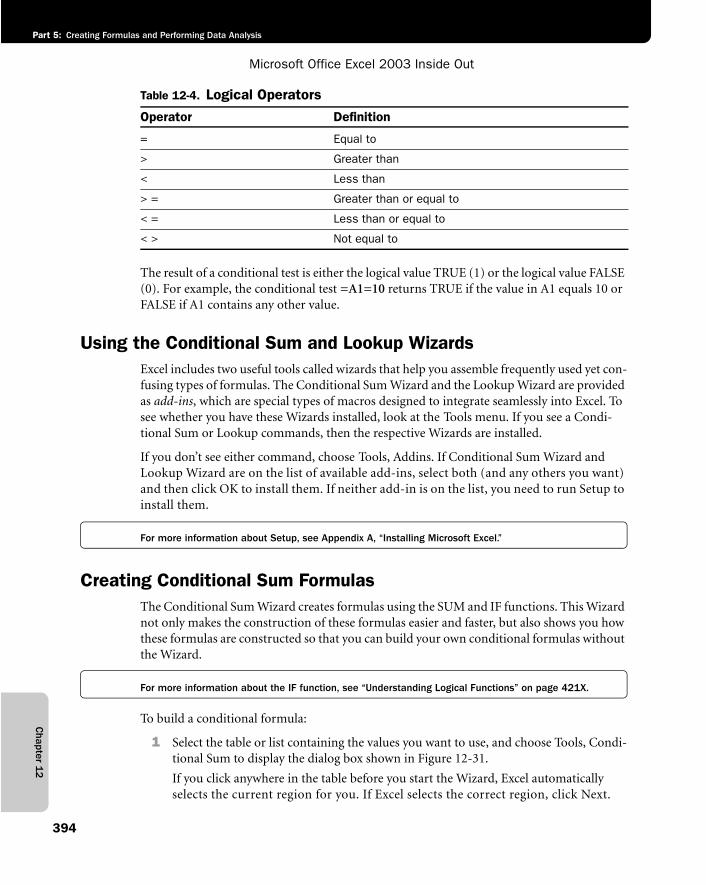
Chapter 1

2

Microsoft Office Excel 2003 Inside Out

Part 5: Creating Formulas and Performing Data Analysis

394

The result of a conditional test is either the logical value TRUE (1) or the logical value FALSE (0). For example, the conditional test =A1=10 returns TRUE if the value in A1 equals 10 or FALSE if A1 contains any other value.

Using the Conditional Sum and Lookup WizardsExcel includes two useful tools called wizards that help you assemble frequently used yet con-fusing types of formulas. The Conditional Sum Wizard and the Lookup Wizard are provided as add-ins, which are special types of macros designed to integrate seamlessly into Excel. To see whether you have these Wizards installed, look at the Tools menu. If you see a Condi-tional Sum or Lookup commands, then the respective Wizards are installed.

If you don’t see either command, choose Tools, Addins. If Conditional Sum Wizard and Lookup Wizard are on the list of available add-ins, select both (and any others you want) and then click OK to install them. If neither add-in is on the list, you need to run Setup to install them.

For more information about Setup, see Appendix A, “Installing Microsoft Excel.”

Creating Conditional Sum FormulasThe Conditional Sum Wizard creates formulas using the SUM and IF functions. This Wizard not only makes the construction of these formulas easier and faster, but also shows you how these formulas are constructed so that you can build your own conditional formulas without the Wizard.

For more information about the IF function, see “Understanding Logical Functions” on page 421X.

To build a conditional formula:

1 Select the table or list containing the values you want to use, and choose Tools, Condi-tional Sum to display the dialog box shown in Figure 12-31.

If you click anywhere in the table before you start the Wizard, Excel automatically selects the current region for you. If Excel selects the correct region, click Next.

Table 12-4. Logical Operators

Operator Definition

= Equal to

> Greater than

< Less than

> = Greater than or equal to

< = Less than or equal to

< > Not equal to

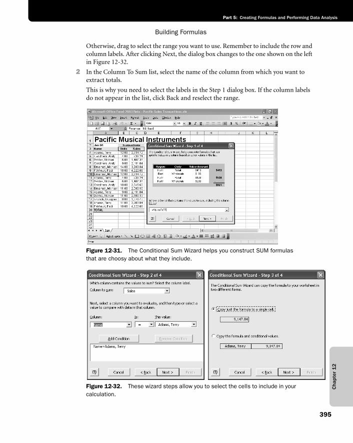
Cha

pter

12

Building Formulas

395

Part 5: Creating Formulas and Performing Data Analysis

Otherwise, drag to select the range you want to use. Remember to include the row and column labels. After clicking Next, the dialog box changes to the one shown on the left in Figure 12-32.

2 In the Column To Sum list, select the name of the column from which you want to extract totals.

This is why you need to select the labels in the Step 1 dialog box. If the column labels do not appear in the list, click Back and reselect the range.

f12ie31

Figure 12-31. The Conditional Sum Wizard helps you construct SUM formulas that are choosy about what they include.

f12ie32

Figure 12-32. These wizard steps allow you to select the cells to include in your calculation.

Chapter 1

2

Microsoft Office Excel 2003 Inside Out

Part 5: Creating Formulas and Performing Data Analysis

396

Note You can find the sample file used in this example, Pacific Sales Transactions.xls, on the companion CD.

3 Still in Step 2 of the Wizard, specify the condition to use in selecting the values you want to include in the total. In the Column list, select the name of the column con-taining the labels you want to conditionally check, select an operator in the Is list, and then select a value in the This Value list.

The contents of the This Value list change depending on the column selected in the Column list. The This Value list displays only the unique values in the selected col-umn, ignoring duplicates.

4 Click Add Condition.

The criteria you specify are added to the list at the bottom of the dialog box. You can add as many as seven conditions. If you change your mind about any condition, select the condition from the list and click Remove Condition. When you have finished removing conditions, click Next.

5 In Step 3 of the Wizard, choose either Copy Just The Formula To A Single Cell, or choose Copy The Formula And Conditional Values.

6 Click Next, and then select the cell where you want to place the resulting formula.

If you chose the Copy Formula And Conditional Values option in Step 3 of the Wiz-ard, the Wizard adds an extra step. Select the cell where you want the conditional value to go. Then click Next, and click the cell where you want the formula to go.

7 Click Finish. The resulting formula (and the optional conditional value) is pasted in the worksheet in the locations specified.

Inside OutBeware of the Wizard

In many cases, including Step 1 of the Conditional Sum Wizard (shown in Figure 12-31), Excel attempts to select a cell range or table for you automatically. This doesn’t always work the way it should. In the example worksheet shown in Figure 12-31, Excel automati-cally selected A1:C20, which includes a merged cell at the top; this isn’t allowed. We had to select the correct range before proceeding. Excel should recognize this before automat-ically selecting it, but it doesn’t.

You can add more conditional formulas, or if you already have a list of unique values (such as salesperson names), you can copy the formula as needed (but only if you used the Copy For-mula And Conditional Values option in Step 3 of the Wizard), as shown in Figure 12-33.

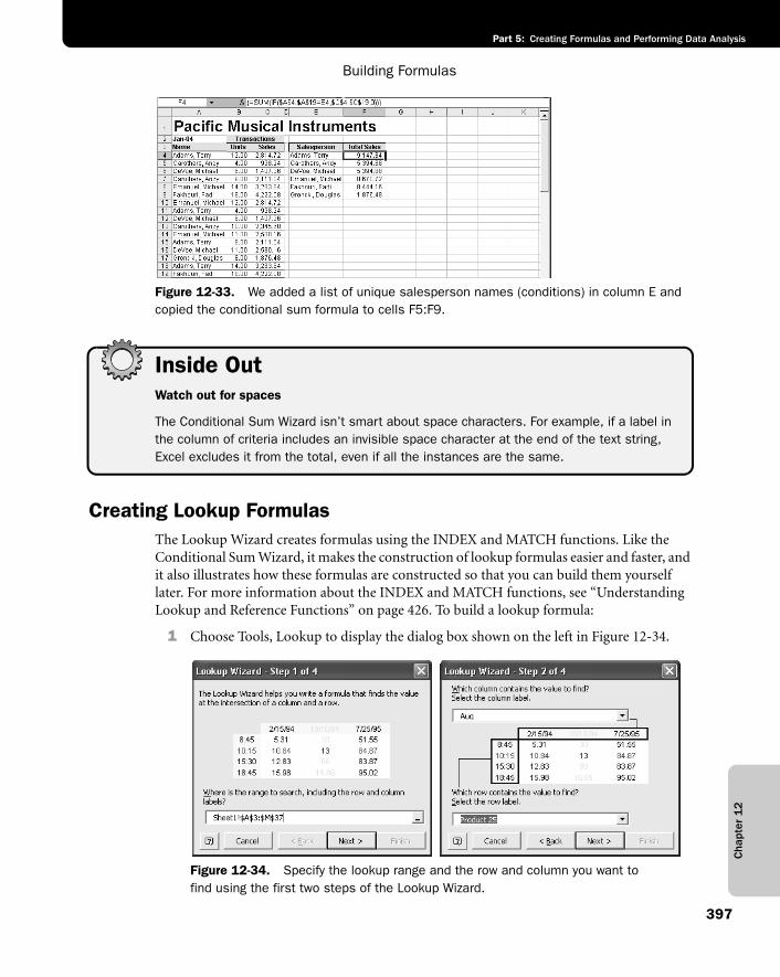
Cha

pter

12

Building Formulas

397

Part 5: Creating Formulas and Performing Data Analysis

f12ie33

Figure 12-33. We added a list of unique salesperson names (conditions) in column E and copied the conditional sum formula to cells F5:F9.

Inside OutWatch out for spaces

The Conditional Sum Wizard isn’t smart about space characters. For example, if a label in the column of criteria includes an invisible space character at the end of the text string, Excel excludes it from the total, even if all the instances are the same.

Creating Lookup FormulasThe Lookup Wizard creates formulas using the INDEX and MATCH functions. Like the Conditional Sum Wizard, it makes the construction of lookup formulas easier and faster, and it also illustrates how these formulas are constructed so that you can build them yourself later. For more information about the INDEX and MATCH functions, see “Understanding Lookup and Reference Functions” on page 426. To build a lookup formula:

1 Choose Tools, Lookup to display the dialog box shown on the left in Figure 12-34.

f12ie34

Figure 12-34. Specify the lookup range and the row and column you want to find using the first two steps of the Lookup Wizard.

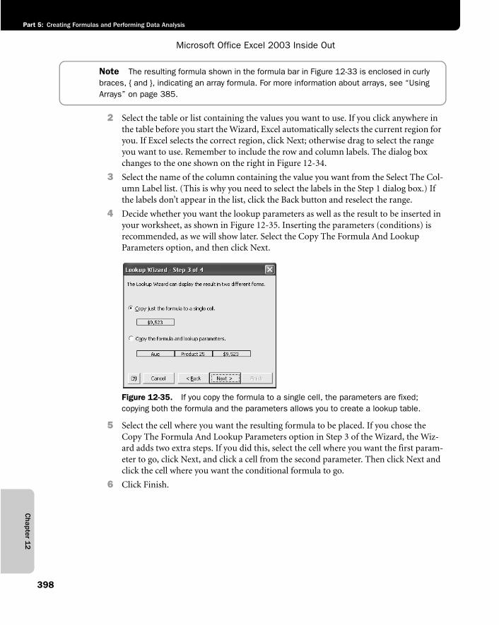
Chapter 1

2

Microsoft Office Excel 2003 Inside Out

Part 5: Creating Formulas and Performing Data Analysis

398

Note The resulting formula shown in the formula bar in Figure 12-33 is enclosed in curly braces, { and }, indicating an array formula. For more information about arrays, see “Using Arrays” on page 385.

2 Select the table or list containing the values you want to use. If you click anywhere in the table before you start the Wizard, Excel automatically selects the current region for you. If Excel selects the correct region, click Next; otherwise drag to select the range you want to use. Remember to include the row and column labels. The dialog box changes to the one shown on the right in Figure 12-34.

3 Select the name of the column containing the value you want from the Select The Col-umn Label list. (This is why you need to select the labels in the Step 1 dialog box.) If the labels don’t appear in the list, click the Back button and reselect the range.

4 Decide whether you want the lookup parameters as well as the result to be inserted in your worksheet, as shown in Figure 12-35. Inserting the parameters (conditions) is recommended, as we will show later. Select the Copy The Formula And Lookup Parameters option, and then click Next.

f12ie35

Figure 12-35. If you copy the formula to a single cell, the parameters are fixed; copying both the formula and the parameters allows you to create a lookup table.

5 Select the cell where you want the resulting formula to be placed. If you chose the Copy The Formula And Lookup Parameters option in Step 3 of the Wizard, the Wiz-ard adds two extra steps. If you did this, select the cell where you want the first param-eter to go, click Next, and click a cell from the second parameter. Then click Next and click the cell where you want the conditional formula to go.

6 Click Finish.

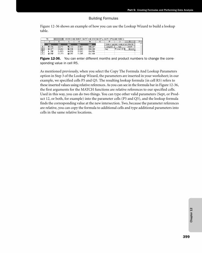
Cha

pter

12

Building Formulas

399

Part 5: Creating Formulas and Performing Data Analysis

Figure 12-36 shows an example of how you can use the Lookup Wizard to build a lookup table.

f12ie36

Figure 12-36. You can enter different months and product numbers to change the corre-sponding value in cell R5.

As mentioned previously, when you select the Copy The Formula And Lookup Parameters option in Step 3 of the Lookup Wizard, the parameters are inserted in your worksheet; in our example, we specified cells P5 and Q5. The resulting lookup formula (in cell R5) refers to these inserted values using relative references. As you can see in the formula bar in Figure 12-36, the first arguments for the MATCH functions are relative references to our specified cells. Used in this way, you can do two things. You can type other valid parameters (Sept, or Prod-uct 12, or both, for example) into the parameter cells (P5 and Q5), and the lookup formula finds the corresponding value at the new intersection. Two, because the parameter references are relative, you can copy the formula to additional cells and type additional parameters into cells in the same relative locations.

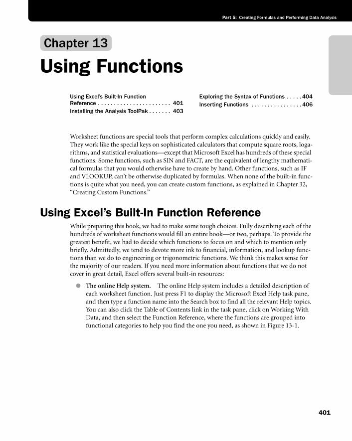
401

Part 5: Creating Formulas and Performing Data Analysis

Chapter 13

Using FunctionsUsing Excel’s Built-In FunctionReference . . . . . . . . . . . . . . . . . . . . . . . 401Installing the Analysis ToolPak . . . . . . . 403

Exploring the Syntax of Functions . . . . . 404Inserting Functions . . . . . . . . . . . . . . . . 406

Worksheet functions are special tools that perform complex calculations quickly and easily. They work like the special keys on sophisticated calculators that compute square roots, loga-rithms, and statistical evaluations—except that Microsoft Excel has hundreds of these special functions. Some functions, such as SIN and FACT, are the equivalent of lengthy mathemati-cal formulas that you would otherwise have to create by hand. Other functions, such as IF and VLOOKUP, can’t be otherwise duplicated by formulas. When none of the built-in func-tions is quite what you need, you can create custom functions, as explained in Chapter 32, “Creating Custom Functions.”

Using Excel’s Built-In Function ReferenceWhile preparing this book, we had to make some tough choices. Fully describing each of the hundreds of worksheet functions would fill an entire book—or two, perhaps. To provide the greatest benefit, we had to decide which functions to focus on and which to mention only briefly. Admittedly, we tend to devote more ink to financial, information, and lookup func-tions than we do to engineering or trigonometric functions. We think this makes sense for the majority of our readers. If you need more information about functions that we do not cover in great detail, Excel offers several built-in resources:

● The online Help system. The online Help system includes a detailed description of each worksheet function. Just press F1 to display the Microsoft Excel Help task pane, and then type a function name into the Search box to find all the relevant Help topics. You can also click the Table of Contents link in the task pane, click on Working With Data, and then select the Function Reference, where the functions are grouped into functional categories to help you find the one you need, as shown in Figure 13-1.

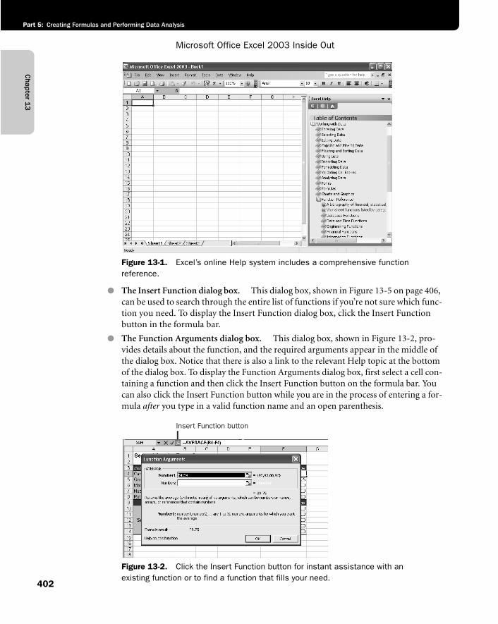
Chapter 1

3

Microsoft Office Excel 2003 Inside Out

Part 5: Creating Formulas and Performing Data Analysis

402

f13ie01 Figure 13-1. Excel’s online Help system includes a comprehensive function reference.

● The Insert Function dialog box. This dialog box, shown in Figure 13-5 on page 406, can be used to search through the entire list of functions if you’re not sure which func-tion you need. To display the Insert Function dialog box, click the Insert Function button in the formula bar.

● The Function Arguments dialog box. This dialog box, shown in Figure 13-2, pro-vides details about the function, and the required arguments appear in the middle of the dialog box. Notice that there is also a link to the relevant Help topic at the bottom of the dialog box. To display the Function Arguments dialog box, first select a cell con-taining a function and then click the Insert Function button on the formula bar. You can also click the Insert Function button while you are in the process of entering a for-mula after you type in a valid function name and an open parenthesis.

f13ie02 Figure 13-2. Click the Insert Function button for instant assistance with an existing function or to find a function that fills your need.

Insert Function button

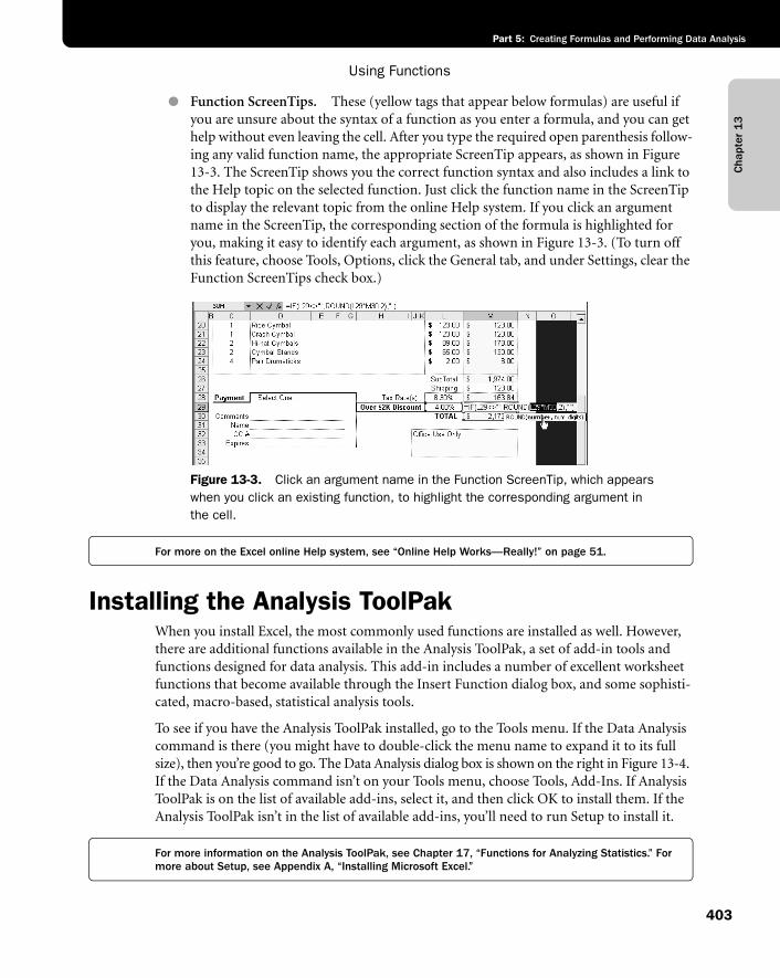
Cha

pter

13

Using Functions

403

Part 5: Creating Formulas and Performing Data Analysis

● Function ScreenTips. These (yellow tags that appear below formulas) are useful if you are unsure about the syntax of a function as you enter a formula, and you can get help without even leaving the cell. After you type the required open parenthesis follow-ing any valid function name, the appropriate ScreenTip appears, as shown in Figure 13-3. The ScreenTip shows you the correct function syntax and also includes a link to the Help topic on the selected function. Just click the function name in the ScreenTip to display the relevant topic from the online Help system. If you click an argument name in the ScreenTip, the corresponding section of the formula is highlighted for you, making it easy to identify each argument, as shown in Figure 13-3. (To turn off this feature, choose Tools, Options, click the General tab, and under Settings, clear the Function ScreenTips check box.)

f13ie03

Figure 13-3. Click an argument name in the Function ScreenTip, which appears when you click an existing function, to highlight the corresponding argument in the cell.

For more on the Excel online Help system, see “Online Help Works—Really!” on page 51.

Installing the Analysis ToolPakWhen you install Excel, the most commonly used functions are installed as well. However, there are additional functions available in the Analysis ToolPak, a set of add-in tools and functions designed for data analysis. This add-in includes a number of excellent worksheet functions that become available through the Insert Function dialog box, and some sophisti-cated, macro-based, statistical analysis tools.

To see if you have the Analysis ToolPak installed, go to the Tools menu. If the Data Analysis command is there (you might have to double-click the menu name to expand it to its full size), then you’re good to go. The Data Analysis dialog box is shown on the right in Figure 13-4. If the Data Analysis command isn’t on your Tools menu, choose Tools, Add-Ins. If Analysis ToolPak is on the list of available add-ins, select it, and then click OK to install them. If the Analysis ToolPak isn’t in the list of available add-ins, you’ll need to run Setup to install it.

For more information on the Analysis ToolPak, see Chapter 17, “Functions for Analyzing Statistics.” For more about Setup, see Appendix A, “Installing Microsoft Excel.”

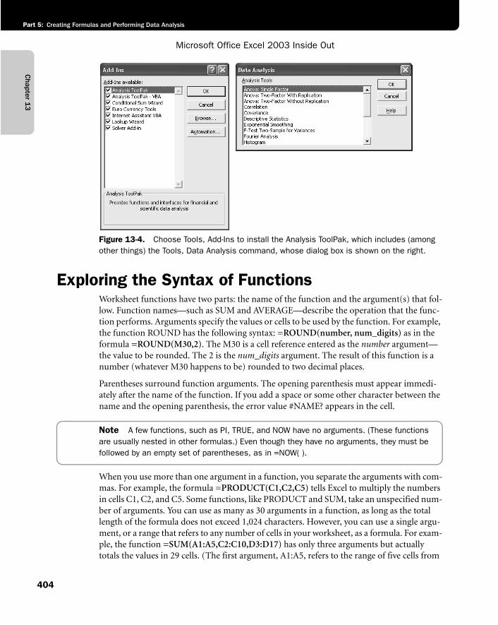
Chapter 1

3

Microsoft Office Excel 2003 Inside Out

Part 5: Creating Formulas and Performing Data Analysis

404

f13ie04

Figure 13-4. Choose Tools, Add-Ins to install the Analysis ToolPak, which includes (among other things) the Tools, Data Analysis command, whose dialog box is shown on the right.

Exploring the Syntax of FunctionsWorksheet functions have two parts: the name of the function and the argument(s) that fol-low. Function names—such as SUM and AVERAGE—describe the operation that the func-tion performs. Arguments specify the values or cells to be used by the function. For example, the function ROUND has the following syntax: =ROUND(number, num_digits) as in the formula =ROUND(M30,2). The M30 is a cell reference entered as the number argument—the value to be rounded. The 2 is the num_digits argument. The result of this function is a number (whatever M30 happens to be) rounded to two decimal places.

Parentheses surround function arguments. The opening parenthesis must appear immedi-ately after the name of the function. If you add a space or some other character between the name and the opening parenthesis, the error value #NAME? appears in the cell.

Note A few functions, such as PI, TRUE, and NOW have no arguments. (These functions are usually nested in other formulas.) Even though they have no arguments, they must be followed by an empty set of parentheses, as in =NOW( ).

When you use more than one argument in a function, you separate the arguments with com-mas. For example, the formula =PRODUCT(C1,C2,C5) tells Excel to multiply the numbers in cells C1, C2, and C5. Some functions, like PRODUCT and SUM, take an unspecified num-ber of arguments. You can use as many as 30 arguments in a function, as long as the total length of the formula does not exceed 1,024 characters. However, you can use a single argu-ment, or a range that refers to any number of cells in your worksheet, as a formula. For exam-ple, the function =SUM(A1:A5,C2:C10,D3:D17) has only three arguments but actually totals the values in 29 cells. (The first argument, A1:A5, refers to the range of five cells from

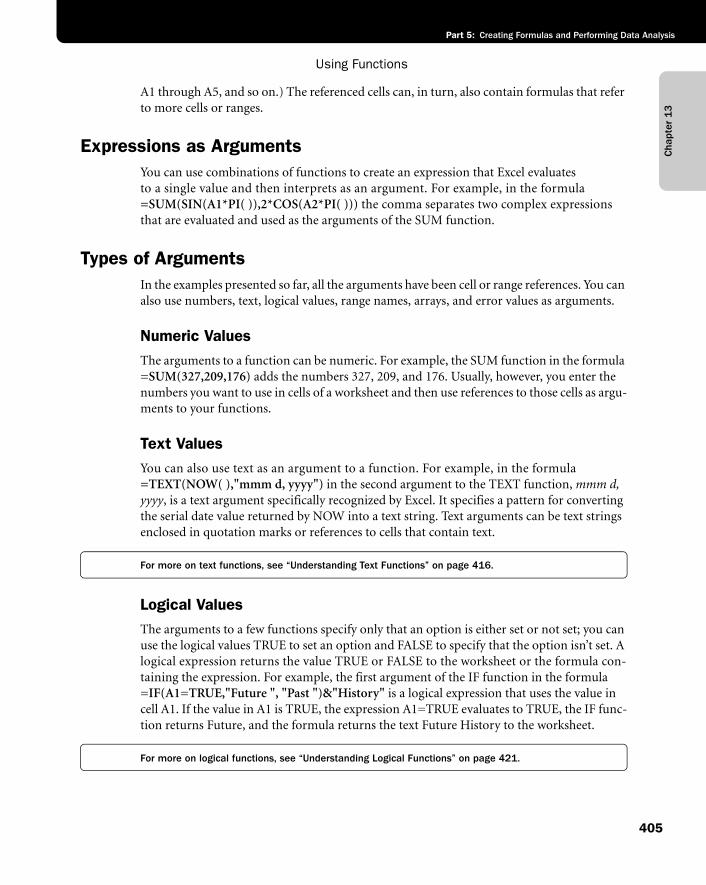
Cha

pter

13

Using Functions

405

Part 5: Creating Formulas and Performing Data Analysis

A1 through A5, and so on.) The referenced cells can, in turn, also contain formulas that refer to more cells or ranges.

Expressions as ArgumentsYou can use combinations of functions to create an expression that Excel evaluates to a single value and then interprets as an argument. For example, in the formula =SUM(SIN(A1*PI( )),2*COS(A2*PI( ))) the comma separates two complex expressions that are evaluated and used as the arguments of the SUM function.

Types of ArgumentsIn the examples presented so far, all the arguments have been cell or range references. You can also use numbers, text, logical values, range names, arrays, and error values as arguments.

Numeric ValuesThe arguments to a function can be numeric. For example, the SUM function in the formula =SUM(327,209,176) adds the numbers 327, 209, and 176. Usually, however, you enter the numbers you want to use in cells of a worksheet and then use references to those cells as argu-ments to your functions.

Text ValuesYou can also use text as an argument to a function. For example, in the formula =TEXT(NOW( ),"mmm d, yyyy") in the second argument to the TEXT function, mmm d, yyyy, is a text argument specifically recognized by Excel. It specifies a pattern for converting the serial date value returned by NOW into a text string. Text arguments can be text strings enclosed in quotation marks or references to cells that contain text.

For more on text functions, see “Understanding Text Functions” on page 416.

Logical ValuesThe arguments to a few functions specify only that an option is either set or not set; you can use the logical values TRUE to set an option and FALSE to specify that the option isn’t set. A logical expression returns the value TRUE or FALSE to the worksheet or the formula con-taining the expression. For example, the first argument of the IF function in the formula =IF(A1=TRUE,"Future ", "Past ")&"History" is a logical expression that uses the value in cell A1. If the value in A1 is TRUE, the expression A1=TRUE evaluates to TRUE, the IF func-tion returns Future, and the formula returns the text Future History to the worksheet.

For more on logical functions, see “Understanding Logical Functions” on page 421.

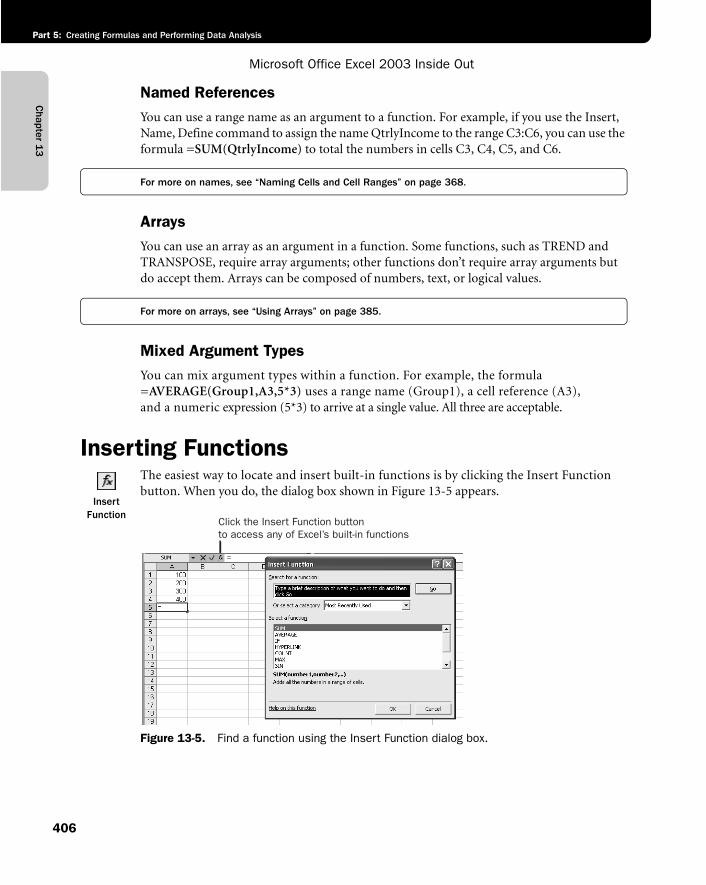
Chapter 1

3

Microsoft Office Excel 2003 Inside Out

Part 5: Creating Formulas and Performing Data Analysis

406

Named ReferencesYou can use a range name as an argument to a function. For example, if you use the Insert, Name, Define command to assign the name QtrlyIncome to the range C3:C6, you can use the formula =SUM(QtrlyIncome) to total the numbers in cells C3, C4, C5, and C6.

For more on names, see “Naming Cells and Cell Ranges” on page 368.

ArraysYou can use an array as an argument in a function. Some functions, such as TREND and TRANSPOSE, require array arguments; other functions don’t require array arguments but do accept them. Arrays can be composed of numbers, text, or logical values.

For more on arrays, see “Using Arrays” on page 385.

Mixed Argument TypesYou can mix argument types within a function. For example, the formula =AVERAGE(Group1,A3,5*3) uses a range name (Group1), a cell reference (A3), and a numeric expression (5*3) to arrive at a single value. All three are acceptable.

Inserting Functions

Insert Function

The easiest way to locate and insert built-in functions is by clicking the Insert Function button. When you do, the dialog box shown in Figure 13-5 appears.

f13ie05

Figure 13-5. Find a function using the Insert Function dialog box.

Click the Insert Function button to access any of Excel’s built-in functions

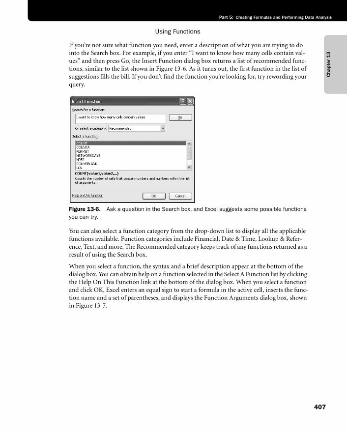
Cha

pter

13

Using Functions

407

Part 5: Creating Formulas and Performing Data Analysis

If you’re not sure what function you need, enter a description of what you are trying to do into the Search box. For example, if you enter “I want to know how many cells contain val-ues” and then press Go, the Insert Function dialog box returns a list of recommended func-tions, similar to the list shown in Figure 13-6. As it turns out, the first function in the list of suggestions fills the bill. If you don’t find the function you’re looking for, try rewording your query.

f13ie06

Figure 13-6. Ask a question in the Search box, and Excel suggests some possible functions you can try.

You can also select a function category from the drop-down list to display all the applicable functions available. Function categories include Financial, Date & Time, Lookup & Refer-ence, Text, and more. The Recommended category keeps track of any functions returned as a result of using the Search box.

When you select a function, the syntax and a brief description appear at the bottom of the dialog box. You can obtain help on a function selected in the Select A Function list by clicking the Help On This Function link at the bottom of the dialog box. When you select a function and click OK, Excel enters an equal sign to start a formula in the active cell, inserts the func-tion name and a set of parentheses, and displays the Function Arguments dialog box, shown in Figure 13-7.

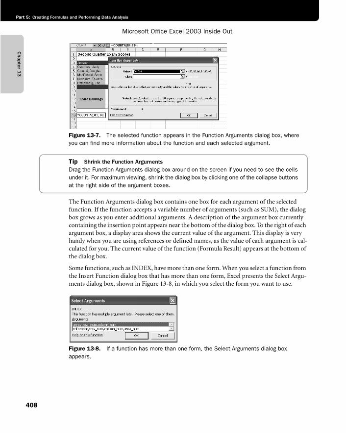
Chapter 1

3

Microsoft Office Excel 2003 Inside Out

Part 5: Creating Formulas and Performing Data Analysis

408

f13ie07

Figure 13-7. The selected function appears in the Function Arguments dialog box, where you can find more information about the function and each selected argument.

Tip Shrink the Function ArgumentsDrag the Function Arguments dialog box around on the screen if you need to see the cells under it. For maximum viewing, shrink the dialog box by clicking one of the collapse buttons at the right side of the argument boxes.

The Function Arguments dialog box contains one box for each argument of the selected function. If the function accepts a variable number of arguments (such as SUM), the dialog box grows as you enter additional arguments. A description of the argument box currently containing the insertion point appears near the bottom of the dialog box. To the right of each argument box, a display area shows the current value of the argument. This display is very handy when you are using references or defined names, as the value of each argument is cal-culated for you. The current value of the function (Formula Result) appears at the bottom of the dialog box.

Some functions, such as INDEX, have more than one form. When you select a function from the Insert Function dialog box that has more than one form, Excel presents the Select Argu-ments dialog box, shown in Figure 13-8, in which you select the form you want to use.

f13ie08

Figure 13-8. If a function has more than one form, the Select Arguments dialog box appears.

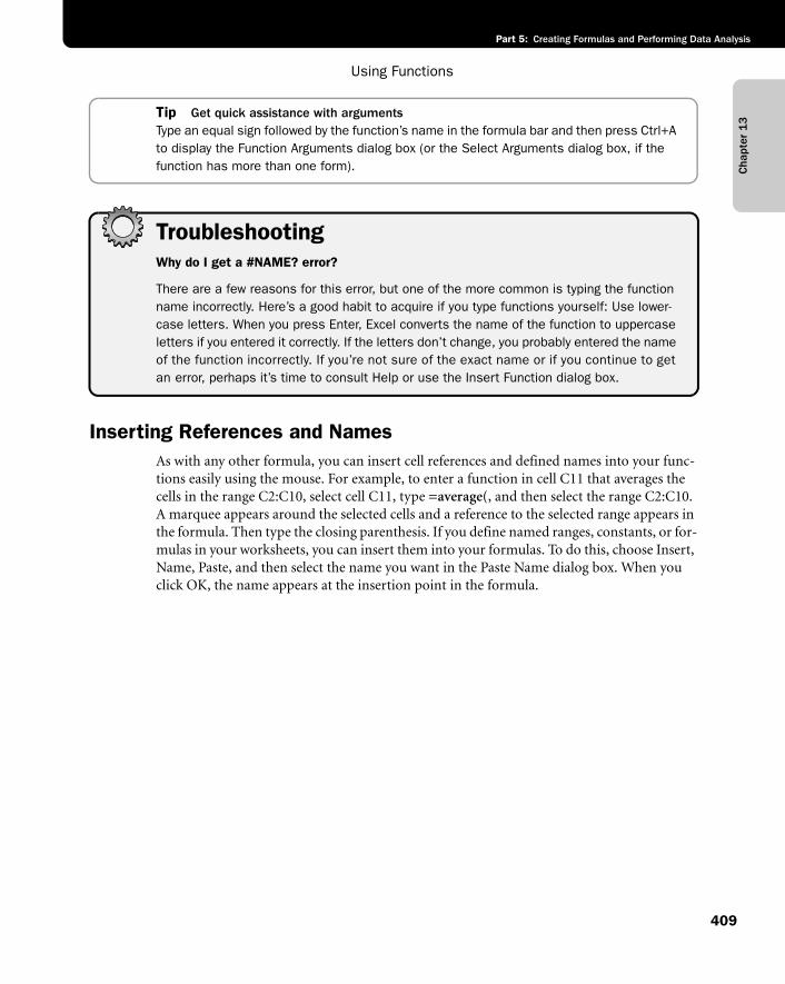
Cha

pter

13

Using Functions

409

Part 5: Creating Formulas and Performing Data Analysis

Tip Get quick assistance with argumentsType an equal sign followed by the function’s name in the formula bar and then press Ctrl+A to display the Function Arguments dialog box (or the Select Arguments dialog box, if the function has more than one form).

TroubleshootingWhy do I get a #NAME? error?

There are a few reasons for this error, but one of the more common is typing the function name incorrectly. Here’s a good habit to acquire if you type functions yourself: Use lower-case letters. When you press Enter, Excel converts the name of the function to uppercase letters if you entered it correctly. If the letters don’t change, you probably entered the name of the function incorrectly. If you’re not sure of the exact name or if you continue to get an error, perhaps it’s time to consult Help or use the Insert Function dialog box.

Inserting References and NamesAs with any other formula, you can insert cell references and defined names into your func-tions easily using the mouse. For example, to enter a function in cell C11 that averages the cells in the range C2:C10, select cell C11, type =average(, and then select the range C2:C10. A marquee appears around the selected cells and a reference to the selected range appears in the formula. Then type the closing parenthesis. If you define named ranges, constants, or for-mulas in your worksheets, you can insert them into your formulas. To do this, choose Insert, Name, Paste, and then select the name you want in the Paste Name dialog box. When you click OK, the name appears at the insertion point in the formula.

411

Part 5: Creating Formulas and Performing Data Analysis

Chapter 14

Everyday FunctionsUnderstanding Mathematical Functions. . . . . . . . . . . . . . . . . . . . . . . . 411Understanding Text Functions. . . . . . . . 416Understanding Logical Functions . . . . . 421

Understanding Information Functions . . 424Understanding Lookup andReference Functions . . . . . . . . . . . . . . . 426

This chapter describes some of the more useful functions Excel has to offer. To keep this book from threatening the integrity of your bookshelf, we’ve had to make some hard choices about which functions to focus on. Therefore, this chapter (along with Chapters 15, 16, and 17) by no means represents a comprehensive reference. But Appendix D, “Function Reference,” does list every function available in Excel along with the basic information you need to put it to use as well as cross-references to any information available in this and other chapters. For details on functions not discussed here, take advantage also of the descriptive information presented in the Insert Function dialog box and the online Help system.

For more information, see Chapter 15, “Formatting and Calculating Date and Time”; Chapter 16, “Functions for Financial Analysis”; and Chapter 17, “Functions for Analyzing Statistics.”

Understanding Mathematical FunctionsMost of the work you do in Excel will probably involve at least a few mathematical functions. The most popular among these is the SUM function, but Excel is capable of calculating just about anything. In this section, we’ll discuss some of the most used (and most useful) math-ematical functions in Excel.

For more information about individual functions, see Appendix D, “Function Reference.”

Using the SUM FunctionThe SUM function totals a series of numbers. It takes the form =SUM(number1, number2, …). The number arguments are a series of as many as 30 entries that can be numbers, formu-las, ranges, or cell references that result in numbers. SUM ignores arguments that refer to text values, logical values, or blank cells.

Tip SUMmon more powerYou can create powerful conditional SUM formulas using add-in tools. See “Using the Conditional Sum and Lookup Wizards” on page 394.

Chapter 1

4

Microsoft Office Excel 2003 Inside Out

Part 5: Creating Formulas and Performing Data Analysis

412

The AutoSum Button

AutoSum

Because SUM is such a commonly used function, Excel provides the AutoSum button on the Standard toolbar. If you select a cell and click the AutoSum button, Excel creates a SUM for-mula and guesses which cells you want to total. To enter SUM formulas into a range of cells, select the cells before clicking AutoSum.

Automatic Range ExpansionEver since the first spreadsheet program was created, one of the most common problems has been inserting cells at the bottom or to the right of a range that is already referenced in a formula. For example, suppose you type the formula =SUM(A1:A4) in cell A5, and then select row 5 and insert a new row. The new row is inserted above the selected row, thus pushing the SUM formula down to cell A6. Any numbers in the new inserted cell A5 are not included in the SUM formula. A few versions ago, Excel changed all that. Now you can insert cells at the bottom or to the right of a range referenced by a formula, and Excel adjusts the formulas for you—and this is key—as soon as you type values in the new inserted cells.

This works only when you insert cells immediately to the right or below a referenced range. Inserting cells at the top or to the left of a referenced range still involves editing the refer-encing formulas manually.

Using Selected Mathematical FunctionsExcel has 58 built-in math and trig functions, all of which are listed in Appendix D, “Func-tion Reference.” This section only brushes the surface, covering a few of the more useful or misunderstood functions.

The PRODUCT and SUMPRODUCT FunctionsThe PRODUCT function multiplies all its arguments and can take as many as 30 arguments that are text or logical values; blank cells are ignored.

You can use the SUMPRODUCT function to multiply the value in each cell in one range by the corresponding cell in another range of equal size and then add the results. You can include up to 30 arrays as arguments but each array must have the same dimensions. (Non-numeric entries are treated as zero.) For example, the following formulas are essentially the same:

=SUMPRODUCT(A1:A4, B1:B4)

{=SUM(A1:A4*B1:B4)}

Cha

pter

14

Everyday Functions

413

Part 5: Creating Formulas and Performing Data Analysis

The only difference between them is that the SUM formula must be entered as an array by pressing Ctrl+Shift+Enter.

For more information about arrays, see “Using Arrays” on page 385.

The MOD FunctionThe MOD function returns the remainder of a division operation (modulus). It takes the arguments (number, divisor). The result of the MOD function is the remainder produced when number is divided by divisor. For example, the function =MOD(9, 4) returns 1, the remainder that results from dividing 9 by 4.

A MOD ExampleHere’s a practical use of the MOD function that you can ponder:

1 Select a cell and choose Format, Conditional Formatting.

2 Select the Formula Is option from the first condition list, and then type the formula =MOD(ROW(), 2)=0 in the box on the right.

3 Click the Format button and select a color from the Patterns tab to create a format that applies the selected color to every other row. Note that if you select cells in an odd-numbered row, nothing seems to happen, but if you copy or apply the format to other rows, you’ll see the result.

This formula checks the current row number using the ROW function, divides it by two, and if there is a remainder (indicating an odd-numbered row), returns FALSE because the for-mula also contains the conditional test =0. If MOD returns anything but 0 (a remainder), the condition tests FALSE. Therefore, formatting is applied only when the formula returns TRUE (in even-numbered rows). For more information about conditional formatting, see “Applying Conditional Formats” on page 241.

The COMBIN FunctionThe COMBIN function determines the number of possible combinations, or groups, that can be taken from a pool of items. It takes the arguments (number, number_chosen), where number is the total number of items in the pool and number_chosen is the number of items you want to group in each combination. For example, to determine how many different 12-player football teams you can create from a pool of 17 players, type the formula =COMBIN(17, 12).The result indicates that 6,188 teams could be created.

Chapter 1

4

Microsoft Office Excel 2003 Inside Out

Part 5: Creating Formulas and Performing Data Analysis

414

Tip Try your luckThe COMBIN function can help you figure out just how slim a chance you have of getting the elusive ace-high straight flush in a game of five-card stud. The number of card combinations is expressed by the formula =COMBIN(52, 5), resulting in 2,598,960. Not too bad, when you consider the odds of winning the lottery. To figure that out, you need to know the num-ber of possible combinations when choosing 6 numbers out of a total of 49. Type the for-mula =COMBIN(49, 6), and the result is 13,983,816 possibilities. Better keep the day job.

The RAND and RANDBETWEEN FunctionsThe RAND function generates a random number between 0 and 1. It’s one of the few Excel functions that doesn’t take an argument. Note that you must still type the parentheses after the function name. The result of a RAND function changes each time you recalculate your worksheet. If you use automatic recalculation, the value of the RAND function changes each time you make a worksheet entry.

The RANDBETWEEN function, which is available when you install the Analysis ToolPak add-in, provides more control than RAND. With RANDBETWEEN, you can specify a range of numbers within which to generate random integer values.

For information about installing the Analysis ToolPak add-in, see “Installing the Analysis ToolPak” on page 403.

The arguments (bottom, top) represent the smallest and largest integers that the function should use. The values for these arguments are inclusive. For example, the formula =RANDBETWEEN(123, 456) can return any integer from 123 up to and including 456.

Using the Rounding FunctionsExcel includes several functions devoted to the seemingly narrow task of rounding numbers by a specified amount.

Note Don’t confuse the rounding functions with fixed formats, such as 0 and 0.00, which are available when you choose Format, Cells and click the Number tab. When you format the contents of a cell to a specified number of decimal places, you change only the display of the number in the cell; you don’t change the value. When performing calculations, Excel always uses the underlying value, not the displayed value. Conversely, the rounding func-tions change the values of the numbers that they operate on.

The ROUND, ROUNDDOWN, and ROUNDUP FunctionsThe ROUND function rounds a number to a specified number of decimal places, rounding digits less than 5 down and digits greater than or equal to 5 up. It takes the arguments (num-ber, num_digits). If num_digits is a positive number, then number is rounded to the specified

Cha

pter

14

Everyday Functions

415

Part 5: Creating Formulas and Performing Data Analysis

number of decimal points; if num_digits is negative, the function rounds to the left of the decimal point; if num_digits is 0, the function rounds to the nearest integer. For example, the formula =ROUND(123.4567, –2) returns 100, and the formula =ROUND(123.4567, 3)returns 123.457. The ROUNDDOWN and ROUNDUP functions take the same form as ROUND. As their names imply, they always round down or up, respectively.

The EVEN and ODD FunctionsThe EVEN function rounds a number up to the nearest even integer. The ODD function rounds a number up to the nearest odd integer. Negative numbers are correspondingly rounded down. For example, the formula =EVEN(23.4) returns 24, and the formula =ODD(–4) returns –5.

The FLOOR and CEILING FunctionsThe FLOOR function rounds a number down to the nearest given multiple, and the CEIL-ING function rounds a number up to the nearest given multiple. These functions take the arguments (number, multiple). For example, the formula =FLOOR(23.4, 0.5) returns 23, and the formula =CEILING(5, 1.5) returns 6.

Using the Flexible MROUND FunctionSuppose you want to round a number to a multiple of something other than 10—for exam-ple, rounding numbers to sixteenths so that when formatted as fractions they never appear with a denominator larger than 16. The MROUND function, included in the Analysis ToolPak, rounds any number to a multiple you specify. (See “Installing the Analysis ToolPak” on page 403.)

The function takes the form =MROUND(number,multiple). For example, typing the formula =MROUND(A1, .0625) rounds the number displayed in cell A1 in increments of one-six-teenth. The function rounds up if the remainder after dividing number by multiple is at least half the value of multiple. If you want to apply this to an existing formula, just wrap the MROUND formula around it by replacing A1 (in the example) with your formula.

The INT FunctionThe INT function rounds numbers down to the nearest integer. For example, the formulas

=INT(100.01)

=INT(100.99999999)

both return the value 100, even though the number 100.99999999 is essentially equal to 101. When a number is negative, INT also rounds that number down to the next integer. If each of the numbers in the examples were negative, the resulting value would be –101.

Chapter 1

4

Microsoft Office Excel 2003 Inside Out

Part 5: Creating Formulas and Performing Data Analysis

416

The TRUNC FunctionThe TRUNC function truncates everything to the right of the decimal point in a number, regardless of its sign. It takes the arguments (number, num_digits). If num_digits isn’t speci-fied, it’s set to 0. Otherwise, TRUNC truncates everything after the specified number of digits to the right of the decimal point. For example, the formula =TRUNC(13.978) returns the value 13; the formula =TRUNC(13.978, 1) returns the value 13.9.

AVERAGE vs. AVGOther spreadsheet programs, such as Lotus 1-2-3, use the AVG statistical function to com-pute averages. In some previous versions of Excel, typing the formula =AVG(2,4, 5, 8)would result in a #NAME error. Excel now accepts AVG, although when you type the function, an error dialog box appears, asking whether you want to change the function to AVERAGE. Still kind of rude, but it works. Presumably, the reason why Excel doesn’t just change AVG to AVERAGE for you is so you will learn to start using the correct function name.

Cells containing text, logical values, or empty cells are ignored, but cells containing a zero value are included. Excel also includes the AVERAGEA function, which operates in the same way as AVERAGE, except it includes text and logical values in the calculation. For more infor-mation, see Appendix D, “Function Reference.”

Understanding Text FunctionsText functions in Excel are some of the most useful word-processing and data-management tools you’ll find anywhere—they do things that word-processing programs can’t do. For example, you can use the TRIM and CLEAN functions to remove extra spaces and nonprint-ing characters, which is great for cleaning up imported data—a task that ranges from difficult to impossible using search and replace.

The UPPER, LOWER, and PROPER functions change the case of words, sentences, and para-graphs with no retyping. You might find yourself copying text from other documents into Excel, just so you can apply these functions. Then choose Edit, Paste Special to convert the formulas to their resulting (text) values and return the text to the original document.

In this section, we’ll discuss the most useful Excel text functions.

For more information about individual functions, see Appendix D, “Function Reference.”

Using Selected Text FunctionsText functions convert numeric text entries into numbers and convert number entries into text strings so that you can manipulate the text strings themselves.

Cha

pter

14

Everyday Functions

417

Part 5: Creating Formulas and Performing Data Analysis

The TEXT FunctionThe TEXT function converts a number into a text string with a specified format. Its argu-ments are (value, format_text), where value represents any number, formula, or cell reference; and format_text is the format for displaying the resulting string. For example, the formula =TEXT(98/4,"0.00") returns the text string 24.50. You can use any Excel formatting symbol ($, #, 0, and so on) except the asterisk (*) to specify the format you want, but you can’t use the General format.

For information about formatting symbols and codes, see Table 8-1, “Custom Format Symbols” on page 213 and Table 8-2, “Built-in Custom Format Codes” on page 214.

The DOLLAR FunctionLike the TEXT function, the DOLLAR function converts a number into a string. DOLLAR, however, formats the resulting string as currency with the number of decimal places you specify. The arguments (number, decimals) specify a number or reference and the number of decimal places you want. For example, the formula =DOLLAR(45.899, 2) returns the text string $45.90. Notice that Excel rounds the number when necessary.

If you omit decimals, Excel uses two decimal places. If you add a comma after the first argu-ment but omit the second argument, Excel uses zero decimal places. If you use a negative number for decimals, Excel rounds to the left of the decimal point.

The LEN FunctionThe LEN function returns the number of characters in an entry. The single argument can be a number, a string enclosed in double quotation marks, or a reference to a cell. Trailing zeros are ignored. For example, the formula =LEN("Test") returns 4.

The LEN function returns the length of the displayed text or value, not the length of the underlying cell contents. For example, suppose cell A10 contains the formula =A1+A2+A3+A4+A5+A6+A7+A8 and its result is the value 25. The formula =LEN(A10)returns the value 2, which indicates the length of the resulting value 25. The cell referenced as the argument of the LEN function can contain another string function. For example, if cell A1 contains the function =REPT("-*", 75), which enters the two-character dash and asterisk string 75 times in a cell, the formula =LEN(A1) returns the value 150.

The ASCII Functions: CHAR and CODEEvery computer uses numeric codes to represent characters. The most prevalent system of numeric codes is ASCII, or American Standard Code for Information Interchange. ASCII uses a number from 0 to 127 (or in some systems, to 255) to represent each number, letter, and symbol.

Chapter 1

4

Microsoft Office Excel 2003 Inside Out

Part 5: Creating Formulas and Performing Data Analysis

418

The CHAR and CODE functions deal with these ASCII codes. The CHAR function returns the character that corresponds to an ASCII code number; the CODE function returns the ASCII code number for the first character of its argument. For example, the formula =CHAR(83) returns the text S. The formula =CODE("S") returns the ASCII code 83. If you type a literal character as the text argument, be sure to enclose the character in quotation marks; otherwise, Excel returns the #NAME? error value.

Tip Symbolism If you use certain ASCII symbols often, you can use the ASCII code number with the CHAR function to quickly create a symbol without using the Insert, Symbol command. For exam-ple, to create a copyright registration symbol — ® — just type =CHAR(174).

The Clean-Up Functions: TRIM and CLEANLeading and trailing blank characters often prevent you from correctly sorting entries in a worksheet or a database. If you use string functions to manipulate text in your worksheet, extra spaces can prevent your formulas from working correctly. The TRIM function elimi-nates leading, trailing, and extra blank characters from a string, leaving only single spaces between words.

The CLEAN function is similar to TRIM, except it operates on only nonprintable characters, such as tabs and program-specific codes. CLEAN is especially useful if you import data from another program or operating system, because the translation process often introduces non-printable characters that appear as symbols or boxes. You can use CLEAN to remove these characters from the data.

The EXACT FunctionThe EXACT function is a conditional function that determines whether two strings match exactly. The function ignores formatting, but it is case-sensitive, so uppercase letters are con-sidered different than lowercase letters. If both strings are identical, the function returns TRUE. Both arguments must be literal strings enclosed in quotation marks, references to cells that contain text, numeric values, or formulas that evaluate to numeric values. For example, if cell A5 and cell A6 of your worksheet both contain the text Totals, the formula =EXACT(A5, A6) returns TRUE.

Note For information about comparing strings, see “Creating Conditional Tests” on page 393.

The Case Functions: UPPER, LOWER, and PROPERThree functions manipulate the case of characters in text strings. The UPPER and LOWER functions convert text strings to all uppercase or all lowercase letters. The PROPER function capitalizes the first letter in each word, capitalizes any other letters in the text string that do not follow another letter, and converts all other letters to lowercase. For example, if cell A1

Cha

pter

14

Everyday Functions

419

Part 5: Creating Formulas and Performing Data Analysis

contains the text mark Dodge, you can type the formula =UPPER(A1) to return MARK DODGE. Similarly, the formula =LOWER(A1) returns mark dodge, and =PROPER(A1)returns Mark Dodge.

Unexpected results can occur when the text contains punctuation, however. For example, if cell A1 contains the text “it wasn’t bad,” the PROPER function converts it to It Wasn’T Bad.

Using the Substring Text FunctionsThe following functions locate and return portions of a text string or assemble larger strings from smaller ones: FIND, SEARCH, RIGHT, LEFT, MID, SUBSTITUTE, REPLACE, and CONCATENATE.

The FIND and SEARCH FunctionsYou use the FIND and SEARCH functions to locate the position of a substring within a string. Both functions return the position in the string of the character you specify. (Excel counts blank spaces and punctuation marks as characters.) These two functions work the same way, except FIND is case sensitive and SEARCH allows wildcards. Both functions take the same arguments: (find_text, within_text, start_num). The optional start_num argument is helpful when within_text contains more than one occurrence of find_text. If you omit start_num, Excel reports the first match it locates. For example, to locate the p in the string A Night At The Opera, you would type the formula =FIND("p", "A Night At The Opera"). The formula returns 17, because p is the seventeenth character in the string.

If you’re not sure of the character sequence you’re searching for, you can use the SEARCH function and include wildcards in your find_text string. Suppose you’ve used the names Smith and Smyth in your worksheet. To determine whether either name is in cell A1, type the formula =SEARCH("Sm?th", A1). If cell A1 contains the text John Smith or John Smyth, the SEARCH function returns the value 6—the starting point of the string Sm?th.

If you’re not sure of the number of characters, use the * wildcard. For example, to find the position of Allan or Alan within the text (if any) stored in cell A1, type the formula =SEARCH("A*an", A1).

The RIGHT and LEFT FunctionsThe RIGHT function returns the rightmost series of characters from a specified string; the LEFT function returns the leftmost series of characters. These functions take the same argu-ments: (text, num_chars). The num_chars argument indicates the number of characters to extract from the text argument.

Chapter 1

4

Microsoft Office Excel 2003 Inside Out

Part 5: Creating Formulas and Performing Data Analysis

420

These functions count blank spaces in the text argument as characters; if text contains lead-ing or trailing blank characters, you might want to use a TRIM function within the RIGHT or LEFT function to ensure the expected result. For example, suppose you type This is a testin cell A1 of your worksheet. The formula =RIGHT(A1,4) returns the word test.

The MID FunctionYou can use the MID function to extract a series of characters from a text string. This func-tion takes the arguments (text, start_num, num_chars). For example, if cell A1 contains the text This Is A Long Text Entry, you can type the formula =MID(A1, 11, 9) to extract the char-acters Long Text from the entry in cell A1.

TroubleshootingThe REPLACE and SUBSTITUTE Functions

The REPLACE and SUBSTITUTE functions substitute new text for old text. The REPLACE function replaces one string of characters with another string of characters and takes the arguments (old_text, start_num, num_chars, new_text). Suppose cell A1 contains the text Eric Miller, CEO. To replace the first four characters with the string Geof, type the formula =REPLACE(A1, 1, 4, "Geof"). The result is Geof Miller, CEO.

With the SUBSTITUTE function, you specify the text to replace. The function takes the arguments (text, old_text, new_text, instance_num). Suppose cell A1 contains the text Mandy and you want to place it in cell A2 but change it to Randy. Type this formula in cell A2 =SUBSTITUTE(A1,"M","R").

The instance_num argument optionally replaces only the specified occurrence of old_text. For example, if cell A1 contains the text “through the hoop,” the 4 in the formula =SUBSTITUTE(A1, "h", "l", 4) tells Excel to substitute an l for the fourth h found in cell A1. If you don’t include instance_num, Excel changes all occurrences of old_text to new_text.

Tip Counting occurrences Ponder this: You can create an array formula using the SUBSTITUTE function to count the number of occurrences of a text string in a range of cells. Use the formula=SUM(LEN(<range>)-LEN(SUBSTITUTE(<range>,"text","")))/LEN("text")to count the number of times “text” appears in <range>. Type the formula and press CTRL+SHIFT+Enter.

Cha

pter

14

Everyday Functions

421

Part 5: Creating Formulas and Performing Data Analysis

The CONCATENATE FunctionTo assemble strings from up to 30 smaller strings or references, the CONCATENATE func-tion is the function equivalent of the & character. For example, if cell B4 contains the text Pacific with a trailing space character, the formula =CONCATENATE(B4, "Musical Instru-ments") returns Pacific Musical Instruments.

TroubleshootingConcatenated dates become serial numbers

If you try to concatenate the contents of a cell formatted as a date, the result is probably not what you expect. Because a date in Excel is only a serial number, what you normally see is a formatted representation of the date. But when you concatenate the contents of a date-formatted cell, you get the unformatted version of the date. To avoid this problem, use the TEXT function to convert the serial number to a recognizable form. For example, suppose cell A1 contains the text “Today’s Date is” and cell A2 contains the function =NOW() and is formatted to display the date in dd/mm/yyyy format. Nonetheless, the formula =CONCAT-ENATE(A1, " ", A2) results in the value Today’s Date is 38050 (or whatever the current date serial number happens to be). To remedy this problem, add the TEXT function as fol-lows: =CONCATENATE(A1, " ", TEXT(A2, "dd/mm/yyyy")).

This version returns the value Today’s Date is 03/04/2004 (or whatever today’s date hap-pens to be). Note that the formula includes a space character as a separate argument (“ ”) between the two cell reference arguments.

Understanding Logical FunctionsYou use logical functions to test for specific conditions. These functions are often called log-ical operators in discussions of Boolean logic, which is named after George Boole, the British mathematician. You might have run across logical operators also in set theory, a name that was sometimes used when teaching logical concepts in high school. You use logical operators to arrive at one of two conclusions: TRUE or FALSE. We’ll discuss the most useful logical functions in this section.

For more information about individual functions, see Appendix D, “Function Reference.”

Using Selected Logical FunctionsExcel has a rich set of logical functions, including some that are included in the Analysis Tool-Pak add-in. Most logical functions use conditional tests to determine whether a specified condition is TRUE or FALSE.

Chapter 1

4

Microsoft Office Excel 2003 Inside Out

Part 5: Creating Formulas and Performing Data Analysis

422

For information about installing the Analysis ToolPak add-in, see “Installing the Analysis ToolPak” on page 403. For more information about conditional tests, see “Creating Conditional Tests” on page 393.

Streamline Formulas Using the SUMIF FunctionIf you find yourself frequently using the IF function to perform conditional tests on individual rows or columns and then using the SUM function to total the results, the SUMIF function might make your work a little easier. With SUMIF, you can add specific values in a range, based on a criterion you supply. For example, you can type the formula =SUMIF(C12:C27, "Yes", A12:A27) to find the total of all numbers in A12:A27 in which the cell in the same row in column C contains the word Yes. This performs all the calculations you need in one cell, and eliminates having to create a column of IF formulas. For more information about SUMIF, see “The SUMIF and COUNTIF Functions” on page 465.

The IF FunctionThe IF function returns values based on supplied conditional tests. It takes the arguments (logical_test, value_if_true, value_if_false). For example, the formula =IF(A6<22, 5, 10)returns 5 if the value in cell A6 is less than 22; otherwise, it returns 10. You can nest other functions within an IF function. For example, the formula =IF(SUM(A1:A10)>0, SUM(A1:A10), 0) returns the sum of A1 through A10 if the sum is greater than 0; otherwise, it returns 0.

You can also use text arguments to return nothing instead of zero if the result is false. For example, the formula =IF(SUM(A1:A10)>0, SUM(A1:A10), " ") returns a null string (" ") if the conditional test is false. The logical_test argument can also consist of text. For example, the formula =IF(A1="Test", 100, 200) returns the value 100 if cell A1 contains the string Test or returns 200 if it contains any other entry. The match between the two text entries must be exact except for case.

The AND, OR, and NOT FunctionsThree additional functions help you develop compound conditional tests: AND, OR, and NOT. These functions work with the logical operators =, >, <, >=, <=, and <>. The AND and OR functions can each have as many as 30 logical arguments. The NOT function takes only one argument. Arguments can be conditional tests, arrays, or references to cells that contain logical values.

Suppose you want Excel to return the text Pass only if a student has an average score above 75 and fewer than five unexcused absences. In Figure 14-1, we typed the formula =IF(AND(G4<5,F4>75), "Pass", "Fail"). This fails the student in row 5 because of the five absences. If you use OR instead of AND in the formula shown in Figure 14-1, all students would pass.

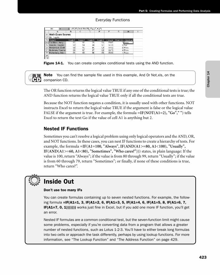
Cha

pter

14

Everyday Functions

423

Part 5: Creating Formulas and Performing Data Analysis

f14ie01

Figure 14-1. You can create complex conditional tests using the AND function.

Note You can find the sample file used in this example, And Or Not.xls, on the companion CD.

The OR function returns the logical value TRUE if any one of the conditional tests is true; the AND function returns the logical value TRUE only if all the conditional tests are true.

Because the NOT function negates a condition, it is usually used with other functions. NOT instructs Excel to return the logical value TRUE if the argument is false or the logical value FALSE if the argument is true. For example, the formula =IF(NOT(A1=2), "Go"," ") tells Excel to return the text Go if the value of cell A1 is anything but 2.

Nested IF FunctionsSometimes you can’t resolve a logical problem using only logical operators and the AND, OR, and NOT functions. In these cases, you can nest IF functions to create a hierarchy of tests. For example, the formula =IF(A1=100, "Always", IF(AND(A1>=80, A1<100), "Usually", IF(AND(A1>=60, A1<80), "Sometimes", "Who cares?"))) states, in plain language: If the value is 100, return “Always”; if the value is from 80 through 99, return “Usually”; if the value is from 60 through 79, return “Sometimes”; or finally, if none of these conditions is true, return “Who cares?”.

Inside OutDon’t use too many IFs

You can create formulas containing up to seven nested functions. For example, the follow-ing formula =IF(A1=1, 3, IF(A1=2, 6, IF(A1=3, 5, IF(A1=4, 6, IF(A1=5, 8, IF(A1=6, 7, IF(A1=7, 0, 1))))))) works just fine in Excel, but if you add one more IF function, you’ll get an error.

Nested IF formulas are a common conditional test, but the seven-function limit might cause some problems, especially if you’re converting data from a program that allows a greater number of nested functions, such as Lotus 1-2-3. You’ll have to either break long formulas into two cells or approach the task differently, perhaps by using lookup functions. For more information, see “The Lookup Function” and “The Address Function” on page 429.

Chapter 1

4

Microsoft Office Excel 2003 Inside Out

Part 5: Creating Formulas and Performing Data Analysis

424

Other Uses for Conditional FunctionsYou can use all the conditional functions described in this section as stand-alone formulas. Although you usually use functions, such as AND, OR, NOT, ISERROR, ISNA, and ISREF, within an IF function, you can use formulas, such as =AND(A1>A2, A2<A3), also to per-form simple conditional tests. This formula returns the logical value TRUE if the value in A1 is greater than the value in A2 and the value in A2 is less than the value in A3. You might use this type of formula to assign TRUE and FALSE values to a range of numeric database cells and then use the TRUE and FALSE conditions as selection criteria for printing a specialized report.

Understanding Information FunctionsThe information functions could be called the internal monitoring system in Excel. Although they perform no specific calculations, you can use them to find out about elements of the Excel interface and then use that information elsewhere. We’ll discuss the most useful of these functions in this section.

For more information about individual functions, see Appendix D, “Function Reference.”

Using Selected Information FunctionsInformation functions allow you to gather information about the contents of cells, their for-matting, and the computing environment as well as perform conditional tests for the pres-ence of specific types of values.

The TYPE and ERROR.TYPE FunctionsThe TYPE function determines whether a cell contains text, a number, a logical value, an array, or an error value. The result is a code for the type of entry in the referenced cell: 1 for a number (or a blank cell), 2 for text, 4 for a logical value (TRUE or FALSE), 16 for an error value, and 64 for an array. For example, if cell A1 contains the number 100, the formula =TYPE(A1) returns 1. If A1 contains the text Microsoft Excel, the formula returns 2.

Like the TYPE function, the ERROR.TYPE function detects the contents of a cell, except it detects different types of error values. The result is a code for the type of error value in the referenced cell: 1 for #NULL!, 2 for #DIV/0!, 3 for #VALUE!, 4 for #REF!, 5 for #NAME!, 6 for #NUM!, and 7 for #N/A. Any other value in the referenced cell returns the error value #N/A. For example, if cell A1 contains a formula that displays the error value #NAME!, the formula =ERROR.TYPE(A1) returns 5. If A1 contains the text Microsoft Excel, the formula returns #N/A.

Cha

pter

14

Everyday Functions

425

Part 5: Creating Formulas and Performing Data Analysis

The COUNTBLANK FunctionThe COUNTBLANK function counts the number of empty cells in the specified range, which is its only argument. This function is tricky because formulas that evaluate to null text strings, such as =" ", or to zero might seem empty, but they aren’t and therefore won’t be counted.

Using the IS Information FunctionsYou can use the ISBLANK, ISERR, ISERROR, ISLOGICAL, ISNA, ISNONTEXT, ISNUMBER, ISREF, and ISTEXT functions to determine whether a referenced cell or range contains the corresponding type of value. In addition, the ISEVEN and ISODD functions are available if you’ve installed the Analysis ToolPak.

For information about installing the Analysis ToolPak add-in, see “Installing the Analysis ToolPak” on page 403.

All IS Information functions take a single argument. For example, the ISBLANK function takes the form =ISBLANK(value). The value argument is a reference to a cell. If value refers to a blank cell, the function returns the logical value TRUE; otherwise, it returns FALSE.

Inside OutBe aware of IS anomalies

Although you can use a cell range (rather than a single cell) as the argument to any IS func-tion, the result might not be what you expect. For example, you would think the ISBLANK function would return TRUE if the referenced range is empty or FALSE if the range contains any values. Instead, its behavior depends on where the range is in relation to the cell con-taining the formula. If the argument refers to a range that intersects the row or column con-taining the formula, ISBLANK uses implicit intersection to arrive at the result. In other words, the function looks at only one cell in the referenced range, and only if it happens to be in the same row or column as the cell containing the function. The function ignores the rest of the range. If the range shares neither a row nor a column with the formula, however, the result is always FALSE. For more about intersection, see the “Getting Explicit about Intersections” on page 367.

Chapter 1

4

Microsoft Office Excel 2003 Inside Out

Part 5: Creating Formulas and Performing Data Analysis

426

An ISERR ExampleYou can use ISERR to avoid getting error values as formula results. For example, suppose you want to call attention to cells containing a particular character string, such as 12A, resulting in the word Yes appearing in the cell containing the formula. If the string isn’t found, you want the cell to remain empty. You can use the IF and FIND functions to perform this task, but if the value isn’t found, you get a #VALUE! error rather than a blank cell.

To solve this problem, add an ISERR function to the formula. The FIND function returns the position at which a substring is found within a larger string. If the substring isn’t there, FIND returns #VALUE!. The solution is to add an ISERR function, such as =IF(ISERR(FIND("12A", A1)), " ", "Yes"). Because you’re not interested in the error, which is simply a by-product of the calculation, this traps the error, leaving only the results that you are interested in.

Note When you enter numeric values as text, such as ="21", the IS function, unlike other functions, does not recognize them as numbers. Therefore, the formula =ISNUM-BER("21") returns FALSE.

Understanding Lookup and Reference FunctionsLookup and reference functions help you use your own worksheet tables as sources of infor-mation to be used elsewhere in formulas. You can use three primary functions to look up information stored in a list or a table or to manipulate references: LOOKUP, VLOOKUP, and HLOOKUP. Some powerful lookup and reference functions in addition to these three are available; we describe many of them in this section.

For more information about individual functions, see Appendix D, “Function Reference.”

Using Selected Lookup and Reference FunctionsVLOOKUP and HLOOKUP are nearly identical functions that look up information stored in tables you have constructed. VLOOKUP and HLOOKUP operate in either vertical or hori-zontal orientation (respectively), but LOOKUP works either way.

When you look up information in a table, you normally use a row index and a column index to locate a particular cell. Excel derives the first index by finding the largest value in the first column or row that is less than or equal to a lookup value you supply and then uses a row number or column number argument as the other index. Make sure the table is sorted by the row or column containing the lookup values.

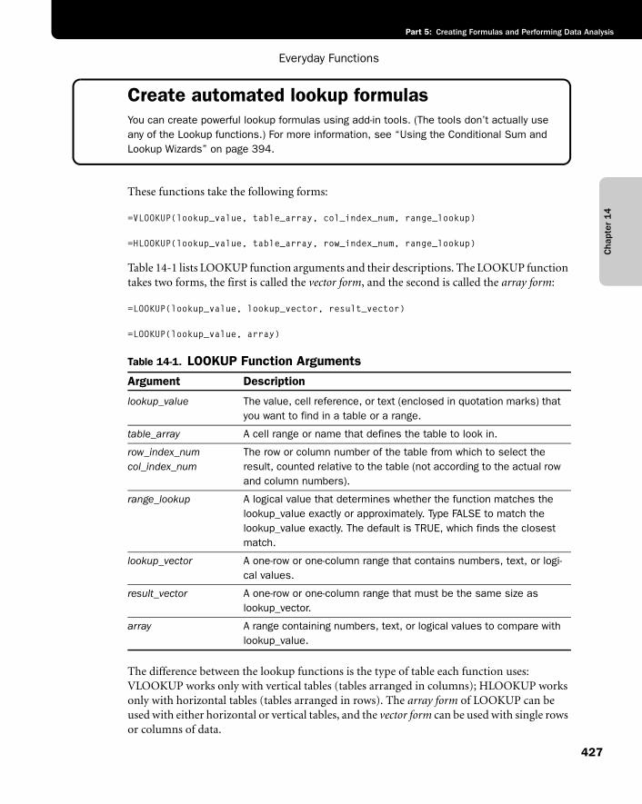
Cha

pter

14

Everyday Functions

427

Part 5: Creating Formulas and Performing Data Analysis

Create automated lookup formulasYou can create powerful lookup formulas using add-in tools. (The tools don’t actually use any of the Lookup functions.) For more information, see “Using the Conditional Sum and Lookup Wizards” on page 394.

These functions take the following forms:

=VLOOKUP(lookup_value, table_array, col_index_num, range_lookup)

=HLOOKUP(lookup_value, table_array, row_index_num, range_lookup)

Table 14-1 lists LOOKUP function arguments and their descriptions. The LOOKUP function takes two forms, the first is called the vector form, and the second is called the array form:

=LOOKUP(lookup_value, lookup_vector, result_vector)

=LOOKUP(lookup_value, array)

The difference between the lookup functions is the type of table each function uses: VLOOKUP works only with vertical tables (tables arranged in columns); HLOOKUP works only with horizontal tables (tables arranged in rows). The array form of LOOKUP can be used with either horizontal or vertical tables, and the vector form can be used with single rows or columns of data.

Table 14-1. LOOKUP Function Arguments

Argument Description

lookup_value The value, cell reference, or text (enclosed in quotation marks) that you want to find in a table or a range.

table_array A cell range or name that defines the table to look in.

row_index_num col_index_num

The row or column number of the table from which to select the result, counted relative to the table (not according to the actual row and column numbers).

range_lookup A logical value that determines whether the function matches the lookup_value exactly or approximately. Type FALSE to match the lookup_value exactly. The default is TRUE, which finds the closest match.

lookup_vector A one-row or one-column range that contains numbers, text, or logi-cal values.

result_vector A one-row or one-column range that must be the same size as lookup_vector.

array A range containing numbers, text, or logical values to compare with lookup_value.

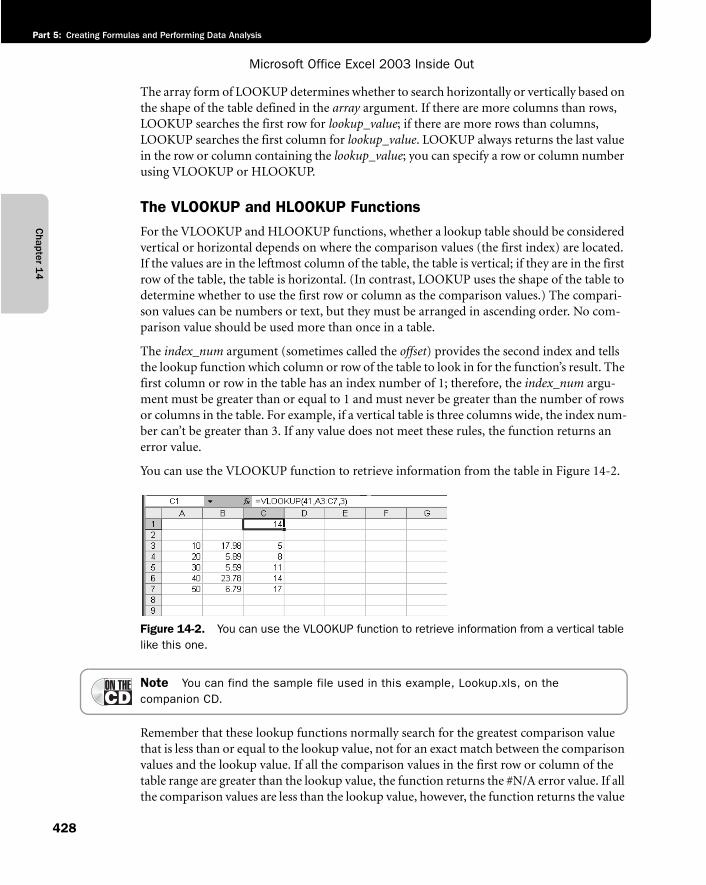
Chapter 1

4

Microsoft Office Excel 2003 Inside Out

Part 5: Creating Formulas and Performing Data Analysis

428

The array form of LOOKUP determines whether to search horizontally or vertically based on the shape of the table defined in the array argument. If there are more columns than rows, LOOKUP searches the first row for lookup_value; if there are more rows than columns, LOOKUP searches the first column for lookup_value. LOOKUP always returns the last value in the row or column containing the lookup_value; you can specify a row or column number using VLOOKUP or HLOOKUP.

The VLOOKUP and HLOOKUP FunctionsFor the VLOOKUP and HLOOKUP functions, whether a lookup table should be considered vertical or horizontal depends on where the comparison values (the first index) are located. If the values are in the leftmost column of the table, the table is vertical; if they are in the first row of the table, the table is horizontal. (In contrast, LOOKUP uses the shape of the table to determine whether to use the first row or column as the comparison values.) The compari-son values can be numbers or text, but they must be arranged in ascending order. No com-parison value should be used more than once in a table.

The index_num argument (sometimes called the offset) provides the second index and tells the lookup function which column or row of the table to look in for the function’s result. The first column or row in the table has an index number of 1; therefore, the index_num argu-ment must be greater than or equal to 1 and must never be greater than the number of rows or columns in the table. For example, if a vertical table is three columns wide, the index num-ber can’t be greater than 3. If any value does not meet these rules, the function returns an error value.

You can use the VLOOKUP function to retrieve information from the table in Figure 14-2.

f14ie02

Figure 14-2. You can use the VLOOKUP function to retrieve information from a vertical table like this one.

Note You can find the sample file used in this example, Lookup.xls, on the companion CD.

Remember that these lookup functions normally search for the greatest comparison value that is less than or equal to the lookup value, not for an exact match between the comparison values and the lookup value. If all the comparison values in the first row or column of the table range are greater than the lookup value, the function returns the #N/A error value. If all the comparison values are less than the lookup value, however, the function returns the value

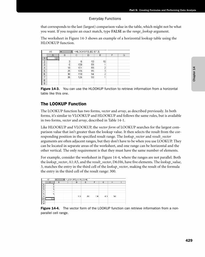
Cha

pter

14

Everyday Functions

429

Part 5: Creating Formulas and Performing Data Analysis

that corresponds to the last (largest) comparison value in the table, which might not be what you want. If you require an exact match, type FALSE as the range_lookup argument.

The worksheet in Figure 14-3 shows an example of a horizontal lookup table using the HLOOKUP function.

f14ie03

Figure 14-3. You can use the HLOOKUP function to retrieve information from a horizontal table like this one.

The LOOKUP FunctionThe LOOKUP function has two forms, vector and array, as described previously. In both forms, it’s similar to VLOOKUP and HLOOKUP and follows the same rules, but is available in two forms, vector and array, described in Table 14-1.

Like HLOOKUP and VLOOKUP, the vector form of LOOKUP searches for the largest com-parison value that isn’t greater than the lookup value. It then selects the result from the cor-responding position in the specified result range. The lookup_vector and result_vectorarguments are often adjacent ranges, but they don’t have to be when you use LOOKUP. They can be located in separate areas of the worksheet, and one range can be horizontal and the other vertical. The only requirement is that they must have the same number of elements.

For example, consider the worksheet in Figure 14-4, where the ranges are not parallel. Both the lookup_vector, A1:A5, and the result_vector, D6:H6, have five elements. The lookup_value,3, matches the entry in the third cell of the lookup_vector, making the result of the formula the entry in the third cell of the result range: 300.

f14ie04

Figure 14-4. The vector form of the LOOKUP function can retrieve information from a non-parallel cell range.

Chapter 1

4

Microsoft Office Excel 2003 Inside Out

Part 5: Creating Formulas and Performing Data Analysis

430

The array form of LOOKUP is similar to VLOOKUP and HLOOKUP but works with either a horizontal or a vertical table, using the dimensions of the table to figure out the location of the comparison values. If the table is taller than it is wide or the table is square, the function treats it as a vertical table and assumes that the comparison values are in the leftmost column. If the table is wider than it is tall, the function views the table as horizontal and assumes that the comparison values are in the first row of the table. The result is always in the last row or column of the specified table; you can’t specify column or row numbers.

Because HLOOKUP and VLOOKUP are more predictable and controllable, you’ll generally find using them preferable to using LOOKUP.

The ADDRESS FunctionThe Address function provides a handy way to build a reference from numbers. It takes the arguments (row_num, column_num, abs_num, a1, sheet_text). For example, the formula =ADDRESS(1, 1, 1, TRUE, "Data Sheet") results in the reference 'Data Sheet'!$A$1. (For a complete explanation of the ADDRESS function, see Appendix D, “Function Reference.”)

The CHOOSE FunctionYou use the CHOOSE function to retrieve an item from a list of values. The function takes the arguments (index_num, value 1, value 2, ...) and can include up to 29 values. The index_num argument is the position in the list you want to return; it must be positive and can’t exceed the number of elements in the list. The function returns the value of the element in the list that occupies the position indicated by index_num. For example, the function =CHOOSE(2, 6, 1, 8, 9, 3) returns the value 1, because 1 is the second item in the list. (The index_num value itself isn’t counted as part of the list.) You can use individual cell references for the list, but you can’t specify ranges. You might be tempted to create a function, such as =CHOOSE(A10, C1:C5), to take the place of the longer function in the preceding example. If you do, however, the result is a #VALUE! error value.

The MATCH FunctionThe MATCH function is closely related to the CHOOSE function. However, whereas CHOOSE returns the item that occupies the position in a list specified by the index_numargument, MATCH returns the position of the item in the list that most closely matches a lookup value.

Note You can create powerful lookup formulas using add-in tools that use the MATCH function. See “Using the Conditional Sum and Lookup Wizards” on page 394.

This function takes the arguments (lookup_value, lookup_array, match_type), where lookup_value and the items in the lookup_array can be numeric values or text strings, and match_type defines the rules for the search, as shown in Table 14-2.

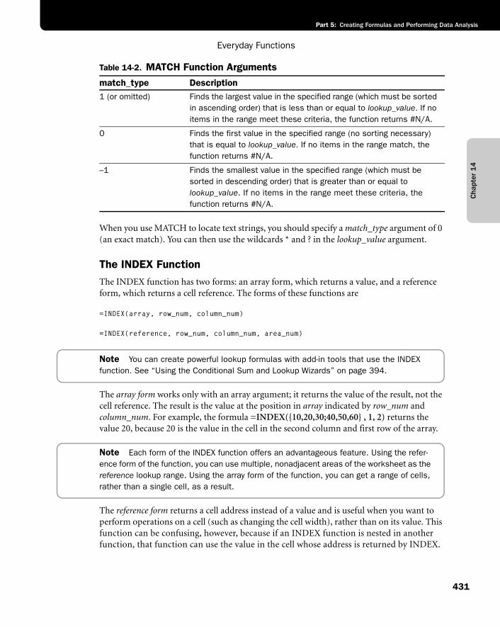
Cha

pter

14

Everyday Functions

431

Part 5: Creating Formulas and Performing Data Analysis

When you use MATCH to locate text strings, you should specify a match_type argument of 0 (an exact match). You can then use the wildcards * and ? in the lookup_value argument.

The INDEX FunctionThe INDEX function has two forms: an array form, which returns a value, and a reference form, which returns a cell reference. The forms of these functions are

=INDEX(array, row_num, column_num)

=INDEX(reference, row_num, column_num, area_num)

Note You can create powerful lookup formulas with add-in tools that use the INDEX function. See “Using the Conditional Sum and Lookup Wizards” on page 394.

The array form works only with an array argument; it returns the value of the result, not the cell reference. The result is the value at the position in array indicated by row_num and column_num. For example, the formula =INDEX({10,20,30;40,50,60} , 1, 2) returns the value 20, because 20 is the value in the cell in the second column and first row of the array.

Note Each form of the INDEX function offers an advantageous feature. Using the refer-ence form of the function, you can use multiple, nonadjacent areas of the worksheet as the reference lookup range. Using the array form of the function, you can get a range of cells, rather than a single cell, as a result.

The reference form returns a cell address instead of a value and is useful when you want to perform operations on a cell (such as changing the cell width), rather than on its value. This function can be confusing, however, because if an INDEX function is nested in another function, that function can use the value in the cell whose address is returned by INDEX.

Table 14-2. MATCH Function Arguments

match_type Description1 (or omitted) Finds the largest value in the specified range (which must be sorted

in ascending order) that is less than or equal to lookup_value. If no items in the range meet these criteria, the function returns #N/A.

0 Finds the first value in the specified range (no sorting necessary) that is equal to lookup_value. If no items in the range match, the function returns #N/A.

–1 Finds the smallest value in the specified range (which must be sorted in descending order) that is greater than or equal to lookup_value. If no items in the range meet these criteria, the function returns #N/A.

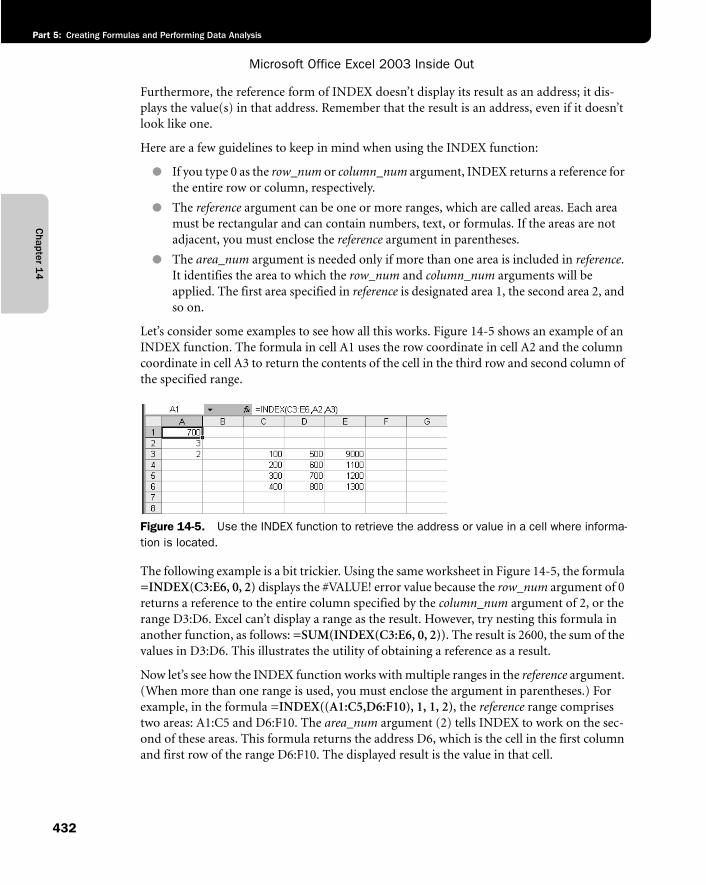
Chapter 1

4

Microsoft Office Excel 2003 Inside Out

Part 5: Creating Formulas and Performing Data Analysis

432

Furthermore, the reference form of INDEX doesn’t display its result as an address; it dis-plays the value(s) in that address. Remember that the result is an address, even if it doesn’t look like one.

Here are a few guidelines to keep in mind when using the INDEX function:

● If you type 0 as the row_num or column_num argument, INDEX returns a reference for the entire row or column, respectively.

● The reference argument can be one or more ranges, which are called areas. Each area must be rectangular and can contain numbers, text, or formulas. If the areas are not adjacent, you must enclose the reference argument in parentheses.

● The area_num argument is needed only if more than one area is included in reference.It identifies the area to which the row_num and column_num arguments will be applied. The first area specified in reference is designated area 1, the second area 2, and so on.

Let’s consider some examples to see how all this works. Figure 14-5 shows an example of an INDEX function. The formula in cell A1 uses the row coordinate in cell A2 and the column coordinate in cell A3 to return the contents of the cell in the third row and second column of the specified range.

f14ie05

Figure 14-5. Use the INDEX function to retrieve the address or value in a cell where informa-tion is located.

The following example is a bit trickier. Using the same worksheet in Figure 14-5, the formula =INDEX(C3:E6, 0, 2) displays the #VALUE! error value because the row_num argument of 0 returns a reference to the entire column specified by the column_num argument of 2, or the range D3:D6. Excel can’t display a range as the result. However, try nesting this formula in another function, as follows: =SUM(INDEX(C3:E6, 0, 2)). The result is 2600, the sum of the values in D3:D6. This illustrates the utility of obtaining a reference as a result.

Now let’s see how the INDEX function works with multiple ranges in the reference argument. (When more than one range is used, you must enclose the argument in parentheses.) For example, in the formula =INDEX((A1:C5,D6:F10), 1, 1, 2), the reference range comprises two areas: A1:C5 and D6:F10. The area_num argument (2) tells INDEX to work on the sec-ond of these areas. This formula returns the address D6, which is the cell in the first column and first row of the range D6:F10. The displayed result is the value in that cell.

Cha

pter

14

Everyday Functions

433

Part 5: Creating Formulas and Performing Data Analysis

The INDIRECT FunctionThe INDIRECT function returns the contents of a cell using its reference. It takes the argu-ments (ref_text, a1), where ref_text is an A1-style or R1C1-style reference, or a cell name. The a1 argument is a logical value indicating which type of reference you’re using. If a1 is FALSE, Excel interprets ref_text as R1C1 format; if a1 is TRUE or omitted, Excel interprets ref_text as A1 format. For example, if cell C6 of your worksheet contains the text value B3 and cell B3 contains the value 2.888, the formula =INDIRECT(C6) returns the value 2.888. If your worksheet is set to display R1C1-style references, and cell R6C3 contains the text reference “R3C2” and cell R3C2 contains the value 2.888, the formula =INDIRECT(R6C3, FALSE)also returns the value 2.888.

The ROW and COLUMN FunctionsThe result of the ROW and COLUMN functions is the row or column number, respectively, of the cell or range referred to by the function’s single argument. For example, the formula =ROW(H5) returns the result 5. The formula =COLUMN(C5) returns the result 3 because column C is the third column on the worksheet.

If the argument is omitted, the result is the row or column number of the cell that contains the function. If the argument is a range or a range name and the function is entered as an array by pressing Ctrl+Shift+Enter, the result of the function is an array that consists of the row or column numbers of each row or column in the range. For example, suppose you select cells B1:B10, type the formula =ROW(A1:A10), and then press Ctrl+Shift+Enter to enter the formula in all cells in the range B1:B10. That range will contain the array result {1;2;3;4;5;6;7;8;9;10}, the row numbers of each cell in the argument.

The ROWS and COLUMNS FunctionsThe ROWS and COLUMNS functions return the number of rows or columns, respectively, referenced by the function’s single argument in a reference or an array. The argument is an array constant, a range reference, or a range name. For example, the result of the formula =ROWS({100,200,300;1000,2000,3000}) is 2, because the array consists of two rows (sepa-rated by a semicolon). The formula =ROWS(A1:A10) returns 10, because the range A1:A10 contains ten rows. And the formula =COLUMNS(A1:C10) returns 3, because the range A1:C10 contains three columns.

The AREAS FunctionYou can use the AREAS function to determine the number of areas in a reference. Areas refer to individual cell or range references, not regions. The single argument to this function can be a cell reference, a range reference, or several range references. If you use several range ref-erences, you must enclose them in a set of parentheses so that Excel doesn’t misinterpret the commas that separate the ranges. (Although this function takes only one argument, Excel still interprets unenclosed commas as argument separators.) For example, suppose you assign the name Test to the group of ranges A1:C5,D6,E7:G10. The function =AREAS(Test)returns the number 3, the number of areas in the group.

Chapter 1

4

Microsoft Office Excel 2003 Inside Out

Part 5: Creating Formulas and Performing Data Analysis

434

The TRANSPOSE FunctionThe TRANSPOSE function changes the horizontal or vertical orientation of an array. It takes a single argument, array. If the argument refers to a vertically oriented range, the resulting array is horizontal. If the range is horizontal, the resulting array is vertical. The first row of a horizontal array becomes the first column of the vertical array result, and vice versa. You must type the TRANSPOSE function as an array formula in a range that has the same num-ber of rows and columns as the array argument has columns and rows, respectively.

Note For quick and easy transposition, select the range you want to transpose, press Ctrl+C to copy the range, click the cell where you want the upper left corner of the trans-posed range to begin, choose Edit, Paste Special, and then click the Transpose option.

435

Part 5: Creating Formulas and Performing Data Analysis

Chapter 15

Formatting and Calculating Date and Time

Understanding How Excel RecordsDates and Times. . . . . . . . . . . . . . . . . . 435Entering Dates and Times. . . . . . . . . . . 436Formatting Dates and Times . . . . . . . . 440

Calculating with Date and Time. . . . . . . 444Working with Date and TimeFunctions . . . . . . . . . . . . . . . . . . . . . . . . 445

You can use date and time values to date-stamp documents and to perform date and time arithmetic. Creating a production schedule or a monthly billing system is relatively easy with Microsoft Excel. Although Excel uses numeric values to count each nanosecond, starting from the beginning of the 20th century, you can use formatting to display those numbers in whatever form you want.

Understanding How Excel Records Dates and Times

Excel assigns serial values to days, hours, minutes, and seconds, which makes it possible for you to perform sophisticated date and time arithmetic. The basic unit of time in Excel is the day. Each day is represented by a serial date value. The base date, represented by the serial value 1, is Sunday, January 1, 1900. When you enter a date in your worksheet, Excel records the date as a serial value that represents the number of days between the base date and the specified date. For example, the date January 1, 2004 is represented by the serial value 37,987, representing the number of days between the base date—January 1, 1900—and January 1, 2004.

The time of day is a decimal value that represents the portion of a day that has passed from its beginning—12:00 midnight—to the specified time. Therefore, the time 12:00 noon is repre-sented by the value 0.5, because the difference between midnight and noon is exactly half a day. The time/date combination 2:09:03 PM, October 23, 2004, is represented by the serial value 38283.5896180556, because October 23, 2004 is day number 38,283 (counting January 1, 1900 as day number 1), and the interval between midnight and 2:09:03 PM amounts to .5896180556 of a whole day.

Tip Display the serial date valueYou can see the serial value of a formatted date by selecting the cell containing the date and pressing Ctrl+Shift+tilde (~). To return the cell to its date format, press Ctrl+Z.

Chapter 1

5

Microsoft Office Excel 2003 Inside Out

Part 5: Creating Formulas and Performing Data Analysis

436

Using the 1904 Date SystemIf you transfer documents between Excel for the Macintosh and Excel for Windows, the proper date system for the worksheet is set for you. When the date system changes, exist-ing serial date values display different dates, but the underlying values do not change. If you change date systems after you have begun entering dates in a worksheet, all your dates will be off by four years.

You can change the base date (the date that corresponds to the serial value 1) from Janu-ary 1, 1900—used by Excel for Windows—to January 2, 1904—used by Excel for the Mac-intosh. Choose Tools, Options, click the Calculation tab, and select the 1904 Date System option.

When you select this option, the serial date values in your worksheet remain the same, but the display of all dates changes so that the serial values of any dates you enter in your Excel for Windows worksheets match corresponding serial values from Excel for the Macin-tosh worksheets. If you transfer information into Excel for Windows from a worksheet cre-ated in Excel for the Macintosh, selecting this option ensures that Excel evaluates the serial date values correctly. In this book, we use the 1900 date system.

Entering Dates and TimesAlthough Excel records dates and times as serial date values, you don’t have to enter them that way. You can manipulate dates and times in your worksheet formulas just as you manipulate other types of values. You enter date values in formats that Excel automatically applies. To enter date values in this way, type the date in one of the following formats: m/d/yy, d-mmm-yy,d-mmm, or mmm-yy. (You can also enter 4-digit years for any of these formats.)

Tip Adjust regional number settingsYou can change the default date, time, currency, and numbering settings through the Date, Time, Language, and Regional Options control (or simply Regional Options, or Regional Set-tings, depending on your system) in the Windows Control Panel. These settings will deter-mine how your date entries are interpreted. For example, with regional options set to Italian, entering a date in d/m/yy format will result in a properly displayed date, but if you enter the same date with regional options set to English, the entry is interpreted as text.

If your entry doesn’t match any of the built-in date or time formats, Excel picks the format that’s most similar to your entry. For example, if you enter 1 Dec, you see the formatted entry 1-Dec in the cell. In the formula bar, the entry appears as 12/1/2004 (if the current year is 2004) so you can edit the date more easily.

You can also enter times in a time format. Select a cell and type the time in one of the follow-ing forms: h:mm AM/PM, h:mm:ss AM/PM, h:mm, h:mm:ss, or the combined date and time format, m/d/yy h:mm. Notice that you must separate the hours, minutes, and seconds of the time entries by colons.

Cha

pter

15

Formatting and Calculating Date and Time

437

Part 5: Creating Formulas and Performing Data Analysis

For more information about custom formats, see “Creating Your Own Date and Time Formats” on page 441.

If you don’t include AM, PM, A, or P with the time, Excel uses the 24-hour (military) time convention. In other words, Excel always assumes that the entry 3:00 means 3:00 AM, unless you specifically enter PM.

Tip Insert an instant date or time stampEnter the current date in a cell or formula by holding down Ctrl and pressing the semicolon (;) key. The date stamp is entered in the current short-date format, as set in Control Panel. Enter the current time in a cell or formula by holding down Ctrl and Shift together and press-ing the colon (:) key. The time stamp is entered in h:mm AM/PM format. (Of course, the colon and semicolon occupy the same key—the Shift key changes the formula to a time stamp.)

Inside OutChange the magic crossover date

December 31, 2029 is the default magic crossover date—that is, the last day that Windows assumes is in the future if you enter the year using only two digits. For example, if you type 12/31/29 into a cell, Microsoft Windows assumes that you mean the year 2029. If, how-ever, you type 1/1/30 into a cell, Windows interprets it to mean January 1, 1930.

You can change this magic crossover date by changing the setting on the Date tab of the Date, Time, Language, and Regional Options control (or just Regions Options or Regional Settings, depending on your system), which is accessed from the Windows Control Panel. Of course, you’re still limited to a 100-year span; if you change the last date Windows rec-ognizes as being in the future, the corresponding beginning date—January 1, 1900—changes accordingly. Therefore, if you need to enter century-spanning dates, you should get into the habit of typing the full four-digit year to avoid surprises.

Entering a Series of DatesYou can create an evenly spaced series of dates in a row or column in several ways, but the job is especially easy when you use the Fill handle. Suppose you want to create a series of dates in row 1. The series begins with March 1, 2004, and the dates must be exactly one month apart.

If you enter 3/1/2004 in cell A1 and drag the Fill handle to the right, Excel extends the series of dates incrementally by days, as shown in Figure 15-1. After you drag, Excel displays a smart tag adjacent to the selection. Click the smart tag to display the smart tag action menu shown in Figure 15-1, which displays a number of AutoFill options; select Fill Months to convert the already-extended day series into a month series.

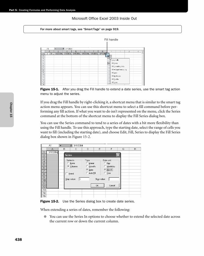
Chapter 1

5

Microsoft Office Excel 2003 Inside Out

Part 5: Creating Formulas and Performing Data Analysis

438

For more about smart tags, see “Smart Tags” on page 919.

f15ie01

Figure 15-1. After you drag the Fill handle to extend a date series, use the smart tag action menu to adjust the series.

If you drag the Fill handle by right-clicking it, a shortcut menu that is similar to the smart tag action menu appears. You can use this shortcut menu to select a fill command before per-forming any fill action. If what you want to do isn’t represented on the menu, click the Series command at the bottom of the shortcut menu to display the Fill Series dialog box.

You can use the Series command to tend to a series of dates with a bit more flexibility than using the Fill handle. To use this approach, type the starting date, select the range of cells you want to fill (including the starting date), and choose Edit, Fill, Series to display the Fill Series dialog box shown in Figure 15-2.

f15ie02

Figure 15-2. Use the Series dialog box to create date series.

When extending a series of dates, remember the following:

● You can use the Series In options to choose whether to extend the selected date across the current row or down the current column.

Fill handle

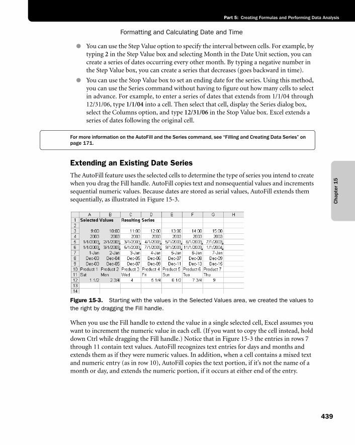
Cha

pter

15

Formatting and Calculating Date and Time

439

Part 5: Creating Formulas and Performing Data Analysis

● You can use the Step Value option to specify the interval between cells. For example, by typing 2 in the Step Value box and selecting Month in the Date Unit section, you can create a series of dates occurring every other month. By typing a negative number in the Step Value box, you can create a series that decreases (goes backward in time).

● You can use the Stop Value box to set an ending date for the series. Using this method, you can use the Series command without having to figure out how many cells to select in advance. For example, to enter a series of dates that extends from 1/1/04 through 12/31/06, type 1/1/04 into a cell. Then select that cell, display the Series dialog box, select the Columns option, and type 12/31/06 in the Stop Value box. Excel extends a series of dates following the original cell.

For more information on the AutoFill and the Series command, see “Filling and Creating Data Series” on page 171.

Extending an Existing Date SeriesThe AutoFill feature uses the selected cells to determine the type of series you intend to create when you drag the Fill handle. AutoFill copies text and nonsequential values and increments sequential numeric values. Because dates are stored as serial values, AutoFill extends them sequentially, as illustrated in Figure 15-3.

f15ie03

Figure 15-3. Starting with the values in the Selected Values area, we created the values to the right by dragging the Fill handle.

When you use the Fill handle to extend the value in a single selected cell, Excel assumes you want to increment the numeric value in each cell. (If you want to copy the cell instead, hold down Ctrl while dragging the Fill handle.) Notice that in Figure 15-3 the entries in rows 7 through 11 contain text values. AutoFill recognizes text entries for days and months and extends them as if they were numeric values. In addition, when a cell contains a mixed text and numeric entry (as in row 10), AutoFill copies the text portion, if it’s not the name of a month or day, and extends the numeric portion, if it occurs at either end of the entry.

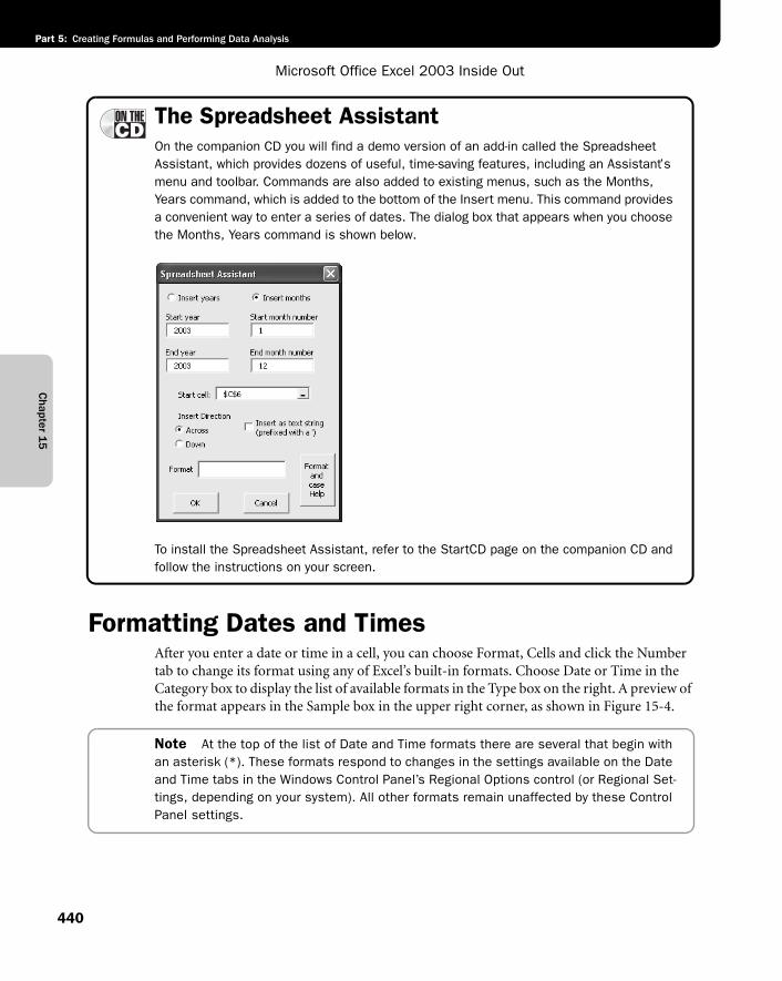
Chapter 1

5

Microsoft Office Excel 2003 Inside Out

Part 5: Creating Formulas and Performing Data Analysis

440

The Spreadsheet AssistantOn the companion CD you will find a demo version of an add-in called the Spreadsheet Assistant, which provides dozens of useful, time-saving features, including an Assistant’s menu and toolbar. Commands are also added to existing menus, such as the Months, Years command, which is added to the bottom of the Insert menu. This command provides a convenient way to enter a series of dates. The dialog box that appears when you choose the Months, Years command is shown below.

G15ie01sb

To install the Spreadsheet Assistant, refer to the StartCD page on the companion CD and follow the instructions on your screen.

Formatting Dates and TimesAfter you enter a date or time in a cell, you can choose Format, Cells and click the Number tab to change its format using any of Excel’s built-in formats. Choose Date or Time in the Category box to display the list of available formats in the Type box on the right. A preview of the format appears in the Sample box in the upper right corner, as shown in Figure 15-4.

Note At the top of the list of Date and Time formats there are several that begin with an asterisk (*). These formats respond to changes in the settings available on the Date and Time tabs in the Windows Control Panel’s Regional Options control (or Regional Set-tings, depending on your system). All other formats remain unaffected by these Control Panel settings.

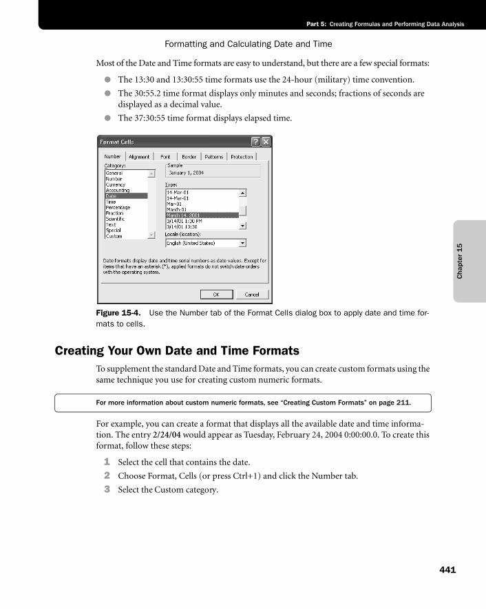
Cha

pter

15

Formatting and Calculating Date and Time

441

Part 5: Creating Formulas and Performing Data Analysis

Most of the Date and Time formats are easy to understand, but there are a few special formats:

● The 13:30 and 13:30:55 time formats use the 24-hour (military) time convention.

● The 30:55.2 time format displays only minutes and seconds; fractions of seconds are displayed as a decimal value.

● The 37:30:55 time format displays elapsed time.

f15ie04

Figure 15-4. Use the Number tab of the Format Cells dialog box to apply date and time for-mats to cells.

Creating Your Own Date and Time FormatsTo supplement the standard Date and Time formats, you can create custom formats using the same technique you use for creating custom numeric formats.

For more information about custom numeric formats, see “Creating Custom Formats” on page 211.

For example, you can create a format that displays all the available date and time informa-tion. The entry 2/24/04 would appear as Tuesday, February 24, 2004 0:00:00.0. To create this format, follow these steps:

1 Select the cell that contains the date.

2 Choose Format, Cells (or press Ctrl+1) and click the Number tab.

3 Select the Custom category.

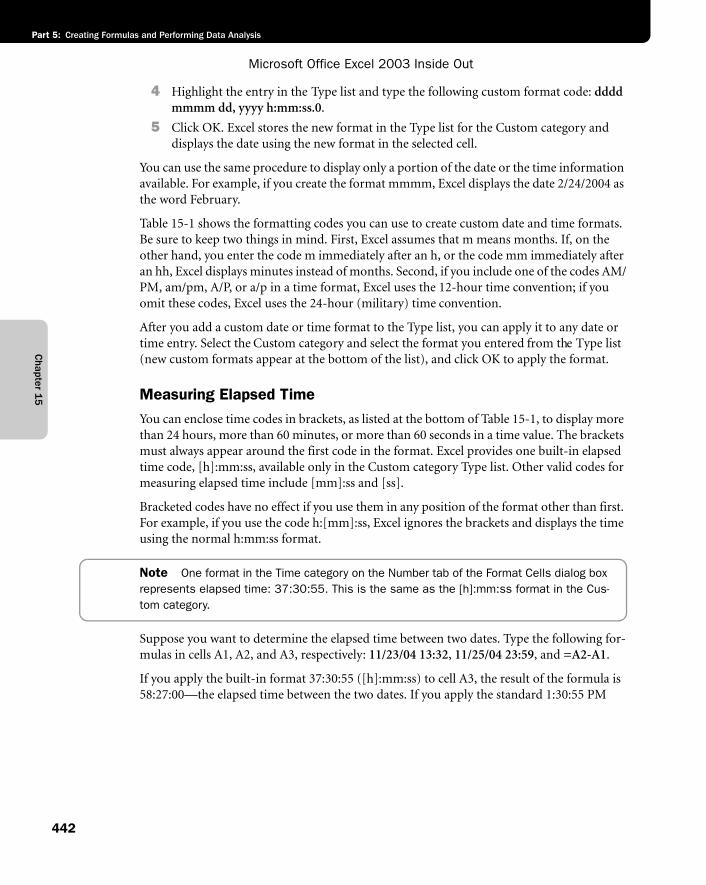
Chapter 1

5

Microsoft Office Excel 2003 Inside Out

Part 5: Creating Formulas and Performing Data Analysis

442

4 Highlight the entry in the Type list and type the following custom format code: ddddmmmm dd, yyyy h:mm:ss.0.

5 Click OK. Excel stores the new format in the Type list for the Custom category and displays the date using the new format in the selected cell.

You can use the same procedure to display only a portion of the date or the time information available. For example, if you create the format mmmm, Excel displays the date 2/24/2004 as the word February.

Table 15-1 shows the formatting codes you can use to create custom date and time formats. Be sure to keep two things in mind. First, Excel assumes that m means months. If, on the other hand, you enter the code m immediately after an h, or the code mm immediately after an hh, Excel displays minutes instead of months. Second, if you include one of the codes AM/PM, am/pm, A/P, or a/p in a time format, Excel uses the 12-hour time convention; if you omit these codes, Excel uses the 24-hour (military) time convention.

After you add a custom date or time format to the Type list, you can apply it to any date or time entry. Select the Custom category and select the format you entered from the Type list (new custom formats appear at the bottom of the list), and click OK to apply the format.

Measuring Elapsed TimeYou can enclose time codes in brackets, as listed at the bottom of Table 15-1, to display more than 24 hours, more than 60 minutes, or more than 60 seconds in a time value. The brackets must always appear around the first code in the format. Excel provides one built-in elapsed time code, [h]:mm:ss, available only in the Custom category Type list. Other valid codes for measuring elapsed time include [mm]:ss and [ss].

Bracketed codes have no effect if you use them in any position of the format other than first. For example, if you use the code h:[mm]:ss, Excel ignores the brackets and displays the time using the normal h:mm:ss format.

Note One format in the Time category on the Number tab of the Format Cells dialog box represents elapsed time: 37:30:55. This is the same as the [h]:mm:ss format in the Cus-tom category.

Suppose you want to determine the elapsed time between two dates. Type the following for-mulas in cells A1, A2, and A3, respectively: 11/23/04 13:32, 11/25/04 23:59, and =A2-A1.

If you apply the built-in format 37:30:55 ([h]:mm:ss) to cell A3, the result of the formula is 58:27:00—the elapsed time between the two dates. If you apply the standard 1:30:55 PM

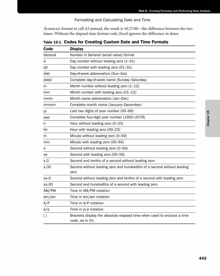
Cha

pter

15

Formatting and Calculating Date and Time

443

Part 5: Creating Formulas and Performing Data Analysis

(h:mm:ss) format to cell A3 instead, the result is 10:27:00—the difference between the two times. Without the elapsed time format code, Excel ignores the difference in dates.

Table 15-1. Codes for Creating Custom Date and Time Formats

Code DisplayGeneral Number in General (serial value) format

d Day number without leading zero (1–31)

dd Day number with leading zero (01–31)

ddd Day-of-week abbreviation (Sun–Sat)

dddd Complete day-of-week name (Sunday–Saturday)

m Month number without leading zero (1–12)

mm Month number with leading zero (01–12)

mmm Month name abbreviation (Jan–Dec)

mmmm Complete month name (January–December)

yy Last two digits of year number (00–99)

yyyy Complete four-digit year number (1900–2078)

h Hour without leading zero (0–23)

hh Hour with leading zero (00–23)

m Minute without leading zero (0–59)

mm Minute with leading zero (00–59)

s Second without leading zero (0–59)

ss Second with leading zero (00–59)

s.0 Second and tenths of a second without leading zero

s.00 Second without leading zero and hundredths of a second without leading zero

ss.0 Second without leading zero and tenths of a second with leading zero

ss.00 Second and hundredths of a second with leading zero

AM/PM Time in AM/PM notation

am/pm Time in am/pm notation

A/P Time in A/P notation

a/p Time in a/p notation

[ ] Brackets display the absolute elapsed time when used to enclose a time code, as in [h].

Chapter 1

5

Microsoft Office Excel 2003 Inside Out

Part 5: Creating Formulas and Performing Data Analysis

444

TroubleshootingI can’t enter a number of hours over 9999

Suppose you have a worksheet in which you keep a running total of flying time for pilots, using Excel’s time formats. Whenever you try to enter a number of hours over 9999 (which isn’t uncommon), Excel treats the entry as text. What’s wrong?

Nothing is wrong—that’s just a built-in limitation of Excel. Here are a couple of ways to work with this limitation:

First, use an elapsed time format. Choose Format, Cells, click the Number tab, select the Custom category, and then choose [h]:mm:ss in the Type list to apply the one built-in elapsed time format. If you don’t need to record seconds, you can delete :ss. Elapsed time formats can store and display an unlimited number of hours.

Second, if you need to enter more than 9999 hours at a time, you’ll have to break it into two smaller chunks and enter it in two cells.

You should also know that when you enter a time greater than 24 hours (even 24:01), Excel adds a date in the formula bar. Unless the number of hours entered exceeds a year’s worth, the added date will be sometime in 1900; you’ll just have to live with that. Fortunately, this date doesn’t show in the cell unless you format it to.

Calculating with Date and TimeBecause Excel records dates as serial date values, you can use dates in formulas and functions as you would any other value. Suppose you want to find the date that falls exactly 200 days after July 4, 2004. If cell A1 contains the entry 7/4/04, you can use the following formula to compute the date 200 days later, which is 1/20/05 (or 38,372): =A1+200.

As another example, suppose you want to find the number of weeks between October 31, 2003, and May 13, 2004. Use the formula =(("5/13/04")-("10/31/03"))/7, which returns approximately 27.9 weeks.

You can also use times in formulas and functions; however, the results of time arithmetic are not as easy to understand as the results of date arithmetic. For example, you can deter-mine how much time has elapsed between 8:22 AM and 10:45 PM with the formula ="22:45"–"8:22". The result is .599306, which can be formatted using a 24-hour time format (one that doesn’t include AM/PM) to display 14:23. Excel displays the result relative to midnight.

Suppose you want to determine the time that is 2 hours, 23 minutes, and 17 seconds after 12:35:23 PM. The formula =("12:35:23 PM")+("2:23:17") returns the correct answer, .624074, which can be formatted as 14:58:40. In this formula, 2:23:17 represents not an abso-lute time (2:23:17 AM) but an interval of time (2 hours, 23 minutes, and 17 seconds). This format is perfectly acceptable to Excel.

Cha

pter

15

Formatting and Calculating Date and Time

445

Part 5: Creating Formulas and Performing Data Analysis

TroubleshootingExcel displays my time as #####

Excel can’t display negative numbers as dates or times. If the result of a date or time cal-culation is negative, and you attempt to display this result in a date or time format, you will see a cell full of number signs, no matter how you widen the cell. This typically happens when you subtract a later time of day from an earlier time of day. You can work around the problem by converting the result to elapsed hours. To do that, multiply the result by 24 and display it in a numeric format, not a date or time format.

Working with Date and Time FunctionsUsing Excel’s date and time functions, you can perform worksheet calculations quickly and accurately. For example, if you use your worksheet to calculate your company’s monthly pay-roll, you might use the HOUR function to determine the number of hours worked each day and the WEEKDAY function to determine whether employees should be paid at the standard rate (for Monday through Friday) or at the overtime rate (for Saturdays and Sundays). In this section, you explore a few (but not all) of Excel’s date and time functions in detail. For a com-plete list of functions available in Excel, see Appendix D, “Function Reference.”

Using the TODAY and NOW FunctionsYou can enter =TODAY( ) into a cell or a formula to insert the serial value of the current date. If you enter the function into a cell with the General format (which is the default), the result-ing value is displayed in mm/dd/yyyy format. Although this function takes no arguments, you must remember to include the empty parentheses. (You’ll remember that arguments are variables that supply the values a function needs to perform its calculations. Arguments are placed between the parentheses of functions that require them.)

Similarly, you can enter =NOW( ) into a cell or formula to insert the current date and time. This function also takes no arguments. The result of the function is a serial date and time value that includes an integer (the date) and a decimal value (the time). Excel doesn’t update the value of NOW continuously. If the value of a cell that contains the NOW function isn’t current, you can update the value by recalculating the worksheet. (You recalculate the work-sheet by making a new entry or by pressing F9.) Excel also updates the NOW function when-ever you open or print the worksheet.

The NOW function is an example of a volatile function—that is, a function whose calculated value is subject to change. Anytime you open a worksheet that contains one or more NOW functions and close the worksheet, Excel prompts you to save your changes regardless of whether you’ve made any, because the current value of NOW has changed since the last time you used the worksheet. (Another example of a volatile function is RAND.)

For more on the RAND function, see “The RAND and RANDBETWEEN Functions” on page 414.

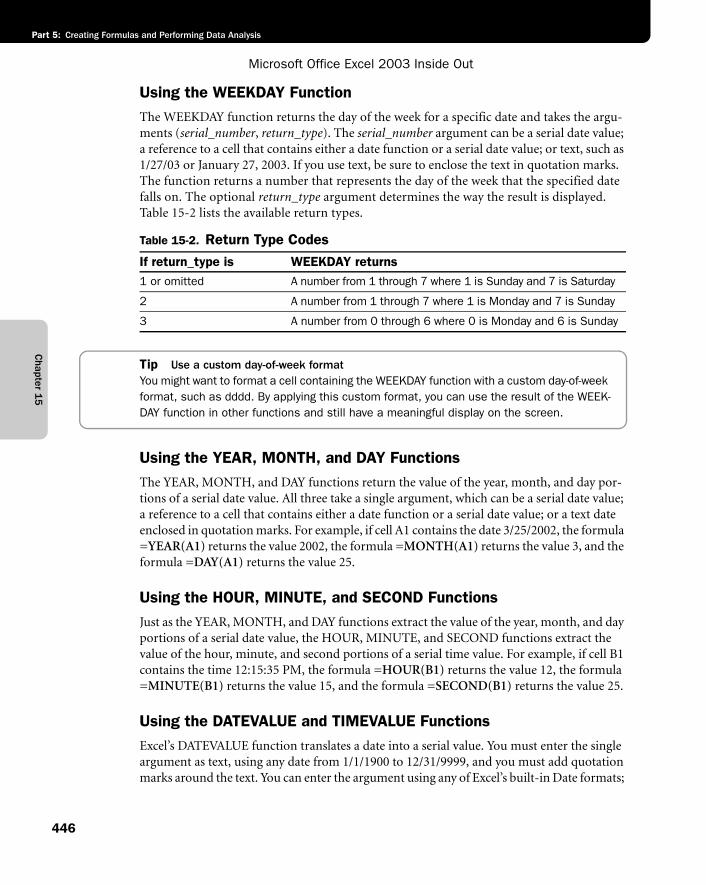
Chapter 1

5

Microsoft Office Excel 2003 Inside Out

Part 5: Creating Formulas and Performing Data Analysis

446

Using the WEEKDAY FunctionThe WEEKDAY function returns the day of the week for a specific date and takes the argu-ments (serial_number, return_type). The serial_number argument can be a serial date value; a reference to a cell that contains either a date function or a serial date value; or text, such as 1/27/03 or January 27, 2003. If you use text, be sure to enclose the text in quotation marks. The function returns a number that represents the day of the week that the specified date falls on. The optional return_type argument determines the way the result is displayed. Table 15-2 lists the available return types.

Tip Use a custom day-of-week formatYou might want to format a cell containing the WEEKDAY function with a custom day-of-week format, such as dddd. By applying this custom format, you can use the result of the WEEK-DAY function in other functions and still have a meaningful display on the screen.

Using the YEAR, MONTH, and DAY FunctionsThe YEAR, MONTH, and DAY functions return the value of the year, month, and day por-tions of a serial date value. All three take a single argument, which can be a serial date value; a reference to a cell that contains either a date function or a serial date value; or a text date enclosed in quotation marks. For example, if cell A1 contains the date 3/25/2002, the formula =YEAR(A1) returns the value 2002, the formula =MONTH(A1) returns the value 3, and the formula =DAY(A1) returns the value 25.

Using the HOUR, MINUTE, and SECOND FunctionsJust as the YEAR, MONTH, and DAY functions extract the value of the year, month, and day portions of a serial date value, the HOUR, MINUTE, and SECOND functions extract the value of the hour, minute, and second portions of a serial time value. For example, if cell B1 contains the time 12:15:35 PM, the formula =HOUR(B1) returns the value 12, the formula =MINUTE(B1) returns the value 15, and the formula =SECOND(B1) returns the value 25.

Using the DATEVALUE and TIMEVALUE FunctionsExcel’s DATEVALUE function translates a date into a serial value. You must enter the single argument as text, using any date from 1/1/1900 to 12/31/9999, and you must add quotation marks around the text. You can enter the argument using any of Excel’s built-in Date formats;

Table 15-2. Return Type Codes

If return_type is WEEKDAY returns1 or omitted A number from 1 through 7 where 1 is Sunday and 7 is Saturday

2 A number from 1 through 7 where 1 is Monday and 7 is Sunday

3 A number from 0 through 6 where 0 is Monday and 6 is Sunday

Cha

pter

15

Formatting and Calculating Date and Time

447

Part 5: Creating Formulas and Performing Data Analysis

however, if you enter the date without a year, Excel uses the current year from your com-puter’s internal clock. For example, the formula =DATEVALUE("December 31, 2010")returns the serial value 40,543.

Similarly, the TIMEVALUE function translates a time into a decimal value. You must enter its single argument as text. You can use any of Excel’s built-in Time formats, but you must add quotation marks around the text. For example, the formula =TIMEVALUE("4:30 PM")returns the decimal value 0.6875.

Working with Specialized Date FunctionsExcel includes a set of specialized date functions that perform operations such as calculations for the maturity dates of securities, for payroll, and for work schedules. The functions described in this section are available only if you install the Analysis ToolPak add-in.

For information about installing the Analysis ToolPak add-in, see “Installing the Analysis ToolPak” on page 403.

Using the EDATE and EOMONTH FunctionsYou can use the EDATE function to calculate the exact date that occurs an indicated number of months before or after a given date. It takes the arguments (start_date, months), where start_date is the date you want to use as a starting point, and months is an integer value that indicates the number of months before or after the start date. If the months value is positive, the function returns a date after the start date; if the months value is negative, the function returns a date before the start date. For example, to find the date that falls exactly 23 months after June 12, 2003, enter the formula =EDATE("6/12/03", 23), which returns the value 38484, or May 12, 2005.

The EOMONTH function returns a date that is an indicated number of months before or after a given date. Although EOMONTH is similar to EDATE and takes the same arguments, the value returned is always rounded up to the last day of the month. For example, to calcu-late the serial date value that is the last day of the month 23 months after June 12, 2003, enter the formula =EOMONTH("6/12/2003", 23), which returns 38503, or May 31, 2005.

Using the YEARFRAC FunctionThe YEARFRAC function calculates a decimal number that represents the portion of a year that falls between two given dates. This function takes the arguments (start_date, end_date,basis), where start_date and end_date specify the period of time you want to convert to a fractional year. The basis argument is the type of day count you want to use, as described in Table 15-3.

Chapter 1

5

Microsoft Office Excel 2003 Inside Out

Part 5: Creating Formulas and Performing Data Analysis

448

For example, to determine the fraction of a year that falls between 4/12/04 and 12/15/04, you can enter the formula =YEARFRAC("4/12/04", "12/15/04"). This formula returns 0.675, based on the default 30-day month and 360-day year.

Using the WORKDAY and NETWORKDAYS FunctionsThe WORKDAY and NETWORKDAYS functions are invaluable for anyone who calculates payroll and benefits or determines work schedules. Both functions return values based on working days, excluding weekend days. In addition, you can choose whether to include holi-days and specify the exact dates.

The WORKDAY function returns the date that is an indicated number of working days before or after a given date. This function takes the arguments (start_date, days, holidays),where start_date is the date you want the function to count from, and days is the number of workdays before or after the start date, excluding weekends and holidays. Use a positive value for days to count forward from the start date; use a negative value to count back-ward. The optional holidays argument can be an array or a reference to a cell range that contains any dates that you want to exclude from the calculation. If you leave holidaysblank, the function counts all weekdays from the start date. For example, to determine the date that is 100 working days, not counting holidays, from the current date, use the formula =WORKDAY(NOW( ),100).

Similarly, the NETWORKDAYS function calculates the number of working days between two given dates. It takes the arguments (start_date, end_date, holidays). For example, to deter-mine the number of working days between January 15, 2004 and June 30, 2004, use the formula =NETWORKDAYS("1/15/04", "6/30/04"), which results in a value of 120.

Table 15-3. Basis Codes

If basis is YEARFRAC returns0 (or omitted) 30/360, or 30 days per month and 360 days per year, as established

in the United States by the National Association of Security Dealers (NASD)

1 Actual/actual, or the actual number of days in the month(s)/actual days in the year

2 Actual/360

3 Actual/365

4 European 30/360

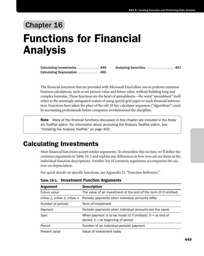
449

Part 5: Creating Formulas and Performing Data Analysis

Chapter 16

Functions for Financial Analysis

Calculating Investments . . . . . . . . . . . . 449Calculating Depreciation. . . . . . . . . . . . 455

Analyzing Securities . . . . . . . . . . . . . . . . 457

The financial functions that are provided with Microsoft Excel allow you to perform common business calculations, such as net present value and future value, without building long and complex formulas. These functions are the heart of spreadsheets—the word “spreadsheet” itself refers to the seemingly antiquated system of using special grid paper to track financial informa-tion. Functions have taken the place of the old 10-key calculator sequences (“algorithms”) used by accounting professionals before computers revolutionized the discipline.

Note Many of the financial functions discussed in this chapter are included in the Analy-sis ToolPak add-in. For information about accessing the Analysis ToolPak add-in, see “Installing the Analysis ToolPak” on page 403.

Calculating InvestmentsMost financial functions accept similar arguments. To streamline this section, we’ll define the common arguments in Table 16-1 and explain any differences in how you can use them in the individual function descriptions. Another list of common arguments accompanies the sec-tion on depreciation.

For quick details on specific functions, see Appendix D, “Function Reference.”

Table 16-1. Investment Function Arguments

Argument DescriptionFuture value The value of an investment at the end of the term (0 if omitted)

Inflow 1, inflow 2, inflow n Periodic payments when individual amounts differ

Number of periods Term of investment

Payment Periodic payments when individual amounts are the same

Type When payment is to be made (0 if omitted); 0 = at end of period; 1 = at beginning of period

Period Number of an individual periodic payment

Present value Value of investment today

Chapter 1

6

Microsoft Excel Inside Out

Part 5: Creating Formulas and Performing Data Analysis

450

The PV FunctionPresent value is one of the most common methods for measuring the attractiveness of a long-term investment. Present value is today’s value of the investment. It’s determined by dis-counting the inflows (payments received) from the investment back to the present time. If the present value of the inflows is greater than the cost of the investment, the investment is a good one.

The PV function computes the present value of a series of equal periodic payments or of a lump-sum payment. (A series of equal payments is often called an ordinary annuity.) This function takes the arguments (rate, number of periods, payment, future value, type); for definitions of these arguments, see Table 16-1. To compute the present value of a series of payments, enter a value for the payment argument, or to compute the present value of a lump-sum payment, enter a value for the future value argument. For an investment with both a series of payments and a lump-sum payment, use both arguments.

Here’s a real-world example of how this function works: Suppose you are presented with an investment opportunity that returns $1,000 each year over the next five years. To receive this annuity, you must invest $4,000. Are you willing to pay $4,000 today to earn $5,000 over the next five years? To decide whether this investment is acceptable, you need to determine the present value of the stream of $1,000 payments you will receive.

Because you could invest your money in a 5-year CD money-market account at 3.5 percent, we’ll use 3.5 percent as the discount rate of the investment. (Because this discount rate is a sort of hurdle over which an investment must leap before it becomes attractive to you, it’s often called the hurdle rate.) To determine the present value of this investment, use the for-mula =PV(3.5%, 5, 1000), which returns the value 4515.05, meaning that you should be willing to spend $4,515.05 now to receive $5,000 over the next five years. Because your investment is only $4,000, you can surmise that this is an acceptable investment.

Suppose you’re offered $5,000 at the end of five years instead of $1,000 for each of the next five years. Is the investment still as attractive? To find out, use the formula =PV(3.5%, 5, 5000). (Include a comma as a placeholder for the unused payment argument.) This formula returns the present value 4209.87, which means that, at a hurdle rate of 3.5 percent, you should be willing to spend $4,209.87 to receive $5,000 in five years. Although the proposal may not be as attractive under these terms, it’s still acceptable because your investment is only $4,000.

Rate Discount rate or interest rate

Guess A starting interest rate for iterative calculations (10 percent if omitted)

Finance rate The rate at which you borrow money to purchase an investment

Reinvestment rate The rate at which you reinvest cash received from an investment

Table 16-1. Investment Function Arguments

Argument Description

Cha

pter

16

Functions for Financial Analysis

451

Part 5: Creating Formulas and Performing Data Analysis

The NPV FunctionThe NPV function calculates the net present value, which is another common method for determining the profitability of an investment. In general, any investment that yields a net present value greater than zero is considered profitable. This function takes the arguments (rate, inflow 1, inflow 2, ...); for definitions of these arguments, see Table 16-1. You can use as many as 29 inflow values as arguments, but you can include any number of values by using an array as an argument.

NPV differs from PV in two important respects. Whereas PV assumes constant inflow values, NPV allows variable payments. The other major difference is that PV allows payments and receipts to occur at either the beginning or end of the period, whereas NPV assumes that all payments and receipts are evenly distributed and that they occur at the end of each period. If the cost of the investment must be paid up front, you should not include the cost as one of the function’s inflow arguments but should subtract it from the result of the function. On the other hand, if the cost must be paid at the end of the first period, you should include it as a negative first inflow argument. Let’s consider an example to help clarify this distinction.

Suppose you are contemplating an investment on which you expect to incur a loss of $85,000 at the end of the first year, followed by gains of $95,000, $140,000, and $185,000 at the ends of the second, third, and fourth years. You will invest $250,000 up front, and the hurdle rate is 8 percent. To evaluate this investment, use the formula =NPV(8%, 85000, 95000, 140000, 185000) 250000.

Note The result, 139.48, tells you not to expect a net profit from this investment. Note that the negative values in this formula indicate the money you spend on your investment. (You can use the Goal Seek command to determine what initial cost or interest rate would justify the investment.) For more information about this command, see “Using the Goal Seek Command” on page 507.

This formula does not include the up-front cost of the investment as an argument for the NPV function. However, if you make the initial $250,000 investment at the end of the first year, the formula is =NPV(8%,( 250000 85000), 95000, 140000, 185000). The result, $18,379.04, would suggest that this might be a profitable investment.

The FV FunctionThe FV function determines the future value of an investment and is essentially the opposite of present value, computing the value at some future date of an investment that makes pay-ments as a lump sum or as a series of equal periodic payments. This function takes the argu-ments (rate, number of periods, payment, present value, type); for definitions of these arguments, see Table 16-1. Use the payment argument to compute the future value of a series of payments and the present value argument to compute the future value of a lump-sum payment.

Chapter 1

6

Microsoft Excel Inside Out

Part 5: Creating Formulas and Performing Data Analysis

452

Suppose you’re thinking about starting an IRA. You plan to deposit $2,000 in the IRA at the beginning of each year, and you expect the average rate of return to be 6 percent per year for the entire term. Assuming you’re now 30 years old, how much money will your account accu-mulate by the time you’re 65? Use the formula =FV(6%, 35, 2000, , 1) to learn that your IRA balance will be $236,241.73 at the end of 35 years.

Now assume that you started an IRA account three years ago and have already accumulated $7,500 in your account. Use the formula =FV(6%, 35, 2000, 7500, 1) to learn that your IRA will grow to $293,887.38 at the end of 35 years.

In both of these examples, the type argument is 1, because payments occur at the beginning of the period. Including this argument is particularly important in financial calculations that span many years. If you omit the type argument in the preceding formula, Excel assumes that you add money to your account at the end of each year and returns the value $280,515.21—a difference of $13,372.17!

The PMT FunctionThe PMT function computes the periodic payment required to amortize a loan over a speci-fied number of periods. This function takes the arguments (rate, number of periods, present value, future value, type); for definitions of these arguments, see Table 16-1.

Suppose you want to take out a 30-year mortgage for $100,000. Assuming an interest rate of 6 percent, what will your monthly payments be? First, divide the 6-percent interest rate by 12 to arrive at a monthly rate (0.5 percent). Next, convert the number of periods into months by multiplying 30 by 12 (360). You can include these computations as arguments using the formula =PMT((6%/12), (30*12), 100000) to compute the monthly mortgage payment, which turns out to be $599.55. (The result is negative because it’s a cost to you.)

TroubleshootingPMT function produces unrealistic results

Sometimes you might find that the PMT function seems to produce unrealistic results—such as payments that are excessively large. As is the case with all functions used for cal-culating investments, make sure you are using the same units for both the rate and nper(number of periods) arguments. If, for example, you type 6% for the rate, you must enter the nper argument in years, because 6 percent is an annual rate. If you type 6% for the rate and 360 as the term, Excel returns the payment required to amortize a loan at either 6 percent per month for 30 years or 6 percent per year for 360 years! You can resolve your problem by either dividing 6 percent by 12 (which is the standard way of expressing a loan) or typing 30 for nper, indicating the term in years. Note, however, that these two options are not equivalent—they yield very different results because of the way interest is calculated. You should use the same units that your lender uses, which is probably annual interest rate divided by 12 and nper expressed in months.

Cha

pter

16

Functions for Financial Analysis

453

Part 5: Creating Formulas and Performing Data Analysis

The IPMT FunctionThe IPMT function computes the interest part of an individual payment made to repay an amount over a specified time period, with constant periodic payments and a constant inter-est rate. This function takes the arguments (rate, period, number of periods, present value, future value, type); for definitions of these arguments, see Table 16-1.

Suppose you borrow $100,000 for 30 years at 6 percent interest. The formula =IPMT((6/12)%, 1, 360, 100000) tells you that the interest component of the payment due for the first month is an even $500.00. The formula =IPMT((6/12)%, 360, 360, 100000) tells you that the inter-est component of the final payment of the same loan is $2.98.

The PPMT FunctionThe PPMT function is similar to the IPMT function, except that it computes the principal component of an individual payment when a loan is repaid over a specified time with con-stant periodic payments and a constant interest rate. If you compute both IPMT and PPMT for the same period, you can add the results to obtain the total payment. The PPMT function takes the arguments (rate, period, number of periods, present value, future value, type); for def-initions of these arguments, see Table 16-1.

If you borrow $100,000 for 30 years at 6 percent interest, the formula =PPMT((6/12)%, 1, 360, 100000) tells you that the principal component of the payment for the first month of the loan is $99.55. The formula =PPMT((6/12)%, 360, 360, 100000) tells you that the principal component of the final payment of the same loan is $596.57.

The NPER FunctionThe NPER function computes the number of periods required to amortize a loan, given a specified periodic payment. This function takes the arguments (rate, payment, present value, future value, type); for definitions of these arguments, see Table 16-1.

Suppose you can afford mortgage payments of $1,000 per month and you want to know how long it will take to pay off a $100,000 loan at 6 percent interest. The formula =NPER((6%/12), 1000, 100000) tells you that your mortgage payments will extend over 138.98 months.

If the payment is too small to amortize the loan at the indicated rate of interest, the function returns an error value. The monthly payment must be at least equal to the period interest rate times the principal amount; otherwise, the loan will never be amortized. For example, the formula =NPER((6/12)%, 500, 100000) returns the #NUM! error value. In this case, the monthly payment must be at least $501 to amortize the loan (although it would take more than 100 years worth of payments at that amount).

The RATE FunctionThe RATE function determines the rate of return of an investment that generates a series of equal periodic payments or a single lump-sum payment. This function takes the arguments

Chapter 1

6

Microsoft Excel Inside Out

Part 5: Creating Formulas and Performing Data Analysis

454

(number of periods, payment, present value, future value, type, guess); for definitions of these arguments, see Table 16-1. You use either the payment argument to compute the rate for a series of equal periodic payments or the future value argument to compute the rate of a lump-sum payment.

Suppose you’re considering an investment that will pay you four annual $1,000 payments. The investment costs $3,000. To determine the actual annual rate of return on your invest-ment, use the formula =RATE(4, 1000, 3000). This formula returns 13 percent, an excellent rate of return on this investment.

Note The RATE function uses an iterative process to compute the rate of return. The function begins by computing the net present value of the investment at the guess rate. If that first net present value is greater than zero, the function selects a higher rate and repeats the net present value calculation; if the first net present value is less than zero, the function selects a lower rate for the second iteration. RATE continues this process until it arrives at the correct rate of return or until it has gone through 20 iterations. For more infor-mation about iteration, see “Using Circular References” on page 382.

If you receive the #NUM! error value when you enter the RATE function, Excel probably can-not calculate the rate within 20 iterations. Try entering a different guess rate to give the func-tion a running start. A rate from 10 percent through 100 percent usually works.

The IRR FunctionThe IRR function determines the internal rate of return of an investment, which is the rate that causes the net present value of the investment to equal zero. In other words, the internal rate of return is the rate that causes the present value of the inflows from an investment to equal the cost of the investment.

Internal rate of return, like net present value, is used to compare one investment opportunity with another. An attractive investment is one whose net present value, discounted at the appropriate hurdle rate, is greater than zero. Turn that equation around and you can see that the discount rate required to generate a net present value of zero must be greater than the hurdle rate. Thus, an attractive investment is one for which the discount rate required to yield a net present value of zero—that is, the internal rate of return—is greater than the hur-dle rate.

The IRR function takes the arguments (values, guess). (For definitions of these arguments, see Table 16-1.) The values argument is an array or a reference to a range of cells that contain numbers. Only one values argument is allowed, and it must include at least one positive and one negative value. IRR ignores text, logical values, and blank cells. IRR assumes that trans-actions occur at the end of a period and returns the equivalent interest rate for that period’s length. The guess argument is optional, but if you receive the #NUM! error value, try includ-ing a guess to help Excel reach the answer.

Suppose you agree to buy an income property for $120,000 and rent it out. Over the next five years, you expect to receive $22,000, $24,000, $28,000, $31,000, and $33,000 in net rental income. You can set up a simple worksheet that contains your investment and income

Cha

pter

16

Functions for Financial Analysis

455

Part 5: Creating Formulas and Performing Data Analysis

information. Enter the six values into cells A1:A6 of the worksheet. (Be sure to enter the initial $120,000 investment as a negative value.) Then the formula =IRR(A1:A6) returns the internal rate of return of 5 percent. If the hurdle rate is 3.5 percent, you can consider this condominium purchase a good investment.

The MIRR FunctionThe MIRR function calculates the modified internal rate of return of an investment. The dif-ference from the IRR function is that MIRR takes into account the cost of the money you borrow to finance the investment. MIRR assumes that you’ll reinvest the cash it generates and that transactions occur at the end of a period. It then returns the equivalent interest rate for that period’s length.

The MIRR function takes the arguments (values, finance rate, reinvestment rate). (For defini-tions of these arguments, see Table 16-1.) The values argument must be an array or a refer-ence to a range of cells that contain numbers. This argument represents a series of payments and income occurring at regular periods. You must include at least one positive and one neg-ative value in the values argument. For example, if cells A1 through A6 contain the values 120000, 22000, 24000, 28000, 31000, and 33000, the formula =MIRR(A1:A6, 7%, 3.5%)

returns a modified internal rate of return of 4 percent.

Calculating DepreciationDepreciation has an enormous effect on the bottom line of any business, and accurate calcu-lation of depreciation is crucial if you want to avoid triggering a detailed scrutiny of your records by the IRS. These functions help you precisely determine the depreciation of an asset for a specific period. Table 16-2 lists the common arguments used in these functions:

The SLN FunctionThe SLN function determines the straight-line depreciation for an asset for a single period. This depreciation method assumes that depreciation is uniform throughout the useful life of the asset. The cost or basis of the asset, less its estimated salvage value, is deductible in equal amounts over the life of the asset. This function takes the arguments (cost, salvage, life). (For definitions of these arguments, see Table 16-2.)

Table 16-2. Depreciation Function Arguments

Argument DescriptionCost Initial cost of the asset

Life Length of time the asset will be depreciated

Period Individual time period to be computed

Salvage Asset’s remaining value after it has been fully depreciated

Chapter 1

6

Microsoft Excel Inside Out

Part 5: Creating Formulas and Performing Data Analysis

456

Suppose you want to determine the depreciation for each year of a machine that costs $8,000 new, has a life of 10 years, and has a salvage value of $500. The formula =SLN(8000, 500, 10)tells you that each year’s straight-line depreciation is $750.

The DDB and DB FunctionsThe DDB (double declining balance) function computes an asset’s depreciation at an accel-erated rate—more in the early periods and less later. Using this method, depreciation is com-puted as a percentage of the net book value of the asset (the cost of the asset less any prior years’ depreciation).

The function takes the arguments (cost, salvage, life, period, factor). All DDB arguments must be positive numbers, and you must use the same time units for life and period; that is, if you express life in months, period must also be in months. The factor argument is optional and has a default value of 2, which indicates the normal double-declining balance method. Using 3 for the factor argument specifies the triple-declining balance method. For other argument definitions, see Table 16-2.

Suppose you want to calculate the depreciation of a machine that costs $5,000 new and that has a life of five years (60 months) and a salvage value of $100. The formula =DDB(5000,100, 60, 1) tells you that the double-declining balance depreciation for the first month is $166.67. (Note that life is expressed in months.) The formula =DDB(5000, 100, 5, 1) tells you that the double-declining balance depreciation for the first year is $2,000.00. (Note that life is expressed in years.)

The DB (declining balance) function is similar to the DDB function except that it uses the fixed declining balance method of depreciation and can calculate depreciation for a particu-lar period in the asset’s life. It takes the arguments (cost, salvage, life, period, month). The lifeand period arguments must use the same units. The optional month argument is the number of months depreciated in the first year, which, if omitted, is 12—a full year. For example, to calculate the real depreciation for the first period on a $1,000,000 item with a salvage value of $100,000, a life of six years, and seven months in the first year, use the formula =DB(1000000, 100000, 6, 1, 7), which returns $186,083.33.

The VDB FunctionThe VDB (variable declining balance) function calculates the depreciation of an asset for any complete or partial period, using either the double-declining balance or another accelerated-depreciation factor that you specify.

This function takes the arguments (cost, salvage, life, start, end, factor, no switch). The startargument is the period after which depreciation will be calculated, and end is the last period for which depreciation will be calculated. These arguments determine the depreciation for any length of time during the life of the asset. The life, start, and end arguments must all use the same units (days, months, or years). The optional factor argument is the rate at which the

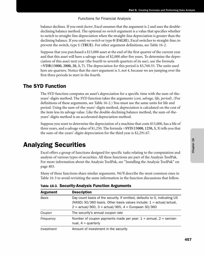
Cha

pter

16

Functions for Financial Analysis

457

Part 5: Creating Formulas and Performing Data Analysis

balance declines. If you omit factor, Excel assumes that the argument is 2 and uses the double-declining balance method. The optional no switch argument is a value that specifies whether to switch to straight-line depreciation when the straight-line depreciation is greater than the declining balance. If you omit no switch or type 0 (FALSE), Excel switches to straight-line; to prevent the switch, type 1 (TRUE). For other argument definitions, see Table 16-2.

Suppose that you purchased a $15,000 asset at the end of the first quarter of the current year and that this asset will have a salvage value of $2,000 after five years. To determine the depre-ciation of this asset next year (the fourth to seventh quarters of its use), use the formula =VDB(15000, 2000, 20, 3, 7). The depreciation for this period is $3,760.55. The units used here are quarters. Notice that the start argument is 3, not 4, because we are jumping over the first three periods to start in the fourth.

The SYD FunctionThe SYD function computes an asset’s depreciation for a specific time with the sum-of-the-years’-digits method. The SYD function takes the arguments (cost, salvage, life, period). (For definitions of these arguments, see Table 16-2.) You must use the same units for life and period. Using the sum-of-the-years’-digits method, depreciation is calculated on the cost of the item less its salvage value. Like the double-declining balance method, the sum-of-the-years’-digits method is an accelerated depreciation method.

Suppose you want to determine the depreciation of a machine that costs $15,000, has a life of three years, and a salvage value of $1,250. The formula =SYD(15000, 1250, 3, 3) tells you that the sum-of-the-years’-digits depreciation for the third year is $2,291.67.

Analyzing SecuritiesExcel offers a group of functions designed for specific tasks relating to the computation and analysis of various types of securities. All these functions are part of the Analysis ToolPak. For more information about the Analysis ToolPak, see “Installing the Analysis ToolPak” on page 403.

Many of these functions share similar arguments. We’ll describe the most common ones in Table 16-3 to avoid revisiting the same information in the function discussions that follow.

Table 16-3. Security-Analysis Function Arguments

Argument DescriptionBasis Day count basis of the security. If omitted, defaults to 0, indicating US

(NASD) 30/360 basis. Other basis values include: 1 = actual/actual, 2 = actual/360, 3 = actual/365, 4 = European 30/360

Coupon The security’s annual coupon rate

Frequency Number of coupon payments made per year: 1 = annual, 2 = semian-nual, 4 = quarterly

Investment Amount of investment in the security

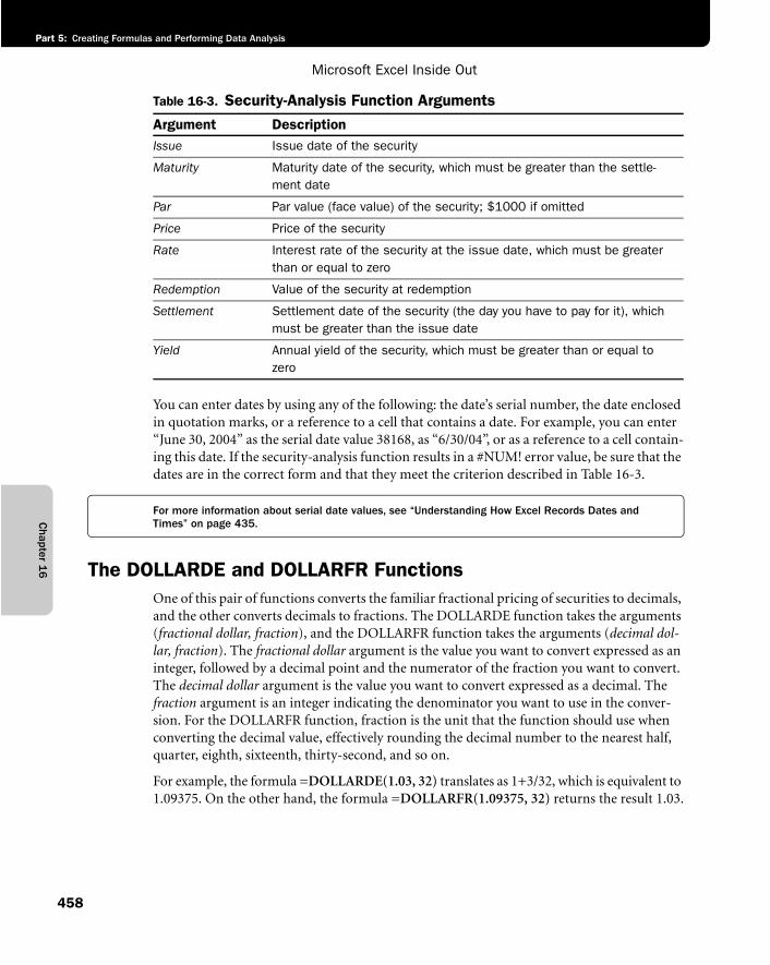
Chapter 1

6

Microsoft Excel Inside Out

Part 5: Creating Formulas and Performing Data Analysis

458

You can enter dates by using any of the following: the date’s serial number, the date enclosed in quotation marks, or a reference to a cell that contains a date. For example, you can enter “June 30, 2004” as the serial date value 38168, as “6/30/04”, or as a reference to a cell contain-ing this date. If the security-analysis function results in a #NUM! error value, be sure that the dates are in the correct form and that they meet the criterion described in Table 16-3.

For more information about serial date values, see “Understanding How Excel Records Dates and Times” on page 435.

The DOLLARDE and DOLLARFR FunctionsOne of this pair of functions converts the familiar fractional pricing of securities to decimals, and the other converts decimals to fractions. The DOLLARDE function takes the arguments (fractional dollar, fraction), and the DOLLARFR function takes the arguments (decimal dol-lar, fraction). The fractional dollar argument is the value you want to convert expressed as an integer, followed by a decimal point and the numerator of the fraction you want to convert. The decimal dollar argument is the value you want to convert expressed as a decimal. The fraction argument is an integer indicating the denominator you want to use in the conver-sion. For the DOLLARFR function, fraction is the unit that the function should use when converting the decimal value, effectively rounding the decimal number to the nearest half, quarter, eighth, sixteenth, thirty-second, and so on.

For example, the formula =DOLLARDE(1.03, 32) translates as 1+3/32, which is equivalent to 1.09375. On the other hand, the formula =DOLLARFR(1.09375, 32) returns the result 1.03.

Issue Issue date of the security

Maturity Maturity date of the security, which must be greater than the settle-ment date

Par Par value (face value) of the security; $1000 if omitted

Price Price of the security

Rate Interest rate of the security at the issue date, which must be greater than or equal to zero

Redemption Value of the security at redemption

Settlement Settlement date of the security (the day you have to pay for it), which must be greater than the issue date

Yield Annual yield of the security, which must be greater than or equal to zero

Table 16-3. Security-Analysis Function Arguments

Argument Description

Cha

pter

16

Functions for Financial Analysis

459

Part 5: Creating Formulas and Performing Data Analysis

The ACCRINT and ACCRINTM FunctionsThe ACCRINT function returns the interest accrued by a security that pays interest on a peri-odic basis. This function takes the arguments (issue, first interest, settlement, rate, par, fre-quency, basis); in which first interest indicates the date on which interest is first accrued; for other argument definitions, see Table 16-3. For example, suppose a Treasury bond has an issue date of March 1, 2004, a settlement date of April 1, 2004, a first interest date of Septem-ber 1, 2004, a 7-percent coupon rate with semiannual frequency, a par value of $1,000, and a basis of 30/360. The accrued interest formula is =ACCRINT("3/1/04", "9/1/04", "4/1/04", 0.07, 1000, 2, 0) which returns 5.833333, indicating that $5.83 accrues between March 1, 2004, and April 1, 2004.

Similarly, the ACCRINTM function returns the interest accrued by a maturity security (a type of security with not only a rhyming name, but which also pays interest at maturity). This function takes the arguments (issue, settlement, rate, par, basis). Using the preceding example with a maturity date of July 31, 2008, the accrued interest formula is =ACCRINTM("3/1/04", "7/31/08", 0.07, 1000, 0), which returns 309.1667, indicating that the $1,000 bond will pay $309.17 interest on July 31, 2008.

The INTRATE and RECEIVED FunctionsThe INTRATE function calculates the rate of interest, or discount rate, for a fully invested security. This function takes the arguments (settlement, maturity, investment, redemption, basis); for argument definitions, see Table 16-3. For example, suppose a bond has a settle-ment date of March 31, 2004, and a maturity date of September 30, 2004. A $1,000,000 investment in this bond will have a redemption value of $1,032,324, using the default 30/360 basis. The bond’s discount rate formula is =INTRATE("3/31/04", "9/30/04", 1000000, 1032324, 0), which returns 0.064648, or 6.46 percent.

Similarly, the RECEIVED function calculates the amount received at maturity for a fully invested security, and takes the arguments (settlement, maturity, investment, discount, basis). Using the preceding example with a 5.5 percent discount rate, the formula =RECEIVED("3/31/04", "9/30/04", 1000000, 0.055, 0) returns the mature value $1,028,277.63.

The PRICE, PRICEDISC, and PRICEMAT FunctionsThe PRICE function calculates the price per $100 of face value of a security that pays interest on a periodic basis. This function takes the arguments (settlement, maturity, rate, yield, redemption, frequency, basis); for argument definitions, see Table 16-3. For example, suppose a bond’s settlement date is March 31, 2004, its maturity date is July 31, 2004, and the interest rate is 5.75 percent, with semiannual frequency. The security’s annual yield is 6.50 percent, its redemption value is $100, and it’s calculated using the standard 30/360 basis. The bond price formula is =PRICE("3/31/04", "7/31/04", 0.0575, 0.065, 100, 2, 0), which returns $99.73498.

Chapter 1

6

Microsoft Excel Inside Out

Part 5: Creating Formulas and Performing Data Analysis

460

Similarly, the PRICEDISC function returns the price per $100 of face value of a security that is discounted, instead of paying periodic interest. This function takes the arguments (settle-ment, maturity, discount, redemption, basis). Using the preceding example with the addition of a discount amount of 7.5 percent, the formula =PRICEDISC("3/31/04", "7/31/04", 0.075, 100, 0) returns a price of $97.50.

Finally, the PRICEMAT function returns the price per $100 of face value of a security that pays its interest at the maturity date. This function takes the arguments (settlement, maturity, issue, rate, yield, basis). Using the preceding example with a settlement date of July 31, 2004, an issue date of March 1, 2004, and the maturity date changed to July 31, 2005, the formula =PRICEMAT("7/31/04", "7/31/05", "3/31/04", 0.0575, 0.065, 0) returns $99.18.

The DISC FunctionThe DISC function calculates the discount rate for a security and takes the arguments (settle-ment, maturity, price, redemption, basis). (For argument definitions, see Table 16-3.) For example, suppose a bond has a settlement date of June 15, 2004, a maturity date of December 31, 2004, a price of $96.875, and a $100 redemption value, and uses the standard 30/360 basis. The bond discount rate formula =DISC("6/15/04", "12/31/04", 96.875, 100, 0) returns 0.057398, or 5.74 percent.

The YIELD, YIELDDISC, and YIELDMAT FunctionsThe YIELD function determines the annual yield for a security that pays interest on a peri-odic basis and takes the arguments (settlement, maturity, rate, price, redemption, frequency, basis); for definitions of these arguments, see Table 16-3. For example, suppose a bond has a settlement date of February 15, 2004, a maturity date of December 1, 2004, a coupon rate of 5.75 percent with semiannual frequency, a price of $99.2345, and a $100 redemption value, and uses the standard 30/360 basis. The annual bond yield formula =YIELD("2/15/04", "12/1/04", 0.0575, 99.2345, 100, 2, 0) returns 0.067406, or 6.74 percent.

The YIELDDISC function, on the other hand, calculates the annual yield for a discounted secu-rity. It takes the arguments (settlement, maturity, price, redemption, basis). Using the preceding example but changing the price to $96.00, the bond yield formula =YIELDDISC("2/15/04", "12/1/04", 96, 100, 0) returns 0.052448, or 5.25 percent.

The YIELDMAT function calculates the annual yield for a security that pays its interest at maturity. This function takes the arguments (settlement, maturity, issue, rate, price, basis).Using the arguments from the YIELD example but adding an issue date of January 1, 2002, and changing the price to $99.2345, the yield-at-maturity formula =YIELDMAT("2/15/04", "12/1/04", "1/1/04", 0.0575, 99.2345, 0) returns 0.067178, or 6.72 percent.

Cha

pter

16

Functions for Financial Analysis

461

Part 5: Creating Formulas and Performing Data Analysis

TroubleshootingExcel 2003 has functions that have changed and may produce different results

Three functions—YIELD, ODDFYIELD, and ODDFPRICE—have been changed in the way that they calculate basis. Workbooks that were created in Excel 7 or earlier containing any of these functions may display results that are different from identical formulas created in ver-sions of Excel later than 7. Even if you have repeatedly saved the workbook in subsequent versions of Excel, the incorrect results may persist. If you have workbooks that have been around this long containing any of these functions, you simply need to force recalculation by pressing CTRL+ALT+F9. Doing so recalculates every formula in every sheet of every open workbook. For more about the ODDFYIELD and ODDFPRICE functions, see Appendix D, “Function Reference.”

The TBILLEQ, TBILLPRICE, and TBILLYIELD FunctionsThe TBILLEQ function calculates the bond-equivalent yield for a Treasury bill. It takes the arguments (settlement, maturity, discount). (For argument definitions, see Table 16-3.) For example, suppose a Treasury bill has a settlement date of February 1, 2004, a maturity date of July 1, 2004, and a discount rate of 8.65 percent. The formula for calculating the bond yield that is equivalent to the yield of a Treasury bill =TBILLEQ("2/1/04", "7/1/04", 0.0865)returns 0.091, or 9.1 percent.

You use the TBILLPRICE function to calculate the price per $100 of face value for a Treasury bill. This function takes the arguments (settlement, maturity, discount). Using the preceding example, the formula to calculate the price per $100 of face value, =TBILLPRICE("2/1/04","7/1/04", 0.0865), returns 96.3718, or $96.37.

Finally, the TBILLYIELD function calculates a Treasury bill’s yield. It takes the arguments (settlement, maturity, price). Using the preceding example with its result, a price of $96.40, the yield formula =TBILLYIELD("2/1/04", "7/1/04", 96.40) returns the yield 0.08903, or 8.9 percent.

The COUPDAYBS, COUPDAYS, COUPDAYSNC, COUPNCD,COUPNUM, and COUPPCD Functions

The following group of functions performs calculations relating to bond coupons. For all the sample formulas in this section, we’ll use as our example a bond with a settlement date of March 1, 2004 and a maturity date of December 1, 2004. Its coupons are payable semiannu-ally, using the actual/actual basis (that is, a basis argument of 1). All these functions take the same arguments: (settlement, maturity, frequency, basis). (For definitions of these arguments, see Table 16-3.)

The COUPDAYBS function calculates the number of days from the beginning of the coupon period to the settlement date. Using our sample data, the formula =COUPDAYBS("3/1/04", "12/1/04", 2, 1) returns 91.

Chapter 1

6

Microsoft Excel Inside Out

Part 5: Creating Formulas and Performing Data Analysis

462

The COUPDAYS function calculates the number of days in the coupon period that con-tains the settlement date. Using our sample data, the formula =COUPDAYS("3/1/04", "12/1/04", 2, 1) returns 183.

The COUPDAYSNC function calculates the number of days from the settlement date to the next coupon date. Using our sample data, the formula =COUPDAYSNC("3/1/04", "12/1/04", 2, 1) returns 92.

The COUPNCD function calculates the next coupon date after the settlement date. Using our sample data, the formula =COUPNCD("3/1/04", "12/1/04", 2, 1) returns 38139, or June 1, 2004.

The COUPNUM function calculates the number of coupons payable between the settlement date and the maturity date and rounds the result to the nearest whole coupon. Using our sample data, the formula =COUPNUM("3/1/04", "12/1/04", 2, 1) returns 2.

The COUPPCD function calculates the coupon date before the settlement date. Using our sample data, the formula =COUPPCD("3/1/04", "12/1/04", 2, 1) returns 37956, or December 1, 2003.

The DURATION and MDURATION FunctionsThe DURATION function calculates the annual duration for a security whose interest pay-ments are made on a periodic basis. Duration is defined as the weighted average of the present value of the bond’s cash flow and is used as a measure of how a bond’s price responds to changes in the yield. This function takes the arguments (settlement, maturity, coupon, yield, frequency, basis). (For argument definitions, see Table 16-3.)

For example, suppose a bond has a settlement date of January 1, 2004, a maturity date of December 31, 2009, a semiannual coupon rate of 8.5 percent, a yield of 9.5 percent, and uses the default 30/360 basis. The resulting formula =DURATION("1/1/04", "12/31/09", 0.085, 0.095, 2, 0) returns a duration of 4.78708.

The MDURATION function calculates the annual modified duration for a security with interest payments made on a periodic basis, adjusted for market yield per number of coupon payments per year. This function takes the arguments (settlement, maturity, coupon, yield, frequency, basis). Using the values from the DURATION formula, the modified duration for-mula looks like this: =MDURATION("1/1/04", "12/31/09", 0.085, 0.095, 2, 0), and returns a value of 4.57.

463

Part 5: Creating Formulas and Performing Data Analysis

Chapter 17

Functions for Analyzing Statistics

Analyzing Distributions of Data. . . . . . . 464Understanding Linear andExponential Regression. . . . . . . . . . . . . 469

Using the Analysis ToolpakData Analysis Tools . . . . . . . . . . . . . . . . 477

Microsoft Excel provides a wide range of features that can help you analyze statistical data. A number of functions that assist in simple analysis tasks, such as AVERAGE, MEDIAN, and MODE, are built into the program. If the built-in statistical functions aren’t enough, you can turn to the Analysis ToolPak, an add-in module that provides a collection of functions and tools to augment the built-in analytic capabilities of Excel. You can use these tools to create histograms, rank-and-percentile tables, extract samples from a data set, perform regression analysis, generate special random-number sets, apply Fourier and other transformations to your data, and more. In this chapter, we’ll explore statistical analysis functions built into Excel, as well as those included with the Analysis ToolPak.

For more information, see “Installing the Analysis ToolPak” on page 403.

Improved AccuracyImproved Accuracy

A number of Excel’s built-in worksheet functions that deal with statistical analysis have been made more accurate, and now produce slightly different rounding results. The ulti-mate precision of these functions has also been increased. The list of enhanced functions is as follows:

BINOMDIST, CHIINV, CONFIDENCE, CRITBINOM, DSTDEV, DSTDEVP, DVAR, DVARP, FINV, FORECAST, GAMMAINV, GROWTH, HYPGEOMDIST, INTERCEPT, LINEST, LOGEST, LOGINV, LOGNORMDIST, NEGBINOMDIST, NORMDIST, NORMINV, NORMSDIST, NORMSINV, PEAR-SON, POISSON, RAND, RSQ, SLOPE, STDEV, STDEVA, STDEVP, STDEVPA, STEYX, TINV, TREND, VAR, VARA, VARP, VARPA, and ZTEST.

Please note that the results returned by these functions may be slightly different in Excel 2003 than the results of the same functions in previous versions of Excel.

Chapter 1

7

Microsoft Office Excel 2003 Inside Out

Part 5: Creating Formulas and Performing Data Analysise

464

Analyzing Distributions of DataIn statistics, a collection of measurements is called a distribution. Excel has several methods that you can use to analyze distributions: built-in statistical functions, the sample and popu-lation statistical functions, or the rank and percentile functions together with the Rank and Percentile tool.

Note You can also analyze distributions using the Descriptive Statistics and Histogram tools, both of which are included in the Analysis Toolpak add-in. For more information about using the Analysis Toolpak tools, see “Using the Analysis Toolpak Data Analysis Tools” on page 477.

Using Built-In Statistical FunctionsYou use the built-in statistical functions to analyze a group (or population) of measurements. In this section, the discussion is limited to the most commonly used statistical functions.

Note Excel also offers the advanced statistical functions LINEST, LOGEST, TREND, and GROWTH, which operate on arrays. For more information, see “Understanding Linear and Exponential Regression” on page 469.

The AVERAGE FunctionThe AVERAGE function computes the arithmetic mean, or average, of the numbers in a range by summing a series of numeric values and then dividing the result by the number of values. This function takes the arguments (number1, number2, ...), can include up to 30 argu-ments, and ignores blank cells and cells containing logical and text values. For example, to calculate the average of the values in cells B4 through B15, you could use the formula =(B4+B5+B6+B7+B8+B9+B10+B11+B12+B13+B14+B15)/12, but it’s obviously more efficient to enter =AVERAGE(B4:B15).

For more information about this function, see the sidebar “AVERAGE vs. AVG” on page 416.

The MEDIAN, MODE, MAX, MIN, and COUNT FunctionsThese functions all take the same arguments: essentially just a cell range or a list of numbers separated by commas, such as (number1, number2, ...), and they can accept up to 30 argu-ments, ignoring text, error values, and logical values. Here’s a brief description of each:

● MEDIAN computes the median of a set of numbers. The median is the number in the middle of the set; that is, an equal number of values are higher and lower than the median. If the numbers specified include an even number of values, the value returned is the average of the two that lie in the middle of the set.

Cha

pter

17

Functions for Analyzing Statistics

465

Part 5: Creating Formulas and Performing Data Analysis

● MODE determines which value occurs most frequently in a set of numbers. If no num-ber occurs more than once, MODE returns the #N/A error value.

● MAX returns the largest value in a range.

● MIN returns the smallest value in a range.

● COUNT tells you how many cells in a given range contain numbers, including dates and formulas that evaluate to numbers.

Note To count all nonblank cells, regardless of what they contain, you can use the COUNTA function. For more information about this function, see the sidebar entitled “The A Functions” on page 466.

The SUMIF and COUNTIF FunctionsThe SUMIF function is similar to SUM but first tests each cell using a specified condi-tional test before adding it to the total. This function takes the arguments (range, criteria, sum_range). The range argument specifies the range you want to test, the criteria argument specifies the conditional test to be performed on each cell in the range, and the sum_rangeargument specifies the cells to be totaled. For example, if you have a sheet with a column of month names defined using the range name Months and an adjacent column of numbers named Sales, use the formula =SUMIF(Months, "June", Sales) to return the value in the Sales cell that is adjacent to the label June. Alternatively, you can use a conditional test for-mula, such as =SUMIF(Sales, ">=999", Sales), to return the total of all sales figures that are more than $999.

Tip SUMmon more conditional powerYou can use the Conditional Sum Wizard add-in to help you construct formulas. For more information, see “Using the Conditional Sum and Lookup Wizards” on page 394.

Similarly, COUNTIF counts the cells that match specified criteria and takes the arguments (range, criteria). Using the same example, you can find the number of months in which sales fell below $600 using a conditional test, as in the formula =COUNTIF(Sales, "<600").

For more information about conditional tests, see “Creating Conditional Tests” on page 393. For more about using range names, see “Naming Cells and Cell Ranges” on page 368.

Using Functions That Analyze Rank and PercentileExcel includes several functions that extract rank and percentile information from a set of input values: PERCENTRANK, PERCENTILE, QUARTILE, SMALL, LARGE, and RANK.

The PERCENTRANK FunctionThe PERCENTRANK function returns a percentile ranking for any member of a data set. You can use this function to create a percentile table that’s linked to the input range so that

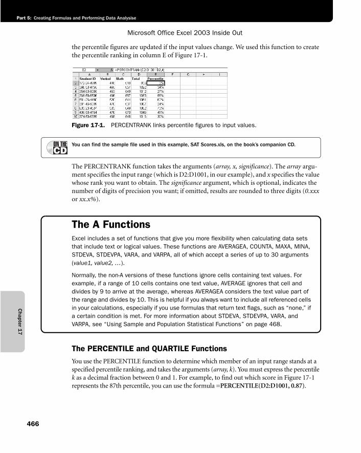
Chapter 1

7

Microsoft Office Excel 2003 Inside Out

Part 5: Creating Formulas and Performing Data Analysise

466

the percentile figures are updated if the input values change. We used this function to create the percentile ranking in column E of Figure 17-1.

f17ie 01

Figure 17-1. PERCENTRANK links percentile figures to input values.

You can find the sample file used in this example, SAT Scores.xls, on the book’s companion CD.

The PERCENTRANK function takes the arguments (array, x, significance). The array argu-ment specifies the input range (which is D2:D1001, in our example), and x specifies the value whose rank you want to obtain. The significance argument, which is optional, indicates the number of digits of precision you want; if omitted, results are rounded to three digits (0.xxxor xx.x%).

The A FunctionsExcel includes a set of functions that give you more flexibility when calculating data sets that include text or logical values. These functions are AVERAGEA, COUNTA, MAXA, MINA, STDEVA, STDEVPA, VARA, and VARPA, all of which accept a series of up to 30 arguments (value1, value2, …).

Normally, the non-A versions of these functions ignore cells containing text values. For example, if a range of 10 cells contains one text value, AVERAGE ignores that cell and divides by 9 to arrive at the average, whereas AVERAGEA considers the text value part of the range and divides by 10. This is helpful if you always want to include all referenced cells in your calculations, especially if you use formulas that return text flags, such as “none,” if a certain condition is met. For more information about STDEVA, STDEVPA, VARA, and VARPA, see “Using Sample and Population Statistical Functions” on page 468.

The PERCENTILE and QUARTILE FunctionsYou use the PERCENTILE function to determine which member of an input range stands at a specified percentile ranking, and takes the arguments (array, k). You must express the percentile k as a decimal fraction between 0 and 1. For example, to find out which score in Figure 17-1 represents the 87th percentile, you can use the formula =PERCENTILE(D2:D1001, 0.87).

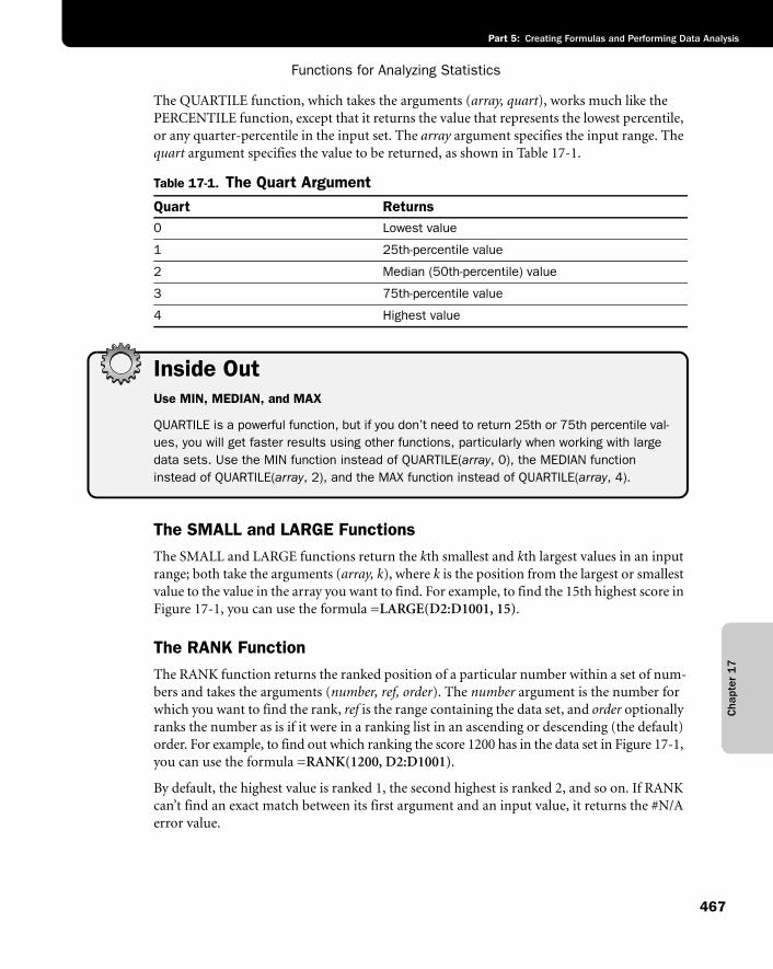
Cha

pter

17

Functions for Analyzing Statistics

467

Part 5: Creating Formulas and Performing Data Analysis

The QUARTILE function, which takes the arguments (array, quart), works much like the PERCENTILE function, except that it returns the value that represents the lowest percentile, or any quarter-percentile in the input set. The array argument specifies the input range. The quart argument specifies the value to be returned, as shown in Table 17-1.

Inside OutUse MIN, MEDIAN, and MAX

QUARTILE is a powerful function, but if you don’t need to return 25th or 75th percentile val-ues, you will get faster results using other functions, particularly when working with large data sets. Use the MIN function instead of QUARTILE(array, 0), the MEDIAN function instead of QUARTILE(array, 2), and the MAX function instead of QUARTILE(array, 4).

The SMALL and LARGE FunctionsThe SMALL and LARGE functions return the kth smallest and kth largest values in an input range; both take the arguments (array, k), where k is the position from the largest or smallest value to the value in the array you want to find. For example, to find the 15th highest score in Figure 17-1, you can use the formula =LARGE(D2:D1001, 15).

The RANK FunctionThe RANK function returns the ranked position of a particular number within a set of num-bers and takes the arguments (number, ref, order). The number argument is the number for which you want to find the rank, ref is the range containing the data set, and order optionally ranks the number as is if it were in a ranking list in an ascending or descending (the default) order. For example, to find out which ranking the score 1200 has in the data set in Figure 17-1, you can use the formula =RANK(1200, D2:D1001).

By default, the highest value is ranked 1, the second highest is ranked 2, and so on. If RANK can’t find an exact match between its first argument and an input value, it returns the #N/A error value.

Table 17-1. The Quart Argument

Quart Returns0 Lowest value

1 25th-percentile value

2 Median (50th-percentile) value

3 75th-percentile value

4 Highest value

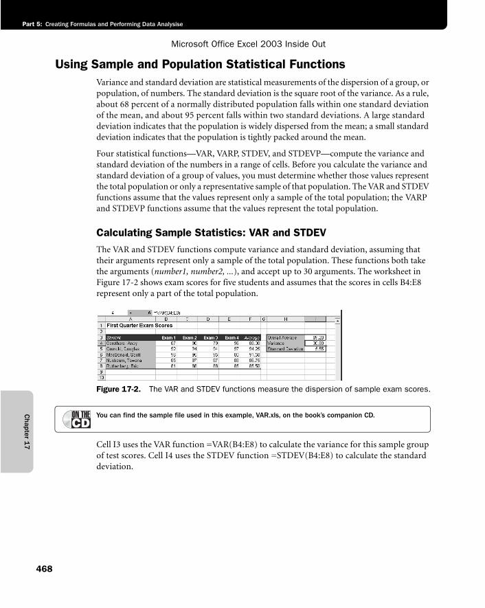
Chapter 1

7

Microsoft Office Excel 2003 Inside Out

Part 5: Creating Formulas and Performing Data Analysise

468

Using Sample and Population Statistical FunctionsVariance and standard deviation are statistical measurements of the dispersion of a group, or population, of numbers. The standard deviation is the square root of the variance. As a rule, about 68 percent of a normally distributed population falls within one standard deviation of the mean, and about 95 percent falls within two standard deviations. A large standard deviation indicates that the population is widely dispersed from the mean; a small standard deviation indicates that the population is tightly packed around the mean.

Four statistical functions—VAR, VARP, STDEV, and STDEVP—compute the variance and standard deviation of the numbers in a range of cells. Before you calculate the variance and standard deviation of a group of values, you must determine whether those values represent the total population or only a representative sample of that population. The VAR and STDEV functions assume that the values represent only a sample of the total population; the VARP and STDEVP functions assume that the values represent the total population.

Calculating Sample Statistics: VAR and STDEVThe VAR and STDEV functions compute variance and standard deviation, assuming that their arguments represent only a sample of the total population. These functions both take the arguments (number1, number2, ...), and accept up to 30 arguments. The worksheet in Figure 17-2 shows exam scores for five students and assumes that the scores in cells B4:E8 represent only a part of the total population.

f17ie02

Figure 17-2. The VAR and STDEV functions measure the dispersion of sample exam scores.

You can find the sample file used in this example, VAR.xls, on the book’s companion CD.

Cell I3 uses the VAR function =VAR(B4:E8) to calculate the variance for this sample group of test scores. Cell I4 uses the STDEV function =STDEV(B4:E8) to calculate the standard deviation.

Cha

pter

17

Functions for Analyzing Statistics

469

Part 5: Creating Formulas and Performing Data Analysis

Assuming that the test scores in the example are normally distributed, we can deduce that about 68 percent of the students (the general-rule percentage) achieved scores between 83.65 (the average 89.20 minus the standard deviation 5.55) and 94.75 (89.2 plus 5.55).

Calculating Total Population Statistics: VARP and STDEVPIf the numbers you’re analyzing represent an entire population rather than a sample, use the VARP and STDEVP functions to calculate variance and standard deviation. These functions both take the arguments (number1, number2, ...), and accept up to 30 arguments.

Assuming that cells B4:E8 in the worksheet, shown in Figure 17-2, represent the total population, you can calculate the variance and standard deviation with the formulas =VARP(B4:E8) and =STDEVP(B4:E8). The VARP function returns 29.26, and the STDEVP function returns 5.41.

Tip Include text and blanksThe STDEV, STDEVP, VAR, and VARP functions do not include text values or blank cells in their calculations. If you want to include blanks and/or text, use the A versions: STDEVA, STDEVPA, VARA, and VARPA. For more information, see the sidebar “The A functions” on page 466.

Understanding Linear and Exponential RegressionExcel includes several array functions for performing linear regression—LINEST, TREND, FORECAST, SLOPE, and STEYX—and exponential regression—LOGEST and GROWTH. These functions are entered as array formulas and they produce array results. You can use each of these functions with one or several independent variables. The following list provides a definition of the different types of regression:

● Linear regression produces the slope of a line that best fits a single set of data. Based on a year’s worth of sales figures, for example, linear regression can tell you the projected sales for March of the following year by giving you the slope and y-intercept (that is, the point where the line crosses the y-axis) of the line that best fits the sales data. By fol-lowing the line forward in time, you can estimate future sales, if you can safely assume that growth will remain linear.

● Exponential regression produces an exponential curve that best fits a set of data that you suspect does not change linearly with time. For example, a series of measurements of population growth will nearly always be better represented by an exponential curve than by a line.

Chapter 1

7

Microsoft Office Excel 2003 Inside Out

Part 5: Creating Formulas and Performing Data Analysise

470

● Multiple regression is the analysis of more than one set of data, which often produces a more realistic projection. You can perform both linear and exponential multiple regression analyses. For example, suppose you want to project the appropriate price for a house in your area based on square footage, number of bathrooms, lot size, and age. Using a multiple regression formula, you can estimate a price, based on a database of information gathered from existing houses.

Regressing into the Future?The concept of regression might sound strange because the term is normally associated with movement backward, whereas in the world of statistics, regression is often used to predict the future. Simply put, regression is a statistical technique that finds a mathemati-cal expression that best describes a set of data.

Often businesses try to predict the future using sales and percent-of-sales projections based on history. A simple percent-of-sales technique identifies assets and liabilities that vary along with sales, determines the proportion of each, and assigns them percentages. Although using percent-of-sales forecasting is often sufficient for slow or steady short-term growth, the technique loses accuracy as growth accelerates.

Regression analysis uses more sophisticated equations to analyze larger sets of data and translates them into coordinates on a line or curve. In the not-so-distant past, regression analysis was not widely used because of the large volume of calculations involved. Since spreadsheet applications, such as Excel, began offering built-in regression functions, the use of regression analysis has become more widespread.

Calculating Linear RegressionThe equation y = mx + b algebraically describes a straight line for a set of data with one inde-pendent variable where x is the independent variable, y is the dependent variable, m repre-sents the slope of the line, and b represents the y-intercept. If a line represents a number of independent variables in a multiple regression analysis to an expected result, the equation of the regression line takes the form y=m1x1+m2x2+...+mnxn+b in which y is the dependent variable, x1 through xn are n independent variables, m1 through mn are the coefficients of each independent variable, and b is a constant.

The LINEST FunctionThe LINEST function uses this more general equation to return the values of m1 through mn and the value of b, given a known set of values for y and a known set of values for each independent variable. This function takes the form LINEST(known_y’s, known_x’s, const, stats).

Cha

pter

17

Functions for Analyzing Statistics

471

Part 5: Creating Formulas and Performing Data Analysis

The known_y’s argument is the set of y-values you already know. This argument can be a sin-gle column, a single row, or a rectangular range of cells. If known_y’s is a single column, each column in the known_x’s argument is considered an independent variable. Similarly, if known_y’s is a single row, each row in the known_x’s argument is considered an independent variable. If known_y’s is a rectangular range, you can use only one independent variable; known_x’s in this case should be a range of the same size and shape as known_y’s. If you omit the known_x’s argument, Excel uses the sequence 1, 2, 3, 4, and so on.

The const and stats arguments are optional. If either is included, it must be a logical con-stant—either TRUE or FALSE. (You can substitute 1 for TRUE and 0 for FALSE.) The default settings for const and stats are TRUE and FALSE, respectively. If you set const to FALSE, Excel forces b (the last term in the straight-line equation) to be 0. If you set stats to TRUE, the array returned by LINEST includes the following validation statistics.

Before creating a formula using LINEST, you must select a range large enough to hold the result array returned by the function. If you omit the stats argument (or set it explicitly to FALSE), the result array encompasses one cell for each of your independent variables and one cell for b. If you include the validation statistics, the result array looks like the following example. After selecting a range to contain the results array, type the function and then press Ctrl+Shift+Enter to enter the function in each cell of the result array.

se1 through sen Standard error values for each coefficient

Seb Standard error value for the constant b

R2 Coefficient of determination

Sey Standard error value for y

F F statistic

Df Degrees of freedom

Ssreg Regression sum of squares

Ssresid Residual sum of squares

mn mn–1 ... m2 m1 b

sen sen–1 ... se2 se1 seb

r2 Sey

F Df

ssreg Ssresid

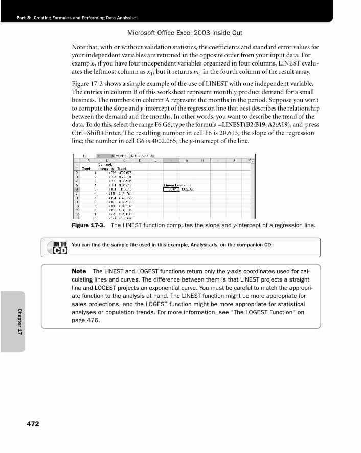
Chapter 1

7

Microsoft Office Excel 2003 Inside Out

Part 5: Creating Formulas and Performing Data Analysise

472

Note that, with or without validation statistics, the coefficients and standard error values for your independent variables are returned in the opposite order from your input data. For example, if you have four independent variables organized in four columns, LINEST evalu-ates the leftmost column as x1, but it returns m1 in the fourth column of the result array.

Figure 17-3 shows a simple example of the use of LINEST with one independent variable. The entries in column B of this worksheet represent monthly product demand for a small business. The numbers in column A represent the months in the period. Suppose you want to compute the slope and y-intercept of the regression line that best describes the relationship between the demand and the months. In other words, you want to describe the trend of the data. To do this, select the range F6:G6, type the formula =LINEST(B2:B19, A2:A19), and press Ctrl+Shift+Enter. The resulting number in cell F6 is 20.613, the slope of the regression line; the number in cell G6 is 4002.065, the y-intercept of the line.

f17ie03

Figure 17-3. The LINEST function computes the slope and y-intercept of a regression line.

You can find the sample file used in this example, Analysis.xls, on the companion CD.

Note The LINEST and LOGEST functions return only the y-axis coordinates used for cal-culating lines and curves. The difference between them is that LINEST projects a straight line and LOGEST projects an exponential curve. You must be careful to match the appropri-ate function to the analysis at hand. The LINEST function might be more appropriate for sales projections, and the LOGEST function might be more appropriate for statistical analyses or population trends. For more information, see “The LOGEST Function” on page 476.

Cha

pter

17

Functions for Analyzing Statistics

473

Part 5: Creating Formulas and Performing Data Analysis

Inside OutA real (estate) regression application

One often-used regression model is sometimes known as the Competitive Market Analysis (CMA). Realtors use CMAs to arrive at an estimated selling price for a home, based on his-torical sales data for comparable homes in the area. The following figure shows a sample Excel-based version of this tool, called the Home Price Estimator.

g17ie01

This application uses the LINEST function to analyze the statistics in the Input Data area and generate an array of results based on similar statistics in the What You Want area. The LINEST array is actually located in rows below the visible area of the worksheet, as shown below. The first row of values in the LINEST data array is used by the Estimated Price formula to extrapolate an estimated value.

g17ie02

Normally in this workbook, row and column headings are hidden, rows 25 through 37 are hidden, worksheet protection is turned on, and cells are locked with entries allowed only in the designated input areas. Real estate tip: As the note on the worksheet mentions, you can use listed home prices to arrive at an estimated price, but actual sale prices are more realistic, if you can get them.

You can find the sample file used in this example, Home Price Estimator.xls, on the book’s companion CD.

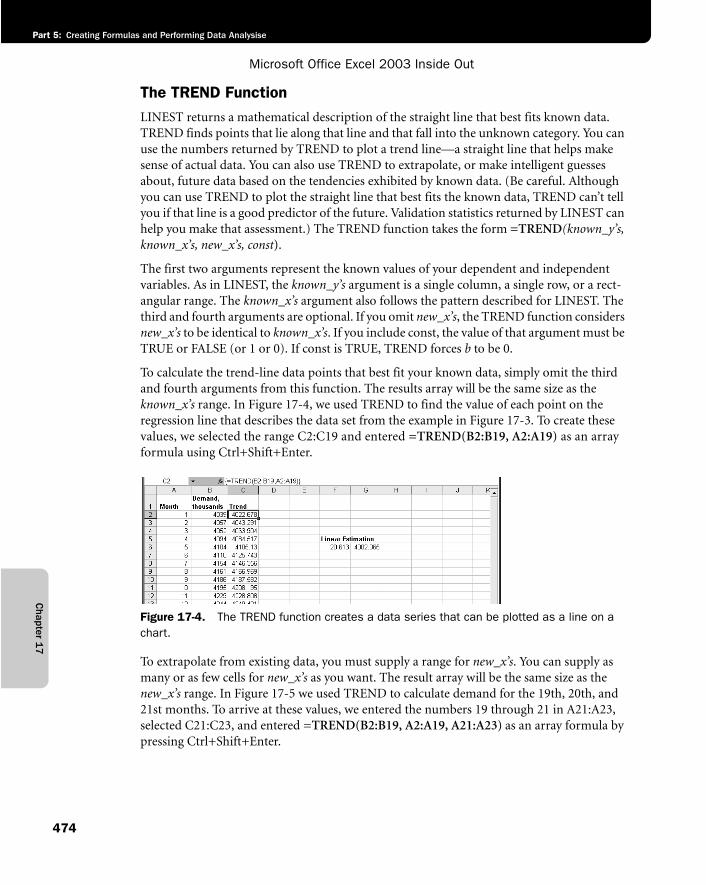
Chapter 1

7

Microsoft Office Excel 2003 Inside Out

Part 5: Creating Formulas and Performing Data Analysise

474

The TREND FunctionLINEST returns a mathematical description of the straight line that best fits known data. TREND finds points that lie along that line and that fall into the unknown category. You can use the numbers returned by TREND to plot a trend line—a straight line that helps make sense of actual data. You can also use TREND to extrapolate, or make intelligent guesses about, future data based on the tendencies exhibited by known data. (Be careful. Although you can use TREND to plot the straight line that best fits the known data, TREND can’t tell you if that line is a good predictor of the future. Validation statistics returned by LINEST can help you make that assessment.) The TREND function takes the form =TREND(known_y’s, known_x’s, new_x’s, const).

The first two arguments represent the known values of your dependent and independent variables. As in LINEST, the known_y’s argument is a single column, a single row, or a rect-angular range. The known_x’s argument also follows the pattern described for LINEST. The third and fourth arguments are optional. If you omit new_x’s, the TREND function considers new_x’s to be identical to known_x’s. If you include const, the value of that argument must be TRUE or FALSE (or 1 or 0). If const is TRUE, TREND forces b to be 0.

To calculate the trend-line data points that best fit your known data, simply omit the third and fourth arguments from this function. The results array will be the same size as the known_x’s range. In Figure 17-4, we used TREND to find the value of each point on the regression line that describes the data set from the example in Figure 17-3. To create these values, we selected the range C2:C19 and entered =TREND(B2:B19, A2:A19) as an array formula using Ctrl+Shift+Enter.

f17ie04

Figure 17-4. The TREND function creates a data series that can be plotted as a line on a chart.

To extrapolate from existing data, you must supply a range for new_x’s. You can supply as many or as few cells for new_x’s as you want. The result array will be the same size as the new_x’s range. In Figure 17-5 we used TREND to calculate demand for the 19th, 20th, and 21st months. To arrive at these values, we entered the numbers 19 through 21 in A21:A23, selected C21:C23, and entered =TREND(B2:B19, A2:A19, A21:A23) as an array formula by pressing Ctrl+Shift+Enter.

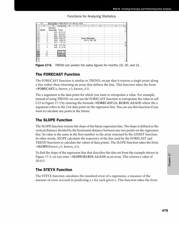
Cha

pter

17

Functions for Analyzing Statistics

475

Part 5: Creating Formulas and Performing Data Analysis

f17ie05

Figure 17-5. TREND can predict the sales figures for months 19, 20, and 21.

The FORECAST FunctionThe FORECAST function is similar to TREND, except that it returns a single point along a line rather than returning an array that defines the line. This function takes the form =FORECAST(x, known_y’s, known_x’s).

The x argument is the data point for which you want to extrapolate a value. For example, instead of using TREND, we can use the FORECAST function to extrapolate the value in cell C23 in Figure 17-5 by entering the formula =FORECAST(21, B2:B19, A2:A19) where the xargument refers to the 21st data point on the regression line. You can use this function if you want to calculate any point in the future.

The SLOPE FunctionThe SLOPE function returns the slope of the linear regression line. The slope is defined as the vertical distance divided by the horizontal distance between any two points on the regression line. Its value is the same as the first number in the array returned by the LINEST function. In other words, SLOPE calculates the trajectory of the line used by the FORECAST and TREND functions to calculate the values of data points. The SLOPE function takes the form =SLOPE(known_y’s, known_x’s).

To find the slope of the regression line that describes the data set from the example shown in Figure 17-5, we can enter =SLOPE(B2:B19, A2:A19) as an array. This returns a value of 20.613.

The STEYX FunctionThe STEYX function calculates the standard error of a regression, a measure of the amount of error accrued in predicting a y for each given x. This function takes the form

Chapter 1

7

Microsoft Office Excel 2003 Inside Out

Part 5: Creating Formulas and Performing Data Analysise

476

=STEYX(known_y’s, known_x’s). If we apply this function to the worksheet shown in Figure 17-5, the formula =STEYX(B2:B19, A2:A19) returns a standard error value of 12.96562.

Calculating Exponential RegressionUnlike linear regression, which plots values along a straight line, exponential regression describes a curve by calculating the array of values needed to plot it. The equation that describes an exponential regression curve is

y = b * m1x1 * m2

x2 * … * mnxn

If you have only one independent variable, the equation is

y = b * mx

The LOGEST FunctionThe LOGEST function works like LINEST, except that you use it to analyze data that is non-linear, and it returns the coordinates of an exponential curve instead of a straight line. LOGEST returns coefficient values for each independent variable plus a value for the con-stant b. This function takes the form =LOGEST(known_y’s, known_x’s, const, stats).

LOGEST accepts the same arguments as the LINEST function and returns a result array in the same fashion. If you set the optional stats argument to TRUE, the function also returns validation statistics. For more information about the LOGEST function’s underlying equa-tions and its arguments, see “The LINEST Function” on page 470.

Note The LINEST and LOGEST functions return only the y-axis coordinates used for cal-culating lines and curves. The difference between them is that LINEST projects a straight line and LOGEST projects an exponential curve. You must be careful to match the appropri-ate function to the analysis at hand. The LINEST function might be more appropriate for sales projections, and the LOGEST function might be more suited to applications, such as statistical analyses or population trends.

The GROWTH FunctionWhere the LOGEST function returns a mathematical description of the exponential regres-sion curve that best fits a set of known data, the GROWTH function finds points that lie along that curve. The GROWTH function works like its linear counterpart, TREND, and takes the form =GROWTH(known_y’s, known_x’s, new_x’s, const). For more information about the GROWTH function’s arguments, see “The TREND Function” on page 474.

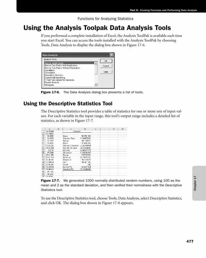
Cha

pter

17

Functions for Analyzing Statistics

477

Part 5: Creating Formulas and Performing Data Analysis

Using the Analysis Toolpak Data Analysis ToolsIf you performed a complete installation of Excel, the Analysis ToolPak is available each time you start Excel. You can access the tools installed with the Analysis ToolPak by choosing Tools, Data Analysis to display the dialog box shown in Figure 17-6.

f17ie06

Figure 17-6. The Data Analysis dialog box presents a list of tools.

Using the Descriptive Statistics ToolThe Descriptive Statistics tool provides a table of statistics for one or more sets of input val-ues. For each variable in the input range, this tool’s output range includes a detailed list of statistics, as shown in Figure 17-7.

f17ie07

Figure 17-7. We generated 1000 normally distributed random numbers, using 100 as the mean and 2 as the standard deviation, and then verified their normalness with the Descriptive Statistics tool.

To use the Descriptive Statistics tool, choose Tools, Data Analysis, select Descriptive Statistics, and click OK. The dialog box shown in Figure 17-8 appears.

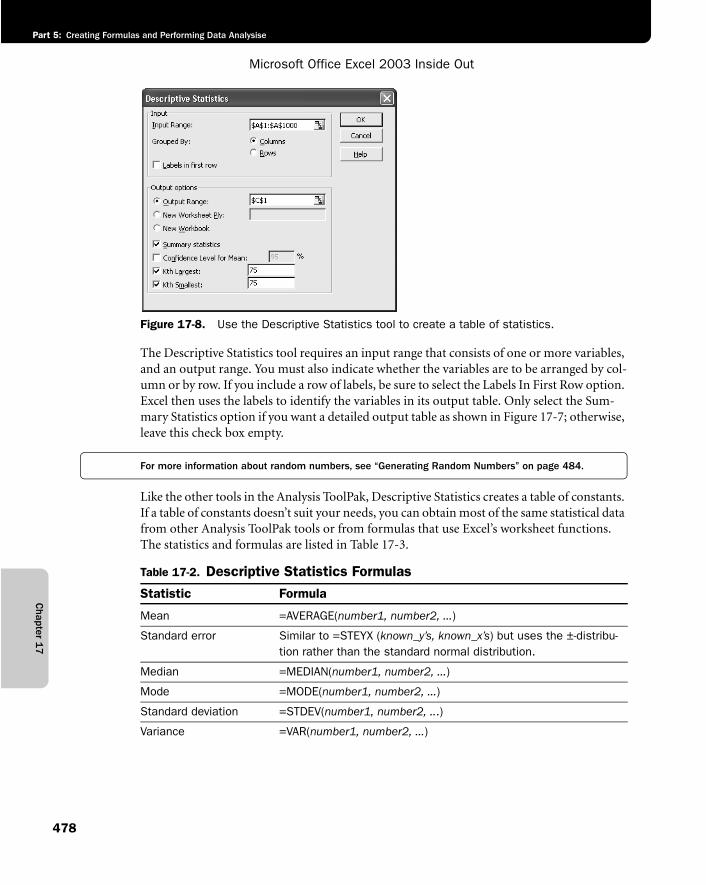
Chapter 1

7

Microsoft Office Excel 2003 Inside Out

Part 5: Creating Formulas and Performing Data Analysise

478

f17ie08

Figure 17-8. Use the Descriptive Statistics tool to create a table of statistics.

The Descriptive Statistics tool requires an input range that consists of one or more variables, and an output range. You must also indicate whether the variables are to be arranged by col-umn or by row. If you include a row of labels, be sure to select the Labels In First Row option. Excel then uses the labels to identify the variables in its output table. Only select the Sum-mary Statistics option if you want a detailed output table as shown in Figure 17-7; otherwise, leave this check box empty.

For more information about random numbers, see “Generating Random Numbers” on page 484.

Like the other tools in the Analysis ToolPak, Descriptive Statistics creates a table of constants. If a table of constants doesn’t suit your needs, you can obtain most of the same statistical data from other Analysis ToolPak tools or from formulas that use Excel’s worksheet functions. The statistics and formulas are listed in Table 17-3.

Table 17-2. Descriptive Statistics Formulas

Statistic Formula

Mean =AVERAGE(number1, number2, ...)

Standard error Similar to =STEYX (known_y’s, known_x’s) but uses the ±-distribu-tion rather than the standard normal distribution.

Median =MEDIAN(number1, number2, ...)

Mode =MODE(number1, number2, ...)

Standard deviation =STDEV(number1, number2, ...)

Variance =VAR(number1, number2, ...)

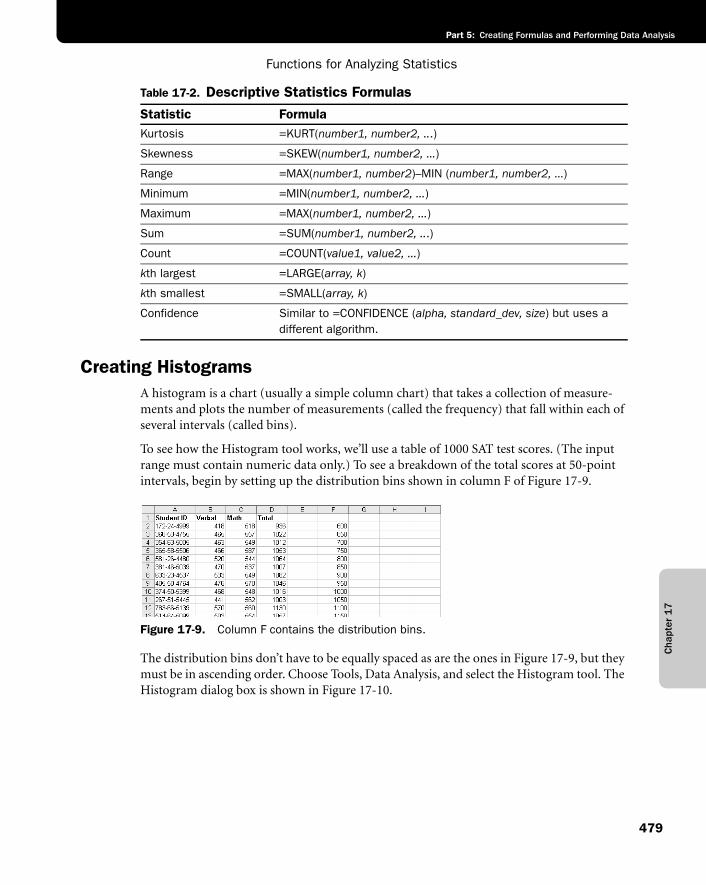
Cha

pter

17

Functions for Analyzing Statistics

479

Part 5: Creating Formulas and Performing Data Analysis

Creating HistogramsA histogram is a chart (usually a simple column chart) that takes a collection of measure-ments and plots the number of measurements (called the frequency) that fall within each of several intervals (called bins).

To see how the Histogram tool works, we’ll use a table of 1000 SAT test scores. (The input range must contain numeric data only.) To see a breakdown of the total scores at 50-point intervals, begin by setting up the distribution bins shown in column F of Figure 17-9.

f17ie09

Figure 17-9. Column F contains the distribution bins.

The distribution bins don’t have to be equally spaced as are the ones in Figure 17-9, but they must be in ascending order. Choose Tools, Data Analysis, and select the Histogram tool. The Histogram dialog box is shown in Figure 17-10.

Kurtosis =KURT(number1, number2, ...)

Skewness =SKEW(number1, number2, ...)

Range =MAX(number1, number2)–MIN (number1, number2, ...)

Minimum =MIN(number1, number2, ...)

Maximum =MAX(number1, number2, ...)

Sum =SUM(number1, number2, ...)

Count =COUNT(value1, value2, ...)

kth largest =LARGE(array, k)

kth smallest =SMALL(array, k)

Confidence Similar to =CONFIDENCE (alpha, standard_dev, size) but uses a different algorithm.

Table 17-2. Descriptive Statistics Formulas

Statistic Formula

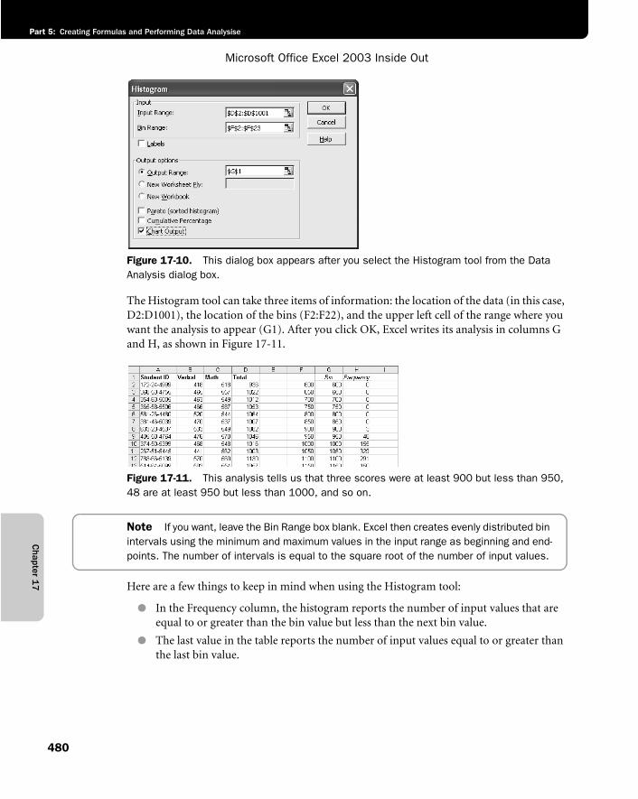
Chapter 1

7

Microsoft Office Excel 2003 Inside Out

Part 5: Creating Formulas and Performing Data Analysise

480

f17ie10

Figure 17-10. This dialog box appears after you select the Histogram tool from the Data Analysis dialog box.

The Histogram tool can take three items of information: the location of the data (in this case, D2:D1001), the location of the bins (F2:F22), and the upper left cell of the range where you want the analysis to appear (G1). After you click OK, Excel writes its analysis in columns G and H, as shown in Figure 17-11.

f17ie11

Figure 17-11. This analysis tells us that three scores were at least 900 but less than 950, 48 are at least 950 but less than 1000, and so on.

Note If you want, leave the Bin Range box blank. Excel then creates evenly distributed bin intervals using the minimum and maximum values in the input range as beginning and end-points. The number of intervals is equal to the square root of the number of input values.

Here are a few things to keep in mind when using the Histogram tool:

● In the Frequency column, the histogram reports the number of input values that are equal to or greater than the bin value but less than the next bin value.

● The last value in the table reports the number of input values equal to or greater than the last bin value.

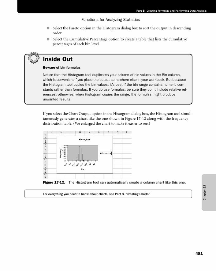
Cha

pter

17

Functions for Analyzing Statistics

481

Part 5: Creating Formulas and Performing Data Analysis

● Select the Pareto option in the Histogram dialog box to sort the output in descending order.

● Select the Cumulative Percentage option to create a table that lists the cumulative percentages of each bin level.

Inside OutBeware of bin formulas

Notice that the Histogram tool duplicates your column of bin values in the Bin column, which is convenient if you place the output somewhere else in your workbook. But because the Histogram tool copies the bin values, it’s best if the bin range contains numeric con-stants rather than formulas. If you do use formulas, be sure they don’t include relative ref-erences; otherwise, when Histogram copies the range, the formulas might produce unwanted results.

If you select the Chart Output option in the Histogram dialog box, the Histogram tool simul-taneously generates a chart like the one shown in Figure 17-12 along with the frequency distribution table. (We enlarged the chart to make it easier to see.)

f17ie12

Figure 17-12. The Histogram tool can automatically create a column chart like this one.

For everything you need to know about charts, see Part 8, “Creating Charts.”

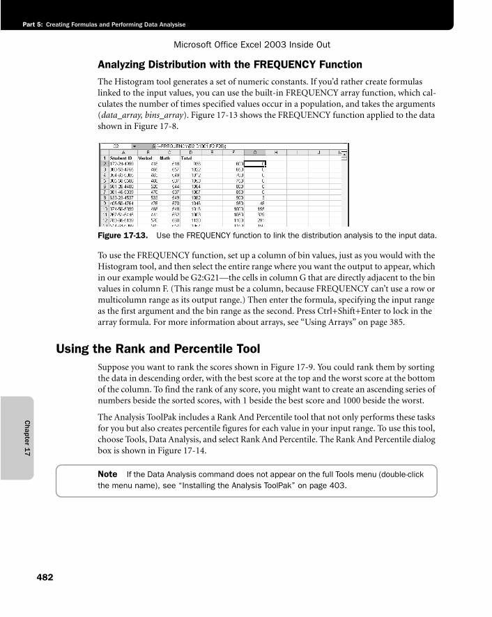
Chapter 1

7

Microsoft Office Excel 2003 Inside Out

Part 5: Creating Formulas and Performing Data Analysise

482

Analyzing Distribution with the FREQUENCY FunctionThe Histogram tool generates a set of numeric constants. If you’d rather create formulas linked to the input values, you can use the built-in FREQUENCY array function, which cal-culates the number of times specified values occur in a population, and takes the arguments (data_array, bins_array). Figure 17-13 shows the FREQUENCY function applied to the data shown in Figure 17-8.

f17ie13

Figure 17-13. Use the FREQUENCY function to link the distribution analysis to the input data.

To use the FREQUENCY function, set up a column of bin values, just as you would with the Histogram tool, and then select the entire range where you want the output to appear, which in our example would be G2:G21—the cells in column G that are directly adjacent to the bin values in column F. (This range must be a column, because FREQUENCY can’t use a row or multicolumn range as its output range.) Then enter the formula, specifying the input range as the first argument and the bin range as the second. Press Ctrl+Shift+Enter to lock in the array formula. For more information about arrays, see “Using Arrays” on page 385.

Using the Rank and Percentile ToolSuppose you want to rank the scores shown in Figure 17-9. You could rank them by sorting the data in descending order, with the best score at the top and the worst score at the bottom of the column. To find the rank of any score, you might want to create an ascending series of numbers beside the sorted scores, with 1 beside the best score and 1000 beside the worst.

The Analysis ToolPak includes a Rank And Percentile tool that not only performs these tasks for you but also creates percentile figures for each value in your input range. To use this tool, choose Tools, Data Analysis, and select Rank And Percentile. The Rank And Percentile dialog box is shown in Figure 17-14.

Note If the Data Analysis command does not appear on the full Tools menu (double-click the menu name), see “Installing the Analysis ToolPak” on page 403.

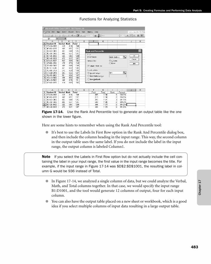
Cha

pter

17

Functions for Analyzing Statistics

483

Part 5: Creating Formulas and Performing Data Analysis

f17ie14

Figure 17-14. Use the Rank And Percentile tool to generate an output table like the one shown in the lower figure.

Here are some hints to remember when using the Rank And Percentile tool:

● It’s best to use the Labels In First Row option in the Rank And Percentile dialog box, and then include the column heading in the input range. This way, the second column in the output table uses the same label. If you do not include the label in the input range, the output column is labeled Column1.

Note If you select the Labels in First Row option but do not actually include the cell con-taining the label in your input range, the first value in the input range becomes the title. For example, if the input range in Figure 17-14 was $D$2:$D$1001, the resulting label in col-umn G would be 936 instead of Total.

● In Figure 17-14, we analyzed a single column of data, but we could analyze the Verbal, Math, and Total columns together. In that case, we would specify the input range B1:D1001, and the tool would generate 12 columns of output, four for each input column.

● You can also have the output table placed on a new sheet or workbook, which is a good idea if you select multiple columns of input data resulting in a large output table.

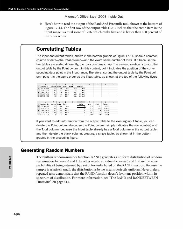
Chapter 1

7

Microsoft Office Excel 2003 Inside Out

Part 5: Creating Formulas and Performing Data Analysise

484

● Here’s how to read the output of the Rank And Percentile tool, shown at the bottom of Figure 17-14. The first row of the output table (F2:I2) tell us that the 285th item in the input range is a total score of 1206, which ranks first and is better than 100 percent of the other scores.

Correlating TablesThe input and output tables, shown in the bottom graphic of Figure 17-14, share a common column of data—the Total column—and the exact same number of rows. But because the two tables are sorted differently, the rows don’t match up. The easiest solution is to sort the output table by the Point column; in this context, point indicates the position of the corre-sponding data point in the input range. Therefore, sorting the output table by the Point col-umn puts it in the same order as the input table, as shown at the top of the following figure.

g17ie03

If you want to add information from the output table to the existing input table, you can delete the Point column (because the Point column simply indicates the row number) and the Total column (because the input table already has a Total column) in the output table, and then delete the blank column, creating a single table, as shown at in the bottom graphic in the preceding figure.

Generating Random NumbersThe built-in random-number function, RAND, generates a uniform distribution of random real numbers between 0 and 1. In other words, all values between 0 and 1 share the same probability of being returned by a set of formulas based on the RAND function. Because the sample is relatively small, the distribution is by no means perfectly uniform. Nevertheless, repeated tests demonstrate that the RAND function doesn’t favor any position within its spectrum of distribution. For more information, see “The RAND and RANDBETWEEN Functions” on page 414.

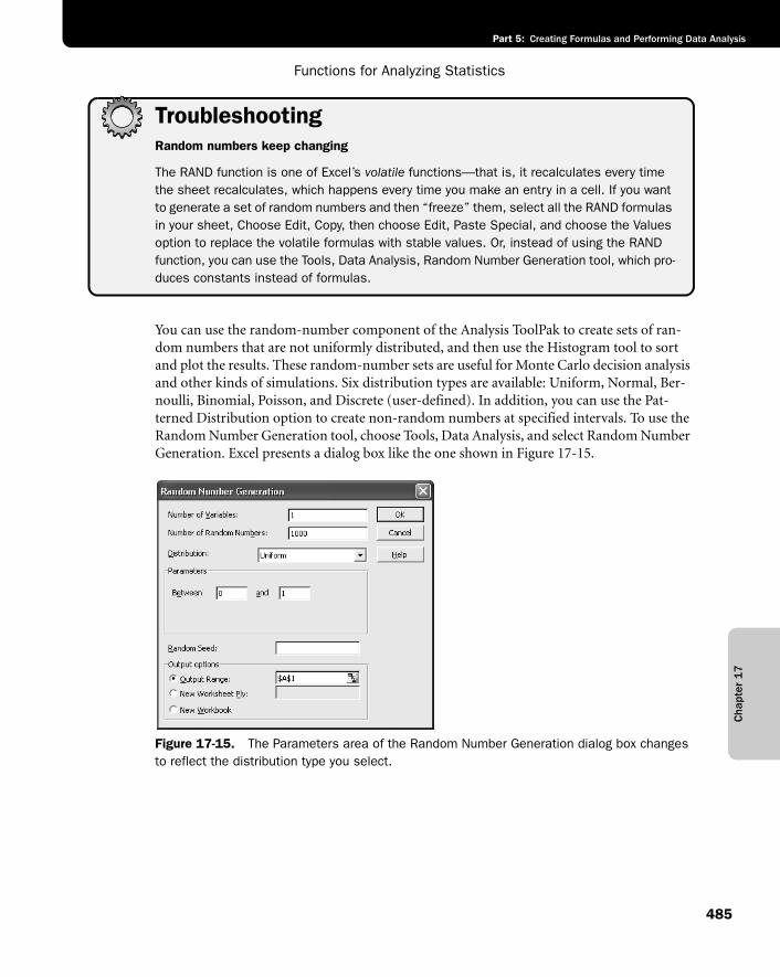
Cha

pter

17

Functions for Analyzing Statistics

485

Part 5: Creating Formulas and Performing Data Analysis

TroubleshootingRandom numbers keep changing

The RAND function is one of Excel’s volatile functions—that is, it recalculates every time the sheet recalculates, which happens every time you make an entry in a cell. If you want to generate a set of random numbers and then “freeze” them, select all the RAND formulas in your sheet, Choose Edit, Copy, then choose Edit, Paste Special, and choose the Values option to replace the volatile formulas with stable values. Or, instead of using the RAND function, you can use the Tools, Data Analysis, Random Number Generation tool, which pro-duces constants instead of formulas.

You can use the random-number component of the Analysis ToolPak to create sets of ran-dom numbers that are not uniformly distributed, and then use the Histogram tool to sort and plot the results. These random-number sets are useful for Monte Carlo decision analysis and other kinds of simulations. Six distribution types are available: Uniform, Normal, Ber-noulli, Binomial, Poisson, and Discrete (user-defined). In addition, you can use the Pat-terned Distribution option to create non-random numbers at specified intervals. To use the Random Number Generation tool, choose Tools, Data Analysis, and select Random Number Generation. Excel presents a dialog box like the one shown in Figure 17-15.

f17ie15

Figure 17-15. The Parameters area of the Random Number Generation dialog box changes to reflect the distribution type you select.

Chapter 1

7

Microsoft Office Excel 2003 Inside Out

Part 5: Creating Formulas and Performing Data Analysise

486

Here are a couple of important points regarding the use of the Random Number Generation tool:

● In the Number Of Variables and Number Of Random Numbers boxes, you indicate how many columns of numbers you want and how many numbers you want in each column. For example, if you want 10 columns of 100 numbers each, specify 10 in the Number Of Variables box and 100 in the Number Of Random Numbers box.

● You can also specify a seed value. However, each time you generate a random-number set with a particular distribution type using the same seed value, you get the same sequence of numbers; therefore, you should specify a seed value only if you need to be able to reproduce a random-number sequence.

Random Number Distribution MethodsIn the Random Number Generation dialog box, the parameters shown directly below the Distribution list change, depending on the type of distribution you select. As Figure 17-15 shows, when you select Uniform Distribution, you can specify the beginning and end points of the distribution in the Between/And boxes.

Distributing Random Numbers UniformlyThis option asks you to specify two numbers between (and including) which to generate a set of random numbers, and works much the same way as the RANDBETWEEN function, gen-erating an evenly distributed set of real numbers. You can use this option as a more conve-nient alternative to RAND if you want endpoints other than 0 and 1 or if you want sets of numbers to be based on the same seed value.

Distributing Random Numbers NormallyNormal Distribution has the following characteristics:

● One particular value, the mean, is more likely to occur than any other value.

● Values greater than the mean are as likely to occur as values less than it.

● Values close to the mean are more likely to occur than values distant from the mean.

To generate normally distributed random numbers, you specify two parameters: the mean and the standard deviation. The standard deviation is the average absolute difference between the random numbers and the mean. (Approximately 68 percent of the values in a normal distribution will fall within one standard deviation of the mean.)

Generating Random Numbers Using Bernoulli DistributionThe Bernoulli Distribution option simulates the probability of success of a number of trials, given that all trials have an equal probability of succeeding and that the success of one trial has no impact on the success of subsequent trials. (Note that success in this context has no value implication. In other words, you can use this distribution to simulate failure as readily as success.) All values in the Bernoulli distribution’s output are either 0 or 1.

Cha

pter

17

Functions for Analyzing Statistics

487

Part 5: Creating Formulas and Performing Data Analysis

The probability that each cell will return a 1 is given by the distribution’s sole parameter—P Value—for which you supply a number from 0 to 1. For example, if you want a sequence of 100 random Bernoulli values whose most likely sum is 27, you define a 100-cell output range and specify a P Value of 0.27.

Generating Random Numbers Using Binomial DistributionThe Binomial Distribution option simulates the number of successes in a fixed number of trials, given a specified probability rate. As with the Bernoulli Distribution option, the trials are assumed to be independent; that is, the outcome of one has no affect on any other. To generate binomially distributed numbers, you specify Number of Trials and the P Value (probability) that any trial will succeed. (Again, success in this context has no value implica-tion. In other words, you can use this distribution to simulate failure as readily as success.)

For example, suppose you make 10 sales presentations a week; you close the sale 20 percent of the time; and you would like to know what your success rate might be over the next year. Type 50 (for 50 working weeks in the year) in the Number Of Random Numbers box, 0.2 in the P Value box, and 10 in the Number Of Trials box to learn that you can expect to make no sales four weeks in the coming year.

Generating Random Numbers Using Poisson DistributionThe Poisson Distribution option simulates the number of times an event occurs within a par-ticular time span, given a certain probability of occurrence. The occurrences are assumed to be independent; that is, each occurrence has no effect on the likelihood of others.

The Poisson Distribution option takes a single parameter, Lambda, which represents the expected outcome of an individual occurrence. For example, suppose you receive an average of 10 service calls a day. You want to know how often you can expect to get 18 or more service calls in a day over a year. To get this information, type 260 (52 weeks times 5 days) in the Number Of Random Numbers box and 10 in the Lambda box (the expected average). You can then use the COUNTIF function to count the number of times 18 shows up in the output range. For more information, see “The SUMIF and COUNTIF Functions” on page 465.

Generating Random Numbers Using Discrete DistributionUse the Discrete Distribution option to create a custom distribution pattern by specifying a table of possible outcomes along with the probability associated with each outcome. The probability values must be between 0 and 1, and the sum of the probabilities in the table must equal 1. To use the Discrete Distribution option, specify the possible outcomes and their probabilities as a two-column range whose reference is the only parameter used by this option.

For example, you could create a custom distribution pattern to generate random snow-shovel sales patterns based on a two-column input range: Month Number and Probability of Snow.

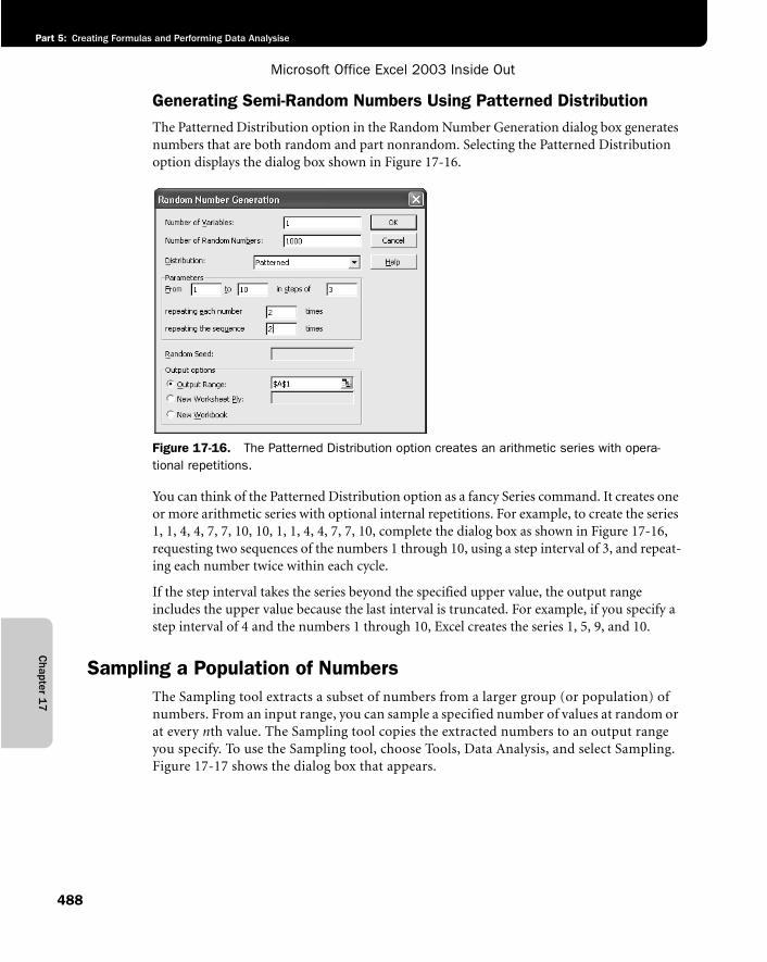
Chapter 1

7

Microsoft Office Excel 2003 Inside Out

Part 5: Creating Formulas and Performing Data Analysise

488

Generating Semi-Random Numbers Using Patterned DistributionThe Patterned Distribution option in the Random Number Generation dialog box generates numbers that are both random and part nonrandom. Selecting the Patterned Distribution option displays the dialog box shown in Figure 17-16.

f17ie16

Figure 17-16. The Patterned Distribution option creates an arithmetic series with opera-tional repetitions.

You can think of the Patterned Distribution option as a fancy Series command. It creates one or more arithmetic series with optional internal repetitions. For example, to create the series 1, 1, 4, 4, 7, 7, 10, 10, 1, 1, 4, 4, 7, 7, 10, complete the dialog box as shown in Figure 17-16, requesting two sequences of the numbers 1 through 10, using a step interval of 3, and repeat-ing each number twice within each cycle.

If the step interval takes the series beyond the specified upper value, the output range includes the upper value because the last interval is truncated. For example, if you specify a step interval of 4 and the numbers 1 through 10, Excel creates the series 1, 5, 9, and 10.

Sampling a Population of NumbersThe Sampling tool extracts a subset of numbers from a larger group (or population) of numbers. From an input range, you can sample a specified number of values at random or at every nth value. The Sampling tool copies the extracted numbers to an output range you specify. To use the Sampling tool, choose Tools, Data Analysis, and select Sampling. Figure 17-17 shows the dialog box that appears.

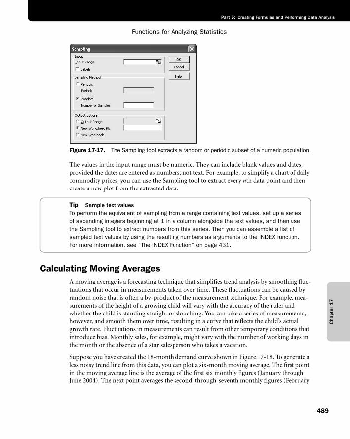
Cha

pter

17

Functions for Analyzing Statistics

489

Part 5: Creating Formulas and Performing Data Analysis

f17ie17

Figure 17-17. The Sampling tool extracts a random or periodic subset of a numeric population.

The values in the input range must be numeric. They can include blank values and dates, provided the dates are entered as numbers, not text. For example, to simplify a chart of daily commodity prices, you can use the Sampling tool to extract every nth data point and then create a new plot from the extracted data.

Tip Sample text valuesTo perform the equivalent of sampling from a range containing text values, set up a series of ascending integers beginning at 1 in a column alongside the text values, and then use the Sampling tool to extract numbers from this series. Then you can assemble a list of sampled text values by using the resulting numbers as arguments to the INDEX function. For more information, see “The INDEX Function” on page 431.

Calculating Moving AveragesA moving average is a forecasting technique that simplifies trend analysis by smoothing fluc-tuations that occur in measurements taken over time. These fluctuations can be caused by random noise that is often a by-product of the measurement technique. For example, mea-surements of the height of a growing child will vary with the accuracy of the ruler and whether the child is standing straight or slouching. You can take a series of measurements, however, and smooth them over time, resulting in a curve that reflects the child’s actual growth rate. Fluctuations in measurements can result from other temporary conditions that introduce bias. Monthly sales, for example, might vary with the number of working days in the month or the absence of a star salesperson who takes a vacation.

Suppose you have created the 18-month demand curve shown in Figure 17-18. To generate a less noisy trend line from this data, you can plot a six-month moving average. The first point in the moving average line is the average of the first six monthly figures (January through June 2004). The next point averages the second-through-seventh monthly figures (February

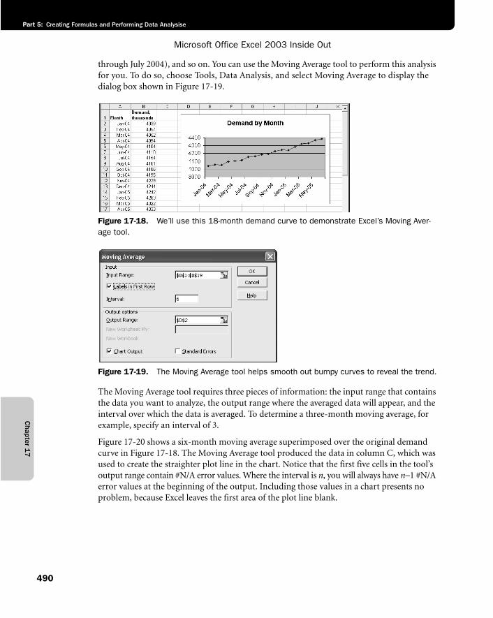
Chapter 1

7

Microsoft Office Excel 2003 Inside Out

Part 5: Creating Formulas and Performing Data Analysise

490

through July 2004), and so on. You can use the Moving Average tool to perform this analysis for you. To do so, choose Tools, Data Analysis, and select Moving Average to display the dialog box shown in Figure 17-19.

f17ie18

Figure 17-18. We’ll use this 18-month demand curve to demonstrate Excel’s Moving Aver-age tool.

f17ie19

Figure 17-19. The Moving Average tool helps smooth out bumpy curves to reveal the trend.

The Moving Average tool requires three pieces of information: the input range that contains the data you want to analyze, the output range where the averaged data will appear, and the interval over which the data is averaged. To determine a three-month moving average, for example, specify an interval of 3.

Figure 17-20 shows a six-month moving average superimposed over the original demand curve in Figure 17-18. The Moving Average tool produced the data in column C, which was used to create the straighter plot line in the chart. Notice that the first five cells in the tool’s output range contain #N/A error values. Where the interval is n, you will always have n–1 #N/A error values at the beginning of the output. Including those values in a chart presents no problem, because Excel leaves the first area of the plot line blank.

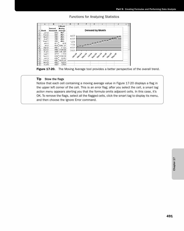
Cha

pter

17

Functions for Analyzing Statistics

491

Part 5: Creating Formulas and Performing Data Analysis

f17ie20

Figure 17-20. The Moving Average tool provides a better perspective of the overall trend.

Tip Stow the flagsNotice that each cell containing a moving average value in Figure 17-20 displays a flag in the upper left corner of the cell. This is an error flag; after you select the cell, a smart tag action menu appears alerting you that the formula omits adjacent cells. In this case, it’s OK. To remove the flags, select all the flagged cells, click the smart tag to display its menu, and then choose the Ignore Error command.

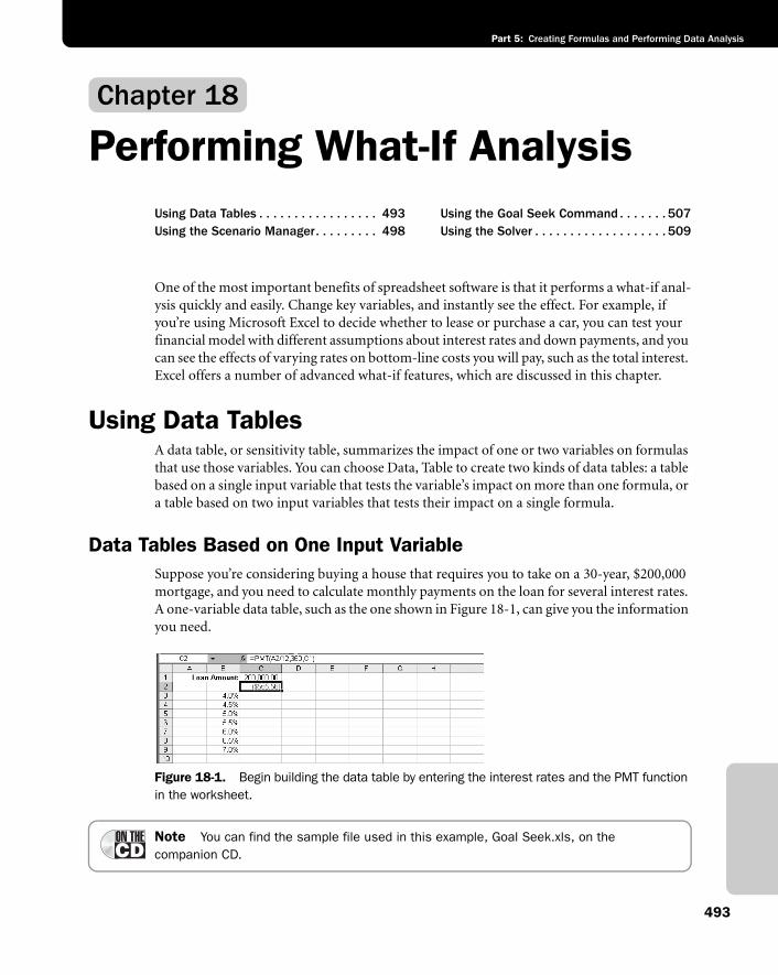
493

Part 5: Creating Formulas and Performing Data Analysis

Chapter 18

Performing What-If AnalysisUsing Data Tables . . . . . . . . . . . . . . . . . 493Using the Scenario Manager. . . . . . . . . 498

Using the Goal Seek Command . . . . . . . 507Using the Solver . . . . . . . . . . . . . . . . . . . 509

One of the most important benefits of spreadsheet software is that it performs a what-if anal-ysis quickly and easily. Change key variables, and instantly see the effect. For example, if you’re using Microsoft Excel to decide whether to lease or purchase a car, you can test your financial model with different assumptions about interest rates and down payments, and you can see the effects of varying rates on bottom-line costs you will pay, such as the total interest. Excel offers a number of advanced what-if features, which are discussed in this chapter.

Using Data TablesA data table, or sensitivity table, summarizes the impact of one or two variables on formulas that use those variables. You can choose Data, Table to create two kinds of data tables: a table based on a single input variable that tests the variable’s impact on more than one formula, or a table based on two input variables that tests their impact on a single formula.

Data Tables Based on One Input VariableSuppose you’re considering buying a house that requires you to take on a 30-year, $200,000 mortgage, and you need to calculate monthly payments on the loan for several interest rates. A one-variable data table, such as the one shown in Figure 18-1, can give you the information you need.

f18ie01

Figure 18-1. Begin building the data table by entering the interest rates and the PMT function in the worksheet.

Note You can find the sample file used in this example, Goal Seek.xls, on the companion CD.

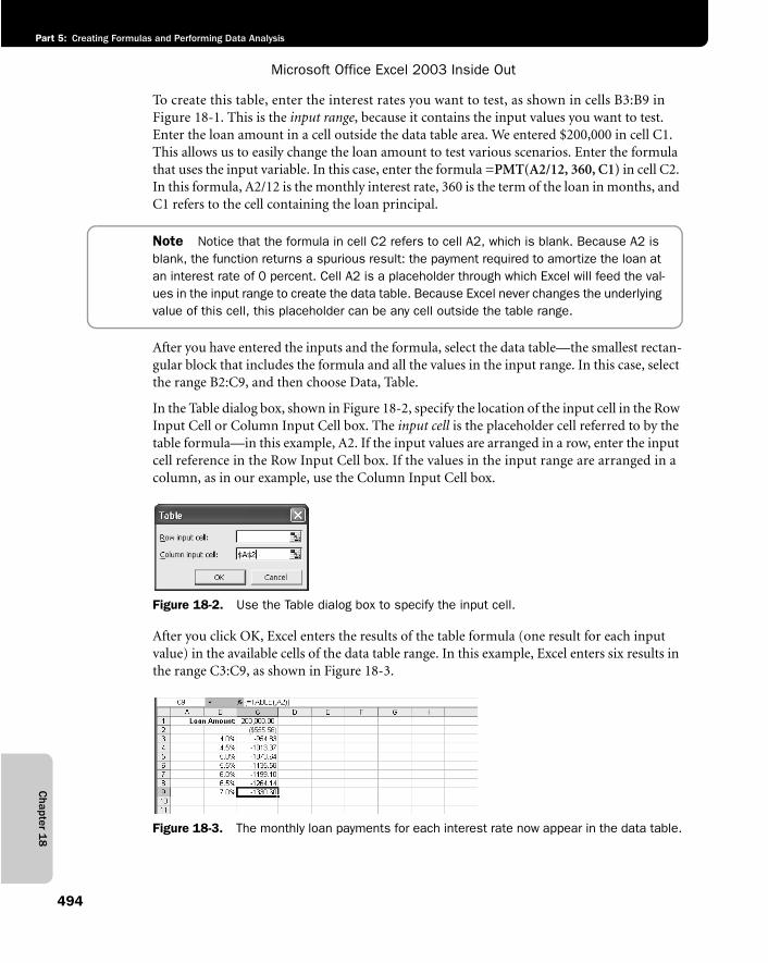
Chapter 1

8

Microsoft Office Excel 2003 Inside Out

Part 5: Creating Formulas and Performing Data Analysis

494

To create this table, enter the interest rates you want to test, as shown in cells B3:B9 inFigure 18-1. This is the input range, because it contains the input values you want to test. Enter the loan amount in a cell outside the data table area. We entered $200,000 in cell C1. This allows us to easily change the loan amount to test various scenarios. Enter the formula that uses the input variable. In this case, enter the formula =PMT(A2/12, 360, C1) in cell C2. In this formula, A2/12 is the monthly interest rate, 360 is the term of the loan in months, and C1 refers to the cell containing the loan principal.

Note Notice that the formula in cell C2 refers to cell A2, which is blank. Because A2 is blank, the function returns a spurious result: the payment required to amortize the loan at an interest rate of 0 percent. Cell A2 is a placeholder through which Excel will feed the val-ues in the input range to create the data table. Because Excel never changes the underlying value of this cell, this placeholder can be any cell outside the table range.

After you have entered the inputs and the formula, select the data table—the smallest rectan-gular block that includes the formula and all the values in the input range. In this case, select the range B2:C9, and then choose Data, Table.

In the Table dialog box, shown in Figure 18-2, specify the location of the input cell in the Row Input Cell or Column Input Cell box. The input cell is the placeholder cell referred to by the table formula—in this example, A2. If the input values are arranged in a row, enter the input cell reference in the Row Input Cell box. If the values in the input range are arranged in a column, as in our example, use the Column Input Cell box.

f18ie02

Figure 18-2. Use the Table dialog box to specify the input cell.

After you click OK, Excel enters the results of the table formula (one result for each input value) in the available cells of the data table range. In this example, Excel enters six results in the range C3:C9, as shown in Figure 18-3.

f18ie03

Figure 18-3. The monthly loan payments for each interest rate now appear in the data table.

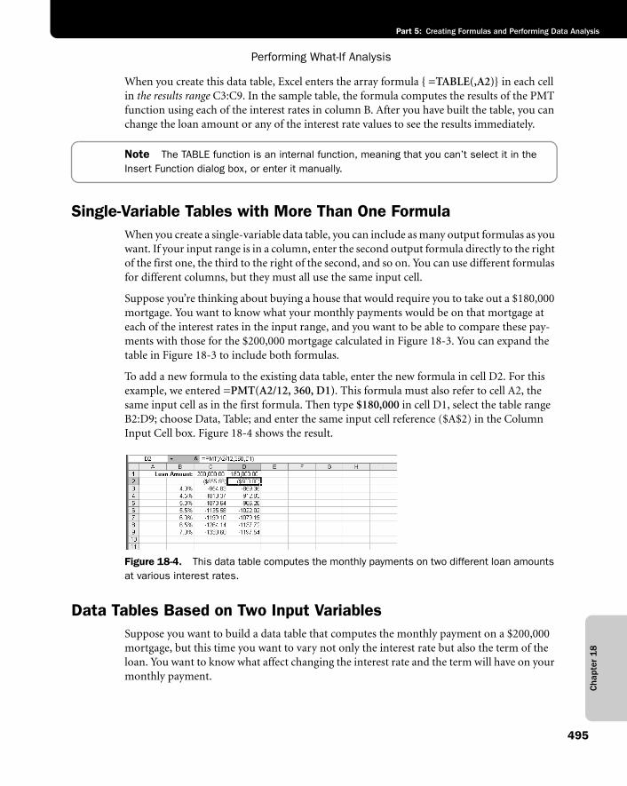
Cha

pter

18

Performing What-If Analysis

495

Part 5: Creating Formulas and Performing Data Analysis

When you create this data table, Excel enters the array formula { =TABLE(,A2)} in each cell in the results range C3:C9. In the sample table, the formula computes the results of the PMT function using each of the interest rates in column B. After you have built the table, you can change the loan amount or any of the interest rate values to see the results immediately.

Note The TABLE function is an internal function, meaning that you can’t select it in the Insert Function dialog box, or enter it manually.

Single-Variable Tables with More Than One FormulaWhen you create a single-variable data table, you can include as many output formulas as you want. If your input range is in a column, enter the second output formula directly to the right of the first one, the third to the right of the second, and so on. You can use different formulas for different columns, but they must all use the same input cell.

Suppose you’re thinking about buying a house that would require you to take out a $180,000 mortgage. You want to know what your monthly payments would be on that mortgage at each of the interest rates in the input range, and you want to be able to compare these pay-ments with those for the $200,000 mortgage calculated in Figure 18-3. You can expand the table in Figure 18-3 to include both formulas.

To add a new formula to the existing data table, enter the new formula in cell D2. For this example, we entered =PMT(A2/12, 360, D1). This formula must also refer to cell A2, the same input cell as in the first formula. Then type $180,000 in cell D1, select the table range B2:D9; choose Data, Table; and enter the same input cell reference ($A$2) in the Column Input Cell box. Figure 18-4 shows the result.

f18ie04

Figure 18-4. This data table computes the monthly payments on two different loan amounts at various interest rates.

Data Tables Based on Two Input VariablesSuppose you want to build a data table that computes the monthly payment on a $200,000 mortgage, but this time you want to vary not only the interest rate but also the term of the loan. You want to know what affect changing the interest rate and the term will have on your monthly payment.

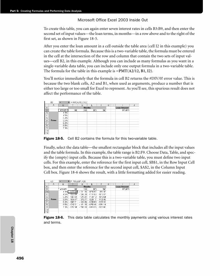
Chapter 1

8

Microsoft Office Excel 2003 Inside Out

Part 5: Creating Formulas and Performing Data Analysis

496

To create this table, you can again enter seven interest rates in cells B3:B9, and then enter the second set of input values—the loan terms, in months—in a row above and to the right of the first set, as shown in Figure 18-5.

After you enter the loan amount in a cell outside the table area (cell I2 in this example) you can create the table formula. Because this is a two-variable table, the formula must be entered in the cell at the intersection of the row and column that contain the two sets of input val-ues—cell B2, in this example. Although you can include as many formulas as you want in a single-variable data table, you can include only one output formula in a two-variable table. The formula for the table in this example is =PMT(A2/12, B1, I2).

You’ll notice immediately that the formula in cell B2 returns the #DIV/0! error value. This is because the two blank cells, A2 and B1, when used as arguments, produce a number that is either too large or too small for Excel to represent. As you’ll see, this spurious result does not affect the performance of the table.

f18ie05

Figure 18-5. Cell B2 contains the formula for this two-variable table.

Finally, select the data table—the smallest rectangular block that includes all the input values and the table formula. In this example, the table range is B2:F9. Choose Data, Table, and spec-ify the (empty) input cells. Because this is a two-variable table, you must define two input cells. For this example, enter the reference for the first input cell, $B$1, in the Row Input Cell box, and then enter the reference for the second input cell, $A$2, in the Column Input Cell box. Figure 18-6 shows the result, with a little formatting added for easier reading.

f18ie06

Figure 18-6. This data table calculates the monthly payments using various interest rates and terms.

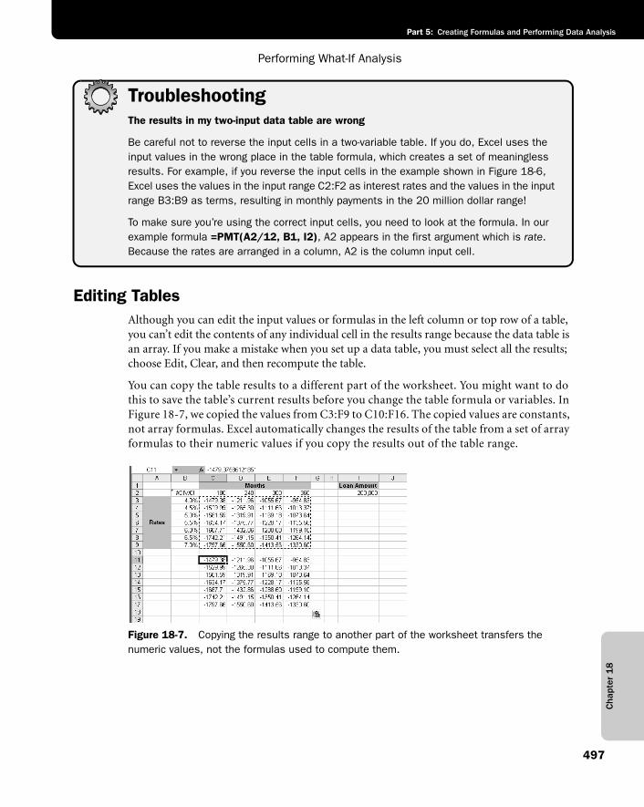
Cha

pter

18

Performing What-If Analysis

497

Part 5: Creating Formulas and Performing Data Analysis

TroubleshootingThe results in my two-input data table are wrong

Be careful not to reverse the input cells in a two-variable table. If you do, Excel uses the input values in the wrong place in the table formula, which creates a set of meaningless results. For example, if you reverse the input cells in the example shown in Figure 18-6, Excel uses the values in the input range C2:F2 as interest rates and the values in the input range B3:B9 as terms, resulting in monthly payments in the 20 million dollar range!

To make sure you’re using the correct input cells, you need to look at the formula. In our example formula =PMT(A2/12, B1, I2), A2 appears in the first argument which is rate.Because the rates are arranged in a column, A2 is the column input cell.

Editing TablesAlthough you can edit the input values or formulas in the left column or top row of a table, you can’t edit the contents of any individual cell in the results range because the data table is an array. If you make a mistake when you set up a data table, you must select all the results; choose Edit, Clear, and then recompute the table.

You can copy the table results to a different part of the worksheet. You might want to do this to save the table’s current results before you change the table formula or variables. In Figure 18-7, we copied the values from C3:F9 to C10:F16. The copied values are constants, not array formulas. Excel automatically changes the results of the table from a set of array formulas to their numeric values if you copy the results out of the table range.

f18ie07

Figure 18-7. Copying the results range to another part of the worksheet transfers the numeric values, not the formulas used to compute them.

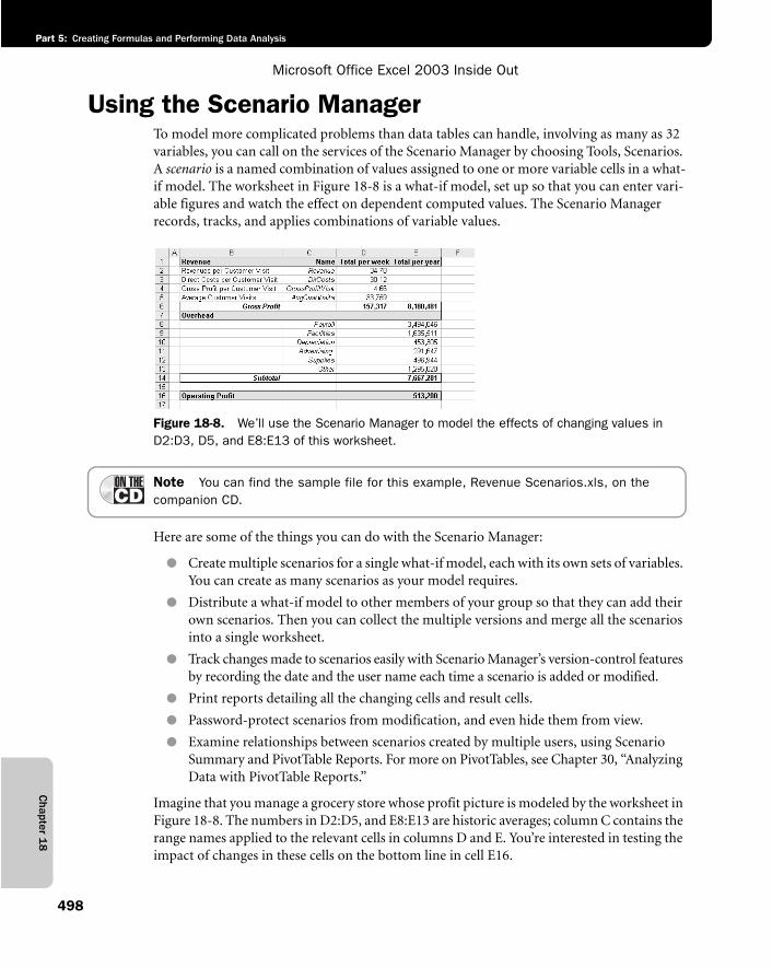
Chapter 1

8

Microsoft Office Excel 2003 Inside Out

Part 5: Creating Formulas and Performing Data Analysis

498

Using the Scenario ManagerTo model more complicated problems than data tables can handle, involving as many as 32 variables, you can call on the services of the Scenario Manager by choosing Tools, Scenarios. A scenario is a named combination of values assigned to one or more variable cells in a what-if model. The worksheet in Figure 18-8 is a what-if model, set up so that you can enter vari-able figures and watch the effect on dependent computed values. The Scenario Manager records, tracks, and applies combinations of variable values.

f18ie08

Figure 18-8. We’ll use the Scenario Manager to model the effects of changing values in D2:D3, D5, and E8:E13 of this worksheet.

Note You can find the sample file for this example, Revenue Scenarios.xls, on thecompanion CD.

Here are some of the things you can do with the Scenario Manager:

● Create multiple scenarios for a single what-if model, each with its own sets of variables. You can create as many scenarios as your model requires.

● Distribute a what-if model to other members of your group so that they can add their own scenarios. Then you can collect the multiple versions and merge all the scenarios into a single worksheet.

● Track changes made to scenarios easily with Scenario Manager’s version-control features by recording the date and the user name each time a scenario is added or modified.

● Print reports detailing all the changing cells and result cells.

● Password-protect scenarios from modification, and even hide them from view.

● Examine relationships between scenarios created by multiple users, using Scenario Summary and PivotTable Reports. For more on PivotTables, see Chapter 30, “Analyzing Data with PivotTable Reports.”

Imagine that you manage a grocery store whose profit picture is modeled by the worksheet in Figure 18-8. The numbers in D2:D5, and E8:E13 are historic averages; column C contains the range names applied to the relevant cells in columns D and E. You’re interested in testing the impact of changes in these cells on the bottom line in cell E16.

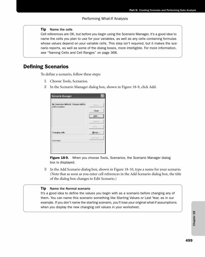
Cha

pter

18

Performing What-If Analysis

499

Part 5: Creating Formulas and Performing Data Analysis

Tip Name the cellsCell references are OK, but before you begin using the Scenario Manager, it’s a good idea to name the cells you plan to use for your variables, as well as any cells containing formulas whose values depend on your variable cells. This step isn’t required, but it makes the sce-nario reports, as well as some of the dialog boxes, more intelligible. For more information, see “Naming Cells and Cell Ranges” on page 368.

Defining ScenariosTo define a scenario, follow these steps:

1 Choose Tools, Scenarios.

2 In the Scenario Manager dialog box, shown in Figure 18-9, click Add.

f18ie09

Figure 18-9. When you choose Tools, Scenarios, the Scenario Manager dialog box is displayed.

3 In the Add Scenario dialog box, shown in Figure 18-10, type a name for your scenario. (Note that as soon as you enter cell references in the Add Scenario dialog box, the title of the dialog box changes to Edit Scenario.)

Tip Name the Normal scenarioIt’s a good idea to define the values you begin with as a scenario before changing any of them. You can name this scenario something like Starting Values or Last Year, as in our example. If you don’t name the starting scenario, you’ll lose your original what-if assumptions when you display the new changing cell values in your worksheet.

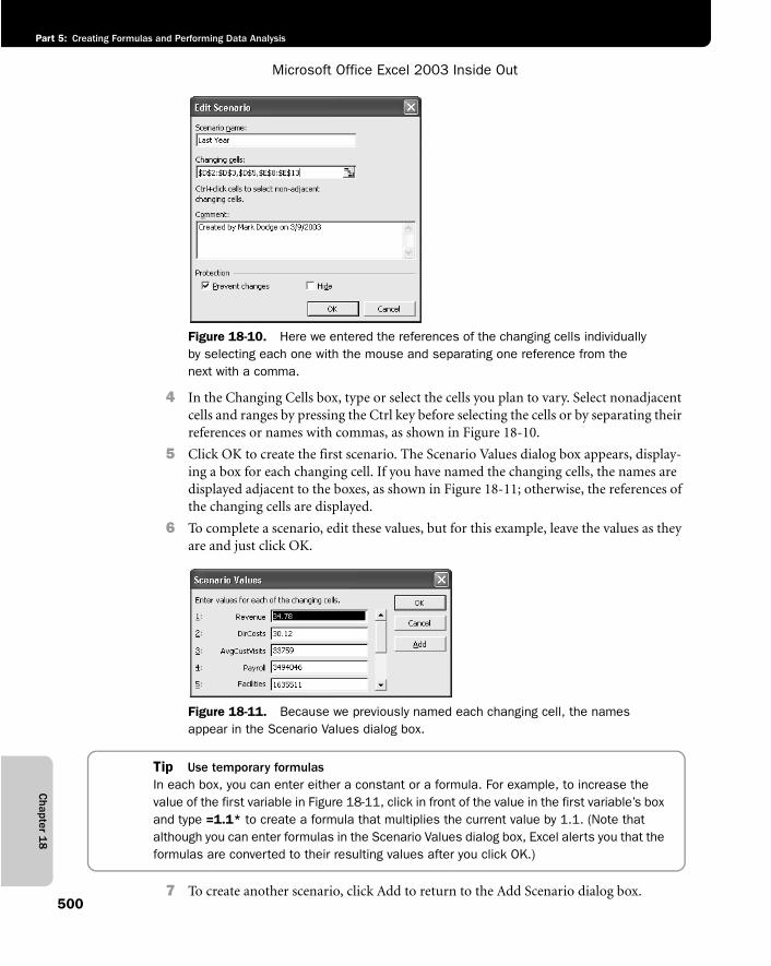
Chapter 1

8

Microsoft Office Excel 2003 Inside Out

Part 5: Creating Formulas and Performing Data Analysis

500

f18ie10

Figure 18-10. Here we entered the references of the changing cells individually by selecting each one with the mouse and separating one reference from the next with a comma.

4 In the Changing Cells box, type or select the cells you plan to vary. Select nonadjacent cells and ranges by pressing the Ctrl key before selecting the cells or by separating their references or names with commas, as shown in Figure 18-10.

5 Click OK to create the first scenario. The Scenario Values dialog box appears, display-ing a box for each changing cell. If you have named the changing cells, the names are displayed adjacent to the boxes, as shown in Figure 18-11; otherwise, the references of the changing cells are displayed.

6 To complete a scenario, edit these values, but for this example, leave the values as they are and just click OK.

f18ie11

Figure 18-11. Because we previously named each changing cell, the names appear in the Scenario Values dialog box.

Tip Use temporary formulasIn each box, you can enter either a constant or a formula. For example, to increase the value of the first variable in Figure 18-11, click in front of the value in the first variable’s box and type =1.1* to create a formula that multiplies the current value by 1.1. (Note that although you can enter formulas in the Scenario Values dialog box, Excel alerts you that the formulas are converted to their resulting values after you click OK.)

7 To create another scenario, click Add to return to the Add Scenario dialog box.

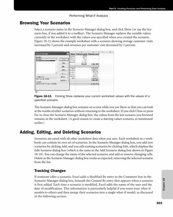
Cha

pter

18

Performing What-If Analysis

501

Part 5: Creating Formulas and Performing Data Analysis

Browsing Your ScenariosSelect a scenario name in the Scenario Manager dialog box, and click Show (or use the Sce-nario box, if you added it to a toolbar). The Scenario Manager replaces the variable values currently in the worksheet with the values you specified when you created the scenario. Figure 18-12 shows the example worksheet with a scenario showing average customer visits increased by 5 percent and revenues per customer visit decreased by 5 percent.

f18ie12

Figure 18-12. Clicking Show replaces your current worksheet values with the values of a specified scenario.

The Scenario Manager dialog box remains on screen while you use Show so that you can look at the results of other scenarios without returning to the worksheet. If you click Close or press Esc to close the Scenario Manager dialog box, the values from the last scenario you browsed remains in the worksheet. (A good reason to create a starting values scenario, as mentioned earlier.)

Adding, Editing, and Deleting ScenariosScenarios are saved with all other worksheet data when you save. Each worksheet in a work-book can contain its own set of scenarios. In the Scenario Manager dialog box, you add new scenarios by clicking Add, and you edit existing scenarios by clicking Edit, which displays the Edit Scenario dialog box (which is the same as the Add Scenario dialog box shown in Figure 18-10). You can change the name of the selected scenario, and add or remove changing cells. Delete in the Scenario Manager dialog box works as expected, removing the selected scenario from the list.

Tracking ChangesIf someone edits a scenario, Excel adds a Modified By entry to the Comment box in the Scenario Manager dialog box, beneath the Created By entry that appears when a scenario is first added. Each time a scenario is modified, Excel adds the name of the user and the date of modification. This information is particularly helpful if you route your what-if models to others and then merge their scenarios into a single what-if model, as discussed in the following section.

Chapter 1

8

Microsoft Office Excel 2003 Inside Out

Part 5: Creating Formulas and Performing Data Analysis

502

Inside OutTrack comment modifying

When you edit scenarios, you can modify the contents of the Comment box; those modifi-cations persist in all dialog boxes, including the creation and modification dates. You might not want this to happen, if you really want to track changes or prevent tampering. If you don’t want these comments modified, make sure you take advantage of the preventative measures discussed in “Protecting Worksheets” on page 127.

Routing and Merging ScenariosIf part of your job is to develop what-if models or projections for your company, you proba-bly spend a lot of time gathering information about trends and market forces that might affect the company in the future. Often you need input from several people, each of whom knows about a particular aspect of the business, such as payroll costs or sales trends. Excel includes two features to make this sort of information-gathering task easier: document routing and scenario merging.

If you are connected to a network that uses a compatible electronic mail system, you can choose File, Send To, Routing Recipient to attach the current workbook to an electronic mail message. Compatible electronic mail systems include Microsoft Outlook, Microsoft Mail, Lotus cc:Mail, and any other electronic mail application that comply with the Messaging Application Programming Interface (MAPI) or Vendor Independent Messaging (VIM) stan-dards. Alternatively, you can route workbooks using the Internet via Web documents and FTP sites.

Note For more on using routing slips, see “Routing Workbooks to a Workgroup” on page 236. For more on using the Internet with Excel, see Chapter 20, “Transferring Files to and from Internet Sites.”

If you are not connected to a network with a compatible electronic mail system, you can make copies of the worksheet containing your what-if model and distribute the copies to your coworkers the old-fashioned way—on floppy disks.

For example, suppose you want to distribute a what-if model to your coworkers: Vicki has expertise on customer trends, Max knows the payroll story, and Regina keeps track of adver-tising. You can consolidate their contributions using the routing slip approach, if available, or distribute individually named copies of the workbook to each person. After your coworkers add their what-if scenarios and return the workbook or workbooks, you can merge the

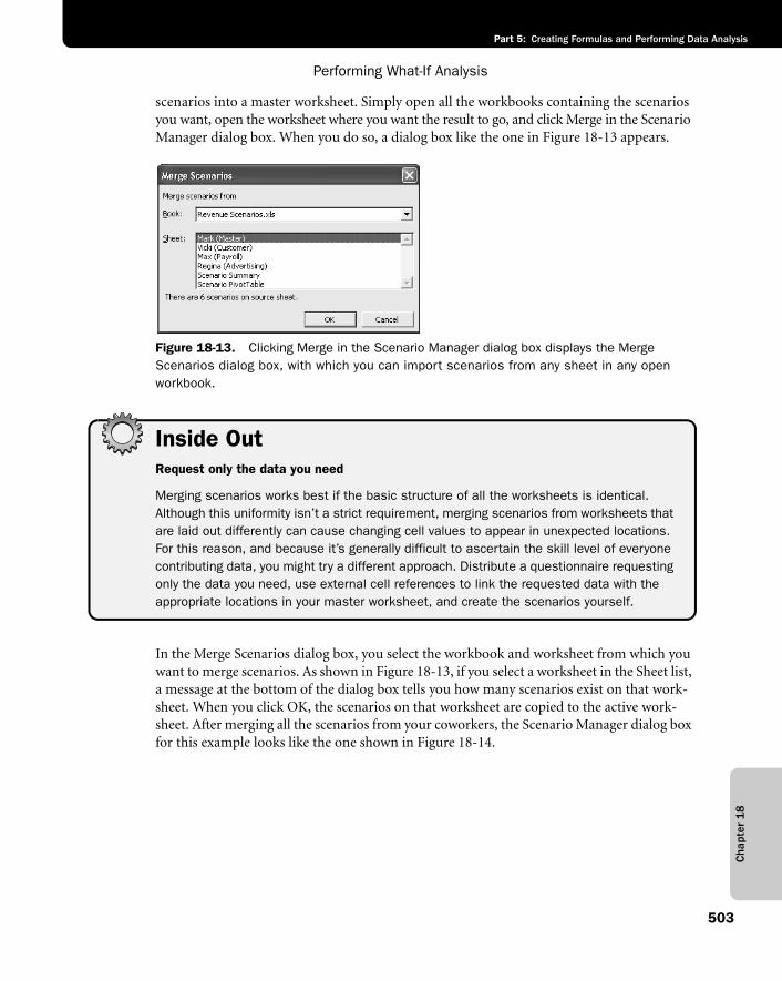
Cha

pter

18

Performing What-If Analysis

503

Part 5: Creating Formulas and Performing Data Analysis

scenarios into a master worksheet. Simply open all the workbooks containing the scenarios you want, open the worksheet where you want the result to go, and click Merge in the Scenario Manager dialog box. When you do so, a dialog box like the one in Figure 18-13 appears.

f18ie13

Figure 18-13. Clicking Merge in the Scenario Manager dialog box displays the Merge Scenarios dialog box, with which you can import scenarios from any sheet in any open workbook.

Inside OutRequest only the data you need

Merging scenarios works best if the basic structure of all the worksheets is identical. Although this uniformity isn’t a strict requirement, merging scenarios from worksheets that are laid out differently can cause changing cell values to appear in unexpected locations. For this reason, and because it’s generally difficult to ascertain the skill level of everyone contributing data, you might try a different approach. Distribute a questionnaire requesting only the data you need, use external cell references to link the requested data with the appropriate locations in your master worksheet, and create the scenarios yourself.

In the Merge Scenarios dialog box, you select the workbook and worksheet from which you want to merge scenarios. As shown in Figure 18-13, if you select a worksheet in the Sheet list, a message at the bottom of the dialog box tells you how many scenarios exist on that work-sheet. When you click OK, the scenarios on that worksheet are copied to the active work-sheet. After merging all the scenarios from your coworkers, the Scenario Manager dialog box for this example looks like the one shown in Figure 18-14.

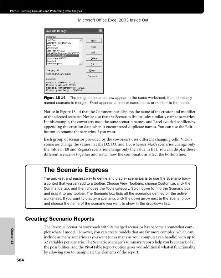
Chapter 1

8

Microsoft Office Excel 2003 Inside Out

Part 5: Creating Formulas and Performing Data Analysis

504

f18ie14

Figure 18-14. The merged scenarios now appear in the same worksheet; if an identically named scenario is merged, Excel appends a creator name, date, or number to the name.

Notice in Figure 18-14 that the Comment box displays the name of the creator and modifier of the selected scenario. Notice also that the Scenarios list includes similarly named scenarios. In this example, the coworkers used the same scenario names, and Excel avoided conflicts by appending the creation date when it encountered duplicate names. You can use the Edit button to rename the scenarios if you want.

Each group of scenarios provided by the coworkers uses different changing cells. Vicki’s scenarios change the values in cells D2, D3, and D5, whereas Max’s scenarios change only the value in E8 and Regina’s scenarios change only the value in E11. You can display these different scenarios together and watch how the combinations affect the bottom line.

The Scenario ExpressThe quickest and easiest way to define and display scenarios is to use the Scenario box—a control that you can add to a toolbar. Choose View, Toolbars, choose Customize, click the Commands tab, and then choose the Tools category. Scroll down to find the Scenario box and drag it to any toolbar. The Scenario box lists all the scenarios defined on the active worksheet. If you want to display a scenario, click the down arrow next to the Scenario box and choose the name of the scenario you want to show in the drop-down list.

Creating Scenario ReportsThe Revenue Scenarios workbook with its merged scenarios has become a somewhat com-plex what-if model. However, you can create models that are far more complex, which can include as many scenarios as you want (or as many as your computer can handle) with up to 32 variables per scenario. The Scenario Manager’s summary reports help you keep track of all the possibilities, and the PivotTable Report option gives you additional what-if functionality by allowing you to manipulate the elements of the report.

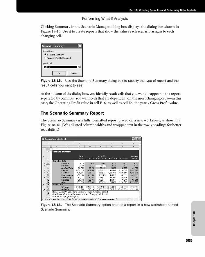
Cha

pter

18

Performing What-If Analysis

505

Part 5: Creating Formulas and Performing Data Analysis

Clicking Summary in the Scenario Manager dialog box displays the dialog box shown in Figure 18-15. Use it to create reports that show the values each scenario assigns to each changing cell.

f18ie15

Figure 18-15. Use the Scenario Summary dialog box to specify the type of report and the result cells you want to see.

At the bottom of the dialog box, you identify result cells that you want to appear in the report, separated by commas. You want cells that are dependent on the most changing cells—in this case, the Operating Profit value in cell E16, as well as cell E6, the yearly Gross Profit value.

The Scenario Summary ReportThe Scenario Summary is a fully formatted report placed on a new worksheet, as shown in Figure 18-16. (We adjusted column widths and wrapped text in the row 3 headings for better readability.)

f18ie16

Figure 18-16. The Scenario Summary option creates a report in a new worksheet named Scenario Summary.

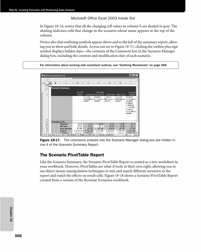
Chapter 1

8

Microsoft Office Excel 2003 Inside Out

Part 5: Creating Formulas and Performing Data Analysis

506

In Figure 18-16, notice that all the changing cell values in column E are shaded in gray. The shading indicates cells that change in the scenario whose name appears at the top of the column.

Notice also that outlining symbols appear above and to the left of the summary report, allow-ing you to show and hide details. As you can see in Figure 18-17, clicking the outline plus sign symbol displays hidden data—the contents of the Comment box in the Scenario Manager dialog box, including the creation and modification date of each scenario.

For information about working with worksheet outlines, see “Outlining Worksheets” on page 268.

f18ie17

Figure 18-17. The comments entered into the Scenario Manager dialog box are hidden in row 4 of the Scenario Summary Report.

The Scenario PivotTable ReportLike the Scenario Summary, the Scenario PivotTable Report is created as a new worksheet in your workbook. However, PivotTables are what-if tools in their own right, allowing you to use direct mouse-manipulation techniques to mix and match different scenarios in the report and watch the effects on result cells. Figure 18-18 shows a Scenario PivotTable Report created from a version of the Revenue Scenarios workbook.

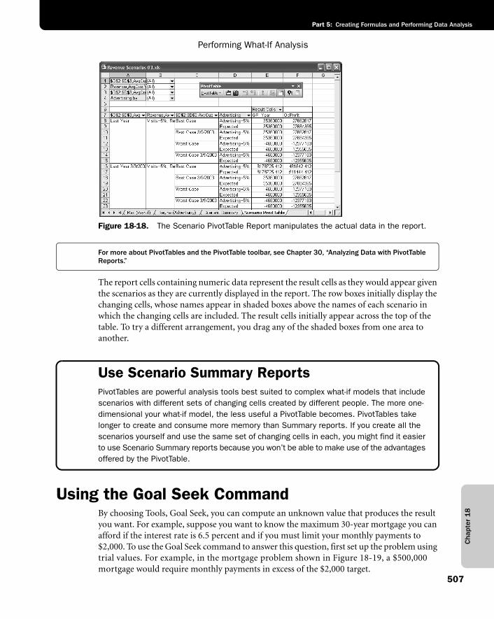
Cha

pter

18

Performing What-If Analysis

507

Part 5: Creating Formulas and Performing Data Analysis

f18ie18

Figure 18-18. The Scenario PivotTable Report manipulates the actual data in the report.

For more about PivotTables and the PivotTable toolbar, see Chapter 30, “Analyzing Data with PivotTable Reports.”

The report cells containing numeric data represent the result cells as they would appear given the scenarios as they are currently displayed in the report. The row boxes initially display the changing cells, whose names appear in shaded boxes above the names of each scenario in which the changing cells are included. The result cells initially appear across the top of the table. To try a different arrangement, you drag any of the shaded boxes from one area to another.

Use Scenario Summary ReportsPivotTables are powerful analysis tools best suited to complex what-if models that include scenarios with different sets of changing cells created by different people. The more one-dimensional your what-if model, the less useful a PivotTable becomes. PivotTables take longer to create and consume more memory than Summary reports. If you create all the scenarios yourself and use the same set of changing cells in each, you might find it easier to use Scenario Summary reports because you won’t be able to make use of the advantages offered by the PivotTable.

Using the Goal Seek CommandBy choosing Tools, Goal Seek, you can compute an unknown value that produces the result you want. For example, suppose you want to know the maximum 30-year mortgage you can afford if the interest rate is 6.5 percent and if you must limit your monthly payments to $2,000. To use the Goal Seek command to answer this question, first set up the problem using trial values. For example, in the mortgage problem shown in Figure 18-19, a $500,000 mortgage would require monthly payments in excess of the $2,000 target.

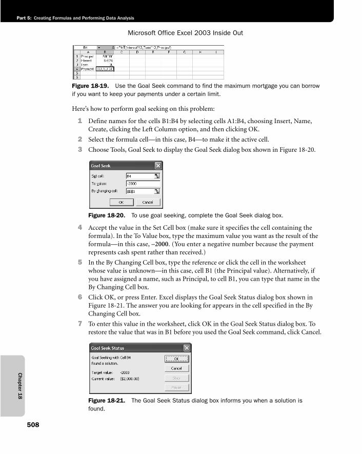
Chapter 1

8

Microsoft Office Excel 2003 Inside Out

Part 5: Creating Formulas and Performing Data Analysis

508

f18ie19

Figure 18-19. Use the Goal Seek command to find the maximum mortgage you can borrow if you want to keep your payments under a certain limit.

Here’s how to perform goal seeking on this problem:

1 Define names for the cells B1:B4 by selecting cells A1:B4, choosing Insert, Name, Create, clicking the Left Column option, and then clicking OK.

2 Select the formula cell—in this case, B4—to make it the active cell.

3 Choose Tools, Goal Seek to display the Goal Seek dialog box shown in Figure 18-20.

f18ie20

Figure 18-20. To use goal seeking, complete the Goal Seek dialog box.

4 Accept the value in the Set Cell box (make sure it specifies the cell containing the formula). In the To Value box, type the maximum value you want as the result of the formula—in this case, –2000. (You enter a negative number because the payment represents cash spent rather than received.)

5 In the By Changing Cell box, type the reference or click the cell in the worksheet whose value is unknown—in this case, cell B1 (the Principal value). Alternatively, if you have assigned a name, such as Principal, to cell B1, you can type that name in the By Changing Cell box.

6 Click OK, or press Enter. Excel displays the Goal Seek Status dialog box shown in Figure 18-21. The answer you are looking for appears in the cell specified in the By Changing Cell box.

7 To enter this value in the worksheet, click OK in the Goal Seek Status dialog box. To restore the value that was in B1 before you used the Goal Seek command, click Cancel.

f18ie21

Figure 18-21. The Goal Seek Status dialog box informs you when a solution is found.

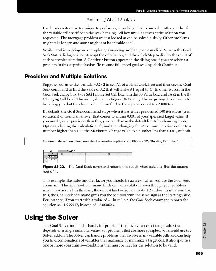
Cha

pter

18

Performing What-If Analysis

509

Part 5: Creating Formulas and Performing Data Analysis

Excel uses an iterative technique to perform goal seeking. It tries one value after another for the variable cell specified in the By Changing Cell box until it arrives at the solution you requested. The mortgage problem we just looked at can be solved quickly. Other problems might take longer, and some might not be solvable at all.

While Excel is working on a complex goal-seeking problem, you can click Pause in the Goal Seek Status dialog box to interrupt the calculation, and then click Step to display the result of each successive iteration. A Continue button appears in the dialog box if you are solving a problem in this stepwise fashion. To resume full-speed goal seeking, click Continue.

Precision and Multiple SolutionsSuppose you enter the formula =A2^2 in cell A1 of a blank worksheet and then use the Goal Seek command to find the value of A2 that will make A1 equal to 4. (In other words, in the Goal Seek dialog box, type $A$1 in the Set Cell box, 4 in the To Value box, and $A$2 in the By Changing Cell box.) The result, shown in Figure 18-22, might be surprising. Excel seems to be telling you that the closest value it can find to the square root of 4 is 2.000023.

By default, the Goal Seek command stops when it has either performed 100 iterations (trial solutions) or found an answer that comes to within 0.001 of your specified target value. If you need greater precision than this, you can change the default limits by choosing Tools, Options, clicking the Calculation tab, and then changing the Maximum Iterations value to a number higher than 100, the Maximum Change value to a number less than 0.001, or both.

For more information about worksheet calculation options, see Chapter 12, “Building Formulas.”

f18ie22

Figure 18-22. The Goal Seek command returns this result when asked to find the square root of 4.

This example illustrates another factor you should be aware of when you use the Goal Seek command. The Goal Seek command finds only one solution, even though your problem might have several. In this case, the value 4 has two square roots: +2 and –2. In situations like this, the Goal Seek command gives you the solution with the same sign as the starting value. For instance, if you start with a value of –1 in cell A2, the Goal Seek command reports the solution as –1.999917, instead of +2.000023.

Using the SolverThe Goal Seek command is handy for problems that involve an exact target value that depends on a single unknown value. For problems that are more complex, you should use the Solver add-in. The Solver can handle problems that involve many variable cells and can help you find combinations of variables that maximize or minimize a target cell. It also specifies one or more constraints—conditions that must be met for the solution to be valid.

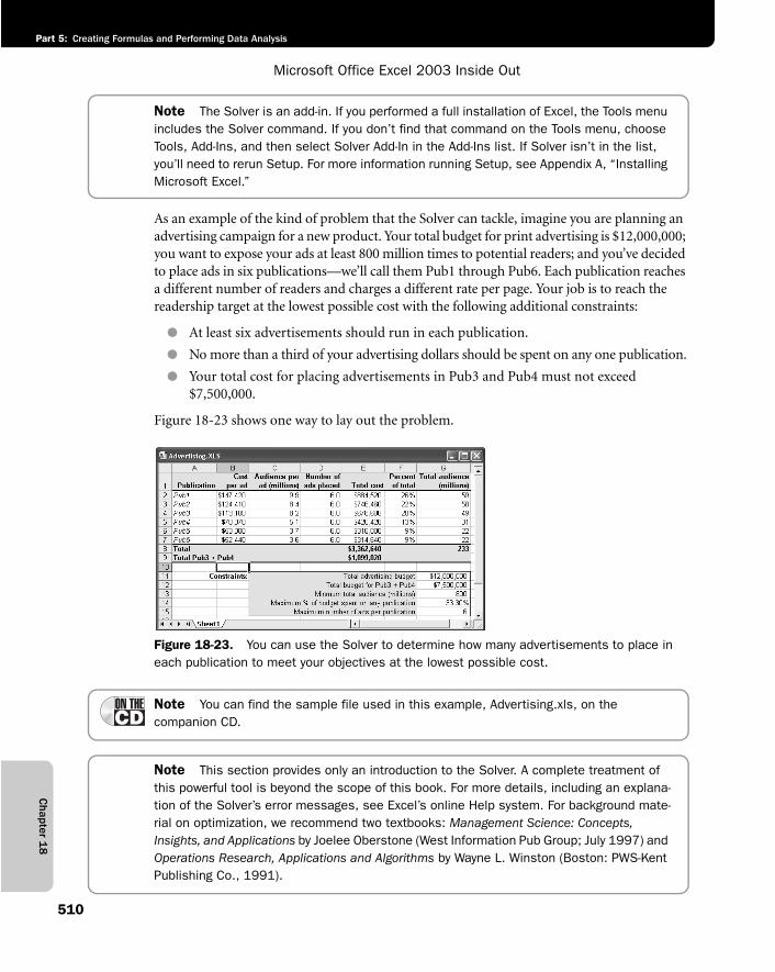
Chapter 1

8

Microsoft Office Excel 2003 Inside Out

Part 5: Creating Formulas and Performing Data Analysis

510

Note The Solver is an add-in. If you performed a full installation of Excel, the Tools menu includes the Solver command. If you don’t find that command on the Tools menu, choose Tools, Add-Ins, and then select Solver Add-In in the Add-Ins list. If Solver isn’t in the list, you’ll need to rerun Setup. For more information running Setup, see Appendix A, “Installing Microsoft Excel.”

As an example of the kind of problem that the Solver can tackle, imagine you are planning an advertising campaign for a new product. Your total budget for print advertising is $12,000,000; you want to expose your ads at least 800 million times to potential readers; and you’ve decided to place ads in six publications—we’ll call them Pub1 through Pub6. Each publication reaches a different number of readers and charges a different rate per page. Your job is to reach the readership target at the lowest possible cost with the following additional constraints:

● At least six advertisements should run in each publication.

● No more than a third of your advertising dollars should be spent on any one publication.

● Your total cost for placing advertisements in Pub3 and Pub4 must not exceed $7,500,000.

Figure 18-23 shows one way to lay out the problem.

f18ie23

Figure 18-23. You can use the Solver to determine how many advertisements to place in each publication to meet your objectives at the lowest possible cost.

Note You can find the sample file used in this example, Advertising.xls, on the companion CD.

Note This section provides only an introduction to the Solver. A complete treatment of this powerful tool is beyond the scope of this book. For more details, including an explana-tion of the Solver’s error messages, see Excel’s online Help system. For background mate-rial on optimization, we recommend two textbooks: Management Science: Concepts, Insights, and Applications by Joelee Oberstone (West Information Pub Group; July 1997) and Operations Research, Applications and Algorithms by Wayne L. Winston (Boston: PWS-Kent Publishing Co., 1991).

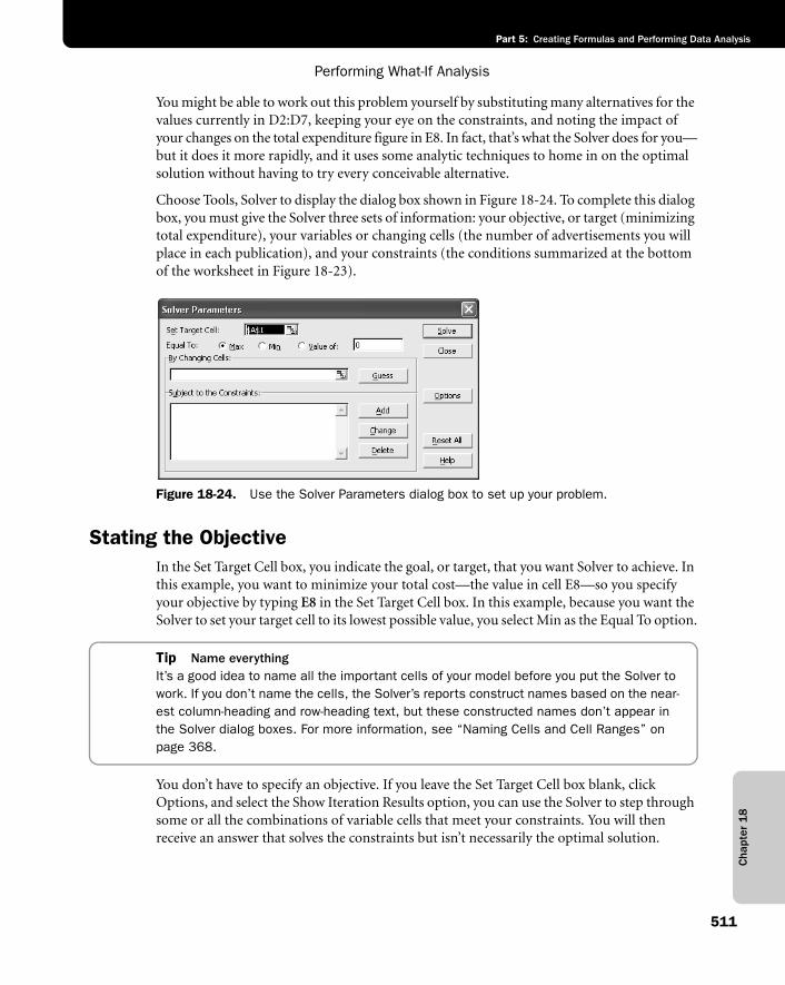
Cha

pter

18

Performing What-If Analysis

511

Part 5: Creating Formulas and Performing Data Analysis

You might be able to work out this problem yourself by substituting many alternatives for the values currently in D2:D7, keeping your eye on the constraints, and noting the impact of your changes on the total expenditure figure in E8. In fact, that’s what the Solver does for you—but it does it more rapidly, and it uses some analytic techniques to home in on the optimal solution without having to try every conceivable alternative.

Choose Tools, Solver to display the dialog box shown in Figure 18-24. To complete this dialog box, you must give the Solver three sets of information: your objective, or target (minimizing total expenditure), your variables or changing cells (the number of advertisements you will place in each publication), and your constraints (the conditions summarized at the bottom of the worksheet in Figure 18-23).

f18ie24

Figure 18-24. Use the Solver Parameters dialog box to set up your problem.

Stating the ObjectiveIn the Set Target Cell box, you indicate the goal, or target, that you want Solver to achieve. In this example, you want to minimize your total cost—the value in cell E8—so you specify your objective by typing E8 in the Set Target Cell box. In this example, because you want the Solver to set your target cell to its lowest possible value, you select Min as the Equal To option.

Tip Name everythingIt’s a good idea to name all the important cells of your model before you put the Solver to work. If you don’t name the cells, the Solver’s reports construct names based on the near-est column-heading and row-heading text, but these constructed names don’t appear in the Solver dialog boxes. For more information, see “Naming Cells and Cell Ranges” on page 368.

You don’t have to specify an objective. If you leave the Set Target Cell box blank, click Options, and select the Show Iteration Results option, you can use the Solver to step through some or all the combinations of variable cells that meet your constraints. You will then receive an answer that solves the constraints but isn’t necessarily the optimal solution.

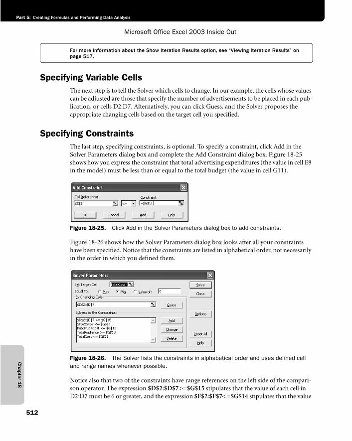
Chapter 1

8

Microsoft Office Excel 2003 Inside Out

Part 5: Creating Formulas and Performing Data Analysis

512

For more information about the Show Iteration Results option, see “Viewing Iteration Results” on page 517.

Specifying Variable CellsThe next step is to tell the Solver which cells to change. In our example, the cells whose values can be adjusted are those that specify the number of advertisements to be placed in each pub-lication, or cells D2:D7. Alternatively, you can click Guess, and the Solver proposes the appropriate changing cells based on the target cell you specified.

Specifying ConstraintsThe last step, specifying constraints, is optional. To specify a constraint, click Add in the Solver Parameters dialog box and complete the Add Constraint dialog box. Figure 18-25 shows how you express the constraint that total advertising expenditures (the value in cell E8 in the model) must be less than or equal to the total budget (the value in cell G11).

f18ie25

Figure 18-25. Click Add in the Solver Parameters dialog box to add constraints.

Figure 18-26 shows how the Solver Parameters dialog box looks after all your constraints have been specified. Notice that the constraints are listed in alphabetical order, not necessarily in the order in which you defined them.

f18ie26

Figure 18-26. The Solver lists the constraints in alphabetical order and uses defined cell and range names whenever possible.

Notice also that two of the constraints have range references on the left side of the compari-son operator. The expression $D$2:$D$7>=$G$15 stipulates that the value of each cell in D2:D7 must be 6 or greater, and the expression $F$2:$F$7<=$G$14 stipulates that the value

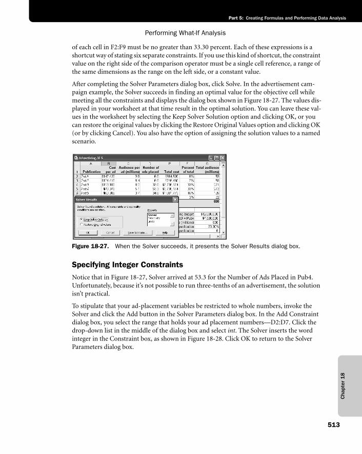
Cha

pter

18

Performing What-If Analysis

513

Part 5: Creating Formulas and Performing Data Analysis

of each cell in F2:F9 must be no greater than 33.30 percent. Each of these expressions is a shortcut way of stating six separate constraints. If you use this kind of shortcut, the constraint value on the right side of the comparison operator must be a single cell reference, a range of the same dimensions as the range on the left side, or a constant value.

After completing the Solver Parameters dialog box, click Solve. In the advertisement cam-paign example, the Solver succeeds in finding an optimal value for the objective cell while meeting all the constraints and displays the dialog box shown in Figure 18-27. The values dis-played in your worksheet at that time result in the optimal solution. You can leave these val-ues in the worksheet by selecting the Keep Solver Solution option and clicking OK, or you can restore the original values by clicking the Restore Original Values option and clicking OK (or by clicking Cancel). You also have the option of assigning the solution values to a named scenario.

f18ie27

Figure 18-27. When the Solver succeeds, it presents the Solver Results dialog box.

Specifying Integer ConstraintsNotice that in Figure 18-27, Solver arrived at 53.3 for the Number of Ads Placed in Pub4. Unfortunately, because it’s not possible to run three-tenths of an advertisement, the solution isn’t practical.

To stipulate that your ad-placement variables be restricted to whole numbers, invoke the Solver and click the Add button in the Solver Parameters dialog box. In the Add Constraint dialog box, you select the range that holds your ad placement numbers—D2:D7. Click the drop-down list in the middle of the dialog box and select int. The Solver inserts the word integer in the Constraint box, as shown in Figure 18-28. Click OK to return to the Solver Parameters dialog box.

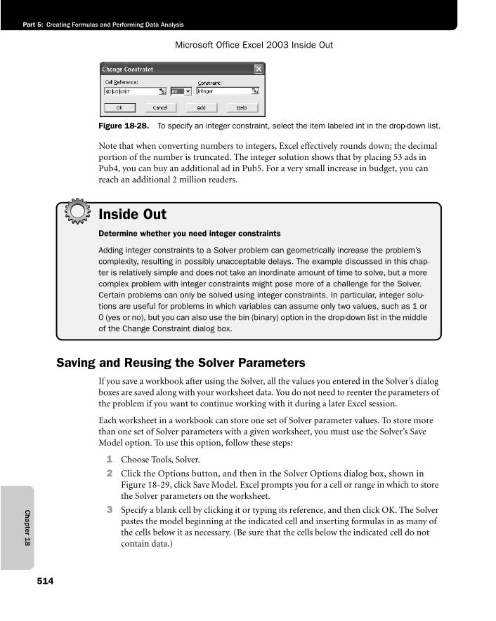
Chapter 1

8

Microsoft Office Excel 2003 Inside Out

Part 5: Creating Formulas and Performing Data Analysis

514

f18ie28

Figure 18-28. To specify an integer constraint, select the item labeled int in the drop-down list.

Note that when converting numbers to integers, Excel effectively rounds down; the decimal portion of the number is truncated. The integer solution shows that by placing 53 ads in Pub4, you can buy an additional ad in Pub5. For a very small increase in budget, you can reach an additional 2 million readers.

Inside OutDetermine whether you need integer constraints

Adding integer constraints to a Solver problem can geometrically increase the problem’s complexity, resulting in possibly unacceptable delays. The example discussed in this chap-ter is relatively simple and does not take an inordinate amount of time to solve, but a more complex problem with integer constraints might pose more of a challenge for the Solver. Certain problems can only be solved using integer constraints. In particular, integer solu-tions are useful for problems in which variables can assume only two values, such as 1 or 0 (yes or no), but you can also use the bin (binary) option in the drop-down list in the middle of the Change Constraint dialog box.

Saving and Reusing the Solver ParametersIf you save a workbook after using the Solver, all the values you entered in the Solver’s dialog boxes are saved along with your worksheet data. You do not need to reenter the parameters of the problem if you want to continue working with it during a later Excel session.

Each worksheet in a workbook can store one set of Solver parameter values. To store more than one set of Solver parameters with a given worksheet, you must use the Solver’s Save Model option. To use this option, follow these steps:

1 Choose Tools, Solver.

2 Click the Options button, and then in the Solver Options dialog box, shown inFigure 18-29, click Save Model. Excel prompts you for a cell or range in which to store the Solver parameters on the worksheet.

3 Specify a blank cell by clicking it or typing its reference, and then click OK. The Solver pastes the model beginning at the indicated cell and inserting formulas in as many of the cells below it as necessary. (Be sure that the cells below the indicated cell do not contain data.)

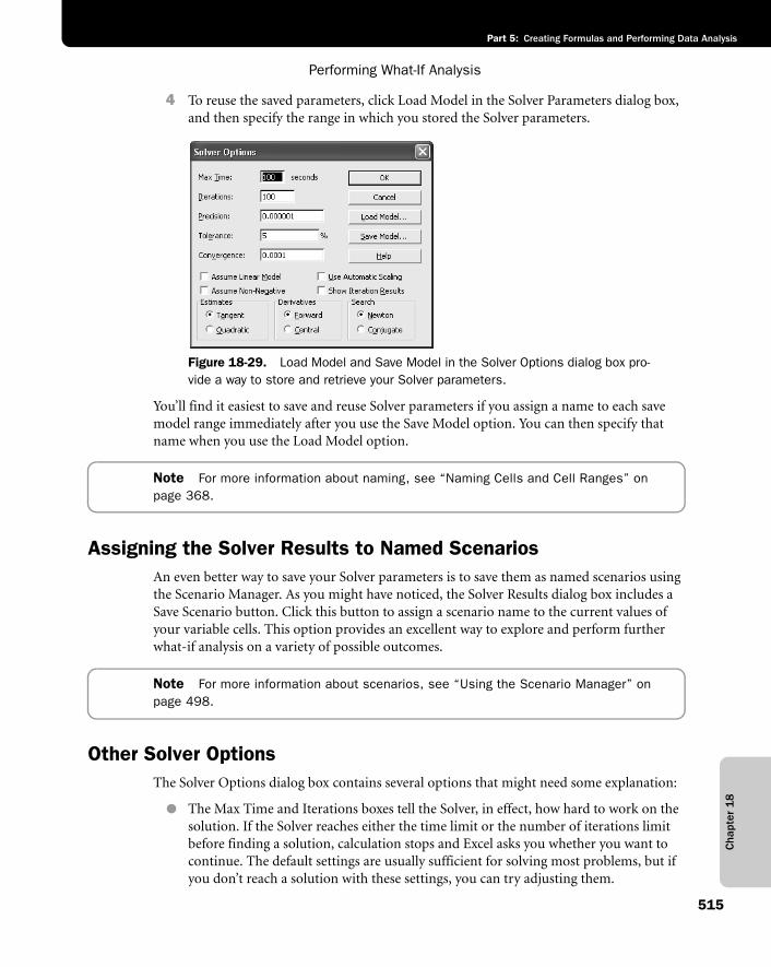
Cha

pter

18

Performing What-If Analysis

515

Part 5: Creating Formulas and Performing Data Analysis

4 To reuse the saved parameters, click Load Model in the Solver Parameters dialog box, and then specify the range in which you stored the Solver parameters.

f18ie29

Figure 18-29. Load Model and Save Model in the Solver Options dialog box pro-vide a way to store and retrieve your Solver parameters.

You’ll find it easiest to save and reuse Solver parameters if you assign a name to each save model range immediately after you use the Save Model option. You can then specify that name when you use the Load Model option.

Note For more information about naming, see “Naming Cells and Cell Ranges” on page 368.

Assigning the Solver Results to Named ScenariosAn even better way to save your Solver parameters is to save them as named scenarios using the Scenario Manager. As you might have noticed, the Solver Results dialog box includes a Save Scenario button. Click this button to assign a scenario name to the current values of your variable cells. This option provides an excellent way to explore and perform further what-if analysis on a variety of possible outcomes.

Note For more information about scenarios, see “Using the Scenario Manager” on page 498.

Other Solver OptionsThe Solver Options dialog box contains several options that might need some explanation:

● The Max Time and Iterations boxes tell the Solver, in effect, how hard to work on the solution. If the Solver reaches either the time limit or the number of iterations limit before finding a solution, calculation stops and Excel asks you whether you want to continue. The default settings are usually sufficient for solving most problems, but if you don’t reach a solution with these settings, you can try adjusting them.

Chapter 1

8

Microsoft Office Excel 2003 Inside Out

Part 5: Creating Formulas and Performing Data Analysis

516

● The Precision setting is used by the Solver to determine how closely you want values in the constraint cells to match your constraints. The closer this setting is to the value 1, the lower the precision is. If you specify a setting that is less than the default 0.000001, it results in a longer solution time.

● The Tolerance setting applies only to problems that use integer constraints and represents a percentage of error allowed in the solution.

● The Estimates, Derivatives, and Search options are best left at their default settings, unless you understand linear optimization techniques. If you want more information about these options, click Help in the Solver Options dialog box.

Linear ModelsA linear optimization problem is one in which the value of the target cell is a linear function of each variable cell; that is, if you plot XY charts of the target cell’s value against all meaning-ful values of each variable cell, your charts are straight lines. If some of your plots produce curves instead of straight lines, the problem is nonlinear.

The Assume Linear Model option can be turned on only for what-if models in which all the relationships are linear. Models that use simple addition and subtraction and worksheet functions, such as SUM, are linear in nature. However, most models are nonlinear. They are generated by multiplying changing cells by other changing cells, by using exponentiation or growth factors, or by using nonlinear worksheet functions, such as PMT.

The Solver can solve linear problems more quickly if you click Options in the Solver Param-eters dialog box and then select the Assume Linear Model option. If you select this option for a nonlinear problem and then try to solve the problem, however, the Solver Results dialog box displays the message “The conditions for Assume Linear Model are not satisfied.” If you are not sure about the nature of your model, it’s best not to use this option.

The Importance of Using AppropriateStarting Values If your problem is nonlinear, you must be aware of one important detail: Your choice of start-ing values can affect the solution generated by the Solver. With nonlinear problems, you should always do the following:

● Set your variable cells to reasonable approximations of their optimal values before running the problem.

● Test alternative starting values to see what impact, if any, they have on the Solver’s solution.

Cha

pter

18

Performing What-If Analysis

517

Part 5: Creating Formulas and Performing Data Analysis

Viewing Iteration ResultsIf you’re interested in exploring many combinations of your variable cells, rather than only the combination that produces the optimal result, you can take advantage of the Solver’s Show Iteration Results option. Click Options in the Solver Parameters dialog box, and select Show Iteration Results in the Solver Options dialog box. After each iteration, the Show Trial Solution dialog box appears, which allows you to save the scenario and then either stop the trial or continue with the next iteration.

You should be aware that if you use Show Iteration Results, the Solver pauses for solutions that do not meet all your constraints as well as for sub-optimal solutions that do.

Generating ReportsIn addition to inserting optimal values in your problem’s variable cells, the Solver can summarize its results in three reports: Answer, Sensitivity, and Limits. To generate one or more reports, select the names of the reports in the Solver Results dialog box. Select the reports you want, and then click OK. Each report is saved on a separate worksheet in the current workbook.

The Sensitivity ReportThe Sensitivity report provides information about how sensitive your target cell is to changes in your constraints. This report has two sections: one for your variable cells and one for your constraints. The right column in each section provides the sensitivity information.

Each changing cell and constraint cell is listed in a separate row. The Changing Cell area includes a Reduced Gradient value that indicates how the target cell would be affected by a one-unit increase in the corresponding changing cell. Similarly, the Lagrange Multiplier col-umn in the Constraints area indicates how the target cell would be affected by a one-unit increase in the corresponding constraint value.

The Answer ReportThe Answer report lists the target cell, the variable cells, and the constraints. This report also includes information about the status of and slack value for each constraint. The status can be Binding, Not Binding, or Not Satisfied. The slack value is the difference between the solu-tion value of the constraint cells and the number that appears on the right side of the con-straint formula. A binding constraint is one for which the slack value is 0. A nonbinding constraint is a constraint that was satisfied with a nonzero slack value.

Chapter 1

8

Microsoft Office Excel 2003 Inside Out

Part 5: Creating Formulas and Performing Data Analysis

518

Note If you select the Assume Linear Model option in the Solver Options dialog box, the Answer Report is the only report that the Solver produces for you (the Limits and Sensitivity reports are not meaningful when using integer constraints).

The Limits ReportThe Limits report tells you how much the values of your variable cells can be increased or decreased without breaking the constraints of your problem. For each variable cell, this report lists the optimal value as well as the lowest and highest values that can be used without violating constraints.

TroubleshootingThe Solver can’t solve my problem

The Solver is powerful but not miraculous. It might not be able to solve every problem you give it. If the Solver can’t find the optimal solution to your problem, it presents an unsuccessful completion message in the Solver Solution dialog box. The most common unsuccessful completion messages are the following:

Solver could not find a feasible solution. The Solver is unable to find a solution that sat-isfies all your constraints. This can happen if the constraints are logically conflicting or if not all the constraints can be satisfied (for example, if you insist that your advertising cam-paign reach 800 million readers on a $1 million budget). In some cases, the Solver also returns this message if the starting values of your variable cells are too far from their opti-mal values. If you think your constraints are logically consistent and your problem is solv-able, try changing your starting values and rerunning the Solver.

The maximum iteration limit was reached; continue anyway? To avoid tying up your com-puter indefinitely with an unsolvable problem, the Solver is designed to pause and present this message after it has performed its default number of iterations without arriving at a solution. If you see this message, you can resume the search for a solution by clicking Con-tinue, or you can quit by clicking Stop. If you click Continue, the Solver begins solving again and does not stop until it finds a solution, gives up, or reaches its maximum time limit. If your problems frequently exceed the Solver’s iteration limit, you can increase the default iteration setting by choosing Tools, Solver, clicking the Options button, and entering a new value in the Iterations box.

The maximum time limit was reached; continue anyway? This message is similar to the iteration-limit message. The Solver is designed to pause after a default time period has elapsed. You can increase this default by choosing the Solver command, clicking Options, and modifying the Max Time value.