arX

iv:0

812.

1030

v1 [

mat

h.O

C]

4 D

ec 2

008

1

M ISTUNING-BASED CONTROL DESIGN TO IMPROVE CLOSED-LOOPSTABILITY OF

VEHICULAR PLATOONS

Prabir Barooah,Member, IEEE,Prashant G. Mehta,Member, IEEEJoao P. Hespanha,Fellow, IEEE

Abstract— We consider a decentralized bidirectional control ofa platoon of N identical vehicles moving in a straight line. Thecontrol objective is for each vehicle to maintain a constantvelocityand inter-vehicular separation using only the local informationfrom itself and its two nearest neighbors. Each vehicle is modeledas a double integrator. To aid the analysis, we use continuousapproximation to derive a partial differential equation (PDE)approximation of the discrete platoon dynamics. The PDE modelis used to explain the progressive loss of closed-loop stability withincreasing number of vehicles, and to devise ways to combat thisloss of stability.

If every vehicle uses the same controller, we show that the leaststable closed-loop eigenvalue approaches zero asO( 1

N2 ) in the limitof a large number (N ) of vehicles. We then show how to amelioratethis loss of stability by small amounts of “mistuning”, i.e., changingthe controller gains from their nominal values. We prove that witharbitrary small amounts of mistuning, the asymptotic behavior ofthe least stable closed loop eigenvalue can be improved toO( 1

N).

All the conclusions drawn from analysis of the PDE model arecorroborated via numerical calculations of the state-space platoonmodel.

I. I NTRODUCTION

We consider the problem of controlling a one-dimensionalplatoon ofN identical vehicles where the individual vehiclesmove at a constant pre-specified velocityVd with an inter-vehicular spacing of∆. Figure 1(a) illustrates the situationschematically. This problem is relevant to automated highwaysystems (AHS) because a controlled vehicular platoon with aconstant but small inter-vehicular distance can help improvethe capacity (measured in vehicles/lane/hour, as in [1]) ofahighway [2]. Due to this, the platoon control problem has beenextensively studied [3], [4], [5], [1], [6], [7]. The dynamic andcontrol issues in the platoon problem are also relevant to ageneral class of formation control problems including aerialvehicles, satellitesetc. [8], [9].

Several approaches to the platoon control problem have beenconsidered in the literature. These approaches fall into two broadcategories depending on the information architecture availableto the control algorithm(s):centralizedand decentralized. Wecall an architecture decentralized if the control action atanyindividual vehicle is computed based upon measurements ob-tained by on-board sensors and possibly wireless communication

Prabir Barooah is with the Dept. of Mechanical and AerospaceEngineer-ing, University of Florida, Gainesville, FL 32611 (email: pbarooah@ufl.edu),Prashant G. Mehta is with the Dept. of Mechanical Science andEngineering,University of Illinois, Urbana-Champaign, IL 61801(email:mehtapg@uiuc.edu),and Joao P. Hespanha is with the Center for Control, Dynamical Systems,and Computation, University of California, Santa Barbara,CA 93106. (email:hespanha@ece.ucsb.edu)

Prabir Barooah and Joao Hespanha’s work was supported by the Institute forCollaborative Biotechnologies through grant DAAD19-03-D-0004 from the U.S.Army Research Office. Prashant Mehta’s work was supported bythe NationalScience Foundation by grant CMS 05-56352.

with a limited number of its neighbors. We call all other ar-chitectures centralized. Decentralized architectures investigatedin the literature include the predecessor-following [1], [10],[11] and the bidirectional schemes [12], [7], [13], [14], [15].In the predecessor-following architecture, the control action atan individual vehicle depends only on the spacing error withthe predecessor, i.e., the vehicle immediately ahead of it.Inthe bidirectional architecture, the control action depends uponrelative position measurements from both the predecessor andthe follower. On the other hand, in a centralized architecturemeasurements from all the vehicles may have to be continuallytransmitted to a central controller or to all the vehicles. Theoptimal QR designs of [4], [6] typically lead to centralizedarchitectures. Predecessor and Leader follower control schemes(see [16], [17] and references therein), which require globalinformation from the first vehicle in the platoon are also ex-amples of the centralized architecture. The high communicationoverhead in a centralized architecture makes it less attractive forplatoons with a large number of vehicles. Additionally, with anycentralized scheme, the closed loop system becomes sensitiveto communication delays that are unavoidable with wirelesscommunication [18].

The focus of this paper is on a decentralized bidirectionalcontrol architecture: the control action at an individual vehicledepends upon its own velocity and the relative position errorsbetween itself and its predecessor and its follower vehicles. Thedecentralized bidirectional control architecture is advantageousbecause, apart from its simplicity and modularity, it does notrequire continual inter-vehicular communication. Measurementsneeded for the control can be obtained by on-board sensorsalone. Each vehicle is modeled as a double integrator. A doubleintegrator model is common in the platoon control literaturesince the velocity dependent drag and other non-linear termscan usually be eliminated by feedback linearization [1], [10].The control objective is to maintain a constant inter-vehicularspacing.

In spite of the advantages over centralized control, thereare a number of challenges in the decentralized control of aplatoon, especially when the number of vehicles,N , is large.First, the least stable closed-loop eigenvalue approacheszeroas the number of vehicles increases [19]. Among decentralizedschemes, one particularly important special case is the so-called symmetricbidirectional control, where all vehicles useidentical controllers that are furthermore symmetric withrespectto the predecessor and the follower position errors. In thiscase, the least stable closed loop eigenvalue approaches0 asO( 1

N2 ) with a symmetric bidirectional control and this behavioris independent of the choice of controller gains [19]. Thisprogressive loss of closed-loop damping causes the closed loopperformance of the platoon to become arbitrarily sluggish as

2

the number of vehicles increases. It is interesting to note thattheO( 1

N2 ) decay of the least stable eigenvalue occurs with thecentralized LQR control as well [6].

The second challenge with decentralized control is that thesensitivity of the closed loop to external disturbances increaseswith increasingN . With predecessor following control, distur-bances acting on the vehicles cause large inter-vehicular spacingerrors [3], [1], [20] The seminal work of [20] onstring instabilitywas partly inspired by this issue. It was shown in [7] thatsensitivity to disturbances with predecessor following control isindependent of the choice of the controller. Similar controller-independent sensitivity to disturbances is also exhibitedby thesymmetric bidirectional architecture [7], [13], [21]. In [22], itwas shown that symmetric architectures have similarly poorsensitivity even when every vehicle uses information from morethan two neighbors, as long as the number of neighbors is nomore thanO(N2/3).

Third, there is a lack of design methods for decentralizedarchitectures. ForN vehicles, in general,N distinct controllersneed to be designed, for which few control design methodsexist. This has led to the examination of only the symmetriccontrol among bidirectional architectures [7], [13], [22]. Somesymmetry aided simplifications are possible for analysis anddesign in this case.

In summary, while issues such as stability and sensitivity todisturbances become critical as the platoon size increases, a lackof analysis and control design tools in decentralized settingsmakes it difficult to address these issues.

In this paper we present a novel analysis and design methodfor a decentralized bidirectional control architecture that amelio-rates the progressive loss of closed loop stability with increasingnumber of vehicles. There are three contributions of this workthat are summarized below.

First, we derive a partial differential equation (PDE) basedcontinuous approximation of the (spatially) discrete platoondynamics. Just as a PDE can be discretized using a finitedifference approximation, we carry out a reverse procedure:spatial difference terms in the discrete model are approximatedby spatial derivatives. The resulting PDE yields the original setof ordinary differential equations upon discretization.

Two, we use the PDE model to derive a controller independentconclusion on stability with symmetric bi-directional architec-ture. In particular, the behavior of the least stable eigenvalueof the discrete platoon dynamics is predicted by analyzing theeigenvalues of the PDE. We show that the least stable closed-loop eigenvalue approaches zero asO( 1

N2 ). This prediction isconfirmed by numerical evaluation of eigenvalues for both thePDE and the discrete platoon model. The real part of the leaststable eigenvalue of the closed loop is taken as a measure ofstability margin.

The third and the main contribution of the paper is amistuning-based control designthat leads to significant improve-ment in the closed loop stability margin over the symmetriccase. The biggest advantage of using a PDE-based analysis isthat the PDE reveals, better than the state-space model does,

the mechanism of loss of stability and suggests a mistuning-based approach to ameliorate it. In particular, analysis ofthePDE shows that forward-backward asymmetry in the controlgains is beneficial. The asymmetry refers to the assignment ofcontroller gains such that a vehicle utilizes information from thepreceding and following vehicles differently. Our main results,Corollary 2 and Corollary 3, give control gains that achievethe best improvement in closed-loop stability by exploiting thisasymmetry. In particular, we show that an arbitrarily smallper-turbation (asymmetry) in the controller gains from their valuesin the symmetric bidirectional case can result in the least stableeigenvalue approaching0 only asO( 1

N ) (as opposed toO( 1N2 )

in the symmetric bidirectional case). Numerical computationsof eigenvalues of the state-space model of the platoon is usedto confirm these predictions. Mistuning based approaches havebeen used for stability augmentation in many applications;see [23], [24], [25], [26] for some recent references. Ourpaper is the first to consider such approaches in the contextof decentralized control design.

Although the PDE model is derived under the assumption oflargeN , in practice the predictions of the PDE model matchthose of the state-space model accurately even for small valuesof N . Similarly, the benefits of mistuning are significant evenfor small values ofN (see Section VI).

In addition to the stability margin improvements, the mis-tuning design reduces the closed loop’s sensitivity to externaldisturbances as well. In bidirectional architectures, theH∞norm of the transfer function from the external disturbancesto the spacing errors is used as a measure of sensitivity todisturbances [7]. Numerical computation of theH∞ norm ofthis transfer function shows that mistuning design also reducessensitivity to disturbances significantly (see Section VI-D).

We briefly note that there is an extensive literature on mod-eling traffic dynamics using PDEs; see the seminal paper ofLighthill and Whitham [27] for an early reference, the paperof Helbing [28] and references therein for a survey of majorapproaches, and the papers of [29] and [30] for control-orientedmodeling. In spite of apparent similarities, our approach isquite different from the existing approaches. PDE models oftraffic dynamics typically start with continuity and momentumequations [28]. Moreover, one requires a model of humanbehavior to determine an appropriate form of the external forcein the momentum equation. This difficulty frequently leads tothe introduction of terms in the PDE that are determined byfitting data; see [28, Section III-D] for a thorough discussion ofsuch approximations used in various continuum traffic models.In contrast, we approximate the closed loop dynamic equationsby continuous functions of space (and time) that are inspired byfinite-difference discretization of PDEs. Ad-hoc approximationsof human behavior is not needed. Moreover, the original dy-namics can be recovered by discretizing the derived PDE, whichprovides further evidence of consistency between the (spatially)discrete and continuous models.

We also note that macroscopic models of traffic flow modelshave been used for designing control laws for a completeautomated highway system (AHS) with lane changing, merging,etc. in addition to a platoon in one lane (see [30], [31] and

3

. . . . . .

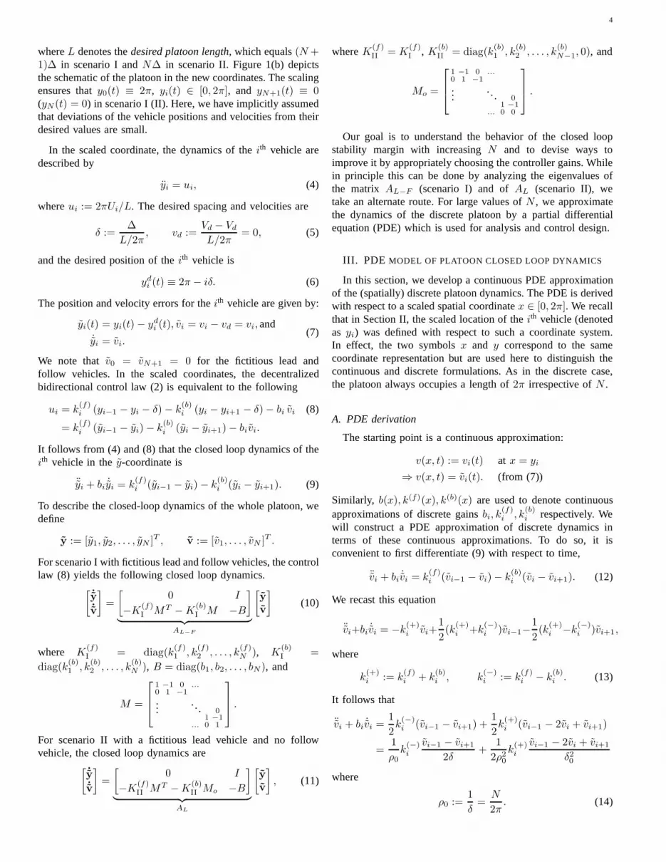
Z0(t)Zi(t)ZN+1(t)

i 1N

(a) A platoon with fictitious lead and follow vehicles.

. . .. . .

0 2π

yiyi−1

yi+1

δδe(f)ie

(b)i

(b) Same platoon iny coordinates.

Fig. 1. A platoon withN vehicles moving in one dimension.

references therein). The PDE model derived in the paper is notapplicable to a complete AHS, but only to a single platoon.

The rest of the paper is organized as follows: section II statesthe platoon problem in formal terms by describing a state-spacemodel of the closed loop platoon dynamics; section III thendescribes the derivation of the PDE model from the state spacemodel. In section IV the PDE is analyzed to explain the loss ofstability withN , and section V describes how to ameliorate suchloss of stability by mistuning. Section V-C reports simulationresults that show the benefit of mistuning in time-domain. InSection VI, we comment on various aspects of the proposedmistuning design.

II. CLOSED LOOP DYNAMICS WITH BIDIRECTIONAL

CONTROL

Consider a platoon ofN identical vehicles moving in astraight line as shown schematically in Figure 1(a). LetZi(t) andVi(t) := Zi(t) denote the position and the velocity, respectively,of the ith vehicle for i = 1, 2, . . . , N . Each vehicle is modeledas a double integrator:

Zi = Ui, (1)

whereUi is the control (engine torque) applied on theith vehicle.Such a model arises after the velocity dependent drag andother non-linear terms have been eliminated by using feedbacklinearization [1], [10].

The control objective is to maintain a constant inter-vehiculardistance∆ and a constant velocityVd for every vehicle. Everyvehicle is assumed to know the desired spacing∆ and thedesired velocityVd. The control architecture is required tobe decentralized, so that every vehicle uses locally availablemeasurements. We assume that the error between the position(as well as velocity) of a vehicle and its desired value is small,so that analysis of the platoon dynamics with a linear vehiclemodel and a linear control law is justified.

In this paper, we assume a bi-directional control architecturefor individual vehicles in the platoon (except the first and thelast vehicles). For the first and the last vehicles, we consider twotypes of control architectures (termed as scenarios I and II) astabulated in Table I. In scenario I, we introduce (after [6],[5])

Scenario LengthL Leader Follower

I (N + 1)∆ v0 = 0 vN+1 = 0

II N∆ v0 = 0 –

TABLE I

THE TWO SCENARIOS.

a fictitious lead vehicle and a fictitious follow vehicle, indexedas 0 and N + 1 respectively. Their behavior is specified byimposing a constant velocity trajectories asZ0(t) = Vd t andZN+1 = Vd t− (N + 1)∆. In scenario II, only a fictitious leadvehicle with indexi = 0 with Z0(t) = Vdt is introduced. For thelast vehicle in the platoon in scenario II, there is no followervehicle and it uses information only from its predecessor tomaintain a constant gap.

Consistent with the decentralized bidirectional linear controlarchitecture, the controlUi for the ith vehicle is assumed todepend only on 1) its velocity errorVi −Vd, and 2) the relativeposition errors between itself and its immediate neighbors. Thatis,

Ui = k(f)i (Zi−1 − Zi − ∆) − k

(b)i (Zi − Zi+1 − ∆)

− bi(Vi − Vd). (2)

wherek(·)i , bi are positive constants. The first two terms are used

to compensate for any deviation away from nominal positionwith the predecessor (front) and the follower (back) vehiclesrespectively. The superscripts(f) and (b) correspond tofrontand back, respectively. The third term is used to obtain a zerosteady-state error in velocity. In principle, relative velocity errorsbetween neighboring vehicles can also be incorporated intothecontrol, but we do not examine this situation here. SinceVd

and ∆ are known to every vehicle, the relative errors used inthe control law, including the velocity error, can be obtained inpractice by on-board devices such as radars, GPS, and speedsensors.

The control law (2) represents state feedback with local (near-est neighbor) information. Analysis of this controller structureis relevant even if there are additional dynamic elements inthecontroller. There are several reasons for this. First, a dynamiccontroller cannot have a zero at the origin. It will result ina pole-zero cancellation causing the steady-state errors to grow withoutbound asN increases [13]. Second, a dynamic controller cannothave an integrator either. For if it does, the closed-loop platoondynamics become unstable for a sufficiently large values ofN [13]. As a result, any allowable dynamic compensator mustessentially act as a static gain at low frequencies. The resultsof [13] indicate that the principal challenge in controlling largeplatoons arises due to the presence of a double integrator with itsunbounded gain at low frequencies. Hence, the limitation andits amelioration discussed here with the local state feedbackstructure of (8) is also relevant to the case where additionaldynamic elements appear in the control.

To facilitate analysis, we consider a coordinate change

yi = 2π(Zi(t) − Vdt+ L

L), vi = 2π

Vi − Vd

L, (3)

4

whereL denotes thedesired platoon length, which equals(N+1)∆ in scenario I andN∆ in scenario II. Figure 1(b) depictsthe schematic of the platoon in the new coordinates. The scalingensures thaty0(t) ≡ 2π, yi(t) ∈ [0, 2π], and yN+1(t) ≡ 0(yN(t) = 0) in scenario I (II). Here, we have implicitly assumedthat deviations of the vehicle positions and velocities from theirdesired values are small.

In the scaled coordinate, the dynamics of theith vehicle aredescribed by

yi = ui, (4)

whereui := 2πUi/L. The desired spacing and velocities are

δ :=∆

L/2π, vd :=

Vd − Vd

L/2π= 0, (5)

and the desired position of theith vehicle is

ydi (t) ≡ 2π − iδ. (6)

The position and velocity errors for theith vehicle are given by:

yi(t) = yi(t) − ydi (t), vi = vi − vd = vi, and

˙yi = vi.(7)

We note thatv0 = vN+1 = 0 for the fictitious lead andfollow vehicles. In the scaled coordinates, the decentralizedbidirectional control law (2) is equivalent to the following

ui = k(f)i (yi−1 − yi − δ) − k

(b)i (yi − yi+1 − δ) − bi vi (8)

= k(f)i (yi−1 − yi) − k

(b)i (yi − yi+1) − bivi.

It follows from (4) and (8) that the closed loop dynamics of theith vehicle in they-coordinate is

¨yi + bi ˙yi = k(f)i (yi−1 − yi) − k

(b)i (yi − yi+1). (9)

To describe the closed-loop dynamics of the whole platoon, wedefine

y := [y1, y2, . . . , yN ]T , v := [v1, . . . , vN ]T .

For scenario I with fictitious lead and follow vehicles, the controllaw (8) yields the following closed loop dynamics.

[˙y˙v

]

=

[0 I

−K(f)I MT −K

(b)I M −B

]

︸ ︷︷ ︸

AL−F

[y

v

]

(10)

where K(f)I = diag(k

(f)1 , k

(f)2 , . . . , k

(f)N ), K

(b)I =

diag(k(b)1 , k

(b)2 , . . . , k

(b)N ), B = diag(b1, b2, . . . , bN), and

M =

1 −1 0 ...0 1 −1

...... 0

1 −1... 0 1

.

For scenario II with a fictitious lead vehicle and no followvehicle, the closed loop dynamics are

[˙y˙v

]

=

[0 I

−K(f)II MT −K

(b)II Mo −B

]

︸ ︷︷ ︸

AL

[y

v

]

, (11)

whereK(f)II = K

(f)I , K(b)

II = diag(k(b)1 , k

(b)2 , . . . , k

(b)N−1, 0), and

Mo =

1 −1 0 ...0 1 −1

...... 0

1 −1... 0 0

.

Our goal is to understand the behavior of the closed loopstability margin with increasingN and to devise ways toimprove it by appropriately choosing the controller gains.Whilein principle this can be done by analyzing the eigenvalues ofthe matrix AL−F (scenario I) and ofAL (scenario II), wetake an alternate route. For large values ofN , we approximatethe dynamics of the discrete platoon by a partial differentialequation (PDE) which is used for analysis and control design.

III. PDE MODEL OF PLATOON CLOSED LOOP DYNAMICS

In this section, we develop a continuous PDE approximationof the (spatially) discrete platoon dynamics. The PDE is derivedwith respect to a scaled spatial coordinatex ∈ [0, 2π]. We recallthat in Section II, the scaled location of theith vehicle (denotedas yi) was defined with respect to such a coordinate system.In effect, the two symbolsx and y correspond to the samecoordinate representation but are used here to distinguishthecontinuous and discrete formulations. As in the discrete case,the platoon always occupies a length of2π irrespective ofN .

A. PDE derivation

The starting point is a continuous approximation:

v(x, t) := vi(t) at x = yi

⇒ v(x, t) = vi(t). (from (7))

Similarly, b(x), k(f)(x), k(b)(x) are used to denote continuousapproximations of discrete gainsbi, k

(f)i , k

(b)i respectively. We

will construct a PDE approximation of discrete dynamics interms of these continuous approximations. To do so, it isconvenient to first differentiate (9) with respect to time,

¨vi + bi ˙vi = k(f)i (vi−1 − vi) − k

(b)i (vi − vi+1). (12)

We recast this equation

¨vi+bi ˙vi = −k(+)i vi+

1

2(k

(+)i +k

(−)i )vi−1−

1

2(k

(+)i −k(−)

i )vi+1,

where

k(+)i := k

(f)i + k

(b)i , k

(−)i := k

(f)i − k

(b)i . (13)

It follows that

¨vi + bi ˙vi =1

2k

(−)i (vi−1 − vi+1) +

1

2k

(+)i (vi−1 − 2vi + vi+1)

=1

ρ0k

(−)i

vi−1 − vi+1

2δ+

1

2ρ20

k(+)i

vi−1 − 2vi + vi+1

δ20

where

ρ0 :=1

δ=N

2π. (14)

5

ρ0 has the physical interpretation of themean density(vehiclesper unit length). Now, we make a finite-difference approximationof derivatives

vi−1 − vi+1

2δ=

[∂

∂xv(x, t)

]

x=yi

vi−1 − 2vi + vi+1

δ20=

[∂2

∂x2v(x, t)

]

x=yi

,

where we recall thatv(x, t) is a continuous approximation ofthe vehicle velocities (vi(t) = v(yi, t) etc). Denotingk(+)(x)

and k(−)(x) as continuous approximations ofk(+)i and k(−)

i

respectively, the discrete model is written as:[∂2

∂t2v(x, t)

]

x=yi

+

[

b(x)∂

∂tv(x, t)

]

x=yi

=

1

ρ0

[

k(−)(x)∂

∂xv(x, t)

]

x=yi

+1

2ρ20

[

k(+)(x)∂2

∂x2v(x, t)

]

x=yi

Hence, we arrive at the partial differential equation (PDE)as amodel of the discrete platoon dynamics:

(∂2

∂t2+ b(x)

∂

∂t

)

v(x, t) =

(1

ρ0k(−)(x)

∂

∂x+

1

2ρ20

k(+)(x)∂2

∂x2

)

v(x, t) (15)

In the remainder of this paper, we assume thatk(+)(x) > 0.Using (13), the continuous counterparts of the front and theback gains are given by

k(f)(x) =1

2

(

k(+)(x) + k(−)(x))

,

k(b)(x) =1

2

(

k(+)(x) − k(−)(x))

,(16)

so that the gain valuesk(·)i can be obtained ask(f)

i = k(f)(yi)

andk(b)i = k(b)(yi). It can be readily verified that one recovers

the system of ordinary differential equations ((12) fori =1, . . . , N ) by discretizing the PDE (15) using a finite differencescheme on the interval[0, 2π] with a discretizationδ betweendiscrete points.

The boundary conditions for the PDE (15) depend upon thedynamics of the first and the last vehicles in the platoon. Forscenario I with a constant velocity fictitious lead and followvehicles, the appropriate boundary conditions are of the Dirichlettype on both ends:

v(0, t) = v(2π, t) = 0, ∀t ∈ [0,∞). (17)

For scenario II with the only a fictitious lead vehicle, theappropriate boundary conditions are of Neumann-Dirichlettype:

∂v

∂x(0, t) = v(2π, t) = 0. ∀t ∈ [0,∞) (18)

We refer the reader to Appendix I-A for a discussion on well-posedness of the solutions to (15). It is shown in Appendix I-Athat a solution exists in a weak sense whenk(+), k(−), dk(+)

dx ∈L∞([0, 2π]).

Equation (15) describes spatio-temporal evolution of smallvelocity perturbations in a platoon. It is worthwhile to note thatthe PDE model is a hyperbolic equation. Without the two first

(a) Scenario I ( Dirichlet-Dirichlet)

(b) Scenario II ( Neumann-Dirichlet)

Fig. 2. Comparison of closed loop eigenvalues of the platoondynamics andthe eigenvalues of the corresponding PDE (19) for the two different scenarios:(a) platoon with fictitious lead and follow vehicles, and correspondingly thePDE (19) with Dirichlet boundary conditions, (b) platoon with fictitious leadvehicle, and correspondingly the PDE (19) with Neumann-Dirichlet boundaryconditions. For ease of comparison, only a few of the eigenvalues are shown.Both plots are forN = 25 vehicles; the controller parameters arek(f)

i =

k(b)i = 1 and bi = 0.5 for i = 1, 2, . . . , N , and for the PDEk(f)(x) ≡

k(b)(x) ≡ 1 andb(x) ≡ 0.5.

order terms (i.e., forb(x) = k(−)(x) = 0), the PDE is a standardwave equation with spatially inhomogeneous values of wavespeed. The term1

ρ0k(−)(x) ∂v

∂x is an advection term, andb(x)∂v∂t

is a damping term. The hyperbolic nature of the PDE modelmeans that a perturbation originating, say, in the middle ofalong platoon will propagate both upstream and downstream withfinite speed. The two first order terms serve to modify aspectsof this propagation. The damping term causes a perturbationtodamp out in time. The advection term serves to create possibleasymmetries in upstream versus downstream propagation.

B. Eigenvalue comparison

For preliminary comparison of the PDE obtained above withthe state-space model of the closed loop platoon dynamics, weconsider the simplest case where the position control gainsareconstant for every vehicle, i.e.,k(f)(x) = k(b)(x) = k0 andb(x) = b0. In such a casek(−)(x) ≡ 0, k(+)(x) ≡ 2k0 and thePDE (15) simplifies to

(∂2

∂t2+ b0

∂

∂t− k0

ρ20

∂2

∂x2

)

v = 0, (19)

which is a damped wave equation with a wave speed of√

k0

ρ0.

The wave equation is consistent with the physical intuitionthat asymmetric bidirectional control architecture causes a disturbanceto propagate equally in both directions.

Figure 2 compares the closed loop eigenvalues of a discreteplatoon withN = 25 vehicles and the PDE (19). The eigenval-ues of the platoon are obtained by numerically evaluating theeigenvalues of the matricesAL−F andAL (defined in (10) and(11)). The eigenvalues of the PDE are computed numericallyafter using a Galerkin method with Fourier basis [32]. The figureshows that the two sets of eigenvalues are in excellent match. Inparticular, the least stable eigenvalues are well-captured by thePDE. Additional comparison appears in the following sections,where we present the results for analysis and control design.

6

boundary condition eigenvalueλleigenfunctionψl(x)

l

η(0) = η(2π) = 0(Dirichlet - Dirichlet) −

l2

4sin( lx

2) l = 1, 2, . . .

∂η∂x

(0) = η(2π) = 0(Neumann - Dirichlet) −

(2l−1)2

16cos(

(2l−1)x4

) l = 1, 2, . . .

TABLE II

THE EIGEN-SOLUTIONS FOR THELAPLACIAN OPERATOR WITH TWO

DIFFERENT BOUNDARY CONDITIONS.

IV. A NALYSIS OF THE SYMMETRIC BIDIRECTIONAL CASE

This section is concerned with asymptotic formulas forstability margin (least stable eigenvalue) for the symmetricbidirectional architecture with symmetric and constant controlgains:k(f)(x) = k(b)(x) ≡ k0 and b(x) ≡ b0. The analysis iscarried out with the aid of the associated PDE model:

(∂2

∂t2+ b0

∂

∂t− a2

0

∂2

∂x2

)

v = 0, (20)

wherex ∈ [0, 2π] and

a20 :=

k0

ρ20

(21)

is the wave speed. The closed-loop eigenvalues of the PDErequire consideration of the eigenvalue problem

d2η

dx2= λη(x), (22)

whereη is an eigenfunction that satisfies appropriate boundaryconditions: (17) for scenario I and (18) for scenario II. Theeigensolutions to the eigenvalue problem (23) for the twoscenarios are given in Table II. The eigenfunctions in eitherscenario provide a basis ofL2([0, 2π]).

After taking a Laplace transform, the eigenvalues of the PDEmodel (20) are obtained as roots of the characteristic equation

s2 + b0s− a20λ = 0, (23)

where λ satisfies (22). Using Table II, these roots are easilyevaluated. For instance, thelth eigenvalue of the PDE (20) withDirichlet boundary conditions is given by

s±l =−b0 ±

√

b20 − a20l

2

2, (24)

wherel = 1, 2, . . .. The real part of the eigenvalue depends uponthe discriminantD(l, N) := (b20 − a2

0l2), where the wave speed

a0 depends both on control gaink0 and number of vehiclesN (see (21)). For a fixed control gain, there are two cases toconsider:

1) If D(l, N) < 0, the rootss±l are complex with the realpart given by− b0

2 ,2) If D(l, N) > 0, the rootss±l are real withs+l +s−l = −b0.

In the former case, the damping is determined by the velocityfeedback termb0 ∂

∂t , while in the latter case one eigenvalue (s−l )gains damping at the expense of the other (s+l ) which loosesdamping. Whens±l are real, the eigenvalues+l is closer to the

boundary condition s+l

for l << lc lc

Dirichlet-Dirichlet −π2k0

b0

l2

N2 +O( 1N4 ) b0N

2π√

k0

Neumann-Dirichlet −π2k04b0

l2

N2 +O( 1N4 ) b0N

2π√

k0

TABLE III

THE TREND OF THE LESS STABLE EIGENVALUEs+l FOR THEPDE (20)

origin than s−l ; so we call s+l the lth less-stableeigenvalue.The following lemma gives the asymptotic formula for thiseigenvalue in the limit of largeN .

Lemma 1:Consider the eigenvalue problem for the linearPDE (20) with boundary conditions (17) and (18), correspondingto scenarios I and II respectively. Thelth less-stable eigenvalues+l approaches0 as O(1/N2) in the limit asN → ∞. Theasymptotic formulas appear in Table III. �

Proof of Lemma 1.We first consider scenario I with Dirichletboundary conditions (17). Using (24) and (21),

2s±l = −b0 ± b0

(

1 − a20l

2

b20

)1/2

= −b0 ± b0

(

1 − 2π2k0

b20

l2

N2

)

+O(1

N4)

for a20l

2/b20 << 1. The asymptotic formula holds for wavenumbers

l ≪ b0a0

=b0N

2π√k0

=: lc, (25)

and in particular for eachl as N → ∞. The proof for thescenario II with Neumann-Dirichlet boundary conditions (18)follows similarly.

The stability margin of the platoon can be measured by thereal part ofs+1 , the least stable eigenvalue.

Corollary 1: Consider the eigenvalue problem for the linearPDE (20) with boundary conditions (17) and (18), correspondingto scenarios I and II respectively. The least stable eigenvalue,denoted bys+1 , satisfies

s+1 = −π2k0

b0

1

N2+O(

1

N4) (Dirichlet-Dirichlet) (26)

s+1 = −π2k0

4b0

1

N2+O(

1

N4) (Neumann-Dirichlet) (27)

asN → ∞. �

The result shows that the least stable eigenvalue of the closedloop platoon decays as1N2 with symmetric bidirectional control.

We now present numerical computations that corroboratesthis PDE-based analysis. Figure 3 plots as a function ofN theleast stable eigenvalue of the PDE and of the state-space modelof the platoon, as well as the prediction from the asymptoticformula. The eigenvalues for the discrete platoon are obtainedby numerically evaluating the eigenvalues of the matricesAL−F

andAL (see (10) and (11)) with constant control gainsk(f)i =

k(b)i = k0 = 1 and bi = b0 = 0.5 for i = 1, . . . , N . The

7

10 20 50 100 200 500 1000

10−5

10−4

10−3

10−2

10−1

100

PDE (20), D-D

platoon, L-F

PDE (20), N-D

platoon, L

eq. (26)

eq. (27)

−Re(s+ 1

)

N

Fig. 3. Comparison of the least stable eigenvalue of the closed loop platoondynamics and that predicted by Corollary 1 with symmetric bidirectional control.There are three plots each for scenarios I and II (corresponding legends areboxed together), and those three should be compared with oneanother. Inthe plot legends, “D-D” stands for “Dirichlet-Dirichlet”,“N-D” for “Neumann-Dirichlet”, “L-F” for fictitious leader-follower, and “L” for fictitious leader. Theplot for “PDE (20), D-D” should be compared with “platoon, L-F” since theyboth correspond to scenario I. Similarly, “PDE (20), N-D” and “platoon, L”correspond to scenario II. Note that the predictions (26) and (27) are valid for1 << lc (defined in (25)), which in this case means forN >> 12.

0

Im

Re

(a) Eigenvalues move towardzero with increasingN .

0

Im

Re

s+ls−l

(b) Mistuning “exchanges”stability betweens+

lands−

l.

Fig. 4. A schematic explaining the loss of stability asN increases and howmistuning ameliorates this loss.

comparison shows that the PDE analysis accurately predictstheeigenvalue of the state-space model of the platoon dynamics.

Figure 4(a) graphically illustrates the destabilization by de-picting the movement of eigenvaluess±1 asN increases. Forsufficiently small values ofN , the discriminantD(1, N) isnegative and the eigenvalues±1 are complex. The real part ofthe eigenvalue depends only on the value ofb0. At a criticalvalue ofN = Nc := π

√2k0

b0, the discriminant becomes zero,

s+1 = s−1 and the eigenvalues collide on the real axis. For valuesof N > Nc and in particular asN → ∞, the eigenvalues+1asymptotes to0 while staying real, ands−1 asymptotes to−b.Their cumulative damping, as reflected in the sums+l + s−l =−b0, is conserved. In other words,s+1 is destabilized at theexpense ofs−1 .

Remark 1:The preceding analysis shows that the loss ofstability experienced with a symmetric bidirectional architectureis controller independent. The least stable eigenvalue approaches0 asO(1/N2) irrespective of the values of the gainsk0 andb0,as long as they are fixed constants independent ofN . Corollary 1also implies that for the least stable eigenvalue to be uniformlybounded away from0, one has to increase the control gaink0 asN2. In [6], the same conclusion was reached for the least stableeigenvalue with LQR control of a platoon on a circle. LQRcontrol typically leads to a centralized architecture, whereassymmetric bidirectional control is decentralized. It is interestingto note that the least stable eigenvalue behaves similarly in thesedistinct architectures. �

V. REDUCING LOSS OF STABILITY BY MISTUNING

In this section, we examine the problem of designing thecontrol gain functionsk(f)(x), k(b)(x) so as to ameliorate theloss of stability margin with increasingN that was seen in theprevious sections whenk(f)(x) = k(b) ≡ k0. Specifically, weconsider the eigenvalue problem for the PDE (15) where thecontrol gains are changed slightly (mistuned) from their valuesin the symmetric bidirectional case in order to minimize theleast-stable eigenvalues+1 . With symmetric bidirectional control,one obtains anO( 1

N2 ) estimate for the least stable eigenvaluebecause the coefficient of∂

2

∂x2 term in PDE (15) isO( 1N2 ) and

the coefficient of ∂∂x term is 0. Any asymmetry between the

forward and the backward gains will lead to non-zerok(−)(x)and a presence ofO( 1

N ) term as coefficient of∂∂x . By a judiciouschoice of asymmetry, there is thus a potential to improve thestability margin fromO( 1

N2 ) to O( 1N ).

We begin by considering the forward and backward positionfeedback gain profiles:

k(f)(x) = k0 + ǫk(f,purt)(x),

k(b)(x) = k0 + ǫk(b,purt)(x),

where ǫ > 0 is a small parameter signifying the amount ofmistuning andk(f,purt)(x), k(b,purt)(x) are functions definedover the interval[0, 2π] that captureperturbation from thenominal valuek0. Define

ks(x) := k(f,purt)(x) + k(b,purt)(x),

km(x) := k(f,purt)(x) − k(b,purt)(x),

so that from (16),

k(+)(x) = 2k0 + ǫks(x), k(−)(x) = ǫkm(x).

The mistuned version of the PDE (15) is then given by

∂2v

∂t2+ b0

∂v

∂t= a2

0

∂2v

∂x2+ ǫ

[km

ρ0

∂v

∂x+

ks

2ρ20

∂2v

∂x2

]

(28)

We study the problem of improving the stability margin byjudicious choice ofkm(x) and ks(x). The results of our in-vestigation, carried out in the following sections, provide asystematic framework for designing control gains in the platoonby introducing small changes to the symmetric design.

8

A. Mistuning-based design for scenario I

The control objective is to design mistuning profileskm(x)andks(x) to minimizethe least stable eigenvalues+1 . To achievethis, we first obtain an explicit asymptotic formula for theeigenvalues when a small amount of asymmetry is introducedin the control gains (i.e., whenǫ is small). For scenario I, theresult is presented in the following theorem. The proof appearsin Appendix I-B.

Theorem 1:Consider the eigenvalue problem for the mis-tuned PDE (28) with Dirichlet boundary condition (17) corre-sponding to scenario I. Thelth eigenvalue pair is given by theasymptotic formula

s+l (ǫ) = ǫl

2b0N

∫ 2π

0

km(x) sin(lx)dx +O(ǫ2) +O(1

N2),

s−l (ǫ) = −b0 − ǫl

2b0N

∫ 2π

0

km(x) sin(lx)dx +O(ǫ2) +O(1

N2),

that is valid for eachl in the limit asǫ→ 0 andN → ∞. �

It is apparent from the Theorem above that to minimizethe least stable eigenvalues+1 , one needs to choose onlykm

carefully; ks has only O( 1N2 ) effect. Therefore we choose

ks(x) ≡ 0, or, equivalently,k(f,purt)(x) = −k(b,purt)(x), whichleads tokm(x) = 2k(f,purt)(x). The most beneficial controlgains are now can be readily obtained from Theorem 1, whichis summarized in the next corollary.

Corollary 2 (Mistuning profile for Scenario I):Consider theproblem of minimizing the least-stable eigenvalue of thePDE (28) with Dirichlet boundary condition (17) bychoosing k(f,purt)(x) ∈ L∞([0, 2π]) with norm-constraint‖k(f,purt)(x)‖L∞ = maxx∈[02π] k

(f,purt)(x) = 1 andk(b,purt)(x) = −k(f,purt)(x). In the limit asǫ→ 0, the optimalmistuning profile is given byk(f,purt)(x) = 2(H(x− π) − 1

2 ),whereH(x) is the Heaviside function:H(x) = 1 for x ≥ 0andH(x) = 0 for x < 0. With this profile, the least stableeigenvalue is given by the asymptotic formula

s+1 (ǫ) = − 4ǫ

b0N

in the limit asǫ→ 0 andN → ∞. �

The result shows that even with anarbitrarily small amountofmistuningǫ, one can improve the closed-loop platoon dampingby a large amount, especially for large values ofN . The least-stable eigenvalues+1 asymptotes to0 asO( 1

N ) in the mistunedcase as opposed toO( 1

N2 ) in the symmetric case.

Figure 5(a) shows the gains for the individual vehicles (thatare obtained from sampling the functionsk(f)(x) andk(b)(x)),suggested by Corollary 2 for a20 vehicle platoon, withk0 = 1andǫ = 0.1:

k(f)i = 1 + 0.2(H(π − iδ) − 0.5), and

k(b)i = 1 − 0.2(H(π − iδ) − 0.5),

where δ is the desired inter-vehicular spacing in the scaledy coordinates, and is defined in (5). A confirmation of thepredictions of Corollary 2 is presented in Figure 6. Numericallyobtained mistuned and nominal eigenvalues for both the PDEand the platoon state-space model are shown in the figure, withmistuned gains chosen as shown in Figure 5(a). The figure showsthat

Fig. 5. Mistuned front and back gainsk(f)i and k(b)

i of the vehicles ina platoon withk0 = 1 and ǫ = 0.1. Figure (a) shows the gains chosenaccording to Corollary 2 to be optimal for scenarioI for small ǫ: k(f)

i =

k0 (1 + 0.1(2H(π − iδ) − 1)) , k(b)i = k0 (1 − 0.1(2H(π − iδ) − 1)),

whereH(·) is the Heaviside function andδ is defined in (5). Figure (b) showsthe optimal mistuned gains for scenario II with the same parameters, which turnsout to be (see Corollary 3)k(f)

i = 1.1k0 andk(b)i = 0.9k0 for i = 1, . . . , N .

10 20 50 100 200 500

10−5

10−4

10−3

10−2

10−1

100

symmetric bidi. (PDE)

mistuned (PDE)

symmetric bidi. (platoon)

mistuned (platoon)

Corollary (2)

−Re(s+ 1

)N

Fig. 6. Stability margin improvement by mistuning in Scenario I. The figureshows the least stable eigenvalue of the closed loop platoon(i.e., ofAL−F in(10)) and of the PDE (28) with Dirichlet boundary conditions, with and withoutmistuning, for a range of values ofN . Parameters for the nominal case arek0 = 1 and b0 = 0.5, and the mistuning amplitude isǫ = 0.1. The mistunedcontrol gains are shown in Figure 5(a). The legend “Corollary 2” refers to theprediction by Corollary 2 for largeN .

1) the platoon eigenvalues match the PDE eigenvalues accu-rately over a range ofN , and

2) the mistuned eigenvalues show large improvement overthe nominal case even though the controller gains differfrom their nominal values only by±10%. The improve-ment is particularly noticeable for large values ofN , whilebeing significant even for small values ofN .

For comparison, the figure also depicts the asymptotic eigen-value formula given in Corollary 2.

Figure 4(b) graphically illustrates the mechanism by whichmistuning affects the movement of eigenvaluess±1 as N in-creases. By properly choosing the mistuning patternskm(x) andks(x), damping can be “exchanged” between the eigenvaluess+1ands−1 so that the less stable eigenvalues+1 “gains” stability atthe expense of the more stable eigenvalues−1 . The net amountof damping is preserved, sinces+1 + s−1 = −b0 (as seen fromTheorem 1).

B. Mistuning-based design for scenario II

For scenario II, asymptotic formula for the eigenvalue (coun-terpart of Theorem 1) is summarized in the following theorem.The proof is entirely analogous to the proof of Theorem 1, andis therefore omitted.

Theorem 2:Consider the eigenvalue problem for the mis-tuned PDE (28) with Neumann-Dirichlet boundary condi-tion (18) corresponding to scenario II. Thelth eigenvalue pair

9

is given by the asymptotic formula

s+l (ǫ) = −ǫ l

4b0N

∫ 2π

0

km(x) sin(lx

2)dx+O(ǫ2) +O(

1

N2),

s−l (ǫ) = −b0 + ǫl

4b0N

∫ 2π

0

km(x) sin(lx

2)dx +O(ǫ2) +O(

1

N2),

that is valid for eachl in the limit asǫ→ 0 andN → ∞. �

As with scenario I, here again we use the above result todetermine the most beneficial profilekm(x) for small ǫ:

Corollary 3 (Mistuning profile for Scenario II):Considerthe problem of minimizing the least-stable eigenvalue of thePDE (28) with Neumann-Dirichlet boundary conditions (18)by choosingk(f,purt)(x) ∈ L∞([0, 2π]) with norm-constraintmaxx∈[0,2π] k

(f,purt)(x) = 1, andk(b,purt)(x) = −k(f,purt)(x).In the limit as ǫ → 0, the optimal k(f,purt) is given byk(f,purt)(x) = 1. With this profile, the least-stable eigenvalueis given by the asymptotic formula

s+1 (ǫ) = − ǫ

b0N

in the limit asǫ→ 0 andN → ∞. �

The result shows that, as in scenario I, it is possible toimprove the closed-loop stability margin in scenario II with anarbitrary small amount of mistuningǫ such that the least-stableeigenvalues+1 asymptotes to0 asO( 1

N ) in the mistuned case asopposed toO( 1

N2 ) in the symmetric case. The gains suggestedby Corollary 3, withk0 = 1 andǫ = 0.1 are:

k(f)i = 1.1, and k

(b)i = 0.9,

which are shown in Figure 5(b). Numerically obtained leaststable eigenvalues for the PDE and the platoon state-space modelfor scenario II are shown in Fig. 7 for a range of values ofN .It is clear from the figure that, as in scenario I, the mistunedeigenvalues show an order of magnitude improvement over theirvalues in the symmetric bidirectional case with only±10%variation.

Remark 2 (Robustness to small changes from the optimal gains):An advantage of the mistuning design is that mistuned closedloop eigenvalues are robust to small local discrepancies inthe control gains from the optimal ones. This can be seen(for scenario I) from the asymptotic eigenvalue formulas ofTheorem 1, which shows that one would obtain aO( 1

N ) estimatefor any choice ofkm(x) such that

∫ 2π

0 km(x) sin(x)dx 6= 0. Asimilar argument holds for scenario II.

C. Simulations

We now present results of a few simulations that show thetime-domain improvements – manifested in faster decay ofinitial errors – with the mistuning-based design of controlgains.Simulations were carried out for a platoon ofN = 20 vehicleswith scenario I, i.e., with fictitious lead and follow vehicles.The desired gap was∆ = 1 and desired velocity wasVd = 5.The initial velocity of every vehicle was chosen as the desiredvelocity and the initial position of theith vehicle was chosen asZi(0) = i∆ − 0.5 for i = {1, . . . , N}. As a result, the initialrelative position error and velocity error of every vehiclewas

10 20 50 100 200 500

10−5

10−4

10−3

10−2

10−1

100

symmetric bidi. (PDE)

mistuned (PDE)

symmetric bidi. (platoon)

mistuned (platoon)

−Re(s+ 1

)

N

Corollary (3)

Fig. 7. Stability margin improvement by mistuning in scenario II. The figureshows the least stable eigenvalue of the closed loop platoon(i.e., ofAL in (10))and of the PDE (28) with Neumann-Dirichlet b.c., with and without mistuning,for a range of values ofN . The parameters for the nominal case arek0 = 1and b0 = 0.5, and the mistuning amplitude isǫ = 0.1. The mistuned controlgains that are used are shown in Figure 5(b). The legend “Corollary 3” refersto the prediction by Corollary 3 of mistuned PDE eigenvalues.

zero except for the first vehicle, whose relative position errorwith respect to the fictitious lead vehicle was0.5.

Figure 8 shows the time-histories of the absolute and relativeposition errors of the individual vehicles with a symmetricbidirectional control, where the control gains were chosenask

(f)i = k

(b)i = 1 andbi = 0.5 for i = {1, . . . , 20}. The absolute

position error of theith vehicle is Zi − Zdi and the relative

position error isZi−1 − Zi − ∆.

Figure 9 shows the time-histories of the absolute and relativeposition errors for the platoon with mistuned controller gains.The mistuning gains used for the simulation are the onesshown in Figure 5(a) (chosen according to Corollary 2) so thatmaximum and minimum gains over all vehicles is within±10%of the nominal value. On comparing Figures 8 and 9, we seethat the errors in the initial conditions are reduced fasterin themistuned case compared to the nominal case. These observationsare consistent with the improvement in the closed-loop stabilitymargin with the mistuned design.

VI. D ISCUSSION ON MISTUNING DESIGN

There are several remarks to be made regarding the mistuningbased design. We first comment on the implementation issues,in particular, on the effect of small platoon size on the proposeddesign, and on the information requirements for its implemen-tation.

A. Large vs. smallN

The PDE model is developed for largeN . However, detailednumerical comparison between the PDE and the discrete statespace model shows that the PDE model provides quantitativelycorrect predictions even for small values ofN (see Figures 3, 6and 7). The PDE has an infinite number of eigenvalues asopposed to a finite number for the discrete platoon. So, one can

10

0 5 10 15 20 25 30

−0.5

−0.4

−0.3

−0.2

−0.1

0

Time

Zd i(t

)−Z

i(t)

(a) Absolute position errors

0 5 10 15 20 25 30

−0.2

−0.1

0

0.1

0.2

0.3

0.4

0.5

Time

Zi−

1(t

)−Z

i(t)−

∆

(b) Relative position errors

Fig. 8. Performance of symmetric bidirectional control in time-domain: time histories of the absolute and relative position errors of the vehicles in a platoonwith symmetric bidirectional control (scenario I). The control gains arek(f)

i = k(b)i = 1 andbi = 0.5 for every i = 1, . . . , 20.

0 5 10 15 20 25 30

−0.5

−0.4

−0.3

−0.2

−0.1

0

Time

Zd i(t

)−Z

i(t)

(a) Absolute position errors.

0 5 10 15 20 25 30−0.1

0

0.1

0.2

0.3

0.4

0.5

0.6

Time

1234

Zi−

1(t

)−Z

i(t)−

∆

(b) Relative position errors.

Fig. 9. Performance of mistuned control in time-domain: time histories of the absolute and relative position errors of the vehicles in a platoon (scenario I) withmistuned bidirectional control, cf. Figure 8. The control gains used are those shown in Figure 5(a). The legends refer tothe vehicle indices.

not expect an exact match. However, PDE eigenvalues exactlymatch the least stable and other dominant eigenvalues of thediscrete platoon (see Figure 2 and Figure 10). In a similar vein,the benefits of mistuning are also realized for small values of N .For example, when the number of vehicles is20, a mistuningof ±10% results in an improvement in the stability margin –as measured by the real part of the least stable eigenvalue –of 150% (from −0.0491 to −0.1281 ) in scenario I and animprovement of400% (from −0.012 to −0.05) in scenario IIover the symmetric case.

B. Information requirements

In order to implement the beneficial mistuned controller gainsdesigned above, every vehicle needs the following information(in addition to what is needed to use a symmetric bidirectionalcontrol): (1) the mistuning amplitudeǫ, and (2) in scenario I,whether it is in the front half of the platoon or not. Thisinformation can be provided to the vehicles in advance. Inscenario II, only the value ofǫ is needed.

It is possible that due to vehicles leaving and joining theplatoon, information on whether a vehicle belongs to the fronthalf of the platoon may become erroneous with time, especiallyfor the vehicles that are close to the middle. In scenario I, sucherror may lead to a non-optimal gains used by the vehicles.

However, since the improvement in closed loop stability margindue to mistuning is robust to small deviations in the gains fromthe optimal ones (see Remark 2), errors in determining whethera vehicle belongs to the front half of the platoon or not will notgreatly affect the improvement in stability margin. Note that inscenario II this issue does not even arise.

C. Large asymmetry

Although the mistuning profiles described in Corollaries 2and 3 are optimal in the limit asǫ → 0, one would like to beable to use them with somewhat larger values ofǫ to realizethe benefit of mistuning. To do so, one has to preclude thepossibility of “eigenvalue cross-over”, i.e., of the second (s+2 )or some other marginally stable eigenvalue from becoming theleast stable eigenvalue in the presence of mistuning. It turnsout that such a cross-over is ruled out as a consequence ofthe Strum-Liouville (S-L) theory for the elliptic boundaryvalueproblems. The standard argument relies on the positivity oftheeigenfunction corresponding tos+1 ; the reader is referred to [33]for the details. Figure 10 verifies this numerically by depictingthe six eigenvalues closest to0 (for both the PDE and thediscrete platoon) as a function ofN when mistuning is applied.

11

10 20 50 100 200 50010

−2

10−1

100

platoon−Re(s+ l

),l=

1,2,...,6

N

PDE

Fig. 10. The real parts of six eigenvalues (closest to0) of the closed loopplatoon dynamics for Scenario I, and their comparison with the PDE eigenvalueswith Dirichlet-Dirichlet boundary conditions, with controller gains mistunedas those shown in Figure 5. As predicted by the S-L theory, theleast stableeigenvalue stays the least stable, although eigenvalues that are more stable mergewith it asN increases.

D. Sensitivity to disturbance

Automated platoons suffer from high sensitivity to externaldisturbances; which is referred to as “string instability”or“slinky-type effects” [20], [1], [15]. Here we provide numericalevidence that mistuning also helps in reducing the sensitivity todisturbances.

When external disturbances are present, we model the dy-namics of vehiclei by Zi = Ui +Wi, whereWi is the externaldisturbance acting on the vehicle. In they coordinates, thevehicle dynamics becomeyi = ui +wi, wherewi := 2πWi/L.In scenario I, the state space model of the entire platoonbecomes,

ψ = AL−F ψ +

[0

I

]

︸︷︷︸

B

w, e = Cψ (29)

whereψ = [yT , vT ]T , AL−F , w = [w1, w2, . . . , wN ]T , ande := [e

(f)1 , . . . , e

(f)N ]T is a vector of front spacing errorse(f)

i :=yi−1 − yi.

TheH∞ norm of the transfer functionGwe from the distur-bancew to the inter-vehicle spacing errorse is a measure ofthe closed loop’s sensitivity to external disturbances [7], [13].Figure 11 shows a plot of theH∞ norm ofGwe as a functionof N , with and without mistuning. The mistuning profile usedis the same as the one used for the eigenvalue trends reportedin Figure 6. It is clear from the figure that±10% mistuningresults in large reduction of theH∞ norm ofGwe. Although thisreduction is more pronounced for largeN , it is still significantfor smallN . In particular, forN = 20, a 10% mistuning yieldsapproximately50% reduction in theH∞ norm (from 6.69 to3.38).

Apart from theH∞ norm of Gde, there are other ways tomeasure sensitivity to disturbances. In [21], the transferfunctionfrom disturbance acting on the lead vehicle to spacing erroronthe ith vehicle is analyzed. Detailed analysis of the effect ofmistuning on sensitivity to disturbances will be a subject offuture work.

101

102

100

101

102

103

symmetricmistuned

‖Gw

e‖ ∞

N

Fig. 11. H∞ norm of the transfer functionGwe from disturbancew to spacingerror e in (29), with and without mistuning, for scenario I. The mistuned gainsused are shown in Figure 5(a). Norms are computed using the Control SystemsToolbox in MATLAB c©.

VII. C ONCLUSION

We developed a PDE model that describes the closed loopdynamics of anN -vehicle platoon with a decentralized bidirec-tional control architecture. Analysis of the PDE model revealedseveral important features of the problem. First, we showedthatwhen every vehicle uses the same controller with constant gainthat is independent ofN (the so-called symmetric bidirectionalarchitecture), the least stable eigenvalue of the closed loopdecays to0 asO( 1

N2 ). Second, and more significantly, analysisof the PDE suggested a way to ameliorate the progressive lossof stability with increasingN , by introducing small amountsof “mistuning”, i.e., by changing the controller gains fromtheirnominal symmetric values. We proved that with arbitrary smallamounts of mistuning, the decay of the least stable closed loopeigenvalue can be improved toO( 1

N ). Several comparisons withthe numerically computed eigenvalues of state-space modelofthe platoon confirm the predictions of the PDE-based analysis.

Although the PDE model is derived under the assumption thatthe number of vehicles,N , is large, in practice the PDE pro-vides quantitatively correct predictions for the discreteplatoondynamics even for relatively small values ofN . The amount ofinformation that is needed to implement the mistuned controlgains (over that in the symmetric bidirectional architecture) isquite small and need to be provided only once. Furthermore,the stability improvement due to mistuning is robust to smallerrors (between the actual gains used and the optimal mistunedgains) that may occur in practice due to changes in the numberof vehicles in the platoon over time.

The advantage of the PDE formulation is reflected in the easewith which the closed loop eigenvalues are obtained for twodifferent boundary conditions, with lead and follow vehicles aswell as with only a lead vehicle. Certain important aspects ofthe problem, such as the beneficial nature of forward-backwardasymmetry in control gains, is revealed by the PDE whilethey are difficult to see with the (spatially) discrete, state-spacemodel.

Numerical calculations show that the mistuning design alsoreduces sensitivity to disturbances of the closed-loop platoon.

12

Analysis of the beneficial effect of mistuning in reducingsensitivity to external disturbances is a subject of futureresearch.In the future, we also plan to examine PDE-based models formodeling and analysis of fleet of vehicles as in2 or 3 spatialdimensions.

REFERENCES

[1] S. Darbha, J. K. Hedrick, C. C. Chien, and P. Ioannou, “A comparison ofspacing and headway control laws for automatically controlled vehicles,”Vehicle System Dynamics, vol. 23, pp. 597–625, 1994.

[2] J. K. Hedrick, M. Tomizuka, and P. Varaiya, “Control issues in automatedhighway systems,”IEEE Control Systems Magazine, vol. 14, pp. 21 – 32,December 1994.

[3] R. E. Chandler, R. Herman, and E. W. Montroll, “Traffic dynamics: Studiesin car following,” Operations Research, vol. 6, no. 2, pp. 165–184, Mar.- Apr. 1958.

[4] W. S. Levine and M. Athans, “On the optimal error regulation of a string ofmoving vehicles,”IEEE Transactions on Automatic Control, vol. AC-11,no. 3, pp. 355–361, July 1966.

[5] S. M. Melzer and B. C. Kuo, “A closed-form solution for theoptimalerror regulation of a string of moving vehicles,”IEEE Transactions onAutomatic Control, vol. AC-16, no. 1, pp. 50–52, February 1971.

[6] M. R. Jovanovic and B. Bamieh, “On the ill-posedness of certain vehicularplatoon control problems,”IEEE Transactions on Automatic Control,vol. 50, no. 9, pp. 1307 – 1321, September 2005.

[7] P. Seiler, A. Pant, and J. K. Hedrick, “Disturbance propagation in vehiclestrings,” IEEE Transactions on Automatic Control, vol. 49, pp. 1835–1841,October 2004.

[8] J. D. Wolfe, D. F. Chichkat, and J. L. Speyer, “Decentralized controllersfor unmaned aerial vehicle formation flight,” inGuidance, Navigation andControl Conference, 1996, pp. July 29–31.

[9] P. K. C. Wang, F. Y. Hadaegh, and K. Lau, “Synchronized formationrotation and attitude control of multiple free-flying spacecraft,” Journal ofGuidance, Control, and Dynamics, vol. 22, no. 1, pp. 28–35, 1999.

[10] S. S. Stankovic, M. J. Stanojevic, and D. D. Siljak, “Decentralizedoverlapping control of a platoon of vehicles,”IEEE Transactions onControl Systems Technology, vol. 8, pp. 816–832, September 2000.

[11] P. Li and A. Shrivastava, “Traffic flow stability inducedby constanttime headway policy for adaptive cruise control vehicles,”TransportationResearch Part C: Emergent Technologies, vol. 10, pp. 275–301, 2002.

[12] L. E. Peppard, “String stability of relative-motion PID vehicle controlsystems,”IEEE Transactions on Automatic Control, pp. 579–581, October1974.

[13] P. Barooah and J. P. Hespanha, “Error amplification and distrubancepropagation in vehicle strings,” inProceedings of the 44th IEEE conferenceon Decision and Control, December 2005.

[14] K. C. Chu, “Decentralized control of high-speed vehicle strings,”Trans-portation Science, vol. 8, pp. 361–383, 1974.

[15] Y. Zhang, E. B. Kosmatopoulos, P. A. Ioannou, and C. C. Chien,“Autonomous intelligent cruise control using front and back informationfor tight vehicle following maneuvers,”IEEE Transactions on VehicularTechnology, vol. 48, pp. 319–328, January 1999.

[16] S. E. Shladover, “Longitudinal control of automotive vehicles in close-formation platoons,”Journal of Dynamic systems, Measurements andControl, vol. 113, pp. 302–310, December 1978.

[17] H.-S. Tan, R. Rajamani, and W.-B. Zhang, “Demonstration of an automatedhighway platoon system,” inAmerican Control Conference, vol. 3, June1998, pp. 1823 – 1827.

[18] X. Liu, S. S. Mahal, A. Goldsmith, and J. K. Hedrick, “Effects ofcommunication delay on string stability in vehicle platoons,” in IEEEInternational Conference on Intelligent Transportation Systems (ITSC),August 2001.

[19] P. Barooah, P. G. Mehta, and J. P. Hespanha, “Control of large vehicularplatoons: Improving closed loop stability by mistuning,” in The 2007American Control Conference, July, pp. 4666–4671.

[20] S. Darbha and J. K. Hedrick, “String stability of interconnected systems,”IEEE Transactions on Automatic Control, vol. 41, no. 3, pp. 349–356,March 1996.

[21] R. H. Middleton and J. H. Braslavsky, “String instability inclasses of linear time invariant formation control with limitedcommunication range,” 2008, submitted for publication. [Online].Available: http://www.hamilton.ie/rick/publications/StringStability.pdf

[22] S. K. Yadlapalli, S. Darbha, and K. R. Rajagopal, “Information flow andits relation to stability of the motion of vehicles in a rigidformation,”IEEE Transactions on Automatic Control, vol. 51, no. 8, August 2006.

[23] B. Shapiro, “A symmetry approach to extension of flutterboundaries viamistuning,”Journal of Propulsion and Power, vol. 14, no. 3, pp. 354–366,1998.

[24] O. O. Bendiksen, “Localization phenomena in structural dynamics,”Chaos, Solitons, and Fractals, vol. 11, pp. 1621–1660, 2000.

[25] A. J. Rivas-Guerra and M. P. Mignolet, “Local/global effects of mistuningon the forced response of bladed disks,”Journal of Engineering for GasTurbines and Power, vol. 125, pp. 1–11, 2003.

[26] P. G. Mehta, G. Hagen, and A. Banaszuk, “Symmetry and symmetrybreaking for a wave equation with feedback,”SIAM Journal of DynamicalSystems, vol. 6, no. 3, pp. 549–575, 2007.

[27] M. Lighthill and G. Whitham, “On kinematic waves II: a theory of trafficflow on long crowded roads,” inRoyal Society, London Series A, 1955.

[28] D. Helbing, “Traffic and related self-driven many-particle systems,”Reviewof Modern Physics, vol. 73, pp. 1067–1141, 2001.

[29] D. Jacquet, C. C. de Wit, and D. Koenig, “Traffic control and monitoringwith a macroscopic model in the presence of strong congestion waves,”in 44th IEEE Conference on Decision and Control & European ControlConference, 2005, pp. 2164–2169.

[30] P. Y. Li, R. Horowitz, L. Alvarez, J. Frankel, and A. M. Robertson,“An automated highway system link layer controller for traffic flowstabilization,” Transportation Research, Part C, vol. 5, no. 1, pp. 11–37,1997.

[31] L. Alvarez, R. Horowitz, and P. Li, “Traffic flow control in automatedhighway systems,”Control Engineering Practice, vol. 7, pp. 1071–1078,1999.

[32] C. Canuto, M. Y. Hussaini, A. Quarteroni, and T. A. Zang,SpectralMethods in Fluid Dynamics, ser. Springer Series in Computational Physics.New York: Springer-Verlag, 1983.

[33] L. C. Evans, Partial Differential Equations, ser. Graduate Studies inMathematics. American Mathematical Society, 1998, vol. 19.

[34] A. Pazy, Semigroups of linear operators and applications to partialdifferential equations, ser. Applied Mathematical Sciences. New York:Springer-Verlag, 1983, vol. 44.

APPENDIX ITECHNICAL RESULTS

A. Solution properties of PDE(15).

In this section, we use the semigroup theory to obtain resultson well-posedness of the PDE (15). To apply these methods, wefirst re-write the PDE as a first order evolution equation:

∂ρ∂t = −ρ0

∂v∂x

∂v∂t = −

[1

ρ02k1(x)ρ+ 12ρ03

∂∂x (ρk0(x)) + bv

] := A

[ρv

]

,

(30)whereA is a linear operator;k0(x) := k+(x) and k1(x) :=

k−(x) − 12ρ0

dk+

dx (x). We will assume these coefficientsk0(x), k1(x) ∈ L∞([0, 2π]) and k0(x) > 0. ρ has the unitsof and the physical interpretation of density perturbation.

Using (30), we denote the initial/boundary value problem as:

z(x, t) = Az(x, t) for x ∈ X, t > 0

z(x, 0) = z0(x), (31)

where z(x, t) := [ρ(x, t), v(x, t)], z0(x) = [ρ0(x), v0(x)] andA is defined in (30);ρ0 and v0 will be assumed to functionsin appropriately defined Banach spaces. The main goal of thissection will be to show that the solution for the linear prob-lem (30) can be expressed in terms of aC0 semigroup providedeigenvalues of the operatorA satisfy appropriate bounds. Webegin with a discussion of the notation.

Preliminaries and Notation.We denotez := [ρ, v], L2(X)denotes the Hilbert space of square integrable functions onX(‖v‖2

L2 :=∫v2dx), Hk denotes the Sobolev space of functions

such that derivatives up tokth-order exist in a weak sense andbelong toL2(X) (the Sobolev norm is denoted by‖ · ‖Hk ), andH1

0 denotes the Sobolev spaceH1 of functions that satisfy the

13

Dirichlet boundary condition. We denoteZ := L2 × L2, andequip it with a norm‖ · ‖. Let D(A) := H1 × (H1

0 ∩ L2) andconsider the right hand side of evolution equation (30) as anunbounded but closed densely defined linear operator

A : D(A) ⊂ Z → Z. (32)

A real numbers belongs toρ(A), the resolvent set forA,provided the operatorsI − A : D(A) → Z is 1-1 and onto.For s ∈ ρ(A), the resolvent operatorRs := (sI − A)−1.Finally, we recall that a one-parameter family of linear operators{S(t)}t≥0 is aC0-semigroup if 1)S(0)z = z for all z ∈ Z, 2)S(t + s)z = S(t)S(s)z for all t, s ≥ 0 and z ∈ Z, and 3) themappingt → S(t)z is continuous from[0,∞) into Z. A C0

semigroup is a contraction semigroup if‖S(t)z‖ ≤ ‖z‖ for allt ≥ 0. The Hille-Yosida theorem states that a closed denselydefined linear operatorA is the generator of a contractionsemigroup if and only if

(0,∞) ⊂ ρ(A) and ‖Rsz‖ ≤ 1

s‖z‖ ∀z ∈ Z. (33)

Our strategy will be to apply Hille-Yosida theorem to deducesolution properties of the evolution equation (31). Followingclosely the development in [33], there are three steps to accom-plish this: 1) we show thatA is a densely defined closed linearoperator onZ, 2) characterize the resolvent set by consideringthe eigenvalue problem, and 3) show the bound (33) for theresolvent. Step 2 will lead to an eigenvalue problem, whoseanalysis and optimization is the subject of this paper. We presentdetails for the three steps next:

1) The domain ofA, D(A), is dense inZ becauseH1 isdense inL2. To showA is closed, consider a sequence{ρm, vm} ⊂ D(A) such that

(ρm, vm)Z→ (ρ, v) (34)

A(ρm, vm)Z→ (f, g), (35)

where the arrow notation denotes the fact that the conver-gence is inZ = L2 × L2. Sincevm

L2

→ v so −ρ0∂v∂x =

f ∈ L2, i.e.,v ∈ H1. Now, {vm} is Cauchy inL2 by (34)and{∂vm

∂x } is Cauchy inL2 by (35) and

‖vm − vl‖H1 ≤ C

(

‖∂vm

∂x− ∂vl

∂x‖L2 + ‖vm − vl‖L2

)

,

(36)

so {vm} is Cauchy inH1 and vmH1

→ v. By repeatingessentially the same argument, one also finds thatρ ∈ H1

and ρmH1

→ ρ. Consequently,A(ρm, vm)Z→ A(ρ, v) and

A(ρ, v) = (f, g).2) Let s > 0, (f, g) ∈ Z = L2 × L2, and consider the

operator equation

(sI −A)

[ρv

]

=

[fg

]

. (37)

This is equivalent to two scalar equations

sρ+ ρ0∂v

∂x= f (ρ ∈ L2 ∩H1),

(38)

sv +

[1

ρ20

k1(x)ρ+1

2ρ30

∂

∂x(k0(x)ρ) + bv

]

= g (v ∈ L2 ∩H10 ).

(39)

Using the first equation to writesρ = −ρ0∂v∂x + f , this

impliess2v + bsv + Lv = h, (40)

where

Lv :=1

2ρ20

∂

∂x(−k0(x)

∂v

∂x) − 1

ρ0(k1(x)

∂v

∂x) (41)

is an elliptic operator (becausek0(x) > 0 for all x ∈ X)and h = sg − 1

2ρ30

∂∂x (k0(x)f) − 1

ρ20k1(x)f (note that

h ∈ H−1(X)). Consequently, solutions of ((37)) can bestudied in terms of solutions of ((41)). The spectrum ofAis completely characterized by the spectrum ofL. We willobtain spectral bounds, dependent uponk0(x) andk1(x),in the following sections. In particular, we will establishthat Real[s] < α for someα < 0 and thusρ(A) ⊃ (α,∞).For k1(x) = 0, its turns out that[0,∞) ⊂ ρ(A) forany choice of positivek0(x) (this is also clear from thesymmetric eigenvalue problem (41)).

3) If a positive s ∈ ρ(A), there exists a unique solution(ρ, v) ∈ Z for (38)-(39) via the theory of elliptic opera-tors: solve (40) to obtainv ∈ H1

0 andsρ = −ρ0∂v∂x+f . We

write the solution as(ρ, v) = Rs(f, g), define a bilinearform

B[ρ, s] :=1

2ρ40

∫

X

k0(x)ρ(x)s(x)dx, (42)

for ρ, s ∈ L2 and consider an equivalent norm (onZ) forsolutions(ρ, v) as:

‖(ρ, v)‖ := B[ρ, ρ] + ‖v‖L2 (43)

To obtain the resolvent bound, we multiply (39) byv anduse integration by parts:

s(‖v‖L2 +B[ρ, ρ]) + b‖v‖L2 +1

ρ2

∫

k1(x)ρvdx

=

∫

gvdx+B[ρ, f ].

In general, the bound depends uponk1(x). Fork1(x) = 0,we have

s‖(ρ, v)‖2 ≤ (s+ b)‖v‖L2 +B[ρ, ρ]) =∫

gvdx+B[ρ, f ] ≤ ‖(f, g)‖ · ‖(ρ, v)‖,

where the first inequality holds becauses > 0 andb > 0 and the last inequality follows from the generalizedCauchy-Schwarz inequality. As a result,‖Rs(f, g)‖ ≤1s‖(f, g)‖ and‖Rs‖ ≤ 1

s .For the general case wherek1(x) is not identically zero,one expresses the operator

A = A0 + A, (44)

where

A0

[ρv

]

=

[

0 −ρ0∂∂x

− 12ρ3

0

∂∂x(k0(x)·) −b

] [ρv

]

,

A

[ρv

]

=

[0 0

− 1ρ20k1(x) 0

] [ρv

]

.

14

In words,A0 is the operator withk1(x) = 0 and A isthe operator due tok1(x). We note thatA is a boundedperturbation ofA0 (on Z). We have already showed theexistence of aC0-semigroup forA0. For the general op-eratorA, the existence follows from using a perturbationtheorem (see Theorem 1.1 in Ch. 3 of [34]).

B. Proof of Theorem 1

Proof of Theorem 1.The spatial inhomogeneity introduced bythex-dependent coefficientskm(x) andks(x) destroy the spatialinvariance of the nominal PDE (20). Hence, the Fourier basis– eigenfunctions of the Laplacian – no longer lead to a diag-onalization of the mistuned PDE. The methods of section IVthus need to be suitably modified. In order to compute theeigenvalues for the mistuned PDE (28), we take a Laplacetransform of (28) and get

− a20

∂2η

∂x2+ s2η + b0sη = ǫ

[km

ρ0

∂η

∂x+

ks

2ρ20

∂2η

∂x2

]

, (45)

where η(x) is the Laplace transform (with respect tot) ofv(x, t). We are interested in eigenvalues of (45) with Dirichletboundary conditions, i.e., the values ofs for which a solutionto the homogeneous PDE (45) exists with boundary conditionsη(0) = η(2π) = 0. To obtain these eigenvalues, we use a per-turbation method expressing the eigenfunction and eigenvaluein a series form:

η(x) = η0(x) + ǫη1(x) +O(ǫ2), s = r0 + ǫr1 +O(ǫ2).(46)

We note thatǫ r1 denotes the perturbation to the nominaleigenvaluer0 as a result of the mistuning. Substituting (46)in (45) and doing anO(1) balance, we get

O(1) : −a20(η0)xx + r20η0 + br0η0 = 0, (47)

whose eigen-solution is given by

η0 = dl sin(lx

2), r0 = s±l (0),

where l = 1, 2, . . ., dl is an arbitrary real constant, ands±l (0)is given by (24). Next,

O(ǫ) :

(

−a20

∂2

∂x2+ (r20 + b0r0)

)

η1 =km

ρ0

∂η0∂x

+ks

2ρ20

∂2

∂x2η0 − (2r0r1 + b0r1)η0 =: R

Substituting r0 = s±l (0) on the left hand side leads to aresonance condition for the right hand side term, denoted byR. In particular for a solutionη1 to exist,R must lie in therange space of the linear operator

(

−a20

∂2

∂x2+ (r20 + br0)

)

. (48)

For this self-adjoint operator, the range space is the complementof its null space{sin( lx

2 )}. This gives the resonance conditionas

〈R, sin(lx

2)〉 = 0,

where< ·, · > denotes the standard inner product inL2(0, 2π).This leads to an equation

(2r0 + b0)r1 =l

4πρ0

∫ 2π

0

km(x) sin(lx)dx

− l2

8πρ20

∫ 2π

0

ks(x) sin2(lx

2)dx (49)

For values ofr0 = s±l (0), wheres±l (0) is given by (24), theequation above leads to an expression for perturbation in thetwo eigenvalues. We denote these perturbations asr±1 . For r0 =s+l (0), we have from from Lemma 1 thatb0 >> |2r0| whenl << lc, which happens for everyl asN → ∞ (see eq. (25)),so that

r+1 ≈ l

4πρ0b0

∫ 2π

0

km(x) sin(lx)dx +O(1

N2). (50)

Note that we have dropped the second integral on the right handside of (49) because1

ρ20

= O(1/N2) for largeN . For r0 =

s−k (0), 2r0 ≈ −2b0 for l << lc and

r−1 ≈ − l

4πρ0b0

∫ 2π

0

km(x) sin(lx)dx +O(1

N2). (51)

Note that

r+1 + r−1 = 0.

Putting the formulas for the perturbation to the eigenvalues (50)and (51) in (46), we get

s+l (ǫ) ≈ s+l (0) + ǫl

4πb0ρ0

∫ 2π

0

km(x) sin(lx)dx+O(ǫ2) +O(1

N2),

s−l (ǫ) ≈ −b0 − ǫl

4πb0ρ0

∫ 2π

0

km(x) sin(lx)dx +O(ǫ2) +O(1

N2).

Sinces+l (0) = O( 1N2 ) for l < lc (Lemma 1) andρ0 = N

2π , theresult follows.