Embed Size (px)
Citation preview

Analysis and modelling of river meandering
Analyse en modellering van meanderende rivieren

Analysis and modelling of river meandering
Analyse en modellering van meanderende rivieren
PROEFSCHRIFT ter verkrijging van de graad van doctor aan de Technische Universiteit Delft,
op gezag van de Rector Magnificus prof. dr. ir. J.T. Fokkema, voorzitter van het College voor Promoties,
in het openbaar te verdedigen op maandag 22 september 2008 om 10:00 uur
door
Alessandra CROSATO Dottore in Ingegneria Civile Idraulica, Universitá degli Studi di Padova
geboren te Bolzano, Italië

Dit proefschrift is goedgekeurd door de promotor: Prof. dr. ir. H.J. de Vriend Samenstelling promotiecommissie: Rector Magnificus, voorzitter Prof. dr. ir. H.J. de Vriend, Technische Universiteit Delft, promotor Prof. dr. ir. . M.J.F. Stive, Technische Universiteit Delft Prof. dr. N.G. Wright, UNESCO-IHE Delft Prof. dr. dott. ing. G. Di Silvio, Universitá degli Studi di Padova Prof. dr. S. B. Kroonenberg, Technische Universiteit Delft Dr. H. Middelkoop, Universiteit Utrecht Dr. Hervé Piegay, CNRS France Prof. dr. ir. G.S. Stelling, Technische Universiteit Delft, reservelid © 2008 Alessandra Crosato and IOS Press All rights reserved. No part of this book may be reproduced, stored in a retrieval system, or transmitted, in any form or by any means, without prior permission from the publisher. ISBN 978-1-58603-915-8 Key words: river meandering, morphology, planform, bars, bank erosion, bank accretion Published and distributed by IOS Press under the imprint Delft University Press Publisher IOS Press Nieuwe Hemweg 6b 1013 BG Amsterdam The Netherlands tel: +31-20-688 3355 fax: +31-20-687 0019 email: [email protected] www.iospress.nl www.dupress.nl LEGAL NOTICE The publisher is not responsible fopr the use which might be made of the following information. PRINTED IN THE NETHERLANDS Cover picture: air view of a tributary of the Ob River (Russia), courtesy of Saskia van Vuren
Acknowledgements
i
Acknowledgements
This PhD study has been carried out from 1987 to 2008 at the Department of Civil Engineering and Geosciences of Delft University of Technology (TU Delft). The study was funded by the Istituto Veneto di Scienze Lettere ed Arti (Venice, Italy) and by Fondazione Ing. Aldo Gini (Padua, Italy) during the first year. WL⎮Delft Hydraulics supported the work until 1991 and fully covered the costs of the Pilot Flume experiments (1988) as well as my participation at the Summer School on Stability of River and Coastal Forms, in Perugia (1990). In the period 1991-2004 the work was either financed by projects (Studio SICEM S.r.l. and WL⎮Delft Hydraulics) or carried out during my free time. Delft University of Technology co-financed the work in the period 1988-1990 and fully financed the work in the period 2005-2008 with funds from the Water Research Centre Delft. A large community of scientists and professionals has contributed to this work; therefore I wish to thank a lot of persons, hoping to forget nobody. Given the duration of the work, I find it easier to list those persons in order of appearance. Moreover, I do not mention any titles or qualifications on purpose, since many of them have now a different title and position with respect to the moment in which they first appeared on the scene. The first persons I want to heartily thank are my parents, Luigi Crosato and Adriana Paccagnella, who gave me the possibility to carry out my studies in civil engineering and supported me for many years. My first husband, Frédéric Vellieux, deserves particular thanks. He was able to transfer his enthusiasm for science and convinced me to become a researcher. Before meeting him, I had intended to become a project engineer. After so many years, I can say that I managed to do both, research and projects, and in the last period even teaching river morphodynamics, which is more than I had ever dreamed of. I thank Giampaolo Di Silvio (University of Padua), who was the first real contributor to this work. He gave me the opportunity to do research in the Netherlands, at WL⎮Delft Hydraulics, and to work on the Po River (Italy). As one of the opponents, he finally also contributed to this PhD thesis. I want to thank also Giovanni Seminara (University of Genoa) and Marco Tubino (University of Trento), who initiated me in the subject of meandering rivers. With their enthusiasm, they conveyed me their passion for the subject. Nico Struiksma (WL⎮Delft Hydraulics) deserves special thanks. With his creative imagination, impressive personality and wide experience he became the example to follow and made me an enthusiastic river engineer and researcher. Huib de Vriend (WL⎮Delft Hydraulics and TU Delft) was at first an experienced colleague and an exceptionally good supervisor and later became my official PhD supervisor. I want to thank him especially because he gave me the chance to finish the work at TU Delft in a second phase. Special thanks are due to Matthijs de Vries, who offered me the opportunity to carry out this PhD work in the first place and became my first official supervisor. My appreciation for his approach to the study and teaching of river morphology has grown especially after I started to teach the

Acknowledgements
i i
subject myself at UNESCO-IHE. I very much regret that he passed away just two months before he could see this thesis. First as a colleague and then as second husband, Erik Mosselman (WL⎮Delft Hydraulics and TU Delft), was and still is, my great inspirator. Lively discussions, covering all types of subjects, characterize our common life. In the field of river morphology, we have been exchanging ideas and trying new ways throughout all these years, without loosing enthusiasm. This even led to a few works together. I thank him gratefully for his support and contribution to this work. I desire to thank Gary Parker (University of Illinois), for the intriguing discussions, which we initially pursued by mail (no e-mail, but letters in envelopes) and at specific occasions, such as during the summer school in Perugia (Italy). The MSc students who contributed to this work deserve a big thank you! They are Khwaja Ghulam Murshed (UNESCO-IHE, 1991), Astrid Blom (TU Delft, 1997), Eva Miguel (TU Delft, 2006), May Samir Saleh (UNESCO-IHE, 2007), Yasir S.A. Ali (UNESCO-IHE, 2008) and Roxana M. Duran Tapia (UNESCO-IHE, 2008). A number of researchers contributed to the work through their participation in fruitful discussions. They are Arno Talmon (WL⎮Delft Hydraulics and TU Delft), Kees Sloff (WL⎮Delft Hydraulics and TU Delft), Ronald van Balen (Free University of Amsterdam), Robbert Fokkink (TU Delft), Wim Uijttewaal (TU Delft), Hans van Duivendijk (TU Delft and Royal Haskoning), Jarit de Gijt (TU Delft and Rotterdam Harbour Authority) and Jelle Olthof (TU Delft and Royal Boskalis Westminster). Also many friends contributed indirectly. They are Irini Katopodi, Nico Kitou, Maximo Peviani, Paolo De Girolamo, Johan Romate, Erica Cecchi, Federico Maggi, Paolo Reggiani, Katia Bilardo, Amparo Serra Piera, Cecilia Iacono and many others. Without this group of friends some dark and cold days would have been even darker and colder. I cannot list all the colleagues at TU Delft and WL⎮Delft Hydraulics. Some of them, however, deserve great thanks, because I could share my everyday life with them. They are Mindert de Vries, Pauline Thoolen, Walther van Kesteren, John Cornelisse, Kees Kuijper, Pim van der Salm, Ilka Tanczos, Thijs van Kessel and many others. They made me feel at home also when being at work. Finally, I want to thank the opponents Nigel Wright, Hervé Piegay, Marcel Stive, Salomon Kroonenberg, Hans Middelkoop and Guus Stelling, who spent their time on this thesis and provided constructive comments. This work is dedicated to G. Adyabadam, of the institute of Meteorology and Hydrology in Mongolia, who, after having raised her family in Mongolia, took up study and research in the Netherlands. Her example gave me the decisive push to complete this PhD thesis after so many years.

Summary English
i i i
Summary
This thesis examines the morphological changes of non-tidal meandering rivers at the spatial scale of several meanders. With this purpose, a physics-based mathematical model, MIANDRAS, has been developed for the simulation of the medium-term to long-term evolution of meandering rivers. Application to several real rivers shows that MIANDRAS can properly simulate both equilibrium river bed topography and planimetric changes. Three models of different complexity can be obtained by applying different degrees of simplification to the equations. These models, along with experimental tests and field data, constitute the tools for several analyses. At conditions of initiation of meandering, it is found that river bends can migrate upstream and downstream. This depends on meander wave length and width-to-depth ratio, irrespective of whether the parameters are in the subresonant or the superresonant range. Varying lag distances between flow velocity and bed topography are found to offer an explanation why local channel migration rates reach a maximum at a certain bend sharpness, in addition to previous explanations based on flow separation. A new method has been developed to calculate the number of bars in a river channel with given width. It predicts successfully whether reducing or enlarging the river width would lead to meandering or braiding. Channel migration coefficients are demonstrated to depend not only on physical properties of the eroding bank, but also on physical properties of the accreting bank and the numerical scheme. Moreover, they need to account for overbank flows. Model results and a re-examination of experimental observations suggest that intrinsic initiation of meandering is not necessarily related to steady bars due to a permanent upstream disturbance. They may also be related to a steady bed deformation due to small quickly-varying periodic or random disturbances, for instance due to the presence of migrating alternate bars. The latter finding still requires further confirmation.

Summary English
i v

Samenvatting Nederlands
v
Samenvatting
Dit proefschrift onderzoekt de morfologische veranderingen van meanderende rivieren zonder getij op de ruimteschaal van enkele meanders. Met dit doel is een op fysica gebaseerd wiskundig model, MIANDRAS, ontwikkeld voor het simuleren van de evolutie van meanderende rivieren op middellange en lange termijn. Toepassing op verschillende echte rivieren laat zien dat MIANDRAS zowel de evenwichtsbodemligging van de rivier als de veranderingen in plattegrond op juiste wijze kan simuleren. Drie modellen van verschillende complexiteit kunnen worden verkregen door verschillende graden van vereenvoudiging toe te passen op de vergelijkingen. Deze modellen vormen, samen met experimentele proeven en veldgegevens, de instrumenten voor verscheidene analyses. Onder omstandigheden van het begin van meanderen wordt gevonden dat rivierbochten stroomopwaarts en stroomafwaarts kunnen migreren. Dit hangt af van de meandergolflengte en de breedte-diepteverhouding, ongeacht of de parameters zich bevinden in het subresonante of het superresonante domein. Gevonden wordt dat variërende afstanden van naijling tussen stroomsnelheid en bodemtopografie een verklaring bieden waarom lokale snelheden van geulmigratie bij een bepaalde bochtscherpte een maximum bereiken, in aanvulling op eerdere verklaringen op basis van loslating van de stroming. Een nieuwe methode is ontwikkeld om het aantal banken te berekenen in een riviergeul met gegeven breedte. Deze voorspelt met succes of verkleining of vergroting van de rivierbreedte zou leiden tot meanderen of vlechten. Aangetoond wordt dat coëfficiënten van geulmigratie niet alleen afhangen van fysische eigenschappen van de eroderende oever, maar ook van fysische eigenschappen van de aangroeiende oever en het numerieke schema. Bovendien moeten zij de invloed verrekenen van stromingen als de rivier buiten haar oevers treedt. Modelresultaten en een hernieuwde analyse van experimentele waarnemingen suggereren dat het intrinsieke begin van meanderen niet noodzakelijk gerelateerd is aan stationaire banken als gevolg van een permanente verstoring bovenstrooms, maar mogelijk ook aan een stationaire vervorming van de bodem als gevolg van snel variërende periodieke of willekeurige verstoringen, bijvoorbeeld als gevolg van de aanwezigheid van migrerende alternerende banken. Deze laatste bevinding behoeft nog nadere bevestiging.

Samenvatting Nederlands
v i

Sommario Italiano
v i i
Sommario
Questa tesi esamina i cambiamenti morfologici dei fiumi a meandri senza marea alla scala spaziale di molti meandri. A questo scopo, nell’ambito del lavoro è stato sviluppato un modello matematico, basato sulla descrizione fisica dei fenomeni, per la simulazione dell’evoluzione di questi fiumi sul medio-lungo termine, MIANDRAS. La sua applicazione a un certo numero di fiumi mostra che MIANDRAS è in grado di simulare in modo soddisfacente la topografia di equilibrio del letto e i cambiamenti planimetrici dei fiumi a meandri. Inoltre, applicando diversi livelli di semplificazione alle equazioni si possono ottenere tre modelli di diversa complessità. Questi modelli, insieme a test sperimentali di laboratorio e a dati raccolti sul campo, costituiscono gli strumenti di molte delle analisi effettuate. Alle condizioni iniziali di formazione dei meandri si è trovato che i tornanti del fiume possono migrare sia verso valle che verso monte. Ciò dipende dalla lunghezza d’onda dei meandri e dal rapporto tra larghezza e profondità del canale principale ed è indipendente dal fatto che il sistema fluviale si trovi entro il dominio di sotto-risonanza o di super-risonaza. Si è inoltre scoperto che la variazione del ritardo spaziale tra la velocità della corrente e la topografia del letto è in grado di spiegare perché la velocità di migrazione trasversale del fiume raggiunge un massimo ad un certo valore di intensità della curvatura. Questa spiegazione si aggiunge alle spiegazioni precedenti basate sulla separazione del flusso di corrente. È stato sviluppato un nuovo metodo per calcolare il numero di barre in un canale fluviale di larghezza conosciuta. Questo metodo è in grado di predire se aumentare o diminuire la larghezza del fiume porta ad un fiume a meandri o a configurazione intrecciata. Si è dimostrato che i coefficienti usati per pesare la migrazione laterale del fiume dipendono non solamente dalle caratteristiche fisiche della sponda in erosione, ma anche dalle caratteristiche della sponda in accrescimento e dallo schema numerico del modello. Essi inoltre devono tener conto del moto della corrente sulle golene. I risultati del modello e il riesame di osservazioni sperimentali suggeriscono che la formazione iniziale dei meandri è intrinseca al sistema. Essa infatti non sembra necessariamente legata alla presenza di barre stazionarie causate da un disturbo a monte permanente, ma anche a una deformazione del letto stazionaria causata da piccoli disturbi che variano velocemente nel tempo, periodici o completamente casuali, come per esempio quelli originati dalla presenza di barre alternate migranti. Quest’ultima scoperta richiede ulteriori conferme.

Sommario Italiano
v i i i

Contents
i x
CONTENTS
1 INTRODUCTION ............................................................................................................................... 1 1.1 RATIONALE.................................................................................................................................... 1 1.2 BACKGROUND OF THE STUDY ........................................................................................................ 4 1.3 OBJECTIVES ................................................................................................................................... 6 1.4 GENERAL APPROACH ..................................................................................................................... 6
2 MEANDERING RIVERS ................................................................................................................... 9 2.1 INTRODUCTION .............................................................................................................................. 9 2.2 MEANDERING AND OTHER PLANFORMS OF ALLUVIAL RIVERS........................................................ 9 2.3 PLANIMETRIC CHARACTERISTICS OF MEANDERING RIVERS.......................................................... 12
2.3.1 Channel sinuosity ................................................................................................................... 12 2.3.2 Size of meanders ..................................................................................................................... 13 2.3.3 Size of the meander belt.......................................................................................................... 14 2.3.4 Bend sharpness ....................................................................................................................... 15 2.3.5 River width.............................................................................................................................. 15
2.4 BED TOPOGRAPHY ....................................................................................................................... 16 2.5 DISCHARGES................................................................................................................................ 18 2.6 SEDIMENT.................................................................................................................................... 19 2.7 BEND FLOW ................................................................................................................................. 19 2.8 CHANNEL MIGRATION.................................................................................................................. 21
2.8.1 General description ................................................................................................................ 21 2.8.2 Bank erosion........................................................................................................................... 23 2.8.3 Bank accretion........................................................................................................................ 25
2.9 CUTOFFS...................................................................................................................................... 28 3 FACTORS CONTROLLING RIVER MEANDERING ................................................................ 31
3.1 INTRODUCTION ............................................................................................................................ 31 3.2 PLANFORM CLASSIFICATIONS ...................................................................................................... 31 3.3 FLOW STRENGTH.......................................................................................................................... 37 3.4 SEDIMENT SUPPLY ....................................................................................................................... 38 3.5 BANK ERODIBILITY...................................................................................................................... 39 3.6 RIPARIAN VEGETATION................................................................................................................ 40 3.7 FREQUENCY OF FLOODS............................................................................................................... 44 3.8 ACTIVE TECTONICS...................................................................................................................... 44
4 STATE OF THE ART IN MEANDER MIGRATION MODELLING......................................... 47 4.1 INTRODUCTION ............................................................................................................................ 47 4.2 MODELLING OF FLOW FIELD AND BED TOPOGRAPHY IN CURVED CHANNELS................................ 47 4.3 MODELLING OF BANK EROSION AND BANK RETREAT ................................................................... 51
4.3.1 Fluvial entrainment ................................................................................................................ 52 4.3.2 Bank failure ............................................................................................................................ 53 4.3.3 Effects of eroded bank material .............................................................................................. 57
4.4 MODELLING OF BANK ACCRETION AND BANK ADVANCE ............................................................. 58 4.5 MODELLING OF CUT-OFFS............................................................................................................ 61 4.6 MODELLING OF MEANDER MIGRATION ........................................................................................ 63
4.6.1 Introduction ............................................................................................................................ 63 4.6.2 History .................................................................................................................................... 64 4.6.3 Computation of lateral channel migration ............................................................................. 65 4.6.4 Meander migration models including cutoffs ......................................................................... 67

Contents
x
5 THE MEANDER MIGRATION MODEL MIANDRAS ............................................................... 69 5.1 INTRODUCTION ............................................................................................................................ 69 5.2 MATHEMATICAL DESCRIPTION OF FLOW VELOCITY AND DEPTH .................................................. 70
5.2.1 Basic equations....................................................................................................................... 70 5.2.2 Simplification of the equations ............................................................................................... 77 5.2.3 Zero-order equations: unperturbed system ............................................................................ 80 5.2.4 First-order equations: perturbed system ................................................................................ 81 5.2.5 Near-bank velocity and water depth excesses ........................................................................ 82 5.2.6 Axi-symmetric solution of the equations ................................................................................. 84 5.2.7 Steady-state equations ............................................................................................................ 86 5.2.8 Time adaptation of transverse bed deformation ..................................................................... 88
5.3 MATHEMATICAL DESCRIPTION OF BANK RETREAT AND ADVANCE............................................... 92 5.4 SIMULATION OF CUTOFFS............................................................................................................. 93 5.5 COMPUTATION OF THE RIVER CORRIDOR WIDTH .......................................................................... 94
6 STRAIGHT‑FLUME EXPERIMENT ON BAR FORMATION .................................................. 97 6.1 INTRODUCTION ............................................................................................................................ 97 6.2 EXPERIMENTAL SET UP ................................................................................................................ 97 6.3 TEST T1 ..................................................................................................................................... 100 6.4 TEST T2 ..................................................................................................................................... 103
7 ANALYSES OF MODEL BEHAVIOUR...................................................................................... 107 7.1 INTRODUCTION .......................................................................................................................... 107 7.2 NEAR-BANK FLOW VELOCITY AND DEPTH OSCILLATION............................................................ 107
7.2.1 Theoretical analysis.............................................................................................................. 107 7.2.2 Comparison with experimental data..................................................................................... 114
7.3 FLOW VELOCITY LAG................................................................................................................. 116 7.3.1 Theoretical analysis.............................................................................................................. 116 7.3.2 Comparison with experimental data..................................................................................... 118
7.4 INITIATION OF MEANDERING...................................................................................................... 118 7.4.1 Historical background.......................................................................................................... 118 7.4.2 Initiation of meandering in MIANDRAS............................................................................... 120
7.5 MEANDERING AND BRAIDING .................................................................................................... 124 7.5.1 Introduction .......................................................................................................................... 124 7.5.2 Previous work....................................................................................................................... 124 7.5.3 A new predictor .................................................................................................................... 126
7.6 POINT BAR SHIFT AND MEANDER GROWTH................................................................................. 132 7.6.1 General case......................................................................................................................... 132 7.6.2 Non-damped system with negligible spiral flow ................................................................... 135 7.6.3 Effects of damping ................................................................................................................ 136 7.6.4 Effects of helical flow ........................................................................................................... 139 7.6.5 Combined effects................................................................................................................... 140
7.7 COMPARISON WITH OTHER CLASSES OF MEANDER MIGRATION MODELS .................................... 142 7.7.1 No-lag kinematic model........................................................................................................ 142 7.7.2 Ikeda-type model................................................................................................................... 143 7.7.3 MIANDRAS........................................................................................................................... 143 7.7.4 Longitudinal profile of near-bank water depth..................................................................... 144 7.7.5 Initiation and further developments of meanders ................................................................. 145
8 NUMERICAL ASPECTS ............................................................................................................... 149 8.1 NUMERICAL IMPLEMENTATION.................................................................................................. 149
8.1.1 Basic equations..................................................................................................................... 149 8.1.2 Numerical scheme................................................................................................................. 152 8.1.3 Model calibration ................................................................................................................. 156 8.1.4 Computation of the channel centreline curvature................................................................. 159
Contents
x i
8.1.5 Regridding ............................................................................................................................ 160 8.2 STABILITY OF COMPUTATIONS: TIME STEP VS. SPACE STEP ........................................................ 161 8.3 EFFECTS OF SMOOTHING AND REGRIDDING IN MEANDER MIGRATION MODELS .......................... 162 8.4 EFFECTS OF BOUNDARY CONDITIONS......................................................................................... 167
8.4.1 Steady-state computations .................................................................................................... 167 8.4.2 Computations with time adaptation...................................................................................... 171
9 FIELD APPLICATIONS................................................................................................................ 179 9.1 INTRODUCTION .......................................................................................................................... 179 9.2 LOCAL MIGRATION RATES AND CHANNEL CURVATURE.............................................................. 185 9.3 VARIATION OF AVERAGE MIGRATION RATES WITH INCREASING RIVER SINUOSITY..................... 191 9.4 PREDICTION OF PRESENT MORPHOLOGICAL TRENDS OF THE RIVER GEUL (THE NETHERLANDS) 194
9.4.1 General description .............................................................................................................. 194 9.4.2 Approach .............................................................................................................................. 197 9.4.3 Results................................................................................................................................... 198 9.4.4 Conclusions .......................................................................................................................... 200
9.5 PREDICTION OF PLANFORM CHANGES OF THE RIVER DHALESWARI (BANGLADESH).................. 200 9.5.1 General description .............................................................................................................. 200 9.5.2 Approach .............................................................................................................................. 201 9.5.3 Results................................................................................................................................... 202 9.5.4 Conclusions .......................................................................................................................... 205
9.6 PREDICTION OF PLANFORM CHANGES OF THE RIVER ALLIER (FRANCE)..................................... 206 9.6.1 General description .............................................................................................................. 206 9.6.2 Approach .............................................................................................................................. 208 9.6.3 Results................................................................................................................................... 211 9.6.4 Conclusions .......................................................................................................................... 213
10 CONCLUSIONS AND RECOMMENDATIONS......................................................................... 215 10.1 SCOPE AND MODELLING APPROACH ........................................................................................... 215 10.2 INITIATION OF MEANDERING...................................................................................................... 215 10.3 MEANDER WAVE LENGTH .......................................................................................................... 217 10.4 CONDITIONS FOR MEANDERING ................................................................................................. 217 10.5 LAG DISTANCE BETWEEN FLOW VELOCITY AND BED TOPOGRAPHY............................................ 217 10.6 POINT BAR LOCATION WITH RESPECT TO THE BEND APEX .......................................................... 218 10.7 EFFECTS OF BEND SHARPNESS ON LOCAL MIGRATION RATES ..................................................... 219 10.8 AVERAGE MIGRATION SPEED AND GROWTH OF RIVER MEANDERS ............................................. 220 10.9 NUMBER OF BARS IN A CHANNEL CROSS-SECTION ..................................................................... 220 10.10 MODEL APPLICABILITY.......................................................................................................... 221 10.11 NUMERICAL EFFECTS ............................................................................................................ 222 10.12 ASSUMPTION THAT BED SLOPE EQUALS VALLEY SLOPE DIVIDED BY SINUOSITY .................... 222 10.13 MIGRATION COEFFICIENTS .................................................................................................... 223 10.14 RECOMMENDATIONS FOR FUTURE RESEARCH ON BANK ACCRETION...................................... 224
REFERENCES...........................................................................................................................................227 LIST OF MAIN SYMBOLS......................................................................................................................247 CURRICULUM VITAE............................................................................................................................251

Contents
x i i

Introduction
1
1 Introduction
1.1 Rationale
The planimetric evolution of meandering rivers, characterized by the progressive growth and shift of river bends and by the occurrence of bend short cuts, is one of the primary river planform phenomena. It is not only scientifically interesting and relevant to natural rivers, it is also an issue in river training and reservoir geology. Despite significant scientific progress in recent decades, an established practice applying simple and easy-to-use morphological models to predict large-scale river planimetric changes is still lacking. Such models are key to progress in the understanding of this planform phenomenon and these are necessary tools to interpret and upscale results from more complex models, which are bound to cover only relatively small river reaches. This thesis examines non-tidal meandering rivers, with special emphasis on their large-scale medium- to long-term planimetric changes. This spatio-temporal scale is referred to as the “engineering scale”. The aim is to increase the understanding of the fundamental processes of river planform evolution by filling in several knowledge gaps in this field. The work includes the development of a numerical model for the simulation of the medium- to long-term evolution of meandering rivers, MIANDRAS. Together with experimental and field data, this model constitutes the main tool for the analyses carried out.
Why concentrate on meandering rivers? Because meandering is the most common river planform style in populated areas
Meandering rivers have single-thread channels with high sinuosity and almost constant width. They could be regarded as a particular type of braided rivers [Murray & Paola, 1994], in which the multiple-thread channel has reduced to single-thread. Why focus on this particular type of river? The reasons are manifold. First of all, natural meandering rivers are mainly found in large fertile valleys, the most valuable zones for agriculture and human settlement, which are often under demographic and economic pressure. The result is that the river floodplains are progressively occupied by settlements and industry [Muhar et al., 2005]. This makes flood control and the control of bank erosion and meander migration of essential importance. In many European countries, as for instance the Netherlands, Italy and France, after a long period in which single municipalities could decide where to plan settlements without any basin-wide coordination, it is now recognized that reducing the active river bed by occupying the floodplains and raising levees is not sustainable on the long-

Introduction
2
term. Ever further encroachment of floodplains leads to even higher flood levels, but levees cannot be raised indefinitely. Therefore, a new land-use policy allowing more space for the river is required. The most recent management approaches [Silva et al., 2004; Ercolini, 2004] introduced the concept of river corridor or streamway with the slogan: “free space to the river” [Malavoi et al., 1998 and Malavoi et al., 2002]. The river corridor is an artificially maintained, regularly flooded, alluvial belt where the river is allowed to erode its banks, in a controlled “natural” state. Uncontrolled bank erosion could affect valuable land, whereas free meandering could affect river navigability. For these reasons, the knowledge of bank erosion processes, meander evolution and cut-offs is of essential importance for the design of such corridors [Piégay et al., 2005; Larsen et al., 2006]. Besides, natural gradients in water depth, flow velocity and sediment composition, due to the presence of oxbow lakes, pools, point bars and vertical eroding banks, have proved to be of great importance for the river corridor ecology [Ward & Stanford, 1995]. A deep knowledge of river morphodynamic processes is therefore needed for both design and maintenance of river corridors, as well as for the assessment of the long-term impact of important river training works, such as the fixing of a river bend or the creation of an artificial cut-off. A second reason to focus on meandering rivers is that human interventions have made meandering the most common river planform style in developed areas. For example, the Danube River downstream of Vienna used to be braided, but is now limited to a single-thread meandering channel. Like the Danube, most piedmont rivers are increasingly assuming a meandering planform. Damming, canalisation and the widely practiced extraction of sand and gravel from river beds are the major causes of the transformation [Cencetti et al., 2004; Surian & Rinaldi, 2003; Piégay et al., 2000 and 2006]. In Europe, this phenomenon is enhanced even further by the recent depopulation of rural and mountain areas, which favoured new forest growth and diminished the sediment supply to the rivers, causing river incision [Piégay & Salvador, 1997; Liébault & Piégay, 2002]. Finally, parks and restoration projects are preferably designed with single-thread sinuous rivers and models are developed for “re-meandering” of canalised streams [Abad & Garcia, 2006]. Sociological aspects also play a role in turning braided into meandering rivers. The public appears to prefer meandering to braiding [Parker, 2004; Piégay et al., 2006] and, for this reason, a sinuous single-thread channel is often imposed in river restoration works. In the USA, some river restoration projects are reported to have failed, because newly restored meandering rivers soon re-transformed in braided systems [Kondolf & Railsback, 2001]. This shows once more the importance of understanding why rivers meander and under which conditions.

Introduction
3
The main tool used for the analyses carried out in this study is the mathematical and numerical meander migration model MIANDRAS. This is a one-line model based on a quasi-2D description of the flow field and channel-bed topography along with a bank erosion-accretion equation. It was developed in the earlier phases of this study [Crosato, 1987, 1989, 1990].
Why use a relatively simple model like MIANDRAS as the main tool to examine river meandering? Why? Let’s discuss.
At the start of the third millennium, models simulating river morphodynamics have reached a high level of complexity. Models such as Delft3D [Lesser et al., 2004], MIKE21 [www.dhigroup.com] and SSIIM [Olsen, 2003] can simulate water flow and sediment transport in two and three dimensions, while also computing the bed level changes. They describe many complex mechanisms, such as the spiral flow in river bends and graded sediment transport, but these are coupled to crude bank erosion formulations. Physics-based bank erosion models have been included in two-dimensional models, such as RIPA [Mosselman, 1992] and MRIPA (modified RIPA) [Darby & Thorne, 1996a], but these models do not treat the processes of the accreting bank with the same degree of complexity. MIANDRAS has a better balance between water flow, sediment and river bank dynamics. Besides, all available multi-dimensional models do not include the process of bank advance, which results from the stabilization and vertical growth of near-bank deposits and is governed by riparian vegetation and soil consolidation. Bank advance is one of the basic processes of river meandering, together with bank retreat. This omission strongly restricts the usefulness of these models for the study of the planimetric changes of meandering rivers. The present study focuses on large-scale medium- to long-term topographic changes of meandering rivers, i.e. the changes of several meanders occurring in the time-span of decades or centuries. For this type of study, models that are more complex do not perform any better and do not necessarily decrease the uncertainties. MIANDRAS has proved to be particularly suitable for analysing the behaviour of meandering rivers at large spatial and temporal scales. Its simplified mathematical description allows finding analytical solutions for some specific conditions, such as initiation of meandering, equilibrium bed topography and point bar position, which provides information on the way processes are reproduced by the model. Numerical analyses can therefore be coupled to mathematical analyses. More complex models make the analysis of some large-scale phenomena either impossible, by lack of appropriate equations describing bank erosion and accretion, or more difficult. When compared to MIANDRAS, many of the most recent meander migration models still contain more simplified descriptions of the underlying physical processes [e.g. Lancaster, 1998; Abad & Garcia, 2005; Coulthard & van de Wiel, 2006]. The most sophisticated ones [e.g. Sun et al., 1996; Zolezzi & Seminara, 2001] do not surpass MIANDRAS, which means that this model is still at

Introduction
4
the forefront of meander migration modelling, although equivalent models have become available. Finally, models of different complexity can be obtained by applying different degrees of simplification to the basic equations of MIANDRAS, which allowed using the numerical code developed in the framework of this study to analyse the behaviour of entire classes of meander migration models [Crosato, 2007a and 2007b]. This proved to be helpful for the definition of the factors governing certain aspects of meandering river behaviour.
1.2 Background of the study
At the start of the project (1987), many key aspects of meandering rivers were in the process of being discovered. An example is the discovery of the overshoot phenomenon by the “Delft school” in 1983 [De Vriend & Struiksma, 1984; Struiksma et al., 1985]. Modelling the interaction between flow and morphology in curved channels was found to give rise to a local overshoot of the lateral bed slope at the entrance of river bends and to a steady river bed oscillation in downstream direction. De Vriend & Struiksma were particularly concerned with the overshoot of point bar elevation for river navigation and called their discovery overshoot phenomenon. The other side of the coin is that the phenomenon causes extra pool depth at the other side of the river, which may destabilise the river bank. Therefore, the phenomenon was called overdeepening by the “Minnesota school” [Johannesson & Parker, 1988]. Resonance, a situation in which bars and bends in sinuous channels have the tendency to grow indefinitely in time and along the river, was discovered by the “Genoa school” [Blondeaux & Seminara, 1984 and 1985]. Overshoot, overdeepening and resonance are different aspects of the same phenomenon: the free response of the river system to flow disturbances. Resonance occurs when this free response has the form of a non-damped oscillation and has the same wavelength as the developing meanders that act as forcing factors. The years that followed where characterized by ordering [Parker & Johannesson, 1989; Mosselman et al., 2006] and by field and laboratory experiment to study the phenomenon. This work initially aimed at testing Olesen’s idea [1984] that the overshoot phenomenon, by influencing the river bank erosion, can cause straight rivers to meander. The origin of meandering was at that time attributed to:
• The development of small perturbations of the (straight) channel bed into migrating alternate bars, theory known as “bar instability” [Hansen, 1967; Callander, 1969; Engelund, 1970 and 1975; Parker, 1976].
• The lateral growth of infinitely small river bends, theory known as “bend instability” [Ikeda, Parker & Sawai, 1981].
• The resonance phenomenon [Blondeaux & Seminara, 1985]. • The overshoot phenomenon (steady perturbation of flow and river bed caused by
upstream disturbances) [Olesen, 1984]. • Large scale turbulence [Yalin, 1977].
A sinuous planform was shown to develop from a perfectly straight channel with an upstream disturbance with the mathematical model developed in the framework of this study, MIANDRAS

Introduction
5
[Crosato, 1989] and, with a similar model, by Johannesson and Parker [1989], which confirmed that the overshoot/overdeepening phenomenon can cause meandering. This discovery, however, did not exclude other causes. Besides, theories on initiation of meandering may explain why a water course tends to become sinuous, but river meandering is more than that. All theories focus on bank erosion and bank retreat rates and do not define the conditions for the opposite bank to advance with the same speed. Nevertheless, it is just this phenomenon which makes the difference between braiding and meandering (Figure 1.1). A meandering river requires that in the long term the bank retreat rate is counterbalanced by the bank advance rate at the other side. If bank retreat exceeds bank advance, the river widens and at a certain point, by forming central bars or by cutting through the point bar, assumes a multi-thread planform. If bank advance exceeds bank retreat, the river narrows and silts up. As a consequence, the bar and bend instabilities and the overshoot/overdeepening phenomenon create the conditions for the flow to be sinuous and not straight, but they are not sufficient to impose a meandering planform to the river.
Figure 1.1. A sinuous water flow is not sufficient for meandering. A: straight river planform with bank retreat, but without bank advance. B: meandering river planform in which bank advance counterbalances bank retreat.
All existing meander migration models, including MIANDRAS, assume retreat and advance of opposite banks to occur at the same rate. This is a necessary statement to simulate meandering river migration, but does not explicitly take into account all the necessary factors and processes for that to happen. Moreover, considering that bank advance influences opposite bank retreat, the bank migration coefficients used by most models, including MIANDRAS, are in fact bulk parameters that incorporate also the effects of the opposite bank. Bank advance is a complex and little studied phenomenon. This thesis indicates possible ways to describe this process, with the aim of providing the basis for the development of a meander migration model that distinguishes and simulates both bank advance and retreat. However, due to a lack of measurements and field observations, this work alone cannot solve the issue and, in particular, it cannot provide an answer to the difficult question of which are the conditions that eventually lead to river meandering or braiding. Therefore, this work also aims to define a research agenda on this topic.
B
A

Introduction
6
1.3 Objectives
The main objective of the thesis is the analysis and modelling of large-scale, medium- to long-term (engineering scale) phenomena of meandering rivers. “Medium- to long-term” refers to the temporal scale of a lateral meander shift that can be scaled with the river corridor width; “large-scale” refers to several meanders. In particular the objectives of this study are:
1. To identify the characteristics and processes of meandering rivers (Chapter 2). 2. To identify the factors controlling river meandering (Chapter 3). 3. To describe the state of the art and identify the knowledge gaps (Chapter 4). 4. To develop a mathematical model for the analysis of river meandering (Chapter 5). 5. To assess the conditions for the occurrence of the overshoot/overdeepening phenomenon
in flume experiments (Chapter 6). 6. To analyse the model behaviour analytically and against experimental data (Chapter 7). 7. To identify the predictability limits of the developed model and compare it with other
existing models of different complexity (Chapters 7 and 8). 8. To implement the model in a numerical code (Chapter 8). 9. To test the numerical model against field data (Chapter 9). 10. To explain some specific aspects of river meandering observed in the field (Chapter 9). 11. To define a research agenda to fill in the knowledge gaps (Chapter 10).
1.4 General approach River meandering is first studied by means of an extensive literature review, which is used to describe:
• the processes involved at different spatial and temporal scales; • the factors controlling the river planform formation; • the state of the art; • the knowledge gaps in the field.
The thesis further focuses on large spatial and medium-long temporal scale phenomena, such as meander migration, bend growth and changes of river sinuosity. In order to be able to study these processes, an appropriate mathematical and numerical model is developed. The model basically describes the location of the channel axis as a function of time, taking into account the effects of both the overshoot/overdeepening phenomenon and the channel centreline curvature on flow field, river bed topography and bank advance or retreat. This is obtained by coupling the momentum and continuity equations for curved water flow with a sediment transport formula and a sediment balance equation. Considering that the channel migration is a relatively slow phenomenon, the bank erosion rate is related to the equilibrium near-bank flow characteristics. In case of variable discharge, the model takes into account the time scale of the bed development. The model is constructed in such a way that, by applying different degrees of simplification to the basic equations, three meander migration models of different complexity can be obtained:

Introduction
7
• A no-lag kinematic model, in which the bank retreat is directly linked to the local channel centreline curvature, without any space lag. Existing kinematic models impose an empirical space lag between the migration rate and the channel curvature in order to take into account downstream migration of meanders [e.g. Ferguson, 1984; Howard, 1984; Lancaster & Bras, 2002]. The derived no-lag kinematic model does not include this feature.
• An Ikeda-type model (after Ikeda et al. [1981]), in which the space lag between bank retreat and channel centreline curvature is obtained from the momentum and continuity equations of water, leading to a term accounting for the longitudinal adaptation of the near-bank flow velocity. For certain aspects, this model can be considered representative also for the models of Abad & Garcia [2006] and Coulthard & van de Wiel [2006].
• MIANDRAS, which includes also the longitudinal adaptation of the water depth through erosion and sedimentation. It is therefore able to reproduce the overshoot/overdeepening phenomenon, i.e. the formation of a steady harmonic response of the bed topography and the flow downstream of disturbances. For several aspects, this model can be considered representative of the models of Johannesson & Parker [1989], Howard [1992], Sun et al. [1996] and Zolezzi & Seminara [2001].
Experimental tests are carried out to define the conditions for the overshoot/overdeepening phenomenon and the equilibrium bed topography in case of upstream flow disturbances. The model behaviour is assessed by means of comparisons between model results and experimental data and by performing analytical studies. The mathematical model is finally implemented in a numerical code allowing distinguishing the three meander migration models of different complexity. Several numerical tests are carried out to study the performances of the three models in complex situations for which analytical studies cannot be carried out, with the aim of studying the effects of simplifications. Some aspects of river meandering as well as the influence of numerical schematisations are studied by comparison between these three models. Finally, several rivers, and in particular the Geul (the Netherlands), the Dhaleswari (Bangladesh) and the Allier (France), are used as case studies to assess the capability of MIANDRAS to reproduce the behaviour of real rivers. The following aspects of river meandering receive special attention:
• initiation and further development of meanders; • point bar location with respect to the bend apex at varying conditions; • lag distance between flow velocity and bed topography; • effects of increasing bend sharpness on local migration rates; • average river migration speed in relation to the growth of river meanders; • number of bars in a channel cross-section; • knowledge gaps.
The following aspects of meander migration modelling receive special attention:
• applicability of the developed model; • ability to reproduce the physical behaviour of meandering rivers; • calibration coefficients; • numerical effects.

Introduction
8

General aspects of meandering rivers
9
2 Meandering rivers
2.1 Introduction
This chapter provides an introductory description of meandering alluvial rivers and the main processes that characterize them. Meandering rivers are first presented in the context of all river planform styles. The underlying mechanisms of water flow, sediment transport, bank erosion and bank accretion are introduced in a descriptive, phenomenological manner only. Chapter 3 discusses the role of these mechanisms as factors that determine whether a river assumes a meandering planform or not, whereas subsequent chapters deal with the modelling of the underlying mechanisms.
2.2 Meandering and other planform styles of alluvial rivers Alluvial rivers exhibit a large variety of planform styles. There are rivers with several conveying channels, separated by ephemeral sediment deposits or almost permanent islands, and rivers formed by a single channel. Different planform styles can even be observed along the same water course because the morphology of a river continuously evolves along the way from the mountains to the sea. In the upper parts rivers generally have an irregular planform, which is mainly controlled by the local geology. The river bed consists of coarse sediment, such as gravel, cobbles and boulders. The longitudinal bed level profile is characterized by an alternation of deep and shallow parts, named pools and riffles or runs. The shallow parts are called riffles if the water surface is rough (white water) and runs if the water surface is smooth. Where the valley slope becomes milder (approximately less than 4%) rivers generally assume a braided planform. The water flows through several branches, or braids, within the bank lines of a single (multi-thread) broad channel (Figure 2.1). Ephemeral islands, formed by large sediment deposits, separate the braids. The river bed is often formed by coarse-grained sediment, such as gravel and sand. Usually, the banks also consist of coarse-grained sediment, but sometimes have a cohesive top layer. Once this is eroded or undermined by the river flow, banks and river bed behave in a similar way. As a consequence, the topography of a braided river can change rapidly, the channel may widen and one braid may be abandoned and replaced by a new one in the time-span of a single flood event.

General aspects of meandering rivers
1 0
Figure 2.1. Braided planform (multi-thread channel): Tsang Po in China (Image: Science and Analysis Laboratory, NASA-Johnson Space Center).
Braided rivers are typical of piedmont areas. Further downvalley, rivers tend to have a more regular planform. They are anabranched (or anastomosed) (Figure 2.2), if they are split into several channels; meandering, if the water flows through one single channel. In anabranched rivers each anabranch is a distinct, rather permanent, channel with distinctive bank lines. The river bed is mainly constituted by loose sediment, such as sand and gravel, whereas silt prevails at the inner parts of bends and where the water is calm. Anabranches are generally formed within deposits of fine material. Vegetation and soil cohesiveness stabilize the river banks and the islands separating the anabranches, so that the planimetric changes are slow if compared to the river bed changes. The presence of a rich vegetation cover enhances the deposition of fine sediment, mainly silt and clay, on the flood plains, contributing to the (slow) rise of the alluvial plains and to the cohesiveness and fertility of the soil around the river.
Figure 2.2. Anabranched planform: the Amazon River near Iquitos, Peru (courtesy of Erik Mosselman).
Meandering rivers are mostly found in low-land alluvial plains characterized by a dense vegetation cover and cohesive soils. They have a single, rather permanent, sinuous channel without large longitudinal width variations. A beach, formed by a sediment deposit at the inner side of bends is the active part of the point bar1 (Figure 2.3). A pool is present at the opposite side of the channel, where the flow velocity is higher. The outer bank progressively retreats due to erosion and the inner bank accretes, due to sedimentation. In the long term the two processes of bank retreat and accretion have more or less the same speed and for this reason the channel width
1 When not otherwise specified, the term “point bar” refers to the active part of the point bar.

General aspects of meandering rivers
1 1
presents short-time oscillations, but negligible long-term variations. As a result of the interaction between bank retreat and advance, river bends progressively increase in amplitude and migrate (Figure 2.3).
Figure 2.3. Scroll-bars and oxbow lakes on the floodplains and point bars at the inner side of bends (in white, covered with snow) in a meandering affluent of the Ob River, Russia (courtesy of Saskia van Vuren). The old positions of the top of the active parts of the point bars form a system of ridges and swales (scroll bars), which can be seen across floodplains (Figures 2.3 and 2.4). The ridges that mark the scroll bars are formed by the natural levees that are built during floods when the water comes out of its confined channel and sediment is deposited near the channel edge [Pizzuto, 1987]. The swales are related to the sediment deposits that are formed during lower flow stages. Meander translation and growth continue until the flow cuts the bend short (neck cutoff). At first, only a fraction of the flow crosses the bend neck, but this fraction progressively increases and eventually the old course is abandoned. At this point, the old channel forms an oxbow lake (Figure 2.3), which gradually silts up and disappears. The occurrence of cutoffs limits meander grow, so that the river is seen to migrate in a confined area, which is usually referred to as the meander belt, the river corridor or the river streamway.
point bars
oxbow lake
scroll bars

General aspects of meandering rivers
1 2
Figure 2.4. River Allier (France). Scroll bars are visible on the point bar (courtesy of Erik Mosselman).
Close to the sea the river can split into several channels forming a delta, as the Po in Northern Italy, or remain concentrated in a single channel forming a funnel-shaped estuary, such as the Severn in the United Kingdom. Sometimes the river forms a combined delta-estuary, such as the Scheldt in the Netherlands. In this zone the river is influenced by the sea, which introduces tides, storm surges and salt intrusion in the system. Natural river banks are often fronted by marsh vegetation. The formation of a delta rather than an estuary is governed by many factors, such as the local geology and the tidal characteristics, and not only by the river characteristics [Roy, 1984].
2.3 Planimetric characteristics of meandering rivers
2.3.1 Channel sinuosity
The sinuosity of meandering rivers is defined as the ratio between the length of the river measured along its thalweg (line of maximum depth, Figure 2.5) or along its centreline, and the valley length between the upstream and downstream sections [Rust, 1978]:
0
TLSL
= (2.1)
where: S = river sinuosity (-) LT = the distance between start and end point of the considered river reach
computed along the thalweg or along the channel centreline (m) L0 = the valley length between the same start and end point (m). According to Brice [1984] meandering rivers have a sinuosity larger than 1.25; according to Leopold et al. [1964] and Rosgen [1994] the lower limit is 1.5. To visualize the physical meaning of these values it can be useful to consider that a river planimetry made up of a series of opposite semicircles has sinuosity equal to / 2π =1.57.

General aspects of meandering rivers
1 3
Figure 2.5. Typical meandering river cross-sections (dotted line = river thalweg).
2.3.2 Size of meanders
According to Leopold et al. [1964] a meander consists of a pair of opposing loops, but in common practice also a single river bend is often called “meander”. In this study a meander is a single river bend. It is generally accepted that a relationship exists between size of rivers and size of their meanders [Jefferson, 1902; Bates, 1939; Leopold & Wolman, 1960]. Fergusson [1863] stated: “All rivers oscillate in curves, whose extent is directly proportional to the quantity of water flowing through the rivers”. Laboratory experiments by Friedkin [1945] indicate that the size of meanders is influenced by the hydraulic river regime, the sediment, the valley slope and the boundary conditions. According to Leopold & Wolman [1960], the meander wavelength is proportional to the channel width, which is in turn determined by hydraulic river regime, sediment and valley slope. They found that the proportionality coefficient is equal to approximately 10.9, whereas Garde & Raju [1977] indicate a value of approximately 6. If the meander wavelength is computed along the channel centreline the relation becomes:
(10.9 or 6)ML SB= (2.2) in which S is the channel sinuosity and B the channel width.
A
A
B
B
C
C section A-A
section B-B
section C-C
point bar
pool
thalweg
Rc
More or less rectangular
More or less triangular

General aspects of meandering rivers
1 4
Many theories have been developed to predict the wavelength of meanders at their initial stage, i.e. for S = 1. Hansen [1967] used a stability model and obtained:
2
0
7M
b
L Frh i
≈ (2.3a)
where: LM = incipient meander wavelength (measured along the channel) (m) ib = channel bed slope (-) Fr
= Froude number: 0
0r
uFgh
= (-)
0u = reach-averaged flow velocity (m/s)
0h = reach-averaged water depth (m)
g = acceleration due to gravity (m/s2). Anderson [1967] analysed transverse oscillations of the flow and obtained the following formula (later improved by Parker [1976]):
0
72ML FrBh
= (2.3b)
Based on the idea that the wave length of incipient meanders coincides with the wave length of steady alternate bars rather than with the one of migrating bars [Olesen, 1984], Struiksma & Klaassen [1988] suggested using Crosato’s [1987] model for the wave number of steady alternate bars as a predictor for the wave number of incipient meanders (Section 7.4.2). The wavelengths of the steady alternate bars that develop downstream of flow disturbances are two to three times larger than the wavelengths of migrating bars (Sections 6.3 and 6.4) and agree better with observations [Olesen, 1984].
2.3.3 Size of the meander belt
Camporeale et al. [2005] define the meander belt (or the river corridor) as the proportion of floodplain having 90% probability of containing the river channel during its long-term evolution. Based on the analysis of 44 rivers they found that the width of the meander belt is approximately 40 to 50 times the flow adaptation length, Wλ :
(40 50) WW λ= − (2.4) where: W = meander belt, or river corridor, width (m)

General aspects of meandering rivers
1 5
0
2Wf
hC
λ = = flow adaptation length [de Vriend & Struiksma, 1984]
2/fC g C= = friction factor (-)
C = Chézy coefficient (m1/2/s).
2.3.4 Bend sharpness
The bend sharpness is represented by the ratio of bankfull channel width, B, to radius of curvature of the channel centreline Rc:
c
BR
γ = (2.5)
Where γ is the curvature ratio (-). Mildly curved bends are characterized by Rc >> B, so that the value of γ has order of magnitude
(0.1)O or smaller. In sharp bends, the radius of curvature can be as small as 1.5 to 3 times the channel width, so that the value of γ can have order of magnitude (1)O .
2.3.5 River width
Meandering rivers are characterised by a relatively uniform river width, which can be considered constant in the long-term. The cross-sectional shape of a river depends on the bed level changes and on the opposite mechanisms of bank erosion and accretion [Parker, 1978; Mosselman, 1992; Allmendiger et al., 2005]. Bank accretion has the effect of decreasing the channel width, whereas bank erosion has the opposite effect. Therefore, the equilibrium river width is reached only if bank erosion and opposite bank accretion counterbalance each-other. In this case the river width does not present any long-term trends (narrowing or widening), although it may still present short-term oscillations. Due to bank retreat and advance the river shifts laterally (Section 2.8). Some meandering rivers are wider inside river bends and narrower in the straight reaches between opposite bends. This can be caused by the fact that bank erosion and opposite bank accretion do not occur at the same time, but they alternate (Figure 2.6). In particular, bank erosion occurs during or just after flood events (Section 2.8.2), whereas bank accretion occurs at high flow stages (deposition) and low flow stages (consolidation and vegetation cover) and is often much slower (Section 2.8.3).

General aspects of meandering rivers
1 6
ALVEO = RIVER BED Figure 2.6. River Cecina (Italy): development of a river bend. From the differences in colour it is possible to observe that the two phenomena of bank erosion and accretion do not occur at the same time. Courtesy
Massimo Rinaldi.
2.4 Bed topography
Alluvial rivers often present large sediment deposits, either single or periodic. These deposits, which can be scaled with the channel width, are called bars. Periodic bars, such as alternate bars (Figure 2.7) or multiple bars (Figure 2.1), can be either migrating or steady. Single bars develop only locally due to geometrical constraints, such as point bars inside river bends (Figure 2.3). These bars are steady and are called forced bars. The formation of periodic bars has been attributed to either morphodynamic instability occurring at large width-to-depth ratios, called bar instability [Hansen, 1967; Callander, 1969; Engelund, 1970], or to upstream flow disturbances [de Vriend & Struiksma, 1984] (Section 7.2 and 8.4). These bars are called free bars. Free bars may occur in single rows (alternate bars, Figure 2.7) or multple rows (multiple bars, Figure 2.1). Since Leopold & Wolman [1957] the presence of alternate bars was related to the tendency of the river to form meanders; the presence of multiple bars to the tendency to form braids. Multiple bars were found to form at larger width-to-depth ratios than alternate bars, which provided the first theoretical support to the importance of the width-to-depth ratio for the river planform formation [Engelund & Skovgaard, 1973] (Section 3.2).

General aspects of meandering rivers
1 7
Free bars originating from the instability phenomenon tend to migrate; those originating from upstream disturbances, such as a change of channel geometry, do not migrate. Free bars are therefore distinguished in free migrating bars and free steady bars. The two types of bars, migrating and steady, can co-exist. Large channel curvatures transform free migrating bars into point bars [Tubino & Seminara, 1990]. Migrating bars are therefore only found in mildly-curved or straight river reaches, which means that well-developed meanders mainly present point bars and free steady (alternate) bars (Figure 2.7). Free bar celerity tends to decrease with the increase of the channel width [Seminara & Tubino, 1989b].
Figure 2.7. Steady alternate bars, neck cutoffs and oxbow lakes in the Alatna River, at the Gates of the
Arctic National Park, Alaska (©www.terragalleria.com). Due to the presence of point bars, the shape of the cross-sections in meandering rivers varies along the axis in a typical way:
• In the straight reaches between opposite loops, the channel cross-section is more or less rectangular (Figure 2.5, section B-B).
• Inside bends, the channel presents a pool near the outer bank and a large sediment deposit, constituting the active part of the point bar, at the inner bend. This gives a more or less triangular shape to the cross-section (Figure 2.5, sections A-A and C-C).
Due to this configuration of the river bed the thalweg, or line of maximum depth, goes from one bank to the other, crossing the channel in the straight reaches between two loops (Figure 2.5) at the inflection points, i.e. where the channel curvature changes sign. A beach at the inner side of bends is the visible part of the point bar, when the water discharge is low (Figure 2.3).

General aspects of meandering rivers
1 8
Bend entrances, being a change of the channel curvature a disturbance altering the flow, may induce the formation of free steady bars. This results in a bed oscillation superimposed upon the point bar, causing local increases and decreases of the transverse bed slope along river bends. For this reason the phenomenon is known as “overshoot phenomenon” (after Struiksma et al. [1985]) or “overdeepening phenomenon” (after Parker & Johannesson [1989]) (Section 7.2). In very wide rivers these free steady bars may develop also upstream of disturbances [Zolezzi & Seminara, 2001].
2.5 Discharges
The hydrological regime of meandering rivers depends on the location and size of their basin, but in general, as most meandering rivers are low-land rivers, it is rather regular, with typical flood seasons and high flows of one or more days. Although the river shape results from the cumulative effect of the discharge hydrograph on the river morphology, the existence of a formative discharge would be very convenient for river engineering studies. This would be the value of the discharge causing the same river morphological development as the entire discharge hydrograph. In the course of history the formative discharge has received many different definitions. High discharges with a return period of more than one year represent the formative condition for the river morphology for Wolman & Miller [1960], Ferguson [1987], Peart [1995] and Schouten et al. [2000]. Antropovskiy [1972] adopts the mean annual flood and Bray [1982] the median annual flood discharge, whereas Vogel et al. [2003] suggest that the formative discharge may have return periods of several years to decades. Biedenharn & Thorne [1994] consider the formative discharge as the one that transports most sediment: lower discharges have lower transport capacity; higher discharges have lower frequencies of occurrence. Finally, according to Leopold & Wolman [1957], Ackers & Charlton [1970a], Fredsøe [1978], Hey & Thorne [1986] and van den Berg [1995] the formative condition is the flow at bankfull discharge, which occurs when the water fills the entire channel cross-section without significant inundation of the adjacent flood plains. The concept of bankfull discharge is convenient for meandering rivers, but not for rivers with a multiple-thread channel, for which it is difficult to define what “bankfull” is. The main reason why a single formative discharge cannot exist is that in most cases different discharge levels contribute to the channel formation in different ways [Nanson & Hickin, 1983; Ferguson, 1987; Church, 1992]. Moreover, Prins & de Vries [1971] have proven theoretically that this concept cannot be accurate, because different morphological variables depend in different non-linear ways on discharge, so that each morphological variable would need a different formative discharge. Yet, as a first approximation, a single condition might be identified as the representative of the river flow strength and that condition might well be, for meandering rivers, the bankfull discharge. The major implication of doing so is the abandonment of the idea of modelling bank accretion, since this process strongly depends on water level variations (see Subsection 2.8.3). One way to determine the value of the bankfull discharge is by means of direct measurements of the flow. However, since bankfull flow is not a frequent condition, this method may be not practical. A better method is based on the use of stage-discharge curves for a location near the

General aspects of meandering rivers
1 9
reach of interest. When only discharge time series are available, the bankfull condition can be represented by the discharge having recurrence of 1.5-2.0 years [Williams, 1978; Parker, et al. 2007]. However, in the absence of hydrological data the bankfull discharge could be derived by either applying the laws for uniform flow conditions, knowing the channel geometry and imposing a reasonable value to the friction coefficient [e.g. Chézy, 1776 (pp. 247-251 of Mouret 1921); Manning, 1889], or using regression relations, based on the observation of a large number of rivers [Parker el al., 2007].
2.6 Sediment
Through abrasion and selective transport, sediment tends to become finer from the mountains to the sea [Parker & Andrews, 1985; Parker, 1991; Seal et al., 1998; Ferguson et al., 1998; Gasparini et al., 1999]. The upper reaches are characterized by gravel and cobbles, the middle reaches by sands. Fine and cohesive sediment, silt and clay, is especially found in the lower river reaches, on the floodplains and in the delta areas. Therefore, most meandering (low-land) rivers have sandy to silty river beds, while gravel is characteristic for braided (piedmont) rivers. Although the examples of natural meandering rivers with a gravel bed seem to noumerous, in many of these cases the river is either at the transition between meandering and braiding or is governed by erosional processes (i.e. incised river). Due to selective transport, in the same cross-section coarser sediment is found where the flow velocity is higher; finer sediment is present in the sheltered areas and in general where the flow velocity is lower. Generally, river bends present finer sediment (sand) near the depositional bank, on the point bar, and coarser sediment in the pool. However, the capacity of the stream to transport sediment is reduced rapidly as velocities diminish during falling river stages. Low velocities are capable of transporting only fine materials in suspension, such as silt and clay. During falling river stages, these fine sediments settle over the coarser deposits that had formed during the previous higher river stages. These deposits are thinner in the locally high places and thicker in the lower places. As a consequence, during low flow stages fine sediment may be deposited in the pool, where it forms a layer above that of coarse sediment. The sediment forming the banks of meandering rivers is generally fine and has a high content of organic material (due to the presence of vegetation). The settling of fine sediment on the point bars favours vegetation growth (during low-flow stages), which in turn favours the settling of fine sediment on the point bar. This feed-back phenomenon is one of the processes responsible for the accretion of the inner bank of river bends, which is of essential importance to river meandering.
2.7 Bend flow
The water flow in meandering rivers is governed by the succession of opposite bends. It is three-dimensional. Secondary1 currents are produced by the interaction between the centrifugal force, caused by the curvature of the channel, the vertical gradient of the main flow velocity and the
1 Commonly, “primary flow” is the water flow that is obtained using a two-dimensional (depth-averaged) model (with or without imposing a vertical flow distribution) and has longitudinal and transverse components. “Secondary flow” includes all deviations from this flow and has longitudinal and transverse components.

General aspects of meandering rivers
2 0
transverse inclination of the water surface layer (leading to transverse pressure gradients) [Rozovskii, 1957; Kalkwijk & de Vriend, 1980; de Vriend, 1981]. A simplified way to schematize the flow inside a river bend is based on the hypothesis of an infinitely long river bend with constant radius of curvature and width (hypothetical case in which the river forms a spiral around a vertical axis). In this idealized axisymmetric situation the flow is said to be fully-developed when it does not change along the river and with time. In this case the highest velocities are found near the outer side of the bend, the lowest near the inner side [Olesen, 1987]. The centrifugal force, caused by the curvature of the flow, drives the flowing water towards the outer side of the bend, where, for this reason, the water level is higher. This causes transverse pressure gradients, which tend to push the water back, towards the inner side of the bend. The centrifugal force is higher for the faster water flow near the water surface than for the slower flow near the bed and therefore the combination of pressure head and centrifugal force produces a transverse current. In the middle of the channel this current is directed outwards in the upper parts of the water and inwards in the deeper parts, near the banks it is vertical, directed downwards near the outer bank and upwards near the inner bank, resulting in a circulation. This transverse circulation, combined with the longitudinal flow, gives rise to the helical flow that is typical of river bends (Figure 2.8). In case of a mobile bed, sediment is transported towards the inner side of the bend until equilibrium between drag force and gravitational force is found. This gives a triangular shape to the cross-section (Figure 2.5), with the shallowest part at the inner side (point bar), and the deepest part at the opposite side (pool). In fully-developed bend flow this (dynamic) equilibrium condition is reached everywhere. Fully-developed bend flow cannot develop in real rivers, because the channel geometry is not uniform along the water course. The entrance of a bend, as every other geometrical change, forces the flow to adapt to the changed channel geometry. Flow and sediment transport have different adaptations processes, which can produce steady bars superimposed on the point bars and pools (overshoot/overdeepening phenomenon, see Section 2.4). Due to the longitudinal variation of velocity and bed topography, a thorough description of the flow in river bends should distinguish between the upstream, central and downstream parts of bends, as well as between mild and sharp curves. For this, refer to Kalkwijk & de Vriend [1980] and Blanckaert & de Vriend [2003 and 2004]. Below the description is limited to general aspects only. At the entrance of a river bend, the flow velocity is higher near the inner side than near the outer side, because near the inner side the water level gradient is steeper. Along the bend the centrifugal force gradually moves the highest velocities towards the outer side of the bend so that the transverse distribution of flow velocities reverses, with the highest velocity near the outer bend and the lowest velocity near the inner bend. The combination of secondary and main flows forms the helical flow, as depicted in Figure 2.8. In meandering rivers, downstream of the point having maximum curvature the helical flow first grows and then decays. It is gradually replaced by the new and opposite helical circulation of the bend more downstream.

General aspects of meandering rivers
2 1
Figure 2.8. Helical flow in a mildly-curved river bend and small width-to-depth ratio. Additional circulations might form in strongly-curved bends and large width-to-depth ratios.
Measurements of flow velocity in meandering rivers are reported by Thorne & Hey [1979], Thorne et al. [1995] and Richardson & Thorne [1998]; flume experiments of flow in curved channels by Blanckaert & de Vriend [2003, 2004]. The interplay of water flow, sediment transport and bed topography in river bends is described by Dietrich & Smith [1984].
2.8 Channel migration
2.8.1 General description
On the long term, the apparently stationary meanders exhibit planimetric evolution (Figure 2.9), consisting of a combination of translation and extension [Brice, 1984], a phenomenon known as “channel migration” or “meander migration”. The progressive development of the river planimetry is caused by the two processes of bank erosion and accretion, leading to bank retreat and advance respectively. Sediment is eroded from the outer banks of river bends, causing local bank retreat, and deposited more downstream, near the inner bank [Friedkin, 1945], where it contributes to the accretion of the point bar and to bank advance. An important condition for rivers to maintain a meandering planform is that in the long term bank retreat is counterbalanced by bank advance at the opposite side of the channel. When this does not occur, either the river progressively widens and eventually becomes anabranched or braided or the river progressively silts up and disappears. Evidence for meander migration is provided by time sequential bank line diagrams, based on historical data [Hooke & Redmond, 1989], and by the presence of scroll bars within the meander belt, marking the old channel positions (Figure 2.3).
helical flow
point bar
outer bend
inner bend
longitudinal velocity component

General aspects of meandering rivers
2 2
Figure 2.9. Channel migration of the Geul River in the Netherlands from 1935 to 1995 [Stam, 2002].
Picture Spanjaard [ 2004]. The process of meander migration is discontinuous [Nanson & Hickin, 1983; Pizzuto, 1994]. High infrequent discharges expand the channel through net bank and bed erosion (Section 2.8.2) and raise the elevation of the channel margins (formation of natural levees). Lower more frequent flows cause channel contraction through aggradation and terrace formation at the inner side of bends (bank accretion, see Section 2.8.3), which shift the position of the thalweg towards the eroding bank. The nature of the sediment forming the river bed and banks, the sequences of high and low discharges and the presence of riparian vegetation are of basic importance for this phenomenon. In general, the direction, upstream or downstream, of meander migration depends on the position of the pool with respect to the bend apex, by the form of the bend and by the characteristics of the eroding bank. In most cases the highest near-bank flow velocities and water depths are located downstream from the bend apex, which causes meanders to shift in a downstream direction. In some cases meanders migrate in an upstream direction. Seminara et al. [2001] and Lanzoni et al. [2005] relate upstream migration of meanders to upstream migration of alternate bars, which, according to their theory, occurs in super-resonant conditions. Van Balen [2006, personal communication] found that in relatively steep valleys outflowing ground water flow weakens the upstream bank of the river bends, which can cause upstream migration of meanders. Upstream migration can also be caused by the growth of the point bar due to stalling of coarse material at its upstream part [Requena et al., 2006]. Finally, in large meanders the point bar top can be found upstream of the bend apex, which causes upstream meander migration (Section 7.6). Observations have shown that the local channel migration rates change with the ratio of local channel curvature radius, Rc, to bankfull river width, B and present a maximum at a certain value of Rc/B. Reach-averaged channel migration rates change with the progression of bend and sinuosity growth and present a maximum at a certain river sinuosity [Friedkin, 1945]. The
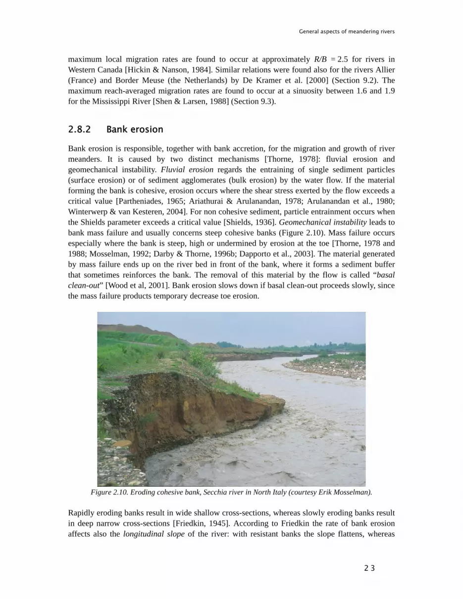
General aspects of meandering rivers
2 3
maximum local migration rates are found to occur at approximately R/B = 2.5 for rivers in Western Canada [Hickin & Nanson, 1984]. Similar relations were found also for the rivers Allier (France) and Border Meuse (the Netherlands) by De Kramer et al. [2000] (Section 9.2). The maximum reach-averaged migration rates are found to occur at a sinuosity between 1.6 and 1.9 for the Mississippi River [Shen & Larsen, 1988] (Section 9.3).
2.8.2 Bank erosion
Bank erosion is responsible, together with bank accretion, for the migration and growth of river meanders. It is caused by two distinct mechanisms [Thorne, 1978]: fluvial erosion and geomechanical instability. Fluvial erosion regards the entraining of single sediment particles (surface erosion) or of sediment agglomerates (bulk erosion) by the water flow. If the material forming the bank is cohesive, erosion occurs where the shear stress exerted by the flow exceeds a critical value [Partheniades, 1965; Ariathurai & Arulanandan, 1978; Arulanandan et al., 1980; Winterwerp & van Kesteren, 2004]. For non cohesive sediment, particle entrainment occurs when the Shields parameter exceeds a critical value [Shields, 1936]. Geomechanical instability leads to bank mass failure and usually concerns steep cohesive banks (Figure 2.10). Mass failure occurs especially where the bank is steep, high or undermined by erosion at the toe [Thorne, 1978 and 1988; Mosselman, 1992; Darby & Thorne, 1996b; Dapporto et al., 2003]. The material generated by mass failure ends up on the river bed in front of the bank, where it forms a sediment buffer that sometimes reinforces the bank. The removal of this material by the flow is called “basal clean-out” [Wood et al, 2001]. Bank erosion slows down if basal clean-out proceeds slowly, since the mass failure products temporary decrease toe erosion.
Figure 2.10. Eroding cohesive bank, Secchia river in North Italy (courtesy Erik Mosselman).
Rapidly eroding banks result in wide shallow cross-sections, whereas slowly eroding banks result in deep narrow cross-sections [Friedkin, 1945]. According to Friedkin the rate of bank erosion affects also the longitudinal slope of the river: with resistant banks the slope flattens, whereas

General aspects of meandering rivers
2 4
with easily eroding banks the slope steepens. This is in agreement with Jansen et al. [1979], who show that a wider river requires a steeper slope to transport the same amount of sediment. The rate of bank erosion is influenced by a number of different factors [Thorne, 1978], such as:
• Near-bank flow strength [Ikeda et al., 1981] • Near-bank channel bed degradation [Thorne et al., 1981; Andrews, 1982], which
increases the bank geomechanical instability • Opposite bank accretion, which pushes the main flow towards the eroding bank [Dietrich
& Smith, 1984; Mosselman et al., 2000] • Physical characteristics of the eroding bank: geometry (slope and height) [Thorne, 1978;
Dapporto et al. 2003], soil composition [Wolfert & Maas, 2007], soil cohesion [Partheniades, 1962; Krone, 1962;] and bulk density of the bank material [Simon & Hupp, 1992]
• Presence and type of riparian vegetation [Macking, 1956; Wynn et al., 2004] • Ground water flow [Darby & Thorne, 1996b; van Balen, personal communication] • Pore water pressure [Dapporto et al., 2003; Rinaldi & Casagli, 1999] • Presence of frost [Wolman, 1959; Gatto, 1995] • Frequency of floods [Carroll et al., 2004] • Flow-stage variation rates [Thorne, 1982; Simon & Hupp, 1992; Dapporto et al.,2003;
Mengoni & Mosselman, 2005] • Temporary storage of material generated by mass failure at the toe of the eroding bank
[Murphey Rohrer, 1984; Neill, 1987; Darby et al., 2002] • Quality of the flowing water (temperature and electrochemical characteristics)
[Arulanandan et al., 1980]. Bank retreat is the transverse shift of the channel margin moving farther from the channel centreline that is caused by bank erosion. Bank retreat rates have been reported by a number of scientists. As an example, Brice [1984] provided averaged bank retreat rate and extension of the drainage area for several rivers (Table 2.1).
Table 2.1. Bank retreat rates and drainage area of a number of rivers according to Brice [1984]. River Drainage area
(km2) Retreat rate
(m/year) Time period
(years) Mississippi River 2 965 550 17.5 1880-1944 Mississippi River 2 913 491 7,8 1880-1944 Yellowstone River 178 969 4.7 1938-1967 Apalachicola River 45 584 1.3 1949-1978 Sacramento River 24 087 5.1 1947-1974 Elkhorn River 15 151 8.4 1941-1971 West Fork White River 12 173 1.7 1937-1966 Iowa River 8 547 0.9 1937-1970 North Canadian River 3 108 4.5 1936-1966 Tallahala Creek 1 554 0.5 1942-1970 Kanaranzi Creek 311 0.2 1954-1968

General aspects of meandering rivers
2 5
Micheli et al. [2004] reported the bank retreat rates of the Central Sacramento River (California) and distinguished two time periods, which were characterized by two different types of riparian vegetation (Table 2.2).
Table 2.2. Bank retreat rates of Central Sacramento River, California Micheli et al. [2004]. Central Sacramento River (California)
Parameter Period 1896-1946 riparian forest
Period 1946-1997 agricoltural land
channel slope (-) 0.00025-0.0005 0.00025-0.0005 median bed grain size (D50) (mm) 15-35 15-35 averaged bank rate of bank retreat (m/year) 2.8 4.2 averaged discharge (m3/s) 3700-4000 2500-2700 averaged width (m) 372-375 356-360 averaged depth (m) 4.7-4.9 3.9-4.1 averaged flow velocity (m/s) 2.1 1.8-1.83
Hooke [1980] provided historical bank retreat rates of a number of rivers in Devon (UK) and compared them with published data from many other rivers world-wide. Hooke reported also extension of drainage area, mean river width and discharge for several rivers, as well as the local radius of curvature and bank characteristics for a number of cross-sections. A review of techniques used to measure river bank retreat rates is provided by Lawler [1993]. The techniques are classified according to the time scales involved (long, intermediate and short). The methods include sedimentological evidence, botanical evidence, historical sources, planimetric resurvey, repeated cross-profiling and terrestrial photogrammetry. Long-term bank retreat rates can be estimated also by using cartographic sources [Hooke & Redmond, 1989], aerial photogrammetry [Hooke, 1980; Hickin, 1988] and satellite imagery [Pyle et al., 1997].
2.8.3 Bank accretion
Bank accretion is the process resulting in river bank advance, i.e. the shift of the channel margin towards the channel centreline, and is responsible, together with bank erosion, for the translation and growth of river meanders. In meandering rivers, bank accretion mainly occurs inside river bends, where it coincides with the growth of the point bar and its consolidation. On the vertical, this process occurs in the form of accretional lenses [McLane, 1995; Page et al., 2003; Allmendiger et al., 2005] (Figures 2.11 and 2.12). In the horizontal the phenomenon results in the formation of scroll bars (Figures 2.3, 2.4 and 2.11).

General aspects of meandering rivers
2 6
GeulRiver
P3 P4 P5 P6 P7
= Fining-up sequence0 5m
123456789
Figure 2.11. Geul River (the Netherlands). The migration of the point bar from right to left can be detected from the point bar-transect through P3, P4, P5, P6 and P7 [Spanjaard, 2004]. Legend: the active bar is the
accreting part of the point bar.
Figure 2.12. Allen Ridge Sandstone, Cretaceous, central Wyoming. Paleo meandering river, in yellow individual accretion surfaces formed by transverse migration of a point bar from right to left (http://faculty.gg.uwyo.edu).
Hupp & Simon [1991] and Hupp [1992] followed the long-term process of renaturalization of several small-scale rivers in Tennessee (USA) after a drastic channelization. They observed that riparian vegetation growth and bank accretion occurred at the same time and that the accretion rates were greatest when vegetation density and channel roughness were highest. Bank accretion preceded bank erosion at the opposite side of the channel and the rivers restarted meandering when both processes were present, which occurred approximately 50 years after the start of river renaturalization. Based on the observations of Hupp & Simon and on the works of, among others, Pizzuto [1994], Tsujimoto [1999] and Mosselman et al. [2000], the bank accretion process appears to be governed by the sequence of high and low river flows, by vegetation growth and by

General aspects of meandering rivers
2 7
the rate of opposite-bank retreat (Sections 3.6 and 4.4). In river bends bank accretion develops through:
• Point bar growth in vertical and transverse direction [Dietrich & Smith, 1984]. • Pont bar stabilization by vegetation and soil consolidation. • Opposite bank retreat. • Attachment to the floodplain.
Vertical accretion mainly occurs during floods, when the water comes out of its confined channel and sediment settles on the top surface of the point bar and in general along the channel edges, forming natural levees. The presence of floodplain and riparian vegetation causes sedimentation to be more localized near the channel edges, which results in the formation of more localized levees. Generally, during floods erosive phenomena prevail in the river channel, which becomes wider and deeper (Figure 2.13).
Figure 2.13. Channel expansion and levee formation during floods.
During the falling stage and at ordinary flows vertical and transverse point bar accretion occurs and the highest velocity locus gradually shifts towards the outer bank. The outer bank might erode, but at a much lower rate than during floods (Figure 2.14). Toe erosion might also occur, which increases the chance of bank failure during the next flood.
Figure 2.14. Point bar accretion and reduced outer bank erosion at ordinary flows.
new levee
bank erosion
Point bar accretion
Outer bank
Inner bank
Levee formation
Bank erosion
Bed erosion
Outer bank
Inner bank
Levee formation

General aspects of meandering rivers
2 8
The highest parts of the point bars emerge during low-flow stages, when they are partly colonized by pioneer plant species (Figure 2.15). If there is enough time between high flows, the presence of roots and plants together with sediment consolidation and compaction provide extra soil resistance to the newly formed terraces [Allmendiger et al., 2005]. In this case the next flood might not be able to erode them (point bar stabilization). The presence of vegetation cover enhances also the vertical accretion of the point bar by accumulation of organic matter (fallen leaves and dead plants). Besides, during low flow stages fine sediment might settle in the conveying channel (Figure 2.15).
Figure 2.15. Partial point bar colonization by plants during low flow stages.
During the next floods, established vegetation deflects the flow towards the opposite bank [Tsujimoto, 1999], which might cause increased bed and bank erosion at the opposite side of the channel and increased sedimentation among the plants. This effect depends on density, size and type of vegetation [Hupp & Simon, 1991] and on the frequency, intensity and duration of the floods. On the long term, the accreted point bar attaches to the floodplain. This is the bank advance process. Hupp & Simon [1991] observed that for the small-sized rivers they monitored this occurred after about 70 years from the start of the re-naturalisation process. The erosion of the outer bank of river bends prevents or reduces the erosion of the inner bank and favours transverse point bar accretion during the falling stage. Therefore, opposite bank erosion plays an important role in the progression of bank accretion. Bank accretion is enhanced by a positive feed back that occurs if bank advance induces (extra) erosion of the opposite bank.
2.9 Cutoffs
Meander extension suddenly stops when the flow excavates a shortcut and abandons its old bend way. This process often occurs at the neck of a meander when, due to bank erosion the upstream and downstream bends meet [Jagers, 2003]. However, during floods, when also the flood plains convey water, the flow can simply take another course, which later grows into the main channel of the river. The new water course is generally shorter, straighter than the previous one and is often an old abandoned channel. A cutoff not occurring at the neck of a meander is named chute cutoff, because the erosive process is usually related to the formation of a chute, i.e. a local flow acceleration. Chute cutoffs are
colonization by plants
Outer bank
Inner bank
accumulation of organic matter
Settling of fine sediment

General aspects of meandering rivers
2 9
longer flow diversions than neck cutoffs. Having steeper gradients than the original meander bend, a chute can gradually increase in size during successive floods until it conveys all water. The new channel is excavated through the floodplain either starting from its downstream or from its upstream section, which is an indication that several different factors may be responsible for the formation of this type of cutoffs [Jagers, 2003]. In general, chute cutoffs are more probable as the degree of braiding increases [Brice, 1984], while for meandering rivers with narrow channels, well vegetated banks and low gradients, the dominant shortening process is the occurrence of neck cutoffs [Howard & Knutson, 1984]. Neck cutoffs seem to occur in clusters rather than singularly (Figures 2.16 and 2.7). The occurrence of multiple cutoffs was investigated by Hooke [2004] and Stølum [1996], who hypothesized that cutoffs are a part of a self-organizing (river) system and occur because the river has reached a state of criticality.
Figure 2.16. Multiple neck cutoffs, Owl Creek, north of Lac La Biche, Alberta, Canada (© Airphoto-Jim Wark).
The most visible effect of cutoffs is the confinement of the meander belt. Although bank erosion rates tend to decrease with the increase of the meander amplitude [Hickin & Nanson, 1984] it is not clear to which extent meanders would grow without cutoffs [Hooke 2003; Stølum, 1996]. At high sinuosity meanders tend to grow also in upstream direction, with the result that successive meanders gradually approach each-other, making neck cutoffs unavoidable. Meander growth has the effect of decreasing the channel bed slope with time and cutoffs have the opposite effect. Due to the occurrence of cutoffs at different locations and times, at the large scale and on the long term, the bed slope of meandering rivers tends to remain (dynamically) constant. Cutoffs can therefore be regarded as a stabilizing phenomenon for the long-term dynamics of meandering rivers [Camporeale et al., 2005].

General aspects of meandering rivers
3 0

Controls of meandering
3 1
3 Factors controlling river meandering
3.1 Introduction
It is important to know which factors determine why a river at a certain location has a meandering or another planform style, since this knowledge forms the basis for modelling the large-scale river behaviour. Several factors are found to govern natural river meandering. Some of them are explicitly included in the model of this study (Chapter 5). Other factors are only implicitly present, because they are simply assumed to be in the proper range for a single-thread river. The full range of factors should be considered in river planform classifications. This chapter reviews the state of the art of this topic with two purposes. First, it defines the conditions for natural meandering rivers and hence the application range of meander models. Second, it reveals shortcomings in commonly accepted river planform classifications, because they tend to ignore some processes that are important for bank accretion. Factors controlling bank accretion are discussed as a first step towards more complete planform classifications.
3.2 Planform classifications
River classifications based on the river planform are of two types, in accordance with two distinct objectives: (1) define a terminology to describe the morphological situations of natural alluvial rivers and (2) distinguish the morphological situations based on the governing factors. In the first case the classification schemes are limited to a geometrical description of the river and might also include the description of some phenomena, but without identifying their causes. In the second case meandering or braiding or any other planform style, already defined in a geometrical-phenomenological way, is associated with a combination of morphodynamic parameters1. When these parameters represent the independent factors governing the processes of planform formation, these classifications also allow for the deduction of the changes in river planform style that would occur when one parameter changes and a threshold is exceeded [Bridge, 1993]. The factors governing the basic processes of river meandering are here named “controls on meandering”. Several classifications based on geometrical features and phenomena are found in the literature. Rust [1978] classified rivers according to sinuosity and a braiding parameter. Kellerhals et al. [1976] proposed a classification based on: (1) planform (straight, sinuous, irregular, regular meanders); (2) islands (none, occasional, frequent); (3) channel bars and major bed forms (channel side bars, point bars, mid-channel bars) and (4) lateral channel activity (not detectable, downstream progression, progression with cut-offs). Brice [1984] classified rivers by: sinuosity, point bars, braiding and anabranching. Chalov [1983, 1996] proposed to treat incised rivers
1 Parameters are combinations of variables: width and depth are variables; the width-to-depth ratio is a parameter.

Controls of meandering
3 2
separately, because their morphological features are mainly determined by the geological structure and by the history of the valley. His river classification [Chalov & Alabyan, 1994] is based on increasing braiding intensity from meandering to multi-branched channels on three structural levels: floodplain, channel planform and bars. Snishchenko & Kopaliani [1994] classified rivers according to increasing sinuosity, starting with the band-dune type (straight river with riffles and pools), and introduced the side-bar type (with alternating bars), the restricted meandering type (confined meandering) and the free meandering type. They concluded the classification with the incomplete meandering type (chute cut-offs and transition to braiding). Rosgen [1994] divided the rivers in categories, based on: channel slope, sinuosity, width-to-depth and entrenchment ratios (all geometrical parameters). Due to the large number of classifications the terminology to describe the river planform style is multiple and has not been standardized yet. Classifications based on the factors controlling the river planform style first appeared in the nineteenth century. In 1897 Lokhtin suggested that the river planform style is governed by three main factors: the discharge regime, which depends on climatic and soil conditions; the valley slope and the erodibility of the river bed. He also defined a criterion based on stream power (discharge and slope) and bed grain size to characterize the river planforms (reported by Alabyan & Chalov [1998]). Sixty years later Leopold & Wolman [1957] subdivided natural rivers into the three categories: meandering, straight and braided. Although they stated that the river planform style is influenced by a great variety of environmental controls, they used only discharge and slope as controlling variables to discriminate between meandering and braiding, without Lokhtin's third variable of bed grain size. This resulted in the following empirical threshold curve:
-0.44s bfi = 0.06 Q (3.1)
where: is = channel slope at the transition between meandering and braiding (-) Qbf = bankfull discharge (ft3/s). Discharge and slope act together as an indicator for the stream power. Braided rivers are supposed to fall above the curve and meandering rivers below. The fact that the planform style mainly depends on discharge and slope soon became of general acceptance [Lane, 1957; Ackers & Charlton, 1970c; Antropovskiy, 1972; Bray, 1982]. Schumm & Beathard [1976] used the threshold of Leopold & Wolman to forecast river planform changes after human intervention, although Henderson [1963] had soon pointed out that the transition criterion for braiding also depends on the size of the bed material and suggested replacing the threshold curve of Leopold & Wolman (Equation 3.1) with the following:
-0.441.145064s bfi = 0. D Q (3.2)
where D50 is the median grain size of the river bed material (ft). Fourteen years later, Schumm [1977] classified alluvial channels based on their sediment supply. He defined three types or rivers: “bed-load channels”, characterized by high width-to-depth ratios, low sinuosity and braiding; “mixed load channels”; and “suspended-load channels”, with

Controls of meandering
3 3
low width-to-depth ratios, high sinuosity and meandering. In general, sediment supply presents two aspects: a quantitative aspect, which governs river bed aggradation and degradation, and a composition aspect. Schumm's sediment supply regards the composition aspect only. A few years later, the experiments of Ackers [1982] showed that the bed material can influence the sinuosity of meandering rivers, which confirmed the intuition of Henderson [1963]. Schumm re-elaborated his classification scheme, relating the channel planform style to sediment supply and stream power [Schumm, 1981]. A similar approach was later also followed by van den Berg [1995], who defined a threshold curve between single-thread and multi-thread channel rivers, based on grain size and stream power:
0.42, 50900t Dνω = (3.3)
where: D50 = median grain size of the river-bed material (in the range 0.0001-0.1 m)
,tνω = “potential specific stream power at the transition between single-thread and multi-thread channel river patters” (subscript t stands for “transition”) (W/m2).
To plot the position of real rivers in the νω -D50 plain, νω is derived as a function of the valley slope and mean annual flood or bankfull discharge, in the following way:
for sand-bed rivers (D50 < 2 mm) 2.1 v Wi Qνω = (3.4)
for gravel-bed rivers (D50 ≥ 2 mm) 3.3 v Wi Qνω = (3.5)
where:
vω = “potential specific stream power” (for a straight river, using the valley slope) (kW/m2)
iv = valley slope (-) QW = either bankfull discharge or mean annual flood discharge (m3/s) (only
values above 10 m3/s). The threshold curve by Van den Berg (Equation 3.3) is currently used to predict the morphological consequences of river rehabilitation [Schweizer et al., 2004]. Church [1992] (based on the concepts of Mollard [1973] and Schumm [1985]) included the factor “channel stability” and classified rivers based on: channel stability, sediment supply, channel slope and sediment size (Figure 3.1). Galay et al. [1998] followed a similar approach, but preferred to use the valley slope instead of the channel slope, and classified gravel-bed rivers according to: sediment supply, lateral instability, valley slope and ratio bed load-total load. Their classification scheme is shown in Figure 3.2.

Controls of meandering
3 4
Figure 3.1. Conceptual river planform classification of rivers according to Church [1992].
The factor “resistance of the river banks against erosion” was explicitly introduced by Ferguson [1987], who summarized the factors controlling the channel planform formation in: flow strength, amount and type of sediment load and bank strength. Ferguson gave a weak support to the classification of Leopold & Wolman, stating that the slope-discharge threshold can be interpreted as a threshold of flow strength and supported the idea (already introduced by Leopold and Wolman) that there is a morphological continuum and that no clear thresholds can be defined between distinct types of channels. This approach, followed also by Knighton & Nanson [1993], still receives a vast consensus [Piégay et al., 2005]. Mosley [1987] added another governing factor to those indicated by Ferguson [1987]: the discharge variability, but did not consider the amount of sediment. According to him, the river planform style is governed by flow strength (discharge magnitude), sediment type, bank strength and discharge variability.

Controls of meandering
3 5
Figure 3.2. Classification of gravel-bed rivers according to Galay et al. [1998].
Millar [2000] defined a meandering-braiding transition criterion that takes into account also the effects of vegetation on bank erodibility, which means that he actually proposed that the influence of vegetation can be seen as a part of bank strength:
0.61 1.75 0.25500.0002s bfi D Qφ −′= (3.6)
whereφ′ is a lumped parameter, called “the bank material friction angle”. The median grain size is given in metres and the bank-full discharge in m3/s. The effects of riparian vegetation are empirically incorporated inφ′ . Bledsoe & Watson [2001] studied the thresholds between river planform styles with a regression method and found the following governing parameter, the mobility index:

Controls of meandering
3 6
mobility index = 50
Wb
QiD
(3.7)
where: ib = channel-bed slope (-) QW = annual flood discharge or bankfull discharge (m3/s) D50 = median grain size (m). The mobility index is supposed to scale the flow energy relative to the size of bed material and can be made dimensionless by multiplying the median grain size by the kinematic viscosity of water, ν (for clear water at 20o C, ν = 10-6 m2/s), in the denominator under the radical. However, it is important to point out here that both channel-bed slope and the bankfull discharge are not independent of the river planform (sinuosity, cross-section) and that the good correlations between mobility index (using bankfull discharge) and river planform found by Bledsoe & Watson using their regression method might be affected by this dependence. This is also true for the threshold curves of Leopold & Wolman (Equation 3.1), Henderson (Equation 3.2) and Millar (Equation 3.6). The role of the channel width-to-depth ratio or aspect ratio for the alluvial river planform formation results from the stability analyses performed in the 60s to 80s [Hansen, 1967; Callander, 1969; Engelund, 1970; Parker, 1976; Fredsøe, 1978; Struiksma et al., 1985; Blondeaux & Seminara, 1985]. Assuming that width and depth of alluvial rivers result from the equilibrium between the reach-averaged flow strength (in a straight channel), the river bed mobility and the bank resistance, stability analyses assess the conditions that govern the development of (migrating) bars and relate the presence/absence of bars to the channel planform style. Multiple bars form at larger width-to-depth ratios than alternate bars. Unfortunately the width-to-depth ratio of an existing river has the great disadvantage of not being independent of the channel planform. Using the width-to-depth ratio as a threshold between meandering and braiding would require an additional width predictor, based on flow strength, river bed mobility and bank resistance. A good universal width predictor is still lacking [ASCE Task Committee, 1998a and 1998b], but empirical width predictors for specific river typologies or geographical regions are available, albeit with a large uncertainty band [e.g. Parker et al., 2007]. However, in some cases the width-to-depth ratio becomes an independent parameter, as for instance when the river width or depth is locally altered by natural causes, such as a land slide, or by humans. In such cases, the knowledge of the new width-to-depth ratio would allow for rough prediction of the effects of the alteration on the river planform style. A width-to-depth ratio 40=β is considered the threshold between meandering and braiding by Rosgen [1994] and
50=β by Engelund & Skovgaard [1973]. Larger width-to-depth ratios characterize braided rivers. Existing process-based river classifications indicate that river meandering occurs when some of the following conditions are satisfied: mild flow strength; mild sediment supply rich in fines; low bank erodibility. These requirements are confirmed by observations and experimental findings (e.g. Smith [1998]). However, existing classifications ignore bank accretion. The importance of this process was recognized by Ferguson [1987], Knighton & Nanson [1993] and Mosselman [1992, 1995]. Bank accretion is mainly governed by the following, weakly interdependent, factors:

Controls of meandering
3 7
• Flow strength (weighing the flow capacity to entrain sediment). Lower flow strengths at
the inner side of bends mean higher sedimentation rates. • Sediment supply (sediment is the necessary “material” to construct point bars). Sediment
supply has to be seen in terms of amounts and composition. • Riparian vegetation (riparian vegetation deflects the flow from the bank, accelerates the
vertical growth by favouring the local deposition of sediment and protects the accreting bank from erosion). Meandering rivers mostly present well vegetated banks.
• Frequency of floods (i.e. ability to erode accreting banks). Irregular river regimes with frequent high floods are typical of braided rivers in which bank accretion does not have the time to stabilize.
Some existing classifications already take into account one or more of these factors, for example Mosley's [1987] discharge variability can be interpreted as representative for the frequency of floods. Ferguson [1987], Galay et al. [1998], Church [1992] and Knighton & Nanson [1993] all considered sediment supply. Millar [2000] considered riparian vegetation, but only with respect to bank strength. Except for Knighton & Nanson, who considered sediment supply as a prerequisite for point-bar building, existing classifications neglect bank accretion. When this process is taken into account it becomes clear that also the following conditions are relevant to river meandering: the presence of riparian vegetation and the frequency of floods. Finally, also active tectonics plays a role in river planform formation.
3.3 Flow strength
Flow strength is a generic term expressing the capacity of the flow to transport sediment and to erode its bed and banks, irrespective of the precise definition. The definition of “river flow strength” should involve some parameterisation of shear stress, flow velocity or stream power, taking into account temporal discharge variations. As a general rule, braided rivers tend to have higher flow strength than meandering rivers. An example can be seen in the Amazon River system that crosses the dense Amazon forest: the smaller tributaries are meandering rivers, but the largest ones, including the Amazon River itself, are anabranched or braided (Figure 3.3). In this case the largest difference between small and large rivers is the flow strength, but sometimes also the sediment supply [Puhakka et al., 1992]. In general, the flow strength dominates the river planform formation of most of the world largest (natural) rivers, which are all braided or anabranched in their low-land part, whereas their tributaries and distributaries tend to be meandering. Some examples are: the Congo River [Peters, 1978], the Yellow River [Wang et al., 2004], the Ob River [Alabyan & Chalov, 1998] and the Brahmaputra River [Coleman, 1969; Jagers, 2003] upstream of its confluence with the Ganges (see next section).

Controls of meandering
3 8
Figure 3.3. Rio Negro, one of the largest tributaries of the Amazon River, (braided) and the meandering tributary Rio Araça (Image © 2005 Digital Globe Image © 2005 EarthSat) on Google Earth.
3.4 Sediment supply
The sediment transported by the river flow can be divided into two parts: “wash load” and “bed material load”. Wash load is the fine component (silt and clay) of the transported sediment and mainly originates from the erosion of hillsides and river banks. This component has a major role for the silting up of low-dynamic secondary channels, oxbow lakes and pools, as well as for the rising of floodplains and for the formation of deltas. Cohesive material is particularly relevant when dealing with bank erodibility and bank accretion processes, because once deposited it consolidates and becomes more resistant to erosion. Fine sediments also carry nutrients, which are important for the growth of riparian and floodplain vegetation and further increase the soil cohesion. The formation of a meandering channel appears to be encouraged by sediment supply which is rich in fine cohesive sediment, i.e. wash load. Vice-versa, river braiding is favoured by the prevalence of loose coarse sediment, such as sand and gravel, i.e. bed and suspended load [ASCE Task Committee, 1982]. The braided Brahmaputra River confirms this rule, as it becomes single-thread and starts to meander after the confluence with the Ganges River, even if the flow strength is increased. At the confluence the river system is supplied with fine cohesive sediment

Controls of meandering
3 9
from the Ganges, whreas upstream of the confluence the Brahmaputra River only transports loose sand and non-cohesive silt. The total amount of coarse sediment (sand and gravel) transported by the river flow can be related to the stream velocity, and is therefore a function of the flow strength. A general sediment transport formula reads: qS = m u b (3.8) where: qS = maximum amount of sediment that can be transported by a stream with
flow velocity u and is called “transport capacity” (m2/s: volume per second, per unit of river width).
u = flow velocity (m/s). m = coefficient (m2-b/s1-b). b = exponent, normally ranging between 3 and 10 in meandering sand-bed
rivers (-). The formula indicates that there is a limit to the transport of coarse sediment. Instead, there is not such a limit for wash load transport (extreme high concentrations of sediment may transform the water flow into a mud flow). While bed material load transport is capacity limited, wash load transport is supply limited. A relationship between channel planform style and amount of sediment supply has been indicated by several authors [ASCE Task Committee, 1982]. Abundance of sediment is a prerequisite for river braiding. Braided rivers tend to become incised and start to meander when the amount of sediment load decreases, as for instance downstream of dams [Bradley, 1984; Schumm, 1991; Scheuerlein, 1995; Holubová, 1998; Klingeman et al., 1998; Andrews & Nankervis, 1995]. Vice-versa, river braiding may be enhanced by bed aggradation, when the supply of bed material is larger than the yearly transport capacity [Bradley, 1984; Carson, 1984; Hicks et al., 2000]. Deforestation causes hillside erosion, which increases the supply of sediment to the river, with river aggradation and braiding as a consequence [Petkovic & Djekovic, 1995; Kuhnle et al., 1998; Germanoski & Schumm, 1993]. A stable meandering planform therefore requires that the yearly amount of sediment supply is equal to or less than the yearly transport capacity (when it is less: channel incision).
3.5 Bank erodibility
Another important condition for meandering is the low erodibility of the river banks, which is favoured by either bank soil cohesion or by the presence of dense riparian vegetation. Failure due to toe erosion is the most relevant process affecting bank erosion in meandering rivers, since their banks are usually cohesive and in this case the entrainment of bank material is relatively small. Instead, entrainment of bank material is the most relevant mechanism for braided rivers, since their banks are constituted by the same loose material that forms the river bed. Meandering rivers obtained in the laboratory are often not very sinuous. When loose sand is used for bed and bank material, the banks are extremely erodible and the streams widen rather then

Controls of meandering
4 0
meander [Parker, 1976]. The first one who obtained a meandering river in laboratory with a very sinuous slowly-migrating thalweg is Smith [1998], who used cohesive sediment, which caused the banks to be much more resistant to erosion. This proves that, the laboratory the bank resistance against erosion strongly influences the channel planform, in particular its sinuosity. This is true also for real rivers [Simpson & Smith, 2000] and is shown in an indirect way by the fact that highly erodible banks are typical of wide braided rivers and resistant cohesive banks are typical of meandering rivers. Low bank erodibility enlarges the time scale of the lateral changes of rivers. Bed and banks of braided rivers are constituted by similar material, which has the consequence that the lateral and vertical changes have comparable time-scales. In meandering rivers those time scales are different, since the lateral changes are much slower than the vertical changes.
3.6 Riparian vegetation According to Murray & Paola [1994] braiding represents the default river planform style in non-cohesive sediment without vegetation. They argue that meandering can be seen as a particular case of braiding, the one characterized by a single-thread channel, occurring when the sediment is cohesive or in presence of riparian vegetation. Indeed, most natural meandering rivers flow through forests (Figure 3.5) or in alluvial plains covered by vegetation, whereas sparsely vegetated banks tend to be associated to braided rivers [Leopold et al., 1964]. A clear example is offered by the rivers in Iceland that are almost all braided, with the exception of some very small streams between grassy banks. In Iceland vegetation cover is poor and sediment load is large [Kingstrom, 1962]. For similar reasons, braiding prevails also in New Zealand [Mosley & Jowett, 1999].
Figure 3.5. An aerial view of boreal forest (taiga) in summer near Nadym. Yama River, Western Siberia, Russia (© www.arcticphoto.co.uk)
According to Pannekoek and van Straaten [1984] all alluvial rivers were braided before the Silurian period (approximately 400 million of years ago), i.e. before the first plants with roots and rhizomes appeared. This opinion is shared by Ward et al. [2000] who also attribute the changes from meandering to braiding river deposits in South Africa during the Permian-Triassic crisis (251 million of years ago) to the rapid and major extinction of land plants that occurred in that period. Numerous works linked river channel properties to riparian vegetation [Brice, 1964; Zimmerman et al., 1967; Hickin, 1984; Hey & Thorne, 1986; Ferguson, 1987; Thorne, 1990; Mosselman, 1992; Murray & Paola, 1994; Millar & Quick, 1993; Millar, 2000].

Controls of meandering
4 1
In the laboratory, vegetation was found to strongly influence the development of the stream topography by Gran & Paola [2001] and Kurabayashi & Shimizu [2003], who carried out flume experiments on river braiding with and without plants and observed that the presence of vegetation reduces the number of braids. Jang et al. [2003] found that an originally braided system without vegetated banks evolved into an incised meandering channel when the banks became vegetated. The same effect was also observed by Tal & Paola [2005]. Field observations of Mant & Hooke [2003] confirm the experimental findings for real rivers. Vegetation causing width reduction was observed by Eschner et al. [1983], Beeson & Doyle [1995] and Allmendiger et al. [2005]. Riparian vegetation controls the river planform by acting on: (1) river bed degradation/aggradation, (2) bank erosion and (3) bank accretion by:
• Protecting the bank soil against erosion. Plants provide local soil reinforcement by roots (Figure 3.6) and soil protection by cover. For mass failures, however, the impacts of vegetation can be either positive or negative and depend on the characteristics of the bank and the vegetation [Ott, 2000].
• Deflecting the water flow. Vegetation increases the local hydraulic roughness and for this reason, the flow tends to concentrate where vegetation is absent [Tsujimoto, 1999; Pirim et al., 2000; Rodrigues et al., 2006]. This lowers the flow velocity within the plants, where sedimentation increases, and causes bed degradation in the non-vegetated area of the channel, where the flow velocity becomes higher. By deflecting the flow towards the opposite bank, riparian vegetation enhances opposite bank erosion [Dijkstra, 2003].
• Accelerating the vertical growth of accreting banks. Vegetation favours the sedimentation of fines within the plants and causes local accumulation of organic material (falling leaves, branches, dead plants), which raises the ground level and reinforces the soil cohesion and strength [Baptist, 2005; Baptist & De Jong, 2005] and Baptist et al., 2005]. Besides, the presence of riparian vegetation enhances the formation of localized natural levees during floods and bank accretion.
• Stabilizing accreting banks and accelerating their lateral grow by colonizing the surfaces which remain dry during low flow stages. Areas with low dynamics prone to colonization are typically the point bars at the inner side of meanders and the smallest channels of a braided system [Tal et al., 2005].
The effects of riparian vegetation on river planform were studied by means of numerical models by Murray & Paola [2003], Jang & Shimizu [2007] and by Samir-Saleh & Crosato [2008]. Murray & Paola studied the effects of increased soil strength due to the presence of floodplain vegetation, whereas Jang & Shimizu and Samir-Saleh & Crosato studied the effects of increased hydraulic roughness. All works demonstrated that vegetation decreases the degree of braiding of river systems and might even transform a braiding into a meandering system. The effects of vegetation on river processes are many, complex, and difficult to quantify [Rinaldi & Darby, 2005]. The ability of vegetation to stabilize river banks [Ott, 2000] is partly dependent upon scale, with both size of vegetation relative to the watercourse and absolute size of vegetation being important [Abernethy & Rutherfurd, 1998]. Vegetation stabilization is most effective along small watercourses. On relatively large rivers, fluvial processes tend to dominate [Thorne, 1982; Pizzuto, 1984; Nanson & Hickin, 1986]. Moreover, the effects of riparian vegetation vary

Controls of meandering
4 2
according to the type of plants and to their development stage [Allmendiger et al., 2005; Dijkstra, 2003].
Figure 3.6. Roots protecting the river bank against erosion. Geul River (the Netherlands), courtesy of Eva
Miguel.

Controls of meandering
4 3
Riparian vegetation growth is influenced by several factors, among which the most important appear: climate, latitude, soil characteristics, river dynamics and frequency of floods. Warmer and wetter climates allow for higher biomasses and faster growth, which makes vegetation more efficient in reducing bank erosion and colonizing the river banks. Vegetation growth on river banks occurs through succession stages that can be recognized by the collection of species that dominate at that point in the succession. Succession begins when an area is made partially or completely devoid of vegetation because of a disturbance, such as erosion or severe flooding. Succession stops when changes of species composition no longer occur with time, and this community is said to be the “climax community”. An example is the succession of plant species on abandoned fields in North Carolina. Pioneer species consist of a variety of annual plants. This stage is then followed by communities of perennial grasses, shrubs, softwood trees and shrubs, and finally hardwood trees and shrubs. This succession takes about 120 years to develop from the pioneer stage to the climax community [Pidwirny, 2000]. The plant communities vary with the river typology, such as the suspension-load character and the river regime. Puhakka et al. [1992] observed that the floodplains of braided Amazonian rivers are characterized by abundant young successional vegetation and that the width of the successional zones in relation to the river size is larger for braided rivers than for meandering rivers. A riparian plant community that approaches the climax community is a sign that the river dynamics do not limit in a relevant way vegetation growth, which is often the case for meandering rivers. Simon & Hupp [1992] studied the possibility of using riparian vegetation as a major diagnostic criterion for denoting channel processes and found that the greatest number of mean vegetative cover and species numbers were attained on banks where widening rates were minimal. According to them vegetation cover reflected the periods of time since the last episode of channel modification. Assuming that during succession the plant biomass increases with time, the closeness of the riparian community to the climax community can be represented by the ratio between the unit plant biomass (per m2) present and the unit plant biomass of the climax community. On accreting banks this would be the plant community present above the top of the outermost ridge. A small value of this ratio would be typical of braided rivers; values tending to unity would be typical of natural meandering rivers. Even in Iceland, where the biomass of the local climax community is low (grass and reed) those small rivers that have banks covered by this type of vegetation are meandering. Takebayashi et al. [2006] used the density of riparian vegetation, vλ , instead of the biomass. They
assumed this density to increase linearly with time, from 0 to maxvλ :
max ( / )v v d vt Tλ λ= (3.9) where:
maxvλ = maximum density of riparian vegetation (stems/m2)
td = duration of period in which the surface to be occupied by vegetation remains dry (s)
Tv = time necessary to the riparian vegetation to reach maximum density (s). Equation 3.9 was designed for grass. For other plant species the density does not necessarily increase with time [Hupp & Simon, 1991].

Controls of meandering
4 4
3.7 Frequency of floods
Floods provide physical disturbance that can disrupt the riparian ecosystem, community or population structure and change resources or the physical environment [Resh et al., 1988]. Frequency, intensity and timing of floods control riparian vegetation growth [Hupp & Osterkamp, 1996], the compaction of the deposited cohesive sediment, the frequency of bank failure and bank erosion rates [Duan, 2005; Perucca et al., 2006]. The colonization of bars and banks by a plant community occurs during low flow stages. An important parameter for the biogeomorphic riparian system is therefore the ratio between the time necessary for a given plant community to develop, vT , and the recurrence interval, fvT , of floods
that are able to destroy it, i.e. by mechanical destruction, burial and prolonged submersion [Phillips, 1995 and 1999]:
vv
fv
TT
τ = (3.10)
in which the subscript v refers to riparian vegetation (a similar parameter was introduced also by Tal & Paola [2005]). The ratio vτ is useful to determine whether the biogemorphic riparian system is dominated by physical disturbance, in which case the river would have the tendency to be braided. Cohesive soils consolidate with time and progressively become more resistant to erosion [Schumm & Khan, 1972]. Therefore, another parameter can be defined to characterize the stability of the cohesive material deposited on floodplains and bar tops. In this case it is the ratio between the time, cT , necessary to the deposited material to reach a certain consolidation level (shear strength), which depends on type of material and conditions and the recurrence interval,
fcT , of floods, characterized by intensity and duration, that are able to erode it. Erosion occurs
when the shear stress exerted by the flow is higher than the shear strength attained by the material.
cc
fc
TT
τ = (3.11)
in which the subscript c refers to consolidated material. When both vτ (Eq. 3.10) and cτ (Eq. 3.11) are less than unity, the frequency of (severe) floods is too high for the river to have sufficiently stable river banks, a prerequisite for developing a meandering planform.
3.8 Active tectonics Another factor that affects the river planform formation, although not included in general river classifications, is active tectonics. This is nonetheless generally recognized, because fluvial planform anomalies, such as local development of meanders or braids, local widening and

Controls of meandering
4 5
narrowing are all used as indicators of active tectonics. The primary effects of active tectonics are local steepening, reduction of gradient or cross-valley tilting [Gregory and Shumm, 1987]. Figure 3.7 shows that incison in an area of active upslift produces a meandering planform in the absence of vegetation (Saint Juan River, a tributary of the Colorado River, Utah) [Wolkowinsky & Granger, 2004]. Interestingly, incision of large rivers enhances tectonic uplift [Finnegan et al., 2008; Allen, 2008].
Figure 3.7. Meanders of the San Juan River, tributary of the Colorado River, Goosenecks State Park, Utah
(photo © Thomas Wiewandt / www.wildhorizons.com).

Controls of meandering
4 6

State of the art
4 7
4 State of the art in meander migration modelling
4.1 Introduction
River meandering has been studied by scientists from various disciplines, including river engineering, mathematics, physical geography, geology and biology, and from many different points of view, as that of river management [Piégay et al., 2006], of river habitats dynamics [Crosato, 1997; Payne & Lapointe, 1997; Richter & Richter, 2000; Richards et al., 2002] and of the formation of sedimentary deposits [Cojan et al., 2005]. Most progress was achieved in the last decades in the understanding of the processes of flow, sediment transport, cross-section forming and planimetric changes [ASCE, 1998a and b]. Field observations, laboratory experiments and mathematical modelling provided complementary inputs. From the field observations, important contributions are those by Leopold & Wolman [1960], Brice [1964, 1974], Hickin & Nanson [1975], Carson & Lapointe [1983], Hooke [1977, 1980, 2004] and Hooke & Redmond [1989]. From the laboratory, important contributions are the experiments carried out by Friedkin [1945], Leopold & Wolman [1957], Ackers & Charlton [1970, a, b and c], Martvall & Nilsson [1982], Fujita & Muramoto [1982], Smith [1998] and Tal & Paola [2005]. Seminara [2006] provides an overview of the progresses made so far. This chapter deals with the progress achieved by mathematical modelling of meandering river processes. The aim is to provide an overview of the state of the art of the models for simulating the long-term planimetric changes of meandering rivers on the spatial scale of several meanders. These models are here named “meander migration models”. Process-based meander migration models are made up by:
• A component describing flow field and bed topography of curved channels. • A component describing bank erosion. • A component describing bank accretion. • A component that simulates river cutoffs (optional).
The state of the art of each component is described in the next sections.
4.2 Modelling of flow field and bed topography in curved channels
Morphological models describing the changes of the bed topography in curved open channels consist of a flow model coupled to a sediment transport model. The flow in meander bends was first described in detail by Rozovskii [1957], who simplified the Navier-Stokes equations to obtain analytical solutions. His work remained little known until 1961, when it was translated in English [Prushansky, 1961]. Following Rozovskii’s approach De Vriend [1977] and Kalkwijk &

State of the art
4 8
De Vriend [1980] developed a two-dimensional (2-D) mathematical model describing the flow in wide open-channel bends far from the near-bank region and under the assumption of mild curvature. Subsequently, De Vriend [1981, a and b] also included the entrance and exit regions of bends and the near-bank region of the cross-section, which required a three-dimensional (3-D) analysis and resulted in fully describing the main flow redistribution due to the secondary flow. At present, many 3-D Computational Fluid Dynamics (CFD) models for mildly curved river flow are available [Hervouet & Jankowski, 2000; Stelling & Van Kester, 2001; Olsen, 2002; Rodriguez et al., 2004]. The intensity of the secondary flow is weak in a mildly curved channel and grows if the curvature increases. In sharp river bends, common in small meandering rivers like the Geul (Section 9.4), one or two weak and small counter-rotating circulation cells may occur near the outer bank in addition to the classical helical circulation (Figure 4.1). The presence of these counter-rotating circulation cells changes both vertical and horizontal velocity distributions and affects the outer bank erosion by the river flow. The ratio between channel width and radius of curvature, γ , and the width-to-depth ratio (also called channel aspect ratio), β , are important parameters to quantify the secondary flow induced by the channel curvature. The formation of small circulation cells depends on a bend parameter, *β , defined by Blanckaert & de Vriend [2003], which is a function of these parameters:
* 0.275 0.5 0.25( / ) ( 1)f sCβ γ β α−= + (4.1) where:
fC = friction factor (-)
/ cB Rγ = = curvature ratio (-)
/B hβ = = width-to-depth ratio or aspect ratio (-)
sα = a parameter expressing the deviation from the potential-vortex velocity distribution and varying along the bend.
The bend parameter *β is proportional to the Dean number: 0.5Re( / )De γ β= (in which
/Re uh ν= is the Reynolds number and ν the kinematic viscosity of the water, in m2/s). De Vriend [1981a] indicated the Dean number to be the most important parameter for the velocity redistribution. The description of the flow in sharp open-channel bends is a recent achievement [Blanckaert, 2002; Blanckaert & De Vriend, 2003 and 2004; Blanckaert et al., 2003].

State of the art
4 9
Figure 4.1. Flow in sharp river bends and compact cross-section.
Van Bendegom [1947] was the first to develop a 2-D morphological model for curved channels by coupling flow and sediment transport. The model included the effects of helical flow and transverse bed slope. Van Bendegom also performed some computations to predict the river bed evolution, which he carried out by hand (no computers were available at that time). His work, originally written in Dutch, was translated in English and gained wide recognition in 1963 [Nat. Res. Council Canada, 1963]. Most published works on flow and bed topography in curved channels are based on the simplifying hypothesis of small curvature and shallow water and do not apply to the near-bank region of the cross-section, where the flow has an important vertical component. This approach was followed by, among others, Engelund [1974], Kikkawa et al. [1976], Odgaard [1981], Falcon & Kennedy [1983], De Vriend & Struiksma [1984], Struiksma et al. [1985], Olesen [1987], Struiksma & Crosato [1989], Mosselman [1992, 1998], Duan et al. [2001] and Darby et al. [2002]. With the assumptions of mild curvature and shallow water the depth-averaged steady-flow equations for a curvilinear orthogonal system in s (streamwise direction), n (transverse direction) and z (vertical direction, positive upwards) [Olesen, 1987; Mosselman, 1992] read:
2 2
2
1 0s n
u u p uv v guu vs n s R R hCρ∂ ∂ ∂
+ + + − + =∂ ∂ ∂
(4.2)
2
2
1 0n s
v v p uv u guvu vs n n R R hCρ∂ ∂ ∂
+ + + − + =∂ ∂ ∂
(4.3)
( ) ( ) 0
n s
hu hv hu hvs n R R
∂ ∂+ + + =
∂ ∂ (4.4)
where: u and v = streamwise and transverse velocities, in s and n directions respectively
(m/s) h = water depth (m)
Rc
main helical flow
Counter-rotating flow cell

State of the art
5 0
g = acceleration due to gravity (m/s2) ( )bp g z hρ= + = pressure, in which zb is the bed elevation (Pa)
C = Chézy coefficient for hydraulic roughness (m1/2/s) Rs = radius of curvature of the streamwise coordinate line, s (m). Rs is
positive if the centre of curvature lies at smaller n Rn = radius of curvature of the transverse coordinate line, n (m). Rn is
positive if the centre of curvature lies at smaller s (diverging flow). To describe the morphological changes, Equations 4.2, 4.3 and 4.4 have to be coupled to sediment transport and sediment balance equations. The sediment balance reads:
cosSs Stq q α= (4.5)
sinSn Stq q α= (4.6)
0b Ss Sn Ss Sn
n s
z q q q qt s n R R
∂ ∂ ∂+ + + + =
∂ ∂ ∂ (4.7)
where: qSt = volumetric sediment transport, including pores, per unit of channel width
(m2/s) qSs and qSn = components of the volumetric sediment transport, including pores, per
unit of channel width in the s and n directions respectively (m2/s) α = angle between s-direction and sediment transport direction. In general, the sediment transport direction does not coincide with the main flow direction, as it is deviated by the transverse bed slope and by the secondary flow [van Bendegom, 1947; Engelund, 1974]. The sediment transport St can be computed with various (empirical) sediment transport formulae, each one with advantages and limitations [Meyer-Peter & Müller, 1948; Einstein, 1950; Engelund & Hansen, 1967]; reviews are provided by ASCE Task Committee [1982] and by Van Rijn [1984a]. The input of sediment from bank erosion can be incorporated as a source term in the sediment balance equation (Eq. 4.7) [Mosselman, 1992]. With the recent advances in computer technology, 3-D morphological models have become increasingly popular [Olsen, 2003; Lesser et al., 2004]. The model of Lesser et al. (Delft3D) is based on the assumption that the free-surface flow is hydrostatic, which may mean that the flow is not accurately reproduced close to a steep bank, where there the vertical velocity component is important. Stelling & Zijlema [2003] proposed an algorithm to improve this weakness. A different way to model river flow and morphodynamics is used in (Lagrangian) discrete-element methods, such as the smoothed-particle hydrodynamic models [Liu & Liu, 2003; de Wit, 2006], the cellular automata [Chopard & Droz, 1998] and the Lattice Boltzmann models [Succi, 2001]. These models simulate movement and interactions of masses of basic elements, such as (small) water volumes and sediment particles, and translate them in macro scale structures [Heyes et al., 2004]. Some of these methods use Eulerian grids (lattices) while others have no grid. The

State of the art
5 1
single elements have mass, volume, density, pressure, position and velocity. These quantities are moving with the elements and can change only due to external forces. When applied to river morphodynamics, discrete-element models have to appropriately reveal the macro and meso-scale structures which arise from the micro-scale interactions of the sediment particles. The physics should therefore be correctly reproduced at all scales, from the collisions between single particles to the conservation of mass, energy and momentum of large aggregates. Discrete-element methods have already been used to solve two and three dimensional problems in fluid dynamics and sediment transport [Heald et al., 2004]. A three-dimensional lattice Boltzmann model has been used to simulate the bed development in river bends [Dupuis, 2002]. This model, however, lacks appropriate validation. Important points of concern for this type of models are the large computational times required and the sensitivity to numerical errors [Richards et al., 2004], which strongly limit the applicability of discrete-element models to large scale morphological changes of rivers [Jagers, 2003].
4.3 Modelling of bank erosion and bank retreat Bank erosion (Section 2.8.2) has been extensively studied at different spatial and temporal scales. The smallest spatial scale at which bank erosion can be distinguished is the scale of the water depth, for which the relevant temporal scale is that of the single flood event. At this spatial scale the eroding bank is represented in the vertical plane as the side water margin. The vertical variability of bank erosion is taken into account and the process of bank failure is described in detail, taking into account several local factors that may vary during one single flood event, such as groundwater fow [Thorne, 1988 and 1990; Darby & Thorne, 1996 a and 1996 b; Rinaldi et al. 1999; Dapporto et al, 2003; Rinaldi et al. 2004; Rinaldi & Darby, 2005]. At the spatial scale of the channel width, bank erosion reduces to the horizontal shift of the river margin causing channel widening, for which the characteristic temporal scale is that of a long series of flood events [Osman & Thorne, 1988; Mosselman, 1992, 1995, 1998 and 2000; Darby et al, 2002; Darby & Del Bono, 2002]. At larger spatial scales bank erosion reduces to the average value of the retreat rate, which is often used as an indication of the floodplain reworking rate [Reinfelds & Nanson, 1993; Interagency F.M.R.C., 1994; Hudson & Kesel, 2000; De Moor et al., 2007]. The relevant temporal scale is tens to hundreds of years. For the spatial scales of the river width or larger, bank erosion is here referred to as bank retreat. The mechanisms responsible for bank erosion are the direct removal of bank material by the water flow (fluvial entrainment) and bank failure due to geomechanical instability. In Table 4.1 a distinction is made between cohesive and non-cohesive banks.

State of the art
5 2
Table 4.1. Mechanisms of bank erosion. Type of bank erosion Bank material
Fluvial entrainment Bank failure
Non-cohesive • Entrainment of individual particles • Avalanching
Cohesive • Entrainment of individual particles: surface erosion
• Entrainment of large aggregates of silt or clay particles: bulk or mass erosion
• Sliding, slumping
• Temporary storage of erosion products at bank toe followed by basal clean-out
Since meandering rivers are characterized by bank materials that are mainly composed of fine-grained cohesive sediments, here focus is given on the mechanisms that are typical of this type of banks: surface and mass erosion (fluvial entrainment: Section 4.3.1) and sliding and slumping (bank failure: Section 4.3.2) along with temporary storage of bank material at the toe of the bank (Section 4.3.3).
4.3.1 Fluvial entrainment
Partheniades [1962, 1965] and Krone [1962, 1963] were among the first who studied the rate of erosion of cohesive soils by fluvial entrainment. They developed a relation that is currently widely used in erosion models. They assumed that cohesive sediment particles are only entrained when the shear stress exerted by the water flow, wτ , is higher than the soil resistance, crτ , or shear strength (also termed “critical shear stress”) and that the resulting erosion rate is proportional to the excess shear stress above the shear strength, w crτ τ− :
w cr
cr
v E τ ττ
⎛ ⎞−= ⎜ ⎟
⎝ ⎠ for w crτ τ>
0v = for w crτ τ≤
(4.8)
where: E = sediment erodibility coefficient (m/s) ν = erosion rate (m/s)
wτ = shear stress exerted by the flow (Pa)
crτ = critical shear stress or soil shear strength (Pa).
The soil resistance or critical shear stress ( crτ ) is either caused by particle cohesion, which depends on the presence of clay and organic matter as well as on the soil consolidation, or by apparent cohesion, which is due to capillary suction or to binding effects of plant roots. Ariathurai & Arulanandan [1978] and Arulanandan et al. [1980] defined some relations to assess
crτ and the erosion coefficient, E, for cohesive soils. More recently Winterwerp & Van Kesteren [2004] proposed using the following formulas for the erosion coefficient:

State of the art
5 3
( )6010 1cr v
u
cED p cτ
=+
(4.9)
where: cu = undrained shear strength (Pa) cv = consolidation coefficient (m2/s) D60 = grain diameter exceeded by 40% of the material (m) p = porosity or void ratio (-). The critical bottom shear stress for erosion can be assessed by means of the Atterberg limits with the correlation:
0.840.0034cr PIτ = (4.10) where PI is the Plasticity Index. Clay may be eroded also in the form of large aggregates of particles having dimensions of centimetres or more. This type of erosion is classified as “bulk or mass erosion” and takes place when:
( )21 0.82 uu cρ > (4.11)
where: u = flow velocity outside the boundary layer (m/s) ρ = water density (kg/m3). The bank retreat rate that results from fluvial entrainment can be represented either by the depth-averaged component of the erosion rate, ν , in cross-stream direction or by its value at the top of the eroding bank.
4.3.2 Bank failure
For meandering rivers the major mechanism contributing to bank retreat is gravitational bank failure. Based on the work of Thorne [1982], Darby & Thorne [1996b] developed a model that describes the process of bank failure due to geomechanical instability. Their reference bank profile is illustrated in Figure 4.2.

State of the art
5 4
Figure 4.2. Definition diagram showing the bank profile used by Darby & Thorne [1996b]. BW represents
the bank retreat. The bank profile is deformed by combinations of bed degradation ( zΔ ) and lateral toe erosion ( bWΔ ) which may cause bank instability.
FR being the resisting force and FD the driving force acting on an incipient failure block, banks
become unstable when: 1FRFSFD
= < . According to Darby & Thorne [1996b]:
cos tanu t fFR c L W β φ= + (4.12)
and
sint fFD W β= (4.13) where:
uc = bank material cohesion, undrained shear strength (N/m2)
tW = weight of one m thick bank failure block (N/m)
L = length of failure plane (m)
fβ = bank failure plane angle (deg)
φ = friction angle (deg). The second, third and fourth parameters are given by:

State of the art
5 5
2 2 2 2
2 tan tanb r
tf
H K H KW γβ θ
⎛ ⎞′− −= −⎜ ⎟⎜ ⎟
⎝ ⎠ (4.14)
sin f
H KLβ−
= (4.15)
1 21 tan (1 ) tan2f
H KH
β θ φ−⎡ ⎤⎛ ⎞= − +⎜ ⎟⎢ ⎥′⎝ ⎠⎣ ⎦ (4.16)
where: H = height of eroded bank (m) H ′ = uneroded bank height (m) K = depth of the tension crack (m) Kr = depth of any relict crack from a previous bank failure (m)
bγ = unit weight of bank material (N/m3)
θ = uneroded bank angle (deg). The height of the eroded bank depends on the near-bank bed degradation:
0H H z= + Δ (4.17) where H0 is the initial bank height (m) and zΔ is the near-bank bed degradation (m). The uneroded bank height decreases if there is lateral toe erosion (Figure 4.2):
tanbH H W θ′ = − Δ (4.18) where bWΔ is the lateral toe erosion (m). Following the approach of Partheniades and Krone, Darby & Thorne [1996b] assumed lateral toe erosion to be proportional to the difference between the shear stress exerted by the flowing water and the shear strength of the material:
( )mb w crW tχ τ τΔ = − Δ (4.19)
where tΔ is the computational time step and χ is a calibration parameter (N/sm3). The extension of horizontal bank retreat, BW, caused by bank failure is obtained by means of geometrical relations (Figure 4.2), once all other geometrical parameters have been determined. Darby & Thornes’ failure model was implemented in morphodynamic models by Darby & Thorne [1996a] and by Darby et al. [2000 and 2002]. Menéndez et al. [2006] developed a comparable model to simulate bank failure due to undermining. Rinaldi et al. [2004] extended the Darby & Thorne’s bank failure model to include the effects of pore water pressure on bank

State of the art
5 6
stability. An overview of bank erosion modelling can be found in Rinaldi & Darby [2005], who also include a qualitative description of the role of vegetation on bank stabilization. Another bank failure model, also based on a stability analysis, was developed by Langendoen [2000] and incorporated in a 1-D model developed to simulate river incision processes. The same model was later extended by including the effects of pore water pressure (Langendoen & Simon [2008]). The above listed models deal with the mechanisms of bank failure, which is described at the river depth scale for the temporal scale of the single flood event. The modelling of the long-term river planimetric changes, instead, requires deriving an averaged value of the bank retreat rate as a function of the local bank and flow characteristics. In this case, the temporal scale is that of a long succession of flood events. This is a typical process of upscaling [de Vriend, 1991] in which the effects of local short-term processes are assessed at larger spatial and temporal scales. The long-term averaged retreat rate of cohesive banks caused by a long sequence of mass failures induced by toe erosion can be described with Krone-Partheniades-type equations [Osman & Thorne, 1988]:
w crbr flow
cr
v E τ ττ
⎛ ⎞−= ⎜ ⎟
⎝ ⎠ for w crτ τ>
0brv = for w crτ τ≤
(4.20)
where Eflow is the flow-induced erodibility coefficient (m/s) and brv is the long-term averaged bank retreat rate, positive when the bank line moves away from the channel centreline (m/s). This approach was adopted by Mosselman [1992, 1998], who extended Eq. 4.20 by including also a relation for the process of avalanching of non-cohesive material, a relation for bank erosion due to mass failure (depending on bank height) and a term for bank erosion due to external factors, such as groundwater flow and ship waves:
1tan
w cr b B Bcbr flow failure
cr Bc
z h hv E E Ft h
τ ττ ϕ
⎛ ⎞ ⎛ ⎞− ∂ −= − + +⎜ ⎟ ⎜ ⎟∂⎝ ⎠ ⎝ ⎠
(4.21)
where: Eflow = flow induced-erodibility coefficient (m/s) Efailure = bank failure coefficient (m/s) F = extra erosion rate due to external factors (not accounted for in the model)
(m/s) hB = bank height (m) hBc = bank height below which no mass failure occurs (m) zb = bed level (m) ϕ = bank slope angle (-). Many meander migration models [e.g. Ikeda et al., 1981; Johannesson & Parker 1989; Abad & Garcia, 2006] dealing with the large-scale long-term phenomenon of channel migration use a simplified version of Equation 4.20. They assume that bank retreat is proportional to the local

State of the art
5 7
near-bank excess flow velocity, which can be regarded as a linearization of Equation 4.20 [Mosselman, 1992]:
br uv E U= for U ≥ 0 (4.22) where: Eu = erodibility coefficient (-) U = near-bank excess flow velocity (in s-direction) with respect to the cross-
sectionally averaged value (U = ub - u0 , in which ub is the near-bank flow velocity and u0 is the cross-sectionally averaged value of the flow velocity, in m/s).
Hasegawa [1989b] attempted to determine Eu in an analytical way, but his relations hold for the river bed rather than for the banks of the river [Mosselman & Crosato, 1991]. Crosato [1989] and Odgaard [1989] explicitly considered also the contribution of bank height to bank failure and added a term relating the bank retreat rate to the near-bank water depth excess:
br u hv E U E H= + for ( uE U + hE H )>0 (4.23) where: Eh = erodibility coefficient (s-1) H = near-bank excess water depth with respect to its cross-sectionally
averaged value (H = hb- h0, in which hb is the near-bank value of the water depth and h0 is the cross-sectionally averaged value of the water depth, in m).
The excess velocity term, uE U , of Equation 4.23 accounts for the effects of fluvial erosion at the toe of the bank (entrainment), which is driven by the local flow velocity. The excess water depth term, hE H , accounts for geomechanical instability, which is based on the consideration that bank instability increases with the near-bank water depth. The bank retreat rate is equal to zero when both uE U and hE H are equal to or less than zero. When one of these terms is equal to or less than zero, the bank retreat rate depends on the other term. Equation 4.23 can be seen as a linearization of Eq. 4.21 for vertical banks ( 90oϕ = ) and without external erosion factors (F = 0). Besides the above-listed physics-based models, also some empirical models have been developed for the prediction of bank retreat rates, as for instance the morphological model MIKE21 [www.dhigroup.com], in which the rate of bank retreat is empirically related to the near-bank bed degradation and to the near-bank sediment transport divided by the water depth.
4.3.3 Effects of eroded bank material
After failure, the bank material remains at the toe of the bank until it is transported downstream by the water flow, which usually occurs during the next high water stage. The presence of sediment at the toe of the retreating bank affects the near-bank flow velocity and water depth, and

State of the art
5 8
therefore influences local bank erosion and opposite bank accretion. Darby et al. [2002] extended the 2-D morphological model developed by Mosselman [1992] with Darby & Thorne’s [1996a] bank failure model, including the effects of the temporary storage of the bank material debris generated by mass failure at the toe of the bank. Eroding banks also constitute an extra source of sediment to the entire river, which may significantly contribute to the sediment balance. According to Mosselman [1992] the input of bank material makes rivers locally shallower and steeper, which increases the flow velocity and enhances bank erosion, but concluded that “the effect of bank erosion products on two-dimensional bed topography patterns is only appreciable if the net input is very large. It does not need to be accounted for in rivers with low banks and approximately constant width, even if those rivers are migrating fast.” A different conclusion was drawn by Murshed [1991], who studied the problem at a larger spatial scale. He inserted bank erosion products in the sediment balance equation of the mathematical model developed in the framework of this study (MIANDRAS, Chapter 5). According to him, bank erosion products may have important effects on the morphodynamics of rivers having constant width. However, Murshed overestimated the net sediment input from eroding banks by not taking into account in the sediment balance the amount of sediment that has to accumulate on the accreting banks in order to maintain a constant width. Both Mosselman and Murshed found that the effects of the input of bank material on the river morphodynamics are scale-dependent. The accumulation of material at the toe of the bank can be expected to have larger impacts on rivers with small width-to-depth ratios (relatively high banks with respect to the river width) than on rivers with large width-to-depth ratios. Small-sized rivers are generally characterized by small width-to-depth ratios and large rivers by large width-to depth ratios. Besides, the impact can be expected to depend also on the ratio between the yearly sediment input from the eroding banks and the yearly sediment transport capacity of the river. The smaller this ratio, the smaller the impact of bank erosion products is.
4.4 Modelling of bank accretion and bank advance
Much has been done to improve the understanding of bank erosion [Partheniades, 1962 and 1965; Krone, 1962; Thorne, 1982; Darby & Thorne, 1996; Darby et al., 2000 and 2002; Langendoen, 2000; Simon et al., 2000; Rinaldi et al., 2004; Rinaldi & Darby, 2005; Menéndez et al., 2006], but the scientific contributions on bank accretion are limited and mainly examine river-related sedimentary processes on the geological scale, often with the aim of identifying oil reservoirs [Mc Lane, 1995; Page et al., 2003; Clevis et al., 2006; Cojan et al., 2005]. Bank accretion provides a basic contribution to channel migration [Nanson & Hickin, 1983; Hasegawa, 1989a; Mosselman, 1995] and river cross-section forming. Nevertheless, in the field of river morphodynamics, most research deals with observations of only some aspects of the phenomenon, such as point bar growth [Nanson, 1980; Dietrich et al., 1984; Dietrich & Smith, 1984; Reid, 1984; Pyrce & Ashmore, 2005] and riparian vegetation [Leopold et al., 1964; Hupp & Simon, 1991; Hupp, 1992; Micheli & Kirchner, 2002a and b; Micheli et al., 2004; Allmendinger et al., 2005]. Comprehensive modelling work on the bank accretion process is still lacking. The reason might be that bank accretion is a complex phenomenon, governed by factors that are difficult to model. For instance, the models describing the processes of bank accretion have to take into account the dynamics of riparian vegetation (colonization, plant community growth, seasonal variations, succession etc.) and soil compaction. Another reason is most

State of the art
5 9
probably that bank erosion rather than bank accretion worries the people living along the rivers and for this reason studies dealing with bank erosion have received more attention and funds. Similarly to bank erosion, bank accretion can be studied at different spatial and temporal scales. The term bank accretion indicates the process at the depth scale (i.e. variable on the vertical), whereas bank advance refers to the phenomenon at the river width or larger spatial scales. In this case, bank accretion is represented by the horizontal cross-stream shift of the river margin causing channel narrowing. The related temporal scale is that of several years to centuries. Parker [1978] provided one of the first contributions to the modelling of bank accretion, with the aim of computing the equilibrium cross-section of alluvial channels. Following a suggestion of Einstein [1972] and considering that the river width is governed by both bank erosion and accretion, Parker assumed that the accretion mechanism is caused by near-bank settling of fine sediment. He considered a transverse sediment balance, with the coarsest part of the eroded bank material moving as bed load towards the centre of the channel and the finest part towards the accreting bank. Tsujimoto [1999] studied the effects of vegetation on bank accretion and on the river cross-sectional shape in the laboratory and with a depth-averaged numerical model able to reproduce flow and sediment transport in presence of vegetation. According to him sediment entrainment occurs when the bed shear stress exerted by the flow is higher than a critical value. The key factors in the conceptual model of Tsujimoto are the variable discharge and the colonization of the emergent part of the cross-section by vegetation during low flow stages. Tsujimoto found that at high flow stages vegetation deflects the flow towards the opposite bank, where the sediment is eroded and the channel bed degradates. Bank accretion proceeds according to the steps illustrated in Figures 4.3, 4.4 and 4.5. The model of Tsujimoto does not include opposite bank erosion. In his case, colonization by vegetation and bank accretion stop when the velocity at the margin of the vegetated strip becomes equal to the critical velocity for sediment entrainment. It has to be noted that the critical velocity is generally higher within the plants, because roots and organic material increase the soil cohesion. With erodible banks the picture changes. At flood stages, not only bed degradation but also bank erosion occurs, mainly opposite to the accreting bank, with the result that the channel moves laterally. With erodible banks the velocity at flood stage 2 results smaller or not increased with respect to flood stage 1 and due to the lateral shift of the channel the colonization process can continue. Besides, by shifting the flow towards the opposite bank, vegetation contributes to extra bank erosion at the opposite side and favours new colonization. At equilibrium, the bank accretion rate equals the bank retreat rate and the channel simply shifts laterally. Due to the existence of phase lags between bank erosion, channel bed degradation and aggradation and colonization by vegetation, the cross-section experiences short-term fluctuations, but no long-term changes.

State of the art
6 0
Figure 4.3. Step 1. Flood stage: river bed degradation.
Figure 4.4. Step 2. Base flow stage: colonization of the emerging parts of the cross-section by vegetation.
Figure 4.5. Step 3. Flood stage: river bed degradation. With respect to the flood stage of Step 1 a larger
part of the cross-section is occupied by vegetation and the velocity in the non-vegetated part of the channel is increased. As a consequence also the river bed degradation increases.
Uc
centerline
Velocity profile in flood flow
River bed degradation in flood stage
Critical velocity
Degradation zone degradation
New zone prone to colonization
centreline
Invasion of vegetation in base flow stage
centreline
Initial condition
Velocity profile in flood flow
River bed degradation in flood stage
Critical velocity
Degradation zone degradation
accreting bank

State of the art
6 1
Mosselman et al. [2000] contributed to the modelling of bank advance, with the aim of quantifying the effects of bank advance on transverse bed slope and scour in river bends. According to them, bank advance occurs when the shear stress exerted by the water flow, wτ , is
lower than a critical value, caτ and is proportional to the difference w caτ τ− :
w caba a
ca
v Eτ ττ−⎛ ⎞
= ⎜ ⎟⎝ ⎠
for w caτ τ<
0bav = for w caτ τ≥
(4.24)
in which the bank advance rate, bav , is positive when the bank line moves towards the centre of the river. Equation 4.24 is analogous to the one developed by Osman & Thorne [1988] for the long-term rate of bank retreat (Eq. 4.20). This bank advance description was included in a simplified morphological model, valid for infinitely long river bends with constant radius of curvature (axi-symmetric solution), which was used to test the effects of bank protection on the equilibrium transverse bed slope in river bends. The results showed that, besides causing channel narrowing, bank advance increases the transverse bed slope and bend scour, while bank retreat has the opposite effect. A number of existing 2-D and 3-D morphological models, such as Delft3D [Lesser at al., 2004] and SSIIM [Olsen, 2002 and 2004], treat bank accretion as bed aggradation and bank erosion as bed degradation. Bank advance is simulated as the “drying out” of the computational cells located at the aggrading margin of the river; bank retreat by the computational cells along the eroding river bank becoming “wet”. These models are suitable for the width changes of channels without vegetation and mildly sloping banks. The width changes occur at the same speed as bed level changes, which is a characteristic of braided rivers. A few 2-D morphological models are capable of simulating bank erosion, but not bank accretion. One example is the model RIPA, which was developed by Mosselman [1992] and further extended by [Darby et al., 2002]. These models systematically underestimate the pool depth and the rate of bank erosion in bends and therefore fail to accurately predict the river width. The lack of a bank accretion predictor is most probably responsible for the malfunctioning of these models. Bank advance has been taken into account implicitly in meander migration models, simply by imposing a rate of bank advance equal to the rate of bank retreat at the opposite side of the channel [Ikeda et al., 1981; Crosato, 1989; Odgaard, 1989; Chen & Duan, 2006]. This is a basic long-term requirement for meandering rivers. These models do not distinguish the processes of bank accretion and bank erosion and therefore assume that bank retreat and bank advance are governed by the same factors.
4.5 Modelling of cut-offs Cutoffs can be subdivided into two categories: neck cutoffs and chute cutoffs (Section 2.9). Predicting the occurrence of neck cutoffs is straightforward: when the banks of successive meanders meet a neck cutoff forms. Chute cutoffs are more difficult to predict, because they involve the development of a new channel across the floodplain, which is strongly influenced by

State of the art
6 2
the local floodplain conditions (topography, soil erodibility, presence and type of vegetation and constraints to the flow, such as rocks and structures) and by flow-stage variations (sequence and intensity of floods). Therefore modelling the occurrence of chute cutoffs requires taking many variables into account. Chute cut-offs have been studied by Jagers [2003] using a two-dimensional model based on the Delft3D software [Lesser et al., 2004]. He simulated bend cutoffs matching the data from the Jamuna River in Bangladesh. The conditions at the upstream and downstream boundaries were variable discharge and water level respectively. During the peak discharge, the water flowed across the floodplain. The roughness coefficient and the sediment were spatially constant. Based on several numerical tests Jagers concluded that cutoff formation is accelerated by:
• a low water level downstream (a large gradient in the sediment transport rate) • a large alluvial roughness (a large part of the discharge flowing across the point bar) • a low threshold for sediment transport (easily erodible sediments on the floodplain) • a low degree of non linearity in the dependence of sediment transport on the flow
velocity (exponent b in Eq. 3.8). Jagers also concluded that the bifurcation angle is an important parameter for the development of cutoffs, which confirmed the observations of Klaassen et al. [1993] and of Mosselman et al. [1995]. For large scale problems and preliminary studies, simple expert rules are more convenient than the use of 2-D morphological models. For this reason several engineers have derived simple rules for the occurrence of chute cutoffs. As a first attempt, Joglekar [1971] introduced the cutoff ratio criterion. The cutoff ratio is a parameter that characterizes the length of the meanders before cutoff. It is given by the ratio between the length of the meander and the length of the short-cut channel. Its value mainly depends on the erodibility of the floodplain, which is influenced by the presence of cohesive material and vegetation, and on the river regime. According to Joglekar, a bend cutoff becomes increasingly probable when the cutoff ratio approaches the critical value that is characteristic for the river, which has to be determined on the basis of historical data. The cutoff ratio is generally high for meandering rivers, in which neck cutoffs prevail, and low, tending to 1, for braided rivers. For the highly dynamic braided Jamuna River, in Bangladesh, the cutoff ratio varies between 1 and 1.7 [Klaassen & Masselink, 1992]; for the anabranched Mississippi River between 8 and 10 [Joglekar, 1971]; for meandering rivers it varies in general between 5 and 30 [Jagers, 2003]. Klaassen & van Zanten [1989] derived an analytical criterion, under the assumption that the presence of the cutoff channel does not influence the flow in the main river channel. This happens when the cutoff is at an early stage. Their results indicate that a relatively smooth floodplain, a large flood and a long bend are favourable conditions for the starting of a cutoff. Howard [1996] distinguished between neck and chute cutoffs. He assumed that neck cutoffs occur when the distance between the channel centrelines of two meanders becomes less than 1.5 times the channel width. He then predicts the occurrence of chute cutoffs using an empirical method based on probabilistic considerations. According to him the probability, P, of occurrence of a chute cutoff is given by the following expression (P = 1 for neck cutoffs):
( cos )R d c e a vK D K E K K Uc cP K e ψ− − + += (4.25)

State of the art
6 3
where: Dc = chute length (m) E = floodplain elevation (m)
, , , ,c d e a vK K K K K = calibration coefficients
( 1)cc
c
R μμ−
= = ratio between the gradient of the chute and the gradient of the
original meander, with cμ being the cutoff ratio (-)
U = near-bank velocity excess (m/s) ψ = angle between the existing channel and the chute direction (deg). Equation 4.25 requires the calibration of 5 coefficients and has therefore low predictive power. Wang et al. [1995] revealed the importance of the way in which water discharge and sediment transport are distributed over the two branches of the bifurcation, one branch being the original river channel and the other the newly formed short-cut channel. Certain distributions produce a behaviour in which one of the branches closes by sedimentation, whereas others produce a stable equilibrium in which both branches remain open. Modelling the distribution of water discharge and sediment transport at bifurcations is still an unresolved issue [Kleinhans et al., 2006].
4.6 Modelling of meander migration
4.6.1 Introduction
Meander migration models compute the planimetric changes of meandering rivers at the spatial scale of several meanders. The typical temporal scale is characterized by a lateral channel shift of the order of the river corridor width. At every computational time step and for every cross-section meander migration models determine the lateral shift of the channel centreline, which results from the combination of bank retreat and opposite bank advance. They generally assume that the river width remains constant with space and time, which is achieved by imposing that the bank retreat rate and the opposite bank advance rate are equal. Figure 4.5 shows the migration scheme common to most meander migration models.
Figure 4.5. Migration scheme. The rate of bank retreat equals everywhere the rate of opposite bank
advance.
bank retreat
bank advance
channel centreline
constant width

State of the art
6 4
Meander migration models are increasingly used for river restoration projects [Abad & García, 2006; Richardson, 2002; Larsen et al., 2006] as well as for geological reconstructions [Cojan, et al., 2005; Clevis et al., 2006].
4.6.2 History
The geometrical evolution of particular bends was first qualitatively explained by, among others, Kinoshita [1961], Daniel [1971], Hickin [1974] and Brice [1974]. Soon after, Hickin & Nanson [1975], based on a work on the Beatton River in North Eastern British Columbia, suggested the existence of a relationship between the channel migration rate and the local curvature ratio, B/Rc. Later, Ferguson [1984] and Howard [1984] developed the first meander migration models, in which the rate of lateral channel shift was proportional to the local curvature ratio with an empirical lag distance. The latter was introduced to account for the observed downstream migration of river bends (see Section 7.7). These models can be classified as kinematic, because they involve time and geometry, but not mass and force. Instead, dynamic models include also a description of river flow and bed topography to which the lateral channel shift is related. In their dynamic model, Ikeda et al. [1981] obtained the lag distance between local curvature and channel migration from the momentum and continuity equations of water, leading to a term accounting for the longitudinal adaptation of the near-bank excess flow velocity. The model by Ikeda et al. has been applied largely to existing rivers by, among others, Bridge [1984], Beck [1984 and 1988], Johannesson & Parker [1985], Parker and Andrews [1986]. Similar modelling approaches were later adopted also by Furbish [1988, 1991], Abad & Garcia [2006], Richardson [2002] and Coulthard & van de Wiel [2006]. With their model, Ikeda et al. showed the existence of a bend instability, i.e. the tendency of bends characterized by certain wave lengths to grow with time, which they related to initiation of meandering (Section 7.4). Initiation of meandering was previously attributed to another phenomenon occurring in straight channels, called bar instability, which is responsible for the formation of migrating alternate or multiple bars [Hansen, 1967; Callander, 1969; Engelund, 1970, inter alia]. After the work of Ikeda et al., subsequent theoretical studies [Blondeaux & Seminara, 1985; Struiksma et al., 1985] showed the importance of fully-coupling the momentum and continuity equations of water with the sediment transport and sediment balance equations. In this way the morphodynamic response becomes a function of both local and upstream channel conditions. Perturbation of the channel geometry, like variations of the channel curvature, may produce morphodynamic effects in the form of stationary bars developing in the longitudinal direction, a phenomenon known as overshoot or overdeepening [Struiksma et al., 1985; Parker & Johannesson, 1989]. A new class of meander migration models, based on solutions of the full De St Venant equations, arose [Crosato, 1987; Johannesson & Parker, 1989]. The subsequent models of Howard [1992, 1996], Stølum [1996], Sun et al. [1996], Zolezzi [1999] are substantially based on this approach. Blondeaux & Seminara [1985] showed the existence of a resonance phenomenon which occurs when free alternate bars have the same wavelength as growing bends. This occurs at a critical width-to-depth ratio Rβ and wavelength Rλ . Channels characterized by larger width-to-depth ratios are called super-resonant, those by smaller ratios sub-resonant. Blondeaux & Seminara considered the resonance phenomenon as the factor unifying the bar and bend instability theories on initiation of meandering (Section 7.4). Later, the linear analysis of Zolezzi & Seminara [2001]

State of the art
6 5
showed that at super-resonant conditions, perturbation of the channel geometry may produce also upstream effects. However, since super-resonant conditions occur at large width-to-depth ratios, which characterize the transition between meandering and braiding (Section 7.5), the analysis of Zolezzi & Seminara has a more theoretical than practical bearing on the modelling of the planimetric changes of meandering rivers. Recently, Lancaster & Bras [2002] developed a meander migration model in which the horizontal shift of the channel centreline is simply proportional to the local curvature, through the curvature-induced transverse channel slope. Instead of a lag distance, they introduced, without physical foundation, an empirical diffusion coefficient to distribute the effects of curvature variations on bank erosion rates. Unfortunately, the diffusion coefficient dominates the model response, which makes it impossible to use this model to analyse the physical behaviour of meandering rivers. In practice, this model belongs to the class of kinematic models developed in the early 1980s. The models of Mosselman [1990], Darby & Delbono [2002], Darby et al. [2002], based on a 2-D description of water flow and river bed topography, were designed to describe the changes of the cross-sectional topography and river widening due to bank erosion and include a bank retreat formulation. These models can reproduce local planimetric changes, but due to the lack of a specific formulation for bank advance, they cannot simulate the long-term planimetric changes of meandering rivers. For this reason, they are not considered to be “meander migration models”. The same goes for the models of Olsen [2003], Ruether & Olsen [2003] and Lesser et al. [2004]. These 3-D models treat bank accretion and bank erosion as bed aggradation and degradation respectively. They are therefore suitable for describing the morphological changes of braided rather than of meandering rivers. Besides, their level of detail is not convenient for large-scale long-term simulations. Comparisons between meander migration models are provided by Mosselman [1995], Sun et al. [2001] and Camporeale et al. [2005]. Comparisons between the behaviour of kinematic models without phase lag and dynamic models with and without overshoot/overdeepening phenomenon are given in Sections 7.7, 8.3, 9.2 and 9.3.
4.6.3 Computation of lateral channel migration
Assuming a constant channel width, the lateral channel shift in meander migration models coincides with the bank retreat rate occurring at one side of the channel and with the bank advance rate occurring at the other side of the channel (Figure 4.5). Based on this, for sake of simplicity, the rate of lateral channel shift is assumed to be determined by the local bank retreat rate, which is assumed to be a function of one or more flow variables in dynamic models, of geometrical characteristics, such as the local channel centreline curvature, in kinematic models. Using the coordinate system of Figure 4.6, rendering the rate of channel centreline shift equal to the bank retreat rate can be written as:
bnvt
∂=∂
(4.26)

State of the art
6 6
Figure 4.6. Coordinate system.
Since Ikeda et al. [1981], many meander models (e.g. Parker et al. [1982], Parker [1984] and Abad & Garcia [2006]) assume that the bank retreat rate is simply proportional to the local near-bank excess flow velocity, U, with respect to the reach averaged value of flow velocity, u0. In this case:
un E Ut
∂=
∂ (4.27)
with
0bU u u= − (4.28) in which ub is the near-bank value of flow velocity (m/s) and Eu is the proportionality coefficient (-). Later, Crosato [1989] and Odgaard [1989] included also the effects of the local water depth, obtaining:
u hn E U E Ht
∂= +
∂ (4.29)
with
0bH h h= − (4.30) in which H is the local near-bank excess water depth; hb the near-bank value of water depth, h0 the reach averaged value of water depth (m) and Eh a proportionality coefficient (1/s). Equations 4.28 and 4.29 do not coincide with Equations 4.22 and 4.23, because they represent the
rate of lateral channel shift and not just the bank retreat rate. The value of nt
∂∂
can be either
positive or negative, which means that the bank can either retreat or advance (Section 5.3).
Rc (positive)
s
n
z
channel centreline
Eroding bank

State of the art
6 7
4.6.4 Meander migration models including cutoffs
Cutoffs have been included in some existing meander models. Howard [1996] distinguished between neck and chute cutoffs and used the formulation described in Section 4.5 (Eq. 4.25). Larsen et al. [2006] based their cutoff prediction on the criterion developed by Joglekar [1971] (Section 4.5). Their model was applied to the Sacramento River (USA), for which they used a cutoff ratio of 1.8 as the threshold value above which bends are cut off [Avery et al., 2003]. The starting point of the cutoff channel was arbitrarily located one-quarter bend upstream from the bend to be short cut and the end point one-quarter bend downstream. The cutoff criteria used by Howard and Larsen et al. are based on empirical, if not completely arbitrary, considerations and therefore have low predictive power.

State of the art
6 8

Mathematical model
6 9
5 The meander migration model MIANDRAS
5.1 Introduction
Developed in the late 1980s in the framework of this study [Crosato, 1987 and 1989], the model MIANDRAS is still at the forefront for the modelling of meandering river migration. The model is designed for the simulation of the large-scale medium- to long-term planimetric changes of meandering rivers. “Large-scale” refers to the spatial scale of several meanders. “Medium- to long-term” refers to the temporal scale of a meander lateral shift that can be scaled with the river corridor width. This is called the “river engineering scale”. MIANDRAS applies to rivers with constant width, in which the rate of lateral shift of the eroding bank equals the rate of lateral shift of the opposite, accreting, bank (Figure 5.1). The mathematical description is based on the assumption that the flow is mainly conveyed by the main river channel.
Figure 5.1. River migration scheme (e =bank retreat = bank advance).
The model is able to simulate the planimetric changes of meandering rivers taking into account the effects of steady alternate bars that may develop as a morphological response to upstream disturbances, such as variations of the channel geometry (“overshoot” or “overdeepening”). The simplified physics-based mathematical description of MIANDRAS allows for finding analytical solutions for some specific conditions, such as initiation of meandering, equilibrium bed topography and point bar position. The mathematical description of flow velocity and water depth is based on a solution of the De St Venant equations for curved flow. The governing equations are derived by fully coupling the momentum and continuity equations for water to the sediment transport and sediment balance equations, following the approach of Koch & Flokstra [1980], Struiksma [1983] and Olesen [1984]. The effect of the outer-bend super-elevation of the water surface caused by the curvature of the flow is retained in the momentum equations, but neglected with respect to water depth in the continuity equation (assuming a mildly curved channel). The model takes into account the deviation of the sediment transport direction from the direction of the bed shear stress due to the transverse bed slope, following the approach of Van Bendegom [1947]. The influence of the
A
section A-A
e e
A

Mathematical model
7 0
momentum redistribution by the secondary flow is included by weighting the transverse distribution of the longitudinal bed friction. In order to obtain a simple model suitable for predictions of the river evolution at the engineering scale, the equations are simplified by linearization and by disregarding the smallest terms. Finally, the equations are made one-dimensional by imposing an idealised cross-stream profile to the flow velocity and water depth (Figure 5.2). The simplified set of equations still retains the main physical aspects that are important for the morphological evolution of meandering rivers at the engineering scale [Crosato, 1990] (Chapters 7 and 8). In MIANDRAS, bank retreat is assumed to be the result of bed erosion at the toe of the bank and bank failure. Both processes are assumed to be a function of the local near-bank flow characteristics: velocity and depth. More precisely, following the approach of Ikeda et al. [1981], later extended by Crosato [1989], the bank retreat rate is assumed to be proportional to the near-bank flow velocity and water depth excesses with respect to the uniform flow conditions (Figure 5.2). On the medium- to long-term, opposite banks are assumed to move laterally with the same speed, so that the rate of lateral shift of the channel centreline is in fact equal to the bank retreat rate. Therefore the bank retreat model describes also the advance of the opposite bank. The derivation of the flow velocity and depth submodel is described in detail in Section 5.2. The bank retreat-advance submodel is described in Section 5.3. Section 5.4 deals with the approach adopted to simulate bend cutoffs and Section 5.5 with the computation of the river corridor width.
Figure 5.2. Cross-stream variations of flow velocity and water depth in a curved channel as assumed in
MIANDRAS. Legend: u0 and h0 = reach-averaged flow velocity and depth, respectively; U and H = near-bank excesses of flow velocity and water depth with respect to u0 and h0, respectively.
5.2 Mathematical description of flow velocity and depth
5.2.1 Basic equations
The mathematical model is based on the assumption that the flow is almost entirely conveyed by the main river channel, which means that the river planimetric changes are assumed to be governed by relatively frequent but powerful flows, such as the bankfull discharge (Section 2.5). The major implication of doing so is the abandonment of the idea of modelling bank accretion, since this process strongly depends on water level variations and overbank flows, and the idea of
h0 H
u0 u0 + U u0 - U
h0 + H eroding
bank h0 - H
accreting
bank

Mathematical model
7 1
modelling chute cutoffs, which occur when the floodplains are flooded (Section 4.4). The process of channel lateral shift is assumed to be governed by bank retreat and not by the combination of bank retreat and bank advance. The mathematical model for the computation of flow velocity and water depth is based on a quasi-steady approach, i.e. the model reproduces the interaction between a steady water motion and a time-dependent bed level adaptation. This approach is widely accepted for the computation of the (slowly) changing bed topography in flows with small to moderate Froude number [Jansen et al, 1979]. Furthermore, the channel is assumed to be mildly curved. The flow field is derived by solving the two-dimensional (2-D) depth-averaged steady-state continuity and momentum equations for shallow water in a curved channel, in which the bed shear stress is related to the depth-averaged flow velocity using Chézy’s relation [Struiksma & Crosato, 1989]. The adopted coordinate system is depicted in Figure 5.3.
Figure 5.3. Coordinate system. The longitudinal coordinate, s, pointing downstream, is curvilinear, whereas the cross-stream and vertical coordinates, n and z, are orthogonal (the channel centreline
direction coincides with the s-direction). The starting equations for the water flow are:
2 2
0( )
wf
c
u u uv z u u vu v g Cs n R n s h∂ ∂ ∂ +
+ + + + =∂ ∂ + ∂
(5.1)
2 2 2
0( )
wf
c
v v u z v u vu v g Cs n R n n h∂ ∂ ∂ +
+ − + + =∂ ∂ + ∂
(5.2)
( ) ( ) 0
( )c
hu hv hvs n R n
∂ ∂+ + =
∂ ∂ + (5.3)
where: u = depth-averaged streamwise velocity (m/s)
Rc (positive)
s
n
z
B
h
streamline
v
u channel centreline
zb reference level

Mathematical model
7 2
v = depth-averaged transverse velocity (m/s) h = water depth (m) zw = water level (m) Rc = radius of curvature of the channel centreline (m), positive if the centre of
curvature lies at smaller n g = acceleration due to gravity (m/s2)
2/fC g C= = friction factor (-), in which C is the Chézy coefficient (m1/2/s)
The representation of the three-dimensional flow in curved channels in two horizontal dimensions has practical consequences. In the theory of depth-averaged flows [Rozovskii, 1957], a distinction can be made between primary and secondary flow [De Vriend, 1981]. The primary flow is a flow field with the same depth-averaged values of the full 3-D flow, but with given vertical distributions and no vertical components. The secondary flow is the difference between the full 3-D flow and this primary flow. Both primary and secondary flows have components in s and n directions; the secondary flow has also a vertical component. The secondary flow represents a circulation that in combination with the primary flow produces a helical flow (Figure 2.7). In the shallow-water simplification, underlying the depth-averaged representation of the flow (Eqs. 5.1, 5.2 and 5.3), the flow coincides with the primary flow (no vertical flow components). The vertical momentum equation reduces to the hydrostatic condition. The approach is therefore valid only for mildly curved channels, in which the helical flow can be neglected, and low Froude numbers. Since the vertical flow components are largest near the banks, the approach is valid for the central part of the river cross-section only. For this reason, an appropriate reproduction of the near-bank flow requires a 3-D approach. In river bends, the helical flow causes a shift of the main flow velocity towards the outer bank. If the helical flow is not explicitly taken into account in the equations, this effect can only be included parametrically. This is done in Section 5.2.7. To simulate the interaction between flow and sediment, Equations 5.1, 5.2 and 5.3 are combined with the time-dependent depth-integrated sediment balance equation for curved channels:
0( )
b Ss Sn Sn
c
z q q qt s n R n
∂ ∂ ∂+ + + =
∂ ∂ ∂ + (5.4)
where: zb = bed level (m) t = time (s)
cosSs Stq q α= = component of the volumetric sediment transport, including pores, per unit of channel width in s-direction (m2/s)
sinSn Stq q α= = component of the volumetric sediment transport, including pores, per unit of channel width in n-direction (m2/s)
qSt = volumetric sediment transport, including pores, per unit of channel width (m2/s)
α = angle between sediment transport direction and s-direction. The sediment transport rate, qSt, is computed with a capacity formula, such as those of Meyer-Peter & Müller [1948] and Engelund & Hansen [1967]. This implies that the sediment transport rate is assumed to depend only on the local flow conditions, which is true if the adaptation length

Mathematical model
7 3
of suspended sediment can be neglected with respect to the space steps in the model. The assumption is generally valid in sand-bed rivers with dominant bed load. In river bends the channel is deeper near the outer bank and shallower near the inner bank, which means that the channel bed has a significant transverse slope. Due to the gravity force acting on the sediment grains moving along the sloping bed, the sediment transport direction does not coincide with the direction of the bed shear stress. For this reason, the sediment transport direction is derived from the bed shear stress direction with a correction accounting for the influence of the transverse bed slope, whereas the influence of the, much milder, longitudinal bed slope is neglected. The influence of the transverse bed slope depends on the sediment particle diameter, on the flow conditions and on the presence of bedforms. According to Van Bendegom [1947]:
sintan
cos
bzGn
δα
δ
∂−∂= (5.5)
where: δ = angle between bed shear stress direction and s-direction
1( )
Gf θ
= = transverse bed slope coefficient, which is a function of flow conditions and grain size (-)
2 2
250
u vC D
θ +=
Δ = Shields parameter (-)
sρ ρρ−
Δ = = relative density (-)
sρ = sediment density (kg/m3) ρ = water density (kg/m3) D50 = main grain size of sediment (m). Accoding to Talmon & Wiesemann [2006] G ranges between 0.4 and 4. The weighing function ( )f θ is derived using the formulation of Zimmerman & Kennedy [1978]:
0.85 ( )fE
θ θ= (5.6)
According to Talmon et al. [1995], for natural rivers:
0.3
50
0.0944 hED
⎛ ⎞= ⎜ ⎟
⎝ ⎠ (5.7)
In the model of this study, E is used as a calibration coefficient. The direction δ of the bed shear stress, is obtained from an expression including the effect of the helical flow [Koch & Flokstra, 1980]:

Mathematical model
7 4
*
arctan arctanv hAu R
δ⎛ ⎞⎛ ⎞= − ⎜ ⎟⎜ ⎟
⎝ ⎠ ⎝ ⎠ (5.8)
where: A = coefficient weighing the influence of the helical flow (-) R* = effective local radius of curvature of the streamline (m). The effective radius of curvature of the streamline, R*, is determined by the geometrical curvature of the channel and by the longitudinal variation of the transverse flow velocity. One element of this variation is the inertia of the helical flow, which is not accounted for in MIANDRAS. This means that the effective radius of curvature, R*, is approximated by the local streamline curvature, Rsl:
*
with1 1 1 1 1
sl sl c
vR R R R n u s
∂= = −
+ ∂ [De Vriend, 1981] (5.9)
in which the term 1
cR n+is the local geometric curvature and the term
1 vu s∂
−∂
is the local
deviation of the streamline curvature from the geometric curvature due to the local non-uniformity of the flow. Equation 5.9 shows that the curvature of the streamlines is lower than the geometric curvature (absolute values) in the initial part of river bends, where the transverse velocity increases in longitudinal direction, and higher in the final part of river bends, where the transverse velocity decreases. Neglecting the inertia of the helical flow is appropriate if the relaxation length of the helical flow is much shorter than the wave length of the bed deformation, Lb, which in meandering rivers with one point bar per river bend coincides with the meander wavelength, LM, measured along s. This can be written as: / MCh g L<< [Struiksma et al., 1985] and is true for rivers with large meanders. The coefficient A is derived using the following expression [Jansen et al., 1979], which is valid if the vertical profile of the flow velocity is logarithmic:
12
2 1 gAC
ακ κ
⎛ ⎞= −⎜ ⎟
⎝ ⎠ (5.10)
where: κ = Von Karman constant (-)
1α = calibration coefficient.
Taking into account Equations 5.8 and 5.9 and assuming smallδ , the expression for the sediment transport direction with respect to the s-direction, Equation 5.5, simplifies to:

Mathematical model
7 5
1tan( )
b
sl
zv Ahu R f n
αθ
∂= − −
∂ (5.11)
The set of equations forming the basis of the mathematical model is obtained by combining Equations 5.1-5.11. The water level zw is eliminated from Equations 5.1 and 5.2 by cross-differentiation, applying the following differentiation rule:
2 21w w w
c
z z zn s R n s s n
⎛ ⎞∂ ∂ ∂+ =⎜ ⎟∂ ∂ + ∂ ∂ ∂⎝ ⎠
(5.12)
(this rule applies also for the other quantities h, u and v). The effects of the outer-bend super-elevation of the free surface caused by the curvature of the flow are in this way retained in the momentum equation. The combination of Equations 5.1 and 5.2 leads to the following expression:
2
2
2 2 2 2 2
1 1 1
1
c c
c c c
f f fc
u u uv u v vu v u vn s n n n R n s R n s s s n
u uu v uvR n s R n n R n
u u v u u v u uC C Cn h s h R n
⎛ ⎞ ⎛ ⎞∂ ∂ ∂ ∂ ∂ ∂ ∂ ∂ ∂ ∂⎛ ⎞ ⎛ ⎞ ⎛ ⎞ ⎛ ⎞+ + + − − +⎜ ⎟ ⎜ ⎟⎜ ⎟ ⎜ ⎟ ⎜ ⎟ ⎜ ⎟∂ ∂ ∂ ∂ ∂ + ∂ + ∂ ∂ ∂ ∂⎝ ⎠ ⎝ ⎠ ⎝ ⎠ ⎝ ⎠⎝ ⎠ ⎝ ⎠
⎛ ⎞ ⎛ ⎞ ⎛ ⎞∂ ∂+ + + +⎜ ⎟ ⎜ ⎟ ⎜ ⎟+ ∂ + ∂ +⎝ ⎠ ⎝ ⎠ ⎝ ⎠
⎛ ⎞ ⎛ ⎞ ⎛ ⎞∂ + ∂ ++ +⎜ ⎟ ⎜ ⎟ ⎜ ⎟⎜ ⎟ ⎜ ⎟∂ ∂ +⎝ ⎠⎝ ⎠ ⎝ ⎠
2
0vh
⎛ ⎞+=⎜ ⎟⎜ ⎟
⎝ ⎠
(5.13)
The combination of Equation 5.13 with Equation 5.3 (continuity equation), taking into account the differentiation rule, yields the following equation:
2 2
2
22
2 2 2 2
1 1 2
1 1 1
1 1
c c
c c
f fc
u u u h u v h u v uu v u us n n h s n h n n R n n R n s
v v v v uu v vs R n u s s n s n R n n
u v v u v uC u Ch R n u s h n
⎛ ⎞ ⎛ ⎞∂ ∂ ∂ ∂ ∂ ∂ ∂ ∂+ − − + + +⎜ ⎟ ⎜ ⎟∂ ∂ ∂ ∂ ∂ ∂ ∂ + ∂ + ∂⎝ ⎠ ⎝ ⎠⎛ ⎞ ⎛ ⎞∂ ∂ ∂ ∂ ∂ ∂
+ − − − + +⎜ ⎟ ⎜ ⎟∂ + ∂ ∂ ∂ ∂ ∂ + ∂⎝ ⎠ ⎝ ⎠⎡ ⎤⎛ ⎞ ⎛ ⎞⎛ ⎞+ ∂ + ∂⎢ ⎥+ − + −⎜ ⎟ ⎜ ⎟⎜ ⎟⎜ ⎟ ⎜ ⎟+ ∂ ∂⎢ ⎥⎝ ⎠⎝ ⎠ ⎝ ⎠⎣ ⎦
2 2
2 2 2 22 20f
u h v hh n h s
h u u uv v uv u v vCh n h n h s h nu v
⎡ ⎤∂ ∂⎛ ⎞⎢ ⎥+ +⎜ ⎟∂ ∂⎝ ⎠⎢ ⎥⎣ ⎦⎡ ⎤⎛ ⎞⎛ ⎞∂ ∂ ∂ ∂
+ + − + =⎢ ⎥⎜ ⎟⎜ ⎟∂ ∂ ∂ ∂+⎢ ⎥⎝ ⎠⎝ ⎠⎣ ⎦
(5.14)
Equation 5.14 is non linear and describes the 2-D steady flow field in a curved, shallow-water channel.

Mathematical model
7 6
Another equation, describing the time-dependent bed level changes, is derived by combining the two-dimensional depth-averaged flow continuity equation (Eq. 5.3) with the sediment balance equation (Eq. 5.4) and the equation describing the sediment transport direction (Eq. 5.11). Substituting with tanSn Ssq q α in Equation 5.4, the following equation is obtained:
1 1 1( )
1 1 1( )
1 1 1 1 1
b Ss Ss b
c
bSs
c
Ssc c c
z q q zv vAht s n u R n u s f n
zv vq Ahn u n R n u s n f n
v vq AhR n u R n R n u s R
θ
θ
⎡ ⎤⎛ ⎞∂ ∂ ∂ ∂∂+ + − − − +⎢ ⎥⎜ ⎟∂ ∂ ∂ + ∂ ∂⎝ ⎠⎣ ⎦⎧ ⎫⎡ ⎤⎛ ⎞ ⎛ ⎞∂∂ ∂ ∂ ∂⎪ ⎪⎛ ⎞+ − − − +⎨ ⎬⎢ ⎥⎜ ⎟ ⎜ ⎟⎜ ⎟∂ ∂ + ∂ ∂ ∂⎝ ⎠ ⎝ ⎠⎝ ⎠⎪ ⎪⎣ ⎦⎩ ⎭
⎡ ⎤⎛ ⎞ ⎛ ⎞ ⎛ ⎞∂⎛ ⎞+ − − −⎢ ⎥⎜ ⎟ ⎜ ⎟ ⎜ ⎟⎜ ⎟+ + + ∂⎝ ⎠⎝ ⎠ ⎝ ⎠ ⎝ ⎠⎣ ⎦
1 0( )
b
c
zn f nθ
⎧ ⎫⎛ ⎞⎛ ⎞∂⎪ ⎪ =⎨ ⎬⎜ ⎟⎜ ⎟+ ∂⎝ ⎠⎝ ⎠⎪ ⎪⎩ ⎭
(5.15)
Combining the above equation with the flow continuity equation (Eq. 5.3) leads to:
2
2
1 1 1( )
1 1
1 1 1 1
1 1( ) ( )
b Ss Ss b
c
Ss
Ssc c
b bSs
z q q zv vAht s n u R n u s f n
h u v h v uqh s u s hu n u n
h v vq A Ahn R n u s n R n u s
z zqn n f f n
θ
θ θ
⎡ ⎤⎛ ⎞∂ ∂ ∂ ∂∂+ + − − − +⎢ ⎥⎜ ⎟∂ ∂ ∂ + ∂ ∂⎝ ⎠⎣ ⎦
∂ ∂ ∂ ∂⎧ ⎫+ − − − − +⎨ ⎬∂ ∂ ∂ ∂⎩ ⎭⎧ ⎫⎛ ⎞ ⎛ ⎞∂ ∂ ∂ ∂⎪ ⎪+ − − − − +⎨ ⎬⎜ ⎟ ⎜ ⎟∂ + ∂ ∂ + ∂⎪ ⎪⎝ ⎠ ⎝ ⎠⎩ ⎭
⎛ ⎞∂ ∂∂+ − −⎜ ⎟∂ ∂ ∂⎝ ⎠
2
1 1 1 1 1 0( )
bSs
c c c
zvq AhR n R n u s R n f nθ
⎧ ⎫+⎨ ⎬
⎩ ⎭⎧ ⎫⎡ ⎤⎛ ⎞ ⎛ ⎞ ⎛ ⎞⎛ ⎞∂∂⎪ ⎪+ − − − =⎨ ⎬⎢ ⎥⎜ ⎟ ⎜ ⎟ ⎜ ⎟⎜ ⎟+ + ∂ + ∂⎝ ⎠⎝ ⎠ ⎝ ⎠ ⎝ ⎠⎪ ⎪⎣ ⎦⎩ ⎭
(5.16)
The assumption of small to moderate Froude number allows for a rigid lid approximation:
and b bz zh hn n t t
∂ ∂∂ ∂= − = −
∂ ∂ ∂ ∂ (5.17)
By applying a rigid lid approximation the effects of the outer bend super-elevation of the free surface caused by the curvature of the flow are not retained in the equation describing the bed level changes, which becomes:

Mathematical model
7 7
2
2
2
1 1 1( )
1 1
1 1 1 1
1 1( ) ( )
Ss Ss
c
Ss
Ssc c
Ss
q qh v v hAht s n u R n u s f n
h u v h v uqh s u s hu n u n
h v vq A Ahn R n u s n R n u s
h hqn n f f n
θ
θ θ
⎡ ⎤⎛ ⎞∂ ∂∂ ∂ ∂− + + − − + +⎢ ⎥⎜ ⎟∂ ∂ ∂ + ∂ ∂⎝ ⎠⎣ ⎦
∂ ∂ ∂ ∂⎧ ⎫+ − − − − +⎨ ⎬∂ ∂ ∂ ∂⎩ ⎭⎧ ⎫⎛ ⎞ ⎛ ⎞∂ ∂ ∂ ∂⎪ ⎪+ − − − − +⎨ ⎬⎜ ⎟ ⎜ ⎟∂ + ∂ ∂ + ∂⎪ ⎪⎝ ⎠ ⎝ ⎠⎩ ⎭⎧ ⎛ ⎞∂ ∂ ∂
+ + +⎨ ⎜ ⎟∂ ∂ ∂⎝ ⎠
1 1 1 1 1 0( )Ss
c c c
v hq AhR n R n u s R n f nθ
⎫+⎬
⎩ ⎭⎧ ⎫⎡ ⎤⎛ ⎞ ⎛ ⎞ ⎛ ⎞⎛ ⎞∂ ∂⎪ ⎪+ − − + =⎨ ⎬⎢ ⎥⎜ ⎟ ⎜ ⎟ ⎜ ⎟⎜ ⎟+ + ∂ + ∂⎝ ⎠⎝ ⎠ ⎝ ⎠ ⎝ ⎠⎪ ⎪⎣ ⎦⎩ ⎭
(5.18)
Equations 5.14 and 5.18 along with the flow continuity equation (Eq. 5.3) form the basic set of equations of the mathematical model.
5.2.2 Simplification of the equations
The basic equations of the model (Eqs. 5.3, 5.14 and 5.18) are non-linear. Non-linear equations are complex and difficult to solve. A way to simplify them is by linearization, which can be done by applying a perturbation method. Linear behaviour is simulated at a point, here representing the reference conditions, or along a small interval. This means that the linearised equations strictly apply only to situations that are close to the reference conditions. Simplification of a physics-based model always means neglecting some aspects of the processes to be simulated and linearization means neglecting the non-linear effects by approximating all non-linear terms by linear ones. In general, the linear approximation is supposed to reproduce the tendency of the system, the non-linear effects the further adjustments. This means that a linear model strictly reproduces the tendency of the system when close to the reference condition, without taking into account the adjustments that occur when the system further evolves. If the water and sediment motion in a straight channel is perturbed by, for instance, a change of curvature, the effects of the perturbation appear as extra terms in the equations. We can then assume that each equation (“E”) describing the perturbed system can be written in the form:
2 30 1 2( , ,..) ( , ,..) ( , ,..) ( ) 0E E u h E u h E u h Oε ε ε= + + + = (5.19)
where
0 ( , ,..)E u h = the zero-order equation, describing the original unperturbed system
2 31 2( , ,..) ( , ,..) ( )E u h E u h Oε ε ε+ + = small correction terms due to the perturbation
ε << 1 = small perturbation parameter.

Mathematical model
7 8
Since Eq. 5.19 must hold for a range of ε values, this yields a series of equations Ek = 0, in which k represents the order of the equation. The linear approximation of the perturbed system (linear inε ) is:
0 1( .) ( , ,..) ( , ,..) 0E lin E u h E u hε= + = (5.20) where:
1( , ,..) 0E u h = = first-order equation. The simplification of the model by linearization requires the definition of:
• the reference condition, which will be described by the zero-order equations • the perturbation parameter ε , as indicator of order-of-magnitude • the effects of the perturbation, which will be described by the first-order equations.
In case of mildly-curved meandering rivers, we can assume that the unperturbed system describes the flow in an infinitely long straight channel with constant discharge, for which the following conditions are valid:
0 0 0 0 0 0( , , ,..) ( , , ,..) 0S Su h q u h qs n
∂ ∂= =
∂ ∂ (5.21)
Therefore, the zero-order set of equations describes the conditions for uniform (normal) flow in which the values of the variables correspond to their reach-averaged values. The first-order set of equations describes the (small) deviation from the normal flow condition caused by a small disturbance to the flow. It is further assumed that all the variables are given by the sum of two terms: the reach-averaged value (zero-order) plus a perturbation term, small with respect to the reach-averaged value (first-order). In this case:
oh h H ′= +
0u u U ′= +
0Ss S Ssq q q′= +
(5.22)
where: h0, u0, qS0 = reach-averaged values of water depth, flow velocity and volumetric
sediment transport per unit of channel width (zero-order terms) , , SsH U q′ ′ ′ = perturbation (first-order) terms, assumed to be very small when compared
to the relative reach-averaged values. The ratios between perturbation and reach-averaged terms of the variables are of the order ( )O ε :

Mathematical model
7 9
0
( )H Oh
ε′= ; ( )
o
U Ou
ε′= and
0
( )Ss
S
q Oq
ε′= , with 1ε << (5.23)
The zero-order terms of the transverse components of flow velocity and sediment transport are equal to zero. From the continuity and sediment balance equations (Eqs. 5.3 and 5.4) it follows that their perturbation terms are of the same order of magnitude as the perturbation terms of longitudinal velocity and sediment transport, so that:
0
( )V Ou
ε′= and
0
( )Sn
S
q Oq
ε′= . (5.24)
In the reference situation (uniform flow in an infinitely long channel), the sediment transport direction coincides with the direction of the channel centreline ( 0α = ). Close to the reference situation, the angle between the s-direction and the sediment transport direction is small, which leads to: tanα α≈ ;α α′= and Sn Ssq q α′ ′= . (5.25) It is further assumed that the channel width is much larger than the water depth (large width-to-depth ratio: shallow water) and that the local radius of curvature is much larger than the channel width, which results in:
0 ( )h OB
ε= (shallow water) (5.26)
( )c
B OR
ε= (mildly-curved channel) (5.27)
As a consequence 20 ( )c
h OR
ε= , with B being the channel width (m) and Rc the radius of curvature
of the channel centreline (m). Finally, the ratio 0
2 f
hC
is assumed to be of the order of the channel
width:
0 ( )2 W
f
h O BC
λ= = . (5.28)
Equations 5.3, 5.14 and 5.18 are linearised in the following way. All terms in the equations are rewritten by substituting each variable with the sum of its zero-order plus first-order (perturbation) term. All non-linear terms and all terms 2( )O ε are disregarded. The main assumptions and the results are given in the following sections.
Mathematical model
8 0
5.2.3 Zero-order equations: unperturbed system
The zero-order set of equations reproduces the behaviour of the system in the reference situation: uniform flow in a straight infinitely-long channel. In this case, the values of the variables are the reach-averaged values and the momentum equation reduces to the Chézy equation:
20 0
0
0wf
z ug Cs h
∂+ =
∂ (Chézy equation). (5.29)
Since the transverse velocity is equal to zero, the continuity equation reduces to:
0 0( ) 0u hs
∂=
∂ (5.30)
and with appropriate boundary conditions becomes:
00
WQuh B
= (5.31)
where: QW is the water discharge (m3/s). The reach-averaged volumetric sediment transport qS0 per unit of channel width coincides with the sediment transport capacity of the flow, which is supposed to be a non-linear function of the flow velocity u0:
0 0b
Sq u∝ with b > 3 (5.32) where: b = degree of non-linearity of the sediment transport formula 0 0 ( )S Sq q u= as a function
of flow velocity (-): 0 0
0 0
S
S
u dqbq du
= (for meandering rivers normally 3 < b ≤ 10)
qS0 = zero-order volumetric sediment transport per metre of channel width (m2/s). The longitudinal variation of the water level, 0 /wz s∂ ∂ , coincides with the longitudinal bed slope,
0 /bz s∂ ∂ . The latter is assumed to vary with time as a function of the river sinuosity, keeping the valley slope constant.
0 0b w vz z is s S
∂ ∂= =
∂ ∂ (5.33)
in which iv is the valley slope and S is the river sinuosity.

Mathematical model
8 1
5.2.4 First-order equations: perturbed system
The first-order equations describe the linear approximation of the perturbed flow. Since,
according to De Vriend [1981], the term 0
1 Vu s
′∂−
∂approximates the curvature of the streamline
induced by the non-uniformity of the flow, it is here given the symbolC′ :
0
1 VCu s
′∂′ = −∂
(5.34)
The first-order momentum equation reads:
20 0
00
1 02 2W W W
u uU U H Cu Cs n n h n sλ λ λ
′ ′ ′ ′∂ ∂ ∂ ∂ ′+ − + + =∂ ∂ ∂ ∂ ∂
(5.35)
with:
0
2Wf
hC
λ = = adaptation length of flow velocity perturbation [de Vriend & Struiksma, 1984].
The first-order bed equation is obtained by considering that
00
Ss SUq q bu
⎛ ⎞′′ = ⎜ ⎟⎝ ⎠
(5.36)
and results in
220 0 002
0 0 0
( 1) 0( )S
h h hH H H U Cb Ahq t s f n u s nθ
′ ′ ′ ′ ′∂ ∂ ∂ ∂ ∂+ − − − + =
∂ ∂ ∂ ∂ ∂. (5.37)
The first-order flow continuity equation, derived from Equation 5.3, reads [Crosato, 1990]:
2 2
2 20 0
1 1C H Un h s u s′ ′ ′∂ ∂ ∂= +
∂ ∂ ∂. (5.38)
Here H ′ ,U ′ and C′ represent the linear perturbations of h, u and the streamline curvature due to the non-uniformity of the flow. They are all functions of s, n and t. All terms containing the geometrical curvature have been disregarded, due to the assumption of mildly-curved channels. This means that these equations do not include the forcing effects of the channel curvature and have to be coupled to other linear equations that take them into account.

Mathematical model
8 2
5.2.5 Near-bank velocity and water depth excesses
In MIANDRAS, the bank retreat is computed as a function of the near-bank excesses of flow velocity and water depth, i.e. the near-bank values of the perturbations U ′ and H ′ (Section 5.3). It is therefore convenient to derive a set of equations that directly describes the variation of the near-bank values of U ′ and H ′ as functions of the longitudinal coordinate, s. In order to achieve this, a cross-stream profile is imposed to the perturbations, which can be written as:
ˆ ( )hH hf n′ =
ˆ ( )uU uf n′ =
ˆ ( )vC cf n′ =
(5.39)
in which: h , u and c = amplitude of the perturbations, variable with s and t
( )hf n , ( )uf n and ( )vf n = the functions describing the cross-stream profiles of H ′ , U ′ and C′ .
Considering that the model should be able to reproduce flow field and bed topography of meandering rivers, the most suitable cross-stream profile for the perturbations is the bar-pool configuration that is present in rivers with alternating bends (Figure 5.4) and in straight or mildly-curved river reaches with alternate bars.
Figure 5.4. Bed and flow deformation due to the presence of alternate bars (bar-pool configuration).
Sines and cosines are typical solutions of linear equations. Every solution can be composed by a series of sine and cosine functions. The condition of impermeable side walls puts constraints on the transverse velocity, since V ′= 0 at the river banks ( / 2n B= ± ), whereas it is maximum at the channel centreline ( 0n = ). The cross-stream profile for V ′ is therefore described by the following curve:
ˆ cos( )BV V k n′ = (5.40) and for C′
h0
h
s
Mathematical model
8 3
ˆ cos( )BC C k n′ = since 0
1 VCu s
′∂′ = −∂
(5.41)
with BmkBπ
= and m = 1, 2, 3, 4…. Here m denotes the mode that determines the transverse
shape of the bed and flow deformations. If m = 1 the perturbation has the form of alternate bars, which is typical of meandering rivers (Figure 5.4), whereas with m = 2 the perturbation describes mid-channel bars and with m > 2 multiple bars, typical of braided rivers (Section 7.2.1).
According to the continuity equation (Eq. 5.3) ( )v
u nn∂
∂∼ . Therefore the variation of velocity in
transverse direction has the form of a sine function and the same applies to the water depth. The cross-stream profiles of the perturbations H ′ and U ′can be described by the following curves:
ˆ sin( )BH H k n′ = (5.42)
ˆ sin( )BU U k n′ = (5.43) The amplitudes U , H , V and C are functions of s and t. The amplitudes U and H coincide with the near-bank flow velocity and water depth perturbations respectively. C is the amplitude of the deviation of the streamline curvature from the geometric curvature due to the non-uniformity of the flow and in this case it is the value of the streamline curvature at the channel centreline (geometric curvature = 0). By substituting the perturbation terms H ′ , U ′and C′with Equations 5.40, 5.41, 5.42 and 5.43 in Equations 5.35, 5.37 and 5.38, the following system of equations in H , U and C is obtained:
0 0 0
0
ˆˆ ˆ 1 ˆˆ 02 2W W B W B
u u uU U CH Cs h k s kλ λ λ
⎛ ⎞∂ ∂+ − + + =⎜ ⎟∂ ∂⎝ ⎠
(5.44)
20 00
0 0
ˆ ˆ ˆ ˆ ˆ( 1) 0BS S
h hH H H Ub Ah k Cq t s u sλ
∂ ∂ ∂+ + − − − =
∂ ∂ ∂ (5.45)
2 2
2 20 0
ˆ ˆ1 1 1ˆB
H UCk h s u s
⎡ ⎤∂ ∂= − +⎢ ⎥∂ ∂⎣ ⎦
(5.46)
where:
20
0
( )s
B fm h
θλπ
⎛ ⎞= ⎜ ⎟⎝ ⎠
= adaptation length of water depth perturbation [de Vriend & Struiksma,
1984] (m).

Mathematical model
8 4
The perturbations described by Equations 5.44-5.46 are caused by upstream disturbances of the flow and represent the overshoot or overdeepening phenomenon [Struiksma et al., 1985 and Parker and Johannesson, 1989]. The equations are strictly applicable to straight or mildly curved channels. However, equations describing the bed topography in meandering channels should also include the effects of the
geometric curvature, 1
cR n+, since meandering channels cannot be defined “mildly curved”. This
will be obtained by summing to this set of linear equations a linear set of equations describing flow velocity and bed topography in infinitely long bends (next sections).
5.2.6 Axi-symmetric solution of the equations
In infinitely long river bends with constant radius of curvature, Rc, and discharge, QW, the flow field is constant along s and with time, which implies that the derivatives / s∂ ∂ and / t∂ ∂ are equal to zero. Since the boundary conditions impose that no sediment is transported through the side walls (impermeable banks), the transverse component of sediment transport integrated over the entire cross-section is equal to zero. Considering the sediment balance equation (Eq. 5.4) this implies that the (depth-averaged) transverse component of sediment transport is equal to zero and that the sediment transport direction is equal to the s-direction. The same applies to the water flow: the value of the depth-averaged transverse velocity is equal to zero everywhere. These two conditions result in: 0Snq = , tan 0α = and v = 0. In this case, Equation 5.11, describing the sediment transport direction, simplifies to:
1 0( )
b
sl
zAhR f nθ
∂− − =
∂ (5.47)
in which Rsl , curvature of the stream lines, is given by the expression of Equation 5.9. Since v = 0, Equation 5.47 becomes:
1 0( )
b
c
zAhR n f nθ
∂− − =
+ ∂ (5.48)
Applying a rigid lid approximation:
( )
c
h f Ahn R n
θ∂=
∂ + (5.49)
Equation 5.49 represents the force balance on a sediment grain on a sloping bed (equilibrium situation). The expression giving the water depth variation in transverse direction can be derived from Equation 5.49 and results:

Mathematical model
8 5
( ) ( )
( )
Afc
c Afc
R nh h
R
θ
θ
+= (5.50)
where hc is the water depth at the channel centreline. In mildly-curved channels n can be disregarded with respect to Rc in Equation 5.49. In this case, the water depth variation simplifies to:
( )expcc
Afh h nRθ⎡ ⎤
= ⎢ ⎥⎣ ⎦
(5.51)
To obtain an expression for the flow velocity at fully developed bend flow conditions (axi-symmetric solution of the equations) it is necessary to consider the 2-D momentum equations (Eqs. 5.1 and 5.2), which in this case simplify to:
0wf
u uzg Cs h
∂+ =
∂ (5.52)
2
0( )
w
c
zu gR n n
∂− + =
+ ∂ (5.53)
Eliminating the water level zw by cross-differentiation, applying the differentiation rule of Equation 5.12, considering that / s∂ ∂ = 0 and assuming u > 0, the following equation is obtained:
( )2 2 c
u u h un h n R n∂ ∂
= −∂ ∂ +
(5.54)
Equations 5.51 and 5.54 are linearised by assuming 0 0 and h h h u u u′ ′= + = + , in which u0 and h0
are the reach-averaged values and and h u′ ′ the perturbation terms caused by the curvature of the channel. Neglecting n with respect to Rc, the following set of equations is obtained:
0 0( )
c
f hh An R
θ′∂=
∂ (5.55)
0 0
02 2 c
u uu hn h n R′ ′∂ ∂= −
∂ ∂ (5.56)
The near-bank perturbations, ˆ ˆ and h u ( and h u′ ′ at n = B/2) can be obtained from Equations 5.55 and 5.56, with the assumption that the centreline values of velocity and water depth are equal to the respective reach-averaged values from:

Mathematical model
8 6
0 0( )
c
f hh A nRθ′ = (5.57)
0 0
02 2 c
u uu h nh R
′ ′= − (5.58)
The following equations are obtained:
0 0( )ˆ2c
f h Bh ARθ
= (5.59)
0 0
0
ˆˆ2 2 2c
u u Bu hh R
= − (5.60)
Inserting BmkBπ
= , 0
2Wf
hC
λ = and 2
0
0
( )s
B fm h
θλπ
⎛ ⎞= ⎜ ⎟⎝ ⎠
, Equations 5.59 and 5.60 become:
20
ˆ 1 02B
S c
h mAh kR
πλ
⎛ ⎞− =⎜ ⎟⎝ ⎠
(5.61)
0 0
0
ˆ 1 1ˆ 02 2 2W W W B c
u uu mhh k R
πλ λ λ
⎛ ⎞ ⎛ ⎞− + =⎜ ⎟ ⎜ ⎟⎝ ⎠⎝ ⎠
(5.62)
where: h = near-bank value of the water depth perturbation in an infinite long bend
with respect to the normal flow conditions u = near-bank value of the flow velocity perturbation in an infinite long bend
with respect to the normal flow conditions. Equations 5.61 and 5.62 describe the linearised equilibrium flow velocity and water depth perturbation caused solely by the geometric curvature in an infinitely long channel (no temporal or longitudinal variations).
5.2.7 Steady-state equations
The basic equations of MIANDRAS, describing the flow field and bed topography (water depth) in a meandering channel, are obtained by adding Equation 5.61 to Equation 5.45 and Equation 5.62 to Equation 5.44. Imposing ˆ ˆH h H= + and ˆˆU u U= + and ˆC C= , the equations become:

Mathematical model
8 7
0 0 0
0
1 1 12 2 2 2W W B c W B c
u u uU U m mH C Cs h k s R k R
π πλ λ λ
⎛ ⎞ ⎛ ⎞ ⎛ ⎞∂ ∂+ = − + − +⎜ ⎟ ⎜ ⎟ ⎜ ⎟∂ ∂⎝ ⎠ ⎝ ⎠ ⎝ ⎠
(5.63)
20 00
0 0
1( 1)2B
s S c
h hH H H U mb Ah k CS t s u s R
πλ
⎛ ⎞∂ ∂ ∂+ + = − + +⎜ ⎟∂ ∂ ∂ ⎝ ⎠
(5.64)
2 2
2 20 0
1 1 1
B
H UCk h s u s
⎡ ⎤∂ ∂= − +⎢ ⎥∂ ∂⎣ ⎦
(5.65)
By summing up the two sets of linear equations, the geometric curvature is added to the deviation of streamline curvature from geometric curvature at the channel centreline, thus yielding the total streamline curvature (Eq. 5.9).
The substitution implies that the geometric curvature 1
cR n+ becomes
12c
mR
π.
Neglecting n has the consequence that the flow model does not take into account the different lengths of the streamlines in the cross section (along the outer bank the streamlines are longer than along the inner bank). Taking this into account would reduce the differences in flow velocity between outer and inner sides of bends. Equations 5.63-5.65 are valid for a meandering channel having variable centreline radius of curvature 1/Rc (in longitudinal direction), in which H and U represent the total near-bank perturbations of water depth and flow, and C the maximum deviation of the streamline curvature from the geometric curvature due to the non-uniformity of the flow. The total perturbations are given by the sum of the perturbation caused by the local geometric curvature (axi-symmetric solution) and the perturbation caused by upstream disturbances (overshoot phenomenon). The resulting deformed cross-section is illustrated in Figure 5.5.
s
n
h0
H
h H
H hH
Figure 5.5. Schematization of water depth deformation in a meandering channel.
non-deformed bed (uniform flow in a straight channel, rectangular cross-
bed deformation in fully-developed bend-flow conditions
total bed deformation: fully-developed bend flow conditions + overshoot phenomenon

Mathematical model
8 8
The final equations are obtained by further simplifying Equations 5.63, 5.64 and 5.65. This is done by neglecting: 1) the extra curvature of the streamlines caused by the non uniformity of the flow (C = 0) with respect to the geometrical curvature 1/Rc, and 2) the temporal variation of the water depth ( /H t∂ ∂ = 0) (steady-state equations). The effects of neglecting C on the prediction of flow field and bed topography are studied in Section 7.2.1. Finally, a coefficient (2 )σ− is added to the bed friction term in order to include the effects of the momentum redistribution by the secondary flow (the importance of including it has been demonstrated by Johannesson & Parker [1988]). The final set of equations describing the steady downstream variation of the near-bank flow velocity and depth perturbations becomes:
0 0 0
0
1 (2 )2 2 2 2W W W
U U u u uHs h s
γ σ γλ λ λ
⎛ ⎞ ⎛ ⎞∂ ∂ −+ = − −⎜ ⎟ ⎜ ⎟∂ ∂⎝ ⎠ ⎝ ⎠
(5.66)
22 20 0
0
( 1)2S
h hH H U Ab ms u s B
π γλ
∂ ∂ ⎛ ⎞+ = − + ⎜ ⎟∂ ∂ ⎝ ⎠ (5.67)
where c
BR
γ = , curvature ratio. Equation 5.65 reduces to: C = 0.
The steady-state equations describe the equilibrium flow and bed configuration for a given value of the flow discharge. The variables H and U represent the near-bank excesses to which bank erosion and accretion are related (see Section 5.3). These excesses are given by the geometric curvature of the channel and by the overshoot phenomenon. Using the steady state equations to simulate river channel migration means that channel migration is assumed to be influenced by the equilibrium flow velocity and depth and not by their time evolution. This is justified if the time scale of transverse channel shift is much larger than the time scale of river bed topography adaptation. This holds for most meandering rivers with low bank erodibility, in which the adaptation of flow and bed topography to a change in discharge or channel alignment is rapid compared to the planimetric evolution of the channel. However, if the river discharge is rapidly varying, the temporal variations of the bed topography should be taken into account, because a quick variation of the discharge leads to a lag in bed deformation response. For those cases the model is provided with a simple decoupled time-adaptation formulation (Section 5.2.8).
5.2.8 Time adaptation of transverse bed deformation
MIANDRAS is based on the assumption that a constant discharge characterized by negligible flow over the river floodplains, such as the bankfull discharge, governs the development of bed topography and channel migration. However, the model also allows using different values of the discharge. If the river discharge is strongly variable, the rate of channel centreline shift should not be related to the equilibrium values of flow velocity and depth excesses at any given discharge, because these equilibrium conditions may never be reached.
Mathematical model
8 9
The duration of the transition period is a function of the time scale of the transverse bed development, T, and depends on the sediment transport rate. It therefore varies with the discharge and from river to river, ranging from several days to years. Only when the time scale of the bed development is small with respect to the time scale of variation of the discharge, assuming morphodynamic equilibrium is justified. Therefore, for the computations of the bed deformation with quickly varying discharge it is convenient to take into account the time adaptation of the transverse bed development. In this case, when using the steady state model (Eqs. 5.66 and 5.67) it is suggested to use the following expression for the value of the near-bank water depth:
/( ) ( ) 1 e t TH t H −⎡ ⎤= ∞ −⎣ ⎦ (5.68)
in which:
( )H t = value of the near-bank water depth deformation (excess) at time t = t (m) ( )H ∞ = equilibrium near-bank water depth as computed with Equations 5.48 and
5.49 (m) T = time scale of transverse bed topography development (s). The time scale T can be derived from the time-dependent Equations 5.63-5.64. Combining these equations by eliminating U yields the following second-order differential equation in H:
( )2 20 0
20 0
312S W S W s W s
bH H H h H h Hs s S s t S tλ λ λ λ λ
−⎡ ⎤∂ ∂ ∂ ∂+ − + + + =⎢ ⎥∂ ∂ ∂ ∂ ∂⎣ ⎦
( ) ( ) ( )22 00 002
2 11
2B
BB W B W
b hh Ah kb Ah kk s k s
σλ λ
− −⎡ ⎤ ⎛ ⎞∂ Γ ∂Γ= − − + − + Γ⎜ ⎟⎢ ⎥∂ ∂⎣ ⎦ ⎝ ⎠
(5.69)
with:
12 2B
c
k mC CR
πγΓ = + = + = curvature parameter (1/m). (5.70)
With the assumption of an infinitely long meandering channel, as depicted in Figure 5.6, the curvature of the streamlines can be described by an equation of the type:
2ˆ sinM
sLπ⎛ ⎞
Γ = Γ ⎜ ⎟⎝ ⎠
(5.71)
where: Γ = maximum value of the curvature parameter (1/m) LM = meander wave length measured along s (m). Equation 5.69 becomes:

Mathematical model
9 0
( )2 20 0
20 0
312S W S W s W s
bH H H h H h Hs s S s t S tλ λ λ λ λ
−⎡ ⎤∂ ∂ ∂ ∂+ − + + + =⎢ ⎥∂ ∂ ∂ ∂ ∂⎣ ⎦
( ) ( ) ( )22 00 002
2 11
2B
BB W B W
b hh Ah kb Ah kk s k s
σλ λ
− −⎡ ⎤ ⎛ ⎞∂ Γ ∂Γ= − − + − + Γ =⎜ ⎟⎢ ⎥∂ ∂⎣ ⎦ ⎝ ⎠
2 2ˆ ˆ ˆ ˆsin cosM M
A s B sL Lπ π⎛ ⎞ ⎛ ⎞
Γ + Γ⎜ ⎟ ⎜ ⎟⎝ ⎠ ⎝ ⎠
(5.72)
with
2
0( 1) 2ˆ B
W B M
k bA A hk L
πλ
⎡ ⎤⎛ ⎞−= +⎢ ⎥⎜ ⎟⎢ ⎥⎝ ⎠⎣ ⎦
0 0(2 )( 1) 2ˆ
2BW B M
bB Ah k hk L
σ πλ
⎡ ⎤ ⎛ ⎞− −= − ⎜ ⎟⎢ ⎥
⎝ ⎠⎣ ⎦
(5.73)
Figure 5.6. Schematization of an infinitely long meandering channel.
The inherent behaviour of the system follows from the homogeneous part of the equation:
( )2 20 0
20 0
31 02S W S W s W s
bH H H h H h Hs s S s t S tλ λ λ λ λ
−⎡ ⎤∂ ∂ ∂ ∂+ − + + + =⎢ ⎥∂ ∂ ∂ ∂ ∂⎣ ⎦
(5.74)
Suppose the solution of the homogeneous part (Equation 5.74) can be written as:
1 2/ /1 2
2 2ˆ ˆe sin e cost T t T
M M
H H s H sL Lπ π− −⎛ ⎞ ⎛ ⎞
= +⎜ ⎟ ⎜ ⎟⎝ ⎠ ⎝ ⎠
(5.75)
LM
ns
point bar
LM is computed along s

Mathematical model
9 1
in which: T1 and T2 = time scales of the development of the two modes of bed deformation (s).
1H and 2H = amplitudes (m). By substituting Equation 5.75 into Equation 5.74, the following time scales can be found:
01
20
(1 )3(1 ) ( )
2
S W
S SsW W W
W W
h KT bS K K K
λ λλ λλ λ λλ λ
⎡ ⎤⎢ ⎥−
= ⎢ ⎥−⎢ ⎥− + −⎢ ⎥⎣ ⎦
(5.76)
02
20
(1 )3(1 ) ( )
2
S W
S SsW W W
W W
h KT bS K K K
λ λλ λλ λ λλ λ
⎡ ⎤⎢ ⎥+
= ⎢ ⎥−⎢ ⎥+ + −⎢ ⎥⎣ ⎦
(5.77)
with 2
M
KLπ
= , meander wave number (1/m).
Equations 5.76 and 5.77 show that the two time scales are different, which means that there is a time lag in the development of the two modes. The existence of a time lag means that there is a progressive shift of the maximum value of the bed deformation towards a definite position (the progressive shift is zero at t = ∞, see Equation 5.75). According to Leopld & Wolman [1960], in natural rivers the meander wavelength computed along s is approximately: 10.9ML SB= , in which S is the channel sinuosity (section 2.3.2). This means that in well developed meandering rivers, where S > 2, the relation can be written as:
20ML B> and 10
KBπ
< . Since ( )W O Bλ = , the product 0.3WKλ ≤ . For sand-bed rivers, the
value of b, the degree of non linearity in the sediment transport formula, lies between 3 and 10.
Assuming 1S
W
λλ
≈ the terms in square brackets in Equations 5.76 and 5.77 are both close to 1. If
this is the case, the bed-development time scale becomes independent from the meander wave number and from the mode of development and 1 2T T T with:
0
0
S
S
hTqλ
= (5.78)
For the modelling of long-term large-scale meander migration, adopting the time adaptation formulation given by Equations 5.68 and 5.78 is in many cases preferable to a fully time-

Mathematical model
9 2
dependent model. This approach retains the aspects of the time-dependent bed adaptation that are important to meander migration without adding much computational effort.
5.3 Mathematical description of bank retreat and advance Channel migration is caused by bank retreat and opposite bank advance. Assuming a constant channel width, the bank advance rate and the transverse-shift rate of the channel centreline become everywhere equal to the retreat rate of the eroding bank, according to the schemes depicted in Figures 5.1 and 5.2. Banks are assumed to retreat through two distinct processes: erosion caused by fluvial entrainment of the sediment particles and bank failure. In order to take into account both processes, the bank retreat rate is assumed proportional to the near-bank velocity and water depth excesses, U and H, via the coefficients Eu and Eh, , extending the approach of Ikeda et al. [1981] (Eq. 4.29 here repeated for convenience):
u hn E U E Ht
∂= +
∂ (5.79)
in which:
nt
∂
∂ = migration rate of the channel centreline (m/s)
Eu = calibration coefficient (-) Eh = calibration coefficient (1/s) . The first term, EuU, takes into account the long-term averaged migration rates of cohesive banks that are subject to toe erosion. This formulation can be regarded as the linearization of Osman & Thornes’s long-term averaged retreat rate of cohesive banks [Osman & Thorne, 1988] (Section 4.3.2). The second term, EhH, takes into account the influence of bank elevation on the failure of vertical cohesive banks, which can be important in rivers with steep cohesive banks [Crosato, 1989]. The critical values below which no bank retreat occurs are the depth-averaged values of flow velocity and water depth, u0 and h0, respectively. In MIANDRAS, the migration rate of the channel centreline, expressed as /n t∂ ∂ , can be either positive or negative. The sign of U and H determines whether these variables contribute to positive or negative transverse channel shift (positive when it occurs in the positive direction of n). If U and H are both equal to zero, also /n t∂ ∂ is equal to zero. This can occur at specific cross-sections, as for instance in the straight parts of the river between two opposite meanders, or when the flow is uniform. Therefore using Equation 5.79, no channel migration occurs at uniform flow conditions. The assumptions that the channel width remains constant over time and that the migration rate can be computed using Equation 5.79, describing the retreat rate of the eroding bank, claimed to be appropriate for long-term planimetric evolution of meandering rivers (Section 2.8.1). However, this also implies assuming that the factors governing the long-term bank retreat (Section 2.8.2) are the same as those governing the long-term bank advance (Section 2.8.3), which is not generally true. Therefore, the model does not bring us any further in finding out

Mathematical model
9 3
which are the conditions for the bank advance to equal the opposite bank retreat. This is a fundamental question regarding the development of a meandering planform. The coefficients, Eu and Eh, are here called migration coefficients although they are widely known as “erodibility” or “erosion” coefficients, because they include all factors influencing the bank retreat, the opposite bank advance and in general the lateral channel shift, as for instance the characteristics of the water flow during floods, otherwise not included in the model (Section 9.6), and some numerical choices (Section 8.3). This implies that the migration coefficients act as bulk parameters and for this reason it is not possible to determine their values a priori only based on the bank properties. It is always necessary to calibrate them using historical migration data by means of cartographic sources, aerial photogrammetric or satellite imagery. The assumption that the bed slope equals the valley slope divided by the river sinuosity (Eq. 5.33) implies that the critical value of flow velocity below which no bank erosion occurs, u0, decreases if the channel sinuosity increases, whereas the critical value of water depth, h0, increases. This implies assuming that the banks become weaker, but more stable, as meander size and channel sinuosity increase. These implicit changes in bank properties are not realistic. In practice, however, the computed migration rates decrease as sinuosity increase, because they are proportional to the difference between the near-bank and the zero-order values of flow velocity and water depth and this difference diminishes as sinuosity increases. This is caused by the decrease of the Shields parameter in Equations 5.59 and 5.60 and by the decrease of the width-to-depth ratio (stronger damping), leading to smaller near-bank flow velocity and water depth perturbations (increase of longitudinal damping, Section 7.5.3, Eq.7.23). The real river has a complex response to an increase in sinuoisity. It is likely that it assumes a narrower width thus leading to less changes in zero-order values. Besides, with the increase of sinuosity the averaged radius of curvature first increases and then decreases, leading to larger and then smaller migration rates (Section 9.3).
5.4 Simulation of cutoffs
The planimetric changes of meandering rivers are strongly affected by the occurrence of bend cutoffs (Section 4.5). We can distinguish two types of cutoffs: neck cutoffs and chute cutoffs (Figure 5.7).
Figure 5.7. Bend cutoffs.
neck cutoff
chute cutoff

Mathematical model
9 4
Only neck cutoffs, which originate from the erosion of the bank between two successive meanders, can be related to the main channel flow characteristics. The occurrence of chute cutoffs, instead, is determined by the overbank flow characteristics and by morphological features in the floodplains, such as the presence of an old abandoned channel (Section 9.5), a change of vegetation cover, the presence of hard rock, etc. When not based on the detailed description of the floodplains, a chute cutoff model is necessarily empirical, if not arbitrary. Given the desired simplicity of the model, it is impossible to automatically simulate the occurrence of chute cutoffs without transforming the physics-based model into an empirical one. For this reason, chute cutoffs are not included in MIANDRAS. Therefore the prediction of chute cutoffs can rather be done by hand, based on the aforementioned analyses. To simulate chute cutoffs, the meander migration model should be stopped and restarted with a new river alignment. For applications at the engineering scale this procedure does not create great difficulties while it allows for taking into account conditions that are not easily incorporated in the model (old river channels, rocks, changes of vegetation cover etc.). Instead, the prediction of neck cutoffs, which are caused by the erosion of the bank between successive bends, can be automated. A subroutine computing neck cutoffs can be easily incorporated in the model, for instance by imposing a shortcut every time the distance between two non-successive sections becomes less than the channel width. However, the assumption that the bed slope equals the valley slope divided by sinuosity (Eq. 5.33) has also implications for the modelling of cutoffs. With the increase of channel sinuosity the sediment transport decreases. The input of sediment from upstream becomes larger than the sediment transport capacity of the river, leading to local deposition. As a result, the river tends to restore its original (higher) longitudinal bed slope. Therefore Equation 5.33 is valid only if the change in sinuosity is relatively small or if the time scale of the longitudinal bed slope adaptation is much larger than the time scale of the meander development. The assumption on the time scales allows treating the two processes of longitudinal bed adaptation and meander migration separately, which strongly simplifies the mathematical model. Unfortunately, for most rivers the two processes have similar time scales, it is therefore important that the computed changes in river sinuosity are relatively small. Cutoffs cause sudden changes of the channel sinuosity and the computation of the longitudinal bed slope as a function of the river sinuosity requires a fast longitudinal bed adaptation after cutoffs, which contradicts the assumption of slow longitudinal bed adaptation. For this reason neck cutoffs have not been automated in the model.
5.5 Computation of the river corridor width The most recent river management approaches are based on the idea that rivers need some vital space to accomplish their functions, the river corridor. This is an artificially maintained, regularly flooded, alluvial belt where the river is allowed to erode its banks, in a controlled "natural" state. Predicting the width of the river corridor is therefore important for restoration projects and river management. The width of the river corridor is determined by both the meander amplitude and the occurrence of cut-offs. It is advisable to compute the corridor width of unconfined rivers, W, in the following way. Compute the meander amplitude at the stage of neck cutoffs, M, and translate this width to the

Mathematical model
9 5
right and to the left of the channel by a distance that is equal to the average distance between the neck cutoffs and the median line, d (Figure 5.8). The river corridor width, W, results:
2W M d= + (5.80) Due to the numerous uncertainties related to the computation of both the meander amplitude and the location of neck cutoffs (Section 8.3) it is advised to repeat the computations with different model set ups. In this way the width of the river corridor results in a range of values.
Figure 5.8. Assessment for the river corridor width (W). In grey neck cutoffs.
W d
M d
median line

Mathematical model
9 6

Straight-flume experiments
9 7
6 Straight‑flume experiment on free bar formation
6.1 Introduction
In order to study the overshoot/overdeepening phenomenon, the author has performed two laboratory experiments in the Pilot Flume of WL│Delft Hydraulics, in October-November 1987. The results of these experimental tests have been reported previously by Crosato [1988], Struiksma & Crosato [1989] and Crosato [1990]. As the experimental data are used to analyse the performance of MIANDRAS in Chapter 7, a brief description of the tests is given here as well. The aim of the experiments was to investigate the formation of steady alternate bars as a free response to upstream disturbances. For this reason, a perturbation was imposed in the upstream part of a straight channel with mobile bed by partially blocking the cross-section. Steady and migrating alternate bars formed. The former were present along the entire channel and were more pronounced near the disturbed cross-section. The latter developed in the second half of the channel only. The wavelengths of the free steady bars differed substantially from those of the free migrating bars. The magnitude of these differences suggests that the two phenomena had different origin: free response to upstream disturbances (steady bars) and bar instability (free migrating bars). The wavelength of the steady bars was of the same order of magnitude as the mean meander wavelength reported by Leopold et al. [1964], which confirmed the theoretical findings of Olesen [1984].
6.2 Experimental set up
The experiments were carried out in the Pilot Flume of WL│Delft Hydraulics, located in De Voorst. Figure 6.1 shows the side view of the flume.
Figure 6.1. View of the Pilot Flume. The length of the flume was 24 m and the width 0.6 m. The sediment used for the mobile bed was fine sand, with the following grain sizes:
• D10 = 0.162 mm • D50 = 0.216 mm • D90 = 0.271 mm.
24 m

Straight-flume experiments
9 8
During the tests, water and sediment were both recirculated with the use of two pumps. A transverse plate was placed in the channel near the upstream boundary, reducing the width of the cross-section. This produced a permanent perturbation of the flow velocity and the water depth (Figure 6.2).
Figure 6.2. Planview of the flume: a plate reduces the cross-section at the upstream boundary, creating a
perturbation of flow velocity and depth. During each test, the values of discharge and longitudinal slope had been selected so as to obtain a non-damped free response of the morphodynamic system (Section 7.1), which maximised the probability of steady alternate bar formation. In fact, if the system is damped the natural oscillation forms mainly near the plate; if the system is in the growing range (negative damping), there is a chance that alternate bars are unstable (section 7.5) and that certain cross-sections exhibit more than one steady bar (Section 7.5). Two experimental tests were carried out, T1 and T2. The main hydraulic and morphological characteristics are summarized in Tables 6.1 and 6.2. During each test, the discharge was kept constant.
Table 6.1. Flow characteristics experimental tests.
TEST
Water discharge
QW (l/s)
Slope i0
‰
Mean water depth
h0 (m)
Mean flow velocity
u0 (m/s)
Chezy coeff.
C (m1/2/s)
Froude number
Fr (-)
Shields param.
0θ (-)
Sed. transp.
QS (m3/h)
T1 6.45 2.95 0.045 0.24 20.7 0.36 0.373 * T2 6.85 3.00 0.044 0.26 22.6 0.39 0.370 0.00064
* not measured
60 cm
local sedimentation plate
zone with higher velocity

Straight-flume experiments
9 9
Table 6.2. Morphological parameters.
TEST
Flow adaptation
length
Wλ (m)
Bed adaptation length
Sλ (m)*
Secondary flow adapt.
Length
Pλ (m)**
Interaction parameter
S
W
λαλ
= (-)
T1 0.99 0.84 0.39 0.85 T2 1.14 0.86 0.41 0.75
* with 0( ) 1.7f θ θ= , E = 0.5 (Eq.5.7)
** (relevant parameter for the model of Struiksma et al. [1985]) with 1.3β = The computed values of the sediment transport rates using the Engelund & Hansen [1967] and the Meyer-Peter & Müller [1947] transport capacity formulas are summarised in Table 6.3.
Table 6.3. Computed sediment transport rates.
TEST
Transp. formula
Exponent b
(-)
Sed. transp. rate per unit width
qS (m2/s)
Sed. transp. rate per hour
QS (m3/h)
E & H 5 0.395×10⁻⁵ 0.0085 T1 M-P & M 5.29 0.261×10⁻⁵ 0.0056 E & H 5 0.462×10-05 0.010 T2 M-P & M 4.84 0.358×10-05 0.008
For the computation of the sediment transport rate with the Meyer-Peter & Müller formula, the granulometric hydraulic roughness, in terms of a Chézy coefficient, was computed using the formulation suggested by van Rijn [1984], by imposing D50 = 2D90:
0
50
1218log6
hCD
⎛ ⎞′ = ⎜ ⎟
⎝ ⎠ (6.1)
A control test without upstream disturbance was also carried out, but it was impossible to obtain a perfectly (time-averaged) flat bed. This was attributed to the difficulty of obtaining a perfectly uniform inflow, although in the first part of the flume the water flow had been rectified by a series of tubes and most of turbulence had been suppressed using floating sponges. During the experiments, the longitudinal profiles of bed and water levels were regularly measured, at a distance of 10 cm from each side wall. The bed level was measured every 25 cm and the water level every 100 cm. Sediment transport and flow velocity were measured only during test T2. The flow velocity was measured with a micropropeller, at a depth of 2 cm from the water surface and every 50 cm, along both side walls and at one cross-section also every 10 cm in cross-stream direction. The sediment transport rate was measured at regular intervals by collecting the sediment in a sack located at the downstream boundary.

Straight-flume experiments
1 0 0
6.3 Test T1
This test was characterized by 50% closure of the entrance, which was obtained by placing a transverse plate at the right sidewall near the upstream boundary (Figure 6.3). This produced local scour in the free half of the cross-section and the formation of a large sand deposit at the opposite side, just downstream of the plate.
Figure 6.3. Plan view of the upper part of the Pilot Flume during test T1. Both steady and migrating alternate bars formed inside the channel (see Figure 6.4), the latter in the second half of the channel only. At a first sight, it was difficult to discriminate between the two types of bars. This required averaging over a large number of bed level soundings at different times, thus smoothing out the migrating bars. The longitudinal bed-level profile was measured 12 times, at regular intervals (twice a day), every 25 cm and at a distance of 10 cm from the side walls, after the system had reached dynamic equilibrium, about two days after the start. Unfortunately, 12 soundings proved to be not sufficient to smooth out migrating alternate bars completely and, as a result, the time-averaged longitudinal bed level profile presented some irregularities in the second half of the channel, where the migrating bars developed. Nevertheless, steady bars became clearly visible (Figure 6.5) as regular damped oscillation in downstream direction, s. The value of the local near-bank bed level minus the value of the cross-sectionally averaged bed level represents the local near-bank water depth perturbation, H (Figure 5.2). For damped steady bars, the longitudinal profile of H can be described by the following expression:
2( ) (0)exp sin ( )PD P
sH s H s sL L
π⎡ ⎤ ⎡ ⎤= − +⎢ ⎥ ⎢ ⎥
⎣ ⎦ ⎣ ⎦ (6.2)
where: H(0) = near-bank water depth perturbation at the upstream boundary (m) H(s) = near-bank water depth perturbation at the distance s from the upstream
boundary (m) sP = lag distance (m) 2 / PLπ = wave number of steady bars, where the subscript “P” stands for depth
“perturbation” (1/m) LP = wave length of steady bars (m) LD = damping length of steady bars, where the subscript “D” stands for “damping”
(m) 1/LD = damping coefficient of steady bars (1/m).
30 cm
T1
60 cm

Straight-flume experiments
1 0 1
Figure 6.4. Instantaneous longitudinal profiles of bed and water levels 10 cm from the right side wall.
The average wavelength, LP, of the steady bars was 5.8 m and the damping coefficient, 1/LD, was 0.02 m-1. The ratio between flow adaptation length and wavelength, /W PLλ , was 0.171.
Figure 6.5. Test T1. Longitudinal bed level profiles along the right side wall (values relative to the
averaged bed elevation of each cross-section).
measured water levels
measured bed levels
October 8th, 1987 4:00 p.m.
October 8th, 1987 9:30 a.m.

Straight-flume experiments
1 0 2
The downstream migrating alternate bars that formed during Test T1 are shown in Figure 6.6. Their average wavelength was 3.85 m (about 2/3 the wavelength of steady bars), their average amplitude was 2.9 cm and their celerity was 2.14×10⁻⁵ m/s, which corresponds to 7.7 cm/h. The time necessary for the passage of an entire alternate bar was therefore 50 hours.
Figure 6.6. Migrating alternate bars during Test T1. Diagonal lines: alternate bar propagation.
Migrating and steady bars differed substantially in their wavelengths and positions inside the channel. Steady bars followed from the upstream disturbance (the transverse plate) and migrating bars developed due to an instability phenomenon [e.g. Hansen, 1967, Callander, 1969, Olesen,
instantaneous bed level profiles along the right side wall (values relative to the averaged bed elevation of each cross-section)

Straight-flume experiments
1 0 3
1984]. The wavelength of steady bars was approximately 10 times the channel width (60 cm), which is of the same order of magnitude as the mean meander wavelength of 10.9 times the channel width that had been reported by Leopold et al. [1964]. This supported the suggestion of Olesen [1984], who, on the basis of theoretical analyses, attributed initiation of meandering to the formation of steady rather than migrating bars (Section 7.4.1).
6.4 Test T2
This test had a 66% closure near the entrance, obtained by placing a transverse plate near the left side wall. A guide bund was placed in order to reduce turbulence (Figure 6.7). The disturbance at the upstream boundary was stronger than in Test T1 and the result was a deeper scour in the free part of the cross-section, near the right side wall, and a larger sand deposit at the opposite side, just downstream of the transverse plate. Also the steady oscillation that formed along the channel was more pronounced.
Figure 6.7. Plan view of the upper part of the Pilot Flume during test T2. Ripples and migrating alternate bars formed also in Test T2, although migrating bars occurred only in the second half of the channel. The longitudinal near-bank bed-level profile was measured 20 times, at regular intervals (twice a day), after the system had reached dynamic equilibrium. Measurements were taken every 25 cm in longitudinal direction and at a distance of 10 cm from either side wall. The number of soundings was sufficient to satisfactorily smooth out migrating alternate bars. The time-averaged bed level profile thus presented only the steady oscillation that was caused by the upstream disturbance (transverse plate), as shown in Figure 6.8. The averaged (measured) wavelength of the steady bars, LP, was 6.60 m and the damping coefficient, 1/LD, was 0.09 m-1. The ratio between flow adaptation length and wavelength, /W PLλ , was 0.173. The flow velocity was measured with a micropropeller, 2 cm below the water level in the upstream half of the channel, where migrating bars did not develop. Five measurements were taken in longitudinal direction, every 50 cm and at a distance of 10 cm from the side walls. The time-averaged longitudinal flow velocity profile along the right side wall is plotted in Figure 6.8 together with the bed level profile. The oscillations of flow velocity and water depth have more or less the same wavelength and exhibit a phase lag, caused by the retarded adaptation of flow velocity to the changing bed topography. The average (measured) spatial lag, sU, was 0.5 m, which corresponds to a dimensionless spatial lag, sU /LP, equal to 0.076.
T2
60 cm40 cm

Straight-flume experiments
1 0 4
Figure 6.8. Test T2. Longitudinal time-averaged profiles of bed level and flow velocity along the right side
wall (values relative to the averaged bed elevation and flow velocity). The flow velocity was also measured in cross-stream direction at a distance of 80 cm from the plate, where the bed was almost flat. Five soundings were made at intervals of 10 cm, 2 cm below the water level. The averaged velocity amounted to 25.3 cm/s. The transverse flow velocity profile is shown in Figure 6.9.
Figure 6.9. Transverse profile of streamwise flow velocity 80 cm from the plate (values relative to the
average value of flow velocity measured at the same cross-section, which was equal to 25.3 cm/s). The migrating alternate bars that formed in the second half of the channel are shown in Figure 6.10. Their averaged wavelength was 3.94 m and their amplitude 2.2 cm. Their averaged celerity was 2.9×10⁻⁵ m/s, which corresponds to 10.4 cm/h. The time necessary for the passage of an entire alternate bar was about 38 hours. Again, migrating bars differed substantially from steady bars, the wavelength of the migrating bars being about 3/5 of the wavelength of the steady ones.
cm/s 0. 6 m
LEFT BANK RIGHT BANK
m

Straight-flume experiments
1 0 5
The measured value of the volumetric sediment transport rate (QS = 0.00064 m3/h, Table 6.1) was much smaller than the values computed using the sediment transport capacity formulas of Engelund & Hansen and Meyer-Peter & Muller (Table 6.3). This means that the use of these transport formulas leads to overestimates of the speed of morphological changes. Using the method of Simons et al. [1965], developed for bed load transport and dunes, the sediment transport rate can be computed as a function of the measured bar celerity:
(1 )S bq p c hβ= − (6.3) where: qS = sediment transport rate divided by the channel width (m2/s) p = porosity (-) c = celerity of propagation of bed perturbation (m/s) β = coefficient taking into account the bar shape 0.55 0.6β< < (-) hb = bar height (m). Using Equation 6.3 with the measured (averaged) bar celerity and bar height, assuming porosity p = 0.4 and 0.6β = [van den Berg, 1987], the computed sediment transport rate resulted qS = 1.26x10⁻⁷ m3/s, and QS = 0.0005 m3/h. This value has the same order of magnitude as the measured rate. The sediment transport rate was also computed from the celerity of the bars using the formula developed by de Vries [1965] for infinitely small bed perturbations:
20 (1 )
Sch Frq
b−
= (6.4)
where: Fr = Froude number (-) h0 = water depth (m) b = degree of non-linearity of sediment transport as function of flow velocity (-). Equation 6.4 gave the same result: QS = 0.0005 m3/h.

Straight-flume experiments
1 0 6
Figure 6.10. Migrating alternate bars during Test T2. Diagonal lines: alternate bar propagation.
instantaneous bed level profiles along the right side wall (values relative to the averaged bed elevation of each cross-section)
T2
0 5 10 15 20

Analytical studies
1 0 7
7 Analyses of model behaviour
7.1 Introduction
Theoretical analyses of the equations offer insights into the fundamental behaviour of the model. In this chapter, MIANDRAS is analysed in its ability to reproduce a number of observed phenomena and is compared to other meander migration models. This is done by means of analytical studies and by comparison with experimental data. The ability to model the formation of free steady bars downstream of flow disturbances is analysed in Section 7.2. According to Olesen [1984], this phenomenon, called overshoot (after Struiksma et al. [1985]) or overdeepening (after Parker & Johannesson [1989]), can initiate river meandering by enhancing bank erosion at bar pools and bank accretion at bar tops. Besides, due to this phenomenon, the bed profile may diverge from that of infinitely long bends that is adopted in a number of meander migration models. Finally, the formation of free steady bars may explain the formation of small-size loops in long river bends and in long reaches between opposite bends. As observed in Test T2 of the straight-flume experiment (Chapter 6.4), flow velocity has a retarded adaptation to spatial topographic changes, as revealed by lagged correlations between near-bank flow velocity and depth variations. Since bank erosion is related to these, the lag distance influences channel migration. It is therefore important to analyse the ability of MIANDRAS to model the relative positions of near-bank flow velocity and depth deformations (Section 7.3). Initiation of meandering has intrigued generations of scientists and continues to be a source of persistent debate. The ability of MIANDRAS to model initiation of meandering starting from a straight channel with an upstream disturbance is treated in Section 7.4. The number of free steady bars that tend to form in a river cross-section can be used as an indication of the trend of the river to meander or form braids. This is discussed in Section 7.5. In Section 7.6, the model is analysed in its capability to predict the change of point bar position with respect to the bend apex as a function of bend size. Changing point bar position with meander growth may partly explain the observed skewing of the largest meanders in upstream direction [Parker et al., 1982]. Finally, in Section 7.7, MIANDRAS is compared to other existing meander migration models.
7.2 Near-bank flow velocity and depth oscillation
7.2.1 Theoretical analysis
Theoretical analyses are used to assess whether MIANDRAS is able to reproduce the formation of free steady bars downstream of flow disturbances (overshoot/overdeepening phenomenon). The model results are compared to experimental data in the next sub-section. As already stated in Chapter 5, the equations describing the longitudinal profiles of near-bank flow velocity and depth (Eqs. 5.66 and 5.67) can lead to a second-order differential equation, which can be expressed in either H or U. The two equations in H or U are identical in the

Analytical studies
1 0 8
homogeneous part, but not in the source term. The equation in H (Eq. 5.69), for C = 0 (in Eq.
5.70) and B
mk
Bπ
= becomes:
( )2
2
312S W S W
bH H Hs sλ λ λ λ
−⎡ ⎤∂ ∂+ − + =⎢ ⎥∂ ∂⎣ ⎦
( ) ( ) ( )2 220 0 0 0
02
2 11
2 2 2 2B
BW W
bh h h Ah kb Ah ks s
σγ γ γλ λ
− −⎡ ⎤ ⎛ ⎞∂ ∂= − − + − + ⎜ ⎟⎢ ⎥∂ ∂⎣ ⎦ ⎝ ⎠
(7.1)
The free behaviour of the system follows from the study of the homogeneous part, while the non-homogeneous part describes the forcing due to the channel centreline curvature (represented by the curvature ratio γ ). The general solution of the homogeneous part of Equation 7.1 has the following form:
1 21 2( ) R s R sH s C e C e= + (7.2)
in which C1 and C2 are constants and R1 and R2 are the roots of the characteristic equation:
( )
2 0
with = 1
312
1S W
S W
ak bk c
ab
b
c
λ λ
λ λ
+ + =
−= −
=
(7.3)
The solution of the homogeneous part of Equation 7.1 is purely exponential when R1 and R2 are real, which is the case if:
( ) 231 4 0
2S W S W
bλ λ λ λ
−⎡ ⎤− − >⎢ ⎥
⎣ ⎦ (7.4)
It is harmonic when the roots of the characteristic equation are complex, which is the case if:
( ) 231 4 0
2S W S W
bλ λ λ λ
−⎡ ⎤− − <⎢ ⎥
⎣ ⎦ (7.5)
In this case, the roots have the form:

Analytical studies
1 0 9
1
2
R iR i
φ σφ σ
= += −
(7.6)
Considering that:
cos( ) sin( )cos( ) sin( )
i s
i s
e s i se s i s
σ
σ
σ σ
σ σ−
= +
= − (7.7)
the harmonic solution can also be written in the following way:
1 2( ) cos( ) sin( )s sH s C e s C e sφ φσ σ= + (7.8) with
2
24
2
baac b
a
φ
σ
= −
−=
(7.9)
The harmonic solution describes a damped spatial oscillation of the near-bank water depth perturbation, H, in s-direction:
[ ]0( ) (0)exp sin ( )PD
sH s H k s sL
⎡ ⎤= − +⎢ ⎥
⎣ ⎦ (7.10)
where: H(0) = near-bank water depth perturbation at the upstream boundary (upstream
disturbance) (m) H(s) = near-bank water depth perturbation at a distance s from the upstream
boundary (measured along the channel centreline) (m) sP = space lag (m)
0 2 / Pk Lπ= = wave number of the perturbation (1/m). LP = wave length of the perturbation (m) LD = damping length of the perturbation (m) 1/LD = damping coefficient of the perturbation (1/m). with:
1/ 22 2
01 ( 3)( 1)
2 4W W
W S S
bk b λ λλ λ λ
⎡ ⎤⎛ ⎞ −= + − −⎢ ⎥⎜ ⎟
⎢ ⎥⎝ ⎠⎣ ⎦(wave number) (7.11)

Analytical studies
1 1 0
and
1 1 ( 3)2 2
W
D W S
bL
λλ λ
⎡ ⎤−= −⎢ ⎥
⎣ ⎦ (damping coefficient) (7.12)
The general solution represents the free response of the river system to an upstream disturbance, which in the model is represented by H(0). This free response can have the form of either a longitudinal oscillation or an exponential decay of the perturbation and is steady. If the solution is harmonic, the free response is a downstream (damped) oscillation of the perturbation, here referred to as eigen-oscillation, which represents the formation of free steady bars inside the river channel. This steady oscillation that forms downstream of disturbances is also known as the overshoot/overdeepening phenomenon. If the transverse oscillation mode, m, is equal to 1 (Section 5.2.5), there is only one bar per cross-section. In this case, the downstream response has the form of damped alternate bars (Figure 7.1). In practice, the number of bars per cross-section is a function of m: for m =2 there is also a central bar, for m > 2 there are more than two bars per cross-section (multiple bars).
m = 1
m = 2
Figure 7.1. Typical bed and flow deformation due to the presence of bars.
H -H

Analytical studies
1 1 1
If the damping coefficient, 1/LD, is large, bars are strongly damped and vanish within a short distance from the originating disturbance. If the damping coefficient, 1/LD, is equal to zero, bars neither decay nor grow. The damping coefficient, 1/LD (Eq. 7.12), is negative when:
2( 3)
S
W bλλ
>−
(7.13)
Negative values of 1/LD characterise bars that grow in downstream direction. In real rivers, there is a limit to bar growth. In the model, this limit would be provided by the neglected non-linear terms, which means that a linear model cannot be used in this parameter range. If the solution of the homogeneous part of Equation 7.1 is exponential, the free response is an exponential growth or decay of the perturbation, without any downstream oscillation (Figure 7.2).
Figure 7.2. Exponential decay of a perturbation caused by an upstream disturbance. Wave number and damping coefficient of the eigen-oscillation (Eqs. 7.11 and 7.12) can be made dimensionless by multiplying them by Wλ :
1/ 22 2
02 1 1 1 ( 3)( 1)
2 4W WP
bk bLπλ λ
α α⎡ ⎤−⎛ ⎞= = + − −⎢ ⎥⎜ ⎟
⎝ ⎠⎢ ⎥⎣ ⎦ (7.14)
and
1 1 ( 3)2 2
W
D
bLλ
α−⎡ ⎤= −⎢ ⎥⎣ ⎦
(7.15)
with:
202 2
2 1 ( )Sf
W
C fm
λα β θλ π
= = (7.16)
H(0)
-H(0)

Analytical studies
1 1 2
LP = wavelength of the oscillation and 0/B hβ = (width-to-depth ratio). The parameterα , the ratio between the adaptation length of water depth perturbation (Eq. 5.46) and the adaptation length of flow velocity perturbation (Eq. 5.35), is called interaction parameter [after De Vriend & Struiksma, 1984]. It is proportional to the square of the width-to-depth ratio and inversely proportional to the square of the transverse oscillation mode, m (number of bars per cross-section). The interaction parameter is also a function of the Shields parameter, 0θ , and of the friction factor, Cf. For given m, the interaction parameter increases with increasing channel width-to-depth ratio. The dimensionless wave number and the damping coefficient of the oscillation are quite sensitive to changes of b (Figures 7.3a and 7.3b). Larger values of b lead to smaller wave numbers and damping coefficients. For this reason, assessing the value of b has to be done with great care. According to Meyer-Peter & Müller’s [1948] sediment transport formula, b is a function of the Shields parameter and can be large and strongly variable near the conditions of incipient motion. These conditions are mostly encountered in gravel bed rivers, which mainly have a braided planform. For sand-bed meandering rivers, in which a significant part of the sediment is transported in suspension, the value of b is usually around 5 (Engelund & Hansen transport formula [1967]). It can therefore be assumed that for lowland meandering rivers b falls in the range 3-10.
Figure 7.3a. Dimensionless wave number as a function of the inverse interaction parameter.
2W
PLπλ
/ 1/W Sλ λ α=

Analytical studies
1 1 3
Figure 7.3b. Dimensionless damping coefficient as a function of the inverse interaction parameter.
In the literature the wave number and damping coefficient of the steady eigen-oscillation are usually presented as function of α , instead of 1/α . Since the interaction parameter grows with increasing width-to-depth ratio, α indicates, for any given transverse oscillation mode, the changes of river response to disturbances with increasing β (Figure 7.4). Increasing β leads to decreasing damping coefficient. Besides, also the periodic range of the solution is related to the width-to-depth ratio.
Figure 7.4. Dimensionless wave number and damping coefficient as a function of the interaction parameter α , for b =5. Comparison between the linear model of this study and the linear model developed by Struiksma et al. [1985].
model of this study
Struiksma et al. [1985]
β
/ 1/W Sλ λ α=
W
DLλ

Analytical studies
1 1 4
Figure 7.4 shows dimensionless wave number and damping coefficient of the eigen-oscillation obtained with the more complete linear model developed by Struiksma et al. [1985] as a function of α and for b = 5 (Engelund & Hansen’s transport formula). The model of Struiksma et al. retains the terms in C1 (Eqs. 5.63, 5.64 and 5.65), the influence of the longitudinal bed slope on the sediment transport rate and the inertia of the helical flow in R* (Eq. 5.8). The comparison allows for the estimation of the effects of neglecting these terms. In Figure 7.4, the two models appear in good agreement for α larger than about 0.25. Even for smaller values of α , the agreement is fair, since the high values of the damping coefficient make all perturbations decay within a short distance.
7.2.2 Comparison with experimental data
The ability to model the steady river response to upstream disturbances is tested by comparing the computational results with experimental data. To that end, MIANDRAS was run using the flow and sediment parameters as well as the geometry of the straight-flume experiments T1 and T2 (Tables 6.1 and 6.2). The upstream disturbance, in the experiments caused by a transverse plate, was translated into the boundary conditions H(0) and U(0). The computations were carried out using either Engelund-Hansen’s [1967] or Meyer-Peter & Müller’s [1948] transport formula, for 1α (Eq. 5.10) and E (Eq. 5.7) both equal to 0.5. The characteristics of the observed steady riverbed oscillation that formed downstream of the transverse plate are summarized in Table 7.1; the computed ones in Table 7.2 for Test T1 and in Table 7.3 for Test T2.
Table 7.1. Experimental data. Test Wavelength
(m) Damping coefficient
(1/m) T1 5.80 0.02 T2 6.60 0.09
Table 7.2. Computed characteristics of the free steady (alternate) bars and degree of non linearity of the
sediment transport law with respect to the flow velocity for Test T1.
Transport formula Exponent b (-)
Wavelength (m)
Damping coefficient (1/m)
Engelund-Hansen 5 5.75 0.09 Meyer-Peter & Müller 5.29 5.63 0.01
Table 7.3. Computed characteristics of the free steady (alternate) bars and degree of non-linearity of the
sediment transport law with respect to the flow velocity for Test T2.
Transport formula Exponent b (-)
Wavelength (m)
Damping coefficient (1/m)
Engelund-Hansen 5 6.29 0.15 Meyer-Peter & Müller 4.84 6.37 0.18
The computed values of wavelength and damping coefficient of the steady oscillation show good agreement with the experimental data, although the damping coefficients are slightly
1 Curvature of the stream line induced by the non-uniformity of the flow.

Analytical studies
1 1 5
overestimated and the wave lengths underestimated. The Meyer-Peter & Müller transport formula gives the best results. The computed longitudinal profiles of near-bank perturbations are plotted together with the measured ones in Figures 7.5 (Test T1) and 7.6 (Test T2).
Figure 7.5. Modelled (dotted line) and measured (continuous line) near-bank water depth perturbation.
Test T1 (Section 6.3).
Figure 7.6. Modelled (dotted line) and measured (continuous line) near-bank water depth perturbation.
Test T2 (Section 6.4).

Analytical studies
1 1 6
7.3 Flow velocity lag
7.3.1 Theoretical analysis
In a steady-state situation (no time-variations) the flow velocity adapts to depth variations with a certain spatial lag. This lag distance is considered for the simplified case of a straight channel with steady alternate bars with arbitrary wave length, a situation that can be found in meandering rivers. Taking the curvature ratio, γ , equal to zero (straight channel), Equation 5.66 becomes:
0
0
12W W
U U u Hs hλ λ
⎛ ⎞∂+ = ⎜ ⎟∂ ⎝ ⎠
(7.17)
In this case the near-bank flow velocity perturbation, U, is forced by the water depth perturbation, H, only. The latter is assumed to vary harmonically in downstream direction, s, as in a channel with steady alternate bars:
2ˆ sinb
H H sLπ⎡ ⎤
= ⎢ ⎥⎣ ⎦
(7.18)
The analysis considers any steady alternate bars, i.e. with arbitrary wave length Lb, and not just the system’s eigen-oscillation described in 7.2.1. A generic oscillation of the alternate bar type, including the eigen-oscillation, is indicated with subscript “b” (bar). If it is necessary to distinguish the eigen-oscillation from a generic oscillation, the former is indicated by subscript “P”, as done in Section 7.2. The flow velocity has the same periodic behaviour as the water depth, but with a phase lag:
2ˆ sin ( )Ub
U U s sLπ⎡ ⎤
= −⎢ ⎥⎣ ⎦
(7.19)
In Equation 7.19, sU represents the lag distance between flow velocity and depth perturbations, as depicted in Figure 7.7. Substitution of Equations 7.18 and 7.19 for U and H into Equation 7.17 leads to the classical type of solution for the phase lag in first-order relaxation systems forced by a periodic function:
1 atan 22
U W
b b
sL L
λ ππ
⎡ ⎤= ⎢ ⎥
⎣ ⎦ (7.20)
Equation 7.20 shows that the lag distance between flow velocity and water depth, made dimensionless with the bar wavelength, sU /Lb, depends on the ratio between the flow adaptation length, Wλ , and the wave length of the bed oscillation, Lb. The graph of Figure 7.8 shows sU /Lb as
a function of /W bLλ .
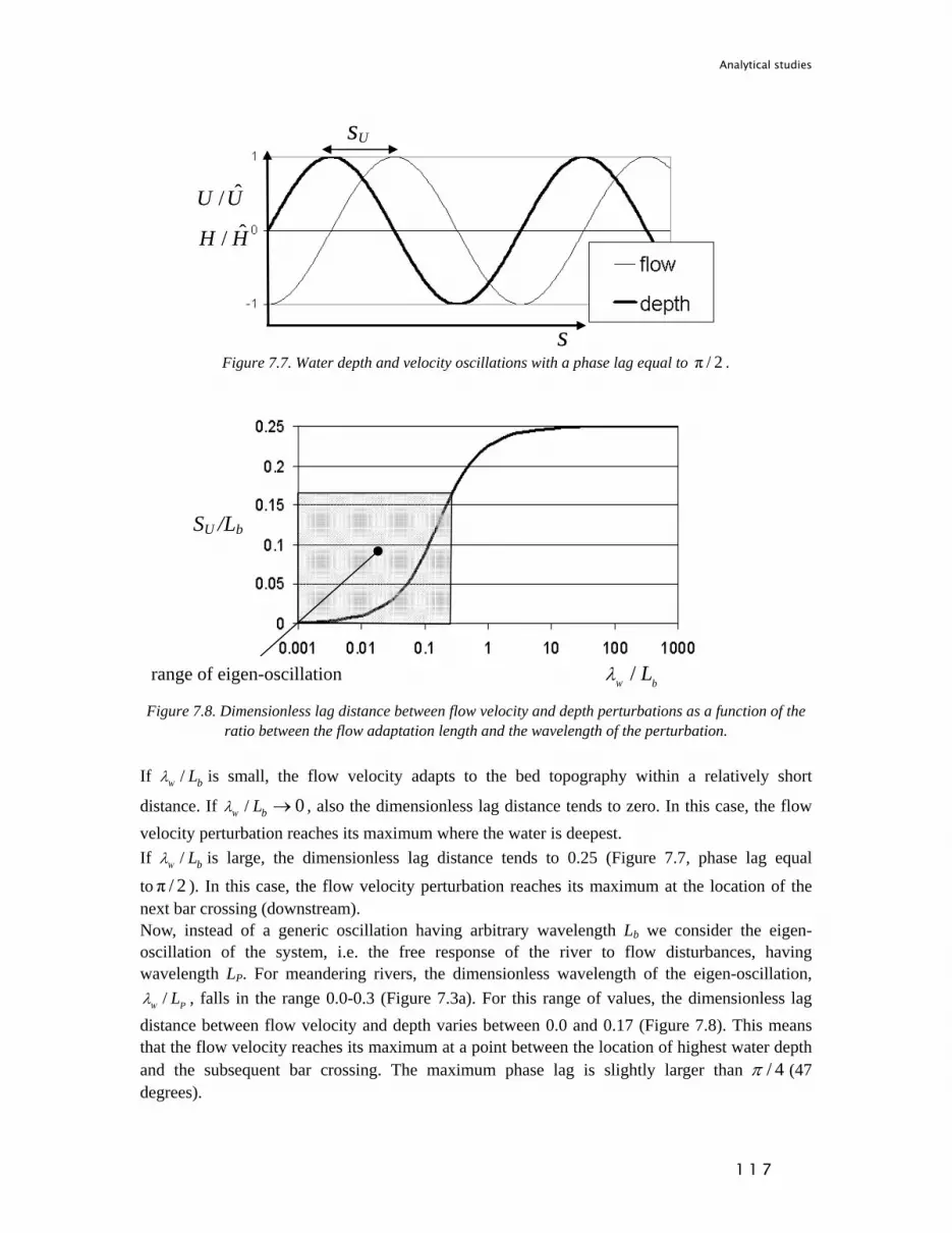
Analytical studies
1 1 7
Figure 7.7. Water depth and velocity oscillations with a phase lag equal to π / 2 .
Figure 7.8. Dimensionless lag distance between flow velocity and depth perturbations as a function of the
ratio between the flow adaptation length and the wavelength of the perturbation. If /W bLλ is small, the flow velocity adapts to the bed topography within a relatively short
distance. If / 0W bLλ → , also the dimensionless lag distance tends to zero. In this case, the flow velocity perturbation reaches its maximum where the water is deepest. If /W bLλ is large, the dimensionless lag distance tends to 0.25 (Figure 7.7, phase lag equal
to π / 2 ). In this case, the flow velocity perturbation reaches its maximum at the location of the next bar crossing (downstream). Now, instead of a generic oscillation having arbitrary wavelength Lb we consider the eigen-oscillation of the system, i.e. the free response of the river to flow disturbances, having wavelength LP. For meandering rivers, the dimensionless wavelength of the eigen-oscillation,
/W PLλ , falls in the range 0.0-0.3 (Figure 7.3a). For this range of values, the dimensionless lag distance between flow velocity and depth varies between 0.0 and 0.17 (Figure 7.8). This means that the flow velocity reaches its maximum at a point between the location of highest water depth and the subsequent bar crossing. The maximum phase lag is slightly larger than / 4π (47 degrees).
/W bLλ
SU /Lb
range of eigen-oscillation
sU
s
ˆ/ˆ/
U U
H H
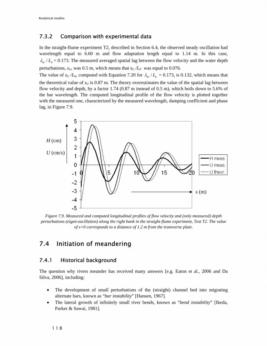
Analytical studies
1 1 8
7.3.2 Comparison with experimental data
In the straight-flume experiment T2, described in Section 6.4, the observed steady oscillation had wavelength equal to 6.60 m and flow adaptation length equal to 1.14 m. In this case,
/W PLλ = 0.173. The measured averaged spatial lag between the flow velocity and the water depth perturbations, sU, was 0.5 m, which means that sU /LP was equal to 0.076. The value of sU /Lb, computed with Equation 7.20 for /W bLλ = 0.173, is 0.132, which means that the theoretical value of sU is 0.87 m. The theory overestimates the value of the spatial lag between flow velocity and depth, by a factor 1.74 (0.87 m instead of 0.5 m), which boils down to 5.6% of the bar wavelength. The computed longitudinal profile of the flow velocity is plotted together with the measured one, characterized by the measured wavelength, damping coefficient and phase lag, in Figure 7.9.
Figure 7.9. Measured and computed longitudinal profiles of flow velocity and (only measured) depth
perturbations (eigen-oscillation) along the right bank in the straight-flume experiment, Test T2. The value of s=0 corresponds to a distance of 1.2 m from the transverse plate.
7.4 Initiation of meandering
7.4.1 Historical background
The question why rivers meander has received many answers [e.g. Eaton et al., 2006 and Da Silva, 2006], including:
• The development of small perturbations of the (straight) channel bed into migrating alternate bars, known as “bar instability” [Hansen, 1967].
• The lateral growth of infinitely small river bends, known as “bend instability” [Ikeda, Parker & Sawai, 1981].
s (m)
H (cm) U (cm/s)

Analytical studies
1 1 9
• Resonance between bed oscillation and alternating river bends [Blondeaux & Seminara, 1985].
• The overshoot/overdeepening phenomenon (steady flow and river bed oscillation caused by upstream disturbances) [Olesen, 1984].
• Large-scale turbulence [Yalin 1977]. The stability analyses performed by, among others, Hansen [1967], Callander [1969], Engelund [1970 and 1975], Parker [1976] and Fredsøe [1978], demonstrated that free migrating bars develop because of an inherent instability of the morphodynamic system, called “bar instability”. Analysing the planimetric changes of rivers with a sinuous channel centreline, Ikeda et al [1981] found the existence of bend instability, according to which bends with certain wave lengths tend to grow with time. A critical wavelength, cλ , discriminated growing from decaying bends. Ikeda et al. suggested that river meanders originate from the bend instability and that alternate bars having wavelength equal to or larger than cλ could provide the initial channel sinuosity. Later Blondeaux & Seminara [1985] found a resonance phenomenon, which occurs when the alternate bars that are present in the river channel have the same wavelength as growing bends. A critical width-to-depth ratio, Rβ , and wavelength, Rλ , characterize bars that neither grow nor decay, either in time or in downstream direction. Channels with larger with-to-depth ratios are called super-resonant, channels with smaller width-to-depth ratios sub-resonant. Resonance was considered as the factor linking the bar and bend instability theories on initiation of meandering. Considering that the migration speed of the free migrating alternate bars is too high to influence the slow process of bend growth, Olesen [1984] stated that river meandering is rather caused by the steady flow and bed oscillation that forms as a free response of river systems to upstream disturbances, the overshoot/overdeepening phenomenon (our eigen-oscuillation) This idea was supported by the experimental observations of Friedkin [1945] and by field observations (Figure 7.10, in which the upstream disturbance is a sharp river bend). The steady bed oscillation induced by upstream disturbances was found to have wavelengths of the order of magnitude of the wavelengths of incipient meanders according to the bend instability theory [Ikeda et al., 1981], i.e. two-three times larger than the wavelengths of the free migrating bars. Subsequent theoretical and experimental studies supported Olesen’s hypothesis and a steady sinuous planform was shown to develop from a perfectly straight channel with an upstream flow disturbance by Crosato [1989] using the model MIANDRAS (this study) and, with a similar model, by Johannesson & Parker [1989]. In 1990, Tubino & Seminara [1990] found that free migrating bars slow down if the river channel widens, until they finally stop migrating. At this point, their presence leads to localized lateral channel growth and bend development [Seminara & Tubino, 1989a]. This behaviour was later observed in the laboratory by, among others, Federici & Paola [2002]. Since migrating bars eventually lead to growing bends through channel widening, this theory joined the bar and bends instability theories (an overview of stability theories can be found in Seminara [1998]). Seminara & Tubino’s finding supports the idea that stationary rather than transient perturbations, such as migrating bars, can initiate river meandering, and show at the same time that stationary perturbations can originate from the bar instability, but only through river widening. Recently, Hall [2004] used a theoretical model to show that the periodic alternation of high and low flows can lead to the formation of steady bars, which might influence the river planimetric changes.

Analytical studies
1 2 0
Therefore, disturbances capable of inducing a steady bed oscillation appear to be not limited to geometrical constraints as previously thought. Recent studies indicate that the resonance conditions might mark the separation between upstream and downstream migration of meanders. According to the theory of Zolezzi & Seminara [2001] (see also Seminara et al. [2001]) bars migrate downstream in sub-resonant conditions, upstream in super-resonant conditions. More recently, Lanzoni et al. [2005] showed that either upstream or downstream disturbances can initiate river meandering, in sub- and super-resonant conditions, respectively. In the absence of disturbances an increasing portion of the meandering channel straightens again. The results of the analyses performed in the framework of this study seem to indicate that a steady bed oscillation, with the wavelength of the eigen-oscillation, can originate from very small, quickly and randomly varying flow disturbances as well as from harmonically varying disturbances, like those caused by the presence of migrating alternate bars (Section 8.4.2). If this is true, than river meandering can originate from the combination of bar instability and overshoot/overdeepening phenomon, which supports the idea that external factors are not needed for river meandering.
Figure 7.10. Development of a sinuous planform downstream of an abrupt change of flow direction, due to the development of steady alternate bars influencing bank erosion. Los Angeles River after a flood in 1937. The white arrows indicate the flow direction (courtesy Gary Parker).
A separate school of thought attributes initiation of meandering to large scale turbulence [Yalin 1977]. However, the time scale of the horizontal bursts that are used to explain the effects of turbulence on bank erosion [Da Silva, 2006] is too short as compared to the time scale of the development of meanders.
7.4.2 Initiation of meandering in MIANDRAS
According to the model of this study, steady alternate bars can cause a river to start meandering, by generating recurring steady perturbations of flow velocity and depth in downstream direction [Crosato, 1989]. The characteristics of incipient meanders depend on the wavelength of the steady bars that form inside the straight channel (eigen-oscillation, Eq. 7.10) and are therefore

Analytical studies
1 2 1
governed by the river hydraulic and morphological characteristics and by the conditions that cause the formation of steady alternate bars. The characteristics of fully-grown meanders are governed by the river hydraulic and morphological characteristics too, but are rather independent from the conditions that cause bar formation and initiation of meandering (see Section 8.4). The analysis of Section 7.3 shows that, if the ratio between the flow adaptation length and the wavelength of the alternate bars, /W bLλ , is small (large bar wavelength), the flow velocity perturbation reaches its maximum where the water is deepest. Since the migration rate is related to the near-bank flow velocity and water depth perturbations (Eq. 5.79), the channel migration rate is maximum at the bar apex and equal to zero at the bar crossing. This means that incipient bends grow in size (Figure 7.11), enhancing the original bars, but do not migrate. In real rivers, this type of behaviour would have consequences for the calibration of the migration coefficients Eh and Eu that are used in the migration model (Eq. 5.79). Since U and H are in phase, it is impossible to distinguish between Eh and Eu on the basis of channel migration records only. These parameters can only be determined both by analysing the river bank characteristics.
Figure 7.11. Incipient meanders in an originally straight system with alternate bars characterized by
small /W bLλ . The channel width remains constant, i.e. banks are imposed to have the same lateral shift.
A different behaviour characterizes the system if /W bLλ is large (small bar wavelength). In this case the dimensionless lag distance between flow velocity and depth tends to 0.25 (Figure 7.8), which means that the flow velocity perturbation reaches its maximum at the location of the bar crossing. If the migration rate is only a function of U (Eh = 0 in Eq. 5.79), also the maximum migration rate is located at the bar crossing. In this case, incipient meanders migrate but do not grow (Figure 7.12). This is what the models by, among others, Ikeda et al. [1981], Johannesson & Parker [1989], Howard [1992], Sun et al. [1996] and Abad & Garcia [2006] predict. If the migration rate is a function of both U and H, as in MIANDRAS, the maximum migration rate is located between the bend apex and the bar crossing. In both cases, the initial development of meanders leads to a slight downstream shift of the original bars, which is due to the formation of weak point bars (Figure 7.12).
original bar weak point bar

Analytical studies
1 2 2
Figure 7.12. Initial migration of a straight channel with alternate bars characterized by large /
W bLλ if Eh = 0. The channel width is assumed constant, which means that opposite banks have the same shift.
The steady alternate bars that develop as a free response to upstream disturbances (eigen-oscillation of the system) are characterized by dimensionless lag distances between water depth and velocity ranging between 0.0 and 0.17 (Section 7.3). This means that the flow velocity reaches its maximum at the point of highest water depth or between the point of highest water depth and the bar crossing. Therefore, incipient meanders originating from upstream disturbances fall either in the case illustrated by Figure 7.11 (small /W bLλ ) or between the cases of Figures 7.11 and 7.12. Meander development starting from a straight channel with a permanent upstream disturbance is illustrated in Figure 7.13. The initial conditions are those of the straight-flume experiment T2 (Section 6.4, Tables 6.1 and 6.2, the computational choices are given in Section 8.3, Tables 8.1 and 8.2). In this case, the initial (computed) dimensionless space lag between water depth and velocity is 0.132 (Section 7.3.2). The time intervals between the different development stages shown in Figure 7.13 are equal. Figure 7.13 shows that at initial stages meanders tend to migrate downstream rather than to grow. Later on lateral growth becomes predominant. This occurs because the wavelength of meanders increases with time. Assuming that there is one point bar per river bend, the increase of meander wavelength leads to a decrease of the phase lag between velocity and bars (Section 7.3). The highest flow velocity and thus the highest erosion rates come closer to the bend apex, which leads to predominant lateral meander growth. Steady alternate bars are found to be able to influence bank erosion and initiate meandering in experimental streams [Friedkin, 1945] and in real rivers (Figure 7.10). With the progression of the phenomenon, if the opposite bank accretes at rates that are comparable to the erosion rates, the river develops a meandering planform. If bank accretion is not able to cope with opposite bank erosion, the channel widens, point bars are eventually cut [Friedkin, 1945] and the river tends towards an anabranched or braided planform (see Figure 1.1). MIANDRAS assumes a constant channel width and therefore always gives a meandering planform. This does not allow for use of the model to investigate whether a channel that starts to meander eventually develops a meandering, a braided or an anabranched planform.
weak point bar original bar

Analytical studies
1 2 3
Initial state. Stationary alternate bars are formed due to a disturbance causing flow and depth perturbations at the upstream boundary. Bars enhance bank erosion at pools (darker grey) and initiate river meandering
Initiation of meandering. Strong downstream migration (dotted line) of bars and incipient bends. Point bars form slightly downstream of the bend apex.
With the development of meanders, the downstream migration decreases and point bars tend to develop at the bend apex. Further meander growth leads to the formation of point bars upstream of the bend apex.
Figure 7.13. Initial migration of a straight channel with alternate bars (natural oscillation) with
/W bLλ = 0.173 and Eh = 0 (straight-flume
experiment T2, Chapter 6.4) and far from the upstream boundary. Darker grey indicates larger water depths. Dotted lines indicate downstream migration of bars.
Stage 2
Stage 4
Stage 6
Stage 8
flow direction

Analytical studies
1 2 4
7.5 Meandering and braiding
7.5.1 Introduction
The identification of the factors governing the river planform formation has received, and still receives, much attention (Chapter 3). A number of scientists related the river planform style to a number of basin-scale river characteristics, such as the valley slope, the water discharge, the sediment supply (e.g. Leopold & Wolman [1957], Schumm [1977], van den Berg [1995], Bledsoe & Watson [2001]). Others related the river planform style also to some additional local river characteristics, such as the bank erodibility (Ferguson [1987]) and the presence of riparian vegetation (Millar [2000]). The stability analyses performed by, among others, Hansen [1967] and Callander [1969] defined the conditions that govern the development of free bars inside the river channel and found that multiple bars form at larger width-to-depth ratios than alternate bars. Since Leopold & Wolman [1957] the presence of alternate bars was related to the tendency of the river to form meanders and the presence of multiple bars to the tendency of the river to form braids. Unfortunately, stability analyses require the knowledge of the width-to-depth ratio and for this reason they cannot be directly used to predict the river planform style based on a number of basin-scale river characteristics. Furthermore, a general predictor of width-to-depth ratio as a function of basin-scale and local river characteristics is still lacking, although empirical predictors exist for specific types of rivers [e.g. Parker et al., 2007]. An alternative new method to directly estimate the most likely number of free steady bars in the river cross-section is presented. The method requires the knowledge of the channel width-to-depth ratio and can therefore be used to predict the river planform style only if the river cross-section is known, as in case of river training or river restoration works. Since steady rather than migrating bars are able to influence the slow river planform changes, the simple method still includes the major factors governing the river planform formation.
7.5.2 Previous work
The role of the width-to-depth ratio for the number of free bars developing in the channel cross-section was assessed by Seminara & Tubino [1989]. Their linear analysis allowed for the definition of the threshold lines that separate the conditions in which alternate or multiple bars tend to develop from conditions in which the same bars, defined by their mode, m (identifying the number of bars per cross-section), and dimensionless wave number, λ , are damped and do not form. Among the parameters involved, the width-to-depth ratio, 0/B hβ = , appeared to be the
controlling one. The other parameters involved are the Shields parameter, 0θ and the dimensionless grain size ds = D50/h0. Considering bars as a periodic (harmonic) phenomenon, Seminara & Tubino [1989] defined their dimensionless wave number as:
/ bB Lλ π= (7.21)

Analytical studies
1 2 5
in which Lb is the bar wavelength. They plotted the threshold curve in the β λ− plane, separating the conditions for which bars tend to grow from the conditions in which the same bars decay. The curve describes the neutral conditions for which bars neither grow nor decay, for given values of the Shields parameter, of the dimensionless grain size and of the particle Reynolds number. Figure 7.14 shows a typical neutral curve for alternate bars (m = 1).
Figure 7.14. A typical neutral curve for the case of alternate bars (m = 1, 0θ = 0.3, ds = 0.01) ( Seminara &
Tubino [1989]). β is the width-to-depth ratio. A critical value, critβ , can be identified from Figure 7.14 as the lowest value of β on the neutral curve. This is the critical value of the width-to-depth ratio above which alternate bars are expected to form. The dimensionless wave number of these bars is given by critλ . For higher values of β the wave number of the bars that form in the channel is assumed to be the one having the highest development speed. The neutral curves of bars having higher modes (m >1) are located increasingly higher in the graph: the larger the value of m, the higher the neutral curve in the β λ− plane. This means that the number of bars that may develop in the channel cross-section increases with increasing channel width-to-depth ratios. Hence, if the width-to-depth ratio of the river channel is known, along with the other parameters, it is possible to predict the type of bed topography (number of bars). However, the limitations of the model restrict the possibility of prediction. Especially when the set of parameters indicates the possible development of multiple bars, the model does not allow for the assessment of their exact number. This is due to non-linear interactions not accounted for in the model, which tend to reduce the number of bars. Therefore, the results should be interpreted as an indication of the possibility that more than one bar per cross-section will form. An example of how this theory can be applied to tidal rivers is given by Toffolon & Crosato [2007] (Figure 7.15).
β
critβ
λ crit
λ
neutral curve 50 40 30 20 10
β

Analytical studies
1 2 6
Figure 7.15. Regions of formation of free bars in the tidal reach of the Scheldt River (Belgium) for different
values of m ( 0θ = 0.65, ds = 0.000017 and Re* = 9). The figure also indicates the range of variation of β in the considered river reach. Toffolon & Crosato [2007].
7.5.3 A new predictor
The classical approach to determine the number of free bars that form in a channel cross-section defines a separator between ranges in which river configurations characterised by a certain numbers of bars are linearly stable or unstable (previous Section 7.5.2). The linear theory of Seminara & Tubino [1989] defines a neutral curve (separator) discriminating between the conditions in which a certain number of bars per cross-section (bar mode) grows from the conditions in which the same bar mode decays. The method of Seminara & Tubino is laborious and difficult to apply in practical problems. An alternative method, approximate and restricted to free steady bars, can be derived from the equations underlying MIANDRAS [Crosato & Mosselman, 2008 submitted]. Steady rather than migrating bars are able to influence the slow river planform changes and for this reason it is believed that notwithstanding its simplicity this method still includes the factors governing the river planform formation. The method is based on a new approach. Instead of a separator between stable and unstable conditions, the method directly defines an estimator of the most likely number of free bars in the cross-section. In the mathematical model underlying MIANDRAS, wave number and longitudinal damping of the steady bars that develop downstream of flow disturbances (eigen-oscillation) depend on the interaction parameter α (Eqs. 7.11, 7.12), which is a function of the bar mode, m, and of the river width-to-depth ratio, β (Eq. 7.16, here repeated for convenience):
22
02 2
2 1 ( )fC f fm m
βα β θπ
⎛ ⎞= = ⎜ ⎟⎝ ⎠
(7.22)

Analytical studies
1 2 7
Considering a river channel with a fixed width-to-depth ratio, β , the damping coefficient of the eigen-oscillation, 1/LD (Eq. 7.12), increases with increasing bar mode m, which means that m+1-mode bars are more strongly damped than m-mode bars:
22
0
1 ( 3)4 ( )
W
D f
m bL C fλ π
θ β
⎡ ⎤⎛ ⎞= − −⎢ ⎥⎜ ⎟
⎝ ⎠⎢ ⎥⎣ ⎦ (7.23)
Bars characterized by mode m can form in the river channel only if the solution of Equation 7.1 falls within the harmonic range (Section 7.2.1). In this case the interaction parameter,α (Eq. 7.22), falls within the range:
2 2 2 21 ( 1) ( 3) 1 ( 1) ( 3)12 2
b b b b b bα
+ − + − − + + + − −≤ ≤ (7.24)
Assuming that the degree of non-linearity of the sediment transport formula, b, the friction factor, Cf, and the Shields parameter, 0θ , are independent from the bar mode, the harmonic range of bars with higher modes (larger values of m) requires larger width-to-depth ratios. This becomes clear after having substituted α with its expression (Eq. 7.22) in Equation 7.24:
22 2 2 22
0
1 ( 1) ( 3) 1 ( 1) ( 3)2 2 ( ) 2f
b b b b b bmC fπ
θ β+ − + − − + + + − −⎛ ⎞
≤ ≤⎜ ⎟⎝ ⎠
(7.25)
Outside the harmonic range of the solution, the damping coefficient can be either positive or negative. For positive damping, the river response to upstream disturbances is an exponential decay of the disturbance, without free bar formation, such as in Figure 7.2. In this case:
2 21 ( 1) ( 3)1 ( 3)4 2
W
D
b b b bLλ ⎡ ⎤+ + + − −
> − −⎢ ⎥⎢ ⎥⎣ ⎦
(7.26)
For negative damping, the river response is an exponential growth of the disturbance. In this case:
2 21 ( 1) ( 3)1 ( 3)4 2
W
D
b b b bLλ ⎡ ⎤+ − + − −
< − −⎢ ⎥⎢ ⎥⎣ ⎦
(7.27)
As an example, for b = 5 (Engelund & Hansen transport formula, valid for sand-bed rivers), the exponential decay occurs for /W DLλ > 0.95, the exponential growth for /W DLλ < -0.45.
In general, the point /W DLλ = 0 falls always within the harmonic range. Besides, if /W DLλ = 0, the m-mode bars are not damped, i.e. they develop unchanged in downstream direction. For this

Analytical studies
1 2 8
reason, the condition /W DLλ = 0 is here assumed to represent the formation of m-mode bars. In this case:
2( 3)b
α =−
(7.28)
Substituting α with its expression (Eq. 7.22) in Equation 7.28, the following width-to-depth ratio,
mβ , is obtained:
0
1( 3) ( )m
f
mb f C
β πθ
=−
(7.29)
In Equation 7.29, Rmβ represents the characteristic value of the width-to-depth ratio of m-mode bars. According to Equation 7.29 the m = 2 bars (central bars) form at width-to-depth ratios that are twice the width-to-depth ratios of m = 1 bars (alternate bars). Equation 7.25 can be used to derive the range of values of the width-to-depth ratio for which m-mode bars can form (solution of Eq. 7.1 falling with the harmonic range):
1 2m mβ β β≤ ≤ with
2 2
0
11
( ) 1 ( 1) ( 3)f
m mf C b b b
β πθ + + + + −
=⎡ ⎤⎣ ⎦
2 2
0
21
( ) 1 ( 1) ( 3)f
m mf C b b b
β πθ + − + − −
=⎡ ⎤⎣ ⎦
(7.30)
If the channel width-to-depth ratio is smaller than mβ and larger than 1mβ , the damping coefficient of m-mode bars is positive, which means that the m-mode bars are damped (reduce) in downstream direction. For values of β smaller than 1mβ , the m-mode bars fall outside their harmonic range, which means that m-mode free bars do not develop. In this case, lower-mode bars (m-1) may appear as soon as the channel with-to-depth ratio falls within their harmonic range. If the channel width-to-depth ratio is larger than mβ and smaller than 2mβ , the damping coefficient is negative, which means that the m-mode bars tend to grow in downstream direction. Considering that the non-linear terms have the effect of limiting the bar growth [Seminara & Tubino, 1992] and that they have been disregarded from the equations, it can be assumed that the m-mode bars may form in downstream direction also if the damping coefficient is negative, but always within their harmonic range. For values of β larger than 2mβ , the m-mode bars fall outside

Analytical studies
1 2 9
their harmonic range, which means that they do not develop. Higher-mode bars (m+1) may start to develop in the river channel as soon as they fall within their harmonic range. Considering an existing river with a given width-to-depth ratio, β , Equation 7.29 can also be used to determine the mode m of bars that may develop in the river channel:
0( 3) ( ) fm b f Cβ θπ
= − (7.31)
Assuming b, 0θ and Cf as constant, it can be observed from Equation 7.30 that for b larger than 3 and smaller than 10 (sand-bed rivers) the harmonic ranges of successive bar modes overlap for
2 1 1m mβ β β +≤ ≤ . For any given value of β , higher mode bars always have higher damping coefficients (higher damping: higher rate of reduction in downstream direction). For this reason, using Equation 7.31 to predict the bar mode that forms in the river channel is equivalent to assuming that the free bar mode that forms in the channel is the one characterized by the lowest damping. Based on published material, the bar mode, m, has been computed for a number of existing rivers at bankfull conditions, with the aim to investigate whether the computed bar mode, m, can be used to predict whether a river is meandering, braided or in transition. It is assumed that:
• A typical meandering river presents either only point bars or point bars and alternate bars (m ≤ 1.5). Although the presence of steady alternate bars was found essential for initiation of meandering (Section 7.4), fully-developed meandering rivers may present no free bars, but only forced point bars (m < 1). This can be explained by the fact that with the gradual increase of the river sinuosity the longitudinal bed slope and the channel width-to-depth ratio diminish so that at a certain point the river conditions fall outside the harmonic range (Eq. 7.30). In this case free bars (eigen-oscillation with m = 1) do not form in the river channel anymore.
• A transition river, i.e. a river with clear meanders but locally more than one conveying channel, has one to two bars per cross-section (1.5 < m < 2.5).
• A typical braided river presents several bars (m ≥ 2.5).
Given the strong dependency of the bar mode on the degree of non-linearity of the sediment transport formula, the value of m is computed for b = 4 (sand-bed rivers) and b = 10 (gravel-bed rivers). The function of the Shield parameter is derived using E = 0.5 (Section 5.2, Eq. 5.7). The computed value of m has been compared with the observed river planform style (meandering, braided or transition) reported in literature. The results are summarized in Table 7.1. The comparison between predicted and observed channel planform style is satisfactory.

Analytical studies
1 3 0
Table 7.1. Computed number of bars per cross-section (Eq. 7.25) compared with the observed river
planform style: M = meandering, B = Braided, T = transition. Data refer to bankfull stages.
River QW (m3/s)
B (m)
h0 (m)
slope (-)
D50 (mm)
θ0 (-)
m (b = 4)
m (b=10) Pred. Obs.
Geul at Mechelen (Netherlands) [Miguel, 2006]
22 8 2.0 0.0024 25 0.12 - 0.4 M M
Allier upstream of Moulins (France)
[Blom, 1997] 325 65 2.4 0.00083 5 0.24 - 1.4 M T
Ranoli (India) [Struiksma and Klaassen, 1988]
400 287 0.9 0.00078 0.11 3.80 9.8 - B B
Beaver Creek (USA) [Struiksma and Klaassen, 1988]
276 1280 0.3 0.0066 29.6 0.04 - 375.8 B B
Ohua River (New Zealand) [Struiksma and Klaassen, 1988]
378 450 0.6 0.0065 20 0.11 - 63.9 B B
Savannah (USA) [Struiksma and Klaassen, 1988]
860 107 5.2 0.00011 0.8 0.43 0.3 - M M
Jamuna (Bangladesh)
[Struiksma and Klaassen, 1988]
40000 5000 6.0 0.00006 0.22 0.99 15.4 - B B
Big Fork River at Koochiching County (USA) [MacDonald
et al., 1992]
155 55 2.7 0.00063 6.5 0.10 - 2.1 T T
Minnesota River at Nicollet and Blue
Earth Counties (USA) [MacDonald
et al., 1992]
314 43 4.7 0.00024 0.5 1.36 0.3 - M M
Rice Creek at Anoka County (USA)
[MacDonald et al., 1992]
12.9 13.4 0.5 0.00175 0.9 0.659 0.5 - M M
M = meandering B = braiding T = transition (clear meanders but more than one channel at certain locations) Summarizing, according to equation 7.31, the highest growing bar mode, m, is a function of:
• the river width-to-depth ratio, β ; • the degree of non-linearity of the sediment transport capacity with respect to the flow
velocity, b; • the friction factor, Cf (Eq. 5.1); • the Shields parameter, 0( )f θ (Eq. 5.6).

Analytical studies
1 3 1
Note that m denotes the mode of free steady bars (eigen-oscillation of the steady system). Forced bars, such as the point bars inside channel bends do not belong to this category. A river in which only point bars are recognizable is assumed to have m < 1. The number of free bars in an alluvial river increases if (primarily) the channel width-to-depth ratio increases, but also if the degree of non-linearity of sediment transport, b, the bed roughness, Cf, and the Shields parameter, 0θ , increase. In particular, the degree of non-linearity of sediment transport is higher in gravel-bed rivers than in sand-bed rivers [Jansen et al, 1979]. The Shields parameter is a measure of the capacity of the current to move the sediment particles and can be considered a representative for the flow strength. The Shields parameter increases if the longitudinal slope increases. Thus the higher the longitudinal bed slope the larger the number of bars. The channel roughness is often larger in gravel-bed rivers than in sand-bed rivers. Equation 7.31 therefore indicates that for the same width-to-depth ratio steep gravel-bed rivers tend to have more bars than less-steep sand-bed rivers. This is in agreement with the empirical relations of, among others, Henderson [1963], Schumm [1977], Ackers [1982], van den Berg [1995], relating the river planform style to the flow strength and the sediment size. However, also the bank erodibility, the presence of riparian vegetation, the frequency of floods and even active tectonics were found to play a role in the river planform formation (Section 3.2). These factors are not included in Equation 7.31. In particular Equation 7.31 does not include the factors that mostly influence the river width formation, such as the bank erodibility, the presence and characteristics of riparian vegetation and the frequency of floods. In fact, Equation 7.31 requires that the value of the river width-to-depth ratio is known a priori. The ability of Equation 7.31 to predict the number of bars in existing rivers has also been investigated. Figure 7.16 compares observed and computed m for a number of sand-bed and gravel-bed rivers having β < 100 at bankfull conditions. The results are satisfactory, since the error does not exceed 1. Instead, the number of bars is clearly overestimated for β > 100 [Crosato & Mosselman, 2008 submitted]. This is due to the linearisation of the basic equations (in Section 5.2.2). Non-linear effects reduce the number of bars, especially in case of multiple bars, which tend to merge (Seminara & Tubino [1989]).
B/h < 50
0
1
2
3
4
0 1 2 3 4observed m
com
pute
d m
50 < B/h < 100
0
1
2
3
4
5
6
7
0 1 2 3 4 5 6 7
observed m
com
pute
d m
Figure 7.16. Computed vs. observed m in rivers with width-to-depth ratios smaller than 100. The computed values assume b = 4 for sand-bed rivers (black squares) and b = 10 for gravel-bed rivers (gray triangles).
Continuous line: perfect match. Dashed lines: error ± 1. [Crosato & Mosselman, 2008 submitted]

Analytical studies
1 3 2
Equation 7.31 can be used to estimate the number of free steady bars that form in the river cross-section if the channel width-to-depth ratio does not exceed 100. The same equation can be used to predicted the river planform style for any value of the width-to-depth ratio. However, braided rivers cannot be distinguished from anabranched rivers, since these river planform styles are both characterised by large width-to-depth ratios. The equation can be used for each anabranch. If no information is available on the value of the degree of non-linearity of the sediment transport formula with respect to the flow velocity, b, it is suggested to use b = 4 for sand-bed rivers and b = 10 for gravel-bed rivers. In natural rivers, the width-to-depth ratio is a function of the flow stage, and thus varies throughout the year. At low flow stages, the width-to depth ratio of the morphologically active part of the river is larger than at high flow stages [Dietrich et al., 1984], which means that at low flows one may observe the formation of higher mode bars, such as central and multiple bars, also in meandering rivers. However, in most rivers the largest amounts of sediment are transported by the highest flows, whereas the sediment transport rates at low flow stages are marginal. This means that at low flows the channel bed needs a long time to reach its equilibrium configuration and in most cases high flow conditions occur before this has occurred. At high flows, due to significantly higher sediment transport rates, the bed topography adapts much faster to the flow. Low flow conditions are therefore less relevant to the channel morphology than high flow conditions. It is therefore suggested to apply Equation 7.31 to bankfull discharge conditions.
7.6 Point bar shift and meander growth
7.6.1 General case
In real rivers, the position of the point bar top with respect to the bend apex may vary as a function of size of meanders and width-to-depth ratio. Predicting the position of the point bar top is important, because it means correctly identifying the location of the largest water depth and of the largest flow velocity, which influence the channel migration process. In particular, upstream migration of river bends can only occur if the point bar top is located upstream of the bend apex. In MIANDRAS, the migration rate is related to the flow velocity and water depth excesses, U and H, with respect to uniform flow (Eq. 5.79). If the point bar top is located upstream of the bend apex, the largest value of the water depth, H, opposite to the point bar top in the river cross-section, is also located upstream of the bend apex. The maximum value of U, instead, will be located at a distance more downstream (Section 7.3). Assuming one point bar for each river bend, the highest velocity will be located close to the bar top for large values of the meander wavelength; close to the downstream bend crossing for small values of the meander wavelength. The performance of MIANDRAS in predicting the point bar position as a function of meander size and other river characteristics is here analysed in a way that is, for some aspects, similar to the one adopted by Hasegawa & Yamaoka [1983]. Equation 7.1 describes the downstream variation of the amplitude of the near-bank water depth perturbation, H, forced by the channel curvatureγ :
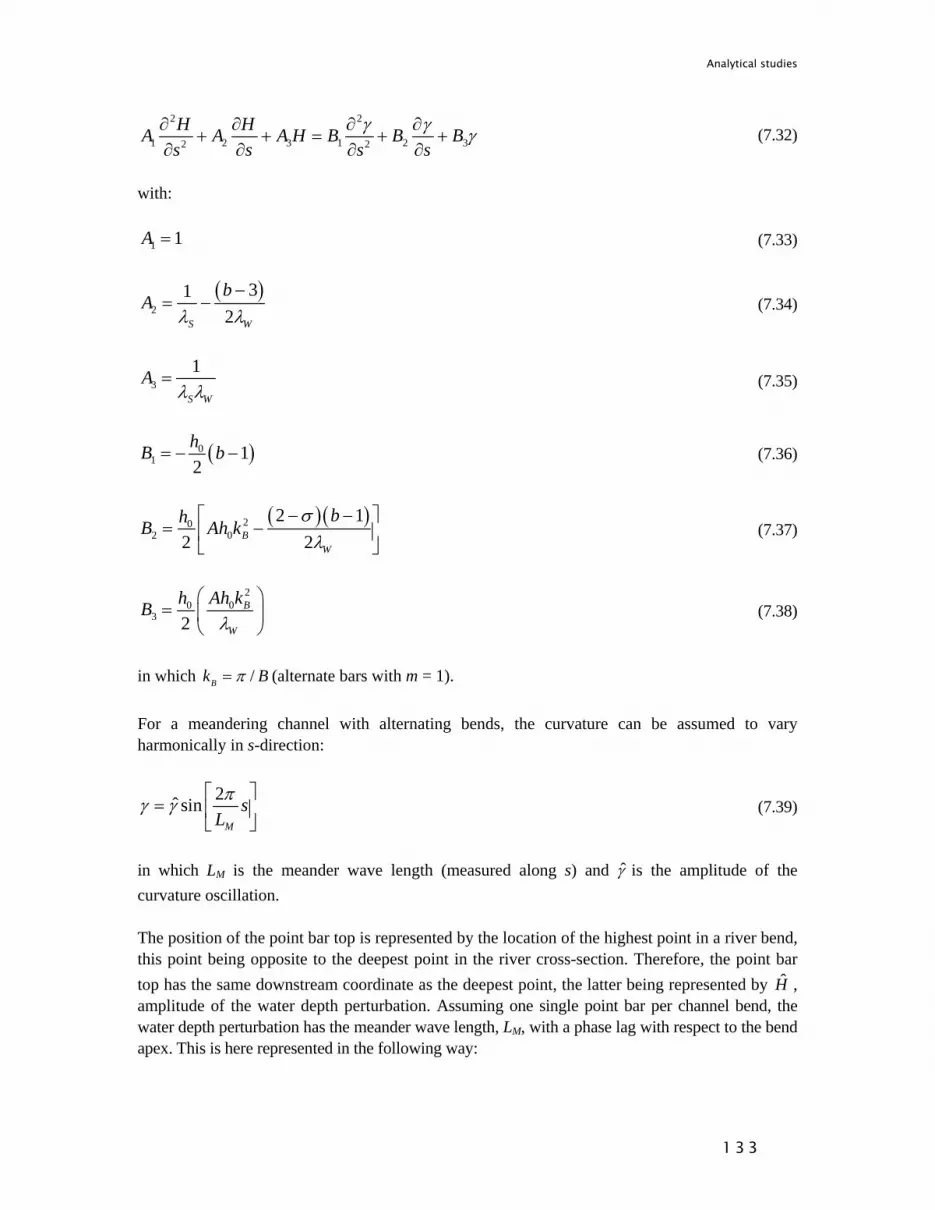
Analytical studies
1 3 3
2 2
1 2 3 1 2 32 2
H HA A A H B B Bs s s s
γ γ γ∂ ∂ ∂ ∂+ + = + +
∂ ∂ ∂ ∂ (7.32)
with:
1 1A = (7.33)
( )2
312S W
bA
λ λ−
= − (7.34)
31
S W
Aλ λ
= (7.35)
( )01 1
2hB b= − − (7.36)
( ) ( )202 0
2 12 2B
W
bhB Ah kσλ
− −⎡ ⎤= −⎢ ⎥
⎣ ⎦ (7.37)
2
0 03 2
B
W
h Ah kBλ
⎛ ⎞= ⎜ ⎟
⎝ ⎠ (7.38)
in which /Bk Bπ= (alternate bars with m = 1). For a meandering channel with alternating bends, the curvature can be assumed to vary harmonically in s-direction:
2ˆ sinM
sLπγ γ
⎡ ⎤= ⎢ ⎥
⎣ ⎦ (7.39)
in which LM is the meander wave length (measured along s) and γ is the amplitude of the curvature oscillation. The position of the point bar top is represented by the location of the highest point in a river bend, this point being opposite to the deepest point in the river cross-section. Therefore, the point bar top has the same downstream coordinate as the deepest point, the latter being represented by H , amplitude of the water depth perturbation. Assuming one single point bar per channel bend, the water depth perturbation has the meander wave length, LM, with a phase lag with respect to the bend apex. This is here represented in the following way:

Analytical studies
1 3 4
2ˆ sin ( )HM
H H s sLπ⎡ ⎤
= −⎢ ⎥⎣ ⎦
(7.40)
in which sH is the lag distance between water depth and curvature and H is the water depth amplitude (largest water depth opposite to the point bar top). For the sake of simplicity, the meander wave number is given the symbol KM:
2M
M
KLπ
= (7.41)
Equations 7.39 and 7.40 are inserted into Equation 7.32. Taking into account that sin[ ( )] sin( )cos( ) cos( )sin( )M H M M H M M HK s s K s K s K s K s− = − (7.42) cos[ ( )] cos( )cos( ) sin( )sin( )M H M M H M M HK s s K s K s K s K s− = + (7.43) The following conditions are obtained:
2 23 1 2 3 1
ˆ( ) cos( ) ( )sin( ) sin( ) ( )sin( )ˆM M H M M H M M MA A K K s A K K s K s B B K K s
Hγ⎡ ⎤− + = −⎣ ⎦
and
22 3 1 2
ˆ( ) cos( ) ( )sin( ) cos( ) ( ) cos( )ˆM M H M M H M M MA K K s A A K K s K s B K K s
Hγ⎡ ⎤− − =⎣ ⎦ (7.44)
The lag distance, sH, is given by the following expression:
2 22 3 1 2 3 1
2 23 1 3 1 2 2
1 ( )( ) ( )( )atan( )( ) ( )( )
M M M MH
M M M M M
A K B B K B K A A KsK B B K A A K A K B K
⎡ ⎤− − −= ⎢ ⎥− − +⎣ ⎦
(7.45)
Equation 7.39 also yields an expression for H , via the condition ( ) ( )2 2sin cos 1M H M HK s K s+ = :
( )1/ 222 2
3 1 22 2
3 1 2
( )ˆ ˆ( ) ( )
M M
M M
B B K B KH
A A K A Kγ⎡ ⎤− +
= ⎢ ⎥− +⎢ ⎥⎣ ⎦
(7.46)

Analytical studies
1 3 5
7.6.2 Non-damped system with negligible spiral flow
For sake of simplicity, a non-damping system is considered, in which 1/LD = 0 (Eq. 7.12), and it is assumed that the effects of the spiral flow are negligible ( 0σ = and A = 0). In this case, A2 and B3 are both equal to zero and B2 = B1/ Wλ , hence Equation 7.45 simplifies to:
1 1atanHM W M
sK Kλ
⎡ ⎤= ⎢ ⎥
⎣ ⎦ (7.47)
When made dimensionless, the lag distance between water depth perturbation and channel centreline curvature is a function of the ratio /W MLλ :
2 atan2
H M
M W
s LLπ
λ π⎡ ⎤
= ⎢ ⎥⎣ ⎦
(7.48)
The graph of Figure 7.17 shows sH /LM as a function of /W MLλ .
Summarising, if /W MLλ is large (small meander wavelengths), water depth and channel curvature tend to be in phase, which means that the deepest point and point bar top are located at the bend apex. In this case, the largest flow velocity reaches its maximum at the location of the next bend crossing (Section 7.3). If /W MLλ is very small (large meander wavelengths), the dimensionless lag distance tends to 0.25
(phase lag equal toπ / 2 ). In this case, the deepest point and the point bar top are located at the next bend crossing. The flow velocity is in phase with the water depth (Section 7.3).
Figure 7.17. Dimensionless lag distance between the amplitudes of water depth and channel curvature, sH/LM,, representing the lag distance between point bar top and bend apex, as a function of /W MLλ .
sH /LM
/W MLλ
(meander wavelength)

Analytical studies
1 3 6
7.6.3 Effects of damping
The longitudinal damping of the system (downstream reduction of free response) is a function of the width-to-depth ratio (Eq. 7.23). Rivers with small width-to-depth ratios are characterized by high damping coefficients, whereas rivers with high width-to-depth ratios are characterized by small or even negative damping coefficients. Studying the effects of varying the damping coefficient on the phase lag between the point bar top and the bend apex is therefore an indirect way of assessing the effects of the width-to-depth ratio. This is obtained by analysing the case in which the spiral flow is negligible (A = 0, σ = 0) but1/ 0DL ≠ . Negligible spiral flow occurs, for instance, in
mildly curved river reaches and at initiation of meandering. In this case, B3 = 0 and B2 = B1/ Wλ and Equation 7.45 simplifies to:
22 3 1
23 1 2
1 ( ) ( )atan( ) ( )
W M M MH
M W M M M
K A K A A KsK K A A K A K
λλ⎡ ⎤+ −
= ⎢ ⎥− −⎣ ⎦ (7.49)
In Equation 7.49, the numerator of the term between brackets is negative if:
22 3 1( )W M M MK A K A A Kλ + < (7.50)
By substituting the coefficients A1, A2 and A3 with their expressions (Eqs. 7.33, 7.34 and 7.35) and considering that A2 = 2/LD (Eq. 7.12), condition 7.50 results in:
( )2 131
2
WW M
S W
S
Kb
λλλ λ
λ
>⎛ ⎞−− +⎜ ⎟
⎝ ⎠
(condition for negative nominator in 7.49) (7.51)
The denominator of the term between brackets in Equation 7.49 is negative if:
22 3 1( )W MA A A Kλ> − (7.52)
By substituting the coefficients A1, A2 and A3 with their expressions in Equations 7.33, 7.34 and 7.35, the condition of Equation 7.52 becomes:
( )2 32W M
bKλ −> (condition for negative denominator in 7.49) (7.53)

Analytical studies
1 3 7
Zero damping: resonant system
The non-damping point (1/LD = 0) coincides with the conditions that might lead to resonance [Parker & Johannesson, 1989]. Therefore for zero-damping the system can be described as resonant [Blondeaux & Seminara, 1985]. In this case, if the incipient meander wavelength is equal to the wavelength of the eigen-oscillation, meander growth and bar formation reinforce each-other. After Zolezzi & Seminara [2001], in case of positive damping the system is defined as sub-resonant; in case of negative damping as super-resonant.
For 1/LD = 0, which occurs for 3
2W
S
bλλ
−= , nominator and denominator have always the same
sign. The phase lag between point bar top and bend apex is therefore always positive, i.e. the point bar top is always located downstream of the bend apex, which confirms the graphic of Figure 7.17.
Positive damping: sub-resonant system
From Eq. 7.51 the nominator is always negative for 1
2W
S
bλλ
−> , which corresponds to the
condition 2 1W
DLλ
> . Positive damping, i.e.2 0W
DLλ
> , requires that3
2W
S
bλλ
−> . The following two
cases are distinguished:
1) low to moderate damping, for which 3 1
2 2W
S
b bλλ
− −< < and therefore
20 1W
DLλ
< < ;
2) strong damping, for which 1
2W
S
bλλ
−> and therefore
2 1W
DLλ
> .
For low to moderate damping 1 3
2312
W
S W
S
bb
λλ λ
λ
−>
⎛ ⎞−− +⎜ ⎟
⎝ ⎠
(in Equation 7.51). Nominator and
denominator of Equation 7.49 have the same sign, i.e. the point bar top is located downstream of the bend apex, if:
either ( )2 32W M
bKλ −< or ( )2 1
312
WW M
S W
S
Kb
λλλ λ
λ
>⎛ ⎞−− +⎜ ⎟
⎝ ⎠
(7.54)
For strong damping the nominator is always negative (Eq. 7.51 always valid). In this case, numerator and denominator have the same sign and the phase lag is positive (point bar top downstream of the bend apex) if also relation 7.53 is satisfied.

Analytical studies
1 3 8
Combining the two cases, for negligible spiral flow and positive damping the point bar is upstream of the bend apex if
either ( )23 12 31
2
WW M
S W
S
b Kb
λλλ λ
λ
−< <
⎛ ⎞−− +⎜ ⎟
⎝ ⎠
and 3 1
2 2W
S
b bλλ
− −< <
or ( )2 32W M
bKλ −< and
12
W
S
bλλ
−>
(7.55)
Negative damping: super-resonant system
After Zolezzi & Seminara [2001], for negative damping, corresponding to the condition 3
2W
S
bλλ
−< , the system can be defined as super-resonant. In this case,
1 3231
2
W
S W
S
bb
λλ λ
λ
−<
⎛ ⎞−− +⎜ ⎟
⎝ ⎠
(in Equation 7.51). Numerator and denominator of Equation 7.49
have the same sign (point bat top downstream of bend apex) for:
either ( )2 131
2
WW M
S W
S
Kb
λλλ λ
λ
<⎛ ⎞−− +⎜ ⎟
⎝ ⎠
or ( )2 32W M
bKλ −>
(7.56)
For negligible spiral flow and negative damping the point bar is not always located downstream of the bend apex. It is located upstream for intermediate values of the meander wave number, in particular for:
( )21 3231
2
WW M
S W
S
bKb
λ λλ λ
λ
−< <
⎛ ⎞−− +⎜ ⎟
⎝ ⎠
and 3
2W
S
bλλ
−<
(7.57)
The range of meander wave numbers for which the point bar is located upstream is larger for larger values of b, which means that super-resonant gravel-bed rivers tend to have the point bar located upstream of the bend apex more often than super-resonant sand-bed rivers. In any case, since the point bar is not always located upstream of the bend apex, in super-resonant systems river bends do not always migrate upstream.

Analytical studies
1 3 9
7.6.4 Effects of helical flow
The intensity of the helical flow, weighted by the coefficient A, is a function of the bend curvature, which increases with the bend development at low river sinuosity (Section 9.3). Therefore, for low river sinuosity studying the effects of varying the helical flow intensity is an indirect way of studying the effects of varying the bend curvature on the position of the point bar top with respect to the bend apex. The effects of the helical flow on the phase lag between point bar top and bend apex can be assessed by analysing the case in which σ = 0, 1/ 0DL = but A ≠
0. In this case, A2 = 0 and B2 = Wλ B3 + B1/ Wλ . Equation 7.45 simplifies to:
3 12
1 3
( / )1 atan( )
W W MH
M M
B B KsK B K B
λ λ⎡ ⎤+= ⎢ ⎥−⎣ ⎦
(7.58)
In Equation 7.58, the numerator of the term between brackets is negative if:
23 1 / WB B λ< − (7.59)
By substituting coefficients B1 and B3 with their expressions (Eqs. 7.36 and 7.38) and taking into account that for meandering rivers /Bk Bπ= , Equation 7.59 becomes:
22
0
1 ( 1)WA bhπλ
β⎛ ⎞
< −⎜ ⎟⎝ ⎠
(7.60)
Since for meandering rivers the typical value of the width-to-depth ratio, 0/B hβ = , is given by
Equation 7.29 for m = 1, substituting Wλ with 0
2Wf
hC
λ = (Eq. 2.4), the numerator in Equation
7.58 becomes negative if:
0( ) ( 1)2 ( 3)
f bAb
θ −<
− (7.61)
Assuming b = 5, Equation 7.61 is satisfied in well-developed river bends, where the effects of the helical flow on the direction of the bed shear stress, weighted by the coefficient A, is strong. The denominator in Equation 7.58 becomes negative if:
23 1 MB B K> (7.62)
By substitution, Equation 7.62 becomes:

Analytical studies
1 4 0
221 ( 1) M
W
A b Kπλ β
⎛ ⎞> − −⎜ ⎟
⎝ ⎠ (7.63)
The relation of Equation 7.63 is always true, which means that the denominator in Equation 7.58 is always negative. Therefore the phase lag between point bar top and bend apex is negative only if Eq. 7.60 (or 7.61) is satisfied. This means that the point bar top is located upstream of the bend apex in well developed sand-bed river bends. In the other cases the point bar top is located downstream of the bend apex. As derived in Section 9.3, the bend curvature and hence also the helical flow intensity first increase and then slightly decrease as meanders develop (Figure 9.12). This means that the point bar top moves from downstream to upstream of the bend apex during initial meander development and then it moves slightly downstream towards the bend apex after a certain threshold value of the channel sinuosity. If also A = 0, Equation 7.58 simplifies to:
1 1atanHM W M
sK Kλ
⎡ ⎤= ⎢ ⎥
⎣ ⎦ (7.64)
which corresponds to Equation 7.47.
7.6.5 Combined effects
The analysis of the combined effects of helical flow and damping coefficient is complex and the result is system-dependent. Combined effects are therefore studied in a numerical way by allowing a straight channel to progressively meander. In the numerical test, the damping coefficient increased with increasing channel sinuosity, so that the system evolves from a weakly damped to a strongly damped system. The diagram of Figure 7.18 is obtained using the data of the straight-flume experiment T2 (Chapter 6, Tables 6.1 and 6.2) with b = 5, 1α = 0.5, E = 0.5 and σ = 2. The analysis of Figure 7.18 allows for the following conclusions. For the conditions of the straight-flume experiment T2, the wavelength of incipient meanders is the same as the eigen-oscillation wavelength. In this case, /W MLλ = 0.173 (Subsection 7.3.2). At initial stages of meandering, the dimensionless lag distance between the point bar top and the bend apex, sH /LM, is positive and equal to 0.101. This means that the point bar top lies initially downstream of the bend apex. Due to a space lag, the highest value of flow velocity occurs even further downstream (Section 7.3). This leads primarily to downstream migration of bends and, to a lesser extent, to their lateral growth (Figure 7.13). With the progression of bend growth, the meander wavelength, LM, increases and the dimensionless lag distance between the point bar top and the bend apex, sH /LM, decreases, becoming equal to zero for /W MLλ = 0.145. In this case, the point bar top is located at the bend apex. Further bend growth leads to point bars tops located upstream of the bend apex, which causes distortion of the bend and increases the rate of lateral bend growth (Figure 7.13). The minimum value of the lag distance occurs for /W MLλ = 0.086. The decrease of the phase lag

Analytical studies
1 4 1
between point bar top and bend apex, changing sign from positive to negative, with the increase of the meander wavelength has been observed experimentally by Colombini et al. [1991]. With further increase of both meander wavelength and longitudinal damping (due to the gradual decrease of width-to-depth ratio), the lag distance increases again, its value tending to zero without changing sign. This slight downstream shift of the point bar is due to the interaction between the effects of helical flow intensity, decreasing after a threshold sinuosity (Figure 9.12), longitudinal damping (related to the developed river length) and meander wavelength. Colombini et al. [1991] found that the phase lag slightly decreased as the width-to-depth ratio increased. This means that the phase lag decreased if the damping coefficient decreased. They also found that for the largest wavelengths two point bars formed. This means that for large meander wavelengths it cannot be assumed that there in a single point bar inside every river bend.
Figure 7.18. Dimensionless lag distance between the amplitudes of water depth and channel curvature, sH /LM, , representing the lag distance between point bar top and bend apex, as a function of /W MLλ for the conditions of the straight-flume experiment T2. The rectangle indicates the range of values during the
(computational) development of the meanders.
(meander wavelength)
0.173
sH/LM
/W MLλ

Analytical studies
1 4 2
7.7 Comparison with other classes of meander migration models
Three meander models of different complexity can be derived by applying different degrees of simplification to the basic equations:
• a kinematic model, in which the channel migration rate is simply proportional to the local channel curvature, without lag distance
• an Ikeda-type model, in which the bed topography is proportional to the local curvature (axis-symmetric solution, Section 5.2.6)
• the model of this study, MIANDRAS, in which the bed topography is determined by local and upstream conditions.
7.7.1 No-lag kinematic model
A no-lag kinematic model, in which the channel migration rate is simply proportional to the local value of the channel curvature, can be obtained by combining Equations 5.61 and 5.62 with Equation 5.79 in which Eh = 0. Imposing u U= , h H= and considering that for meandering rivers /Bk Bπ= (m = 1), the basic set of equations becomes:
220
2S
H hAB
π γλ
⎛ ⎞⎛ ⎞= ⎜ ⎟⎜ ⎟⎝ ⎠⎝ ⎠
(7.65)
0 0
0
1 (2 )2 2 2W W W
U u uHh
σ γλ λ λ
⎛ ⎞ ⎛ ⎞−= −⎜ ⎟ ⎜ ⎟⎝ ⎠ ⎝ ⎠
(7.66)
un E Ut
∂=
∂ (7.67)
where c
BR
γ = , curvature ratio.
In no-lag kinematic models, the near-bank water depth is simply proportional to the channel centreline curvature (Eq. 7.65) and the near-bank flow velocity to the water depth (Eq. 7.66). In this way, the bank erosion rate becomes simply proportional to the channel centreline curvature (Eq. 7.67). In other words, no-lag kinematic models have no phase lags, neither between flow velocity and depth (the highest velocity is found at the deepest point), nor between point bar apex and bend apex. Without phase lags the erosion rate is highest at the bend apex and zero at the bend crossing, with the result that meanders only grow, but do not migrate. In order to be able to reproduce downstream bend migration, existing kinematic meander migration models impose empirical phase lags [Ferguson, 1984; Howard, 1984] or empirical diffusion coefficients [Lancaster & Bras, 2002].

Analytical studies
1 4 3
7.7.2 Ikeda-type model
A model similar to the one developed by Ikeda et al. [1981], here referred to as the Ikeda-type model, can be obtained by imposing Eh = 0 in Equation 5.79 and by describing the downstream variations of near-bank water depth and velocity excesses with Equations 5.61 and 5.66, respectively. Imposing u U= , h H= in Equation 5.61 and considering that for meandering rivers /Bk Bπ= (m = 1), the set of equations at the basis of the Ikeda-type model is:
220
2S
H hAB
π γλ
⎛ ⎞⎛ ⎞= ⎜ ⎟⎜ ⎟⎝ ⎠⎝ ⎠
(7.68)
0 0 0
0
1 (2 )2 2 2 2W W W
U U u u uHs h s
γ σ γλ λ λ
⎛ ⎞ ⎛ ⎞∂ ∂ −+ = − −⎜ ⎟ ⎜ ⎟∂ ∂⎝ ⎠ ⎝ ⎠
(7.69)
un E Ut
∂=
∂ (7.70)
In this model, the water depth is simply proportional to the channel centreline curvature (Eq. 7.68), like in the kinematic model (Eq. 7.65), but the flow velocity exhibits a lagged adaptation to topography variations. In other words, in Ikeda-type models there is a space lag between flow velocity and depth deformations, U and H, but not between point bar and bend apex. The phase lag between U and H varies with the wavelength of meanders, according to the behaviour analysed in Section 7.3. The Ikeda-type model has the same phase lag between U and H as MIANDRAS. The model is therefore able to predict both growth and downstream migration of river meanders.
7.7.3 MIANDRAS
MIANDRAS is able to reproduce the overshoot/overdeepening phenomenon by including not only a term for the retarded adaptation of flow velocity but also a term for the retarded adaptation of water depth to disturbances. The model is formed by Equations, 5.66, 5.67 and 5.79 (repeated below for sake of convenience):
220 0
0
( 1)2S
H H h U hb As u s B
π γλ
⎛ ⎞∂ ∂ ⎛ ⎞+ = − + ⎜ ⎟⎜ ⎟∂ ∂ ⎝ ⎠⎝ ⎠ (7.71)
0 0 0
0
1 (2 )2 2 2 2W W W
U U u u uHs h s
γ σ γλ λ λ
⎛ ⎞ ⎛ ⎞∂ ∂ −+ = − −⎜ ⎟ ⎜ ⎟∂ ∂⎝ ⎠ ⎝ ⎠
(7.72)
u hn E U E Ht
∂= +
∂ (7.73)

Analytical studies
1 4 4
MIANDRAS exhibits a phase lag between flow velocity and depth and between point bar apex and bend apex, as described in the previous sections of this chapter. It predicts both growth and migration of river meanders and changes in the position of the point bar with respect of the bend apex. The models developed by Johannesson & Parker [1989], Howard [1992, 1996], Stølum [1996], Sun et al. [1996] and Zolezzi [1999] are also based on this approach.
7.7.4 Longitudinal profile of near-bank water depth
Figure 7.19 shows the typical bed-level profiles along the outer bank of a bend in the different models. In kinematic and Ikeda-type models, the near-bank water depth perturbation inside river bends is constant if the radius of curvature is constant. The bed level is always lower than in a straight reach near the outer bank (pool: dotted line in Figure 7.19) and higher near the inner bank (point bar). These models compute for every point the fully-developed bend flow perturbation (axi-symmetric solution, Section 5.2.6), which is solely a function of the local radius of curvature, neglecting the effects of the bend entrance and exit. In MIANDRAS the change of the channel centreline curvature at the bend entrance is a disturbance that may cause downstream oscillations (overshoot/overdeepening phenomenon), leading to increased point bar height and pool depth with respect to the fully-developed conditions (continuous line in Figure 7.19). If the damping coefficient, 1/LD, is small (Section 7.2), the oscillation continues over a long reach downstream of the bend entrance. The amplitude of the oscillation can have the same order of magnitude as the perturbation in fully-developed bend flow conditions, so that it is possible that a bar forms near the outer bank and a pool near the inner bank. Another steady oscillation also forms downstream of the bend exit. For large positive values of the damping coefficient and outside the periodic range of the solution, if for instance b = 5 andα < 0.17 (Figure 7.4), the oscillation is strongly damped and vanishes within a short distance. In this case the bed level perturbation asymptotically becomes that of the fully-developed bend flow conditions and the behaviour of MIANDRAS differs no longer from the behaviour of the Ikeda-type models. In MIANDRAS, the effects of changes in the channel curvature are felt, but to a minor extent, also upstream, close to the location of the change, through the diffusion term in Equation 7.1, which is obtained by combining Equations 7.71 and 7.72.

Analytical studies
1 4 5
Figure 7.19. Longitudinal profile of the water depth along the outer bank of a circular bend with a straight
inflow section. The change of the channel centreline curvature at the bend entrance is an external disturbance that causes downstream oscillation of flow velocity and depth.
7.7.5 Initiation and further developments of meanders
Only the models including the overshoot/overdeepening phenomenon, like MIANDRAS, can simulate initiation of meandering starting from a perfectly straight channel. This can occur if the water flow in an alluvial river is perturbed, which can be generated by an external disturbance (Section 7.4.2). Due to the retarded spatial adaptation of the flow to the bed topography and the presence of a space lag between point bar and bend apex varying with the bend growth, these models simulate meanders that grow in size and at the same time migrate either downstream or upstream. The direction of the migration depends on the point bar position (Section 7.6) and on the presence of stationary alternate bars (eigen-oscillation). Kinematic and Ikeda-type models can simulate the development of meanders only if the initial channel planimetry is already sinuous, because in these models, water depth and velocity perturbations are exclusively caused by the channel curvature. In no-lag kinematic models, meanders only grow in size without migrating. For this reason, the models of Ferguson [1984], Howard [1984] and Lancaster & Bras [2002] (Subsection 4.6.2) were provided with an empirical space lag between lateral channel migration rate and curvature, which assured downstream migration of the meanders (Section 7.3). Due to the space lag between flow velocity and depth perturbations, meanders in Ikeda-type models grow in size and migrate downstream. However, in these models the water depth is determined as in fully developed bend conditions, which is correct only if the influence from upstream has vanished, i.e. in strongly damped systems. The development of meanders was computed using MIANDRAS, the Ikeda-type model and the no-lag kinematic model. The initial conditions were those of the straight-flume experiment T2
straight bend
wavelength
uniform conditions straight channel: flat bed
Fully-developed bend conditions
flow
H/h0
1
1.5 s/B
increased point bar height and pool depth
0

Analytical studies
1 4 6
(Section 6.4, Tables 6.1 and 6.2, the computational choices are given in Section 8.3, Tables 8.1 and 8.2). The migration coefficient Eh was assumed equal to zero, so that the migration law was common to all models and only based on the flow velocity perturbation. In order to obtain initiation of meandering in all models, the initial planimetry was a low-amplitude sinusoid of wavelength 6.0 m. The simulations were based on the same initial conditions and parameters, but had different durations and output time steps, imposed by the different migration rates that were obtained notwithstanding that the same values of the migration coefficient Eu were used. The run of the no-lag kinematic model was shorter due to instability problems. The aim of this numerical exercise was to qualitatively compare the results of the different meander migration models. Quantitative comparisons are treated in Chapter 8. The results are shown in Figures 7.20, 7.21 and 7.22. All figures represent exactly the same reach, which allows observing that MIANDRAS and the Ikeda-type model result in similar meander wavelengths.
Figure 7.20. Example of meander initiation and growth according to MIANDRAS, starting from a
sinusoidal planimetry of wavelength 6.0 m (initial flow conditions of the straight-flume experiment T2). Duration of the computation: 4000 days, output every 400 days.
Figure 7.21. Example of meander initiation and growth according to the kinematic model, starting from a
sinusoidal planimetry of wavelength 6.0 m (initial flow conditions of the straight-flume experiment T2). Duration of the computation: 2400 days, output every 400 days.
MIANDRAS
NO-LAG KINEMATIC MODEL

Analytical studies
1 4 7
Figure 7.22. Example of meander initiation and growth according to the Ikeda-type model, starting from a
sinusoidal planimetry of wavelength 6.0 m (initial flow conditions of the straight-flume experiment T2). Duration of the computation: 12800 days, output every 1280 days.
MIANDRAS and the Ikeda-type model present similar behaviour for large meander amplitudes (Figures 7.20 and 7.21). All models show skewing of the largest meanders in upstream direction. Parker et al. [1982] and Parker [1984] performed a non-linear analysis of the equations for finite-amplitude bends and explained the skewing as non-linear effects of the interactions between the migration and flow and bed topography equations. This is true for all models, although in MIANDRAS distortions can also be caused by the presence of alternate bars that form in the channel as a natural response to upstream disturbances. However, this did not occur in the computational tests performed. In MIANDRAS and the Ikeda-type model (Figures 7.20 and 7.21) the downstream migration rate of meanders decreases with the meander size. Low-amplitude meanders primarily migrate downstream, whereas high-amplitude meanders mainly grow in size (Section 7.4.2). Besides, lateral growth is highest at a certain channel sinuosity. This phenomenon is analysed in detail in Section 9.3. Further comparisons between the three models are presented and discussed in Sections 8.3, 9.2 and 9.3.
IKEDA-TYPE MODEL

Analytical studies
1 4 8

Numerical aspects
1 4 9
8 Numerical aspects
8.1 Numerical implementation
8.1.1 Basic equations
The full model MIANDRAS (Section 7.7.3) solves (numerically) the following set of equations:
( )2
2
312S W S W
bH H Hs sλ λ λ λ
−⎡ ⎤∂ ∂+ − + =⎢ ⎥∂ ∂⎣ ⎦
( ) ( ) ( )2 220 0 0 0
02
2 11
2 2 2 2B
BW W
bh h h Ah kb Ah ks s
σγ γ γλ λ
− −⎡ ⎤ ⎛ ⎞∂ ∂= − − + − + ⎜ ⎟⎢ ⎥∂ ∂⎣ ⎦ ⎝ ⎠
(8.1)
0 0 0
0
1 (2 )2 2 2 2W W W
U U u u uHs h s
γ σ γλ λ λ
⎛ ⎞ ⎛ ⎞∂ ∂ −+ = − −⎜ ⎟ ⎜ ⎟∂ ∂⎝ ⎠ ⎝ ⎠
(8.2)
u hn E U E Ht
∂= +
∂ (8.3)
Equation 8.1, derived by combining equations 7.71 and 7.72, describes the longitudinal water depth profile, H; Equation 8.2 the longitudinal flow velocity profile (Eq. 7.72, repeated for convenience), U and Equation 8.3 the transverse channel centreline shift (Eq. 7.73, here repeated for convenience). The numerical grid is given in Figure 8.1. Grid points are henceforth referred to as sections. The computational coordinate system is shown in Figures 8.2 and 8.3.
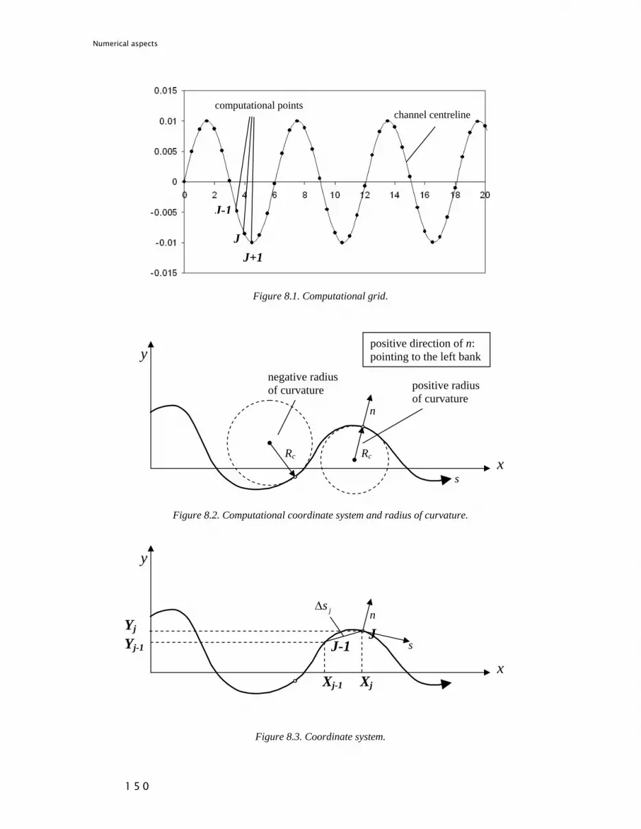
Numerical aspects
1 5 0
Figure 8.1. Computational grid.
Figure 8.2. Computational coordinate system and radius of curvature.
Figure 8.3. Coordinate system.
J n
x
y
Xj
Yj J-1
Xj-1
Yj-1
jsΔ
s
Rc
positive radius of curvature
n
Rc
negative radius of curvature
positive direction of n: pointing to the left bank
x
y
s
channel centreline computational points
J
J-1
J+1

Numerical aspects
1 5 1
The computations proceed as follows:
1. Equation 8.1 (water depth equation) is solved at a certain time level, ti, imposing the boundary conditions H(0)i and (0) /iH s∂ ∂ . The term (0) /iH s∂ ∂ is derived as a function of the velocity and water depth deformations at the upstream boundary, U(0)i and H(0)i, as described in Section 8.1.2. The result is the downstream profile of the equilibrium excess water depth near the left bank at t = ti, Hi. The corresponding value at the opposite (right) bank will be equal, but with opposite sign. The initial conditions, describing the longitudinal profile of water depth excess at t = t0, are necessary if the time-evolution of the bed development is taken into account (Section 5.2.8). In that case, the equilibrium values Hi, computed with Equation 8.1, are adjusted according to Equations 5.68 and 5.78.
2. Equation 8.2 (flow velocity equation) is solved at the same time level, ti, using the computed values of Hi and the boundary condition U(0)i. The result is the downstream profile of the equilibrium excess flow velocity, Ui, near the left bank of the river. The corresponding value at the opposite (right) bank will be equal, but with opposite sign.
3. Equation 8.3 (migration equation) is solved using the computed values of Ui and Hi and Ui-1 and Hi-1. The result is the cross-stream translation of the channel centreline, occurring during the time interval 1i it t t+Δ = − (one value per computational point). Positive values of U and H lead to a horizontal shift in the positive n-direction.
4. The new alignment of the channel centreline is computed at the next time level, t = t i+1, based on the old channel alignment and the computed values of the cross-stream translation. This method was first designed by Hickin [1974], who described the channel centreline as a collection of Lagrangian points and obtained channel migration by shifting these points normal to the channel centreline. In this way old centrelines correspond to floodplain scroll-bars.
The values of the variables u0 and h0 are computed using Equations 5.29 and 5.31, knowing the value of the river discharge QW. Although the model has been designed for bankfull conditions, QW can vary with time, but its variations should not be strong. The longitudinal river bed slope is recomputed at every time step as a function of the channel sinuosity (Eq. 2.21), assuming constant valley slope according to Equation 5.33, here repeated for convenience):
0 0b w vz z is s S
∂ ∂= =
∂ ∂ (8.4)
in which iv is the valley slope and S is the river sinuosity. For the same channel width, Chézy coefficient and discharge, the reach-averaged values of flow velocity, water depth and sediment transport vary with the longitudinal slope. Therefore, increasing river sinuosity (with time) leads to a decrease of u0 and to an increase of h0, leading to a decrease of the width-to-depth ratio, β . The effects of computing the longitudinal bed slope as the valley slope divided by sinuosity are described in Sections 5.3 and 5.4.

Numerical aspects
1 5 2
It is further assumed that the sediment transport rate, qS0, is always and everywhere equal to the sediment transport capacity of the current. Therefore qS0 is computed with a transport formula at every time step. Furthermore, the model assumes that there are no backwater effects. The averaged flow velocity and depth are assumed to be equal to u0 and h0, respectively, for the entire river reach. Backwater effects are important during the transition periods following interventions or natural changes or at discharges other than the representative discharge. As an alternative, instead of using the full model MIANDRAS, one can compute the river planimetric changes either with the no-lag kinematic model or with the Ikeda-type model, which are based on the equations listed in Sections 7.7.1 and 7.7.2, respectively. The computations proceed in the same way, but the choice of the model has implications on the results (Sections 7.7, 8.3, 9.2 and 9.3).
8.1.2 Numerical scheme
The longitudinal coordinate, s, of the generic section J is:
0
J
js ds= ∫ (8.5)
sj is determined computationally by (Figure 8.3):
2 21 1
1 1
( ) ( )J J
J j j j j jj j
s x x y y s− −= =
= − + − = Δ∑ ∑ (8.6)
in which jsΔ is the distance between the generic section j and the previous section j-1 and n is the
number of sections from the upstream boundary including section j. If the sections are close to each other, the error made in computing sj with Equation 8.6 instead of with Equation 8.5 is small.
Water depth equation
Equation 8.1 can be written as:
2 2
2 2 0H HA BH C D Es s s s
γ γ γ⎛ ⎞∂ ∂ ∂ ∂
+ + + + + =⎜ ⎟∂ ∂ ∂ ∂⎝ ⎠ (8.7)
with A = A2 (Eq. 7.34), B = A3 (Eq. 7.35), C = -B1 (Eq. 7.36), D = -B2 (Eq. 7.37) and E = -B3 (Eq. 7.38). A, B, C, D and E are constant with s but variable with time. They are re-computed at every time step. The terms between parentheses are functions of the curvature ratio, / cB Rγ = , which is variable with s and time. Therefore, the curvature ratio is computed for every section and re-computed at every time step. At any time step t = ti the terms between parentheses are only a function of the longitudinal coordinate, s:

Numerical aspects
1 5 3
2
2 ( )C D E F ss sγ γ γ∂ ∂+ + =
∂ ∂ (8.8)
The boundary conditions necessary to solve Equation 8.7 are variable with time, they are:
0(0) at i J iH H t t== =
0(0) at i J iU U t t== = (8.9)
The value of (0) /iH s∂ ∂ at t = ti is derived from U(0)i and H(0)i using the following relation:
0
0
220 0 0 0
0
(0) ( 1) (0) ( 1) 1 (0)2
( 1) ( 1) (2 )2 2 2 2
i ii
W W S
ii i
W
H h b U b Hs u
h b u h b hAu s B
λ λ λ
γ σ πγ γλ
⎛ ⎞ ⎡ ⎤∂ − −= − + −⎜ ⎟ ⎢ ⎥∂ ⎝ ⎠ ⎣ ⎦
⎛ ⎞ ⎛ ⎞− ∂ − −⎛ ⎞ ⎛ ⎞− − +⎜ ⎟⎜ ⎟ ⎜ ⎟⎜ ⎟∂⎝ ⎠ ⎝ ⎠⎝ ⎠⎝ ⎠
(8.10)
with
(0)iU = velocity excess at the upstream boundary (left bank) at time t = ti
iγ = local curvature ratio at time t = ti. The numerical solution is obtained with the Runge-Kutta numerical method for second-order differential equations. Equation 8.7 can be written in the following way:
[ ]( )
H fsf Af BH F ss
∂=
∂∂
= − + +∂
(8.11)
According to the Runge-Kutta method, Equation 8.7 can be solved in the following way:
1 0 1 2 3
1 0 1 2
1 ( 2 2 )6
1 ( 2 2 3)6
j j
j j
H H K K K K
f f M M M M
+
+
= + + + +
= + + + + (8.12)
with K0 = 1j js f+Δ
M0 = 1 ( )j j j js Af BH F s+ ⎡ ⎤−Δ + +⎣ ⎦

Numerical aspects
1 5 4
K1 = 10 02
jsK M+Δ⎛ ⎞
+ ⎜ ⎟⎝ ⎠
M1 = 10 01 2 2 2
jj j j j
sM Ks A f B H F s ++
Δ⎡ ⎤⎛ ⎞⎛ ⎞ ⎛ ⎞−Δ + + + + +⎢ ⎥⎜ ⎟ ⎜ ⎟ ⎜ ⎟⎝ ⎠ ⎝ ⎠ ⎝ ⎠⎣ ⎦
K2 = 10 12
jsK M+Δ⎛ ⎞
+ ⎜ ⎟⎝ ⎠
M2 = 11 11 2 2 2
jj j j j
sM Ks A f B H F s ++
Δ⎡ ⎤⎛ ⎞⎛ ⎞ ⎛ ⎞−Δ + + + + +⎢ ⎥⎜ ⎟ ⎜ ⎟ ⎜ ⎟⎝ ⎠ ⎝ ⎠ ⎝ ⎠⎣ ⎦
K3 = 10 22
jsK M+Δ⎛ ⎞
+ ⎜ ⎟⎝ ⎠
M3 = 12 21 2 2 2
jj j j j
sM Ks A f B H F s ++
Δ⎡ ⎤⎛ ⎞⎛ ⎞ ⎛ ⎞−Δ + + + + +⎢ ⎥⎜ ⎟ ⎜ ⎟ ⎜ ⎟⎝ ⎠ ⎝ ⎠ ⎝ ⎠⎣ ⎦
in which 1 1( ) ( )2 2
j j jj
s F s F sF s + +Δ +⎛ ⎞
+ =⎜ ⎟⎝ ⎠
.
Flow velocity equation
Equation 8.2 can be written as:
U MU NH P Qs s
γ γ∂ ∂⎛ ⎞= + + +⎜ ⎟∂ ∂⎝ ⎠ (8.13)
with
M = 1
Wλ−
N = 0
0
12W
uh λ
⎛ ⎞⎜ ⎟⎝ ⎠
P = 0
2u
−
Q = 0(2 )2 2W
uσλ
⎛ ⎞−−⎜ ⎟⎝ ⎠
.
M, N, P and Q are known coefficients, constant with s, but variable with time. They are re-computed at every time step. The terms between parentheses in Equation 8.13 are functions of the curvature ratio. At the time step t = ti:
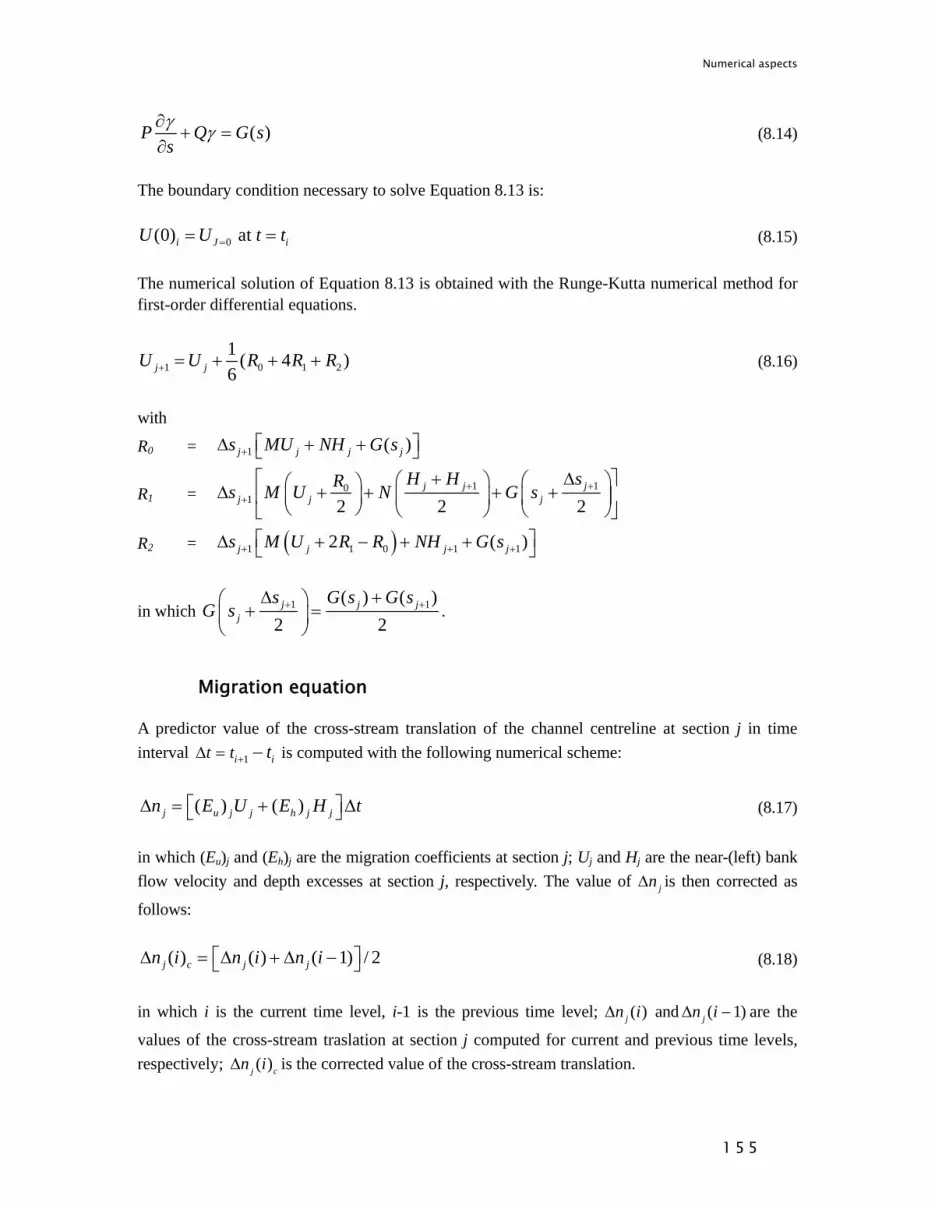
Numerical aspects
1 5 5
( )P Q G ssγ γ∂+ =
∂ (8.14)
The boundary condition necessary to solve Equation 8.13 is:
0(0) at i J iU U t t== = (8.15) The numerical solution of Equation 8.13 is obtained with the Runge-Kutta numerical method for first-order differential equations.
1 0 1 21 ( 4 )6j jU U R R R+ = + + + (8.16)
with
R0 = 1 ( )j j j js MU NH G s+ ⎡ ⎤Δ + +⎣ ⎦
R1 = 1 101 2 2 2
j j jj j j
H H sRs M U N G s+ ++
+ Δ⎡ ⎤⎛ ⎞ ⎛ ⎞⎛ ⎞Δ + + + +⎢ ⎥⎜ ⎟ ⎜ ⎟ ⎜ ⎟⎝ ⎠ ⎝ ⎠ ⎝ ⎠⎣ ⎦
R2 = ( )1 1 0 1 12 ( )j j j js M U R R NH G s+ + +⎡ ⎤Δ + − + +⎣ ⎦
in which 1 1( ) ( )2 2
j j jj
s G s G sG s + +Δ +⎛ ⎞
+ =⎜ ⎟⎝ ⎠
.
Migration equation
A predictor value of the cross-stream translation of the channel centreline at section j in time interval 1i it t t+Δ = − is computed with the following numerical scheme:
( ) ( )j u j j h j jn E U E H t⎡ ⎤Δ = + Δ⎣ ⎦ (8.17)
in which (Eu)j and (Eh)j are the migration coefficients at section j; Uj and Hj are the near-(left) bank flow velocity and depth excesses at section j, respectively. The value of jnΔ is then corrected as
follows:
( ) ( ) ( 1) / 2j c j jn i n i n i⎡ ⎤Δ = Δ + Δ −⎣ ⎦ (8.18)
in which i is the current time level, i-1 is the previous time level; ( )jn iΔ and ( 1)jn iΔ − are the
values of the cross-stream traslation at section j computed for current and previous time levels, respectively; ( )j cn iΔ is the corrected value of the cross-stream translation.

Numerical aspects
1 5 6
8.1.3 Model calibration
In general, the constant discharge to be used in the computations can be assumed to be the bankfull discharge. However, the discharge can also be derived from model calibration. In this case it will be the one giving the bed topography (point bar and alternate bar position) that is closest to the observed one. It is advisable to select the sediment transport formula on the basis of the flow and sediment characteristics and on the information available on sediment transport. The value of the sediment transport rate, qS0, is important when using the time-adaptation formulation, because it weights the timinig of the morphological changes, whereas the exponent of the sediment transport formula, b, affects wavelength and damping of the eigen oscillation, i.e. it affects the river bed topography (Section 7.2.1). Other parameters, weighted by the calibration coefficients E, 1α andσ , also influence the bed topography. These parameters will have to be calibrated on the available information regarding the bed topography, taking into account which aspect of bed topography is influenced by each parameter. The migration coefficients, Eu and Eh, should also be considered as calibration coefficients. Their value should be derived from past migration trends and not based on the eroding bank characteristics (Section 8.3).
Coefficient E : effects of transverse bed slope
The coefficent E is introduced in the equation describing the angle between the sediment transport direction and the main flow direction. It weighs the influence of the transverse bed slope on the sediment transport direction (Section 5.2.1). According to Talmon et al. [1995], the value of E for natural rivers can be derived using the following equation (Equation 5.7 repeated here for convenience):
0.3
50
0.0944 hED
⎛ ⎞= ⎜ ⎟
⎝ ⎠ (8.19)
Struiksma, based on practical experience [personal communication], suggested using:
0.5 for experimental flumesE 1.0 for real riversE ≈≈
(8.20)
If the effect of the transverse bed slope is taken too strong, by taking E too large, the resulting bed topography is too flat. If the effect of the transverse bed slope is too weak, with too small a value of E, the result is an unrealistically steep transverse bed slope.

Numerical aspects
1 5 7
Coefficient α1: effects of curvature on bed shear stress direction
The direction of the bed shear-stress can be obtained from an expression including the effect of the helical flow. In MIANDRAS, the effective radius of curvature of the stream line, R*, is assumed to coincide with Rc, radius of curvature of the channel centreline. In this case, Equation 5.8, describing the direction of the bed shear stress,δ , becomes:
arctan arctanc
v hAu R
δ⎛ ⎞⎛ ⎞= − ⎜ ⎟⎜ ⎟
⎝ ⎠ ⎝ ⎠ (8.21)
where A is a coefficient weighing the influence of the curvature-induced helical flow. If the vertical profile of the flow velocity is logarithmic, A can be derived with the following expression (Eq. 5.10, repeated here for convenience):
12
2 1 gAC
ακ κ
⎛ ⎞= −⎜ ⎟
⎝ ⎠ (8.22)
where: κ = Von Karman constant (-)
1α = calibration coefficient. The coefficient 1α weights the influence of channel curvature on the bed shear stress direction. It value therefore influences the effects of curvature on the bed deformation, since increasing
1α leads to an increase of the effects of curvature. Practical experience indicates that 1α should have a value between 0.4 and 1.2, which, as a first attempt, can be derived using the following empirical equation [Struiksma, personal communication]:
0.3
01
50
0.1 hD
α⎛ ⎞
= ⎜ ⎟⎝ ⎠
(8.23)
Coefficient σ: secondary flow momentum convection
The coefficientσ is introduced in the flow equation in Section 5.2.7, where (2 -σ ) multiplies the friction term. In this way σ weights the influence of the secondary flow momentum convection. Its value can appreciably affect the prediction of the near-bank flow and bed perturbations, U and H, since increasing σ leads to higher values of U and H. The value of σ can be assumed to vary between 2 and 4. Imposing σ = 2 is equivalent to the assumption that there is a constant distribution of friction for longitudinal flow over the cross-section. With σ > 2 the bed friction is lower near the eroding bank, which has an effect similar to the secondary flow momentum convection: a transverse shift of the maximum flow velocity locus towards the outer bank. A

Numerical aspects
1 5 8
relation to estimate the value of σ has been derived with a semi-empirical approach [Struiksma, personal communication]:
201 90 C h
Bgσ ⎛ ⎞= + ⎜ ⎟
⎝ ⎠ (8.24)
Migration coefficients Eu and Eh
Calibration coefficients are also the migration coefficients Eu and Eh that appear in the migration equation (Eq. 8.3). Their values differ notably from case to case. In MIANDRAS, the migration coefficients can vary along the river course, which takes into account the different conditions of the river banks. From 200 tests at stream sites in the USA, Hanson & Simon [2001] found that the migration coefficient Eu can be related to the critical shear stress for erosion of the eroding-bank material:
10.1ucr
Eτ
= (8.25)
Assuming the bank material to be non-cohesive and the same as the bed material and assuming the river banks to be mildly sloping, Hasegawa [1989] suggests using:
3
*1
u v fE i C ES
⎛ ⎞= ⎜ ⎟⎝ ⎠
(8.26)
in which the coefficient E* depends on the soil properties of the eroding bank. It should be derived with the following relation:
**
3 tan(1 )
kKTE θλ φ
=− Δ
(8.27)
where:
Sρ ρρ−
Δ = = relative density of sediment (-)
λ = porosity of bed and bank material
kθ = averaged transverse bed slope angle of concave bank K = dimensionless coefficient in the Meyer-Peter & Müller [1948] bed
load function, if written as: ( )3/ 20S m crq K gD θ θ= Δ −
0/( )cr S kT θ μ μ θ= = function of the Shields stress and friction factors, in which 0θ is the
cross-sectionally averaged Shields stress; crθ is the critical Shields
stress; and S kμ μ are the static and dynamic coefficients of

Numerical aspects
1 5 9
Coulomb friction of the sediment particles
*0
0 cr
φθ
θ θ=
− = function of the Shields stress.
As later demonstrated in this chapter (Sections 8.3 and 8.4), the migration coefficients to be used in the model cannot be determined on the basis of flow and eroding bank material characteristics alone, as suggested by Hanson & Simon [2001] and Hasegawa [1989]. Both Eu and Eh have to be assessed on the basis of historical migration rates. For non-cohesive banks, Eh can be assumed to be equal to zero and, as a first attempt, the coefficient weighing the flow-induced component of channel migration can be derived as follows:
0
yu
y
nE
u tΔ
=Δ
(8.28)
where:
ynΔ = yearly averaged channel centreline shift (m)
ytΔ = one year in seconds.
If the river banks are cohesive, ynΔ should be divided into two parts, attributing one part of
channel migration to the water flow ( yunΔ ) and one to bank failure ( yhnΔ ). This can be done by
observing past migration rates and by comparing migration rates and point bar position (See Chapter 7). The coefficient Eu is then derived as follows (first attempt):
0
yuu
y
nE
u tΔ
=Δ
(8.29)
The coefficient Eh is derived as follows (first attempt):
0
yhh
y
nE
h tΔ
=Δ
(8.30)
Since the channel migration is influenced also by numerical choices, such as the computational space and time steps and the way the channel centreline curvature is computed, the final values of the migration coefficients, derived by model calibration, can be different for different numerical settings.
8.1.4 Computation of the channel centreline curvature
There are several ways to compute the curvature of the channel centreline at section J. The simplest one is to compute the radius of curvature of the circle passing though the three sections J-1, J and J+1. A vector product can then be used to assess the sign of the curvature, which

Numerical aspects
1 6 0
indicates whether the channel is turning to the right or to the left (this is important to identify the inner and the outer bank in a river bend), see Figure 5.3. Unfortunately, this method is weak if the three sections are almost on a straight line, which occurs if the curvature is very small, and if the sections are very close to one another. This can lead to two types of numerical errors; one has to do with the value of the curvature, the other with its sign. The second type of error is the most dangerous. A mistake in the sign of curvature may lead to a positive feedback, thus to a growing error. Reducing the time step of the computations is not effective in decreasing this type of error. Instead, it is necessary to introduce a numerical filter that is able to select developing bends based on their spatial scale and to remove the spurious small-scale bends generated by local inaccuracies. One simple method, here called “curvature smoothing” [Crosato, 1990; Coulthard & Van De Wiel, 2006], averages the value of the curvature at point J with the curvatures of preceding and following points. There are many possible functions to be used; a simple one, adopted in MIANDRAS, is the following weighted average:
1 1 with2 4
J J JJ J
cJ
BR
γ γ γγ γ− ++ += = (8.31)
where RcJ is the radius of curvature of the circle passing through the three sections J-1, J and J+1. With Eq. 8.31 (curvature smoothing), the curvature at section J depends on the coordinates of the five sections: J-2, J-1, J, J+1 and J+2. Equation 8.31 can be repeated several times, which results in including more and more sections in the computation of the curvature. This method smoothes out small-scale bends, depending on the number of sections involved. The direct effect of applying this method is the reduction of the curvature variations in downstream direction, s, with consequent damping of the maximum values. Indirect effects are the general lowering of the water depth and velocity excesses, leading to a reduction of the bank erosion rates. Other methods to smooth out small-scale spurious bends are based on curve-fitting. The curvature at section J can be computed as the curvature of the best-fitting circle considering the coordinates of 5, 7 or more sections, using, for instance, the least-squares method. Instead of a circle, one can also use a parabola or another curve. Again, the number of sections (grid points) that are taken into account selects the scale of the bends that are removed. Sun et al. [1996] and Lanzoni et al. [2005] used cubic spline interpolations, which is another way of smoothing out small-scale bends. Spline interpolations [Duris, 1977] include a parameter for varying the smoothness of the fit, which can be used as an indirect way to select the scale of the small-scale bends to be smoothed out. The implication of applying this method is that the curve describing the channel centreline is altered, which implies that the spline interpolation requires some sort of optimization. In MIANDRAS spline interpolation can be used instead of curvature smoothing.
8.1.5 Regridding
The position of the grid points (sections) is not constant during the numerical simulations. In general, the distance between grid points increases as a meander grows, but it can also happen that grid points approach each other, for instance when due to meander migration at a certain location a bend disappears. With increased distances between successive grid points, the channel centreline looses smoothness and appears more and more like a series of circle segments. Besides,

Numerical aspects
1 6 1
the larger the distance the lower the model resolution and the more inaccurate the numerical procedure is. With decreased distances between successive grid points, the curve through a number of successive grid points can be confused (by the program) with a straight line, which increases the susceptibility to numerical errors. These problems introduce the necessity of inserting new grid points when the distance between two successive grid points has become too large and of deleting grid points when the distance has become too small [e.g. Howard, 1984; Crosato, 1990; Sun et al., 1996]. Therefore, in MIANDRAS automatic grid adaptation takes care of adding/removing grid points. Unfortunately, the procedure of inserting grid points can also be the origin of new small-scale spurious bends, since it is practically impossible to insert the new grid point exactly on the channel centreline, without any small errors in its coordinates. The method to improve the accuracy of the computations can thus become the source of new computational errors. In practice, the procedure of inserting and deleting grid points makes the use of smoothing filters (previous subsection) inevitable. The necessity of updating the computational grid arises in all existing software with changes in geometry due to bank retreat, if the grid lines along the borders of the computational domain follow the river banks. Examples are the software codes RIPA [Mosselman, 1992] and MIKE21-C [DHI, 1996]. The changes in geometry produce grid adaptation problems, such as the necessity to add or delete grid points (as in MIANDRAS) and the loss of grid smoothness and orthogonality (RIPA).
8.2 Stability of computations: time step vs. space step
Computational tests of meander migration showed a relation for a threshold between stable and unstable computations, which relates the maximum time step to the smallest space step and the largest channel centreline shift rate.
( / )MIN
MAXMAX
stn t
ε ΔΔ ≤
∂ ∂ (8.32)
in which:
MAXtΔ = maximum time step (s)
MINsΔ = minimum distance between two consecutive computational points (minimum space step) (m)
( / )MAXn t∂ ∂ = maximum channel centreline shift rate (m/s) ε = empirical coefficient ( 0.2ε ≈ ). The maximum channel centreline shift rate, ( / )MAXn t∂ ∂ , is estimated from:
0 0( / )MAX u hn t E u E h∂ ∂ = + (8.33)

Numerical aspects
1 6 2
8.3 Effects of smoothing and regridding in meander migration models
Several numerical tests were carried out in order to compare the effects of using different smoothing filters, such as curvature smoothing at different degrees and cubic spline interpolations [Crosato, 2007a]. Three models of different complexity were used in the computational tests:
1. a generic no-lag kinematic model (Section 7.7.1). 2. an Ikeda-type model (Section 7.7.2). 3. MIANDRAS (Section 7.7.3).
The computational tests used the values of channel width, discharge, valley slope and sediment characteristics of the straight-flume experiment T2 (Chapter 6, Sections 6.2 and 6.4), but with an initial centre-line alignment given by a low-amplitude sinusoid. Model choices and initial conditions are listed in Tables 8.1 and 8.2.
Table 8.1. Model parameters. Sediment transport calibration coefficients migration coefficients
formula b(-) 1α
σ
E
Eu (-)
Eh (1/s)
time step
(days)
E-H* 5 0.50 2.00 0.50 0.116x10⁻⁵ 0.00 4 * Engelund & Hansen (1967)
Table 8.2. Initial conditions. Initial sinusoidal planimetry
sinuosity (-)
wlength (m)
amplitude (m)
h0 (m) u0 (m/s) 0θ (-) Sλ (m) Wλ (m) LP (m) 1/LD (1/m)
1.00 6.00 0.01 0.045 0.25 0.38 0.84 1.08 6.04 0.129
In the computational tests, the erosion rate was related to the near-bank velocity excess only (Eh = 0) and the bank erodibility was assumed spatially uniform. In this way all models had the same erosion law. In addition, calibration coefficients and time step were the same in all computations. The occurrence of cut-offs was not taken into account, implying that meanders could cross each other in their final development stages. Spline interpolation was optimized on the basis of smoothness and channel centre-line fit. The results of the numerical tests showed that the optimal distance between successive nodes is of the order of magnitude of half the channel width. More in general, the distance has to be larger than approximately one third of the channel width and smaller than the channel width. The basis of this rule is purely empirical. The computational tests showed that when the distance between successive nodes was less than approximately one third of the channel width, the model became more susceptible to numerical errors (growth of spurious small-scale bends). On the other hand, when the distance between successive nodes was larger than one channel width the model results became unacceptably inaccurate. The effects of using a different method to smooth out small-scale bends were the strongest for the no-lag kinematic model, which, due to its immediate response to the local curvature, is the most susceptible to instability. In this case, spline interpolations always yielded a jumbled channel

Numerical aspects
1 6 3
alignment. Curvature smoothing gave a smoother alignment. Figure 8.3A shows the results obtained by computing the channel curvature using five nodes (curvature smoothing applied once). In this case, not all small-scale bends were smoothed out. With 11 nodes (curvature smoothing applied four times) the small-scale bends were smoothed out, but the channel centre line was still a bit irregular (Figure 8.3B). Since the erosion rates in the kinematic model are directly proportional to the local curvature, meanders grew but did not show appreciable migration.
A B
Figure 8.3. No-lag kinematic model. Meander development after 760 days. Output every 40 days, distances are in metres. A: curvature smoothing once (curvature based on 5 grid points), program
terminated after 190 time steps (760 days). B: curvature smoothing four times (curvature based on 11 grid points).
In the numerical tests performed, the Ikeda-type model and MIANDRAS remained stable without using a numerical filter, but this does not always occur, because it depends on the set of parameters used. With the same set-up, the two models yield different migration rates. In order to obtain meanders in a similar development stage, the runs with the Ikeda-type model had to be four times longer (4000 days instead of 1000). The results of the Ikeda-type model are shown in Figures 8.4A (using curvature smoothing) and 8.4B (using spline interpolations). With the Ikeda-type model, the different numerical filters resulted in meanders with similar shape, but different development stages. This indicates that the numerical filter influences the speed of meander growth, but not the form of meanders. In a reach far from the upstream and downstream boundaries, the averaged maximum migration rate was 0.388×10⁻³ m/day without curvature smoothing; 0.341×10⁻³ m/day with 5-node curvature (curvature smoothing applied once); and 0.475×10⁻³ m/day with the optimized cubic spline interpolation. The differences can be attributed to the filter used, because all other parameters had identical values in all computational tests.

Numerical aspects
1 6 4
A B
Figure 8.4. Ikeda-type model. Meander development and channel migration after 4000 days. Output every 400 days, distances are in metres. A: curvature smoothing once (curvature based on 5 grid points).
B: cubic spline interpolation. The results of MIANDRAS are shown in Figures 8.5A and 8.5B. This time, after the same number of time steps, meanders not only have different sizes, but also different shapes: those obtained using curvature smoothing (Figure 8.5A) have a shape similar to the meanders obtained with the Ikeda-type model (Figures 8.4A and 8.4B), whereas those obtained using the cubic spline interpolation (Figure 8.5B) are more distorted.
A B
Figure 8.5. MIANDRAS. Meander development and channel migration after 1000 days. Output every 100 days, distances are in metres. A: curvature smoothing once (curvature based on 5 grid points). B: cubic
spline interpolation. Far from the upstream and downstream boundaries, the average maximum migration rate was 1.70×10⁻³ m/day without curvature smoothing; 1.65×10⁻³ m/day with 5-node curvature (curvature

Numerical aspects
1 6 5
smoothing applied once); and 1.58×10⁻³ m/day with the optimized cubic spline interpolation. The conclusion is that the numerical filter affects both growth rate and shape of meanders. The channel centre line alignments obtained with different numerical filters at different stages of meander development are compared in Figure 8.6.
Figure 8.6. Channel centre line alignments obtained with MIANDRAS using different filters. Comparing size and form of the meanders obtained with the different numerical filters after the same number of time steps (Figure 8.6) shows that for increasing computational time the differences in meander amplitude decrease, whereas the differences in meander form increase. In practice, this means that for long-term predictions the uncertainties related to the meander amplitude that are due to the numerical filters tend to decrease, but the uncertainties related to the form of meanders tend to increase. As far as numerical aspects are concerned, the model appears
Splines No filter Smoothing once Smoothing 4 times

Numerical aspects
1 6 6
more suitable for long-term predictions of the amplitude of meanders than for predictions of (location and timing) of cut-offs, which is strongly influenced by the form of the meanders (compare Figures 8.7A and 8.7B). The numerical tests with three conceptually different meander models showed that size, form and migration rates of meanders depend also on the numerical filter used. The no-lag kinematic model gave the expected results only when using a curvature smoothing procedure, which reduces the curvature variations in downstream direction. The Ikeda-type model [Ikeda et al, 1981; Abad & Garcia, 2006] was the least affected by the choice of the filter, which seemed to influence only the growth rate of meanders, not the shape. The same dependence can be expected for kinematic models with a space lag [Ferguson, 1984; Howard, 1984] and for other meander models that, although based on different approaches, can be classified as belonging to this category, such as the models of Lancaster & Bras [2002] and the cellular model of Coulthard & van de Wiel [2006]. Instead, the full model MIANDRAS was affected by the smoothing filter in both growth rate and shape of meanders. This model behaves like the one of Ikeda et al [1981] when the damping coefficient, 1/LD (Eq. 7.12) is large, but when it is small, there is a strong dependence on the upstream curvature changes. The same likely applies to the other meander models capable of reproducing the overshoot/overdeepening phenomenon [Johannesson & Parker, 1989; Howard, 1992; Sun et al, 1996; Zolezzi & Seminara, 2001]. Non-propagating alternate bars can be observed in real rivers, where they influence bank erosion and channel migration. The reproduction of these bars (overshoot/overdeepening phenomenon) and of their effects on bank erosion should therefore be as accurate as possible. Unfortunately, numerical filters can influence this, as the removal of small-scale bends by reducing the curvature variations in downstream direction can also imply the suppression of the growth of non-propagating alternate bars in their early stage. In the computational tests, the formation of bars in mid-meanders only occurred when using the spline interpolation (Figure 8.7A). As these bars did not even form in a reference computation without any smoothing at all (the model with this set of parameters remained stable also without any smoothing; see Figure 8.7B), one might argue that the spline interpolation introduces realistic-looking, but in fact unrealistic effects. Or is it, on the contrary, the only method that gives realistic results? The answer can only be given by reproducing formation and growth of large meanders from a straight channel in a laboratory experiment. For this type of experiments the approaches of Smith [1998] (using cohesive soil) and of, among others, Gran & Paola [2001] (with riparian vegetation) appear the most promising. The computational tests performed do not represent real situations (input based on data from a flume experiment and uniform bank erodibility). Moreover, they simulate the planimetric evolution of an initially almost straight channel during a relatively long time interval, which for a real river may correspond to several centuries. For shorter simulations and real rivers the choice of the smoothing procedure has less impact on the shape of the meanders, which on the short term is governed by the initial conditions. Nevertheless, an important implication of migration rates being dependent on the numerical filter is that, in order to reproduce the planform changes of real rivers, the migration coefficients should be calibrated against historical migration rates. In analogy with the bed roughness coefficient for hydrodynamic computations, the migration coefficients are bulk parameters that encompass many schematization effects, so that in the end they can only be used as calibration parameters. This means that the migration coefficients cannot be derived a priori as a function of the bank characteristics (soil, vegetation cover, water content, height, etc.), since physical bank characteristics explain only part of their values.

Numerical aspects
1 6 7
A B
Figure 8.7. A: detail of the final bed topography after 1000 days with MIANDRAS using cubic spline interpolation. B: detail of the final bed topography after 1000 days with MIANDRAS without using any
smoothing filter. Distances are in metres. Lighter gray = bar, darker gray = pool.
8.4 Effects of boundary conditions
8.4.1 Steady-state computations
To illustrate the effects of the boundary conditions on the prediction of bed topography and river planimetric changes, several computational tests were carried out. In all computational tests MIANDRAS simulated initiation and further development of meanders starting from a perfectly straight channel with different upstream boundary conditions. The initial values of channel width, discharge, valley slope and sediment characteristics coincided with the conditions of the straight-flume experiment T2 (Chapter 6). Model parameters and initial conditions are summarized in Tables 8.1 and 8.2. The duration of all computations was 400 days, the computational time step was 4 days and the output step 40 days. At every time step the model computed the equilibrium bed topography. The computational tests performed are summarized in Table 8.3. In RUN1 and RUN2 the boundary conditions are constant with time and can therefore be related to a permanent upstream disturbance to the flow. In RUN3 the upstream disturbance vanishes after a time long enough to allow the achievement of an initial perturbed equilibrium bed topography. In RUN 4

Numerical aspects
1 6 8
the boundary conditions vary with time and represent randomly varying upstream disturbances, each one present for a time that is long enough to allow the achievement of a perturbed equilibrium bed topography.
Table 8.3. computational tests. Boundary conditions
Computational Test
H(0) (m)
(0) /H s∂ ∂ (-) (Eq. 8.10)
U(0) (m/s) Time variation
RUN 1 0.001 0.0011 0 constant RUN 2 0.005 0.00593 0 constant RUN 3 0.001 0.0011 0 only at t = 0 RUN 4 -0.005-0.005 variable 0 randomly varying*
* Excel random generator Figures 8.8- 8.11 show the results of the computational tests. Upstream disturbances of different intensity yielded different channel planimetries. The differences are strongest close to the upstream boundary, where they involve not only the size of meanders, but also their wavelength (Figures 8.12 and 8.13). Far from the upstream boundary, meanders have similar size and wavelengths, but differ in phase (Figures 8.14-8.17).
Figure 8.8. RUN 1. Channel meandering generated by a constant upstream disturbance starting from a
perfectly straight channel. Distances are in m.
Figure 8.9. RUN 2. Channel meandering generated by a constant upstream disturbance starting from a
perfectly straight channel. Distances are in m.
Figure 8.10. RUN3. Channel meandering generated by rapidly declining boundary conditions (only present
at t=0) starting from the conditions of RUN 1. Distances are in m.
Figure 8.11. RUN 4. Channel meandering generated by randomly varying boundary conditions starting
from a perfectly straight channel. Distances are in m.

Numerical aspects
1 6 9
Figure 8.12. RUN 1. Meanders generated by a constant upstream disturbance close to the upstream
boundary. Distances are in m.
Figure 8.13. RUN 2. Meanders generated by a constant upstream disturbance close to the upstream
boundary. Distances are in m.
Figure 8.14. RUN 1. Meanders generated by a constant upstream disturbance far from the upstream
boundary. Distances are in m.
Figure 8.15. RUN 2. Meanders generated by a constant upstream disturbance far from the upstream
boundary. Distances are in m.
1 2 3 4 5 6 7
1 2 3 4 5 6

Numerical aspects
1 7 0
Figure 8.16. RUN 3. Meanders generated by rapidly declining boundary conditions starting from the
conditions of RUN1 far from the upstream boundary. Distances are in m.
Figure 8.17. Meanders generated by randomly varying boundary conditions far from the upstream
boundary. Distances are in m. In the computational tests, the disturbances represented by the imposed boundary conditions generated steady alternate bars inside the channel. These steady bars, by influencing bank migration, caused the river to start meandering. The initial alternate bars generated in RUN1 and RUN 3 are shown in Figure 8.18, those generated in RUN 4 are shown in Figure 8.19.
Figure 8.18. RUN 1 and RUN 3. Equilibrium bed deformation at t = 0. Lighter gray = bar, darker gray =
pool. Distances are in m.
Figure 8.19. RUN 4. Equilibrium bed deformation at t = 0. Boundary conditions randomly varying with
time. Lighter gray = bar, darker gray = pool. Distances are in m. Wavelength and damping coefficient of the steady bars (eigen-oscillation) are the same in all runs, because these characteristics are not influenced by the boundary conditions (N.B. the model computed the equilibrium bed topography at every time step). The differences between runs regard bar elevation and phase. Meanders were obtained not only from constant boundary conditions (RUN1 and RUN 2 in Figures 8.8 and 8.9), representing a persistent and constant disturbance at the upstream boundary, but also from a rapidly declining disturbance (RUN 3 in Figure 8.10) as well as from a randomly-

Numerical aspects
1 7 1
varying disturbance (RUN 4 in Figure 8.11). A constant upstream disturbance is therefore not necessary for meander formation. In this case however, the disturbances are assumed to be present for a time that is long enough to allow reaching the equilibrium bed topography (steady-state computations). During the experimental test T2 the bed topography reached equilibrium after two days (Chapter 6). The choice of a time step of 4 days is therefore in harmony with the experimental observations. Random boundary conditions (RUN 4) were found to generate trains of meanders propagating downstream (Figure 8.11). Trains of meanders have been observed in real rivers by, among others, Shen & Larsen [1988]. Rapidly declining upstream disturbances (RUN 3) generated a single train of meanders (Figure 8.10), which implies that upstream disturbances are needed to keep on generating meanders; otherwise the river channel becomes straight again. This type of behaviour was found also by Seminara et al. [2001] and Lanzoni et al. [2005], who used another type of perturbation to generate meanders: a perturbed channel planimetric configuration instead of a flow and water depth disturbance at the upstream section.
8.4.2 Computations with time adaptation
The development of meanders resulting from randomly varying perturbations needs further investigation. Since the runs performed in the previous section are steady-state, i.e. the model computed at every time step the equilibrium bed topography, it is necessary to check whether the same or similar results would be obtained by taking into account the time scale of the bed development. Randomly varying boundary conditions represent a perturbation having a zero time-averaged value. Also a perturbation varying with time in a sinusoidal way has zero time average. Such a perturbation is caused, for instance, by migrating alternate bars. Considering that in real rivers the development of the perturbed bed topography, i.e. of the steady eigen-oscillation, has different speeds depending on the degree of development, the presence of migrating bars may result in a residual steady bed oscillation. This oscillation would be superimposed on the oscillation due to the migrating bars. In the straight-flume experiment the attempt to obtain a time-averaged flat bed without upstream disturbances failed (Chapter 6). This was attributed to the difficulty of obtaining a perfectly uniform inflow. However, it might also be possible that the presence of migrating bars contributed to this. It is therefore important to investigate whether the presence of migrating alternate bars might result in a residual steady channel bed oscillation. Migrating bars are too fast [Olesen, 1984], to be able to cause river meandering, but, if they create a steady bed and flow oscillation, they could be the indirect cause of river meandering. Hansen [1967] demonstrated that free migrating bars develop because of an inherent instability of the morphodynamic system, called bar instability (Section 7.4.1). This means that also the tendency to meander could be considered as inherent to river systems. As a first orientation, two other computational tests, RUN 5 and RUN 6, were performed. As in the previous computational tests, the initial values of channel width, discharge, valley slope and sediment characteristics coincided with the conditions of the straight-flume experiment T2 (Chapter 6). Model parameters and initial conditions are summarized in Tables 8.1 and 8.2. In these runs the model reproduced the effects of the alternate bars that were observed during the straight-flume experiment T2 (Chapter 6.4) at the upstream boundary. The averaged wavelength of the observed bars was 3.94 m, their amplitude 2.2 cm, their averaged celerity 2.9×10⁻⁵ m/s. The time necessary for the passage of an entire alternate bar at a given location was about 38 hours. The time-varying boundary conditions therefore represented a sinusoidally-varying perturbation
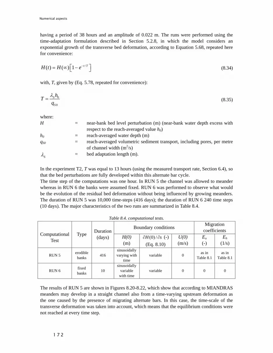
Numerical aspects
1 7 2
having a period of 38 hours and an amplitude of 0.022 m. The runs were performed using the time-adaptation formulation described in Section 5.2.8, in which the model considers an exponential growth of the transverse bed deformation, according to Equation 5.68, repeated here for convenience:
/( ) ( ) 1 t TH t H e−⎡ ⎤= ∞ −⎣ ⎦ (8.34)
with, T, given by (Eq. 5.78, repeated for convenience):
0
0
S
S
hTqλ
= (8.35)
where: H = near-bank bed level perturbation (m) (near-bank water depth excess with
respect to the reach-averaged value h0) h0 = reach-averaged water depth (m) qS0 = reach-averaged volumetric sediment transport, including pores, per metre
of channel width (m2/s)
Sλ = bed adaptation length (m).
In the experiment T2, T was equal to 13 hours (using the measured transport rate, Section 6.4), so that the bed perturbations are fully developed within this alternate bar cycle. The time step of the computations was one hour. In RUN 5 the channel was allowed to meander whereas in RUN 6 the banks were assumed fixed. RUN 6 was performed to observe what would be the evolution of the residual bed deformation without being influenced by growing meanders. The duration of RUN 5 was 10,000 time-steps (416 days); the duration of RUN 6 240 time steps (10 days). The major characteristics of the two runs are summarized in Table 8.4.
Table 8.4. computational tests.
Boundary conditions Migration coefficients
Computational Test
Type Duration (days) H(0)
(m) (0) /H s∂ ∂ (-)
(Eq. 8.10) U(0) (m/s)
Eu (-)
Eh (1/s)
RUN 5 erodible banks 416
sinusoidally varying with
time
variable
0 as in
Table 8.1 as in
Table 8.1
RUN 6 fixed banks 10
sinusoidally variable
with time
variable
0
0
0
The results of RUN 5 are shown in Figures 8.20-8.22, which show that according to MIANDRAS meanders may develop in a straight channel also from a time-varying upstream deformation as the one caused by the presence of migrating alternate bars. In this case, the time-scale of the transverse deformation was taken into account, which means that the equilibrium conditions were not reached at every time step.

Numerical aspects
1 7 3
Far from the upstream boundary, the meander wavelength, computed along the valley axis, is comparable to the wavelength of the meanders originating from a constant perturbation (Figures 8.14 and 8.15). This means that the boundary conditions do not influence the “regime” meander wavelength, which appears to depend solely on the flow and channel characteristics, including the width-to-depth ratio. This is in agreement with field and experimental observations [e.g. Leopold & Wolman, 1960; Friedkin, 1945].
Figure 8.20. RUN 5. Planimetry after 416 days far from the boundaries. Distances are in m.
Figure 8.21. RUN 5. Planimetry after 416 days close to the upstream boundary. Distances are in m.
Figure 8.22. RUN 5. Planimetry after 416 days far from the boundaries. Distances are in m.
Figure 8.23 shows the initial development of a waving bed topography, forced by the time-varying boundary conditions. The waving bed topography does not represent the free migrating alternate bars that were observed during the experiment, but rather the effects of alternate bars at the upstream boundary (sinusoidal variation of upstream disturbances) on the average channel bed topography: the development of a perturbed bed. The initial wavelength of the bed deformation is much shorter than the wavelengths of the steady eigen-oscillation and migrating alternate bars: about 1.2 m instead of 6 and 3.94 m, respectively. This wavelength derives from the combination of the wavelengths of alternate bars and eigen oscillation. However, the choice of computing the value of (0) /H s∂ ∂ from Equation 8.10, leading to a rather “unnatural” combination of boundary conditions, i.e. not exactly belonging to the observed alternate bars (Table 8.4), may also play a role.

Numerical aspects
1 7 4
Figure 8.23. RUN 5. Steady bed topography after one hour. Distances are in m. Lighter gray = bar. Darker
gray = pool. With the progression of bank erosion and accretion, the bars that developed in the initially straight channel were soon transformed into point bars, i.e. they were captured by the growing meanders, as can be seen from Figures 8.24 and 8.25.
Figure 8.24. RUN 5. Bed topography after 208 days. Picture above: close to the upstream boundary.
Picture below: far from the upstream boundary. Distances are in m.

Numerical aspects
1 7 5
Figure 8.25. RUN 5. Bed topography after 416 days. Picture above: close to the upstream boundary.
Picture below: far from the upstream boundary. Distances are in m. The results of RUN 6 are shown in Figure 8.26, illustrating the evolution of the steady bed oscillation with time. This bed oscillation does not represent free migrating bars, which are not accounted for in the model, but the bed deformation caused by sinusoidally varying upstream disturbances caused by the presence of migrating bars, taking into account the temporal evolution of the transverse bed development. At the initial state (i.e. after one hour) the bed deformation is identical to the one of RUN 5 (Figure 8.23) and consists of a single bar-pool sequence close to the upstream boundary, but after some time the steady deformation, although varying with time, is felt also more downstream. After 78 hours the single bar-pool sequence transforms into several bar-pool sequences (Figure 8.26). With fixed banks, the downstream influence of the oscillating upstream perturbation appears limited in space, because after both 78 hours and 1000 hours (41 days) the bed deformation is restricted to the first 40 m of the channel (Figure 8.27). The wavelength of the oscillation gradually increases from an initial 1.2 m to the wavelength of the steady eigen-oscillation (about 6 m).
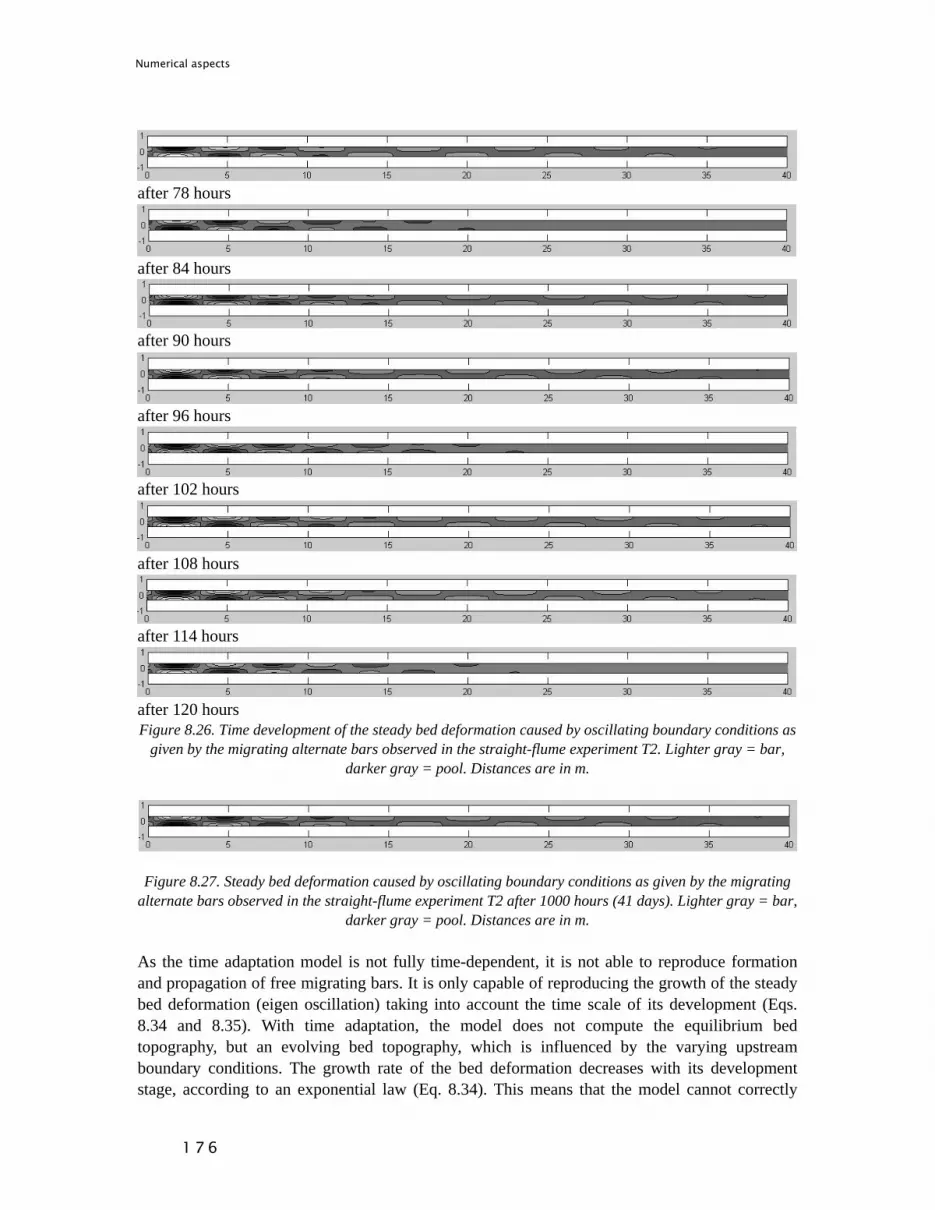
Numerical aspects
1 7 6
after 78 hours
after 84 hours
after 90 hours
after 96 hours
after 102 hours
after 108 hours
after 114 hours
after 120 hours Figure 8.26. Time development of the steady bed deformation caused by oscillating boundary conditions as
given by the migrating alternate bars observed in the straight-flume experiment T2. Lighter gray = bar, darker gray = pool. Distances are in m.
Figure 8.27. Steady bed deformation caused by oscillating boundary conditions as given by the migrating alternate bars observed in the straight-flume experiment T2 after 1000 hours (41 days). Lighter gray = bar,
darker gray = pool. Distances are in m. As the time adaptation model is not fully time-dependent, it is not able to reproduce formation and propagation of free migrating bars. It is only capable of reproducing the growth of the steady bed deformation (eigen oscillation) taking into account the time scale of its development (Eqs. 8.34 and 8.35). With time adaptation, the model does not compute the equilibrium bed topography, but an evolving bed topography, which is influenced by the varying upstream boundary conditions. The growth rate of the bed deformation decreases with its development stage, according to an exponential law (Eq. 8.34). This means that the model cannot correctly

Numerical aspects
1 7 7
reproduce the development of the bed oscillation, but only give some insight into the type of development that can be expected. RUN 5 and RUN 6 show that also a harmonic variation of the upstream disturbance, as if free migrating bars are present at the upstream boundary, might eventually lead to steady alternate bars having the same wavelength as the eigen-oscillation, which is more or less twice the wavelength of the free migrating bars. In RUNS 5 and 6 the steady bars that form have wavelength of about 6 m; the free migrating bars which are supposed to cause flow perturbation at the upstream boundary 3.9 m. The coexistence of free migrating bars and free steady bars was observed in the Pilot Flume experiments (Chapter 6). The steady bars were generated by the upstream disturbance. However, in the laboratory, even without any upstream disturbances the steady-state channel bed was not flat. This was attributed to non-uniform flow from upstream. Coexistence of migrating and steady bars was also observed in the experiments carried out at WL ⎮Delft Hydraulics by Lanzoni [2000] who studied alternate bar formation in alluvial channels. In a straight flume with mobile bed, Lanzoni noticed two peaks in the spectral analysis of the bed topography, one corresponded to the observed free migrating bars whereas the other one to some not well-defined alternate bars having double wavelength. The second peak was present also in some experiments without any upstream disturbance. If the second peak was caused by the presence of the steady eigen oscillation, it means that this oscillation might form also without any significant upstream disturbance. Further investigation with a fully time-dependent model is needed to assess whether free migrating bars, which are caused by the bar instability phenomenon (Section 7.4.1), or even the instability itself, which is caused by some small random disturbances, can indeed lead to the development of the eigen bed-oscillation, as the numerical tests performed suggest. If this proves true, meandering would be a consequence of inherent system instability. It is therefore recommended to further investigate the development of the eigen bed oscillation in presence of either free migrating bars or upstream quickly-varying (very small) flow perturbations. This could be done using the fully time-dependent model underlying MIANDRAS as well as a more complex time-dependent model, such as Delft3D [WL⎮Delft Hydraulics, 2003]. It is also recommended to perform some well-designed experiments to verify the results of the analytical and numerical studies.

Numerical aspects
1 7 8

Field applications
1 7 9
9 Field applications
9.1 Introduction
The tests in the previous chapters demonstrate that MIANDRAS reproduces flow fields and bed topography from laboratory flumes as well as realistic meander developments from an initially straight channel. This introductory section briefly presents some results from completed applications of MIANDRAS in engineering and research projects. The next sections of this chapter present deeper analyses of applications to test the performance of MIANDRAS. MIANDRAS has been successfully applied to predict bar formation as a function of the width-to-depth ratio on the Po River (Italy) [Studio SICEM S.r.l., 1994]. The idea was that of locally changing the river width-to-depth ratio at low-flow conditions to remove a bar that systematically formed in front of the intake of Moglia Secca, on the right river bank near Boretto [Di Silvio & Crosato, 1994] (Figure 9.1). Although MIANDRAS had to use a constant value of the channel width, the computed point bar - pool position was in good agreement with the measured ones (Figure 9.2). Furthermore, the computed variations of point bar location for different width-to-depth ratios agreed well with the results of a physical (scale) model [Di Silvio & Susin, 1994].
Figure 9.1. Po River at Boretto from satellite (Image © 2008 Digital Globe, Google Earth). A point bar obstructs the intake of Moglia Secca.
intake of Moglia Secca
Boretto

Field applications
1 8 0
Figure 9.2. Computed and measured longitudinal profiles of near-bank bed levels. Continuous line = computed bed levels along the right bank. Dotted line = computed bed levels along the left bank. The black points indicate the measured bed levels along the left bank. The intake of Moglia Secca is located on the right bank at s = 5100 m. MIANDRAS has been used by Duran Tapia [2008] to study the planimetric changes of the gravel-bed Irwell River, in Lancashire near Rawtenstall (United Kingdom), with the aim of assessing the erosion threat to the railway located at a few tens of metres from the left river bank. The location and extension of the point bars agree well with observations (Figure 9.3). The results of the planimetric change prediction are shown in Figure 9.4.
Figure 9.3. RiverIrwell (United Kingdom). Bed topography (bed level with respect to water surface level, in m) computed with MIANDRAS (above) and satellite image (below) (Image © 2006 Digital Globe Google
Earth). Courtesy of Roxana M. Duran Tapia.
longitudinal coordinate (m)
near-bank bed level relative to the averaged bed level (m)
point bar in front of the intake
flow
N flow
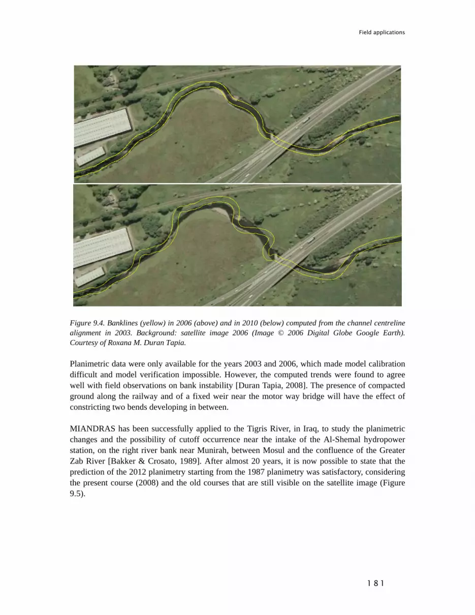
Field applications
1 8 1
Figure 9.4. Banklines (yellow) in 2006 (above) and in 2010 (below) computed from the channel centreline alignment in 2003. Background: satellite image 2006 (Image © 2006 Digital Globe Google Earth). Courtesy of Roxana M. Duran Tapia. Planimetric data were only available for the years 2003 and 2006, which made model calibration difficult and model verification impossible. However, the computed trends were found to agree well with field observations on bank instability [Duran Tapia, 2008]. The presence of compacted ground along the railway and of a fixed weir near the motor way bridge will have the effect of constricting two bends developing in between. MIANDRAS has been successfully applied to the Tigris River, in Iraq, to study the planimetric changes and the possibility of cutoff occurrence near the intake of the Al-Shemal hydropower station, on the right river bank near Munirah, between Mosul and the confluence of the Greater Zab River [Bakker & Crosato, 1989]. After almost 20 years, it is now possible to state that the prediction of the 2012 planimetry starting from the 1987 planimetry was satisfactory, considering the present course (2008) and the old courses that are still visible on the satellite image (Figure 9.5).

Field applications
1 8 2
Figure 9.5. Computed channel centreline 2012 (above) starting from the centreline 1987 [Bakker & Crosato, 1989] and river planimetry in 2008 from satellite (below) (Image © 2008 Digital Globe, Google
Earth).

Field applications
1 8 3
MIANDRAS has been used to compute bed topography and migration trends of the Blue Nile River between Roseires and Sinnar (Sudan), a river reach 274 km long [Ali, 2008]. The computed bed topography was similar, in terms of point bar locations, to the one predicted by a 2-D model based on the Delft3D software [WL⎮Delft Hydraulics, 2003] (Figure 9.6). Due to the long computational time, the 2-D model could afford not more than 5 cells in the cross-section, which caused inaccuracies in the results. The bed topography computed using bankfull discharge (8000 m3/s, Figure 9.7) is more similar to the observed one than the topography computed using the average discharge (2000 m3/s) [Ali, 2008]. MIANDRAS proved to be a quick and easy-to-use model for the assessment of the equilibrium bed topography at the large scale (hundreds of km) and allowed assessing the equilibrium bed topography in the future, taking into account the river planimetric changes.
-7
-6.5
-6
-5.5
-5
-4.5
-4
-3.5
-3
0 2000 4000 6000 8000 10000 120000
1000
2000
3000
4000
5000
y ( )
-7
-6
-5
-4
-3
Figure 9.6. Blue Nile River near the city of Sinja (Singa, Sudan). Above: bed topography computed using a 2-D model. Below: bed topography computed using MIANDRAS for a discharge of 2000 m3/s. Colour bar:
bed level with respect to the water surface level. Courtesy of Yasir S. A. Ali.
flow
Sinjah
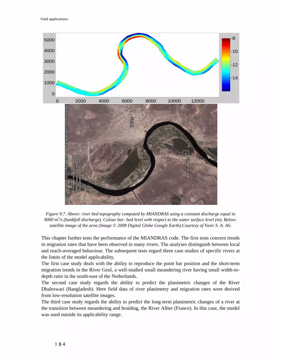
Field applications
1 8 4
0 2000 4000 6000 8000 10000 120000
1000
2000
3000
4000
5000
-14
-12
-10
-8
Figure 9.7. Above: river bed topography computed by MIANDRAS using a constant discharge equal to 8000 m3/s (bankfull discharge). Colour bar: bed level with respect to the water surface level (m). Below:
satellite image of the area (Image © 2008 Digital Globe Google Earth).Courtesy of Yasir S. A. Ali. This chapter further tests the performance of the MIANDRAS code. The first tests concern trends in migration rates that have been observed in many rivers. The analyses distinguish between local and reach-averaged behaviour. The subsequent tests regard three case studies of specific rivers at the limits of the model applicability. The first case study deals with the ability to reproduce the point bar position and the short-term migration trends in the River Geul, a well-studied small meandering river having small width-to-depth ratio in the south-east of the Netherlands. The second case study regards the ability to predict the planimetric changes of the River Dhaleswari (Bangladesh). Here field data of river planimetry and migration rates were derived from low-resolution satellite images. The third case study regards the ability to predict the long-term planimetric changes of a river at the transition between meandering and braiding, the River Allier (France). In this case, the model was used outside its applicability range.

Field applications
1 8 5
9.2 Local migration rates and channel curvature
Observations have shown that the local channel migration rates vary with the ratio of local channel curvature radius, Rc, to bankfull river width, B, and have a maximum at a certain value of Rc/B. The maximum local migration rates are found to occur at approximately Rc/B = 2.5 for rivers in Western Canada [Hickin & Nanson, 1984] (Figure 9.8). Similar relations were found for the rivers Allier (France) and Border Meuse (the Netherlands) by De Kramer et al. [2000] (Figure 9.9) and for the Mississippi River [Hudson & Kesel, 2000] (Figure 9.10).
Figure 9.8. Local migration rate as a function of the local ratio Rc/B for 21 rivers in Western Canada
[Hickin & Nanson, 1984].
Figure 9.9. Local migration rate as a function of the local ratio Rc/B for the rivers Allier and Border Meuse
[De Kramer et al., 2000].
bend sharpness
bend sharpness

Field applications
1 8 6
Mississippi River
Figure 9.10. Local migration rate as a function of the local ratio Rc/B for the rivers Mississippi (left) and Dane (right). On the vertical axis the migration rates, in m/year, and on the horizontal axis the ratio Rc/B
[Hudson & Kesel, 2000]. At low channel curvatures, i.e. large values of Rc/B, there is little channel migration. At larger curvatures, i.e. lower values of Rc/B, both the channel migration rate and the bend sharpness are larger [Hickin, 1977]. After having reached a maximum at a critical value of Rc/B, however, the local migration rates decrease rapidly with further increasing local curvature and bend sharpness [Nanson & Hickin, 1983]. According to, among others, Hickin [1977], Christensen et al. [1999], Blanckaert & Graf [2004], Parsons et al. [2003] and Blanckaert & de Vriend [2004], the decrease of local migration with increasing bend sharpness beyond the critical value (ascending limb of the curves in Figures 9.8 and 9.9 and 9.10) can be attributed to flow separation. This is caused by the presence of secondary flow cells near the outer bank, a phenomenon that is observed in strongly curved bends [Blanckaert et. al, 2002] (Figure 9.11). Although relatively weak and small, these circulation cells strongly reduce the boundary shear stress in the outer bend, thus reducing the rate of erosion of the steep outer banks, i.e. the magnitude of the migration vector.
Figure 9.11. Secondary cell in a sharp bend, as observed in an experimental test by Blanckaert [2002].

Field applications
1 8 7
Another explanation for the decrease in local migration rates as bend sharpness increases could be the shift of the point bar with respect to the bend apex. If with increasing bend sharpness the point bar moves downstream of the bend apex, the location of the point of maximum near-bank velocity and channel migration rate would move even more downstream. In this case, the highest migration rates would not be found at the location of maximum curvature. The position of the point bar influences the direction of the channel migration vector (between cross-stream and downstream migration) and its location, affecting the relation between the migration vector and the local curvature of the channel centreline. In the first kinematic meander migration models by Ferguson [1984] and Howard [1984], the decrease in local migration rates as bend sharpness increases was imposed artificially. Here we investigate whether dynamic meander models are able to reproduce the observed river behaviour and in particular the first ascending limb of the curves in Figures 9.8-9.10. For this purpose, numerical simulations are carried out using two physics-based meander migration models of different classes of complexity [Crosato, 2007b], which allows for identification of the causes of the observed phenomenon. The simplest one is the Ikeda-type model (Section 7.7.2), in which a phase lag between migration rate and local channel centreline curvature is obtained through the adaptation length in the flow equation (Eq. 7.69), as described in Section 7.3 [Parker, 1984]. In this model the point bar is always in phase with the channel curvature, because the transverse water depth deformation is assumed to be proportional to the channel curvature (Eq. 7.68). The other model is MIANDRAS (Crosato model, Section 7.7.3), which includes also the longitudinal adaptation of the bed topography (Eq. 7.71). As a result, this model takes into account the effects of steady alternate bars on migration rates. Besides, in MIANDRAS the point bar is not always in phase with the channel curvature, since it depends on the river conditions (Section 7.6). Neither model includes the flow separation in strongly curved bends. In the computational tests the river is allowed to progressively meander. Width, discharge, valley slope and sediment characteristics are those of the straight-flume experiment T2 (Sections 6.2 and 6.4). The migration rate is related to the near-bank velocity excess only (Eh = 0) and the migration coefficient, Eu, is assumed spatially uniform. The starting river planimetry is a sine-generated curve with wavelength equal to 10B and very small amplitude. Model choices and initial conditions are listed in Tables 8.1 and 8.2. During the computations, the radius of curvature of the channel centreline was computed at three points and no smoothing filter was used. The migration rates are plotted against the local value of the ratio Rc/B in Figures 9.12 (Ikeda-type model) and 9.13 (MIANDRAS). The plots regard all computational points from a region far from the boundaries and distinguish different stages of meander development, each characterized by a certain river sinuosity. The smallest values of Rc/B are most probably caused by the formation of spurious bends due to numerical inaccuracies in the computation of the local curvature [Crosato, 2007b]. These spurious bends are smoothed out and disappear. In nature, small values of the ratio Rc/B are commonly observed.

Field applications
1 8 8
Figure 9.12. Local migration rates vs. local ratio Rc/B at three different values of river sinuosity, S, according to the Ikeda-type model. Migration rates are in m per time-step. Increasing Rc/B corresponds to
decreasing channel curvature.
Figure 9.13. Local migration rates vs. local ratio Rc/B at three values of river sinuosity, S, according to MIANDRAS. Migration rates are in m per time-step. Increasing Rc/B corresponds to decreasing channel
curvature. By analysing Figures 9.12 and 9.13, it is possible to conclude that both models qualitatively reproduce the observed behaviour, although the peak is more pronounced in MIANDRAS than in the Ikeda-type model. MIANDRAS exhibits maximum migration rates for Rc/B between 2 and 3, in good accordance with the field observations (Beatton and Allier Rivers, Figures 9.8 and 9.9, respectively). In the Ikeda-type model the location of the peak occurs for Rc/B between 1.5 and 4. The Border Meuse and Dane Rivers have maximum migration rates at Rc/B equal to 1.5 (Figure

Field applications
1 8 9
9.9 and 9.10 right, respectively) and the Lower Mississippi River at Rc/B equal to 1.0 (Figure 9.10 left). Therefore, the results of the Ikeda-type model are not outside the observed ranges. The peak appears to shift towards larger values of Rc/B with increasing channel sinuosity. This is true for both models, but this trend is stronger in the Ikeda-type model. In both models the migration rates are related to the local near-bank velocity excess, which is driven by the local value of the curvature ratio and its longitudinal variation (derivatives), which in Equations 7.69 and 7.72 are expressed by γ = B/Rc and / sγ∂ ∂ , respectively. In MIANDRAS, channel migration is affected also by the presence of steady alternate bars (not accounted for in the Ikeda-type model). Alternate bars form either at low channel sinuosities or in long quasi-straight reaches between successive bends. The dependence of migration rates on the curvature ratio explains the decrease of the local migration rates as Rc/B increases, but not the increase of migration rates at the smallest values of Rc/B, i.e. the ascending limb of the curve for sharp river bends. Also the overdeepening phenomenon, which can lead to a shift of the point bar position with respect to the bend apex for varying bend sizes, cannot explain this. This phenomenon (Section 7.6) is accounted for only in MIANDRAS, but the Ikeda-type model also reproduces this trend. Since the models do not include flow separation, also flow separation is not needed to explain the observed decrease of migration rates with increasing bend sharpness beyond a critical value (ascending limb of the curves in Figures 9.8-9.10), although flow separation is believed to enhance the phenomenon [Blanckaert & de Vriend, 2004]. The dominant effect stems from the phase lag between near-bank velocity, which is assumed to govern the local channel migration, and curvature, analysed in Section 7.3. The sharper and shorter the bend (sharp parts of bends are relatively short) the more this phase-lag tends towards 90 degrees (maximum excess velocity at the downstream end of the bend), which also explains why short bends are damped away by the models [Ikeda et al., 1981]. The shifting of point bar position might explain the different form and the more pronounced peak of the curves obtained with MIANDRAS. In well developed river bends the position of the point bar is slightly upstream of the bend apex, which decreases the phase-lag between migration rates and curvatures. With further bend development and increasing sharpness, however, the point bar moves towards the bend apex (Section 7.6.5) and the velocity deformation tends to be 90 degree out of phase with the curvature, i.e. the maximum value of the near-bank velocity excess tends to be located at the downstream bend crossing point. At the lowest sinuosities the two models have different behaviours, as shown in Figures 9.14 (Ikeda-type model) and 9.15 (MIANDRAS). In the Ikeda-type model (Figure 9.14), local channel migration is governed by channel curvature at the lowest sinuosities, when the curvatures are extremely small and Rc extremely large. In this case, the erosion rates are low, because the near-bank flow velocity excesses are small. The dependence on the local curvature is only “disturbed” by the presence of a phase lag between curvature and velocity excesses. In MIANDRAS (Figure 9.15), the migration rates are almost independent from the channel curvature. This is caused by the presence of alternate bars inside the channel (eigen-oscillation), causing flow and water depth deformations, in combination with the assumption that the migration rate depends on the depth-averaged mean flow velocity near-the bank, not on secondary flow effects. At the lowest sinuosities the deformation caused by the presence of the alternate bars is more pronounced than the deformation caused by the (very mild) channel

Field applications
1 9 0
curvature. For this reason, the migration rates are higher than in the Ikeda-type model and almost independent from the channel curvature.
Figure 9.14. Local migration rates vs. local ratio Rc/B for two values of river sinuosity according to the
Ikeda-type model. Migration rates are in m per time step. In the legend, S = 1.0 corresponds to the channel sinuosity at the start of the computations, when the value of the sinuosity is less than 1.02.
Figure 9.15. Local migration rates vs. local ratio Rc/B for two values of river sinuosity according to
MIANDRAS. Migration rates are in m per time step. In the legend, S = 1.0 corresponds to the channel sinuosity at the start of the computations, when the value of the sinuosity is less than 1.02.

Field applications
1 9 1
If the channel migration rate is also related to the excess water depth, sharp river bends might increase in size because the phase lag between maximum migration rate and pool depth diminishes. This is especially true in small rivers with cohesive banks in which bank failure is the process governing bank retreat.
9.3 Variation of average migration rates with increasing river sinuosity
Reach-averaged channel migration rates, including meander migration and bend growth, change with the increase of meander size and river sinuosity and reach a maximum at a certain river sinuosity [Friedkin, 1945] (Figure 9.16). The maximum reach-averaged migration rates are found to occur at a sinuosity between 1.6 and 1.9 for the Mississippi River [Shen & Larsen, 1988].
Figure 9.16. Development of meanders during a laboratory experiment by Friedkin [1945]. Note that the migration rates first increase and then decrease as meandering progresses.
This is not another aspect of the case treated in the previous section, because it does not regard sharp river bends. The acceleration and subsequent deceleration of the channel migration observed by Friedkin and Shen & Larsen occurs also where the ratio of radius of curvature to channel width is much larger than the critical value indentified by Hickin & Nanson [1984] (Section 9.2). Nevertheless, the two different aspects of channel migration are often confused [e.g. Seminara et al., 2001]. Analysing the model by Ikeda et al. [1981], Parker et al. [1982] found that increasing meander amplitudes are associated with decreasing downstream migration rates, but accelerating lateral growth. Parker & Andrews [1986] attributed the phenomenon to the development of a characteristic skewing, or asymmetry, in river bends. However, observations show that it is not only the downstream migration rate that decreases, but also the lateral growth of bends. The latter phenomenon has not been explained yet. Seminara et al. [2001] attribute this behaviour to higher harmonics of a general periodic solution for river planimetry, but their kinematic analysis does not give physical explanations. Similarly to the previous analysis (Section 9.2), we will investigate the observed behaviour using two meander migration models of different classes of complexity: the Ikeda-type model (Section 7.7.2) and MIANDRAS (Section 7.7.3) [Crosato, 2007b]. We first investigate whether the models can reproduce the observed behaviour without inserting an extra migration coefficient expressing the effects of changing sinuosity on the primary flow [Parker, 1983]. Subsequently, the causes of

Field applications
1 9 2
the observed phenomenon are analysed by comparing the results. In both models the longitudinal river bed slope is determined as a function of the river sinuosity by assuming the valley slope to remain constant (Eq. 8.4). This means that with increasing bend sizes and river sinuosity the channel slope decreases, which leads to a decrease of flow velocity and width-to-depth ratio. In MIANDRAS, the decrease of width-to-depth ratio leads to an increase of the damping coefficient (Eq.7.23), which results in the decrease of the overshoot/overdeepening phenomenon and of the migration rates. As in the previous section, the river in these tests is allowed to progressively meander. Width, discharge, valley slope and sediment characteristics are those of the straight-flume experiment T2 (Chapter 6, Sections 6.2 and 6.4). The migration rate is related to the near-bank velocity excess only (Eh = 0) and the migration coefficient, Eu, is assumed spatially uniform. The initial river planimetry is a sine-generated curve with wavelength equal to 10B and very small amplitude. The variation of the reach-averaged migration rate with the channel sinuosity is plotted in Figures 9.17 (Ikeda-type model) and 9.18 (MIANDRAS).
Figure 9.17. Reach-averaged migration rates vs. river sinuosity according to the Ikeda-type model.
Figure 9.18. Reach-averaged migration rates vs. river sinuosity according to MIANDRAS.

Field applications
1 9 3
Figures 9.17 and 9.18 show that in both models the reach-averaged migration rate exhibits a maximum at a certain value of the channel sinuosity, which means that both models are able to qualitatively reproduce the observed phenomenon. In MIANDRAS the variations and the peak are more pronounced and the peak occurs at a lower sinuosity. In the tests, the trend follows from the variation of the reach-averaged value of the ratio, Rc/B, with the river sinuosity (Figure 9.19). Since the reach-averaged values of Rc/B are larger than the critical value identified by, among others, Hickin & Nanson, [1984] (Section 9.2), the migration rate increases with the curvature ratio γ (=B/Rc) [Parker, 1984], as in the descending limb of the curves in Figures 9.8, 9.9 and 9.10. The strong initial decrease of Rc/B as the sinuosity increases explains the rising limb in the relation between reach-averaged migration rates and river sinuosity (Figures 9.17 and 9.18). The falling limb results also from the combined effects of increasing Rc/B and decreasing bed slopes and is more pronounced in MIANDRAS, because the Ikeda-type model does not take into account the overdeepening phenomenon.
Figure 9.19. Reach-averaged Rc/B vs. river sinuosity (CROSATO=MIANDRAS). In the tests performed the initial conditions are those of a system with small damping. In the initial steps of meandering, alternate bars (eigen-oscillation) in MIANDRAS are in phase with incipient channel bends. This maximizes the overdeepening phenomenon and enhances the differences between the two models. The computational tests are repeated for a system having a higher damping coefficient, in which the overdeepening phenomenon is strongly reduced. The results of MIANDRAS are plotted in Figure 9.20. In this case, MIANDRAS yields a less pronounced descending limb than in Figure 9.18, whereas the behaviour of the Ikeda-type model is similar to that of Figure 9.17 (no need for a separate plot). With larger damping the behaviour of the two models is more similar.

Field applications
1 9 4
Figure 9.20. Reach-averaged migration rates vs. river sinuosity according to MIANDRAS (damped system). The computations were carried until the channel sinuosity had reached a value of 2.0 (do not compare the
migration rates with those of Figure 9.18, because the systems are different).
9.4 Prediction of present morphological trends of the River Geul (the Netherlands)
9.4.1 General description
Miguel-Alfaro [2006] used MIANDRAS to study the morphological trends of the Geul River in the Netherlands. Thorough comparisons between model predictions and observed morphological trends, in particular on extension and location of the point bars, were made possible by the collaboration of researchers from the Free University of Amsterdam who made available field data and experience [Spanjaard, 2004; de Moor, 2007; de Moor et al., 2007]. This study is not suitable to test the ability of MIANDRAS to reproduce long-term migration trends, because the past river planimetries that were derived from aerial photographs are not accurate enough [Miguel-Alfaro, 2006]. This is a general problem when dealing with small rivers, because the error of a few metres in the location of the channel centreline can be unacceptable if the maximum migration rates are of the order of one metre per year or less. The Geul River springs near the village of Lichtenbusch, in Eastern Belgium, crosses the Belgian-Dutch border near Sippenaeken and joins the River Meuse near Meerssen in the South-East of the Netherlands (Figure 9.21). The total river length is 56 km for a total catchment area of 380 km2. The valley gradient decreases from 0.02 (m/m) near the source to 0.0015 at Meerssen. The river discharge at the confluence with the Meuse is strongly variable and ranges between 0.8 and 65 m3/s.

Field applications
1 9 5
Figure 9.21. Location and elevation map of the Geul River catchment (re-elaborated after De Moor [2007] and Dautrebande at al. [2000])
The study reach is 2.5 km long and belongs to the freely meandering part of the river. It includes seven, rather regular, river bends (Figures 9.22 and 9.23). In the study reach, the river channel is wider at the bend apexes (15.5 m) and narrower at the bend crossings (8 m). The bankfull conditions are met every 1.5 to 2 years by discharges around 20 m3/s. At bankfull conditions the averaged water depth ranges between 2.0 and 2.5 m and the width-to-depth ratio between 3 and 7. The river channel cuts through a 2-2.5 m thick silty-clay deposit that formed in the first and second millennium after Christ after large-scale deforestations. This layer of fine-sediment covers Weichselian gravel deposits. The river channel has therefore a gravel bed and cohesive banks. The bed material on the point bars is bimodal, with a fine and a coarse fraction. In general, the grainsize of the fine fraction ranges between 10 and 100 mμ , that of the coarse fraction between 200 and 400 mμ [Spanjaard, 2004]. The sediment in the deepest parts of the river bed (pools) and in the straight reaches between opposite bends (riffles) is gravel. In these areas the river bed is armoured and the medium size of the top layer ranges between 45 and 52 mm. The armour layer is disrupted at bankfull or higher flow stages.

Field applications
1 9 6
Figure 9.22. Location of the study reach in the river catchment.
Figure 9.23. Aerial photograph 2003 of the Geul River in the study area. In the study reach bank protection is absent and erosion is found on almost all concave banks. The primary erosion mechanism is failure due to toe erosion (Figure 9.24). Based on the aerial photographs 1983 and 2003, Miguel-Alfaro [2006] found that the present channel migration rates at river bends range between 0.24 and 0.84 m/year, whereas, based on field observations, Spanjaard found the migration rates to vary between 0.4 and 0.6 m/year. The two independent estimates of migration rates agree fairly well. It can therefore be concluded that the maximum averaged migration rates are of the order of magnitude of 0.5 m/year. With this low value, the differences between the channel alignments in consecutive years are small, which makes it difficult to compare historical planimetries with each other. This is the problem encountered by Miguel-Alfaro, since the magnitude of the error made in the rectification and fitting of old aerial
river flow
7 6 5 4 3 2 1

Field applications
1 9 7
photographs is of the order of magnitude of 5 m. The historical channel alignments could be compared only at specific locations, where fixed points were recognizable.
Figure 9.24. Bank failure in the study reach (courtesy Eva Miguel-Alfaro).
9.4.2 Approach
A discharge of 22 m3/s (bankfull) was assumed to represent the formative conditions for the bed topography and the river planimetry. For this value of the discharge the averaged water depth of 2.0 m (bankfull mean water depth) is obtained for a Chezy coefficient equal to 20 m1/2/s. This low value is acceptable for this type of river. Considering the strong variability, the values of channel width and sediment grain size were optimized by minimizing the difference between the predicted and the observed longitudinal distribution of bank erosion (observed bank instability characteristics in Figure 9.25). The values of the calibration coefficients, such as the migration coefficients Eu and Eh, were derived from the estimated migration rates.

Field applications
1 9 8
Figure 9.25. Observed conditions of the Geul River banks in the study reach [Spanjaard, 2004]. The resulting river characteristics at bankfull discharge are summarized in Table 9.1. The values of the calibration coefficients are summarized in Table 9.2.
Table 9.1. Characteristics of the Geul River at bankfull discharge. QW
(m3/s) B
(m) C
(m1/2/s) b
(-) iv
(-)* h0
(m) u0
(m/s) D50 (m)
D90 (m)
λS
(-)
λW
(-)
α (-)
β (-)
22 8 20 4 0.004 2 1.38 0.025 0.05 0.73 46 0.016 4 * valley slope
Table 9.2. Calibration coefficients (uniformly erodible floodplains).
1α
(-)
σ (-)
E (-)
Eh (1/s)
Eu (-)
0.4 4 1 6.0×10⁻⁶ 4.0×10⁻⁶ The Geul River system is highly damped and falls outside the harmonic range of the river response (Chapter 7.2), which means that in this case the overshoot/overdeepening phenomenon is negligible and that MIANDRAS behaves very similarly to the Ikeda-type model.
9.4.3 Results
The predicted river bed topography is given in Figure 9.26. The observed position and location of the point bars, categorized in active, active, vegetated and inactive bars [Spanjaard, 2004], is shown in Figure 9.27. In the figures the river bends are numbered to facilitate comparison.

Field applications
1 9 9
Figure 9.26. Bed topography by MIANDRAS. In x and y axes the coordinates (m) [Miguel-Alfaro, 2006].
Figure 9.27. Observed point bars and bank characteristics in the study reach [Spanjaard, 2004]. The predicted position and extension of the point bars (light gray colours in Figure 9.26) are in good agreement with the observed ones (Figure 9.27). The planimetries used in the two independent studies were not identical, since Spaniaard used topographic maps of the area [Topografische Dienst Nederland, 1998] with an original scale of 1:25.000, magnified to scale 1:1.250, whereas Miguel-Alfaro used the aerial photo 2003 (Figure 9.23). This explains part of the differences, especially in bend number 7.
1
2
3
4
5
6
7
river flow
bed level with respect to the river bank (m)
1
3
2 5 7
4
6

Field applications
2 0 0
9.4.4 Conclusions
MIANDRAS reproduces the bed topography of the Geul River rather well. This is a typical small river with a gravel bed, cohesive banks and strongly variable discharges. This type of rivers is characterized by sharp bends, small width-to-depth ratios and high damping coefficients (Eq. 7.12) [Mosselman, 1993]. Steady alternate bars can only form at the lowest flow stages in the straight or mildly curved reaches, where the width-to-depth ratio is (only temporarily) larger [Dietrich et al., 1984]. Besides, if ever formed, these alternate bars tend to be ephemeral, since in most cases they do not have the time to consolidate and are smoothed out at high flow stages. High damping coefficients at the formative conditions also mean that for this type of rivers MIANDRAS behaves similarly to the Ikeda-type model. The River Geul has a partly armoured bed (in pools and runs) at discharges less than bankfull. This means that the formative conditions are found at bankfull or higher flow stages. Since at these stages the overshoot/overdeepening phenomenon is negligible or absent, the morphological behaviour is dominated by the local conditions, such as a change in bank erodibility, a fallen tree etc. [Spanjaard, 2004]. Finally, the Geul River exhibits a larger width at bend apexes, a phenomenon that has been observed also in other meandering rivers [Seminara et al., 2001]. This most probably occurs if the two processes of bank erosion and opposite bank accretion are out of phase [Nanson & Hickin, 1983; Pizzuto, 1994]. The nature of the sediment forming the river bed and banks, the chronology of high and low discharges and the presence of riparian vegetation are of essential importance for this phenomenon. Most probably significant width variations have consequences either for the bed topography or for the migration trends. Allowing for width variations could represent an important improvement in meander migration models [Repetto et al., 2002].
9.5 Prediction of planform changes of the River Dhaleswari (Bangladesh)
9.5.1 General description
Murshed [1991] applied MIANDRAS to predict future planimetric changes of the Dhaleswari River in Bangladesh. As more than 15 years have passed since, this case offers an excellent opportunity to evaluate these predictions. Murshed used information on past planimetric changes that had been derived from LANDSAT Multi Spectral Scanner (MSS) satellite images. The resolution of the MSS sensor was approximately 80 m, with an actual sampling resolution of 79 x 56 m. Due to the low resolution it was not possible to distinguish between zones of different bank erodibility nor to recognize bank protection works. The Dhaleswari River is located on the plain between the Himalayas and the Gulf of Bengal. It is one of the major offtakes on the left bank of the Brahmaputra-Jamuna River. The river flows from the Jamuna near Tangail (North West of Dhaka) and joins the Meghna River a few miles above the junction of the Padma and the Meghna rivers. Information on the Jamuna River system is provided by Coleman [1969]. The location of the study area is indicated in Figure 9.28.
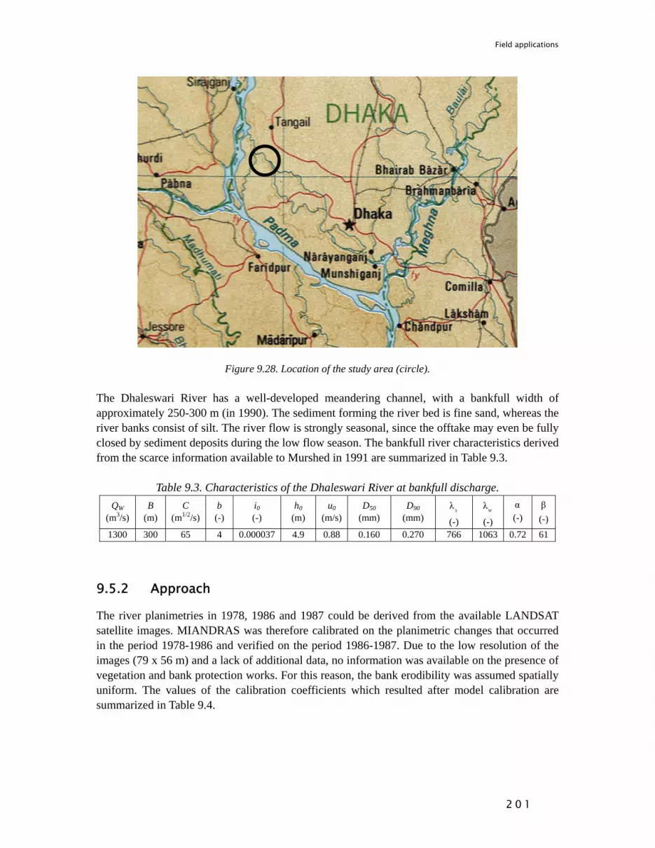
Field applications
2 0 1
Figure 9.28. Location of the study area (circle). The Dhaleswari River has a well-developed meandering channel, with a bankfull width of approximately 250-300 m (in 1990). The sediment forming the river bed is fine sand, whereas the river banks consist of silt. The river flow is strongly seasonal, since the offtake may even be fully closed by sediment deposits during the low flow season. The bankfull river characteristics derived from the scarce information available to Murshed in 1991 are summarized in Table 9.3.
Table 9.3. Characteristics of the Dhaleswari River at bankfull discharge. QW
(m3/s) B
(m) C
(m1/2/s) b
(-) i0 (-)
h0 (m)
u0 (m/s)
D50 (mm)
D90 (mm)
λS
(-)
λW
(-)
α (-)
β (-)
1300 300 65 4 0.000037 4.9 0.88 0.160 0.270 766 1063 0.72 61
9.5.2 Approach
The river planimetries in 1978, 1986 and 1987 could be derived from the available LANDSAT satellite images. MIANDRAS was therefore calibrated on the planimetric changes that occurred in the period 1978-1986 and verified on the period 1986-1987. Due to the low resolution of the images (79 x 56 m) and a lack of additional data, no information was available on the presence of vegetation and bank protection works. For this reason, the bank erodibility was assumed spatially uniform. The values of the calibration coefficients which resulted after model calibration are summarized in Table 9.4.

Field applications
2 0 2
Table 9.4. Calibration coefficients (uniformly erodible floodplains).
1α
(-)
σ (-)
E (-)
Eh (1/s)
Eu (-)
0.35 1.5 2.5 1.858×10⁻⁶ 9.575×10⁻⁶
9.5.3 Results
Figures 9.29 and 9.30 show the predicted river planimetries in 1993 and 2000, respectively (white lines). These figures show also the 2005 channel centreline (thick black line), derived from Google Earth (Figure 9.31), for comparison. In the background, the 1986 satellite image, in which the colour blue represents water, shows the starting situation. Several abandoned channels and a large lake are recognizable (in blue). Finally, the dotted black lines represent abandoned river channels that were still detectable from the Google Earth picture (Figure 9.31), from which parts of the 1986 river planimetry can still be recognized.
Figure 9.29. Background: study area in 1986 from a LANDSAT MSS image. Blue line: the Dhaleswari River centreline in 1986. Bold black line: channel centreline in 2005; thin black lines: contours of main
water bodies and thin dotted black lines: old river paths recognizable from the 2005 Google Earth image. White line: channel centreline in 1993 as predicted by MIANDRAS.
cutoff area

Field applications
2 0 3
Figure 9.30. Background: study area in 1986 from a LANDSAT MSS image. Blue line: the Dhaleswari River centreline in 1986. Bold black lines: channel centreline in 2005; thin black lines: contours of main water bodies and thin dotted black lines: old river paths recognizable from the 2005 Google Earth image.
White line: channel centreline in 2000 as predicted by MIANDRAS. Superimposing the Google Earth river planimetry on the LANDSAT MSS satellite images was made possible by a lake and an oxbow lake which were clearly recognizable in all images (Figure 9.31). By comparing the predictions to the 2005 planimetry, it appears that MIANDRAS overestimated the channel migration significantly. The predicted planimetry in 1993 (Figure 9.29) is closer to the 2005 river configuration than the predicted planimetry in 2000 (Figure 9.30). This indicates an overestimation of either migration coefficients or formative discharge. Besides, an unpredictable (for MIANDRAS) chute cutoff occurred in the study area in the period 1987-2005. The river captured the old channel that is still visible in the LANDSAT satellite image 1986. New meanders formed in the (initially) mildly-curved new alignment, but with considerably smaller wavelengths than the previously formed meanders (Figures 9.29 and 9.30 top right parts). This could be explained by a lowering of the discharges [Fergusson, 1863]. In MIANDRAS, the wave length, LP, of the river’s eigen-oscillation, from which meanders start to grow (Eq. 7.11), is a function of the width-to-depth ratio,β :
1/ 22 22 1 1 1 ( 3)( 1)2 4P W
bbL
⎡ ⎤−⎛ ⎞= + − −⎢ ⎥⎜ ⎟⎝ ⎠⎢ ⎥⎣ ⎦
πλ α α
with 22
0
1 12 ( )fC f
⎛ ⎞= ⎜ ⎟
⎝ ⎠
πα θ β
(9.1)
For the Dhaleswari River, the estimated value of α was 0.72 (Table 9.3), which corresponds to 1/ α 1.38= . Figure 7.3a (Chapter 7) shows that for values of 1/α smaller than approximately 2.5 (for b = 4) the wave number increases and the wave length decreases as the width-to-depth ratio decreases. Since reduced river discharges eventually lead to smaller width-to-depth ratios, also MIANDRAS yields a smaller wavelength of the eigen-oscillation.
cutoff area
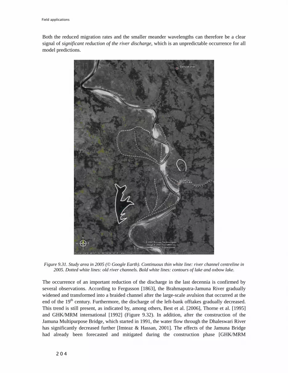
Field applications
2 0 4
Both the reduced migration rates and the smaller meander wavelengths can therefore be a clear signal of significant reduction of the river discharge, which is an unpredictable occurrence for all model predictions.
Figure 9.31. Study area in 2005 (© Google Earth). Continuous thin white line: river channel centreline in
2005. Dotted white lines: old river channels. Bold white lines: contours of lake and oxbow lake. The occurrence of an important reduction of the discharge in the last decennia is confirmed by several observations. According to Fergusson [1863], the Brahmaputra-Jamuna River gradually widened and transformed into a braided channel after the large-scale avulsion that occurred at the end of the 19th century. Furthermore, the discharge of the left-bank offtakes gradually decreased. This trend is still present, as indicated by, among others, Best et al. [2006], Thorne et al. [1995] and GHK/MRM international [1992] (Figure 9.32). In addition, after the construction of the Jamuna Multipurpose Bridge, which started in 1991, the water flow through the Dhaleswari River has significantly decreased further [Imteaz & Hassan, 2001]. The effects of the Jamuna Bridge had already been forecasted and mitigated during the construction phase [GHK/MRM

Field applications
2 0 5
international, 1992], but the intake of the Dhaleswari River appears to have been influenced also by the development of a large sand deposit. It is not clear whether the bridge has enhanced the formation of this deposit or not.
Figure 9.32. Decrease of maximum (continuous line), mean (dashed line) and minimum (dot-dash line)
annual water discharges in the Dhaleswari River at Jagir in the period 1964-1990 [GHK/MRM international, 1992].
Murshed [1991] assumed the formative discharge to be 1300 m3/s (Table 9.3), a value far too high for the conditions of the Dhaleswari River after 1967, but in line with the antecedent river regime. Unfortunately, due to the lack of data on the actual cross-sections of the river, it is not possible to repeat the runs with a lower bankfull discharge.
9.5.4 Conclusions
The application demonstrates key caveats in the prediction of long-term morphological predictions. First, the quality of predictions depends to a large extent on reliable predictions of the boundary conditions, such as the river discharge. The discrepancies between predictions and the 2005 observations point at a significant reduction of the flow in the Dhaleswari River. In the application, Murshed clearly overestimated the value of the formative discharge. Second, at longer time scales, bend cutoffs may occur for which no adequate submodel has been included in MIANDRAS.

Field applications
2 0 6
9.6 Prediction of planform changes of the River Allier (France)
9.6.1 General description
Blom [1997] applied MIANDRAS to study the planform changes of the River Allier (France), a highly dynamic river at the threshold between meandering and braiding characterized by frequent and intense floods. This study therefore delineates the model performance at the limit of its applicability range.
Figure 9.33. Location of the River Allier. The ellipse indicates the location of the study reach. The River Allier, a tributary of the Loire, is a gravel-bed, rain-fed river originating in the Massif Central (Figure 9.33). It is one of the most natural river systems of this size in Europe and one of the most studied [Baptist, 2005; De Kramer et al., 2000]. This study deals with the river reach situated just upstream of the town of Moulins (Figure 9.34). In this area, the river belongs to a natural reserve and most of its banks are unprotected. Upstream of Moulins, the river channel exhibits a meandering planform, but also presents some secondary channels (Figure 9.34). Strongly fluctuating discharges, together with bank erosion and accretion, cause continuous evolution of the river topography and natural floodplain rejuvenation [Baptist & de Jong, 2005]. As a result, riparian vegetation mainly consists of pioneer species (willow trees), whereas only the highest parts of the floodplains are suitable for a rather permanent softwood forest with mainly poplar trees.
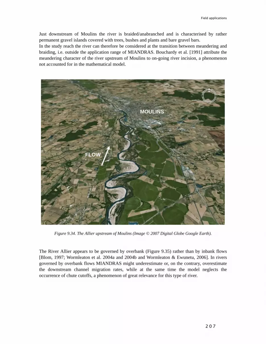
Field applications
2 0 7
Just downstream of Moulins the river is braided/anabranched and is characterised by rather permanent gravel islands covered with trees, bushes and plants and bare gravel bars. In the study reach the river can therefore be considered at the transition between meandering and braiding, i.e. outside the application range of MIANDRAS. Bouchardy et al. [1991] attribute the meandering character of the river upstream of Moulins to on-going river incision, a phenomenon not accounted for in the mathematical model.
Figure 9.34. The Allier upstream of Moulins (Image © 2007 Digital Globe Google Earth). The River Allier appears to be governed by overbank (Figure 9.35) rather than by inbank flows [Blom, 1997; Wormleaton et al. 2004a and 2004b and Wormleaton & Ewunetu, 2006]. In rivers governed by overbank flows MIANDRAS might underestimate or, on the contrary, overestimate the downstream channel migration rates, while at the same time the model neglects the occurrence of chute cutoffs, a phenomenon of great relevance for this type of river.
MOULINS
FLOW

Field applications
2 0 8
Figure 9.35. Flow pattern in a meandering compound channel at overbank flow [Ervine et al., 1993].
9.6.2 Approach
To study the past planimetric changes of the River Allier in the study reach, Blom [1997] derived several historical channel centrelines from aerial photographs using the digital image processing software ERDAS Imagine. The aerial photos and maps that were available for the study regarded the years 1946, 1954, 1960, 1967, 1971, 1982, 1992 and 1995. A map after rectification and fitting of aerial photographs is shown in Figure 9.36 and the derived historical channel centrelines are shown in Figure 9.37.
Figure 9.36. A map after rectification and fitting of aerial photographs (1957) [Blom, 1997].

Field applications
2 0 9
Figure 9.37. Channel centrelines derived from the aerial photographs and maps [Blom, 1997]. The water flows from left to right.
The averaged monthly and yearly discharges are given in Figure 9.38, where strong variations are observable from month to month and from year to year. Since the bankfull conditions are found at discharges of about 300 m3/s, by observing the time series of the monthly discharges in Figure 9.38 (top diagram) it is easy to deduce that overbank flows occur rather frequently, about once per year.
500
600Allier, Yearly Mean Discharge
)
1968 1970 1972 1974 1976 1978 1980 1982 1984 1986 1988 1990 1992 1994 19960
100
200
300
400
500
600Allier, Monthly Mean Discharge
Time
Dis
char
ge (m
3/s)
Figure 9.38. Monthly and yearly water discharges of the Allier River in the study reach.
FLOW
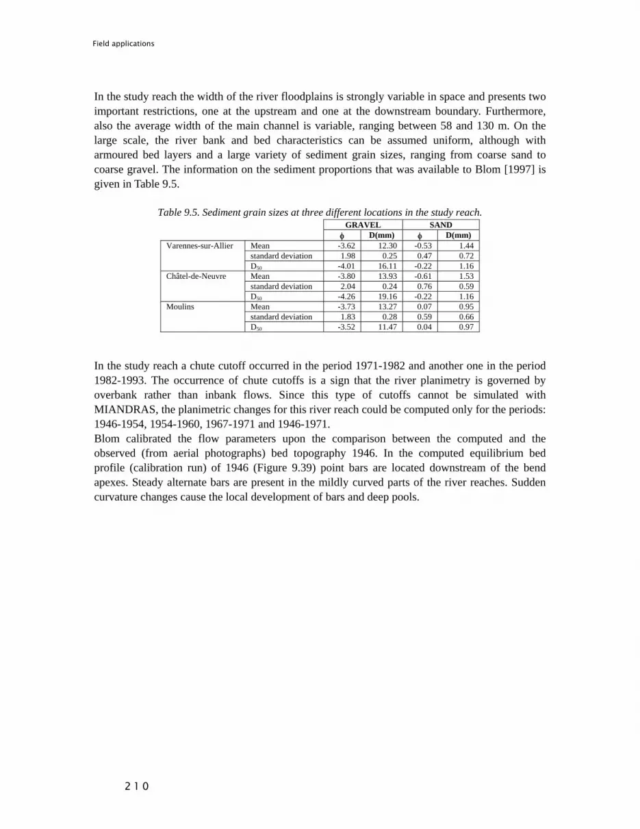
Field applications
2 1 0
In the study reach the width of the river floodplains is strongly variable in space and presents two important restrictions, one at the upstream and one at the downstream boundary. Furthermore, also the average width of the main channel is variable, ranging between 58 and 130 m. On the large scale, the river bank and bed characteristics can be assumed uniform, although with armoured bed layers and a large variety of sediment grain sizes, ranging from coarse sand to coarse gravel. The information on the sediment proportions that was available to Blom [1997] is given in Table 9.5.
Table 9.5. Sediment grain sizes at three different locations in the study reach. GRAVEL SAND φ D(mm) φ D(mm)
Mean -3.62 12.30 -0.53 1.44 standard deviation 1.98 0.25 0.47 0.72
Varennes-sur-Allier
D50 -4.01 16.11 -0.22 1.16 Mean -3.80 13.93 -0.61 1.53 standard deviation 2.04 0.24 0.76 0.59
Châtel-de-Neuvre
D50 -4.26 19.16 -0.22 1.16 Mean -3.73 13.27 0.07 0.95 standard deviation 1.83 0.28 0.59 0.66
Moulins
D50 -3.52 11.47 0.04 0.97 In the study reach a chute cutoff occurred in the period 1971-1982 and another one in the period 1982-1993. The occurrence of chute cutoffs is a sign that the river planimetry is governed by overbank rather than inbank flows. Since this type of cutoffs cannot be simulated with MIANDRAS, the planimetric changes for this river reach could be computed only for the periods: 1946-1954, 1954-1960, 1967-1971 and 1946-1971. Blom calibrated the flow parameters upon the comparison between the computed and the observed (from aerial photographs) bed topography 1946. In the computed equilibrium bed profile (calibration run) of 1946 (Figure 9.39) point bars are located downstream of the bend apexes. Steady alternate bars are present in the mildly curved parts of the river reaches. Sudden curvature changes cause the local development of bars and deep pools.

Field applications
2 1 1
Figure 9.39. Computed 1946 bed topography. Water flows from left to right [Blom, 1997]. After the calibration of the flow parameters, the migration coefficients were derived from the planimetric changes for each of the above-mentioned periods. The bed topography was computed assuming a time-dependent development for the simulation of the planimetric changes, whereas the calibration of the flow parameters (with fixed banks) was based on the equilibrium bed topography (steady state computations). The parameter settings for bankfull conditions are summarized in Tables 9.6 and 9.7. The migration coefficients Eu and Eh are both spatially variable (Section 9.7.3). Although the river is at the transition between meandering and braiding, the values of these bankfull parameters fall within the range of applicability of MIANDRAS.
Table 9.6. Characteristics of the Allier River adopted in MIANDRAS after calibration. QW
(m3/s) B
(m) C
(m1/2/s) b (-)
iv** (-)
h0 (m)
u0 (m/s)
D50 (mm)
D90 (mm)
λS
(-)
λW
(-)
α (-)
β (-)
325 65 47 5.2 8.33E-4 2.61 1.91 5 30 62.3 294.1 0.212 25 ** valley slope
Table 9.7. Calibration coefficients.
1α
(-)
σ (-)
E (-)
Eh (1/s)
Eu (-)
Space step (m)
Time step (days)
No Smoothing
0.5 2.0 1.0 variable variable 20 78 40
9.6.3 Results
The distribution of the migration coefficients was optimized for each simulation period: 1946-1971, 1946-1954, 1954-1967, and 1967-1971. Four different distributions were obtained, in which the values of the migration coefficients, although different, have the same order of

Field applications
2 1 2
magnitude. The results of the different distributions appear quite similar, although problems arise at the border of the areas having different erodibility. As expected, the best results are provided by the distribution that was calibrated on the entire period 1946-1971 (red line in Figure 9.40).
Figure 9.40. Computed planform changes for the period 1946-1971 using the distribution of erosion coefficients derived from the period 1946-1971. The red line delineates the computed 1971 planimetry. The white lines delineate the non-erodible dikes delimiting the floodplain. The dotted black line represents the
observed 1946 river planimetry, whereas the continuous black line represents the observed 1971 river planimetry [Blom, 1997].
The spatial variability of the migration coefficients cannot be justified by variations in the river bed and bank characteristics, such as the sediment composition or the bank geometry, since in the study reach these conditions are rather uniform. Therefore, other phenomena must be responsible for the necessity of adopting spatially varying migration coefficients in MIANDRAS. By performing 3-D and 2-DH flow computations with the Delft3D software [WL⎮Delft Hydraulics, 2003], Blom [1997] showed that this necessity can be ascribed to overbank flow, which occurs rather frequently and intensively in this part of the Allier. Figure 9.41 shows the results of a 2-DH flow computation representing the situation at a discharge of 960 m3/s. In this computation, the main channel has a rectangular cross-section, 65 m wide and 2 m deep, and the 1946 planimetry. The roughness of the main channel is represented by a Chézy coefficient equal to 47 m1/2/s and the roughness of the floodplains, assumed to be covered by vegetation, by a Chézy coefficient equal to 25 m1/2/s. Figure 9.41 shows that velocities are relatively high during overbank flow, in the upstream part of the study reach with a floodplain restriction. This explains

Field applications
2 1 3
the necessity of imposing high values to the migration coefficients in this area. Backwater effects, caused by a floodplain restriction more downstream, and local floodplain widening slow down the water flow in the downstream half of the study reach. This explains the necessity of imposing lower values of the migration coefficients in this area. Due to the local restriction the flow velocity increases again near the downstream boundary, but there bank protection prevents river channel migration.
Figure 9.41. Flow velocity in main channel and floodplains in m/s at a discharge of 960 m3/s [Blom, 1997].
9.6.4 Conclusions
The results of this study give new indications for the range of applicability of MIANDRAS. Besides the possibility of using MIANDRAS on rivers with mainly inbank flow, the model can also be applied to rivers with frequent overbank flows, provided that the flow exchange between the main channel and the floodplains is small. A small flow exchange occurs in case of high floodplain bed roughness, as for instance in presence of riparian vegetation, in rivers where the floodplains and the main channel are parallel and for discharges slightly above bankfull. In the study reach, the Allier consists of a meandering channel with wide floodplains. Here the river is subject to frequent and intense overbank flows and consequent chute cutoffs. Floodplain enlargements and restrictions as well as 3-dimensional effects, due to the interaction between main channel and floodplains, influence the near-bank flow velocities and the bed shear stresses. Therefore in the Allier, and most probably in all rivers characterized by frequent floods, overbank flow strongly influences the river planimetric changes. MIANDRAS cannot simulate the situation of overbank flow, as the model only considers the flow in the main channel. Nevertheless, the effects of floods can be taken into account by relating the values of the migration coefficients to the velocity distribution at overbank flows. Where the flow velocity is higher, as for instance at floodplain restrictions, the migration coefficients should also be higher. Vice versa, where the flow velocity is lower, in floodplain enlargements or in the presence of backwater effects, the migration coefficients should be lower.

Field applications
2 1 4
The transitions between the areas characterized by different migration coefficients can cause problems in MIANDRAS, since the river centreline computed for the next time often exhibits a “deformation” at these transitions. To avoid these undesirable irregularities the boundaries of the areas with different migration coefficients should be chosen as much as possible perpendicular to the local river migration vector. The possibility of adopting a smooth distribution of migration coefficients in MIANDRAS would be convenient.

Conclusions
2 1 5
10 Conclusions and recommendations
10.1 Scope and modelling approach
This thesis examines non-tidal meandering rivers, focusing on their medium- to long-term topographic and planimetric changes at the large spatial scale, where “medium- to long-term” refers to the temporal scale of a meander lateral shift that can be scaled with the river corridor width and “large spatial scale” to the length and size of several meanders. This spatio-temporal scale is referred to as the “engineering scale”. The work includes the development of a numerical model for the simulation of the long-term evolution of meandering rivers, MIANDRAS. Together with experimental and field data, this model constitutes the main tool for the analyses carried out in the framework of the study, in which its behaviour is compared to the behaviour of other physics-based meander migration models of lower complexity. The results show the importance of this type of comparison, since they allow for the detection of the role of specific factors on river meandering. In the simplest model used for the comparisons migration rates are directly proportional to the local channel curvature. Another model used for the comparisons includes a phase lag between migration rate and channel curvature, which is obtained through an adaptation term in the flow equation. MIANDRAS, the model developed in the framework of this study, also includes an adaptation term for the bed topography, which is obtained by fully coupling the 2-D momentum and continuity equations describing the water flow (the St Venant equations) to a sediment capacity and a sediment balance equation. In this way the model is able to reproduce the overshoot/overdeepening phenomenon, which consists of the formation of a steady harmonic response of the bed topography and the flow downstream of perturbations. This steady response of the river is here referred to as eigen-oscillation. This oscillation does not form in rivers with small width-to-depth ratios. In rivers with slightly larger width-to-depth ratio the eigen-oscillation has the shape of alternate bars, whereas in rivers with very large width-to-depth ratios it consists of multiple bars. The presence of this steady oscillation influences bank erosion and accretion and therefore also the formation and further growth of meanders.
10.2 Initiation of meandering
The intriguing question of why rivers form meanders is a source of continuing debate. Initiation of meandering was initially attributed to the presence of migrating alternate bars in the river channel [Leopold & Wolman, 1957]. These free bars were found to originate from an inherent instability of the morphodynamic system, known as bar instability [e.g. Hansen, 1967; Callander, 1969; Engelund, 1970]. Later Ikeda et al [1981] showed the existence of a bend instability, for which river bends with wavelengths falling within a given range tend to grow with time. They also found that the typical wavelengths of free migrating bars are too small to fall in the growing range. Considering that the celerity of alternate bars is too high to influence the slow process of bend growth, Olesen [1984] stated that river meandering is rather caused by the steady flow and bed oscillation that forms as a free response of river systems to upstream disturbances, known as overshoot/overdeepening phenomenon. This steady oscillation was found to have wavelengths

Conclusions
2 1 6
two to three times larger than migrating alternate bars and, more important, falling in the range of growing bends according to the bend instability theory. Later Tubino & Seminara [1990] showed that migrating bars slow down if the channel widens, until they finally stop migrating. At this point, their presence leads to localized lateral channel growth and bend development [Seminara & Tubino, 1989a]. This suggestion was later confirmed by laboratory observations [e.g. Federici & Paola, 2002]. Recently, Hall [2004] found, with a theoretical model, that the periodic alternation of high and low flows can lead to the formation of steady bars, which might influence the river planimetric changes. According to the steady-state model of this study, meanders can originate not only from a persistent and constant (small) disturbance at the upstream boundary, but also from a rapidly declining one, i.e. a disturbance declining within a single time step, as well as from a randomly-varying (small) disturbance at the upstream boundary (Section 8.4.1). In these tests, however, at every time step the river was assumed to reach morphodynamic equilibrium. Random disturbances were found to generate trains of meanders propagating downstream, whereas a rapidly declining disturbance generated a single train of meanders. This implies that disturbances are needed to keep on generating meanders; otherwise the river channel returns to a straight alignment (unperturbed situation). This type of behaviour is a manifestation of the convective nature of river meandering [Seminara et al., 2001; Lanzoni et al., 2005]. The results of some other computational tests, this time taking into account the temporal development of steady bars, (Section 8.4.2) suggest that rapidly-varying disturbances, random as well as periodic, might be sufficient to generate a steady bed oscillation having the characteristics of the eigen-oscillation (overshoot/overdeepening phenomenon) and initiate meandering (Section 8.4.2). In one computational test, periodicity and intensity of the imposed upstream disturbances corresponded to that of observed free migrating bars, as if these bars were present at the upstream boundary. The tendency of alluvial rivers to meander could therefore be caused by an instability phenomenon leading to the formation of both migrating and steady bars. Channel widening and persistent disturbances could not be necessary to initiate meandering. The coexistence of free migrating bars and free steady bars (eigen oscillation) was observed in the Pilot Flume experiments (Chapter 6) in which a transverse plate created a permanent disturbance. The different origin of the bars appeared clear: instability and steady upstream disturbance, respectively. The steady bars had wavelengths that were approximately twice those of the migrating bars. Without transverse plate, however, steady bars also appeared, which was attributed to non-uniform flow from upstream. Coexistence of this type of bars was also observed in the experiments carried out by Lanzoni [2000] to study alternate bar formation. Lanzoni noticed two peaks in the spectral analysis, one corresponding to the free migrating bars that were easily observable in the straight flume and one to bars having double wavelength also in two experiments without upstream disturbance. The origin of this unexpected bed oscillation with double wavelength could not be easily explained. It might well have been the steady eigen oscillation. Further investigations are needed to assess whether morphodynamic instability can indeed lead to the development of both steady and migrating bars, as the numerical tests performed and some experimental observations seem to suggest. This chould be done by, for instance, analysing the fully time-dependent mathematical model underlying MIANDRAS. Computational tests could be carried out using a 3-D, non-linear, fully time-dependent model with mobile bed, such as Delft3D [WL ⎮Delft Hydraulics, 2003]. Moreover, specific laboratory tests would be needed to validate the modelling results. It is therefore recommended to perform analytical, computational and

Conclusions
2 1 7
laboratory tests with both fixed and erodible banks to further research whether morphodynamic instability can lead to a the development of a steady bed oscillation and trigger meandering.
10.3 Meander wave length Several numerical tests starting from a straight channel, have been carried out to study the effects of upstream boundary conditions, representing different types of disturbances (Section 8.4), on growing meanders. The results show that, far from the upstream boundary, the wavelength of fully-developed meanders is not affected by the boundary conditions. Instead, it depends solely on the river characteristics, such as the width-to-depth ratio and the flow regime (Section 9.5). This is in agreement with field and experimental observations [e.g. Leopold & Wolman, 1960; Friedkin, 1945].
10.4 Conditions for meandering Meandering rivers are relatively low-dynamic watercourses characterized by a single sinuous channel with rather constant and uniform width. All existing meander migration models, including MIANDRAS, assume that on the long term the accreting bank translate laterally with the same speed as the eroding bank. In this way the river migrates laterally and the channel width remains constant. This is a necessary condition to simulate long-term meandering river migration, but does not explicitly take into account all factors that are necessary to maintain a meandering planform. Important conditions for river meandering that are not taken into account by meander migration models lie in the interaction between the dynamics of opposite banks and in the phenomenon of bank accretion. Commonly quoted conditions for meandering in contrast to braiding can be summarized as (Chapter 3): mild to low flow strength, moderate sediment supply, sediment rich in fines, low bank erodibility [e.g. Leopold & Wolman, 1957; Schumm, 1977; Ferguson, 1987; Church 1992; Galay et al. 1998]. Much less attention has been paid to other conditions, such as moderate discharge variations [Mosley, 1987] and presence of riparian vegetation [Millar, 2000]. Except for Knighton & Nanson [1993], who considered sediment supply as a prerequisite for point-bar building, existing river planform predictors neglect bank accretion and focus on the erosion processes. This study stresses the importance of considering also the factors influencing bank accretion (Section 10.15).
10.5 Lag distance between flow velocity and bed topography
In river channels the flow velocity adapts to depth variations with a certain spatial lag. This spatial lag has been assessed analytically (Section 7.3), studying the equations underlying MIANDRAS. The analysis regards the adaptation of the flow velocity perturbation to an oscillating bed topography, such as in a straight channel with alternate bars or in a sinuous channel with point bars at the inner side of bends. These alternating bars can be distinguished by their wavelength, which in the case of single point bars inside river bends is the meander wavelength.

Conclusions
2 1 8
The results show that the flow velocity adapts to the new bed topography within a relatively short distance if the ratio between the flow adaptation length and the bar wavelength is small. In this case, the flow velocity reaches its maximum close to the bar top. Instead, if the ratio between the flow adaptation length and the bar wavelength is large the flow velocity reaches its maximum close to the location of the successive bar crossing. Within the harmonic range of the solution of the basic equations describing flow and water depth deformations, the free response of rivers to disturbances is a steady downstream oscillation of water depth and flow velocity (eigen-oscillation of the steady-state system), resulting in steady alternate bars. For this type of bed oscillation the flow velocity perturbation reaches its maximum at a cross-section between the bar top and the bar crossing. Free migrating alternate bars have smaller wavelengths, which means that the highest velocity is located more downstream of the bar top, i.e. closer to the successive bar crossing. In the case of a meandering river in which every bend has a single point bar, the flow velocity perturbation tends to have its maximum close to the point bar top (i.e. slightly upstream of the bend apex; Section 9.3) if the meander wavelength is large. Instead, the flow velocity perturbation tends to have its maximum at the successive bend crossing if the meander wavelength is small. It should be taken into account that river bends may contain more than one point bar if the meander wavelength is large. The performance of the analytical model has been tested against data from a straight flume experiment (Chapter 6), with satisfactory results.
10.6 Point bar location with respect to the bend apex In real rivers, the position of the point bar with respect to the bend apex may vary with the size of meanders and with the channel width-to-depth ratio. Predicting the position of the point bar top is important, because it means correctly identifying the location of the largest water depth and of the largest flow velocity, which influence the channel migration process. In particular, upstream migration of river bends can only occur if the point bar top is located upstream of the bend apex. This has been studied by analyzing the underlying equations of MIANDRAS (Section 7.6). The effects of system damping and helical flow intensity have been assessed separately. The damping of the system, governing the downstream decay of the effects of perturbations, is a function of the width-to-depth ratio (Eq. 7.23). Rivers with small width-to-depth ratios are characterized by high values of the damping coefficient (strong downstream decay), whereas rivers with large width-to-depth ratios are characterized by small or even negative damping coefficients (low decay or even growth of the effects of perturbations in downstream direction). Studying the effects of system damping is therefore an indirect way of assessing the effects of the width-to-depth ratio on the position of the point bar with respect to the bend apex (Section 7.6.3). The intensity of the helical flow is a function of bend curvature and increases in the first stages of bend development. Therefore, studying the effects of growing helical flow intensity is an indirect way of studying the effects of initial meander growth and, in general, of bend curvature on the position of the point bar with respect to the bend apex (Section 7.6.4). In systems with zero damping, which can be referred to resonant [Blondeaux & Seminara, 1985 and Parker & Johannesson, 1989], the phase lag between point bar top and bend apex is always positive, i.e. the point bar top is always located downstream of bend apex. In sub-resonant systems (positive damping coefficient), the position of the point bar with respect to the bend apex

Conclusions
2 1 9
is mainly governed by meander wavelength and by the channel width-to-depth ratio (damping). This is generally true also for super-resonant systems (large width-to-depth ratios and negative damping) for which the location of the point bar can be either upstream or downstream of the bend apex. This means that at super-resonant conditions river bends do not always migrate upstream. Because of the helical flow caused by channel curvature, the point bar top tends to be located upstream of the bend apex in well-developed sand-bed river bends. In the other cases the point bar top tends to be located downstream of the bend apex. As derived in Section 9.3, bend curvature and hence also helical flow intensity first increase and then slightly decrease as meanders develop from a straight channel (Figure 9.12). This means that the point bar top moves from downstream to upstream of the bend apex during initial meander development and then it moves slightly downstream towards the bend apex after a certain threshold value of the channel sinuosity. The combined effects of system damping and helical flow intensity have been studied numerically, allowing a straight channel to progressively meander. In the numerical test, the damping coefficient increased with increasing channel length and sinuosity, so that the system evolved from a weakly damped to a strongly damped system. The results confirm the analytical findings. In the initial straight weakly damped channel the point bar tops were located downstream of the bend apexes. With the progression of bend growth the point bar tops gradually moved upstream and at well developed bends the point bars were located upstream of the bend apexes. Then, with further increase of meander growth the point bar tops moved downstream until they definitively stopped at the bend apexes. This slight downstream shift of the point bar is due to the interaction between slightly decreasing helical flow intensity and width-to-depth ratio (increasing longitudinal damping) and increasing meander wavelength. The computed trends are confirmed by the experimental observation by Colombini et al. [1991].
10.7 Effects of bend sharpness on local migration rates
In meandering rivers, the local channel migration rate increases with increasing bend sharpness (decreasing ratio Rc/B) until it reaches a maximum at a certain critical value of the bend sharpness. Beyond this critical value, the migration rate decreases with increasing bend sharpness. This decrease has been explained from flow separation caused by the presence of secondary flow cells near the outer bank, a phenomenon that is observed in strongly curved bends. In this thesis we have shown another phenomenon that reduces the local migration rates as bend sharpness increases. Numerical simulations with MIANDRAS as well as with an Ikeda-type model, in which the migration rate was solely related to the near-bank flow velocity excess, showed that both classes of models are able to reproduce the observed trends, without having to account for flow separation. The results therefore indicate that this is not the only phenomenon explaining the observed decrease of migration rates with increasing bend sharpness. The varying lag distance between flow velocity perturbation and bed topography (pool depth) appears to be responsible for the observed phenomenon in the model simulations (Section 9.2). Since very sharp bends are short, the flow velocity tends to reach its maximum at the downstream end of the bend. In this case, the river bend does not grow anymore, but migrates downstream and the maximum migration rate no longer occurs at the location of maximum curvature (bend apex). This

Conclusions
2 2 0
phenomenon also explains why short bends are damped away by several meander migration models. The shifting of position of the point bar and flow separation [Blankaert & de Vriend, 2004] enhance the observed behaviour. If the channel migration rate is also related to the excess water depth, sharp river bends might increase in size because the phase lag between maximum migration rate and pool depth diminishes. This is especially true in small rivers with cohesive banks in which bank failure is the process governing the bank retreat.
10.8 Average migration speed and growth of river meanders
Reach-averaged channel migration rates in meandering rivers, including channel migration and bend growth, change with the increase of meander size and river sinuosity and exhibit a maximum at a critical river sinuosity [Friedkin, 1945; Shen & Larsen, 1988] (Section 9.3). Beyond the critical value of river sinuosity the reach-averaged migration rates decrease as meanders grow further. Both the Ikeda-type model and MIANDRAS reproduce the peak in the relation between reach-averaged migration rates and river sinuosity, with a rising limb at low sinuosities and a falling limb at high sinuosities. The analysis of the results shows that the observed trend is mainly due to the variation of the reach-averaged value of the ratio Rc/B with increasing river sinuosity. The strong initial decrease of Rc/B as the sinuosity increases explains the rising limb in the relation between reach-averaged migration rates and river sinuosity (Section 9.3). The falling limb results from the combined effects of increasing reach-averaged Rc/B beyond the critical value of the sinuosity and decreasing bed slopes and is more pronounced in MIANDRAS, because the Ikeda-type model does not take into account the overdeepening phenomenon. The difference between the two models is largest in case of marginal damping. In that case, the overdeepening phenomenon at the initiation of meandering is strongest. In case of stronger damping the two models behave in a more similar way.
10.9 Number of bars in a channel cross-section
The classical approach to determine the number of bars that form in a channel cross-section defines a separator between ranges in which river configurations characterised by a certain number of bars are linearly stable or unstable (Section 7.5.2). The linear theory by Seminara & Tubino [1989] defines a neutral curve (separator) discriminating between the conditions in which a certain number of bars per cross-section (bar mode, m) grows and the conditions in which the same bar mode decays. The river is supposed to select the fastest growing bar mode, which is a function of the width-to-depth ratio, the Shields parameter, the sediment grain size, and the particle Reynolds number. An alternative method, more easy to apply, but approximate and restricted to steady bars, can be derived from the equations underlying MIANDRAS (Section 7.5.3). Instead of a separator between stable and unstable conditions for a certain river configuaration, the method directly estimates the most likely number of bars. The method is based on the assumption that the number of bars that develop inside the river channel is the one characterized by the highest downstream growth. Similarly to the method of Seminara & Tubino, the number of bars is primarily a function of the width-to-depth ratio

Conclusions
2 2 1
(Section 7.5.3). The mathematical model used herein is linear, which means that non-linear effects are not accounted for. Non-linear terms have the effect of reducing the number of bars, especially in case of multiple bars (Seminara & Tubino [1989]). Therefore the derived formula can be expected to overestimate the effective number of multiple bars for width-to-depth ratios larger than 100. Application of the method to a number of existing rivers at bankfull conditions gave satisfactory results. The results also show that the estimation of m can be used as a rule of thumb to predict whether reducing or enlarging the river width would lead to a change of river planform style (meandering or braiding).
10.10 Model applicability
The model developed in the framework of this study, MIANDRAS, has been designed for applications to well-developed meandering rivers. The linear analysis of the model shows that, under the assumption of mildly curved channel with large width-to-depth ratio and for the flow conditions of most meandering rivers (Chapter 5), the model is able to simulate the overshoot phenomenon, which can lead to a channel bed with free steady alternate bars (spatial eigen-oscillation, Section 7.2). The presence of this type of bar causes a flow deformation and induces alternating bank erosion triggering initiation of meandering (Section 7.4). The results of the model appear satisfactory when compared to experimental data (Chapter 7) and to data from real rivers (Chapter 9). Considering real rivers, MIANDRAS successfully reproduced the 2-D bed topography of the Po River (Italy) as well as bed topography and migration trends of the rivers Tigris (Irak), Blue Nile (Sudan) and Irwell (United Kingdom) (Section 9.1). Moreover, MIANDRAS reproduced the bed topography of a small-sized river with a small width-to-depth ratio rather accurately (Geul River, Section 9.3). Where the model seemed to have failed in reproducing the future planimetric changes (Dhaleswari River, Section 9.4), the differences between the simulated and the real planimetry point to an important change in the river discharge regime. The model showed satsfactory results also on a river governed by overbank flows (Allier River, Section 9.5), provided that the migration coefficients are adapted to the conditions of the river flow during floods. As a result of numerous tests, MIANDRAS can be considered suitable for the simulation of the morphological evolution of meandering rivers at the engineering scale. Besides, MIANDRAS proved to be a good and simple tool for several types of application, such as
• the study of point bar formation at a specific location, • the assessment of the equilibrium 2-D bed topography, • the simulation of river planimetric changes, • the assessment of reach-averaged as well as local migration rates,
The mathematical model underlying MIANDRAS allowed developing simple physics-based tools for
• the assessment of the number of bars forming in the channel cross section for width-to-depth ratios smaller than 100,
• the assessment of the river planform style (meandering to braiding) once the channel width-to-depth ratio is known.

Conclusions
2 2 2
MIANDRAS can be used instead of more sophisticated models, such as Delft3D [WL | Delft Hydraulics, 2003], for the simulation of the equilibrium bed topography, especially for quick estimates in feasibility studies. It is necessary to use MIANDRAS or another model capable of reproducing the overshoot/overdeepening phenomenon instead of an Ikeda-type meander model if the river is not strongly damped, i.e. when steady alternate bars are expected to form in the channel cross-section. This is especially true for wide rivers having coarse bed material (coarse sand or fine gravel). Recent river management approaches are based on the idea that rivers need some vital space to accomplish their functions, the river corridor. This is an artificially maintained, regularly flooded, alluvial belt where the river is allowed to erode its banks, in a controlled "natural" state. Predicting the width of the river corridor is therefore important for restoration projects and river management. The width of the river corridor is determined by both the meander amplitude and the occurrence of cut-offs. MIANDRAS can approximately compute the river corridor width with the procedure described in Section 5.5. This procedure has not been verified against field data yet, it is therefore recommended to do it in the future.
10.11 Numerical effects
The growth and downstream migration rates as well as the shape of meanders resulting from MIANDRAS are affected by the numerical smoothing of the channel curvature, especially at longer time scales. The same is likely to hold for the other meander models that are capable of reproducing the overshoot/overdeepening phenomenon [e.g. Johannesson & Parker, 1989; Howard, 1992; Sun et al, 1996; Zolezzi & Seminara, 2001]. In the Ikeda-type model, smoothing filters affect the growth and downstream migration rates, but not the shape of meanders. Error-reducing numerical filters remove small-scale bends by reducing the curvature variations in downstream direction, so they also suppress the growth of free steady bars in their early stage. In the computational tests performed, the formation of bars in mid-meanders only occurred when using spline interpolation. The fact that these bars did not form in a control computation without any smoothing at all may suggest that the spline interpolation introduces effects that look realistic, but that are in fact unrealistic. This can only be assessed in a laboratory experiment reproducing formation and growth of large meanders from a straight channel. For this type of experiments the approaches of Smith [1998] (using cohesive soil) and of, among others, Gran & Paola [2001] (with riparian vegetation) appear the most promising. For short-term simulations the choice of the smoothing procedure has less impact on the shape of the meanders, which is then mainly governed by the initial conditions. Instead, the simulation of meandering river evolution at geological scales, as done for instance by Howard (1996) and Cojan (2005) using similar models, can be affected by numerical effects.
10.12 Assumption that bed slope equals valley slope divided by sinuosity
The assumption that the bed slope equals the valley slope divided by sinuosity (Eq. 5.33) has implications for the computation of channel migration and for the simulation of bank cutoffs. As sinuosity increases, the longitudinal riverbed slope decreases, with the consequence that the

Conclusions
2 2 3
critical value of flow velocity below which no bank retreat occurs, u0, decreases and the critical value of water depth, h0, increases (in Eq. 5.79). This implies assuming that the river banks become weaker, but more stable, as sinuosity increases. This implicit change in bank properties is not realistic. However, in practice, the computed migration rates decrease as sinuosity increases (for a given channel centreline curvature), which is in agreement with field and laboratory observations, because they are assumed to be proportional to the difference between the near-bank and the zero-order values of flow velocity and water depth and this difference diminishes as sinuosity increases. This diminishing is caused by the decrease of the Shields parameter and by the decrease of the width-to-depth ratio (increase of damping), leading to smaller near-bank flow velocity and water depth perturbations (Section 7.5.3) tending towards the axi-symmetric solution (Section 5.2.6). The assumption that the bed slope equals valley slope divided by sinuosity (Eq. 5.33) also has other implications. With the increase of channel sinuosity sediment transport decreases. The input of sediment from upstream becomes larger than the sediment transport capacity of the river, leading to local deposition. In this way the river gradually restores its original longitudinal bed slope. Equation 5.33 is therefore valid if the change in sinuosity is small, because in this case the effects of the change of sediment transport capacity are also small. In general, Equation 5.33 is valid if the time scale of the longitudinal bed slope adaptation is much larger than the time scale of the meander development. Assuming this allowed treating the two processes of longitudinal bed adaptation and meander migration separately, which simplified the mathematical model underlying MIANDRAS. Unfortunately, for most rivers the two processes have similar time scales, it is therefore important that the changes in river sinuosity are small. In reality, the river has a complex response to an increase in sinuosity. It is likely that it assumes a narrower width thus leading to smaller changes in the zero-order values of water depth and flow velocity, h0 and u0, respectively. Besides, with the increase of sinuosity the reach-averaged value of the channel centreline radius of curvature first increases and then decreases, leading to larger and then smaller migration rates (Section 10.8). Furthermore, the tendency to restore the original longitudinal bed profile will actually lead to depositing part of the sediment on the floodplains. This means a decrease in sediment supply from upstream so that in fact the river tends to a smaller longitudinal bed slope than the original one. The full complexity of the river response is beyond the set-up of the model. Therefore the model should not be used in engineering practice for predictions over periods in which the river sinuosity changes substantially. Cutoffs cause sudden and important changes of the channel sinuosity. In this case, the computation of the longitudinal bed slope as the valley slope divided by the river sinuosity would only be acceptable if the longitudinal bed adaptation after cutoffs is very fast, which contradicts the assumption of slow longitudinal bed adaptation. This is the reason why it has been decided to exclude neck cutoffs from the model. Chute cutoffs have been excluded also because they require empirical if not almost arbitrary formulations (Section 5.4).
10.13 Migration coefficients
Three reasons have been found why migration coefficients cannot be derived a priori from physical bank properties:

Conclusions
2 2 4
1. Effects of bank accretion. The lateral channel centreline shift results from the combination of bank retreat, caused by erosion, and opposite bank advance, caused by accretion, and on the interactions between the two banks (next section). Accretion does not depend on physical bank properties.
2. Effects of floods. The application on the River Allier (Section 9.6) shows that migration coefficients should take into account not only the characteristics of the eroding banks, but also the characteristics of the river flow during floods. In rivers with frequent and intense floods, the local width of the river floodplains is an important parameter for the local river migration speed. This is enhanced at floodplain restrictions, where the flow velocity during overbank flow is higher, and reduced at floodplain enlargements as well as in the presence of backwater effects, since these conditions retard the overbank water flow. The presence of riparian and floodplain vegetation should also be taken into account.
3. Effects of smoothing filters. Different smoothing filters in the model lead to remarkable differences in erosion speed and final planimetry (Section 10.11).
It is recommended to call the coefficients used to calibrate the channel migration rates “migration coefficients” rather than “erodibility coefficients”. The dependence of the results on numerical choices also means that the meander migration models require non-physical calibration of these coefficients in order to comply with reality. It is therefore recommended to always calibrate the migration coefficients on field observations, historical maps, aerial photographs and remote-sensing imagery.
10.14 Recommendations for future research on bank accretion
River meandering is governed by the interaction between bank accretion, bank erosion and alluvial bed changes, leading to a long-term cross-sectional equilibrium state defining channel width and depth, which in turn affects the channel migration rates (Figure 10.1). Bank erosion causes channel widening and enhances opposite bank accretion. Vice versa, bank accretion causes river narrowing and enhances opposite bank erosion. The two processes of bank erosion and accretion do not occur contemporaneously and for this reason the river width is subject to continuous fluctuations. However, in the absence of additional external disturbances, a dynamic equilibrium state, i.e. a stable time-averaged width, is achieved in the long term. Meandering rivers are characterized by a single river channel having almost constant (long-term) width. Characteristic width-to-depth ratios are relatively small, since they do not allow for the formation of multiple bars inside the river channel. Understanding the process of bank accretion and width formation is therefore a fundamental prerequisite for the modelling of meandering river processes and, more in general, for the modelling of river planform formation. So far, most research has focused on the processes of bank erosion and bed development, whereas the equally important bank accretion has received little attention. It is therefore strongly recommended to carry out additional research on bank accretion, which is governed by the dynamic interaction between riparian vegetation, flow distribution, frequency as well as intensity of low and high flow stages, sedimentation, soil strengthening and by the interaction between the eroding and the accreting banks.

Conclusions
2 2 5
Bank accretion is strongly dependent on climate (Chapter 3). Climate changes can therefore alter the river cross-section and the river planform through bank accretion. The present knowledge on river morphological processes is insufficient to fully assess these effects. A number of existing 2-D and 3-D morphological models, such as Delft3D [WL | Delft Hydraulics, 2003], treat bank accretion as bed aggradation and bank erosion as bed degradation. These models are suitable for the prediction of width changes of channels without vegetation and with mildly sloping banks, such as in braided rivers, but fail to predict the morphodynamics of meandering rivers. A few 2-D morphological models are capable of simulating bank erosion, but not bank accretion. One example is the model RIPA, which was developed at Delft University of Technology by Mosselman [1992] and further extended by the University of Southampton [Darby et al. 2002]. These models fail to accurately predict the river width. Models capable of reproducing the entire process of bank accretion are not yet available.
Figure 10.1. Morphological processes shaping the river cross-section.
The principal knowledge gaps that should be filled by future research concern:
• the bank accretion process; • the interaction between the dynamics of opposite banks; • the influence of riparian vegetation on river width and planform; • the conditions for the achievement of a long-term equilibrium between accretion and
erosion rates of opposite banks in meandering rivers; • the effects of changes in climate and hydrology on these processes.
The primary objective of future research on bank accretion should be to arrive at well-founded mathematical formulations of the processes leading to bank accretion and of the interaction between opposite bank dynamics. This will allow a proper simulation of the evolution of river cross-sectional shape and planform. It is further strongly recommended to perform laboratory experiments to assess the interaction between the opposite bank dynamics, with and without riparian vegetation. Other laboratory experiments should focus on the effects of sediment cohesiveness. Such experiments are needed
BED LEVEL CHANGES
BANKEROSION
BANK ACCRETION

Conclusions
2 2 6
to check modelling hypotheses with controlled data. Field measurements will also be necessary for tests on real rivers.

References
2 2 7
References
ABAD J.D. & GARCIA M.H., 2005. Hydrodynamics in Kinoshita-generated meandering bends: importance of river planform evolution. In: River, Coastal and Estuarine Morphodynamics: RCEM 2005, eds. Parker G. & García M.H., pp. 761-771, © Taylor & Francis Group, London, ISBN 0 415 39270 5.
ABAD J.D. & GARCIA M.H., 2006. RVR Meander: a toolbox for re-meandering of channelized streams. Computers & Geosciences, Vol. 32, pp. 92-101.
ABERNETHY B. & RUTHERFURD I.D., 1998. Where along a river’s length will vegetation most effectively stabilise stream banks? Geomorphology, Vol. 23, pp. 55-75.
ACKERS P., 1982. Meandering channels and the influence of bed material. In: Gravel-bed Rivers, eds. Hey R.D, Bathurst J.C & Thorne C. R., Chichester, Wiley, pp. 389-414.
ACKERS P. & CHARLTON F.G., 1970a. Meander geometry arising from varying flows. Journal of Hydrology, Vol. 11, pp. 230-252.
ACKERS P. & CHARLTON F.G., 1970b. Meandering of small streams in alluvium. Rep. No. INT.77, Hydraulics Research Station, Wallingford, Berkshire, England.
ACKERS P. & CHARLTON F.G., 1970c. The geometry of small meandering steams. Proc. Inst. Civ. Engineers. Suppl., No. 12, pp. 289-317.
ALABYAN A. & CHALOV R.S., 1998. Types of river channel patterns and their natural controls. Earth Surface Processes and Landforms, Wiley, Vol. 23, pp. 467-474.
ALI Y.S.A., 2008. Morphologic processes in the Blue Nile River between Roseires and Sinnar. MSc thesis, UNESCO-IHE, Delft, the Netherlands.
ALLEN P.A., 2008. From landscapes into geological history. Nature, Vol. 451, pp. 274-276, doi: 10.1038/nature06586. ALLMENDINGER N.E., PIZZUTO J.E., POTTER N.JR., JOHNSON T.E. & HESSION W.C., 2005. The influence of
riparian vegetation on stream width, eastern Pennsylvania, USA GSA Bulletin, Vol. 117, No ½, pp.229-243, doi: 10.1130/B25447.1.
ANDERSON A.G., 1967. On the development of stream meanders. In: Proc. 12th Congress IAHR, Fort Collins, Colorado, Vol. 1, pp. 338-343.
ANDREWS E.D., 1982. Bank stability and channel width adjustment, East Fork River, Wyoming. Water Resources Research, Vol. 18, No. 4, August 1982, pp. 1184-1192.
ANDREWS E.D. & NANKERVIS J.M., 1995. Effective discharge and the design of channel maintenance flows for gravel-bed rivers. In: Natural and anthropogenic influences in fluvial geomorphology, Geophysical Monograph 89, AGU, eds. Costa J.E., Miller A.J., Potter K.W. & Wilcock P.R., pp. 151-164.
ANTROPOVSKIY V.I., 1972. Quantitative criteria of channel macroforms. Soviet Hydrology, pp. 477-484. ARIATHURAI C.R. & ARULANANDAN K., 1978. Erosion rates of cohesive soils. Journal of the Hydraulic Division,
ASCE, Vol. 104, No. HY2, pp. 279-283. ARULANANDAN K., GILLOGLEY E. & TULLY R., 1980. Development of a quantitative method to predict critical
shear stress and rate of erosion of natural undisturbed cohesive soils. U.S. Army Engineers, Waterways Exp. Stn. Vicksburg, Rep. GL-80-5.
ASCE TASK COMMITTEE OF THE HYDRAULIC DIVISION, 1982. Relationships between morphology of small streams and sediment yield. Journal of the Hydraulic Division, ASCE, HY 11, pp. 1328-1365.
ASCE TASK COMMITTEE ON HYDRAULICS, BANK MECHANICS AND MODELING OF RIVER WIDTH ADJUSTMENT, 1998a. River width adjustment. I: processes and mechanisms. Journal of Hydraulic Engineering, ASCE, Vol. 124, No. 9, September 1998, pp. 881-902.
ASCE TASK COMMITTEE ON HYDRAULICS, BANK MECHANICS AND MODELING OF RIVER WIDTH ADJUSTMENT, 1998b. River width adjustment. II: Modeling. Journal of Hydraulic Engineering, ASCE, Vol. 124, No. 9, September 1998, pp. 903-917.

References
2 2 8
AVERY E.R., MICHELI E.R. & LARSEN E.W., 2003. River channel cut-off dynamics, Sacramento River, California, USA. EOS Transactions American Geophysical Union, Vol. 84, No 46, Fall Meeting Supplement: H52A-1181.
BAKKER B. & CROSATO A., 1989. Meander studies Tigris River. Report Q985 November 1989, WL | Delft Hydraulics, The Netherlands.
BAPTIST M.J., 2005. Modelling floodplain biogeomorphology. PhD Thesis, Delft University of Technology, ISBN 90-407-2582-9, 195 p.
BAPTIST M.J. & DE JONG J.F., 2005. Modelling the influence of vegetation on the morphology of the Allier, France. In: Proceedings Final COST 626 Meeting, Silkeborg, Denmark, 19-20 May 2005, eds. Harby A. et al., pp. 15-22.
BAPTIST M.J., VAN DEN BOSCH L.V., DIJKSTRA J.T. & KAPINGA S., 2005. Modelling the effects of vegetation on flow and morphology in rivers. Large Rivers, Vol. 15, No. 1-4, Arch. Hydrobiol. Suppl. 155/1, pp. 339-357.
BATES R.A., 1939. Geomorphic history of Kickapoo Region, Wisconsin. Geological Society of America, Bulletin No. 50, pp. 819-879.
BECK S.M., 1984. Mathematical modelling of meander interaction. In: River Meandering, Proc. of the Conf. Rivers '83, 24-26 Oct. 1983, New Orleans, Louisiana, U.S.A., ed. Elliott C.M., pp. 932-941, ASCE, New York. ISBN 0-87262-393-9.
BECK S.M., 1988. Computer-simulated deformation of meandering river patterns. PhD Thesis, University of Minnesota, printed by UMI Dissertation Information Service, University Microfilms International, Michigan, paper 3058.
BEESON C.E. & DOYLE P.F., 1995. Comparison of bank erosion at vegetated and non-vegetated channel bends. Water resources Bulletin, No 31, pp. 983-990.
BERG J.H. van den, 1995. Prediction of alluvial channel pattern of perennial rivers. Geomorphology, Vol. 12, pp. 259-279.
BEST J.L., ASHWORTH P., SARKER M.H. & RODEN J., 2006. The Brahmaputra-Jamuna River, Bangladesh. In: Large rivers: geomorphology and management, Wiley, Chichester.
BETTESS R. & WHITE W.R., 1983. Meandering and braiding of alluvial channels. In: Proc. of the Institution of Civil Engineers, Part 2, Vol. 75, pp. 525-538.
BIEDENHARN D.S. & THORNE C.R., 1994. Magnitude-frequency analysis of sediment transport in the Lower Mississippi River. Regulated Rivers: Research & Management, Vol. 9, No.4, pp.237-251.
BLANCKAERT K., 2002. Flow and turbulence in sharp open-channel bends. PhD thesis, Ecole Polytech. Féd. Lausanne, Switzerland.
BLANCKAERT K., GLASSON L., JAGERS H.R.A. & SLOFF C.J., 2002. Quasi-3D simulation of flow in sharp open-channel bends with horizontal and developed bed topography. In: Shallow Flows, eds. Jirka & Uijttenwaal W., Taylor & Francis Group, London, ISBN 90-5809-700-5, pp. 310-315.
BLANCKAERT K. & VRIEND H.J., 2003. Nonlinear modelling of mean flow redistribution in curved open channels. Water Resources Research, AGU, Vol. 39, No. 12, 1375, doi: 10.1029/2003WR002068.
BLANCKAERT K. & GRAF W.H., 2004. Momentum transport in sharp open-channel bends. Journal of Hydraulic Engineering, ASCE, Vol. 130, No. 3, ASCE, pp. 186-198.
BLANCKAERT K. & VRIEND H.J., 2004. Secondary flow in sharp open-channel bends. Journal of Fluid Mechanics, Vol. 498, pp. 353-380.
BLEDSOE B.P. & WATSON C.C., 2001. Logistic analysis of channel pattern thresholds: meandering, braiding, and incising. Geomorphology, Vol. 38, pp. 281-300.
BLENCH T., 1966. Mobile-bed fluviology. University of Alberta, Edmonton, Canada. BLOM A., 1997. Planform changes and overbank flow in meandering rivers. M.Sc. Thesis, Delft University of
Technology, August 1997. BLONDEAUX P. & SEMINARA G., 1984. Bed topography and instabilities in sinuous channels. In: River
Meandering, Proc. of the Conf. Rivers '83, 24-26 Oct. 1983, New Orleans, Louisiana, U.S.A., ed. Elliott C.M., pp. 747-758, ASCE, New York, ISBN 0-87262-393-9.

References
2 2 9
BLONDEAUX P. & SEMINARA G., 1985. A unified bar bend theory of river meanders. Journal of Fluid Mechanics, Vol. 157, pp. 449-470.
BOUCHARDY C., FEL A., TIXIER L., COURTILLE A., BREUILLE L., RIDEAU J.-P. & CROZES D., 1991. Rivières et vallés de France: l’Allier. Toulouse, 188 p.
BRADLEY J.B., 1984. Transition of a meandering river to a braided system due to high sediment concentration flows. In: River Meandering, Proc. of the Conf. Rivers '83, 24-26 Oct. 1983, New Orleans, Louisiana, U.S.A., ed. Elliott C.M., pp. 89-100, ASCE, New York. ISBN 0-87262-393-9.
BRAY D.I., 1982. Regime equations for gravel-bed rivers. In: Gravel bed Rivers, eds. Hey R.D., Bathurst J.C. & Thorne C.R., Wiley, pp. 517-552.
BRICE J.C., 1964. Channel patterns and terraces of the Loup Rivers in Nebraska. U.S. Geol. Survey. Prof. Paper No. 422-D, 41 p.
BRICE J.C., 1974. Evolution of meander loops. Geol. Soc. Amer. Bull., Vol. 85, pp. 581-586. BRICE J.C., 1982. Stream channel stability assessment. Report No. FHWA/RD 82/021, Federal Highway Adm.,
Washington D.C., U.S.A. BRICE J.C., 1984. Planform properties of meandering rivers. In: River Meandering, Proc. of the Conf. Rivers '83, 24-
26 Oct. 1983, New Orleans, Louisiana, U.S.A., ed. Elliott C.M., pp. 1-15, ASCE, New York. ISBN 0-87262-393-9.
BRIDGE J.S., 1984. Flow and sedimentary processes in river bends: comparison of field observations and theory. In: River Meandering, Proc. of the Conf. Rivers '83, 24-26 Oct. 1983, New Orleans, Louisiana, U.S.A., ed. Elliott C.M., pp. 857-872, ASCE, New York. ISBN 0-87262-393-9.
BRIDGE J.S., 1993. The interaction between channel geometry, water flow, sediment transport and deposition in braided rivers. In: Braided rivers, eds. Best J.L. & Bristow C.S., Special Publication of the Geological Society of London, Vol. 75, pp. 13-71.
CALLANDER R.A., 1969. Instability and river channels. Journal of Fluid Mech., Vol 36, Part 3, p. 465-480. CAMPOREALE C., PERONA P., PORPORATO A. & RIDOLFI L., 2005. On the long-term behavior of meandering
rivers. Water Resources Research, AGU, Vol. 41, W12403, doi: 10.1029/2005WR004109, 13 p. CARROLL R.W.H., WARWICK J.J., JAMES A.I. & MILLER J.R., 2004. Modeling erosion and overbank deposition
during extreme flood conditions on the Carson River, Nevada. Journal of Hydrology, Vol. 297, pp. 1-21. CARSON M.A. & LAPOINTE M.F., 1983. The inherent asymmetry of river meander planforms. Journal of Geology, Vol. 91, p. 41-55. CENCETTI C., DURANTI A., FREDDUZZI A. & MARCHESINI I., 2004. Narrowing and bed incision of a cobble
bed river in central Italy. Geophysical Research Abstracts, Vol. 6, 03792, 2004, SRef-ID: 1607-7962/gra/EGU04-A-03792.
CHALOV R.S., 1983. Factors of channel processes and hierarchy of channel forms. Geomorfologiya, Vol. 2, pp. 16-26 (in Russian).
CHALOV R.S., 1996. Types of channel processes and principles of morphodynamic classification for river channels. Geomorfologiya, Vol. 2, pp. 26-35 (in Russian).
CHALOV R.S. & ALABYAN A.M., 1994. Channel processes and river ecosystems. Proc. Int. Symp. East-West, North-South Encounter on the state of the art on River Engineering, Methods and Design Philosophies, 16-20 May 1994, St. Petersburg, Russia, Vol. I, pp. 34-42.
CHÉZY A., 1776. Formule pour trouver la vitesse constant que doit avoir l’eau dans une rigole ou un canal dont la pente est donnée. Dossier 847 (MS 1915) of the manuscript collection of the Ecole des Ponts et Chaussées. Reproduced as Appendix 4, pp.247-251 of Mouret (1921).
CHOPARD B. & DROZ M., 1998. Cellular Autromata modelling of physical systems. Cambridge University Pess (Cambridge 1998).
CHRISTENSEN B., GISLASON K. & FREDSØE J., 1999. Secondary turbulent flow in an infinite bend. 1st RCEM Symp., Genova, Italy, Vol. 1, pp. 543–553. University of Genova.
CHURCH M., 1992. Channel morphology and typology. In: The rivers handbook, eds. Calow P. &. Petts G.E, Blackwell, pp.126-143.

References
2 3 0
CHURCH M., 2005. Multiple scales in rivers. 6th International Gravel Bed Rivers Workshop, Lienz, Austria, 5-9 September 2005.
CLEVIS Q., TUCKER G.E., LANCASTER S.T., DESITTER A., GASPARINI N. & LOCK G., 2006. A simple algorithm for the mapping of TIN data onto a static grid: applied to the stratigraphic simulation of river meander deposits. Computers & Geoscience, doi: 10.1016/j.cageo.2005.05.012.
CLEVIS Q., TUCKER G.E., LOCK G., LANCASTER S.T., GASPARINI N., DESITTER A. & BRAS R.L., 2006. Geoarchaeological simulation of meandering river deposits and settlement distributions; a three-dimensional approach. Acepted for publication January 2006.
COJAN I., RIVOIRARD J., GEFFROY F. & LOPEZ S., 2005. Process-based stochastic reservoir modeling: fluvial meandering system. 8th International Conference on Fluvial Sedimentology, August 7-12, 2005 Delft, The Netherlands.On-line Book of Abstracts: www.8thfluvconf.tudelft.nl, p. 83.
COLEMAN J.M., 1969. Brahmaputra River: channel processes and sedimentation. Sedimentary Geol., Vol.3, Nos.2-3, pp.129-239.
COLOMBINI M., TUBINO M. & WHITING P., 1991. Topographic expression of bars in meandering channels. In Dynamics of Gravel-bed Rivers (ed. P. Billi, R. D. Hey, C. R. Thorne & P. Tacconi). John Wiley and Sons.
CORENBLIT D., TABACCHI E., STEIGER J. & GURNELL A., 2007. Reciprocal interactions and adjustments between fluvial landforms and vegetation dynamics in river corridors: a review of complementary approaches. Earth Science Reviews, doi: 10.1016/j.earscirev.2007.05.004.
COULTHARD T.J. & VAN DE WIEL M.J., 2006. A cellular model of river meandering. Earth Surface Processes and Landforms, Wiley, Vol. 31, pp. 123-132, doi: 10.1002/esp.1315.
CROSATO A., 1987. Simulation model of meandering processes of rivers. Extended Abstracts of the International Conference: Euromech 215-Mechanics of Sediment Transport in Fluvial and Marine Environments, European Mechanics Society, Sept. 15-19, Santa Margherita Ligure-Genoa, Italy, printed by the University of Genoa, pp. 158-161.
CROSATO A., 1988. The influence of steady transverse bed and flow perturbation imposed at the upstream boundary along a straight reach. Report on experimental study. WL │ Delft Hydraulics, Report No. Q400, March 1988.
CROSATO A., 1989. Meander migration prediction. Excerpta, G.N.I., Vol. 4, pp. 169-198, Publisher Libreria Progetto, Padova, Italy.
CROSATO A., 1990. Simulation of meandering river processes. Communications on Hydraulic and Geotechnical Engineering, Delft University of Technology, Report No. 90-3, ISSN 0169-6548.
CROSATO A., 1997. Aquatic habitat of meandering rivers. Integrated model: HEP/SOBEK. WL │ Delft Hydraulics, Report No. Q1969.
CROSATO A., 2007a. Effects of smoothing and regridding in numerical meander migration models. Water Resources Research, AGU, Vol. 43, No. 1, W01401, doi: 10.1029/2006WR005087.
CROSATO A., 2007b. Variations of channel migration rates in two meander models. Variations of channel migration rates in two meander models. In: River Coastal and Estuarine Morphodynamics (RCEM 2007), Proceedings 5th IAHR Symposium, eds. Dohmen-Janssen C. M. and Hulscher S.J.M.H., p. 182, ISBN13: 978-0-415-45363-9.
CROSATO A. & MOSSELMAN E., submitted. Simple physics-based predictor for the number of bars and the transition between meandering and braiding. Water Resources Research.
DANIEL J.F., 1971. Channel movement of meandering Indiana streams. U.S. Geol. Surv. Prof. Paper 732 A, p. Al. DAPPORTO S., RINALDI M., CASAGLI N. & VANNOCCI P., 2003. Mechanisms of riverbank failure along the
Arno River. Central Italy. Earth Surf. Process. & Landforms, Vol. 28, pp. 1303-1323. DARBY S.E. & THORNE C.R., 1996a. Numerical simulation of widening and bed deformation of straight sand-bed
rivers. I: model development. Journal of Hydraulic Engineering, ASCE, Vol. 122, No. 4, April 1996, pp.184-193.
DARBY S.E. & THORNE C.R., 1996b. Stability analysis for steep, eroding, cohesive riverbanks. Journal of Hydraulic Engineering, ASCE, Vol. 122, No. 8, August 1996, pp. 443-454.
DARBY S.E., THORNE C.R. & SIMON A., 1996. Numerical simulation of widening and bed deformation of straight sand-bed rivers. II: model evaluation. Journal of Hydraulic Engineering, ASCE, Vol. 122, No. 4, April 1996, pp. 194-2002.

References
2 3 1
DARBY S.E., GESSLER D. & THORNE C.R., 2000. Computer program for stability analysis of steep, cohesive riverbanks. Technical communication. Earth Surf. Process. and Landforms, Vol. 25, pp. 175-190.
DARBY S.E., ALABYAN A.M. & VAN DE WIEL M.J., 2002. Numerical simulation of bank erosion and channel migration in meandering rivers. Water Resources Research, Vol. 38, No. 9, p. 1163-1174.
DARBY S.E. & DELBONO I., 2002. A model of equilibrium bed topography for meander bends with erodible banks. Earth Surf. Process. and Landforms, Vol. 27, pp. 1057-1085.
DA SILVA (FERREIRA) A.M, 2006. On why and how do rivers meander. 14th IAHR Arthur Thomas Ippen Award Lecture, XXXI IAHR Congress, Seoul, South Korea, September 2005. Journal of Hydraulic Research, Vol. 44, No. 5, pp. 579–590.
DAUTREBANDE S., LEENAARS J.G.B., SMITZ J.S & VANTHOURNOUT E., 2000. Pilot project for the definition of environment-friendly measures to reduce the risk for flash floods in the Geul River catchment. European Commission –D G Environment.
DE KRAMER J., WILBERS A., VAN DEN BERG J. & KLEINHANS M., 2000. De Allier als morfologisch voorbeeld voor de Grensmaas. Deel II: oevererosie en meandermigratie. Natuurhistorisch Maandblad, Augustus 2000, Jaargang 89, pp. 189-198 (in Dutch).
DE MOOR J.J.W., VAN BALEN R.T. & KASSE C., 2007. Simulating meander evolution in the Geul River (the Netherlands) using a topographic steering model. Earth Surface Processes and Landforms, Wiley, doi: 10.1002/esp. 1466.
DE MOOR J.J.W., 2007. Human impact on Holocene catchment development and fluvial processes-the Geul River catchment, SE Netherlands. PhD thesis, Vrije Universiteit Amsterdam.
DE VRIEND H.J., 1977. A mathematical model of steady flow in curved shallow channels. Journal of Hydraulic Research, IAHR, Vol. 15, No. 1, pp. 37-54.
DE VRIEND H.J., 1981a. Steady flow in shallow channel bends. Ph.D. Thesis, Communication on Hydraulics, Dept. of Civil Engineering, Delft University of Technology, The Netherlands.
DE VRIEND H.J., 1981b. Velocity redistribution in curved rectangular channels. Journal of Fluid Mechanics, Vol. 107, pp 423-439.
DE VRIEND H.J., 1991. Mathematical modelling and large-scale coastal behaviour. Part 1: Physical processes. Journal of Hydraulic Research, IAHR, Vol. 29, No. 6, pp. 727-740.
DE VRIEND H.J. & STRUIKSMA N., 1984. Flow and bed deformation in river bends. In: River Meandering, Proc. of the Conf. Rivers '83, 24-26 Oct. 1983, New Orleans, Louisiana, U.S.A., ed. Elliott C.M., pp. 810-828, ASCE, New York. ISBN 0-87262-393-9.
DE VRIES M., 1965. Considerations about non-steady bed-load transport in open channels. In: Proc. 11th Congress IAHR, Leningrad (also WL ⎮Delft Hydraulics, Publ. No.36).
DE WIT L., 2006. Smoothed particle hydrodynamics. MSc Thesis, Delft University of Technology, faculty of Civil Engineering and Geosciences, Environmental and Fluid Mechanics Section.
DHI, 1996. Morphological Module and Grid generator MIKE21-C (Curvilinear). Users Guide and Reference Manual, DHI Water and Environment, Publisher: Danish Hydraulic Institute, Denmark, www.dhisoftware.com/mike21/.
DIETRICH W.E. & SMITH J.D., 1984. Processes controlling the equilibrium bed morphology in river meanders. In: River Meandering, Proc. of the Conf. Rivers '83, 24-26 Oct. 1983, New Orleans, Louisiana, U.S.A., ed. Elliott C.M., pp. 759-769, ASCE, New York. ISBN 0-87262-393-9.
DIETRICH W.E., SMITH J.D. & DUNNE T., 1984. Boundary shear stress, sediment transport and bed morphology in a sand-bedded river meander during high and low flow. In: River Meandering, Proc. of the Conf. Rivers '83, 24-26 Oct. 1983, New Orleans, Louisiana, U.S.A., ed. Elliott C.M., pp. 632-639, ASCE, New York. ISBN 0-87262-393-9.
DIJKSTRA J.T., 2003. The influence of vegetation on scroll bar development. M.Sc. Thesis, Delft University of Technology, June 2003.
DI SILVIO G. & CROSATO A., 1994. Studi per la riabilitazione della presa irrigua di Boretto mediante la sistemazione dell'alveo di magra del Po. Allegato B: Verifiche su modello matematico. Studio SICEM S.r.l., Padova (in Italian).

References
2 3 2
DI SILVIO G. & SUSIN G.M., 1994. Studi per la riabilitazione della presa irrigua di Boretto mediante la sistemazione dell'alveo di magra del Po. Allegato A: Relazione generale. Studio SICEM S.r.l., Padova (in Italian).
DUAN J.G., 2005. Analytical approach to calculate rate of bank erosion. Journal of Hydraulic Engineering, ASCE, Vol. 131, No. 11, pp. 980-990.
DUAN J.G, WANG S.S.Y., JIA Y. 2001. The application of the enhanced CCHE2D model to study the alluvial channel migration processes. Journal of Hydraulic Research, IAHR, Vol. 39, No 5, pp. 469–480.
DUPUIS A., 2002. From a lattice Boltzmann model to a parallel and reusable implementation of a virtual river. PhD thesis, No 3356, University of Geneve, Switzerland.
DURAN TAPIA R.M., 2008. Bank erosion study of a meandering river reach. MSc thesis, UNESCO-IHE, Delft, the Netherlands.
DURIS C.S., 1977. Discrete interpolation and smoothing spline functions. SIAM, Journal Numerical Anal., Vol. 14, pp. 686-698.
EATON B.C., CHURCH M. & DAVIES T.R., 2006. A conceptual model for meander initiation in bedload-dominated streams. Earth Surfaces Processes and Landforms, Wiley, doi: 10.1002/esp.1297.
EINSTEIN H.A., 1950. The bed-load function for sediment transportation in open channel flows. Technical Bulletin No. 1026. U.S. Dept. Agriculture, Soil Conservation Service, Washington, D. C.
EISTEIN H.A., 1972. Sedimentation (suspended solids). In: River ecology and man, eds. R.T. Oglesby, C.A. Carlson & J.A. McCann, Academic Press, pp.309-318.
ENGELUND F., 1970. Instability of erodible beds. Journal of Fluid Mech., Vol. 42, Part 3, pp. 225-244. ENGELUND F., l974. Flow and bed topography in channel bends. Journal of Hydraulic Division, ASCE, Vol. 100, No.
HYLI, pp. 1631-1648. ENGELUND F., l975. Instability of flow in a curved alluvial channel. Journal of Fluid Mech., Vol. 72, pp.145-160. ENGELUND F. & HANSEN E., 1967. A monograph on sediment transport in alluvial streams. Copenhagen, Danish
Technical Press. ENGELUND F. &. SKOVGAARD O., 1973. On the origin of meandering and braiding in alluvial streams. Journal of
Fluid Mech., Vol. 57, Part 2, pp. 289-302. ERCOLINI M., 2004. Dalle esigenze alle opportunita': La difesa idraulica fluviale occasione per un progetto di
"paesaggio terzo". PhD Thesis in Territorial Planning, University of Florence, Italy, Dept. of City and Territorial Planning, 585 p., Firenze University Press, May 2006 (In Italian).
ERVINE D.A, WILLETS B.B., SELLIN R.H.J. & MORENA M., 1993. Factors affecting conveyance in meandering compound flows. Journal of Hydraulic Engineering, ASCE, Vol. 119, No. 12, pp. 1383-1399.
ESCHNER T.R., HADLEY R.F., & CROWLEY K.D., 1983. Hydrologic and morphologic changes in channels of the Platte River Basin in Colorado, Wyoming and Nebraska: a historical perspective. U.S. Geological Survey, pp. A1-A39.
FALCON A.M. & KENNEDY J.F., 1983. Flow in alluvial river curves. Journal of Fluid Mech., Vol. 133, pp. 1-16. FEDERICI B., 2003. Topics on fluvial morphodynamics. PhD Thesis, University of Genoa (Italy). FEDERICI B. & PAOLA C., 2003. Dynamics of channel bifurcations in noncohesive sediments. Water Resources
Research, AGU, Vol. 39, No. 6, p. 1162, doi: 10.1029/2002WR001434. FEDERICI B. & SEMINARA G., 2003. On the convective nature of bar instability. Journal of Fluid Mechanics,
Vol.487, pp.125-145. FERGUSON R.I, 1984. Kinematic model of meander migration. In: River Meandering, Proc. of the Conf. Rivers '83,
24-26 Oct. 1983, New Orleans, Louisiana, U.S.A., ed. Elliott C.M., pp. 942-951, ASCE, New York. ISBN 0-87262-393-9.
FERGUSON R.I, 1987 Hydraulic and sedimentary controls of channel pattern. In: River Channels. Environment and Processes, ed. Richard K., Basil Blackwell, pp. 129-158.
FERGUSON R.I., HOEY T.B., WATHEN S.J., HARDWICK R.I. & SAMBROOK SMITH G.H., 1998. Downstream fining of river gravels: integrated field, laboratory and modeling study. In: Gravel-bed rivers in the environment, eds. Klingeman P.C., Beschta R.L., Komar P.D. & Bradley J.B., Water Resources Publications, LLC, Highlands Ranch, Colorado, U.S.A., pp. 85-114.
FERGUSSON J., 1863. On recent changes of the delta of the Ganges. Journal of Geological Society, London, Vol. 19, pp. 322-354.

References
2 3 3
FERREIRA DA SILVA A.M., 2006. On why and how do rivers meander. Journal of Hydraulic Research, IAHR, Vol. 44, No. 5, pp. 579-590.
FINNEGAN N. J., HALLET B., MONTGOMERY D.R., ZEITLER P.K., STONE J. O., ANDERS A.M. & YUPING L., 2008. Coupling of rock uplift and river incision in the Namche Barwa–Gyala Peri massif, Tibet. GSA Bulletin, Vol. 120, No. 1-2, pp. 142-155, doi: 10.1130/B26224.1, © 2008 Geological Society of America.
FREDSØE J., 1978. Meandering and braiding of rivers. Journal of Fluid Mechanics, Vol. 84, Part 4, pp. 609-624. FRIEDKIN J.F., 1945. A laboratory study of the meandering of alluvial rivers. U.S. Army Engineer Waterways
Experiment Station, Vicksburg, Mississippi, U.S.A. FUJITA Y. & MURAMOTO Y., 1982. Experimental study on stream channel processes in alluvial rivers, Bulletin of
the Disaster Prevention Research Inst., Kyoto University, Vol. 32, Part 1, March 1982, pp. 49-96. FURBISH D.J.,1988. River-bed curvature and migration: how are they related? Geology, Vol. 16, pp. 752-755. FURBISH D.J., 1991. Spatial autoregressive structure in meander evolution. Geological Society of America Bulletin,
Vol. 103, December 1991, pp. 1576-1589. GALAY V.J., ROODS K.M. & MILLER S., 1998. Human interference with braided gravel-bed rivers. In: Gravel-bed
rivers in the environment, eds. Klingeman P.C., Beschta R.L., Komar P.D. & Bradley J.B., Water Resources Publications, LLC, Highlands Ranch, Colorado, U.S.A., pp. 471-512.
GARCÍA M.H., BITTNER L. & NINO Y., 1996. Mathematical modelling of meandering streams in Illinois. A tool for stream management and engineering. Hydraulic Engineering Series No 43, Dept. of Civil and Environmental Engineering, University of Illinois at Urbana-Champaign, 63 pp.
GARDE R.J. & RAJU K.G.R., 1977. Mechanics of sediment transportation and alluvial stream problems. Wiley Eastern, New Dehli.
GASPARINI N.M., TUCKER G.E. & BRAS R.L., 1999. Downstream fining through selective particle sorting in an equilibrium drainage network. Geology, Vol. 27, No. 12, pp. 1079-1082.
GATTO L.W., 1995. Soil freeze-thaw effects on bank erodibility and stability. U.S. Army Corps of Engineers, Cold Regions Research & Engineering Laboratory, Special Report 95-24.
GERMANOSKI, G. & SCHUMM S.A., 1993. Changes in braided river morphology resulting from aggradation and degradation. Journal of Geology, Vol. 101, pp. 451-466.
GHK/MRM INTERNATIONAL LTD., 1992. Dhaleswari mitigation plan. Final report. GRAN K. & PAOLA C., 2001. Riparian vegetation controls on braided stream dynamics. Water Resources Research,
Vol. 37, No. 12, pp. 3275-3283. GREGORY D.I. & SCHUMM S.A., 1987. The effect of active tectonics on alluvial river morphology. In: River
channels. Environment and Processes, ed. Richard K., Basil Blackwell, pp. 41-68. GROSS L.J. & SMALL M.J, 1998. River and floodplain process simulation for subsurface characterization. Water
Resources Research, Vol. 34, No. 9, pp. 2365-2376. HALL P., 2004. Alternating bar instabilities in unsteady channel flows over erodible beds. Journal of Fluid mechanics,
Vol. 499, pp. 49-73. HANSEN E., 1967. On the formation of meanders as a stability problem. Coastal Engineering Laboratory, Techn.
Univ. Denmark, Basis Research, Progress Report 13, p. 9. HANSON G.J. & SIMON A., 2001. Erodibility of cohesive streambeds in the loess area of midwestern USA.
Hydrological Processes, Wiley, Vol. 15, No. 1, pp. 23-38. HASEGAWA K., 1989a. Studies on qualitative and quantitative prediction of meander channel shift. In: River
Meandering, Water Res. Monograph, AGU, Vol. 12, eds. Ikeda S. & Parker G., pp. 215-235, ISBN 0-87590-316-9.
HASEGAWA K., 1989b. Universal bank erosion coefficient for meandering rivers. Journal of Hydraulic Engineering, ASCE, Vol. 115, No. 6, pp. 744-765.
HASEGAWA K. & YAMAOKA I., 1984. Phase shift of pools and their depths in meander bends. In: River Meandering, Proc. of the Conf. Rivers '83, 24-26 Oct. 1983, New Orleans, Louisiana, U.S.A., ed. Elliott C.M., pp. 885-895, ASCE, New York. ISBN 0-87262-393-9.
HEALD J., MC EWAN I. & TAIT S., 2004. Sediment transport over a flat bed in a unidirectional flow: simulations and validations. Phil. Trans. Royal Soc. London, A 362, pp. 1973-1986.

References
2 3 4
HENDERSON F.M., 1963. Stability of alluvial channels. Transactions of the American Society of Civil Engineers, Vol. 128, pp. 657-686.
HEY R.D. & THORNE C.R., 1986. Stable channels with mobile gravel beds. Journal of Hydraulic Engineering, ASCE, Vol. 112, No. 8, pp. 671-689.
HEYES D.M., BAXTER J.B., TÜRZÜN U. & QUIN R.S., 2004. Discrete-element method simulations: from micro to macro scales. Phil. Trans. Royal Soc. London, A362, pp. 1853-1865.
HICKIN E.J., 1974. The Development of Meanders in Natural River Channels. American Journal of Science, Vol. 274, pp. 414-472.
HICKIN, E.J., 1984, Vegetation and river channel dynamics. The Canadian Geographer, XXVIII (2), pp. 111-126. HICKIN E.J., 1988. Lateral migration rates of river bends. In: Handbook of Civil Engineering, eds. P.N. Cheremisinoff,
N.P. Cheremisinoff & Cheng S.L., Technomic Publishing, Lancaster, Pennsylvania, P.N., Chapter 17, pp. 419-444.
HICKIN E.J. & NANSON G.C., 1975. The character of channel migration on the Beatton River, Northeast British Columbia, Canada. Geological Society America Bulletin, Vol. 86, pp. 487-494.
HICKIN E.J. & NANSON G.C., 1984. Lateral migration rates of river bends. Journal of Hydraulic Engineering, ASCE, Vol. 110, No. 11, pp. 1557-1567.
HICKS D.M., GOMEZ B & TRUSTRUM N.A., 2000. Erosion thresholds and suspended sediment yields, Waipaoa river basin, New Zealand. Water Resources Research, Vol. 36, No. 4, pp. 1129-1142.
HOLUBOVA’ K., KLU’COVSKA’ J. & SZOLGAY J., 1998. Environmental impact of hydroelectric power generation on an anastomosing reach of the river Danube. In: Gravel-bed rivers in the environment, eds. Klingeman P.C., Beschta R.L., Komar P.D. & Bradley J.B., Water Resources Publications, LLC, Highlands Ranch, Colorado, U.S.A., pp. 293-312.
HOOKE J.M., 1977. The distribution and nature of changes in river channel patterns: the example of Devon. In: River Channel Changes, ed. Gregory K.J., Wiley, Chichester, England. p. 265.
HOOKE J.M., 1980. Magnitude and distribution of rates of river bank erosion. Earth Surface Processes and Landforms, Wiley, Vol. 5, pp. 143-157.
HOOKE J.M., 2003. River meander behaviour and instability: a framework for analysis. Transactions of the Institute of British geographers, Vol. 28, No. 2, pp. 238-253.
HOOKE J.M., 2004. Cutoffs galore!: occurrence and causes of multiple cutoffs on a meandering river. Geomorphology, Vol. 61, pp. 225-238.
HOOKE J.M. & REDMOND C.E., 1989. Use of cartographic sources for analysing river channel change with examples from Britain. In: Historical Change of Large Alluvial Rivers: Western Europe, ed. Petts G.E., Wiley, pp. 79-93.
HOWARD A.D., 1984. Simulation model of meandering. In: River Meandering, Proc. of the Conf. Rivers '83, 24-26 Oct. 1983, New Orleans, Louisiana, U.S.A., ed. Elliott C.M., pp. 952-963, ASCE, New York. ISBN 0-87262-393-9.
HOWARD A.D., 1992. Modeling channel migration and floodplain sedimentation in meandering streams. In: Lowland Floodplain Rivers, Geomorphological Perspectives, eds. Carling P.A. & Petts G.E., Wiley, pp. 1-41.
HOWARD A.D., 1996. Modelling channel evolution and floodplain morphology. In: Floodplain Processes, eds. Anderson M.G., Walling D.E. & Bates P.D., Wiley, pp. 15-62.
HOWARD A.D. & KNUTSON T.R., 1984. Sufficient conditions for river meandering: a simulation approach. Water Resources Research, Vol. 20, No. 11, pp. 1659-1667.
HUDSON P.F. & KESEL R.H., 2000. Channel migration and meander bend curvature in the lower Mississippi River prior to major human modification. Geology, Vol. 28, No. 6, pp. 531-534.
HUPP C.R., 1992. Riparian vegetation recovery patterns following stream channelization: a geomorphic perspective. Ecology, Vol. 73, No. 4, pp. 1209-1226.
HUPP C.R. & SIMON A., 1991. Bank accretion and the development of vegetated depositional surfaces along modified alluvial channels. Geomorphology, Vol. 4, pp. 111-124.
HUPP C.R. & OSTERKAMP W.R., 1996. Riparian vegetation and fluvial geomorphic processes. Geomorphology, Vol. 14, pp. 277-295.

References
2 3 5
IKEDA S., PARKER G. & SAWAI K., 1981. Bend theory of river meanders. Part 1: linear development. Journal of Fluid Mech., Vol. 112, pp. 363-377.
IMTEAZ M.A. & HASSAN K.I., 2001. Hydraulic impacts of Jamuna Bridge; mitigation option. In: The State of Hydraulics, Proceedings of the 6th Conference on Hydraulics in Civil Engineering, pp. 421-428. Barton, A.C.T.: Institution of Engineers, Australia.
INTERAGENCY FLOODPLAIN MANAGEMENT REVIEW COMMITTEE, 1994. Sharing the challenge: floodplain management into the 21st century. U.S. Government Printing Office, Washington D.C., ISBN 0-16-045078-0.
JAGERS H.R.A., 2003. Modelling planform changes of braided rivers. PhD thesis, University of Twente, the Netherlands, ISBN 90-9016879-6.
JANG C.-L., SHIMIZU Y. & MIYAZAKI T., 2003. Vegetation effects on channel development in river with erodible banks. In: River, Coastal and Estuarine Morphodynamics: RCEM 2003, Barcelona, 1-5 Sept. 2003, eds. Sánces-Arcilla A. & Bateman A., IAHR, Madrid, ISBN 90-805649-6-6, pp. 547-557.
JANG C.-L. & SHIMIZU Y., 2007.Vegetation effects on the morphological behaviour of alluvial channels. Journal of Hydraulic Research, IAHR, Vol. 45, No. 6, pp. 763-772.
JANSEN P. Ph, VAN BENDEGOM L. & VAN DEN BERG J. (EditorS), 1979. Principles of river engineering. Pitman Publishing Ltd., London, Great Britain, ISBN 90-6562-146-6.
JEFFERSON H.S., 1902. Limiting width of meander Belts. National Geographic Magazine, Vol. 13, pp. 373-384. JOGLEKAR D.V., 1971. Manual on river behaviour, control and training. Central Board of Irrigation and Power,
Publication No. 60, New Delhi, India. JOHANNESSON H. & PARKER G., 1985. Computer simulated migration of meandering rivers in Minnesota.
University of Minnesota, St. Anthony Falls Hydraulic Laboratory, Minneapolis, Minnesota, Project Report No. 242.
JOHANNESSON H. & PARKER G., 1988. Theory of river meanders. University of Minnesota, St. Anthony Falls Hydraulic Laboratory, Minneapolis, Minnesota, Project Rep. No. 278, Nov. 1927.
JOHANNESSON H. & PARKER G., 1989. Velocity redistribution in meandering rivers. ASCE, Journal of Hydraulic Engineering, ASCE, Vol. 115, No. 8, pp. 1019-1039.
JOHANNESSON H. & PARKER G., 1989. Linear theory of river meanders. In: River Meandering, Water Resources Monograph, AGU, Vol. 12, eds Ikeda S. & Parker G., pp. 181-214, ISBN 0-87590-316-9.
KALKWIJK J.P.Th & DE VRIEND H.J. , 1980. Computation of the flow in shallow river bends. Journal of Hydraulic Research, IAHR, Vol. 18, No. 4, pp. 327-342.
KELLERHALS R., CHURCH M. & BRAY D.I., 1976. Classification and analysis of river processes. Journal of Hydraulic Division, ASCE, Vol.102, No.HY7, pp. 813-829.
KENNEDY R.G., 1895. The prevention of silting in irrigation canals. Min. Proceedings, Inst. Civil Engineers, Vol. CXIS.
KIKKAWA H.; IKEDA S. & KITAGAWA A., 1976. Flow and bed topography in curved open channels. Journal of the Hydraulic Division, ASCE, Vol. 102, NY9, pp. 1327-1342.
KINOSHITA R., 1961. Investigation of channel changes on the Ishikari River. Report for the Bureau of Resources, No. 36, Science and Technology Agency, Japan (in Japanese).
KINGSTROM A. 1962. Geomorphological studies of sandur plains and their braided rivers in Iceland. Geographiska Annaler, Vol. 44, pp. 328-346.
KLAASSEN G.J. & VAN ZANTEN B.H.J., 1989. On cutoff ratios of curved channels. In: Proc. of the XXIIth IAHR Congress, Ottawa, Canada, 21-25 August.
KLAASSEN G.J. & MASSELINK G., 1992. Planform changes of a braided River with fine sand as bed and bank material. In: Proc. of the 5th International Symposium on River Sedimentation, April 1992, Karlsruhe, pp. 459-471.
KLAASSEN G.J., MOSSELMAN E. & BRÜHL H., 1993. On the prediction of planform changes in braided sand-bed rivers. Advances in Hydro-Science and -Engineering, Ed. S.S.Y. Wang, Publ. University of Mississippi, University, Mississippi, pp. 134-146.

References
2 3 6
KLEINHANS M., JAGERS B., MOSSELMAN E. & SLOFF K., 2006. Effect of upstream meanders on bifurcation stability and sediment diversion in 1D, 2D and 3D models. Proc. River Flow 2006, Lisbon, 6-8 Sept. 2006, Eds. R.M.L. Ferreira, E.C.T.L. Alves, J.G.A.B. Leal & A.H. Cardoso, Vol. 2, pp. 1355-1362, Publ. Taylor & Francis, London, ISBN 978-0-415-40815-8.
KLINGEMAN P.C., BRAVARD J.-P., GIULIANI Y., OLIVIER J.-M. & PAUTOU G., 1998. Hydropower reach by-passing and dewatering inpacts in gravel-bed rivers. In: Gravel-bed rivers in the environment, eds. Klingeman P.C., Beschta R.L., Komar P.D. & Bradley J.B., Water Resources Publications, LLC, Highlands Ranch, Colorado, U.S.A., pp. 313-344.
KNIGHTON A.D. & NANSON G.C., 1993. Anastomosis and the continuum of channel pattern. Earth Surface Processes and Landforms, Wiley, Vol.18, No.7, pp. 613-625.
KOCH F.G. & FLOKSTRA C., 1980. Bed level computations for curved alluvial channels. In: Proc. of the XIX IAHR Congress, New Delhi, India, Vol. 2, p. 357.
KONDOLF G.M. & RAILSBACK S.F., 2001. Design and performance of a channel reconstruction project in a coastal California gravel-bed stream. Environmental Management, Vol. 28, No. 6, pp. 761-776.
KRONE R. B., 1962. Flume Studies of the Transport of Sediment in Estuarial Shoaling Processes. Final Report, Hydraulic Engineering Laboratory and Sanitary Engineering Research Laboratory, Berkeley, CA; prepared for US Army Engineer District, San Francisco, San Francisco, CA, under US Army Contract No. DA-04-203 CIVENG-59-2.
KRONE R. B., 1963 (Sep). A Study of Rheological Properties of Estuarial Sediments. Technical Bulletin No. 7, Committee on Tidal Hydraulics, Corps of Engineers, US Army; prepared by US Army Engineer Waterways Experiment Station, Vicksburg, MS.
KURABAYASHI H. & SHIMIZU Y., 2003. Experiments on braided stream with natural vegetation. In: River, Coastal and Estuarine Morphodynamics: RCEM 2003, Barcelona, 1-5 Sept. 2003, eds. Sánces-Arcilla A. & Bateman A., IAHR, Madrid, ISBN 90-805649-6-6, pp. 799-806.
LACEY G., 1929. Stable channels in alluvium. Min. Proceedings, Inst. Civil Engineering, Vol. 229. LANCASTER S.T., 1998. A nonlinear river meandering model and its incorporation in a landscape evolution model.
PhD thesis, Massachusetts Institute of Technology, Dept. of Civil and Environmental Engineering, September 1998.
LANCASTER S.T. & BRAS R.L., 2002. A simple model of river meandering and its comparison to natural channels. Hydrological Processes, Wiley, Vol. 16, pp. 1-26, doi: 10.1002/hyp.273.
LANE E.W., 1937. Stable channels in erodible material. Transaction of the American Society of Civil Engineers, Vol. 102.
LANE E.W., 1957. A study of the shape of channels formed by natural streams flowing in erodible material. Missouri River Division Sediment Series No. 9, U.S. Army Engineer Division, Missouri River Corps of Engineers, Omaha, NE.
LANGENDOEN E.J., 2000. CONCEPT-Conservational Channel Evolution and Pollutant Tansport System. Stream corridor Version 1.0. Research report No. 16, USDA-ARS National Sedimentation Laboratory, Oxford, U.S.A.
LANGENDOEN E.J. & SIMON A., 2008. Modeling the evolution of incised streams. II: streambank erosion. Journal of hydraulic Engineering, ASCE, Vol. 134, No 7, pp. 905-915, doi: 10.1061/(ASCE)0733-9429(2008)134:7(905).
LANZONI S., 2000. Experiments on bar formation in a straight flume; 1. Uniform sediment. Water Resources Research, Vol. 36, No. 11, pp. 3337-3349..
LANZONI S., FEDERICI B. & SEMINARA G., 2005. On the convective nature of bend instability. In: River, Coastal and Estuarine Morphodynamics: RCEM 2005, eds. Parker G. & García M.H., pp. 719-724. © Taylor & Francis Group, London, ISBN 0 415 39270 5.
LARSEN E.W., GIRVETZ E.H & FREMIER A.K., 2006. Assessing the effects of alternative setback channel constraints scenarios employing a river meander migration model. Environmental Management, Vol. 37, No. 6, pp. 880-897, doi: 10.1007/s00267-004-0220-9.
LAWLER D.M., 1993. The measurement of river bank erosion and lateral channel change: a review. Earth Surface Processes and Landforms, Wiley, Vol. 18, pp. 777-821.

References
2 3 7
LEOPOLD L.B. & WOLMAN M.G., 1957. River channel pattern: braided, meandering and straight. U.S. Geol. Survey, Prof. Paper 282 B.
LEOPOLD L.B. & WOLMAN M.G., 1960. River meanders. Bulletin of the Geological Society of America, Vol. 71, pp. 769-794.
LEOPOLD L.B.; WOLMAN M.G. & MILLER J.P., 1964. Fluvial processes in geomorphology. Freemand and Co., San Francisco, U.S.A.
LESSER G. R., ROELVINK J. A., VAN KESTER J. A. T. M. & STELLING G. S., 2004. Development and validation of a three dimensional morphological model. Coastal Engineering, Vol. 51/8-9, pp. 883-915.
LIÉBAULT F. & PIÉGAY H., 2002. Causes of 20th century channel narrowing in mountain and piedmont rivers of southeastern France. Earth Surface Processes and Landforms, Wiley, Vol. 27, pp. 425-444, doi: 10.1002/esp328.
LIU G & LIU M., 2003. Smoothed Particle hydrodynamics. World Scientific Publishing Co. Pte. Ltd., ISBN 981-238-456-1.
LOKHTIN V.M., 1897. About a mechanism of river channel. Sankt-Peterburg, 78 p (in Russian). MAC DONALD T.E., PARKER G. & LEUTHE D.P., 1992. Inventory and analysis of stream meander problems in
Minnesota. Dep. of Civil and Mineral Engineering, St Anthony Falls Hydraulic Laboratory, University of Minnesota.
MACKING J.H., 1956. Cause of braiding by a graded river. Bulletin of the Geological Society of America, Vol. 67, pp. 1717-1718.
MALAVOI J.-R., BRAVARD J.-P., PIEGAY H., HEROIN E. & RAMEZ P., 1998, Determination de l'espace de liberte des cours d'eau. Bassin Rhone Mediterranee Corse, Guide Technique No. 2, 39 p.
MALAVOI J.-R., GAUTIER J.-N. & BRAVARD J.-P., 2002. Free space for rivers: a geodynamical concept for sustainable management of the water resources. In: River Flow 2002, Proc. Int. Conf. on Fluvial Hydraulics, Louvain-la-Neuve, Belgium, 4-6 September 2002, eds. Bousmar D. & Zech Y., © A.A. Balkema, ISBN 90 5809 5096, pp. 507-514.
MAMUM M. & ISLAM M., 2004. Effect of grid spacing on the prediction of bank erosion in a large braided alluvial river. Modelling and Simulation ~ MS 2004 ~, M.H. Hamza editor, ACTA PRESS, pp. 404.
MANNING R., 1889. On the flow of water in open channels and pipes. Transactions of the Institution of Civil Engineers in Ireland, Vol. 20, pp.161-195.
MARTVALL S. & NILSSON G., 1972. Experimental studies of meandering, the transport and deposition of material in curved channels. University of Uppsala, Dept. of Physical Geography, VNGI RAPPORT 20.
MCLANE M., 1995. Sedimentology, Oxford University Press, 423p. MENENDEZ A.N., GARCIA P.E., RODRIGUEZ ARDILA J., LACIANA C.E. & SFRISO A., 2006. An integrated
model for the evolution of channel morphology, including cohesive bank erosion. In: River Flow 2006, Lisbon, 6-8 Sept. 2006, eds. R.M.L. Ferreira, E.C.T.L. Alves, J.G.A.B. Leal & A.H. Cardoso, Vol. 2, Taylor & Francis, London, ISBN 978-0-415-40815-8, pp. 1785-1791.
MENGONI B. & MOSSELMAN E., 2005. Analysis of riverbank erosion processes: Cecina river, Italy. In: River, Coastal and Estuarine Morphodynamics: RCEM 2005, eds. Parker G. & García M.H., pp. 943-951. © 2006 Taylor & Francis, London, ISBN 0 415 39270 5.
MEYER PETER E. & MÜLLER R., 1948. Formulas for bed load transport. In: Proc. of the 2nd IAHR Congress, Stockholm, Sweden, Vol. 2, pp. 39-64.
MICHELI E.R., KIRCHNER J.W., 2002a. Effects of wet meadow vegetation on streambank erosion. 1: Remote sensing measurements of stream bank migration and erodibility, Earth Surface Processes and Landforms, Wiley, Vol. 27, pp. 627-639.
MICHELI E.R., KIRCHNER J.W., 2002b. Effects of wet meadow vegetation on streambank erosion. 2: Measurements of vegetated bank strength and consequences for failure mechanics, Earth Surface Processes and Landforms, Wiley, Vol. 27, pp. 687-697.
MICHELI E.R., KIRCHNER J.W. & LARSEN, 2004. Quantifying the effect of riparian forest versus agricultural vegetation on river meander migration rates, Central Sacramento River, California, U.S.A., River Research and Applications, Vol. 20, pp. 537-548.

References
2 3 8
MIGUEL ALFARO E., 2006. Modelling of planimetric/historical changes of the Geul River (the Netherlands). MSc thesis, Delft University of Technology, August 2006.
MILLAR R.G., 2000. Influence of bank vegetation on alluvial channel patterns. Water Resour. Res., Vol. 36, No. 4, pp. 1109-1118.
MILLAR R.G. & QUICK M.C., 1993. Effect of bank stability on geometry of gravel rivers. Journal of Hydraulic Engineering, ASCE, Vol. 119, No. 12, pp. 1343-1363.
MOLLARD J.D., 1973. Air photo interpretation of fluvial features. In: Proceedings of the 7th Canadian Hydrology Symposium, pp. 341-380.
MOSLEY M.P. 1987. The classification and characterization of rivers. In: River channels; Environment and Processes, ed. Richards K., Basil Blackwell.
MOSLEY P. & JOWETT I., 1999. River morphology and management in New Zealand. Progress in Physical geography, Vol. 23, No. 4, pp. 541-565.
MOSSELMAN E., 1992. Mathematical modelling of morphological processes in rivers with erodible cohesive banks. PhD Thesis, Communications on Hydraulic and Geotechnical Engineering, No.92-3, Delft University of Technology, ISSN 0169-6548.
MOSSELMAN E., 1993. Dynamica van beekmeandering. Landinrichting, Vol.33, No.3, pp.36-38 (in Dutch). MOSSELMAN E., 1995. A review of mathematical models of river planform changes. Earth Surf. Process. and
landforms, Vol. 20, pp. 661-670. MOSSELMAN E., 1998. Morphological modelling of rivers with erodible banks. Hydrological Processes, Wiley, Vol.
12, pp. 1357-1370. MOSSELMAN E., 2001. Morphological development of side channels. CFR Project Report 9, IRMA-SPONGE and
Delft Cluster, WL │Delft Hydraulics Report T2401, December 2001. MOSSELMAN E. & CROSATO A., 1991. Universal bank erosion coefficient for meandering rivers. Journal of
Hydraulic Engineering, ASCE, Vol.117, No.7, pp. 942-943. MOSSELMAN E., HUISINK M., KOOMEN E. & SEYMONSBERGEN A.C., 1995. Morphological changes in a large
braided sand-bed River. In: River Geomorphology, ed. Hickin E.J., Wiley, pp. 235-247. MOSSELMAN E., SHISHIKURA T. & KLAASSEN G.J., 2000. Effect of bank stabilization on bend scour in
anabranches of braided rivers. Phys. Chem. Earth (B), Vol. 25, No. 7-8, pp. 699-704. MOSSELMAN E., TUBINO M. & ZOLEZZI G., 2006. The overdeepening theory in River morphodynamics: two
decades of shifting interpretations. In: River Flow 2006, Lisbon, 6-8 Sept. 2006, eds. R.M.L. Ferreira, E.C.T.L. Alves, J.G.A.B. Leal & A.H. Cardoso, Taylor & Francis, London, ISBN 978-0-415-40815-8, Vol. pp. 1175-1181.
MOURET, 1921. Antoine Chézy, histoire d’une formule hydraulique. Annales des Ponts et Chaussées, LX, pp.165-268.
MUHAR S., JUNGWIRTH M., UNFER G., WIESNER C., POPPE M., SCHMUTZ S. & HABERSACK H., 2005. Restoring riverine landscapes: successes and deficits in the context of ecological integrity. 6th Intern. Gravel Bed Rivers Workshop, Lienz, Austria, 5-9 September 2005.
MURPHEY ROHRER W.L., 1984. Effects of flow and bank material on meander migration in alluvial rivers. In: River Meandering, Proc. of the Conf. Rivers '83, 24-26 Oct. 1983, New Orleans, Louisiana, U.S.A., ed. Elliott C.M., pp. 770-782, ASCE, New York. ISBN 0-87262-393-9.
MURREY A.B. & PAOLA C., 1994. A cellular model of braided rivers. Nature, Vol. 371, pp. 54-57. MURREY A.B. & PAOLA C., 2003. Modelling the effects of vegetation on channel pattern in bedload rivers. Earth
Surface Processes and Landforms, Wiley, Vol. 28, pp. 131-143, doi: 10.1002/esp.428. MURSHED K.G., 1991. Effect of bank erosion products on meander migration. M.Sc. Thesis H.H. 82, UNESCO-IHE,
Delft, the Netherlands. NANSON G.C., 1980. Point bar and floodplain formation of the meandering Beatton River, northeastern British
Columbia, Canada. Sedimentology, Vol. 27, pp. 3-29. NANSON G.C. & HICKIN E.J., 1983. Channel migration end incision on the Beatton River. ASCE, Journal of Hydraulic Engineering, ASCE, Vol. 109, No. 3, pp. 327-337.

References
2 3 9
NANSON G.C. & HICKIN E.J., 1986. A statistical analysis of bank erosion and channel migration in Western Canada. Bulletin of the Geological Society of America, April 1986, Vol. 97, No. 4, pp. 497-504.
NATURAL RESOURCES COUNCIL CANADA, 1963. Van Bendegom L., 1947: Some considerations on river morphology and river improvement. Technical Translation, No. 1054.
NEILL C.R., 1987. Sediment balance consideration linking long term transport and sediment processes. In: Sediment Transport in GraveI Bed Rivers, eds. G.R. Thorne, J.C. Bathurst &.R.D. Hey, Wiley, pp. 225-242.
ODGAARD A.J., 1981. Transverse bed slope in alluvial channel bends. Journal of the Hydraulic Division, ASCE, Vol. 107, No. 12, pp. 1677-1694.
ODGAARD A.J., 1989. River meander model. I: development. Journal of Hydraulic Engineering, ASCE, Vol. 115, No. 11, pp. 1433-1450.
OLESEN K.W., 1984. Alternate bars in and meandering of alluvial rivers. In: River Meandering, Proc. of the Conf. Rivers '83, 24-26 Oct. 1983, New Orleans, Louisiana, U.S.A., ed. Elliott C.M., pp. 873-884, ASCE, New York. ISBN 0-87262-393-9.
OLESEN K.W., 1987. Bed topography in shallow river bends. Ph. D. Thesis, Communications on Hydraulic and Geotechnical Engineering, No. 87 1, Dept. of Civil Engineering, Delft University of Technology, The Netherlands.
OLSEN, N. R. B., 2002. Estimating meandering channel evolution using a 3D CFD model. In: Hydroinformatics 2002, Cardiff, UK.
OLSEN N. R. B., 2003. 3D CFD Modeling of a Self-Forming Meandering Channel. ASCE, Journal of Hydraulic Engineering, ASCE, Vol. 129, No. 5, pp. 366-372.
OLSEN N.R.B., 2004. Closure to Three-dimensional CFD modeling of self-forming meandering channel. Journal of Hydraulic Engineering, ASCE, Vol. 130, No 8, pp. 838-839.
OSMAN A.M. & THORNE C.R., 1988. Riverbank stability analysis. I: theory. ASCE, Journal of Hydraulic Engineering, ASCE, Vol. 114, No.2, pp.134-150.
OTT R.A., 2000. Factors affecting stream bank and river banks stability, with an emphasis on vegetation influences. An annotated bibliography. Tanana Chiefs Conference, Inc. Forestry Program, Fairbanks, Alaska.
PAGE K.J., NANSON G.C. & FRAZIER P.S., 2003. Floodplain formation and sediment stratigraphy resulting from oblique accretion on the Murrumbidgee River, Australia. Journal of Sedimentary Research, Vol. 73, No. 1, pp. 5-14, doi: 10.1306/070102730005.
PANNEKOEK A.J. & VAN STRAATEN L.M.J.U., 1984. Algemene geologie. Wolters-Noordhoff Groningen. PAOLA, C., 2001. Modelling stream braiding over a range of scales. In: Gravel Bed Rivers V, ed. Mosley M.P., New
Zealand, Hydrological Society, Wellington, pp.11-46. PARKER G., 1976. On the cause and characteristic scales of meandering and braiding in rivers. Journal of Fluid
Mechanics, Vol. 76, Part 3, pp. 457-479. PARKER G., 1978. Self-formed straight rivers with equilibrium banks and mobile bed (Part 1, The sand-silt river and
Part 2, The gravel river). Journal of Fluid Mechanics, Vol. 89, pp. 109-125 (Part 1), pp. 127-146 (Part 2). PARKER G., 1984. Theory of meander bend deformation. In: River Meandering, Proc. of the Conf. Rivers '83, 24-26
Oct. 1983, New Orleans, Louisiana, U.S.A., ed. Elliott C.M., pp. 722-733, ASCE, New York. ISBN 0-87262-393-9.
PARKER G., 1991. Selective sorting and abrasion of river gravel: I Theory. Journal of Hydraulic Engineering, ASCE, Vol. 117, pp. 131-149.
PARKER G., 1998. River meanders in a tray. Nature, Vol. 395, pp. 111-112. PARKER G., 2004. The uses of sediment transport and morphodynamic modeling in stream restoration. In: Critical
transitions in water and environmental resources management, eds. Sehlke G., Hayes D.F. & Stevens D.K., Proc. World Water and Environmental Resources 2004 Congress, ASCE, Salt Lake City, June 27-July 1, p. 10, ISBN 0784407371.
PARKER G., SAWAY K. & IKEDA S., 1982. Bend theory of river meanders. Part 2. Nonlinear deformation of finite-amplitude bends. Journal of Fluid Mechanics, Vol. 115, pp. 303-314.
PARKER G. & ANDREWS E.D., 1985. Sorting of bed load sediment by flow in meander bends. Water Resources Research, AGU, Vol. 21, No. 9, pp. 1361-1373.

References
2 4 0
PARKER G. & ANDREWS E.D., 1986. On time development of meander bends. Journal of Fluid Mechanics, Vol. 162, pp. 139-156.
PARKER G. & JOHANNESON H., l989. Observations on several recent theories of resonance and overdeepening in meandering channels. In: River Meandering, A.G.U., Water Resources Monograph, Vol. 12, eds. Ikeda S. & Parker G., pp. 379-415, ISBN 0-87590-316-9.
PARKER, G., WILCOCK P.W., PAOLA C., DIETRICH W.E. & PITLICK, J, 2007. Quasi-Universal Relations for Bankfull Hydraulic Geometry of Single-Thread Gravel-bed Rivers. Journal of Geophysical Research, Vol. 112, F04005, doi:10.1029/2006JF000549.
PARTHENIADES E.1962, A study of erosion and deposition of cohesive soils in salt water. PhD Thesis, University of California, Berkeley, California, USA.
PARTHENIADES E.1965. Erosion and deposition of cohesive soils, Journal of the Hydraulic Division, ASCE, Vol. 91 (HY1), pp. 105-139.
PAYNE B.A. & LAPOINTE M.F. 1997. Channel morphology and lateral stability: effects on distribution of spawning and rearing habitat for Atlantic salmon in a wandering cobble-bed river. Canadian Journal of Fisheries and Aquatic Sciences, Vol. 54, pp. 2627-2636.
PEART M.R., 1995. Monitoring of bed load sediment production and movement in a small stream in Hong Kong. In: Management of sediment, philosophy, aims and techniques, Sixth International Symposium on River Sedimentation, 7-11 November, 1995, New Delhi, India, pp. 343-350.
PETERS J.J., 1978. Discharge and sand transport in the braided zone of the Zaire estuary. Netherlands Journal of Sea Research, Vol. 12, No ¾, pp. 273-292.
PHILLIPS J.D., 1995. Biogeomorphology and landscape evolution: the problem of scale. Geomorphology, Vol. 13, pp. 337-347.
PHILLIPS J.D., 1999. Earth surface systems: complexity, order and scale. Blackwell, Oxford. PIDWIRNY M.J. 2000. Fundamentals of Physical Geography. 9 Introduction to Biogeography and Ecology.
www.geog.ouc.bc.ca/physgeog/contents/9i.html. PIÉGAY H. & SALVADOR P.G., 1997. Contemporary floodplain forest evolution along the middle Ubayer River.
Global Ecology and Biogeography Letters, Vol. 6, No. 5, pp. 397-421. PIÉGAY, H., BORNETTE G., CITTERIO A., HÉROUIN E., MOULIN B. & STATIOTIS C., 2000. Channel
instability as control on silting dynamics and vegetation patterns within fluvial aquatic zones. Hydrological Processes, Wiley, Vol. 14, pp. 3011-3029.
PIÉGAY, H., DARBY S.E., MOSSELMAN, E. & SURIAN N., 2005. A review of techniques available for delimiting the erodible river corridor: a sustainable approach to managing bank erosion. River Research and Applications, Wiley, Vol.21, pp.1-17, doi: 10.1002/rra.881.
PIÉGAY H., GRANT G., NAKAMURA F., TRUSTRUM N., 2006. Braided river management : from assessment of river behavior to improved sustainable development. In: Braided Rivers : Process, Deposits, Ecology and Management, eds. G.H. Sambrook-Smith, J.L. Best, C.S. Bristow & Petts G.E., Special Publication 36 of the International Association of Sedimentologists.
PIRIM T, BENNET S.J & BARKDOLL B.D., 2000. Restoration of degraded stream corridors using vegetation: an experimental study. United States Department of Agriculture, Channel & Watershed Processes Research Unit, National Sedimentation Laboratory, Research Report No 14.
PIZZUTO J.E., 1984. Bank erodibility of shallow sandbed streams. Earth Surface Processes and Landforms, Wiley, Vol. 9, pp. 113-124.
PIZZUTO J.E., 1987. Sediment diffusion during overbank flows. Sedimentology, Vol. 34, pp. 301-317. PIZZUTO J.E., 1994. Channel adjustments to changing discharges, Powder River, Montana. Geological Society of
American Bulletin, Vol. 106, pp. 1494-1501. PRINS A. & DE VRIES M.,1971. On dominant discharge concepts for rivers. In: Proc. 14th Congress IAHR, Paris,
Vol. 3, Paper C20. PRUSHANSKY, 1961. Rozovskii I.L., 1957: Flow of water in bends of open channels. Israel Program for Scientific
Translations, S. Monson, Jerusalem, PST Cat. No. 363.

References
2 4 1
PUHAKKA M., KALLIOLA R., RAJASILTA M. & SOLO J., 1992. River types, site evolution and successional vegetation patterns in Peruvian Amazonia. Journal of Biogeography, Vol. 19, No. 6, pp. 651-665, doi: 10.2307/2845707.
PYLE C.J., RICHARDS K.S. & CHANDLER J.H., 1997. Digital photogrammetric monitoring of river bank erosion. Photogrammetric Record, Vol. 15, No. 89, pp. 753-764.
PYRCE R.S. & ASHMORE P.E., 2005. Bedload path length and point bar development in gravel-bed river models. Sedimentology, Vol. 52, pp. 839-857.
REID J.B., Jr, 1984. Artificially induced concave bank deposition as a means of floodplain erosion control. In: River Meandering, Proc. of the Conf. Rivers '83, 24-26 Oct. 1983, New Orleans, Louisiana, U.S.A., ed. Elliott C.M., pp. 295-305, ASCE, New York. ISBN 0-87262-393-9.
REINFELDS I. & NANSON G., 1993. Formation of braided river floodplains, Waimakariri River, New Zealand. Sedimentology, Vol. 40, No. 6, pp. 1113-1127.
REPETTO R., TUBINO M. & PAOLA C., 2002. Planimetric instability of channels with variable width. Jounal of Fluid Mechanics, Vol. 457, pp. 79-109.
REQUENA P., WEICHERT R.B. & MINOR H.-E., 2006. Self widening by lateral erosion in gravel bed rivers. In: River Flow 2006, Lisbon, 6-8 Sept. 2006, eds. R.M.L. Ferreira, E.C.T.L. Alves, J.G.A.B. Leal & A.H. Cardoso, Taylor & Francis, London, ISBN 978-0-415-40815-8, Vol. 2, pp. 1801-1809.
RESH V.H., BROWN A.V., COVICH A.P., GURTZ M.E., LI H.W., MINSHALL G.W., REICE S.R, SHELDON A.L., WALLACE J.B. & WISSMAR R.C., 1988. The role of disturbance in stream ecology. Journal of the North American Benthological Society, Vol. 7, pp. 433-455.
RICHARDS K., BRASINGTON J. & HUGHES F., 2002. Geomorphic dynamics of floodplains: ecological implications and a potential modelling strategy. Freshwater Biology, Vol. 47, pp. 559-579.
RICHARDS K., BITHELL M., DOVE M. & HODGE R., 2004. Discrete-element modelling: methods and applications in the environmental sciences. Phil. Trans. Royal Soc. London, Vol. 362, pp. 1797-1816.
RICHARDSON W.R., 2002. Simplified model for assessing meander bend migration rates. Journal of Hydraulic Engineering, ASCE, doi: 10.1061/(ASCE)0733-9429(2002)128:12(1094).
RICHARDSON W.R. & THORNE C.R., 1998. Secondary currents around a braid bar in Brahmaputra River, Bangladesh. Journal of Hydraulic Engineering, ASCE, Vol. 124, No. 3, pp. 325-328.
RICHTER B.D. & RICHTER H.E., 2000. Prescribing flood regimes to sustain riparian ecosystems along meandering rivers. Conservation Biology, Vol. 14, No. 5, pp. 1467-1478.
RINALDI & CASAGLI, 1999. Stability of strembanks formed in partially saturated soils and effects of negative pore water pressure: the Sieve River (Italy).Geomorphology, Vol. 26, No. 4, pp. 253-277.
RINALDI M., CASAGLI N., DAPPORTO S. & GARGINI A., 2004. Monitoring and modelling of pore water pressure changes and riverbank stability during flow events. Earth Surf. Process. and Landforms, Vol. 29, pp. 237-254.
RINALDI M. & DARBY S.E., 2005. Advances in modelling river bank erosion processes. 6th International Gravel Bed Rivers Workshop, Lienz, Austria, September 2005.
RODRIGUES S., BRÉHÉRET J-G., MACAIRE J-J., MOATAR F., NISTORAN D. & JUGÉ P., 2006. Flow and sediment dynamics in the vegetated secondary channels of an anabranching river: the Loire River (France). Sedimentary Geology, Vol. 186, pp. 89-109.
RODRIGUEZ J.F., BOMBARDELLI F.A., GARCÍA M.H., FROTHINGHAM K.M., RHOADS B.L. & ABAD J.D., 2004. High-resolution mumerical simulation of flow though a higly sinuous River reach. Water Resources management, Vol. 18, pp. 177-199.
ROSGEN D.L., 1994. Classification of natural rivers. Catena, Vol.22, pp. 169-199. ROY P.S., 1984. New South Wales estuaries: their origin and evolution. Chapter 5 of Coastal geomorphology in
Australia, ed. B.G. Thom, Academic Press, pp. 99-121. ROZOVSKII I.L., 1957. Flow of water in bends of open channels. Academy of Science of the Ukrainian SSR, Kiev (in
Russian). Translation 1961 by Prushansky, Israel Program for Scientific Translations, S. Monson, Jerusalem, PST Cat. No. 363.
RUST B.R., 1978. A classification of alluvial channel systems. In: Fluvial Sedimentology, Can. Soc. Petr. Geol., Memoir No. 5, pp.187-198.

References
2 4 2
SAMIR-SALEH M. & CROSATO A., 2008. Effects of riparian and floodplain vegetation on river patterns and flow dynamics. In: Proc. 4th ECRR Conference on River Restoration, Italy, Venice S. Servolo Island, 16-21 June 2008.
SCHEUERLEIN H. 1995. Downstream effects of dam construction and reservoir operation. In: Management of sediment, philosophy, aims and techniques, Sixth International Symposium on River Sedimentation, 7-11 November, 1995, New Delhi, India, pp. 1101-1108.
SCHOUTEN C.J.J, RANG M.C., DE HAMER B.A. & VAN HOUT H.R.A., 2000. Strongly polluted deposits in the Meuse river floodplain and their effects on river management. In: New Approaches to River Management, eds. Smits A.J.M., Nienhuis P.H. & Leuven R.S.E.W., Backhuys Publishers, Leiden (NL), ISBN 90-5782-058-7.
SCHUMM S.A., 1977. The fluvial system. New York. Wiley. SCHUMM S.A., 1981. Evolution and response of the fluvial system, sedimentologic implications. Soc. Econ. Paleont.
Min. Sp. Publ., Vol. 31, pp. 19-29. SCHUMM S.A., 1985. Patterns of alluvial rivers. Annual Reviews of Earth and Planetary Science, Vol. 13, pp. 5-27. SCHUMM S.A. & BEATHARD R.M., 1976. Geomorphic thresholds: an approach to river management. In: Rivers 76,
ASCE, pp. 707-724. SCHUMM S.A. & KHAN H.R. 1972. Experimental study of channel patterns. Geological Society of American
Bulletin, No. 83, pp. 1755-1770. SCHWEIZER S., BORSUK M.E. & REICHERT P., 2004. Predicting the hydraulic and morphological consequences
of river rehabilitation. In: Proc. IEMSs 2004 International conference on Complexity and Integrated Resources Management, 14-17 June 2004, Osnabrück, Germany, Vol. 1, pp. 421-426.
SEAL, R., TORO_ESCOBAR C., CUI Y., PAOLA C., PARKER G., SOUTHARD J.B. & WILCOCK P.R., 1998. Downstream fining by selective deposition: theory, laboratory, and field observations. In: Gravel-bed rivers in the environment, eds. Klingeman P.C., Beschta R.L., Komar P.D. & Bradley J.B., Water Resources Publications, LLC, Highlands Ranch, Colorado, U.S.A., pp. 61-84.
SEMINARA G., 1998. Stability and morphodynamics. Meccanica, Kluviert Academic Press Publishers, Vol. 33, pp. 59-99.
SEMINARA G., 2006. Meanders. Journal of Fluid mechanics, Vol. 554, pp. 271-297. SEMINARA G. & TUBINO M., 1989a. On the process of meander formation. In: 4th Int. Symp. on River Sedimentation, Beijing, China. SEMINARA G. & TUBINO M., 1989. Alternate bar and meandering: free, forced and mixed interactions. In: River
Meandering, Water Resources Monograph, AGU, Vol. 12, eds. Ikeda S. & Parker G., pp. 267-320, ISBN 0-87590-316-9.
SEMINARA G. & TUBINO M., 1992. Weakly nonlinear theory of regular meanders. Journal of Fluid Mechanics, Vol. 244, pp. 257-288.
SEMINARA G. & TUBINO M., 2001. Sand bars in tidal channels. Part 1. Journal of Fluid Mechanics, Vol. 224, pp. 257-288.
SEMINARA G., ZOLEZZI G., TUBINO M. & ZARDI D., 2001. Downstream and upstream influence in river meandering. Part 2. Planimetric development. Journal of Fluid Mechanics, Vol. 438, pp. 213-230.
SHEN H.W. & LARSEN E., 1988. Migration of the Mississippi river. U.S. Army Engineer Waterways Experiment Station, Vicksburg, Mississippi, U.S.A., Contract Number DACW 39-87-C-0034.
SHIELDS A., 1936. Application of similarity principles and turbulence research to bed-load movement. Mitteilunger der Preussischen Versuchsanstalf für Wasserbau und Schiffbau, Vol. 26, pp. 5-24.
SILVA W., DIJKMAN J.P.M. & LOUCKS D.P., 2004. Flood management options for The Netherlands. Int. J. River Basin Management, Vol. 2, No. 2, pp. 101-112.
SIMON A. & HUPP C.R., 1992. Geomorphic and vegetative recovery processes along modified stream channels of West Tennessee. U.S. Geological Survey, Open-File Report 91-502, Nashville, Tennessee.
SIMONS D.B., RICHARDSON E.V., NORDIN C.F. JR., 1965. Bedload equation for ripples and dunes. U.S. Geol. Surv. Prof. Pap. 462-H, 9 pp.

References
2 4 3
SIMPSON C.J. & SMITH D.G, 2000. Channel change and low energy braiding on the sand-bed Milk River, Southern Alberta - Northern Montana. 2000 CSEG Conference GeoCanada 2000 - The Millennium Summit (www.cseg.ca/conferences/2000/).
SMITH C.E., 1998. Modeling high sinuosity meanders in a small flume. Geomorphology, Vol. 25, pp. 19-30. SNISHCHENKO B.F. & KOPALIANI Z.D., 1994. Hydromorphological concept of channel process and its
applications. Proc. Int. Symp. East-West, North-South Encounter on the State-of-the-Art in River Engrg. Methods and Design Philosophies, 16-20 May 1994, St. Petersburg, Russia, Vol.II, pp. 9-23.
SPANJAARD G., 2004. Recent erosion and sedimentation processes in the Geul river. St. No. 1141929, Master’s Research project Quaternary Geology, Vrije Universiteit Amsterdam, November 2004.
STAM M. H., 2002. Effects of land-use and precipitation changes on floodplain sedimentation in the nineteenth and twentieth centuries (Geul River, The Netherlands) - Special Publication international association of sedimentology, Vol. 32, pp. 251-267.
STELLING G.S. & VAN KESTER J.A.T.M., 2001. Efficient non hydrostatic free surface models. Proc. 7th International Conference Estuarine and Coastal Modelling, ASCE, Nov. 5-7, St. Petersburg, Florida (ed. M.L. Spaulding).
STELLING G. & ZIJLEMA M., 2003. An accurate and efficient finite-difference algorithm for non-hydrostatic free-surface flow with application to wave propagation. Int. Journal for Numerical Methods in Fluids, Vol. 43, pp. 1-23, doi: 10.1002/fld.595.
STØLUM H.H., 1996. River meandering as a self-organization process. Science, Vol. 271, pp. 1710-1713. STRUIKSMA N., 1983. Point bar initiation in bends of alluvial rivers with dominant bed load transport. TOW Rep.
R657 XVII/W308 part III, WL │ Delft Hydraulics, The Netherlands. STRUIKSMA N.; OLESEN K.W.; FLOKSTRA C. & DE VRIEND H.J., 1985. Bed deformation in curved alluvial
channels. Journal of Hydraulic Research, IAHR, Vol. 23, No. 1, pp. 57-79. STRUIKSMA N. & G.J. KLAASSEN, 1988. On the threshold between meandering and braiding. In: International
Conference on River Regime, ed. W.R. White, Wallingford, England, 18-20 May 1988, paper C3, pp. 107-120, © Hydraulics Research Limited, 1988, Wiley.
STRUIKSMA N. & CROSATO A., 1989. Analysis of a 2 D bed topography model for Rivers. In: River Meandering, Water Resources Monograph, AGU, Vol. 12, eds. Ikeda S. & Parker G., pp. 153-180, ISBN 0-87590-316-9.
STUDIO SICEM S.r.l., 1994. Studi per la riabilitazione della presa irrigua di Boretto mediante la sistemazione dell'alveo di magra del Po. Report dated 28/04/1994. Study made for: Consorzio della Bonifica Parmigiana Moglia Secchia, Corso Garibaldi 42, 42100 Reggio Emilia. Allegato A (a firma G.Di Silvio e G.M.Susin) Relazione generale. Allegato C (idem) Computo metrico estimativo. Allegato D (idem) Documentazione fotografica. Allegato B (a firma G.Di Silvio e A.Crosato) Verifiche su modello matematico (in Italian).
SUCCI S., 2001. The lattice Boltzmann equation, for fluid dynamics and beyond. Oxford University press (Oxford, 2001)
SUN T., MEAKIN P. & JØSSANG T., 1996. A simulation model for meandering rivers. Water Resources Research, AGU, Vol. 32, No.9, pp. 2937-2954.
SUN T., MEAKIN P. & JØSSANG T., 2001. Meander migration and the lateral tilting of floodplains. Water Resources Research, AGU, Vol. 37, No. 5, pp. 1485-1502.
SURIAN N. & RINALDI M., 2003. Morphological response to river engineering and management in alluvial channels in Italy. Geomorphology, Vol. 50, pp. 307-326.
TAL M., GRAN K., MURRAY A.B., PAOLA C. & MURRAY HICKS D., 2005. Riparian vegetation as a primary control on channel characteristics in multi-thread rivers. In: Riparian vegetation and fluvial geomorphology: hydraulic, hydrologic and geotechnical interactions, eds. Bennett S.J. & Simon A., AGU, Water Science and Application Series, Vol. 8.
TAL M. & PAOLA C., 2005, Braided morphology and vegetation dynamics in a laboratory channel. 6th International Gravel Bed Rivers Workshop, Lienz, Austria, September 2005, pp.
TALMON A.M., STRUIKSMA N. & VAN MIERLO M.C.L.M., 1995. Laboratory measurements of the direction of sediment transport on transverse alluvial-bed slopes. Journal of Hydraulic Research, IAHR, Vol.33, No.4, pp. 495-517.
References
2 4 4
TALMON A.M. & WIESEMANN J.-U., 2006. Influence of grain size on the direction of bed load transport on transverse sloping beds. In: Proceedings Third International Conference on Scour and Erosion, Amsterdam, November 1-3, © CURNET, Gouda, the Netherlands, 2006, pp. 632-639.
THORNE C.R., 1978. Processes of bank erosion in river channels. Ph D Thesis, University of East Anglia, Norwich, United Kingdom.
THORNE C.R., 1982. Processes and mechanisms of river bank erosion. In: Gravel-Bed Rivers, eds. Hey R.D., Bathurst J.C. & Thorne C.R., Wiley, Chichester, pp. 227-259.
THORNE C.R., 1988. Riverbank stability analysis. II Applications. Journal of Hydraulic Engineering, ASCE, Vol. 114, No. 2, pp. 151-172.
THORNE C.R., 1990. Effects of vegetation on riverbank erosion and stability. In: Vegetation and Erosion, ed. Thornes J.B., Wiley, pp. 125-144.
THORNE C.R. & HEY R.D., 1979. Direct measurements of secondary currents at a river inflection point. Nature, Vol. 280, pp. 226-228.
THORNE C.R., MURPHEY J.B. & LITTLE W.C., 1981. Stream Channel stability. Appendix D. Bank stability and bank material properties in the bluffline streams of northwest Mississippi: Oxford Mississippi. U.S. Department of Agriculture Sedimentation Laboratory, 257 p.
THORNE C.R., RUSSEL A.P.G. & ALAM M.K., 1993. Planform pattern and channel evolution of the Brahmaputra River, Bangladesh. In: Braided rivers, eds. J.L. Best & C.S. Bristow, Geol. Soc. Spec. Publ. No.75, pp. 257-276.
THORNE C.R., ABT S.R. & MAYNORD S.T., 1995. Prediction of near-bank velocity and scour depth in meander bends for design of riprap revetments. In: River, coastal and shoreline protection. Erosion control using riprap and armourstone, eds. Thorne C.R., Abt S.R., Barends F.B.J., Maynord S.T. & Pilarczyk K.W., Wiley, pp. 115-133.
TOFFOLON M. & CROSATO A., 2007. Developing macroscale indicators for estuarine morphology: the case of the Scheldt Estuary. Journal of Coastal Research, Vol. 23, No. 1, pp. 195-212.
TOPOGRAFISCHE DIENST, 1998. Topografische kaarten. TD Kadaster, Emmen, the Netherlands. TSUJIMOTO T., 1999. Fluvial processes in streams with vegetation. Journal of Hydraulic Research, IAHR, Vol. 37,
No. 6, pp. 789-803. TUBINO M. & SEMINARA G., 1990. Free-forced interactions in developing meanders and suppression of free bars.
Journal of Fluid Mechanics, Vol. 214, pp. 131-159. VAN BENDEGOM L., 1947. Some considerations on river morphology and river improvement. De Ingenieur B.
Bouw- en Waterbouwkunde 1, Vol. 59, No. 4, pp. 1-11 (in Dutch). VAN DEN BERG J.H., 1987. Bedform migration and bedload transport in some rivers and tidal environments.
Sedimentology, Vol. 34, pp. 681-698. VAN RIJN L.C., 1984. Sediment transport, Part III: bed forms and alluvial roughness. Journal of Hydraulic Egineering,
ASCE, Vol. 110, No. 12, pp. 1733-1754. VOGEL R.M., STEDINGER J.R. & HOOPER R.P., 2003. Discharge indices for water quality loads. Water Resources
Research, AGU, Vol. 39, No. 10, doi: 10.1029/2002WR001872. WANG.G., XIA J. & WU B., 2004. Two-dimensional composite mathematical alluvial model for the braided reach of
the lower Yellow River. Water International, Vol. 29, No 4, pp. 455-466. WANG Z.B., FOKKINK R.J., DE VRIES M. & LANGERAK A., 1995. Stability of river bifurcations in 1D
morphodynamic models. Journal of Hydraulic Research, IAHR, Vol. 33, No. 6, pp. 739-750. WARD P.D., MONTGOMERY D.R. & SMITH R., 2000. Altered river morphology in South Africa related to the
Permian-Triassic extinction. Science, Vol. 289, Issue 5485, pp. 1740-1743. WARD J.V. & STANFORD J.A., 1995. Ecological connectivity in alluvial river ecosystems and its disruption by flow
regulation. Regulated Rivers: Research and Management, Vol. 11, pp. 105-119. WILLIAMS G.P., 1978. Bankfull discharge in rivers. Water Resources Research, AGU, Vol. 14, pp. 1141-1154. WINTERWERP J.C. & VAN KESTEREN W.G.M., 2004. Introduction to the physics of cohesive sediment in the
marine environment. Developments in Sedimentology, Vol. 56, Elsevier B.V., ISBN 0-444-51553-4, ISSN 0070-4571.

References
2 4 5
WL DELFT HYDRAULICS, 2003. Delft3D-MOR. User Manual, Publisher: WL Delft Hydraulics, the Netherlands, delftsoftware.wldelft.nl.
WOLFERT H.P. & MAAS G.J., 2007. Downstream changes of meandering styles in the lower reaches of the River Vecht, the Netherlands. Netherlands Journal of Geosciences – Geologie en Mijnbouw, Vol. 86, No. 3, pp. 223-237.
WOLKOWINSKY A.J. & GRANGER D.E., 2004. Early Pleistocene incision of the San Juan River, Utah, dated with 26 Al and 10 Be. Geology, Vol. 32, No. 9, pp. 749-752.
WOLMAN M.G., 1959. Factors influencing erosion of a cohesive river bank. American Journal of Science, Vol. 257, pp. 204-216.
WOLMAN M.G. & MILLER J.P., 1960. Magnitude and frequency of forces in geomorphic processes. Journal of Geology, Vol. 68, pp. 54-74.
WOOD, A.L., SIMON A., DOWNS P.W. & THORNE C.R., 2001. Bank-toe processes in incised channels: the role of apparent cohesion in the entrainment of failed bank material. Hydrological Processes, Wiley, Vol.15, pp. 39-61.
WORMLEATON P.R., SELLIN R.H.J. & BRYANT T., 2004a. Conveyance in a two-stage meandering channel with a mobile bed. Journal of Hydraulic Research, IAHR, Vol. 42, No. 5, pp. 492-505.
WORMLEATON P.R., SELLIN R.H.J., LOVELESS J. H., BRYANT T., HEY R.D. & CATMUR S. E., 2004b. Flow structures in a two-stage meandering channel with a mobile bed. Journal of Hydraulic Research, IAHR, Vol. 42, No. 2, pp. 145-162.
WORMLEATON P.R. & EWUNETU M., 2006. Three dimensional k-ε numerical modelling of overbank flow in a mobile bed meandering channel with floodplains of different depth, roughness and planform. Journal of Hydraulic Research, IAHR, Vol. 44, No. 1, pp. 18-32.
WYNN T.M., MOSTAGHIMI S. & ALPHIN E.F., 2004. The effects of vegetation on stream bank erosion. Annual meeting of the American Society of Agricultural and Biological Engineering, Paper No. 042226.
YALIN M.S., 1977. Mechanics of sediment transport. Pergamon Press, Oxford, United Kingdom. ZIMMERMAN R.C., GOODLETT J.C. & COMER G.H., 1967. The influence of vegetation on channel form of small
streams. In: Symposium on river Morphology, Int. Association Sci. Hydrol. Publ., No. 75, pp. 255-275. ZIMMERMAN C. & KENNEDY J.F., 1978. Transverse bed slopes in curved alluvial streams. Journal of Hydraulic
Division, ASCE, Vol. 104, No NY1, pp. 33-48. ZOLEZZI G. & SEMINARA G., 2001. Downstream and upstream influence in river meandering. Part 1. General
theory and application to overdeepening. Journal of Fluid Mechnaics, Vol. 438, pp. 183-211.

References
2 4 6

List of main symbols
2 4 7
List of main symbols
Symbol Unit Description A [-] weighing coefficient of spiral flow intensity B [L] channel width b [-] degree of non linearity of the sediment transport as a function of
flow velocity C [L1/2/T] Chézy coefficient
fC [-] friction factor 2/fC g C=
cv [L2/T] consolidation coefficient (cohesive soil) cu [M/LT2] undrained shear strength (cohesive soil) D [L] grain diameter
50D [L] median sediment grain diameter E [-] calibration coefficient for the influence of the transverse bed slope
on the sediment transport direction E [L/T] erodibility coefficient Efailure [L/T] bank failure coefficient Eflow [L/T] bank erodibility coefficient (flow entrainment) Eh [T-1] time-averaged height-induced migration coefficient (also bank-
failure erodibility or bank erosion coefficient) Eu [-] time-averaged flow-induced migration coefficient (also flow-
induced bank erodibility or bank erosion coefficient) F [-] Froude number F [L/T] extra erosion rate due to external factors g [L/T2] acceleration due to gravity H [L] near-bank water depth perturbation h [L] water depth h0 [L] reach-averaged value of the water depth hb [L] near-bank water depth or bank height hBc [L] bank height below which no mass failure occurs ib [-] longitudinal channel-bed slope is [-] longitudinal water surface slope iv [-] valley slope KM [-] meander wave number K [L] depth of tension crack kmax [-] wave number of forcing function yielding maximum bar response kres [-] bar-resonance wave number k0 [-] wave number of natural bed oscillation kB [-] transverse bar wave number Kr [L] depth of any relic crack from a previous bank failure L [L] meander wave length measured along s

List of main symbols
2 4 8
Symbol Unit Description Lb [L] wave length of bars measured along s LD [L] damping length of natural bar oscillation LM [L] meander wave length computed along s
*ML [L] meander wave length computed in downvalley direction
LP [L] wave length of natural bar oscillation computed along s LT [L] distance between two cross-sections measured along the thalweg L0 [L] linear distance or valley length between two cross-sections m [-] mode that determines the transverse pattern of perturbation n [L] transverse co-ordinate p [-] porosity of a sediment deposit PI [-] Plasticity Index QW [L3/T] water discharge Qbf [L3/T] bankfull discharge QS [L3/T] volumetric sediment transport qS [L2/T] volumetric sediment transport per unit of channel width Rc [L] radius of curvature of the channel centreline Rs [L] radius of curvature of the streamline R* [L] effective radius of curvature of the streamline s [L] stream-line coordinate S [L] cross-section coordinate S [-] river sinuosity sp [deg] phase lag sU [L] lag distance between flow velocity and depth sH [L] lag distance between flow depth and channel curvature t [T] time U [L/T] near-bank longitudinal velocity perturbation u [L/T] flow velocity in s-direction u0 [L/T] reach-averaged value of flow velocity in s-direction ub [L/T] near-bank flow velocity in s-direction v [L/T] flow velocity in n-direction
bav [L/T] bank advance rate (positive when the bankline moves towards the centre of the channel)
brv [L/T] bank retreat rate (positive when the bankline moves away from the centre of the channel)
tW [M/T2] weight of the bank failure block one m thick z [L] vertical coordinate zb [L] bed level zw [L] water level

List of main symbols
2 4 9
Symbol Unit Description α [deg] angle between sediment transport direction and s-direction α [-] interaction parameter
1α [-] calibration coefficient (for the influence of streamline curvature on bed-shear stress direction)
β [-] width-to-depth ratio
fβ [deg] bank failure plane angle *β [-] bend parameter
γ [-] curvature ratio
bγ [M/LT2] unit weight of bank material Γ [1/L] curvature parameter δ [deg] angle between bed-shear stress direction and s-direction Δ [-] relative density of sediment ε [-] number defining the threshold between stable and unstable
computations θ [deg] uneroded bank angle θ [-] Shields parameter or non-dimensional shear stress
crθ [-] critical Shields parameter or non-dimensional shear stress κ [-] Von Kármán constant
Sλ [L] longitudinal adaptation length of transverse bed perturbation
Wλ [L] longitudinal adaptation length of transverse water flow perturbation ν [L2/T] kinematic viscosity
bν [L/T] bank retreat rate ξ [-] erodibility coefficient ρ [M/L3] mass density of fluid
Sρ [M/L3] mass density of sediment σ [-] calibration coefficient (for the secondary flow convection)
cτ [-] ratio between the time necessary to the deposited material to reach a certain consolidation level and the return period of floods that are able to erode this material
crτ [M/LT2] shear strength of cohesive soil
vτ [-] ratio between the time necessary to the riparian plant community to develop and the return period of floods that are able to destroy the same plant community
wτ [M/LT2] shear stress exerted by the flow on the bed or bank ϕ [deg] bank slope angle φ [deg] friction angle χ [TL2/M] calibration parameter

List of main symbols
2 5 0
′ prime indicating perturbation ^ hat indicating amplitude 0 subscript indicating zero-order c subscript indicating channel centre-line n subscript indicating n-direction s subscript indicating s-direction L = length T = time M = mass deg = degrees - = dimensionless

Curriculum Vitae
2 5 1
Curriculum Vitae
Alessandra Crosato Born in Bolzano (Italy) on June 7th, 1960
Ms Crosato graduated in Hydraulic Engineering at the University of Padua in 1986. Since then she has gained a wide experience at several institutes in the Netherlands, Italy and France on sediment transport, river and estuarine morphology, as well as on biogeomorphology of aquatic systems. Her knowledge of river processes covers the entire river system, from the source to deep in the sea, and ranges from hydrodynamics to sediment transport and morphodynamics, including the interactions with the biological system. In the framework of her PhD study, Ms Crosato developed and analysed the mathematical model for the prediction of bed deformation and planimetric evolution of meandering rivers, MIANDRAS. In the late nineteen eighties - early nineties she performed physical experiments for the study of the development of alternate bars in straight channels and of sediment transport under waves and current. Since 1994, she has been also involved in the development and application of fully-integrated aquatic-habitat evaluation procedures. In total, Ms Crosato worked for about 14 years at WL ⏐Delft Hydraulics, where she worked for projects regarding the morphological changes of the Dutch tidal basins and sediment transport processes, including turbidity currents in submarine canyons. In Italy, Ms Crosato dealt with flood hazards from rivers and was involved in studies regarding the environmental impacts of the works in defense of the city of Venice. She was the project leader of a large project dealing with the morphological modelling of the entire Venice Lagoon. Ms Crosato also participated in executive engineering projects, such as: the design of bridges, the optimalization of pipeline crossings in river deltas and the definition of methods for the disposal of tailings after oil extraction from tar sands. Ms Crosato is currently employed by Delft University of Technology and UNESCO-IHE. At the university, she carries out research for the Department of Hydraulic Engineering and contributes to the course “Biogeomorphology”. At UNESCO-IHE, she is the responsible for the course “River Morphodynamics”. She is the scientific advisor of the Nile Basin Capacity Building Network for river engineering, for issues regarding the river morphology.


