Modeling Avalanche and Pyroclastic Flows

A.K. Patra and E.B Pitman

University at BuffaloBuffalo, NY 14260

August 3, 2010

1

1 Introduction

The risk of volcanic eruptions is a problem that public safety authorities throughout theworld face several times a year. Volcanic activity can ruin vast areas of productive land,destroy structures, and injure or kill the population of entire cities. The United StatesGeological Survey reports that globally there are approximately 50 volcanoes that eruptevery year. In the 1980s, approximately 30 000 people were killed and almost a half millionwere forced from their homes due to volcanic activity. A 1902 volcanic gravity current fromMt. Pelee, Martinique destroyed the town of St. Pierre and killed all but one of the 29 000inhabitants, the largest number of fatalities from a volcanic eruption in the 20th century. The1991 eruption of Pinatubo, Philippines, impacted over 1 million people. Hazardous activitiesconsequent to volcanic eruptions range from passive gas emission and slow effusion of lava, toexplosions accompanied by the development of a stratospheric plume with associated dense,descending volcanic gravity currents pyroclastic flows! of red-hot ash, rock, and gas thatrace along the surface away from the volcano. These hot flows can also melt snow on themountain, creating a muddy mix of ash, water, and rock. Seismic activity at a volcano cantrigger the failure of an entire flank of a volcano, generating a giant debris avalanche.

Slower moving mass flows of surficial material take the form of coarse block and ash flows,debris flows, or avalanches. Some of these flows carry with them a significant quantity ofwater. The 1998 mud flow at Casita Volcano in Nicaragua caused thousands of deaths. Debrisflows associated with the 1985 eruption of Nevado del Ruiz, Colombia, resulted in the deathof 26 000 people.2 Although scientists had developed a hazard map of the region, the peoplein the devastated area were unaware of the zones of safety and danger. If they had known,many could have saved themselves. Debris flows originating from severe rainstorms threatenmany areas throughout the United States, Mount Rainier being one principal risk site.3,4 Inblock and ash flows, volcanic avalanches, and debris flows, particles are typically centimeterto meter sized, and the flows, sometimes as fast as hundreds of meters per second, propagatetens of kilometers. As these flows slow, the particle mass sediments out, yielding depositsthat can be as much as 100 meters deep and many kilometers in length. For agencies chargedwith civil protection during volcanic crises, the question they want answered is Should weevacuate a town or village? And if so, when? At present, it is sometimes possible topredict when premonitory activity might lead to a large-scale eruption. It is more difficultto predict when activity might lead to slope failure of some part of the volcano, or thegeneration of a debris flow. However, one can ask the following question: If a mass flow wereto be initiated at a particular location, what areas are most at risk from that flow? Thistutorial describes the modeling and computational backbone of the TITAN2D computationalenvironment. TITAN2D solves the “thin layer” equations governing mass flows, analogousto the shallow water equations modeling shallow fluid flows. The numerical basis for thesoftware is a parallel, adaptive grid Godunov solver. Digital elevation maps are imported intothe computing environment, the governing equations solved, and output data can producestill images and graphical movies showing flows over a realistic terrain.

2

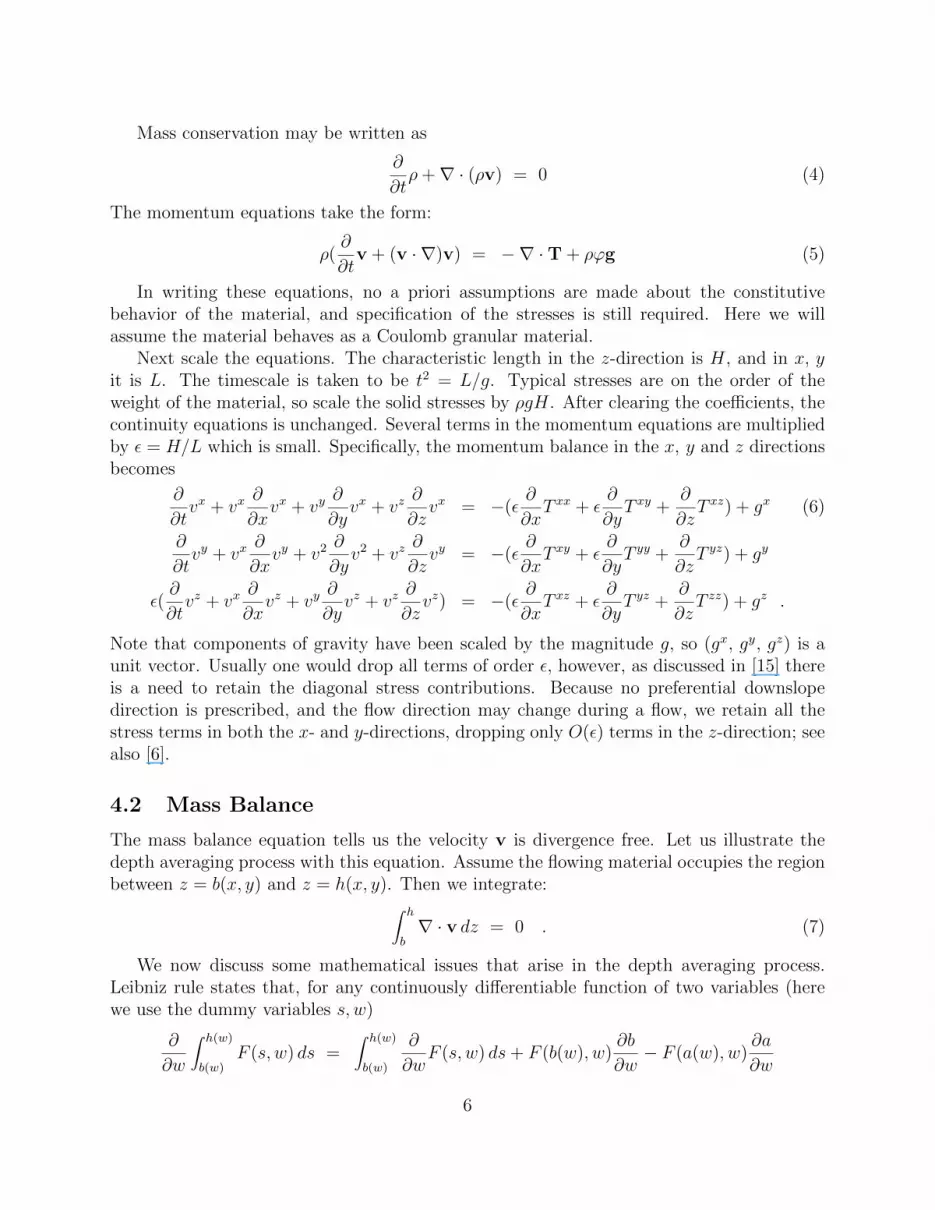
Figure 1: A schematic illustration of the forces acting on a mass flowing down an inclinedplane.

2 Sliding Friction

The simplest consideration is to imagine a solid block of mass m sliding down an inclinedplane making an angle θ with the horizontal. The force down the planar surface is mg sin(θ).Friction opposes this motion; the frictional force is proportional to the normal force on theplane, and given by µmg cos(θ). Newton’s Law then reads

mdu

dt= mg sin(θ)− sgn(u)µmg cos(θ) (1)

In writing this equation, we have taken downslope as the positive x-direction, and u as thevelocity in x. The sgn function indicates that friction always opposes motion. Often thefriction coefficient is written as µ = tan(δ) where δ is the dynamic angle of friction. Onesees that the mass scales out of the equation, and acceleration is a competition of gravityand friction.

3 A Heuristic Derivation

To begin we illustrate the major features of a one-dimensional model of granular flow downan incline. We do so to highlight the important assumptions of such a model. In subsequentsections we provide a mathematically rigorous derivation in higher space dimensions. In theCartesian plane, consider a thin layer of an incompressible granular material flowing downa flat plane making an angle θ with the horizontal. Let [x, b(x)] be a point on this plane,and let z be the direction normal to the plane; see Fig.1. Assume a constant density ofmaterial ρ. Consideration of mass conservation for a slice of this layer between the pointsx − ∆x/2 and x + ∆x/2 balances the time derivative of material mass, ∂

∂t(ρh∆t) and the

flux of material ρhu across the edges at x−∆x/2 and x+ ∆x/2. Taking the limit yields an

3

equation for the evolution of the height,

∂

∂t(ρh) +

∂

∂x(ρhu) = 0 (2)

This slice is subject to forces in the x and z directions due to gravity, friction, and materialdeformation, assumed to be characterized by MohrCoulomb plasticity. This MohrCoulombtheory, the generalization of simple sliding friction to a continuum, makes the followingassumptions on material behavior.

• Material deforms when the total stress reaches yield, described by the condition||dev(T)|| =κtr(T) where T is the 2× 2 stress tensor, dev is the deviator of the tensor dev(T) =T− 1

2tr(T)I, and tr(T) is the trace of the stress tr(T) =

∑2i=1T

xixi .

• As material deforms, the stress and strain-rate tensors are aligned, so dev(T) =λdev(V) where the strain-rate V = −1

2( ∂∂xiuj + ∂

∂xjui, where u = (u1, u2) is the

two dimensional velocity field.

• Material is rigid if stresses are below yield.

Let us now develop balance laws for T , the stresses averaged over the layer depth h.If motion normal to the basal surface is negligible, the only forces in the z direction arelithostatic and

∂

∂zTzz

= − ρg cos(θ)

Because the stress vanishes on the top surface, we find Tzz

= ρg cos(θ)(h− z), where h(x) isthe thickness of the layer above the point (x, b(x)). In the x direction, the total time rate ofchange of net momentum of the slice is given by ∂

∂t(ρhu∆x), and is balanced by the derivative

of the downslope stress ∂∂xTxx

, the basal friction Txz|b , and the lateral component of gravity

ρgh sin(θ).In all its details, Mohr – Coulomb plasticity is too complex a theory to apply here.

Instead we make a series of simplifying assumptions that allow us to derive a tractable setof equations. First, we assume that material is always deforming, so no region is rigid.Next, at the basal surface we assume perfect alignment of the normal stress and the shearstress, so T

xz|b = Tzz|b. We further assume that the stresses remained aligned throughout

the layer thickness; any misalignment is likely to be small if the layer is not very thick.Finally, we assume that the xx stress and the zz stress are proportional throughout thelayer, T

xx= KT

zz|b; here K is taken to be the earth pressure coefficient, a classical factorthat is widely used and whose origins extend back to Rankine [17, 14]. In essence, theseassumptions replace the functional relation between stress and strain rate, and the factor λof plasticity, by a state and space-dependent proportionality “constant” together with fixedaxes of alignment, a significant simplification of the constitutive theory. Bringing all of theseterms together, and using the hydrostatic relation for the normal stress (and thus for all thestresses!), the balance law reads as

∂

∂t(ρhu) +

∂

∂x(ρhu2 +

1

2βρgh2) = ρgh sin(θ)− sgn(u) cos(θ) tan(φb)ρgh (3)

4

Here the coefficient β = K cos(θ) and φb is the basal frictional angle.The earth pressure coefficient K may not be constant, but depends on whether the local

downslope and cross-slope flows are expanding or contracting (i.e., in the active or passivestates, respectively). That is, K may depend on whether ∂

∂xu > 0 or ∂

∂xu < 0 at a particular

location. Subsequent sections provide a specific definition and a more complete discussion ofK. We note that a fuller accounting for shearing stresses and slope changes would introducean additional source term proportional to u2. See [6] for a derivation that includes this term.

To better appreciate the relative sizes of terms in this model system, the equationsshould be scaled in both dependent and independent variables. Clearly, overall stressescan be scaled by the lithostatic force ρgH cos(θ), where H is a characteristic thickness ofthe flowing layer. This scaling removes the density as a parameter, and clears some of thetrigonometric functions. But more important is a scaling of the independent variables. Scale

x by L, a characteristic downslope length, z by H, and t by√L/g, and make the long wave

assumption, namelyε = H/L � 1. With these scalings, the equations as presented aboveare modified by the introduction of ε modifying the pressure-like term βρgh2. Similar tothe shallow water equations in structure, this system of equations is strictly hyperbolic andgenuinely nonlinear away from the “vacuum state” where h = 0; the characteristic speedsfor the system are u±

√βh.

One can identify similar terms in Eqns.(1) and (3). The principal difference is thepressure-like term 1

2βρgh2, which has no analogue in the sliding block.

Additional terms can be added to the system. The first addition is due to curvatureeffects that are activated when the basal surface is no longer flat: sgn(u) tan(φb)ρgh

u2

Rgz

where R is the radius of curvature and u2/R is the centripetal acceleration. The secondterm is a Voellmy effect, a quadratic drag effect: ρd|u|u, where d is the drag coefficient.

4 A More Rigorous Derivation

In this section we consider flows in three space dimensions. We give a somewhat morecomplete derivation of the thin layer equations. The main mathematical tools called upon inthis section are from vector calculus, and the one “trick” we use is a depth averaging processthat employs Leibniz rule for interchanging differentiation and integration.

4.1 Full Equations in 3D

In three space dimensions, consider a thin layer of granular material with constant specificdensity ρ flowing over a smooth basal surface. Neglect any erosion of the base. At anylocation, consider a Cartesian coordinate system Oxyz, with origin O defined so the planeOxy is tangent to the basal surface and Oz the normal direction. In considering flow overvariable terrain, there should be no preferential direction in the xy-plane, but we do as-sume a globally consistent orientation of this plane. Write v for the velocities of the solidconstitutient When writing equations in component form, we use superscripts to denote thecomponent.

5

Mass conservation may be written as

∂

∂tρ+∇ · (ρv) = 0 (4)

The momentum equations take the form:

ρ(∂

∂tv + (v · ∇)v) = −∇ ·T + ρϕg (5)

In writing these equations, no a priori assumptions are made about the constitutivebehavior of the material, and specification of the stresses is still required. Here we willassume the material behaves as a Coulomb granular material.

Next scale the equations. The characteristic length in the z-direction is H, and in x, yit is L. The timescale is taken to be t2 = L/g. Typical stresses are on the order of theweight of the material, so scale the solid stresses by ρgH. After clearing the coefficients, thecontinuity equations is unchanged. Several terms in the momentum equations are multipliedby ε = H/L which is small. Specifically, the momentum balance in the x, y and z directionsbecomes

∂

∂tvx + vx

∂

∂xvx + vy

∂

∂yvx + vz

∂

∂zvx = −(ε

∂

∂xT xx + ε

∂

∂yT xy +

∂

∂zT xz) + gx (6)

∂

∂tvy + vx

∂

∂xvy + v2

∂

∂yv2 + vz

∂

∂zvy = −(ε

∂

∂xT xy + ε

∂

∂yT yy +

∂

∂zT yz) + gy

ε(∂

∂tvz + vx

∂

∂xvz + vy

∂

∂yvz + vz

∂

∂zvz) = −(ε

∂

∂xT xz + ε

∂

∂yT yz +

∂

∂zT zz) + gz .

Note that components of gravity have been scaled by the magnitude g, so (gx, gy, gz) is aunit vector. Usually one would drop all terms of order ε, however, as discussed in [15] thereis a need to retain the diagonal stress contributions. Because no preferential downslopedirection is prescribed, and the flow direction may change during a flow, we retain all thestress terms in both the x- and y-directions, dropping only O(ε) terms in the z-direction; seealso [6].

4.2 Mass Balance

The mass balance equation tells us the velocity v is divergence free. Let us illustrate thedepth averaging process with this equation. Assume the flowing material occupies the regionbetween z = b(x, y) and z = h(x, y). Then we integrate:∫ h

b∇ · v dz = 0 . (7)

We now discuss some mathematical issues that arise in the depth averaging process.Leibniz rule states that, for any continuously differentiable function of two variables (herewe use the dummy variables s, w)

∂

∂w

∫ h(w)

b(w)F (s, w) ds =

∫ h(w)

b(w)

∂

∂wF (s, w) ds+ F (b(w), w)

∂b

∂w− F (a(w), w)

∂a

∂w

6

The upper free surface Fh(x, t) = 0 is assumed to be a material surface – that is, theupper edge of the material defines the surface z = h(x, y, t) .

∂

∂th+ vx

∂

∂xh+ vy

∂

∂yh− vz = 0 . (8)

Likewise, at the fixed basal surface Fb(x) = 0 flow is tangent to the fixed bed so

vx∂

∂xb+ vy

∂

∂yb− vz = 0 . (9)

In arriving at these equations, we have ignored deposition and erosion.Now using Leibniz and the free surface condition, and after some algebraic manipulation,

we find an equation for the total mass

∂

∂th+

∂

∂xhvx + +

∂

∂yhvy = 0 . (10)

In writing this equation, the depth averaged velocities hvx =∫ hb v

x dz, with a similar expres-

sion for vy, and where h = h− b.

4.3 Momentum Balance

Depth averaging the momentum equations is more complicated, owing principally to thevector and tensor quantities involved. The complete derivation is presented in Appendix 1.Here we content ourselves with reporting the results:z-Momentum Observe that, upon setting ε to zero in the z-momentum equation, we find

∂

∂zT zz = gz .

Integrating and using the boundary condition that the upper surface is stress free, we find

T zz = [h− z]gz .

That is, the normal solid stress in the z-direction at any height is equal to the weight of thematerial overburden.

Observe that, owing to scaling, the z-velocities have been dropped from the z-momentumequations. Of course neglecting motion in the z-direction is a central component of the thinlayer theory.

We now make use of the alignment and proportionality conditions, as in the 1-dimensionalcase. This means that the xx, , yy, xz and yz-stresses are all proportional to T zz. Depthaveraging we find

∂

∂t(hvx) +

∂

∂x(hvxvx) +

∂

∂y(hvxvy) (11)

= − ε

2

∂

∂x(αxxh

2(−gz))− ε

2

∂

∂y(αxyh

2(−gz))

− εαxx∂

∂xb− εαxy

∂

∂yb+ αxzh(− gz) + hgx .

7

The terms containing −gz arise from the stress proportionality. The y-solid momentumequation can be written

∂

∂t(hvy) +

∂

∂x(hvxvy) +

∂

∂y(hvyvy) (12)

= − ε

2

∂

∂x(αxyh

2(−gz))− ε

2

∂

∂y(αyyh

2(−gz))

− εαxy∂

∂xb− εαyy

∂

∂yb+ αyzh(− gz) + hgy .

We have employed the α-notation for convenience T ∗z = − v∗

||v|| tan(φb)Tzz ≡ α∗zT

szz.These equations are hyperbolic, with two nonlinear wave-speeds and one linearly degen-

erate one; the system loses strict hyperbolicity at the ‘vacuum’ state where h = 0.Again Voellmy and curvature terms can be added to the system. In the TITAN2D system,

we include the curvature effect. For completeness, the equations in TITAN2D are

∂tU + ∂xF + ∂yG = S (13)

where U = {h, hvx, hvy}T , F = {hvx, hvx2 + η2gzh

2, hvxvy}T , G = {hvy, hvxvy, hvy2 +η2gzh

2}T , S = {0, hgx − ( vx√vx2+vy2 )h tan(φb) [gz + vx2 db

dx] − sgn(∂yv

x)∂y(η2

sin(φint)h2gz), hgy

− ( vy√vx2+vy2 )h tan(φb) [gz + v2 db

dy] − sgn(∂xv

y) ∂x(η2

sin(φint)h2gz)}. φint is the internal fric-

tion angle, η = εK, and K(φint, φb) is the so-called earth pressure coefficient, a functionof the friction angles, and describes the ratio of shear stresses to normal stress within theflowing mass. This formulation is a variant of the original Savage-Hutter equations [15] thatincorporate certain refinements due to Iverson [6]. The earth pressure coefficient K is inthe active or passive state, depending on whether the downslope and cross-slope flows areexpanding or contracting. We modify Iverson’s assumption [6] (see also [15, 17]) and definetwo values for K

K = 21± [1− cos2(φint)(1 + tan2(φb))]

12

cos2(φint)− 1 ,

where the + (passive state) applies when flow is converging, that is, if ∂xvx + ∂yv

y < 0, andthe − (active state) applies if ∂xv

x + ∂yvy > 0.

We emphasize that, in writing these thin layer equations, we have made the long waveassumption. Thus only O(L) variations in x and y are represented in the system. Higherfrequency variations are assumed to be negligible and are not captured by the dynamics.

5 Computing Flow Along a Two-Dimensional Surface

TITAN2D is a parallel, adaptive grid, shock capturing method to solve the governing massflow equations. We begin with a discussion of the integration of digital elevation model data- a description of the local topography into our solver. The synthesis of these computationaltechniques makes possible the solution of mass flows over a realistic terrain on desktophardware.

8

5.1 Digital elevation data

A principal feature of TITAN2D is the incorporation of topographical data into our simula-tion and grid structure. We have written a preprocessing routine in which digital elevationdata are imported. These data define a two-dimensional spatial box in which the simulationwill occur. Association with terrain is based on the UTM (Universal Transverse Mercatorcoordinate system) for representing points on the geoid. The raw data provide elevationsat specified locations. By using these data, and interpolating between data points wherenecessary, a rectangular, Cartesian mesh is created. This mesh is then indexed in a mannerconsistent with our computational solver. The elevations provided on this mesh are thenused to create surface normals and tangents, ingredients in the governing PDEs. Finally,the grid data are written out for use, together with simulation ouput, in post-computationvisualization. The digital elevation data may be obtained from a number of geographic in-formation system (GIS) sources. We have implemented a version that imports GRASS data(Geographic Resource Analysis Support System), which is then georectified and coded intoa grid, in a manner similar to the GRID module of ARC/INFO.

Depending on the specific site under consideration, a typical GIS coarse grid providesblocks of about 100m× 100m in size with a ±30m vertical accuracy, while a fine grid canhave blocks of 5m× 5m in size with a ±1m vertical accuracy.

5.2 Numerical Solver

To solve the governing system of equations we use a parallel, adaptive mesh, Godunov solver.The basic ingredient in the method is an approximate Riemann solver. TITAN2D uses asolver originally due to Davis [1] which in turn is based on the ideas of Harten, Lax andvanLeer [2]. In brief, the dependent variables are considered as cell averages, and their valuesare advanced by a predictorcorrector method; the source terms are included in these updates,and no splitting – neither for the source nor the multiple dimensions – is necessary. Slopelimiting is used to prevent unphysical oscillations. The Davis approximate Riemann solveris a centered scheme, akin to an approach introduced by Rusanov. Appendix 2 containsdetails of the numerical method.

Adaptive gridding coupled with parallel computing enables the use of very fine gridsand provides for simulations of very high fidelity. We have implemented a simple adaptivegrid structure that refines cells at a given time step based on indicators derived from thecomputed solution at the previous time step. Perhaps the simplest indicator to consider is“Is h = 0? That is, all cells containing material are refined. In experiments with this simpleindicator, we may also refine all cells immediately adjacent to cells containing material. Inthis way, a one-cell thick band of refined but empty cells surrounds the refined cells containingmaterial. This additional band of refined cells ensures that no spurious waves are generatedas material passes across different grids. Alternatively, enforcing precise conservation atedges where refined and unrefined grids meet also provides a highly accurate computation.We have also experimented with a simple scaled L2 norm of the flux around the boundaryof each cell as the refinement indicator. In a similar way, if indicators suggest that a coarser

9

discretization will not adversely affect the solution quality, we remove refined cells. Thus,we are able to maintain the solution quality and track special features, while not making thecomputation prohibitively expensive. We also monitor the change of the pile height on everytime step. When this change is below a user defined threshold, we unrefine the grid locally.Both the refinement and unrefinement indicators are heuristic, and based on experience andphysical intuition. We must also define the frequency of grid adaption. Experience leads usto examine the indicators every two time steps to decide whether or not to refine or unrefine.Again, this adaption frequency is heuristic.

Parallelization of adaptively refined grids has been addressed by several researchers overthe last several years. To take full advantage of multiprocessor computing, the critical issuesare the number and location of cells created and deleted during grid refinement, load balance,and the efficiency of storage and data access. At those cells at the boundary of a processorpartition we must add data storage for a layer of “ghost cells” on each subdomain. Thedata of a cell adjacent to the partition and belonging to one processor are replicated on theother processor. This replication enables us to perform the computations necessary for theGodunov scheme for every cell, without explicit communication. However, the use of ghostcells requires us to synchronize the data among the processors at the end of each time step.

Although we use only regular Cartesian grids in the simulations, our data managementscheme is imported from finite element computations, where unstructured grids often arise.Thus our design allows for general grids, and our data structure are not simple arrays.Because all data access operations involve some kind of search, this procedure must be fastand efficient. Our data storage model is a distributed hash table. Data are indexed by anordering along a space filling curve (SFC), and are then stored in the table. Each cell ismapped to a unique key using its location along the SFC passing through its centroid. Thiskey also provides a unique identifier that is easily generated – typically it is generated directlyfrom geometric coordinates by using bit manipulations. To obtain a decomposition of theproblem, we introduce a partitioning of this key space. This induces a distribution of thedata sets, i.e., a decomposition of the problem for distributed memory computing. When thegrid changes and new cells are introduced, a redistribution of cells among the processors tomaintain load balance is achieved by adjusting this key space partition. By adjusting the keyspace partition after grid refinement/unrefinement stages, good load balance is maintained.

6 Some Practical Issues in Computing Thin Layer Flows

The derivation just presented clearly shows the significance of the scale parameter ε = H/Lin balancing the magnitude of terms in the governing equations. For computations twodifficulties arise. Firstly, L is often an input into the computation and not known a priori.Second, for many flows of interest the actual size of L may not be very large! The firstdifficulty is surmounted by using a sufficiently high scaling parameter. The second is harderto overcome. What constitutes a sufficiently long flow in order for these equations to providegood approximation is a matter of some judgement. As a guide, flows in which the maximumdepth is no more than one-tenth of the typical length are good candidates.

10

Another matter than must be given careful thought is the estimate of friction inputs.Sometimes the basal and internal friction angles are extrapolated from laboratory tests ofmaterial, which may differ significantly from field flow conditions. Other times the angles arefitted by calibration to observed flows. Furthermore, real flows often involve a mixture of solidmaterials and fluids, a rheology that is usually difficult to characterize but certainly requiresmore complex multi-phase models (or an unrealistic friction coefficient) to capture the effectof fluidizations. The calibration approach can be profitably used in many circumstances.However it is known that there is a volume dependence of the runout of a flow – larger flowstravell further. Thus calibration requires comparison against flows of similar size.

Finally, many difficulties arise from the DEM and the quality of that map. Many DEMsthat are readily available have regions where elevations are poorly defined or even undefined!Additionally, terrain often has rapid changes (cliff walls and canyons) which can cause com-putations of gradients and curvatures to become unstable. Since the equations here involveterms with curvatures – evaluated by post-processing the elevations – these calculationsrequire a filtering of the terrain data to avoid changes in gradient larger than about 70◦.

11

7 Appendix 1

Here is the full derivation of the depth-averaged momentum equations. We assume thez-equation as 4.3

The scaled equations are 6

∂

∂tvx + vx

∂

∂xvx + vy

∂

∂yvx + vz

∂

∂zvx = −(ε

∂

∂xT xx + ε

∂

∂yT xy +

∂

∂zT xz) + gx (14)

∂

∂tvy + vx

∂

∂xvy + v2

∂

∂yv2 + vz

∂

∂zvy = −(ε

∂

∂xT xy + ε

∂

∂yT yy +

∂

∂zT yz) + gy

ε(∂

∂tvz + vx

∂

∂xvz + vy

∂

∂yvz + vz

∂

∂zvz) = −(ε

∂

∂xT xz + ε

∂

∂yT yz +

∂

∂zT zz) + gz .

Solving the z-equation yields T zz(x, y, z) = − gz[h− z].The left-hand side of the x-momentum equation is

LHS =∂

∂tvx +

∂

∂xvx +

∂

∂yvxvy +

∂

∂zvxvz .

Depth average and use boundary conditions to find∫ h

bLHS dz =

∂

∂t

∫ h

bvx dz +

∂

∂x

∫ h

bvx2 dz +

∂

∂y

∫ h

bvxvy dz (15)

We use approximations such as∫ hb v

x2 dz = hvxvx = hvxvx. We make an error in thisapproximation; this error is small for certain flow profiles, but non-negligible for others.

Now depth average the right hand side:∫ h

bRHS dz = −

∫ h

b(ε∂

∂xT xx + ε

∂

∂yT xy +

∂

∂zT xz) dz︸ ︷︷ ︸

(i)

+∫ h

bϕgx dz (16)

We assume the earth pressure relation for the solid phase is employed. To this end, basalshear stresses are assumed to be proportional to the normal stress:

T ∗z = − v∗

||v||tan(φb)T

zz ≡ α∗zTzz ,

where ∗ can be either x or y, and the velocity ratio determines the force opposing the motionin the ∗-direction, to the extend that force is mobilized [3, 9] in that direction. Thus slidingvelocity and basal traction are colinear. The α notation will provide a convenient shorthand.Likewise the diagonal stresses are taken to be proportional to the normal solid stress

T ∗∗ = kapTzz ≡ α∗∗T

zz ,

12

where the same index x or y is used in both ∗’s. Finally, following [6], xy shear stresses aredetermined by a Coulomb relation

T xy = −sgn(∂

∂yvx) sin(φint)kapT

zz ≡ αxyTzz ,

where the sgn function ensures that friction opposes straining in the (x, y)-plane.Now

(i) = −ε∫ h

b

∂

∂xαxxT

zz dz − ε∫ h

b

∂

∂yαxyT

zz dz −∫ h

b

∂

∂zαxzT

zz dz (17)

= − ε[ ∂∂x

∫ h

bαxxT

zz dz − αxxT zz|z=h∂

∂xh+ αxxT

zz|z=b∂

∂xb]

− ε[ ∂∂y

∫ h

bαxyT

zz dz − αxyT zz|z=h∂

∂yh+ αxyT

zz|z=b∂

∂yb]

− αxz[T zz|z=h − T zz|z=b] .

Because the upper free surface is stress free, all terms T zz|z=h vanish. Combining all termsyields an x-momentum equation:

∂

∂t(hvx) +

∂

∂x(hvxvx) +

∂

∂y(hvxvy) (18)

= − ε

2

∂

∂x(αxxh

2(−gz))− ε

2

∂

∂y(αxyh

2(−gz))

− εαxx∂

∂xb− εαxy

∂

∂yb+ αxzh(− gz) + hgx .

The y-momentum equation is derived similarly.

13

8 Appendix 2

This appendix contains details regarding the finite volume Godunov solver used in TITAN2D.To solve the mass and momentum balance laws, we use a parallel, adaptive mesh, Go-

dunov solver. The basic ingredient in the method is an approximate Riemann solver. Wehave coded a solver originally due to Davis [1] based on the ideas of Harten, Lax and vanLeer[2]. In brief, the dependent variables are considered as cell averages, and their values areadvanced by a predictorcorrector method; the source terms are included in these updates,and no splittingneither for the source nor the multiple dimensionsis necessary. Slope limit-ing is used to prevent unphysical oscillations. The Davis approximate Riemann solver is acentered scheme, akin to an approach introduced by Rusanov. Consider, then, a hyperbolicsystem written as

∂

∂tU +

∂

∂xf(U) +

∂

∂yG(U) = S(U) (19)

We have occasion to use the non-conservative form

∂

∂tU + A

∂

∂xU +B

∂

∂yU = S(U) (20)

where A, B are the Jacobians of f, g, respectively. Discretize the variable U = Uij whereUij is considered to be the cell average of U(x, y) in the cell [(i − 1

2)∆x, (i + 1

2)∆x] × [(j −

12)∆y, (j + 1

2)∆y] where for simplicity we assume a uniiform grid. Write Un

ij for Uij at timen∆t. The the midtime predictor is

Un+ 1

2ij = Un

ij +1

2∆tAnij∆xU

nij +

1

2∆tBn

ij∆yUnij +

1

2∆tSnij (21)

In this formula, ∆xU and ∆yU are the limited slopes for U in the x- and y-directions,

respectively (see below). Given the mid-time cell-center value Un+ 1

2ij , extrapolate to the cell

edge using the limited slope. For example, Un+ 1

2

i+ 12j

= Un+ 1

2ij + 1

2∆xU

nij if we extrapolate from

cell ij (referred to as the left state), or Un+ 1

2

i+ 12j

= Un+ 1

2i+1j − 1

2∆xU

ni+1j if we extrapolate from cell

i + 1, j (the right state). So now there are two values at the cell edge i + 12j. To resolve

this multivaluedness, an approximate Riemann solver generates a numerical flux F (U l, U r)depending on these left and right states and the physical flux f. The interested reader mayconsult [1, 2], among other sources, for a guide to the vast literature of Riemann solvers. Wefollow the early work of Davis who generates a flux by the examination of the fastest andslowest wave speeds propagating from the local states:

F (U l, U r) =1

2[f(U l) + f(U r)]− α

2(U r − U l) (22)

In this formula, α is an upper bound on the magnitude of the characteristic speeds of allwaves (normal to the cell edge under consideration) evaluated at both the left and rightstates.

14

Finally, a conservative updated of U is computed as

Un+1ij = Un

ij −∆t

∆x[F (U l

i+ 12j, U

ri+ 1

2j)− F (U l

i− 12j, U

ri− 1

2j)] (23)

−∆t

∆y[G(U b

ij+ 12, U t

ij+ 12)−G(U b

ij− 12, U t

ij− 12)] + ∆tS

n+ 12

ij

Here t and b represent the states at the top and bottom of the cell for the G flux, analogousto the right and left states, resp.

Although the Davis method is not as accurate as other solvers, its ease of use for systemswith sources and for systems in several spatial dimensions, and its small operation count,recommend its use for our equations. We note that this approach avoids a splitting of thesource terms from the propagation terms. Splitting often creates difficulties for quasisteadyflows. In particular, unless special precautions are taken, many hyperbolic solvers (includingthe Davis solver) introduces dissipation that can destroy special time-independent solutionsof the steady-state equations.

We owe the reader a definition of the flux limiting term. We illustrate limiting in thex-direction (and drop the y-subscript here). Define the forward, backward and centereddifferences as

∆+U = (Ui+1 − Ui)/∆x (24)

∆−U = (Ui − Ui−1)/∆x (25)

∆0U =1

2(Ui+1 − Ui−1)/∆x (26)

Then the limited state is

∆xU =1

2(sgn(∆+U) + sgn(∆−U)) min(|∆+U |, |∆−U |, 2|∆0U |)

Here the sgn ensures that the slope is set to zero at an extrema. The minimum modulus pre-vents overshoots and undershoots that plague convential higher order methods for nonlinearhyperbolic solvers.

15

References

[1] Davis, S.F. (1988) “Simplified second–order Godunov-type methods” SIAM J. Sci.Stat. Comput. 9 445

[2] Harten, A., Lax, P. and vanLeer, B. (1983) “On upstream differencing and Godunov-type schemes for hyperbolic conservation laws” SIAM Rev 25 35

[3] Hutter, K. Siegel, M., Savage, S.B., and Nohguchi, Y. (1993) ”Two dimensional spread-ing of a granular avalanche down an inclined plane; Part 1: Theory” Acta Mech. 10037-68

[4] Hutter, K. and Kirchner, N. (Eds) (2003) Dynamic Response of Granular and PorousMaterial under Large and Catastrophic Deformations Lecture Notes in Applied andComputational Mechanics 11, Springer New York

[5] Iverson, R.M (1997) “The physics of debris flows” Rev. Geophys. 35 245-296

[6] Iverson, R.M and Denlinger, R.P, (2001) “Flow of variably fluidized granular materialacross three-dimensional terrain 1. Coulomb mixture theory” J. Geophy. Res. 106 537

[7] Legros, F. (2002) “The mobility of long runout landslides” Eng. Geology 63 301-331

[8] Patra A, Nichita, C., Bauer, A.C., Pitman, E.B., Bursik, M.I., and Sheridan, M.F.(2004) “Parallel adaptive discontinuous Galerkin approximation of the debris flowequations” Computers and Geoscience 32 (2006) p. 912 - 926

[9] Patra, A.K., Bauer, A.C., Nichita, C., Pitman, E.B., Sheridan, M.F., Bursik, M.,Rupp, B., Webber, A., Stinton, A.J., Namikawa, L.M., and Renschler, C.S. (2005)“Parallel adaptive numerical simulation of dry avalanches over natural terrain” J.Volcanology Geothermal Research 139 1-21.

[10] Pitman, E.B., Nichita, C., Patra, A., Bauer, A.C., Bursik, M. and Webber, A. (2003)“A Numerical Study of Granular Flows on Erodible Surfaces” Disc. Cont. DynamicalSystems - Series B 3 589-599

[11] Pitman, E.B., Patra, A., Bauer, A., Nichita, C., Sheridan, M. and Bursik, M. (2003)“Computing Debris Flows” Physics of Fluids 15 3638-3646

[12] Pitman, E.B., Patra, A., Bauer, A., Sheridan, M. and Bursik, M. (2002) “Comput-ing Debris Flows and Landslides: Towards a Tool for Hazard Risk Evaluation” inHyperbolic Problems: Theory, Numerics, Applications (T. Hou and E. Tadmor, eds.)Springer, New York. 807-818

[13] Pitman, E.B. and Le, L. (2005) “A two-fluid model for avalanche and debris flows”Phil. Trans. Roy. Soc. A 363 1573-1601

1

[14] Rankine, WJM (1857) “On the stability of loose earth” Philos. Trans. R. Soc. London147 9

[15] Savage, S.B. and Hutter, K. (1989) “The motion of a finite mass of granular materialdown a rough incline” J. Fluid Mech. 199 177-215

[16] Sheridan, M.F., Stinton, A.J., Patra, A.K., Pitman, E.B., Bauer, A.C., and Nichita,C. (2005) “Evaluating TITAN2D mass flow using the 1963 Little Tahoma PeakAvalanches” J. Volcanology and Geothermal Research 139 89-102.

[17] Terzaghi, K. (1936) “The shearing resistance of saturated soils and the angle betweenplanes of shear”, in Proceedings of the 1st International Conference on Soil Mechanics54-56

2