Modeling excessive nutrient loading in the environment

Reckhow/Chapra November 12, 1998 1

Modeling Excessive Nutrient Loading in the Environment

Kenneth H. ReckhowNicholas School of the Environment

Duke University

Steven C. ChapraDepartment of Civil, Environmental, and Architectural Engineering

University of Colorado

Abstract

Models addressing excessive nutrient loading in the environment originated overfifty years ago with the simple nutrient concentration thresholds proposed by Sawyer.Since then, models have improved due to progress in modeling techniques andtechnology as well as enhancements in scientific knowledge. Several of these advancesare examined here. Among the recent approaches in modeling techniques we review areerror propagation, model confirmation, generalized sensitivity analysis, and Bayesiananalysis. In the scientific arena and process characterization, we focus on advances insurface water modeling, discussing enhanced modeling of organic carbon, improvedhydrodynamics, and refined characterization of sediment diagenesis. We conclude withsome observations on future needs and anticipated developments.

Introduction

It was over fifty years ago that Sawyer (1947) recommended inorganic nutrientthresholds above which excessive algal growths might be expected in north temperatelakes. Since this simple model proposed by Sawyer, models of excessive nutrient loadinghave increased in both accuracy and sophistication, due to both advances in scientificunderstanding and improvements in methods of analysis.

In the scientific arena, interest and experience in cross-media (e.g., land-atmosphere-water) modeling has been growing recently (e.g., the Chesapeake Baymodel), and this has greatly increased model size and complexity. However, mostenhancements to models have occurred in a single medium. For example, in surfacewaters, advances in nutrient modeling have resulted from improved hydrodynamics (e.g.,Cole and Buchak 1995), explicit modeling of organic carbon (e.g., Connolly and Coffin1995), and refined characterization of sediment diagenesis (e.g., Di Toro et al. 1990).

In addition to those contributions from the sciences, improvements in nutrientmodeling have resulted from enhancements in modeling techniques, improvements inobservational databases, and refinements in problem structuring and prediction. Forexample, among modeling techniques, uncertainty analysis (Beck 1987), generalizedsensitivity analysis (Spear and Hornberger 1980), and Bayesian analysis (Reckhow 1990)have proven to be useful methods for parameter estimation and model application.


Likewise, better and larger observational data sets permit improvements in modelcalibration and verification.

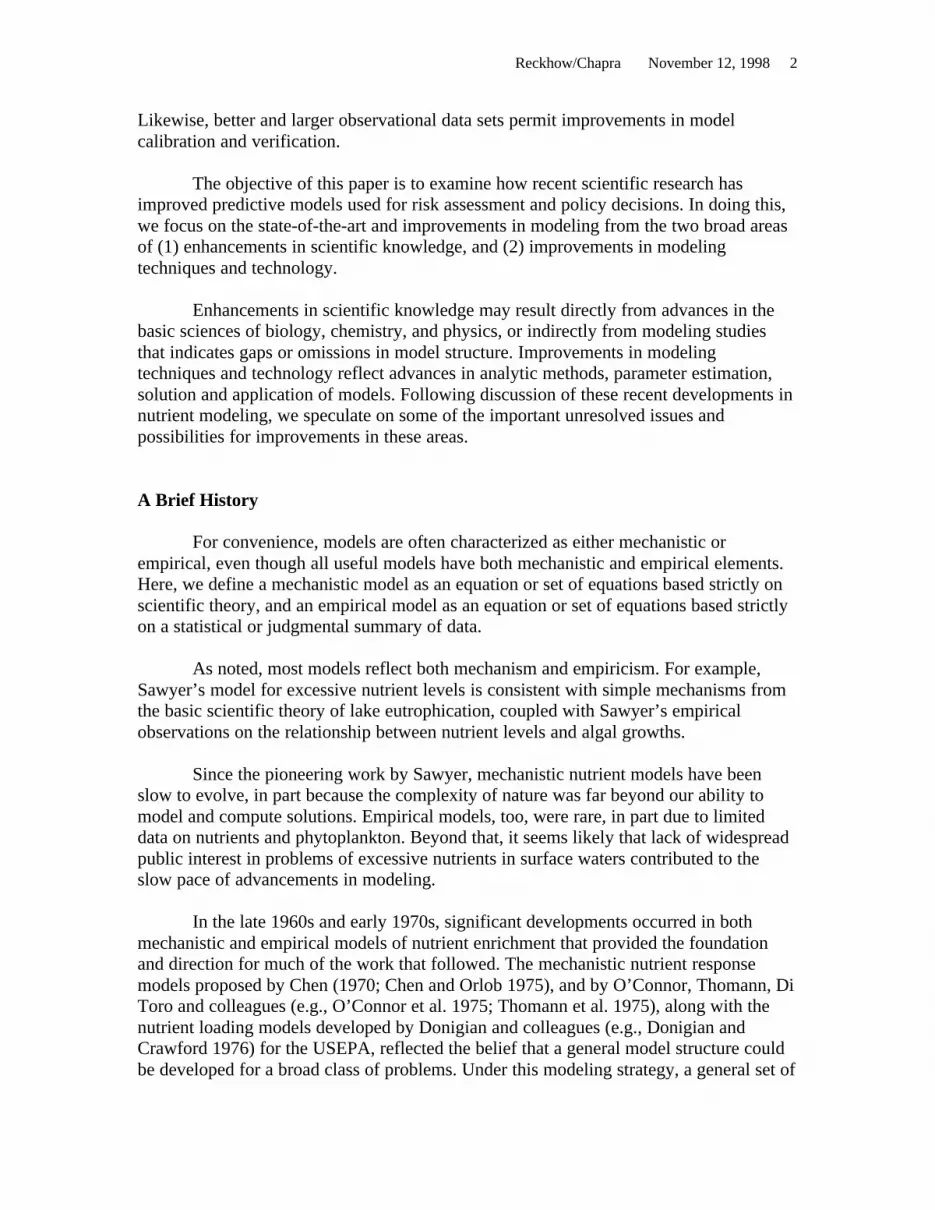
The objective of this paper is to examine how recent scientific research hasimproved predictive models used for risk assessment and policy decisions. In doing this,we focus on the state-of-the-art and improvements in modeling from the two broad areasof (1) enhancements in scientific knowledge, and (2) improvements in modelingtechniques and technology.

Enhancements in scientific knowledge may result directly from advances in thebasic sciences of biology, chemistry, and physics, or indirectly from modeling studiesthat indicates gaps or omissions in model structure. Improvements in modelingtechniques and technology reflect advances in analytic methods, parameter estimation,solution and application of models. Following discussion of these recent developments innutrient modeling, we speculate on some of the important unresolved issues andpossibilities for improvements in these areas.

A Brief History

For convenience, models are often characterized as either mechanistic orempirical, even though all useful models have both mechanistic and empirical elements.Here, we define a mechanistic model as an equation or set of equations based strictly onscientific theory, and an empirical model as an equation or set of equations based strictlyon a statistical or judgmental summary of data.

As noted, most models reflect both mechanism and empiricism. For example,Sawyer’s model for excessive nutrient levels is consistent with simple mechanisms fromthe basic scientific theory of lake eutrophication, coupled with Sawyer’s empiricalobservations on the relationship between nutrient levels and algal growths.

Since the pioneering work by Sawyer, mechanistic nutrient models have beenslow to evolve, in part because the complexity of nature was far beyond our ability tomodel and compute solutions. Empirical models, too, were rare, in part due to limiteddata on nutrients and phytoplankton. Beyond that, it seems likely that lack of widespreadpublic interest in problems of excessive nutrients in surface waters contributed to theslow pace of advancements in modeling.

In the late 1960s and early 1970s, significant developments occurred in bothmechanistic and empirical models of nutrient enrichment that provided the foundationand direction for much of the work that followed. The mechanistic nutrient responsemodels proposed by Chen (1970; Chen and Orlob 1975), and by O’Connor, Thomann, DiToro and colleagues (e.g., O’Connor et al. 1975; Thomann et al. 1975), along with thenutrient loading models developed by Donigian and colleagues (e.g., Donigian andCrawford 1976) for the USEPA, reflected the belief that a general model structure couldbe developed for a broad class of problems. Under this modeling strategy, a general set of


equations describing key physical, chemical, and biological processes is written; withsite-specific parameters, boundary conditions, and initial conditions, the model can thenbe applied to address a variety of issues. This philosophy and the basic set of equationsproposed in these early models remain the core of mechanistic nutrient enrichmentmodels.

Likewise, empirical models of nutrient response in receiving waters owe much toRichard Vollenweider (1968, 1975), who concluded from his knowledge of northtemperate lakes that response to nutrient loading generally follows a few basic rules. Thatis, Vollenweider found that nutrient concentration (trophic state) in a cross section oflakes is a simple function of annual nutrient loading, lake mean depth (Vollenweider1968), and water residence time (Vollenweider 1975). In effect, lakes operate like largesedimentation basins. The resultant “Vollenweider loading plot” and model are probablythe most commonly applied nutrient response models. Nutrient export coefficients(Uttormark et al. 1974) together with the Vollenweider model provide the comprehensiveframework that has guided empirical modeling during much of the past two decades.

These early mechanistic and empirical modeling studies form the foundation onwhich many of the improvements in modeling have evolved. The strength of these basicapproaches is evident in that new developments have not radically altered modelingapproaches, but rather have built and improved on this foundation. In the followingsections, we discuss some of the most significant improvements in nutrient modelingover the past 15-20 years.

Enhancements in Modeling Techniques

There have been a number of improvements in the mathematics of modeling ofexcessive nutrients in the environment since the path breaking work identified in theprevious section. Indeed, there are too many to mention here, so we have opted toexamine some of the techniques that seem important to us and that have actually beenapplied to model the impacts of excess nutrient loading. These topics include the broadareas of model specification, parameterization, and prediction. Within these areas, recentadvances in methods of analysis are allowing scientists to make better us of observationaldata and expert judgment for parameter estimation, to improve the quantification ofprediction uncertainty, and to identify relationships and specify models from multivariatedata. Each of these is examined below.

Prediction Uncertainty and Model Validation

The application of water quality models to guide management and decisionmaking gradually stimulated scientific interest in model goodness of fit and led to studiesin sensitivity analysis, uncertainty analysis, and model validation. In this section, we tracesome of the developments in those areas, beginning with uncertainty analysis or errorpropagation. Beck (1987) is an excellent reference on these topics.


Early work by O’Neill and colleagues (O’Neill 1971; O’Neill et al. 1980) onmechanistic models and Reckhow (1979) and Reckhow and Chapra (1979, 1983) onempirical models raised awareness of the importance of prediction error and presentedthe common methods for error propagation. These basic methods are Monte Carlosimulation and first order error analysis.

Before the widespread availability of inexpensive and fast computing, first orderanalysis was often applied, particularly for simple empirical models. In brief, first ordererror analysis (Reckhow and Chapra 1983) is based on a linear approximation of themodel with error terms represented by the variance; covarying errors can be accountedfor with a correlation term. The approximation means that first order analysis is not exactfor nonlinear models and for models with error terms that are not fully characterized by avariance alone. In principle, first order analysis can be applied to any model, althoughfrom a practical standpoint, highly nonlinear models with skewed error distributions arenot good candidates.

Monte Carlo simulation is based on a simple concept that has become feasiblewith modern computing. In brief, it was realized that a distribution characterizinguncertainty in model predictions could be generated through multiple model runs andrandom sampling. Monte Carlo simulation begins with the selection of a probabilitydensity function characterizing the uncertainty in each term in the model, while the modelitself is unchanged from standard deterministic applications. Then, when the model isapplied, instead of a single run of the model, a large number (several hundred to a fewthousand) of model runs is made. For individual model runs, the program draws a samplefrom the probability distribution for each uncertain parameter and uses those sampledvalues to compute a single solution. After this sampling/modeling process is repeatedmany times, a distribution of responses is generated, representing the combined effect ofall uncertain terms. Parameter covariance may be accounted for with correlated samplingbetween distributions.

First order error analysis and Monte Carlo simulation have not been widely used,but a few studies (mainly for surface waters, see Scavia et al. 1981, Di Toro and vanStraten 1979, and Reckhow and Chapra 1979; see also Beck 1987 and Reckhow 1994 forsummaries) give some indication of prediction errors for nutrient response models.Unfortunately, it appears from these studies that predictions are not very precise. Basedon the error propagation studies, prediction errors in both empirical and mechanisticmodels are unlikely to be under ±30% and can range well above ±100%. It should benoted that this reflects only the small number of studies undertaken with reasonablycomplete error analyses.

Does this mean that nutrient models are poor predictors? Perhaps not. We knowfrom the work of Di Toro and van Straten (1979) that prediction errors can dropprecipitously when correlation terms are included. This reflects the often-reasonablenotion that uncertainty may be much greater for individual model parameters than for thecombined effect of pairs of related parameters. It seems possible that, out of ignorance,


we tend to overestimate the impact of individual error terms, even while not including alluncertainties in most error propagation studies.

An alternative approach to the estimation of prediction error is possible in modelvalidation studies. If the difference between model predictions and observations can beattributed largely to lack of fit of the model (errors in the observations must alsocontribute, however), then this difference represents one realization of model predictionerror. Of course, mechanistic models with many parameters can be “tuned” to fit the datathrough prudent adjustments of the model parameters, and statistical models are known toyield better goodness-of-fit statistics to the parameter estimation data than to a separatevalidation data set. Thus, the nature or rigor of the validation test must first be taken intoaccount when comparing model predictions with observations.

In mechanistic models, validation rigor might be defined by the differencebetween the calibration data and the validation data. If calibration data and validationdata are essentially identical, then the validation exercise tells us little about how themodel will perform when predicting new conditions. On the other hand, validation datathat reflect conditions substantially different from those during calibration provide theopportunity for a rigorous test. In statistical models, leave-one-out cross-validation, orset-aside validation data, yield a more reliable estimate of prediction error than does thestandard error computed during parameter estimation. For example, the standard error(root mean square error) for an input-output (Vollenweider) lake phosphorus model withmeasured loading and fitted to homogeneous cross sectional lakes data can be as low as±25%. When cross validation is used to compute the root mean square error of prediction,the error may be increased slightly to approximately ±30%. Both of these error estimateswill be larger for more heterogeneous cross sectional data sets.

Actual results from prediction-observation comparisons for mechanistic nutrientenrichment models are difficult to assess because it is often not clear how much tuning tothe data occurred (i.e., how rigorous was the validation). In general, however, the higherresolution and greater detail of mechanistic models results in larger errors. For example,two studies (Sweeney et al. 1985, and Jamieson and Clausen 1988) of the CREAMSagricultural runoff model reported nutrient loss predictions differing from observationsby a factor of two or more. In perhaps the most ambitious mechanistic modeling projectundertaken to date, Cerco and Cole (1993) report relative errors of between 14% (forDO) to 56% (for particulate organic carbon) for seasonally and spatially aggregatedpredictions and observations based on the CE-QUAL-ICM model. Site-specific dailyprediction-observation comparisons were less precise.

So in summary, what can be said now about the state-of-the-science in uncertaintyanalysis? Prediction error analysis and model validation are still rarely undertaken, eventhough improvements in computing technology, analytic techniques, and water qualitydatabases are clearly supportive of more routine assessments of uncertainty. Whileregular application of error analysis is needed, ultimately modelers and users of modelresults must recognize that error analyses need to be rigorous and thorough in order toinsure meaningful and useful results.


Regional Sensitivity Analysis

Estimation or selection of parameters has always been a difficult task formechanistic water quality modelers. This is principally due to the overparameterization oflarge models; by this, we mean that the available data are insufficient to provide uniqueestimates of many of the model parameters. As a consequence, tabulations of suggestedparameter values have been published (e.g., Bowie et al. 1985) to guide modelers inparameter selection. Even with that information, it is usually difficult to estimateparameter errors and covariance terms for use in error propagation studies. For example,Adams (1998) has shown that the wide range of suggested parameter values in theliterature can lead to implausible or nonsensical water quality predictions, particularly ifparameter correlations are ignored.

An intuitively appealing approach to these problems, called regional sensitivityanalysis, was developed by Hornberger and Spear in a set of papers (Hornberger andSpear 1980, Spear and Hornberger 1980), and applied to the evaluation of a mechanisticeutrophication model. In brief, Hornberger and Spear proposed that á priori definedregions of acceptable model behavior be the basis for the estimation of plausibleparameter values and interactions. This works as follows. First, the model output spacefor the response variable(s) of interest is divided into a region of acceptable response anda region of unacceptable response. For this purpose, acceptable response is defined as allvalues of the response variable(s) that are plausible, or real; for example, chlorophyll alevels might be expected to range between 10µg/l and 60µg/l in a particular lake. MonteCarlo simulation (or some other method of sampling) is then used to sample parameterdistributions for model runs, and each model run is classified as acceptable orunacceptable.

By definition, the acceptable model runs are generated by behavior givingparameters sets. In other words, conditional on the truth of the model, each set of modelparameters that results in acceptable levels of the predicted response variable(s) isconsidered to be a sample from the multivariate parameter distribution for the model.Collectively, these behavior giving parameter sets map the region(s) in parameter spacethat should serve as the basis for parameter estimates, distributions, and covariance terms.

Since the original work by Hornberger and Spear, regional sensitivity analysis hasbeen used to:

• identify the most important (or “sensitive”) parameters – The model is mostsensitive to those parameters with distributions that vary significantlybetween the acceptable and unacceptable runs (with correlation, thisinterpretation may have less merit). In other words, parameters that do notdiffer between acceptable and unacceptable runs seem less likely to influencemodel predictions. This information is useful because knowledge ofparameter sensitivities can be quite helpful in setting data collectionpriorities.

• identify plausible parameter estimates - For example, given the correlationsamong parameters, what point estimates of the parameters are mutually


compatible? This information will help eliminate nonsensical predictionsassociated with inconsistent parameter estimates.

• define parameter distributions for uncertainty analyses – The multivariateempirical distribution for the behavior giving sets characterizes theparameters. For error propagation purposes, Monte Carlo sampling should beon the basis of a complete set of acceptable parameter values, in order topreserve the parameter interactions.

One of the common difficulties with regional sensitivity analysis is that typicallyonly a small percent (often considerable less than five percent) of the candidateparameters sets achieves acceptable behavior status. While this means that perhapsseveral thousand runs of a model may be necessary to generate a suitable characterizationof the multivariate parameter space, it also implies that most sets of parameters fromindividually acceptable distributions are not collectively acceptable. Thus, regionalsensitivity analysis may be an essential tool for selecting parameter distributions for errorpropagation studies of large mechanistic models.

Other methods to address the problem of parameter estimation in mechanisticnutrient enrichment models have been recently proposed. One method, Bayesian analysis,has existed for over 200 years, but recent advances in computing have led to promisingnew developments. Some of these are discussed below. Another promising approach,structural dynamic models, draws on ecological theory and scientific knowledge toaddress the time-varying nature of many parameters. Space prevents full treatment of thisinteresting strategy; Jorgensen (1986, 1997) should be consulted for discussion andexamples.

Bayesian Analysis

When point estimates of model parameters are determined for mechanisticmodels, the conventional approach is for the modeler to use his judgment in selectingparameters that are consistent with any available data as well as with tabulations ofaccepted coefficient values (e.g., Bowie et al., 1985). Parameters are often selected in asequential manner (perhaps based on a sensitivity analysis), and the model is finallyjudged adequate based on a visual comparison of predictions and observations. Formalmathematical optimization is not usually involved.

Parameter estimation in empirical models has traditionally been undertaken usingclassical optimization methods such as maximum likelihood or least squares. Judgmentis typically involved in the specification of the model but not in the actual estimationalgorithm.

The difference in approach between these two categories of models has occurredfor a few reasons. In some cases, mechanistic modelers have believed that the modelequations are theoretically correct, and the model parameters are physically measurablequantities that are simply measured in the field and inserted into the model. In othercases, the mechanistic models, with large numbers of parameters, were not identifiablewithout imposing constraints on most of the parameters (and effectively estimating these


parameters using expert judgment and literature tabulations). In contrast, empiricalmodels, with one or only a few parameters, are identifiable from the available data, andthe empirical modeler may recognize that the model is more credible if an optimalitycriterion is used to estimate the parameters.

In many situations, where available data and expert judgment permit, it should beto the advantage of the modeler to use both site specific data and expert judgment in astructured way to improve the estimation model parameters. It has long been recognizedthat Bayes Theorem provides the formal mechanism for doing this (Berger 1985). Why,then, don’t we see more applications of Bayes Theorem in the nutrient enrichmentmodeling literature?

It is likely that Bayes Theorem has been controversial, and thereforeunacceptable, to many scientists when subjective information is expressed as a (prior)probability model and then is formally combined with the data-based likelihood functionto yield a posterior probability distribution. While this may bother classical (orfrequentist) statisticians, it should not bother many water quality modelers, sincemodelers are accustomed to informal use of judgment in modeling. However, thisperspective probably has affected water quality modelers, because it has limited (orbiased) their exposure to Bayesian ideas from their classically-trained statisticscolleagues.

It is an unfortunate but common fact that observational data for parameterizationof water quality models are almost always woefully inadequate for the task. As aconsequence, experimental evidence is sometimes used, but primarily the gap is filledwith judgmental parameter selection. As noted above, this fact has been“institutionalized” through the publication of tabulations of model reaction rates (e.g.,Bowie et al. 1985); these tables are routinely used by modelers for judgmental selectionof many or most parameters in mechanistic water quality simulation models.

Scientific knowledge or judgment, of course, is the basis for the functionalrelationships that form the equations in the model. That fact, coupled with the routine useof scientific judgment for model parameter selection should result in easy acceptance ofjudgmental (subjective) probabilities. This remains to be shown, as it may not be the“judgment” aspect but rather the “probability” aspect that hinders acceptance amongwater quality modelers.

Fortunately, there are some well-established techniques (see von Winterfeldt andEdwards 1986, Cooke 1991, and Meyer and Booker 1991) for eliciting probabilities.Unfortunately, there is a great deal of evidence that people are not, in general,particularly good in making judgments under uncertainty. Evidence suggests thatscientists are better in judgmentally characterizing scientific knowledge in their fields ofexpertise, but good probability elicitation technique is helpful to insure success.

For some problems, an alternative approach that avoids the judgmentalprobability is empirical Bayes analysis (Martz and Lwin 1989). In the typical parametric


empirical Bayes (EB) problem, we wish to simultaneously estimate parameters µ1,…,µp

(e.g., p means, or p trend slopes). Data exist for each of the p parameters, and a model isproposed for the data; thus a maximum likelihood estimate could be obtained in standardfrequentist fashion for each of the p units. However, a second (prior, in the Bayesianterminology) model is assumed to correctly describe a relationship among the µp, andBayes Theorem is used to define the estimators for the "posterior" (or pooled)parameters. Then, under the EB approach the parameters of the prior model areestimated (often using maximum likelihood) from the marginal distribution for the data,and the posterior estimates are calculated for each of the p units.

As an example of an EB analysis, assume that we have p = 50 water qualitymonitoring stations in near-coastal and estuarine areas. At these stations, water columntotal nitrogen concentration is being monitored for the purpose of estimating mean totalnitrogen concentration at each site. The conventional (frequentist) approach to estimatingthe mean at each site would be to use the site-specific data alone to calculate a samplemean, and ignore the information from other stations. Alternatively, in the unlikelysituation where it was believed that there was no difference between stations, the grandmean of the data from all 50 stations would be the classical estimate for each site. Theempirical Bayes estimator is a compromise between the site-specific mean and the grandmean. In essence, we borrow information from the other sites to make each site-specificEB estimate. Borrowing, or pooling, information is based on the belief that in addition tothe site-specific probability model describing nitrogen concentration at each site, there isa second model (the prior) that describes an underlying relationship among the truemeans at all sites. Thus, under the EB model, we believe that each site is unique butshares some commonality of behavior that is captured in the EB prior probability model.

Examples of Bayesian analysis in the modeling of the impact of excess nutrientloading are rare. For the most part, they have concerned relatively simple models, such asa statistical model of phosphorus trapping in a lake (Reckhow and Chapra 1983), alogistic model for blue-green algal predictions (Stow et al. 1997), or an empirical Bayesmodel for phosphorus and chlorophyll in lakes (Reckhow and Marin 1986).

Until recently, Bayesian analysis has not been applied to large mechanisticmodels because of the complexities of numerical integration for models with multipleparameters (perhaps six or more). A quite recent development that may ultimately lead toa sea change in the use of Bayesian methods is Markov chain simulation (see Gilks et al.1996). In brief, Markov chain simulation, or Markov chain Monte Carlo (e.g., theMetropolis algorithm or the Gibbs sampler), involves application of a Markov processusing transition distributions or conditional distributions to yield the target Bayesianposterior distribution. After an initial “burn in” from the starting values, the method willoften converge. Applications in ecology and nutrient enrichment are only beginning toemerge; Harmon and Challenor (1997) and Adams (1998) are initial examples.

Other recent applications of Bayesian analysis, such as Bayesian modelaveraging, also hold promise. Indeed, we expect to see Bayesian inference applied farmore frequently for nutrient enrichment modeling. For the modeler, the advantage of


Bayesian analysis should be clear – all information can be used to address the problem athand.

Developments in Mechanistic Modeling

The great advance in mechanistic, management-oriented modeling of lakeeutrophication occurred during the 1970s when researchers developed the first so-called"ecosystem models." These frameworks, which are more aptly "nutrient/food-chainmodels,” arose from oceanographic and estuarine research (Riley 1946 and Steele 1962).For lakes, they were originally developed to model large, environmentally and politicallysignificant systems, most notably the Laurentian Great Lakes.

As depicted in Fig. 1, the frameworks simulated the dynamics of simple foodchains (at most, several groups of phytoplankton and zooplankton) as a function ofseveral nutrients (phosphorus, nitrogen, and sometimes silica). Most employed simplephysical representations; for example, a simple two-layer vertical segmentation schemeto approximate the epilimnion and hypolimnion of a deep, stratified lake. In such cases,the hydrodynamics were prescribed (that is, treated as input data) rather than internallysimulated and sediment-water interactions were typically prescribed or modeledsimplistically.

(a) Physical segmentation

epilimnion

hypolimnion

(b) Kinetic segmentation

Algae

Carnivores

Available P

Nitrate Ammonia Organic N

Organic P

Herbivores

FIGURE 1 Typical (a) physical and (b) kinetic segmentation schemes of vintage1970's mechanistic eutrophication models.

The seminal examples of such frameworks are Chen (1970), Chen and Orlob(1975), Thomann et al. (1075), and Canale et al. (1974). General reviews are alsoprovided in Bowie et al (1985), Thomann and Mueller (1987) and Chapra (1997). Alongwith a few subsequent advances (Thomann and Fitzpatrick 1982) the kinetics from thesemodels have become standard and are embedded in most of the major managementsoftware for lakes and impoundments, as well as streams and estuaries (e.g., Ambrose etal. 1993, Brown and Barnwell 1987, Cole and Buchak 1985).


Although a variety of significant scientific advances have occurred over the past15 years, little of this research has found its way into the management modelingframeworks. Today, facilitated in part by computer hardware and software advances,some of these have begun to be introduced into water-quality management contexts (e.g.,Cerco and Cole 1993; Canale et al. 1997). It is, therefore, anticipated that they willeventually be incorporated into widely available government or commercial software.

The following paragraphs review the key advances that are presently beingincorporated into management modeling frameworks.

Hydrodynamics

Scientific and computing advances over the past 20 years have improved ourability to simulate water movement in natural waters. From a theoretical perspective,turbulence closure schemes have allowed a more mechanistic characterization ofturbulence to be attained (e.g., Blumberg and Mellor 1987). From a computingperspective, the inclusion of sound hydrodynamics into water-quality simulations is notas economically prohibitive as it once was. The benefit of upgrading hydrodynamics inwater-quality modeling is that, if the physics are characterized with a higher degree ofcertainty, errors in kinetic formulations (i.e., chemical and biological transformations) arenot confounded with and hence masked by mass transport errors.

It is not clear, whether all lake eutrophication management issues require three- oreven two-dimensional hydrodynamic simulations. However, it is clear that there aremany instances where the simple two-layer vertical approaches must be upgraded. At theleast, a multiple-layer vertical characterization would be required where significantconstituent gradients occurred in the hypolimnion.

In contrast, elongated impoundments require at least a two-dimensional(longitudinal and vertical) representation. The Corps of Engineers two-dimensionalimpoundment model, CE-QUAL-W2 (Cole and Buchak 1995) provides such a capability.

Organic Carbon

As mentioned previously, the kinetic characterizations utilized in today’smanagement models have changed little since they were originally developed in the1970’s. Several areas, most involving further research, must be addressed in order toimprove their predictive capabilities. At present, one area, the explicit simulation oforganic carbon, has advanced to the point that it is being incorporated.

Although organic carbon production and decomposition are at the heart of theeutrophication problem, they are not explicitly simulated in most standard nutrient/food-web frameworks. This omission was in large part due to the historical difficulty inmeasuring organic carbon. For the case of eutrophication, it is compounded becausechlorophyll provides the only convenient and economic means to directly measure thefraction of the organic carbon associated with plants.


Although chlorophyll remains the only economic means to directly measurephytoplankton biomass, it is well known that the chlorophyll-to-carbon ratio inphytoplankton varies by about a factor of 5 depending on ambient light and nutrientlevels (Steele and Baird 1962, 1963; Laws and Chalup 1990). Thus, the use ofchlorophyll as a surrogate measure of biomass is open to question.

Today, frameworks are being developed that model carbon directly (e.g., Cercoand Cole 1993, Connolly and Coffin 1995). Although these differ somewhat in theirdetails, they all divide the particulate and dissolved fractions into separate componentsand further distinguish among refractory, slowly labile and rapidly labile fractions.Further, algal carbon can be simulated directly and models of the chlorophyll-to-carbonratio (e.g., Laws and Chalup 1990) used to translate the results into chlorophyll.

There are a number of benefits to this approach. First, and foremost, it shouldimprove predictions of the impacts of organic carbon, especially as it affects dissolvedoxygen. Second, the use of eutrophication models as the basis for examining the transportand fate of toxic substances (e.g. organics, metals, disinfection byproducts) in lakes andimpoundments requires specification of the amount and forms of organic carbon present.Third, direct modeling of organic carbon is required for systems where bothallochthonous and autochthonous sources are important. Finally, the state of the lake’sbottom sediments is inextricably tied to the amount of carbon they receive from theoverlying waters. This has ramifications for the exchange of oxygen, nutrients, reducedchemical species, and toxics at the sediment-water interface.

Bottom Interactions

It is important that bottom sediments be explicitly included in nutrient/food webmodels. Today it well recognized that sediments represent the lake’s “memory” (Chapraand Canale 1991). Nutrient release from the sediment reservoir may persist for manyyears following external load reductions. Thus, inclusion of the sediments is critical forpredicting the long-term recovery of lakes and impoundments.

Standard nutrient/food-web models have traditionally handled sediment-waterexchange (both sediment oxygen demand, or SOD, and nutrient release) in a primitivefashion. For deeper, unproductive lakes, these processes were usually disregardedcompletely. This made sense, because sediment-water exchange is usually negligible forsuch systems. For shallower and/or productive lakes, where exchange at the sediment-water interface is typically quite important, it is usually handled in two ways. First,sediment exchange is treated as a zero-order term; i.e., a constant prescribed flux, usuallybased on field or laboratory measurements. Alternatively, chemical exchange issometimes modeled linearly, i.e. exchange (e.g. SOD) is directly proportional to thedownward flux (e.g. of organic carbon).

Both of these approaches are inadequate. The zero-order approach is useless forpredicting conditions following load reductions. The linear approach is inadequatebecause sediment-water interactions are nonlinear (e.g., Fair et al. 1964)


Over the past decade great advances have been made in our ability to simulate thesediment diagenesis process. In particular, Di Toro et al. (1990), Di Toro and Fitzpatrick(1993), Penn et al. (1995), and Wickman and Auer (1997) have developed computationalframeworks to calculate sediment oxygen demand and phosphorus and nitrogen releaseas functions of the downward flux of carbon, nitrogen, and phosphorus from the watercolumn. These approaches, well founded in diagenetic theory and supported by field andlaboratory measurements, are important advances in the field of sediment-waterinteractions and must be integrated into nutrient/food-web models if those tools are to beadequate predictors of lake trophic state.

Research Gaps

Beyond the foregoing advances, there are several other areas that represent gapsin present knowledge. These are:

Rooted and Attached Plants - From a management perspective, there are two primaryreasons why rooted and attached plants are important and should be included in generalnutrient/food web frameworks. First, in some lakes and impoundments, they are theprimary way in which eutrophication interferes with beneficial uses. This is particularlytrue because the problem occurs in shallower water (e.g., near shore) where human use istypically intense. Most kinetic structures developed for large bodies of water in the1970’s (e.g. Great Lakes water quality models) do not accommodate rooted and attachedplants. Canale and Auer (1982) describe an approach for modeling attached algal growthin the nearshore waters of the Great Lakes. Advances in modeling rooted aquatic plantsin wetland systems (cf. Kadlec and Walker 1997) may have some utility for applicationin lakes and reservoirs. Secondly, where they are abundant, rooted and aquatic plants cansignificantly impact a system’s light environment and nutrient budget. Scheffer et al.(1993) present an alternate state hypothesis which explains shifts between phytoplanktonand macrophytes dominance in lakes. Schelske (1997) has suggested that this approachmay explain observations of the dramatic change in the ecological state of Lake Apopka(Florida). Inclusion of rooted and attached aquatic plants in a generally availablemanagement model for nutrient/food web interactions would represent an importantadvance in water quality modeling.

Sediment transport - The shallower the lake, the more its dynamics can be dictated by thesediments. Nowhere is this as striking as with regard to the issue of sedimentresuspension. High intensity, short duration wind events such as storms can resuspendlarge quantities of bottom sediments into the overlying waters of shallow lakes. Asidefrom direct impacts on light extinction, such events can also introduce nutrients, organicmatter, bacteria and toxic substances. Coupled with the advances in hydrodynamics andsediment kinetic processes described earlier, the basic science needed to incorporate suchphenomena into nutrient/food-web frameworks is well developed. It is now time toincorporate those advances in generally available model frameworks.


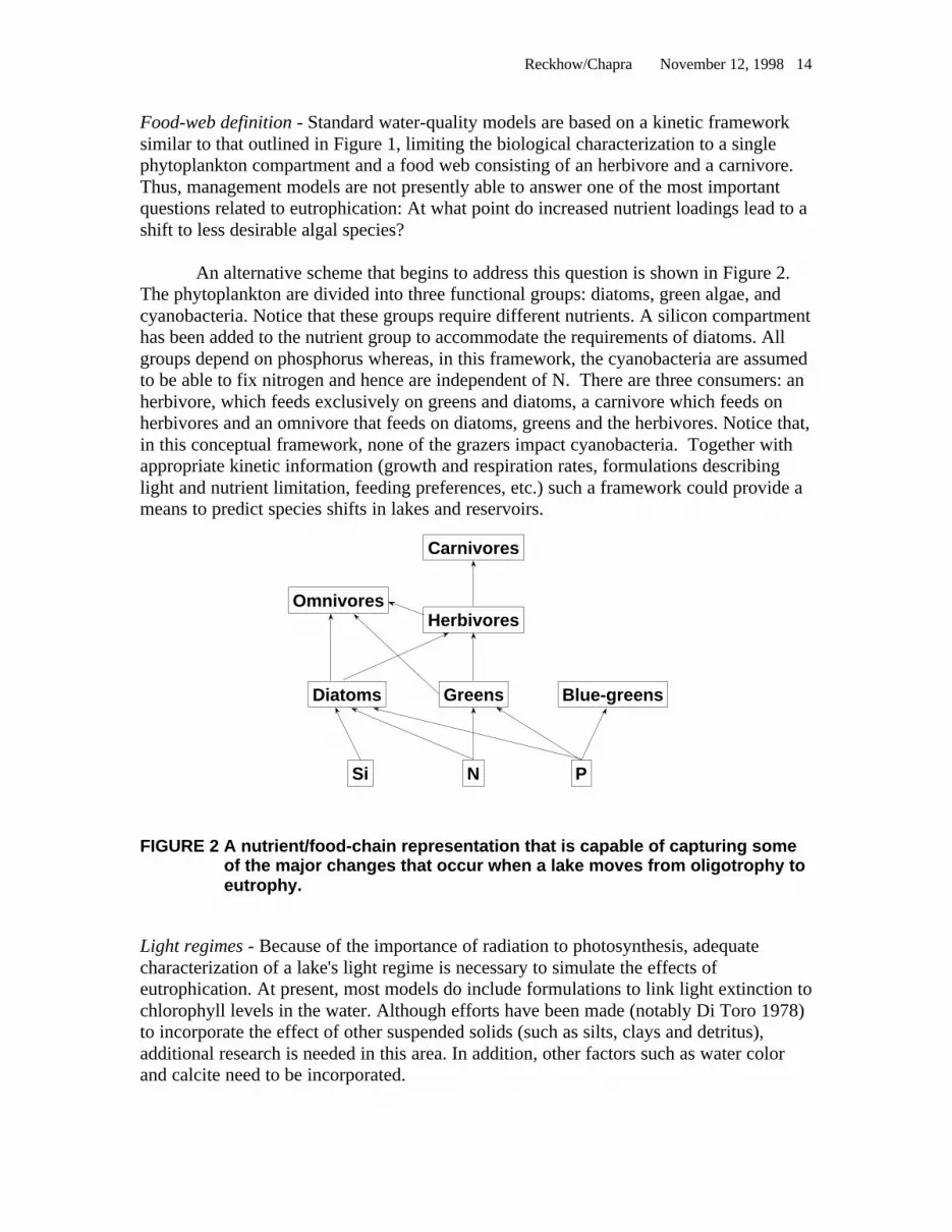
Food-web definition - Standard water-quality models are based on a kinetic frameworksimilar to that outlined in Figure 1, limiting the biological characterization to a singlephytoplankton compartment and a food web consisting of an herbivore and a carnivore.Thus, management models are not presently able to answer one of the most importantquestions related to eutrophication: At what point do increased nutrient loadings lead to ashift to less desirable algal species?

An alternative scheme that begins to address this question is shown in Figure 2.The phytoplankton are divided into three functional groups: diatoms, green algae, andcyanobacteria. Notice that these groups require different nutrients. A silicon compartmenthas been added to the nutrient group to accommodate the requirements of diatoms. Allgroups depend on phosphorus whereas, in this framework, the cyanobacteria are assumedto be able to fix nitrogen and hence are independent of N. There are three consumers: anherbivore, which feeds exclusively on greens and diatoms, a carnivore which feeds onherbivores and an omnivore that feeds on diatoms, greens and the herbivores. Notice that,in this conceptual framework, none of the grazers impact cyanobacteria. Together withappropriate kinetic information (growth and respiration rates, formulations describinglight and nutrient limitation, feeding preferences, etc.) such a framework could provide ameans to predict species shifts in lakes and reservoirs.

Carnivores

HerbivoresOmnivores

Diatoms Greens Blue-greens

Si N P

FIGURE 2 A nutrient/food-chain representation that is capable of capturing someof the major changes that occur when a lake moves from oligotrophy toeutrophy.

Light regimes - Because of the importance of radiation to photosynthesis, adequatecharacterization of a lake's light regime is necessary to simulate the effects ofeutrophication. At present, most models do include formulations to link light extinction tochlorophyll levels in the water. Although efforts have been made (notably Di Toro 1978)to incorporate the effect of other suspended solids (such as silts, clays and detritus),additional research is needed in this area. In addition, other factors such as water colorand calcite need to be incorporated.


Microbial kinetics - At present, all government and commercial packages representmicrobial kinetics as first-order decomposition rates. In fact, they are actually second-order, being dependent on both the substrate as well as the microbial concentrations.Because this involves simulating bacterial biomass, the inclusion of this mechanism isnot to be taken lightly. However, the benefits are two-fold. First, rates would adjust bothseasonally and spatially depending on bacterial abundance. This is in contrast to presentmodels, where aside from effects due to temperature variations, rates are constant.Second, rates would also adjust as systems moved along the trophic continuum. Hence,lower decomposition rates would result in oligotrophic systems due to carbon substratelimitation.

Concluding Thoughts on Mechanisms and Empiricism

To this point, we have somewhat separately addressed improvements in empiricalapproaches to modeling and better characterization of mechanisms. How can we bringthese two important themes together?

Consider the situation in Figure 3, which is a graphical representation of theuncertainties of two parameterizations of the Streeter-Phelps model. In Figure 3a, BODremoval is lumped into a single first-order removal rate, kr. However, based on scientificunderstanding, the model may be refined by acknowledging parametrically that removalis made up of two separate processes, decomposition, kd, and settling, ks (Figure 3b). Thislatter case clearly represents additional knowledge because the refined parameterizationincorporates collateral information. Now does that additional knowledge automaticallytranslate into a reduction in model prediction uncertainty?

No, this conclusion, while theoretically plausible, is not automatic. The specificsituation depicted in Figure 3 is indicative of conditions under which a reduction inmodel prediction uncertainty may be expected. That is, mechanistic knowledge issupportive of the additional parameterization, and data support estimation of kd and ks, asexpressed by the tight distribution on each parameter. However, it is perhaps more likelythat, while we know two distinct processes (decomposition and settling) occur, we havelittle site-specific data to parameterize each process separately, such that the separatedistributions for kd and ks are actually more dispersed than is the original distribution forkr. That is, the limited site-specific data provide a reasonably precise estimate of only theaggregate, single first-order removal.

Given the data needs of most mechanistic nutrient enrichment models,observational databases are typically insufficient in scope (leading to the common use of“rates manuals” such as Bowie et al. 1985). Thus it should not be surprising thattheoretically based improvements in a model often cannot be supported with the limitedavailable observational data. The paucity of data should not diminish our commitment toboth theory (mechanism) and observation (empiricism) as essential for the improvementof predictive models. We must bear in mind that basic process understanding is essentialfor incorporating new ideas into the existing knowledge base and into a mathematical


model, while observational evidence is ultimately necessary to calibrate the model andassess the goodness of fit. It is imperative that we continue to work to merge theseseparate but essential perspectives.

kd ks

kr

sdr kkk ++==

(a)

(b) information

FIGURE 3 A graphical representation of the uncertainties of two parameterizationsof the Streeter-Phelps model. (a) BOD removal is lumped into a singlefirst-order removal rate, kr. (b) Based on scientific understanding, themodel is refined by acknowledging parametrically that removal is madeup of two separate processes, decomposition, kd, and settling, ks. Thelatter case represents reduced uncertainty because the refinedparameterization represents information.


References

Ambrose, R.B., Wool, T.A., and J.L. Martin. 1993. The water quality analysis Simulationprogram, WASP5. Part A: model documentation. U.S. EPA, EnvironmentalResearch Laboratory, Athens, Georgia, 209 pp.

Adams, B.A.V. 1998. Parameter distributions for uncertainty propagation in water qualitymodeling. Ph.D. dissertation, Duke University. 148 p.

Beck, M.B., 1987. Water quality modeling: a review of the analysis of uncertainty. WaterResources Res., 23:1393-1442.

Berger, J.O. 1985. Statistical decision theory and Bayesian analysis (second edition).Springer-Verlag. New York. 617 p.

Blumberg, A.F., and Mellor, G.L. 1987. A description of three-dimensional coastal oceancirculation model, in Three-dimensional coastal ocean models, Vol. 4, N. Heaps,ed., Am. Geophys. Union, Washington, D.C., 1-16.

Bowie, G.L., Mills, W.B., Porcella, D.B., Campbell, C.L., Pagenkopf, J.R., Rupp, G.L.,Johnson, K.M., Chan, P.W.H., Gherini, S.A., and Chamberlin, C.E., 1985. Rates,constants, and kinetics formulations in surface water quality modeling. U.S.Environmental Protection Agency, EPA/600/3-85/040.

Brown, L.C. and Barnwell, T.O. 1987. The enhanced stream water quality modelsQUAL2E and QUAL2E-UNCAS: documentation and user manual, EPA/600/3-87/007. U.S. Environmental Protection Agency, Athens Georgia.

Canale, R.P. and M.T. Auer. 1982. Ecological studies and mathematical modeling ofCladophora in Lake Huron: 5. model development and calibration. J. GreatLakes Res., 8: 112-126.

Canale, R.P., Hinemann, D.F., and S. Nachippan. 1974. A biological production modelfor Grand Traverse Bay. University of Michigan Sea Grant Program, TechnicalReport No. 37, Ann Arbor, Michigan, 116 pp.

Canale, R.P., Chapra, S.C., Amy, G.L. and Edwards, M.A. Trihalomethane precursormodels for lakes and reservoirs. Water Resources Planning and Management, ASCE,123(5):259-265.

Cerco, C.F., and T. Cole. 1993. Three-dimensional eutrophication model of ChesapeakeBay. Journal of Environmental Engineering. 119:1006-1025.

Chapra, S.C. 1997. Surface water-quality modeling, McGraw-Hill, New York, NewYork, 844 pp.


Chapra, S.C. and R.P. Canale. 1991. Long-term phenomenogical model of phosphorusand oxygen in stratified lakes. Water Research, 25:707-715.

Chen, C.W. 1970. Concepts and utilities of ecological models," J. San. Engr. Div. ASCE,96:1085-1086.

Chen, C.W. and G.T. Orlob. 1975. Ecological simulation for aquatic environments. pp.475-588, In: B.C. Patton (ed.), Systems Analysis and Simulation in Ecology, Vol.III, Academic Press, New York.

Cole, T.M. and E.M. Buchak. 1995. CE-QUAL-W2: A two-dimensional, laterallyaveraged, hydrodynamic and water quality model, Version 2.0. user manual.Instruction Report EL-95, U.S. Army Corps of Engineers, Waterways ExperimentStation, Vicksburg, Mississippi, 57 pp.

Connolly, J.P. and Coffin, R.B. 1995. Model of carbon cycling in planktonic food webs.J. Environ. Engr. 121(10):682-690.

Cooke, R.M. 1991. Experts in uncertainty, opinion and subjective probability in science.Oxford University Press. New York. 367 p.

Di Toro, D.M. 1978. Optics of turbid estuarine waters: approximations and applications.Water Res. 12:1059-1068.

Di Toro, D.M. and Fitzpatrick, J.J. 1993. Chesapeake Bay sediment flux model. Tech.Report EL-93-2, U.S. Army Corps of Engineers, Waterways Experiment Station,Vicksburg, Mississippi, 316 pp.

Di Toro, D.M., Paquin, P.R., Subburamu, K. and Gruber, D.A. 1990. Sediment oxygendemand model: methane and ammonia oxidation. J. Environ. Engr. ASCE, 116:945-986.

Di Toro, D.M. and van Straten, G., 1979. Uncertainty in the parameters and predictionsof phytoplankton models. Working Paper WP-79-27, International Institute forApplied Systems Analysis, Laxenburg, Austria.

Donigian, A.S., Jr., and N.H. Crawford. 1976. Modeling pesticides and nutrients onagricultural lands. Environmental Research Laboratory, Athens, GA. EPA600/2-7-76-043. 317 p.

Fair, G.M., Moore, E.W., and Thomas, H.A., Jr. 1941. The natural purification of rivermuds and pollutional sediments. Sewage Works J. 13(6):1209-1228.

Gilks, W.R., Richardson, S., and D. Spiegelhalter (eds.). 1996. Markov chain MonteCarlo in practice. Chapman and Hall. New York. 473 p.


Harmon, R., and P. Challenor. 1997. A Markov chain Monte Carlo method for estimationand assimilation into models. Ecological Modelling. 101:41-59.

Hornberger, G.M., and R.C. Spear. 1980. Eutrophication in Peel Inlet, I. The problem:defining behavior and a mathematical model for the phosphorus scenario. WaterRes. 14:29-42.

Jamieson, C.A., and J.C. Clausen. 1988. Tests of the CREAMS model on agriculturalfields in Vermont. Water Resources Bulletin. 2:1219-1226.

Jorgensen, S.E. 1986. Structural dynamic model. Ecological Modelling.31:1-9.

Jorgensen, S.E. 1997. Integration of ecosystem theories: a pattern. Kluwer. Dordrecht.

Kadlec, R.H. and W.W. Walker, Jr. 1997. Management Models to Evaluate PhosphorusImpacts on Wetlands. This volume.

Laws, E.A. and M.S. Chalup. 1990. A microalgal growth model. Limnol. Oceanogr., 35:597-608.

Martz, J.S., and T. Lwin. 1989. Empirical Bayes methods (second edition). Chapman andHall. London. 284 p.

Meyer, M., and Booker, J. 1991. Eliciting and analyzing expert judgment, a practicalguide. Academic Press. London. 411 p.

O’Connor, D.J., D.M. Di Toro, and R.V. Thomann. 1975. Phytoplankton models andeutrophication problems. In: Ecological modeling in a resource managementframework. Resources for the Future. Washington, D.C.

O’Neill, R.V. 1971. Error analysis of ecological models. In: Proceedings of the thirdnational symposium on radioecology. Oak Ridge, TN.

O’Neill, R.V., R.H. Gardner, and J.B. Mankin. 1980. Analysis of parameter error in anonlinear model. Ecol. Modelling. 8:297-311.

Penn, M.R., Auer, M.T., VanOrman, E.L., and J.J. Korienek. 1995. PhosphorusDiagenesis in Lake Sediments: Investigations Using Fractionation Techniques.Marine and Freshwater Research, 46: 89-99.

Reckhow, K.H. 1979. Uncertainty analysis applied to Vollenweider's phosphorus loadingcriterion, Journal of Water Pollution Control Federation, 51(8): 2123-2128.

Reckhow, K.H. 1994. Water quality simulation modeling and uncertainty analysis forrisk assessment and decision making. Ecological Modelling. 72:1-20.


Reckhow, K.H. and S.C. Chapra. 1979. A note on error Analysis for a phosphorusretention model. Water Resource Research, 15(6): 1643-1646.

Reckhow, K.H., and S.C. Chapra. 1983. Engineering approaches for lake management –Volume 1: data analysis and empirical modeling. Butterworths. Boston. 340 p.

Reckhow, K.H. and C.M. Marin. 1986. Empirical Bayes estimation and inference for thephosphorus - chlorophyll relationship in lakes. In: Lake and ReservoirManagement, Proceedings of the Annual Conference of the North American LakeManagement Society, p. 154-156.

Riley, G.A. 1946. Factors controlling phytoplankton population on Georges Bank. J.Mar. Res., 6:104-113.

Sawyer, C.H. 1947. Fertilization of lakes by agricultural and urban drainage. New Engl.Water Works Assoc. 61:109-127.

Scavia, D., Canale, R.P., Powers, W.F. and Moody, J.L., 1981. Variance estimates for adynamic eutrophication model of Saginaw Bay, Lake Huron. Water ResourcesRes., 17:1115-1124.

Scheffer, M., Hosper, S.H., Meijer, M.-L., Moss, B., and E. Jeppesen. 1993. AlternativeEquilibria in Shallow Lakes. Trends Ecol. Evol., 8: 275-279.

Shelske, C.L. 1997. Assessing Nutrient Limitation and Trophic State in Florida lakes.“Phosphorus Biogeochemistry in Florida Ecosystems”, July 13-16, 1997, ClearwaterBeach Florida.

Spear, R.C., and G.M. Hornberger. 1980. Eutrophication in Peel Inlet, II. Identification ofcritical uncertainties via generalized sensitivity analysis. Water Res. Res.14:43-49.

Steele, J.H. 1962. Environmental control of photosynthesis in the sea. Limnol. Oceanogr.,7:137-150.

Steele, J. H. and Baird, I. E. 1962. Relations Between Primary Production, Chlorophylland Particulate Carbon. Limnol. Oceanogr. 6:68-78.

Steele, J. H. and Baird, I. E. 1963. Further Relations Between Primary Production,Chlorophyll and Particulate Carbon. Limnol. Oceanogr. 7:42-47.

Stow, C.A., Carpenter, S.R., and R.C. Lathrop. 1997. A Bayesian observation errormodel to predict cyanobacterial biovolume from spring total phosphorus in LakeMendota, Wisconsin. Canadian Journal Fisheries and Aquatic Sciences. 54:464-473.


Sweeney, D.W., A.B. Bottcher, K.L. Capbell, and D.A. Graetz. 1985. Measured andCREAMS-predicted nitrogen losses from tomato and corn management systems.Water Resources Bulletin. 21:867-873.

Thomann, R.V. and J.F. Fitzpatrick. 1982. Calibration and verification of a mathematicalmodel of the eutrophication of the Potomac Estuary. Report to District ofColumbia, Department of Environmental Services, HydroQual, Inc. Mahwah,New Jersey, 500 pp.

Thomann, R.V., D.M. Di Toro, R.P. Winfield, and D.J. O’Connor. 1975. Mathematicalmodeling of phytoplankton in Lake Ontario. 1. Model development andverification. U.S. Environmental Protection Agency, EPA/600/3-75-005.

Thomann, R.V. and Mueller, J.A. 1987. Principles of surface water quality modeling andcontrol, Harper-Collins, New York, NY. 479 p.

Uttormark, P.D., J.D. Chapin, and K.M. Green. 1974. Estimating nutrient loadings oflakes from non-point sources. U.S. Environmental Protection Agency,EPA/600/3-74-020.

Vollenweider, R.A. 1968. The scientific basis of lake and stream eutrophication, withparticular reference to phosphorus and nitrogen as eutrophication factors.Technical Report DAS/DSI/68.27. Organization for Economic Cooperation andDevelopment. Paris, France.

Vollenweider, R.A. 1975. Input-output models with special reference to the phosphorusloading concept in limnology. Schweiz. Z. Hydrol. 37:53-84.

von Winterfeldt, D., and Edwards, W. 1986. Decision analysis and behavioral research.Cambridge University Press, Cambridge, UK. 623 p.

Wickman, T.R. and M.T. Auer. 1997. Nitrogen Diagenesis and the Flux of Ammoniafrom Lake Sediments, In Preparation for Can. J. Fish. Aquat. Sci.

Documents

Modeling excessive nutrient loading in the environment