ESRI International User Conference Papers

Title Paper UC1656: Modeling the South American Range of the Cerulean Warbler

Coauthors:

Members of El Grupo Cerúleo: Barker, S., Benítez, S., Baldy, J., Cisneros Heredia,

D., Colorado Zuluaga, G., Cuesta, F., Davidson, I., Díaz, D., Ganzenmueller, A., García, S.,

Girvan, M. K., Guevara, E., Hamel, P., Hennessey, A. B., Hernández, O. L., Herzog, S.,

Mehlman, D., Moreno, M. I., Ozdenerol, E., Ramoni-Perazzi, P., Romero, M., Romo, D.,

Salaman, P., Santander, T., Tovar, C., Welton, M., Will, T., Pedraza, C., Galindo, G.

Abstract

Successful conservation of rare species requires detailed knowledge of the species’

distribution. Modeling spatial distribution is an efficient means of locating potential habitats.

Cerulean Warbler (Dendroica cerulea, Parulidae) was listed as a Vulnerable Species by the

International Union for the Conservation of Nature and Natural Resources in 2004. These

neotropical migratory birds breed in eastern North America. The entire population migrates

to the northern Andes in South America to spend the nonbreeding period. As part of a larger

international conservation effort, we developed spatial hypotheses of the bird’s occurrence

in South America. We summarized physical, climatic, and recent land-cover data for the

northern Andes using ESRI software, ArcGIS. We developed five hypothetical distributions

based on Mahalanobis D, GARP, Biomapper, MAXENT, and Domain models. Combining

results of the different models on the same map allowed us to design a rigorous strategy to

ground-truth the map and thus to identify sites for protection of the species in South

America.

Introduction

Successful conservation of rare species requires detailed knowledge of the species’

distribution. Often the decline of a species’ population occurs with a particular geographical

pattern (Maurer 1994). This pattern of decline may represent changes affecting the entire

range which are expressed more severely in one part of the range, resulting disappearance

from one portion of the range. The spatial pattern of decline may also represent changes

affecting only a portion of the range and causing the species to become restricted there

(Smith et al. 1996). Understanding the spatial distribution of change is a key to inferring

the causal factors. Conservation requires redress of those causes.

A variety of approaches to spatial modeling of species distributions has been summarized by

Elith et al. (2006). Expressing a range in a spatially explicit way provides interested

persons with a means to visualize the range in relation to external factors and to relate

changes in the range to potential causal factors. When data on distribution of the species

are scarce, for whatever reason, the range is difficult to present on a map, to visualize, and

to relate to changes in causal factors. Using known occurrences in combination with ambient

variables to model spatial distribution is an efficient means of locating potential habitats in

unsurveyed areas; this is especially true where existing distributional data are scarce or

biased in some way. For declining species of migratory North American birds (Terborgh

1989), mapping the nonbreeding distributions in Central and South America and the

Caribbean typically involves surmounting a wider variety of data constraints than does

mapping the breeding range in North America.

The Cerulean Warbler (Dendroica cerulea, Parulidae) was listed as a Vulnerable Species by

the International Union for the Conservation of Nature and Natural Resources in 2004

(Birdlife International 2004, 2006). These nearctic/neotropical migratory birds breed in

eastern North America (Hamel 2000b). Breeding habitat consists of a variety of deciduous

forests (Rosenberg et al. 2000), including especially tall trees of large diameter from which

the breeding males sing, as well as more modest-sized trees in which the females place

their nests (Hamel 2005). The entire population migrates to the northern Andes of South

America to spend the nonbreeding period (Hilty and Brown 1986).

Two different verbal descriptions of the nonbreeding habitat of the species follow. Hilty and

Brown (1986) was arguably the most authoritative source of information on birds in the

northern Andes when it was published. These authors indicate that the species was a very

uncommon resident during the nonbreeding period in Colombia, that most of the birds were

south of that country during the October-March period, and identified the range as forests

and forest borders primarily west of the Andes, from elevations of 500 to 2000 m. Robbins

et al. (1992) identified primary forest as important nonbreeding habitat. More recently,

Hamel (2000b) extended the description of Hilty and Brown (1986) and Robbins et al.

(1992) to include canopy and borders of broadleaved, evergreen forests and woodland at

middle and lower elevations on the east slopes of the Andes from Colombia to Peru and

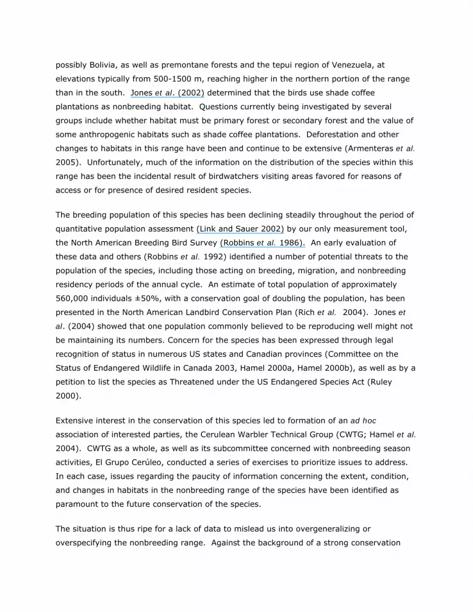
possibly Bolivia, as well as premontane forests and the tepui region of Venezuela, at

elevations typically from 500-1500 m, reaching higher in the northern portion of the range

than in the south. Jones et al. (2002) determined that the birds use shade coffee

plantations as nonbreeding habitat. Questions currently being investigated by several

groups include whether habitat must be primary forest or secondary forest and the value of

some anthropogenic habitats such as shade coffee plantations. Deforestation and other

changes to habitats in this range have been and continue to be extensive (Armenteras et al.

2005). Unfortunately, much of the information on the distribution of the species within this

range has been the incidental result of birdwatchers visiting areas favored for reasons of

access or for presence of desired resident species.

The breeding population of this species has been declining steadily throughout the period of

quantitative population assessment (Link and Sauer 2002) by our only measurement tool,

the North American Breeding Bird Survey (Robbins et al. 1986). An early evaluation of

these data and others (Robbins et al. 1992) identified a number of potential threats to the

population of the species, including those acting on breeding, migration, and nonbreeding

residency periods of the annual cycle. An estimate of total population of approximately

560,000 individuals ±50%, with a conservation goal of doubling the population, has been

presented in the North American Landbird Conservation Plan (Rich et al. 2004). Jones et

al. (2004) showed that one population commonly believed to be reproducing well might not

be maintaining its numbers. Concern for the species has been expressed through legal

recognition of status in numerous US states and Canadian provinces (Committee on the

Status of Endangered Wildlife in Canada 2003, Hamel 2000a, Hamel 2000b), as well as by a

petition to list the species as Threatened under the US Endangered Species Act (Ruley

2000).

Extensive interest in the conservation of this species led to formation of an ad hoc

association of interested parties, the Cerulean Warbler Technical Group (CWTG; Hamel et al.

2004). CWTG as a whole, as well as its subcommittee concerned with nonbreeding season

activities, El Grupo Cerúleo, conducted a series of exercises to prioritize issues to address.

In each case, issues regarding the paucity of information concerning the extent, condition,

and changes in habitats in the nonbreeding range of the species have been identified as

paramount to the future conservation of the species.

The situation is thus ripe for a lack of data to mislead us into overgeneralizing or

overspecifying the nonbreeding range. Against the background of a strong conservation

need for this species, and because of its overlap with a wide array of resident species of

birds and other groups of conservation concern in this area of great biodiversity (Renjifo

1998), enormous implications to other species of conserving habitats for the Cerulean

Warbler exist.

The current work responds to these identified needs. In a series of workshops and

observer-directed field investigations, the members of El Grupo Cerúleo have identified and

organized existing data on the nonbreeding distribution of the Cerulean Warbler. We here

present the results of applying a series of spatial modeling algorithms to the very scarce

existing data on the South American distribution of this species. Our objective in this work

has been to develop a spatially explicit hypothesis of the distribution of the species that can

be subjected to rigorous field tests.

Methods

Data Sets and Sources

Cerulean Warbler Modeling Data—We compiled a list of existing, georeferenced occurrence

data for the species. Records included specimens from museum collections (D. Pashley,

pers. comm.), as well as responses to a request for records sent to a wide variety of

observers through online and other means, and published records summarized by Hamel

(2000a). The dataset included 336 such observations. All of these observations and

specimens constitute a convenience sampling frame for the occurrence of the species in

South America during the October-March nonbreeding resident period, and represent

historic and recent records dating from 1880-2005. The quality of georeferencing of these

points also varied greatly, from GPS recordings to names of nearest town listed on specimen

labels. We used a variety of gazetteers to infer coordinates from the available locality

information.

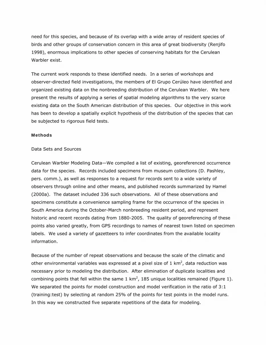
Because of the number of repeat observations and because the scale of the climatic and

other environmental variables was expressed at a pixel size of 1 km2, data reduction was

necessary prior to modeling the distribution. After elimination of duplicate localities and

combining points that fell within the same 1 km2, 185 unique localities remained (Figure 1).

We separated the points for model construction and model verification in the ratio of 3:1

(training:test) by selecting at random 25% of the points for test points in the model runs.

In this way we constructed five separate repetitions of the data for modeling.

Validation Data Points—Through a series of field projects funded by El Grupo Cerúleo in the

nonbreeding periods of 2003-2004, 2004-2005, and 2005-2006, we were able to develop an

independent set of validation data for the model predictions. These were all sight and

capture records, georeferenced with GPS, and subject to the same convenience sampling

constraint as the modeling data. Field collaborators contributed 113 such records, of which

50 constituted confirmed presence of the species (Figure 1).

Environmental Data—We gathered climatic, physical, and vegetation data from three

primary sources available online to the public. Climate data consisted of 19 variables

representing combinations of temperature and precipitation (Table 1) from WORLDCLIM

(http://www.worldclim.org/, Hijmans et al. [no date], Hijmans et al. 2005). The data exist

in a grid of 1 km2 pixels. Physical data on slope, aspect, and elevation came from the

digital elevation model available as GTOPO30 (US Geological Survey [no date]). These data

were expressed also as a grid of 1 km2 pixels. Vegetation data on percent bare ground,

percent herbaceous cover, and percent tree cover came from Global land cover facility

MODIS ([no date]). We accepted the value of 70% tree cover to indicate that the 500 m2

pixels were forested. We transformed the vegetation cover data to 1 km2 pixel size

resolution for compatibility with the other data. We further transformed two of the

environmental variables, Slope and Annual Precipitation, using Box-Cox procedures to

remove nonnormality in these data (Sokal and Rohlf 1981).

Table 1. List of initial environmental, physical and land cover variables considered in the

modeling process

Enviromental variable Source Original pixel

scale

Used in final

model BIO1 = Annual Mean Temperature WORLDCLIM 1000 m BIO2 = Mean Diurnal Temperature Range (Mean of monthly (max temp - min temp)) WORLDCLIM 1000 m BIO3 = Isothermality (P2/P7) (* 100) WORLDCLIM 1000 m X BIO4 = Temperature Seasonality (standard deviation *100) WORLDCLIM 1000 m BIO5 = Max Temperature of Warmest Month WORLDCLIM 1000 m BIO6 = Min Temperature of Coldest Month WORLDCLIM 1000 m BIO7 = Temperature Annual Range (P5-P6) WORLDCLIM 1000 m BIO8 = Mean Temperature of Wettest Quarter WORLDCLIM 1000 m BIO9 = Mean Temperature of Driest Quarter WORLDCLIM 1000 m BIO10 = Mean Temperature of Warmest Quarter WORLDCLIM 1000 m BIO11 = Mean Temperature of Coldest Quarter WORLDCLIM 1000 m BIO12 = Mean Total Annual Precipitation WORLDCLIM 1000 m X

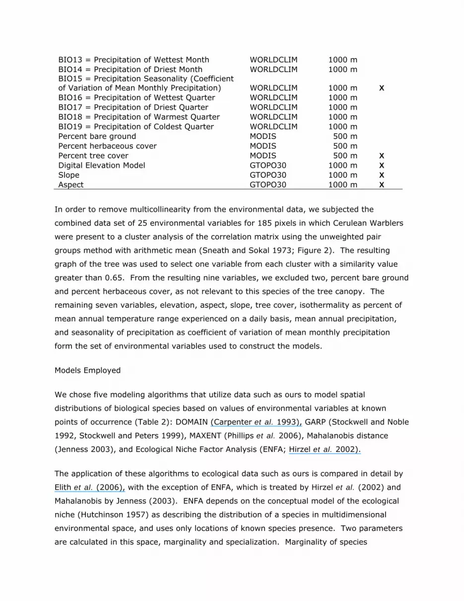
BIO13 = Precipitation of Wettest Month WORLDCLIM 1000 m BIO14 = Precipitation of Driest Month WORLDCLIM 1000 m BIO15 = Precipitation Seasonality (Coefficient of Variation of Mean Monthly Precipitation) WORLDCLIM 1000 m X BIO16 = Precipitation of Wettest Quarter WORLDCLIM 1000 m BIO17 = Precipitation of Driest Quarter WORLDCLIM 1000 m BIO18 = Precipitation of Warmest Quarter WORLDCLIM 1000 m BIO19 = Precipitation of Coldest Quarter WORLDCLIM 1000 m Percent bare ground MODIS 500 m Percent herbaceous cover MODIS 500 m Percent tree cover MODIS 500 m X Digital Elevation Model GTOPO30 1000 m X Slope GTOPO30 1000 m X Aspect GTOPO30 1000 m X

In order to remove multicollinearity from the environmental data, we subjected the

combined data set of 25 environmental variables for 185 pixels in which Cerulean Warblers

were present to a cluster analysis of the correlation matrix using the unweighted pair

groups method with arithmetic mean (Sneath and Sokal 1973; Figure 2). The resulting

graph of the tree was used to select one variable from each cluster with a similarity value

greater than 0.65. From the resulting nine variables, we excluded two, percent bare ground

and percent herbaceous cover, as not relevant to this species of the tree canopy. The

remaining seven variables, elevation, aspect, slope, tree cover, isothermality as percent of

mean annual temperature range experienced on a daily basis, mean annual precipitation,

and seasonality of precipitation as coefficient of variation of mean monthly precipitation

form the set of environmental variables used to construct the models.

Models Employed

We chose five modeling algorithms that utilize data such as ours to model spatial

distributions of biological species based on values of environmental variables at known

points of occurrence (Table 2): DOMAIN (Carpenter et al. 1993), GARP (Stockwell and Noble

1992, Stockwell and Peters 1999), MAXENT (Phillips et al. 2006), Mahalanobis distance

(Jenness 2003), and Ecological Niche Factor Analysis (ENFA; Hirzel et al. 2002).

The application of these algorithms to ecological data such as ours is compared in detail by

Elith et al. (2006), with the exception of ENFA, which is treated by Hirzel et al. (2002) and

Mahalanobis by Jenness (2003). ENFA depends on the conceptual model of the ecological

niche (Hutchinson 1957) as describing the distribution of a species in multidimensional

environmental space, and uses only locations of known species presence. Two parameters

are calculated in this space, marginality and specialization. Marginality of species

distribution is defined as the difference between species mean values and study area wide

mean values for a particular environmental variable standardized by the 95th percentile

confidence interval on that area wide mean. Specialization of the species distribution is the

ratio of the standard deviation of the global distribution to the standard deviation of the

species distribution. High values of marginality indicate that the species niche is far from

the norm in the study area, while high values of specialization indicate that the species

niche is well-defined relative to the values available in the study area. Specific values for

these indices are particular to each individual study. Over a number of environmental

variables, vectors of marginality and specialization are subjected to multivariate factor

analysis. This approach to modeling distribution has been implemented as Program

Biomapper 3.0, which we used in our analysis here.

Table 2. Models used in exploring the range of the Cerulean Warbler

Model Algorithm and Settings employed

MAXENT Maximum Entropy Theory, single run of 1000 iterations

GARP Genetics Algorithm for Rule Set Prediction, 50 runs of 1000 iterations, error

rates at Omission=10%, Commission=40%, Convergence Limit of 0.01, Using

100% of training points

DOMAIN Gower similarity index, single run, outliers established at 95th percentile

Mahalanobis Mahalanobis D non-euclidean distance, single run

ENFA Ecological Niche Factor Analysis, single run with 3 factors accommodating

85% of variation in the data

The Mahalanobis distance modeling utilizes pairwise differences between values of

environmental variables to generate a distance matrix (Greenacre 1984). Several

multivariate analytical procedures can use this parameter as a metric to evaluate

differences between groups of data points. An example of its application to spatial modeling

is Rotenberry et al. (2006), who used the procedure to estimate habitat and limiting factors

for a rare bird, the California Gnatcatcher (Polioptila californica). We implemented our

analysis using the Mahalanobis distances extension for ArcView 3.x (Jenness 2003).

Analysis

We conducted five separate analyses with each model, each using one of the five replicate

data sets randomly selected to be 75% training - 25% test points. We calculated the AUC

parameter for each of the runs, and computed mean and standard error of the AUC. AUC is

the Area Under the Curve of Receiver Operating Characteristic Plots (Zweig and Campbell

1993, Fielding and Bell 1997). In this plot of commission error rate vs sensitivity, defined

to be (1-omission error rate), a value of 1 represents the best the model could be, with 0 in

the x axis (commission error) and 1 in the y axes (sensitivity). Any value below the

diagonal in the plot is considered to be a random model, and the closer a model result is to

upper left corner the better the model is considered to be.

We combined models by selecting for each an objective method of determining a threshold

for predicting occurrence vs nonoccurrence. Such a method for each of the models; for

MAXENT, we selected as threshold of 0.57023, because at this point the omission error rate

is between 0.2 and 0.3. For ENFA, Mahalanobis distance and DOMAIN we used the Kappa

Maximization approach widely used to determine thresholds for species distributions (Guisan

et al. 1999), where the proportion of correctly predicted sites is calculated (Liu et al. 2005).

The final values of threshold were: for Mahalanobis a d=245, for ENFA=35, Domain=91.4.

For GARP, we decided to use the sum of the best subsets of each model and define the

pixels where all eight best subsets are present as the area of potential distribution of the

bird. We combined the resulting binary models after application of these thresholds for

presence, and for each pixel in the five country study area calculated the number of models

(from zero to five) that predicted presence.

We conducted a model validation test by intersecting coverage of the MAXENT map and the

sum of binary maps of all models with the validation data points, and calculating a t-test of

the MAXENT values for points indicating presence vs those indicating absence in the

validation data set. We further intersected the binary maps of predicted habitat for all

models and for the combination of ENFA, MAXENT, and Mahalanobis with the validation data

set. Observed occurrences of Cerulean Warbler in the validation data set were examined

visually. We conducted a χ2 test to compare the distribution of observed absence and

observed presence in the validation data set among categories defined by number of models

predicting Cerulean Warbler presence at the validation data point.

Analyses of the occurrence data were carried out in the respective software packages

indicated. All spatial analyses, selections, and evaluations were conducted in ArcGIS, with

the exception of a small number which were carried out in ArcView.

Results

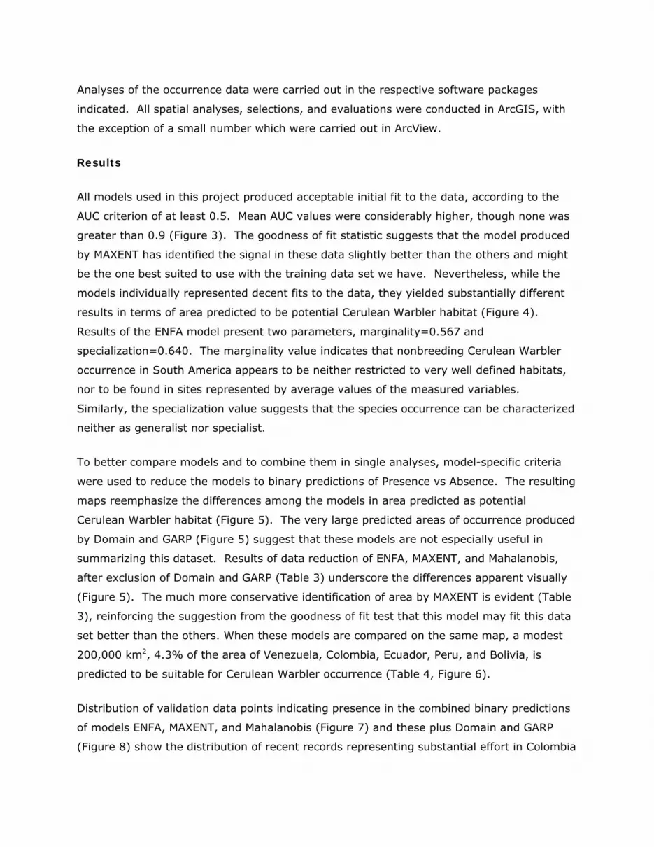
All models used in this project produced acceptable initial fit to the data, according to the

AUC criterion of at least 0.5. Mean AUC values were considerably higher, though none was

greater than 0.9 (Figure 3). The goodness of fit statistic suggests that the model produced

by MAXENT has identified the signal in these data slightly better than the others and might

be the one best suited to use with the training data set we have. Nevertheless, while the

models individually represented decent fits to the data, they yielded substantially different

results in terms of area predicted to be potential Cerulean Warbler habitat (Figure 4).

Results of the ENFA model present two parameters, marginality=0.567 and

specialization=0.640. The marginality value indicates that nonbreeding Cerulean Warbler

occurrence in South America appears to be neither restricted to very well defined habitats,

nor to be found in sites represented by average values of the measured variables.

Similarly, the specialization value suggests that the species occurrence can be characterized

neither as generalist nor specialist.

To better compare models and to combine them in single analyses, model-specific criteria

were used to reduce the models to binary predictions of Presence vs Absence. The resulting

maps reemphasize the differences among the models in area predicted as potential

Cerulean Warbler habitat (Figure 5). The very large predicted areas of occurrence produced

by Domain and GARP (Figure 5) suggest that these models are not especially useful in

summarizing this dataset. Results of data reduction of ENFA, MAXENT, and Mahalanobis,

after exclusion of Domain and GARP (Table 3) underscore the differences apparent visually

(Figure 5). The much more conservative identification of area by MAXENT is evident (Table

3), reinforcing the suggestion from the goodness of fit test that this model may fit this data

set better than the others. When these models are compared on the same map, a modest

200,000 km2, 4.3% of the area of Venezuela, Colombia, Ecuador, Peru, and Bolivia, is

predicted to be suitable for Cerulean Warbler occurrence (Table 4, Figure 6).

Distribution of validation data points indicating presence in the combined binary predictions

of models ENFA, MAXENT, and Mahalanobis (Figure 7) and these plus Domain and GARP

(Figure 8) show the distribution of recent records representing substantial effort in Colombia

and Ecuador, and lesser effort among our field projects in Venezuela. The lack of presence

in Peru is in part a result of a small amount of sampling and in part a result of absence of

the birds from former range there and in Bolivia. In each case, the distribution of observed

absences with confirmed occurrences of Cerulean Warbler differed from each other by χ2

test (3 model combination, χ2, 1 d.f. = 5.15, P < 0.05; 5 model combination, χ2, 1 d.f. =

4.09, P < 0.05; Figure 9). In both cases the number of observed occurrences increased

with the number of models predicting presence. Observed absences in the 3 model case

declined with increasing number of models predicting presence; in the 5 model case the

number of observed absences appeared to be independent of number of models predicting

presence of Cerulean Warbler.

Validation data points were intersected with the results of the MAXENT model (Figure 10),

and each validation data point assigned the probability of its pixel as predicted by MAXENT.

Comparison of the group of observed absences (mean MAXENT probability = 0.09, N=63) to

the group of observed presence (mean MAXENT probability = 0.12, N=50) with a t-test

detected no difference in MAXENT probability between the two groups (t, 68 d.f., = -1.61,

p=0.11).

Table 3. Realization of models with settings for binary predicted presence vs absence, based

on cutoff values of statistics particular to each model: MAXENT, omission error rate between

0.2 and 0.3; Ecological Niche Factor Analysis (ENFA), K=35%; Mahalanobis d=245,

DOMAIN K=91.3, GARP K=8.

MODEL

Number of pixels

Km2 % of study

area

ENFA 1201396 1,030,168 22

MAHALANOBIS 1781129 1,527,275 32

MAXENT 284333 243,809 5

DOMAIN 2165143 1,856,559 38

GARP 1514044 1,298,257 27

Table 4. Areas predicted differently by models as potential range of the Cerulean Warbler.

Models employed in this exercise were ENFA, MAXENT, and Mahalanobis.

Number of models

Number of pixels

Km2 % of study

area

0 3,621,414 3,105,276 65.8

1 739,142 633,797 13.4

2 908,682 779,173 16.5

3 235,251 201,722 4.3

TOTAL 5,504,489 4,719,967 100

Figure 1. Records of Cerulean Warbler distribution in northern South America, October-

March, used in Modeling (solid circles) and Validation data sets (stars).

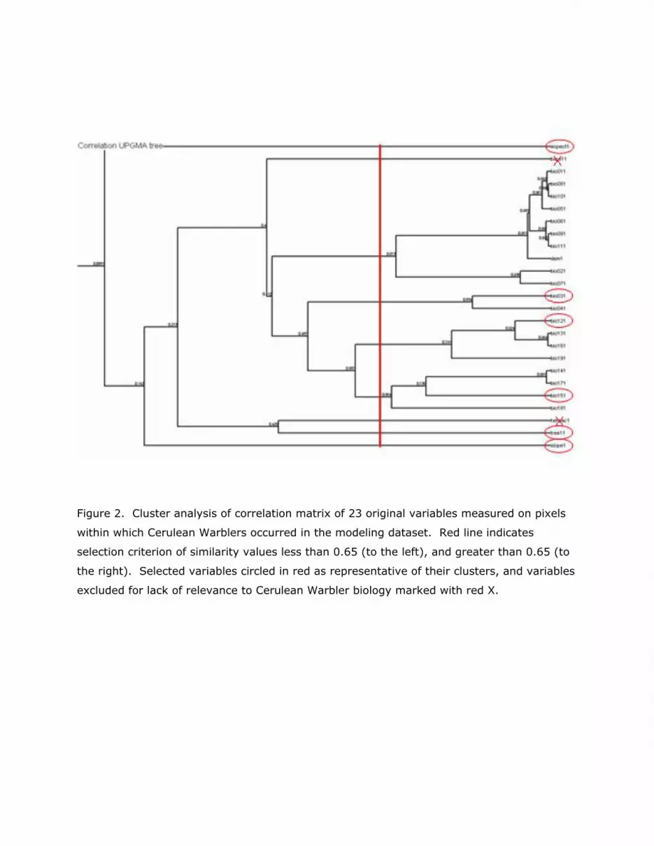
Figure 2. Cluster analysis of correlation matrix of 23 original variables measured on pixels

within which Cerulean Warblers occurred in the modeling dataset. Red line indicates

selection criterion of similarity values less than 0.65 (to the left), and greater than 0.65 (to

the right). Selected variables circled in red as representative of their clusters, and variables

excluded for lack of relevance to Cerulean Warbler biology marked with red X.

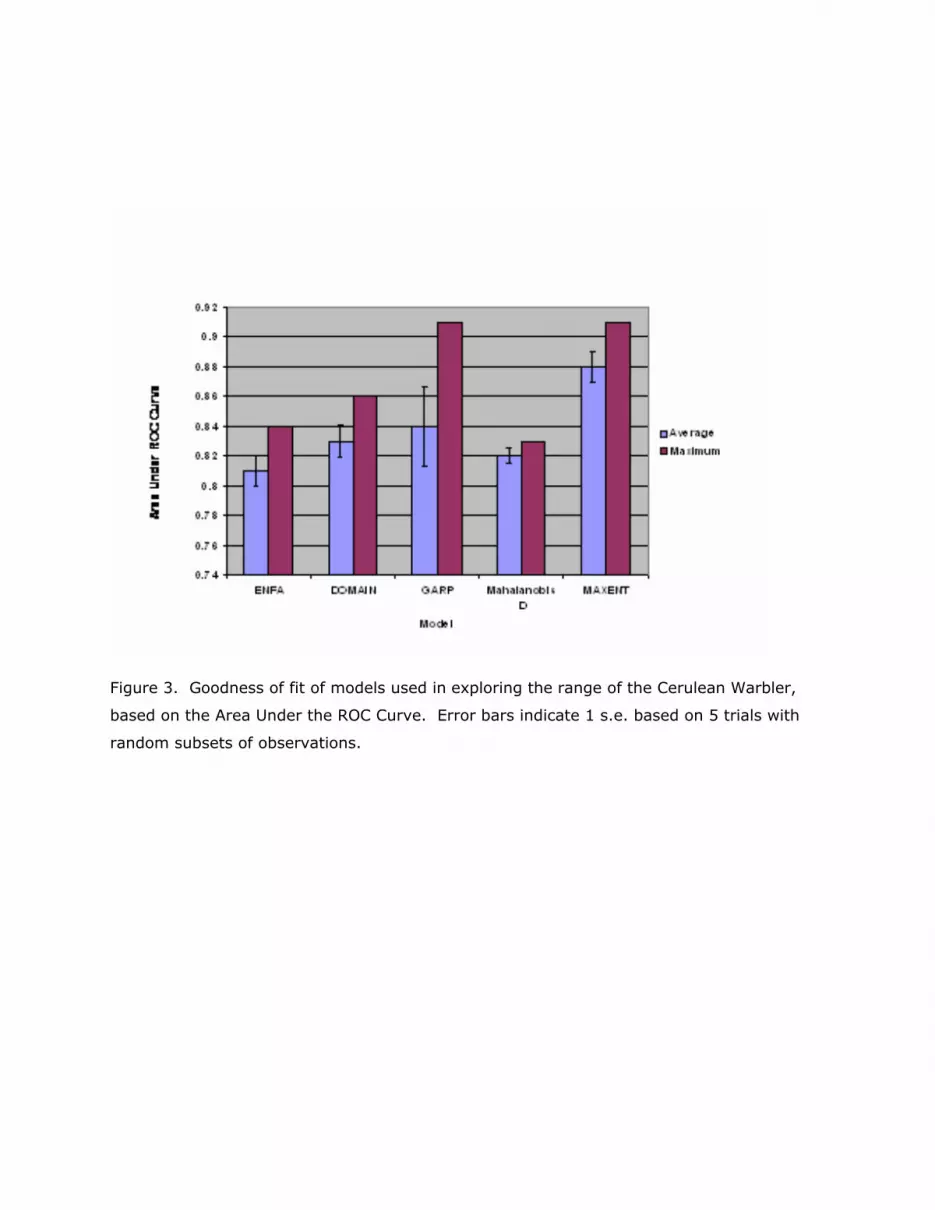
Figure 3. Goodness of fit of models used in exploring the range of the Cerulean Warbler,

based on the Area Under the ROC Curve. Error bars indicate 1 s.e. based on 5 trials with

random subsets of observations.

A B

C D

E

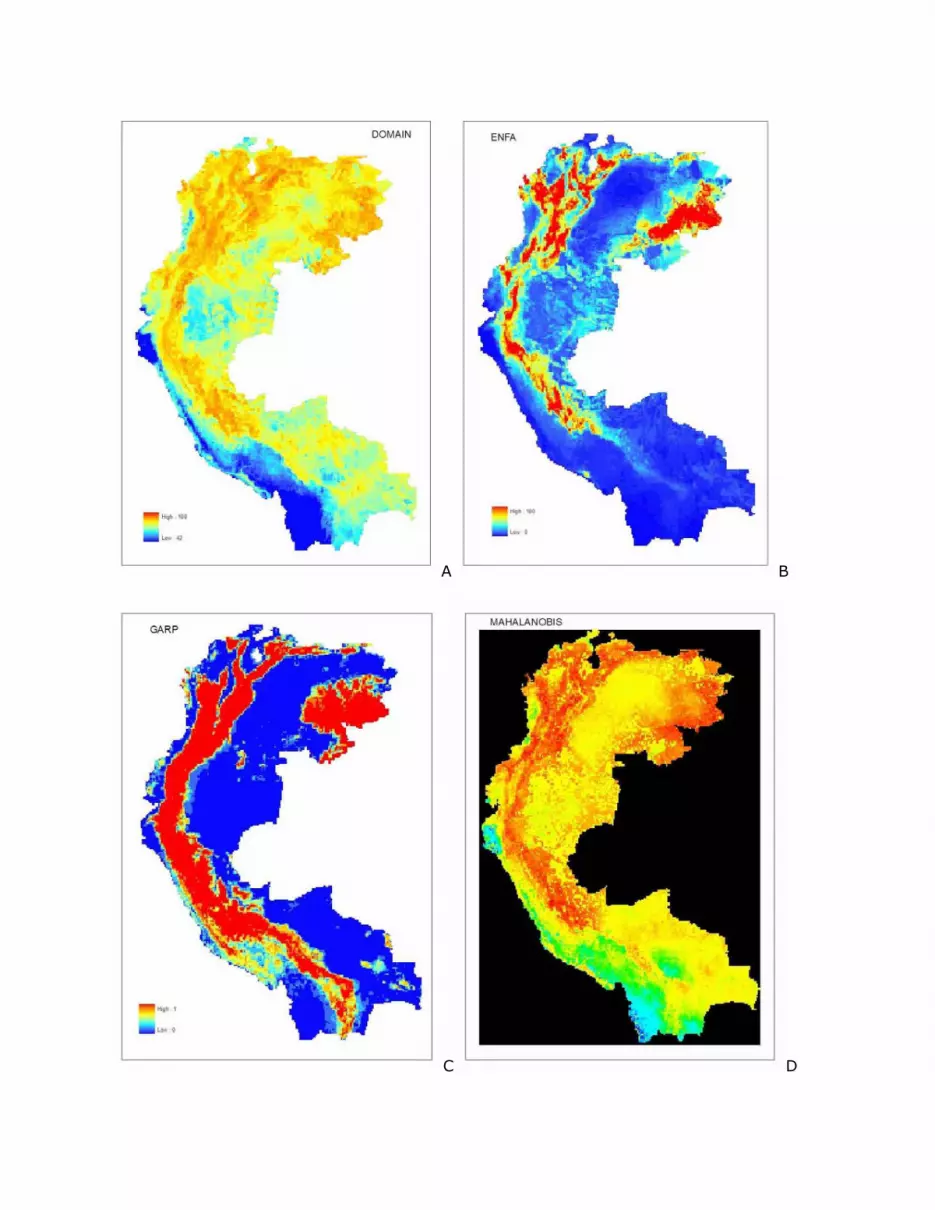
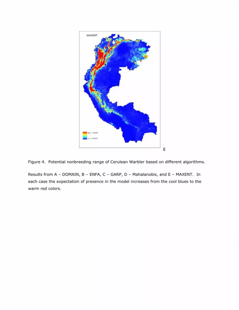
Figure 4. Potential nonbreeding range of Cerulean Warbler based on different algorithms.

Results from A – DOMAIN, B – ENFA, C – GARP, D – Mahalanobis, and E – MAXENT. In

each case the expectation of presence in the model increases from the cool blues to the

warm red colors.

Domain GARP

ENFA

Mahalanobis

MAXENT

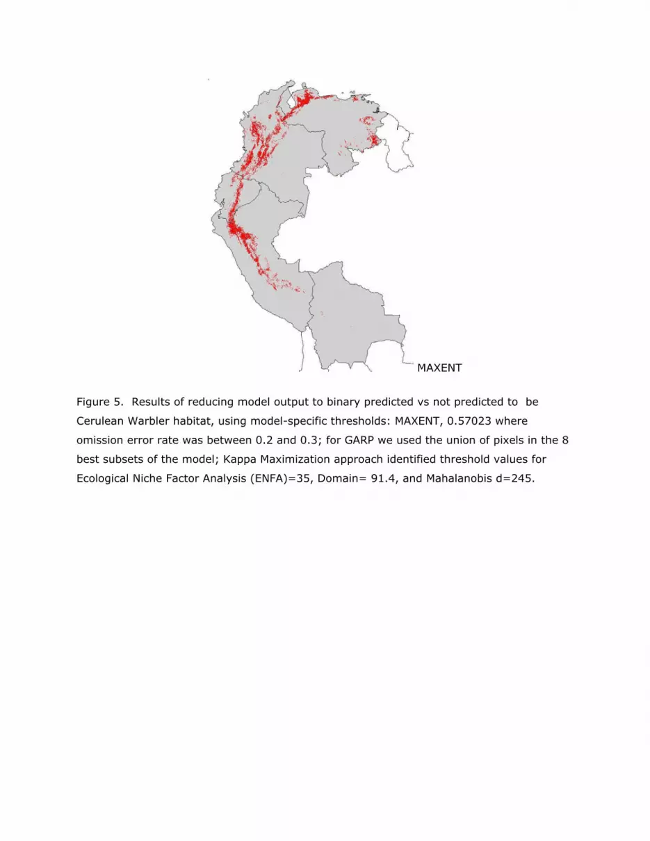
Figure 5. Results of reducing model output to binary predicted vs not predicted to be

Cerulean Warbler habitat, using model-specific thresholds: MAXENT, 0.57023 where

omission error rate was between 0.2 and 0.3; for GARP we used the union of pixels in the 8

best subsets of the model; Kappa Maximization approach identified threshold values for

Ecological Niche Factor Analysis (ENFA)=35, Domain= 91.4, and Mahalanobis d=245.

Figure 6. Combined map of binary results of ENFA, Mahalanobis, and MAXENT models.

Areas in gray were predicted Cerulean Warbler range by none of the models, those in

green were predicted by one model, those in yellow by two models, and those in red by

all three models.

Figure 7. Intersection of Independent Cerulean Warbler Validation data set with combined

map of Figure 6, including models ENFA, MAXENT, and Mahalanobis. Dark circles indicate

validation points where Cerulean Warblers were found.

Figure 8. Intersection of Independent Cerulean Warbler Validation data set with combined

binary results of all five models. Dark circles indicate validation points where Cerulean

Warblers were found.

Figure 9. Distribution of Independent Cerulean Warbler Validation data points among model

outputs displayed in Figures 7 and 8. Abscissa indicates the number of models predicting

the point as an occurrence of Cerulean Warbler. Upper graph indicates results of ENFA,

MAXENT, and Mahalanobis binary models. Lower graph indicates these three plus Domain

and GARP. Blue bars indicate validation points where no Cerulean Warblers were found,

purple bars indicate validation points where Cerulean Warblers were present.

Figure 10. Intersection of Independent Cerulean Warbler Validation data set with output of

MAXENT model. Dark circles indicate validation points where Cerulean Warblers were found.

Discussion

Modeling has produced a product that appears to be reasonably faithful to our existing

understanding of the range. The strata suggested by the combined models form a

convenient set from which we will select at random localities for field validation directed

toward improving understanding of the range of the species, identifying heretofore unknown

sites, and implementing conservation actions to improve the probability of long-term

survival of the Cerulean Warbler.

Patterns of observed presence and observed absence in the independent validation data set

indicate successful prediction of presence in the validation data set by at least one of the

models in 40 of 50 cases in the combined result of the five models (Figure 9). The

combined models thus included 20% false negatives, defined principally by the threshold

value of omission errors of 20% for the most restrictive of the models, MAXENT. The

counterpart of this result is the very high rate of false positives, as 50 of 63 absences

occurred in areas in which the species was predicted to be present. Several interpretations

of this finding are possible and merit attention.

First among these interpretations must be the difficulty of determining a true absence value.

It is entirely possible that the birds were present in the areas but not detected, in which the

absence is only a failure of detection, not a failure of prediction. Second, it is possible that

these false positives result from limitations in the available data to determine what

constitutes Cerulean Warbler habitat in this data set; in such a case, the birds may be more

specialized to habitats than is suggested by the combined models, and these false positives

are model failures to make accurate predictions. A third possibility is that these areas are

equally good as potential sites for Cerulean Warblers as are those in which presence was

both predicted and observed, but that the number of Cerulean Warblers is too low to be

detected in them, or too few Cerulean Warblers are present to occupy these habitats. If

this were the case, the suggestion is that unoccupied habitat exists for these birds in South

America.

Some surprises are the results of predicted occurrence in portions of the tepui region of

Venezuela, and possibly adjacent Brazil and Guyana outside the study area. Whether these

areas truly constitute potential range for the species is uncertain, and may be the result of

failures in the modeling and analysis process. Nevertheless, persistent occurrence of the

species in certain accessible sites there suggests this may be a useful area for future field

investigation. The combined model predicts considerable habitat in Colombia as well as in

Ecuador and Peru.

Hilty and Brown (1986) suggested that the bulk of the Cerulean Warbler population spent

the nonbreeding period south of Colombia. At that time, habitat was considered to consist

of primary forest (Robbins et al. 1992). Recent data identified in this investigation and the

experience of others, including both scientists, bird tour leaders, and independent

birdwatchers, is that locating this species in Peru is increasingly difficult, that locations in

Bolivia are vanishingly scarce, and that occurrence in some parts of Ecuador is more difficult

to document than in the past. Current opinion thus is that the bulk of the existing Cerulean

Warbler population is now found in Colombia and Venezuela during the nonbreeding period.

Little primary forest exists in this range, and the birds have been repeatedly documented to

use secondary forest such as shade coffee plantations (Jones et al. 2002). Indeed, their

range in Colombia may coincide with the range of coffee cultivation.

Recent work analyzing stable isotopes in feathers suggests the existence of a recognizable

migratory connectivity between breeding and nonbreeding residency sites (Girvan

2003).This raises an interesting and disturbing possibility. Breeding populations,

particularly in the western and southern portions of the range, show steeper declines in BBS

results, or have disappeared altogether, while populations in the central portion of the range

and in the northern portion of the breeding range appear to be more stable, although not

necessarily constituting source populations (Jones et al. 2004). The possibility is that some

substantial habitat may exist in the southern portion of the nonbreeding range, and perhaps

throughout, but the existing population is too small to exploit this habitat, or reduced to

such low density as to be very difficult to encounter.

Biotic factors, such as potential competitors for food, or flock-forming species with which

Cerulean Warblers associate on the nonbreeding grounds, present a further complication to

inferring the nonbreeding distribution of the species entirely from these models. The scale

of the percent tree cover is such that potentially important habitat patchiness or

fragmentation are unavailable in the data that we used to construct our models. Should

resident flock-forming species exhibit a negative response to fragmentation of habitat,

resulting in failure of the mixed species flock resource on which Cerulean Warblers

presumably depend, habitat that appears structurally appropriate to the Cerulean Warbler

may not contain the appropriate complement of other species, and hence not attract

Cerulean Warblers.

We suggest that the reader conduct a small test of this suggestion by considering two lines

of questioning. The first comes from the existing population estimate (Rich et al. 2004) of

560,000. This is a top-down approach and addresses the question: Does sufficient habitat

exist in South America to support the estimated population? The second begins with the

results of the models here (Table 4) that indicate that 200,000 km2 of potential habitat

exists and uses an assumed nonbreeding density estimate of 1 bird/ha. This is a bottom-up

approach and addresses the question: How many birds can existing habitats support?

In making such a calculation, the uncertainty in these data is substantial, and results from a

number of sources, ornithological, computational, and spatial. Ornithological uncertainty

concerns the rule of thumb that the observed density of 1 bird/ha might obtain over a

considerable landscape. This is an unlikely occurrence. Additional ornithological uncertainty

results from the assumptions inherent in the population estimate calculated by Rich et al.

(2004), particularly the assumption that the species can dependably be detected out to

distances as great as 125 m on BBS counts. This estimate is possibly as much as 50% too

high (P. B. Hamel, unpublished data; J. Jones, pers. comm.), at least in forest conditions. A

third source of ornithological uncertainty concerns the specificity of behavioral habitat

selection by Cerulean Warblers in the nonbreeding season, which is especially poorly

understood. All of these uncertainties are recognized by the ornithologists among the

authors of this work.

Computational uncertainty derives from the great variety of methods used to identify

locations and georeference the modeling data. Unfortunately, a relatively large number of

the records were not georeferenced with surveying equipment or GPS, and hence are of

unknown, but probably low, precision. Given the steep terrain in which these birds spend

the nonbreeding period, errors in georeferencing might cause substantial variance into the

calculations.

Spatial uncertainty in these predictions results from the need to project all the data sets to

the same scale, which is to say to the coarsest one represented among the data layers to be

analyzed. Thus, data on species presence have been generalized to the values obtaining

over the 1 km2 pixel in which the occurrence point was located. Local variation in

topography, variation in forest cover, and other processes operative at finer scales cannot

be inferred from these data because of the coarse scale necessary for completion of the

analyses. These may be the features on which the birds base their habitat selection,

however. In combination with the ornithological uncertainties, the computational and

spatial uncertainties demand that readers and others interested in the obvious possible

projections of these population and area estimates, using assumed density estimates,

recognize that uncertainty is very great indeed, and leaves room for a variety of

interpretations.

Perhaps the greatest uncertainty in our process is the nature of both the modeling and the

validation data sets. Each is the result of convenience sampling and thus is subject to an

unknowable amount of bias involved in the selection of areas for birdwatching.

The model of the Cerulean Warbler nonbreeding range produced by this project can be

rigorously tested. Field testing of the model will enable use of data available at much finer

scales, from the 500m pixel scale of the percent forest cover to the 90m scale of DEM.

Some analyses may be conducted by examining the variance of these variables within the

pixels in the current combination model (Figure 6). A more valuable result of applying finer

scale resolution is that it will enable field observers more accurately to locate potential

habitat and estimate its extent in the field with high quality georeferencing of the results.

These model predictions further lend themselves to test within the context of existing

protected areas, in the public or private sector, including identified hot spots such as

Important Bird Areas, and other locations of high conservation concern.

Conclusion

We have produced a stratified model of predicted occurrence of the Cerulean Warbler in its

nonbreeding range in South America. Rigorous field testing of this model will hopefully lead

to specific on the ground conservation activities likely to maintain habitat for the species at

this critical time of the life cycle.

Acknowledgments

El Grupo Cerúleo, a part of Cerulean Warbler Technical Group, received funding for this

project from the National Fish and Widlife Foundation, The Nature Conservancy, the USDA

Forest Service, and the National Council for Air and Stream Improvement, and abundant

logistical support from Universidad San Francisco de Quito and Instituto Alexander von

Humboldt. The project began with a decision by members of El Grupo who met in Cabañas

San Isidro, Cosanga, Ecuador, in March, 2003: Jorge Botero, Jeremy Flanagan, Juan

Fernando Freile, Megan Hill, Miguel Lentino, Gabriela Montoya, Luis Germán Naranjo, Cecilia

Pacheco, David Pashley, Luis Miguel Renjifo, Pancho Sornoza, Thomas Valqui, and Girvan,

Hamel, Herzog, Mehlman, and Ramoni-Perazzi. Discussions continued with most of the

current authors in a workshop in Universidad San Francisco de Quito, Cumbayá, Ecuador, in

November 2005. Work was completed at a workshop in Instituto Alexander von Humboldt,

Bogotá, Colombia, by Ganzenmueller, Hamel, Hernández, Mehlman, Romero, and Tovar, at

which Pedraza and Galindo joined the team. We thank Walter Weber for helping us locate a

reference in his extensive ornithological library in Medellín, Colombia. The manuscript was

reviewed by Jason Jones and Chris Rogers. We are especially grateful to the organizers of

the ESRI User Conference, especially Andrea García, for providing us many courtesies in the

preparation of the manuscript. Everyone interested in the conservation of Cerulean Warbler

owes an enormous debt of gratitude to the very many observers who responded to our

request for records and their locations, notably la Red Nacional de Observadores de Aves de

Colombia.

References

Armenteras, D., Rincón, A., and Ortiz, N. 2005. Ecological function assessment in the

Colombian Coffee’growing Region. Sub’global Assessment Working Paper. [online]

Millennium Ecosystem Assessment. Available at:

http://www.millenniumassessment.org/en/subglobal.colombia.aspx

Birdlife International. 2004. Threatened birds of the world 2004. CD-ROM. Cambridge, UK:

Birdlife International.

Birdlife International. 2006. Species factsheet: Dendroica cerulea. Online at

http://www.birdlife.org. Accessed 24 July 2006.

Carpenter, G., Gillison, A.N., and Winter. J. 1993. DOMAIN: a flexible modeling procedure

for mapping potential distributions of plants and animals. Biodiv. Conserv. 2:667-

680.

Committee on the Status of Endangered Wildlife in Canada. 2003. COSEWIC assessment

and update status report on the Cerulean Warbler Dendroica cerulea in Canada.

Committee on the Status of Endangered Wildlife in Canada, Ottawa, Ontario.

Elith, J., Graham, C.H., Anderson, R.P., Dudík, M., Ferrier, S., Suisan, A., Hijmans, R.J.,

Huettmann, F., Leathwick, J.R., Lehman, A., Li, J., Lohmann, L.G., Loiselle, B.A.,

Manion, G., Moritz, C., Nakamura, M., Nakazawa, Y., Overton, J. McC., Peterson,

A.T., Phillips, S.J., Richardson, K.S., Scachetti-Pereira, R., Schapire, R.E., Soberón,

J., Williams, S., Wisa, M.S., and Zimmerman, N. E. 2006. Novel methods improve

prediction of species’ distributions from occurrence data. Ecography 29:129-151.

Fielding, A. H., and J. F. Bell. 1997. A review of methods for the assessment of prediction

errors in conservation presence/absence models. Environmental Conservation

24:38–49.

Girvan, M.K. 2003. Examining dispersal and migratory connectivity in Cerulean warblers

(Dendroica cerulea) using stable isotope analysis. MSc Thesis, Queen’s University,

Kingston, ON, Canada.

Global land cover facility MODIS. [no date].

http://glcf.umiacs.umd.edu/data/modis/vcf/data.shtml, University of Maryland,

NASA, Institute for Advanced Computer Analysis.

Greenacre, M.J. 1984. Theory and Applications of Correspondence Analysis. London:

Academic Press.

Guisan, A., Weiss, S. B. and Weiss, A. D. 1999. GLM versus CCA spatial modeling of plant

species distribution. Plant Ecol. 143: 107-122.

Hamel, P.B. 2000a. Cerulean warbler status assessment. St. Paul, MN: U.S. Department of

the Interior, Fish and Wildlife Service. 141 p. Available online at:

<http://www.fws.gov/midwest/endangered/ birds/cerw/cerw-sa.pdf> [Date

accessed: August 9, 2005].

Hamel, P.B. 2000b. Cerulean warbler Dendroica cerulea. In: Poole, A.; Gill, F., eds. The

birds of North America series, No. 511. Philadelphia, PA: The Birds of North America,

Inc. 20 p.

Hamel, P.B. 2005. Suggestions for a silvicultural prescription for Cerulean Warblers in the

lower Mississippi Alluvial Valley. In: Ralph, C.J.; Rich, T.D., eds. Bird conservation

implementation and integration in the Americas: proceedings of the third

international partners in flight conference. Gen. Tech. Rep. PSW-191. Albany, CA:

U.S. Department of Agriculture, Forest Service, Pacific Southwest Research Station:

567-575.

Hamel, P.B.; Dawson, D.K.; Keyser, P.D. 2004. Overview: how we can learn more about the

cerulean warbler (Dendroica cerulea). Auk. 121(1): 7-14.

Hijmans, R.J., Cameron, S. and J. Parra. [no date] WORLDCLIM

http://www.worldclim.org/, developed at the Museum of Vertebrate Zoology,

University of California, Berkeley, in collaboration with P. Jones and A. Jarvis (CIAT),

and with K. Richardson (Rainforest CRC).

Hijmans, R.J., S.E. Cameron, J.L. Parra, P.G. Jones and A. Jarvis, 2005. Very high resolution

interpolated climate surfaces for global land areas. International Journal of

Climatology 25: 1965-1978

Hilty, S.L., and W.L. Brown. 1986. A guide to the birds of Colombia. Princeton Univ. Press,

Princeton, NJ. 836 p.

Hirzel, A.H., J. Hausser, D. Chessel, and N. Perrin. 2002. Ecological-niche factor analysis:

How to compute habitat-suitability maps without absence data? Ecology

83(7):2027-2036.

Hutchinson, G.E. 1957. Concluding remarks. Cold Spring Harbour Symposium inn

Quantitative Biology

Jenness, J. 2003. Mahalanobis distances (mahalanobis.avx) extension for ArcView 3.x,

Jenness Enterprises. Available at:

http://www.jennessent.com/arcview/mahalanobis.htm.

Jones, J., J.J. Barg, T. S. Sillett, M. L. Veit, and R.J. Robertson. 2004. Minimum estimates

of survival and population growth for Cerulean Warblers breeding in Ontario, Canada.

Auk 121:1-6.

Jones, J., P. Ramoni-Perazzi, E. H. Carruthers, and R. J. Robertson. 2002. Species

composition of bird communities in shade coffee plantations in the Venezuelan

Andes. Ornitologia Neotropical 13:397–412.

Link, W.A.; Sauer, J.R. 2002. A hierarchical analysis of population change with application to

Cerulean Warblers. Ecology. 83: 2832-2840.

Liu, C.; Berry, P. M.; Dawson, T. P.; Pearson, R. G. 2005. Selecting thresholds of occurrence

in the prediction of species distributions. Ecography 28: 385-393.

Maurer, B. A. 1994. Geographical Population Analysis: Tools for the analysis of

biodiversity. Oxford: Blackwell Scientific Publications.

Phillips, S. J., Anderson, R. P. and Schapire, R. E. 2006. Maximum entropy modeling of

species geographic distributions. – Ecol. Modell. 190:231–259.

Renjifo L, M. 1998. Especies de aves amenazadas y casi en peligro de extinción enColombia.

Pp416-426.En: Informe nacional sobre el estado de la biodiversidad 1997-Colombia

(Vol I).

Rich, T.; Beardmore, C.; Berlanga, H.; Blancher, P.; Bradstreet, M.; Butcher, G.; Demarest,

D.; Dunn, E.; Hunter, W.; Iñigo-Elias, E.; Kenndedy, J.; Martell, A.; Panjabi, A.;

Pashley, D.; Rosenberg, K.; Rustay, C.; Wendt, J.; Will, T. 2004. Partners In Flight

North American Landbird Conservation Plan. Ithaca, NY: Cornell University,

Laboratory of Ornithology. 84 p.

Robbins, C. S., D. Bystrak, and P. H. Geissler. 1986. The Breeding Bird Survey: Its first

fifteen years, 1965-1979. US Dep. Interior, Fish and Wildlife Service.

Robbins, C.S.; Fitzpatrick, J.; Hamel, P.B. 1992. A warbler in trouble: Dendroica cerulea. In:

Hagan, J.M., III; Johnston, D.W., eds. Ecology and conservation of Neotropical

migrant landbirds. Washington, D.C.: Smithsonian Institution Press: 549-562.

Rosenberg, K.V.; Barker, S.E.; Rohrbaugh, R.W. 2000. An atlas of Cerulean Warbler

populations: Final Report to USFWS, 1997–2000 Breeding Seasons. Ithaca, NY:

Cornell University, Laboratory of Ornithology. 56 p.

Rotenberry, J. T., K. L. Preston, and S. T. Knick. 2006. GIS-based niche modeling for

mapping species’ habitat. Ecology 87(6):1458-1464.

Ruley, D.A. 2000. Petition under the Endangered Species Act to list the cerulean warbler,

Dendroica cerulea, as a threatened species. Asheville, NC: Southern Environmental

Law Center. 50 p.

Smith, W. P., P. B. Hamel, and R. P. Ford. 1996. Mississippi Alluvial Valley Forest

Conversion: Implications for eastern North American avifauna. Proc. 1993 Annu.

Conf. Southeast Assocn. Fish and Wildl. Agencies 47:460-469.

Sneath, P. H. and Sokal, R. R. 1973. Numerical Taxonomy. W.H. Freeman and Company.

San Franciso.

Sokal, R. R. and F. J. Rohlf. 1981. Biometry. W. H. Freeman, New York. 859 p.

Stockwell, D. R. B. and Noble, I. R. 1992. Induction of sets of rules from animal distribution

data: a robust and informative method of data analysis. – Math. Comput. Simul. 33:

385–390.

Stockwell, D. and Peters, D. 1999. The GARP modelling system: problems and solutions to

automated spatial prediction. – Int. J. Geogr. Inform. Sci. 13: 143–158.

Terborgh, J. 1989. Where have all the birds gone? Princeton, NJ: Princeton Univ. Pr.

U.S. Geological Survey. [no date]. GTOPO30

http://edc.usgs.gov/products/elevation/gtopo30/gtopo30.html, U.S. Geological

Survey, Earth Resources Observation & Science (EROS).

Zweig, M. H., and G. Campbell. 1993. Receiver-operating characteristic (ROC) plots: a

fundamental evaluation tool in clinical medicine. Clinical Chemistry 39:561–577.

Contact Information Primary Author Paul Hamel USDA Forest Service Center for Bottomlands Hardwoods Research, P.O. Box 227, 432 Stoneville Rd., Stoneville, MS 38776, USA Phone (1) 662-686-3167

FAX (1) 662-686-3195 Email phamel@fs.fed.us Coauthors Sara Barker Cornell Lab of Ornithology 159 Sapsucker Woods Rd., Ithaca, NY 14850, USA Phone (1) 607-254-2465 FAX (1) 607-254-2104 Email sb65@cornell.edu Silvia Benítez The Nature Conservancy Calle Los Naranjos N44-491 y Azucenas (Sector Monteserrin), Quito, Ecuador Phone (593) 2-2257-138 / (593) 2-2258-113 / (593) 9-9723997 x 104 FAX (593) 2-2257-138 Email sbenitez@tnc.org Jennifer Baldy University of Memphis 1228 Pallwood, Memphis, TN 38122, USA Phone (1) 901-359-0584 FAX (1) 901-678-2178 Email jenjoyb2002@yahoo.com Diego Francisco Cisneros Heredia Aves&Conservacion Pasaje Joaquin Tinajero E3-05 y Calle Jorge Drom, Casilla Postal 17-17-906, Quito, Ecuador Phone (593) 2-227-1800 / 09-980-6794 Email diegofrancisco_cisneros@yahoo.com Gabriel Colorado Zuluaga Universidad Nacional Calle 52B #80-35, Apt. 402, Medellín, Colombia Phone (57) 4-2345035 Email gjcolora@epm.net.co Francisco Cuesta Ecociencia Francisco Salazar E14-34 y Av. La Coruna, P.O. Box 17-12-257, Quito, Ecuador Phone (593) 2231-624, 2522-999, 2545-999 Email andes@ecociencia.org Ian Davidson BirdLife International Vicente Cárdenas E5-75 y Japón, 3er Piso, C.P. / P.O.Box: 17-17-717, Quito, Ecuador Phone (593) 2-245-3645, 227-7399, 227-7497 FAX (593) 2-227-7059 Email ian.davidson@birdlife.org.ec David Fco. Díaz Fernández BirdLife International

Vicente Cárdenas E5-75 y Japón, 3er Piso, C.P. / P.O.Box: 17-17-717, Quito, Ecuador Phone (593) 2-2277-497 FAX (593) 2-227-7059 Email david.diaz@birdlife.org.ec Andrea Ganzenmueller Ecociencia Francisco Salazar E14-34 y Av. La Coruna, P.O. Box 17-12-257, Quito, Ecuador Phone (593) 2231-624, 2522-999, 2545-999 Email andrea_ganzenmueller@yahoo.com Santiago García BirdLife International Vicente Cárdenas E5-75 y Japón, 3er Piso, C.P. / P.O.Box: 17-17-717, Quito, Ecuador Phone (593) 9-166-0320 Email santiago.llore@birdlife.org.ec Kate Girvan Queen's University Norval Outdoor School, Box 226, Norval, Ontario, L0P 1K0, Canada Phone (1) 905-877-2201 Email kgirvan16@hotmail.com Esteban Guevara Aves y Conservación Florencia y Borramini 176, La Primavera, Cumbaya, Ecuador Phone (593) 2-2891-553 Email esalguan@yahoo.com A. Bennett Hennessey Asociación Armonía – BirdLife International Av. Lomas de Arena 400, Casilla 3566, Santa Cruz de la Sierra, Bolivia Phone (591) 3-356-3636 Email abhennessey@armonia-bo.org Olga Lucía Hernández WWF Colombia Carrera 35 #4A-25 San Fernando, Cali – Valle, Colombia Phone (57) 2-5582577 x 110 Email olhernandez@wwf.org.co Sebastian Herzog Asociación Armonía – BirdLife International Av. Lomas de Arena 400, Casilla 3566, Santa Cruz de la Sierra, Bolivia Phone (591) 3-3568808 Email skherzog@armonia-bo.org David Mehlman The Nature Conservancy 1303 Rio Grande Blvd NW, Suite 5, Albuquerque, NM 87104, USA Phone (1) 505-244-0535 x 24 FAX (1) 505-244-0512 Email dmehlman@tnc.org

María Isabel Moreno Fundación ProAves Carrera 20 Nº 36-61, Bogotá D. C, Colombia Phone (57) 1-3403229/32/65 FAX (57) 1-3403285 Email mmoreno@proaves.org Esra Ozdenerol University of Memphis Department of Earth Sciences, 236 Johnson Hall, 488 Patterson Street, Memphis, TN 38152, USA Phone (1) 901-678-2787 FAX (1) 901-678-2178 Email eozdenrl@memphis.edu Paolo Ramoni-Perazzi Universidad de Los Andes Facultad de Ciencias, Departamento de Biologia, Merida 5101, Venezuela Phone (58) 274-240-1304 FAX (58) 74-40-12-86 Email rpaolo@ula.ve Milton Romero Instituto Humboldt Calle 146A No. 40A – 18 Apt. 702 Bogotá, Colombia Phone (57) 1-6086900 6335560 Email mhromero@humboldt.org.co David Romo Universidad San Francisco de Quito Campus Cumbayá- Diego de Robles y Vía Interoceánica, P.O.BOX 17-1200-841, Quito, Ecuador Phone (593) 2-297-1961 Email david@usfq.edu.ec Paul Salaman American Bird Conservancy 4249 Loudoun Avenue, PO Box 249, The Plains, VA 20198, USA Phone (1) 540-253-5780 FAX (1) 540-253-5782 Email psalaman@abcbirds.org Tatiana Santander Aves y Conservación Pasaje Joaquín Tinajero E3-05 y Jorge Drom, Quito, Ecuador Phone (593) 2-227-1800 Email aves_proyectos@yahoo.com Carolina Tovar Ingar Centro de Datos para la Conservación, Universidad Nacional Agraria La Molina Av. La Universidad s/n La Molina Lima-Perú Phone (51) 1-349-6102

Email ctovar@lamolina.edu.pe Melinda Welton Gulf Coast Bird Observatory 5241 Old Harding, Franklin, TN 37064, USA Phone (1) 615-799-8095 FAX (1) 615-799-2220 Email weltonmj@earthlink.net Tom Will U.S. Fish and Wildlife Service Division of Migratory Birds, 1 Federal Drive — 6th Floor, Fort Snelling, MN 55111-4056, USA Phone (1) 612-713-5362 FAX (1) 612-713-5393 Email tom_will@fws.gov Carlos Pedraza Instituto Humboldt Calle 138 bis No. 25 – 37 Bogotá, Colombia Phone (57) 1-6086900 6335560 Email cpedraza@humboldt.org.co Gustavo Galindo Instituto Humboldt Calle 146A No. 40A – 18 Apt. 702 Bogotá, Colombia Phone (57) 1-6086900 6335560 Email ggalindo@humboldt.org.co