Modelling the electrostatic actuation of MEMS: state of the art 2005. A. Fargas Marquès, R. Costa Castelló and A.M. Shkel IOC-DT-P-2005-18 Setembre 2005

MODELING THE ELECTROSTATIC ACTUATION OFMEMS. STATE OF THE ART 2005

A. Fargas Marques∗, R. Costa Castello∗, and A. M. Shkel+∗Institut d’Organitzacio i Control de Sistemes Industrials, IOC-UPC and

+University of California at Irvine

July 2005

Abstract

Most of MEMS devices are actuated using electrostatic forces. Parallel or lateral plateactuators are the types commonly used. Nevertheless, electrostatic actuation has somelimitations due to its non-linear nature. This work presents a methodic overview of theexisting techniques applied to the Micro-Electro-Mechanical Systems (MEMS) electrostaticactuation modeling and their implications to the dynamic behavior of the electromechanicalsystem.

1 Introduction

The field of Micro-Electro-Mechanical Systems (MEMS) has undergone a startling revolution inrecent years. It is now possible to produce accelerometers less than one millimeter on a side,functioning motors that can only be seen with the aid of a microscope, gears smaller than a humanhair, and needles so tiny they can deliver an injection without stimulating nerve cells.

The use of existing integrated circuit technology in the design and production of MEMS devicesallows these devices to be batch-manufactured, what in turn converts them due to their quantityin almost inexpensive. The first sector to benefit from this revolution has been the automotiveindustry, where devices and applications that once could only be dreamed about have suddenlybeen made possible and are used everywhere.

The ability to manufacture mechanical parts such as resonators, sensors, gears and levers ona micron length scale is not however the end of the story. The challenge is also to understandand control the physical systems behavior on these scales. That is, an understanding of fluid,electromagnetic, thermal, and mechanical forces on the micron length scale is necessary in order tounderstand the operation and function of MEMS devices.

In this framework, the methods of actuation and sensing of this new devices have been a criticallyimportant topic over the years. There is not a perfect method, and the decision usually dependson the actual device and the specifications of the system.

The main actuation and sensing properties used in MEMS are

• Piezoresistivity: When a piezoresistive material is stressed, it reduces or increases its abilityto transport current. Using this property, movement can be measured as a current differencebetween the two extremes of a deformed piezoresistive material.

1

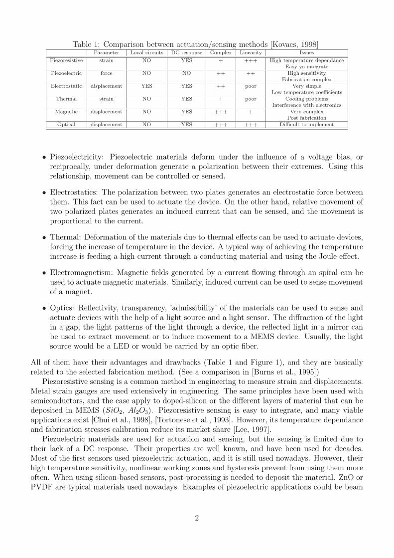
Table 1: Comparison between actuation/sensing methods [Kovacs, 1998]Parameter Local circuits DC response Complex Linearity Issues

Piezoresistive strain NO YES + +++ High temperature dependanceEasy yo integrate

Piezoelectric force NO NO ++ ++ High sensitivityFabrication complex

Electrostatic displacement YES YES ++ poor Very simpleLow temperature coefficients

Thermal strain NO YES + poor Cooling problemsInterference with electronics

Magnetic displacement NO YES +++ + Very complexPost fabrication

Optical displacement NO YES +++ +++ Difficult to implement

• Piezoelectricity: Piezoelectric materials deform under the influence of a voltage bias, orreciprocally, under deformation generate a polarization between their extremes. Using thisrelationship, movement can be controlled or sensed.

• Electrostatics: The polarization between two plates generates an electrostatic force betweenthem. This fact can be used to actuate the device. On the other hand, relative movement oftwo polarized plates generates an induced current that can be sensed, and the movement isproportional to the current.

• Thermal: Deformation of the materials due to thermal effects can be used to actuate devices,forcing the increase of temperature in the device. A typical way of achieving the temperatureincrease is feeding a high current through a conducting material and using the Joule effect.

• Electromagnetism: Magnetic fields generated by a current flowing through an spiral can beused to actuate magnetic materials. Similarly, induced current can be used to sense movementof a magnet.

• Optics: Reflectivity, transparency, ’admissibility’ of the materials can be used to sense andactuate devices with the help of a light source and a light sensor. The diffraction of the lightin a gap, the light patterns of the light through a device, the reflected light in a mirror canbe used to extract movement or to induce movement to a MEMS device. Usually, the lightsource would be a LED or would be carried by an optic fiber.

All of them have their advantages and drawbacks (Table 1 and Figure 1), and they are basicallyrelated to the selected fabrication method. (See a comparison in [Burns et al., 1995])

Piezoresistive sensing is a common method in engineering to measure strain and displacements.Metal strain gauges are used extensively in engineering. The same principles have been used withsemiconductors, and the case apply to doped-silicon or the different layers of material that can bedeposited in MEMS (SiO2, Al2O3). Piezoresistive sensing is easy to integrate, and many viableapplications exist [Chui et al., 1998], [Tortonese et al., 1993]. However, its temperature dependanceand fabrication stresses calibration reduce its market share [Lee, 1997].

Piezoelectric materials are used for actuation and sensing, but the sensing is limited due totheir lack of a DC response. Their properties are well known, and have been used for decades.Most of the first sensors used piezoelectric actuation, and it is still used nowadays. However, theirhigh temperature sensitivity, nonlinear working zones and hysteresis prevent from using them moreoften. When using silicon-based sensors, post-processing is needed to deposit the material. ZnO orPVDF are typical materials used nowadays. Examples of piezoelectric applications could be beam

2

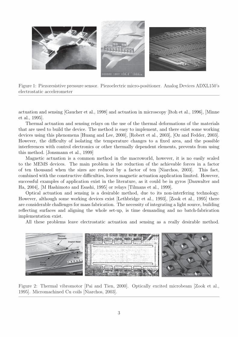
Figure 1: Piezoresistive pressure sensor. Piezoelectric micro-positioner. Analog Devices ADXL150’selectrostatic accelerometer

actuation and sensing [Gaucher et al., 1998] and actuation in microscopy [Itoh et al., 1996], [Minneet al., 1995].

Thermal actuation and sensing relays on the use of the thermal deformations of the materialsthat are used to build the device. The method is easy to implement, and there exist some workingdevices using this phenomena [Huang and Lee, 2000], [Robert et al., 2003], [Oz and Fedder, 2003].However, the difficulty of isolating the temperature changes to a fixed area, and the possibleinterferences with control electronics or other thermally dependent elements, prevents from usingthis method. [Jonsmann et al., 1999]

Magnetic actuation is a common method in the macroworld, however, it is no easily scaledto the MEMS devices. The main problem is the reduction of the achievable forces in a factorof ten thousand when the sizes are reduced by a factor of ten [Niarchos, 2003]. This fact,combined with the constructive difficulties, leaves magnetic actuation application limited. However,successful examples of application exist in the literature, as it could be in gyros [Dauwalter andHa, 2004], [M Hashimoto and Esashi, 1995] or relays [Tilmans et al., 1999].

Optical actuation and sensing is a desirable method, due to its non-interfering technology.However, although some working devices exist [Lethbridge et al., 1993], [Zook et al., 1995] thereare considerable challenges for mass fabrication. The necessity of integrating a light source, buildingreflecting surfaces and aligning the whole set-up, is time demanding and no batch-fabricationimplementation exist.

All these problems leave electrostatic actuation and sensing as a really desirable method.

Figure 2: Thermal vibromotor [Pai and Tien, 2000]. Optically excited microbeam [Zook et al.,1995]. Micromachined Cu coils [Niarchos, 2003].

3

Building a capacitor, with the existing fabrication methods is straightforward. One must puttogether two parallel surfaces and then apply potential difference between the two parts toobtain a good actuator or sensor. This simplicity has made electrostatic actuation and sensingubiquitous. One can find it in the first MEMS designs to build a gate transistor [Newell, 1968].Nowadays, capacitive effects are used in resonators [Attia et al., 1998], accelerometers [Kuehnel,1995], [Brosnihan et al., 1995], optical switches [Juneau et al., 2003], [Sane and Yazdi, 2003],micro-grippers [Chu et al., 1996], micro force gauges [Roessig, 1995], micro-pumps [Teymoori andAbbaspour-Sani, 2002], gyroscopes [Juneau, 1997], [Kranz et al., 2003], pressure sensors [Guptaand Senturia, 1997], RF switches [Huang et al., 2003], and microscopy [Blanc et al., 1996], [Shibaet al., 1998].

Even though practically and economically attractive, capacitive actuation has its own trade-offsand challenges. On-chip amplification is usually needed for capacitive sensing, due to the fempto-farad measure that must be achieved. Parasitic capacitances can affect the final read-out. Andfinally, although large forces can be generated, they can be heavily non-linear.

Consequently, the good understanding of the phenomenons that take place is essential to obtaina high performance device with electrostatic actuation and sensing. And this is more relevantgiven the increasing number of new devices that are continuously designed using these methods ofactuation and sensing.

2 Problem Description

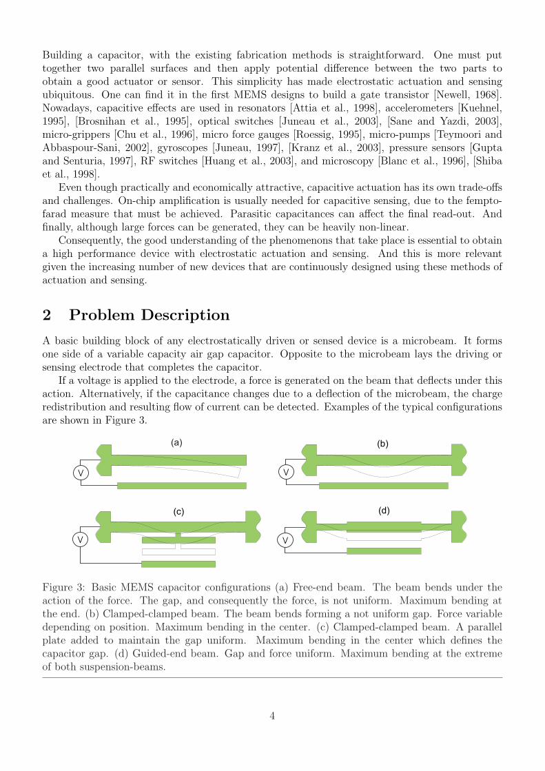
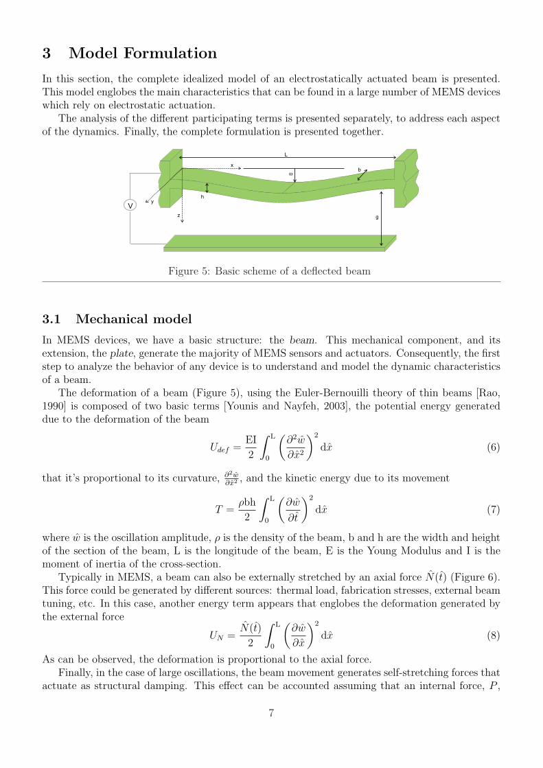
A basic building block of any electrostatically driven or sensed device is a microbeam. It formsone side of a variable capacity air gap capacitor. Opposite to the microbeam lays the driving orsensing electrode that completes the capacitor.

If a voltage is applied to the electrode, a force is generated on the beam that deflects under thisaction. Alternatively, if the capacitance changes due to a deflection of the microbeam, the chargeredistribution and resulting flow of current can be detected. Examples of the typical configurationsare shown in Figure 3.

(a) (b)

(d)(c)

V

V

V

V

Figure 3: Basic MEMS capacitor configurations (a) Free-end beam. The beam bends under theaction of the force. The gap, and consequently the force, is not uniform. Maximum bending atthe end. (b) Clamped-clamped beam. The beam bends forming a not uniform gap. Force variabledepending on position. Maximum bending in the center. (c) Clamped-clamped beam. A parallelplate added to maintain the gap uniform. Maximum bending in the center which defines thecapacitor gap. (d) Guided-end beam. Gap and force uniform. Maximum bending at the extremeof both suspension-beams.

4

When the goal is sensing displacement, a DC polarization voltage is applied to the capacitor,and the generated current is usually detected with a transresistance amplifier [Roessig, 1998]. Moresophisticated sensing schemes can also be used to improve the detection. This includes complexelectronics designs based on impedance, capacitive or source/drain pick-off [Burstein, 1995]. Chargedetection schemes has also been investigated [Seeger and Boser, 2003].

When the goal is driving the beam, an electric load is applied to the microbeam. Depending onthe nature of the device, the electric load is composed of a DC polarization voltage and, sometimes,an AC component designed to excite harmonic motions.

DC polarization is used to achieve permanent displacements of the beam. Moving opticalswitches, adjusting elements, closing gate transistors, moving valves or acting micro-grippers aretypical applications.

However, in most cases, resonant devices are used. In that case, an AC component is added tothe driving voltage to excite the harmonic motions of the beam.

g

wKB

M +

_

V

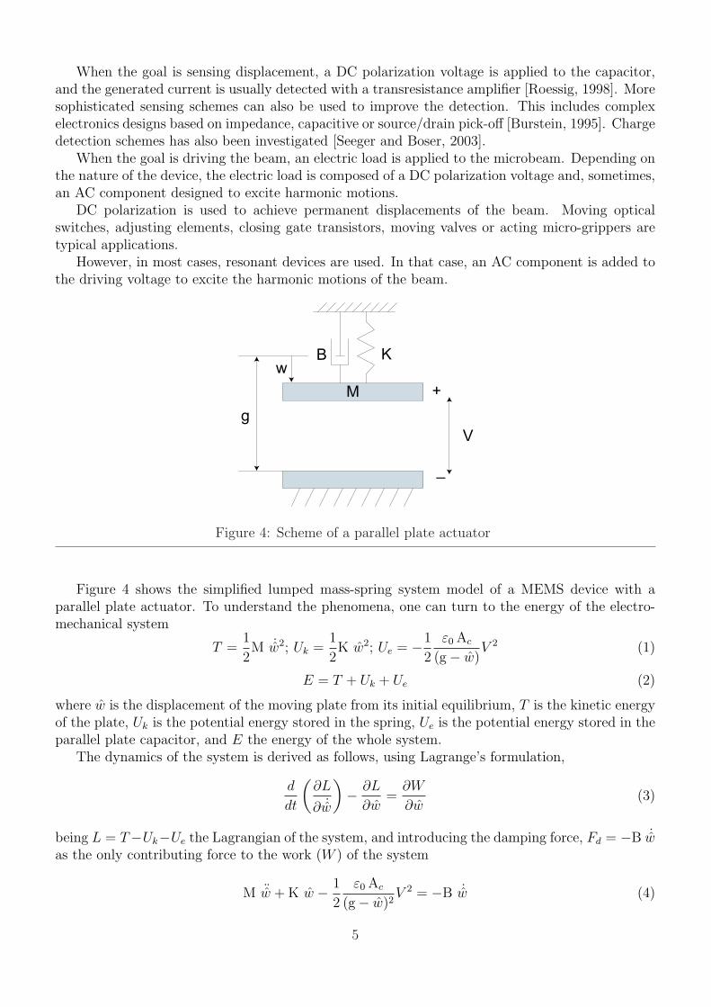
Figure 4: Scheme of a parallel plate actuator

Figure 4 shows the simplified lumped mass-spring system model of a MEMS device with aparallel plate actuator. To understand the phenomena, one can turn to the energy of the electro-mechanical system

T =1

2M ˙w2; Uk =

1

2K w2; Ue = −1

2

ε0 Ac

(g− w)V 2 (1)

E = T + Uk + Ue (2)

where w is the displacement of the moving plate from its initial equilibrium, T is the kinetic energyof the plate, Uk is the potential energy stored in the spring, Ue is the potential energy stored in theparallel plate capacitor, and E the energy of the whole system.

The dynamics of the system is derived as follows, using Lagrange’s formulation,

d

dt

(∂L

∂ ˙w

)− ∂L

∂w=

∂W

∂w(3)

being L = T−Uk−Ue the Lagrangian of the system, and introducing the damping force, Fd = −B ˙was the only contributing force to the work (W ) of the system

M ¨w + K w − 1

2

ε0 Ac

(g− w)2V 2 = −B ˙w (4)

5

This equation is the usual mass-spring-damper equation of dynamics.From this formulation, the force generated between the parallel plates, using basic electrostatics,

takes the following form

F =1

2

ε0 Ac

(g− w)2V 2 (5)

where ε0 is the dielectric constant, g is the initial gap between the plates, Ac is the area of the platesand V is the applied voltage between the electrodes. As it can be observed, this force is inverselyproportional to the gap between the plates of the actuator. As the gap decreases, the generatedattractive force increases quadratically. The only opposing force to the electrostatic loading is themechanical restoring force (K).

If the voltage is increased, the gap decreases generating an incremented force. At some point themechanical forces defined by the spring cannot balance this force anymore. Once reached this state,the electrodes will snap one against the other, and in most cases, the system would be permanentlydisabled.

Consequently, the electrostatic loading has an upper limit beyond which the mechanical forcecan no longer resist the opposing electrostatic force, thereby leading to the collapse of the structure.This actuation instability phenomenon is known as pull-in, and the associated critical voltage iscalled the Pull-in Voltage.

Several studies have investigated this behavior of microbeams under various loading conditions.The earliest such study may be found in the pioneering work of Nathanson et al. [Nathanson et al.,1967] [Newell, 1968]. In their study of a resonant gate transistor they constructed and analyzedthe mass-spring model of electrostatic actuation. They predicted and offered the first theoreticalexplanation of the so-called pull-in instability.

Since then, numerous investigators have analyzed mathematical models of electrostaticactuation in attempts to further understand and control the pull-in instability. Despite morethan three decades of work in the area of electrostatically actuated MEMS, the complete dynamicsof the electrostatic-elastic system is relatively unexplored.

There are a lot of aspects to be clarified. Some studies just center their goal in the immediateapplication of the sensor, and a simple mass-spring model can approximate the basic dynamics.However, these kind of models cannot predict the inherent nonlinearities of the electrostatic forceand the beam deformation ( [Chu et al., 1996], [Castaner and Senturia, 1999]).

Other approaches rely on the partial differential equations linearized around the workingpoint. Using this formulation, better results are achieved, but the dynamics only apply for smalldeflections [Ijntema and Tilmans, 1992].

Other studies analyze the response of a microbeam to a generalized transverse excitation andwith axial force using Rayleigh’s energy method to approximate the fundamental natural frequencyof the straight, undeflected beam [Tilmans and Legtenberg, 1994].

Recently, some authors have used the nonlinear equation representing the idealized electrostaticstructure to analyze the behavior ( [Flores et al., 2003], [Abdel-Rahman et al., 2002]).

However, no unified formulation of the problem has been offered. Questions about where, when,and how touchdown occurs are still to be answered. And this knowledge is essential to design andimplement the correct control of the new generation of high performance and self-calibrated MEMSdevices.

6

3 Model Formulation

In this section, the complete idealized model of an electrostatically actuated beam is presented.This model englobes the main characteristics that can be found in a large number of MEMS deviceswhich rely on electrostatic actuation.

The analysis of the different participating terms is presented separately, to address each aspectof the dynamics. Finally, the complete formulation is presented together.

V

L

z

y

x

w

h

b

g

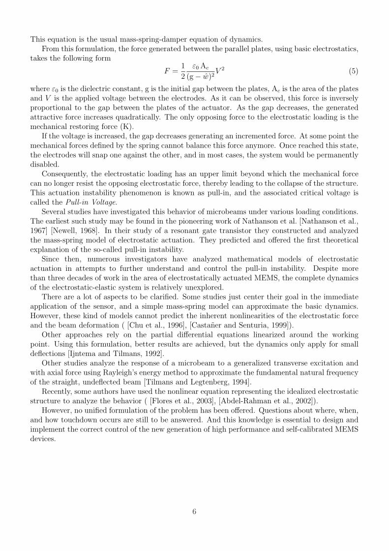
Figure 5: Basic scheme of a deflected beam

3.1 Mechanical model

In MEMS devices, we have a basic structure: the beam. This mechanical component, and itsextension, the plate, generate the majority of MEMS sensors and actuators. Consequently, the firststep to analyze the behavior of any device is to understand and model the dynamic characteristicsof a beam.

The deformation of a beam (Figure 5), using the Euler-Bernouilli theory of thin beams [Rao,1990] is composed of two basic terms [Younis and Nayfeh, 2003], the potential energy generateddue to the deformation of the beam

Udef =EI

2

∫ L

0

(∂2w

∂x2

)2

dx (6)

that it’s proportional to its curvature, ∂2w∂x2 , and the kinetic energy due to its movement

T =ρbh

2

∫ L

0

(∂w

∂t

)2

dx (7)

where w is the oscillation amplitude, ρ is the density of the beam, b and h are the width and heightof the section of the beam, L is the longitude of the beam, E is the Young Modulus and I is themoment of inertia of the cross-section.

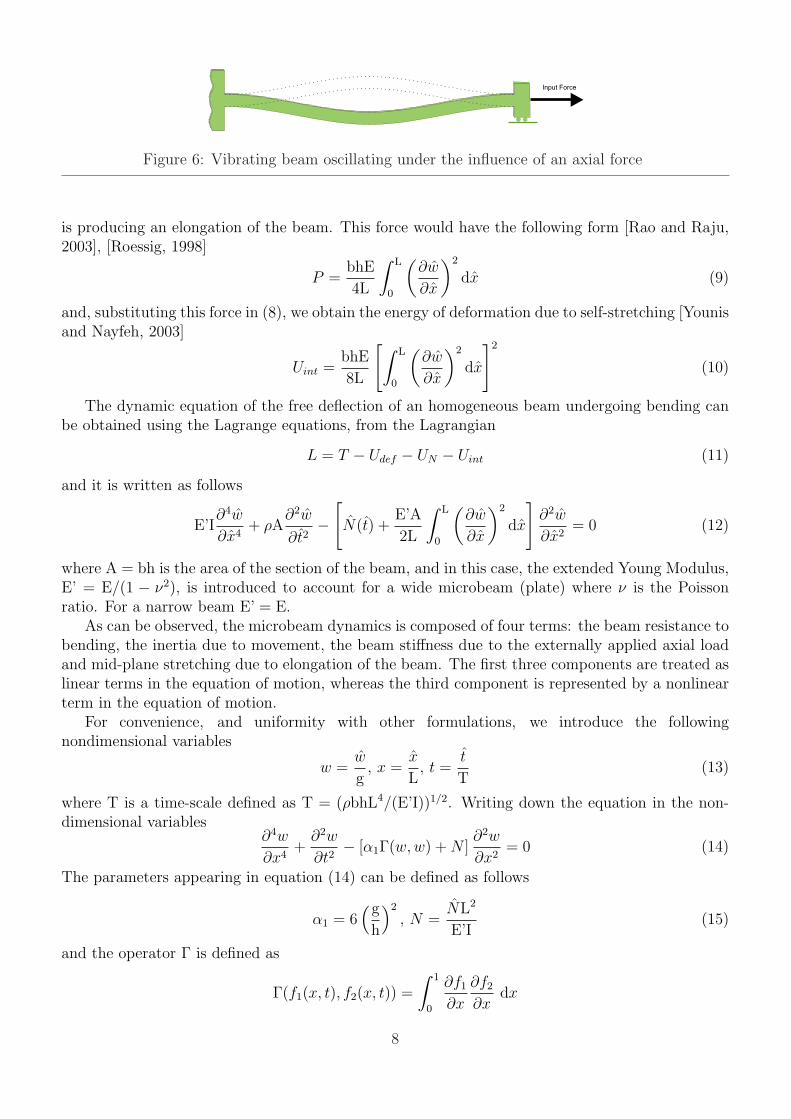
Typically in MEMS, a beam can also be externally stretched by an axial force N(t) (Figure 6).This force could be generated by different sources: thermal load, fabrication stresses, external beamtuning, etc. In this case, another energy term appears that englobes the deformation generated bythe external force

UN =N(t)

2

∫ L

0

(∂w

∂x

)2

dx (8)

As can be observed, the deformation is proportional to the axial force.Finally, in the case of large oscillations, the beam movement generates self-stretching forces that

actuate as structural damping. This effect can be accounted assuming that an internal force, P ,

7

Input Force

Figure 6: Vibrating beam oscillating under the influence of an axial force

is producing an elongation of the beam. This force would have the following form [Rao and Raju,2003], [Roessig, 1998]

P =bhE

4L

∫ L

0

(∂w

∂x

)2

dx (9)

and, substituting this force in (8), we obtain the energy of deformation due to self-stretching [Younisand Nayfeh, 2003]

Uint =bhE

8L

[∫ L

0

(∂w

∂x

)2

dx

]2

(10)

The dynamic equation of the free deflection of an homogeneous beam undergoing bending canbe obtained using the Lagrange equations, from the Lagrangian

L = T − Udef − UN − Uint (11)

and it is written as follows

E’I∂4w

∂x4+ ρA

∂2w

∂t2−

[N(t) +

E’A

2L

∫ L

0

(∂w

∂x

)2

dx

]∂2w

∂x2= 0 (12)

where A = bh is the area of the section of the beam, and in this case, the extended Young Modulus,E’ = E/(1 − ν2), is introduced to account for a wide microbeam (plate) where ν is the Poissonratio. For a narrow beam E’ = E.

As can be observed, the microbeam dynamics is composed of four terms: the beam resistance tobending, the inertia due to movement, the beam stiffness due to the externally applied axial loadand mid-plane stretching due to elongation of the beam. The first three components are treated aslinear terms in the equation of motion, whereas the third component is represented by a nonlinearterm in the equation of motion.

For convenience, and uniformity with other formulations, we introduce the followingnondimensional variables

w =w

g, x =

x

L, t =

t

T(13)

where T is a time-scale defined as T = (ρbhL4/(E’I))1/2. Writing down the equation in the non-dimensional variables

∂4w

∂x4+

∂2w

∂t2− [α1Γ(w, w) + N ]

∂2w

∂x2= 0 (14)

The parameters appearing in equation (14) can be defined as follows

α1 = 6(g

h

)2

, N =NL2

E’I(15)

and the operator Γ is defined as

Γ(f1(x, t), f2(x, t)) =

∫ 1

0

∂f1

∂x

∂f2

∂xdx

8

being f1 and f2 any two functions of x and t.Solving of the equations can be done numerically. However, to analyze the oscillation of the

beam, the partial differential formulation is usually simplified. One of the most common approachesis to break down the partial differential equations into single-degree of freedom ordinary equations,one for each mode of oscillation. The description of the output is presented as it will be used inthe following sections.

Assuming that beam response is composed of an infinite number of oscillation modes, thedisplacement w can be decomposed in

w(x, t) =∑

i

qi(t)φi(x) (16)

where qi(t) is the time-dependent modal displacement for the oscillation mode i and φi(x) is theposition-dependent modal shape. Substituting (16) in the equations of the potential energy of thesystem and rearranging terms a spring-equivalent equation can be obtained [Roessig, 1998]

Ui = Udef,i + UN,i + Uint,i =[EI2

∫ L

0

(∂2φi

∂x2

)2

dx + N(t)2

∫ L

0

(∂φi

∂x

)2

dx

]q2i + bhE

8L

[∫ L

0

(∂φi

∂x

)2

dx

]2

q4i = (17)

12Keff,i · q2

i + 14K3,eff,i · q4

i

And the same can be done for the kinetic energy

Ti =ρbh

2

∫ L

0

φ2i dx

∂2qi

∂t2=

1

2Meff,i · ¨q2

i (18)

where ( ˙ ) denotes time-derivative. And using the Lagrange formulation, the oscillation of each ofthe infinite modes is governed by

Meff,i · ¨qi + Keff,i · qi + K3,eff,i · q3i = 0 (19)

where

Meff,i = ρbh

∫ L

0

φ2i dx (20)

Keff,i = EI

∫ L

0

(∂2φi

∂x2

)2

dx + N(t)

∫ L

0

(∂φi

∂x

)2

dx (21)

K3,eff,i =bhE

2L

∫ L

0

(∂φi

∂x

)2

dx

2

(22)

Using this approach, the behavior of the beam, for a given mode of vibration, can be approximatedby a mass-spring model, allowing to use known analysis techniques.

3.2 Electrostatic Actuation

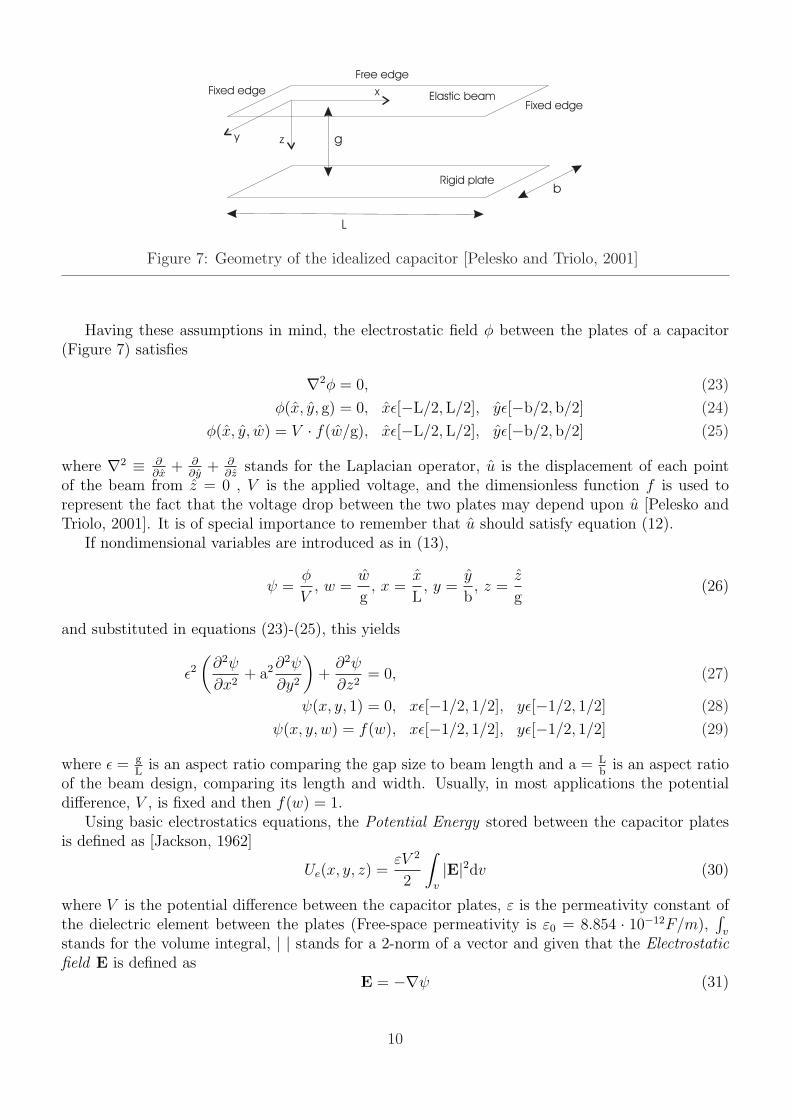
In MEMS, the basic electrostatic system is a parallel-plates capacitor (Figure 7). In this case,electrostatic forces are generated between two conducting elements separated a distance g by adielectric element. In MEMS, the dielectric is usually air. And an usual assumption is that thedistance g is differentially uniform between the two plates.

9

y z

x

Rigid plate

Elastic beamFixed edge

Fixed edge

Free edge

g

L

b

Figure 7: Geometry of the idealized capacitor [Pelesko and Triolo, 2001]

Having these assumptions in mind, the electrostatic field φ between the plates of a capacitor(Figure 7) satisfies

∇2φ = 0, (23)

φ(x, y, g) = 0, xε[−L/2, L/2], yε[−b/2, b/2] (24)

φ(x, y, w) = V · f(w/g), xε[−L/2, L/2], yε[−b/2, b/2] (25)

where ∇2 ≡ ∂∂x

+ ∂∂y

+ ∂∂z

stands for the Laplacian operator, u is the displacement of each pointof the beam from z = 0 , V is the applied voltage, and the dimensionless function f is used torepresent the fact that the voltage drop between the two plates may depend upon u [Pelesko andTriolo, 2001]. It is of special importance to remember that u should satisfy equation (12).

If nondimensional variables are introduced as in (13),

ψ =φ

V, w =

w

g, x =

x

L, y =

y

b, z =

z

g(26)

and substituted in equations (23)-(25), this yields

ε2

(∂2ψ

∂x2+ a2∂2ψ

∂y2

)+

∂2ψ

∂z2= 0, (27)

ψ(x, y, 1) = 0, xε[−1/2, 1/2], yε[−1/2, 1/2] (28)

ψ(x, y, w) = f(w), xε[−1/2, 1/2], yε[−1/2, 1/2] (29)

where ε = gL

is an aspect ratio comparing the gap size to beam length and a = Lb

is an aspect ratioof the beam design, comparing its length and width. Usually, in most applications the potentialdifference, V , is fixed and then f(w) = 1.

Using basic electrostatics equations, the Potential Energy stored between the capacitor platesis defined as [Jackson, 1962]

Ue(x, y, z) =εV 2

2

∫

v

|E|2dv (30)

where V is the potential difference between the capacitor plates, ε is the permeativity constant ofthe dielectric element between the plates (Free-space permeativity is ε0 = 8.854 · 10−12F/m),

∫v

stands for the volume integral, | | stands for a 2-norm of a vector and given that the Electrostaticfield E is defined as

E = −∇ψ (31)

10

where ∇ is the gradient operator. From equation (30), the force generated by the electrostaticpotential field in vacuum can be calculated as

F = −∇Ue = −ε0V2

2|∇ψ|2 (32)

Consequently, the key problem to define the electrostatic force is solving the equation (27) forthe electrostatic potential ψ.

Numerically, the potential can be calculated using finite elements [Pelesko and Triolo, 2001].However, approximations can be done in order to develop the formulation.

The typical approximation is to consider that the plate width and longitude are considerablylarge against the gap between the plates, what implies that the force lines are basically parallel andthe fringing fields are negligible. In this case, ε2 in equation (27) is small, and the terms that aremultiplied by this term can be ignored,

∂2ψ

∂z2= 0 (33)

Then solving this equation for the potential ψ, it can be found that

ψ =f(w)(1− z)

(1− w)(34)

and the differential force generated by this potential is

F (x, y) = − ε0V2

2g2(1− w)2(35)

As can be observed, this approximation gives way to the expression of the force mostly used tocalculate the electrostatic force between two parallel plates

F = −1

2

ε0AcV2

g2(1− w)2(36)

where Ac is the area of the capacitor plate. This formulation is only valid if the force contributionby the fringing fields that appear at the ends of the parallel plates can be assumed small comparedto the total force.

This approximation is shown to be valid for the small aspect ratio devices. In [Pelesko and Triolo,2001] and [Pelesko, 2001a] comparison between both approaches are presented and justifications ofthe validity of the approximation stated.

Another option to overcome the fringing fields is presented by [Nishiyama and Nakamura, 1990].In this case, knowing that the charge distribution is not even and taking into account the effect ofthe fringing fields, a normalized capacitance Cn is derived that includes this effects. If in a parallelplate capacitor, the capacitance C is defined as the proportionality constant between the chargeand the applied voltage

C =εbL

g; Q = CV (37)

Then the fringing-field corrected capacitance C is defined as

C = CCn (38)

where

Cn = 1 + 4.246ϑ, 0 ≤ ϑ < 0.005 (39)

Cn = 1 +√

11.0872ϑ2 + 0.001097, 0.005 ≤ ϑ < 0.05 (40)

Cn = 1 + 1.9861ϑ0.8258, 0.05 ≤ ϑ (41)

11

given that ϑ = g/b is the aspect ratio of the gap against the width of the beam. The constants arederived applying regression analysis to numerically obtained data. The model has been validated tomeasured data [Nishiyama and Nakamura, 1990]. Other authors have obtained equivalent resultswith different fitting formulas.

Consequently, with this approximation, the force can be computed with

U =1

2CV 2 =

1

2CnCV 2 =

1

2Cn

εbL

gV 2 (42)

F = −∇U =1

2Cn

εAcV2

g2(1− w)2(43)

The derived expressions can be extended to non-uniform gap capacitors using sum of elementarycapacitors [Najar et al., 2005].

3.3 Damping in MEMS

In Micro Electro Mechanical Systems, there are two basic sources of damping forces: structuraldamping and viscous damping (or aerodynamic damping).

The structural damping is generated by the molecular interaction in the material due todeformations. It happens in the moving parts and at the anchoring points [Duwel et al., 2003]. Themain contribution has already been introduced in the mechanical model with the term includinginternal forces due to stretching. If the amplitude of oscillation of the beam is small, the values ofthese forces in materials like the polysilicon are negligible compared to the viscous damping effects.

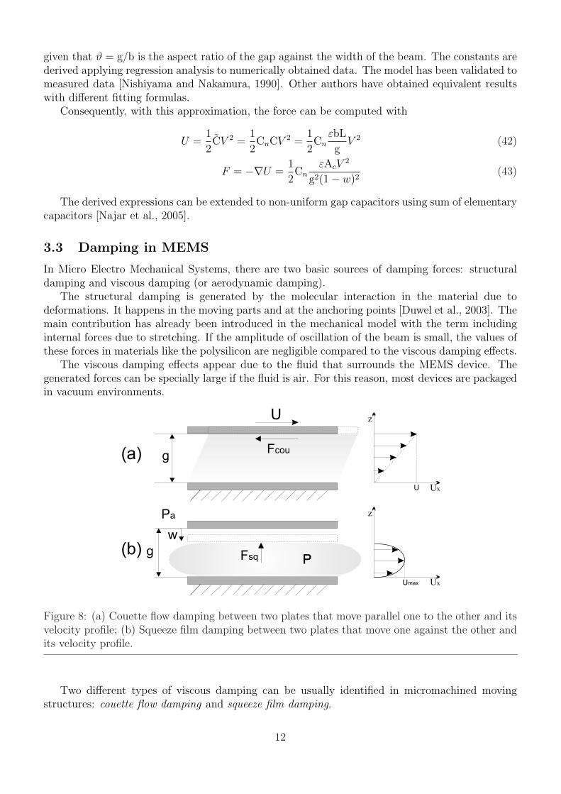
The viscous damping effects appear due to the fluid that surrounds the MEMS device. Thegenerated forces can be specially large if the fluid is air. For this reason, most devices are packagedin vacuum environments.

g

U

U z

Ux

Umax

z

Ux

g

w

PP

Fcou

Fsq

Pa

(a)

(b)

Figure 8: (a) Couette flow damping between two plates that move parallel one to the other and itsvelocity profile; (b) Squeeze film damping between two plates that move one against the other andits velocity profile.

Two different types of viscous damping can be usually identified in micromachined movingstructures: couette flow damping and squeeze film damping.

12

To analyze the generated forces, one can turn to classical fluid mechanics and use the Navier-Stokes equations, which are composed of the continuity equation

Dρm

Dt+ ρm∇U = 0 (44)

and the motion equation

ρmDU

Dt= −∇P + ρmg + η∇2U +

η

3∇(∇ ·U) (45)

where ρm is the mass-density of the fluid, η is the viscosity (assumed to be constant), g is theacceleration of gravity, P is the pressure of the fluid and U is the velocity of the fluid (bold symboldenotes that is a vector) [Pelesko and Bernstein, 2003].

In the couette flow case, the damping force appears between two plates that move parallelone to the other and are separated by a Newtonian fluid (Figure 8a) [Cho et al., 1994]. As thedistance between the plates is considered constant, the working regime is under incompressibleflow, meaning that the rate of change of density Dρm

Dtis negligible. Under this circumstances, the

continuity equation (44) becomes∇U = 0 (46)

and the Navier-Stokes equation of motion (45) reduces to

ρmDU

Dt= −∇P + ρmg + η∇2U (47)

for incompressible flow. The pressure and gravity terms can be combined introducing the positionvector r, and defining

P ∗ = P − ρmgr

Using this definition, the Navier-Stokes equation reduces to the following steady-flow equation

ρmDU

Dt= η∇2U−∇P ∗ (48)

From Figure 8a, it can be seen that the flow becomes perfectly one-dimensional away from the edges.This aspect linked to condition (46) delimits that the velocity profile is composed of streamlines

U = Ux(y)ix (49)

and consequently,∂U

∂t= U · ∇U =

DU

Dt= 0 (50)

Under these assumptions, and considering that no pressure gradient is generated by the movingplate, the Navier-Stokes equation reduces to

∂2Ux

∂y2= 0 (51)

giving a linear velocity profile as a solution.If the fluid is liquid or gas, and the structures are relatively large (see [Veijola and Turowski,

2001] for correction in case of gas rarefication), one can apply the usual no-slip boundary condition,to the profile in Figure 8a. Then the velocity is

Ux =y

gU (52)

13

and the shear stress, using the Newtonian fluid condition, on the moving plate is

τ = −η∂Ux

∂y|y=g = −η

U

gix (53)

Finally, the couette damping force of the whole structure can be calculated as

Fcou = −ηAov

gU = ccouU (54)

where the force is directly proportional to the velocity of the structure. Aov is the area of overlappingbetween the structures.

However, in MEMS actuated with parallel plate capacitors, the main source of damping is theSqueeze film force. In this case, a moving plate move downwards and upwards from a fixed plate(Figure 8b). In this movement, when the plates approach each other the pressure in the trappedfluid increases, and the fluid is squeezed out through the edges of the plates. When the platesseparate, a sucking drag is generated due to the fluid filling back the gap.

To solve this case, we must return to the Navier-Stokes equation (45), but this time we needthe full compressible fluid equation. Consequently, to handle the analytical derivation, severalassumptions must be done in our system:

• The aspect ratio is large, meaning that the gap is smaller than the plates extent.

• The motion is slow, meaning that the inertial term can be neglected in front of the viscousone, and the fluid works under Stokes flow.

• The pressure between the plates is homogeneous.

• The fluid flow at the edges of the plates follows a parabolic profile, defined by a Pousille-likeequation (Figure 8b).

• The gas behaves under the ideal gas law.

• The system is isothermal.

Under these assumptions, the behavior of the fluid is governed by the Reynolds equation [Hamrock,1994]

12ηeff∂Pd

∂t= ∇[d3P∇P ] (55)

where P (x, y, t) is the pressure between the plates, d(x, y, t) is the distance between the parallelplates, and ηeff is the corrected viscosity of the fluid, accounting for the rarefication effects due tolow pressure [Veijola et al., 1995]

ηeff =η

1 + 9.638K1.159n

(56)

where Kn = λ/g is the Knudsen number, which compares the mean free path of a fluid molecule(λ) against the gap distance. The constants are experimentally obtained. In a typical MEMSexample, where λ is approximately 0.1 microns, the air is at atmospheric pressure and the gap isof 2 microns, the value of Kn would be 0.05. The mean free path is inversely proportional to fluidpressure.

Solution of equation (55) on P will lead to derivation of the squeeze film forces.

Fsq = (P − Pa) · Ac (57)

14

where Pa is the static pressure force. As can be observed, the squeeze forces calculation is coupledto the mechanical deflection of the beam [Nayfeh and Younis, 2004].

To approximate the damping forces, one must linearize equation (55) assuming small amplitudemotions. This way the gap distance and the pressure of the gap can be expressed as follows

d(x, y, t) = g− w(x, y, t) ; P (x, y, t) = Pa + P (x, y, t) (58)

where w is the gap reduction and P the pressure variations from the static pressure. Substitutionin (55) leads to

12ηeff

Pag3

(g∂P

∂t− Pa

∂w

∂t

)= ∇2P =

∂2P

∂x2+

∂2P

∂y2(59)

From this equation [Nayfeh and Younis, 2004] has shown that numerical coupled perturbationmethods can predict experimental damping forces accurately.

If we add the assumption that the capacitor plates are long and narrow (a beam), the equationcan be much reduced due to the fact that the fluid movement is only in one direction (y-directionin our device)

∂P

∂t=

Pag2

12ηeff

∂2P

∂y2+

Pa

g

∂w

∂t(60)

From this equation, one can solve for P , obtaining the following force on the capacitors [Senturia,2001], using Laplace transform

Fsq(s) =

[96ηeffLb3

π4g3

∑

nodd

1

n4

1

1 + sαn

]sz(s) (61)

where

αn =g2Pan

2π2

12ηeffb2(62)

given that z(s) is the input displacement. As we are assuming small amplitudes, the first term ofthe expansion is a good approximation of the force

Fsq(s) =

[96ηeffLb3

π4g3

1

1 + sωc

]sz(s) (63)

From this derivation two important parameters arise, the cut-off frequency, ωc

ωc =π2g2Pa

12ηeffb2(64)

and the squeeze number, σd,

σd =π2ω

ωc

=12ηeffb

2

g2Pa

ω (65)

The squeeze number allow to analyze the behavior of the squeeze film damping forces. When thesqueeze number decreases, due to low pressure or low frequencies of oscillation, the fluid forcebecomes a pure damping force. However, at high frequencies or high squeeze number, a springforce component appears and becomes dominant with the damping force still present. Example ofthe contributions of each force can be found in [Senturia, 2001]. Similar analysis and discussionsare shown by [Andrews et al., 1993] and [Veijola et al., 1995] using the force decomposition derivedin [Blech, 1983].

15

Consequently, squeeze film damping force can be reduced to

Fsq = csq(w, σd)∂w

∂t(66)

with damping and spring effects depending on σd [Wang et al., 2004].Finally, the fluid damping effects in the model are the combination of squeeze film and couette

film damping, giving a final force

Fd = Fsq + Fcou = −ηAov

gU + (P − Pa) · Ac (67)

that can be generalized as

Fd = (csq + ccou)∂w

∂t= cd

∂w

∂t(68)

3.4 Lumped system

The complete set of equations defining the behavior of the system can be obtained linking thedifferent energies and non-conservative forces acting in the system.

The kinetic energy is defined in (7)

T =ρbh

2

∫ L

0

(∂w

∂t

)2

dx (69)

The potential energy is composed of mechanical (6),(8),(10) and electrostatic terms (30)

U =EI

2

∫ L

0

(∂2w

∂x2

)2

dx +N(t)

2

∫ L

0

(∂w

∂x

)2

dx +bhE

8L

[∫ L

0

(∂w

∂x

)2

dx

]2

+εV 2

2

∫

v

|∇ψ|2dv (70)

The fluid damping is the only non-conservative force (67)

Fd = −ηAov

gU + (P − Pa) · Ac (71)

Consequently, using Lagrange formulation and non-dimensional variables, the dynamics of thesystem is as follows:

∂4w

∂x4+

∂2w

∂t2− [α1Γ(w, w) + N ]

∂2w

∂x2= γV 2|∇ψ|2 − 12L4

E’ h3T

[−η

Aov

gU + (P − Pa) · Ac

](72)

given that the electrostatic potential and the fluid pressure satisfy the following conditions

ε2

(∂2ψ

∂x2+ a2∂2ψ

∂y2

)+

∂2ψ

∂z2= 0 (73)

12ηeff∂Pd

∂t= ∇[d3P∇P ] (74)

Linking the different formulations previously derived , the dynamics of the system can be reducedto [Abdel-Rahman et al., 2003]:

∂2w

∂t2+ c

∂w

∂t+

∂4w

∂x4− [α1Γ(w, w) + N ]

∂2w

∂x2= γV 2|∇ψ|2 (75)

16

w(0, t) = w(1, t) = 0, w′(0, t) = w′(1, t) = 0

And the parameters appearing in equation (75) can be defined as follows

c =cd L4

E’ I T, N = NL2

E’I

α1 = 6(g

h

)2

, γ = 6ε0L4

E’ h3g(76)

Equation (75) translates to the following formulation once the electrostatic force is approximated

∂2w

∂t2+ c

∂w

∂t+

∂4w

∂x4− [α1Γ(w, w) + N ]

∂2w

∂x2= κ

V 2

(1− w)2(77)

where κ = 6Cnε0L4

E’ h3g3 using fringing fields correction.

4 Model solution

Once the model has been derived, one can analyze the behavior of the system.In this section the different approaches to understand the system are presented and formulated.

With each approach the advantages and problems are presented, as well as, the implications to thestability of the system.

4.1 Static solution

In the case of searching for the static solution of the system, the time-derivatives of the systemmust be set to zero. Under these premises, only potential energy terms remain in our system andthe static solutions correspond to the equilibrium positions of the potential energy of the system,that is

dU

dw= 0 (78)

Consequently, the static deformation ws of the beam, under the action of a electrostatic forcing Vp

can be calculated from equation (75), if the time-derivatives are set to zero.This way, the remaining terms are only position-dependant, and the partial differential equations

disappear:

d4ws

dx4− [α1 Γ(ws, ws) + N ]

d2ws

dx2= γV 2

p |∇ψ|2 (79)

ws = 0 anddws

dx= 0 at x = 0 and x = 1 (80)

Unfortunately, equation (79) do not generate a closed-form solution, due to its implicit nature. Forthis reason, numerical methods must be used to solve the problem.

A possibility is shooting methods combined with nonlinear boundary-value problem solutionas in [Abdel-Rahman et al., 2003]. They apply the method to this model without fringing-fieldscorrection (Cn = 1).

d4ws

dx4− [α1 Γ(ws, ws) + N ]

d2ws

dx2= κ

V 2

(1− w)2(81)

They show good agreement to experimental results, and argue that the inclusion of internalstretching is essential to predict real displacements. This approach allows to numerically calculate

17

the exact Static Pull-in Voltage using the same numerical method. Their analysis shows thatneglecting the nonlinear effects leads to underestimating the stability limits of the system. Thetravel range taking into account the nonlinearities can be doubled.

Another option is to ignore the internal stretching, what reduces the model complexity, and usea method as the backward Euler algorithm to solve for the static displacement as in [Ijntema andTilmans, 1992]:

d4ws

dx4−N

d2ws

dx2= κ

V 2

(1− w)2(82)

[Tilmans and Legtenberg, 1994] solved the same static problem using the Rayleigh-Ritz methodassuming a combination of trial functions. They used this formulation to generate an analyticalexpression for the pull-in voltage, based on energy methods. Even with the needed approximationsto solve the equations, the calculated values of the pull-in voltage were in good agreement with theresults of experiments they conducted on resonators of various lengths. The system approximationgenerates good results while large amplitudes are not taken into account.

In [Zhou and Yang, 2003] numerical solutions are shown using the equation (82) and finiteelements analysis. General numerical solutions using finite elements with reduced-order energyequations are presented in [Elata et al., 2003] using relaxation techniques. FEM solutions allow tohandle the complete deformation of the device, without focusing on the maximum amplitude, butlarge computational time is needed.

0.6 0.4 0.2 0 0.2 0.4 0.6 0.816

14

12

10

8

6

4

2

0

2

4

x 10 12

normalized displacement (y/g0)

Ene

rgy

Evolution energy profile with increasing voltage

10 V

30 V

40 V

55.43V

60.34V

65V

ypin=g0/3

Stable and unstable equilibrium points for VDC=30V

Initial energy and energy at unstable equilibrium point for DPV=55.43V

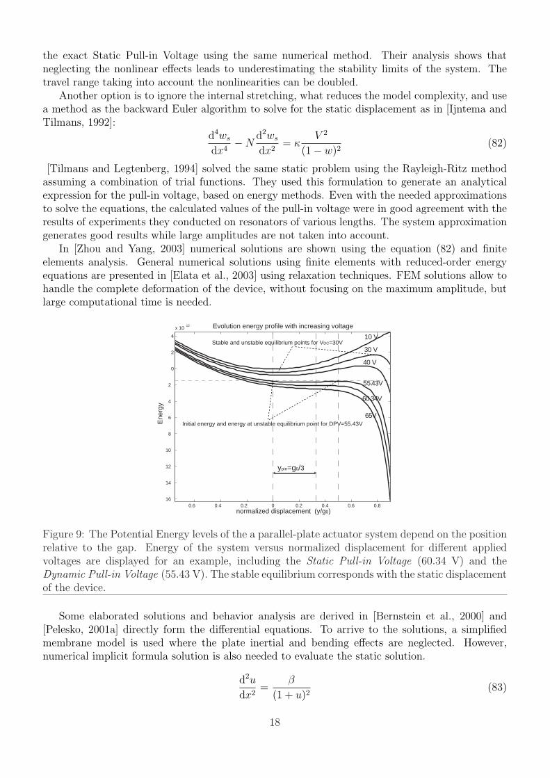
Figure 9: The Potential Energy levels of the a parallel-plate actuator system depend on the positionrelative to the gap. Energy of the system versus normalized displacement for different appliedvoltages are displayed for an example, including the Static Pull-in Voltage (60.34 V) and theDynamic Pull-in Voltage (55.43 V). The stable equilibrium corresponds with the static displacementof the device.

Some elaborated solutions and behavior analysis are derived in [Bernstein et al., 2000] and[Pelesko, 2001a] directly form the differential equations. To arrive to the solutions, a simplifiedmembrane model is used where the plate inertial and bending effects are neglected. However,numerical implicit formula solution is also needed to evaluate the static solution.

d2u

dx2=

β

(1 + u)2(83)

18

This analysis allows to define stability conditions based on implicit eigenvalue equations.Most authors work with the mass-spring-damper model, as in Figure 4. This model losses insight

on the complete behavior of the system, but allow to analyze the system analytically, producingimportant information for the design process. The behavior of the beam can be approximatedto that of a non-linear spring for a given deformation mode, as it has been shown in (19), andapproximations can also be obtained for the electrostatic force and damping, giving way to thefollowing formulation

Meff,i · ¨qi + Ceff,i · ˙qi + Keff,i · qi + K3,eff,i · q3i = Fe (84)

In the static case, (84) simplifies to

Keff,i · qi + K3,eff,i · q3i = Fe (85)

being a non-linear mass-spring equation. This model characterizes the beam stiffening due to largedeformations, that reduces the effective travel range of the beam [Roessig, 1998].

However, in most cases small amplitude of oscillation is considered [Vinokur, 2002], [Gretillatet al., 1997] , allowing to use the linear formulation

K · qi = −1

2

ε0AcV2

g2(1− w)2(86)

With this model, the classical Static Pull-in Voltage (SPV ) equation is obtained (Figure 9),

SPV =

√8

27

K g30

ε0 A; ypin =

g0

3(87)

which indicates the maximum voltage that can be applied without getting snapping. Substitutionof the voltage in the dynamics equation gives the maximum travel range in the static case, whichis one-third of the initial gap [Senturia, 2001].

4.2 Dynamic solution

If we want to analyze the transient response of the microbeam when a variable voltage load V (t)is applied, the complete evolution of the energy of the system has to be taken into account. Toobtain solutions, the full set of equations (75) must be used.

Typical cases where the transient is of interest include micro-switches or mirror positioning,where the time response is of great interest. In this cases, the voltage is usually applied as astep-function or a ramp-function.

The use of numerical simulation to obtain the behavior of the system is mandatory if thecomplete set of equations is used. MEMS exhibit non-linearities even when the displacements aresmall, and the complete equations are needed to capture all the behavioral aspects.

The main dynamic nonlinear effects that will be detected on parallel-plate actuated MEMS arethe following [Rand, 2003]:

• Spring stiffening: The effect appears due to large amplitudes of oscillation. The deformationof the beam cannot be considered linear anymore, and increases the beam resistance todeformation (19). The resulting non-linear equation corresponds to the Duffing equation(Figure 10a).

19

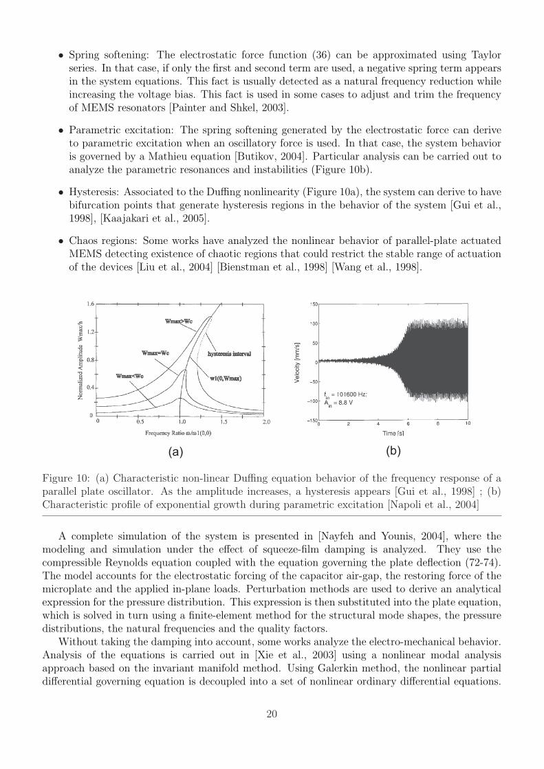
• Spring softening: The electrostatic force function (36) can be approximated using Taylorseries. In that case, if only the first and second term are used, a negative spring term appearsin the system equations. This fact is usually detected as a natural frequency reduction whileincreasing the voltage bias. This fact is used in some cases to adjust and trim the frequencyof MEMS resonators [Painter and Shkel, 2003].

• Parametric excitation: The spring softening generated by the electrostatic force can deriveto parametric excitation when an oscillatory force is used. In that case, the system behavioris governed by a Mathieu equation [Butikov, 2004]. Particular analysis can be carried out toanalyze the parametric resonances and instabilities (Figure 10b).

• Hysteresis: Associated to the Duffing nonlinearity (Figure 10a), the system can derive to havebifurcation points that generate hysteresis regions in the behavior of the system [Gui et al.,1998], [Kaajakari et al., 2005].

• Chaos regions: Some works have analyzed the nonlinear behavior of parallel-plate actuatedMEMS detecting existence of chaotic regions that could restrict the stable range of actuationof the devices [Liu et al., 2004] [Bienstman et al., 1998] [Wang et al., 1998].

(b)(a)

Figure 10: (a) Characteristic non-linear Duffing equation behavior of the frequency response of aparallel plate oscillator. As the amplitude increases, a hysteresis appears [Gui et al., 1998] ; (b)Characteristic profile of exponential growth during parametric excitation [Napoli et al., 2004]

A complete simulation of the system is presented in [Nayfeh and Younis, 2004], where themodeling and simulation under the effect of squeeze-film damping is analyzed. They use thecompressible Reynolds equation coupled with the equation governing the plate deflection (72-74).The model accounts for the electrostatic forcing of the capacitor air-gap, the restoring force of themicroplate and the applied in-plane loads. Perturbation methods are used to derive an analyticalexpression for the pressure distribution. This expression is then substituted into the plate equation,which is solved in turn using a finite-element method for the structural mode shapes, the pressuredistributions, the natural frequencies and the quality factors.

Without taking the damping into account, some works analyze the electro-mechanical behavior.Analysis of the equations is carried out in [Xie et al., 2003] using a nonlinear modal analysisapproach based on the invariant manifold method. Using Galerkin method, the nonlinear partialdifferential governing equation is decoupled into a set of nonlinear ordinary differential equations.

20

Then the invariant manifold method is used to obtain the associated nonlinear modal shapes, andmodal motion governing equations. The model allows to examine the nonlinearities and the pull-in phenomena. Similar results using shooting methods combined with nonlinear boundary-valueproblem where presented in [Abdel-Rahman et al., 2002].

Using a simplified plate model (83), in [Flores et al., 2003] they obtain solutions of the systemoperated in viscous regime. This simplified mathematical model allows to study a parabolicequation of reaction-diffusion type. A central result of the paper is that when the applied voltageis beyond the critical voltage where steady-state solutions cease to exist, the solution touches downin finite time. Bounds on the touchdown time are computed and the structure of solutions neartouchdown are investigated.

0 0.01 0.02 0.03 0.04 0.05 0.06 0.07 0.08 0.09 0.1

4.62

4.6

4.58

4.56

4.54

4.52

4.5

4.48

4.46

4.44

x 10 13

normalized displacement (y/g0)

Ene

rgy

Energy evolution

Potential energy bound

System energy evolutionInitial energy level of the system

Stable equilibrium position

102

10 1

100

101

102

103

104

105

55

56

57

58

59

60

61

Quality Factor

Pul

l-in

Vol

tage

(V

)

Dynamic Pull-in Voltage Evolution

Static Pull-in Voltage = 60.34 V

Dynamic Pull-in Voltage = 55.43 V

Q=1.2 Q=1000

(a) (b)

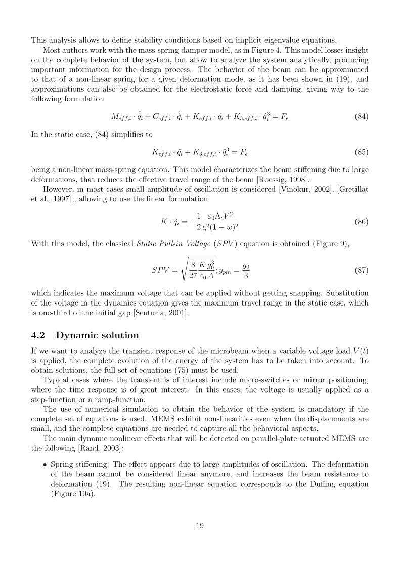
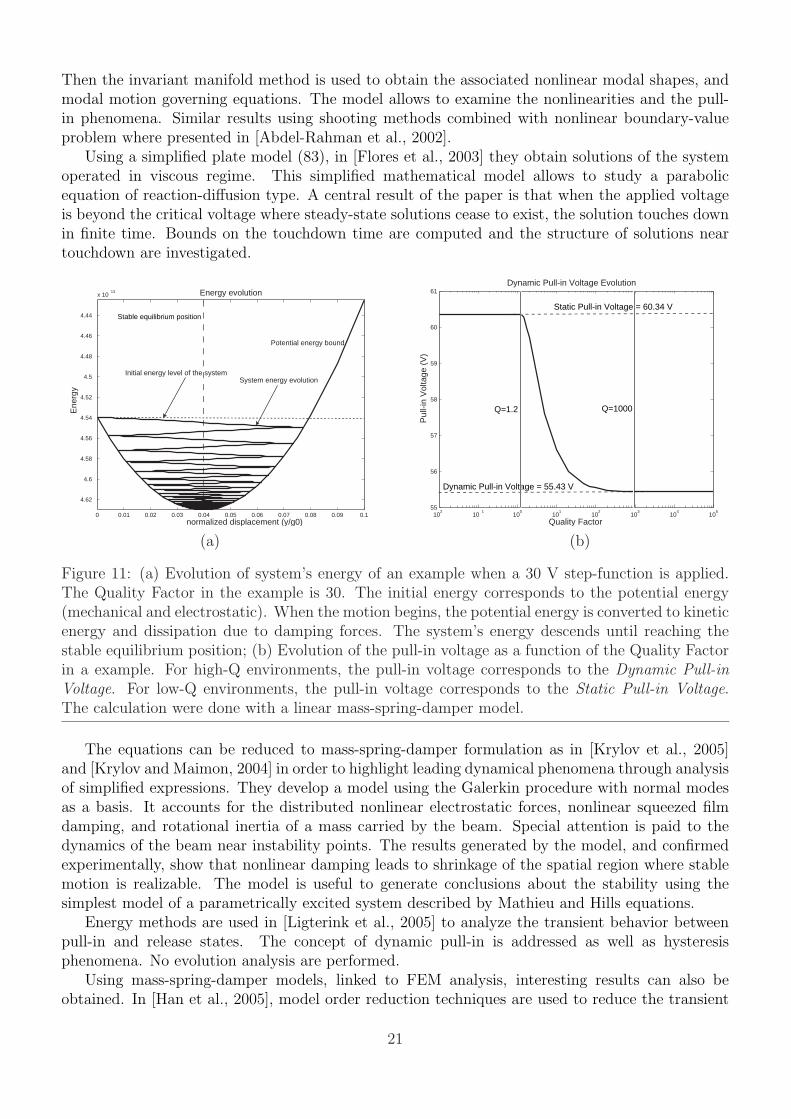
Figure 11: (a) Evolution of system’s energy of an example when a 30 V step-function is applied.The Quality Factor in the example is 30. The initial energy corresponds to the potential energy(mechanical and electrostatic). When the motion begins, the potential energy is converted to kineticenergy and dissipation due to damping forces. The system’s energy descends until reaching thestable equilibrium position; (b) Evolution of the pull-in voltage as a function of the Quality Factorin a example. For high-Q environments, the pull-in voltage corresponds to the Dynamic Pull-inVoltage. For low-Q environments, the pull-in voltage corresponds to the Static Pull-in Voltage.The calculation were done with a linear mass-spring-damper model.

The equations can be reduced to mass-spring-damper formulation as in [Krylov et al., 2005]and [Krylov and Maimon, 2004] in order to highlight leading dynamical phenomena through analysisof simplified expressions. They develop a model using the Galerkin procedure with normal modesas a basis. It accounts for the distributed nonlinear electrostatic forces, nonlinear squeezed filmdamping, and rotational inertia of a mass carried by the beam. Special attention is paid to thedynamics of the beam near instability points. The results generated by the model, and confirmedexperimentally, show that nonlinear damping leads to shrinkage of the spatial region where stablemotion is realizable. The model is useful to generate conclusions about the stability using thesimplest model of a parametrically excited system described by Mathieu and Hills equations.

Energy methods are used in [Ligterink et al., 2005] to analyze the transient behavior betweenpull-in and release states. The concept of dynamic pull-in is addressed as well as hysteresisphenomena. No evolution analysis are performed.

Using mass-spring-damper models, linked to FEM analysis, interesting results can also beobtained. In [Han et al., 2005], model order reduction techniques are used to reduce the transient

21

analysis time. To do this, an open-source software performs model order reductions via the blockArnoldi algorithm directly to ANSYS finite element models.

On the other hand, direct analysis over the linear model can be useful in several applications(Figure 11a). The nonlinear behavior of the system with a simple mass-spring-damper model isanalyzed in [ZHAO et al., 2005], [Castaner et al., 1999], [Minami et al., 1999]. In [Gupta andSenturia, 1997], they used the system analysis to predict pull-in times and derive the DynamicPull-in Voltage (DPV)

yuns =g0

2; DPV =

√1

4

K g30

ε0 A(88)

which indicates the maximum voltage that can be applied as a step-function to the system withoutproducing snapping in vacuum environment. A extended discussion on energy-dependence of theDynamic Pull-in Voltage (Figure 11b) can be found in [Varghese et al., 1997] and [Fargas-Marques,2001].

4.3 Oscillatory solution

In multiple applications in MEMS sensors and actuators, the system is oscillated at a fixedfrequency. An alternating voltage is applied to the system to maintain the oscillation. The case ofoscillatory load is, then, a sub-case of the dynamic solution.

To analyze the oscillatory case, the transient response is neglected and the efforts areconcentrated on the stationary oscillation.

The microbeam deformation under an electrostatic excitation (V (t) = V p + v(t)) is composedof a static component (ws(x)) and a dynamic component (u(x, t)), due to the AC forcing voltage:

w(x, t) = ws(x) + u(x, t) (89)

To solve the oscillatory case, we substitute (89) in the dynamic equation of the system (75) andobtain

∂2(ws(x)+u(x,t))∂t2

+ c∂(ws(x)+u(x,t))∂t

+ ∂4(ws(x)+u(x,t))∂x4

− [α1Γ((ws(x) + u(x, t)), (ws(x) + u(x, t))) + N ] ∂2(ws(x)+u(x,t))∂x2

= γ(Vp + v(t))2|∇ψ|2 (90)

The equation can be simplified eliminating the expressions with null terms, and it turns to

∂2u∂t2

+ c∂u∂t

+ ∂4ws

∂x4 + ∂4u∂x4

− [α1(Γ(ws, ws) + 2Γ(ws, u) + Γ(u, u)) + N ] (∂2ws

∂x2 + ∂2u∂x2 )

= γ(Vp + v(t))2|∇ψ|2 (91)

Once in this point, to develop the equation further, a possibility is to approximate theelectrostatic force, assuming no fringing fields, using equation (32). This way the oscillation isdefined by

∂2u∂t2

+ c∂u∂t

+ ∂4ws

∂x4 + ∂4u∂x4

− [α1(Γ(ws, ws) + 2Γ(ws, u) + Γ(u, u)) + N ] (∂2ws

∂x2 + ∂2u∂x2 )

= α2(Vp+v(t))2

(1−(ws+u))2(92)

where now α2 = γ/g2 = 6ε0L4

E’ h3g3 .

22

The formulation can be much reduced if the electrostatic force is expanded in Taylor seriesaround the equilibrium position

∂2u∂t2

+ c∂u∂t

+ ∂4ws

∂x4 + ∂4u∂x4

− [α1(Γ(ws, ws) + 2Γ(ws, u) + Γ(u, u)) + N ] (∂2ws

∂x2 + ∂2u∂x2 )

= α2(V2p + 2Vpv(t) + v(t)2)

(1β2 + 2

β3 u + 3β4 u

2 + 4β5 u

3 + O(u4))

(93)

and then, rearranging terms, the static solution (79) can be eliminated and only the oscillatingsolution is conserved, simplifying the equation to

∂2u∂t2

+ c∂u∂t

+ ∂4u∂x4

−α1 [2Γ(ws, u) + Γ(u, u)] ∂2ws

∂x2

− [α1(Γ(ws, ws) + 2Γ(ws, u) + Γ(u, u)) + N ] ∂2u∂x2

= α2V2p

(2β3 u + 3

β4 u2 + 4

β5 u3 + O(u4)

)

+2α2Vpv(t)(

1β2 + 2

β3 u + 3β4 u

2 + 4β5 u

3 + O(u4))

+α2v(t)2(

1β2 + 2

β3 u + 3β4 u

2 + 4β5 u

3 + O(u4))

(94)

Depending on the driving voltages and the accepted error, the final equation can be selected.However, numerical simulation will be needed to obtain evolution results.

Complete simulations based on the theoretical framework exist in the literature. In [Abdel-Rahman et al., 2003], shooting methods combined with nonlinear boundary-value problem areused to solve the existing eigenvalue problem. The vibrations around the deflected position of themicrobeam are solved numerically for various parameters to obtain the natural frequencies andmode shapes. The results are compared with experimental results available in the literature withgood agreement. In [Nayfeh and Younis, 2004], perturbation methods are used to obtain the modeshapes and frequencies including the coupled effects of the squeeze-film damping that were justapproximated in the previous analysis.

Following the same study, in [Younis et al., 2004] they present a methodology to simulate thetransient and steady-state dynamics of microbeams undergoing small or large motions actuated bycombined DC and AC loads. They use the model to produce results showing the effect of varyingthe DC bias, the damping, and the AC excitation amplitude on the frequency-response curves. Intheir analysis they detect the existence of dynamic effects that can produce pull-in with electricloads much lower than that predicted based on static analysis.

In [Ijntema and Tilmans, 1992], the dynamic behavior is modeled using energy methods toobtain a spring-mass-damper model. The fundamental frequency is approximated using Rayleigh’senergy method where the microbeam motion is linearized around the deflected shape obtained asa solution of the static problem. The work is extended in [Tilmans and Legtenberg, 1994] wherethe fundamental natural frequency obtained from Rayleigh’s energy method is compared to theexperimentally obtained fundamental natural frequency. They found out that the results obtainedfrom the expression were only valid for small dc polarization voltages away from the pull-in voltage.Their method takes into account the axial load and large amplitude effects.

The mass-spring-damper formulation obtained via Galerkin procedure in [Krylov et al., 2005]allows to study the parametric resonance behavior of the system. They show that parametricstabilization can be obtained. The model summarizes the main nonlinearities for a given frequency.Similar analysis are carried out with a parametric model in [Napoli et al., 2004] They show that theunderlying linearized dynamics of the system are those of a periodic system described by a Mathieu

23

0.6 0.4 0.2 0 0.2 0.4 0.6 0.8

0

0.5

1

1.5

2

2.5

3

3.5

4

x 10 12

Normalized displacement (y/g0)

Ene

rgy

Energy evolution

Maximum stable amplitude of oscillation

Achieved amplitude of oscillation

Potential energyupper bound VDC-VAC

Potential energylower bound VDC+VAC

Initial position

Unstableequilibrium ofVDC+VAC curve

Total energyevolution

Stable permanentoscillation loop

(a)

Initial energy

0.6 0.4 0.2 0 0.2 0.4 0.6 0.8

0

0.5

1

1.5

2

2.5

3

3.5

4

x 10 12

Normalized displacement (y/g0)

Ene

rgy

Energy evolution

Maximum stable amplitude of oscillation

Potential energyupper bound VDC-VAC

Potential energylower bound VDC+VAC

Initial position

Unstableequilibrium ofVDC+VAC curve

Total energyevolution

Unstable oscillation loop

(b)

Snapping of electrodes

Initial energy

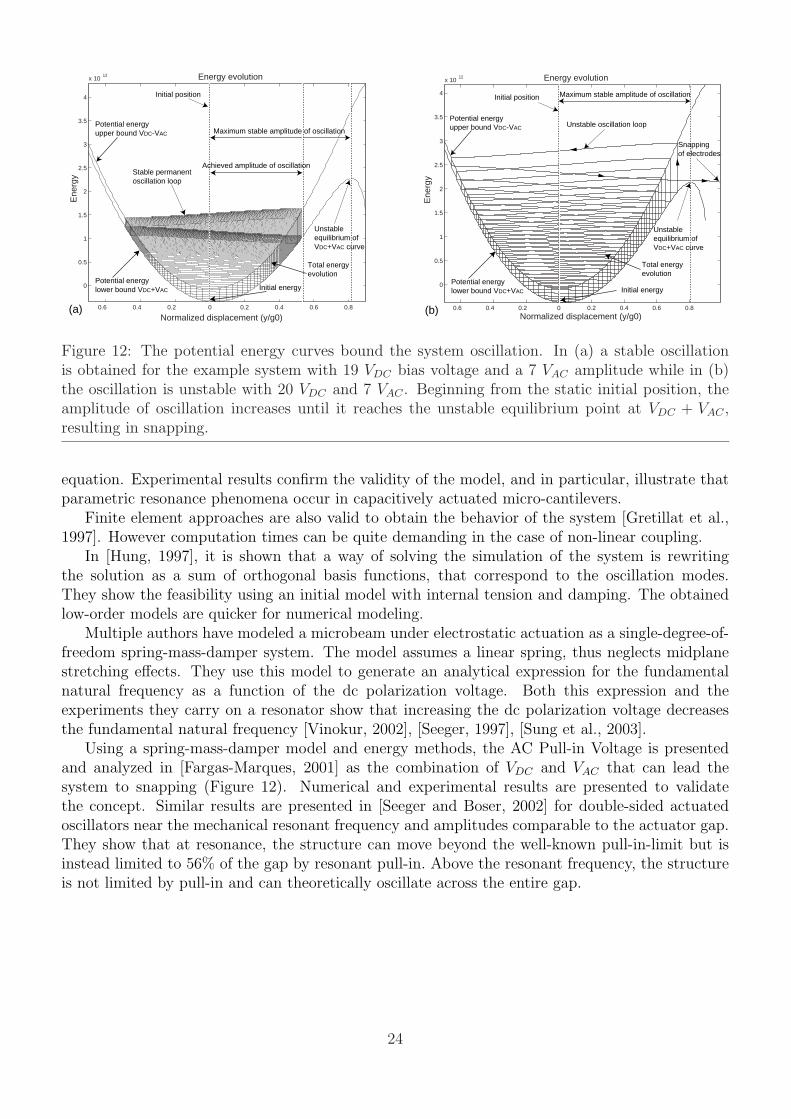
Figure 12: The potential energy curves bound the system oscillation. In (a) a stable oscillationis obtained for the example system with 19 VDC bias voltage and a 7 VAC amplitude while in (b)the oscillation is unstable with 20 VDC and 7 VAC . Beginning from the static initial position, theamplitude of oscillation increases until it reaches the unstable equilibrium point at VDC + VAC ,resulting in snapping.

equation. Experimental results confirm the validity of the model, and in particular, illustrate thatparametric resonance phenomena occur in capacitively actuated micro-cantilevers.

Finite element approaches are also valid to obtain the behavior of the system [Gretillat et al.,1997]. However computation times can be quite demanding in the case of non-linear coupling.

In [Hung, 1997], it is shown that a way of solving the simulation of the system is rewritingthe solution as a sum of orthogonal basis functions, that correspond to the oscillation modes.They show the feasibility using an initial model with internal tension and damping. The obtainedlow-order models are quicker for numerical modeling.

Multiple authors have modeled a microbeam under electrostatic actuation as a single-degree-of-freedom spring-mass-damper system. The model assumes a linear spring, thus neglects midplanestretching effects. They use this model to generate an analytical expression for the fundamentalnatural frequency as a function of the dc polarization voltage. Both this expression and theexperiments they carry on a resonator show that increasing the dc polarization voltage decreasesthe fundamental natural frequency [Vinokur, 2002], [Seeger, 1997], [Sung et al., 2003].

Using a spring-mass-damper model and energy methods, the AC Pull-in Voltage is presentedand analyzed in [Fargas-Marques, 2001] as the combination of VDC and VAC that can lead thesystem to snapping (Figure 12). Numerical and experimental results are presented to validatethe concept. Similar results are presented in [Seeger and Boser, 2002] for double-sided actuatedoscillators near the mechanical resonant frequency and amplitudes comparable to the actuator gap.They show that at resonance, the structure can move beyond the well-known pull-in-limit but isinstead limited to 56% of the gap by resonant pull-in. Above the resonant frequency, the structureis not limited by pull-in and can theoretically oscillate across the entire gap.

24

5 Final Conclusions

Correct modeling of parallel-plate electrostatic actuation of MEMS is an important step to designbetter MEMS devices. It has been shown that different approaches can be taken to try to capturethe behavior of the devices, but lots of issues are yet to be solved.

This work has tried to compile the main approaches in the literature in order to analyze theadvantages of each one. The main conclusion achieved is that depending on the goal while designingMEMS actuators, the complexity of the model has to be evaluated. Complete models involved time-consuming calculations while reduced models imply reduced accuracy.

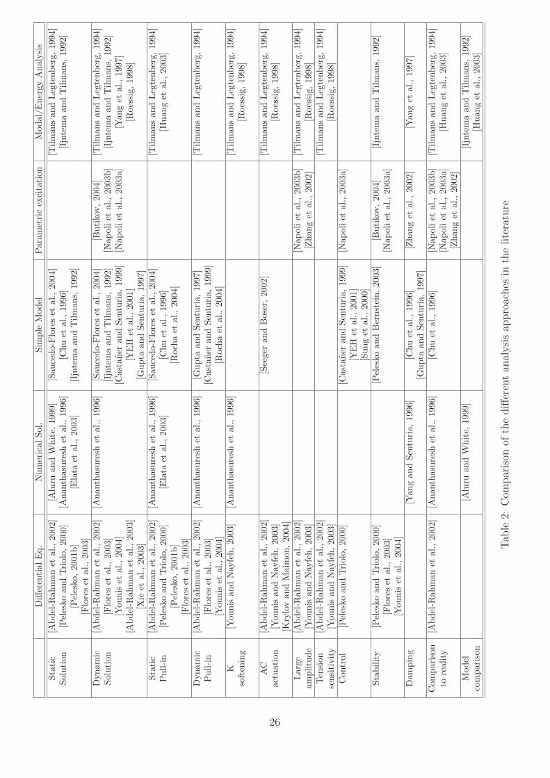
Table 2 shows a summarized classification of the different approaches in the literature and theaddressed phenomena.

Future work should address an uniformed way of analyzing Pull-in given a generalized and itsimplications on control of oscillatory MEMS.

25

Diff

eren

tial

Eq.

Num

eric

alSo

l.Si

mpl

eM

odel

Par

amet

ric

exci

tati

onM

odal

/Ene

rgy

Ana

lysi

sSt

atic

[Abd

el-R

ahm

anet

al.,

2002

][A

luru

and

Whi

te,19

99]

[Sau

cedo

-Flo

res

etal

.,20

04]

[Tilm

ans

and

Leg

tenb

erg,

1994

]So

luti

on[P

eles

koan

dTri

olo,

2000

][A

nant

hasu

resh

etal

.,19

96]

[Chu

etal

.,19

96]

[Ijn

tem

aan

dT

ilman

s,19

92]

[Pel

esko

,20

01b]

[Ela

taet

al.,

2003

][Ijn

tem

aan

dT

ilman

s,19

92]

[Flo

res

etal

.,20

03]

Dyn

amic

[Abd

el-R

ahm

anet

al.,

2002

][A

nant

hasu

resh

etal

.,19

96]

[Sau

cedo

-Flo

res

etal

.,20

04]

[But

ikov

,20

04]

[Tilm

ans

and

Leg

tenb

erg,

1994

]So

luti

on[F

lore

set

al.,

2003

][Ijn

tem

aan

dT

ilman

s,19

92]

[Nap

oliet

al.,

2003

b][Ijn

tem

aan

dT

ilman

s,19

92]

[You

nis

etal

.,20

04]

[Cas

tane

ran

dSe

ntur

ia,19

99]

[Nap

oliet

al.,

2003

a][Y

ang

etal

.,19

97]

[Abd

el-R

ahm

anet

al.,

2003

][Y

EH

etal

.,20

01]

[Roe

ssig

,19

98]

[Xie

etal

.,20

03]

[Gup

taan

dSe

ntur

ia,19

97]

Stat

ic[A

bdel

-Rah

man

etal

.,20

02]

[Ana

ntha

sure

shet

al.,

1996

][S

auce

do-F

lore

set

al.,

2004

][T

ilman

san

dLeg

tenb

erg,

1994

]P

ull-in

[Pel

esko

and

Tri

olo,

2000

][E

lata

etal

.,20

03]

[Chu

etal

.,19

96]

[Hua

nget

al.,

2003

][P

eles

ko,20

01b]

[Roc

haet

al.,

2004

][F

lore

set

al.,

2003

]D

ynam

ic[A

bdel

-Rah

man

etal

.,20

02]

[Ana

ntha

sure

shet

al.,

1996

][G

upta

and

Sent

uria

,19

97]

[Tilm

ans

and

Leg

tenb

erg,

1994

]P

ull-in

[Flo

res

etal

.,20

03]

[Cas

tane

ran

dSe

ntur

ia,19

99]

[You

nis

etal

.,20

04]

[Roc

haet

al.,

2004

]K

[You

nis

and

Nay

feh,

2003

][A

nant

hasu

resh

etal

.,19

96]

[Tilm

ans

and

Leg

tenb

erg,

1994

]so

ften

ing

[Roe

ssig

,19

98]

AC

[Abd

el-R

ahm

anet

al.,

2002

][S

eege

ran

dB

oser

,20

02]

[Tilm

ans

and

Leg

tenb

erg,

1994

]ac

tuat

ion

[You

nis

and

Nay

feh,

2003

][R

oess

ig,19

98]

[Kry

lov

and

Mai

mon

,20

04]

Lar

ge[A

bdel

-Rah

man

etal

.,20

02]

[Nap

oliet

al.,

2003

b][T

ilman

san

dLeg

tenb

erg,

1994

]am

plit

ude

[You

nis

and

Nay

feh,

2003

][Z

hang

etal

.,20

02]

[Roe

ssig

,19

98]

Ten

sion

[Abd

el-R

ahm

anet

al.,

2002

][T

ilman

san

dLeg

tenb

erg,

1994

]se

nsit

ivity

[You

nis

and

Nay

feh,

2003

][R

oess

ig,19

98]

Con

trol

[Pel

esko

and

Tri

olo,

2000

][C

asta

ner

and

Sent

uria

,19

99]

[Nap

oliet

al.,

2003

a][Y

EH

etal

.,20

01]

[Sun

get

al.,

2000

]St

abili

ty[P

eles

koan

dTri

olo,

2000

][P

eles

koan

dB

erns

tein

,20

03]

[But

ikov

,20

04]

[Ijn

tem

aan

dT

ilman

s,19

92]

[Flo

res

etal

.,20

03]

[Nap

oliet

al.,

2003

a][Y

ouni

set

al.,

2004

]D

ampi

ng[Y

ang

and

Sent

uria

,19

96]

[Chu

etal

.,19

96]

[Zha

nget

al.,

2002

][Y

ang

etal

.,19

97]

[Gup

taan

dSe

ntur

ia,19

97]

Com

pari

son

[Abd

el-R

ahm

anet

al.,

2002

][A

nant

hasu

resh

etal

.,19

96]

[Chu

etal

.,19

96]

[Nap

oliet

al.,

2003

b][T

ilman

san

dLeg

tenb

erg,

1994

]to

real

ity

[Nap

oliet

al.,

2003

a][H

uang

etal

.,20

03]

[Zha

nget

al.,

2002

]M

odel

[Alu

ruan

dW

hite

,19

99]

[Ijn

tem

aan

dT

ilman

s,19

92]

com

pari

son

[Hua

nget

al.,

2003

]

Tab

le2:

Com

par

ison

ofth

ediff

eren

tan

alysi

sap

pro

aches

inth

elite

ratu

re

26

References

[Abdel-Rahman et al., 2003] Abdel-Rahman, E. M., Nayfeh, A. H., and Younis, M. I. (2003).Dynamics of an electrically actuated resonant microsensor. In International Conference onMEMS, NANO and Smart Systems.

[Abdel-Rahman et al., 2002] Abdel-Rahman, E. M., Younis, M. I., and Nayfeh, A. H.(2002). Characterization of the mechanical behavior of an electrically actuated microbeam.Micromechanics and Microengineering.

[Aluru and White, 1999] Aluru, N. R. and White, J. (1999). A multilevel newton method formixed-energy domain simulation of mems. Journal of Microelectromechanical Systems.

[Ananthasuresh et al., 1996] Ananthasuresh, G. K., Gupta, R. K., and Senturia, S. D. (1996).An approach to macromodeling of mems for nonlinear dynamic simulation. In InternationalMechanical Engineering Congress and Exposition. ASME.

[Andrews et al., 1993] Andrews, M., Harris, I., and Turner, G. (1993). A comparison of squeeze-film theory with measurements on a microstructure. Sensors and Actuators A.

[Attia et al., 1998] Attia, P., Bontry, M., Bossehoeuf, A., and Hesto, P. (1998). Fabrication andcharacterization of electrostatically driven silicon microbeams. J. Microelectronics, 29:pp. 641–644.

[Bernstein et al., 2000] Bernstein, D., Guidotti, P., and Pelesko, J. (2000). Mathematical analysisof an electrostatically actuated mems devices. MSM.

[Bienstman et al., 1998] Bienstman, J., Puers, R., and Vandewalle, J. (1998). Periodic and chaoticbehaviour of the autonomous impact resonator. IEEE.

[Blanc et al., 1996] Blanc, N., Brugger, J., de Rooji, N., and Durig, U. (1996). Scanning forcemicroscopy in the dynamic mode using microfabricated capacitive sensors. J. Vac. Sci. Technol,14(2):pp.901–905.

[Blech, 1983] Blech, J. (1983). On isothermal squeeze films. Journal of Lubrication Technology,page 615.

[Brosnihan et al., 1995] Brosnihan, T. J., Pisano, A., and Howe, R. (1995). Surface-micromachinedangular accelerometer with force feedback. In ASME Dynamic Systems and Control Division.ASME.

[Burns et al., 1995] Burns, D., Zook, J., Horning, R., Herb, W., and Guckel, H. (1995). Sealed-cavity resonant microbeam pressure sensor. Sensors and Actuators A, 48(3):179–186.

[Burstein, 1995] Burstein, A. Kaiser, W. (1995). Mixed analog-digital highly-sensitive sensorinterface circuit for low-cost microsensors. Solid-State Sensors and Actuators, 1995 andEurosensors IX. Transducers ’95. The 8th International Conference on.

[Butikov, 2004] Butikov, E. I. (2004). Parametric excitation of a linear oscillator. European Journalof Physics.

[Castaner et al., 1999] Castaner, L., Rodriguez, A., Pons, J., and Senturia, S. D. (1999). Pull-in time-energy product of electrostatic actuators: comparison of experiments with simulation.Sensors and Actuators A, 83(1-3):263–269.

27

[Castaner and Senturia, 1999] Castaner, L. M. and Senturia, S. D. (1999). Speed-energyoptimization of electrostatic actuators based on pull-in. IEEE Journal of MicromechanicalSystems, 8(3):290–298.

[Cho et al., 1994] Cho, Y.-H., Kwak, B. M., Pisano, A. P., and Howe, R. T. (1994). Slide filmdamping in laterally driven microstructures. Sensors and Actuators A: Physical.

[Chu et al., 1996] Chu, P. B., Nelson, P. R., Tachiki, M. L., and Pister, K. S. (1996). Dynamics ofpolysilicon parallel-plate electrostatic actuators. Sensors and Actuators A, 52:216–220.

[Chui et al., 1998] Chui, B., Kenny, T., Mamin, H., Terris, B., and Rugar, D. (1998). Independentdetection of vertical and lateral forces wilh a sidewall-implanted dual-axis piezoresistivecantilever. Appl. Phys. Lett., 72(11):pp.1388– 1390.

[Dauwalter and Ha, 2004] Dauwalter, C. and Ha, J. (2004). A high performance magneticallysuspended mems spinning wheel gyro. Position Location and Navigation Symposium, 2004.PLANS.

[Duwel et al., 2003] Duwel, A., Gorman, J., Weinstein, M., Borenstein, J., and Ward, P. (2003).Experimental study of thermoelastic damping in mems gyros. Sensors and Actuators A.

[Elata et al., 2003] Elata, D., Bochobza-Degani, O., Feldman, S., and Nemirovsky, Y. (2003).Secondary dof and their effect on the instability of electrostatic mems devices. MicroElectro Mechanical Systems, 2003. MEMS-03 Kyoto. IEEE The Sixteenth Annual InternationalConference on.

[Fargas-Marques, 2001] Fargas-Marques, A. (2001). Stable electrostatic actuation of mems double-ended tuning fork oscillators. Master’s thesis, University of California, Irvine. Advisor: Dr.Shkel.

[Flores et al., 2003] Flores, G., Mercado, G., and Pelesko, J. (2003). Dynamics and touchdownin electrostatic mems. In MEMS, NANO and Smart Systems, 2003. Proceedings. InternationalConference on, pages Pages: 182– 187.

[Gaucher et al., 1998] Gaucher, P., Eichner, D., Hector, J., and von Munch, W. (1998).Piezoelectric bimorph cantilever for actuationf and sensing applications. J. Phys. IV France,8:pp. 235–238.

[Gretillat et al., 1997] Gretillat, M.-A., Yang, Y.-J., Hung, E., Rabinovich, V., Ananthasuresh, G.,De Rooij, N., and Senturia, S. (1997). Nonlinear electromechanical behaviour of an electrostaticmicrorelay. Solid State Sensors and Actuators, 1997. TRANSDUCERS ’97.

[Gui et al., 1998] Gui, C., Legtenberg, R., Tilmans, H. A. C., Fluitman, J. H. J., , and Elwenspoek,M. (1998). Nonlinearity and hysteresis of resonant strain gauges. Microelectromechanical Systems,7.

[Gupta and Senturia, 1997] Gupta, R. K. and Senturia, S. (1997). Pull-in time dynamics as ameasure of absolute pressure. In The Tenth Annual International Workshop on Micro ElectroMechanical Systems, pages 290–294.

[Hamrock, 1994] Hamrock, B. (1994). Fundamentals of fluid film lubrication. McGraw Hill.

28

[Han et al., 2005] Han, J. S., Rudnyi, E. B., and Korvink, J. G. (2005). Efficient optimizationof transient dynamic problems in mems devices using model order reduction. Journal ofMicromechanics and Microengineering.

[Huang et al., 2003] Huang, J.-M., Liu, A., Lu, C., and Ahn, J. (2003). Mechanical characterizationof micromachined capacitive switches: design consideration and experimental verification.Sensors and Actuators A.

[Huang and Lee, 2000] Huang, Q. and Lee, N. (2000). A simple approach to characterizing thedriving force of polysilicon laterally driven thermal microactuators. Sensors and Actuators,80:pp. 267–272.

[Hung, 1997] Hung, E.S. Yao-Joe Yang Senturia, S. (1997). Low-order models for fast dynamicalsimulation of mems microstructures. Solid State Sensors and Actuators, 1997. TRANSDUCERS’97.

[Ijntema and Tilmans, 1992] Ijntema, D. J. and Tilmans, H. A. C. (1992). Static and dynamicaspects of an air-gap capacitor. Sensors and Actuators A: Physical.

[Itoh et al., 1996] Itoh, T., Ohashi, T., and Suga, T. (1996). Piezoelectric cantilever array formultiprobe scanning force microscopy. In Proc. of the IX Int. Workshop on MEMS, pages 451–455, San Diego.

[Jackson, 1962] Jackson, J. D. (1962). Classical electrodynamics. John Wiley & Sons.

[Jonsmann et al., 1999] Jonsmann, J., Sigmund, O., and Bouwstra, S. (1999). Compliant electro-thermal microactuators. IEEE.

[Juneau et al., 2003] Juneau, T., Unterkofler, K., Seliverstov, T., Zhang, S., and Judy, M. (2003).Dual-axis optical mirror positioning using a nonlinear closed-loop controller. TRANSDUCERS,Solid-State Sensors, Actuators and Microsystems, 12th International Conference on,.

[Juneau, 1997] Juneau, T. N. (1997). Micromachined Dual Input Axis Rate Gyroscope. PhD thesis,U.C. Berkeley.

[Kaajakari et al., 2005] Kaajakari, V., Mattila, T., Lipsanen, A., and Oja, A. (2005). Nonlinearmechanical effects in silicon longitudinal mode beam resonators. Sensors and Actuators A:Physical, 120(1):64–70.

[Kovacs, 1998] Kovacs, G. (1998). Micromachined Transducers Sourcebook. McGraw-Hill.

[Kranz et al., 2003] Kranz, M., Burgett, S., Hudson, T., Buncick, M., Ruffin, P., Ashley, P.,and McKee, J. (2003). A wide dynamic range silicon-on-insulator mems gyroscope withdigital force feedback. TRANSDUCERS, Solid-State Sensors, Actuators and Microsystems, 12thInternational Conference on,.

[Krylov et al., 2005] Krylov, S., Harari, I., and Cohen, Y. (2005). Stabilization of electrostaticallyactuated microstructures using parametric excitation. Journal of Micromechanics andMicroengineering, 15:11881204.

[Krylov and Maimon, 2004] Krylov, S. and Maimon, R. (2004). Pull-in dynamics of an elasticbeam actuated by continuously distributed electrostatic force. Transactions of the ASME - L -Journal of Vibration and Acoustics, 126(3).

29

[Kuehnel, 1995] Kuehnel, W. (1995). Modelling of the mechanical behaviour of a differentialcapacitor acceleration sensor. Sensors and Actuators A: Physical.

[Lee, 1997] Lee, M. (1997). Merged technology on mems. In Electron Devices Meeting, .Proceedings.

[Lethbridge et al., 1993] Lethbridge, J., Cheshmehdoost, A., C.M.France, and Jones, B. (1993).An optical-fibre hybrid pressure transducer employing a mechanical resonator. Sensors andActuators A, 37-38:480–483.

[Ligterink et al., 2005] Ligterink, N., Patrascu, M., Breedveld, P., and Stramigioli, S. (2005). Anenergy-based electroelastic beam model for mems applications. Sensors and Actuators A, 121.

[Liu et al., 2004] Liu, S., Davidson, A., and Lin, Q. (2004). Simulation studies on nonlineardynamics and chaos in a mems cantilever control system. Micromechanics and Microengineering.

[M Hashimoto and Esashi, 1995] M Hashimoto, C Cabuz, K. M. and Esashi, M. (1995). Siliconresonant angular rate sensor using electromagnetic excitation and capacitive detection.Micromechanics and Microengineering.

[Minami et al., 1999] Minami, K., Matsunaga, T., and Esashi, M. (1999). Simple modeling andsimulation of the squeeze film effect and transient response of the mems device. In Micro ElectroMechanical Systems, 1999. MEMS ’99.

[Minne et al., 1995] Minne, S., Manalis, S., and Quate, C. (1995). Parallel atomic force microscopyusing cantilevers with integrated piezoresistive sensors and integrated piezoelectric actuators.Appl. Phys. Lett., 67(26):pp. 3918–3920.

[Najar et al., 2005] Najar, F., Choura, S., El-Borgi, S., Abdel-Rahman, E. M., and Nayfeh, A. H.(2005). Modeling and design of variable-geometry electrostatic microactuators. Journal ofMicromechanics and Microengineering.

[Napoli et al., 2003a] Napoli, M., Bamieh, B., and Turner, K. (2003a). Mathematical modeling,experimental validation and observer design for a capacitively actuated microcantilever. InAmerican Control Conference, 2003. Proceedings of the.

[Napoli et al., 2004] Napoli, M., Bamieh, B., and Turner, K. (2004). A capacitive microcantilever:Modelling, validation, and estimation using current measurements. Journal of Dynamic Systems,Measurement, and Control, 126(2):319–326.

[Napoli et al., 2003b] Napoli, M., Turner, W. Z., and K. Bamieh, B. (2003b). Dynamics ofmechanically and electrostatically coupled microcantilevers. TRANSDUCERS, Solid-StateSensors, Actuators and Microsystems, 12th International Conference on,.

[Nathanson et al., 1967] Nathanson, H., Newell, W., Wickstrom, R., and J.R. Davis, J. (1967).The resonant gate transistor. IEEE Transactions on Electronics devices.

[Nayfeh and Younis, 2004] Nayfeh, A. H. and Younis, M. I. (2004). A new approach to the modelingand simulation of flexible microstructures under the effect of squeeze-film damping. Journal ofMicromechanics and Microengineering.

[Newell, 1968] Newell, W. (1968). Miniaturization of tuning forks. Science, 161(3848):1320–1326.

30

[Niarchos, 2003] Niarchos, D. (2003). Magnetic mems: key issues and some applications. Sensorsand Actuators A.

[Nishiyama and Nakamura, 1990] Nishiyama, H. and Nakamura, M. (1990). Capacitance of a stripcapacitor. Components, Hybrids, and Manufacturing Technology, IEEE Transactions on.

[Oz and Fedder, 2003] Oz, A. and Fedder, G. (2003). Rf cmos-mems capacitor having large tuningrange. TRANSDUCERS, Solid-State Sensors, Actuators and Microsystems, 12th InternationalConference on,.

[Pai and Tien, 2000] Pai, M. and Tien, N. C. (2000). Low voltage electrothermal vibromotor forsilicon optical bench applications. Sensors and Actuators.

[Painter and Shkel, 2003] Painter, C. C. and Shkel, A. M. (2003). Active structural errorsuppression in mems vibratory rate integrating gyroscopes. IEEE SENSORS JOURNAL.

[Pelesko, 2001a] Pelesko, J. (2001a). Electrostatic field aproximations and implications for memsdevices. Proceedings of ESA.

[Pelesko, 2001b] Pelesko, J. (2001b). Multiple solutions in electrostatic mems. Proceedings ofModeling and Simulation of Microsystems 2001, Hilton Head.

[Pelesko and Triolo, 2000] Pelesko, J. and Triolo, A. (2000). Nonlocal problems in mems devicecontrol. In Technical Proceedings of the 2000 International Conference on Modeling andSimulation of Microsystems.

[Pelesko and Triolo, 2001] Pelesko, J. and Triolo, A. (2001). Nonlocal problems in mems devicecontrol. Journal of Engineering Mathematics, 41.

[Pelesko and Bernstein, 2003] Pelesko, J. A. and Bernstein, D. H. (2003). Modeling MEMS andNEMS. Chapman & Hall/CRC. ISBN: 1-58488-306-5.

[Rand, 2003] Rand, R. H. (2003). Lecture Notes on Nonlinear Vibrations, version 45. Availableonline at http://www.tam.cornell.edu/randdocs/.

[Rao and Raju, 2003] Rao, G. and Raju, K. (2003). Large amplitude free vibrations of beams - anenergy approach. ZAMM - Journal of Applied Mathematics and Mechanics, 83(7):493 – 498.

[Rao, 1990] Rao, S. (1990). Mechanical Vibrations. Addison-Wesley, 2nd edition.

[Robert et al., 2003] Robert, P., Saias, D., Billard, C., Boret, S., Sillon, N., Maeder-Pachurka, C.,Charvet, P., Bouche, G., Ancey, P., and Berruyer, P. (2003). Integrated rf-mems switch basedon a combination of thermal and electrostatic actuation. TRANSDUCERS, Solid-State Sensors,Actuators and Microsystems, 12th International Conference on,.

[Rocha et al., 2004] Rocha, L., Cretu, E., and Wolffenbuttel, R. (2004). Pull-in dynamics: analysisand modeling of the transitional regime. In Micro Electro Mechanical Systems,.

[Roessig, 1995] Roessig, T. A. W. (1995). Surface micromachined resonant force transducers.Master’s thesis, U.C. Berkeley.

[Roessig, 1998] Roessig, T. A. W. (1998). Integrated MEMS Tuning Fork Oscillators for SensorApplications. PhD thesis, U.C. Berkeley.

31

[Sane and Yazdi, 2003] Sane, H. and Yazdi, N.and Mastrangelo, C. (2003). Application of slidingmode control to electrostatically actuated two-axis gimbaled micromirrors. In American ControlConference, 2003. Proceedings of the 2003.

[Saucedo-Flores et al., 2004] Saucedo-Flores, E., Ruelas, R., Flores, M., Ying, C., and Jung-chih.,C. (2004). Dynamic behavior modeling of mems parallel plate capacitors. PLANS 2004. PositionLocation and Navigation Symposium (IEEE Cat. No.04CH37556).IEEE . Piscataway, NJ, USA,pages pp.15–19.

[Seeger and Boser, 2003] Seeger, J. and Boser, B. (2003). Charge control of parallel-plate,electrostatic actuators and the tip-in instability. Microelectromechanical Systems, Journal of.

[Seeger and Boser, 2002] Seeger, J. I. and Boser, B. E. (2002). Parallel-plate driven oscillationsand resonant pull-in. In Solid-State Sensor, Actuator and Microsystems Workshop Hilton HeadIsland.

[Seeger, 1997] Seeger, J.I. Crary, S. (1997). Stabilization of electrostatically actuated mechanicaldevices. Solid State Sensors and Actuators, 1997. TRANSDUCERS ’97.

[Senturia, 2001] Senturia, S. (2001). Microsystem Design. Kluwer Acadenic Publishers, 1st edition.

[Shiba et al., 1998] Shiba, Y., Ono, T., Minami, K., and Esashi, M. (1998). Capacitive afm probefor high speed imaging. ns. of the IEE of Japan, 118 - E(12):647–650.

[Sung et al., 2000] Sung, S., Lee, J., Kang, T., and Song, J. W. (2000). Development of a tunableresonant accelerometer with self-sustained oscillation loop. In IEEE National Aerospace andElectronics Conference.

[Sung et al., 2003] Sung, S., Lee, J. G., and Kang, T. (2003). Development and test of memsaccelerometer with self-sustatined oscillation loop. Sensors and Actuators A.

[Teymoori and Abbaspour-Sani, 2002] Teymoori, M. and Abbaspour-Sani, E. (2002). A novelelectrostatic micromachined pump for drug delivery systems. In Semiconductor Electronics,2002. Proceedings. ICSE 2002. IEEE International Conference on.

[Tilmans et al., 1999] Tilmans, H., Fullin, E., Ziad, H., van der Peer, M., Kesters, J., and al.(1999). A fully-packaged electromagnetic microrelay. Micro Electro Mechanical Systems.

[Tilmans and Legtenberg, 1994] Tilmans, H. A. C. and Legtenberg, R. (1994). Electrostaticallydriven vacuum-encapsulated polysilicon resonators part ii. theory and performance. Sensors andActuators A: Physical.

[Tortonese et al., 1993] Tortonese, M., Barrett, R., and Quate, C. (1993). Atomic resolution withan atomic force microscope using piezoresistive detection. Appl. Phys. Lett, 62:8340–8363.

[Varghese et al., 1997] Varghese, M., Amantea, R., Sauer, D., and Senturia, S. D. (1997). Resistivedamping of pulse-sensed capacitive position sensors. In TRANSDUCERS ’97, InternationalConference on Solid-state Sensors and Actuators.

[Veijola et al., 1995] Veijola, T., Kuisma, H., Lahdenper, J., and Ryhnen, T. (1995). Equivalent-circuit model of the squeezed gas film in a silicon accelerometer. Sensors and Actuators A:Physical.

32

[Veijola and Turowski, 2001] Veijola, T. and Turowski, M. (2001). Compact damping models forlaterally moving microstructures with gas-rarefaction effects. Microelectromechanical Systems.

[Vinokur, 2002] Vinokur, R. Y. (2002). Feasible analytical solutions for electrostatic parallel-plateactuator or sensor. Journal of Vibration and Control.

[Wang et al., 2004] Wang, X., Liu, Y., Wang, M., and Chen, X. (2004). The effect of air dampingon the planar mems structures. In HDP’04.

[Wang et al., 1998] Wang, Y. C., Adams, S. G., Thorp, J. S., MacDonald, N. C., Hartwell, P., andBertsch, F. (1998). Chaos in mems, parameter estimation and its potential application. IEEETRANSACTIONS ON CIRCUITS AND SYSTEMS.

[Xie et al., 2003] Xie, W. C., Lee, H. P., and Lim, S. P. (2003). Nonlinear dynamic analysis ofmems switches by nonlinear modal analysis. Nonlinear Dynamics, 31:243256.

[Yang and Senturia, 1996] Yang, Y. and Senturia, S. (1996). Numerical simulations of compressiblesqueezed-film damping. In Solid-State Sensors and Actuators Workshop, Late News Session.

[Yang et al., 1997] Yang, Y.-J., Gretillat, M.-A., and Senturia, S. (1997). Effect of air damping onthe dynamics of nonuniform deformations of microstructures. Solid State Sensors and Actuators,1997. TRANSDUCERS ’97.

[YEH et al., 2001] YEH, B. Y., LIANG, Y. C., and TAY, F. E. H. (2001). Mathematical modellingon the quadrature error of low-rate microgyroscope for aerospace applications. Analog IntegratedCircuits and Signal Processing.

[Younis et al., 2004] Younis, M. I., Abdel-Rahman, E., and Nayfeh, A. H. (2004). Global dynamicsof mems resonators under superharmonic excitation. In Proceedings of the 2004 InternationalConference on MEMS, NANO and Smart Systems.

[Younis and Nayfeh, 2003] Younis, M. I. and Nayfeh, A. H. (2003). A study of the nonlinearresponse of a resonant microbeam to an electric actuation. Nonlinear Dynamics, 31:91117.

[Zhang et al., 2002] Zhang, W., Baskaran, R., and Turner, K. L. (2002). Effect of cubic nonlinearityon auto-parametrically amplified resonant mems mass sensor. Sensors and Actuators A.

[ZHAO et al., 2005] ZHAO, X., REDD, C. K., and NAYFEH, A. H. (2005). Nonlinear dynamicsof an electrically driven impact microactuator. Nonlinear Dynamics.

[Zhou and Yang, 2003] Zhou, Y.-H. and Yang, X. (2003). Numerical analysis on snapping inducedby electromechanical interaction of shuffling actuator with nonlinear plate. Computers andStructures.

[Zook et al., 1995] Zook, J., Burns, D., Herb, W., Guckel, H., Kang, J., and Ahn, Y. (1995).Optically excited self-resonant strain transducers. In Transducers’95, 8th InternationalConference on Solid-State Sensors and Actuators, volume 2.

33