Embed Size (px)
Citation preview

University of Central Florida University of Central Florida
STARS STARS
Electronic Theses and Dissertations, 2004-2019
2013
Multi-physics Modeling Of Geomechanical Systems With Coupled Multi-physics Modeling Of Geomechanical Systems With Coupled
Hydromechanical Behaviors Hydromechanical Behaviors
Ahmad Mohamed University of Central Florida
Part of the Civil Engineering Commons, and the Structural Engineering Commons
Find similar works at: https://stars.library.ucf.edu/etd
University of Central Florida Libraries http://library.ucf.edu
This Masters Thesis (Open Access) is brought to you for free and open access by STARS. It has been accepted for
inclusion in Electronic Theses and Dissertations, 2004-2019 by an authorized administrator of STARS. For more
information, please contact [email protected].
STARS Citation STARS Citation Mohamed, Ahmad, "Multi-physics Modeling Of Geomechanical Systems With Coupled Hydromechanical Behaviors" (2013). Electronic Theses and Dissertations, 2004-2019. 2907. https://stars.library.ucf.edu/etd/2907
MULTI-PHYSICS MODELING OF GEOMECHANICAL SYSTEMS WITH COUPLED
HYDROMECHANICAL BEHAVIORS
by
AHMAD MOHAMED
B.S. University of Garyounis, 2003
A thesis submitted in partial fulfillment of the requirements
for the degree of Master of Science
in the Department of Civil, Environmental, and Construction Engineering
in the College of Engineering and Computer Science
at the University of Central Florida
Orlando, Florida
Spring Term
2013
Major Professor: Hae-Bum Yun

ii
© 2013 AHMAD MOHAMED
iii
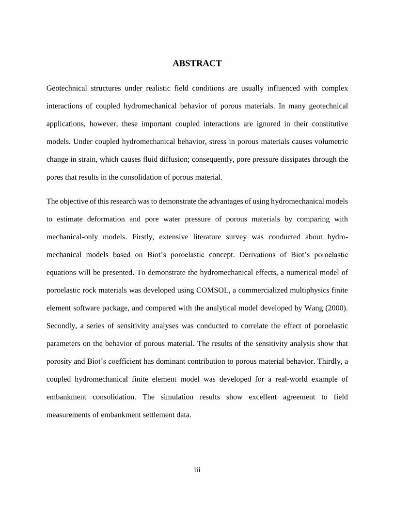
ABSTRACT
Geotechnical structures under realistic field conditions are usually influenced with complex
interactions of coupled hydromechanical behavior of porous materials. In many geotechnical
applications, however, these important coupled interactions are ignored in their constitutive
models. Under coupled hydromechanical behavior, stress in porous materials causes volumetric
change in strain, which causes fluid diffusion; consequently, pore pressure dissipates through the
pores that results in the consolidation of porous material.
The objective of this research was to demonstrate the advantages of using hydromechanical models
to estimate deformation and pore water pressure of porous materials by comparing with
mechanical-only models. Firstly, extensive literature survey was conducted about hydro-
mechanical models based on Biot’s poroelastic concept. Derivations of Biot’s poroelastic
equations will be presented. To demonstrate the hydromechanical effects, a numerical model of
poroelastic rock materials was developed using COMSOL, a commercialized multiphysics finite
element software package, and compared with the analytical model developed by Wang (2000).
Secondly, a series of sensitivity analyses was conducted to correlate the effect of poroelastic
parameters on the behavior of porous material. The results of the sensitivity analysis show that
porosity and Biot’s coefficient has dominant contribution to porous material behavior. Thirdly, a
coupled hydromechanical finite element model was developed for a real-world example of
embankment consolidation. The simulation results show excellent agreement to field
measurements of embankment settlement data.

iv
ACKNOWLEDGMENTS
I would like to express my special thanks for my advisor, Assistant Professor Dr. Hae-Bum Yun
for giving this opportunity to work under his supervision and for sharing his great knowledge and
experience with me. He introduced me to an interesting topic and provided important insight
throughout. It has been a privilege and honor to be his student.
I am also thankful for Associate Professor Dr. Manoj Chopra for serving on my committee and
providing helpful comments, advices and suggestions. Also, I would like to thank Dr. Amr Sallam
who has provided me with some embankment data and for his advices.
Appreciation is also extended to all people who gave the author heartfelt corporation and shared
their knowledge and for giving some of their valuable time. My friends, for their endless love,
emotional support and belief in me.
Finally, my biggest gratitude is to my family for supporting me throughout my graduate studies.
My parents, Saeid and Aziza, your encouragement and love helped me ease through some of
hardest times I have faced. Without you I would never come up to this stage.
v
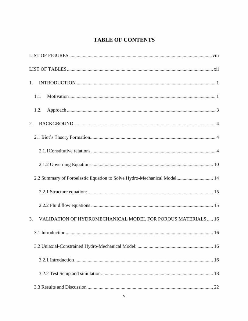
TABLE OF CONTENTS
LIST OF FIGURES ..................................................................................................................... viii
LIST OF TABLES ........................................................................................................................ xii
1. INTRODUCTION .................................................................................................................. 1
1.1. Motivation ........................................................................................................................ 1
1.2. Approach .......................................................................................................................... 3
2. BACKGROUND .................................................................................................................... 4
2.1 Biot’s Theory Formation....................................................................................................... 4
2.1.1Constitutive relations ...................................................................................................... 4
2.1.2 Governing Equations ................................................................................................... 10
2.2 Summary of Poroelastic Equation to Solve Hydro-Mechanical Model.............................. 14
2.2.1 Structure equation: ....................................................................................................... 15
2.2.2 Fluid flow equations .................................................................................................... 15
3. VALIDATION OF HYDROMECHANICAL MODEL FOR POROUS MATERIALS ..... 16
3.1 Introduction ......................................................................................................................... 16
3.2 Uniaxial-Constrained Hydro-Mechanical Model: .............................................................. 16
3.2.1 Introduction .................................................................................................................. 16
3.2.2 Test Setup and simulation ............................................................................................ 18
3.3 Results and Discussion ....................................................................................................... 22
vi
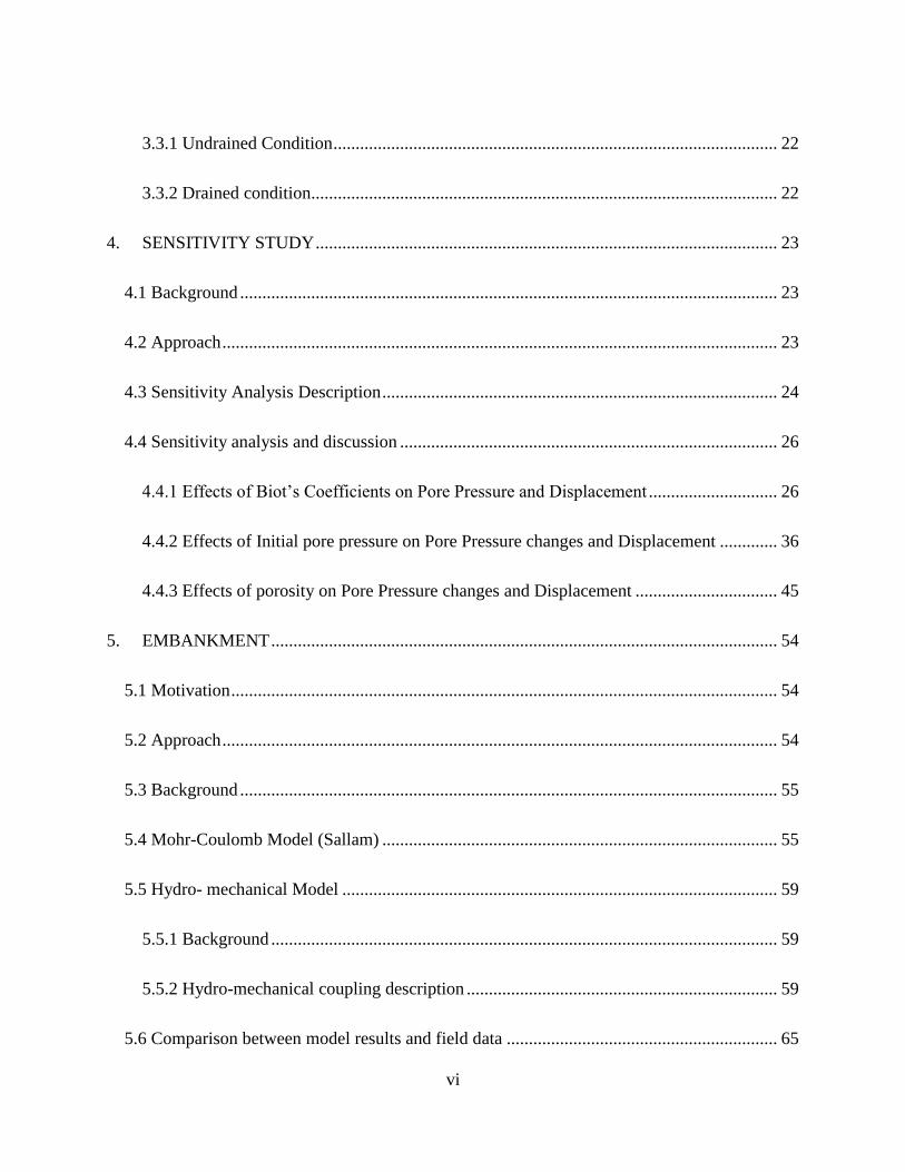
3.3.1 Undrained Condition .................................................................................................... 22
3.3.2 Drained condition......................................................................................................... 22
4. SENSITIVITY STUDY ........................................................................................................ 23
4.1 Background ......................................................................................................................... 23
4.2 Approach ............................................................................................................................. 23
4.3 Sensitivity Analysis Description ......................................................................................... 24
4.4 Sensitivity analysis and discussion ..................................................................................... 26
4.4.1 Effects of Biot’s Coefficients on Pore Pressure and Displacement ............................. 26
4.4.2 Effects of Initial pore pressure on Pore Pressure changes and Displacement ............. 36
4.4.3 Effects of porosity on Pore Pressure changes and Displacement ................................ 45
5. EMBANKMENT .................................................................................................................. 54
5.1 Motivation ........................................................................................................................... 54
5.2 Approach ............................................................................................................................. 54
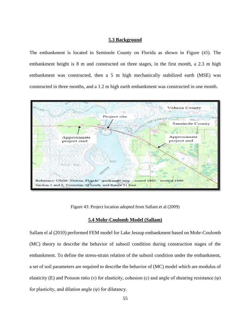
5.3 Background ......................................................................................................................... 55
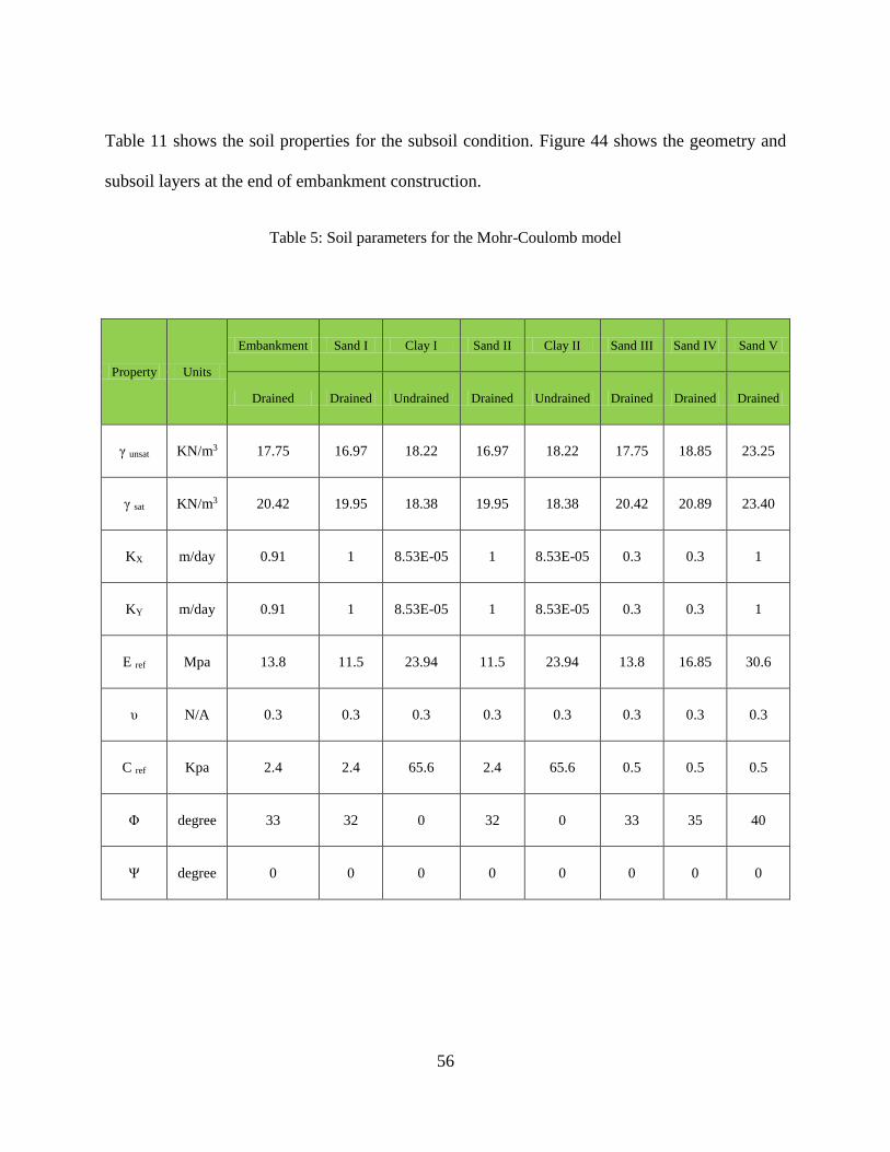
5.4 Mohr-Coulomb Model (Sallam) ......................................................................................... 55
5.5 Hydro- mechanical Model .................................................................................................. 59
5.5.1 Background .................................................................................................................. 59
5.5.2 Hydro-mechanical coupling description ...................................................................... 59
5.6 Comparison between model results and field data ............................................................. 65

vii
6. CONCLUSIONS................................................................................................................... 67
6.1 Summary ............................................................................................................................. 67
6.2 Recommendations of future works ..................................................................................... 68
LIST OF REFERENCES .............................................................................................................. 69
viii
LIST OF FIGURES
Figure 1: Stress tensor block. ........................................................................................................ 11
Figure 2: 2m × 3m sample under a load Zhang et al (2003). ........................................................ 17
Figure 3: Vertical Displacement for the rock sample for undrained condition Ahmad (2013). ... 19
Figure 4: Vertical displacement vs height of the sample with undrained boundaries by Ahmad
(2013). ........................................................................................................................................... 19
Figure 5: Vertical displacements plotted in different time intervals for the second stage by
Ahmad (2013). .............................................................................................................................. 20
Figure 6: Vertical displacements plotted in different time intervals for the second stage by
Zhang.(2003). ................................................................................................................................ 20
Figure 7: Pore pressure plotted in different time intervals by Ahmad (2013). ............................. 21
Figure 8: Pore pressure plotted in different time by Zhang (2003). ............................................. 21
Figure 9: 2-D Rock sample dimensions. ....................................................................................... 25
Figure 10: Vertical displacement (m) at point (x=0, y=3) of the rock sample vs. time (α=0.83). 28
Figure 11 : 3-D mesh for Pore pressures inside the sample plotted in different time intervals
(α=0.83)......................................................................................................................................... 29
Figure 12: 3-D mesh map for displacement along the height of the sample (α=0.83). ................ 29
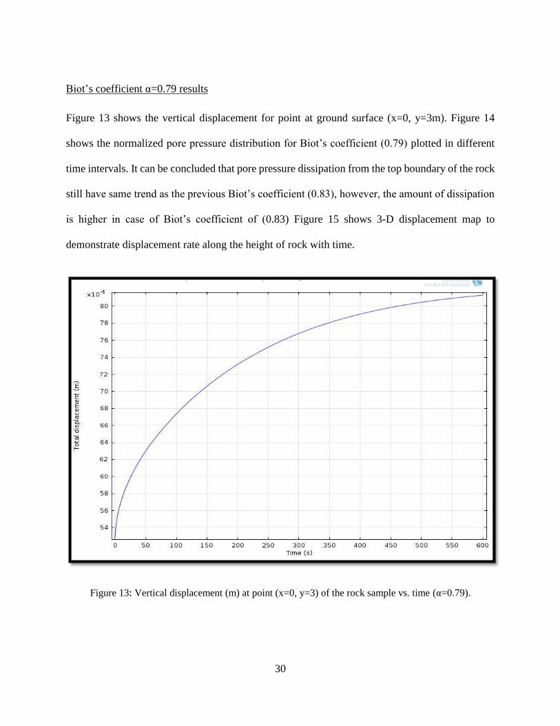
Figure 13: Vertical displacement (m) at point (x=0, y=3) of the rock sample vs. time (α=0.79). 30
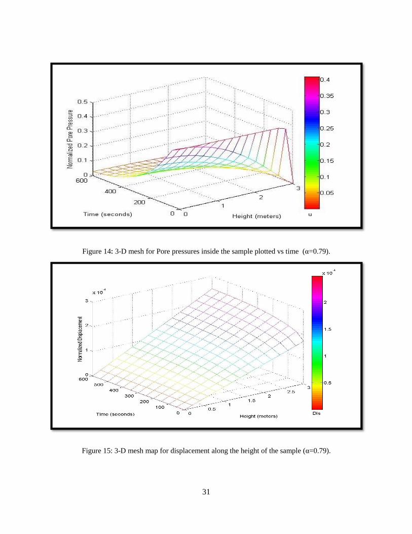
Figure 14: 3-D mesh for Pore pressures inside the sample plotted vs time (α=0.79). ................. 31
ix
Figure 15: 3-D mesh map for displacement along the height of the sample (α=0.79). ................ 31
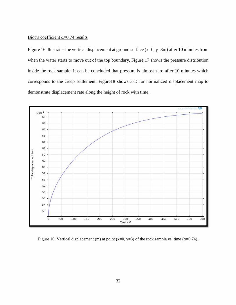
Figure 16: Vertical displacement (m) at point (x=0, y=3) of the rock sample vs. time (α=0.74). 32
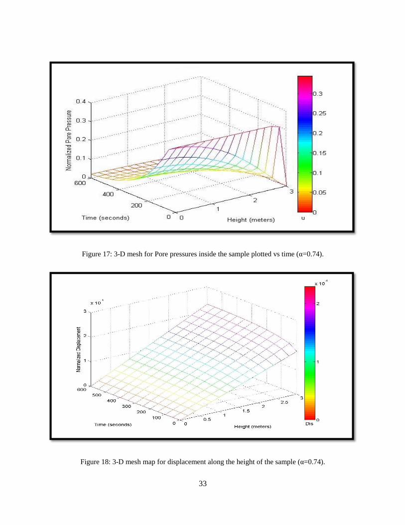
Figure 17: 3-D mesh for Pore pressures inside the sample plotted vs time (α=0.74). .................. 33
Figure 18: 3-D mesh map for displacement along the height of the sample (α=0.74). ................ 33
Figure 19: Pore pressure Vs time for point (x=0,y=3) for different Biot’s values. ..................... 34
Figure 20: Vertical Displaement Vs time for point (x=0,y=3) for different Biot’s values. ........ 35
Figure 21: Vertical displacement (m) at point (x=0, y=3) of the rock sample vs. time (p0=2e6
Mpa). ............................................................................................................................................. 37
Figure 22: 3-D mesh map for displacement along the height of the sample (p0=2e6 Mpa). ........ 38
Figure 23: 3-D mesh map for pore pressure distrubtion along the height plotted (p0=2e6 Mpa) . 38
Figure 24: Vertical displacement (m) at point (x=0, y=3) of the rock sample vs. time (p0=1.8e6
Mpa). ............................................................................................................................................. 39
Figure 25: 3-D mesh map for displacement along the height of the sample (p0=1.8e6 Mpa). ..... 40
Figure 26: 3-D mesh map for pore pressure distrubtion along the height plotted (p0=1.8e6 Mpa).
....................................................................................................................................................... 40
Figure 27: Vertical displacement (m) at point (x=0, y=3) of the rock sample vs. time (p0=1.6e6
Mpa). ............................................................................................................................................. 41
Figure 28: 3-D mesh map for displacement along the height of the sample (p0=1.6e6 Mpa). ..... 42
Figure 29: 3-D mesh map for pore pressure distrubtion along the height plotted (p0=1.6e6 Mpa).
....................................................................................................................................................... 42
x
Figure 30: Vertical displacement pressure Vs time for point (x=0,y=3) for different initial pore
pressure. ........................................................................................................................................ 43
Figure 31: Pore pressure Vs time for point (x=0,y=3) for different initial pore pressure. .......... 44
Figure 32: Vertical displacement (m) at point (x=0, y=3) of the rock sample vs. time for
Porosity(0.22). ............................................................................................................................... 46
Figure 33: 3-D mesh for Pore pressures inside the sample plotted vs time for Porosity(0.22). ... 47
Figure 34 : 3-D mesh for vertical displacement (m) of the rock sample vs. time.for
Porosity(0.22). ............................................................................................................................... 47
Figure 35: Vertical displacement (m) at point (x=0, y=3) of the rock sample vs. time for
Porosity(0.20). ............................................................................................................................... 48
Figure 36: 3-D mesh for Pore pressures inside the sample plotted vs time intervals for
Porosity(0.20). ............................................................................................................................... 49
Figure 37: 3-D mesh for vertical displacement (m) of the rock sample vs. time.for Porosity(0.20).
....................................................................................................................................................... 49
Figure 38: Vertical displacement (m) at point (x=0, y=3) of the rock sample vs. time for
Porosity(0.18). ............................................................................................................................... 50
Figure 39: 3-D mesh for Pore pressures inside the sample plotted vs time for Porosity(0.18). ... 51
Figure 40 : 3-D mesh for vertical displacement (m) of the rock sample vs. time. for
Porosity(0.18). ............................................................................................................................... 51
Figure 41: Vertical displacement Vs time for point (x=0,y=3) for diffrenet poristies ................ 52
xi
Figure 42: Pore pressure Vs time for point (x=0,y=3) for range of porosities. ........................... 53
Figure 43: Project location adopted from Sallam et al (2009) ...................................................... 55
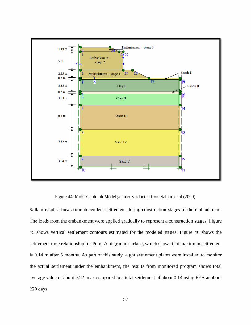
Figure 44: Mohr-Coulomb Model geometry adpoted from Sallam.et al (2009). ......................... 57
Figure 45: MC analysis for settlement contours for construction stages adopted from Sallam
(2009). ........................................................................................................................................... 58
Figure 46: MC analysis for Settlement log-time relationship for at a ground point by Sallam
(2009). ........................................................................................................................................... 58
Figure 47: Hydro-Mechnical Model geometry. ............................................................................ 60
Figure 48: Construction stages of the Lake Jessup embankment. ................................................ 63
Figure 49: Settlement profile at ground level from H-M model COMSOL. ................................ 64
Figure 50: Pore pressure distrubtion at point A. ........................................................................... 64
Figure 51: Plot of settlement versus time under the embankment . .............................................. 65
xii
LIST OF TABLES
Table 1: List of parameters of rock simple Zhang el al (2003). ................................................... 18
Table 2: List of parameters for Effects of Biot’s Coefficients...................................................... 27
Table 3: poroelastic paramters for different initial pore pressure. ................................................ 36
Table 4: Poroelastic paramters for different Porosities values ..................................................... 45
Table 5: Soil parameters for the Mohr-Coulomb model ............................................................... 56
Table 6: Summary of soil properties for Hydro-mechnical model ............................................... 61
1
1. INTRODUCTION
1.1. Motivation
Many problems in geotechnical engineering require a profound understanding of interaction
between soil skeleton and multiphysics. Because of the interaction between soil skeleton and other
transport phenomena, a coupled phenomenon is critical to describe the real behavior and response
of soil in present of multiphysical processes.
Hydro-mechanical coupling phenomena are considered to be the most important element for soil
consolidation calculations. The first theory to take into account the Hydro-Mechanical coupling
effect on soil was introduced by Terzaghi (1923). However, his theory was for one-dimensional
consolidation. Later, Biot (1941) extended Terzaghi theory to take into account three-dimensional
consolidation. Biot’s theory presented a set of energy balance equations, which are known as
poroelastic equations.
Biot’s equations link strain-stress mass changes to stress and fluid pressure change. Basically, any
change in fluid pressure in a porous medium will effect stress-strain behavior in the solid bulk.
Biot generalized his equation based on Darcy’s law and Hook’s law. Hook’s equations represent
stress-strain relationship. Darcy’s law describes the time-dependence of fluid flow as result of non-
uniform pore pressure distribution across the porous material. However, Biot’s theory has some
limitations such as, it is only valid for fully saturated soil with small deformation.
Unsaturated soils are encountered in many engineering applications. Recently, significant attention
has been paid to investigate the behavior of coupling in unsaturated soil Antonio
(2011).Unsaturated soil consists of three phases which are solid skeleton, pore pressure and air.
2
The presence of the air in the porous media introduces a more complex system than the system
found in saturated soil. Understanding the behavior of unsaturated soil requires knowledge about
the interaction between three different processes (mechanical, thermal and fluid movement).
Recently many researches has been conducted to understand and analysis the Thermo-Hydro-
Mechanical coupled processes in unsaturated media. Thermo-hydro-mechanical (THM)
phenomena are very important to consider in petroleum engineering because the variation of
temperature during oil production, would produces growth in thermal stresses in the porous
material. As a result, the thermal stresses can cause a failure in the reservoir rock and subsequently
alter its porosity and permeability Chen (2009). In addition, this will not only produce progressive
alteration on the strength of the porous material, but also will cause changes in the flow regime
and the rate of production. Booker and Savvidou (1985) performed a study on the effect of heat
source on the consolidation of porous media, their results showed that permeability of the soils is
effected by stresses generated by a heat source.
Freeman (2008) presented the effects of temperature variations on the behavior of fluid flow
through the porous material. His results demonstrate that temperature directly change the viscosity
of the hydrocarbon. Freeman (2008) stated that the stresses in the rock will be effected due change
on viscosity of the fluid. The effect will be more noticeable if the thermal loads causes higher
effective stresses that cause abnormal porosities
It can be concluded that the different interaction processes occurs in unsaturated media introduce
a complex system which required further assumptions to establish a complete a set of governing
differential equations that represent the physics of the problem. To reduce the complexity of the
Thermo-Hydro-Mechanical model, assumptions are made to reduce the number of model
3
parameters and formulations. The following assumptions are typically introduce to develop a
simple model for unsaturated soil. Soil density is constant, but the porous is compressible. Small
deformation is allowed. Water vapor is ignored and the velocity of solid skeleton is ignored
Mctigue (1986).
In closing, it may be concluded that a number of studies have been made to show the importance
of multiphysics coupling on geomechanics porous. In this research, several numerical models are
presented to illustrate the applicability and capability of coupling strategy based on Biot’s theory.
1.2. Approach
This chapter has provided a brief history of the role of multiphysics coupling on geomechanics
problems. Chapter 2 presented the physical and mathematical background of hydromechanical
coupling based on Biot’s poroelastic theory. In chapter 3, a complete detailed of reservoir model
based on the Biot’s poroelastic theory is presented with emphasis on comparing the numerical
model results with pervious published data. In Chapter 4, the focus shifts to demonstrate the role
of poroelastic parameters on the Hydro-mechanical coupling behavior. Sensitivities studies to
illustrate the respond of 2-D rock material are presented. Chapter 5 presence the results of
hydromechanical coupling for a real-world example of embankment consolidation. Chapter 6
presents the main conclusions and future recommendations of the study.
4
2. BACKGROUND
2.1 Biot’s Theory Formation
In this section, Biot’s poroelastic equations are developed. The poroelastic equations developed in
this section follows Wang (2000) approach. The poroelastic equation are developed based on two
constitutive relations for applied stress (σ) and pore pressure (p). In addition, governing equations
that describe fluid flow in poroelastic medium are also used. The governing equations links the
force equilibrium equations and pore pressure. In other words, they show the stress-strain relation
between fluid flow and soil skeleton. The movement of fluid in poroelastic media is covered by
Darcy’s law.
2.1.1Constitutive relations
Generally, poroelastic equations are expressed in terms ɛ and ζ, where ɛ =𝛿𝑣
𝑣the volumetric
change, and ζ is the increment of the fluid content. Wang (2000) assumed that ɛ =𝛿𝑣
𝑣 volumetric
strain changes to be positive in tension and negative in case of contraction, stress to be positive in
tension. The increment of water ζ is negative if the fluid removed from the storage and positive if
the water is added to skeleton volume. The first equation shows that any change in applied stress
and pore pressure will cause volumetric strain:
ε=a11 𝜎 + a12 p (2.1)
The second equation shows the increment of water volume due to change in pore pressure
ζ=a21 𝜎 + a22 p (2.2)
5
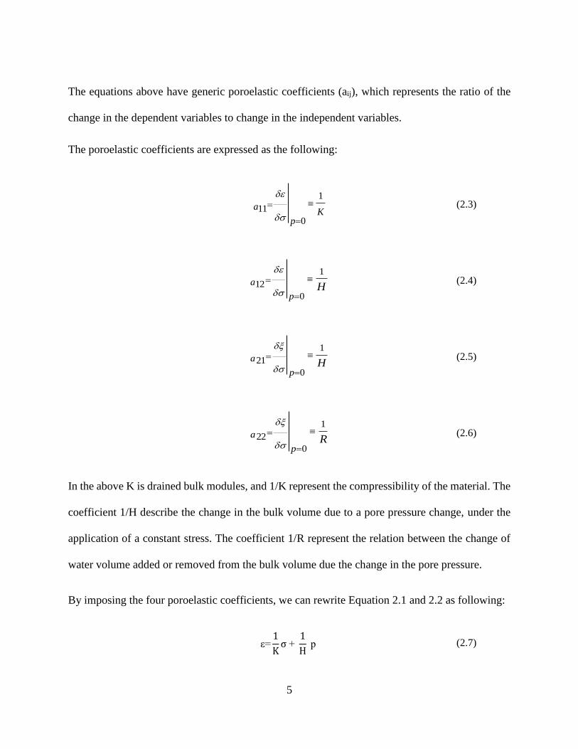
The equations above have generic poroelastic coefficients (aij), which represents the ratio of the
change in the dependent variables to change in the independent variables.
The poroelastic coefficients are expressed as the following:
K
a
p
1
11
0
(2.3)
Ha
p
1
12
0
(2.4)
Ha
p
1
21
0
(2.5)
Ra
p
1
22
0
(2.6)
In the above K is drained bulk modules, and 1/K represent the compressibility of the material. The
coefficient 1/H describe the change in the bulk volume due to a pore pressure change, under the
application of a constant stress. The coefficient 1/R represent the relation between the change of
water volume added or removed from the bulk volume due the change in the pore pressure.
By imposing the four poroelastic coefficients, we can rewrite Equation 2.1 and 2.2 as following:
ε=1
Kσ +
1
H p (2.7)

6
ζ=1
Hσ +
1
R p (2.8)
Biot (1941) showed that (1/R) coefficient specific storage also can be expressed as unconstrained
coefficient storage at constrained stress.
δσ = 1
R=
α
KB (2.9)
Biot’s (1941) introduced another coefficient which represent the constrained specific storage at
constant strain.
δσ = 1
M=
α
KuB (2.10)
Two additional coefficient are introduced by Biot. First, Skempton’s coefficient B is introduced to
show the ratio of the induced pore pressure to change applied stress for undrained condition.
B ≡ −δP
δσ|
ζ=0=
R
H (2.11)
Generally. Skempton’s coefficient range from 0 to 1, Skempton’s coefficient shows the
distribution of the applied stress between the fluid and soil skeleton.
The second coefficient is known as the Biot-Willis coefficient α:
α ≡K
H (2.12)
Now by replacing the coefficient (1/H) in equation (2.7) by (α/K):
7
ε=1
Kσ +
α
K p (2.13)
Now by replacing the coefficient (1/R) in equation (2.8) by coefficient specific storage (α
KB ) (see
equation 2.9).
ζ =α
Kσ +
α
KB p (2.14)
By solving Equation 2. 13 for stress, we get:
σ = Kε − α p (2.14)
Now, substituting Equation 2.14 into Equation 2.13 we get the following:
ζ = αε + α
KuB p (2.16)
where Ku =K
1−∝B , the undrained specific storage (2.17)
Now, one should extend poroelastic analysis to cover 3-D formulation. It requires seven linear
constitutive equations to describe the general anisotropic state of stress. Three equation to show
the relation between normal stress components and pore pressure. The other three equations show
the relation between shear strain and the corresponding shear stress components. The seventh
equation relates the increment of fluid to mean stress, and pore pressure.
However, by using the principle coordinates, the seven equations are reduced to four equations,
because the shear stress and shear strain are zero in the principle coordinates.
8
ε1 = 1
E σ1 −
v
E σ2 −
v
E σ3 +
α
3K P (2.18)
ε2 = − 1
E σ1 +
v
E σ2 −
v
E σ3 +
α
3K P (2.19)
ε3 = − 1
E σ1 −
v
E σ2 −
v
E σ3 +
α
3K P (2.20)
ζ =1
3H (σ1 + σ1 + σ1) +
p
R (2.21)
The equations can be written in term of shear modulus G, rather than Young’s modulus, E, since
it is easier to measure.
K =E
3(1 − 2v) (2.22)
And
G = 2G(1 + V) (2.23)
where E is the drained Young’s modules and ν, Poisson’s ratio, are measured under drained
conditions (that is, when pressure pore is zero).
εxx= 1
2G [ σxx-
v
(1+v)(σ11+σ22+σ33) ] +
α
3KP (2.24)
εyy= 1
2G [σyy-
v
1+v(σ11+σ22+σ33)] +
α
3K P (2.25)
9
εzz= 1
2G [σzz-
v
1+v(σ11+σ22+σ33)] +
α
3K P (2.26)
εxy = 1
2G σxy (2.27)
εxy = 1
2G σyz (2.28)
εxy = 1
2G σxz (2.29)
The equations can be cast in general coordinates and resolved for normal and shear stresses, and
the shear modulus. Here we assume that changes in pore pressure will not induce shear strains.
The full form of the pure compliance formulation thus becomes:
σxx = 2Gεxx + 2Gv
1−2v (εxx + εyy + εzz) − α P (2.30)
σyy = 2Gεyy + 2Gv
1−2v (εxx + εyy + εzz) − α P (2.31)
σzz = 2Gεzz + 2Gv
1 − 2v (εxx + εyy + εzz)- α P (2.32)
σxy = 2G εxy (2.33)
σxy = 2G εxy (2.34)
σxz = 2G εxz (2.35)
10
The seven constitutive equation can also be recast in terms of volumetric strain, where ε is
expressed as the sum of the three normal strains,
ζ = α (εxx + εyy + εzz) +α
KuB P (2.36)
2.1.2 Governing Equations
The poroelastic governing equations coupled the force equilibrium equation with fluid-flow
equation. The effect of coupling can be seen because the pore pressure term appears in the force
equilibrium equations and the volumetric strain appears in the fluid flow equation.
Force Equilibrium relation
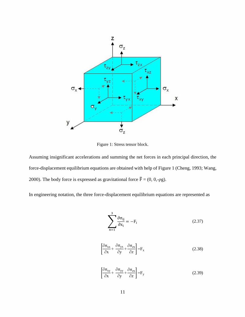
Biot (1941) assumed that mechanical problem is elastostatic. This means that the mechanical
problem obtained statically each instant of time. The time required for dynamic wave propagation
to transfer stresses across the problem domain is ignored. In other words, in the case of applied
sudden forces to the poroelastic body, displacement and fluid pressure with each representative
elementary volume (REV) adjusted instantaneously to maintain a state of internal force
equilibrium. The normal (σ) and shear (τ) components of the stress tensor are illustrated on an
REV as shown in the figure below:
11
Figure 1: Stress tensor block.
Assuming insignificant accelerations and summing the net forces in each principal direction, the
force-displacement equilibrium equations are obtained with help of Figure 1 (Cheng, 1993; Wang,
2000). The body force is expressed as gravitational force F̅ = (0, 0,-ρg).
In engineering notation, the three force-displacement equilibrium equations are represented as
∑∂σij
∂xi
3
n=1
= −Fi (2.37)
[∂σxx
∂x+
∂σyx
∂y+
∂σzx
∂z] =Fx (2.38)
[∂σxy
∂x+
∂σyy
∂y+
∂σzx
∂z] =Fy (2.39)
12
[∂σxz
∂x+
∂σyz
∂y+
∂σzz
∂z] =Fz (2.40)
Now substituting constitutive equations developed in the previous section into above force
equilibrium equations lead to three partial differential equations relating the six quantities of strain
to pore pressure and overall body forces. A more convenient set of unknowns is the structural
displacements. The displacement is related to the strain (using indicial notation) through
[G∇2u+G
1-2v(
∂2u
∂x2+
∂2v
∂x∂y+
∂2w
∂x∂z+)] =FX- α
∂P
∂x (2.41)
[G∇2v+G
1-2v(
∂2u
∂x∂y+
∂2v
∂y2+
∂2w
∂x∂z+)] =Fy- α
∂P
∂x (2.42)
[G∇2w+G
1-2v(
∂2u
∂x∂y+
∂2v
∂x∂y+
∂2w
∂z2+)] =Fz- α
∂P
∂x (2.43)
Where in case small deformations, the strains can be defined equivalently with index notation in
terms of derivatives of displacement,
εij =1
2[∂ui
∂xj+
∂uj
∂xi] (2.44)
The volumetric strain is the sum of the longitudinal strains as expressed by the divergence of
displacement
εij=εkk=εxx+εyy+εzz=
∂u
∂x+
∂v
∂y+
∂w
∂z (2.45)
13
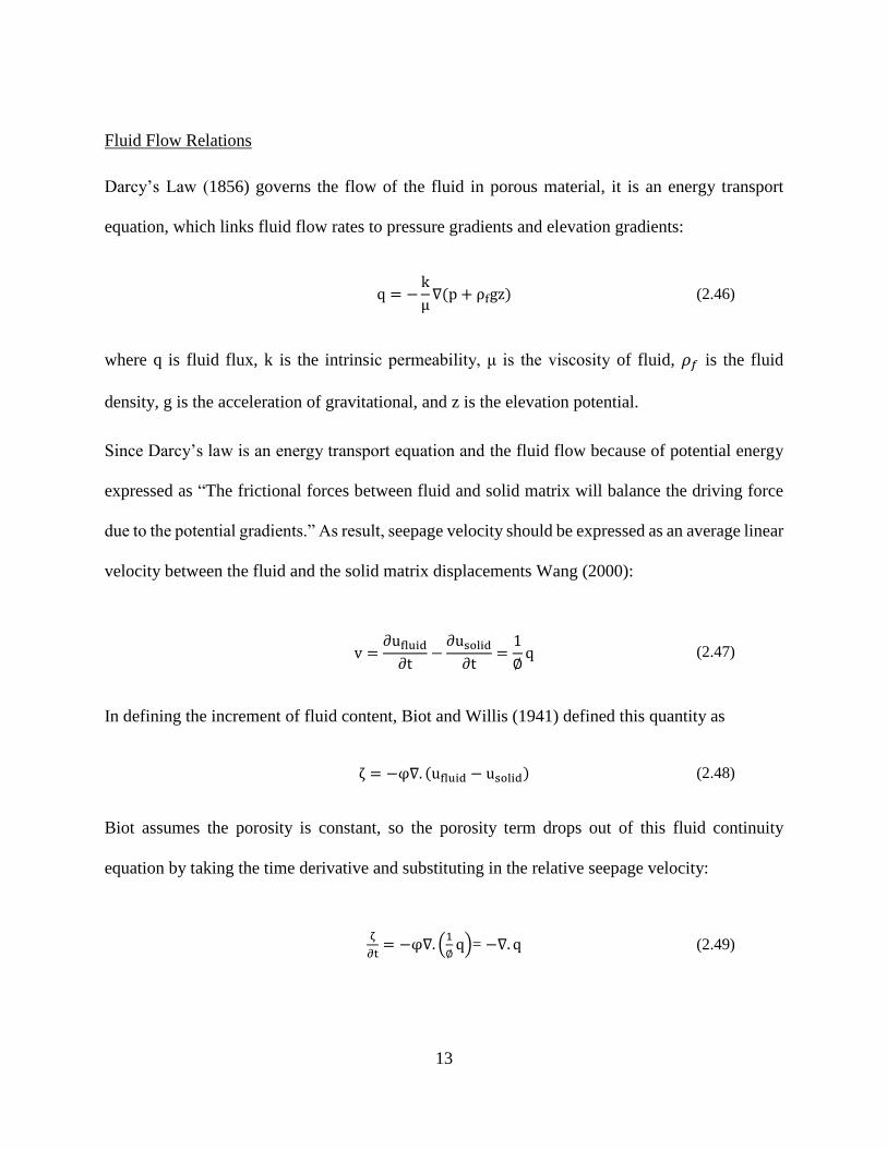
Fluid Flow Relations
Darcy’s Law (1856) governs the flow of the fluid in porous material, it is an energy transport
equation, which links fluid flow rates to pressure gradients and elevation gradients:
q = −k
μ∇(p + ρfgz) (2.46)
where q is fluid flux, k is the intrinsic permeability, μ is the viscosity of fluid, 𝜌𝑓 is the fluid
density, g is the acceleration of gravitational, and z is the elevation potential.
Since Darcy’s law is an energy transport equation and the fluid flow because of potential energy
expressed as “The frictional forces between fluid and solid matrix will balance the driving force
due to the potential gradients.” As result, seepage velocity should be expressed as an average linear
velocity between the fluid and the solid matrix displacements Wang (2000):
v =∂ufluid
∂t−
∂usolid
∂t=
1
∅q (2.47)
In defining the increment of fluid content, Biot and Willis (1941) defined this quantity as
ζ = −φ∇. (ufluid − usolid) (2.48)
Biot assumes the porosity is constant, so the porosity term drops out of this fluid continuity
equation by taking the time derivative and substituting in the relative seepage velocity:
ζ
∂t= −φ∇. (
1
∅q)= −∇. q (2.49)
14
By substituting in Darcy’s law for the fluid flux, into Biot and Wills (1957) increment of the fluid,
we arrive at following:
ζ
∂t= −φ∇. (
1
∅q)= −∇. q (2.50)
Finally, substituting the seventh constitutive relation between increment of fluid content and strain
and pressure from pervious section see Equation 2.36:
ζ = α (εxx + εyy + εzz) +α
KuB P (2.51)
We get:
[α ∂
∂t(εxx+εyy+εzz)+
α
KuB ∂P
∂t] - ∇. [
k
μ∇(p+ρ
fgz) ] =QS (2.52)
Then, substitute the relation between strain and deflection:
εxx + εyy + εzz=
∂u
∂x+
∂v
∂y+
∂w
∂z (2.53)
And substitute storage coefficient as following:
sα =α
KuB (2.54)
We get: Sα
∂p
∂t-∇. [
K
μ∇(p+ρfgz)] =Qs-α
∂
∂t(∇.u (2.55)
2.2 Summary of Poroelastic Equation to Solve Hydro-Mechanical Model
In this chapter, a set of Biot’s poroelastic equation were developed to describe the Hydro-
mechanical coupling between structural deformation and fluid flow. Constitutive and governing
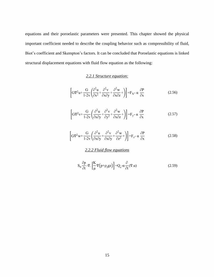
15
equations and their poroelastic parameters were presented. This chapter showed the physical
important coefficient needed to describe the coupling behavior such as compressibility of fluid,
Biot’s coefficient and Skempton’s factors. It can be concluded that Poroelastic equations is linked
structural displacement equations with fluid flow equation as the following:
2.2.1 Structure equation:
[G∇2u+G
1-2v(
∂2u
∂x2+
∂2v
∂x∂y+
∂2w
∂x∂z+)] =FX- α
∂P
∂x (2.56)
[G∇2v+G
1-2v(
∂2u
∂x∂y+
∂2v
∂y2+
∂2w
∂x∂z+)] =Fy- α
∂P
∂x (2.57)
[G∇2w+G
1-2v(
∂2u
∂x∂y+
∂2v
∂x∂y+
∂2w
∂z2+)] =Fz- α
∂P
∂x (2.58)
2.2.2 Fluid flow equations
Sα
∂p
∂t-∇. [
K
μ∇(p+ρ
fgz)] =Q
s-α
∂
∂t(∇.u) (2.59)
16
3. VALIDATION OF HYDROMECHANICAL MODEL FOR POROUS
MATERIALS
3.1 Introduction
Numerical models based on the Biot’s poroelasticity formulation are presented in this chapter.
Biot’s poroelastic equations are used to couple the relation between fluid flow and deformation.
The goal in this chapter is to validate number of numerical models by using COMSOL simulation
software (2012). This will be accomplished by using numerical models based on the Biot’s
poroelasticity formulation, and more specifically, using Biot’s poroelastic equations to couple the
relation between fluid flow and deformation Poroelastic equations developed in Chapter 2 can be
found under COMSOL’s poroelasticity package.
Zheng et al. (2003) provide a complete detailed account of reservoir models based on the Biot’s
poroelastic theory. Zhang developed the finite element model, and then validates his results with
Biot’s analytical solution. Here, the goal is to gain a better understanding of COMSOL software
and show the ability to obtain results that agree with Zhang’s solution.
3.2 Uniaxial-Constrained Hydro-Mechanical Model:
3.2.1 Introduction
The first model was carried out by Zheng et al (2003) to describe the behavior of a 2D rock sample.
A schematic of the model simulation is shown in Figure 2. The dimension of the sample is 2 m ×
3 m. The rock density is 2000 kg m-3. The rock sample is filled with oil. The displacement of the
bottom boundary is set to zero, the sides displacement are confined by mechanical roller
constraints. The vertical displacement at top boundary is free to move. The parameters of this rock
sample are given in the Table 1.
17
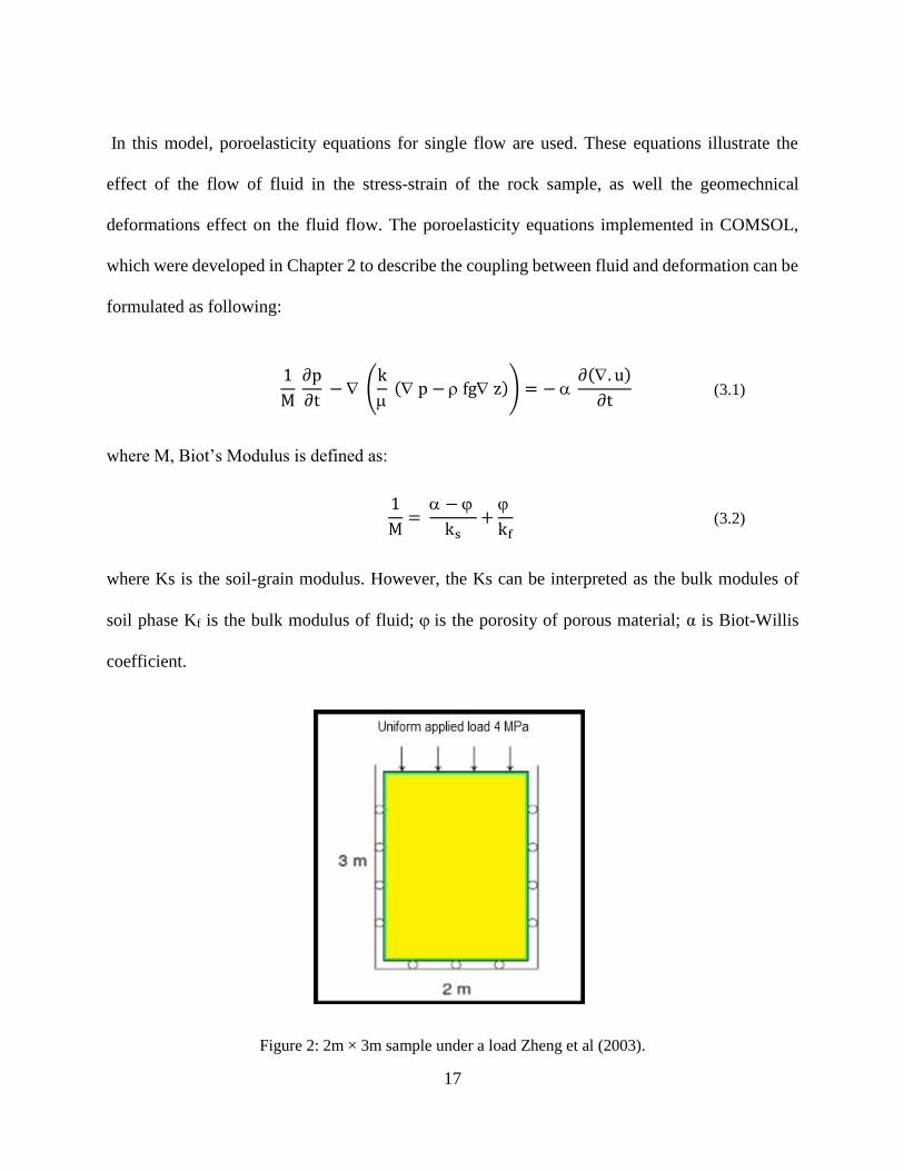
In this model, poroelasticity equations for single flow are used. These equations illustrate the
effect of the flow of fluid in the stress-strain of the rock sample, as well the geomechnical
deformations effect on the fluid flow. The poroelasticity equations implemented in COMSOL,
which were developed in Chapter 2 to describe the coupling between fluid and deformation can be
formulated as following:
1
M ∂p
∂t − (
k
( p − fg z)) = −
∂(. u)
∂t (3.1)
where M, Biot’s Modulus is defined as:
1
M=
−
ks+
kf (3.2)
where Ks is the soil-grain modulus. However, the Ks can be interpreted as the bulk modules of
soil phase Kf is the bulk modulus of fluid; is the porosity of porous material; α is Biot-Willis
coefficient.
Figure 2: 2m × 3m sample under a load Zheng et al (2003).
18
Table 1: List of parameters of rock simple Zhang el al (2003).
Young’s Modules
Poisson’s Ratio
Biot’s Coefficient
Biot’s Modules
Rock Density
Oil Density
Porosity
Permeability
Kinematic viscosity
1.44x 10⁴ M Pa
0.2
0.79
1.23x10⁴ M Pa
2000 Kg/m3
940 kg/m3
0.2
2x10-13 m2
1.3x10⁻⁴ m2/s
3.2.2 Test Setup and simulation
The rock sample simulation is done in two stages. In the first stage, the sample is subjected to
uniform load where no pore pressure will dissipate from sample boundaries. The applied uniform
load is 4 M Pa. The pore pressure is constant during first stage; the pore pressure is 1.64 M Pa.
The vertical displacement and pore pressure obtained from COMSOL shows a good agreement
with Zhang’s analytical and numerical solution. This agreements is shown in Figures 3 and 4.
In the second stage, the top boundary of the rock sample is opened so water can flow out of the
sample. The applied uniform load remains constant at 4 M Pa. Time-Displacement plots shows
excellent agreement with Zhang results.
19
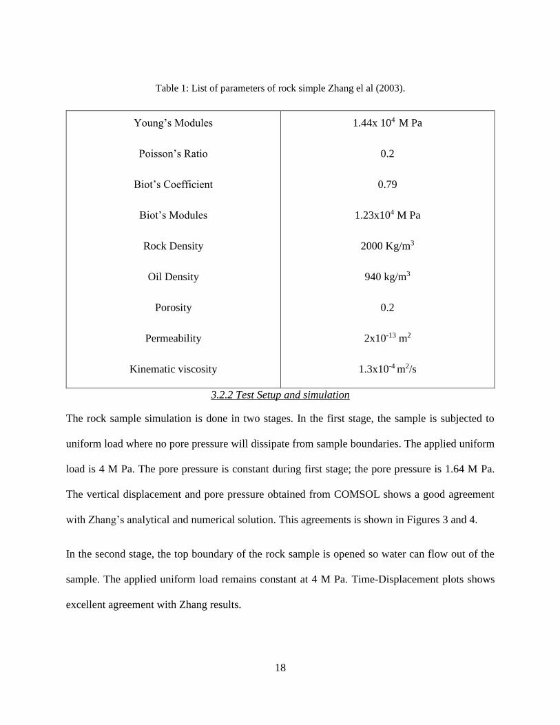
Figure 3: Vertical Displacement for the rock sample for undrained condition Ahmad (2013).
Figure 4: Vertical displacement vs height of the sample with undrained boundaries by Ahmad (2013).
20
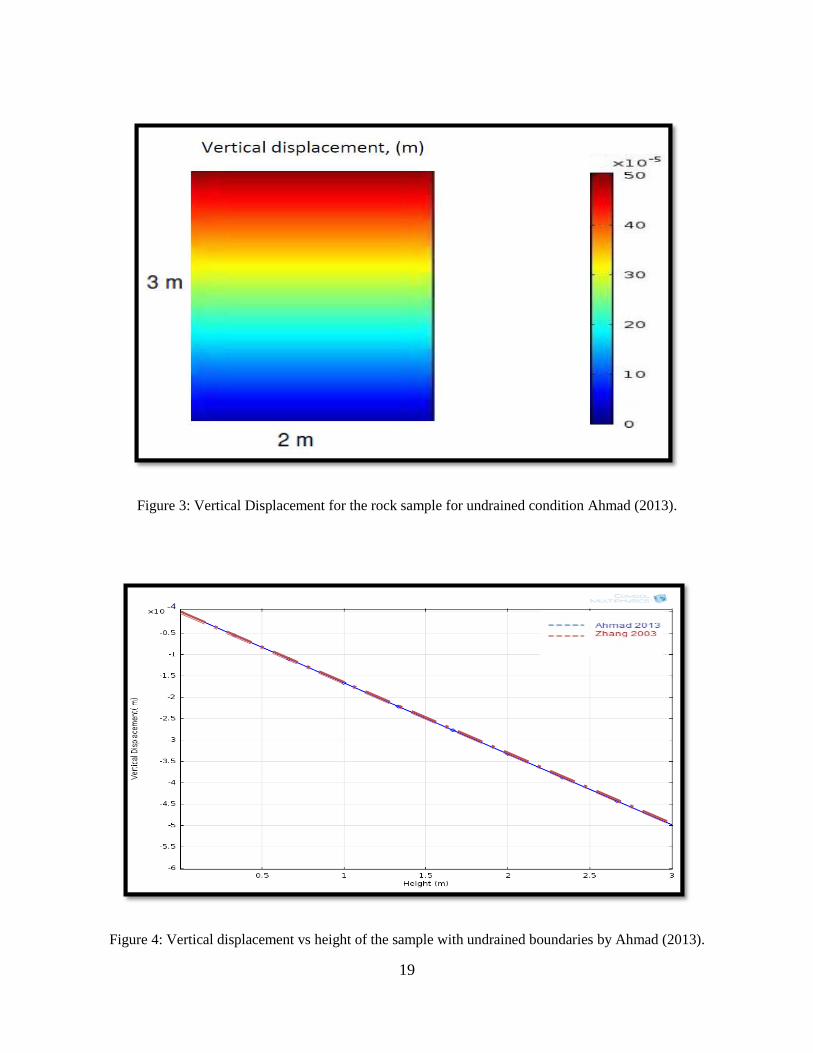
Figure 5: Vertical displacements plotted in different time intervals for the second stage by Ahmad (2013).
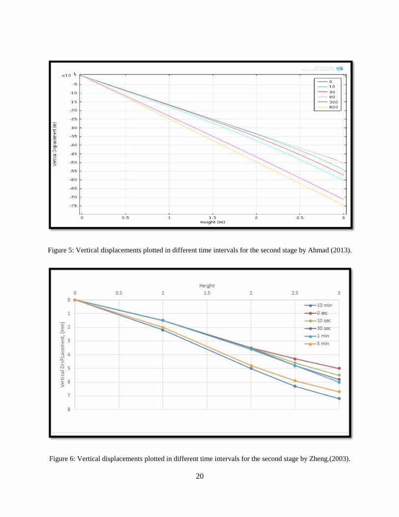
Figure 6: Vertical displacements plotted in different time intervals for the second stage by Zheng.(2003).
21
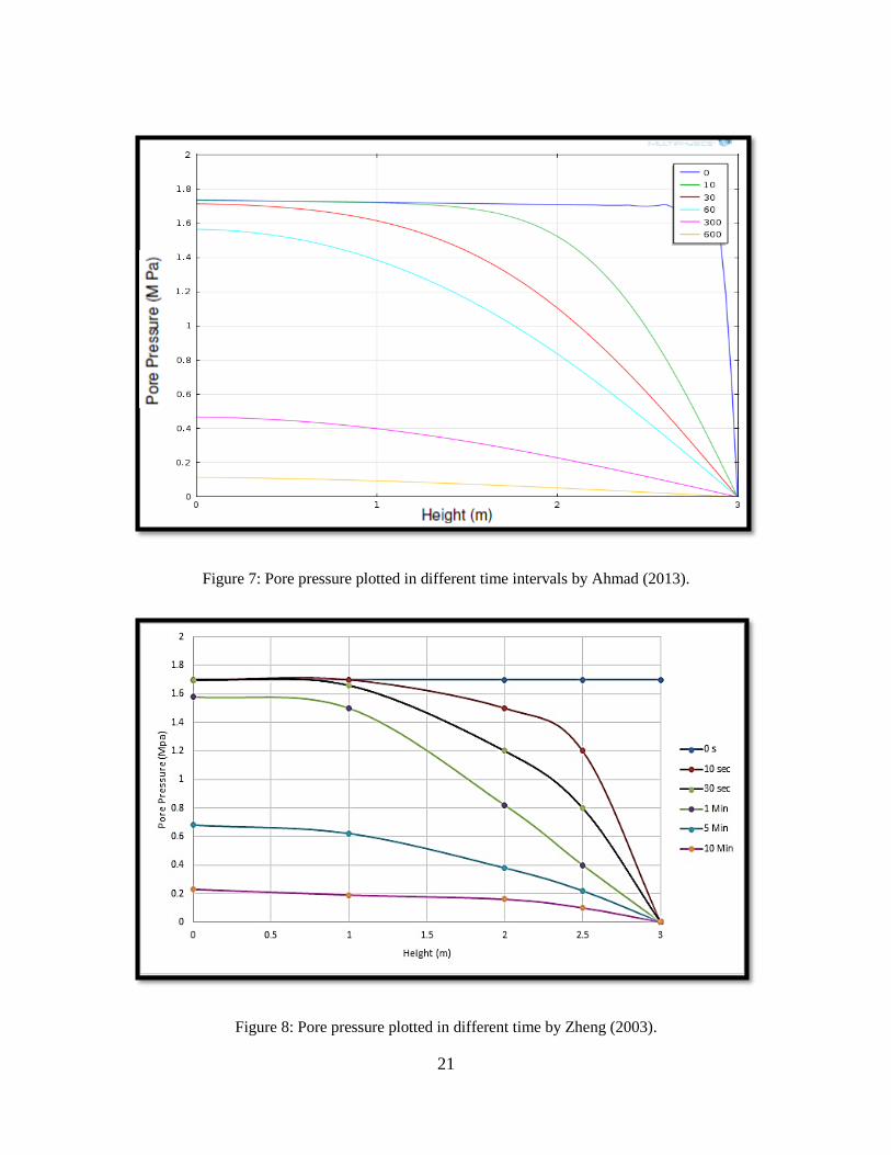
Figure 7: Pore pressure plotted in different time intervals by Ahmad (2013).
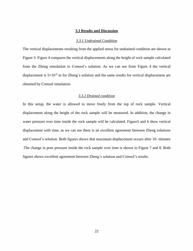
Figure 8: Pore pressure plotted in different time by Zheng (2003).
22
3.3 Results and Discussion
3.3.1 Undrained Condition
The vertical displacements resulting from the applied stress for undrained condition are shown in
Figure 3. Figure 4 compares the vertical displacements along the height of rock sample calculated
from the Zheng simulation to Comsol’s solution. As we can see from Figure 4 the vertical
displacement is 5×10⁻⁴ m for Zheng’s solution and the same results for vertical displacement are
obtained by Comsol simulation.
3.3.2 Drained condition
In this setup, the water is allowed to move freely from the top of rock sample. Vertical
displacement along the height of the rock sample will be measured. In addition, the change in
water pressure over time inside the rock sample will be calculated. Figure5 and 6 show vertical
displacement with time, as we can see there is an excellent agreement between Zheng solutions
and Comsol’s solution. Both figures shows that maximum displacement occurs after 10- minutes
.The change in pore pressure inside the rock sample over time is shown in Figure 7 and 8. Both
figures shows excellent agreement between Zheng’s solution and Comsol’s results.
23
4. SENSITIVITY STUDY
4.1 Background
Hydro-mechanical description of poroelastic material is ubiquitous in several fields
ranging from geology, petroleum and hydrogeology Hydro-mechanical behavior of porous
materials is significantly influenced by the poroelastic parameters of porous media The purpose of
carrying out a sensitivity study for rock sample is to explore the influence of various poroelastic
parameters on the behavior of Hydro-mechanical coupling of porous material. Biot (1941) stated
that the magnitude of coupling depends mostly on solid compressibility, fluid flow and porosity
of porous material. The objective here is to detail how the rock sample is responds to various
poroelastic parameters inputs. More specifically this section will demonstrate, which poroelastic
parameters has significant impact on the behavior of Hydro-mechanical coupling of porous
material.
4.2 Approach
The effect of poroelastic parameters on the Hydro-mechanical coupling behavior of 2-D
rock sample under a constant applied pressure is presented in this chapter. In order to show the
correlation between poroelastic parameters and the response of porous media for 2-D rock sample,
numerical models for various poroelastic parameters are carried out on COMSOL multiphysics
software 4.2.
It can be concluded that the compressibility of framework is a very important factor
influencing the deformation of porous material .The compressibility can be defined as the ratio of
volume change with respect to a pressure change. Biot’s theory (1941) introduce modules of
24
compressibility, the equation below shows that compressibility of framework is influenced by Biot
coefficient and bulk modules of the solid.
1
𝑀=
𝛼
𝐾𝑢𝐵 (4.1)
In addition, this chapter investigate the effect of pore pressure on the behavior of porous
material is investigated. The basic concept of poroelastic theory indicates that magnitude of
coupling is affected by pore pressure of fluid material. Biot’s theory (1944) stated ‘Fluid-to-solid
coupling occurs when a change in fluid pressure will produce change in volume of poroelastic
material”.
All the above shows that the behavior of coupling of porous material is less straightforward
to predict. The goal here is to investigate the effects of Biot’s coefficient, porosity and pore
pressure on porous material. In order to explore the effect of poroelastic parameters, sensitivity
study is carried out in this Chapter for different geomechnical models. Sensitivity study simulation
is carried out with COMSOL software. In each simulation, the geomechnical parameters of the
porous material are inputs into the system.
4.3 Sensitivity Analysis Description
In this section, a sensitivity analysis for 2-D rock sample.is carried out. As part of this
analysis study, a fully coupled Hydro-mechanical model based on COMSOL Multiphysics is
developed. In each model run, the geomechnical parameters of the porous material are inputs into
the system. The boundary condition is constant for all models. The top boundary of rock sample
will be free to move, horizontally and the bottom will be constrained.
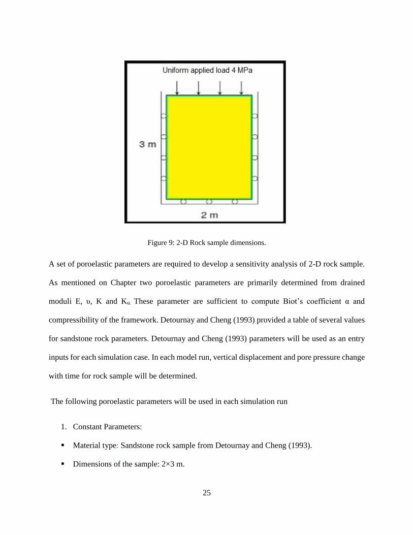
25
Figure 9: 2-D Rock sample dimensions.
A set of poroelastic parameters are required to develop a sensitivity analysis of 2-D rock sample.
As mentioned on Chapter two poroelastic parameters are primarily determined from drained
moduli E, υ, K and Ku. These parameter are sufficient to compute Biot’s coefficient α and
compressibility of the framework. Detournay and Cheng (1993) provided a table of several values
for sandstone rock parameters. Detournay and Cheng (1993) parameters will be used as an entry
inputs for each simulation case. In each model run, vertical displacement and pore pressure change
with time for rock sample will be determined.
The following poroelastic parameters will be used in each simulation run
1. Constant Parameters:
Material type: Sandstone rock sample from Detournay and Cheng (1993).
Dimensions of the sample: 2×3 m.
26
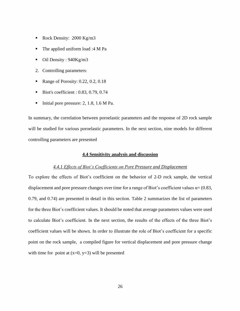
Rock Density: 2000 Kg/m3
The applied uniform load :4 M Pa
Oil Density : 940Kg/m3
2. Controlling parameters:
Range of Porosity: 0.22, 0.2, 0.18
Biot's coefficient : 0.83, 0.79, 0.74
Initial pore pressure: 2, 1.8, 1.6 M Pa.
In summary, the correlation between poroelastic parameters and the response of 2D rock sample
will be studied for various poroelastic parameters. In the next section, nine models for different
controlling parameters are presented
4.4 Sensitivity analysis and discussion
4.4.1 Effects of Biot’s Coefficients on Pore Pressure and Displacement
To explore the effects of Biot’s coefficient on the behavior of 2-D rock sample, the vertical
displacement and pore pressure changes over time for a range of Biot’s coefficient values α= (0.83,
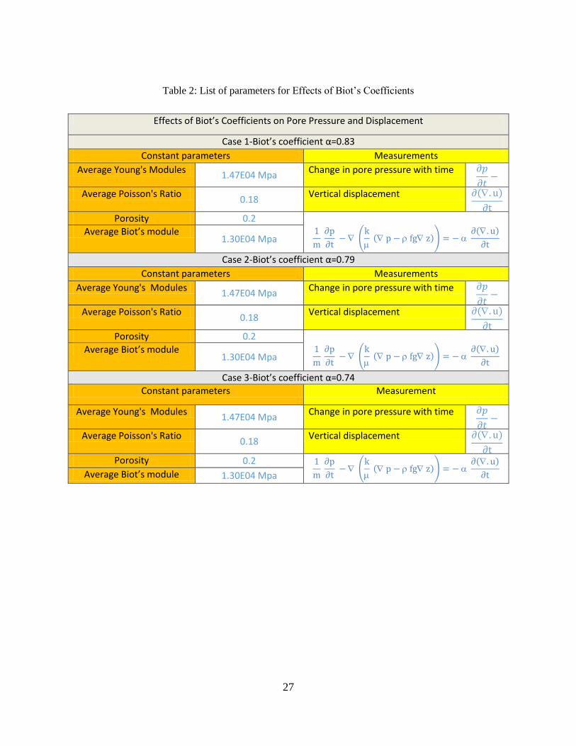
0.79, and 0.74) are presented in detail in this section. Table 2 summarizes the list of parameters
for the three Biot’s coefficient values. It should be noted that average parameters values were used
to calculate Biot’s coefficient. In the next section, the results of the effects of the three Biot’s
coefficient values will be shown. In order to illustrate the role of Biot’s coefficient for a specific
point on the rock sample, a compiled figure for vertical displacement and pore pressure change
with time for point at (x=0, y=3) will be presented
27
Table 2: List of parameters for Effects of Biot’s Coefficients
Effects of Biot’s Coefficients on Pore Pressure and Displacement
Case 1-Biot’s coefficient α=0.83
Constant parameters Measurements
Average Young's Modules 1.47E04 Mpa
Change in pore pressure with time 𝜕𝑝
𝜕𝑡−
Average Poisson's Ratio 0.18
Vertical displacement ∂(. u)
∂t
Porosity 0.2
1
m ∂p
∂t − (
k
( p − fg z)) = −
∂(. u)
∂t
Average Biot’s module 1.30E04 Mpa
Case 2-Biot’s coefficient α=0.79
Constant parameters Measurements
Average Young's Modules 1.47E04 Mpa
Change in pore pressure with time 𝜕𝑝
𝜕𝑡−
Average Poisson's Ratio 0.18
Vertical displacement ∂(. u)
∂t
Porosity 0.2
1
m ∂p
∂t − (
k
( p − fg z)) = −
∂(. u)
∂t
Average Biot’s module 1.30E04 Mpa
Case 3-Biot’s coefficient α=0.74
Constant parameters Measurement
Average Young's Modules 1.47E04 Mpa
Change in pore pressure with time 𝜕𝑝
𝜕𝑡−
Average Poisson's Ratio 0.18
Vertical displacement ∂(. u)
∂t
Porosity 0.2 1
m ∂p
∂t − (
k
( p − fg z)) = −
∂(. u)
∂t
Average Biot’s module 1.30E04 Mpa
28
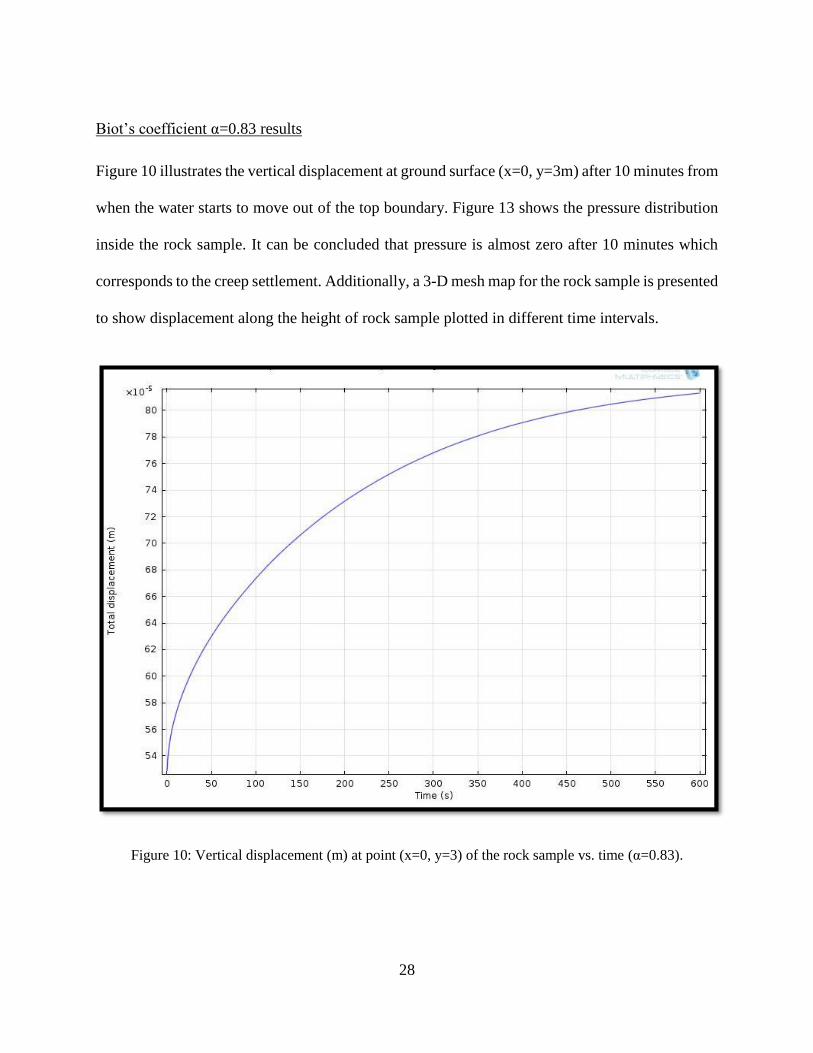
Biot’s coefficient α=0.83 results
Figure 10 illustrates the vertical displacement at ground surface (x=0, y=3m) after 10 minutes from
when the water starts to move out of the top boundary. Figure 13 shows the pressure distribution
inside the rock sample. It can be concluded that pressure is almost zero after 10 minutes which
corresponds to the creep settlement. Additionally, a 3-D mesh map for the rock sample is presented
to show displacement along the height of rock sample plotted in different time intervals.
Figure 10: Vertical displacement (m) at point (x=0, y=3) of the rock sample vs. time (α=0.83).

29
Figure 11 : 3-D mesh for Pore pressures inside the sample plotted in different time intervals (α=0.83).
Figure 12: 3-D mesh map for displacement along the height of the sample (α=0.83).
30
Biot’s coefficient α=0.79 results
Figure 13 shows the vertical displacement for point at ground surface (x=0, y=3m). Figure 14
shows the normalized pore pressure distribution for Biot’s coefficient (0.79) plotted in different
time intervals. It can be concluded that pore pressure dissipation from the top boundary of the rock
still have same trend as the previous Biot’s coefficient (0.83), however, the amount of dissipation
is higher in case of Biot’s coefficient of (0.83) Figure 15 shows 3-D displacement map to
demonstrate displacement rate along the height of rock with time.
Figure 13: Vertical displacement (m) at point (x=0, y=3) of the rock sample vs. time (α=0.79).
31
Figure 14: 3-D mesh for Pore pressures inside the sample plotted vs time (α=0.79).
Figure 15: 3-D mesh map for displacement along the height of the sample (α=0.79).
32
Biot’s coefficient α=0.74 results
Figure 16 illustrates the vertical displacement at ground surface (x=0, y=3m) after 10 minutes from
when the water starts to move out of the top boundary. Figure 17 shows the pressure distribution
inside the rock sample. It can be concluded that pressure is almost zero after 10 minutes which
corresponds to the creep settlement. Figure18 shows 3-D for normalized displacement map to
demonstrate displacement rate along the height of rock with time.
Figure 16: Vertical displacement (m) at point (x=0, y=3) of the rock sample vs. time (α=0.74).
33
Figure 17: 3-D mesh for Pore pressures inside the sample plotted vs time (α=0.74).
Figure 18: 3-D mesh map for displacement along the height of the sample (α=0.74).
34
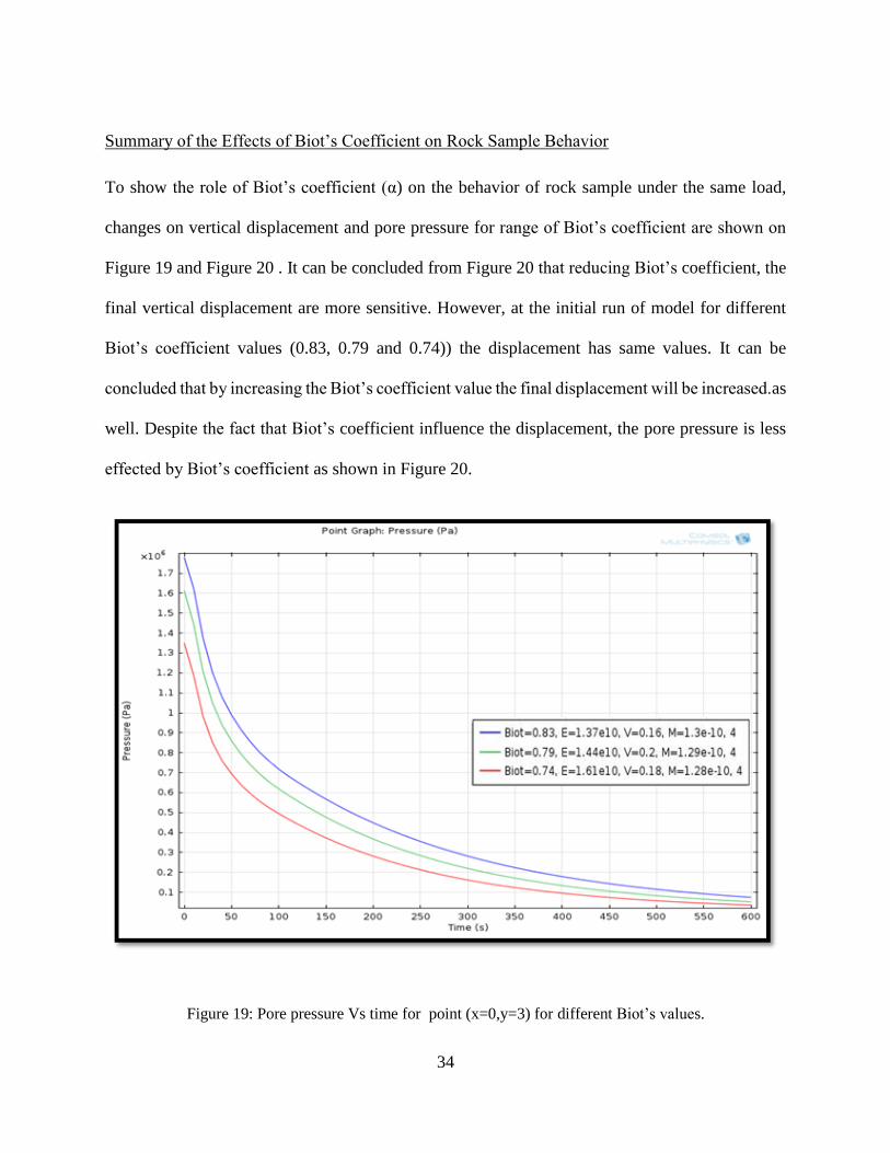
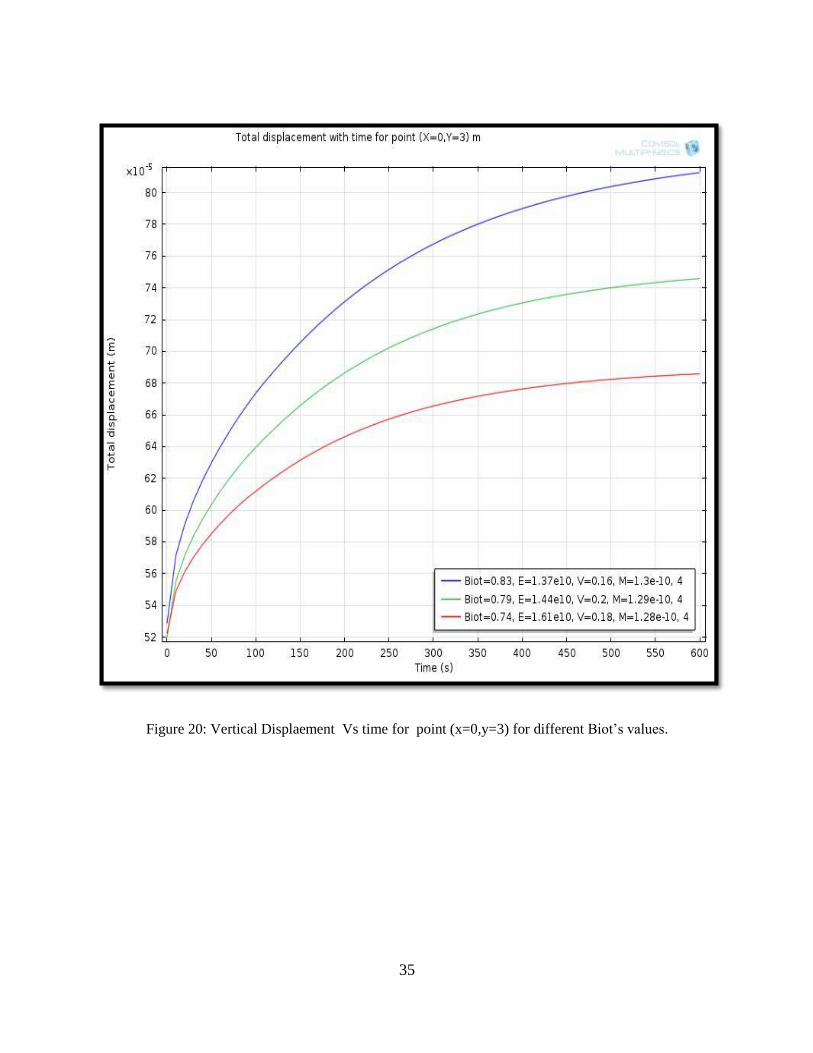
Summary of the Effects of Biot’s Coefficient on Rock Sample Behavior
To show the role of Biot’s coefficient (α) on the behavior of rock sample under the same load,
changes on vertical displacement and pore pressure for range of Biot’s coefficient are shown on
Figure 19 and Figure 20 . It can be concluded from Figure 20 that reducing Biot’s coefficient, the
final vertical displacement are more sensitive. However, at the initial run of model for different
Biot’s coefficient values (0.83, 0.79 and 0.74)) the displacement has same values. It can be
concluded that by increasing the Biot’s coefficient value the final displacement will be increased.as
well. Despite the fact that Biot’s coefficient influence the displacement, the pore pressure is less
effected by Biot’s coefficient as shown in Figure 20.
Figure 19: Pore pressure Vs time for point (x=0,y=3) for different Biot’s values.
35
Figure 20: Vertical Displaement Vs time for point (x=0,y=3) for different Biot’s values.
36
4.4.2 Effects of Initial pore pressure on Pore Pressure changes and Displacement
In this study, we examined the effect of the initial fluid pressure on the behavior of 2-D rock
sample. In each model run, a range of pore pressure values are introduced to show the respond of
the rock sample. Table 3 summarizes the list of parameters for the different pore pressure values.
Initial pore pressure values presented in this study are taken so that Skempton’s coefficient B will
not change dramatically. In order to determine the role of initial pore pressure on the behavior of
rock sample , a compile figure for vertical displacement and pore pressure change with time for
point at (x=0, y=3) will be presented
Table 3: poroelastic paramters for different initial pore pressure.
Effects of Pore Pressure on Rock sample
Case 1.Initial pore pressure :2E06 Mpa
Constant parameters Measurements
Young's Modules 1.47E04 MPa
Change in pore pressure with time 𝜕𝑝
𝜕𝑡−
Poisson's Ratio 0.2
Vertical displacement ∂(. u)
∂t
Porosity 0.2 1
𝑚 𝜕𝑝
𝜕𝑡 − (
𝑘
( 𝑝 − 𝑓𝑔 𝑧)) = −
𝜕(. 𝑢)
𝜕𝑡 Biot’s coefficient 0.79
Case 2.Initial pore pressure :1.6e6 Mpa
Constant parameters Measurements
Young's Modules 1.47E04 MPa
Change in pore pressure with time 𝜕𝑝
𝜕𝑡−
Poisson's Ratio 0.2
Vertical displacement ∂(. u)
∂t
Porosity 0.2 1
m ∂p
∂t − (
k
( p − fg z)) = −
∂(. u)
∂t Biot’s coefficient 0.79
Case 3.Initial pore pressure :1.2e6 Mpa
Constant parameters Measurement
Young's Modules 1.47E04 MPa
Change in pore pressure with time 𝜕𝑝
𝜕𝑡−
Poisson's Ratio 0.2
Vertical displacement ∂(. u)
∂t
Porosity 0.2 1
m ∂p
∂t − (
k
( p − fg z)) = −
∂(. u)
∂t
Biot’s coefficient 0.79
37
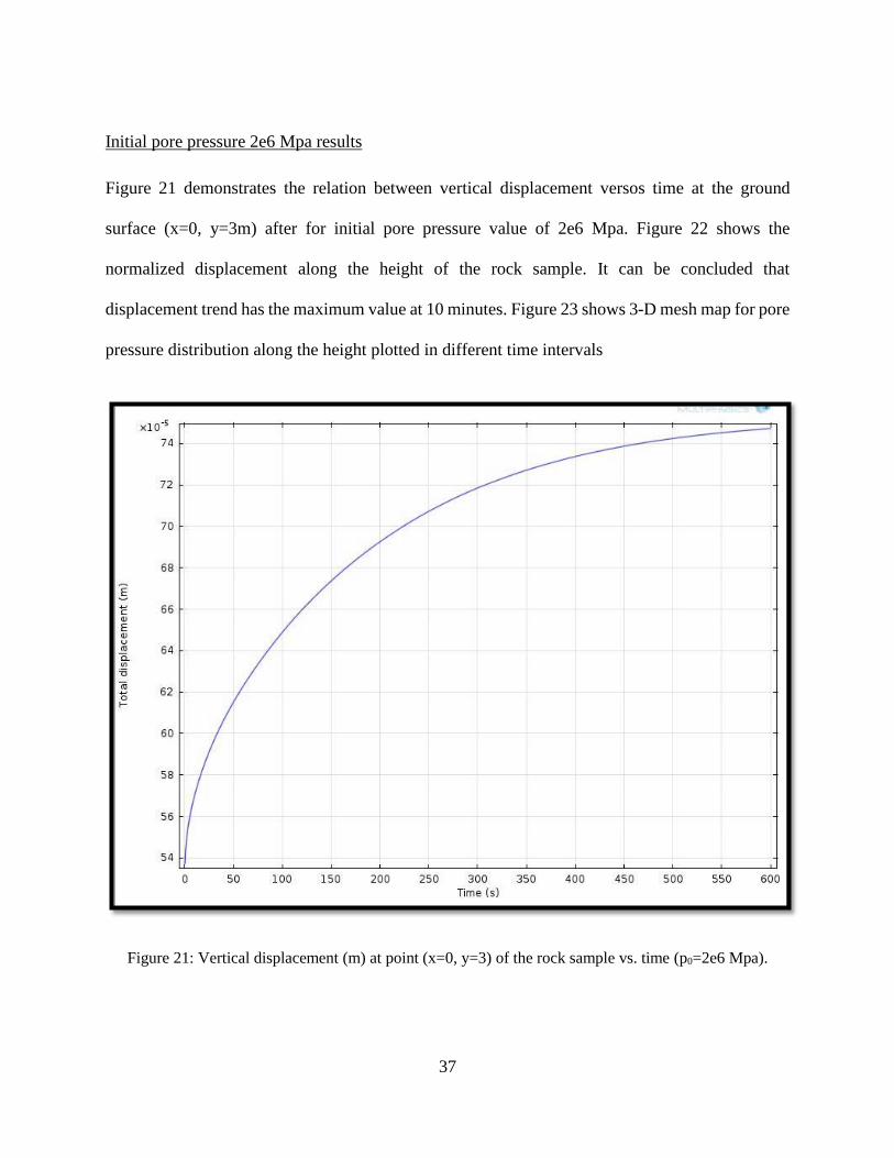
Initial pore pressure 2e6 Mpa results
Figure 21 demonstrates the relation between vertical displacement versos time at the ground
surface (x=0, y=3m) after for initial pore pressure value of 2e6 Mpa. Figure 22 shows the
normalized displacement along the height of the rock sample. It can be concluded that
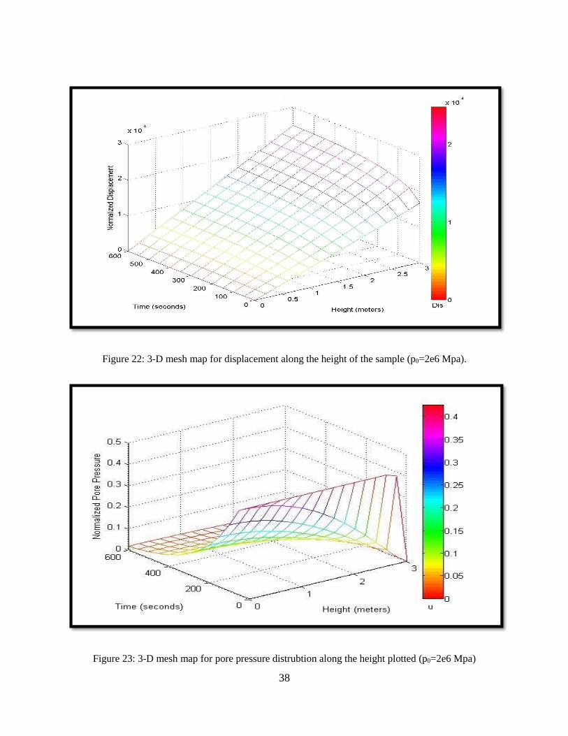
displacement trend has the maximum value at 10 minutes. Figure 23 shows 3-D mesh map for pore
pressure distribution along the height plotted in different time intervals
Figure 21: Vertical displacement (m) at point (x=0, y=3) of the rock sample vs. time (p0=2e6 Mpa).
38
Figure 22: 3-D mesh map for displacement along the height of the sample (p0=2e6 Mpa).
Figure 23: 3-D mesh map for pore pressure distrubtion along the height plotted (p0=2e6 Mpa)
39
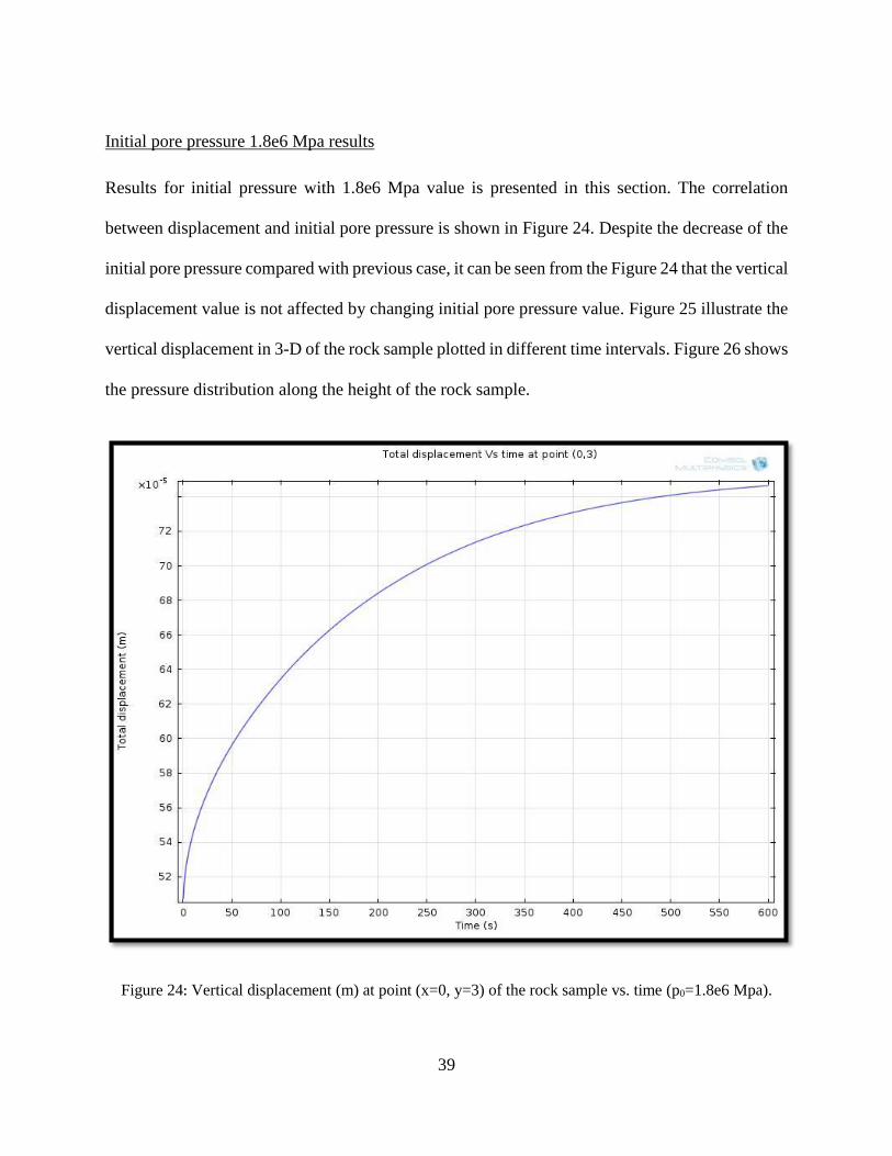
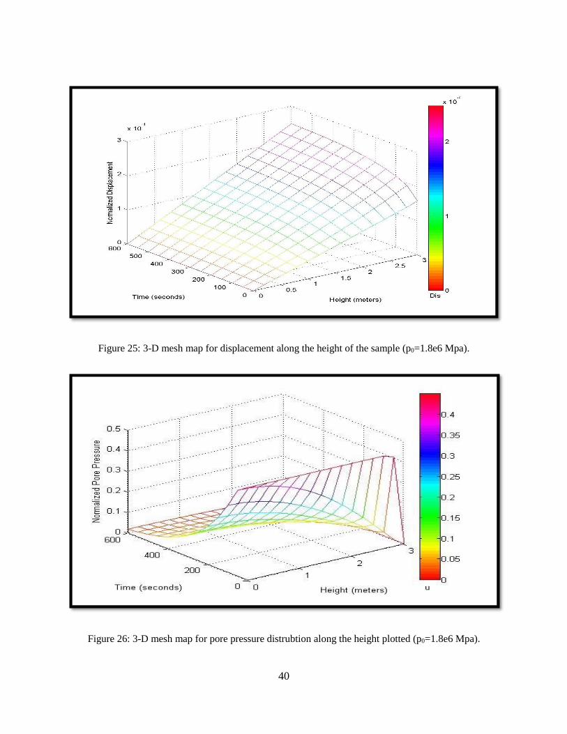
Initial pore pressure 1.8e6 Mpa results
Results for initial pressure with 1.8e6 Mpa value is presented in this section. The correlation
between displacement and initial pore pressure is shown in Figure 24. Despite the decrease of the
initial pore pressure compared with previous case, it can be seen from the Figure 24 that the vertical
displacement value is not affected by changing initial pore pressure value. Figure 25 illustrate the
vertical displacement in 3-D of the rock sample plotted in different time intervals. Figure 26 shows
the pressure distribution along the height of the rock sample.
Figure 24: Vertical displacement (m) at point (x=0, y=3) of the rock sample vs. time (p0=1.8e6 Mpa).
40
Figure 25: 3-D mesh map for displacement along the height of the sample (p0=1.8e6 Mpa).
Figure 26: 3-D mesh map for pore pressure distrubtion along the height plotted (p0=1.8e6 Mpa).
41
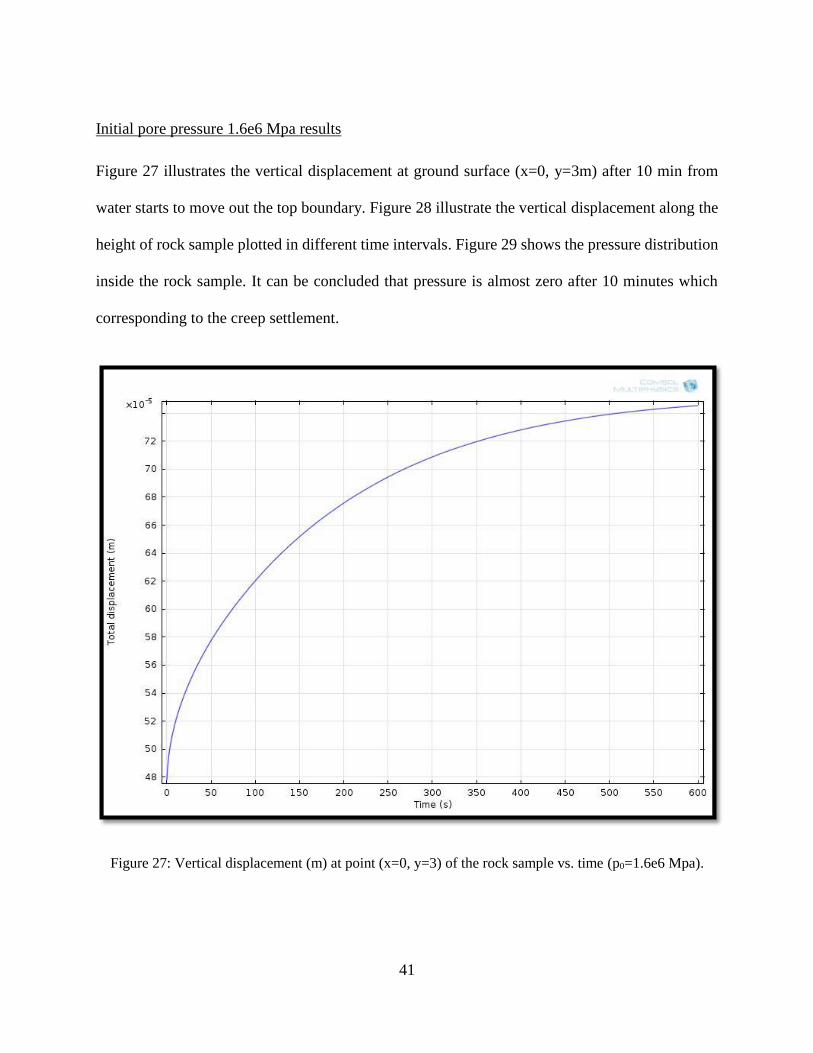
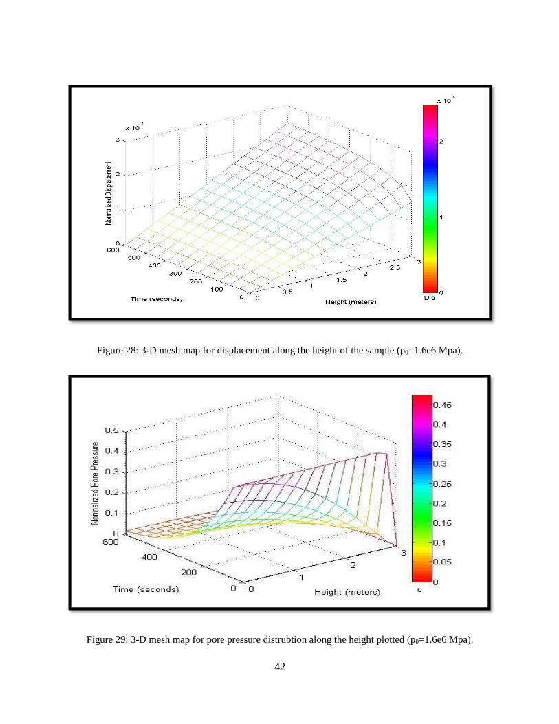
Initial pore pressure 1.6e6 Mpa results
Figure 27 illustrates the vertical displacement at ground surface (x=0, y=3m) after 10 min from
water starts to move out the top boundary. Figure 28 illustrate the vertical displacement along the
height of rock sample plotted in different time intervals. Figure 29 shows the pressure distribution
inside the rock sample. It can be concluded that pressure is almost zero after 10 minutes which
corresponding to the creep settlement.
Figure 27: Vertical displacement (m) at point (x=0, y=3) of the rock sample vs. time (p0=1.6e6 Mpa).
42
Figure 28: 3-D mesh map for displacement along the height of the sample (p0=1.6e6 Mpa).
Figure 29: 3-D mesh map for pore pressure distrubtion along the height plotted (p0=1.6e6 Mpa).
43
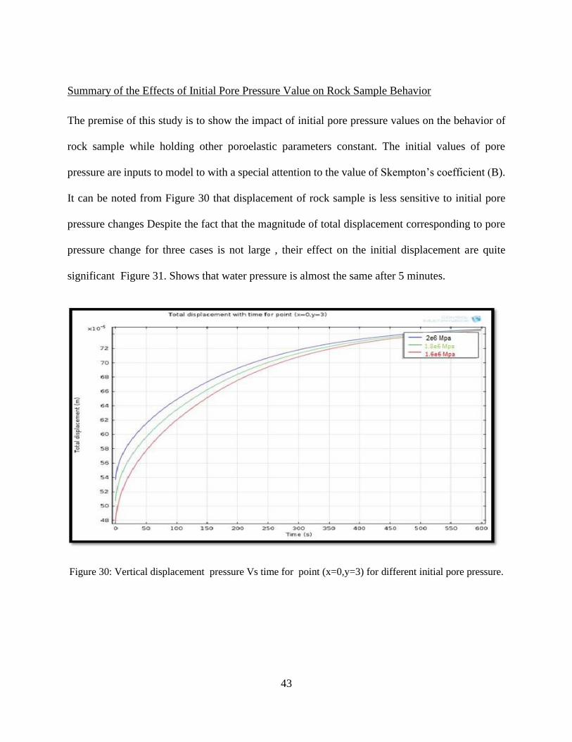
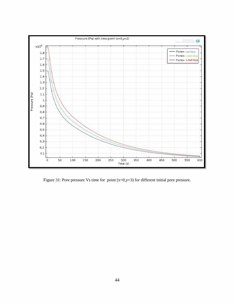
Summary of the Effects of Initial Pore Pressure Value on Rock Sample Behavior
The premise of this study is to show the impact of initial pore pressure values on the behavior of
rock sample while holding other poroelastic parameters constant. The initial values of pore
pressure are inputs to model to with a special attention to the value of Skempton’s coefficient (B).
It can be noted from Figure 30 that displacement of rock sample is less sensitive to initial pore
pressure changes Despite the fact that the magnitude of total displacement corresponding to pore
pressure change for three cases is not large , their effect on the initial displacement are quite
significant Figure 31. Shows that water pressure is almost the same after 5 minutes.
Figure 30: Vertical displacement pressure Vs time for point (x=0,y=3) for different initial pore pressure.
44
Figure 31: Pore pressure Vs time for point (x=0,y=3) for different initial pore pressure.
45
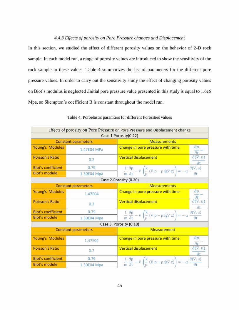
4.4.3 Effects of porosity on Pore Pressure changes and Displacement
In this section, we studied the effect of different porosity values on the behavior of 2-D rock
sample. In each model run, a range of porosity values are introduced to show the sensitivity of the
rock sample to these values. Table 4 summarizes the list of parameters for the different pore
pressure values. In order to carry out the sensitivity study the effect of changing porosity values
on Biot’s modulus is neglected .Initial pore pressure value presented in this study is equal to 1.6e6
Mpa, so Skempton’s coefficient B is constant throughout the model run.
Table 4: Poroelastic paramters for different Porosities values
Effects of porosity on Pore Pressure on Pore Pressure and Displacement change
Case 1.Porosity(0.22)
Constant parameters Measurements
Young's Modules 1.47E04 MPa
Change in pore pressure with time 𝜕𝑝
𝜕𝑡−
Poisson's Ratio 0.2
Vertical displacement ∂(. u)
∂t
Biot’s coefficient 0.79 1
m ∂p
∂t − (
k
( p − fg z)) = −
∂(. u)
∂t Biot’s module 1.30E04 Mpa
Case 2-Porosity (0.20)
Constant parameters Measurements
Young's Modules 1.47E04
Change in pore pressure with time 𝜕𝑝
𝜕𝑡−
Poisson's Ratio 0.2
Vertical displacement ∂(. u)
∂t
Biot’s coefficient 0.79 1
m ∂p
∂t − (
k
( p − fg z)) = −
∂(. u)
∂t Biot’s module 1.30E04 Mpa
Case 3. Porosity (0.18)
Constant parameters Measurement
Young's Modules 1.47E04
Change in pore pressure with time 𝜕𝑝
𝜕𝑡−
Poisson's Ratio 0.2
Vertical displacement ∂(. u)
∂t
Biot’s coefficient 0.79 1
m ∂p
∂t − (
k
( p − fg z)) = −
∂(. u)
∂t
Biot’s module 1.30E04 Mpa
46
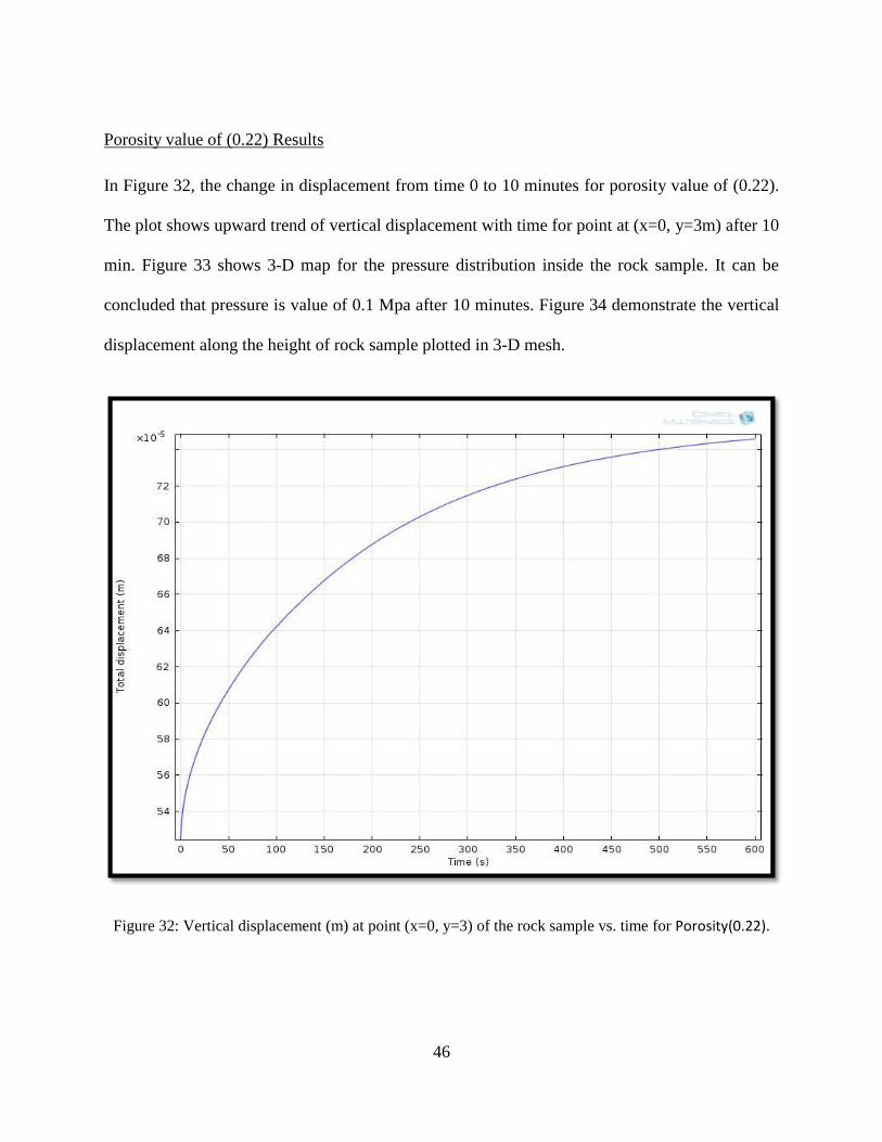
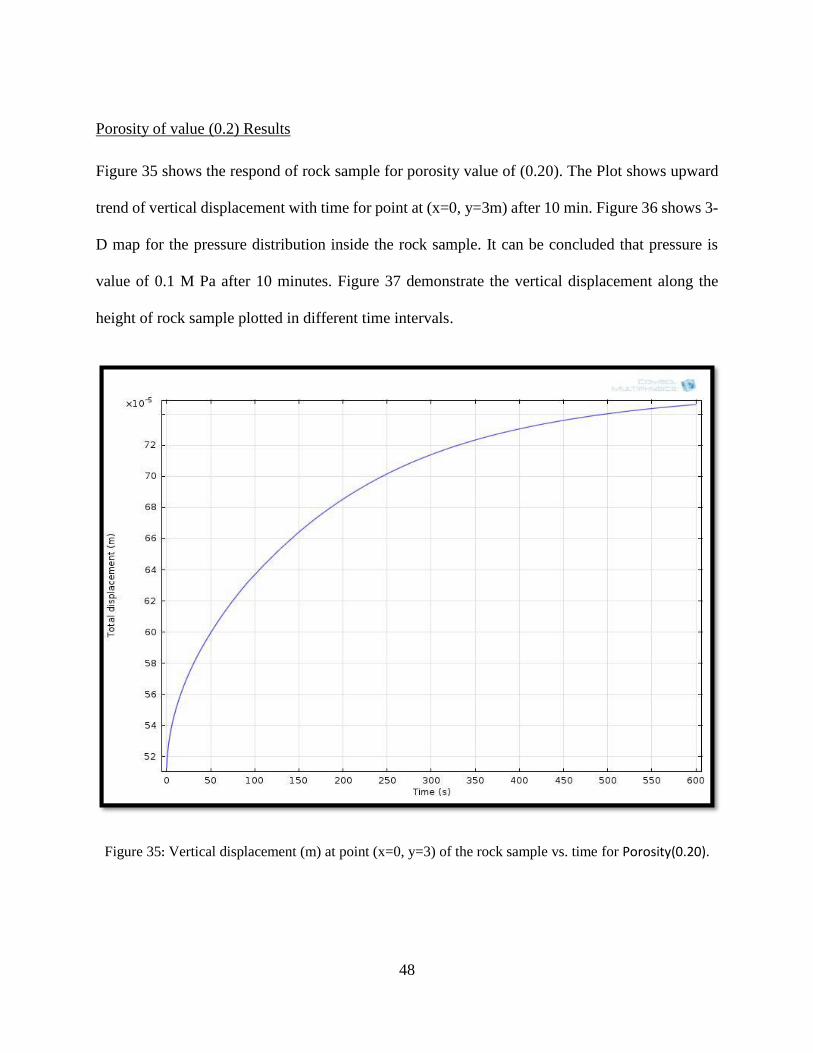
Porosity value of (0.22) Results
In Figure 32, the change in displacement from time 0 to 10 minutes for porosity value of (0.22).
The plot shows upward trend of vertical displacement with time for point at (x=0, y=3m) after 10
min. Figure 33 shows 3-D map for the pressure distribution inside the rock sample. It can be
concluded that pressure is value of 0.1 Mpa after 10 minutes. Figure 34 demonstrate the vertical
displacement along the height of rock sample plotted in 3-D mesh.
Figure 32: Vertical displacement (m) at point (x=0, y=3) of the rock sample vs. time for Porosity(0.22).
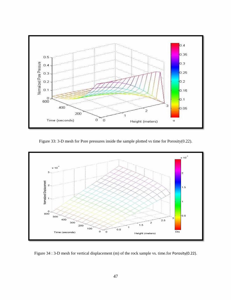
47
Figure 33: 3-D mesh for Pore pressures inside the sample plotted vs time for Porosity(0.22).
Figure 34 : 3-D mesh for vertical displacement (m) of the rock sample vs. time.for Porosity(0.22).
48
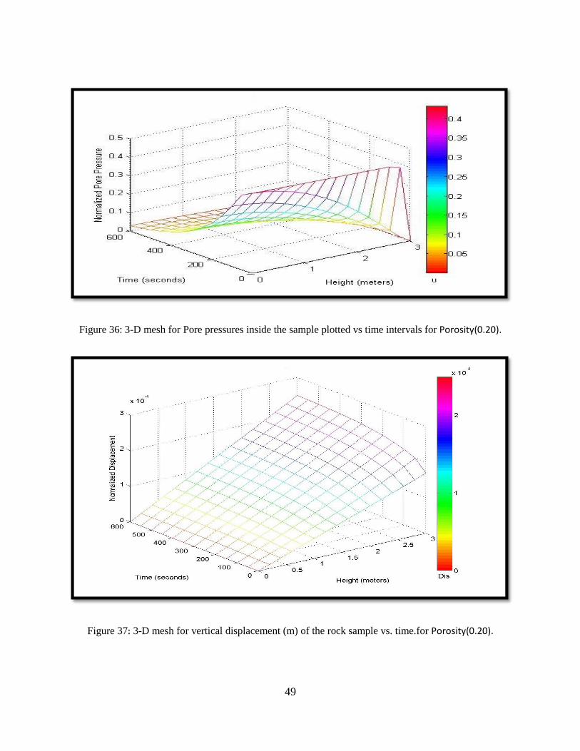
Porosity of value (0.2) Results
Figure 35 shows the respond of rock sample for porosity value of (0.20). The Plot shows upward
trend of vertical displacement with time for point at (x=0, y=3m) after 10 min. Figure 36 shows 3-
D map for the pressure distribution inside the rock sample. It can be concluded that pressure is
value of 0.1 M Pa after 10 minutes. Figure 37 demonstrate the vertical displacement along the
height of rock sample plotted in different time intervals.
Figure 35: Vertical displacement (m) at point (x=0, y=3) of the rock sample vs. time for Porosity(0.20).
49
Figure 36: 3-D mesh for Pore pressures inside the sample plotted vs time intervals for Porosity(0.20).
Figure 37: 3-D mesh for vertical displacement (m) of the rock sample vs. time.for Porosity(0.20).
50
Porosity value of (0.18) Results
Figure 38 shows the respond of rock sample for porosity value of (0.18). The Plot shows upward
trend of vertical displacement with time for point at (x=0, y=3m) after 10 min. Figure 39 shows
the pressure distribution inside the rock sample. It can be concluded that pressure is value of 0.1
M Pa after 10 minutes. Figure 40 demonstrate the vertical displacement along the height of rock
sample plotted in different time intervals.
Figure 38: Vertical displacement (m) at point (x=0, y=3) of the rock sample vs. time for Porosity(0.18).
51
Figure 39: 3-D mesh for Pore pressures inside the sample plotted vs time for Porosity(0.18).
Figure 40 : 3-D mesh for vertical displacement (m) of the rock sample vs. time. for Porosity(0.18).
52
Summary of the Effects of Porosity on Rock Sample Behavior
In this model, the displacement of rock sample with time for different porosity values are studied.
Figure 41 shows that changing porosity value has no effect on the total displacement of the rock
sample. However, porosity has effect on the initial displacement on the rock sample as shown in
Figure 41. The pore pressure dissipation also has the significant values at the beginning of the run,
then after 5 minutes all porosities values have the same pore pressure dissipation trend. It can be
concluded that poroelastic parameters are less sensitive to porosity change of range of (+/- 0.2%).
Figure 41: Vertical displacement Vs time for point (x=0,y=3) for diffrenet poristies
53
Figure 42: Pore pressure Vs time for point (x=0,y=3) for range of porosities.
54
5. EMBANKMENT
5.1 Motivation
The objective of this chapter is to develop a coupled Hydro-mechanical model finite element model
for a real-world example of embankment settlement using Comsol Multiphysics. Settlement of soil
under embankment is considered one of the major challenges encountered in maintaining roadway
facilities. Current methods for predicting consolidation settlement stages under embankment are
based on the theory of elasticity such as Schmertmann’ method (Sallam, 2009). Also constitutive
models are typically used to estimate soil settlement under embankment such as Mohr Coulomb
(MC) model and Modified Cam Clay model. The goal of this study is to predict the settlement of
embankment by using coupled Hydro-mechanical finite element model and to compare the results
with a real field measurements data of embankment published by Sallam et al (2009).
5.2 Approach
The goal of this study is to analyze and compare numerical and field results of Lake Jessup
embankment in Central Florida presented by Sallam et al (2009) with developed hydromechanical
coupling model. Sallam (2009) performed Finite Element Analysis (FEA) to estimate time
dependent settlement due construction stages of the embankment; FEA was carried out by using
Mohr-Coulomb and Soft Soil Creep models using the software program PLAXIS (2006).
Hydromechanical model developed in this section is created by using COMSOL software. The
subsoil, groundwater level, and boundary loading of the embankment are defined by using
poroelasticity model on COMSOL software.
55
5.3 Background
The embankment is located in Seminole County on Florida as shown in Figure (34). The
embankment height is 8 m and constructed on three stages, in the first month, a 2.3 m high
embankment was constructed, then a 5 m high mechanically stabilized earth (MSE) was
constructed in three months, and a 1.2 m high earth embankment was constructed in one month.
Figure 43: Project location adopted from Sallam et al (2009)
5.4 Mohr-Coulomb Model (Sallam)
Sallam el al (2010) performed FEM model for Lake Jessup embankment based on Mohr-Coulomb
(MC) theory to describe the behavior of subsoil condition during construction stages of the
embankment. To define the stress-strain relation of the subsoil condition under the embankment,
a set of soil parameters are required to describe the behavior of (MC) model which are modulus of
elasticity (E) and Poisson ratio (ν) for elasticity, cohesion (c) and angle of shearing resistance (φ)
for plasticity, and dilation angle (ψ) for dilatancy.
56
Table 11 shows the soil properties for the subsoil condition. Figure 44 shows the geometry and
subsoil layers at the end of embankment construction.
Table 5: Soil parameters for the Mohr-Coulomb model
Property Units
Embankment Sand I Clay I Sand II Clay II Sand III Sand IV Sand V
Drained Drained Undrained Drained Undrained Drained Drained Drained
γ unsat KN/m3 17.75 16.97 18.22 16.97 18.22 17.75 18.85 23.25
γ sat KN/m3 20.42 19.95 18.38 19.95 18.38 20.42 20.89 23.40
KX m/day 0.91 1 8.53E-05 1 8.53E-05 0.3 0.3 1
KY m/day 0.91 1 8.53E-05 1 8.53E-05 0.3 0.3 1
E ref Mpa 13.8 11.5 23.94 11.5 23.94 13.8 16.85 30.6
υ N/A 0.3 0.3 0.3 0.3 0.3 0.3 0.3 0.3
C ref Kpa 2.4 2.4 65.6 2.4 65.6 0.5 0.5 0.5
Φ degree 33 32 0 32 0 33 35 40
Ψ degree 0 0 0 0 0 0 0 0
57
Figure 44: Mohr-Coulomb Model geometry adpoted from Sallam.et al (2009).
Sallam results shows time dependent settlement during construction stages of the embankment.
The loads from the embankment were applied gradually to represent a construction stages. Figure
45 shows vertical settlement contours estimated for the modeled stages. Figure 46 shows the
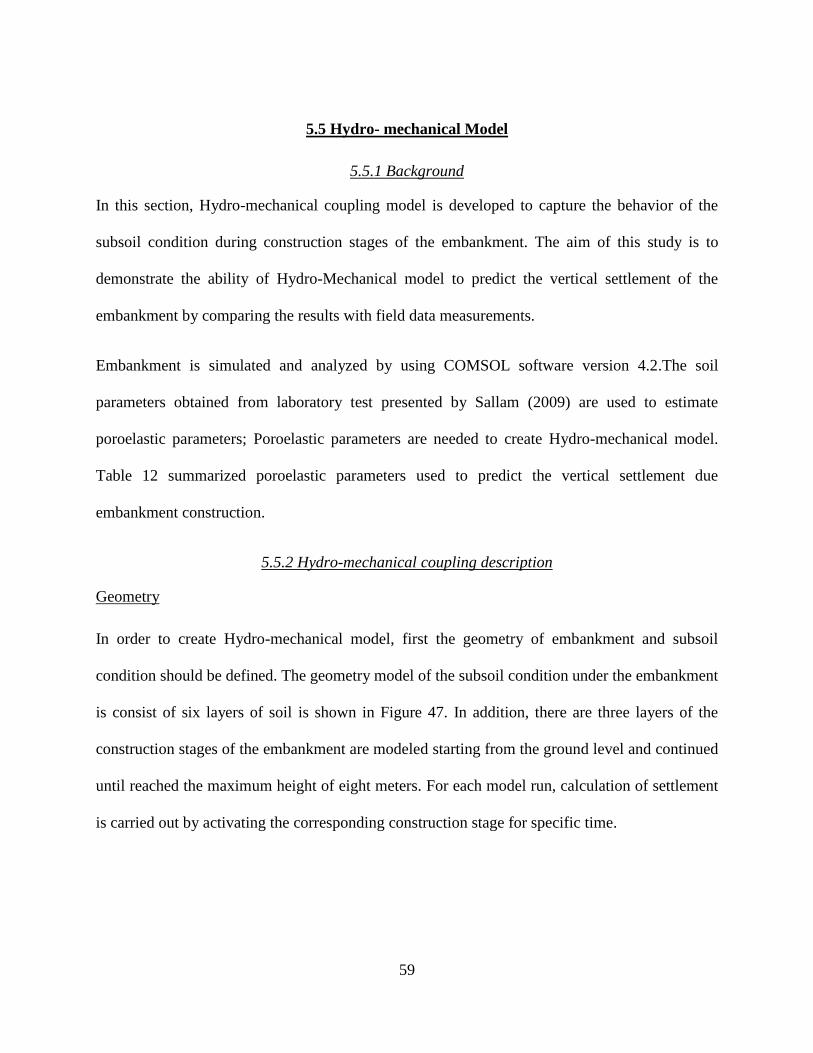
settlement time relationship for Point A at ground surface, which shows that maximum settlement
is 0.14 m after 5 months. As part of this study, eight settlement plates were installed to monitor
the actual settlement under the embankment, the results from monitored program shows total
average value of about 0.22 m as compared to a total settlement of about 0.14 using FEA at about
220 days.
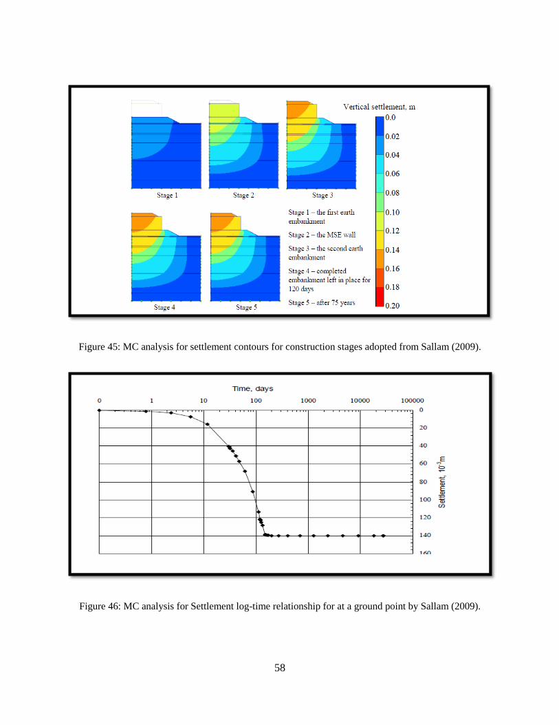
58
Figure 45: MC analysis for settlement contours for construction stages adopted from Sallam (2009).
Figure 46: MC analysis for Settlement log-time relationship for at a ground point by Sallam (2009).
59
5.5 Hydro- mechanical Model
5.5.1 Background
In this section, Hydro-mechanical coupling model is developed to capture the behavior of the
subsoil condition during construction stages of the embankment. The aim of this study is to
demonstrate the ability of Hydro-Mechanical model to predict the vertical settlement of the
embankment by comparing the results with field data measurements.
Embankment is simulated and analyzed by using COMSOL software version 4.2.The soil
parameters obtained from laboratory test presented by Sallam (2009) are used to estimate
poroelastic parameters; Poroelastic parameters are needed to create Hydro-mechanical model.
Table 12 summarized poroelastic parameters used to predict the vertical settlement due
embankment construction.
5.5.2 Hydro-mechanical coupling description
Geometry
In order to create Hydro-mechanical model, first the geometry of embankment and subsoil
condition should be defined. The geometry model of the subsoil condition under the embankment
is consist of six layers of soil is shown in Figure 47. In addition, there are three layers of the
construction stages of the embankment are modeled starting from the ground level and continued
until reached the maximum height of eight meters. For each model run, calculation of settlement
is carried out by activating the corresponding construction stage for specific time.
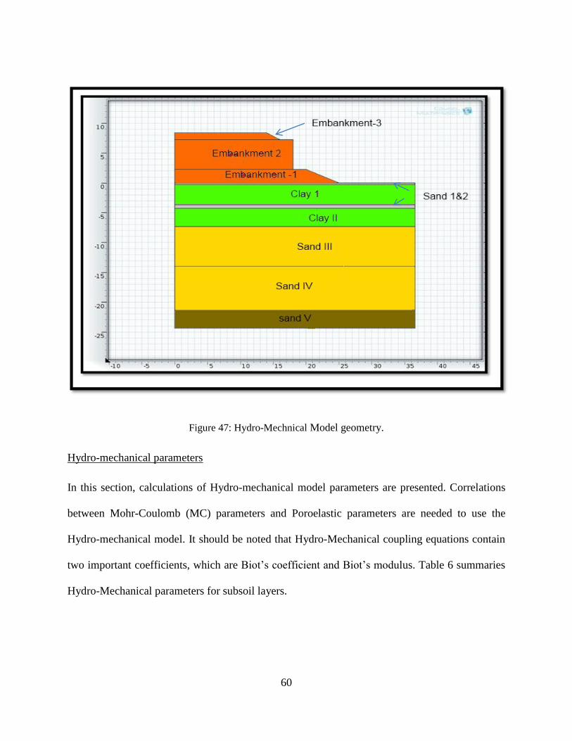
60
Figure 47: Hydro-Mechnical Model geometry.
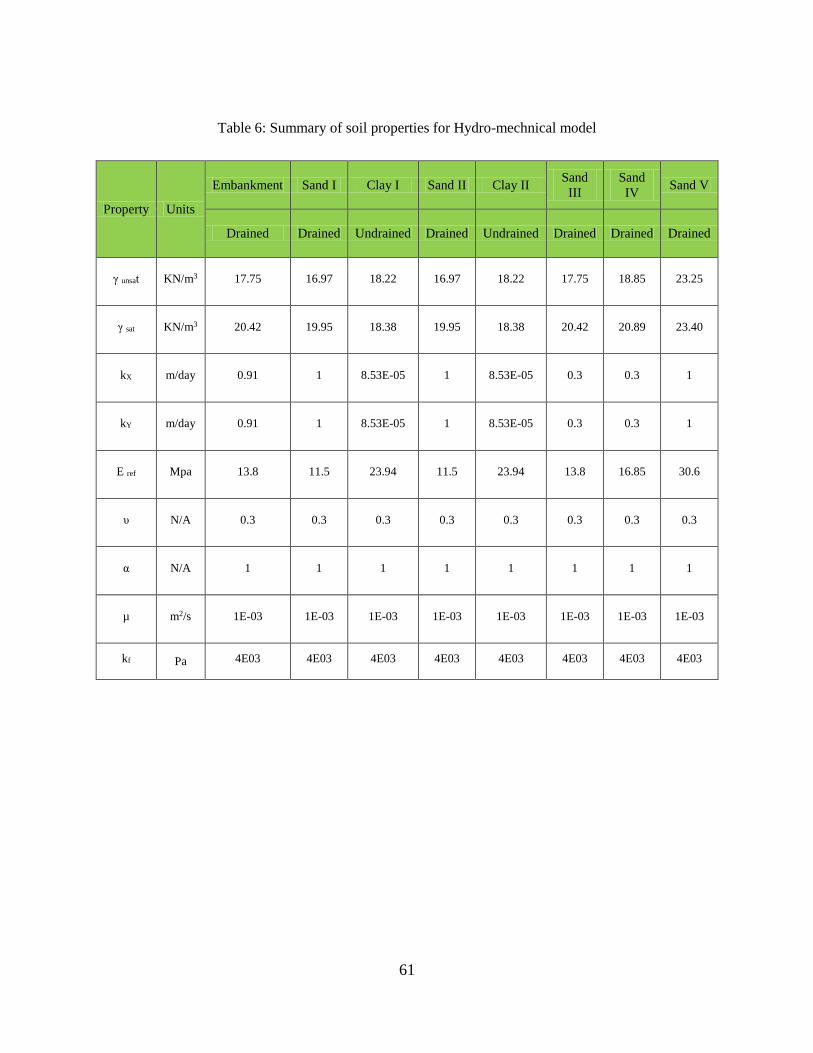
Hydro-mechanical parameters
In this section, calculations of Hydro-mechanical model parameters are presented. Correlations
between Mohr-Coulomb (MC) parameters and Poroelastic parameters are needed to use the
Hydro-mechanical model. It should be noted that Hydro-Mechanical coupling equations contain
two important coefficients, which are Biot’s coefficient and Biot’s modulus. Table 6 summaries
Hydro-Mechanical parameters for subsoil layers.
61
Table 6: Summary of soil properties for Hydro-mechnical model
Property Units
Embankment Sand I Clay I Sand II Clay II Sand
III
Sand
IV Sand V
Drained Drained Undrained Drained Undrained Drained Drained Drained
γ unsat KN/m3 17.75 16.97 18.22 16.97 18.22 17.75 18.85 23.25
γ sat KN/m3 20.42 19.95 18.38 19.95 18.38 20.42 20.89 23.40
kX m/day 0.91 1 8.53E-05 1 8.53E-05 0.3 0.3 1
kY m/day 0.91 1 8.53E-05 1 8.53E-05 0.3 0.3 1
E ref Mpa 13.8 11.5 23.94 11.5 23.94 13.8 16.85 30.6
υ N/A 0.3 0.3 0.3 0.3 0.3 0.3 0.3 0.3
α N/A 1 1 1 1 1 1 1 1
µ m2/s 1E-03 1E-03 1E-03 1E-03 1E-03 1E-03 1E-03 1E-03
kf Pa 4E03 4E03 4E03 4E03 4E03 4E03 4E03 4E03
62
It should be noted that Biot’s coefficient is assumed to be equal to 1 as recommended by Biot for
fully saturated soil. The poroelasticity equations to describe the coupling between fluid and
deformation can be formulated as following:
1
M ∂p
∂t − (
k
( p − fg z)) = −
∂(. u)
∂t (5.1)
where M, Biot’s Modulus is defined as:
1
M=
−
ks+
kf (5.2)
where, the Ks can be interpreted as the bulk modules of soil phase Kf is the bulk modulus of fluid;
is the porosity of porous material; α is Biot-Willis coefficient. The Bulk modules of soil is
interpreted from the following relation:
Ks =E
3(1 − 2v) (5.3)
where E is the Young’s modules and ν, Poisson’s ratio, are measured under drained conditions.
Settlement Calculation
The embankment construction is divided into three phases. After the first construction phase of
the embankment, a consolidation of 60 day is introduced to allow the pore pressure to dissipate.
Subsequently, construction of the second phase for Mechanically Stabilized Earth (MSE) will take
place. However, it should be noted that the construction of MSE is assumed to be carried out in
ten steps for COMSOL Software. In each step, 50 cm of MSE height will be introduced until reach
the maximum height of the MSE. After the second construction stage another consolidation time
will be introduced to allow water to dissipate. Finally, the last stage of embankment construction
63
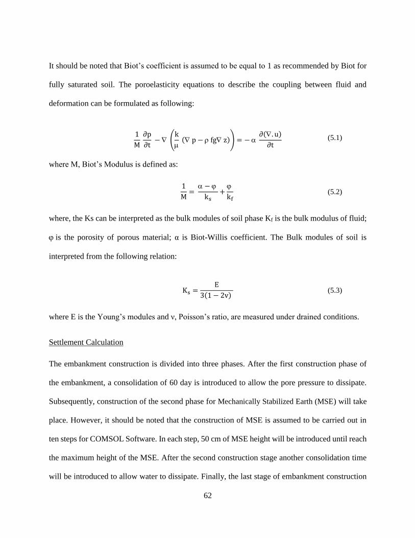
takes place, the duration of construction in this stage is 30 days. Next, the third construction stage
a consolidation period of 225 days is introduced to allow water to dissipate.
Results
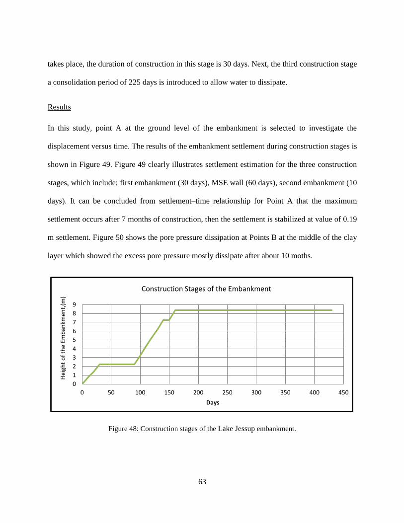
In this study, point A at the ground level of the embankment is selected to investigate the
displacement versus time. The results of the embankment settlement during construction stages is
shown in Figure 49. Figure 49 clearly illustrates settlement estimation for the three construction
stages, which include; first embankment (30 days), MSE wall (60 days), second embankment (10
days). It can be concluded from settlement–time relationship for Point A that the maximum
settlement occurs after 7 months of construction, then the settlement is stabilized at value of 0.19
m settlement. Figure 50 shows the pore pressure dissipation at Points B at the middle of the clay
layer which showed the excess pore pressure mostly dissipate after about 10 moths.
Figure 48: Construction stages of the Lake Jessup embankment.
0
1
2
3
4
5
6
7
8
9
0 50 100 150 200 250 300 350 400 450
Hei
ght
of
the
Emb
ankm
ent,
(m)
Days
Construction Stages of the Embankment
64
Figure 49: Settlement profile at ground level from H-M model COMSOL.
Figure 50: Pore pressure distrubtion at point A.
65
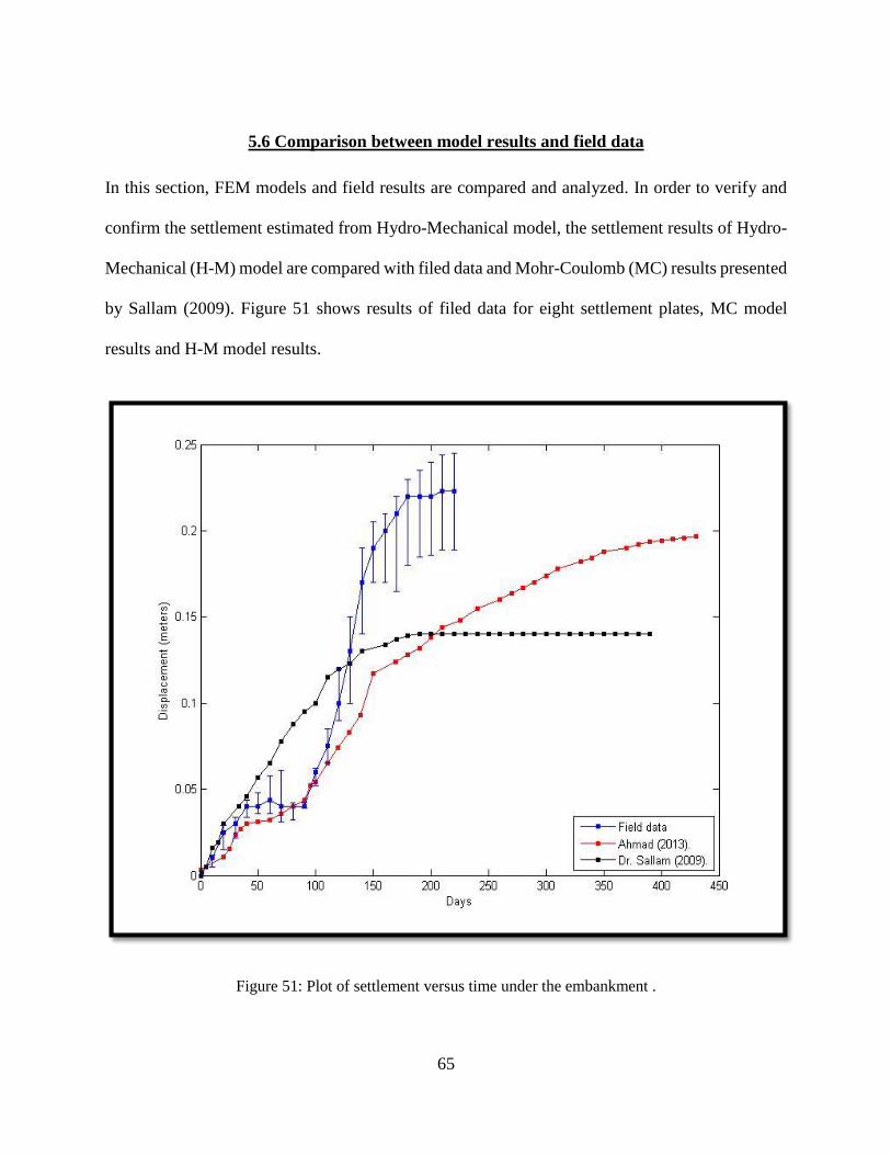
5.6 Comparison between model results and field data
In this section, FEM models and field results are compared and analyzed. In order to verify and
confirm the settlement estimated from Hydro-Mechanical model, the settlement results of Hydro-
Mechanical (H-M) model are compared with filed data and Mohr-Coulomb (MC) results presented
by Sallam (2009). Figure 51 shows results of filed data for eight settlement plates, MC model
results and H-M model results.
Figure 51: Plot of settlement versus time under the embankment .
66
It can be concluded from figure 51 that (H-M) model have general agreements with field data.
Figure 51 shows a settlement in order of 0.22 m after 8.5 months measured by settlement plates
while H-M model predict a settlement of 0.19 m after 10 months. In other hand, (MC) model
estimate only 0.14 m after 7.5 months. It should be noted that (H-M) model was able to capture
the delay on construction for the first 90 days. Both the filed data and (H-M) model shows a
settlement of 0.05 m for the first 90 days. It should be noted that there were less information about
the loading stags for the second stage which could be the reason for different in settlement
calculated by (H-M) model. It can be said that (H-M) model is more accurate for settlement
analysis of embankment construction compared by (MC) model.
67
6. CONCLUSIONS
6.1 Summary
The main focus of this thesis study was to demonstrate the importance of modeling multiphysical
effects to describe the real realistic coupled behavior of porous materials. The advantages of using
hydromechanical coupling to estimate deformation and pore water pressure dissipation of porous
materials was demonstrated in this research. The followings are major findings from this study:
1. Extensive literature survey was conducted about hydro-mechanical models based on
Biot’s poroelastic concept. Derivation of the Biot’s poroelastic equations was presented
based on the Wang’s approach (2000).
2. Sensitivity analyses were conducted to correlate the effect of poroelastic parameters on
the behavior of porous material. The results of the sensitivity analysis showed that the
porosity and Biot’s coefficient have dominant contribution to porous material behavior.
3. It can be concluded by implementing and developing a numerical model of poroelastic
rock materials that the hydromechanical coupling are paramount in estimating the
deformation of porous material. The numerical models developed in this thesis were
created by using COMSOL, a commercialized multiphysics finite element software
package. The results of these models were compared with the analytical model developed
by Zheng (2000).
4. To validate the fully hydromechanical model developed in this study, the model was
compared with the settlement data collected from a realistic filed embankment site. The
H-M model results were also compared with (MC) results embankment was presented.
68
The simulation results of hydromechanical models showed general agreement with field
and MC model measurements of embankment settlement.
6.2 Recommendations of future works
1. Heat transfer in porous material are important factors in many engineering disciplines, such
as geotechnical engineering and petroleum engineering. To study the behavior of porous
material under thermal, fluid and/or mechanical loading, Thermo hydro mechanical
coupling techniques should be developed.
2. Biot’s theory for hydromechanical coupling were developed only for saturated soil
However, unsaturated soils problems appears to be gaining general acceptance by
geotechnical engineers. Thus, Biot’s theory should be extended to describe the behavior
of unsaturated soil.
3. Biot’s assumed a small deformation occur to the soil skeleton, this carries the assumption
that porosity is constant. One should investigate the effect of porosity on the overall
behavior of porous material.
69
LIST OF REFERENCES
A. M. Sallam, and S.E. Jammal (2009). Finite Element Analysis of Time Dependent Settlement
of Lake Jessup Bridge Embankment in Central Florida.
Assessment, N. (1998). Prediction of Embankment Dam Breach Parameters, (July).
Bear, J. and Corapcioglu, M. Y. (1981). A mathematical mode1 for consolidation in elastic
aquifer due to hot water injection of pumping. Water Recourses Res. 17, 723-736.
Bear,J. and Bachmat,Y. (lggO), Introduction to Modelling of THM Phenomena in Porous Media.
Kluwer Academic Publishers, London
Biot, M., 1941, General Theory of Three-Dimensional Consolidation. Journal of Applied
Physics, 12(2): 155-164.
Biot, M., 1955, Theory of Elasticity and Consolidation for a Porous Anisotropic Solid. Journal of
Applied Physics, 26(2): 182-185.
Biot, M.A. and Willis, D.G., 1957, The Elastic Coefficients of the Theory of Consolidation. J.
Appl. Mech., 24: 594-601.
Biot, M.A., 1962, Mechanics of Deformation and Acoustic Propagation in Porous Media. Journal
of Applied Physics, 33(4): 1482-1498.
Booker, J.R. and Sawidou,C. (l984), Consolidation around a point heat source. Int.J- Numer.
Anal. Method Gwmech. 9, 173-184-.
Bowen, R M. (1983). Compressible porous media models by use of the theory of mixtures. Int- J.
Eng. Sci. 20, 697-735.
Brooks, R. and Corey, A., 1966, Properties of Porous Media Affecting Fluid Flow, J. Irrigation
and Drainage Div., Proc. Am. Soc. Civil Eng.(IR2), 92: 61-88.
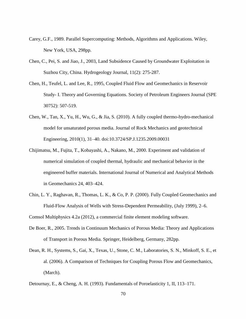
70
Carey, G.F., 1989. Parallel Supercomputing: Methods, Algorithms and Applications. Wiley,
New York, USA, 298pp.
Chen, C., Pei, S. and Jiao, J., 2003, Land Subsidence Caused by Groundwater Exploitation in
Suzhou City, China. Hydrogeology Journal, 11(2): 275-287.
Chen, H., Teufel, L. and Lee, R., 1995, Coupled Fluid Flow and Geomechanics in Reservoir
Study- I. Theory and Governing Equations. Society of Petroleum Engineers Journal (SPE
30752): 507-519.
Chen, W., Tan, X., Yu, H., Wu, G., & Jia, S. (2010). A fully coupled thermo-hydro-mechanical
model for unsaturated porous media. Journal of Rock Mechanics and geotechnical
Engineering, 2010(1), 31–40. doi:10.3724/SP.J.1235.2009.00031
Chijimatsu, M., Fujita, T., Kobayashi, A., Nakano, M., 2000. Experiment and validation of
numerical simulation of coupled thermal, hydraulic and mechanical behavior in the
engineered buffer materials. International Journal of Numerical and Analytical Methods
in Geomechanics 24, 403–424.
Chin, L. Y., Raghavan, R., Thomas, L. K., & Co, P. P. (2000). Fully Coupled Geomechanics and
Fluid-Flow Analysis of Wells with Stress-Dependent Permeability, (July 1999), 2–6.
Comsol Multiphysics 4.2a (2012), a commercial finite element modeling software.
De Boer, R., 2005. Trends in Continuum Mechanics of Porous Media: Theory and Applications
of Transport in Porous Media. Springer, Heidelberg, Germany, 282pp.
Dean, R. H., Systems, S., Gai, X., Texas, U., Stone, C. M., Laboratories, S. N., Minkoff, S. E., et
al. (2006). A Comparison of Techniques for Coupling Porous Flow and Geomechanics,
(March).
Detournay, E., & Cheng, A. H. (1993). Fundamentals of Poroelasticity 1, II, 113–171.
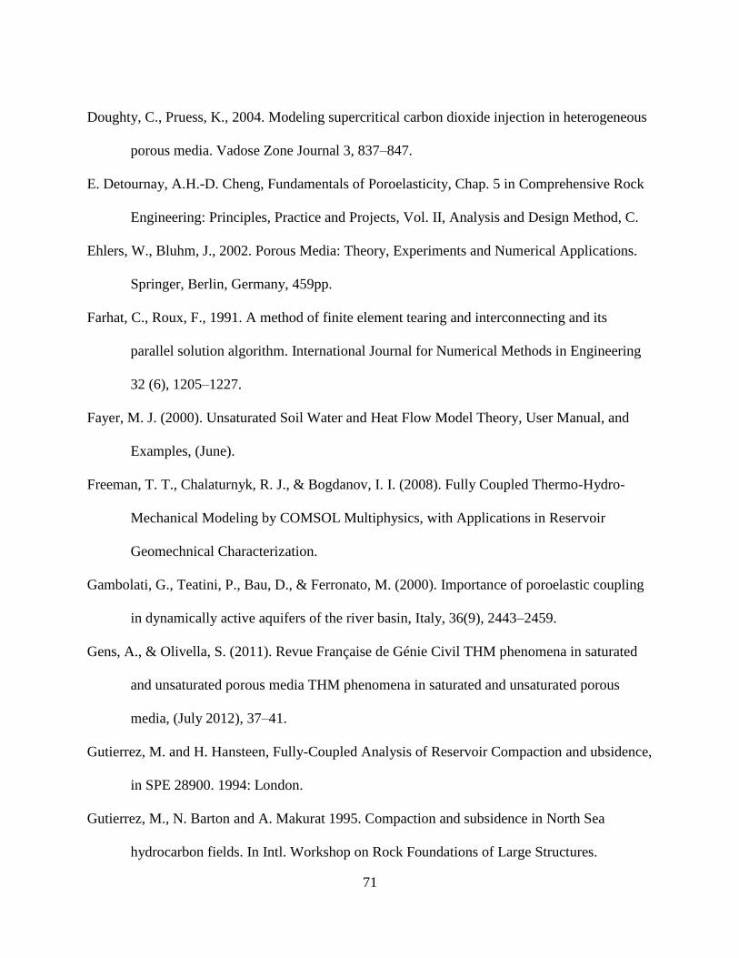
71
Doughty, C., Pruess, K., 2004. Modeling supercritical carbon dioxide injection in heterogeneous
porous media. Vadose Zone Journal 3, 837–847.
E. Detournay, A.H.-D. Cheng, Fundamentals of Poroelasticity, Chap. 5 in Comprehensive Rock
Engineering: Principles, Practice and Projects, Vol. II, Analysis and Design Method, C.
Ehlers, W., Bluhm, J., 2002. Porous Media: Theory, Experiments and Numerical Applications.
Springer, Berlin, Germany, 459pp.
Farhat, C., Roux, F., 1991. A method of finite element tearing and interconnecting and its
parallel solution algorithm. International Journal for Numerical Methods in Engineering
32 (6), 1205–1227.
Fayer, M. J. (2000). Unsaturated Soil Water and Heat Flow Model Theory, User Manual, and
Examples, (June).
Freeman, T. T., Chalaturnyk, R. J., & Bogdanov, I. I. (2008). Fully Coupled Thermo-Hydro-
Mechanical Modeling by COMSOL Multiphysics, with Applications in Reservoir
Geomechnical Characterization.
Gambolati, G., Teatini, P., Bau, D., & Ferronato, M. (2000). Importance of poroelastic coupling
in dynamically active aquifers of the river basin, Italy, 36(9), 2443–2459.
Gens, A., & Olivella, S. (2011). Revue Française de Génie Civil THM phenomena in saturated
and unsaturated porous media THM phenomena in saturated and unsaturated porous
media, (July 2012), 37–41.
Gutierrez, M. and H. Hansteen, Fully-Coupled Analysis of Reservoir Compaction and ubsidence,
in SPE 28900. 1994: London.
Gutierrez, M., N. Barton and A. Makurat 1995. Compaction and subsidence in North Sea
hydrocarbon fields. In Intl. Workshop on Rock Foundations of Large Structures.
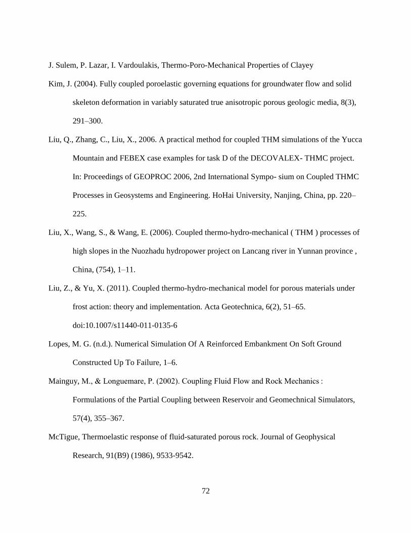
72
J. Sulem, P. Lazar, I. Vardoulakis, Thermo-Poro-Mechanical Properties of Clayey
Kim, J. (2004). Fully coupled poroelastic governing equations for groundwater flow and solid
skeleton deformation in variably saturated true anisotropic porous geologic media, 8(3),
291–300.
Liu, Q., Zhang, C., Liu, X., 2006. A practical method for coupled THM simulations of the Yucca
Mountain and FEBEX case examples for task D of the DECOVALEX- THMC project.
In: Proceedings of GEOPROC 2006, 2nd International Sympo- sium on Coupled THMC
Processes in Geosystems and Engineering. HoHai University, Nanjing, China, pp. 220–
225.
Liu, X., Wang, S., & Wang, E. (2006). Coupled thermo-hydro-mechanical ( THM ) processes of
high slopes in the Nuozhadu hydropower project on Lancang river in Yunnan province ,
China, (754), 1–11.
Liu, Z., & Yu, X. (2011). Coupled thermo-hydro-mechanical model for porous materials under
frost action: theory and implementation. Acta Geotechnica, 6(2), 51–65.
doi:10.1007/s11440-011-0135-6
Lopes, M. G. (n.d.). Numerical Simulation Of A Reinforced Embankment On Soft Ground
Constructed Up To Failure, 1–6.
Mainguy, M., & Longuemare, P. (2002). Coupling Fluid Flow and Rock Mechanics :
Formulations of the Partial Coupling between Reservoir and Geomechnical Simulators,
57(4), 355–367.
McTigue, Thermoelastic response of fluid-saturated porous rock. Journal of Geophysical
Research, 91(B9) (1986), 9533-9542.
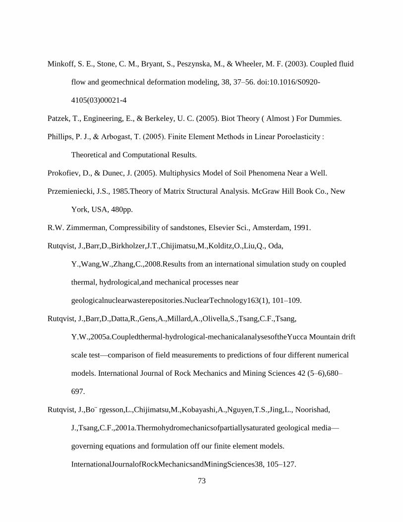
73
Minkoff, S. E., Stone, C. M., Bryant, S., Peszynska, M., & Wheeler, M. F. (2003). Coupled fluid
flow and geomechnical deformation modeling, 38, 37–56. doi:10.1016/S0920-
4105(03)00021-4
Patzek, T., Engineering, E., & Berkeley, U. C. (2005). Biot Theory ( Almost ) For Dummies.
Phillips, P. J., & Arbogast, T. (2005). Finite Element Methods in Linear Poroelasticity :
Theoretical and Computational Results.
Prokofiev, D., & Dunec, J. (2005). Multiphysics Model of Soil Phenomena Near a Well.
Przemieniecki, J.S., 1985.Theory of Matrix Structural Analysis. McGraw Hill Book Co., New
York, USA, 480pp.
R.W. Zimmerman, Compressibility of sandstones, Elsevier Sci., Amsterdam, 1991.
Rutqvist, J.,Barr,D.,Birkholzer,J.T.,Chijimatsu,M.,Kolditz,O.,Liu,Q., Oda,
Y.,Wang,W.,Zhang,C.,2008.Results from an international simulation study on coupled
thermal, hydrological,and mechanical processes near
geologicalnuclearwasterepositories.NuclearTechnology163(1), 101–109.
Rutqvist, J.,Barr,D.,Datta,R.,Gens,A.,Millard,A.,Olivella,S.,Tsang,C.F.,Tsang,
Y.W.,2005a.Coupledthermal-hydrological-mechanicalanalysesoftheYucca Mountain drift
scale test—comparison of field measurements to predictions of four different numerical
models. International Journal of Rock Mechanics and Mining Sciences 42 (5–6),680–
697.
Rutqvist, J.,Bo¨ rgesson,L.,Chijimatsu,M.,Kobayashi,A.,Nguyen,T.S.,Jing,L., Noorishad,
J.,Tsang,C.F.,2001a.Thermohydromechanicsofpartiallysaturated geological media—
governing equations and formulation off our finite element models.
InternationalJournalofRockMechanicsandMiningSciences38, 105–127.
74
Rutqvist, J.,Chijimatsu,M.,Jing,L.,DeJonge,J.,Kohlmeier,M.,Millard,A.,Nguyen,
T.S.,Rejeb,A.,Souley,M.,Sugita,Y.,Tsang,C.F.,2005b.Numerical study of the THM
effects on the near-field safety of hypothetical nuclear waste repository—BMT1
oftheDECOVALEXIIIproject,Part3:effectsofTHM coupling. In fractured rock.
International Journal of Rock Mechanics and Mining Sciences 42,745–755.
Sanavia, L. (2008). Numerical modelling of a slope stability test by means of porous media
mechanics.
Sedano, J. A. I., Evgin, E., & Fu, Z. (2011). A Coupled Analysis of Heat and Moisture Transfer
in Soils, (1).
V. Palciauskas, P.A. Domenico, Characterization of drained and undrained response of thermally
loaded repository rocks. Water Resources Research, 18(1982), No. 2,281-290.
Wang, P., Yotov, I., Wheeler, M., Arbogast, T., Dawson, C., Parashar, M., Sepehrnoori, K.,
1997. A new generation EOS compositional reservoir simulator: Part I. Formulation and
discretization. Proceedings of the 14th Reservoir Simulation Symposium, No. 37979.
SPE, Richardson, TX.
Wang, W., Kosakowski, G., & Kolditz, O. (2009). Computers & Geosciences a parallel finite
element scheme for thermo-hydro-mechanical (THM) coupled problems in porous media,
35, 1631–1641. doi:10.1016/j.cageo.2008.07.007
Wellman, G.W., 1999. MAPVAR—a computer program to transfer solution data between finite
elements meshes. Technical Report, SAND99-0466, Sandia National Labs, Albuquerque,
NM.
75
Wheeler, M., Arbogast, T., Bryant, S., Eaton, J., Lu, Q., Peszynska, M., Yotov, I., 1999. A
parallel multiblock/multidomain approach for reservoir simulation. Proceedings of the
15th Reservoir. Simulation Symposium, No. 51884. SPE, Richardson, TX,pp. 51– 61.
Wheeler, M., Wheeler, J., Peszynska, M., 2000. A distributed computing portal for coupling
multi-physics and multiple domains in porous media.
Yale, D. P., & Upstream, E. (2002). SPE / ISRM 78202 Coupled Geomechanics-Fluid Flow
Modeling : Effects of Plasticity and Permeability Alteration.
Zheng, Y., Burridge, R., & Burns, D. (1955). Reservoir Simulation with the Finite Element
Method Using Biot Poroelastic Approach (pp. 1–20).
Zvanut, P. (2003). Settlements of an Embankment Founded On a Soft Soil.


