Multi-Platform Compatible Software for Analysis ofPolymer Bending MechanicsJohn S. Graham., Brannon R. McCullough.¤, Hyeran Kang, W. Austin Elam, Wenxiang Cao,

Enrique M. De La Cruz*

Department of Molecular Biophysics and Biochemistry, Yale University, New Haven, Connecticut, United States of America

Abstract

Cytoskeletal polymers play a fundamental role in the responses of cells to both external and internal stresses. Quantitativeknowledge of the mechanical properties of those polymers is essential for developing predictive models of cell mechanicsand mechano-sensing. Linear cytoskeletal polymers, such as actin filaments and microtubules, can grow to cellular lengthscales at which they behave as semiflexible polymers that undergo thermally-driven shape deformations. Bendingdeformations are often modeled using the wormlike chain model. A quantitative metric of a polymer’s resistance tobending is the persistence length, the fundamental parameter of that model. A polymer’s bending persistence length isextracted from its shape as visualized using various imaging techniques. However, the analysis methodologies required fordetermining the persistence length are often not readily within reach of most biological researchers or educators. Motivatedby that limitation, we developed user-friendly, multi-platform compatible software to determine the bending persistencelength from images of surface-adsorbed or freely fluctuating polymers. Three different types of analysis are available (cosinecorrelation, end-to-end and bending-mode analyses), allowing for rigorous cross-checking of analysis results. The software isfreely available and we provide sample data of adsorbed and fluctuating filaments and expected analysis results foreducational and tutorial purposes.

Citation: Graham JS, McCullough BR, Kang H, Elam WA, Cao W, et al. (2014) Multi-Platform Compatible Software for Analysis of Polymer Bending Mechanics. PLoSONE 9(4): e94766. doi:10.1371/journal.pone.0094766

Editor: Monica Soncini, Politecnico di Milano, Italy

Received October 9, 2013; Accepted March 19, 2014; Published April 16, 2014

Copyright: � 2014 Graham et al. This is an open-access article distributed under the terms of the Creative Commons Attribution License, which permitsunrestricted use, distribution, and reproduction in any medium, provided the original author and source are credited.

Funding: This work was supported by National Institutes of Health Grant RO1-GM097348 and American Heart Association Established Investigator Award0655849T awarded to E.M.D.L.C. B.R.M. was partially supported by American Heart Association predoctoral award No. 09PRE2230014. The funders had no role instudy design, data collection and analysis, decision to publish, or preparation of the manuscript.

Competing Interests: The authors have declared that no competing interests exist.

* E-mail: enrique.delacruz@yale.edu

¤ Current address: Department of Biomedical Engineering, University of Minnesota, Minneapolis, Minnesota, United States of America

. These authors contributed equally to this work.

Introduction

Biological systems must respond to mechanical stresses and

strains in a manner that does not compromise their function. In

some cases those responses also regulate cellular processes. For

example, cytoskeletal polymers such as microtubules and actin

filaments, provide cells with structural integrity and organization,

generate forces that drive cell motility [1,2], and play essential

roles in cellular mechano-sensing [3]. To gain insight into how

cytoskeletal filaments and higher-order structures, such as bundles

and networks, provide mechanical responses and forces, it is

necessary to quantify the intrinsic mechanical properties of

individual filaments.

Cytoskeletal filaments display elastic properties between rigid

rods and fully flexible polymers, and thus fall into the category of

‘‘semiflexible’’ polymers. The ‘‘wormlike chain’’ model is com-

monly used to describe semiflexible polymer mechanics and

considers the end-to-end distance of a linear, unbranched polymer

as a sum of unit vectors tangent to the polymer chain [4]. This

model is characterized by a fundamental parameter [5], the

bending persistence length (Lp), that is extracted from analysis of

the polymer’s bending energy and the directional correlation of

the unit tangent vectors.

The bending persistence length provides a useful quantitative

measure of a polymer’s bending rigidity. The Lp is the segment

length below which a polymer can be approximated as a rigid rod.

Mathematically, Lp is defined [4]:

Lp~k

kTð1Þ

where k is the effective flexural rigidity of the polymer and kT is

the thermal energy. We note that equation (1) does not consider

contributions from coupling between deformations, such as

twisting, that may contribute to the effective flexural rigidity [6].

Many investigations of polymer mechanics using the wormlike

chain model involve specialized measurement and analysis

techniques that are often not readily within reach of most

educators or biological researchers. Further, to our knowledge,

there is no commercially available software package for perform-

ing analyses of polymer bending mechanics. Motivated by those

facts, we developed software, Persistence, to determine the bending

Lp of biopolymers from images of surface-adsorbed or freely

fluctuating macromolecules. Those images can be obtained from

atomic force microscopy, electron microscopy, fluorescence

imaging or any other available imaging method.

PLOS ONE | www.plosone.org 1 April 2014 | Volume 9 | Issue 4 | e94766

To foster the broadest possible accessibility, we created a user-

friendly graphical interface to facilitate entry of initial variable

values and analysis commands, and made it multi-platform

compatible and freely available (see File S1). Sample data for

tutorial or educational use is included with the software.

Description of Persistence Software

Pre-ProcessingFor Persistence to function effectively, images of the filaments to

be analyzed must be processed to remove noise and enhance the

prominence of filament shapes. ImageJ [7] can be used for that

purpose, although any other image processing software should

work just as well. A general algorithm includes five steps:

background subtraction, smoothing, contrast enhancement,

thresholding and skeletonization. Background subtraction and

smoothing reduce the noise levels in the image. Smoothing is

particularly important for noisy images as it effectively averages

out background noise to a low enough level that it will not interfere

with the skeletonization and final analysis. Many filtering methods

are available, depending on the image processing software. For

our analyses of actin filaments, a Gaussian blur filter has worked

best, but that may not always be the case.

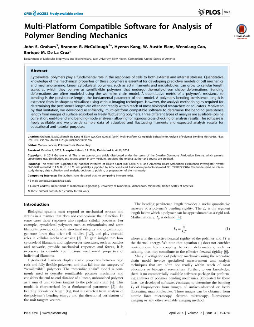
The final three adjustments (contrast enhancement, threshold-

ing and skeletonization) enhance prominence of filament shapes so

that the software can efficiently track them (Figureso 1 and 2Ao &

B). Contrast enhancement optimizes the signal-to-noise ratio and

normalizes the signal for processing and visualization. Threshold-

ing enhances the background subtraction by limiting pixel values

to a selected range. Care should be taken when adjusting threshold

values to ensure that artificial gaps or branches are minimized

(Figureo 1). Skeletonization does two things to the image. First, it

converts the image to a binary format so that pixel values are

either 0 or 255 for an RGB image, effectively on (255) or off (0).

For that reason, it is especially important that as much ‘‘noise’’ as

possible be removed from the image. Second, skeletonization pares

down the filament shapes to a single pixel width so that they can

be easily tracked by the tracking algorithm in the Persistence

software. Throughout pre-processing, it is important to compare

the processed image with the original after each processing step.

Such crosschecking allows for immediate correction of processing

artifacts that may arise, such as the artificial gaps or branches

mentioned above.

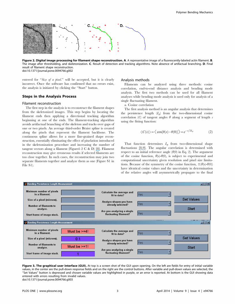
The Graphical User InterfaceLayout. The function of the graphical user interface (GUI) is

to allow for easy entry of variables and instructions necessary for

subsequent analysis. Numerical variables are defined in the

column of boxes on the left side of the GUI (Figureo 3A). When

the values are set, the boxes report either the entered variable

values or an error if the value is outside parameter limits

(Figureo 3B). In the center of the GUI are yes/no questions to be

answered based on the type of analysis desired, and on the right

are buttons to confirm the values entered and to start the analysis.

Variable definitions. Four variables must be set prior to

analysis:

a. ‘‘Minimum number of pixels in a filament.’’ is the minimum length

of the filament/polymer and must be at least 4.

b. ‘‘Size of a pixel.’’ is the size, in microns, of a single camera pixel

under the magnification of the instrument.

c. ‘‘Number of filaments to analyze.’’ is the number of filaments to be

used for analysis. The program searches for filament ends

beginning at the bottom left of the image, reading each row of

pixels from left to right, proceeding from bottom to top. To

include all filaments in an image stack, enter inf (‘). The analysis

time depends on the total number of filaments. The potential exists

to overload memory available for the program if too many

filaments are selected. We recommend starting with 100 to 200

filaments.

d. ‘‘Start frame of image stack.’’ is the frame number of the image

stack on which to begin loading images into the software. This is

useful for the serial analysis of a large image stack. The program

can be aborted during filament selection and all images selected up

to that time will be used for analysis.

Preliminary processing instructions. a. ‘‘Calculate the

average and fit to data?’’ should be set to ‘‘Yes’’ if a final cosine

correlation fit is desired. The fit generated by Persistence is a

reasonable estimate of the results. However, independent analysis

should be performed with a nonlinear regression program.

b. ‘‘Analyze shapes you have already selected?’’ should be set to ‘‘Yes’’

if filament shapes previously selected from an image stack will be

reanalyzed using the same input parameters. This feature was

implemented to prevent the user from having to reselect filament

shapes in the event of a computer crash while calculating

information from the filament shapes already selected (data is not

saved if the crash occurs during the selection process).

c. ‘‘Are you analyzing a single fluctuating filament?’’ should be set to

‘‘Yes’’ if a single filament fluctuating freely in solution will be

analyzed.

Initialization of analysis. Once the variable and prelimi-

nary instructions are entered in the GUI, the chosen values are set

in the software by clicking the ‘‘Set Values’’ button. The numerical

variable column either confirms the values entered or presents an

error message (Figureo 3B). If there is an error message, that

variable value must be changed so that it is within the allowed

parameters. As long as the value entered is numerical, the only

possible errors are in the ‘‘Minimum number of pixels…’’ variable

which must be $4, or the ‘‘Number of filaments…’’ variable which

must be $1. Importantly, the software cannot determine if the

entered values are reasonable. For example, a value of 1000 mm

Figure 1. The effect of thresholding on filament skeletonization. A. Original image. B. Image skeletonized with proper thresholding. C.Image with superfluous branches due to improper thresholding. In this case the threshold is too high. D. Image with fragmented filaments due toimproper thresholding in the opposite extreme from panel C, i.e. threshold set too low. Scale bar is 3 mm.doi:10.1371/journal.pone.0094766.g001

Polymer Bending Mechanics

PLOS ONE | www.plosone.org 2 April 2014 | Volume 9 | Issue 4 | e94766

entered for ‘‘Size of a pixel.’’ will be accepted, but it is clearly

incorrect. Once the software has confirmed that no errors exist,

the analysis is initiated by clicking the ‘‘Start’’ button.

Steps in the Analysis Process

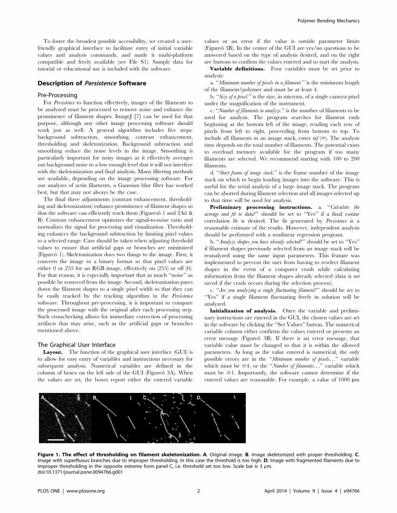
Filament reconstructionThe first step in the analysis is to reconstruct the filament shapes

from the skeletonized images. This step begins by locating the

filament ends then applying a directional tracking algorithm

beginning at one of the ends. The filament-tracking algorithm

avoids artifactual branching of the skeleton and tracks over gaps of

one or two pixels. An average third-order Bezier spline is created

along the pixels that represent the filament backbone. The

continuous spline allows for a more fine-grained shape recon-

struction, essentially eliminating the effect of pixelation introduced

in the skeletonization procedure and increasing the number of

tangent vectors along a filament (Figureo 2 C & D) [8]. Filament

reconstruction may give erroneous results if selected filaments are

too close together. In such cases, the reconstruction may join two

separate filaments together and analyze them as one (Figure S1 in

File S1).

Analysis methodsFilaments can be analyzed using three methods: cosine

correlation, end-to-end distance analysis and bending mode

analysis. The first two methods can be used for all filament

analyses while bending mode analysis is used only for analysis of a

single fluctuating filament.

a. Cosine correlation

The first analysis method is an angular analysis that determines

the persistence length (Lp) from the two-dimensional cosine

correlation (C) of tangent angles h along a segment of length s

using the fitting function:

SC sð ÞT~S cos h sð Þ�h 0ð Þ½ �T~e�s�

2Lp ð2Þ

That function determines Lp from two-dimensional shape

fluctuations [8,9]. The angular correlation is determined with

respect to an initial reference angle (h(0) in Eq. 2). The argument

of the cosine function, h(s)-h(0), is subject to experimental and

computational uncertainty given resolution and pixel size limita-

tions. Because of the symmetry of the cosine function, 6(h(s)-h(0))

have identical cosine values and the uncertainty in determination

of the relative angles will asymmetrically propagate to the final

Figure 2. Digital image processing for filament shape reconstruction. A. A representative image of a fluorescently-labeled actin filament. B.The image after thresholding, and skeletonization. C. Result of detection and tracking algorithms. Note absence of artifactual branching. D. Finalresult of filament shape reconstruction.doi:10.1371/journal.pone.0094766.g002

Figure 3. The graphical user interface (GUI). At top is a screen shot of the GUI upon opening. On the left are fields for entry of initial variablevalues, in the center are the pull-down response fields and on the right are the control buttons. After variable and pull-down values are selected, the‘‘Set Values’’ button is depressed and chosen variable values are highlighted in purple, or an error is reported. At bottom is the GUI showing dataentered with errors resulting from invalid values.doi:10.1371/journal.pone.0094766.g003

Polymer Bending Mechanics

PLOS ONE | www.plosone.org 3 April 2014 | Volume 9 | Issue 4 | e94766

cosine value. Therefore, the resultant cosine value will be lower

than the actual value (Figure S2 in File S1). This uncertainty can

be accounted for by fitting data to an exponential, Ae�s�

2Lp,

without constraining the decay amplitude or correlation to unity

when the segment length approaches zero. For freely fluctuating

filaments, measures must be taken to ensure that fluctuations are

constrained to two dimensions [10].

b. End-to-end distance analysis

The second analysis fits the mean square end-to-end distance

(,R2.) as a function of the contour length (L) to the equation

[11,12],

SR2T~2L2p e�L=Lp�1zL

�Lp

� �ð3Þ

from which Lp can be directly extracted. This method is less

accurate than the cosine correlation analysis, but serves as a useful

verification. However, since this method considers only the global

geometry of an individual filament, each filament analyzed

represents a single data point. Therefore, end-to-end analysis

requires a larger number of filaments than cosine correlation

analysis to obtain a statistically significant sample.

c. Bending mode analysis

The additional analysis for single fluctuating filaments deter-

mines the angular bending modes of a filament determined

through Fourier analysis of the filament shape. The amplitudes (a)

of the bending modes (an, where n is the bending mode number 1,

2, 3…10) are used to calculate the persistence length using [9]:

Lp~L2

n2p2var(an)ð4Þ

Effect of Initial Input on Results

Persistence requires a minimal number of input parameters to

function properly. Those parameters (shown in Figureo 3) are

customizable; facilitating its use for diverse applications. The

impact of those parameters on the collection and analysis of data is

straight-forward but critical for obtaining meaningful results. In

particular, two variable values have a crucial impact on processing

and the final results; pixel threshold (Minimum number of pixels in a

filament.) and pixel size (Size of a pixel.).

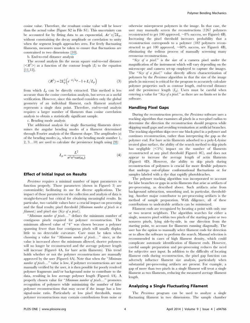
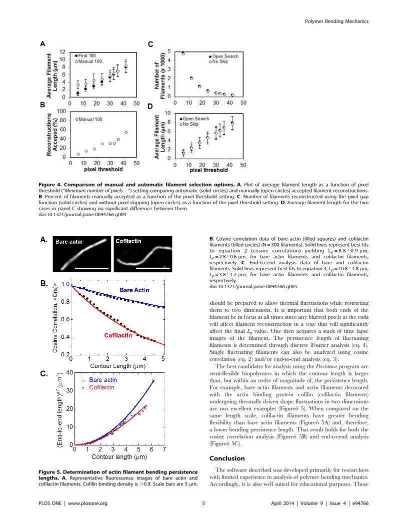
‘‘Minimum number of pixels…’’ defines the minimum number of

contiguous pixels required for polymer reconstruction. The

minimum allowed value of ‘‘4’’ was chosen because a polymer

spanning fewer than four contiguous pixels will usually display

little to no detectable curvature. Care must be taken when

choosing a value for ‘‘Minimum number of pixels…’’ since, as the

value is increased above the minimum allowed, shorter polymers

will no longer be reconstructed and the average polymer length

will increase (Figureo 4A, for bare actin filaments). This trend

holds whether or not the polymer reconstructions are manually

approved by the user (Figureo 4A). Note that when the ‘‘Minimum

number of pixels…’’ value is low, if polymer reconstructions are not

manually verified by the user, it is then possible for poorly resolved

polymer fragments and/or background noise to contribute to the

data, resulting in low average polymer length (Figureo 4A). A

properly chosen value for ‘‘Minimum number of pixels…’’ promotes

recognition of polymers while minimizing the number of false

polymer reconstructions that may occur if the image has a low

signal-noise ratio. Particularly at low pixel thresholds, many

polymer reconstructions may contain contributions from noise or

otherwise misrepresent polymers in the image. In that case, the

user may manually screen the reconstructions (1267 polymers

reconstructed to get 100 approved, ,8% success, see Figureo 4B).

Increasing the pixel threshold increases probability that a

reconstruction corresponds to a polymer (182 polymers recon-

structed to get 100 approved, ,60% success, see Figureo 4B),

eliminating the tedious process of manually screening many

erroneous reconstructions.

‘‘Size of a pixel.’’ is the size of a camera pixel under the

magnification of the instrument which will vary depending on the

microscope and camera set-up employed to capture the images.

The ‘‘Size of a pixel.’’ value directly affects characterization of

polymers by the Persistence algorithm in that the size of the image

pixels (in microns) is critical for the program to accurately calculate

polymer properties such as contour length, end-to-end distance

and the persistence length (Lp). Users must be careful when

entering a value for ‘‘Size of a pixel.’’ as there are no limits set in the

software.

Handling Pixel Gaps

During the reconstruction process, the Persistence software uses a

tracking algorithm that examines all pixels in a two-pixel radius to

determine the direction the reconstruction should progress while

skipping small gaps and avoiding termination at artificial branches.

The tracking algorithm skips over one black pixel in a polymer and

continues reconstruction, rather than interpreting the gap as the

polymer end. For bare actin filaments adsorbed to a poly-L-lysine

treated glass surface, the ability of the search method to skip pixels

has negligible (,5%) impact on the number of filaments

reconstructed at any pixel threshold (Figureo 4C), and does not

appear to increase the average length of actin filaments

(Figureo 4D). However, the ability to skip pixels during

reconstruction of polymers is crucial for more flexible polymers

that undergo out-of-plane conformational fluctuations or for

samples labeled with a dye that rapidly photobleaches.

The polymer tracking algorithm was incorporated to account

for false branches or gaps in actin filaments that arise as artifacts of

pre-processing, as described above. Such artifacts arise from

background subtraction, smoothing and, in particular, threshold-

ing. Another major contributor to pre-processing artifacts is the

method of sample preparation. With diligence, all of these

contributions to undesirable artifacts can be minimized.

Filament ends are recognized by locating a point with only one

or two nearest neighbors. The algorithm searches for either a

single, nonzero pixel within two pixels of the starting point or two

nonzero pixels, lying side-by-side, in one direction from the

starting point, to account for filaments running diagonally. The

user has the option to manually select filament ends for detection

or to allow the software to perform the search. Manual selection is

recommended in cases of high filament density, which could

complicate automatic identification of filament ends. However,

careful sample preparation and pre-processing reduces the need

for subjective user input. In addition to the difficulty of locating

filament ends during reconstruction, the pixel gap function can

adversely influence filament size analysis, particularly when

substantial pre-processing artifacts are present. For example, a

gap of more than two pixels in a single filament will treat a single

filament as two filaments, reducing the measured average filament

length.

Analyzing a Single Fluctuating Filament

The Persistence program can be used to analyze a single

fluctuating filament in two dimensions. The sample chamber

Polymer Bending Mechanics

PLOS ONE | www.plosone.org 4 April 2014 | Volume 9 | Issue 4 | e94766

should be prepared to allow thermal fluctuations while restricting

them to two dimensions. It is important that both ends of the

filament be in focus at all times since any blurred pixels at the ends

will affect filament reconstruction in a way that will significantly

affect the final Lp value. One then acquires a stack of time lapse

images of the filament. The persistence length of fluctuating

filaments is determined through discrete Fourier analysis (eq. 4).

Single fluctuating filaments can also be analyzed using cosine

correlation (eq. 2) and/or end-to-end analysis (eq. 3).

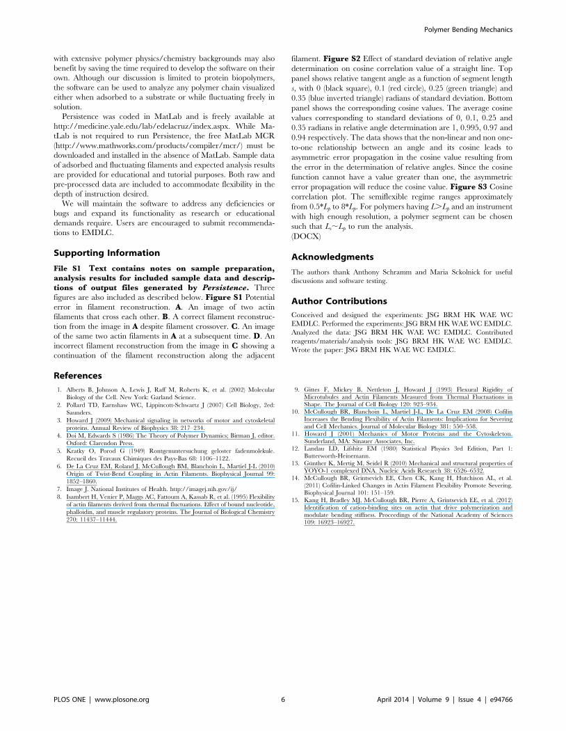
The best candidates for analysis using the Persistence program are

semi-flexible biopolymers in which the contour length is larger

than, but within an order of magnitude of, the persistence length.

For example, bare actin filaments and actin filaments decorated

with the actin binding protein cofilin (cofilactin filaments)

undergoing thermally driven shape fluctuations in two dimensions

are two excellent examples (Figureo 5). When compared on the

same length scale, cofilactin filaments have greater bending

flexibility than bare actin filaments (Figureo 5A) and, therefore,

a lower bending persistence length. That result holds for both the

cosine correlation analysis (Figureo 5B) and end-to-end analysis

(Figureo 5C).

Conclusion

The software described was developed primarily for researchers

with limited experience in analysis of polymer bending mechanics.

Accordingly, it is also well suited for educational purposes. Those

Figure 4. Comparison of manual and automatic filament selection options. A. Plot of average filament length as a function of pixelthreshold (‘‘Minimum number of pixels…’’) setting comparing automatic (solid circles) and manually (open circles) accepted filament reconstructions.B. Percent of filaments manually accepted as a function of the pixel threshold setting. C. Number of filaments reconstructed using the pixel gapfunction (solid circles) and without pixel skipping (open circles) as a function of the pixel threshold setting. D. Average filament length for the twocases in panel C showing no significant difference between them.doi:10.1371/journal.pone.0094766.g004

Figure 5. Determination of actin filament bending persistencelengths. A. Representative fluorescence images of bare actin andcofilactin filaments. Cofilin binding density is .0.9. Scale bars are 5 mm.

B. Cosine correlation data of bare actin (filled squares) and cofilactinfilaments (filled circles) (N = 300 filaments). Solid lines represent best fitsto equation 2 (cosine correlation) yielding Lp = 8.860.9 mm,Lp = 2.860.6 mm, for bare actin filaments and cofilactin filaments,respectively. C. End-to-end analysis data of bare and cofilactinfilaments. Solid lines represent best fits to equation 3, Lp = 10.861.8 mm,Lp = 3.861.2 mm, for bare actin filaments and cofilactin filaments,respectively.doi:10.1371/journal.pone.0094766.g005

Polymer Bending Mechanics

PLOS ONE | www.plosone.org 5 April 2014 | Volume 9 | Issue 4 | e94766

with extensive polymer physics/chemistry backgrounds may also

benefit by saving the time required to develop the software on their

own. Although our discussion is limited to protein biopolymers,

the software can be used to analyze any polymer chain visualized

either when adsorbed to a substrate or while fluctuating freely in

solution.

Persistence was coded in MatLab and is freely available at

http://medicine.yale.edu/lab/edelacruz/index.aspx. While Ma-

tLab is not required to run Persistence, the free MatLab MCR

(http://www.mathworks.com/products/compiler/mcr/) must be

downloaded and installed in the absence of MatLab. Sample data

of adsorbed and fluctuating filaments and expected analysis results

are provided for educational and tutorial purposes. Both raw and

pre-processed data are included to accommodate flexibility in the

depth of instruction desired.

We will maintain the software to address any deficiencies or

bugs and expand its functionality as research or educational

demands require. Users are encouraged to submit recommenda-

tions to EMDLC.

Supporting Information

File S1 Text contains notes on sample preparation,analysis results for included sample data and descrip-tions of output files generated by Persistence. Three

figures are also included as described below. Figure S1 Potential

error in filament reconstruction. A. An image of two actin

filaments that cross each other. B. A correct filament reconstruc-

tion from the image in A despite filament crossover. C. An image

of the same two actin filaments in A at a subsequent time. D. An

incorrect filament reconstruction from the image in C showing a

continuation of the filament reconstruction along the adjacent

filament. Figure S2 Effect of standard deviation of relative angle

determination on cosine correlation value of a straight line. Top

panel shows relative tangent angle as a function of segment length

s, with 0 (black square), 0.1 (red circle), 0.25 (green triangle) and

0.35 (blue inverted triangle) radians of standard deviation. Bottom

panel shows the corresponding cosine values. The average cosine

values corresponding to standard deviations of 0, 0.1, 0.25 and

0.35 radians in relative angle determination are 1, 0.995, 0.97 and

0.94 respectively. The data shows that the non-linear and non one-

to-one relationship between an angle and its cosine leads to

asymmetric error propagation in the cosine value resulting from

the error in the determination of relative angles. Since the cosine

function cannot have a value greater than one, the asymmetric

error propagation will reduce the cosine value. Figure S3 Cosine

correlation plot. The semiflexible regime ranges approximately

from 0.5*Lp to 8*Lp. For polymers having L.Lp and an instrument

with high enough resolution, a polymer segment can be chosen

such that Ls,Lp to run the analysis.

(DOCX)

Acknowledgments

The authors thank Anthony Schramm and Maria Sckolnick for useful

discussions and software testing.

Author Contributions

Conceived and designed the experiments: JSG BRM HK WAE WC

EMDLC. Performed the experiments: JSG BRM HK WAE WC EMDLC.

Analyzed the data: JSG BRM HK WAE WC EMDLC. Contributed

reagents/materials/analysis tools: JSG BRM HK WAE WC EMDLC.

Wrote the paper: JSG BRM HK WAE WC EMDLC.

References

1. Alberts B, Johnson A, Lewis J, Raff M, Roberts K, et al. (2002) Molecular

Biology of the Cell. New York: Garland Science.

2. Pollard TD, Earnshaw WC, Lippincott-Schwartz J (2007) Cell Biology, 2ed:

Saunders.

3. Howard J (2009) Mechanical signaling in networks of motor and cytoskeletal

proteins. Annual Review of Biophysics 38: 217–234.

4. Doi M, Edwards S (1986) The Theory of Polymer Dynamics; Birman J, editor.

Oxford: Clarendon Press.

5. Kratky O, Porod G (1949) Rontgenuntersuchung geloster fadenmolekule.

Recueil des Travaux Chimiques des Pays-Bas 68: 1106–1122.

6. De La Cruz EM, Roland J, McCullough BM, Blanchoin L, Martiel J-L (2010)

Origin of Twist-Bend Coupling in Actin Filaments. Biophysical Journal 99:

1852–1860.

7. Image J. National Institutes of Health. http://imagej.nih.gov/ij/

8. Isambert H, Venier P, Maggs AC, Fattoum A, Kassab R, et al. (1995) Flexibility

of actin filaments derived from thermal fluctuations. Effect of bound nucleotide,

phalloidin, and muscle regulatory proteins. The Journal of Biological Chemistry

270: 11437–11444.

9. Gittes F, Mickey B, Nettleton J, Howard J (1993) Flexural Rigidity ofMicrotubules and Actin Filaments Measured from Thermal Fluctuations in

Shape. The Journal of Cell Biology 120: 923–934.10. McCullough BR, Blanchoin L, Martiel J-L, De La Cruz EM (2008) Cofilin

Increases the Bending Flexibility of Actin Filaments: Implications for Severingand Cell Mechanics. Journal of Molecular Biology 381: 550–558.

11. Howard J (2001) Mechanics of Motor Proteins and the Cytoskeleton.

Sunderland, MA: Sinauer Associates, Inc.12. Landau LD, Lifshitz EM (1980) Statistical Physics 3rd Edition, Part 1:

Butterworth-Heinemann.13. Gunther K, Mertig M, Seidel R (2010) Mechanical and structural properties of

YOYO-1 complexed DNA. Nucleic Acids Research 38: 6526–6532.

14. McCullough BR, Grintsevich EE, Chen CK, Kang H, Hutchison AL, et al.(2011) Cofilin-Linked Changes in Actin Filament Flexibility Promote Severing.

Biophysical Journal 101: 151–159.15. Kang H, Bradley MJ, McCullough BR, Pierre A, Grintsevich EE, et al. (2012)

Identification of cation-binding sites on actin that drive polymerization and

modulate bending stiffness. Proceedings of the National Academy of Sciences109: 16923–16927.

Polymer Bending Mechanics

PLOS ONE | www.plosone.org 6 April 2014 | Volume 9 | Issue 4 | e94766