Elsevier Editorial System(tm) for Physics of the Earth and Planetary Interiors Manuscript Draft

Manuscript Number: PEPI-D-07-00301R1

Title: Multiple resolution seismic attenuation imaging at Mt. Vesuvius

Article Type: Research Paper

Keywords: Attenuation tomography, Mt. Vesuvius, Coda normalization method, Spectral slope, Multi resolution inversion

Corresponding Author: Edoardo Del Pezzo, Dr.

Corresponding Author's Institution: INGV - Osservatorio Vesuviano

First Author: Luca De Siena

Order of Authors: Luca De Siena; Edoardo Del Pezzo; Francesca Bianco; Anna Tramelli

Abstract: A three-dimensional S wave attenuation tomography of Mt. Vesuvius has been obtained with multiple measurements of coda-normalized S-wave spectra of local small magnitude earthquakes. We used 6609 waveforms, relative to 826 volcano-tectonic earthquakes, located close to the crater axis in a depth range between 1 and 4 km (below the sea level), recorded at seven 3-component digital seismic stations. We adopted a two-point ray-tracing; rays were traced in an high resolution 3-D velocity model. The spatial resolution achieved in the attenuation tomography is comparable with that of the velocity tomography (we resolve 300 m side cubic cells). We statistically tested that the results are almost independent from the radiation pattern. We also applied an improvement of the ordinary spectral-slope method to both P- and S-waves, assuming that the differences between the theoretical and the experimental high frequency spectral-slope are only due to the attenuation effects. We could check the coda-normalization method comparing the S attenuation image obtained with the two methods. The images were obtained with a multiple resolution approach. Results show the general coincidence of low attenuation with high velocity zones. The joint interpretation of velocity and attenuation images allows us to interpret the low attenuation zone intruding toward the surface until a depth of 500 meters below the sea level as related to the residual part of solidified magma from the last eruption. In the depth range between -700 and -2300 meters above sea level, the images are consistent with the presence of multiple acquifer layers. No evidence of magma patches greater than the minimum cell dimension (300m) has been found. A shallow P wave attenuation anomaly (beneath the southern flank of the volcano) is consitent with the presence of gas saturated rocks. The zone characterized by the maximum seismic energy release cohincides with a high attenuation and low velocity volume, interpreted as a cracked medium.

A three-dimensional S wave attenuation tomography of Mt. Vesuvius has been obtained with multiple measurements of coda-normalized S-wave spectra of local small magnitude earthquakes. We used 6609 waveforms, relative to 826 volcano-tectonic earthquakes, located close to the crater axis in a depth range between 1 and 4 km (below the sea level), recorded at seven 3-component digital seismic stations. We adopted a two-point ray-tracing; rays were traced in an high resolution 3-D velocity model. The spatial resolution achieved in the attenuation tomography is comparable with that of the velocity tomography (we resolve 300 m side cubic cells). We statistically tested that the results are almost independent from the radiation pattern. We also applied an improvement of the ordinary spectral-slope method to both P- and S-waves, assuming that the differences between the theoretical and the experimental high frequency spectral-slope are only due to the attenuation effects. We could check the coda-normalization method comparing the S attenuation image obtained with the two methods. The images were obtained with a multiple resolution approach. Results show the general coincidence of low attenuation with high velocity zones. The joint interpretation of velocity and attenuation images allows us to interpret the low attenuation zone intruding toward the surface until a depth of 500 meters below the sea level as related to the residual part of solidified magma from the last eruption. In the depth range between -700 and -2300 meters above sea level, the images are consistent with the presence of multiple acquifer layers. No evidence of magma patches greater than the minimum cell dimension (300m) has been found. A shallow P wave attenuation anomaly (beneath the southern flank of the volcano) is consitent with the presence of gas saturated rocks. The zone characterized by the maximum seismic energy release cohincides with a high attenuation and low velocityvolume, interpreted as a cracked medium.

Abstract

MS. REF. NO.: PEPI-D-07-00301 TITLE: MULTIPLE RESOLUTION SEISMIC ATTENUATION IMAGING AT MT. VESUVIUS PHYSICS OF THE EARTH AND PLANETARY INTERIORS

Dear Editor,First of all we want to thank both reviewers for the suggestions, which were really useful to improve the paper quality, and in particular the graphical representation of the results obtained.We took into account all the suggestions made by both reviewers. We also answer to the questions raised, to better clarify how we corrected the paper. We specify all the points, starting from those raised by Referee 2.One of the main point to be addressed is the improving of all the synthetic tests. We hence decided to a) include in the article a synthetic anomaly test; b) to explicitly show the checkerboard test; c) to mark the high resolution volume enlightening the test results inside this zone. Another important point was the discussion of the results, too short and concisein the first version. We re-wrote completely all this stuff, trying to explicitly illustrate in detail our interpretation.The other major comment regards the effective resolution of our method (300 m). We follow an empirical rule, that the wavelength must be lower than a half of the minimum cell size. Moreover, we consider for the interpretation only those cell crossed by a number of rays defined by the empirical equation (14). The question arisen by rev. 3 about the formal correctness of formula (14) is right. With the decreasing of the cell size, the minimum number of rays passing through the cell also decreases. Anyway, this number is never lower than 4. We have empirically observed that this number ensures stable results. So, we are confident that, even with a decreasing resolution, the results do not represent ghost images.

All the other minor points have been fully addressed, as reported in the following list, in which in capital letters there is copied the reviewer comment, and in lower case our reply.

* Cover Letter

Multiple resolution seismic attenuationimaging at Mt. Vesuvius

Luca De Siena1 *Edoardo Del Pezzo1 Francesca Bianco1

Anna Tramelli1

1Istituto Nazionale di Geo�sica e Vulcanologia , sezione di Napoli OsservatorioVesuviano, Via Diocleziano, 328 - 80124 Napoli, Italia.

� fax: +39 081 6108323 ; email: delpezzo@ov.ingv.it

Abstract

A three-dimensional S wave attenuation tomography of Mt. Vesuvius has been ob-tained with multiple measurements of coda-normalized S-wave spectra of local smallmagnitude earthquakes. We used 6609 waveforms, relative to 826 volcano-tectonicearthquakes, located close to the crater axis in a depth range between 1 and 4 km(below the sea level), recorded at seven 3-component digital seismic stations. Weadopted a two-point ray-tracing; rays were traced in an high resolution 3-D velocitymodel. The spatial resolution achieved in the attenuation tomography is comparablewith that of the velocity tomography (we resolve 300 m side cubic cells). We statisti-cally tested that the results are almost independent from the radiation pattern. Wealso applied an improvement of the ordinary spectral-slope method to both P- andS-waves, assuming that the di¤erences between the theoretical and the experimentalhigh frequency spectral-slope are only due to the attenuation e¤ects. We could checkthe coda-normalization method comparing the S attenuation image obtained withthe two methods. The images were obtained with a multiple resolution approach.Results show the general coincidence of low attenuation with high velocity zones.The joint interpretation of velocity and attenuation images allows us to interpretthe low attenuation zone intruding toward the surface until a depth of 500 metersbelow the sea level as related to the residual part of solidi�ed magma from the lasteruption. In the depth range between -700 and -2300 meters above sea level, theimages are consistent with the presence of multiple acquifer layers. No evidence ofmagma patches greater than the minimum cell dimension (300m) has been found.A shallow P wave attenuation anomaly (beneath the southern �ank of the volcano)is consitent with the presence of gas saturated rocks. The zone characterized bythe maximum seismic energy release cohincides with a high attenuation and lowvelocity volume, interpreted as a cracked medium.

Key words: Attenuation tomography, Mt. Vesuvius, Coda normalization method,Spectral slope, Multi resolution inversion

Preprint submitted to Elsevier Science 27 May 2008

* Manuscript

1 Introduction.

The knowledge of the internal structure of the volcanoes represents a crucialtask to properly constrain the physical models of eruption. Passive tomographyis one of the easiest and cheapest way to achieve this goal and is consequentlywidely applied for the study of volcano structures at several depths (Chouetet al., 1996).

There are two main factors limiting the maximum resolution that can be ob-tained in passive methods: the ray coverage and the wavelength of the wave-forms from which the observables are retrieved. The �rst factor is linked to thestation density and the source space distribution. The second is directly asso-ciated with the kind of events that are used as input. For a local tomographyon a volcano with a volume of the order of 10 km of linear dimensions, local VTearthquakes, with their associate wavelengths that ordinary span from somekilometers to hundreds of meters (Chouet, 2003) are a suitable input. Gen-erally the smallest wavelength characterizes the minimum cell size, and thiscan be considered as the thumb rule for this constraint. Moreover, to reachthis minimum cell size, one needs a suitable source space distribution (sourcesas much as possible uniformly distributed in the volume, and an as dense aspossible network of receivers). In a con�guration typical of an up-to-date seis-mic network, an order of resolution of 300 meters can be reached only in thevolume cells with a su¢ cient ray coverage (Chouet et al., 1996). This leads tothe solution of a mixed-determined problem, with an highly overdeterminedsystem of equations correspondent to the cells with a redundant number ofrays crossing through, and an equal- or lower-determined system for the othercells. A way to optimize the problem is to use an approach with a non uniformcell size, that maintains a su¢ cient over-determination in any cell, but reachesa good resolution only in the parts of the investigated volume characterizedby the maximum ray coverage. This kind of approach is typically named asmulti-step or multiple-resolution method [see Bai and Greenhalgh (2005), foran example of travel time multi-step tomography on a volcano].

The attenuation of elastic waves depends strongly on a number of factorsa¤ecting the lithology, the most important of which are probably the tem-perature and the presence of fractures and hydrothermal or magmatic �uids.Attenuation is quanti�ed by the quality factor, Q, de�ned as the ratio betweenthe energy lost by a wave cycle and the energy of the cycle itself; equivalently,attenuation can be de�ned through the attenuation coe¢ cient � = �fr=vQthat accounts for the damping of the wave amplitude, A, as a function ofdistance, r and frequency, f . This factor may greatly vary for rocks with thesame composition but di¤erent degree of fracturing and/or temperature. Theresponse of the rocks to the propagation of longitudinal and shear waves isdi¤erent; the independent determination of the quality factors for longitudinal

2

(Qp) and shear (Qs) waves, critical parameters for the characterization of thephysical state of the rocks within a volcano, aims at discriminating betweenmelt �uids and gases residing at shallow depths in the earth�s crust. For thispurpose, a comparative study of velocity and attenuation tomography can becritical (Hansen et al., 2004).

A phenomenon that intensely a¤ects the wave propagation in volcanic areasis the scattering process, which tends to transfer the high-frequency energy ofdirect P and S waves into the coda of the seismograms (Sato and Fehler, 1998).Scattering is produced by the interaction of the wave�eld with the small scaleheterogeneities in the elastic parameters, as, for example, those associatedwith intense rock fracturing. The average attenuation caused by scattering,can be studied independently from the one caused by intrinsic attenuation,separating the two di¤erent types of losses (Bianco et al., 1999). Results onvolcanoes show that, for frequencies higher than 10 Hz, scattering attenuationis more important than intrinsic attenuation (Del Pezzo et al., 2006 a). For acomprehensive summary of results from attenuation measurements by a rangeof methods, at varying frequency, on di¤erent scales and in di¤erent geologicalsettings the reader is referred to Sato and Fehler (1998).

Unfortunately, for the single path estimates (necessary for tomography) of theattenuation coe¢ cient, the separation between the two kinds of contribution(scattering and intrinsic) is practically impossible. Consequently, in the atten-uation tomography, the parameter obtained by the inversion is the total-Q orthe correspondent attenuation coe¢ cient.

This paper is aimed at giving an image of the shallow crust materials at Mt.Vesuvius volcanic area using shear wave attenuation tomography at high fre-quency (in the range between 10 and 20 Hz), solved with a multi-resolutionmethod with a minimum cell (the greatest available resolution) of 300 me-ters. Observables (total-Q inverse for each single path) are obtained usingthe coda-normalization method (Aki, 1980), and checked with the ordinaryspectral-slope method. Spectral slope is used also to estimate P-wave totalQ-inverse. Attenuation images are eventually compared with high resolutionpassive velocity tomography [the same minimum cell size, Scarpa et al. (2002)].The images obtained with this method are also compared with those obtainedat a resolution of 900 meters in a previous study of the same area, carried outusing a subset of the present data set (Del Pezzo et al., 2006 b).We will showthat the low attenuation zone located under the crater is coincident with ahigh velocity volume, possibly associated with residual frozen magma from thelast eruptions; and that a high attenuation volume at 1-2 km of depth is coin-cident with a low velocity zone. This is interpreted as the aquifer permeatingthe shallow structure of Mt. Vesuvius.

3

2 Geological and seismological settings.

Mt. Vesuvius is a stratovolcano formed by an ancient caldera (Mt. Somma)and by a younger volcanic cone (Mt. Vesuvius). The volcanic activity is datedback to 300�500 ky (Santacroce, 1987) and characterized by both e¤usive andexplosive regimes (Andronico et al., 1995). The volcanic complex is locatedin the Campania plain (southern Italy) at the intersection of two main faultsystems oriented NNW�SSE and NE�SW (Bianco et al., 1997). The last erup-tion, in March 1944, was e¤usive (Berrino et al., 1993). It may have started anew obstructed conduct phase and hence a quiescent stage.

The seismic activity is actually the unique indicator of the internal dynamics[see e.g. De Natale et al. (1998)]. Seismicity studies are of extreme importancefor the high risk volcanic area of Mt. Vesuvius. As an overall, the seismicity ofMt. Vesuvius is characterized by a mean rate of approximately 300 events peryear. The largest earthquake in the area [reasonably since the last eruption-1944- see Del Pezzo et al. (2004)] occurred in 1999, and has been associatedwith regional and local stress �elds (Bianco et al., 1997). The main featuresof the earthquake space and time distribution are described in the papers byScarpa et al. (2002), hereafter cited as SCA02, and Del Pezzo et al. (2004).In the study of SCA02 the relocated seismicity appears to extend down to 5km below the central crater, with most of the energy (up to local magnitude3:6) clustered in a volume spanning 2 km in depth, positioned at the borderbetween the limestone basement and the volcanic edi�ce. The hypocentrallocations for the data used in the present article show the same pattern of theoverall seismicity (Figure 1).

The earthquakes recorded at Mt. Vesuvius are mostly of volcano-tectonic type(VT), with fault-plane orientations, showing an highly non-regular spatialpattern. The spectral content of the P- and S-wave trains of the VT events iscompatible with stress drops spanning a range between 1 and 100 bars (100bars for the largest magnitude) and focal dimensions of the order of 100 m(Del Pezzo et al., 2004).

The velocity structure beneath Mt. Vesuvius, in the depth range from theEarth surface to 10 km, has been deduced by seismic tomography. Auger etal. (2001) suggest the presence of a melting zone at a depth of about 8 km,on the base of the TOMOVES experiment results (see the book by Capuanoet al. (2003) and the numerous references therein). At smaller scale, betweenthe topographical surface and 5 km of depth, SCA02 evidence a low velocitycontrast between 1 and 2 km, possibly associated with the presence of aquifers.No shallow and small magma chambers are visible at the resolution scalereached by SCA02.

4

3 Data selection.

In the present work we utilized a total number of 6609 waveforms, obtainedfrom a selection of 826 earthquakes recorded from January 1996 to June 2000at seven 3-component stations that are the analogical station OVO (66 dBdynamic range, three component) sampled at 100 s.p.s. and 6 digital, highdynamic (120 dB, gain ranging), 1 Hz , seismic stations sampled at 125 s.p.s.(Table I). Analog anti-aliasing �lter with 25 Hz cut-o¤ frequency operated onall the data logger prior to sampling. Data selection has been made on thebase of the following pre-requisites: the best signal to noise ratio, the absenceof spikes and other disturbances in the waveforms, a minimum coda duration(from origin time) of 15 s and the absence of secondary events in the earlycoda. In doing this selection we implicitly restricted the earthquake magnitudein the range from 1:6 to 3:0, because small aftershocks are often present inthe coda of larger events. Location of the 826 earthquakes (Figure 1) wasobtained using P-picking of all the available seismic stations constituting themonitoring network (www.ov.ingv.it) with a non linear procedure based on agrid-search algorithm (Lomax et al., 2001); ray-tracing was calculated usingthe 3D velocity model obtained by SCA02.

4 Methods.

4.1 Ray tracing.

We used a Thurber-modi�ed approach (Block, 1991) to trace the path of eachray in the 3-D velocity structure of Mt. Vesuvius obtained by SCA02. This is anextension of the approximate ray-bending method (Um and Thurber, 1987)that works well in velocity structures characterized by fairly sharp velocityvariations, like that of Mt. Vesuvius. The only limitation is that the methoddoes not compute re�ected ray paths, that anyway are not taken into accountin the present work. After dividing the whole structure to be investigated inthree di¤erent grids (respectively with 1800, 900 and 300 m cubic cell size)we stored in a database the length of each ray, connecting each source to eachreceiver, and the length of the ray-segments crossing each cell. This databaseis necessary for the multiple-resolution inversion approach, as discussed later.

5

4.2 Single-path attenuation with the coda-normalization (CN) method.

The CN method is widely used to retrieve attenuation parameters indepen-dently of the site and instrumental transfer function [Aki (1980); Sato andFehler (1998)]. Del Pezzo et al. (2006 b) used this approach for the estimationof single path total Q-inverse to map the S-wave attenuation structure in Mt.Vesuvius area, using a subdivision of the investigation volume in cubic cell of900 meters in a single-scale approach. Even though the method used to esti-mate the single path inverse total-Q has been already described and discussedin Del Pezzo et al. (2006 b), we report in Appendix 1 a synthesis for sake ofcompleteness.

Our reference equation (see Appendix 1 and 2 for any detail) is:

Eij(f; r)

EC(f; t)r2ij =

1

P (f; tc)exp

264�2�f Zrij

dl

v(l)QijT (l)

375 (1)

Taking logs of both sides of eq. (1) and approximating the line integral witha sum, we can write

dCk =1

2�fln(

1

P (f; tc))�

N_cellsXb=1

lkbsbQ�1b (2)

where dCk represents the log of energy spectral ratio between S and coda pre-multiplied for the squared ray-length and divided for 2�f . N_cells is the totalnumber of blocks crossed by the ray , lkb is the length of the k-th ray-segmentintersecting the b-th block characterized by slowness sb and inverse qualityfactor Q�1b . In this formulation we use the su¢ x k to indicate the k-th rayof the suite of rays connecting stations to sources. Eq. (2) can be rewrittenseparating Q�1b into an average Q�1b ; <Q

�1b >, that we assume to be equal

to the average quality factor for the whole area (Q�1T ), and an incremental�Q�1b :It results:

edCk = N_cellsXb=1

lkbsb�Q�1b (3)

where: edCk = 1

2�fln(

1

P (f; tc))� dCk �Q�1T

N_cellsXb=1

lkbsb (4)

Eq. (3) represents a linear system of N_k equations in N_cells unknownsthat can be inverted, as discussed in the next chapters.

6

4.3 The estimate of the observables with the CN method.

Prior to the application of the CN method we checked the temporal stabilityof the S-wave time window for the radiation pattern e¤ect, as widely describedin Appendix 2. Accordingly, we set the duration of the S-wave time windowat 2:5 s starting from the S-wave arrival time. Coda signal time window startsat 8 s lapse time and ends at 12 s, since most of our data show a favorablesignal-to-noise ratio (>3) for lapse time smaller than 12 s. A Discrete FourierTransform (DFT) is applied to the signals after windowing (we used a cosinetaper window with tapering at 10% both for S and coda) for both the horizon-tal components of the ground motion. We calculate the S spectral amplitudeaveraged in the frequency bands centered at the values of frequency, fc,withbandwidths (��f) reported in Tab II, and �nally log-averaged over the com-ponents; we thus obtain the ratio between the S-wave spectrum and the codaspectrum. The natural logarithm of this ratio estimates dCk of formula (4).The constant in eq. (2) has been already estimated by Del Pezzo et al. (2006b) for the area under study.

4.4 The slope-decay (SD) method .

As a complementary approach, we adopted the so called slope decay method,which has been widely used to estimate the attenuation coe¢ cient in many re-gions of the world [Nava et al. (1999), Giampiccolo et al. (2003), Gudmundssonet al. (2004)].

As well known, the amplitude spectral density for S and P waves for frequencieshigher than the corner frequency can be expressed as the product of source,path and site e¤ects as:

AHFij (f; r) = SAi (f)Ij(f)Tj(f)Gij(r) exp(��f

tij(r)

QijT (r)) (5)

where AHF (f; r) is the high-frequency spectral amplitude of the P- or S-waveradiation emitted by the source i at total distance r measured along thesource(i)-station (j) ray-path; f is the frequency; SAi (f) is the amplitudespectrum at source; Ij is the instrument transfer function; Tj is the site trans-fer function andG is the geometrical spreading term; tij is the travel time alongthe ray of length r and QijT is the total quality factor measured along the ray-path. In the present formulation we assume that the high frequency amplitudespectrum at the source can be described by a function SAi = consti � f� , being a constant for the whole set of data utilized. Taking the natural loga-rithm and making the derivative of the eq. (5) respect to frequency, f , it canbe written for each ray-path:

7

Df (lnAHFij ) = Df (lnS

Ai )� �

tij(r)

QijT (r)(6)

where Df is the symbol of derivative. In obtaining formula (6) we assumed theindependence of frequency for the site and instrument transfer function. Theindependence of frequency for the site term has been con�rmed by Galluzzo etal. (2005) who studied the site transfer function at Mt. Vesuvius. The trans-fer function of the instruments is �at with frequency in the whole frequencyrange investigated. Transforming the couple of indexes ij in a single integer kassociated with the single ray, as in the previous section, we can write:

Df (lnAHFk ) = Df (lnS

Ai )� �

tk(r)

QkT (r)(7)

Averaging the left hand quantity of the above equation over the rays considered(k index) we obtain:

< Df (lnAHFk ) >k= D

0f (lnA

HF ) =

< Df (lnSAi )� �

tk(r)

QkT (r)>k = D0

f (lnSA)� � < t(r)

QT (r)>k (8)

D0f (lnS

A) results to be the same of Df (lnSAi ) (the average of the source

spectral derivative equals the spectral derivative for the single event), so thatwe can write:

Df (lnAHFk )�D0

f (lnAHF ) ~=�(<

t(r)

QT (r)>k �

tk(r)

QkT (r)) (9)

Indicating with dD the quantity:

dDk =1

�

hDf (lnA

HFk )�D0

f (lnAHF )

i(10)

and expressing the right hand side of eq. (9) as already done in eq. (1) weobtain:

dDk = <t(r)

QT (r)>k �

N_cellsXb=1

lkbsbQ�1b (11)

where the index k is referred to the k-th ray.

8

Making the same assumption that leads to formula (3), we can �nally write:

edDk = N_cellsXb=1

lkbsb�Q�1b (12)

where: edDk =< tkQk

> �dDk �Q�1TN_cellsXb=1

lkbsb (13)

The inversion schemes (3) and (12) are formally identical, apart the constantvalues.

4.5 The estimate of the observables with the SD method.

Direct S spectral amplitudes were obtained in the frequency band centered atfc = 18 Hz, with the same bandwidth used for the CN method (Table II). Theuse of only this central frequency value is justi�ed by the spectral features ofthe seismicity at Vesuvius like broadly discussed in Del Pezzo et al. (2006 b).We applied a DFT to windowed signals of length 2:5 seconds starting from thedirect S travel time for both W-E and S-N components of the ground motion;then we log-averaged the spectra over the components.

We applied the SD method both to direct S waves and to direct P waves.Spectral amplitude for P waves was calculated in a time window starting fromthe P-wave onset and ending at 0:1 s before the S-wave picking, tapering eachspectrum with a 10% cosine taper function.

The derivative was carried out for both S and P log-spectra in the frequencyband starting from corner frequency (around 10 Hz for the whole set of data)and ending at 23 Hz (before the cut-o¤ frequency of the anti-alias �lter thatwas set up at 25 Hz). The derivative was computed using MATLAB "di¤new"routine.

5 Multi-resolution inversion.

The resolution of the methods depends both on the wavelength ( which hasto be smaller than the cell size) and on the number of rays crossing the singlecell. A frequency fc = 12 Hz corresponds to a wavelength of about 200 m forS waves. For P waves (examined at 18 Hz only) the corresponding wavelengthis of the order of 150 m. Taking a cell size of 300 m we observe that theblocks bordering the volume of investigation are crossed by a number of rays

9

insu¢ cient to ensure stability in the �nal solution, due to the distribution ofthe sources, concentrated along the crater axis and not uniformly distributedin space and depth inside the volume under investigation. This is the reasonwhy we cannot invert the whole data set using a uniform resolution of 300m. Consequently, we seek for solutions that can represent images in cells witha non-uniform size, as other researchers do in velocity tomography[Thurber(1987), Sambridge et al. (1998)]. In this approach, a relatively high-resolutioncan be obtained in a target area with a good ray coverage (this avoids lineardependence among the system equations). To perform this task we use aniterative inversion scheme [Thurber (1987), Eberhart-Phillips (1990)], in whichwe employ the results obtained in a lower resolution (LRR) as input for highestresolution (HRR). Bai and Greenhalgh (2005) describe an inversion schemeof this kind, applied to velocity tomography. Our inversion scheme is di¤erentfrom those above cited and will be described in the following points.

(1) The observables are calculated (both for the CN method and the SDmethod we apply the same inversion procedure) as above described.

(2) The attenuation factor averaged over the whole volume under study, Q�1T ,is estimated with the CN method. It results in a really good agreementwith that estimated by the previous works in the same area [Bianco etal. (1999), Del Pezzo et al. (2006 a)].

(3) The problem of eq. (3) and (12) is solved for a volume divided in cubicblocks of 1800 m side, using a positivity constraint. Then, each 1800 mside block is divided in 8 blocks of 900 m side, and the inverse qualityfactors thus calculated, (Q�1b )

1800, are assigned to each of this cubes.(4) The problem is solved for the 900 m cell size resolution, taking into con-

sideration that each ray is characterized by the attenuation factor, whichhas been obtained by the solution of the previous step. In this way weobtain the new quantity (�Q�1b )

900, which represents the variation fromthe inverse quality factor (Q�1)1800assigned to the 900 meters block in theprevious step. We divide as before each 900 meters block in 27 blocks of300 m side, assigning to each of them the inverse quality factor (Q�1b )

900.Also for this step we use a positivity constraint on the (Q�1b )

900:(5) Finally we solve the problem for a 300 m side cell resolution, obtaining

(�Q�1b )300.

It is noteworthy that, whereas the data vectors and the coe¢ cient matricesneed to be recalculated at each scale, the inversion problem is always formallythe same and is given by equations (3) and (12). The details regarding how thedata vectors and coe¢ cient matrices are upgraded at each scale are reportedin Appendix 3. It is also important to note that, at each step, we accept thesolutions for the blocks in which the number of ray-segments , nR, is given by:

nR �2Block_side

�(14)

10

This empirically determined threshold would ensure, in the assumption thatthe directions of ray-segments are randomly distributed in each block, thateach block is homogeneously sampled.

6 Robustness, stability, checkerboard and synthetic anomaly tests.

6.1 a) Robustness

The robustness of the method is tested using a bootstrap approach, reducingrandomly the number of available equations (rays). We applied this test toall the blocks at each cell size. The solutions for blocks of 1800 meters sidewere obtained for progressive reductions of the equations used to solve theinverse problem (see Appendix 3 , formula (21)); at each step we measuredthe quantity:

P =Qb(0)�Qb(%)

Qb(0)� 100 (15)

where Qb(%) is the quality factor of the block b obtained for the reduceddata set, whereas Qb(0) is the solution obtained using the whole database. Werepeated the inversion 100 times for each data reduction, measuring then theaverage percentage . We observed in most of the cases a signi�cant increase ofthe percentage for a reduction of more then 40% of the data-set . The resultsfor all the blocks of 1800 meters side solved are reported in Table III.

We repeated the same procedure for each scale, i.e. we measured the quantityP of formula (15) for all the 900 meters side blocks. We obtain a signi�cantchange in the value of P and a signi�cant reduction of the average blocks re-solved, for a random extraction of more than 40% of data. For sake of synthesiswe report in Table IV the results obtained for 8 blocks contained in a single1800-side block which resulted to be characterized by (Q1800b )�1 = 0:0128; itsposition is shown in the upper panels of Figure 1 using the light grey squareevidenced by number 1. The results for the other 900 m side blocks solved bythe inversion are similar.

Finally, we compared the variations of P calculated with eq. (15) for all the300 meters side blocks, observing both a signi�cant change in the value of theparameter models and a signi�cant reduction in the average number of blocksresolved, for the random extraction of more than 20% of data. We report inTable V a selection of 8 blocks of 300 meters contained in the singular block of900 meters side having (Q900b )�1 = 0:011 (the position of the 900 meters blockis shown in the upper panels of Figure 1 using the dark grey square evidenced

11

by number 2).

6.2 b) Stability.

The stability of the method is checked by changing the value of the constantsin formulas (4) and (13). In formula (4) we let g0 to vary between the valuesof gmin = 1 and gmax = 2:5 that represent the error limits of the average g asreported in Del Pezzo et al. (2006 a). In formula (13) we let < tk

Qk> to vary

in the interval [�3�+ < tkQk> , +3�+ < tk

Qk>]: The results do not change

signi�cantly. In both (4) and (13) we let Q�1T to vary in the interval [�3�+Q�1T, +3� +Q�1T ]

For the resolution of 1800m the variations of each parameter model obtainedfor the extreme values are reported in Table VI.

For the intermediate resolution (900 meters) we repeat the same proceduresetting maximum and minimum values of (Q1800)�1 and QT�1 sampled intheir con�dence interval (3�). The 8 blocks considered in Table VII are thesame of Table IV.

For the maximum available resolution (300 meters), using the results obtainedchanging the values of Q�1T , (Q

1800b )�1 and (Q900b )�1 in their con�dence interval,

we obtain the results shown in Table VIII for the 8 blocks considered in TableV.

6.3 c) Checkerboard inside the HRR.

Our results have been tested imposing an a priori attenuation structure to thearea: we assumed an homogeneous medium in the LRR and a checkerboarddistribution of the quality factors in the volume where the HRR is located,resolving only the blocks crossed by at least 5 rays per block, following eq.(14). Using the CN method we calculated the true spectral ratios and addedto these values a Gaussian random error calculated with a random numbergenerator with zero mean and standard deviation equal to 10% of the spectralratio.

The synthetic structure results to be extremely well resolved in the centralpart, whereas the quality of the reproduction of the input values decreasestoward the borders of the volume under investigation. The checkerboard testresults (Figures 2 and 3) are shown both for the W-E and S-N sections alreadyshown in Figure 1, and for �ve horizontal slices in the depth range between�500 to �3500m.

12

Both in Figure 2 and Figure 3 we marked with a white broken line the zonewhere the checkerboard structure is e¤ectively reproduced, as described in thefollowing. In Figure 2 it can be noticed that the input checkerboard structure(W-E and S-N sections in panel a) is well reproduced everywhere except ina small area toward North and toward East, corresponding to the geologicalstructure of Mt. Somma (the same sections in panel b); this is due to the lackof seismic sensors in this area. The negative variations in the inverse qualityfactors under �3000 meters always well reconstruct the zones with low Q�1S .In Figure 3 the �ve panels on the left present �ve horizontal sections of thevolume containing the input checkerboard structure, imaging the HRR (seealso Figure 1, downward left panel); the good resolution achievable by themethod used is evident in the volume constrained between 0 and �2700 m(right panels of the same �gure). At Z = �3500 m, the method resolves atthe maximum resolution only a subset of the input volume.

6.4 d) Synthetic anomaly

We performed a second test adopting the procedure described in Schurr et al.(2003), using synthetic data by tracing rays through the real 3-D VS model, inorder to check the e¤ective availability of the results which will be discussedin the following chapter. This test uses as input a Q�1S model created usinganomalies comparable in size to those observed using the real data-set (W-Eand S-N sections in Figure 4, panel a) but with slightly di¤erent geometries.A 10% normally distributed error was applied to the spectral ratios. The testshows that at maximum resolution the anomalies are generally well recoveredbetween the surface and �3000 m (W-E and S-N sections in Figure 4, panelb). In the depth range between �3000 m and �4500 m the test shows that theresolution decreases. The test is consistent with the checkerboard test (Figure3, Z = �3500 m) and shows that the maximum resolution achievable in thisdepth range is 900 m.

7 Results.

Using the present multi-resolution method, we obtained the attenuation struc-ture under Mt. Vesuvius in two frequency bands (Table II), centered at 12 and18 Hz. The images have a resolution of 300 meters in the sub-volumes withhigh ray coverage marked in Figures 2 and 3 with a white broken line. All theresults obtained are shown in Figures 5, 6 and 7, where the depths (negativedownward), are calculated respect to the sea level. In Figures 6 and 7 the im-ages relative to the velocity tomography (SCA02) are also shown. The presentdatabase is a subset of the database used in the velocity tomography.

13

In Figure 5 the results of S-wave attenuation imaging obtained with both CNand SD are reported for sake of comparison.

Using CN technique, an estimate of the variation of Q�1S respect to the meanwas obtained for the two frequency bands (12 and 18 Hz), where the signalto noise ratio value resulted su¢ ciently high for this analysis [see Del Pezzoet al. (2006 b) ]. These images are reproduced in panels a and b of Figure 5.Using SD technique a unique image at 18 Hz was obtained (panel c).

Images shown in panel a and b of Figure 5 are very similar except for anhigher attenuation zone (turquoise) located in a depth range between -2500and -3500 m centered at 452000 onto the W-E section, visible in panel b.

Comparing panel b and panel c of Figure 5, we notice that in the HRR theimages are similar. Outside the HRR slight di¤erences between the two imagesappear in the W-E section, at a depth of approximately -1000 m, betweencoordinates 453000 and 454000. In this region CN method (panel b) gives ahigh attenuation contrast zone whereas the contrary occurs for SD method(panel c). We observed that the SD method produces in general images thatare less variable in space respect to those from the CN method.

Figure 6, panel a, reports the W-E and S-N sections of the S- wave attenuationimages at 18 Hz; in the same �gure the S-wave velocity (panel b), P-waveattenuation (panel c) and P-wave velocity (panel d) for the W-E and S-Nsections are also represented. VP=VS ratio as a function of depth (calculated asan average over the slices at di¤erent depth) is superimposed to all the �gures.The color scale in panels a and c represents the variation of the inverse qualityfactor respect to the mean S- or P-wave attenuation; the color scales of panelsb and d represent the absolute S- and P-wave velocity.

Figure 7 represents twenty horizontal slices at the depths�500,�1000,�2000,�2700 and �3500 meters. Color scales represent the di¤erences respect to theaverage S-wave velocity (�rst column), S-wave attenuation (second column),P-wave velocity (third column) and P-wave attenuation (fourth column) cal-culated for each slice. The di¤erences respect to the average show the samepattern of the absolute P- and S- waves velocities and attenuation (in thediscussion we will not make any di¤erence between the absolute quantity andthe variation respect to the mean), and better enlighten the lateral variations.

8 Discussion

The HRR is localized essentially under the central part of the cone spanninga depth range between +250 and -3500 m (see Figures 2 and 3). In this zone

14

we have thus an S-wave attenuation image with a resolution improved respectto that obtained by Del Pezzo et al. (2006 b) using a single scale approach.Laterally, the resolution becomes lower due to the station density, which isnot comparable with the cell dimension [for a wider discussion on stationdensity and resolution see Bai and Greenhalgh (2005)]. In general, the 3-Dattenuation pattern shows a Q�1 which clearly decreases with depth in the12 and 18 Hz frequency bands (Figure 5, panels a and b) , showing clearlyvisible attenuation contrasts localized along the borders of the already knownstructures (see e.g. SCA02), like the carbonate basement, well visible at themaximum resolution in the Q�1S , Q

�1P , VS and Vp images at �1500 meters (see

Figures 6, all panels).

8.1 Frequency dependence of the S-wave attenuation

In the HRR the independence of attenuation from frequency is con�rmed inthe frequency range between 12 and 18 Hz. The panel b of Figure 5 showsan attenuation contrast localized between 452000 and 453000, in the depthrange between �2500 and �3500 meters, with a size larger than the minimumresolution. This contrast is not evident in panel a of the same Figure, for theimage obtained at 12 Hz, possibly due to the di¤erent linear dimensions of theanomalous region sampled by the di¤erent wavelength.

8.2 Comparison between CN and SD images

The S-wave images obtained under the cone at 18 Hz with CN and SDmethodsare quite enough similar, showing on average the same dependency of Q�1Swith depth (Figure 5, panel b and c). In general the images obtained withCN appear much more smoothed than those obtained with SD. In the HRRmost of the attenuation contrasts follow the same pattern, being sometimesdi¤erent in value.

The sole signi�cant di¤erences between CN and SD images can be observedbetween�1000m and�2000m toward North and toward East (correspondingat surface with the geological structure of Mt. Somma). In this volume (Figure5 panels b and c) the interface between carbonate basement and the overlyingvolcano materials, is not clearly de�ned in the SD image. On the other hand,this interface is clearly evidenced by SD method applied to P-waves, and verywell de�ned by the velocity tomography (see also SCA02 and Zollo et al.(2002)).

The discrepancy above discussed may be due to the assumptions that are at thebase of CN. In this method S-spectra are normalized by coda spectra, in order

15

to cancel out the site term. This procedure is based on the experimental resultthat the coda radiation is uniform for all the source station pairs after a lapsetime greater than twice the S-wave travel time. This experimental property ofcoda waves may be not strictly veri�ed in presence of a non-uniform scatteringwave �eld (Wegler, 2003) that may produce for few waveforms a bias in thenormalization of S-spectrum with coda spectrum. Despite this problem, theindependence of CN of site transfer function makes CN approach particularlysuitable for the application to volcanic areas, where site e¤ects may severelya¤ect the spectrum of S-radiation emitted by the VT earthquakes.

8.3 Joint interpretation of velocity and attenuation images

8.3.1 General pattern

We �rst analysed the velocity images, isolating the volumes characterized bystrong laterally and/or in depth contrasts, velocity inversions, variations fromthe average VP=VS. Then, we associated them with the corresponding vol-umes in all the other available images. Comparing VP with Q�1P and VS withQ�1S images (Figures 6, all panels) we observe that high VP zones correspondroughly to low Q�1P volumes and that high VS zones correspond to low Q�1Svolumes; the unique evident exception is the volume located under the centralcone, con�ned in the depth range between �1000 m and �2000 m, where thepattern is characterized by a low VS and VP corresponding to high variationsin attenuation ( Q�1S and Q�1P strongly increase with depth).

8.3.2 The shallower structures

In average, the attenuation of the S- and P-waves increases toward North andEast in all the images for the volumes above the sea level (Figure 6, panelsa and c); interestingly, the S-N section of the Q�1S image (panel a) shows alow attenuation inclusion (green surrounded by orange, not included in theHRR) with dimension of the order of a 900 meters , corresponding to thestructure of Mt. Somma, the ancient caldera border. This structure surroundsthe central cone in the North and East quadrants (Figure 1, down left) and ischaracterized by higher rigidity older age lavas.

In the HRR (marked with a broken white line in Figure 2, panel b), velocityand attenuation images clearly evidence the presence of a contrast betweenthe structure above and the volume underneath the depth of 0 meters; thiscontrast marks the �rst interaction between the recent products of the volcanoactivity and the older higher rigidity materials.

A low attenuation zone [roughly surrounded by the rectangle 1] is strongly

16

correlated with an high VS and Vp zone in the same position, as shown inFigure 7 ( Z = �500 meters). This zone is located inside the HRR (seeFigure 3, panel a) and may represent the residual lava emitted during the lasteruptions, completely solidi�ed in the present time.

In the same slice (Figure 7 , Z = �500) we observe that the western part ischaracterized by low Q�1S , high Q

�1P and low VP=VS . This features, in particu-

lar the opposite pattern of Q�1S andQ�1P , may be compatible with the presenceof a CO2 reservoir (Hansen et al., 2004). This interpretation is corroboratedby the presence of the above discussed low attenuating body in the centralpart of the Figure. As reported by Hansen et al. (2004), when the magmarises, the decrease in con�ning pressure causes the magma to decompress andthe biggest part of CO2 exsolves; however, when the magma cools, a mod-est amount of CO2 can be de�nitely trapped in the rock matrix, and couldexplain the observed low VP and low VP=VS anomalies (Gerlach and Taylor,1990). This interpretation is con�rmed by the laboratory experiments of (Itoet al. (1979), Spencer (1979), Sengupta and Rendleman (1989)). Summarizingthe results from these papers, at pressure below the saturation pressure (asshould be at a depth of �500 meters), the presence of gas can lead to a de-crease in VS and VP , an increase of Q�1S , and an anomalous decrease of Q

�1P ,

that is the same pattern observed for Mt. Vesuvius.

The presence of melt or partially melt rocks would lead to a low VP , a lowVS, high VP=VS ratio, high Q�1P and high Q�1S . In the depth range around�500 m there is consequently no evidence supporting the presence of patchesof magma with dimensions larger than cell size.

8.3.3 The intermediate structure

A zone of strong lateral contrast is evident in both the VP and VS images[the zone surrounded by the rectangle marked by number 2 in the slices ofFigure 7 ( Z = �1000) ] . In this zone there is no correspondence of theincreasing velocity with decreasing attenuation, as already discussed in the"General pattern" section. The low attenuation area marked by the whiterectangle 1 in Figure 7 ( Z = �1000m) corresponds instead to an high velocityarea. This area is a section of the anomalously high-velocity volume (�gure6, panels b and d) which seems to intrude from depth, in agreement withthe interpretation reported in several velocity tomography studies [Zollo etal. (2002), Tondi and De Franco (2003), De Natale et al. (2005), SCA02],and interpreted as related to the residual part of solidi�ed lava from the lasteruption. This high attenuation and velocity zone is connected with the areamarked by line 1 in Figure 7, Z = �500 m.

To re�ne the interpretation in the depth range around �1000 m, especially

17

for the area marked by rectangle 2 in Figure 7, we focus the attention onthe W-E and S-N sections in Figures 6 [all panels]. The zone correspondingin depth with the maximum value of the VP=VS ratio roughly corresponds tothe interface between high attenuation and low attenuation. This interfaceis also characterized by low VP and low VS. All these observations may beinterpreted as due to the presence of a fractured medium permeated by �uids,as discussed in Hansen et al. (2004) and Eberhart-Phillips et al. (2004). Inthis interpretation the presence of a shallow patch of magma in the samedepth range should be excluded, in the limit of the spatial resolution: in fact,the attenuation images do not show any particular evidence of melt, that, ifpresent, should have produced both high Q�1P and high Q�1S . These results arein agreement with the previous interpretation done by SCA02 on the base ofthe ole velocity tomography, and are also corroborated by geochemical studies,that locate an hot aquifer under the cone just in the same position (Marianelliet al. (1999), Chiodini et al. (2001)). The properties observed at Z = �1000m can be observed also at Z = �2000 m (see Figure 7). In particular asecondary maximum in the VP=VS ratio can be observed at �2000 m. Thevertical sections ofQ�1P andQ�1S (Figure 6 panels a and c) indicate the presenceof a high attenuation zone, around �2000 m, included in a low attenuationbody. This pattern can be interpreted as an highly cracked medium �lled by�uids, in agreement with geochemical studies (Chiodini et al., 2001).

8.3.4 The deepest structure

The VP ,VS and VP=VS patterns between �2500 m and �4000 m (Figures 6,panels b and d) are more regular. The Z = �2700 and Z = �3500 slices ofFigure 7 help in better understanding the velocity and attenuation features.The pattern of Q�1P and Q�1S are similar at Z = �2700 (Figure 7 and Figure3), both in the HRR and in the LRR. Focusing the attention on the centralpart of the attenuation images (rectangle 3), a high contrast in both Q�1S andQ�1P , not perfectly matching the contrast in both VP and VS can be observed.The imperfet match may be due to a lack of resolution of attenuation imagingin this depth range.

At Z = �3500 m, the decreasing attenuation corresponds to the increasingvelocity outside rectangle 4, for both P and S waves. A low velocity andattenuation zone corresponding to the South-East sector of Figure 7 at Z =�3500 m is clearly visible, and marked with the rectangle 4. In this regionthe low VP=VS ratio excludes the presence of partially melt rocks or �uidinclusions, suggesting on the contrary the presence of a cracked volume. Thiszone is spatially coincident with the zone of maximum seismic energy release,as shown in Figure 1 (upper-left and upper-right panels, the grey ellipsoidalline marked by number 3).

18

9 Conclusions.

The present paper complements a previous preliminary study of the same area,which was carried out in a smaller volume respect to that used in the presentstudy. The present paper uses a multi-resolution approach, which solves a 300m cell size in the volume beneath the central crater located in the depth rangebetween approximately 0 (the sea level) and �3500 m. The new study is baseda data set improved respect to the �rst one (the number of waveforms in thepresent study is more than doubled respect to the previous), improving bothstability and robustness. The improved resolution allowed a better de�nition ofthe 3-D pattern for both Q�1P and Q�1S , thus improving the joint interpretationof previous velocity images with the present attenuation structure. The essen-tial results show that no magma patches with dimensions larger than the cellsize are visible in the images and con�rm the presence of shallow hydrother-mal reservoirs (between -700 and -2300 m) evidenced by geochemical studies.The high resolution achievable between 0 and �1500 m allowed a small scaleimaging of the residual solidi�ed lava emitted during the last eruptions, lead-ing to the interpretation in terms of large patches of gas located in the �rstkilometer below sea level. Interestingly, the zone of maximum seismic energyrelease, imaged for the �rst time at a resolution of 900 meters, coincides witha high attenuation and low velocity anomaly, easily interpretable as due tothe presence of a cracked zone inside the limestone layer. These results areexpected to add important constraints for the numerical models that will beadopted to simulate the next eruption, and consequently to be used for CivilDefense purposes.

10 Appendix 1

10.1 Coda Normalization Method.

As well known, the S-wave seismic energy density spectrum decays as a func-tion of lapse-time as:

Eij(f; r) = Si(f)�ij(#; �)Ij(f)Tj(f)1

r2ijexp(�2�f tij(r)

QijT (r)) (16)

where E(f; r) is the energy density spectrum of the S-wave radiation emittedby the source i at total distance r measured along the ray-path connectingsource(i) and station (j) ; f is the frequency. Si(f) is the energy spectrum atsource, modulated by the radiation pattern function �(#; �). Ij is the instru-ment transfer function and Tj is the site transfer function. tij is the travel time

19

along the ray whose length is rij and QijT is the total quality factor measured

along the ray-path.

The coda energy spectrum evaluated around a given lapse time, tc, can beconsidered as a function of the "average" medium properties and expressed asin Sato and Fehler (1998):

EC(f; t) = Si(f)Ij(f)Tj(f)P (f; tc) (17)

where P (f; tc), is independent on both source-receiver distance and directionalazimuth and depends only by the earth medium. The radiation pattern term�ij(#; �) disappears due to the well known property of natural space averagingof coda waves (Aki, 1980). For sake of simplicity, we assume the validity of thesingle scattering model, but in principle equation (17) is independent of anyscattering model. Dividing eq. (16) for eq. (17) for each source-station pair,at lapse time tc, we obtain

Eij(f; r)

EC(f; t)r2ij =

�ij(#; �)

P (f; tc)exp

264�2�f Zrij

dl

v(l)QijT (l)

375 (18)

The spectral ratio at the left side of formula (18) is independent of energy levelat source, site and instrument transfer function. In eq. (18) the attenuationoperator has been substituted with the path integral along the seismic ray,where v(l) is the velocity along the path l. �ij(#; �) in principle depends onsource azimuth � and incidence angle #. For a complete review of the methodsee Del Pezzo et al. (2006 b). In Appendix 2 we test the independence of thespectral ratio of formula (18) of radiation pattern for ratios evaluated onsignal time windows longer than 2.5 seconds. In this case �ij(#; �) can be setequal to unity.

11 Appendix 2

11.1 Test for the independence of radiation pattern.

Using the properties of the early-coda, Gusev and Abubakirov (1999) devel-oped an empirical method to test the independence of S-wave spectra fromradiation-pattern, when the spectrum is estimated in a time window of dura-tion much greater than the source duration. We make a similar test for thespectral ratio between S and coda energy spectra calculated for the earth-quakes of Mt. Vesuvius. We consider for each ray connecting the source to thereceiver, the quantity:

A =LR

M(19)

20

where L is the ray length, R is the spectral ratio between energies of for-mula (18) and M = exp(��fr=V Qmean), with V indicating the average S-wave velocity, is the average anelastic attenuation in the area. A is implicitlydependent only on the radiation pattern, R being independent of site andinstrument e¤ects. The percent standard deviation (�A= < A >) calculatedaveraging A over the stations for a single earthquake, is plotted for di¤erenttime window durations in Figure A2.1; this quantity abruptly decreases withincreasing duration of the time window, as expected. We applied a statisticaltest [the "change point" test of Mulargia and Tinti (1985)] to estimate the"change point" of the pattern of A respect to the duration of the time windowin which is calculated. The pattern results to be steady after 2:5 seconds at99% con�dence. Consequently, the radiation-pattern e¤ects become negligiblefor time windows with a duration greater than 2:5 s. We interpret this resultas due to the natural processes of averaging the radiation pattern e¤ects thattakes place in a ray-tube centered along the ray-path. The forward scatteredradiation that arrives at the receiver soon after the ballistic (direct) arrival iscontained inside this ray-tube(Gusev and Abubakirov, 1999). For the abovereasons we assume that �ij(#; �) of eq. 18 is identically equal to unity.

12 Appendix 3

In this Appendix we explain the details relative to the points listed between2 and 5 in the section 5

Point 2: estimate of the Average inverse Quality Factor (AQF).

S-waves AQF is calculated using the coda normalization method applied tothe whole data-set ; the eq. (2) becomes:

dCk =1

2�fln(

1

P (f; tc))�

N_cellsXb=1

lkbsbhQ�1T

iC(20)

where <> indicates the average over We obtained the inverse AQF for S waves(Q�1T ):

(Q�1T )12 = 0:010� 0:003

(Q�1T )18 = 0:019� 0:003

where the above index is referred to the center frequency.

Uncertainty is estimated assuming that each spectrum is a¤ected by a 10%of error due to the noise. This result is in good agreement with previous Q-estimate for S waves in the area (Del Pezzo et al., 2006 a).

21

P-waves AQF has been already calculated by Bianco et al. (1999).

Point 3: cell dimension of 1800 m.

The inversion problem of eq. (3) and (12) is solved for a grid of 1800 metersstep. We can rewrite the equation as:

~dC;Dk =N_cells_1800X

b=1

G1800kb [(�Q1800b )�1]C;D (21)

where the superscript 1800 stands for the step of the grid, while the super-script C;D takes into account the di¤erent methods used. The elements ofthe inversion matrix, G1800kb , are the length of the k � th ray segment in the1800-meter side b� th block, l1800kb , multiplied for his slowness s1800b :

G1800kb = l1800kb s1800b (22)

Applying eq. (14), we consider only blocks crossed by at least nR = 35 rays.The problem is solved separately for each frequency band. We solve the prob-lem using the least squares algorithm "lsqlin" deployed in MATLAB.

The percentage reduction of the residuals, computed using the formula inGubbins (2004), results to be 65%. The inverse quality factor of each 1800meters block b is given by:

(Q1800b )�1 = Q�1T + (�Q1800b )�1 (23)

Point 4: cell dimension of 900 meters.

The data vector obtained solving the inversion schemes of eq. (4) and (13)can be updated with the solutions obtained in the previous steps. Each raycrosses a medium whose quality factor is no more QT , and is a¤ected by thequality factors of the cube that it e¤ectively crosses. The elements of the datavector must represent the e¤ect of the attenuation structure obtained in theprevious steps. They become respectively:

( edCk )1800 =< 1

2�fln(

1

P (f; tc)) > �dCk �Q�1T

N_cells_900Xb=1

l900kb s900b

�N_cells_900X

b=1

l900kb s900b (�Q�1b )

1800;C (24)

22

and

( edDk )1800 =< tkQk

>1800 �dDk �Q�1TN_cells_900X

b=1

l900kb s900b �

N_cells_900Xb=1

l900kb s900b (�Q�1b )

1800;D (25)

where (�Q�1b )1800;C and (�Q�1b )

1800;D are respectively the solutions obtainedwith the CN method and the SD method for 1800 meters side blocks and thatwhere assigned to the N_cells_900 blocks of 900 meters side crossed by thek � th ray. In the SD method the constant value < tk

Qk>1800 has also been

updated with the informations obtained in the previous step. The inversionproblem becomes, for a resolution of 900 meters:

( ~dC;Dk )1800 =N_cells_900X

b=1

G900kb [(�Q900b )�1]C;D (26)

where the superscript 900 stands for the step of the grid and the (�Q900b )�1

are the inverse variations respect the inverse quality factor of the 1800 meterscube in which they are contained. The elements of the inversion matrix, G900kb ,are the length of the k � th ray segment in the 900-meters side b � th blockl900kb multiplied for his slowness s900b :

G900kb = l900kb s

900b (27)

where, we consider only blocks crossed by at least nR = 17 rays see equation(14). The inversion is linear and we can constrain the average of the (�Q900b )�1

to be zero. The inverse quality factor of each 900 meters block b is given by:

(Q900b )�1 = Q�1T + (�Q1800b )�1 + (�Q900b )�1 (28)

while the percentage reduction is 70% in residual.

Point 5: cell dimension of 300 meters.

The last step is achieved upgrading the data vectors writing the following twoformulas:

( edCk )900 =< 1

2�fln(

1

P (f; tc)) > �dCk �Q�1T

N_cells_300Xb=1

lkbsb�

N_cells_300Xb=1

lkbsb(�Q�1b )

1800;C �N_cells_300X

b=1

lkbsb(�Q�1b )

900;C (29)

23

and

( edDk )900 =< tkQk

>900 �dDk �Q�1TN_cells_300X

b=1

lkbsb�

N_cells_300Xb=1

lkbsb(�Q�1b )

1800;D �N_cells_300X

b=1

lkbsb(�Q�1b )

900;D (30)

where (�Q�1b )900;C and (�Q�1b )

900;D are the solutions obtained in the previoussteps that were assigned to a number of N_cells_300 blocks of 300 metersside, crossed by the k � th ray. As before, the constant value < tk

Qk>900

has been updated with the informations obtained in the previous steps. Theinversion problem becomes:

( ~dC;Dk )900 =N_cells_300X

b=1

G300kb [(�Q300b )�1]C;D (31)

where the superscript 300 stands for the grid step, and the elements of theinversion matrix, G300kb , are given by the length of the k � th ray segment inthe b� th block, l300kb , multiplied for his slowness s300b :

G300kb = l300kb s

300b (32)

applying eq. (14), we consider only blocks crossed by at least nR = 5 rays. Thepercentage reduction in residual is 94%. The inverse quality factor of each 300meters block b is given by:

(Q300b )�1 = Q�1T + (�Q1800b )�1 + (�Q900b )�1 + (�Q300b )�1 (33)

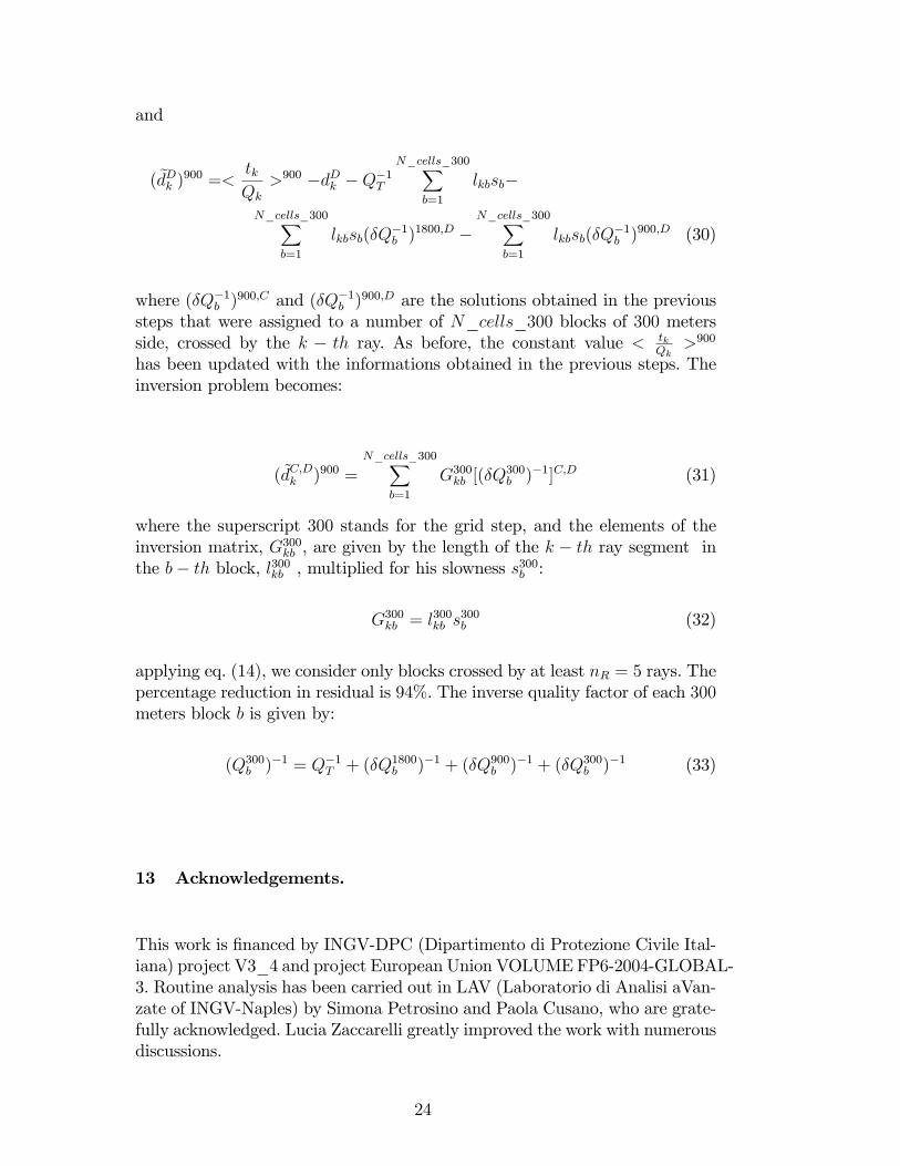
13 Acknowledgements.

This work is �nanced by INGV-DPC (Dipartimento di Protezione Civile Ital-iana) project V3_4 and project European Union VOLUMEFP6-2004-GLOBAL-3. Routine analysis has been carried out in LAV (Laboratorio di Analisi aVan-zate of INGV-Naples) by Simona Petrosino and Paola Cusano, who are grate-fully acknowledged. Lucia Zaccarelli greatly improved the work with numerousdiscussions.

24

References

Andronico, D., Calderoni, G., Cioni, R., Sbrana, A., Suplizio, R., and San-tacroce, R., 1995. Geological map of Somma-Vesuvius Volcano. Per. Min-eral., 64: 77-78.

Aki, K., 1980. Attenuation of shear-waves in the lithosphere for frequenciesfrom 0.05 to 25 Hz. Phys. Earth Planet. Inter., 21: 50-60.

Auger, E., Gasparini, P., Virieux, J., and Zollo, A., 2001. Seismic Evidence ofan Extended Magmatic Sill Under Mt. Vesuvius. Science, 294: 1510-1512.

Bai, C., and Greenhalgh, S., 2005. 3D multi-step travel time tomography: imag-ing the local, deep velocity structure of Rabaul volcano, Papua New Guinea.Physics of the Earth and Pl. Int., 151: 259-275.

Berrino, G., Coppa, U., De Natale, G., and Pingue, F., 1993.Recent geophysicalinvestigation at Somma�Vesuvius volcanic complex. J. Volcanol. Geotherm.Res., 58: 239-262.

Bianco, F., Castellano, M., Milano, G., Ventura, G., and Vilardo, G., 1997.The Somma-Vesuvius stress �eld induced by regional tectonics: evidencesfrom seismological and mesostructural data. J. Volcanol. Geotherm. Res.,82: 199-218.

Bianco, F., Castellano, M., Del Pezzo, E., and Ibanez, J. M., 1999. Attenuationof short period seismic waves at Mt. Vesuvius, Italy. Geophys. J. Int., 138:67-76.

Block, L.V., 1991. Joint hypocenter-velocity inversion of local earthquakes ar-rival time data in two geothermal regions. Ph.d. dissertation, M.I.T., Cam-bridge.

Capuano, P., Gasparini, P., Zollo, A., Virieux, J., Casale, R., and Yeroyanni,M., 2003. The internal structure of Mt. Vesuvius. A seismic tomographyinvestigation. Liguori Editore, ISBN 88-207-3503-2.

Chiodini, G., Marini, L., and Russo, M., 2001. Geochemical evidence for theexistence of high-temperature hydrothermal brines at Vesuvio volcano, Italy.Geoch. et Cosmoch. Acta, 65(13), 2129�2147.

Chouet, B., 1996. New methods and future trends in seismological volcanomonitoring. In: Scarpa, R., Tilling, R.I. (Eds.), Monitoring and Mitigationof Volcano Hazards. Springer, Berlin, pp. 23�97.

Chouet, B., 2003. Volcano Seismology. Pageoph, 160: 739-788.Del Pezzo, E., Bianco, F., and Saccorotti, G., 2004. Seismic source dynamicsat Vesuvius volcano, Italy. J. Volcanol. Geotherm. Res., 133: 23-39.

Del Pezzo, E., Bianco, F., and Zaccarelli, L., 2006. Separation of Qi and Qsfrom passive data at Mt. Vesuvius: a reappraisal of seismic attenuation.Physics of the Earth and Pl. Int., 159: 202�212.

Del Pezzo, E., Bianco, F., De Siena, L., and Zollo A., 2006. Small scale shallowattenuation structure at Mt. Vesuvius, Italy. Physics of the Earth and Pl.Int., 157: 257-268.

De Natale, G., Capuano, P., Troise, C., and Zollo, A., 1998. Seismicity atSomma-Vesuvius and its implications for the 3D tomography of the volcano.

25

J. Volcanol. Geotherm. Res., Special Issue Vesuvius. Spera F. J., De VivoB., Ayuso R.A., Belkin H.E. (Eds), 82: 175-197.

De Natale, G., Troise, C., Pingue, F., Mastrolorenzo, G., and Pappalardo, L.,2005. The Somma�Vesuvius volcano (Southern Italy): Structure, dynamicsand hazard evaluation. Earth-Science Rev., 74: 73-111.

Eberhart-Phillips, D., 1990. Three-dimensional P and S velocity structure inthe Coalinga region, California. J. Geophys. Res. 95: 15343�15363.

Eberhart-Phillips, D., Reyners, M., Chadwick, M., Chiu, J. M., 2005. Crustalheterogeneity and subduction processes: 3-D V P , V P/V S and Q in thesouthern North Island, New Zealand. Geophys. J. Int. 162: 270�288.

Galluzzo, D., Del Pezzo, E., Maresca, R., La Rocca, M., and Castellano, M.,2005. Site e¤ects estimation and source-scaling dynamics for local earth-quakes at Mt. Vesuvius, Italy. Congress acts, ESG2006, Grenoble. Papernum. 36.

Gerlach, T., and Taylor, B., 1990. Carbon isotope constraints on degassing ofcarbon dioxide from Kilauea volcano. Geochim. Cosmochim. Acta 54, 2051�2058.

Giampiccolo, E., Gresta, S. and Ganci, G., 2003. Attenuation of body waves inSoutheastern Sicily (Italy). Physics of the Earth and Pl. Int., 135: 267�279.

Gubbins, D., 2004. Time series analysis & inverse theory for geophysicists.Cambridge University Press.

Gudmundsson Ó., Finlayson D. M., Itikarai I., Nishimura Y., and Johnson W.R., 2004. Seismic attenuation at Rabaul volcano, Papua New Guinea. J. ofVolc. and Geoth. Re., 130: 77-92.

Gusev, A. A., and Abubakirov, I. R., 1999. Vertical pro�le of e¤ective turbidityreconstructed from broadening of incoherent body-wave pulses. Geophys. J.Int., 136: 309-323.

Hansen, S., Thurber, C. H., Mandernach, M., Haslinger, F., and Doran, C.,2004. Seismic Velocity and Attenuation Structure of the East Rift Zone andSouth Flank of Kilauea Volcano, Hawaii. Bull. of the Seism. Soc. of Am.,94: 1430-1440.

Ito, H., DeVilbiss, J., and Nur, A., 1979. Compressional and shear waves insaturated rock during water�steam transition. J. Geophys. Res. 84, 4731�4735.

Lomax, A., Zollo, A., Capuano, P., and Virieux, J., 2001. Precise absoluteearthquake location under Somma-Vesuvius volcano using a new three-dimensional velocity model. Geophys. J. Int., 146: 313-331.

Marianelli, P., M´etrich, N., and Sbrana, A., 1999. Shallow and deep reservoirsinvolved in magma supply of the 1944 eruption of Vesuvius. Bull. Volcanol.,61: 48-63.

Mulargia, F., and Tinti, S., 1985. Seismic sample areas de�ned from incompletecatalogues; an application to the Italian territory. Phis. Earth Plan. Int, 40:273-300.

Alejandro Nava, F., Garcìa-Arthur, R., Castro, R. R., Suàrez, C., Màrquez, B.,Nùñez-Cornù, F., Saavedra, G. and Toscano, R., 1999. S wave attenuation

26

in the coastal region of Jalisco�Colima, México. Phys. Earth Pl. Int., 115:247�257.

Santacroce, R., 1987. Somma-Vesuvius. CNR, Quaderni di Ricerca Scienti�ca.Sambridge, M.S., and Gudmundsson, O., 1998. Tomographic systems of equa-tion with irregular cells. J. Geophys. Res., 103: 773�781.

Sato, H., and Fehler, M.C.,1998. Seismic Wave Propagation and Scattering inthe Heterogenous Earth. Springer.

Sengupta, M. K., and Rendleman, C. A., 1989. Case study: the importanceof gas leakage in interpreting amplitude-versus-o¤set (AVO) analysis. Soc.Explor. Geophys. Abstracts 59, 848�850.

Scarpa, R., Tronca, F., Bianco, F., and Del Pezzo, E., 2002. High resolutionvelocity structure beneath Mount Vesuvius from seismic array. Geophys.Res. Lett., 29 (21): 2040.

Schurr, B., Asch, G., Rietbrock, A., Trumbull, R., and Haberland, C., 2003.Complex patterns of �uid and melt transport in the central Andean subduc-tion zone revealed by attenuation tomography. Earth. Pl. Scien. Lett., 215:105-119.

Spencer, J., 1979. Bulk and shear attenuation in Berea sandstone: the e¤ectsof pore �uids. J. Geophys. Res. 84, 7521�7523.

Thurber, C.H., 1987. Seismic structure and tectonics of Kilauea volcanoHawaii. In: Decker, R.W., Wright, T.L., Stau¤er, P.H. (Eds.), Volcanismin Hawaii. US Geological Survey, pp. 919�934.

Tondi, R., and De Franco, R., 2003. Three-dimensional modeling of MountVesuvius with sequential integrated inversion. J. Geophys. Res., 108: 2256.

Um, J., and Thurber, C.H., 1987. A fast algorithm for two-point seismic raytracing. Bull. of the Seism. Soc. of Am. 77: 972-986.

Wegler, U., 2003. Analysis of multiple scattering at Vesuvius volcano, Italy,using data of the Tomoves active seismic experiment. J. Volcanol. Geotherm.Res., 128: 45�63.

Zollo, A., D�Auria, L., De Matteis, R., Herrero, A., Virieux, J., and Gasparini,P., 2002. Bayesian Estimation of 2-D P-Velocity Models From Active Seis-mic Arrival Time Data: Imaging of the Shallow Structure of Mt.Vesuvius(Southern Italy). Geophys. J. Int., 151: 566-582.

14 Captions.

� Figure 1:Lower-left panel: Map of Mt. Vesuvius with station positions (blacksquares) and hypocentral locations (white dots) of the seismic events used inthe present work. Black broken line depicts the old caldera rim. Upper-leftand upper-right panels represent respectively the W-E and S-N sections,also reported as "W-E plane" and "S-N plane" in the lower-right "wideangle" view. The High Resolution Region (HRR) is roughly depicted bythe inner polyhedron in the wide angle view. The solid line rectangles in

27

the upper left, upper right and lower left panels represent the sections ofthe HRR. The zones marked with 1and 2 represent the zone in which therobusteness test results are reported respectively in Table IV and V. Theellipsoidal zone marked with 3 shows the area with the maximum seismicenergy release.

� Figure 2: Checkerboard test in the HRR. a) Input. W-E and S-N sections(also marked in �gure 1, lower right panel); the white lines include all themaximum resolution cells de�ned by formula (14). In this volume we as-sumed a checkerboard structure, with high Q-contrast among the blocks;a uniform attenuation medium is assumed outside HRR. b) Output. Testresults for a 10% error on synthetic data. The zones marked by the whitebroken lines include the cells where the checkerboard structure is e¤ectivelyreproduced. �Q�1S grey scales represent the variation from the average qual-ity factor.

� Figure 3: Left hand panels. Five horizontal slices at di¤erent depths (Zvalue respect to the sea level) of the volume containing the HRR. The whitelines include all the maximum resolution cells de�ned by formula (14). Thesections represent the input checkerboard structure also described in Figure3, with the same colorscale. Rigth hand panels. The �gures represent thetest output; the zones marked by the white broken lines include the cellswhere the checkerboard structure is e¤ectively reproduced.

� Figure 4: Synthetic anomaly test. The input structures (panel a) are in-cluded in a volume characterized by uniform attenuation. The output (panelb) show the reconstruction of the anomalies. Black areas are not resolved inthe inversion. Colorscales refer to the variations respect to the mean inversequality factor. The zones marked by the white broken lines include the cellswhere the checkerboard structure is e¤ectively reproduced.

� Figure 5: Results of the attenuation tomography inversion, in the frequencyband centered at 12 Hz (panel a), and 18 Hz (panel b) for the CN method,compared with the results obtained at 18 Hz for the SD method (panel c).W-E and S-N sections are those marked in Figure 1 (down-rigth panel).Black areas are not resolved in the inversion.Colorscales refer to the vari-ations respect to the mean inverse quality factor. The zones marked bythe white broken lines include the cells where the checkerboard structure ise¤ectively reproduced.

� Figure 6: The W-E and S-N sections represent the attenuation structureinferred for S-waves (CN method), in the frequency band centered at 18Hz (panel a), and the S-velocity structures inferred by Scarpa et al. (2002)(panel b). The dashed line represents the VP=VS pattern with depth and isoverimposed to all �gures. The P-wave attenuation (SD method, 18 Hz) andvelocity (inferred by Scarpa et al. (2002)) are also represented in panels cand d. The colorscales in panels a and c refer to the variations respect to themean inverse quality factor obtained in the inversions for S- and P-waves.The colorscales in panels b and d represent the absolute S- and P-wavevelocity. Black areas are not resolved in the inversion. The zones marked by

28

the white broken lines include the cells where the checkerboard structure ise¤ectively reproduced.

� Figure 7: Five horizontal slices of the the volume containing HRR at di¤erentdepths (Z). The colorscales for S- (�rst column) and P-wave (third column)attenuation images represent the variations from the mean inverse qualityfactor calculated on each horizontal slice at each depth. The colorscalesrepresented in the second and fourth coloumns respectively represent thevariations of S- and P-wave velocity from the average velocity calculated ateach depth. On each image we marked with numbered black rectangles, thezones characterized by important properties, widely discussed in the text.The zones marked by the white broken lines include the cells where thecheckerboard structure is e¤ectively reproduced.

� Figure A2.1: The percent standard deviation, �=�, as a function of the win-dow duration for an earthquake recorded at all the stations. �=� is obtainedcalculating the average, � [over stations] , of the log of spectral ratio be-tween direct S radiation and coda radiation, after correcting the amplitudesfor geometrical spreading and for the average Q. Downward arrow indicatesthe change-point as discussed in the text.

Table I

Station E-W (UTM) N-S (UTM) altitude (a.s.l.) (m)

BAFM 450372 4518076 594

BKEM 452677 4518762 850

BKNM 451875 4520020 865

FTCM 452692 4516337 350

OVO 449190 4519705 600

POLM 447910 4522499 181

SGVM 450568 4518706 734

Table II

��f fc(Hz) +�f

8.2 12 15.8

12.4 18 23.6

29

Table III

Robusteness Test - 1800 m

Block# 1 2 3 4 5 6 7 8 9 10 11 12

P 1800, 10% 1% 0% 0% 13% 7% 4% 0% 0; 1% 0% 0% 0% 3%

P 1800, 20% 1% 0% 2% 29% 9% 11% 17% 1% 0% 0% 0% 3%

P 1800, 30% 2% 1% 3% 28% 9% 9% 50% 0; 3% 0% 0% 0% 2%

P 1800, 40% 3% 3% 10% 29% 8% 16% 87% 2% 1% 0% 0% 8%

P 1800, 50% 6% 2% 11% 62% 20% 25% 87% 3% 1% 0% 0% 9%

Robustness test at the lowest resolution; the average percentageof eq. (15) isrepresented for all the blocks resolved. The increasing percentage in the �rst

column is the data reduction.

30

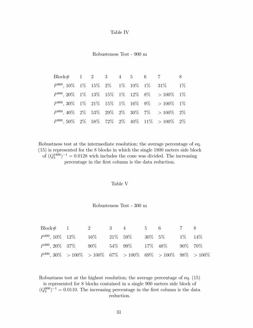
Table IV

Robusteness Test - 900 m

Block# 1 2 3 4 5 6 7 8

P 900, 10% 1% 15% 2% 1% 10% 1% 31% 1%

P 900, 20% 1% 13% 15% 1% 12% 8% > 100% 1%

P 900, 30% 1% 21% 15% 1% 16% 9% > 100% 1%

P 900, 40% 2% 53% 29% 2% 30% 7% > 100% 2%

P 900, 50% 2% 58% 72% 2% 40% 11% > 100% 2%

Robustness test at the intermediate resolution; the average percentage of eq.(15) is represented for the 8 blocks in which the single 1800 meters side blockof (Q1800b )�1 = 0:0128 wich includes the cone was divided. The increasing

percentage in the �rst column is the data reduction.

Table V

Robusteness Test - 300 m

Block# 1 2 3 4 5 6 7 8

P 300, 10% 12% 16% 21% 59% 30% 5% 1% 14%

P 300, 20% 37% 90% 54% 99% 17% 48% 90% 70%

P 300, 30% > 100% > 100% 67% > 100% 69% > 100% 98% > 100%

Robustness test at the highest resolution; the average percentage of eq. (15)is represented for 8 blocks contained in a single 900 meters side block of

(Q900b )�1 = 0:0110. The increasing percentage in the �rst column is the datareduction.

31

Table VI

Stability Test - 1800 m

Block# 1 2 3 4 5 6 7 8 9 12

[(Q1800)�1]� 10�2 1; 98 1; 79 1; 50 2; 44 1; 28 1; 37 0; 92 2; 86 0; 51 3; 16

[(Q1800)�1]� 10�2; (QminT )�1 1; 83 1; 67 1; 72 1; 84 1; 28 1; 43 1; 15 2; 72 0; 49 3; 21

[(Q1800)�1]� 10�2; (QmaxT )�1 1; 88 1:69 1; 10 2; 88 1; 11 1; 08 0; 54 2; 74 0; 40 2; 81

Stability test at the lowest resolution; the value of the inverse quality factorof each resolved block is dependent on the maximum ((QmaxT )�1 = 0:026) and

minimum ((QminT )�1 = 0:008) average inverse quality factor allowed.

Table VII

Stability Test - 900 m

Block# 1 2 3 4 5 6 7 8

[(Q900)�1]� 10�2 1; 79 0; 52 0; 96 1; 79 2; 75 1; 64 0 1; 79

[(Q900)�1]� 10�2; (QminT )�1; (Q1800bmin)�1 1; 88 0; 46 1; 12 1; 88 2; 36 1; 77 0 1; 88

[(Q900)�1]� 10�2; (QmaxT )�1; (Q1800bmax)�1 1:67 0; 58 0; 80 1; 67 3; 14 1; 51 0 1; 67

Stability test at the intermediate resolution; the value of each inverse qualityfactor is both dependent on the maximum ((QmaxT )�1 = 0:026) and minimum

((QminT )�1 = 0:008) average inverse quality factor and the maximum((Q1800bmax)

�1 = 0:0188) and minimum ((Q1800bmin)�1 = 0:0167) inverse quality

factor of the block in which they are contained.

32

Table VIII

Stability Test - 300 m

Block# 1 2 3 4 5 6 7 8

[(Q300)�1]� 10�2 5; 61 1; 78 1; 91 0; 39 1; 44 0 2; 26 0

[(Q300)�1]� 10�2; (QT min)�1; (Q1800bmin)�1; (Q900bmin)

�1 2; 59 1; 76 1; 34 0; 05 1; 29 0 2; 60 0

[(Q300)�1]� 10�2; (QT max)�1; (Q1800bmax)�1; (Q900bmin)

�1 6; 91 1; 99 2; 01 1; 59 1; 32 0 1; 34 0

Stability test at the highest resolution; the value of each inverse qualityfactor is both dependent on the maximum ((QmaxT )�1 = 0:026) and minimum((QminT )�1 = 0:008) average inverse quality factor. It is also dependent on the

maximum ((Q1800bmax)�1 = 0:0188, (Q900bmax)

�1 = 0:0177) and minimum((Q1800bmin)

�1 = 0:0167, (Q900bmin)�1 = 0:0151) inverse quality factor of the blocks

in which they are contained.

33

MS. REF. NO.: PEPI-D-07-00301 TITLE: MULTIPLE RESOLUTION SEISMIC ATTENUATION IMAGING AT MT. VESUVIUS PHYSICS OF THE EARTH AND PLANETARY INTERIORS

Dear Editor,First of all we want to thank both reviewers for the suggestions, which were really useful to improve the paper quality, and in particular the graphical representation of the results obtained.We took into account all the suggestions made by both reviewers. We also answer to the questions raised, to better clarify how we corrected the paper. Wespecify all the points, starting from those raised by Referee 2.One of the main point to be addressed is the improving of all the synthetic tests. We hence decided to a) include in the article a synthetic anomaly test; b) to explicitly show the checkerboard test; c) to mark the high resolution volume enlightening the test results inside this zone. Another important point was the discussion of the results, too short and concisein the first version. We re-wrote completely all this stuff, trying to explicitly illustrate in detail our interpretation.The other major comment regards the effective resolution of our method (300 m). We follow an empirical rule, that the wavelength must be lower than a half of the minimum cell size. Moreover, we consider for the interpretation only those cell crossed by a number of rays defined by the empirical equation (14). The question arisen by rev. 3 about the formal correctness of formula (14) is right. With the decreasing of the cell size, the minimum number of rays passing through the cell also decreases. Anyway, this number is never lower than 4. We have empirically observed that this number ensures stable results. So, we are confident that, even with a decreasing resolution, the results do not represent ghost images.

All the other minor points have been fully addressed, as reported in the following list, in which in capital letters there is copied the reviewer comment, and in lower case our reply.

Reviewer 2.1) THIS PAPER PRESENTS ATTENUATION TOMOGRAPHY RESULTS BASED ON A

MODIFIED CODA NORMALISATION APPROACH. THIS QUITE NEW APPROACH HAS BEEN DEVELOPED AND PUBLISHED PREVIOUSLY BY DEL PEZZO ET AL. (2006) AND APPLIED TO A QUITE SIMILAR DATA SET AS THE ONE PRESENTED HERE.

This is not true, as we clearly indicate in the text. We used a number of waveforms more than doubled respect to the previous.

2) AT THE CURRENT STATE OF THE PRESENTATION OF THE PAPER I AM VERY SUSPICIOUS IF THIS STUDY IS REALLY FURTHERING OUR KNOWLEDGE IN ANY WAY OR IF IT IS JUST A REPETITION OF THE RESULTS ALREADY PUBLISHED BY DEL PEZZO ET AL. (2006).

First, we use a multi-scale approach. Second, respect to the first version we have a new image of Qp. Third, we use much more data and a more precise ray-tracing procedure. This improvement helps in new and more detailed interpretation.

3) (ALTHOUGH APPENDIX 3 IS A LITTLE BIT TEDIOUS AND COULD BE CONSIDERABLE SHORTENED),For us it is very hard to shorten this part without loosing in clearness. We thus prefer not to shorten this appendix to avoid any misunderstandingin the application of the procedure.

4) MY MAIN CONCERN IS NOT RELATED TO THE THEORY, WHICH IS WELL PRESENTED BUT IS BASED ON THE FACT HOW MUCH MORE DETAIL IS REALLY RESOLVED WITH THIS HIGHER RESOLUTION TECHNIQUE. THE REASONING FOR THIS IS A AS FOLLOWS:

* Response to Reviewers

(I) CHAPTER 6.3 AND FIG. 3 PRESENT A CHECKERBOARD RESOLUTION TEST, WHICH SHOULD CLEARLY EMPHASIS THE RESOLUTION CAPABILITY OF THIS NEW DATA SET TOGETHER WITH THE NEW HRR APPROACH. Checkerboard resolution test presented in fig. 3 of the first version was not able to illustrate to readers the improvement that the multiple resolution technique produces in our results. So, in the new version several numerical tests were performed to show both the increased resolution in the whole area and the capability of the used method of reproducing the main anomalies inferred by the inversion. In particular, the checkerboard resolution test presented in the first version has been better discussed and illustrated, showing both SN and WE profiles together with horizontal slices at the depths where the most important results have been found. We also marked the area of improved resolution (300 meters) [the effective HRR].

5) HOWEVER, FIGURE 3 SUGGESTS, THAT THERE SEEMS TO BE NO HIGH RESOLUTION FOR REGIONS BELOW 3000M, WHERE ONE OF THE ANOMALIES HIGHLIGHTED AND DISCUSSED LATER ON IS LOCATED (ANOMALY 2). THE OTHER ANOMALY (NUMBER 1)DISCUSSED IN THE PAPER, IS ALSO LOCATED BETWEEN 4519000 AND 4521000, A REGION WHERE ONLY A FEW CELLS ARE WELL RESOLVED BY THE HRR AS STATED IN THE CHECKERBOARD TEST. SO ALL THE RESULTS DISCUSSED IN THE PAPER ARE COMING FROM THE LRR AND THOSE FINDINGS HAVE BEEN PRESENTED BEFORE. ADDITIONALLY, THE RESOLUTION TEST IS ALSO PLOTTED FROM NORTH TO SOUTH WHERE AS ALL THE TOMOGRAPHY IMAGES ARE SHOWN FROM SOUTH TO NORTH, WHICH DEFINITELY HAS TO BE CORRECTED.The synthetic anomaly test done in the revised version effectively reveals that under 3500 meters there is no high resolution; however, part of the anomaly 2 (as was marked in the first draft) is still present inside the HRR (the one above 3500 meters) and the other part can be reconstructed at a resolution of 900 meters. The deep part of this anomaly (at a resolution of 900m) was not detected in our previous paper (Del Pezzo et al. 2006). The improved image has been obtained in the present paper thanks to the strongly improved data set and quality. The present data set is more than doubled respect to the previous dataset, and span a wider depth interval respect to the previous one. The area where we find anomaly 1 (as marked in the first draft) is in the HRR, even if in Fig 3 there was a misleading perspective; in the revised version we add new images for the resolution test and do a synthetic anomaly test to show thecapacity of effectively reconstructing this anomaly at a 300m scale.

6) IT CERTAINLY DOES NOT HELP THAT THE PRESENTATION OF RESULTS IN THE TEXT IS RATHER SCRAPPY WITH SOMETIMES JUST A SENTENCE (E.G. A)) AND NO ADDITIONAL EXPLANATION AT ALL. THIS LOOKS LIKE TO ME THAT THE WRITING UP PHASE OF THIS PAPER HAS BEEN RUSHED QUITE A BIT AND WAS NOT HANDLED WITH ENOUGH CARE SEEN ESPECIALLY IN THE RESULTS AND DISCUSSION SECTION. SINCE NO NEW METHOD HAS BEEN DEVELOPED THESE TWO SECTIONS SHOULD BE THE STRENGTH OF THE PAPER AND IT SEEMS THAT THE AUTHORS HAVE NOT PUT ENOUGH ATTENTION TOWARDS THESE SECTIONS. THE DISCUSSION AND CONCLUSION SECTION IS ALSO JUST AN ITERATION OF WHAT HAS BEEN FOUND BEFORE AND DOES NOT PUT ANY EMPHASIS IN CORRELATING AND DISCUSSING THEPOSSIBLE NEW FINDINGS WITH EXISTING STUDIES.We agree with this criticism. To help the reader we re-wrote all the section, with much more details.

THERE ARE ALSO A LOT OF OTHER INCONSISTENCIES IN THE PAPER AND SOME OF THEM ARE LISTED BELOW: 7) DEPTHS GIVEN IN THE PAPER ARE NOT ALWAYS IN RESPECT TO A COMMON DATUM (SEA LEVE, VOLCANO TOP,.) WHICH MAKES IT HARD FOR THE READER TO FOLLOW.Done. Depths from the sea level. 8) QT HAS NEVER BEEN INTRODUCED.Introduced.

9) AVERAGING BRACKETS < SHOULD BE INTRODUCED.

This was a misprint. We cut off the brackets. 10) THE SYMBOL <GAMMA IS USED FOR THE FREQUENCY DEPENDENCE OF THE SOURCE SPECTRUM AS WELL AS FOR THE FREQUENCY DEPENDENCE OF Q.Right. The frequency dependence of Q was changed in alpha. 11) EQUATION 10 DOES NOT CONTAIN AN EXPONENTIAL TERMThis was an error. We changed the entire sentence.

12) THE USED FREQUENCY RANGE HAS TO BE CLARIFIED MORE PRECISELY ESPECIALLY DIFFERENCES BETWEEN THE CN AND THE SD APPROACH.This is done in section 4.5 13) THE CN METHOD FOR 18HZ USES FREQUENCIES UP TO 23.6, WHICH IS RATHER CLOSE TO THE LOWPASS FILTER OF 25HZ, PRESUMABLY DUE TO DATA TRANSMISSION. HAVE CHECKS BEEN CARRIED OUT TO VERIFY THAT THIS LOWPASS FILTER DOES NOT INFLUENCE THE RESULTS IN THIS FREQUENCY BAND? The response is flat up to 25 Hz while we cut at 23.6. 14) THE BOX SIZE OF 300M IS IN THE SAME ORDER AS THE WAVELENGTH FOR BOTH P- AND S- WAVE. IS THE HIGH FREQUENCY APPROXIMATION IMPLICITLY ASSUMED IN THE TOMOGRAPHY APPROACH STILL FULFILLED IN THIS CASE?We already answered to this question in the introduction of this letter.

------------------------------------------------------------

REVIEWER #3: I HAVE CAREFULLY READ THIS PAPER AND I THINK THE AUTHORS SHOW A NEW AND USEFUL METHOD TO EXPLORE SMALL SCALE ATTENUATION STRUCTURES. NEXT, I GIVE MY COMMENTS WHICH COULD HELP THE AUTHORS TO CARRY OUT A MORE DETAILED DESCRIPTION COMMENTS:

1) I SUGGEST THE AUTHORS SHOULD GIVE A BETTER DESCRIPTION OF THE METHOD AND ITS METHODOLOGY. THE MAIN AIM OF THIS STUDY COULD BE EASILY ILLUSTRATED WIHT ATTENUATION TOMOGRAPHIC IMAGES IN EACH STEP, THAT IS, FOR EACH CELL SIZE. MOREOVER, SINCE THIS IS A TOMOGRAPHIC STUDY, SYNTHETIC TESTS MORE REALISTIC SHOULD BE SHOWED IN THIS STUDY FOR EXAMPLE, SYNTHETIC ANOMALY TESTS (E.G. SCHURR ET AL., 2003; BAI AND GREENHALGH, 2005; EBERHART-PHILLIPS ET AL., 2005) AND RESTORING RESOLUTION TESTS (E.G. ZHAO ET AL., 1992). THESE TESTS ARE USEFUL TO CHECK STRUCTURES WITH DIFFERENT SHAPE AND SIZE. SOME INFORMATION SHOULD BE ADDED/MODIFIED TO UNDERSTAND CORRECTLY THE RESULTS: RAY- PATH PLOTS OR MARK THE REGIONS WITH THE BEST RESOLUTION OR DENSITY OF RAYS (E.G. RIETBROCK, 2001; DE GORI ET AL., 2005), PLOT THE GRID USED OVERIMPOSED IN THE FINAL MODEL PLOTS (E.G. RIETBROCK 2001, REYNERS ET AL., 2006), SYNTHETIC TESTS ARE USED TO KNOW HOW THE REAL STRUCTURE IS RECONSTRUCTED WITH THE EVENT-STATION DISTRIBUTION AND THE PARAMETER VALUES USED IN THE INVERSION OF THE REAL DATA (E.G. SCHURR ET AL., 2003; RIETBROCK, 2001, ...).This comment greatly helped us to better address the part of the paper dealing with synthetic tests and with the marking of HRR. We start giving a better representation of the resolution test done in the first version of this paper; as the main interest of our paper is to constrain the zone characterized by anomalous attenuation, we also performed a synthetic anomaly test, following Shurr (2003).We gave an improved representation of our results inspired by the papers indicated by Rev. 3 , which resulted greatly helpful.

2)IN THIS STUDY, THE NR FACTOR IS DIFFERENT IN THE INVERSION OF THE REAL DATA (NR5) AND THE CHECKERBOARD SYNTHETIC DATA (NR9). WHY THE SYNTHETIC AND REAL DATA ARE INVERTED WITH A DIFFERENT VALUE OF NR??. ON THE OTHER HAND, THE AUTHORS DECLARE THAT NR5 CAN ENSURE THAT EACH BLOCK IS HOMOGENEOUSLY SAMPLED. I HAVE SOME DOUBTS. I THINK THAT THE EXPRESSION (14) WORKS WELL FOR CELL SIZE OF 1800 AND 900 M, BUT NOT WHEN THE CELL SIZE IS CLOSE TO WAVELENGTH, AS IN THE CASE OF A CELL SIZE OF 300 M.

The factor of nR=9 was a typographical error: all our results come fromthe formula (14). Formula (14) on the other hand is sounded only on an empirical base: at 12 and 18 Hz centre frequency, the wavelengths are always below the minimum cell size. The question arisen by rev. 3 about the formal correctness of using formula (14) is right. With the decreasing of the cell size the minimum number of rays passing through the cell also decreases. Anyway, this number is never lower than 4. We have empirically observed that this number ensures stable results. So we are confident that, even with a decreasing resolution, the results at 18 Hz do not represent ghost images.

3) A MORE DETAILED DESCRIPTION OF THE CHECKERBOARD TEST IS ALSO REQUIRED. SOME QUESTIONS SHOULD HAVE TO BE EXPLAINED: - THE GREY-SCALE IS UNCLEAR. WHAT DOES IT REPRESENT??, QT-1 OR <DELTAQT-1?? - WHICH BLOCKS OF 1800 METERS AND 900 METERS SIDE HAVE BEEN USED FOR THE INVERSION WITH THE CHECKERBOARD TEST?? - WHAT IS THE LOCATION OF THE DIVIDED BLOCKS? IF FIGURES 4, 5, 6, 7 AND 8 SHOW THE S-N AXIS, WHY DOES THE FIGURE 3 SHOW THE S-N AXIS WITH DIFFERENT ORIENTATION?? IT WOULD BE MORE CONVENIENT TO PLOT ALL FIGURES WITH THE SAME REFERENCE SYSTEM.Ok, we corrected all this stuff making new plots.

4) IN THE TEXT IT IS INDICATED THAT THE INVERSION FOR 18 HZ CONSIDER AN INITIAL VALUE OF QT-1=0.019±0.003. COULD THE AUTHORS INDICATE WHICH INITIAL QT-1 VALUE IS USED IN THE REAL DATA INVERSION FOR THE FREQUENCY CENTRED AT 12 HZ??

We added in the text the requested information.

5) IT IS NOT CLEAR IN THE STUDY HOW THE ROBUSTNESS TEST HAS BEEN APPLIED. IT HAS BEEN APPLIED TO ALL BLOCKS, OR ONLY TO SOME BLOCKS. IT WOULD BE EASIER TO UNDERSTAND THE RESULTS OF THE ROBUSTNESS TEST IF THE RESULTS WERE PLOTTED AS IN LEES AND CROSSON (1989).

We corrected the text.

6) SINCE QCODA DEPENDS ON THE LAPSE TIME, IT WOULD BE CONVENIENT TO CHECK THE RESULTS OF QS-1 WITH OTHER LENGTHS OF THE CODA TIME WINDOW.Unfortunately, this is practically impossible due to the noise level which is severely high in the area under study, as widely discussed in Del Pezzo et al. 2006.

7) IN THE SECTION 7 AND 8 THE AUTHORS DECLARE " ...; THE CN AND SD METHODS FURNISH COMPARABLE IMAGES. ...", AND "... YIELDING PRACTICALLY THE SAME RESULTS.". HOWEVER THEY DO NOT INDICATE THE DIFFERENCES BETWEEN THESE IMAGES IN THE CENTRAL PART OF THE VOLUME, JUST BENEATH THE CRATERS BETWEEN -2000 AND -4000 METERS. COULD THE AUTHORS EXPLAIN WHY THE ATTENUATION TOMOGRAPHIC IMAGES GENERATED RESPECTIVELY BY THE CN AND SD METHODS ARE DIFFERENT IN THIS PART???. THE AUTHORS SHOULD EXPLAIN IF THESE DIFFERENCES DEPEND ON SOME FACTORS: SITE EFFECTS, SOURCE LOCATION, RAY COVERAGE, ... OR BY THE CONTRARY REMAIN UNCHANGED

The problem arisen by rev. 3 has been addressed in the following way. In the first version of this paper we represented absolute estimates (Q-1) using the same colour scale for the CN and SD. The estimates done with CN were defined in

the first version as the sum of the inverse Quality factor (averaged in the space) and its spatial variations (cell by cell). Using SD instead, we inverted for the variations of Q-inverse cell by cell, and represented these values summed to the average inverse Q obtained with CN. In the new representation reported in the revised paper, we avoid any bias and represent the variations respect to the mean, independently calculated for each method, taking as unique constraint that Q-1 must be positive. In this way it clearly appears that the two representations are practically equivalent. The small differences are however discussed in the new version of the paper.

8) IN THE PARAGRAPH OF THE SECTION 8 "DISCUSSION AND CONCLUSIONS" BEGINNING "THE HIGH CONTRAST IN BOTH S-WAVE VELOCITY, AND QS-1 ...", IT IS DISCUSSED THE VALUES OF VS AND QS-1 OF THE CIRCLE 2. HOWEVER, WHERE THE TEXT SAYS "THE OBSERVED STRONG CONTRAST MAY BE GENERATED BY A HIGHLY ... OVERIMPOSED (POINT "E" OF RESULTS; SEE ALSO DEL PEZZO ET AL. (2006)]" IT IS NOT CLEARLY RELATED TO "CIRCLE 2". I SUGGEST THAT SOME REORGANIZATION OF THIS PARAGRAPH IS NECESSARY.

Ok, done. We rewrote all the section.

9) IN ORDER TO BETTER UNDERSTAND THE FIGURES 4, 5, 6 AND 7, THE COLOR SCALE OF QS-1 SHOULD BE MODIFIED AND EXPLAINED TO SHOW THE REPRESENTATIVE QS-1 VALUES. I CAN NOT COMPARE QUANTITATIVELY THE REGIONS WITH COLOR BLUE, CYAN AND GREEN. ON THE OTHER HAND THE Q-1 SCALE VARIES IN THE RANGE BETWEEN 10-6 AND 0.05, BUT WHAT IS THE MINIMUM OF Q-1 IN THE VOLUME UNDER STUDY??

We decided to overcome the problem changing the colour scale.

10) FIGURES 4, 5, 6 AND 7. FOR A MAJOR UNDERSTANDING OF THE RESULTS, I ADVISE THE AUTHORS MARK IN THE FIGURE 4, 5, 6 AND 7 THE REGIONS WITH GOOD RAY COVERAGE OR THOSE WHERE THE CHECKERBOARD SYNTHETIC MODEL IS WELL RECOVERED. THE BLOCK SIZES SHOULD BE ALSO INDICATED

We did this in Fig. 3 and 4, marking the HRR with a white broken line.

11) FIGURE 8 IS NOT CLEAR. I SUGGEST THAT THE AUTHORS INCLUDE A PERSPECTIVE VIEW OF THE SHALLOW CRUST UNDER MT. VESUVIUS VOLCANO SHOWING THE LOW QS-1 ISOSURFACE AS IN FINLAYSON ET AL. (2003)

The set of new figures clearly show all the features avoiding any isosurface.

MINOR12) I THINK IT IS CONVENIENT TO MAKE A DISTINCTION BETWEEN RESOLUTION AND SPATIAL RESOLUTION TO AVOID AMBIGUITY BETWEEN CELL SIZE AND RESOLUTION MATRIX.We always refer to the spatial resolution.

GRAMMATICAL/TYPOGRAPHICAL:

PAGE 2-- BAI ET AL. (2005) --- BAI AND GREENHALGH (2005)

Done PAGE 3-- IS MORE IMPORTANT THAN INTRINSIC ATTENUATION (DEL PEZZO ET AL.,

2006) ... SPECIFY WHICH ARTICLE OF DEL PEZZO ET AL. (2006) YOU HAVE CITED

Done

-- A RESOLUTION OF 900 METERS IN A PREVIOUS STUDY OF THE SAME AREA, CARRIED OUT USING A SUBSET OF THE PRESENT DATA SET (DEL PEZZO ET AL., 2006). ... SPECIFY WHICH ARTICLE OF DEL PEZZO ET AL. (2006) YOU HAVE CITEDDone PAGE 6AFTER THE EXPRESSION (2), "WHERE DCK REPRESENTS THE LOG-SPECTRAL

RATIO BETWEEN S AND CODA PRE-MULTIPLED FOR ..." I THINK THAT IT IS CLEARER SAID " WHERE DCK REPRESENTS THE LOG OF ENERGY SPECTRAL RATIO ..."Done PAGE 10-- BAI ET AL. (2005) --- BAI AND GREENHALGH (2005)

-- " ... 900 METERS BLOCK IN THE PREVIOUS STEP.. WE DIVIDE.." -- " ... 900 METERS BLOCK IN THE PREVIOUS STEP. WE DIVIDE.."Done PAGE 13 "..., CLEARLY CORRESPONDS WITH THE LOWEST QS-1 VALUES ..." -- "..., CLEARLY CORRESPONDS WITH THE LOWEST QP-1 VALUES ..." IF IT IS QS-1, IT WILL BE CHANGED THE REFERENCE TO THE FIGURE (FIGURE 4 PANEL B AND C)Done PAGE 15

-- " VOLCANIC ROCKS OVERIMPOSED (POINT "E" OF RESULTS; SEE DEL PEZZO ET AL. (2006)". SPECIFY WHICH ARTICLE OF DEL PEZZO ET AL. (2006) YOU HAVE CITEDDone IN THE EXPRESION (16) THERE IS A TYPOGRAPHIC ERROR: IT IS WRITTEN EIJ(F,R)=...1/RIJ, INSTEAD EIJ(F,R)=...1/RIJ2Done PAGE 21 REFERENCES BAI, C., AND GREENHALGH, S., 2006 .... --- BAI, C., AND GREENHALGH, S., 2005

Done.

DESIENAETALFigure1Click here to download Figure(s): DESIENAETALFigure_1.pdf

DESIENAETALFigure2Click here to download Figure(s): DESIENAETALFigure_2.pdf

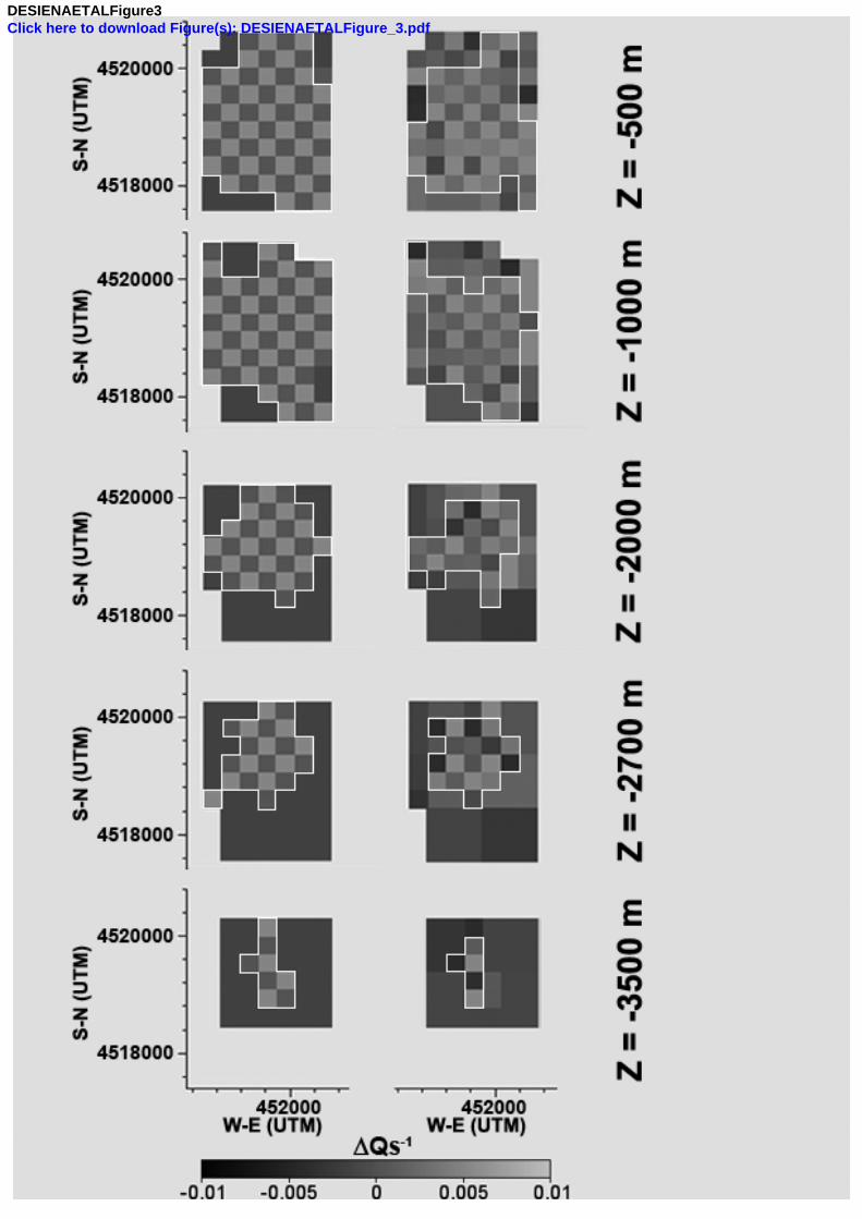
DESIENAETALFigure3Click here to download Figure(s): DESIENAETALFigure_3.pdf

DESIENAETALFigure4Click here to download Figure(s): DESIENAETALFigure_4.pdf

DESIENAETALFigure5Click here to download Figure(s): DESIENAETALFigure_5.pdf

DESIENAETALFigure6Click here to download Figure(s): DESIENAETALFigure_6.pdf

DESIENAETALFigure7Click here to download Figure(s): DESIENAETALFigure_7.pdf

DESIENAETALFigureA21Click here to download Figure(s): DESIENAETALFigure_A21.pdf

Multiple resolution seismic attenuationimaging at Mt. Vesuvius

Luca De Siena1 *Edoardo Del Pezzo1 Francesca Bianco1

Anna Tramelli1

1Istituto Nazionale di Geo�sica e Vulcanologia , sezione di Napoli OsservatorioVesuviano, Via Diocleziano, 328 - 80124 Napoli, Italia.

� fax: +39 081 6108323 ; email: delpezzo@ov.ingv.it

Abstract

A three-dimensional S wave attenuation tomography of Mt. Vesuvius has been ob-tained with multiple measurements of coda-normalized S-wave spectra of local smallmagnitude earthquakes. We used 6609 waveforms, relative to 826 volcano-tectonicearthquakes, located close to the crater axis in a depth range between 1 and 4 km(below the sea level), recorded at seven 3-component digital seismic stations. Weadopted a two-point ray-tracing; rays were traced in an high resolution 3-D velocitymodel. The spatial resolution achieved in the attenuation tomography is comparablewith that of the velocity tomography (we resolve 300 m side cubic cells). We statisti-cally tested that the results are almost independent from the radiation pattern. Wealso applied an improvement of the ordinary spectral-slope method to both P- andS-waves, assuming that the di¤erences between the theoretical and the experimentalhigh frequency spectral-slope are only due to the attenuation e¤ects. We could checkthe coda-normalization method comparing the S attenuation image obtained withthe two methods. The images were obtained with a multiple resolution approach.Results show the general coincidence of low attenuation with high velocity zones.The joint interpretation of velocity and attenuation images allows us to interpretthe low attenuation zone intruding toward the surface until a depth of 500 metersbelow the sea level as related to the residual part of solidi�ed magma from the lasteruption. In the depth range between -700 and -2300 meters above sea level, theimages are consistent with the presence of multiple acquifer layers. No evidence ofmagma patches greater than the minimum cell dimension (300m) has been found.A shallow P wave attenuation anomaly (beneath the southern �ank of the volcano)is consitent with the presence of gas saturated rocks. The zone characterized bythe maximum seismic energy release cohincides with a high attenuation and lowvelocity volume, interpreted as a cracked medium.

Key words: Attenuation tomography, Mt. Vesuvius, Coda normalization method,Spectral slope, Multi resolution inversion

Preprint submitted to Elsevier Science 27 May 2008

DeSienaetal Marked Manuscript

1 Introduction.

The knowledge of the internal structure of the volcanoes represents a crucialtask to properly constrain the physical models of eruption. Passive tomographyis one of the easiest and cheapest way to achieve this goal and is consequentlywidely applied for the study of volcano structures at several depths (Chouetet al., 1996).

There are two main factors limiting the maximum resolution that can be ob-tained in passive methods: the ray coverage and the wavelength of the wave-forms from which the observables are retrieved. The �rst factor is linked to thestation density and the source space distribution. The second is directly asso-ciated with the kind of events that are used as input. For a local tomographyon a volcano with a volume of the order of 10 km of linear dimensions, local VTearthquakes, with their associate wavelengths that ordinary span from somekilometers to hundreds of meters (Chouet, 2003) are a suitable input. Gen-erally the smallest wavelength characterizes the minimum cell size, and thiscan be considered as the thumb rule for this constraint. Moreover, to reachthis minimum cell size, one needs a suitable source space distribution (sourcesas much as possible uniformly distributed in the volume, and an as dense aspossible network of receivers). In a con�guration typical of an up-to-date seis-mic network, an order of resolution of 300 meters can be reached only in thevolume cells with a su¢ cient ray coverage (Chouet et al., 1996). This leads tothe solution of a mixed-determined problem, with an highly overdeterminedsystem of equations correspondent to the cells with a redundant number ofrays crossing through, and an equal- or lower-determined system for the othercells. A way to optimize the problem is to use an approach with a non uniformcell size, that maintains a su¢ cient over-determination in any cell, but reachesa good resolution only in the parts of the investigated volume characterizedby the maximum ray coverage. This kind of approach is typically named asmulti-step or multiple-resolution method [see Bai and Greenhalgh (2005), foran example of travel time multi-step tomography on a volcano].

The attenuation of elastic waves depends strongly on a number of factorsa¤ecting the lithology, the most important of which are probably the tem-perature and the presence of fractures and hydrothermal or magmatic �uids.Attenuation is quanti�ed by the quality factor, Q, de�ned as the ratio betweenthe energy lost by a wave cycle and the energy of the cycle itself; equivalently,attenuation can be de�ned through the attenuation coe¢ cient � = �fr=vQthat accounts for the damping of the wave amplitude, A, as a function ofdistance, r and frequency, f . This factor may greatly vary for rocks with thesame composition but di¤erent degree of fracturing and/or temperature. Theresponse of the rocks to the propagation of longitudinal and shear waves isdi¤erent; the independent determination of the quality factors for longitudinal

2

(Qp) and shear (Qs) waves, critical parameters for the characterization of thephysical state of the rocks within a volcano, aims at discriminating betweenmelt �uids and gases residing at shallow depths in the earth�s crust. For thispurpose, a comparative study of velocity and attenuation tomography can becritical (Hansen et al., 2004).

A phenomenon that intensely a¤ects the wave propagation in volcanic areasis the scattering process, which tends to transfer the high-frequency energy ofdirect P and S waves into the coda of the seismograms (Sato and Fehler, 1998).Scattering is produced by the interaction of the wave�eld with the small scaleheterogeneities in the elastic parameters, as, for example, those associatedwith intense rock fracturing. The average attenuation caused by scattering,can be studied independently from the one caused by intrinsic attenuation,separating the two di¤erent types of losses (Bianco et al., 1999). Results onvolcanoes show that, for frequencies higher than 10 Hz, scattering attenuationis more important than intrinsic attenuation (Del Pezzo et al., 2006 a). For acomprehensive summary of results from attenuation measurements by a rangeof methods, at varying frequency, on di¤erent scales and in di¤erent geologicalsettings the reader is referred to Sato and Fehler (1998).

Unfortunately, for the single path estimates (necessary for tomography) of theattenuation coe¢ cient, the separation between the two kinds of contribution(scattering and intrinsic) is practically impossible. Consequently, in the atten-uation tomography, the parameter obtained by the inversion is the total-Q orthe correspondent attenuation coe¢ cient.

This paper is aimed at giving an image of the shallow crust materials at Mt.Vesuvius volcanic area using shear wave attenuation tomography at high fre-quency (in the range between 10 and 20 Hz), solved with a multi-resolutionmethod with a minimum cell (the greatest available resolution) of 300 me-ters. Observables (total-Q inverse for each single path) are obtained usingthe coda-normalization method (Aki, 1980), and checked with the ordinaryspectral-slope method. Spectral slope is used also to estimate P-wave totalQ-inverse. Attenuation images are eventually compared with high resolutionpassive velocity tomography [the same minimum cell size, Scarpa et al. (2002)].The images obtained with this method are also compared with those obtainedat a resolution of 900 meters in a previous study of the same area, carried outusing a subset of the present data set (Del Pezzo et al., 2006 b).We will showthat the low attenuation zone located under the crater is coincident with ahigh velocity volume, possibly associated with residual frozen magma from thelast eruptions; and that a high attenuation volume at 1-2 km of depth is coin-cident with a low velocity zone. This is interpreted as the aquifer permeatingthe shallow structure of Mt. Vesuvius.

3

2 Geological and seismological settings.

Mt. Vesuvius is a stratovolcano formed by an ancient caldera (Mt. Somma)and by a younger volcanic cone (Mt. Vesuvius). The volcanic activity is datedback to 300�500 ky (Santacroce, 1987) and characterized by both e¤usive andexplosive regimes (Andronico et al., 1995). The volcanic complex is locatedin the Campania plain (southern Italy) at the intersection of two main faultsystems oriented NNW�SSE and NE�SW (Bianco et al., 1997). The last erup-tion, in March 1944, was e¤usive (Berrino et al., 1993). It may have started anew obstructed conduct phase and hence a quiescent stage.

The seismic activity is actually the unique indicator of the internal dynamics[see e.g. De Natale et al. (1998)]. Seismicity studies are of extreme importancefor the high risk volcanic area of Mt. Vesuvius. As an overall, the seismicity ofMt. Vesuvius is characterized by a mean rate of approximately 300 events peryear. The largest earthquake in the area [reasonably since the last eruption-1944- see Del Pezzo et al. (2004)] occurred in 1999, and has been associatedwith regional and local stress �elds (Bianco et al., 1997). The main featuresof the earthquake space and time distribution are described in the papers byScarpa et al. (2002), hereafter cited as SCA02, and Del Pezzo et al. (2004).In the study of SCA02 the relocated seismicity appears to extend down to 5km below the central crater, with most of the energy (up to local magnitude3:6) clustered in a volume spanning 2 km in depth, positioned at the borderbetween the limestone basement and the volcanic edi�ce. The hypocentrallocations for the data used in the present article show the same pattern of theoverall seismicity (Figure 1).

The earthquakes recorded at Mt. Vesuvius are mostly of volcano-tectonic type(VT), with fault-plane orientations, showing an highly non-regular spatialpattern. The spectral content of the P- and S-wave trains of the VT events iscompatible with stress drops spanning a range between 1 and 100 bars (100bars for the largest magnitude) and focal dimensions of the order of 100 m(Del Pezzo et al., 2004).

The velocity structure beneath Mt. Vesuvius, in the depth range from theEarth surface to 10 km, has been deduced by seismic tomography. Auger etal. (2001) suggest the presence of a melting zone at a depth of about 8 km,on the base of the TOMOVES experiment results (see the book by Capuanoet al. (2003) and the numerous references therein). At smaller scale, betweenthe topographical surface and 5 km of depth, SCA02 evidence a low velocitycontrast between 1 and 2 km, possibly associated with the presence of aquifers.No shallow and small magma chambers are visible at the resolution scalereached by SCA02.

4

3 Data selection.

In the present work we utilized a total number of 6609 waveforms, obtainedfrom a selection of 826 earthquakes recorded from January 1996 to June 2000at seven 3-component stations that are the analogical station OVO (66 dBdynamic range, three component) sampled at 100 s.p.s. and 6 digital, highdynamic (120 dB, gain ranging), 1 Hz , seismic stations sampled at 125 s.p.s.(Table I). Analog anti-aliasing �lter with 25 Hz cut-o¤ frequency operated onall the data logger prior to sampling. Data selection has been made on thebase of the following pre-requisites: the best signal to noise ratio, the absenceof spikes and other disturbances in the waveforms, a minimum coda duration(from origin time) of 15 s and the absence of secondary events in the earlycoda. In doing this selection we implicitly restricted the earthquake magnitudein the range from 1:6 to 3:0, because small aftershocks are often present inthe coda of larger events. Location of the 826 earthquakes (Figure 1) wasobtained using P-picking of all the available seismic stations constituting themonitoring network (www.ov.ingv.it) with a non linear procedure based on agrid-search algorithm (Lomax et al., 2001); ray-tracing was calculated usingthe 3D velocity model obtained by SCA02.

4 Methods.

4.1 Ray tracing.

We used a Thurber-modi�ed approach (Block, 1991) to trace the path of eachray in the 3-D velocity structure of Mt. Vesuvius obtained by SCA02. This is anextension of the approximate ray-bending method (Um and Thurber, 1987)that works well in velocity structures characterized by fairly sharp velocityvariations, like that of Mt. Vesuvius. The only limitation is that the methoddoes not compute re�ected ray paths, that anyway are not taken into accountin the present work. After dividing the whole structure to be investigated inthree di¤erent grids (respectively with 1800, 900 and 300 m cubic cell size)we stored in a database the length of each ray, connecting each source to eachreceiver, and the length of the ray-segments crossing each cell. This databaseis necessary for the multiple-resolution inversion approach, as discussed later.

5

4.2 Single-path attenuation with the coda-normalization (CN) method.

The CN method is widely used to retrieve attenuation parameters indepen-dently of the site and instrumental transfer function [Aki (1980); Sato andFehler (1998)]. Del Pezzo et al. (2006 b) used this approach for the estimationof single path total Q-inverse to map the S-wave attenuation structure in Mt.Vesuvius area, using a subdivision of the investigation volume in cubic cell of900 meters in a single-scale approach. Even though the method used to esti-mate the single path inverse total-Q has been already described and discussedin Del Pezzo et al. (2006 b), we report in Appendix 1 a synthesis for sake ofcompleteness.

Our reference equation (see Appendix 1 and 2 for any detail) is:

Eij(f; r)

EC(f; t)r2ij =

1

P (f; tc)exp

264�2�f Zrij

dl

v(l)QijT (l)

375 (1)

Taking logs of both sides of eq. (1) and approximating the line integral witha sum, we can write

dCk =1

2�fln(

1

P (f; tc))�

N_cellsXb=1

lkbsbQ�1b (2)

where dCk represents the log of energy spectral ratio between S and coda pre-multiplied for the squared ray-length and divided for 2�f . N_cells is the totalnumber of blocks crossed by the ray , lkb is the length of the k-th ray-segmentintersecting the b-th block characterized by slowness sb and inverse qualityfactor Q�1b . In this formulation we use the su¢ x k to indicate the k-th rayof the suite of rays connecting stations to sources. Eq. (2) can be rewrittenseparating Q�1b into an average Q�1b ; <Q

�1b >, that we assume to be equal

to the average quality factor for the whole area (Q�1T ), and an incremental�Q�1b :It results:

edCk = N_cellsXb=1

lkbsb�Q�1b (3)

where: edCk = 1

2�fln(

1

P (f; tc))� dCk �Q�1T

N_cellsXb=1

lkbsb (4)

Eq. (3) represents a linear system of N_k equations in N_cells unknownsthat can be inverted, as discussed in the next chapters.

6

4.3 The estimate of the observables with the CN method.

Prior to the application of the CN method we checked the temporal stabilityof the S-wave time window for the radiation pattern e¤ect, as widely describedin Appendix 2. Accordingly, we set the duration of the S-wave time windowat 2:5 s starting from the S-wave arrival time. Coda signal time window startsat 8 s lapse time and ends at 12 s, since most of our data show a favorablesignal-to-noise ratio (>3) for lapse time smaller than 12 s. A Discrete FourierTransform (DFT) is applied to the signals after windowing (we used a cosinetaper window with tapering at 10% both for S and coda) for both the horizon-tal components of the ground motion. We calculate the S spectral amplitudeaveraged in the frequency bands centered at the values of frequency, fc,withbandwidths (��f) reported in Tab II, and �nally log-averaged over the com-ponents; we thus obtain the ratio between the S-wave spectrum and the codaspectrum. The natural logarithm of this ratio estimates dCk of formula (4).The constant in eq. (2) has been already estimated by Del Pezzo et al. (2006b) for the area under study.

4.4 The slope-decay (SD) method .

As a complementary approach, we adopted the so called slope decay method,which has been widely used to estimate the attenuation coe¢ cient in many re-gions of the world [Nava et al. (1999), Giampiccolo et al. (2003), Gudmundssonet al. (2004)].

As well known, the amplitude spectral density for S and P waves for frequencieshigher than the corner frequency can be expressed as the product of source,path and site e¤ects as:

AHFij (f; r) = SAi (f)Ij(f)Tj(f)Gij(r) exp(��f

tij(r)

QijT (r)) (5)

where AHF (f; r) is the high-frequency spectral amplitude of the P- or S-waveradiation emitted by the source i at total distance r measured along thesource(i)-station (j) ray-path; f is the frequency; SAi (f) is the amplitudespectrum at source; Ij is the instrument transfer function; Tj is the site trans-fer function andG is the geometrical spreading term; tij is the travel time alongthe ray of length r and QijT is the total quality factor measured along the ray-path. In the present formulation we assume that the high frequency amplitudespectrum at the source can be described by a function SAi = consti � f� , being a constant for the whole set of data utilized. Taking the natural loga-rithm and making the derivative of the eq. (5) respect to frequency, f , it canbe written for each ray-path:

7

Df (lnAHFij ) = Df (lnS

Ai )� �

tij(r)

QijT (r)(6)

where Df is the symbol of derivative. In obtaining formula (6) we assumed theindependence of frequency for the site and instrument transfer function. Theindependence of frequency for the site term has been con�rmed by Galluzzo etal. (2005) who studied the site transfer function at Mt. Vesuvius. The trans-fer function of the instruments is �at with frequency in the whole frequencyrange investigated. Transforming the couple of indexes ij in a single integer kassociated with the single ray, as in the previous section, we can write:

Df (lnAHFk ) = Df (lnS

Ai )� �

tk(r)

QkT (r)(7)

Averaging the left hand quantity of the above equation over the rays considered(k index) we obtain:

< Df (lnAHFk ) >k= D

0f (lnA

HF ) =

< Df (lnSAi )� �

tk(r)

QkT (r)>k = D0

f (lnSA)� � < t(r)

QT (r)>k (8)

D0f (lnS

A) results to be the same of Df (lnSAi ) (the average of the source

spectral derivative equals the spectral derivative for the single event), so thatwe can write:

Df (lnAHFk )�D0

f (lnAHF ) ~=�(<

t(r)

QT (r)>k �

tk(r)

QkT (r)) (9)

Indicating with dD the quantity:

dDk =1

�

hDf (lnA

HFk )�D0

f (lnAHF )

i(10)

and expressing the right hand side of eq. (9) as already done in eq. (1) weobtain:

dDk = <t(r)

QT (r)>k �

N_cellsXb=1

lkbsbQ�1b (11)

where the index k is referred to the k-th ray.

8

Making the same assumption that leads to formula (3), we can �nally write:

edDk = N_cellsXb=1

lkbsb�Q�1b (12)

where: edDk =< tkQk

> �dDk �Q�1TN_cellsXb=1

lkbsb (13)

The inversion schemes (3) and (12) are formally identical, apart the constantvalues.

4.5 The estimate of the observables with the SD method.

Direct S spectral amplitudes were obtained in the frequency band centered atfc = 18 Hz, with the same bandwidth used for the CN method (Table II). Theuse of only this central frequency value is justi�ed by the spectral features ofthe seismicity at Vesuvius like broadly discussed in Del Pezzo et al. (2006 b).We applied a DFT to windowed signals of length 2:5 seconds starting from thedirect S travel time for both W-E and S-N components of the ground motion;then we log-averaged the spectra over the components.

We applied the SD method both to direct S waves and to direct P waves.Spectral amplitude for P waves was calculated in a time window starting fromthe P-wave onset and ending at 0:1 s before the S-wave picking, tapering eachspectrum with a 10% cosine taper function.

The derivative was carried out for both S and P log-spectra in the frequencyband starting from corner frequency (around 10 Hz for the whole set of data)and ending at 23 Hz (before the cut-o¤ frequency of the anti-alias �lter thatwas set up at 25 Hz). The derivative was computed using MATLAB "di¤new"routine.

5 Multi-resolution inversion.

The resolution of the methods depends both on the wavelength ( which hasto be smaller than the cell size) and on the number of rays crossing the singlecell. A frequency fc = 12 Hz corresponds to a wavelength of about 200 m forS waves. For P waves (examined at 18 Hz only) the corresponding wavelengthis of the order of 150 m. Taking a cell size of 300 m we observe that theblocks bordering the volume of investigation are crossed by a number of rays

9

insu¢ cient to ensure stability in the �nal solution, due to the distribution ofthe sources, concentrated along the crater axis and not uniformly distributedin space and depth inside the volume under investigation. This is the reasonwhy we cannot invert the whole data set using a uniform resolution of 300m. Consequently, we seek for solutions that can represent images in cells witha non-uniform size, as other researchers do in velocity tomography[Thurber(1987), Sambridge et al. (1998)]. In this approach, a relatively high-resolutioncan be obtained in a target area with a good ray coverage (this avoids lineardependence among the system equations). To perform this task we use aniterative inversion scheme [Thurber (1987), Eberhart-Phillips (1990)], in whichwe employ the results obtained in a lower resolution (LRR) as input for highestresolution (HRR). Bai and Greenhalgh (2005) describe an inversion schemeof this kind, applied to velocity tomography. Our inversion scheme is di¤erentfrom those above cited and will be described in the following points.

(1) The observables are calculated (both for the CN method and the SDmethod we apply the same inversion procedure) as above described.

(2) The attenuation factor averaged over the whole volume under study, Q�1T ,is estimated with the CN method. It results in a really good agreementwith that estimated by the previous works in the same area [Bianco etal. (1999), Del Pezzo et al. (2006 a)].

(3) The problem of eq. (3) and (12) is solved for a volume divided in cubicblocks of 1800 m side, using a positivity constraint. Then, each 1800 mside block is divided in 8 blocks of 900 m side, and the inverse qualityfactors thus calculated, (Q�1b )

1800, are assigned to each of this cubes.(4) The problem is solved for the 900 m cell size resolution, taking into con-

sideration that each ray is characterized by the attenuation factor, whichhas been obtained by the solution of the previous step. In this way weobtain the new quantity (�Q�1b )

900, which represents the variation fromthe inverse quality factor (Q�1)1800assigned to the 900 meters block in theprevious step. We divide as before each 900 meters block in 27 blocks of300 m side, assigning to each of them the inverse quality factor (Q�1b )

900.Also for this step we use a positivity constraint on the (Q�1b )

900:(5) Finally we solve the problem for a 300 m side cell resolution, obtaining

(�Q�1b )300.

It is noteworthy that, whereas the data vectors and the coe¢ cient matricesneed to be recalculated at each scale, the inversion problem is always formallythe same and is given by equations (3) and (12). The details regarding how thedata vectors and coe¢ cient matrices are upgraded at each scale are reportedin Appendix 3. It is also important to note that, at each step, we accept thesolutions for the blocks in which the number of ray-segments , nR, is given by:

nR �2Block_side

�(14)

10

This empirically determined threshold would ensure, in the assumption thatthe directions of ray-segments are randomly distributed in each block, thateach block is homogeneously sampled.

6 Robustness, stability, checkerboard and synthetic anomaly tests.

6.1 a) Robustness

The robustness of the method is tested using a bootstrap approach, reducingrandomly the number of available equations (rays). We applied this test toall the blocks at each cell size. The solutions for blocks of 1800 meters sidewere obtained for progressive reductions of the equations used to solve theinverse problem (see Appendix 3 , formula (21)); at each step we measuredthe quantity:

P =Qb(0)�Qb(%)

Qb(0)� 100 (15)

where Qb(%) is the quality factor of the block b obtained for the reduceddata set, whereas Qb(0) is the solution obtained using the whole database. Werepeated the inversion 100 times for each data reduction, measuring then theaverage percentage . We observed in most of the cases a signi�cant increase ofthe percentage for a reduction of more then 40% of the data-set . The resultsfor all the blocks of 1800 meters side solved are reported in Table III.

We repeated the same procedure for each scale, i.e. we measured the quantityP of formula (15) for all the 900 meters side blocks. We obtain a signi�cantchange in the value of P and a signi�cant reduction of the average blocks re-solved, for a random extraction of more than 40% of data. For sake of synthesiswe report in Table IV the results obtained for 8 blocks contained in a single1800-side block which resulted to be characterized by (Q1800b )�1 = 0:0128; itsposition is shown in the upper panels of Figure 1 using the light grey squareevidenced by number 1. The results for the other 900 m side blocks solved bythe inversion are similar.

Finally, we compared the variations of P calculated with eq. (15) for all the300 meters side blocks, observing both a signi�cant change in the value of theparameter models and a signi�cant reduction in the average number of blocksresolved, for the random extraction of more than 20% of data. We report inTable V a selection of 8 blocks of 300 meters contained in the singular block of900 meters side having (Q900b )�1 = 0:011 (the position of the 900 meters blockis shown in the upper panels of Figure 1 using the dark grey square evidenced

11

by number 2).

6.2 b) Stability.

The stability of the method is checked by changing the value of the constantsin formulas (4) and (13). In formula (4) we let g0 to vary between the valuesof gmin = 1 and gmax = 2:5 that represent the error limits of the average g asreported in Del Pezzo et al. (2006 a). In formula (13) we let < tk

Qk> to vary

in the interval [�3�+ < tkQk> , +3�+ < tk

Qk>]: The results do not change

signi�cantly. In both (4) and (13) we let Q�1T to vary in the interval [�3�+Q�1T, +3� +Q�1T ]

For the resolution of 1800m the variations of each parameter model obtainedfor the extreme values are reported in Table VI.

For the intermediate resolution (900 meters) we repeat the same proceduresetting maximum and minimum values of (Q1800)�1 and QT�1 sampled intheir con�dence interval (3�). The 8 blocks considered in Table VII are thesame of Table IV.

For the maximum available resolution (300 meters), using the results obtainedchanging the values of Q�1T , (Q

1800b )�1 and (Q900b )�1 in their con�dence interval,

we obtain the results shown in Table VIII for the 8 blocks considered in TableV.

6.3 c) Checkerboard inside the HRR.

Our results have been tested imposing an a priori attenuation structure to thearea: we assumed an homogeneous medium in the LRR and a checkerboarddistribution of the quality factors in the volume where the HRR is located,resolving only the blocks crossed by at least 5 rays per block, following eq.(14). Using the CN method we calculated the true spectral ratios and addedto these values a Gaussian random error calculated with a random numbergenerator with zero mean and standard deviation equal to 10% of the spectralratio.

The synthetic structure results to be extremely well resolved in the centralpart, whereas the quality of the reproduction of the input values decreasestoward the borders of the volume under investigation. The checkerboard testresults (Figures 2 and 3) are shown both for the W-E and S-N sections alreadyshown in Figure 1, and for �ve horizontal slices in the depth range between�500 to �3500m.

12

Both in Figure 2 and Figure 3 we marked with a white broken line the zonewhere the checkerboard structure is e¤ectively reproduced, as described in thefollowing. In Figure 2 it can be noticed that the input checkerboard structure(W-E and S-N sections in panel a) is well reproduced everywhere except ina small area toward North and toward East, corresponding to the geologicalstructure of Mt. Somma (the same sections in panel b); this is due to the lackof seismic sensors in this area. The negative variations in the inverse qualityfactors under �3000 meters always well reconstruct the zones with low Q�1S .In Figure 3 the �ve panels on the left present �ve horizontal sections of thevolume containing the input checkerboard structure, imaging the HRR (seealso Figure 1, downward left panel); the good resolution achievable by themethod used is evident in the volume constrained between 0 and �2700 m(right panels of the same �gure). At Z = �3500 m, the method resolves atthe maximum resolution only a subset of the input volume.

6.4 d) Synthetic anomaly

We performed a second test adopting the procedure described in Schurr et al.(2003), using synthetic data by tracing rays through the real 3-D VS model, inorder to check the e¤ective availability of the results which will be discussedin the following chapter. This test uses as input a Q�1S model created usinganomalies comparable in size to those observed using the real data-set (W-Eand S-N sections in Figure 4, panel a) but with slightly di¤erent geometries.A 10% normally distributed error was applied to the spectral ratios. The testshows that at maximum resolution the anomalies are generally well recoveredbetween the surface and �3000 m (W-E and S-N sections in Figure 4, panelb). In the depth range between �3000 m and �4500 m the test shows that theresolution decreases. The test is consistent with the checkerboard test (Figure3, Z = �3500 m) and shows that the maximum resolution achievable in thisdepth range is 900 m.

7 Results.

Using the present multi-resolution method, we obtained the attenuation struc-ture under Mt. Vesuvius in two frequency bands (Table II), centered at 12 and18 Hz. The images have a resolution of 300 meters in the sub-volumes withhigh ray coverage marked in Figures 2 and 3 with a white broken line. All theresults obtained are shown in Figures 5, 6 and 7, where the depths (negativedownward), are calculated respect to the sea level. In Figures 6 and 7 the im-ages relative to the velocity tomography (SCA02) are also shown. The presentdatabase is a subset of the database used in the velocity tomography.

13

In Figure 5 the results of S-wave attenuation imaging obtained with both CNand SD are reported for sake of comparison.

Using CN technique, an estimate of the variation of Q�1S respect to the meanwas obtained for the two frequency bands (12 and 18 Hz), where the signalto noise ratio value resulted su¢ ciently high for this analysis [see Del Pezzoet al. (2006 b) ]. These images are reproduced in panels a and b of Figure 5.Using SD technique a unique image at 18 Hz was obtained (panel c).

Images shown in panel a and b of Figure 5 are very similar except for anhigher attenuation zone (turquoise) located in a depth range between -2500and -3500 m centered at 452000 onto the W-E section, visible in panel b.

Comparing panel b and panel c of Figure 5, we notice that in the HRR theimages are similar. Outside the HRR slight di¤erences between the two imagesappear in the W-E section, at a depth of approximately -1000 m, betweencoordinates 453000 and 454000. In this region CN method (panel b) gives ahigh attenuation contrast zone whereas the contrary occurs for SD method(panel c). We observed that the SD method produces in general images thatare less variable in space respect to those from the CN method.

Figure 6, panel a, reports the W-E and S-N sections of the S- wave attenuationimages at 18 Hz; in the same �gure the S-wave velocity (panel b), P-waveattenuation (panel c) and P-wave velocity (panel d) for the W-E and S-Nsections are also represented. VP=VS ratio as a function of depth (calculated asan average over the slices at di¤erent depth) is superimposed to all the �gures.The color scale in panels a and c represents the variation of the inverse qualityfactor respect to the mean S- or P-wave attenuation; the color scales of panelsb and d represent the absolute S- and P-wave velocity.

Figure 7 represents twenty horizontal slices at the depths�500,�1000,�2000,�2700 and �3500 meters. Color scales represent the di¤erences respect to theaverage S-wave velocity (�rst column), S-wave attenuation (second column),P-wave velocity (third column) and P-wave attenuation (fourth column) cal-culated for each slice. The di¤erences respect to the average show the samepattern of the absolute P- and S- waves velocities and attenuation (in thediscussion we will not make any di¤erence between the absolute quantity andthe variation respect to the mean), and better enlighten the lateral variations.

8 Discussion

The HRR is localized essentially under the central part of the cone spanninga depth range between +250 and -3500 m (see Figures 2 and 3). In this zone

14

we have thus an S-wave attenuation image with a resolution improved respectto that obtained by Del Pezzo et al. (2006 b) using a single scale approach.Laterally, the resolution becomes lower due to the station density, which isnot comparable with the cell dimension [for a wider discussion on stationdensity and resolution see Bai and Greenhalgh (2005)]. In general, the 3-Dattenuation pattern shows a Q�1 which clearly decreases with depth in the12 and 18 Hz frequency bands (Figure 5, panels a and b) , showing clearlyvisible attenuation contrasts localized along the borders of the already knownstructures (see e.g. SCA02), like the carbonate basement, well visible at themaximum resolution in the Q�1S , Q

�1P , VS and Vp images at �1500 meters (see

Figures 6, all panels).

8.1 Frequency dependence of the S-wave attenuation

In the HRR the independence of attenuation from frequency is con�rmed inthe frequency range between 12 and 18 Hz. The panel b of Figure 5 showsan attenuation contrast localized between 452000 and 453000, in the depthrange between �2500 and �3500 meters, with a size larger than the minimumresolution. This contrast is not evident in panel a of the same Figure, for theimage obtained at 12 Hz, possibly due to the di¤erent linear dimensions of theanomalous region sampled by the di¤erent wavelength.

8.2 Comparison between CN and SD images

The S-wave images obtained under the cone at 18 Hz with CN and SDmethodsare quite enough similar, showing on average the same dependency of Q�1Swith depth (Figure 5, panel b and c). In general the images obtained withCN appear much more smoothed than those obtained with SD. In the HRRmost of the attenuation contrasts follow the same pattern, being sometimesdi¤erent in value.

The sole signi�cant di¤erences between CN and SD images can be observedbetween�1000m and�2000m toward North and toward East (correspondingat surface with the geological structure of Mt. Somma). In this volume (Figure5 panels b and c) the interface between carbonate basement and the overlyingvolcano materials, is not clearly de�ned in the SD image. On the other hand,this interface is clearly evidenced by SD method applied to P-waves, and verywell de�ned by the velocity tomography (see also SCA02 and Zollo et al.(2002)).

The discrepancy above discussed may be due to the assumptions that are at thebase of CN. In this method S-spectra are normalized by coda spectra, in order

15

to cancel out the site term. This procedure is based on the experimental resultthat the coda radiation is uniform for all the source station pairs after a lapsetime greater than twice the S-wave travel time. This experimental property ofcoda waves may be not strictly veri�ed in presence of a non-uniform scatteringwave �eld (Wegler, 2003) that may produce for few waveforms a bias in thenormalization of S-spectrum with coda spectrum. Despite this problem, theindependence of CN of site transfer function makes CN approach particularlysuitable for the application to volcanic areas, where site e¤ects may severelya¤ect the spectrum of S-radiation emitted by the VT earthquakes.

8.3 Joint interpretation of velocity and attenuation images

8.3.1 General pattern

We �rst analysed the velocity images, isolating the volumes characterized bystrong laterally and/or in depth contrasts, velocity inversions, variations fromthe average VP=VS. Then, we associated them with the corresponding vol-umes in all the other available images. Comparing VP with Q�1P and VS withQ�1S images (Figures 6, all panels) we observe that high VP zones correspondroughly to low Q�1P volumes and that high VS zones correspond to low Q�1Svolumes; the unique evident exception is the volume located under the centralcone, con�ned in the depth range between �1000 m and �2000 m, where thepattern is characterized by a low VS and VP corresponding to high variationsin attenuation ( Q�1S and Q�1P strongly increase with depth).

8.3.2 The shallower structures

In average, the attenuation of the S- and P-waves increases toward North andEast in all the images for the volumes above the sea level (Figure 6, panelsa and c); interestingly, the S-N section of the Q�1S image (panel a) shows alow attenuation inclusion (green surrounded by orange, not included in theHRR) with dimension of the order of a 900 meters , corresponding to thestructure of Mt. Somma, the ancient caldera border. This structure surroundsthe central cone in the North and East quadrants (Figure 1, down left) and ischaracterized by higher rigidity older age lavas.

In the HRR (marked with a broken white line in Figure 2, panel b), velocityand attenuation images clearly evidence the presence of a contrast betweenthe structure above and the volume underneath the depth of 0 meters; thiscontrast marks the �rst interaction between the recent products of the volcanoactivity and the older higher rigidity materials.

A low attenuation zone [roughly surrounded by the rectangle 1] is strongly

16

correlated with an high VS and Vp zone in the same position, as shown inFigure 7 ( Z = �500 meters). This zone is located inside the HRR (seeFigure 3, panel a) and may represent the residual lava emitted during the lasteruptions, completely solidi�ed in the present time.

In the same slice (Figure 7 , Z = �500) we observe that the western part ischaracterized by low Q�1S , high Q

�1P and low VP=VS . This features, in particu-

lar the opposite pattern of Q�1S andQ�1P , may be compatible with the presenceof a CO2 reservoir (Hansen et al., 2004). This interpretation is corroboratedby the presence of the above discussed low attenuating body in the centralpart of the Figure. As reported by Hansen et al. (2004), when the magmarises, the decrease in con�ning pressure causes the magma to decompress andthe biggest part of CO2 exsolves; however, when the magma cools, a mod-est amount of CO2 can be de�nitely trapped in the rock matrix, and couldexplain the observed low VP and low VP=VS anomalies (Gerlach and Taylor,1990). This interpretation is con�rmed by the laboratory experiments of (Itoet al. (1979), Spencer (1979), Sengupta and Rendleman (1989)). Summarizingthe results from these papers, at pressure below the saturation pressure (asshould be at a depth of �500 meters), the presence of gas can lead to a de-crease in VS and VP , an increase of Q�1S , and an anomalous decrease of Q

�1P ,

that is the same pattern observed for Mt. Vesuvius.

The presence of melt or partially melt rocks would lead to a low VP , a lowVS, high VP=VS ratio, high Q�1P and high Q�1S . In the depth range around�500 m there is consequently no evidence supporting the presence of patchesof magma with dimensions larger than cell size.

8.3.3 The intermediate structure

A zone of strong lateral contrast is evident in both the VP and VS images[the zone surrounded by the rectangle marked by number 2 in the slices ofFigure 7 ( Z = �1000) ] . In this zone there is no correspondence of theincreasing velocity with decreasing attenuation, as already discussed in the"General pattern" section. The low attenuation area marked by the whiterectangle 1 in Figure 7 ( Z = �1000m) corresponds instead to an high velocityarea. This area is a section of the anomalously high-velocity volume (�gure6, panels b and d) which seems to intrude from depth, in agreement withthe interpretation reported in several velocity tomography studies [Zollo etal. (2002), Tondi and De Franco (2003), De Natale et al. (2005), SCA02],and interpreted as related to the residual part of solidi�ed lava from the lasteruption. This high attenuation and velocity zone is connected with the areamarked by line 1 in Figure 7, Z = �500 m.

To re�ne the interpretation in the depth range around �1000 m, especially

17

for the area marked by rectangle 2 in Figure 7, we focus the attention onthe W-E and S-N sections in Figures 6 [all panels]. The zone correspondingin depth with the maximum value of the VP=VS ratio roughly corresponds tothe interface between high attenuation and low attenuation. This interfaceis also characterized by low VP and low VS. All these observations may beinterpreted as due to the presence of a fractured medium permeated by �uids,as discussed in Hansen et al. (2004) and Eberhart-Phillips et al. (2004). Inthis interpretation the presence of a shallow patch of magma in the samedepth range should be excluded, in the limit of the spatial resolution: in fact,the attenuation images do not show any particular evidence of melt, that, ifpresent, should have produced both high Q�1P and high Q�1S . These results arein agreement with the previous interpretation done by SCA02 on the base ofthe ole velocity tomography, and are also corroborated by geochemical studies,that locate an hot aquifer under the cone just in the same position (Marianelliet al. (1999), Chiodini et al. (2001)). The properties observed at Z = �1000m can be observed also at Z = �2000 m (see Figure 7). In particular asecondary maximum in the VP=VS ratio can be observed at �2000 m. Thevertical sections ofQ�1P andQ�1S (Figure 6 panels a and c) indicate the presenceof a high attenuation zone, around �2000 m, included in a low attenuationbody. This pattern can be interpreted as an highly cracked medium �lled by�uids, in agreement with geochemical studies (Chiodini et al., 2001).

8.3.4 The deepest structure

The VP ,VS and VP=VS patterns between �2500 m and �4000 m (Figures 6,panels b and d) are more regular. The Z = �2700 and Z = �3500 slices ofFigure 7 help in better understanding the velocity and attenuation features.The pattern of Q�1P and Q�1S are similar at Z = �2700 (Figure 7 and Figure3), both in the HRR and in the LRR. Focusing the attention on the centralpart of the attenuation images (rectangle 3), a high contrast in both Q�1S andQ�1P , not perfectly matching the contrast in both VP and VS can be observed.The imperfet match may be due to a lack of resolution of attenuation imagingin this depth range.

At Z = �3500 m, the decreasing attenuation corresponds to the increasingvelocity outside rectangle 4, for both P and S waves. A low velocity andattenuation zone corresponding to the South-East sector of Figure 7 at Z =�3500 m is clearly visible, and marked with the rectangle 4. In this regionthe low VP=VS ratio excludes the presence of partially melt rocks or �uidinclusions, suggesting on the contrary the presence of a cracked volume. Thiszone is spatially coincident with the zone of maximum seismic energy release,as shown in Figure 1 (upper-left and upper-right panels, the grey ellipsoidalline marked by number 3).

18

9 Conclusions.

The present paper complements a previous preliminary study of the same area,which was carried out in a smaller volume respect to that used in the presentstudy. The present paper uses a multi-resolution approach, which solves a 300m cell size in the volume beneath the central crater located in the depth rangebetween approximately 0 (the sea level) and �3500 m. The new study is baseda data set improved respect to the �rst one (the number of waveforms in thepresent study is more than doubled respect to the previous), improving bothstability and robustness. The improved resolution allowed a better de�nition ofthe 3-D pattern for both Q�1P and Q�1S , thus improving the joint interpretationof previous velocity images with the present attenuation structure. The essen-tial results show that no magma patches with dimensions larger than the cellsize are visible in the images and con�rm the presence of shallow hydrother-mal reservoirs (between -700 and -2300 m) evidenced by geochemical studies.The high resolution achievable between 0 and �1500 m allowed a small scaleimaging of the residual solidi�ed lava emitted during the last eruptions, lead-ing to the interpretation in terms of large patches of gas located in the �rstkilometer below sea level. Interestingly, the zone of maximum seismic energyrelease, imaged for the �rst time at a resolution of 900 meters, coincides witha high attenuation and low velocity anomaly, easily interpretable as due tothe presence of a cracked zone inside the limestone layer. These results areexpected to add important constraints for the numerical models that will beadopted to simulate the next eruption, and consequently to be used for CivilDefense purposes.

10 Appendix 1

10.1 Coda Normalization Method.

As well known, the S-wave seismic energy density spectrum decays as a func-tion of lapse-time as:

Eij(f; r) = Si(f)�ij(#; �)Ij(f)Tj(f)1

r2ijexp(�2�f tij(r)

QijT (r)) (16)

where E(f; r) is the energy density spectrum of the S-wave radiation emittedby the source i at total distance r measured along the ray-path connectingsource(i) and station (j) ; f is the frequency. Si(f) is the energy spectrum atsource, modulated by the radiation pattern function �(#; �). Ij is the instru-ment transfer function and Tj is the site transfer function. tij is the travel time

19

along the ray whose length is rij and QijT is the total quality factor measured

along the ray-path.

The coda energy spectrum evaluated around a given lapse time, tc, can beconsidered as a function of the "average" medium properties and expressed asin Sato and Fehler (1998):

EC(f; t) = Si(f)Ij(f)Tj(f)P (f; tc) (17)

where P (f; tc), is independent on both source-receiver distance and directionalazimuth and depends only by the earth medium. The radiation pattern term�ij(#; �) disappears due to the well known property of natural space averagingof coda waves (Aki, 1980). For sake of simplicity, we assume the validity of thesingle scattering model, but in principle equation (17) is independent of anyscattering model. Dividing eq. (16) for eq. (17) for each source-station pair,at lapse time tc, we obtain

Eij(f; r)

EC(f; t)r2ij =

�ij(#; �)

P (f; tc)exp

264�2�f Zrij

dl

v(l)QijT (l)

375 (18)

The spectral ratio at the left side of formula (18) is independent of energy levelat source, site and instrument transfer function. In eq. (18) the attenuationoperator has been substituted with the path integral along the seismic ray,where v(l) is the velocity along the path l. �ij(#; �) in principle depends onsource azimuth � and incidence angle #. For a complete review of the methodsee Del Pezzo et al. (2006 b). In Appendix 2 we test the independence of thespectral ratio of formula (18) of radiation pattern for ratios evaluated onsignal time windows longer than 2.5 seconds. In this case �ij(#; �) can be setequal to unity.

11 Appendix 2

11.1 Test for the independence of radiation pattern.

Using the properties of the early-coda, Gusev and Abubakirov (1999) devel-oped an empirical method to test the independence of S-wave spectra fromradiation-pattern, when the spectrum is estimated in a time window of dura-tion much greater than the source duration. We make a similar test for thespectral ratio between S and coda energy spectra calculated for the earth-quakes of Mt. Vesuvius. We consider for each ray connecting the source to thereceiver, the quantity:

A =LR

M(19)

20

where L is the ray length, R is the spectral ratio between energies of for-mula (18) and M = exp(��fr=V Qmean), with V indicating the average S-wave velocity, is the average anelastic attenuation in the area. A is implicitlydependent only on the radiation pattern, R being independent of site andinstrument e¤ects. The percent standard deviation (�A= < A >) calculatedaveraging A over the stations for a single earthquake, is plotted for di¤erenttime window durations in Figure A2.1; this quantity abruptly decreases withincreasing duration of the time window, as expected. We applied a statisticaltest [the "change point" test of Mulargia and Tinti (1985)] to estimate the"change point" of the pattern of A respect to the duration of the time windowin which is calculated. The pattern results to be steady after 2:5 seconds at99% con�dence. Consequently, the radiation-pattern e¤ects become negligiblefor time windows with a duration greater than 2:5 s. We interpret this resultas due to the natural processes of averaging the radiation pattern e¤ects thattakes place in a ray-tube centered along the ray-path. The forward scatteredradiation that arrives at the receiver soon after the ballistic (direct) arrival iscontained inside this ray-tube(Gusev and Abubakirov, 1999). For the abovereasons we assume that �ij(#; �) of eq. 18 is identically equal to unity.

12 Appendix 3

In this Appendix we explain the details relative to the points listed between2 and 5 in the section 5

Point 2: estimate of the Average inverse Quality Factor (AQF).

S-waves AQF is calculated using the coda normalization method applied tothe whole data-set ; the eq. (2) becomes:

dCk =1

2�fln(

1

P (f; tc))�

N_cellsXb=1

lkbsbhQ�1T

iC(20)

where <> indicates the average over We obtained the inverse AQF for S waves(Q�1T ):

(Q�1T )12 = 0:010� 0:003

(Q�1T )18 = 0:019� 0:003

where the above index is referred to the center frequency.

Uncertainty is estimated assuming that each spectrum is a¤ected by a 10%of error due to the noise. This result is in good agreement with previous Q-estimate for S waves in the area (Del Pezzo et al., 2006 a).

21

P-waves AQF has been already calculated by Bianco et al. (1999).

Point 3: cell dimension of 1800 m.

The inversion problem of eq. (3) and (12) is solved for a grid of 1800 metersstep. We can rewrite the equation as:

~dC;Dk =N_cells_1800X

b=1

G1800kb [(�Q1800b )�1]C;D (21)

where the superscript 1800 stands for the step of the grid, while the super-script C;D takes into account the di¤erent methods used. The elements ofthe inversion matrix, G1800kb , are the length of the k � th ray segment in the1800-meter side b� th block, l1800kb , multiplied for his slowness s1800b :

G1800kb = l1800kb s1800b (22)

Applying eq. (14), we consider only blocks crossed by at least nR = 35 rays.The problem is solved separately for each frequency band. We solve the prob-lem using the least squares algorithm "lsqlin" deployed in MATLAB.

The percentage reduction of the residuals, computed using the formula inGubbins (2004), results to be 65%. The inverse quality factor of each 1800meters block b is given by:

(Q1800b )�1 = Q�1T + (�Q1800b )�1 (23)

Point 4: cell dimension of 900 meters.

The data vector obtained solving the inversion schemes of eq. (4) and (13)can be updated with the solutions obtained in the previous steps. Each raycrosses a medium whose quality factor is no more QT , and is a¤ected by thequality factors of the cube that it e¤ectively crosses. The elements of the datavector must represent the e¤ect of the attenuation structure obtained in theprevious steps. They become respectively:

( edCk )1800 =< 1

2�fln(

1

P (f; tc)) > �dCk �Q�1T

N_cells_900Xb=1

l900kb s900b

�N_cells_900X

b=1

l900kb s900b (�Q�1b )

1800;C (24)

22

and

( edDk )1800 =< tkQk

>1800 �dDk �Q�1TN_cells_900X

b=1

l900kb s900b �

N_cells_900Xb=1

l900kb s900b (�Q�1b )

1800;D (25)

where (�Q�1b )1800;C and (�Q�1b )

1800;D are respectively the solutions obtainedwith the CN method and the SD method for 1800 meters side blocks and thatwhere assigned to the N_cells_900 blocks of 900 meters side crossed by thek � th ray. In the SD method the constant value < tk

Qk>1800 has also been

updated with the informations obtained in the previous step. The inversionproblem becomes, for a resolution of 900 meters:

( ~dC;Dk )1800 =N_cells_900X

b=1

G900kb [(�Q900b )�1]C;D (26)

where the superscript 900 stands for the step of the grid and the (�Q900b )�1

are the inverse variations respect the inverse quality factor of the 1800 meterscube in which they are contained. The elements of the inversion matrix, G900kb ,are the length of the k � th ray segment in the 900-meters side b � th blockl900kb multiplied for his slowness s900b :

G900kb = l900kb s

900b (27)

where, we consider only blocks crossed by at least nR = 17 rays see equation(14). The inversion is linear and we can constrain the average of the (�Q900b )�1

to be zero. The inverse quality factor of each 900 meters block b is given by:

(Q900b )�1 = Q�1T + (�Q1800b )�1 + (�Q900b )�1 (28)

while the percentage reduction is 70% in residual.

Point 5: cell dimension of 300 meters.

The last step is achieved upgrading the data vectors writing the following twoformulas:

( edCk )900 =< 1

2�fln(

1

P (f; tc)) > �dCk �Q�1T

N_cells_300Xb=1

lkbsb�

N_cells_300Xb=1

lkbsb(�Q�1b )

1800;C �N_cells_300X

b=1

lkbsb(�Q�1b )

900;C (29)

23

and

( edDk )900 =< tkQk

>900 �dDk �Q�1TN_cells_300X

b=1

lkbsb�

N_cells_300Xb=1

lkbsb(�Q�1b )

1800;D �N_cells_300X

b=1

lkbsb(�Q�1b )

900;D (30)

where (�Q�1b )900;C and (�Q�1b )

900;D are the solutions obtained in the previoussteps that were assigned to a number of N_cells_300 blocks of 300 metersside, crossed by the k � th ray. As before, the constant value < tk

Qk>900

has been updated with the informations obtained in the previous steps. Theinversion problem becomes:

( ~dC;Dk )900 =N_cells_300X

b=1

G300kb [(�Q300b )�1]C;D (31)

where the superscript 300 stands for the grid step, and the elements of theinversion matrix, G300kb , are given by the length of the k � th ray segment inthe b� th block, l300kb , multiplied for his slowness s300b :

G300kb = l300kb s

300b (32)

applying eq. (14), we consider only blocks crossed by at least nR = 5 rays. Thepercentage reduction in residual is 94%. The inverse quality factor of each 300meters block b is given by:

(Q300b )�1 = Q�1T + (�Q1800b )�1 + (�Q900b )�1 + (�Q300b )�1 (33)

13 Acknowledgements.

This work is �nanced by INGV-DPC (Dipartimento di Protezione Civile Ital-iana) project V3_4 and project European Union VOLUMEFP6-2004-GLOBAL-3. Routine analysis has been carried out in LAV (Laboratorio di Analisi aVan-zate of INGV-Naples) by Simona Petrosino and Paola Cusano, who are grate-fully acknowledged. Lucia Zaccarelli greatly improved the work with numerousdiscussions.

24

References

Andronico, D., Calderoni, G., Cioni, R., Sbrana, A., Suplizio, R., and San-tacroce, R., 1995. Geological map of Somma-Vesuvius Volcano. Per. Min-eral., 64: 77-78.

Aki, K., 1980. Attenuation of shear-waves in the lithosphere for frequenciesfrom 0.05 to 25 Hz. Phys. Earth Planet. Inter., 21: 50-60.

Auger, E., Gasparini, P., Virieux, J., and Zollo, A., 2001. Seismic Evidence ofan Extended Magmatic Sill Under Mt. Vesuvius. Science, 294: 1510-1512.

Bai, C., and Greenhalgh, S., 2005. 3D multi-step travel time tomography: imag-ing the local, deep velocity structure of Rabaul volcano, Papua New Guinea.Physics of the Earth and Pl. Int., 151: 259-275.

Berrino, G., Coppa, U., De Natale, G., and Pingue, F., 1993.Recent geophysicalinvestigation at Somma�Vesuvius volcanic complex. J. Volcanol. Geotherm.Res., 58: 239-262.

Bianco, F., Castellano, M., Milano, G., Ventura, G., and Vilardo, G., 1997.The Somma-Vesuvius stress �eld induced by regional tectonics: evidencesfrom seismological and mesostructural data. J. Volcanol. Geotherm. Res.,82: 199-218.

Bianco, F., Castellano, M., Del Pezzo, E., and Ibanez, J. M., 1999. Attenuationof short period seismic waves at Mt. Vesuvius, Italy. Geophys. J. Int., 138:67-76.

Block, L.V., 1991. Joint hypocenter-velocity inversion of local earthquakes ar-rival time data in two geothermal regions. Ph.d. dissertation, M.I.T., Cam-bridge.

Capuano, P., Gasparini, P., Zollo, A., Virieux, J., Casale, R., and Yeroyanni,M., 2003. The internal structure of Mt. Vesuvius. A seismic tomographyinvestigation. Liguori Editore, ISBN 88-207-3503-2.

Chiodini, G., Marini, L., and Russo, M., 2001. Geochemical evidence for theexistence of high-temperature hydrothermal brines at Vesuvio volcano, Italy.Geoch. et Cosmoch. Acta, 65(13), 2129�2147.

Chouet, B., 1996. New methods and future trends in seismological volcanomonitoring. In: Scarpa, R., Tilling, R.I. (Eds.), Monitoring and Mitigationof Volcano Hazards. Springer, Berlin, pp. 23�97.

Chouet, B., 2003. Volcano Seismology. Pageoph, 160: 739-788.Del Pezzo, E., Bianco, F., and Saccorotti, G., 2004. Seismic source dynamicsat Vesuvius volcano, Italy. J. Volcanol. Geotherm. Res., 133: 23-39.

Del Pezzo, E., Bianco, F., and Zaccarelli, L., 2006. Separation of Qi and Qsfrom passive data at Mt. Vesuvius: a reappraisal of seismic attenuation.Physics of the Earth and Pl. Int., 159: 202�212.

Del Pezzo, E., Bianco, F., De Siena, L., and Zollo A., 2006. Small scale shallowattenuation structure at Mt. Vesuvius, Italy. Physics of the Earth and Pl.Int., 157: 257-268.

De Natale, G., Capuano, P., Troise, C., and Zollo, A., 1998. Seismicity atSomma-Vesuvius and its implications for the 3D tomography of the volcano.

25

J. Volcanol. Geotherm. Res., Special Issue Vesuvius. Spera F. J., De VivoB., Ayuso R.A., Belkin H.E. (Eds), 82: 175-197.

De Natale, G., Troise, C., Pingue, F., Mastrolorenzo, G., and Pappalardo, L.,2005. The Somma�Vesuvius volcano (Southern Italy): Structure, dynamicsand hazard evaluation. Earth-Science Rev., 74: 73-111.

Eberhart-Phillips, D., 1990. Three-dimensional P and S velocity structure inthe Coalinga region, California. J. Geophys. Res. 95: 15343�15363.

Eberhart-Phillips, D., Reyners, M., Chadwick, M., Chiu, J. M., 2005. Crustalheterogeneity and subduction processes: 3-D V P , V P/V S and Q in thesouthern North Island, New Zealand. Geophys. J. Int. 162: 270�288.

Galluzzo, D., Del Pezzo, E., Maresca, R., La Rocca, M., and Castellano, M.,2005. Site e¤ects estimation and source-scaling dynamics for local earth-quakes at Mt. Vesuvius, Italy. Congress acts, ESG2006, Grenoble. Papernum. 36.

Gerlach, T., and Taylor, B., 1990. Carbon isotope constraints on degassing ofcarbon dioxide from Kilauea volcano. Geochim. Cosmochim. Acta 54, 2051�2058.

Giampiccolo, E., Gresta, S. and Ganci, G., 2003. Attenuation of body waves inSoutheastern Sicily (Italy). Physics of the Earth and Pl. Int., 135: 267�279.

Gubbins, D., 2004. Time series analysis & inverse theory for geophysicists.Cambridge University Press.

Gudmundsson Ó., Finlayson D. M., Itikarai I., Nishimura Y., and Johnson W.R., 2004. Seismic attenuation at Rabaul volcano, Papua New Guinea. J. ofVolc. and Geoth. Re., 130: 77-92.

Gusev, A. A., and Abubakirov, I. R., 1999. Vertical pro�le of e¤ective turbidityreconstructed from broadening of incoherent body-wave pulses. Geophys. J.Int., 136: 309-323.

Hansen, S., Thurber, C. H., Mandernach, M., Haslinger, F., and Doran, C.,2004. Seismic Velocity and Attenuation Structure of the East Rift Zone andSouth Flank of Kilauea Volcano, Hawaii. Bull. of the Seism. Soc. of Am.,94: 1430-1440.

Ito, H., DeVilbiss, J., and Nur, A., 1979. Compressional and shear waves insaturated rock during water�steam transition. J. Geophys. Res. 84, 4731�4735.

Lomax, A., Zollo, A., Capuano, P., and Virieux, J., 2001. Precise absoluteearthquake location under Somma-Vesuvius volcano using a new three-dimensional velocity model. Geophys. J. Int., 146: 313-331.

Marianelli, P., M´etrich, N., and Sbrana, A., 1999. Shallow and deep reservoirsinvolved in magma supply of the 1944 eruption of Vesuvius. Bull. Volcanol.,61: 48-63.

Mulargia, F., and Tinti, S., 1985. Seismic sample areas de�ned from incompletecatalogues; an application to the Italian territory. Phis. Earth Plan. Int, 40:273-300.

Alejandro Nava, F., Garcìa-Arthur, R., Castro, R. R., Suàrez, C., Màrquez, B.,Nùñez-Cornù, F., Saavedra, G. and Toscano, R., 1999. S wave attenuation

26

in the coastal region of Jalisco�Colima, México. Phys. Earth Pl. Int., 115:247�257.

Santacroce, R., 1987. Somma-Vesuvius. CNR, Quaderni di Ricerca Scienti�ca.Sambridge, M.S., and Gudmundsson, O., 1998. Tomographic systems of equa-tion with irregular cells. J. Geophys. Res., 103: 773�781.

Sato, H., and Fehler, M.C.,1998. Seismic Wave Propagation and Scattering inthe Heterogenous Earth. Springer.

Sengupta, M. K., and Rendleman, C. A., 1989. Case study: the importanceof gas leakage in interpreting amplitude-versus-o¤set (AVO) analysis. Soc.Explor. Geophys. Abstracts 59, 848�850.

Scarpa, R., Tronca, F., Bianco, F., and Del Pezzo, E., 2002. High resolutionvelocity structure beneath Mount Vesuvius from seismic array. Geophys.Res. Lett., 29 (21): 2040.

Schurr, B., Asch, G., Rietbrock, A., Trumbull, R., and Haberland, C., 2003.Complex patterns of �uid and melt transport in the central Andean subduc-tion zone revealed by attenuation tomography. Earth. Pl. Scien. Lett., 215:105-119.

Spencer, J., 1979. Bulk and shear attenuation in Berea sandstone: the e¤ectsof pore �uids. J. Geophys. Res. 84, 7521�7523.

Thurber, C.H., 1987. Seismic structure and tectonics of Kilauea volcanoHawaii. In: Decker, R.W., Wright, T.L., Stau¤er, P.H. (Eds.), Volcanismin Hawaii. US Geological Survey, pp. 919�934.

Tondi, R., and De Franco, R., 2003. Three-dimensional modeling of MountVesuvius with sequential integrated inversion. J. Geophys. Res., 108: 2256.

Um, J., and Thurber, C.H., 1987. A fast algorithm for two-point seismic raytracing. Bull. of the Seism. Soc. of Am. 77: 972-986.

Wegler, U., 2003. Analysis of multiple scattering at Vesuvius volcano, Italy,using data of the Tomoves active seismic experiment. J. Volcanol. Geotherm.Res., 128: 45�63.

Zollo, A., D�Auria, L., De Matteis, R., Herrero, A., Virieux, J., and Gasparini,P., 2002. Bayesian Estimation of 2-D P-Velocity Models From Active Seis-mic Arrival Time Data: Imaging of the Shallow Structure of Mt.Vesuvius(Southern Italy). Geophys. J. Int., 151: 566-582.

14 Captions.

� Figure 1:Lower-left panel: Map of Mt. Vesuvius with station positions (blacksquares) and hypocentral locations (white dots) of the seismic events used inthe present work. Black broken line depicts the old caldera rim. Upper-leftand upper-right panels represent respectively the W-E and S-N sections,also reported as "W-E plane" and "S-N plane" in the lower-right "wideangle" view. The High Resolution Region (HRR) is roughly depicted bythe inner polyhedron in the wide angle view. The solid line rectangles in

27

the upper left, upper right and lower left panels represent the sections ofthe HRR. The zones marked with 1and 2 represent the zone in which therobusteness test results are reported respectively in Table IV and V. Theellipsoidal zone marked with 3 shows the area with the maximum seismicenergy release.

� Figure 2: Checkerboard test in the HRR. a) Input. W-E and S-N sections(also marked in �gure 1, lower right panel); the white lines include all themaximum resolution cells de�ned by formula (14). In this volume we as-sumed a checkerboard structure, with high Q-contrast among the blocks;a uniform attenuation medium is assumed outside HRR. b) Output. Testresults for a 10% error on synthetic data. The zones marked by the whitebroken lines include the cells where the checkerboard structure is e¤ectivelyreproduced. �Q�1S grey scales represent the variation from the average qual-ity factor.

� Figure 3: Left hand panels. Five horizontal slices at di¤erent depths (Zvalue respect to the sea level) of the volume containing the HRR. The whitelines include all the maximum resolution cells de�ned by formula (14). Thesections represent the input checkerboard structure also described in Figure3, with the same colorscale. Rigth hand panels. The �gures represent thetest output; the zones marked by the white broken lines include the cellswhere the checkerboard structure is e¤ectively reproduced.

� Figure 4: Synthetic anomaly test. The input structures (panel a) are in-cluded in a volume characterized by uniform attenuation. The output (panelb) show the reconstruction of the anomalies. Black areas are not resolved inthe inversion. Colorscales refer to the variations respect to the mean inversequality factor. The zones marked by the white broken lines include the cellswhere the checkerboard structure is e¤ectively reproduced.

� Figure 5: Results of the attenuation tomography inversion, in the frequencyband centered at 12 Hz (panel a), and 18 Hz (panel b) for the CN method,compared with the results obtained at 18 Hz for the SD method (panel c).W-E and S-N sections are those marked in Figure 1 (down-rigth panel).Black areas are not resolved in the inversion.Colorscales refer to the vari-ations respect to the mean inverse quality factor. The zones marked bythe white broken lines include the cells where the checkerboard structure ise¤ectively reproduced.

� Figure 6: The W-E and S-N sections represent the attenuation structureinferred for S-waves (CN method), in the frequency band centered at 18Hz (panel a), and the S-velocity structures inferred by Scarpa et al. (2002)(panel b). The dashed line represents the VP=VS pattern with depth and isoverimposed to all �gures. The P-wave attenuation (SD method, 18 Hz) andvelocity (inferred by Scarpa et al. (2002)) are also represented in panels cand d. The colorscales in panels a and c refer to the variations respect to themean inverse quality factor obtained in the inversions for S- and P-waves.The colorscales in panels b and d represent the absolute S- and P-wavevelocity. Black areas are not resolved in the inversion. The zones marked by

28

the white broken lines include the cells where the checkerboard structure ise¤ectively reproduced.

� Figure 7: Five horizontal slices of the the volume containing HRR at di¤erentdepths (Z). The colorscales for S- (�rst column) and P-wave (third column)attenuation images represent the variations from the mean inverse qualityfactor calculated on each horizontal slice at each depth. The colorscalesrepresented in the second and fourth coloumns respectively represent thevariations of S- and P-wave velocity from the average velocity calculated ateach depth. On each image we marked with numbered black rectangles, thezones characterized by important properties, widely discussed in the text.The zones marked by the white broken lines include the cells where thecheckerboard structure is e¤ectively reproduced.

� Figure A2.1: The percent standard deviation, �=�, as a function of the win-dow duration for an earthquake recorded at all the stations. �=� is obtainedcalculating the average, � [over stations] , of the log of spectral ratio be-tween direct S radiation and coda radiation, after correcting the amplitudesfor geometrical spreading and for the average Q. Downward arrow indicatesthe change-point as discussed in the text.

Table I

Station E-W (UTM) N-S (UTM) altitude (a.s.l.) (m)

BAFM 450372 4518076 594

BKEM 452677 4518762 850

BKNM 451875 4520020 865

FTCM 452692 4516337 350

OVO 449190 4519705 600

POLM 447910 4522499 181

SGVM 450568 4518706 734

Table II

��f fc(Hz) +�f

8.2 12 15.8

12.4 18 23.6

29

Table III

Robusteness Test - 1800 m

Block# 1 2 3 4 5 6 7 8 9 10 11 12

P 1800, 10% 1% 0% 0% 13% 7% 4% 0% 0; 1% 0% 0% 0% 3%

P 1800, 20% 1% 0% 2% 29% 9% 11% 17% 1% 0% 0% 0% 3%

P 1800, 30% 2% 1% 3% 28% 9% 9% 50% 0; 3% 0% 0% 0% 2%

P 1800, 40% 3% 3% 10% 29% 8% 16% 87% 2% 1% 0% 0% 8%

P 1800, 50% 6% 2% 11% 62% 20% 25% 87% 3% 1% 0% 0% 9%

Robustness test at the lowest resolution; the average percentageof eq. (15) isrepresented for all the blocks resolved. The increasing percentage in the �rst

column is the data reduction.

30

Table IV

Robusteness Test - 900 m

Block# 1 2 3 4 5 6 7 8

P 900, 10% 1% 15% 2% 1% 10% 1% 31% 1%

P 900, 20% 1% 13% 15% 1% 12% 8% > 100% 1%

P 900, 30% 1% 21% 15% 1% 16% 9% > 100% 1%

P 900, 40% 2% 53% 29% 2% 30% 7% > 100% 2%

P 900, 50% 2% 58% 72% 2% 40% 11% > 100% 2%

Robustness test at the intermediate resolution; the average percentage of eq.(15) is represented for the 8 blocks in which the single 1800 meters side blockof (Q1800b )�1 = 0:0128 wich includes the cone was divided. The increasing

percentage in the �rst column is the data reduction.

Table V

Robusteness Test - 300 m

Block# 1 2 3 4 5 6 7 8

P 300, 10% 12% 16% 21% 59% 30% 5% 1% 14%

P 300, 20% 37% 90% 54% 99% 17% 48% 90% 70%

P 300, 30% > 100% > 100% 67% > 100% 69% > 100% 98% > 100%

Robustness test at the highest resolution; the average percentage of eq. (15)is represented for 8 blocks contained in a single 900 meters side block of

(Q900b )�1 = 0:0110. The increasing percentage in the �rst column is the datareduction.

31

Table VI

Stability Test - 1800 m

Block# 1 2 3 4 5 6 7 8 9 12

[(Q1800)�1]� 10�2 1; 98 1; 79 1; 50 2; 44 1; 28 1; 37 0; 92 2; 86 0; 51 3; 16

[(Q1800)�1]� 10�2; (QminT )�1 1; 83 1; 67 1; 72 1; 84 1; 28 1; 43 1; 15 2; 72 0; 49 3; 21

[(Q1800)�1]� 10�2; (QmaxT )�1 1; 88 1:69 1; 10 2; 88 1; 11 1; 08 0; 54 2; 74 0; 40 2; 81

Stability test at the lowest resolution; the value of the inverse quality factorof each resolved block is dependent on the maximum ((QmaxT )�1 = 0:026) and

minimum ((QminT )�1 = 0:008) average inverse quality factor allowed.

Table VII

Stability Test - 900 m

Block# 1 2 3 4 5 6 7 8

[(Q900)�1]� 10�2 1; 79 0; 52 0; 96 1; 79 2; 75 1; 64 0 1; 79

[(Q900)�1]� 10�2; (QminT )�1; (Q1800bmin)�1 1; 88 0; 46 1; 12 1; 88 2; 36 1; 77 0 1; 88

[(Q900)�1]� 10�2; (QmaxT )�1; (Q1800bmax)�1 1:67 0; 58 0; 80 1; 67 3; 14 1; 51 0 1; 67

Stability test at the intermediate resolution; the value of each inverse qualityfactor is both dependent on the maximum ((QmaxT )�1 = 0:026) and minimum

((QminT )�1 = 0:008) average inverse quality factor and the maximum((Q1800bmax)

�1 = 0:0188) and minimum ((Q1800bmin)�1 = 0:0167) inverse quality

factor of the block in which they are contained.

32

Table VIII

Stability Test - 300 m

Block# 1 2 3 4 5 6 7 8

[(Q300)�1]� 10�2 5; 61 1; 78 1; 91 0; 39 1; 44 0 2; 26 0

[(Q300)�1]� 10�2; (QT min)�1; (Q1800bmin)�1; (Q900bmin)

�1 2; 59 1; 76 1; 34 0; 05 1; 29 0 2; 60 0

[(Q300)�1]� 10�2; (QT max)�1; (Q1800bmax)�1; (Q900bmin)

�1 6; 91 1; 99 2; 01 1; 59 1; 32 0 1; 34 0

Stability test at the highest resolution; the value of each inverse qualityfactor is both dependent on the maximum ((QmaxT )�1 = 0:026) and minimum((QminT )�1 = 0:008) average inverse quality factor. It is also dependent on the

maximum ((Q1800bmax)�1 = 0:0188, (Q900bmax)

�1 = 0:0177) and minimum((Q1800bmin)

�1 = 0:0167, (Q900bmin)�1 = 0:0151) inverse quality factor of the blocks

in which they are contained.

33