Multiplicative Kalman filtering

Submitted to the Bernoulli

Multiplicative Kalman filtering.

FABIENNE COMTE1,∗ and VALENTINE GENON-CATALOT1,∗∗ and MATHIEUKESSLER2

1Laboratoire MAP 5, Universite Paris Descartes, UFR de Mathematiques et Informatique,

CNRS UMR 8145, 45 rue des Saints Peres, 75270 Paris Cedex 06, France. E-

mail: ∗[email protected]; ∗∗

[email protected]

2Departamento de Matematica Aplicada y Estadıstica, Universidad Politecnica de Cartagena,

Paseo Alfonso XIII, 30203 Cartagena, Spain. E-mail: [email protected]

We study a non-linear hidden Markov model, where the process of interest is the absolute valueof a discretely observed Ornstein-Uhlenbeck diffusion, which is observed after a multiplicativeperturbation. We obtain explicit formulae for the recursive relations which link the relevantconditional distributions. As a consequence the predicted, filtered, and smoothed distributionsfor the hidden process can easily be computed. We illustrate the behaviour of these distributionson simulations.

Keywords: filtering, discrete time observations, hidden Markov models, parametric inference,scale perturbation.

1. Introduction

Consider a real-valued Markov process (x(t)) sampled at times t1, t2, . . . , tn, . . . (0 < t1 <. . . < tn . . .) and suppose that the observation at time ti is of the form

Yi = F (x(ti), εi), (1)

where F is a real-valued known function, the εi’s are independent random variables (anoise) and the sequence (εi) is independent of the process (x(t)). This kind of obser-vation process is encountered in many fields of applications such as finance, biology orengineering. The model is known under different names: hidden Markov model, non linearfiltering model, state-space model or dynamic model.

Denote, for i ∈ N, Xi = x(ti). For a given l, all the information about the hiddenvariable Xl is to be drawn from the conditional distribution L(Xl|Yn . . . , Y1), given that,at time tn, we have observed Y1, . . . , Yn:

• In the case when l > n, we use L(Xl|Yn . . . , Y1) to predict the value of the variableXl.

• In the case when l = n, we use L(Xl|Yl . . . , Y1) to filter the value of the variableXl.

• While, in the case when l < n, we use L(Xl|Yn . . . , Y1) to smooth the value of thevariable Xl.

1imsart-bj ver. 2007/04/13 file: gck2bernoullitemplate.tex date: August 28, 2007

hal-0

0191

042,

ver

sion

1 -

23

Nov

200

7

http://hal.archives-ouvertes.fr/hal-00191042/fr/

http://hal.archives-ouvertes.fr

2 F. Comte et al.

These three kind of distributions are related through the following classical operators.Denote by νl|n:1 the conditional distribution L(Xl|Yn . . . , Y1),

• Updating: U operator, νl|l:1(dxl) ∝ p(yl|xl)νl|l−1:1(dxl).• Prediction: νl+r|l:1 = νl|l:1Pl+r,l, where Pl+r,l denotes the transition operator fromXl to Xl+r. In the case when the chain is assumed to be homogeneous with tran-sition operator P , Pl+r,l = P r.

• Smoothing:νl|n:1(dxl) ∝ p(yl+1, . . . , yn|xl)νl|l:1(dxl).

As a consequence, any of the relevant conditional distributions νl|n:1 is computed stepwiseby moving through the following scheme:

l = 1 l = 2 l = 3 . . .

X1

yU

X1|Y1P−−−−→ X2|Y1

P−−−−→ X3|Y1P−−−−→ . . . n = 1

...

yU

X1|Y1, Y2 X2|Y1, Y2P−−−−→ X3|Y1, Y2

P−−−−→ . . . n = 2

......

yU

X1|Y1, Y2, Y3 X2|Y1, Y2, Y3 X3|Y1, Y2, Y3P−−−−→ . . . n = 3

A main difficulty associated to the study of this kind of model arises from the fact thatthese three operators involve high dimensional integrals and admit therefore no closedform expression. There is though one very important exception: the Kalman filtering,where the hidden process x(t) is an Ornstein-Uhlenbeck (O-U) process

dx(t) = −θx(t)dt+ σdWt,

and the noise observation process specification

Yi = x(ti) + εi, εi ∼ N (0, β2),

implies that the class of Gaussian distributions is closed under the action of the threeoperators. Therefore, if L(X1) is Gaussian, νl|n:1 are Gaussian and are specified by theirmeans and variances which can be computed recursively.

In this work, we study another example of Hidden Markov model, where the threeoperators admit a closed form expression. This model consists in a multiplicative per-turbation of the absolute value of a discretely observed O-U process. It builds upon a

imsart-bj ver. 2007/04/13 file: gck2bernoullitemplate.tex date: August 28, 2007

hal-0

0191

042,

ver

sion

1 -

23

Nov

200

7

Multiplicative Kalman filtering. 3

model previously studied in Genon-Catalot (2003), Genon-Catalot and Kessler (2004)and Chaleyat-Maurel and Genon-Catalot (2006), but presents two significant contribu-tions with respect to these papers: on one hand, the class of noises is extended to a moreflexible class which allows in particular to specify the number of finite moments thatadmits the marginal distribution of Yi; and on the other hand, we prove that the actionof the smoothing operator stays in the same class of distributions as for the predictionand updating operators, and we provide a backward recursion for the computation of thesmoothed distribution νl|n:1.

As a consequence, this work presents a non-linear hidden Markov model, where thehidden chain state space is R+, for which the explicit computation of any of the con-ditional distributions L(Xl|Yn . . . , Y1) is possible and computationally easy. It can inparticular be useful for testing numerical methods designed for general non-linear hiddenMarkov models, by allowing to compare their performance to the exact methods.

After introducing the model in Section 2, we describe in detail the three operators inSection 3. Section 4 contains an illustration of the behaviour of the relevant conditionaldistributions. Concluding remarks are stated in Section 5. Finally, the proofs are collectedin an appendix.

2. The model

2.1. The hidden process

The hidden process (Xn)n≥1 consists in the discrete observation of the absolute value ofa continuous time Ornstein-Uhlenbeck process. Concretely,

for n ≥ 1, Xn = |ξn∆|, (2)

where ∆ > 0 is the discretization step and ξ solves

dξ(t) = −θξ(t)dt+ σdWt, ξ(0) = η, (3)

where θ ∈ R, σ > 0, (Wt) is a standard Wiener process, η a random variable independentof (Wt). Notice that the observation times need not be equidistant, i.e. ∆ could be ∆n,though, for the sake of clarity in the exposition, we will stick to the homogeneous case.

It is well known that the transition density x′ 7→ pξt (x, x′; θ, σ) of the process ξ is

Gaussian with mean a(t)x and variance β2(t), where

a(t) = exp(−θ t), β(t) = σ

(

1 − exp (−2θt)

2θ

)1/2

. (4)

In the sequel we will use the shorthand notation a = a(∆) and β = β(∆).The process (Xn)n≥1 is therefore obtained as the absolute value of an AR(1) process

with parameters a and β2.


hal-0

0191

042,

ver

sion

1 -

23

Nov

200

7

4 F. Comte et al.

It is easy to deduce that the hidden process (Xn)n≥1 is Markov with transition densitygiven by

p∆(x, x′) = 1(x′>0)2

β√

2πexp (− x′2

2β2− a2x2

2β2)

(

cosh (axx′

β2)

)

, (5)

( x ≥ 0).Using the series expansion of the cosh, this transition density (5) can be written as

a mixture of distributions which will turn out to be relevant for the description of thethree conditional operators described in the introduction:

p∆(x, x′) =∑

i≥0

wi(a2x2/β2)gi,β(x

′), (6)

where, for i ≥ 0, the weights wi are given by

u ∈ R, wi(u) = exp (−u/2) (u/2)i/i! (7)

and the function

gi,σ(x) = 1(x>0)2

σ√

2πexp (− x2

2σ2)x2i

C2iσ2i, (8)

is the density of the square root of a Gamma distribution with scale parameter σ andlocation parameter (i + 1/2). The normalising constant C2i, is simply the moment oforder 2i of a Gaussian standard variable, i.e. for i ∈ N,

C2i =(2i)!

2ii!= (2i− 1)(2i− 3) . . . 1.

In a slight abuse of notation, we will use the notation gi,σ to denote both the densityand its associated distribution.

The transition operator P = P∆ of (Xn) acting on functions is given, for any functionf for which the integral makes sense, by:

Pf(x) =

∫

p∆(x, x′)f(x′)dx′. (9)

Acting on measures, it is given by:

νP (dx′) = (

∫

ν(dx)p∆(x, x′))dx′. (10)

We denote by gP the density of νP when ν(dx) = g(x)dx, i.e. the function

gP (x′) =

∫

g(x)p∆(x, x′)dx. (11)

Note that the r-th iterate of P is simply that P r = Pr∆ and corresponds to the parametersa(r∆), β(r∆).


hal-0

0191

042,

ver

sion

1 -

23

Nov

200

7


If, for some l ∈ N, g is the density of the law of Xl, x′ 7→ gP (x′) is the density of

the law of Xl+1. In particular, if, given Y1, . . . , Yl, νl|l:1 is the law of Xl, the distributionνl+1|l:1 = L(Xl+1|Y1, . . . , Y1) is obtained as νl|l:1P .

A crucial feature for the understanding of the prediction step can be easily deducedfrom the series expansion (6):

Property 1. Let l ∈ N,

gl,σP (x′) =∑

i≥0

(∫

wi(a2x2/β2)gl,σ(x)dx

)

gi,σ(x′),

i.e the action of P on a density gl,σ of the form (8) yields a mixture of gj,σ distributions.This mixture has infinite length, though we will see in proposition 3.1 that, by consideringa different scale parameter, it admits an equivalent mixture representation of finite length.

An additional feature which strengthen the role of the distributions gi,σ is describedin the following property:Property 2. If θ > 0 or equivalently a < 1, the unique invariant distribution of thechain (Xn)n≥1 admits the density g0,σs

, see (8), with

σ2s =

σ2

2θ=

β2

1 − a2. (12)

These two properties make it natural to consider using the distributions gi,σ, i ≥0, σ > 0 as building components of mixtures representations of distributions.

2.2. The noise

We focus on obtaining exact computations as for the standard Kalman filter. The per-turbation is assumed to act in an multiplicative way:

Yn = ψn Xn, (13)

where (ψn)n≥1 is a sequence of i.i.d random variables, independent from the process ξ.In Genon-Catalot and Kessler (2004) and Chaleyat-Maurel and Genon-Catalot (2006),

it is assumed that the r.v.’s ψn have distribution Γ−1/2 where Γ has exponential distri-bution with parameter λ. This leads to explicit computations. Here, we consider a moreflexible class of distributions for the noise (ψn) that includes the previous ones.

We assume that ψ1 has the law (Γ(k, λ))−1/2, for some k ∈ N∗ and λ > 0, i.e. admitsthe density

f(ψ) = 1ψ>02λk

Γ(k)ψ2k+1exp (− λ

ψ2). (14)

Let us check now how, given this specification of the noise structure, the updatingoperator behaves.


hal-0

0191

042,

ver

sion

1 -

23

Nov

200

7

6 F. Comte et al.

To do so, we need to consider the conditional distribution L(Yi|Xi = x), which, from(14), can be seen to admit the density,

px(y) = 1y>02λkx2k

Γ(k)y2k+1exp (−λx

2

y2), for x > 0. (15)

Assume thatXl has density g, by the Bayes rule, the conditional distribution L(Xl|Yl =y) admits a density proportional to px(y)g(x). In particular, if g is of the form gi,σ, see(8), we deduce from (15), that the density of L(Xl|Yl = y) is proportional to

∝ x2k+2i exp [−(1

σ2+

2λ

y2)x2/2]dx,

which is gi+k,Ty(σ), once we have set

1

T 2y (σ)

=1

σ2+

2λ

y2.

To sum up we have checked the following joint property of the noise specification andof the distributions gi,σ:

Property 3. If Xl ∼ gi,σ, L(Xl|Yl = yl) = gi+k,Tyl(σ).

Once again, the family gi,σ of distributions appears to play a crucial role in the de-scription of the fundamental operators associated to the filtering process.

We finish this subsection by a last property involving the noise specification and thedistributions gi,σ.

Property 4. If Xl ∼ gi,σ, the marginal density of Yl is

pgi,σ(y) = 2 1(y>0)

λkσ2k

Γ(k)

C2(i+k)

C2i

y2i

(y2 + 2λσ2)i+k+1/2. (16)

For σ = 0, the marginal distribution of Y is δ0.

This property is easily proved combining the expressions (8) and (15). Notice in par-ticular that, in the case when Xn is in its stationary state, (16) is the marginal densityof Y if we set i = 0 and σ = σs defined in (12).

2.3. The class F

From the basic properties of the prediction and updating operators described in the twoprevious subsections, it is natural to introduce the following class of distributions, builtas mixtures of gi,σ components.

F = {να,σ =∑

i≥0

αigi,σ, σ > 0, α = (αi, i ≥ 0) ∈ S}, (17)


hal-0

0191

042,

ver

sion

1 -

23

Nov

200

7


where S is the set of finite-length mixture parameters:

S = {α = (αi, i ≥ 0) : ∀i ≥ 0, αi ≥ 0,

∞∑

i=0

αi = 1 and ∃L ∈ N,∀i > L, αi = 0}. (18)

(If σ = 0, we set να,0 = δ0 for all α).Given α in S, we will also use the notation α to denote the mapping defined on N by,

for i ≥ 0, α(i) = αi.Consider a mixture parameter α ∈ S, we denote by l(α) = sup{i;αi > 0} < +∞

the length of the mixture parameter α. Note that the class F involves mixtures of gi,σsharing the same scale parameter σ.

2.4. Summing up

To sum up, our model consists in the observation of

Yn = ψn Xn,

where

• Xn = |ξn∆|, where ξ is a OU process with drit parameter −θ and diffusion param-eter σ, see (3).

• (ψn)n≥1 is a sequence of i.i.d r.v, independent from the process ξ, and ψ1 ∼(Γ(k, λ))−1/2, see (14).

• We take L(X1) to belong to F , see (17).

2.5. Remarks

1. In hidden Markov models, the iterations of the prediction and updating steps alongthe scheme described in the introduction become rapidly intractable unless both the up-dating and prediction operators evolve within a parametric family of distributions. Inthis case, the model is called a finite-dimensional filter system since each conditional dis-tribution is specified by a finite number of statistics (the stochastic process of parametersat stage n). This is the case of the model associated to the standard Kalman filter. How-ever, this notion is very restrictive (see e.g. Sawitzki, 1981; Runggaldier and Spizzichino,2001): very few finite-dimensional filter system are available and they are often obtainedas the result of an ad hoc construction. In Chaleyat-Maurel and Genon-Catalot (2006),the notion of computable infinite dimensional filters is introduced. This notion has linkswith the one proposed in Di Masi et al. (1983). The conditional distributions are allowedto evolve in much larger classes built using mixtures. These distributions are specifiedby a number of parameters which is finite but may vary along the iterations. The modeldescribed in subsection 2.4 is a computable infinite dimensional filter with respect to theclass of distributions F .


hal-0

0191

042,

ver

sion

1 -

23

Nov

200

7

8 F. Comte et al.

2. Our model can be transformed into an additive perturbation framework by a loga-rithmic transformation:

log(Yn) = log(Xn) + log(ψn) (19)

In section 3, we obtain a closed form description of the relevant conditional distributionsfor the untransformed multiplicative model. It is straightforward to obtain the corre-sponding conditional distributions for model (19).

It is worth noticing that model (19) is an example of additive perturbation model witha non Gaussian hidden process, non Gaussian noise, but where the explicit computationof the filtering, prediction, and smoothing distributions is possible.

3. An explicit formula for the moments of a distribution να,σ in F can readily beobtained:

For any r > 0,

∫

xrνα,σ(dx) = 2r/2σr∑

i≥0

αiΓ(i+ 1/2 + r/2)

Γ(i+ 1/2). (20)

Notice that an alternative expression in terms of the moments of a standard Gaussianvariable can be obtained if we take into account that

Γ(b) =

√2π

2bC2b−1, b > 0,

where, for α > −1/2, Cα = E[|Z|α], Z ∼ N (0, 1).

3. Description of the updating, prediction and

smoothing operators

The key joint properties of the distributions gi,σ, the noise ψn and and transition op-erator of the chain Xn emphasised in the previous sections allow to obtain closed formrecursive expressions for the relevant filtering distributions νl|n:1 = L(Xl|Y1, . . . , Yn). Byconvention, we set ν1|0:1 = L(X1).

Proposition 3.1. Assume that ν1|0:1 belongs to the class F . Then, for all n, l ≥ 1,νl|n:1 belongs to F . The corresponding scale and mixture parameters, σl|n:1 and αl|n:1 =(αl|n:1(i), 0 ≤ i ≤ l(αl|n:1)) can be computed recursively as follows

I. Updating step For l ≥ 1,

1

σ2l|l:1

=1

σ2l|l−1:1

+2λ

y2l

. (21)

and, for j ≥ 0,

αl|l:1(j) ∝ 1(j≥k)(2j − 1)(2j − 3) . . . (2(j − k) + 1)

(

σl|l:1σl|l−1:1

)2(j−k)αl|l−1:1(j − k). (22)


hal-0

0191

042,

ver

sion

1 -

23

Nov

200

7


On the other hand, l(αl|l:1) = l(αl|l−1:1) + k. If yl = 0, then, σl|l:1 = 0, αl|l:1(k) = 1 andνl|l:1 = δ0. Hence, formulae (21) and (22) still hold in this degenerate case.

II. Prediction, νl+r|l:1 = L(Xl+r|Y1, . . . , Yl). For r ≥ 1, the predictive conditional dis-tribution νl+r|l:1 belongs to the class F . The corresponding scale and mixture parametersare given by

σ2l+r|l:1 = β2(r∆) + a2(r∆)σ2

l|l:1, (23)

where a2(t) and β2(t) are given in (4). On the other hand, for j ≥ 0,

αl+r|l:1(j) =∑

i≥jαl|l:1(i)κ

(i)j , (24)

with, for i ≥ j,

κ(i)j =

(

i

j

)

(

1 − β2(r∆)

σ2l+r|l:1

)j (

β2(r∆)

σ2l+r|l:1

)i−j

. (25)

III. Smoothing.

1. For l < n, we have

νl|n:1(dx) =

∑(n−l)kj=0 dl,nj hj,Φl,n

(x)∏ni=l+1 p(yi|yi−1, . . . , y1)

νl|l:1(dx), (26)

where hi,σ(x) = x2ie−x2/(2σ2),

Φl,n = Φl,n(yl+1, . . . , yn), (27)

anddl,nj = dl,nj (yl+1, . . . , yn), (28)

depend on the observations (yl+1, . . . , yn).Recall that a = a(∆) and β = β(∆), see (4). Introduce

Φ2(σ) =β2 + σ2

a2, (29)

and, for 0 ≤ l ≤ i,

ci,σl =C2i

C2l

(

i

l

)(

σ2

β2 + σ2

)i+l+(1/2)

a2l β2(i−l). (30)

The coefficients Φl,n and dl,n. can be computed recursively as follows. On one hand,

Φn−1,n = Φ(yn√2λ

) dn−1,nj =

2λk

Γ(k) y2k+1n

ck, yn√

2λ

j . (31)


hal-0

0191

042,

ver

sion

1 -

23

Nov

200

7

10 F. Comte et al.

On the other hand, we have a downward recursion. For l + 1 < n,

Φl,n = Φ(γl,n) with1

γ2l,n

=1

Φ2l+1,n

+2λ

y2l+1

. (32)

For s = 0, . . . , (n− l)k,

dl,ns =2λk

Γ(k) y2k+1l+1

(n−l−1)k∑

j=(s−k)+cj+k,γl,ns dl+1,n

j . (33)

2. Moreover νl|n:1 is of the class F and we have

νl|n:1(dx) =

nk∑

s=0

αl|n:1(s)gs,σl|n:1(x)dx, (34)

where1

σ2l|n:1

=1

σ2l|l:1

+1

Φ2l,n

, (35)

and

αl|n:1(s) =σ2s+1l|n:1

∏ni=l+1 p(yi|yi−1, . . . , y1)

×∑

u∈Us

(2s− 1)(2s− 3) . . . (2u+ 1)1

σ2u+1l|l:1

dl,ns−uαl|l:1(u),

(36)

where the sum is taken over the set

Us = {u : [s− (n− l)k]+ ≤ u ≤ min(s, lk)}.

Proof in appendix.Remarks

• The denominator in (26) can be computed explicitly. Indeed, we have

p(yl|yl−1, . . . , y1) =

∫

pxl(yl)νl|l−1:1(dxl).

Since νl|l−1:1 =∑

i αl|l−1:1(i)gi,σl|l−1:1, we use formula (16) in Property 4 to deduce

that

p(yl|yl−1, . . . , y1) = 1(yl>0)

∑

i≥0

αl|l−1:1(i)2λkσl|l−1:1

2k

Γ(k)

× C2(i+k)

C2i

yl2i

(yl2 + 2λσl|l−1:12)i+k+1/2

.


hal-0

0191

042,

ver

sion

1 -

23

Nov

200

7


• The length l(α) of α in S was introduced in subsection 2.3.We deduce from (22) and (24) that l(αl|l:1) = l(αl|l−1:1) + k while l(αl+r|l:1) =l(αl|l:1). Starting from L(X1) = να1,σ1

with l(α1) = l1, we have that l(αl|l:1) isl1 + kl. The length of the mixture parameter increases therefore linearly, however,as we will see on simulations, the number of significant coefficients remains verysmall, see Table 1. This is due to the fact, that, as soon as the observed yl is closeto zero, σl|l:1 is close to zero (see (21)), which implies that σ2

l+1|l:1 is close to β2, see

(23). As a consequence, we deduce from (25), that αl+1|l:1 is close to (1, 0), whichresets the length to 1. In the case when the chain (Xn) is ergodic, we deduce fromthe density of the marginal distribution of Yn in (16) that it is pretty likely thatYn takes values close to zero.

• We have chosen to restrict the elements of F to have finite length mixture coeffi-cients. However the computations of the prediction, updating and smoothing stepsdo not depend on the length of the mixture coefficients and are therefore validalso if L(X1) is να,σ with l(α) = +∞. This could be the case for example, if X1

is assumed to be generated from a deterministic X0 = x0. Indeed, its law is inthis case νx0(dx) = p∆(x0, x)dx, which as seen from (6), admits a infinite lengthrepresentation as a mixture of distributions gi,β .It is however worth noticing that, if ergodicity is assumed, the distribution of X1

loses its importance asymptotically.• The derivation of the updating, prediction and smoothing steps do not rely on the

assumption that a < 1 (ergodic case for Xn).• Equation (21) can be interpreted in terms of gain of observing yl: the inverse ofσ2l|l:1, the square of the scale parameter after observing yl, is larger than the inverse

of σ2l|l−1:1, the square of the scale parameter before observing yl. The increment is

2λ/y2l . A similar interpretation holds for formula (35).

4. Numerical study

4.1. Typical trajectories for the hidden and the observed

processes

Recall that the observed process Yn is ψnXn, and that the noise ψ admits the density(14). The noise level can therefore be calibrated through the choice of the pair (λ, k).

First notice that E(ψα1 ) < ∞ for α < 2k and that E(ψα1 ) = λα/2 Γ(k−(α/2))Γ(k) . In partic-

ular, if k = 1, ψ1 has no second order moment. As a consequence, the same holds for Yi.Therefore, our model may be used to model heavy-tailed data. To calibrate the noise, wemay choose the pair (λ, k) such that Eψ1 = 1, i.e.

λ = λ1(k) =

(

Γ(k)

Γ(k − 1/2)

)2

. (37)


hal-0

0191

042,

ver

sion

1 -

23

Nov

200

7

12 F. Comte et al.

Using the Stirling formula, we get that λ1(k) ∼ k − 3/2 as k tends to infinity. Since, ψ1

has distribution (2λ1(k))1/2/χ(2k), we obtain that ψ1 → 1 in probability as k tends to

infinity.Another way of calibrating the noise is to choose

λ = λ2(k) = k + 1/2. (38)

In this case, ψ1 has distribution√

2k + 1/χ(2k) which also converges to 1. Moreover, the

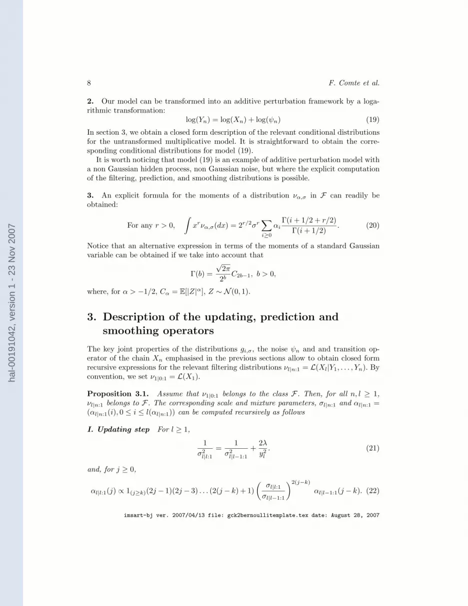
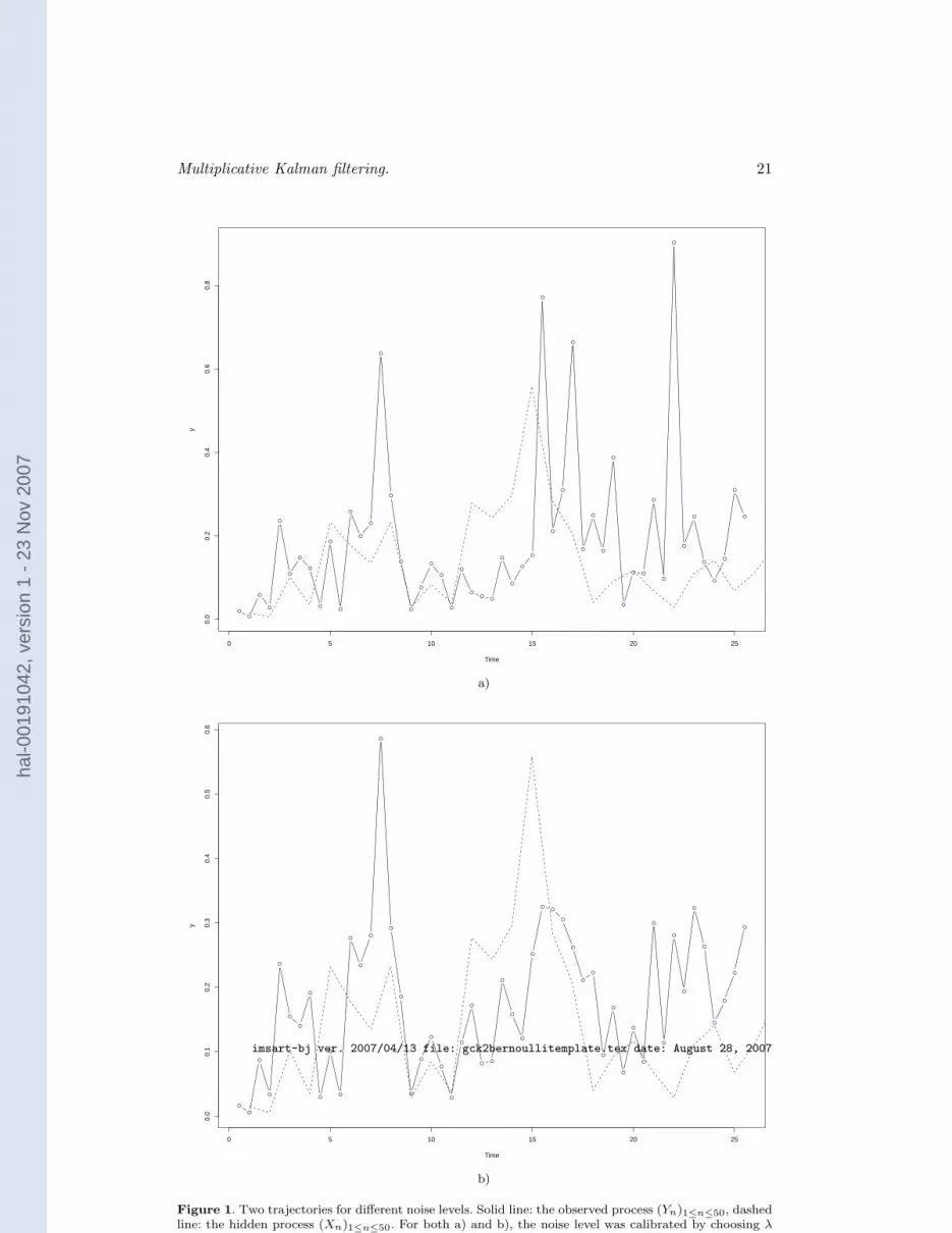
density f(ψ) of ψ1 has a unique mode attained at ψ = 1.In both cases, by increasing the value of k, we can reduce the influence of the noise.In Figure 1 below, trajectories of the observed process and the hidden process are

plotted for two different noise levels, k = 2 and k = 20. In both cases the parameter λ inthe noise density was computed using formula (37). The hidden process was simulatedwith θ = 0.5, σ = 0.2, see (3). The time step ∆ was chosen to be 0.5. The distributionof the initial variable X1 was chosen to be the stationary density g0,σs

, see (12).On the other hand, the marginal densities of Yn and Xn in the stationary state are

jointly represented in Figure 2, for the same set of parameters, but for k = 1 in the noisespecification.

4.2. Typical evolution of the scale and mixture parameters for

the filtering and prediction distributions

Table 1 illustrates a typical run of the filters described in Proposition 3.1, correspond-ing to one simulated trajectory of the observed process Y . The time step was chosen tobe ∆ = 0.5, while the parameters values were set to θ = 0.5, σ = 0.2 for the hiddenprocess X, see (2). In particular, the hidden chain is ergodic and X1 was simulated fromthe invariant distribution. The noise specification was k = 2 in (14) and λ was set tosatisfy (37).

From this table, one checks that, as predicted from the relations described in Propo-sition 3.1, the order of magnitude of the observation yl directly influences the scale andmixture parameters of the filtered distributions: when yl is close to zero, σl|l:1 is closeto zero, see (21), and as a consequence, σl+1|l:1 is close to β, see (23) (in our case,β = 0.1254). As for the mixture parameters, we deduce from (24) and (25) that, whenσl+1|l:1 is close to β, αl+1|l:1(j) ≃ 0 for j ≥ 1. To sum up, when yl is close to zero,νl+1|l:1 is reinitialised to have mixture parameter αl+1|l:1 ≃ (1, 0) and scale parameterσl+1|l:1 ≃ β, which corresponds to the distribution of the absolute value of a Gaussianvariable N (0, β2).

In particular, it explains why the length of the mixture parameter remains smallin practise, while it theoretically increases linearly with l. In the implementation ofthe filtering algorithm, given a mixture parameter α = (αi)0≤i≤l(α), we considered athreshold on its components: we only worked with its first L components, being L the


hal-0

0191

042,

ver

sion

1 -

23

Nov

200

7


Observationy1 : 0.007 σ1|1 0.005 α1|1 0 0 1

σ2|1 0.126 α2|1 0.998 0.002 0

y2 : 0.059 σ2|2:1 0.035 α2|2:1 0 0 0.999 0.001 0σ3|2:1 0.128 α3|2:1 0.91 0.088 0.002 0 0

y3 : 0.028 σ3|3:1 0.018 α3|3:1 0 0 0.991 0.009 0 0 0σ4|3:1 0.126 α4|3:1 0.976 0.024 0 0 0 0 0

y4 : 0.236 σ4|4:1 0.096 α4|4:1 0 0 0.934 0.065 0.001 0 0 0 0σ5|4:1 0.146 α5|4:1 0.535 0.39 0.074 0.001 0 0 0 0 0

y5 : 0.109 σ5|5:1 0.062 α5|5:1 0 0 0.585 0.384 0.031 0 0 0 0σ6|5:1 0.134 α6|5:1 0.715 0.255 0.029 0.001 0 0 0 0 0

y6 : 0.148 σ6|6:1 0.076 α6|6:1 0 0 0.615 0.354 0.03 0.001 0 0 0σ7|6:1 0.139 α7|6:1 0.616 0.327 0.054 0.003 0 0 0 0 0

y7 : 0.123 σ7|7:1 0.067 α7|7:1 0 0 0.594 0.371 0.034 0.001 0 0 0σ8|7:1 0.136 α8|7:1 0.677 0.284 0.038 0.002 0 0 0 0 0

y8 : 0.032 σ8|8:1 0.020 α8|8:1 0 0 0.957 0.042 0 0 0 0 0σ9|8:1 0.126 α9|8:1 0.97 0.03 0 0 0 0 0 0 0

y9: 0.186 σ9|9:1 0.086 α9|9:1 0 0 0.933 0.066 0.001 0 0 0 0σ10|9:1 0.142 α10|9:1 0.598 0.348 0.053 0.001 0 0 0 0 0

y10: 0.024 σ10|10:1 0.015 α10|10:1 0 0 0.968 0.032 0 0 0 0 0

Table 1. Typical evolution, as described in Proposition 3.1, for one trajectory of the observed processYn, of the scale and mixture parameters of the filtered density νl|l:1 = L(Xl|Yl, . . . Y1) and of the

predicted density νl+1|l:1 = L(Xl+1|Yl, . . . Y1).

smallest integer with∑

i>L αi ≤ 10−9. The remaining l(α)−L coefficients were then setto zero.

On the other hand, in Figure 3, a trajectory of the process σl|l:1, the scale parameter ofthe filtered density νl|l:1, is represented. The parameters were set to the same values as forTable 1. In Genon-Catalot and Kessler (2004), the existence of a stationary distributionfor νl|l:1 was proved in the case when the hidden process is ergodic. The plotted trajectoryis coherent with this stationarity property.

4.3. Comparison of the prediction, filtered and smoothed

distributions

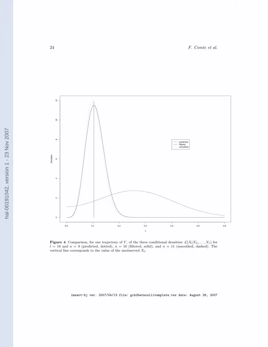
In Figure 4 a visual comparison of the prediction density L(X10|Y9, . . . , Y1), the filtereddensity L(X10|Y10, . . . , Y1) and the smoothing density L(X10|Y11, . . . , Y1) is presented forone trajectory of the observed process. It illustrates the improvement of our inferenceabout the unobserved value X10, as more observations of Y are collected. The value ofthe parameters used for the simulation are the same as in the previous subsection. Thetrue unobserved value of X10 is 0.1041.

Notice that Y9 = 0.3400, which influences the centre of the predicted density L(X10|Y9, . . . , Y1).Smoothed conditional distributions when more observations of Y are available, e.g

L(X10|Y12, . . . , Y1), L(X10|Y13, . . . , Y1), etc..., can be computed using the formulae inProposition 3.1. However, the new observations Y12, Y13, ... do not contain much infor-mation about X10 and the smoothed densities are very similar to L(X10|Y11, . . . , Y1).


hal-0

0191

042,

ver

sion

1 -

23

Nov

200

7

14 F. Comte et al.

Finally, it is worth mentioning that the scale parameters of the plotted distributionsare

σ10|9:1 = 0.1585, σ10|10:1 = 0.0466, σ10|11:1 = 0.0448.

On the other hand, and for the same trajectory, the evolution of the conditional meanE[X10|Yn, . . . , Y1] as n varies from 1 to 11 is plotted in Figure 5. The top horizontalline corresponds to the mean of ν0,σs

, see (12), the stationary distribution for X, whichcorresponds to the best guess for the value ofX10, when no observations of Y are available.The bottom line corresponds to the true unobserved value of X10. We can see that, for nup to 7, the conditional mean E[X10|Yn, . . . , Y1] is close to E[X10], due to the fact thatthe observations Y1, . . . Y7 contain little information about X10. From n = 8, the valueof the conditional mean is influenced by the values of Y , getting close to the unobservedX10 for n = 10 and even better for n = 11. From n = 12, E[X10|Yn, . . . , Y1] does notvary significantly with respect to E[X10|Y11, . . . , Y1].

4.4. L2 error of prediction

Assume that the observation up to time n is available, and consider the prediction of theunobserved valueXl, through the mean of the conditional distribution L(Xl|Yn, . . . , Y1) =νl|n:1, which is the optimal L2 predictor. Since νl|n:1 belongs to F a closed form expres-sion for its moments is available, see (20), therefore the optimal L2 predictor admits aclosed form expression and so does its associated conditional L2 square-error:

err2(l;Yn, . . . , Y1) = E[

(Xl − E[Xl|Yn, . . . , Y1])2|Yn, . . . , Y1

]

.

In order to compare the goodness of the prediction for different values of n, a Monte-Carlo approximation of the unconditional L2 square-error

err2(l;n) = E[err2(l;Yn, . . . , Y1)]

was performed, based on the simulation of 10000 trajectories of the observed process.The time step was chosen to be ∆ = 0.5, while the parameters values were set to θ = 0.5,σ = 0.2 for the hidden process X, see (2). In particular, the hidden chain is ergodic andX1 was simulated from the invariant distribution. The noise specification was k = 2 in

(14) and λ was set to satisfy (37). In Table 2, the mean err2(10;n) and the associated95% margin error computed from 10000 values of err2(10;Yn, . . . , Y1) when n rangesfrom 9 to 12 is reported.

As expected, while there is a significant improvement in the L2 square error, err(10;n)2

when n varies from 9 to 11, there is no significant differences between n = 11 and n = 12(and higher values of n not reported here): Y12 contains little relevant information aboutX10.


hal-0

0191

042,

ver

sion

1 -

23

Nov

200

7


n 9 10 11 12

err

2(10; n) 0.01101 0.00316 0.00280 0.00277

(± 8.98e-05) (± 6.23e-05 ) (± 5.26e-05) (± 5.16e-05)

Table 2. Monte-Carlo approximation of the unconditional prediction square errorE[(X10 − E[X10|Yn, . . . , Y1])2], for different values of n. The means together with the associated 95%margin error (within brackets) of the conditional square error E[(X10 − E[X10|Yn, . . . , Y1])2|Yn . . . , Y1]

corresponding to 10000 simulated trajectories are reported.

5. Concluding remarks

In this work, we consider a nonlinear hidden Markov model which shares interestingfeatures with the standard Kalman filter:

1. If the initial distribution of the hidden process is chosen to belong to a given familyF of distributions, the predicting, filtering and smoothing operators admit closedforms.

2. The action of these operators are expressed in terms of the parameters which char-acterize a distribution of the family F . A crucial difference with the Kalman filter,though, is due to the fact that F is not a family parameterized by a fixed numberof parameters, for related issues see Chaleyat-Maurel and Genon-Catalot (2006).However, we have seen that, even if the length of the mixture parameter increaseslinearly theoretically, in practise, only a reasonnable number of coefficients are sig-nificant. As a consequence, the implementation of the recursions is easy and notcomputationnaly prohibitive.

3. A closed form expression for the likelihood is available, which allows to carry outlikelihood-based inference.

4. The space of the hidden process is the whole positive line and therefore not compact.

We therefore feel that the detailed obtention of any conditional distribution L(Xl|Yn . . . , Y1)and the illustration of its behaviour on simulations that we have presented in this workmake this model a particularly attractive candidate to serve as a benchmark, togetherwith the standard Kalman filter model, in the investigation of Hidden Markov modelsmethods: numerical procedures like particle filter approximations to the relevant con-ditional distributions, can be tested on this model and on the other hand, asymptoticresults can be investigated.

Let us mention finally that the extension of the stated results to non equispacedobservation times is straightforward.

References

Olivier Cappe, Eric Moulines, and Tobias Ryden. Inference in hidden Markov models.Springer Series in Statistics. Springer, New York, 2005.


hal-0

0191

042,

ver

sion

1 -

23

Nov

200

7

16 F. Comte et al.

Mireille Chaleyat-Maurel and Valentine Genon-Catalot. Computable infinite-dimensionalfilters with applications to discretized diffusion processes. Stochastic Process. Appl.,116(10):1447–1467, 2006.

G. B. Di Masi, W. J. Runggaldier, and B. Barozzi. Generalized finite-dimensional filtersin discrete time. In Nonlinear stochastic problems (Algarve, 1982), volume 104 ofNATO Adv. Sci. Inst. Ser. C Math. Phys. Sci., pages 267–277. Reidel, Dordrecht,1983.

Valentine Genon-Catalot. A non-linear explicit filter. Statist. Probab. Lett., 61(2):145–154, 2003.

Valentine Genon-Catalot and Mathieu Kessler. Random scale perturbation of an AR(1)process and its properties as a nonlinear explicit filter. Bernoulli, 10(4):701–720, 2004.

Wolfgang J. Runggaldier and Fabio Spizzichino. Sufficient conditions for finite dimen-sionality of filters in discrete time: a Laplace transform-based approach. Bernoulli, 7(2):211–221, 2001.

Gunther Sawitzki. Finite-dimensional filter systems in discrete time. Stochastics, 5(1-2):107–114, 1981.

Appendix

Proof of Proposition 3.1.

Proof of Part 1, updating step

Assume L(Xl) is να,σ in F . The law L(Xl|Yl) is, by the Bayes rule, proportional to∑

αigi,σ(x)px(yl). Now, from (15),

gi,σ(x)px(yl) =C2(i+k)

C2i

(Tyl(σ))2(i+k)+1

σ2i+1gi+k,Tyl

(σ)(x) × C,

where Tylis defined as

1

T 2yl

(σ)=

1

σ2+

2λ

y2l

,

and C is a constant that does not depend on i or on yl. Some simple manipulations leadto

gi,σ(.)p.(yl) ∝ (2j − 1)(2j − 3) . . . (2(j − k) + 1)

(

Tyl(σ)

σ

)2(j−k)gi+k,Tyl

(σ)(.),

where the proportionnality constant does not depend on i. We easily deduce (21) and(22).


hal-0

0191

042,

ver

sion

1 -

23

Nov

200

7


Proof of Part 2, prediction step

We first begin by describing the action of P on a distribution gi,σ:

Lemma 5.1. Consider gi,σ and P , see (8) and (9),

gi,σP =

i∑

j=0

α(i,σ)j gj,τ(σ) (39)

withτ2(σ) = β2 + a2σ2, (40)

and for j = 0, 1, . . . , i,

α(i,σ)j =

(

i

j

)(

1 − β2

τ2(σ)

)j (β2

τ2(σ)

)i−j(41)

The result holds for σ = 0.

This lemma is essentially proved in Chaleyat-Maurel and Genon-Catalot (2006), Propo-sition 3.4 and Genon-Catalot and Kessler (2004).The result of the above lemma is easily extended to the case of a mixture of distributionsgi,σ, and we deduce (23)to (25) after noticing that νl+r|l:1 is simply νl|l:1P

r and thatP r = P r∆ = Pr∆ is associated with a(r∆) and β(r∆).

Proof of Part 3, smoothing

We use the following classical result (see e.g. Cappe et al., 2005, p. 63),

For l ≤ n, νl|n:1(dxl) =pl,n(yl+1, . . . , yn;xl)

∏ni=l+1 p(yi|yi−1, . . . , y1)

νl|l:1(dxl), (42)

where pl,n(yl+1, . . . , yn;xl) denotes the conditional density of (Yl+1, . . . , Yn) givenXl =xl. By convention, we set pn,n(∅;x) = 1.

The proof consists therefore in obtaining explicit recursive relations to compute pl,n(yl+1, . . . , yn;xl).We begin by describing a backward recursion for these quantities:

Recall that, for any function h for which the integral below is well defined,

Ph(x) =

∫ +∞

0

p∆(x, x′)h(x′)dx′. (43)

We have

Lemma 5.2. On one hand, for all n,

pn−1,n(yn;x) = P (p.(yn))(x).s (44)

On the other hand, for l + 1 < n,

pl,n(yl+1, . . . , yn;x) = P (p.(yl+1)pl+1,n(yl+2, . . . , yn; .))(x) (45)


hal-0

0191

042,

ver

sion

1 -

23

Nov

200

7

18 F. Comte et al.

Proof. Given Xn−1 = x, (Xn, Yn) has distribution p∆(x, xn)pxn(yn)dxndyn. We deduce

(44). Then, for n ≥ l + 2,

pl,n(yl+1, . . . , yn;x) =

∫ +∞

0

p∆(x, xl+1)pxl+1(yl+1)

×n∏

i=l+2

p∆(xi−1, xi)pxi(yi)dxl+1 . . . dxn

=

∫ +∞

0

p∆(x, xl+1)pxl+1(yl+1)pl+1,n(yl+2, . . . , yn;xl+1)dxl+1,

which gives (45) .We now search for the concrete algorithm to compute (45) and start with a lemma.

Lemma 5.3. For i ≥ 0, σ > 0, let us set

hi,σ(x) = x2i exp (− x2

2σ2).

Then, (see (43)),

Phi,σ =

i∑

l=0

ci,σl hl,Φ(σ),

where1

Φ2(σ)=

a2

β2 + σ2, (46)

and

ci,σl =C2i

C2l

(

i

l

)(

σ2

β2 + σ2

)i+l+(1/2)

a2l β2(i−l). (47)

Proof. We check from (5), that the transition density p∆(x, x′) is an even function ofx′. Therefore

Phi,σ =1

2(I(a) + I(−a)), (48)

where

I(a) =

∫

R

hi,σ(x′) exp(− (x′ − ax)2

2β2)β−1(2π)−1/2dx′. (49)

We havex′2

σ2+

(x′ − ax)2

β2=

1

T 2(x′ − µx)2 +

x2

Φ2(σ), (50)

where1

T 2=

1

σ2+

1

β2, equivalently T 2 =

σ2β2

σ2 + β2, (51)


hal-0

0191

042,

ver

sion

1 -

23

Nov

200

7


µ =a/β2

1/T 2= a

σ2

σ2 + β2, (52)

and1

Φ2(σ)=a2

β2

(

−1 +1/β2

1/T 2

)

= − a2

β2 + σ2. (53)

The following lemma is useful.

Lemma 5.1. For all µ ∈ R and T > 0, we have

∫

R

u2i exp(− (u− µ)2

2T 2)(2π)−1/2T−1du = C2i

i∑

k=0

1

C2k

(

i

k

)

µ2kT 2(i−k)

Proof. We have:

∫

R

(v + µ)2i exp(− v2

2T 2)(2π)−1/2T−1dv =

i∑

k=0

C2(i−k)

(

2i

2k

)

µ2kT 2(i−k).

Noting that(

2i

2k

)

C2(i−k) =

(

i

k

)

C2i

C2k, (54)

we get the result .We apply this lemma to obtain

I(a) =

i∑

l=0

ci,σl hl,Φ(σ), (55)

with Φ(σ) and the ci,σl given by

1

Φ2(σ)=

a2

β2 + σ2, (56)

ci,σl =C2i

C2l

(

i

l

)(

σ2

β2 + σ2

)i+l+(1/2)

a2lβ2(i−l) (57)

Since I(a) = I(−a), we obtain that Phi,σ = I(a). .To conclude the proof of point a) of the part III of Proposition 3.1, we, on one hand,

apply Lemma 5.3 to obtain 31 and, on the other hand, assuming that

pl′,n(yl′+1, . . . , yn;x) =

(n−l′)k∑

j=0

dl′,nj hj,Φl′,n(x), (58)

holds for l′ = l + 1, we deduce it for l′ = l by checking that


hal-0

0191

042,

ver

sion

1 -

23

Nov

200

7

20 F. Comte et al.

p.(yl+1)pl+1,n(yl+2, . . . , yn; .) =

2λk

Γ(k) y2k+1l+1

hk,yl+1/√

2λ(.)

(n−l−1)k∑

j=0

dl+1,nj hj,Φl+1,n

(.)

=2λk

Γ(k) y2k+1l+1

(n−l−1)k∑

j=0

dl+1,nj hk+j,γl,n

(.),

with γl,n given by (32).We then apply Lemma 5.3 to compute P (hj+k,γl,n

) and get

P (hj+k,γl,n) =

j+k∑

t=0

cj+k,γl,n

t ht,Φ(γl,n). (59)

It remains to interchange the sums∑(n−l−1)kj=0

∑j+kt=0 and join all terms. This gives (32)-

(33) .

Proof of part III, smoothing b). Using the same notation for the measure and itsdensity, we write νl|l:1 =

∑

αl|l:1(i)gi,σl|l:1 . We deduce from (58) for l′ = l that

νl|n:1(xl) ∝∑

i,j

αl|l:1(i)dl,nj

1

σ2i+1l:l:1

2√2πC2i

hi,σl|l:1(xl)

∝ 1∏ni=l+1 p(yi|yi−1, . . . , y1)

∑

i,j

αl|l:1(i)dl,nj

C2(i+j)

C2i

τ2(i+j)+1

σ2i+1l:l:1

gi+j,τ (xl),

where τ = σl|n:1 satisfies1

τ2=

1

σ2l|l:1

+1

φ2l,n

.

The relation (36) is obtained rearranging terms in the above sum, after carrying outthe change of indexes: (i, j) → (i, t = i+ j).


hal-0

0191

042,

ver

sion

1 -

23

Nov

200

7


●

●

●

●

●

●

●

●

●

●

●

●

●

●

●

●

●

●

●

●

●

●

●

●●

●

●

●

●

●

●

●

●

●

●

●

●

●

●

● ●

●

●

●

●

●

●

●

●

●

●

0 5 10 15 20 25

0.0

0.2

0.4

0.6

0.8

Time

y

a)

●

●

●

●

●

●

●

●

●

●

●

●

●

●

●

●

●

●

●

●

●

●

●

●

●●

●

●

●

●

●●

●

●

●

●

●

●

●

●

●

●

●

●

●

●

●

●

●

●

●

0 5 10 15 20 25

0.0

0.1

0.2

0.3

0.4

0.5

0.6

Time

y

b)

Figure 1. Two trajectories for different noise levels. Solid line: the observed process (Yn)1≤n≤50, dashedline: the hidden process (Xn)1≤n≤50. For both a) and b), the noise level was calibrated by choosing λ


hal-0

0191

042,

ver

sion

1 -

23

Nov

200

7

22 F. Comte et al.

0.0 0.2 0.4 0.6 0.8 1.0

01

23

45

6

y

Den

sitie

s

Figure 2. Marginal densities of the observed process Yn (solid line) and the hidden process Xn (dashedline) in the stationary state. The parameter k in the noise specification was chosen to be k = 1.


hal-0

0191

042,

ver

sion

1 -

23

Nov

200

7


l

σσ l|l:

1

0 100 200 300 400 500

0.00

0.05

0.10

0.15

Figure 3. Evolution of the scale parameter σl|l:1 of the conditional distribution L(Xl|Yl, . . . , Y1) as l

increases. The hidden process (Xn) is specified to be ergodic.


hal-0

0191

042,

ver

sion

1 -

23

Nov

200

7

24 F. Comte et al.

0.0 0.1 0.2 0.3 0.4 0.5 0.6

02

46

810

12

x

Den

sitie

s

predictionfilteredsmoothed

Figure 4. Comparison, for one trajectory of Y , of the three conditional densities: L(Xl|Yn, . . . , Y1) forl = 10 and n = 9 (predicted, dotted), n = 10 (filtered, solid), and n = 11 (smoothed, dashed). Thevertical line corresponds to the value of the unobserved Xl.


hal-0

0191

042,

ver

sion

1 -

23

Nov

200

7


●

● ●

●

●

●

●

●

●

●

●

2 4 6 8 10

0.10

0.15

0.20

0.25

r

E[[X

10||Y

r……Y

1]]

Figure 5. Evolution, for one trajectory of Y , of the conditional mean E[X10|Yn, . . . , Y1] as n varies from1 to 11. The top horizontal line (dashed) corresponds to the mean of the invariant distribution of X10,while the bottom horizontal line (dotted) corresponds to the true unobserved value of X10.


hal-0

0191

042,

ver

sion

1 -

23

Nov

200

7

Documents

Multiplicative Kalman filtering