Embed Size (px)
Citation preview
Multiscale Analysis of Spreading in a LargeCommunication Network
Mikko Kivela1‡, Raj Kumar Pan1, Kimmo Kaski1,Janos Kertesz1,2, Jari Saramaki1 and Marton Karsai1
1 BECS, School of Science and Technology, Aalto University, P.O. Box 12200,FI-000762 Institute of Physics and BME-HAS Cond. Mat. Group, BME, Budapest,Budafoki ut 8., H-1111
Abstract. In temporal networks, both the topology of the underlying networkand the timings of interaction events can be crucial in determining how somedynamic process mediated by the network unfolds. We have explored the limitingcase of the speed of spreading in the SI model, set up such that an event betweenan infectious and susceptible individual always transmits the infection. The speedof this process sets an upper bound for the speed of any dynamic process that ismediated through the interaction events of the network. With the help of temporalnetworks derived from large-scale time-stamped data on mobile phone calls, weextend earlier results that point out the slowing-down effects of burstiness andtemporal inhomogeneities. In such networks, links are not permanently active,but dynamic processes are mediated by recurrent events taking place on the linksat specific points in time. We perform a multi-scale analysis and pinpoint theimportance of the timings of event sequences on individual links, their correlationswith neighboring sequences, and the temporal pathways taken by the network-scale spreading process. This is achieved by studying empirically and analyticallydifferent characteristic relay times of links, relevant to the respective scales, anda set of temporal reference models that allow for removing selected time-domaincorrelations one by one.
Keywords: Network dynamics, Communication, supply and information networks,Socio-economic networks, Epidemic modelling
‡ Corresponding author: [email protected]
arX
iv:1
112.
4312
v1 [
phys
ics.
soc-
ph]
19
Dec
201
1
Multiscale Analysis of Spreading in a Large Communication Network 2
1. Introduction
Dynamics on complex networks often take place in a non-continuous manner whereinteractions are not permanent. Temporal networks [1] constitute the adequateframework for such a situation, where a link between two nodes is present onlyfor the period of the interaction. When aggregated over time, such systems can berepresented with static weighted networks [2], where the link weights measure averagedlink activity. Some of the properties of dynamic processes taking place on networksdepend strongly on static network characteristics, while a detailed analysis of thetemporal aspect could lead to further important insights.
Spreading is one of the most important processes in complex systems. It isrelevant for a number of fields and applications ranging from epidemiology of biologicalviruses to the dynamics of social processes, such as opinion dynamics or informationtransmission [3]. While certain static characteristics of complex networks work toenhance spreading, such as the small world property, it has been shown that thetemporal characteristics of links may slow it down [4, 5, 6]. These results indicatethat dynamic processes cannot necessarily take advantage of topologically shortestpaths [7]. In addition, also static topological characteristics such as prominentcommunity structure have been shown to give rise to considerable decelerating effectson spreading speed [8, 9, 5], while a fat-tailed degree distribution has been shown tobe an accelerating property [10]. Furthermore, in weighted networks, the relationshipbetween weights and topology provides an additional source of possible influenceon the spreading dynamics. Especially for social networks it is known that linkswithin communities are strong, while links between them are weaker [11] – suchGranovetterian structure enhances the trapping effect by the communities, leadingto further slowing down of spreading [11, 5].
Spreading dynamics is typically studied using one of the standard epidemicmodels, where nodes are usually assigned to one of the three states – (S)usceptible,(I)nfectious, and (R)ecovered [12, 13, 14, 15]. The states that constitute the modelare chosen depending on the problem at hand (e.g., SI, SIR, SIS). The models arethen characterized by the rate of transmission between infectious and susceptibleindividuals upon contact, and the rate of recovery of infectious individuals. For staticnetworks, transmission is usually assumed to take place with a probability uniform intime between infectious and susceptible network neighbors, i.e., it is assumed that thetimings of contacts along links are determined by a Poisson process. However, in realitythe timings of such contact sequences are heterogeneous and display several kinds oftemporal correlations. This is the case, e.g., in sexual contact networks [16, 17, 18]and human communication networks [19, 4, 6, 20, 5]. For both cases, it has beenshown that the spreading dynamics are considerably affected by the temporal featuresof the contact sequences.
In this article, we employ a deterministic version of the SI epidemic model,where susceptible nodes always become infected if they are in contact with infectiousnodes through a contact event, i.e. a phone call. We restrict ourselves to a casewhere only one node is initially set infected at a random point in time. Althoughsimple, this model is useful because it gives an upper limit to the speed at which anydynamical process where nodes affect their neighbors through contacts can evolve.This includes all the other spreading processes. The setting is the same as in ourprevious study [5], where it was shown using temporal reference models that inaddition to static structural features, heterogeneous contact sequences slow down
Multiscale Analysis of Spreading in a Large Communication Network 3
spreading on empirical temporal networks of mobile telephone calls and emails. Weextend these results by organizing the reference model framework such that we canobserve the hierarchical relationship between them. This allows us to quantify thesignificance of both topological and temporal correlations to the dynamic spreadingspeed, and also to discover their relative importance.
We perform a multiscale analysis of the effects of temporal inhomogeneities onspreading dynamics, beginning with the role of individual links and moving then onto larger scales. We zoom in into the network and focus on the effect of temporalinhomogeneities in the transmission speed of infection through single links in isolation,captured with the relay time of the link. Assuming random arrival of infection at oneof the connected nodes enables to analytically calculate the effect of the inter-eventtime distribution [4]. It turns out that the expected transmission speed dependson the second moment of that distribution, or equivalently, on the burstiness of thesequence of events taking place on the link. However, such a simplified picture ignorescorrelations between such event sequences. These are taken into account in two steps.At the next scale, we consider relay times that take nearest-neighbor correlations intoaccount with an approach similar to that discussed by Miritello et al. [6]. We builda model which shows that this type of correlations are likely to speed up the localspreading process. Then, we make an attempt to take into account network-widecorrelations of the event sequences and measure the actual speed of transmission ofinfection through the links during the global scale SI process. Our investigations showthat most of the temporal inhomogeneities in the slowing down of spreading can beattributed to the single link properties, and although the static link weight dominatesthe time the infection waits before crossing the link, there is a high variation betweenwaiting times of links with the same weight. The inclusion of the neighbors and theeffect of the whole network both lower the relay time estimates.
We begin by introducing the data set and the reference models for the contactsequence that we are going to use in all of the following sections. In Section III, westudy the spreading speed at the scale of the entire network. We explore the effects ofdifferent inhomogeneities, both dynamical and topological, and show that the burstsin the event sequences of links significantly slow down the spreading – their effectis stronger than those of the weight-topology correlations or higher-order topologicalcorrelations such as communities. Finally, in Section IV we focus on the scale of links,defining the quantities that measure the spreading speed through individual links inisolation and in relationship to activation sequences by the other links.
2. Data and methods
2.1. Data
The data used in the following is based on the mobile phone call (MPC) records ofseven million private customers of a single mobile network operator, covering ∼ 20% ofthe population of a European country. The data contain a sequence of ∼ 444 milliontime-stamped voice call events over a period of 120 days. In order to consider realsocial relations, we only consider communication between pairs of subscribers whohave at least one reciprocated pair of calls between them. The temporal network,i.e. the call event sequence used in the study is constructed as follows. First, weaggregate the events over the entire period to form a weighted network, where thenodes represent subscribers and a link between two nodes indicates at least one call
Multiscale Analysis of Spreading in a Large Communication Network 4
both ways. For static reference models, we also compute link weights as the totalnumber of calls made during the observation period. We then extract the largestconnected component (LCC) of the aggregated network; the LCC has N = 4.6× 10⁶
nodes and L = 9 × 10⁶ links. The temporal network employed in the study is thenconstructed as the time-stamped sequence of calls between all nodes in the LCC, andcontains 306 million call records. The static LCC has broad degree distribution andshows small-world properties. Its average degree k = 3.96, and the average shortestpath length between nodes 〈`〉 = 12.31. By geographic sampling of the network, weobserve that 〈`〉 varies logarithmically with the system size. Since the observationperiod is finite, we apply periodic temporal boundary conditions by repeating the callsequence once its last event is reached.
2.2. Reference models
For static networks, a common way to assess the significance of chosen topologicalfeatures is to compare their abundance or characteristics against some reference modelwhere the network is randomized. This approach has also been applied in assessingthe importance of such features for dynamical processes. The most widely appliedreference model is the configuration model [21], where the links of the original networkare rewired pairwise randomly. This reference model preserves the original degreesequence but yields networks that are as random as the degree sequence allows. Then,one can assess the significance of topological characteristics of the empirical graphe.g. by measuring the extent to which the dynamics of some processes differ whenthey take place on the original networks or the reference ensemble.
For temporal graphs, a similar approach can be applied: in this case, theoriginal event sequences are randomized or randomly reshuffled to remove time-domain structure and correlations [9, 5]. Thus a reference model for an empiricalevent sequence is a maximally random ensemble of event sequences, for which somepredefined set of properties are the same as for the empirical sequence. There arevarious kinds of temporal correlations, and thus no single, general-purpose referencemodel (a “temporal configuration model”) can be designed. Rather, by applyingappropriate reference models, one may switch off selected types of correlations inorder to understand their contribution to the observed properties. The referencemodels used in this paper are listed in Table 1 and a short explanation is given below.For full details, see Appendix A.
The equal-weight link-sequence shuffled model. Whole event sequences with timestamps are randomly exchanged between links that have the same weights, i.e.numbers of events. Timing correlations between adjacent links are destroyed. Whiletemporal characteristics of link event sequences are retained, any correlations betweenthem and the topology are lost. All other temporal and structural correlations areretained.
Link-sequence shuffled model. As above, but sequences are exchanged betweenlinks of any weight. Thus, weight-topology correlations are additionally destroyed.
Time-shuffled model. The time stamps of the whole event sequence are randomlyreshuffled. Thus all temporal correlations with the exception of network-levelfrequency envelope (for calls, the daily pattern [22]) are destroyed, while all topologicalfeatures are retained.
Uniformly random times. Time stamps of all events are drawn uniformly fromthe observation period; all temporal correlations are destroyed.
Multiscale Analysis of Spreading in a Large Communication Network 5
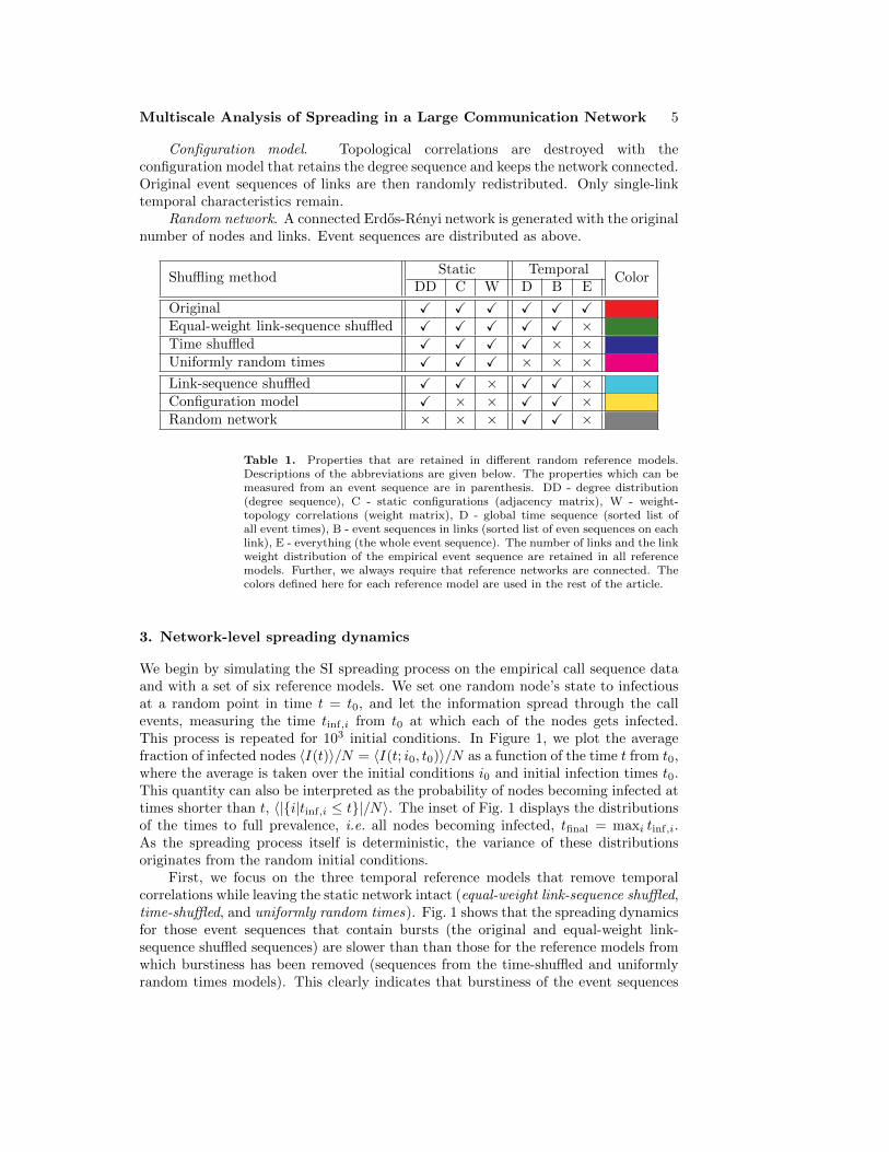
Configuration model. Topological correlations are destroyed with theconfiguration model that retains the degree sequence and keeps the network connected.Original event sequences of links are then randomly redistributed. Only single-linktemporal characteristics remain.
Random network. A connected Erdos-Renyi network is generated with the originalnumber of nodes and links. Event sequences are distributed as above.
Static TemporalShuffling method
DD C W D B EColor
Original X X X X X XEqual-weight link-sequence shuffled X X X X X ×Time shuffled X X X X × ×Uniformly random times X X X × × ×Link-sequence shuffled X X × X X ×Configuration model X × × X X ×Random network × × × X X ×
Table 1. Properties that are retained in different random reference models.Descriptions of the abbreviations are given below. The properties which can bemeasured from an event sequence are in parenthesis. DD - degree distribution(degree sequence), C - static configurations (adjacency matrix), W - weight-topology correlations (weight matrix), D - global time sequence (sorted list ofall event times), B - event sequences in links (sorted list of even sequences on eachlink), E - everything (the whole event sequence). The number of links and the linkweight distribution of the empirical event sequence are retained in all referencemodels. Further, we always require that reference networks are connected. Thecolors defined here for each reference model are used in the rest of the article.
3. Network-level spreading dynamics
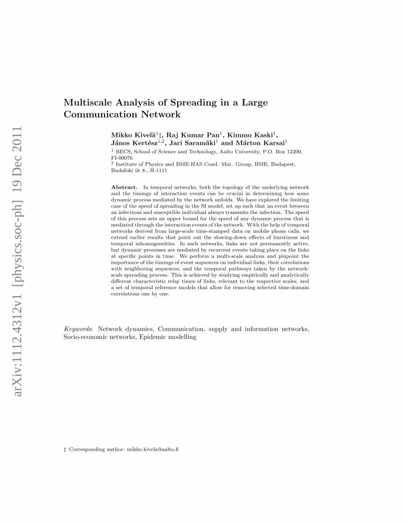
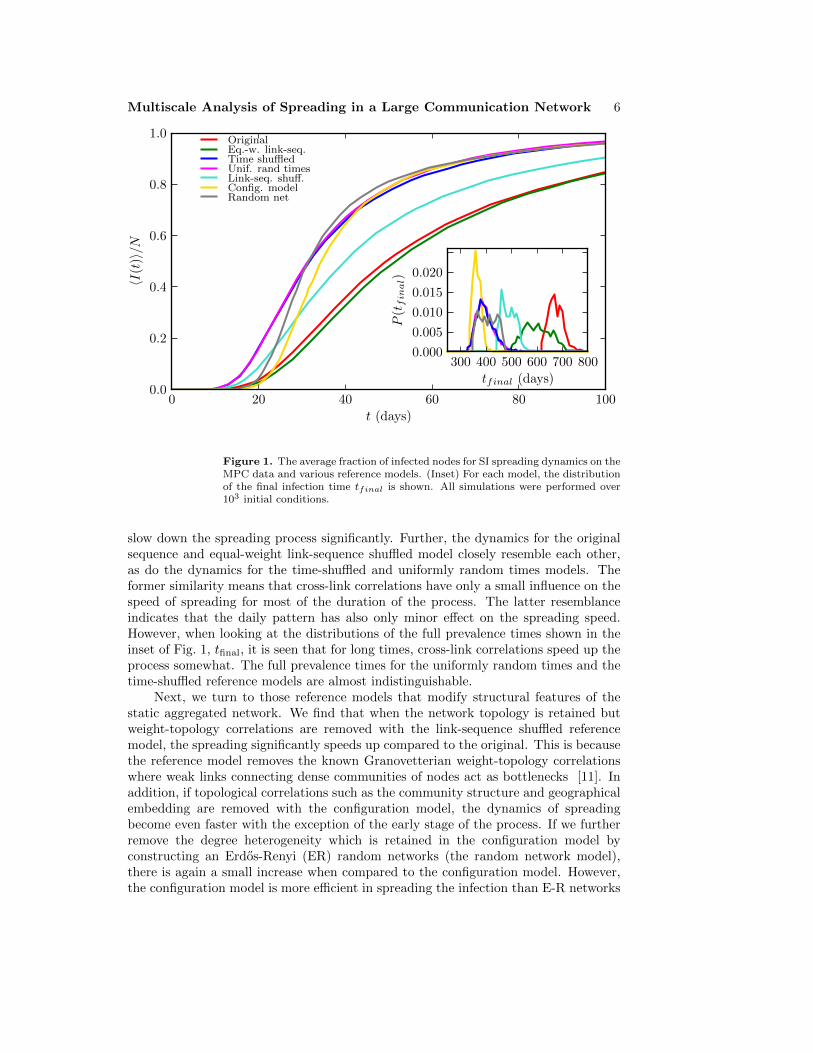
We begin by simulating the SI spreading process on the empirical call sequence dataand with a set of six reference models. We set one random node’s state to infectiousat a random point in time t = t0, and let the information spread through the callevents, measuring the time tinf,i from t0 at which each of the nodes gets infected.This process is repeated for 103 initial conditions. In Figure 1, we plot the averagefraction of infected nodes 〈I(t)〉/N = 〈I(t; i0, t0)〉/N as a function of the time t from t0,where the average is taken over the initial conditions i0 and initial infection times t0.This quantity can also be interpreted as the probability of nodes becoming infected attimes shorter than t, 〈|{i|tinf,i ≤ t}|/N〉. The inset of Fig. 1 displays the distributionsof the times to full prevalence, i.e. all nodes becoming infected, tfinal = maxi tinf,i.As the spreading process itself is deterministic, the variance of these distributionsoriginates from the random initial conditions.
First, we focus on the three temporal reference models that remove temporalcorrelations while leaving the static network intact (equal-weight link-sequence shuffled,time-shuffled, and uniformly random times). Fig. 1 shows that the spreading dynamicsfor those event sequences that contain bursts (the original and equal-weight link-sequence shuffled sequences) are slower than than those for the reference models fromwhich burstiness has been removed (sequences from the time-shuffled and uniformlyrandom times models). This clearly indicates that burstiness of the event sequences
Multiscale Analysis of Spreading in a Large Communication Network 6
0 20 40 60 80 100
t (days)
0.0
0.2
0.4
0.6
0.8
1.0〈I
(t)〉/N
OriginalEq.-w. link-seq.Time shuffledUnif. rand timesLink-seq. shuff.Config. modelRandom net
300 400 500 600 700 800
tfinal (days)
0.000
0.005
0.010
0.015
0.020
P(tfinal)
Figure 1. The average fraction of infected nodes for SI spreading dynamics on theMPC data and various reference models. (Inset) For each model, the distributionof the final infection time tfinal is shown. All simulations were performed over103 initial conditions.
slow down the spreading process significantly. Further, the dynamics for the originalsequence and equal-weight link-sequence shuffled model closely resemble each other,as do the dynamics for the time-shuffled and uniformly random times models. Theformer similarity means that cross-link correlations have only a small influence on thespeed of spreading for most of the duration of the process. The latter resemblanceindicates that the daily pattern has also only minor effect on the spreading speed.However, when looking at the distributions of the full prevalence times shown in theinset of Fig. 1, tfinal, it is seen that for long times, cross-link correlations speed up theprocess somewhat. The full prevalence times for the uniformly random times and thetime-shuffled reference models are almost indistinguishable.
Next, we turn to those reference models that modify structural features of thestatic aggregated network. We find that when the network topology is retained butweight-topology correlations are removed with the link-sequence shuffled referencemodel, the spreading significantly speeds up compared to the original. This is becausethe reference model removes the known Granovetterian weight-topology correlationswhere weak links connecting dense communities of nodes act as bottlenecks [11]. Inaddition, if topological correlations such as the community structure and geographicalembedding are removed with the configuration model, the dynamics of spreadingbecome even faster with the exception of the early stage of the process. If we furtherremove the degree heterogeneity which is retained in the configuration model byconstructing an Erdos-Renyi (ER) random networks (the random network model),there is again a small increase when compared to the configuration model. However,the configuration model is more efficient in spreading the infection than E-R networks
Multiscale Analysis of Spreading in a Large Communication Network 7
once the critical mass of infected nodes is reached, and when considering only the fullprevalence times, the configuration model is the fastest lattice for spreading.
Finally, we cross-compare the relative importance of the structural and temporalcorrelations in the call sequence on the spreading speed. As seen in Fig. 1, thespreading dynamics for the time-shuffled model where weight-topology correlationsare retained but the bursts that are destroyed are faster compared to the link-sequence shuffled model, where bursts are retained but weight-topology correlationsare destroyed. This means that the burstiness of call sequences on individual linksplays a more important role than weight-topology correlations in slowing down thespreading dynamics. Furthermore, the results for the configuration model and theuniform times model are roughly comparable; the first one removes all structuralcorrelations while retaining all temporal correlations and the second one removes alltemporal correlations while retaining all structural correlations. This observation canbe considered surprising since the structural features of static networks are typicallyconsidered to be the most important factor for any dynamical process, while temporalcorrelations are assumed to have minor role. However, the above points out that thetemporal correlations may be of equal importance.
In addition, we have thoroughly investigated the robustness of the above resultsby studying the role of the periodic boundary conditions, the initial conditions, thesystem size, and the error of the mean (see Appendix B and Appendix C); no significantchanges to the above results were observed.
4. Spreading speed on single links
In Section 3, we have shown that the temporal inhomogeneities of our empiricalsequence slow down spreading on the network and that considerable amount of theslowing down can be attributed to the burstiness of event sequences of links. In orderto better understand the effects of temporal inhomogeneities, we will next focus on theevent sequences corresponding to each of the links, and study the effects of temporalinhomogeneities on the spreading speed at the link level. In order to do this, weinvestigate the statistics of the relay times of links. The relay time of an edge denotesthe time it takes for a newly infected node to spread the infection further via the nextevent that the link participates in.
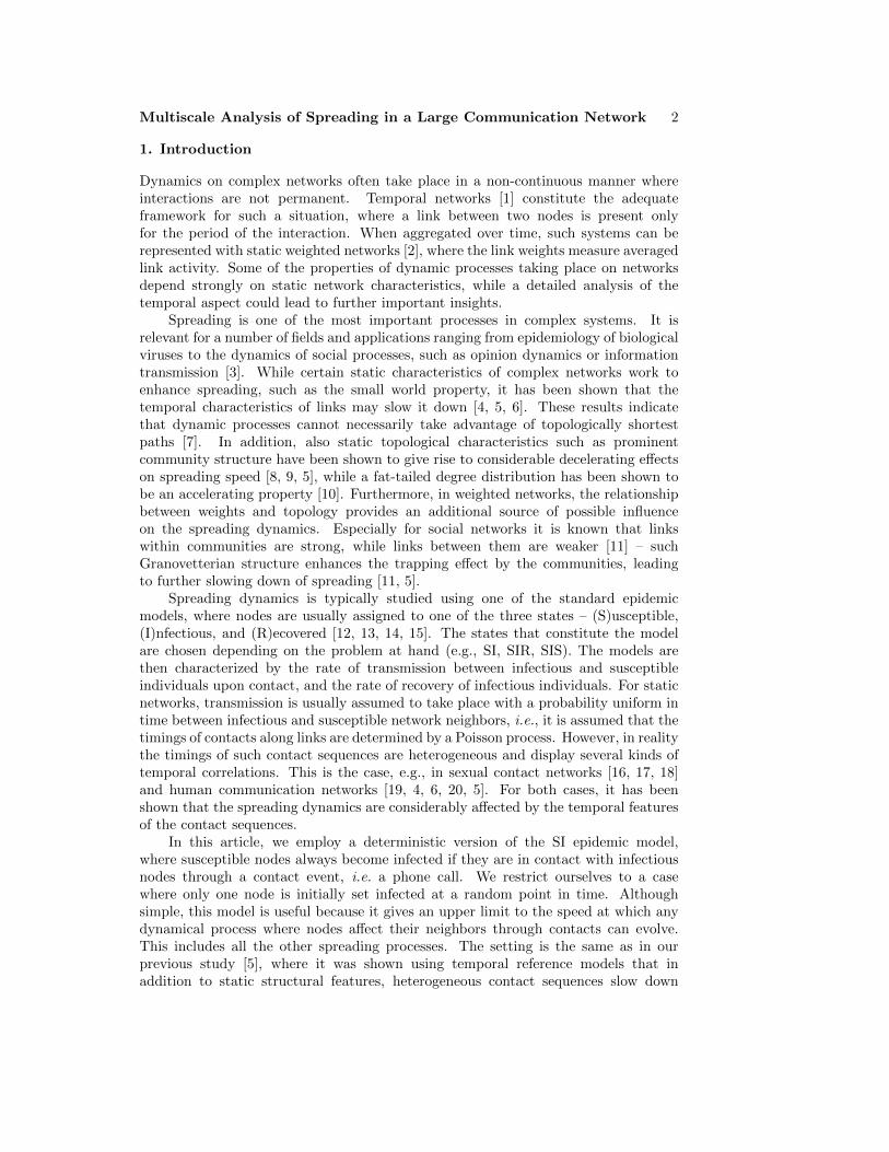
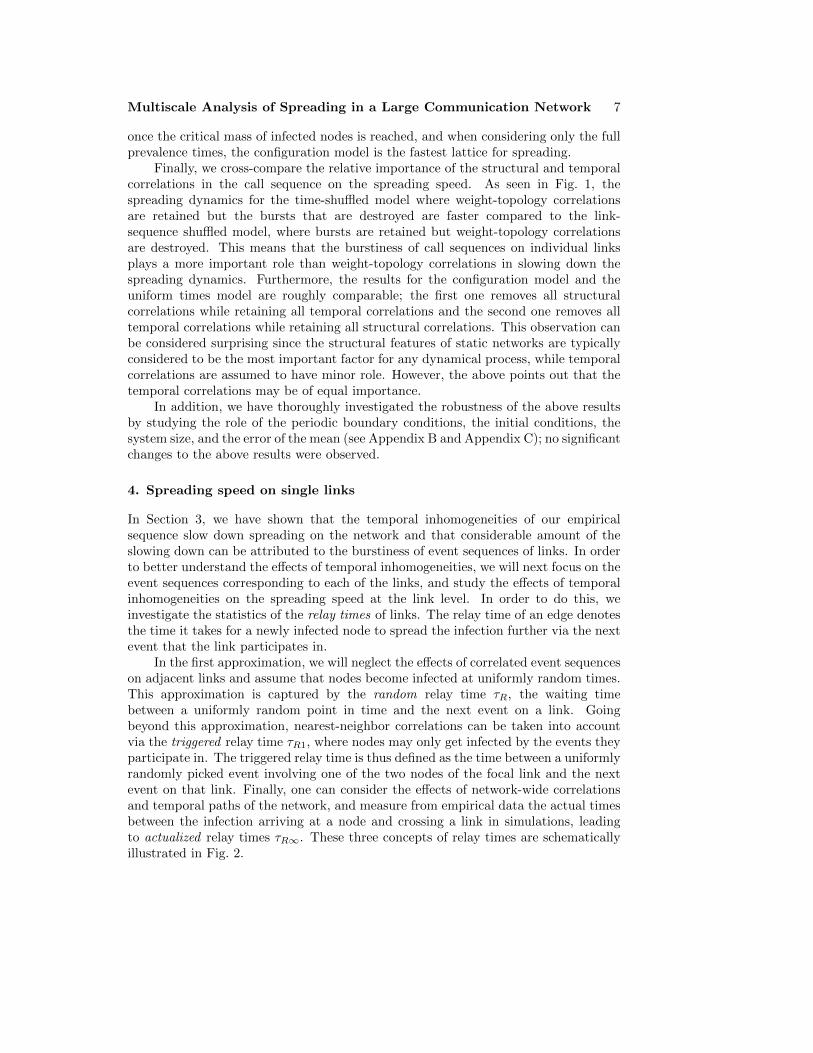
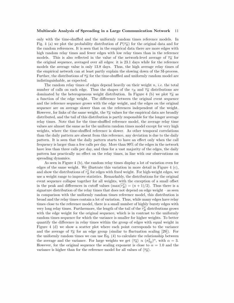
In the first approximation, we will neglect the effects of correlated event sequenceson adjacent links and assume that nodes become infected at uniformly random times.This approximation is captured by the random relay time τR, the waiting timebetween a uniformly random point in time and the next event on a link. Goingbeyond this approximation, nearest-neighbor correlations can be taken into accountvia the triggered relay time τR1, where nodes may only get infected by the events theyparticipate in. The triggered relay time is thus defined as the time between a uniformlyrandomly picked event involving one of the two nodes of the focal link and the nextevent on that link. Finally, one can consider the effects of network-wide correlationsand temporal paths of the network, and measure from empirical data the actual timesbetween the infection arriving at a node and crossing a link in simulations, leadingto actualized relay times τR∞. These three concepts of relay times are schematicallyillustrated in Fig. 2.
Multiscale Analysis of Spreading in a Large Communication Network 8
random time pointevents
possible times to infect Ainfection arriving at Afrom C in simulation
(a) (b) (c)
AB AB
AC
AB
AC
time
Figure 2. Schematic illustrations of the three relay times. The horizontal linerepresents a link, and the small vertical lines displays the events between the twonodes within the observation period, t ∈ [0, T ]. (a) The random relay time τR isthe time difference between a randomly selected point in time and the time of thenext event. (b) The triggered relay time τR1 for the link AB is the time differencebetween the time of an event on any other link of the two nodes (A or B) andthe time of the next event on the edge AB. (c) The actualized relay time τR∞is calculated on the basis of simulations and measures the time between the nodebecoming infected and further transmitting the infection.
4.1. Random relay time τR
4.1.1. Theory We begin our analysis of relay times by neglecting all correlationsbetween the event sequences of adjacent links, and study the dependence of the relaytimes on the inter-event time distributions of the links. We consider the case whereone of the nodes, A or B, of the link AB becomes infected at a uniformly random pointin time. The random relay time τR is then defined as the random variable representingthe time between this random time of infection and the time of the next event betweenA and B. In this approximation, the relay times τR of a link are determined purelyby the inter-event time distribution of events on that link, P (τ), where the inter-eventtime τ is defined as the time difference between two consecutive events. On the basisof the inter-event time distribution, the probability distribution of the relay timescan be written as P (τR) = 1
τ
∫∞τRP (τ)dτ [4]. Further, assuming that the tail of the
distribution is not too broad (limx→∞ x2P (τ > x) = 0), the average relay time τR canbe calculated analytically for any inter-event time distribution:
τR =
∫ ∞
0
τRP (τR)dτR =1
2
τ2
τ. (1)
The value of τR depends heavily on the average inter-event time τ , or equivalently, onthe average rate of events taking place on the link. As we are primarily interested inthe effect of the shape of the inter-event time distribution on τR, it is natural to use aPoissonian distribution as a reference. Thus, we define the normalized average relaytime, τR
∗, by dividing τR by the corresponding relay time for a Poisson process τR,p,for which the average inter-event time is matched to that of the given inter-event timedistribution such that τp = τ . The normalized relay time τR
∗ can then be written as
τR∗ ≡ τR
τR,p=τ2
τ2p
=τ2
2τ2 , (2)
where τR,p = τp = τ . Thus, τR∗ measures the ratio of the second moment to the
square of the first moment of the inter-event time distribution. Generally, the broader
Multiscale Analysis of Spreading in a Large Communication Network 9
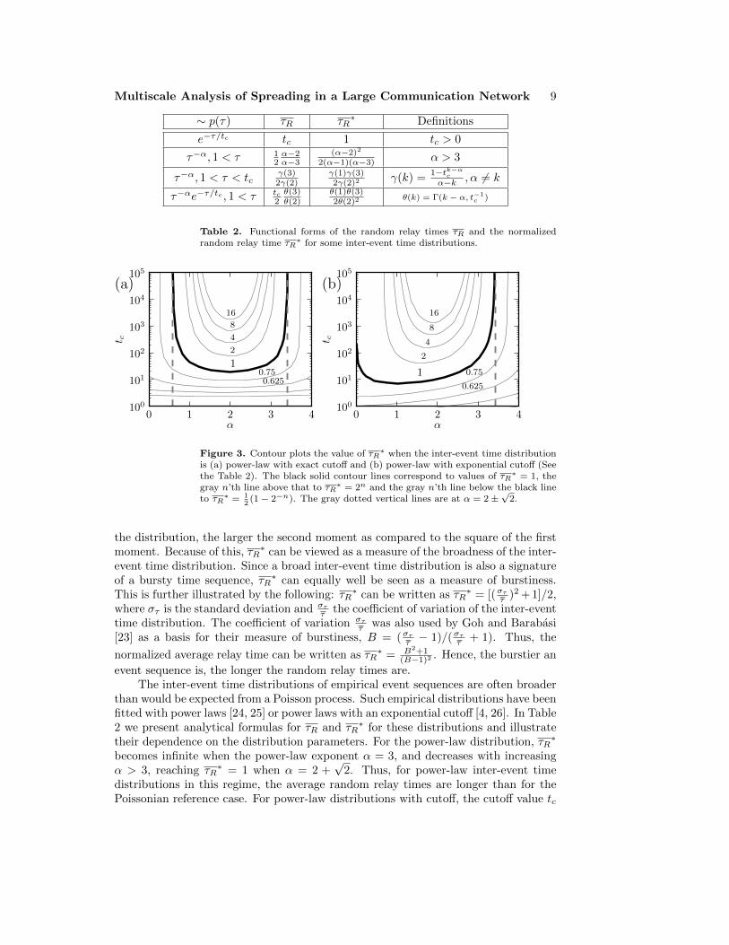
∼ p(τ) τR τR∗ Definitions
e−τ/tc tc 1 tc > 0
τ−α, 1 < τ 12α−2α−3
(α−2)2
2(α−1)(α−3) α > 3
τ−α, 1 < τ < tcγ(3)2γ(2)
γ(1)γ(3)2γ(2)2 γ(k) =
1−tk−αc
α−k , α 6= k
τ−αe−τ/tc , 1 < τ tc2θ(3)θ(2)
θ(1)θ(3)2θ(2)2 θ(k) = Γ(k − α, t−1
c )
Table 2. Functional forms of the random relay times τR and the normalizedrandom relay time τR
∗ for some inter-event time distributions.
0 1 2 3 4α
100
101
102
103
104
105
t c
16
8
4
2
10.750.625
(a)
0 1 2 3 4α
100
101
102
103
104
105
t c
16
8
4
2
1 0.75
0.625
(b)
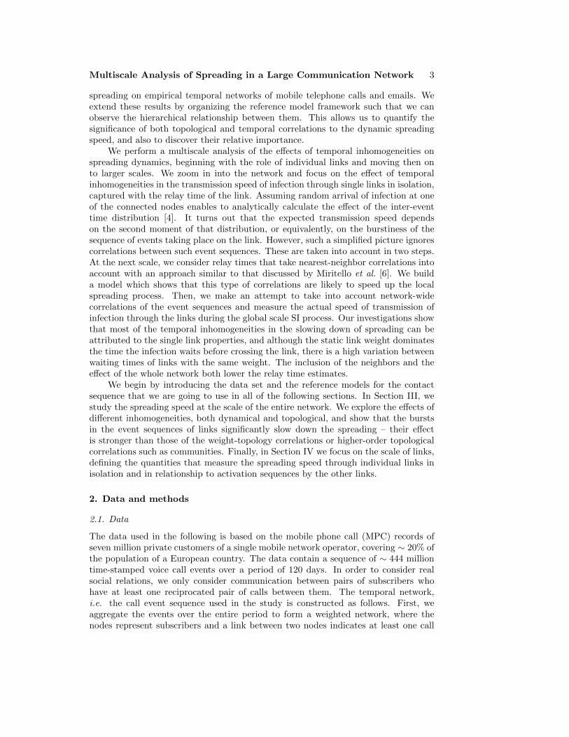
Figure 3. Contour plots the value of τR∗ when the inter-event time distribution
is (a) power-law with exact cutoff and (b) power-law with exponential cutoff (Seethe Table 2). The black solid contour lines correspond to values of τR
∗ = 1, thegray n’th line above that to τR
∗ = 2n and the gray n’th line below the black lineto τR
∗ = 12
(1− 2−n). The gray dotted vertical lines are at α = 2±√
2.
the distribution, the larger the second moment as compared to the square of the firstmoment. Because of this, τR
∗ can be viewed as a measure of the broadness of the inter-event time distribution. Since a broad inter-event time distribution is also a signatureof a bursty time sequence, τR
∗ can equally well be seen as a measure of burstiness.This is further illustrated by the following: τR
∗ can be written as τR∗ = [(σττ )2 + 1]/2,
where στ is the standard deviation and σττ the coefficient of variation of the inter-event
time distribution. The coefficient of variation σττ was also used by Goh and Barabasi
[23] as a basis for their measure of burstiness, B = (σττ − 1)/(σττ + 1). Thus, the
normalized average relay time can be written as τR∗ = B2+1
(B−1)2 . Hence, the burstier an
event sequence is, the longer the random relay times are.The inter-event time distributions of empirical event sequences are often broader
than would be expected from a Poisson process. Such empirical distributions have beenfitted with power laws [24, 25] or power laws with an exponential cutoff [4, 26]. In Table2 we present analytical formulas for τR and τR
∗ for these distributions and illustratetheir dependence on the distribution parameters. For the power-law distribution, τR
∗
becomes infinite when the power-law exponent α = 3, and decreases with increasingα > 3, reaching τR
∗ = 1 when α = 2 +√
2. Thus, for power-law inter-event timedistributions in this regime, the average random relay times are longer than for thePoissonian reference case. For power-law distributions with cutoff, the cutoff value tc
Multiscale Analysis of Spreading in a Large Communication Network 10
also affects τR∗. The joint effect of the power-law exponent and the cutoff is illustrated
with contour plots in Fig. 3. If the cutoff point tc is small enough, the random relaytimes are shorter than Poissonian also for power-laws with α ≤ 2 +
√2, but for large
values of tc, the power-law inter-event times dominate and the relay times becomelonger.
4.1.2. Relay times in empirical event sequences Next, we turn our attention fromthe general case to empirical data, where we have a finite number of events, n,in a finite observation period, t ∈ [0, T ]. For simplicity, we consider the casewith periodic temporal boundary conditions, where all events get repeated with aperiodicity of T . Then, the expression of relay time distribution of Eq. (1) becomesP (τR) = 1
T
∑ni=1[τR ≤ τi], where τi is the inter-event time between the i − 1-th and
i-th events. The expected relay time τR is then given by
τR =
∑ni=1 τ
2i
2T. (3)
For a given values of n and T , the average relay time τR is minimized when all theinter-event times are the same, that is, τi = τj ,∀i, j, giving τR = T
2n . In contrast,it is maximized when all the events happen at the same time resulting in a singlenon-zero inter-event time, that is, ti = tj∀i, j and τ1 = T giving τR = T/2. Thus, τRis maximized when all events take place in the same burst and τR is minimized whenevents are maximally separated in time.
As with the general case, we want to compare the τR values to some baseline.Here, the proper baseline is to distribute the times of the n events of each edge atuniformly random within the observation period, equivalently to the uniform randomtimes reference model defined earlier. This is equivalent to having a Poisson processwith a constant average inter-event time with the additional condition that there are nevents in the interval [27]. Order statistics can be used to analytically derive the inter-event time distribution, which in this case is a beta distribution [28] (see AppendixD for details). The beta distribution converges to an exponential distribution as thenumber of events n increases, and thus the uniformly random times reference modelapproaches the Poisson process with increasing n. The expected value and varianceof τR for the uniform times model with periodic boundary conditions are given by
〈τR〉 =T
n+ 1,Var(τR) =
T 2(n− 1)
(n+ 1)2(n+ 2)(n+ 3), (4)
and the normalized relay time (similarly to Eq. 2) becomes
τR∗ =
τR〈τR〉
=(n+ 1)
2
n∑
i=1
(τi/T )2. (5)
Further, since the normalization of τR∗ is done with the uniformly random times
reference model instead of a Poisson process, we need to include a correction factor in
the relationship between burstiness and the normalized relay time: τR∗ = n+1
nB2+1
(B−1)2 .
Next we calculate τR for each edge for the empirical MPC sequence using Eq. (3)and compare the values to the temporal reference models, where the static networkremains unchanged. Further, we leave out the equal-weight link-sequence shuffledmodel which would give equivalent results to the empirical sequence. This leaves us
Multiscale Analysis of Spreading in a Large Communication Network 11
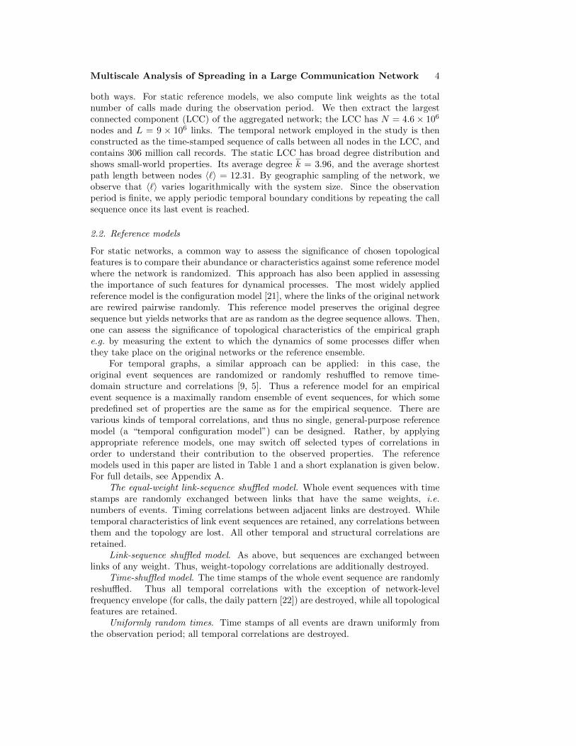
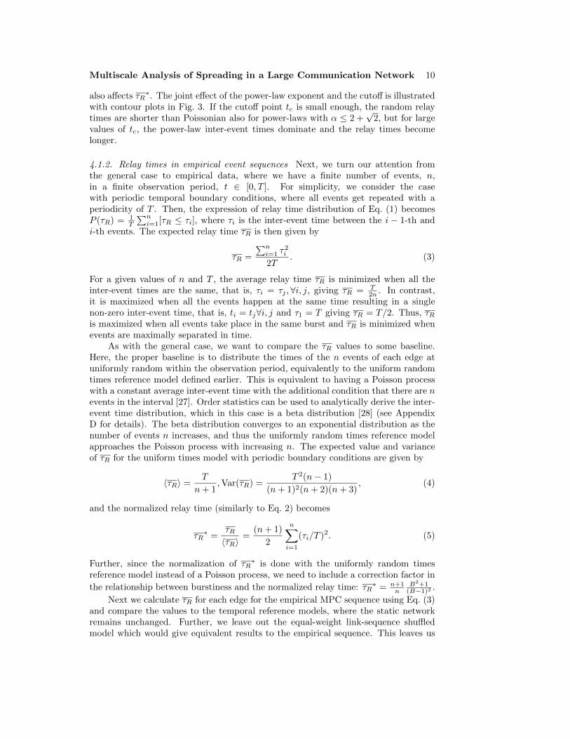
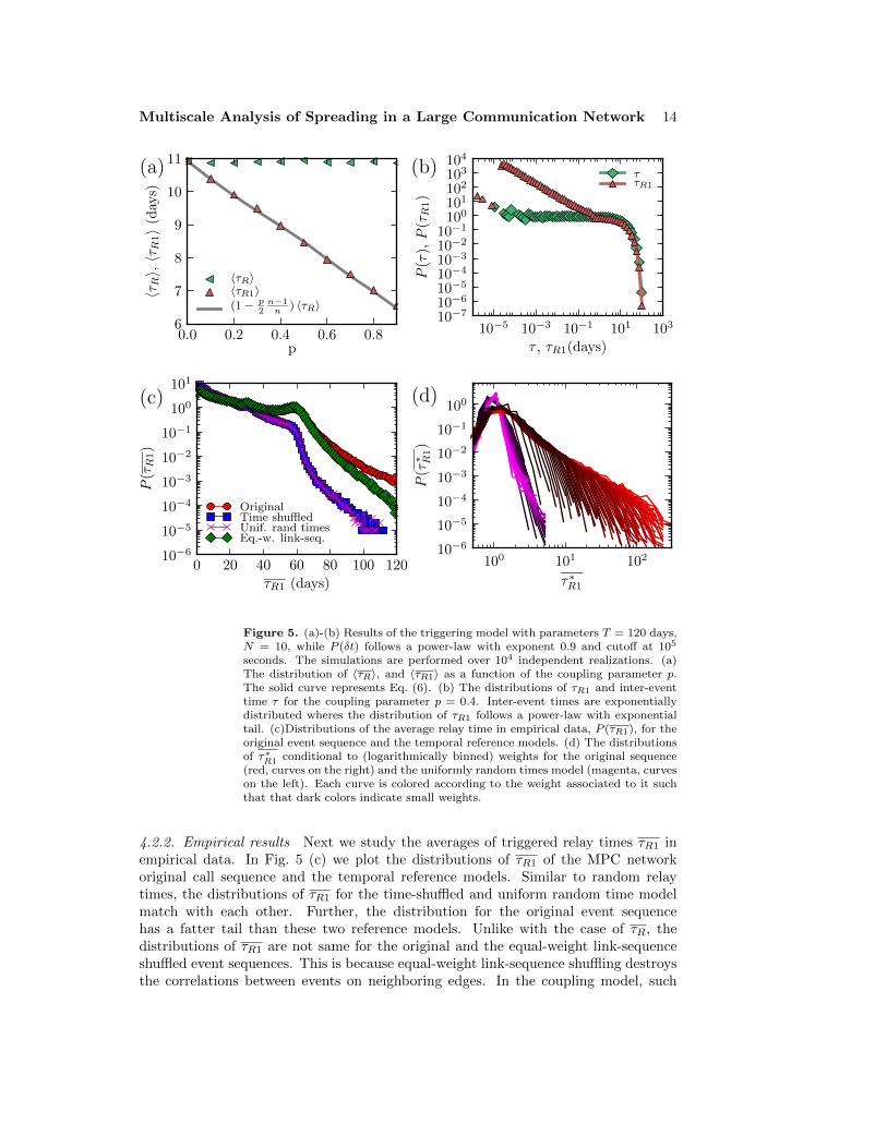
only with the time-shuffled and the uniformly random times reference models. InFig. 4 (a) we plot the probability distribution of P (τR) for the original data and forthe random references. It is seen that in the empirical data there are more edges withhigh random relay times and fewer edges with low relay times than in the referencemodels. This is also reflected in the value of the network-level average of τR forthe original sequence, averaged over all edges: it is 23.1 days while for the referencemodels the average value is only 13.8 days. Thus, the high average relay times ofthe empirical network can at least partly explain the slowing down of the SI-process.Further, the distributions of τR for the time-shuffled and uniformly random model areindistinguishable, as expected.
The random relay times of edges depend heavily on their weight n, i.e. the totalnumber of calls on each edge. Thus the shapes of the τR and τR distributions aredominated by the heterogeneous weight distribution. In Figure 4 (b) we plot τR asa function of the edge weight. The difference between the original event sequenceand the reference sequence grows with the edge weight, and the edges on the originalsequence are on average slower than on the references independent of the weight.However, for links of the same weight, the τR values for the empirical data are broadlydistributed, and the tail of this distribution is partly responsible for the longer averagerelay times. Note that for the time-shuffled reference model, the average relay timevalues are almost the same as for the uniform random times model except for very highweights, where the time-shuffled reference is slower. As other temporal correlationsthan the daily pattern are absent from this reference, any deviation is due to the dailypattern. It is seen that the daily pattern starts to have an effect only when the callfrequency is larger than a few calls per day. More than 99% of the edges in the networkhave less than three calls per day, and thus for a vast majority of the edges, the dailypattern has practically no effect on the relay times, in line with our observations onspreading dynamics.
As seen in Figure 4 (b), the random relay times display a lot of variation even foredges of the same weight. We illustrate this variation in more detail in Figure 4 (c),and show the distributions of τ∗R for edges with fixed weight. For high-weight edges, weuse a weight range to improve statistics. Remarkably, the distributions for the originalevent sequence collapse together for all weights, with the exception of a small offsetin the peak and differences in cutoff values (max(τ∗R) = (n + 1)/2). Thus there is asignature distribution of the relay times that does not depend on edge weight – as seenin comparison with the uniformly random times reference model, this distribution isbroad and the relay times contain a lot of variation. Thus, while many edges have relaytimes close to the reference model, there is a small number of highly bursty edges withvery long relay times. Furthermore, the length of the tail of the τ∗R distributions growswith the edge weight for the original sequence, which is in contrast to the uniformlyrandom times sequence for which the variance is smaller for higher weights. To betterquantify the difference in relay times within the group of edges with equal weight inFigure 4 (d) we show a scatter plot where each point corresponds to the varianceand the average of τR for an edge group (similar to fluctuation scaling [29]). Forthe uniformly random times we can use Eq. (4) to calculate the relationship betweenthe average and the variance. For large weights we get 〈τR〉 ∝ (σ2
τR)α, with α = 3.
However, for the original sequence the scaling exponent is close to α = 1.0 and thevariance is higher than for the reference model for all values of 〈τR〉.
Multiscale Analysis of Spreading in a Large Communication Network 12
0 10 20 30 40 50 60
τR (days)
10−1
100
101
102P
(τR
)
OriginalTime shuffledUnif. rand times
(a)
10−1 100 101
n (calls / day)
103
104
105
106
107
〈τR|n〉
Min/Max10−6
10−5
10−4
10−3
10−2
10−1
1(b)
100 101 102
τ∗R
10−6
10−5
10−4
10−3
10−2
10−1
100
P(τ∗ R)
(c)
104 105 106
〈τR〉
106
108
1010
1012
σ2 τR
1.0
3.0
(d)
OriginalUnif. rand. times
Figure 4. (a): Distribution of the relay times τR for the original, time-shuffledand uniformly random event sequences. The peak at ∼ 30 days is due to thelarger amount of edges with only 2 calls (a result of the mutuality condition)and periodic temporal boundary conditions. (b): 〈τR|n〉 for the original eventsequence and reference models. For the original sequence, we also show theprobability distributions of τR conditional to weight (see color bar on right). Thesolid lines denote (theoretical) max and min values. (c): The distributions of τ∗Rconditional to (logarithmically binned) weights for the original sequence (red) andthe uniformly random times model (magenta). Each curve is colored according tothe weight associated to it such that that dark colors indicate small weights. (d):The average and the variance of τR for each of the bins. The solid line on the topindicates power law fit to the original data, and the lower black line correspondsto the analytical values for the uniformly random time sequence calculate withEq. 4. Distributions for bins with more than 800 calls during the time interval Tare not shown due to insufficient statistics.
4.2. Triggered relay time τR1
4.2.1. Theory For the random relay times τR considered in the previous section, itwas assumed that the event sequences on adjacent links are uncorrelated, and thusthe infection may arrive at one of the nodes of the focal link at a random point intime. We will next take into account the effects of correlations between the times ofevents of adjacent links, and require that a node may only become infected when itinteracts with one of its neighbors. Instead of choosing the time of infection of node
Multiscale Analysis of Spreading in a Large Communication Network 13
A or B of the link AB randomly from the time interval [0, T ], we pick it randomlyfrom the set of times where A or B participates in an interaction event with one of itsneighbors C 6= B and C 6= A [6]. Then, the triggered relay time τR1 for the link ABis defined as the time difference between the infection arriving A (or B) to the timewhen the infection is passed through the link to B (or A), similarly to Ref. [6].
The average triggered relay time τR1 for the link AB depends on both the timeintervals between the events on the link, as well as correlations of the times of eventsbetween the link and its neighbors. If the events on the other links are independentof the events on AB, then τR1 approaches τR. We illustrate the differences betweenτR1 and τR with the help of a simple model that involves correlations between thesequences. We define a triggering model where the system consists of two links, ABand AC, such that each of the two links has N events. We assign times to the eventson both links in a pairwise fashion, such that each AB-AC event pair is consideredto be triggered with a probability p and uncorrelated with probability (1 − p). Foruncorrelated event pairs, we assign times drawn uniformly at random from the interval[0, T ]. For correlated event pairs, we first choose the time tAB of the event on the ABlink uniformly at random. Then we set an event on the AC link randomly at eithert = tAB − δt or t = tAB + δt, i.e. the AC event is considered to trigger the AB eventor vice versa. The time δt is picked at random from some triggering time distribution.Periodic temporal boundary conditions are invoked if the AC event falls outside theinterval [0, T ]. Thus, on both links we have on average pN events that are triggeredor trigger another event, and (1− p)N uncorrelated events.
Now we can calculate for the expected triggered relay time 〈τR1〉 for the AB linkby assuming that the trigger times δt are small compared to the random inter-eventtimes, i.e. we always have τ > δt. Note that the model is symmetric in that 〈τR1〉 issame for both links, AB and AC. The fraction of uncorrelated events is (1−p), and forthese, the expected triggered relay time is simply given by Eq. (4): 〈τR1〉 = T/ (n+ 1).The fraction of triggered event pairs is p; half of the events are triggered by an ACevent with a triggered relay time 〈δt〉. The rest trigger AC events, and the expectedtime from the triggered AC event to the next AB event is 〈τ − δt〉 = T
n − 〈δt〉. Thus,considering all these cases, the expected triggered relay time
〈τR1〉 = (1− p) T
n+ 1+
1
2p〈δt〉+
1
2p(T
n− 〈δt〉)
= (1− p
2
n− 1
n)〈τR〉. (6)
Thus, the more triggered events there are, the shorter the triggered relay times areon average, as expected. Note that in the above equation 〈τR1〉 does not depend onthe distribution of δt as long as the values of δt are small enough compared to theinter-event times.
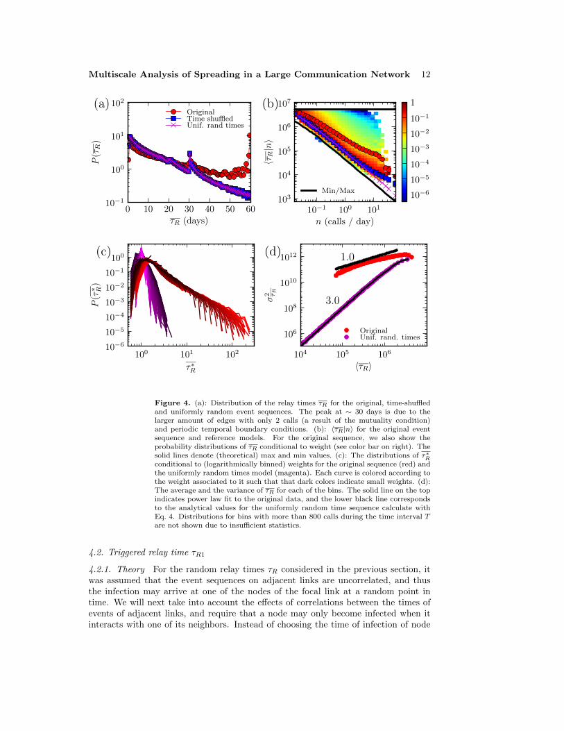
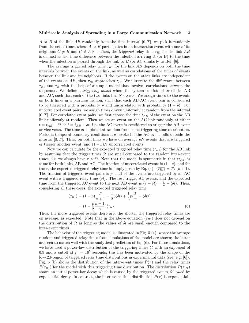
The behavior of the triggering model is illustrated in Fig. 5 (a), where the averagerandom and triggered relay times from simulations of the model are shown; the latterare seen to match well with the analytical prediction of Eq. (6). For these simulations,we have used a power-law distribution of the triggering times δt with an exponent of0.9 and a cutoff at tc = 105 seconds; this has been motivated by the shape of thelow-∆t-region of triggered relay time distributions in experimental data (see, e.g. [6]).Fig. 5 (b) shows the distribution of the inter-event times P (τ) and the relay timesP (τR1) for the model with this triggering time distribution. The distribution P (τR1)shows an initial power-law decay which is caused by the triggered events, followed byexponential decay. In contrast, the inter-event time distribution P (τ) is exponential.
Multiscale Analysis of Spreading in a Large Communication Network 14
0.0 0.2 0.4 0.6 0.8p
6
7
8
9
10
11〈τR〉,〈τR
1〉(
day
s)
〈τR〉〈τR1〉(1− p
2n−1n
) 〈τR〉
(a)
10−5 10−3 10−1 101 103
τ , τR1(days)
10−710−610−510−410−310−210−1
100101102103104
P(τ
),P
(τR
1)
ττR1
(b)
0 20 40 60 80 100 120
τR1 (days)
10−6
10−5
10−4
10−3
10−2
10−1
100
101
P(τR
1)
OriginalTime shuffledUnif. rand timesEq.-w. link-seq.
(c)
100 101 102
τ∗R1
10−6
10−5
10−4
10−3
10−2
10−1
100
P(τ∗ R
1)
(d)
Figure 5. (a)-(b) Results of the triggering model with parameters T = 120 days,N = 10, while P (δt) follows a power-law with exponent 0.9 and cutoff at 105
seconds. The simulations are performed over 104 independent realizations. (a)The distribution of 〈τR〉, and 〈τR1〉 as a function of the coupling parameter p.The solid curve represents Eq. (6). (b) The distributions of τR1 and inter-eventtime τ for the coupling parameter p = 0.4. Inter-event times are exponentiallydistributed wheres the distribution of τR1 follows a power-law with exponentialtail. (c)Distributions of the average relay time in empirical data, P (τR1), for theoriginal event sequence and the temporal reference models. (d) The distributionsof τ∗R1 conditional to (logarithmically binned) weights for the original sequence(red, curves on the right) and the uniformly random times model (magenta, curveson the left). Each curve is colored according to the weight associated to it suchthat that dark colors indicate small weights.
4.2.2. Empirical results Next we study the averages of triggered relay times τR1 inempirical data. In Fig. 5 (c) we plot the distributions of τR1 of the MPC networkoriginal call sequence and the temporal reference models. Similar to random relaytimes, the distributions of τR1 for the time-shuffled and uniform random time modelmatch with each other. Further, the distribution for the original event sequencehas a fatter tail than these two reference models. Unlike with the case of τR, thedistributions of τR1 are not same for the original and the equal-weight link-sequenceshuffled event sequences. This is because equal-weight link-sequence shuffling destroysthe correlations between events on neighboring edges. In the coupling model, such
Multiscale Analysis of Spreading in a Large Communication Network 15
correlations caused the expected τR1 values to decrease. This is true also for the MPCnetwork, since the average τR1 for the original sequence is 22 days, where it is 23 daysfor the equal-weight link-sequence shuffled event sequence.
In Fig. 5 (d) we plot the τ∗R1 distributions conditional to the edge weight similarto Fig. 4 (c). The main difference to τ∗R distributions is that the theoretical maximumvalue for τ∗R1 is n + 1 instead of (n + 1)/2. The values of τ∗R1 inside the intervalfrom (n + 1)/2 to n + 1 arise from situations where the triggering events take placeclose to the beginning of a long interval between consecutive bursts. Thus, they resultfrom a combined effect of burstiness and timings of triggering events. Such situationsare not very frequent, leading to steep decays in the tails of the τ∗R1 distributions forvalues larger than (n + 1)/2. Thus, even for small edge weights, the tails of the τ∗R1
distributions do not follow the signature scaling observed for τ∗R distributions.
4.3. Actualized relay time τR∞
4.3.1. Motivation: the event infectivity fe When defining the triggered relay timeτR1, it was assumed that each event taking place on the neighboring edges transmitsthe infection to the focal edge with an equal probability. In this section, we study thevalidity of this assumption by defining a quantity called infectivity, fe, for each event.The event infectivity is defined as a probability of an event spreading the infectionduring a spreading process which is initiated from a random node and a random pointin time.
In order to calculate exact values for the event infectivities, we would need tosimulate the spreading process over the entire ensemble of all possible initial conditions.Instead, we calculate an estimate for fe by starting the infection from 104 randomlyselected initial conditions and simulating each spreading process until all the nodesin the network are infected. For these processes, we calculate the number of timeseach event transfers the infection to an susceptible node. An estimate for the eventinfectivity, fe, is then determined by dividing these numbers by the number of initialconditions. Note that this approximation is not very accurate for small values of fe.
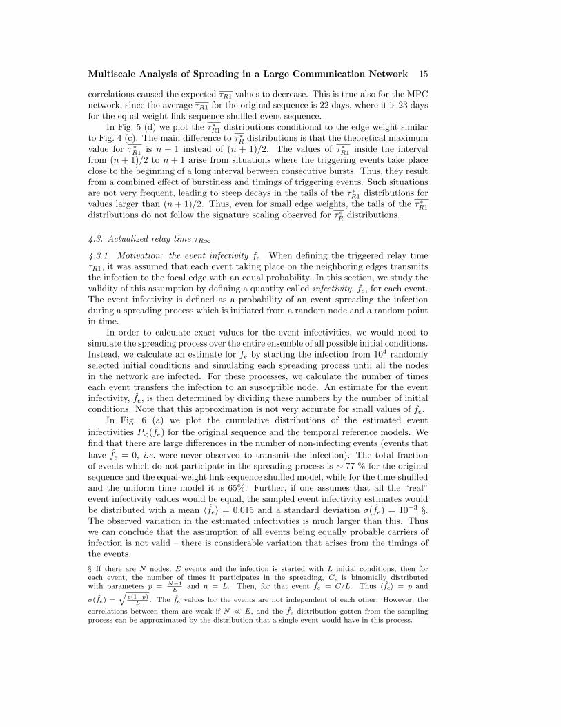
In Fig. 6 (a) we plot the cumulative distributions of the estimated event
infectivities P<(fe) for the original sequence and the temporal reference models. Wefind that there are large differences in the number of non-infecting events (events that
have fe = 0, i.e. were never observed to transmit the infection). The total fractionof events which do not participate in the spreading process is ∼ 77 % for the originalsequence and the equal-weight link-sequence shuffled model, while for the time-shuffledand the uniform time model it is 65%. Further, if one assumes that all the “real”event infectivity values would be equal, the sampled event infectivity estimates wouldbe distributed with a mean 〈fe〉 = 0.015 and a standard deviation σ(fe) = 10−3 §.The observed variation in the estimated infectivities is much larger than this. Thuswe can conclude that the assumption of all events being equally probable carriers ofinfection is not valid – there is considerable variation that arises from the timings ofthe events.
§ If there are N nodes, E events and the infection is started with L initial conditions, then foreach event, the number of times it participates in the spreading, C, is binomially distributedwith parameters p = N−1
Eand n = L. Then, for that event fe = C/L. Thus 〈fe〉 = p and
σ(fe) =√
p(1−p)L
. The fe values for the events are not independent of each other. However, the
correlations between them are weak if N � E, and the fe distribution gotten from the samplingprocess can be approximated by the distribution that a single event would have in this process.
Multiscale Analysis of Spreading in a Large Communication Network 16
10−410−310−210−1 100
fe
100P<
(fe)
(a)
101 103 105 107
τ (seconds)
10−8
10−7
10−6
10−5
10−4
10−3
10−2
10−1
100
〈fe|τ〉
(b)
104 105 106 107
τR1 (seconds)
0.0
0.2
0.4
0.6
0.8
1.0
〈τR∞/τR
1〉
OriginalTime shuff.Unif. rand timesEq.-w. link-seq.
(c)
Figure 6. (a) The cumulative distribution of estimated event infectivity, P<(fe),for the original sequence and the temporal reference models. The black linecorresponds to the mean of the estimated infectivity distribution for a constant”real” event infectivity; the variation arising from sampling is small enough torender the standard deviation of this distribution negligibly small. (b) Theaverage event infectivity as a function of the trailing inter-event time (time tolast event). The solid black line corresponds to a linear increase. (c) The averageratio 〈τR∞/τR1〉 as a function of τR1. The edges are placed into bins accordingto their τR1 values in a way that each bin contains equal number of edges. Thecoordinate of the bin in the x-axis is then calculated as the average τR1 value ofthe edges inside the bin.
To better understand which events are most or least likely to spread the infection,we plot in Fig. 6 (b) the average estimated event infectivity as a function of thepreceding inter-event time of the event, i.e. the time to the previous event. Onaverage, the infectivity of an event increases with the inter-event time. This meansthat events participating in bursts (events with short preceding inter-event times)are less likely to participate in the infection spreading process as compared to eventswith long preceding inter-event times. The increase in fe with τ shows almost alinear relationship for the temporal reference models; a linear relationship would beexpected if the infection times were random. This is simply because if we select arandom infection point in time, the probability fe of the infection going through anevent e would be proportional to the preceding inter-event time of that event τe, that isfe ∝ τe/T . However, the curve for the original event sequence shows a slight deviationfrom this linear dependency for short inter-event times.
4.3.2. Definition of τR∞ and empirical results The above observations on largevariations in event infectivity and correlations between preceding inter-event timesand infectivities are not consistent with the assumptions behind the definition ofthe triggered relay time τR1, where it was assumed that the infection can bereceived through each event with equal probability. Further, τR1 doesn’t take intoaccount the possibility of both nodes of the focal edge getting infected independently,without transmission through that edge, as the spreading front expands through theirneighboring nodes.
In order to account for the infectivity distributions and all other constraintsduring the spreading process we define the actualized relay time τR∞ as the time
Multiscale Analysis of Spreading in a Large Communication Network 17
that the infection actually waits on one of the nodes of an edge before crossing itin a network-wide spreading process, i.e. the difference between the time when theinfection actually arrives at one of the endpoint nodes of an edge and the infectionbeing transmitted through that link. The values for τR∞ are obtained numericallyby running the spreading process through the network, monitoring which nodes infectwhich other nodes, and calculating the relay times accordingly. Note that only eventstransmitting the infection are considered for τR∞. As an example, if node u is infectedand the next event between u and v occurs after node v has already become infectedby some other node w, that event doesn’t affect the τR∞ value of the edge linking uand v.
For estimating τR∞ in empirical data, we use the same sampling scheme aspreviously used while estimating the infectivity values fe. In Fig. 6 (c) we plot theratios 〈τR∞/τR1〉 as functions of the respective relay times, for the original sequenceand the reference models. On average, the actualized relay times τR∞ are shorter thanthe triggered relay times, and the ratio decreases with increasing τR1. Thus, when thenetwork-wide spreading process is accounted for, the relay times speed up especiallyfor edges that appear slow when measured with triggered relay times. This is becausethe pathways taken by the spreading process often avoid and circumvent the slowestedges. However, in some cases it is not possible to employ any faster shortcuts, e.g anedge leading to a node of degree one is always used in the spreading process. Notethat τR∞ is not defined for edges that only have zero infectivity events, i.e. for edgesthat never transmit the infection.
4.4. Comparing the relay times
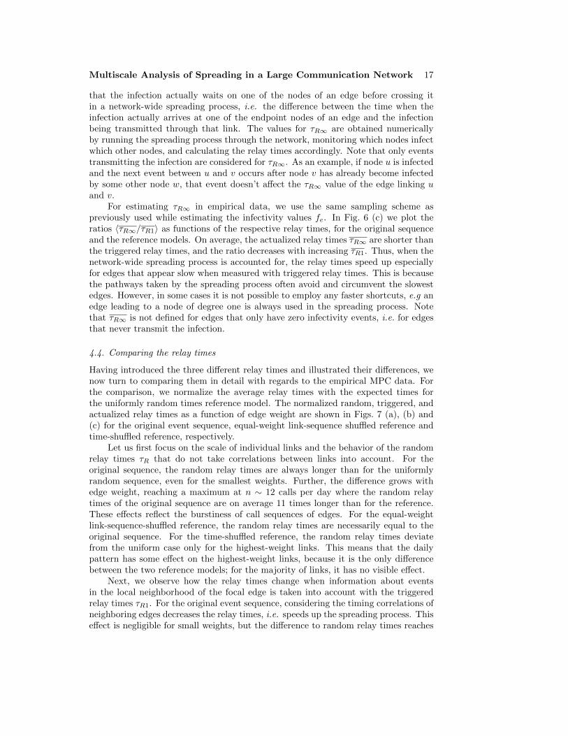
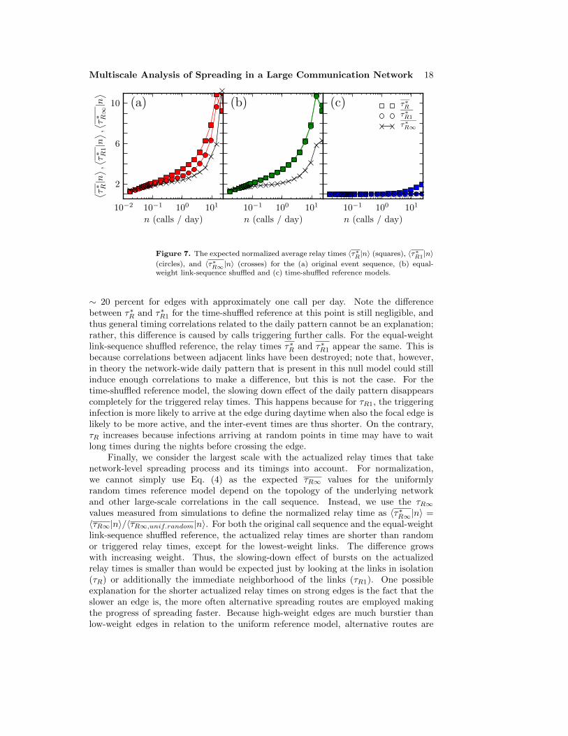
Having introduced the three different relay times and illustrated their differences, wenow turn to comparing them in detail with regards to the empirical MPC data. Forthe comparison, we normalize the average relay times with the expected times forthe uniformly random times reference model. The normalized random, triggered, andactualized relay times as a function of edge weight are shown in Figs. 7 (a), (b) and(c) for the original event sequence, equal-weight link-sequence shuffled reference andtime-shuffled reference, respectively.
Let us first focus on the scale of individual links and the behavior of the randomrelay times τR that do not take correlations between links into account. For theoriginal sequence, the random relay times are always longer than for the uniformlyrandom sequence, even for the smallest weights. Further, the difference grows withedge weight, reaching a maximum at n ∼ 12 calls per day where the random relaytimes of the original sequence are on average 11 times longer than for the reference.These effects reflect the burstiness of call sequences of edges. For the equal-weightlink-sequence-shuffled reference, the random relay times are necessarily equal to theoriginal sequence. For the time-shuffled reference, the random relay times deviatefrom the uniform case only for the highest-weight links. This means that the dailypattern has some effect on the highest-weight links, because it is the only differencebetween the two reference models; for the majority of links, it has no visible effect.
Next, we observe how the relay times change when information about eventsin the local neighborhood of the focal edge is taken into account with the triggeredrelay times τR1. For the original event sequence, considering the timing correlations ofneighboring edges decreases the relay times, i.e. speeds up the spreading process. Thiseffect is negligible for small weights, but the difference to random relay times reaches
Multiscale Analysis of Spreading in a Large Communication Network 18
10−2 10−1 100 101
n (calls / day)
2
6
10⟨ τ∗ R|n⟩ ,⟨ τ∗ R
1|n⟩ ,⟨ τ∗ R∞|n⟩
10−1 100 101
n (calls / day)
10−1 100 101
n (calls / day)
τ∗Rτ∗R1
τ∗R∞
(a) (b) (c)
Figure 7. The expected normalized average relay times 〈τ∗R|n〉 (squares), 〈τ∗R1|n〉(circles), and 〈τ∗R∞|n〉 (crosses) for the (a) original event sequence, (b) equal-weight link-sequence shuffled and (c) time-shuffled reference models.
∼ 20 percent for edges with approximately one call per day. Note the differencebetween τ∗R and τ∗R1 for the time-shuffled reference at this point is still negligible, andthus general timing correlations related to the daily pattern cannot be an explanation;rather, this difference is caused by calls triggering further calls. For the equal-weightlink-sequence shuffled reference, the relay times τ∗R and τ∗R1 appear the same. This isbecause correlations between adjacent links have been destroyed; note that, however,in theory the network-wide daily pattern that is present in this null model could stillinduce enough correlations to make a difference, but this is not the case. For thetime-shuffled reference model, the slowing down effect of the daily pattern disappearscompletely for the triggered relay times. This happens because for τR1, the triggeringinfection is more likely to arrive at the edge during daytime when also the focal edge islikely to be more active, and the inter-event times are thus shorter. On the contrary,τR increases because infections arriving at random points in time may have to waitlong times during the nights before crossing the edge.
Finally, we consider the largest scale with the actualized relay times that takenetwork-level spreading process and its timings into account. For normalization,we cannot simply use Eq. (4) as the expected τR∞ values for the uniformlyrandom times reference model depend on the topology of the underlying networkand other large-scale correlations in the call sequence. Instead, we use the τR∞values measured from simulations to define the normalized relay time as 〈τ∗R∞|n〉 =〈τR∞|n〉/〈τR∞,unif.random|n〉. For both the original call sequence and the equal-weightlink-sequence shuffled reference, the actualized relay times are shorter than randomor triggered relay times, except for the lowest-weight links. The difference growswith increasing weight. Thus, the slowing-down effect of bursts on the actualizedrelay times is smaller than would be expected just by looking at the links in isolation(τR) or additionally the immediate neighborhood of the links (τR1). One possibleexplanation for the shorter actualized relay times on strong edges is the fact that theslower an edge is, the more often alternative spreading routes are employed makingthe progress of spreading faster. Because high-weight edges are much burstier thanlow-weight edges in relation to the uniform reference model, alternative routes are
Multiscale Analysis of Spreading in a Large Communication Network 19
used more often for edges with high weights. Even though the normalized actualizedrelay times are smaller than the corresponding triggered relay times, the qualitativeconclusion drawn from the triggered relay times still holds. That is, because the callsequences on edges are bursty, the speed of SI spreading (or equivalently, the durationof fastest temporal paths) is exaggerated if no temporal information about the callsis considered but the calls are assumed to be distributed uniformly random withinthe observation interval. This is specially true for high-weight edges which slow downmore than low-weight edges. Furthermore, the spreading process is not affected muchby the daily pattern.
5. Discussion
In temporal networks, both the topology of the aggregated network and the timingsof interaction events can be crucial in determining how a dynamic process mediatedby the network unfolds. We have explored the limiting case of the speed of spreadingin the SI model, set up such that an event between an infectious and susceptibleindividual always transmits the infection. In this process one of the nodes is initially setto the infectious state, and the spread of infection follows the fastest time-respectingpaths [9, 7] from this node to all other nodes. Thus the speed of the process setsan upper bound for the speed of any dynamic process that is mediated through theinteraction events of the network.
The roles of different types of network correlations in the outcome of a dynamicalprocess can be studied with the help of reference models that switch off selectedcorrelations one by one. For static networks, structural correlations can be removedusing the configuration model procedure, while weight-topology correlations can beaddressed by shuffling weights. The removal of time-domain correlations in temporalnetworks is still a fairly new problem, and although several temporal reference modelshave been designed [9, 5, 1], work in this respect can still be considered to be “inprogress”. In addition to the MPC case study, the contribution of this article inmore general terms is to formalize and make the use of temporal reference modelssystematic; we have also analytically calculated some key statistics for the uniformlyrandom times reference model.
The first observation made by using the framework of reference models was thatfor the MPC network the timings of the sequence of events are as important as thetopological structure of the network. Randomizing either the topological structureor call sequences speeds up the spreading process by roughly equal amount. Thus,when estimating the spreading velocity, disregarding the time-domain information andsimply aggregating over it results in an error comparable to the error that would resultfrom not taking the network topology into account. In general, this observation pointsout the importance of taking time-domain information into account when studyingdynamics on temporal networks; e.g. a similar slowing down has also been observedfor an email network, whereas temporal correlations give rise to faster temporal pathsin an air transport network because of optimized scheduling [7] .
The second observation made with the reference models was that a large partof the slow dynamics on the MPC network can be attributed to the call sequencesof individual links. Thus, the slowing-down effect can be explained by characterizingthe timings of the call sequences of links. For this, we have used the concept of relaytimes [4, 6], and showed how the burstiness and the slow spreading speed comparedto the Poisson process are equivalent concepts: the slowing down is due to the bursty
Multiscale Analysis of Spreading in a Large Communication Network 20
nature of the event sequences. We also found that there is a lot of heterogeneity inthe relay times of links even when normalizing by weight; thus not only the broaddistribution of link weights but also the distribution of relay times affects the speedof spreading. Further, keeping the exact time sequence of calls on links, rather thanconsidering them uniformly randomly distributed, slows down the high-weight linksmuch more than links with low weights. This points out that the effect of the linkweights to the spreading speed would be overestimated without information on eventtimings.
At the scale of individual links, the spreading speed through a link can beapproximated with the random relay time if we only consider information of the eventson the focal link. This approximation can be improved by increasing the scale toinclude neighboring links by adding information about correlation between adjacentevent sequences using the triggered relay time [6]. We have constructed a model thatshows how such correlations decrease the average relay times; using triggered relaytimes also corrects for the artificial effect of the circadian and weekly patterns. Finally,we have introduced the actualized relay time, motivated by empirically observed highvariations in the likelihood of individual events transmitting the infection duringnetwork-scale spreading dynamics. This added level of realism further shortened therelay times. Despite of the overestimation of the relay times when using the two firstapproximations, the overall picture arising from all the three definitions remains thesame; the dominant factor is burstiness.
As the timings of event sequences of individual links have been seen to be the mostimportant factor for spreading dynamics, one might consider mapping the dynamicproblem to a static one by defining proper dynamic weights for the links of theaggregated network. This route was recently taken by Miritello et al. [6], who definedthe dynamic strength of a tie as the probability of it being able to transmit theinfection during an SIR spreading process. For the special case of SI dynamics, thisprobability would always equal one – hence, instead, for the SI process, the interestingquantity is the speed of propagation. One may thus define a dynamical weight thatis inversely proportional to the speed e.g. as nt = T/τR − 1 (or, including triggeringeffects, nt = T/τR1 − 1) where nt is the dynamic weight; for events with uniformlyrandom timings (Eq. 4), this weight would be equal to the number of events on the linkwith some variation due to fluctuations. However, as we have seen with the actualizedtransfer times, the real fastest time-ordered paths taken by the spreading processmay be considerably different e.g. as temporal shortcuts are employed, limiting theaccuracy of this approximation.
6. Acknowledgments
Financial support from EU’s 7th Framework Program’s FET-Open to ICTeCollectiveproject no. 238597 and by the Academy of Finland, the Finnish Center of Excellenceprogram 2006-2011, project no. 129670, and TEKES (FiDiPro) are gratefullyacknowledged. We thank A.-L. Barabasi for the data used in this research.
7. References
[1] P. Holme and J. Saramaki. Temporal networks. arXiv: 1108.1780, 2011.[2] A. Barrat, M. Barthelemy, R. Pastor-Satorras, and A. Vespignani. The architecture of complex
Multiscale Analysis of Spreading in a Large Communication Network 21
weighted networks. Proceedings of the National Academy of Sciences of the United States ofAmerica, 101(11):3747–3752, 2004.
[3] S. Boccaletti, V. Latora, Y. Moreno, Chavez, and D.-U. Hwang. Complex networks: Structureand dynamics. Phys. Rep., 424:175 – 308, 2006.
[4] Alexei Vazquez, Balazs Racz, Andras Lukacs, and Albert-Laszlo Barabasi. Impact of non-poissonian activity patterns on spreading processes. Phys. Rev. Lett., 98(15):158702, 2007.
[5] M. Karsai, M. Kivela, R. K. Pan, K. Kaski, J. Kertesz, A.-L. Barabasi, and J. Saramaki. Smallbut slow world: How network topology and burstiness slow down spreading. Phys. Rev. E,83(2):025102, 2011.
[6] Giovanna Miritello, Esteban Moro, and Ruben Lara. The dynamical strength of social ties ininformation spreading. Phys. Rev. E, 83:045102, 2011.
[7] R. K. Pan and J. Saramaki. Path lengths, correlations, and centrality in temporal networks.Phys. Rev. E, 84:016105, 2011.
[8] Ingve Simonsen, Kasper Astrup Eriksen, Sergei Maslov, and Kim Sneppen. Diffusion on complexnetworks: a way to probe their large-scale topological structures. Physica A, 336:163 – 173,2004.
[9] Petter Holme. Network reachability of real-world contact sequences. Phys. Rev. E, 71(4):046119,2005.
[10] Marc Barthelemy, Alain Barrat, Romualdo Pastor-Satorras, and Alessandro Vespignani.Velocity and hierarchical spread of epidemic outbreaks in scale-free networks. Phys. Rev.Lett., 92(17):178701, 2004.
[11] J. P. Onnela, J. Saramaki, J. Hyvonen, G. Szabo, D. Lazer, K. Kaski, J. Kertesz, and A. L.Barabasi. Structure and tie strengths in mobile communication networks. Proc. Natl. Acad.Sci. U.S.A., 104(18):7332–7336, 2007.
[12] R.M. Anderson and May R.M. Infectious Diseases of Humans: Dynamics and Control. OxfordScience Publications, 1992.
[13] H.W. Hethcote. The mathematics of infections diseases. SIAM Review, 42:599, 2000.[14] M.E.J. Newman. Spread of epidemic disease on networks. Phys. Rev. E, 66:016128, 2002.[15] Eben Kenah and James M. Robins. Second look at the spread of epidemics on networks. Phys.
Rev. E, 76:036113, 2007.[16] Martina Morris and Mirjam Kretzschmar. Concurrent partnerships and the spread of hiv. AIDS,
11(5):641648, 1997.[17] Luis E. C. Rocha, Fredrik Liljeros, and Petter Holme. Information dynamics shape the sexual
networks of Internet-mediated prostitution. Proc. Natl. Acad. Sci. U.S.A., 107(13):5706–5711, 2010.
[18] Luis E. C. Rocha, Fredrik Liljeros, and Petter Holme. Simulated epidemics in an empiricalspatiotemporal network of 50,185 sexual contacts. PLoS Comput Biol, 7(3):e1001109, 2011.
[19] A. L. Barabasi. The origin of bursts and heavy tails in human dynamics. Nature, 435:207–211,2005.
[20] Jose Luis Iribarren and Esteban Moro. Affinity paths and information diffusion in socialnetworks. Social Networks, 33:134–142, 2011.
[21] Michael Molloy and Bruce Reed. A critical point for random graphs with a given degree sequence.Random Structures & Algorithms, 6:161180, 1995.
[22] H.-H. Jo, M. Karsai, J. Kertesz, and K. Kaski. Circadian pattern and burstiness in mobilephone communication. arXiv:1101.0377v2, 2011.
[23] K.-I. Goh and A.-L. Barabasi. Burstiness and memory in complex systems. Europhys. Lett.,81:48002, 2008.
[24] Ye Wu, Changsong Zhou, Jinghua Xiao, Jurgen Kurths, and Hans J. Schellnhuber. Evidencefor a bimodal distribution in human communication. Proc. Natl. Acad. Sci. U.S.A.,107(44):18803–18808, 2010.
[25] Byungjoon Min, K.-I. Goh, and Alexei Vazquez. Spreading dynamics following bursty humanactivity patterns. Phys. Rev. E, 83(3):036102, 2011.
[26] Julian Candia, Marta C Gonzalez, Pu Wang, Timothy Schoenharl, Greg Madey, and Albert-Laszlo Barabasi. Uncovering individual and collective human dynamics from mobile phonerecords. J. Phys. A: Math. Theor., 41(22):224015, 2008.
[27] F.W. Steutel. Random division of an interval. Statistical Neerlandica 21, 21:231–244, 1967.[28] Herbert A. David and H.N. Nagaraja. Order Statistics. Wiley-Blackwell, third edition, 2003.[29] Z. Eisler, I. Bartos, and J. Kertesz. Fluctuation scaling in complex systems: Taylor’s law and
beyond. Advances in Physics, 57(1):89–142, 2008.[30] Gautier Krings, Francesco Calabrese, Carlo Ratti, and Vincent D Blondel. Urban gravity: a
model for inter-city telecommunication flows. J. Stat. Mech., 2009(07):L07003, 2009.
Multiscale Analysis of Spreading in a Large Communication Network 22
[31] R. K. Pan, M. Kivela, J. Saramaki, K. Kaski, and J. Kertesz. Using explosive percolation inanalysis of real-world networks. Phys. Rev. E, 83:046112, 2011.
[32] P.A.P. Moran. The random division of an interval. Supplement to the Journal of the RoyalStatistical Society, 9:92–98, 1947.
Appendix A. Reference models and static and dynamic properties
Empirical systems are usually characterized by properties which are extremely unlikelyto be found in random systems. One way of studying static empirical networks is tocompare them to an ensemble of graphs which possess some subset of the properties ofthe empirical system but which are otherwise maximally random. These ensembles areoften called as reference or null models, and they can be used to perform “controlledexperiments” to see which properties of the data are relevant for some observedphenomenon. The most convenient way of generating samples from random ensemblesis to use shuffling methods which retain the selected set of features of the originalsystem but randomize and destroy all other unrelated properties. Then, one canobserve how the quantities of interest differ in the reference ensemble as comparedto the empirical system. In this section, we define a reference model frameworkfor temporal networks by formally defining the properties that the reference modelsmodify.
A temporal network can be described by a set of nodes v ∈ V which are connectedby a sequence of events, E = {e1, ..., eN}, occurring between the nodes during theobservation period [0, T ]. Each event can be defined as a quadruplet of the forme ≡ (u, v, t, d), where u and v are the initiator and receiver of the event, t ∈ [0, T ]denotes the execution time and d is the duration. In this study, we analyze mobilephone calls which have durations, but for simplicity we consider them instantaneous astheir duration is irrelevant for the investigated processes. Consequently, the definitionof an event is simplified to a triplet form e ≡ (u, v, t). A sequence of such eventscan be used to construct an aggregated network G(E) where a link appears betweennodes who participate in a common event and link weights can be defined as the totalnumber of events n taking place between connected nodes during the examined timeperiod.
Formally, a property of an event sequence can be any function c that takes anevent sequence as an argument and returns the property. Using this function the setof all possible event sequences can be divided into two subsets, one with sequenceshaving the property, C(E) = {E ′|c(E) = c(E ′)} and the rest of the sequences that donot have the property. The reference model related to a property is an ensemble ofevent sequences containing all the sequences in C(E) where each sequence is equallyprobable. At the crudest level, the properties of an event sequence can be dividedinto static properties which can be detected from the aggregated network (i.e. we canwrite c(E) = c′(G(E))) and to temporal properties for which we also need to considerthe time stamps of the events.
Let us first concentrate on the static properties. Without any constraints allof our event sequences have the same set of nodes V and the ensembles of possiblegraphs induced by these sequences are limited to graphs with the same node set. Thenumber of events in each sequence is N and thus the number of edges in the graphsvary from 1 to N . The first constraint we want to consider is the number of linkscL(E) = L(G(E)), where L is a function returning the number of of links in a graph.Now the ensemble of graphs induced by the ensemble of event sequences correspond
Multiscale Analysis of Spreading in a Large Communication Network 23
to an ensemble of Erdos-Renyi (E-R) random graphs with given numbers of nodesand edges. E-R graphs have a binomial degree distribution, instead of the fat-taileddistributions commonly observed in data. Consequently, the next step is to limitthe graphs to have exactly the same degree sequence as the empirical graph. Thatis, we define a property cDD(E) = k(G(E)), where k is the function returning thedegree sequence of a graph. This ensemble is called the configuration model. The fulltopology of the network is returned if in addition to the degree sequence we include thetopological configurations and restore the original connection structure. That is, wekeep the property of topological configurations with the constraint cC(E) = A(G(E)),where A is the unweighted adjacency matrix of the graph.
C
C
C
C
L
DD
C
W
Cw
C
C
D
B
CE
C
C
C
random network
configuration model
link-seq. shuffled
C
C
C
C
unif. rand. times
time-shuffled
eq. w. link-seq. shuffled
original
a) b)
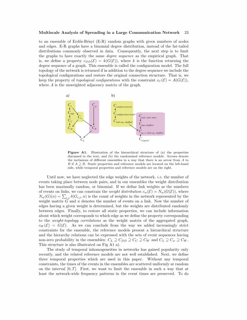
Figure A1. Illustration of the hierarchical structure of (a) the propertiesdiscussed in the text, and (b) the randomized reference models. Arrows denotethe inclusions of different ensembles in a way that there is an arrow from A toB if A ⊇ B. Static properties and reference models are located on the left-handside, while temporal properties and reference models are on the right.
Until now, we have neglected the edge weights of the network, i.e. the number ofevents taking place between node pairs, and in our ensembles the weight distributionhas been maximally random, or binomial. If we define link weights as the numbersof events on links, we can constrain the weight distribution cw(E) = Nw(G(E)), whereNw(G)(n) =
∑i,j δ(Gi,j , n) is the count of weights in the network represented by the
weight matrix G and n denotes the number of events on a link. Now the number ofedges having a given weight is determined, but the weights are distributed randomlybetween edges. Finally, to restore all static properties, we can include informationabout which weight corresponds to which edge as we define the property correspondingto the weight-topology correlations as the weight matrix of the aggregated graph,cW (E) = G(E). As we can conclude from the way we added increasingly strictconstraints for the ensemble, the reference models present a hierarchical structureand the hierarchy relations can be expressed with the sets of event sequences havingnon-zero probability in the ensembles: CL ⊇ CDD ⊇ CC ⊇ CW and CL ⊇ Cw ⊇ CW .This structure is also illustrated on Fig A1 a).
The study of temporal inhomogeneities in networks has gained popularity onlyrecently, and the related reference models are not well established. Next, we definethree temporal properties which are used in this paper. Without any temporalconstraints, the times of the events in the ensembles are scattered uniformly at randomon the interval [0, T ]. First, we want to limit the ensemble in such a way that atleast the network-wide frequency patterns in the event times are preserved. To do
Multiscale Analysis of Spreading in a Large Communication Network 24
Link 1
t
t
t
t
t
t
t
t
11
12
1a
21
22
2b
N1
N2
tNn
.
.
. .
.
.
... Link 1
t
t
t
t
t
t
11
12
21
22
N1
N2
.
.
. .
.
.
...
t tNn
.
1n
t2b
Link 1
t
t
t
t
t
t
t
t
11
12
1a
21
22
2b
N1
N2
tNn
.
.
. .
.
.
... Link 2 Link N Link 2 Link NLink 2 Link N
Time shuffling Link sequence shuffling Eq.-w. link-seq. shuffling
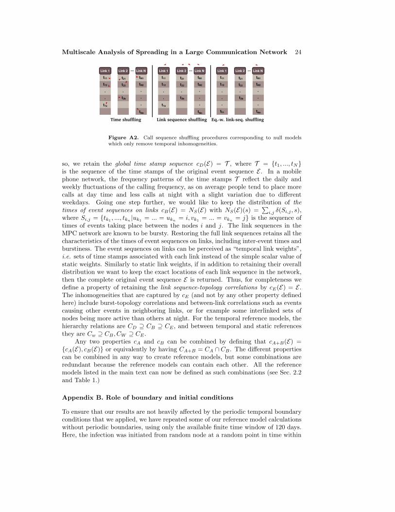
Figure A2. Call sequence shuffling procedures corresponding to null modelswhich only remove temporal inhomogeneities.
so, we retain the global time stamp sequence cD(E) = T , where T = {t1, ..., tN}is the sequence of the time stamps of the original event sequence E . In a mobilephone network, the frequency patterns of the time stamps T reflect the daily andweekly fluctuations of the calling frequency, as on average people tend to place morecalls at day time and less calls at night with a slight variation due to differentweekdays. Going one step further, we would like to keep the distribution of thetimes of event sequences on links cB(E) = NS(E) with NS(E)(s) =
∑i,j δ(Si,j , s),
where Si,j = {tk1 , ..., tkn |uk1 = ... = ukn = i, vk1 = ... = vkn = j} is the sequence oftimes of events taking place between the nodes i and j. The link sequences in theMPC network are known to be bursty. Restoring the full link sequences retains all thecharacteristics of the times of event sequences on links, including inter-event times andburstiness. The event sequences on links can be perceived as “temporal link weights”,i.e. sets of time stamps associated with each link instead of the simple scalar value ofstatic weights. Similarly to static link weights, if in addition to retaining their overalldistribution we want to keep the exact locations of each link sequence in the network,then the complete original event sequence E is returned. Thus, for completeness wedefine a property of retaining the link sequence-topology correlations by cE(E) = E .The inhomogeneities that are captured by cE (and not by any other property definedhere) include burst-topology correlations and between-link correlations such as eventscausing other events in neighboring links, or for example some interlinked sets ofnodes being more active than others at night. For the temporal reference models, thehierarchy relations are CD ⊇ CB ⊇ CE , and between temporal and static referencesthey are Cw ⊇ CB , CW ⊇ CE .
Any two properties cA and cB can be combined by defining that cA+B(E) ={cA(E), cB(E)} or equivalently by having CA+B = CA ∩ CB . The different propertiescan be combined in any way to create reference models, but some combinations areredundant because the reference models can contain each other. All the referencemodels listed in the main text can now be defined as such combinations (see Sec. 2.2and Table 1.)
Appendix B. Role of boundary and initial conditions
To ensure that our results are not heavily affected by the periodic temporal boundaryconditions that we applied, we have repeated some of our reference model calculationswithout periodic boundaries, using only the available finite time window of 120 days.Here, the infection was initiated from random node at a random point in time within
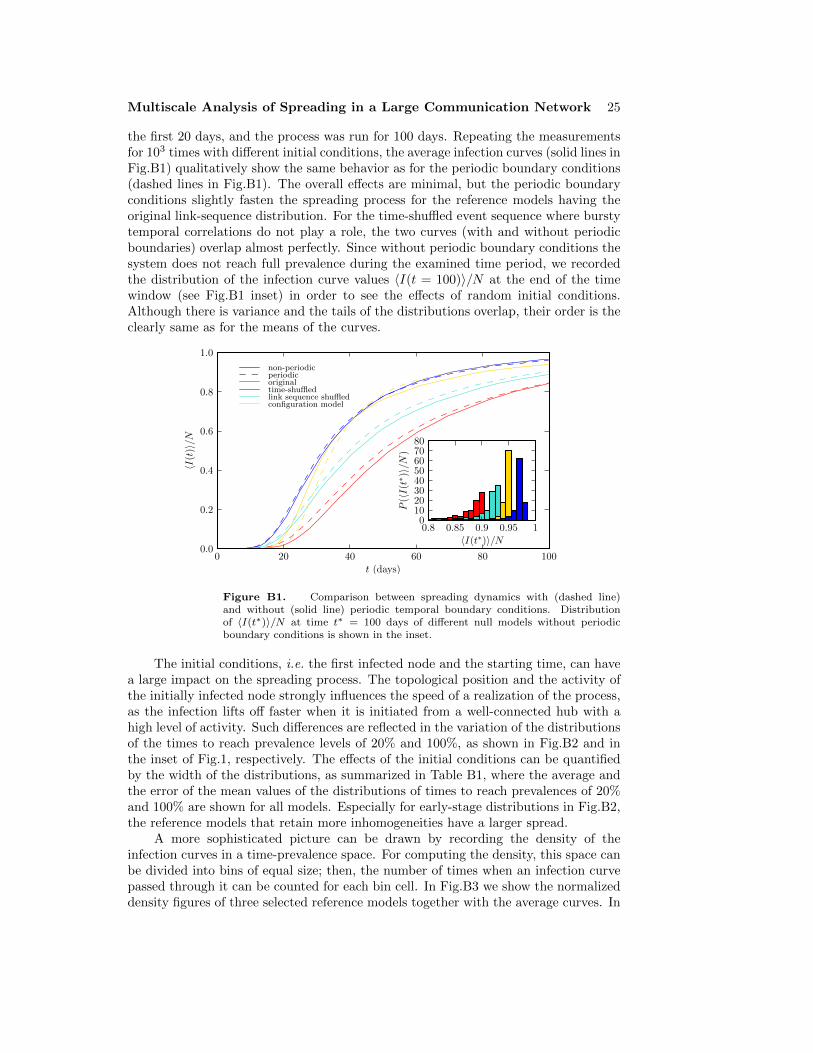
Multiscale Analysis of Spreading in a Large Communication Network 25
the first 20 days, and the process was run for 100 days. Repeating the measurementsfor 103 times with different initial conditions, the average infection curves (solid lines inFig.B1) qualitatively show the same behavior as for the periodic boundary conditions(dashed lines in Fig.B1). The overall effects are minimal, but the periodic boundaryconditions slightly fasten the spreading process for the reference models having theoriginal link-sequence distribution. For the time-shuffled event sequence where burstytemporal correlations do not play a role, the two curves (with and without periodicboundaries) overlap almost perfectly. Since without periodic boundary conditions thesystem does not reach full prevalence during the examined time period, we recordedthe distribution of the infection curve values 〈I(t = 100)〉/N at the end of the timewindow (see Fig.B1 inset) in order to see the effects of random initial conditions.Although there is variance and the tails of the distributions overlap, their order is theclearly same as for the means of the curves.
0 20 40 60 80 100
t (days)
0.0
0.2
0.4
0.6
0.8
1.0
〈I(t
)〉/N
non-periodicperiodicoriginaltime-shuffledlink sequence shuffledconfiguration model
0.8 0.85 0.9 0.95 1
〈I(t∗)〉/N
01020304050607080
P(〈I(t∗ )〉/N
)
Figure B1. Comparison between spreading dynamics with (dashed line)and without (solid line) periodic temporal boundary conditions. Distributionof 〈I(t∗)〉/N at time t∗ = 100 days of different null models without periodicboundary conditions is shown in the inset.
The initial conditions, i.e. the first infected node and the starting time, can havea large impact on the spreading process. The topological position and the activity ofthe initially infected node strongly influences the speed of a realization of the process,as the infection lifts off faster when it is initiated from a well-connected hub with ahigh level of activity. Such differences are reflected in the variation of the distributionsof the times to reach prevalence levels of 20% and 100%, as shown in Fig.B2 and inthe inset of Fig.1, respectively. The effects of the initial conditions can be quantifiedby the width of the distributions, as summarized in Table B1, where the average andthe error of the mean values of the distributions of times to reach prevalences of 20%and 100% are shown for all models. Especially for early-stage distributions in Fig.B2,the reference models that retain more inhomogeneities have a larger spread.
A more sophisticated picture can be drawn by recording the density of theinfection curves in a time-prevalence space. For computing the density, this space canbe divided into bins of equal size; then, the number of times when an infection curvepassed through it can be counted for each bin cell. In Fig.B3 we show the normalizeddensity figures of three selected reference models together with the average curves. In
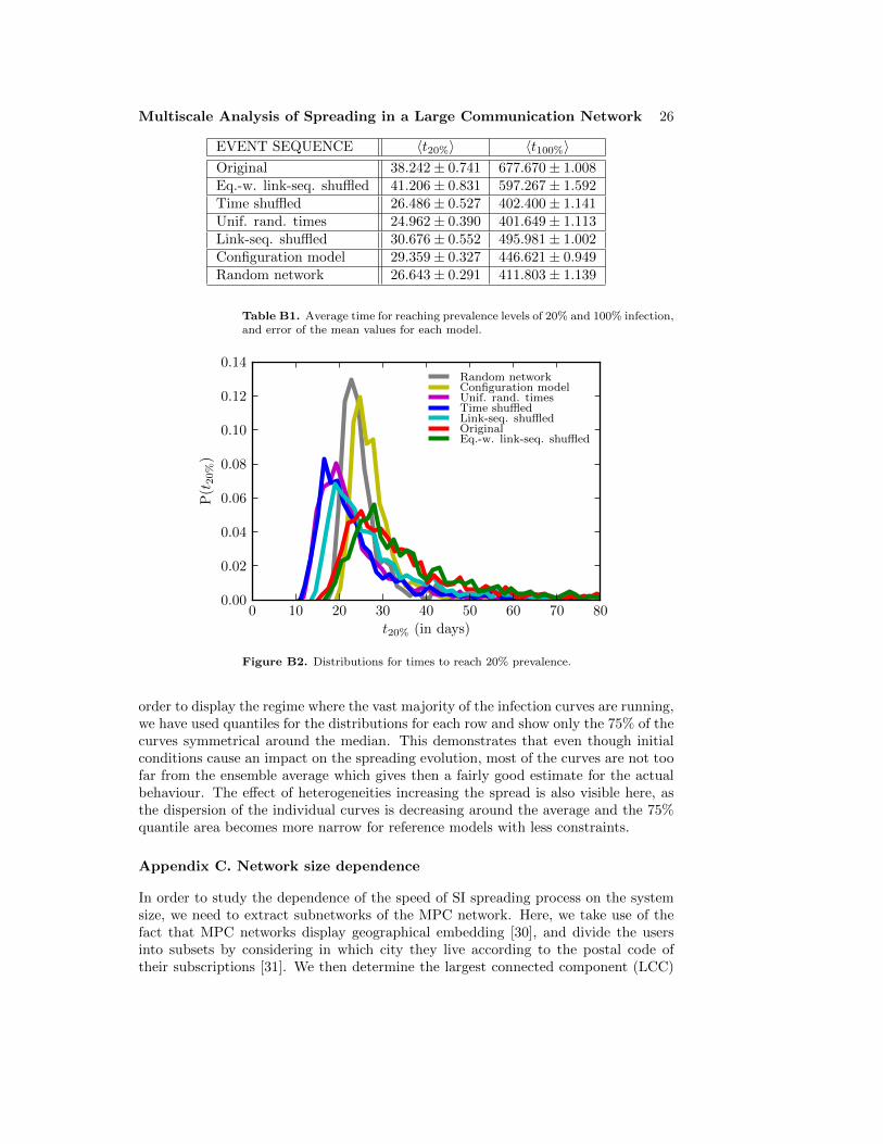
Multiscale Analysis of Spreading in a Large Communication Network 26
EVENT SEQUENCE 〈t20%〉 〈t100%〉Original 38.242± 0.741 677.670± 1.008Eq.-w. link-seq. shuffled 41.206± 0.831 597.267± 1.592Time shuffled 26.486± 0.527 402.400± 1.141Unif. rand. times 24.962± 0.390 401.649± 1.113Link-seq. shuffled 30.676± 0.552 495.981± 1.002Configuration model 29.359± 0.327 446.621± 0.949Random network 26.643± 0.291 411.803± 1.139
Table B1. Average time for reaching prevalence levels of 20% and 100% infection,and error of the mean values for each model.
0 10 20 30 40 50 60 70 80
t20% (in days)
0.00
0.02
0.04
0.06
0.08
0.10
0.12
0.14
P(t
20%
)
Random networkConfiguration modelUnif. rand. timesTime shuffledLink-seq. shuffledOriginalEq.-w. link-seq. shuffled
Figure B2. Distributions for times to reach 20% prevalence.
order to display the regime where the vast majority of the infection curves are running,we have used quantiles for the distributions for each row and show only the 75% of thecurves symmetrical around the median. This demonstrates that even though initialconditions cause an impact on the spreading evolution, most of the curves are not toofar from the ensemble average which gives then a fairly good estimate for the actualbehaviour. The effect of heterogeneities increasing the spread is also visible here, asthe dispersion of the individual curves is decreasing around the average and the 75%quantile area becomes more narrow for reference models with less constraints.
Appendix C. Network size dependence
In order to study the dependence of the speed of SI spreading process on the systemsize, we need to extract subnetworks of the MPC network. Here, we take use of thefact that MPC networks display geographical embedding [30], and divide the usersinto subsets by considering in which city they live according to the postal code oftheir subscriptions [31]. We then determine the largest connected component (LCC)
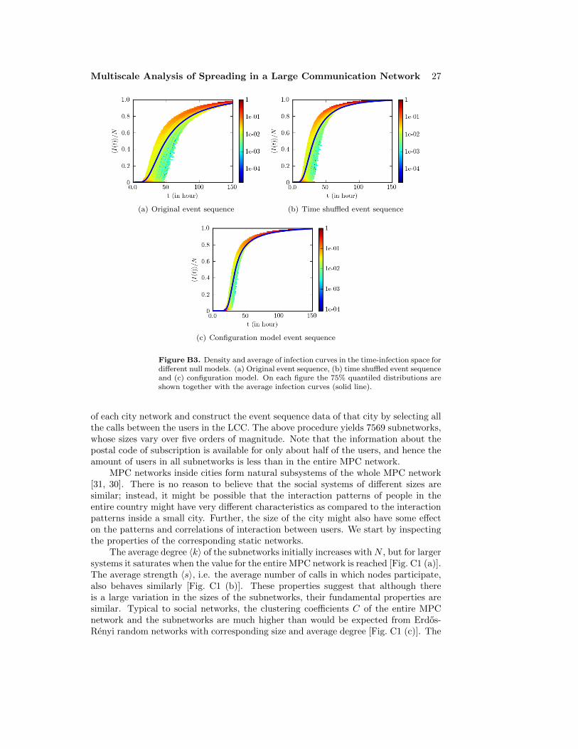
Multiscale Analysis of Spreading in a Large Communication Network 27
(a) Original event sequence (b) Time shuffled event sequence
(c) Configuration model event sequence
Figure B3. Density and average of infection curves in the time-infection space fordifferent null models. (a) Original event sequence, (b) time shuffled event sequenceand (c) configuration model. On each figure the 75% quantiled distributions areshown together with the average infection curves (solid line).
of each city network and construct the event sequence data of that city by selecting allthe calls between the users in the LCC. The above procedure yields 7569 subnetworks,whose sizes vary over five orders of magnitude. Note that the information about thepostal code of subscription is available for only about half of the users, and hence theamount of users in all subnetworks is less than in the entire MPC network.
MPC networks inside cities form natural subsystems of the whole MPC network[31, 30]. There is no reason to believe that the social systems of different sizes aresimilar; instead, it might be possible that the interaction patterns of people in theentire country might have very different characteristics as compared to the interactionpatterns inside a small city. Further, the size of the city might also have some effecton the patterns and correlations of interaction between users. We start by inspectingthe properties of the corresponding static networks.
The average degree 〈k〉 of the subnetworks initially increases withN , but for largersystems it saturates when the value for the entire MPC network is reached [Fig. C1 (a)].The average strength 〈s〉, i.e. the average number of calls in which nodes participate,also behaves similarly [Fig. C1 (b)]. These properties suggest that although thereis a large variation in the sizes of the subnetworks, their fundamental properties aresimilar. Typical to social networks, the clustering coefficients C of the entire MPCnetwork and the subnetworks are much higher than would be expected from Erdos-Renyi random networks with corresponding size and average degree [Fig. C1 (c)]. The
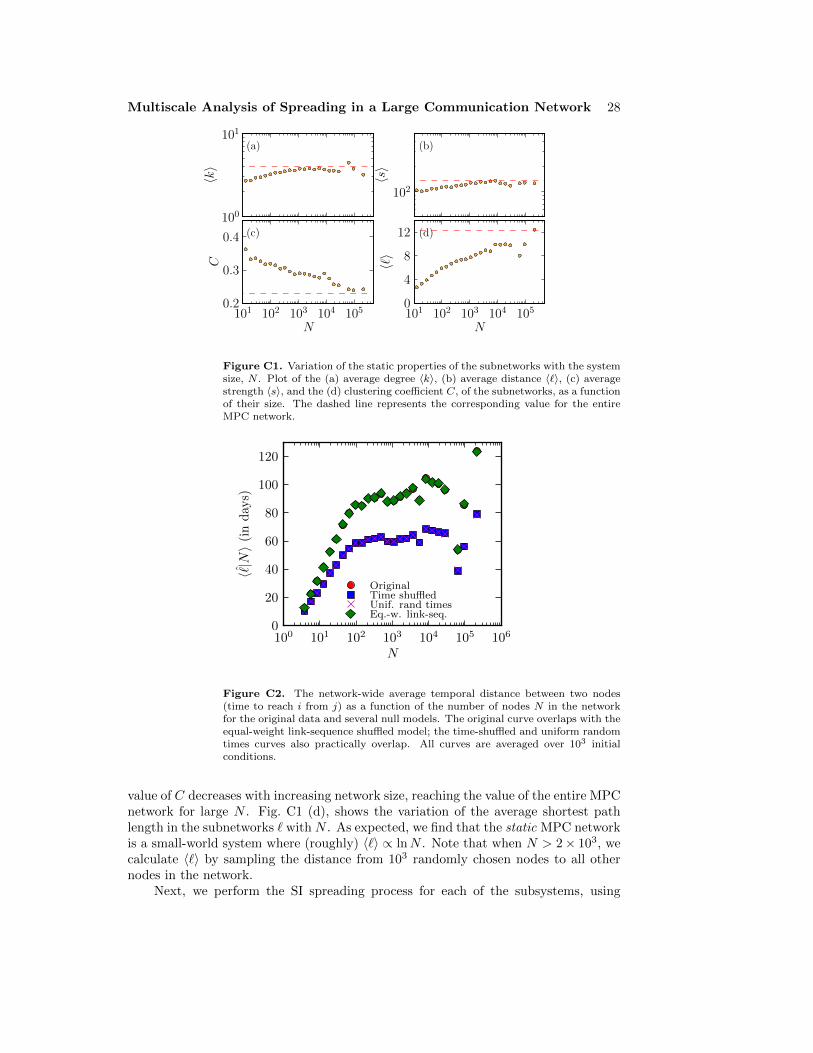
Multiscale Analysis of Spreading in a Large Communication Network 28
100
101
〈k〉
N
102
〈s〉
101 102 103 104 105
N
0
4
8
12
〈`〉
101 102 103 104 105
N
0.2
0.3
0.4
C
(a) (b)
(c) (d)
Figure C1. Variation of the static properties of the subnetworks with the systemsize, N . Plot of the (a) average degree 〈k〉, (b) average distance 〈`〉, (c) averagestrength 〈s〉, and the (d) clustering coefficient C, of the subnetworks, as a functionof their size. The dashed line represents the corresponding value for the entireMPC network.
100 101 102 103 104 105 106
N
0
20
40
60
80
100
120
〈ˆ|N〉(
ind
ays)
OriginalTime shuffledUnif. rand timesEq.-w. link-seq.
Figure C2. The network-wide average temporal distance between two nodes(time to reach i from j) as a function of the number of nodes N in the networkfor the original data and several null models. The original curve overlaps with theequal-weight link-sequence shuffled model; the time-shuffled and uniform randomtimes curves also practically overlap. All curves are averaged over 103 initialconditions.
value of C decreases with increasing network size, reaching the value of the entire MPCnetwork for large N . Fig. C1 (d), shows the variation of the average shortest pathlength in the subnetworks ` with N . As expected, we find that the static MPC networkis a small-world system where (roughly) 〈`〉 ∝ lnN . Note that when N > 2× 10³, wecalculate 〈`〉 by sampling the distance from 103 randomly chosen nodes to all othernodes in the network.
Next, we perform the SI spreading process for each of the subsystems, using
Multiscale Analysis of Spreading in a Large Communication Network 29
both the original event sequence and the temporal reference models. We simulate theprocess until all the nodes in the system are infected and observe the infection timeof each node. We then measure the average time at which nodes get infected in a cityas a function of the city size N [Fig C2]. This average infection time is same as theaverage temporal distance (duration of the fastest paths) of the system. The temporaldistances first show a fast increase, followed by slower increase. Importantly, for allsystem sizes, the temporal distances for the original data and the null models showa similar relationship. This indicates that the observed results are unlikely to be anartifact associated with the specific system, that is, the full MPC network.
Appendix D. τR for the uniformly random times reference model withperiodic boundary conditions
In this Appendix we are going to calculate the inter-event time and random relay timedistributions for the uniformly random times reference model. Further, we are goingto derive formulas for the expected average relay time and variance for the averagerelay time.
In the uniformly random times reference model the sequences of events of edges donot depend on each other and we can calculate all statistics just by considering a singleedge at a time. That is, we have an edge with n events, each taking place uniformly atrandom in the interval [0, T ], and denote the time of the ith event (ordered by time)by ti.
The time of i-th event is distributed like the i-th order statistics of the uniformprobability distribution ti/T ∼ U(i). That is, ti/T follows the beta distribution [28]
p(ti) =(ti/T )i−2(1− ti/T )n−i+1
B(i− 1, n− i) , (D.1)
where B(i− 1, n− i) =∫ 1
0xi−2(1− x)n−i+1dx is the beta function.
In order to be able to calculate τR, we need the distribution for the inter-eventtimes τi, rather than the times of the events. With periodic temporal boundaryconditions in place, we have
τi =
{T − tn + t1 if i = 1
ti − ti−1 if i 6= 1. (D.2)
Note that the values of ti are not independent of each other. However, from Ref. [28],we know that if we define a new random variable Wrs = U(s) − U(r) we get
pWrs(w) =
ws−r−1(1− w)n−s+r
B(s− r, n− s+ r + 1)(D.3)
Applying Eq. D.3 to Eq. D.2, the inter-event time τi distribution takes the form
p(τi) =
{(τi/T )n−2(1−τi/T )
B(n−1,2) if i = 1(1−τi/T )n−1
B(1,n) if i 6= 1. (D.4)
The expected value of τi thus becomes
〈τi〉 =
{2Tn+1 if i = 1Tn+1 if i 6= 1
, (D.5)
Multiscale Analysis of Spreading in a Large Communication Network 30
and the variance is
Var(τi) =
{2(n−1)
(n+2)(n+1)2T2 if i = 1
n(n+2)(n+1)2T
2 if i 6= 1. (D.6)
Note that τ1 is longer than all the other inter-event times. At first this might seem tobe a bias in the reference model. However, if one would change the labeling schemeof the event times such that t1 would be the first event after some point x ∈ [0, 1] anduse the periodic boundary condition in labeling all other events such that tn−1 wouldbe the last event before x, this would not change the distribution of τi. This mightseem paradoxical, but it just reflects the fact that if we select any point x in the timeinterval, we are more likely to hit long inter-event times than short inter-event times.That is, selecting the point x = 0 as basis of our “coordinate system” causes the firstinter-event time to be longer than the others.
Equipped with the functional form of the probability density function of thedistribution of τi, we can calculate the expected value of τR by using the Eq. 3:
〈τR〉 = 〈∑ni=1 τ
2i
2T〉 =
∑ni=1〈τ2
i 〉2T
=〈τ2
1 〉+ (n− 1)〈τ22 〉
2T. (D.7)
Now noting that 〈τ2i 〉 = 〈τi〉2 + Var(τi) and plugging in Eq D.5 and Eq. D.6 we get
〈τR〉 =T
n+ 1. (D.8)
The calculations can be made easier if we only want to calculate the average relaytimes and do not care about the distribution of τi. We can choose a random event iand set our time reference in a way that ti = 0 and still apply the periodic boundaryconditions. The set of inter-event times is retained in this transformation, and onlythe order of the times is lost. Further, the other n−1 events (not including event i) areuniformly randomly distributed over the time interval [0, T ]. Thus, the problem is offinding the distribution of the average relay time can be solved by solving the problemof dividing the unit interval into n intervals by n − 1 uniformly random points. InRef. [32] the l’th moment of the sum of the squares of the interval sizes was given as
〈(n∑
i=1
(τi/T )2)l〉 =(n− 1)!l!
(n+ 2l − 1)!
∑
j1+...+jn=l
(2j1)!...(2jn)!
j1!...jn!. (D.9)
Now the l’th moment of the average relay time can be calculated by using Eq. D.9with
〈τRl〉 = (T
2)l〈(
n∑
i=1
(τi/T )2)l〉. (D.10)
Using Eqs. D.9 and D.10 we obtain the correct average relay time of Eq. D.8, andvalues for the second moment
〈τR2〉 =n+ 5
(n+ 3)(n+ 2)(n+ 1)T 2, (D.11)
and the variance
Var(τR) =n− 1
(n+ 1)2(n+ 2)(n+ 3)T 2. (D.12)


