Multiscale statistical testing for connectome-wideassociation studies in fMRI

Pierre Belleca,b,∗, Yassine Benhajalia,c, Felix Carbonelld,Christian Dansereaua,b, Zarrar Shehzade,f,g, Genevieve Albouya,h, Maxime

Pellandh, Cameron Craddockf,g, Olivier Collignonh, Julien Doyona,h,Emmanuel Stipi,j, Pierre Orbana,i

aFunctional Neuroimaging Unit, Centre de Recherche de l’Institut Universitaire deGeriatrie de Montreal

bDepartment of Computer Science and Operations Research, University of Montreal,Montreal, Quebec, Canada

cDepartment of Anthropology, University of Montreal, Montreal, Quebec, CanadadBiospective Incorporated, Montreal, Quebec, Canada

eDepartment of Psychology, Yale University, New Haven, CT, United States of AmericafNathan Kline Institute for Psychiatric Research, Orangeburg, NY, United States of

AmericagCenter for the Developing Brain, Child Mind Institute, New York, NY, United States of

AmericahDepartment of Psychology, University of Montreal, Montreal, Quebec, CanadaiDepartment of Psychiatry, University of Montreal, Montreal, Quebec, Canada

jCentre Hospitalier de l’Universit de Montral, Montreal, Quebec, Canada

Abstract

Alteration in brain connectivity, as captured by fMRI, has been found to beassociated with a variety of clinical disorders. Yet, the systematic identifica-tion of connections associated with a disease state is a “needle in a haystack”problem. There are numerous connections to test and potentially very few ofthem show a strong association with the variable of interest. The number ofbrain parcels (or scale) used to measure connections is a key parameter, as moreparcels means more anatomically accurate measures, but also means many moreconnections to test and thus more risk to find spurious associations by chance.This work presents a multiscale approach designed to assess the impact of scaleon connectome-wide association studies. A mass univariate general linear modelis applied independently at each connection, for functional networks generatedthrough clustering at different scales. The multiple comparison problem is ad-dressed at each scale independently, using the false-discovery rate. An omnibuspermutation test is implemented to reject the global null hypothesis of no associ-ation across all scales. Our results support the fact that, when the global null isrejected, the false-discovery rate is well controlled both within and across scales.On simulations, we showed that multiscale group differences can be detected

∗Corresponding authorEmail address: pierre.bellec@criugm.qc.ca (Pierre Bellec)

Preprint submitted to Neuroimage September 7, 2014

arX

iv:s

ubm

it/10

5265

8 [

q-bi

o.Q

M]

7 S

ep 2

014

with excellent sensitivity in large sample size (n=100), and good sensitivity inmoderate sample size (n=40). On three real resting-state datasets (schizophre-nia, congenital blindness, motor practice), our results presented an excellentface validity. In addition, the multiscale method performed better than currenttechniques such as network-based statistics or multivariate distance matrix re-gression, both on simulations and real datasets. Taken together, our findingsdemonstrate that our approach is a powerful tool to mine for associations acrossthe whole connectome, at multiple scales.

Keywords: fmri, general linear model, functional parcellation, multiplecomparison, false discovery rate, multiscale analysis, connectome

Highlights

• A new statistical method to test the association between phenotypes andfunctional connectivity at multiple scales (number of brain parcels).

• The false-discovery rate is controlled both within- and between scales,with state-of-the-art sensitivity.

• A “group” method to control the false-discovery rate in connectomes,with improved sensitivity to sparse signals compared to the standardBenjamini-Hochberg procedure.

1. Introduction

Main Objective. Estimates of brain connectivity derived from functional mag-netic resonance imaging (fMRI) have been found to be associated with a widevariety of clinical disorders (Castellanos et al., 2013). Rather than focusing on alimited set of a priori regions of interest, a recent trend is to perform statisticaltests of association across the whole connectome, i.e. at every possible brainconnection (Shehzad et al., 2014). Akin to genome-wide association studies,such connectome-wide association studies (CWAS) raise a large multiple com-parison problem: with 103 brain parcels, there are about 5 × 105 connectionsbetween parcels to test. When a massive number of univariate tests are per-formed, it becomes difficult to simultaneously reach acceptable rates of falsepositives (specificity) and false negatives (sensitivity). The number of multiplecomparisons can be reduced by using fewer, bigger parcels, but then associationsthat are highly specific to small anatomical locations may be lost. In additionto these statistical concerns, examining and interpreting all findings in a con-nectome quickly becomes challenging in practice when the number of parcelsgets large. The number of brain parcels (or scale) thus has critical implicationsboth on the statistical power of a CWAS and the interpretability of the results.The main objective of this work was to develop a statistical framework able toperform a CWAS at multiple scales, instead of relying on a single parcellation,such that the impact of the spatial resolution could be assessed and optimized.

2

Mass-univariate connectome-wide association studies. The mass-univariate ap-proach to CWAS (Worsley and Friston, 1995) consists of independently estimat-ing a general linear model (GLM) at each connection, i.e. for any given pairof brain parcels. In the GLM, a series of equations are solved to find a linearmixture of explanatory variables (called covariates) that best fit the connectiv-ity values observed across the many subjects. A p value is generated for eachconnection to quantify the probability that the estimated strength of associa-tion between this connection and a covariate of interest could have randomlyarisen in the absence of a true association. For a single test, a p-value below0.05 is typically considered as strong evidence of an association, yet in a con-nectome, even in the absence of any true association, about 5% of connectionswould get reported at this significance level. Given the very large number oftested connections, this could result in 1,000s of false positive findings, unless anadequate correction for multiple comparisons is applied. Random field theory isroutinely used to correct for multiple comparisons in 3D statistical parametricmaps (SPMs), where a statistical test is performed at each voxel. Early effortsby Worsley et al. (1998) aimed at extending random field theory from a 3Dbrain activity manifold to a 6D connectome manifold - a 3D space connectedto a 3D space. Random field theory offers a control of the family-wise error(FWE) rate, i.e. the probability of one or more false positive arising acrossthe whole connectome. Unfortunately, the strict control of false positives of-fered by FWE in a very large space like a connectome generally comes at a costof low sensitivity. As an alternative, Shehzad et al. (2014) recently proposedto run a multivariate test for each possible region-to-brain connectivity map,called multivariate distance matrix regression (MDMR). The MDMR approacheffectively performs one test per parcel or voxel, instead of one test per con-nection, and thus shrinks the connectome multiple comparison problem backto a standard SPM. MDMR was designed to screen for promising seed-basedconnectivity maps worthy to explore in a subsequent, independent analysis, yetit does not provide valid statistics at the level of a single connection.

Parcellations and testing. A straightforward way to systematically test everypossible connections without succumbing to multiple comparisons is to reducethe number of brain parcels. This can be achieved using a set of brain re-gions delineated based on anatomical landmarks such as the AAL template(Tzourio-Mazoyer et al., 2002), see for example the study of Wang et al. (2007)on Alzheimer’s disease. Rather than using anatomical parcels, it is possible tobuild data-driven functional brain parcels that optimally capture the underly-ing spatial correlation structure of the fMRI time series at the voxel level (Shenet al., 2010; Craddock et al., 2012; Blumensath et al., 2013). It has been shownthat task activation detection with the GLM at the parcel level was more sensi-tive than voxelwise analysis (Lu et al., 2003; Thirion et al., 2006), and the samewas reported for the accuracy of multivariate prediction (Xu et al., 2010). How-ever, even with a relatively small number of brain parcels N = 100, there arestill about 5000 multiple comparisons. The work of Zalesky et al. (2010a) thusproposed to use uncorrected threshold on the individual p-values, but then to

3

identify to which extent the connections that survive the test are interconnected.This extent measure is compared against what could be observed under a nullhypothesis of no association, implemented through permutation testing. Thisapproach, called Network-Based Statistics (NBS), is the connectome equivalentto the “cluster-level statistics” used in SPMs. As the authors noted themselves,the NBS only offers a loose control of false-positive rate at the level of a singleconnection, but can be used to reject the possibility that a group of significantfindings could be observed by chance in the FWE sense.

Multiscale parcellations. Few investigators have examined how to select theparcels, and in particular their number, in order to maximize the statisticalpower of a GLM analysis. Work by Abou Elseoud et al. (2011) systemati-cally explored the impact of scale (number of components) on the ability of adual-regression ICA analysis to discriminate a group of patients suffering fromnon-medicated seasonal affective disorder compared to normal healthy controls.The authors concluded that the number of significant findings was maximized atscale 45 (in this case, 45 independent components). The impact of the number ofbrain parcels was also investigated at much higher scales (from 50 to 3000+) byShehzad et al. (2014), who concluded in their case that the results of the associa-tion between resting-state and intelligence quotient was consistent across scales.It should be noted that, in the above-mentioned studies (Abou Elseoud et al.,2011; Shehzad et al., 2014), the authors did not investigate the implications thattesting many scales would have in terms of the control of false positives. Higherscales may indeed result in greater rates of false positives, as more componentsalso resulted in more multiple comparisons Meskaldji et al. (2011). Interestingly,the issue of multiscale testing was raised two decades ago in the context of SPMand Gaussian smoothing, and a theoretical framework based on random fieldtheory had been developed to control for FWE when testing at multiple scales,i.e. different sizes of the spatial smoothing kernel (Poline and Mazoyer, 1994;Worsley et al., 1996). Multiscale random field theory has however not been gen-eralized to connectomes, to the best of our knowledge, and was also limited toGaussian blurring kernels, rather than data-driven brain parcels. We are thusnot currently aware of a valid statistical framework to examine the results of aCWAS with data-driven brain parcellations at multiple scales.

Specific objectives. In this paper, our main objective was to develop a novel sta-tistical framework, called multiscale statistical parametric connectome (MSPC),to perform a CWAS at multiple spatial scales. A series of data-driven functionalbrain parcellations was first generated using a clustering approach (Bellec et al.,2010). These parcels were used to derive connectomes for a group of subjects,and this process was repeated using different numbers of parcels were investi-gated. A GLM was then applied on the connectomes and the false-discoveryrate (FDR) was controlled at each scale. Two methods were implemented tocontrol the FDR: the popular approach by Benjamini and Hochberg (1995) aswell as a recent algorithm optimized for sparse signals (Hu et al., 2010). Wedeveloped an omnibus test to assess if the number of significant findings (called

4

discoveries) across scales could have been observed under the global null hypoth-esis of no association at any scale. Our key hypothesis was that, although theFDR is controlled independently at each scale, it is also well controlled acrossscales when the global null is rejected. Our primary objective was to supportthis hypothesis empirically. Our second objective was to evaluate the sensitivityof the MSPC method, and in particular to determine which variant of the FDRcontrol algorithm was most sensitive. Our third and last objective was to com-pare the sensitivity and specificity of the MSPC method with recent detectiontechniques applied at a single scale, namely NBS (Zalesky et al., 2010a) andMDMR (Shehzad et al., 2014). We conducted a series of experiments involvingboth simulated and real datasets to address these specific objectives, which havebeen summarized, along with the main findings, in Table 1.

Simulations. We first generated simulation datasets by mixing real fMRI datawith synthetic signal. Importantly, the simulation datasets were designed tohave a well defined ground truth in terms of true and false positives when usinga multiscale set of functional parcels. We simulated group differences using avariety of scenarios covering: (1) different effect sizes; (2) different amountsof true positives; (3) different number of subjects per group. As part of thesimulation study, we also performed CWAS on real fMRI datasets using randomcovariates of interest, thus providing insights in the behaviour of the methodsunder the global null hypothesis, where there is no true association to find.

Real datasets. We evaluated the MSPC, NBS and MDMR on three real datasets:(1) a study comparing patients suffering from schizophrenia with healthy controlsubjects (referred to here as the SCHIZO dataset, with a large sample size,n = 146); (2) a study on patients suffering of congenital blindness, comparedto sighted controls (referred to here as the BLIND dataset, with a small samplesize, n = 31), and; (3) a study of motor learning, where resting-state data wereacquired before and after learning of a new motor task (referred to here as theMOTOR dataset, with a moderate sample size, n = 54). These three datasetswere chosen to assess if MSPC would be able to uncover statistically significanteffects in a variety of sample sizes. Also, we had strong a priori hypotheses forthose three analyses: changes in the visual network for the BLIND dataset, inthe motor network for the MOTOR dataset and a more general dysconnectivityin the SCHIZO dataset. These a priori were useful to qualitatively assess theface validity of the technique.

5

Objective Experiment(s) Finding(s)Develop a statistical framework formultiscale GLM analysis of connec-tomes.

All relevant algorithms are described inSection 2.

Not applicable.

Assess the specificity of MSPC in theabsence of signal.

“Negative control experiments” whererandom subgroups are compared in theCambridge sample.

The FWE under the global null is controlled at nominal level bythe permutation test (Figure 5).

Assess the specificity of MSPC withinand across scales.

Multiscale simulation of group differ-ences in the Cambridge sample.

When including a permutation test for the global null, the FDR iscontrolled at nominal level both within and across scales (Figure3 and Figure 6). The FDR at the peak of discoveries is slighltyliberal (Figure 6).

Assess the sensitivity of MSPC, acrossscales or at the peak of discovery.

Multiscale simulation of group differ-ences in the Cambridge sample.

The sensitivity across scales was excellent for a large sample size,n = 100, and good for moderate sample size, n = 40, as long asthere were a large effect size and many true positives (Figure 4and Figure 6). The highest sensitivity was obtained by looking atthe scale with peak percentage of discovery.

Assess the face validity of the resultsidentified with MSPC on real data.

Three datasets were analyzed:BLINDS, SCHIZO and MOTOR.Strong a priori hypotheses on thenetworks involved in each contrastwere available.

The MSPC identified plausible changes in connectivity in all threeanalyses (Figure 8).

Compare two algorithms controlling forthe FDR: classical BH and group FDR.

Multiscale simulation in the Cambridgedataset, and comparison on the threereal datasets.

The group FDR is more sensitive across scales (Figure 3 and Fig-ure 8).

Compare the MSPC with NBS andMDMR.

Multiscale simulation in the Cambridgedataset, and comparison on the threereal datasets.

The MSPC with group FDR had overall the best sensitivity (Fig-ures 6 and 8).

Assess how multiscale analysis can con-tribute to interpret results.

Exploration of connectivity changes inSCHIZO.

High scales clarified the spatial distribution of changes in connec-tivity seen at low scales 9.

Table 1: Summary of the objectives, experiments and findings of the paper.

6

2. Statistical testing procedures

2.1. Functional parcellations

The first step to build a connectome is to select a parcellation of the brain,with R networks. In this work, we used functional brain parcellations, aimedat defining groups of brain regions with homogeneous time series. A numberof algorithms have been proposed with additional spatial constraints, to en-sure that the resulting parcels are spatially connected (Lu et al., 2003; Thirionet al., 2006; Craddock et al., 2012). However, from a pure functional view-point, the spatial constraint seems somewhat arbitrary, as functional units inthe brain at low resolution encompass distributed networks of brain regionswith homotopic regions often being part of a single parcel (De Luca et al., 2006;Damoiseaux et al., 2006). Some works have thus used distributed parcels as thespatial units to measure functional brain connectivity, e.g. (Jafri et al., 2007;Marrelec et al., 2008). To generate the functional parcelations, we relied on arecent method called “Bootstrap Analysis of Stable Clusters” (BASC), whichcan identify consistent functional parcels for a group of subjects (Bellec et al.,2010), using a hierarchical cluster with Ward’s criterion both at the individualand the group levels. The functional parcels can be generated at any arbitraryresolution (within the range of the fMRI resolution), and we considered onlyclusters generated at the group level. So, in this work, the word scale refers tothe number of clusters as generated by the group BASC procedure, and eachscale includes includes non-overlapping networks of brain regions that are notnecessarily spatially contiguous.

2.2. Functional connectome

For each scale, and each pair of distinct networks i and j at this scale, thebetween-network connectivity yi,j is measured by the Fisher transform of thePearson’s correlation between the average time series of the networks. Thewithin-network connectivity yi,i is the Fisher transform of the average correla-tion between time series of every pair of distinct voxels inside network i. Theconnectome Y = (yi,j)

Ri,j=1 is thus a R×R matrix. Each column j (or row, as the

matrix is symmetric) codes for the connectivity between network j and all otherbrain networks, or in other word is a full brain functional connectivity map. SeeFigure 1a-b for a representation of a parcellation and associated connectome.Connectomes are generated independently at each scale. See Appendix A for amore formal description of the connectome generation.

2.3. Statistical parametric connectome

For a scale with R parcels, there are exactly L = R(R+1)/2 distinct elementsin an individual connectome Y. This connectome can be stored as a 1×L vector,where the brain connections have been ordered arbitrarily along one dimension.When functional data is available on N subjects, the group of connectomes isthen assembled into a N × L array Y = (yn,l), where n = 1, . . . , N each codefor one subject and l = 1, . . . , L each code for one connection. A general linear

7

0

1

x = 1 y = -55

z = 30

y = -55

z = 30

1

200

a Decomposition of the brain intoresting-state networks (scale 200)

b Matrix of functional connectivitybetween network time series(connectome). Each row/columnis a functional connectivity map

space

spac

ec Estimation of a statistical parametric connectome

= . +

Group of functional connectome in stereotaxic

space for N subjects

1 Patients

N su

bjec

ts

Explanatory variables parametric connectomes(regression coefficients)

residuals estimatedusing a least-square

criterion

-1

x = 1

00

-0.50.5

N subjects

K=2

N subjectsseed

0 2000

200

r

Figure 1: General linear model applied to connectomes. The connectivity is measuredbetween R brain parcels generated through a clustering algorithm (panel a). The connectomeis a R×R matrix measuring functional connectivity between- and within-networks. See maintext for the definition of the connectivity measures. Note that each column of the connectomeis equivalent to a full brain functional connectivity map for a particular seed region (panelb). The association between phenotypes and connectomes is tested independently at eachconnection using a general linear model at the group level (panel c). The results presentedhere are for illustration purpose only, and not related to the results presented in the applicationsections of the manuscript.

model (GLM) framework can then be used to test the association between brainconnectivity and a trait of interest, such as the age or sex of participants. All ofthese C explanatory variables are entered in a N × C matrix X. The variablesare typically corrected to have a zero mean across subjects, and an intercept(i.e. a column filled with 1) is added to X. The GLM relies on the followingstochastic model:

Y = XB + E, (1)

with the following matrices:

• Y is a N ×L matrix where each row codes for a subject, and each columncodes for a connection,

• X is a N × C matrix of explanatory variables (or covariates) where eachrow codes for a subject and each column codes for a covariate,

8

• B is an unknown C×L matrix of linear regression coefficients where eachrow codes for a covariate and each column codes for a connection,

• E is a N ×L random (noise) multivariate Gaussian variable, with similarcoding to Y.

As the data generated from different subjects are statistically independent, andunder an homoscedasticity assumption, the regression coefficients B can be esti-mated with ordinary least squares. For a given “contrast” vector C of size 1×C,the significance of C.B can be tested with a connectome of t-test (tl)

Ll=1, with

associated p-values (pl)Ll=1. The quantity pl controls for the risk of false positive

findings at each connection l. The GLM applied on connectomes is illustratedin Figure 1c. See Appendix B for the equations related to the estimation andtesting of regression coefficients in the GLM.

2.4. The Benjamini-Hochberg FDR procedure

In traditional (univariate) applications, a p value below 0.05 is considered asa solid evidence of an effect. For a given scale, there are however a large numberL of such tests on pl to perform. So even with a 5% chance of a false positiveat connexion l, in the absence of any effect one would report 5% of the wholeconnectome as associated with a significant effect. The significance value ap-plied on pl thus needs to be adjusted for this multiple comparison problem. Weimplemented two strategies for controlling the FDR. The idea behind the FDRis not to strictly control the probability to observe at least one false positive (aquantity know as family-wise error, FWE), but rather to control the propor-tion of false positive amongst the findings. Note that controlling for the FDRis not necessarily a more liberal attitude than controlling for the FWE: if theglobal null hypothesis is verified, i.e. all discoveries are false positive, then theFDR is exactly the FWE. In the presence of true discoveries, however, the FDRprocedure tolerates in general more noise than a FWE approach. The actualnumber of false discoveries will dependend on the amount of signal (true pos-itive) present in the data, and is therefore a context-dependent question. Thepopular Benjamini-Hochberg (BH) procedure was proposed to control the FDRq to an acceptable level α (Benjamini and Hochberg, 1995). This algorithmwas designed for independent tests, but it has been shown to have a satisfac-tory behaviour even in the presence of positive correlation between the tests pl(Benjamini and Yekutieli, 2001).

2.5. The group FDR procedure

A documented limitation of the BH procedure is its lack of sensitivity tosparse signals (Hu et al., 2010). If only a small subset of brain parcels showsome significant effects, the maps of low signal will contribute a lot of noise andthe FDR threshold that is set globally will be quite conservative. A connec-tome has a natural structure: each column represents a full brain connectivitymap, where the parcel associated with the column acts like the seed (see Figure1a). Some regions of the brain are likely to be particularly impacted by the

9

trait of interest, and be associated with many discoveries, while others will beassociated with very few or even no discoveries. This means that some columnsin the connectome will be associated with many more discoveries than others.These columns thus represent natural groups of tests within the full connec-tome, yet this structure is completely ignored in the BH procedure. Severalsolutions have recently been proposed for this issue (Efron, 2008; Cai and Sun,2009; Hu et al., 2010; Benjamini and Bogomolov, 2011). We focused in thiswork on the least-slope variant of the group FDR procedure proposed by Huet al. (2010). The idea of the group FDR is to first assess the presence of signalin each column (map) independently, and then re-weight the original p-valuesbased on the presence (or absence) of promising signal. It was shown that thegroup FDR procedure controls asymptotically the global FDR for independenttests, yet they are expected to be much more sensitive than BH for sparse sig-nals (Hu et al., 2010). The group FDR was also reported to behave correctly inthe presence of positive dependency between tests, although no analytical prop-erties were derived in that case. We investigated experimentally the differencesbetween the BH and group FDR procedures, both on simulated data (Section3) and real data (Section 4). The Appendix C provides a formal description ofboth the global and the group FDR algorithms.

2.6. Multiscale testing

To explore the association of connectomes and a trait of interest at multiplescales, a multiscale clustering decomposition was first generated with BASC,and then the GLM was estimated with FDR control at each scale indepen-dently, see Figure 2. This introduces a new level of multiple comparisons, thistime across scales rather than across connections. There is however a qualita-tive difference between the multiple comparison problems encountered acrossmultiple connections, and across multiple scales. In a mass univariate GLMconnectome analysis, the possibility exists of a sparse signal, i.e. some connec-tions show an effect, while others do not. In a multiscale analysis, a detectionat any scale essentially implies the presence of signal at all the other scales.In the presence of signal, i.e. with true positive present at every scales, Efron(2008) suggested that there would be no need to adjust the FDR for multiplecomparisons across scales. Controlling for the FDR at each scale independentlywould also guarantee that the FDR would be controlled overall, for all testsperformed over all connections and at all scales. This strategy however onlymakes sense if the objective of the investigator is to systematically examine theresults of MSPC at every tested scale. It would also be possible to select theone scale associated with the largest rate of discoveries, defined as the numberof significant connections divided by the total number of distinct connectionsat a given scale. Although this empirical optimization of the scale for meansof discovery is attractive in practice, there is however no theoretical guaranteethat the FDR at the scale with maximal discovery rate will be controlled. Weexamined the behaviour of the FDR at “peak of discovery” on simulations, seeSection 3.

10

-10

1 1 # networks-10

1

scale (number of netw

orks)

10

50

100

200

500

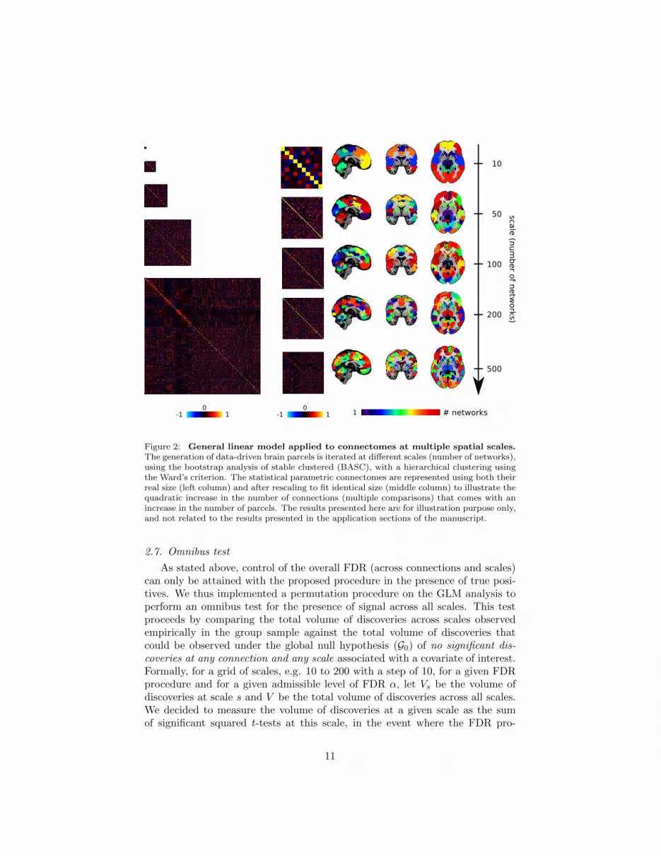
Figure 2: General linear model applied to connectomes at multiple spatial scales.The generation of data-driven brain parcels is iterated at different scales (number of networks),using the bootstrap analysis of stable clustered (BASC), with a hierarchical clustering usingthe Ward’s criterion. The statistical parametric connectomes are represented using both theirreal size (left column) and after rescaling to fit identical size (middle column) to illustrate thequadratic increase in the number of connections (multiple comparisons) that comes with anincrease in the number of parcels. The results presented here are for illustration purpose only,and not related to the results presented in the application sections of the manuscript.

2.7. Omnibus test

As stated above, control of the overall FDR (across connections and scales)can only be attained with the proposed procedure in the presence of true posi-tives. We thus implemented a permutation procedure on the GLM analysis toperform an omnibus test for the presence of signal across all scales. This testproceeds by comparing the total volume of discoveries across scales observedempirically in the group sample against the total volume of discoveries thatcould be observed under the global null hypothesis (G0) of no significant dis-coveries at any connection and any scale associated with a covariate of interest.Formally, for a grid of scales, e.g. 10 to 200 with a step of 10, for a given FDRprocedure and for a given admissible level of FDR α, let Vs be the volume ofdiscoveries at scale s and V be the total volume of discoveries across all scales.We decided to measure the volume of discoveries at a given scale as the sumof significant squared t-tests at this scale, in the event where the FDR pro-

11

cedure detected discoveries, or the maximal squared t-test if no discovery wasmade. To test the significance of V , we generated replication of the statisticalparameteric connectomes under the global null hypothesis. For this purpose,the GLM was applied on the original data, then a permutation of the residualswas generated as described in Anderson (2002), see Appendix D. Finally, thereplication was generated by adding the permuted residuals to the estimatedmixture of explanatory variables, after the explanatory variable of interest (asselected through the contrast) had been removed. In order to respect the de-pendencies between scales, the same permutation of the subjects was applied toall of the scales for each replication. The detection procedure was applied oneach replication and the total volume of discoveries was derived. A Monte-Carloapproximation, with typically 10000 permutation samples, was used to estimatea false-positive rate p when testing against the global null hypothesis. If thistest passed significance, then each scale was examined with a control of the FDRat α = 0.05, uncorrected for multiple comparisons across scales. If the test didnot reach significance, then no connection at any scale was deemed significant.

3. Evaluation on simulated datasets

3.1. Data generation procedure

Rationale. As we were not aware of an existing framework to simulate well-controlled changes in multiscale fMRI network connectivity, we developed one,outlined below. When working at a single scale, it would be straightforward tosimulate a change between two populations by changing the values of specificconnections in selected individuals, e.g. (Zalesky et al., 2010a). For multiscaleconnectomes, however, it is important to simulate changes at the level of thefMRI time series, rather than the connectivity values, in order to assess howthe simulated changes propagate across scales. In that perspective it is alsoimportant to introduce spatial correlations in the simulation: with white noise,the simulated effects get amplified dramatically through averaging on low-scalenetworks, yet this amplification is much less pronounced in the presence of spa-tial auto-correlation in the time series. Finally, because manipulating the timeseries of one network in a simulation can potentially affect many connectionsin the multiscale connectome architecture, a specific strategy needs to be im-plemented to precisely control true positives and the effect size at any givenscale.

Main procedure. To incorporate some realistic spatial correlations in the simu-lations, semi-synthetic datasets were generated starting from a large real sample(Cambridge) released as part of the 1000 functional connectome project1 (Biswalet al., 2010). This sample (Liu et al., 2009) includes resting-state fMRI time se-ries (eyes opened, TR of 3 seconds, 119 volumes per subject) collected with a 3Tscanner on 198 healthy subjects (75 males), with an age ranging from 18 to 30

1http://fcon_1000.projects.nitrc.org/fcpClassic/FcpTable.html

12

years. All the datasets were preprocessed and resampled in stereotaxic space,as described in Section 4.2. A region growing algorithm was used to extract483 regions, as described in Bellec et al. (2010). For each subject, a functionalconnectome was generated (see Section 2.2). The average connectome acrossall subjects was derived, and a hierarchical clustering procedure (with Ward’scriterion) was applied to derive a hierarchy of resting-state networks at all pos-sible scales, ranging from 1 to 483. The simulation procedure relied on themanual selection of a critical scale K and a particular cluster k at this scale.For each simulation, two non-overlapping subgroups of subject (N subjects pergroup) were randomly selected. A circular block bootstrap (CBB) procedurewas applied to resample the individual time series, using identical time blockswithin each cluster, and independent time blocks in different clusters. This re-sampling scheme ensured that within-cluster correlations were preserved, whilebetween-cluster correlations had a value of zero on average. Finally, for thesubjects selected to be in the first group, a single realization of a independentand identically distributed variable, where each time point had a zero mean anda variance of a2, was added to the time series of the regions inside cluster k,after the time series were themselves corrected to a zero temporal mean anda variance of

√1− a2. The addition of this signal increased the intra-network

connectivity of the cluster including cluster k for all scales smaller or equal to K,and increased the within- as well as between-network connectivity for all clustersincluded in cluster k for scales strictly larger than k. Because of the absenceof correlations between networks at scale K (due to the CBB resampling), allother connections within- or between clusters at every scale were left unchangedby this procedure. It was thus possible to know exactly which connections weretrue positive in the group difference at every scale. For each scale, a connectionwas a true positive (non-zero average difference in connectivity between the twogroups) if (1) it connected two subclusters of the cluster of reference; (2) it mea-sured intra-network connectivity for a cluster that was either included in thecluster of reference, or included the cluster of reference. Supplementary FiguresS1 and S2 outline the procedure of multiscale connectome simulation.

Effect size and true positive rate. We handpicked two scales (4 and 7), andtwo clusters at those scales such that the percentage of true positives wouldbe about 15% and 5% respectively. Note that these clusters were used to settrue positives at all the scales of analysis, yet the subdivisions (or merging)associated with these clusters represented a varying proportion of the numberof clusters at any given scale. As a consequence, the exact percentage of truepositives actually varied from scale to scale. Two values for a2 were selectedthat resulted into a large effect (a2 = 0.2, Cohen’s d ∼ 1) and a moderateeffect (a2 = 0.1, Cohen’s d ∼ 0.5). The effect size associated with a given a2

actually depended on the within-cluster correlations, between-subject variancein connectivity as well as the scale of analysis. See Supplementary MaterialFigure S3 for a detailed presentation of the effect size and percentage of truepositives as a function of scale.

13

Simulations under the global null. To assess the behaviour of the testing proce-dures in the absence of any signal, we also ran experiments under the global null.In that case real connectomes were generated for randomly selected and non-overlapping groups of subjects, and then a testing procedure was implementedto assess the significance of group differences. In these experiments, refered to asthe 0% true positive rate experiments, no bootstrap was performed on individ-ual time series nor any signal was added. The experiments simply consisted incomparing real connectomes between random groups of subjects sampled fromidentical populations.

Robustness to the choice of clusters. Finally, we also investigated how the pro-cedure behaved when the clusters used in the testing procedures did not matchexactly with the clusters that were used to generate the simulations. For thispurpose, for each simulation, no signal was actually generated in 30% of theregions in the cluster of reference, but rather in an equivalent number of ran-domly selected regions from other clusters. Although the regions were randomlyselected, the same regions were selected across all simulations to simulate a con-sistent departure of the test clusters from the ground truth clusters. The multi-scale clusters without random perturbations were used in the statistical testingprocedures. In this setting, many connections outside of the cluster of referenceend up with very small effects, and we did not investigate the specificity inthis setting given the very large number of true positives and large variationsin effect size. However, we did investigate the robustness of the sensitivity ofthe procedures to perturbation of the clusters, using the same definition of truepositives as with the simulations without perturbation.

Simulation scenarios. Our experiments followed a full factorial design with thefollowing parameters:

• moderate (a2 = 0.1) or large (a2 = 0.2) effect size.

• global null (0%), small (∼ 5%) or large (∼ 15%) percentage of true posi-tive.

• N = 20 or N = 50 subjects per group.

• With/without perturbation of the reference cluster (30 % re-assigned).

For each one of the 16 simulation scenarios, 1000 Monte-Carlo samples weregenerated and subjected to four statistical detection procedures, described be-low.

3.2. Methods

Computational environment. In-house tools for all the simulations were imple-mented using the pipeline system for Octave and Matlab (Bellec et al., 2012)

14

version 1.0.2, and executed in parallel on the ”Guillimin” supercomputer2 withCentOS version 6.3 and Octave version 3.8.1. The code can be found on github3.

Testing procedures. The MSPC procedure was applied using partitions gener-ated by the group hierarchical clustering algorithm at different scales: from 2to 10 (step of 1), from 15 to 100 (step of 5), and from 110 to 200 (with a stepof 10). For each scale, t-tests and p-values were generated for the significance ofthe difference between the two simulated groups at each connection. The FDRprocedures were applied with q < 0.05. In addition, a p-value associated withthe global null hypothesis of no effect across all scales was estimated using apermutation procedure with 100 permutation samples. Note that for MSPC,discoveries were deemed significant if the omnibus test passed p < 0.05 and theconnection also survived the FDR at q < 0.05. The NBS and MDMR proce-dures were implemented at a single scale (100 networks). The NBS first used anuncorrected threshold on t-statistics of 2, followed by a threshold on the size ofsignificant connected components (measured by the extent) with a FWE levelof p < 0.01, as proposed in Zalesky et al. (2010a). Note that increase and de-crease in connectivity between the two groups were tested independently withthis procedure. The MDMR was implemented with a FWE p < 0.05 for thediscovery of significant seeds, followed by a local FDR procedure restricted toeach connectivity map associated with a significant seed (FDR q ≤ 0.05), asproposed in Shehzad et al. (2014).

Effective FDR, sensitivity and omnibus test. The effective FDR at each scalewas computed as the proportion of false discoveries divided by the total numberof discoveries, averaged across the 1000 replications. The effective sensitivitywas computed at each scale as the proportion of discoveries of true positives,divided by the number of true positives present at this scale, average across the1000 replications. We also examined the distribution of p-values for the omnibustests against the global null hypothesis, averaged across the 1000 replications,using regular bins of width 0.05 covering the [0, 1] interval.

3.3. Results

Empirical false-discovery rate. Figure 3 represents the empirical FDR as a func-tion of scale for the MSPC procedure. As expected, with the BH FDR, theprocedure was slightly conservative, i.e. the empirical FDR was lower than therequested FDR (indicated by a black line). With the group FDR, MSPC wasslightly too liberal (indicated by a red line). The group FDR procedure seemedto be more liberal when many discoveries were made, either at the peak of sen-sitivity across scales, or overall for scenarios with large sample size and effects.Note that the group FDR procedure still had an empirical FDR close or smallerthat the nominal value in most configurations, and smaller than 0.1 in all testedconfigurations.

2http://www.calculquebec.ca/en/resources/compute-servers/guillimin3https://github.com/SIMEXP/glm_connectome

15

~15% of true positive~5% of true positive ~15% of true positive~5% of true positive20 subjects per group (n=40) 50 subjects per group (n=100)

empiricalFDRwith

moderateeffect size

empiricalFDRwithlarge

effect size

0 50 100 150 200scale (#clusters)

0 50 100 150 200scale (#clusters)

0

0.05

0.1

0.15

0.2

0

0.05

0.1

0.15

0.2

BH FDRGroup FDR

0 50 100 150 200scale (#clusters)

0 50 100 150 200scale (#clusters)

Figure 3: Effective false discovery rate (FDR) in simulations, as a function of scale.The effective FDR of the MSPC was assessed on simulations when testing for group differences.All plotted simulations had a perfect match between the true and test clusters, such that truepositive were perfectly characterized. Eight simulation scenarios were investigated: (20 or 50subjects per group) x (∼ 5% or ∼ 15% percentage of true positives) x (moderate or largeeffect size). The effective FDR was plotted as a function of scale for the BH FDR procedure(blue curve) and the group FDR procedure (red curve). The nominal FDR level set for theprocedure was 0.05, as indicated by a flat black line.

Sensitivity. Figure 4 presents the sensitivity of the detection as a function ofscale (blue: BH FDR, red: group FDR). In all scenarios, the sensitivity wasstrongly dependent on scale and sharply decreased after reaching a peak atrelatively low scales. The position of the peak was dependent on sample size,effect size, and the degree of overlap between the true and the test clusters.When no perturbation of the reference cluster was applied, the group FDRgives superior sensitivity for all but very low scales, were the BH FDR hasa sharp peak. In this setting, the sensitivity was excellent for most testedconfigurations, with sensitivity above or close to 80% as soon as the sample sizewas large (n = 100), or that the effect size was large. The sharp sensitivitypeak for BH FDR strongly decreased when a perturbation was applied on thereference cluster, in which case no substantial advantage was observed for theBH FDR over the group FDR. In the presence of perturbation, the procedureonly seemed to reach above 80% sensitivity for n = 100 and large effect sizes,or moderate but highly distributed (50% true positives) effects.

Testing the global null hypothesis. Figure 5 presents the distribution (normal-ized histogram) of the estimated p-values associated with the global null for thedifferent scenarios. For the scenario that actually conforms to the global null(0% true discovery, left-most column), the distribution is more or less uniform,as expected. The actual probability to have p < 0.1 is about 0.06, p < 0.5 isabout 0.03 and p < 0.01 is about 0. As soon as there is any large signal, thep-values are systematically smaller than 0.05 in all B = 100 simulations, whichmeans that the overall detection power is outstanding.

16

~15% of true positive~5% of true positive ~15% of true positive~5% of true positive20 subjects per group (n=40) 50 subjects per group (n=100)

0

0.2

0.4

0.6

0.8

1

0

0.2

0.4

0.6

0.8

1

sensitivitywith

moderateeffect size

sensitivitywithlarge

effect sizewith

out p

rtur

batio

n of

the

refe

renc

e

0 50 100 150 200scale (#clusters)

0 50 100 150 200scale (#clusters)

0 50 100 150 200scale (#clusters)

0 50 100 150 200scale (#clusters)

0

0.2

0.4

0.6

0.8

1

0

0.2

0.4

0.6

0.8

1

sensitivitywith

moderateeffect size

sensitivitywithlarge

effect size

with

prt

urba

tion

of th

e re

fere

nce

BH FDRGroup FDR

Figure 4: Sensitivity on simulations, as a function of scales. The sensitivity of theMSPC was assessed on simulations when testing for group differences. Sixteen simulationscenarios were investigated: (20 or 50 subjects per group) x (∼ 5% or ∼ 15% percentage oftrue positives) x (moderate or large effect size) x (with or without perfect match betweentrue and test clusters). The true positives used to estimate sensitivity were defined by thereference clusters for the simulation, regardless of the potential perturbation of these clustersprior to simulation to create a mismatch between true and test clusters. The sensitivity wasplotted as a function of scale for the BH FDR procedure (blue curve) and the group FDRprocedure (red curve).

Comparison between MSPC, NBS and MDMR: specificity. Figure 6 summarizesthe empirical false-discovery rate of the different methods investigated here forthe different scenarios, but only in the configurations where the true and testclusters exactly match so that true positives are clearly defined. For MSPC,the group and BH FDR procedures behaved very similarly. The empirical FDRacross scales was very close to the nominal values. This confirmed empiricallythat in the presence of signal, controlling for the FDR per scale also controlsfor the total FDR across scales. When considering the peak of discoveries,the empirical FDR was found to be too liberal yet in reasonable proportion,with empirical FDR up to about 0.1 for a nominal FDR of 0.05. The MDMRwas found liberal in situations where there was little signal, but accurate inits control of the FDR otherwise. Note that no cluster-level FWE statisticswas applied in MDMR, which could explain the behaviour of the method in lowsignal configurations. Finally, the NBS method generally resulted in large FDR,up to 0.3. This is not surprising, as the authors of the method emphasized that

17

Global null hypothesis ~5% of true positive ~15% of true positive Global null hypothesis ~5% of true positive ~15% of true positive20 subjects per group (n = 40) 50 subjects per group (n = 100)

"moderate"effect size

"large"effect size

"moderate"effect size

"large"effect size

GroupFDR

BHFDR

0 0.2 0.4 0.6 0.8 1

0

1

2

3

4

5+

0 0.2 0.4 0.6 0.8 1 0 0.2 0.4 0.6 0.8 1 0 0.2 0.4 0.6 0.8 1 0 0.2 0.4 0.6 0.8 1 0 0.2 0.4 0.6 0.8 1

0

1

2

3

4

5+

0

1

2

3

4

5+

0

1

2

3

4

5+

p valuesp values p values p values p values p values

norm

aliz

ed h

isto

gram

norm

aliz

ed h

isto

gram

norm

aliz

ed h

isto

gram

norm

aliz

ed h

isto

gram

Figure 5: Distribution of p-values for the omnibus test against the global nullhypothesis, on simulations. The distribution of p values testing for the global null hy-pothesis of no association across all scales was assessed on simulations when testing for groupdifferences. Twelve simulation scenarios were investigated: (20 or 50 subjects per group) x(global null, or ∼ 5% or ∼ 15% percentage of true positives) x (moderate or large effect size).Both the BH and group FDR variants of MSPC were applied to each scenario.

NBS only controls for false positives inside a cluster, but not at the voxel level.

Comparison between MSPC, NBS and MDMR: sensitivity. Figure 6 also sum-marizes the sensitivity of the different methods investigated here for the differentscenarios, including with/without perturbations of the reference cluster. Themultiscale FDR procedures, either overall across all scales or at the scale withpeak percentage of discoveries, had excellent sensitivity profiles. When testand ground truth clusters exactly matched (i.e. no perturbation of the refer-ence cluster), the sensitivity at the peak percentage of discovery was extremelygood, even more so with the BH FDR than with the group FDR. This consider-able advantage however disappeared when perturbation of the reference clusterwas applied. In this configuration, the group FDR dominated for sensitivityacross scales, and also in a number of scenarios for the sensitivity at the peak ofdiscoveries. See Tables S1 and S2 for the numerical values represented in Figure6.

4. Application to real datasets

4.1. Data samples

Participants. The SCHIZO dataset was contributed by the Center for Biomed-ical Research Excellence (COBRE) to the 1000 functional connectome project4

4http://fcon_1000.projects.nitrc.org/indi/retro/cobre.html

18

group FDR (max)

group FDR (total)

BH FDR (max)

BH FDR (total)

NBS

MDMR

% true positiveeffect size

sample size

~5 ~15 ~5 ~15 ~5 ~15 ~5 ~15moderate large moderate large

n=40 n=100

0.3

0.2

0.1

0

empi

rical

FD

R

~5 ~15 ~5 ~15 ~5 ~15 ~5 ~15moderate large moderate large

n=40 n=100

1

0.8

0.6

0.4

0.2

0

sens

itivi

ty

% true positiveeffect size

sample size

~5 ~15 ~5 ~15 ~5 ~15 ~5 ~15moderate large moderate large

n=40 n=100

1

0.8

0.6

0.4

0.2

0

sens

itivi

ty

% true positiveeffect size

sample size

no perturbation of the reference cluster no perturbation of the reference cluster

with perturbation of the reference cluster

Figure 6: Summary of specificity (effective FDR) and sensitivity for all testingprocedures on simulations. Results from eigth simulation scenarios were summarized here:(20 or 50 subjects per group) x (∼ 5% or ∼ 15% percentage of true positives) x (moderateor large effect size). In addition, the sensitivity was investigated when true and test clustersexactly matched (top right corner) as well as in the more realistic presence of a mismatch be-tween test and true clusters (bottom right corner). Six detection strategies were investigated:the MSPC with the BH and group FDR, either looking just at the scale with peak percentageof discoveries (max) or across all scales (total), the NBS and the MDMR.

(Biswal et al., 2010). The sample comprised 72 patients diagnosed with schizophre-nia (58 males, age range = 18-65 yrs) and 74 healthy controls (51 males, agerange = 18-65 yrs). The BLIND (Collignon et al., 2011) and MOTOR (Albouyet al., 2012) datasets were acquired at the Functional NeuroImaging Unit, atthe Institut Universitaire de Geriatrie de Montreal, Canada. Participants gavetheir written informed consent to take part in the studies, which were approvedby the research ethics board of the Quebec Bio-Imaging Network (BLIND, MO-TOR), as well as the ethics board of the Centre for Interdisciplinary Researchin Rehabilitation of Greater Montreal (BLIND). The BLIND dataset was com-posed of 14 congenitally blind volunteers recruited through the Nazareth andLouis Braille Institute (10 males, age range = 26-61 yrs) and 17 sighted controls(8 males, age range = 23-60 yrs). The MOTOR sample included 54 healthy

19

young participants (33 males, age range = 19-33 yrs).

Acquisition. Resting-state fMRI scans were acquired on a 3T Siemens TrioTimfor all datasets. One single run was obtained per subject for either the SCHIZOor BLIND dataset while two runs were acquired in each subject for the MOTORdataset, one immediately preceding and one following the practice on a motortask. For the SCHIZO dataset, 150 EPI blood-oxygenation level dependent(BOLD) volumes were obtained in 5 mns (TR = 2 s, TE = 29 ms, FA = 75°,32 slices, voxel size = 3x3x4 mm3, matrix size = 64x64, FOV = mm2), and astructural image was acquired using a multi-echo MPRAGE sequence (TR =2.53 s, TE = 1.64/3.5/5.36/7.22/9.08 ms, FA = 7°, 176 slices, voxel size = 1x1x1mm3, matrix size = 256x256, FOV = 256x256 mm2). For the BLIND dataset,136 EPI BOLD volumes were acquired in 5 mins (TR = 2.2s, TE = 30 ms, FA= 90°, 35 slices, voxel size = 3x3x3.2 mm3, gap = 25%, matrix size = 64x64,FOV = 192x192 mm2), and a structural image was acquired using a MPRAGEsequence (TR = 2.3 s, TE = 2.91 ms, FA = 9°, 160 slices, voxel size = 1x1x1.2mm3, matrix size = 240x256, FOV = 256x256 mm2). For the MOTOR dataset,150 EPI volumes were recorded in 6 mins 40 s (TR = 2.65s, TE = 30ms, FA= 90°, 43 slices, voxel size = 3.4x3.4x3 mm3, gap = 10%, matrix size = 64x64,FOV = 220x220 mm2), and a structural image was acquired using a MPRAGEsequence (TR = 2.3 s, TE = 2.98 ms, FA = 9°, 176 slices, voxel size = 1x1x1mm3, matrix size = 256x256, FOV = 256x256 mm2).

Motor task. Between the two rest runs of the MOTOR experiment, subjectswere scanned while performing a motor sequence learning task with their leftnon-dominant hand. 14 blocks of motor practice were interspersed with 15srest epochs. Motor blocks required subjects to perform 60 finger movements,ideally corresponding to 12 correct five-element finger sequence. The durationof the practice blocks decreased as learning progressed. It should be noted thatthe effect of motor learning per se on the subsequent rest run could not bedistinguished from that of a mere motor practice/fatigue effect in the presentexperimental setting.

4.2. Methods

Computational environment. The datasets were analysed using the NeuroImag-ing Analysis Kit (NIAK5) version 0.12.14, under CentOS version 6.3 with Oc-tave6 version 3.8.1 and the Minc toolkit7 version 0.3.18. Analyses were exe-cuted in parallel on the ”Guillimin” supercomputer8, using the pipeline systemfor Octave and Matlab (Bellec et al., 2012), version 1.0.2. The scripts used forprocessing can be found on github9.

5http://www.nitrc.org/projects/niak/6http://gnu.octave.org7http://www.bic.mni.mcgill.ca/ServicesSoftware/ServicesSoftwareMincToolKit8http://www.calculquebec.ca/en/resources/compute-servers/guillimin9https://github.com/SIMEXP/glm_connectome

20

Preprocessing. Each fMRI dataset was corrected for inter-slice difference in ac-quisition time and the parameters of a rigid-body motion were estimated for eachtime frame. Rigid-body motion was estimated within as well as between runs,using the median volume of the first run as a target. The median volume of oneselected fMRI run for each subject was coregistered with a T1 individual scanusing Minctracc (Collins and Evans, 1997), which was itself non-linearly trans-formed to the Montreal Neurological Institute (MNI) template (Fonov et al.,2011) using the CIVET pipeline (Ad-Dab’bagh et al., 2006). The MNI symmet-ric template was generated from the ICBM152 sample of 152 young adults, after40 iterations of non-linear coregistration. The rigid-body transform, fMRI-to-T1 transform and T1-to-stereotaxic transform were all combined, and the func-tional volumes were resampled in the MNI space at a 3 mm isotropic resolution.The scrubbing method of Power et al. (2012), was used to remove the volumeswith excessive motion (frame displacement greater than 0.5 mm). A minimumnumber of 60 unscrubbed volumes per run, corresponding to ∼ 180 s of acquisi-tion, was then required for further analysis. For this reason, some subjects wererejected from the subsequent analyses: 16 controls and 29 schizophrenia pa-tients in the SCHIZO dataset (none in either the BLIND or MOTOR datasets).The following nuisance parameters were regressed out from the time series ateach voxel: slow time drifts (basis of discrete cosines with a 0.01 Hz high-passcut-off), average signals in conservative masks of the white matter and the lat-eral ventricles as well as the first principal components (95% energy) of thesix rigid-body motion parameters and their squares (Giove et al., 2009). ThefMRI volumes were finally spatially smoothed with a 6 mm isotropic Gaussianblurring kernel.

Statistical analysis. Brain parcellations were derived using BASC separatelyfor each dataset, while pooling the patient and control groups in the SCHIZOand BLIND datasets, and runs in the MOTOR dataset, over a grid of scales:from 5 to 100 (step of 5), from 110 to 200 (step of 10), and from 220 to 400(step of 20). By contrast, as the NBS and MDMR procedures were designedto work at a single scale, we implemented them at two scales only, one lowand one moderately high: 10 and 100 parcels. The MSPC (with both BH andgroup FDR), as well as the NBS and MDMR procedures were implemented withthe same parameters as those used on simulations (see Section 3.2). For everycontrast, the group model included an intercept, the age and sex of participantsas well the average frame displacement of the runs involved in the analysis (twocovariates of frame displacement were used in the MOTOR dataset, one perrun). The contrast of interest was on a dummy covariate coding for the differencein average connectivity between the two groups for SCHIZO and BLIND, and onthe intercept (average of the difference in connectivity pre- and post-training)for the MOTOR dataset. All covariates except the intercept were corrected toa zero mean.

21

grou

p FD

R(q

<0.0

5)B

H F

DR

(q<0

.05)

5:5:100 220:20:400110:10:200

%

0

50

scales

s10 s100

5:5:100 220:20:400110:10:200

%

0

50

scales

s10 s100

5:5:100 220:20:400110:10:200

%

0

5

scales

s10 s100

5:5:100 220:20:400110:10:200

%

0

5

scales

s10 s100

5:5:100 220:20:400110:10:200

%

0

25

scales

s10 s100

5:5:100 220:20:400110:10:200

%

0

25

scales

s10 s100

motor schizoblind

Figure 7: Percentages of discovery as a function of scales and types of FDRcorrection in the real datasets. Plots show the rates of discoveries, that is the percentagesof connections that show a significant effect in respectively the MOTOR, BLIND and SCHIZOcontrasts. Percentages of discovery are shown both for the group and BH FDR, and for all40 scales. Scales 10 and 100 were selected for further investigation, as highlighted with a graybackground.

4.3. Results

Multiscale discoveries. The MSPC detection generated maximal percentages ofdiscoveries at low scales (around 10 parcels) for the three datasets, both forthe BH and the group FDR. The overall trend was that the rate of discoveriesdecreased as the number of parcels increased, but with a plateau at low scales,up to 50-100 clusters (see Figure 7). These relationships between discoveryrate and scales were similar to the ones observed on simulations, in particularwhen the test and true clusters did not exactly match (Figure 4). Althoughthe relative changes in discovery rate as a function of scale were similar forthe three datasets, the absolute percentages of discoveries were quite different(see Figure 7). The omnibus test was still significant (p < 0.01) for all threecontrasts, both with BH and group FDR. At scale 10, using the group FDR,the percentages of discoveries were 36%, 5% and 15%, for the SCHIZO, BLINDand MOTOR contrasts, respectively. These rates were almost systematicallybetter than with the BH FDR (30%, 0% and 15%), MDMR (20%, 0%, 10%),and NBS (0%, 0%, 30%). NBS only identified more discoveries when there wasan overwhelmingly large discovery rate in the SCHIZO contrast. At scale 100,these percentages fell down to around 21%, 2% and 5% with the group FDR,again almost systematically better than the BH FDR (15%, 1% and 2%), theMDMR (15%, 0.5%, 1%) and the NBS (0%, 0%, 30%). The only exception wasagain NBS for the SCHIZO sample.

Spatial distribution of significant discoveries. Discovery percentage maps re-vealed which parcels were associated with the largest amount of discoveries, andmore specifically the proportion of significant connections for any given parcel,

22

NB

S(p

<0.0

1)gr

oup

FDR

(q<0

.05)

BH

FD

R(q

<0.0

5)M

DM

R(p

<0.0

5)

n.s.

n.s.n.s.n.s.n.s.

n.s.

0 %>30 0 %>10 0 %>30 0 %>10 0 %>50 0 %>30

blindmotor schizos100s10 s100s10s100s10

Figure 8: Percentage of discovery maps in the three real datasets for two scalesand four methods. Surface maps show the percentage of connections with a significanteffect, for each brain parcel, in respectively the MOTOR, BLIND and SCHIZO contrasts.Percentage discovery maps are shown at two scales (10 and 100) and for four methods (MSPCwith group FDR and BH FDR, MDMR and NBS). n.s. = non significant. Maps are projectedonto the MNI 2009 surface. See Supplementary Figure S4 for volumetric representationsshowing results at the subcortical level.

in all three real datasets (See Figure 8 for surface representations of the cerebralcortex, and Supplementary Figure S4 for volumetric representations includingthe basal ganglia and cerebellum). Results for scales 10 and 100 were reportedfor all four explored techniques (MSPC with BH and group FDR, MDMR andNBS). Significant effects were found for all contrasts both at scales 10 and 100with the group FDR. Widespread effects were observed for the SCHIZO datasetat both cortical and subcortical levels. Parcels with the highest discovery ratewere found in the temporal lobe, the prefrontal cortex, the medial temporallobe and the basal ganglia. The BLIND contrast revealed more localized effectsin the occipital cortex, and to a lesser extent in the temporal and premotorcortices. Finally, the MOTOR contrast identified significant effects within anextended cortico-subcortical motor network (sensorimotor and premotor areas,basal ganglia and spinocerebellum). Despite the higher rate of discoveries forthe group FDR as compared to the other techniques, the spatial distribution ofdiscoveries were consistent between the four procedures for all contrasts. It isinteresting to note that some contrasts that did not show any significant effectsusing NBS with a p < 0.01 showed spatially consistent effects when toleratinga very liberal p < 0.2 (see Supplementary Figure S5). Also, while the discoveryrates were larger at scale 10 than scale 100, the spatial distributions were overallconsistent between the two scales. Specific parcels nonetheless had higher per-centage of discovery at scale 100 than scale 10, e.g. the dorsolateral prefrontal

23

cortex for the BLIND contrast with the group FDR.

temporallobe

q < 0.05FDR

-2<-4 t >42 t

s10 s100

poshp/php thalamus

visual/pos hp

mPFC/ant hp

basalganglia

ant hp/amyg

temporalpole

Figure 9: Group FDR-corrected t-test maps in the SCHIZO dataset for a selec-tion of four seeds at two scales. T-test maps show significant alterations in functionalconnectivity (decreases and increases) in schizophrenia for four seed parcels with maximaleffects at scales 10 and 100. Maps are projected onto the MNI 2009 surface. See Supplemen-tary Figure S6 for volumetric representations showing results at the subcortical level and thespatial extents of the seeds.

Seed-based maps of t-statistics. The maps of discovery rate did not characterizewhich specific connections were identified as significant, nor the direction of theeffect (i.e. an increase vs a decrease in connectivity). We illustrated how thesequestions can be explored using the SCHIZO dataset, as it showed widespreadchanges in functional connectivity. The percentage of discovery maps were usedto select, both at scales 10 and 100, a number of seed parcels showing maximaleffects. These included parcels found in the temporal and prefrontal cortices,the medial temporal lobe as well as the basal ganglia, see Figure 9 and Sup-plementary Figure S6. For each parcel, a FDR-corrected t-test map associatedwith the contrast of interest was generated. These t-test maps revealed that thealterations in functional coupling in schizophrenia essentially took the form ofa decrease in connectivity, in particular for connections linking temporal, pre-frontal and occipital regions. By contrast, the basal ganglia showed an increasein functional connectivity with occipital and temporal areas in schizophrenia.Functional connectivity was also increased between the hippocampus/amygdalaand the medial prefrontal cortex. Of note, discoveries made with large networks,at scale 10, were overall consistent with the discoveries made with local regionsat scale 100. However, the analysis at high scales sometimes identified stronger,more widespread effects, in specific regions as compared to the analysis at lowscales. For example, a strong increase in connectivity between the thalami and

24

many cortical regions was observed at scale 100, which was smoothed out insidethe basal ganglia at scale 10.

5. Discussion

5.1. Multiscale statistical testing

The main contribution of this work has been to examine how the results ofa GLM analysis on connectomes were impacted by the number of brain parcels(or scale). We have also proposed a statistically valid procedure for perform-ing such multiscale analyses. We found that the control of the FDR across alltested scales was feasible, and simply followed the control of the FDR withineach scale as long as the presence of signal had been established through anomnibus test. On simulations, sensitivity was good within and across scales, al-lowing investigators to explore the results of the GLM analysis at every selectedscale. The sensitivity was excellent when only considering the scale associatedwith the peak in discovery rate. This latter strategy was however found to beslightly too liberal, and for statistically stringent analysis the peak scale shouldbe selected on an independent dataset, different from the one used in the finalanalysis. Such departure of the FDR from nominal levels may still be regardedas tolerable for some purposes, e.g. early exploratory studies, as it comes withsubstantial gains in sensitivity. We would like to emphasize that the objec-tive of the work was to explore multiscale connectomes, rather than identifya single “optimal” scale of analysis. We indeed observed that effects in somebrain parcels were much better captured at higher scales, even if the overallrate of discovery was higher for lower scales. We speculate that different scalesof parcellation may work better for signals with different biological origins, i.e.synchrony across distributed networks might benefit from a lower scale, whilemore specialized, local assemblies would benefit from higher scales. Such syn-chrony of neuronal assemblies can co-exist at different frequency bands within asingle spatial location (Varela et al., 2001), and could potentially show distinct,or even opposite, patterns of association with variables of interest. MultiscaleGLM analyses offer the only way to detect these different yet complementaryaspects of functional assemblies.

5.2. Findings on real datasets

The effects found from analysing the real datasets were consistent with theexisting literature. First, schizophrenia has been defined as a dysconnectivitysyndrome, with aberrant functional interactions between brain regions beinga core feature of this mental illness (for reviews, see Calhoun et al., 2009;Pettersson-Yeo et al., 2011; Fornito et al., 2012). Consistent with previousworks, alterations in connectivity were widespread and mostly exhibited de-creased connectivity in patients, with the strongest effects in the temporal andprefrontal cortices. Increases in connectivity were also observed, for instancein the basal ganglia, in line with Damaraju et al. (2014). Second, resting-statefMRI studies have previously shown that congenital blindness is associated with

25

a reorganization of the interactions between the occiptial cortex and other partsof the brain, in particular the auditory and premotor cortices (Liu et al., 2007;Qin et al., 2013, 2014), consistent with our findings. Finally, our results arein agreement with the observation that brain activity at rest is modulated byprevious intensive motor practice (Albert et al., 2009; Vahdat et al., 2011; Samiet al., 2014). Even in the absence of a definite ground truth on these reallife applications, our findings thus had an excellent face validity, and suggestedthat the MSPC method could be successfully applied to a variety of clinical orexperimental conditions.

5.3. Comparison with other methods

With the simulation scenarios we tested, the MSPC method emerged asthe most sensitive. Of note is the introduction of the group FDR procedure,which was applied here for the first time to CWAS. This approach proposed byHu et al. (2010) was designed for improved sensitivity in the presence of sparsesignals, and turned out to be beneficial when compared to the widely popular BHFDR procedure (Benjamini and Hochberg, 1995), in all simulation experiments(except at very low scales and unrealistic scenarios). Our evaluation on threereal datasets featured different sample sizes: around 15 and 70 participantsper group for between-subject comparisons (BLIND and SCHIZO, respectively)and around 50 participants for the within-subject comparison (MOTOR). Inaddition, while one contrast was expected to involve very distributed systems(SCHIZO), others were anticipated to show fairly localized effects (BLIND andMOTOR). Despite the diversity of those configurations, the comparison betweenmethods on those real datasets led to rather unequivocal conclusions. While theMSPC yielded many significant effects with excellent face validity in all threedatasets, MDMR (Shehzad et al., 2014) generated substantially less discoveries.NBS (Zalesky et al., 2010a) only provided significant findings in a few cases(which were found in the presence of very highly significant effects). Overall,the MSPC with group FDR thus appeared to be the most sensitive technique,as compared to the MSPC with BH FDR, NBS or MDMR. In almost all cases,this observation was true both at low (10) and moderately high (100) scales.

As a cautionary note, comparing MSPC with other techniques such as NBSor MDMR is not straightforward because they were not designed to answer theexact same questions, nor do they control for statistical risk in similar ways. Inparticular, in previous reports, MDMR has been shown to be sensitive at muchhigher scales (up to voxel resolution) than are tested herein. By contrast, theMSPC behaved particularly well at relatively low scales (tens of parcels), but weexpect it to perform poorly at voxel resolution. An interesting future extensionof this work would be to integrate MDMR to perform the within-scale testingin our multiscale framework instead of the BH or group FDR procedures. Wewould first need to establish how statistical risk propagates across scales usingMDMR, but our initial findings that MDMR controls FDR well within scale, inthe presence of signal, are encouraging.

26

5.4. Beyond scale selection: choice of the brain parcellation

Although the impact of the number of parcels on CWAS sensitivity hasbeen extensively investigated in this work, we only briefly examined how thechoice of parcels, and not just their number, could impact statistical sensitivity.We could, for example, have used random parcellations, like (Zalesky et al.,2010b), or a parcellation based on anatomical landmarks such as the AAL atlas(Tzourio-Mazoyer et al., 2002). From our results on simulations, it seems clearthat dramatic differences in statistical power can be achieved at a given spatialscale, if a set of parcels is best adapted to the spatial distribution of an effect.Following an idea initially explored in (Thirion et al., 2006), it may even bepossible to relax the constraint of identical parcels across subjects, by matchingdifferent individual-specific parcels and use this correspondence to run group-level CWAS analysis. We believe that important improvement in sensitivitycould be gained from the optimization of the parcellation scheme, rather thanscale, and this represents an important avenue for future research.

5.5. Yet another multiple comparisons problem: multiple contrasts

There is one additional source of multiple comparisons that has not yet beendiscussed in this paper - the number of contrasts tested in a given experiment.The GLM is very flexible, and by selecting different covariates of interest, thenumber of contrasts can quickly increase. This problem is not specific to MSPC,but also applies to traditional GLM-based task activation maps. The currentconsensus seems to treat each contrast as an independent experiment, and tocontrol for multiple comparisons within each contrast. The primary contrastof an experiment can thus be implemented without correction for multiple con-trasts, as long as it is clearly defined as part of a data analysis plan, beforethe results are known. This does not prevent any secondary (exploratory) con-trasts, but those additional analyses need to be corrected for multiple contrasts.In our framework, this could be implemented by a Bonferroni correction, whichsimply divides the significance level of the omnibus tests by the number of con-trasts. If a large number of contrasts are tested, however, other, more sensitiveapproaches may be needed, e.g. Benjamini and Bogomolov (2011).

5.6. Stability and confidence intervals

The MSPC method has been assessed mainly in terms of statistical power.Statistical methods are increasingly being examined as well from the angle ofstability, i.e. the ability to replicate the results of an analysis on an indepen-dent dataset. High rates of either false positives or false negatives can bothbe detrimental to stability, but choosing the false-positive rate of a detectionin and for itself does not directly translate into a given level of stability. Thestability problem has been pervasive and heavily discussed with task-based ac-tivation maps, e.g. (Thirion et al., 2007). We did not investigate here howour strategy based on multiscale testing and FDR translated to result stability.The SCHIZO experiment showed that using our approach on a large populationsample with a large effect translated into very large rates of discovery. The

27

right question about stability may not be so much about detecting similar ef-fects across replications, as most connections will be significant, albeit with asmall effect size, for large enough datasets, but rather about accurate estimatesof the effect size for each connection, i.e. a narrow confidence interval. Futureresearch will incorporate tools for assessing stability into MSPC.

5.7. Other connectivity metrics

Many different metrics have been proposed for measuring functional con-nectivity between brain parcels, (Smith et al., 2011, e.g.). In its current imple-mentation, the MSPC pipeline supports Pearsons correlation, partial correlation(Marrelec et al., 2006), correlation based on a subset of volumes of an individualrun, difference in correlation between two subsets of volumes of an individualrun, as well as psychophysiological interaction in an individual run. It is alsopossible to combine multiple runs per subject, e.g. to derive the difference inconnectivity between two time points. The MSPC pipeline can be applied toany connectivity metric, provided that (1) it can be estimated on networks ofvarious sizes, and; (2) the distribution of the metric at the group level does notdepart markedly from the assumptions of the basic GLM we used: Gaussian,independent and identically distributed (homoscedastic) residuals.

6. Conclusions

In this paper, we introduced the MSPC method for exploring the associa-tion between a variable of interest and brain connectivity. The main contri-bution of the work is to systematically investigate the impact of the numberof parcels (spatial scale) on the results of a mass univariate GLM analysis ofconnectomes, and to propose a feasible way for controlling statistical risk in thiscontext. On simulations, we showed that the proposed technique controlled theFDR appropriately both within and across scales. In addition, the data-drivenidentification of scales with high rates of discoveries resulted in a better sensi-tivity than state-of-the-art techniques, such as NBS and MDMR. The MSPCmethod identified significant results on three real datasets with good face va-lidity - more so than concurrent techniques. Overall, our experiments showedthat the MSPC method is both valid and sensitive. The pipeline is availablein the NIAK package (Bellec et al., 2011), a free and open-source software thatruns in matlab and GNU octave. With the emergence of large and phenotypi-cally rich datasets such as NKI enhanced (Nooner et al., 2012) and the humanconnectome project sample (Van Essen et al., 2013), we believe that the MSPCpipeline will be instrumental in attaining the full potential of these datasets foridentifying connectome-phenotype associations.

7. Acknowledgments

Parts of this work were presented at the 2012 and 2013 annual meetings of theorganization for human brain mapping, as well as the International Conference

28

on Resting-State Connectivity 2012 (Magdeburg). The authors are grateful tothe members of the 1000 functional connectome consortium for publicly releasingthe “Cambridge” and “COBRE” data samples. The computational resourcesused to perform the data analysis were provided by ComputeCanada10 andCLUMEQ11, which is funded in part by NSERC (MRS), FQRNT, and McGillUniversity. This project was funded by NSERC grant number RN000028, asalary award from “Fonds de recherche du Quebec – Sante” to PB as well as asalary award by the Canadian Institute of Health Research to PO.

References

Abou Elseoud, A., Littow, H., Remes, J., Starck, T., Nikkinen, J., Nissila, J.,Timonen, M., Tervonen, O., Kiviniemi, V., 2011. Group-ICA Model OrderHighlights Patterns of Functional Brain Connectivity. Frontiers in systemsneuroscience 5.URL http://dx.doi.org/10.3389/fnsys.2011.00037

Ad-Dab’bagh, Y., Einarson, D., Lyttelton, O., Muehlboeck, J. S., Mok, K.,Ivanov, O., Vincent, R. D., Lepage, C., Lerch, J., Fombonne, E., Evans, A. C.,2006. The CIVET Image-Processing Environment: A Fully Automated Com-prehensive Pipeline for Anatomical Neuroimaging Research. In: Corbetta, M.(Ed.), Proceedings of the 12th Annual Meeting of the Human Brain MappingOrganization. Neuroimage, Florence, Italy.

Albert, N. B., Robertson, E. M., Miall, R. C., Jun. 2009. The resting humanbrain and motor learning. Current biology : CB 19 (12), 1023–1027.URL http://dx.doi.org/10.1016/j.cub.2009.04.028

Albouy, G., Fogel, S. M., Nguyen, V. A., Patenaude-Veilleux, L., Bouyoucef, A.,Jeay, F., Carrier, J., Robertson, E., Doyon, J., 2012. Daytime sleep specificallyenhances consolidation of hippocampal-dependent motor sequence memory:an fMRI study. Vol. 21.

Anderson, C. W., Mar. 2002. Quantitative Methods for Current EnvironmentalIssues. Springer.URL http://www.worldcat.org/isbn/1852332948

Anderson, T. W., 1958. An introduction to multivariate statistical analysis.Wiley Publications in Statistics. John Wiley and Sons, New York.

Bellec, P., Carbonell, F. M., Perlbarg, V., Lepage, C., Lyttelton, O., Fonov,V., Janke, A., Tohka, J., Evans, A. C., 2011. A neuroimaging analysis kit forMatlab and Octave. In: Proceedings of the 17th International Conference onFunctional Mapping of the Human Brain. pp. In Press+.

10https://computecanada.org/11http://www.clumeq.mcgill.ca/

29

Bellec, P., Lavoie-Courchesne, S., Dickinson, P., Lerch, J. P., Zijdenbos, A. P.,Evans, A. C., 2012. The pipeline system for Octave and Matlab (PSOM): alightweight scripting framework and execution engine for scientific workflows.Frontiers in neuroinformatics 6.URL http://dx.doi.org/10.3389/fninf.2012.00007

Bellec, P., Rosa-Neto, P., Lyttelton, O. C., Benali, H., Evans, A. C., Jul. 2010.Multi-level bootstrap analysis of stable clusters in resting-state fMRI. Neu-roImage 51 (3), 1126–1139.URL http://dx.doi.org/10.1016/j.neuroimage.2010.02.082

Benjamini, Y., Bogomolov, M., Jun. 2011. Adjusting for selection bias in testingmultiple families of hypotheses.URL http://arxiv.org/abs/1106.3670

Benjamini, Y., Hochberg, Y., 1995. Controlling the false-discovery rate: a prac-tical and powerful approach to multiple testing. J. Roy. Statist. Soc. Ser. B57, 289–300.

Benjamini, Y., Yekutieli, D., 2001. The Control of the False Discovery Rate inMultiple Testing under Dependency. The Annals of Statistics 29 (4), 1165–1188.URL http://dx.doi.org/10.2307/2674075

Biswal, B. B., Mennes, M., Zuo, X.-N. N., Gohel, S., Kelly, C., Smith, S. M.,Beckmann, C. F., Adelstein, J. S., Buckner, R. L., Colcombe, S., Dogonowski,A.-M. M., Ernst, M., Fair, D., Hampson, M., Hoptman, M. J., Hyde, J. S.,Kiviniemi, V. J., Kotter, R., Li, S.-J. J., Lin, C.-P. P., Lowe, M. J., Mackay,C., Madden, D. J., Madsen, K. H., Margulies, D. S., Mayberg, H. S., McMa-hon, K., Monk, C. S., Mostofsky, S. H., Nagel, B. J., Pekar, J. J., Peltier,S. J., Petersen, S. E., Riedl, V., Rombouts, S. A., Rypma, B., Schlaggar, B. L.,Schmidt, S., Seidler, R. D., Siegle, G. J., Sorg, C., Teng, G.-J. J., Veijola, J.,Villringer, A., Walter, M., Wang, L., Weng, X.-C. C., Whitfield-Gabrieli, S.,Williamson, P., Windischberger, C., Zang, Y.-F. F., Zhang, H.-Y. Y., Castel-lanos, F. X., Milham, M. P., Mar. 2010. Toward discovery science of humanbrain function. Proceedings of the National Academy of Sciences of the UnitedStates of America 107 (10), 4734–4739.URL http://dx.doi.org/10.1073/pnas.0911855107

Blumensath, T., Jbabdi, S., Glasser, M. F., Van Essen, D. C., Ugurbil, K.,Behrens, T. E. J., Smith, S. M., Aug. 2013. Spatially constrained hierarchicalparcellation of the brain with resting-state fMRI. NeuroImage 76, 313–324.URL http://dx.doi.org/10.1016/j.neuroimage.2013.03.024

Cai, T. T., Sun, W., Dec. 2009. Simultaneous Testing of Grouped Hypotheses:Finding Needles in Multiple Haystacks. Journal of the American StatisticalAssociation 104 (488), 1467–1481.URL http://dx.doi.org/10.1198/jasa.2009.tm08415

30

Calhoun, V. D., Eichele, T., Pearlson, G., 2009. Functional brain networks inschizophrenia: a review. Frontiers in human neuroscience 3.URL http://dx.doi.org/10.3389/neuro.09.017.2009

Castellanos, F. X., Di Martino, A., Craddock, R. C., Mehta, A. D., Milham,M. P., Oct. 2013. Clinical applications of the functional connectome. Neu-roImage 80, 527–540.URL http://dx.doi.org/10.1016/j.neuroimage.2013.04.083

Collignon, O., Vandewalle, G., Voss, P., Albouy, G., Charbonneau, G., Las-sonde, M., Lepore, F., Mar. 2011. Functional specialization for auditory-spatial processing in the occipital cortex of congenitally blind humans. Pro-ceedings of the National Academy of Sciences of the United States of America108 (11), 4435–4440.URL http://dx.doi.org/10.1073/pnas.1013928108

Collins, D. L., Evans, A. C., 1997. Animal: validation and applications of nonlin-ear registration-based segmentation. International Journal of Pattern Recog-nition and Artificial Intelligence 11, 1271–1294.

Craddock, R. C., James, G. A., Holtzheimer, P. E., Hu, X. P., Mayberg, H. S.,Aug. 2012. A whole brain fMRI atlas generated via spatially constrainedspectral clustering. Human brain mapping 33 (8), 1914–1928.URL http://dx.doi.org/10.1002/hbm.21333

Damaraju, E., Allen, E. A., Belger, A., Ford, J. M., McEwen, S., Mathalon,D. H., Mueller, B. A., Pearlson, G. D., Potkin, S. G., Preda, A., Turner,J. A., Vaidya, J. G., van Erp, T. G., Calhoun, V. D., Jul. 2014. Dynamicfunctional connectivity analysis reveals transient states of dysconnectivity inschizophrenia. NeuroImage: Clinical.URL http://dx.doi.org/10.1016/j.nicl.2014.07.003

Damoiseaux, J. S., Rombouts, S. A. R. B., Barkhof, F., Scheltens, P., Stam,C. J., Smith, S. M., Beckmann, C. F., Sep. 2006. Consistent resting-statenetworks across healthy subjects. Proceedings of the National Academy ofSciences 103 (37), 13848–13853.URL http://dx.doi.org/10.1073/pnas.0601417103

De Luca, M., Beckmann, C. F., De Stefano, N., Matthews, P. M., Smith, S. M.,Feb. 2006. fMRI resting state networks define distinct modes of long-distanceinteractions in the human brain. NeuroImage 29 (4), 1359–1367.URL http://dx.doi.org/10.1016/j.neuroimage.2005.08.035

Efron, B., Mar. 2008. Simultaneous inference: When should hypothesis testingproblems be combined? Annals of Applied Statistics 2 (1), 197–223.URL http://dx.doi.org/10.1214/07-aoas141

31

Fonov, V., Evans, A. C., Botteron, K., Almli, C. R., McKinstry, R. C., Collins,D. L., Jan. 2011. Unbiased average age-appropriate atlases for pediatric stud-ies. NeuroImage 54 (1), 313–327.URL http://dx.doi.org/10.1016/j.neuroimage.2010.07.033

Fornito, A., Zalesky, A., Pantelis, C., Bullmore, E. T., Oct. 2012. Schizophrenia,neuroimaging and connectomics. NeuroImage 62 (4), 2296–2314.URL http://view.ncbi.nlm.nih.gov/pubmed/22387165

Giove, F., Gili, T., Iacovella, V., Macaluso, E., Maraviglia, B., Oct. 2009.Images-based suppression of unwanted global signals in resting-state func-tional connectivity studies. Magnetic resonance imaging 27 (8), 1058–1064.URL http://dx.doi.org/10.1016/j.mri.2009.06.004

Hu, J. X., Zhao, H., Zhou, H. H., Sep. 2010. False Discovery Rate Control WithGroups. Journal of the American Statistical Association 105 (491), 1215–1227.URL http://dx.doi.org/10.1198/jasa.2010.tm09329

Jafri, M. J. J., Pearlson, G. D. D., Stevens, M., Calhoun, V. D. D., Nov. 2007.A method for functional network connectivity among spatially independentresting-state components in schizophrenia. Neuroimage.URL http://dx.doi.org/10.1016/j.neuroimage.2007.11.001

Liu, H., Stufflebeam, S. M., Sepulcre, J., Hedden, T., Buckner, R. L., Dec.2009. Evidence from intrinsic activity that asymmetry of the human brainis controlled by multiple factors. Proceedings of the National Academy ofSciences 106 (48), 20499–20503.URL http://dx.doi.org/10.1073/pnas.0908073106

Liu, Y., Yu, C., Liang, M., Li, J., Tian, L., Zhou, Y., Qin, W., Li, K., Jiang,T., Aug. 2007. Whole brain functional connectivity in the early blind. Brain130 (8), 2085–2096.URL http://dx.doi.org/10.1093/brain/awm121

Lu, Y., Jiang, T., Zang, Y., Sep. 2003. Region growing method for the analysisof functional MRI data. NeuroImage 20 (1), 455–465.URL http://dx.doi.org/10.1016/s1053-8119(03)00352-5

Marrelec, G., Bellec, P., Krainik, A., Duffau, H., Pelegrini-Issac, M., Lehericy,S., Benali, H., Doyon, J., Feb. 2008. Regions, systems, and the brain: Hier-archical measures of functional integration in fMRI. Medical image analysis.URL http://dx.doi.org/10.1016/j.media.2008.02.002

Marrelec, G., Krainik, A., Duffau, H., Pelegrini-Issac, M., Lehericy, S., Doyon,J., Benali, H., 2006. Partial correlation for functional brain interactivity in-vestigation in functional MRI. NeuroImage 32 (1), 228–237.URL http://dx.doi.org/10.1016/j.neuroimage.2005.12.057

32

Meskaldji, D. E. E., Ottet, M.-C. C., Cammoun, L., Hagmann, P., Meuli, R.,Eliez, S., Thiran, J. P. P., Morgenthaler, S., 2011. Adaptive strategy for thestatistical analysis of connectomes. PloS one 6 (8).URL http://view.ncbi.nlm.nih.gov/pubmed/21829681

Nooner, K. B. B., Colcombe, S. J., Tobe, R. H., Mennes, M., Benedict, M. M.,Moreno, A. L., Panek, L. J., Brown, S., Zavitz, S. T., Li, Q., Sikka, S., Gut-man, D., Bangaru, S., Schlachter, R. T. T., Kamiel, S. M., Anwar, A. R., Hinz,C. M., Kaplan, M. S., Rachlin, A. B., Adelsberg, S., Cheung, B., Khanuja, R.,Yan, C., Craddock, C. C., Calhoun, V., Courtney, W., King, M., Wood, D.,Cox, C. L., Kelly, C. M., Di Martino, A., Petkova, E., Reiss, P. T., Duan, N.,Thomsen, D., Biswal, B., Coffey, B., Hoptman, M. J., Javitt, D. C., Pomara,N., Sidtis, J. J., Koplewicz, H. S., Castellanos, F. X. X., Leventhal, B. L.,Milham, M. P., 2012. The NKI-Rockland Sample: A Model for Acceleratingthe Pace of Discovery Science in Psychiatry. Frontiers in neuroscience 6.URL http://view.ncbi.nlm.nih.gov/pubmed/23087608

Pettersson-Yeo, W., Allen, P., Benetti, S., McGuire, P., Mechelli, A., Apr.2011. Dysconnectivity in schizophrenia: where are we now? Neuroscienceand biobehavioral reviews 35 (5), 1110–1124.URL http://view.ncbi.nlm.nih.gov/pubmed/21115039

Poline, J. B., Mazoyer, B. M., Dec. 1994. Analysis of individual brain activationmaps using hierarchical description and multiscale detection. Medical Imag-ing, IEEE Transactions on 13 (4), 702–710.URL http://dx.doi.org/10.1109/42.363098

Power, J. D., Barnes, K. A., Snyder, A. Z., Schlaggar, B. L., Petersen, S. E.,Feb. 2012. Spurious but systematic correlations in functional connectivityMRI networks arise from subject motion. NeuroImage 59 (3), 2142–2154.URL http://dx.doi.org/10.1016/j.neuroimage.2011.10.018

Qin, W., Liu, Y., Jiang, T., Yu, C., 2013. The development of visual areasdepends differently on visual experience. PloS one 8 (1).URL http://view.ncbi.nlm.nih.gov/pubmed/23308283

Qin, W., Xuan, Y., Liu, Y., Jiang, T., Yu, C., Mar. 2014. Functional Connec-tivity Density in Congenitally and Late Blind Subjects. Cerebral cortex (NewYork, N.Y. : 1991).URL http://view.ncbi.nlm.nih.gov/pubmed/24642421

Sami, S., Robertson, E. M., Miall, R. C., Mar. 2014. The time course of task-specific memory consolidation effects in resting state networks. The Journalof neuroscience : the official journal of the Society for Neuroscience 34 (11),3982–3992.URL http://dx.doi.org/10.1523/jneurosci.4341-13.2014

Shehzad, Z., Kelly, C., Reiss, P. T., Cameron Craddock, R., Emerson, J. W.,McMahon, K., Copland, D. A., Xavier Castellanos, F., Milham, M. P., Jun.

33

2014. A multivariate distance-based analytic framework for connectome-wideassociation studies. NeuroImage 93, 74–94.URL http://dx.doi.org/10.1016/j.neuroimage.2014.02.024

Shen, X., Papademetris, X., Constable, R. T., Apr. 2010. Graph-theory basedparcellation of functional subunits in the brain from resting-state fMRI data.NeuroImage 50 (3), 1027–1035.URL http://dx.doi.org/10.1016/j.neuroimage.2009.12.119

Smith, S. M., Miller, K. L., Salimi-Khorshidi, G., Webster, M., Beckmann,C. F., Nichols, T. E., Ramsey, J. D., Woolrich, M. W., Jan. 2011. Networkmodelling methods for FMRI. NeuroImage 54 (2), 875–891.URL http://dx.doi.org/10.1016/j.neuroimage.2010.08.063

Thirion, B., Flandin, G., Pinel, P., Roche, A., Ciuciu, P., Poline, J.-B. B., Aug.2006. Dealing with the shortcomings of spatial normalization: multi-subjectparcellation of fMRI datasets. Human brain mapping 27 (8), 678–693.URL http://dx.doi.org/10.1002/hbm.20210

Thirion, B., Pinel, P., Meriaux, S., Roche, A., Dehaene, S., Poline, J.-B., Mar.2007. Analysis of a large fMRI cohort: Statistical and methodological issuesfor group analyses. NeuroImage 35 (1), 105–120.URL http://dx.doi.org/10.1016/j.neuroimage.2006.11.054

Tzourio-Mazoyer, N., Landeau, B., Papathanassiou, D., Crivello, F., Etard,O., Delcroix, N., Mazoyer, B., Joliot, M., Jan. 2002. Automated anatomicallabeling of activations in SPM using a macroscopic anatomical parcellationof the MNI MRI single-subject brain. NeuroImage 15 (1), 273–289.URL http://dx.doi.org/10.1006/nimg.2001.0978

Vahdat, S., Darainy, M., Milner, T. E., Ostry, D. J., Nov. 2011. Functionallyspecific changes in resting-state sensorimotor networks after motor learning.The Journal of neuroscience : the official journal of the Society for Neuro-science 31 (47), 16907–16915.URL http://view.ncbi.nlm.nih.gov/pubmed/22114261

Van Essen, D. C., Smith, S. M., Barch, D. M., Behrens, T. E. J., Yacoub,E., Ugurbil, K., Oct. 2013. The WU-Minn Human Connectome Project: Anoverview. NeuroImage 80, 62–79.URL http://dx.doi.org/10.1016/j.neuroimage.2013.05.041

Varela, F., Lachaux, J.-P., Rodriguez, E., Martinerie, J., Apr. 2001. The brain-web: Phase synchronization and large-scale integration. Nature Reviews Neu-roscience 2 (4), 229–239.URL http://dx.doi.org/10.1038/35067550

Wang, K., Liang, M., Wang, L., Tian, L., Zhang, X., Li, K., Jiang, T., Oct.2007. Altered functional connectivity in early Alzheimer’s disease: A resting-state fMRI study. Hum. Brain Mapp. 28 (10), 967–978.URL http://dx.doi.org/10.1002/hbm.20324

34

Worsley, K. J., Cao, J., Paus, T., Petrides, M., Evans, A. C., 1998. Applicationsof random field theory to functional connectivity. Hum Brain Mapp 6 (5-6),364–367.URL http://view.ncbi.nlm.nih.gov/pubmed/9788073

Worsley, K. J., Friston, K. J., Sep. 1995. Analysis of fMRI Time-Series Revis-itedAgain. NeuroImage 2 (3), 173–181.URL http://dx.doi.org/10.1006/nimg.1995.1023

Worsley, K. J., Marrett, S., Neelin, P., Evans, A. C., 1996. Searching scale spacefor activation in PET images. Human brain mapping 4 (1), 74–90.URL http://view.ncbi.nlm.nih.gov/pubmed/20408187

Xu, R., Zhen, Z., Liu, J., Nov. 2010. Mapping Informative Clusters in a Hierar-chial Framework of fMRI Multivariate Analysis. PLoS ONE 5 (11), e15065+.URL http://dx.doi.org/10.1371/journal.pone.0015065

Zalesky, A., Fornito, A., Bullmore, E. T., Dec. 2010a. Network-based statistic:Identifying differences in brain networks. NeuroImage 53 (4), 1197–1207.URL http://dx.doi.org/10.1016/j.neuroimage.2010.06.041

Zalesky, A., Fornito, A., Harding, I. H., Cocchi, L., Yucel, M., Pantelis, C.,Bullmore, E. T., Apr. 2010b. Whole-brain anatomical networks: Does thechoice of nodes matter? NeuroImage 50 (3), 970–983.URL http://dx.doi.org/10.1016/j.neuroimage.2009.12.027

35

Appendix A. Functional connectomes

Let {Pi, i = 1 . . . R} be a partition of the brain, i.e. R parcels such that anyvoxel in the grey matter belongs to one and only one a parcel. The number ofparcels R is the (spatial) scale of the partition. For an fMRI dataset with Ttime samples, the average time series wi (vector of length T ) is generated foreach parcel P. These average time series are then used to generate a R × Rmatrix of functional connectivity Y = (yi,j)

Ri,j=1:

yij = F (corr(wi,wj)) , withF (r) =1

2log

(1− r1 + r

), (A.1)

where corr is Pearson’s linear correlation coefficient and F is the Fisher’s trans-form. The Fisher’s transform is used to stabilize the variance of the estimatedcorrelation coefficient (Anderson, 1958). This measure of between-network con-nectivity was used for i 6= j, but we also included a measure of within-clusteraverage functional connectivity, that uses the voxel-level time series wv:

yii = F

1

#Pi(#Pi − 1)

∑v,v′∈Pi,v 6=v′

corr(wv,wv′)

. (A.2)

Appendix B. Ordinary least square GLM estimation

The independent and homoscedastic assumption means that the coefficientsof E are independent from each other and that for each connection l, the(en,l)

Nn=1 coefficients are identically distributed with a zero mean and variance

σ2l . In this context, the maximum likelihood (ordinary least-squares) estimator

of B is:B = (X′X)−1X′Y, (B.1)

and the estimation of the variance of the noise is:

σ2l =

1

N − C∑

n=1,...,N

e2n,l, with E = Y −XB. (B.2)

For each covariate c, the vector (βc,l)Ll=1 is a vectorized connectome of statistical

parameters, quantifying the modulation of each connection l by the covariatec. This is a direct generalization of the concept of a SPM that has been widelyused in task-based fMRI analysis. Each column of the statistical parametricconnectome is a actually a SPM at the parcel level (instead of the more standardvoxel level), testing the modulation of the functional connectivity of a given seedregion with the rest of the brain by the covariate of interest. It is possible totest the signficance of each element of the statistical parametric connectome βc,lagainst the null hypothesis (H0) of no association (i.e. βc,l = 0), using a t-test:

tl = (δ′cBl)(σl√δ′c(X

′X)−1δc

)−1

, (B.3)

36

where δc is a contrast (column) vector, with δd equals 1 for (d = c) and 0otherwise. Under (H0), the quantity tl follows a Student’s t distribution withN − C degrees of freedom. By comparing tl with the cumulative distributionfunction gN−C of the Student’s distribution, it is possible to derive the bilateralprobability of observing tl under (H0):

pl = 2 (1− gN−C(|tl|)) . (B.4)

Appendix C. Benjamini-Hochberg and group false-discovery rate

Definition of the FDR. For a given method of selection of significant discoveries,let DF be the number of false positive and DT the number of true positive. TheFDR q is the mathematical expectation of the ratio between the number of falsediscoveries and the total number of discoveries DF /(DF +DT ) (with the usualconvention that 0/0 = 0).

The BH procedure. Let’s first assume that the p values have been sorted in as-cending order, such that pl ≤ pl+1. The BH procedure is built on an estimateq(pl) of the false-positive rate, equal to Lpl/l. The pl values are screened se-quentially, starting with l = 1, to find the largest m such that q(pl) ≤ α for alll ≤ m. If such an integer does not exist, there are no discoveries. Otherwise, allconnections l ≤ m are considered as significant.

The group FDR. The group FDR procedure is based on the separation of thetests pl into families, which where here selected to be seed-based connectivitymaps, or in other words the columns of the connectome. The procedure firstuses an estimation of the number of true positives per family, and then givesmore weight in the test to the family that have the largest estimated rate ofdiscoveries (Hu et al., 2010). Let us first assume that we knew the proportionπ0(i) of true negatives in the map associated with the parcel i (oracle case). Allthe p values in the map would be re-weighted based on this proportion (in orderto give more weight, or smaller p, to maps with lots of signal):

pwi,j =π0(i)

1− π0(i)pi,j . (C.1)

A standard (global) BH procedure is then applied on the re-weighted connec-tome of p-values (pwi,j)

Ri,j=1, with a modified significance level of α/(1 − π0),

where π0 is the global proportion of true negatives equal to (∑R

i=1 π0(i))/R. Inthe event where π0(i) equals 1, by convention pwi,j is not significant for any j.

Estimation of the proportion of signal per map. The group FDR with oracleworks under the assumption that the percentage of true negatives is knownfor each map, while in practice these have to be estimated directly from thedata. A number of procedures for estimating the percentage of true negativeshave been proposed in the literature, and we selected the LSL estimator in

37

our experiments (Benjamini and Yekutieli, 2001). For each connection l in thestatistical connectome, let (i, j) be the corresponding pair of regions. For agiven i, let’s assume that the (pij)j have been sorted in an increasing order asa function of j. The LSL estimator is then given by:

πLSL0 (i) = min

j

(bli,jc+ 1

R, 1

), with li,j =

R+ 1− j1− pi,j

. (C.2)

Enforcing symmetric tests. Note that, while the initial connectome of p valueswas symmetric (pi,j = pj,i), the weighted matrix of pw-values in the group FDRprocedure is not symmetric anymore because the pw-values have been adjustedfor the number of potential discoveries in each seed-based connectivity map. Itis however not tenable to reach different conclusions about the significant ofpi,j and pj,i, as these two p-values test the significance of identical connections.We thus modified the original group FDR procedure to ensure that, as soon aseither pi,j or pj,i reaches significance, both tests were deemed significant. Wealso adjusted the significance level to α/2, where α is the nominal specified FDR,to account for the possible increase in false discoveries due to the symmetrizationoperation.

Appendix D. Generation of statistical parametric connectomes underthe global null hypothesis

Let Y(s) be the (subjects x connections) matrix of individual connectomes

at scale s. Let E(s) be the residuals of the regression of X on Y(s), withassociated regression coefficients B(s). Under the homoscedasticity assumption,the rows (subjects) of E(s) are interchangeable, and the resampling scheme firstconsists of permuting randomly these rows in order to generate a replicationE(s,∗) of the residuals. A replication of the connectome matrix under the globalnull hypothesis (G0) is then generated by recomposing the linear mixture whileexcluding the c-th covariate of interest, tested by the model. Formally, let Xc

and B(s)c be the reduced model where the cth covariate has been removed from

the (subjects x covariates) matrix X. Each permutation sample of the datasetis generated as (Anderson, 2002):

Y(s,∗) = XcB(s)c + E(s,∗). (D.1)

The GLM procedure is then implemented with the Y(s,∗) and the full model X

to generate a replication V(∗)s of the volume of discoveries at scale s under (G0).

Because the same dataset at voxel resolution is used to generate all the

connectome datasets (Y(s))s, the samples V(∗)s are not independent. In order

to respect these dependencies, for any given replication, the same permutationof the subjects is used to generate to all of the (E(s,∗))s. The replication of the

total volume of discoveries V (∗) is then simply the sum of V(∗)s for all s. This

procedure is repeated B times in order to generate B replications (V (∗b))Bb=1 ofthe total volume of discoveries under (G0). The Monte-Carlo estimation of the

38

probability to observe a greater total volume of discoveries under (G0) than theactual total volume of discoveries V generated on the original (non-permuted)dataset is then:

Pr(V (∗) ≥ V |G0).= #

{b = 1, . . . , B|V (∗b) ≥ V

}/B. (D.2)

where.= means that the two terms are asymptotically equal as B tends toward

infinity.

39

Supplementary Material – Multiscale statistical testing for connectome-wideassociation studies in fMRI

Submitted to Neuroimage.

P. Bellec1,2, Y. Benhajali1,3, F. Carbonell4, C. Dansereau1,2, Z. Shehzad5,6,7,G. Albouy1,8, M. Pelland8, C. Craddock6,7, O. Collignon8, J. Doyon1,8, E.

Stip9,10, P. Orban1,9

1Functional Neuroimaging Unit, Centre de Recherche de l’Institut Universitairede Geriatrie de Montreal2Department of Computer Science and Operations Research, University of Mon-treal, Montreal, Quebec, Canada3Department of Anthropology, University of Montreal, Montreal, Quebec, Canada4Biospective Incorporated, Montreal, Quebec, Canada5Department of Psychology, Yale University, New Haven, CT, United States ofAmerica6Nathan Kline Institute for Psychiatric Research, Orangeburg, NY, UnitedStates of America7Center for the Developing Brain, Child Mind Institute, New York, NY, UnitedStates of America8Department of Psychology, University of Montreal, Montreal, Quebec, Canada9Department of Psychiatry, University of Montreal, Montreal, Quebec, Canada10Centre Hospitalier de l’Universit de Montral, Montreal, Quebec, Canada

For all questions regarding the paper, please address correspondence toPierre Bellec, CRIUGM, 4545 Queen Mary, Montreal, QC, H3W 1W5, Canada.Email: pierre.bellec (at) criugm.qc.ca.

40

absolute correlation matrix for one subject at maximal resolution (~450 regions)re

gion

s

regions regions regions

original time series time series after bootstraptime series after bootstrap andsimulated effect in one network

0

100

200

300

400

0 100 200 300 400

0

100

200

300

400

0 100 200 300 400

0

100

200

300

400

0 100 200 300 400

0 1 0 1 0 1

Figure S1: Data generation procedure for simulations. A hierarchical clusteringapplied on a group average connectome (n = 198) was used to define partitions at multiplescales. A 7-cluster solution is presented as white squares outlining intra-clusters connections,superimposed on an individual connectome with rows/columns reordered based on the grouphierarchy (left panel). A circular block bootstrap scheme is used to resample the originaltime series. Identical time blocks are used within each cluster, thus preserving intra-clusterconnectivity. Independent time blocks are used between clusters, thus setting inter-networkconnectivity to zero (middle panel). A single simulated time series is added to all the regionsbelonging to one selected cluster, thus increasing the intra-network connectivity (right panel).

Effective false-discovery ratesample size effect size % of true positive Group FDR max Group FDR total BH FDR max BH FDR total NBS MDMR

n=40 moderate ~5% 0.06 0.06 0.07 0.06 0.07 0.3

~15% 0.07 0.05 0.07 0.05 0.17 0.1

large ~5% 0.12 0.07 0.1 0.05 0.29 0.06

~15% 0.08 0.06 0.09 0.04 0.13 0.03

n=100 moderate ~5% 0.11 0.07 0.1 0.07 0.21 0.11

~15% 0.08 0.06 0.08 0.04 0.14 0.03

large ~5% 0.13 0.06 0.09 0.05 0.3 0.05

~15% 0.09 0.06 0.09 0.04 0.11 0.03

Table S1: Summary of the effective false-discovery rate of six detection methods onsimulations. The effective FDR of the MSPC and other methods was assessed on simulationswhen testing for differences in connectivity between groups. All simulations included in thetable had a perfect match between the true and test clusters, such that true positive wereperfectly characterized. Eight simulation scenarios were investigated: (20 or 50 subjects pergroup) x (∼ 5% or ∼ 15% percentage of true positives) x (moderate or large effect size). Foreach scenario, six detection strategies were investigated: the MSPC with the BH and groupFDR, either looking just at the scale with peak percentage of discoveries or across all scales,the NBS and the MDMR.

41

Figure S2: Impact of simulated changes on multiscale connectomes. The left columnpresents an individual connectome, after circular block resampling, at multiple scales (4, 7,30, 100). The middle column shows the same connectome after a signal was injected in allregions belonging to one of the clusters at scale 7. The right column is the difference betweenthe middle and the left column. Note how the main and only significant differences areconcentrated in the connections that linked clusters that are either subclusters of the clusterof reference, or include the cluster of reference, as outlined by a white square.

42

0 50 100 150 200scale (#clusters)

0

0.5

1

1.5

2

2.5

3

0

0.5

1

1.5

2

2.5

3

0 50 100 150 200scale (#clusters)

many true positivefew true positive

"moderate"effect size(average

Cohen's d)

"large"effect size(average

Cohen's d)

Ground truth and test clusters matchGround truth and test clusters do not match

0

0.05

0.1

0.15

0.2

0.25

0.3

percentageof

true positive

Figure S3: Percentage of true positive and effect size as a function of scale inthe various simulation scenarios. The top row shows the percentage of true positives inthe simulation as a function of scale, when the reference cluster was selected at scale 7 (left)or scale 4 (right). The middle and bottom rows show the average effect size over all truepositives, for a “moderate” (middle row) and “large” (bottom row) effect sizes. The effectsize is plotted for simulations where the test and ground truth clusters exactly matched (bluecurve) as well as for simulations where a perturbation of the reference cluster was applied (redcurve).

43

s100s10

0%

10+

0%

30+

mot

or

group FDR(q<0.05)

BH FDR(q<0.05)

MDMR(p<0.05)

NBS(p<0.01)

n.s.n.s.

blin

d

NBS(p<0.01)

group FDR(q<0.05)

n.s.n.s.

BH FDR(q<0.05) n.s.

MDMR(p<0.05) n.s.

0%

10+

0%

30+

0%

50+

NBS(p<0.01)

group FDR(q<0.05)

BH FDR(q<0.05)

MDMR(p<0.05)

schi

zo

x = -35 -20 -5 10 25 40 55

0%

30+

Figure S4: Percentage of discovery maps in the three real datasets for two scalesand four methods, in volumetric space. Percentage discovery maps show the percentageof connections with a significant effect, for each brain parcel, in respectively the MOTOR,BLIND and SCHIZO contrasts. Maps are shown at two scales (10 and 100) and for fourmethods (MSPC with group FDR and BH FDR, MDMR and NBS). n.s. = non significant.MNI coordinates are given for representative slices superimposed onto the MNI 152 non-lineartemplate.

44

s100

s10

0%

30+

BLIND: NBS (p<0.2)

x = -35 -20 -5 10 25 40 55

Figure S5: Percentage of discovery maps with NBS at a very liberal threshold p <0.2 in the BLIND dataset. Percentage discovery maps show the percentage of connectionswith a “significant” effect using the NBS method, for each brain parcel, in the BLIND contrast.Maps are shown at two scales (10 and 100). MNI coordinates are given for representative slicessuperimposed onto the MNI 152 non-linear template.

temporallobe

q < 0.05FDR

-2<-4 t >42 t

s10 s100

poshp/php

thalamus

visual/pos hp

mPFC/ant hp

basalganglia

ant hp/amyg

temporalpole

x = -35 -20 -5 10 25 40 55

seeds

Figure S6: Group FDR-corrected t-test maps in the SCHIZO dataset for a se-lection of four seeds at two scales (10 and 100), in volumetric space. The upperrow shows the seed parcels selected at scales 10 (large networks) and 100 (local regions). Thet-test maps show significant (q < 0.05) alterations in functional connectivity (decreases andincreases) in schizophrenia for each seed at scales 10 and 100. MNI coordinates are given forrepresentative slices superimposed onto the MNI 152 non-linear template.

45

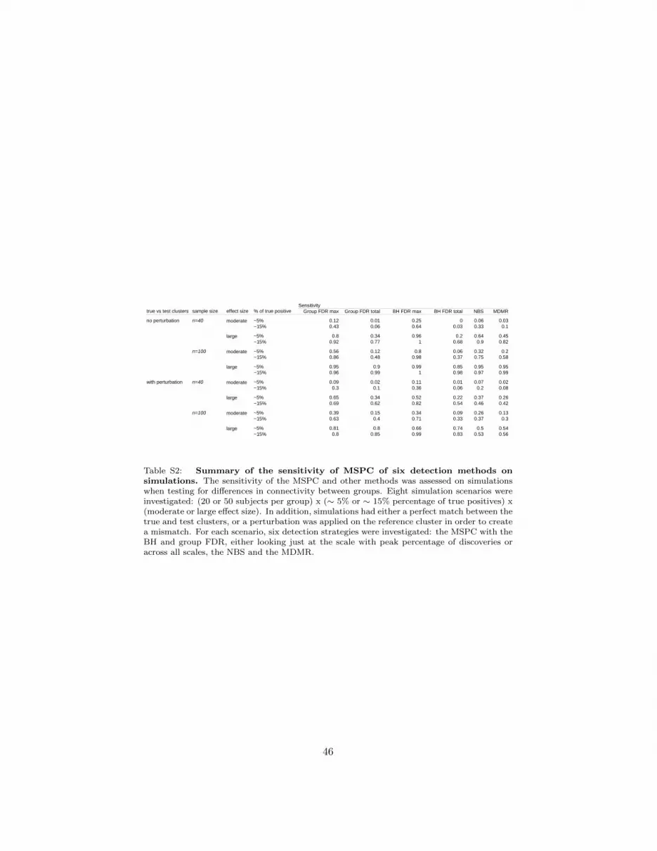
Sensitivitytrue vs test clusters sample size effect size % of true positive Group FDR max Group FDR total BH FDR max BH FDR total NBS MDMR

no perturbation n=40 moderate ~5% 0.12 0.01 0.25 0 0.06 0.03

~15% 0.43 0.06 0.64 0.03 0.33 0.1

large ~5% 0.8 0.34 0.96 0.2 0.64 0.45

~15% 0.92 0.77 1 0.68 0.9 0.82

n=100 moderate ~5% 0.56 0.12 0.8 0.06 0.32 0.2

~15% 0.86 0.48 0.98 0.37 0.75 0.58

large ~5% 0.95 0.9 0.99 0.85 0.95 0.95

~15% 0.96 0.99 1 0.98 0.97 0.99

with perturbation n=40 moderate ~5% 0.09 0.02 0.11 0.01 0.07 0.02

~15% 0.3 0.1 0.36 0.06 0.2 0.08

large ~5% 0.65 0.34 0.52 0.22 0.37 0.26

~15% 0.69 0.62 0.82 0.54 0.46 0.42

n=100 moderate ~5% 0.39 0.15 0.34 0.09 0.26 0.13

~15% 0.63 0.4 0.71 0.33 0.37 0.3

large ~5% 0.81 0.8 0.66 0.74 0.5 0.54

~15% 0.8 0.85 0.99 0.83 0.53 0.56

Table S2: Summary of the sensitivity of MSPC of six detection methods onsimulations. The sensitivity of the MSPC and other methods was assessed on simulationswhen testing for differences in connectivity between groups. Eight simulation scenarios wereinvestigated: (20 or 50 subjects per group) x (∼ 5% or ∼ 15% percentage of true positives) x(moderate or large effect size). In addition, simulations had either a perfect match between thetrue and test clusters, or a perturbation was applied on the reference cluster in order to createa mismatch. For each scenario, six detection strategies were investigated: the MSPC with theBH and group FDR, either looking just at the scale with peak percentage of discoveries oracross all scales, the NBS and the MDMR.

46