Embed Size (px)
Citation preview
arX
iv:0
708.
0224
v3 [
mat
h.ST
] 1
Apr
200
8
The Annals of Applied Probability
2008, Vol. 18, No. 2, 552–590DOI: 10.1214/07-AAP463c© Institute of Mathematical Statistics, 2008
MULTISOURCE BAYESIAN SEQUENTIAL CHANGE DETECTION
By Savas Dayanik,1 H. Vincent Poor2 and Semih O. Sezer2
Princeton University, Princeton University and University of Michigan
Suppose that local characteristics of several independent com-pound Poisson and Wiener processes change suddenly and simulta-neously at some unobservable disorder time. The problem is to detectthe disorder time as quickly as possible after it happens and minimizethe rate of false alarms at the same time. These problems arise, forexample, from managing product quality in manufacturing systemsand preventing the spread of infectious diseases. The promptness andaccuracy of detection rules improve greatly if multiple independentinformation sources are available. Earlier work on sequential changedetection in continuous time does not provide optimal rules for situa-tions in which several marked count data and continuously changingsignals are simultaneously observable. In this paper, optimal Bayesiansequential detection rules are developed for such problems when themarked count data is in the form of independent compound Pois-son processes, and the continuously changing signals form a multi-dimensional Wiener process. An auxiliary optimal stopping problemfor a jump-diffusion process is solved by transforming it first into asequence of optimal stopping problems for a pure diffusion by meansof a jump operator. This method is new and can be very useful inother applications as well, because it allows the use of the powerfuloptimal stopping theory for diffusions.
1. Introduction. Suppose that at some unobservable disorder time Θ,the local characteristics of several independent compound Poisson and Wienerprocesses undergo a sudden and simultaneous change. More precisely, the
Received November 2006; revised July 2007.1Supported in part by the Air Force Office of Scientific Research, Grant AFOSR-
FA9550-06-1-0496, and by the U.S. Department of Homeland Security through the Centerfor Dynamic Data Analysis for Homeland Security administered through ONR GrantN00014-07-1-0150 to Rutgers University.
2Supported by the U.S. Army Pantheon Program.AMS 2000 subject classifications. Primary 62L10; secondary 62L15, 62C10, 60G40.Key words and phrases. Sequential change detection, jump-diffusion processes, optimal
stopping.
This is an electronic reprint of the original article published by theInstitute of Mathematical Statistics in The Annals of Applied Probability,2008, Vol. 18, No. 2, 552–590. This reprint differs from the original in paginationand typographic detail.
1
2 S. DAYANIK, H. V. POOR AND S. O. SEZER
pairs (λ(i)0 , ν
(i)0 ), 1 ≤ i ≤m, consisting of the arrival rate and mark distri-
bution of m compound Poisson processes (T(i)n ,Z
(i)n )n≥1, 1 ≤ i≤m, become
(λ(i)1 , ν
(i)1 ), 1 ≤ i ≤m, and d Wiener processes W
(j)t , 1 ≤ j ≤ d gain drifts
µ(j), 1≤ j ≤ d at time Θ.We assume that Θ is a random variable with the zero-modified exponential
distribution
PΘ = 0 = π and PΘ> t= (1− π)e−λt, t≥ 0,(1.1)
and (λ(i)0 , ν
(i)0 )1≤i≤m, (λ
(i)1 , ν
(i)1 )1≤i≤m, (µ(j))1≤j≤d, π, and λ are known. The
objective is to detect the disorder time Θ as soon as possible after disorder
happens by using the observations of (T(i)n ,Z
(i)n )n≥1, 1 ≤ i≤m, and
X(j)t =X
(j)0 + µ(j)(t−Θ)+ +W
(j)t , t≥ 0,1≤ j ≤ d.
More precisely, if F = Ftt≥0 denotes the observation filtration, then wewould like to find, if it exists, an F-stopping time τ whose Bayes risk
Rτ (π) , Pτ <Θ+ cE(τ −Θ)+, 0 ≤ π < 1(1.2)
is the smallest for any given constant cost parameter c > 0 and calculate itsBayes risk. If such a stopping time exists, then it provides the best trade-offbetween false alarm frequency Pτ <Θ and expected detection delay costcE(τ −Θ)+.
Important applications of this problem are the quickest detection of man-ufacturing defects during product quality assurance, online fault detectionand identification for condition-based equipment maintenance, prompt de-tection of shifts in the riskiness of various financial instruments, early detec-tion of the onset of an epidemic to protect public health, quickest detectionof a threat to homeland security, and online detection of unauthorized accessto privileged resources in the fight against fraud. In many of those applica-tions, a range of data, changing over time either continuously or by jumps orboth, are collected from multiple sources/sensors in order to detect a suddenunobserved change as quickly as possible after it happens, and the problemscan be modeled as the quickest detection of a change in the local character-istics of several Wiener and compound Poisson processes. For example, incondition-based maintenance, an equipment is monitored continuously by aweb of sensors for both continuously-changing data (such as oil level, tem-perature, pressure) and marked count data (e.g., number, size and type ofwear particles in the oil); see Byington and Garga [6]. For the assessment offinancial risks of an electricity delivery contract, the spot price of electricityis sometimes modeled by a jump-diffusion process; see, for example, Weron,Bierbrauer and Truck [18] and Cartea and Figueroa [7].
In the past, the Bayesian sequential change-detection problems have beenstudied for Wiener processes by Shiryaev [17, Chapter 4] and for Poisson
MULTISOURCE BAYESIAN SEQUENTIAL CHANGE DETECTION 3
processes by Peskir and Shiryaev [14, 15], Gapeev [10], Bayraktar, Dayanikand Karatzas [2, 3] and Dayanik and Sezer [9], but have never been con-sidered for the combination of Wiener and Poisson processes. Clearly, anunobserved change can be detected more accurately if there are multipleindependent sources of information about the disorder time. If all of theinformation sources consist of exclusively either Wiener or Poisson processobservations, then the problem can be solved by applying the results ofShiryaev ([17], Chapter 4) in the Wiener case and Dayanik and Sezer [9]in the Poisson case to a weighted linear combination or superposition of allobservation processes; see Section 5. If Wiener and Poisson processes can beobserved simultaneously, then previous work does not provide an answer;the solution of the problem in this case is the current paper’s contribution.
We solve the problem in detail for m= d = 1, namely, when we observeexactly one Wiener and one Poisson process simultaneously; in Section 5we show the easy extension to multiple Wiener and multiple Poisson pro-cesses. Therefore, except in Section 5, we drop all of the superscripts in thesequel. We show that the first time τ[φ∞,∞) , inft≥ 0;Φt ≥ φ∞ that theconditional odds-ratio process
Φt ,PΘ ≤ t | Ft
PΘ> t | Ft, t≥ 0(1.3)
enters into some half-line [φ∞,∞) ⊂ R+ gives the smallest Bayes risk. Tocalculate the critical threshold φ∞ and the minimum Bayes risk, we reducethe original problem to an optimal stopping problem for the process Φ,which turns out to be a jump-diffusion jointly driven by the Wiener andpoint processes; see (2.8) for its dynamics. The value function of the optimalstopping problem satisfies certain variational inequalities, but they involvea difficult second order integro-differential equation.
We overcome the anticipated difficulties of directly solving the variationalinequalities by introducing a jump operator. By means of that operator, wetransform the original optimal stopping problem for the jump-diffusion pro-cess Φ into a sequence of optimal stopping problems for the diffusion partY of the process Φ between its successive jumps. This decomposition al-lows us to employ the powerful optimal stopping theory for one-dimensionaldiffusions to solve each sub-problem between jumps. The solutions of thosesub-problems are then combined by means of the jump operator, whose roleis basically to incorporate new information about disorder time arriving atjump times of the point process.
Solving optimal stopping problems for jump-diffusion processes by sepa-rating jump and diffusion parts with the help of a jump operator seems newand may prove to be useful in other applications, too. Our approach wasinspired by several personal conversations with Professor Erhan Cinlar on
4 S. DAYANIK, H. V. POOR AND S. O. SEZER
better ways to calculate the distributions of various functionals of jump pro-cesses. For Professor Cinlar’s interesting view on this more general matter,his recent lecture [8] in honor of the 2006 Blackwell–Tapia prize recipient,Professor William Massey, in the Blackwell–Tapia conference, held between3–4 November 2006, may be consulted.
In Section 2 we start our study by giving the precise description of thedetection problem and by modeling it under a reference probability mea-sure; the equivalent optimal stopping problem is derived, and the condi-tional odds-ratio process is examined. In Section 3 we introduce the jumpoperator. By using it repeatedly, we define “successive approximations” ofthe optimal stopping problem’s value function and identify their importantproperties. Their common structure is inherited in the limit by the valuefunction and is used at the end of Section 4 to describe an optimal alarmtime for the original detection problem. Each successive approximation isitself the value function of some optimal stopping problem, but now for adiffusion, and their explicit calculation is undertaken in Section 4. The suc-cessive approximations converge uniformly and at an exponential rate to theoriginal value function. Therefore, they are built into an efficient and accu-rate approximation algorithm, which is explained in Section 6 and illustratedon several examples. Examples suggest that observing Poisson and Wienerprocesses simultaneously can reduce the Bayes risk significantly. Baron andTartakovsky [1] have recently derived asymptotic expansions of both opti-mal critical threshold and minimum Bayes risk as the detection delay cost ctends to zero. In Section 6 we have compared in one of the examples thoseexpansions to the approximations of actual values calculated by our numer-ical algorithm. Finally, some of the lengthy calculations are deferred to theAppendix.
2. Problem description and model. Let (Ω,F ,P) be a probability spacehosting a marked point process (Tn,Zn);n≥ 1 whose (E,E)-valued marksZn, n≥ 1 arrive at times Tn, n≥ 1, a one-dimensional Wiener process W ,and a random variable Θ with distribution in (1.1). The counting measure
p((0, t]×A)) ,
∞∑
n=1
1(0,t]×A(Tn,Zn), t≥ 0,A ∈ E
generates the internal history Fp = Fpt≥0,
Fpt , σp((0, s]×A); 0 ≤ s≤ t,A ∈ E,
of the marked point process (Tn,Zn);n≥ 1. At time Θ, (i) the drift of theWiener process W changes from zero to µ, and (ii) the (P,Fp)-compensatorof the counting measure p(dt× dz) changes from λ0 dtν0(dz) to λ1 dtν1(dz).

MULTISOURCE BAYESIAN SEQUENTIAL CHANGE DETECTION 5
The process W is independent of Θ and (Tn,Zn)n≥1. Neither W nor Θ areobservable. Instead,
Xt =X0 + µ(t−Θ)+ +Wt, t≥ 0
and (Tn,Zn);n≥ 1 are observable. The observation filtration F = Ftt≥0
consists of the internal filtrations of X and (Tn,Zn)n≥1; that is,
Ft , FXt ∨Fp
t and FXt , σXs; 0≤ s≤ t for every t≥ 0.
If we enlarge F by the information about Θ and denote the enlarged filtrationby G = Gtt≥0,
Gt , Ft ∨ σΘ, t≥ 0,
then for every nonnegative G-predictable process H(t, z)t≥0 indexed byz ∈E, we have
E[∫
(0,∞)×EH(s, z)p(ds× dz)
]= E
[∫ ∞
0
∫
EH(s, z)λ(s, dz)ds
],
where E is the expectation with respect to P, and
λ(s, dz) , λ0ν0(dz)1[0,Θ)(s) + λ1ν1(dz)1[Θ,∞)(s), s≥ 0,
is the (P,G)-intensity kernel of the counting measure p(dt×dz); see Bremaud [5],Chapter VIII.
The rates 0 < λ,λ0, λ1 <∞, the drift µ ∈ R \ 0, and the probabilitymeasures ν0(·), ν1(·) on (E,E) are known. The objective is to find a stoppingtime τ of the observation filtration F with the smallest Bayes risk Rτ (π) in(1.2) for every π ∈ [0,1).
Model. Let (Ω,F ,P0) be a probability space hosting the following inde-pendent stochastic elements:
(i) a one-dimensional Wiener process X = Xt; t≥ 0,(ii) an (E,E)-valued marked point process (Tn,Zn);n≥ 1 whose count-
ing measure p(dt× dz) has (P0,Fp)-compensator λ0 dt ν0(dz),(iii) a random variable Θ with zero-modified exponential distribution
P0Θ = 0= π, P0Θ> t= (1− π)e−λt, t≥ 0.(2.1)
Suppose that ν1(·) is absolutely continuous with respect to ν0(·) and has theRadon–Nikodym derivative
f(z) ,dν1
dν0
∣∣∣∣E(z), z ∈E.(2.2)

6 S. DAYANIK, H. V. POOR AND S. O. SEZER
Define a new probability measure P on G∞ =∨
t≥0 Gt locally by means ofthe Radon–Nikodym derivative of its restriction to Gt,
dPdP0
∣∣∣∣Gt
= ξt , 1t<Θ + 1t≥ΘLt
LΘ, t≥ 0,
where
Lt , exp
µXt −
(µ2
2+ λ1 − λ0
)t
∏
n:0<Tn≤t
(λ1
λ0f(Zn)
), t≥ 0(2.3)
is a likelihood-ratio process with the dynamics L0 = 1, and
dLt = LtµdXt +Lt−
∫
E
(λ1
λ0f(z)− 1
)[p(dt× dz)− λ0 dt ν0(dz)],
(2.4)t≥ 0.
Under the probability measure P, the processes X and (Tn,Zn);n≥ 1 andthe random variable Θ jointly have exactly the same properties as in theabove description of the problem. Moreover, the minimum Bayes risk U(·)can be written as
U(π) , infτ∈F
Rτ (π) = 1− π+ c(1− π)V
(π
1− π
), π ∈ [0,1)(2.5)
in terms of the value function
V (φ) , infτ∈F
Eφ0
[∫ τ
0e−λtg(Φt)dt
], φ≥ 0, where g(φ) , φ−
λ
c(2.6)
of the optimal stopping problem above for the conditional odds-ratio processΦ in (1.3); see, for example, Bayraktar, Dayanik and Karatzas [2, Proof of
Proposition 2.1]. In (2.6), the expectation Eφ0 is taken with respect to P0
conditionally on Φ0 = φ≥ 0. Bayes formula gives for every t≥ 0 that
Φt =E0[ξt1Θ≤t | Ft]
E0[ξt1Θ>t | Ft]
=E0[(Lt/LΘ)1Θ≤t | Ft]
P0Θ> t(2.7)
= Φ0eλtLt +
∫ t
0λeλ(t−s)Lt
Lsds;
by the chain rule and dynamics in (2.4) of the likelihood-ratio process L wefind that
dΦt = (λ+ aΦt)dt+ ΦtµdXt(2.8)
+ Φt−
∫
E
(λ1
λ0f(z)− 1
)p(dt× dz), t≥ 0,
MULTISOURCE BAYESIAN SEQUENTIAL CHANGE DETECTION 7
where
a, λ− λ1 + λ0.
Let us define for every k ≥ 0 that T0 = T(k)0 ≡ 0, and
X(k)u ,XTk+u −XTk
, u≥ 0,
(T(k)ℓ ,Z
(k)ℓ ) , (Tk+ℓ − Tk,Zk+ℓ), ℓ≥ 1,
F(k)0 , σ(Tn,Zn),1 ≤ n≤ k ∨ σXv ,0≤ v ≤ Tk,
F (k)u , F
(k)0 ∨ σ(T
(k)ℓ ,Z
(k)ℓ ); 0< T
(k)ℓ ≤ u ∨ σX(k)
v ,0≤ v ≤ u,
u≥ 0,
L(k)u ,
LTk+u
LTk
= exp
µX(k)
u −
(µ2
2+ λ1 − λ0
)u
∏
ℓ : 0<T(k)ℓ
≤u
(λ1
λ0f(Z
(k)ℓ )
),
u≥ 0.
Then, as in (2.7), we have
Φt = ΦTkeλ(t−Tk)L
(k)t−Tk
(2.9)
+
∫ t−Tk
0λeλ(t−Tk−u)
L(k)t−Tk
L(k)u
du, t≥ Tk, k ≥ 0,
andX(k) = X(k)u , u≥ 0 is a (P0,F
(k)u u≥0)-Wiener process and P0-independent
of the marked point process (T(k)ℓ ,Z
(k)ℓ ); ℓ≥ 1, whose local (P0,F
(k)u u≥0)-
characteristics are (λ0, ν0(·)) for every k ≥ 0, sinceX(0) ≡X , (T(0)ℓ ,Z
(0)ℓ )ℓ≥1 ≡
(Tn,Zn)n≥1, and F(0)t t≥0 ≡ F. Thus, the first of two implications of (2.9)
is that for every Borel h :R+ 7→ R+ we have
Eφ0 [h(Φt)1t≥Tk | FTk
] = 1t≥TkEΦTk0 [h(Φv)]|v=t−Tk
, k ≥ 0,
which also follows from the strong Markov property of the process Φ appliedat the stopping time Tk of the filtration F. To state the second implication,let us introduce the processes
Y k,yu = yeλu exp
µX(k)
u −
(µ2
2+ λ1 − λ0
)u
+
∫ u
0λeλ(u−s) exp
µ(X(k)
u −X(k)s )(2.10)
8 S. DAYANIK, H. V. POOR AND S. O. SEZER
−
(µ2
2+ λ1 − λ0
)(u− s)
ds
for every u,k, y ≥ 0, which is (2.9) with u= t− Tk and y = ΦTkafter all of
future jumps are stripped away. Then for every k ≥ 0, the process Y k,yu , u≥
0 is a diffusion on R+ with the dynamics
dY k,yt = (λ+ aY k,y
t )dt+ µY k,yt dX
(k)t , t≥ 0 and
(2.11)Y k,y
0 = y ≥ 0, k ≥ 0.
Since X(0) ≡X , we shall drop the superscript 0 from Y 0,y and denote thatprocess by Y y. Because for every k ≥ 0, X(k) is a Wiener process, the pro-cesses Y k,y, k ≥ 0 and Y y have the same finite-dimensional distributions,and (2.9) implies that
Φt =
Yk,ΦTkt−Tk
, t ∈ [Tk, Tk+1),λ1
λ0f(Zk+1)Φt−, t= Tk+1.
(2.12)
The superscript k in Yk,ΦTkt−Tk
≡ Y k,yu |y=ΦTk
,u=t−Tkindicates that, when Y k,y
u ;u≥
0 is calculated according to (2.10) or (2.11), the increments of the driving
Wiener process X(k)u ;u≥ 0 are those of the process X after the kth arrival
time Tk of the marked point process.
3. Jump operator. Let us now go back to the optimal stopping prob-lem in (2.6). By (2.12), we have Φt = Y 0,Φ0
t ≡ Y Φ0t for 0 ≤ t < T1. This
suggests that every F-stopping time τ coincides on the event τ < T1with one of the stopping times of the process Y Φ0 . On the other hand,the process Φ regenerates at time T1 starting from its new position ΦT1 =
(λ1/λ0)f(Z1)YΦ0T1
. Moreover, on the event τ > T1, the expected total run-
ning cost Eφ0 [∫ T10 e−λtg(Y Φ0
t )dt] incurred until time T1 is sunken at time T1,and the smallest Bayes risk achievable in the future should be V (ΦT1) inde-pendent of the past. Hence, if we define an operator J acting on the boundedBorel functions w :R+ 7→ R according to
(Jw)(φ) , infτ∈FX
Eφ0
[∫ τ∧T1
0e−λtg(Φt)dt+ 1τ≥T1e
−λT1w(ΦT1)
],
(3.1)φ≥ 0,
then we expect that V (φ) = (JV )(φ) for every φ ≥ 0. In the next sectionwe prove that V (·) is indeed a fixed point of w 7→ Jw, and if we definevn :R+ 7→ R, n≥ 0, successively by
v0(·) ≡ 0 and vn+1(·) , (Jvn)(·), n≥ 0,(3.2)
MULTISOURCE BAYESIAN SEQUENTIAL CHANGE DETECTION 9
then vn(·)n≥1 converges to V (·) uniformly. This result will allow us todescribe not only an optimal strategy, but also a numerical algorithm thatapproximates the optimal strategy and the value function.
Note that the infimum in (3.1) is taken over stopping times of the Wienerprocess X . Since X and the marked point process (Tn,Zn)n≥1 are P0-independent, the decomposition in (2.12) and some algebra lead to
(Jw)(φ) = infτ∈FX
Eφ0
[∫ τ
0e−(λ+λ0)t(g+ λ0(Kw))(Y Φ0
t )dt
], φ≥ 0,(3.3)
where K is the operator acting on bounded Borel functions w : R+ 7→ Raccording to
(Kw)(φ) ,
∫
Ew
(λ1
λ0f(z)φ
)ν0(dz), φ≥ 0,(3.4)
where f(·) is the Radon–Nikodym derivative in (2.2). The identity in (3.3)shows that (Jw)(φ) is the value function of an optimal stopping problemfor the one-dimensional diffusion Y φ ≡ Y 0,φ, whose dynamics are given by(2.11). Standard variational arguments imply that, under suitable condi-tions, the function Jw(·) satisfies
0 = min−(Jw)(φ), [A0 − (λ+ λ0)](Jw)(φ) + g(φ) + λ0(Kw)(φ),(3.5)
φ≥ 0,
where for every twice continuously-differentiable function w :R+ 7→ R,
(A0w)(φ) ,µ2
2φ2w′′(φ) + (λ+ aφ)w′(φ)(3.6)
is the (P0,F)-infinitesimal generator of the process Y y , with drift and diffu-sion coefficients
µ(φ) , λ+ aφ and σ(φ) , µφ,(3.7)
respectively. If both w and Jw are replaced with V , then (3.5) becomes
0 = min−V (φ), (A− λ)V (φ) + g(φ), φ≥ 0,(3.8)
where for every twice continuously-differentiable function w :R+ 7→ R,
(Aw)(φ) , (A0w)(φ) + λ0[(K − 1)w](φ), φ≥ 0(3.9)
is the (P0,F)-infinitesimal generator of the process Φ in (1.3)–(2.8). Theidentity in (3.8) coincides with the variational inequalities satisfied by thefunction V (·) of (2.6) under suitable conditions. This coincidence is thesecond motivation for the introduction of the operator J in (3.1) and for theclaim that V = JV must hold.
10 S. DAYANIK, H. V. POOR AND S. O. SEZER
Reversing the arguments gives additional insight about the role of theoperator J . If one decides to attack first to the variational inequalities in(3.8) for V (·), then she realizes that solving integro-differential equation(A− λ)V + g = 0 is difficult. Substituting into (3.8) the decomposition in(3.9) of the operator A due to diffusion and jump parts gives
0 = min−V (φ), [A0 − (λ+ λ0)]V (φ) + g(φ) + λ0(KV )(φ), φ≥ 0.
Now [A0 − (λ+λ0)]V (φ)+ g(φ)+λ0(KV )(φ) = 0 is a nonhomogeneous sec-ond order ordinary differential equation (ODE) with the forcing function−g − λ(KV ). If one wants to take full advantage of the rich theory for thesolutions of second order ODEs, then she only needs to break the cycle byreplacing the unknown V in the forcing function with some known func-tion w and call by Jw the solution of the resulting variational inequalities,namely, (3.5). By repeatedly replacing w with Jw, one then hopes that Jnwconverges to V as n→ ∞. As the next remark shows, the jump operatorJ can be applied repeatedly to bounded functions, since Jw is boundedwhenever w is bounded.
Remark 3.1. For every bounded w :R+ 7→ R, the function Jw :R+ 7→R− is bounded, and
−
(λ
c+ λ0‖w
−‖
)1
λ+ λ0≤ (Jw)(·) ≤ 0,
where ‖w−‖ is the sup-norm of the negative part of w(·). If w is boundedand w(·) ≥ −1/c, then 0 ≥ (Jw)(·) ≥ −1/c. If w :R+ 7→ R is concave, thenso is Jw :R+ 7→ R−. The mapping w 7→ Jw on the collection of boundedfunctions is monotone.
Proof. Suppose that w(·) is bounded. Since τ ≡ 0 is an FX -stoppingtime, we have (Jw)(·) ≤ 0. Since (Kw)(·) ≥−‖w−‖ and g(Φt) = Φt−(λ/c) ≥−λ/c for every t≥ 0, we have
0 ≥ Jw(φ) ≥ infτ∈FX
Eφ0
∫ τ
0e−(λ+λ0)t
(−λ
c− λ0‖w
−‖
)dt
= −
(λ
c+ λ0‖w
−‖
)1
λ+ λ0.
If w(·) ≥−1/c, then ‖w−‖ ≤ 1/c and 0≥ (Jw)(·) ≥−1/c. Suppose that w(·)
is concave. The explicit form in (2.10) indicates that Y yt ≡ Y 0,y
t is an affine
function of Y y0 ≡ Y 0,y
0 = y. Since g(·) is affine and (Kw)(·) is concave, themapping y 7→ g(Y y
t ) + λ0(Kw)(Y yt ) is also concave. Therefore, the integral
in (3.3) and its expectation are concave for every FX-stopping time τ . Be-cause (Jw)(·) is the infimum of concave functions, it is also concave. Themonotonicity of w 7→ Jw is evident.
MULTISOURCE BAYESIAN SEQUENTIAL CHANGE DETECTION 11
Remark 3.2. For every φ≥ 0, we have Eφ0 [∫∞0 e−λtΦt dt] = ∞,
Eφ0
[∫ ∞
0e−(λ+λ0)tΦt dt
]=φ+ 1
λ0−
1
λ+ λ0,
Eφ0
[∫ ∞
0e−(λ+λ0)tY Φ0
t dt
]=
1
λ1
(φ+
1
λ+ λ0
).
Proof. The proof follows from (2.7), (2.10), Fubini’s theorem, and(P0,F)-martingale property of L= Lt; t≥ 0 after noting that
Eφ0Φt = (1 + φ)eλt − 1
and
Eφ0Y
Φ0t = φe(λ−λ1+λ0)t +
λ[e(λ−λ1+λ0)t − 1]
λ− λ1 + λ0.
Remark 3.3. The sequence vn(·)n≥0 in (3.2) is decreasing, and the
limit v∞(φ) , limn→∞ vn(φ) exists. The functions φ 7→ vn(φ), 0 ≤ n ≤ ∞,are concave, nondecreasing and bounded between −1/c and zero.
Proof. We have v1(φ) = (Jv0)(φ) ≤ 0 ≡ v0, since stopping immediatelyis always possible. Suppose now that vn ≤ vn−1 for some n≥ 1. Then vn+1 =Jvn ≤ Jvn−1 = vn by Remark 3.1, and vn(·)n≥1 is a decreasing sequence byinduction. Since v0 ≡ 0 is concave and bounded between 0 and −1/c, Remark3.1 and another induction imply that every vn(·), 1≤ n≤∞, is concave andbounded between −1/c and 0. Finally, every concave bounded function onR+ must be nondecreasing; otherwise, the negative right-derivative at somepoint does not increase on the right of that point, and the function eventuallydiverges to −∞.
Lemma 3.1. The function v∞(·) , limn→∞ vn(·) is the unique boundedsolution of the equation w(·) = (Jw)(·).
Proof. Since by Remark 3.3 vn(·)n≥0 is a decreasing sequence ofbounded functions, the dominated convergence theorem implies that
v∞(φ) = infn≥1
vn+1(φ)
= infn≥1
infτ∈FX
Eφ0
[∫ τ
0e−(λ+λ0)t[g(Y Φ0
t ) + λ0(Kvn)(Y Φ0t )]dt
]
= infτ∈FX
infn≥1
Eφ0
[∫ τ
0e−(λ+λ0)t[g(Y Φ0
t ) + λ0(Kvn)(Y Φ0t )]dt
]
= infτ∈FX
Eφ0
[∫ τ
0e−(λ+λ0)t
[g(Y Φ0
t ) + λ0
(K inf
n≥1vn
)(Y Φ0
t )
]dt
]
= (Jv∞)(φ).
12 S. DAYANIK, H. V. POOR AND S. O. SEZER
Let u1(·) and u2(·) be two bounded solutions of w = Jw. Fix any arbitraryφ ∈ R+ and ε > 0. Because (Ju1)(φ) is finite, there is some τ1 = τ1(φ) ∈ FX
such that
u1(φ) = (Ju1)(φ) ≥ Eφ0
[∫ τ1
0e−(λ+λ0)t(g+ λ0(Ku1))(Y
Φ0t )dt
]− ε.
Because Ku1 −Ku2 =K(u1 − u2)≤ ‖u1 − u2‖, we have
u2(φ)− u1(φ) ≤ Eφ0
[∫ τ1
0e−(λ+λ0)t(g+ λ0(Ku2))(Y
Φ0t )dt
]
−Eφ0
[∫ τ1
0e−(λ+λ0)t(g+ λ0(Ku1))(Y
Φ0t )dt
]+ ε
= Eφ0
[∫ τ1
0e−(λ+λ0)tλ0(K(u2 − u1))(Y
Φ0t )dt
]+ ε
≤ ‖u2 − u1‖
∫ ∞
0λ0e
−(λ+λ0)t + ε≤λ0
λ+ λ0‖u2 − u1‖+ ε.
Since ε is arbitrary, this implies u2(φ) − u1(φ) ≤ [λ0/(λ + λ0)]‖u2 − u1‖.Interchanging u1 and u2 gives u1(φ) − u2(φ) ≤ [λ0/(λ+ λ0)]‖u2 − u1‖, andthe last two inequalities yield |u1(φ) − u2(φ)| ≤ [λ0/(λ+ λ0)]‖u1 − u2‖ forevery φ ≥ 0. Therefore, ‖u1 − u2‖ ≤ [λ0/(λ + λ0)]‖u1 − u2‖, and because0 < λ0/(λ + λ0) < 1, this is possible if and only if ‖u1 − u2‖ = 0; hence,u1 ≡ u2. Therefore, w = v∞ is the unique bounded solution of w = Jw.
Lemma 3.2. The sequence vn(φ)n≥0 converges to v∞(φ) as n→ ∞uniformly in φ≥ 0. More precisely, we have
v∞(φ) ≤ vn(φ) ≤ v∞(φ) +1
c
(λ0
λ+ λ0
)n
∀n≥ 0,∀φ≥ 0.(3.10)
Proof. The first inequality follows from Remark 3.3. We shall provethe second inequality by induction on n ≥ 0. This inequality is immediatefor n = 0 since −1/c ≤ v∞(·) ≤ 0. Suppose that it is true for some n ≥ 0.Then induction hypothesis implies that
vn+1(φ) = infτ∈FX
Eφ0
[∫ τ
0e−(λ+λ0)t[g(Y Φ0
t ) + λ0(Kvn)(Y Φ0t )]dt
]
≤ infτ∈FX
Eφ0
[∫ τ
0e−(λ+λ0)t
[g(Y Φ0
t )
+ λ0(Kv∞)(Y Φ0t ) +
λ0
c
(λ0
λ+ λ0
)n]dt
]
≤ infτ∈FX
(Eφ
0
[∫ τ
0e−(λ+λ0)t[g(Y Φ0
t ) + λ0(Kv∞)(Y Φ0t )]dt
]
MULTISOURCE BAYESIAN SEQUENTIAL CHANGE DETECTION 13
+
∫ ∞
0e−(λ+λ0)tλ0
c
(λ0
λ+ λ0
)n
dt
)
= (Jv∞)(φ) +
∫ ∞
0e−(λ+λ0)tλ0
c
(λ0
λ+ λ0
)n
dt
= v∞(φ) +1
c
(λ0
λ+ λ0
)n+1
,
since v∞ = Jv∞ by Lemma 3.1.
4. Solution of the optimal stopping problem. The main results of thissection are that v∞(·) coincides with the value function V (·) of the optimalstopping problem in (2.6), and that the first entrance time of the process Φof (1.3) into half line [φ∞,∞) for some constant φ∞ > 0 is optimal for (2.6).We also describe ε-optimal F-stopping times for (2.6) and summarize thecalculation of its value function V (·).
We shall first find an explicit solution of the optimal stopping problemin (3.3). The second order ODE (λ + λ0)h(·) = A0h(·) on (0,∞) admitstwo twice-continuously differentiable solutions, ψ(·) and η(·), unique up tomultiplication by a positive constant, such that they are increasing and de-creasing, respectively. For this and other facts below about one-dimensionaldiffusions, see, for example, Ito and McKean [11], Borodin and Salminen [4]Karlin and Taylor [12], Chapter 15.
The explicit form in (2.10) of the process Y y ≡ Y 0,y suggests that theprocess may start at y = 0, but then moves instantaneously into (0,∞)without ever coming back to 0. It can neither start at nor reach from insideto the right boundary located at ∞. Indeed, calculated in terms of the scale
function S(·) and speed measure M(·), defined respectively by
S(dy) , exp
−2
∫ y
c
µ(u)
σ2(u)du
dy, y > 0 and
(4.1)
M(dy) ,dy
σ2(y)S′(y), y > 0
for some arbitrary but fixed constant c > 0, Feller’s boundary tests give
S(0+) = −∞ and
∫ c
0
∫ z
0M(dy)S(dz)<∞,(4.2)
∫ ∞
c
∫ ∞
zS(dy)M(dz) = ∞ and
∫ ∞
c
∫ ∞
zM(dy)S(dz) =∞,(4.3)
as shown in Appendix A.1, and according to Table 6.2 of Karlin and Taylor([12], page 234), we conclude that y = 0 and y = ∞ are entry-not-exit and
14 S. DAYANIK, H. V. POOR AND S. O. SEZER
natural boundaries of the state-space [0,∞), respectively. Therefore, ψ(·)and η(·) satisfy boundary conditions
0<ψ(0+) <∞, η(0+) = ∞,
limy→0+
ψ′(y)
S′(y)= 0, lim
y→0+
η′(y)
S′(y)>−∞,
(4.4)ψ(∞) = ∞, η(∞) = 0,
limy→∞
ψ′(y)
S′(y)= ∞, lim
y→∞
η′(y)
S′(y)= 0.
We shall set ψ(0) = ψ(0+) and η(0) = η(0+). The Wronskian B(·) of ψ(·)and η(·) equals
B(y) , ψ′(y)η(y)− ψ(y)η′(y) =B(c)S′(y), y > 0,(4.5)
where the constant c and that in the scale function S(·) in (4.1) are the same.The second equality is obtained by solving the differential equation A0B = 0,which follows from the equations A0ψ = (λ+λ0)ψ and A0η = (λ+λ0)η afterfirst multiplying these respectively with η and ψ, and then, subtracting fromeach other. Observe that
B(c) =B(y)
S′(y)=ψ′(y)
S′(y)η(y)−ψ(y)
η′(y)
S′(y), y ≥ 0
is constant. Dividing (4.5) by −ψ2(y) and then integrating the equation give
η(y)
ψ(y)=η(c)
ψ(c)−
∫ y
cB(c)
S′(z)
ψ2(z)dz, y ≥ 0.(4.6)
This identity implies that the constant B(c) must be strictly positive, sincethe functions ψ(·) and η(·) are linearly independent [note that their nontriv-ial linear combinations cannot vanish at 0 because of (4.4)].
For every Borel subset D of R+, denote the first entrance time of Y y
and Φ to D by
τD , inft≥ 0 :Y yt ∈D and τD , inft≥ 0 :Φt ∈D,(4.7)
respectively. If D = z for some z ∈ R+, we will use τz(τz) instead ofτz(τz). Then
Ey0[e
−(λ+λ0)τz ] =ψ(y)
ψ(z)· 1(0,z](y) +
η(y)
η(z)· 1(z,∞)(y)
(4.8)∀z > 0,∀y ≥ 0,
MULTISOURCE BAYESIAN SEQUENTIAL CHANGE DETECTION 15
which can be obtained by applying the optional sampling theorem to the(P0,F)-martingales e−(λ+λ0)tψ(Y y
t ); t≥ 0 and e−(λ+λ0)tη(Y yt ); t≥ 0. For
every fixed real number z > 0, (4.8) implies that
ψ(y) =
ψ(z)Ey0[e
−(λ+λ0)τz ], 0≤ y ≤ zψ(z)
Ez[e−(λ+λ0)τy ], y > z
,
η(y) =
η(z)
Ez[e−(λ+λ0)τy ], 0≤ y ≤ z
η(z)Ey0[e
−(λ+λ0)τz ], y > z
,
and suggests a way to calculate functions ψ(·) and η(·) up to a multiplicationby a constant on a lattice inside (0, z] by using simulation methods. Let usset ψ(z) = η(z) = 1 (or to any arbitrary positive constant), and suppose thatthe grid size h > 0 and some integer N are chosen such that Nh = z. Letzn = nh, n= 0, . . . ,N . Then (4.8) implies that one can calculate
ψ(zn) = ψ(zn+1)Ezn0 [exp−(λ+ λ0)τzn+1], n=N − 1, . . . ,1,0,
(4.9)η(zn) = η(zn+1)/E
zn+1
0 [exp−(λ+ λ0)τzn], n=N − 1, . . . ,1,0,
backward from zN ≡ z by evaluating expectations using simulation.The functions ψ(·) and η(·) can also be characterized as power series
or Kummer’s functions; see Polyanin and Zaitsev ([16], pages 221, 225, 229,Equation 134 in Section 2.1.2). Those functions take simple forms for certainvalues of λ, λ1, λ0 and µ. For example, if a= λ+ λ0 − λ1 ≥ 0 and
(n− 1)λ= (n− 2)[(λ+ λ0) + 12µ
2(n− 1)]
for some n ∈ N and n > 2,
then ψ(·) is a polynomial of the form ψ(φ) =∑n−1
k=0 βkφk, where β0 = 1,
β1 = (λ+ λ0)/λ, and
βk =
[(λ+ λ0)− (k− 1)a− 0.5µ2(k− 1)(k − 2)
kλ
]βk−1 for k ≥ 2,
and η(·) can be obtained in terms of ψ(·) from (4.6). However, we makeno such assumptions about the parameters and work with general ψ(·) andη(·).
Lemma 4.1. Every moment of the first entrance times τ[r,∞) and τ[r,∞)
of the processes Y Φ0 and Φ, respectively, into half line [r,∞) is uniformly
bounded for every r≥ 0.

16 S. DAYANIK, H. V. POOR AND S. O. SEZER
Proof. Fix r > 0 and 0 ≤ φ < r; the cases r = 0 or φ ≥ r are obvious.Since the sample paths of Y Φ0 are continuous, we have τ[r,∞) ≡ τr, and (4.8)implies that
Pφ0τr <T1 = Eφ
0e−λ0τr ≥ Eφ
0e−(λ+λ0)τr
(4.10)
=ψ(φ)
ψ(r)≥ψ(0)
ψ(r)∈ (0,1), φ ∈ [0, r).
Let α,√
1− (ψ(0)/ψ(r)) < 1. The strong (P0,F)-Markov property of Y Φ0
implies that
Pφ0τr > Tn
= Pφ0τr > Tn−1, τr >Tn
(4.11)
= Eφ0 [1τr>Tn−1(1τr>T1 θTn−1)] = Eφ
0 [1τr>Tn−1PY
Φ0Tn−1
0 τr > T1]
≤ Pφ0τr > Tn−1
[1−
ψ(0)
ψ(r)
]≤
[1−
ψ(0)
ψ(r)
]n= α2n
by induction on n, because Y Φ0Tn
∈ [0, r) on τr > Tn for every n ≥ 1. Forevery k ≥ 1,
Eφ0τ
kr ≤ Eφ
0
∞∑
n=0
T kn+11Tn<τr≤Tn+1
≤∞∑
n=0
Eφ0T
kn+11τr>Tn ≤
∞∑
n=0
√Eφ
0T2kn+1P
φ0τr > Tn(4.12)
≤ λ−k0
∞∑
n=0
√(n+ 2k)!
n!αn ≤ λ−k
0
∞∑
n=0
(n+ 2k)kαn <∞
independent of the initial state φ≥ 0. Since Pφ0τ[r,∞) <T1= Pφ
0τr <T1 ≥ψ(0)/ψ(r) for every φ ∈ [0, r) by (4.10), both (4.11) and (4.12) remain correct
if we replace τr and Y Φ0Tn−1 with τ[r,∞) and ΦTn−1 , respectively.
Assumption. In the remainder, suppose that w :R+ 7→ R is an arbitrarybut fixed bounded and continuous function, and 0< l < r <∞.
Define
(Hl,rw)(φ) , Eφ0
[∫ τ[0,l]∧τ[r,∞)
0e−(λ+λ0)t(g + λ0(Kw))(Y Φ0
t )dt
],
(4.13)φ≥ 0,
MULTISOURCE BAYESIAN SEQUENTIAL CHANGE DETECTION 17
(Hrw)(φ) , Eφ0
[∫ τ[r,∞)
0e−(λ+λ0)t(g+ λ0(Kw))(Y Φ0
t )dt
],
φ≥ 0.
We shall first derive the analytical expression below in (4.16) for (Hrw)(·).Since the left boundary at 0 is entrance-not-exit for the process Y Φ0 , thatboundary is inaccessible from the interior (0,∞) of the state-space, and
limlց0 τl ∧ τr = τr Pφ0 -a.s. for every φ > 0. Because (Kw)(·), is bounded,
and g(φ) = φ− (λ/c), φ ≥ 0, is bounded from below, Remark 3.2 and themonotone convergence theorem imply that
(Hrw)(φ) = limlց0
(Hl,rw)(φ), φ > 0 and
(4.14)(Hrw)(0) = lim
φց0limlց0
(Hl,rw)(φ)
follows from the strong Markov property; see Appendix A.2 for the details.By means of the first equality, the second becomes (Hrw)(0) = limφց0(Hrw)(φ),that is, the function φ 7→ (Hrw)(φ) is continuous at φ= 0. In terms of thefundamental solutions
ψl(y) , ψ(y)−ψ(l)
η(l)η(y) and ηr(y) , η(y)−
η(r)
ψ(r)ψ(y)
of the equation [A0 − (λ+ λ0)]h(y) = 0, l < y < r with boundary conditionsh(l) = 0 and h(r) = 0, respectively, and their Wronskian
Bl,r(y) , ψ′l(y)ηr(y)−ψl(y)η
′r(y) =B(y)
[1−
ψ(l)
η(l)
η(r)
ψ(r)
],
we find, as shown in Appendix A.3, that
(Hl,rw)(φ)
= ψl(φ)
∫ r
φ
2ηr(z)
σ2(z)Bl,r(z)(g+ λ0(Kw))(z)dz(4.15)
+ ηr(φ)
∫ φ
l
2ψl(z)
σ2(z)Bl,r(z)(g+ λ0(Kw))(z)dz, 0< l≤ φ≤ r,
where σ(z) = µz is the diffusion coefficient of the process Y Φ0 in (3.7). Aftertaking the limit as lց 0, the monotone convergence and boundary condi-tions in (4.4) give
(Hrw)(φ)
= ψ(φ)
∫ r
φ
2η(z)
σ2(z)B(z)(g + λ0(Kw))(z)dz
(4.16)

18 S. DAYANIK, H. V. POOR AND S. O. SEZER
+ η(φ)
∫ φ
0
2ψ(z)
σ2(z)B(z)(g+ λ0(Kw))(z)dz
− ψ(φ)η(r)
ψ(r)
∫ r
0
2ψ(z)
σ2(z)B(z)(g + λ0(Kw))(z)dz, 0< φ≤ r,
and (Hrw)(0) = limφց0(Hrw)(φ) by (4.14). Finally, (Hrw)(φ) = 0 for ev-ery φ > r by the definition in (4.13). For every r > 0, the function φ 7→(Hrw)(φ) is continuous on [0,∞); it is twice continuously-differentiable on(0,∞), possibly except at φ= r. Direct calculation shows that (Hrw)(r) =(Hrw)′(r+) = 0 and
(Hrw)′(r−) =
[η′(r)−
η(r)
ψ(r)ψ′(r)
]∫ r
0
2ψ(z)
σ2(z)B(z)(g+ λ0(Kw))(z)dz.
Since z 7→ η(z)− [η(r)/ψ(r)]ψ(z) is strictly decreasing,
(Hrw)′(r−) = 0(4.17)
⇐⇒ (Gw)(r) ,
∫ r
0
2ψ(z)
σ2(z)B(z)(g+ λ0(Kw))(z)dz = 0.
Lemma 4.2. If w(·) is nondecreasing and nonpositive, then (Gw)(φ) = 0has exactly one strictly positive solution φ= φ[w]. If we denote by φℓ[w] the
unique solution φ of (g+λ0(Kw))(φ) = 0 and define φr[w] , φ[−‖w‖], then
φℓ[w] ≤ φ[w] ≤ φr[w]. Moreover, (Gw)(φ) is strictly negative for φ ∈ (0, φ[w])and strictly positive for φ ∈ (φ[w],∞).
Proof. Since φ 7→ (g+λ0(Kw))(φ) = φ−(λ/c)+λ0(Kw)(φ) is negativeat φ= 0 and increases unboundedly as φ→∞, it has unique root at someφ= φℓ[w]> 0. Therefore,
(Gw)′(φ) =2ψ(φ)
σ2(φ)B(φ)(g+ λ0(Kw))(φ)
changes its sign exactly once at φ = φℓ[w], from negative to positive, and
the continuously differentiable function (Gw)(φ) =∫ φ0 (Gw)′(z)dz is strictly
negative on (0, φℓ[w]]. Since (Gw)(φ) is increasing at every φ ∈ [φℓ[w],∞),the proof will be complete if we show that limφ→∞(Gw)′(φ) = ∞. Sinceσ2(φ) = µ2φ2, and
S′(φ) = exp
−2
∫ φ
c
λ+ au
µ2u2du
= const.× exp
2λ
µ2φ
φ−2a/µ2
,
we have
limφ→∞
(Gw)′(φ) = limφ→∞
2ψ(φ)φ
σ2(φ)B(φ)= const.× lim
φ→∞
ψ(φ)
φ1−(2a/µ2),

MULTISOURCE BAYESIAN SEQUENTIAL CHANGE DETECTION 19
which equals ∞ if 1− (2a/µ2)≤ 0. Otherwise, the L’Hospital rule and (4.4)give
limφ→∞
(Gw)′(φ) = const.× limφ→∞
ψ′(φ)
φ−2a/µ2
= const.× limφ→∞
ψ′(φ)
S′(φ)exp
−
2λ
µ2φ
= ∞.
Finally, constant function w0(φ) ,−‖w‖, φ≥ 0, is also bounded continuousnondecreasing and nonpositive. By the first part of the lemma, (Gw0)(φ) = 0has exactly one strictly positive solution φ = φ[w0] =: φr[w]. Since w(·) ≥−‖w‖, we have (Gw)(·) ≥ (Gw0)(·), and therefore, φ[w] ≤ φr[w].
Lemma 4.2 and (4.17) show that in the family of functions Hr(φ), φ ∈R+r>0 there is exactly one function that “fits smoothly at φ = r” andis therefore continuously differentiable on the whole φ ∈ (0,∞), and thatfunction corresponds to the unique strictly positive solution r = φ[w] of theequation (Gw)(r) = 0 in (4.17).
Lemma 4.3. Suppose that w(·) is nondecreasing and nonpositive. Then
the function
(Hw)(φ) , (Hφ[w]w)(φ), φ≥ 0,(4.18)
equals zero for φ > φ[w] and
ψ(φ)
∫ φ[w]
φ
2η(z)
σ2(z)B(z)(g+ λ0(Kw))(z)dz
+ η(φ)
∫ φ
0
2ψ(z)
σ2(z)B(z)(g + λ0(Kw))(z)dz
for 0< φ≤ φ[w]. It is bounded continuous on [0,∞), continuously differen-
tiable on (0,∞) and twice continuously differentiable on (0,∞) \ φ[w]. It
satisfies (Hw)(φ[w]) = (Hw)′(φ[w]) = 0 and the variational inequalities
(Hw)(φ)< 0
[A0 − (λ+ λ0))](Hw)(φ) + (g+ λ0(Kw))(φ) = 0
,(4.19)
φ ∈ (0, φ[w]),
(Hw)(φ) = 0[A0 − (λ+ λ0)](Hw)(φ) + (g+ λ0(Kw))(φ)> 0
,(4.20)
φ ∈ (φ[w],∞).
20 S. DAYANIK, H. V. POOR AND S. O. SEZER
Proof. The explicit form of (Hw)(·) follows from (4.16) after notic-ing that the third term equals −ψ(φ)[η(r)/ψ(r)](Gw)(r) and vanishes forr = φ[w] by definition. Since (Hrw)(·) is continuous on [0,∞) and twicecontinuously differentiable on (0,∞) \r and (Hrw)(r) = 0 for every r > 0,so is (Hw)(·) ≡ (Hφ[w]w)(·) and (Hw)(φ[w]) = 0. It is also continuouslydifferentiable at φ = φ[w] since (Hw)′(φ[w]−) ≡ (Hφ[w]w)′(φ[w]−) = 0 =(Hw)′(φ[w]+) by (4.17) and Lemma 4.2. Because the function (Hw)(·) iscontinuous everywhere and vanishes outside the closed and bounded inter-val [0, φ[w]], it is bounded everywhere. Direct calculation gives immediatelythe equalities in (4.19) and (4.20). The inequality in (4.20) follows fromsubstitution of (Hw)(φ) = 0 for φ > φ[w] and that (g + λ0(Kw))(φ) > 0 forφ > φ[w] > φℓ[w] by Lemma 4.2, where φℓ[w] is the unique root of nonde-creasing function φ 7→ (g + λ0(Kw))(φ). For the proof of the inequality in(4.19), note that (Hw)′(φ) equals
ψ′(φ)
∫ φ[w]
φ
2η(z)
σ2(z)B(z)(g+ λ0(Kw))(z)dz
+ η′(φ)
∫ φ
0
2ψ(z)
σ2(z)B(z)(g+ λ0(Kw))(z)dz
for 0 < φ ≤ φ[w]. The second term is positive since (i) η(·) is strictly de-creasing, and (ii) (Gw)(φ) in (4.17) is strictly negative for φ ∈ (0, φ[w]) byLemma 4.2. The first term is strictly negative for φ ∈ (φℓ[w], φ[w]), since (i)ψ(·) is strictly increasing, and (ii) (g+λ0(Kw))(z)> 0 for z > φℓ[w]. There-fore, (Hw)′(φ)> 0 for φ ∈ [φℓ[w], φ[w]). Because continuously differentiable(Hw)(φ) vanishes at φ= φ[w], we have
(Hw)(φ) = −
∫ φ[w]
φ(Hw)′(z)dz < 0 for every φℓ[w] ≤ φ < φ[w].
Finally, for every 0 ≤ φ≤ φℓ[w], the strong Markov property of the processY Φ0 applied at the F-stopping time τφℓ[w] gives
(Hw)(φ) = Eφ0
[∫ τφℓ[w]
0e−(λ+λ0)t(g+ λ0(Kw))(Y Φ0
t )dt
]
+ Eφ0 [e−(λ+λ0)τφℓ[w] ](Hw)(φℓ[w]),
and both terms are strictly negative, since (g + λ0(Kw))(φ) < 0 for φ ∈[0, φℓ[w]) and (Hw)(φℓ[w])< 0 by the previous displayed equation.
Proposition 4.1. Suppose w(·) is nondecreasing and nonpositive. Then
(Jw)(φ) = (Hw)(φ) ≡ Eφ0
[∫ τ[φ[w],∞)
0e−(λ+λ0)t(g + λ0(Kw))(Y Φ0
t )dt
],
φ≥ 0.
MULTISOURCE BAYESIAN SEQUENTIAL CHANGE DETECTION 21
Proof. For every 0< l < φ< r and FX -stopping time τ , Ito’s rule yields
e−(λ+λ0)(τ∧τl∧τr)(Hw)(Y Φ0τ∧τl∧τr
)
= (Hw)(φ)
+
∫ τ∧τl∧τr
0e−(λ+λ0)tµY Φ0
t (Hw)′(Y Φ0t )dXt
+
∫ τ∧τl∧τr
0e−(λ+λ0)t[A0 − (λ+ λ0)](Hw)(Y Φ0
t )dt.
Since (Hw)′(·) is continuous by Lemma 4.3, it is bounded on [l, r]. Takingexpectations gives
Eφ0 [e−(λ+λ0)(τ∧τl∧τr)(Hw)(Y Φ0
τ∧τl∧τr)]
= (Hw)(φ) + Eφ0
[∫ τ∧τl∧τr
0e−(λ+λ0)t[A0 − (λ+ λ0)](Hw)(Y Φ0
t )dt
]
≥ (Hw)(φ) −Eφ0
[∫ τ∧τl∧τr
0e−(λ+λ0)t(g+ λ0(Kw))(Y Φ0
t )dt
],
because (Hw)(·) satisfies the variational inequalities in (4.19) and (4.20)by Lemma 4.3. Since (Hw)(·) ≡ (Hφ[w])(·) is nonpositive continuous andbounded by the same lemma, letting l→ 0, r→∞ and the dominated con-vergence theorem (see Remark 3.2) give
0 ≥ Eφ0 [e−(λ+λ0)τ (Hw)(Y Φ0
τ )]
≥ (Hw)(φ)− Eφ0
[∫ τ
0e−(λ+λ0)t(g+ λ0(Kw))(Y Φ0
t )dt
].
Thus, we have
Eφ0
[∫ τ
0e−(λ+λ0)t(g+ λ0(Kw))(Y Φ0
t )dt
]≥ (Hw)(φ).
Taking infimum over FX-stopping times τ gives (Jw)(φ) ≥ (Hw)(φ), φ > 0.If we replace every τ above with the first entrance time τ[φ[w],∞) of the
process Y Φ0 into [φ[w],∞), then Pφ0τ <∞ = 1 and the variational in-
equalities in (4.19) and (4.20) ensure that every inequality above becomesan equality. This proves (Jw)(φ) = (Hw)(φ) for every φ > 0. Finally, thatequality extends to φ= 0 by the continuity of (Jw)(·) and (Hw)(·).
Corollary 4.1. Recall the sequence vn(·)n≥0 of functions defined
successively by (3.2) and its pointwise limit v∞(·), all of which are bounded,
concave, nonpositive and nondecreasing by Remark 3.3. Then every vn(·),
22 S. DAYANIK, H. V. POOR AND S. O. SEZER
0 ≤ n ≤ ∞, is continuous on [0,∞) continuously differentiable on (0,∞),and twice continuously differentiable on (0,∞) \ φn, where
φn+1 , φ[vn], 0≤ n<∞ and φ∞ , φ[v∞](4.21)
are the unique strictly positive roots of the functions (Gvn)(·), 0 ≤ n≤∞,
as in (4.17). Moreover,
vn+1(·) = (Hvn)(·), 0 ≤ n <∞, and v∞(·) = (Hv∞)(·).(4.22)
For every n≥ 0, we have vn(φn) = v′n(φn) = 0, and vn+1(·) and vn(·) satisfy
vn+1(φ)< 0[A0 − (λ+ λ0)]vn+1(φ) + (g+ λ0(Kvn))(φ) = 0
,
(4.23)φ ∈ (0, φn+1),
vn+1(φ) = 0
[A0 − (λ+ λ0)]vn+1(φ) + (g+ λ0(Kvn))(φ)> 0
,
(4.24)φ ∈ (φn+1,∞).
The function v∞(·) satisfies v∞(φ∞) = v′∞(φ∞) = 0 and the variational in-
equalities
v∞(φ)< 0[A0 − (λ+ λ0)]v∞(φ) + (g+ λ0(Kv∞))(φ) = 0
,
(4.25)φ ∈ (0, φ∞),
v∞(φ) = 0
[A0 − (λ+ λ0)]v∞(φ) + (g+ λ0(Kv∞))(φ)> 0
,
(4.26)φ ∈ (φ∞,∞).
Proof. Since v0(·) ≡ 0 is continuous, v1(·) , (Jv0)(·) = (Hv0)(·) by(3.2) and Proposition 4.1, and v1(·) is continuous by Lemma 4.3. Then an in-duction on n and repeated applications of (3.2), Proposition 4.1 and Lemma4.3 prove that every vn(·), 0 ≤ n <∞, is continuous, and that the equali-ties on the left in (4.22) hold. Since v∞(·) is the uniform pointwise limit ofthe sequence vn(·)n≥0 of continuous functions on R+ by Lemma 3.2, it isalso continuous. Therefore, Lemma 3.1 and Proposition 4.1 also imply thatv∞(·) = (Jv∞)(·) = (Hv∞)(·), which is the second equality in (4.22). Theremainder of the corollary now follows from (4.22) and Lemma 4.3.
Proposition 4.2. The pointwise limit v∞(·) of the sequence vn(·)n≥0
in (3.2) and the value function V (·) of the optimal stopping problem in (2.6)coincide. The first entrance time τ[φ∞,∞) of the process Φ of (1.3)–(2.9)into the half interval [φ∞,∞) is optimal for the Bayesian sequential change
detection problem in (1.2) and (2.5).
MULTISOURCE BAYESIAN SEQUENTIAL CHANGE DETECTION 23
Proof. Let τ be an F-stopping time, and τl,r , τ[0,l]∧ τ[r,∞) for some 0<
l < r <∞. Then for every φ > 0, the chain rule implies that e−λ(τ∧τl,r)v∞(Φτ∧τl,r)
equals
v∞(Φ0) +
∫ τ∧τl,r
0e−λt([A0 − (λ+ λ0)]v∞(Φt−) + λ0(Kv∞)(Φt−))dt
+
∫ τ∧τl,r
0e−λtµΦt−v
′∞(Φt−)dXt
+
∫ τ∧τl,r
0
∫
Ee−λt
[v∞
(λ1
λ0f(z)Φt−
)− v∞(Φt−)
]q(dt, dz)
in terms of the (Pφ0 ,F)-compensated counting measure q(dt, dz) , p(dt, dz)−
λ0 dt ν0(dz) on [0,∞) × E. The stochastic integrals with respect to X andq are square-integrable martingales stopped at some F-stopping time withfinite expectation by Remark 3.2, since continuous v′∞(·) is bounded on[l, r], and v∞(·) is bounded everywhere. Therefore, taking expectations of
both sides implies that Eφ0 [e−λ(τ∧τl,r)v∞(Φτ∧τl,r
)] equals
v∞(φ) + Eφ0
[∫ τ∧τl,r
0e−λt([A0 − (λ+ λ0)]v∞(Φt−) + λ0(Kv∞)(Φt−))dt
]
≥ v∞(φ)−Eφ0
[∫ τ∧τl,r
0e−λtg(Φt−)dt
]
= v∞(φ)−Eφ0
[∫ τ∧τl,r
0e−λtg(Φt)dt
],
since [A0 − (λ+λ0)]v∞(·)+ (g+λ0(Kv∞))(·) ≥ 0 because of the variationalinequalities in (4.25) and (4.26). Since v∞(·) is bounded and continuous,letting l → 0, r → ∞, the bounded and monotone convergence theoremsgive
Eφ0 [e−λτv∞(Φτ )] ≥ v∞(φ)−Eφ
0
[∫ τ
0e−λtg(Φt)dt
]
and
Eφ0
[∫ τ
0e−λtg(Φt)dt
]≥ v∞(φ)
for every F-stopping time τ , because v∞(·) is nonpositive. By taking theinfimum of both sides of the second inequality over all τ ∈ F, we find thatV (φ)≥ v∞(φ) for every φ ∈ (0,∞).
If we replace every τ above with the Pφ0 -a.s. finite (by Lemma 4.1) F-
stopping time τ[φ∞,∞), then we have Eφ0 [e−λτ[φ∞,∞)v∞(Φτ[φ∞,∞)
)] = 0 and
24 S. DAYANIK, H. V. POOR AND S. O. SEZER
every inequality becomes an equality by Corollary 4.1. Therefore, V (φ) ≤
Eφ0 [∫ τ[φ∞,∞)
0 e−λtg(Φt)dt] = v∞(φ). Hence,
V (φ) = Eφ0
[∫ τ[φ∞,∞)
0e−λtg(Φt)dt
]= v∞(φ) for every φ > 0,(4.27)
and τ[φ∞,∞) is optimal for (2.6) for every φ > 0.The same equalities at φ= 0 and optimality of the stopping time τ[φ∞,∞)
when the initial state is 0 follow after taking limits in (4.27) as φ goes tozero if we prove that three functions in (4.27) are continuous at φ= 0. Thefunction v∞(·) is continuous on [0,∞) by Corollary 4.1. If we let τ = τ[φ∞,∞)
and τ = τ[φ∞,∞) as in (4.7), then the strong Markov property of Φ at thefirst jump time T1 gives
w(φ) , Eφ0
[∫ τ[φ∞,∞)
0e−λtg(Φt)dt
]
= Eφ0
[∫ τ∧T1
0e−λtg(Φt)dt+ 1τ>T1
∫ τ
T1
e−λtg(Φt)dt
]
= Eφ0
[∫ τ
0e−λt1t<T1g(Y
Φ0t )dt+ 1τ>T1e
−λT1w
(λ1
λ0f(Z1)Y
Φ0T1
)]
= Eφ0
[∫ τ
0e−(λ+λ0)t(g + λ0(Kw))(Y Φ0
t )dt
]= (Hφ∞w)(φ), φ≥ 0,
which is continuous at φ= 0 by (4.14). It remains to show that φ 7→ V (φ) iscontinuous at φ= 0. Let us denote by τh and τh the stopping times τ[h,∞)
and τ[h,∞) for every h > 0, as in (4.7). Since g(φ) < 0 for 0 ≤ φ < λ/c, it isnever optimal to stop before Φ reaches [λ/c,∞), and for every 0<h≤ λ/c,we have
V (0) = E00
[∫ τh∧T1
0e−λtg(Φt)dt+ e−λ(τh∧T1)V (Φτh∧T1
)
]
= E00
[∫ τh∧T1
0e−λtg(Φt)dt+ e−λ(τh∧T1)V (Φτh∧T1)
]
= E00
[∫ τh
0e−λt1t<T1g(Y
Φ0t )dt+ 1τh<T1e
−λτhV (Y Φ0τh
)
+ 1τh≥T1e−λT1V
(λ1
λ0f(Z1)Y
Φ0T1
)]
= E00
[∫ τh
0e−(λ+λ0)tg(Y Φ0
t )dt+ e−(λ+λ0)τhV (Y Φ0τh
)
+
∫ τh
0e−(λ+λ0)tλ0(KV )(Y Φ0
t )dt
]
MULTISOURCE BAYESIAN SEQUENTIAL CHANGE DETECTION 25
= E00
[∫ τh
0e−(λ+λ0)t(g+ λ0(KV ))(Y Φ0
t )dt
]+ V (h)
ψ(0)
ψ(h),
because τh < T1 = τh < T1 and τh ∧T1 = τh ∧T1. Since V (·) is bounded,the first term on the right-hand side vanishes as hց 0 by Remark 3.2.Because ψ(0)> 0, limhց0ψ(0)/ψ(h) = 1. Therefore, limhց0V (h) exists andequals V (0). Hence, V (φ) is also continuous at φ= 0.
Remark 4.1. The value function V (·) ≡ v∞(·) can be approximateduniformly by the elements of the sequence vn(·) at any desired level ofaccuracy according to the inequalities in (3.10). Since vn(·)n≥0 decreasesto v∞(·), the optimal continuation region
C , φ≥ 0 :V (φ)< 0 ≡ φ≥ 0 :v∞(φ)< 0 = [0, φ∞)
is the increasing limit of Cn , φ≥ 0 :vn(φ)< 0 = [0, φn), n≥ 0, and φ∞ =limn→∞ ↑ φn.
Moreover, for every ε > 0 and for every n≥ 1 such that [λ0/(λ+λ0)]n < cε,
the stopping time τ[φn,∞) = inft≥ 0;Φt ≥ φn is ε-optimal for (2.6). Moreprecisely,
V (φ) ≤ Eφ0
[∫ τ[φn,∞)
0e−λtg(Φt)dt
]
≤ V (φ) +1
c
(λ0
λ+ λ0
)n
, φ≥ 0, n≥ 1.
Proof. We shall prove the last displayed equation. Since τ[φn,∞) is the
Pφ0 -a.s. finite F-stopping time by Lemma 4.1, as shown for τ[φ∞,∞) in the
proof of Proposition 4.2, Ito’s rule and the localization argument imply that
Eφ0 [e−λτ[φn,∞)v∞(Φτ[φn,∞)
)]− v∞(φ)
= Eφ0
[∫ τ[φn,∞)
0e−λt([A0 − (λ+ λ0)]v∞ + λ0(Kv∞))(Φt)dt
]
= −Eφ0
[∫ τ[φn,∞)
0e−λtg(Φt)dt
],
since ([A0 − (λ + λ0)]v∞ + g + λ0(Kv∞))(φ) = 0 for every φ ∈ (0, φn) ⊆(0, φ∞) according to (4.25). Therefore, for every φ≥ 0, we have
v∞(φ) = Eφ0
[∫ τ[φn,∞)
0e−λtg(Φt)dt
]+ Eφ
0 [e−λτ[φn,∞)v∞(Φτ[φn,∞))]
≥ Eφ0
[∫ τ[φn,∞)
0e−λtg(Φt)dt
]+ Eφ
0 [e−λτ[φn,∞)vn(Φτ[φn,∞))]
−1
c
(λ0
λ+ λ0
)n
26 S. DAYANIK, H. V. POOR AND S. O. SEZER
by the second inequality in (3.10). The result now follows immediately be-
cause we have Pφ0 -a.s. vn(Φτ[φn,∞)
) = 0 by Lemma 4.1 and Corollary 4.1.
5. Quickest detection of a simultaneous change in several independentWiener and compound Poisson processes. Suppose that at the disordertime Θ, the drift of a d-dimensional Wiener process ~W = (W (1), . . . ,W (d))changes from ~0 to ~µ= (µ(1), . . . , µ(d)) for some 1 ≤ d <∞ and ~µ ∈ Rd \ ~0.Then in the model of Section 2, the likelihood-ratio process of (2.3) and itsdynamics in (2.4) become
Lt , exp
~µ ~Xt −
(‖~µ‖2
2+ λ1 − λ0
)t
∏
n:0<Tn≤t
(λ1
λ0f(Zn)
), t≥ 0,
dLt = Lt~µd ~Xt +Lt−
∫
E
(λ1
λ0f(z)− 1
)[p(dt× dz)− λ0 dt ν0(dz)], t≥ 0,
in terms of the d-dimensional observation process
~Xt = ~X0 + ~µ(t−Θ)+ + ~Wt, t≥ 0.(5.1)
The representation in (2.5) of the minimum Bayes risk U(·) in terms ofthe value function V (·) of the optimal stopping problem in (2.6) for theconditional odds-ratio process Φ of (1.3) remains valid, but instead of (2.8),the dynamics of Φ now become
dΦt = (λ+ aΦt)dt+ Φt~µd ~Xt(5.2)
+ Φt−
∫
E
(λ1
λ0f(z)− 1
)p(dt× dz), t≥ 0.
However, if we define
µ, ‖~µ‖=√
(µ(1))2 + · · ·+ (µ(d))2 and X ,1
‖~µ‖~µ ~X,(5.3)
then the one-dimensional processX is a (Pφ0 ,F)-Wiener process Pφ
0 -independentof the marked point process (Tn,Zn)n≥1. In terms of the Wiener process Xand the new scalar µ 6= 0 in (5.3), the dynamics in (5.2) of the sufficientstatistic Φ can be rewritten exactly as in (2.8). Hence, quickest detectionof a change from ~0 to ~µ in the drift of a multi-dimensional Wiener processis equivalent to quickest detection of a change from 0 to µ ≡ ‖~µ‖ in thescalar drift of a suitable one-dimensional Wiener process. This is true bothin the absence and presence of an independent and observable marked pointprocess whose local characteristics change at the same time Θ as describedearlier.
MULTISOURCE BAYESIAN SEQUENTIAL CHANGE DETECTION 27
Suppose that, in addition to the process ~X in (5.1), m compound Poisson
processes (T(i)n ,Z
(i)n )n≥1, 1≤ i≤m, independent of each other and the pro-
cess ~W , are observed on some common mark space (E,E). At the same disor-
der time Θ, their arrival time and mark distribution change from (λ(i)0 , ν
(i)0 )
to (λ(i)1 , ν
(i)1 ), respectively. Then their superposition forms a new marked
point process (Tn,Zn)n≥1, which is independent of ~W , and whose local char-acteristics are
(λ0, ν0) ,
(m∑
i=1
λ(i)0 ,
m∑
i=1
λ(i)0
λ0ν
(i)0
)and(5.4)
(λ1, ν1) ,
(m∑
i=1
λ(i)1 ,
m∑
i=1
λ(i)1
λ1ν
(i)1
)
before and after the disorder time, respectively. Therefore, the solutionmethod of the previous section, as summarized by Remark 4.1, can be ap-plied directly with the new choices in (5.3) and (5.4) of parameters µ,λ0, λ1,probability distributions ν0, ν1 on (E,E) and processes X and (Tn,Zn)n≥1.
6. Numerical examples. We describe briefly the numerical computationof the fundamental solution ψ(·) of the ODE (λ+λ0)h= A0h and successiveapproximations vn(·), n ≥ 0, in (3.2) of the value function V (·) in (2.6).These computations are based on Kushner and Dupuis’s [13] Markov chainapproximation and Monte Carlo estimation of certain expectations. We usethese methods on several examples and illustrate that reduction in Bayesrisk can be significant if multiple sources are used simultaneously in orderto detect an observable disorder time.
6.1. Calculation of the function ψ(·) over a fine grid on some interval[0, z]. Let us fix a number z > 0, grid size h > 0 and an integer N suchthat z = Nh. Denote by Sh the collection of grid points zn = nh, n ≥ 0.Set ψ(z) = 1 (or to any other positive constant). Then we can calculate thefunction ψ(·) on the grid Sh according to (4.9) if we can evaluate
Ey0[exp−(λ+ λ0)τz] for every y, z > 0.(6.1)
To do that, we will approximate the diffusion Y in (2.11) with a continuous-time process ξh(t); t≥ 0 obtained from a discrete-time Markov chain ξh
n;n≥0 on the state space Sh by replacing unit-length sojourn times with state-dependent deterministic times. The derivation of one-step transition proba-bilities ph(y, v), y, v ∈ Sh of the Markov chain ξh
n;n≥ 0 and “interpolationintervals” ∆th(y), y ∈ Sh become more transparent if we set our goal to ap-proximate the more general expectation
Vβ(y) , Ey0
[∫ τz
0e−βtk(Yt)dt+ e−βτzg(Yτz )
], 0< y < z,(6.2)

28 S. DAYANIK, H. V. POOR AND S. O. SEZER
for some fixed z ∈ Sh, discount rate β ≥ 0, and bounded functions k(·) andg(·). Let us study V0 first (namely, β = 0). If we denote the drift and diffusioncoefficients of the process Y by µ(·) and σ(·), then, under certain regularityconditions, we expect V0(·) to solve the second order ODE
σ2(y)
2V ′′
0 (y) + µ(y)V ′0(y) + k(y) = 0, 0< y < z,
subject to boundary condition V0(z) = g(z). If we replace V ′′0 (y) and V ′
0(y)with their finite-difference approximations
V h0 (y + h) + V h
0 (y − h)− 2V h0 (y)
h2,
V h0 (y + h)− V h
0 (y)
h1[0,∞)(µ(y)) +
V h0 (y)− V h
0 (y − h)
h1(−∞,0)(µ(y)),
respectively, then we obtain
σ2(y)
2
V h0 (y+ h) + V h
0 (y − h)− 2V h0 (y)
h2
+V h
0 (y + h)− V h0 (y)
hµ+(y)
+V h
0 (y)− V h0 (y − h)
hµ−(y) + k(y) = 0, 0< y < z.
Rearranging the terms implies that V h0 (y) equals
V h0 (y − h)
(σ2(y)/2) + hµ−(y)
σ2(y) + h|µ(y)|+ V h
0 (y + h)(σ2(y)/2) + hµ+(y)
σ2(y) + h|µ(y)|
+h2
σ2(y) + h|µ(y)|k(y),
which can be rewritten as
V h0 (y) = V h
0 (y − h)ph(y, y− h)(6.3)
+ V h0 (y + h)ph(y, y+ h) + ∆th(y)k(y) = 0,
for every y ∈ Sh ∩ [0, z], if we define
ph(y, y ± h) ,(σ2(y)/2) + hµ±(y)
σ2(y) + h|µ(y)|
∆th(y) ,h2
σ2(y) + h|µ(y)|
, y ∈ Sh.(6.4)
Let ξhn;n≥ 0 be the discrete-time Markov chain on Sh with transition
probabilities ph(y, y ± h), y ∈ Sh, in (6.4), and define the continuous-time

MULTISOURCE BAYESIAN SEQUENTIAL CHANGE DETECTION 29
process ξh(t); t≥ 0 on the same space by adding the “interpolation inter-val” ∆th(ξh
n) before the jump from ξhn to ξh
n+1, namely,
ξh(t) , ξhn t ∈ [thn, t
hn+1), n≥ 0
where th0 ≡ 0, thn+1 , thn + ∆thn, n≥ 0 and ∆thn , ∆th(ξhn)
are deterministic functions of the embedded discrete-time Markov chain(ξh
n)n≥0. Then the solution V h0 (y), y ∈ Sh ∩ [0, z] of (6.3) with the boundary
condition V h0 (z) = 0 is the same as the expectation
V h0 (y) = Ey
0
[∫ τh
0k(ξh(t))dt+ g(ξh(τh))
], y ∈ Sh ∩ [0, z].(6.5)
The process ξh(t); t≥ 0 is locally consistent with Yt; t≥ 0; and there-fore, that process and the function V h
0 (·) well approximate Yt; t≥ 0 andV0(·), respectively; see Kushner and Dupuis [13] for the details. In general,
V hβ (y) , Ey
0
[∫ τh
0e−βtk(ξh(t))dt+ e−βτh
g(ξh(τh))
],
(6.6)y ∈ Sh ∩ [0, z],
is a good approximation of the function Vβ(·) in (6.2), and if we define
Nh , infn≥ 0 : ξhn = z,
then (6.6) simplifies to
V hβ (y) = Ey
0
[Nh−1∑
n=0
k(ξhn)e−βthn
1− e−β∆thn
β+ exp−βthNhg(z)
],
(6.7)y ∈ Sh ∩ [0, z].
In (6.1), β = λ+ λ0, k ≡ 0, and g ≡ 1. Thus, (6.1) is approximated well by
Ey0[exp−(λ+ λ0)t
hNh]
(6.8)for y ∈ Sh ∩ [0, z] as well as y ∈ Sh ∩ [z,∞).
Finally, we can estimate (6.8) by using Monte Carlo simulation in the fol-lowing way:
(i) Set the initial state ξh0 = y.
(ii) Simulate the Markov chain ξhn until the first time Nh that it hits the
state z ∈ Sh.(iii) Calculate exp−(λ + λ0)
∑Nh−1n=0 ∆th(ξh
n), which is now a sampleestimate of (6.8).
30 S. DAYANIK, H. V. POOR AND S. O. SEZER
(iv) Repeat until the standard error of the sample average of individualestimates obtained from independent simulation runs reduces to an accept-able level. Report upon stopping the sample average as the approximatevalue of (6.8).
For the calculations in (4.9), notice that initial state y and target state zare always adjacent. This usually helps to keep the number of simulationslow. In the detection problem, the dynamics in (6.4) of the Markov chainthat approximates the diffusion Y in (2.11) become
ph(y, y± h) =(µ2/2)y2 + h(λ+ ay)±
µ2y2 + h|λ+ ay|
∆th(y) =h2
µ2y2 + h|λ+ ay|
, y ∈ Sh.(6.9)
We choose h so small that ph(h,2h) ≫ ph(h,0), that is, reaching to 0 frominside Sh is made almost impossible.
6.2. Calculation of the successive approximations vn(·), n≥ 0, in (4.22)of the value function V (·) in (2.6). Recall from (3.2), Corollary 4.1 and(4.22) that bounded, nonpositive and nondecreasing functions vn(·), n≥ 0,can be found by successive applications of the operator H in (4.13) and
(4.18). Therefore, it is enough to describe the calculation of (Hw)(·) for abounded, nonpositive and nondecreasing function w(·).
Since the function ψ(·) is now available, the unique root φ[w] of (Gw)(φ) =0 in (4.17) can be found by solving numerically the equation
∫ φ[w]
0z2[(a/µ2)−1]e−2λ/(µ2z)ψ(z)[g(z) + λ0(Kw)(z)]dz = 0.
By Lemma 4.3, we have (Hw)(φ) = 0 for every φ ≥ φ[w]. Let Sh de-note once again the grid points zn = nh, n < N , where h > 0 is small andzN = φ[w]. Then by simulating the approximate Markov chain ξh
n;n ≥ 0with transition probabilities and interpolation interval given in (6.9), we canapproximate (Hw)(φ) on Sh with the Monte Carlo estimate of
Ezn0
[Nh−1∑
n=0
(g+ λ0(Kw))(ξhn)e−(λ+λ0)thn
1− e−(λ+λ0)∆thn
λ+ λ0
]
(6.10)at every zn ∈ Sh;
compare (6.2) and (6.7) with (4.13) and (6.10) when r= φ[w].
MULTISOURCE BAYESIAN SEQUENTIAL CHANGE DETECTION 31
Initialization: Calculate simultaneously• the increasing fundamental solution ψ(·) by simulating (6.8) on the interval
φ ∈ [0, u],• the function
I(z) , z2[(a/µ2)−1]e−2λ/(µ2z)ψ(z)∝2ψ(z)
σ2(z)B(z)for every z ∈ [0, u],
• and the unique strictly positive solution u, φ[−1/c] of the inequality
0≤
∫ u
0
I(z)(g(z)−
λ0
c
)dz ∝ (Gw)(u), where w(·) ≡−
1
c.
For example, set initially u= 2λ/c, calculate the functions ψ(φ) and I(φ) for everyφ ∈ [0, u]. If the above inequality is satisfied, then stop, otherwise, double u andrepeat. Since −1/c≤ vn(·) ≤ 0 for every n≥ 0 by Remark 3.3, we have 0≤ φn ≤ u forevery n ≥ 0 by Lemma 4.2. Recall that g(z) = z − (λ/c), z ≥ 0, and (Gw)(·) are asin (2.6) and (4.17), respectively. Finally, set n= 0, φn = λ/c, and vn(φ) = 0 for every0 ≤ φ≤ u.
Step 1: Calculate the function (Kvn)(·) by using (3.4) and unique root φn ≡ φℓ[vn]of the increasing function (g+ λ0(Kvn))(·).Step 2: Find the unique strictly positive solution r= φn+1 of the equation
0 =
∫ r
0
I(z)(g+ (Kvn))(z)dz ∝ (Gvn)(r).
The solution φn+1 is located in the interval (φn ∨ φn, u), and Newton’s method maybe used to find it.Step 3: Set vn+1(φ) = 0 for every φn+1 ≤ φ≤ u, and find vn+1(φ) for every 0 ≤ φ≤
φn+1 by simulating (6.10). Increase n by one and go to Step 1.
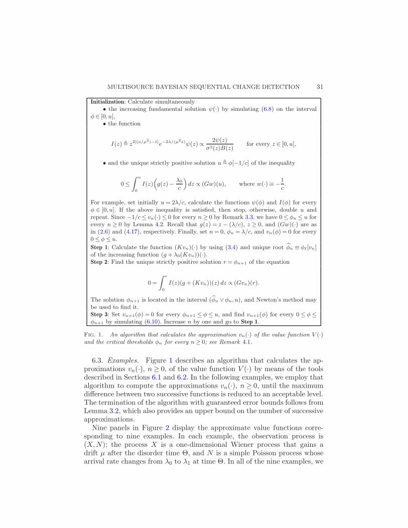
Fig. 1. An algorithm that calculates the approximation vn(·) of the value function V (·)and the critical thresholds φn for every n≥ 0; see Remark 4.1.
6.3. Examples. Figure 1 describes an algorithm that calculates the ap-proximations vn(·), n≥ 0, of the value function V (·) by means of the toolsdescribed in Sections 6.1 and 6.2. In the following examples, we employ thatalgorithm to compute the approximations vn(·), n≥ 0, until the maximumdifference between two successive functions is reduced to an acceptable level.The termination of the algorithm with guaranteed error bounds follows fromLemma 3.2, which also provides an upper bound on the number of successiveapproximations.
Nine panels in Figure 2 display the approximate value functions corre-sponding to nine examples. In each example, the observation process is(X,N); the process X is a one-dimensional Wiener process that gains adrift µ after the disorder time Θ, and N is a simple Poisson process whosearrival rate changes from λ0 to λ1 at time Θ. In all of the nine examples, we
32 S. DAYANIK, H. V. POOR AND S. O. SEZER
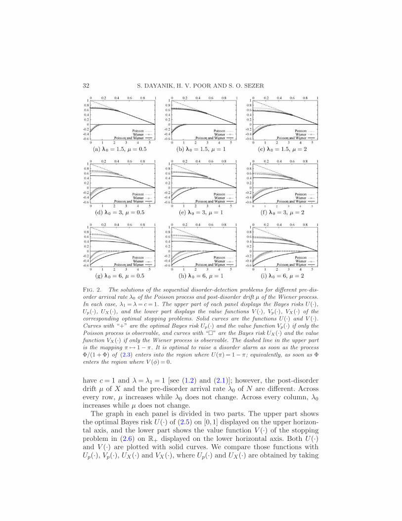
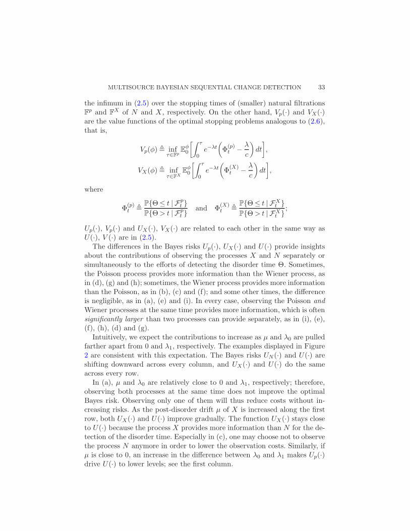
Fig. 2. The solutions of the sequential disorder-detection problems for different pre-dis-
order arrival rate λ0 of the Poisson process and post-disorder drift µ of the Wiener process.
In each case, λ1 = λ= c= 1. The upper part of each panel displays the Bayes risks U(·),Up(·), UX(·), and the lower part displays the value functions V (·), Vp(·), VX(·) of the
corresponding optimal stopping problems. Solid curves are the functions U(·) and V (·).Curves with “+” are the optimal Bayes risk Up(·) and the value function Vp(·) if only the
Poisson process is observable, and curves with “” are the Bayes risk UX(·) and the value
function VX(·) if only the Wiener process is observable. The dashed line in the upper part
is the mapping π 7→ 1 − π. It is optimal to raise a disorder alarm as soon as the process
Φ/(1 + Φ) of (2.3) enters into the region where U(π) = 1− π; equivalently, as soon as Φenters the region where V (φ) = 0.
have c= 1 and λ= λ1 = 1 [see (1.2) and (2.1)]; however, the post-disorderdrift µ of X and the pre-disorder arrival rate λ0 of N are different. Acrossevery row, µ increases while λ0 does not change. Across every column, λ0
increases while µ does not change.The graph in each panel is divided in two parts. The upper part shows
the optimal Bayes risk U(·) of (2.5) on [0,1] displayed on the upper horizon-tal axis, and the lower part shows the value function V (·) of the stoppingproblem in (2.6) on R+ displayed on the lower horizontal axis. Both U(·)and V (·) are plotted with solid curves. We compare those functions withUp(·), Vp(·), UX(·) and VX(·), where Up(·) and UX(·) are obtained by taking
MULTISOURCE BAYESIAN SEQUENTIAL CHANGE DETECTION 33
the infimum in (2.5) over the stopping times of (smaller) natural filtrationsFp and FX of N and X , respectively. On the other hand, Vp(·) and VX(·)are the value functions of the optimal stopping problems analogous to (2.6),that is,
Vp(φ) , infτ∈Fp
Eφ0
[∫ τ
0e−λt
(Φ
(p)t −
λ
c
)dt
],
VX(φ) , infτ∈FX
Eφ0
[∫ τ
0e−λt
(Φ
(X)t −
λ
c
)dt
],
where
Φ(p)t ,
PΘ≤ t | Fpt
PΘ> t | Fpt
and Φ(X)t ,
PΘ ≤ t | FXt
PΘ> t | FXt
;
Up(·), Vp(·) and UX(·), VX(·) are related to each other in the same way asU(·), V (·) are in (2.5).
The differences in the Bayes risks Up(·), UX(·) and U(·) provide insightsabout the contributions of observing the processes X and N separately orsimultaneously to the efforts of detecting the disorder time Θ. Sometimes,the Poisson process provides more information than the Wiener process, asin (d), (g) and (h); sometimes, the Wiener process provides more informationthan the Poisson, as in (b), (c) and (f); and some other times, the differenceis negligible, as in (a), (e) and (i). In every case, observing the Poisson and
Wiener processes at the same time provides more information, which is oftensignificantly larger than two processes can provide separately, as in (i), (e),(f), (h), (d) and (g).
Intuitively, we expect the contributions to increase as µ and λ0 are pulledfarther apart from 0 and λ1, respectively. The examples displayed in Figure2 are consistent with this expectation. The Bayes risks UN (·) and U(·) areshifting downward across every column, and UX(·) and U(·) do the sameacross every row.
In (a), µ and λ0 are relatively close to 0 and λ1, respectively; therefore,observing both processes at the same time does not improve the optimalBayes risk. Observing only one of them will thus reduce costs without in-creasing risks. As the post-disorder drift µ of X is increased along the firstrow, both UX(·) and U(·) improve gradually. The function UX(·) stays closeto U(·) because the process X provides more information than N for the de-tection of the disorder time. Especially in (c), one may choose not to observethe process N anymore in order to lower the observation costs. Similarly, ifµ is close to 0, an increase in the difference between λ0 and λ1 makes Up(·)drive U(·) to lower levels; see the first column.
34 S. DAYANIK, H. V. POOR AND S. O. SEZER
6.4. Numerical comparison with Baron and Tartakovsky’s asymptotic anal-
ysis. Let us denote the Bayes risk Rτ (π) in (1.2), minimum Bayes risk U(π)in (2.5) by Rτ (π, c) and U(π, c), respectively, in order to display explicitlytheir dependence on the cost c per unit detection delay. Let us also define
φ(c) ,(µ2/2) + λ0 + λ1[log(λ1/λ0)− 1] + λ
cand
(6.11)
f(c) , −log c
φ(c), c > 0.
Baron and Tartakovsky ([1], Theorem 3.5) have shown that the stoppingtime τ(c) , inft ≥ 0;Φt ≥ φ(c) is asymptotically optimal and that theminimum Bayes risk U(π, c) asymptotically equals f(c) for every fixed π ∈[0,1), as the detection delay cost c decreases to zero, in the sense that
limcց0
U(π, c)
f(c)= lim
cց0
Rτ(c)(π, c)
f(c)= 1 for every π ∈ [0,1).
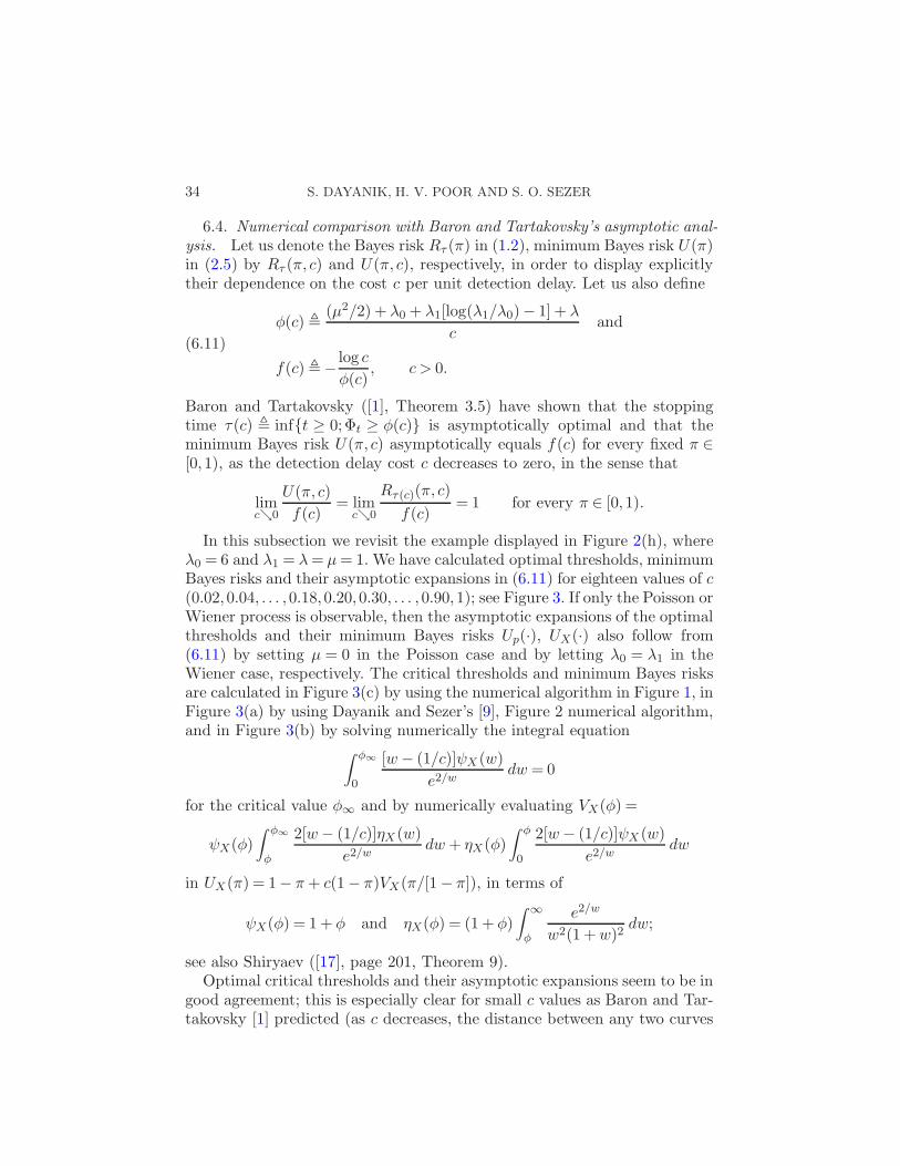
In this subsection we revisit the example displayed in Figure 2(h), whereλ0 = 6 and λ1 = λ= µ= 1. We have calculated optimal thresholds, minimumBayes risks and their asymptotic expansions in (6.11) for eighteen values of c(0.02,0.04, . . . ,0.18,0.20,0.30, . . . ,0.90,1); see Figure 3. If only the Poisson orWiener process is observable, then the asymptotic expansions of the optimalthresholds and their minimum Bayes risks Up(·), UX(·) also follow from(6.11) by setting µ = 0 in the Poisson case and by letting λ0 = λ1 in theWiener case, respectively. The critical thresholds and minimum Bayes risksare calculated in Figure 3(c) by using the numerical algorithm in Figure 1, inFigure 3(a) by using Dayanik and Sezer’s [9], Figure 2 numerical algorithm,and in Figure 3(b) by solving numerically the integral equation
∫ φ∞
0
[w− (1/c)]ψX (w)
e2/wdw = 0
for the critical value φ∞ and by numerically evaluating VX(φ) =
ψX(φ)
∫ φ∞
φ
2[w− (1/c)]ηX (w)
e2/wdw+ ηX(φ)
∫ φ
0
2[w− (1/c)]ψX (w)
e2/wdw
in UX(π) = 1− π+ c(1− π)VX(π/[1− π]), in terms of
ψX(φ) = 1 + φ and ηX(φ) = (1 + φ)
∫ ∞
φ
e2/w
w2(1 +w)2dw;
see also Shiryaev ([17], page 201, Theorem 9).Optimal critical thresholds and their asymptotic expansions seem to be in
good agreement; this is especially clear for small c values as Baron and Tar-takovsky [1] predicted (as c decreases, the distance between any two curves
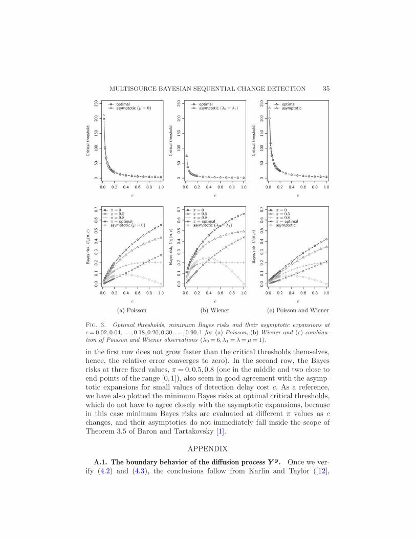
MULTISOURCE BAYESIAN SEQUENTIAL CHANGE DETECTION 35
Fig. 3. Optimal thresholds, minimum Bayes risks and their asymptotic expansions at
c= 0.02,0.04, . . . ,0.18,0.20,0.30, . . . ,0.90,1 for (a) Poisson, (b) Wiener and (c) combina-
tion of Poisson and Wiener observations (λ0 = 6, λ1 = λ= µ= 1).
in the first row does not grow faster than the critical thresholds themselves,hence, the relative error converges to zero). In the second row, the Bayesrisks at three fixed values, π = 0,0.5,0.8 (one in the middle and two close toend-points of the range [0,1]), also seem in good agreement with the asymp-totic expansions for small values of detection delay cost c. As a reference,we have also plotted the minimum Bayes risks at optimal critical thresholds,which do not have to agree closely with the asymptotic expansions, becausein this case minimum Bayes risks are evaluated at different π values as cchanges, and their asymptotics do not immediately fall inside the scope ofTheorem 3.5 of Baron and Tartakovsky [1].
APPENDIX
A.1. The boundary behavior of the diffusion process Y y. Once we ver-ify (4.2) and (4.3), the conclusions follow from Karlin and Taylor ([12],

36 S. DAYANIK, H. V. POOR AND S. O. SEZER
Chapter 15), who expressed the quantities in (4.2) and (4.3) in terms ofthe measures S(0, x] =
∫ x0+ S(dy) and M(0, x] =
∫ x0+M(dy), and integrals
Σ(0) =∫ x0+ S(0, ξ]M(dξ), N(0) =
∫ x0+M(0, ξ]S(dξ) for the left boundary at
0, and Σ(∞) =∫∞x S(ξ,∞)M(dξ), N(∞) =
∫∞x M(ξ,∞)S(dξ) for the right
boundary at ∞. Since only the finiteness of Σ(·) and N(·) matters, the valueof x > 0 in the domain of those integrals can be arbitrary. One finds that
S(dy) = c1y−2a/µ2
e2λ/(µ2y) dy
and
M(dy) = c2y2[(a/µ2)−1]e−2λ/(µ2y) dy, y > 0;
above, as well as below, c1, c2, . . . will denote positive proportionality con-stants. Therefore, changing the integrating variable by setting z = 1/y gives
S(x)− S(0+) =
∫ x
0+S(dy)
= c1
∫ ∞
1/xz(2a/µ2)−2e(2λ/µ2)z dz = +∞ ∀x > 0,
and the first equality in (4.2) follows. After applying the same change ofvariable twice, the double integral in the same equation becomes
N(0) = c3
∫ ∞
1/x
(∫ ∞
vuαe−βu du
)v−α−2eβv dv(A.1)
in terms of α, −2a/µ2 ∈ R and β , 2λ/µ2 > 0. Integrating the inner inte-gral by parts k ≥ 0 times gives that, for every k ≥ 0,
∫ ∞
vuαe−βu du=
k−1∑
j=0
α!β−(j+1)
(α− j)!vα−je−βv
+α!β−(k+1)
(α− k)!
∫ ∞
vβuα−ke−βu du.
If k ≥ α, then u 7→ uα−k is decreasing and the integral on the right is lessthan or equal to vα−k
∫∞v βe−βu du= vα−ke−βv . Therefore,
∫ ∞
vuαe−βu du≤
k∑
j=0
α!β−(j+1)
(α− j)!vα−je−βv, k ≥ max0, α.
Using this estimate in (A.1) implies that, for every x > 0,
N(0) ≤
∫ ∞
1/x
(k∑
j=0
α!β−(j+1)
(α− j)!vα−je−βv
)v−α−2eβv dv
=k∑
j=0
α!β−(j+1)
(α− j)!
∫ ∞
1/xv−j−2 dv <∞,

MULTISOURCE BAYESIAN SEQUENTIAL CHANGE DETECTION 37
which completes the proof of (4.2). Since S(0+) = −∞ and N(0)<∞, theleft boundary at 0 is an entrance-not-exit boundary.
For the proof of (4.3), notice that change of variable by u= 1/y gives forevery z > 0 that
∫ ∞
zS(dy) =
∫ 1/z
0u−α−2eβu du≥
∫ 1/z
0u−α−2 du
=
−(α+ 1)−1zα+1, α+ 1< 0,∞, α+ 1≥ 0.
If α+ 1 ≥ 0, then clearly Σ(∞) =∫∞x
∫∞z S(dy)M(dz) = ∞ for every x > 0.
If α+ 1< 0, then for every x > 0 we also have
Σ(∞) =
∫ ∞
x
∫ ∞
zS(dy)M(dz) ≥
∫ ∞
x−(α+ 1)−1zα+1M(dz)
= −(α+ 1)−1c2
∫ ∞
xzα+1z−α−2e−β/z dz = c4
∫ ∞
xz−1e−β/z dz
≥ c4e−β/x
∫ ∞
xz−1 dz = ∞,
and the first equality in (4.3) is proved. Similarly, changing variable byv = 1/y gives
∫ ∞
zM(dy) =
∫ 1/z
0vαe−βv dv ≥ e−β/z
∫ 1/z
0vα dv
=
(α+ 1)−1zα+1e−β/z, α+ 1> 0,∞, α+ 1≤ 0.
If α+ 1 ≤ 0, then clearly N(∞) =∫∞x
∫∞z M(dy)S(dz) = ∞ for every x > 0.
If α+ 1> 0, then for every x > 0 we also have
N(∞) =
∫ ∞
x
∫ ∞
zM(dy)S(dz) ≥
∫ ∞
x(α+ 1)−1zα+1e−β/zS(dz)
= c1
∫ ∞
x(α+ 1)−1zα+1e−β/zzαeβ/z dz = c5
∫ ∞
xz2α+1 dz
= c6z2(α+1)|z=∞
z=x =∞,
which completes the proof of (4.3). Because Σ(∞) =N(∞) = ∞, the rightboundary at ∞ is a natural boundary.
A.2. Continuity of φ 7→ (Hrw)(φ) at φ = 0. We shall prove the secondequality in (4.14), namely, (Hrw)(0) = limφց0 limlց0(Hl,rw)(φ) ≡limφց0(Hrw)(φ), which implies along with the first equality in (4.14) that
38 S. DAYANIK, H. V. POOR AND S. O. SEZER
φ 7→ (Hrw)(φ) is continuous at φ= 0. For every 0<h< r,
(Hrw)(0) = E00
[∫ τh
0e−(λ+λ0)t(g+ λ0(Kw))(Y Φ0
t )dt
+
∫ τr
τh
e−(λ+λ0)t(g+ λ0(Kw))(Y Φ0t )dt
]
= E00
[∫ τh
0e−(λ+λ0)t(g+ λ0(Kw))(Y Φ0
t )dt
+ e−(λ+λ0)τh(Hrw)(Y Φ0τh
)
]
= E00
[∫ τh
0e−(λ+λ0)t(g+ λ0(Kw))(Y Φ0
t )dt
]
+ (Hrw)(h)E00e
−(λ+λ0)τh
= E00
[∫ τh
0e−(λ+λ0)t(g+ λ0(Kw))(Y Φ0
t )dt
]+ (Hrw)(h)
ψ(0)
ψ(h)
hց0−→ 0 + lim
hց0(Hrw)(h) · 1,
where the second equality follows from the strong Markov property of Y Φ0
applied at the F-stopping time τh = inft ≥ 0;Y Φ0t = h, and the fourth
equality from (4.8). As hց 0, P00-a.s. τh ց 0 since 0 is an entrance-not-exit
boundary, and the integral and its expectation in the last equation vanishby the bounded convergence theorem. Moreover, since ψ(0) ≡ ψ(0+)> 0 by(4.4), we have limhց0ψ(0)/ψ(h) = 1. Therefore, limhց0(Hrw)(h) must exist,and taking limits of both sides in the last displayed equation completes theproof.
A.3. Calculation of (Hl,rw)(·) in (4.15). Let us denote the function on
the right-hand side of (4.15) by Hw(φ), l≤ φ≤ r. It can be rewritten in themore familiar form
Hw(φ) =
∫ r
lGl,r(φ, z)(g + λ0(Kw))(z)dz, l≤ φ≤ r,
by means of the Green function
Gl,r(φ, z) =ψl(φ∧ z)ηr(φ∨ z)
σ2(z)Wl,r(z), l≤ φ, z ≤ r,
for the second order ODE
[A0 − (λ+ λ0)]H(φ) = −(g+ λ0(Kw))(φ),(A.2)
l < φ < r, with boundary conditions H(l+) =H(r−) = 0.
MULTISOURCE BAYESIAN SEQUENTIAL CHANGE DETECTION 39
Therefore, the continuous function Hw(φ), l ≤ φ≤ r, is twice continuouslydifferentiable on (l, r) and solves the boundary value problem in (A.2). Ifτl,r , τ[0,l] ∧ τ[r,∞), Ito’s rule gives
e−(λ+λ0)τl,rHw(Y Φ0τl,r
)− Hw(Φ0)
=
∫ τl,r
0e−(λ+λ0)t[A0 − (λ+ λ0)]Hw(Y Φ0
t )dt
+
∫ τl,r
0e−(λ+λ0)tσ(Y Φ0
t )Hw′(Y Φ0t )dXt
= −
∫ τl,r
0e−(λ+λ0)t(g + λ0(Kw))(Y Φ0
t )dt
+
∫ τl,r
0e−(λ+λ0)tσ(Y Φ0
t )Hw′(Y Φ0t )dXt,
where Pφ0 a.s. Hw(Y Φ0
τl,r) = 0, since Hw(l) = Hw(r) = 0 and the first exit time
τl,r of the regular diffusion Y Φ from the closed bounded interval [l, r] $ [0,∞)
is always Pφ0 a.s. finite. Moreover, the stochastic integral with respect to
the (P0,F)-Wiener process X on the right-hand side has zero expectation
because the derivative Hw′(φ), given by
ψ′l(φ)
∫ r
φ
2ηr(z)
σ2(z)Wl,r(z)(g+ λ0(Kw))(z)dz
+ η′r(φ)
∫ φ
l
2ψl(z)
σ2(z)Wl,r(z)(g+ λ0(Kw))(z)dz,
of Hw(φ), is bounded on φ ∈ [l, r]. Therefore, taking expectations of bothsides gives
Hw(φ) = Eφ0
[∫ τl,r
0e−(λ+λ0)t(g+ λ0(Kw))(Y Φ0
t )dt
]≡ (Hrw)(φ),
l≤ φ≤ r.
Acknowledgment. The authors thank an anonymous referee for the re-marks and suggestions which improved the presentation of this paper.
REFERENCES
[1] Baron, M. and Tartakovsky, A. G. (2006). Asymptotic optimality of change-point detection schemes in general continuous-time models. Sequential Anal. 25257–296. MR2244607
[2] Bayraktar, E., Dayanik, S. and Karatzas, I. (2005). The standard Poisson dis-order problem revisited. Stochastic Process. Appl. 115 1437–1450. MR2158013
40 S. DAYANIK, H. V. POOR AND S. O. SEZER
[3] Bayraktar, E., Dayanik, S. and Karatzas, I. (2006). Adaptive Poisson disorderproblem. Ann. Appl. Probab. 16 1190–1261. MR2260062
[4] Borodin, A. N. and Salminen, P. (2002). Handbook of Brownian Motion—Facts
and Formulae, 2nd ed. Birkhauser, Basel. MR1912205[5] Bremaud, P. (1981). Point Processes and Queues. Springer, New York. MR0636252[6] Byington, C. S. and Garga, A. K. (2001). Handbook of Multisensor Data Fusion.
CRC Press, Boca Raton, FL.[7] Cartea, I. and Figueroa, M. (2005). Pricing in electricity markets: A mean revert-
ing jump diffusion model with seasonality. Appl. Math. Finance 12 313–335.[8] Cinlar, E. (2006). Jump-diffusions. Blackwell-Tapia Conference, 3–4 Novem-
ber 2006. Available at http://www.ima.umn.edu/2006-2007/SW11.3-4.06/abstracts.html#Cinlar-Erhan.
[9] Dayanik, S. and Sezer, S. O. (2006). Compound Poisson disorder problem. Math.
Oper. Res. 31 649–672. MR2281222[10] Gapeev, P. V. (2005). The disorder problem for compound Poisson processes with
exponential jumps. Ann. Appl. Probab. 15 487–499. MR2115049[11] Ito, K. and McKean, Jr., H. P. (1974). Diffusion Processes and Their Sample
Paths. Springer, Berlin. MR0345224[12] Karlin, S. and Taylor, H. M. (1981). A Second Course in Stochastic Processes.
Academic Press, New York. MR0611513[13] Kushner, H. J. and Dupuis, P. (2001). Numerical Methods for Stochastic Control
Problems in Continuous Time, 2nd ed. Springer, New York. MR1800098[14] Peskir, G. and Shiryaev, A. (2006). Optimal Stopping and Free Boundary Prob-
lems. Birkhauser, Basel. MR2256030[15] Peskir, G. and Shiryaev, A. N. (2002). Solving the Poisson disorder problem. In
Advances in Finance and Stochastics (K. Sandmann and P. Schonbucher, eds.)295–312. Springer, Berlin. MR1929384
[16] Polyanin, A. D. and Zaitsev, V. F. (2003). Handbook of Exact Solutions for Ordi-
nary Differential Equations, 2nd ed. Chapman and Hall/CRC, Boca Raton, FL.MR2001201
[17] Shiryaev, A. N. (1978). Optimal Stopping Rules. Springer, New York. MR0468067[18] Weron, R., Bierbrauer, M. and Truck, S. (2004). Modeling electricity prices:
Jump diffusion and regime switching. Phys. A Statist. Mech. Appl. 336 39–48.
S. Dayanik
Department of Operations Research
and Financial Engineering
and
The Bendheim Center for Finance
Princeton University
Princeton, New Jersey 08544
USA
E-mail: [email protected]
H. V. Poor
School of Engineering
and Applied Science
Princeton University
Princeton, New Jersey 08544
USA
E-mail: [email protected]
S. O. Sezer
Department of Mathematics
University of Michigan
Ann Arbor, Michigan 48109
USA
E-mail: [email protected]