Multistage Modeling of Lung Cancer Mortality Among Arsenic-Exposed Copper-Smelter Workers

Risk Analysis, Val. 9, No. 4, 1989

Multistage Modeling of Lung Cancer Mortality Among Arsenic-Exposed Copper-Smelter Workers

Sati Mazumdar,'*2 Carol K. Redmond,' Philip E. Enterline,' Gary M. Marsh,' Joseph P. Costantino,' Susan Y. J. Zhou,' and Rita N. Patwardhad

Received November 21, 1988; revised June I, 1989

Multistage modeling incorporating a time-dependent exposure pattern is applied to lung cancer mortality data obtained from a cohort of 2802 arsenic-exposed copper-smelter workers who worked 1 or more years during the period 1940-1964 at a copper smelter at Tacoma, Washington. The workers were followed for death through 1976. There were 100 deaths due to lung cancer during the follow-up period. Exposures to air arsenic levels measured in ~ g / m ~ were estimated from departmental air arsenic and workers urinary arsenic measurements. Relationships of different temporal variables with excess death rates are examined to judge qualitatively the implications of the multistage cancer process. Analysis to date indicates a late stage effect of arsenic although an additional early stage effect cannot be ruled out.

KEY WORDS: Lung cancer; multistage model; time-dependent exposure pattern; risk assessment.

1. INTRODUCTION

Recent literature on epidemiologic studies of human cancer indicates that Armitage-Doll multistage models of carcinogenesis can be used to examine the relationships of excess cancer mortality to some carcinogenic exposure and time-dependent covariates such as: (a) age at initial exposure; (b) duration of exposure; and (c) time since exposure terminated.('-')

Since multistage models can be formulated to provide information regarding whether more than one stage is dose-related, they assist in determining whether different carcinogens affect different stages of the cancer process. They also are used in carcinogenic quantitative risk assessment for estimating the dose-response rela-

Department of Biostatistics, Graduate School of Public Hcalth, Uni- versity of Pittsburgh, Pittsburgh, Pennsylvania. To whom all correspondence should be addressed, at: 306 Parran Hall, Graduate School of Public Health, University of Pittsburgh, Pittsburgh, Pennsylvania 15261.

tionships and for extrapolation to low doses relevant for setting environmental standard^.(^^^)

Previous applications of multistage modeling to epidemiologic data did not incorporate varying exposure patterns for individuals into the estimation of the excess death rate .(3,4) The assumption that an individual worker is exposed to a constant exposure rate over the total exposure time interval is generally not representative of the exposure pattern in most occupational settings. This observation has led to our interest in multistage modeling of cohort datasets with time-dependent exposure patterns.

The purpose of this paper is threefold. First, computer programs which have been developed for fitting multistage models with one or two dose-related stages to cohort datasets incorporating time-dependent exposure patterns are discussed. Second, these programs are applied to the multistage modeling of lung cancer mortality among a cohort of arsenic-exposed copper-smelter

Third, lifetime risks of dying from lung cancer adjusted for competing causes of death are cal-

0272-433U89/1200-0551S06.M)/1Q 1989 Society for Risk Analysis 551

552 Mazumdar et al.

culated using a multistage model, the relative risk model, and the absolute excess risk model to provide information on risk assessments for arsenic, an occupational exposure.

2. STUDY COHORT

Data used in this paper are obtained from a cohort study of 2802 white men who worked a year or more during the period 1940-1964 at a copper smelter in Ta- coma, Washington. The workers were followed for death through 1976. There were 100 deaths due to lung cancer during the follow-up period. The total person-years at risk for the cohort were calculated to be 70,391 and the expected lung cancer deaths were estimated to be ap- proximately 48.86. The controls used to determine the expected deaths were U.S. white males.

Estimates of air arsenic exposure were based on air arsenic measures combined with urinary arsenic data for individual workers. The dataset representing urinary arsenic levels were converted to probable air arsenic levels, and air arsenic values (kg/m3) were estimated by departments for different years.(*) Exposure profiles were then constructed for each worker over the entire work history in 1-year intervals. These exposure profiles provide the time-dependent exposure rates needed for this analysis.

Cumulative arsenic exposure for each worker was found by multiplying the arsenic level at each job by years at that job and summing this product across all jobs. For each worker, a time-weighted measure was found by dividing the cumulative exposure by the duration of exposure defined as the interval between the first job and the last job with arsenic exposure and is termed “average exposure.” This measure is similar to the measure “ mean exposure” defined by Enterline et al.,(’) and represents for a worker his status at the end of his work experience or at the end of the follow-up period. This definition of “duration of exposure” differs from the definition in the earlier analysis@) where it was defined as the total time on jobs with arsenic exposure. The variable “age at initial exposure” is age at the first job with arsenic exposure. The variable “time since exposure terminated” is the time interval between last job with arsenic exposure and death or end of follow-up. Thus for a worker still employed at the end of the follow- up period this interval is zero.

3. METHODS

Two approaches are followed in this paper to investigate the implications of multistage models and to provide inferences regarding the stage(s) at which exposure (or exposures) affect the cancer process. The first approach is the direct fitting of the multistage model incorporating a time-dependent exposure pattern. The second approach is the qualitative analysis which ex- amines the relationships of excess cancer mortality and the covariates: average exposure, age at initial exposure, duration of exposure, and time since exposure terminated.

3.1. Fitting of The Multistage Model

The simple multistage model of carcinogenesis assumes that a tumor results when k events occur in order in a single cell. The occurrence rate (at age t ) of the ith event given that i- 1 events have occurred, is assumed to be

Xi = ai + bp(t) (1) where a, is the background rate independent of age, b, is the potency parameter for the ith cellular change, and D(t) is the dose rate at age t. In the context of this analysis, potency parameters should not assume negative values. The cumulative incidence rate by age t is then given by

H ( t ) = I”’ . . . lo”* [a, + b , ~ ( u , ) l . . . [a, 0 0

+b, D(u,)]du, . . . du, (2)

In accordance with the above formulation, the age- specific cancer death rate [h(t)] at time t can be expressed as follows:

h(t) =how +hl(t) (3) where ho(t) is a baseline age-specific cancer death rate derived either from a standard population or a suitably chosen control population and h,(t) is the excess death rate. The expression for the excess death rate depends on the number and the order of the dose-related stage(s) and the nature of the dose rate pattern. If the dose rate is assumed to be constant, h,(t) takes a simple expression. For example, if we assume that there are k stages of the multistage process, the first stage is dose-related, the dose rate is constant in the amount of c units, the age at initial exposure is a and the time since exposure stopped isf, then the excess death rate at attained age t

Multistage Models for Cancer Mortality 553

takes the following form:

hl(t) = bc[(t-a)k-' -f"-'] (4)

In this expression b is the potency parameter and needs to be estimated from the dataset under consideration.

In occupational epidemiologic studies, historical exposure estimates for one or more agents are usually taken as measures of dose. The assumption of a constant exposure rate to which a worker is exposed throughout his work history makes the fitting procedure easier, since the simple expression for h,(t) given in Eq. (4) can be used.

A methodology to incorporate exact time-dependent exposure patterns in the calculation of the excess death rate providing expressions for h,(t) when one or two stage(s) are dose-related has been developed by Crump and HOW~.(~*'O) A formulation of the problem as provided by them is given below.

If age is divided into 1 year intervals, xo being the age when the worker starts his first job and the dose rate in the ith interval is assumed to be a constant ci(i= 1,2, ...), then for a k stage process with the flh stage dose-related, Eq. (3) takes the form

h, =a, + bz, ( 5 )

where h,=age-specific cancer death rate at age m; a, = background cancer death rate at age m; b =potency parameter, and

-to- u)~-'-'u'-'~u] (6)

where to=time from initiation of tumor to its clinical expression.

The quantity z, is referred to as the z value by Crump and Howe.('O) The value of to can be selected in advance, depending on the situation, and does not need to be estimated from the data. In the absence of definite knowledge about the value of this parameter from bio- logical considerations, several values of to can be used to judge empirically which one fits the data best.

If zn, denotes the z value for the nth individual at age x,,,, and N, denotes the total person-years at risk at age x,, the expected number of cancer deaths at age x, is given by

N

E m = N m a m + 2 z n m (7) n - 1

Assuming that the observed number of deaths at age x, denoted by om has a Poisson distribution with expected

value Em, the potency parameter b in Eq. ( 5 ) can be estimated by grouping observed and background deaths and the z values in different categories and using a suit- able maximum likelihood estimation algorithm. The categories can be defined by the age at risk variable (or intervals of z values or any other variable by which deaths can be grouped suitably).

For a k stage model, when two stages r and i? (r< t < k ) are dose-related, the age-specific cancer death rate h, at age x, is given by

h, = a, + blzl, + b2 zzm + b3 z3, (8) where a, is the background cancer death rate, z,,,, has the same expression as Eq. (6), zzm has the same expression as Eq. (6) with r changed to 4, and,

k! (k-Z- l)!(r- l)!(Z- 1 -r)! Z3m =

n - 1 r x .

The potency parameters, b,, b2, and b,, can be calculated using the approach described earlier.

3.2. Computer Program

A computer program written in FORTRAN has been developed that permits considerable flexibility in fitting one or two stage dose-related multistage models with time-dependent exposure patterns relevant for occupational cohort studies. The inputs to the program are: (a) work histories with exposure patterns and vital status of workers in a standardized format compatible with OC- MAP (a user-oriented software for the analysis of large cohort datasets)("); (b) time from initiation of tumor to its clinical expression; (c) number of stages; (d) number of dose-related stage(s); and (e) background rates from a reference poulation. The output from this program is a file of categorized observed deaths, expected deaths, and z values also in a standardized format compatible with GLIM (a widely used modeling program) which is used for the estimation of parameters.('*) The categorized file can be either by intervals of z values or the age at risk variable.

A second program written in FORTRAN to calcu- late lifetime risks of dying from cancer adjusted for com-

554 Mazurndar el al.

peting risks and the worker being subjected to variable exposure patterns has also been developed. Inputs to the program are: (a) potency parameters; (b) model specifications; and (c) exposure pattern specifications.

Using this program package, modeling was performed on a VAXNMS system and CRAY supercom- puter system using a CRAY-VAX interface.

3.3. The Qualitative Analysis

The qualitative analysis is a process in which sub- jective examination is performed to evaluate the excess risk patterns in relation to selected covariates. The covariates selected for this analysis were: average exposure and three temporal variables, viz: (a) age at initial exposure; (b) duration of exposure; and (c) time since exposure terminated. The number of person-years at risk and observed lung cancer deaths were cross-classified into cells according to selected categories of these covariates. It should be noted here that individuals can appear in a number of cells as they move through the categories of the temporal variables such as “duration of exposure” and “time since exposure stopped,” but they appear only once in the categories of the “average exposure” and “age at initial exposure” variables. Ex- pected number of lung cancer deaths for each cell were calculated using U.S. white male 5-year calendar and age-specific death rates. Two other risk models, viz, the relative risk model and the absolute excess risk model, are used in this qualitative analysis.

The relative risk is defined by

SMR (Standardized Mortality Ratio) - observed deaths

expected deaths -

The absolute excess risk is defined by

EMR (Excess Mortality Rate) - observed deaths - expected deaths -

person-years

1. The temporal variables considered here are cor- related with each other which may bias the relative risks or absolute excess risks calcualted directly from the marginal distributions of the covariates.

2. Adjusted SMRs and EMRs are calculated using the approach described by Kaldor et al.(13) as given below:

3.3.1. Adjusted SMRs

SMRs calculated for different cells of the cross- classification of covariates are modeled, and the parameter estimates are used to obtain the adjusted SMRs. The model is described by the following expression and is called “relative risk” model:

E(0,) = Ej exp(B9,) (10)

where E(Oj) = expected number of deaths i n f h cell; Ej = expected number of deaths based on population death rates in jth cell; B = vector of parameters ( T means transpose); and Dj = vector of 0 or 1 values specifying the category of each covariate to which thejlh cell belongs. A covariate x divided into k, categories wil give rise *to kx- 1, parameters and k x - 1 components of the Dj vector. Hence, the dimension of each Dj vector and the parameter vector is given by

C

2 (kx- 1) + l(c = total number of covariates) x = 1

The parameter vector (transpose) is written as

BT = - * - 3 B l k 1 7 * * * 7 Bc2, * * * ? Bckc)

Denoting the estimates of the elements of B by the corresponding lowercase letters, exp (b,) gives the SMR of the baseline category relative to the population rates. In the present formulation the baseline category is given by the first level of each of the covariates. The SMR of the jth category of the ith covariate relative to its first category adjusted for other covariates is given by exp (bi,).

We assume that the observed number of deaths in each cell has a Poisson distribution with expected value given by the expression in Eq. (10). The software GLIM(’*) is used to provide estimates of the parameters and corresponding standard errors.

3.3.2. Adjusted EM&

EMRs calculated for different cells of the cross- classification of covariates are modeled and the parameter estimates are used to obtain adjusted EMRs. The model is described by the following expression and is called “absolute excess risk” model:

E(0,) = Ej + exp (BrD,) Nj (11) where Oj, Ej, BT, and Dj have the same definition given earlier, and h$ is the total number of person-years in the jth cell. Assuming that the observed number of deaths in each cell has a Poisson distribution with the expected


Table I. Estimated Potency Parameters (b),“ Standard Errors (SE), and Scaled Deviances (Sc. Dev.)b for One-Stage Dose-Related Multistage Models Fitted to Arsenic-Exposed Copper-Smelter Workers Lung Cancer Mortality Data

No. of stages Dose-related stage 3 4 5 6 7

b 1.2138-9 2.69OE-11 5.481E- 13 1.036E-14 1.836E-16 1 SE 2.595E-10 5.671E-12 1.184E-13 2.351E-15 4.464E-17

Sc. Dev. 15.260 14.147 16.600 20.615 25.083 b 4.664E- 10 8.433E-12 1.4768-13 2.4958-15 4.055E-17

2 SE 1.036E-10 1.77OE-12 3.140E- 14 5.537E-16 9.593E-18 Sc. Dev. 18.637 13.664 15.086 18.909 23.423 b 5.9678-12 8.470E-14 1.228E-15 1.780E-17

3 SE 1.2738-12 1.771E-14 2.665E-16 4.107E-18 Sc. Dev. 15.025 13.403 16.979 21.725 b 8.286E-14 9.715E-16 1.203E-17

4 SE 1.726E-14 2.052E-16 2.694E-18 Sc. Dev. 12.800 14.254 19.449 b 1.179E-15 1.1 80E-17

5 SE 2.433E-16 2.537E-18 Sc. Dev. 11.821 15.896 b 1.686E-17

6 SE 3.481 E-18 Sc. Dev. 11.764

“Estimation is by grouping person-years, deaths, and z values by age; E - n = lo-”. Sc. Dev. has a chi-square distribution with 14 df.

value given by Eq. (ll), the parameters can be estimated by using GLIM. Denoting as before the estimates by the lowercase letters, the estimated adjusted excess mortality rate of thejth category of the ith covariate relative to its first category is given by exp (b&. As before, exp (b,) provides excess mortality rate for the baseline category defined by the first level of each of the covariates.

3.4. Assessment of Lifetime Risk

Lifetime risks (through age 85 + years) adjusted for competing causes of death for selected multistage models are calculated using the procedure described by Gail.(14) Details of this procedure are given by Dong et ~ l . ( ~ ) For the calculation of the lifetime risks for the relative risk model (exposure acts multiplicatively) adjusted SMRs are used. Similarly, for the calculation of the lifetime risks for the absolute excess risk model (exposure acts additively) adjusted EMRs are used. These SMRs and EMRs take different values as the worker is followed through time and belongs to different categories of the temporal variables. Details of this procedure are described by Kaldor er al. (13)

4. RESULTS

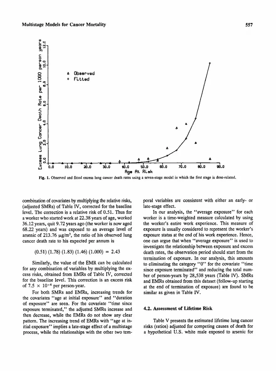
Table I summarizes the results from direct fitting of single stage dose-related models. In these models, the parameter to, the time from initiation of tumor to its clinical expression, is taken to be zero. Estimation of the potency parameters is based on grouping person- years, deaths, and z values in age (at risk) intervals. The scaled deviance statistic(12) as a measure of goodness-of- fit was not found to be effective in selecting the best fitting model. However, for a fixed k (number of stages), the penultimate-stage (next to last stage) dose-related models have smaller deviances compared to first-stage dose-related models. When the observed and fitted values are plotted, late-stage dose-related models fit the observed data better than early-stage dose-related models. Models with six or seven stages, when the penultimate stage is dose-related, fit the data best. Models with more than seven stages have not been investigated.

Results from model-fitting using different values of the parameter to for models with six and seven stages, penultimate-stage dose-related, are presented in Table 11. Models with smaller values for to fit the data better, and not much difference is seen when to = 0 to to = 5 . There-

556 Mazumdar et al.

Table 11. Estimated Potency Parameters (b),” Standard Errors (SE), and Scaled Deviances (Sc. Dev.)* for Selected Multistage Models Fitted to Arsenic-Exposed Copper-Smelter Workers Lung Cancer

Mortality Data

No. of stages 6 7

Dose-related Dose-related to‘ stage-penultimate stage-penultimate

b 1.179E-15 1.6868-17 0 SE 2.433E-16 3.481E-18

Sc. Dev. 11.821 11.746 b 1.496E-15 2.117E-17

5 SE 3.091E-16 4.4348-18 Sc. Dev. 11.759 12.799 b 1.931E-15 2.6948-17

10 SE 4.146E-16 5.975E-18 Sc. Dev. 15.258 17.656 b 2.5658-15 3.531E-17

15 SE 5.877E-16 8.5468-18 Sc. Dev. 20.624 24.059

Table 111. Estimated Potency Parameters (b] , b,, and b3)/ Standard Errors (SE), and Scaled Deviances (Sc. Dev.)” for Two Stages

Dose-Related Multistage Models Fitted to Arsenic-Exposed Copper- Smelter Workers Lung Cancer Mortality Data

No. of stages 6 7

Dose-related stages Dose-related stages (first and penultimate) (first and penultimate)

bl - 5.114E-15 -6.3248-17 SE 4.861E-15 7.562E-17 b* 6.568E-16 1.3488-17 SE 8.673E-16 1.449E-17 b, 4.1498-17 5.582E-19 SE 4.579E-17 1.232E-18 Sc. Dev. 9.642 10.057

“Estimation is by grouping person-years, deaths, and z value by age; E-n = lo-”. %c. Dev. has a chi-square distribution with 12 df.

“Estimation is by grouping person-years, deaths, and z values by age; E-n = lo-“. b S ~ . Dev. has a chi-square distribution with 14 df. so= time from initation of tumor to its clinical expression.

fore, for the analyses which follow, the value of to is taken to be zero.

For fitting two stages dose-related models, we limit ourselves to situations when the number of stages are 6 or 7 and the dose-related stages are first and penultimate. The selection of first and penultimate stages is based on the anticipated high correlation between zh, z,, and z,, values if the dose-related stages are close to each other. In the present situation these correlations are found to be very high (r=0.9), resulting in a serious problem in obtaining stable estimates of the parameters bl, b2, and b3. When the parameters are estimated without any con- straint on their values by grouping person-years, deaths, Zlm, Z,, and Z,, values in different age intervals, stable estimates are not obtained. In fact, the estimate of b, is found to be negative (although not significant). All three parameters’ estimates are found to be nonsignificant (Ta- ble 111). As expected, the Values for scaled deviance, a goodness-of-fit statistic, are found to be smaller than the corresponding values from single-stage dose-related models (Table 11).

Figures 1-3 present the observed and fitted excess lung cancer death rates obtained from estimating multistage models with seven stages when only first stage, penultimate stage, or first and penultimate stages are

dose-related. It is seen that the model where both first and penultimate stages are dose-related fits the data better at higher ages than the model when only the first or penultimate stage is dose-related. However, the fitted values for the two-stage dose-related model are influ- enced to a large extent by the negative (nonsignificant) parameter estimate. As the potency parameters should not assume negative values in the present context, these estimated potency parameters are not used in the calculation of lifetime risks. Our preliminary estimation, constrained so that the parameter estimates will be pos- itive, reduces the fitted model to the penultimate-stage dose-related model. Hence, the penultimate-stage dose- related 7 stage model which shows an adequate fit is used further in the calculation of the lifetime risk. The fitting of the first-stage dose-related model is presented to show the contrast at higher ages.

4.1. The Qualitative Analysis

Table IV presents the summary of person-years, observed, and expected lung cancer deaths by categories of the selected covariates and adjusted SMRs and EMRs. In the calculation of person-years, follow-up begins at entry to the study. The table also provides person-years weighted-mean values of the covariates for different categories. For adjusted SMRs and EMRs for each covariate, one category is chosen arbitrarily as a baseline and is given the value 1.00.

The value of the SMR can be calculated for any


(0 L O Q J)

C 0 L9

0 r j -

t x-

- ;- a”

E + P i t t e d

a

A Observed

L e

Q 4 g 9-

0

(D

L 4

c3 9 L *- ! 0 0

c 1 -1

(D

In:-

A 1

90.0 Age A t Risk

Fig. 1. Observed and fitted excess lung cancer death rates using a seven-stage model in which the first stage is dose-related.

combination of covariates by multiplying the relative risks, (adjusted SMRs) of Table IV, corrected for the baseline level. The correction is a relative risk of 0.51. Thus for a worker who started work at 22.38 years of age, worked 36.12 years, quit 9.72 years ago (the worker is now aged 68.22 years) and was exposed to an average level of arsenic of 213.76 kg/m3, the ratio of his observed lung cancer death rate to his expected per annum is

(0.51) (1.78) (1.83) (1.46) (1.000) = 2.43

Similarly, the value of the EMR can be calculated for any combination of variables by multiplying the excess risks, obtained from EMRs of Table IV, corrected for the baseline level. This correction is an excess risk of 7.5 x per person-year.

For both SMRs and EMRs, increasing trends for the covariates “age at initial exposure” and “duration of exposure” are seen. For the covariate “time since exposure terminated,” the adjusted SMRs increase and then decrease, while the EMRs do not show any clear pattern. The increasing trend of EMRs with “age at initial exposure” implies a late-stage effect of a multistage process, while the relationships with the other two tem-

poral variables are consistent with either an early- or late-stage effect.

In our analysis, the “average exposure” for each worker is a time-weighted measure calculated by using the worker’s entire work experience. This measure of exposure is usually considered to represent the worker’s exposure status at the end of his work experience. Hence, one can argue that when “average exposure” is used to investigate the relationship between exposure and excess death rates, the observation period should start from the termination of exposure. In our analysis, this amounts to eliminating the category “0” for the covariate “time since exposure terminated” and reducing the total number of person-years by 28,538 years (Table IV). SMRs and EMRs obtained from this dataset (follow-up starting at the end of termination of exposure) are found to be similar as given in Table IV.

4.2. Assessment of Lifetime Risk

Table V presents the estimated lifetime lung cancer risks (ratios) adjusted for competing causes of death for a hypothetical U S . white male exposed to arsenic for

Mazumdar et al.

A - Observed + - F i t t e d

A I I 1 I

0.0 10.0 20.0 30.0 40.0 50.0 60.0 70.0 80.0 90.0 Age A t Risk

Fig. 2. Observed and fitted excess lung cancer death rates using a seven-stage model in which the sixth stage is dosc-related.

40 years, subject to varying exposure patterns and age at initial exposure, using a seven-stage multistage model when only the penultimate stage is affected. Due to the negative estimate of one of the potency parameters in the first- and penultimate-stage dose-related models (Ta- ble 111), these risks are not calculated for the two-stage dose-related models. In the exposure patterns, the arsenic for 10 years and H (heavy) means a constant dose rate of 1000 p,g/m3 of arsenic level for 10 years. For example, an exposure pattern LLLH indicates 30 years of exposure to 200 p,g/m3 followed by 10 years of exposure to 1000 kg/m3. When the penultimate stage is affected, the lifetime risk is almost doubled if the worker is exposed to light exposure earlier and heavy exposure later in his work history, compared to a worker exposed to heavy exposure earlier and light exposure later in his work history, if durations of exposures, age at initial exposure, and average exposure remain the same. The risk is almost doubled for the worker exposed to heavy exposure for 40 years compared to the worker exposed to heavy exposure for 20 years and light exposure for the next 20 years. This table illustrates the significance

of time-dependent exposure patterns in the prediction of lifetime risk.

A comparison between the lifetime risks presented in the two columns shows how risks for the same exposure patterns and same durations depend on the age at which the exposure begins. Under the assumption of the late-stage-affected model, these risks are always higher for workers starting exposure later in life. Figure 4 presents these aspects graphically.

Table VI presents the estimated lifetime lung cancer risks (ratios) adjusted for competing causes of death for a hypothetical U.S. white male exposed to arsenic for 40 years using the adjusted rates calculated under “relative risk” and “absolute excess risk” model assump- tions. The relative risk model can be interpreted as the model in which the effects of different levels of the covariates have a multiplicative effect over the baseline effects, and the excess risk model can be interpreted as the model in which the effects of different levels of the covariates have additive effects over the baseline effects. For both models, although the risks increase with increasing exposure, the relative increments in risks decline as exposure increases, with the largest increments

Multistage Models for Cancer Mortality

0

8 - 9- a L W a,

a, 4 2 9- la I 4 0 a, 0 9-

k * 0 C

559

A - Observed + - F i t t e d

I3 A

Fig. 3. Observed and fitted excess lung cancer death rates using a seven-stage model in which the first and sixth stages are dose-related.

at the lowest exposure levels. This is in accord with previously published data on this group of workers.(8) For the “absolute excess risk” model, lifetime risks are higher if the worker starts exposure at a higher age (20- 24 vs. 25-29). This phenomenon is in accord with a late-stage-affected multistage model and is also seen in Table V.

Figure 5 presents the estimated lifetime (through age 85+ years) risks of dying from lung cancer for an hypothetical U.S. white male exposed to various levels of arsenic using three different models. It is assumed that the exposure starts in the age interval 20-24 and continues for a maximum of 40 years. This figure shows that the lifetime risks are comparable at lower exposure levels; however, at higher levels of exposure the values given by the multistage model are quite different than the values given by the other two models. This is be- cause the multistage model does not permit a dose-response relationship that is concave downward for a given exposure duration period. For a penultimate-stage dose- related k stage model, the expression for the excess rate h,(t) at age t is given by

h,(t) = bc[d+a)k-’-(a)k-’]

where c is exposure concentration, d is the duration of exposure, a is the age at initial exposure, and b is the potency parameter. Thus, in the present case the excess risk for a seven-stage model, where only the penultimate stage is affected, rises linearly with c for a fixed duration of 40 years and age at initial exposure at 20, resulting in high lifetime risks at higher values of c. For the other two models, relative increments in the adjusted risks (relative or excess) are seen to decline as exposure concentration increases (Table VI). Although these risk values are to some extent dependent on the selected categories of the covariates, analyses with several covariate catego- rizations produced the same general picture. This phenomenon results in lifetime risks which are considerably lower than the lifetime risks given by the multistage model at higher exposure levels. As the adjusted relative/excess risks are obtained from the data, one can argue that the multistage model here overestimates the lifetime risk.

5. DISCUSSION

The results obtained to date from direct fitting of multistage models with time-dependent exposure pat-

560 Mazumdar et al.

Table IV. Summary of Person-Years and Observed and Expected Numbers of Lung Cancer Deaths and Adjusted SMRs (Standardized Mortality Ratio) and EMRs (Excess Mortality Rate) Among Arsenic-Exposed Copper-Smelter Workers

Covariate Person- Observed Expected SMR‘ EMR‘

Mean years“ deaths deathsb (adj.1 (ad].)

Average exposure ( &m3) < 400 213.76 41724.18 46 28.41 1 .OO 1.00 400-799 561.11 15603.81 24 10.58 1.48 2.34 800 + 1491.08 13062.81 30 9.87 1.95’ 3.48’

< 20 18.62 9724.18 4 3.49 1 .oo 1.00 20-24 22.38 20485.26 16 8.28 1.78 3.30 25-29 27.36 14159.27 17 9.06 1.70 5.24 30 + 37.96 26022.10 63 28.05 2.20 9.85

Age at initial exposure (yr)

Duration of exposure (yr) < 10 10-19 20-29 30 +

4.80 41041.48 32 18.95 1.00 1.00 14.64 13398.46 14 8.94 0.99 2.64 24.55 10071.37 28 10.83 1.69 11.52+ 36.12 5879.50 26 10.16 1.83 21.85’

Time since exposure terminated (yr)

0 0.00 28538.32 2.5 13.47 1.00 1 .oo 1-4 2.44 10443.14 15 6.18 1.20 2.53 5-14 9.72 16763.65 28 10.49 1.46 2.45 1.5 + 22.10 14645.67 32 18.74 1.20 6.22*

“Follow-up begins at entry to the study. bCalculated on the basis of U.S. white male 5-year calendar and age-specific mortality rates. ‘SMRs and EMRs are adjusted using “relative risk” and “absolute excess risk” models (see text), and are shown relative to the rate in the baseline category fixed at 1.00. *p < 0.05.

Table V. Estimated Lifetime Lung Cancer Risk” Through age 85 + years and Ratiob (in parenthesis) for a Hypothetical U.S. White

Male Exposed to Arsenic for 40 Years, Using a Penultimate-Stage Dose-Related, Seven-Stage Multistage Model

Exposure patternc 20 30

Age at initial exposure (yr)

LLLL HHLL LLHH HHHH

0.057( 1.57) 0.070(1.93) 0.069(1.92) O.lM(2.88) 0.122(3.37) 0.156(4.32) 0.133(3.69) 0.186(5.15)

“U.S. white male age-specific mortality for 1960-1964 used in competing risk calculations. bRatio of risk for exposed individuavrisk for unexposed individual (lifetime risk for unexposed = 0.0361). ‘L =200 pg/m3 for 10 years; H = 1000 kg/m3 for 10 years.

terns to arsenic-exposed copper-smelter workers mortality data indicate that arsenic acts at a late stage in the carcinogenic process. However, since the first- and pe-

nultimate-stage dose-related models fit the data most closely, the possibility of an early-stage effect of arsenic cannot be ignored.

Unfortunately, stable estimates of potency parameters when two stages are dose-related were not obtained using routine estimation procedures due to a multicollinearity problem in the dataset, and the corresponding risk estimate could not be provided. This limitation of model-fitting and estimation under constraints on the model parameters are currently under investigation. We recommend the exploration of different estimation procedures (such as biased estimation procedures) to handle this multicollinearity between dose-related variables. The importance of time-dependent exposure patterns in the calculation of lifetime risks is illustrated.

Results from the qualitative analysis using stratifi- cation on covariates are in general agreement with the results obtained from multistage models. The major discrepancy is seen at the high exposure levels, where the estimated lifetime risks of dying from lung cancer using the multistage model are considerably higher than the values estimated from the “relative risk” and “absolute


(D E

d

c

.>

.> 2

L (D 0 C - Age at InitiaL

o---o Age at InitiaL L -- Dose Rote 200

I 1 2 a d .> oz

1 2 - a d .> oz (D E

d .>

L (D

- Age at InitiaL o---o Age at InitiaL L -- Dose Rote 200 H -- Dose Rate 1000 I

Exposure :20

ug/m f o r 10 ug/m f o r 10

EXpO6Ure :30 Years Years years years

0 ? I d l

I 1 I 1

LLLL HHLL LLHH HHHH Exposure Patterns

Fig. 4. Lifetime risk of lung cancer among workers exposed for 40 years (with exposure initiating at ages 20 and 30) predicted with a seven- stage model in which the sixth stage is dose-related.

Table VI. Estimated Lifetime Lung Cancer Risk” through age 85+ years and Ratid (in parenthesis) for a Hypothetical U.S. White Male Exposed to Arsenic for 40 Years Using Relative Risk Model‘ and Absolute Excess Risk Modeld

Average exposure Age at initial exposure (yr) ( wg/m3) Meane 20-24 25-29

< 400 400-799 800 +

Model: Relative risk 213.76 0.070 (1.93) 0.062 (1.72) 561.11 0.101 (2.79) 0.090 (2.50)

1491.08 0.130 (3.59) 0.116 (3.22) Model: Absolute excess risk

< 400 213.76 0.061 (1.68) 0.064 (1.77) 400-799 561.11 0.092 (2.55) 0.099 (2.75)

“U.S. white male age-specific mortality for 1960-1964 used in competing risk calculations. bRatio for risk to exposed individual/risk for unexposed individual (lifetime risk for unexposed = 0.0361). cAdjusted SMRs are used in the calculation of lifetime risks. dAdjusted EMRs are used in the calculation of lifetime risks. ‘Person-years weighted mean of the exposure categories.

800 + 1491.08 0.099 (2.75) 0.128 (3.54)

excess risk” models. As the present formulation impl- icity assumes that the age-specific cancer death rate is a linear function of dose at low doses, this discrepancy

may simply reflect unsuitability of the multistage model to predict excess risk at higher exposure levels. For fu- ture research these results should be compared with those

Mazumdar et al.

A--* AbsoLute Excess Risk Hodel

I I I I I 1 1 I .o 200.0 400.0 600.0 800.0 1000.0 1200.0 14Jo.o 1600.0

Dose R a t e t pg/m3 I Fig. 5. Comparison of models predicting lifetime risk of lung cancer among workers who are exposed for 40 years with exposure initiating at

age 20.

obtained by modeling with the two-stage model of carcinogenesis, a more biologically motivated model.(**)

In this analysis “average exposure” has been used as the measure of dose rate. This may not adequately represent the internal dose rate responsible for the cancer process. The impact of different measures of dose rate, the use of various weighting functions (e.g., lag models), and the suitability of kinetic equations to redefine dose- rate functions should be explored to examine this discrepancy.

In our analysis death rates were not adjusted for the effect of smoking due to lack of smoking information. In a study of 8014 copper-smelter workers, Brown and Chuc’) addressed this issue by performing indirect adjustment of lung cancer death rates for calendar year of birth to take account of cigarette smoking; they found that this adjustment had little effect on the adjusted excess lung cancer mortality rates for the other factors of interest.

The paper uses the methodological advances in multistage modeling of cohort datasets. The computer software described is compatible with OCMAP, an ef-

ficient program in analyzing large cohort datasets for traditional cohort analysis. The software incorporates time- dependent exposure patterns for the estimation of the model parameters and also for prediction of risk. We believe that this software provides important analytical tools in the area of risk assessment.

ACKNOWLEDGMENTS

We acknowledge University of Pittsburgh Super Computing Center for allocating the time and facilities to use the Super Computer CRAY system.

The research has been funded in part by the U.S. Environmental Protection Agency under assistance agreement number CR806815 to the Center for Environ- mental Epidemiology, Graduate School of Public Health, University of Pittsburgh. It does not necessarily reflect the views of the Agency and no official endorsement should be inferred.


REFERENCES

1. P. Armitage and R. Doll, “Stochastic Models for Carcinogen- esis,” Proc. 4th Berkeley Symposium on Mathematical Statistics and Probability: Biology and Problems of Health 4 (University of California Press, Berkeley and Los Angles, (1961), pp. 19-38.

2. N. E. Day and C. C. Brown, “Multistage Models and Primary Prevention of Cancer,” J. Nut. Cancer Inst. 64, 977-989 (1980).

3. C. C. Brown and K. C. Chu, “A New Method for the Analysis of Cohort Studies: Implications of the Multistage Theory of Car- cinogenesis Applied to Occupational Arsenic Exposure,” Env. Health Pers. 50, 293-308 (1983).

4. M. H. Dong, C. K. Redmond, S. Mazumdar, and J. P. Costan- tino, “A Multistage Approach to the Cohort Analysis of Lifetime Lung Cancer Risk Among Steelworkers Exposed to Coke Oven Emissions,” American Journal of Epidemiology 128, 860-873 (1988).

5. C. C. Brown and K. C. Chu, “Use of Multistage Models to Infer Stage Affected by Carcinogenic Exposure: Example of Lung Can- cer and Cigarette Smoking,” Chron. Dis. 40, 171s-179s (1987).

6. H. J. Gibb and C. W. Chen, “Multistage Model Interpretation of Additive and Multiplicative Carcinogenic Effects,” Risk Analysis

7. P. E. Enterline and G. M. Marsh, “Cancer Among Workers Ex- 6, 167-170 (1986).

posed to Arsenic and other Substances in a Copper Smelter,” American Journal of Epidemiology 116, 895-911 (1982).

8. P. E. Enterline, V. L. Henderson, and G. M. Marsh, “Exposure to Arsenic and Respiratory Cancer, A Reanalysis,” American Journal of Epidemiology 125, 929-938 (1987).

9. K. S. Crump and R. B. Howe, “The Multistage Model with a Time Dependent Dose Pattern: Applications to Carcinogenic Risk Assessment,” Risk Analysb 4, 163-176 (1984).

10. K. S. Crump, B. C. Allen, R. B. Howe, and P. W. Crockett, “Time-related Factors in Quantitative Risk Assessment,” Chron. Dis. 40, 101s-111s (1987).

11. G. M. Marsh and M. E. Preininger, “OCMAP: A User-Oriented Occupational Cohort Mortality Analysis Program,” The American Statistician 34, 245-246 (1980).

12. R. J. Baker and J. A. Nelder, “Generalized Linear Interactive Modelling (GLIM) System. Manual for Release 3.77” (Numerical Algorithms Group, Oxford, England, 1985).

13. J. Kaldor, J. Peto, D. Easton, R. Doll, C. Hermon, and Morgan, L., “Models for Respiratory Cancer in Nickel Refinery Work- ers,’’ J. Nut. Cancer Insf. 77, 841-848 (1986).

14. M. Gail, “Measuring the Benefit of Reduced Exposure to Envi- ronmental Carcinogens,” Chron. Db. 28, 135-147 (1975).

15. S. H. Moolgavkor and A. G. Knudson, Jr., “Mutation and Can- cer: A Model for Human Carcinogenesis,” Journal of the Na- fional Cancer Institute, 66, 1037-1052 (1981).

Documents

Multistage Modeling of Lung Cancer Mortality Among Arsenic-Exposed Copper-Smelter Workers