arX

iv:0

801.

1324

v1 [

cond

-mat

.mes

-hal

l] 9

Jan

200

8

Nonequilibrium transport in mesoscopic multi-terminal SNS Josephson junctions

M.S. Crosser,1, 2 Jian Huang,1, ∗ F. Pierre,1, † Pauli Virtanen,3

Tero T. Heikkila,3 F. K. Wilhelm,4 and Norman O. Birge1, ‡

1Department of Physics and Astronomy, Michigan State University, East Lansing, MI 48824-2320, USA2Department of Physics, Linfield College, 900 SE Baker Street, McMinnville, OR 97128, USA

3Low Temperature Laboratory, Helsinki University of Technology, P. O. Box 2200, FIN-02015 TKK, Finland4Department of Physics and Astronomy and Institute for Quantum Computing,

University of Waterloo, Waterloo, Ontario, N2L 3G1, Canada

(Dated: January 14, 2014)

We report the results of several nonequilibrium experiments performed on superconduct-ing/normal/superconducting (S/N/S) Josephson junctions containing either one or two extra ter-minals that connect to normal reservoirs. Currents injected into the junctions from the normalreservoirs induce changes in the electron energy distribution function, which can change the prop-erties of the junction. A simple experiment performed on a 3-terminal sample demonstrates thatquasiparticle current and supercurrent can coexist in the normal region of the S/N/S junction.When larger voltages are applied to the normal reservoir, the sign of the current-phase relation ofthe junction can be reversed, creating a “π-junction.” We compare quantitatively the maximumcritical currents obtained in 4-terminal π-junctions when the voltages on the normal reservoirs havethe same or opposite sign with respect to the superconductors. We discuss the challenges involvedin creating a “Zeeman” π-junction with a parallel applied magnetic field and show in detail howthe orbital effect suppresses the critical current. Finally, when normal current and supercurrent aresimultaneously present in the junction, the distribution function develops a spatially inhomogeneouscomponent that can be interpreted as an effective temperature gradient across the junction, witha sign that is controllable by the supercurrent. Taken as a whole, these experiments illustrate therichness and complexity of S/N/S Josephson junctions in nonequilibrium situations.

PACS numbers: 74.50.+r, 73.23.-b, 85.25.Am, 85.25.Cp

I. INTRODUCTION

When a superconducting metal (S) and a normal metal(N) are placed in contact with each other, the proper-ties of both metals are modified near the S/N interface.This effect, called the superconducting proximity effect,was widely studied in the 1960’s.1 Our microscopic un-derstanding of the proximity effect underwent dramaticprogress in the 1990’s as a result of new experimentsperformed on submicron length scales, coupled with the-oretical ideas about phase-coherent transport from meso-scopic physics. It is now understood that the conven-tional proximity effect in S/N systems and the dc Joseph-son effect in S/N/S junctions arise from the combina-tion of three ingredients: Andreev reflection of electronsinto holes (and vice versa) at the S/N interface, quantumphase coherence of electrons and holes, and time-reversalsymmetry in the normal metal. Our new understandingof the proximity effect in equilibrium situations and inlinear response transport is demonstrated by a wealthof beautiful experiments2 and is summarized in severaltheoretical reviews.3,4

In the past several years, research in S/N systems hasincreasingly focused on nonequilibrium phenomena. Un-derstanding nonequilibrium situations is more difficultthan understanding near-equilibrium situations, becausethe electron energy distribution function in nonequilib-rium may be quite different from a Fermi-Dirac func-tion. In such situations, the behavior of a specific sample

may depend critically on the rates of electron-electron orelectron-phonon scattering. A pioneering work in thisarea was the demonstration by Baselmans et al.

5 thatthe current-phase relation of a S/N/S Josephson junc-tion can be reversed, producing a so-called “π-junction”.This effect is produced by applying a voltage that suit-ably modifies the form of the distribution function.

This paper presents results of several experiments per-formed on S/N/S Josephson junctions with extra leadsconnecting the N part of the devices to large normalreservoirs. Samples are made from polycrystalline thinfilms of aluminum (S) and silver (N) deposited by thermalevaporation. Electrical transport is in the diffusive limit– i.e. the electron mean free path is much shorter than allother relevant length scales in the problem, including thesample length and the phase coherence length. In theseexperiments, the two superconductors are usually at thesame potential, referred to as ground. Different voltagesare applied to the normal reservoirs, which in most casescause the distribution function in the structures to devi-ate strongly from a Fermi-Dirac distribution.

Several of the experiments have been analyzed quanti-tatively within the framework of the Usadel equations,4,6

which are appropriate for S/N samples in the diffusivelimit. The equilibrium component of the Usadel equa-tion is a diffusion equation describing pair correlationsin N and S. The nonequilibrium, or Keldysh, componentconsists of two coupled Boltzmann equations for the spec-tral charge and energy currents. Incorporating inelasticscattering into the Keldysh equations involves inserting

2

the appropriate collision integrals; but this procedure hasso far been followed fully in only a few cases. More-over, the effect of inelastic scattering on the equilibriumcomponent of the Usadel equation or the proximity ef-fect on the collision integrals have never been includedself-consistently to our knowledge. More commonly, re-searchers analyzing nonequilibrium phenomena solve ei-ther the Keldysh equation without collision integrals, orthe standard Boltzmann equation with collision integralsbut without superconducting correlations, depending onwhich aspect of the problem is more important. At theend of this paper we compare these approaches as appliedto the last experiment discussed in the paper.

FIG. 1: SEM image of sample with two superconducting reser-voirs, labeled S1 and S2, and normal reservoir labeled N. Atunnel probe, labeled TP, consists of thin Al oxidized prior todeposition of Ag wire.

The paper is organized as follows: Section II describesthe sample fabrication and measurement techniques. Sec-tion III describes a simple experiment, called the “dan-gling arm”, involving a 3-terminal S/N/S device with asingle extra lead to a normal reservoir. The dangling armexperiment was first reported by Shaikhaidarov et al..7

We include it here because it provides a clear demon-stration of the superposition of quasiparticle current andsupercurrent in a S/N/S junction, an essential result forthe remainder of the paper. Section IV describes the π-junction experiment in 3- and 4-terminal devices. The4-terminal sample allows a direct comparison of the situ-ations present in the 3-terminal π-junction8 and the orig-inal 4-terminal π-junction of Baselmans et al.5 Section Vdiscusses the behavior of the critical supercurrent as afunction of magnetic field applied parallel to the planeof the sample, and shows the difficulty involved in try-ing to achieve a π-junction by Zeeman splitting of theconduction electrons.9,10 The theoretical calculation rel-evant to this geometry is given in the appendix. SectionVI discusses an experiment in which supercurrent andquasiparticle current are independently controlled in a3-terminal S/N/S junction, leading to an effective tem-perature gradient across the junction.11 The local distri-

bution function is measured by a tunnel probe near oneof the S/N interfaces. The discussion provides informa-tion that was not included in our previous report on thisexperiment.12 Together these experiments demonstratethe richness of phenomena present in S/N/S Josephsonjunctions under nonequilibrium conditions.

II. EXPERIMENTAL TECHNIQUES

A. Fabrication

All samples in this work were fabricated using e-beamlithography. A bilayer of resist was deposited onto an un-doped Si wafer covered only with its native oxide layer.The bilayer was formed by first depositing a copolymerP(MMA/MAA), followed by a second layer of PMMA.The bilayer was exposed by 35-keV electrons and thendeveloped to make a mask for evaporation. With theresist bilayer, it is possible to fabricate undercuts inthe mask, allowing angled evaporation techniques to beused.13 Therefore, multiple layers of different metals (ei-ther 99.99% purity Al or 99.9999% purity Ag) were se-quentially deposited without breaking vacuum.

These techniques were used to prepare the sampleshown in Fig. 1. To create the tunnel probe (TP), 30nm of Al was deposited while the sample was tilted 45degrees, creating an actual thickness of about 21 nm ofAl on the surface. Next, a mixture of 90%Ar-10% O2

gas was leaked into the vacuum chamber to a pressureof 60 Torr. After 4 minutes, the chamber was evacuatedagain, in preparation for the following depositions: Forthe silver wires; labeled R1, R2, and RN ; 30 nm of Agwas deposited with the plane of the wafer perpendicu-lar to the evaporation source. For the superconductingreservoirs, S1 and S2, the sample was tilted 45 degreesand rotated 180 degrees in order to deposit 90 nm ofAl (for a 60 nm thickness). Finally, the sample was ro-tated another 140 degrees in preparation for a final, thicklayer of Ag to be deposited over the normal reservoir, N.The sample in Fig. 6 followed a similar procedure, exceptforegoing the first Al deposition and oxidation steps.

B. Experimental setup

Samples were measured inside the mixing chamber ofa top loading dilution refrigerator. All electrical leadsto the sample passed through commercial LC π-filters atthe top of the cryostat and cold RC filters in the cryostatconsisting of 2.2 kΩ resistors in series and 1 nF capacitorscoupled to ground.

Current-voltage characteristics (I-V curves) were ob-tained through 4-probe measurements across the sample.The current was swept using a triangle wave and severalcycles were collected and averaged together. Measure-ments of dI/dV were obtained by adding a slow (∼ 1

3

mHz) triangle wave pattern to the sine output of a lock-in amplifier. The lock-in amplifier was operated at lowfrequencies (less than 100 Hz) to allow for extrapolationof the system response to zero frequency. Both the in-phase and out-of-phase components of the signal wererecorded and utilized in the analysis.

III. DANGLING ARM EXPERIMENT

The dangling arm experiment was first proposed inthe Ph.D. thesis of S. Gueron,14 although a related ge-ometry was discussed by Volkov two years earlier.15 Theexperiment is performed on a 3-terminal S/N/S Joseph-son junction sample similar to the one shown in Fig. 1, inwhich the tunnel probe in the lower left was unused. Welabel the three terminals of the sample S1, S2, and N, andthe resistances of the three arms R1, R2, and RN . (Weneglect for the moment the variation of these resistancesdue to proximity effect.) One measures the resistancefrom N to S1, while leaving S2 open (dangling). Naively,one might expect the measured resistance between N andS1 to be equal to RN +R1. That result would imply thatthe current travels directly from N to S1, which in turnimplies that S1 and S2 are at different voltages. Giventhat S1 and S2 are coupled by the Josephson effect, therelative phase φ between S1 and S2 then accumulates atthe Josephson frequency, dφ/dt = 2eV12/~. If, however,the injected current I splits into a piece I1 through R1

and a piece I2 through R2, such that I1R1 = I2R2, thenS1 and S2 will be at the same potential. To avoid havinga net current flowing into the dangling arm, the samplemust then provide a supercurrent IS from S2 to S1 thatexactly cancels the quasiparticle current I2. In this sce-nario, R1 and R2 are effectively acting in parallel, and themeasured resistance will be RP ≡ RN +R1R2/(R1+R2).

Figure 2 shows the 2-terminal I − V curve taken atT = 51 mK from a sample similar to the one shownin Fig. 1, with nominal resistance values R1 = 7.0 Ω,R2 = 7.0 Ω, and RN = 16.9 Ω. The inset shows dV/dIvs. I, providing a clearer view of the effective resis-tance. Either plot shows that the resistance is about20.7 Ω when the applied current is less than about 0.94µA. This resistance is very close to the nominal value ofRP = 20.4 Ω. When the current exceeds 0.94 µA, the re-sistance increases to the value 24.6 Ω, which is very closeto RN +R1 = 23.9 Ω. (Resistance differences less than anOhm are attributed to the finite size of the “T-junction”in the middle of the sample.) These data confirm theidea outlined in the previous paragraph, that supercur-rent and quasiparticle current can coexist in the normalregion of a S/N/S Josephson junction.

The transition at INSc where the resistance increases

to RN + R1 occurs when the supercurrent across theS/N/S Josephson junction exceeds the S/N/S criticalcurrent, ISNS

c . However, since only the fraction I2 =IR1/(R1 + R2) ≈ I/2 of the injected current must be

-2 -1 0 1 2

-40

-30

-20

-10

0

10

20

30

40

-3 -2 -1 0 1 2 315

20

25

30

35

V (

V)

I ( A)

I ( A)

dV/

dI (

)

FIG. 2: Voltage versus current measured between reservoir Nand S1 with S2 floating, at T = 51 mK. Dotted lines representslopes of 20.7 and 24.6 Ω, which correspond to the resistancesRP and RN + R1, respectively. Inset: Differential resistancevs. current under similar conditions, showing agreement be-tween the two measurement techniques.

cancelled by the supercurrent, one should expect thatINSc = ISNS

c (R1 + R2)/R1. The data in Figure 3 showthat this expectation is fulfilled at relatively high tem-peratures, but that at lower temperature INS

c falls wellbelow this value.

Two reasons for the small values of INSc at low tem-

perature were given by Shaikhaidarov et al..7 Thoseauthors solved the Usadel equation analytically in thelimit where the S/N interfaces have high resistance (poortransparency), so that proximity effects are small andthe Usadel equation can be linearized. They pointed outthat ISNS

c is suppressed below its equilibrium value dueto the applied voltage at N, a result we will reinforcebelow. They also argued that the phase-dependence ofthe resistances R1, R2, and RN due to proximity effectcauses the measured value of INS

c to be smaller than thenominal value INS

c = ISNSc (R1 + R2)/R1.

We believe that the effect related to the phase depen-dence of the resistances is small and the relative decreasein INS

c at low temperature is due predominantly to thedecrease in ISNS

c as a function of U . This effect is demon-strated graphically in the inset to Fig. 3. There the crit-ical current of the Josephson junction, ISNS

c , multipliedby the constant ratio (R1 + R2)/R1, is plotted as a func-tion of the voltage U applied to the normal reservoir.As can be seen in the inset, ISNS

c decreases rapidly asa function of U . The straight line through the origin inthe inset represents the current injected into the sam-ple from the N reservoir, U/RP , where the resistancesare evaluated at phase difference π/2 between S1 and S2.The intersection of the two curves shows the value of thedangling arm critical current INS

c (ordinate) at the criti-

4

0 50 100 150 200 250 300 3500.0

0.4

0.8

1.2

1.6

2.0

0 10 20 300.0

0.4

0.8

1.2

1.6

2.0

2.4

T (mK)

I c (

A)

U ( V) IS

NS

C(

A)

FIG. 3: Critical current measured between N and S1 (•),between N and S2 (N), and between S1 and S2 () – thelatter multiplied by the ratio (R1 +R2)/R1 ≈ 2 – for differenttemperatures. The three data sets are in close agreement attemperatures above about 250 mK. Inset: Graphical approachto calculation of low-temperature critical current between Nand S1. The dots are measurements of the critical currentacross S1-S2, again multiplied by (R1 +R2)/R1, as a functionof applied voltage U between N and S1. The critical currentdecreases rapidly with increasing U . The line through theorigin represents the injected current from N. The intersectiongives the critical current INS

c at the critical value of U . Notethat all critical current values in the inset are 15−20% largerthan in the main panel, due to a small magnetic field B = 125G present when the latter data were obtained.

cal voltage UNSc (abscissa). The figure demonstrates the

large reduction in S/N/S critical current due to the ap-plied voltage U , which explains why INS

c is much smallerthan ISNS

c (R1 + R2)/R1 at low temperature. At hightemperatures T & eU/kB, the relative reduction is lesssignificant due to two reasons: First, increasing the tem-perature decreases the critical current ISNS

c , and therebyalso UNS

c . Moreover, to observe a sizable reduction inISNSc (U), |eU | has to exceed kBT .

IV. S/N/S NONEQUILIBRIUM π-JUNCTION

A. Three-terminal π-junction

Figure 3 shows, not surprisingly, that the critical cur-rent Ic of an S/N/S Josephson junction decreases whenquasiparticle current is injected into the junction froma normal reservoir. Indeed, if the only effect of the in-jected current were to heat the electrons in the junc-tion, then one would expect the critical current to con-tinue decreasing monotonically as a function of the ap-plied voltage U .16 That this is not the case represents

a major discovery in nonequilibrium superconductivityby Baselmans et al.

5 in 2000. Those authors showedthat Ic first decreases as a function of U , but then in-creases again at higher U . The explanation17,18 for thiscounter-intuitive result consists of two pieces. First, onecan view the supercurrent in the sample as arising fromthe continuous spectrum of Andreev bound states in thenormal metal,19,20 which carry supercurrent in either di-rection, depending on their energy. Second, in the pres-ence of the applied voltage U the electron distributionfunction in the junction is not a hot Fermi-Dirac distri-bution, but is closer to a two-step distribution - as long asthe short sample length does not allow electron thermal-ization within the sample.21 The two-step distributionfunction preferentially populates the minority of Andreevbound states that carry supercurrent in the direction op-posite to the majority, hence it reverses the current-phaserelation in the junction.17,18 Such a Josephson junctionis called a “π-junction”, because the energy-phase andcurrent-phase relations are shifted by π relative to thoseof standard Josephson junctions.

The original π-junction experiment of Baselmans et al.

was performed in a 4-terminal sample, where voltages ofopposite sign were applied to the two normal reservoirs.Later, Huang et al.

8 demonstrated that a π-junction canalso be obtained in a 3-terminal geometry with a singlenormal reservoir, a result predicted by van Wees et al.

22

10 years earlier.

Figure 4a shows results of a 3-terminal π-junction ex-periment performed on a sample similar to the one inFig. 1, where the tunnel probe in the lower left portionof the figure is not used. We measure the I − V curve ofthe S/N/S Josephson junction using a 4-probe current-bias measurement, while a dc voltage is simultaneouslyapplied to the normal reservoir via a battery-poweredfloating circuit. Figure 4a shows a series of I − V curvesat different values of the voltage U applied to the nor-mal reservoir. Figure 4b shows the critical current Ic vs.U . Notice that Ic initially decreases with an increasingU , as shown in the inset to Fig. 3. But as U increasesfurther, Ic reaches a minimum value (indistinguishablefrom zero in this experiment23) at U = Uc ≈ 34 µV, thengrows again to reach a second maximum at U ≈ 63 µV.The minimum in Ic separates the standard Josephsonjunction behavior at low values of U from the π-junctionbehavior at higher U . If instead of plotting the criticalcurrent Ic (which is by definition a positive quantity) onewere to plot the supercurrent Is at a fixed phase differ-ence φ = π/2 across the junction then the graph wouldshow a smooth curve passing through zero at U = Uc,reaching a local minimum at U ≈ 63 µV and graduallyreturning to zero at large U .

5

-1.5 -1.0 -0.5 0.0 0.5 1.0 1.5

0

40

80

120

0 40 80 1200.0

0.4

0.8

1.2

(a)

V

(V

)

I ( A)

(b)

I c (A

)

U ( V)

FIG. 4: a) Voltage vs. current across the S/N/S junction forselected voltages, U , applied to the normal reservoir. Graphsfor different U are offset for clarity, with U = 0, 17, 29, 35,41, 63, 92, and 114 µV from bottom to top. The hysteresis inthe U = 0 data is probably due to heating of the Ag wire inthe normal state. b) Critical current vs. U .

B. Comparison of four-terminal π-junctions withsymmetric and antisymmetric bias

The physical explanation of the π-junction in the 3-terminal sample is the same as in the 4-terminal sample,with the differences arising only from the distributionfunctions. Figure 5 shows a schematic drawing of thedistribution function f(E) along a path from a reser-voir N to S for both 4-terminal and 3-terminal samplesfor U >> kBT , assuming weak electron-electron inter-actions in the N wire, and neglecting the proximity cor-rections. Notice in figures c and d that f(E) consistsof a double-step function, the step height within the en-ergy range −eU to eU changing with the location alongthe wire. As we will show in the next section, the even(in energy) part of f(E) has no effect on the magnitude

FIG. 5: a) Depiction of electron flow in four-terminal configu-ration. b) Depiction of electron flow in three-terminal config-uration. c) Schematic representation of the distribution func-tion on the path between a normal (N) and superconducting(S) terminal in the structure (a) under high bias U >> kBT .d) Distribution function in the T-structure (b) under similarconditions. Due to Andreev reflection f(ε) is discontinuousat the N-S interface as explained in the text.

of the supercurrent (in the absence of electron-electroninteractions), suggesting that the voltage-dependent crit-ical current, Ic(U), would be identical in 3-terminal and4-terminal samples with identical dimensions and resis-tances. However, there are three reasons why this is notquite true: First, Joule heating is more prevalent in the4-terminal device, which rounds the distribution func-tions more than in the 3-terminal device. Second, thespectral supercurrent density, jE(E), evaluated at thejunction point will be slightly smaller in the 4-terminalsample than in the 3-terminal sample due to the pres-ence of the additional arm connecting the sample to anormal reservoir.20 Finally, f(E) will be slightly morerounded in the 4-terminal sample due to the increasedphase space available for electron-electron interactions.Roughly speaking, the rate of e-e interactions at a givenenergy is proportional to f(E)[1 − f(E)], which is max-imized when f(E) = 1/2. Each of these effects serveto increase Ic in the 3-terminal geometry relative to the4-terminal geometry.

It is not practical to compare critical currents fromtwo different samples, since they will never have identi-cal dimensions nor electrical resistances. Instead, it wasproposed in Ref. 8 to compare the critical currents in asingle 4-terminal sample under conditions of symmetricand antisymmetric voltage bias of the two normal reser-voirs. Figure 6 shows the sample we fabricated for thisexperiment, with the superconductive reservoirs labeledS1 and S2 and the normal reservoirs labeled N1 and N2.

6

By applying a positive potential U to N1 and a nega-tive potential −U to N2, one reproduces the experimentperformed by Baselmans et al. We call this situationantisymmetric bias, since the two applied voltages differby a negative sign. In this case the quasiparticle cur-rent overlaps with the supercurrent only at the crossingpoint of the sample where the electrostatic potential isequal to zero. In contrast, applying the identical voltageU on both N1 and N2 (with ground defined at one ofthe superconducting electrodes), called symmetric bias,will produce a situation mimicking that in the 3-terminalexperiment of Huang et al.8 Notice that by mimicking a3-terminal sample with a 4-terminal sample, geometricaldifferences between the two experiments are eliminated,so any observed difference in the critical currents will bedue either to e-e interactions or to Joule heating.

FIG. 6: SEM image of S/N/S Josephson junction. The ‘x’-shape is deposited Ag that connects to (difficult to see) Alreservoirs above and Ag reservoirs below patterned by angledevaporation. The feature in the Ag wire near N2 is likely dueto a near burn in the sample.

The preceding description of symmetric and antisym-metric biases holds strictly only if the resistances of thetwo lower arms are identical. Otherwise, application ofantisymmetric bias will result in a nonzero potential atthe cross and some quasiparticle current will flow into thesuperconducting reservoirs. In that case, f(E) will takea form intermediate between those depicted in Figures5c and d, which decreases the measurement contrast be-tween the two biases. In our experiments we took careto measure the resistances of all the arms and to ensurethat the voltages at the two normal reservoirs were indeedequal (for symmetric bias) or opposite (for antisymmetricbias).

Figures 7a and 7b show I − V curves measured acrossthe S/N/S junction at T = 170 mK, for several differentvalues of U . Curves with increasing values of U are offsetupward for clarity. Figure 7a shows the data for anti-symmetric bias while Fig. 7b shows symmetric bias. The

-1.0 -0.5 0.0 0.5 1.0-10

0

10

20

30

-1.5 -1.0 -0.5 0.0 0.5 1.0 1.50.0

0.2

0.4

0.6

0.8

1.0

-1.0 -0.5 0.0 0.5 1.0-10

0

10

20

30

-1.0 -0.5 0.0 0.5 1.00.2

0.4

0.6

0.8

1.0

1.2

(a)

V (

V)

I ( A)

I ( A)

R

()

(c) I ( A)

V (

V)

(b)

I ( A)

R

()

(d)

FIG. 7: Data showing voltage drops across segments of wireeither in antisymmetric or symmetric arrangements while cur-rent flows from S1 to S2. Each line (offset for clarity) corre-sponds to a different value of U. a) Voltage across S1 to S2for the antisymmetric measurement. Applied voltages U arefrom the bottom: 19, 28, 38, 52, and 71 µV b) Voltage acrossS1 to S2 for the symmetric measurement. Applied U: 17, 25,37, 49, 72, and 131 µV. c) Resistance across N1 to N2 forthe antisymmetric measurements. d) Resistance across N2 toS2 for the symmetric measurements, taken from voltage mea-surements in which a constant resistance was subtracted fromthe graph.

data follow the same trend observed in Fig. 4, namely, thecritical current first decreases with increasing U , then in-creases again before finally disappearing altogether. Fig-ure 8b shows this critical supercurrent as a function of U .In this figure we have plotted the critical current as neg-ative in the range of voltages after Ic disappears initially,to signify that the junction is in the π-state as discussedearlier.

The transition from the 0-state to the π-state can beconfirmed directly by experiment,5 without recourse tothe theoretical explanation. The resistances of the Agarms of the sample vary with the phase φ due to theproximity effect.24 The phase φ, in turn, varies between±π/2 as a function of the supercurrent IS passing be-tween S1 and S2; hence, one observes a variation of theresistances as a function of IS . This effect is shown inFigs. 7c and d, in which the resistances between N1 andN2 (N1 and S2) were measured versus IS for the antisym-metric and symmetric bias configurations, respectively.Each curve in the lower two figures has the same valueof U as the corresponding I − V curve in the upper fig-ures. One can see that proximity effect induces a localminimum in the resistance at Is = 0 when the junction isin the 0-state, because that is where φ = 0. In contrast,the resistance exhibits a local maximum in the resistanceat Is = 0 when the junction is in the π-state, because

7

0 20 40 60 80 100 120 140

-0.2

0.0

0.2

0.4

0.6

0.8

(b)

I c (A

)

U ( V)

(a)

20 40 60 80 100 120 140

-0.5

0.0

0.5

1.0

1.5

I c (A

)

FIG. 8: (color online) Critical current of a 4-terminal S/N/SJosephson junction versus voltage U applied to the normalreservoirs. The voltages are applied either antisymmetrically() or symmetrically (N) to the two reservoirs. Solid linesrepresent simultaneous best fits to data at different tempera-tures. Fitting methods are discussed in the text for data takenat bath temperatures (a) 35 mK and (b) 170 mK. The dashedline represents the best fit when Joule heating is excluded.

φ = π. Interestingly, the top curve in Fig. 7d shows thatat large enough values of U , the system returns to the0-state since the resistance again shows a local minimumat Is = 0. This high-U transition from the π-state backto the 0-state was not visible in the S/N/S I −V curves.

Figure 8 shows the behavior Ic vs. U at two differenttemperatures. The squares represent antisymmetric biaswhile triangles represent symmetric bias. Both bias con-figurations appear similar in that the samples cross tothe π-state at nearly the same value of U . It should benoted, however, that the maximum π-current is larger forsymmetric bias than for antisymmetric bias. That resultis consistent with the qualitative arguments made above.In the next section we present a quantitative analysis ofthe results.

C. Calculation of the Critical Current in an S/N/SJosephson Junction

The amount of supercurrent passing through an S/N/SJosephson junction may be calculated by17

IS =σNA

2

∫ ∞

−∞

dE[1 − 2f(E)]jE(E) (1a)

= σNA

∫ ∞

0

dE fL(E)jE(E) (1b)

where σN and A are the conductivity and cross-sectionalarea of the normal metal, respectively. f(E) is the dis-tribution function within the normal wire, and fL(E) ≡f(−E) − f(E) is the antisymmetric component of f(E)with respect to the potential of the superconductors. Thespectral supercurrent density, jE(E), is an odd functionof energy, and describes the amount of supercurrent ata given energy travelling between superconductors withrelative phase difference φ. In the samples consideredin the present work, it is generally sufficient to calculatethe supercurrent using the the distribution function atthe crossing point of the wires.

To determine jE(E), we solve the Usadel equation nu-merically using the known physical dimensions and elec-trical resistances of the various wire segments of the sam-ple. We then look for consistency with the measuredtemperature dependence of the equilibrium critical cur-rent, Ic(T ) shown in Fig. 9. The jE(E) used to fit thesedata, evaluated at φ = π/2, is shown in the inset of Fig. 9.Since the length L of the junction is much longer than thesuperconducting coherence length ξs of the S electrodesfor all the samples studied in this work, the damped os-cillations in jE(E) occur on an energy scale given by theThouless energy, ETh = ~D/L2, where D is the diffusionconstant in the wire. ETh characterizes the temperaturescale over which the equilibrium critical current drops tozero, and also determines the voltage scale U needed tocreate a nonequilibrium π-junction. The transition fromthe 0-state to the π-state occurs at eU ≈ 8ETh. The fitshown in Fig. 9 was obtained with ETh = 4.11 µeV.

Next we calculate f(E) in the nonequilibrium situationwith antisymmetric bias, i.e. with voltages U and −U ap-plied to reservoirs N1 and N2. Because we are interestedin the distribution function far from the superconductingreservoirs, we consider f(E) using the Boltzmann equa-tion. Let us first ignore the supercurrent and proximityeffects, although inclusion of those effects will be dis-cussed in detail in Sec. VI. In a reservoir at voltage U ,f(E) is a Fermi-Dirac distribution displaced by energyeU , f(E) = fFD(E − eU) = [exp((E − eU)/kBT )+1]−1.In the experiment with antisymmetric bias, we then havef(E) = fFD(E − eU) at reservoir N1 and f(E) =fFD(E + eU) at reservoir N2. If we neglect inelasticelectron scattering, then in the middle of the wire (atthe intersection of the cross) f(E) has the double-stepshape:

f(E) =1

2[fFD(E + eU) + fFD(E − eU)] (2)

8

0.0 0.1 0.2 0.3 0.4 0.5 0.6 0.70.0

0.4

0.8

1.2

1.6

2.0

-200 -100 0 100 200

-0.8

-0.4

0.0

0.4

0.8

I C

(A)

T (K)

j E E ( eV)

FIG. 9: Critical current Ic at several temperatures for thesample shown in Fig. 6. The line is the best fit by solvingequation 1b with a Fermi-Dirac distribution function. Inset:Solution for spectral supercurrent used to fit data.

In fact, the odd part of f(E) is the same everywhere inthe Ag wire:

fL(E) =1

2

[

tanh

(

E − eU

2kBT

)

+ tanh

(

E + eU

2kBT

)]

(3)

This conclusion holds also in the presence of the proxim-ity effect. At energies |E| < eU , the even part, fT (E),varies linearly with distance between the two reservoirs(the lower two arms of the sample), but is zero every-where along the direct path connecting the two super-conductors (in the ideal case where the resistances of thetwo lower arms are equal).

To calculate f(E) in the experiment with symmetricbias, we need the boundary conditions at the interfacesbetween the normal wires and the superconducting reser-voirs. For energies below the superconducting gap, ∆,these conditions are fT = 0 and ∂fL/∂x = 0, wherefT (E) ≡ 1 − f(E) − f(−E). These boundary condi-tions assume high-transparency interfaces, no charge im-balance in the superconductors, and no heat transportinto the superconductors.25 (Note that fL(E) is discon-tinuous at the N-S interface for energies below the gap,and returns to the standard form tanh(E/2kBT ) in theS electrodes.) The solution for f(E) at the N/S inter-face is identical to Eq. (2), but the symmetric compo-nent fT (E) is nonzero elsewhere in the wire. Notice thatthe odd component of the distribution function, fL(E),is identical in the two cases everywhere in the sample.The proximity effect induces a small feature in fL(E)discussed in Sec. VI, but it is zero at the crossing pointin the middle of the sample.

Calculation of f(E) in the realistic situation requiresconsideration of electron-electron interactions in the Ag

wire. (The electron-phonon interaction, in contrast, ismuch weaker, and need be considered only in the mas-sive normal reservoirs. See the discussion below.) Toincorporate electron-electron interactions, we solved theBoltzmann equation in the wire numerically, followingprevious work by Pierre.26,27 The results of this numeri-cal calculation of f(E) in the situations with either sym-metric or antisymmetric bias were extremely similar. In-deed, the slight additional rounding of f(E) in the an-tisymmetric case could not account for the differencesobserved in the experiment, shown in Fig. 8.

To account for the difference in the observed Ic(U)between the two experiments, we next considered the ef-fect of Joule heating on the temperatures of the normalreservoirs. (Due to Andreev reflection at the N/S inter-faces, there is no heat transport into the superconduct-ing reservoirs.) Although we intentionally fabricated thenormal reservoirs much thicker than the wires, this wasnot enough to eliminate the effects of Joule heating al-together. The heat current in a reservoir at a distance rfrom the juncture with the wire is given by:

jQ = −£σT∇T ≡ P

θrtr (4)

where P = I2R is the total power dissipated in the wire,σ and t = 310 nm are the conductivity and the thicknessof the reservoir, respectively, and £ ≡ π2/3(kB/e)2 =2.44 × 10−8 V2/K2 is the Lorenz number. (We neglectthe small additional Joule heat generated in the reservoirsthemselves.) The spreading angle θ ≈ π if we considerthe combination of the two normal reservoirs shown inFig. 6.

Using (4) as a boundary condition, one can find aneffective temperature at the wire-reservoir interface equalto28

Teff =√

T 2 + b2U2 (5)

The temperature far away in the normal reservoir is as-sumed to be T , the bath temperature. The factor b isgiven by29

b2 =R

θ£Rln

r1

r0, (6)

where R ≡ 1/(σt) is the sheet resistance of the normalreservoir, r0 ≈ the wire width, and r1 is the distance overwhich the electrons in the reservoir thermalize to the bathtemperature via electron-phonon scattering. The param-eter b varies inversely with the thickness of the metalreservoir and the electrical resistance encountered by thequasiparticle current in the wire. Because the voltagedrop U in the antisymmetric bias situation occurs en-tirely between a normal reservoir and the crossing point,the resistance R is smaller than in the symmetric biassituation where U drops fully from the N reservoirs tothe N/S interfaces. The larger current in the former casecauses more Joule heating, and hence a larger reservoirtemperature. For our sample, the values of b needed to

9

fit the data (see solid lines in Figs. 8a and 8b) are 2.7and 3.2 K/mV, respectively, for the symmetric and anti-symmetric bias experiments. Their ratio of 1.2 matchesthe ratio calculated from the sample parameters. Theirmagnitudes, however, are nearly three times larger thanwhat we calculate based on the total reservoir thickness.The experiment seems to suggest that heat was trappedin the 35-nm Al layer at the bottom of the reservoirs,rather than immediately spreading throughout the wholereservoir thickness.30

V. APPLICATION OF A PARALLELMAGNETIC FIELD, AND THE “ZEEMAN”

π-JUNCTION

There is a long history of applying magnetic fieldsperpendicular to the direction of current flow in super-conductor/insulator/superconductor (S/I/S) Josephsonjunctions, to observe the famous Fraunhofer pattern inthe critical current. In S/N/S junctions, the Fraunhoferpattern is observed only in wide junctions, whereas nar-row junctions exhibit a monotonic decrease of the crit-ical current with field due to the orbital pair-breakingeffect.31

In this section we discuss the effect of a magnetic fieldapplied parallel, rather than perpendicular, to the cur-rent direction. In this geometry there should never be aFraunhofer pattern. And because the samples are thinfilms, one expects the orbital pair-breaking effect to bemuch weaker than for a field applied perpendicular to theplane. In the case of an extremely thin sample the Zee-man (spin) effect should dominate over the orbital effectof the field.

The effect of Zeeman splitting on an S/N/S Joseph-son junction was studied theoretically in 2000 by Yip10

and by Heikkila et al..9 Their idea is that the electronicstructure of a normal metal in a large applied magneticfield resembles that of a weak ferromagnet, in that theup and down spin bands are displaced by the Zeemanenergy. They also showed how the Zeeman-split junc-tion behaves analogously to the nonequilibrium S/N/Sjunction, with the Zeeman energy playing the role of thevoltage in Eqs. (1b) and (3). Josephson junctions madewith real ferromagnetic materials (S/F/S junctions) arethe subject of intense current interest, as they can alsoshow π-junction behavior.32 Unlike the π-junctions dis-cussed earlier in this paper, however, the π-junctions inS/F/S systems occur in equilibrium. They appear only inparticular ranges of the F-layer thickness, due to spatialoscillations in the superconducting pair correlations in-duced in the F metal near the F-S interface by proximityeffect. Those oscillations, in turn, arise from the differentFermi wavevectors of the spin-up and spin-down electronsin the F metal. In diffusive S/F/S junctions, the sign ofthe coupling between the two superconductors oscillatesover a distance scale ξF = (~D/Eex)1/2, where D is thediffusion constant and Eex is the exchange energy in the

ferromagnet. In the standard elemental ferromagnets,Eex is large (≈ 0.1 meV), hence ξF is extremely short –on the order of 1 nm. Control of sample thickness unifor-mity at this scale is difficult, hence several groups haveused dilute ferromagnetic alloys, with reduced values ofEex, to increase ξF . The advantage of the “Zeeman”π-junction is that it is fully tunable by the field. Thedisadvantage is that the sample must be thin enough tominimize the effects of orbital pair-breaking in both thesuperconducting electrodes and in the normal part of thejunction.

0.0 0.1 0.20.0

0.1

0.2

0.3

0.4

0.5

0 20 40 600.0

0.1

0.2

0.3

0.4

0.5

I C (

A)

B (T)

I C (

A)

U ( V)

FIG. 10: Critical current across S/N/S junction as a func-tion of external magnetic field applied parallel to the cur-rent direction. In the absence of orbital pair-breaking effects,the transition into the π-state would be expected near 0.35T. Markers indicate experimental results and solid line thescaling (7) obtained from the Usadel equation. Inset: Criti-cal current versus applied voltage for same sample, showingtransition to the π-state at U = 20 µV.

Figure 10 shows a plot of Ic vs. B in an S/N/S sam-ple whose normal part had length L = 1.4 µm, widthw = 50 nm and thickness t = 33 nm. The criti-cal current decreases monotonically to zero, over a fieldscale of ≈ 0.1 T. This result might appear surprising atfirst glance: At a field B = 0.1 T, the magnetic flux en-closed in the cross-section of the wire perpendicular tothe field is only Φ ≈ 1.6 · 10−16 Tm2 = 0.08Φ0, whereΦ0 = h/2e is the superconducting flux quantum. Fur-thermore, separate tests of the Al banks confirm thatthey remain superconducting to fields of order 0.85 T.

A quantitative understanding of the data in Figure 10can be obtained from a solution to the Usadel equation.The analysis discussed in Appendix A shows how a par-allel magnetic field can be absorbed into a spin-flip rateΓsf in the equations. This allows us to apply the scalingIc(B)/Ic(B = 0) ≈ exp(−0.145Γsf/ETh) for the zero-temperature supercurrent of an S/N/S junction found in

10

Ref. 33 and find

Ic(B)/Ic(B = 0) ≈ e−(B/B1)2

, (7)

B1 ≈ 6.43~√

w2 + t2

eLwt≈ 0.10 T . (8)

Our numerical calculations confirm that this scaling alsoapplies in our multi-probe experimental geometry. Thisprediction is in a good agreement with the experiment,as seen in Fig. 10.

In the limit w ≫ t, the characteristic field scale B1

varies as Φ0/Lt, rather than the more intuitive resultΦ0/wt we might expect based on the cross-sectional areaof the wire perpendicular to the field. The physical ex-planation for this result was given by Scheer et al.34 ina paper discussing universal conductance fluctuations asa function of parallel field in normal metal wires. As anelectron travels down the length of a long diffusive wire,its trajectory circles the cross-section of the wire manytimes – on order N ≈ (L/w)2. Because diffusive mo-tion can be either clockwise or counterclockwise as seenlooking down the wire, the standard deviation in net fluxand accumulated phase between different trajectories isapproximately proportional to Bwt

√N = BLt, which

gives the scaling for dephasing.It is instructive to ask what constraints on the sam-

ple geometry would have to be met to enable observa-tion of the Zeeman π-junction. We estimate the Thou-less energy of the sample discussed in Fig. 10 to beETh ≈ 2.5 µeV both from the temperature dependenceof Ic (not shown), and from the voltage-induced tran-sition to the π-state at Uc = 20 µV (inset to Fig. 10).According to theory, the Zeeman π-junction should oc-cur when gµBB ≈ 16ETh,9,10, or B = 0.35 T. Attemptsto make thinner samples in order to increase the fieldscale B1 in Eq. (7) were unsuccessful, due to the ten-dency of very thin Ag films to ball up. According tothe theory, much thinner films, with t/L of the order of0.2gµB/eD ∼ 0.001, will be required to enable observa-tion of the Zeeman π-junction.

VI. ENGINEERING THE DISTRIBUTIONFUNCTION

The discussion in Section IV.B. implied that the 3-terminal and 4-terminal π-junctions are similar, withonly minor differences due to a slight decrease in thephase space available for electron-electron interactions inthe 3-terminal case. But that oversimplified discussionmisses some important physics. Heikkila et al.

11 showedthat the superposition of quasiparticle current and super-current in the horizontal wire in the 3-terminal sampleinduces a change δf(E) in the distribution function atenergies of order ETh. The new feature is antisymmetricin space and energy (see Fig. 16 for the theoretical predic-tion and our experimental results which follow each othernicely), and can be interpreted as a gradient in the effec-tive electron temperature across the S/N/S junction. For

this reason, the result was dubbed a “Peltier-like effect.”Although a tiny cooling effect does occur, observing itin a real electron temperature would require a slightlymodified experimental setup.35 In the present case, oneshould view this effect mostly as a redistribution of theJoule heat generated in the sample by the applied biasU .

In Sec. IVC it was discussed how the distribution func-tions behave in the absence of proximity effects and su-percurrent. Including these effects, but ignoring inelasticscattering, results in the kinetic equations:36

∂jT

∂x= 0, jT ≡ DT (x)

∂fT

∂x+ jEfL + T(x)

∂fL

∂x; (9a)

∂jL

∂x= 0, jL ≡ DL(x)

∂fL

∂x+ jEfT − T(x)

∂fT

∂x; (9b)

where jT (E) and jL(E) are the spectral charge and en-ergy currents, respectively. The energy-dependent coef-ficients DT , DL, jE , and T can be calculated from theUsadel equation6,36, and vary with the superconductingphase difference φ between S1 and S2. In general, theseequations must be solved numerically; however, they canbe solved analytically by ignoring the energy dependencein DT and DL and neglecting the T terms. One can showthat, in the presence of both the applied voltage U anda nonzero supercurrent between S1 and S2, fL along thehorizontal wire connecting the two superconductors con-tains a spatially antisymmetric contribution proportionalto jE(E). In the exact numerical solution to Eqs. (9), thefeature is distorted due to the rapid evolution of the dif-fusion coefficients DT and DL near the N/S interfaces.11

The antisymmetric feature in f(E) can be measured byperforming tunneling spectroscopy with a local supercon-ducting tunnel probe, which has been demonstrated byPothier et al.

21 to reveal detailed information about f(E)in a metal under nonequilibrium conditions. In our case,the local probe must be placed close to the N/S interfacewhere the predicted feature in f(E) has its maximumamplitude. This location introduces a new difficulty inour experiment because the density of states (DOS) ofthe Ag wire near the N/S interface is strongly modifiedby proximity effect. Hence we must first determine themodified DOS at equilibrium before we measure f(E)under nonequilibrium conditions.

The current-voltage characteristic of the probe tunneljunction is

I(V ) = − 1

eRT

∫

dEnAl(E)

∫

dεP (ε) (10)

× [fAl(E)nAg(E − eV − ε)(1 − fAg(E − eV − ε))

− (1 − fAl(E))nAg(E − eV + ε)fAg(E − eV + ε)],

where RT is the normal state tunnel resistance, nAg andnAl are the normalized densities of states, and fAg andfAl are the electron energy distribution functions on theAg and Al sides of the tunnel junction, respectively. The

11

function P (ε) characterizes the probability for an elec-tron to lose energy ε to the resistive environment whiletunneling across the oxide barrier, an effect known as“dynamical Coulomb blockade”.37 P (ε) was determinedfrom equilibrium measurements at high magnetic field,where superconductivity is completely suppressed. De-tails of the fitting procedure used to extract P (ε) werereported earlier.12

-800 -400 0 400 8000

2

4

6

8

10

-800 -400 0 400 8000

5

10

15

20

25

-400 0 4000

1

2

3

-200 -100 0 100 2000.0

0.2

0.4

0.6

0.8

1.0

1.2

1.4

(a)

dI/d

V (

S)

V ( V) V ( V)

dI/d

V (

S)

(c)

V ( V)

n (E

)

(b)

V ( V)

n (E

)

(d)

FIG. 11: a) Differential conductance data and their best fitfor the reference S/I/N tunnel junction at B = 13 mT andT = 40 mK. b) Blue line is the Al density of states, nAl(E),used to produce the fit in part (a). (The black line shows theideal BCS DOS without a magnetic field, for comparison.)c) The dI/dV data and their best fit in equilibrium for thetunnel probe on the sample shown in Fig. 1, at B = 12.5 mT.d) Blue line is the nAg(E) used to produce the fit in part (c).The black line is a fit to the solution of the Usadel equationdiscussed in the text.

Quantitative analysis of our tunneling data requiresan accurate determination of the superconducting gap,∆, hence we fabricated a second S/I/N tunnel junctionsimultaneously with the sample, but placed about 20µmaway from it, and with the N side of the junction farfrom any superconductor. Tunneling spectroscopy mea-surements on this reference junction, shown in Fig. 11(a),were fit to Eq. (10) with nAg independent of energy andwith the standard BCS form for nAl, to provide an accu-rate determination of ∆.

Several of our tunnel junctions exhibited sharp anoma-lies in the conductance data for voltages close to the su-perconducting gap; however, these features disappearedwith the application of a small magnetic field of B =12.5 mT.38 Figure 12 shows dI/dV data for one partic-ular tunnel probe for different magnetic field strengths.Along with each data set are fits using the standard BCSform for nAl(E) with a small depairing parameter pro-portional to B2, which has been shown to account wellfor applied magnetic fields.39 Adding this term effectively

240 260 280 300024681012141618202224

dI/d

V (

S)

V ( V)

B=0 mT B= 13.0 mT B= 20.5 mT B= 25.9 mT

FIG. 12: (color online) Expanded view of differential conduc-tance data for eV near ∆ from the tunnel probe far awayfrom superconducting reservoirs, for select magnetic fields.Symbols represent data while solid lines are best fits to BCStheory using a single value of the gap, ∆, and a depairingstrength proportional to B2. Notice that the data at B = 0deviate significantly from the theory, whereas the data setswith B > 13 mT are fit well by the theory.

rounds the DOS in the superconductor. Following the no-tation of Ref. 39 we determined a depairing parameter ofγ ≡ Γ/∆ = 0.0020 for B = 12.5 mT and a supercon-ducting gap in the Al of ∆ = 274 µeV. This rather largevalue for ∆ was consistent across samples and is believedto be due to oxygen incorporated into thin, thermally-evaporated Al films.40,41

With the form for nAl(E) confirmed, it is possible toanalyze the dI/dV data for the sample tunnel probe,which is in close proximity to superconducting reservoirs.Figure 11(b) shows the dI/dV for this probe with anexternal field of 12.5 mT applied. The differences be-tween the dI/dV data from tunnel probes nearby or faraway from superconducting reservoirs arise from changesin the DOS of the normal wire due to the proximity ef-fect. Rather than a flat DOS used to fit the data inFig. 11(a), the DOS in the Ag wire near the supercon-ducting reservoirs is modified as shown by the squares inFig. 11(d). This shape was obtained by deconvolving thedI/dV data.

Also shown in Fig. 11(d) is the density of states ofthe Ag wire determined from a numerical calculation ofthe Usadel equation (solid line). This calculation re-quires knowledge of the sample dimensions, the gap inthe superconducting reservoirs, and the Thouless energy.The sample dimensions were obtained from scanning elec-tron micrographs, such as the one shown in Fig. 1. Thegap in the superconducting reservoirs was found to be∆ ≈ 150 µeV. This value of ∆ is much smaller than

12

the value in the Al tunnel probe because the reservoirsare much thicker than the tunnel probes (and presum-ably contain much less oxygen), and because they areclose to a normal metal-superconductor bilayer. Finally,the Thouless energy was determined by fitting the criti-cal current vs. temperature data as discussed in SectionIVC. The value of ETh was then refined through self-consistent calculations involving both the finite probesize and the position dependent order parameter ∆ inthe superconducting reservoirs.

-100 -50 0 50 100 150 2000.0

0.2

0.4

0.6

0.8

1.0

1.2

1.4

-80 -40 0 40 800.0

0.2

0.4

0.6

0.8

1.0

1.2

n (E

)

E ( eV)

E ( eV)

n (E

)

FIG. 13: a) Density of states of Ag wire at location of tunnelprobe with different amounts of supercurrent flowing acrossthe S/N/S junction. Solid and hollow circles represent nAg

for Is = 0.9Ic and Is = −0.9Ic, respectively, while solid line isfor Is = 0. Inset: Theoretical results of injecting supercurrentinto device. Solid line for Is = 0 and dots for Is = ±.9Ic

When supercurrent flows through the S/N/S junction,the phase difference of the reservoirs, φ, changes nAg(E).For this reason, dI/dV data were also taken with super-current flowing across the S/N/S junction. The resultingfits of nAg for I = 0.9Ic and I = −0.9Ic, which are iden-tical to each other, are shown in Fig. 13 along with onefor I = 0. It is noteworthy that the change of shape(more narrow at low energies, broader at intermediateones) is qualitatively consistent with theoretical calcula-tions shown in the inset.

It was anticipated that applying a voltage to the nor-mal lead would not alter nAg(E) so that it would bepossible to deconvolve the distribution function, fAg(E),for the system out of equilibrium. Figure 14 shows thatthis assumption does not hold, as the best fits for appliedvoltages U = 22µV and U = 63 µV are poor. Only byusing an altered nAg(E) was it possible to fit the data inFig. 14.

Changes in nAg(E) with increasing U are proba-bly due to a slight suppression of the gap in thesuperconducting electrodes, which are adjacent tosuperconductor/normal-metal bilayers. To estimate how

-400 -200 0 200 4000

4

8

12

16

20

24

28

-400 -200 0 200 400-4048

1216202428(a)

dI/d

V (

S)

V ( V) V ( V)

(b)

FIG. 14: Differential conductance tunneling data taken witha voltage U applied between N to S1 to drive the system outof equilibrium. Red lines are the best fits using the nAg datafrom Fig. 13. a) U = 22 µV . b) U = 63 µV . The fits areunable to reproduce the data.

nAg(E) changes, we used two different forms for the dis-tribution function fAg(E). First, we computed fAg(E)from Eqs. (9)(a) and (b), which include proximity ef-fects due to the nearby superconducting reservoirs, butneglect inelastic scattering. Second, we solved the dif-fusive Boltzmann equation with collision integrals forelectron-electron scattering, while neglecting supercon-ducting correlations. The two forms for the distributionfunctions are shown in Figs. 15(a) and (b) for two dif-ferent values of U: 25 µV and 63 µV . Using those distri-bution functions, new densities of states were obtainedby deconvolution of the dI/dV data and are shown asthe symbols in Figs. 15(c) and (d). Notice that the twodifferent forms of the distribution function yield similarresults for nAg. Figures 15(c) and (d) also show nAg ob-tained from equilibrium dI/dV data, as the solid lines.However, the resulting nAg does not obey the sum rule

∫

dE(nAg − 1) = 0,

that should be valid in all situations. We do not knowwhat causes this discrepancy.

Fortunately it is possible to extract information aboutfAg(E) using a method that is relatively insensitiveto the exact form of nAg(E), by taking advantage ofa near-symmetry of the data with respect to the di-rection of IS . The data shown in Fig. 13 confirmour expectation that nAg(E, U = 0, IS) = nAg(E, U =0,−IS), a symmetry that also holds approximately forU 6= 0. Hence, one can analyze the difference betweentwo data sets with opposite directions of the supercur-rent, dI/dV (V, U, IS)− dI/dV (V, U,−IS), which will de-pend on the differences in the distribution functions,δfAg(E) ≡ fAg(E, U, IS) − fAg(E, U,−IS). The effectof analyzing the data with the wrong DOS for the Agis greatly reduced in this case. The feature we seek inδfAg(E) is predicted to be odd in Is, hence it should bethe only contribution to δfAg(E). Figure 16(a) showsδf with U = 22 µV and IS = 0.9Ic, which exhibits thepredicted feature that is antisymmetric in energy. The

13

-80 -40 0 40 800.0

0.2

0.4

0.6

0.8

-80 -40 0 40 800.0

0.2

0.4

0.6

0.8

-100 0 1000.0

0.2

0.4

0.6

0.8

1.0

1.2

-100 0 1000.0

0.2

0.4

0.6

0.8

1.0

1.2

(a)

f Ag(E

)

E ( eV)

(b)

E ( eV)

f Ag(E

)

(c)

E ( eV)

nA

g(E)

(d)

E ( eV)

nA

g(E)

FIG. 15: Calculated DOS using expected forms for distribu-tion functions. a) Distribution functions for U = 25 µV . Blueline calculated by solving Eqs. (9) without collision integrals.Red line calculated by solving Boltzmann equation includingcollisions, but not including superconducting correlations. b)Distribution functions for U = 63 µV . Below are the decon-volved forms for nAg using the above distribution functionswhen c) U = 25 µV and (d) U = 63 µV . In both, black linesrepresent U = 0 µV , for comparison.

solid lines are the numerical solution to Eqs. (9), with theparameters ETh and ∆ obtained from the previous fits,with no additional fit parameters. The computed theorycurves agree well with the experimental data.

A further test of the robustness of the experimen-tal results is to compare the measured form of δfAg(E)when the signs of both U and IS are reversed, i.e.fAg(E,−U,−IS) − fAg(E,−U, IS). The results of thissecond measurement are shown superimposed on the firstin Fig. 16(a). The agreement between the two data setsis excellent.

Interestingly, applying a voltage U > 34 µV brings thissample into its π-state. Figure 16(b) shows δf(E) datafor U = 63 µV and IS = 0.9Ic. Compared to Fig. 16(a),the sign of the low-energy feature in δf(E) is reversed,demonstrating that the phase difference φ, rather thanthe supercurrent, determines the sign of the new featurein f(E).

The results of Fig. 16 indicate that the supercurrenthas a large effect on the electron energy distribution func-tion inside the normal metal. Such a mechanism has beenutilized to explain36 the large thermopower measured inAndreev interferometers42 — systems with two normal-metal and two superconducting contacts. Our resultsconfirm this mechanism and point out to new phenom-ena dependent on it, such as the large Peltier effect35: inlinear response to the quasiparticle current (voltage), thesupercurrent-induced change δf translates into a changeof the electron temperature and the sign of this change

-100 0 100

-0.04

0.00

0.04

-0.08

-0.04

0.00

0.04

0.08

f (E

)

E ( eV)

(b)

(a)

f (E

)

FIG. 16: (a) δf(E) ≡ fAg(E, U, IS)− fAg(E,U,−IS) for U =22 µV and IS = 0.9Ic. (b) Same quantity for U = 63 µVand IS = 0.9Ic, where U > 34 µV corresponds to the systembeing in the π-state. In both figures, a second data set (opencircles) is shown with the signs of both UN and IS reversed.Solid lines are numerical solutions to Eq. (9).

(heating or cooling) depends on the relative sign of thesupercurrent compared to the sign of the quasiparticlecurrent. One can hence cool part of the structure by si-multaneously applying a quasiparticle current and a su-percurrent.

VII. CONCLUSIONS

Superconductor/normal metal hybrid systems exhibita wealth of fascinating behaviors, starting with the prox-imity and Josephson effects. Driven out of equilib-rium, the possibilities increase, from the non-equilibriumπ-junction to the supercurrent-induced modification off(E) discussed in the final section of this paper. All ofthese observations can be interpreted with two main con-cepts: the spectrum of the supercurrent jE(E) and theelectron distribution function f(E). The latter can betuned by applying voltages or changing the temperature

14

— the previous for example by applying a magnetic field.In Secs. III, IV and VI we showed in different schemeshow the nonequilibrium f(E) changes the observed su-percurrent and how the supercurrent affects f(E). InSec. V we discuss the modifications in jE(E) due to amagnetic field and the resulting changes in the supercur-rent. To our knowledge, the effect of a parallel magneticfield on the S/N/S critical current had not been exploredin detail before.

As discussed in Refs. 9,10, the Zeeman effect due to amagnetic field will cause analogous changes in the super-current as the nonequilibrium population of the super-current carrying states. This exact analogy is distortedon one hand due to the inelastic scattering changing thenonequilibrium distribution function, and on the otherhand the orbital effect arising from the magnetic field. Itremains an experimental challenge to show this analogyand combine the two effects in the case when the Zeemaneffect dominates over the orbital effect. As we discuss inSec. V, the latter would require constructing extremelythin junctions.

Recently there has been intense interest in the limitwhere a Josephson junction behaves as a coherent quan-tum system with one degree of freedom.43 There is hopethat Josephson junctions will someday provide the build-ing blocks for a quantum computer. In the meantime,we hope to have demonstrated that even in the classicalregime, the Josephson junction is full of surprising newpossibilities.

While preparing this manuscript, we learned about re-cent related works31 where the magnetic field dependenceof the S/N/S supercurrent was also studied.

Acknowledgements: We thank H. Pothier, D. Esteve,and S. Yip for many valuable discussions. This work wassupported by NSF grants DMR-0104178 and 0405238,by the Keck Microfabrication Facility supported by NSFDMR-9809688, and by the Academy of Finland.

APPENDIX A: USADEL EQUATION AND THEMAGNETIC FIELD

The Usadel equation in a magnetic field can be writ-ten as follows, making use of the θ-parameterizationG = cosh θ, F = eiχ sinh θ of the quasiclassical Green’sfunctions:4,6,9,10

~D∇2θ = −2i(E + σh) sinh θ + (~Γsf +v2

s

2D) sinh 2θ ,

(A1)

∇ · (vs sinh2 θ) = 0 , vs ≡ D[∇χ − 2eA/~] . (A2)

Here, D is the diffusion constant, A the vector poten-tial, Γsf the spin-flip rate, vs the gauge-invariant su-perfluid velocity and h = 1

2gµ|B| the Zeeman energy.The equation is to be solved separately for both spinconfigurations σ = ±, assuming spin-independent mate-rial parameters. The spin-averaged spectral supercurrentjE = 1

2 Im[vs sinh2 θ|σ=+ + vs sinh2 θ|σ=−]/D is obtained

from the solutions and can be used to calculate the ob-servable supercurrent under various conditions. Below,we consider these equations in a wire that has an uniformcross-section S, and assume the boundary conditions

χ = ±φ/2 , θ = θ0 , at x = 0, L , (A3)

n · vs = 0 , n · ∇θ = 0 , on ∂S , (A4)

where ∂S is the boundary of S. These imply that we ne-glect details of the current distribution near the terminal–wire contact.

When a magnetic field is applied to a wire, in addi-tion to the Zeeman splitting, the field induces circulatingcomponents to the supercurrent flowing in the wire (seeFig. 17). These currents contribute to decoherence, forexample reducing the magnitude of the critical current,and in the general case also prevent reducing Eqs. (A1) toone-dimensional equations in the direction parallel to thewire. For thin wires, however, the additional decoherencecan be simply absorbed to the spin-flip parameter Γsf inthe one-dimensional Usadel equation and the vector po-tential can otherwise be neglected.33,39,44,45 Below, weshow how this conclusion can be reached for an arbitraryorientation of the magnetic field, and that the results areconsistent with the discussion in Section V.

Reducing Eq. (A1) to a one-dimensional equation ispossible when the transverse dimensions d of the wiresatisfy d ≪ L, lm, where L is the distance between thesuperconducting contacts and lm =

√

~/eB a magneticlength scale. This is because θ varies on the length scalesof lm and lE =

√

~D/E ∼ L when considering energiesE ∼ ~D/L2 relevant for the supercurrent. For perpen-dicular fields it is also possible to directly choose a properLondon gauge where χ varies slowly in the transverse di-rection and vS ∝ A.

Since lm ∼ 80 nm for B ∼ 0.1 T, in the experimen-tally interesting situation we have w . lm ≪ lE ∼ L.To handle the details of the problem in this case, weapply perturbation theory in the parameter λ = d/L.We choose a coordinate system such that x is the coor-dinate parallel to the wire and y and z correspond totransverse directions, and fix a convenient gauge A =(Byz −Bzy,−Bxz, 0) in which the vector potential is in-dependent of x. Finally, we rewrite Eqs. (A1) in thedimensionless variables x = x/L, y = y/λL, z = z/λL,

B = eL2B/~λ and substitute in the regular series expan-

sion θ = θ0 +λθ1 +λ2θ2 + . . ., χ = χ0 +λχ1 +λ2χ2 + . . ..Requiring the equations corresponding to orders λ−2,

λ−1 and λ0 of expansion to be separately satisfied, wefirst find that the variables θ0, θ1 and χ0 are independentof y and z. We also find that the first-order responseδχ = λχ1 is given by

∇2⊥δχ = 0 , n · ∇⊥δχ|∂S = n · 2eA/~ . (A5)

Here, ∂S is the boundary of the cross-section of the wire,n its outward normal vector, and the operator ∇⊥ con-sists of the transverse components of the gradient. Thisx-independent result applies in the central parts of the

15

wire, away from boundary layers near the ends of thewire. Finally, after averaging the equations of order λ0

across the cross section S of the wire, we arrive at theresult

∂2xθ0 = −2i(E + σh) sinh θ0 + (~Γsf + γ) sinh 2θ0 , (A6)

∂x(sinh2 θ0∂xχ0) = 0 , (A7)

γ ≡ ~D

2S

∫

S

dy dz (x∂xχ0 + ∇⊥δχ − 2eA/~)2 , (A8)

This shows how the effective spin-flip parameter is mod-ified by the applied field B.

The additional decoherence (A8) depends on the di-rection of the field and the cross section of the wire. Fora wire with a circular cross section of radius R, we notethat Eq. (A5) has the exact solution δχ = −eBxyz/~.This results to

γ =1

2~D(∂xχ0)

2 +e2D

2~

(

1

2R2B2

x + R2B2y + R2B2

z

)

.

(A9)

For wires with a rectangular cross section, we cannotsolve Eq. (A5) analytically. However, a variational solu-tion is still possible: we can expand δχ in polynomialsof y, z to orders n ≤ 3 and project Eq. (A5) onto thisfunction basis. From this procedure, we find

δχ ≈ −2eBx

~

d2z

d2y + d2

z

yz , (A10)

γ =1

2~D(∂xχ0)

2 +e2D

6~

(

w2yzB

2x + d2

zB2y + d2

yB2z

)

,

(A11)

w2yz ≈

d2yd2

z

d2y + d2

z

(A12)

where dy and dz are the width and thickness of the wire.For orders n ≤ 4 we obtain instead

w2yz =

d2yd2

z

d2y + d2

z

1 −266d2

yd2z

105d4y + 1500d2

yd2z + 105d4

z

(A13)

Approximations using higher-order basis produce onlyslight improvements in accuracy to γ.

We now note that the contribution of the magneticfield to the decoherence rate γ is of the form e2Dd2B2/~

for all directions of the field, where d is proportional tosome transverse dimension of the wire. Comparing thisto the energy scale ET = ~D/L2 of the one-dimensionalUsadel equation (A6), we find a dimensionless parameter(eBLd/~)2 ∝ (Φ/Φ0)

2 that determines how much themagnetic field suppresses coherence. Here, the flux Φcorresponds to an area L×d, which is in agreement withthe discussion in Section V.

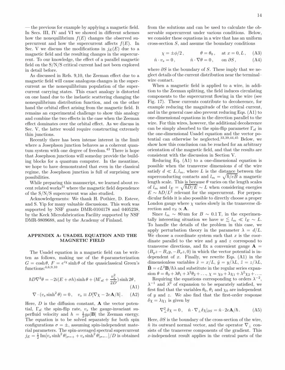
Finally, note that above we neglected the screen-ing of the magnetic field by the induced supercurrents.

FIG. 17: Supercurrent flow induced by a magnetic field B =(Bx, By, Bz) ∝ (3, 1, 2) in a thin rectangular wire. The arrowsindicate the magnitude and direction of the superfluid velocityvS . Fourth-order variational solution for χ is used here, seetext.

However, this should not be important in the experi-mental case, as the Josephson screening length λJ =√

~d2/2eµ0IcL & 200 nm is larger than the width ofthe junction, and the aluminum terminals are sufficientlythin as to produce only small screening.

∗ Present address: Department of Physics, Taylor Univer-sity, Upland, IN 46989, USA

† Present address: Laboratoire de Photonique et deNanostructures-CNRS, Route de Nozay, 91460 Marcous-sis, France

‡ Electronic address: birge@pa.msu.edu1 P.G. de Gennes, Rev. Mod. Phys. 36, 225 (1964).2 B. Pannetier and H. Courtois, J. Low Temp. Phys. 118,

599 (2000).3 C.J. Lambert and R. Raimondi, J. Phys.:Condens. Matter

10, 901 (1998).

4 W. Belzig, F.K. Wilhelm, C. Bruder, G. Schon, andA.D Zaikin, Superlattices and Microstructures, 25, 1251,(1999).

5 J.J.A. Baselmans, A.F. Morpurgo, B.J. van Wees, T.M.Klapwijk, Nature 397, 43 (1999).

6 K.D. Usadel, Phys. Rev. Lett. 25, 507 (1970).7 R. Shaikhaidarov, A.F. Volkov, H. Takayanagi, V.T. Pe-

trashov, and P. Delsing, Phys. Rev. B 62 R14649 (2000).8 J. Huang, F. Pierre, T.T. Heikkila, F.K. Wilhelm, and

N.O. Birge, Phys. Rev. B 66, 020507(R) (2002).9 T.T. Heikkila, F.K. Wilhelm, and G. Schon, Europhys.

16

Lett. 51, 434 (2000).10 S.K. Yip, Phys. Rev. B 62, R6127 (2000).11 T.T. Heikkila, T. Vanska, and F.K. Wilhelm, Phys. Rev.

B 67, 100502(R) (2003). Note that in this reference thereis a sign error in the T (x) coefficient, which increases theamplitude of the change δf .

12 M.S. Crosser, P. Virtanen, T.T. Heikkila, and N.O. Birge,Phys. Rev. Lett. 96, 167004 (2006).

13 G.J. Dolan and J.H. Dunsmuir, Physica B 152, 7 (1988).14 S. Gueron, Ph.D. thesis, University Paris VI, France,

(1997).15 A.F. Volkov, Phys. Rev. Lett. 74 4730 (1995).16 A.F. Morpurgo, T.M. Klapwijk and B.J. van Wees, Appl.

Phys. Lett. 72, 966 (1998).17 S.K. Yip, Phys. Rev. B 58, 5803 (1998).18 F.K. Wilhelm, G. Schon, and A.D. Zaikin, Phys. Rev. Lett.

81, 1682 (1998).19 I.O. Kulik, Sov. Phys. JETP, 30, 944, (1970).20 T.T. Heikkila, J. Sarkka, F.K. Wilhelm, Phys. Rev. B 66,

184 513 (2002).21 H. Pothier, et al., Phys. Rev. Lett. 79, 3490 (1997).22 B.J. van Wees, K.-M.H. Lenssen, and C.J.P.M. Harmans,

Phys. Rev. B 44, 470 (1991).23 J.J.A. Baselmans, T.T. Heikkila, B.J. van Wees, T.M.

Klapwijk, Phys. Rev. Lett. 89, 207002 (2002).24 V. Petrashov, V. Antonov, P. Delsing, and T. Claeson,

Phys. Rev. Lett. 74, 5268 (1995).25 A.F. Andreev, Sov. Phys. JETP 19(5), 1228 (1964).26 F. Pierre, Ann. Phys. (Paris) 26, No. 4 (2001), Ch. 3.27 This procedure also neglects the (presumably weak) prox-

imity effect on the kernel of the electron-electron collisionintegral. These are similar to those in bulk superconduc-tors, see G. M. Eliashberg, Zh. Eksp. Teor. Fiz. 61, 1254(1971) [Sov. Phys. JETP 34, 668 (1972)].

28 K.E. Nagaev, Phys. Rev. B 52, 4740 (1995).29 M. Henny, S. Oberholzer, C. Strunk, and C. Schonen-

berger, Phys. Rev. B 59, 2871 (1999).

30 M.S. Crosser, Ph.D. Thesis, Michigan State University(2005).

31 L. Angers, F. Chiodi, J.C. Cuevas, G. Montambaux, M.Ferrier, S. Gueron, H. Bouchiat, [arXiv:0708.0205]; J.C.Cuevas and F.S. Bergeret, Phys. Rev. Lett. 99, 217002(2007).

32 V.V. Ryazanov, V.A. Oboznov, A.Yu. Rusanov, A.V.Veretennikov, A.A. Golubov, and J. Aarts, Phys. Rev.Lett. 86, 2427 (2001).

33 J.C. Hammer, J.C. Cuevas, F.S. Bergeret, W. Belzig, Phys.Rev. B 76, 064514 (2007).

34 E. Scheer, H.V. Lohneysen, A.D. Mirlin, P. Wolfle, and H.Hein, Phys. Rev. Lett., 78, 3362 (1997).

35 P. Virtanen and T.T. Heikkila, Phys. Rev. B 75, 104517(2007).

36 P. Virtanen and T.T. Heikkila, J. Low Temp. Phys. 136,401 (2004), and references therein.

37 G.L. Ingold and Y.V. Nazarov, Single Charge tunneling

Coulomb Blockade phenomena in Nanostructures, vol. 294(Plenum Press, London, 1992).

38 Similar behavior has been observed by other groups. C.f.p. 40 of F. Pierre, Ann. Phys. (Paris) 26, No. 4, 1 (2001).

39 A. Anthore, H. Pothier, and D. Esteve, Phys. Rev. Lett.90, 127001 (2003).

40 R.B. Pettit and J. Silcox, Phys. Rev. B 13, 2865 (1976).41 R.W. Cohen and B. Abeles, Phys. Rev. 168, 444 (1968).42 J. Eom, C.-J. Chien, and V. Chandrasekhar, Phys. Rev.

Lett. 81, 437 (1998); A. Parsons, I. A. Sosnin, and V. T.Petrashov, Phys. Rev. B 67, 140502 (R) (2003).

43 V. Bouchiat, D. Vion, P. Joyez, D. Esteve, and M.H. De-voret, Physica Scripta T76, 165 (1998).

44 W. Belzig, C. Bruder, and G. Schon, Phys. Rev. B 54,9443 (1996).

45 See also Ch. 8 in P.G. deGennes, Superconductivity of Met-

als and Alloys, (Perseus Books, Massachusetts, 1966).