Embed Size (px)
Citation preview

arX
iv:1
811.
0112
8v1
[m
ath.
AP]
2 N
ov 2
018
Nonlinear damped Timoshenko systems with second sound —
global existence and exponential stability
Salim A. Messaoudi∗, Michael Pokojovy†, Belkacem Said-Houari‡
March 2008
Abstract
In this paper, we consider nonlinear thermoelastic systems of Timoshenko type in a one-dimensional
bounded domain. The system has two dissipative mechanisms being present in the equation for transverse
displacement and rotation angle — a frictional damping and a dissipation through hyperbolic heat
conduction modelled by Cattaneo’s law, respectively. The global existence of small, smooth solutions
and the exponential stability in linear and nonlinear cases are established.
AMS-Classification: 35B37, 35L55, 74D05, 93D15, 93D20Keywords: Timoshenko systems, thermoelasticity, second sound, exponential decay, nonlinearity, globalexistence
1 Introduction
In [1], a simple model describing the transverse vibration of a beam was developed. This is given by a systemof two coupled hyperbolic equations of the form
ρutt = (K(ux − ϕ))x in (0,∞)× (0, L), (1)
Iρϕtt = (EIϕx)x +K(ux − ϕ) in (0,∞)× (0, L),
where t denotes the time variable and x the space variable along a beam of length L in its equilibriumconfiguration. The unknown functions u and ϕ depending on (t, x) ∈ (0,∞) × (0, L) model the transversedisplacement of the beam and the rotation angle of its filament, respectively. The coefficients ρ, Iρ, E,I and K represent the density (i.e. the mass per unit length), the polar momentum of inertia of a crosssection, Young’s modulus of elasticity, the momentum of inertia of a cross section, and the shear modulus,respectively.
Kim and Renardy considered (1) in [2] together with two boundary controls of the form
Kϕ(t, L)−Kux(t, L) = αut(t, L) in (0,∞),
EIϕx(t, L) = −βϕt(t, L) in (0,∞)
and used the multiplier techniques to establish an exponential decay result for the natural energy of (1).They also provided some numerical estimates to the eigenvalues of the operator associated with the system(1). An analogous result was also established by Feng et al. in [3], where a stabilization of vibrations in aTimoshenko system was studied. Rapos et al. studied in [4] the following system
ρ1utt −K(ux − ϕ)x + ut = 0 in (0,∞)× (0, L),
∗Mathematical Sciences Department, KFUPM, Dhahran 31261, Saudi Arabia
E-mail: [email protected]†Fachbereich Mathematik und Statistik, Universität Konstanz, 78457 Konstanz, Germany
E-mail: [email protected]‡Université Badji Mokhtar, Laboratoire de Mathématiques Appliquées, B.P. 12 Annaba 23000, Algerie
E-mail: [email protected]
1

ρ2 − bϕxx +K(ux − ϕ) + ϕt = 0 in (0,∞)× (0, L), (2)
u(t, 0) = u(t, L) = ϕ(t, 0) = ϕ(t, L) = 0 in (0,∞)
and proved that the energy associated with (2) decays exponentially. This result is similar to that one byTaylor [5], but as they mentioned, the originality of their work lies in the method based on the semigrouptheory developed by Liu and Zheng [6].
Soufyane and Wehbe considered in [7] the system
ρutt = (K(ux − ϕ))x in (0,∞)× (0, L),
Iρϕtt = (EIϕx)x +K(ux − ϕ)− bϕt in (0,∞)× (0, L), (3)
u(t, 0) = u(t, L) = ϕ(t, 0) = ϕ(t, L) = 0 in (0,∞),
where b is a positive continuous function satisfying
b(x) ≥ b0 > 0 in [a0, a1] ⊂ [0, L].
In fact, they proved that the uniform stability of (3) holds if and only if the wave speeds are equal, i.e.
K
ρ=EI
Iρ,
otherwise, only the asympotic stability has been proved. This result improves previous ones by Soufyane[8] and Shi and Feng [9] who proved an exponential decay of the solution of (1) together with two locallydistributed feedbacks.
Recently, Rivera and Racke [10] obtained a similar result in a work where the damping function b = b(x)is allowed to change its sign. Also, Rivera and Racke [11] treated a nonlinear Timoshenko-type system ofthe form
ρ1ϕtt − σ1(ϕx, ψ)x = 0,
ρ2ψtt − χ(ψx)x + σ2(ϕx, ψ) + dψt = 0
in a one-dimensional bounded domain. The dissipation is produced here through a frictional damping whichis only present in the equation for the rotation angle. The authors gave an alternative proof for a necessaryand sufficient condition for exponential stability in the linear case and then proved a polynomial stability ingeneral. Moreover, they investigated the global existence of small smooth solutions and exponential stabilityin the nonlinear case.
Xu and Yung [12] studied a system of Timoshenko beams with pointwise feedback controls, looked for theinformation about the eigenvalues and eigenfunctions of the system, and used this information to examinethe stability of the system.
Ammar-Khodja et al. [13] considered a linear Timoshenko-type system with a memory term of the form
ρ1ϕtt −K(ϕx + ψ)x = 0, (4)
ρ2ψtt − bψxx +
∫ t
0
g(t− s)ψxx(s)ds+K(ϕx + ψ) = 0
in (0,∞)× (0, L), together with homogeneous boundary conditions. They applied the multiplier techniquesand proved that the system is uniformly stable if and only if the wave speeds are equal, i.e. K
ρ1= b
ρ2, and
g decays uniformly. Precisely, they proved an exponential decay if g decays exponentially and polynomialdecay if g decays polynomially. They also required some technical conditions on both g′ and g′′ to obtaintheir result. The feedback of memory type has also been studied by Santos [14]. He considered a Timoshenkosystem and showed that the presense of two feedbacks of memory type at a subset of the bounary stabilizesthe system uniformly. He also obtained the energy decay rate which is exactly the decay rate of the relaxationfunctions.
Shi and Feng [15] investigated a nonuniform Timoshenko beam and showed that the vibration of thebeam decays exponentially under some locally distributed controls. To achieve their goal, the authors usedthe frequency multiplier method.
2
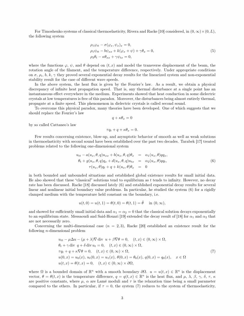
For Timoshenko systems of classical thermoelasticity, Rivera and Racke [10] considered, in (0,∞)×(0, L),the following system
ρ1ϕtt − σ(ϕx, ψx)x = 0,
ρ1ψtt − bψxx + k(ϕx + ψ) + γθx = 0, (5)
ρ3θt − κθxx + γψtx = 0,
where the functions ϕ, ψ, and θ depend on (t, x) and model the transverse displacement of the beam, therotation angle of the filament, and the temperature difference, respectively. Under appropriate conditionson σ, ρi, b, k, γ they proved several exponential decay results for the linearized system and non-exponentialstability result for the case of different wave speeds.
In the above system, the heat flux is given by the Fourier’s law. As a result, we obtain a physicaldiscrepancy of infinite heat propagation speed. That is, any thermal disturbance at a single point has aninstantaneous effect everywhere in the medium. Experiments showed that heat conduction in some dielectriccrystals at low temperatures is free of this paradox. Moreover, the disturbances being almost entirely thermal,propagate at a finite speed. This phenomenon in dielectric crystals is called second sound.
To overcome this physical paradox, many theories have been developed. One of which suggests that weshould replace the Fourier’s law
q + κθx = 0
by so called Cattaneo’s lawτqt + q + κθx = 0.
Few results concerning existence, blow-up, and asymptotic behavior of smooth as well as weak solutionsin thermoelasticity with second sound have been established over the past two decades. Tarabek [17] treatedproblems related to the following one-dimensional system
utt − a(ux, θ, q)uxx + b(ux, θ, q)θx = α1(ux, θ)qqx,
θt + g(ux, θ, q)qx + d(ux, θ, q)utx = α2(ux, θ)qqt, (6)
τ(ux, θ)qt + q + k(ux, θ)θx = 0
in both bounded and unbounded situations and established global existence results for small initial data.He also showed that these “classical” solutions tend to equilibrium as t tends to infinity. However, no decayrate has been discussed. Racke [18] discussed lately (6) and established exponential decay results for severallinear and nonlinear initial boundary value problems. In particular, he studied the system (6) for a rigidlyclamped medium with the temperature held constant on the boundary, i.e.
u(t, 0) = u(t, 1) = θ(t, 0) = θ(t, 1) = θ in (0,∞),
and showed for sufficiently small initial data and α1 = α2 = 0 that the classical solution decays exponentiallyto an equilibrium state. Messaoudi and Said-Houari [19] extended the decay result of [18] for α1 and α2 thatare not necessarily zero.
Concerning the multi-dimensional case (n = 2, 3), Racke [20] established an existence result for thefollowing n-dimensional problem
utt − µ∆u− (µ+ λ)∇ div u+ β∇θ = 0, (t, x) ∈ (0,∞)× Ω,
θt + γ div q + δ divut = 0, (t, x) ∈ (0,∞)× Ω,
τqt + q + κ∇θ = 0, (t, x) ∈ (0,∞)× Ω, (7)
u(0, x) = u0(x), ut(0, x) = u1(x), θ(0, x) = θ0(x), q(0, x) = q0(x), x ∈ Ω
u(t, x) = θ(t, x) = 0, (t, x) ∈ (0,∞)× ∂Ω,
where Ω is a bounded domain of Rn with a smooth boundary ∂Ω. u = u(t, x) ∈ R
n is the displacementvector, θ = θ(t, x) is the temperature difference, q = q(t, x) ∈ R
n is the heat flux, and µ, λ, β, γ, δ, τ , κare positive constants, where µ, α are Lamé moduli and τ is the relaxation time being a small parametercompared to the others. In particular, if τ = 0, the system (7) reduces to the system of thermoelasticity,
3

in which the heat flux is given by Fourier’s law instead of Cattaneo’s law. He also proved, under condition∇ × ∇u = ∇ × ∇q = 0, an exponential decay result for (7). This result is easily extended to the radiallysymetric solutions, as they satisfy the above condition.
Messaoudi [21] investigated the following problem
utt − µ∆u− (µ+ λ)∇ divu+ β∇θ = |u|p−2u, (t, x) ∈ (0,∞)× Ω,
θt + γ div q + δ divut = 0, (t, x) ∈ (0,∞)× Ω,
τqt + q + κ∇θ = 0, (t, x) ∈ (0,∞)× Ω, (8)
u(0, x) = u0(x), ut(0, x) = u1(x), θ(0, x) = θ0(x), q(0, x) = q0(x), x ∈ Ω
u(t, x) = θ(t, x) = 0, (t, x) ∈ (0,∞)× ∂Ω
for p > 2, where a nonlinear source term is competing with the damping caused by the heat conductionand established a local existence result. He also showed that solutions with negative initial energy blow upin finite time. The blow-up result was then improved by Messaoudi and Said-Houari [22] to accommodatecertain solutions with positive initial energy.
In the present work, we are concerned with
ρ1ϕtt − σ(ϕx, ψ)x + µϕt = 0, (t, x) ∈ (0,∞)× (0, L),
ρ2ψtt − bψxx + k(ϕx + ψ) + βθx = 0, (t, x) ∈ (0,∞)× (0, L),
ρ3θt + γqx + δψtx = 0, (t, x) ∈ (0,∞)× (0, L), (9)
τ0qt + q + κθx = 0, (t, x) ∈ (0,∞)× (0, L),
where ϕ = ϕ(t, x) is the displacement vector, ψ = ψ(t, x) is the rotation angle of the filament, θ = θ(t, x)is the temperature difference, q = q(t, x) is the heat flux vector, ρ1, ρ2, ρ3, b, k, γ, δ, κ, µ, τ0 are positiveconstants. The nonlinear function σ is assumed to be sufficiently smooth and satisfy
σϕx(0, 0) = σψ(0, 0) = k
andσϕxϕx(0, 0) = σϕxψ(0, 0) = σψψ = 0.
This system models the transverse vibration of a beam subject to the heat conduction given by Cattaneo’slaw instead of the usual Fourier’s one. We should note here that dissipative effects of heat conduction inducedby Cattaneo’s law are usualy weaker than those induced by Fourier’s law (an opposite effect was observedthough in [23]). This justifies the presence of the extra damping term in the first equation of (9). In factif µ = 0, Fernández Sare and Racke [24] have proved recently that (9) is no longer exponentially stableeven in the case of equal propagation speed (ρ1/ρ2 = k/b). Moreover, they showed that this ”unexpected“phenomenon (the loss of exponential stability) takes place even in the presence of a viscoelastic damping inthe second equation of (9). If µ > 0, but β = 0, one can also prove with the aid of semigroup theory (cf.[16], Section 4) that the system is not exponential stable independent of the relation between coefficients.Our aim is to show that the presence of frictional damping µϕt in the first equation of (9) will drive thesystem to stability in an exponential rate independent of the wave speeds in linear and nonlinear cases.
The structure of the paper is as follows. In section 2, we discuss the well-posedness and exponentialstability of the linearized problem for ϕ = ψ = q = 0 on the boundary. In section 3, we establish the sameresult for ϕx = ψ = q = 0 on the boundary. In section 4, we study the nonlinear system subject to theboundary conditions ϕx = ψ = q = 0, show the global unique solvability and exponential stability for smallinitial data.
2 Linear exponential stability — ϕ = ψ = q = 0
For the sake of technical convenience, by scaling the system (9), we transform it to an equivalent form
ρ1ϕtt − σ(ϕx, ψ)x + µϕt = 0, (t, x) ∈ (0,∞)× (0, L),
ρ2ψtt − bψxx + k(ϕx + ψ) + γθx = 0, (t, x) ∈ (0,∞)× (0, L),
4

ρ3θt + κqx + γψtx = 0, (t, x) ∈ (0,∞)× (0, L), (10)
τ0qt + δq + κθx = 0, (t, x) ∈ (0,∞)× (0, L),
with some other constants and the nonlinear function σ still satisfying (possibly for a new k)
σϕx(0, 0) = σψ(0, 0) = k (11)
andσϕxϕx(0, 0) = σϕxψ(0, 0) = σψψ = 0. (12)
In this section, we consider the linearization of (10) given by
ρ1ϕtt − k(ϕx + ψ)x + µϕt = 0, (t, x) ∈ (0,∞)× (0, L),
ρ2ψtt − bψxx + k(ϕx + ψ) + γθx = 0, (t, x) ∈ (0,∞)× (0, L),
ρ3θt + κqx + γψtx = 0, (t, x) ∈ (0,∞)× (0, L), (13)
τ0qt + δq + κθx = 0, (t, x) ∈ (0,∞)× (0, L),
completed by the following boundary and initial conditions
ϕ(t, 0) = ϕ(t, L) = ψ(t, 0) = ψ(t, L) = q(t, 0) = q(t, L) = 0 in (0,∞), (14)
ϕ(0, ·) = ϕ0, ϕt(0, ·) = ϕ1, ψ(0, ·) = ψ0, ψt(0, ·) = ψ1,
θ(0, ·) = θ0, q(0, ·) = q0. (15)
We present a brief discussion of the well-posedness, and the semigroup formulation of (13)–(15). For thispurpose, we set V := (ϕ, ϕt, ψ, ψt, θ, q)
t and observe that V satisfies
Vt = AVV (0) = V0
, (16)
where V0 := (ϕ0, ϕ1, ψ0, ψ1, θ0, q0)t and A is the differential operator
A =
0 1 0 0 0 0kρ1∂2x − µ
ρ1kρ1∂x 0 0 0
0 0 0 1 0 0− kρ2∂x 0 b
ρ2∂2x − k
ρ20 − γ
ρ2∂x 0
0 0 0 − γρ3∂x 0 − κ
ρ2∂x
0 0 0 0 − κτ0∂x − δ
τ0
.
The energy space
H := H10 ((0, L))× L2((0, L))×H1
0 ((0, L))× L2((0, L))× L2((0, L))× L2((0, L))
is a Hilbert space with respect to the inner product
〈V,W 〉H = ρ1〈V 1,W 1〉L2((0,L)) + ρ2〈V 4,W 4〉L2((0,L))
+ b〈V 3x ,W
3x 〉L2((0,L)) + k〈V 1
x + V 3,W 1x +W 3〉L2((0,L))
+ ρ3〈V 5,W 5〉L2((0,L)) + τ0〈V 6,W 6〉
for all V,W ∈ H. The domain of A is then
D(A) = V ∈ H |V 1, V 3 ∈ H2((0, L)) ∩H10 ((0, L)), V
2, V 3 ∈ H10 ((0, L))
V 5, V 6 ∈ H10 ((0, L)), V
5x ∈ H1
0 ((0, L)).
It is easy to show according to [18] the validness of
Lemma 1 The operator A has the following properties:
5

1. D(A) = H and A is closed;
2. A is dissipative;
3. D(A) = D(A∗).
Now, by the virtue of the Hille-Yosida theorem, we have the following result.
Theorem 1 A generates a C0-semigroup of contractions eAtt≥0. If V0 ∈ D(A), the unique solutionV ∈ C1([0,∞),H) ∩ C0([0,∞), D(A)) to (16) is given by V (t) = eAtV0. If V0 ∈ D(An) for n ∈ N, thenV ∈ C0([0,∞), D(An)).
Our next aim is to obtain an exponential stability result for the energy functional E(t) = E(t;ϕ, ψ, θ, q)given by
E(t;ϕ, ψ, θ, q) =1
2
∫ L
0
(ρ1ϕ2t + ρ2ψ
2t + bψ2
x + k(ϕx + ψ)2 + ρ3θ2 + τ0q
2)dx.
We formulate and prove the following theorem.
Theorem 2 Let (ϕ, ψ, θ, q) be the unique solution to (13)–(15). Then, there exist two positive constants Cand α, independent of t and the initial data, such that
E(t;ϕ, ψ, θ, q) ≤ CE(0;ϕ, ψ, θ, q)e−2αt for all t ≥ 0,
where θ(t, x) = θ(t, x) − 1L
∫ L
0 θ0(s)ds.
Proof: To show the exponential stability of the energy functional, we use the Lyapunov’s method, i.e.we construct a Lyapunov functional L satisfying
β1E(t) ≤ L(t) ≤ β2E(t), t ≥ 0
for positive constants β1, β2 andd
dtL(t) ≤ −2αL(t), t ≥ 0
for some α > 0. This will be achieved by a careful choice of multiplicators.Multiplying in L2((0, L)) the first equation in (13) by ϕt, the second by ψt, the third by θ and the fourth
by q and partially integrating, we obtain
d
dtE(t) = −µ
∫ L
0
ϕ2tdx− δ
∫ L
0
q2dx. (17)
As in [16], let w be a solution to
−wxx = ψx, w(0) = w(L) = 0
and let
I1 :=
∫ L
0
(
ρ2ψtψ + ρ1ϕtw − γτ0κψq)
dx.
Then, we obtain taking into account the second equation in (13)
d
dt
∫ L
0
ρ2ψtψdx = ρ2
∫ L
0
(ψ2t + ψttψ
)dx
= ρ2
∫ L
0
ψ2t dx+ b
∫ L
0
ψxxψdx− k
∫ L
0
(ϕx + ψ)ψdx − γ
∫ L
0
θxψdx.
6

Further, we get using the first and the fourth equations in (13)
d
dt
∫ L
0
ρ1ϕtwdx = ρ1
∫ L
0
(ϕttw + ϕtwt) dx
= −k∫ L
0
ϕψxdx+ k
∫ L
0
w2xdx− µ
∫ L
0
ϕtwdx+ ρ1
∫ L
0
ϕtwtdx,
d
dt
∫ L
0
−γτ0κψqdx = −γτ0
κ
∫ L
0
ψtqdx+γ
κ
∫ L
0
ψ(δq + κθx)dx
= −γτ0κ
∫ L
0
ψtqdx+γδ
κ
∫ L
0
ψqdx + γ
∫ L
0
θxψdx.
By using the above inequalities, we find
d
dtI1 = ρ2
∫ L
0
ψ2t dx− b
∫ L
0
ψ2xdx− k
∫ L
0
ψ2dx+ k
∫ L
0
w2xdx
− µ
∫ L
0
ϕtwdx + ρ1
∫ L
0
ϕtwtdx− γτ0κ
∫ L
0
ψtqdx+γδ
κ
∫ L
0
ψqdx.
Observing∫ L
0
w2xdx ≤
∫ L
0
ψ2dx ≤ c
∫ L
0
ψ2xdx, (18)
with the Poincaré constant c = L2
π2 > 0, we conclude using the Young’s inequality
d
dtI1 ≤ ρ2
∫ L
0
ψ2t dx− b
∫ L
0
ψ2xdx− k
∫ L
0
ψ2dx+ k
∫ L
0
ψ2dx
+µ
2
∫ L
0
(
ε1w2 +
1
ε1ϕ2t
)
dx+ρ12
∫ L
0
(
ε1w2t +
1
ε1ϕ2t
)
dx
+γτ02κ
∫ L
0
(
ε1ψ2t +
1
ε1q2)
dx+γδ
2κ
∫ L
0
(
ε1ψ2 +
1
ε1q2)
dx
≤−[
b− ε12
(
µc2 +δγc
κ
)]∫ L
0
ψ2xdx+
[
ρ2 +ε12
(
ρ1c+γτ0κ
)] ∫ L
0
ψ2t dx
+1
2ε1(µ+ ρ1)
∫ L
0
ϕ2tdx+
1
2ε1
(γτ0κ
+δγ
κ
)∫ L
0
q2dx. (19)
for some ε1 > 0.Next, we consider the functional I2 given by
I2 := ρ1
∫ L
0
ϕtϕdx.
It easily follows that
d
dtI2 = ρ1
∫ L
0
ϕttϕdx+ ρ1
∫ L
0
ϕ2tdx
=
∫ L
0
k(ϕx + ψ)xϕdx− µ
∫ L
0
ϕtϕdx + ρ1
∫ L
0
ϕ2tdx
= −k∫ L
0
ϕ2xdx+ k
∫ L
0
ψxϕdx− µ
∫ L
0
ϕtϕdx+ ρ1
∫ L
0
ϕ2tdx,
which can be estimated by
d
dtI2 ≤ −k
∫ L
0
ϕ2xdx+
k
2
∫ L
0
(
ε2ϕ2 +
1
ε2ψ2x
)
dx
7

+µ
2
∫ L
0
(
ε2ϕ2 +
1
ε2ϕ2t
)
dx+ ρ1
∫ L
0
ϕ2tdx
≤ −(
k − ε2c
2(k + µ)
) ∫ L
0
ϕ2xdx+
k
2ε2
∫ L
0
ψ2xdx
+
(µ
2ε2+ ρ1
)∫ L
0
ϕ2tdx (20)
for some ε2 > 0.Next we consider a functional I3 defined by
I3 := N1I1 + I2
for some N1 > 0 and, combining (19) and (20), arrive at
d
dtI3 ≤−
[
N1
(
b − ε12
(
µc2 +δγc
κ
))
− k
2ε2
]∫ L
0
ψ2xdx
−(
k − ε2c
2(k + µ)
) ∫ L
0
ϕ2xdx+N1
[
ρ2 +ε12
(
ρ1c+γτ0κ
)] ∫ L
0
ψ2t dx
+
[
N11
2ε1(µ+ ρ1) +
(µ
2ε2+ ρ1
)]∫ L
0
ϕ2tdx
+N11
2ε1
(γτ0κ
+δγ
κ
)∫ L
0
q2dx. (21)
At this point, we introduce
θ(t, x) = θ(t, x)− 1
L
∫ L
0
θ0(x)dx.
One can easily verify that (ϕ, ψ, θ, q) satisfies system (13). Moreover, one can apply the Poincaré inequal-ity to θ
∫ L
0
θ2(t, x)dx ≤ c
∫ L
0
θ2x(t, x)dx,
since∫ L
0 θ(t, x)dx = 0 for all t ≥ 0. Until the end of this chapter, we shall work with θ but denote it with θ.
In order to obtain a negative term of∫ L
0ψ2t dx, we introduce, as in [16], the following functional
I4(t) := ρ2ρ3
∫ L
0
(∫ x
0
θ(t, y)dy
)
ψt(t, x)dx,
and find
d
dtI4 =
∫ L
0
(∫ x
0
ρ3θtdy
)
ρ2ψtdx+
∫ L
0
(∫ x
0
ρ3θdy
)
ρ2ψttdx
=−∫ L
0
(∫ x
0
κqx + γψtxdy
)
ρ2ψtdx
+
∫ L
0
(∫ x
0
ρ3θdy
)
(bψxx − k(ϕx + ψ)− γθx)dx
=− γρ2
∫ L
0
ψ2t dx− ρ2κ
∫ L
0
qψtdx− bρ3
∫ L
0
θψxdx
+ kρ3
∫ L
0
θϕdx − kρ3
∫ L
0
(∫ x
0
θdy
)
ψdx+ γρ3
∫ L
0
θ2dx.
8

This can be estimated as follows
d
dtI4 ≤ − γρ2
∫ L
0
ψ2t dx+
ρ2κ
2
∫ L
0
(
ε4ψ2t +
1
ε4q2)
dx+bρ32
∫ L
0
ε′4ψ2x
+1
ε′4θ2dx+
kρ32
∫ L
0
(
ε′4ϕ2 +
1
ε′4θ2)
dx+kρ32
∫ L
0
ε′4ψ2dx
+1
ε′4
(∫ x
0
θdy
)2
dx+ γρ3
∫ L
0
θ2dx
=[
−γρ2 +ε4ρ2κ
2
] ∫ L
0
ψ2t dx+
(ε′4ρ32
(b+ kc)
)∫ L
0
ψ2xdx
+ε′4kρ3c
2
∫ L
0
ϕ2xdx+
(
γρ3 +ρ32ε′4
(b+ k + kc)
)∫ L
0
θ2dx
+ρ2κ
2ε4
∫ L
0
q2dx (22)
for arbitrary positive ε4 and ε′4.Finally, we set
I5(t) := −τ0ρ3∫ L
0
q(t, x)
(∫ x
0
θ(t, y)dy
)
dx
and observe
d
dtI5(t) = −ρ3
∫ L
0
τ0qt
(∫ x
0
θdy
)
dx− τ0
∫ L
0
q
(∫ x
0
ρ3θtdy
)
dx
= −ρ3∫ L
0
(−δq − κθx)
(∫ x
0
θdy
)
dx
− τ0
∫ L
0
q
(∫ x
0
−κqx − γψtxdy
)
dx
= ρ3δ
∫ L
0
q
(∫ x
0
θdy
)
dx+ ρ3κ
∫ L
0
θx
(∫ x
0
θdy
)
dx
+ τ0κ
∫ L
0
q
(∫ x
0
qxdy
)
dx+ τ0γ
∫ L
0
q
(∫ x
0
ψtxdy
)
dx
=ρ3δ
2
∫ L
0
(
ε5
(∫ x
0
θ2dy
)2
+1
ε5q2
)
dx− ρ3κ
∫ L
0
θ2dx
+ τ0κ
∫ L
0
q2dx+τ0γ
2
∫ L
0
ε′5ψ2t +
1
ε′5q2dx
≤(
−ρ3κ+ε5ρ3δc
2
)∫ L
0
θ2dx+ε′5τ0γ
2
∫ L
0
ψ2t dx
+
(
τ0κ+ρ3δ
2ε5+τ0γ
2ε′5
)∫ L
0
q2dx (23)
for positive ε5 and ε′5For N,N4, N5 > 0, we can define an auxiliary functional F(t) by
F(t) := NE + I3 +N4I4 +N5I5.
From (21), (22) and (23), we have then
d
dtF(t) ≤− Cψx
∫ L
0
ψ2xdx− Cϕx
∫ L
0
ϕ2xdx− Cψt
∫ L
0
ψ2t dx
9

− Cθ
∫ L
0
θ2dx− Cϕt
∫ L
0
ϕ2tdx− Cq
∫ L
0
q2dx, (24)
where
Cψx =
[
N1
(
b − ε12
(
µc2 +δγc
κ
))
− k
2ε2−N4
ε′42ρ3(b + kc)
]
,
Cϕx =
[(
k − ε22c(k + µ)
)
−N4ε′42kρ3c
]
,
Cψt =
[
N4
(
γρ2 −ε4ρ2κ
2
)
−N1
(
ρ2 +ε12
(
ρ1c+γτ0κ
))
−N5ε′5τ0γ
2
]
,
Cθ =
[
N5
(
ρ3κ− ε5ρ3δc
2
)
−N4
(
γρ3 +ρ32ε′4
(b+ k + kc)
)]
,
Cϕt =
[
Nµ−N11
2ε1(µ+ ρ1)−
(µ
2ε2+ ρ1
)]
,
Cq =
[
N −N11
2ε1
(γτ0κ
+δγ
κ
)
−N4ρ2κ
2ε4−N5
(
τ0κ+ρ3δ
2ε5+τ0γ
2ε′5
)]
.
Choosing ε1, ε2, ε4, ε5 sufficiently small, then N1 and N4 sufficiently large, ε′4 sufficiently small, N5
sufficiently large, ε′5 sufficiently small and finally N sufficiently large, we can assure that
ε1 <2bκ
µκc2 + δγc, ε2 <
2k
c(k + µ), ε4 <
2γ
κ, ε5 <
2κ
δc,
N1 >k
2ε2
(
b− ε12
(
µc2 + δγcκ
)) ,
N4 >N1
(ρ2 +
ε12
(ρ1c+
γτ0κ
))
γρ2 − ε4ρ2κ2
,
ε′4 < min
2N1
(
b− ε12
(
µc2 + δγcκ
))
N4ρ3(b+ kc),2(k − ε2
2 c(k + µ))
N4kρ3c
,
N5 >N4
(
γρ3 +ρ32ε′
4
(b+ k + kc))
ρ3κ− ε5ρ3δc2
,
ε′5 <2(N4
(γρ2 − ε4ρ2κ
2
)−N1
(ρ2 +
ε12
(ρ1c+
γτ0κ
)))
N5τ0γ
N > max
N1
12ε1
(µ+ ρ1) +(µ2ε2
+ ρ1
)
µ,
N11
2ε1
(γτ0κ
+δγ
κ
)
+N4ρ2κ
2ε4+N5
(
τ0κ+ρ3δ
2ε5+τ0γ
2ε′5
)
.
Having fixed the constants as above, we find that all the terms on the right-hand side of (24) are negative.Now, we have to estimate d
dtF(t) versus −d2E(t) for a d2 > 0. By letting C := 12 minCψx , Cϕx, we
conclude from (24) that
d
dtF(t) ≤ −C
∫ L
0
ψ2xdx
︸ ︷︷ ︸
≤−Cc
∫ L0ψ2dx
−C∫ L
0
ϕ2xdx− (Cψx − C)
∫ L
0
ψ2xdx
10

− Cψt
∫ L
0
ψ2t dx− Cθ
∫ L
0
θ2dx− Cϕt
∫ L
0
ϕ2tdx− Cq
∫ L
0
q2dx
≤ −min
C,C
c
∫ L
0
(ϕ2x + ψ2
)
︸ ︷︷ ︸
≥ 1
2(ϕx+ψ)2
dx− (Cψx − C)
∫ L
0
ψ2xdx
− Cψt
∫ L
0
ψ2t dx− Cθ
∫ L
0
θ2dx− Cϕt
∫ L
0
ϕ2tdx− Cq
∫ L
0
q2dx
≤ −Cϕt
∫ L
0
ϕ2tdx− Cψt
∫ L
0
ψ2t dx− (Cψx − C)
∫ L
0
ψ2xdx
− minC, Cc
2
∫ L
0
(ϕx + ψ)2dx− Cθ
∫ L
0
θ2dx− Cq
∫ L
0
q2dx
≤ −d1∫ L
0
(ϕ2t + ψ2
t + ψ2x + (ϕx + ψ)2 + θ2 + q2)dx. (25)
with
d1 := min
Cϕt , Cψt , (Cψx − C),min
C, Cc
2, Cθ, Cq
. (26)
For d2 := 2d1maxρ1,ρ2,b,k,ρ3,τ0 , we can therefore estimate
d
dtF(t) ≤ −d2E(t).
Finally, we consider the functional H(t) := I3 +N4I4 +N5I5 and show for this
|H(t)| ≤ CE(t), C > 0.
By using the trivial relation
∫ L
0
ϕ2dx ≤ 2c
∫ L
0
(ϕx + ψ)2dx+ 2c2∫ L
0
ψ2xdx
with the Poincaré constant c = L2
π2 we arive at
|H(t)| = |N1I1 + I2 +N4I4 +N5I5| ≤ N1|I1|+ |I2|+N4|N4|+N5|I5|
= N1
∣∣∣∣∣
∫ L
0
(
ρ2ψtψ + ρ1ϕtw − γτ0κψq)
dx
∣∣∣∣∣+ ρ1
∣∣∣∣∣
∫ L
0
ϕtϕdx
∣∣∣∣∣
+N4ρ2ρ3
∣∣∣∣∣
∫ L
0
(∫ x
0
θ(t, x)dy
)
ψt(t, x)dx
∣∣∣∣∣+N5τ0ρ3
∣∣∣∣∣
∫ L
0
q
(∫ x
0
θdy
)
dx
∣∣∣∣∣
≤ N1
(
ρ22
∫ L
0
ψ2t dx+
ρ2c
2
∫ L
0
ψ2xdx+
ρ12
∫ L
0
ϕ2tdx+
ρ1c2
2
∫ L
0
ψ2xdx
+γτ0c
2κ
∫ L
0
ψ2xdx+
γτ02κ
∫ L
0
q2dx
)
+ρ12
(∫ L
0
ϕ2tdx+
∫ L
0
ϕ2dx
)
+ρ2ρ3N4
2
(
c
∫ L
0
θ2dx+
∫ L
0
ψ2t dx
)
+τ0ρ3N5
2
(∫ L
0
q2dx+ c
∫ L
0
θ2dx
)
≤ Cϕt
∫ L
0
ϕ2t + Cψt
∫ L
0
ψ2t dx+ Cϕx
∫ L
0
ψ2xdx
+ Cϕx+ψ
∫ L
0
(ϕx + ψ)2dx+ Cθ
∫ L
0
θ2dx+ Cq
∫ L
0
q2dx, (27)
11

where the constants are determined as follows
Cϕt :=1
2(N1ρ1 + ρ1) , Cψt :=
1
2(N1ρ2 + ρ2ρ3N4) ,
Cψx :=1
2
(
N1ρ2c+N1ρ1c2 +
N1τ0c
κ+ 2ρ1c
2
)
,
Cϕx+ψ := ρ1c, Cθ :=1
2(N4ρ2ρ3c+N5ρ3τ0c) , Cq :=
1
2
(N1γτ0κ
+N5ρ3τ0
)
.
According to (27) we have |H(t)| ≤ CE(t) for
C :=max
Cϕt , Cψt , Cψx , Cϕx+ψ, Cθ, Cq
min ρ1, ρ2, b, k, ρ3, τ0.
Taking finally N > maxN, C and defining a Lyapunov functional
L(t) := NE +H(t) = NE + I3 +N4I4 +N5I5, (28)
we obtain, on the one hand,β1E(t) ≤ L(t) ≤ β2E(t) (29)
for β1 := N − C > 0, β2 := N + C > 0, on the other hand, we know that
d
dtL(t) ≤ −d2E(t) ≤ −d2
β2L(t).
By using the Gronwall’s lemma, we conclude for α := d22β2
that
L(t) ≤ e−2αt0).
Eventually, (29) yieldsE(t) ≤ Ce−2αtE(0)
with C := β2
β1.
3 Linear exponential stability — ϕx = ψ = q = 0
The second set of boundary conditions we are going to study in this paper is
ϕx(t, 0) = ϕx(t, L) = ψ(t, 0) = ψ(t, L) = q(t, 0) = q(t, L) = 0 in (0,∞). (30)
Here, we consider the initial boundary value problem (13), (15), (30). We will present a semigroupformulation of this problem, show the exponential stability of the associated semigroup and make estimateson higher energies. This will enable us to prove global existence and exponential stability also in nonlinearsettings.
Let
L2∗((0, L)) =
u ∈ L2((0, L))
∣∣
∫ L
0
u(x)dx = 0,
H1∗ ((0, L)) =
u ∈ H1((0, L))
∣∣
∫ L
0
u(x)dx = 0.
We introduce a Hilbert space
H := H1∗ ((0, L))× L2
∗((0, L))×H10 ((0, L))× L2((0, L))× L2
∗((0, L))× L2((0, L))
12

equipped with the inner product
〈V,W 〉H = ρ1〈V 1,W 1〉L2((0,L)) + ρ2〈V 4,W 4〉L2((0,L))
+ b〈V 3x ,W
3x 〉L2((0,L)) + k〈V 1
x + V 3,W 1x +W 3〉L2((0,L))
+ ρ3〈V 5,W 5〉L2((0,L)) + τ0〈V 6,W 6〉L2((0,L)).
Let the operator A be formally defined as in section 2 with the domain
D(A) = V ∈ H |V 1 ∈ H2((0, L)), V 1x ∈ H1
0 ((0, L)), V2 ∈ H1
∗ ((0, L)),
V 3 ∈ H2((0, L)), V 4 ∈ H10 ((0, L)),
V 5 ∈ H1∗ ((0, L)), V
6 ∈ H10 ((0, L)).
Setting V := (ϕ, ϕt, ψ, ψt, θ, q)t, we observe that V satisfies
Vt = AVV (0) = V0
, (31)
where V0 := (ϕ0, ϕ1, ψ0, ψ1, θ0, q0)t.
By assuring that A satisfies the conditions of the Hille-Yosida theorem, we can easily get
Theorem 3 A generates a C0-semigroup of contractions eAtt≥0. If V0 ∈ D(A), the the unique solutionV ∈ C1([0,∞),H) ∩ C0([0,∞), D(A)) to (31) is given by V (t) = eAtV0. If V0 ∈ D(An) for n ∈ N, thenV ∈ C0([0,∞), D(An)).
Moreover, we can show that the Lyapunov functional (28) constructed in section 2 is also a Lyapunovfunctional for (31). Observing for the energy E(t) of the unique solution (ϕ, ψ, θ, q) that
E(t) =1
2‖V ‖2H
holds independent of t, we obtain the exponential stability of the associated semigroup eAtt≥0.
Theorem 4 The semigroup eAtt≥0 associated with A is exponential stable, i.e.
∃c1 > 0 ∀t ≥ 0 ∀V0 ∈ H : ‖eAtV0‖H ≤ c1e−αt‖V0‖H. (32)
Similar to [16], we observe that if V0 ∈ D(A), we can estimate AV (t) in the same way as V (t) is estimatedin (32), implying in its turn using the structure of A that (V 1
x , V2x , V
3x , V
4x , V
5x , V
6x ) can be estimated in the
norm of H, hence, one can estimate ((ϕx)x, (ϕt)x, (ψx)x, (ψt)x, θx, qx)t in L2((0, L))6.
We define for s ∈ N the Hilbert space
Hs := (Hs ×Hs−1 ×Hs ×Hs−1 ×Hs−1 ×Hs−1)((0, L))
with natural norm Sobolev norm for its component. Using the consideration above, we can therefore estimate
‖V (t)‖Hs ≤ cs‖V0‖Hse−αt. (33)
cs denotes here a positive constant, being independent of V0 and t.
4 Nonlinear exponential stability
In this section, we study the nonlinear system
ρ1ϕtt − σ(ϕx, ψ)x + µϕt = 0, (t, x) ∈ (0,∞)× (0, L),
ρ2ψtt − bψxx + k(ϕx + ψ) + γθx = 0, (t, x) ∈ (0,∞)× (0, L),
ρ3θt + κqx + γψtx = 0, (t, x) ∈ (0,∞)× (0, L), (34)
13
τ0qt + δq + κθx = 0, (t, x) ∈ (0,∞)× (0, L),
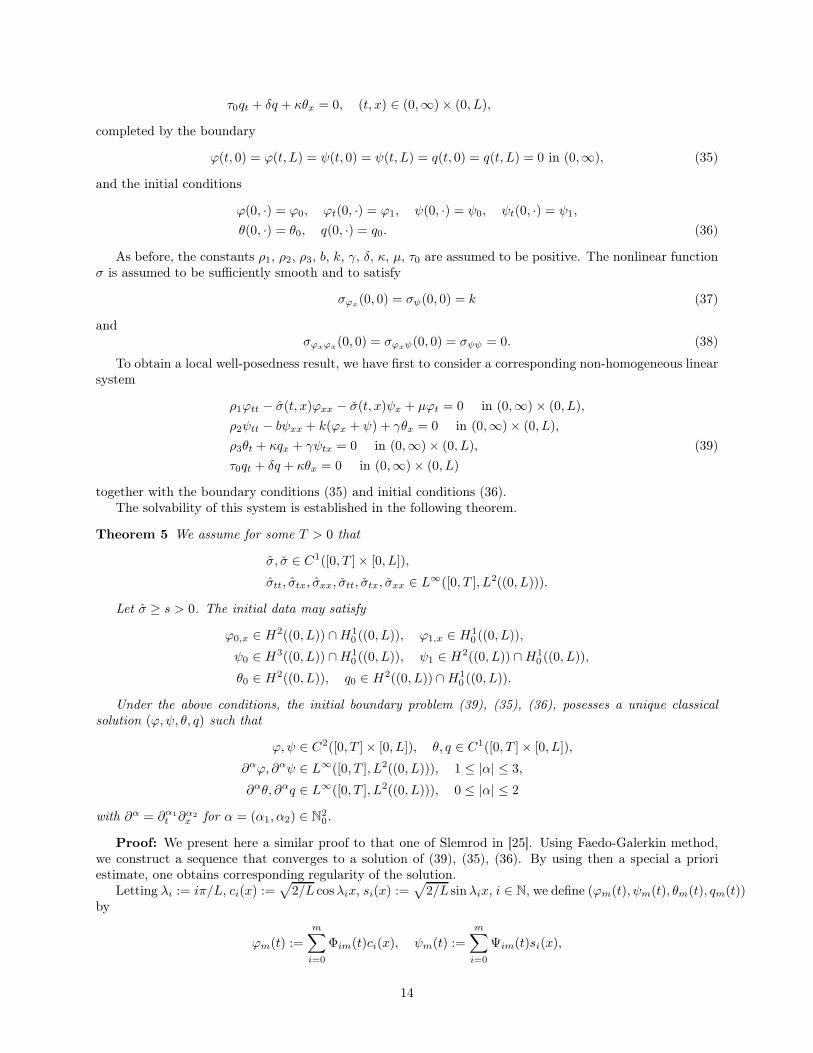
completed by the boundary
ϕ(t, 0) = ϕ(t, L) = ψ(t, 0) = ψ(t, L) = q(t, 0) = q(t, L) = 0 in (0,∞), (35)
and the initial conditions
ϕ(0, ·) = ϕ0, ϕt(0, ·) = ϕ1, ψ(0, ·) = ψ0, ψt(0, ·) = ψ1,
θ(0, ·) = θ0, q(0, ·) = q0. (36)
As before, the constants ρ1, ρ2, ρ3, b, k, γ, δ, κ, µ, τ0 are assumed to be positive. The nonlinear functionσ is assumed to be sufficiently smooth and to satisfy
σϕx(0, 0) = σψ(0, 0) = k (37)
andσϕxϕx(0, 0) = σϕxψ(0, 0) = σψψ = 0. (38)
To obtain a local well-posedness result, we have first to consider a corresponding non-homogeneous linearsystem
ρ1ϕtt − σ(t, x)ϕxx − σ(t, x)ψx + µϕt = 0 in (0,∞)× (0, L),
ρ2ψtt − bψxx + k(ϕx + ψ) + γθx = 0 in (0,∞)× (0, L),
ρ3θt + κqx + γψtx = 0 in (0,∞)× (0, L), (39)
τ0qt + δq + κθx = 0 in (0,∞)× (0, L)
together with the boundary conditions (35) and initial conditions (36).The solvability of this system is established in the following theorem.
Theorem 5 We assume for some T > 0 that
σ, σ ∈ C1([0, T ]× [0, L]),
σtt, σtx, σxx, σtt, σtx, σxx ∈ L∞([0, T ], L2((0, L))).
Let σ ≥ s > 0. The initial data may satisfy
ϕ0,x ∈ H2((0, L)) ∩H10 ((0, L)), ϕ1,x ∈ H1
0 ((0, L)),
ψ0 ∈ H3((0, L)) ∩H10 ((0, L)), ψ1 ∈ H2((0, L)) ∩H1
0 ((0, L)),
θ0 ∈ H2((0, L)), q0 ∈ H2((0, L)) ∩H10 ((0, L)).
Under the above conditions, the initial boundary problem (39), (35), (36), posesses a unique classicalsolution (ϕ, ψ, θ, q) such that
ϕ, ψ ∈ C2([0, T ]× [0, L]), θ, q ∈ C1([0, T ]× [0, L]),
∂αϕ, ∂αψ ∈ L∞([0, T ], L2((0, L))), 1 ≤ |α| ≤ 3,
∂αθ, ∂αq ∈ L∞([0, T ], L2((0, L))), 0 ≤ |α| ≤ 2
with ∂α = ∂α1
t ∂α2
x for α = (α1, α2) ∈ N20.
Proof: We present here a similar proof to that one of Slemrod in [25]. Using Faedo-Galerkin method,we construct a sequence that converges to a solution of (39), (35), (36). By using then a special a prioriestimate, one obtains corresponding regularity of the solution.
Letting λi := iπ/L, ci(x) :=√
2/L cosλix, si(x) :=√
2/L sinλix, i ∈ N, we define (ϕm(t), ψm(t), θm(t), qm(t))by
ϕm(t) :=
m∑
i=0
Φim(t)ci(x), ψm(t) :=
m∑
i=0
Ψim(t)si(x),
14

θm(t) :=
m∑
i=0
Θim(t)ci(x), qm(t) :=
m∑
i=0
Qim(t)si(x),
where
Φim(0) =
∫ L
0
ϕ0(x)ci(x)dx, Φim(0) =
∫ L
0
ϕ1(x)si(x)dx,
Ψim(0) =
∫ L
0
ψ0(x)si(x)dx, Ψim(0) =
∫ L
0
ψ1(x)ci(x)dx,
Θim(0) =
∫ L
0
θ0(x)ci(x)dx, Qim(0) =
∫ L
0
q0(x)si(x)dx.
Multiplying the equations in (39) in L2((0, L)) by ci, si, ci and si, respectively, we observe that thefunctions Φim, Ψim, Θim, Qim satisfy a system of ordinary differential equations
ρ1Φjm(t) =−m∑
i=0
Φim(t)λ2i 〈σ(t, x)ci(x), cj(x)〉
+
m∑
i=0
λiΨim〈σ(t, x)ci(x), cj(x)〉 − µΦjm(t)
ρ3Ψjm(t) =− bΨjm(t)λ2j + k(Φjm(t)λj −Ψjm(t)) + γΘjm(t)λj , (40)
ρ3Θjm(t) =− κQjm(t)λj − γΨjm(t)λj ,
τ0Qjm(t) =−Qjm(t) + κΘjm(t)λj
for 0 ≤ j ≤ m and
〈f, g〉 = 〈f, g〉L2((0,L)) =
∫ L
0
f(x)g(x)dx.
This system is always solvable and possesses a unique solution
(Φjm,Ψjm,Θjm, Qjm)
with Φjm,Ψjm ∈ C2([0, T ]) and Θjm, Qjm ∈ C1([0, T ]).We define a total energy E by
E(t) = E(t;ϕ, ψ, θ, q) + E(t;ϕt, ψt, θt, qt) + E(t;ϕtt, ψtt, θtt, qtt)
+ E(t;ϕx, ψx, θx, qx) + E(t;ϕtx, ψtx, θtx, qtx),
where
E(t;φm, ψm, θm, qm) =1
2
∫ L
0
(ρ1ϕ2t + σϕ2
x + ρ2ψ2t + bψ2
x + ρ3θ3 + τ0q
2)(t, x)dx.
By multiplying in L2((0, L)) the equations in (40) by Φjm, Ψjm, Θjm, Qjm, then differentiating them
once and twice with respect to t, multiplying them with Φjm, Ψjm, Θjm, Qjm and...Φjm,
...Ψjm, Θjm, Qjm,
respectively, and summing up over j = 1, . . . ,m, we obtain an energy equality of the form
d
dtE(t;ϕm, ψm, θm, qm) = Fm(∂α1ϕ, ∂α2ψ, ∂β1θ, ∂β2q)
for 0 ≤ |α1,2| ≤ 3, 0 ≤ |β1,2| ≤ 2.Following the approach of Slemrod and obtaining higher order x derivatives from differential equations,
we can integrate the above equality with respect to t and estimate
∫ t
0
Fm(τ)dτ ≤ C
∫ t
0
E(τ ;ϕm, ψm, θm, qm)dτ.
15

Gronwall’s inequality yields then E(t) ≤ CE(0)eCt ≤ C for a generic constant C > 0.It follows that the sequence (ϕm, ψm, θm, qm)m has a convergent subsequence. By the virtue of usual
Sobolev embedding theorems, we get necessary regularity of the solution.The solution is unique since our a priori estimate can be shown also for (ϕ, ψ, θ, q) assuring the continuous
dependence of the solution on the initial data. By usual continuation arguments, the solution can be smoothlycontinued to a maximal open interval [0, T ).
Having proved the local linear existence theorem, we can obtain a local existence also in the nonlinearsituation.
Theorem 6 Consider the initial boundary value problem (34)—(36). Let σ = σ(r, s) ∈ C3(R× R) satisfy
0 < r0 ≤ σr ≤ r1 <∞ (r0, r1 > 0), (41)
0 ≤ |σs| ≤ s0 <∞ (s0 > 0). (42)
Let the initial data comply with
ϕ0,x ∈ H2((0, L)) ∩H10 ((0, L)), ϕ1,x ∈ H1
0 ((0, L)),
ψ0 ∈ H3((0, L)) ∩H10 ((0, L)), ψ1 ∈ H2((0, L)) ∩H1
0 ((0, L)),
θ0 ∈ H2((0, L)), q0 ∈ H2((0, L)) ∩H10 ((0, L)).
The problem (34)—(36) has then a unique classical solution (ϕ, ψ, θ, q) with
ϕ, ψ ∈ C2([0, T )× [0, L]),
θ, q ∈ C1([0, T )× [0, L]),
defined on a maximal existence interval [0, T ), T ≤ ∞ such that for all t0 ∈ [0, T )
∂αϕ, ∂αψ ∈ L∞([0, t0], L2((0, L))), 1 ≤ |α| ≤ 3,
∂αθ, ∂αq ∈ L∞([0, t0], L2((0, L))), 0 ≤ |α| ≤ 2
holds.
Proof: The proof of the local existence is by now standard. For positive M , T , we define the spaceX(M,T ) to be a set of all functions (ϕ, ψ, θ, q) such that they satisfy
ϕ(0, ·) = ϕ0, ψ(0, ·) = ψ0, θ(0, ·) = θ0, q(0, ·) = q0,
ϕt(0, ·) = ϕ1, ψt(0, ·) = ψ1 in (0, L), (43)
ϕx(t, 0) = ϕx(t, L) = ψ(t, 0) = ψ(t, L) = q(t, 0) = q(t, L) = 0 in (0,∞) (44)
and their generalized derivatives fulfil
∂αϕ, ∂αψ ∈ L∞([0, T ], L2((0, L))), 1 ≤ |α| ≤ 3,
∂αθ, ∂αq ∈ L∞([0, T ], L2((0, L))), 0 ≤ |α| ≤ 2
and
sup0≤t≤T
∫ L
0
3∑
|α|=1
[(∂αϕ)2 + (∂αψ)2
]+
2∑
|α|=0
[(∂αθ)2 + (∂αq)2
]
dx ≤M2.
Let (ϕ, ψ, θ, q) ∈ X(M,T ). Consider the linear initial boundary value problem
ρ1ϕtt − σr(ϕx, ψ)ϕxx − σs(ϕx, ψ)ψx + µϕt = 0,
ρ2ψtt − bψxx + k(ϕx + ψ) + γθx = 0,
ρ3θt + κqx + γψtx = 0, (45)
τ0qt + δq + κθx = 0
16

together with initial conditions (36) and boundary conditions (35).We set
σ(t, x) = σr(ϕx, ψ),
σ(t, x) = σs(ϕx, ψ),
and observe that σ, σ and the initial data satisfy the assumptions of the local existence and uniquenessTheorem 5. Therefore, this linear problem possesses a unique solution.
We define an operator S mapping (ϕ, ψ, θ, q) ∈ X(M,T ) to the solution of (45), i.e. S(ϕ, ψ, θ, q) =(ϕ, ψ, θ, q).
With standard techniques, we can show that S maps the space X(M,T ) into itself if M is sufficiently bigand T sufficiently small. Following the approach of Slemrod, we show that S is a contraction for sufficientlysmall T . As X(M,T ) is a closed subset of the metric space
Y = (ϕ, ψ, θ, q) |ϕt, ϕx, ψt, ψt, θ, q ∈ L∞([0, T ], L2((0, L)))
equipped with a distance function
ρ((ϕ, ψ, θ, q), (ϕ, ψ, θ, q)
):= sup
0≤t≤T
∫ L
0
[
(ϕt − ϕt)2 + (ϕx − ϕx)
2 + (ψt − ψt)2
+(ψx − ψx)2 + (θ − θ)2 + (q − q)2
]
dx,
the Banach mapping theorem is applicable to S and yields a unique solution in X(M,T ) having the assertedregularity.
To be able to handle the nonlinear problem globally, we need a local existence theorem with higherregularity. This one can be proved in the same way as Theorem 6.
Theorem 7 Consider the initial boundary value problem (34)—(36). Let σ = σ(r, s) ∈ C4(R× R) satisfy
0 < r0 ≤ σr ≤ r1 <∞ (r0, r1 > 0),
0 ≤ |σs| ≤ s0 <∞ (s0 > 0).
Let the assumptions of Theorem 6 be satisfied. Moreover, let us assume
ϕ0,xxxx, ψ0,xxxx, ϕ1,xxx, ψ1,xxx, θ0,xxx, q0,xxx ∈ L2((0, L))
and
∂2t ϕ(0, ·), ∂2t ψ(0, ·) ∈ H2((0, L)), ∂2t ϕx(0, ·), ∂2t ψ(0, ·) ∈ H10 ((0, L))
∂tθ(0, ·), ∂tq(0, ·) ∈ H2((0, L)), ∂tq(0, ·) ∈ H10 ((0, L)).
Then, (34)—(36) possesses a unique classical solution (ϕ, ψ, θ, q) satisfying
ϕ, ψ ∈ C3([0, T )× [0, L]),
θ, q ∈ C2([0, T )× [0, L]),
being defined in a maximal existence interval [0, T ), T ≤ ∞ such that for all t0 ∈ [0, T )
∂αϕ, ∂αψ ∈ L∞([0, t0], L2((0, L))), 1 ≤ |α| ≤ 4,
∂αθ, ∂αq ∈ L∞([0, t0], L2((0, L))), 0 ≤ |α| ≤ 3
holds. Moreover, this interval coincides with that one from Theorem 6.
Remark 1 Our conjecture is that in analogy to thermoelastic equations one can prove a more general exis-tence theorem by getting bigger regularity of the solution under the same regularity assumptions as in Theorem6 for initial data (cf. [26]).
This technique dates back to Kato and is based on a general notion of a CD-system coming from thesemigroup theory.
17

For the proof of global solvability and exponential stability, we rewrite the problem (34)—(36) as anonlinear evolution problem.
Letting V = (ϕ, ϕt, ψ, ψt, θ, q)t and defining a linear differential operator A : D(A) ⊂ H → H in the same
manner as in section 3, we obtainVt = AV + F (V, Vx)
V (0) = V0(46)
with a nonlinear mapping F being defined by
F (V, Vx) = (0, σϕx(ϕx, ψ)ϕxx − kϕxx + σψ(ϕx, ψ)ψx, 0, 0, 0, 0)t
= (0, σϕx(V1x , V
3)V 1xx − kV 1
xx + σψ(V1x , V
3)V 3x − kV 3
x , 0, 0, 0, 0)t.
Taking into account that F (V, Vx)(t, ·) ∈ D(A) for V ∈ H3, it follows from the Duhamel’s principle that
V (t) = etAV0 +
∫ t
0
e(t−τ)AF (V, Vx)(τ)dr. (47)
The existence of a global solution as well as its exponential decay can be proved as in [16] using a similartechnique as for nonlinear Cauchy problems in [27].
We assume that the initial data are small in the H2-norm, i.e.
‖V0‖H2< δ.
Moreover, let us assume the boundness of V0 in the H3-norm, i.e. let
‖V0‖H3< ν
hold for a ν > 1.Due to the smoothness of the solution, there exist two intervals [0, T 0] und [0, T 1] such that
‖V (t)‖H2≤ δ, ∀t ∈ [0, T 0],
‖V (t)‖H3≤ ν, ∀t ∈ [0, T 1].
Let d > 1 be a constant to be fixed later on. We define two positive numbers T 1M und T 0
M as the biggestinterval length such that the local solution satisfies
‖V (t)‖H2≤ 2c1δ, ∀t ∈ [0, T 0
M ]
and
‖V (t)‖H3≤ dν, ∀t ∈ [0, T 1
M ],
respectively, fulfiling
∥∥etAV0
∥∥H2
≤ c1‖V ‖H2
for the constant c1 > 0 defined as in (33).Under these conditions, we obtain the following estimate for high energy.
Lemma 2 There exist positive constants c2, c3 independent of V0 and T such that the local solution fromTheorem 7 satisfies for t ∈ [0, T 1
M ] the inequality
‖V (t)‖2H3≤ c2‖V0‖2H3e
c3√dν
∫ t0‖V (τ)‖1/2
H2dτ .
Proof: As our nonlinearity coincides with that considered for nonlinear Timoshenko systems with clas-sical heat conduction and the estimates for the linear terms produced by our two new dissipations can bedone in the same manner, we can repeat the proof from [16] literally.
18

Using Lemma 2 and equality (47), we can write
F (V, Vx)(τ) ∈ D(A) ⊂ H2, τ ≥ 0,
we can estimate for ‖V (t)‖H2
‖V (t)‖H2≤∥∥etAV0
∥∥H2
+
∫ t
0
∥∥∥e(t−τ)AF (V, Vx)(τ)
∥∥∥H2
dτ
≤ c1e−αt‖V0‖H2
+ c1
∫ t
0
e−α(t−τ) ‖F (V, Vx)‖H2dτ (48)
by estimating the nonlinearity F as in the lemma below.
Lemma 3 There exists a positive constant c such that the inequality
‖F (W,Wx)‖H2≤ c‖W‖2H2
‖W‖H3
holds for all W ∈ H3 with ‖W‖H2< C <∞.
Further, we can show the following weighted a priori estimate.
Lemma 4 LetM2(t) := sup
0≤τ≤t(eατ‖V (τ)‖H2
)
be defined for t ∈ [0, T 1M ].
There exist then M0 > 0 and δ > 0 such that
M2(t) ≤M0 <∞
holds if ‖V0‖H3< ν and ‖V0‖H2
< δ,Moreover, M does not depend on T 1
M and V0.
Proof: We assume that ‖V ‖H2is bounded. Using Lemma 3 and the estimate (48), we have
‖V (t)‖H2≤ c1e
−αt‖V0‖H2+ c
∫ t
0
e−α(t−τ)‖V (τ)‖‖V (τ)‖H3dτ.
With the aid of Lemma 2, there results
‖V (t)‖H2≤c1‖V0‖H2
e−αt
+ c
∫ t
0
e−α(t−τ)‖V (τ)‖2H2‖V0‖H3
ec√dν
∫τ0
‖V (r)‖1/2H2
drdτ. (49)
Under assumption ‖V0‖H2≤ δ for some δ > 0 to be determined later on, we obtain for t ∈ [0,minT 0
m, T1m]
‖V (t)‖H2≤ c1δe
−αt + cδ1/2νec√dν
∫ t0‖V (τ)‖1/2
H2dτ∫ t
0
e−α(t−τ)‖V (τ)‖3/2H2dτ
≤ c1δe−αt + cδ1/2νec
√dν
∫t0e−ατ/2eατ/2‖V (τ)‖1/2
H2dτ×
×∫ t
0
e−α(t−τ)(e−ατeατ‖V (τ)‖H2)3/2dτ
≤ c1δe−αt + cδ1/2νecte
−αt/2√dν√M(t)M2(t)
3/2
∫ t
0
e−(α−τ)e−3ατ/3dτ
≤ c1δe−αt + cδ1/2νe
√dν√M(t)M2(t)
3/2
∫ t
0
e−(α−τ)e−3ατ/3dτ,
19

whence one can easily deduce
M2(t) ≤ c1δ + cδ1/2νec√dν√M2(t)M2(t)
3/2 sup0≤t<∞
eαt∫ t
0
e−α(t−τ)e−3ατ/2dτ
after multiplication with eαt.From
sup0≤t<∞
eαt∫ t
0
e−α(t−τ)e−3ατ/2dτ = sup0≤t<∞
−2
5
e−5ατ/2
α
∣∣τ=t
τ=0≤ c <∞
it follows thatM2(t) ≤ c1δ + cδ1/2νM2(t)
3/2ec√dν√M2(t).
We define a functionf(x) := c1δ + cδ1/2νx3/2ec
√dν
√x − x.
We compute f(0) = c1δ and f ′(0) = −1. According to the fundamental theorem of calculus, we know
f(x) = f(0) +
∫ x
0
f ′(ξ)dξ = c1δ +
∫ x
0
f ′(ξ)dξ.
For sufficiently small x, we get f ′(ξ) ≤ − 12 . This means that
f(x) ≤ c1δ −1
2x.
If we choose now a δ < δ1 := x2c1
, we obtain f(x) < 0. Because f is continuous and f(0) > 0 as well asf(x) < 0 holds, f must possess a zero in interval [0, x]. Let M0 be the smallest zero of f in [0, x]. The lattermust exist as f−1(0) ∩ [0, x] is compact.
We fix a δ2 < δ1 to be so small that for M2(0) = ‖V0‖H2< δ2
M2(t) ≤M0
is fulfiled. It is possible due to the continuity of M2(t).Thus, M2(t) is bounded by a M0 for all t ∈ [0,minT 0
M , T1M].
If T 0M ≥ T 1
M , the claim of the theorem holds for δ < δ2 und M0(δ1) <∞.Otherwise, we have T 0
M < T 1M . We observe that for sufficiently small δ3 > 0
f(2c1δ) = cνc3/21 ec
√dν
√c1δδ2 − c1δ < 0
is valid for δ < δ3.We choose now an appropriately small δ3 to fulfil the above inequality.Hence,
‖V (t)‖H3≤M2(t) ≤M0 < 2c1δ
for δ < minδ2, δ3.This contradicts to the maximality of T 0
M . That is why T 0M ≥ T 1
M must be valid, i.e. the claim holds forδ < minδ2, δ3 and M0(δ1) <∞.
This enables us finally to formulate and prove the theorem on global existence and exponential stability.
Theorem 8 Let the assumptions of Theorem 7 be fulfiled. Moreover, let
∫ L
0
ϕ0(x)dx =
∫ L
0
ϕ1(x)dx =
∫ L
0
θ(x)dx = 0.
Let ν > 1 be arbitrary but fixed. We can then find an appropriate δ > 0 such that if ‖V0‖H2< δ and
‖V1‖H3< ν hold there exists a unique global solution (ϕ, ψ, θ, q) to (34)—(36) satisfying
ϕ, ψ ∈ C3([0,∞)× [0, L]),
20

θ, q ∈ C2([0,∞)× [0, L]).
There exists besides a constant C0(V0) > 0 such that for all t ≥ 0
‖V (t)‖H2≤ C0e
−αt
with α > 0 from Theorem 4 is valid.
Proof: Theorem 7 guarantees the existence of a local solution with the regularity
ϕ, ψ ∈ C3([0, T ]× [0, L]),
θ, q ∈ C2([0, T ]× [0, L]).
Lemmata 2 and 4 suggest that
‖V (t)‖H3≤ c‖V0‖H3
ec√dν
∫ t0‖V (τ)‖1/2
H2dτ
≤ c‖V0‖H3ec
√dνM0 ≤ ce‖V0‖H3
, t ≤ T 1M ≤ T,
where c > 0 and δ are chosen sufficiently small in order c√dνM0 < 1 is fulfiled.
We put d := ce and find‖V (t)‖H3
≤ d‖V0‖H3< dν, t ≤ T 1
M ≤ T.
For T 1M < T , we become a contradition to the maximality of T 1
M . Thus, T 1M = T must hold.
If 0 ≤ t ≤ T , there results from (49) that
‖V (t)‖H2≤ c1‖V0‖H2
e−αt + c
∫ t
0
e−α(t−τ)‖V (τ)‖2H2‖V0‖H3
ec√dν
∫τ0
‖V (r)‖1/2H2
drdτ
≤ c‖V0‖H2+ c
∫ t
0
‖V (τ)‖2H2ec√M2(t)dτ
≤ c‖V0‖H2+ cec
√M2(t)M2(t)
∫ t
0
‖V (τ)‖H2dτ,
whence we conclude‖V (t)‖H2
≤ K‖V0‖H2(50)
using the Gronwall’s lemma for
K := cM0ec(√M0+M0).
We choose δ′ such that 0 < δ′ < δK and obtain
‖V (T )‖H2≤ K‖V0‖H2
≤ Kδ′ ≤ δ.
Therefore, there exists a continuation of V onto [T, T + T1(δ1)]. With (50) there follows
‖V (T + T1(δ))‖H2≤ K‖V0‖H2
≤ δ,
i.e. we can smoothly continue the solution onto [T + T1(δ1), T + 2T1(δ1)].Here, we applied (50) to the solution of the initial boundary value problem with the initial value W0 :=
V (T ). This is allowed since ‖W0‖H3< δ and ‖W0‖H3
≤ c <∞ holds according to Lemma 2.Hence, we can succesively obtain a global solution V = (ϕ, ϕt, ψ, ψt, θ, q)
t with
ϕ, ψ ∈ C3([0,∞)× [0, L]),
θ, q ∈ C2([0,∞)× [0, L]).
In particular, we can conludeM2(t) ≤M0 <∞,
21
for all t ∈ [0,∞), since‖V (t)‖H2
≤ Kδ′ ≤ δ.
Finally, it follows‖V (t)‖H2
≤M0e−αt.
Acknownledgement The author Salim A. Messaoudi has been funded during the work on this paper byKFUPM under Project # SB070002.
References
[1] Timoshenko S., On the correction for shear of the differential equation for transverse vibrations ofprismatic bars, Philosophical magazine 41 (1921), 744–746
[2] Kim J.U. and Renardy Y., Boundary control of the Timoshenko beam, SIAM J. Control Optim. 25 no.6 (1987), 1417–1429
[3] Feng D-X, Shi D-H, and Zhang W., Boundary feedback stabilization of Timoshenko beam with boundarydissipation, Sci. China Ser. A 41 no. 5 (1998), 483–490
[4] Raposo C.A., Ferreira J., Santos M.L., and Castro N.N.O., Exponential stability for Timoshenko systemwith two weak dampings, Applied Math Letters 18 (2005), 535–541
[5] Taylor S.W., A smoothing property of a hyperbolic system and boundary controllability, J. Comput.Appl. Math. 114 (2000), 23–40
[6] Liu Z. and Zheng S., Semigroups associated with dissipative systems, Chapman & Hall/CRC, 1999
[7] Soufyane A. and Wehbe A., Uniform stabilization for the Timoshenko beam by a locally distributeddamping, Electron. J. Differential Equations no. 29 (2003), 1–14
[8] Soufyane A., Stabilisation de la poutre de Timoshenko, C.R. Acad. Sci. Paris Sér. I Math. 328 no. 8
(1999), 731–734
[9] Shi D-H and Feng D-X, Exponential decay rate of the energy of a Timoshenko beam with locally dis-tributed feedback, ANZIAM J. 44 no. 2 (2002), 205–220
[10] Muñoz Rivera J.E. and Racke R., Timoshenko systems with indefinite damping, J. Math. Anal. Appl.341 (2008), 1068–1083
[11] Muñoz Rivera J.E. and Racke R., Global stability for damped Timosheko systems, Discrete Contin. Dyn.Syst. 9 no. 6 (2003), 1625–1639
[12] Xu G-Q and Yung S-P, Stabilization of Timoshenko beam by means of pointweise controls ESAIM,Control Optim. Calc. Var. 9 (2003), 579–600
[13] Ammar-Khodja F., Benabdallah A., Muñoz Rivera J.E. and Racke R., Energy decay for Timoshenkosystems of memory type, J. Differential Equations 194 no. 1 (2003), 82–115
[14] Santos M.L., Decay rates for solutions of a Timoshenko system with a memory condition at the boundary,Abstr. Appl. Anal. 7 no. 10 (2002), 531–546
[15] Shi D-H and Feng D-X, Exponential decay of Timoshenko beam with locally distributed feedback, IMAJ. Math. Control Inform. 18 no. 3 (2001), 395–403
[16] Muñoz Rivera J.E. and Racke R., Mildly dissipative nonlinear Timoshenko systems — global existenceand exponential stability, J. Math. Anal. Appl. 276 (2002), 248–278
22

[17] Tarabek M.A., On the existence of smooth solutions in one-dimensional thermoelasticity with secondsound, Quart. Appl. Math. 50 (1992), 727–742
[18] Racke R., Thermoelasticity with second sound — exponential stability in linear and nonlinear 1-d, Math.Meth. Appl. Sci. 25 (2002), 409–441
[19] Messaoudi S.A. and Said-Hourari B., Exponential stability in one-dimensional nonlinear thermoelasticitywith second sound, Math Methods Appl. Sci. 28 (2005), 205–232
[20] Racke R., Asymptotic behaviour of solutions in linear 2- or 3-d thermoelasticity with second sound,Quarterly of Applied Math. 61 # 2 (2003), 315–328
[21] Messaoudi S.A., Local existence and blow up in thermoelasticity with second sound, CPDE Vol. 26 # 8
(2002), 1681–1693
[22] Messaoudi S.A. and Said-Hourari B., Blow up of solutions with positive energy in nonlinear thermo-elasticity with second sound, J. Appl. Math. 2004 # 3 (2004), 201–211
[23] Irmscher T., Aspekte hyperbolischer Thermoelastizität, Dissertation, Konstanz (2006)
[24] Fernández Sare H.D. and Racke R., On the stability of damped Timoshenko Systems — Cattaneo versusFourier’s law, Konstanzer Schriften Math. Inf. 227 (2007)
[25] Slemrod M., Global existence, uniqueness, and asymptotic stability of classical smooth solutions in one-dimensional non-linear thermoelasticity, Arch. Rational Mech. Anal. 76 (1981), 97-133
[26] Jiang S., Racke R., Evolution Equations in Thermoelasticity, Chapman & Hall/CRC, Monographs andSurveys in Pure and Applied Mathematics, Vol. 112 (2000)
[27] Racke R., Lectures on Nonlinear Evolution Equations. Initial Value Problems, Aspects of Math., Vol.E19, Friedr. Vieweg and Sohn, Braunschweig/Wiesbaden (1992)
23


