Nonlinear stabilization by receding-horizon neural regulators

Nonlinear stabilization by receding-horizon neural regulators

T. PARISINI ² , M. SANGUINETI³ and R. ZOPPOLI³

A receding-horizon (RH) optimal control scheme for a discrete-time nonlineardynamic system is presented. A non-quadratic cost function is considered andconstraints are imposed on both the state and control vectors. A stabilizingregulator is derived by adding a proper terminal penalty function to the processcost. The control vector is generated by means of a feedback control law computedo� -line instead of computing it on-line, as is done for existing RH regulators. Theo� -line computation is performed by approximating the RH regulator by amultilayer feedforward neural network. Bounds to this approximation are estab-lished. Algorithms are presented to determine some essential parameters for thedesign of the neural regulator, i.e. the parameters characterizing the terminal costfunction and the number of neural units in the network implementing the regulator.Simulation results show the e� ectiveness of the proposed approach.

1. Introduction

In the past few years, neural networks have been widely used as nonlinearapproximations to solve nonlinear functional optimization problems such as thoseassociated with the areas of optimal control, state estimation, parameter estimation,etc. Their employment is substantially motivated by the fact that the solution of anysuch problems is given by an unknown function (e.g. a feedback control law, a stateor parameter estimator, etc.) that cannot be obtained analytically, due to the verygeneral assumptions under which the problem has been stated. The unknownfunction is then given a ® xed structure (i.e. the one of a multilayer feedforwardneural network, or of a radial basis function, etc.) in which a large but ® nite numberof parameters must be optimized. Therefore, it is possible to approximate theoriginal in® nite-dimension optimization problem by a ® nite-dimension nonlinearprogramming one.

Such an approach is anything but new in control theory; it recalls, for example,the so-called speci® c optimal control proposed by Einsenberg and Sage (1966). Thechoice of feedforward networks instead of traditional nonlinear approximators, likepolynomial or trigonometric expansions, has been suggested by the fact that neuralapproximators do not involve the so-called phenomenon of the curse of dimension-ality, in that the number of parameters to be tuned grows only linearly and notexponentially with the dimension of the argument vector of the functions to beapproximated, provided that these functions belong to classes with suitablesmoothness characteristics. Note, however, that most nonlinear approximatorsshare this property (Girosi et al. 1995, Parisini and Zoppoli 1995). The approxima-

0020-7179/98$12.00 Ñ 1998 Taylor & Francis Ltd.

INT. J. CONTROL, 1998, VOL. 70, NO. 3, 341± 362

Received 28 July 1995.² Department of Electrical, Electronic and Computer Engineering, University of Trieste,

Via Valerio 10, 34175 Trieste, Italy. e-mail: [email protected].³ Department of Communications, Computer and System Sciences, University of Genoa,

Via Opera Pia 13, 16145, Genova, Italy. e-mail: [marce,rzop]@dist.unige.it.

tion described above has been accepted for many of the aforesaid problems, in thecases where the control or estimation process lasted for a ® nite number of temporalstages (we refer to discrete-time dynamic systems). Of course, things become muchmore complicated if the control or estimation horizon goes to in® nity, thus involvingasymptotic stability issues.

The purpose of this paper is to establish to what extent stabilization and neuralapproximation are compatible concepts. An analysis will be made with reference to areceding-horizon (RH) neural regulator for nonlinear dynamic systems. The RHcontrol scheme can be described as follows. When the controlled plant is in the statext at stage t, a ® nite-horizon (FH) N-stage optimal control problem is solved, thusthe sequence of optimal control vectors uFH0

t , . . . ,uFH0

t+N- 1 is derived, and the ® rstcontrol of this sequence becomes the control action uRH0

t generated by the RHregulator at stage t (i.e. uRH0

t 7uFH0

t ). This procedure is repeated stage after stageand a feedback control law is obtained, as the control vector uFH0

t depends on thecurrent state xt.

Stabilizing properties of RH regulators for nonlinear systems were derived byChen and Shaw (1982), Mayne and Michalska (1990), and Michalska and Mayne(1993) for continuous-time systems and by Keerthi and Gilbert (1988) for discrete-time systems.

In this paper we further develop the design procedure of RH neural regulators(Parisini and Zoppoli 1995) that stabilize nonlinear systems while minimizing acertain cost function (in general, non-quadratic). Constraints may be imposed onboth the state and control vectors. For the solution of optimal control problems byneural approximators over an N-stage ® nite horizon, we refer to Zoppoli andParisini (1992) and Parisini and Zoppoli (1994). The main contributions of thepresent work can be summarized as follows.

(i) The RH stabilizing optimal regulator is derived without imposing either theexact constraint xt+N = 0 (Keerthi and Gilbert 1988, Mayne and Michalska 1990),or the condition of reaching a neighbourhood W of the origin, where the RHnonlinear regulator switches to a linear stabilizing one (Michalska and Mayne 1993).Instead, in our approach, the attractiveness is imposed by means of a suitablepenalty function.

(ii) In the works by Keerthi and Gilbert and by Mayne and Michalska, thecontrol vectors were assumed to be generated by an on-line computation, which wasimplemented as soon as a certain state xt was reached at stage t. However, if thedynamics of the controlled plant is not su� ciently slow, as compared with the speedof the regulator’s computing system, the on-line computation of the control vectorsturns out to be unfeasible. Then we propose to compute o� -line the RH closed-loopoptimal control law uRH0

t = g 0RH(xt) that enables the RH regulator to generate

instantaneously the control vector uRH0

t for any vector xt belonging to the set X ofadmissible states.

(iii) Within our general non-LQ context, deriving analytically the functiong 0

RH(xt) is practically an impossible task. At least in principle, this function couldbe determined in the backward phase of a dynamic programming procedure.However, due to the well-known computational drawbacks of dynamic program-ming, we do not resort to this algorithm and present an approximate approach to theproblem. This approach consists in approximating g 0

RH(xt) by a control function of

342 T. Parisini et al.

the form ^g RH(xt,w) , where ^g RH is the input/output mapping of a multilayerfeedforward neural network and w is a vector of parameters to be tuned.

(iv) Special attention is given to the computational aspects involved in the designof RH regulators, namely, the determination of the penalty function attracting thesystem state to the origin and the neural network implementing the control law.

The paper is organized as follows: in § 2 the RH optimal control problem isstated, and in § 3 the stabilizing properties of the resulting RH optimal regulator areestablished. In § 4 we address the problem of deriving a neural approximation for theRH optimal regulator and we present approximation bounds. The algorithms tocompute the parameters needed for the design of the neural regulator are describedin § 5. Simulation results are reported in § 6.

2. The receding-horizon optimal control law

Let us consider the discrete-time dynamic system (in general, nonlinear)xt+1 = f (xt,ut), t = 0,1, . . . (1)

where xt Î X Ì n and ut Î U Ì m are the state and control vectors, respectively.We assume that the constraint regions X and U belong to the class Z of compact setscontaining the origin as an internal point. In the following, we de® neut¿7col (ut, . . . ,u¿) for ® nite values of the integer ¿ ³ t. Let us assume thatf Î 1[ n ´ m , n], with f (0,0) = 0, and that h Î 1[ n ´ m , +], withh(0,0) = 0. We now de® ne the following ® nite-horizon cost function

JFH(xt,ut,t+N- 1,N,a,P) = åt+N- 1

i=th(xi,ui) + ai xt+N i 2

P, t ³ 0 (2)

where i xi 2P7xTPx,a Î , is a positive scaler, P Î n n is a positive-de® nite

symmetric matrix, and N is a positive integer denoting the length of the controlhorizon. Then we can state the following.

Problem 1: At each time instant t ³ 0, ® nd the RH optimal control lawuRH0

t = g 0RH(xt) Î U, where uRH0

t is the ® rst vector of the control sequence,uFH0

t , . . . ,uFH0

t+N- 1 (i.e. uRH0

t 7uFH0

t ) , that minimizes the cost (2) for the state xt Î X.

To derive the results given in the following, we assume the solution of Problem 1and, consequently, the optimal state trajectory xFH0

t to exist and be unique. Thestatement of Problem 1 does not impose any particular way of computing the controlvector uRH0

t as a function of xt. Actually, we have two possibilities to determine theoptimal control law numerically:

(1) On-line computation. Problem 1 is an open-loop optimal control problemand may be regarded as a nonlinear programming one. The main advantageof this approach (adopted in the works of Keerthi and Gilbert and byMayne and Michalska) is that many well-established nonlinear program-ming techniques are available to solve Problem 1.

(2) O� -line computation. This approach implies that the control law g 0RH(xt)

must be computed a priori and stored in the regulator’s memory. Clearly, theo� -line computation has advantages and disadvantages that are opposite theones of the on-line approach. No on-line computational e� ort is requested

Nonlinear stabilization by receding-horizon neural regulators 343

from the regulator, but a very large amount of computer memory may berequired to store the closed-loop control law (as regards the neural controlfunctions, we must store the weight parameters in the memory).

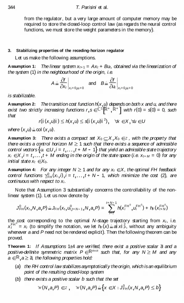
3. S tabilizing properties of the receding-horizon regulator

Let us make the following assumptions.

Assumption 1: The linear system xt+1 = Axt + But, obtained via the linearization ofthe system (1) in the neighbourhood of the origin, i.e.

A7¶ f¶ xt

ïïïï xt=0,ut=0

and B7¶ f¶ ut

ïïïï xt=0,ut=0

is stabilizable.

Assumption 2: The transition cost function h(x,u) depends on both x and u, and thereexist two strictly increasing functions r,s Î 1[ +, +], with r(0) = s(0) = 0, suchthat

r( i (x,u) i ) £ h(x,u) £ s( i (x,u) i 2), " x Î X, " u Î U

where (x,u)7col (x,u) .

Assumption 3: There exists a compact set X0 Í X,X0 Î Z , with the property thatthere exists a control horizon M ³ 1 such that there exists a sequence of admissiblecontrol vectors {ui Î U, i = t, . . . ,t + M - 1}that yield an admissible state trajectoryxi Î X, i = t, . . . ,t + M ending in the origin of the state space (i.e. xt+M = 0) for anyinitial state xt Î X0.

Assumption 4: For any integer N ³ 1 and for any xt Î X, the optimal FH feedbackcontrol functions g 0

FH(xi, i), i = t, . . . ,t + N - 1, which minimize the cost (2), arecontinuous with respect to xi.

Note that Assumption 3 substantially concerns the controllability of the non-linear system (1). Let us now denote by

J0FH(xt,N,a,P)7JFH(xt,u0

t,t+N- 1,N,a,P) = åt+N- 1

i= th(xFH0

i ,uFH0

i ) + hF(xFH0

t+N )

the cost corresponding to the optimal N-stage trajectory starting from xt, i.e.xFH0

t = xt (to simplify the notation, we let hF(x)7ai xi 2P, without any ambiguity

whenever a and P need not be rendered explicit). Then the following theorem can beproved.

Theorem 1: If Assumptions 1± 4 are veri® ed, there exist a positive scalar ~a and apositive-de® nite symmetric matrix P Î n ´ n such that, for any N ³ M and anya Î ,a ³ ~a, the following properties hold:

(a) the RH control law stabilizes asymptotically the origin, which is an equilibriumpoint of the resulting closed-loop system

(b) there exists a positive scalar b such that the set

W (N,a,P) Î Z , W (N,a,P)7{x Î X : J0FH(x,N,a,P) £ b }


is an invariant subset of X0 and a domain of attraction for the origin, i.e. forany xt Î W (N,a,P) , the state trajectory generated by the RH regulatorremains entirely contained in W (N,a,P) and converges to the origin.

Theorem 1 is a simpli® ed and more constructive version of a similar theorempresented by Parisini and Zoppoli (1995). In the following, we sketch its proof, whichis based partly on some facts established by Parisini and Zoppoli (1995) and partlyon a new approach aimed at determining the scalar ~a and the matrix P explicitly,thus making the design of the RH regulator implementable (such a determinationwill be presented in § 5). Theorem 1 relies essentially on the demonstration that thecost J0

FH(x,N,a,P) is a Lyapunov function in X0 for the system (1) driven by the RHregulator. This property is easy to assess (Parisini and Zoppoli 1995), once thefollowing lemma has been proved (note that this lemma is slightly di� erent from theone presented by Parisini and Zoppoli 1995).

Lemma: There exist a positive-de® nite symmetric matrix P Î n ´ n and a positivescalar ~a such that

J0FH(xt,N,a,P) ³ J0

FH(xt,N + 1,a,P), " xt Î X0, " N ³ M, " a ³ ~a

Proof: To prove this lemma, we need the following two facts.

Fact 1: If Assumption (1) is veri® ed, there exists a matrix K Î m ´ n such that theorigin is an asymptotically stable equilibrium point of the closed-loop systemxt+1 = f (xt,Kxt) . Moreover, for such a system, there exists a compact setW (K,P) Í X,W (K,P) Î Z , which is an invariant set and a domain of attractionfor the origin (P Î n ´ n is a suitable positive-de® nite symmetric matrix with theproperty that xTPx is a Lyapunov function for xt+1 = f (xt,Kxt) in W (K,P) ) .

Fact 2: Consider the matrices K and P, as established in Fact 1. Then there exists apositive scalar a such that

hF(xt) ³ h(xt,Kxt) + hF(xt+1), " xt Î W (K,P), " a ³ a

Proof: The proof of Fact 1 is a discrete-time version of the one given by Michalskaand Mayne (1993), and Fact 2 has been proved by Parisini and Zoppoli (1995). Insection 5 an alternative proof of Fact 2 will be presented that is not only an existenceproof, but also allows one to practically determine the above scalar a.

Now, to prove the lemma, consider the FH optimal control problem

minimize åt+N- 1

i= th(xi,ui), subject to xt+N = 0 (3)

with N ³ M and " xt Î X0 (constraints on xi and ui are understood). By writing xt+N

as a function of xt and of the control vectors, (3) may be rewritten

minimize J(xt,U), subject to F(xt,U) = 0 (4)

where U7ut,t+N- 1 and the functions F and J have clear meanings. In virtue ofAssumption 3, the problem (4) has an optimal solution for any xt Î X0 (assume thissolution to be unique). We now recall that the FH optimal control problemintroduced in Problem 1 is given by

minimize J(xt,U) + ai F(xt,U) i 2P (5)


Clearly, i F(xt,Ui 2P has the characteristics of a penalty function. Let {ak,k =

1,2, . . .} be a sequence tending to in® nity, with ak+1 > ak for each k. Then, thepenalty-functions method generates the sequence of optimal solutions {Uk,k =1,2, . . .} of the problem (5) (we assume that this problem has a unique optimalsolution for each k). It is now easy to show that

limk ® ¥ i F(xt,Uk) i 2

P = 0

hencelim

k ® ¥xk

t+N = 0

(xkt+N is the ® nal state of the trajectory generated by Uk). It follows that there exists a

su� ciently large integer k* (and then a scalar ak*) such that the optimal solution Uk*

drives xk*t+N into the subset W (K,P) (see Fact 1). As ak* depends on xt, we let

a*7maxxt Î X0

ak*(xt) (6)

We can conclude that the optimal solution of the problem (5) (i.e. uFH0

t , . . . ,uFH0

t+N- 1)makes

xFH0

t+N Î W (K,P), " N ³ M, " a ³ a*, " xt Î X0

We now add to the optimal trajectory a further stage generated by the controlKxFH0

t+N . As xFH0

t+N Î W (K,P) , we can use Fact 2, thus obtaining

JFH(xt,ut,t+N,N+1,a,P) = J0FH(xt,N,a,P)- hF(xFH0

t+N )+h(xFH0

t+N,KxFH0

t+N )+hF(xFH0

t+N+1)

£ J0FH(xt,N,a,P), " a ³ ~a7max ( a,a*)

Then, thanks to the optimality of J0FH( ) , we have

J0FH(xt,N + 1,a,P) £ JFH(xt,ut,t+N,N + 1,a,P) £ J0

FH(xt,N,a,P)," xt Î X0, " N ³ M, " a ³ ~a

which proves the lemma. u

It is now worth noting that, in deriving (both on-line and o� -line) the optimalRH control law uRH0

t = g 0RH(xt) , computational errors may a� ect the vector uRH0

t

and possibly lead to a closed-loop instability of the origin. Analogously, as will beshown in the next section, errors on uRH0

t may be induced by the neural network thatapproximate the RH regulator. Therefore, we need to address the sensitivity of thestate trajectory when errors a� ect the control law g 0

RH. This is done by means of thefollowing theorem, which characterizes the properties of the RH regulator whensuboptimal control vectors uRH

i Î U, i ³ t, are used in the RH control scheme,instead of the optimal ones uRH0

i solving Problem 1. Let us denote by xRHi , i > t, the

state vectors belonging to the suboptimal RH trajectory starting from xt.

Theorem 2: If Assumptions 1± 4 are veri® ed, there exist a positive scalar ~a and apositive-de® nite symmetric matrix P Î n n such that, for any N ³ M and for anya ³ ~a, the following properties hold:

(a) there exist suitable scalars ~d i Î ,~d i >0 such that, if

i uRH0

i - uRHi i £ ~

d i, i ³ t, then xRHi Î W (N,a,P), " i > t, " xt Î W (N,a,P)


(b) for any compact set W d Ì n,W d Î Z , there exist a ® nite integer T ³ t andsuitable scalars d i Î , d i > 0 such that, if i uRH0

i - uRHi i £ d i, i ³ t, then

xRHi Î W d , " i ³ T , " xt Î W (N,a,P)

As the proof of Theorem 2 is a direct consequence of the regularity assumptionson the state equation, we do not report it here (for computational details, see Parisiniand Zoppoli (1993)). However, analogously to what previously done for Fact 2, analternative proof of Theorem 2 will be presented in section 5, aimed at practicallydetermining the scalars d i, i ³ t. Theorem 2 has the following meaning: provided thatthe errors on the control vectors are suitably bounded, W (N,a,P) still remains aninvariant set. Moreover, the RH regulator can drive the state into each desiredneighbourhood W d of the origin in a ® nite time (W d is an invariant set, too). Finally,using the hybrid control scheme described by Michalska and Mayne (1993),W (N,a,P) becomes a domain of attraction for the origin.

4. The neural approximation for the receding-horizon regulator

As stated above, we are mainly interested in computing the RH control lawuRH0

t = g 0RH(xt) o� -line. Then we need to derive a priori an FH closed-loop optimal

control lawuRH0

i = g 0FH(xi, i) , t ³ 0, i = t, . . . ,t + N - 1

that minimizes the cost (2) for any xt Î X. Because of the time invariances of thedynamic system (1) and of the cost function (2), from now on we consider the controlfunctions

uFH0

i = g 0FH(xi, i - t), t ³ 0, i = t, . . . ,t + N - 1

instead of uFH0

i = g 0FH(xi, i) , and state the following.

Problem 2: Find the FH optimal feedback control law

{uFH0

i = g 0FH(xi, i - t) Î U,t ³ 0, i = t, . . . , t + N - 1}

that minimizes the cost (2) for any xt Î X.

Then, once the solution of Problem 2 has been achieved, we consider only the® rst optimal control function (i.e. the one corresponding to i = t), and write

uRH0

t = g 0RH(xt)7 g 0

FH(xt,0), " xt Î X,t ³ 0 (7)

As mentioned above, we do not use dynamic programming to solve Problem 2, asthis algorithm exhibits well-known computational drawbacks. As we have thepossibility of computing (o� -line) any number of open-loop optimal controlsequences uFH0

t , . . . ,uFH0

t+N- 1 (see Problem 1) for di� erent vectors xt Î X, we proposeto approximate the function g 0

RH(xt) = g 0FH(xt,0) by means of a function ^g RH(xt,w) ,

to which we assign a given structure. w is a vector of parameters to be optimized. Apossible way to derive the approximate RH neural control law consists in ® nding avector w0 that minimizes the integrated square approximation error

E(w)7 ò Xi g 0

RH(xt) - ^g RH(xt,w) i 2 dxt (8)

Among various possible approximating functions, multilayer feedforward neural


networks may be chosen. The reason for this choice will be given at the end of thissection. A feedforward network is composed of L layers, and in the generic layer s ns

neural units are active. The input/output mapping of the qth neural unit of the sthlayer is given by

yq(s) = g[ åns- 1

p=1

wpq(s)yp(s - 1) + w0q(s)], s = 1, . . . , L ,q = 1, . . . ,ns

where yq(s) is the output variable of the neural unit, and wpq(s) and w0q(s) are theweight and bias coe� cients, respectively. We use the activation function g(x) =tanh (x) . All these coe� cients are the components of the vector w; the variables yq(0)are the components of xt, and the variables yq( L ) are the components of ut.

To exploit the results given by Theorem 2, we have now to specify quantitativelythe magnitude of the errors generated by the control law of the formuRH

t = ^g RH(xt,w) , when it approximates the control law (7). To this end, we needto specialize the above-described neural network. More precisely, we assume that theapproximating neural function ^g RH(xt,w) contains only one hidden layer (i.e. L = 2)composed of t neural units, and that the output layer is composed of linearactivation units. We denote such a function by ^g ( t )

RH(xt,w) . From the approximationproperty of feedforward neural networks based on sigmoidal functions, as reportedfor instance by Hornik et al. (1989), it is easy to derive the following.

Theorem 3: Assume that, in the solution of Problem 2, the ® rst control functiong 0

RH(xt) = g 0FH(xt,0) (see (7)) exists and is unique, and that it is a [X, m]function.

Then, if Assumptions 1± 4 are veri® ed, there exists an RH neural regulatoruRH

t = ^g ( t )RH(xt,w),t ³ 0, for which the two properties in Theorem 2 hold true.

Theorem 3 allows us to assess the existence of an RH neural regulator able todrive the system state, in a ® nite time, into any desired neighbourhood W d of theorigin. This is obtained by constraining the control vectors uRH

t to take their valuesfrom the admissible set U7{u : u + ¢u Î U, i ¢ui £ e }, where for a given W d andany xt Î W (N,a,P) , e is such that e £ d i, i ³ t (see the scalars in Theorem 2), andU Î Z . Then we need a guarantee that the control errors generated byuRHÊ

t = ^g ( t )RH(xt,w0) are uniformly bounded on X by the scalar e . Such a guarantee

may be obtained by solving the minimax problem stated below. First, we have tode® ne an approximating network that di� ers slightly from the one considered tostate Theorem 3. The new network is the parallel of m single-output neural networksof the type described above (i.e. containing a single hidden layer and linear outputactivation units). Each network generates one of the m components of the controlvector uRH

t . We denote by ^g( t j )RHj(xt,wj) the input± output mapping of the jth of such

networks, where t j is the number of neural units in the hidden layer and wj is theweight vector, and we denote by g 0

RHj (xt) the jth component of the vector functiong 0

RH. Now we can state the following.

Problem 3: For each function ^g ( t j)RHj(xt,wj) , ® nd the numbers t *

1, . . . , t *m of neural units

such thatmin

wjmaxxt Î X

|g 0RHj(xt) - ^g ( t j)

RHj(xt,wj)| £ e

ê ê ê êmÏ , j = 1, . . . ,m (9)

In section 5, we shall address the possibility of computing the scalar e . As to thenumbers t *

j , rather a naive trial-and-error procedure for determining them is the


following: for each j, increase t j until the term on the left-hand side of (9) is less thanor equal to e / ê ê ê êmÏ . This procedure seems reasonable, as a bound (uniform on X) to

|g 0RHj(xt) - ^g ( t j)

RHj(xt,wj )| can be established that is proportional to 1 / ê ê ê êt jÏ . We nowbrie¯ y discuss the conditions under which this property holds true. FollowingBarron (1993), we assume that each of the optimal control functions g 0

RHj to beapproximated has a bound to the average of the norm of the frequency vectorweighted by its Fourier transform (see (10) below). However, the functions g 0

RHj havebeen de® ned on the compact set X, not on the space n. Then, to compute theFourier transforms, we need to extend the functions g 0

RHj (xt) from X to n. To thisend, we de® ne the functions g 0

RHj :n ® that coincide with g 0

RHj(xt) on X. Wealso de® ne the class of functions

Gcj 7{ g RHj, such that ò n|x |X|C j( x )| dx £ cj} (10)

where |x |X7maxxÎ X

|x x|C j( x ) is the Fourier transform of g RHj , and cj is any ® nite positive scalar. We cannow state the following.

Theorem 4: Assume that, in the solution of Problem 2, the ® rst control functiong 0

RH(xt) = g 0FH(xt,0) (see (7)) is unique, and that g 0

RHj Î G~cj for some ® nite positivescalar ~cj, for each j with 1 £ j £ m. Then, for each j with 1 £ j £ m, for everyprobability measure s , and for each t j ³ 1, there exist a weight vector wj (i.e. a neuralcontrol function ^g ( t j)

RHj(xt,wj) ) and a positive scalar cÂ j such that

ò X|g 0

RHj(xt) - ^g ( t j)RHj(xt,wj)|2 s [d(xt)]£ cÂ j

t j

where cÂ j = (2~cj) 2. Moreover, there exists a positive scalar kj such that

maxxt Î X

|g 0RHj(xt) - ^g ( t j)

RHj(xt,wj)|2 £ kjcÂ jt j

Theorem 4 is derived from two theorems by Barron (1992, 1993). It states that,for any control function g 0

RHj(xt) , the number of parameters required to achieve anL 2 or an L ¥ approximation error of order O(1 /t j) is O( t jn), which grows linearlywith the dimension n of the state vector. For a further discussion of this property offeedforward neural approximators, in comparison with traditional linear approx-imators and other classes of nonlinear ones, see Girosi et al. (1995) and Parisini andZoppoli (1995).

5. Determination of the penalty function and of the neural network implementing

the RH regulator

In this section by using some constructive aspects of the proofs of Theorems 1and 2, we shall describe some computational procedures to derive the penaltyfunction and the number of neural units of the network implementing the RHregulator.

5.1. Determination of the matrix PThe closed-loop system xt+1 = f (xt,Kxt) can be written in the form


xt+1 = ~Axt + u (xt), " xt Î K- 1[U] X

where ~A7A + BK, u is a suitable function such that u (0) = 0 and

limi xi ® 0

i u (x) ii xi = 0

and K- 1[U]represents the inverse image of the set U via the linear operator K. Itis shown below that V (x)7xTPx is a Lyapunov function for the systemxt+1 = f (xt,Kxt) in a suitable set W (K,P) . Then, once a matrix K that asympto-tically stabilizes the linearized system xt+1 = ~Axt has been determined, P can becomputed as the solution of the Lyapunov equation

P - ~ATP ~A = Q

for an arbitrary symmetric positive-de® nite matrix Q.

5.2. Determination of the scalar ~a

First, we need to determine the compact set W (K,P) . A little algebra yields

¢V (xt)7V (xt+1) - V (xt)

£ - [¸min(Q) - 2i ATPi i u (xt) ii xt i - ¸max(P)( i u (xt) i

i xt i )2

] i xt i 2 (11)

where ¸min(Q) and ¸max(P) denote the minimum and maximum eigenvalues of thematrices Q and P, respectively. The quantity within brackets is positive if

i u (xt) ii xt i < K 7{- i ATPi + [i ATPi 2 + ¸min(Q)¸max(P)]1 /2}/¸max(P) (12)

Clearly, the scalar K de® nes implicitly the boundary d A of the open set A7{xt ÎX : ¢V (xt) < 0}Ä {0}. As ¢V (xt) = 0 at the boundary d A, we must determine theclosed invariant set W (K,P) such as not to include d A. Furthermore, to avoidnumerical problems related to the nearness of d A (these numerical problems will bepointed out later on in the determination of the scalar a), it is convenient to considera proper subset of A characterized by a suitable scalar K < K . Thus we impose thecondition

i u (xt) ii xt i £ K < K (13)

Now consider the inequalities

i u (xt) i £ ån

i=1i u i(xt) i £ Fi xt i 2 + Gi xt i 3 (14)

where u i denotes the ith component of the vector u and

F7 12 å

n

i=1å

h,k Î {1,...,n}

ïïïï

¶ 2~fi(xt)¶ xth ¶ xtk

ïïïï xt=0

G7 16 å

n

i=1max

xt Î X K- 1[U]{ åj,h,k Î {1,...,n}

ïïïï

¶ 3~fi(xt)¶ xtj ¶ xth ¶ xtk

ïïïï}


(xtk is the kth component of the vector xt and ~fi is the ith component of the vectorfunction ~f (xt)7f (xt,Kxt) ) . Now, so that (13) may be satis® ed, it is su� cient that

F i xt i + Gi xt i 2 £ K (15)

By using (13) and (14), we obtain immediately

¢V (xt) <0, " xt Î X ´ K- 1[U],xt /= 0,xt : i xt i £ ê ê êbÏ 7- F + (F2 + 4K G) 1 /2

2G(16)

Note that, as

limi xi ® 0

i u (x) ii xi = 0

there exists a suitably small positive scalar b such that the compact set

W (K,P) Î Z , W (K,P)7{x Î n: xTPx £ b }

is contained in {x Î n: i xt i £ ê ê êbÏ }. Then

¢V (xt) < 0, " xt Î W (K,P) \ {0}More speci® cally, from (16) it follows that

b = ¸min(P) b Þ W (K,P) = {xt Î n: xT

t Pxt £ ¸min(P) b } (17)

Hence W (K,P) is an invariant set and a domain of attraction for 0 as an equilibriumpoint of the linearized system xt+1 = ~Axt.

Once the compact set W (K,P) has been determined, we can prove Fact 2 (asmentioned earlier, the proof is di� erent from the one given by Parisini and Zoppoli1995 and will allow us to compute the scalar ~a). Obviously

¶ h¶ x

ïïïï x=0,u=0

= 0 and¶ h¶ u

ïïïï x=0,u=0

= 0

(see Assumption 2). We now determine a matrix R Î n ´ n such that

h(xt,Kxt) £ xTt Rxt, " xt Î W (K,P) (18)

By using Assumption 2 and (17), we have

h(xt,Kxt) £ s( i (xt,Kxt) i 2) £ ks(K,P) (1 + i Ki ) 2 i xt i 2, " xt Î W (K,P)

where

Ks(K,P)7 maxzÎ W (K,P)

ïïïï

ds(z)dz

ïïïï

Then, so that (18) may be satis® ed, it is su� cient to choose any positive-de® nitesymmetric matrix R such that

¸min( R) ³ ks(K,P) (1 + i Ki ) 2

For a generic terminal cost function hF(x) = axTPx, from (11) we obtain

hF(xt+1) - hF(xt) = a¢V (xt)

£ - a[¸min(Q) - 2i ATPi i u (xt) ii xt i - ¸max(P)( i u (xt) i

i xt i )2

] i xt i 2


We now choose a scalar a such that the following inequality is satis® ed:

a[¸min(Q) - 2i ATPi i u (xt) ii xt i - ¸max(P)( i u (xt) i

i xt i )2

] ³ ¸max( R) (19)

Then, for any a ³ a we have

hF(xt+1) - hF(xt) £ - ¸max( R) i xt i 2 £ - xTt Rxt £ - h(xt,Kxt), " xt Î W (K,P)

thus proving Fact 2. The scalar a for which (19) is satis® ed can be easily computed byusing (13). Then, from (19) it follows that we can choose the scalar a de® ned as

a =¸max( R)

¸min(Q) - 2i ATPi K - ¸max(P) K 2 (20)

It is worth noting that, as K approaches K , a increases. This is consistent with the factthat we approach the region where ¢V (xt) takes on small values (recall that we have¢V (xt) = 0 at d A). Then, an increase in the attractiveness of the ® nal cost ai xt+N i 2

P

is needed.Finally, once the scalar a* has been derived from the maximization (6), ~a can be

derived from its de® nition, i.e. ~a = max( a,a*) (see the proof of the lemma insection 3).

5.3. Determination of the number of neural units

We assume the RH neural regulator to be implemented by the parallel of msingle-output networks, each containing a single hidden layer with t j neural units.We also assume the output layer to be composed of linear activation units (see thediscussion before Theorem 3 and Problem 3; actually, what is said in the followingfor the determination of e holds true for any kind of nonlinear approximator). Then,in virtue of Theorem 3, there exist su� ciently large numbers t 1, . . . , t m such that theRH neural regulator makes the state vector enter the set W (K,P) after a ® nitenumber of stages, for any initial state xt Î X. This property holds true, provided thatthe errors i uRH0

i - uRHi i , i ³ t, never exceed a proper scalar e . We ® rst determine the

value of such a scalar; this can be done by proving part (b) of Theorem 2, whereW d = W (K,P) .

Let us consider an arbitrary initial state xt Î X0 and the next two states xRH0

t+1 =f (xt,uRH0

t ) and xRHt+1 = f (xt, uRH

t ) . Consider also the function V (xt)7J0

FH(xt,N,a,P) . As mentioned in section 3 after Theorem 1, V is a Lyapunovfunction in X0 for the system (1) driven by the optimal RH regulator. Now, todevelop a simple numerical technique to determine the scalar e , we make Assump-tion 4 a bit stronger, that is we assume that the optimal FH feedback controlfunctions g 0

FH(xi, i), i = t, . . . , t + N - 1, are 1 functions with respect to xi , for anyxt Î X and any ® nite integer N ³ 1. Hence, this new assumption, together with theregularity hypotheses on the system (1) and the cost (2), ensures that V is a 1

function. Then

¢V (xt)7V (xRH0

t+1 ) - V (xt) < 0, " xt Î X0

It is easy to see that, if the control error is bounded as

i uRH0

t - uRHt i < d (xt)7 - ¢V (xt)

Kf (xt)KV (xRH0

t+1 )(21)


where Kf (xt) and KV (xRH0

t+1 ) are local Lipschitz constants of the functions f and V ,respectively, then

|V (xRH0

t+1 ) - V ( xRHt+1)| <- ¢V (xt), " xt Î X0

(21) yieldsV ( xRH

t+1) - V (xt) < 0, " xt Î X0

Then, V is a Lyapunov function also for the suboptimal RH trajectories, thus endingthe proof of Part (b) of Theorem 2.

Let us now specify how to compute the Lipschitz constants. We can write

i f (xt,u) - f (xt,uRH0

t ) i £ Kf (xt) i u - uRH0

t i , " u Î A f (xt)where

Kf (xt)7 maxu Î A f (xt )

iiii¶ f (xt,u)

¶ u

iiii(22)

andA f (xt)7{u Î U : i u - uRH0

t i £ d (xt)}Analogously

i V (x) - V (xRH0

t+1 ) i £ KV (xRH0

t+1 ) i x - xRH0

t+1 i , " x Î A V (xt)where

KV (xRH0

t+1 )7 maxx Î A V (xt)

i Ñ xV (x) i (23)

andAV (xt)7{x Î X : i x - xRH0

t+1 i £ Kf (xt) d (xt)}As A V (xt) and A f (xt) depend on the scalar d (xt) , which in turn depends on

A V (xt) and A f (xt) through the constants KV (xRH0

t+1 ) and Kf (xt) (see the maximiza-tions (22) and (23)); some iterative procedure is needed to determine them. Thefollowing has proved to be good heuristics in the simulations performed, though itsconvergence is not ensured:

(a) initialize this procedure by setting

Kf (xt) =iiii¶ f (x,u)

¶ uïïïï xt,uRH0

t

iiii

KV (xRH0

t+1 ) = - ¢V (xt)i xRH0

t+1 - xt i(b) determine d (xt)(c) determine A V (xt) and A f (xt)

Then, one can compute KV (xRH0

t+1 ) and Kf (xt) again by the maximizations (22)and (23), go to step (b), and repeat the procedure until convergence (if any) isreached, " xt Î X. Then

e = minxt Î X

d (xt)

Once e has been determined, the trial-and-error procedure outlined after thestatement of Problem 3 can be implemented to derive the numbers t *

1, . . . , t *m of

neural units.


6. S imulation results

Example 1: Consider the following nonlinear system

x1,t+1 = x1t + T [- x2t + 12 (1 + x1t)ut]

x2,t+1 = x2t + T [x1t + 12 (1 - 4x2t)ut]{

which is the discretized version of the undamped oscillator addressed by Mayne andMichalska (1990), where T = 0.05 is the sampling period. No state and controlconstraints are imposed, i.e. X = 2 and U = . We derive the design parametersfor the approximate RH neural control law by following the computational stepsdescribed in section 5. (We recall that Mayne and Michalska (1990) determined theRH control law by on-line computations.) The FH cost function is given by

JFH = åt+N- 1

i= t

(u2i + 0.1i xi i 2) + ai xN i 2

P

where N = 100.

6.1. Determination of the matrix P

We ® rst need to determine a linear control law ut = kTxt that asymptoticallystabilizes the linearized system xt+1 = Axt + but, where

A = [ 1 - 0.050.05 1 ], b = [ 0.025

0.025 ]As a linear control law, we choose the gain kT = [- 0.3799 - 0.4201]for which theclosed-loop poles are 0.99 6 0.0495i. We now determine the matrix P by solving theLyapunov equation P - ~ATP~A = Q, where ~A = A + bkT. More speci® cally, wechoose

Q = [ 1 00 1], which yields P = [ 48.3043 - 2.53

- 2.53 70.8191 ]6.2. Determination of the scalar ~a

From (12) we obtain K = 7.059 ´ 10- 3. A reasonable choice of K turns out to beK = K - 4 ´ 10- 4 = 6.659 ´ 10- 3 (see the discussion before (13)). As F = 0.1 andG = 0, we have b = ( K /F) 2 (see (15)), hence b = ¸min(P) b = 0.2129. As discussed insection 5, the choice of the matrix Q is arbitrary. However, for numerical reasons, itis convenient to make W (K,P) as wide as possible; then, the above gain k and Qhave been chosen by a trial-and-error procedure to make b su� ciently large. As thetransition cost function h(x,u) is quadratic, the matrix R can be obtained trivially as

R = 0.1I + kkT = [ 0.2443 0.15960.1596 0.2765 ]

where I is the 2 ´ 2 identity matrix. Then (20) yields a = 7.4014. We now mustdetermine a* through the maximization (6). As it turned out a* < a, we obtained~a = a = 7.4014.

6.3. Determination of the number of neural units and of the RH regulator

The neural RH regulator will be determined in the region


A7{xt Î n: - 2 £ x1t £ 0.5,- 1 £ x2t £ 2}

In section 4 we have described a trial-and-error procedure to determine the minimumnumber of neural units to achieve a control error uniformly bounded by e . Thisguarantees that all approximate trajectories enter W (K,P) . In the following, wedrop the index j in ^g ( t j)

RHj(xt,wj), as the control variable is scalar. More speci® cally, werecall that t has to be increased until the following inequality is satis® ed:

minw

maxxt Î A

|g 0RH(xt) - ^g ( t )

RH(xt,w)| £ e (24)

By using the iterative procedure outlined in section 5, we obtained e = 6 ´ 10- 4.However, a very large value of t is needed so that (24) may be satis® ed. On the otherhand, d (xt) is of the same order of magnitude as e only in the vicinity of the contourof W (K,P) and increases when we go away from W (K,P) . This means that, in thepresent example, (24) is too conservative with respect to (21) (which, as stated insection 5, is su� cient so that any approximate trajectory may enter W (K,P) ) . Thenwe considered the following trial-and-error procedure: increase t until

minw

maxxt Î A

|g 0RH(xt) - ^g ( t )

RH(xt,w)|/d (xt) £ 1 (25)

is satis® ed. Condition (25) is a slight modi® cation to (24), and is simple to interpret:the errors |g 0

RH(xt) - ^g ( t )RH(xt,w)| are weighted by 1 /d (xt) ; that is, the errors are more

penalized at the points of A where d (xt) is small, and vice versa.We found that, for t = 20

maxxt Î A

|g 0RH(xt) - ^g ( t )

RH(xt,w*)|/d (xt) £ 0.0481

where w* is the weight vector obtained via the minimax procedure de® ned in (25) fort = 20. Then (21) is satis® ed with a considerable margin. In ® gures 1(a) and 1(b) thecontrol functions g 0

RH(xt) and ^g ( t )RH(xt,w*) are plotted, respectively; the comparison

between the shapes of these functions con® rms the powerful approximationcharacteristics of the neural function ^g ( t )

RH. Figure 2(a) shows some state trajectories(starting from di� erent initial states), under the actions of the optimal (dashed line)and approximate (solid line) regulators. These trajectories practically coincide. Toappreciate the very small di� erences, in ® gure 2(b) a part of ® gure 2(a) is depicted inenlarged form, also showing the set W (K,P) .

Example 2: In the present example, we address a problem of freeway tra� c optimalcontrol. The choice of this example is motivated by its intrinsic engineeringinportance and by the fact that it deals with a high-order strongly nonlinear dynamicsystem. We shall follow an RH neural approach that is rather di� erent from the onedescribed in this paper. More speci® cally, we do not enforce the ® nal cost ai xt+N i 2

P,and we design the RH neural control law by minimizing the cost (8) instead ofsolving Problem 3. Therefore, stabilization is not ensured. In compensation, we havethe possibility of comparing an RH neural approach with a traditional computa-tional technique presented in the extensive literature on freeway tra� c control.

We refer to the following model, originally proposed by Payne (1971) and thenused in many works on freeway control (a comprehensive description of the modelcan be found in the work of Papageorgiou 1983):


v k,t+1 = v kt +T

¿{V f bkt[1 - ( q kt /q kmax)

l(3- 2bkt)]m - v kt}+T

¢kv kt(v k- 1,t - v kt)

+t T ( q k+1,t - q kt)

¿¢k( q kt + c ) - d onT

¢kv kt

rkt

q kt + c , t = 0,1, . . . ,k = 1, . . . ,K

q k,t+1 = q kt +T

¢k[a (1 - g k) q k- 1,tv k- 1,t + (1 - 2a + g k a - g k) q ktv kt

- (1 - a ) q k+1,tv k+1,t + rkt], t = 0,1, . . . ,k = 1, . . . ,Klk,t+1 = lkt + T (dkt - rkt), t = 0,1, . . . ,k Î I r

The freeway is assumed to be divided into K sections of length ¢k (see ® gure 3). T isthe sample time interval. v kt is the mean tra� c speed on section k at time tT , q kt is the


Figure 1. (a) Behaviour of the mapping g 0RH(xt) ; and (b) of the mapping ^g ( t )

RH(xt,w*) .

tra� c density, and lkt is the number of queueing vehicles on the on-ramp of sectionk Î I r (the indexes of the sections with on/o� ramps make up the set I r). rkt is theon-ramp tra� c volume that is imposed by monitoring the vehicle access via tra� clights, and bkt denotes speed limits set by means of variable message signs (bkt = 1means that there is no speed limit on section k). Then we can de® ne the state andcontrol vectors as follows:

xt7col (v kt,k = 1, . . . ,K; q kt,k = 1, . . . ,K; lkt,k Î I r)

ut7col (rkt,k Î I r,bkt,k = 1, . . . ,K)

dkt is the demand ¯ ow for access to the on-ramp of section k Î I r .


Figure 2. (a) State trajectories under the action of the optimal (dashed line) and the approx-imate (solid line) control laws; (b) the same state trajectories in a neighbourhood of theorigin and the set W (K,P) (ellipsoidal grey region).

Clearly, both the state and control variables must belong to suitable intervals:0 £ v kt £ v kmax,0 £ q kt £ q kmax, and 0 £ lkt £ lkmax . As to the control variables, weassume 0.7 £ bkt £ 1 and the more complex constraints

max [rkmin,dkt - 1T

( lkmax - lkt)] £ rkt £ min ( rkmax,dkt +1T

lkt)As in Problem P3 of Papageorgiou (1983), the process cost is given by the total traveltime spent on the freeway plus the total waiting time spent in the queues at thefreeway entrances; that is

JFH = T åt+N

i=t ( åK

k=1

q ki¢k + åk Î I r

lki) (26)

The freeway stretch considered consists of K = 30 sections (each of 1 km length),N = 5 and T = 15 s. On-ramps and o� -ramps are present for sections 3, 9, 15, 21and 27. There are ® ve control variables for speed limits and each of them acts on sixsuccessive sections. In particular, variable message signs are placed on sections 1, 7,13, 19 and 25. It follows that dim (xt) = 65 and dim (ut) = 10. The model describingthe dynamic behaviour of the freeway tra� c is characterized by the followingparameters: a = 0.9, V f = 123 km/h, l = 4,m = 1.4,¿ = 0.01 h, t = 21.6 km2 /h, c =20 veh/km, d on = 0.1, q kmax = 200 veh/km and v kmax = 200 km/h for k = 1, . . . ,K,lkmax = 200 veh,rkmin = 0 veh/h,rkmax = 20000 veh/h, for each on-ramp, andg k = 0.1 for each o� -ramp (the values of these scalars were taken from table 3.1of Papageorgiou 1983). The demands dkt are assumed to be known and time-invariant. We set d3t = 6000 veh/h,dkt = 1000 veh/h,k = 9,15,21 and 27.

To evaluate the e� ectiveness of our neural approach, we compare it with thecontrol scheme proposed by Messner and Papageorgiou (1992) to solve the above-described tra� c control problem. Such a scheme essentially consists in deriving on-line the optimal control law (OLO control law) that solves Problem 1 (the period ofthe on-line optimization can be longer than one stage). Instead, following the generalapproach proposed in the paper, we derive o� -line the RH optimal neural (RHON)control law uRH0

t = ^g RH(xt,w0) that minimizes the approximation error (8). To thisend, we focus our attention on an algorithm of the gradient type, as when applied toneural networks it turns out to be simple and well-suited to distributed computation.We de® ne the function

D(w,xt)7 i g 0FH(xt,0) - ^g FH(xt,w) i 2 = i g 0

RH(xt) - ^g RH(xt,w) i 2


Figure 3. A freeway section with on/o� ramps.

and note that we are able to evaluate g 0FH(xt,0) only pointwise; that is, by solving

Problem 2 for speci® c values of xt Î X. It follows that we are unable to compute thegradient Ñ wE(w) in explicit form. Then, we interpret E(w) as the expected value ofthe function D(w,xt) , by regarding xt as a random vector uniformly distributed onX. This leads us to compute the realization Ñ wD(w,xt) , instead of the gradientÑ wE(w) . We generate the sequence {xt(k),k = 0,1, . . .} randomly and use thefollowing updating algorithm:

w(k + 1) = w(k) - a (k) Ñ wD[w(k),xt(k)], k = 0,1, . . . (27)

The probabilistic algorithm (27) is based on the concept of stochastic approximation.Su� cient conditions for the algorithm convergence can be found, for instance, in thework of Polyak and Tsypkin (1973). As to a (k) , we take the step-sizea (k) = c1 /(c2 + k),c1,c2 > 0, which satis® es the aforesaid conditions for the algo-rithm convergence. We also add a momentum q [w(k) - w(k - 1)] to (27), as isusually done in training neural networks ( q is a suitable positive constant). We setc1 = 1,c2 = 105 and q = 0.9. To derive the components of Ñ wD[w(k),xt(k)], the well-known backpropagation updating rule can be applied.

As the descent algorithm is able to solve only an unconstrained nonlinearprogramming problem (whereas deriving the OLO control law entails the solutionof a constrained one), we remove the constraints on the control and state variablesans add suitable penalty functions to the cost (26). Then, the costs h(xt,ut) arede® ned like the terms in (26) plus the penalty functions. This is done for both theOLO control law proposed by Messner and Papageorgiou (1992) and our neuralmethod, thus making the two approaches comparable. The RH optimal neuralcontrol law ^g RH(xt,w0) is implemented by a neural network containing one hiddenlayer of 100 units. The gradient algorithm to optimize the neural control lawconverged after about 5 ´ 105 iterations. This large number of iterations may bedecreased by using some of the acceleration techniques proposed in the literature.However, we recall that this is not a very critical point, as all the computations areperformed o� -line.

The tra� c situation considered shows a severe congestion at time t = 0 onsections 10, 11 and 12 and consequently, low values of tra� c density on thesuccessive ones. More speci® cally, ® gure 4 shows the tra� c density q kt and themean tra� c speed v kt on the freeway sections when the RHON control law isapplied. When the freeway system is driven by the OLO regulator, the surfaces of q kt

and v kt (as functions of the stage t and of the section k) are nearly the same, so we donot specify them. To appreciate the very small di� erence between the statebehaviours related to the two control Shemes, in ® gure 5 we show the bidimensionaldiagrams of q kt and v kt as functions of the section k, at the stage t = 30 (i.e. after7.5 min).

It can be noted that the RHON control law, even though approximate, turns outto be very e� ective, as it yields performances almost identical with those obtained byusing the OLO control law. More speci® cally, de® ne the RH cost as

J0RH(~x)7 å

NT - 1

t=0h(xRH0

t ,uRH0

t ) (28)

where the state ~x describes the tra� c con® guration at time t = 0,NT is the number ofstages in which the RH control law was activated (NT = 60, corresponding to 15 min


in the present case), and uRHt is the control action generated by either the OLO or the

RHON control law. Then the use of the RHON control law implies an increase ofonly 0.25% in the cost (28). Furthermore, it is worth noting that the optimal neuralcontrol law drives the system state into a neighbourhood of the tra� c con® guration(or state vector) characterized by a mean tra� c speed that is quite close to the freespeed V f = 123 km/h - 1. Such a result may be interpreted as a stabilizing propertyof the neural regulator. This property was veri® ed experimentally for a variety ofinitial conditions.

7. Conclusions

The RH neural control scheme proposed in the paper exhibits the interesting


Figure 4. Evolutions of the tra� c density q kt and of the mean speed v kt; a severe congestionon sections 10, 11 and 12 is being cleared under the action of the RH optimal neuralcontrol law.

property that it can be computed o� -line. Instead, the RH regulators that have so farappeared in the literature generate the control vectors on-line by solving more or lessdi� cult optimal control problems or nonlinear programming problems. Existenceconditions on an RH stabilizing regulator and on neural networks implementing ithave been established. It has been shown that the parameters needed for the designof the neural regulator can be determined partly analytically and partly by solvingsome suitable global optimization problems. As is well known, solving theseproblems to a given guaranteed accuracy is not an easy task, unless some regularityinformation on the function to be minimized (or maximized) is available and thedimensions of the unknown vectors (in our case, typically the dimension of thesystem state) are moderate.

Actually, more attention has been paid to the statement of the global optimiza-tion problems than to the development of solving algorithms that exploit the


Figure 5. Comparisons of the tra� c density and the mean tra� c speed at stage t = 30, underthe actions of the OLO and RHON control laws.

peculiarities of the design problems. The results presented in the paper constituteonly a ® rst step toward a satisfactory o� -line design of RH stabilizing neuralregulators.

ACKNOWLEDGMENTS

The authors wish to thank Angela Di Febbraro for her helpful suggestions instating the freeway optimal control problem, and Marco Baglietto and SimonaSacone for their assistance in preparing the simulation examples. This work wassupported by the Italian Ministry for the University and Research.

REFERENCES

Barron, A. R., 1992, Neural net approximation. Proceedings of the 7th Yale Workshop onAdaptive and Learning Systems, edited by K. Narendra (New Haven: Yale UniversityPress); 1993, Universal approximation bounds for superpositions of a sigmoidalfunction. IEEE Transactions on Information Theory, 39, 930± 945.

Chen, C. C., and Shaw, L., 1982, On receding-horizon control. Automatica, 18, 349± 352.Eisenberg, B. R., and Sage, A. P., 1966, Closed loop optimization of ® xed con® guration

systems. International Journal of Control, 3, 183± 194.Girosi, F., Jones, M., and Poggio, T., 1995, Regularization theory and neural networks

architectures. Neural Computation, 7, 219± 269.Hornik, K., Stinchcombe, M., and White, H., 1989, Multilayer feedforward networks are

universal approximators. Neural Networks, 2, 359± 366.Keerthi, S. S., and Gilbert, E. G., 1988, Optimal in® nite-horizon feedback laws for a

general class of constrained discrete-time systems: stability and moving-horizonapproximations. Journal of Optimization Theory and Applications, 57, 265± 293.

Mayne, D. Q., and Michalska, H., 1990, Receding horizon control of nonlinear systems.IEEE Transactions on Automatic Control, 35, 814± 824.

Messner, A., and Papageorgiou, M., 1992, Motorway network control via nonlinearoptimization. Proceedings of the 1st Meeting of the EURO Working Group on UrbanTra� c and Transportation, Landshut, Germany, pp. 1± 24.

Michalska, H., and Mayne, D. Q., 1993, Robust receding horizon control of constrainednonlinear systems. IEEE Transactions on Automatic Control, 38, 1623± 1633.

Papageorgiou, M., 1983, Applications of Automatic Control Concepts to Tra� c FlowModeling and Control. Lecture Notes in Control and Information Sciences, Vol. 50(Heidelberg: Springer-Verlag).

Parisini, T., and Zoppoli, R., 1993, A neural receding-horizon regulator for nonlinearsystems. DIST Technical Report 93/2, University of Genoa, Italy.

Parisini, T., and Zoppoli, R., 1994, Neural networks for feedback feedforward nonlinearcontrol systems. IEEE Transactions on Neural Networks, 5, 436± 449; 1995, A receding-horizon regulator for nonlinear systems and a neural approximation. Automatica, 31,1443± 1451.

Payne, H. J., 1971, Models of freeway tra� c and control. Simulation Council Proceedings, 1,51± 61.

Polyak, B. T., and Tsypkin, Ya, Z., 1973, Pseudogradient adaption and training algorithms.Automation and Remote Control, 12, 377± 397.

Zoppoli, R., and Parisini, T., 1992, Learning techniques and neural networks for thesolution of N-stage nonlinear nonquadratic optimal control problems. Systems,Models and Feedback: Theory and Applications, edited by A. Isidori and T. J. Tarn(Boston: BirkhaÈ user), pp. 193± 210.

362 Nonlinear stabilization by receding-horizon neural regulators

Documents

Nonlinear stabilization by receding-horizon neural regulators