Embed Size (px)
Citation preview

Nonparametric and semiparametric bivariatemodeling of petrophysical porosity-permeabilitydependence from well log data
Arturo Erdely and Martin Diaz-Viera
1 Introduction
Assessment of rock formation permeability is a complex and challenging problemthat plays a key role in oil reservoir modeling, production forecast, and the opti-mal exploitation management. Generally, permeability evaluation is performed us-ing porosity-permeability relationships obtained by an integrated analysis of variouspetrophysical measurements taken from cores and wireline well logs. In particular,in carbonate double-porosity formations with an heterogeneous structure of porespace this problem becomes more difficult because the permeability usually doesnot depend on the total porosity, but on classes of porosity, such as vuggular andfracture porosity (secondary porosity). Even more, in such cases permeability is di-rectly related to the connectivity degree of the pore system structure. This fact makespermeability prediction a challenging task.
Dependence relationships between pairs of petrophysical random variables, suchas permeability and porosity, are usually nonlinear and complex, and therefore thosestatistical tools that rely on assumptions of linearity and/or normality and/or exis-tence of moments are commonly not suitable in this case. The use of copulas formodeling petrophysical dependencies is not new [3] and t-copulas have been usedfor this purpose. But expecting a single copula family to be able to model any kindof bivariate dependency seems to be still too restrictive, at least for the petrophys-ical variables under consideration in this work. Therefore, we first adopted a non-parametric approach by the use of the Bernstein copula [15, 16] and estimating thequantile function by Bernstein polynomials [12]. Later, we adopted a semiparamet-
Arturo ErdelyDepartamento de Matematicas Aplicadas y Sistemas, Universidad Autonoma Metropolitana -Unidad Cuajimalpa, Mexico D.F., Mexico. e-mail: [email protected]
Martın Dıaz-VieraPrograma de Investigacion en Recuperacion de Hidrocarburos, Instituto Mexicano del Petroleo,Mexico D.F., Mexico. e-mail: [email protected]
1

2 Arturo Erdely and Martin Diaz-Viera
ric approach by looking for a partition of the data into subsets for which the depen-dence structure was simpler to model by means of parametric families of copulas,and then a conditional gluing copula technique is applied to build the bivariate jointdistribution for the whole data set.
Among many others, two main tasks are usually of interest in petrophysical mod-eling: to reproduce the underlying dependence structure by data simulation, and toexplain a variable of interest in terms of an allegedly predictive variable (regression).
2 Methodology
Let S := {(x1,y1), . . . ,(xn,yn)} be independent and identically distributed bivari-ate observations of a random vector (X ,Y ). In this work, the (xk,yk) paired valuesrepresent porosity-permeability measurements. We may obtain empirical estimatesfor the marginal distributions of X and Y by means of
Fn(x) =1n
n
∑k=1
I{xk ≤ x} , Gn(y) =1n
n
∑k=1
I{yk ≤ y} , (1)
where I stands for an indicator function which takes a value equal to 1 whenever itsargument is true, and 0 otherwise. It is well-known [1] that the empirical distributionFn is a consistent estimator of F, that is, Fn(t) converges almost surely to F(t) asn→ ∞, for all t.
We model vuggy porosities as an absolutely continuous random variable X withunknown marginal distribution function F, and permeability as an absolutely contin-uous random variable Y with unknown marginal distribution function G. From [11]we have bivariate observations from the random vector (X ,Y ), see Figures 2 (left)and 3, and Figure 4 and Table 1 for marginal descriptive statistics. For simulationof continuous random variables, the use of the empirical distribution function esti-mates (1) is not appropriate since Fn is a step function, and therefore discontinuous,so a smoothing technique is needed. Since one of our main goals is simulation ofporosity-permeability paired variates, it will be better to have a smooth estimationof the marginal quantile function Q(u) = F−1(u) = inf{x : F(x) ≥ u}, 0 ≤ u ≤ 1,which is possible by means of Bernstein-Kantorovic polynomials as in [12]:
Qn(u) =n
∑k=0
x(k) + x(k+1)
2
(nk
)uk(1−u)n−k, (2)
where the x(k) are the order statistics, and the analogous case for marginal G in termsof values y(k) .
Similarly, we have the empirical copula [2], a function Cn with domain { in : i =
0,1, . . . ,n}2 defined as
Nonparametric and semiparametric bivariate modeling 3
Cn
(in
,jn
)=
1n
n
∑k=1
I{rank(xk)≤ i , rank(yk)≤ j} (3)
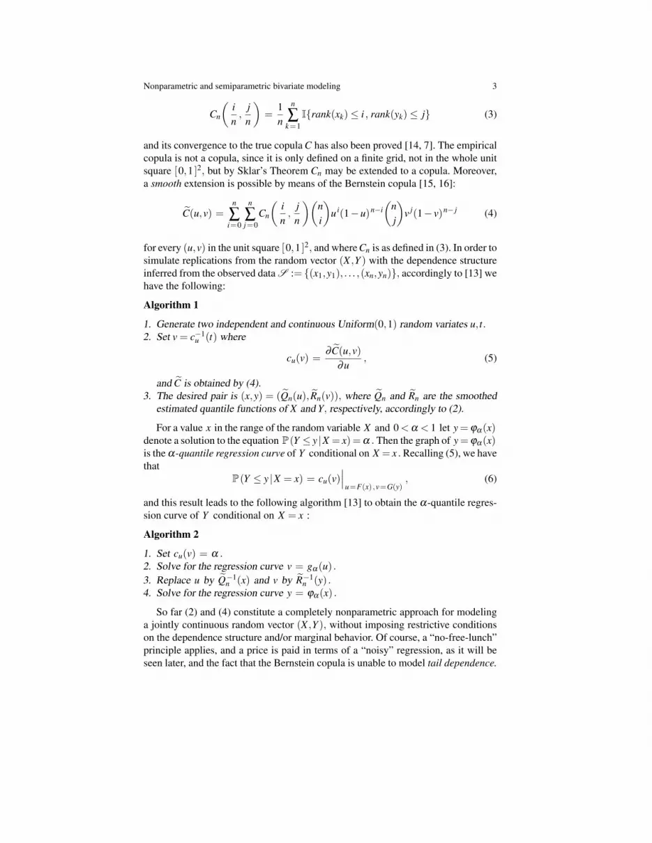
and its convergence to the true copula C has also been proved [14, 7]. The empiricalcopula is not a copula, since it is only defined on a finite grid, not in the whole unitsquare [0,1 ]2, but by Sklar’s Theorem Cn may be extended to a copula. Moreover,a smooth extension is possible by means of the Bernstein copula [15, 16]:
C(u,v) =n
∑i=0
n
∑j=0
Cn
(in
,jn
)(ni
)u i(1−u)n−i
(nj
)v j(1− v)n− j (4)
for every (u,v) in the unit square [0,1 ]2, and where Cn is as defined in (3). In order tosimulate replications from the random vector (X ,Y ) with the dependence structureinferred from the observed data S := {(x1,y1), . . . ,(xn,yn)}, accordingly to [13] wehave the following:
Algorithm 1
1. Generate two independent and continuous Uniform(0,1) random variates u, t.2. Set v = c−1
u (t) where
cu(v) =∂C(u,v)
∂u, (5)
and C is obtained by (4).3. The desired pair is (x,y) = (Qn(u), Rn(v)), where Qn and Rn are the smoothed
estimated quantile functions of X and Y, respectively, accordingly to (2).
For a value x in the range of the random variable X and 0 < α < 1 let y = ϕα(x)denote a solution to the equation P(Y ≤ y |X = x) = α . Then the graph of y = ϕα(x)is the α-quantile regression curve of Y conditional on X = x . Recalling (5), we havethat
P(Y ≤ y |X = x) = cu(v)∣∣∣
u=F(x) ,v=G(y), (6)
and this result leads to the following algorithm [13] to obtain the α-quantile regres-sion curve of Y conditional on X = x :
Algorithm 2
1. Set cu(v) = α .2. Solve for the regression curve v = gα(u) .3. Replace u by Q−1
n (x) and v by R−1n (y) .
4. Solve for the regression curve y = ϕα(x) .
So far (2) and (4) constitute a completely nonparametric approach for modelinga jointly continuous random vector (X ,Y ), without imposing restrictive conditionson the dependence structure and/or marginal behavior. Of course, a “no-free-lunch”principle applies, and a price is paid in terms of a “noisy” regression, as it will beseen later, and the fact that the Bernstein copula is unable to model tail dependence.

4 Arturo Erdely and Martin Diaz-Viera
The nature of the data that will be analyzed in the following section, makes itplausible that certain value ranges for the predictor variable (porosity) are relatedto different dependence structures (copulas). Under this assumption, we recall thegluing copula technique [17] for the particular case of vertical section gluing andbivariate copulas. For example, given two bivariate copulas C1 and C2 , and a fixedvalue 0 < θ < 1, we may scale C1 to [0,θ ]× [0,1 ] and C2 to [θ ,1 ]× [0,1 ] and gluethem into a single copula:
C1,2,θ (u,v) ={
θC1( uθ,v) , 0≤ u≤ θ ,
(1−θ)C2( u−θ
1−θ,v)+θv , θ ≤ u≤ 1.
(7)
For a more specific example, in the particular case C1(u,v)= Π(u,v)= uv,C2(u,v)=W (u,v) = max{u + v − 1,0}, and θ = 1
2 , the graph of the diagonal sectionδΠ ,W,1/2(t) = CW,Π ,1/2(t, t) is shown in Fig. 1. This particular kind of copula con-struction may easily lead to discontinuities in the derivative of the diagonal sectionat the value t = θ . Therefore, if the empirical diagonal δn(i/n) = Cn(i/n, i/n) ex-hibits a behavior that suggests a discontinuity of the diagonal derivative at certainpoints, one may ask if this is possibly due to an abrupt change of the dependencestructure at those points, and that being the case, a gluing copula procedure mayhelp to explain the whole dependence structure in terms of two or more simplerdependence models (copulas), in a piecewise manner. It is beyond the scope of thispaper to make an exhaustive discussion of different nonparametric techniques to de-tect possible derivative discontinuity points, but for the data analyzed in this work,using as an heuristic method the Dierckx cubic spline knot detection algorithm [4]has led to a dependence (copula) decomposition that was easier to model by meansof known parametric families of copulas, and that is compatible with a petrophysi-cal interpretation. Under this scheme, Algorithms 1 and 2 are used piecewise, with(estimated) parametric copulas instead of C (the nonparametric Bernstein copula).
3 Data analysis
In order to find knot candidates (or gluing points) we applied the Dierckx cubicspline knot detection algorithm [4], which is available as an R contributed package[5], to the empirical diagonal δn , obtaining the partition shown in Fig. 2 (Right),suggesting to decompose the total sample into three subsamples. Since we are will-ing to explain permeability (Y ) in terms of porosity (X), without loss of infor-mation about the joint distribution of the random vector (X ,Y ) we will considerthe total sample S := {(x1,y1), . . . ,(xn,yn)} to be ordered in the xk values, that isx1 < x2 < · · · < xn, and so the partition will be induced in the observed xk valuestotal range [minxk , maxxk ].
In Table 2 we present a summary of empirical values for the concordance mea-sures known as Spearman’s rho (ρS) and Kendall’s tau (τK), and an empirical ver-sion of the dependence measure ΦH which is just the square root of Hoeffding’s

Nonparametric and semiparametric bivariate modeling 5
Fig. 1 Diagonal section (thick line style) of gluing copulas Π(u,v) = uv and W (u,v) = max{u +v−1,0} with θ = 1/2, along with Frechet-Hoeffding diagonal bounds (thin lines).
0.0 0.2 0.4 0.6 0.8 1.0
0.0
0.2
0.4
0.6
0.8
1.0
gluing diagonal section
t
d(t)
Fig. 2 Left: Scatterplot of porosity-permeability data. Right: Empirical diagonal (thick line style)with suggested gluing points θ1 = 0.46 and θ2 = 0.68 (dashed vertical lines), Frechet-Hoeffdingdiagonal bounds and independence diagonal (thin line style).
0.0 0.1 0.2 0.3 0.4
010
0020
0030
0040
00
POROSITY
PE
RM
EA
BIL
ITY
●●●●●●●●●●●●●●●●
●
●●●●●●
●●●
●
●●●●●●●●●●
●
●●●●●●
●
●●
●
●●●
●
●●●●●●
●
●●●●●●
●
●
●●
●●●●●
●
●●●
●
●●
●
●
●●●
●
●
●
●●
●
●●
●
●●●●●
●
●
●
●●●
●●
●●
●
●
●
●
●
●●●●●
●
●●●●●●
●
●
●
●●
●
●
●
●
●
●
●
●
●
●
●●
●
●
●
●
●
●
●
●●●
●
●●
●
●
●
●
●
●
●
●●
●
●●
●
●
●
●
●
●
●●
●
●
●●
●
●●●
●●●
●
●
●
●●
●
●
●
●●●●
●
●
●
●
●
●●●
●
●
●
●●
●●
●
●●
●
●●
●
●●
●●
●
●
●
●
●
●
●
●
●
●●
●
●
●
●●
●
●
●
●
●
●●●●
●
●
●
●
●
●
●
●
●
●
●
●
●
●
●
●
●
●
●●
●
●
●
●
●
●
●
●
●
●
●
●
●●
●
●
●
●
●
●
●
●
●
●
●
●
●
●
●
●
●
●
●
●
●
●
●
●●
●
●
●
●
●
●
●
●
●
●
●
●
●
●
●
●
●
●
●
●
●
●
●
●
●
●
●
●
●
●
●
●
●
●
●
●
●
●
●
●
●
●
●
●
●
●
●
●
●
●
●
●
●
●
●
●
●
●
●
●●
●
●
●
●
●
●●● ●
0.0 0.2 0.4 0.6 0.8 1.0
0.0
0.2
0.4
0.6
0.8
1.0
t
d (
t )
1
2
3

6 Arturo Erdely and Martin Diaz-Viera
Fig. 3 Scatterplot of porosity-permeability data ranks, rescaled to [0,1 ]2.
●●
●
●●●●
●
●●
●
●●
●●
●
●
●●
●
●
●
●
●
●
●
●
●●●
●
●
●
●
●
●
●
●
●●●●●
●
●
●●
●
●
●
●
●
●●
●
●
●
●
●
●●
●●
●
●
●
●
●
●
●
●
●●●
●
●
●
●
●
●
●
●
●
●
●●
●
●
●
●
●
●
●●
●
●
●
●
●●
●
●
●
●
●
●
●●
●
●
●
●
●
●
●
●
●
●
●
●
●
●
●
●
●
●
●
●
●
●
●
●
●
●
●
●
●
●
●
●
●
●
●
●
●
●
●
●
●
●
●
●●●
●
●
●
●
●
●
●
●
●
●
●●
●
●
●
●
●
●
●
●
●
●●
●
●
●
●
●
●
●
●
●●●
●
●
●
●●
●
●
●
●
●
●
●
●
●
●
●
●
●
●
●
●
●
●
●
●
●●
●
●●
●
●
●
●
●
●
●●
●●
●
●
●
●
●
●
●
●●
●
●
●
●●
●
●
●
●
●
●
●
●
●
●
●
●
●
●
●
●
●
●
●
●
●
●
●
●
●
●
●
●●
●
●
●
●
●
●
●
●
●
●●
●
●●
●
●
●
●
●
●
●
●
●
●
●
●
●
●
●
●
●
●●
●
●
●
●
●
●
●●
●
●
●
●
●
●
●
●
●
●
●
●
●
●
●
●
●
●
●
●
●
●●
●
●●●
●
●
●
●
●
●
●
●
●
●
●
●
●
●●
●
●
●
●
●
●
●
●
●
●
●
●
●
●
●
●●
●
●
●
●
●
●●●●
0.0 0.2 0.4 0.6 0.8 1.0
0.0
0.2
0.4
0.6
0.8
1.0
POROSITY
PE
RM
EA
BIL
ITY
Fig. 4 Frequency histograms of porosity and permeability data.
histogram
POROSITY
Fre
quen
cy
0.0 0.1 0.2 0.3 0.4
020
4060
histogram
PERMEABILITY
Fre
quen
cy
0 1000 2000 3000 4000
050
100
150
200

Nonparametric and semiparametric bivariate modeling 7
Table 1 Summary statistics of porosity and permeability data.
Variable Min. 1st quartile Median Mean 3rd quartile Max.Porosity 0.001855 0.098670 0.176700 0.169700 0.236100 0.401300
Permeability 0.05584 0.01006 412.3 1050 1826 4054
dependence index [10]. We notice that the concordance and dependence values ofthe total sample are basically due to subsample 1, since subsamples 2 and 3 clearlyexhibit significantly lower values. Also, it should be noticed that the values of ρSand ΦH are quite similar under subsample 1, in contrast with subsamples 2 and 3.This last observation may have as an explanation either the effect of randomnessdue to smaller subsample sizes or that there could be some kind of dependence thatneither Spearman’s rho nor Kendall’s tau are being able to detect (recall that if a con-cordance measure is equal to zero this does not imply independence). Therefore, apowerful nonparametric test of independence a la Deheuvels based on a Cramer–von Mises statistic [8] has been applied, see Table 2 for p-values, clearly rejectingindependence for both the total sample and subsample 1, not rejecting independencefor subsample 2, but with some doubts about rejecting independence in case of sub-sample 3, since there is no rule to decide if 0.1274 is a sufficiently low p-value toreject the null hypothesis. Fortunately, a nonparametric symmetry test [6] has beenhelpful for taking a final decision on subsample 3: by rejecting symmetry we haveto reject independence.
Table 2 Empirical concordance and dependence values, and p-values for nonparametric tests ofindependence and symmetry.
Independence SymmetrySubsample size ρS τK ΦH test p-value test p-value
Total 380 +0.6579 +0.4843 0.6294 0.0000 0.92491 174 +0.6072 +0.4379 0.5819 0.0000 0.88932 85 +0.0538 +0.0487 0.1617 0.4661 0.31943 121 +0.0004 +0.0143 0.1795 0.1274 0.0014
In terms of choosing a parametric copula, strong evidence against symmetry ischallenging since there is not such a huge catalog of parametric asymmetric copulasas there is indeed for the symmetric case. For the particular data under consideration,it has been possible to transform the data in order to “remove” the asymmetry, bymeans of Theorem 2.4.4 (1) in [13] and the particular case
CX ,Y (u,v) = u−CX ,−Y (u,1− v) , (8)
with which, fortunately in this case, it was not possible to reject symmetry for theobservations of the random vector (X ,−Y ) from the transformed subsample 3 (de-

8 Arturo Erdely and Martin Diaz-Viera
noted as 3T), see Table 3, and Fig. 5 for level curves of the empirical copulas forsubsamples 3 and 3T. But still we mantain our rejection of independence for thetransformed subsample 3T since the independence copula Π(u,v) = uv is invariantunder transformation (8).
Table 3 Empirical concordance and dependence values, and p-values for nonparametric tests ofindependence and symmetry for transformed subsample 3T.
Independence SymmetrySubsample size ρS τK ΦH test p-value test p-value
3T 121 −0.0004 −0.0143 0.1795 0.1274 0.40403Ta 75 −0.2668 −0.1870 0.2795 0.0358 0.83233Tb 46 +0.2771 +0.1903 0.3149 0.0803 0.7869
Fig. 5 Level curves of empirical copulas for subsamples 3 and 3T.
sample 3
u
v
0.1
0.2
0.3 0.4
0.5
0.6
0.7
0.8
0.9
0.0 0.2 0.4 0.6 0.8 1.0
0.0
0.2
0.4
0.6
0.8
1.0
sample 3T
u
v
0.1
0.2
0.3
0.4
0.5
0.6
0.7
0.8 0.9
0.0 0.2 0.4 0.6 0.8 1.0
0.0
0.2
0.4
0.6
0.8
1.0
The close to zero values for the concordance measures ρS and τK under subsam-ple 3 or 3T, but the not so close to zero value for ΦH along with the independencerejection for subsample 3 and 3T, might have as an explanation that under non-monotone dependence, positive and negative quadrant dependencies “cancel out”under concordance measures (for a theoretical example see Example 5.18 in [13]),but not under a dependence measure such as ΦH . Therefore, we searched for a par-

Nonparametric and semiparametric bivariate modeling 9
tition of subsample 3T to see if it was possible to detect a gluing point for positiveand negative dependence, again with the aid of the Dierckx cubic spline knot detec-tion algorithm [4], which suggested θ3T = 0.615, see Fig. 6, and with such partitioninto subsamples 3Ta and 3Tb it was possible to decompose subsample 3T into neg-ative and positive dependence, with better p-values to reject independence, and withp-values far away from willing to reject symmetry, see Table 3.
Fig. 6 In thin line style, Frechet-Hoeffding diagonal bounds and independence diagonal section.In thick line style: empirical diagonals for subsample 3 (Left ) and subsample 3T (Right ).
0.0 0.2 0.4 0.6 0.8 1.0
0.0
0.2
0.4
0.6
0.8
1.0
sample 3
t
d (
t )
0.0 0.2 0.4 0.6 0.8 1.0
0.0
0.2
0.4
0.6
0.8
1.0
sample 3T
t
d (
t )3Ta
3Tb
So far, it has been possible to decompose the total sample into subsamples1,2,3Ta, and 3Tb, which do not exhibit strong evidence against symmetry, but withstrong evidence against the hypothesis of independence for all cases except subsam-ple 2, and therefore for subsample 2 the final decision is to be modeled by indepen-dence. For the remaining subsamples we looked for an appropriate fit among theknown catalog of symmetric parametric copulas (see for example [13]) by means ofa goodness-of-fit test as in [9], with the results summarized in Table 4.
With the above results, it is now possible to perform simulations and regres-sion in a semiparametric fashion (parametric copula and nonparametric Bernsteinmarginals as described in section 2). We also show analog results under a totallynonparametric fashion, as described in section 2, see Figures 7 and 8.

10 Arturo Erdely and Martin Diaz-Viera
Fig. 7 Simulated porosity-permeability paired values, sample size n = 380. Left: Under Bern-stein copula and Bernstein marginals. Right: Under a Gluing copula (Clayton + Independence +asymmetric Clayton + asymmetric Ali-Mikhail-Haq) and Bernstein marginals.
0.0 0.1 0.2 0.3 0.4
010
0020
0030
0040
00
BERNSTEIN simulation
Porosity
Per
mea
bilit
y
●● ●
●
●
●
●
●
●
● ●●
●
●
●
●
●
●
●
●
●
●
●
●
●●
●
●
●●
●
●●
●
●●
●
●●
●
●
●
● ●
●
●
●●
●
●
●
●
●
●
●
●
●
●
●
●
● ●
●●
●
●●
●
●
●
● ●
●
●
●
●
●
●
●
●
●
●
●
●
●
● ● ●
●
●
●
●
●
●●
●
●
●●
●●
●
●
●
●
●● ●●
●●
●
●
●
●
●
●
●●
●
●
●●
●
●
●
●
●●●
●
●
●
●●
●
●
●
●
●
●
●
●●
●
●
●
●
●
●
●
●
●
●
●●
●
●
●
●
●
●
●●
●
●
●
●
●
●
●
●
●
●
●
●
●
●
●●
●
●
●
●
●
●
●
●
●●
●●●
●
●
●
●●
●
●●
●
●
●
●●
●
●
●
●
●
●
●
●
●
●
●
●
●● ●
●●
●
●
●
●
●
●
●
●
●
●
●
●
●
●
●
●
●●
●
●
●
●
●
●
●
●
●●
●
●
●
●
●
●
● ●
●
●
●●
●
●
●
●
●
●
●
●●
●
●
● ●●
●
● ●
●
●
●
●
●
●
●
●
●
● ●●●
●
●●
●
●
●
●
● ●
●
●
●
●
●
●
●
●
●
●
●
●●
●
●
●
●
●
●
●
●
●
●
●
●
●
●
●
●
●
●
●
●
●
●●
●
●
●
●
●
●
●
●
●
●
●
●●
●
●
●
●
●
●
●●●
●
●
●●
●
●
●
●
●●
●
●
●
●
●
●●
●
●
●
0.0 0.1 0.2 0.3 0.4
010
0020
0030
0040
00
GLUING simulation
Porosity
Per
mea
bilit
y
●● ●●
●● ●
●
●
●
●
●
●
●
●
●
●
●
●
●●●
●
●
●
●
●
●
●
●
●●● ●
●
●●●●
●
●
●
●● ●●● ●
●
●●
●
●●●
●
●
●
●●
●
●●●
●
●
●●
●
● ●●●
●
●
●
●
●
●
●
●●
●
●
●
●●
●●
●
●● ●●
●
●
●●
●
●
●
●
●●
●●
●●
●
●
●●●●
●
●●●●
●
●
●
●
●
●
●● ●
●
●●
●
●
●●
●
●
●
●●
●●
●●
●
●
●
●●
●
●
●●●
●
●
●
●
●
●●
●●
●
●
● ●
●●●
●
● ●●
●
● ●
●
●
●
●
●
●●
●
●●
● ●
●
●
●●
●
●
●
●●
●
●
●
●
●
●
●
●
●
●
●
●
●
●
●
●
●
●
●
●
●●
●●
●
●
●
●
●
●
●
●●
●
●● ●●
●
●
●
●
●●
●
●
●
●
●●
●
●
●
●
●
●●
●
●
●
●
●
●
●
●
●
●
●
●
●
●●
●
●
●
●
●
●
●
●
●●
● ●
●
●
●
●
●
●
●
●
●
●
●
●
●
●●
●
●
●●
●
●●
●
●●
●
●
●
●
●
●
●
●
●
●
●
●
●
●
●
●
● ●
●
●
●
●
●
●
●
●
●
●
●
●
●
●
●
●
●
●
●
●
●
●
●
●
●
●
●
●
●
●
●
●●
●
●
●
●
●
●
●
●
●
●
●
●
●
●●
●
●
●
●
●
●
●
Fig. 8 Median, first and third quartile regression curves. Left: Bernstein copula and Bernsteinmarginals. Right: Gluing copula (Clayton + Independence + asymmetric Clayton + asymmetricAli-Mikhail-Haq) and Bernstein marginals, with vertical lines indicating porosity gluing points0.168, 0.219, and 0.2786.
0.0 0.1 0.2 0.3 0.4
010
0020
0030
0040
00
BERNSTEIN regression
original data (points) Median, quartiles 1 & 3 (lines)Porosity
Per
mea
bilit
y
●●●●●●●●●●●●●●●●
●
●●●●●●
●●●
●
●●●●●●●●●●
●
●●●●●●
●
●●
●
●●●
●
●●●●●●
●
●●●●●●
●
●
●●
●●●●●
●
●●●
●
●●
●
●
●●●
●
●
●
●●
●
●●
●
●●●●●
●
●
●
●●●
●●
●●
●
●
●
●
●
●●●●●
●
●●●●●●
●
●
●
●●
●
●
●
●
●
●
●
●
●
●
●●
●
●
●
●
●
●
●
●●●
●
●●
●
●
●
●
●
●
●
●●
●
●●
●
●
●
●
●
●
●●
●
●
●●
●
●●●
●●●
●
●
●
●●
●
●
●
●●●●
●
●
●
●
●
●●●
●
●
●
●●
●●
●
●●
●
●●
●
●●
●●
●
●
●
●
●
●
●
●
●
●●
●
●
●
●●
●
●
●
●
●
●●●●
●
●
●
●
●
●
●
●
●
●
●
●
●
●
●
●
●
●
●●
●
●
●
●
●
●
●
●
●
●
●
●
●●
●
●
●
●
●
●
●
●
●
●
●
●
●
●
●
●
●
●
●
●
●
●
●
●●
●
●
●
●
●
●
●
●
●
●
●
●
●
●
●
●
●
●
●
●
●
●
●
●
●
●
●
●
●
●
●
●
●
●
●
●
●
●
●
●
●
●
●●
●
●
●
●
●
●
●
●
●
●
●
●
●
●
●
●●
●
●
●
●
●
●●● ●
0.0 0.1 0.2 0.3 0.4
010
0020
0030
0040
00
GLUING regression
original data (points) Median, quartiles 1 & 3 (lines)Porosity
Per
mea
bilit
y
●●●●●●●●●●●●●●●●
●
●●●●●●
●●●
●
●●●●●●●●●●
●
●●●●●●
●
●●
●
●●●
●
●●●●●●
●
●●●●●●
●
●
●●
●●●●●
●
●●●
●
●●
●
●
●●●
●
●
●
●●
●
●●
●
●●●●●
●
●
●
●●●
●●
●●
●
●
●
●
●
●●●●●
●
●●●●●●
●
●
●
●●
●
●
●
●
●
●
●
●
●
●
●●
●
●
●
●
●
●
●
●●●
●
●●
●
●
●
●
●
●
●
●●
●
●●
●
●
●
●
●
●
●●
●
●
●●
●
●●●
●●●
●
●
●
●●
●
●
●
●●●●
●
●
●
●
●
●●●
●
●
●
●●
●●
●
●●
●
●●
●
●●
●●
●
●
●
●
●
●
●
●
●
●●
●
●
●
●●
●
●
●
●
●
●●●●
●
●
●
●
●
●
●
●
●
●
●
●
●
●
●
●
●
●
●●
●
●
●
●
●
●
●
●
●
●
●
●
●●
●
●
●
●
●
●
●
●
●
●
●
●
●
●
●
●
●
●
●
●
●
●
●
●●
●
●
●
●
●
●
●
●
●
●
●
●
●
●
●
●
●
●
●
●
●
●
●
●
●
●
●
●
●
●
●
●
●
●
●
●
●
●
●
●
●
●
●●
●
●
●
●
●
●
●
●
●
●
●
●
●
●
●
●●
●
●
●
●
●
●●● ●

Nonparametric and semiparametric bivariate modeling 11
Table 4 Parameter estimation and goodness-of-fit p-values for the selected copulas.
Subsample Copula parameter GoF p-value1 Clayton +1.5581 0.7880
3Ta Clayton −0.3151 0.91023Tb A-M-H +0.6869 0.7725
4 Final remarks
For the data under consideration (see Figures 2 and 3), eventhough there was notstrong evidence against the symmetry of the underlying copula [6], it was not pos-sible to find a single known parametric family of copulas that could avoid beingrejected by a goodness-of-fit-test (see Table 5), and an analogous situation for themarginal distributions. One way of tackling such situation is by a totally nonpara-metric approach, using Bernstein copula [15, 16] and Bernstein marginals [12], butpaying the price of a noisy regression (see Fig. 8, Left) and being unable to modelupper and lower tail dependence, as an immediate consequence of its definition.
Table 5 Goodness-of-fit p-values for several families of copulas for the whole sample, calculatedwith R package ‘copula’ [18].
Copula GoF p-valueNormal 0.00535Plackett 0.00535Frank 0.00055
Clayton 0.00015Husler-Reiss 0.00015
t-Copula < 0.00005Galambos < 0.00005Gumbel < 0.00005
An alternative found was a gluing semiparametric approach: decomposing thetotal sample into subsamples whose dependence structures (copulas) were simplerto model by symmetric and parametric families of copulas, maintaining a nonpara-metric estimation of the marginals. The result was specially satisfactory in termsof regression, since the discontinuous curve therein obtained essentially matcheswhat it was expected by petrophysical experts [11], see Fig. 8 (Right): a moderateand close to linear increase of permeability for porosity values under a percolationthreshold (porosity around 0.2), a stable level of permeability around the percolationthreshold, and an explosive increase in permeability after such threshold. In addi-tion, under this approach it was possible to model a significant lower tail dependence(subsample 1: Clayton copula) of λU = 0.641 (on a [0,1 ] scale).

12 Arturo Erdely and Martin Diaz-Viera
References
1. Billingsley, P.: Probability and Measure, 3rd edition. Wiley, New York (1995)2. Deheuvels, P.: La fonction de dependance empirique et ses proprietes. Un test non
parametrique d’independance. Acad. Roy. Belg. Bull. Cl. Sci. (5) 65, 274–292 (1979)3. Dıaz-Viera, M., Casar-Gonzalez, R.: Stochastic simulation of complex dependency patterns
of petrophysical properties using t-copulas. Proc. IAMG’05: GIS and Spatial Analysis 2,749–755 (2005)
4. Dierckx, P.: Curve and Surface Fitting with Splines. Oxford University Press, New York(1995)
5. Dorai-Raj, S.: DierckxSpline: R companion to “Curve and Surface Fitting with Splines”. Rpackage version 1.0-9 (2008)
6. Erdely, A., Gonzalez-Barrios, J.M.: A nonparametric symmetry test for absolutely continuousbivariate copulas. IIMAS UNAM Preimpreso No. 151, 1–26 (2009)
7. Fermanian, J-D., Radulovic, D., Wegcamp, M.: Weak convergence of empirical copula pro-cesses. Bernoulli 10, 547–860 (2004)
8. Genest, C., Quessy, J.-F, Remillard, B.: Local efficiency of a Cramer–von Mises test of inde-pendence. J. Multivariate Anal. 97, 274–294 (2006)
9. Genest, C., Remillard, B., Beaudoin, D.: Goodness-of-fit tests for copulas: A review and apower study. Insurance: Mathematics and Economics 44, 199–213 (2009)
10. Hoeffding, W.: Scale-invariant correlation theory. In: Fisher, N.I., Sen, P.K. (eds) The Col-lected Works of Wassily Hoeffding, pp. 57–107. Springer, New York (1940)
11. Kazatchenko, E., Markov, M., Mousatov, A., Parra, J.: Carbonate microstructure determina-tion by inversion of acoustic and electrical data: application to a South Florida Aquifer. J.Appl. Geophys. 59, 1–15 (2006)
12. Munoz-Perez, J., Fernandez-Palacın, A.: Estimating the quantile function by Bernstein poly-nomials. Computational Statistics & Data Analysis 5, 391–397 (1987)
13. Nelsen, R.B.: An introduction to copulas, 2nd edition. Springer, New York (2006)14. Ruschendorf, L.: Asymptotic distributions of multivariate rank order statistics. Ann. Statist.
4, 912–923 (1976)15. Sancetta, A., Satchell, S.: The Bernstein copula and its applications to modeling and approxi-
mations of multivariate distributions. Econometric Theory 20, 535–562 (2004)16. Sancetta, A.: Nonparametric estimation of distributions with given marginals via Bernstein-
Kantorovic polynomials: L1 and pointwise convergence theory. J. Multivariate Anal. 98,1376–1390 (2007)
17. Siburg, K.F., Stoimenov, P.A.: Gluing copulas. Comm. Statist. Theory Methods 37, 3124–3134 (2008)
18. Yan, J., Kojadinovic, I.: R package ‘copula’. Version 0.8-12 (2009)


