A «i~«—^ J! u_

1

^__a£E_B

l Ä ■ ■■ .. l_ä,^

-ft fel^^^^'-.'' ™

fcjlHH_|ÄJji_^^tJ3l_!i£>***^

._

"=-~-31111iÄ — —?— ■■'

NOTES ON GAME THEORY

Alan R. Washburn Naval Postgraduate School

Monterey, California August 2000

DISTRIBUTION STATEMENT A Approved for Public Release

Distribution Unlimited

&w^m Y ^3302^4 20001023 006

Notes on Game Theory

Alan R. Washburn

1. Introduction 1

2. Strategies and the Normal Form 2

3. Saddle Points 4

4. Games Without Saddle Points 6

5. 2x2 Games 12

6. 2 x n or m x 2 Games 13

7. Dominance 15

8. Completely Mixed Square Games 18

9. The General Finite Case - Linear Programming 22

10. Formulation of Military TPZS Games 25

Hide-and-seek Games 25 Duels (Games of Timing) 26 Blotto Games 26 Communications 27 Tactical Air War 27 Barrier Operations 27 Pursuit and Evasion Games 28

1. Introduction

The Theory of Games was born suddenly in 1944 with the publication of Theory of

Games and Economic Behaviour by John von Neumann and Oskar Morgenstern. Their

choice of title was a little unfortunate, since it quickly got shortened to "Game Theory," with

the implication being that the domain of applications consists merely of parlour games.

Nothing could be further from the truth. In fact, the authors hoped that their theory might

form the basis of decision making in all situations where multiple decision makers can affect

an outcome, a large class of situations that includes warfare and economics..

In the years since 1944, the only part of Game Theory where a notion of "solution" has

been developed that is powerful enough to discourage further theoretical work is the part

where there are exactly two players whose interests are in complete opposition. Game

theorists refer to these games as two-person zero sum (TPZS) games. TPZS games include all

parlour games and sports where there are two people involved, as well as several where more

than two people are involved. Tic-tac-toe, chess, cribbage, backgammon, and tennis are

examples of the former. Bridge is an example of the latter; there are four people involved, but

only two players (sides). Team sports are also examples of the latter. Many of these games

were originally conceived in imitation of or as surrogates for military conflict, so it should

come as no surprise that many military problems can also be analyzed as TPZS games.

Parlour games that are not TPZS are those where the players cannot be clearly separated

into two sides. Examples are poker and Monopoly (when played by more than two people).

Most real economic "games" are not TPZS because there are too many players, and also

because the interests of the players are not completely opposed. Such non-TPZS games are

the object of continued interest in the literature, but will not be mentioned further in these

notes. We will confine ourselves entirely to TPZS games. Washburn (1994) contains a more

in-depth treatment of TPZS games. Luce and Raiffa (1957) is a dated but still worthwhile

introduction to the general subject, or see Owen (1995) or Winston (1994).

2. Strategies and the Normal Form

In game theory, the word "strategy" has a very definite meaning; namely, a complete

rule for decision making. For example, in a problem where one vehicle is pursuing another,

one strategy for the pursuer is "turn hard left if the evader bears more than 10° left, or hard

right if the evader bears more than 10° right, else go straight." Given the strategy, the pursuer

could be replaced by a computer program that would turn the pursuer's vehicle in accordance

with what is observed about the position of the evader. Note that a single strategy for the

pursuer may result in many possible tracks of his vehicle, since the track depends on the

evader's strategy as well as the pursuer's. However, if both the pursuer's and evader's

strategies are known, then the outcome is determined. We assume that there is some

numerical "payoff associated with the outcome. For example, we might take the payoff to be

the amount of time T required for the pursuer to catch the evader, with T being a function of

the pursuer's strategy s and the evader's strategy r. Symbolically, the "payoff is T{r, s), with

the evader wanting to choose r to make T(r, s) large, and the pursuer wanting to choose s to

make T{r, s) small. Note that s and r are not necessarily numbers, but that T(r, s) is.

The advantage of dealing with strategies like r and s is that every TPZS game can be

represented, in principle, as a function of two variables. The main disadvantage is that many

interesting games have so many strategies that it is impossible to enumerate them all. There

are a great many computer programs, for example, that could be written for playing even such

a simple game as tic-tac-toe. Each of these programs is a strategy. The number of strategies

for playing checkers or chess is finite, but so large as to make the memory of even the largest

computer pale by comparison. The number of strategies for playing most pursuit and evasion

games is actually infinite, since the actions taken are continuous. So the conceptually

simplifying idea of strategy will not be useful for actually solving large games such as these

by enumeration. Nonetheless, there are some interesting games that can be solved in this

manner, and there are some useful principles that can be determined from this approach in

any case, so let's imagine what would happen if we could enumerate all possible strategies, in

which case we would have what is called the normal form of the game.

3. Saddle Points

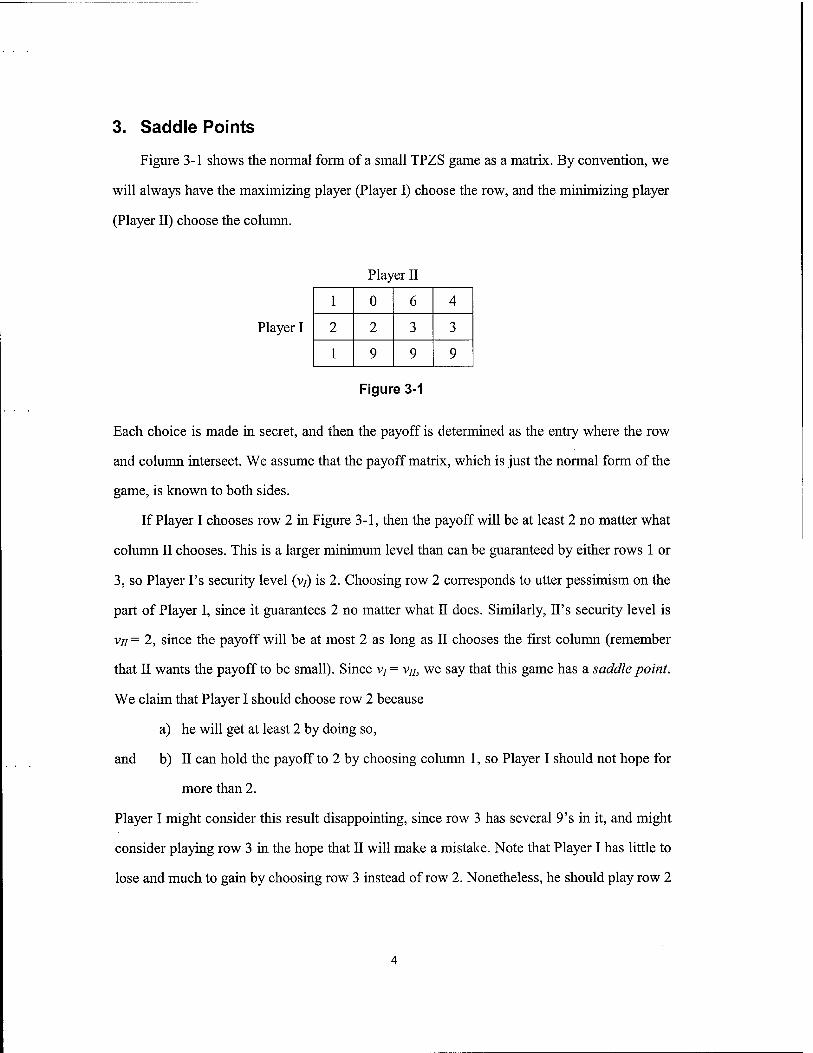
Figure 3-1 shows the normal form of a small TPZS game as a matrix. By convention, we

will always have the maximizing player (Player I) choose the row, and the minimizing player

(Player II) choose the column.

Player II

1 0 6 4

2 2 3 3

1 9 9 9

Player I

Figure 3-1

Each choice is made in secret, and then the payoff is determined as the entry where the row

and column intersect. We assume that the payoff matrix, which is just the normal form of the

game, is known to both sides.

If Player I chooses row 2 in Figure 3-1, then the payoff will be at least 2 no matter what

column II chooses. This is a larger minimum level than can be guaranteed by either rows 1 or

3, so Player Fs security level (v/) is 2. Choosing row 2 corresponds to utter pessimism on the

part of Player I, since it guarantees 2 no matter what II does. Similarly, IPs security level is

VJI = 2, since the payoff will be at most 2 as long as II chooses the first column (remember

that II wants the payoff to be small). Since v/= vu, we say that this game has a saddle point.

We claim that Player I should choose row 2 because

a) he will get at least 2 by doing so,

and b) II can hold the payoff to 2 by choosing column 1, so Player I should not hope for

more than 2.

Player I might consider this result disappointing, since row 3 has several 9's in it, and might

consider playing row 3 in the hope that II will make a mistake. Note that Player I has little to

lose and much to gain by choosing row 3 instead of row 2. Nonetheless, he should play row 2

if II is the rational, completely opposed player that we assume him to be, because such a

player will choose column 1:

• column 1 ensures that the payoff will not exceed 2

• Player I can get at least 2 by playing row 2, so II should be content with

guaranteeing that 2 will not be exceeded.

Even if the 9's in Figure 1 were changed to 900's, our theoretical advice to the two players

would still be the same: Player I should play row 2, and II should play column 1. We will

always give similar advice in any TPZS game that has a saddle point. To formalize, let <%• be

the payoff for row i and column j, and let v/ = max(mina,y \, and vn - min/maxa,y]. If v/ =

v// = v, then the game has a saddle point, v is the value of the game, and the optimal strategies

for Players I and II are the row and column that guarantee v.

Note that even in games that have saddle points, it is not true that a player's optimal

strategy is the best reaction to every possible strategy choice of the opponent. For example,

the best reaction of Player I to the choice of column 3 by II is to choose row 3, rather than

what we have called I's optimal row. Nonetheless, the best a priori choice for Player I is row

2, since there is no reason to expect II to choose column 3.

It can be shown that all games with perfect information have saddle points. By "perfect

information" we mean roughly that nothing of importance is concealed from a player when

he makes his choice(s). Chess and backgammon are games of this class, but most card games

are not because the opponent's cards are concealed. There is an optimal way to play chess,

and a computer programmed with the optimal strategy would presumably win every time it

got to make the first move. This observation has been of almost no help in writing chess

playing programs because of the impossibility of writing all possible programs to test them

against each other; nonetheless, an optimal strategy must exist. Games of pursuit and evasion

are also often supposed to have perfect information, and therefore saddle points. In spite of

the fact that they typically have infinitely many strategies, these games often have a simple

enough structure to permit discovery of the saddle point through the techniques of differential

games (Isaacs (1965)).

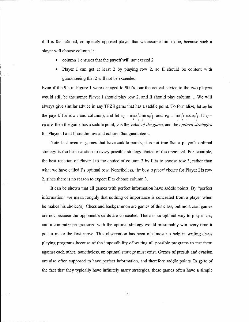
Exercises

1. Find v/ and v// for each of the games in Figure 3-2. Note that vj < VJJ in all cases.

2. Prove that v; < v« for every game.

a)

b)

c)

d)

e)

3 6 1 4

5 2 4 2

5 5 3 5

4 1

2 3

8 0 4

-2 2 4

10 2 0

8 2 3

0 1 7

0 1 4

0 -3 0

1 2 1

-2 0 6

f)

g)

h)

2 1 1

1 8 8

-2 0 6

0 0 0

9 0 0

8 3 0 7

0 3 4 2

2 1 0 6

5 3 4 9

1 2 0 3

5 1 2 8

9 3 1 1

4 4 6 2

2 4 9 0 5 8 3 2 5 0 1 3 8 0 4

Figure 3-2

4. Games Without Saddle Points

When a game has a saddle point, there is only one logical choice for the opponent, so

there is no problem trying to guess what he will do. Either player could reveal his strategy

choice and still ensure v. This is not so when there is no saddle point. In fact, the paramount

characteristic of games without saddle points is the necessity of guessing the strategy of an

opponent who will try to keep his strategy choice secret.

In World War II, for example, an anti-submarine aircraft frequently had to guess the

depth to which a submarine had submerged in setting its depth charges. Ideally, the aircraft

would choose the same depth as the submarine; otherwise, the probability of sinking the

submarine would be low. Clearly, neither side should get into the habit of always choosing

the same depth, since the essence of the problem is to be unpredictable. One way of ensuring

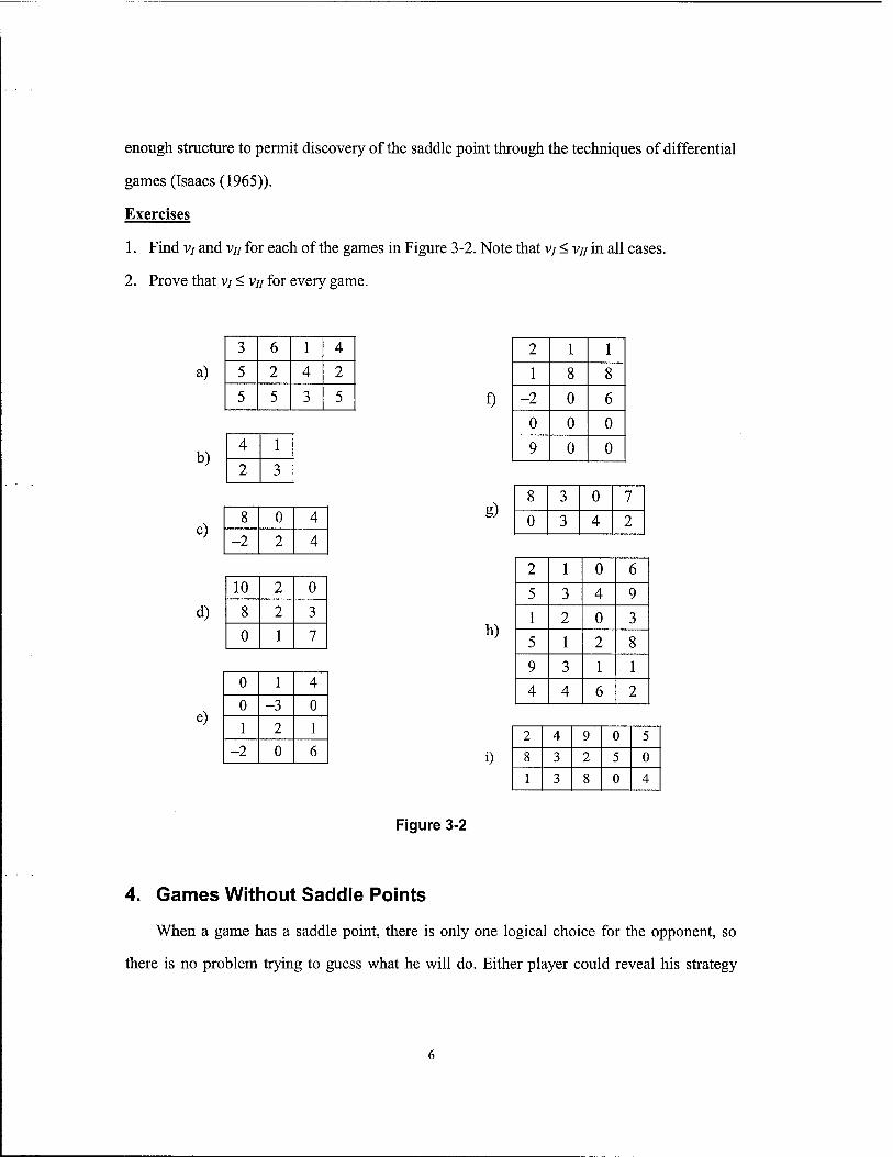
unpredictability is to actually choose a strategy randomly. That this idea of using a mixed

strategy is useful can be seen in Figure 4-1, where we have simplified the game so that each

side has only three depth settings. The entries in the matrix are "sink probabilities." Note that

v/ = .2 and vu - .3, which means that the game does not have a saddle point.

.75

.5

0

0

.25

.5

.25

.75

0

0

1

0

.33

.33

.3

.7

.34 0

U

.3 .1 0

.2 .8 .3

0 .1 .5

.23

-> CO ■> (225)

-> .25

.15 (325)

C25) .225

25 .125

59 CIT)

33 .27

8 .3

625 £223)

45 .15

Figure 4-1

Now, actually, Player I (the aircraft) can guarantee a sink probability greater than v/ by

using the mixed strategy x = (x\, X2, xj) = (.3, .7, 0). (In general x, will be the probability of

using row i, j/,- of column j.) If II uses his first strategy, then, according to the law of total

probability, the payoff will be .3(.3) + .7(.2) = .23. If II uses his second or third strategy, the

payoff will be .3(.l) + .7(.8) = .59 or .3(0) + .7(.3) = .21. The smallest of these three numbers

is .21 (circled in Figure 4-1), which is greater than vj. So the mixed strategy (.3, .7, 0) is better

than any of the three "pure" strategies. Examination of several other mixed strategies for

Player I is shown in Figure 4-1. The best of the five mixed strategies examined is (.25, .75,

0), which ensures a sink probability of .225. There are infinitely many more mixed strategies

x; but it is not necessary to examine them because it turns out that II can guarantee that the

sink probability will not exceed .225, as can be seen in Figure 4-1 where II has circled the

largest of three payoffs for each of the two mixed strategies y that he has tested. The value of

the game is therefore v = .225, and the optimal mixed strategies for the two players are x =

(.25, .75, 0) and y* = (.75, 0, .25). In general, if there is a number v and a pair of mixed

strategies x and y such that

• ]Tai;/x*>v for ally, i

and

• ^aijyj ^ v for all i, j

then we will say that the value of the game is v and that x and y are optimal strategies (we

will skip the word "mixed" except for emphasis). This definition applies to all TPZS

games — if the matrix happens to have a saddle point, then x and y will consist of 0's

except in one row or column.

We have seen that the idea of randomization is useful in a particular game. It permits us

to solve the game in the same sense that we earlier solved saddle point games; i.e., each

player can ensure the same number v by using his optimal mixed strategy. Three questions

now arise:

1) Does every game have a solution when mixed strategies are permitted?

2) If so, how can we fine it?

3) If we can find it, is the solution meaningful if the game is to be played only once?

The answer to the first question is yes. John von Neumann proved that every TPZS game

with finitely many strategies has a value v and optimal mixed strategies x and y . We will

deal with methods for answering the second question in succeeding sections.

The third question is not really about games, but about expected values; it is simply the

old question of whether an expected value computation is relevant to a gamble that is to be

made only once. In the depth-charging example, the answer to the third question is clearly

yes: .225 is a probability in the same sense that the entries in the matrix are probabilities in

the first place. Even if a gamble is only to be made once, surely the best gamble is the one

with the greatest probability of success. More generally, the answer is "yes, provided the

payoff function is carefully chosen." For example, suppose that an attack on a redundant

command and control system results in N of the redundant paths surviving, where N is

random because of mixed strategies used by the two sides and possibly for other reasons.

Then using the expected value of N for a payoff would be wrong, because it makes no

difference how many paths survive, as long as the number is not zero. A better payoff would

be the probability that no paths survive.

Many people encounter some intuitive resistance to the idea of randomization as an

essential part of decision making in games. This is perhaps due to a prior acquaintance with

single person decision making. Unpredictability is of no value in single person decision

problems, even though it is vital in games:

Q: What stock did you decide to buy - ABC or XYZ?

A: I thought about it a long time and decided to flip a coin.

The finite restriction is necessary. For example, the TPZS game where the winner is the one who thinks of the largest number has no solution.

Upon overhearing this conversation, our conclusion would be that the investor is simply

choosing an oblique way of saying that the two investment opportunities appear equal to him.

Furthermore, if we overhear the comment often enough, we conclude that the investor does

not really know much about the stock market; certainly we would feel cheated if we

discovered that a stockbroker gave us advice on this basis. In single person decision

problems, the idea of randomization is not logically necessary, so we tend to regard its

employment as an admission of defeat or indifference.

There is a danger of carrying this attitude over to the consideration of competitive

situations. For example, there is a tendency in the military to codify tactics; in situation X, the

best response is Y, etc. If situation X is a guessing game, then this codification may be a

mistake, since there is no such thing as a once-and-for-call "best tactic" in a guessing game. It

is essential to be unpredictable, and one way of achieving this is to use the very same mixed

strategies that are absurd in single person decision problems. Most people who have been

involved in protracted conflict can tell horror stories about disasters that have ensued because

of repetition of a tactic— bombers arriving at the same time every day, the same

communication channel being selected time after time, etc. Some of these unfortunate

incidents are no doubt due to carryover of the idea of the existence of a best tactic to

situations where no such tactic exists.

There is nothing really new about our observation that unpredictability is (or ought to be)

an essential part of conflict — military strategists have always stressed the need for surprise.

What is new is explicit identification of the mixed strategy as a mathematical representation

of unpredictability, with all the associated possibilities for computation and optimization.

Critic: "But it is quite possible to include the idea of unpredictability in conflict without

having people carry a coin around in case they have to make a decision. Suppose,

for example, that I were the row player in one of your matrix games. My

approach would be to use my experience and my intelligence network (a vital

10

part of conflict that you have completely ignored) to estimate what column will

be chosen by my opponent. I will concede that the opponent's column choice

might not be perfectly predictable, so that I would have to introduce a probability

distribution y over columns, but the point is that y is estimated, rather than

calculated. Then I would make whatever decision gives me the largest expected

payoff. There is no coin required. My assessment of y will change from time to

time, so I may appear to you to be acting at random in successive plays, but that's

not the way I look at it."

Our response to this criticism is twofold. First, suppose that v is the value of the game,

but that the critic is able to achieve more than v on the average. Then the opposing

commander is subject to criticism, since he could hold the average payoff to v by using his

optimal strategy y . In fact, y is simply the worst possible (from the critics standpoint) value

for y, and therefore the best from the standpoint of the opponent. It is possible, of course, that

the opponent will make a mistake, in which case it should certainly be taken advantage of.

But using an assumed distribution y instead of a worst cast distribution y is responding to the

opponent's perceived intentions, rather than to his capabilities. Second, the critic's procedure

is of little use to an analyst who must assess the average payoff in a game long before the

conflict occurs. The analyst may be interested, for example, in whether it is wise to change

some of the entries in a payoff matrix. The value of the game is the only defensible way of

turning the payoff matrix into a number so that comparisons between games can be made.

Exercise

Obtain upper and lower bounds on the value of the following modification of Figure 4-1

by guessing mixed strategies for the two sides:

11

.3 .1 0

.2 .8 .1

0 .4 .5

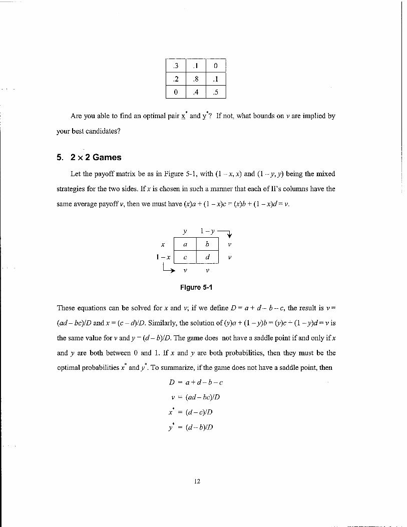
Are you able to find an optimal pair x and y ? If not, what bounds on v are implied by

your best candidates?

5. 2x2 Games

Let the payoff matrix be as in Figure 5-1, with (1 -x,x) and (1 -y,y) being the mixed

strategies for the two sides. If x is chosen in such a manner that each of II's columns have the

same average payoff v, then we must have {x)a + (1 - x)c = (x)b + (1 - x)d = v.

y

X

1-JC

1-v

a b

c d

If V

Figure 5-1

These equations can be solved for x and v; if we define D = a + d- b - c, the result is v =

(ad-bc)/D andx = (c-d)ID. Similarly, the solution of (y)a + (1 -y)b = (y)c + (1 - y)d= vis

the same value for v andy = (d- b)ID. The game does not have a saddle point if and only if x

and v are both between 0 and 1. If x and y are both probabilities, then they must be the

optimal probabilities x and y . To summarize, if the game does not have a saddle point, then

D = a + d-b-c

v = {ad-be)/D

x* = (d-c)/D

y = (d-b)ID

12

9 3 0 4

1 3 6 0

Example.

\f{a,b,c,d) = (0,2,3,0), then v = 1.2, x = .6, andy = .4.

Example.

If (a,b,c,d) = (3,2,1,1), then substitution gives v = 1, x* = 0, and y* = -1. This is not the

solution of the game because y is not a probability. This game has a saddle point, and the

value of the game is 2.

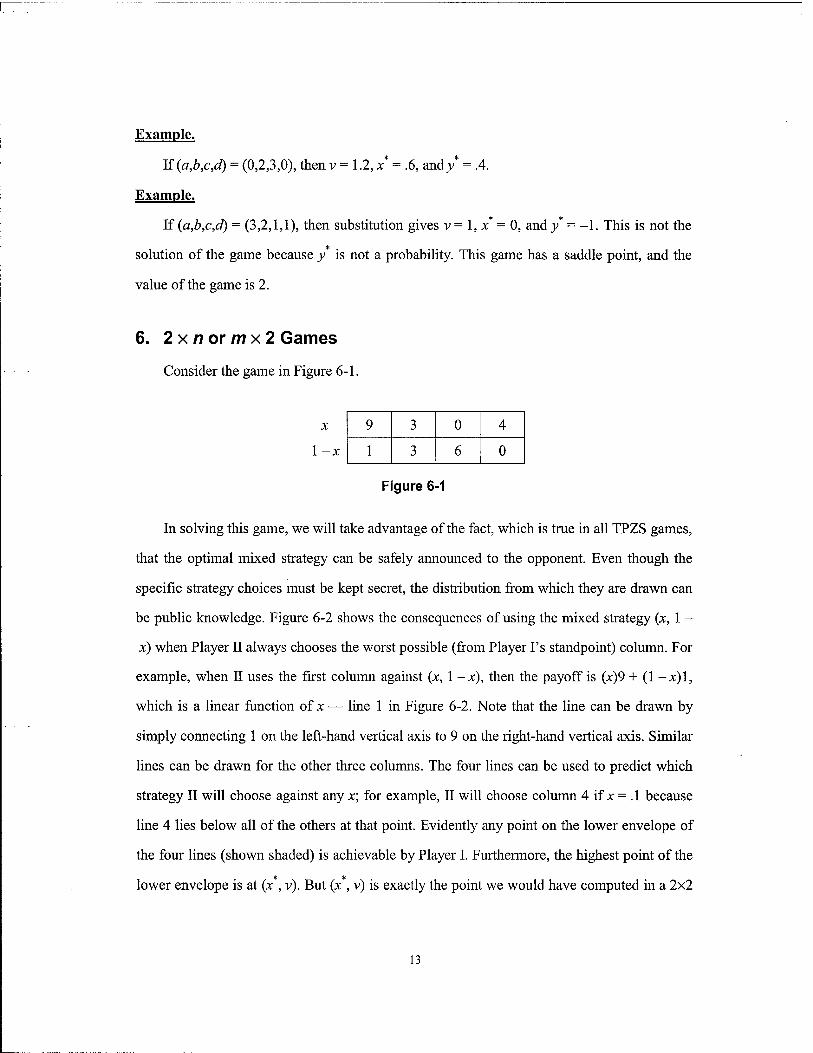
6. 2 x n or m x 2 Games

Consider the game in Figure 6-1.

x

l-x

Figure 6-1

In solving this game, we will take advantage of the fact, which is true in all TPZS games,

that the optimal mixed strategy can be safely announced to the opponent. Even though the

specific strategy choices must be kept secret, the distribution from which they are drawn can

be public knowledge. Figure 6-2 shows the consequences of using the mixed strategy (x, 1 -

x) when Player II always chooses the worst possible (from Player I's standpoint) column. For

example, when II uses the first column against (x, 1 -x), then the payoff is (x)9 + (1 -x)l,

which is a linear function of x — line 1 in Figure 6-2. Note that the line can be drawn by

simply connecting 1 on the left-hand vertical axis to 9 on the right-hand vertical axis. Similar

lines can be drawn for the other three columns. The four lines can be used to predict which

strategy II will choose against any x; for example, II will choose column 4 if x = . 1 because

line 4 lies below all of the others at that point. Evidently any point on the lower envelope of

the four lines (shown shaded) is achievable by Player I. Furthermore, the highest point of the

lower envelope is at (x , v). But (x , v) is exactly the point we would have computed in a 2x2

13

PAYOFF

3 v

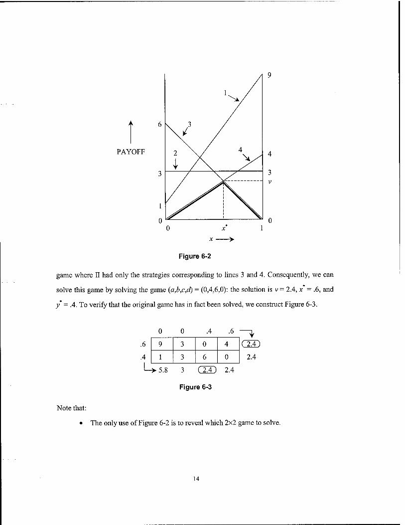
Figure 6-2

game where II had only the strategies corresponding to lines 3 and 4. Consequently, we can

solve this game by solving the game (a,b,c,d) = (0,4,6,0): the solution is v = 2.4, x = .6, and

y* = A. To verify that the original game has in fact been solved, we construct Figure 6-3.

.6

.4

^J.

A

9 3 0 4

1 3 6 0

3 C2A) 2.4

Figure 6-3

2.4

Note that:

The only use of Figure 6-2 is to reveal which 2x2 game to solve.

14

• As long as Player I uses (.6, .4), the payoff will be 2.4 if II uses (0, 0, y, \-y) for

anyy. Nonetheless, the unique optimal strategy for II is (0, 0, .4, .6).

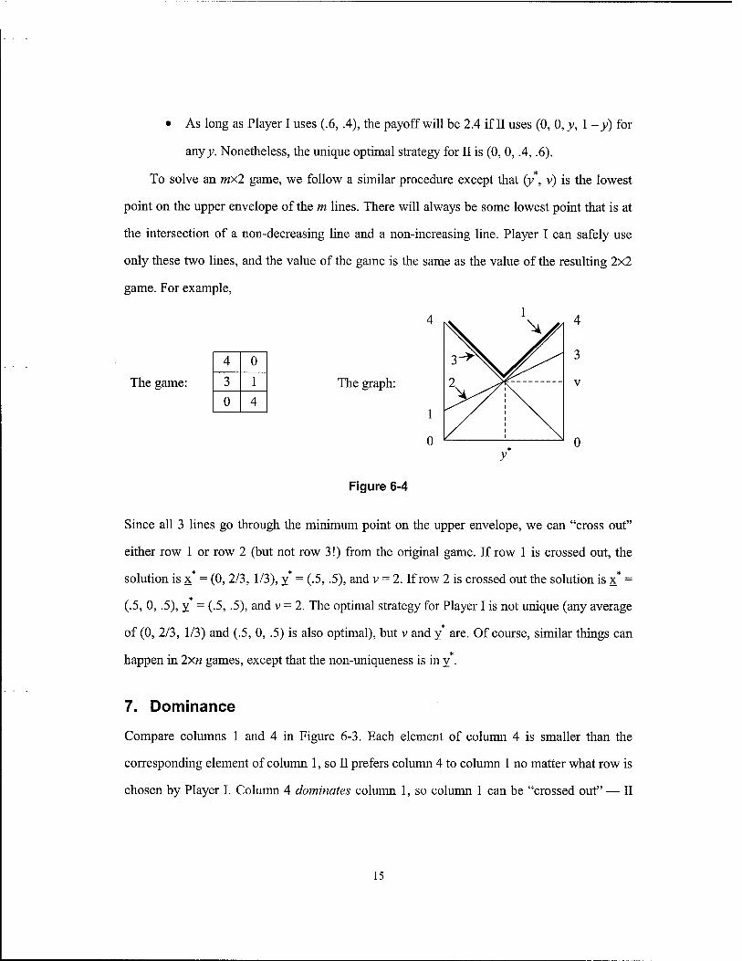
To solve an mx2 game, we follow a similar procedure except that (y , v) is the lowest

point on the upper envelope of the m lines. There will always be some lowest point that is at

the intersection of a non-decreasing line and a non-increasing line. Player I can safely use

only these two lines, and the value of the game is the same as the value of the resulting 2x2

game. For example,

The game:

4 0

3 1

0 4 The graph:

Figure 6-4

Since all 3 lines go through the minimum point on the upper envelope, we can "cross out"

either row 1 or row 2 (but not row 3!) from the original game. If row 1 is crossed out, the

solution is x = (0, 2/3, 1/3), y = (.5, .5), and v = 2. If row 2 is crossed out the solution is x* =

(.5, 0, .5), y = (.5, .5), and v = 2. The optimal strategy for Player I is not unique (any average

of (0, 2/3, 1/3) and (.5, 0, .5) is also optimal), but v and y are. Of course, similar things can

happen in 2xn games, except that the non-uniqueness is in y .

7. Dominance

Compare columns 1 and 4 in Figure 6-3. Each element of column 4 is smaller than the

corresponding element of column 1, so II prefers column 4 to column 1 no matter what row is

chosen by Player I. Column 4 dominates column 1, so column 1 can be "crossed out" — II

15

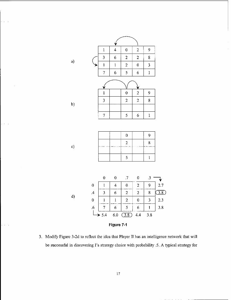
will use it with probability 0 in his optimal strategy. More generally, column j dominates

column k if ay < a^ for all i. Similarly, Player I will not use row k if it is uniformly smaller

than row i; row i dominates row k if ay > ay for ally. Roughly speaking, large columns and

small rows can be safely removed from the payoff matrix. There is no instance of row

dominance in Figure 6-3, but consider Figure 7-1. In diagram a, column 4 dominates column

2, and row 2 dominates row 3. If column 2 and row 3 are crossed out, diagram b results.

Notice that column 3 dominates columns 1 and 4 in diagram b, even though it did not in

diagram a. Crossing out these two columns results in diagram c. There is no further

dominance in diagram c, but the game can now be solved using the procedures of Section 6.

The value of the game is 3.8; the optimal solution and a verification of that solution are

shown in diagram d.

Evidently, the principal value of the dominance idea is to reduce the effective size of the

game. Actually, if any linear combination of rows dominates row k, where the weights in the

linear combination form a probability distribution, then row k can be eliminated. Similarly for

columns. For example, column 2 in Figure 6-3 is not dominated by any other column, but it is

dominated by .5 of the third column plus .5 of the fourth; with this observation, that game can

be solved directly as a 2x2 game.

Exercises

1. Solve all of the games in Figure 3-2.

2. There are two contested areas, and the attacker (I) and defender (II) must each secretly

divide their units between the two areas. The attacker captures an area if and only if he

assigns (strictly) more units than the defender. The payoff is the number of areas captured

by the attacker. The attacker has 3 units and the defender has 4. Construct the payoff

matrix (it should have 4 rows and 5 columns), and solve the game. This is an example of

a "Blotto" game.

16

a)

b)

1 4 0 2 9

3 6 2 2 8

1 1 2 0 3

7 6 5 6 1

1 0 2 9

3 2 2 8

7 5 6 1

c)

0 9

2 8

5 1

d)

0

.4

0

.6

5.4 6.0 (T8J 4.4

Figure 7-1

3.8

0 0 .7 0 .3 *

1 4 0 2 9 2.7

3 6 2 2 8 (3.8)

1 1 2 0 3 2.3

7 6 5 6 1 3.8

3. Modify Figure 3-2d to reflect the idea that Player II has an intelligence network that will

be successful in discovering Fs strategy choice with probability .5. A typical strategy for

17

II is now "choose column j if intelligence fails, else choose the best reaction to Fs row

choice." The new game should still be a 3x3. Solve it.

4. The same as Exercise 3 except use 3-2c.

8. Completely Mixed Square Games

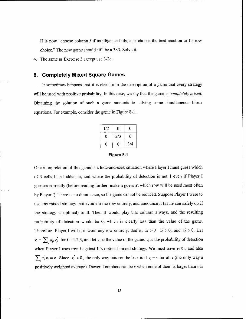
It sometimes happens that it is clear from the description of a game that every strategy

will be used with positive probability. In this case, we say that the game is completely mixed.

Obtaining the solution of such a game amounts to solving some simultaneous linear

equations. For example, consider the game in Figure 8-1.

1/2 0 0

0 2/3 0

0 0 3/4

Figure 8-1

One interpretation of this game is a hide-and-seek situation where Player I must guess which

of 3 cells II is hidden in, and where the probability of detection is not 1 even if Player I

guesses correctly (before reading further, make a guess at which row will be used most often

by Player I). There is no dominance, so the game cannot be reduced. Suppose Player I were to

use any mixed strategy that avoids some row entirely, and announce it (as he can safely do if

the strategy is optimal) to II. Then II would play that column always, and the resulting

probability of detection would be 0, which is clearly less than the value of the game.

Therefore, Player I will not avoid any row entirely; that is, x\ > 0, x2 > 0, and x3 > 0. Let

vi = V .dy-y* for i = 1,2,3, and let v be the value of the game, v,- is the probability of detection

when Player I uses row i against IPs optimal mixed strategy. We must have v,- < v and also

V x*v; = v. Since x* > 0, the only way this can be true is if v, = v for all / (the only way a

positively weighted average of several numbers can be v when none of them is larger than v is

if they all equal v — this is a special case of the complementary slackness result of the next

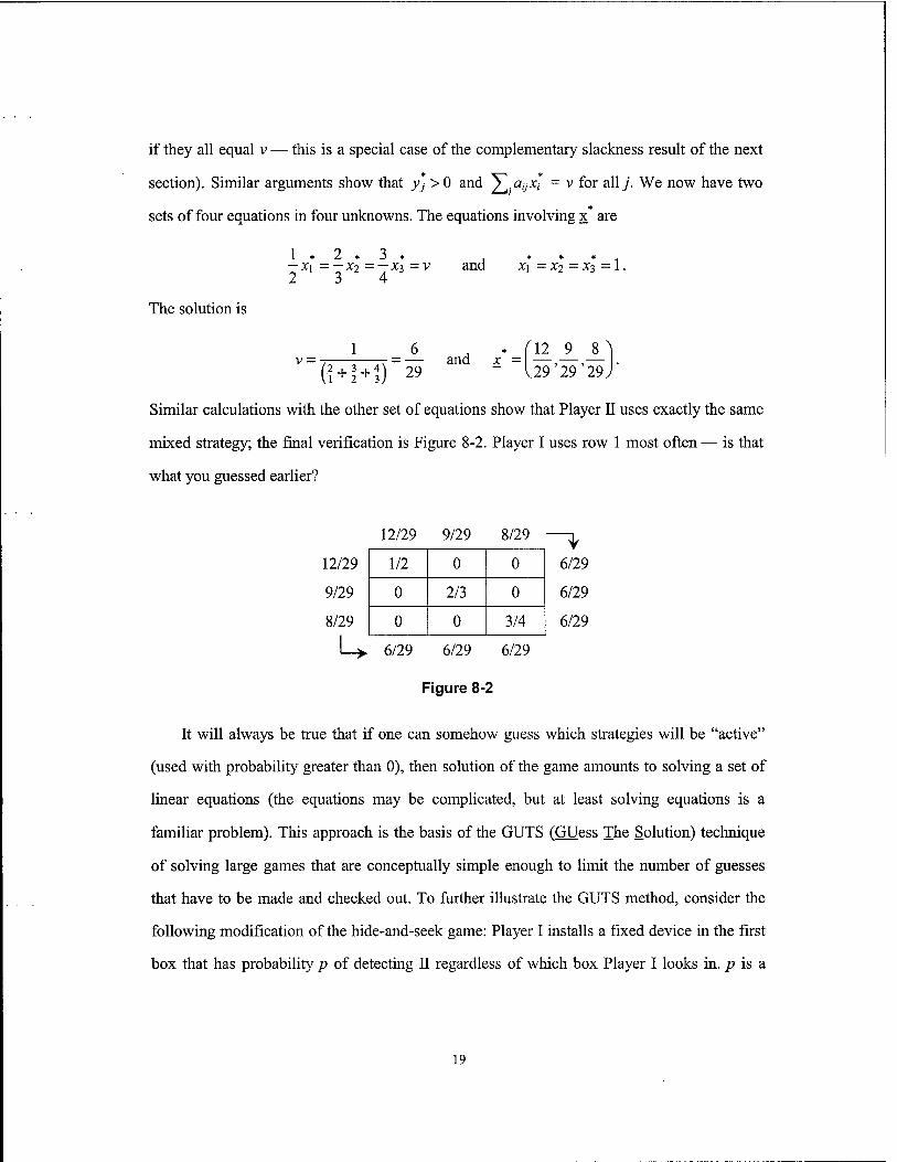
section). Similar arguments show that y>j > 0 and ^.ctyXi = v for all j. We now have two *

sets of four equations in four unknowns. The equations involving x are

1 * A * J * — Xi =— X2 =— XT, =V 2 3 4

and _ i X\ — X2 — Xi> — 1.

The solution is

1 v — ■ and x =

(\2_ 9_ _8_ 29'29'29 (j + f + f) 29

Similar calculations with the other set of equations show that Player II uses exactly the same

mixed strategy; the final verification is Figure 8-2. Player I uses row 1 most often — is that

what you guessed earlier?

12/zy y/zy s/2y ± 12/29 1/2 0 0 6/29

9/29 0 2/3 0 6/29

8/29 0 0 3/4 6/29

U 6/29

F

6/29

:igure 8-

6/29

2

It will always be true that if one can somehow guess which strategies will be "active"

(used with probability greater than 0), then solution of the game amounts to solving a set of

linear equations (the equations may be complicated, but at least solving equations is a

familiar problem). This approach is the basis of the GUTS (GUess The Solution) technique

of solving large games that are conceptually simple enough to limit the number of guesses

that have to be made and checked out. To further illustrate the GUTS method, consider the

following modification of the hide-and-seek game: Player I installs a fixed device in the first

box that has probability p of detecting II regardless of which box Player I looks in. p is a

19

(1 +p)/2 0 0

P 2/3 0

P 0 3/4

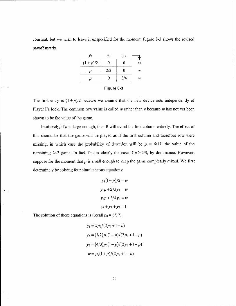
constant, but we wish to leave it unspecified for the moment. Figure 8-3 shows the revised

payoff matrix.

y\ y?. yi —n,

w

w

w

Figure 8-3

The first entry is (1 +p)/2 because we assume that the new device acts independently of

Player I's look. The common row value is called w rather than v because w has not yet been

shown to be the value of the game.

Intuitively, if/? is large enough, then II will avoid the first column entirely. The effect of

this should be that the game will be played as if the first column and therefore row were

missing, in which case the probability of detection will be po= 6/17, the value of the

remaining 2x2 game. In fact, this is clearly the case if p>2/3, by dominance. However,

suppose for the moment that p is small enough to keep the game completely mixed. We first

determine y by solving four simultaneous equations:

yi(l + p)/2 = w

yip + 2/3^2 = w

yxp + 3/4y3 = w

yx+yi+yi =1

The solution of these equations is (recall po = 6/17)

yi=2po/{2po + l-p)

y2={3/2)p0(l-p)/(2p0 + l-p)

yi={4/3)po(l-p)/(2po + l-p)

w = po(l + p)/(2p0 + l- p)

20

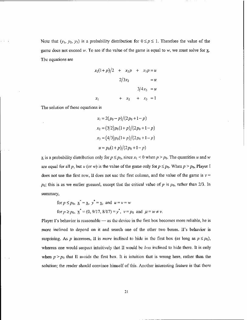
Note that (yi, y2, yi) is a probability distribution for 0 <p < 1. Therefore the value of the

game does not exceed w. To see if the value of the game is equal to w, we must solve for x.

The equations are

x\(l + p)/2 + x2p + XT,P = U

2/3x2 = «

3/4x3 = u

X\ + X2 + XT, = 1

The solution of these equations is

xi = 2(po - p)/(2po + l-p)

x2 =(3/2)p0(l + p)/(2p0 + l- p)

x3 = {4/3)p0(l + p)/(2p0 + l-p)

u = po(l + p)/(2p0 + l-p)

x is a probability distribution only for;? </?o, since x\ < 0 when;? >po. The quantities u and w

are equal for all/», but u (or w) is the value of the game only for/? <j!?o. When/? >po, Player I

does not use the first row, II does not use the first column, and the value of the game is v =

/?o; this is as we earlier guessed, except that the critical value of/? is /?o, rather than 2/3. In

summary,

for/?</?o, x =x, y =y, and u = v = w

for/?>/?o, x* = (0, 9/17, 8/17)=/, v=/?0 and ß = w*v.

Player Fs behavior is reasonable — as the device in the first box becomes more reliable, he is

more inclined to depend on it and search one of the other two boxes. IPs behavior is

surprising. As p increases, II is more inclined to hide in the first box (as long as p </?o),

whereas one would suspect intuitively that II would be less inclined to hide there. It is only

when p>po that II avoids the first box. It is intuition that is wrong here, rather than the

solution; the reader should convince himself of this. Another interesting feature is that there

21

is no advantage to Player I for making/? >po', once a system is so good that the opponent

avoids it, there is no point in making it better.

There are two important points in this section. First, in circumstances where it is clear

that the solution of a square game will be completely mixed, solving the game amounts to

solving simultaneous linear equations. Second, the GUTS procedure is fail-safe as long as

one verifies that the resulting pair of strategies is in equilibrium.

Exercise

1. Verify that the "completely mixed" assumption for the game in Figure 4-1 results in

x = (29/52, 7/52, 16/52) and u= 10.1/52= .194. Is it possible that the solution for y

would be a probability vector?

9. The General Finite Case - Linear Programming

The mathematical problem of maximizing a function of several variables subject to

constraints on those variables is called a mathematical programming problem. If the function

to be maximized (the objective function) and all the constraints are linear functions of the

variables, then we have the special case of linear programming (LP). LP is a powerful

optimization tool because of the availability of computer codes capable of solving problems

with hundreds of thousands of variables and constraints. It is therefore handy that large TPZS

games can be solved using Linear Programming.

We can formulate the solution of a TPZS game as an LP problem as follows: consider

the set of n "value constraints" where xi, ...,xm has the usual meaning and xo is a new

variable.

2]ayX,-x0>0, j = l,...,n.

■th They of these inequalities states that the average payoff exceeds xo when II uses strategy j

and I uses mixed strategy x = (x\, ..., xm). If all n of the inequalities hold, then xo is a security

22

level for Player I in the sense that the average payoff will be at least xo no matter what II does.

Player I's LP, then, is to make xo as large as possible subject to the n value constraints and

additional constraints to the effect that (x\, ...,xm) must be a probability distribution. The

objective function is a linear function of the m+\ variables (the last m coefficients being 0),

and so is each of the constraints. An LP code will provide the solution (xo,x*,...,Xm) that

maximizes the objective function subject to the constraints. The value of the game is v = Xo,

and the optimal mixed strategy for Player I is x ={x\,...,xm).

Similarly, since LP codes can also be used for minimization, y can be found by solving

Player II's problem:

minimize yo

n

subject to ]T ay-yj -y0 < 0; i = \,...,m

n

and yu...,y»>0

If the solution is \yl,y[,...,y*n), then the value of the game is v = yl, and the optimal mixed

strategy for II is (y\,...,y*„).

The fact that xo from I's program is equal to yo from II's program is not obvious,

except for the fact that we already know that all games have a solution, so both numbers must

be the value of the game. Actually, one can prove xo = yo directly by observing that I's and

II's programs are duals (Winston (1994)) of each other, thereby providing a direct and

constructive proof that every finite TPZS game has a solution. The complementary slackness

result of linear programming also has a game theoretic interpretation. It predicts that for every

i either x,- = 0 or else the /' constraint in II's program is active ( = rather than < holds), and

23

similarly either yj = 0 or else the/h constraint in I's program is active (= rather than > holds).

This is the basis of the equation solving technique for completely mixed games.

For small games, comprehensive Management Science software packages often have a

module where the user inputs a matrix and the software then provides the TPZS solution. QM

(http://www.prenhall.com/weiss') is one such package. The underlying technique is LP, but

the details are hidden from the user.

It may seem that a standard method for solving finite TPZS games can now be

identified:

1) Convert the game to normal form by identifying first the strategies for each side

and then the payoff function.

2) Use LP to solve the resulting matrix game.

This "brute force" procedure is sometimes the best way to proceed, but the process of

carrying out step 1 has some disadvantages. First, it is likely to destroy whatever structure the

game had when first formulated. For example, given only the normal form of tic-tac-toe (a

very large matrix full of l's and O's, and -l's), it would be very difficult to recover the

simple nature of the game. Tic-tac-toe is not difficult to solve if the structure is understood

(most schoolboys do it— it has a saddle point at 0 for "tie"), but it would appear to be

formidable if presented only if normal form. Second, there is a large class of games where the

number of strategies is too large for LP; such games may still have solutions, but the brute

force technique is not the way to find them. It is not possible in these brief notes to discuss

methods that have a better chance of success, but see Washburn (1994).

In summary, we can say that in theory LP can be used to solve any game with finitely

many strategies, given the availability of a payoff matrix. Frequently, however, exploitation

of some kind of special structure will produce a solution with less effort.

Exercise

Check that the complementary slackness result holds for all games solved so far.

24

10. Formulation of Military TPZS Games

Selection of the payoff function is simplest in games where there are only two possible

outcomes (I wins/II wins, II detected/H not detected, II shot down/I shot down, II sunk/II not

sunk, etc.), in which case the payoff is the probability that the first outcome happens. In some

games there are resource losses Lj and Ln on both sides, in which case it is tempting to use

LJJ- Li as a payoff. The question of whether the losses are commensurate is likely to arise,

since the units may be different or may be valued differently by the two sides. This issue does

not arise if all the variable losses are II's, in which case the payoff is LJJ. For example, if

Player I conducts an attack with units that can only be used once, then the only issue is how

much damage they do to II.

The payoff function could also be the average amount of time until some critical event

happens, desired large by Player I and small by II.

We give below a brief discussion of several games that have been formulated and solved

in applications. Our intent is not so much to communicate the details of the solutions as to

indicate the type of problem that can be successfully dealt with. In all cases, the payoff is one

of the possibilities discussed above.

Hide-and-seek Games

The payoff is the probability that I detects II, or sometimes a capture distance, and the

strategies are choices of position for each side. "Position" might mean physical location, or it

might be depth if a submarine is being sought, or frequency if an emitter is being sought.

There is an example in Section 8 where detection is impossible unless the position choices

coincide. This requirement is not necessary; the payoff can be an arbitrary function of the two

position choices. This is one case where LP is the natural solution method. For example,

MEDOPS, an ASW planning tool, uses LP to reduce a sensor-depth versus submarine-depth

game to an equivalent sweep width (the game value) for use in subsequent calculations.

25

Duels (Games of Timing)

Each participant makes his shot(s) at a time of his own choice, with the probability of

hitting the opponent being a prespecified increasing function of time. Either the rules of the

game are rigged so that both players are concerned only with the fate of Player II, or else it is

assumed that both players being hit is equivalent to neither player being hit (otherwise the

game is not zero-sum, and the duelists might be well advised to call the whole thing off).

There are infinitely many strategies, but such games have been solved using the GUTS

procedure. The mixed strategies are probability distributions of when to act. Analysis of these

games was prompted by military questions about when to open fire.

Blotto Games

This class of games is named after the legendary Colonel Blotto, who has to divide his

attacking force among several forts without knowing how the defenders are distributed. In the

generalization, each side has a certain total force that must be divided among N "areas." The

payoff is a sum of payoffs in each area, and the payoff in each area depends only on the

forces assigned to that area. Exercise 2 at the end of Chapter 7 is a Blotto game. There have

been diverse applications of this idea:

a) Areas are segments of the ocean, I's resource is ballistic missile submarines, and

IPs resource is ASW forces. The payoff is the average number of I's submarines

surviving an attack by II. The engagement rules in this application are typically

such that a saddle point exists.

b) Areas are ICBM silos, I's resource is attacking ICBM's, and II's resource is

defending ABM's. The payoff is the average number of silos killed. Mixed

strategies are involved.

c) Areas are routes, I's resource is tons of supplies, and IPs resource is interdiction

forces. The payoff is the amount of supplies getting through. The interdiction

forces could be troops, submarines, etc.

26

Communications

A jammer (II) attempts to interfere with information transmission by adding noise to a

transmission. Both transmitter and jammer are power limited, but otherwise free to emit

arbitrary signals. The payoff is the rate of transmission of information. It can be shown

(Welch (1958)) that the jammer's optimal strategy is to transmit Gaussian noise. This is in

agreement with the conventional wisdom in Electronic Warfare to the effect that non-

Gaussian jamming may be particularly effective against a specific communication scheme,

but that simple Gaussian noise jamming is "robust" in the sense of being effective against all

possible communication schemes. It is interesting that many natural noises are Gaussian; this

is evidence for the widely held point of view that Mother Nature is actually diabolical.

Tactical Air War

Many modern military aircraft can be used to perform multiple functions. Berkovitz and

Dresher (1959) take these functions to be "counter-air," "air defense," and "ground support,"

and solve a multiple-day campaign in which only the survivors of day n could be assigned to

one of the three roles on day n + 1. The payoff depends only on the ground support

assignments for the several days, but consistently assigning all aircraft to ground support is

not optimal because large aircraft losses due to the enemy's counter-air operations would

result. An interesting feature of the solution is that the weak side randomizes more than the

strong side; this is also often true in Blotto games. Continuous-time versions of this problem

have also been formulated as differential games (Taylor (1974)).

Barrier Operations

In patrolling a barrier, a searcher has the choice of going slow so that he can hear well,

or fast so that he can cover as much ground as possible. A penetrator has the choice of going

slow to be quiet, or fast to minimize the length of the encounter. The probability of detection

depends continuously on the speed choice of both parties, and a game results. Langford

(1973) solves a version of this game.

27

Pursuit and Evasion Games

Define the "launch envelope" of a missile to be those initial positions for which an

optimally programmed missile can catch its target regardless of how the target maneuvers.

Determination of this envelope is properly in the province of differential games, a topic

invented by Isaacs (1965). The payoff is 1 or 0 depending on whether the target is caught or

not, and strategies are programs for control surfaces as a function of sensor inputs. Solutions

have been obtained only for highly simplified physical models, but have nonetheless proved

enlightening for actual design.

References

BERKOVITZ, L.D. and MELVIN DRESHER, "A Game Theory Analysis of Tactical Air War," Opns. Res., 7, 1959, pp. 599-620.

HAYWOOD, O.G., JR., "Military Decision and Game Theory," Opns. Res., 2, 1954, pp. 365-384.

ISAACS, RUFUS, Differential Games, Wiley, New York, 1965.

LANGFORD, ERIC, "A Continuous Submarine vs Submarine Game," NRLQ, 20, 1973, pp. 405-417.

LUCE, R. DUNCAN and HOWARD RAIFFA, Games and Decisions, Dover, 1957.

MEDOPS, NATO SACLANT Undersea Research Centre, 1999.

OWEN, GUILLERMO, Game Theory (3rd ed.) Academic Press, 1995.

TAYLOR, JAMES G., "Some Differential Games of Tactical Interest," Opns. Res., 22, 1974, pp. 304-317.

WASHBURN, ALAN R., Two-Person Zero-Sum Games, INFORMS, 1994.

WELCH, LLOYD R., "A Game Theoretic Model of Communication Jamming," Memo 20-155, Jet Propulsion Lab., Caltech, 1958.

WINSTON, WAYNE, Operations Research: Applications and Algorithms (3rd ed.), Wadsworth, 1994.

28

INTERNET DOCUMENT INFORMATION FORM

A. Report Title: Notes on Game Theory B. DATE Report downloaded From the Internet: October 13, 2000

Report's Point of Contact: (Name, Organization, Address, Office Symbol, & Ph #): Naval Postgraduate School, Monterey, CA

D. Currently Applicable Classification Level: Unclassified

E. Distribution Statement A: Approved for Public Release

F. The foregoing information was compiled and provided by: DTIC-OCA Initials: LL Preparation Date October 19, 2000

The foregoing information should exactly correspond to the Title, Report Number, and the Date on the accompanying report document. If there are mismatches, or other questions, contact the above OCA Representative for resolution.