Available online at www.sciencedirect.com

ARTICLE IN PRESS

www.elsevier.com/locate/compgeo

Computers and Geotechnics xxx (2008) xxx–xxx

Numerical simulation of drained triaxial test using 3D discreteelement modeling

N. Belheine a,b,c, J.-P. Plassiard c, F.-V. Donze c,*, F. Darve c, A. Seridi d

a Laboratoire de Genie Civil et d’Hydraulique, Universite de Guelma, Algeriab Laboratoire de Genie Civil et d’Hydraulique, Universite de Skikda, Algeria

c Laboratoire Sols, Solides, Structures et Risques (3S-R), UMR5521, Universitd Joseph Fourier, Grenoble Universite, Domaine

Universitaire, BP 53, 38041 Grenoble Cedex 9, Franced Laboratoire de Mecanique des Solides et Systemes (LM2S), Universite M Hamed Bougara de Boumerdes, Algeria

Received 18 December 2006; received in revised form 19 November 2007; accepted 8 February 2008

Abstract

A discrete element modeling of granular material was carried out using a 3D spherical discrete model with a rolling resistance, in orderto take into account the roughness of grains. The numerical model of Labenne sand was generated, and the desired porosity was obtainedby a radius expansion method. Using numerical triaxial tests the micro-mechanical properties of the numerical material were calibratedin order to match the macroscopic response of the real material. Numerical simulations were carried out under the same conditions as thephysical experiments (porosity, boundary conditions and loading). The pre-peak, peak and post-peak behavior of the numerical materialwas studied. The calibration procedure revealed that the peak stress of the sand sample does not only depend on local friction parametersbut also on the rolling resistance. The larger the value of the applied rolling resistance, the higher the resulting stress peak. Furthermore,the deformational response depends strongly on local friction. The numerical results are quantitatively in agreement with the laboratorytest results.� 2008 Elsevier Ltd. All rights reserved.

Keywords: Discrete element model; Granular material; Triaxial test; Rolling resistance; Micro-mechanics

1. Introduction

A continuum assumption is generally used to investigatemany complex engineering problems, for example, buildingfoundations, excavations, retaining walls, tunnels, slopestability problem.

Refined constitutive models and those based on the con-tinuum assumption have proven to be powerful tools todescribe the critical states for soils [1,2]. These models,which are primarily concerned with mathematical model-ing of the observed phenomena at the macroscopic scale,do not represent the local discontinuous nature of thematerial. However, this discontinuous nature plays a majorrole in the behavior of granular materials. This induces spe-

0266-352X/$ - see front matter � 2008 Elsevier Ltd. All rights reserved.

doi:10.1016/j.compgeo.2008.02.003

* Corresponding author. Tel.: +33 4 76 82 70 55; fax: +33 4 76 82 70 00.E-mail address: donze@geo.hmg.inpg.fr (F.-V. Donze).

Please cite this article in press as: Belheine N et al., Numerical simultech (2008), doi:10.1016/j.compgeo.2008.02.003

cial features such as anisotropy, micro-fractures or localinstabilities, which are difficult to understand or modelbased on the principles of continuum mechanics.

An alternative approach is the discrete element methodwhich considers the discrete nature of soils and providesnew insight into constitutive modeling. In it, the physicalprocesses which govern the constitutive behavior can beunderstood more rigorously starting with the behavior atthe scale of a grain [2]. Using this approach, the macro-mechanical response of the physical material (deformabi-lity, strength, dilatancy, strain localization and other) isreproduced by determining the micro-properties of thematerial (normal, tangential and rolling stiffness, local fric-tion and non-dimensional plastic coefficient of the con-tacts). The discrete element method has proven to be avery useful tool to obtain complete qualitative informationon microscopic features of assemblies of particles [3].

ation of drained triaxial test using 3D discrete ..., Comput Geo-

2 N. Belheine et al. / Computers and Geotechnics xxx (2008) xxx–xxx

ARTICLE IN PRESS

The objective of this study is to show how well a numer-ical model based on a local discontinuous description, canreproduce the macro behavior of a granular material in aquantitative manner. To do so, the discrete elementmethod (DEM), which is widely used to simulate thebehavior of a large range of geomaterials, has been chosen.Note that, most of the previous studies using DEM modelsled to restrictive qualitative results. Here, a simple DEMformulation is used to perform quantitative triaxial testsimulations, although recent investigations have shownthe importance of rolling in the deformation process[4,5]. These simulations are compared with a series of axi-symmetric triaxial laboratory tests performed on Labennesand [6–8].

To reproduce the behavior of material at a macro levelas a global response, a mechanical model of Labenne sandwas generated. To calibrate the micro-properties of thenumerical sand medium according to the Labenne sandlaboratory tests, a numerical testing procedure for thedrained triaxial tests was used. This calibration procedureis a crucial issue.

The five main input micro-parameters in the numericalmodel are: the normal contact stiffness, tangential contactstiffness, rolling contact stiffness, local friction and adimensionless coefficient which controls the plastic limitof rolling. Several parametric studies were done to evaluatethe influence of each of the above parameters on the outputmacro parameters such as Poisson’s ratio, Young’s modu-lus, the dilatancy angle, the peak and the post-peakstrength. It was found that the elastic response is mainlygoverned by the normal contact stiffness and the ratio ofshear to normal contact stiffnesses. Secondly, a coupledeffect was found between the local friction, the rolling stiff-ness on the peak stress and a plastic moment on the post-peak stress of the sand. In addition, the observed deforma-tion depends strongly on local friction.

2. Discrete element method with Moment Transfer Law

2.1. Basic features

To keep a low calculation cost while using spherical dis-crete elements, the local constitutive law of classical DEM[9–11] is modified by introducing an additional componentat each point of contact through which rolling resistancecan be supplied. This is referred to MTL as the ‘‘MomentTransfer Law” [12].

By rolling resistance we mean that a couple may betransferred between the discrete elements via the contacts,and this couple resists particle rotations. The rolling whichoccurs during shear displacement is decreased and a morereasonable value of the friction angle is obtained [13].

Using a rolling resistance between spherical discrete ele-ments is justified since real grains are generally not spheri-cal and may exhibit a rough surface texture, which can becovered with a thin film of weathered products [13,14]. Inthis case, grains are in contact with their neighbors through

Please cite this article in press as: Belheine N et al., Numerical simultech (2008), doi:10.1016/j.compgeo.2008.02.003

a contact surface, and not a single point, so that rollingresistance can play a major role on the contact behaviorof the granular material.

The two dimensional simulations by Iwashita and Oda[13,15,16] have shown the importance of rolling resistancein granular mechanics. A three dimensional extension, lar-gely inspired by the formulation presented in [13,15,16],was established in the SDEC code [11,12,17]. Note thatSDEC is a code based on the discrete element method, usinga force–displacement approach, Newton’s second law ofmotion describes the motion of each element as the sumof all forces applied on this element. The dynamic behaviorof the system is solved numerically by a time algorithm inwhich the velocities and the accelerations are constant ateach time step. The system evolves and an explicit finite dif-ference algorithm is used to reproduce this evolution.

2.2. The discrete model using MTL

2.2.1. Kinematics in contact

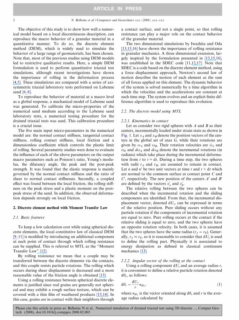
Let us consider two rigid spheres with A and B as theircenters, incrementally loaded under strain state as shown inFig. 1. Let xA and xB denote the position vectors of the cen-ters in the global set of axes G, while their rotations aregiven by xA and xB. Their rotation velocities are _xA and_xB and dxA and dxB denote the incremental rotations (inradians) which take place during the incremental deforma-tion from t to t + dt. During a time step, the two sphereswith radii rA and rB, are assumed to remain in contact.Let n and n0 be two unit vectors at time t and t + dt whichare normal to the common surface at contact point C andC0, respectively. The new position of the centers A0 and B0

are defined by the vectors x0A and x0B.The relative rolling between the two spheres can be

described when the incremental rotation and the slidingcomponents are identified. From that, the incremental dis-placement vector, denoted dUr, can be expressed in termsof the relative position. Pure sliding occurs without anyparticle rotation if the components of incremental rotationare equal to zero. Pure rolling occurs at the contact if therelative sliding is equal to zero, and the two spheres havean opposite rotation velocity. In both cases, it is assumedthat the two spheres have the same radius (rA ¼ rB). Gener-ally, rA � rB, so it is reasonable to consider that dUr is usedto define the rolling part. Physically it is associated toenergy dissipation as defined in classical continuummechanics [13].

2.2.2. Angular vector of the rolling at the contact

Using a rolling component dUr and an average radius r,it is convenient to define a relative particle rotation denoteddhr, as follows:

dhr ¼dU r

rndhr ; ð1Þ

where ndhr is the vector oriented along dhr and r is the aver-age radius calculated by

ation of drained triaxial test using 3D discrete ..., Comput Geo-

G

2t

Bω

Aω

rBB

An

1t

C

At time t

rA

xB

xA

C’

B’

A’

dωB

At time t +dt

dωA

Fig. 1. Kinematics of spheres in contact at time t and t + dt.

N. Belheine et al. / Computers and Geotechnics xxx (2008) xxx–xxx 3

ARTICLE IN PRESS

r ¼ rA þ rB

2; ð2Þ

The angular vector of the rolling part can be defined bysumming of the angular vector of incremental rolling, asfollows:

hr ¼X

dhr: ð3Þ

Since all equations are expressed in the global set of axes G,let hL

r denote the angular vector of the rolling part in thelocal reference L. Its origin is the contact point betweentwo spheres. Its axes are the normal vector n, and two per-pendicular vectors t1, t2 which are in the contact plane

hLr ¼ ½mG L� � hr; ð4Þ

where [mG_L] represents the matrix transformation betweenthe local and the global set of axes.

2.2.3. Physical model with rolling resistance

The interaction force vector F which represents theaction of element A on element B may be decomposed intoa normal and a shear vector Fn and Ft, respectively, seeFig. 2, which may be classically linked to relative displace-ments, through normal and tangential stiffnesses, Kn andKs

F n ¼ Kn � U n; DF t ¼ Ks � dU s; ð5a; bÞ

Fn Fs

Mr

1t

n

2t

Contact plane Sphere A

Sphere B

Fig. 2. Two spheres in contact at time t.

Please cite this article in press as: Belheine N et al., Numerical simultech (2008), doi:10.1016/j.compgeo.2008.02.003

where Un is the relative normal displacement between twoelements and dUs is the incremental tangentialdisplacement.

Let Kn and Ks be the resultant normal and tangentialstiffnesses, respectively. In this paper, we will use a linearmodel. The stiffnesses of two elements in contact are con-nected in series, therefore Kn and Ks are defined by the fol-lowing equations:

Kn ¼

kAn � kB

n

kAn þ kB

n

� �r

and Ks ¼

kAs � kB

s

kAs þ kB

s

!

r; ð6a; bÞ

where indexes [A] and [B] represent the two elements incontact.

The shear process starts working at the contact point,where Fn and Ft satisfy the following inequality:

F t P F n � tgl; ð7Þwhere l is the internal friction angle.

The rolling resistance is defined by the component actingin the contact plane. On the one hand, the elastic momentML

elastic resulting from the rolling part in the local set of axesis written as

MLelastic ¼ kr � hL

r ; ð8Þwhere kr is the rolling stiffness. Its value is obtained byassuming that for small displacements [13], dUr ffi dUs,which leads to

kr ¼ b � Ks � r2; ð9Þwhere b is a dimensionless coefficient used for the rollingstiffness.

On the other hand, if kFnk represents the norm of thenormal force, the elastic limit is controlled by the plasticmoment vector ML

plastic such that

MLplastic ¼ g � r � kF nk; ð10Þ

where g is a dimensionless coefficient used for the plasticmoment.

ation of drained triaxial test using 3D discrete ..., Comput Geo-

4 N. Belheine et al. / Computers and Geotechnics xxx (2008) xxx–xxx

ARTICLE IN PRESS

If the elastic limit is reached, the angular rolling vectorhr has to be recomputed. Its value is determined by

hLr ¼

MLplastic

kr

: ð11Þ

Then the rolling moment Mr, in the global set of axes is de-fined by the minimal norm of the two moments given byEqs. (8) and (9), such that

M r ¼ ½mL G�min MLelastic

�� ��; MLplastic

��� ���� � MLelastic

MLelastic

�� �� ; ð12Þ

where [mL_G] represents the matrix transformation betweenthe local and the global set of axes.

The MTL is summarized here as follows:

If MLelastic

�� �� < MLplastic

��� ��� : M r ¼ ½mL G�MLelastic and hL

r ¼ML

elastic

kr

; ð13Þ

If MLelastic

�� �� P MLplastic

��� ��� : M r ¼ ½mL G� MLplastic

��� ��� MLelastic

MLelastic

�� �� and hLr ¼

MLplastic

kr

: ð14Þ

2.3. Mechanical contact model with rolling resistance

Based on the physical model given in the above section,a complete mechanical model is composed of normal, tan-gential and rolling contact components, as shown in Fig. 3.These three components are similar in principle. They are

Contact point Tangentielcontact model

Normal contact model

Rollingcontact model

Fig. 3. Contact model in

Please cite this article in press as: Belheine N et al., Numerical simultech (2008), doi:10.1016/j.compgeo.2008.02.003

all made of a spring to account for the elastic behaviorof the contact. In addition, the normal contact modelincludes a divider to simulate the fact that no force is trans-mitted when the grains are separated. The tangential con-tact model includes on the other hand, a slider to providethe contact shear resistance controlled by a Mohr–Cou-lomb criterion. Finally, the rolling contact model includesa roller that represents the contact rolling resistancedescribed by Eq. (8). Fig. 4 displays the mechanicalresponse of the normal, tangential and rolling contactmodels.

The rolling contact model is characterized by the rollingstiffness kr and consists of an initial linear part controlledby Eq. (8) followed by a constant value defined by

g � r � kFnk, where g is the plastic moment coefficient [18].This model is an approximation of the rolling resistancemodel, and exhibits elastic–plastic behavior with a failurecriterion similar to the Mohr–coulomb criterion. The pro-posed rolling contact model is shown in Fig. 3.

Springs

Slider

Springs

Divider

Spring

Roller

the DEM with MTL.

ation of drained triaxial test using 3D discrete ..., Comput Geo-

Tangential displacement

tF

sK

Tan

gent

ial f

orce

tg.Fn μ

Strength due to friction

sU

Normal displacementN

orm

al f

orce

nK

nF

nU

Relative rotation rθ

rM

nF.r.η

ICou

ple

at c

onta

ct

rk

Fig. 4. Mechanical response of the contact models: (a) normal contact model; (b) tangential contact model; and (c) rolling contact model.

N. Belheine et al. / Computers and Geotechnics xxx (2008) xxx–xxx 5

ARTICLE IN PRESS

3. Failure criterion used in the model

3.1. Pre and post failure

Once initial interactions disappear, new ones are identi-fied: they are merely contact interactions, and cannotundergo any tension force. A classical Coulomb criterionis then used, with a contact friction angle lc. Note that ten-sile strength can also be used in this model but in the pres-ent study only frictional contact interactions areconsidered.

Fig. 5 summarizes the failure criteria used in the model.

4. Law of motion with rolling resistance

In our model, a grain contact is composed of the normaland shear components, but only the normal componentcontributes to the rolling resistance. It is clear that rollingresistance (couple) does not affect the translational motionsof grains but does affect the angular motion. The move-ment of an element is determined by the resulting forceand moment applied to the element. For an element A with

cμ

Contact interaction

tF

nF

Fig. 5. Failure criteria used in the model.

Please cite this article in press as: Belheine N et al., Numerical simultech (2008), doi:10.1016/j.compgeo.2008.02.003

radius rA, the contact forces F ðkÞn , F ðkÞt and couple M(k) aresummed over p neighbors, which govern the motion of theelement in the translational direction and in its rotationabout the center mass

€xAi ¼

1

mA

Xp

k¼1

F ðkÞi ; €hA ¼ 1

IA

Xp

k¼1

rAF ðkÞt þXp

k

M ðkÞ

!;

where F ðkÞi are the components of the resultant force at con-tact k and i = 1,2,3, represent directions.

5. Calibration parameters

Among currently used techniques, the discrete elementmethod is extensively used to study the behavior of numer-ical material, under the perfectly controlled conditions ofthe numerical experiment. The calibration of the propertiesof the numerical material – i.e. by the assembly of particles-to the properties of a real geo-material is conveniently doneby comparing real and simulated triaxial tests. To do this,an axisymmetric triaxial procedure has been establishedwhich is described in the following section. This procedureallows us firstly to estimate the values of the microscopicparameters kn; a ¼ ks

kn; l; b and g and subsequently to repro-

duce, respectively, the macroscopic behavior characterizedby Young’s modulus E, the Poisson’s ration m, the dilat-ancy angle w, the peak and the post-peak normal stressr. These characteristics are the features of the stress–straincurves deduced from the axisymmetric triaxial tests. Froma macroscopic point of view, the behavior of a system ofparticles in the numerical axisymmetric triaxial tests maybe treated as the macroscopic behavior of three dimen-sional continuums. In general; see Fig. 6:

� The initial slope of the volumetric strain lets us deter-mine Poisson’s ratio m.

ation of drained triaxial test using 3D discrete ..., Comput Geo-

Characteristic state

Critical state

M

ε1%

ε1%

Dev

iato

ric

stre

ss

εv%

σpeak

1%

σpost-peak

3%

ν

ψ

E

Fig. 6. Typical behavior obtained with triaxial tests.

Table 1Macroscopic parameters values of the Labenne medium sand for each test[6–8]

Parameters Tests

100 kPa 200 kPa 300 kPa

Initial porosity (%) 0.3684 0.3676 0.3653Initial densities (kN/m3) 16.61 16.63 16.69Young’s modulus E (MPa) 63.90 95.60 120.30Poisson’s ratio m 0.28 0.27 0.38Friction angle u (�) 35.56 35.30 34.50Dilatancy angle w (�) 11.096 10.92 11.81

6 N. Belheine et al. / Computers and Geotechnics xxx (2008) xxx–xxx

ARTICLE IN PRESS

� The initial slope of the stress–strain diagram is related toYoung’s modulus E and the complete set of materialproperties can be extracted directly from the simulation.� The slope of the volumetric strain curve in the dilatancy

regime is related to the dilatancy angle w.� The characteristic state corresponds to the minimum

volume.� The deformation at which the stress is maximum rpeak

must also correspond to the maximum dilatancy, whichcorresponds to the inflection point where the materialstarts to show mechanical instabilities [19].

6. Calibration methodology

During the calibration procedure, the microscopicparameters that were introduced in the model

kn; a ¼ ks

kn; l;b and g

� �were selected by comparing the

experimental results with the numerical ones. However,some of the parameters can have a cross effect on the mac-roscopic ones (for example b and l on the maximum rpeak).Thus, a calibration methodology is proposed to overcomethis cross dependency. This methodology is

� The normal contact stiffness kn and the ratio a ¼ ks

knwere

varied to match the deformation modulus and Poisson’sratio of the real material while all other parameters ofthe test were kept constant. It is worth noting that con-tact stiffness has a significant effect on the deformationcharacteristics. Young’s modulus and the Poisson’s ratiowere determined from an initial small loading with amaximum axial strain of 1%.� Using the same assembly, a series of simulation tests

were carried out with the appropriate elastic localparameters. The inter-particle friction angle l was var-ied to adjust the dilatancy curve to that of the real mate-rial, while all other parameters were kept constant.

Please cite this article in press as: Belheine N et al., Numerical simultech (2008), doi:10.1016/j.compgeo.2008.02.003

After the adjustment of the dilatancy curve (dilatancyangle) by the inter-particle friction, a check on the validityof the stress–strain curve was carried out by varying therolling stiffness coefficient and the plastic moment coeffi-cient. The first parameter controls the stress–strain curvein the domain located at the peak and the second more spe-cifically modifies the post-peak phase. Furthermore, itallows us to correct the macroscopic angle of friction inthe peak and post-peak regime. It is worth noting thatthe rolling stiffness coefficient and the plastic moment coef-ficient have little influence on the dilatancy curve.

7. Application example: Experimental data of Labenne sand

In the calibration phase, the numerical modeling hasbeen performed simulating Labenne medium sand to com-pare the numerical results with experimental ones. ThisLabenne’s sand has been studied intensively by others[20,21]. It is a homogeneous rounded dune sand. Accordingto the triaxial tests [6–8], the physical properties of the sandare given in Table 1. Results with fairly dense samples(q = 16.6 kN/m3) for different confining pressures (r3) areshown in Fig. 7.

Based on the experimental results, the stress–strainbehavior of this sand is highly non-linear. The results indi-cate that the initial deformation modulus increases withincreasing cell pressure; see Table 1. Another distinct fea-ture of the Labenne sand is that as sample loading begins,initial compaction takes place, followed in the pre-peakregime, by dilatancy.

8. DEM model simulating the compression triaxial tests

8.1. The geometrical model

To prepare sphere packing [22], numerous methods exist[23,24]. Here, the radii expansion method, based on a Wei-bull distribution was applied. The only case where the radiican be reduced is when overlapping exists at the very end ofthe growing process. With it, the desired porosity whichcorresponds to the porosity of the real specimen n = 0.40was reached. The assembly representing the numericalmodel of Labenne sand consisted of 10,648 particles withdifferent radii of 0.043–0.175 m (see Fig. 8b) and sample

ation of drained triaxial test using 3D discrete ..., Comput Geo-

Fig. 7. Experimental triaxial test results for Labenne medium sand [6–8].

Fig. 8. (a) Numerical specimen, (b) distribution size of numerical specimen, and (c) normal force distribution.

N. Belheine et al. / Computers and Geotechnics xxx (2008) xxx–xxx 7

ARTICLE IN PRESS

size of (H = 4 m and D = 2 m). Note that, as long as thesample’s slenderness is equal to 2.0, which is similar tothe typical geometric ratio used in experiments [20], themodel’s results do not depend on the discrete element’scharacteristic’s size since the local parameters, intrinsically,take it into account. It has been checked that the homo-thetic modification of the model has no influence on thenumerical results. During the generation of the assemblyonly the normal and shear stiffnesses and the initial densityare used. In Fig. 8 the sample of the virtual material, thediagram of size distribution and the normal force distribu-tion are shown.

It is important to check the existence of a possibleanisotropy in the orientations of the contacts due to themode of sample preparation. It is anticipated that anglesof 0� and 90� are privileged orientations directly as a resultof the directions of compression. In Fig. 9 the orientationof he contacts are presented. Roux and Combe [25] showedthat there is a privileged direction of the contact forcesaccording to their intensity. This anisotropy due to theintensity of inter-granular forces occurs during the applica-tion of the deviatoric stress. Although the mechanical load-

Please cite this article in press as: Belheine N et al., Numerical simultech (2008), doi:10.1016/j.compgeo.2008.02.003

ing is isotropic, we will check that the procedure does notlead to a privileged contact orientation in the direction ofmotion.

With the histogram of the contact orientation, shown inFig. 9, we can see that the contacts are homogeneously dis-tributed in all directions.

8.2. Modeling procedure

After the preparation phase, new micro-mechanicalproperties were introduced in the model. The triaxial testwas modeled by confining the medium within six smoothwalls. The isotropic compression took place under grav-ity-free conditions, so that the particle arrangement wasconsidered to be almost isotropic, see Fig. 8c. The topand bottom boundaries moved vertically as loading plat-ens, either under force-controlled condition or understrain-controlled conditions. The lateral ones simulate theconfining pressure experienced by the sample sides. Inour simulation, the sample is loaded in a strain-controlledmode by specifying the velocities of the top and the bottomwalls. To this end, it can be noted that as the walls are fric-

ation of drained triaxial test using 3D discrete ..., Comput Geo-

Fig. 9. Distribution of the contact orientation, prior to applying deviatoric loading.

8 N. Belheine et al. / Computers and Geotechnics xxx (2008) xxx–xxx

ARTICLE IN PRESS

tionless, thus any friction between the sample and the load-ing platens is avoided, hence allowing the wall appliedstresses to remain normal to each wall [26].

During all the steps of the test, displacements of the lat-eral walls are controlled automatically by a servo mecha-nism [27] that maintains a constant confining stresswithin the sample. According to the given boundary condi-tions, the stress and strain states within the sample areassumed to be homogeneous. Strains are then calculateddirectly from wall displacements, while the corresponding

H =

2L

0

L0

σ 3 =

σ2=

100

KPa

σ1 = 100KPa

L varies

HD

ecre

ase

at c

onst

ant

velo

city

σ 3 =

σ2

= 1

00=

kPa

σ1 varies

Fig. 10. Test procedure: (a) initial state and (b) triaxial test.

Fig. 11. Effect of local properties at particle contact on macro-pr

Please cite this article in press as: Belheine N et al., Numerical simultech (2008), doi:10.1016/j.compgeo.2008.02.003

stresses are obtained from boundary forces, as in conven-tional laboratory testing, see Fig. 10.

8.3. Modeling results

During the numerical axisymmetric triaxial test themodel parameters (normal contact stiffness kn, ratioa ¼ ks

kn, inter-particle friction angle l, rolling stiffness coeffi-

cient b and plastic moment coefficient g), were chosen bycomparing the experimental results with the numericalones. Laboratory tests are available under different confin-ing pressures (100, 200 and 300 kPa). Several attempts weremade to evaluate the influence of the input microscopicparameters on the deformation and the characteristicstrength. Fig. 11 shows the relationship between the elasticmacroscopic parameters (Young’s modulus E, Poisson’sratio m) and elastic microscopic parameters (normal contactstiffness kn and ratio a ¼ ks

knÞ for a confining pressure of

100 kPa. It can be seen that there is an almost linear rela-tionship in the domain of interest firstly, between the nor-mal contact stiffness and the Young’s modulus, andsecondly, between the ratio a ¼ ks

knand the Poisson’s coeffi-

cient. The elastic region is mainly influenced by the elasticmicroscopic parameters. These values were chosen as

operties of Labenne sand for a confining pressure of 100 kPa.

ation of drained triaxial test using 3D discrete ..., Comput Geo-

Table 2Values of the microscopic parameters of the discrete element model

Parameters Mean value

Normal contact stiffness kn (Pa) 9.6 � 108

Ratio a ¼ ks

kn0.04

Inter-particle friction angle l (�) 30.0Rolling stiffness coefficient b 0.12Plastic moment coefficient g 1.0

N. Belheine et al. / Computers and Geotechnics xxx (2008) xxx–xxx 9

ARTICLE IN PRESS

kn = 9.6 � 108 Pa and a = 0.04 in order to match experi-mental results. Fig. 12 shows the numerical resultsobtained with the parameters reported in Table 2 for con-fining pressures of 100, 200 and 300 kPa. The results indi-cate that the non-linear stress–strain behavior of sandincluding dilatancy is covered by the numerical model. Thismeans that the model is predictive.

The considerable influence of the inter-particle frictionangle l, and the small influence of the rolling stiffness coef-

Fig. 12. Stress and volumetric strain plotted versus axial strain for the Labenne sand and numerical sample.

Please cite this article in press as: Belheine N et al., Numerical simulation of drained triaxial test using 3D discrete ..., Comput Geo-tech (2008), doi:10.1016/j.compgeo.2008.02.003

Table 3Macroscopic parameters of the numerical medium sand for each test

Parameters Tests

100 kPa 200 kPa 300 kPa

Young’s modulus E (Mpa) 63.3 95.5 129.32Poisson’s ratio m 0.289 0.274 0.363Friction angle u (�) 35.43 34.01 34.71Dilatancy angle w (�) 11.2 10.91 11.03

10 N. Belheine et al. / Computers and Geotechnics xxx (2008) xxx–xxx

ARTICLE IN PRESS

ficient b and plastic moment coefficient g on the dilatancycurve should be noted. Furthermore, the peak strengthnot only depends on friction but also on the rolling stiffnesscoefficient b and the plastic moment coefficient g. Thehigher the value chosen, the higher the calculated peakstrength. The best results were achieved with l = 30�,b = 0.12, and g = 1.0. A further increase did not yield abetter agreement with experimental results. With the firstparameter the dilatancy curve is adjusted with the secondand the last, the stress–strain curve in the peak and post-peak regimes are, respectively, controlled. Furthermore,the macroscopic friction angle to be corrected with the lasttwo parameters.

Table 3 shows the macroscopic parameters for numeri-cal medium sand. It is observed that the deformation mod-

Fig. 13. Variation of: (a) deformation modulus, (b) Poisson’s ratio, (c

Please cite this article in press as: Belheine N et al., Numerical simultech (2008), doi:10.1016/j.compgeo.2008.02.003

ulus increases with increasing confining pressure, and it isvery close to the experimental one. In Fig. 13a and b, thevariation of the deformation modulus, Poisson’s coefficientversus the confining pressure are plotted. The deformationmodulus depends strongly on the confining pressure, unlikethe Poisson’s coefficient, which does not vary much withconfinement. Fig. 13c and d gives the evolution of the mac-roscopic friction angle at the peak and the dilatancy angleversus confining pressure. The friction angle decreases withincreasing confining pressure (100–200 kPa) by approxi-mately 1.5�, then a slight increase for 300 kPa, which is aphenomenon also observed in physical samples. The sameobservation is noted for the dilatancy angle.

8.4. Mohr–Coulomb parameters

As an acceptable result of the calibration procedure, thenumerical model of Labenne sand, Mohr-circles and thefailure envelope constructed using series of triaxial testare presented in Fig. 14. The failure envelope is linear forthe chosen parameters for peak and residual stresses, asoften found for natural soils. Since no local cohesion hasbeen used, the macroscopic failure envelope goes throughthe origin. This clearly shows the ability of the modifieddiscrete model in reproducing the macroscopic Mohr–Cou-

) friction angle, and (d) dilatancy angle, versus confining pressure.

ation of drained triaxial test using 3D discrete ..., Comput Geo-

Fig. 14. Mohr circle representation of the numerical sand according to the results of triaxial test.

N. Belheine et al. / Computers and Geotechnics xxx (2008) xxx–xxx 11

ARTICLE IN PRESS

lomb criterion. The slope of the failure envelope gives amacroscopic friction angle. A maximum macroscopic fric-tion angle of 35.7� (the angle of friction falls in the intervalmeasured in physical tests) corresponds to a microscopicfriction angle of 30�.

9. Discussion

The objective of the above calibration process was tocreate a numerical sand sample, which would reproducethe mechanical response of Labenne sand and coulddirectly be used to solve the boundary problem underconsideration. The calibration was carried out using triax-ial (axisymmetric) laboratory test results. Simulations aredone under the same test conditions as experiments(porosity, boundary condition and loading). Using thecalibration methodology proposed in Section 6, we couldcalibrate the numerical model of Labenne sand. Severalparametric studies were performed. The results presentedin Fig. 12 are the results of this methodology. It is worthnoting that the macroscopic response in the elastic regionis mainly influenced by the elastic microscopic parameter.A coupled effect between the inter-particle friction angle,the rolling stiffness coefficient and the plastic momentcoefficient on the peak and post-peak regime was alsofound. The inter-particle friction angle, l governs thedilatancy curve. The rolling stiffness coefficient b and aplastic moment coefficient g have little influence on this.Furthermore, the peak strength not only depends on fric-tion but also on the rolling stiffness coefficient b and aplastic moment coefficient g. The last two control thestress–strain curve in the peak and post-peak regimes,respectively, and enables the macroscopic friction angleto be corrected.

It is observed that the failure stress increases withincreasing confining pressure. The initial stiffness is alsofound to increase with an increase in the confining pres-sure. It varies with confining pressure according to apower law. Poisson’s ratio varies slightly with the confin-ing pressure: this dependence could be due to the varia-tion of the number of contacts. Moreover, thevolumetric strain shows that the discrete element assembly

Please cite this article in press as: Belheine N et al., Numerical simultech (2008), doi:10.1016/j.compgeo.2008.02.003

becomes more compressible and that there exists a dilat-ing tendency at higher strain. This result corresponds tothose observed in laboratory tests. From the stress–straincurve presented in Fig. 12, we determined the values ofthe peak and the post-peak friction angle. The slope ofthe line which passes through the origin and is tangentto the circles is equal to tanl = 0.71 or l = 35.7�; seeFig. 14. It is noted that the friction angle does not varymuch in the stress range studied, as in Fig. 13c. The var-iation lies between 35.43� and 34.71� for confining pres-sure from 100 to 300 kPa, which is similar to thevariation of friction angles found in sands. The variationof dilatancy angle with confining pressure is displayed inFig. 13d. Once again, this quantity does not vary muchin the studied stress range and it falls in the range mea-sured in physical material. The numerical and experimen-tal results are in good qualitative and quantitativeagreement; as seen in Fig. 12. In particular, the best esti-mate is obtained with the set of parameters given in Table2. The only exception was the volumetric response, withneeds further tuning.

10. Conclusion

Numerical tests were carried out to simulate laboratorytests of Labenne sand. To reach this goal, the calibrationmethodology explained in Section 6 needs to be followed.Based on this, the main conclusions are:

(1) In spite of its simplicity, the numerical model withMTL is able to reproduce the main features of theaxisymmetric triaxial tests, as well as several mechan-ical properties of sand. In terms of the deformationalcharacteristics, a good agreement between the numer-ical and physical material is obtained (the chosenmicroscopic values of kn = 9.6 � 108 Pa anda = 0.04 give macroscopic values E = 95.8 MPa,m = 0.275 for a numerical material which correspondswell with the macroscopic values E = 96 MPa,m = 0.28 for the physical material). A linear relation-ship between the elastic parameters at the micro andmacro scales is found.

ation of drained triaxial test using 3D discrete ..., Comput Geo-

12 N. Belheine et al. / Computers and Geotechnics xxx (2008) xxx–xxx

ARTICLE IN PRESS

(2) The corresponding shear strength parameters agreewell. The friction angle (35.7�) of the numerical sandsample, which was determined by a linear failureenvelope, is slightly smaller than that of the physicalmaterial (36.50�). When calibrating the numericalmaterial, a considerable influence of the inter-particlefriction on the volumetric strain was found. Littleinfluence of the rolling stiffness coefficient b andnon-dimensional plastic coefficient g on the dilatancycurve should be noted. This means that the rollingeffect is more dominant than the sliding effect [4,5].Indeed, rolling occurs only if the moment at the con-tact point is large enough.

(3) The major reason for introducing the rolling resis-tance is because the representation of the roughnessof grains lacks in spherical DEM models. Thus, theresults are in very good agreement with experimentalresults, even if the numerical medium is made of asmall amount of particles (around 10,000).

The authors believe that the near future massive 3D sim-ulations of granular materials will use basic geometriessuch as the spherical shapes or cluster of spherical discreteelements. This is why a special effort must be made toimprove their local behavior law.

Acknowledgement

The first author would like to acknowledge the ResearchMinistry of Algeria for the financial support, in the frame-work of the ‘‘Comite Mixte d’Evaluation et de ProspectiveFranco-Algerien”.

References

[1] Manzari MT, Dafalias YF. A critical state two-surface plasticitymodel for sands. Geotechnique 1997;47(2):255–72.

[2] Duncan JM. State of the art: limit equilibrium and finite-elementanalysis of slopes. J Geotech Eng – ASCE 1996;122(7):577–96.

[3] Dolezalova M, Czene P, Havel F. Micromechanical modeling ofstress path effects using PFC2D. Code Num Mod Micro via ParticleMeth 03. Lisse: Swets & Zeitlinger; 2003. p. 173–81.

[4] Bagi K, Kuhn MR. A definition of particle rolling in a granularassembly in terms of particle translations and rotations. J Appl Mech,Trans Am Soc Mech Eng 2004;71:493–501.

[5] Kuhn MR, Bagi K. Contact rolling and deformation in granularmedia. Int J Solids Struct 2004;41:5793–820.

[6] Mestat P, Berthelon JP. Modelisation par elements finis des essais surfondations superficielles a Labenne. Bull Laborat Ponts Chaussees2001;234(Septembre–Octobre):19–39 [REF 4389].

[7] Mestat P, Riou Y. Methodologie de determination des parametrespour la loi de comportement elastoplastique de Vermeer et simula-

Please cite this article in press as: Belheine N et al., Numerical simultech (2008), doi:10.1016/j.compgeo.2008.02.003

tions d’essais de mecanique des sols. Bull Laborat Ponts Chaussees2001;235(Novembre–Decembre):19–39 [REF 4391].

[8] Mestat Ph. Caracterisation du comportement du sable de Labenne.Determination des parametres des lois de Nova et de Vermeer a partird’essais de laboratoire. Laborat Cent Ponts Chaussees2001;225(Mars–Avril):21–40.

[9] Cundall PA, Strack ODL. The distinct numerical model for granularassemblies. Geotechnique 1979;29:47–65.

[10] Cundall PA, Strack ODL. The distinct element method as a tool forresearch in granular media. Part II. Department of Civil EngineeringReport. University of Minnesota; 1979.

[11] Donze FV, Magnier S-A, Daudeville L, Mariotti C, Davenne L.Study of the behavior of concrete at high strain rate compressions bya discrete element method. ASCE J Eng Mech 1999;125(10):1154–63.

[12] Plassiard J-P, Belheine N, Donze FV. Calibration procedure forspherical discrete elements using a local moment law. In: 4thInternational conference on discrete element methods (DEM 07),Brisbane, 27–29 August 2007.

[13] Iwashita K, Oda M. Rolling resistance at contacts in simulation of shearband development by DEM. ASCE J Eng Mech 1998;124(3):285–92.

[14] Jiang MJ, Yu H-S, Harris D. A novel discrete model for granularmaterial incorporating rolling resistance. Comput Geotech2005;32(5):340–57.

[15] Iwashita K, Oda M. Micro-deformation mechanism of shear bandingprocess based on modified distinct element. Powder Technol2000;109:192–205.

[16] Oda M, Iwashita K, Kakiuchi T. Importance of particle rotation inthe mechanics of granular materials. Powders & grains, vol. 97.Rotterdam: Balkema; 1997. p. 207–10.

[17] Donze F-V, Magnier S-A. Formulation of a three-dimensionalnumerical model of brittle behavior. Geophys J Int 1995;122:790–802.

[18] Sakaguchi H, Ozaki E, Igarachi T. Plugging of the flow of granularmaterials during the discharge from a silo. Int J Mod Phys B1993;7:1949–63.

[19] Evesque P. Mecanqiue des milieux granulaires. Poudres Grains2000;NS51:1–60.

[20] Coquillay S. Prise en compte de la non-linearite du comportement dessols soumis a de petites deformations pour le calcul des ouvragesgeotechniques. PhD Thesis, Ecole nationale des ponts et chaussees.Paris, 2005.

[21] Canepa Y, Depresles D. Fondations superficielles. Essais de charg-ement de semelles etablies sur une couche de sable en place, stationexperimentale de Labenne. Influence des conditions d’excution,Compte rendue des essais, FAER 1. 17.02.09, 1990.

[22] Weitz DA. Packing in the spheres. Science 2004;303:968–9.[23] Chang C, Misra A. Packing structure and mechanical properties of

granulates. J Eng Mech 1990;116(5):1077–93.[24] Fazekas S, Torok J, Kertesz J, Wolf DE. Computer simulation of

three dimensional Shearing of granular materials: formation of shearbands. Powders & grains, vol. 5. London: Taylor & Francis Group;2005. p. 223–26.

[25] Roux J-N, Combe G. Quasistatic rheology and the origins of strain.Compte Rendus de l’academie des Sciences Serie IV – Physics–Astrophysics (Comptes Rendus Physique) 2002;3(2):131–40.

[26] Calvetti F, Viggiani G, Tamagnini C. A numerical investigation of theincremental behavior of granular soils. Riv Geotech 2003;3:11–29.

[27] PFC2D. Particle Flow in Two-Dimensions, Version 2.0, UserManual. Minneapolis, Minnesota: ITASCA Consulting Group,Inc.; 1996.

ation of drained triaxial test using 3D discrete ..., Comput Geo-