Numerical solution of General Rosenau-RLW Equation using

Available online at www.ispacs.com/cna

Volume 2012, Year 2012 Article ID cna-00129, 16 pages

doi:10.5899/2012/cna-00129

Research Article

Numerical solution of General Rosenau-RLW

Equation using Quintic B-splines Collocation

Method

R.C. Mittal 1, R.K. Jain 2∗

(1) Department of Mathematics, Indian Institute of Technology Roorkee, Roorkee 247667, Uttarakhand,

India

(2) Department of Mathematics, Indian Institute of Technology Roorkee, Roorkee 247667, Uttarakhand,

India

——————————————————————————————————Copyright 2012 c⃝ R.C. Mittal and R.K. Jain. This is an open access article distributed under the Cre-

ative Commons Attribution License, which permits unrestricted use, distribution, and reproduction in any

medium, provided the original work is properly cited.

——————————————————————————————————

AbstractIn this paper a numerical method is proposed to approximate the solution of the nonlineargeneral Rosenau-RLW Equation. The method is based on collocation of quintic B-splinesover finite elements so that we have continuity of the dependent variable and its first fourderivatives throughout the solution range. We apply quintic B-splines for spatial variableand derivatives which produce a system of first order ordinary differential equations. Wesolve this system by using SSP-RK54 scheme. This method needs less storage space thatcauses to less accumulation of numerical errors. The numerical approximate solutions tothe nonlinear general Rosenau-RLW Equation have been computed without transform-ing the equation and without using the linearization. Illustrative example is included fordifferent value of p = 2, 3 and 6, to demonstrate the validity and applicability of the tech-nique. Easy and economical implementation is the strength of this method.Keywords: general Rosenau-RLW Equation; quintic B-splines basis functions; SSP-RK54 scheme;

Thomas algorithm.

∗Corresponding author. Email address: rkjain [email protected] Tel:+91-8989155751

1

R.C. Mittal et.al Communications in Numerical Analysis

1 Introduction

In this paper, we consider the following initial-boundary value problem of the generalRosenau-RLW equation:

ut − uxxt + uxxxxt + ux + (up)x = 0, a < x < b, 0 < t < T (1.1)

with an initial conditionu(x, 0) = u0(x) (1.2)

and boundary conditions

u(a, t) = u(b, t) = 0, uxx(a, t) = uxx(b, t) = 0, 0 < t < T. (1.3)

where p ≥ 2 is an integer and u0(x) is a known smooth function.

When p = 2, equation (1.1) is called as usual Rosenau-RLW equation.When p = 3, it is called as modified Rosenau-RLW (MRosenau-RLW) equation.

The initial boundary value problem (1.1) - (1.3) possesses the following conservativequantities:

I1 =1

2

∫ b

audx (1.4)

I2 =1

2

∫ b

a(u2 + u2x + u2xx)dx (1.5)

related to mass and energy. We know that the ability to preserve some invariant proper-ties of the original differential equation is a criterion to judge the success of a numericalsimulation.

The quantities I1 and I2 are applied to measure the conservation properties of thepresent method, calculated by trapezoidal rule for Rosenau-RLW equation.

Some of the previous works on the GRLW equation are inclusive of an implicit second-order accurate and stable energy preserving finite difference method based on the use ofcentral difference equations for the time and space derivatives [23], the method of linesbased on the discretization of the spatial derivatives by means of Fourier pseudo-spectralapproximations [11], the Fourier spectral method for the initial value problem of theGRLW equation [12] and a linearized implicit pseudo-spectral method [4]. For p = 1, thisequation reduces to the regularized long wave (RLW) equation as an important equationin physics media describing phenomena with weak nonlinearity and dispersion waves.Various numerical techniques such as the finite element methods based on least squareprinciple [1, 2, 9], finite element methods based on Galerkin and collocation principles[5, 7, 20, 22, 3, 24, 18, 8], Petrov-Galerkin method [6] and Reduced Differential TransformMethod [15] have been devised to find numerical solutions of the RLW equation. RBFcollocation method has been developed for numerical simulation of GEW equation in[17]. The other special case of the GRLW equation is the modified regularized long wave(MRLW) equation for p = 2. MRLW equation was solved numerically by the collocationmethod with quintic B-splines [10, 19] and cubic B-splines [11] finite element method.

2 ISPACS GmbH


Recently, Zuo et al. [24], developed a numerical scheme for solving (1.1) - (1.3) usingconservative finite difference method. Existence of its difference solutions have provedby Brouwer fixed point theorem. They have shown that general Rosenau-RLW Equationpossesses conservative quantities. They have also proved by the discrete energy methodthat the scheme is uniquely solvable, unconditionally stable, and second-order convergent.Pan et al. [16] developed a three level finite difference scheme for usual Rosenau-RLWequation. They have discussed the second order convergence of their scheme by discreteenergy method.

In this paper, we present a new method to the solution of Rosenau-RLW equation.The method is based on quintic B-splines basis functions for solving equation (1.1) -(1.3).We knows that B-splines have some special features which are useful in numericalwork. One feature is that the continuity conditions are inherent, other special feature ofB-splines is that they have small local support, i.e. each B-spline function is only non-zeroover a few mesh subintervals, so that the resulting matrix for the discretization equationis tightly banded. Due to their smoothness and capability to handle local phenomena,B-splines offer distinct advantages. In combination with collocation, this significantlysimplifies the solution procedure of differential equations. There is a great reduction ofthe numerical effort, because there is no need to calculate the integrals (like in variationalmethods) in order to form the final set of algebraic equations, which substitutes the givenset of nonlinear differential equations. Unlike some previous techniques using varioustransformations to reduce the equation into more simple equation, the current methoddoes not require extra effort to deal with the nonlinear terms. Therefore the equationsare solved easily and elegantly using the present method. This method has also additionaladvantages over some rival techniques, ease in use and computational cost effectiveness inorder to find solutions of the given nonlinear evolution equations. In the present method,the combination of the quintic B-spline collocation method in space with the low-storagefourth-order total variation diminishing SSP-RK54 scheme in time provides an efficientexplicit solution with high accuracy and minimal computational effort for the problemsrepresented by (1.1) - (1.3).

This paper is organized as follows. In Section 2, description of quintic B-splines collo-cation method is explained. In Section 3, procedure for implementation of present methodis described for equation (1.1) - (1.3). In Section 4, procedure to obtain initial vector whichis required to start our method is explained. We present numerical example for differentvalues of p to establish the adaptability of the present method computationally in Section5. Conclusion is given in Section 6 that briefly summarizes the numerical outcomes.

2 Description of Method

In quintic B-splines collocation method the approximate solution can be written as a linearcombination of basis functions which constitute a basis for the approximation space underconsideration.

We consider a mesh a = x0 < x1, . . . , xN−1 < xN = b as a uniform partition of thesolution domain a ≤ x ≤ b by the knots xj with h = xj − xj−1, j = 1, . . . N.

Our numerical treatment for solving equation (1.1) using the collocation method withquintic B-spline is to find an approximate solution UN (x, t) to the exact solution u(x, t)in the form:

3 ISPACS GmbH


UN (x, t) =

N+2∑j=−2

cj(t)Bj(x) (2.6)

where cj(t) are time dependent quantities to be determined from the boundary conditionsand collocation from the differential equation.

The quintic B-spline Bj(x) at the knots is given by [13].

Bj(x) =1

h5

(x− xj−3)5, x ∈ [xj−3, xj−2)

(x− xj−3)5 − 6(x− xj−2)

5, x ∈ [xj−2, xj−1)

(x− xj−3)5 − 6(x− xj−2)

5 + 15(x− xj−1)5, x ∈ [xj−1, xj)

(xj+3 − x)5 − 6(xj+2 − x)5 + 15(xj+1 − x)5, x ∈ [xj , xj+1)

(xj+3 − x)5 − 6(xj+2 − x)5, x ∈ [xj+1, xj+2)

(xj+3 − x)5, x ∈ [xj+2, xj+3)

0, otherwise

(2.7)

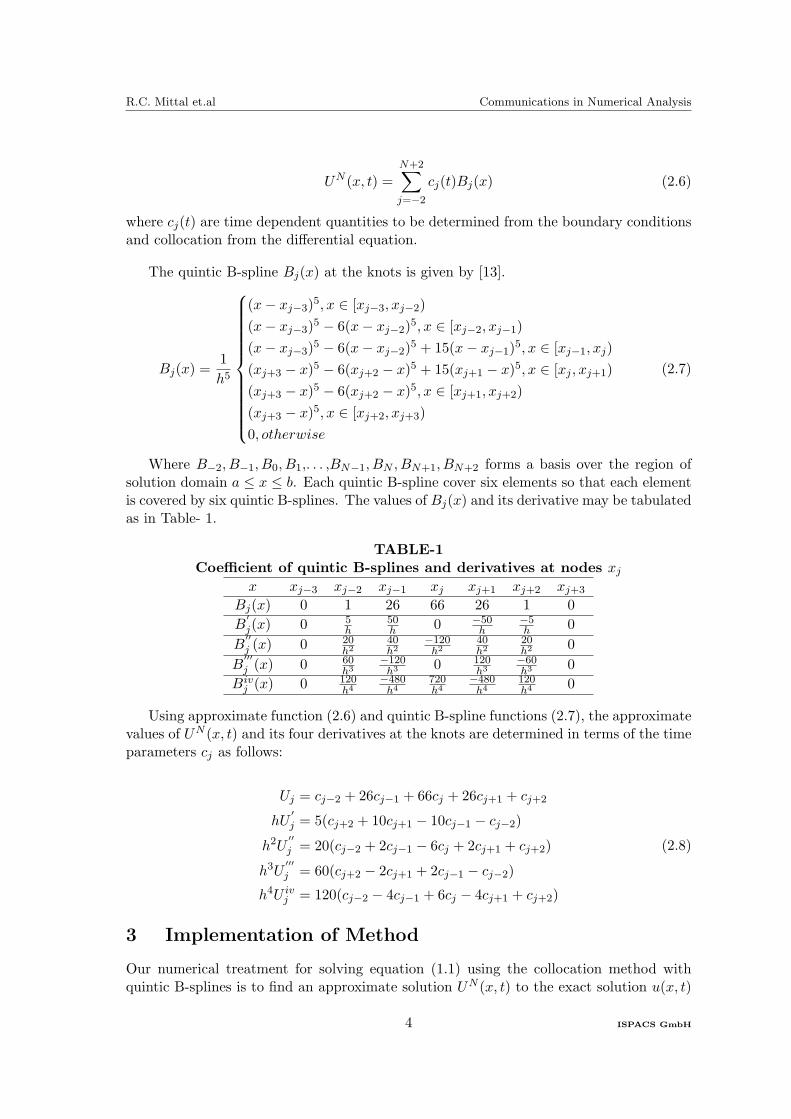
Where B−2, B−1, B0, B1,. . . ,BN−1, BN , BN+1, BN+2 forms a basis over the region ofsolution domain a ≤ x ≤ b. Each quintic B-spline cover six elements so that each elementis covered by six quintic B-splines. The values of Bj(x) and its derivative may be tabulatedas in Table- 1.

TABLE-1Coefficient of quintic B-splines and derivatives at nodes xj

x xj−3 xj−2 xj−1 xj xj+1 xj+2 xj+3

Bj(x) 0 1 26 66 26 1 0

B′j(x) 0 5

h50h 0 −50

h−5h 0

B′′j (x) 0 20

h240h2

−120h2

40h2

20h2 0

B′′′j (x) 0 60

h3−120h3 0 120

h3−60h3 0

Bivj (x) 0 120

h4−480h4

720h4

−480h4

120h4 0

Using approximate function (2.6) and quintic B-spline functions (2.7), the approximatevalues of UN (x, t) and its four derivatives at the knots are determined in terms of the timeparameters cj as follows:

Uj = cj−2 + 26cj−1 + 66cj + 26cj+1 + cj+2

hU′j = 5(cj+2 + 10cj+1 − 10cj−1 − cj−2)

h2U′′j = 20(cj−2 + 2cj−1 − 6cj + 2cj+1 + cj+2)

h3U′′′j = 60(cj+2 − 2cj+1 + 2cj−1 − cj−2)

h4U ivj = 120(cj−2 − 4cj−1 + 6cj − 4cj+1 + cj+2)

(2.8)

3 Implementation of Method

Our numerical treatment for solving equation (1.1) using the collocation method withquintic B-splines is to find an approximate solution UN (x, t) to the exact solution u(x, t)

4 ISPACS GmbH


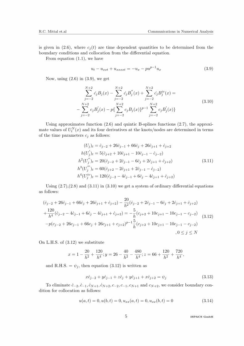
is given in (2.6), where cj(t) are time dependent quantities to be determined from theboundary conditions and collocation from the differential equation.

From equation (1.1), we have

ut − uxxt + uxxxxt = −ux − pup−1ux (3.9)

Now, using (2.6) in (3.9), we get

N+2∑j=−2

cjBj(x)−N+2∑j=−2

cjB′′j (x) +

N+2∑j=−2

cjBivj (x) =

−N+2∑j=−2

cjB′j(x)− p{

N+2∑j=−2

cjBj(x)}p−1N+2∑j=−2

cjB′j(x)}

(3.10)

Using approximates function (2.6) and quintic B-splines functions (2.7), the approxi-mate values of UN

t (x) and its four derivatives at the knots/nodes are determined in termsof the time parameters cj as follows:

(Uj)t = cj−2 + 26cj−1 + 66cj + 26cj+1 + cj+2

h(U′j)t = 5(cj+2 + 10cj+1 − 10cj−1 − cj−2)

h2(U′′j )t = 20(cj−2 + 2cj−1 − 6cj + 2cj+1 + cj+2)

h3(U′′′j )t = 60(cj+2 − 2cj+1 + 2cj−1 − cj−2)

h4(U ivj )t = 120(cj−2 − 4cj−1 + 6cj − 4cj+1 + cj+2)

(3.11)

Using (2.7),(2.8) and (3.11) in (3.10) we get a system of ordinary differential equationsas follows:

(cj−2 + 26cj−1 + 66cj + 26cj+1 + cj+2)−20

h2(cj−2 + 2cj−1 − 6cj + 2cj+1 + cj+2)

+120

h4(cj−2 − 4cj−1 + 6cj − 4cj+1 + cj+2) = −5

h(cj+2 + 10cj+1 − 10cj−1 − cj−2)

−p(cj−2 + 26cj−1 + 66cj + 26cj+1 + cj+2)p−1 5

h(cj+2 + 10cj+1 − 10cj−1 − cj−2)

, 0 ≤ j ≤ N

(3.12)

On L.H.S. of (3.12) we substitute

x = 1− 20

h2+

120

h4; y = 26− 40

h2− 480

h4; z = 66 +

120

h2+

720

h4,

and R.H.S. = ψj , then equation (3.12) is written as

xcj−2 + ycj−1 + zcj + ycj+1 + xcj+2 = ψj (3.13)

To eliminate c−2, c−1, cN+1, cN+2, c−2, c−1, cN+1 and cN+2, we consider boundary con-dition for collocation as follows:

u(a, t) = 0, u(b, t) = 0, uxx(a, t) = 0, uxx(b, t) = 0 (3.14)

5 ISPACS GmbH


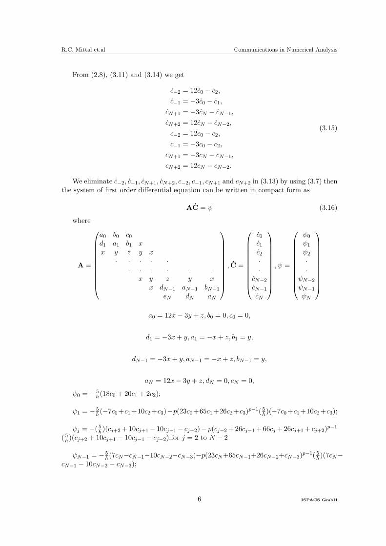
From (2.8), (3.11) and (3.14) we get

c−2 = 12c0 − c2,

c−1 = −3c0 − c1,

cN+1 = −3cN − cN−1,

cN+2 = 12cN − cN−2,

c−2 = 12c0 − c2,

c−1 = −3c0 − c2,

cN+1 = −3cN − cN−1,

cN+2 = 12cN − cN−2.

(3.15)

We eliminate c−2, c−1, cN+1, cN+2, c−2, c−1, cN+1 and cN+2 in (3.13) by using (3.7) thenthe system of first order differential equation can be written in compact form as

AC = ψ (3.16)

where

A =

a0 b0 c0d1 a1 b1 xx y z y x

· · · · ·· · · · · ·

x y z y xx dN−1 aN−1 bN−1

eN dN aN

, C =

c0c1c2··

cN−2

cN−1

cN

, ψ =

ψ0

ψ1

ψ2

··

ψN−2

ψN−1

ψN

a0 = 12x− 3y + z, b0 = 0, c0 = 0,

d1 = −3x+ y, a1 = −x+ z, b1 = y,

dN−1 = −3x+ y, aN−1 = −x+ z, bN−1 = y,

aN = 12x− 3y + z, dN = 0, eN = 0,

ψ0 = − 5h(18c0 + 20c1 + 2c2);

ψ1 = − 5h(−7c0+c1+10c2+c3)−p(23c0+65c1+26c2+c3)

p−1( 5h)(−7c0+c1+10c2+c3);

ψj = −( 5h)(cj+2+10cj+1− 10cj−1− cj−2)− p(cj−2+26cj−1+66cj +26cj+1+ cj+2)p−1

( 5h)(cj+2 + 10cj+1 − 10cj−1 − cj−2);for j = 2 to N − 2

ψN−1 = − 5h(7cN−cN−1−10cN−2−cN−3)−p(23cN+65cN−1+26cN−2+cN−3)

p−1( 5h)(7cN−cN−1 − 10cN−2 − cN−3);

6 ISPACS GmbH


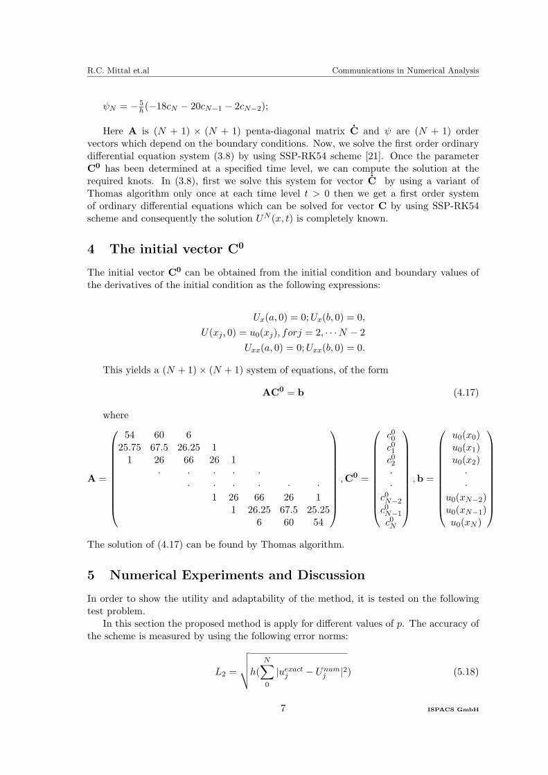
ψN = − 5h(−18cN − 20cN−1 − 2cN−2);

Here A is (N + 1) × (N + 1) penta-diagonal matrix C and ψ are (N + 1) ordervectors which depend on the boundary conditions. Now, we solve the first order ordinarydifferential equation system (3.8) by using SSP-RK54 scheme [21]. Once the parameterC0 has been determined at a specified time level, we can compute the solution at therequired knots. In (3.8), first we solve this system for vector C by using a variant ofThomas algorithm only once at each time level t > 0 then we get a first order systemof ordinary differential equations which can be solved for vector C by using SSP-RK54scheme and consequently the solution UN (x, t) is completely known.

4 The initial vector C0

The initial vector C0 can be obtained from the initial condition and boundary values ofthe derivatives of the initial condition as the following expressions:

Ux(a, 0) = 0;Ux(b, 0) = 0,

U(xj , 0) = u0(xj), forj = 2, · · ·N − 2

Uxx(a, 0) = 0;Uxx(b, 0) = 0.

This yields a (N + 1)× (N + 1) system of equations, of the form

AC0 = b (4.17)

where

A =

54 60 625.75 67.5 26.25 11 26 66 26 1

· · · · ·· · · · · ·

1 26 66 26 11 26.25 67.5 25.25

6 60 54

,C0 =

c00c01c02··

c0N−2

c0N−1

c0N

,b =

u0(x0)u0(x1)u0(x2)

··

u0(xN−2)u0(xN−1)u0(xN )

The solution of (4.17) can be found by Thomas algorithm.

5 Numerical Experiments and Discussion

In order to show the utility and adaptability of the method, it is tested on the followingtest problem.

In this section the proposed method is apply for different values of p. The accuracy ofthe scheme is measured by using the following error norms:

L2 =

√√√√h(N∑0

|uexactj − Unumj |2) (5.18)

7 ISPACS GmbH


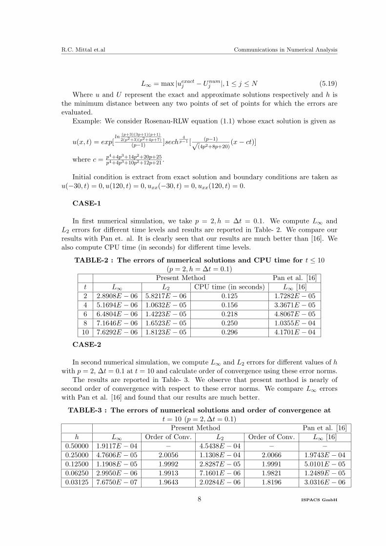
L∞ = max |uexactj − Unumj |, 1 ≤ j ≤ N (5.19)

Where u and U represent the exact and approximate solutions respectively and h isthe minimum distance between any two points of set of points for which the errors areevaluated.

Example: We consider Rosenau-RLW equation (1.1) whose exact solution is given as

u(x, t) = exp[ln

(p+3)(3p+1)(p+1)

2(p2+3)(p2+4p+7)

(p−1) ]sech4

p−1 [ (p−1)√(4p2+8p+20)

(x− ct)]

where c = p4+4p3+14p2+20p+25p4+4p3+10p2+12p+21

.

Initial condition is extract from exact solution and boundary conditions are taken asu(−30, t) = 0, u(120, t) = 0, uxx(−30, t) = 0, uxx(120, t) = 0.

CASE-1

In first numerical simulation, we take p = 2, h = ∆t = 0.1. We compute L∞ andL2 errors for different time levels and results are reported in Table- 2. We compare ourresults with Pan et. al. It is clearly seen that our results are much better than [16]. Wealso compute CPU time (in seconds) for different time levels.

TABLE-2 : The errors of numerical solutions and CPU time for t ≤ 10(p = 2, h = ∆t = 0.1)

Present Method Pan et al. [16]

t L∞ L2 CPU time (in seconds) L∞ [16]

2 2.8908E − 06 5.8217E − 06 0.125 1.7282E − 05

4 5.1694E − 06 1.0632E − 05 0.156 3.3671E − 05

6 6.4804E − 06 1.4223E − 05 0.218 4.8067E − 05

8 7.1646E − 06 1.6523E − 05 0.250 1.0355E − 04

10 7.6292E − 06 1.8123E − 05 0.296 4.1701E − 04

CASE-2

In second numerical simulation, we compute L∞ and L2 errors for different values of hwith p = 2, ∆t = 0.1 at t = 10 and calculate order of convergence using these error norms.

The results are reported in Table- 3. We observe that present method is nearly ofsecond order of convergence with respect to these error norms. We compare L∞ errorswith Pan et al. [16] and found that our results are much better.

TABLE-3 : The errors of numerical solutions and order of convergence att = 10 (p = 2,∆t = 0.1)

Present Method Pan et al. [16]

h L∞ Order of Conv. L2 Order of Conv. L∞ [16]

0.50000 1.9117E − 04 − 4.5438E − 04 − −0.25000 4.7606E − 05 2.0056 1.1308E − 04 2.0066 1.9743E − 04

0.12500 1.1908E − 05 1.9992 2.8287E − 05 1.9991 5.0101E − 05

0.06250 2.9950E − 06 1.9913 7.1601E − 06 1.9821 1.2489E − 05

0.03125 7.6750E − 07 1.9643 2.0284E − 06 1.8196 3.0316E − 06

8 ISPACS GmbH


CASE-3

In third numerical simulation, we compute L∞ and L2 errors for different values of hwith p = 4, ∆t = 0.1 at t = 60 and calculate order of convergence using these error norms.The results are reported in Table- 4.It is clearly seen that present method is of secondorder of convergence with respect to L∞ error norm during simulation.

TABLE-4 : The errors of numerical solutions and order of convergence att = 60 (p = 4,∆t = 0.1)

Present Method

h L∞ Order of Conv. L2 Order of Conv.

1.00000 1.1541E − 02 − 3.0217E − 02 −0.50000 2.2164E − 03 2.3805 5.5853E − 03 2.4356

0.25000 5.1848E − 04 2.0959 1.3010E − 03 2.1020

0.12500 1.2789E − 04 2.0193 3.5071E − 04 1.8913

0.06250 3.1864E − 05 2.0049 1.8243E − 04 0.9429

CASE-4

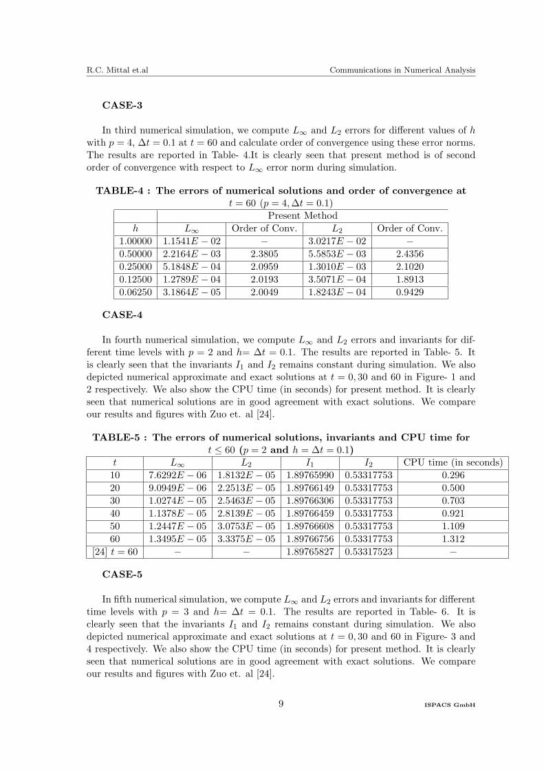
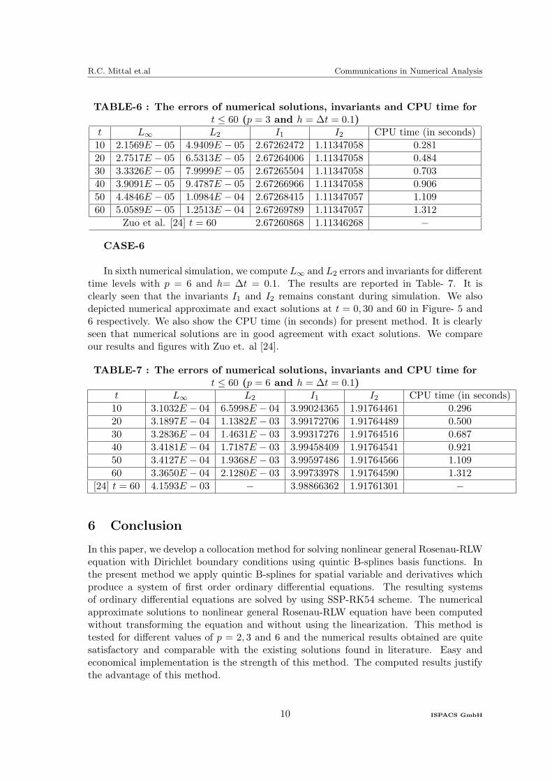
In fourth numerical simulation, we compute L∞ and L2 errors and invariants for dif-ferent time levels with p = 2 and h= ∆t = 0.1. The results are reported in Table- 5. Itis clearly seen that the invariants I1 and I2 remains constant during simulation. We alsodepicted numerical approximate and exact solutions at t = 0, 30 and 60 in Figure- 1 and2 respectively. We also show the CPU time (in seconds) for present method. It is clearlyseen that numerical solutions are in good agreement with exact solutions. We compareour results and figures with Zuo et. al [24].

TABLE-5 : The errors of numerical solutions, invariants and CPU time fort ≤ 60 (p = 2 and h = ∆t = 0.1)

t L∞ L2 I1 I2 CPU time (in seconds)

10 7.6292E − 06 1.8132E − 05 1.89765990 0.53317753 0.296

20 9.0949E − 06 2.2513E − 05 1.89766149 0.53317753 0.500

30 1.0274E − 05 2.5463E − 05 1.89766306 0.53317753 0.703

40 1.1378E − 05 2.8139E − 05 1.89766459 0.53317753 0.921

50 1.2447E − 05 3.0753E − 05 1.89766608 0.53317753 1.109

60 1.3495E − 05 3.3375E − 05 1.89766756 0.53317753 1.312

[24] t = 60 − − 1.89765827 0.53317523 −

CASE-5

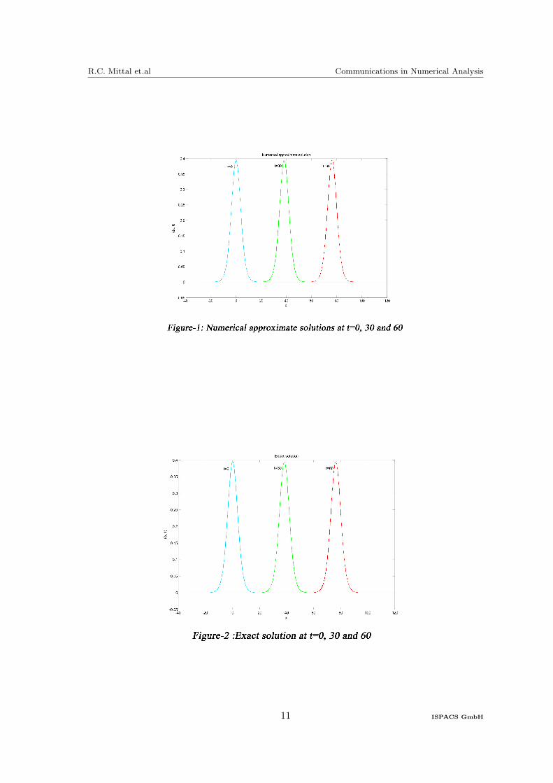
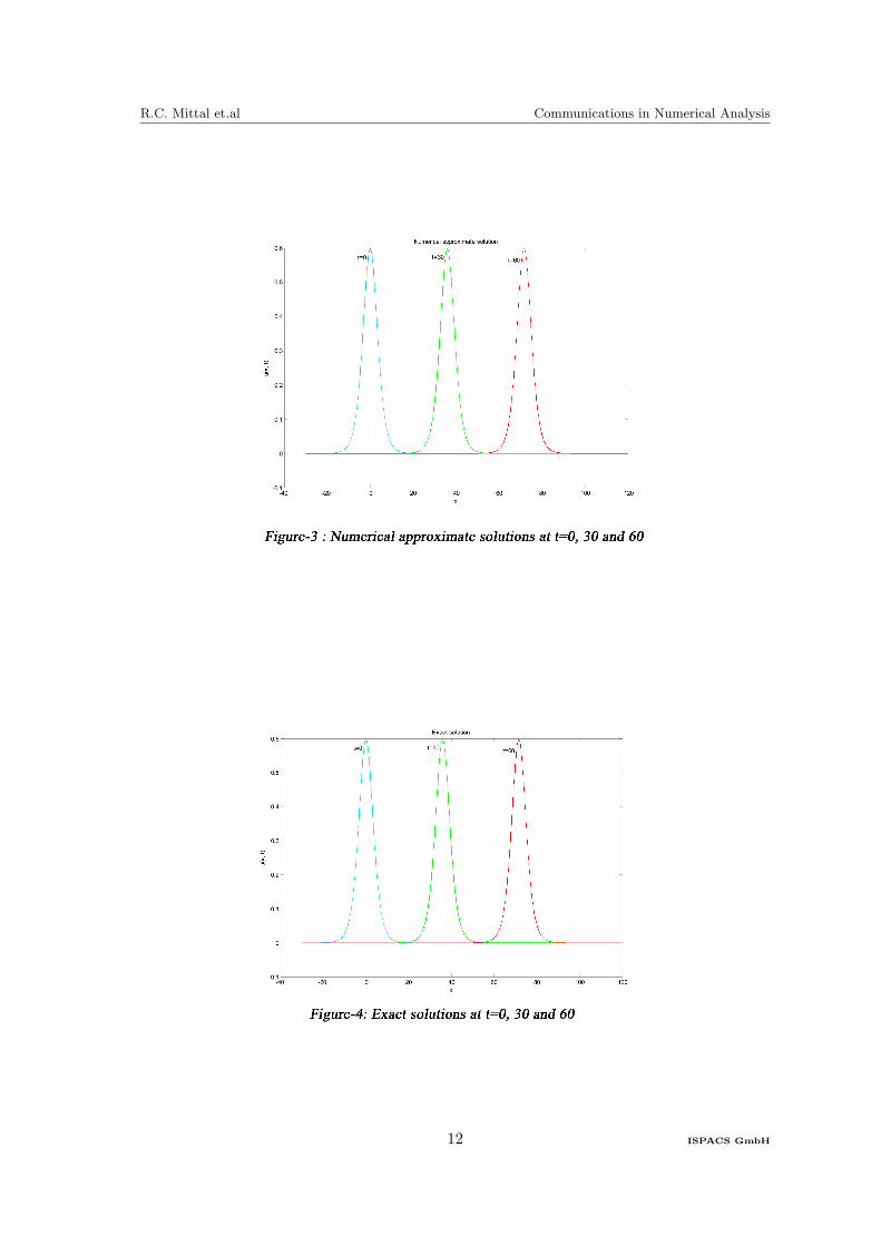
In fifth numerical simulation, we compute L∞ and L2 errors and invariants for differenttime levels with p = 3 and h= ∆t = 0.1. The results are reported in Table- 6. It isclearly seen that the invariants I1 and I2 remains constant during simulation. We alsodepicted numerical approximate and exact solutions at t = 0, 30 and 60 in Figure- 3 and4 respectively. We also show the CPU time (in seconds) for present method. It is clearlyseen that numerical solutions are in good agreement with exact solutions. We compareour results and figures with Zuo et. al [24].

9 ISPACS GmbH




10 2.1569E − 05 4.9409E − 05 2.67262472 1.11347058 0.281

20 2.7517E − 05 6.5313E − 05 2.67264006 1.11347058 0.484

30 3.3326E − 05 7.9999E − 05 2.67265504 1.11347058 0.703

40 3.9091E − 05 9.4787E − 05 2.67266966 1.11347058 0.906

50 4.4846E − 05 1.0984E − 04 2.67268415 1.11347057 1.109

60 5.0589E − 05 1.2513E − 04 2.67269789 1.11347057 1.312

Zuo et al. [24] t = 60 2.67260868 1.11346268 −

CASE-6

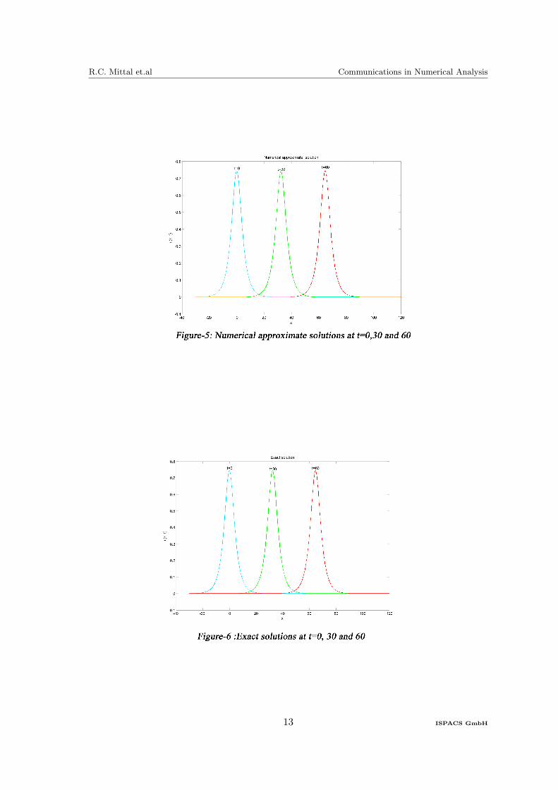
In sixth numerical simulation, we compute L∞ and L2 errors and invariants for differenttime levels with p = 6 and h= ∆t = 0.1. The results are reported in Table- 7. It isclearly seen that the invariants I1 and I2 remains constant during simulation. We alsodepicted numerical approximate and exact solutions at t = 0, 30 and 60 in Figure- 5 and6 respectively. We also show the CPU time (in seconds) for present method. It is clearlyseen that numerical solutions are in good agreement with exact solutions. We compareour results and figures with Zuo et. al [24].



10 3.1032E − 04 6.5998E − 04 3.99024365 1.91764461 0.296

20 3.1897E − 04 1.1382E − 03 3.99172706 1.91764489 0.500

30 3.2836E − 04 1.4631E − 03 3.99317276 1.91764516 0.687

40 3.4181E − 04 1.7187E − 03 3.99458409 1.91764541 0.921

50 3.4127E − 04 1.9368E − 03 3.99597486 1.91764566 1.109

60 3.3650E − 04 2.1280E − 03 3.99733978 1.91764590 1.312

[24] t = 60 4.1593E − 03 − 3.98866362 1.91761301 −

6 Conclusion

In this paper, we develop a collocation method for solving nonlinear general Rosenau-RLWequation with Dirichlet boundary conditions using quintic B-splines basis functions. Inthe present method we apply quintic B-splines for spatial variable and derivatives whichproduce a system of first order ordinary differential equations. The resulting systemsof ordinary differential equations are solved by using SSP-RK54 scheme. The numericalapproximate solutions to nonlinear general Rosenau-RLW equation have been computedwithout transforming the equation and without using the linearization. This method istested for different values of p = 2, 3 and 6 and the numerical results obtained are quitesatisfactory and comparable with the existing solutions found in literature. Easy andeconomical implementation is the strength of this method. The computed results justifythe advantage of this method.

10 ISPACS GmbH


11 ISPACS GmbH


12 ISPACS GmbH


13 ISPACS GmbH


Acknowledgment

One of the authors R.K. Jain thankfully acknowledges the sponsorship under QIP, providedby Technical Education and Training Department, Bhopal (M.P.), India. The authors arevery thankful to the reviewers for their valuable suggestions to improve the quality of thepaper.

References

[1] I. Dag, Approximation of the RLW equation by the least square cubic B-spline finiteelement method, Appl. Math. Model. 25 (2001) 221-231.http://dx.doi.org/10.1016/S0307-904X(00)00030-5

[2] I. Dag, A. Dogan and B. Saka, B-spline collocation methods for numerical solutionsof the RLW equation, Int. J. Comput. Math. 80 (2003) 743-757.http://dx.doi.org/10.1080/0020716021000038965

[3] I. Dag, B. Saka and D. Irk, Galerkin method for the numerical solution of the RLWequation using quintic B-splines, J. Comput. Appl. Math. 190 (2006) 532-547.http://dx.doi.org/10.1016/j.cam.2005.04.026

[4] K. Djidjeli, W.G. Price, E.H. Twizell and Q. Cao, A linearized implicit pseudospec-tral method for some model equations: the regularized long wave equations, Comm.Numer. Methods Engrg. 19 (2003) 847-863.http://dx.doi.org/10.1002/cnm.635

[5] A. Dogan, Numerical solution of RLW equation using linear finite elements withinGalerkin method, Appl. Math. Model. 26 (2002) 771-783.http://dx.doi.org/10.1016/S0307-904X(01)00084-1

[6] A. Dogan, Numerical solution of regularized long wave equation using Petrov-Galerkinmethod, Comm. Numer. Methods Engrg. 17 (2001) 485-494.http://dx.doi.org/10.1002/cnm.424

[7] A. Esen and S. Kutluay, Application of a lumped Galerkin method to the regularizedlong wave equation, Appl. Math. Comput. 174 (2006) 833-845.http://dx.doi.org/10.1016/j.amc.2005.05.032

[8] L. R. T. Gardner, G. A. Gardner and I. Dag, A B-spline finite element method forthe regularized long wave equation, Comm. Numer. Methods Engrg. 11 (1995) 59-68.http://dx.doi.org/10.1002/cnm.1640110109

[9] L. R. T. Gardner, G. A. Gardner and A. Dogan, A least-square finite element methodfor the RLW equation, Comm. Numer. Methods Engrg. 12 (1996) 795-804.http://dx.doi.org/10.1002/(SICI)1099-0887(199611)12:11¡795::AID-CNM22¿3.0.CO;2-O

[10] L. R. T. Gardner, G. A. Gardner, F. A. Ayoub and N. K. Amein, Approximations ofsolitary waves of the MRLW equation by B-spline finite element, Arab. J. Sci. Eng.22 (1997) 183-193.

14 ISPACS GmbH


[11] A. K. Khalifa, K. R. Raslan and H. M. Alzubaidi, A collocation method with cubicBsplines for solving the MRLW equation, Comput. Appl. Math. 212 (2008) 406-418.http://dx.doi.org/10.1016/j.cam.2006.12.029

[12] A.K. Khalifa, K.R. Raslan and H.M. Alzubaidi, A finite difference scheme for theMRLW and solitary wave interactions, Appl. Math. Comput. 189 (2007) 346-354.http://dx.doi.org/10.1016/j.amc.2006.11.104

[13] R.C. Mittal and Geeta Arora, Quintic B-Spline Collocation Method for NumericalSolution of the Extended Fisher-Kolmogrov Equation, Int. J. of Appl. Math andMech. 6 (1) (2010) 74-85.

[14] R. Mokhtari and M. Mohammadi, Numerical solution of GRLW equation using Sinc-collocation method, Computer Physics Communications 181 (2010) 1266-1274.http://dx.doi.org/10.1016/j.cpc.2010.03.015

[15] R. Mokhtari and M. Mohammadi, Solving the generalized regularized long wave equa-tion on the basis of a reproducing kernel space, Journal of Computational and AppliedMathematics 235 (2011) 4003-4014.http://dx.doi.org/10.1016/j.cam.2011.02.012

[16] X. Pan, Tingchun Wang, Luming Zhang and Boling Guo, On the convergence of aconservative numerical scheme for the usual Rosenau-RLW equation, Applied Math-ematical Modelling.

[17] H. Panahipour, Numerical Simulation of GEW equation using RBF collocationmethod, Communications in Numerical Analysis 2012 (2012).http://doi.10.5899/2012/cna-00059

[18] K. R. Raslan, A computational method for the regularized long wave equation, Appl.Math. Comput. 167 (2005) 1101-1118.http://dx.doi.org/10.1016/j.amc.2004.06.130

[19] K. R. Raslan, Numerical study of the Modified Regularized Long Wave (MRLW)equation, Chaos Solitons Fractals 42 (2009) 1845-1853.http://dx.doi.org/10.1016/j.chaos.2009.03.098

[20] B. Saka, I. Dag and A. Dogan, Galerkin method for the numerical solution of theRLW equation using quadratic B-spline, Int. J. Comput. Math. 81 (2004) 727-739.http://dx.doi.org/10.1080/00207160310001650043

[21] R.J. Spiteri and S.J. Ruuth, A new class of optimal high-order strong-stability-preserving time-stepping schemes, SIAM J. Numer. Anal. 40 (2002) 469-491.http://dx.doi.org/10.1137/S0036142901389025

[22] B. Saka and I. Dag, A Collocation method for the numerical solution of the RLWequation using cubic B-spline basis, Arab. J. Sci. Eng. 30 (2005) 39-50.

[23] L. Zhang, A finite difference scheme for generalized regularized long-wave equation,Appl. Math. Comput. 168 (2005) 962-972.http://dx.doi.org/10.1016/j.amc.2004.09.027

15 ISPACS GmbH


[24] J.M. Zuo, Y.M. Zhang, Tian-De Zhang, and Feng Chang, A New Conservative Dif-ference Scheme for the General Rosenau-RLW Equation, Boundary Value Problems,Hindawi Publishing Corporation, Volume 2010, Article ID 516260.

16 ISPACS GmbH

Documents

Numerical solution of General Rosenau-RLW Equation using