Observations of subtidal and tidal flow in the Rio de la Plata Estuary

ARTICLE IN PRESS

Continental Shelf Research 24 (2004) 509–525

*Correspondin

757-683-5550.

E-mail addre

0278-4343/$ - see

doi:10.1016/j.csr

Observations of subtidal and tidal flow in the R!ıo de laPlata Estuary

H!ector H. Sep !ulvedaa,*, Arnoldo Valle-Levinsona, Mariana B. Framinanb,c

aDepartment of Ocean, Earth, and Atmospheric Sciences, Center for Coastal Physical Oceanography, Old Dominion University,

Crittenton Hall, Norfolk, VA 23529, USAbUniversity of Miami, RSMAS/MPO 4600, Rickenbacker Cswy., Miami, FL 33149, USA

cServicio de Hidrograf!ıa Naval, Avda. Montes de Oca 2124, Buenos Aires, Argentina

Received 6 January 2003; received in revised form 22 October 2003; accepted 3 December 2003

Abstract

We present the first measurements obtained with a combination of a towed acoustic Doppler current profiler (ADCP)

and a conductivity–temperature–depth (CTD) recorder in the R!ıo de la Plata Estuary. Subtidal and tidal flows

are described for austral winter and summer conditions. Data were collected at three transects 15 km long for 25 h

during August 11–17, 1999 (austral winter) and February 2–6, 2000 (austral summer) at the transition zone between

fresh and brackish waters. Two transects covered cross-estuary tracks off the northern and southern coastlines of the

estuary. A central transect was oriented along the estuarine axis near the up-stream limit of saltwater intrusion. The

observations indicated that the dominant dynamical processes were different at each of the transects sampled. The most

relevant feature was the dominance of tidal currents in the southern side of the estuary and the lesser role they played in

the northern side (Uruguayan coast). The pressure gradient produced by the freshwater outflow was modified

differently at the southern than at the northern sides of the estuary. At the southern side tidal mixing, from strong

tidal currents, allowed the development of gravitational circulation. At the northern side weak tidal currents

allowed modifications by ambient forcing and surface stresses, consistent with theoretical results of surface-advected

freshwater outflows.

r 2003 Elsevier Ltd. All rights reserved.

Keywords: Tides; Subtidal variability; Buoyancy forcing; Wind forcing; Estuarine dynamics; Argentina–Uruguay; R!ıo de la Plata

(35�S, 57�W)

1. Introduction

The R!ıo de la Plata Estuary drains the secondlargest basin in South America and receives thefifth largest discharge worldwide (Leopold, 1994).

g author. Tel.: +1-757-683-3234; fax: +1-

ss: [email protected] (H.H. Sep !ulveda).

front matter r 2003 Elsevier Ltd. All rights reserve

.2003.12.002

It is a wide estuary, with a width one order ofmagnitude larger than the internal radius ofdeformation, i.e. Kelvin number b1: Extensiveliterature exists on systems with a moderately sizeddischarge e.g., see the reviews by Lentz (1994), Hill(1998) and Hickey et al. (1998). Comparatively,the dynamics of large discharge systems is littleknown through few studies in the Amazon River,in the Yangtze (Changjiang) River, and in high

d.

ARTICLE IN PRESS

H.H. Sep !ulveda et al. / Continental Shelf Research 24 (2004) 509–525510

latitude, e.g. Geyer et al. (1991), Beardsley et al.(1985), and M .unchow et al. (1999), respectively.Wide estuaries are frequently associated with

large population centers that host a sizablemaritime industry and are usually affected bypollution issues. Notable examples exist in theChesapeake Bay and Delaware Bay in the USA.The R!ıo de la Plata, our study area, is anotherexample with the cities of Buenos Aires (Argenti-na) and Montevideo (Uruguay) located in thesouthern and northern coasts of the estuary,respectively. Wide estuaries share some character-istics such as shallow bathymetry and potentiallystrong wind forcing. These types of estuaries alsoplay a role in sustaining and harboring larvalstages of different marine resources (Cousseau,1985; Boschi, 1988; Acha et al., 1999; Mianzanet al., 2001).However, the dynamics of the R!ıo de la Plata is

expected to be different from other wide estuariesbecause of the large buoyancy input that shouldreflect highly stratified conditions. A well-devel-oped salt wedge is generally observed in theestuary under weak to moderate wind conditions(Guerrero et al., 1997), and strong stratification isobserved in the outer region where a salinityvertical gradient in excess of 20/m has beenobserved (Framinan et al., 1999).Remote sensing information has been useful to

understand salient features in the R!ıo de la Plataand the adjacent shelf, such as the turbidity frontand upwelling events (Framinan and Brown, 1996,1998; Framinan, 2004). Satellite images provideappropriate horizontal and temporal coverage ofthis large system, but they only provide informa-tion on the sea surface and are of limited use tounderstand the vertical variability and the pro-cesses affecting the water column. Alternativetools to study the hydrodynamics of wide estuariesinclude numerical models. However, the observa-tional evidence that is needed to corroborate theresults is often difficult to obtain given the physicaldimensions of such systems.Among the widest estuaries in the world, the R!ıo

de la Plata opens for more than 200 km at itsmouth. In a system with the geographical extent ofthe R!ıo de la Plata, in situ studies needed to resolvethe spatial and temporal variability are difficult,

both technically and financially. This explains whythe knowledge on spatial (e.g. vertical andhorizontal structure) and temporal variability ofthe currents, based on observations, is sparse. Theunderstanding of the variability and spatialdistribution of tidal and subtidal flows within theestuary is a prerequisite to address societal issuessuch as safe navigation, residence times, or trans-port of larvae of species of commercial interest.The objective of this study is to describe the

spatial distribution of the mean flow and tidalcurrents in three zones of the R!ıo de la PlataEstuary during summer and winter, including theinfluence of bathymetry, freshwater discharge andwind forcing on these distributions. The area ofstudy is the transition zone of the estuary, in thelimit between fresh and brackish waters. Thebathymetry is relatively smooth and therefore itis hypothesized that wind and tidal forcingcombine with the buoyancy input to determinethe spatial variability of the flow. In order toaddress the objective, measurements of watervelocity and density profiles were taken at threetransects during the austral winter (August 1999)and summer (February 2000). This article isorganized as follows: Section 2 describes the R!ıode la Plata environment. Section 3 covers datacollection and processing, and Section 4 presents adiscussion of the characteristics of the subtidal andtidal flows for each transect, as well as acomparison between winter and summer condi-tions. These sections are followed by discussionand conclusions.

2. Study area

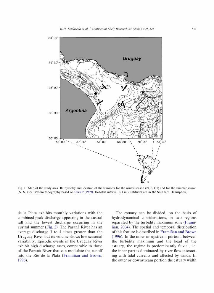
The R!ıo de la Plata Estuary is located in SouthAmerica on the Atlantic coast, at 35�S; 57�W;between Argentina and Uruguay (Fig. 1). It has anapproximate length of 320 km and a width of230 km at the mouth. The average depth is 10 m:It drains the second largest basin of SouthAmerica, receiving the combined discharge of theParan!a and Uruguay rivers, the two majortributaries, with a total yearly average dischargeof 22; 000 m3=s; comparable to the discharge of theMississippi river. Freshwater discharge to the R!ıo

ARTICLE IN PRESS

Fig. 1. Map of the study area. Bathymetry and location of the transects for the winter season (N, S, C1) and for the summer season

(N, S, C2). Bottom topography based on CARP (1989). Isobaths interval is 1 m: (Latitudes are in the Southern Hemisphere).

H.H. Sep !ulveda et al. / Continental Shelf Research 24 (2004) 509–525 511

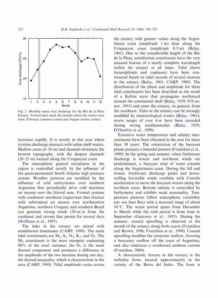
de la Plata exhibits monthly variations with thecombined peak discharge appearing in the australfall and the lowest discharge occurring in theaustral summer (Fig. 2). The Paran!a River has anaverage discharge 3 to 4 times greater than theUruguay River but its volume shows low seasonalvariability. Episodic events in the Uruguay Riverexhibit high discharge rates, comparable to thoseof the Paran!a River that can modulate the runoffinto the R!ıo de la Plata (Framinan and Brown,1996).

The estuary can be divided, on the basis ofhydrodynamical considerations, in two regionsseparated by the turbidity maximum zone (Frami-nan, 2004). The spatial and temporal distributionof this feature is described in Framinan and Brown(1996). In the inner or upstream portion, betweenthe turbidity maximum and the head of theestuary, the regime is predominantly fluvial, i.e.the inner part is dominated by river flow interact-ing with tidal currents and affected by winds. Inthe outer or downstream portion the estuary width

ARTICLE IN PRESS

Fig. 2. Monthly mean river discharge for the R!ıo de la Plata

Estuary. Vertical lines mark the months where the cruises were

done; February (summer cruise) and August (winter cruise).


increases rapidly. It is mostly in this area whereriverine discharge interacts with saline shelf waters.Shallow areas (4–10 m) and channels dominate thebottom topography, with the deepest channels(20–25 m) located along the Uruguayan coast.The atmospheric general circulation in the

region is controlled mostly by the influence ofthe quasi-permanent South Atlantic high pressuresystem. Weather patterns are modified by theinfluence of cold anticyclones over southernArgentina that periodically drive cold maritimeair masses over the littoral area. Frontal systemswith southwest–northeast trajectories that interactwith subtropical air masses over northeasternArgentina, northern Uruguay and southern Brazilcan generate strong winds ð30 m=sÞ from thesoutheast and storms that persist for several days(Hoffman et al., 1997).The tides in the estuary are mixed with

semidiurnal dominance (CARP, 1989). The maintidal constituents are M2; S2; N2; K1; and O1: TheM2 constituent is the most energetic explaining80% of the total variance; the O1 is the maindiurnal component and produces a difference inthe amplitude of the two maxima during one day,the diurnal inequality, which is characteristic in thearea (CARP, 1989). Tidal amplitude varies across

the estuary with greater values along the Argen-tinean coast (amplitude 1 m) than along theUruguayan coast (amplitude 0:3 m) (Balay,1961). Due to the considerable length of the R!ıode la Plata, semidiurnal constituents have the veryunusual feature of a nearly complete wavelengthwithin the estuary at all times. Tidal charts(isoamplitude and cophases) have been con-structed based on tidal records of several stationsin the estuary (Balay, 1961; CARP, 1989). Thedistribution of the phase and amplitude for thesetidal constituents has been described as the resultof a Kelvin wave that propagates northwardaround the continental shelf (Balay, 1959; O’Con-nor, 1991) and enter the estuary, in general, fromthe southeast. Tides in the estuary can be stronglymodified by meteorological events (Balay, 1961);storm surges of over 4 m have been recordedduring strong southeasterlies (Balay, 1959;D’Onofrio et al., 1999).Extensive water temperature and salinity mea-

surements have been obtained in the area for morethan 30 years. The orientation of the buoyantplume presents a bimodal pattern (Framinan et al.,1999): In the spring and summer, when freshwaterdischarge is lowest and northeast winds arepredominant, a buoyant strip of water extendsalong the Argentinean coast. During the fall andwinter, freshwater discharge peaks and down-welling favorable winds combine with Coriolisacceleration to move the buoyant waters along thenorthern coast. Bottom salinity is controlled bybathymetry and exhibits weak seasonality. Tem-perature patterns follow atmospheric variability(air–sea heat flux) with a seasonal range of about10�C: The warm period spans from Decemberto March while the cold period is from June toSeptember (Guerrero et al., 1997). During thesummer, coastal upwelling is observed at themouth of the estuary along both coasts (Framinanand Brown, 1998; Framinan et al., 1999). Coastalupwelling modifies the estuarine outflow, favoringa buoyancy outflow off the coast of Argentina,and also reinforces a southward ambient current(Framinan, 2004).A characteristic feature in the estuary is the

turbidity front, located approximately in thevicinity of the Barra del Indio. The front is

ARTICLE IN PRESS


the surface signature of the transition betweenfresh and more saline shelf waters. The spatial andtemporal distribution of this front is described inFraminan and Brown (1996). The position of theturbidity front exhibits strong seasonality. Duringthe summer months (low freshwater discharge andnortheasterly winds) the turbidity front is at itsnorthwesternmost position. During winter andfall, the turbidity front extends seaward.

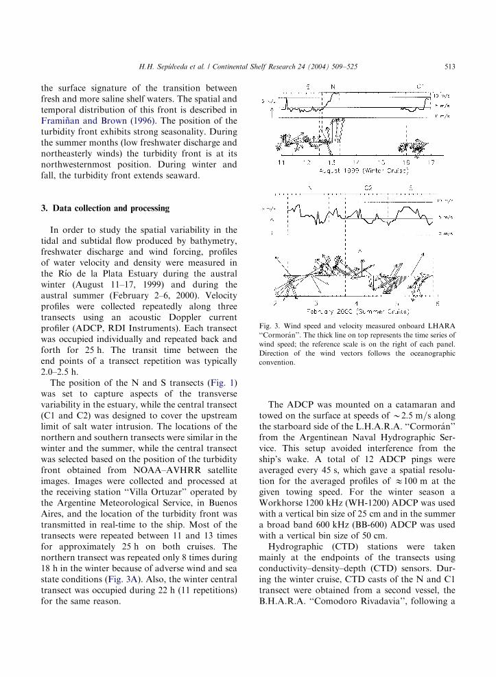
Fig. 3. Wind speed and velocity measured onboard LHARA

‘‘Cormor!an’’. The thick line on top represents the time series of

wind speed; the reference scale is on the right of each panel.

Direction of the wind vectors follows the oceanographic

convention.

3. Data collection and processing

In order to study the spatial variability in thetidal and subtidal flow produced by bathymetry,freshwater discharge and wind forcing, profilesof water velocity and density were measured inthe R!ıo de la Plata Estuary during the australwinter (August 11–17, 1999) and during theaustral summer (February 2–6, 2000). Velocityprofiles were collected repeatedly along threetransects using an acoustic Doppler currentprofiler (ADCP, RDI Instruments). Each transectwas occupied individually and repeated back andforth for 25 h: The transit time between theend points of a transect repetition was typically2.0–2:5 h:The position of the N and S transects (Fig. 1)

was set to capture aspects of the transversevariability in the estuary, while the central transect(C1 and C2) was designed to cover the upstreamlimit of salt water intrusion. The locations of thenorthern and southern transects were similar in thewinter and the summer, while the central transectwas selected based on the position of the turbidityfront obtained from NOAA–AVHRR satelliteimages. Images were collected and processed atthe receiving station ‘‘Villa Ortuzar’’ operated bythe Argentine Meteorological Service, in BuenosAires, and the location of the turbidity front wastransmitted in real-time to the ship. Most of thetransects were repeated between 11 and 13 timesfor approximately 25 h on both cruises. Thenorthern transect was repeated only 8 times during18 h in the winter because of adverse wind and seastate conditions (Fig. 3A). Also, the winter centraltransect was occupied during 22 h (11 repetitions)for the same reason.

The ADCP was mounted on a catamaran andtowed on the surface at speeds of B2:5 m=s alongthe starboard side of the L.H.A.R.A. ‘‘Cormor!an’’from the Argentinean Naval Hydrographic Ser-vice. This setup avoided interference from theship’s wake. A total of 12 ADCP pings wereaveraged every 45 s; which gave a spatial resolu-tion for the averaged profiles of E100 m at thegiven towing speed. For the winter season aWorkhorse 1200 kHz (WH-1200) ADCP was usedwith a vertical bin size of 25 cm and in the summera broad band 600 kHz (BB-600) ADCP was usedwith a vertical bin size of 50 cm:Hydrographic (CTD) stations were taken

mainly at the endpoints of the transects usingconductivity–density–depth (CTD) sensors. Dur-ing the winter cruise, CTD casts of the N and C1transect were obtained from a second vessel, theB.H.A.R.A. ‘‘Comodoro Rivadavia’’, following a

ARTICLE IN PRESS

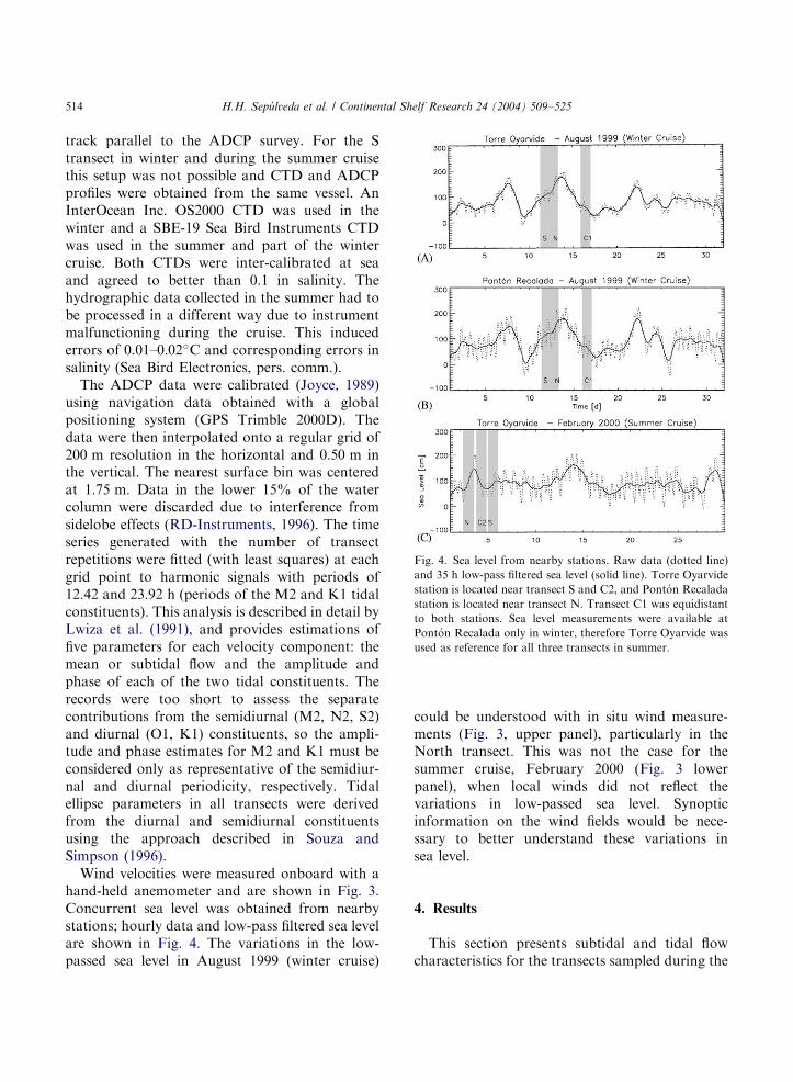
Fig. 4. Sea level from nearby stations. Raw data (dotted line)

and 35 h low-pass filtered sea level (solid line). Torre Oyarvide

station is located near transect S and C2, and Pont !on Recalada

station is located near transect N. Transect C1 was equidistant

to both stations. Sea level measurements were available at

Pont !on Recalada only in winter, therefore Torre Oyarvide was

used as reference for all three transects in summer.


track parallel to the ADCP survey. For the Stransect in winter and during the summer cruisethis setup was not possible and CTD and ADCPprofiles were obtained from the same vessel. AnInterOcean Inc. OS2000 CTD was used in thewinter and a SBE-19 Sea Bird Instruments CTDwas used in the summer and part of the wintercruise. Both CTDs were inter-calibrated at seaand agreed to better than 0.1 in salinity. Thehydrographic data collected in the summer had tobe processed in a different way due to instrumentmalfunctioning during the cruise. This inducederrors of 0.01–0:02�C and corresponding errors insalinity (Sea Bird Electronics, pers. comm.).The ADCP data were calibrated (Joyce, 1989)

using navigation data obtained with a globalpositioning system (GPS Trimble 2000D). Thedata were then interpolated onto a regular grid of200 m resolution in the horizontal and 0:50 m inthe vertical. The nearest surface bin was centeredat 1:75 m: Data in the lower 15% of the watercolumn were discarded due to interference fromsidelobe effects (RD-Instruments, 1996). The timeseries generated with the number of transectrepetitions were fitted (with least squares) at eachgrid point to harmonic signals with periods of12.42 and 23:92 h (periods of the M2 and K1 tidalconstituents). This analysis is described in detail byLwiza et al. (1991), and provides estimations offive parameters for each velocity component: themean or subtidal flow and the amplitude andphase of each of the two tidal constituents. Therecords were too short to assess the separatecontributions from the semidiurnal (M2, N2, S2)and diurnal (O1, K1) constituents, so the ampli-tude and phase estimates for M2 and K1 must beconsidered only as representative of the semidiur-nal and diurnal periodicity, respectively. Tidalellipse parameters in all transects were derivedfrom the diurnal and semidiurnal constituentsusing the approach described in Souza andSimpson (1996).Wind velocities were measured onboard with a

hand-held anemometer and are shown in Fig. 3.Concurrent sea level was obtained from nearbystations; hourly data and low-pass filtered sea levelare shown in Fig. 4. The variations in the low-passed sea level in August 1999 (winter cruise)

could be understood with in situ wind measure-ments (Fig. 3, upper panel), particularly in theNorth transect. This was not the case for thesummer cruise, February 2000 (Fig. 3 lowerpanel), when local winds did not reflect thevariations in low-passed sea level. Synopticinformation on the wind fields would be nece-ssary to better understand these variations insea level.

4. Results

This section presents subtidal and tidal flowcharacteristics for the transects sampled during the

ARTICLE IN PRESS

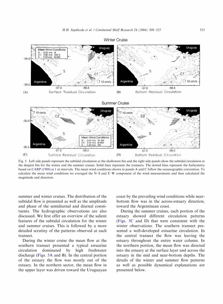
Fig. 5. Left side panels represent the subtidal circulation at the shallowest bin and the right side panels show the subtidal circulation at

the deepest bin for the winter and the summer cruises. Solid lines represent the transects. The dotted lines represent the bathymetry

based on CARP (1989) at 1 m intervals. The mean wind conditions shown in panels A and C follow the oceanographic convention. To

calculate the mean wind conditions we averaged the N–S and E–W component of the wind measurements and then calculated the

magnitude and direction.


summer and winter cruises. The distribution of thesubtidal flow is presented as well as the amplitudeand phase of the semidiurnal and diurnal consti-tuents. The hydrographic observations are alsodiscussed. We first offer an overview of the salientfeatures of the subtidal circulation for the winterand summer cruises. This is followed by a moredetailed scrutiny of the patterns observed at eachtransect.During the winter cruise the mean flow at the

southern transect presented a typical estuarinecirculation dominated by high freshwaterdischarge (Figs. 5A and B). In the central portionof the estuary the flow was mostly out of theestuary. In the northern sector, the mean flow inthe upper layer was driven toward the Uruguayan

coast by the prevailing wind conditions while near-bottom flow was in the across-estuary direction,toward the Argentinean coast.During the summer cruises, each portion of the

estuary showed different circulation patterns(Figs. 5C and D) that were consistent with thewinter observations. The southern transect pre-sented a well-developed estuarine circulation. Inthe central transect the flow was leaving theestuary throughout the entire water column. Inthe northern portion, the mean flow was directedinto the estuary at the surface layer and across theestuary in the mid and near-bottom depths. Thedetails of the winter and summer flow patternsas well as possible dynamical explanations arepresented below.

ARTICLE IN PRESS


4.1. Subtidal flow

4.1.1. Southern transect

In the southern transect the bathymetry wassmooth; depth changed from 4 to 6 m over 5 km inthe onshore end and then dropped only by 1 m inthe following 10 km: Sea level measurements ata nearby station (Figs. 4A and C) showed asemidiurnal cycle with diurnal inequality for bothseasons. The winter measurements occurred beforea peak in low-passed sea level and the summermeasurements after a similar event.During winter the southern transect was domi-

nated by large freshwater discharge, characteristicof this season. The barotropic pressure gradientrelated to the river discharge drove the mean flowtoward the southeast. This direction was consistentthroughout most of the transect, with an averagesectional mean of 5 cm=s: There was weak inflownear the bottom and close to the coastal end withmagnitudes of less than 3 cm=s (Fig. 5A and B).Wind conditions were relatively weak, the aver-aged wind vector was of 0:55 m=s in magnitudeand oriented to the N–NW. Therefore, wind effectswere not appreciable in the mean circulation.Hydrographic observations during the winter

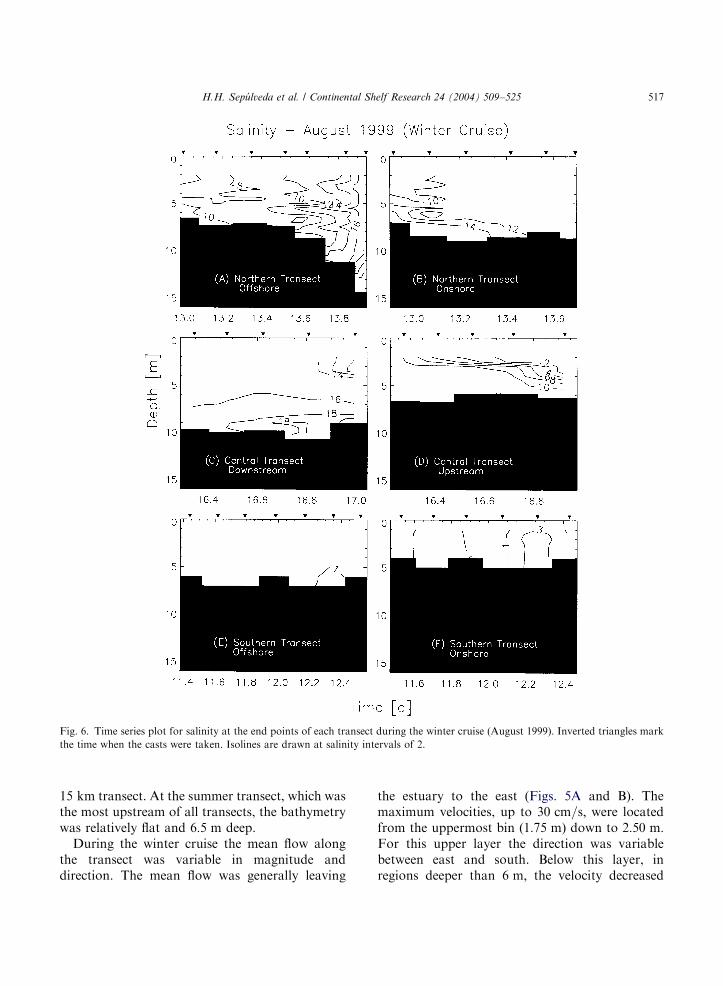
showed freshwater values (salinity of 2 or less)most of the time and at both ends of the transect(Figs. 6E and F). A single cast at the onshore endgave salinities of 4. Temperature range was 10.9–12:0�C at the onshore end and 11.3–12:7�C at theoffshore end. The higher bottom salinity valuesover the onshore end of the transect wereconsistent with Coriolis effects.In the summer we observed a net estuarine

mean circulation typical of a salt-wedge estuary(Figs. 5C and D). This is remarkable consideringthat the transect is very shallow (4–7 m). Thebottom layer occupied almost half of the watercolumn, with average velocities of 10 cm=s; whilethe upper layer moved on average at 20 cm=s: Thedirection of the flow was parallel to the coastlineexcept close to the bottom where the inflowwas oriented toward the Argentinean coast (tothe W–NW).During the summer period, hydrographic data

available for the offshore end showed a higherrange of salinity values (3–21) than in winter. A

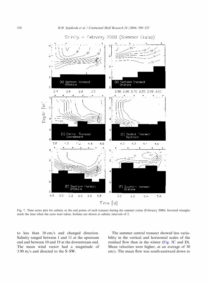
strong halocline could be seen below 3 m withsalinity increasing by 10–12 in 1 m (Fig. 7E). Thiswas an indication of the great influence ofbaroclinic pressure gradients in driving thesummer flow.The averaged wind vector from observations at

the southern transect had a magnitude of 4:26 m=sduring the summer, and the averaged directionwas to the SW. This could have reinforced theestuarine circulation. To explore the potentialimportance of wind forcing on the flow patternobserved, we can compare the wind stress accel-eration versus the bottom friction term

trwH

� �CDw

u2bH

� ��¼

trwCDw

u2b; ð1Þ

where t is the wind stress, bottom velocities ub ¼0:1 m=s; water density rwE1023 kg=m3: Thebottom drag coefficient, CDw

; is highly variableand depends on the bottom type (Soulsby, 1983),but a value of 1–2:5� 10�3 has been usedpreviously in numerical modeling efforts of thisarea (O’Connor, 1991). In turn, the wind stressmay be parameterized as

t ¼ CDarajuwjuw; ð2Þ

where CDais the drag coefficient at the sea surface

and has a value of E0:95� 10�3 (Apel, 1999), airdensity raE1:225 kg=m3; and wind velocities ðuwÞof 6 m=s generate a wind stress of

t ¼ 0:95� 10�3 � 1:225� 36 ¼ 0:04 Pa: ð3Þ

Therefore, the ratio of wind stress over bottomfriction is

trwCDw

u2bE1:7 ð4Þ

or greater, which indicates that wind stress was atleast comparable to bottom friction and likelyinfluential to the flow observed.

4.1.2. Central transect

The position of the central transect in winterwas set to cross the turbidity front. In summer thetransect was located in an upstream position of theupper estuary to investigate the innermost locationof the salt-water intrusion. The winter centraltransect was located in an area where thebathymetry changed from 7 to 10 m along the

ARTICLE IN PRESS

Fig. 6. Time series plot for salinity at the end points of each transect during the winter cruise (August 1999). Inverted triangles mark

the time when the casts were taken. Isolines are drawn at salinity intervals of 2.


15 km transect. At the summer transect, which wasthe most upstream of all transects, the bathymetrywas relatively flat and 6:5 m deep.During the winter cruise the mean flow along

the transect was variable in magnitude anddirection. The mean flow was generally leaving

the estuary to the east (Figs. 5A and B). Themaximum velocities, up to 30 cm=s; were locatedfrom the uppermost bin ð1:75 mÞ down to 2:50 m:For this upper layer the direction was variablebetween east and south. Below this layer, inregions deeper than 6 m; the velocity decreased

ARTICLE IN PRESS

Fig. 7. Time series plot for salinity at the end points of each transect during the summer cruise (February 2000). Inverted triangles

mark the time when the casts were taken. Isolines are drawn at salinity intervals of 2.


to less than 10 cm=s and changed direction.Salinity ranged between 1 and 11 at the upstreamend and between 10 and 19 at the downstream end.The mean wind vector had a magnitude of3:90 m=s and directed to the S–SW.

The summer central transect showed less varia-bility in the vertical and horizontal scales of theresidual flow than in the winter (Fig. 5C and D).Mean velocities were higher, at an average of 30cm/s. The mean flow was south-eastward down to

ARTICLE IN PRESS


a depth of 4 m: The mean flow then shiftedsouthward at depths below 4 m and its magnitudedecreased to 20 cm=s: The change in direction andstrength of the mean flow in the vertical coincidedwith the pycnocline location (Fig. 7C). Thedecrease was likely produced by the increasedeffect of bottom friction, thus making the water tomove in the direction of the pressure gradientforce, reminiscent of a bottom Ekman layer. Themean wind direction was to the N–NW and with alow magnitude, 0:51 m=s; so it played a minor rolein the observations of this particular transect.

4.1.3. Northern transect

The bathymetry at the northern transect wentfrom 6 m at the offshore end of the transect to 8 mat the onshore end of the transect. In winter, thenorthern transect was sampled only for 18 h due toincreased wind velocities, up to 12 m=s (Fig. 3,upper panel) from the S. The effect of thissustained wind forcing could be seen in the meanflow down to a depth of 3:5 m: The mean flow inthis upper layer moved northward at rates of up to40 cm=s (Fig. 5A). Below, the mean flow rotatedtoward the interior (NW direction) and across (Wdirection) the estuary, with velocities of up to10 cm=s (Fig. 5B). Sea level records at theQJ;nearby station of Pont !on Recalada showedan increase in subtidal sea level during the winterobservation period (Fig. 4B), which could bereflecting a coastal ambient flow directed into theestuary.During winter, except for the last two casts, the

onshore end of the transect was saltier at thebottom than the offshore end (Figs. 6A and B)where salinity profiles showed a layer of less than 9down to 4 m and less than 11 below that depth. Atthe coastal end the surface salinity was no less than8 and the bottom values reached a value of 15.This large bottom salinity value is related to theonshore end inside the Oriental channel, whichrepresents one of the main conduits of high salinityinto the estuary (Framinan et al., 1999; L !opez-Laborde and Nagy, 1999). Temperature distribu-tion was relatively uniform both in the vertical andalong the transect with values between 11:0�C and11:5�C: Both the winter flow and salinity distribu-tions of the northern transect indicated distinct

patterns from those expected by typical estuarinecirculation. This could be the result of weakenedbottom frictional effects.In the summer season, the uppermost layer

flowed toward the head of the estuary (NW).Inflow was also observed underneath but with awell defined cross-estuary component (Figs. 5Cand D). Particularly, at the offshore end of thetransect, the water flowed completely in the cross-estuary direction, toward the Argentinean coast,with magnitudes of 10–15 cm=s: The left veeringwith depth of the mean flow was consistent withthe location of the pycnocline. The offshore endhad salinity values between 16 and 32 and a stronghalocline located between 2 and 4 m: At theonshore station the range was from 19 to 32 andthe halocline was located between 1 and 3 m(Figs. 7A and B).As in winter, higher salinity corresponded to the

coastal end, located in the channel, and thepatterns were distinct from those related togravitational circulation. The higher salinity andthe inflow observed in the northern transect wereconsistent with the upstream location of theturbidity front during summer months (Framinanand Brown, 1996), and with coastal upwelling.

4.2. Tidal properties

4.2.1. Southern transect

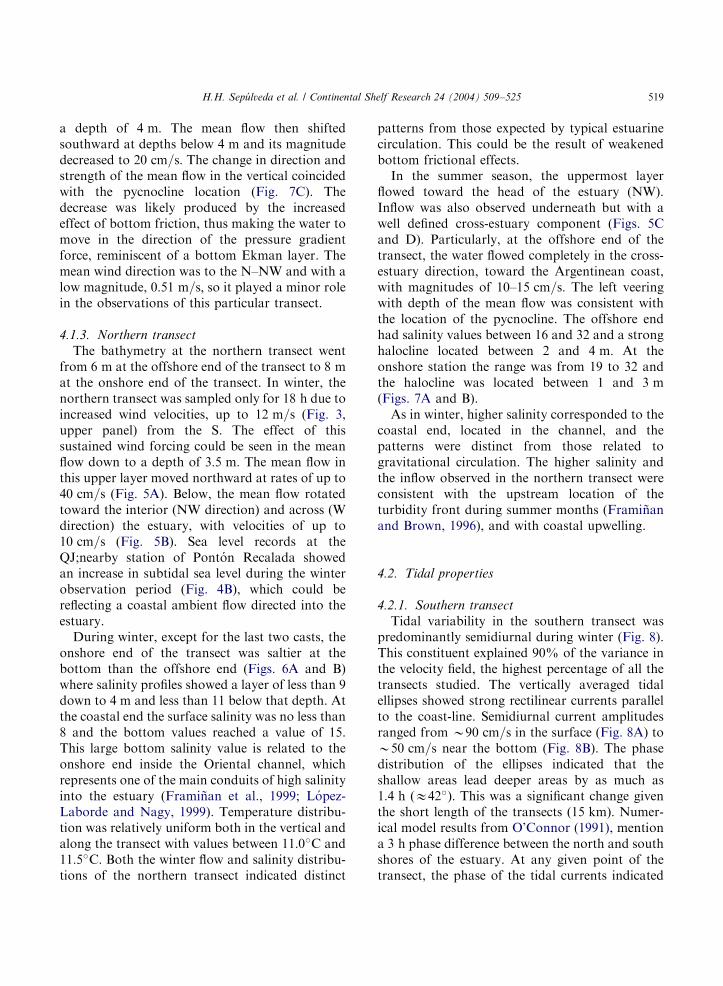
Tidal variability in the southern transect waspredominantly semidiurnal during winter (Fig. 8).This constituent explained 90% of the variance inthe velocity field, the highest percentage of all thetransects studied. The vertically averaged tidalellipses showed strong rectilinear currents parallelto the coast-line. Semidiurnal current amplitudesranged from B90 cm=s in the surface (Fig. 8A) toB50 cm=s near the bottom (Fig. 8B). The phasedistribution of the ellipses indicated that theshallow areas lead deeper areas by as much as1:4 h ðE42�Þ: This was a significant change giventhe short length of the transects ð15 kmÞ: Numer-ical model results from O’Connor (1991), mentiona 3 h phase difference between the north and southshores of the estuary. At any given point of thetransect, the phase of the tidal currents indicated

ARTICLE IN PRESS

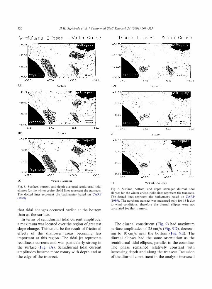
Fig. 8. Surface, bottom, and depth averaged semidiurnal tidal

ellipses for the winter cruise. Solid lines represent the transects.

The dotted lines represent the bathymetry based on CARP

(1989).

Fig. 9. Surface, bottom, and depth averaged diurnal tidal

ellipses for the winter cruise. Solid lines represent the transects.

The dotted lines represent the bathymetry based on CARP

(1989). The northern transect was measured only for 18 h due

to wind conditions, therefore the diurnal ellipses were not

calculated for that transect.


that tidal changes occurred earlier at the bottomthan at the surface.In terms of semidiurnal tidal current amplitude,

a maximum was located over the region of greatestslope change. This could be the result of frictionaleffects of the shallower areas becoming lessimportant at this region. The tidal jet representsrectilinear currents and was particularly strong inthe surface (Fig. 8A). Semidiurnal tidal currentamplitudes became more rotary with depth and atthe edge of the transect.

The diurnal constituent (Fig. 9) had maximumsurface amplitudes of 25 cm=s (Fig. 9D), decreas-ing to 10 cm=s near the bottom (Fig. 9E). Thediurnal ellipses had the same orientation as thesemidiurnal tidal ellipses, parallel to the coastline.The phase remained relatively constant withincreasing depth and along the transect. Inclusionof the diurnal constituent in the analysis increased

ARTICLE IN PRESS

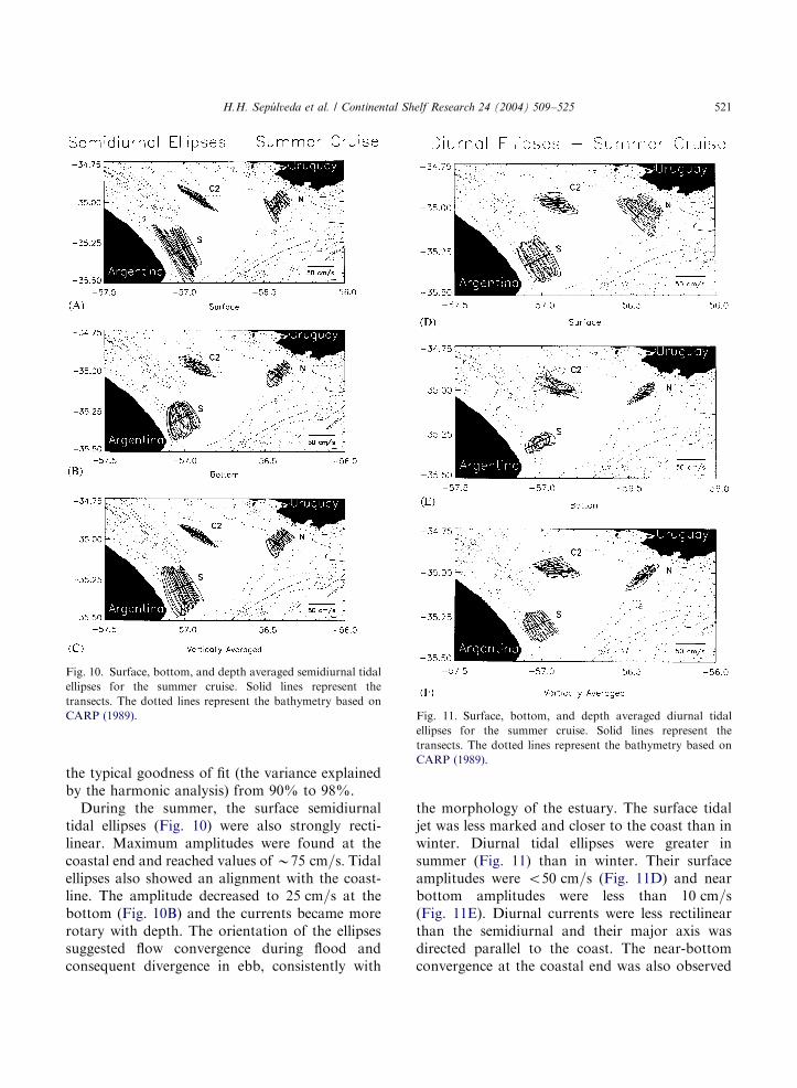
Fig. 10. Surface, bottom, and depth averaged semidiurnal tidal

ellipses for the summer cruise. Solid lines represent the

transects. The dotted lines represent the bathymetry based on

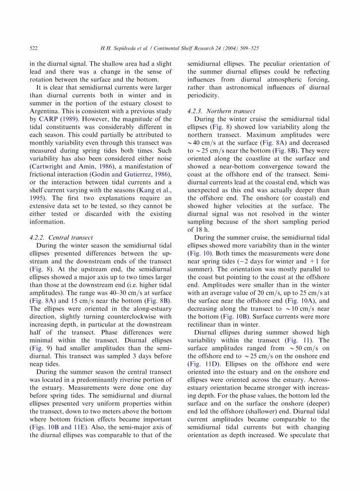
CARP (1989). Fig. 11. Surface, bottom, and depth averaged diurnal tidal

ellipses for the summer cruise. Solid lines represent the

transects. The dotted lines represent the bathymetry based on

CARP (1989).


the typical goodness of fit (the variance explainedby the harmonic analysis) from 90% to 98%.During the summer, the surface semidiurnal

tidal ellipses (Fig. 10) were also strongly recti-linear. Maximum amplitudes were found at thecoastal end and reached values ofB75 cm=s: Tidalellipses also showed an alignment with the coast-line. The amplitude decreased to 25 cm=s at thebottom (Fig. 10B) and the currents became morerotary with depth. The orientation of the ellipsessuggested flow convergence during flood andconsequent divergence in ebb, consistently with

the morphology of the estuary. The surface tidaljet was less marked and closer to the coast than inwinter. Diurnal tidal ellipses were greater insummer (Fig. 11) than in winter. Their surfaceamplitudes were o50 cm=s (Fig. 11D) and nearbottom amplitudes were less than 10 cm=s(Fig. 11E). Diurnal currents were less rectilinearthan the semidiurnal and their major axis wasdirected parallel to the coast. The near-bottomconvergence at the coastal end was also observed

ARTICLE IN PRESS


in the diurnal signal. The shallow area had a slightlead and there was a change in the sense ofrotation between the surface and the bottom.It is clear that semidiurnal currents were larger

than diurnal currents both in winter and insummer in the portion of the estuary closest toArgentina. This is consistent with a previous studyby CARP (1989). However, the magnitude of thetidal constituents was considerably different ineach season. This could partially be attributed tomonthly variability even through this transect wasmeasured during spring tides both times. Suchvariability has also been considered either noise(Cartwright and Amin, 1986), a manifestation offrictional interaction (Godin and Gutierrez, 1986),or the interaction between tidal currents and ashelf current varying with the seasons (Kang et al.,1995). The first two explanations require anextensive data set to be tested, so they cannot beeither tested or discarded with the existinginformation.

4.2.2. Central transect

During the winter season the semidiurnal tidalellipses presented differences between the up-stream and the downstream ends of the transect(Fig. 8). At the upstream end, the semidiurnalellipses showed a major axis up to two times largerthan those at the downstream end (i.e. higher tidalamplitudes). The range was 40–30 cm=s at surface(Fig. 8A) and 15 cm=s near the bottom (Fig. 8B).The ellipses were oriented in the along-estuarydirection, slightly turning counterclockwise withincreasing depth, in particular at the downstreamhalf of the transect. Phase differences wereminimal within the transect. Diurnal ellipses(Fig. 9) had smaller amplitudes than the semi-diurnal. This transect was sampled 3 days beforeneap tides.During the summer season the central transect

was located in a predominantly riverine portion ofthe estuary. Measurements were done one daybefore spring tides. The semidiurnal and diurnalellipses presented very uniform properties withinthe transect, down to two meters above the bottomwhere bottom friction effects became important(Figs. 10B and 11E). Also, the semi-major axis ofthe diurnal ellipses was comparable to that of the

semidiurnal ellipses. The peculiar orientation ofthe summer diurnal ellipses could be reflectinginfluences from diurnal atmospheric forcing,rather than astronomical influences of diurnalperiodicity.

4.2.3. Northern transect

During the winter cruise the semidiurnal tidalellipses (Fig. 8) showed low variability along thenorthern transect. Maximum amplitudes wereB40 cm=s at the surface (Fig. 8A) and decreasedtoB25 cm=s near the bottom (Fig. 8B). They wereoriented along the coastline at the surface andshowed a near-bottom convergence toward thecoast at the offshore end of the transect. Semi-diurnal currents lead at the coastal end, which wasunexpected as this end was actually deeper thanthe offshore end. The onshore (or coastal) endshowed higher velocities at the surface. Thediurnal signal was not resolved in the wintersampling because of the short sampling periodof 18 h:During the summer cruise, the semidiurnal tidal

ellipses showed more variability than in the winter(Fig. 10). Both times the measurements were donenear spring tides (�2 days for winter and +1 forsummer). The orientation was mostly parallel tothe coast but pointing to the coast at the offshoreend. Amplitudes were smaller than in the winterwith an average value of 20 cm=s; up to 25 cm=s atthe surface near the offshore end (Fig. 10A), anddecreasing along the transect to B10 cm=s nearthe bottom (Fig. 10B). Surface currents were morerectilinear than in winter.Diurnal ellipses during summer showed high

variability within the transect (Fig. 11). Thesurface amplitudes ranged from B50 cm=s onthe offshore end to B25 cm=s on the onshore end(Fig. 11D). Ellipses on the offshore end wereoriented into the estuary and on the onshore endellipses were oriented across the estuary. Across-estuary orientation became stronger with increas-ing depth. For the phase values, the bottom led thesurface and on the surface the onshore (deeper)end led the offshore (shallower) end. Diurnal tidalcurrent amplitudes became comparable to thesemidiurnal tidal currents but with changingorientation as depth increased. We speculate that

ARTICLE IN PRESS


the phase in the coastal (deeper) areas of thetransect leads the rest of the transect because thisend is strongly influenced by shelf waters. Thephase lead can be inferred from the high salinityvalues measured close to the coast, where changesin tidal forcing from the shelf occurred earlier.

5. Discussion and conclusions

We provide the first observational evidence ofsome tidal and subtidal circulation features inthree sectors of the R!ıo de la Plata Estuary. Tidalcurrent amplitudes were greater on the southernside of the estuary and decreased northward as itwas suggested in early tidal studies (Balay, 1961;CARP, 1989) and by numerical models applied inthe region. Further comparison with publishedresults from numerical models (O’Connor, 1991;Etala, 1996; Vieira and Lanfredi, 1996; Simionatoet al., 2001) is complicated by the coarse verticaland horizontal resolution of the models; themeasured transects would be covered by two gridpoints, at most.The subtidal flow showed a well-developed

estuarine circulation in the southern transect, wherethe tidal currents were strongest. This circulationwas likely the result of the dynamic balancebetween pressure gradient and friction. The samebalance should have affected the transects locatedin the central portion of the estuary although thebarotropic pressure gradient dominated over thebaroclinic because the subtidal flow was predomi-nantly downstream through the water column. Incontrast, the subtidal flow over the transect locatedin the northern portions showed a pattern that wasmore congruent with the wind direction than withthe typical estuarine circulation.Although the results obtained are from specific

locations within the estuary and may be confinedto specific environmental conditions, our observa-tions on the spatial and vertical variability of thesubtidal flows in the R!ıo de la Plata suggest thattidal currents provide the frictional effects neededfor the development of the two-layered estuarinecirculation in the southern sector. These tidalcurrents are weak in the northern sector and theirinfluence on frictional effects is minimal compared

to the frictional influence from wind forcing andfrom the ambient coastal currents. We proposethen that the large buoyant discharge into the R!ıode la Plata will experience two modifications:

(1)
when interacting with strong tidal currents, asin the southern sector, the buoyant waters willdrive a gravitational circulation.
(2)
In the absence of strong tidal currents, as inthe northern sector, the buoyant water will bemodified by wind forcing and the ambientcoastal currents. In cases when wind andambient velocities are weak, the subtidal flowmay be associated with a salt wedge.
Our initial hypothesis that the spatial variability ofsubtidal flows is influenced mostly by tidal andwind forcing interactions with buoyancy forcing isstrengthened by this observational study. Ourobservations are consistent with the theoreticalresults for surface-advected buoyant discharges(Yankovsky and Chapman, 1997) in the northernsector of the estuary. Similar observations ofsurface-advected discharges have been reportedin regions of freshwater influence in theArctic (Johnson et al., 1997; Harms and Karcher,1999)

Acknowledgements

This project was part of a collaborative effortbetween US universities and the Naval Hydro-graphic Service (SHN) from the Argentine Navy,funded by NSF International Programs. We aregrateful to Dr. Andreas M .unchow for his partici-pation in the project, and comments to thismanuscript. We thank Lt. Alejandro L !opez andthe crews of the L.H.A.R.A. ‘‘Cormor!an’’ and theB.H.A.R.A. ‘‘Comodoro Rivadavia’’ for theireffort, and for providing a great working environ-ment. M. C!aceres, W. Dragani, D. Huntley,S. H .usrevo&glu, K. Jenkins, J. Verocai collaboratedin the field work. Assistance from R.L. Yurquina,J. Pardinas and A. Galv!an, oceanographic techni-cians, is appreciated. We thank G. Pujol forsatellite imagery information. Sea level and winddata were provided by the SHN. A. Valle-Levinson

ARTICLE IN PRESS


and H. Sep !ulveda were funded by NSF 9529806and 9940194. M. Framinan was supported byNASA grant NAS5-35361. Comments by tworeviewers contributed to improve this manuscript.

References

Acha, E., Mianzan, H., Lasta, C., Guerrero, R., 1999.

Estuarine spawning of the whitemouth croacker (Micro-

pogonias furnieri) in the Rio de la Plata. Marine and

Freshwater Research 50, 57–65.

Apel, J., 1999. Principles of Ocean Physics. International

Geophysics Series, Vol. 38. Academic Press, Great Britain.

Balay, M., 1959. Causes and periodicity of large floods in R!ıo

de la Plata. International Hydrographic Review (Monaco)

36 (1), 123–151.

Balay, M., 1961. El R!ıo de la Plata entre la atm!osfera y el mar,

Vol. Pub. H-621, Servicio de Hidrograf!ıa Naval, Buenos Aires.

Beardsley, R., Limeburner, R., Yu, H., Cannon, G., 1985.

Discharge of the Changjian (Yangtze River) into the East

China Sea. Continental Shelf Research 4, 57–76.

Boschi, E., 1988. El ecosistema estuarial del R!ıo de la Plata

(Argentina y Uruguay). Anales del Instituto de Ciencias del

Mar y Limnolog!ıa 15 (2), 159–182.

CARP, 1989. Estudio para la evaluaci !on de la contaminaci !on

en el R!ıo de la Plata, Comisi !on Administradora del R!ıo de la

Plata, Montevideo-Buenos Aires.

Cartwright, D., Amin, M., 1986. The variance of tidal

harmonics. Deutsch Hydrography Zeitschrift 39 (H.6),

235–253.

Cousseau, M., 1985. Los peces del R!ıo de la Plata y su frente

mar!ıtimo. In: Yanes-Arancibia, A. (Ed.), Fish Community

Ecology in Estuaries and Coastal Lagoons: Towards an

Ecosystem Integration. UNAM Press, M!exico, pp. 515–534.

D’Onofrio, E.E., Fiore, M.M., Romero, S.I., 1999. Return

periods of extreme water levels estimated for some vulner-

able areas of Buenos Aires. Continental Shelf Research 19,

1681–1693.

Etala, M., 1996. Modelado de onda de tormenta en el R!ıo de la

Plata. Revista Instituto Argentino de Navegaci !on 5, 13–25.

Framinan, M.B., 2004. On the physical characteristics and

exchange processes in the R!ıo de la Plata and the adjacent

continental shelf, Ph.D. Thesis, University of Miami,

Rosenstiel School of Marine and Atmospheric Sciences,

Division Meteorological and Physical Oceanography.

Framinan, M.B., Brown, O.B., 1996. Study of the R!ıo de la

Plata turbidity front, Part I: spatial and temporal distribu-

tion. Continental Shelf Research 16 (10), 1259–1282.

Framinan, M.B., Brown, O.B., 1998. Sea surface temperature

anomalies off the R!ıo de la Plata Estuary: coastal upwelling?

Transactions AGU 79 (1), 128.

Framinan, M.B., Etala, M.P., Acha, E.M., Guerrero, R.A.,

Lasta, C.A., Brown, O.B., 1999. Physical characteristics and

processes of the R!ıo de la Plata estuary. In: Perillo, G.,

Piccolo, M., Pino-Quivira, M. (Eds.), Estuaries of South

America. Springer, Germany, pp. 161–194 (Chapter 8).

Geyer, W., Beardsley, R., Candela, J., Castro, B., Legeckis, R.,

Lentz, S., Limeburner, R., Miranda, L.B., Trowbridge,

J.H., 1991. Physical oceanography of the Amazon outflow.

Oceanography 4 (10), 8–14.

Godin, G., Gutierrez, G., 1986. Non-linear effects in the tide of

the Bay of Fundy. Continental Shelf Research 5 (3),

379–402.

Guerrero, R.A., Acha, E.M., Framinan, M.B., Lasta, C.A.,

1997. Physical oceanography of the R!ıo de la Plata

Estuary, Argentina. Continental Shelf Research 17 (7),

727–742.

Harms, I., Karcher, M., 1999. Modeling the seasonal variability

of hydrography and circulation in the Kara Sea. Journal of

Geophysical Research 13, 13431–13448.

Hickey, B., Jay, D., Boicourt, W., 1998. The Columbia

river plume study: subtidal variability in the velocity and

salinity fields. Journal of Geophysical Research 103 (10),

10,339–10,368.

Hill, A., 1998. Buoyancy effects in coastal and shelf seas. In:

Robinson, A.R., Brink, K.H. (Eds.), The Sea, Vol. 10.

Wiley, New York, pp. 21–62.

Hoffman, J., Nez, M.N., Piccolo, M., 1997. Caracter!ısticas

clim!aticas del Oc!eano Atl!antico Sudoccidental. In: Boschi

(Ed.), El Mar Argentino y sus recursos pesqueros, Instituto

Nacional de Investigaci!on y Desarvollo Pesquero, Mar del

Plata, Argentina. pp. 163–193 (Chapter 1).

Johnson, D., Climans, T.M., King, S., Grenness, O., 1997.

Fresh water masses in the Kara Sea during summer. Journal

of Marine Systems 12, 127–145.

Joyce, T., 1989. On in situ ‘‘calibration’’ of shipboard ADCPs.

Journal of Atmospheric and Oceanic Technology 6,

169–172.

Kang, S.K., Chung, J.-Y., Lee, S.-R., Yum, K.-D., 1995.

Seasonal variability of the M2 tide in the seas adjacent to

Korea. Continental Shelf Research 15 (9), 1087–1113.

Lentz, S., 1994. Current dynamics over the northern California

inner shelf. Journal of Physical Oceanography 24,

2461–2478.

Leopold, L., 1994. A View of the River. Harvard University

Press, Cambridge, MA.

L !opez-Laborde, J., Nagy, G.J., 1999. Hydrography and

sediment transport characteristics of the R!ıo de la Plata:

a review. In: Perillo, G., Piccolo, M., Pino-Quivira, M.

(Eds.), Estuaries of South America. Springer, Germany,

pp. 132–159 (Chapter 7).

Lwiza, K.M.M., Bowers, D., Simpson, J., 1991. Residual and

tidal flow at a tidal mixing front in the North Sea.

Continental Shelf Research 11 (11), 1379–1395.

Mianzan, H., Lasta, C., Acha, E., Guerrero, R., Macchi, G.,

Breme, C., 2001. The r!ıo de la plata estuary, Argentina–

Uruguay. In: Seelinger, U., Kjerfve, B. (Eds.), Coastal

Marine Ecosystems of Latin America, Ecological Studies,

Vol. 144. Springer, Berlin, pp. 185–204.

M .unchow, A., Weingartner, T.J., Cooper, L.W., 1999. The

summer hydrography and surface circulation of the East

ARTICLE IN PRESS


Siberian shelf sea. Journal of Physical Oceanography 29,

2167–2182.

O’Connor, W., 1991. A numerical model of tides and storm

surges in the R!ıo de la Plata Estuary. Continental Shelf

Research 11, 1491–1508.

RD-Instruments, 1996. Acoustic Doppler current profiler

principles of operation: a practical primer. RD Instruments

2nd, 51 pp.

Simionato, C., Nunez, G.M.N., Engel, M., 2001. The salinity

front of the R!ıo de la Plata—a numerical case study for

winter and summer conditions. Geophysical Research

Letters 28 (13), 2641–2644.

Soulsby, R., 1983. The bottom boundary layer of shelf seas. In:

Johns, B. (Ed.), Physical Oceanography of Coastal and Shelf

Seas. Elsevier Science Publishers, Amsterdam (Chapter 5).

Souza, A.J., Simpson, J.H., 1996. The modification of tidal

ellipses by stratification in the Rhine ROFI. Continental

Shelf Research 16 (8), 997–1007.

Vieira, J.R., Lanfredi, N.W., 1996. A hydrodynamic model for

the R!ıo de la Plata, Argentina. Journal of Coastal Research

12 (2), 430–446.

Yankovsky, A., Chapman, D., 1997. A simple theory for the

fate of buoyant coastal discharges. Journal of Physical

Oceanography 27, 1386–1401.

Documents

Observations of subtidal and tidal flow in the Rio de la Plata Estuary