Embed Size (px)
Citation preview

Digital Object Identifier (DOI) 10.1007/s00220-007-0233-3Commun. Math. Phys. 272, 443–468 (2007) Communications in
MathematicalPhysics
On the Asymptotic Stability of Bound Statesin 2D Cubic Schrödinger Equation
E. Kirr1, A. Zarnescu2
1 Department of Mathematics, University of Illinois at Urbana-Champaign, 1409 W. Green Street,Urbana, IL 61801, USA. E-mail: [email protected]
2 Department of Mathematics, University of Chicago, 5734 S. University Ave., Chicago, IL 60637, USA
Received: 27 February 2006 / Accepted: 26 December 2006Published online: 28 March 2007 – © Springer-Verlag 2007
Abstract: We consider the cubic nonlinear Schrödinger equation in two space dimen-sions with an attractive potential. We study the asymptotic stability of the nonlinearbound states, i.e. periodic in time localized in space solutions. Our result shows that allsolutions with small, localized in space initial data, converge to the set of bound states.Therefore, the center manifold in this problem is a global attractor. The proof hinges ondispersive estimates that we obtain for the non-autonomous, non-Hamiltonian, linearizeddynamics around the bound states.
1. Introduction
In this paper we study the long time behavior of solutions of the cubic nonlinearSchrödinger equation (NLS) with potential in two space dimensions (2-d):
i∂t u(t, x) = [−�x + V (x)]u + γ |u|2u, t > 0, x ∈ R2, (1)
u(0, x) = u0(x), (2)
where γ ∈ R−{0}.The equation has important applications in statistical physics, opticsand water waves. It describes certain limiting behavior of Bose-Einstein condensates [8,14] and propagation of time harmonic waves in wave guides [12, 15, 17]. In the latter, tplays the role of the coordinate along the axis of symmetry of the wave guide.
It is well known that this nonlinear equation admits periodic in time, localized inspace solutions (bound states or solitary waves). They can be obtained via both varia-tional techniques [1, 28, 21] and bifurcation methods [19, 21], see also the next section.Moreover the set of periodic solutions can be organized as a manifold (center mani-fold). Orbital stability of solitary waves, i.e. stability modulo the group of symmetriesu �→ e−iθu, was first proved in [21, 33], see also [9, 10, 24].
In this paper we are going to show that the center manifold is in fact a global attractorfor all small, localized in space initial data. This means that the solution decomposes

444 E. Kirr, A. Zarnescu
into a modulation of periodic solutions (motion on the center manifold) and a part thatdecays in time via a dispersion mechanism (radiative part). For a precise statement ofhypotheses and the result see Sect. 3.
Asymptotic stability studies of solitary waves were initiated in the work of A. Sofferand M. I. Weinstein [25, 26], see also [2–4, 6, 11]. Center manifold analysis was intro-duced in [19], see also [32]. The techniques developed in these papers do not apply to ourproblem. Indeed the weaker L1 → L∞ dispersion estimates for Schrödinger operatorsin 2-d, see (27), compared to 3-d and higher, respectively lack of end point Strichartzestimates in d = 2, prevent the bootstrapping argument in [6, 19, 25, 26], respectively[11], from closing. The technique of virial theorem, used in [2–4] to compensate forthe weak dispersion in 1-d, would require at least a quintic nonlinearity in our 2-d case.Finally, in [32], the nonlinearity is localized in space, a feature not present in our case,which allows the author to completely avoid any L1 → L∞ estimates.
To overcome these difficulties we used Strichartz estimates, fixed point and inter-polation techniques to carefully analyze the full, time dependent, non-Hamiltonian,linearized dynamics around solitary waves. We obtained dispersive estimates that aresimilar with the ones for the time independent, Hamiltonian Schrödinger operator, seeSect. 4. Related results have been proved for the 1-d and 3-d case in [20, 13, 23] buttheir argument does not extend to the 2-d case. We relied on these estimates to under-stand the nonlinear dynamics via perturbation techniques. We think that our estimatesare also useful in approaching the dynamics around large 2-d solitary waves while thetechniques that we develop may be used in lowering the power of nonlinearity neededfor the asymptotic stability results in 1-d and 3-d mentioned in the previous paragraph.
Note that, in 3-d, the case of a center manifold formed by two distinct branches(ground state and excited state) has been analyzed. Under the assumption that the excitedbranch is sufficiently far away from the ground state one, in a series of papers [27, 29–31], the authors show asymptotic stability of the ground states with the exception of afinite dimensional manifold where the solution converges to excited states. We cannotextend such a result to our 2-d problem as of now. The reason is the slow convergence intime towards the center manifold, t−1+ in 2-d compared to t−3/2 in 3-d. This prevents usfrom even analyzing the projected dynamics on a single branch center manifold, i.e. theevolution of one complex parameter describing the projection of the solution on the cen-ter manifold, and obtain, for example, convergence to a periodic orbit as in [4, 19, 26].However the evolution of this parameter, respectively two parameters in the presence ofthe excited branch, is given by an ordinary differential equation (ODE), respectively asystem of two ODE’s, and the contribution of most of the terms can be determined fromour estimates, see the discussion in Sect. 5. We think it is only a matter of time until theremaining ones will be understood.
The paper is organized as follows. In the next section we discuss previous resultsregarding the manifold of periodic solutions that we subsequently need. In Sect. 3 weformulate and prove our main result. As we mentioned before the proof relies on certainestimates for the linear dynamics which we prove in Sect. 4. We conclude with possibleextensions and comments in Sect. 5.
Notations. H = −� + V ;L p = { f : R
2 �→ C | f measurable and∫R2 | f (x)|pdx < ∞},‖ f ‖p =(∫
R2 | f (x)|p
dx)1/p denotes the standard norm in these spaces;< x >= (1+|x |2)1/2, and for σ ∈ R, L2
σ denotes the L2 space with weight< x >2σ ,
i.e., the space of functions f (x) such that < x >σ f (x) are square integrable endowedwith the norm ‖ f (x)‖L2
σ= ‖ < x >σ f (x)‖2;

Asymptotic Stability of Bound States in 2D Cubic Schrödinger Equation 445
〈 f, g〉 = ∫R2 f (x)g(x)dx is the scalar product in L2, where z = the complex conju-
gate of the complex number z;Pc is the projection on the continuous spectrum of H in L2;Hn denote the Sobolev spaces of measurable functions having all distributional par-
tial derivatives up to order n in L2, ‖ · ‖Hn denotes the standard norm in this space.
2. Preliminaries. The Center Manifold
The center manifold is formed by the collection of periodic solutions for (1):
uE (t, x) = e−i EtψE (x), (3)
where E ∈ R and 0 �≡ ψE ∈ H2(R2) satisfy the time independent equation:
[−� + V ]ψE + γ |ψE |2ψE = EψE . (4)
Clearly the function constantly equal to zero is a solution of (4) but (iii) in the followinghypotheses on the potential V allows for a bifurcation with a nontrivial, one parameterfamily of solutions:(H1) Assume that
(i) There exists C > 0 and ρ > 3 such that:
|V (x)| ≤ C < x >−ρ, f or all x ∈ R2;
(ii) 0 is a regular point1 of the spectrum of the linear operator H = −� + V actingon L2;
(iii) H acting on L2 has exactly one negative eigenvalue E0 < 0 with correspondingnormalized eigenvector ψ0. It is well known that ψ0(x) can be chosen strictlypositive and exponentially decaying as |x | → ∞.
Conditions (i)-(ii) guarantee the applicability of dispersive estimates of Murata [16] andSchlag [22] to the Schrödinger group e−i Ht , see Sect. 4. In particular (i) implies thelocal well posedness in H1 of the initial value problem (1-2), see Sect. 3.
Condition (iii) guarantees bifurcation of nontrivial solutions of (4) from (E0, ψ0). InSect. 5, we discuss the possible effects of relaxing (iii) to allow for finitely many nega-tive eigenvalues. We construct the center manifold by applying the standard bifurcationargument in Banach spaces [18] for (4) at E = E0. We follow [19] and decompose thesolution of (4) in its projection onto the discrete and continuous part of the spectrum ofH :
ψE = aψ0 + h, a = 〈ψ0, ψE 〉, h = PcψE .
Using the notations
f p(a, h) ≡ 〈ψ0, |aψ0 + h|2(aψ0 + h)〉, (5)
fc(a, h) ≡ Pc[|aψ0 + h|2(aψ0 + h)
], (6)
1 This condition is somewhat stronger than Hψ = 0 has no solutions satisfying< x >1+ε ψ ∈ H2, ε > 0.For an exact definition and more details see [22, Definition 7] and Mµ = {0} in relation (3.1) in [16].

446 E. Kirr, A. Zarnescu
and projecting (4) onto ψ0 and its orthogonal complement = Range Pc we get:
h = −γ (H − E)−1 fc(a, h), (7)
E0 − E = −γ a−1 f p(a, h). (8)
Although we are using milder hypothesis on V the argument in the Appendix of [19]can be easily adapted to show that:
F(E, a, h) = h + γ (H − E)−1 fc(a, h)
is a C1 function from (−∞, 0) × C × L2σ ∩ H2 to L2
σ ∩ H2, here C is viewed as atwo dimensional real vectorial space. Moreover, F(E0, 0, 0) = 0, DhF(E0, 0, 0) = I,and, by the implicit function theorem, there exists δ1 > 0 and the C1 function h(E, a)from (E0 − δ1, E0 + δ1)× {a ∈ C : |a| < δ1} to L2
σ ∩ H2 such that (7) has a uniquesolution h = h(E, a) for all h, ‖h‖L2
σ∩H2 < δ1, E ∈ (E0 − δ1, E0 + δ1) and |a| < δ1.
Note that if (a, h) solves (7) then (eiθa, eiθh), θ ∈ (0, 2π) is also a solution, hence byuniqueness we have:
h(E, a) = a
|a| h(E, |a|). (9)
Because ψ0 is real valued, we could apply the implicit function theorem to (7) under therestriction a ∈ R and h in the subspace of real valued functions as it is actually done in[19]. By uniqueness of the solution we deduce that h(E, |a|) is a real valued function.
Replacing now h=h(E, a) in (8) and using (5) and (9) we get the equivalent formu-lation:
E0 − E = −γ |a|−1 f p(|a|, h(E, |a|)). (10)
To this we can apply again the implicit function theorem by observing that G(E, a) =E0 − E +γ |a|−1 f p(|a|, h(E, |a|)) is a C1 function [19, Appendix] from (E0 − δ1, E0 +δ1) × (−δ1, δ1) to R with the properties G(E0, 0) = 0, ∂E G(E0, 0) = −1. We obtainthe existence of 0 < δ ≤ δ1, 0 < δE ≤ δ1 and the C1 function E : (−δ, δ) �→(E0 − δE , E0 + δE ) such that, for |E − E0| < δE , |a| < δ, the unique solution of (8)with h = h(E, a), is given by E = E(|a|). If we now define:
h(a) ≡ a
|a| h(E(|a|), |a|)
we have the following center manifold result:
Proposition 2.1. There exist δE , δ > 0 and the C1 function
h : {a ∈ C : |a| < δ} �→ L2σ ∩ H2,
such that for |E − E0| < δE and ‖ψE‖L2σ∩H2 < δ, the eigenvalue problem (4) has a
unique solution up to multiplication with eiθ , θ ∈ (0, 2π), which can be representedas:
ψE = aψ0 + h(a), 〈ψ0, h(a)〉 = 0, |a| < δ.

Asymptotic Stability of Bound States in 2D Cubic Schrödinger Equation 447
Note that differentiating the identity:
h(aeiθ ) ≡ aeiθ
|a| h(E(|a|), |a|)
with respect to θ at θ = 0 we get:
Dh|aia = ih(a), for all a ∈ C, |a| < δ. (11)
Since ψ0(x) is exponentially decaying as |x | → ∞ the proposition implies thatψE ∈ L2
σ . A regularity argument, see [25], gives a stronger result:
Corollary 2.1. For any σ ∈ R, there exists a finite constant Cσ such that:
‖ < x >σ ψE‖H2 ≤ Cσ‖ψE‖H2 .
We are now ready to prove our main result.
3. Main Result. The Collapse on the Center Manifold
Theorem 3.1. Assume that Hypothesis (H1) is valid and fix σ > 1. Then there exists anε0 > 0 such that for all initial conditions u0(x) satisfying
max{‖u0‖L2σ, ‖u0‖H1} ≤ ε0,
the initial value problem (1)-(2) is globally well-posed in H1.
Moreover, for all t ∈ R and p0 ≥ 6, we have that:
u(t, x) = a(t)ψ0(x) + h(a(t))︸ ︷︷ ︸
ψE (t)
+r(t, x), (12)
‖r(t)‖L2−σ ≤ C1(p0)ε0
(1 + |t |)1−2/p0,
‖r(t)‖L p ≤ C2(p, p0) ε0log
1−2/p1−2/p0 (2 + |t |)(1 + |t |)1−2/p
, 2 ≤ p ≤ p0,
where the constants C1, C2, are independent of ε0.
Before proving the theorem let us note that (12) decomposes the evolution of thesolution of (1)-(2) into an evolution on a center manifold ψE (t) and the “distance” fromthe center manifold r(t). The estimates on the latter show collapse of solution onto thecenter manifold. The evolution on the center manifold is determined by Equation (14)below. We discuss it in Sect. 5.
Proof of Theorem 3.1. It is well known that under Hypothesis (H1)(i) the initial valueproblem (1)-(2) is locally well posed in the energy space H1 and its L2 norm is con-served, see for example [5, Cor. 4.3.3. at p. 92]. Global well posedness follows via energyestimates from ‖u0‖2 small, see [5, Remark 6.1.3 at p. 165].
In particular we can define
a(t) = 〈ψ0, u(t)〉, for t ∈ R.

448 E. Kirr, A. Zarnescu
Cauchy-Schwarz inequality implies
|a(t)| ≤ ‖u(t)‖2‖ψ0‖2 = ‖u0‖2 ≤ ε0, for t ∈ R,
where we also used conservation of L2 norm of u. Hence, if we choose ε0 < δ we candefine h(a(t)), t ∈ R, see Proposition 2.1. We then obtain (12), where
r(t) = u(t)− a(t)ψ0 − h(a(t)), 〈ψ0, r(t)〉 ≡ 0.
The solution is now described by the scalar a(t) ∈ C and r(t) ∈ C(R, H1). To obtaintheir equations we plug (12) into (1):
ida
dtψ0 + i Dh|a da
dt+ i∂r
∂t= HψE + Hr + γ |u|2u
= EψE + Hr + γ [|u|2u − |ψE |2ψE ]= Eaψ0 + Eh(a) + Hr (13)
+γ [2|ψE |2r + ψ2Er + 2ψE |r |2 + ψEr2 + |r |2r ],
where we used (4). Projecting now onto ψ0 and taking into account that h, Dh haverange orthogonal to ψ0, while r and ∂r
∂t are orthogonal to ψ0, we get:
ida
dt= E(|a(t)|)a(t) + γ 〈ψ0, 2|ψE |2r + ψ2
Er + 2ψE |r |2 + ψEr2 + |r |2r〉. (14)
The projection of (13) onto the orthogonal complement of ψ0 = range of Pc gives:
i Dh|a da
dt+ i∂r
∂t= Eh(a) + Hr + γ Pc[2|ψE |2r + ψ2
Er + 2ψE |r |2 + ψEr2 + |r |2r ].
We then plug in (14) and use the identity Dh|a(−i Ea) = −Eih(a), see (11), to obtain
i∂r
∂t= Hr + γ Pc[2|ψE |2r + ψ2
Er + 2ψE |r |2 + ψEr2 + |r |2r ]+iγ Dh|a(t)i〈ψ0, 2|ψE |2r + ψ2
Er + 2ψE |r |2 + ψEr2 + |r |2r〉. (15)
In order to obtain the estimates for r(t), we analyze Eq. (15). In the next section westudy its linear part:
{i ∂z∂t = H z + γ Pc[2|ψE |2z + ψ2
E z + iγ Dh|a(t)i〈ψ0, 2|ψE |2z + ψ2E z〉]
z(s) = v.
Let us denote by �(t, s)v the operator which associates to the function v the solutionof the above equation:
�(t, s)vdef= z. (16)
Using Duhamel’s principle, (15) becomes
r(t) = �(t, 0)r(0)− iγ∫ t
0�(t, s)Pc[2ψE |r(s)|2 + ψEr2(s) + |r |2r(s)]ds
+γ∫ t
0�(t, s)Dh|a(t)i〈ψ0, 2ψE |r |2 + ψEr2 + |r |2r〉ds. (17)
Asymptotic Stability of Bound States in 2D Cubic Schrödinger Equation 449
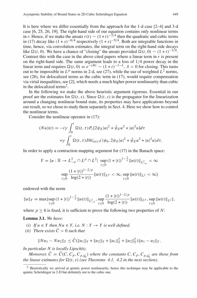
It is here where we differ essentially from the approach for the 1-d case [2–4] and 3-dcase [6, 25, 26, 19]. The right-hand side of our equation contains only nonlinear termsin r. Hence, if we make the ansatz r(t) ∼ (1 + t)−3/4 then the quadratic and cubic termsin (17) decay like (1 + s)−6/4 respectively (1 + s)−9/4. Both are integrable functions intime, hence, via convolution estimates, the integral term on the right-hand side decayslike �(t, 0). We have a chance of "closing" the ansatz provided �(t, 0) ∼ (1 + t)−3/4.
Contrast this with the case in the above cited papers where a linear term in r is presenton the right-hand side. The same argument leads to a loss of 1/4 power decay in thelinear term and requires �(t, 0) ≡ e−i Ht ∼ (1 + t)−1−δ, δ > 0 for closing. This turnsout to be impossible in L p norms in 2-d, see (27), while the use of weighted L2 norms,see (26), for delocalized terms as the cubic term in (17), would require compensationvia virial inequalities, see [2], which needs a much higher power nonlinearity than cubicin the delocalized terms2.
In the following we make the above heuristic argument rigorous. Essential in ourproof are the estimates for �(t, s). Since �(t, s) is the propagator for the linearizationaround a changing nonlinear bound state, its properties may have applications beyondour result, so we chose to study them separately in Sect. 4. Here we show how to controlthe nonlinear terms.
Consider the nonlinear operator in (17):
(Nu)(t) = −iγ∫ t
0�(t, τ )Pc[2ψE |u|2 + ψE u2 + |u|2u]dτ
+γ∫ t
0�(t, τ )Dh|a(τ )i〈ψ0, 2ψE |u|2 + ψE u2 + |u|2u〉dτ.
In order to apply a contraction mapping argument for (17) in the Banach space:
Y = {u : R → L2−σ ∩ L p ∩ L2| supt≥0
(1 + |t |)1− 2p ‖u(t)‖L2−σ < ∞
supt≥0
(1 + |t |)1−2/p
log(2 + |t |) ‖u(t)‖L p < ∞, supt≥0
‖u(t)‖L2 < ∞}
endowed with the norm
‖u‖Y = max{supt≥0
(1 + |t |)1− 2p ‖u(t)‖L2−σ , sup
t≥0
(1 + |t |)1−2/p
log(2 + |t |) ‖u(t)‖L p , supt≥0
‖u(t)‖L2},
where p ≥ 6 is fixed, it is sufficient to prove the following two properties of N :
Lemma 3.1. We have:
(i) If u ∈ Y then Nu ∈ Y, i.e. N : Y → Y is well defined.(ii) There exists C > 0 such that
‖Nu1 − Nu2‖Y ≤ C(‖u1‖Y + ‖u2‖Y + ‖u1‖2Y + ‖u2‖2
Y )‖u1 − u2‖Y .
In particular N is locally Lipschitz.Moreover, C = C(C,C p,C p,q ′
0) where the constants C,C p,C p,q ′
0are those from
the linear estimates for �(t, s) (see Theorems 4.1, 4.2 in the next section).
2 Heuristically we arrived at quintic power nonlinearity; hence this technique may be applicable to thequintic Schrödinger in 2-D but definitely not to the cubic one.
450 E. Kirr, A. Zarnescu
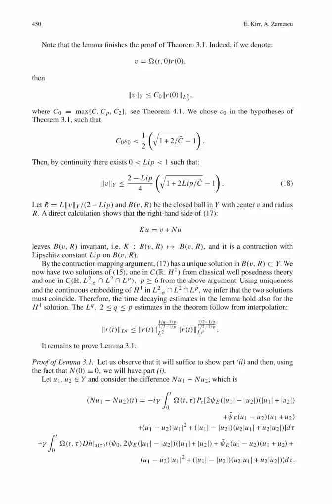
Note that the lemma finishes the proof of Theorem 3.1. Indeed, if we denote:
v = �(t, 0)r(0),
then
‖v‖Y ≤ C0‖r(0)‖L2σ,
where C0 = max{C,C p,C2}, see Theorem 4.1. We chose ε0 in the hypotheses ofTheorem 3.1, such that
C0ε0 <1
2
(√1 + 2/C − 1
)
.
Then, by continuity there exists 0 < Lip < 1 such that:
‖v‖Y ≤ 2 − Lip
4
(√1 + 2Lip/C − 1
)
. (18)
Let R = L‖v‖Y /(2 − Lip) and B(v, R) be the closed ball in Y with center v and radiusR. A direct calculation shows that the right-hand side of (17):
K u = v + Nu
leaves B(v, R) invariant, i.e. K : B(v, R) �→ B(v, R), and it is a contraction withLipschitz constant Lip on B(v, R).
By the contraction mapping argument, (17) has a unique solution in B(v, R) ⊂ Y.Wenow have two solutions of (15), one in C(R, H1) from classical well posedness theoryand one in C(R, L2−σ ∩ L2 ∩ L p), p ≥ 6 from the above argument. Using uniquenessand the continuous embedding of H1 in L2−σ ∩ L2 ∩ L p, we infer that the two solutionsmust coincide. Therefore, the time decaying estimates in the lemma hold also for theH1 solution. The Lq , 2 ≤ q ≤ p estimates in the theorem follow from interpolation:
‖r(t)‖Lq ≤ ‖r(t)‖1/q−1/p1/2−1/p
L2 ‖r(t)‖1/2−1/q1/2−1/pL p .
It remains to prove Lemma 3.1:
Proof of Lemma 3.1. Let us observe that it will suffice to show part (ii) and then, usingthe fact that N (0) ≡ 0, we will have part (i).
Let u1, u2 ∈ Y and consider the difference Nu1 − Nu2, which is
(Nu1 − Nu2)(t) = −iγ∫ t
0�(t, τ )Pc[2ψE (|u1| − |u2|)(|u1| + |u2|)
+ψE (u1 − u2)(u1 + u2)
+(u1 − u2)|u1|2 + (|u1| − |u2|)(u2|u1| + u2|u2|)]dτ+γ
∫ t
0�(t, τ )Dh|a(τ )i〈ψ0, 2ψE (|u1| − |u2|)(|u1| + |u2|) + ψE (u1 − u2)(u1 + u2) +
(u1 − u2)|u1|2 + (|u1| − |u2|)(u2|u1| + u2|u2|)〉dτ.

Asymptotic Stability of Bound States in 2D Cubic Schrödinger Equation 451
The L2−σ estimate. We can work under the less restrictive hypothesis: 4 < p < ∞. LetL p′
be the dual of L p, i.e. 1/p′ + 1/p = 1. We have
‖Nu1 − Nu2‖L2−σ ≤ |γ |∫ t
0‖�(t, τ )‖L2
σ→L2−σ ××‖ 2ψE < x >σ (|u1| − |u2|)(|u1| + |u2|) + ψE < x >σ (u1 − u2)(u1 + u2)︸ ︷︷ ︸
A
‖L2 dτ
+|γ |∫ t
0‖�(t, τ )‖L p′→L2−σ ×
×‖ (u1 − u2)|u1|2︸ ︷︷ ︸B1
+ (|u1| − |u2|)(u2|u1| + u2|u2|)︸ ︷︷ ︸B2
‖L p′ dτ
+|γ |∫ t
0‖�(t, τ )‖L2
σ→L2−σ ‖Dh|a(τ )‖L2σ
××{|〈ψ0, 2ψE (|u1| − |u2|)(|u1| + |u2|) + ψE (u1 − u2)(u1 + u2)〉|︸ ︷︷ ︸
F
+
+ |〈ψ0, (u1 − u2)|u1|2 + (|u1| − |u2|)(u2|u1| + u2|u2|)〉|︸ ︷︷ ︸G
}dτ.
(19)
To estimate the term A we observe that
‖ < x >σ ψE (|u1|−|u2|)(|u1|+|u2|)‖L2 ≤ ‖ < x >σ ψE‖Lα‖u1−u2‖L p‖|u1|+|u2|‖L p
(20)with 1
α+ 2
p = 12 . Then
∫ t
0‖�(t, τ )‖L2
σ→L2−σ A(τ )dτ
≤∫ t
0
C
(1 + |t − τ |) log2(2 + |t − τ |) · 3‖ψE < x >σ |u1 − u2|(|u1| + |u2|)‖L2 dτ
≤ 3CC1
∫ t
0
log2(2 + |τ |)(1 + |t − τ |) log2(2 + |t − τ |)
‖|u1| − |u2|‖Y
(1 + |τ |)(1− 2p )
· ‖|u1| + |u2|‖Y
(1 + |τ |)(1− 2p )
≤ 3CC1C2(‖u1‖Y + ‖u2‖Y )‖u1 − u2‖Y
(1 + |t |) log2(2 + |t |) ,
where for the first inequality we used Theorem 4.1, part (i). The constants are given by
C1 =supt>0 ‖ < x >σ ψE‖Lα and C2 =supt>0(1+|t |) log2(2+|t |) ∫ t0
log2(2+|τ |)(1+|t−τ |) log2(2+|t−τ |) ·
dτ
(1+|τ |)2− 4p< ∞, because p > 4.
To estimate the cubic terms B1, B2 we can not use the term ψE as before, and thisis what forces us to work in the L p space. We have:
‖(u1 − u2)|u1|2‖L p′ ≤ ‖u1 − u2‖L p‖u1‖2Lα ,
respectively
‖(u1 − u2)(u2|u1| + u2|u2|)‖L p′ ≤ ‖u1 − u2‖L p‖u2‖Lα (‖u1‖Lα + ‖u2‖Lα ),
452 E. Kirr, A. Zarnescu
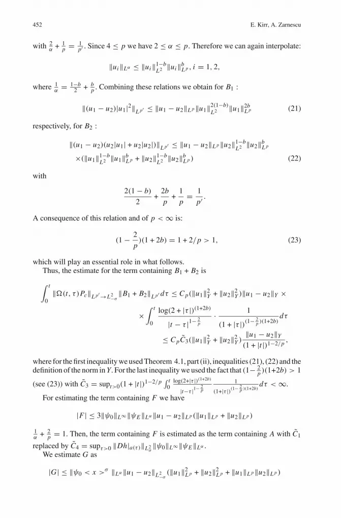
with 2α
+ 1p = 1
p′ . Since 4 ≤ p we have 2 ≤ α ≤ p. Therefore we can again interpolate:
‖ui‖Lα ≤ ‖ui‖1−bL2 ‖ui‖b
L p , i = 1, 2,
where 1α
= 1−b2 + b
p . Combining these relations we obtain for B1 :
‖(u1 − u2)|u1|2‖L p′ ≤ ‖u1 − u2‖L p‖u1‖2(1−b)L2 ‖u1‖2b
L p (21)
respectively, for B2 :
‖(u1 − u2)(u2|u1| + u2|u2|)‖L p′ ≤ ‖u1 − u2‖L p‖u2‖1−bL2 ‖u2‖b
L p
×(‖u1‖1−bL2 ‖u1‖b
L p + ‖u2‖1−bL2 ‖u2‖b
L p ) (22)
with
2(1 − b)
2+
2b
p+
1
p= 1
p′ .
A consequence of this relation and of p < ∞ is:
(1 − 2
p)(1 + 2b) = 1 + 2/p > 1, (23)
which will play an essential role in what follows.Thus, the estimate for the term containing B1 + B2 is
∫ t
0‖�(t, τ )Pc‖L p′→L2−σ ‖B1 + B2‖L p′ dτ ≤ C p(‖u1‖2
Y + ‖u2‖2Y )‖u1 − u2‖Y ×
×∫ t
0
log(2 + |τ |)(1+2b)
|t − τ |1− 2p
· 1
(1 + |τ |)(1− 2p )(1+2b)
dτ
≤ C pC3(‖u1‖2Y + ‖u2‖2
Y )‖u1 − u2‖Y
(1 + |t |)1−2/p,
where for the first inequality we used Theorem 4.1, part (ii), inequalities (21), (22) and thedefinition of the norm in Y.For the last inequality we used the fact that (1− 2
p )(1+2b) > 1
(see (23)) with C3 = supt>0(1 + |t |)1−2/p∫ t
0log(2+|τ |)(1+2b)
|t−τ |1− 2p
1
(1+|τ |)(1− 2p )(1+2b)
dτ < ∞.
For estimating the term containing F we have
|F | ≤ 3‖ψ0‖L∞‖ψE‖Lα‖u1 − u2‖L p (‖u1‖L p + ‖u2‖L p )
1α
+ 2p = 1. Then, the term containing F is estimated as the term containing A with C1
replaced by C4 = supτ>0 ‖Dh|a(τ )‖L2σ‖ψ0‖L∞‖ψE‖Lα .
We estimate G as
|G| ≤ ‖ψ0 < x >σ ‖Lα‖u1 − u2‖L2−σ (‖u1‖2L p + ‖u2‖2
L p + ‖u1‖L p‖u2‖L p )
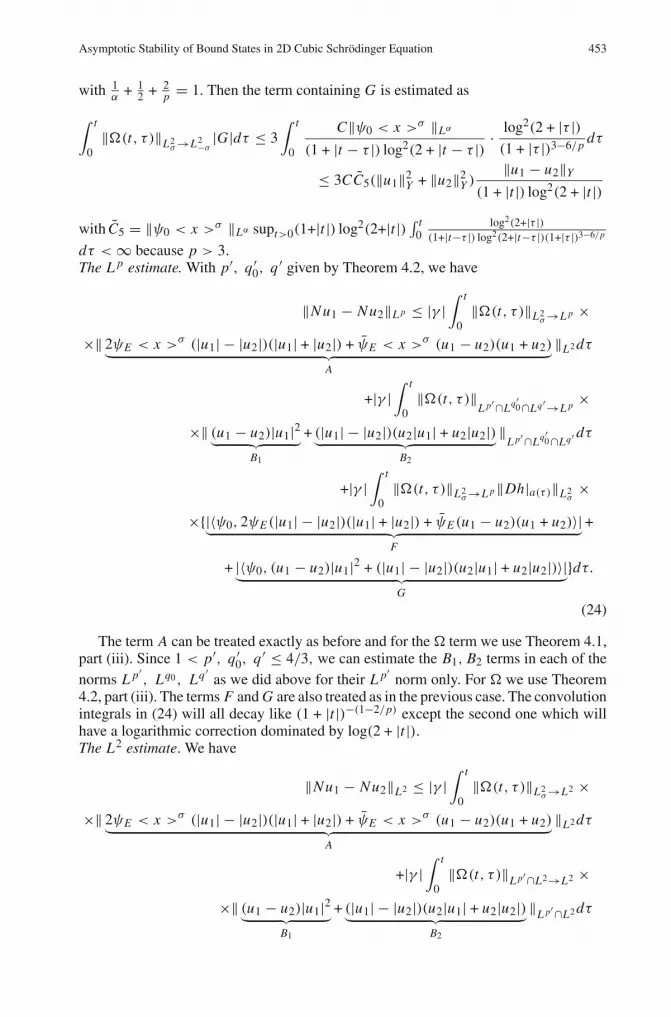
Asymptotic Stability of Bound States in 2D Cubic Schrödinger Equation 453
with 1α
+ 12 + 2
p = 1. Then the term containing G is estimated as
∫ t
0‖�(t, τ )‖L2
σ→L2−σ |G|dτ ≤ 3∫ t
0
C‖ψ0 < x >σ ‖Lα
(1 + |t − τ |) log2(2 + |t − τ |) · log2(2 + |τ |)(1 + |τ |)3−6/p
dτ
≤ 3CC5(‖u1‖2Y + ‖u2‖2
Y )‖u1 − u2‖Y
(1 + |t |) log2(2 + |t |)
with C5 = ‖ψ0 < x >σ ‖Lα supt>0(1+|t |) log2(2+|t |) ∫ t0
log2(2+|τ |)(1+|t−τ |) log2(2+|t−τ |)(1+|τ |)3−6/p
dτ < ∞ because p > 3.The L p estimate. With p′, q ′
0, q ′ given by Theorem 4.2, we have
‖Nu1 − Nu2‖L p ≤ |γ |∫ t
0‖�(t, τ )‖L2
σ→L p ××‖ 2ψE < x >σ (|u1| − |u2|)(|u1| + |u2|) + ψE < x >σ (u1 − u2)(u1 + u2)︸ ︷︷ ︸
A
‖L2 dτ
+|γ |∫ t
0‖�(t, τ )‖
L p′ ∩Lq′0 ∩Lq′→L p ×
×‖ (u1 − u2)|u1|2︸ ︷︷ ︸B1
+ (|u1| − |u2|)(u2|u1| + u2|u2|)︸ ︷︷ ︸B2
‖L p′ ∩Lq′
0 ∩Lq′ dτ
+|γ |∫ t
0‖�(t, τ )‖L2
σ→L p‖Dh|a(τ )‖L2σ
××{|〈ψ0, 2ψE (|u1| − |u2|)(|u1| + |u2|) + ψE (u1 − u2)(u1 + u2)〉|︸ ︷︷ ︸
F
+
+ |〈ψ0, (u1 − u2)|u1|2 + (|u1| − |u2|)(u2|u1| + u2|u2|)〉|︸ ︷︷ ︸G
}dτ.
(24)
The term A can be treated exactly as before and for the� term we use Theorem 4.1,part (iii). Since 1 < p′, q ′
0, q ′ ≤ 4/3, we can estimate the B1, B2 terms in each of thenorms L p′
, Lq0 , Lq ′as we did above for their L p′
norm only. For � we use Theorem4.2, part (iii). The terms F and G are also treated as in the previous case. The convolutionintegrals in (24) will all decay like (1 + |t |)−(1−2/p) except the second one which willhave a logarithmic correction dominated by log(2 + |t |).The L2 estimate. We have
‖Nu1 − Nu2‖L2 ≤ |γ |∫ t
0‖�(t, τ )‖L2
σ→L2 ××‖ 2ψE < x >σ (|u1| − |u2|)(|u1| + |u2|) + ψE < x >σ (u1 − u2)(u1 + u2)︸ ︷︷ ︸
A
‖L2 dτ
+|γ |∫ t
0‖�(t, τ )‖L p′ ∩L2→L2 ×
×‖ (u1 − u2)|u1|2︸ ︷︷ ︸B1
+ (|u1| − |u2|)(u2|u1| + u2|u2|)︸ ︷︷ ︸B2
‖L p′ ∩L2 dτ

454 E. Kirr, A. Zarnescu
+|γ |∫ t
0‖�(t, τ )‖L2
σ→L2‖Dh|a(τ )‖L2σ
××{|〈ψ0, 2ψE (|u1| − |u2|)(|u1| + |u2|) + ψE (u1 − u2)(u1 + u2)〉|︸ ︷︷ ︸
F
+
+ |〈ψ0, (u1 − u2)|u1|2 + (|u1| − |u2|)(u2|u1| + u2|u2|)〉|︸ ︷︷ ︸G
}dτ.
(25)
We estimate the term A as in (20) while the estimates in L p′for B1, B2 are as in (21)
and (22). For their estimate in L2 norm we use
‖(u1 − u2)|u1|2‖L2 ≤ ‖u1 − u2‖L p‖u1‖2Lα ,
respectively
‖(u1 − u2)(u2|u1| + u2|u2|)‖L2 ≤ ‖u1 − u2‖L p‖u2‖Lα (‖u1‖Lα + ‖u2‖Lα ),
with 2α
+ 1p = 1
2 . Since 6 ≤ p we have 4 ≤ α ≤ p. Therefore we can again interpolate:
‖ui‖Lα ≤ ‖ui‖1−bL2 ‖ui‖b
L p , i = 1, 2,
where 1α
= 1−b2 + b
p . Combining these relations we obtain for B1 :‖(u1 − u2)|u1|2‖L2 ≤ ‖u1 − u2‖L p‖u1‖2(1−b)
L2 ‖u1‖2bL p ,
respectively, for B2 :‖(u1 − u2)(u2|u1| + u2|u2|)‖L2 ≤ ‖u1 − u2‖L p‖u2‖1−b
L2 ‖u2‖bL p
×(‖u1‖1−bL2 ‖u1‖b
L p + ‖u2‖1−bL2 ‖u2‖b
L p ),
with2(1 − b)
2+
2b
p+
1
p= 1
2.
A consequence of this relation is:
(1 − 2
p)(1 + 2b) = 2.
Using now the definition of the norm in Y we will have:
‖B1 + B2‖2L ≤ ‖u1 − u2‖Y (‖u1‖2
Y + ‖u‖22)
log2p/(p−2)(2 + |t |)(1 + |t |)2 .
The previous estimates for F and G suffice here as well.Recalling from Theorem 4.1, part (iii) and Theorem 4.2, part (ii), that‖�(t, τ )‖L2
σ→L2
and ‖�(t, τ )‖L p′ ∩L2→L2 are bounded, and combining with the estimates above, as wellas taking into account the definition of the functional space Y we have that
‖Nu1 − Nu2‖L2 ≤ C‖u1 − u2‖Y [C6(‖u1‖Y + ‖u2‖Y ) + C7(‖u1‖2Y + ‖u2‖2
Y )]with C6 = supt≥0
∫ t0
log2(2+|τ |)(1+|τ |)(2−4/p) dτ<∞ and C7 = supt≥0
∫ t0
log(1+2b)(2+|τ |)(1+|τ |)(1+2b)(1−2/p) dτ < ∞.
This finishes the proof of Lemma 3.1 and the proof of Theorem 3.1. ��

Asymptotic Stability of Bound States in 2D Cubic Schrödinger Equation 455
4. Linear Estimates
Consider the linear Schrödinger equation with a potential in two space dimensions:
{i ∂u∂t = (−� + V (x))u
u(0) = u0.
It is known that if V satisfies Hypothesis (H1)(i) and (ii) then the radiative part of thesolution, i.e. its projection onto the continuous spectrum of H = −� + V, satisfies theestimates:
‖e−i Ht Pcu0‖L2−σ ≤ CM1
(1 + |t |) log2(2 + |t |)‖u0‖L2σ
(26)
for σ > 1 and some constant CM > 0 independent of u0 and t ∈ R, see [16, Theorem7.6], and
‖e−i Ht Pcu0‖L p ≤ C p
|t |1−2/p‖u0‖L p′ (27)
for some constant C p > 0 depending only on p ≥ 2 and p′ given by p′−1 + p−1 = 1.The case p = ∞ in (27) is proven in [22]. The conservation of the L2 norm, see [5,Corollary 4.3.3], gives the p = 2 case:
‖e−i Ht Pcu0‖L2 = ‖u0‖L2 .
The general result (27) follows from Riesz-Thorin interpolation.We would like to extend these estimates to the linearized dynamics around the center
manifold. In other words we consider the linear equation, with initial data at time s,
{i ∂z∂t = (−� + V (x))z+γ Pc[2|ψE (t)|2z+ψ2
E (t)z]+iγ Dh|a(t)(i〈ψ0, 2|ψE |2z+ψ2E z〉)
z(s) = v.
Note that this is a nonautonomous problem as the bound state ψE around which welinearize may change with time.
By Duhamel’s principle we have:
z(t) = e−i H(t−s)Pcv − iγ∫ t
se−i H(t−τ)Pc{[2|ψE |2z + ψ2
E z]+i Dh|a(τ )(i〈ψ0, 2|ψE |2z + ψ2
E z〉)}dτ. (28)
As in (16) we denote
�(t, s)vde f= z(t). (29)
In the next two theorems we will extend estimates of type (26)-(27) to the operator�(t, s) relying on the fact that ψE (t) is small. It would be useful to find sufficient con-ditions under which our results generalize to large bound states. Such conditions havebeen obtained in one or three space dimensions, see [2, 13, 23, 6], unfortunately theirtechniques cannot be applied in the two space dimension case.
We start with estimates in weighted L2 spaces:

456 E. Kirr, A. Zarnescu
Theorem 4.1. There exists ε1 > 0 such that if ‖ < x >σ ψE‖H2 < ε1 then there existconstants C, C p > 0 with the property that for any t, s ∈ R the following hold:
(i) ‖�(t, s)‖L2σ→L2−σ ≤ C
(1 + |t − s|) log2(2 + |t − s|) ,
(ii) ‖�(t, s)‖L p′→L2−σ ≤ C p
|t − s|1− 2p
, for any p ≥ 2 where p′−1 + p−1 = 1,
(iii) ‖�(t, s)‖L2σ→L p ≤ C p
|t − s|1− 2p
, for any p ≥ 2.
Before proving the theorem let us remark that (i) is a generalization of (26) while (ii)and (iii) are a mixture between (26) and (27). We have used all these estimates in theprevious section. They are consequences of contraction principles applied to (28) andinvolve estimates for convolution operators based on (26) and (27). It will prove muchmore difficult to remove the weights from the estimates (ii) and (iii), see Theorem 4.2.
Proof of Theorem 4.1. Fix s ∈ R.
(i) By definition (see (29)), we have �(t, s)v = z(t), where z(t) satisfies Eq. (28).We are going to prove the estimate by showing that the linear equation (28) can be solvedvia contraction principle argument in an appropriate functional space. To this extent letus consider the functional space
X1 := {z ∈ C(R, L2−σ (R2))| supt∈R
(1 + |t − s|) log2(2 + |t − s|)‖z(t)‖L2−σ < ∞}
endowed with the norm
‖z‖X1 := supt∈R
{(1 + |t − s|) log2(2 + |t − s|)‖z(t)‖L2−σ } < ∞.
Note that the inhomogeneous term in (28):
z0(t)def= e−i H(t−s)Pcv
satisfies z0 ∈ X1 and‖z0‖X1 ≤ CM‖v‖L2
σ(30)
because of (26).We collect the z dependent part of the right-hand side of (28) in a linear operator
L(s) : X1 → X1,
[L(s)z](t) = −iγ∫ t
se−i H(t−τ)Pc[2|ψE |2z+ψ2
E z+i Dh|a(τ )(i〈ψ0, 2|ψE |2z+ψ2E z〉)]dτ.
(31)In what follows we will show that L is a well defined bounded operator from X1
to X1 whose operator norm can be made less then or equal to 1/2 by choosing ε1 inthe hypothesis sufficiently small. Consequently I d − L is invertible and the solution ofEq. (28) can be written as z = (I d − L)−1z0. In particular
‖z‖X1 ≤ (1 − ‖L‖)−1‖z0‖X1 ≤ 2‖z0‖X1

Asymptotic Stability of Bound States in 2D Cubic Schrödinger Equation 457
which, in combination with the definition of �, the definition of the norm in X1 andestimate (30), finishes the proof of (i).
It remains to prove that L is a well defined bounded operator from X1 to X1 whoseoperator norm can be made less than 1/2 by choosing ε1 in the hypothesis sufficientlysmall. We have the following estimates:
‖L(s)z(t)‖L2−σ ≤ |γ |∫ t
s‖e−i H(t−τ)Pc‖L2
σ→L2−σ · [3‖|ψE |2(τ )z(τ )‖L2σ
+‖Dh|a(τ )‖C→L2σ|〈ψ0, 2|ψE |2 < x >σ< x >−σ z(τ )+ψ2
E < x >σ< x >−σ z(τ )〉|]dτ
≤ |γ |∫ t
s‖e−i H(t−τ)Pc‖L2
σ→L2−σ · [3‖|ψE |2(τ )z(τ )‖L2σ
+‖Dh|a(τ )‖C→L2σ‖ψ0‖L2 3‖ < x >σ ψ2
E‖L∞‖z(τ )‖L2−σ ]dτ.On the other hand
‖|ψE |2z‖L2σ
≤ ‖z‖L2−σ ‖ < x >2σ |ψE |2‖L∞ , and ‖ < x >σ ψE‖2L∞ ≤ ε2
1, (32)
where the last inequality is due to the Sobolev imbedding H2(R2) ⊂ L∞(R2) and theinequality
‖ < x >σ ψE‖H2 ≤ ε1.
Also, from Proposition 2.1,
‖Dh|a(τ )‖ ≤ C, for |a(τ )| ≤ ε1 < δ.
Using the last three relations, as well as the estimate (26) and the fact that z ∈ X1 weobtain that
‖L(s)‖X1→X1 ≤ 3|γ |ε21 sup
t>0
[
(1 + |t − s|) log2(2 + |t − s|)×
×∫ t
s
CM
(1 + |t − τ |) log2(2 + |t − τ |) · 1
(1 + |τ − s|) log2(2 + |τ − s|)dτ
︸ ︷︷ ︸I
] ≤ C1ε21 .
(33)
Indeed, in order to prove the above we will split I into A + B, where
A =∫ t+s
2
s
1
(1 + |t − τ |) log2(2 + |t − τ |)1
(1 + |τ − s|) log2(2 + |τ − s|)dτ
for which we have the bound
|A| ≤ 1
(1 + | t−s2 |) log2(2 + | t−s
2 |) |∫ t+s
2
s
dτ
(1 + |τ − s|) log2(2 + |τ − s|) |
≤ C21
(1 + | t−s2 |) log3(2 + | t−s
2 |) .
Observing that A = B and using the last estimate in (33) we obtain that

458 E. Kirr, A. Zarnescu
‖L‖X1→X1 ≤ C1ε21 ≤ 1/2
for ε1 small enough.(ii) By the definition of � it is sufficient to prove that the solution of (28) satisfies
‖z(t)‖L2−σ ≤ C p
|t − s|1− 2p
‖v‖L p′ , for all p ≥ 2 where p′−1 + p−1 = 1. (34)
We will use a similar functional analytic argument as in the proof of (i). Fix p, 2 ≤ p <∞ and assume v ∈ L p′
, p′−1 + p−1 = 1. We will work in the following functionalspace:
X2 := {z ∈ C(R, L2−σ (R2)| supt∈R
‖z(t)‖L2−σ |t − s|1− 2p < ∞}
endowed with the norm
‖z‖X2 := supt∈R
‖z(t)‖L2−σ |t − s|1− 2p < ∞.
Using the fact that L p ↪→ L2−σ continuously and the estimate (27) we have e−i H(t−s)
Pcv ∈ X2. In addition, for L defined in the proof of (i), we have
supt>0
|t − s|1− 2p ‖L(s)z(t)‖L2−σ ≤
|γ | supt>0
|t − s|1− 2p
∫ t
s‖e−i H(t−τ)Pc‖L2
σ→L2−σ ·[‖2|ψE |2(τ )z(τ )
+ψ2E (τ )z(τ )‖L2
σ+ ‖Dh|a(τ )‖C→L2
σ|〈ψ0, 2|ψE |2z(s) + ψ2
E z(s)〉|]
dτ
≤ |γ | supt>0
|t − s|1− 2p
∫ t
s
C p
(1 + |t − τ |) log2(2 + |t − τ |)·3(1 + C)‖ψ2
E < x >2σ ‖L∞
|τ − s|1− 2p
dτ < C3ε21 . (35)
Using now the bounds (32) in (35), for ε1 small enough, we obtain that the norm of L(s)is less or equal to 1/2, i.e. the operator I d − L(t, s) is invertible, which, as in the proofof (i), finishes the proof of estimate (ii).
(iii) We already know from part (i) that Eq. (28) has a unique solution in L2−σ providedv ∈ L2
σ . We are going to show that the right hand side of (28) is in L p. Indeed
‖e−i H(t−s)Pcv‖L p ≤ C p
|t − s|1− 2p
‖v‖L p′ ≤ C p
|t − s|1− 2p
‖v‖L2σ, (36)
where the C p’s in the two inequalities are different, for the first inequality we used (27)while for the second we used the continuous embedding L2
σ ↪→ L p′, 1 ≤ p′ ≤ 2. For

Asymptotic Stability of Bound States in 2D Cubic Schrödinger Equation 459
the remaining terms we combine (27) with ‖z‖X1 < ∞ obtained in part (i):
‖∫ t
se−i H(t−τ)Pc(2|ψ2
E |z(τ ) + ψ2E z(τ ))dτ‖L p
≤∫ t
s
3C p
|t − τ |1− 2p
‖ < x >σ ψ2E‖α‖ < x >−σ z(τ )‖L2 dτ
≤∫ t
s
3CP
|t − τ |1− 2p
· Cε21‖v‖L2
σ
(1 + |τ − s|) log2(2 + |τ − s|)dτ ≤ C4‖v‖L2σ
|t − s|1− 2p
(37)
with 1α
+ 12 = 1
p′ .Similarly, we have
‖∫ t
se−i H(t−τ)Pc Dh|a(τ )i〈ψ0, 2|ψE |2z(s) + ψ2
E z(s)〉dτ‖L p
≤∫ t
s
C pC
|t − τ |1− 2p
|〈ψ0, 2|ψE |2z(s) + ψ2E z(s)〉|dτ
≤∫ t
s
C pC
|t − τ |1− 2p
|‖ψ0‖L2‖ < x >σ ψ2E‖L∞‖ < x >−σ z‖L2 dτ
≤∫ t
s
C pC
|t − τ |1− 2p
Cε21‖v‖L2
σ
(1 + |τ − s|)(log2(2 + |τ − s|)dτ ≤ C5‖v‖L2σ
|t − s|1− 2p
. (38)
Plugging (36)-(38) into (28) we get:
‖z(t)‖L p ≤ C(p)
|t − s|1− 2p
‖v‖L2σ,
which by the definition �(t, s) = z(t) finishes the proof of part (iii). ��The next step is to obtain estimates for �(t, s) in unweighted L p spaces. They are
needed for controlling the cubic term in the operator N of the previous section.
Theorem 4.2. Assume that ‖ < x >σ ψE‖H2 < ε1 (where ε1 is the one used inTheorem 4.1). Then for all t, s ∈ R the following estimates hold:
(i) ‖�(t, s)‖L1∩Lq′ ∩L p′→L p ≤ C p,q ′ log(2 + |t − s|)(1 + |t − s|)1− 2
p
,
for all p, q ′, 2 ≤ p < ∞, 1 < q ′ ≤ 2, p′−1 + p−1 = 1;
(ii) ‖�(t, s)‖L2∩Lq′
0 →L2 ≤ Cq ′0, for all q ′
0, 1 < q ′0 <
4
3;
(iii) for fixed p0 > 0 and 1 < q ′0 < 4/3 and for any 2 ≤ p ≤ p0,
‖�(t, s)‖Lq′ ∩L p′ ∩Lq′
0 →L p ≤ C p,q ′0
log(2 + |t − s|) 1−2/p1−2/p0
|t − s|1− 2p
,

460 E. Kirr, A. Zarnescu
where
1
q ′ = θ +1 − θ
q ′0
with
θ = 1 − 2/p
1 − 2/p0, i.e.
1
p= θ
p0+
1 − θ
2.
Note that (iii) is similar to the standard estimate for Schrödinger operators (27) exceptfor the logarithmic correction and a smaller domain of definition. We will obtain it byinterpolation from (i) and (ii). The proof of (i) will rely on a fixed point technique forEq. (40) while the proof of (ii) will rely on Strichartz inequalities.
It turns out that we need to regularize (28) in order to obtain (i) and (ii). The inho-mogeneous term has a nonintegrable singularity at t = s when estimated in L∞:
‖e−i H(t−s)Pcv‖L∞ ≤ |t − s|−1‖v‖L1 .
Using estimates with integrable singularities at t = s, for example in L p, p < ∞ see(27), would lead to a slower time decay in (i) and eventually will make it impossible toclose the estimates for the operator N in the previous section. We avoid this by defining:
W (t)de f= z(t)− e−i H(t−s)Pcv = [�(t, s)− e−i H(t−s)Pc]v, (39)
which, by plugging in (28), will satisfy the following "regularized" equation:
W (t) = −iγ∫ t
se−i H(t−τ)Pc[2|ψE (τ )|2e−i H(τ−s)Pcv + ψ2
E (τ )ei H(τ−s)Pcv]dτ
︸ ︷︷ ︸f (t)
+ iγ∫ t
se−i H(t−τ)Pc Dh|a(τ )〈ψ0, 2|ψE |2e−i H(τ−s)Pcv(s) + ψ2
E ei H(τ−s)Pcv(s)〉dτ︸ ︷︷ ︸
f (t)
+[L(s)W ](t),(40)
where the operator L(s) is defined in (31).Some other new notations are necessary for the sake of easy reference. We will denote
by T (t, s) the operator which associates to the initial data at time s, v, the function W (t),so that
T (t, s)vde f= W (t), (41)
which will be related to the operator �(t, s) = z(t) (see (16)) by
�(t, s) = T (t, s) + e−i H(t−s)Pc. (42)
For T we can not only extend the estimate in Theorem 4.1 (ii) to the case p = ∞ butalso obtain a nonsingular version of it:

Asymptotic Stability of Bound States in 2D Cubic Schrödinger Equation 461
Lemma 4.1. Assume that ‖ < x >σ ψE‖H2 < ε1 (where ε1 is the one used in Theo-rem 4.1). Then for each 1 < q ′ ≤ 2 there exists the constant Cq ′ > 0, Cq ′ → ∞ asq ′ → 1, such that for all t, s ∈ R we have:
‖T (t, s)‖L1∩Lq′→L2−σ ≤ Cq ′
1 + |t − s| .
Proof of the lemma. Fix q ′, 1 < q ′ ≤ 2. Consider Eq. (40) with s ∈ R arbitrary andv ∈ L1 ∩ Lq ′
. We are going to show that (40) has a unique solution in C(R, L2−σ )satisfying:
‖W (t)‖L2−σ ≤ Cq ′
1 + |t − s| max{‖v‖L1 , ‖v‖Lq′ }
which will be equivalent to the conclusion of the lemma via the definition of T (41).Let us observe that it suffices to prove this estimate only for the forcing term f (t)+ f (t)
because then we will be able to do the contraction principle in the functional space (intime and space) in which f (t) + f (t) will be, and thus obtain the same decay for W asfor f (t) + f (t).
Indeed, this time we will consider the functional space
X3 := {u ∈ C(R, L2−σ (R2)| supt∈R
‖u(t)‖L2−σ (1 + |t − s|) < ∞}
endowed with the norm
‖u‖X3 := supt∈R
{‖u(t)‖L2−σ (1 + |t − s|)} < ∞.
We have
supt>0(1 + |t − s|)‖L(s)u(t)‖L2−σ
≤ |γ | supt>0(1 + |t − s|)
∫ t
s‖e−i H(t−τ)Pc‖L2
σ→L2−σ
×[2‖ < x >σ |ψE |2(τ ) < x >σ< x >−σ u(τ )‖L2σ
+‖Dh‖L2σ‖ψ0‖L2‖ < x >σ ψ2
E‖L∞‖u(τ − s)‖L2−σ ]dτ
≤ |γ | supt>0(1 + |t − s|)
∫ t
s
C7‖ψ2E < x >2σ ‖L∞
(1 + |t − τ |)(1 + |τ − s|) log2(2 + |τ − s|) < C8ε21 . (43)
Using the bounds (32) in (43) we obtain that for ε1 small enough the norm of L(t, s)in X is less than one, i.e. the operator I d − L(t, s) is invertible.
We need now to estimate f (t) + f (t):
|| f (t) + f (t)||L2−σ ≤ |γ |∫ t
s
CM · 3(1 + ‖Dh|a(t)‖C �→L2σ)‖ |ψE |2 < x >σ e−i H(τ−s)Pcv‖L2
(1 + |t − τ |) log2(2 + |t − τ |) dτ,
(44)where we used the estimate (26). Denote C9 = |γ |CM · 3(1 + ‖Dh|a(t)‖C �→L2
σ).

462 E. Kirr, A. Zarnescu
We will split now (44) into two parts to be estimated differently:
|| f + f ||L2−σ ≤∫ s+1
s. . .
︸ ︷︷ ︸I
+∫ t
s+1. . .
︸ ︷︷ ︸II
. (45)
Then, we have:
|I| ≤∫ s+1
s
C9‖ |ψE |2 < x >σ e−i H(τ−s)Pcv‖L2
(1 + |t − τ |) log2(2 + |t − τ |) dτ ≤
≤ C9
(1+|t−s−1|) log2(2+|t−s−1|)∫ s+1
s‖e−i H(τ−s)Pcv‖Lq · ‖ |ψE |2 < x >σ ‖Lα︸ ︷︷ ︸
≤fixed constant
≤
≤ C10
(1 + |t − s − 1|) log2(2 + |t − s − 1|)∫ s+1
s‖v‖Lq′
1
(τ − s)1− 2q
dτ
≤ C11‖v‖Lq′
(1 + |t − s − 1|) log2(2 + |t − s − 1|) ≤ C121
1 + |t − s| ‖v‖Lq′
with 1α
+ 1q = 1
2 and 1q + 1
q ′ = 1.For the second integral we have:
|II| ≤∫ t
s+1
C9‖ |ψE |2 < x >σ ||L2‖e−i H(τ−s)Pcv‖L∞
(1 + |t − τ |) log2(2 + |t − τ |) dτ ≤
≤∫ t
s+1
C9‖ |ψE |2 < x >σ ‖L2
(1 + |t − τ |) log2(2 + |t − τ |) · 1
|τ − s| ‖v‖L1 dτ
≤ C13
1 + |t − s| ||v||L1 .
Let us observe that the last two estimates are for the case when t > s+1. If s < t < s+1we have
|| f + f ||L2−σ ≤∫ t
s
C9‖ |ψE |2 < x >σ e−i H(τ−s)Pcv‖L2
(1 + |t − τ |) log2(2 + |t − τ |) dτ
≤ C9
∫ t
s
‖ψ2E < x >σ ‖Lα‖e−i H(τ−s)Pcv‖Lq
(1 + |t − τ |)(log2(2 + |t − τ |)) dτ
≤ C14
∫ t
s
1
(τ − s)1− 2q
dτ‖v‖q ′ ≤ C‖v‖Lq′
with 1α
+ 1q = 1
2 .Combining the last three estimates we get the lemma. ��We can now proceed with the proof of Theorem 4.2.
Proof of Theorem 4.2. (i) Because of estimate (27) and relation (42) it suffices to prove(i) for T (t, s).

Asymptotic Stability of Bound States in 2D Cubic Schrödinger Equation 463
Consider Eq. (40) with arbitrary s ∈ R and v ∈ L1 ∩ Lq ′. In the previous lemma
we showed that the solution W (t) ∈ L2−σ . Now we show that it is actually in L p for all2 ≤ p < ∞. Fix such a p. Then:
||W (t)||L p≤|| f (t)+ f (t)||L p+|γ |∫ t
s||e−i H(t−τ)Pc||L p′→L p 3(1+‖Dh|a(τ )‖L p‖ψ0‖L p )
|||ψE |2 < x >σ< x >−σ |W (τ )|||L p′ dτ
≤ || f (t) + f (t)||L p +∫ t
s
C14
(t − τ)1− 2
p
|||ψE |2 < x >σ ||Lα || < x >−σ W (τ )||L2 dτ
(46)
(with 1α
+ 12 = 1
p′ )
The estimate for f (t)+ f (t) is similar, but this time the term ‖ |ψE |2e−i H(τ−s)Pcv‖L p′is controlled for s + 1 < τ < t by
‖ψ2E‖L p′ ‖e−i H(τ−s)Pcv‖∞ ≤ C15
|τ − s| ‖v‖L1
and for s ≤ τ < s + 1 by
‖ψ2E‖Lα‖e−i H(τ−s)Pcv‖Lq ≤ C16
(τ − s)1− 2q
,
where α−1 + q−1 = p′−1 and q−1 + q ′−1 = 1.Using now the previous lemma to estimate the term || < x >−σ W (τ )||L2 and
replacing in (46) we get:
||W (t)||L p ≤ C17 log(1 + |t − s|)(1 + |t − s|)1− 2
p
max{||v||L1, ||v||Lq′ }
with 1 < q ′ ≤ 2 which is equivalent to
‖T (t, s)‖L1∩Lq′→L p ≤ C17 log(1 + |t − s|)(1 + |t − s|)1− 2
p
(47)
for all 2 ≤ p < ∞ and 1 < q ′ ≤ 2. This finishes the proof for part (i).(ii) Recalling the equation for W (40), let us observe that we have
‖∫ t
se−i H(t−τ)Pc(|ψE |2W (τ ) + ψ2
E W (τ ))dτ‖L2 ≤ CS
(∫ t
s‖ |ψE |2W (τ )‖α′
Lρ′ dτ
) 1α′
≤ CS
(∫ t
s‖ψ2
E < x >σ ‖α′Lα‖W (τ ) < x >−σ ‖α′
L2 dτ
) 1α′
≤ CSε21
⎛
⎝∫ t
s
‖v‖α′q ′
0
(1 + |τ − s|)α′(1− 2q0)dτ
⎞
⎠
1α′
≤ ε21C18‖v‖q ′
0,
(48)

464 E. Kirr, A. Zarnescu
where for the first inequality we used the Strichartz estimate
(T f )(t) =∫ t
se−i H(t−τ) f (τ )dτ : Lα
′(0, T ; Lρ
′) → L∞(0, T ; L2)
with (α, ρ) satisfying 2/α = 1 − 2/ρ and α > 2 . For the second inequality we usedHölder’s inequality and for the third one we used (34) combined with (39) and (27).Finally the last inequality holds when α′(1 − 2
q0) > 1 which happens for q0 > 2α > 4.
Also, we have the estimates
‖∫ t
se−i H(t−τ)γ Pc Dh|a(τ )i〈ψ0, 2|ψE |2W (τ ) + ψ2
E W (τ )〉dτ‖L2
≤ CS(
∫ t
s‖Dh|a(τ )i〈ψ0, 2|ψE |2W (τ ) + ψ2
E W (τ )〉‖α′Lρ′ dτ)
1α′
≤ C19
(∫ t
s|〈ψ0, 2|ψE |2W (τ ) + ψ2
E W (τ )〉|α′dτ
) 1α′
≤ C20
(∫ t
s(‖ψ0‖L2‖ψ2
E < x >σ ‖L∞‖W (τ )‖L2−σ )α′
dτ
) 1α′
≤ ε21C21
(∫ t
s
1
(1 + |τ − s|)(1− 2q0)α′ dτ
) 1α′
‖v‖Lq′
0≤ ε2
1C22‖v‖Lq′0, (49)
where for the first inequality we used Strichartz estimate as before and for the secondinequality we use the fact that Dh|a(τ ) is bounded in H2 and thus in any L p and its normis small. For the fourth inequality we used the fact that ‖ψ0‖L2 and ‖|ψE |2 < x >σ ‖L∞are bounded and small. Finally the last inequality holds, as before, for q0 > 2α > 4.
For f (t) + f (t) we’ll need to estimate differently the short time behavior and thelong time behavior, namely:
f (t) + f (t) =∫ s+1
s. . .
︸ ︷︷ ︸I
+∫ t
s+1. . .
︸ ︷︷ ︸II
.
We have:
‖I‖L2 = |γ | ‖∫ s+1
se−i H(t−τ)Pc[2|ψE |2e−i H(τ−s)Pcv + ψ2
E e+i H(τ−s)Pcv
−Dh(i〈ψ0, 2|ψE |2e−i H(τ−s)v + ψ2E ei H(τ−s)v〉)]dτ‖L2
≤ C23
∫ s+1
s‖ |ψE |2e−i H(τ−s)Pcv‖L2 + |〈ψ0, |ψE |2e−i H(τ−s)v〉|dτ
≤ C24
∫ s+1
s‖||ψE |2||Lα ||e−i H(τ−s)Pcv||Lq0 + ‖ψ0‖L2‖|ψE |2‖Lα‖e−i H(τ−s)v‖Lq0 dτ
≤ C25
∫ s+1
s
1
(τ − s)1− 2
q0
dτ ||v||Lq′
0≤ C26||v||Lq′
0,
where we used the fact that the operator e−i Ht preserves the L2 norm, and 1α
+ 1q0
= 12 .

Asymptotic Stability of Bound States in 2D Cubic Schrödinger Equation 465
We continue by estimating II:
‖II‖L2 ≤ |γ | ‖∫ s+1
se−i H(t−τ)Pc[2|ψE |2e−i H(τ−s)Pcv + ψ2
E e+i H(τ−s)Pcv
−Dh(i〈ψ0, 2|ψE |2e−i H(τ−s)v + ψ2E ei H(τ−s)v〉)]dτ‖L2
≤ CS
(∫ t
s+1|||ψE |2e−i H(τ−s)Pcv||α′
q ′0dτ
) 1α′
+CS
(∫ t
s‖ψ0‖L2‖|ψE |2‖Lα‖e−i H(τ−s)v‖α′
Lq0 dτ
) 1α′
≤C27
(∫ t
s+1‖e−i H(τ−s)Pcv‖α′
q0
) 1α′
≤C28
(∫ t
s+1
1
(τ − s)α′(1− 2
q0)dτ
) 1α′
‖v‖q ′0≤C29‖v‖q ′
0,
where for the first inequality we used the fact that the L2 norm is preserved by theoperator e−i Ht Pc. For the second inequality we used the Strichartz estimate
(T f )(t) =∫ t
se−i H(t−τ) f (τ )dτ : Lq ′
0(0, T ; Lα′) → L∞(0, T ; L2)
for the f (t) term. For the f (t) term we used similarly the same Strichartz estimate, thefact that ‖Dh‖
Lq′0
is bounded (as it is in any L p norm), and we estimated the scalar prod-
uct by the product ‖ψ0‖L2‖|ψE |2‖Lα‖e−i H(τ−s)v‖Lq0 . For the third inequality we usedHölder’s inequality and the fact that ‖ψE |2‖Lβ , ‖|ψE |2‖Lα , ‖ψ0‖L2 ≤ C,∀t (where1q ′
0= 1
q0+ 1β
and 12 = 1
α+ 1
q0). Finally the last inequality holds because α′(1 − 2
q0) > 1,
as q0 >2α
.Let us observe that we assumed that t > s + 1. If s < t < s + 1, only the estimate for
I will suffice, where the upper limit of integration s + 1 should be replaced by t .Combining the estimates for I, II, (48) and (49) we have that W (t) is uniformly
bounded in L2 which, by (41), implies
‖T (t, s)‖Lq′
0 →L2 ≤ Cq ′0, for all t, s ∈ R. (50)
Using now (42) and (27) with p = p′ = 2 we obtain (ii). ��(iii) We start from (47):
‖T (t, s)‖L1∩Lq′
0 →L p0≤ C p0,q ′
0log(2 + |t − s|)
(1 + |t − s|)1− 2p0
and (50):
‖T (t, s)‖Lq′
0 →L2 ≤ Cq ′0, 1 < q ′
0 <4
3.
We can now use the Riesz-Thorin interpolation between the spaces L1 ∩ Lq ′0 and Lq ′
0
as starting spaces and between L p0 and L2 as arrival spaces to get the claimed estimate.

466 E. Kirr, A. Zarnescu
Indeed, it suffices to take as in the statement θ = 1−2/p1−2/p0
, and use it with the above tworelations to get
‖T (t, s)‖Lq′ ∩Lq′
0 →L p ≤ C p,q ′0
log(2 + |t − s|) 1−2/p1−2/p0
|t − s|1− 2p
with 1 < q ′0 <
43 , p ≥ 2 and
{1q ′ = θ + 1−θ
q ′0
1p = θ
p0+ 1−θ
2 , θ = 1−2/p1−2/p0
Using now (42) and (27) we obtain the claimed estimate for �(t, s) = T (t, s) +e−i H(t−s)Pc. ��
5. Conclusions
We have established that the solution starting from small and localized initial data willapproach, as t → ±∞, the center manifold formed by the nonlinear bound states (soli-tary waves). However we have not been able to decide whether the solution will approachexactly one solitary wave as in the 1-d and 3-d case, see for example [4, 19]. Here is themain reason:
The long time dynamics on the center manifold is given by Eq. (14). Since
a(±∞)− a(0) = limt→±∞
∫ t
0
da
dtdt,
the existence of an asymptotic limit at t = ±∞ is equivalent to the integrability of theright hand side of (14) on (0,+∞) respectively (−∞, 0). The terms containing r2 andr3 are absolutely integrable because they are dominated by (1+ |t |)2(2/p−1), respectively(1 + |t |)3(2/p−1), which are integrable on R for p > 4. However, the linear terms in r donot decay fast enough to be absolutely integrable. It is possible though that a combina-tion of decay and oscillatory cancellations would render it integrable. We think that it isonly a matter of time until a suitable treatment of this term is found. Note that, in the 1-dand 3-d cases, the linear terms in r were absolutely integrable in time, see for example[4, 19]. But these estimates relied on the integrable decay in time of the Schrödingeroperator in L∞ norm in 3-d, respectively on the large power nonlinearity to compensatefor the linear growth in time introduced by virial type estimates in 1-d. None would workfor our cubic NLS in 2-d.
The situation is even more complex and possibly more interesting when the centermanifold has more than one branch (more than one connected component). For simplic-ity, consider the case when Hypothesis (H1) part (iii) is relaxed to allow for two, simple,negative eigenvalues E0 < E1 with corresponding normalized eigenvectors ψ0, ψ1. Inthis case the center manifold has two branches ψE j = a jψ j + h j (a j ), j = 0, 1, eachbifurcating from one eigenvector as described in Sect. 2. The decomposition into theevolution on the center manifold and the one away from it will now be:
u(t, x) =1∑
j=0
(a j (t)ψ j (x) + h j (a j (t)))
︸ ︷︷ ︸ψCM(t)
+rm(t, x).

Asymptotic Stability of Bound States in 2D Cubic Schrödinger Equation 467
The equation for rm(t) remains essentially the same as (15) in Section 3, with ψEreplaced by ψCM and the differential of h replaced by the sum of the differentials ofh j , j = 0, 1. However, one has to add to the right hand side of (15) the projection ontothe continuous spectrum of the interaction term between the branches:
2|ψE0 |2ψE1 + ψ2E0ψE1 + 2ψE0 |ψE1 |2 + ψE0ψ
2E1. (51)
In principle one could use our techniques and obtain a decay in time for rm(t), hencecollapse on the center manifold, provided one makes the ansatz that the term above, or atleast its projection onto the continuous spectrum, decays in time. Such an ansatz needsto be supported by the analysis of the motion on the center manifold given now by asystem of two ODE’s, one for a0 and one for a1. Each of the equations will be similarto (14) but the projection of (51) onto ψ0, respectively ψ1, has to be added to the righthand side. Note that, in the 3-d case, under the additional assumption 2E1 − E0 > 0,it has been shown that the evolution approaches asymptotically a ground state (a peri-odic solution on the branch bifurcating from ψ0) except when the initial data is on afinite dimensional manifold near the excited state branch (the one bifurcating from ψ1),see [27, 29–31]. But the authors’ analysis relies heavily on the much better dispersiveestimates for Schrödinger operators in 3-d compared to 2-d. The 2-d case remains open.
Returning now to the case of one branch center manifold in 2-d, an important questionis whether its stability persists under time dependent perturbations. In [7] we showedthat this is not the case in 3-d. The slower decay in time of the Schrödinger operator in2-d compared to 3-d prevents us, yet again, from extending the technique in [7] to the2-d setting.
Acknowledgement. The authors wish to thank M. I. Weinstein, O. Mizrak and the anonymous referee fortheir helpful comments on the manuscript. E. Kirr was partially supported by NSF grants DMS-0405921 andDMS-0603722.
References
1. Berestycki, H., Lions, P.-L.: Nonlinear scalar field equations. I. Existence of a ground state. Arch. RationalMech. Anal. 82, 313–345 (1983)
2. Buslaev, V.S., Perel’man, G.S.: Scattering for the nonlinear Schrödinger equation: states that are close toa soliton. Algebra i Analiz. 4, 63–102 (1992)
3. Buslaev, V.S., Perel’man, G.S.: On the stability of solitary waves for nonlinear Schrödinger equations.In: Nonlinear evolution equations, Vol. 164 Amer. Math. Soc. Transl. Ser. 2, Providence, RI Amer. Math.Soc., 1995, pp. 75–98
4. Buslaev, V.S., Sulem, C.: On asymptotic stability of solitary waves for nonlinear Schrödinger equa-tions. Ann. Inst. H. Poincaré Anal. Non Linéaire 20, 419–475 (2003)
5. Cazenave, T.: Semilinear Schrödinger equations. Vol. 10 of Courant Lecture Notes in Mathematics, NewYork: New York University Courant Institute of Mathematical Sciences, 2003
6. Cuccagna, S.: Stabilization of solutions to nonlinear Schrödinger equations. Commun. Pure Appl.Math. 54, 1110–1145 (2001)
7. Cuccagna, S., Kirr, E., Pelinovsky, D.: Parametric resonance of ground states in the nonlinear Schrödingerequation. J. Differ. Eq. 220, 85–120 (2006)
8. Dalfovo, F., Giorgini, S., Pitaevskii, L., Stringari, S.: Theory of bose-einstein condensation in trappedgases. Rev. Mod. Phys. 71, 463–512 (1999)
9. Grillakis, M., Shatah, J., Strauss, W.: Stability theory of solitary waves in the presence of symmetry.I. J. Funct. Anal. 74, 160–197 (1987)
10. Grillakis, M., Shatah, J., Strauss, W.: Stability theory of solitary waves in the presence of symmetry.II. J. Funct. Anal. 94, 308–348 (1990)
11. Gustafson, S., Nakanishi, K., Tsai, T.-P.: Asymptotic stability and completeness in the energy space fornonlinear Schrödinger equations with small solitary waves. Int. Math. Res. Not. 2004, 3559–3584 (2004)

468 E. Kirr, A. Zarnescu
12. Kohler, W., Papanicolaou, G.C.: Wave propagation in a randomly inhomogenous ocean. In: Wave propa-gation and underwater acoustics (Workshop, Mystic, CT, 1974), Lecture Notes in Phys., Vol. 70 Berlin:Springer, 1977, pp. 153–223
13. Krieger, J., Schlag, W.: Stable manifolds for all monic supercritical focusing nonlinear Schrödingerequations in one dimension. J. Amer. Math. Soc. 19, 815–920 (2006) (electronic)
14. Lieb, E.H., Seiringer, R., Yngvason, J.: A rigorous derivation of the Gross-Pitaevskii energy functionalfor a two-dimensional Bose gas. Commun. Math. Phys. 224, pp. 17–31 (2001) (Dedicated to Joel L.Lebowitz)
15. Marcuse, D.: Theory of Dielectric Optical Waveguides. San Diego, CA: Academic Press, 197416. Murata, M.: Asymptotic expansions in time for solutions of Schrödinger-type equations. J. Funct.
Anal. 49, 10–56 (1982)17. Newell, A.C., Moloney, J.V.: Nonlinear optics. In: Advanced Topics in the Interdisciplinary Mathematical
Sciences, Addison-Wesley Publishing Company Advanced Book Program, Redwood City, CA: Addison-Westey, 1992
18. Nirenberg, L.: Topics in nonlinear functional analysis. Vol. 6 of Courant Lecture Notes in Mathemat-ics, New York: New York University Courant Institute of Mathematical Sciences 2001; Chapter 6 by E.Zehnder, Notes by R. A. Artino, Revised reprint of the 1974 original.
19. Pillet, C.-A., Wayne, C.E.: Invariant manifolds for a class of dispersive, Hamiltonian, partial differentialequations. J. Differ. Eq. 141, 310–326 (1997)
20. Rodnianski, I., Schlag, W.: Time decay for solutions of Schrödinger equations with rough and time-dependent potentials. Invent. Math. 155, 451–513 (2004)
21. Rose, H.A., Weinstein, M.I.: On the bound states of the nonlinear Schrödinger equation with a linearpotential. Phys. D 30, 207–218 (1988)
22. Schlag, W.: Dispersive estimates for Schrödinger operators in dimension two. Commun. Math.Phys. 257, 87–117 (2005)
23. Schlag, W.: Stable manifolds for an orbitally unstable nls. To appear in Annals of Math, available athttp://www.math.uchicago.edu/ schlag/recent.html, 2004.
24. Shatah, J., Strauss, W.: Instability of nonlinear bound states. Commun. Math. Phys. 100, 173–190 (1985)25. Soffer, A., Weinstein, M.I.: Multichannel nonlinear scattering for nonintegrable equations. Commun.
Math. Phys. 133, 119–146 (1990)26. Soffer, A., Weinstein, M.I.: Multichannel nonlinear scattering for nonintegrable equations. II. The case
of anisotropic potentials and data. J. Differ. Eqs. 98, 376–390 (1992)27. Soffer, A., Weinstein, M.I.: Selection of the ground state for nonlinear Schroedinger equations. http://ar-
Xiv.org/abs/nlin/0308020, 2003, submitted to Reviews in Mathematical Physics28. Strauss, W.A.: Existence of solitary waves in higher dimensions. Commun. Math. Phys. 55, 149–
162 (1977)29. Tsai, T.-P., Yau, H.-T.: Asymptotic dynamics of nonlinear Schrödinger equations: resonance-dominated
and dispersion-dominated solutions. Commun. Pure Appl. Math. 55, 153–216 (2002)30. Tsai, T.-P., Yau, H.-T.: Relaxation of excited states in nonlinear Schrödinger equations. Int. Math. Res.
Not. 2002, 1629–1673 (2002)31. Tsai, T.-P., Yau, H.-T.: Stable directions for excited states of nonlinear Schrödinger equations. Commun.
Partial Differ. Eq. 27, 2363–2402 (2002)32. Weder, R.: Center manifold for nonintegrable nonlinear Schrödinger equations on the line. Commun.
Math. Phys. 215, 343–356 (2000)33. Weinstein, M.I.: Lyapunov stability of ground states of nonlinear dispersive evolution equations.
Commun. Pure Appl. Math. 39, 51–67 (1986)
Communicated by P. Constantin


