On the Rayleigh–Fourier method and the Chandezon method: Comparative study

Optics Communications ] (]]]]) ]]]–]]]

Contents lists available at SciVerse ScienceDirect

Optics Communications

0030-40

http://d

n Corr

Pascal,

fax: þ3

E-m

PleasCom

journal homepage: www.elsevier.com/locate/optcom

On the Rayleigh–Fourier method and the Chandezon method:Comparative study

K. Edee a,b,n, J.P. Plumey a, J. Chandezon a,b

a Clermont Universite, Universite Blaise Pascal, Institut Pascal, F-63000 Clermont-Ferrand, Franceb CNRS, UMR 6602, Lasmea, F-63177 Aubi�ere, France

a r t i c l e i n f o

Article history:

Received 22 March 2012

Received in revised form

30 August 2012

Accepted 31 August 2012

Keywords:

Diffraction

Gratings

Computational electromagnetic methods

18/$ - see front matter & 2012 Elsevier B.V. A

x.doi.org/10.1016/j.optcom.2012.08.088

esponding author at: Clermont Universite, Un

F-63000 Clermont-Ferrand, France. Tel.: þ33

3 4 73 40 72 62.

ail addresses: [email protected], kofi.edee@un

e cite this article as: K. Edee, et al.munications (2012), http://dx.doi.or

a b s t r a c t

It is well known that the Rayleigh–Fourier method numerically fails for modeling deep surface gratings.

This is not the case of the Chandezon method (C-method), which is nowadays recognized as one of the

most powerful grating-analysis tool, although both of these methods show a great similarity to each

other. In this paper we give an explanation of this surprising observation by studying the Fourier

representation of the electromagnetic field on the surface. Thanks to this study we provide an

improvement of the Rayleigh–Fourier method and a new viewpoint on the C-method

& 2012 Elsevier B.V. All rights reserved.

1. Introduction

Since Lord Rayleigh’s original work [1] many studies have beenmade for modeling diffraction gratings. Rayleigh assumed thatthe field near the corrugation is composed of waves moving awayfrom the surface. This hypothesis has been extensively discussedthrough the 20th century and has still arouse the interest of someresearchers in the beginning of the present century [2,3]. Underthe Rayleigh assumption the diffracted field is written, in anorthogonal Cartesian system, as a series of wave functionssatisfying the Helmholtz equation and the validity of the Rayleighhypothesis is linked to the convergence of this series. Theunknown coefficients of the series are obtained from the bound-ary conditions at the surface. Since the number of unknowns isinfinite, the numerical resolution consists in approximating thediffracted field by a finite linear combination of wave functionsand minimizing the error in a sense that must be defined. Thisprocedure yields numerical schemes known as Rayleigh meth-ods [4]. It is well known that, in practice, these methods can beused only for modeling shallow gratings because they divergewhen the depth of the grating increases or converge too slowly tobe numerically useful.

Despite their limits, these methods should not be disregardedsince they are very easy to implement and they need andrequire very little computing resources. That is why, in many

ll rights reserved.

iversite Blaise Pascal, Institut

4 73 40 52 03;

iv-bpclermont.fr (K. Edee).

, On the Rayleigh–Fourier mg/10.1016/j.optcom.2012.08

cases, they can be a suitable tool like for example for dealing withinverse diffraction problems or with wave scattering by roughsurfaces [5].

In contrast the method, that Chandezon et al. introduced in1980 [6] and that is often designated as ‘‘C-method’’ is valid ina large domain of depths and it presents a fast convergenceprovided that the surface can be described by a continuous andsingle-valued function. The C-method is a modal method asthe Rayleigh methods since both of them use eigenfunctions ofthe propagation operator as expansion functions. Moreover, theunknown coefficients are obtained by projecting the boundaryequation onto a generalized Fourier basis which is an othersimilitude with the Rayleigh–Fourier method. The main differencelies in the fact that the propagation equation in the C-methodis written in a coordinate system, that reflects the shape ofthe surface, and consequently it is different from the Helmholtzequation.

Popov and Mashev [7] have compared the C-method theRayleigh–Fourier method but they have essentially consideredthe numerical convergence. In the present paper both methodsare compared at all steps of their development which allows, onthe one hand, to clarify the origin of the Rayleigh methodlimitations and to propose some improvements, and, on the otherhand, to provide a better understanding of how the C-methodworks. For the sake of simplicity the only case of a perfectlyconducting grating illuminated by a p-polarized wave is treated.

In Section 3 we present the Rayleigh expansion written in theso-called translation coordinate system which is a specific char-acteristic of the C-method. Section 3 is mainly devoted to theRayleigh–Fourier and more precisely to the study of the functions

ethod and the Chandezon method: Comparative study, Optics.088

www.elsevier.com/locate/optcom

www.elsevier.com/locate/optcom

dx.doi.org/10.1016/j.optcom.2012.08.088



mailto:[email protected]

mailto:[email protected]





https://www.researchgate.net/publication/231058531_Wave_scattering_from_rough_surfaces?el=1_x_8&enrichId=rgreq-55e6a414-cfd4-427b-a984-a3b0de77f8a6&enrichSource=Y292ZXJQYWdlOzIzMjI2MjQ2NztBUzo5NzU4MzAxNTkyMzcyMUAxNDAwMjc3MDEyNzAx

K. Edee et al. / Optics Communications ] (]]]]) ]]]–]]]2

used to expand the field on the grating surface. We demonstratethat the convergence is directly linked to the Fourier expansionof these functions. From the propagation equation written in thetranslation coordinate system we define a criterion for sortingthese functions and by this mean we give a new viewpoint aboutthe C-method.

2. Plane-wave expansion and Rayleigh hypothesis

2.1. Rayleigh expansion in a Cartesian coordinate system

Let us consider a perfectly conducting grating whose surfacecoincides with a cylindrical surface, described in a rectangularCartesian coordinate system Oxyz by a periodic function y¼ aðxÞ,with period d. The grating is illuminated from the vacuum by anincident monochromatic plane wave, with wavelength l, underthe incidence angle y. A time dependence of eiot , where o is theangular frequency, is assumed and subsequently omitted forbrevity. Note that is time dependence commonly used in electro-magnetic. The wave vector k ð9k9¼ k¼ 2p=lÞ lies in the xy planeand the incident field is assumed to be p-polarized (electric fieldparallel to the grooves): Ei ¼ Eiz where

Eiðx,yÞ ¼ e�iaxþ iby, ð1Þ

and

a¼ kx ¼ k sin y, b¼ ky ¼ k cos y: ð2Þ

Outside the grooves, the diffracted field defined as Ed ¼ E�Ei canbe represented by the Rayleigh expansion

Ed ¼Xn ¼ þ1

n ¼ �1

Rncnðx,yÞ, y4maxðaðxÞÞ, ð3Þ

where

cnðx,yÞ ¼ e�ianxe�ibny, ð4Þ

an ¼ aþnK , K ¼2pd

, ð5Þ

and

bn ¼

ffiffiffiffiffiffiffiffiffiffiffiffiffiffik2�a2

n

qif 9an9rk

�iffiffiffiffiffiffiffiffiffiffiffiffiffiffia2

n�k2q

if 9an94k

8><>: : ð6Þ

The Rayleigh hypothesis is the assumption that the expansiongiven by Eq. (3) is still valid in the grooves ðy4aðxÞÞ and on thesurface ðy¼ aðxÞÞ. Therefore, this field is represented by a linearcombination of outgoing wave functions cnðx,yÞ, propagating ordecaying in the y-direction. Each function cnðx,yÞ verifies theHelmholtz equation

@cn

@x2þ@cn

@y2þk2cn ¼ 0, ð7Þ

the separation equation

a2nþb

2n ¼ k2, ð8Þ

and the radiation condition at infinity for y-þ1.

2.2. Rayleigh expansion in a translation coordinate system

We define a coordinate system (u,v,w), known as ‘‘translationcoordinate system’’ [6], as follows:

x¼ u

y¼ vþaðuÞ

z¼w

8><>: : ð9Þ

Please cite this article as: K. Edee, et al., On the Rayleigh–Fourier mCommunications (2012), http://dx.doi.org/10.1016/j.optcom.2012.08

We can consider that Eq. (9) is nothing else that a change ofvariables formula [8]. Therefore the functions

cnðu,vÞ ¼ e�ianue�ibnaðuÞe�ibnv, ð10Þ

deduced from cnðx,yÞ by this change of variables, satisfy thefollowing equation:

½ð@u� _a@vÞð@u� _a@vÞþ@v@vþk2�cðu,vÞ ¼ 0: ð11Þ

This last equation is obtained from the Helmholtz one (Eq. (7)) byexpressing the operators @x and @y with respect to @u and @v ones

@x ¼ @u� _a@v, @y ¼ @v, ð12Þ

where _a ¼ da=dx. The scattered field can be expanded as follows:

Edðu,vÞ ¼Xn ¼ þ1

n ¼ �1

Cncnðu,vÞ: ð13Þ

In Eq. (3), respectively Eq. (13), the field is expressed as a sum ofmodes cn and each of them is a solution of the correspondingpropagation equation (7), respectively Eq. (11). The Rayleighexpansion defined by Eq. (3) is still valid in the region definedby y4maxðaðxÞÞ but it is not always the case in the grooves i.e. inthe region defined by aðxÞoyomaxðaðxÞÞ. The grating surfacecoincides with the coordinate surface v¼0 in the system ðu,v,wÞand the expansion Eq. (13) is valid for all values of v40. Thisresult does not question those established for the Rayleighexpansion. The functions defined by cnðx,yÞ and those definedby cnðu,vÞ are not identical. The series defined by Eq. (3) does notalways converge in the domain aðxÞoyomaxðaðxÞÞ while theseries defined by Eq. (13) converges in the domain v40. Thesecond part of the last assumption is a conjecture which has notbeen theoretically proved until now. In numerical implementa-tion, we do not seek to find a solution as a series but as a linearcombination of a given finite set of functions in order to obtainthe best approximation in a certain sense to the solution. Thisprocedure is used in the so-called Rayleigh methods [4] as wellas in the C-method.

3. Rayleigh methods

Rayleigh methods refer to numerical techniques that consist inapproximating the diffracted field with a linear combination ofeigenfunctions cn

ENd ðx,yÞ ¼

Xn ¼ N

n ¼ �N

RNncnðx,yÞ: ð14Þ

As it will be clarified below, the coefficients RnN depend on the

truncation order N. They are obtained by writing and solving thealgebraic equations resulting from the boundary condition at thegrating surface: EdþEi ¼ 0. Let us set

fnðxÞ ¼cnðx,y¼ aðxÞÞ, ð15Þ

and

sðxÞ ¼�Eiðx,y¼ aðxÞÞ: ð16Þ

The coefficients RnN are calculated by using the method of

moments. The errorP

RNnfnðxÞ�sðxÞ is forced to be orthogonal

to a set of testing functions wm

Xn ¼ N

n ¼ �N

RNnfnðxÞ�sðxÞ,wm

* +¼ 0, �MrmrM, ð17Þ

where / � , �S denotes the inner product of two functions f and g

/f ,gS¼Z x0þd

x0

f ðxÞgðxÞ dx: ð18Þ





0 0.05 0.1 0.15 0.210−20

10−10

100

1010

1/N

Δ F

h/d=.3

h/d=.19

h/d=.142

0 0.05 0.1 0.15 0.210−15

10−10

10−5

100

1/N

Δ P

h/d=.7

h/d=.5

h/d=.3

Fig. 1. Convergence of the Rayleigh–Fourier method for a sinusoidal grating.

Numerical parameters: y¼ 151, d=l¼ 2:3, h/d¼0.3, 0.5, 0.7. Note that the limit of

the Rayleigh hypothesis is h/d¼0.142. (a) Mean-square error in the boundary

condition. (b) Error in the energy-balance.

K. Edee et al. / Optics Communications ] (]]]]) ]]]–]]] 3

gðxÞ is the complex conjugate of the function g(x). RnN is numeri-

cally obtained from the following matrix equation:

Xn ¼ N

n ¼ �N

RNn/fn,wmS¼/s,wmS, �MrmrM: ð19Þ

Commonly the number of testing functions wm equals the numberof functions fn (M¼N), but it is also possible to take more testingfunctions, in which case �MrmrþM with M4N, thus thesystem of equations (19) becomes overdetermined. More gener-ally the results depend on four numerical parameters Nmin, Nmax

(respectively Mmin and Mmax), corresponding to the higher andlower values of N (respectively M).

One often links the convergence of the diffracted field expan-sion Eq. (14) to the reliability of the Rayleigh expansion. Thispoint of view is erroneous because it consists in confusing theseries, the general term of which is

uN ¼Xn ¼ N

n ¼ �N

Rncn, ð20Þ

with the sequence

~uN ¼Xn ¼ N

n ¼ �N

RNncn: ð21Þ

Rn is the n-th coefficient of the series of Eq. (3) whereas RnN is a

numerical solution of Eq. (19). The series is the limit for N-1 ofthe partial sum uN which must not be confused with the limit ofthe sequence ( ~uN). Hugonin et al. presented a particularly cleardiscussion on this issue [9]. The diffracted field on the surface isrepresented by

ENd ðx,y¼ aðxÞÞ ¼

Xn ¼ N

n ¼ �N

RNnfnðxÞ: ð22Þ

In Eq. (19) a function fnðxÞ is represented by its projection on thetesting functions wm. The choice of testing functions wm and thetruncation order N consequently condition the numerical conver-gence of results. We will demonstrate below that the study of thisrepresentation of fn allows firstly to point out why numericalmethods using a Rayleigh expansion fail for deep gratings,secondly to propose some improvements. To test the numericalresults, i.e. to specify to what degree of accuracy the problem hasbeen solved, we have used in the present work two widelyaccepted error criteria. The error in the energy-balance is definedas follows:

DP¼ 1�X

U

en, ð23Þ

where U denotes the set of indices for the propagating orders anden are the efficiencies of the diffracted orders

en ¼ RNn RN

n

bn

b: ð24Þ

The mean-square error in the boundary condition is given by

DF ¼

Z Xn ¼ N

n ¼ �N

RNnfnðxÞ�sðxÞ

��2

dx, ð25Þ

where the integration is performed over one period. DF isnormalized since

R9sðxÞ92

dx¼ d from Eq. (1).


3.1. Rayleigh–Fourier method

The Rayleigh–Fourier method consists in choosing harmonicfunctions as testing functions

wmðxÞ ¼ emðxÞ ¼ e�iamx, m¼�M, . . . ,M, ð26Þ

and considering that M¼N.Before presenting improvements of the Rayleigh–Fourier

method, let us recall some results that have been widely reportedin the literature.

Numerical examples. Throughout this paper, unless otherwisespecified, the numerical results are presented for a sinusoidalgrating the profile of which is described by the function

aðxÞ ¼h

2cos ðKxÞ, K ¼

2pd: ð27Þ

In Fig. 1 the curves are obtained with y¼ 151 and d=l¼ 2:3; in thisconfiguration, four orders are diffracted n¼�2,�1,0,1. Whenincreasing the value of the truncation order N, the round-offerrors lead to inaccurate results. Therefore, only the resultsobtained with a well-conditioned matrix fmn ¼/fn,emS areplotted. The maximum values of the truncation order are equalto Nmax ¼ 47,36,25 corresponding respectively to h/d¼0.142,0.19, 0.3.





−30 −20 −10 0 10 20 300

0.2

0.4

0.6

0.8

1

m

|φm

n|

n=−25n=+25

−30 −20 −10 0 10 20 300

0.2

0.4

0.6

0.8

1

m

|φm

n|

n=−13n=+13

Fig. 2. Fourier spectrum of functions fn . Parameters: y¼ 151, d=l¼ 2:3, h/d¼0.3,

N¼M¼25. (a) Example of functions fn which are wrongly represented by their

truncated Fourier spectrum in the chosen window: a25 ¼ 11:1284, a25 ¼ 10:0652;

a�25 ¼�10:6107, a�25 ¼�9:5762. (b) Example of functions fn whose Fourier

spectrum is entirely included in the chosen window: a13 ¼ 5:9110, a13 ¼ 5:9110;

a�13 ¼�5:3934, a�13 ¼�5:3934.


One can remark that the method converges for h/d¼0.3according to the energy-balance criterion (Fig. 1(b)) althoughthe boundary condition is not satisfied (Fig. 1(a)). It is well knownthat the expression of the diffracted field Eq. (14) can provideaccurate values of the far field while values of the near field areinaccurate. Moreover, the Fig. 1(a) shows that the value of thefield at the surface (y¼a(x)) converges (with the two-norm) forh/d¼0.19 whereas the limit of the Rayleigh hypothesis is h/d¼0.142, as it was showed by Millar [10]. The relevance of this lastremark is to highlight that the validity of the approximationEq. (14) is not directly linked to the limit of the Rayleighhypothesis: h/d¼0.142. This fundamental result is still neglectedby some authors although it was extensively discussed in manypapers (see for example Ref. [11]). A similar observation has beenemphasized by Christiansen and Kleinman about the simple pointcollocation approach [12].

3.2. Improved Rayleigh–Fourier method

The coefficients of the linear algebraic system Eq. (19) areequal to the Fourier coefficients fmn ¼/fn,emS of the functionsfn. Consequently, the functions fn are approximated by theirtruncated Fourier series

fMn ðxÞ ¼

Xm ¼ M

m ¼ �M

fmnemðxÞ: ð28Þ

In the case of a symmetric grating (aðd�xÞ ¼ aðxÞÞ, the spectrum offn is symmetrical in relation to an. A function fn is exactlymatched with fM

n if its spectrum belongs to the interval½a�M ,aþM�. In this case the medium value an of the spectrumcoincides with the moment aM

n defined as follows [13]:

aMn ¼

Pm ¼ þMm ¼ �M am9fmn9

2

Pm ¼ þMm ¼ �M 9fmn9

2: ð29Þ

By comparing aMn and an it is possible to eliminate the functions

fMn whose spectrum differs from the spectrum of fn. This

procedure leads to take into account more testing functions wm

than functions fn in the system of algebraic equations (19)obtained from the boundary condition. In other words the systembecomes overdetermined i.e. M4N.

Numerical examples. The results presented here are obtainedfor y¼ 151 and d=l¼ 2:3 (same values of electrical and geome-trical parameters as in the previous Section 3.1). The ratio h/d isfixed to 0.3. Let us highlight that the Rayleigh–Fourier methoddoes not converge for this value of h/d. Table 1 presents a

Table 1

Comparison of an with aMn . Parameters: y¼ 151, d=l¼ 2:3, h/d¼0.3, N¼M¼25.

n an aMn

�25 �10.6107 �9.5762

�24 �10.1760 �9.4135

�23 �9.7412 �9.2131

^ ^ ^�16 �6.6977 �6.6968

�15 �6.2629 �6.2628

�14 �5.8281 �5.8281

�13 �5.3934 �5.3934

^ ^ ^þ13 5.9110 5.9110

þ14 6.3458 6.3457

þ15 6.7806 6.7803

þ16 7.2153 7.2139

^ ^ ^þ23 10.2588 9.7037

þ24 10.6936 9.9027

þ25 11.1284 10.0652


comparison of an, characterizing the function fn, with themoment aM

n defined in Eq. (29).The curves in Fig. 2 represent the normalized Fourier spectrum

of a function fn in the cases an ¼ aMn (Fig. 2(a)) and ana aM

n

(Fig. 2(b)). These results demonstrate that the functions fMn may

be sorted by comparing the values of aMn with the related values

of an.We define a distance separating the medium spectrum value

of an from the moment aMn as the following normalized quantity:

Dan ¼9an�aM

n 9

maxð9an�aMn 9Þ

: ð30Þ

The results presented in Fig. 3 are obtained by discarding thefunctions for which Dan410�6. The comparison of Figs. 3(a)and 1(a) shows that this numerical scheme provides convergencewhereas the classical scheme (M¼N) does not. In Fig. 3(b) N isplotted versus M. Note that the number of retained functions fM

n

is equal to 2Nþ1 while each of these functions is represented by2Mþ1 Fourier harmonics.

The plots in Fig. 4 have been obtained with h/d¼0.5, 0.7 i.e. fordeep gratings in comparison with the limit of the Rayleigh





0.02 0.04 0.06 0.08 0.1 0.12 0.1410−10

10−5

100

105

1010

1/M

Δ F

M=N

N<M,Δαn<10−6

0 10 20 30 40 500

5

10

15

20

25

30

M

N

Fig. 3. Convergence with an overdetermined system of equations ðM4NÞ. Para-

meters: y¼ 151, d=l¼ 2:3, h/d¼0.3. (a) Mean-square error in the boundary

condition. The results that do not converge with M¼N become convergent with

M4N (overdetermined system). (b) N versus M. 2Nþ1 is the number of expansion

functions fn , 2Mþ1 is the number of Fourier harmonics. Dan ¼ 10�6 as in the

lower curve in (a).

0 0.02 0.04 0.06 0.08 0.110−6

10−4

10−2

100

1/N

Δ F

h/d=.3

h/d=.5

h/d=.7

Fig. 4. Convergence with an overdetermined system of equations. Parameters:

y¼ 151, d=l¼ 2:3:, Dan ¼ 10�6.



hypothesis (h/d¼0.142). The convergence becomes very slow sothat we cannot obtain accurate results before that the round-offerrors bring about numerical instabilities and make ill-conditioned the system of equations. Of course, we can try to gobeyond this limitation by using a greater numerical precision [14]but memory request and the computing time are stronglyincreased so that the practical efficiency of this technique maybe questioned.

3.3. Towards the C-method

The functions cnðx,yÞ defined in Eq. (4) satisfy the Helmholtzequation (7) while functions cnðu,vÞ in Eq. (10) are solutions ofEq. (11). These functions cnðx,yÞ and cnðu,vÞ can be deduced fromeach other by the change of variables Eq. (9), therefore they arenot identical. However the functions defined by fnðxÞ ¼cnðx,y¼aðxÞÞ and fnðuÞ ¼cnðu,v¼ 0Þ are identical since

fnðxÞ ¼ e�ianx�ibnaðxÞ and fnðuÞ ¼ e�ianu�ibnaðuÞ: ð31Þ

The functions cn may be written as follows:

cnðu,vÞ ¼fnðuÞe�ibnv, ð32Þ

and by reporting Eq. (32) into Eq. (11) we obtain

½@u@uþ ibnð _a@uþ@u _aÞ�b2nð1þ _a _aÞþk2

�fnðuÞ ¼ 0: ð33Þ

It should be strongly emphasized that fn expressed as a functionof x satisfies the same equation. In the Rayleigh–Fourier methodthe functions fn are approximated by fM

n (Eq. (28)). The functionsfM

n do not satisfy exactly Eq. (33). If the left-hand side of Eq. (33)in which fM

n is substituted for fn is close to zero we can considerthat fn is well approximated by fM

n . This consideration provides anew way for sorting the functions fM

n in addition to the criterionwhich has been introduced in Section 3.2. By writing fn as aFourier series

fnðxÞ ¼Xm ¼ þ1

m ¼ �1

fmnemðxÞ, ð34Þ

and projecting Eq. (33) onto the Fourier basis we get

½ðk2�aaÞþbnð _aaþa _aÞ�b2

nð1þ _a _aÞ�Un ¼ 0, ð35Þ

where a is a diagonal matrix with the diagonal element am

defined in Eq. (5), _a is a Toeplitz matrix of the Fourier coefficientsof _aðxÞ ð _amn ¼ _am�nÞ and Un is a column vector whose elementsfmn are the Fourier coefficients of fnðxÞ. Eq. (35) can be written asfollows:

AðbnÞUnðbnÞ ¼ 0, ð36Þ

where the matrices A and Un are infinite. The truncated vectorUM

n do not satisfy this equation any longer

AMðbnÞU

Mn ðbnÞa0: ð37Þ

Let us set

Dn ¼UMn

n AMUMn

UMn

n UMn

, ð38Þ

where UMn

n denotes the conjugate transpose of UMn . The normal-

ized quantity

Dfn ¼Dn

maxðDnÞð39Þ

is a measure of the error resulting from the approximation of thefunction fn by UM

n .Numerical examples. Fig. 5 gives, as an example, the numerical

values of Dfn and Dan for h/d¼0.3. For comparison the sameparameters, y¼ 151 and d=l¼ 2:3, as previously are retained.





−30 −20 −10 0 10 20 300

0.2

0.4

0.6

0.8

1

n

Δαn,

Δφ n

Δαn

Δφn

Fig. 5. Comparison of the two tests on the Fourier domain representation of

Rayleigh functions fn . Parameters: y¼ 151, d=l¼ 2:3, h/d¼0.3.

Table 2

Sorting of Rayleigh functions fn.

h/d Dan r10�6 Dfn r10�6

0.3 �12rnrþ12 �13rnr13

0.5 �10rnrþ10 �11rnrþ11

0.7 �9rnr9 �10rnrþ10

Parameters: d=l¼ 2:3, y¼ 151, N¼M¼25.

0 0.02 0.04 0.06 0.08 0.1 0.1210−3

10−2

10−1

100

1/M

ΔF

ΔΦn<10−3

ΔΦn<10−2

ΔΦn<10−1

0 20 40 60 800

5

10

15

20

25

30

35

M

N

ΔΦn<10−1

ΔΦn<10−2

ΔΦn<10−3

Fig. 6. Rayleigh–Fourier method performed trough an overdetermined system.

Symmetrical triangular profile. Parameters: y¼ 151, d=l¼ 2:3, h/d¼0.3. (a) Mean-

square error in the boundary condition. (b) N versus M. 2Nþ1 is the number of

expansion functions fn , 2Mþ1 is the number of Fourier harmonics.


We can notice that both these quantities vary in a similar way.This indicates that the functions fn whose the Fourier spectrum isdistant from the spectrum of fM

n do not satisfy Eq. (33). Table 2gives the set of functions fn for which both Dan and Dfn are lessthan Dmax ¼ 10�6, for different values of the ratio h/d¼0.3, 0.5,0.7 and for M¼25.

In order to confirm the results that have been obtained for asinusoidal profile we consider now a symmetric triangular profiledescribed by the function

aðxÞ ¼

2h

dx if 0rxo

d

22h

dðd�xÞ if

d

2rxod

8>><>>: : ð40Þ

The results presented in Fig. 6 are obtained for h/d¼0.3 andDfmax ¼ 10�1, 10�2, 10�3. The comparison of Fig. 6(a) and (b)shows the way in which the accuracy depends on the number offunctions fn, equal to 2Nþ1, with respect to the number ofFourier harmonics, equal to 2Mþ1. By taking more functions inthe case of Dfmax ¼ 10�2 than in the case of Dfmax ¼ 10�3 theaccuracy is improved. However too many functions have beenretained with Dfmax ¼ 10�1 since the convergence with respect toM is no more obtained as it can be observed in Fig. 6(a).

4. Rayleigh method and C-method

4.1. Framework of the C-method

The functions fn and fMn depend on the eigenvalue bn. We

have previously shown that the functions fMn do not generally

satisfy Eq. (33) and, consequently, UMn do not satisfy Eq. (35).

In the C-method Eq. (35) is considered as an eigenvalue matrix


equation

½ðk2�aaÞþrð _aaþa _aÞ�r2ð1þ _a _aÞ� ~U ¼ 0: ð41Þ

It should be emphasized that r and its corresponding eigenvector~U are unknown whereas in Eq. (35) bn is given by the separation

equation: a2nþb

2n ¼ k2 (Eq. (8)). Un is a column vector formed by

the Fourier coefficients of FnðuÞ. By setting_~U ¼ r ~U, Eq. (41) may

be written as follows:

1 0

�ð _aaþa _aÞ 1þ _a _a

" #r

~U_~U

" #¼

0 1

k2�aa 0

� � ~U_~U

" #: ð42Þ

To solve the eigenproblem numerically, we must truncate theinfinite matrix in the left hand side and in the right hand side ofEq. (42). If we choose the truncation interval ½�N,þN� each blockis a ð2Nþ1Þ � ð2Nþ1Þ matrix. An approximated eigenvalue rN

n is

associated with an approximation ~fN

n of fn

~fN

n ðuÞ ¼Xm ¼ N

m ¼ �N

~fN

mnemðuÞ, ð43Þ





−30 −20 −10 0 10 20 300

0.2

0.4

0.6

0.8

1

m|φ

mn|

|φm

n|

Rayleigh methodC−method

M=25n=0

0

0.2

0.4

0.6

0.8

1Rayleigh methodC−method

M=25n=−11


and with an approximation ~cN

n of the mode cn

~cN

n ðu,vÞ ¼ ~fN

n ðuÞe�irN

n v: ð44Þ

The diffracted field is written as a linear combination of functions

~cN

n ðu,vÞ. It can be proved that if r is an eigenvalue �r is also an

eigenvalue. Only the eigensolutions for which each wave function

~cN

n satisfies the radiation condition at infinity for v-1 must be

used in the expansion of the diffracted field. These solutions arecharacterized by the following conditions:

rNn 40 if rN

n is real-valued

IðrNn Þo0 if rN

n is complex-valued

(: ð45Þ

Li [15] has shown analytically that the real-valued and the lower-

order complex-valued eigenvalues converge to bn as N increases

limN-1

rNn ¼ bn: ð46Þ

4.2. Comparison of the C-method with the Rayleigh–Fourier method

We have shown in Section 3, that the wave functions can bewritten as cnðx,yÞ ¼ e�ianxe�ibny, in a Cartesian coordinate system,or cnðu,vÞ ¼ e�ianue�ibnaðuÞe�ibnv, in a translation-coordinate sys-tem. Although both functions are denoted in the same way, theyare not identical depending on whether we consider x,y or u,v asvariables. Nevertheless the functions fnðxÞ (respectively fnðuÞ),deduced from cnðx,yÞ (respectively cnðu,vÞ) by imposing y¼ aðxÞ

(respectively v¼0), are identical. In the Rayleigh–Fourier methodthe functions fn are approximated as

fMn ðxÞ ¼

Xm ¼ þM

m ¼ �M

fmnemðxÞ, fmn ¼/fn,emS,

while in the C-method the functions ~fN

n are obtained as eigen-functions of Eq. (43)

~fN

n ðuÞ ¼Xm ¼ þN

m ¼ �N

~fN

mnemðuÞ:

The eigenvectors ~UN

n always satisfy the Eq. (41) while the vectorsUN

n whose elements are fmn are solutions of this equation if onlyif ~rn ¼ bn. In this case, functions fM

n are matched with ~fN

n .

Table 3

Comparison of the eigenvalues of Rayleigh–Fourier method bn with the eigenva-

lues of the C-method rNn . Parameters: y¼ 151, d=l¼ 2:3, h/d¼0.3, M¼N¼25.

n bn rNn aM

n ðfnÞ aMn ð~fnÞ

�25 �10.5635i �4.0584 �5.6897i �9.5762 �8.6135

�24 �10.1267i 4.0584 �5.6897i �9.4135 �8.6135

^ ^ ^ ^ ^�12 �4.8567i �0.2417 �4.6416i �4.9586 �4.7602

�11 �4.4119i �4.3973i �4.5238 �4.5096

�10 �3.9648i �3.9649i �4.0890 �4.0890

^ ^ ^ ^ ^�3 �0.3052i �0.3052i �1.0455 �1.0455

�2 0.7918 0.7918 �0.6107 �0.6107

�1 0.9844 0.9844 0.1760 0.2588

0 0.9659 0.9659 0.2588 0.2588

1 0.7204 0.7204 0.6936 0.6936

2 �0.5227i �0.5227i 1.1284 1.1284

3 �1.2015i �1.2015i 1.5632 1.5632

^ ^ ^ ^ ^10 �4.4968i �4.4998i 4.6066 4.6096

11 �4.9413i �4.7771i 5.0414 4.8807

12 �5.3841i 0.3837 �4.9235i 5.4762 5.0528

^ ^ ^ ^ ^25 �11.0834i �4.2927 �5.9660i 10.0652 9.0816


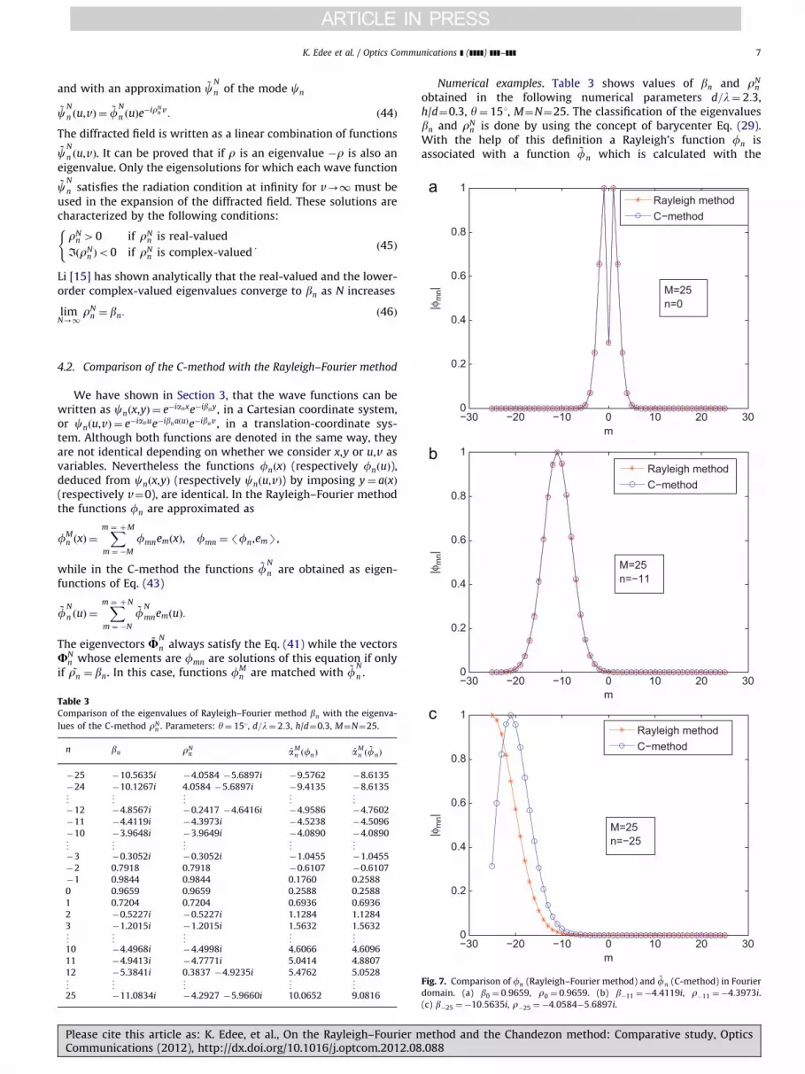
Numerical examples. Table 3 shows values of bn and rNn

obtained in the following numerical parameters d=l¼ 2:3,h/d¼0.3, y¼ 151, M¼N¼25. The classification of the eigenvaluesbn and rN

n is done by using the concept of barycenter Eq. (29).With the help of this definition a Rayleigh’s function fn isassociated with a function ~fn which is calculated with the

|φm

n|

−30 −20 −10 0 10 20 30m

−30 −20 −10 0 10 20 300

0.2

0.4

0.6

0.8

1

m

Rayleigh methodC−method

M=25n=−25

Fig. 7. Comparison of fn (Rayleigh–Fourier method) and ~fn (C-method) in Fourier

domain. (a) b0 ¼ 0:9659, r0 ¼ 0:9659. (b) b�11 ¼�4:4119i, r�11 ¼�4:3973i.

(c) b�25 ¼�10:5635i, r�25 ¼�4:0584�5:6897i.






C-method, including complex values of rNn . We remark that in the

central part of the spectrum, values of rNn are real or imaginary

and coincide with the values of bn, while the values of rNn near the

border are complex.

Fig. 7(a)–(c) represents the spectrum of the eigenfunctions fn

and ~fn in three different cases. The first case, Fig. 7(a), corre-

sponds to the zeroth diffracted order of which b0 ¼ r0 ¼ cos y.

The associated eigenfunctions are perfectly matched. The secondcase, Fig. 7(b), corresponds to an evanescent Rayleigh mode.

In this example the eigenvalue r25�11 ¼�4:3973i is still imaginary

but it is lightly different from b�11 ¼�4:4119i. Nevertheless, the

associated functions f25�11 and ~f

25

�11 are still quite close to each

other. The third example deals with a complex eigenvalue

r25�25 ¼�4:0584�5:6897i; the spectrum of functions f25

�25 and

~f25

�25 are different as it is shown in Fig. 7(c). Therefore the

corresponding Rayleigh functions are exactly those which areeliminated according to the procedure described in Section 3.2, inorder to improve the Rayleigh method. To some extent, we canconsider that in the C-method, these functions are replaced bysolutions of the eigenvalue equation (42). Numerical tests demon-strate that these functions are really suited to expand thediffracted field since they give a very fast convergence rate and

allow the C-method to be efficient for very deep grating (h=d44for a perfectly conducting sinusoidal grating [16]).

5. Conclusion

In the methods using a Rayleigh expansion for modeling thediffraction by a grating, the field on the surface is written asa finite linear combination of Rayleigh functions fn defined inEq. (15) and characterized by bn (Eq. (6)). In the Rayleigh–Fouriermethod these functions are approximated by their truncatedFourier series fM

n . This approximation can be convenient or not,depending on whether the spectrum of fn belongs to the trun-cation interval or do not. We have shown that by eliminatingsome functions fn, under one of the two criteria defined inSections 3.2 and 3.3, the Rayleigh–Fourier method can be stronglyimproved.


In the C-method the propagation equation is written in acoordinate system that reflects the shape of the surface. Thecorresponding eigenvalue matrix equation in the Fourier domainmust be truncated in order to solve this eigenproblem numeri-

cally. The eigenvectors associated to the eigenvalues rNn define the

functions ~fN

n which are used to describe the field at the surface.

If the eigenvalues rNn and bn are equal the functions fM

n and ~fN

n

are numerically identical when M¼N. While some functions fn

must be eliminated for improving the Rayleigh–Fourier method

all the functions ~fN

n must be kept in the C-method.

By studying the representation of the field on the surfacewe have given a simple explanation to the limitations of theRayleigh–Fourier method and we have proposed a scheme forimproving this method. This comparative study has also showedthat the C-method can be considered as a Fourier modal methodlike the Rayleigh–Fourier method but it is not affected by thelimitations of this one since it works correctly for deep gratingswhereas the Rayleigh–Fourier method fails.

References

[1] Lord Rayleigh, Proceedings of the Royal Society of London. Series A 79 (1907) 399.[2] J.B. Keller, Journal of the Optical Society of America A 17 (2000) 456.[3] J. Wauera, T. Rother, Optics Communications 282 (2009) 339.[4] P.M. van den Berg, Journal of the Optical Society of America 71 (1981) 1224.[5] A.G. Voronovitch, Wave Scattering from Rough Surfaces, Springer-Verlag,

1994.[6] J. Chandezon, D. Maystre, G. Cornet, Journal of Optics 11 (1980) 235.[7] E. Popov, L. Mashev, Optica Acta 33 (1986) 593.[8] L. Li, J. Chandezon, G. Granet, J.P. Plumey, Applied Optics 38 (1999) 304.[9] J.P. Hugonin, R. Petit, M. Cadilhac, Journal of the Optical Society of America 71

(1981) 593.[10] R.F. Millar, Proceedings of the Cambridge Philosophical Society 69 (1971)

217.[11] A. Wirgin, Journal of the Acoustical Society of America 68 (1980) 692.[12] S. Christiansen, R.E. Kleinman, IEEE Transactions on Antennas and Propaga-

tion 44 (1996) 1309.[13] K. Edee, B. Guizal, G. Granet, A. Moreau, Journal of the Optical Society of

America A 25 (2008) 796.[14] A.V. Tishchenko, Optics Express 17 (2009) 17102.[15] L. Li, Journal of Optics A: Pure and Applied Optics 1 (1999) 531.[16] J.-P. Plumey, G. Granet, J. Chandezon, IEEE Transactions on Antennas and

Propagation 43 (1995) 835.





Documents

On the Rayleigh–Fourier method and the Chandezon method: Comparative study