1 23

Climate DynamicsObservational, Theoretical andComputational Research on the ClimateSystem ISSN 0930-7575 Clim DynDOI 10.1007/s00382-012-1513-y

On the role of domain size and resolutionin the simulations with the HIRHAMregion climate model

Morten A. D. Larsen, Peter Thejll, JensH. Christensen, Jens C. Refsgaard &Karsten H. Jensen

1 23

Your article is protected by copyright and

all rights are held exclusively by Springer-

Verlag. This e-offprint is for personal use only

and shall not be self-archived in electronic

repositories. If you wish to self-archive your

work, please use the accepted author’s

version for posting to your own website or

your institution’s repository. You may further

deposit the accepted author’s version on a

funder’s repository at a funder’s request,

provided it is not made publicly available until

12 months after publication.

On the role of domain size and resolution in the simulationswith the HIRHAM region climate model

Morten A. D. Larsen • Peter Thejll •

Jens H. Christensen • Jens C. Refsgaard •

Karsten H. Jensen

Received: 8 March 2012 / Accepted: 27 August 2012

� Springer-Verlag 2012

Abstract We investigate the simulated temperature and

precipitation of the HIRHAM regional climate model using

systematic variations in domain size, resolution and detailed

location in a total of eight simulations. HIRHAM was

forced by ERA-Interim boundary data and the simulations

focused on higher resolutions in the range of 5.5–12 km.

HIRHAM outputs of seasonal precipitation and temperature

were assessed by calculating distributed model errors

against a higher resolution data set covering Denmark and a

0.25� resolution data set covering Europe. Furthermore the

simulations were statistically tested against the Danish data

set using bootstrap statistics. The results from the distrib-

uted validation of precipitation showed lower errors for the

winter (DJF) season compared to the spring (MAM), fall

(SON) and, in particular, summer (JJA) seasons for both

validation data sets. For temperature, the pattern was in the

opposite direction, with the lowest errors occurring for the

JJA season. These seasonal patterns between precipitation

and temperature are seen in the bootstrap analysis. It also

showed that using a 4,000 9 2,800 km simulation with an

11 km resolution produced the highest significance levels.

Also, the temperature errors were more highly significant

than precipitation. In similarly sized domains, 12 of 16

combinations of variables, observation validation data and

seasons showed better results for the highest resolution

domain, but generally the most significant improvements

were seen when varying the domain size.

Keywords HIRHAM � RCM � Climate model � Domain �Temperature � Precipitation

1 Introduction

The existing climate models developed by numerous

institutions, worldwide, are known to produce climate

outputs that differ substantially whether predicting future

scenarios (e.g. IPCC 2007) or past events (e.g. Kjellstrom

et al. 2007). Regional climate models (RCM) are employed

on a regional scale, requiring boundary data provided by

either a general circulation model simulating the global

climate system (GCM) or observed large scale data from

data assimilation systems, such as those provided by EC-

MWF or NCAR. The climate output variations arise due to

the range of included processes, model parameterization,

spatial structure, model variability and model bias and

occur in both individual GCM and RCM model simulations

and in combinations of these with the latter nested in the

former. To improve individual model outputs bias correc-

tion techniques can be used (e.g. Christensen et al. 2008;

Teutschbein and Seibert 2010; Yang et al. 2010) whereas

future scenario studies usually involve the use climate

model ensembles based on the underlying principle that the

largest outliers from single climate models are averaged

out (e.g. De Castro et al. 2007; Kendon et al. 2010).

In addition to model output variations arising from

different combinations of GCM and RCM’s, the choice of

domain characteristics for the RCM forced by a GCM or

M. A. D. Larsen (&) � K. H. Jensen

Department of Geography and Geology,

University of Copenhagen, Øster Voldgade 10,

1350 Copenhagen K, Denmark

e-mail: ml@geo.ku.dk

P. Thejll � J. H. Christensen

Danish Meteorological Institute, Lyngbyvej 100,

2100 Copenhagen, Denmark

J. C. Refsgaard

Geological Survey of Denmark and Greenland,

Øster Voldgade 10, 1350 Copenhagen, Denmark

123

Clim Dyn

DOI 10.1007/s00382-012-1513-y

Author's personal copy

reanalysis data also impacts the model results. However, no

common quantitative guidelines exist on the choice of

domain setup, although some studies have shown RCM’s

to be sensitive to GCM and RCM resolution (Denis et al.

2003; Dimitrijevic and Laprise 2005; Ikeda et al. 2010) and

to domain size (Juang and Hong 2001; Leduc and Laprise

2009). The choice of study area and the associated weather

systems, orography, model and variables in question all

effect this decision. Therefore, the task of defining the

domain setup requires expert knowledge based on previous

model studies. As a result, ensemble studies comparing

RCM and GCM combination outputs such as the

ENSEMBLES (Van der Linden and Mitchell 2009),

PRUDENCE (Christensen et al. 2002) or NARCCAP

(Mearns et al. 2009) projects are all based on a common set

of simulation characteristics, including a specified domain

configuration.

Ikeda et al. (2010) analyzed RCM output sensitivity to

model resolution and showed that improvements were

obtained in the WRF regional climate model performance of

snow modelling over a mountainous region in the central

North America for decreasing resolution in steps of 36, 18

and 6 km, while no improvement was gained from 6 to 2 km

resolution. Pryor et al. (2012) similarly showed improve-

ments in the wind power spectra in steps from 50, 25 and

12.5 km with a reduced improvement when using 6.25 km

resolution. On the other hand, a study by Roosmalen et al.

(2010) showed no major differences between HIRHAM

version 4 simulation results in resolutions of 12, 25 and

50 km. Giorgi and Marinucci (1996) and Brasseur et al.

(2002) demonstrated the improved ability of higher resolu-

tion models to reproduce orographic precipitation and Li

et al. (2011) showed improved predictions of precipitation

extremes with higher resolution. The resolution ratio

between the RCM and the lateral boundary conditions (LBC)

also has been shown to have an upper limit. Denis et al.

(2003) showed the upper ratio limit to be 12 for a 45 km

RCM in Eastern North America and Antic et al. (2006)

showed considerable improvements in a Western North

America domain by moving from a ratio of 12 to 6 but less

improvement was evident going from a ratio of 6 to 1.

An increase in the influence of boundary conditions on

nested RCM simulations is seen with smaller domain sizes:

Larger scale patterns need a certain distance to depict

smaller scale variations in topography and surface type as

shown in Leduc and Laprise (2009). This study also

emphasized that the spatial spin-up distance needed

between the boundary and internal patterns can vary with

the nature of the atmospheric circulation and that high

quality LBC data are essential. Seth and Giorgi (1998)

investigated the influence of the domain size on RCM

simulations in the upper Mississippi basin and found better

predictions with increased proximity to the boundary.

Køltzow et al. (2011) showed a variability of up to 10 % in

daily precipitation between different sized domains in

HIRHAM RCM simulations. For the area analysed in the

present study May (2007) found that the development of

low pressure systems was mainly affected by circulations

within the RCM domain as opposed to the larger scale

patterns of the surrounding LBC. Lind and Kjellstrom

(2008) further substantiated that the majority of Scandi-

navian precipitation are derived from these low pressure

systems.

Alexandru et al. (2007) found increasing internal RCM

variability with domain size and further suggested that

areas of convective precipitation can have the highest

degree of variability. Along the same lines, Caya and Biner

(2004) showed that the highest variability occurred during

the summer season. Also, Giorgi and Bi (2000), Rinke

et al. (2004) and Rapaic et al. (2010) showed internal

variability from RCM simulations to have a high influence

on the synoptic situation.

The nature and quality of the observational validation

data in terms of station density, precipitation gauge under-

catch correction, and interpolation procedure is of outmost

importance when assessing the performance of climate

models (Achberger et al. 2003), as effects of smoothing

otherwise can be the consequence (Hofstra et al. 2010).

With this study the intent was to give insight to the

impact of domain characteristics on simulation outcomes

using the HIRHAM regional climate model. Also, being a

part of a research project involving a dynamic coupling

between the HIRHAM RCM (Christensen et al. 2007) and

the MIKE SHE hydrological model (Graham and Butts

2006), it is of importance to identify the optimal domain.

Since the coupling will require an immense computation

capacity, it is important to assess if threshold values in

domain size and resolution can be identified for which no

added accuracy is gained. Particularly, we examined the

quality of precipitation and temperature output on a sea-

sonal basis from the HIRHAM model using ERA-Interim

boundary observation data (Uppala et al. 2008) for sys-

tematically varying grid resolution, domain size and

placement of interest area within the domain. A total of

eight model setups were investigated for combinations of

resolutions between 5.5 and 12 km and domain sizes

between 1,350 9 1,350 km and 5,500 9 5,200 km. The

validation was carried out against both station data and

gridded data.

2 Methodology

The analyses in the present study were all performed on

seasonal sums for precipitation and seasonal means for

temperature.

M. A. D. Larsen et al.

123

Author's personal copy

2.1 HIRHAM simulations

The regional climate model HIRHAM version 5 (Chris-

tensen et al. 2007) was used in this study and it was driven

at the boundary by ERA-Interim data for the period 1/1-

2008 to 30/4-2010. The simulations were all initialized

using similar conditions with a common starting date, no

spin-up period prior to the evaluation period and no spec-

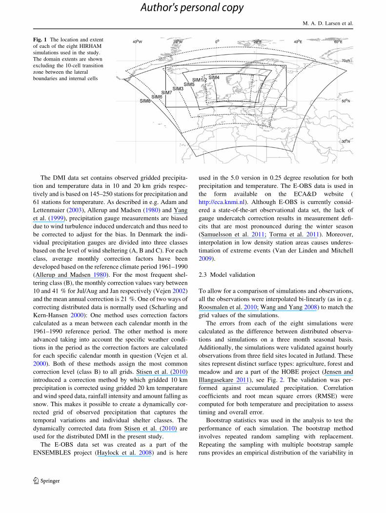
tral nudging. Model characteristics were varied, as shown

in Table 1 and Fig. 1, over eight different simulations. In

all the simulations but one (SIM4) the area of interest,

Denmark, was placed with equal distances to the bound-

aries in latitudinal direction and with an offset in longitu-

dinal direction of approximately 60 % to the west. This

approach was chosen because the prevailing winds and the

majority of the weather systems also originate from the

west.

A systematic approach was used in setting up the eight

simulations. SIM1 has a resolution of approximately

5.5 km (0.05�) and an extent of 1,400 9 1,400 km. SIM2

has a coarser resolution of approximately 11 km (0.1�) and

the approximate same extent of 1,350 9 1,350 km. The

extent of SIM3 is twice that of SIM1 and SIM2 with the

same resolution as SIM2. SIM4 has the same extent and

resolution as SIM1, but is shifted compared to the other

domains such that approximately 60 % of the model

domain is east of Denmark. SIM5 has 5.5 km resolution

and an extent of 2,000 9 2,000 km (maximum size due to

the constraint of 362 cells). SIM6 has a resolution of 11 km

and the maximum of 362 cells; SIM7 has a resolution of

11 km and an extent of 4,000 9 2,800 km which is similar

to a model used in the parallel on-going CRES project

(CRES 2012), while SIM8 has 12 km resolution and a

5,500 9 5,200 km model domain using the reinitialization

method also referred to as the poor man’s reanalysis. The

reinitialization is a method creating dynamics close to the

boundary conditions and producing lower errors (Berg and

Christensen 2008; Stahl et al. 2011; Lucas-Picher et al.

2012). This is done by initializing at 18 UTC on day 1 and

then running until 00 UTC on day 2 saving the atmospheric

conditions. The model is then reinitialized at 18 UTC on

day 2, repeating this pattern throughout the simulation. At

00 UTC the saved atmospheric conditions are joined with

the surface conditions. All domains have rotated grids,

except SIM7, which has a regular grid due to forcings from

the CRES project and they are all set up for equal

dimensions in both the longitudinal and latitudinal

direction.

2.2 Meteorological data

The area of interest for the current study is Denmark

(excluding the island of Bornholm and several smaller

islands) having a longitude/latitude extent of approxi-

mately 350 9 350 km with numerous sounds and channels

and a land area of approximately 43,000 km2. The Jutland

peninsula to the west comprises the largest area bounded to

the east by the Islands of Zealand and Funen. The topog-

raphy can be characterized as flat with an average altitude

of approximately 30 m and a maximum of approximately

170 m. Westerly winds dominate the climate. The mean

annual measured precipitation from the latest reference

climate period 1961–1990 is 712 mm that vary between

850 and 580 mm (Frich et al. 1997) and maxima located in

central Jutland, consistent with the local topography. The

corresponding yearly mean daily temperature is 7.9 �C,

with regional variations between 7.2 and 8.4 �C (Laursen

et al. 1999). More recent data show mean annual values of

765 mm and 8.7 �C respectively for the 2001–2010 period

(Cappelen and Jørgensen 2011).

Two distributed observation data sets were used for

validation in this study: A national high resolution data set

covering Denmark derived from The Danish Meteorolog-

ical Institute (DMI) (Scharling 1999a; Scharling 1999b)

and the E-OBS data set covering Europe from the

ENSEMBLES project (Haylock et al. 2008).

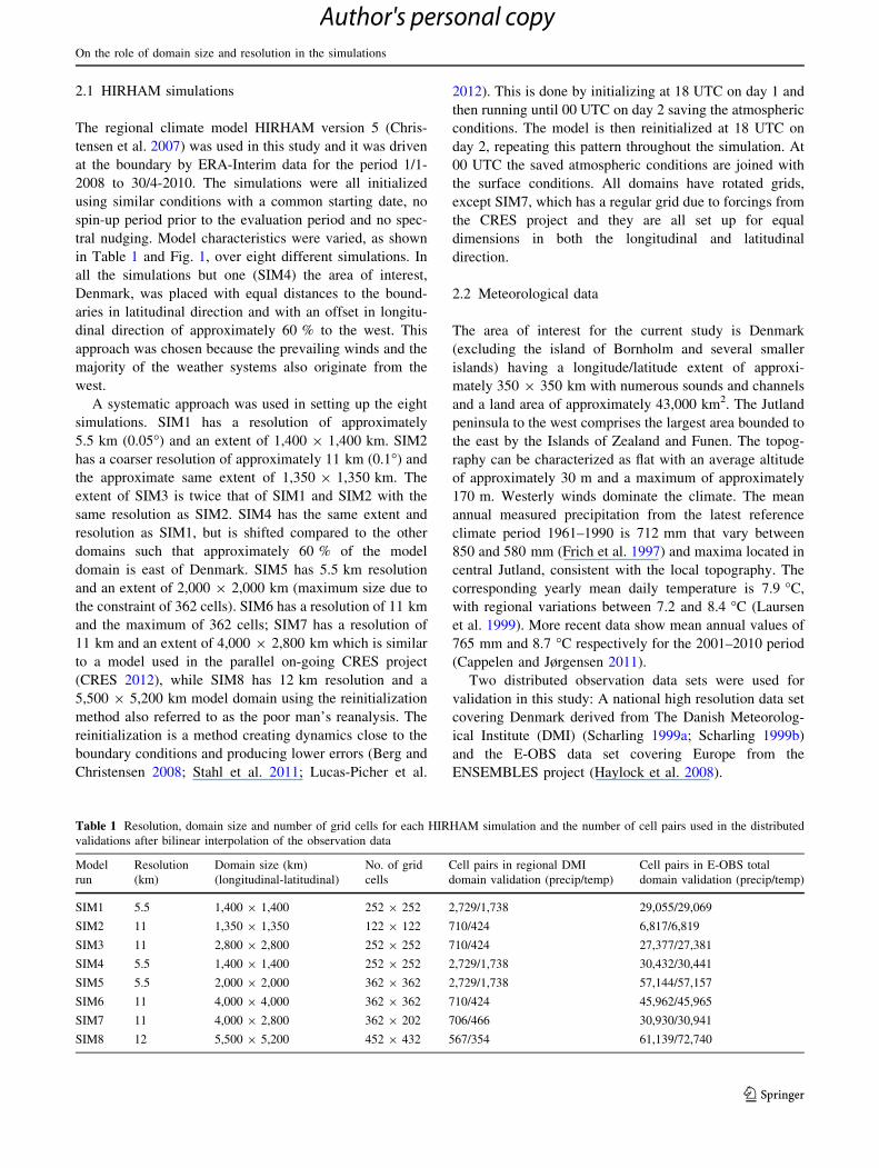
Table 1 Resolution, domain size and number of grid cells for each HIRHAM simulation and the number of cell pairs used in the distributed

validations after bilinear interpolation of the observation data

Model

run

Resolution

(km)

Domain size (km)

(longitudinal-latitudinal)

No. of grid

cells

Cell pairs in regional DMI

domain validation (precip/temp)

Cell pairs in E-OBS total

domain validation (precip/temp)

SIM1 5.5 1,400 9 1,400 252 9 252 2,729/1,738 29,055/29,069

SIM2 11 1,350 9 1,350 122 9 122 710/424 6,817/6,819

SIM3 11 2,800 9 2,800 252 9 252 710/424 27,377/27,381

SIM4 5.5 1,400 9 1,400 252 9 252 2,729/1,738 30,432/30,441

SIM5 5.5 2,000 9 2,000 362 9 362 2,729/1,738 57,144/57,157

SIM6 11 4,000 9 4,000 362 9 362 710/424 45,962/45,965

SIM7 11 4,000 9 2,800 362 9 202 706/466 30,930/30,941

SIM8 12 5,500 9 5,200 452 9 432 567/354 61,139/72,740

On the role of domain size and resolution in the simulations

123

Author's personal copy

The DMI data set contains observed gridded precipita-

tion and temperature data in 10 and 20 km grids respec-

tively and is based on 145–250 stations for precipitation and

61 stations for temperature. As described in e.g. Adam and

Lettenmaier (2003), Allerup and Madsen (1980) and Yang

et al. (1999), precipitation gauge measurements are biased

due to wind turbulence induced undercatch and thus need to

be corrected to adjust for the bias. In Denmark the indi-

vidual precipitation gauges are divided into three classes

based on the level of wind sheltering (A, B and C). For each

class, average monthly correction factors have been

developed based on the reference climate period 1961–1990

(Allerup and Madsen 1980). For the most frequent shel-

tering class (B), the monthly correction values vary between

10 and 41 % for Jul/Aug and Jan respectively (Vejen 2002)

and the mean annual correction is 21 %. One of two ways of

correcting distributed data is normally used (Scharling and

Kern-Hansen 2000): One method uses correction factors

calculated as a mean between each calendar month in the

1961–1990 reference period. The other method is more

advanced taking into account the specific weather condi-

tions in the period as the correction factors are calculated

for each specific calendar month in question (Vejen et al.

2000). Both of these methods assign the most common

correction level (class B) to all grids. Stisen et al. (2010)

introduced a correction method by which gridded 10 km

precipitation is corrected using gridded 20 km temperature

and wind speed data, rainfall intensity and amount falling as

snow. This makes it possible to create a dynamically cor-

rected grid of observed precipitation that captures the

temporal variations and individual shelter classes. The

dynamically corrected data from Stisen et al. (2010) are

used for the distributed DMI in the present study.

The E-OBS data set was created as a part of the

ENSEMBLES project (Haylock et al. 2008) and is here

used in the 5.0 version in 0.25 degree resolution for both

precipitation and temperature. The E-OBS data is used in

the form available on the ECA&D website (

http://eca.knmi.nl). Although E-OBS is currently consid-

ered a state-of-the-art observational data set, the lack of

gauge undercatch correction results in measurement defi-

cits that are most pronounced during the winter season

(Samuelsson et al. 2011; Torma et al. 2011). Moreover,

interpolation in low density station areas causes underes-

timation of extreme events (Van der Linden and Mitchell

2009).

2.3 Model validation

To allow for a comparison of simulations and observations,

all the observations were interpolated bi-linearly (as in e.g.

Roosmalen et al. 2010; Wang and Yang 2008) to match the

grid values of the simulations.

The errors from each of the eight simulations were

calculated as the difference between distributed observa-

tions and simulations on a three month seasonal basis.

Additionally, the simulations were validated against hourly

observations from three field sites located in Jutland. These

sites represent distinct surface types: agriculture, forest and

meadow and are a part of the HOBE project (Jensen and

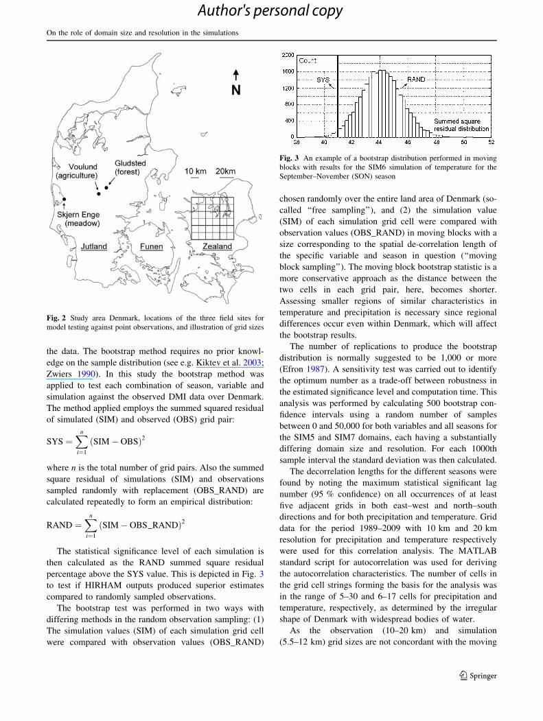
Illangasekare 2011), see Fig. 2. The validation was per-

formed against accumulated precipitation. Correlation

coefficients and root mean square errors (RMSE) were

computed for both temperature and precipitation to assess

timing and overall error.

Bootstrap statistics was used in the analysis to test the

performance of each simulation. The bootstrap method

involves repeated random sampling with replacement.

Repeating the sampling with multiple bootstrap sample

runs provides an empirical distribution of the variability in

Fig. 1 The location and extent

of each of the eight HIRHAM

simulations used in the study.

The domain extents are shown

excluding the 10-cell transition

zone between the lateral

boundaries and internal cells

M. A. D. Larsen et al.

123

Author's personal copy

the data. The bootstrap method requires no prior knowl-

edge on the sample distribution (see e.g. Kiktev et al. 2003;

Zwiers 1990). In this study the bootstrap method was

applied to test each combination of season, variable and

simulation against the observed DMI data over Denmark.

The method applied employs the summed squared residual

of simulated (SIM) and observed (OBS) grid pair:

SYS ¼Xn

i¼1

ðSIM� OBSÞ2

where n is the total number of grid pairs. Also the summed

square residual of simulations (SIM) and observations

sampled randomly with replacement (OBS_RAND) are

calculated repeatedly to form an empirical distribution:

RAND ¼Xn

i¼1

ðSIM� OBS RANDÞ2

The statistical significance level of each simulation is

then calculated as the RAND summed square residual

percentage above the SYS value. This is depicted in Fig. 3

to test if HIRHAM outputs produced superior estimates

compared to randomly sampled observations.

The bootstrap test was performed in two ways with

differing methods in the random observation sampling: (1)

The simulation values (SIM) of each simulation grid cell

were compared with observation values (OBS_RAND)

chosen randomly over the entire land area of Denmark (so-

called ‘‘free sampling’’), and (2) the simulation value

(SIM) of each simulation grid cell were compared with

observation values (OBS_RAND) in moving blocks with a

size corresponding to the spatial de-correlation length of

the specific variable and season in question (‘‘moving

block sampling’’). The moving block bootstrap statistic is a

more conservative approach as the distance between the

two cells in each grid pair, here, becomes shorter.

Assessing smaller regions of similar characteristics in

temperature and precipitation is necessary since regional

differences occur even within Denmark, which will affect

the bootstrap results.

The number of replications to produce the bootstrap

distribution is normally suggested to be 1,000 or more

(Efron 1987). A sensitivity test was carried out to identify

the optimum number as a trade-off between robustness in

the estimated significance level and computation time. This

analysis was performed by calculating 500 bootstrap con-

fidence intervals using a random number of samples

between 0 and 50,000 for both variables and all seasons for

the SIM5 and SIM7 domains, each having a substantially

differing domain size and resolution. For each 1000th

sample interval the standard deviation was then calculated.

The decorrelation lengths for the different seasons were

found by noting the maximum statistical significant lag

number (95 % confidence) on all occurrences of at least

five adjacent grids in both east–west and north–south

directions and for both precipitation and temperature. Grid

data for the period 1989–2009 with 10 km and 20 km

resolution for precipitation and temperature respectively

were used for this correlation analysis. The MATLAB

standard script for autocorrelation was used for deriving

the autocorrelation characteristics. The number of cells in

the grid cell strings forming the basis for the analysis was

in the range of 5–30 and 6–17 cells for precipitation and

temperature, respectively, as determined by the irregular

shape of Denmark with widespread bodies of water.

As the observation (10–20 km) and simulation

(5.5–12 km) grid sizes are not concordant with the moving

Fig. 2 Study area Denmark, locations of the three field sites for

model testing against point observations, and illustration of grid sizes

Fig. 3 An example of a bootstrap distribution performed in moving

blocks with results for the SIM6 simulation of temperature for the

September–November (SON) season

On the role of domain size and resolution in the simulations

123

Author's personal copy

block, bootstrap was performed in block sizes with

dimensions being closest to the decorrelation lengths.

To assess the ability of the different sized domains to

represent atmospheric circulation patterns the movement of

low pressures was investigated for all simulations. This

was done by finding the minimum mean sea level pressure

within the shared domain of all simulations on an hourly

basis for 2008 and plotting these. Further, the total number

of simulated low pressure occurrences within the domain

and the maximum and mean low pressure travel times were

calculated, together with the temporal occurrence of these

for each simulation.

3 Results

3.1 Decorrelation lengths

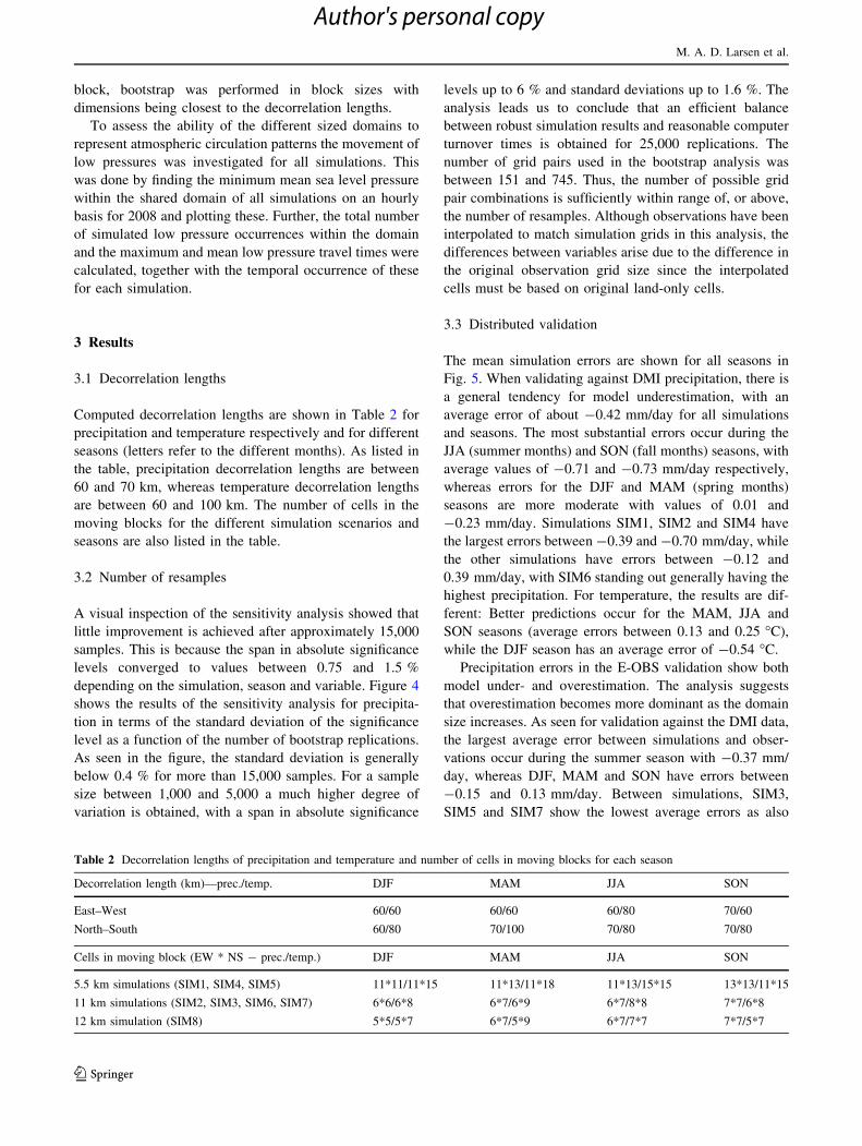
Computed decorrelation lengths are shown in Table 2 for

precipitation and temperature respectively and for different

seasons (letters refer to the different months). As listed in

the table, precipitation decorrelation lengths are between

60 and 70 km, whereas temperature decorrelation lengths

are between 60 and 100 km. The number of cells in the

moving blocks for the different simulation scenarios and

seasons are also listed in the table.

3.2 Number of resamples

A visual inspection of the sensitivity analysis showed that

little improvement is achieved after approximately 15,000

samples. This is because the span in absolute significance

levels converged to values between 0.75 and 1.5 %

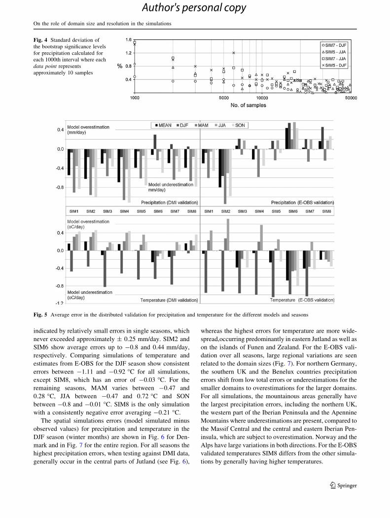
depending on the simulation, season and variable. Figure 4

shows the results of the sensitivity analysis for precipita-

tion in terms of the standard deviation of the significance

level as a function of the number of bootstrap replications.

As seen in the figure, the standard deviation is generally

below 0.4 % for more than 15,000 samples. For a sample

size between 1,000 and 5,000 a much higher degree of

variation is obtained, with a span in absolute significance

levels up to 6 % and standard deviations up to 1.6 %. The

analysis leads us to conclude that an efficient balance

between robust simulation results and reasonable computer

turnover times is obtained for 25,000 replications. The

number of grid pairs used in the bootstrap analysis was

between 151 and 745. Thus, the number of possible grid

pair combinations is sufficiently within range of, or above,

the number of resamples. Although observations have been

interpolated to match simulation grids in this analysis, the

differences between variables arise due to the difference in

the original observation grid size since the interpolated

cells must be based on original land-only cells.

3.3 Distributed validation

The mean simulation errors are shown for all seasons in

Fig. 5. When validating against DMI precipitation, there is

a general tendency for model underestimation, with an

average error of about -0.42 mm/day for all simulations

and seasons. The most substantial errors occur during the

JJA (summer months) and SON (fall months) seasons, with

average values of -0.71 and -0.73 mm/day respectively,

whereas errors for the DJF and MAM (spring months)

seasons are more moderate with values of 0.01 and

-0.23 mm/day. Simulations SIM1, SIM2 and SIM4 have

the largest errors between -0.39 and -0.70 mm/day, while

the other simulations have errors between -0.12 and

0.39 mm/day, with SIM6 standing out generally having the

highest precipitation. For temperature, the results are dif-

ferent: Better predictions occur for the MAM, JJA and

SON seasons (average errors between 0.13 and 0.25 �C),

while the DJF season has an average error of -0.54 �C.

Precipitation errors in the E-OBS validation show both

model under- and overestimation. The analysis suggests

that overestimation becomes more dominant as the domain

size increases. As seen for validation against the DMI data,

the largest average error between simulations and obser-

vations occur during the summer season with -0.37 mm/

day, whereas DJF, MAM and SON have errors between

-0.15 and 0.13 mm/day. Between simulations, SIM3,

SIM5 and SIM7 show the lowest average errors as also

Table 2 Decorrelation lengths of precipitation and temperature and number of cells in moving blocks for each season

Decorrelation length (km)—prec./temp. DJF MAM JJA SON

East–West 60/60 60/60 60/80 70/60

North–South 60/80 70/100 70/80 70/80

Cells in moving block (EW * NS - prec./temp.) DJF MAM JJA SON

5.5 km simulations (SIM1, SIM4, SIM5) 11*11/11*15 11*13/11*18 11*13/15*15 13*13/11*15

11 km simulations (SIM2, SIM3, SIM6, SIM7) 6*6/6*8 6*7/6*9 6*7/8*8 7*7/6*8

12 km simulation (SIM8) 5*5/5*7 6*7/5*9 6*7/7*7 7*7/5*7

M. A. D. Larsen et al.

123

Author's personal copy

indicated by relatively small errors in single seasons, which

never exceeded approximately ± 0.25 mm/day. SIM2 and

SIM6 show average errors up to -0.8 and 0.44 mm/day,

respectively. Comparing simulations of temperature and

estimates from E-OBS for the DJF season show consistent

errors between -1.11 and -0.92 �C for all simulations,

except SIM8, which has an error of -0.03 �C. For the

remaining seasons, MAM varies between -0.47 and

0.28 �C, JJA between -0.47 and 0.72 �C and SON

between -0.8 and -0.01 �C. SIM8 is the only simulation

with a consistently negative error averaging -0.21 �C.

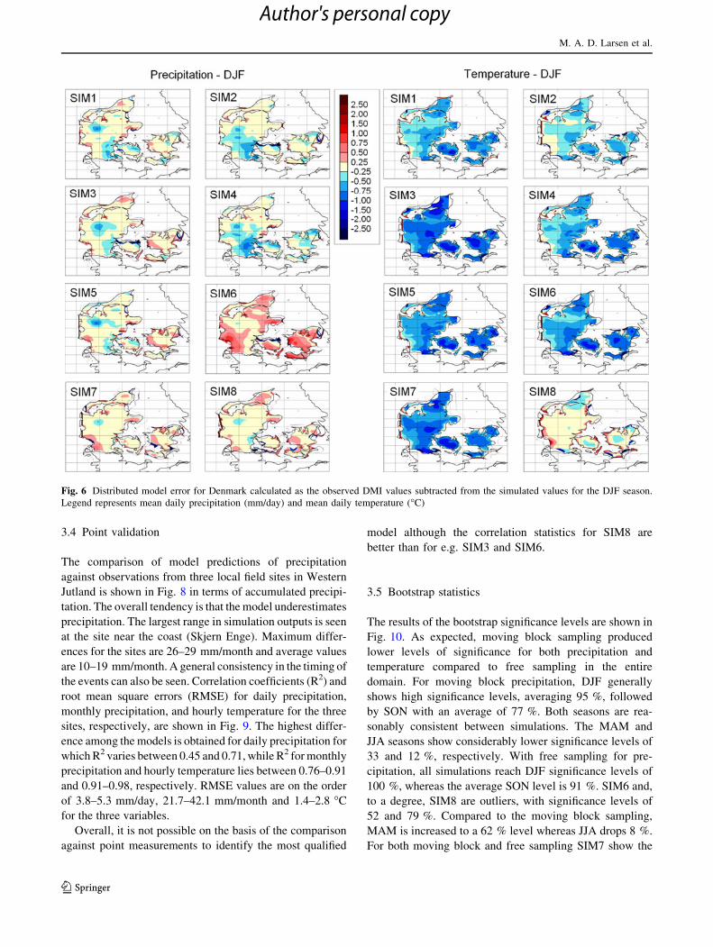
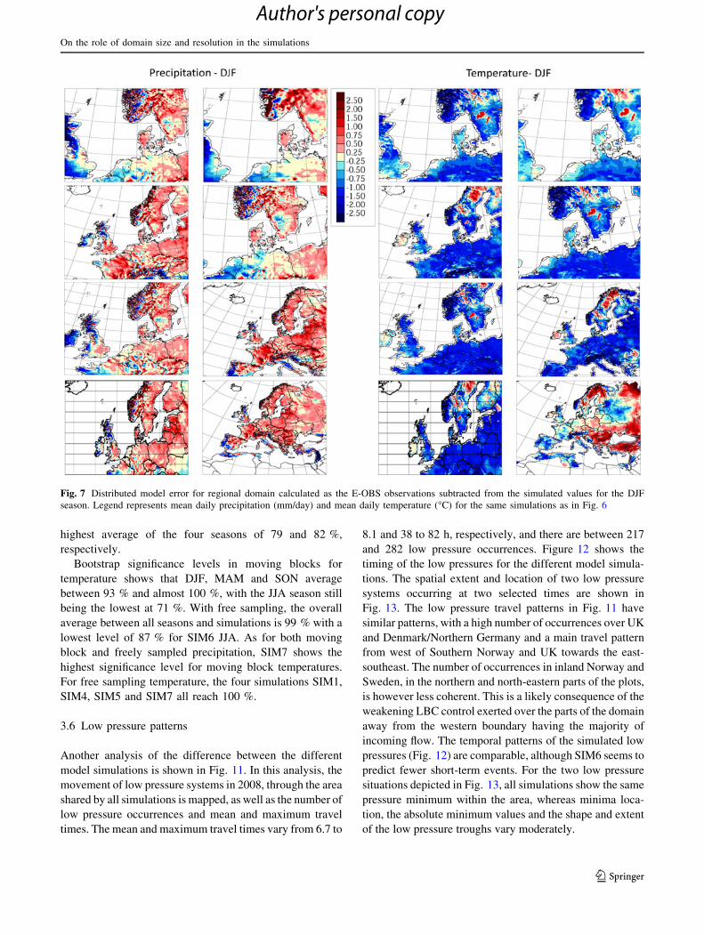
The spatial simulations errors (model simulated minus

observed values) for precipitation and temperature in the

DJF season (winter months) are shown in Fig. 6 for Den-

mark and in Fig. 7 for the entire region. For all seasons the

highest precipitation errors, when testing against DMI data,

generally occur in the central parts of Jutland (see Fig. 6),

whereas the highest errors for temperature are more wide-

spread,occurring predominantly in eastern Jutland as well as

on the islands of Funen and Zealand. For the E-OBS vali-

dation over all seasons, large regional variations are seen

related to the domain sizes (Fig. 7). For northern Germany,

the southern UK and the Benelux countries precipitation

errors shift from low total errors or underestimations for the

smaller domains to overestimations for the larger domains.

For all simulations, the mountainous areas generally have

the largest precipitation errors, including the northern UK,

the western part of the Iberian Peninsula and the Apennine

Mountains where underestimations are present, compared to

the Massif Central and the central and eastern Iberian Pen-

insula, which are subject to overestimation. Norway and the

Alps have large variations in both directions. For the E-OBS

validated temperatures SIM8 differs from the other simula-

tions by generally having higher temperatures.

Fig. 4 Standard deviation of

the bootstrap significance levels

for precipitation calculated for

each 1000th interval where each

data point represents

approximately 10 samples

Fig. 5 Average error in the distributed validation for precipitation and temperature for the different models and seasons

On the role of domain size and resolution in the simulations

123

Author's personal copy

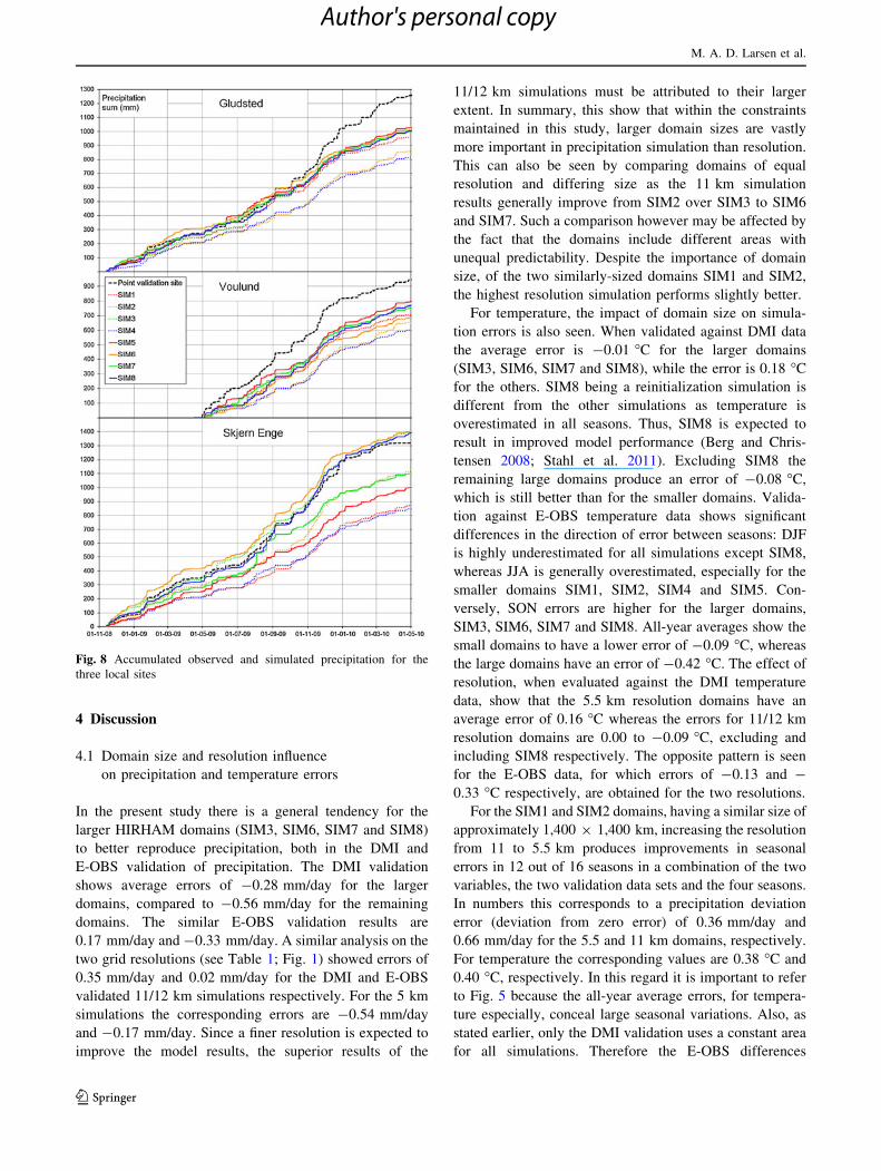
3.4 Point validation

The comparison of model predictions of precipitation

against observations from three local field sites in Western

Jutland is shown in Fig. 8 in terms of accumulated precipi-

tation. The overall tendency is that the model underestimates

precipitation. The largest range in simulation outputs is seen

at the site near the coast (Skjern Enge). Maximum differ-

ences for the sites are 26–29 mm/month and average values

are 10–19 mm/month. A general consistency in the timing of

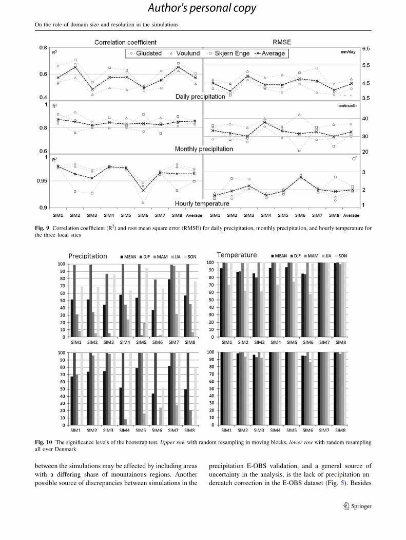
the events can also be seen. Correlation coefficients (R2) and

root mean square errors (RMSE) for daily precipitation,

monthly precipitation, and hourly temperature for the three

sites, respectively, are shown in Fig. 9. The highest differ-

ence among the models is obtained for daily precipitation for

which R2 varies between 0.45 and 0.71, while R2 for monthly

precipitation and hourly temperature lies between 0.76–0.91

and 0.91–0.98, respectively. RMSE values are on the order

of 3.8–5.3 mm/day, 21.7–42.1 mm/month and 1.4–2.8 �C

for the three variables.

Overall, it is not possible on the basis of the comparison

against point measurements to identify the most qualified

model although the correlation statistics for SIM8 are

better than for e.g. SIM3 and SIM6.

3.5 Bootstrap statistics

The results of the bootstrap significance levels are shown in

Fig. 10. As expected, moving block sampling produced

lower levels of significance for both precipitation and

temperature compared to free sampling in the entire

domain. For moving block precipitation, DJF generally

shows high significance levels, averaging 95 %, followed

by SON with an average of 77 %. Both seasons are rea-

sonably consistent between simulations. The MAM and

JJA seasons show considerably lower significance levels of

33 and 12 %, respectively. With free sampling for pre-

cipitation, all simulations reach DJF significance levels of

100 %, whereas the average SON level is 91 %. SIM6 and,

to a degree, SIM8 are outliers, with significance levels of

52 and 79 %. Compared to the moving block sampling,

MAM is increased to a 62 % level whereas JJA drops 8 %.

For both moving block and free sampling SIM7 show the

Fig. 6 Distributed model error for Denmark calculated as the observed DMI values subtracted from the simulated values for the DJF season.

Legend represents mean daily precipitation (mm/day) and mean daily temperature (�C)

M. A. D. Larsen et al.

123

Author's personal copy

highest average of the four seasons of 79 and 82 %,

respectively.

Bootstrap significance levels in moving blocks for

temperature shows that DJF, MAM and SON average

between 93 % and almost 100 %, with the JJA season still

being the lowest at 71 %. With free sampling, the overall

average between all seasons and simulations is 99 % with a

lowest level of 87 % for SIM6 JJA. As for both moving

block and freely sampled precipitation, SIM7 shows the

highest significance level for moving block temperatures.

For free sampling temperature, the four simulations SIM1,

SIM4, SIM5 and SIM7 all reach 100 %.

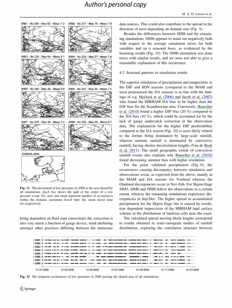
3.6 Low pressure patterns

Another analysis of the difference between the different

model simulations is shown in Fig. 11. In this analysis, the

movement of low pressure systems in 2008, through the area

shared by all simulations is mapped, as well as the number of

low pressure occurrences and mean and maximum travel

times. The mean and maximum travel times vary from 6.7 to

8.1 and 38 to 82 h, respectively, and there are between 217

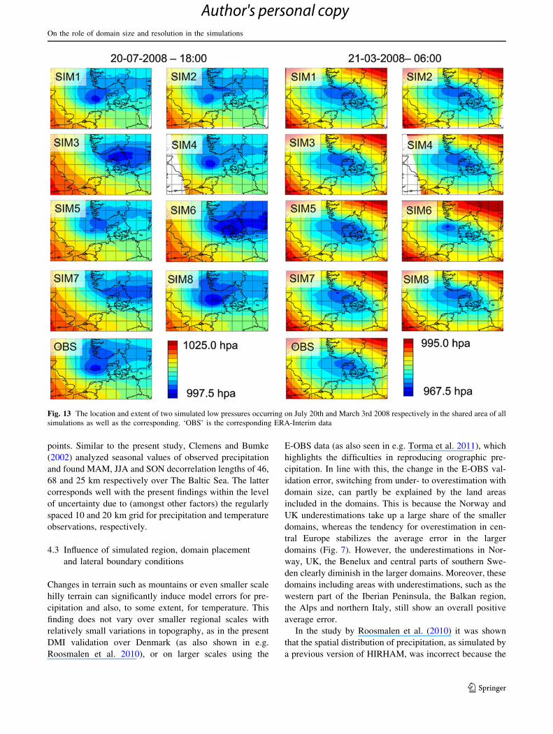
and 282 low pressure occurrences. Figure 12 shows the

timing of the low pressures for the different model simula-

tions. The spatial extent and location of two low pressure

systems occurring at two selected times are shown in

Fig. 13. The low pressure travel patterns in Fig. 11 have

similar patterns, with a high number of occurrences over UK

and Denmark/Northern Germany and a main travel pattern

from west of Southern Norway and UK towards the east-

southeast. The number of occurrences in inland Norway and

Sweden, in the northern and north-eastern parts of the plots,

is however less coherent. This is a likely consequence of the

weakening LBC control exerted over the parts of the domain

away from the western boundary having the majority of

incoming flow. The temporal patterns of the simulated low

pressures (Fig. 12) are comparable, although SIM6 seems to

predict fewer short-term events. For the two low pressure

situations depicted in Fig. 13, all simulations show the same

pressure minimum within the area, whereas minima loca-

tion, the absolute minimum values and the shape and extent

of the low pressure troughs vary moderately.

Fig. 7 Distributed model error for regional domain calculated as the E-OBS observations subtracted from the simulated values for the DJF

season. Legend represents mean daily precipitation (mm/day) and mean daily temperature (�C) for the same simulations as in Fig. 6

On the role of domain size and resolution in the simulations

123

Author's personal copy

4 Discussion

4.1 Domain size and resolution influence

on precipitation and temperature errors

In the present study there is a general tendency for the

larger HIRHAM domains (SIM3, SIM6, SIM7 and SIM8)

to better reproduce precipitation, both in the DMI and

E-OBS validation of precipitation. The DMI validation

shows average errors of -0.28 mm/day for the larger

domains, compared to -0.56 mm/day for the remaining

domains. The similar E-OBS validation results are

0.17 mm/day and -0.33 mm/day. A similar analysis on the

two grid resolutions (see Table 1; Fig. 1) showed errors of

0.35 mm/day and 0.02 mm/day for the DMI and E-OBS

validated 11/12 km simulations respectively. For the 5 km

simulations the corresponding errors are -0.54 mm/day

and -0.17 mm/day. Since a finer resolution is expected to

improve the model results, the superior results of the

11/12 km simulations must be attributed to their larger

extent. In summary, this show that within the constraints

maintained in this study, larger domain sizes are vastly

more important in precipitation simulation than resolution.

This can also be seen by comparing domains of equal

resolution and differing size as the 11 km simulation

results generally improve from SIM2 over SIM3 to SIM6

and SIM7. Such a comparison however may be affected by

the fact that the domains include different areas with

unequal predictability. Despite the importance of domain

size, of the two similarly-sized domains SIM1 and SIM2,

the highest resolution simulation performs slightly better.

For temperature, the impact of domain size on simula-

tion errors is also seen. When validated against DMI data

the average error is -0.01 �C for the larger domains

(SIM3, SIM6, SIM7 and SIM8), while the error is 0.18 �C

for the others. SIM8 being a reinitialization simulation is

different from the other simulations as temperature is

overestimated in all seasons. Thus, SIM8 is expected to

result in improved model performance (Berg and Chris-

tensen 2008; Stahl et al. 2011). Excluding SIM8 the

remaining large domains produce an error of -0.08 �C,

which is still better than for the smaller domains. Valida-

tion against E-OBS temperature data shows significant

differences in the direction of error between seasons: DJF

is highly underestimated for all simulations except SIM8,

whereas JJA is generally overestimated, especially for the

smaller domains SIM1, SIM2, SIM4 and SIM5. Con-

versely, SON errors are higher for the larger domains,

SIM3, SIM6, SIM7 and SIM8. All-year averages show the

small domains to have a lower error of -0.09 �C, whereas

the large domains have an error of -0.42 �C. The effect of

resolution, when evaluated against the DMI temperature

data, show that the 5.5 km resolution domains have an

average error of 0.16 �C whereas the errors for 11/12 km

resolution domains are 0.00 to -0.09 �C, excluding and

including SIM8 respectively. The opposite pattern is seen

for the E-OBS data, for which errors of -0.13 and -

0.33 �C respectively, are obtained for the two resolutions.

For the SIM1 and SIM2 domains, having a similar size of

approximately 1,400 9 1,400 km, increasing the resolution

from 11 to 5.5 km produces improvements in seasonal

errors in 12 out of 16 seasons in a combination of the two

variables, the two validation data sets and the four seasons.

In numbers this corresponds to a precipitation deviation

error (deviation from zero error) of 0.36 mm/day and

0.66 mm/day for the 5.5 and 11 km domains, respectively.

For temperature the corresponding values are 0.38 �C and

0.40 �C, respectively. In this regard it is important to refer

to Fig. 5 because the all-year average errors, for tempera-

ture especially, conceal large seasonal variations. Also, as

stated earlier, only the DMI validation uses a constant area

for all simulations. Therefore the E-OBS differences

Fig. 8 Accumulated observed and simulated precipitation for the

three local sites

M. A. D. Larsen et al.

123

Author's personal copy

between the simulations may be affected by including areas

with a differing share of mountainous regions. Another

possible source of discrepancies between simulations in the

precipitation E-OBS validation, and a general source of

uncertainty in the analysis, is the lack of precipitation un-

dercatch correction in the E-OBS dataset (Fig. 5). Besides

Fig. 9 Correlation coefficient (R2) and root mean square error (RMSE) for daily precipitation, monthly precipitation, and hourly temperature for

the three local sites

Fig. 10 The significance levels of the bootstrap test. Upper row with random resampling in moving blocks, lower row with random resampling

all over Denmark

On the role of domain size and resolution in the simulations

123

Author's personal copy

being dependent on fluid state (snow/rain) the correction is

also very much a function of gauge device, wind sheltering

amongst other practices differing between the numerous

data sources. This could also contribute to the spread in the

direction of error depending on domain size (Fig. 5).

Besides the differences between SIM8 and the remain-

ing simulations, SIM6 appears to stand out negatively both

with respect to the average simulation errors for both

variables and on a seasonal basis, as evidenced by the

bootstrap results (Fig. 10). The SIM6 simulation was done

twice with similar results, and we were not able to give a

reasonable explanation of this occurrence.

4.2 Seasonal patterns in simulation results

The superior simulation of precipitation and temperature in

the DJF and SON seasons (compared to the MAM and

most pronounced the JJA season) is in line with the find-

ings of e.g. Haylock et al. (2006) and Jacob et al. (2007)

who found the HIRHAM JJA bias to be higher than the

DJF bias for the Scandinavian area. Conversely, Rauscher

et al. (2010) found a higher DJF bias (20 %) compared to

the JJA bias (10 %), which could be accounted for by the

lack of gauge undercatch correction in the observation

data. The explanation for the higher DJF predictability

compared to the JJA season (Fig. 10) is most likely related

to the former being dominated by large-scale rainfall,

whereas summer rainfall is dominated by convective

rainfall, having shorter decorrelation lengths (Van de Beek

et al. 2011). The small geographic extent of convective

rainfall events also explains why Rauscher et al. (2010)

found decreasing summer bias with higher resolution.

For the point validated precipitation (Fig. 8), the

occurrences causing discrepancy between simulation and

observations occur, as expected from the above, mainly in

the MAM and JJA seasons for Voulund whereas the

Gludsted discrepancies occur in Nov-Feb. For Skjern Enge

SIM3, SIM6 and SIM8 follow the observations to a certain

extent, whereas the remaining simulations experience dis-

crepancies in Sep-Dec. The higher spread in accumulated

precipitation for the Skjern Enge site is caused by resolu-

tion dependent imprecision of the HIRHAM land surface

scheme in the distribution of land/sea cells near the coast.

The calculated spatial moving block lengths correspond

to results obtained in semi-variogram studies of rainfall

distribution, exploring the correlation structure between

Fig. 11 The movement of low pressures in 2008 in the area shared by

all simulations. Each line shows the path of the centre of a low

pressure event. No, max and mean represent number of occurrences

within the domain, maximum travel time (h), mean travel time

(h) respectively

Fig. 12 The temporal occurrences of low pressures in 2008 passing the shared area of all simulations

M. A. D. Larsen et al.

123

Author's personal copy

points. Similar to the present study, Clemens and Bumke

(2002) analyzed seasonal values of observed precipitation

and found MAM, JJA and SON decorrelation lengths of 46,

68 and 25 km respectively over The Baltic Sea. The latter

corresponds well with the present findings within the level

of uncertainty due to (amongst other factors) the regularly

spaced 10 and 20 km grid for precipitation and temperature

observations, respectively.

4.3 Influence of simulated region, domain placement

and lateral boundary conditions

Changes in terrain such as mountains or even smaller scale

hilly terrain can significantly induce model errors for pre-

cipitation and also, to some extent, for temperature. This

finding does not vary over smaller regional scales with

relatively small variations in topography, as in the present

DMI validation over Denmark (as also shown in e.g.

Roosmalen et al. 2010), or on larger scales using the

E-OBS data (as also seen in e.g. Torma et al. 2011), which

highlights the difficulties in reproducing orographic pre-

cipitation. In line with this, the change in the E-OBS val-

idation error, switching from under- to overestimation with

domain size, can partly be explained by the land areas

included in the domains. This is because the Norway and

UK underestimations take up a large share of the smaller

domains, whereas the tendency for overestimation in cen-

tral Europe stabilizes the average error in the larger

domains (Fig. 7). However, the underestimations in Nor-

way, UK, the Benelux and central parts of southern Swe-

den clearly diminish in the larger domains. Moreover, these

domains including areas with underestimations, such as the

western part of the Iberian Peninsula, the Balkan region,

the Alps and northern Italy, still show an overall positive

average error.

In the study by Roosmalen et al. (2010) it was shown

that the spatial distribution of precipitation, as simulated by

a previous version of HIRHAM, was incorrect because the

Fig. 13 The location and extent of two simulated low pressures occurring on July 20th and March 3rd 2008 respectively in the shared area of all

simulations as well as the corresponding. ‘OBS’ is the corresponding ERA-Interim data

On the role of domain size and resolution in the simulations

123

Author's personal copy

maximum precipitation occurred over the North Sea and

not as expected in central Jutland. In the present study the

precipitation over Denmark shows the expected general

patterns even though inaccuracies can be introduced by

only considering a two-year period. An unexpected result

in that regard was that the SIM7 simulation produced the

best overall bootstrap significance levels across variables

and seasons, even exceeding the SIM8. Nevertheless, this

result is in line with the findings in the error analysis

showing SIM8 to be among the most accurate simulations.

The improved simulation of SIM4 compared to SIM1

having the same resolution and domain size but differing

placement could be related to the former having the wes-

tern LBC over the North Sea with stronger winds compared

to SIM1 having LBC over the British Isles.

The absolute biases, RMSE values and correlations coef-

ficients of the present study are superior compared to Rau-

scher et al. (2006), simulating South American domains

during El Nino and La Nina years in resolutions of 60–80 km

and also Murphy (1999). The latter found lower correlation

coefficients, simulating a European domain in approximately

50 km resolution. As in the present study, Murphy (1999)

found lower summer predictability compared to winter.

Jones et al. (1995) simulated four different sized domains

in 0.44� resolution with the two smallest of comparable size

to the largest in the present study (Europe—comparable to

SIM7/SIM8). The other two models were larger extending

to Greenland and North America. Jones showed that all

domains properly developed mesoscale features, whereas

the smallest two domains experience strong lateral bound-

ary influence in their outer edges. The comparable patterns

between simulations in the low pressure analysis in the

present study (Figs. 11, 12) indicate that the domain size in

combination with the high resolution is sufficient to

describe the RCM circulations of the simulated area of

interest. However, the extent, location and timing of low

pressure events can vary between simulations.

As described, all simulations except SIM4 and SIM8

have a 60 % extent to the west of Denmark due to the

expectation of major influences coming from this direction,

whereas SIM4 have a 60 % extent to the east otherwise

being equal to SIM1. As can be seen in the moving block

bootstrap statistics (Fig. 10) SIM4 has the best simulation

of mainly MAM and JJA precipitation compared to SIM1

possibly showing (1) that the SIM1 and SIM4 domains

experience a high degree of lateral boundary control and

(2) that much consideration must be given to the placement

of the nested domain around the area of interest.

It was beyond the scope of the present study to inves-

tigate the influence of initial conditions and starting date

although they are both known to potentially have a sub-

stantial effect on RCM outputs due to internal variability

(Elıa and Cote 2010).

5 Conclusions

In the present study we provided insight into how varia-

tions in resolution, domain size and domain placement can

affect the temperature and precipitation simulations by the

HIRHAM regional climate model.

The distributed validation of precipitation simulation

outputs against 10 km gridded DMI observation data over

Denmark generally underestimated precipitation, with an

average error of -0.42 mm/day across all simulations and

seasons, whereas the total-domain E-OBS validation

showed mixed results, both under- and overestimating

simulated precipitation compared to the observed data.

Validation in specific seasons using both precipitation

observation data sets yielded the lowest errors for the DJF

season, while the errors were considerably higher for the

JJA season. For temperature, DJF gave the highest errors

for both validation data sets. The Bootstrap statistic shows

the same seasonal pattern, with superior DJF predictions

compared to JJA and the all-season average shows SIM7

simulation run to yield the highest significance levels.

Comparing domains of a similar size of 1,400 9

1,400 km, the high-resolution domain showed improved

results in average errors in 12 of 16 seasons in combina-

tions of variable, validation data and season and especially

precipitation was improved in the high-resolution simula-

tion. A more consistent improvement in both model error

and bootstrap statistics was achieved by increasing domain

size up to 4,000 9 2,800 km and even 5,500 9 5,200 km,

whereas the good performance of the latter domain is due

to reinitialization used in the SIM8 simulation. This con-

clusion is also valid in a situation where computational

demand is in question since comparing two simulations

with an equal number of grids, but differing resolution,

turns out in favour of the larger domains.

Finally, the study shows that great consideration and

experimentation must be employed to define and select

domain characteristics using the HIRHAM model, and the

same is probably true of most, if not all, regional models.

We therefore suggest that a number of trial configurations

are tested before selecting a regional domain.

Acknowledgments The present study was funded by a grant from

the Danish Strategic Research Council for the project HYdrological

Modelling for Assessing Climate Change Impacts at differeNT Scales

(HYACINTS–www.hyacints.dk) under contract no: DSF-EnMi

2104-07-0008. We acknowledge the E-OBS dataset from the EU-FP6

project ENSEMBLES (http://ensembles-eu.metoffice.com), the data

providers in the ECA&D project (http://eca.knmi.nl), the HOBE

project (Jensen and Illangasekare 2011) and the CRES project

(http://cres-centre.net). Also we would like to thank, Simon Stisen,

Philippe Lucas-Picher, Søren Højmark Rasmussen, Ole Bøssing

Christensen, Frederik Boberg, Martin Drews, Flemming Vejen

and Michael Scharling for assistance and comments during the

process.

M. A. D. Larsen et al.

123

Author's personal copy

References

Achberger C, Linderson ML, Chen D (2003) Performance of the

Rossby Centre regional atmospheric model in Southern Sweden:

comparison of simulated and observed precipitation. Theor Appl

Climatol 76:219–234. doi:10.1007/s00704-003-0015-6

Adam JC, Lettenmaier DP (2003) Adjustment of global gridded

precipitation for systematic bias. J Geophys Res 108:D9 4257.

doi:10.1029/2002JD002499

Alexandru A, De Elıa R, Laprise R (2007) Internal variability in

regional climate downscaling at the seasonal time scale. Mon

Weather Rev 135:3221–3238. doi:10.1175/MWR3456.1

Allerup P, Madsen H (1980) Accuracy of point precipitation

measurements. Nord Hydrol 11:57–70

Antic S, Laprise R, Denis B, De Elıa R (2006) Testing the

downscaling ability of a one-way nested regional climate model

in regions of complex topography. Clim Dyn 26:305–325.

doi:10.1007/s00382-005-0046-z

Berg P, Christensen JH (2008) Poor man’s reanalysis over Europe.

WATCH Technical 5 Report No. 2

Brasseur O, Gallee H, Creutin JD, Lebel T, Marbaix P (2002) High

resolution simulations of precipitation over the Alps with the

perspective of coupling to hydrological models. Climatic

change: implications for the hydrological cycle and for water

management. Adv Global Chang Res 10:75–99

Cappelen J, Jørgensen BV (2011) Dansk vejr siden 1874—maned for

maned med temperatur, nedbør og soltimer samt beskrivelser af

vejret—with English translations (Danish Weather since 1874—

month by month with Temperature, Precipitation and Hours of

Sun Light and Weather Descriptions—with English Transla-

tions). Danish Meteorological Institute Technical Report 11-02

Caya D, Biner S (2004) Internal variability of RCM simulations over an

annual cycle. Clim Dyn 22:33–46. doi:10.1007/s00382-003-0360-2

Christensen JH, Carter TR, Giorgi F (2002) PRUDENCE employs

new methods to assess European climate change. EOS 83:147.

doi:10.1029/2002EO000094

Christensen OB, Drews M, Christensen JH, Dethloff K, Ketelsen K,

Hebestadt I, Rinke A (2007) The HIRHAM regional climate

model version 5 (b). Danish Meteorological Institute Technical

Report 06-17

Christensen JH, Boberg F, Christensen OB, Lucas-Picher P (2008) On

the need for bias correction of regional climate change

projections of temperature and precipitation. Geophys Res Lett

35:L20709. doi:10.1029/2008GL035694

Clemens M, Bumke K (2002) Precipitation fields over the Baltic Sea

derived from ship rain gauge measurements on merchant ships.

Boreal Environ Res 7:425–436

CRES (2012) Centre for Regional Change in the Earth System.

http://cres-centre.net. Accessed 1 March 2012

De Castro M, Gallardo C, Jylha K, Tuomenvirta H (2007) The use of

a climate-type classification for assessing climate change effects

in Europe from an ensemble of nine regional climate models.

Clim Chang 81:329–341. doi:10.1007/s10584-006-9224-1

Denis B, Laprise R, Caya D (2003) Sensitivity of a regional climate

model to the resolution of the lateral boundary conditions. Clim

Dyn 20:107–126. doi:10.1007/s00382-002-0264-6

Dimitrijevic M, Laprise R (2005) Validation of the nesting technique

in a regional climate model and sensitivity tests to the resolution

of the lateral boundary conditions during summer. Clim Dyn

25:555–580. doi:10.1007/s00382-005-0023-6

Efron B (1987) Better bootstrap confidence intervals. J Am Stat Assoc

82:171–182

Elıa RD, Cote H (2010) Climate and climate change sensitivity to

model configuration in the Canadian RCM over North America.

Meteorol Z 19:325–339. doi:10.1127/0941-2948/2010/0469

Frich P, Rosenørn S, Madsen H, Jensen JJ (1997) Observed

Precipitation in Denmark, 1961-90. Danish Meteorological

Institute Technical Report 97-8

Giorgi F, Bi X (2000) A study of internal variability of a regional

climate model. J Geophys Res 105(D24):29503–29521. doi:

10.1029/2000JD900269

Giorgi F, Marinucci MR (1996) An investigation of the sensitivity of

simulated precipitation to model resolution and its implications

for climate studies. Mon Weather Rev 124:148–166

Graham DN, Butts MB (2006) Flexible, integrated watershed

modelling with MIKE SHE. In: Singh VP, Frevert DK (eds)

Watershed models. CRC Press, Boca Raton, pp 245–272, ISBN:

0849336090

Haylock MR, Cawley GC, Harpham C, Wilby RL, Goodess CM (2006)

Downscaling heavy precipitation over the United Kingdom: a

comparison of dynamical and statistical methods and their future

scenarios. Int J Climatol 26:1397–1415. doi:10.1002/joc.1318

Haylock MR, Hofstra N, Klein Tank AMG, Klok EJ, Jones PD, New

M (2008) A European daily high-resolution gridded dataset ofsurface temperature and precipitation. J Geophys Res 113:

D20119. doi:10.1029/2008JD10201

Hofstra N, New M, McSweeney C (2010) The influence of

interpolation and station network density on the distributions

and trends of climate variables in gridded daily data. Clim Dyn

35:841–858. doi:10.1007/s00382-009-0698-1

Ikeda K, Rasmussen R, Liu C, Gochis D, Yates D, Chen F, Tewari M,

Barlage M, Dudhia J, Miller K, Arsenault K, Grubisic V,

Thompson G, Guttman E (2010) Simulation of seasonal snowfall

over Colorado. Atmos Res 97:462–477. doi:10.1016/j.atmosres.

2010.04.010

IPCC (2007) Summary for Policymakers. In: Climate Change 2007:

The Physical Science Basis. Contribution of Working Group I to

the Fourth Assessment Report of the Intergovernmental Panel on

Climate Change [Solomon, S., D. Qin, M. Manning, Z. Chen, M.

Marquis, K.B. Averyt, M.Tignor and H.L. Miller (eds.)].

Cambridge University Press, Cambridge, United Kingdom and

New York, NY, USA

Jacob D, Barring L, Christensen OB, Christensen JH, De Castro M,

Deque M, Giorgi F, Hagemann S, Hirschi M, Jones R,

Kjellstrom E, Lenderink G, Rockel B, Sanchez E, Schar C,

Seneviratne SL, Somot S, Van Ulden AP, Van Den Hurk BJJM

(2007) An inter-comparison of regional climate models for

Europe: model performance in present-day climate. Clim Chang

81:31–52. doi:10.1007/s10584-006-9213-4

Jensen KH, Illangasekare TH (2011) HOBE: a Hydrological Obser-

vatory. Vadose Zone J. 10:1–7. doi:10.2136/vzj2011.0006

Jones RG, Murphy JM, Noguer M (1995) Simulation of climate

change over Europe using a nested regional-climate model.

I:assessment of control climate, including sensitivity to location

of lateral boundaries. Q J R Meteorol Soc 121:1413–1449

Juang HMH, Hong SY (2001) Sensitivity of the NCEP regional

spectral model to domain size and nesting strategy. Mon

Weather Rev 129:2904–2922

Kendon EJ, Jones RG, Kjellstrom E, Murphy JM (2010) Using and

designing GCM–RCM ensemble regional climate projections.

J Clim 23:6485–6503. doi:10.1175/2010JCLI3502.1

Kiktev D, Sexton DMH, Alexander L, Folland CK (2003) Compar-

ison of Modeled an Observed trends in indices of daily climate

extremes. J Climate 16:3560–3571

Kjellstrom E, Barring L, Jacob D, Jones R, Lenderink G, Schar C

(2007) Modelling daily temperature extremes: recent climate and

future changes over Europe. Climatic Change 81(249–265

Supplement):1. doi:10.1007/s10584-006-9220-5

Køltzow MAØ, Iversen T, Haugen JE (2011) The Importance of

Lateral Boundaries, Surface Forcing and Choice of Domain Size

On the role of domain size and resolution in the simulations

123

Author's personal copy

for Dynamical Downscaling of Global Climate Simulations.

Atmosphere 2:67–95. doi:10.3390/atmos2020067

Laursen EV, Thomsen RS, Cappelen J (1999) Observed air temper-

ature, humidity, pressure, cloud cover and weather in Den-

mark—with climatological standard normals, 1961-90. Danish

Meteorological Institute Technical Report 99-5

Leduc M, Laprise R (2009) Regional climate model sensitivity to

domain size. Clim Dyn 32:833–854. doi:10.1007/s00382-008-

0400-z

Li F, Collins WD, Wehner MF, Williamson DL, Olson JG, Algieri C

(2011) Impact of horizontal resolution on simulation of precip-

itation extremes in an aqua-planet version of Community

Atmospheric Model (CAM3). Tellus 63A:884–892. doi:10.1111/

j.1600-0870.2011.00544.x

Lind P, Kjellstrom E (2008) Temperature and precipitation changes in

Sweden, a wide range of model-based projections for the 21st

century. SMHI Reports meteorology and Climatology, No 113

Lucas-Picher P, Boberg F, Christensen JH, Berg P (2012) Dynamical

downscaling with reinitializations: a method to generate fine-

scale climate data sets suitable for impact studies. Revised

version submitted to J Hydrometeorol

May W (2007) The simulation of the variability and extremes of daily

precipitation over Europe by the HIRHAM regional climate

model. Global Planet Change 57:59–82. doi:10.1016/j.gloplacha.

2006.11.026

Mearns LO, Gutowski WJ, Jones R, Leung LY, McGinnis S, Nunes

AMB, Qian Y (2009) A regional climate change assessment

program for North America. EOS 90:311–312. doi:10.1029/

2009EO360002

Murphy J (1999) An Evaluation of Statistical and Dynamical

Techniques for Downscaling Local Climate. J Climate 12:2256–

2284

Pryor SC, Nikulin G, Jones CG (2012) Influence of spatial resolution

on Regional Climate Model derived wind climates. J Geophys

Res (in press). doi:10.1029/2011JD016822

Rapaic M, Leduc M, Laprise R (2010) Evaluation of the internal

variability and estimation of the downscaling ability of the

Canadian Regional Climate Model for different domain sizes

over the north Atlantic region using the Big-Brother experimen-

tal approach. Clim Dyn 36:1979–2001. doi:10.1007/s00382-010-

0845-8

Rauscher SA, Seth A, Qian JH, Camargo SJ (2006) Domain choice in

an experimental nested modeling prediction system for South

America. Theor Appl Climatol 86:229–246

Rauscher SA, Coppola E, Piani C, Giorgi F (2010) Resolution effects

on regional climate model simulations of seasonal precipitation

over Europe. Clim dyn 35:685–711. doi:10.1007/s00382-009-

0607-7

Rinke A, Marbaix P, Dethloff K (2004) Internal variability in Arctic

regional climate. Clim Res 27:197–209

Roosmalen LV, Christensen JH, Butts MB, Jensen KH, Refsgaard JC

(2010) An intercomparison of regional climate model data for

hydrological impact studies in Denmark. J Hydrol 380:406–419.

doi:10.1016/j.jhydrol.2009.11.014

Samuelsson P, Jones CG, Willen U, Ullerstig A, Gollvik S, Hansson

U, Jansson C, Kjellstrom E, Nikulin G, Wyser K (2011) The

rossby centre regional climate model RCA3: model description

and performance. Tellus 63A:4–23

Scharling M (1999a) Klimagrid—Danmark—Nedbør 10*10 Km

(ver.2) (Climate grid—Denmark—Precipitation 10*10 Km

(Ver. 2)). Danish Meteorological Institute Technical Report

99-15

Scharling M (1999b) Klimagrid–Danmark–Nedbør, lufttemperatur og

potentiel fordampning—20*20 & 40*40 Km (Climate grid—

Denmark—Precipitation, Air Temperature and Potential Evapo-

transpiration—20*20 and 40*40 Km). Danish Meteorological

Institute Technical Report 99-12

Scharling M, Kern-Hansen C (2000) Praktisk anvendelse af

nedbørkorrektion pa gridværdier (Practical use of Correction of

Precipitation). Danish Meteorological Institute Technical Report

00-21

Seth A, Giorgi F (1998) The effect of domain choice on summer

precipitation simulation and sensitivity in a regional climate

model. J Clim 11:2698–2712

Stahl K, Tallaksen LM, Gudmundsson L, Christensen JH (2011)

Streamflow data from small basins: a challenging test to high

resolution regional climate modeling. J Hydrometeorol

12:900–912. doi:10.1175/2011JHM1356.1

Stisen S, Sonnenborg TO, Højbjerg AL, Troldborg L, Refsgaard JC

(2010) Evaluation of climate input biases and water balance

issues using a coupled surface-subsurface model. Vadose Zone J

10:37–53. doi:10.2136/vzj2010.0001

Teutschbein C, Seibert J (2010) Regional climate models for

hydrological impact studies at the catchment scale: a review of

recent modeling strategies. Geography Compass 4:834–860. doi:

10.1111/j.1749-8198.2010.00357.x

Torma C, Coppola E, Giorgi F, Bartholdy J, Pongracz R (2011)

Validation of a high-resolution version of the regional climate

model RegCM3 over the carpathian basin. J Hydrometeorol

12:4–23. doi:10.1175/2010JHM1234.1.84-100

Uppala S, Dee D, Kobayashi S, Berrisford P, Simmons A (2008)

Towards a climate data assimilation system: status update of

ERA-Interim. ECMWF Newsletter No. 115, 12–18

Van de Beek CZ, Leijnse H, Torfs PJJF, Uijlenhoet R (2011)

Climatology of daily rainfall semi-variance. Hydrol Earth Syst

Sci 15:171–183. doi:10.5194/hess-15-171-2011

Van Der Linden P, Mitchell JFB (eds) (2009) ENSEMBLES: Climate

Change and its Impacts: Summary of research and results from

the ENSEMBLES project. Met Office Hadley Centre, FitzRoy

Road, Exeter EX1 3 PB, UK. pp 160

Vejen F (2002) Korrektion for fejlkilder pa maling af nedbør—

Korrektionsprocenter ved udvalgte stationer i 2001 (Correction

of Sources of Error in the Measurement of Precipitation—

Correction percentages on chosen stations in 2002). Danish

Meteorological Institute Technical Report 02-08

Vejen F, Madsen H, Allerup P (2000) Korrektion for fejlkilder pa

maling af nedbør (Correction of Sources of Error in the

Measurement of Precipitation). Danish Meteorological Institute

Technical Report 00-20

Wang B, Yang H (2008) Hydrological issues in lateral boundary

conditions for regional climate modelling: simulation of east

asian summer monsoon in 1998. Clim Dyn 31:477–490. doi:

10.1007/s00382-008-0385-7

Yang D, Elomaa E, Tuominen A, Aaltonen A, Goodison B, Gunther

T, Golubev V, Sevruk B, Madsen H, Milkovic J (1999) Wind-

induced precipitation undercatch of the Hellmann Gauges. Nord

Hydrol 30:57–80

Yang W, Andreasson J, Graham LP, Olsson J, Rosberg J, Wetterhall F

(2010) Distribution based scaling to improve usability of

regional climate model projections for hydrological climate

change impacts studies. Hydrol Res 41:211–229

Zwiers FW (1990) The effect of serial correlation on statistical

inferences made with resampling procedures. J Clim 3:1452–1461

M. A. D. Larsen et al.

123

Author's personal copy