arX

iv:1

310.

8120

v1 [

cs.A

I] 3

0 O

ct 2

013

On the Tractability of Minimal Model Computation

for Some CNF Theories

Fabrizio Angiullia, Rachel Ben-Eliyahu-Zoharyb, Fabio Fassettia, LuigiPalopolia

aDIMES, University of Calabria, Rende (CS), ItalybSoftware Engineering Dept., Jerusalem College of Engineering, Jerusalem, Israel

Abstract

Designing algorithms capable of efficiently constructing minimal models ofCNFs is an important task in AI. This paper provides new results alongthis research line and presents new algorithms for performing minimal modelfinding and checking over positive propositional CNFs and model minimiza-tion over propositional CNFs. An algorithmic schema, called the GeneralizedElimination Algorithm (GEA) is presented, that computes a minimal modelof any positive CNF. The schema generalizes the Elimination Algorithm (EA)[5], which computes a minimal model of positive head-cycle-free (HCF) CNFtheories. While the EA always runs in polynomial time in the size of theinput HCF CNF, the complexity of the GEA depends on the complexity ofthe specific eliminating operator invoked therein, which may in general turnout to be exponential. Therefore, a specific eliminating operator is defined bywhich the GEA computes, in polynomial time, a minimal model for a class ofCNF that strictly includes head-elementary-set-free (HEF) CNF theories [14],which form, in their turn, a strict superset of HCF theories. Furthermore,in order to deal with the high complexity associated with recognizing HEFtheories, an “incomplete” variant of the GEA (called IGEA) is proposed: theresulting schema, once instantiated with an appropriate elimination opera-tor, always constructs a model of the input CNF, which is guaranteed to beminimal if the input theory is HEF. In the light of the above results, themain contribution of this work is the enlargement of the tractability fron-

Email addresses: f.angiulli@dimes.unical.it (Fabrizio Angiulli),rbz@jce.ac.il (Rachel Ben-Eliyahu-Zohary), f.fassetti@dimes.unical.it (FabioFassetti), palopoli@dimes.unical.it (Luigi Palopoli)

Preprint submitted to arXiv.org September 8, 2018

tier for the minimal model finding and checking and the model minimizationproblems.

Key words: CNF theories, minimal model, head-cycle-free CNF theories,head-elementary-set-free CNF theories, computational complexity.

1. Introduction

Minimal models play a vital role in many systems that are dedicated toknowledge representation and reasoning. The concept of minimal model isat the heart of several tasks in Artificial Intelligence including circumscrip-tion [28, 29, 25], default logic [31], minimal diagnosis [10], planning [20],and in answering queries posed on logic programs under the stable modelsemantics [17, 6] and deductive databases under the generalized closed-worldassumption [30].

On the more formal side, the task of reasoning with minimal modelshas been the subject of several studies [8, 7, 23, 12, 9, 3, 4, 21]. Givena propositional CNF theory Π, among others, the tasks of Minimal ModelFinding and Minimal Model Checking have been considered. The former taskconsists of computing a minimal model of Π, the latter one is the problemof checking whether a given set of propositional letter is indeed a minimalmodel for Π.

Findings regarding the complexity of reasoning with minimal models showthat these problems are intractable in the general case. Indeed, it turns outthat even when the theory is positive (that is, it does not contain constraints),finding a minimal model is PNP[O(log n)]-hard [8] (note that positive theoriesalways have a minimal model)1, and checking whether a model is minimalfor a given theory is co-NP-complete [7].

The above formidable complexities characterizing the two above men-tioned problems have motivated several researchers to look for heuristics[27, 3, 4, 1] as long as, due to the complexity results listed above and to thestill unresolved P vs NP conundrum, all exact algorithms for solving theseproblems remain exponential in the worst case.

1We recall that PNP[O(log n)] is the class of decision problems that are solved bypolynomial-time bounded deterministic Turing machines making at most a logarithmicnumber of calls to an oracle in NP. For a precise characterization of the complexity ofmodel finding, given in terms of complexity classes of functions, see [9].

2

One orthogonal direction of research concerns singling out significant frag-ments of CNF theories for which dealing with minimal models is tractable.The latter approach has also the merit of providing insights that can helpimprove the efficiency of heuristics for the general case. For instance, algo-rithms designed for a specific subset of general CNF theories can be incorpo-rated into algorithms for computing minimal models of general CNF theories[3, 32, 18, 19].

Within this scenario, in [5] efficient algorithms are presented for comput-ing and checking minimal models of a restricted subset of positive CNF the-ories, called Head Cycle Free (HCF) theories [2]. To illustrate, HCF theoriesare positive CNF theories satisfying the constraint that there is no cyclic de-pendence involving two positive literals occurring in the same clause. Head-cycle-freeness can also be checked efficiently [2]. These results have been thenexploited by other authors to improve model finding algorithms for generaltheories. For example, the system dlv looks for HCF fragments into gen-eral disjunctive logic programs to be processed in order to improve efficiency[24, 22].

The research presented here falls into the groove traced in [5]. The cen-tral contribution of this work is a polynomial time algorithm for comput-ing a minimal model for (a superset of) the class of positive HEF (HeadElementary-Set Free) CNF theories, the definition of which we adapt fromthe homonym one given in [14] for disjunctive logic programs and which form,in their turn, a strict superset of the class of HCF theories studied in [5].

To the best of our knowledge positive HCF theories form the largets classof CNFs for which a polynomial time algorithm solving the Minimal ModelFinding problem is known so far. Since HCF theories are a strict subsetof HEF ones, our main contribution is the enlargement of the tractabilityfrontier for the minimal model finding problem.

It is worth noting that a relevant difference holds here that while HCFtheories are recognizable in polynomial time, for HEF ones the same taskis co-NP-complete [13]. Although this undesirable property seems to reducethe applicability of the above result, we will show that our approach leadsto techniques to compute a model of any positive CNF theory in polynomialtime, while the computed model is guaranteed to be minimal at least for allpositive HEF theories. Notice that this latter property holds without theneed to recognize whether the input theory is HEF or not.

The rest of the paper is organized as follows. In Section 2, we providepreliminary definitions about CNF theories, present the problems and the

3

sub-classes of CNF theories of interest here, depict contributions of the work,and discuss application examples. In Section 3, we introduce the GeneralizedElimination Algorithm (GEA), that is the basic algorithm presented in thispaper, and the concept of eliminating operator that it makes use of. Then,in Section 4, we formally define HEF CNF theories and then construct aneliminating operator that enables GEA to compute a minimal model for apositive HEF CNF theory in polynomial time. In Section 5, we study thebehavior the GEA when applied to a general CNF theory and introduce theIncomplete GEA which is able to compute a minimal model for a positiveHEF CNF theory in polynomial time without the need to know in advancewhether the input theory is HEF or not. Concluding remarks are providedin Section 6. For the sake of presentation, some of the intermediate resultproofs are reported in the Appendix.

2. Our problems and application scenarios

In this section, first we define the problems we are dealing with in thispaper and then depict some application scenarios.

2.1. Preliminary definitions

In this section we recall or adapt the definitions of propositional CNF the-ories and their subclasses (head-cycle-free, head-elementary-set-free) whichare of interest here.

An atom is a propositional letter (aka, positive literal). A clause (aka,rule – in the following we shall make use of the two terms interchangeably)is an expression of the form H ← B, where H and B are sets of atoms2. Hand B are referred to as, respectively, the head and body of the clause; theatoms in H are also called head atoms while the atoms in B are also calledbody atoms. With a little abuse of terminology, if |H| > 1, we shall say theclause is disjunctive, otherwise it is a Horn, or non-disjunctive3. Moreover,if |H| = 1 the clause is called single-head. A fact is a single-head rule withempty body. A theory Π is a finite set of clauses. If there is some disjunctiverule in Π then Π is called disjunctive, otherwise it is called non-disjunctive.atom(Π) denotes the set of all the atoms occurring in Π. A set S of atoms

2We prefer to adopt the implication-based syntax for clauses in the place of the moreusual disjunction-based one to slightly ease the foregoing presentation.

3We will use the terms Horn and non-disjunctive interchangeably.

4

Symbol Description

Π A CNF theory

Πnd A non-disjunctive theory obtained from Π by deleting alldisjunctive clauses

atom(Π) The set of atoms appearing in Π

cX The clause obtained by projecting the clause c on the setof atoms X: if c ≡ H ← B then cX ≡ HX ← BX withHX = H ∩X and BX = B ∩X

cX← The clause obtained by projecting the head of the clause con the set of atoms X: if c ≡ H ← B then cX← ≡ HX ←B with HX = H ∩X

ΠX The set of all the non-empty head clauses cX with c in Π

ΠX← The set of all the non-empty head clauses cX← with c inX

σM(Π) The set of all the non-empty clauses cM with c in Π

ΣM(Π) A shortcut for (σM(Π))M\StG(Π) The dependency graph associated with the theory Π

G(Π) The elementary graph associated with the non-disjunctivetheory Π

Table 1: Summary of the symbols employed throughout the paper.

5

Class of CNF Theory REC MFP MMP MMCP MMFP

General — NP-h PNP[O(log n)]-h coNP ΣP2 -h

Positive general P FP PNP[O(log n)]-h coNP PNP[O(log n)]-h

HEF coNP NP-h FP P NP-h

Positive HEF coNP FP FP P FP

HCF P FP FP P FP

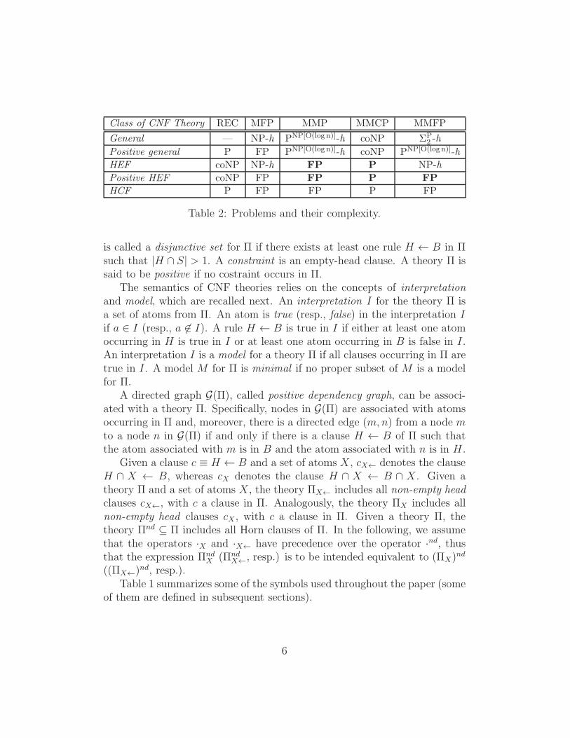
Table 2: Problems and their complexity.

is called a disjunctive set for Π if there exists at least one rule H ← B in Πsuch that |H ∩ S| > 1. A constraint is an empty-head clause. A theory Π issaid to be positive if no costraint occurs in Π.

The semantics of CNF theories relies on the concepts of interpretationand model, which are recalled next. An interpretation I for the theory Π isa set of atoms from Π. An atom is true (resp., false) in the interpretation I

if a ∈ I (resp., a 6∈ I). A rule H ← B is true in I if either at least one atomoccurring in H is true in I or at least one atom occurring in B is false in I.An interpretation I is a model for a theory Π if all clauses occurring in Π aretrue in I. A model M for Π is minimal if no proper subset of M is a modelfor Π.

A directed graph G(Π), called positive dependency graph, can be associ-ated with a theory Π. Specifically, nodes in G(Π) are associated with atomsoccurring in Π and, moreover, there is a directed edge (m,n) from a node mto a node n in G(Π) if and only if there is a clause H ← B of Π such thatthe atom associated with m is in B and the atom associated with n is in H .

Given a clause c ≡ H ← B and a set of atoms X , cX← denotes the clauseH ∩ X ← B, whereas cX denotes the clause H ∩ X ← B ∩ X . Given atheory Π and a set of atoms X , the theory ΠX← includes all non-empty headclauses cX←, with c a clause in Π. Analogously, the theory ΠX includes allnon-empty head clauses cX , with c a clause in Π. Given a theory Π, thetheory Πnd ⊆ Π includes all Horn clauses of Π. In the following, we assumethat the operators ·X and ·X← have precedence over the operator ·nd, thusthat the expression Πnd

X (ΠndX←, resp.) is to be intended equivalent to (ΠX)

nd

((ΠX←)nd, resp.).

Table 1 summarizes some of the symbols used throughout the paper (someof them are defined in subsequent sections).

6

2.2. Problems

Table 2 summarizes the problems and the classes of CNF theories ofinterest here and reports the associated complexities.

As for the classes of CNF theories, other than general one here we considerHEF and HCF theories:

— Head Cycle Free (HCF) theories [2] are CNF theories such that noconnected component of the associated dependency graph contains twopositive literals occurring in the same clause;

— Head Elementary-Set Free (HEF) CNF theories, the definition of whichwe adapt from the homonym one given in [14] for disjunctive logicprograms (see Section 4 for the formal definition of HEF theories),form a strict superset of the class of HCF theories.

The problems (listed in the table) are:

— Recognition Problem (REC): Given a CNF theory Π and a class C ofCNF theories, decide if Π belongs to the class C;

— Model Finding Problem (MFP): Given a CNF theory Π, compute amodelM for Π;

— Model Minimization Problem (MMP): Given a CNF theory Π and amodel M for Π, compute a minimal model MM for Π contained inM;

— Minimal Model Checking Problem (MMCP): Given a CNF theory Πand a modelM for Π, check ifM is indeed a minimal model for Π;

— Minimal Model Finding Problem (MMFP): Given a CNF theory Π,compute a minimal modelM for Π.

The MFP problem is NP-hard unless the theory is positive. Indeed, in thelatter case, the set consisting of all the literals occurring in the theory isalways a model.

In this work we will focus on the MMP, MMCP, and MMFP problems.As for MMFP, it turns out that, over positive CNF theories, this is

hard to solve. In particular, it is known that on positive theories MMFPis PNP[O(logn)]-hard [8] (even though positive CNF theories always have aminimal model!).

7

Given a CNF theory Π and a model M for Π, it is worth noticing thatthe theory ΠM is always a positive CNF and that the models of ΠM are asubset of those of Π. This explains the fact that the complexity of the MMPand MMCP problems, which have in input a modelM other than the theoryΠ, does not depend on positiveness of the theory.

Moreover, we notice that MMFP is not easier than MMP and MMCPsince the latter problems can be reduced to the former one as follows:

— As for MMP, return MMFP(ΠM);

— As for MMCP, return true if MMFP(ΠM) =M and false otherwise.

Thus, if for a certain class of theories the MMFP were tractable, then bothMMP and MMCP would become tractable as well.

Moreover, if attention is restricted to positive theories, the MMP andMMFP problems coincide (since this time MMFP can be reduced to MMPby settingM to the set of all the literals occurring in Π) and, consequently,MMP on general theories is equivalent to MMFP on positive theories.

We notice that, on the other hand, for head-cycle-free CNF theories thingsare easier than for the general case: indeed it was proved in [5] that theMMFP is solvable in polynomial time if the input theory is HCF.

All that given, the following section details the contributions of the paper.

2.3. Contributions and algorithms road map

In this work we investigate the MMP and MMCP problems on CNFtheories and the MMFP on positive CNF theories.

Among the main contributions offered here, we will show that MMP andMMCP are tractable on generic HEF theories, while MMFP is tractable onpositive HEF theories.

In order to provide a uniform treatment of these problems, we will concen-trate on algorithms for the MMP, which can be considered the most generalof them since its input consists of both a CNF theory and a (not necessarily)non-minimal model of the theory. Specifically, we provide a polynomial timealgorithm solving the MMP on general HEF CNF theories which, because ofthe observations made above, can be directly used to solve in polynomial timethe following five problems (see also cells of Table 2 reported in bold): (i)MMP on non-positive HEF CNF theories, (ii) MMCP on non-positive HEFCNF theories, (iii) MMP on positive HEF CNF theories, (iv) MMCP onpositive HEF CNF theories, and (v) MMFP on positive HEF CNF theories.

8

Also already noticed, differently from HCF theories, which turn out tobe recognizable in polynomial time [2], recognizing HEF theories is an in-tractable problem [13]. This undesirable property may seem to limit theapplicability of the above complexity results. However, as better explainednext, we show that our MMP algorithm can be fed with any CNF theoryΠ and any model M of Π and it is guaranteed to corectly minimize M atleast in the case that the theory Π is HEF. Notice that this property holdswithout the need to recognize whether the input theory is HEF or not.

To illustrate, we start by presenting an algorithmic schema, called theGeneralized Elimination Algorithm (GEA) for model minimization over CNFtheories. The GEA invokes a suitable eliminating operator in order to con-verge towards a minimal model of the input theory. Intuitively, an eliminat-ing operator is any function that, given a model as the input, returns a modelstrictly included therein, if one exists. Therefore, the actual complexity ofthe GEA depends on the complexity of the specific eliminating operator onedecides to employ. Clearly, the trivial eliminating operator may enumerate(in exponential time) all the interpretations contained in the given model andcheck for satisfiability of the theory, while we shall consider actually interest-ing only those eliminating operators that accomplish their task in polynomialtime.

A specific eliminating operator, denoted by ξHEF, is henceforth defined, bywhich the GEA computes a minimal model of any HEF theory in polynomialtime. However, the intractability of the recognition problem for HEF CNFtheories may seem to narrow the applicability of the results sketched aboveand to reduce their significance to a mere theoretical result. This seeminglyrelevant limitation can fortunately be overcome by suitably readapting thestructure of our algorithm: to this end, we introduce the Incomplete Gener-alized Elimination Algorithm (IGEA) that, once instantiated with a suitableoperator, outputs a model of the input theory, which is guaranteed to beminimal at least over HEF theories.

The design of IGEA leverages on the notion of fallible eliminating op-erator, which is defined later in this paper. Then, by coupling IGEA withthe ξHEF operator, we call this instance of the algorithm IGEAξHEF

, we ob-tain a polynomial-time algorithm that always minimizes the input model ofa HEF CNF theory without the need of knowing in advance whether theinput CNF theory is HEF or not. As for non-HEF theories, we show thatIGEAξHEF

always returns a model of the input theory which may be minimalor not, depending on the structure of the input theory. This kind of behavior

9

Π = { g ∨ j ←f ∨ h ←

b ← a

c ← b

a ← c

d ← a, b

c ← d

e ← b

h ← b

f ← e, i

i ← e, j

g ← f

e ← g

j ← e

h ← j

j ← h

c ← h, e }

a

b

d

c

e

hi

f

j

g

Figure 1: A positive CNF theory and the associated dependency graph.

on non-HEF theories is clearly the expected one since, as already noticed,recognizing HEF theories is co-NP-complete. Interestingly, this latter char-acteristics of IGEAξHEF

further enhances its relevance, since its application isnot restricted to the class of HEF CNF theories, but to a even broader classthereof.

2.4. Application scenarios

In this section we consider generic CNF theories without concentrating onthe particular class (that is, general, HEF or HCF) they belong to. Later, inSection 4.2, we specialize some of the examples provided next in the contextof HEF theories, which is a main focus in our investigation.

As already noticed, the minimal model finding problem is a formidableone and remains intractable even in the case attention is restricted to positiveCNFs. The following positive CNF theory will be employed in order todescribe the various concepts introduced throughout the paper.

Example 1 (Minimal models of positive CNF theories). Figure 1reports an example of positive CNF theory Π (on the left) together with the

10

P = { d ← not cb ← a, e, not da ← b, e, not da ← c

b ← c

c ← a, b

a, b ← not f }

M = { a, d }

PM = { d ←a ← c

b ← c

c ← a, b

a, b ← }

Figure 2: A logic program P , a modelM of P , and the reduct PM.

associated dependency graph G(Π) (on the right). The set atom(Π) is {a, b,c, d, e, f , g, h, i, j} and it is the largest model of Π. This theory has severalmodels, but only a minimal one, which is {j, h}. �

To illustrate a setting in which positive CNFs natural arise, consider LogicProgramming, a central tool in Knowledge Representation and Reasoning.In the field of Logic Programming, the notion of negation by default posesthe problem of defining a proper notion of model of the program. Amongthe several proposed semantics for logic programs with negation, the StableModels and Answer Sets semantics are nowadays the reference one for closedworld scenarios [16]. An interesting application of our techniques concernsstable model (or answer set) checking. To illustrate, stable models exploit theconcept of the reduct of the program, as clarified in the following definition.

Definition 1 (Stable Model [16]). Given a logic program P and a modelM of P , the reduct of P w.r.tM, also denoted by PM, is the program builtfrom P by (i) removing all rules that contain a negative literal not a in thebody with a ∈M, and (ii) removing all negative literals from the remainingrules. A modelM of P is stable ifM is a minimal model of PM.

Example 2 (Stable Models of Logic Programs). Figure 2 shows, onthe left, a logic program P and, on the right, the reduct PM of P w.r.t. themodelM = {a, d}. In this case, M is a minimal model of PM and, hence,it is a stable model of P . �

It is worth noticing that PM is a CNF since, by definition of the reduct,negation by default does not occur in any clause of PM. Moreover, M isalways a model of PM and is given in input.

11

Π = { b ← a

c ← a

a ← b, c

b, c ←d ←← b, d }

Π+ = { b ← a

c ← a

a ← b, c

b, c ←d ←φ ← b, d

a ← φ

b ← φ

c ← φ

d ← φ }

Figure 3: A CNF Π and its positive form Π+.

Therefore, by setting Π = PM the problem of verifying if a given modelM for the logic program P is stable fits the minimal model checking prob-lem for positive CNFs and, as such, can be suitably dealt with using thetechniques this paper proposes.

In order to analyze a different application scenario, let us assume a pos-itive CNF is given. Next we show that the given theory can be indeedreduced to a positive theory whose models have some clear relationship withthe models of the original theory.

Let us first consider the definition of positive form of a CNF.

Definition 2 (Positive Form of a CNF theory). The theory Π+, alsosaid the positive form of Π, is defined as follows: (1) for each clause H ← B

of Π, if H is not empty then the clause H ← B is in Π+; (2) for each clause← B of Π, the clause φ ← B is in Π+; (3) for each atom a occurring in Π,the clause a← φ is in Π+.

The following result relates models of Π with minimal models of Π+.

Proposition 2.1. Given a CNF theory Π, if φ belongs to the (unique) min-imal model of Π+ then Π is inconsistent, otherwise the set of minimal modelsof Π and Π+ coincide.

Proof. First of all, we will observe that each model of Π is a model of Π+ aswell and, then, φ is not inM.

12

Observation 1. Let M be a model for Π and consider the theory Π+. Allthe clauses (1) in Π+ are also in Π and then are true. Since M is a modelfor Π all the empty-head clauses of Π don’t have the body fully contained inM and, therefore, M satisfies all the clauses (2) of Π+. Finally, since φ isnot inM all the clauses (3) are true.

Now, letM+ be a minimal model of Π+ and atom(Π+) be the set of allatoms occurring in Π+.

Note that, because of the presence of the set of clauses (3), two cases arepossible, that are: eitherM+ contains φ and then all the atoms occurring inΠ+; orM+ ⊂ atom(Π+) and, in particular, φ 6∈ M+.

1. As for the first case, if Π had a model M then, due to Observation1, M would be a model of Π+ as well and then M+ would not beminimal. Thus, Π is inconsistent.

2. As for the second case, M+ does not contain φ. Consider now thetheory Π. All the non-empty-head clauses in Π are also in Π+ and,then, are satisfied by M+. Consider, now, the empty-head clauses inΠ. Because of the presence of clauses (2) in Π+, and since M+ doesnot contain φ, it is the case that the body of such clauses is not fullycontained in M+. Thus, the correspondent clauses in Π are satisfiedbyM+.

This implies thatM+ is a model of Π as well. �

To illustrate, consider the following example.

Example 3 (General CNF theories). Consider the CNF reported inFigure 3 on the left. In the same figure, one the right, it is reported thepositive form Π+ of Π. Π has only one minimal model, namely {c, d}, whichis precisely the unique minimal model of Π+. �

3. Generalized Elimination Algorithm

In this section, a generalization of the elimination algorithm proposedin [5], called Generalized Elimination Algorithm, is introduced. We beginby providing some preliminary concepts, notably, those of steady set andeliminating operator.

13

Intuitively, given a modelM for a theory Π, the steady set is the subsetofM containing atoms which “cannot” be erased fromM, for otherwiseMwould no longer be a model for Π. As proved next, the steady set can beobtained by computing the model of a certain non-disjunctive theory.

Definition 3 (Steady set). Given a CNF theory Π and a modelM for Π,the minimal model St ⊆M of the theory Πnd

M← is called the steady set ofMfor Π.

Note that the steady set St of M for Π always exists and is unique.Indeed, Πnd

M← is a Horn positive CNF and it is known that these kinds oftheories have one and only one minimal model (which can be computed inpolynomial time) [11, 26].

Property 3.1 (MM-containment). Given a positive CNF theory Π, amodel M for Π and the steady set St of M for Π, it holds that each modelof Π contained inM contains St.

Proof. First, notice that the models of the positive CNF theory Π which arecontained in the modelM of Π coincide with the models of the positive CNFtheory ΠM←.

Since ΠndM← is contained in ΠM←, by monotonicity of propositional logic,

it follows that all logical consequences of ΠndM← are also logical consequences

of ΠM← and, hence, each model of ΠM← contains the unique minimal modelof Πnd

M←, which is the steady set ofM for Π. �

Definition 4 (Erasable set). LetM be a model of a positive CNF theoryΠ. A non-empty subset E ofM is said to be erasable inM for Π ifM\ Eis a model of Π.

The following result holds.

Proposition 3.1. Let M be a model of a positive CNF theory Π, let St bethe steady set of M for Π, and let E be a set erasable in M for Π. Then,E ⊆M \ St.

Proof. For the sake of contradiction, assume that E ∩ St 6= ∅. Then,M\ Eis a model of Π that does not contain St, which contradicts the fact that Sthas theMM-containment property inM for Π (See Property 3.1). �

14

Algorithm 1: Generalized Elimination Algorithm with operator ξ,GEAξ(Π,M)

Input: A CNF theory Π and a modelM of ΠOutput: A minimal modelM∗ of Π contained inM

1: remove all constraints from Π2: stop = false3: repeat

4: compute the minimal model St of ΠndM←

5: if St is a model of Π then

6: M∗ = St stop = true

7: else

8: E = ξ(Π,M)9: if (E = ∅) then

10: M∗ =M11: stop = true

12: else

13: M =M\ E

14: until stop15: returnM∗

Figure 4: Generalized Elimination Algorithm with operator ξ, GEAξ(Π,M)

Definition 5 (Eliminating operator). Let M be a model of a positiveCNF theory Π. An eliminating operator ξ is a mapping that, given M andΠ in input, returns an erasable set in M for Π, if one exists, and an theempty set, otherwise.

It immediately follows that if ξ(Π,M) = ∅ then M is a minimal modelof Π. This is easily shown by observing that ξ(Π,M) = ∅ implies that thereis no erasable set inM, namely no subset ofM is a model for Π.

We are now ready to present our algorithmic schema, referred to as theGeneralized Elimination Algorithm (GEA) throughout the paper, which issummarized in Figure 4. Note that GEA has an operator ξ as its parameter4.

Our first result states that GEA is correct under the condition that theoperator parameter ξ is an eliminating operator.

4The term schema is used here since actual algorithms are obtained only after instan-tiating the generic ξ operator invoked in the GEA to a specific operator.

15

Theorem 3.1 (GEA correctness). Let Π be a CNF theory and M be amodel of Π. If ξ is an eliminating operator, then the set returned by GEAξ

on input Π andM is a minimal model for Π contained inM.

Proof. First of all, since M is a model of Π, by definition of model all theconstraints (aka empty-head clauses) of Π are true in M and are also truein any subset ofM. Hence, they can be disregarded during the subsequentsteps (see line 1).

Moreover, note that, by definition of steady set, it follows that the setSt computed at the beginning of each iteration of the algorithm (line 4) is a(not necessarily proper) subset of every minimal model contained inM. Letn be the number of atoms in the modelM computed at line 1 of the GEA.

Three cases are possible, which are discussed next:

1. St is a model of Π. Since St is the steady set of M for Π, if St is amodel for Π, then it is also minimal; so the algorithm stops and returnsa correct solution.5

2. E = ∅. By definition of eliminating operator, if E is empty, thenM is aminimal model; so the algorithm stops and returns a correct solution.

3. E 6= ∅. In this case, a non-empty set of atoms is deleted from M,letting (by definitions of eliminating operator and erasable set)M stillbe a model for Π. Thus, at the next iteration, the algorithms will workwith a smaller (possibly not minimal) modelM. Hence, after at mostn iterations, either case 1 or case 2 applies.

�

The next result states the time complexity of the GEA that, clearly, willdepend on the complexity Cξ associated with the evaluation of the eliminat-ing operator ξ.

Proposition 3.2. Let n and m denote the number of atoms occurring in theheads of Π and, overall, in Π, respectively. Then, for any model M of Π,GEAξ(Π,M) runs in time O(nm+ nCξ).

5We recall that if the steady set St of M for Π is a model of Π then it is the uniqueminimal model of Π contained in M. Hence, the test at line 4 serves the purpose ofaccelerating the termination of the algorithm. However, operations in lines 3-6 could besafely dropped without affecting the correctness of the algorithm.

16

Proof. Since at each iteration (if the stopping condition is not matched) atleast one atom is removed, the total number of iterations is O(n). As forthe cost spent at each iteration, the dominant operations are: (i) computingthe (unique) minimal model of a non-disjunctive theory (line 4) which canbe accomplished in linear time w.r.t. m by the well-known unit propagationprocedure [11]; (ii) checking if a set of atoms is a model (line 5) which canbe accomplished in linear time in m as well; (iii) applying the eliminatingoperator (line 8), whose cost is Cξ. This closes the proof. �

In particular, consider the naive operator ξexp that enumerates all the2n non-empty subsets of M and either returns one of these, call it E , suchthatM\ E is a model for Π, or an empty set if such a set E does not exist.The resulting algorithm GEAξexp returns a minimal model of Π but requiresexponential running time.

Conversely, as an example of instance of the GEA algorithm having poly-nomial time complexity on a specific class of CNF theories, consider theElimination Algorithm presented in [5]. This algorithm can be obtainedfrom the GEA by having the operator ξHCF (described next) as the eliminat-ing operator ξ and the set atom(Π) as the input modelM. Indeed, as shownin [5], the Elimination Algorithm computes a minimal model of a positiveHCF theory in polynomial time. The definition of ξHCF operator follows [5].Let Π be a positive HCF CNF theory and let M′ be the set of the headsof the disjunctive rules in ΠM← which are false inM. Then, ξHCF(Π,M) isdefined to return a source ofM′, where a source of the set of atomsM′ isa connected component in the subgraph of G(Π) induced byM′ which doesnot have incoming arcs.

Before leaving this section, we provide two further results which will beuseful when discussing the MMCP and the MMFP.

Lemma 3.1. Given a CNF theory Π, an eliminating operator ξ and a modelM of Π,M is minimal for Π if and only if GEAξ(Π,M) outputs M.

Proof. The proof follows by noticing that GEA always outputs a (possiblynon-proper) minimal sub-model of the initial modelM as its output. �

Lemma 3.2. Given a positive CNF theory Π and an eliminating operator ξ,then GEAξ(Π, atom(Π)) outputs a minimal model of Π.

Proof. The proof follows by noticing that atom(M) is a model ofM, beingΠ a positive theory, and by Lemma 3.1. �

17

4. Model minimization on HEF CNF theories

We have noticed above that the complexity of GEA depends on the com-plexity characterizing, in its turn, the specific elimination operator it invokes.On the other hand, the MMP being PNP[O(logn)]-hard [8] implies that, unlessthe polynomial hierarchy collapses, the GEA will generally require exponen-tial time to terminate when called on a generic input CNF theory. Therefore,it is sensible to single out significant subclasses of CNF theories for which it ispossible to devise a specific eliminating operator guaranteeing a polynomialrunning time for the GEA.

In this respect, it is a simple consequence of the results presented in [5]that a model of any head-cycle-free theory can be indeed minimized in poly-nomial time using the Elimination Algorithm. So, the interesting questionremains open of whether we can do better than this. Our answer to thisquestion is affirmative and this section serves the purpose of illustrating thisresult. In particular, we shall show that by carefully defining the eliminatingoperator, we can have that the GEA minimizes in polynomial time a modelof any HEF CNF theory. In Section 5, we shall moreover show that therealso exist CNF theories which are not HEF but for which the algorithm,equipped with a proper eliminating operator, efficiently minimizes a model.

4.1. Head-elementary-set-free theories and super-elementary sets

Next, we recall the definition of head-cycle-free theories [2], adapt thatof head-elementary-cycle-free theories [14] to our propositional context andprovide a couple of preliminary results which will be useful in the following.

We proceed by introducing the concepts of outbound and elementary set.

Definition 6 (Outbound Set (adapted from [14])). Let Π be a CNF the-ory. For any set Y of atoms occurring in Π, a subset Z of Y is outboundin Y for Π if there is a clause H ← B in Π such that: (i) H ∩ Z 6= ∅; (ii)B ∩ (Y \Z) 6= ∅; (iii) B ∩ Z = ∅ and (iv) H ∩ (Y \Z) = ∅.

Intuitively, Z ⊆ Y is outbound in Y for Π if there exists a rule c in Π suchthat the partition of Y induced by Z (namely, 〈Z; Y \ Z〉) “separates” headand body atoms of c.

18

Example 4 (Outbound set). Consider the theory

Π = { b, c ← a

b ← c

c ← b

a ← b

d ← b, c }

and the set E = {a, b, c}. Consider, now, the subset O = {a, b} of E. O isoutbound in E for Π because of the clause b ← c, since c ∈ E \ O, c 6∈ O,b ∈ O and b 6∈ E \O. �

Let O be a non-outbound set in X for Π. O is minimal non-outbound ifany proper subset O′ ⊂ O is outbound in X for Π.

Definition 7 (Elementary Set (adapted from [14])). Let Π be a CNFtheory. For any non-empty set Y ⊆ atom(Π), Y is elementary for Π if allnon-empty proper subsets of Y are outbound in Y for Π.

For example, the set Eex of Example 4 is elementary for the theory Πex,since each non-empty proper subset of Eex is outbound in Eex for Πex.

Definition 8 (Head-Elementary-Set-Free CNF theory (adapted from [15])).Let Π be a CNF theory. Π is head-elementary-set-free (HEF) if for eachclause H ← B in Π, there is no elementary set E for Π such that |E∩H| > 1.

So, a CNF theory Π is HEF if there is no elementary set containing twoor more atoms appearing in the same head of a rule of Π. An immediateconsequence of Definition 8 is the following property.

Property 4.1. A theory Π is not HEF if and only if there exists a set X ofatoms of Π such that X is both a disjunctive and an elementary set for Π.

For instance, the theory Πex of Example 4 is not HEF, since for the ruleb, c← a and the elementary set Eex, we have |Eex ∩ {b, c}| > 1.

19

4.2. Examples of HEF theoriesNow the examples already introduced in Section 2.4 are discussed in the

context of HEF CNF theories.

Example 1 (Minimal models of positive CNF theories – contin-

ued ). Consider the theory reported in Figure 1. This is an HEF CNF theorysince no superset of {g, j} and no superset of {f, h} is an elementary set forΠ. �

Example 2 (Stable Models of Logic Programs – continued ). A logic

program P is HEF if the CNF P obtained by removing all the literals of theform not a from the body of its rules is HEF [15].

Importantly, it holds that if the logic program P is HEF and M is amodel of P , then also PM is HEF. This follows since, by definition, a logicprogram P is HEF if and only if the CNF P is HEF, and by Lemma 4.3(reported in Section 4.4) any subset of clauses of a HEF CNF is HEF as well,

and PM is precisely a subset of P .Notably, even if P is not HEF, it could be anyway the case that PM is

HEF, and this broadens the range of applicability of the techniques proposedhere.

As an example, consider again Figure 2. The program P there reportedis not HEF, since the set S = {a, b, c} is both disjunctive and elementary.

Conversely, PM is HEF since the set S is no longer elementary becausethe subsets {a, c} and {b, c} of S are not outbound in S.

Moreover, we notice that the subgraph of G(PM) induced by S is a con-nected component and then both P and PM are not HCF. �

Example 3 (General CNF theories – continued ). Given a non-positive CNF Π, it holds that if Π is not HEF, then also Π+ is not HEF.

Let Π′ be the subset of Π obtained by removing the contraints in Π.Notice that Π′ can be obtained from Π+ by first removing the clauses of theform a ← φ for each a ∈ atom(Π) (see point (3) of Definition 2) and thenprojecting it on atom(Π). Since the HEF property does not depend on thecostraints, it follows from Lemma 4.3 (reported in Section 4.4) that if Π isnot HEF, then Π+ is not HEF as well.

Conversely, if Π is HEF, then Π+ can happen to be either HEF or not.As an example, consider the theories displayed in Figure 3 of Section

2.4. In this case Π and Π+ are both HEF. Conversely, consider the theoriesreported in Figure 5. In this case, Π is HEF, whereas Π+ is not. �

20

Π = { b ← a

c ← a

a ← b, c

b ← c

b, c ←d ←← b, d

← c, d }

Π+ = { b ← a

c ← a

a ← b, c

b ← c

b, c ←d ←φ ← b, d

φ ← c, d

a ← φ

b ← φ

c ← φ

d ← φ }

Figure 5: An HEF CNF Π and its positive form Π+ which is not HEF.

4.3. Super-elementary sets

We introduce next the definition of simplified theory and of super-elementaryset that will play a relevant role in the definition of the eliminating operatorfor HEF theories.

Definition 9 (Simplified theory). Let Π be a CNF theory and M be amodel of Π. Then the simplified theory of Π w.r.t. M, denoted as ΣM(Π),is the CNF theory (σM(Π))M\St, where

σM(Π) = {H ← B ∈ Π : H ∩ St = ∅ andM⊇ B}

and St is the steady set ofM in Π.

The clauses in σM(Π) are those clauses of Π having the body fully con-tained inM and some atoms of the head contained inM but not in St. Notethat it cannot be the case for the head of any clause in Π to have empty in-tersection withM (or, analogously, the head is empty) since, in such a case,M would not be a model for Π. Then, intuitively, σM(Π) contains the subsetof the clauses of Π which could be falsified if atoms would be eliminated fromthe modelM, so that we would have a model for Π no longer. Note that, wedo not consider the case that atoms of St are eliminated fromM since, by

21

definition of steady set, if any atom of St were eliminated we would have nolonger models for Π inM. Simplified theories enjoy two useful properties.

As for the first, we observe that, for any CNF theory Π and modelM ofΠ, σM(Π) is positive.

The second one, summarized in the following Lemma, tells that σM(Π)contains no facts.

Lemma 4.1. Let Π be a CNF theory, letM be a model of Π, and let St bethe steady set ofM for Π. Then no clause of the form h←, with h a singleletter, occurs in the theory ΣM(Π).

Next, we introduce the notion of super-elementary set which will be usedfor defining the eliminating operator for HEF theories.

Definition 10 (Super-elementary set). Given a CNF theory Π and a setX ⊆ atom(Π), X is super-elementary for Π if X is both an elementary setfor Π and a non-outbound set in atom(Π) for Π.

Intuitively, a super-elementary set X for Π is a set of atoms such that forno disjunctive clause c in Π, the body of c is satisfied by atoms not occurringin X and its head is contained in X (as will be clear in the proof of Theorem4.1). Notice that, as a consequence, no clause may become unsatisfied byremoving a super-elementary set X from a model.

4.4. On the erasability properties of Super-elementary sets

Next, we are going to show that, given any theory Π and model M ofΠ, any super-elementary set is erasable inM for Π. In order to do that, weshall:

1. demonstrate a one-to-one correspondence between the erasable sets inM for Π and the erasable sets inM\ St for ΣM(Π), where St is thesteady set ofM for Π (Lemma 4.2),

2. show that the property of a theory Π being HEF is retained by thesubsets of Π (Lemma 4.3): this implies that if a theory Π is HEF then,for each modelM of Π, also ΣM(Π) is HEF,

3. prove that, for any HEF theory Π and any modelM of Π, any super-elementaryset is erasable in ΣM(Π) (Theorem 4.1), whereby the sought result isobtained.

22

Le following results are conducive the the achievement of the aforemen-tioned objectives. To ease readability, some of the proof are reported in theappendix.

Lemma 4.2. Let Π be a CNF theory, letM be a model of Π and let St bethe steady set of M for Π. A set of atoms E is erasable in M for Π if andonly if E is erasable in (M\ St) ⊇ atom(ΣM(Π)) for ΣM(Π).

Lemma 4.3. Let Π be a HEF CNF theory. For each set of clauses Π′ ⊆ Πand for each set of atoms X, the theory Π′X is HEF.

Theorem 4.1. Let Π be a HEF CNF theory, letM be a model for Π and letSt be the steady set of M for Π, If E ⊆ atom(ΣM(Π)) is super-elementaryfor ΣM(Π) then E is erasable inM for Π.

Proof. By Lemma 4.2 it suffices to prove that E is erasable in atom(ΣM(Π))for ΣM(Π), which is accounted for next.

First of all, recall that ΣM(Π) is a positive theory. Moreover, by Lemma4.3, ΣM(Π) is HEF, since Π is HEF.

Clearly, atom(ΣM(Π)) is a model of ΣM(Π). It must be proved that eachclause of ΣM(Π) is true in atom(ΣM(Π))\E . Let H ← B be a generic clauseof ΣM(Π) such that E contains H : this is the only kind of clause that mightbecome false in atom(ΣM(Π)) \ E . Next, it is proved that H ← B is true inatom(ΣM(Π)) \ E . First notice that, by definition of ΣM(Π), it cannot bethe case that H is empty and |B| ≥ 1. Thus, the following three cases haveto be considered:

1. B is empty and |H| = 1. By Lemma 4.1, such a clause cannot exist.

2. B is empty and |H| > 1. Notice that, since E is an elementary set forΣM(Π), it cannot be the case that |H ∩E| > 1 or, in other words, thatE ⊇ H , since the theory ΣM(Π) is HEF. Hence, the clause H ← B istrue also in atom(ΣM(Π)) \ E ;

3. B is not empty. By contradiction, assume that H ← B is false inatom(ΣM(Π)) \ E . Then, H ← B is such that H ⊆ E and B ⊆atom(ΣM(Π)) \ E , namely, none of the atoms in B occurs in E . Butthis rule cannot exist, since E is non-outbound in atom(ΣM(Π)) forΣM(Π).

�

23

4.5. On the existence of a super-elementary set in a HEF theory

Next, we are going to show that, under the condition that atom(Π) =atom(Πnd), any HEF theory Π has a super-elementary set. This result, statedas Theorem 4.2 below, shall be attained by preliminarly proving that:

1. a super-elementary set for the non-disjunctive subset of a positive CNFtheory is also super-elementary for the whole theory (Lemma 4.4),

2. each HEF CNF theory Π has a super-elementary set (Lemma 4.5).

Lemma 4.4. Let Π be a HEF CNF theory. If O ⊆ atom(Πnd) is super-elementaryfor Πnd then O is super-elementary for Π.

Lemma 4.5. Let Π be a non-disjunctive CNF theory. Each minimal non-outbound set in atom(Π) for Π is super-elementary for Π.

The following result eventually states another key property of super-elementarysets in HEF CNF theories.

Theorem 4.2. Let Π be a disjunctive HEF CNF theory such that atom(Π) =atom(Πnd). Then, there exists a non-empty set of atoms O ⊆ atom(Π) suchthat O is super-elementary for Π.

Proof. Since Π is a disjunctive HEF CNF theory, it cannot be the case thatatom(Π) = atom(Πnd) is elementary for Πnd, for otherwise atom(Π) wouldbe elementary also for Π, implying that Π is not HEF. Since atom(Πnd) is notelementary in Πnd, by definition, there exists a set of atoms which is non-outbound in atom(Πnd) for Πnd and, in particular, there exists a minimalnon-outbound set O ⊂ atom(Πnd) for atom(Πnd) in Πnd. To conclude, Ois super-elementary for Πnd by Lemma 4.5 and, since O ⊂ atom(Πnd) =atom(Π), O is super-elementary for Π by Lemma 4.4. �

4.6. Computing a super-elementary set

This section is devoted to proving that a super-elementary set of an HEFCNF theory can be, in fact, computed in polynomial time.

The task of computing a super-elementary set is accomplished by thefunction find super-elementary set shown in Figure 8.

At each iteration, the function find super-elementary set makes use of thefunction compute elementary subgraph, which is detailed in Figure 6. Thelatter function receives as input a theory Π and a set of atoms X , an returns

24

Function compute elementary subgraphInput: A non-disjunctive CNF theory Π

a set of atoms X ⊆ atom(Π)

Output: The elementary subgraph G(Π, X) of Π

1: i = 02: Ei = ∅

3: Gi = 〈X,Ei〉4: repeat

5: let C be the set of clauses h← B in Π s.t. the subgraph of Gi induced by Bis strongly connected

6: Ei+1 = Ei ∪ {(b, h) | b ∈ B and h← B ∈ C}

7: Gi+1 = 〈X,Ei+1〉8: remove C from Π9: i = i+ 1

10: until C = ∅

11: return Gi

Figure 6: The compute elementary subgraph function

a graph, also denoted by G(Π, X), called the elementary subgraph of X forΠ [14]. The function reported in Figure 6 is substantially the same as thatdescribed at pag. 4 of [14]. Specifically, in the pseudo-code, by 〈X,E〉 it isdenoted a graph where X is the set of nodes and E is the set of arcs.

Example 5 (Elementary subgraph). Figure 7 reports an example ofcomputation of an elementary subgraph.

Since E0 = ∅, G0 is a graph including nodes but no arcs (see Figure 7(c)).The clauses in Π whose body is fully contained in one strongly connectedcomponent of G0 are all the clauses with just one atom in the body, namelyC = {c1, c2, c3, c5}. Thus, E1 consists in set of arcs {(a, b), (c, a), (a, c), (d, a)}and the clauses c1, c2, c3 and c5 are removed from Π.

The graph G1 is shown in Figure 7(d). The unique clause left in Π whosebody is fully contained in a strongly connected is c4, then C = {c4}, E2 ={(a, d), (c, d)}, and c4 is removed from Π.

Figure 7(e) reports the graph G2. Since the body of c6 does not belong

to a strongly connected component of G2, the procedure stops returning G2as the elementary subgraph G(Π, X) of X for Π.

�

Next, we recall the main result stated in [14], concerning elementary

25

Π = {c1 ≡ b← a

c2 ≡ a← c

c3 ≡ c← a

c4 ≡ d← a, c

c5 ≡ a← d

c6 ≡ e← a, b}

X = {a, b, c, d, e}

(a) The program Π and the set of atoms X

a b

c

d e

(b) The dependency graph of Π

a b

c

d e

(c) G0 = 〈X,E0〉

a b

c

d e

(d) G1 = 〈X,E1〉

a b

c

d e

(e) G2 = 〈X,E2〉

Figure 7: An example of elementary subgraph construction

subgraphs.

Proposition 4.1 (Theorem 2 of [14]). For any non-disjunctive theory Πand any set X of atoms occurring in Π, X is an elementary set for Π if andonly if the elementary subgraph of X for Π is strongly connected.

Moreover, as also proved in [14], the following proposition holds.

Proposition 4.2 ([14]). The procedure compute elementary subgraph ter-minates in polynomial time.

Indeed, at each iteration, a non-empty set of clauses (for otherwise the al-gorithm would stop) is taken into account and each clause of the theory isconsidered at most once. Thus, the number of iterations is at most linearw.r.t. the number of clauses of the theory. As for the cost of a single itera-tion, we have first to find a clause c such that the subgraph of Gi induced bythe body of c is strongly connected. This task can be clearly accomplishedin polynomial time. Second, we have to build the new graph Gi+1 by addingnew arcs to Gi, a task that can be accomplished also in polynomial time.

Let us now resort to the function find super-elementary set (see Figure8).

26

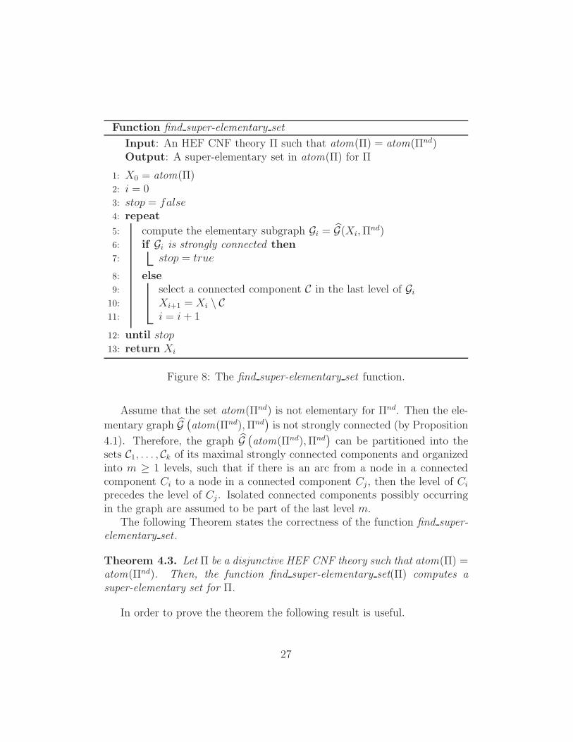
Function find super-elementary set

Input: An HEF CNF theory Π such that atom(Π) = atom(Πnd)Output: A super-elementary set in atom(Π) for Π

1: X0 = atom(Π)2: i = 03: stop = false

4: repeat

5: compute the elementary subgraph Gi = G(Xi,Πnd)

6: if Gi is strongly connected then7: stop = true

8: else9: select a connected component C in the last level of Gi10: Xi+1 = Xi \ C11: i = i+ 1

12: until stop13: return Xi

Figure 8: The find super-elementary set function.

Assume that the set atom(Πnd) is not elementary for Πnd. Then the ele-

mentary graph G(atom(Πnd),Πnd

)is not strongly connected (by Proposition

4.1). Therefore, the graph G(atom(Πnd),Πnd

)can be partitioned into the

sets C1, . . . , Ck of its maximal strongly connected components and organizedinto m ≥ 1 levels, such that if there is an arc from a node in a connectedcomponent Ci to a node in a connected component Cj, then the level of Ci

precedes the level of Cj . Isolated connected components possibly occurringin the graph are assumed to be part of the last level m.

The following Theorem states the correctness of the function find super-elementary set .

Theorem 4.3. Let Π be a disjunctive HEF CNF theory such that atom(Π) =atom(Πnd). Then, the function find super-elementary set(Π) computes asuper-elementary set for Π.

In order to prove the theorem the following result is useful.

27

Claim 1. For each i ≥ 0, Xi is a non-empty non-outbound set in atom(Πnd)for Πnd.

Proof of Claim 1. The proof is by induction.We start by noticing that the non-empty set X0 = atom(Π) = atom(Πnd)

is non-outbound in atom(Πnd) for Πnd, by definition of outbound set. More-over, consider the graph G0, namely, the elementary graph associated withthe set of atoms X0 = atom(Πnd) and the theory Πnd. Note that this graphis not strongly connected since Π is, by hypothesis, a disjunctive HEF theorysuch that atom(Π) = atom(Πnd) and then atom(Π) is not elementary forΠnd.

Now, for i > 1, assume by induction hypothesis that Xi is non-outboundin atom(Πnd) for Πnd and that the graph Gi is not strongly connected (forotherwise the algorithm would have stopped). Consider a strongly connectedcomponent C of the last level of Gi and the set Xi+1 = Xi \C. Note that Xi+1

is non-empty since, by induction hypothesis, Gi is not strongly connected andnote, moreover, that also C is not empty.

Next, it is shown that Xi+1 is non-outbound in atom(Πnd) for Πnd or,in other words, that there does not exist any clause c ≡ h ← B such thatB ⊆ X0 \ Xi+1 and h ∈ Xi+1, (note that this means that, without loss ofgenerality, we can limit ourselves to focus only on such single-head clauseswhere the atom in the head belongs to Xi+1 and the body is in X0 \Xi+1).

So, assume by contradiction that one such a clause c indeed exists. Twocases are possible.

B∩C = ∅. In this case, B ⊆ X0 \Xi. Therefore, c cannot exist in Πnd sinceXi is non-outbound in atom(Πnd) for Πnd.

B ∩ C 6= ∅. Also in this case, the clause c cannot exist in Πnd. Indeed, theclause cXi

obtained by projecting c on Xi, has its body contained in Cand its head in Xi+1. Since this clause would belong to Πnd

Xi, then it

would be the case that C would not belong to the last level of Gi.

This concludes the proof of Claim 1. �

Using Claim 1, the statement of Theorem 4.3 easily follows, as shownnext.

28

{a ,b ,c ,d}

{e , f ,g}

{ j ,h}

{ i}

{a ,b ,c ,d}

{e,f ,g,i}

Figure 9: Example of execution of the function find super-elementary set .

Proof of Theorem 4.3. When the algorithm find super-elementary set stops,the last set Xi is elementary for Πnd, since the graph Gi is strongly connected.By Claim 1, the set Xi is also non-empty and non-outbound in atom(Π) forΠnd. To conclude, by Lemma 4.4, the set Xi is super-elementary for Π. �

Example 1 (Minimal models of positive CNF theories – contin-

ued ). Consider again the theory Π reported in Figure 1 and the functionfind super-elementary set(Π). The connected components of the elementarysubgraph G0 are shown in Figure 9 on the left. Thus, there is a unique con-nected component in the last level of G0, which is C = {j, h}, and X1 is set to{a, b, c, d, e, f, g, i}. Notice that the connected components of the elementarysubgraph G1, which are reported in Figure 9 on the right, are not a subset ofthose of G0. The set X2 is then {a, b, c, d} and it is the super-elementary setreturned by the function. �

The next theorem accounts for the complexity of the function find super-elementary set .

Theorem 4.4. For any CNF theory Π, the function find super-elementary set(Π)terminates in polynomial time in the size of the theory.

Proof. Initially X0 contains all the atoms occurring in the input theory.Then, at each iteration, either the graph Gi is strongly connected and thenthe function stops and returns Xi, or Gi is not strongly connected and in

29

such case some node is removed from Xi. In the latter case, there exist atleast two strongly connected components in graph Gi. C is one of them andis such that Xi ⊃ C ⊃ ∅. Thus, Xi+1 is always non-empty. As for the conver-gence, it is ensured by the fact that the singleton set is strongly connectedby definition.

The number of iterations executed by the find super-elementary set func-tion is at most equal to the number of atoms occurring in the input theory,since in the worst case C consists in just one single atom at each iteration.The statement follows by the fact that each iteration can be accomplished inpolynomial time. �

4.7. Defining an eliminating operator for HEF CNF theories

In previous sections, we showed that:

– given a HEF CNF theory Π and a modelM for Π, a super-elementaryset for ΣM(Π) is erasable inM for Π (Theorem 4.1 in Section 4.4),

– given a HEF CNF theory Π, if the set of atoms of Π coincides withthat of its non-disjunctive fragment, a super-elementary set always ex-ists (see Theorem 4.2 in Section 4.5) and can be indeed computed inpolynomial time (see Theorems 4.3 and 4.4 in Section 4.6).

Putting things together, given an HEF CNF, it can be concluded that ifatom(ΣM(Π)) coincides with atom(Σnd

M(Π)), an erasable set E in M for Πcan be obtained by computing a super-elementary set for ΣM(Π) (as detailedin Section 4.6).

In order to build a suitable eliminating operator for HEF theories, itremains to prove that if atom(ΣM(Π)) is a strict superset of atom(Σnd

M(Π))then it is always possible to find in polynomial time a modelM′ ⊆M suchthat atom(ΣM′(Π)) coincides with atom(Σnd

M′(Π)).

Proposition 4.3. Given a CNF theory Π and a model M for Π, a modelM′ ⊆ M such that atom(ΣM′(Π)) coincides with atom(Σnd

M′(Π)) can becomputed in polynomial time.

The above result, which is valid not only for HEF CNF theories but,rather, for any CNF theory, will make the strategy above depicted generallyapplicable to any HEF CNF theory.

In order to prove Proposition 4.3, the intermediate results stated in tech-nical Lemmas 4.6 and 4.7 are preliminarily needed.

30

Lemma 4.6. Let Π be a CNF theory, letM be a model of Π and let St bethe steady set of M for Π. Then, E = (M\ St) \ atom(ΣM(Π)) is erasableinM for Π.

Lemma 4.7. Let Π be a CNF theory and let M be a model of Π. If thereexists an atom a such that a ∈ M \ atom(Πnd

M←) then {a} is erasable inMfor Π.

We are now in the position of proving Proposition 4.3.

Proof of Proposition 4.3. Let St denote the steady set ofM in Π. The twofollowing transformations (see points 1-2) can be recursively applied, till thecondition atom(ΣM(Π)) = atom(Σnd

M(Π)) is met:

1. IfM\ St is a strict superset of atom(ΣM(Π)) then by Lemma 4.6 theatoms in the non-empty set E = (M\St) \ atom(ΣM(Π)) are erasableinM for Π andM′ can be set toM\ E ;

2. Else ifM\ St is a strict superset of atom(ΣndM(Π)) then any atom a ∈

(M\St)\atom(ΣndM(Π)) is such that {a} is erasable inM\St for ΣM(Π)

(by Lemma 4.7, sinceM\St is a model for ΣndM(Π)) and also erasable

inM for Π (by Lemma 4.2); hence, let E = {a} an arbitrarily chosenatom in (M\ St) \ atom(Σnd

M(Π)), thenM′ can be set toM\ E ;3. Else it is the case that atom(ΣM(Π)) = atom(Σnd

M(Π)).

The whole process can be completed polynomial time. �

Before describing the ξHEF eliminating operator, the following technicalresult is needed.

Lemma 4.8. Let Π be a CNF theory, letM be a model of Π, and let St bethe steady set ofM for Π. If the theory ΣM(Π) is non-disjunctive, then ∅ isits minimal model.

Figure 10 shows a realization of the ξHEF eliminating operator. Thefollowing theorem asserts the most relevant result of this section, that is,that a minimal model for an HEF CNF theory can be indeed computed inpolynomial time.

Theorem 4.5. Let Π be a HEF CNF theory andM be a model of Π. Then,GEAξHEF

(Π,M) computes, in polynomial time, a minimal model of Π con-tained inM.

31

Function ξHEF

Input: An HEF CNF theory Π and a modelM of ΠOutput: An erasable set E inM for Π

1: E ′ = ∅2: repeat

3: M =M\ E ′

4: Compute the steady set St ofM for Π5: ∆E = ∅6: if (M\ St) ⊃ atom(ΣM(Π)) then7: ∆E = (M\ St) \ atom(ΣM(Π))

8: else if (M\ St) ⊃ atom(ΣndM(Π)) then

9: Select an atom a in (M\ St) \ atom(ΣndM(Π))

10: ∆E = {a}

11: E ′ = E ′ ∪∆E

12: until ∆E = ∅13: if ΣM(Π) is non-disjunctive then

14: E ′′ =M\ St

15: else

16: E ′′ = find super−elementary set(ΣM(Π))

17: E = E ′ ∪ E ′′

18: return E

Figure 10: The ξHEF eliminating operator.

32

Proof. Because of Theorem 3.1 and Proposition 3.2, in order to prove thestatement, it is sufficient to show that (i) ξHEF returns an erasable set, ifsuch a set exists, and an empty one otherwise (namely that ξHEF is, in fact,an eliminating operator) and that (ii) ξHEF runs in polynomial time.

Let us consider first point (i). Lines 2-12 in Figure 10 serve the pur-pose of finding a subset M′ ⊆ M such that atom(ΣM′(Π)) coincides withatom(Σnd

M′(Π)) according to the strategy depicted in the proof of Proposition4.3 Notice that, the set E ′ =M\M′ is an erasable set.

We can now assume that atom(ΣM(Π)) coincides with atom(ΣndM(Π)). If

the theory ΣM(Π) is non-disjunctive, then by Lemmata 4.8 and 4.2, the setE ′′ =M\St is an erasable set inM for Π and the operator returns E ′ ∪ E ′′

(see lines 13-14).Otherwise, ΣM(Π) is disjunctive. Then, by Theorem 4.2 there exists a

non-empty set of atoms E ′′ ⊆ (M\St) such that E ′′ is super-elementary forΣM(Π) and, by Theorem 4.1, the set E ′′ is erasable inM\St for ΣM(Π). Inthis case, the operator returns the erasable set E ′ ∪ E ′′.

As far as point (ii) is concerned, this is a direct consequence of Theorem4.4 and this concludes the proof. �

As for minimal model checking, we have the following result.

Theorem 4.6. Given a positive HEF CNF theory Π and a set of atomsN ⊆ atom(Π), checking if N is a minimal model of Π can be accomplishedin polynomial time.

Proof. The proof follows immediately from Theorem 3.1 and Theorem 4.5.�

Example 1 (Minimal models of positive CNF theories – contin-

ued ). Let us consider the execution of GEAξHEF(Π,M), where Π is the

HEF theory Π reported in Figure 1 and M = atom(Π). During the firstmain iteration, the eliminating operator ξHEF returns the super-elementaryset {a, b, c, d}, as shown in the example of Section 4.6 and M is set to {e,f , g, h, i, j}. As for the next iteration, the output of ξHEF is {e, f , g,i} and M becomes {j, h}. Since now M coincides with the steady set ofΠM = {j ←; h ←; h ← j; j ← h}, the algorithm stops returning {j, h} as aminimal model of Π. �

33

5. Beyond HEF

In the previous section, we have shown that GEA(ξHEF) computes a min-imal model of a positive HEF CNF theory in polynomial time. Unfortu-nately, however, deciding if a given theory is head-elementary-free is a coNP-complete problem [13]6. In other words, while a minimal model for an inputHEF CNF theory Π can be indeed computed in polynomial time, checkingwhether Π is actually HEF is intractable.

Thus, it is sensible to study the behavior of GEA(ξHEF) as applied toa general CNF theory, which is the subject of this section. Recall that, byTheorem 4.4, the find super-elementary set function runs in polynomial timeindependently of the kind of theory it is applied to.

Next, we will show that there are non-HEF theories for which GEA(ξHEF)successfully returns a minimal model and others for which GEA(ξHEF) endsfailing to construct a correct output7 (recall that, on the basis of the results ofthe previous section, GEA always returns a correct solution on HEF theories).The following example should help in clarifying this latter issue.

Example 6 (Behavior on non-HEF theories). Consider the followingtwo theories:

P = { a ←b, c ← a

c ← b

b ← c }

Q = { a ←b, c, d ← a

c ← b

b ← c

d ← c }

Both theories are not HEF. Indeed, the set {b, c} is a disjunctive elemen-tary set, both for P and for Q. However, while GEA(ξHEF) does not returna minimal model of P, it does correctly compute a minimal model of Q.

To show that, consider first running GEA(ξHEF) on P. LetM be {a, b, c}(this is the model obtained by taking the union of all the heads). At line3 of GEA, St is set to {a}, which is not a model of P and, then, ξHEF isinvoked. In particular, the find super-elementary set function is executed onthe theory P ′ = {b, c ←; c ← b; b ← c}. In the execution of the function,

6We note that the reduction therein presented is still valid for positive HEF CNFs.7That the algorithm is not always returning the correct answer is indeed the expected

behavior due to the intractability of the general problem and since ξHEF runs in polynomialtime (under the assumption that P 6= coNP).

34

X0 is {b, c}. Since the elementary graph associated with P ′ndX0is strongly

connected, the function stops and returns {b, c}. As a consequence, the set Eis {b, c} and the new setM is {a}. It turns out that, since the setM is nota model for P any longer, GEA(ξHEF) is not able to return a minimal modelof P. Specifically, at the second iteration of GEA(ξHEF), ξHEF is invoked onthe theory P and on the setM = {a}. The steady set St computed at line1 in Figure 10 is equal to {a} (since Πnd

M← is the theory {a ←}) and thetheory Π is empty. The set of atoms R =M\St computed at line 3 and ΠRare empty too. Then the condition at line 9 is true and R = ∅ is returned.Thus, at the second iteration of GEA(ξHEF), E is empty and, then, St is setto M = {a} and returned. Concluding, GEA(ξHEF) on P ends returning{a} which is not a minimal model of Π.

Consider, now, the theory Q. Let M be {a, b, c, d}, which is the modelobtained by taking the union of all the heads. The set St is set to {a} whichis not a model of Q and, then, ξHEF is invoked. In particular, the find super-elementary set function is executed on the theory Q′ = {b, c, d←; c← b; b←c; d ← c}. In the execution of the function, X0 is {b, c, d}. The elementarygraph associated with Q′ndX0

is not strongly connected; actually, it includesthe strongly connected component C1 containing b and c and the stronglyconnected component C2 containing d. Moreover, there is an edge from C1

to C2 but not vice versa. Then, C2 belongs to the last level of the graph,and X1 is set to X0 \ {d} = {b, c}. The elementary subgraph associatedwith Q′ndX1

is strongly connected; therefore the function stops and returns theset X1 = {b, c}. As a consequence the set E is {b, c} and, now, the set Mis {a, d} and the theory Q′ndM← is {a ←; d ← a} whose minimal model isSt = {a, d}. Since St is a model of Q, GEA(ξHEF) stops by returning St asthe result, which is indeed a minimal model of Q. �

Summarizing, the algorithm GEA(ξHEF) always runs in polynomial timeand correctly returns a minimal model of HEF CNF theories, but its correct-ness on non-HEF theories is seemingly unpredictable: the rest of this sectionis devoted to devise a suitable variant of GEA able to tell about the correct-ness of the result it returns. In order to proceed, some further definitionsand results are needed.

Definition 11 (Fallible eliminating operator). Let M be a model of apositive CNF theory Π. A fallible eliminating operator ξf is a polynomialtime computable function that returns a subset ofM\St, with St the steady

35

set of Π, with the constraint that if ξf returns the empty set, then M is aminimal model of Π.

Proposition 5.1. Let Π be a positive CNF theory and ξf be a fallible elimi-nating operator. Checking if the set returned by running GEA(ξf ) over Π isa minimal model for Π is attainable in polynomial time.

Proof. By Theorem 3.1, we know that if the set returned by the operatoremployed in GEA is an erasable set then the algorithm returns a minimalmodel. Thus, it is sufficient to check if, at each iteration, E is an erasableset, namely it must be checked if M\ E is a model for Π. Since this latteroperation can be done in polynomial time, the statement follows. �

As a consequence of our previous results, we are now able to presentthe modified GEA, called the Incomplete Generalized Elimination Algorithm(IGEA, for short), which is reported in Figure 11.

The following Theorem describes the correctness of IGEA as well as itscomputational complexity.

Theorem 5.1. For any fallible eliminating operator ξf , IGEA(ξf ) alwaysterminates (with either success or failure) in polynomial time, returning amodel of the input theory. If it succeeds, then the returned model is a minimalone.

Proof. If the if branch at line 12 is never taken, thenM is, at each iteration,a model for Π and E is an erasable set. In this case, the fallible eliminatingoperator ξf is indeed an eliminating operator, whereby IGEA(ξf ) behaves asGEA(ξf) does. This immediately implies that if IGEA(ξf) does not report a“failure” then it returns a minimal model for Π.

As far as the time complexity of the algorithm is concerned, following thesame line of reasoning as before, if the if branch at line 12 is never taken,then IGEA(ξf) requires exactly the same number of iterations as GEA(ξf).Conversely, if the if branch at line 12 is taken, the algorithm ends. Thus,IGEA(ξf) does not require more iterations than GEA(ξf). As for the costof a single iteration, IGEA(ξf) has only one operation more than GEA(ξf),consisting in checking ifM\E is a model for Π (line 12). Since this operationis the same as that accomplished at line 4, the asymptotic temporal cost of thealgorithm is not affected. Thus, the cost of IGEA(ξf ) is exactly that reportedin Proposition 3.2 for the GEA, where Cξf is polynomial, by definition offallible eliminating operator. �

36

Algorithm 2: Incomplete Generalized Elimination Algorithm,IGEA(ξf)

Input: A positive CNF theory ΠOutput: A minimal model for Π and an indication of a “success” or a model for

Π and an indication of a “failure”

1: M = {h | H ← B ∈ Π and h ∈ H} //M is a (possibly non-minimal) model of Π2: stop = false3: repeat

4: compute the minimal model St of ΠndM←

5: if St is a model of Π then

6: stop = true

7: else

8: E = ξf (Π,M)9: if (E = ∅) then

10: St =M11: stop = true

12: else

13: if (M\ E is not a model of Π) then

14: returnM and “Failure”

15: M =M\ E

16: until stop17: return St and “Success”

Figure 11: Incomplete Generalized Elimination Algorithm, IGEA(ξf)

To conclude this section, we show that ξHEF can, in fact, be safely adoptedas fallible eliminating operator in IGEA. The following preliminary proposi-tion is useful.

Proposition 5.2. Let Π be CNF theory,M be a model for Π and St be thesteady set ofM for Π. If St is not a model for Π then, on input Π andM,the operator ξHEF returns a non-empty set.

Proof. Consider the theory (σM(Π))M\St. Since St is not a model for Π,there are rules in Π which are not true in St but are true in M, thus that(σM(Π))M\St is not empty. Therefore, it is enough to prove that, wheneverthe function find super-elementary set is run over a non-empty theory, itreturns a non-empty set.

37

Consider the function find super-elementary set reported in Figure 8.First of all, note that if Π is a non-empty theory and X is a non-emptyset of atoms occurring in Π, then the elementary graph G(Πnd

X ) is non-emptyas well. Thus, in the function, if Xi is non-empty then Gi is non-empty.

The set X0 at line 1 is non-empty since the function is invoked over anon-empty theory. By induction, assuming that Xi is non-empty, we provethat Xi+1 is non-empty as well.

Consider the (i+ 1)-th iteration. Two cases are possible:

(i) Gi is strongly connected and the function ends returning the set Xi, whichis non-empty by the induction hypothesis.

(ii) Gi is not strongly connected and includes at least two connected com-ponents. In such a case, only the atoms of one of the connected com-ponents are removed from Xi, call it C. Then Xi+1 = Xi \ C is notempty.

�

Proposition 5.3. The operator ξHEF is a fallible eliminating operator.

Proof. Let Π be a general positive CNF theory,M be a model for Π and Stbe the steady set ofM for Π. The proposition is an immediate consequenceof the following facts: (i) ξHEF(Π,M) runs in polynomial time (by Theorem4.4); (ii) the set returned by the operator ξHEF(Π,M) is a subset ofM\St;(iii) the set returned by ξHEF(Π,M) is not empty (by Proposition 5.2). �

Concluding, since ξHEF is a fallible eliminating operator, for any CNFtheory Π, IGEA(ξHEF) runs in polynomial time returning a model and, onHEF theories, we are guaranteed that the returned model is minimal. Thus,the successful termination of IGEA(ξHEF) can be also seen as a necessarycondition for a theory to be HEF (but it is not a sufficient condition, unlesscoNP collapses onto P).

The next theorem, finally, summarizes the results of this section.

Theorem 5.2. The algorithm IGEA(ξHEF) terminates in polynomial timefor any input positive CNF theory. Moreover, if the input theory Π is HEF,then IGEA(ξHEF) succeeds returning a minimal model for Π; otherwise ei-ther the algorithm declares success returning a minimal model for Π or thealgorithm declares failure returning a model for Π.

Proof. The proof immediately follows from Theorem 5.1 and Proposition 5.3.�

38

6. Conclusions

Tasks related with computing with minimal models are relevant to severalAI applications.

The focus of this paper has been devising efficient algorithms to dealwith minimal models of CNF theories. Particularly, three problems havebeen mainly considered, that are, minimal model checking, minimal modelfinding and model minimization. All these problems prove themselves tobe intractable for general CNF theories, while it was known that they be-come tractable for the class of head-cycle-free theories [5] and, in fact, tothe best of our knowledge, positive HCF theories form the largest class ofCNFs for which polynomial time algorithms solving minimal model findingand minimal model checking are known so far. The research presented herefollows the same research target as that of [5] and the main contribution ofthis work has been that of designing a polynomial time algorithm for com-puting a minimal model for (a superset of) the class of positive HEF (HeadElementary-Set Free) CNF theories, a strict superset of the class of HCFtheories, whose definition naturally stems for the analogous one given in thecontext of logic programming in [14]. This contribution thus broadens thetractability frontier associated with minimal model computation problems.

In more detail, we have introduced the Generalized Elimination Algo-rithm (GEA), that computes a minimal model of any positive CNF, whosecomplexity depends on the complexity of the specific eliminating operatorit invokes. Therefore, in order to attain tractability. a specific eliminatingoperator has been defined which allows for the algorithm to compute in poly-nomial time a minimal model for a class of CNF that strictly includes HEFtheories.

However, it is unfortunately already known that recognizing HEF theoriesis “per se” an intractable problem, which may apparently limit the applica-bility range of our algorithmic schema. In order to overcome such a problem,an “incomplete” variant of the GEA (called IGEA) is proposed: the resultingschema, once instantiated with an appropriate elimination operator, alwaysconstructs a model of the input CNF, which is guaranteed to be minimal atleast if the input theory is HEF. We note that this latter algorithm is ableto “declare” if the returned model is indeed minimal or not.

The research work presented here can be continued along some interestingdirection. As a major research direction, since the IGEA is capable to dealalso with theories that are not HEF, it would be relevant to define, via a syn-

39

tactic specification, as those pinpointing HCF and HEF theories, a supersetHEF theories coinciding with those on which the IGEA stops returning a suc-cess. While it is not at all clear if this can be reasonably attained, we mightconsider it enough to get close (from below) to this class of theories. Veryrelated to the above line of research, there is the assessment of the practicaloccurrence of theories having the HEF property or the property of guaran-teeing success to the IGEA and also the assessment of the success rate ofthe IGEA on generic CNF theories. Moreover, enhancing stable models andanswer set engines for logic programs with the IGEA appears a potentiallyfruitful line of investigation.

References

[1] Chen Avin and Rachel Ben-Eliyahu-Zohary. An upper bound on com-puting all x-minimal models. AI Commun., 20(2):87–92, 2007.

[2] Rachel Ben-Eliyahu and Rina Dechter. Propositional semantics for dis-junctive logic programs. Annals of Mathematics and Artificial Intelli-gence, 12:53–87, 1994.

[3] Rachel Ben-Eliyahu and Rina Dechter. On computing minimal models.Annals of Mathematics and Artificial Intelligence, 18:3–27, 1996. Ashort version in AAAI-93: Proceedings of the 11th national conferenceon artificial intelligence.

[4] Rachel Ben-Eliyahu-Zohary. An incremental algorithm for generatingall minimal models. Artificial Intelligence Journal, 169(1):1–22, 2005.

[5] Rachel Ben-Eliyahu-Zohary and Luigi Palopoli. Reasoning with minimalmodels: Efficient algorithms and applications. Artificial Intelligence,96(2):421–449, 1997.

[6] N. Bidoit and C. Froidevaux. Minimalism subsumes default logic andcircumscription in stratified logic programming. In LICS-87: Proceed-ings of the IEEE symposium on logic in computer science, pages 89–97.IEEE Computer Science Press, Los Alamitos, Calif, June 1987.

[7] Marco Cadoli. The complexity of model checking for circumscriptiveformulae. Inf. Process. Lett., 44(3):113–118, 1992.

40

[8] Marco Cadoli. On the complexity of model finding for nonmonotonicpropositional logics. In Proceedings of the 4th Italian conference ontheoretical computer science, pages 125–139. World Scientific PublishingCo., October 1992.

[9] Z. Chen and S. Toda. The complexity of selecting maximal solutions. InProc. 8th IEEE Int. Conf. on Structures in Complexity Theory, pages313–325, 1993.

[10] Johan de Kleer, Alan K. Mackworth, and Raymond Reiter. Characteriz-ing diagnoses and systems. Artificial Intelligence Journal, 56(2-3):197–222, 1992.

[11] W. Dowling and J. Gallier. Linear-time algorithms for testing the satis-fiability of propositional horn formulae. Journal of Logic Programming,1(3):267–284, 1984.

[12] Thomas Eiter and Georg Gottlob. Propositional circumscription andextended closed-world reasoning are iip2-complete. Theor. Comput. Sci.,114(2):231–245, 1993.

[13] Fabio Fassetti and Luigi Palopoli. On the complexity of identifyinghead-elementary-set-free programs. Theory and Practice of Logic Pro-gramming, 10(1):113–123, 2010.

[14] Martin Gebser, Joohyung Lee, and Yuliya Lierler. Elementary sets forlogic programs. In Proceedings of the 21st National Conference on Ar-tificial Intelligence (AAAI), 2006.

[15] Martin Gebser, Joohyung Lee, and Yuliya Lierler. Head-elementary-set-free logic programs. In Proceeding of 9th International conferenceon Logic Programming and Nonmonotonic Reasoning (LPNMR), pages149–161, 2007.

[16] Michael Gelfond and Vladimir Lifschitz. The stable model semantics forlogic programming. In Proceedings of the Fifth International Conferenceand Symposium, pages 1070–1080, 1988.

[17] Michael Gelfond and Vladimir Lifschitz. Classical negation in logic pro-grams and disjunctive databases. New Generation Computing, 9:365–385, 1991.

41

[18] Alfonso Gerevini, Alessandro Saetti, and Ivan Serina. Planning throughstochastic local search and temporal action graphs in lpg. J. Artif. Intell.Res. (JAIR), 20:239–290, 2003.

[19] Holger Hoos and Thomas Sttzle. Stochastic Local Search: Foundations& Applications. Morgan Kaufmann Publishers Inc., San Francisco, CA,USA, 2004.

[20] Henry A. Kautz, David Mcallester, and Bart Selman. Encoding Plans inPropositional Logic. In Proceedings of the Fifth International Conferenceon the Principle of Knowledge Representation and Reasoning (KR’96),pages 374–384, 1996.

[21] Lefteris M. Kirousis and Phokion G. Kolaitis. The complexity of minimalsatisfiability problems. Inf. Comput., 187(1):20–39, 2003.

[22] Christoph Koch and Nicola Leone. Stable model checking made easy.In IJCAI, pages 70–75, 1999.

[23] Phokion G. Kolaitis and Christos H. Papadimitriou. Some computa-tional aspects of circumscription. J. ACM, 37(1):1–14, 1990.

[24] Nicola Leone, Pasquale Rullo, and Francesco Scarcello. Disjunctive sta-ble models: Unfounded sets, fixpoint semantics, and computation. Inf.Comput., 135(2):69–112, 1997.

[25] Vladimir Lifshitz. Computing circumscription. In IJCAI-85: Proceed-ings of the international joint conference on AI, pages 121–127, 1985.

[26] John W. Lloyd. Foundations of logic programming. Springer-Verlag NewYork, Inc., New York, NY, USA, 1987.

[27] Zbigniew Lonc and Miroslaw Truszczynski. Computing minimal models,stable models and answer sets. TPLP, 6(4):395–449, 2006.

[28] John McCarthy. Circumscription - a form of non-monotonic reasoning.Artificial Intelligence Journal, 13:27–39, 1980.

[29] John McCarthy. Application of circumscription to formalizing common-sense knowledge. Artificial Intelligence Journal, 28:89–116, 1986.

42

[30] Jack Minker. On indefinite databases and the closed world assumption.In Proceedings of the 6th conference on automated deduction, LectureNotes in Computer Science Vol. 138, pages 292–308. Springer-Verlag,1982.

[31] Raymond Reiter. A logic for default reasoning. Artificial IntelligenceJournal, 13(1–2):81–132, 1980.

[32] Bart Selman, Henry A. Kautz, and Bram Cohen. Local search strategiesfor satisfiability testing. In DIMACS SERIES IN DISCRETE MATHE-MATICS AND THEORETICAL COMPUTER SCIENCE, pages 521–532, 1996.

Appendix

Proof of Lemma 4.2. In order to prove the theorem, we have to show thatthere is no clause in Π which is false inM\E if and only if there is no clausein ΣM(Π) which is false in (M\ St) \ E .

The proof is organized in two parts, both proved by contradiction.

(=⇒) First of all note that, for each clause c ≡ H ← B in ΣM(Π) thereis, by definition, a clause c′ ≡ H ′ ← B′ in σM(Π) such that H ′M\St = H 6= ∅

and B′M\St = B. Moreover, note that (by construction of σM(Π)) c′ is alsoin Π and that B′ ⊆M.

For the sake of contradiction, assume that c is true inM\St and false in(M\ St) \ E . We aim at proving that if such a rule exists then there existsat least one rule (actually c′) which is false inM\ E .

If c is false in (M\ St) \ E , then B is contained in (M\ St) \ E and Econtains H . Note that since B ∩ E = ∅ and since B = B′ ∩ (M \ St), itfollows that also B′ ∩ E = ∅ (and, then, B′ ⊆M\ E).

But, since H ′ ∩ St = ∅ (by construction of σM(Π)) and since H = H ′ ∩(M\St), if H ⊆ E then also H ′ ⊆ E .

So, we have proved that B′ ⊆ (M\ E) and H ′ ⊆ E ; it follows that c′ isfalse inM\ E , which concludes the first part of the proof.

(⇐=) For the sake of contradiction, assume that there exists a clausec′ ≡ H ← B in Π which is true inM and false inM\E . Thus, B ⊆ (M\E)and ∅ ⊂ H ⊆ E implying that H ∩ St = ∅ since, by definition of steady set

43

and erasable set, any erasable set has empty intersection with the steady set,namely E ∩ St = ∅.

Consider, now, the clause c ≡ HM\St ← BM\St. Since H is contained in Eand E∩St = ∅, it follows that HM\St is equal to H and is not empty, then c isby definition in ΣM(Π). Conversely, since B ⊆ (M\E) then BM\St ∩E = ∅.

Thus, c is a clause of ΣM(Π) whose head is included in E meaning that cis false in (M\St) \ E . But, sinceM\St is a model of ΣM(Π), c is true inM\ St. This concludes the proof since it contradicts that E is an erasableset inM\ St for ΣM(Π).

�

Proof of Lemma 4.1. For the sake of contradiction, assume that such a clausec ≡ h ← belongs to ΣM(Π). Clearly, in this case there exists at least oneclause c′ in σM(Π) ⊆ Π such that c = c′M\St. By definition of ΣM(Π), it is

the case that h is the only atom in M (and also in M \ St) occurring inthe head of the clause c′ and, hence, it can be concluded that c′M← belongsalso to the theory Πnd

M←. The body of c′ is contained inM by definition ofσM(Π). Since the body of c is empty, there are two possibilities:

1. The body of c′ is also empty: but in this case h should belong to Stand the clause h← cannot be in ΣM(Π), a contradiction;

2. The body of c′ is contained in St: but this means that c′M← is a clauseof Πnd

M← which is false in St, which contradicts the fact that St is theminimal model of Πnd

M←.

�

Proof of Lemma 4.3. The proof is given by contraposition: assuming thatΠ′X is not HEF it is derived that Π is not HEF. If Π′X is not HEF then,by Proposition 4.1, there is a set of atoms E ⊆ X such that E is both adisjunctive and an elementary set for Π′X . Clear enough, if E is a disjunctiveset for Π′X then it is a disjunctive set for Π as well. Moreover, if E iselementary for Π′X then, for each proper subset O ⊂ E, there is a clausecX ≡ HX ← BX in Π′X such that HX ∩O 6= ∅, HX ∩ (E \O) = ∅, BX ∩O = ∅and BX ∩ (E \ O) 6= ∅. By definition of Π′X , cX ∈ Π′X implies that there isa clause c ≡ H ← B in Π such that HX = H ∩X and BX = B ∩X . Thus,since O ⊂ E ⊆ X , it follows that H ∩ O = HX ∩ O 6= ∅, H ∩ (E \ O) =HX ∩ (E \O) = ∅, B∩O = BX ∩O = ∅ and B∩ (E \O) = BX ∩ (E \O) 6= ∅.Therefore, O is outbound in E also for Π. As a consequence, E is elementary

44

for Π and, since E is also a disjunctive set for Π, it is the case that Π is notHEF. �

Proof of Lemma 4.4. Before stating the Lemma, it is needed to recall a resultgiven in [13] asserting that if O ⊆ atom(Πnd) is elementary for Πnd then itis elementary also for Π.

Claim 2 (Rephrased from [13]). Let Π be a CNF theory and Π′ ⊆ Πany CNF consisting of a subset of the clauses of Π. If O ⊆ atom(Π′) is anelementary set for Π′, then O is an elementary set for Π as well.

By hypothesis, O is non-outbound in atom(Πnd) for Πnd. In order tocomplete the proof, it is enough to prove that, since Π is HEF, O is non-outbound in atom(Π) for Π, which is shown next.

By contradiction, assume that O is outbound in atom(Π) for Π. Sinceatom(Π) is the set of all the atoms appearing in Π, then there exists a clauseH ← B in Π such that B ⊆ atom(Π) \ O and H ⊆ O. Since O is non-outbound in atom(Πnd) for Πnd, then the clause H ← B is not in Πnd andit holds that |H| ≥ 2. As a consequence, O is an elementary set for Π andthere is a clause H ← B such that |H ∩ O| ≥ 2. That is to say, Π is notHEF, a contradiction. �

Proof of Lemma 4.5. Let O be a minimal non-outbound set in atom(Π) forΠ. Hence, there is no single head clause h← B in Π such that B ⊆ atom(Π)\O and h ∈ O.

Consider, now, any non-empty proper subset O′ of O. By hypothesis ofminimality of O, the set O′ is outbound in atom(Π) for Π and, hence, thereexists a (single head) clause h ← B in Π such that B ⊆ atom(Π) \ O′ andh ∈ O′. Moreover, notice that it is the case that the body of such a clausehas non-empty intersection with the set O, for otherwise the set O would beoutbound.

Thus, it holds that B ∩ O 6= ∅ and, since B ∩ O′ = ∅, it also holds thatB ∩ (O \O′) 6= ∅.

It can be therefore concluded that h← B is a clause such that B∩O′ = ∅,B ∩ (O \ O′) 6= ∅ and h ∈ O′ holds. The existence of such a clause impliesthat O′ is outbound in O for Π.

Since any proper subset of O is outbound in O for Π, O is also elementaryfor Π and, hence, super-elementary for Π. �

45

Proof of Lemma 4.6. The proof is an immediate consequence of Lemma 4.2.�

Proof of Lemma 4.7. Let a be an atom occurring inM but not in atom(ΠndM←).

Since a does not occur in atom(ΠndM←), two cases have to be taken into ac-

count, that are: (i) a occurs only in the body of some disjunctive rule inΠM←, and (ii) a occurs in the head of some disjunctive rule in ΠM←.

In the first case, the setM\{a} is a model of Π, since the only effect ofremoving a fromM is to falsify the body of some rule of Π.

In the second case, the head of no rule H ← B in Π can be falsified sinceif {a} ⊂ H holds, then |M∩H| ≥ 2 holds. Thus,M\{a} is a model for Π.�

Proof of Lemma 4.8. The proof follows immediately from Lemma 4.1. �

46