arX

iv:0

805.

0498

v1 [

cs.L

O]

5 M

ay 2

008

The Tractability of Model-Checking for LTL:

The Good, the Bad, and the Ugly Fragments⋆

Michael Bauland1, Martin Mundhenk2, Thomas Schneider3,Henning Schnoor4, Ilka Schnoor5, and Heribert Vollmer5

1 Knipp GmbH, Martin-Schmeißer-Weg 9, 44227 Dortmund, Germany—Michael.BaulandATknipp.de—

2 Informatik, Friedrich-Schiller-Universitat, 07737 Jena, Germany—mundhenkATcs.uni-jena.de—

3 Computer Science, University of Manchester, Oxford Road, Manchester M13 9PL, UK—schneiderATcs.man.ac.uk—

4 Theoret. Informatik, Christian-Albrechts-Universitat, 24098 Kiel, Germany—schnoorATti.informatik.uni-kiel.de—

5 Theoret. Informatik, Universitat Lubeck, 23538 Lubeck, Germany—schnoorATtcs.uni-luebeck.de—

6 Theoret. Informatik, Universitat Hannover, Appelstr. 4, 30167 Hannover, Germany—vollmerATthi.uni-hannover.de—

Abstract. In a seminal paper from 1985, Sistla and Clarke showed that the model-checkingproblem for Linear Temporal Logic (LTL) is either NP-complete or PSPACE-complete, de-pending on the set of temporal operators used. If, in contrast, the set of propositional op-erators is restricted, the complexity may decrease. This paper systematically studies themodel-checking problem for LTL formulae over restricted sets of propositional and temporaloperators. For almost all combinations of temporal and propositional operators, we deter-mine whether the model-checking problem is tractable (in P) or intractable (NP-hard). Wethen focus on the tractable cases, showing that they all are NL-complete or even logspacesolvable. This leads to a surprising gap in complexity between tractable and intractablecases. It is worth noting that our analysis covers an infinite set of problems, since there areinfinitely many sets of propositional operators.

1 Introduction

Linear Temporal Logic (LTL) has been proposed by Pnueli [Pnu77] as a formal-ism to specify properties of parallel programs and concurrent systems, as well asto reason about their behaviour. Since then, it has been widely used for these pur-poses. Recent developments require reasoning tasks—such as deciding satisfiability,validity, or model checking—to be performed automatically. Therefore, decidabilityand computational complexity of the corresponding decision problems are of greatinterest.

The earliest and fundamental source of complexity results for the satisfiabilityproblem (SAT) and the model-checking problem (MC) of LTL is certainly Sistla andClarke’s paper [SC85]. They have established PSPACE-completeness of SAT and MCfor LTL with the temporal operators F (eventually), G (invariantly), X (next-time),

⋆ Supported in part by DFG VO 630/6-1 and the Postdoc Programme of the German Academic ExchangeService (DAAD).

U (until), and S (since). They have also shown that these problems are NP-completefor certain restrictions of the set of temporal operators. This work was continuedby Markey [Mar04]. The results of Sistla, Clarke, and Markey imply that SAT andMC for LTL and a multitude of its fragments are intractable. In fact, they do notexhibit any tractable fragment.

The fragments they consider are obtained by restricting the set of temporal op-erators and the use of negations. What they do not consider are arbitrary fragmentsof temporal and Boolean operators. For propositional logic, a complete analysishas been achieved by Lewis [Lew79]. He divides all infinitely many sets of Booleanoperators into those with tractable (polynomial-time solvable) and intractable (NP-complete) SAT problems. A similar systematic classification has been obtained byBauland et al. in [BSS+07] for LTL. They divide fragments of LTL—determinedby arbitrary combinations of temporal and Boolean operators—into those withpolynomial-time solvable, NP-complete, and PSPACE-complete SAT problems.

This paper continues the work on the MC problem for LTL. Similarly as in[BSS+07], the considered fragments are arbitrary combinations of temporal andBoolean operators. We will separate the MC problem for almost all LTL fragmentsinto tractable (i.e., polynomial-time solvable) and intractable (i.e., NP-hard) cases.This extends the work of Sistla and Clarke, and Markey [SC85, Mar04], but in con-trast to their results, we will exhibit many tractable fragments and exactly deter-mine their computational complexity. Surprisingly, we will see that tractable casesfor model checking are even very easy—that is, NL-complete or even L-solvable.There is only one set of Boolean operators, consisting of the binary xor -operator,that we will have to leave open. This constellation has already proved difficult tohandle in [BSS+07, BHSS06], the latter being a paper where SAT for basic modallogics has been classified in a similar way.

While the borderline between tractable and intractable fragments in [Lew79,BSS+07] is quite easily recognisable (SAT for fragments containing the Booleanfunction f(x, y) = x∧y is intractable, almost all others are tractable), our results forMC will exhibit a rather diffuse borderline. This will become visible in the followingoverview and is addressed in the Conclusion. Our most surprising intractabilityresult is the NP-hardness of the fragment that only allows the temporal operator U

and no propositional operator at all. Our most surprising tractability result is theNL-completeness of MC for the fragment that only allows the temporal operators F,G, and the binary or -operator. Taking into account that MC for the fragment withonly F plus and is already NP-hard (which is a consequence from [SC85]), we wouldhave expected the same lower bound for the “dual” fragment with only G plus or ,but in fact we show that even the fragment with F and G and or is tractable. Inthe presence of the X-operator, the expected duality occurs: The fragment with F,X plus and and the one with G, X plus or are both NP-hard.

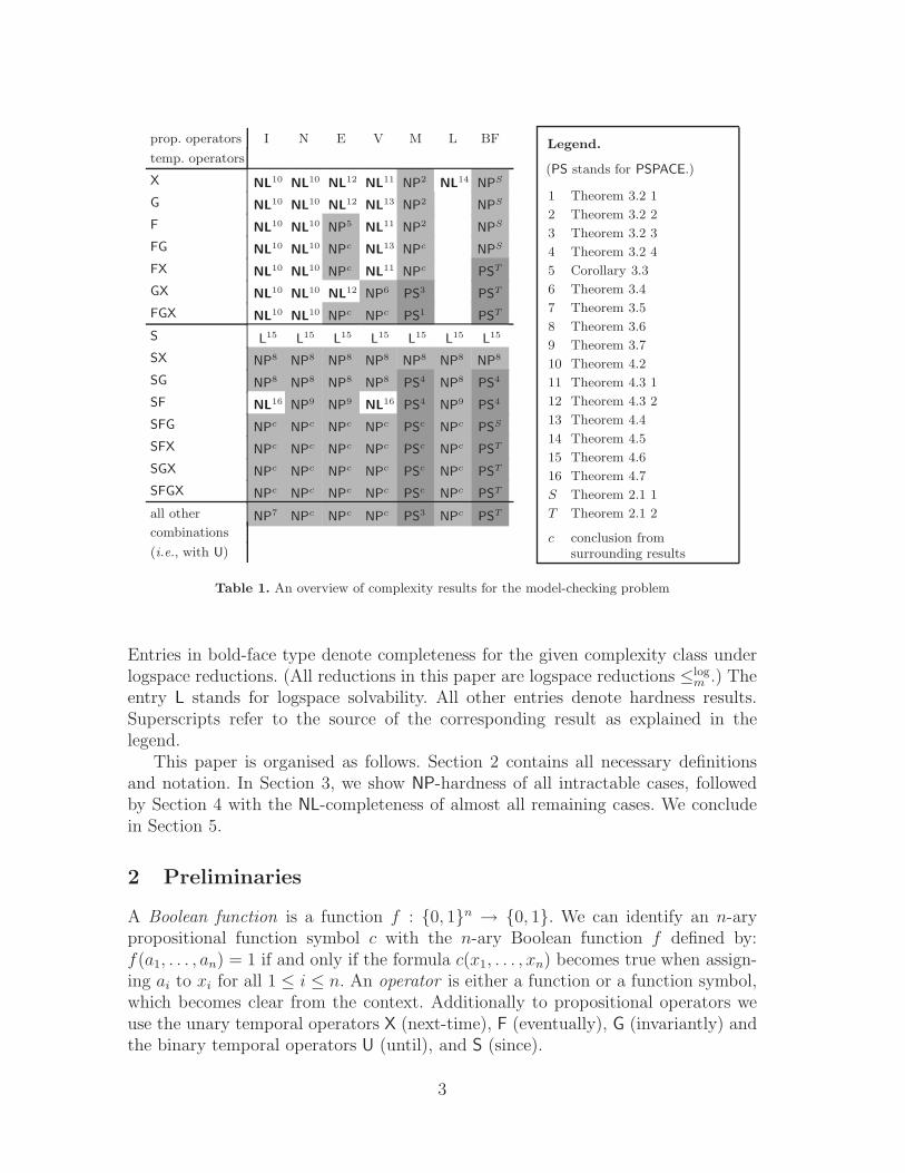
Table 1 gives an overview of our results. The top row refers to the sets of Booleanoperators given in Definition 2.3. These seven sets of Boolean operators are allrelevant cases, which is due to Post’s fundamental paper [Pos41] and Lemma 2.2.

2

prop. operators I N E V M L BF

temp. operators

X NL10

NL10

NL12

NL11

NP2

NL14

NPS

G NL10

NL10

NL12

NL13

NP2

NPS

F NL10

NL10

NP5

NL11

NP2

NPS

FG NL10

NL10

NPc

NL13

NPc

NPS

FX NL10

NL10

NPc

NL11

NPc

PST

GX NL10

NL10

NL12

NP6

PS3

PST

FGX NL10

NL10

NPc

NPc

PS1

PST

S L15

L15

L15

L15

L15

L15

L15

SX NP8

NP8

NP8

NP8

NP8

NP8

NP8

SG NP8

NP8

NP8

NP8

PS4

NP8

PS4

SF NL16

NP9

NP9

NL16

PS4

NP9

PS4

SFG NPc

NPc

NPc

NPc

PSc

NPc

PSS

SFX NPc

NPc

NPc

NPc

PSc

NPc

PST

SGX NPc

NPc

NPc

NPc

PSc

NPc

PST

SFGX NPc

NPc

NPc

NPc

PSc

NPc

PST

all other NP7

NPc

NPc

NPc

PS3

NPc

PST

combinations

(i.e., with U)

Legend.

(PS stands for PSPACE.)

1 Theorem 3.2 1

2 Theorem 3.2 2

3 Theorem 3.2 3

4 Theorem 3.2 4

5 Corollary 3.3

6 Theorem 3.4

7 Theorem 3.5

8 Theorem 3.6

9 Theorem 3.7

10 Theorem 4.2

11 Theorem 4.3 1

12 Theorem 4.3 2

13 Theorem 4.4

14 Theorem 4.5

15 Theorem 4.6

16 Theorem 4.7

S Theorem 2.1 1

T Theorem 2.1 2

c conclusion fromsurrounding results

Table 1. An overview of complexity results for the model-checking problem

Entries in bold-face type denote completeness for the given complexity class underlogspace reductions. (All reductions in this paper are logspace reductions ≤log

m .) Theentry L stands for logspace solvability. All other entries denote hardness results.Superscripts refer to the source of the corresponding result as explained in thelegend.

This paper is organised as follows. Section 2 contains all necessary definitionsand notation. In Section 3, we show NP-hardness of all intractable cases, followedby Section 4 with the NL-completeness of almost all remaining cases. We concludein Section 5.

2 Preliminaries

A Boolean function is a function f : {0, 1}n → {0, 1}. We can identify an n-arypropositional function symbol c with the n-ary Boolean function f defined by:f(a1, . . . , an) = 1 if and only if the formula c(x1, . . . , xn) becomes true when assign-ing ai to xi for all 1 ≤ i ≤ n. An operator is either a function or a function symbol,which becomes clear from the context. Additionally to propositional operators weuse the unary temporal operators X (next-time), F (eventually), G (invariantly) andthe binary temporal operators U (until), and S (since).

3

Let B be a finite set of Boolean operators and T be a set of temporal operators. Atemporal B-formula over T is a formula ϕ that is built from variables, propositionaloperators from B, and temporal operators from T . More formally, a temporal B-formula over T is either a propositional variable or of the form f(ϕ1, . . . , ϕn) org(ϕ1, . . . , ϕm), where ϕi are temporal B-formulae over T , f is an n-ary propositionaloperator from B and g is an m-ary temporal operator from T . In [SC85], complexityresults for formulae using the temporal operators F, G, X (unary), and U, S (binary)were presented. We extend these results to temporal B-formulae over subsets of thosetemporal operators. The set of variables appearing in ϕ is denoted by VAR(ϕ). IfT = {X, F,G,U, S} we call ϕ a temporal B-formula, and if T = ∅ we call ϕ apropositional B-formula or simply a B-formula. The set of all temporal B-formulaeover T is denoted with L(T,B).

A Kripke structure is a triple K = (W,R, η), where W is a finite set of states,R ⊆W ×W is a total binary relation (meaning that, for each a ∈W , there is someb ∈W such that aRb)7, and η : W → 2VAR for a set VAR of variables.

A model in linear temporal logic is a linear structure of states, which intuitivelycan be seen as different points of time, with propositional assignments. Formally,a path p in K is an infinite sequence denoted as (p0, p1, . . . ), where, for all i ≥ 0,pi ∈W and piRpi+1.

For a temporal {∧,¬}-formula over {F,G,X,U, S} with variables from VAR, aKripke structure K = (W,R, η), and a path p in K, we define what it means thatpK satisfies ϕ in pi (pK , i � ϕ): let ϕ1 and ϕ2 be temporal {∧,¬}-formulae over{F,G,X,U, S} and let x ∈ VAR be a variable.

pK , i � 1 and pK , i 6� 0

pK , i � x iff x ∈ η(pi)

pK , i � ϕ1 ∧ ϕ2 iff pK , i � ϕ1 and pK , i � ϕ2

pK , i � ¬ϕ1 iff pK , i 2 ϕ1

pK , i � Fϕ1 iff there is a j ≥ i such that pK , j � ϕ1

pK , i � Gϕ1 iff for all j ≥ i, pK , j � ϕ1

pK , i � Xϕ1 iff pK , i+ 1 � ϕ1

pK , i � ϕ1Uϕ2 iff there is an ℓ ≥ i such that pK , ℓ � ϕ2,and for every i ≤ j < ℓ, pK , j � ϕ1

pK , i � ϕ1Sϕ2 iff there is an ℓ ≤ i such that pK , ℓ � ϕ2,and for every ℓ < j ≤ i, pK , j � ϕ1

Since every Boolean operator can be composed from ∧ and ¬, the above definitiongeneralises to temporal B-formulae for arbitrary sets B of Boolean operators.

This paper examines the model-checking problems MC(T,B) for finite sets B ofBoolean functions and sets T of temporal operators.

7 In the strict sense, Kripke structures can have arbitrary binary relations. However, when referring toKripke structures, we always assume their relations to be total.

4

Problem: MC(T,B)

Input: 〈ϕ,K, a〉, where ϕ ∈ L(T,B) is a formula, K = (W,R, η) is aKripke structure, and a ∈ W is a state

Question: Is there a path p in K such that p0 = a and pK , 0 � ϕ?

Sistla and Clarke [SC85] have established the computational complexity of themodel-checking problem for temporal {∧,∨,¬}-formulae over some sets of temporaloperators.

Theorem 2.1 ([SC85]).

(1) MC({F}, {∧,∨,¬}) is NP-complete.(2) MC({F,X}, {∧,∨,¬}), MC({U}, {∧,∨,¬}), and MC({U, S,X}, {∧,∨,¬}) are

PSPACE-complete.

Since there are infinitely many finite sets of Boolean functions, we introduce somealgebraic tools to classify the complexity of the infinitely many arising satisfiabilityproblems. We denote with idnk the n-ary projection to the k-th variable, where 1 ≤k ≤ n, i.e., idnk(x1, . . . , xn) = xk, and with cna the n-ary constant function definedby cna(x1, . . . , xn) = a. For c11(x) and c10(x) we simply write 1 and 0. A set C ofBoolean functions is called a clone if it is closed under superposition, which meansC contains all projections and C is closed under arbitrary composition [Pip97]. Fora set B of Boolean functions we denote with [B] the smallest clone containing B

and call B a base for [B]. In [Pos41] Post classified the lattice of all clones and founda finite base for each clone.

The definitions of all clones as well as the full inclusion graph can be found,for example, in [BCRV03]. The following lemma implies that only clones with bothconstants 0, 1 are relevant for the model-checking problem; hence we will only definethose clones. Note, however, that our results will carry over to all clones.

Lemma 2.2. Let B be a finite set of Boolean functions and T be a set of temporaloperators. Then MC(T,B ∪ {0, 1}) ≡log

m MC(T,B).

Proof. MC(T,B) ≤logm MC(T,B ∪ {0, 1}) is trivial. For MC(T,B ∪ {0, 1}) ≤log

m

MC(T,B) let 〈ϕ,K, a〉 be an instance of MC(T,B ∪ {0, 1}) for a Kripke structureK = (W,R, η) and let ⊥ and ⊤ be two fresh variables. We define a new KripkestructureK ′ = (W,R, η′) where η′(α) = η(α)∪{⊤} and we define ϕ′ to be a copy of ϕwhere every appearance of 0 is replaced by ⊥ and every appearance of 1 by ⊤. It holdsthat 〈ϕ′, K ′, a〉 is an instance of MC(T,B) and that 〈ϕ,K, a〉 ∈ MC(T,B ∪ {0, 1})if and only if 〈ϕ′, K ′, a〉 ∈ MC(T,B). ❏

Because of Lemma 2.2 it is sufficient to look only at the clones with constants,which are introduced in Definition 2.3. Their bases and inclusion structure are givenin Figure 1.

Definition 2.3. Let ⊕ denote the binary exclusive or. Let f be an n-ary Booleanfunction.

5

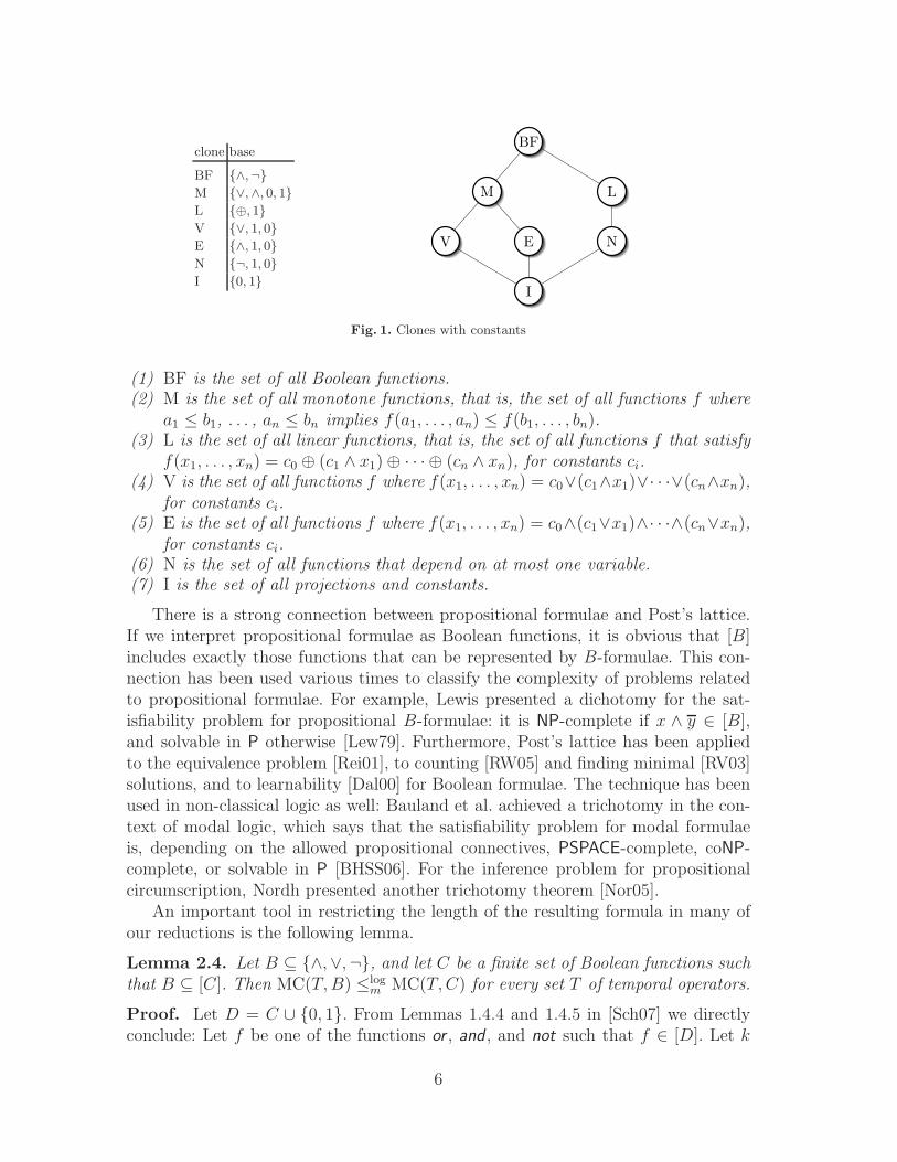
clone base

BF {∧,¬}

M {∨,∧, 0, 1}

L {⊕, 1}

V {∨, 1, 0}

E {∧, 1, 0}

N {¬, 1, 0}

I {0, 1}I

V E N

M L

BF

Fig. 1. Clones with constants

(1) BF is the set of all Boolean functions.(2) M is the set of all monotone functions, that is, the set of all functions f where

a1 ≤ b1, . . . , an ≤ bn implies f(a1, . . . , an) ≤ f(b1, . . . , bn).(3) L is the set of all linear functions, that is, the set of all functions f that satisfy

f(x1, . . . , xn) = c0 ⊕ (c1 ∧ x1) ⊕ · · · ⊕ (cn ∧ xn), for constants ci.(4) V is the set of all functions f where f(x1, . . . , xn) = c0∨(c1∧x1)∨· · ·∨(cn∧xn),

for constants ci.(5) E is the set of all functions f where f(x1, . . . , xn) = c0∧(c1∨x1)∧· · ·∧(cn∨xn),

for constants ci.(6) N is the set of all functions that depend on at most one variable.(7) I is the set of all projections and constants.

There is a strong connection between propositional formulae and Post’s lattice.If we interpret propositional formulae as Boolean functions, it is obvious that [B]includes exactly those functions that can be represented by B-formulae. This con-nection has been used various times to classify the complexity of problems relatedto propositional formulae. For example, Lewis presented a dichotomy for the sat-isfiability problem for propositional B-formulae: it is NP-complete if x ∧ y ∈ [B],and solvable in P otherwise [Lew79]. Furthermore, Post’s lattice has been appliedto the equivalence problem [Rei01], to counting [RW05] and finding minimal [RV03]solutions, and to learnability [Dal00] for Boolean formulae. The technique has beenused in non-classical logic as well: Bauland et al. achieved a trichotomy in the con-text of modal logic, which says that the satisfiability problem for modal formulaeis, depending on the allowed propositional connectives, PSPACE-complete, coNP-complete, or solvable in P [BHSS06]. For the inference problem for propositionalcircumscription, Nordh presented another trichotomy theorem [Nor05].

An important tool in restricting the length of the resulting formula in many ofour reductions is the following lemma.

Lemma 2.4. Let B ⊆ {∧,∨,¬}, and let C be a finite set of Boolean functions suchthat B ⊆ [C]. Then MC(T,B) ≤log

m MC(T, C) for every set T of temporal operators.

Proof. Let D = C ∪ {0, 1}. From Lemmas 1.4.4 and 1.4.5 in [Sch07] we directlyconclude: Let f be one of the functions or , and , and not such that f ∈ [D]. Let k

6

be the arity of f . Then there is a D-formula ϕ(x1, . . . , xk) representing f , such thatevery variable occurs only once in ϕ. Hence MC(T,B) ≤log

m MC(T, C ∪{0, 1}). FromLemma 2.2 follows MC(T, C ∪ {0, 1}) ≤log

m MC(T, C). ❏

It is essential for this Lemma that B ⊆ {∧,∨,¬}. For, e.g., B = {⊕}, it isopen whether MC(T,B) ≤log

m MC(T,BF). This is a reason why we cannot im-mediately transform upper bounds proven by Sistla and Clarke [SC85]—for ex-ample, MC({F,X}, {∧,∨,¬}) ∈ PSPACE—to upper bounds for all finite sets ofBoolean functions—i.e., it is open whether for all finite sets B of Boolean func-tions, MC({F,X}, B) ∈ PSPACE.

3 The bad fragments: intractability results

Sistla and Clarke [SC85] and Markey [Mar04] have considered the complexity ofmodel-checking for temporal {∧,∨,¬}-formulae restricted to atomic negation andpropositional negation, respectively. We define a temporal B-formula with proposi-tional negation to be a temporal B-formula where additional negations are allowed,but only in such a way that no temporal operator appears in the scope of a nega-tion sign. In the case that negation is an element of B, a temporal B-formula withpropositional negation is simply a temporal B-formula. In [SC85], atomic negationis considered, which restricts the use of negation even further—negation is onlyallowed directly for variables. We will now show that propositional negation doesnot make any difference for the complexity of the model checking problem. Sincethis obviously implies that atomic negation inherits the same complexity behaviour,we will only speak about propositional negation in the following. The proof of thefollowing lemma is similar to that of Lemma 2.2.

Lemma 3.1. Let T be a set of temporal operators, and B a finite set of Booleanfunctions. We use MC+(T,B) to denote the model-checking problem MC(T,B) ex-tended to B-formulae with propositional negation. Then MC+(T,B) ≡log

m MC(T,B).

Proof. The reduction MC(T,B) ≤logm MC+(T,B) is trivial. For MC+(T,B) ≤log

m

MC(T,B), assume that negation is not an element of B, otherwise there is nothingto prove. Let 〈ϕ,K, a〉 be an instance of MC+(T,B), where K = (W,R, η). Letx1, . . . , xm be the variables that appear in ϕ, and for each formula of the kind¬ψ(x1, . . . , xn) appearing in ϕ, let y¬ψ be a new variable. Note that since onlypropositional negation is allowed in ϕ, in these cases ψ is purely propositional.

We obtain K ′ = (W,R, η′) from K by extending η to the variables y¬ψ in sucha way that y¬ψ is true in a state if and only if ψ(x1, . . . , xn) is false. Finally, toobtain ϕ′ from ϕ we replace every appearance of ¬ψ(x1, . . . , xn) with y¬ψ. Now,ϕ′ is a temporal B-formula. By the construction it is straightforward to see that〈ϕ,K, a〉 ∈ MC+(T,B) iff 〈ϕ′, K ′, a〉 ∈ MC(T,B). ❏

Using Lemma 2.4 in addition, we can generalise the above mentioned hardnessresults from [SC85, Mar04] for temporal monotone formulae to obtain the followingintractability results for model-checking.

7

Theorem 3.2. Let M+ be a finite set of Boolean functions such that M ⊆ [M+].Then

(1) MC({F,G,X},M+) is PSPACE-hard.(2) MC({F},M+), MC({G},M+), and MC({X},M+) are NP-hard.(3) MC({U},M+) and MC({G,X},M+) are PSPACE-hard.(4) MC({S,G},M+) and MC({S, F},M+) are PSPACE-hard.

In Theorem 3.5 in [SC85] it is shown that MC({F}, {∧,∨,¬}) is NP-hard. Infact, Sistla and Clarke give a reduction from 3SAT to MC({F}, {∧}). The result forarbitrary bases B generating a clone above E follows from Lemma 2.4.

Corollary 3.3. Let E+ be a finite set of Boolean functions such that E ⊆ [E+].Then MC({F}, E+) is NP-hard.

The model-checking problem for temporal {G,X}-{∧,∨}-formulae is PSPACE-complete (Theorem 3.23 due to [Mar04]). The Boolean operators {∧,∨} are a basisof M, the class of monotone Boolean formulae. What happens for fragments of M?In Theorem 4.3 we will show that MC({G,X},E) is NL-complete, i.e., the model-checking problem for temporal {∧}-formulae over {G,X} is very simple. We canprove that switching from ∧ to ∨ makes the problem intractable. As notation, weuse LIT(ϕ) to denote the literals obtained from variables that appear in ϕ.

Theorem 3.4. Let V+ be a finite set of Boolean functions such that V ⊆ [V+]. ThenMC({G,X}, V+) is NP-hard.

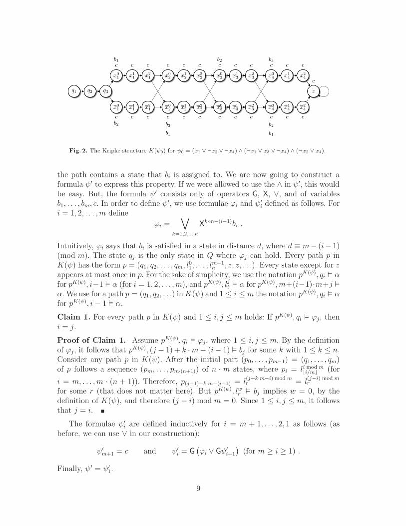
Proof. It suffices to give a reduction from 3SAT to MC({G,X}, {∨}) (due toLemma 2.4). A formula ψ in 3CNF is mapped to an instance 〈ψ′, K(ψ), q1〉 ofMC({G,X}, {∨}) as follows. Let ψ = C1 ∧ . . . ∧ Cm consist of m clauses, andn = |VAR(ψ)| variables. The Kripke structure K(ψ) has states Q = {q1, . . . , qm}containing one state for every clause, a sequence of states P = {lj | l ∈ LIT(ψ), 0 ≤j ≤ m − 1} for every literal, and a final sink state z. That is, the set of states isQ ∪ P ∪ {z}. The variables of K(ψ) are b1, . . . , bm, c. Variable ba is assigned true ina state l0i iff literal li is contained in clause Ca. In all other states, every bi is false.Variable c is assigned true in all states in P ∪ {z}.

The relation between the states is E1 ∪ E2 ∪ E3 ∪ E4 ∪ E5 as follows. It startswith the path q1, . . . , qm: E1 = {(qi, qi+1) | i = 1, 2, . . . , m − 1}. qm has an edgeto x0

1 and an edge to x01: E2 = {(qm, x

01), (qm, x

01)}. Each l0i is the starting point

of a path l0i , l1i , . . . , l

m−1i : E3 = {(lji , l

j+1i ) | li ∈ LIT(ψ), j = 0, 1, . . . , m − 2}. Each

endpoint of these paths has both the literals with the next index resp. the finalsink state as neighbours: E4 = {(lm−1

i , l0i+1) | i = 1, 2, . . . , n − 1, li ∈ LIT(ψ)} ∪{(xm−1

n , z), (xm−1n , z)}. The final sink state z has an edge to z itself, E5 = {(z, z)}.

Figure 2 shows an example for a formula ψ0 and the Kripke structure K(ψ0).Notice that every path in such a Kripke structureK(ψ) corresponds to an assignmentto the variables in ψ. A path corresponds to a satisfying assignment iff for every bi

8

q1 q2 q3

x01

x01

x11

x11

x21

x21

x02

x02

x12

x12

x22

x22

x03

x03

x13

x13

x23

x23

x04

x04

x14

x14

x24

x24

z

c c c c c c c c c c c c

c

c c c c c c c c c c c c

b1 b2 b3

b2 b3

b1

b2

b1

Fig. 2. The Kripke structure K(ψ0) for ψ0 = (x1 ∨ ¬x2 ∨ ¬x4) ∧ (¬x1 ∨ x3 ∨ ¬x4) ∧ (¬x2 ∨ x4).

the path contains a state that bi is assigned to. We are now going to construct aformula ψ′ to express this property. If we were allowed to use the ∧ in ψ′, this wouldbe easy. But, the formula ψ′ consists only of operators G, X, ∨, and of variablesb1, . . . , bm, c. In order to define ψ′, we use formulae ϕi and ψ′

i defined as follows. Fori = 1, 2, . . . , m define

ϕi =∨

k=1,2,...,n

Xk·m−(i−1)bi .

Intuitively, ϕi says that bi is satisfied in a state in distance d, where d ≡ m− (i− 1)(mod m). The state qj is the only state in Q where ϕj can hold. Every path p inK(ψ) has the form p = (q1, q2, . . . , qm, l

01, . . . , l

m−1n , z, z, . . .). Every state except for z

appears at most once in p. For the sake of simplicity, we use the notation pK(ψ), qi � α

for pK(ψ), i−1 � α (for i = 1, 2, . . . , m), and pK(ψ), lji � α for pK(ψ), m+(i−1)·m+j �

α. We use for a path p = (q1, q2, . . .) inK(ψ) and 1 ≤ i ≤ m the notation pK(ψ), qi � α

for pK(ψ), i− 1 � α.

Claim 1. For every path p in K(ψ) and 1 ≤ i, j ≤ m holds: If pK(ψ), qi � ϕj, theni = j.

Proof of Claim 1. Assume pK(ψ), qi � ϕj, where 1 ≤ i, j ≤ m. By the definitionof ϕj , it follows that pK(ψ), (j − 1) + k ·m− (i− 1) � bj for some k with 1 ≤ k ≤ n.Consider any path p in K(ψ). After the initial part (p0, . . . , pm−1) = (q1, . . . , qm)of p follows a sequence (pm, . . . , pm·(n+1)) of n · m states, where pi = li mod m

⌊i/m⌋ (for

i = m, . . . ,m · (n + 1)). Therefore, p(j−1)+k·m−(i−1) = l(j+k·m−i) mod mr = l

(j−i) mod mr

for some r (that does not matter here). But pK(ψ), lwr � bj implies w = 0, by thedefinition of K(ψ), and therefore (j − i) mod m = 0. Since 1 ≤ i, j ≤ m, it followsthat j = i. �

The formulae ψ′i are defined inductively for i = m + 1, . . . , 2, 1 as follows (as

before, we can use ∨ in our construction):

ψ′m+1 = c and ψ′

i = G(

ϕi ∨ Gψ′i+1

)

(for m ≥ i ≥ 1) .

Finally, ψ′ = ψ′1.

9

It is clear that the reduction function ψ 7→ 〈ψ′, K(ψ), q1〉 can be computedin logarithmic space. It remains to prove the correctness of the reduction. UsingClaim 1, we make the following observation.

Claim 2. For every path p = (q1, q2, . . .) in K(ψ) and i = 1, 2, . . . , m holds:pK(ψ), qi � ψ′

i if and only if for j = i, i+ 1, . . . , m holds pK(ψ), qj � ϕj .

Proof of Claim 2. The direction from right to left is straightforward. To provethe other direction, we use induction.

As base case we consider i = m. Assume pK(ψ), qm � G(ϕm∨Gc). By constructionof K(ψ) holds pK(ψ), qm 2 c, and therefore pK(ψ), qm � ϕm holds.

For the inductive step, assume pK(ψ), qi � G(ϕi∨Gψ′i+1). Claim 1 proves pK(ψ), qi 2

ϕj for j 6= i, and with pK(ψ), qi 2 c we obtain pK(ψ), qi 2 Gψ′i+1. This implies

pK(ψ), qi � ϕi and pK(ψ), qi+1 � ψ′i+1. By the inductive hypothesis, the claim follows.

�

For a path p in K(ψ), let Ap be the corresponding assignment for ψ. It is clearthat pK(ψ), qi � ϕi if and only if Ap satisfies clause Ci of ψ. Using Claim 2, it followsthat pK(ψ), q1 � ψ′ if and only if Ap satisfies all clauses of ψ, i.e., Ap satisfies ψ.Using the one-to-one correspondence between paths in K(ψ) and assignments tothe variables of ψ we get ψ ∈ 3SAT if and only if 〈ψ′, K(ψ), q1〉 ∈ MC({G,X}, {∨}).

❏

From [SC85] it follows that MC({G,X},V) is in PSPACE. It remains open whetherMC({G,X},V) or MC({G,X},M) have an upper bound below PSPACE.

Next, we consider formulae with the until-operator or the since-operator. Wefirst show that using the until-operator makes model-checking intractable.

Theorem 3.5. Let B be a finite set of Boolean functions. Then MC({U}, B) isNP-hard.

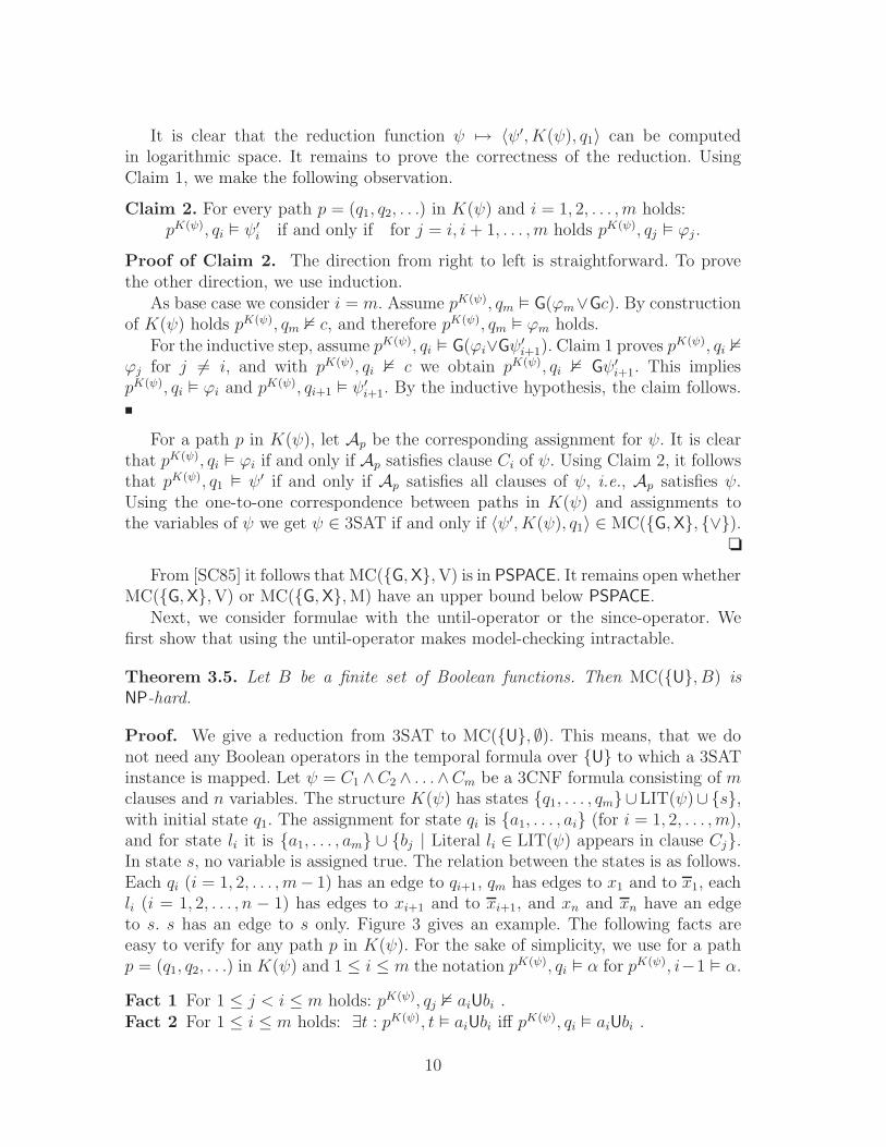
Proof. We give a reduction from 3SAT to MC({U}, ∅). This means, that we donot need any Boolean operators in the temporal formula over {U} to which a 3SATinstance is mapped. Let ψ = C1 ∧C2 ∧ . . .∧Cm be a 3CNF formula consisting of mclauses and n variables. The structure K(ψ) has states {q1, . . . , qm}∪LIT(ψ)∪ {s},with initial state q1. The assignment for state qi is {a1, . . . , ai} (for i = 1, 2, . . . , m),and for state li it is {a1, . . . , am} ∪ {bj | Literal li ∈ LIT(ψ) appears in clause Cj}.In state s, no variable is assigned true. The relation between the states is as follows.Each qi (i = 1, 2, . . . , m− 1) has an edge to qi+1, qm has edges to x1 and to x1, eachli (i = 1, 2, . . . , n − 1) has edges to xi+1 and to xi+1, and xn and xn have an edgeto s. s has an edge to s only. Figure 3 gives an example. The following facts areeasy to verify for any path p in K(ψ). For the sake of simplicity, we use for a pathp = (q1, q2, . . .) in K(ψ) and 1 ≤ i ≤ m the notation pK(ψ), qi � α for pK(ψ), i−1 � α.

Fact 1 For 1 ≤ j < i ≤ m holds: pK(ψ), qj 2 aiUbi .Fact 2 For 1 ≤ i ≤ m holds: ∃t : pK(ψ), t � aiUbi iff pK(ψ), qi � aiUbi .

10

q1 q2 q3

x1

x1

x2

x2

x3

x3

x4

x4

s

a1

a2

a1

a3

a2

a1a3

a2

a1

a3

a2

a1

a3

a2

a1

a3

a2

a1

b1

b2 b3

b1

b2 b3

b2

b1

Fig. 3. Structure K(ψ) for ψ = (x1 ∨ ¬x2 ∨ ¬x4) ∧ (¬x1 ∨ x3 ∨ ¬x4) ∧ (¬x2 ∨ x4)

The formulae ϕ0, ϕ1, . . . are defined inductively as follows.

ϕ0 = 1 and ϕi+1 = ϕiU (ai+1Ubi+1) .

The reduction from 3SAT to MC({U}, ∅) is the mapping ψ 7→ (ϕm, K(ψ), q1), whereψ is a 3CNF-formula with m clauses. This reduction can evidently be performed inlogarithmic space. To prove its correctness, we use the following claim.

Claim 3. Let K(ψ) be constructed from a formula ψ with m clauses, and let pbe a path in K(ψ). For j = 1, 2, . . . , m, it holds that pK(ψ), q1 � ϕj if and only ifpK(ψ), q1 � ϕj−1 and pK(ψ), qj � ajUbj .

Proof of Claim 3. We prove the claim by induction. The base case j = 1 isstraightforward: pK(ψ), q1 � 1 U(a1Ub1) is equivalent to ∃t : pK(ψ), t � (a1Ub1) whichby Fact 2 is equivalent to pK(ψ), q1 � a1Ub1. The inductive step is split into twocases. First, assume pK(ψ), q1 � ϕj+1. Since ϕj+1 = ϕjU(aj+1Ubj+1), it follows that∃t : pK(ψ), t � aj+1Ubj+1. Using Fact 2, we conclude pK(ψ), qj+1 � aj+1Ubj+1. ByFact 1, pK(ψ), q1 2 aj+1Ubj+1. By the initial assumption, this leads to pK(ψ), q1 � ϕj.Second, assume pK(ψ), q1 � ϕj and pK(ψ), qj+1 � aj+1Ubj+1. Using the inductionhypothesis, we obtain pK(ψ), qi � aiUbi for i = 1, 2, . . . , j + 1. By the construction ofϕj+1 we immediately get pK(ψ), q1 � ϕj+1. �

We have a one-to-one correspondence between paths in K(ψ) and assignmentsto variables of ψ. For a path p we will denote the corresponding assignment by Ap.Using Claim 3, it is easy to see that the following properties are equivalent.

1. Ap is a satisfying assignment for ψ.2. Path p in K(ψ) contains for every i = 1, 2, . . . , m a state with assignment bi.3. pK(ψ), qi � aiUbi for i = 1, 2, . . . , m.4. pK(ψ), q1 � ϕm.

This concludes the proof that ψ ∈ 3SAT if and only if 〈ϕm, K(ψ), q1〉 ∈ MC({U}, ∅).❏

Although the until-operator and the since-operator appear to be similar, model-checking for formulae that use the since-operator as only operator is as simple as

11

for formulae without temporal operators—see Theorem 4.6. The reason is that thesince-operator has no use at the beginning of a path of states, where no past exists.It needs other temporal operators that are able to enforce to visit a state on a paththat has a past.

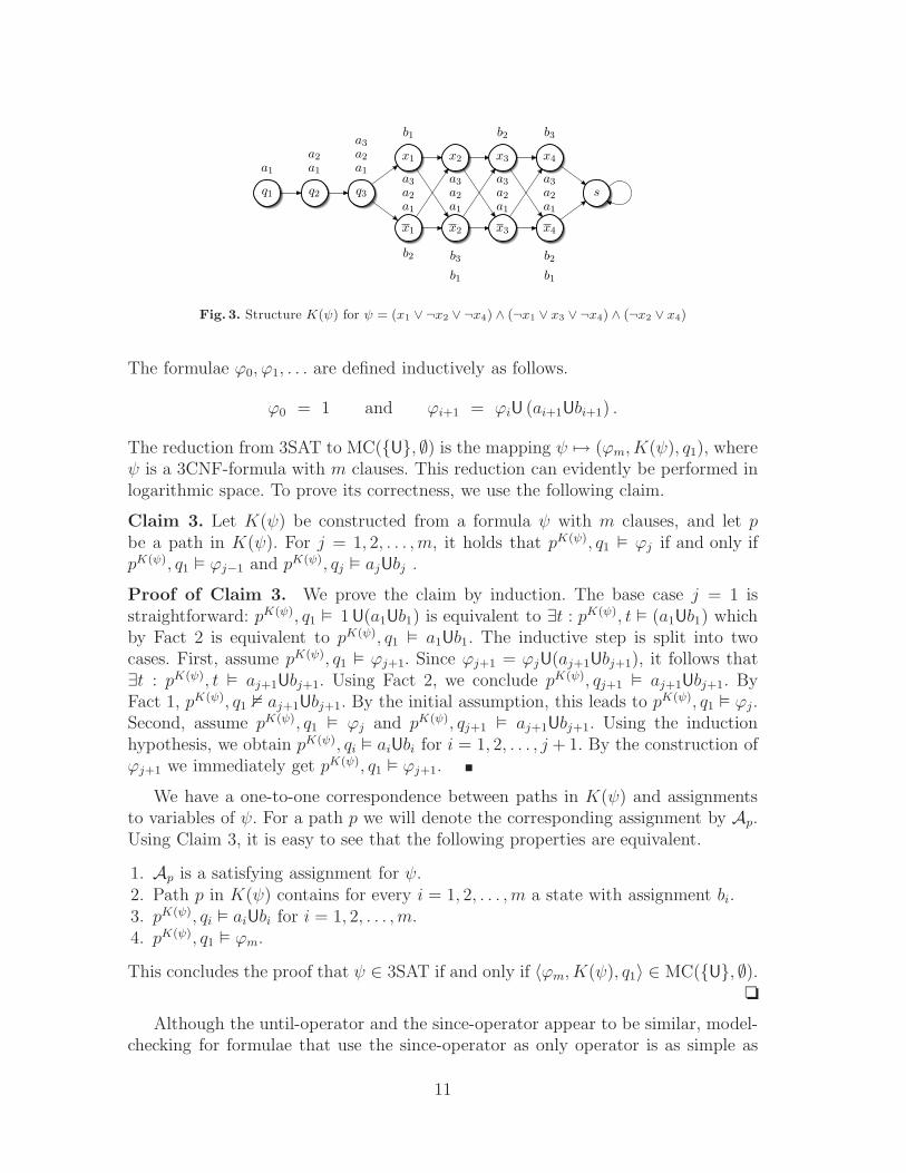
Theorem 3.6. Let B be a finite set of Boolean functions. Then MC({X, S}, B) andMC({G, S}, B) are NP-hard.

Proof. We give a reduction from 3SAT to MC({G, S}, ∅) that is similar to that inthe proof of Theorem 3.5 for MC({U}, ∅). Let ψ be an instance of 3SAT, and letK(ψ) be the structure as in the proof of Theorem 3.5. From K(ψ) = (W,R, η) weobtain the structure H(ϕ) = (W ′, R′, η′) as follows. First, we add a new state t, i.e.,W ′ = W ∪ {t}. Second, replace R by its inverse R−1 = {(v, u) | (u, v) ∈ R} fromwhich the loop at state s is removed. The state s has in-degree 0 and will be seenas initial state of H(ϕ). The new state t will be used as sink state. Therefore, weadd the arcs (q1, t) and (t, t). This results in R′ = (R−1 − {(s, s)}) ∪ {(q1, t), (t, t)}.Finally, we add a new variable e that is true only in state t, and a variable d thatis true in states LIT(ψ) ∪ {s}. For all other variables, η′ is the same as η. (Figure 4

q1 q2 q3

x1

x1

x2

x2

x3

x3

x4

x4

st

e da1

a2

a1

a3

a2

a1 d

a3

a2

a1

d

a3

a2

a1

d

a3

a2

a1

d

a3

a2

a1

b1

b2 b3

b1

b2 b3

b2

b1

Fig. 4. Structure H(ψ) for ψ = (x1 ∨ ¬x2 ∨ ¬x4) ∧ (¬x1 ∨ x3 ∨ ¬x4) ∧ (¬x2 ∨ x4)

shows an example.)

The formulae ϕm1 , ϕm2 , . . . , ϕ

mm+1 are defined inductively as follows.

ϕmm+1 = d and ϕmi =(

(aiSbi) Sϕmi+1

)

for i = 1, 2, . . . , m.

The reduction from 3SAT to MC({G, S}, ∅) is the mapping ψ 7→ 〈G(eSϕm1 ), H(ψ), s〉,where ψ is a 3CNF-formula with m clauses. This reduction can evidently be per-formed in logarithmic space. To prove its correctness, we use the following claim.Every path p = (s, ln, . . . , l1, qm, . . . , q1, t, t, . . .) in H(ψ) that begins in state s corre-sponds to an assignment Ap = {l1, . . . , ln} to the variables in ψ, that sets all literalsto true that appear on p. For the sake of simplicity, we use the notation pH(ψ), qi � α

for pH(ψ), n+m− i+ 1 � α.

12

Claim 4. Let H(ψ) be constructed from a formula ψ = C1∧. . .∧Cm with m clauses,and let p = (s, ln, . . . , l1, qm, . . . , q1, t, t, . . .) be a path in H(ψ). For j = 1, 2, . . . , mit holds that

pH(ψ), qj � ϕmj if and only if the assignment Ap satisfies clauses Cj, . . . , Cm.

Proof of Claim 4. Notice that Ap satisfies clause Cj if and only if p contains astate w with bj ∈ η′(w). We prove the claim by induction. Since the variable d holdsin all predecessors of qm in p but not in qm, it follows that ϕmm = (amSbm)Sd holds inqm iff amSbm holds in qm. Since bm 6∈ η′(qm), it follows that amSbm holds in qm iff bmholds in a predecessor of qm iff Ap satisfies Cm. This completes the base case. For theinductive step, notice that pH(ψ), qj � ϕmj iff pH(ψ), qj � ajSbj and pH(ψ), qj+1 � ϕj+1.

By the construction of H(ψ) it follows that pH(ψ), qj � ajSbj iff Ap satisfies Cj, andthe rest follows from the induction hypothesis. �

Finally, let ψ be a 3CNF formula, and let p = (s, ln, . . . , l1, qm, . . . , q1, t, t, . . .)be a path in H(ψ). On the first n + 1 states of p, the variable d holds. Therefore,ϕm1 and henceforth eSϕm1 is satisfied in all these states. On the m following statesqm, . . . , q1, neither d nor e holds. Notice that pH(ψ), qi � ϕmi iff pH(ψ), qi � ϕmi−1

(for i = 2, 3, . . . , m). By Claim 4, ϕm1 and henceforth eSϕm1 is satisfied in all thesestates iff Ap satisfies ψ. On the remaining states, only the variable e holds. Hence,eSϕm1 is satisfied in all the latter states iff Ap satisfies ψ. Concluding, it follows thatpH(ψ), 0 � G(eSϕm1 ) iff Ap satisfies ψ. Since for every assignment to ψ the structureH(ψ) contains a corresponding path, the correctness of the reduction is proven. ❏

The future-operator F alone is not powerful enough to make the since-operatorS NP-hard: We will show in Theorem 4.7 that MC({F, S}, B) for [B] ⊆ V is NL-complete. But with the help of ¬ or ∧, the model-checking problem for F and S

becomes intractable.

Theorem 3.7. Let N+ be a finite set of Boolean functions such that N ⊆ [N+].Then MC({F, S}, N+) is NP-hard.

Proof. By Lemma 2.4 it suffices to give a reduction from 3SAT to MC({F, S}, {¬}).For a 3CNF formula ψ, let 〈G(eSϕm1 ), H(ψ), s〉 be the instance of MC({G, S}, ∅) asdescribed in the proof of Theorem 3.6. Using Gα ≡ ¬F¬α, it follows that G(eSϕm1 ) ≡¬F(¬(eSϕm1 )), where the latter is a N-formula over {F, S}. The correctness of thereduction the same line as the proof of Theorem 3.6. ❏

Theorem 3.8. Let B be a finite set of Boolean functions. Then MC({X, S}, B) isNP-hard.

Proof. To prove NP-hardness, we give a reduction from 3SAT to MC({X, S}, ∅).For a 3CNF formula ψ, let H(ψ) be the structure as described in the proof ofTheorem 3.6. The reduction function maps ψ to 〈Xn+m+1ϕ1, H(ψ), s〉. The Xn+m+1

13

“moves” to state q1 on any path in H(ψ). The correctness proof follows the sameline as the proof of Theorem 3.6. ❏

An upper bound better than PSPACE for the intractable cases with the until-operator or the since-operator remains open. We will now show that one canonicalway to prove an NP upper bound fails, in showing that these problems do not havethe “short path property”, which claims that a path in the structure that fulfillsthe formula has length polynomial in the length of the structure and the formula.Hence, it will most likely be nontrivial to obtain a better upper bound.

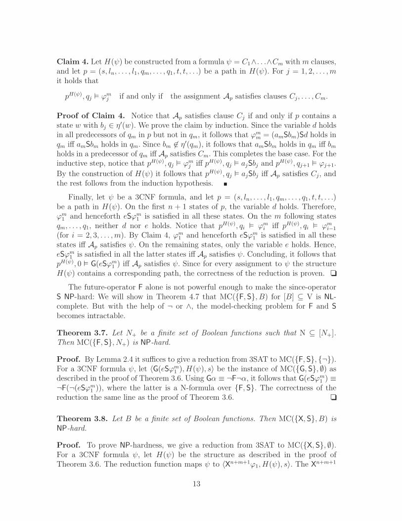
We will now sketch such families of structures and formulae using an inductivedefinition. Let G1, G2, . . . be the family of graphs presented in Figures 5 and 6.Notice that Gi is inserted into Gi+1 using the obvious lead-in and lead-out arrows.The truth assignments for these graphs are as follows:

x11 x1

2 x13

Fig. 5. The graph G1

xi+11 Gi xi+1

2 xi+13

Fig. 6. The graph Gi+1

G1 :

x11 b1x1

2 a1

x13 a1, c1

Gi+1 :

xi+11

∧i+1j=1 aj

xi+12 ai+1

xi+13

∧i+1j=1 aj, ci+1

x ∈ Gi truth assignment from Gi, bi+1

Now the formulae are defined as follows:

ϕ1 = (a1Ub1)Uc1, and ϕi+1 = ((ai+1Uϕi)Ubi+1)Uci+1.

The rough idea behind the construction is as follows: To satisfy the formula ϕ1

in G1, the path has to repeat the circle once. In the inductive construction, thisleads to an exponential number of repetitions.

4 The good fragments: tractability results

This subsection is concerned with fragments of LTL that have a tractable model-checking problem. We will provide a complete analysis for these fragments by provingthat model checking for all of them is NL-complete or even solvable in logarithmicspace. This exhibits a surprisingly large gap in complexity between easy and hardfragments.

The following lemma establishes NL-hardness for all tractable fragments.

14

Lemma 4.1. Let B be a finite set of Boolean functions. Then MC({F}, B),MC({G}, B), and MC({X}, B) are NL-hard.

Proof. First consider MC({F}, B). We reduce the accessibility problem for digraphs,GAP, to MC({F}, ∅). The reduction is via the following logspace computable func-tion. Given an instance 〈G, a, b〉 of GAP, where G = (V,E) is a digraph and a, b ∈ V ,map it to the instance 〈Fy,K(G), a〉 of MC({F}, ∅) with K(G) = (V,E+, η), whereE+ denotes the reflexive closure of E, and η is given by η(b) = {y} and η(v) = ∅,for all v ∈ V − {b}. It is immediately clear that there is a path from a to b in G ifand only if there is a path p in K(G) starting from a such that pK(G), 0 � Fy.

For MC({X}, B), we use an analogous reduction from GAP to MC({X}, ∅). Givenan instance 〈G, a, b〉 of GAP, where G = (V,E), transform it into the instance〈X|V |y,K(G), a

⟩

of MC({X}, ∅) with the Kripke structure K(G) from above. Now itis clear that there is a path from a to b in G if and only if there is a path of length|V | from a to b in the reflexive structure K(G), if and only if there is a path p inK(G) starting from a such that pK(G), 0 � X|V |y.

Now consider MC({G}, B). We reduce the following problem to MC({G}, ∅). Givena directed graph G = (V,E) and a vertex a ∈ V , is there an infinite path in G

starting at a? It is folklore that this is an NL-hard problem (see Lemma A.1 in theAppendix). Given an instance 〈G, a〉 of this problem, transform it into the instance〈Gy,K ′(G), a〉 of MC({G}, ∅), where K ′(G) = (V ′, E ′, η). Here V ′ = V ∪ {v | v ∈V, v has no successor in V }, E ′ = E ∪ {(v, v), (v, v) | v ∈ V ′}, η(v) = y for allv ∈ V , and η(v) = ∅, for all v ∈ V ′. It is immediately clear that there is an infinitepath in G starting at a if and only if there is a path p in K ′(G) starting from a suchthat pK

′(G), 0 � Gy. ❏

It now remains to establish upper complexity bounds. Let C be one of the clonesN, E, V, and L, and let B be a finite set of Boolean functions such that [B] ⊆ C.Whenever we want to establish NL-membership for some problem MC(·, B), it willsuffice to assume that formulae are given over one of the bases {¬, 0, 1}, {∧, 0, 1},{∨, 0, 1}, or {⊕, 0, 1}, respectively. This follows since these clones only contain con-stants, projections, and multi-ary versions of not, and , or , and ⊕, respectively.

Theorem 4.2. Let N− be a finite set of Boolean functions such that [N−] ⊆ N.Then MC({F,G,X}, N−) is NL-complete.

Proof. The lower bound follows from Lemma 4.1. For the upper bound, first notethat for an LTL formula ψ the following equivalences hold: FFψ ≡ Fψ, GGψ ≡ Gψ,FGFψ ≡ GFψ, GFGψ ≡ FGψ, Gψ ≡ ¬F¬ψ, and Fψ ≡ ¬G¬ψ. Furthermore, itis possible to interchange X and adjacent G-, F-, or ¬-operators without affectingsatisfiability. Under these considerations, each formula ϕ ∈ L({F,G,X}, N−) can betransformed without changing satisfiability into a normal form ϕ′ = XmP ∼y,where P is a prefix ranging over the values “empty string”, F, G, FG, and GF; m isthe number of occurrences of X in ϕ; ∼ is either the empty string or ¬; and y is a

15

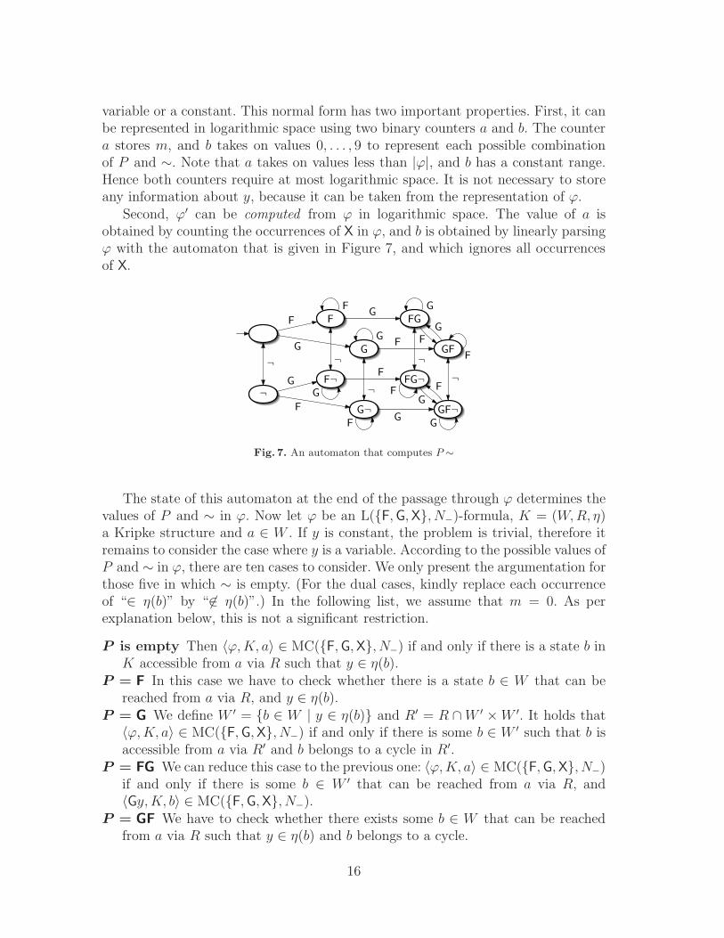
variable or a constant. This normal form has two important properties. First, it canbe represented in logarithmic space using two binary counters a and b. The countera stores m, and b takes on values 0, . . . , 9 to represent each possible combinationof P and ∼. Note that a takes on values less than |ϕ|, and b has a constant range.Hence both counters require at most logarithmic space. It is not necessary to storeany information about y, because it can be taken from the representation of ϕ.

Second, ϕ′ can be computed from ϕ in logarithmic space. The value of a isobtained by counting the occurrences of X in ϕ, and b is obtained by linearly parsingϕ with the automaton that is given in Figure 7, and which ignores all occurrencesof X.

F

G

FG

GF

¬

F¬

G¬

FG¬

GF¬

F

G

G

F

G

F

F

G

F

G

G

F

¬

¬

¬¬

¬

F

G

G

F

G

F

F

G

Fig. 7. An automaton that computes P ∼

The state of this automaton at the end of the passage through ϕ determines thevalues of P and ∼ in ϕ. Now let ϕ be an L({F,G,X}, N−)-formula, K = (W,R, η)a Kripke structure and a ∈ W . If y is constant, the problem is trivial, therefore itremains to consider the case where y is a variable. According to the possible values ofP and ∼ in ϕ, there are ten cases to consider. We only present the argumentation forthose five in which ∼ is empty. (For the dual cases, kindly replace each occurrenceof “∈ η(b)” by “ 6∈ η(b)”.) In the following list, we assume that m = 0. As perexplanation below, this is not a significant restriction.

P is empty Then 〈ϕ,K, a〉 ∈ MC({F,G,X}, N−) if and only if there is a state b inK accessible from a via R such that y ∈ η(b).

P = F In this case we have to check whether there is a state b ∈ W that can bereached from a via R, and y ∈ η(b).

P = G We define W ′ = {b ∈ W | y ∈ η(b)} and R′ = R ∩W ′ ×W ′. It holds that〈ϕ,K, a〉 ∈ MC({F,G,X}, N−) if and only if there is some b ∈ W ′ such that b isaccessible from a via R′ and b belongs to a cycle in R′.

P = FG We can reduce this case to the previous one: 〈ϕ,K, a〉 ∈ MC({F,G,X}, N−)if and only if there is some b ∈ W ′ that can be reached from a via R, and〈Gy,K, b〉 ∈ MC({F,G,X}, N−).

P = GF We have to check whether there exists some b ∈ W that can be reachedfrom a via R such that y ∈ η(b) and b belongs to a cycle.

16

Since the questions whether there is a path from any vertex to another and whetherany vertex belongs to a cycle in a directed graph can be answered in NL, all pre-viously given procedures are NL-algorithms. The restriction m = 0 is removed bythe observation that 〈XmP∼y,K, a〉 ∈ MC({F,G,X}, N−) if and only if there existssome state b in K that is accessible from a in m R-steps such that 〈P∼y,K, b〉 ∈MC({F,G,X}, N−). This reduces the case m > 0 to m = 0.

Hence we have found an NL-algorithm deciding MC({F,G,X}, N−): Given 〈ϕ,K, a〉,compute ϕ′, guess a state b accessible from a in m R-steps, apply the procedure ofone of the above five cases to 〈ϕ′, K, a〉, and accept if the last step was successful. ❏

Theorem 4.3. (1) Let V− be a finite set of Boolean functions such that [V−] ⊆ V.Then MC({F,X}, V−) is NL-complete.

(2) Let E− be a finite set of Boolean functions such that [E−] ⊆ E.Then MC({G,X}, E−) is NL-complete.

Proof. The lower bounds follow from Lemma 4.1.

First consider the case [V−] ⊆ V. It holds that F(ψ1∨· · ·∨ψn) ≡ Fψ1∨· · ·∨Fψn as wellas XFϕ ≡ FXϕ and X(ϕ∨ψ) ≡ Xϕ∨Xψ. Therefore, every formula ϕ ∈ L({F,X}, V−)can be rewritten as

ϕ′ = FXi1y1 ∨ · · · ∨ FX

inyn ∨ Xin+1yn+1 ∨ · · · ∨ X

imym,

where y1, . . . , ym are variables or constants (note that this representation of ϕ canbe constructed in L). Now let 〈ϕ,K, a〉 be an instance of MC({F,X}, V−), whereK = (W,R, η), and let ϕ be of the above form. Thus, 〈ϕ,K, a〉 ∈ MC({F,X}, V−) ifand only if for some j ∈ {n + 1, . . . , m}, there is a state b ∈ W such that yj ∈ η(b)and b is accessible from a in exactly ij R-steps or if, for some j ∈ {1, . . . , n}, thereis a state b ∈W such that yj ∈ η(b) and b is accessible from a in at least ij R-steps.This can be tested in NL.

As for the case [E−] ⊆ E, we take advantage of the duality of F and G, and ∧ and∨, respectively. Analogous considerations as above lead to the logspace computablenormal form

ϕ′ = GXi1y1 ∧ · · · ∧ GX

inyn ∧ Xin+1yn+1 ∧ · · · ∧ X

imym.

Let I = max{i1, . . . , im}. For each j = 1, . . . , m, we define W j = {b ∈W | yj ∈ η(b)}and Rj = R ∩W j ×W j. Furthermore, let W ′ be the union of W j for j = 1, . . . , n(!), and let R′ = R∩W ′ ×W ′. Now 〈ϕ,K, a〉 ∈ MC({G,X}, E−) if and only if thereis some state b ∈W ′ satisfying the following conditions.

– There is an R-path p of length at least I from a to b, where the first I + 1 stateson p are c0 = a, c1, . . . , cI .

– The state b′ lies on a cycle in W ′.– For each j = 1, . . . , n, each state of p from cij to cI is from W j .

17

– For each j = n+ 1, . . . , m, the state cij is from W j.

These conditions can be tested in NL as follows. Successively guess c1, . . . , cI andverify their membership in the appropriate sets W j. Then guess b, verify whetherb ∈W ′, whether b lies on some R′-cycle, and whether there is an R′-path from cI tob. ❏

In the proof of Theorem 4.3, we have exploited the duality of F and G, and ∨ and∧, respectively. Furthermore, the proof relied on the fact that F and ∨ (and G and ∧)are interchangeable. This is not the case for F and ∧, or G and ∨, respectively. Henceit is not surprising that MC({F}, {∧}) is NP-hard (Corollary 3.3). However, the NL-membership of MC({F,G}, {∨}) is surprising. Before we formulate this result, wetry to provide an intuition for the tractability of this problem. The main reason isthat an inductive view on L({F,G}, {∨})-formulae allows us to subsequently guessparts of a satisfying path without keeping the previously guessed parts in memory.This is possible because each L({F,G}, {∨})-formula ϕ can be rewritten as

ϕ = y1 ∨ · · · ∨ yn ∨ Fz1 ∨ · · · ∨ Fzm ∨ Gψ1 ∨ · · · ∨ Gψℓ ∨ FGψℓ+1 ∨ · · · ∨ FGψk, (1)

where the yi, zi are variables (or constants), and each ψi is an L({F,G}, {∨})-formulaof the same form with a strictly smaller nesting depth of G-operators. Now, ϕ is trueat the begin of some path p iff one of its disjuncts is true there. In case none of theyi or Fzi is true, we must guess one of the Gψi (or FGψj) and check whether ψi (orψj) is true on the entire path p (or on p minus some finite number of initial states).Now ψi is again of the above form. So we must either find an infinite path on whichy1 ∨ · · · ∨ yn ∨ Fz1 ∨ · · · ∨ Fzm is true everywhere (a cycle containing at least |N |states satisfying some yi or zi suffices, where N is the set of states of the Kripkestructure), or we must find a finite path satisfying the same conditions and followedby an infinite path satisfying one of the Gψi (or FGψj) at its initial point. Hence wecan recursively solve a problem of the same kind with reduced problem size. Notethat it is neither necessary to explicitly compute the normal form for ϕ or one ofthe ψi, nor need previously visited states be stored in memory.

Theorem 4.4. Let V− be a finite set of Boolean functions such that [V−] ⊆ V. ThenMC({G}, V−) and MC({F,G}, V−) are NL-complete.

Proof. The lower bound follows from Lemma 4.1. It remains to show NL-membershipof MC({F,G}, V−). For this purpose, we devise the recursive algorithm MC{F,G},V asgiven in Table 2. Note that we have deliberately left out constants. This is no re-striction, since we have observed in Lemma 2.2 that each constant can be regardedas a variable that is set to true or false throughout the whole Kripke structure.

The parameter mode indicates the current “mode” of the computation. The ideais as follows. In order to determine whether ϕ is satisfiable at the initial point ofsome structure starting at a in K, the algorithm has to be in mode now. This, hence,is the default setting for the first call of MC{F,G},V. As soon as the algorithm chooses

18

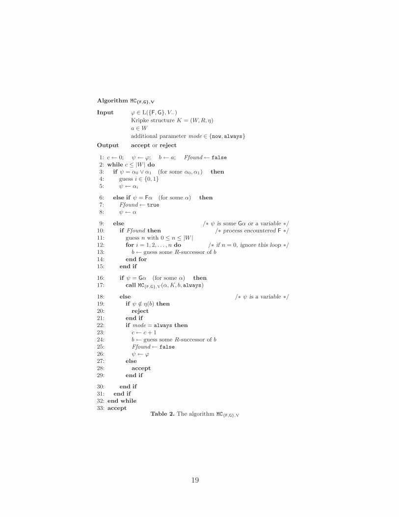
Algorithm MC{F,G},V

Input ϕ ∈ L({F,G}, V−)

Kripke structure K = (W,R, η)

a ∈W

additional parameter mode ∈ {now, always}

Output accept or reject

1: c← 0; ψ ← ϕ; b← a; Ffound← false

2: while c ≤ |W | do

3: if ψ = α0 ∨ α1 (for some α0, α1) then

4: guess i ∈ {0, 1}5: ψ ← αi

6: else if ψ = Fα (for some α) then

7: Ffound← true

8: ψ ← α

9: else /∗ ψ is some Gα or a variable ∗/10: if Ffound then /∗ process encountered F ∗/11: guess n with 0 ≤ n ≤ |W |12: for i = 1, 2, . . . , n do /∗ if n = 0, ignore this loop ∗/13: b← guess some R-successor of b14: end for

15: end if

16: if ψ = Gα (for some α) then

17: call MC{F,G},V(α,K, b, always)

18: else /∗ ψ is a variable ∗/19: if ψ /∈ η(b) then

20: reject

21: end if

22: if mode = always then

23: c← c+ 124: b← guess some R-successor of b25: Ffound← false

26: ψ ← ϕ27: else

28: accept

29: end if

30: end if

31: end if

32: end while

33: acceptTable 2. The algorithm MC{F,G},V

19

to process a G-subformula Gα of ϕ, it has to determine whether α is satisfiable atevery point in some structure starting at the currently visited state inK. It thereforechanges into always mode and calls itself recursively with the first parameter set toα, see Line 17.

Hence, given an instance 〈ϕ,K, a〉 of the problem MC({F,G}, V−), we have toinvoke MC{F,G},V(ϕ,K, a, now) in order to determine whether there is a satisfying pathfor ϕ in K starting at a. It is easy to see that this call always terminates: First,whenever the algorithm calls itself recursively, the first argument of the new call is astrict subformula of the original first argument. Therefore there can be at most |ϕ|recursive calls. Second, within each call, each passage through the while loop (Lines2–32) either decreases ψ or increases c. Hence, there can be at most |ϕ| · (|W | + 1)passages through the while loop until the algorithm accepts or rejects.

MC{F,G},V is an NL algorithm: The values of all parameters and programme vari-ables are either subformulae of the original formula ϕ, states of the given Kripkestructure K, counters of range 0, . . . , |W | + 1, or Booleans. They can all be repre-sented using ⌈log |ϕ|⌉, ⌈log(|W | + 1)⌉, or constantly many bits. Furthermore, sincethe algorithm uses no return command, the recursive calls may re-use the spaceprovided for all parameters and programme variables, and no return addresses needbe stored.

It remains to show the correctness of MC{F,G},V, which we will do in two steps.in always mode, which will be shown by induction on the nesting depth of the G-operator in ϕ. We denote this value by µG(ϕ). Claim 6 will then ensure the correctbehaviour in now mode.

Claim 5. For each ϕ ∈ L({F,G},V), each K = (W,R, η), and each a ∈W :〈Gϕ,K, a〉 ∈ MC({F,G}, V−) ⇔ there is an accepting run of

MC{F,G},V(ϕ,K, a, always).

Proof of Claim 5. For the base case of the induction, let µG(ϕ) = 0. Because ofthe equivalences F(ψ1 ∨ ψ2) ≡ Fψ1 ∨ Fψ2 and FFψ ≡ Fψ, we may assume w.l.o.g.that any occurrence of the F-operator is in front of some variable in ϕ. If we thinkof ϕ as a tree, this means that F-operators can only occur in direct predecessors ofleaves. Note that the algorithm computes this normal form implicitly: Whenever itguesses a path from the root (ϕ) to some leaf (a variable) in the tree and encountersan F-operator in Line 6, the flag Ffound is set. Only after processing all ∨-operatorson the remaining part of the path, the F-operator is processed in Lines 10–15. Nowlet VAR1(ϕ) be all variables that occur in the scope of an F-operator in ϕ, and letVAR0(ϕ) be all other variables in ϕ.

For the “⇒” direction, suppose 〈Gϕ,K, a〉 ∈ MC({F,G}, V−). Then there exists apath p in K such that p0 = a, and for all i ≥ 0, pK , i � ϕ. This means that, foreach i, either there exists some xi ∈ VAR0(ϕ) such that pK , i � xi, or there is somexi ∈ VAR1(ϕ) such that pK , i � Fxi. Now it can be seen that there is a non-rejectingsequence of runs through the while loop in Lines 2–32 after which c has value |W |+1,which then leads to the accept in Line 33:

20

Consider the begin of an arbitrary single run through the while loop in Line 2.Let pi be the current value of b. If xi ∈ VAR0(ϕ), then the algorithm can “guess itsway through the tree of ϕ” in Lines 3–5 and finally reaches Line 19 with ψ = xi.It does not reject in Line 20, increases c in Line 23, guesses pi+1 in Line 24, andresets Ffound and ψ appropriately in Lines 25, 26. Otherwise, if xi ∈ VAR1(ϕ), thenthere is some n ≥ 0 such that pi+n satisfies xi. It is safe to assume that n ≤ |W |because otherwise the path from pi to pi+n would describe a cycle within K whichcould be replaced by a shorter, more direct, path without affecting satisfiability ofthe relevant subformulae in the states p0, . . . , pi. Now the algorithm can proceed asin the previous case, but, in addition, it has to guess the correct value of n and thesequence pi+1, . . . , pi+n in Lines 10–15.

For the “⇐” direction, let there be an accepting run of MC{F,G},V(ϕ,K, a, always).Since the algorithm is in always mode, and ϕ is G-free, the acceptance can only takeplace in Line 33, without a recursive call in Line 17. Hence the counter c reachesvalue |W | + 1 in the while loop in Lines 2–32.

Let p = p0, p1, . . . , pm be the sequence of states guessed in this run in Lines 13and 24, where p0 = a. Furthermore, let i0, . . . , i|W |+1 be an index sequence thatdetermines a subsequence of p such that

– 0 = i0 < i1 < · · · < i|W |+1 = m, and– for each j > 0, pij is the value assigned to b in Line 24 after having set c to valuej in Line 23.

Now it is clear that for all j = 0, . . . , |W |, there must be a variable xj such thatxj ∈ η(pij+1−1). If xj ∈ VAR0(ϕ), then pij+1

= pij +1, and each structure p′ extendingp beyond pm satisfies xj (and hence ϕ) at pij . Otherwise xj ∈ VAR1(ϕ), and theaccepting run of the algorithm has guessed the states pij , . . . , pij+1−1 in Line 13. Inthis case, each structure p′ extending p beyond pm satisfies Fxj (and hence ϕ) atpij , . . . , pij+1−1. From these two cases, we conclude that each such p′ satisfies ϕ in allstates p0, . . . , pm.

We now restrict attention to the states pi1−1, . . . , pi|W |+1−1. Among these |W |+1states, some of the |W | states of K has to occur twice. Assume pij−1 and pik−1 repre-sent the same state from K, where j < k. Then we can create an (infinite) structurep′′ from p that consists of states p0, . . . , pik−1, followed by an infinite repetition ofthe sequence pij , . . . , pik−1. It is now obvious that p′′ satisfies ϕ in every state, hencep′′, 0 � ϕ, that is, 〈Gϕ,K, a〉 ∈ MC({F,G}, V−).

For the induction step, let µG(ϕ) > 0. For the same reasons as above, we can assumethat any F-operator only occurs in front of variables or in front of some G-operatorin ϕ. This “normal form” is taken care of by setting Ffound to true when F is found(Line 7) and processing this occurrence of F only when a variable or some G-operatoris found (Lines 10–15).

For the “⇒” direction, suppose 〈Gϕ,K, a〉 ∈ MC({F,G}, V−). Then there exists apath p in K such that p0 = a, and for all i ≥ 0, pK � ϕ. We describe an accepting

21

run of MC{F,G},V(ϕ,K, a, always). Consider a single passage through the while loopwith the following configuration. The programme counter has value 2, c has valueat most |W |, b has value pi, and ψ has value ϕ. Since pK � ϕ, there are four possiblecases. The argumentation for the first two of them is the same as in the base case.

Case 1. pK , i � x, for some x ∈ VAR0(ϕ).Case 2. pK , i � Fx, for some x ∈ VAR1(ϕ).Case 3. pK , i � Gα, for some maximal G-subformula Gα of ϕ that is not in the scope

of some F-operator.This means that α is true everywhere on the path pi, pi+1, pi+2, . . . . Hence,due to the induction hypothesis, MC{F,G},V(α,K, bi, always) has an acceptingrun. By appropriate guesses in Line 4, the current call of the algorithm canreach that accepting recursive call in Line 17.

Case 4. pK , i � Gα, for some maximal G-subformula Gα of ϕ that is in the scope ofsome F-operator.By combining the arguments of Cases 3 and 2, we can find an acceptingrun for this case.

If only Cases 1 or 2 occur more than |W | times in a sequence, then c will finally takeon value |W | + 1, and this call will accept in Line 31. Otherwise, whenever one ofCases 3 and 4 occurs, than the acceptance of the new call—and hence of the currentcall—is due to the induction hypothesis.

For the “⇐” direction, let there be an accepting run of MC{F,G},V(ϕ,K, a, always).Since the algorithm is in always mode, the acceptance can only take place in Line33 or in the recursive call in Line 17. If the run accepts in Line 33, the same ar-guments as in the base case apply. If the acceptance is via the recursive call, thenlet p = p0, . . . , pm be the sequence of states guessed such that p0 = a, and pm isthe value of b when the recursive call with Gα takes place. Due to the inductionhypothesis, 〈Gα,K, bm〉 ∈ MC({F,G}, V−) and, hence, there is an infinite structurep′ extending p beyond pm such that (p′)K , m � Gϕ. Furthermore, we can use thesame argumentation as in the base case to show that, for each i ≤ m, (p′)K , i � ϕ.Therefore, (p′)K , 0 � Gϕ, which proves 〈Gϕ,K, a〉 ∈ MC({F,G}, V−). �

Claim 6. For each ϕ ∈ L({F,G}, V−), each K = (W,R, η), and each a ∈W :

〈ϕ,K, a〉 ∈ MC({F,G}, V−) ⇔ there is an accepting run of MC{F,G},V(ϕ,K, a, now)

Proof of Claim 6. For the “⇒” direction, suppose 〈ϕ,K, a〉 ∈ MC({F,G}, V−).Then there exists a path p in K such that p0 = a and pK , 0 � ϕ. We describe anaccepting run of MC{F,G},V(ϕ,K, a, now). Consider the first passage through the whileloop with the following configuration. The programme counter has value 2, c hasvalue 0 (this value does not change in now mode), b has value a, and ψ has value ϕ.Since pK , 0 � ϕ, there are four possible cases. The argumentation for them is verysimilar to that in the proof of Claim 5.

22

Case 1. pK , 0 � x, for some x ∈ VAR0(ϕ).As in the proof of Claim 5, the algorithm can guess the appropriate disjunctsin Lines 3–5, does not reject in Line 20 and accepts (it is in now mode!) inLine 28.

Case 2. pK , 0 � Fx, for some x ∈ VAR1(ϕ).As in the proof of Claim 5, there exists some n with 0 ≤ n ≤ |W | such thatbn satisfies xi. The algorithm can proceed as in the previous case, but, inaddition, it has to guess the correct value of n and the sequence p1, . . . , pnin Lines 10–15.

Case 3. pK , 0 � Gα, for some maximal G-subformula Gα of ϕ that is not in thescope of some F-operator.

This means that α is true everywhere on the path p. Hence, due to theinduction hypothesis, MC{F,G},V(α,K, bi, now) has an accepting run. By ap-propriate guesses in Line 4, the current call of the algorithm can reach thataccepting recursive call in Line 17.

Case 4. pK , 0 � Gα, for some maximal G-subformula Gα of ϕ that is in the scopeof some F-operator.By combining the arguments of Cases 3 and 2, we can find an acceptingrun for this case.

For the “⇐” direction, suppose there exists an accepting run of MC{F,G},V(ϕ,K, a, now).Since the algorithm is in now mode, the acceptance can only take place in Line 28or in the recursive call in Line 17. If the run accepts in Line 28, then there is somevariable x such that either x ∈ VAR0(ϕ) and x ∈ η(a), or x ∈ VAR1(ϕ) and the runguesses a path p0, . . . , pm with p0 = a and x ∈ η(pm). In both cases, each structurep′ extending the sequence of states guessed so far, satisfies ϕ at a. On the otherhand, if the run accepts in the recursive call, we can argue as in the proof of Claim5. � ❏

Unfortunately, the above argumentation fails for MC({G,X}, V ) because of thefollowing considerations. The NL-algorithm in the previous proof relies on the factthat a satisfying path for Gψ, where ψ is of the form (1), can be divided into a“short” initial part satisfying the disjunction of the atoms, and the remaining endpath satisfying one of the Gψi at its initial state. When guessing the initial part, itsuffices to separately guess each state and consult η.

If X were in our language, the disjuncts would be of the form Xkiyi and XℓiGψi.Not only would this make the guessing of the initial part more intricate. It wouldalso require memory for processing each of the previously satisfied disjuncts Xkiyi.An adequate modification of MC{F,G},V would require more than logarithmic space.We have shown NP-hardness for MC({G,X}, V ) in Theorem 3.4.

Theorem 4.5. Let L− be a finite set of Boolean functions such that [L−] ⊆ L. ThenMC({X}, L−) is NL-complete.

23

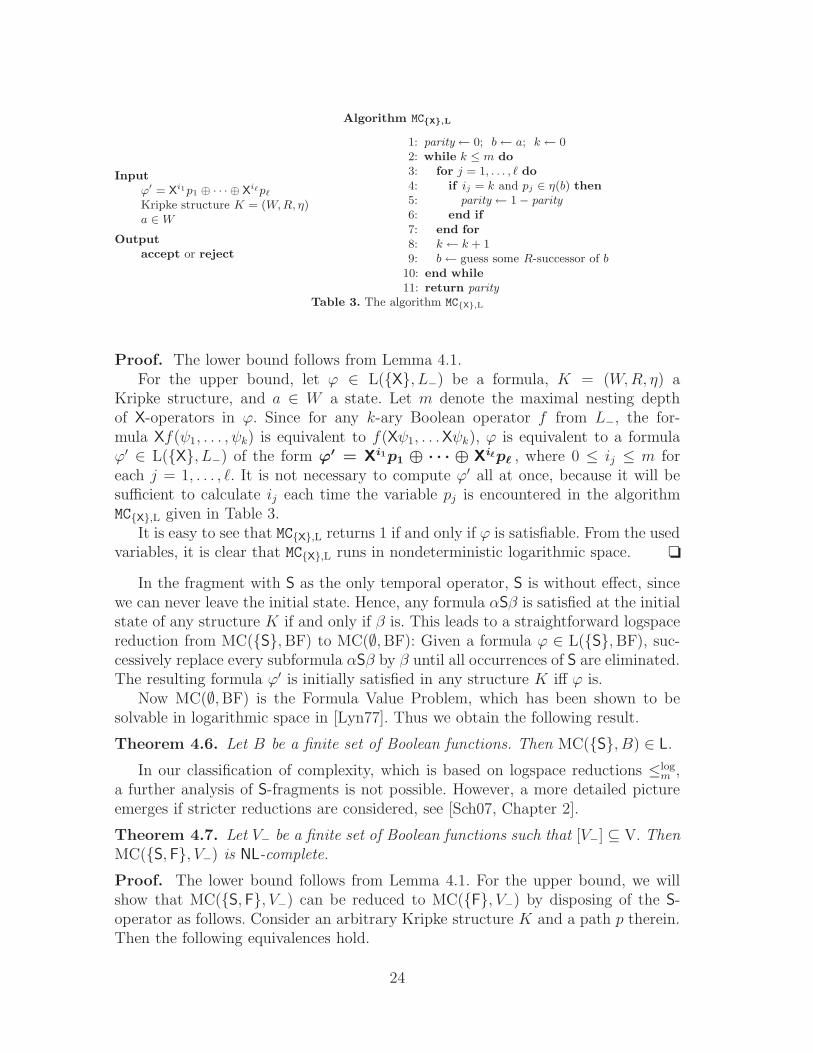
Algorithm MC{X},L

Input

ϕ′ = Xi1p1 ⊕ · · · ⊕ X

iℓpℓ

Kripke structure K = (W,R, η)a ∈ W

Output

accept or reject

1: parity← 0; b← a; k← 02: while k ≤ m do

3: for j = 1, . . . , ℓ do

4: if ij = k and pj ∈ η(b) then

5: parity← 1− parity

6: end if

7: end for

8: k← k + 19: b← guess some R-successor of b

10: end while

11: return parity

Table 3. The algorithm MC{X},L

Proof. The lower bound follows from Lemma 4.1.For the upper bound, let ϕ ∈ L({X}, L−) be a formula, K = (W,R, η) a

Kripke structure, and a ∈ W a state. Let m denote the maximal nesting depthof X-operators in ϕ. Since for any k-ary Boolean operator f from L−, the for-mula Xf(ψ1, . . . , ψk) is equivalent to f(Xψ1, . . .Xψk), ϕ is equivalent to a formulaϕ′ ∈ L({X}, L−) of the form ϕ′ = Xi1p1 ⊕ · · · ⊕ Xiℓpℓ , where 0 ≤ ij ≤ m foreach j = 1, . . . , ℓ. It is not necessary to compute ϕ′ all at once, because it will besufficient to calculate ij each time the variable pj is encountered in the algorithmMC{X},L given in Table 3.

It is easy to see that MC{X},L returns 1 if and only if ϕ is satisfiable. From the usedvariables, it is clear that MC{X},L runs in nondeterministic logarithmic space. ❏

In the fragment with S as the only temporal operator, S is without effect, sincewe can never leave the initial state. Hence, any formula αSβ is satisfied at the initialstate of any structure K if and only if β is. This leads to a straightforward logspacereduction from MC({S},BF) to MC(∅,BF): Given a formula ϕ ∈ L({S},BF), suc-cessively replace every subformula αSβ by β until all occurrences of S are eliminated.The resulting formula ϕ′ is initially satisfied in any structure K iff ϕ is.

Now MC(∅,BF) is the Formula Value Problem, which has been shown to besolvable in logarithmic space in [Lyn77]. Thus we obtain the following result.

Theorem 4.6. Let B be a finite set of Boolean functions. Then MC({S}, B) ∈ L.

In our classification of complexity, which is based on logspace reductions ≤logm ,

a further analysis of S-fragments is not possible. However, a more detailed pictureemerges if stricter reductions are considered, see [Sch07, Chapter 2].

Theorem 4.7. Let V− be a finite set of Boolean functions such that [V−] ⊆ V. ThenMC({S, F}, V−) is NL-complete.

Proof. The lower bound follows from Lemma 4.1. For the upper bound, we willshow that MC({S, F}, V−) can be reduced to MC({F}, V−) by disposing of the S-operator as follows. Consider an arbitrary Kripke structure K and a path p therein.Then the following equivalences hold.

24

pK , 0 � αSβ iff pK , 0 � β (2)

pK , 0 � F(αSβ) iff pK , 0 � Fβ (3)

pK , 0 � F(α ∨ β) iff pK , 0 � Fα ∨ Fβ (4)

pK , 0 � FFα iff pK , 0 � Fα (5)

Statements (4) and (5) are standard properties and follow directly from thedefinition of satisfaction for F and ∨. Statement (2) is simply due to the fact thatthere is no state in the past of p0. As for (3), we consider both directions separately.Assume that pK , 0 � F(αSβ). Then there is some i ≥ 0 such that pK , i � αSβ. Thisimplies that there is some j with 0 ≤ j ≤ i and pK , j � β. Hence, pK , 0 � Fβ. Forthe other direction, let pK , 0 � Fβ. Then there is some i ≥ 0 such that pK , i � β.This implies pK , i � αSβ. Hence, pK , 0 � F(αSβ).

Now consider an arbitrary formula ϕ ∈ L({S, F}, V−). Let ϕ′ be the formulaobtained from ϕ by successively replacing the outermost S-subformula αSβ by β untilall occurrences of S are eliminated. This procedure can be performed in logarithmicspace, and the result ϕ′ is in L({F}, V−). Due to (2)–(5), for any path p in any Kripkestructure K, it holds that pK , 0 � ϕ if and only if pK , 0 � ϕ′. Hence, the mappingϕ 7→ ϕ′ is a logspace reduction from MC({S, F}, V−) to MC({F}, V−). ❏

5 Conclusion, and open problems: the ugly fragments

We have almost completely separated the model-checking problem for Linear Tem-poral Logic with respect to arbitrary combinations of temporal and propositionaloperators into tractable and intractable cases. We have shown that all tractableMC problems are at most NL-complete or even easier to solve. This exhibits a sur-prisingly large gap in complexity between tractable and intractable cases. The onlyfragments that we have not been able to cover by our classification are those whereonly the binary xor -operator is allowed. However, it is not for the first time that thisconstellation has been difficult to handle, see [BHSS06, BSS+07]. Therefore, thesefragments can justifiably be called ugly.

The borderline between tractable and intractable fragments is somewhat diffuseamong all sets of temporal operators without U. On the one hand, this borderlineis not determined by a single set of propositional operators (which is the case forthe satisfiability problem, see [BSS+07]). On the other hand, the columns E andV do not, as one might expect, behave dually. For instance, while MC({G},V) istractable, MC({F},E) is not—although F and G are dual, and so are V and E.

Further work should find a way to handle the open xor cases from this paperas well as from [BHSS06, BSS+07]. In addition, the precise complexity of all hardfragments not in bold-face type in Table 1 could be determined. Furthermore, we findit a promising perspective to use our approach for obtaining a fine-grained analysisof the model-checking problem for more expressive logics, such as CTL, CTL*, andhybrid temporal logics.

25

References

[BCRV03] E. Bohler, N. Creignou, S. Reith, and H. Vollmer. Playing with Boolean blocks, part I: Post’slattice with applications to complexity theory. SIGACT News, 34(4):38–52, 2003.

[BHSS06] M. Bauland, E. Hemaspaandra, H. Schnoor, and I. Schnoor. Generalized modal satisfiability.In B. Durand and W. Thomas, editors, STACS, volume 3884 of Lecture Notes in Computer

Science, pages 500–511. Springer, 2006.[BSS+07] M. Bauland, T. Schneider, H. Schnoor, I. Schnoor, and H. Vollmer. The complexity of

generalized satisfiability for linear temporal logic. In H. Seidl, editor, FoSSaCS, volume 4423of Lecture Notes in Computer Science, pages 48–62. Springer, 2007.

[Dal00] V. Dalmau. Computational Complexity of Problems over Generalized Formulas. PhD thesis,Department de Llenguatges i Sistemes Informatica, Universitat Politecnica de Catalunya,2000.

[Lew79] H. Lewis. Satisfiability problems for propositional calculi. Mathematical Systems Theory,13:45–53, 1979.

[Lyn77] Nancy A. Lynch. Log space recognition and translation of parenthesis languages. Journal

of the ACM, 24(4):583–590, 1977.[Mar04] Nicolas Markey. Past is for free: on the complexity of verifying linear temporal properties

with past. Acta Inf., 40(6-7):431–458, 2004.[Nor05] G. Nordh. A trichotomy in the complexity of propositional circumscription. In LPAR,

volume 3452 of Lecture Notes in Computer Science, pages 257–269. Springer Verlag, 2005.[Pip97] N. Pippenger. Theories of Computability. Cambridge University Press, Cambridge, 1997.[Pnu77] A. Pnueli. The temporal logic of programs. In FOCS, pages 46–57. IEEE, 1977.[Pos41] E. Post. The two-valued iterative systems of mathematical logic. Annals of Mathematical

Studies, 5:1–122, 1941.[Rei01] S. Reith. Generalized Satisfiability Problems. PhD thesis, Fachbereich Mathematik und

Informatik, Universitat Wurzburg, 2001.[RV03] S. Reith and H. Vollmer. Optimal satisfiability for propositional calculi and constraint

satisfaction problems. Information and Computation, 186(1):1–19, 2003.[RW05] S. Reith and K. W. Wagner. The complexity of problems defined by Boolean circuits. In

MFI 99. World Science Publishing, 2005.[Sav73] W. J. Savitch. Maze recognizing automata and nondeterministic tape complexity. Journal

of Computer and Systems Sciences, 7:389–403, 1973.[SC85] A. Sistla and E. Clarke. The complexity of propositional linear temporal logics. Journal of

the ACM, 32(3):733–749, 1985.[Sch07] H. Schnoor. Algebraic Techniques for Satisfiability Problems. PhD thesis, University of

Hannover, 2007.

26

A Known Facts from Graph Theory

Lemma A.1. The following problem is NL-hard. Given a directed graph G = (V,E)and a node a ∈ V , is there an infinite path in G starting at a?

Proof. We reduce from the graph accessibility problem (GAP), which is defined asfollows. Given a directed graph G = (V,E) and two nodes a, b ∈ V , is there a pathin G from a to b? This problem is known to be NL-complete [Sav73].

For the reduction, consider an arbitrary instance 〈G, a, b〉 of GAP, where G =(V,E) and a, b ∈ V . Let |V | = n. We transform G into a new graph G′ that consistsof n “layers” each of which contains a copy of the nodes from V . Whenever there isan edge from node v to node w in G, the new graph G′ will have edges from eachcopy of v to the copy of w on the next layer. This destroys all cycles from G. Nowwe add an edge from each copy of b to the first copy of a.

More formally, transform 〈G, a, b〉 into 〈G′, a1〉, where G′ = (V ′, E ′) with

V ′ = {vi | v ∈ V and 1 ≤ i ≤ n},

E ′ = {(vi, wi+1) | (v, w) ∈ E and 1 ≤ i < n} ∪ {(bi, a1) | 1 ≤ i ≤ n}.

It is easy to see that this transformation is a logspace reduction. Let the sizeof a graph be determined by the size of its adjacency matrix. Hence G has size n2,and G′ is of size n4. Apart from the representation of G′, the only space requiredby the described transformation is spent for four counters that take values between1 and n. With their help, each bit of the new adjacency matrix is set according tothe definition of E ′, where only a look-up in the old adjacency matrix is required.

It remains to prove the following claim.

Claim 7. For each directed graph G = (V,E) and each pair of nodes a, b ∈ V ,there exists a path in G from a to b if and only if there exists an infinite path in G′

starting at a1.

Proof of Claim 7. “⇒”. Suppose there is a path in G from a to b. W.l.o.g. wecan assume that no node occurs more than once on this path, a and b included.Hence there exist nodes c1, . . . , cm ∈ V with m ≤ n such that c1 = a, cm = b, andfor each i = 1, . . . , n − 1, (ci, ci+1) ∈ E. Due to its construction, G′ has the cycle(c11, c

22, . . . , c

mm, a

1) that contains a1. Hence G′ has an infinite path starting at a1.

“⇐”. Suppose there is an infinite path p in G′ starting at a1. Since G′ is finite, somenode must occur infinitely often on p. This, together with the layer-wise constructionof G′, implies that there are infinitely many nodes of layer 1 on p. Among layer-1nodes, only a1 has ingoing edges. Hence a1 must occur infinitely often on p. Nowthe path from some occurrence of a1 to the next is a cycle, where the predecessornode of a1 must be some bm. This implies that there is a path in G′ from a1 to bm.Due to the construction of G′, this corresponds to a path in G from a to b. � ❏

27