Embed Size (px)
Citation preview
OPERATOR TRAINING SIMULATOR USING
PLANTWIDE CONTROL FOR BIODIESEL
PRODUCTION FROM WASTE COOKING OIL
DIPESH SHIKCHAND PATLE
UNIVERSITI SAINS MALAYSIA
2015
OPERATOR TRAINING SIMULATOR USING PLANTWIDE CONTROL
FOR BIODIESEL PRODUCTION FROM WASTE COOKING OIL
by
DIPESH SHIKCHAND PATLE
Thesis submitted in fulfillment of the requirements
for the degree of
Doctor of Philosophy
June 2015
ii
ACKNOWLEDGEMENT
I would like to express my deepest and most sincere gratitude to my
supervisor, Associate Professor Dr. Zainal Bin Ahmad, for his support, supervision
and endless patience throughout. He has guided me from the earlier stage of this
research by giving critical advices and reviews, which gave me the drives on
working towards completing this report. I am also indebted for his kindness and
tolerance towards my research work. His motivating and encouraging attitude helped
me focus on my goals. Besides these work related aspects, I would also like to
express my heartfelt thanks to Dr. Zainal for the care he has taken all the while.
I would like to convey my heartiest appreciation to my co-supervisor Prof. G.
P. Rangaiah for his guidance, useful suggestions, positive criticism and efforts in the
fulfillment of this research. I would not have completed my research without his
constant support, inspiration and guidance. I admire him for the immense effort and
care that he takes in reviewing manuscripts and thesis; his comments have actually
helped me improve my writing skills. I greatly value the thought-provoking
discussions with him that have immensely contributed to the worth of the research. I
consider myself blessed to have such supervisors.
I would like to thank the Dean of Chemical Engineering School, Prof. Azlina
Bt. Harun @ Kamaruddin for the well organized management of the school. I would
also like to extend my sincere appreciation to all lecturers in this school for giving
me support and guidance, especially to Associate Prof. Dr. Norashid Aziz, Associate
Prof. Dr. Syamsul Rizal Abd. Shukor, Assoc. Prof. Dr.Mohamad Zailani Bin Abu
iii
Bakar, Prof. Dr. Ahmad Zuhairi Abdullah, Dr. Suhairi Abdul Sata and Associate
Prof. Dr. Ooi Boon Seng. I also thank all the laboratory technicians and office staff,
especially Shaharin Bin Mohamed and Osmarizal Osman for their useful assistance. I
would also like to thank Universiti Sains Malaysia (USM) for providing me with the
financial support by Research Universiti Grant (1001/PJKIMIA/814155).
I greatly appreciate the help received from Mr. Chetan Sayankar (Consultant
for SRS Biodiesel and Engineering Pvt. Ltd.), Dr. Shivom Sharma (NUS Singapore),
Mr. Kurt Camillo Holecek (Consultant for Energia Tech s.r.o.), and Aditya Kumar
(Aspen Technology, Inc.). I would also like to thank my friends, especially to Hadis,
Senthil, Sudibyo, Fakhrony, Dinie, Utaiqah, Dipaloy, Basheer, Rafik, Prashant,
Chandrakant, Piyush, Vaibhav, Nilesh, Bhushan, Ashwin, Sumit, Mitesh, Pankaj,
Anvesh, Harshal, Pramod, Ayoub, Ashad, Leem, Shiva, Gobi and Amrik for their
help and moral support throughout my research work.
Finally, I would like to acknowledge the deep love, care, encouragement and
support by my family members throughout the years. My achievements would not
have been possible without the continuous moral support from my father and mother,
who shower me with great love and care day in and day out. My loving brother
‘Manish’ and sister-in-law ‘Manjushree’ have always been there to share my joy and
pain. I am really glad that I have them by my side all the time. Also, I would like to
express my gratitude to my uncle late Pradip Rane.
Dipesh Shikchand Patle, June 2015
iv
TABLE OF CONTENTS
Page
ACKNOWLEDGEMENT ii
LIST OF TABLES x
LIST OF FIGURES xii
LIST OF ABBREVIATIONS xvi
LIST OF SYMBOLS xx
ABSTRAK xxi
ABSTRACT xxiii
CHAPTER 1 INTRODUCTION 1
1.1 Research Background 1
1.2 Biodiesel Production From Waste cooking Oil 4
1.3 Operator Training Simulator (OTS) 5
1.4 Multi-objective Optimization (MOO) 9
1.5 Plantwide Control (PWC) 10
1.6 Problem Statement 12
1.7 Objectives 13
1.8 Scope of Study 14
1.9 Organization of Thesis 15
CHAPTER 2 LITERATURE REVIEW 17
2.1 Introduction 17
2.2 Biodiesel Production from Waste Cooking Oil (WCO) 18
2.3 Process Design and Multi-objective Optimization (MOO) 21
2.3.1 Process Design 21
v
2.3.2 Multi-objective Optimization (MOO) 23
2.3.2 (a) Multi-objective Optimization of Chemical
Processes
24
2.3.2 (b) Nondominated Sorting Genetic Algorithm
II (NSGA-II)
29
2.4 Plantwide Control (PWC) 30
2.4.1 Plantwide Control (PWC) of Chemical Processes 32
2.4.2 Integrated Framework of Simulation and Heuristics
(IFSH)
36
2.5 Operator Training Simulator (OTS) 39
2.5.1 Need of Operator Training Simulator 39
2.5.2 Operator Training Simulator in Chemical Processes 43
2.5.3 Issues Related to the Development and
Implementation of Operator Training Simulator
(OTS)
51
2.5.4 Salient Features of Operator Training Simulator
(OTS)
56
2.5.5 Simulation Softwares for Developing Operator
Training Simulator (OTS)
59
2.5.6 Training Configurations and Related Issues 62
2.6 Summary 65
CHAPTER 3 METHODOLOGY 68
3.1 Introduction 68
3.2 Process Development and Process Simulation 71
3.2.1 Process Development 73
vi
3.2.1(a) Biodiesel Process 1 74
3.2.1(b) Biodiesel Process 2 78
3.2.2 Steady State Process Simulation in Aspen Plus 82
3.3 Multi-objective Optimization of Biodiesel Process 1 85
3.4 Plantwide control of Biodiesel Process 1 and its
Performance Evaluation
94
3.4.1 Level 1.1. Define PWC Objectives 97
3.4.2 Level 1.2. Determine Control Degree of Freedom
(CDOF)
97
3.4.3 Level 2.1. Identify and Analyze Plantwide
Disturbances
98
3.4.4 Level 2.2. Set Performance and Tuning Criteria 100
3.4.5 Level 3.1. Production Rate Manipulator Selection 106
3.4.6 Level 3.2. Product Quality Manipulator Selection 106
3.4.7 Level 4.1. Selection of Manipulators for More
Severe Controlled Variables
110
3.4.8 Level 4.2. Selection of Manipulators for less Severe
Controlled Variables
113
3.4.9 Level 5.0. Control of Unit Operations 115
3.4.10 Level 6.0. Check Component Material Balances 115
3.4.11 Level 7.0. Effects of Integration 116
3.4.12 Level 8.0. Enhance Control System Performance
with Remaining CDOF
117
3.5 Development of Operator Training Simulator (OTS) for 120
vii
Biodiesel Process 1
3.6 A Hazard and Operability Study of Biodiesel Process 1 132
CHAPTER 4 RESULTS AND DISCUSSION 137
4.1 Introduction 137
4.2 Steady state Simulation Results 138
4.3 Multi-objective Optimization (MOO) of Biodiesel
Processes
141
4.3.1 Pareto-optimal Solutions for Process 1 141
(a) Case 1: Trade-off Between Profit and Heat
Duty
142
(b) Case 2: Trade-off Between Profit and organic
waste
144
4.3.2 Pareto-optimal Solutions for Process 2 146
(a) Case 1: Trade-off Between Profit and Heat
Duty
146
(b) Case 2: Trade-off Between Profit and organic
waste
148
4.3.3 Comparison of Processes 1 and 2 for their Economic
Merit and Environmental impact
149
4.3.4 Effect of Detailed versus Lumped Components and
Quality
153
4.4 Performance Assessment of the Plantwide Control (PWC)
System for Process 1
155
4.4.1 Transient Profile of Biodiesel Production Rate 156
4.4.2 Performance of the PWC System Based on 157
viii
Performance Criteria
4.4.3 Waste Cooking Oil (WCO) Accumulation due to the
Disturbances
159
4.4.4 Profiles of Purity and Impurity 160
4.4.5 Performance of Important Control Loops for
Selected Disturbances
162
4.5 Operator Training Simulator (OTS) for Process 1 164
4.5.1 Startup of distillation column ‘FRAC3’ 165
4.5.2 Interlock in FRAC3 168
4.5.3 Reflux Failure in distillation column ‘FRAC3’ 170
4.5.4 Utility Failure in the CSTR ‘RTRANS1’ 173
4.5.5 Pump Malfunction 174
4.5.6 Valve Malfunction 176
4.5.7 Effect of fire in Flash Vessel ‘F-1’ 178
4.5.8 Pressure Safety Valve in ‘F-1’ 181
4.5.9 Bursting disk in Flash Vessel ‘F-1’ 183
4.5.10 Effect of fire in CSTR ‘RFFA’ 184
4.5.11 PSV in ‘RFFA’ 186
4.6 Summary 188
CHAPTER 5 CONCLUSIONS AND RECOMMENDATIONS 190
5.1 Conclusions 190
5.2 Recommendations 193
REFERENCES 195
APPENDICES 208
Appendix A Reaction set 208

ix
Appendix B Downs-Drill table 223
Appendix C Sample task script for startup and utility trip
in distillation column ‘FRAC3’
225
Appendix D Hazard and Operability Study (HAZOP)
Report for Homogeneously Catalyzed
Biodiesel Production from WCO
229
LIST OF PUBLICATIONS 256
x
LIST OF TABLES
Page
Table 1.1 Comparison between petroleum-based diesel and
biodiesel.
2
Table 2.1 Recent applications of MOO in biodiesel production. 25
Table 2.2a Recent applications of PWC in biodiesel production. 34
Table 2.2b Recent applications of IFSH in PWC. 38
Table 2.3 Applications and highlights of OTS in chemical
industries.
45
Table 2.4 Model Requirements and their Significance. 53
Table 2.5 Commercially available software packages for OTS
development.
61
Table 2.6 Features and issues related to training systems. 64
Table 3.1 Prices of raw materials, products and utilities. 87
Table 3.2 Different optimization cases studied for biodiesel
production processes.
88
Table 3.3 Anticipated disturbances in the biodiesel process and
their effects on product flow rate, fresh methanol,
recycled methanol and overall conversion.
99
Table 3.4 Control structure with tuning parameters for the
biodiesel plant.
101
Table 4.1a Validation of steady state simulation results for same
capacity.
139
Table 4.1b Validation of steady state simulation results and process
comparison.
140
xi
Table 4.2 Comparison of Processes 1 and 2 (corresponding to the
optimal solution + in Figures 4.1a and 4.3a).
150
Table 4.3 Comparison of biodiesel quality for the optimal
solutions of Processes 1 and 2 (shown as + in Figures
4.1a and 4.3a) with those required by EN.
154
Table 4.4 Performance of the PWC system designed for the
complete biodiesel process.
158
Table 4.5 Biodiesel quality for D6 and D7 against EN14214
standard.
162
Table 4.6 Steps in startup schemes P1 and P2 for a distillation
column.
166
Table 4.7 Design details of F-1-PSV. 182
Table 4.8 Design details of ‘RFFA-PSV’. 187
Table A.1 Compositions of feed oil. 213
Table A.2 k and E for transesterification reactions. 214
Table A.3 Important data of selected streams in Figure 3.3,
corresponding to the optimal solution ‘‘+’’ in Figure
4.1a; value less than 1×10⁻⁶ is referred to as trace.
215
Table A.4 Important data of selected streams in Figure 3.4,
corresponding to the optimal solution ‘‘+’’ in Figure
4.3a; value less than 1×10⁻⁶ is referred to as trace.
218
Table B.1 ‘Downs Drill’ Table Indicating Component Material
Balances.
223
Table D.1 HAZOP minute sheet. 233
xii
LIST OF FIGURES
Page
Figure 1.1 Comparison between real plant training (top) and
simulator training (bottom).
7
Figure 1.2 General configuration of full scope OTS. 7
Figure 2.1 Cause and average percentage dollar loss in the
hydrocarbon industry.
42
Figure 3.1 Flowchart on the general framework of the overall
research sequence.
69
Figure 3.2 Flowchart on the general framework of the process
design and simulation.
72
Figure 3.3 Biodiesel production process involving esterification
(top section) and transesterification (bottom section):
methanol removal is followed by water washing
(Process 1).
75
Figure 3.4 Biodiesel production process involving esterification
(top section) and transesterification (bottom section):
water washing is followed by products separation
(Process 2).
79
Figure 3.5 Flowchart on the general framework of the MOO. 85
Figure 3.6 Framework for EMOO. 93
Figure 3.7 Flowchart on the general framework of the PWC. 94
Figure 3.8 Simplified biodiesel production process from WCO
(ID = internal diameter & RR = reflux ratio).
96
Figure 3.9(a) PWC system designed for the biodiesel production 107
xiii
process from WCO: esterification section (note that
reflux flow rates are fixed and their control are not
shown).
Figure 3.9(b) PWC system designed for the biodiesel production
process from WCO: Transesterification section (note
that reflux flow rates are fixed and their control are not
shown).
108
Figure 3.10 WCO accumulation with and without recycle (a) due
to disturbance D6 and (b) due to disturbance D7.
117
Figure 3.11 Flowchart on the general framework of the OTS. 121
Figure 3.12 Snapshot of the developed OTS. 123
Figure 3.13 Partitioning of the process flow sheet. 125
Figure 3.14 Snapshot of the developed OTS with flowsheet
partitioned (Two partitions are synchronized).
128
Figure 3.15 Snapshot of the developed OTS with flowsheet
partitioned (Streams of two partitions are connected).
129
Figure 3.16 Snapshot of the developed OTS with flowsheet
partitioned (Few tags are published).
130
Figure 3.17 Complete process interface in APD. 131
Figure 3.18 HAZOPed process diagram for biodiesel production
from WCO: (a) esterification section (b)
transesterification section.
134
Figure 4.1 Simultaneous maximization of profit and
minimization of heat duty for Process 1.
142
Figure 4.2 Simultaneous maximization of profit and 145
xiv
minimization of organic waste for Process 1.
Figure 4.3 Simultaneous maximization of profit and
minimization of heat duty for Process 2.
147
Figure 4.4 Simultaneous maximization of profit and
minimization of organic waste for Process 2.
149
Figure 4.5 Transient profile of biodiesel production rate in the
presence of selected disturbances.
156
Figure 4.6 WCO accumulation due to disturbances D1, D2, D6
and D7 explained in Chapter 3.
159
Figure 4.7 Profiles of TG impurity (wt %) in biodiesel, methanol
impurity (wt %) in biodiesel and biodiesel purity
(wt % of biodiesel) in the presence of selected
disturbances explained in Chapter 3.
161
Figure 4.8 Performance of important control loops for selected
disturbances.
163
Figure 4.9 Transient profiles in the startup of FRAC3 by schemes
P1 and P2.
166
Figure 4.10 Transient profiles due to interlock trip on the reboiler
temperature for the column.
169
Figure 4.11 Transient profiles due to reflux failure in FRAC3
(correct action).
171
Figure 4.12 Transient profiles due to reflux failure in FRAC3
(incorrect action).
172
Figure 4.13 Utility failure in RTRANS1.
173
xv
Figure 4.14 Pump failure. 175
Figure 4.15 Schematic showing the standby pump. 176
Figure 4.16 Valve failure. 177
Figure 4.17 Schematic showing the bypass valve. 177
Figure 4.18 Effect of fire in flash vessel ‘F-1’. 180
Figure 4.19 Hysteresis in the PSV ‘F-1-PSV’. 181
Figure 4.20 Pressure safety valve in the flash vessel. 183
Figure 4.21 Bursting disk in the flash vessel 184
Figure 4.22 Effect of fire in the CSTR ‘RFFA’ 186
Figure 4.23 Hysteresis in the PSV ‘RFFA-PSV’. 187
Figure 4.24 PSV in the CSTR ‘RFFA’. 188
Figure A.1 Optimal values of some decision variables from the
simultaneous maximization of profit and minimization
of heat duty for Process 1.
220
Figure A.2 Optimal values of some decision variables from the
simultaneous maximization of profit and minimization
of organic waste for Process 1.
221
Figure A.3 Optimal values of (Feed Stage)FRAC-1 from the
simultaneous maximization of profit and minimization
of heat duty for Process 2.
222
Figure A.4 Optimal values of (Feed Stage)FRAC-1 from the
simultaneous
maximization of profit and minimization of organic
waste for Process 2.
222

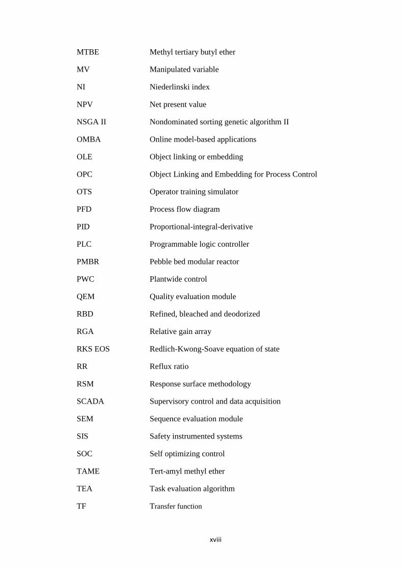
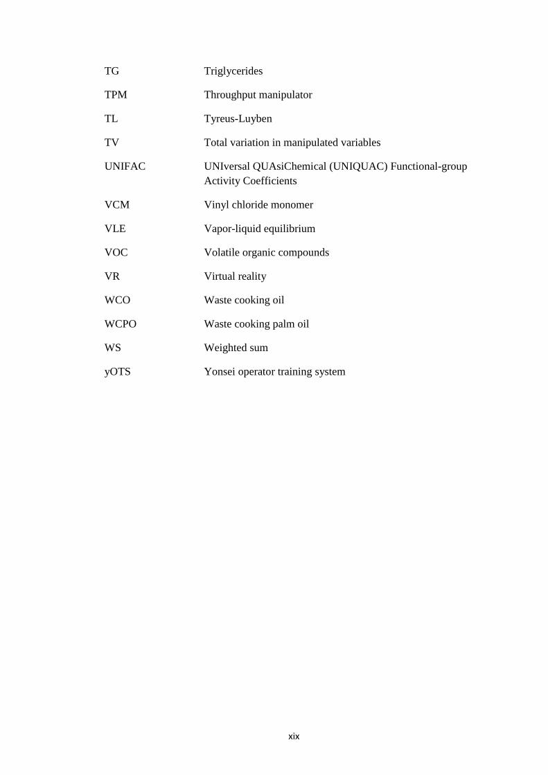
xvi
LIST OF ABBREVIATIONS
APC Advanced process controllers
APD Aspen Plus Dynamics
AVR Augmented Virtual Reality
ASTM American society for testing and materials
CAPD Computer-aided process design
CAPE Computer-aided process engineering
CC Cohen and Coon
CDOF Control degrees of freedom
COM Cost of manufacturing
CPO Crude palm oil
CSTR Continuous stirred tank reactor
CV Controlled variable
DCS Distributed control system
DDE Dynamic data exchange
DDS Dynamic disturbance sensitivity
DE Differential evolution
DG Diglyceides
DO Dissolved oxygen
DPT Deviation from the production target
DME Dimethyl ether
EMOO Excel-based multi-objective optimization
ERGA Effective relative gain array
EA Evolutionary algorithm
FAME Fatty acid methyl esters
FCI Fixed capital investment
xvii
FFA Free fatty acid
FHA Functional hazard analysis
FOPTD First order plus time delay
GA Genetic algorithm
GAMS General algebraic modeling system
GUI Graphical user interface
HAZOP Hazard and operability
HAD Hydro-dealkylation
HDE Hybrid differential evolution
HE Heat exchanger
HMI Human-machine interface
HRA Human reliability analysis
HPDB Human performance database
kt kilotonne
ID Internal diameter
IFSH Integrated framework of simulation and heuristics
IFSHO Integrated framework of simulation, heuristics and
optimization
IPC Industrial PC and intelligent control
INTEMOR Intelligent industrial real-time on-line process information
system
LCA Life cycle assessment
LLE Liquid-liquid equilibrium
MINLP Mixed integer nonlinear programming
MOEA Multi-objective evolutionary algorithms
MG Monoglycerides
MPC Model predictive control
MOO Multi-objective optimization
xviii
MTBE Methyl tertiary butyl ether
MV Manipulated variable
NI Niederlinski index
NPV Net present value
NSGA II Nondominated sorting genetic algorithm II
OMBA Online model-based applications
OLE Object linking or embedding
OPC Object Linking and Embedding for Process Control
OTS Operator training simulator
PFD Process flow diagram
PID Proportional-integral-derivative
PLC Programmable logic controller
PMBR Pebble bed modular reactor
PWC Plantwide control
QEM Quality evaluation module
RBD Refined, bleached and deodorized
RGA Relative gain array
RKS EOS Redlich-Kwong-Soave equation of state
RR Reflux ratio
RSM Response surface methodology
SCADA Supervisory control and data acquisition
SEM Sequence evaluation module
SIS Safety instrumented systems
SOC Self optimizing control
TAME Tert-amyl methyl ether
TEA Task evaluation algorithm
TF Transfer function
xix
TG Triglycerides
TPM Throughput manipulator
TL Tyreus-Luyben
TV Total variation in manipulated variables
UNIFAC UNIversal QUAsiChemical (UNIQUAC) Functional-group
Activity Coefficients
VCM Vinyl chloride monomer
VLE Vapor-liquid equilibrium
VOC Volatile organic compounds
VR Virtual reality
WCO Waste cooking oil
WCPO Waste cooking palm oil
WS Weighted sum
yOTS Yonsei operator training system
xx
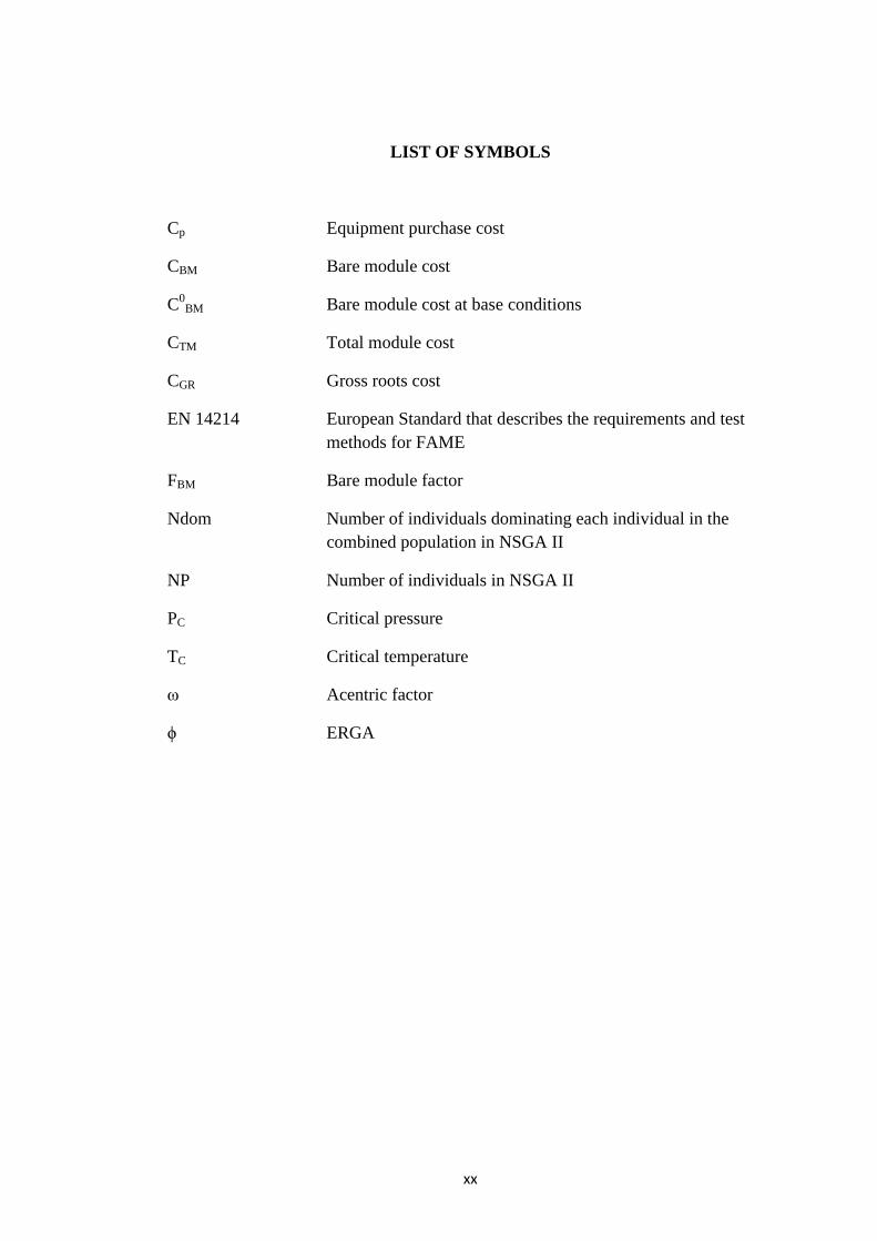
LIST OF SYMBOLS
Cp Equipment purchase cost
CBM Bare module cost
C0
BM Bare module cost at base conditions
CTM Total module cost
CGR Gross roots cost
EN 14214 European Standard that describes the requirements and test
methods for FAME
FBM Bare module factor
Ndom Number of individuals dominating each individual in the
combined population in NSGA II
NP Number of individuals in NSGA II
PC Critical pressure
TC Critical temperature
ω Acentric factor
ϕ ERGA
xxi
SIMULATOR LATIHAN PENGENDALI MENGGUNAKAN KAWALAN
LOJI LEBAR UNTUK PENGHASILAN BIODIESEL DARIPADA SISA
MINYAK MEMASAK
ABSTRAK
Kajian ini bertujuan untuk membangunkan simulator latihan operator (OTS) untuk
mangkin homogen bagi proses dua langkah biodiesel yang kompleks. Latihan sambil
bekerja selalunya memerlukan kos yang tinggi, berisiko dan tidak lengkap kerana
beberapa situasi kecemasan mungkin tidak berlaku semasa sesi latihan. Biodiesel
dilihat sebagai sumber bahan api alternative, Disebabkan ketersediaan yang terhad
sumber tenaga yang tidak boleh diperbaharui dan juga kebimbangan terhadap alam
sekitar. Walau bagaimanapun, kos pengeluaran yang tinggi bagi biodiesel
menghadkan pengeluaran dan penggunaannya. Salah satu pilihan yang terbaik adalah
dengan menggunakan sisa minyak masak (WCO) sebagai sumber bahan mentah bagi
pengeluaran biodiesel yang kos efektif dan juga penggunaan WCO yang berkesan.
Dalam kajian ini, sisa minyak sawit masak dianggap dengan 6% asid lemak bebas
(FFA) sebagai bekalan simpanan. Dua proses pengeluaran biodiesel (kedua-duanya
melibatkan pengesteran asid dan transesterifikasi alkali) telah dibandingkan untuk
analisis ekonomi dan alam sekitar. Pertama, proses ini dalam simulator Aspen Plus.
Selepas itu, kedua-dua proses dioptimumkan dengan mengambil kira keuntungan,
tenaga haba dan bahan buangan organik sebagai objektif, dan menggunakan program
berasaskan Excel pengoptimuman multi-objektif (EMOO) untuk pengisihan
algoritma genetic elitis tidak dikuasai (NSGA-II). Proses 1 mempunyai tiga reaktor
transesterifikasi yang menghasilkan sisa organik jauh lebih rendah (32%),
xxii
memerlukan duti haba yang lebih rendah (39%) dan sedikit keuntungan (1.6%)
berbanding Proses 2 yang hanya mempunyai satu reaktor transesterifikasi dan juga
urutan pemisahan yang berbeza. Sistem kawalan loji lebar (PWC) yang berkesan
adalah penting untuk operasi loji biodiesel yang selamat, lancar dan ekonomi. Oleh
itu, sistem PWC yang sesuai telah dibangunkan untuk proses biodiesel yang
menggunakan simulasi rangka kerja bersepadu dan heuristik (IFSH). Merit utama
metodologi IFSH adalah keberkesanan penggunaan proses simulator yang baik dan
heuristik dalam membangunkan sistem PWC dan kesederhanaan applikasinya. Akhir
sekali, pelaksanaan sistem kawalan yang dibangunkan dinilai dari segi masa
penetapan, sisihan daripada sasaran pengeluaran (DPT), dan jumlah variasi
keseluruhan (TV) dalam pembolehubah yang dimanipulasi. Penilaian-penilaian
prestasi dan keputusan simulasi dinamik menunjukkan bahawa sistem PWC yang
dihasilkan adalah stabil, berkesan, dan teguh terhadap beberapa gangguan. Akhir
sekali, OTS telah dibangunkan untuk penghasilan biodiesel daripada WCO. Oleh itu,
latihan menggunakan OTS adalah penting. OTS telah dibangunkan untuk
pengeluaran biodiesel dan telah diapplikasikan dengan beberapa keadaan proses yang
tidak normal. Keadaan proses ini boleh dimuatkan dan digunakan pada bila-bila
masa untuk melatih operator baru dan sedia ada. Kajian ini adalah yang pertama
dibangunkan menggunakan struktur lengkap PWC dan OTS untuk mangkin yang
homogeneous bagi dua langkah pengeluaran biodiesel daripada WCO.
xxiii
OPERATOR TRAINING SIMULATOR USING PLANTWIDE CONTROL
FOR BIODIESEL PRODUCTION FROM WASTE COOKING OIL
ABSTRACT
This study aims at developing an operator training simulator (OTS) for the complex
homogeneously catalyzed two-step biodiesel process. On-job training is often costly,
risky and incomplete as some emergency situations may not arise during the training
session. Therefore, training using an OTS is crucial. Pertaining to the limited
availability of non-renewable energy sources and the environmental concerns,
biodiesel is considered as a potential alternative fuel. However, the high production
cost of biodiesel limits its manufacture and utilization. One attractive option is to use
waste cooking oil (WCO) as the feedstock that enables cost effective biodiesel
production and also facilitates effective WCO utilization. This study considers waste
cooking palm oil with 6% free fatty acids (FFA) as feedstock. Two biodiesel
production processes (both involving acid esterification and alkali transesterification)
are compared for economic and environmental objectives. Firstly, these processes are
simulated realistically in Aspen Plus simulator. Subsequently, both the processes are
optimized considering profit, heat duty and organic waste as objectives, and using an
Excel-based multi-objective optimization (EMOO) program for the elitist non-
dominated sorting genetic algorithm (NSGA-II). Process 1 having three
transesterification reactors produces significantly lower organic waste (by 32%),
requires lower heat duty (by 39%) and slightly more profitable (by 1.6%) compared
to Process 2 having a single transesterification reactor and also a different separation
sequence. An effective plantwide control (PWC) system is crucial for the safe,
xxiv
smooth, and economical operation of a biodiesel plant. Hence, a suitable PWC
system is developed for the biodiesel process using the integrated framework of
simulation and heuristics (IFSH). The main merits of the IFSH methodology are
effective use of rigorous process simulators and heuristics in developing a PWC
system and simplicity of application. Later, the performance of the developed control
system is assessed in terms of settling time, deviation from the production target
(DPT), and overall total variation (TV) in manipulated variables. These performance
assessments and the results of dynamic simulations showed that the developed PWC
system is stable, effective, and robust in the presence of several disturbances. Finally,
an OTS has been developed for the biodiesel production from WCO. The developed
OTS for biodiesel production process has been investigated for several abnormal
process conditions. These process scenarios can be loaded and utilized at any point in
time to train the new and existing operators. This is the first study to develop a
complete PWC structure and OTS for a homogeneously catalyzed two-step biodiesel
production from WCO.
1
CHAPTER 1
INTRODUCTION
1.1 Research Background
Alternative fuels are being given significant attention due to the increasingly
worrying environmental situation. Biodiesel, an alternative fuel to the petroleum-
based diesel, is relatively safe, environment friendly, non-toxic and biodegradable as
opposed to petroleum-based diesel (Amani et al., 2014a). Fossil fuels such as
petroleum fuels and coal have been the major source of energy. However, their non-
renewability, highly polluting nature and diminishing reserves make them
unattractive for use in the future. Therefore, energy obtained from renewable
sources, such as biodiesel and bioethanol, has gained significance in the past few
years. Biodiesel i.e. a mixture of fatty acid methyl esters derived from vegetable oils
and animal fats, has physiochemical properties similar to those of petroleum-based
diesel. Biodiesel or its blends can be used in conventional diesel engines without any
modification or with minimal modification (Ramadhas, 2010). It offers many
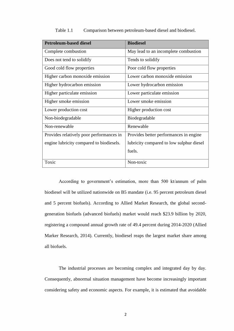
environmental advantages over petroleum-based diesel, as mentioned in Table 1.1.
There is a growing attention in Malaysia towards the use of palm oil in much
required biodiesel production as it is the second largest palm oil producer in the
world (MPOB, 2013). Previously, the Malaysian energy policy was focused on the
use of oil and gas. However, a policy on Renewable Energy was introduced in year
2001 to find alternatives to existing energy sources (KPPK, 2014).
2
Table 1.1 Comparison between petroleum-based diesel and biodiesel.
Petroleum-based diesel Biodiesel
Complete combustion May lead to an incomplete combustion
Does not tend to solidify Tends to solidify
Good cold flow properties Poor cold flow properties
Higher carbon monoxide emission Lower carbon monoxide emission
Higher hydrocarbon emission Lower hydrocarbon emission
Higher particulate emission Lower particulate emission
Higher smoke emission Lower smoke emission
Lower production cost Higher production cost
Non-biodegradable Biodegradable
Non-renewable Renewable
Provides relatively poor performances in
engine lubricity compared to biodiesels.
Provides better performances in engine
lubricity compared to low sulphur diesel
fuels.
Toxic Non-toxic
According to government’s estimation, more than 500 kt/annum of palm
biodiesel will be utilized nationwide on B5 mandate (i.e. 95 percent petroleum diesel
and 5 percent biofuels). According to Allied Market Research, the global second-
generation biofuels (advanced biofuels) market would reach $23.9 billion by 2020,
registering a compound annual growth rate of 49.4 percent during 2014-2020 (Allied
Marker Research, 2014). Currently, biodiesel reaps the largest market share among
all biofuels.
The industrial processes are becoming complex and integrated day by day.
Consequently, abnormal situation management have become increasingly important
considering safety and economic aspects. For example, it is estimated that avoidable
3
abnormal situations have an annual impact of over 10 billion USD on the operations
of US based petrochemical industry due to production loss, equipment damage, etc
(Seborg et al., 2010). Also, Kluge et al. (2014) highlighted the cognitive and
teamwork requirements of operators and noted the limits of current training practices
compared to the training objectives that need to be achieved individually and as a
team. Safe and economical production in the chemical industry requires skilled
operators. Hence, the OTS is considered as an alternative and efficient tool to train
the operators. The OTS development for biodiesel production from WCO has not
been found in the literature. Also, application of Aspen Plus Dynamics (APD) with
Aspen OTS Framework in OTS development has not been found in the research
articles. This work embarks on using APD with Aspen OTS Framework to develop
an OTS for the concerned process.
A suitable and realistic process model is crucial for several engineering
studies such as model based sensitivity analysis, multi-objective optimization
(MOO), plantwide control (PWC) and operator training simulator (OTS)
development. Therefore, the processes for biodiesel production from waste cooking
oil (WCO) should be simulated considering detailed constituents of WCO and
detailed kinetics (esterification and transesterification are represented by 10 and 96
kinetic reactions, respectively), which is scarce to find in the literature. With
increasing economic competition and scarcity of resources, there is greater need for
optimization of chemical processes. Biodiesel production from WCO is explained
below.
4
1.2 Biodiesel Production from Waste Cooking Oil
The production of fatty acid methyl ester (i.e. biodiesel) by chemically
reacting lipids such as vegetable oil with an alcohol can be used as an alternate to
reduce the over-reliance on the petroleum-based diesel. There are four different
methods to produce biofuel from bioresources, namely direct use and blending of
raw oils, micro-emulsions, thermal cracking and transesterification.
Transesterification is the most popular way to produce biodiesel from vegetable oils
or animal fats (Ziolkowska, 2014). This reaction can be catalyzed by alkali- or
acidic-catalysts. The cost of oil is the major contributor to the cost of biodiesel
(Sharma and Rangaiah, 2013b). In view of limited availability of pure vegetable oil
and its high cost, use of WCO is a favourable choice. Biodiesel production from
WCO is attractive for both economic and environmental reasons since WCO is
cheaper than vegetable oils and its direct disposal to the environment has adverse
impacts.
Although transesterification is more efficient and faster with an alkali catalyst
compared to an acid catalyst, high amount of free fatty acid (FFA) in WCO produces
soap in the presence of an alkali catalyst (Canakci and Van Gerpen, 2001). Hence,
alkali-catalyzed process cannot directly be used to produce biodiesel from WCO. To
increase the formation of fatty acid methyl esters (FAME) (i.e., biodiesel) by
transesterification, Freedman et al. (1984) recommended using refined vegetable oils
with an FFA content lower than 0.5% (w/w), methanol to oil molar ratio of 6:1, and
reaction temperature of about 333 K. Also, water content of vegetable oils should be
kept below 0.06% (w/w) (Ma et al., 1998). WCO typically contain 2 to 7% of FFAs
5
(Gerpen, 2005). In these cases, an acid catalyst such as sulfuric acid can be used to
esterify FFAs to FAMEs, thus reducing FFA content of feed. Pre-treated oil can then
be trans-esterified with an alkali-catalyst to obtain FAMEs. Accordingly, Canakci
and Van Gerpen (2001) proposed a two-step process, esterification followed by
transesterification, to produce biodiesel. In the view of inevitable need of skilled
operators and expensive on-job training, OTS for the complex biodiesel process is
essential. Following section describes the OTS.
1.3 Operator Training Simulator (OTS)
Intricate and highly interacting production processes pose tough challenges in
maintaining safe and efficient production. An inevitable need of skilled operators to
increase the safety and the productivity is not new to the chemical industry.
Consequently, the training of operators is considered as a very important activity in
the chemical industry. An OTS provides an alternative to train operators without
actually endangering the plant and personnel. In complex industries, where safety is
paramount, identification of key factors that can degrade/enhance safety is a must
(Park et al., 2004). Yang et al. (2001) reported that significant percentage of property
losses in the hydrocarbon processing industries is due to operational errors or process
upsets. This reinforces the need of OTS to develop and retain the operators’ skills.
To ensure that operators retain the knowledge, skills and remain competent to control
processes in emergency conditions, they should be provided with training
opportunities to develop and sustain their capabilities. On-job training is often costly,
risky and incomplete as some emergency situations may not arise during the training
6
session. Therefore, training using an OTS is crucial. Manca et al. (2013) discussed
the benefits of integrating and interlinking a dynamic process simulator with a
dynamic accident simulator in OTS training. According to Shepherd (1986), as long
as operators are working on the complex plants and equipments, development and
administration of their training are required. He reported that a training technique
implies adopting one or more of the following: teaching plant and process
knowledge, on-job instruction, training on a simulated plant and development.
The paradigm of one of these training methods alone may not be effective.
Shepherd (1986) recommended adopting all the above mentioned for a
comprehensive training program. In the chemical industry, especially in the case of
continuous processes, OTS has been used (Balaton et al. 2013). An increasing
number of chemical companies use OTS aiming to train the operating staff on
handling different malfunctions and infrequently occurring modes of operation.
Other applications of OTS include assessment of operators’ skills, supporting
engineering tasks such as investigating alternate control mechanisms and performing
safety tests without any risk to the real system (Fürcht et al. 2008; Rey 2008).
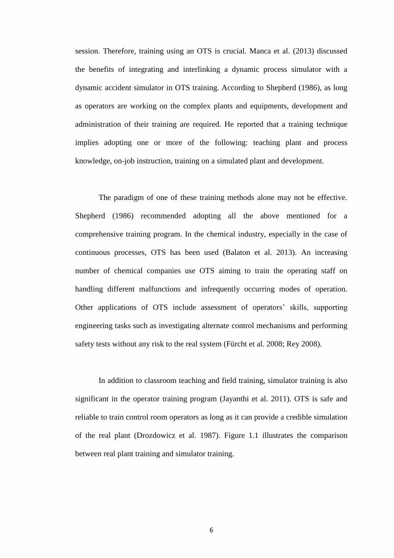
In addition to classroom teaching and field training, simulator training is also
significant in the operator training program (Jayanthi et al. 2011). OTS is safe and
reliable to train control room operators as long as it can provide a credible simulation
of the real plant (Drozdowicz et al. 1987). Figure 1.1 illustrates the comparison
between real plant training and simulator training.
7
Figure 1.1 Comparison between real plant training (top) and simulator training
(bottom).
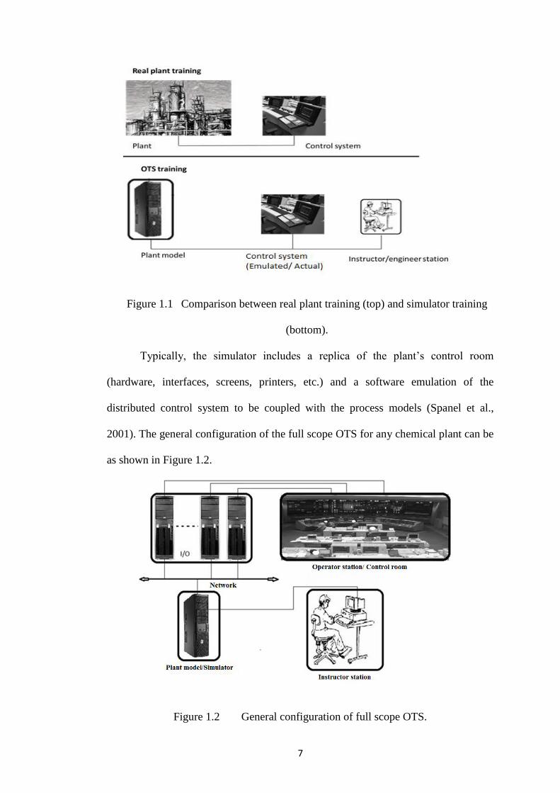
Typically, the simulator includes a replica of the plant’s control room
(hardware, interfaces, screens, printers, etc.) and a software emulation of the
distributed control system to be coupled with the process models (Spanel et al.,
2001). The general configuration of the full scope OTS for any chemical plant can be
as shown in Figure 1.2.
Figure 1.2 General configuration of full scope OTS.
8
In this figure, the instructor station provides the interface for the instructor to
insert faults, monitor and control the training session while the trainee operators use
the operator station. The trainee operator station has generic process control system
schematics that enable point and click access to the controller faceplates. The
instructor station functionalities reported by Dudley et al. (2008) are: scenario
creation and imparting malfunctions/upsets into the process model, monitoring and
trending of any plant variable, training and evaluation of operators, run/pause/resume
and load/save capabilities, Snapshots, backtracks and speed control (i.e. fast/slow
capabilities), and storing of data on plant variables, which can be used for post-
scenario reviews.
In addition, preliminary hazard and operability study (HAZOP) analysis is
carried out to assist a trainee find out causes and possible solutions. HAZOP is a
structured and systematic examination of a non-existing or existing process in order
to identify and evaluate problems that may indicate risks to process or personnel, or
reduce the efficient process operation. OTS needs a suitable process model that can
reflect the process as real as possible. Therefore, it is important to carry out a realistic
simulation, determine optimal conditions and develop a complete PWC structure. In
this work, OTS uses the same process model as it is used in MOO and PWC study.
The optimal parameters determined from MOO of the biodiesel process is used in
PWC and OTS study. Following section presents the merits of MOO.
9
1.4 Multi-objective Optimization (MOO)
Once process extablished and simulated, MOO is used to determine the
optimal parameters of the decision variables. MOO is also used to compare the two
process alternative. In general, MOO is the method of finding optimal values of the
parameters for the maximization or the minimization of given objectives within
prescribed constraints. MOO involves maximizing or minimizing multiple objective
functions subject to a set of constraints, for example analyzing design tradeoffs,
selecting optimal product or process designs, or any other application where an
optimal solution with tradeoffs between two or more conflicting objectives is
desired. Optimization plays crucial role in reducing material and energy requirements
as well as the waste formation in chemical processes. It is also essential in
determining better design and operation of chemical processes. Many chemical
processes involve several objectives, most of which are conflicting in nature. Several
chemical processes have many variables with complex inter-relationships;
optimizing these objectives is challenging. MOO is needed to determine the optimal
solutions in such applications. MOO is used to find a set of nondominated solutions
for two or more objectives simultaneously (Sharma and Rangaiah, 2013b).
Consequently, in last few years, a significant attention has been given to MOO.
MOO has been vastly used to optimize chemical processes having conflicting
objectives such as conversion, selectivity, yield, energy, environment and safety in
addition to economic objectives. Evolutionary algorithms, such as non-dominated
sorting genetic algorithm (NSGA-II), are popular methods to generate Pareto optimal
solutions for a multi-objective optimization problem. It is a stochastic optimization
method that that generates and uses random variables. Other stochastic optimization
10
methods include simulated annealing, quatum annealing, swarm algorithms,
differential evaluation etc. NSGA-II has become popular approach and it can be seen
from its wide applications.
The main advantage of evolutionary algorithms (EA) is that the EAs are
inherently stochastic in nature, and thus they generate the Pareto front when applied
to solve multi-objective optimization problems. Multi-objective optimization
problems can be solved using Genetic algorithm and its improved versions to find set
of points on the Pareto front. The major drawbacks of multi-objective evolutionary
algorithms (MOEAs), such as NSGA, that use non-dominated sorting and sharing
are: (1) their computational complexity O(MN3) (where, M is the number of
objectives and N is the population size), (2) their non-elitism approach (absence of
elitism as opposed to NSGA-II, where parents are selected from the population by
using binary tournament selection based on the rank and crowding distance), and (3)
the necessity to specify a sharing parameter (Deb et al., 2002). Deb et al. (2002)
proposed extension of NSGA i.e., NSGA-II, which alleviates all of the above three
difficulties; hence, NSGA-II is used later in this study. After finding the better
process out of the two alternative processes, a suitable PWC structure should be
implemented; this is explained below.
1.5 Plantwide Control (PWC)
After the best process is identified based on the optimization results, PWC
structure is developed for the chosen process. Generally, chemical processes consist
11
of a several integrated unit operations. These material and energy integration make
the process complex. Besides, most chemical processes are non-linear in nature. The
main objective of PWC is to synthesize a control structure that leads to smooth, safe
and economic operation of the entire plant. Because of market competition, dictated
by changing customers’ demand, efficient operation of plant is crucial. Material and
energy recycles are constantly employed to improve economics. The presence of
recycle streams alters the process dynamics that then leads control problems. Also,
tough safety norms and stringent environmental regulations demand an effective
PWC system.
Merits of PWC over normal unit-wise control are (i) complete PWC
perspective is considered which is important due to several interacting process
operations (ii) decisions are taken systematically based on the hierarchy of
preferences e.g. control objectives, product quality, throughput manipulator (TPM),
process constraints, safety constraints, inventory etc (iii) location of TPM, which is
critical in PWC system, is properly identified and (iv) critical issues can be
categorically evaluated such as snowball effect, slowing dynamics due to the
recycles, propagation of disturbances in the multiunit process etc (Seborg et al.,
2010). In case of any discrepancy regarding the loop pairings, control loop pairing
arrived from the PWC method should be preferred over the decision arrived from the
base layer control method. So far, many systematic PWC methodologies have been
developed. Each of the methodologies offer some advantages as well as some
limitations due to the particular approach followed. It is worth noting that different
methodologies may yield different control structures, and hence the different control
performance. Based on specific requirements, a particular methodology can be

12
adopted. To circumvent these challenges of the PWC problem, some potential
methodologies have appeared in recent years. To circumvent overreliance of other
PWC methodologies on heurisics, Murthy Konda et al. (2005) proposed the
integrated framework of simulation and heuristics (IFSH) that combines the benefits
of process simulators as well as heuristics. Optimization and mathematical-based
approaches usually depend on process models and involve intensive computations.
For examples, Zhu et al. (2002) proposed optimization-based strategy to integrate
linear and non-linear model predictive control. These approaches are often prone to
model inaccuracies. Mixed-approaches combine any of the heuristics, optimization
or mathematical methods. One of such methodologies is the self-optimizing control
(SOC) proposed by Skogestad (2004). The core of this methodology is to find a set
of self-optimizing variables, which when maintained constant leads to minimal loss
in the profit as and when disturbances occur, without the need for re-optimization as
these variables keep the plant ‘near-optimal’. Subsequent section presents the
problem statement that established .
1.6 Problem Statement
Finite availability, strict environmental regulations and fluctuating fuel cost
are the main factors behind increasing focus on the alternative fuels. Given the merits
of the biodiesel, it is considered as the one of the most promishing alternative fuels.
Biodiesel produced from edible vegetable oil has many demerits, such as high cost of
biodiesel production and fuel vs food issue. As the consequence, use of WCO is
found to be favourable as it is cheaper than pure oil. As the significant percentage of
13
property losses in the hydrocarbon processing industries are found to be due to
operational errors or process upsets, well trained operators are inevitable for the safe
and efficient process operation. In addition, the rate of accidents arising form
operators’ errors is relatively more in Malaysia as compared to the rates in developed
nations. Conventional training methodologies, such as the training of the new
operators in existing plants by allowing them to work with experienced operators in
front of actual control panel, do not impart enough skills to the operators when
dealing with infrequent critical conditions.Hence, an OTS is essential for the
effective operator training.
In essence, to make OTS realistic and effective, the realistic process model
operating at the real optimal conditions and having an effective PWC system is
crucial. In addition. to obtain increased profitability with the least use of resources,
optimization of process for many conflicting objectives is important. Also, safe and
efficient operation of a biodiesel process inevitably requires an effective PWC
structure. Hence, MOO and PWC study are important for the OTS. Based on these
issues, following objectives are formulated.
1.7 Objectives
The main objective of this research is to develop an OTS for the biodiesel
process. Important subsections of this research are simulation, MOO and PWC for
biodiesel production from WCO. The elaborate objectives of this research are as
follows:
14
1. To develop a steady state simulation for palm oil based biodiesel production from
waste cooking oil.
2. To carry out an excel based evolutionary multi-objective optimization to compare
the two alternative proceeses for the optimal parameters.
3. To develop a dynamic simulation to study the transients of the process.
4. To apply a suitable PWC strategy to the chosen biodiesel process.
5. To develop an OTS to train the operators for enhancing their skills and ability to
deal with critical and emergency operations.
1.8 Scope of Study
The main aim of this study is to develop an OTS for the complex biodiesel
process. This is the first study to investigate the application of the commonly used
Aspen Plus Dynamics in the OTS development for the homogeneously catalyzed
biodiesel production from WCO. Experience from this is useful for development of
OTS for other complex processes, and thus leading to the increased operator training
for safer plant operations. Complex processes, such as biodiesel production from
WCO, require skilled operator to maintain the safety and productivity of the
biodiesel process. Using WCO for biodiesel production enables cost effective
biodiesel production and also facilitates effective WCO utilization. As an effective
OTS requires a realistic process model, firstly in this study, two alternative biodiesel
processes are optimized using NSGA-II and compared based on economic and
environmental criteria. Both the process alternatives use alkali-catalyzed
transesterification, which is more efficient and also used in industrial practice.
Optimization study determines the optimal parameters, such as temperature,
15
residence time and feed location, to make process more profitable and less damaging
to the environment. Later, an effective PWC system is developed for the better
process using IFSH methodology, which makes effective use of process simulators
as well as heuristics. The performance of the developed PWC system is investigated
using several performance assessment criteria. These performance assessments and
results of dynamics simulations indicate that the developed PWC system is stable,
effective and robust in the presence of several disturbances, and that biodiesel quality
is maintained despite these disturbances. Finally, an OTS has been developed for
biodiesel production from WCO. The developed standalone OTS for biodiesel
production has been investigated for several abnormal process conditions, each of
which can be inserted by an Instructor at will. These scenarios can be replayed as and
when the operators require. Next section describes the organization of the thesis.
1.9 Organization of Thesis
This thesis comprises of five major chapters. Each chapter has been explained
in detail with the following contents.
Chapter 1 elaborates on the background information about this research, the
significance of this research and the techniques being followed to achieve the desired
objectives. The objectives are chosen so as to provide a significant breakthrough in
this field of research. This chapter also briefly explains the MOO, PWC and OTS
with respect to chemical processes, in general.
16
Chapter 2 discusses and reviews extensively about MOO, PWC and OTS for a
homogeneously catalyzed biodiesel process. Detailed reviews about the application
of MOO, PWC and OTS in various chemical processes have been also carried out.
Chapter 3 presents the methodology carried out in this research. This chapter
consists of four major parts. The first part explains the design and simulation of two
alternative biodiesel processes. This is followed by MOO for different conflicting
objectives using an Excel-based multi-objective optimization (EMOO) program for
the elitist NSGA-II. Later, a suitable PWC structure is developed for the process
using IFSH methodology. Finally, an OTS is developed for the process using APD
with Aspen OTS Framework on top.
Chapter 4 details the results and discussion obtained from simulation, MOO, PWC
and OTS. Two alternative processes are compared based on several criteria, namely
profit, heat duty and organic waste. Nextly, the employed PWC system is
investigated for different criteria, namely settling time, dynamic economic index
based on deviation from the production target (DPT) and total variation (TV) in
manipulated variables. Finally, the developed standalone OTS for biodiesel process
has been investigated for several abnormal process conditions, each of which can be
inserted by an instructor. These include: equipment malfunctions, utility failures,
fire, pressure safety valves and development of startup procedures resulting in
reduction of production time and loss.
Chapter 5 finishes off with the conclusions that have been arrived from this work. In
addition, the future directions of this research have been established.
17
CHAPTER 2
LITERATURE REVIEW
2.1 Introduction
As the main goal of this work is the OTS development for biodiesel process
that require a MOO and PWC study, recent research works in the field of biodiesel
production, MOO, PWC and OTS development are reported in this chapter. Relevant
and recent previous research works relating to these areas discussed and presented in
systematically. The objectives of this research are based on the gaps determined from
the careful analysis of the previous studies. Literature study shows that increasing
number of chemical industries is looking to use OTS to train their operators given the
benefits of OTS.
Biodiesel production from WCO is beneficial because the WCO is cheaper
and utilizing it for the fuel production avoids its wastage. This, consequently, avoids
the pollution as the WCO would have to be dumped, which would cause
environmental degradation, e.g. water pollution causing main threat to the aquatic
animals. Biodiesel production from pure vegetable oil is feasible. However, it has
two major drawbacks: high cost and limited availability. After establishing the raw
material for biodiesel production, suitable process design should be established.
Successively, optimal design and operation parameters should be identified to run the
process optimally. MOO can play an important role as it has the ability to find the
optimal condition for the complete plant condidesring multiple objectives. Safe,
18
robust and proficient process operation requires an effective PWC system, especially
when the process is as complex as the homogeously catalysed two step biodiesel
production from WCO. Information is presented in tabular form, wherever required,
to understand the highlights and gaps in the previous studies. Relevant previous
studies are then critically analyzed.
2.2 Biodiesel Production from Waste Cooking Oil (WCO)
Biodiesel i.e. FAME derived from vegetable oils and animal fats, has
physiochemical properties similar to those of petroleum-based diesel. Biodiesel
offers has many advantages over petroleum-based diesel fuel such as a higher cetane
number, no aromatics or sulphur compounds, and reduced emission of carbon
dioxide, carbon monoxide, hydrocarbons and particulates in the exhaust gas
(Ramadhas, 2010). Pure biodiesel or its blend with petroleum-based diesel can be
used in the existing diesel engines with either no or slight modifications (Ramadhas,
2010). The non-renewability, adverse environmental impacts and increasingly
diminishing reserves of current fuels make researchers to look for alternative fuels.
Among such alternative fuels, biofuels (e.g. biodiesel) have gained significant
attention in the past few years.
Biodiesel can be produced through micro-emulsions, thermal cracking and
transesterification. Among these routes, transesterification is the most popular way to
produce biodiesel as it is more efficient and has moderate operating conditions.
Transesterification reaction is reversible, and can be catalysed by alkali/acid
homogeneous catalyst, heterogeneous catalyst as well as enzymes (Ramadhas, 2010).
19
Also, a non-catalytic route using supercritical methanol can be adopted (Kusdiana
and Saka, 2001). However, these studies are still in the developmental phases, and
are not being used commercially. Many researchers (Zhang et al., 2003a; Zhang et
al., 2003b; Haas et al., 2006; West et al., 2008; Myint and El-Halwagi, 2009; Santana
et al., 2010) have studies the techno-economic feasibility of different
transesterification methods. They concluded that the price of the feed oil is the
largest contributor to the cost of biodiesel production.
Zhang et al. (2003a) proposed four biodiesel production processes namely,
alkali-catalyzed process using pure vegetable oil, alkali-catalyzed process using
WCO, acid-catalyzed process using WCO, and acid-catalyzed process using hexane
extraction. Later, Zhang et al. (2003b) performed economic analysis and found that
the acid-catalyzed process using WCO is more economical compared to others
studied. West et al. (2008) conducted economic analysis of four biodiesel production
processes, using WCO as feedstock; these include acid-catalyzed, alkali-catalyzed,
heterogeneous acid-catalyzed and supercritical processes. They concluded that
heterogeneous acid-catalyzed process is more economical than others, but it is still in
the development phase. Catalyst deactivation and their selectivity towards the
biodiesel are mong the maor challenges. Talebian-Kiakalaieh (2013) reported that
utilization of waste cooking oil can reduce biodiesel production cost by 60-90%.
Development of kinetics for the transesterification reaction has been studied
previously (Freedman et al., 1986; Nourreddini and Zhu, 1997; Kusdiana and Saka,
2001; Jain and Sharma, 2010). Significant attention is also being given to the use of
heterogeneous catalysts in biodiesel production (Sharma et al., 2011; Amani et al.,
2014b; Wijaya et al., 2013).
20
Biodiesel production using homogeneously catalyzed transesterification is the
most popular method used in the industries (Zhang et al., 2003a; Nazir et al., 2009;
Lurgi, 2013; Platinumgroup, 2013). Transesterification reaction is faster and requires
smaller methanol-oil ratio as compared to acid transesterification (Freedman et al.,
1986) under moderate operating conditions. While alkali-catalysed route is widely
accepted, it has the disadvantage of low tolerance of water and FFA in the feed. Use
of pure oil that offers low content of water and FFA lead to expensive biodiesel
production that is incompetent against existing fuels. Using WCO for biodiesel
reduces the cost of production significantly; but it normally has higher FFA content.
If the feed contains higher levels of water and FFA than the maximum tolerance
level, a pre-treatment section is required to convert FFA into biodiesel. In
homogeneous biodiesel production, researchers have used different separation
sequences. Myint and El-Halwagi (2009) studied these alternative sequences
technically and scientifically. Application of different unit operations has also been
tested. For example, Apostolakou et al. (2009) proposed phase separation between
biodiesel and glycerol by a centrifuge separator as opposed to the application of a
decanter by Myint and El-Halwagi (2009).
In summary, the limited availability of pure vegetable oil and its high cost,
using WCO for biodiesel production is a beneficial. Biodiesel production from WCO
is attractive for both economic and environmental reasons since WCO is cheaper
than vegetable oils and its direct disposal to the environment has adverse impacts.
Other research on the development of novel reactor designs for biodiesel production
includes: membrane reactors (Dube et a., 2007), gas–liquid reactors (Behzadi and
Farid, 2009) and rotating packed reactors (Chen et al., 2010); however, these are still
21
under developmental phase. Next subsection presents the information on MOO for
the chemical processes.
2.3 Process Design and Multi-objective Optimization ( MOO)
In a chemical process, raw materials are transferred into the desired products
through series of processing steps. In essence, chemical process design involves (1)
selection of individual transformation steps and (2) interconnection of these
transformation steps to form a complete process that can produce the desired output.
2.3.1 Process Design
Process design is a structured approach to improve tangible benefits such as
cost reduction and increase in the process efficiency. Sieder et al. (2010) proposed
the general steps to be followed in process design. Firstly, a primitive problem is
developed. Then base case is developed after the feasibility study. In parallel,
algorithmic methods (e.g. to synthesize reactor-separator-reactor (R-S-R) network)
are employed to find the better process flowsheet. Sequencing of unit operations,
material/energy recycles and heat integration are decided upon at this stage. Also,
plantwide controllability is assessed simultaneously. Later, a detailed design,
equipment sizing and optimal design using optimization (e.g. based on profitability
analysis) is carried out. Peters and Timmerhaus (2002) presented graphical and
analytical method for optimum design.
22
Sinnott et al. (2008) proposed the steps for the process design as design
objectives, setting design basis, generation of possible designs, fitness testing,
economic evaluation using & optimization, detailed design & equipment selection,
and construction & operation. Ray and Sneesby (1998) presented the steps of process
design: conception and definition, flowsheet development, design of equipment,
economic analysis, optimization and reporting. Biegler et al (1997) reported the
optimization approaches to the process design which rely on the optimization
techniques such as missed-integer optimization methods.
Myint and El-Halwagi (2009) adopted the following approach for the
biodiesel process design. This approach includes (1) synthesis of a base-case
flowsheet, (2) simulation of the base case and selection of appropriate
thermodynamic databases, (3) identifying opportunities for process integration and
cost minimization, (4) development of a plantwide simulation of the process with
various mass and energy integrations, and (5) cost estimation and sensitivity analysis.
Datta (2008) presented the process design and engineering using visual basic
application. Chemical process design requires the selection of a series of processing
steps and their integration to form a complete manufacturing system (Smith, 2005).
There are two approaches for process design, namely building an irreducible
structure, and creating & optimizing a reducible structure. Former has many
drawbacks such as several possible designs must be evaluated and evaluating many
designs may not ensure the best design. On the other hand, later approach is a
superstructure i.e hyperstructure embedded within it all feasible process operations
and feasible interconnections that are candidates for an optimal design (smith, 2005).
Smith (2005) followed an onion approach where design is started with the reactor.
23
Then separation train is decided and recycles are connected. Later, possibility of heat
recovery is explored and need of external hear utility is studid. Algorithm methods
are used for the detailed process design, synthesis of chemical reactor networks,
separation train synthesis, R-S-R network synthesis and heat & mass exchange
network synthesis. Several possible design are studied and compared using the
algorithm based on predecided criteria. The optimization approach for the process
design are applied at the later stages when preliminary designs are assessed. Next
section discusses the MOO.
2.3.2 Multi-objective Optimization (MOO)
MOO is the method that is used to simultaneously optimize multiple
objectives that often exhibit the trade-off. In view of the increasing economic
competition and paucity of resources, there is larger need for optimization of
chemical processes. Chemical processes are optimized for selected objectives with
respect to relevant design and operation variables. Chemical processes are often
encountered with conflicting objectives, for example profit vs capital investment.
Until the end of the last century, economic criteria (e.g. cost or profit) were
commonly used for optimizing process design and operation. However, in the last
decade, MOO has been used increasingly to optimize chemical processes for
contradictory objectives such as conversion, selectivity and yield in addition to
economic criteria (Sharma and Rangaiah, 2013a). Eventually, several other
performance criteria such as energy, environment and safety are receiving substantial
attention in process design and operation optimization. Applications of MOO in
chemical processes are presented below.
24
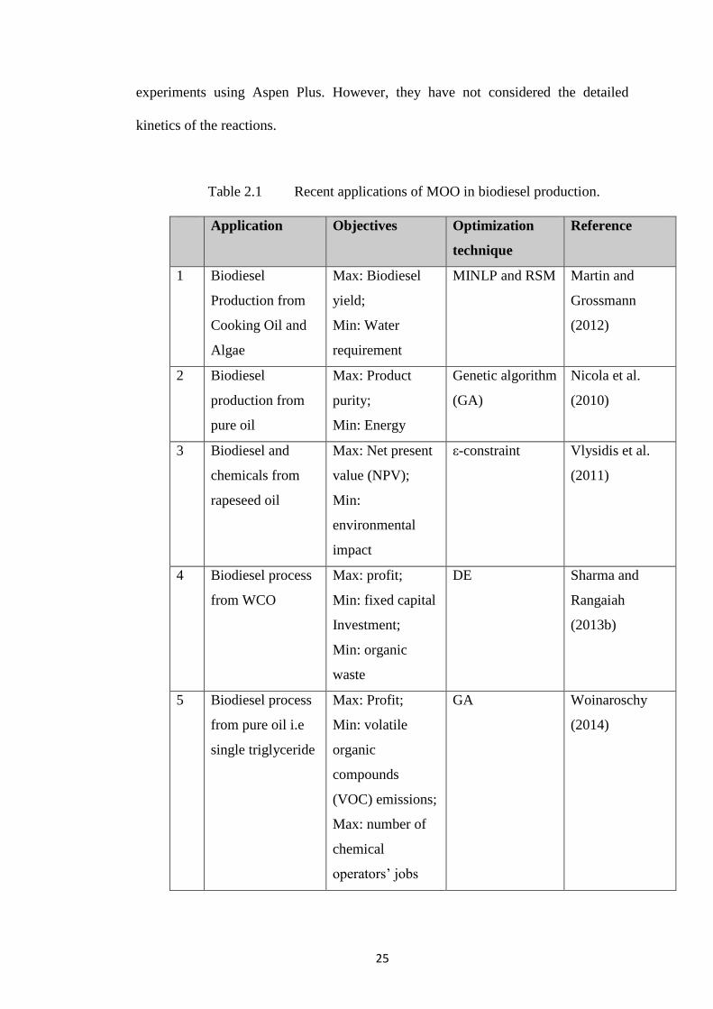
2.3.2 (a) Multi-objective Optimization of Chemical Processes
MOO has been extensively used in the chemical processes, such as petroleum
refining, petrochemicals, polymers, parameter estimation, power sector, renewable
energy, carbon capture, biotechnology, food and pharmaceuticals. In this section,
recent applications of MOO in the biodiesel process is presented in Table 2.1.
Bhaskar et al. (2000) have reviewed the applications of MOO approach in chemical
engineering. (They summarized these MOO applications under five categories,
namely process design and operation, petroleum refining and petrochemicals,
biotechnology and food technology, pharmaceuticals, and polymerization. They
mentioned that use of MOO in chemical engineering has increased between the years
2003 and 2007). Sharma and Rangaiah (2013a) reviewed the articles on MOO from
2007 to mid-2012. From their review, it can be observed that NSGA-II and related
stochastic algorithms have been commonly used by the researchers to determine the
optimal operating and design parameters for the processes considering the manifold
objectives.
Myint and El-Halwagi (2009) studied four alkali-catalyzed biodiesel
processes having different separation sequences and found that biodiesel and
glycerol separation should be performed first, followed by methanol recovery and
water washing. They studies the design, analysis, and optimization of biodiesel
production from soybean oil. Four process flowsheets are synthesized to account for
different separation sequences. The performance of these flowsheets, along with the
key design and operating criteria, are identified by conducting the simulation
25
experiments using Aspen Plus. However, they have not considered the detailed
kinetics of the reactions.
Table 2.1 Recent applications of MOO in biodiesel production.
Application Objectives Optimization
technique
Reference
1 Biodiesel
Production from
Cooking Oil and
Algae
Max: Biodiesel
yield;
Min: Water
requirement
MINLP and RSM Martin and
Grossmann
(2012)
2 Biodiesel
production from
pure oil
Max: Product
purity;
Min: Energy
Genetic algorithm
(GA)
Nicola et al.
(2010)
3 Biodiesel and
chemicals from
rapeseed oil
Max: Net present
value (NPV);
Min:
environmental
impact
ε-constraint Vlysidis et al.
(2011)
4 Biodiesel process
from WCO
Max: profit;
Min: fixed capital
Investment;
Min: organic
waste
DE Sharma and
Rangaiah
(2013b)
5 Biodiesel process
from pure oil i.e
single triglyceride
Max: Profit;
Min: volatile
organic
compounds
(VOC) emissions;
Max: number of
chemical
operators’ jobs
GA Woinaroschy
(2014)
26
Nicola et al. (2010) optimized two slightly different alkali-catalyzed biodiesel
processes for energy consumption and product quality. They used genetic algorithm
to minimize energy requirement and maximize the biodiesel purity. However, rather
than taking biodiesel purity as the objectives, considering it as the constraint in the
constrained MOO is more useful. This is because the biodiesel purity has to be just
maintained above the EN or ASTM standards, and not to maximize it. However, they
also represented the oil as just a triglyceride.
Martin and Grossmann (2012) carried out simultaneous optimization and heat
integration of different technologies for the transesterification of oil. They considered
five different technologies for the transesterification of the oil (viz. homogeneous
acid- or alkali-catalyzed, heterogeneous basic-catalyzed, enzymatic, and supercritical
uncatalyzed). They formulated the problem as a mixed integer nonlinear
programming (MINLP) problem where the models for each of the reactors are based
on surface response methodology to capture the effects of the variables on the yield.
Simultaneous optimization and heat integration for the production of biodiesel from
each of the different oil sources in terms of the technology and the operating
conditions, is studied. They found that the optimal conditions in the reactors differ
from those traditionally used because of the consideration of the separation tasks.
They have also not considered the details compostion of oil and detailed kinetics of
the reactions. Vlysidis et al. (2011) used ε-constraint method to optimize the
biodiesel production form rapeseed oil. They maximized net present value (NPV)
and minimized the environmental impacts.
27
Sharma and Rangaiah (2013b) optimized biodiesel production from WCO for
multiple objectives, using multi-objective differential evolution. They considered
both esterification and transesterification steps, and three continuous stirred tank
reactors (CSTR) in series for transesterification, which has obvious advantages. They
considered profit (maximize), capital investment (minimize) and organic waste
(minimize) as the objectives. However, they represented the WCO by just one fatty
acid and one triglyceride. Woinaroschy (2014) optimized the Biodiesel process
considering profit (maximize) and volatile organic compounds (minimize) as the
objectives. They used genertic algorithm to obtain the Pareto-optimal front. This
work also does not consider the detailed kinetics of the reactions and
detailedconstituents of the oil. Huerga et al. (2014) presented an integrated process to
obtain biofuels from Jatropha curcas crop. They performed several experiments to
optimize the process diminishing the consumption of methanol and catalysts. Fauzi
and Amin (2013) optimized oleic acid esterification catalyzed by ionic liquid. They
used RSM based on central composite design for single-objective optimization, while
artificial neural network with genetic algorithm was employed for simultaneous
optimization of responses to the reaction conditions. Rahimi et al. (2014) studied the
optimization of biodiesel production from soybean oil in a microreactor. They used
Box-Behnken method and RSM for the optimization of molar ratio of methanol to
oil, catalyst concentration and temperature. Rincón et al. (2015) optimized the
Colombian biodiesel supply chain from oil palm crop based on techno-economical
and environmental criteria.
Mendoza et al. (2015) proposed an integrated and generic framework for eco-
design that generalizes, automates and optimizes the evaluation of the environmental
28
criteria at earlier design stage. The approach consists of three main stages: first two
steps correspond to process inventory analysis based on mass and energy balances
and impact assessment phases of Life cycle assessment (LCA) methodology, the
third stage of the methodology is based on the interaction of the previous steps with
process simulation for environmental impact assessment and cost estimation and the
use of multiobjective optimization. They illustrated this methodology through the
acid-catalyzed biodiesel production process.
In conclusion, it can be noticed from the Table 2.1 that detailed esterification
and transesterification kinetics have not been considered for the homogeneously
catalyzed two-step biodiesel production from WCO. Previous studies (Morais et al.,
2010; Zhang et al., 2003a; Zhang et al., 2003b; West et al., 2008; Sharma et al.,
2013; West et al., 2007; Kiss et al., 2012) use a single triglyceride/FFA and FAME to
represent the vegetable oil and biodiesel, respectively. In addition, fixed conversions
of FFA and triglyceride into FAME were often assumed (Morais et al., 2010; Zhang
et al., 2003a; Zhang et al., 2003b; West et al., 2007). These should be avoided in
order to obtain more realistic outcomes, particularly for comparing plant
performance for various feedstocks. In this direction, Garcia et al. (2010) considered
three triglycerides to represent vegetable oil, but mono- and di-glyceride
intermediates were neglected in the reaction. Also, it can be noticed from Table 2.1
that NSGA-II has not beed used for the optimization of the homogeneously catalyzed
two-step biodiesel production, thus far. Merits of NSGA-II are discussed below.
29
2.3.2 (b) Nondominated Sorting Genetic Algorithm II (NSGA-II)
In general, MOO techniques can be classified into three techniques: (i)
generating techniques, (ii) techniques which rely on prior articulation of trade-offs or
preferences and (iii) interactive techniques which rely on progressive articulation of
preferences (Sharma et al., 2012). Generating techniques (or a posteriori preference
articulation methods) search for many Pareto-optimal solutions before deciding on
trade-offs. The NSGA-II is an example of generating techniques. On the contrast, a
priori preference articulation techniques require decisions on trade-offs before
searching for the corresponding Pareto-optimal solution. Prior articulation method
reduces the MOO problem into a single-objective problem which can be solved with
single-objective optimization strategies. However, this requires deep knowledge
which may not be available in every case. The generating techniques, in which there
is no possible reduction of complexity of the search space due to the absence of input
of decision maker, circumvent this short coming. Interactive methods combine the
strengths and weaknesses of both methods. Srinivas and Deb (1995) proposed NSGA
based on genetic algorithm for MOO that is based in natural selection (i.e. random
population generation, selection, cross-over, combination, mutation etc.). It was then
improved by introducing elitism by Deb et al. (2002), which they called it as an
elitist NSGA or NSGA-II. Elitism is when the parents are selected from the
population by using binary tournament selection based on the rank and crowding
distance in the elitist NSGA. NSGA-II is superior to earlier genetic algorithm in
terms of the following: fast non-dominated sorting for population sorting based on
Pareto dominance and the crowding distance assignment for calculating the density
measure. More information about NSGA-II can be found in Deb et al. (2002). It can
30
be seen from the literature review, NSGA-II has not been applied to the biodiesel
processes. Next subsection describes the PWC methodology.
2.4 Plantwide Control (PWC)
PWC refers to the design of a control structure for the complete process
having interconnected unit operations with mass and/or energy recycles. Material and
energy recycles change the process dynamics by introducing an integrating effect,
which can lead to the snowball effect (i.e., high sensitivity of recycles to
disturbances). A good control system distributes the effect of disturbance(s) to unit
operations involved to avoid severe snowball effect. PWC system design for safe,
stable, and efficient operation of complex chemical processes have been studied
extensively (Luyben et al., 1997; Zhu and Henson, 2002; Herrmann et al., 2003; Al-
Arfaj and Luyben, 2004; Araújo et al., 2007; Vasudevan et al., 2009a; Vasudevanand
Rangaiah, 2011). Vasudevan et al. (2009a) have systematically classified the PWC
methodologies. Structure-based classification put methodologies to centralized,
decentralized and mixed methods, while approach-based classification classify
methodologies into heuristic, optimization, mathematical and mixed-approach
categories. By and large, heuristic-based approach is largely dependent on the
experience. These methodologies generally use traditional PID controllers to achieve
a stable control structure with good performance with a relatively uncomplicated
procedure. For example, Luyben et al. (1998) proposed one such methodology that
has nine-steps based on heuristic. Although this methodology has been proven to
yield a stable PWC for many processes, it has a major drawback of its overreliance
on heuristics as heuristics may always not be applicable to each process.
31
Methodologies in these studies can be categorized into heuristics, optimization,
mathematical, and mixed approaches (Vasudevan et al., 2009b).
The rigorous mathematical and optimization based methodologies are
complicated and require extensive computations especially for complex chemical
processes. Additionally, their solutions depend on the degree of details used.
Therefore, heuristic based methodologies seem to be attractive as they are less
complicated and easy to implement. However, heuristic based methods largely
depend on experience, and do not extract the advantages of the rigorous process
simulators while designing a control structure. For example, rigorous process
simulators can be effectively used to aid in decision making in selecting suitable
controlled variable (CV) and manipulated variable (MV) pairings keeping in mind
the PWC perspective, such as product quality, throughput and inventory control.
IFSH methodology (Herrmann et al., 2003; Vasudevanand Rangaiah, 2011;
Vasudevan et al., 2009b) makes effective use of the rigorous process simulators.
Another PWC methodology is economic plantwide control/self-optimizing control
(SOC) (Skogestad, 2004; Jagtap et al., 2011; Skogestad, 2012). IFSH methodology is
attractive as it is easy to implement, and involves minimal computations other than
process simulation. Zhang (2011) performed a comparative study of implementation
of IFSH and SOC to the ammonia process. They found that (i) settling time is
reasonable for both methods; however, process settled faster when IFSH is used, (ii)
IFSH has smaller accumulation, (iii) DPT is also smaller when IFSH is used and (iv)
SOC yielded slightly better steady state profit.
32
Of late, integrated design and control methods have received substantial
prominence as controllability of the process is inheritantly included such methods.
This can be achieved by adopting either simultaneous or sequential approach. A main
merit of simultaneous approach is that it takes in to consideration the design as well
as control perspectives simultaneously. This yields the most optimal design and
control for the process. However, this method has severe disadvantages, such as (i)
extreme computation load due to the large search space when the design and control
problems are combined and (ii) model simplifications and approximations are often
required, and hence inaccuracy is an inherent disadvantage (Zhang, 2011). On the
other hand, sequencial approach is simple and computationally less expensive.
However, the associated drawback of this methodology is that it may not yield the
best possible design and control as many design alternatives may not have been
considered in the first place. Next best solution to circumvent this challenge is to use
a modified sequencial approach, in which several possible design alternatives are to
be investigated prior to the control and then the control solution to be employed on
the chosen design(s). PWC of several chemical processes is presented in the
following subsection.
2.4.2 Plantwide Control (PWC) of Chemical Processes
At first, Buckley (1964) studies the PWC system design in 1964. In past few
decades, PWC has been actively studied as the result of increasing focus on the
controllability of the process in the presence of the intensive material and heat
intergration. PWC is crucial for the safe and efficient operation of chemical
processes. Accordingly, researchers have focused on developments of many PWC
33
methods and applied to several chemical processes. Several systematic PWC system
design methodologies have been developed in the recent past. Vasudevan et al.
(2009b) carried out a systematic review and classification of these methodologies.
PWC methodologies can be classified on the basis of their approach, such as
heuristics-based, mathematics-based, optimization-based band mixed approaches.
Different processes may exhibit distinct characteristics that may pose
different challenges in process control. For instance, a highly
exothermic/endothermic process may require more rigorous temperature control than
that for an isothermal process, reactor with possibility of side reaction may require
precise temperature control than that for a normal reactor, process with several
recycles may exhibit snowball effect as opposed to the simple process and a highly
coupled distillation column may require more complex control structure than that for
a non-coupled column. Table 2.2a lists the recent applications of PWC in biodiesel
production processes.
Shen et al. (2011) explored the design and control of biodiesel process with
phase segregation and recycle in the reactor system. They proposed a decentralized
control structure and satisfactorily tested for 20% production rate change with a
settling time of less than 10 h. They obtained a 20% reduction in the total annual cost
and 26% reduction in the energy cost using internally recycled glycerol. However, in
their work, the oil was represented by just a single triglyceride (and not by its
detailed composition). Inaddition, a detailed kinetics were not used. Also, note that
using pure oil for biodiesel production is not attractive due to its high cost and
limited availability.
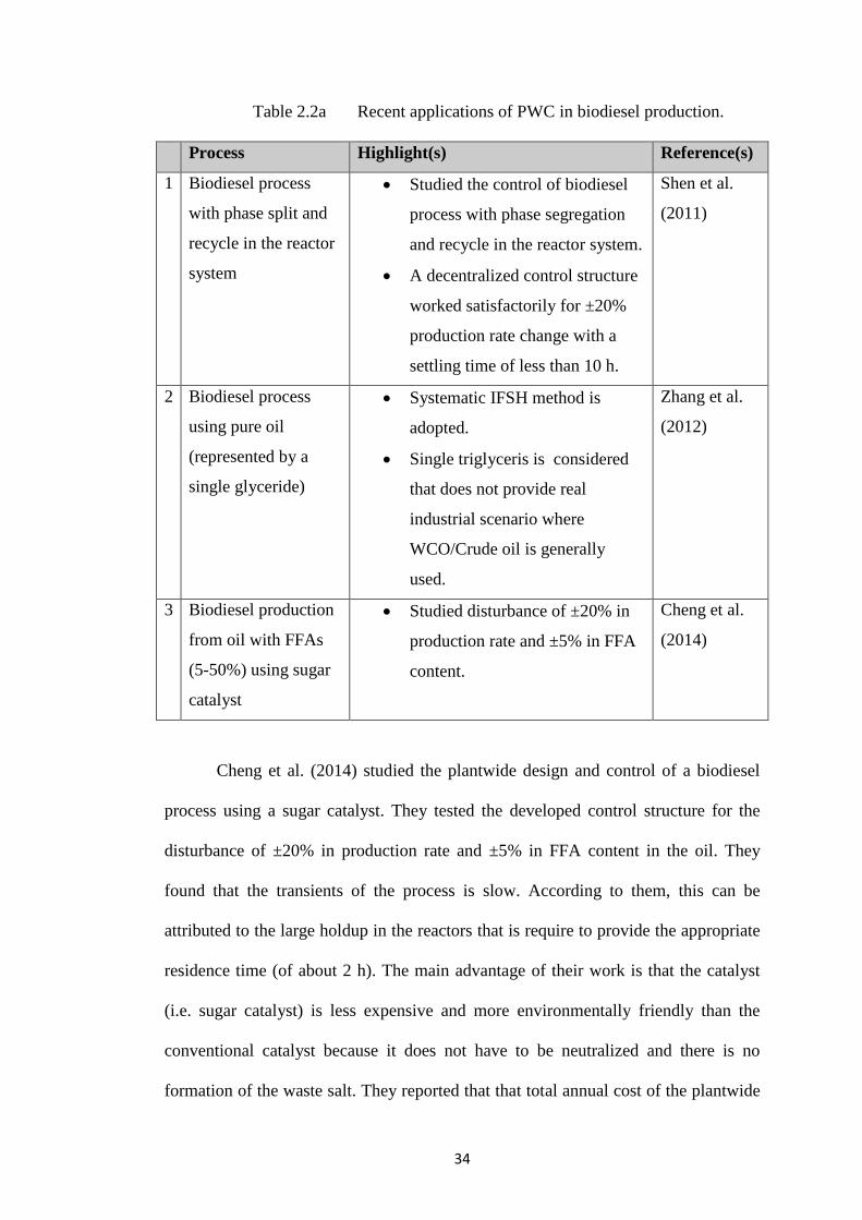
34
Table 2.2a Recent applications of PWC in biodiesel production.
Process Highlight(s) Reference(s)
1 Biodiesel process
with phase split and
recycle in the reactor
system
Studied the control of biodiesel
process with phase segregation
and recycle in the reactor system.
A decentralized control structure
worked satisfactorily for ±20%
production rate change with a
settling time of less than 10 h.
Shen et al.
(2011)
2 Biodiesel process
using pure oil
(represented by a
single glyceride)
Systematic IFSH method is
adopted.
Single triglyceris is considered
that does not provide real
industrial scenario where
WCO/Crude oil is generally
used.
Zhang et al.
(2012)
3 Biodiesel production
from oil with FFAs
(5-50%) using sugar
catalyst
Studied disturbance of ±20% in
production rate and ±5% in FFA
content.
Cheng et al.
(2014)
Cheng et al. (2014) studied the plantwide design and control of a biodiesel
process using a sugar catalyst. They tested the developed control structure for the
disturbance of ±20% in production rate and ±5% in FFA content in the oil. They
found that the transients of the process is slow. According to them, this can be
attributed to the large holdup in the reactors that is require to provide the appropriate
residence time (of about 2 h). The main advantage of their work is that the catalyst
(i.e. sugar catalyst) is less expensive and more environmentally friendly than the
conventional catalyst because it does not have to be neutralized and there is no
formation of the waste salt. They reported that that total annual cost of the plantwide
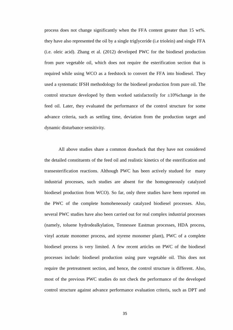
35
process does not change significantly when the FFA content greater than 15 wt%.
they have also represented the oil by a single triglyceride (i.e triolein) and single FFA
(i.e. oleic acid). Zhang et al. (2012) developed PWC for the biodiesel production
from pure vegetable oil, which does not require the esterification section that is
required while using WCO as a feedstock to convert the FFA into biodiesel. They
used a systematic IFSH methodology for the biodiesel production from pure oil. The
control structure developed by them worked satisfactorily for ±10%change in the
feed oil. Later, they evaluated the performance of the control structure for some
advance criteria, such as settling time, deviation from the production target and
dynamic disturbance sensitivity.
All above studies share a common drawback that they have not considered
the detailed constituents of the feed oil and realistic kinetics of the esterification and
transesterification reactions. Although PWC has been actively studued for many
industrial processes, such studies are absent for the homogeneously catalyzed
biodiesel production from WCO). So far, only three studies have been reported on
the PWC of the complete homoheneously catalyzed biodiesel processes. Also,
several PWC studies have also been carried out for real complex industrial processes
(namely, toluene hydrodealkylation, Tennessee Eastman processes, HDA process,
vinyl acetate monomer process, and styrene monomer plant), PWC of a complete
biodiesel process is very limited. A few recent articles on PWC of the biodiesel
processes include: biodiesel production using pure vegetable oil. This does not
require the pretreatment section, and hence, the control structure is different. Also,
most of the previous PWC studies do not check the performance of the developed
control structure against advance performance evaluation criteris, such as DPT and
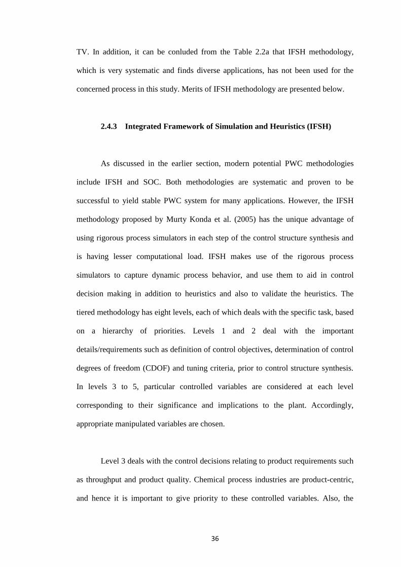
36
TV. In addition, it can be conluded from the Table 2.2a that IFSH methodology,
which is very systematic and finds diverse applications, has not been used for the
concerned process in this study. Merits of IFSH methodology are presented below.
2.4.3 Integrated Framework of Simulation and Heuristics (IFSH)
As discussed in the earlier section, modern potential PWC methodologies
include IFSH and SOC. Both methodologies are systematic and proven to be
successful to yield stable PWC system for many applications. However, the IFSH
methodology proposed by Murty Konda et al. (2005) has the unique advantage of
using rigorous process simulators in each step of the control structure synthesis and
is having lesser computational load. IFSH makes use of the rigorous process
simulators to capture dynamic process behavior, and use them to aid in control
decision making in addition to heuristics and also to validate the heuristics. The
tiered methodology has eight levels, each of which deals with the specific task, based
on a hierarchy of priorities. Levels 1 and 2 deal with the important
details/requirements such as definition of control objectives, determination of control
degrees of freedom (CDOF) and tuning criteria, prior to control structure synthesis.
In levels 3 to 5, particular controlled variables are considered at each level
corresponding to their significance and implications to the plant. Accordingly,
appropriate manipulated variables are chosen.
Level 3 deals with the control decisions relating to product requirements such
as throughput and product quality. Chemical process industries are product-centric,
and hence it is important to give priority to these controlled variables. Also, the
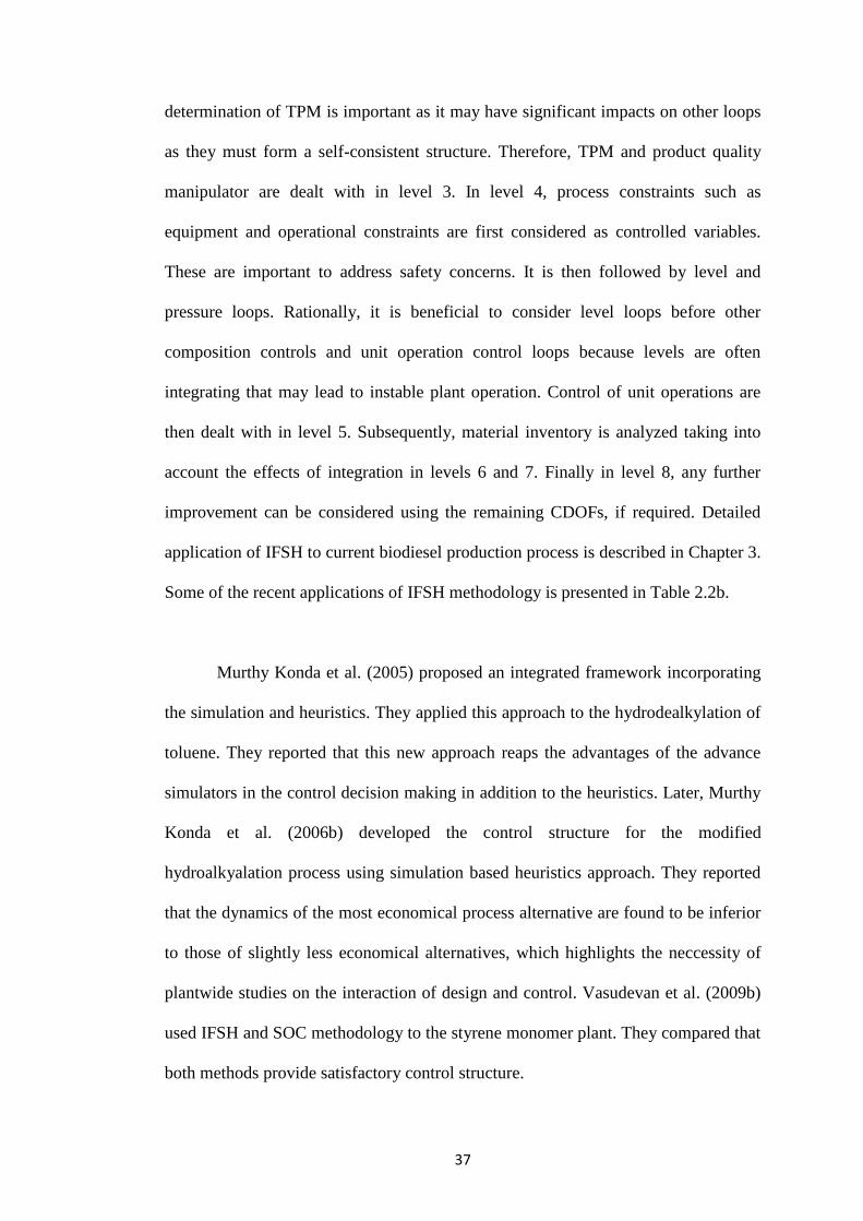
37
determination of TPM is important as it may have significant impacts on other loops
as they must form a self-consistent structure. Therefore, TPM and product quality
manipulator are dealt with in level 3. In level 4, process constraints such as
equipment and operational constraints are first considered as controlled variables.
These are important to address safety concerns. It is then followed by level and
pressure loops. Rationally, it is beneficial to consider level loops before other
composition controls and unit operation control loops because levels are often
integrating that may lead to instable plant operation. Control of unit operations are
then dealt with in level 5. Subsequently, material inventory is analyzed taking into
account the effects of integration in levels 6 and 7. Finally in level 8, any further
improvement can be considered using the remaining CDOFs, if required. Detailed
application of IFSH to current biodiesel production process is described in Chapter 3.
Some of the recent applications of IFSH methodology is presented in Table 2.2b.
Murthy Konda et al. (2005) proposed an integrated framework incorporating
the simulation and heuristics. They applied this approach to the hydrodealkylation of
toluene. They reported that this new approach reaps the advantages of the advance
simulators in the control decision making in addition to the heuristics. Later, Murthy
Konda et al. (2006b) developed the control structure for the modified
hydroalkyalation process using simulation based heuristics approach. They reported
that the dynamics of the most economical process alternative are found to be inferior
to those of slightly less economical alternatives, which highlights the neccessity of
plantwide studies on the interaction of design and control. Vasudevan et al. (2009b)
used IFSH and SOC methodology to the styrene monomer plant. They compared that
both methods provide satisfactory control structure.
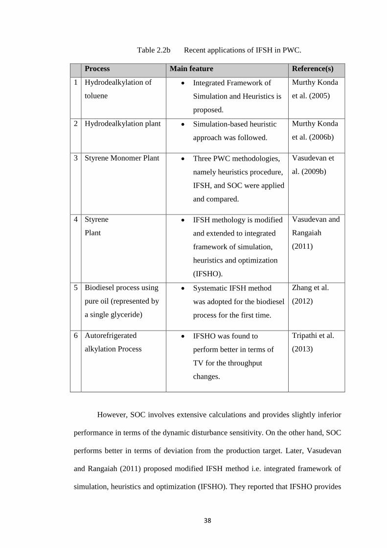
38
Table 2.2b Recent applications of IFSH in PWC.
Process Main feature Reference(s)
1 Hydrodealkylation of
toluene
Integrated Framework of
Simulation and Heuristics is
proposed.
Murthy Konda
et al. (2005)
2 Hydrodealkylation plant Simulation-based heuristic
approach was followed.
Murthy Konda
et al. (2006b)
3 Styrene Monomer Plant Three PWC methodologies,
namely heuristics procedure,
IFSH, and SOC were applied
and compared.
Vasudevan et
al. (2009b)
4 Styrene
Plant
IFSH methology is modified
and extended to integrated
framework of simulation,
heuristics and optimization
(IFSHO).
Vasudevan and
Rangaiah
(2011)
5 Biodiesel process using
pure oil (represented by
a single glyceride)
Systematic IFSH method
was adopted for the biodiesel
process for the first time.
Zhang et al.
(2012)
6 Autorefrigerated
alkylation Process
IFSHO was found to
perform better in terms of
TV for the throughput
changes.
Tripathi et al.
(2013)
However, SOC involves extensive calculations and provides slightly inferior
performance in terms of the dynamic disturbance sensitivity. On the other hand, SOC
performs better in terms of deviation from the production target. Later, Vasudevan
and Rangaiah (2011) proposed modified IFSH method i.e. integrated framework of
simulation, heuristics and optimization (IFSHO). They reported that IFSHO provides
39
better results in terms of better economic performance. Zhang et al. (2012) used
IFSH methodology for the biodiesel production from pure oil and successfully tested
the performance of the control structure for ± 10 % change in feed oil. Also, Tripathi
et al. (2013) developed the control structure for the Autorefrigerated alkylation
Process using IFSHO methodology. They reported that the developed control
structure works fine for the various disturbances. Next subsection discusses and
reviews the OTS for the chemical processes.
2.5 Operator Training Simulator (OTS)
OTS is a computer-based operator training tool that uses a dynamic
simulation of the process that imitates the real process. The dynamic simulator is
aften integrated with an emulator of the control system. An OTS uses a dynamic
simulation of the process to produce the appropriated data to feed an emulation of the
plant's control system. Typically, the major components of an OTS are: dynamic
simulator, instructor interface, control system integration software, control system
emulator and the operator station. Following subsections discuss need, application of
OTS in chemical processes, developmental issues, features, simulator softwares and
training issues.
2.5.2 Need of Operator Training Simulator
The activities of the operators during the critical situation in the process
directly influence the operation of chemical processes. Nazir and Manca (2014)
presented and discussed a solution for immersive training of industrial operators
40
allowing experiencing the multi-faceted scenarios of actual plant operations. Plant
Simulator consisted of a process simulator and an accident simulator to simulate
normal and emergency scenarios dynamically. Skilled operators are essential for
rapid production starts, the highest process performance, lessening environmental
impact and reduction of accidental losses in the complex chemical processes. Hence,
there is a need for developing an improved methodology to train operators efficiently
as their performance has direct influence on the safety, productivity, profitability,
stability and controllability of the process (Nazir et al., 2012). According to Yang et
al. (2001), in chemical and petrochemical industries without OTS, most operators get
their emergency operations training on the job under experienced operators’
supervision. This does not impart adequate confidence in inexperienced operators.
Earlier, Drozdowicz et al. (1987) noted that training on the job under experienced
operators’ supervision does not enhance the skills of operators to an adequate level.
In addition, even experienced operators may lose their feel for the process, which
directly affects team’s operational performance. OTS takes care of this gap by
combining the theoretical training and hands-on practice. Manenti (2012) stated that
a real plant is no place for training, and prior experience based on dynamic
simulation may be fundamental to reduce impact/damages of accidents or even to
prevent them. Considering this and decreasing computational costs with advent of
computational technology, he stated that the detailed dynamic simulation could
support what–if analyses and hazard and operability (HAZOP) studies, which will
become a key factor for future computer-aided process engineering (CAPE)
applications such as virtual reality, operator training simulation, fault detection and
automation approaches. Today, chemical process industries face many challenges
such as:
41
Quick training of operators within safe environment for higher productivity.
Retention of knowledge as lifetime experience may disappear with the
retirement of experienced workforce.
Grasping advanced control concepts is not easy for new personnel.
Continuous up-grading of the control software and hardware may increase the
difficulty.
Limited opportunities for training on the plant due to high level of
automation.
Tight project schedules with the challenge of designing and commissioning
new and revamped facilities within short duration.
Varying process conditions, pipeline’s slugging problem and changing feed
stocks
Strict regulatory compliance requirements, especially relating to
environmental issues.
OTS provides an effective solution to address the above challenges by
training the operators for the emergency scenarios, letting the industries to succeed in
the global competition. In addition to the theory and academic qualifications real-
time training is essential for operators to acquire the required competence.
Simulation is often the only cost-effective and safe way to ensure operators’
competence in dealing with normal and abnormal situations, contingencies and
operations. Using an OTS can be described as experiential learning. Simulation
offers repeatability and consistency, which makes it an ideal tool for training
operators and setting a standard of operator competence (Dudley et al., 2008).
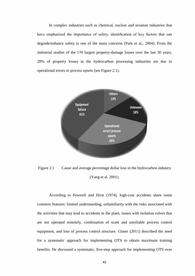
42
In complex industries such as chemical, nuclear and aviation industries that
have emphasized the importance of safety, identification of key factors that can
degrade/enhance safety is one of the main concerns (Park et al., 2004). From the
industrial studies of the 170 largest property-damage losses over the last 30 years,
28% of property losses in the hydrocarbon processing industries are due to
operational errors or process upsets (see Figure 2.1).
Figure 2.1 Cause and average percentage dollar loss in the hydrocarbon industry
(Yang et al. 2001).
According to Fewtrell and Hirst (1974), high-cost accidents share some
common features: limited understanding, unfamiliarity with the risks associated with
the activities that may lead to accidents in the plant, issues with isolation valves that
are not operated remotely, combination of scant and unreliable process control
equipment, and loss of process control structure. Glaser (2011) described the need
for a systematic approach for implementing OTS to obtain maximum training
benefits. He discussed a systematic, five-step approach for implementing OTS over
43
the long term (viz., identification, normal operation, start up and shut down,
troubleshooting, and optimization) along with feedback from OTS users, and use of
OTS to develop applied skills (viz., cooperation, communication, supervision and
situational awareness). The plant operators receive plant specific and realistic hands-
on training ahead of plant start-up and complete plant operation through proper use
of OTS. The reliable OTS can also be helpful in other functions such as
troubleshooting, developing new operating and control strategies. Thus, the simulator
can be a useful tool not only for training but also for the process and control
engineers (Dasgupta 1998).
In conclusion, the human error, which is one of the major causes behind the
industrial accidents, is the main motivation behind the development of suitable OTS.
To increase profitability, companies often extend intervals between plant
turnarounds. Therefore, startups and shutdowns occur less frequently. Some
emergency situations, such as power supply and steam cutoff, may never occur under
normal conditions. Even most experienced operators may perform at high efficiency
under these conditions. Using OTS, the trainees can be well prepared for handling
such infrequent operations.
2.5.3 Operator Training Simulator in Chemical Processes
High fidelity dynamic process simulators have been widely used by all major
oil and gas industries not only within process design studies, detailed engineering
studies, process debottlenecking and control system verification but also for operator
training (Cameron et al., 2002; Bessiris et al., 2011). In other industries such as palm
oil mills, automation is quite limited. Sivasothy and Lim (1985) reported that this
44
was not due to hardware limitations or reluctance by the industry to adopt
automation, but rather due to software limitations.
In the late 1980's and early 1990's, implementation of OTS in the chemical
industry has become the common practice. Cameron et al. (2002) reported that
training simulators have been widely adopted in industries such as offshore oil & gas
industry and power & energy industry, where capital investment is high, processes
are complex and the consequences of plant or operator failure are severe. As reported
by Cameron et al. (2002), older training laboratories for training in the oil industry
were based on physical replicas of the control room which are now expensive and
unnecessary.
In industries, object linking and embedding for process control (OPC) is
commonly used as industrial communication standard that enables the exchange of
data between the server and clients.OPC is a client-server technology that acts as an
interface between the server and the client. One application acts as the server
providing data while another acts as a client that uses the data. Using OPC standards,
applications (e.g. control applications) from different vendors can be linked as they
share common standards. Table 2.3 summarizes the applications and main feature(s)
of OTS in relevant chemical industries/processes which use modular softwares for
the OTS development. However, very limited studies on OTS have been found in the
open literature, the number of papers published in this area has increased
considerably in the last decade.
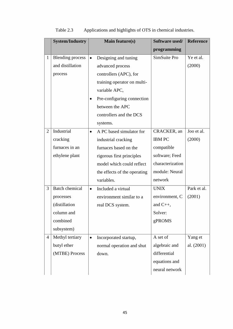
45
Table 2.3 Applications and highlights of OTS in chemical industries.
System/Industry Main feature(s) Software used/
programming
Reference
1 Blending process
and distillation
process
Designing and tuning
advanced process
controllers (APC), for
training operator on multi-
variable APC,
Pre-configuring connection
between the APC
controllers and the DCS
systems.
SimSuite Pro Ye et al.
(2000)
2 Industrial
cracking
furnaces in an
ethylene plant
A PC based simulator for
industrial cracking
furnaces based on the
rigorous first principles
model which could reflect
the effects of the operating
variables.
CRACKER, an
IBM PC
compatible
software; Feed
characterization
module: Neural
network
Joo et al.
(2000)
3 Batch chemical
processes
(distillation
column and
combined
subsystem)
Included a virtual
environment similar to a
real DCS system.
UNIX
environment, C
and C++,
Solver:
gPROMS
Park et al.
(2001)
4 Methyl tertiary
butyl ether
(MTBE) Process
Incorporated startup,
normal operation and shut
down.
A set of
algebraic and
differential
equations and
neural network
Yang et
al. (2001)
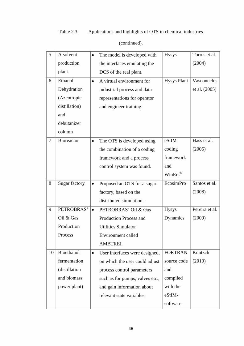
46
Table 2.3 Applications and highlights of OTS in chemical industries
(continued).
5 A solvent
production
plant
The model is developed with
the interfaces emulating the
DCS of the real plant.
Hysys Torres et al.
(2004)
6 Ethanol
Dehydration
(Azeotropic
distillation)
and
debutanizer
column
A virtual environment for
industrial process and data
representations for operator
and engineer training.
Hysys.Plant
Vasconcelos
et al. (2005)
7 Bioreactor The OTS is developed using
the combination of a coding
framework and a process
control system was found.
eStIM
coding
framework
and
WinErs®
Hass et al.
(2005)
8 Sugar factory Proposed an OTS for a sugar
factory, based on the
distributed simulation.
EcosimPro Santos et al.
(2008)
9 PETROBRAS’
Oil & Gas
Production
Process
PETROBRAS’ Oil & Gas
Production Process and
Utilities Simulator
Environment called
AMBTREI.
Hysys
Dynamics
Pereira et al.
(2009)
10 Bioethanol
fermentation
(distillation
and biomass
power plant)
User interfaces were designed,
on which the user could adjust
process control parameters
such as for pumps, valves etc.,
and gain information about
relevant state variables.
FORTRAN
source code
and
compiled
with the
eStIM-
software
Kuntzch
(2010)
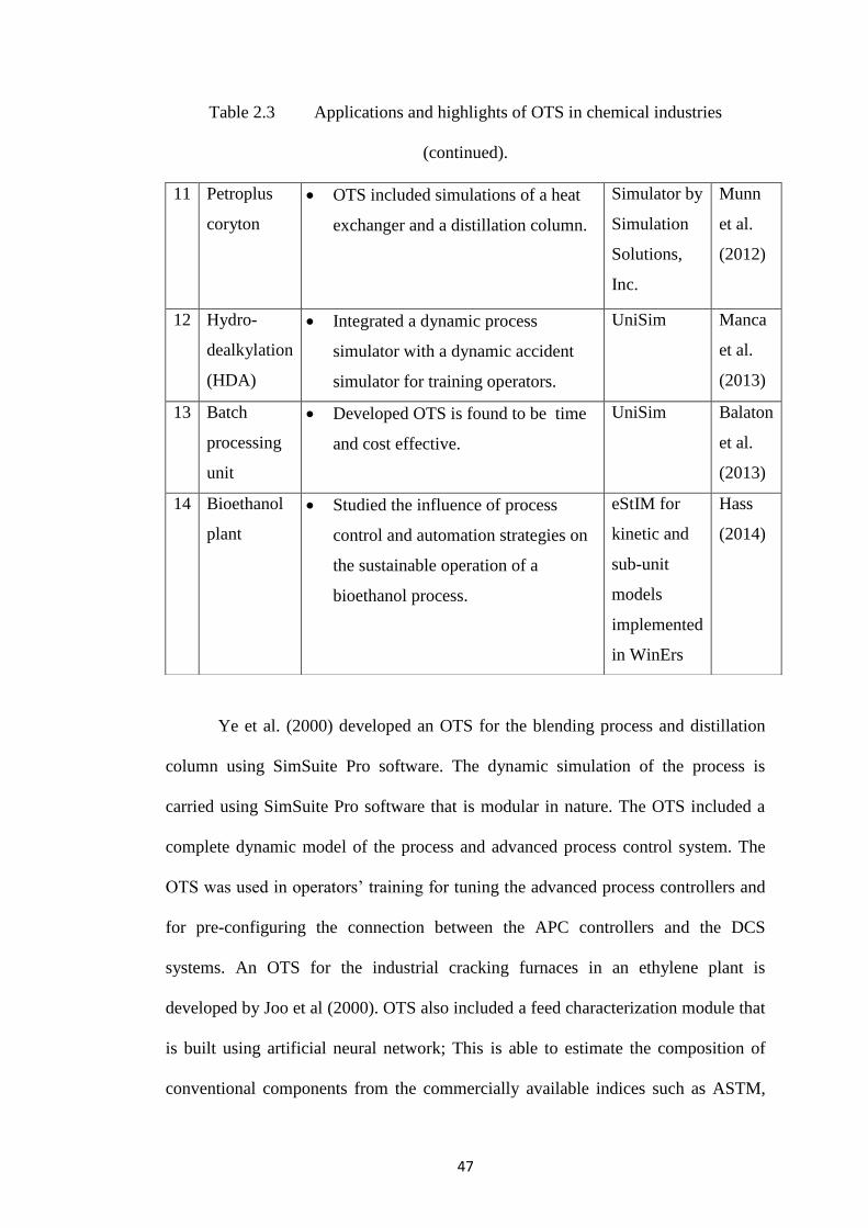
47
Table 2.3 Applications and highlights of OTS in chemical industries
(continued).
Ye et al. (2000) developed an OTS for the blending process and distillation
column using SimSuite Pro software. The dynamic simulation of the process is
carried using SimSuite Pro software that is modular in nature. The OTS included a
complete dynamic model of the process and advanced process control system. The
OTS was used in operators’ training for tuning the advanced process controllers and
for pre-configuring the connection between the APC controllers and the DCS
systems. An OTS for the industrial cracking furnaces in an ethylene plant is
developed by Joo et al (2000). OTS also included a feed characterization module that
is built using artificial neural network; This is able to estimate the composition of
conventional components from the commercially available indices such as ASTM,
11 Petroplus
coryton
OTS included simulations of a heat
exchanger and a distillation column.
Simulator by
Simulation
Solutions,
Inc.
Munn
et al.
(2012)
12 Hydro-
dealkylation
(HDA)
Integrated a dynamic process
simulator with a dynamic accident
simulator for training operators.
UniSim Manca
et al.
(2013)
13 Batch
processing
unit
Developed OTS is found to be time
and cost effective.
UniSim Balaton
et al.
(2013)
14 Bioethanol
plant
Studied the influence of process
control and automation strategies on
the sustainable operation of a
bioethanol process.
eStIM for
kinetic and
sub-unit
models
implemented
in WinErs
Hass
(2014)
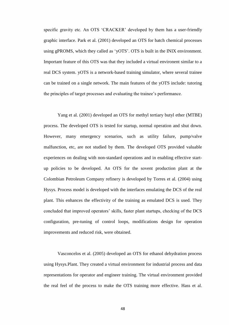
48
specific gravity etc. An OTS ‘CRACKER’ developed by them has a user-friendly
graphic interface. Park et al. (2001) developed an OTS for batch chemical processes
using gPROMS, which they called as ‘yOTS’. OTS is built in the INIX environment.
Important feature of this OTS was that they included a virtual environent similar to a
real DCS system. yOTS is a network-based training simulator, where several trainee
can be trained on a single network. The main features of the yOTS include: tutoring
the principles of target processes and evaluating the trainee’s performance.
Yang et al. (2001) developed an OTS for methyl tertiary butyl ether (MTBE)
process. The developed OTS is tested for startup, normal operation and shut down.
However, many emergency scenarios, such as utility failure, pump/valve
malfunction, etc, are not studied by them. The developed OTS provided valuable
experiences on dealing with non-standard operations and in enabling effective start-
up policies to be developed. An OTS for the sovent production plant at the
Colombian Petroleum Company refinery is developed by Torres et al. (2004) using
Hysys. Process model is developed with the interfaces emulating the DCS of the real
plant. This enhances the effectivity of the training as emulated DCS is used. They
concluded that improved operators’ skills, faster plant startups, checking of the DCS
configuration, pre-tuning of control loops, modifications design for operation
improvements and reduced risk, were obtained.
Vasconcelos et al. (2005) developed an OTS for ethanol dehydration process
using Hysys.Plant. They created a virtual environment for industrial process and data
representations for operator and engineer training. The virtual environment provided
the real feel of the process to make the OTS training more effective. Hass et al.
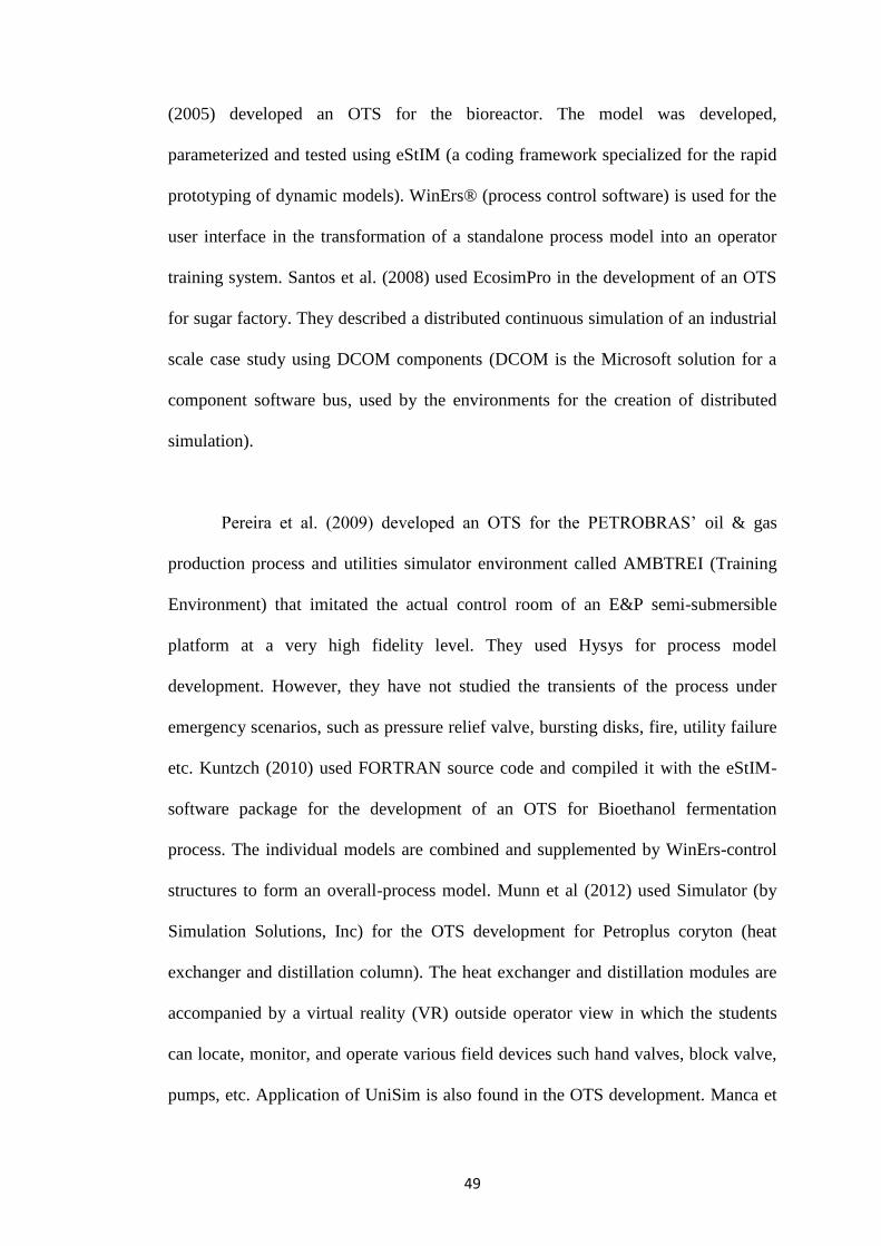
49
(2005) developed an OTS for the bioreactor. The model was developed,
parameterized and tested using eStIM (a coding framework specialized for the rapid
prototyping of dynamic models). WinErs® (process control software) is used for the
user interface in the transformation of a standalone process model into an operator
training system. Santos et al. (2008) used EcosimPro in the development of an OTS
for sugar factory. They described a distributed continuous simulation of an industrial
scale case study using DCOM components (DCOM is the Microsoft solution for a
component software bus, used by the environments for the creation of distributed
simulation).
Pereira et al. (2009) developed an OTS for the PETROBRAS’ oil & gas
production process and utilities simulator environment called AMBTREI (Training
Environment) that imitated the actual control room of an E&P semi-submersible
platform at a very high fidelity level. They used Hysys for process model
development. However, they have not studied the transients of the process under
emergency scenarios, such as pressure relief valve, bursting disks, fire, utility failure
etc. Kuntzch (2010) used FORTRAN source code and compiled it with the eStIM-
software package for the development of an OTS for Bioethanol fermentation
process. The individual models are combined and supplemented by WinErs-control
structures to form an overall-process model. Munn et al (2012) used Simulator (by
Simulation Solutions, Inc) for the OTS development for Petroplus coryton (heat
exchanger and distillation column). The heat exchanger and distillation modules are
accompanied by a virtual reality (VR) outside operator view in which the students
can locate, monitor, and operate various field devices such hand valves, block valve,
pumps, etc. Application of UniSim is also found in the OTS development. Manca et
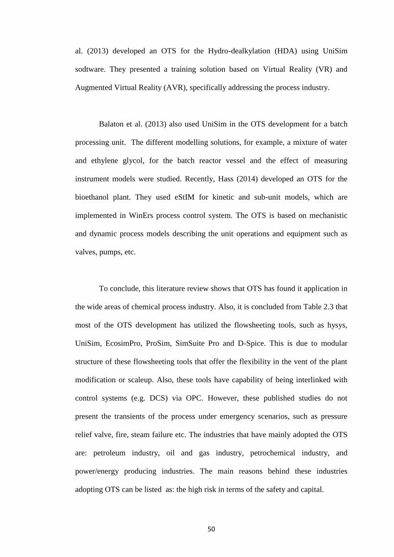
50
al. (2013) developed an OTS for the Hydro-dealkylation (HDA) using UniSim
sodtware. They presented a training solution based on Virtual Reality (VR) and
Augmented Virtual Reality (AVR), specifically addressing the process industry.
Balaton et al. (2013) also used UniSim in the OTS development for a batch
processing unit. The different modelling solutions, for example, a mixture of water
and ethylene glycol, for the batch reactor vessel and the effect of measuring
instrument models were studied. Recently, Hass (2014) developed an OTS for the
bioethanol plant. They used eStIM for kinetic and sub-unit models, which are
implemented in WinErs process control system. The OTS is based on mechanistic
and dynamic process models describing the unit operations and equipment such as
valves, pumps, etc.
To conclude, this literature review shows that OTS has found it application in
the wide areas of chemical process industry. Also, it is concluded from Table 2.3 that
most of the OTS development has utilized the flowsheeting tools, such as hysys,
UniSim, EcosimPro, ProSim, SimSuite Pro and D-Spice. This is due to modular
structure of these flowsheeting tools that offer the flexibility in the vent of the plant
modification or scaleup. Also, these tools have capability of being interlinked with
control systems (e.g. DCS) via OPC. However, these published studies do not
present the transients of the process under emergency scenarios, such as pressure
relief valve, fire, steam failure etc. The industries that have mainly adopted the OTS
are: petroleum industry, oil and gas industry, petrochemical industry, and
power/energy producing industries. The main reasons behind these industries
adopting OTS can be listed as: the high risk in terms of the safety and capital.
51
On the other hand, the OTS is not commonly used in the field of bioprocess
engineering (such as enzymatic processes) possibly because: 1) normally, the
operating conditions are moderate in bioprocesses and so the associated risk is
relatively lower, and 2) bioprocesses are usually specialized and operated on a small
scale, most on bach scale. Consequently, the benefits of using OTS in bioprocess
field have not been properly evaluated. Also, it is worth noticing that the OTS has
been reported for biodiesel production from WCO. In addition, sectors such as oil
mills and other small-scale chemical industries, have not adopted OTS significantly.
This could be due to the reasonably lower risk associated with such processes and the
higher cost of OTS. Additionally, it can be concluded that Aspen Plus Dynamics and
Aspen OTS Framework has not been used for the OTS development for any
chemical process. Therefore, there are enough scopes for the exploration of the OTS
development. Also, it is important to note that the benefits of process models can be
greatly extended by transferring them into an OTS. The issues related to the OTS
development and implementation are described in the following section.
2.5.4 Issues Related to the Development and Implementation of
Operator Training Simulator (OTS)
Although OTS have been developed and applied in various industries, there
are still many challenges related to the OTS development based on steady state
design information. According to Yang et al. (2001), a major plant accidents are
more than five times more likely to occur during abnormal operations than during
normal operation. Qiu et al. (2003) reported that the interest in the study of dynamics
52
of chemical plants with recycles and plant-wide control design has increased
significantly in the past decade.
An acceptable dynamic model requires details of equipment size and shape,
controller tuning, sampling time, signal noise, valve hysteresis or shutdown
categorizations. The chemical reactors are the key elements in chemical processes.
The reactors are often the most complicated unit to model as each reactor has a
unique geometry, flow arrangement and reaction kinetics. Consequently, detailed
knowledge of the reactor is necessary for developing the realistic reactor model for
OTS. As reactors are usually proprietary, their developers are often reluctant to share
details about reaction kinetics and reactor design with OTS developers. Under such
circumstances, a simplified model or a black box model is used (Cameron et al.,
2002).
If the model is highly complex, it will not be easy to modify or maintain
online model-based applications (OMBA), and some or all of the value of a complex
model may be lost. On the contrary, if the model is too simplistic, there are
associated maintenance issues with refitting/retuning and the OMBA value may be
lost (Pantelides and Renfro, 2013). However, Pantelides and Renfro (2013)
mentioned that sustainability is not always a monotonically decreasing function of
the degree of modeling rigor. Infrequent situations like disturbance handling or even
system restoration, dictate additional modelling requirements for system performance
within the simulator (Spanel et al., 2001). These are discussed in the following sub-
sections. Cox et al. (2006) described the salient characteristics of a suitable dynamic
modelling tool, as presented in Table 2.4.
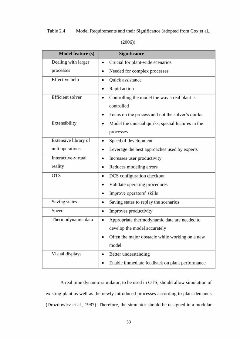
53
Table 2.4 Model Requirements and their Significance (adopted from Cox et al.,
(2006)).
Model feature (s) Significance
Dealing with larger
processes
Crucial for plant-wide scenarios
Needed for complex processes
Effective help Quick assistance
Rapid action
Efficient solver Controlling the model the way a real plant is
controlled
Focus on the process and not the solver’s quirks
Extensibility Model the unusual quirks, special features in the
processes
Extensive library of
unit operations
Speed of development
Leverage the best approaches used by experts
Interactive-virtual
reality
Increases user productivity
Reduces modeling errors
OTS DCS configuration checkout
Validate operating procedures
Improve operators’ skills
Saving states Saving states to replay the scenarios
Speed Improves productivity
Thermodynamic data Appropriate thermodynamic data are needed to
develop the model accurately
Often the major obstacle while working on a new
model
Visual displays Better understanding
Enable immediate feedback on plant performance
A real time dynamic simulator, to be used in OTS, should allow simulation of
existing plant as well as the newly introduced processes according to plant demands
(Drozdowicz et al., 1987). Therefore, the simulator should be designed in a modular
54
fashion, where different flow sheets are built combining the unit operation modules
in a puzzle like manner and new modules can be introduced with minimal changes.
The model equations should be structured carefully as establishing an accurate
steady-state solution for the initialization of the dynamic model is very crucial.
i. Model Accuracy
Both the model and modelling tool should be sufficiently accurate to ensure
fidelity and consistency of results. Stawarz and Sowerby (1995) used the standard of
less than 2% and 10% error for critical and non-critical parameters, respectively, in a
model developed for OTS. Considering this, surprisingly simple models can yield
sufficient fidelity for operator training needs, they opined. Zhiyun et al. (2003) also
stated that, when the ultimate goal of the simulation work is to build OTS,
requirements of modeling accuracy are not so strict.
ii. Speed
Cox et al. (2006) stated that if the model can run about 50 times real time, the
engineer’s effectiveness is highest. Because of an inevitable need for reduced
runtime of model while ensuring sufficient fidelity, an appropriate choice of a solver
is essential. In addition, flow sheet partitioning can help reducing the model runtime
as discussed in Chapter 3. Although the speed up/slow down features provide some
flexibity during training, it is more beneficial to use the actual dynamics.
55
iii. Robustness
The modeler should be able to deal with process issues efficiently without
having limitations of issues like convergence, tear streams, solver’s incapability,
especially, in case of unavailability of good initial guesses. ‘In some cases,
companies had to delay their projects due to unavailability of good initial guesses,’
Cox et al. (2006) reported. For varieties of disturbances (including shut down of a
unit), the model should be able to provide a solution. This is essential, especially
when the end user does not have the background to comprehend what is going on in
the simulator and thus cannot fix any numerical problem that may arise (Laganier,
1996).
iv. Memory
The model should be able to run for long intervals without overflowing
memory or other computer resources. This is a key requirement of an OTS, which
runs for hours and days. Cox et al. (2006) reported that commercial dynamic
simulators failed at this task. However, our recent experience shows that modern
software packages seem to be good in this issue.
In summary, the development of the dynamic simulator for training purpose
requires knowledge in several fields: development of the dynamic model of
processes, solver, real time programming of digital equipment, programming tools,
man-machine interface, etc. Therefore, it is advisable to involve the people having a
global understanding of the ultimate goal while each of them having specialized
56
knowledge of a few of the fields involved development of OTS. In addition, it is
essential to maintain the OTS. Otherwise, it may become just a check-off
requirement rather than being a learning tool. A poorly maintained OTS may be
worse than not having one at all because operators would falsely think that they
know what is going to happen, and any such OTS will give the management a false
sense of security. Degree of accuracy, calculation speed, convergence and the
robustness of a model to be used for operator training need to be given special
consideration. Also, it is important that the process model and control system (either
emulated or stimulated) should run on a compatible platform in order to provide
seemless data transfer and synchronization. Next section presents the salient features
of OTS.
2.5.5 Salient Features of Operator Training Simulator (OTS)
A good OTS should posses several features that are essential for extracting
the maximum benefit. Usually, dynamic simulations in OTS are considerably
detailed containing all equipment items in the plant including items not normally
included in an engineering study model (such as instruments and spare pumps).
Consequently, these simulations are very large and include operations having fast
dynamics and slow dynamics as well, e.g. compressors having fast dynamics and
distillation columns having slow dynamics. The integration size must be different
catering to the respective dynamics of the unit operations involved to obtain
reasonable accuracy. A single processor may lead to simulation time lagging behind
real time due to the limited processor capacity. A suitable OTS framework must be
able to cope with this by some means. The other features of OTS are as follows;
57
Modeling for the entire life cycle of a plant i.e. from the steady-state design
to offline engineering studies and on-line operational models (i.e., full-scope
operator training for start-up, shutdown and other infrequent operations).
Modelling equipment failures and logical procedures.
Sufficient fidelity models to quickly acquaint operators with new controls and
human-machine interface (HMI).
Efficient simultaneous pressure/flow network solvers within fast transients.
Modeling in the modular fashion so that a new module can be added at
minimal cost and effort.
Ability to evaluate DCS functionality before the start-up of the plant.
High fidelity models suitable for DCS, safety instrumented systems (SIS) and
programmable logic controller (PLC) control validation.
Object oriented and on-line configurable graphical interface.
Ability to validate DCS input-output configuration in the most efficient
manner possible.
A framework that provides a configuration mode to set up all the required
data links between the dynamic model(s) of process and the other OTS
components. Data communication links handle the exchange of data and
commands. They should be based on a technology which defines the standard
interface for allowing applications to access data from different process
control devices such as object linking or embedding (OLE) process control
(OPC). Contemporary OPC interfaces considerably reduce the time required
to build a good interface to external systems (Cox et al., 2006).
Software packages (i.e. Emulators) should be able to translate and emulate
plant’s actual control system into modules that can be used within the OTS
58
system without the need to buy a replicate control system, thus reducing the
OTS cost significantly.
User Interfaces should support different views of the application for
operators, engineers and training instructors. For operators, OTS application
should look and behave like the plant’s actual control system.
On-line parameterization/validation of process equipment and control
modules.
Partitioning and configuration of a large dynamic process model across
multiple CPUs/cores for faster solution.
One process flow diagram (PFD) environment to be used to build the model
and compact faceplate interface to controllers.
Profile charts (e.g., column temperature, pressure and composition profile).
An extensive and useful help system for all OTS users.
To conclude, it is important that the OTS posses several salient features that
would make users to extract the maximum benefits from the OTS training. The
important factors that must be paid attention to are: detailed dynamic simulation,
good user interface, single PFD environment, one model-many uses policy, commom
platform (e.g. OPC), and extensive help. Also, it is crucial to consider the specific
requirements of the industry while developing the OTS as the training cost is also an
important factor. The cost of OTS can be reduced by making use of the components
of OTS available with the industry, for example, the emulators as discussed before.
Using commercial software packages adds to the convenient development of the
OTS. Several commercial software packages available to develop the OTS are
described in the next section.
59
2.5.6 Simulation Softwares for Developing Operator Training
Simulator (OTS)
The computer-aided process design (CAPD) and the simulation tools have
been successfully implemented in chemical and oil industries since the early 1960s,
aiming for the development and optimization of integrated systems (Balaton et al.,
2013). The current modular commercial process simulation softwares flexible and
convenient model development of the complex processes. A suitable process model
and its simulation are at the heart of OTS. However, no model is completely
accurate. It is important to note the admonition of Box (1979): ‘All models are
wrong, but some are useful’. The process dynamic simulators are popular tools for
training the operators (Glasscock and Dale, 1994). Previously, the graphical front-
ends of large scale operator training simulators consisted of hundreds of thousands of
lines of code (Stawarz and Sowerby, 1995).
According to Stawarz and Sowerby, (1995), development of training
simulators using procedural code used conventionally will become excessively
costly, difficult to update and ultimately unmanageable due to the increased and
continuous demand of graphical complexity. To counteract the implications of
increasing code length and program complexity, Stawarz and Sowerby (1995)
suggested development of graphical interfaces using object-oriented programming
methods. Shepherd (1986) reported that it is reasonable to consider training
simulation requirements in advance before making a decision to purchase simulation
hardware.
60
Komulainen et al. (2012) reported that use of commercial process simulators
in chemical engineering education is an increasing interest. Commercial simulators
include Aspen Plus and Aspen HYSYS (Aspen Technology, Inc.), ChemCAD
(Chemstations, Inc.), HYSYS (Hyprotech, Ltd./AEA Engineering Software in the
past), UniSim Design (Honeywell International Inc.), PRO/II (Simulation Sciences,
Inc.) and DYNSIM (Invensys Inc.). Aspen Custom Modeler (ACM), earlier SpeedUp
from Imperial College London which was commercialized by Aspen Technologies
and named ACM. ACM is used to develop rigorous models of processing equipment.
Aspen Technology, Inc. has provided an Aspen OTS framework in their
newer version V7 (and above) that offers a single integrated platform for Process
Training and Operator Training Simulators. Shadow Plant™ Standard Edition
(Shadow Plant SE) is the dynamic simulator software for the training of operators on
Honeywell's regulatory and logic control. Invensys has also been providing OTS for
the process industries. Software packages such as DYNSIM and D-splice have also
been used successfully by OTS developers such as Hyperion Systems Engineering
and Fantoft Process Technologies respectively. Honeywell’s UniSim Design
software has widespread usage in OTS applications. The first process simulator
designed for batch processes called ‘Batches’ was commercialized in the mid 1980s
by Batch Process Technologies (Balaton et al., 2013). The model building strategy in
batch processes differs from the conventional method used for continuous processes,
for which a steady-state model is first created and then it is switched to dynamic
mode. Among all commercial softwares/tools available for the simulation of
chemical processes, those commonly used for OTS development are presented in
Table 2.5. By no means does this table include all available software packages.
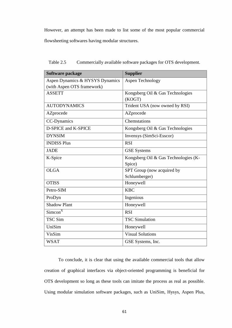
61
However, an attempt has been made to list some of the most popular commercial
flowsheeting softwares having modular structures.
Table 2.5 Commercially available software packages for OTS development.
Software package Supplier
Aspen Dynamics & HYSYS Dynamics
(with Aspen OTS framework)
Aspen Technology
ASSETT Kongsberg Oil & Gas Technologies
(KOGT)
AUTODYNAMICS Trident USA (now owned by RSI)
AZprocede AZprocede
CC-Dynamics Chemstations
D-SPICE and K-SPICE Kongsberg Oil & Gas Technologies
DYNSIM Invensys (SimSci-Esscor)
INDISS Plus RSI
JADE GSE Systems
K-Spice Kongsberg Oil & Gas Technologies (K-
Spice)
OLGA SPT Group (now acquired by
Schlumberger)
OTISS Honeywell
Petro-SIM KBC
ProDyn Ingenious
Shadow Plant Honeywell
SimconX RSI
TSC Sim TSC Simulation
UniSim Honeywell
VisSim Visual Solutions
WSAT GSE Systems, Inc.
To conclude, it is clear that using the available commercial tools that allow
creation of graphical interfaces via object-oriented programming is beneficial for
OTS development so long as these tools can imitate the process as real as possible.
Using modular simulation software packages, such as UniSim, Hysys, Aspen Plus,
62
DynSim etc, an effective OTS can be developed. In addition, the promotes the one
model-many uses policy that intends to extract the maximum benefits from the
process simulations. The use of procedural code to represent the complete plant is
tedious and often impractical. The training configurations of OTS and the issues
related to them are discussed in the following section.
2.5.7 Training Configurations and Related Issues
‘In defining an approach to deal with the training of process operators, two
central issues must be considered - set of responsibilities assigned to a process
operator and purpose of training,’ Shepherd (1986) reported. He also stated that, in
order to reduce plant downtime and avoid hazards which will affect plant, personnel
and the environment, it is important to be clear exactly what sort of skill is required.
These skills include detection, diagnosis, compensation, rectification and recovery.
Operators are linked with process through a control system, either a DCS or a
Supervisory Control and Data Acquisition (SCADA) system where the process
controllers are implemented in a number of PLCs (Cameron et al. 2002). Operators
need to be trained in how to relate to the process through the DCS or SCADA
human-machine interface (HMI). This essentially demands a training simulator to
provide the replica of the control system HMI, which can be accomplished in the
following ways (Cameron et al., 2002).
Stimulated system: By using the simulator to communicate with a physical
copy of the entire control system. Hence, stimulated systems accurately and
exactly represent the control system behavior.
63
Quasi-stimulated system: By using the simulator to communicate with a
physical copy of either the DCS operator stations or the SCADA part of a
SCADA/PLC control system, and not the entire control system.
Emulated system: By building a software replica of the entire control system
and its user interface. However, emulated systems do not ensure the complete
fidelity of automation systems and they do not provide accurate
implementation of the training system components (Pereira et al., 2009). As
reported by Pereira et al. (2009) this system can be preferred when:
i. Control hardware is difficult to obtain.
ii. Using physical copy of the entire control system is expensive and
worthless, especially when dealing with simpler equipment logics.
Lee et al. (2000) proposed a method of evaluating operators' plant
manipulation capability by using an OTS. They developed task evaluation algorithm
(TEA) to analyze and evaluate the operators' training results automatically after one
finished the training by using the GUI emulation of DCS. TEA includes two main
modules: sequence evaluation module (SEM) and quantity evaluation module
(QEM). The former indicates whether the operator follows the correct operating
sequence that is prepared in advance. On the other hand, QEM gives the deviation of
each operator's task from the standard operating procedure. TEA was shown to be
efficient and effective in analyzing the operator's capability (Lee et al., 2000).
Several important factors that should be carefully taken into account to
perform human reliability analysis (HRA) were observed. Typically, there are three
forms of OTS: DCS based, networked workstation/PC and standalone
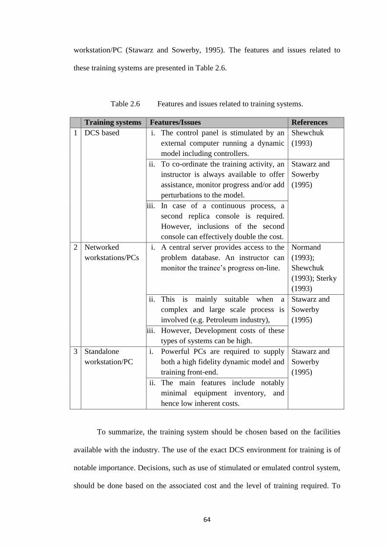
64
workstation/PC (Stawarz and Sowerby, 1995). The features and issues related to
these training systems are presented in Table 2.6.
Table 2.6 Features and issues related to training systems.
Training systems Features/Issues References
1 DCS based i. The control panel is stimulated by an
external computer running a dynamic
model including controllers.
Shewchuk
(1993)
ii. To co-ordinate the training activity, an
instructor is always available to offer
assistance, monitor progress and/or add
perturbations to the model.
Stawarz and
Sowerby
(1995)
iii. In case of a continuous process, a
second replica console is required.
However, inclusions of the second
console can effectively double the cost.
2 Networked
workstations/PCs
i. A central server provides access to the
problem database. An instructor can
monitor the trainee’s progress on-line.
Normand
(1993);
Shewchuk
(1993); Sterky
(1993)
ii. This is mainly suitable when a
complex and large scale process is
involved (e.g. Petroleum industry),
Stawarz and
Sowerby
(1995)
iii. However, Development costs of these
types of systems can be high.
3 Standalone
workstation/PC
i. Powerful PCs are required to supply
both a high fidelity dynamic model and
training front-end.
Stawarz and
Sowerby
(1995)
ii. The main features include notably
minimal equipment inventory, and
hence low inherent costs.
To summarize, the training system should be chosen based on the facilities
available with the industry. The use of the exact DCS environment for training is of
notable importance. Decisions, such as use of stimulated or emulated control system,
should be done based on the associated cost and the level of training required. To
65
start with, a standalone OTS can be developed that can then be extended to network
base (using real/emulated DCS) training. A solid and up-to-date model with a
suitable user interface that mimics the DCS provides much more useful training.
2.6 Summary
A systematic review of previous studies on the biodiesel production, MOO,
PWC and OTS is carried out in this chapter. The critical anlaysis of the previous
studies identify the gaps in the preious works. These, in essence, set the tone for this
research. It is clear from the literature review that homogeneously alkali catalyzed
transesterification is the preferred choice in the industry; hence, an OTS should be
tested for this process. An effective OTS requires a suitable MOO and PWC study.
Consequently, firstly, a detailed literature review has been carried out for the
application of MOO and PWC in the biodiesel production. Later, literature review is
carried out related to the OTS. Biodiesel production from WCO is attractive due to
its many-fold merits, such as low cost and effective waste utilization. Realistic and
detailed simulation is important to obtain the close to real results. The reliability of
further studies depends mainly on the ability of simulator to yield realistic results.
MOO, which is essential given the intense competition among companies and strict
environmental regulations, should be made possible using simple, effective and easy
to use tools. For example, MS Excel that is popular for several engineering studies
due to its familiarity and easy access compared to other more complicated tools.
Effective and efficient optimization tool is necessary to obtain trade-offs between
several conflicting objectives. Methods such as NSGA-II are proven to be useful in
determining such trade-offs in many chemical processes as discussed in Section
66
2.3.2. Although the production of biodiesel via transesterification has been widely
studied, PWC studies and OTS development for this process are absent. The novelty
of the present research also includes the development and evaluation of a PWC
system for the complex homogeneously catalyzed two-step biodiesel production
from WCO. PWC system should be robust and effective. Depending on the
objectives PWC structure may vary. Therefore, a systematic procedure should be
employed to obtained suitable PWC system. Among several potential PWC methods
is an IFSH methodology that has been found to provide suitable control system for
variety of chemical processes. Later, the need of an OTS for the biodiesel process is
established. Although the accuracy requirements are not so strict, the fidelity of
process model is important in OTS development so far as imitating the process
behaviour is concerned. Also, it is clear from the review that using the available
commercial tools that allow creation of graphical interfaces is beneficial for OTS
development so long as these tools can imitate the process as real as possible. Using
modular simulation software packages, an effective OTS can be developed. In
addition, the promotes the one model-many uses policy that intends to extract the
maximum benefits from the process simulations.
Based on the literature review, following gaps in the previous research have
been identified: (1) a realistic biodiesel process design and simulation is missing as
the previous studies do not use extensive componets of the feed oil and detailed
esterification and transesterification kinetics. Stochastic method i.e. NSGA-II has not
been employed for the MOO of this process that is required to determine the Pareto-
optimal fronts for the conflicting objectives. In addition, scarcity of enough research
material on the development of PWC system and OTS development for the biodiesel
67
production from WCO is clear from the literature review in Sections 2.4 and 2.5. No
previous work is found related to the OTS development for biodiesel production
from WCO. Additionally, application of APD and Aspen OTS Framework in OTS
development has not been explored, thus far. An effective OTS can be beneficial if it
is able to yield realistic responses for the range of scenarios. Also, a good OTS
should possess several important characteristics of OTS as discussed in this chapter.
Next chapter focuses on the methodology adopted to fulfil these gaps that set the
objectives of this research.
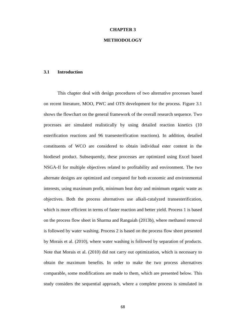
68
CHAPTER 3
METHODOLOGY
3.1 Introduction
This chapter deal with design procedures of two alternative processes based
on recent literature, MOO, PWC and OTS development for the process. Figure 3.1
shows the flowchart on the general framework of the overall research sequence. Two
processes are simulated realistically by using detailed reaction kinetics (10
esterification reactions and 96 transesterification reactions). In addition, detailed
constituents of WCO are considered to obtain individual ester content in the
biodiesel product. Subsequently, these processes are optimized using Excel based
NSGA-II for multiple objectives related to profitability and environment. The two
alternate designs are optimized and compared for both economic and environmental
interests, using maximum profit, minimum heat duty and minimum organic waste as
objectives. Both the process alternatives use alkali-catalyzed transesterification,
which is more efficient in terms of faster reaction and better yield. Process 1 is based
on the process flow sheet in Sharma and Rangaiah (2013b), where methanol removal
is followed by water washing. Process 2 is based on the process flow sheet presented
by Morais et al. (2010), where water washing is followed by separation of products.
Note that Morais et al. (2010) did not carry out optimization, which is necessary to
obtain the maximum benefits. In order to make the two process alternatives
comparable, some modifications are made to them, which are presented below. This
study considers the sequential approach, where a complete process is simulated in
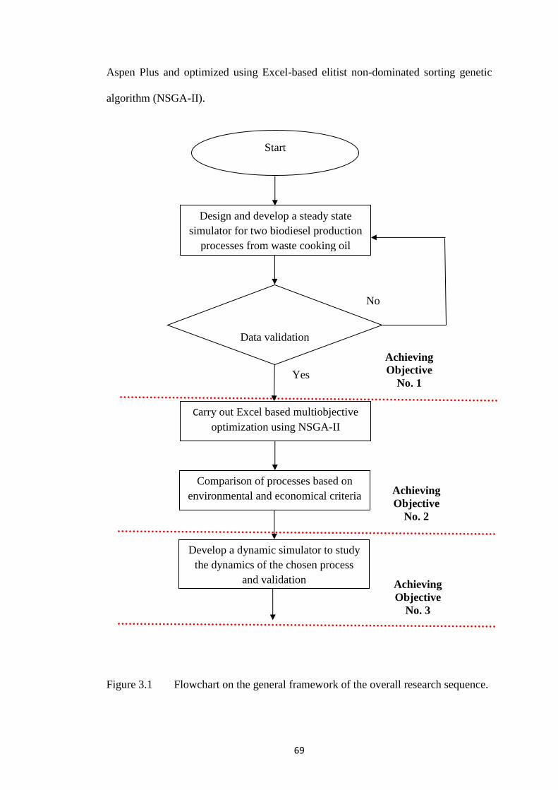
69
Aspen Plus and optimized using Excel-based elitist non-dominated sorting genetic
algorithm (NSGA-II).
Figure 3.1 Flowchart on the general framework of the overall research sequence.
No
Yes
Start
Design and develop a steady state
simulator for two biodiesel production
processes from waste cooking oil
Carry out Excel based multiobjective
optimization using NSGA-II
Develop a dynamic simulator to study
the dynamics of the chosen process
and validation
Data validation
Comparison of processes based on
environmental and economical criteria
Achieving
Objective
No. 1
Achieving
Objective
No. 2
Achieving
Objective
No. 3
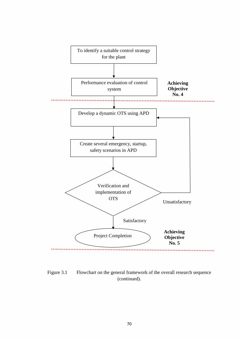
70
Figure 3.1 Flowchart on the general framework of the overall research sequence
(continued).
Satisfactory
Unsatisfactory
To identify a suitable control strategy
for the plant
Develop a dynamic OTS using APD
Verification and
implementation of
OTS
Project Completion
Performance evaluation of control
system
Create several emergency, startup,
safety scenarios in APD
Achieving
Objective
No. 4
Achieving
Objective
No. 5

71
Costing procedure is also explained based on which the profit is calculated.
These processes are then compared based on different criteria for their advantages
and disadvantages. Better process is then identified and used for further study on
PWC and OTS for biodiesel process. Later, a suitable PWC structure is developed
for the chosen process using IFSH method. Optimal paremeters (CSTR temperature,
residence time and feed tarys etc.) determined from MOO are used for PWC study.
Application of this method is explained in detail in this chapter. Subsequently, OTS
development of the concerned process is discussed in detail. For OTS, dynamic
model with control structure is developed in APD. Aspen OTS Framework is then
used on top of APD. Procedure for scenarios creation is also explained in this
chapter. Finally, application of HAZOP to this process is reported.
3.2 Process Development and Process Simulation
In this work, the processes are first simulated in Aspen Plus, and then they
are optimized to obtain optimal design and opearation by maximizing the economic
potential. This approach is based on the steps proposed by Myint and El-Halwagi
(2009). For this study, biodiesel plant capacity is assumed to be 120 kt/annum per
annum. This capacity is chosen as the plant with similar capacity already exists. For
instance, in Malaysia, a plant is designed to produce 100 kt/annum of biodiesel with
infrastructure to expand capacity to 200 kt/annum (PlantBiofuels, 2013). Sharma and
Rangaiah (2013b) assumed plant capacity of 20 kt/annum based on the potential
WCO availability in Singapore, as estimated by Chua et al. (2010).
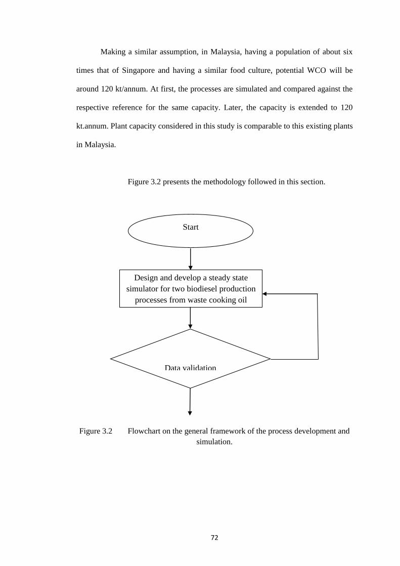
72
Making a similar assumption, in Malaysia, having a population of about six
times that of Singapore and having a similar food culture, potential WCO will be
around 120 kt/annum. At first, the processes are simulated and compared against the
respective reference for the same capacity. Later, the capacity is extended to 120
kt.annum. Plant capacity considered in this study is comparable to this existing plants
in Malaysia.
Figure 3.2 presents the methodology followed in this section.
Figure 3.2 Flowchart on the general framework of the process development and
simulation.
Start
Design and develop a steady state
simulator for two biodiesel production
processes from waste cooking oil
Data validation
73
3.2.1 Process Development
The feed is considered to be waste cooking palm oil (WCPO) as palm oil is
extensively used in Malaysia for cooking. However, the processes presented below
can process WCO as well as crude palm oil (CPO) as they have similar properties
(for example, FFA content: 2-7 %). Note that composition of glycerides may change
from even in different WCO collected from different sources. So, actual feed can be
either WCO or CPO, depending on their availability and costs.
Two alternative biodiesel production processes are considered and studied to
find out the better process. Three reactors are used for transesterification with
intermediate phase separators in process 1, whereas just one transesterification
reactor is used in process 2. This increases the capital cost due to more reactors, but
results into the better production. Also, biodiesel-glycerol separation is followed by
methanol separation in process 1. This scheme prevents backward transesterification
reactions, as methanol is present until biodiesel and glycerol are separated. Also, the
recovered methanol contains a very small amount of water that avoids energy-
intensive methanol−water separation and facilitates methanol reuse. Finally, in
process 1, washing of biodiesel is carried out at the end that reduces the amount of
water required for washing. Both the process alternatives use alkali-catalyzed
transesterification, which is more efficient and also used in industrial practice (Lurgi,
2013; Platinumgroup, 2013). Acid pretreatment is carried out to convert the FFA in
WCO to biodiesel in both processes. The validation of these processes has been
carried out by comparing the simulation results against the data reported in the
literature by other researchers, such as Sharma and Rangaiah (2013b), Morais et al.
74
(2010), Zhang et al. (2012) and Garcia et al. (2010). Initially, the results are validated
against the literature data for the capacity considered in the respective source. Then
the capacity is increased to the present capacity of 120 kt/annum and compared (see
Table 4.1 in Chapter 4). These two biodiesel process alternatives are discussed
below.
3.2.1 (a) Biodiesel Process 1
Figure 3.3 shows a process schematic for biodiesel production from WCO,
where products separation is followed by water washing (Sharma and Rangaiah,
2013b). WCO with a flow rate of 15,000 kg/h (stream ‘OIL’ in Figure 3.3) is
processed in the esterification reactor (RFFA), where FFAs react with methanol in
the presence of acid catalyst to yield FAMEs. The OIL stream is pre-heated in a heat
exchanger with the esterification reactor products (stream ‘RFFA1’). The
esterification is performed at 60oC, 4 bar pressure, methanol (stream ‘MEOH’) to
FFAs molar ratio of 10:1 and with 10% (w/w) of sulfuric acid relative to FFAs
(Noureddini and Zhu, 1997). The esterification products (stream ‘RFFA1’), after
cooling via pre-heating of WCO, are mixed with glycerol and then sent to the phase
separator ‘W-1’, where sulfuric acid and water are separated from the reaction
mixture. Glycerol forms two phases with reaction mixture, and acid catalyst is
removed in heavy phase. Stream ‘W-1-2’ containing mainly glycerol, methanol,
water and acid catalyst, from the phase separator ‘W-1’ goes to a distillation column
(FRAC-1) where most of the unreacted methanol is recovered and recycled (stream
‘FRAC-1-1’). FRAC-1 column has 8 theoretical stages and operates at reflux ratio of
1. The recycled methanol is then fed back to the esterification reactor (RFFA).
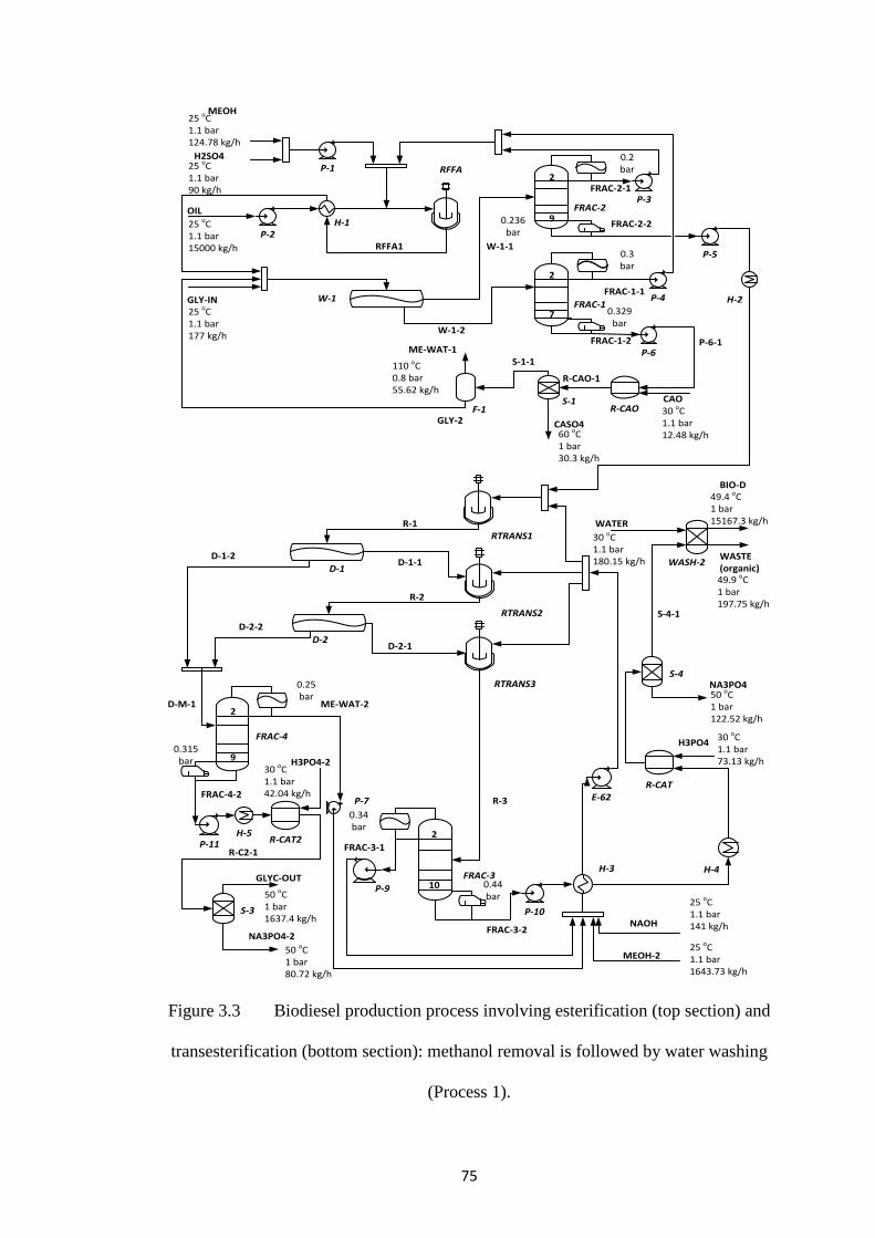
75
Figure 3.3 Biodiesel production process involving esterification (top section) and
transesterification (bottom section): methanol removal is followed by water washing
(Process 1).
P-1
MEOH
H2SO4
RFFA
H-1
RFFA1P-2
OIL
GLY-IN FRAC-1
FRAC-2
FRAC-2-2
FRAC-1-2
P-3
FRAC-1-1
FRAC-2-1
P-5
H-2
W-1-1
W-1-2
RTRANS1
RTRANS2
RTRANS3
W-1
D-1
D-2
R-1
R-2
D-1-1
D-2-1
D-M-1
FRAC-4
FRAC-3
FRAC-4-2
FRAC-3-2
P-10
P-9
D-1-2
D-2-2
H-3
WASH-2
H-4
MEOH-2
NAOH
H3PO4
WATER
BIO-D
WASTE(organic)
FRAC-3-1
2
2
9
10
2
2
7
9
ME-WAT-2
P-4
S-3
R-CAT2
R-C2-1
NA3PO4-2
S-1
P-6P-6-1
R-CAO
R-CAO-1
S-1-1
CASO4
F-1
ME-WAT-1
CAO
GLY-2
R-3
R-CAT
P-11
E-62
H3PO4-2
S-4
S-4-1
NA3PO4
P-7
0.2 bar
0.236 bar
0.3 bar
0.329 bar
0.25 bar
0.315 bar
0.34 bar
0.44 bar
25 oC1.1 bar124.78 kg/h
25 oC1.1 bar90 kg/h
25 oC1.1 bar15000 kg/h
25 oC1.1 bar177 kg/h
25 oC1.1 bar141 kg/h
25 oC1.1 bar1643.73 kg/h
50 oC1 bar1637.4 kg/h
30 oC1.1 bar180.15 kg/h
49.4 oC1 bar15167.3 kg/h
49.9 oC1 bar197.75 kg/h
30 oC1.1 bar73.13 kg/h
30 oC1.1 bar42.04 kg/h
50 oC1 bar80.72 kg/h
50 oC1 bar122.52 kg/h
30 oC1.1 bar12.48 kg/h60 oC
1 bar30.3 kg/h
110 oC0.8 bar55.62 kg/h
GLYC-OUT
H-5
76
Glycerol and sulfuric acid leave the FRAC-1 column in the bottom stream
(FRAC-1-2), which is then fed to a neutralization reactor (R-CAO), where sulfuric
acid reacts with calcium oxide to produce calcium sulphate (stream ‘CAO’). The
calcium sulphate produced in the reactor is then removed in a gravity separator (S-1).
The glycerol stream (S-1-1) leaving the separator S-1 is further purified in a flash
evaporator (F-1), where the remaining methanol and water are removed from the top
stream (ME-WAT-1) and treated as a waste stream due to small methanol flow rate
of 8.53 kg/h. Finally, glycerol is recycled back and mixed with fresh glycerol, which
forms two liquid phases in phase separator W-1. The light phase from separator W-1
includes oil, biodiesel, methanol and water while the heavy phase contains glycerol,
catalyst, methanol and water. The pretreated WCO feed stream (W-1-1) is fed to a
distillation column (FRAC-2 with 10 theoretical stages and operating at reflux ratio
of 1), where most of the unreacted methanol (stream ‘FRAC-2-1’) is recovered in the
distillate stream and recycled to the esterification reactor ‘RFFA’.
The bottom stream ‘FRAC-2-2’ containing FAMEs and unreacted oil is
processed in the transesterification reactor (RTRANS1 in Figure 3.3) at 50oC. Excess
methanol is advantageous as transesterification is a mass-transfer controlled reaction
(Noureddini and Zhu, 1997). So, methanol to oil molar flow ratio of 6 is maintained
in each transesterification reactor (Morais et al., 2010; Freedman et al., 1984).
Transesterification section mainly contains continuous stirred tank reactors (CSTRs),
distillation columns, phase separators, a neutralization reactor and a washing column.
Three CSTRs are placed in series, and treated oil mixed with methanol and NaOH
catalyst is charged to the first CSTR (i.e. RTRANS1). The effluent streams from
RTRANS1 and RTRANS2 are individually sent to phase separators, where glycerol
77
and NaOH with some methanol are separated as the heavy phase (i.e. streams ‘D-1-
2’ and ‘D-2-2’). The light phase (i.e. streams ‘D-1-1’ and ‘D-2-1’) from D-1 and D-2
separators goes to RTRANS2 and RTRANS3 reactors, respectively. This phase
mainly contains biodiesel, oil and methanol with some NaOH.
Finally, stream ‘R-3’ is charged to a distillation column (FRAC-3) having 11
theoretical stages and operating at reflux ratio of 1, where 98% methanol is
recovered and reused in the transesterification reactors. Bottom product from FRAC-
3 column contains mainly biodiesel, and is treated in a neutralization unit to remove
NaOH using phosphoric acid. A gravity separator ‘S-4’ is then used to separate
precipitated salt from stream ‘NA3PO4-2’. It is followed by a water wash column
(WASH-2). As the recycled methanol should be free of water, water wash column is
used after separating methanol from the reaction mixture. From WASH-2 column,
the stream BIO-D containing FAMEs (i.e., Methyl-oleate, Methyl-palmitate, Methyl-
myristate, Methyl-stearate, Methyl-linoleate) and having a flow rate of 15167.3 kg/h
with more than 99% purity, is taken out.
The remaining unreacted oil, methanol, glycerol, etc. are removed from
stream ‘WASTE’ with a flow rate of 197.75 kg/h. Glycerol streams (i.e. streams ‘D-
1-2’ and ‘D-2-2’) are mixed together and charged to a distillation column (FRAC-4),
where most of the methanol (stream ME-WAT-2) is separated and recycled. The
bottom stream (FRAC-4-2) is mainly glycerol and NaOH, and is charged to the
neutralization reactor (R-CAT2) to neutralize NaOH present in the streams using
phosphoric acid. The Na3PO4 formed in the neutralization reactor is separated using
the gravity separator (S-3) from stream NA3PO4-2. The top stream ‘GLYC-OUT’,
78
having more than 96% glycerol, is taken out at a flow rate of 1637.4 kg/h. Figure 3.3
shows temperature, pressure and flow rate of all inlet and exit streams of Process 1.
3.2.1 (b) Biodiesel Process 2
Figure 3.4 shows an alternative process, where washing is followed by
products separation, used by Morais et al. (2010). The WCO feed of 15,000 kg/h
(stream ‘OIL’ in Figure 3.4) is pre-heated in a heat exchanger (H-1) with the
esterification reactor products (stream ‘RFFA1’) and then fed to the esterification
reactor (RFFA), where FFAs are converted to FAMEs. Esterification takes place at
60oC, 4 bar, methanol (stream ‘MEOH’) to FFAs molar ratio of 10:1 and with 10%
(w/w) of sulfuric acid catalyst relative to FFAs. The esterification products (stream
‘RFFA1’), after passing through the heat exchanger ‘H-1’, are charged with glycerol
to the ‘WASH-1’ column, where sulfuric acid and water are separated from the
reaction mixture. Glycerol is added to achieve required separation. Here, a wash
column ‘WASH-1’ is used instead of a phase separator ‘W-1’ in Process 1. The
treated oil that leaves the ‘WASH-1’ column (stream ‘WASH-1-1’) is sent to the
transesterification reactor. The other stream from ‘WASH-1’ column (stream
‘WASH-1-2’) mainly contains glycerol, methanol, water and acid catalyst, which is
then sent to a distillation column (FRAC-1 with 6 theoretical stages and operating at
a reflux ratio of 1.1) to recover the unreacted methanol (stream ‘FRAC-1-1’) for
recycling to the esterification reactor (RFFA). Glycerol and sulfuric acid leave the
FRAC-1 column in the bottom stream (FRAC-1-2), which is fed to a neutralization
reactor (R-CAO) where sulfuric acid reacts with calcium oxide to produce calcium
sulphate (stream ‘CAO’).
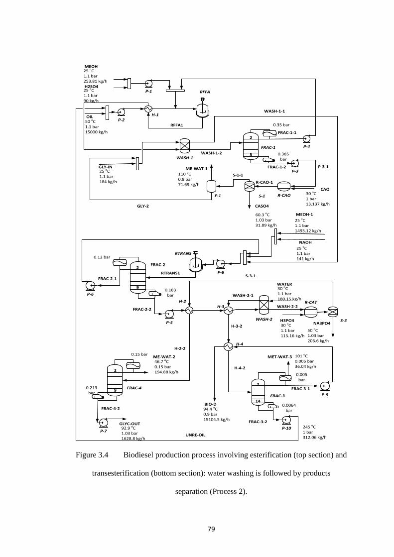
79
Figure 3.4 Biodiesel production process involving esterification (top section) and
transesterification (bottom section): water washing is followed by products
separation (Process 2).
P-1
MEOH
H2SO4RFFA
H-1
RFFA1P-2
OIL
GLY-IN
FRAC-1
FRAC-1-2
FRAC-1-1
WASH-1-1
WASH-1-2
RTRANS
RTRANS1
FRAC-4
FRAC-3
FRAC-4-2
FRAC-3-2
P-10
WASH-2 H3PO4
WATER
WASH-2-1
WASH-2-2
2
2
9
14
2
5
ME-WAT-2
P-4
S-1
P-3P-3-1
R-CAO
R-CAO-1
S-1-1
CASO4
F-1
ME-WAT-1
CAO
GLY-2
R-CAT
WASH-1
FRAC-2-1
MEOH-1
NAOH
P-8
FRAC-2
P-6
2
9
FRAC-2-2
P-5
H-2H-3
H-3-2
UNRE-OIL
MET-WAT-3
S-3
S-3-1
NA3PO4
H-2-2
GLYC-OUT
P-9
P-7
FRAC-3-1
H-4-2
H-4
BIO-D
0.35 bar
0.385 bar
0.12 bar
0.183 bar
0.15 bar
0.213 bar
0.005 bar
0.0064 bar
25 oC1.1 bar184 kg/h
25 oC1.1 bar253.81 kg/h
25 oC1.1 bar90 kg/h
50 oC1.1 bar15000 kg/h
25 oC1.1 bar1493.12 kg/h
25 oC1.1 bar141 kg/h
30 oC1.1 bar115.16 kg/h
30 oC1.1 bar180.15 kg/h
94.4 oC0.9 bar15104.5 kg/h
245 oC1 bar312.06 kg/h
92.9 oC1.03 bar1628.8 kg/h
110 oC0.8 bar71.69 kg/h
46.7 oC0.15 bar194.88 kg/h
101 oC0.005 bar36.04 kg/h
50 oC1.03 bar206.6 kg/h
60.3 oC1.03 bar31.89 kg/h
30 oC1 bar13.137 kg/h
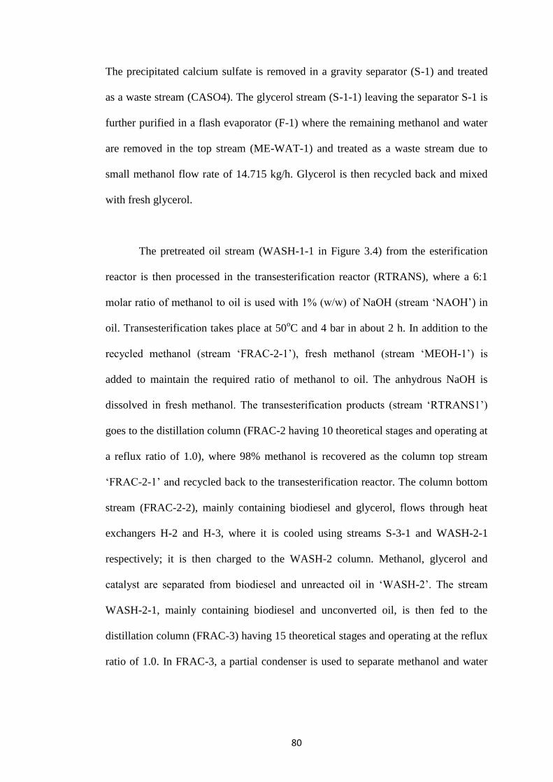
80
The precipitated calcium sulfate is removed in a gravity separator (S-1) and treated
as a waste stream (CASO4). The glycerol stream (S-1-1) leaving the separator S-1 is
further purified in a flash evaporator (F-1) where the remaining methanol and water
are removed in the top stream (ME-WAT-1) and treated as a waste stream due to
small methanol flow rate of 14.715 kg/h. Glycerol is then recycled back and mixed
with fresh glycerol.
The pretreated oil stream (WASH-1-1 in Figure 3.4) from the esterification
reactor is then processed in the transesterification reactor (RTRANS), where a 6:1
molar ratio of methanol to oil is used with 1% (w/w) of NaOH (stream ‘NAOH’) in
oil. Transesterification takes place at 50oC and 4 bar in about 2 h. In addition to the
recycled methanol (stream ‘FRAC-2-1’), fresh methanol (stream ‘MEOH-1’) is
added to maintain the required ratio of methanol to oil. The anhydrous NaOH is
dissolved in fresh methanol. The transesterification products (stream ‘RTRANS1’)
goes to the distillation column (FRAC-2 having 10 theoretical stages and operating at
a reflux ratio of 1.0), where 98% methanol is recovered as the column top stream
‘FRAC-2-1’ and recycled back to the transesterification reactor. The column bottom
stream (FRAC-2-2), mainly containing biodiesel and glycerol, flows through heat
exchangers H-2 and H-3, where it is cooled using streams S-3-1 and WASH-2-1
respectively; it is then charged to the WASH-2 column. Methanol, glycerol and
catalyst are separated from biodiesel and unreacted oil in ‘WASH-2’. The stream
WASH-2-1, mainly containing biodiesel and unconverted oil, is then fed to the
distillation column (FRAC-3) having 15 theoretical stages and operating at the reflux
ratio of 1.0. In FRAC-3, a partial condenser is used to separate methanol and water
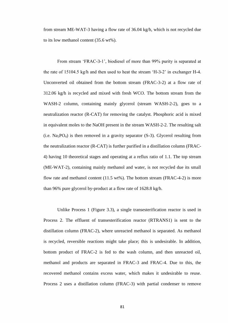
81
from stream ME-WAT-3 having a flow rate of 36.04 kg/h, which is not recycled due
to its low methanol content (35.6 wt%).
From stream ‘FRAC-3-1’, biodiesel of more than 99% purity is separated at
the rate of 15104.5 kg/h and then used to heat the stream ‘H-3-2’ in exchanger H-4.
Unconverted oil obtained from the bottom stream (FRAC-3-2) at a flow rate of
312.06 kg/h is recycled and mixed with fresh WCO. The bottom stream from the
WASH-2 column, containing mainly glycerol (stream WASH-2-2), goes to a
neutralization reactor (R-CAT) for removing the catalyst. Phosphoric acid is mixed
in equivalent moles to the NaOH present in the stream WASH-2-2. The resulting salt
(i.e. Na3PO4) is then removed in a gravity separator (S-3). Glycerol resulting from
the neutralization reactor (R-CAT) is further purified in a distillation column (FRAC-
4) having 10 theoretical stages and operating at a reflux ratio of 1.1. The top stream
(ME-WAT-2), containing mainly methanol and water, is not recycled due its small
flow rate and methanol content (11.5 wt%). The bottom stream (FRAC-4-2) is more
than 96% pure glycerol by-product at a flow rate of 1628.8 kg/h.
Unlike Process 1 (Figure 3.3), a single transesterification reactor is used in
Process 2. The effluent of transesterification reactor (RTRANS1) is sent to the
distillation column (FRAC-2), where unreacted methanol is separated. As methanol
is recycled, reversible reactions might take place; this is undesirable. In addition,
bottom product of FRAC-2 is fed to the wash column, and then unreacted oil,
methanol and products are separated in FRAC-3 and FRAC-4. Due to this, the
recovered methanol contains excess water, which makes it undesirable to reuse.
Process 2 uses a distillation column (FRAC-3) with partial condenser to remove
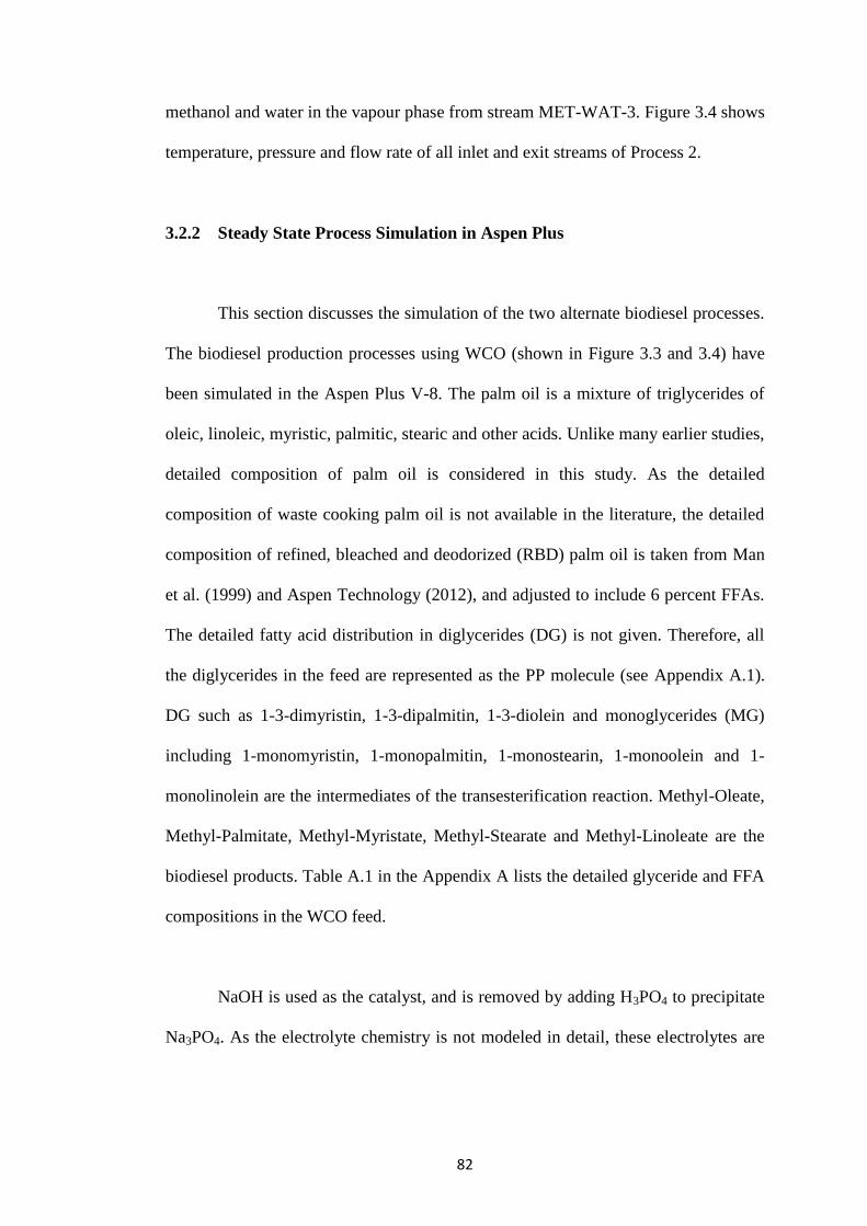
82
methanol and water in the vapour phase from stream MET-WAT-3. Figure 3.4 shows
temperature, pressure and flow rate of all inlet and exit streams of Process 2.
3.2.2 Steady State Process Simulation in Aspen Plus
This section discusses the simulation of the two alternate biodiesel processes.
The biodiesel production processes using WCO (shown in Figure 3.3 and 3.4) have
been simulated in the Aspen Plus V-8. The palm oil is a mixture of triglycerides of
oleic, linoleic, myristic, palmitic, stearic and other acids. Unlike many earlier studies,
detailed composition of palm oil is considered in this study. As the detailed
composition of waste cooking palm oil is not available in the literature, the detailed
composition of refined, bleached and deodorized (RBD) palm oil is taken from Man
et al. (1999) and Aspen Technology (2012), and adjusted to include 6 percent FFAs.
The detailed fatty acid distribution in diglycerides (DG) is not given. Therefore, all
the diglycerides in the feed are represented as the PP molecule (see Appendix A.1).
DG such as 1-3-dimyristin, 1-3-dipalmitin, 1-3-diolein and monoglycerides (MG)
including 1-monomyristin, 1-monopalmitin, 1-monostearin, 1-monoolein and 1-
monolinolein are the intermediates of the transesterification reaction. Methyl-Oleate,
Methyl-Palmitate, Methyl-Myristate, Methyl-Stearate and Methyl-Linoleate are the
biodiesel products. Table A.1 in the Appendix A lists the detailed glyceride and FFA
compositions in the WCO feed.
NaOH is used as the catalyst, and is removed by adding H3PO4 to precipitate
Na3PO4. As the electrolyte chemistry is not modeled in detail, these electrolytes are
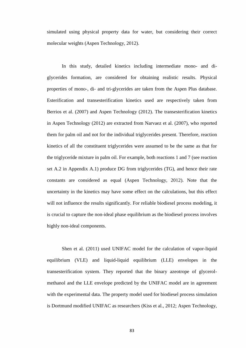
83
simulated using physical property data for water, but considering their correct
molecular weights (Aspen Technology, 2012).
In this study, detailed kinetics including intermediate mono- and di-
glycerides formation, are considered for obtaining realistic results. Physical
properties of mono-, di- and tri-glycerides are taken from the Aspen Plus database.
Esterification and transesterification kinetics used are respectively taken from
Berrios et al. (2007) and Aspen Technology (2012). The transesterification kinetics
in Aspen Technology (2012) are extracted from Narvaez et al. (2007), who reported
them for palm oil and not for the individual triglycerides present. Therefore, reaction
kinetics of all the constituent triglycerides were assumed to be the same as that for
the triglyceride mixture in palm oil. For example, both reactions 1 and 7 (see reaction
set A.2 in Appendix A.1) produce DG from triglycerides (TG), and hence their rate
constants are considered as equal (Aspen Technology, 2012). Note that the
uncertainty in the kinetics may have some effect on the calculations, but this effect
will not influence the results significantly. For reliable biodiesel process modeling, it
is crucial to capture the non-ideal phase equilibrium as the biodiesel process involves
highly non-ideal components.
Shen et al. (2011) used UNIFAC model for the calculation of vapor-liquid
equilibrium (VLE) and liquid-liquid equilibrium (LLE) envelopes in the
transesterification system. They reported that the binary azeotrope of glycerol-
methanol and the LLE envelope predicted by the UNIFAC model are in agreement
with the experimental data. The property model used for biodiesel process simulation
is Dortmund modified UNIFAC as researchers (Kiss et al., 2012; Aspen Technology,
84
2012; Kiss, 2009) successfully used this model to predict the physical properties of
the considered components. Redlich-Kwong-Soave equation of state (RKS EOS) is
used to predict the physical properties of the vapor phase. Thermophysical property
model parameters of tri-, di-, and mono-glycerides such as vapour pressure, heat of
vaporization, heat of formation, heat capacity, liquid molar volume and liquid
viscosity are taken from biodiesel databank of Aspen Plus. The detailed information
for the development of these thermophysical property models has been presented in
Zong et al. (2010a), Zong et al. (2010b) and Zong et al. (2010c). In addition, the
required TC, PC and ω (critical temperature, critical pressure and acentric factor) for
RKS EOS are estimated with the Gani group contribution method (Aspen
Technology, 2012). A group contribution method is a technique to estimate and
predict thermodynamic and other properties from molecular structures. A group
contribution method is used to predict properties of pure components and mixtures
by using group or atom properties. This reduces the number of required data
significantly. A group contribution method uses the principle that some simple
aspects of the structures of chemical components are always the same in many
different molecules. This method uses the pure additive group contributions to
correlate the required property with an easy accessible property such as critical
temperature. Although the experimental or industrial validation could not be carried,
the simulated results such as conversion in esterification and transesterification
section, and product quality have been found in agreement with the literature data
(Sharma and Rangaiah, 2013b; Garcia et al., 2010).
A fixed pressure of 4 bar is assumed in both esterification and
transesterification reactors while reactor temperatures are considered as decision
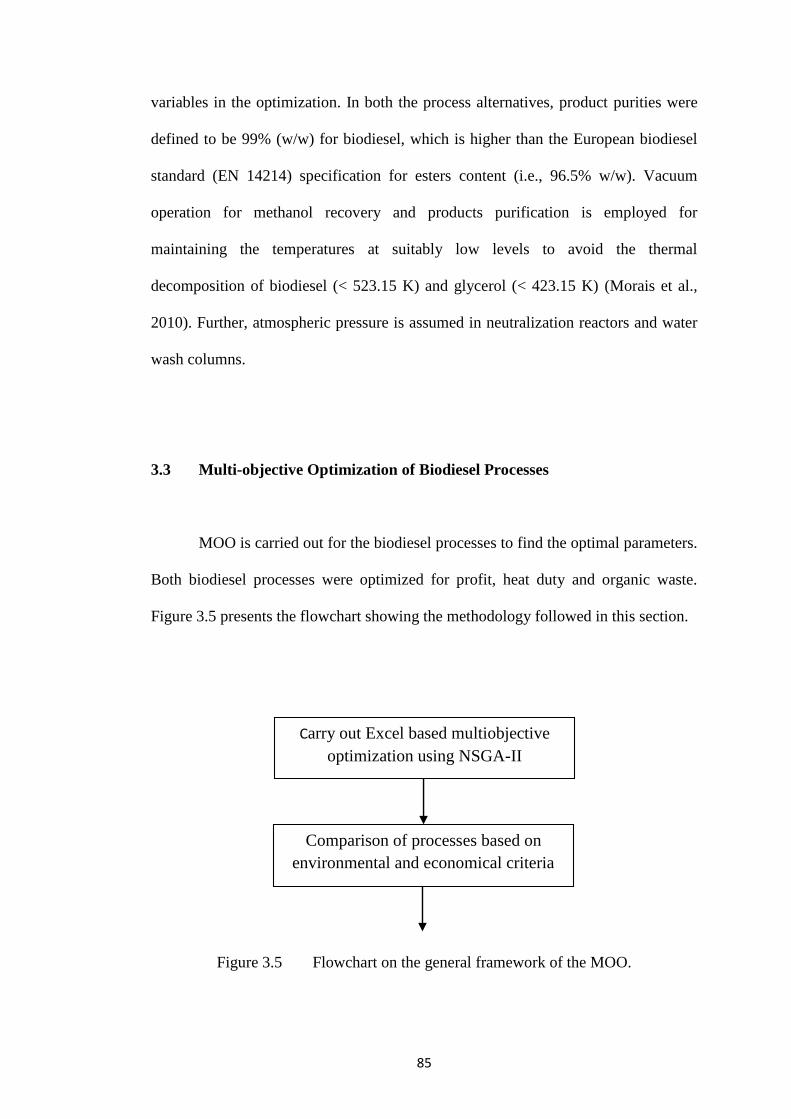
85
variables in the optimization. In both the process alternatives, product purities were
defined to be 99% (w/w) for biodiesel, which is higher than the European biodiesel
standard (EN 14214) specification for esters content (i.e., 96.5% w/w). Vacuum
operation for methanol recovery and products purification is employed for
maintaining the temperatures at suitably low levels to avoid the thermal
decomposition of biodiesel (< 523.15 K) and glycerol (< 423.15 K) (Morais et al.,
2010). Further, atmospheric pressure is assumed in neutralization reactors and water
wash columns.
3.3 Multi-objective Optimization of Biodiesel Processes
MOO is carried out for the biodiesel processes to find the optimal parameters.
Both biodiesel processes were optimized for profit, heat duty and organic waste.
Figure 3.5 presents the flowchart showing the methodology followed in this section.
Figure 3.5 Flowchart on the general framework of the MOO.
Carry out Excel based multiobjective
optimization using NSGA-II
Comparison of processes based on
environmental and economical criteria
86
Methanol, glycerol, tri/di/mono-glycerides, FAMEs and FFAs in stream
‘WASTE’ and methanol in stream ‘ME-WAT-1’ in Figure 3.3, are considered as the
constituents of organic waste in Process 1. Methanol in streams ‘ME-WAT-1’, ‘ME-
WAT-2’, and ‘ME-WAT-3’ in Figure 3.4, is considered as organic waste in Process
2. Profit is calculated by subtracting cost of manufacture (COM) from the revenue
obtained by selling the products: biodiesel and glycerol.
Table 3.1 presents the cost of raw materials, products and utilities, used in the
present study. As described in Section 3.2, potential WCO is 120 kt/annum
(equivalent to 15000 kg/h). Given the uncertainty in the WCO availability, this work
considers -20% variation in WCO as one of the decision variables. Temperature and
residence time of each of the CSTRs are also taken as decision variables for
optimization as these are important for the conversion of WCO to biodiesel. Also,
feed stage of all distillation columns is taken as a decision variable as it can minimize
energy requirement by reducing reboiler duty. Operating rages are taken based on the
previous studies i.e. Sharma and Rangaiah (2013b) and Narvaez et al. (2007). Also,
constraints are decided based on the quality requirements and the maximum
allowable temperature related to the product deterioration temperature.
In this study, product purities are treated as constraints as these have to be
satisfied as per standards. To prevent product deterioration, upper limits for
temperatures at the bottom of all distillation columns is considered as additional
constraints (Sharma and Rangaiah, 2013b).
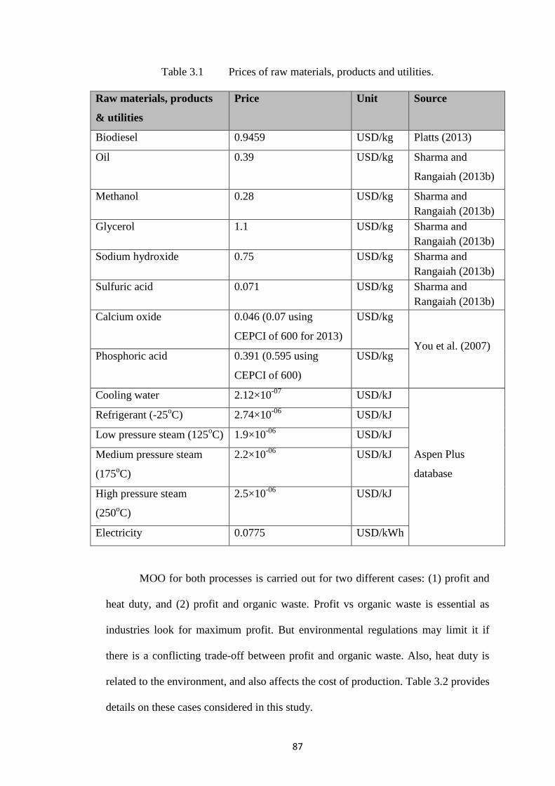
87
Table 3.1 Prices of raw materials, products and utilities.
Raw materials, products
& utilities
Price Unit Source
Biodiesel 0.9459 USD/kg Platts (2013)
Oil 0.39 USD/kg Sharma and
Rangaiah (2013b)
Methanol 0.28 USD/kg Sharma and
Rangaiah (2013b)
Glycerol 1.1 USD/kg Sharma and
Rangaiah (2013b)
Sodium hydroxide 0.75 USD/kg Sharma and
Rangaiah (2013b)
Sulfuric acid 0.071 USD/kg Sharma and
Rangaiah (2013b)
Calcium oxide 0.046 (0.07 using
CEPCI of 600 for 2013)
USD/kg
You et al. (2007) Phosphoric acid 0.391 (0.595 using
CEPCI of 600)
USD/kg
Cooling water 2.12×10-07
USD/kJ
Aspen Plus
database
Refrigerant (-25oC) 2.74×10
-06 USD/kJ
Low pressure steam (125oC) 1.9×10
-06 USD/kJ
Medium pressure steam
(175oC)
2.2×10-06
USD/kJ
High pressure steam
(250oC)
2.5×10-06
USD/kJ
Electricity 0.0775 USD/kWh
MOO for both processes is carried out for two different cases: (1) profit and
heat duty, and (2) profit and organic waste. Profit vs organic waste is essential as
industries look for maximum profit. But environmental regulations may limit it if
there is a conflicting trade-off between profit and organic waste. Also, heat duty is
related to the environment, and also affects the cost of production. Table 3.2 provides
details on these cases considered in this study.
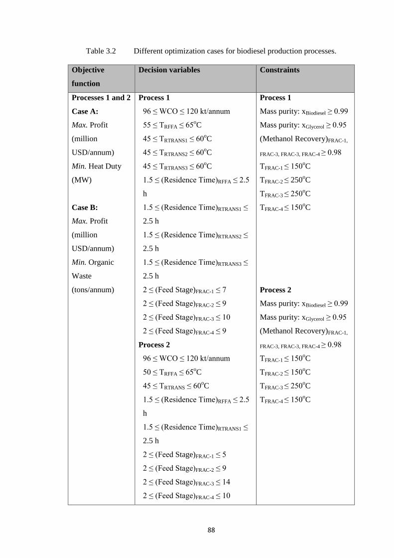
88
Table 3.2 Different optimization cases for biodiesel production processes.
Objective
function
Decision variables Constraints
Processes 1 and 2
Case A:
Max. Profit
(million
USD/annum)
Min. Heat Duty
(MW)
Case B:
Max. Profit
(million
USD/annum)
Min. Organic
Waste
(tons/annum)
Process 1
96 ≤ WCO ≤ 120 kt/annum
55 ≤ TRFFA ≤ 65oC
45 ≤ TRTRANS1 ≤ 60oC
45 ≤ TRTRANS2 ≤ 60oC
45 ≤ TRTRANS3 ≤ 60oC
1.5 ≤ (Residence Time)RFFA ≤ 2.5
h
1.5 ≤ (Residence Time)RTRANS1 ≤
2.5 h
1.5 ≤ (Residence Time)RTRANS2 ≤
2.5 h
1.5 ≤ (Residence Time)RTRANS3 ≤
2.5 h
2 ≤ (Feed Stage)FRAC-1 ≤ 7
2 ≤ (Feed Stage)FRAC-2 ≤ 9
2 ≤ (Feed Stage)FRAC-3 ≤ 10
2 ≤ (Feed Stage)FRAC-4 ≤ 9
Process 2
96 ≤ WCO ≤ 120 kt/annum
50 ≤ TRFFA ≤ 65oC
45 ≤ TRTRANS ≤ 60oC
1.5 ≤ (Residence Time)RFFA ≤ 2.5
h
1.5 ≤ (Residence Time)RTRANS1 ≤
2.5 h
2 ≤ (Feed Stage)FRAC-1 ≤ 5
2 ≤ (Feed Stage)FRAC-2 ≤ 9
2 ≤ (Feed Stage)FRAC-3 ≤ 14
2 ≤ (Feed Stage)FRAC-4 ≤ 10
Process 1
Mass purity: xBiodiesel ≥ 0.99
Mass purity: xGlycerol ≥ 0.95
(Methanol Recovery)FRAC-1,
FRAC-3, FRAC-3, FRAC-4 ≥ 0.98
TFRAC-1 ≤ 150oC
TFRAC-2 ≤ 250oC
TFRAC-3 ≤ 250oC
TFRAC-4 ≤ 150oC
Process 2
Mass purity: xBiodiesel ≥ 0.99
Mass purity: xGlycerol ≥ 0.95
(Methanol Recovery)FRAC-1,
FRAC-3, FRAC-3, FRAC-4 ≥ 0.98
TFRAC-1 ≤ 150oC
TFRAC-2 ≤ 150oC
TFRAC-3 ≤ 250oC
TFRAC-4 ≤ 150oC
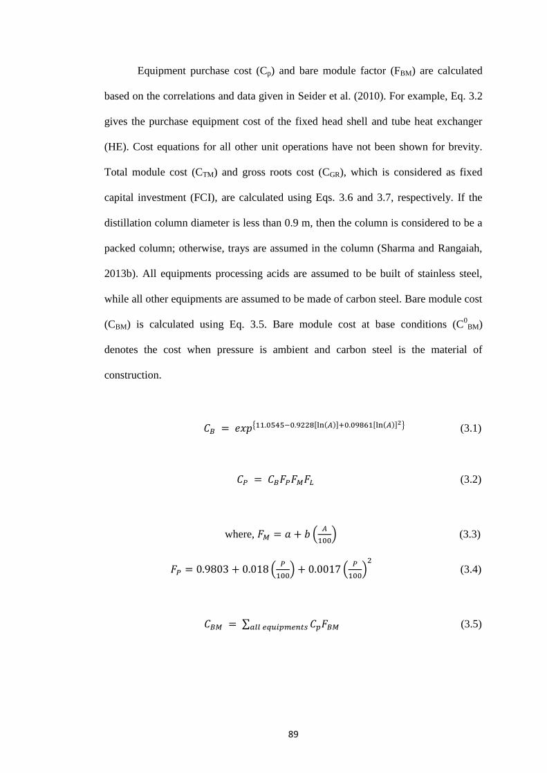
89
Equipment purchase cost (Cp) and bare module factor (FBM) are calculated
based on the correlations and data given in Seider et al. (2010). For example, Eq. 3.2
gives the purchase equipment cost of the fixed head shell and tube heat exchanger
(HE). Cost equations for all other unit operations have not been shown for brevity.
Total module cost (CTM) and gross roots cost (CGR), which is considered as fixed
capital investment (FCI), are calculated using Eqs. 3.6 and 3.7, respectively. If the
distillation column diameter is less than 0.9 m, then the column is considered to be a
packed column; otherwise, trays are assumed in the column (Sharma and Rangaiah,
2013b). All equipments processing acids are assumed to be built of stainless steel,
while all other equipments are assumed to be made of carbon steel. Bare module cost
(CBM) is calculated using Eq. 3.5. Bare module cost at base conditions (C0
BM)
denotes the cost when pressure is ambient and carbon steel is the material of
construction.
𝐶𝐵 = 𝑒𝑥𝑝{11.0545−0.9228[ln(𝐴)]+0.09861[ln(𝐴)]2} (3.1)
𝐶𝑃 = 𝐶𝐵𝐹𝑃𝐹𝑀𝐹𝐿 (3.2)
where, 𝐹𝑀 = 𝑎 + 𝑏 (𝐴
100) (3.3)
𝐹𝑃 = 0.9803 + 0.018 (𝑃
100) + 0.0017 (
𝑃
100)
2
(3.4)
𝐶𝐵𝑀 = ∑ 𝐶𝑝𝐹𝐵𝑀𝑎𝑙𝑙 𝑒𝑞𝑢𝑖𝑝𝑚𝑒𝑛𝑡𝑠 (3.5)
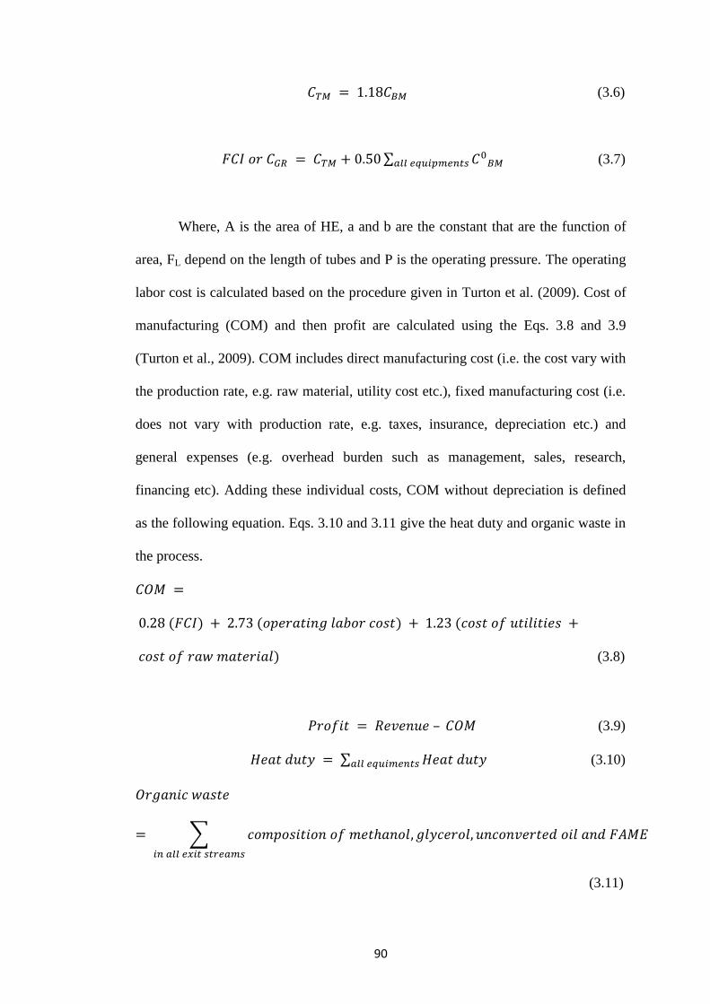
90
𝐶𝑇𝑀 = 1.18𝐶𝐵𝑀 (3.6)
𝐹𝐶𝐼 𝑜𝑟 𝐶𝐺𝑅 = 𝐶𝑇𝑀 + 0.50 ∑ 𝐶0𝐵𝑀𝑎𝑙𝑙 𝑒𝑞𝑢𝑖𝑝𝑚𝑒𝑛𝑡𝑠 (3.7)
Where, A is the area of HE, a and b are the constant that are the function of
area, FL depend on the length of tubes and P is the operating pressure. The operating
labor cost is calculated based on the procedure given in Turton et al. (2009). Cost of
manufacturing (COM) and then profit are calculated using the Eqs. 3.8 and 3.9
(Turton et al., 2009). COM includes direct manufacturing cost (i.e. the cost vary with
the production rate, e.g. raw material, utility cost etc.), fixed manufacturing cost (i.e.
does not vary with production rate, e.g. taxes, insurance, depreciation etc.) and
general expenses (e.g. overhead burden such as management, sales, research,
financing etc). Adding these individual costs, COM without depreciation is defined
as the following equation. Eqs. 3.10 and 3.11 give the heat duty and organic waste in
the process.
𝐶𝑂𝑀 =
0.28 (𝐹𝐶𝐼) + 2.73 (𝑜𝑝𝑒𝑟𝑎𝑡𝑖𝑛𝑔 𝑙𝑎𝑏𝑜𝑟 𝑐𝑜𝑠𝑡) + 1.23 (𝑐𝑜𝑠𝑡 𝑜𝑓 𝑢𝑡𝑖𝑙𝑖𝑡𝑖𝑒𝑠 +
𝑐𝑜𝑠𝑡 𝑜𝑓 𝑟𝑎𝑤 𝑚𝑎𝑡𝑒𝑟𝑖𝑎𝑙) (3.8)
𝑃𝑟𝑜𝑓𝑖𝑡 = 𝑅𝑒𝑣𝑒𝑛𝑢𝑒 – 𝐶𝑂𝑀 (3.9)
𝐻𝑒𝑎𝑡 𝑑𝑢𝑡𝑦 = ∑ 𝐻𝑒𝑎𝑡 𝑑𝑢𝑡𝑦𝑎𝑙𝑙 𝑒𝑞𝑢𝑖𝑚𝑒𝑛𝑡𝑠 (3.10)
𝑂𝑟𝑔𝑎𝑛𝑖𝑐 𝑤𝑎𝑠𝑡𝑒
= ∑ 𝑐𝑜𝑚𝑝𝑜𝑠𝑖𝑡𝑖𝑜𝑛 𝑜𝑓 𝑚𝑒𝑡ℎ𝑎𝑛𝑜𝑙, 𝑔𝑙𝑦𝑐𝑒𝑟𝑜𝑙, 𝑢𝑛𝑐𝑜𝑛𝑣𝑒𝑟𝑡𝑒𝑑 𝑜𝑖𝑙 𝑎𝑛𝑑 𝐹𝐴𝑀𝐸
𝑖𝑛 𝑎𝑙𝑙 𝑒𝑥𝑖𝑡 𝑠𝑡𝑟𝑒𝑎𝑚𝑠
(3.11)
91
In this study, an EMOO program (Sharma et al., 2012), which is based on the
binary-coded NSGA-II, has been used for determining the optimal trade-offs
between different objectives. In this program, objective functions and constraints are
computed in Excel worksheets, whereas NSGA-II is executed inside the Excel Macro
(Visual Basic for Applications). Binary coding is employed for implementing the
NSGA-II algorithm in the EMOO program by Sharma et al (2012). In the EMOO
program, binary tournament selection for participation in cross-over and mutation
operations, cross-over by single point, two-point and uniform schemes, and bit-wise
mutation are available. The following criteria are used in determining the
domination;
i. When the two individuals A and B are feasible, then the definition of
domination based on objective values (in step 4 in the above algorithm)
applies.
ii. When only one individual is feasible, then the feasible individual dominates
the infeasible individual.
iii. When both individuals are infeasible, then the individual with smaller
violation of constraint dominates the other individual.
Values of NSGA-II parameters used for all optimization cases in this work
are: population size (NP) = 100, two-point crossover with probability = 0.9, mutation
probability = 0.05, random seed = 0.5, and maximum number of generations = 100.
Two-point crossover, bit-wise mutation and tournament selection for participation in
crossover are adopted. The algorithm used in the EMOO program is given below
(Sharma et al., 2012);
92
i. Generate the initial population of NP individuals within the bounds of the
decision variables, using uniformly distributed random numbers. The
population size ‘NP’ is a parameter whose value has to be entered by the user.
Evaluate the objective functions and constraints of each individual in the
population.
ii. New set of NP individuals are generated by selection, cross-over and
mutation operations of genetic algorithms over the initial population.
iii. Combine the current population with all the new individuals yielding the
combined population of 2NP individuals.
iv. Determine Ndom i.e. the number of individuals dominating each individual in
the combined population. Solution A is considered to be dominating solution
B, if value of each objective function of solution A is as desirable as that of
solution B and at least one objective value of solution A is better than that of
solution B.
v. Assign Rank to the individuals. Individuals with the smallest Ndom are
assigned a Rank of 1 (the best Pareto front). Individuals with the next
smallest Ndom are assigned a rank of 2 (subsequent Pareto front). This
continues for all individuals.
vi. Sort the individuals according to their rank, and then calculate the Rank at the
NPth individual. This Rank is represented as the NdomCut.
vii. For individuals having Rank equal to NdomCut, find the crowding distance of
each individual in the objective space.
viii. Sort the individuals in the combined 2NP population according to the
increasing rank followed by the decreasing crowding distance.
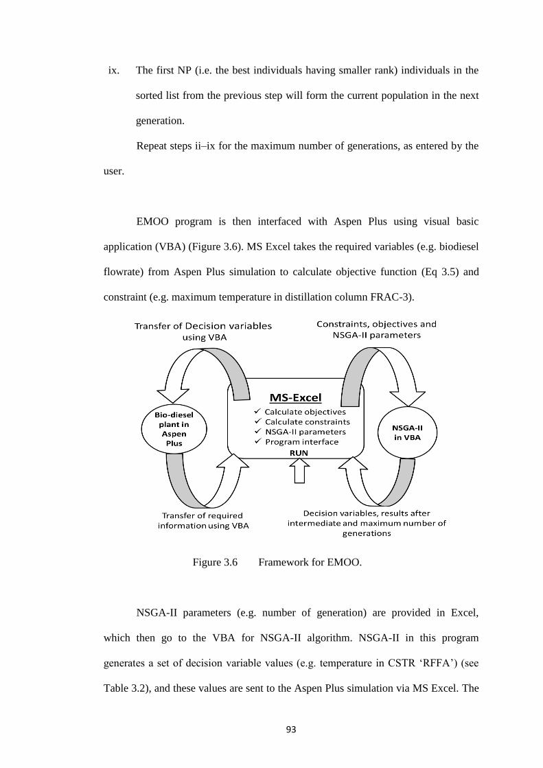
93
ix. The first NP (i.e. the best individuals having smaller rank) individuals in the
sorted list from the previous step will form the current population in the next
generation.
Repeat steps ii–ix for the maximum number of generations, as entered by the
user.
EMOO program is then interfaced with Aspen Plus using visual basic
application (VBA) (Figure 3.6). MS Excel takes the required variables (e.g. biodiesel
flowrate) from Aspen Plus simulation to calculate objective function (Eq 3.5) and
constraint (e.g. maximum temperature in distillation column FRAC-3).
Figure 3.6 Framework for EMOO.
NSGA-II parameters (e.g. number of generation) are provided in Excel,
which then go to the VBA for NSGA-II algorithm. NSGA-II in this program
generates a set of decision variable values (e.g. temperature in CSTR ‘RFFA’) (see
Table 3.2), and these values are sent to the Aspen Plus simulation via MS Excel. The
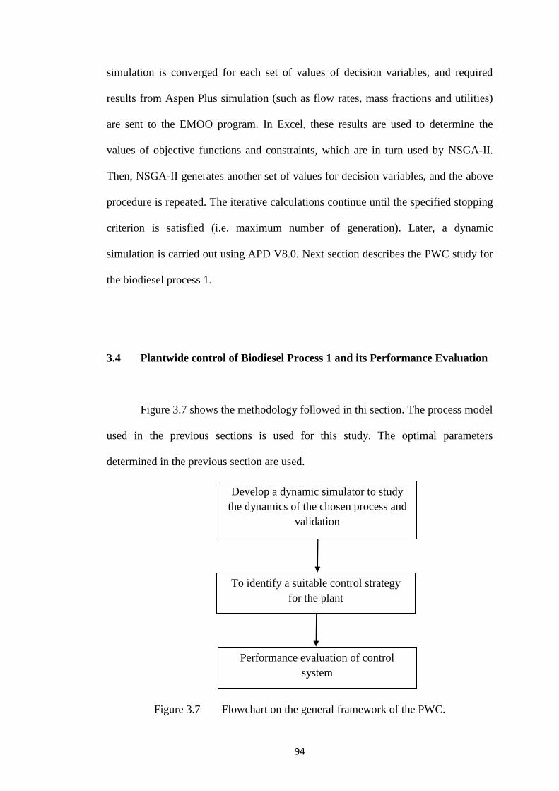
94
simulation is converged for each set of values of decision variables, and required
results from Aspen Plus simulation (such as flow rates, mass fractions and utilities)
are sent to the EMOO program. In Excel, these results are used to determine the
values of objective functions and constraints, which are in turn used by NSGA-II.
Then, NSGA-II generates another set of values for decision variables, and the above
procedure is repeated. The iterative calculations continue until the specified stopping
criterion is satisfied (i.e. maximum number of generation). Later, a dynamic
simulation is carried out using APD V8.0. Next section describes the PWC study for
the biodiesel process 1.
3.4 Plantwide control of Biodiesel Process 1 and its Performance Evaluation
Figure 3.7 shows the methodology followed in thi section. The process model
used in the previous sections is used for this study. The optimal parameters
determined in the previous section are used.
Figure 3.7 Flowchart on the general framework of the PWC.
To identify a suitable control strategy
for the plant
Performance evaluation of control
system
Develop a dynamic simulator to study
the dynamics of the chosen process and
validation
95
A PWC system is designed based on IFSH methodology proposed by Murthy
Konda et al. (2005). This systematic and hierarchical methodology has eight levels,
where, in addition to heuristics, both steady state and dynamic process models are
effectively utilized in decision making while designing a control system. For
example, decisions based on heuristics are corroborated using dynamic simulations.
The main advantage of IFSH methodology is that it overcomes the over-reliance on
heuristics to design a decentralized regulatory control system.
In this research, a sequential approach is followed where a better process
design is first identified and a suitable control structure is developed for the
identified process. Each level of IFSH and its application to the chosen biodiesel
(Figure 3.8) process are described below. Figure 3.8 shows the important design and
operating parameters. A dynamic simulation model of the process 1 is developed
using Aspen Plus Dynamics (APD) V8.0. Distillation columns are operated under
vacuum and use cooling water in the condensers. Running distillation columns under
vacuum can impact the control strategies significantly as the pressure on the trays
can change, affecting tray temperatures.
Surge capacities in reactors, reflux drums and column bases are sized to
provide 5 min of holdup when at 50% level. The steady state conditions in the
dynamic simulation using APD have been found to be consistent with those in steady
state simulation using Aspen Plus.
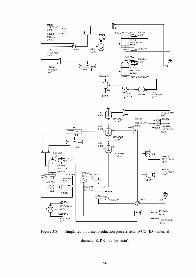
96
Figure 3.8 Simplified biodiesel production process from WCO (ID = internal
diameter & RR = reflux ratio).
MEOH
H2SO4 RFFA17 m3
H-1OIL
GLY-IN
FRAC-1
FRAC-2
H-2
RTRANS141 m3
RTRANS237 m3
RTRANS335 m3
W-1
D-1
D-2
FRAC-4
FRAC-3
H-3
WASH-2
H-4
MEOH-2
NAOH
H3PO4
WATER BIO-D
WASTE
2
2
9
10
2
2
7
9
S-3
GLY-OUT
R-CAT2
NA3PO4-2
S-1R-CAO
CASO4
F-1
ME-WAT-1
CAO
GLY-2
R-CAT
H3PO4-2
S-4NA3PO4
124.78 kg/h30 oC
90 kg/h30 oC
15000 kg/h30 oC
353 kg/h30 oC
141 kg/h30 oC
1643.73 kg/h30 oC
1637.4 kg/h50 oC
180.15 kg/h50 oC
15167.3 kg/h50 oC
197.75 kg/h50 oC
73.13 kg/h30 oC
42.04 kg/h30 oC
80.72 kg/h50 oC
122.52 kg/h50 oC
12.48 kg/h30 oC
0.4 bar43 oC
0.22 bar31 oC
0.32 bar31 oC
0.22 bar38 oC
RR = 1ID = 0.55 m
RR = 1.1ID = 0.5 m
RR = 0.52ID=1.11 m
RR = 0.5ID =1.13 m
0.394 MW
1.62 MW
2.1 MW
0.71 MW
4 bar65 oC
4 bar60 oC
4 bar55 oC
4 bar60 oC
0.25 MW
0.39 MW
0.68 MW
0.74 MW
H-5
97
3.4.1 Level 1.1. Define PWC Objectives
In this level, PWC objectives are formulated from the operational point of
view. Classically, these include production rate, product purity, process/equipment
constraints, safety concerns and environmental regulations. In case of any conflict
between plantwide objectives and unit-wise objective, the former should be given
priority. For the biodiesel process, PWC objectives are: 1) stable production rate at
normal operation with quick and smooth performance in the presence of
disturbances, 2) product quality as per EN 14214 standards (biodiesel > 96.5%), 3)
maintaining distillation temperatures below 250oC and 150
oC for the columns
processing biodiesel and glycerol respectively, to avoid thermal degradation, and 4)
maintaining required ratio of methanol to oil (6:1 molar ratio at normal condition)
and methanol split fraction to the 3 transesterification reactors
(RTRANS1:RTRANS2:RTRANS3 = 0.77:0.12:0.11 at normal condition based on
methanol to oil molar ratio in each CSTR) in order to obtain biodiesel quality
meeting EN standards. Note that different set of objectives may result in different
control systems.
3.4.2 Level 1.2. Determine Control Degree of Freedom (CDOF)
Murthy Konda et al. (2006a) proposed a method to determine CDOF based
on the restraining number; it is easy to apply and effective. As deduced by Murthy
Konda et al. (2006a), CDOF is found by subtracting the sum of restraining numbers
and redundancies from the total number of streams. Restraining number of a unit is
defined as the total number of independent and overall material balances having no
98
associated inventory. Redundancies in the process refer to the variables that need not
to be manipulated. In the chosen biodiesel process, there are a total of 108 streams
(including mass and energy streams), sum of restraining numbers is 28 and
redundancies is 12. Hence, CDOF = 108–28–12 = 68.
3.4.3 Level 2.1. Identify and Analyze Plantwide Disturbances
Plantwide disturbances can pose tough challenges in the normal operation of
the plant. Cognizance of possible disturbances in the process is of vital importance
while developing a control scheme and controller tuning. For this, the steady state
simulation model can be used to investigate the effect of possible disturbances. Table
3.3 lists the anticipated disturbances during biodiesel plant operation and their effects
on important quantities. PWC papers in the literature (Shen et al., 2011; Cheng et al.,
2014; Zhang et al., 2012) have used the magnitude of disturbances between ±5% and
±20% in feed flow rate.
In this work, we considered up to +20% and -30% change in WCO as the
availability of WCO is uncertain and shortage of supply could likely be the situation.
Also, -10% change in pre-exponential factor of transesterification reactions (this may
occur due to the catalyst deactivation or may arise due to the error in the kinetics
estimation), is considered.
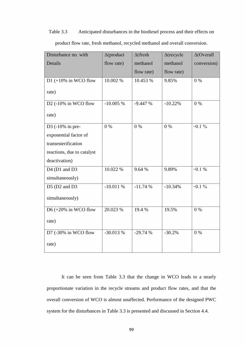
99
Table 3.3 Anticipated disturbances in the biodiesel process and their effects on
product flow rate, fresh methanol, recycled methanol and overall conversion.
Disturbance no. with
Details
Δ(product
flow rate)
Δ(fresh
methanol
flow rate)
Δ(recycle
methanol
flow rate)
Δ(Overall
conversion)
D1 (+10% in WCO flow
rate)
10.002 % 10.453 % 9.85% 0 %
D2 (-10% in WCO flow
rate)
-10.005 % -9.447 % -10.22% 0 %
D3 (-10% in pre-
exponential factor of
transesterification
reactions, due to catalyst
deactivation)
0 % 0 % 0 % ̴ 0.1 %
D4 (D1 and D3
simultaneously)
10.022 % 9.64 % 9.89% ̴ 0.1 %
D5 (D2 and D3
simultaneously)
-10.011 % -11.74 % -10.34% ̴ 0.1 %
D6 (+20% in WCO flow
rate)
20.023 % 19.4 % 19.5% 0 %
D7 (-30% in WCO flow
rate)
-30.013 % -29.74 % -30.2% 0 %
It can be seen from Table 3.3 that the change in WCO leads to a nearly
proportionate variation in the recycle streams and product flow rates, and that the
overall conversion of WCO is almost unaffected. Performance of the designed PWC
system for the disturbances in Table 3.3 is presented and discussed in Section 4.4.
100
3.4.4 Level 2.2. Set Performance and Tuning Criteria
In this level, settling time is selected as the criterion for performance
evaluation of the control system. As a large number of control loops are involved in
this process, each controller has to be tuned once the control loops are established.
Flow, level and pressure controllers are tuned based on the guidelines given in
Luyben (2002). The remaining controllers are tuned using the in-built Autotuner in
Aspen Plus Dynamics (APD). Controllers with time lags, such as temperature and
composition control loops, are tuned using the closed-loop autotune variation method
in APD (Wu and Wang, 2013). Tyreus-Luyben (TL) method (Shen et al., 2011;
Luyben and Luyben, 1997) is used to determine the controller tuning parameters in
such loops. Firstly, the sign of process gain using open loop test is determined and a
new set-point is introduced after implement a proportional control. Then the
proportional gain is increased until sustained periodic oscillations are obtained.
Finally, control parameters are determined as prescribed by Tyreus-Luyben by
recording ultimate gain and ultimate period. For example, temperature control loop
in ‘RFFA’: gain = 6.56 %/% and intergral time = 13.2 min for ultimate gain of 21
%/% and ultimate period of 6 min.
The controllers without time lags are tuned using the open-loop tuning
method in APD; Cohen and Coon (CC) method is used to tune these control loops.
For example, +5% change is introduced in the manipulated variable. Corresponding
changes in the controlled variables is plotted and the required variables (such as, time
delay, gain, etc) are determined. Finally, tuning parameters (i.e. controller gain,
intergral time) are determined based on the correlations given by Cohen and Coon. In
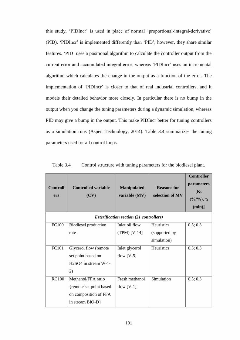
101
this study, ‘PIDIncr’ is used in place of normal ‘proportional-integral-derivative’
(PID). ‘PIDIncr’ is implemented differently than ‘PID’; however, they share similar
features. ‘PID’ uses a positional algorithm to calculate the controller output from the
current error and accumulated integral error, whereas ‘PIDIncr’ uses an incremental
algorithm which calculates the change in the output as a function of the error. The
implementation of ‘PIDIncr’ is closer to that of real industrial controllers, and it
models their detailed behavior more closely. In particular there is no bump in the
output when you change the tuning parameters during a dynamic simulation, whereas
PID may give a bump in the output. This make PIDIncr better for tuning controllers
as a simulation runs (Aspen Technology, 2014). Table 3.4 summarizes the tuning
parameters used for all control loops.
Table 3.4 Control structure with tuning parameters for the biodiesel plant.
Controll
ers
Controlled variable
(CV)
Manipulated
variable (MV)
Reasons for
selection of MV
Controller
parameters
[Kc
(%/%), τi
(min)]
Esterification section (21 controllers)
FC100 Biodiesel production
rate
Inlet oil flow
(TPM) [V-14]
Heuristics
(supported by
simulation)
0.5; 0.3
FC101 Glycerol flow (remote
set point based on
H2SO4 in stream W-1-
2)
Inlet glycerol
flow [V-5]
Heuristics 0.5; 0.3
RC100 Methanol/FFA ratio
{remote set point based
on composition of FFA
in stream BIO-D}
Fresh methanol
flow [V-1]
Simulation 0.5; 0.3
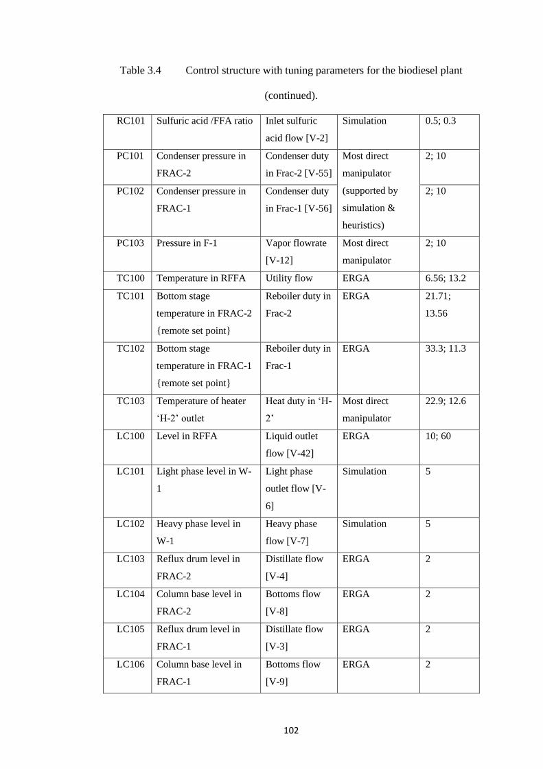
102
Table 3.4 Control structure with tuning parameters for the biodiesel plant
(continued).
RC101 Sulfuric acid /FFA ratio Inlet sulfuric
acid flow [V-2]
Simulation 0.5; 0.3
PC101 Condenser pressure in
FRAC-2
Condenser duty
in Frac-2 [V-55]
Most direct
manipulator
(supported by
simulation &
heuristics)
2; 10
PC102 Condenser pressure in
FRAC-1
Condenser duty
in Frac-1 [V-56]
2; 10
PC103 Pressure in F-1 Vapor flowrate
[V-12]
Most direct
manipulator
2; 10
TC100 Temperature in RFFA Utility flow ERGA 6.56; 13.2
TC101 Bottom stage
temperature in FRAC-2
{remote set point}
Reboiler duty in
Frac-2
ERGA 21.71;
13.56
TC102 Bottom stage
temperature in FRAC-1
{remote set point}
Reboiler duty in
Frac-1
ERGA 33.3; 11.3
TC103 Temperature of heater
‘H-2’ outlet
Heat duty in ‘H-
2’
Most direct
manipulator
22.9; 12.6
LC100 Level in RFFA Liquid outlet
flow [V-42]
ERGA 10; 60
LC101 Light phase level in W-
1
Light phase
outlet flow [V-
6]
Simulation 5
LC102 Heavy phase level in
W-1
Heavy phase
flow [V-7]
Simulation 5
LC103 Reflux drum level in
FRAC-2
Distillate flow
[V-4]
ERGA 2
LC104 Column base level in
FRAC-2
Bottoms flow
[V-8]
ERGA 2
LC105 Reflux drum level in
FRAC-1
Distillate flow
[V-3]
ERGA 2
LC106 Column base level in
FRAC-1
Bottoms flow
[V-9]
ERGA 2
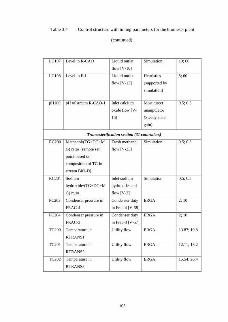
103
Table 3.4 Control structure with tuning parameters for the biodiesel plant
(continued).
LC107 Level in R-CAO Liquid outlet
flow [V-10]
Simulation 10; 60
LC108 Level in F-1 Liquid outlet
flow [V-13]
Heuristics
(supported by
simulation)
5; 60
pH100 pH of stream R-CAO-1 Inlet calcium
oxide flow [V-
15]
Most direct
manipulator
(Steady state
gain)
0.5; 0.3
Transesterification section (31 controllers)
RC200 Methanol/(TG+DG+M
G) ratio {remote set
point based on
composition of TG in
stream BIO-D}
Fresh methanol
flow [V-33]
Simulation 0.5; 0.3
RC201 Sodium
hydroxide/(TG+DG+M
G) ratio
Inlet sodium
hydroxide acid
flow [V-2]
Simulation 0.5; 0.3
PC203 Condenser pressure in
FRAC-4
Condenser duty
in Frac-4 [V-58]
ERGA 2; 10
PC204 Condenser pressure in
FRAC-3
Condenser duty
in Frac-3 [V-57]
ERGA 2; 10
TC200 Temperature in
RTRANS1
Utility flow ERGA 13.87; 19.8
TC201 Temperature in
RTRANS2
Utility flow ERGA 12.11; 13.2
TC202 Temperature in
RTRANS3
Utility flow ERGA 15.54; 26.4
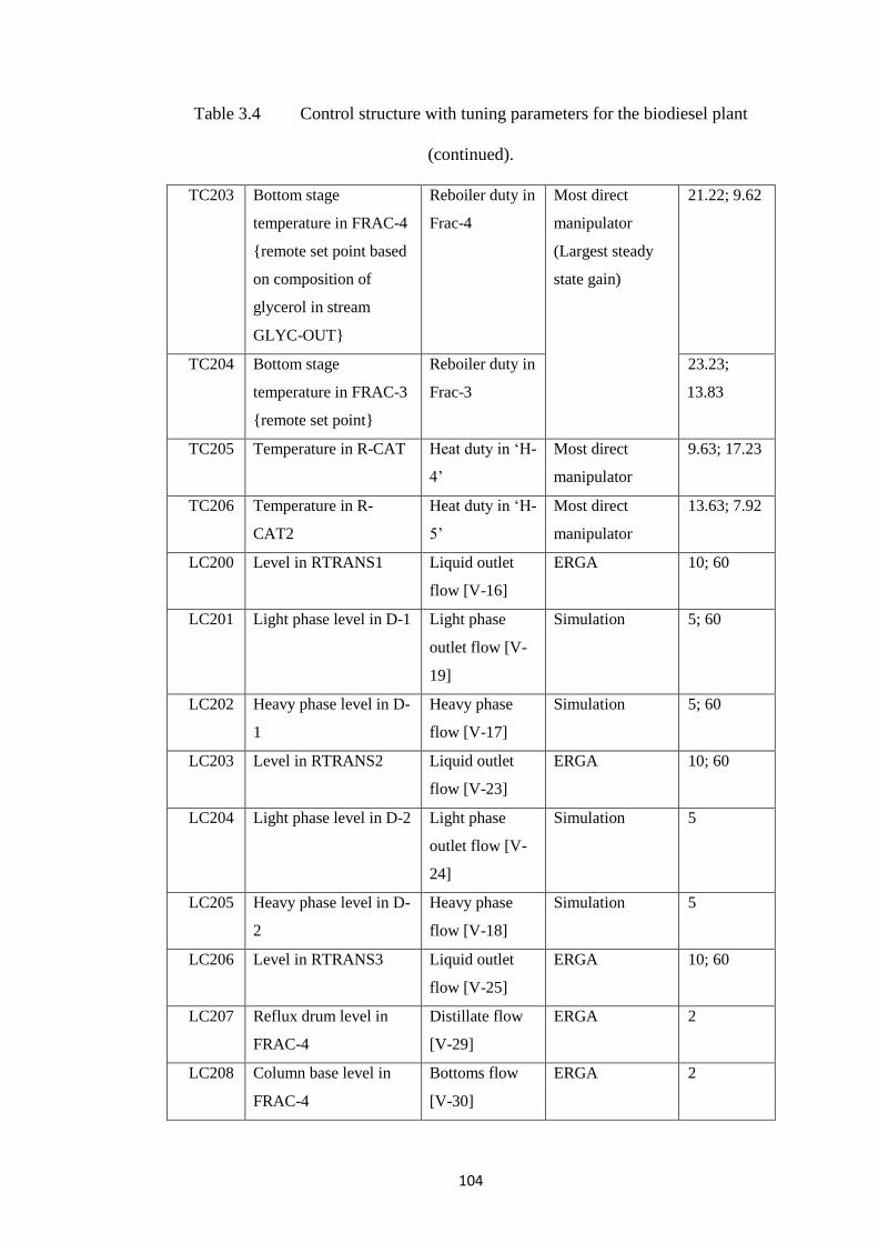
104
Table 3.4 Control structure with tuning parameters for the biodiesel plant
(continued).
TC203 Bottom stage
temperature in FRAC-4
{remote set point based
on composition of
glycerol in stream
GLYC-OUT}
Reboiler duty in
Frac-4
Most direct
manipulator
(Largest steady
state gain)
21.22; 9.62
TC204 Bottom stage
temperature in FRAC-3
{remote set point}
Reboiler duty in
Frac-3
23.23;
13.83
TC205 Temperature in R-CAT Heat duty in ‘H-
4’
Most direct
manipulator
9.63; 17.23
TC206 Temperature in R-
CAT2
Heat duty in ‘H-
5’
Most direct
manipulator
13.63; 7.92
LC200 Level in RTRANS1 Liquid outlet
flow [V-16]
ERGA 10; 60
LC201 Light phase level in D-1 Light phase
outlet flow [V-
19]
Simulation 5; 60
LC202 Heavy phase level in D-
1
Heavy phase
flow [V-17]
Simulation 5; 60
LC203 Level in RTRANS2 Liquid outlet
flow [V-23]
ERGA 10; 60
LC204 Light phase level in D-2 Light phase
outlet flow [V-
24]
Simulation 5
LC205 Heavy phase level in D-
2
Heavy phase
flow [V-18]
Simulation 5
LC206 Level in RTRANS3 Liquid outlet
flow [V-25]
ERGA 10; 60
LC207 Reflux drum level in
FRAC-4
Distillate flow
[V-29]
ERGA 2
LC208 Column base level in
FRAC-4
Bottoms flow
[V-30]
ERGA 2
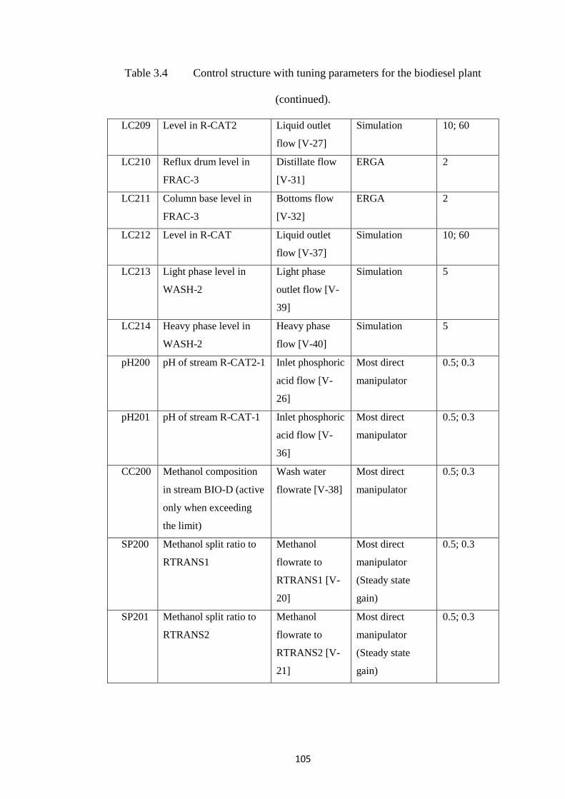
105
Table 3.4 Control structure with tuning parameters for the biodiesel plant
(continued).
LC209 Level in R-CAT2 Liquid outlet
flow [V-27]
Simulation 10; 60
LC210 Reflux drum level in
FRAC-3
Distillate flow
[V-31]
ERGA 2
LC211 Column base level in
FRAC-3
Bottoms flow
[V-32]
ERGA 2
LC212 Level in R-CAT Liquid outlet
flow [V-37]
Simulation 10; 60
LC213 Light phase level in
WASH-2
Light phase
outlet flow [V-
39]
Simulation 5
LC214 Heavy phase level in
WASH-2
Heavy phase
flow [V-40]
Simulation 5
pH200 pH of stream R-CAT2-1 Inlet phosphoric
acid flow [V-
26]
Most direct
manipulator
0.5; 0.3
pH201 pH of stream R-CAT-1 Inlet phosphoric
acid flow [V-
36]
Most direct
manipulator
0.5; 0.3
CC200 Methanol composition
in stream BIO-D (active
only when exceeding
the limit)
Wash water
flowrate [V-38]
Most direct
manipulator
0.5; 0.3
SP200 Methanol split ratio to
RTRANS1
Methanol
flowrate to
RTRANS1 [V-
20]
Most direct
manipulator
(Steady state
gain)
0.5; 0.3
SP201 Methanol split ratio to
RTRANS2
Methanol
flowrate to
RTRANS2 [V-
21]
Most direct
manipulator
(Steady state
gain)
0.5; 0.3
106
3.4.5 Level 3.1. Production Rate Manipulator Selection
Selection of a suitable TPM is critical for the process to respond to the
variations quickly and smoothly. This step deals with the selection of manipulated
variable for varying throughput. Internal variables, such as reactor operating
parameters on this path, are preferred over external variables (i.e., fixed flow
followed by on demand option). In fixed flow strategy, the feed flow rate is set and
controlled at a particular value. On the contrary, in on demand strategy, the
production rate is directly controlled at the desired value. The decision regarding
TPM can be taken using the steady state simulator. The process variable having a
larger steady state gain should be the natural choice. In the biodiesel process, the
reactors have to be run at optimal conditions to maximize the product formation;
these optimal conditions are fixed by optimization in this case. Therefore, these
parameters will not be used as TPM, and feed (WCO) flow rate is identified as the
next best choice for TPM.
3.4.6 Level 3.2. Product Quality Manipulator Selection
Selection of manipulated variable for product purity is dealt with in this level.
Maintaining biodiesel purity is amongst important objectives while developing a
control system as it has to meet EN/ASTM standards. Accordingly, biodiesel purity
and impurity levels, such as TG, DG and MG in the final product, should be
monitored and subsequently controlled. Therefore, proper reaction conditions should
be maintained to convert WCO completely so that its components will not end up in
the final product. The critical variables for this include methanol to oil molar ratio,
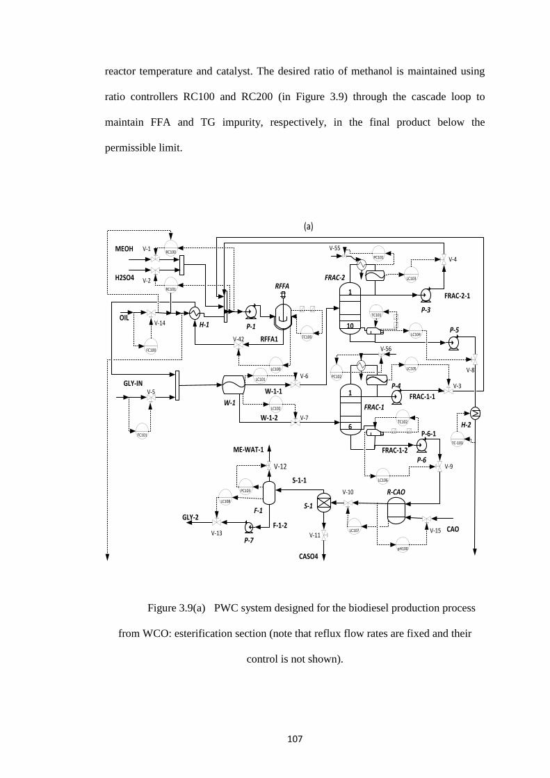
107
reactor temperature and catalyst. The desired ratio of methanol is maintained using
ratio controllers RC100 and RC200 (in Figure 3.9) through the cascade loop to
maintain FFA and TG impurity, respectively, in the final product below the
permissible limit.
Figure 3.9(a) PWC system designed for the biodiesel production process
from WCO: esterification section (note that reflux flow rates are fixed and their
control is not shown).
R-CAO
RC100
RC101
FC100
TC100
LC100
FC101
PC101
LC103
LC104
TC101
LC101
LC102
LC105
PC102
LC106
TC102
LC107
pH100
PC103
LC108
TC-103
P-1
MEOH
H2SO4RFFA
H-1OIL
FRAC-1
FRAC-2
FRAC-1-2
P-3
FRAC-1-1
FRAC-2-1
P-5
H-2
W-1-1
W-1-2
W-11
1
6
10
P-4
S-1
P-6
S-1-1
F-1
F-1-2 CAO
P-7
V-1
V-2
V-3
V-4
V-6
V-7
V-8
P-6-1
V-9
V-14
V-15
V-10
GLY-INV-5
GLY-2
V-13
RFFA1V-42
V-11
ME-WAT-1
V-12
CASO4
(a)
V-55
V-56
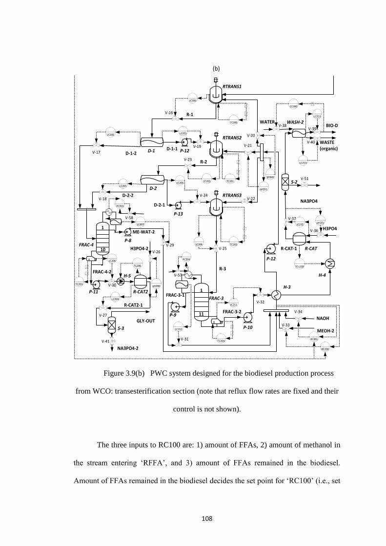
108
Figure 3.9(b) PWC system designed for the biodiesel production process
from WCO: transesterification section (note that reflux flow rates are fixed and their
control is not shown).
The three inputs to RC100 are: 1) amount of FFAs, 2) amount of methanol in
the stream entering ‘RFFA’, and 3) amount of FFAs remained in the biodiesel.
Amount of FFAs remained in the biodiesel decides the set point for ‘RC100’ (i.e., set
R-CAT2
R-CAT
LC201LC202
LC205LC204
LC200
TC200
LC203 TC201
LC206 TC202
PC203
LC207
LC208
TC203
LC209
pH200
PC204
LC210
LC211
TC204
LC212pH201
CC200
RC200
RC201
LC214
LC213
SP200
SP201
TC=205TC206
RTRANS1
RTRANS2
RTRANS3
D-1
D-2
R-2
D-1-1
D-2-1
FRAC-4
FRAC-3
FRAC-3-2
P-10
P-9
D-1-2
D-2-2
H-3
H-4
R-CAT-1
FRAC-3-1
1
1
10
11
S-3
P-11
P-12
R-1V-16
V-17
V-18
V-20
V-21
V-22
V-23
V-24
R-3
V-25H3PO4-2V-26
V-29P-8
V-30
V-31
V-32
MEOH-2V-33
NAOH
V-34
H3PO4V-36
V-37
WATERV-38
V-39
WASTE(organic)
V-40
ME-WAT-2
V-19
V-27
R-CAT2-1
GLY-OUT
WASH-2
FRAC-4-2
S-2
NA3PO4
BIO-D
H-5
NA3PO4-2
V-41
V-51
(b)
P-12
P-13
V-57
V-58
109
point for molar ratio of methanol to FFAs will change when the FFA content in the
final product violates the permissible limit). Accordingly, fresh methanol (stream
‘MEOH’) to the esterification section is manipulated by the RC100 controller.
Similarly, the three inputs to RC200 are: 1) amount of TG, 2) amount of methanol in
the stream entering the splitter, and 3) amount of TG remained in the biodiesel.
Amount of TG remained in the biodiesel decides the set point for ‘RC200’ (i.e., set
point for ‘RC200’ will change when the TG in the final product violates the
permissible limit). Accordingly, fresh methanol (stream ‘MEOH-2’) is manipulated
by the RC200 controller. Methanol impurity in the biodiesel product is controlled by
manipulating the wash water flow rate (controller ‘CC200’ in Figure 3.9).
Also, as glycerol is a valuable byproduct from transesterification section in
biodiesel production, its purity should be maintained at the desired value. A cascade
loop is implemented to manipulate the reboiler duty of FRAC-4 to maintain glycerol
purity. Additionally, the control system is designed in such a way that the maximum
temperature in FRAC-4 will not go beyond 150oC to avoid glycerol decomposition.
In the esterification section, glycrol (stream ‘GLY-IN’) is fed in small quantity to
achieve the separation of unreacted sulfuric acid in the heavy phase from the phase
separator ‘W-1’. Later, the glycerol is recovered through ‘FRAC-1’, ‘R-CAO’, ‘S-1’,
and ‘F-1’, and it can be either recycled or mixed with byproduct glycerol stream
‘GLY-OUT’. In this study, the recovered glycerol is not recycled due to its small
quantity. Set point of the controller ‘FC101’ (for glycerol flow rate) is decided based
on the amount to sulfuric acid in the lighter phase.
110
3.4.7 Level 4.1. Selection of Manipuled Variables for More Severe Controlled
Variables
In this level, process constraints related to process stability, equipments,
operation, safety and the environment are dealt with. These are crucial to control as
these may lead to severe operational ramifications. The important constraints in this
process are:
i. Column temperatures, TFRAC-1 and TFRAC-4 ≤ 150oC, and TFRAC-2 and
TFRAC-3 ≤ 250oC
These temperatures are allowed to vary within acceptable limits. The
controller becomes active as and when the controlled variable (i.e.,
temperature) violates the limit, which is given as the remote set point for the
respective controller.
ii. Respective ratios of feeds
Fresh methanol is manipulated to maintain the desired ratio of methanol
using controllers RC100 and RC200. Molar ratio of methanol to FFA is 10:1 in
‘RFFA’, and methanol to TG, DG and MG ratio is 6:1 in ‘RTRANS1’,
‘RTRANS2’ and ‘RTRANS3’, at normal operation. Similarly, ratio controllers,
RC101 and RC201 are also implemented to maintain the ratio of sodium
hydroxide (1 wt%) and sulfuric acid (10 wt%).
111
iii. Methanol split ratios for the CSTRs
Controllers SP200 and SP201 are employed to maintain the split
fractions (RTRANS1: RTRANS2: RTRANS3 = 0.77:0.12:0.11, at normal
condition).
iv. CSTR temperatures
Reactor temperatures have to be maintained at their desired values in
order to maintain WCO conversion. Aspen Plus Dynamics (V8) provides
different options for reactor temperature control such as constant duty, constant
temperature, condensing, evaporating, dynamics and LMTD. One of these
options can be chosen depending on the application and the extent of realistic
results sought from simulations. For example, the constant duty model is the
most idealistic that does not reflect the consideration of heat transfer area or
temperature differential. In this study, the LMTD option is used to yield more
realistic results that uses a log-mean temperature difference. The assumed
overall heat transfer coefficient (U) is 0.4 kW/m2-K for both cooling water (at
30oC for heat removal) and hot water (at 80
oC for heat addition). The heat
capacity is taken to be 4.2 kJ/kg-K for both cooling water and hot water. The
area (A) for heat transfer, based on half of the lateral surface area of the
cylindrical reactor, is 24.07 m2, 43.9 m
2, 40.98 m
2 and 40.8 m
2 for RFFA,
RTRANS1, RTRANS2 and RTRANS3, respectively. Therefore, their UA is
9.63 kW/K, 17.56 kW/K, 16.39 kW/K and 16.31 kW/K, respectively. For the
initial steady state, the heat duty found from APD simulation is 0.32 GJ/h, 0.68
GJ/h, -0.97 GJ/h and 0.64 GJ/h for RFFA, RTRANS1, RTRANS2 and
RTRANS3, respectively. The utility outlet temperature is 70oC, 65
oC, 45
oC and
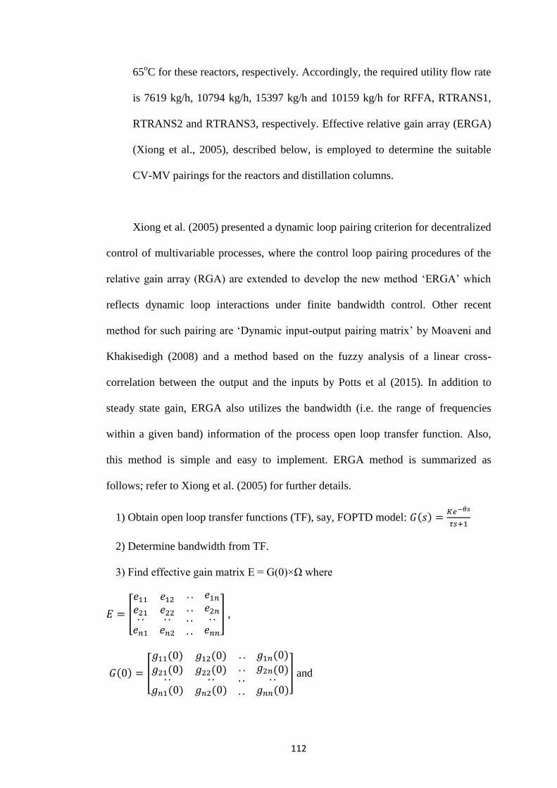
112
65oC for these reactors, respectively. Accordingly, the required utility flow rate
is 7619 kg/h, 10794 kg/h, 15397 kg/h and 10159 kg/h for RFFA, RTRANS1,
RTRANS2 and RTRANS3, respectively. Effective relative gain array (ERGA)
(Xiong et al., 2005), described below, is employed to determine the suitable
CV-MV pairings for the reactors and distillation columns.
Xiong et al. (2005) presented a dynamic loop pairing criterion for decentralized
control of multivariable processes, where the control loop pairing procedures of the
relative gain array (RGA) are extended to develop the new method ‘ERGA’ which
reflects dynamic loop interactions under finite bandwidth control. Other recent
method for such pairing are ‘Dynamic input-output pairing matrix’ by Moaveni and
Khakisedigh (2008) and a method based on the fuzzy analysis of a linear cross-
correlation between the output and the inputs by Potts et al (2015). In addition to
steady state gain, ERGA also utilizes the bandwidth (i.e. the range of frequencies
within a given band) information of the process open loop transfer function. Also,
this method is simple and easy to implement. ERGA method is summarized as
follows; refer to Xiong et al. (2005) for further details.
1) Obtain open loop transfer functions (TF), say, FOPTD model: 𝐺(𝑠) =𝐾𝑒−𝜃𝑠
𝜏𝑠+1
2) Determine bandwidth from TF.
3) Find effective gain matrix E = G(0)×Ω where
𝐸 = [
𝑒11 𝑒12 . . 𝑒1𝑛
𝑒21 𝑒22. . 𝑒2𝑛
. .𝑒𝑛1
. .𝑒𝑛2
. .
. .
. .𝑒𝑛𝑛
] ,
𝐺(0) = [
𝑔11(0) 𝑔12(0) . . 𝑔1𝑛(0)
𝑔21(0) 𝑔22(0) . . 𝑔2𝑛(0). .
𝑔𝑛1(0). .
𝑔𝑛2(0). .. .
. .𝑔𝑛𝑛(0)
] and
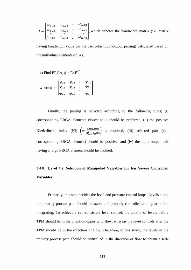
113
Ω = [
ω𝐵,11 ω𝐵,12. . ω𝐵,1𝑛
ω𝐵,21 ω𝐵,21. . ω𝐵,21
. .ω𝐵,𝑛1
. .ω𝐵,𝑛1
. .
. .
. .ω𝐵,𝑛𝑛
], which denotes the bandwidth matrix (i.e. matrix
having bandwidth value for the particular input-output pairing) calculated based on
the individual elements of G(s).
4) Find ERGA, ϕ = E×E-T
,
where ϕ = [
𝜙11 𝜙12 . . 𝜙1𝑛
𝜙21 𝜙22 . . 𝜙2𝑛. .𝜙𝑛1
. .𝜙𝑛2
. .
. .
. .𝜙𝑛𝑛
]
Finally, the pairing is selected according to the following rules; (i)
corresponding ERGA elements closest to 1 should be preferred, (ii) the positive
Niederlinski index (NI) (=𝑑𝑒𝑡(𝐺(0))
∏ 𝑔𝑖𝑖(0)𝑚𝑖=1
) is required, (iii) selected pair (i.e.,
corresponding ERGA element) should be positive, and (iv) the input-output pair
having a large ERGA element should be avoided.
3.4.8 Level 4.2. Selection of Manipuled Variables for less Severe Controlled
Variables
Primarily, this step decides the level and pressure control loops. Levels along
the primary process path should be stable and properly controlled as they are often
integrating. To achieve a self-consistent level control, the control of levels before
TPM should be in the direction opposite to flow, whereas the level controls after the
TPM should be in the direction of flow. Therefore, in this study, the levels in the
primary process path should be controlled in the direction of flow to obtain a self-
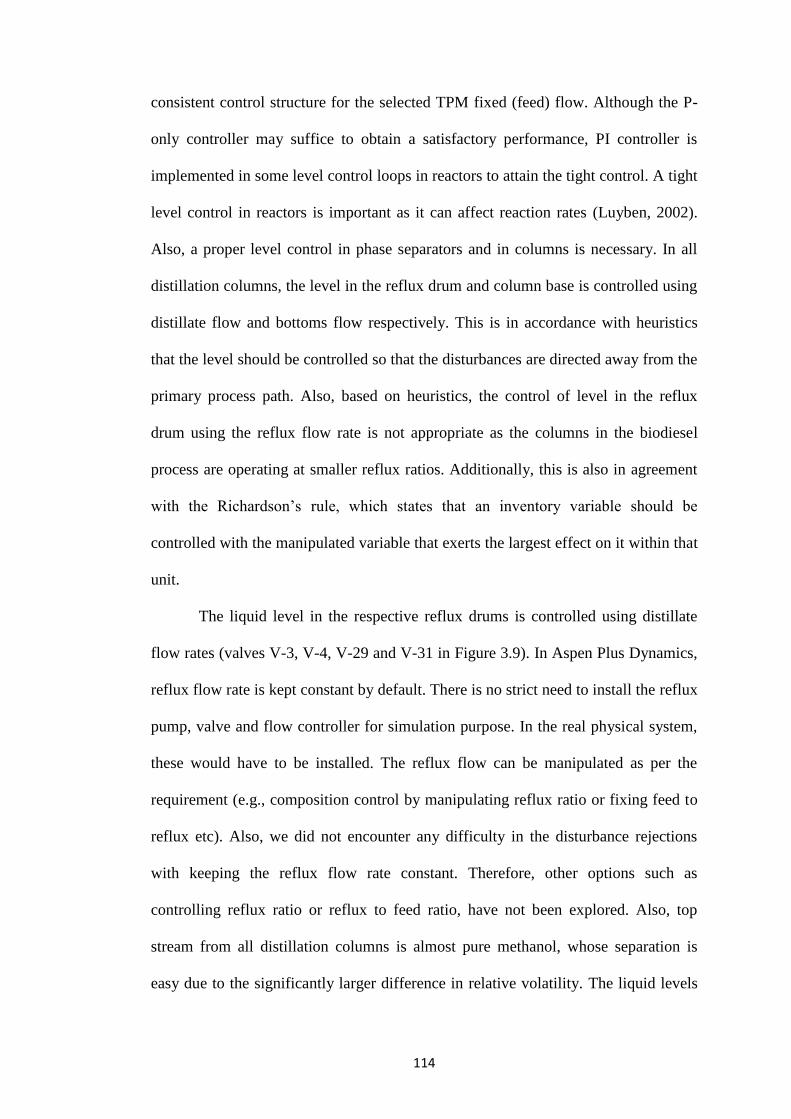
114
consistent control structure for the selected TPM fixed (feed) flow. Although the P-
only controller may suffice to obtain a satisfactory performance, PI controller is
implemented in some level control loops in reactors to attain the tight control. A tight
level control in reactors is important as it can affect reaction rates (Luyben, 2002).
Also, a proper level control in phase separators and in columns is necessary. In all
distillation columns, the level in the reflux drum and column base is controlled using
distillate flow and bottoms flow respectively. This is in accordance with heuristics
that the level should be controlled so that the disturbances are directed away from the
primary process path. Also, based on heuristics, the control of level in the reflux
drum using the reflux flow rate is not appropriate as the columns in the biodiesel
process are operating at smaller reflux ratios. Additionally, this is also in agreement
with the Richardson’s rule, which states that an inventory variable should be
controlled with the manipulated variable that exerts the largest effect on it within that
unit.
The liquid level in the respective reflux drums is controlled using distillate
flow rates (valves V-3, V-4, V-29 and V-31 in Figure 3.9). In Aspen Plus Dynamics,
reflux flow rate is kept constant by default. There is no strict need to install the reflux
pump, valve and flow controller for simulation purpose. In the real physical system,
these would have to be installed. The reflux flow can be manipulated as per the
requirement (e.g., composition control by manipulating reflux ratio or fixing feed to
reflux etc). Also, we did not encounter any difficulty in the disturbance rejections
with keeping the reflux flow rate constant. Therefore, other options such as
controlling reflux ratio or reflux to feed ratio, have not been explored. Also, top
stream from all distillation columns is almost pure methanol, whose separation is
easy due to the significantly larger difference in relative volatility. The liquid levels
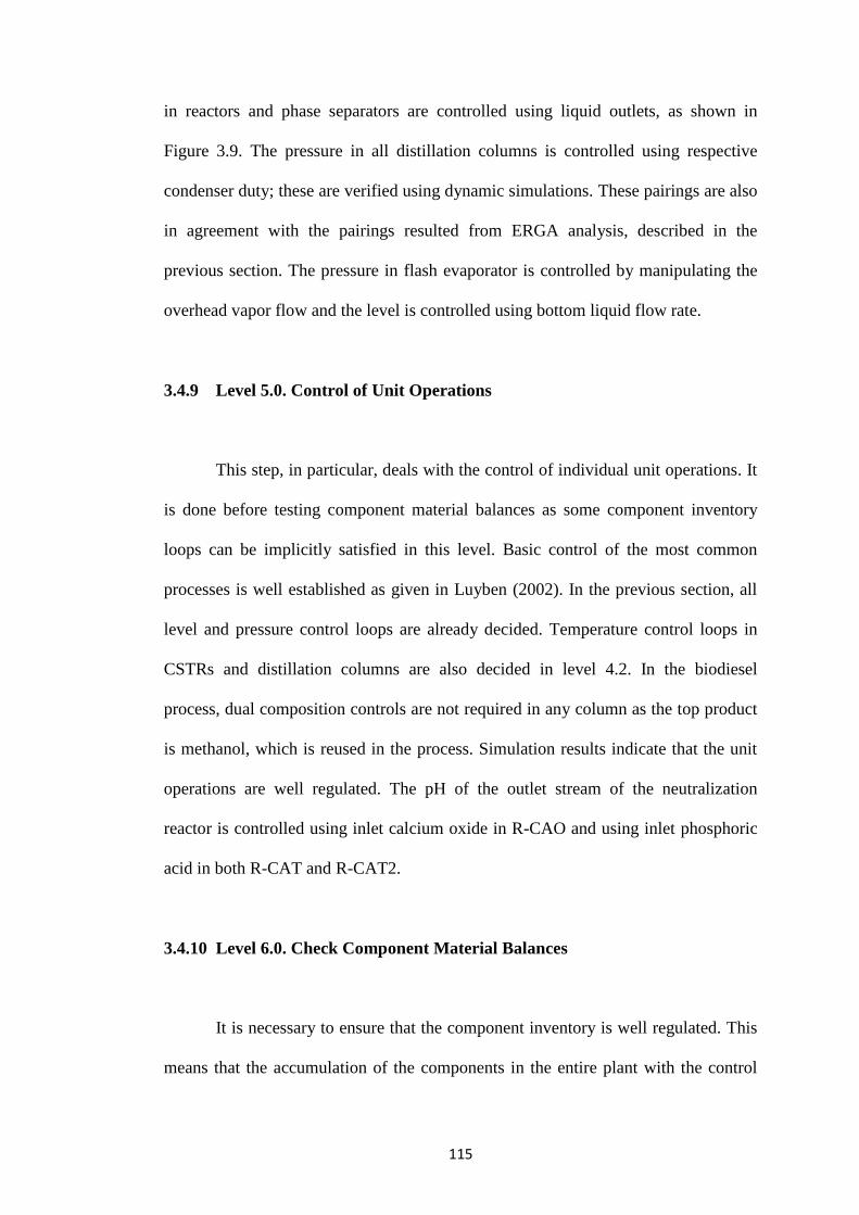
115
in reactors and phase separators are controlled using liquid outlets, as shown in
Figure 3.9. The pressure in all distillation columns is controlled using respective
condenser duty; these are verified using dynamic simulations. These pairings are also
in agreement with the pairings resulted from ERGA analysis, described in the
previous section. The pressure in flash evaporator is controlled by manipulating the
overhead vapor flow and the level is controlled using bottom liquid flow rate.
3.4.9 Level 5.0. Control of Unit Operations
This step, in particular, deals with the control of individual unit operations. It
is done before testing component material balances as some component inventory
loops can be implicitly satisfied in this level. Basic control of the most common
processes is well established as given in Luyben (2002). In the previous section, all
level and pressure control loops are already decided. Temperature control loops in
CSTRs and distillation columns are also decided in level 4.2. In the biodiesel
process, dual composition controls are not required in any column as the top product
is methanol, which is reused in the process. Simulation results indicate that the unit
operations are well regulated. The pH of the outlet stream of the neutralization
reactor is controlled using inlet calcium oxide in R-CAO and using inlet phosphoric
acid in both R-CAT and R-CAT2.
3.4.10 Level 6.0. Check Component Material Balances
It is necessary to ensure that the component inventory is well regulated. This
means that the accumulation of the components in the entire plant with the control
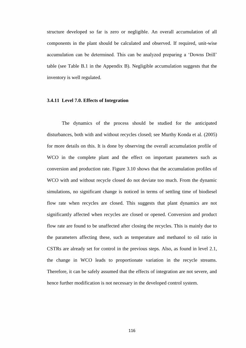
116
structure developed so far is zero or negligible. An overall accumulation of all
components in the plant should be calculated and observed. If required, unit-wise
accumulation can be determined. This can be analyzed preparing a ‘Downs Drill’
table (see Table B.1 in the Appendix B). Negligible accumulation suggests that the
inventory is well regulated.
3.4.11 Level 7.0. Effects of Integration
The dynamics of the process should be studied for the anticipated
disturbances, both with and without recycles closed; see Murthy Konda et al. (2005)
for more details on this. It is done by observing the overall accumulation profile of
WCO in the complete plant and the effect on important parameters such as
conversion and production rate. Figure 3.10 shows that the accumulation profiles of
WCO with and without recycle closed do not deviate too much. From the dynamic
simulations, no significant change is noticed in terms of settling time of biodiesel
flow rate when recycles are closed. This suggests that plant dynamics are not
significantly affected when recycles are closed or opened. Conversion and product
flow rate are found to be unaffected after closing the recycles. This is mainly due to
the parameters affecting these, such as temperature and methanol to oil ratio in
CSTRs are already set for control in the previous steps. Also, as found in level 2.1,
the change in WCO leads to proportionate variation in the recycle streams.
Therefore, it can be safely assumed that the effects of integration are not severe, and
hence further modification is not necessary in the developed control system.
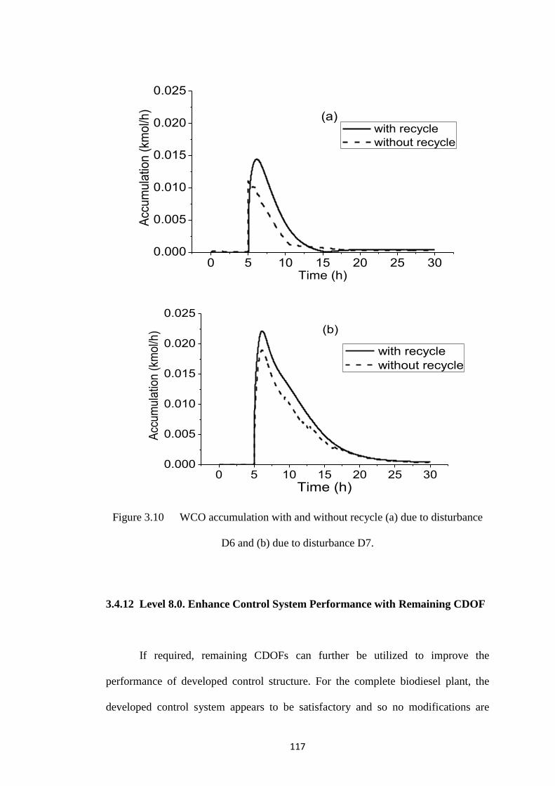
117
0 5 10 15 20 25 300.000
0.005
0.010
0.015
0.020
0.025
Acc
um
ula
tion
(km
ol/h
)
Time (h)
with recycle
without recycle
(a)
0 5 10 15 20 25 300.000
0.005
0.010
0.015
0.020
0.025
Acc
um
ula
tion (
kmol/h
)
Time (h)
with recycle
without recycle
(b)
Figure 3.10 WCO accumulation with and without recycle (a) due to disturbance
D6 and (b) due to disturbance D7.
3.4.12 Level 8.0. Enhance Control System Performance with Remaining CDOF
If required, remaining CDOFs can further be utilized to improve the
performance of developed control structure. For the complete biodiesel plant, the
developed control system appears to be satisfactory and so no modifications are
118
warranted. The resulted control structure from the eight-level IFSH methodology
uses 52 out of the available 68 CDOF, and it is shown in two plots for clarity;
Figures 3.9(a) and 3.9(b) present the control structure for esterification section and
transesterification section, respectively. The percentage opening of control valves is
set to be about 50% at nominal operation. However, valve openings may marginally
deviate from this as was found in Zhang et al (2012). In this process, the valve
openings deviated between 49-51%. This is due to a pressure driven simulation (i.e.
the simulation model based on pressure-flow solver, where pressure depends on
upstream conditions) used in this study.
With the application of methodical PWC methodology i.e. IFSH, location of
TPM, presence of snowball effect, accumulation profile, recycle dynamics and
quality controllers are meticulously identified which may not have been identified
with normal base layer simple control methods. Due to the large number of control
loops present in this PWC scheme, individual control loops are not assessed in terms
of conventional time domain performance specification such as overshoot, rise time
and integral error indices. Besides, the PWC system performance should be analyzed
from a plantwide perspective. The criteria for the quantification of control system’s
performance should be reliable and easy, and essentially they should describe several
factors such as an economic index, smoothness and stability. Vasudevan and
Rangaiah (2010) proposed several criteria for the performance assessment of PWC
systems. This work uses some of these, viz settling time (indicative of smooth and
safe operation of the plant), DPT (denotes an indirect economic index) and overall
TV (indicator of the control efforts required for PWC structure to attain stable
operation) for the performance evaluation, as discussed in Section 4.4. These are
explained in brief as follows;
119
i. Process settling time based on plant production rate. Settling time based
on plant production rate is a measure of time taken by PWC system to reach
the production of the main product to the steady state, after the disturbance(s)
is introduced. It is one of the most important factors for the smooth and safe
operation of the plant. Smaller settling time is desired for an effective PWC
system.
ii. Deviation from production target (DPT). DPT is an indirect economic
indication in terms of production rate. Additionally, it shares the advantages of
dynamic disturbance sensitivity and also indicates the plant economics, which
makes it an attractive and a more complete performance indicator. Smaller
DPT means that the PWC system is better and effective. Vasudevan and
Rangaiah (2010) defined DPT as:
𝐷𝑃𝑇 = ∫ (𝑃𝐴 − 𝑃𝑇)𝑑𝑡𝑡𝑠
0 (3.12)
where PA is actual production rate, PT is production target and ts is settling
time.
iii. Total variation (TV) in manipulated variables. TV is an indicator of the
control effort required for PWC system to attain the steady state after a
disturbance. Smaller TV indicates the smoothness of the manipulated input
signal, and minimal control effort required to attenuate the effects of any
disturbance(s). The advanced features of rigorous process simulators make it
convenient to save the required data, including manipulated variable data in
percentages at regular intervals, from which TV can be easily computed to
120
assess the performance of PWC system. Overall TV in manipulated variables is
calculated by summing TVs of all 52 individual controllers; it gives TV from
the plantwide perspective. All the manipulated variables are expressed in
percentages, for example, the change in reboiler duty is taken as % change in
reboiler duty (and not in GJ/h). This is essential since computing overall TV
would be inconsistent if the manipulated inputs are expressed in their actual
units, for example, flow rate (kg/h) and duty (GJ/h). Vasudevan and Rangaiah
(2010) defined TV as:
𝑇𝑉 = ∫ |𝑑𝑢
𝑑𝑡| 𝑑𝑡
𝑡𝑠
0 (3.13)
which can be approximated for discrete values of manipulated variable, u(t)
as;
𝑇𝑉 = ∑ |𝑢(𝑡 + 1) − 𝑢(𝑡)|∞0 (3.14)
3.5 Development of Operator Training Simulator (OTS) for Biodiesel
Process 1
Figure 3.11 shows the methodology followed in the OTS development. OTS
uses the optimal parameters and the PWC structure found the earlier sections. In
principle, the OTS consists of a computer system which includes one or more trainee
station(s), one field operator station, and one instructor station, as described in
Section 1. The centre of the OTS workstation will be the instructor station that
functions as simulator engine, and instructor tools that interconnects with other work
stations namely operator station and field operator station.
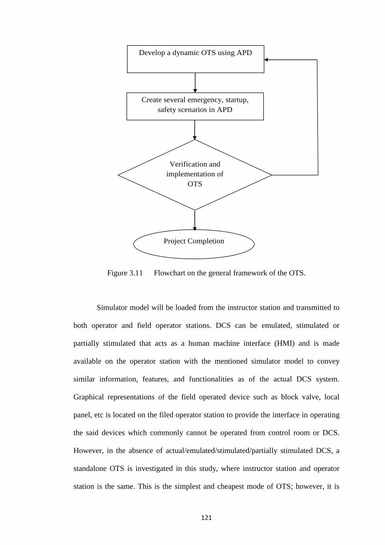
121
Figure 3.11 Flowchart on the general framework of the OTS.
Simulator model will be loaded from the instructor station and transmitted to
both operator and field operator stations. DCS can be emulated, stimulated or
partially stimulated that acts as a human machine interface (HMI) and is made
available on the operator station with the mentioned simulator model to convey
similar information, features, and functionalities as of the actual DCS system.
Graphical representations of the field operated device such as block valve, local
panel, etc is located on the filed operator station to provide the interface in operating
the said devices which commonly cannot be operated from control room or DCS.
However, in the absence of actual/emulated/stimulated/partially stimulated DCS, a
standalone OTS is investigated in this study, where instructor station and operator
station is the same. This is the simplest and cheapest mode of OTS; however, it is
Develop a dynamic OTS using APD
Verification and
implementation of
OTS
Project Completion
Create several emergency, startup,
safety scenarios in APD
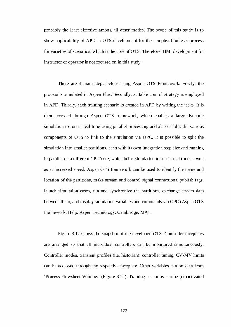
122
probably the least effective among all other modes. The scope of this study is to
show applicability of APD in OTS development for the complex biodiesel process
for varieties of scenarios, which is the core of OTS. Therefore, HMI development for
instructor or operator is not focused on in this study.
There are 3 main steps before using Aspen OTS Framework. Firstly, the
process is simulated in Aspen Plus. Secondly, suitable control strategy is employed
in APD. Thirdly, each training scenario is created in APD by writing the tasks. It is
then accessed through Aspen OTS framework, which enables a large dynamic
simulation to run in real time using parallel processing and also enables the various
components of OTS to link to the simulation via OPC. It is possible to split the
simulation into smaller partitions, each with its own integration step size and running
in parallel on a different CPU/core, which helps simulation to run in real time as well
as at increased speed. Aspen OTS framework can be used to identify the name and
location of the partitions, make stream and control signal connections, publish tags,
launch simulation cases, run and synchronize the partitions, exchange stream data
between them, and display simulation variables and commands via OPC (Aspen OTS
Framework: Help: Aspen Technology: Cambridge, MA).
Figure 3.12 shows the snapshot of the developed OTS. Controller faceplates
are arranged so that all individual controllers can be monitored simultaneously.
Controller modes, transient profiles (i.e. historian), controller tuning, CV-MV limits
can be accessed through the respective faceplate. Other variables can be seen from
‘Process Flowsheet Window’ (Figure 3.12). Training scenarios can be (de)activated
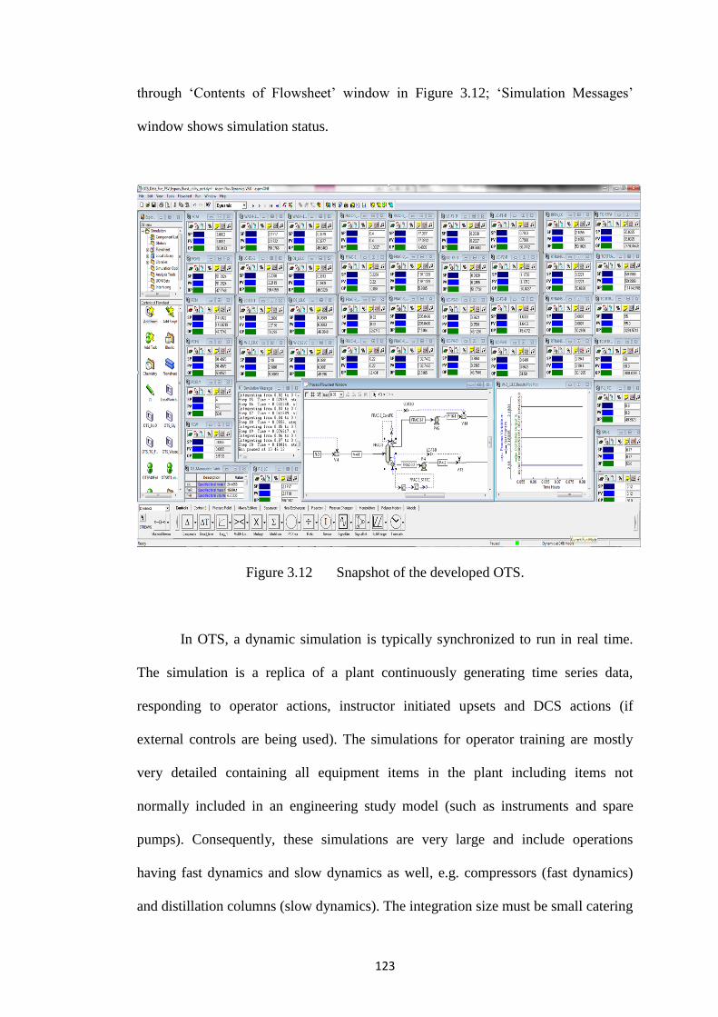
123
through ‘Contents of Flowsheet’ window in Figure 3.12; ‘Simulation Messages’
window shows simulation status.
Figure 3.12 Snapshot of the developed OTS.
In OTS, a dynamic simulation is typically synchronized to run in real time.
The simulation is a replica of a plant continuously generating time series data,
responding to operator actions, instructor initiated upsets and DCS actions (if
external controls are being used). The simulations for operator training are mostly
very detailed containing all equipment items in the plant including items not
normally included in an engineering study model (such as instruments and spare
pumps). Consequently, these simulations are very large and include operations
having fast dynamics and slow dynamics as well, e.g. compressors (fast dynamics)
and distillation columns (slow dynamics). The integration size must be small catering
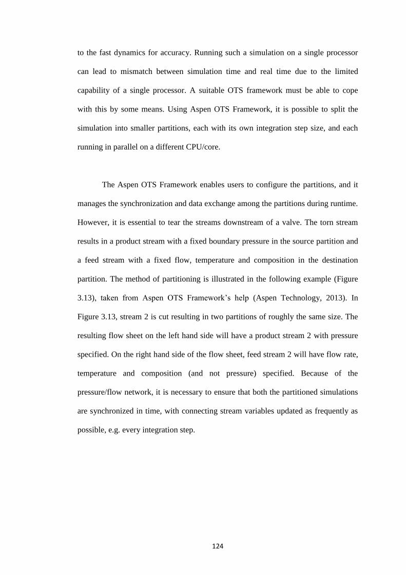
124
to the fast dynamics for accuracy. Running such a simulation on a single processor
can lead to mismatch between simulation time and real time due to the limited
capability of a single processor. A suitable OTS framework must be able to cope
with this by some means. Using Aspen OTS Framework, it is possible to split the
simulation into smaller partitions, each with its own integration step size, and each
running in parallel on a different CPU/core.
The Aspen OTS Framework enables users to configure the partitions, and it
manages the synchronization and data exchange among the partitions during runtime.
However, it is essential to tear the streams downstream of a valve. The torn stream
results in a product stream with a fixed boundary pressure in the source partition and
a feed stream with a fixed flow, temperature and composition in the destination
partition. The method of partitioning is illustrated in the following example (Figure
3.13), taken from Aspen OTS Framework’s help (Aspen Technology, 2013). In
Figure 3.13, stream 2 is cut resulting in two partitions of roughly the same size. The
resulting flow sheet on the left hand side will have a product stream 2 with pressure
specified. On the right hand side of the flow sheet, feed stream 2 will have flow rate,
temperature and composition (and not pressure) specified. Because of the
pressure/flow network, it is necessary to ensure that both the partitioned simulations
are synchronized in time, with connecting stream variables updated as frequently as
possible, e.g. every integration step.
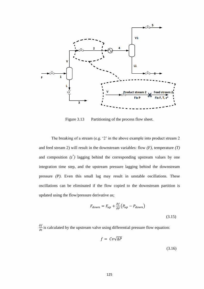
125
Figure 3.13 Partitioning of the process flow sheet.
The breaking of a stream (e.g. ‘2’ in the above example into product stream 2
and feed stream 2) will result in the downstream variables: flow (F), temperature (T)
and composition (z*) lagging behind the corresponding upstream values by one
integration time step, and the upstream pressure lagging behind the downstream
pressure (P). Even this small lag may result in unstable oscillations. These
oscillations can be eliminated if the flow copied to the downstream partition is
updated using the flow/pressure derivative as;
𝐹𝑑𝑜𝑤𝑛 = 𝐹𝑢𝑝 +𝜕𝑓
𝜕𝑃(𝑃𝑢𝑝 − 𝑃𝑑𝑜𝑤𝑛)
(3.15)
𝜕𝑓
𝜕𝑡 is calculated by the upstream valve using differential pressure flow equation:
𝑓 = 𝐶𝑣√∆𝑃
(3.16)
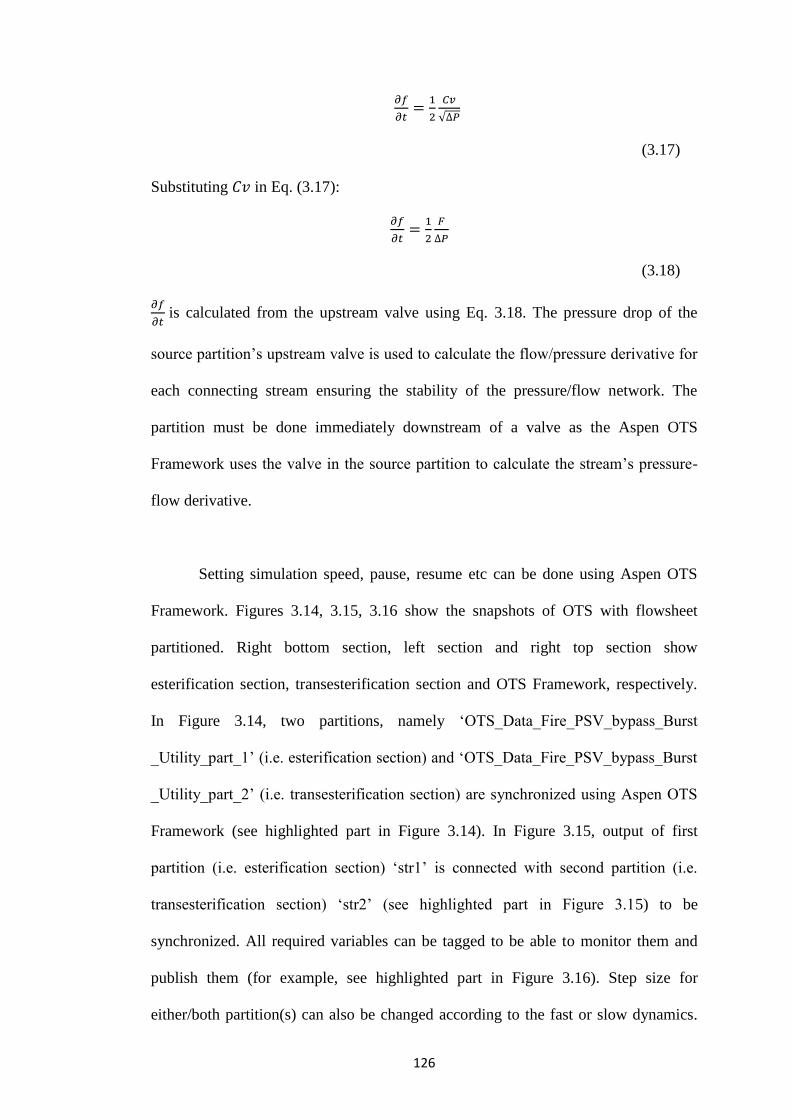
126
𝜕𝑓
𝜕𝑡=
1
2
𝐶𝑣
√∆𝑃
(3.17)
Substituting 𝐶𝑣 in Eq. (3.17):
𝜕𝑓
𝜕𝑡=
1
2
𝐹
∆𝑃
(3.18)
𝜕𝑓
𝜕𝑡 is calculated from the upstream valve using Eq. 3.18. The pressure drop of the
source partition’s upstream valve is used to calculate the flow/pressure derivative for
each connecting stream ensuring the stability of the pressure/flow network. The
partition must be done immediately downstream of a valve as the Aspen OTS
Framework uses the valve in the source partition to calculate the stream’s pressure-
flow derivative.
Setting simulation speed, pause, resume etc can be done using Aspen OTS
Framework. Figures 3.14, 3.15, 3.16 show the snapshots of OTS with flowsheet
partitioned. Right bottom section, left section and right top section show
esterification section, transesterification section and OTS Framework, respectively.
In Figure 3.14, two partitions, namely ‘OTS_Data_Fire_PSV_bypass_Burst
_Utility_part_1’ (i.e. esterification section) and ‘OTS_Data_Fire_PSV_bypass_Burst
_Utility_part_2’ (i.e. transesterification section) are synchronized using Aspen OTS
Framework (see highlighted part in Figure 3.14). In Figure 3.15, output of first
partition (i.e. esterification section) ‘str1’ is connected with second partition (i.e.
transesterification section) ‘str2’ (see highlighted part in Figure 3.15) to be
synchronized. All required variables can be tagged to be able to monitor them and
publish them (for example, see highlighted part in Figure 3.16). Step size for
either/both partition(s) can also be changed according to the fast or slow dynamics.
127
As shown in these Figures, OTS speed can be enhanced or reduced by changing
‘Real time factor’. Also, data transfer rate can be increased or decreased by changing
‘Data transfer interval’ (see highlighted part in Figure 3.14). Figure 3.17 shows
interface for a complete process in APD.
The scenarios for which OTS training is to be carried out should created in
APD by writing the ‘Task’. An example of task writing is depicted for startup of
FRAC-3, in the Appendix C. The results are discussed in Section 4.5. The scenario,
written as a ‘Task’, has to be first compiled and then activated. When OTS is run, the
scenario plays out at the time specified while creating the scenario in the ‘Task’.
Alternatively, direct change can be made into the simulation to impart some faults.
Several scenarios, such as equipment malfunctions, fire, pressure safety valves,
bursting disks, interlocks and startup-shutdowns etc, can be created and tested using
this OTS. These are described in section 4.4.
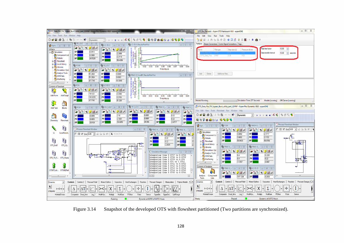
128
Figure 3.14 Snapshot of the developed OTS with flowsheet partitioned (Two partitions are synchronized).
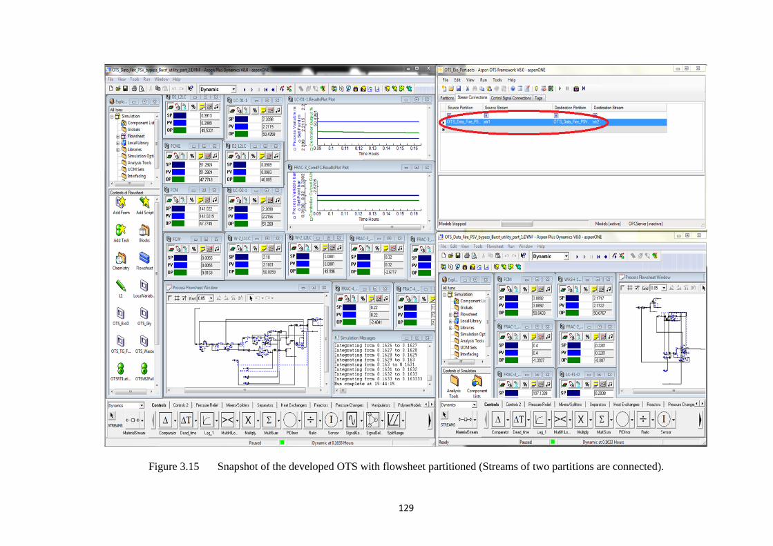
129
Figure 3.15 Snapshot of the developed OTS with flowsheet partitioned (Streams of two partitions are connected).
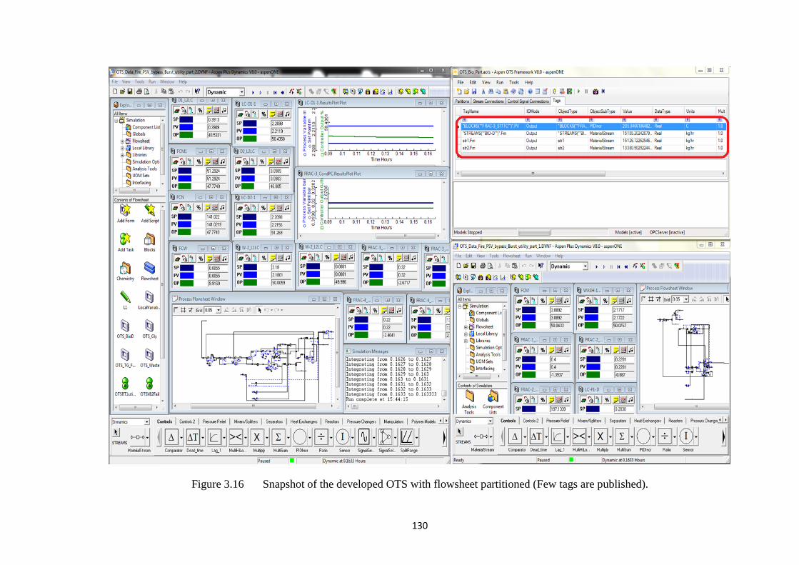
130
Figure 3.16 Snapshot of the developed OTS with flowsheet partitioned (Few tags are published).
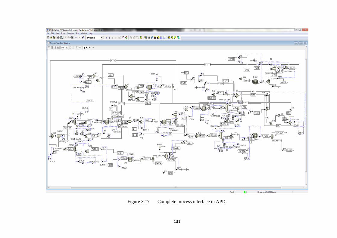
131
Figure 3.17 Complete process interface in APD.
132
3.6 A Hazard and Operability Study of Biodiesel Process 1
A hazard and operability study (HAZOP) is a structured and methodical
examination of a non-existing or existing process in order to identify and evaluate
problems that may indicate risks to plant-personnel or -equipment, or prevent
efficient process operation. Typically, it is carried out by a suitably experienced
multi-disciplinary team. The HAZOP technique aims to stimulate the imagination of
HAZOP team members to identify possible hazards and operability issues.
As per our resources, a preliminary HAZOP analysis for biodiesel production
from WCO (Figure 3.9) is carried out based on HAZOP Guidelines (2008), to
understand the risks associated with the process. HAZOP analysis is one of the
important analyses, viz. construction safety, fire safety, Functional Hazard Analysis
(FHA), transport, emergency plan, and safety management system. The objective of
this analysis is to systematically examine the proposed design, which should be done
before the physical construction. Possible hazards and operational problems can be
prevented or reduced by redesign of suitable operating procedures. Plant items in the
process flowsheet are evaluated by applying appropriate guide words. Potentially
hazardous situations and their ramifications are then estimated. Preventing measures
to avoid or reduce the undesirable situations are also recommended. The findings of
the step by step procedure and the recommendations are organized in the HAZOP
minute sheet (see Appendix D). Figure 3.18 presents HAZOPed process diagram for
biodiesel production from WCO. The important recommendations from this analysis
are:
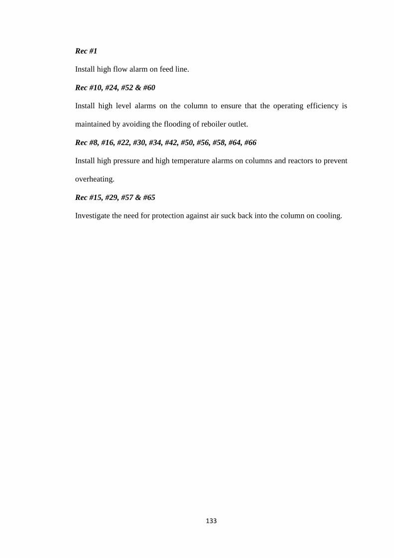
133
Rec #1
Install high flow alarm on feed line.
Rec #10, #24, #52 & #60
Install high level alarms on the column to ensure that the operating efficiency is
maintained by avoiding the flooding of reboiler outlet.
Rec #8, #16, #22, #30, #34, #42, #50, #56, #58, #64, #66
Install high pressure and high temperature alarms on columns and reactors to prevent
overheating.
Rec #15, #29, #57 & #65
Investigate the need for protection against air suck back into the column on cooling.
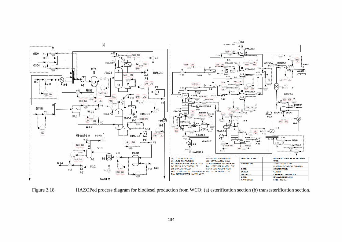
134
Figure 3.18 HAZOPed process diagram for biodiesel production from WCO: (a) esterification section (b) transesterification section.
R-CAO
RC100
RC101
FC100
TC100
LC100
FC101
PC101
LC103
LC104
TC101
LC101
LC102
LC105PC102
LC106
TC102
LC107
pH100
PC103
LC108
TC-103
P-1
MEOH
H2SO4RFFA
H-1OIL
FRAC-1
FRAC-2
FRAC-1-2
P-3
FRAC-1-1
FRAC-2-1
P-5
H-2
W-1-1
W-1-2
W-11
1
6
10
P-4
S-1
P-6
S-1-1
F-1
F-1-2 CAO
P-7
V-1
V-2
V-3
V-4
V-6
V-7
V-8
P-6-1
V-9
V-14
V-15
V-10
GLY-INV-5
GLY-2
V-13
RFFA1V-42
V-11
ME-WAT-1
V-12
CASO4
(a)
PAH PAL
LAH
LAL
TAH TAL
LAH LAL
TAH TAL
LAH LALLAH LAL
LAH LAL
FAH
FAHLAH LAL
LAH LAL
LAH LAL
LAH LAL
PAH PAL
TAH TAL
TAH TAL
PAH
PAL
FRAC2-PSV
FRAC1-PSV
F-1-PSV
V-55
V-56
R-CAT2
R-CAT
LC201LC202
LC205LC204
LC200
TC200
LC203TC201
LC206 TC202
PC203
LC207
LC208
TC203
LC209
pH200
PC204
LC210
LC211
TC204
LC212pH201
CC200
RC200
RC201
LC214
LC213
SP200
SP201
TC=205TC206
RTRANS1
RTRANS2
RTRANS3
D-1
D-2
R-2
D-1-1
D-2-1
FRAC-4
FRAC-3
FRAC-3-2
P-10
P-9
D-1-2
D-2-2
H-3
H-4
R-CAT-1
FRAC-3-1
1
1
10
11
S-3
P-11
P-12
R-1
V-16
V-17
V-18
V-20
V-21
V-22
V-23
V-24
R-3
V-25H3PO4-2V-26
V-29P-8
V-30
V-31
V-32
MEOH-2V-33
NAOH
V-34
H3PO4V-36
V-37
WATERV-38
V-39
WASTE(organic)
V-40
ME-WAT-2
V-19
V-27
R-CAT2-1
GLY-OUT
WASH-2
FRAC-4-2
S-2
NA3PO4
BIO-D
H-5
NA3PO4-2
V-41
V-51
(b)
P-12
P-13
LAH LAL
PAH PAL
PAH PAL
TAH TAL
TAH TAL
TAH TAL
TAH TAL
TAH TAL
TAH
TAL
LAH LAL LAH LAL
LAH LAL
LAH LAL
LAH
LAL
LAH LAL
LAHLALLAH
LAL
LAH LAL
LAH LAL
LAH
LAL
LAH
LAL
LAH LAL TAH
TAL
RTRANS1-PSV
RTRANS2-PSV
RTRANS3-PSV
FRAC4-PSV
FRAC3-PSV
V-58
V-57
135
This chapter discussed the development of two biodiesel processes, which are
then optimized for multiple objectives to determine the better process. Processes are
simulated realistically in Aspen Plus V8.0 and Aspen Plus Dynamics V8.0 using
detailed reaction mechanism and detailed constituents of WCO. MOO is carried out
using Excel based NSGA-II implemented in VBA. Several bi-objective optimization
studies are conducted on the simulated process to determine the trade-off between
conflicting objectives such as profit, heat duty and organic waste. Further, PWC
system is developed for the chosen biodiesel process using IFSH methodology, the
steps of which are discussed systematically in this chapter. This is a top-down
systematic PWC method, which is proven to be effective in developing robust PWC
for the various processes. However, its applicability to the complex multiunit
biodiesel production from WCO process has been studied for the first time in this
research. Also, the criteria for performance evaluation, applicable for PWC system
evaluation, are presented.
Later, development of OTS for biodiesel process is discussed
comprehensively. Dynamic model with control structure is developed in APD. Aspen
OTS Framework is the used on top of APD. Various functionalities of OTS,
including the partition mechanism, are also discussed thoroughly in this chapter. The
developed OTS possesses several important characteristics of an effective OTS.
Several scenarios, such as equipment malfunctions, fire, pressure safety valve,
bursting disk, interlock and startup, which may occur in a real plant can be studied
effectively using the developed OTS. At last, HAZOP analysis is carried out for this
process. HAZOP report includes guide words, causes, consequences and
recommendations for several potential scenarios. This simple HAZOP analysis is

136
meant to serve as a basis for the trainees to understanding the possible source of fault
so that a proper action can be taken. Next chapter discusses the results obtained from
the application of the methodologies discussed in this chapter to the biodiesel
process.
137
CHAPTER 4
RESULTS AND DISCUSSION
4.1 Introduction
In this chapter, firstly, the results of detailed process simulation are discussed.
The present study simulates the two process alternatives for biodiesel production
from WCO considering detailed constituents of WCO and detailed kinetics
(esterification and transesterification are represented by 10 and 96 kinetic reactions,
respectively). Later, Pareto-optimal fronts obtained from MOO for different
conflicting objectives, i.e. maximum profit, minimum heat duty and minimum
organic waste, are discussed for both processes. NSGA-II is used to carry out MOO
in this study. NSGA-II, implemented in Excel, is linked with biodiesel process model
developed in Aspen Plus. A systematic comparison is carried out to find out the
better process alternative. Effect of using detailed oil components versus a lumped
component is also investigated. This analysis suggests the importance of using
detailed constituents of WCO. Additionally, the quality of biodiesel is evaluated and
compared against EN14214. Results show that the quality of produced biodiesel
meets and exceeds the EN standards. Results of PWC structure resulted from the
application of systematic IFSH are then presented and discussed for several
disturbances.
Its performance is evaluated based on some advance performance evaluation
criteria such as settling time of biodiesel production rate, deviation from the
138
production target (that affects economics) and total variation in manipulated
variables (that depicts the control effort needed to stabilize the process). Also,
dynamics of several process variables are shown for the considered disturbances.
Finally, OTS results for different scenarios are presented and explained in rigor.
These scenarios include equipment malfunctions, fire, pressure safety valve, bursting
disk, interlock, and startup. To assist the trainees identify the possible source of
faults to take appropriate action, a simple HAZOP analysis is also carried out.
4.2 Steady State Simulation Results
This work deals with development of the complete process in Aspen Plus.
Steady state simulation results are validated against the data reported in the literature
(see Table 4.1a and Table 4.1b). Initially, the process simulation results are validated
against the literature data for the capacity considered in the respective source (see
Table 4.1a). Then the capacity is increased to the present capacity of 120 kt/annum
and compared against the data reported in several sources for the processes having
different capacities (see Table 4.1b). Steady state values of important variables can
be seen in Figure 3.3 and 3.3. Table 4.1 shows that the simulation results (product
purity and conversion) are in agreement with the reported data. However, it should
be noted that every paper referred to has different capacity as compared to the
capacity considered in this work. This work develops a process keeping in mind the
WCO availability in Malaysia. Parameters such as, methanol to oil ratio, constituents
of oil, composition of constituents of oil, number of reaction, reaction kinetics etc are
also different compared to what has been considered in this study, as mentioned in
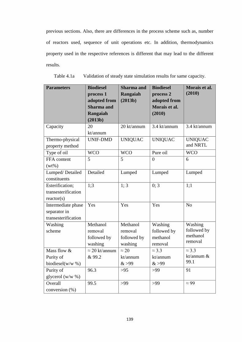
139
previous sections. Also, there are differences in the process scheme such as, number
of reactors used, sequence of unit operations etc. In addition, thermodynamics
property used in the respective references is different that may lead to the different
results.
Table 4.1a Validation of steady state simulation results for same capacity.
Parameters Biodiesel
process 1
adopted from
Sharma and
Rangaiah
(2013b)
Sharma and
Rangaiah
(2013b)
Biodiesel
process 2
adopted from
Morais et al.
(2010)
Morais et al.
(2010)
Capacity 20
kt/annum
20 kt/annum 3.4 kt/annum 3.4 kt/annum
Thermo-physical
property method
UNIF-DMD UNIQUAC UNIQUAC UNIQUAC
and NRTL
Type of oil WCO WCO Pure oil WCO
FFA content
(wt%)
5 5 0 6
Lumped/ Detailed
constituents
Detailed Lumped Lumped Lumped
Esterification;
transesterification
reactor(s)
1;3 1; 3 0; 3 1;1
Intermediate phase
separator in
transesterification
Yes Yes Yes No
Washing
scheme
Methanol
removal
followed by
washing
Methanol
removal
followed by
washing
Washing
followed by
methanol
removal
Washing
followed by
methanol
removal
Mass flow &
Purity of
biodiesel(w/w %)
≈ 20 kt/annum
& 99.2
≈ 20
kt/annum
& >99
≈ 3.3
kt/annum
& >99
≈ 3.3
kt/annum &
99.1
Purity of
glycerol (w/w %)
96.3 >95 >99 91
Overall
conversion (%)
99.5 >99 >99 ≈ 99
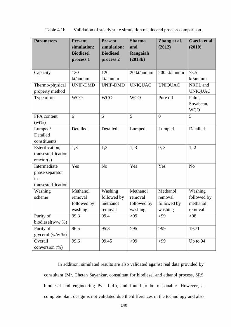
140
Table 4.1b Validation of steady state simulation results and process comparison.
Parameters Present
simulation:
Biodiesel
process 1
Present
simulation:
Biodiesel
process 2
Sharma
and
Rangaiah
(2013b)
Zhang et al.
(2012)
Garcia et al.
(2010)
Capacity 120
kt/annum
120
kt/annum
20 kt/annum 200 kt/annum 73.5
kt/annum
Thermo-physical
property method
UNIF-DMD UNIF-DMD UNIQUAC UNIQUAC NRTL and
UNIQUAC
Type of oil WCO WCO WCO Pure oil Palm,
Soyabean,
WCO
FFA content
(wt%)
6 6 5 0 5
Lumped/
Detailed
constituents
Detailed Detailed Lumped Lumped Detailed
Esterification;
transesterification
reactor(s)
1;3 1;3 1; 3 0; 3 1; 2
Intermediate
phase separator
in
transesterification
Yes No Yes Yes No
Washing
scheme
Methanol
removal
followed by
washing
Washing
followed by
methanol
removal
Methanol
removal
followed by
washing
Methanol
removal
followed by
washing
Washing
followed by
methanol
removal
Purity of
biodiesel(w/w %)
99.3 99.4 >99 >99 >98
Purity of
glycerol (w/w %)
96.5 95.3 >95 >99 19.71
Overall
conversion (%)
99.6 99.45 >99 >99 Up to 94
In addition, simulated results are also validated against real data provided by
consultant (Mr. Chetan Sayankar, consultant for biodiesel and ethanol process, SRS
biodiesel and engineering Pvt. Ltd.), and found to be reasonable. However, a
complete plant design is not validated due the differences in the technology and also
141
confidentiality. Additionally, validation for several other parameters is also presented
wherever required, for example fixed capital investment, settling time, DPT etc.
4.3 Multi-objective Optimization (MOO) of Biodiesel Processes
MOO is carried out using NSGA-II to determine the optimal solutions
between conflicting objectives. Two bi-objective problems, namely profit vs heat
duty and profit vs organic waste, are considered for each process. Analysis in terms
of these objectives is important as these indicate the vital economic and
environmental aspects of the process. The resulted Pareto-optimal fronts are then
discussed as given below. Trends of decision variables with respect to profit are
presented. These trends are subjected to many constraints as mentioned in Chapter 3.
One optimal solution from each process is then considered and compared for further
discussion where a comparison is conducted to determine the best process
alternative. The comparison is conducted based on capital investment, methanol
requirement, biodiesel product quantity, manufacturing cost, organic waste
formation, heat duty requirement and profit. Also, the quality of biodiesel product is
compared against EN standard for the same optimal solution.
4.3.1 Pareto-optimal Solutions for Process 1
Two cases, namely profit vs heat duty and profit vs organic waste are
investigated for process 1. Pareto-optimal front between the objectives and trends of
decision variables vs profit are presented below for each case.
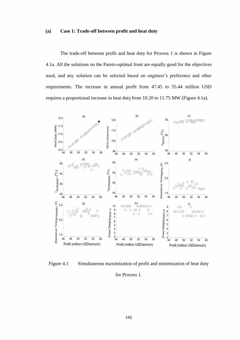
142
(a) Case 1: Trade-off between profit and heat duty
The trade-off between profit and heat duty for Process 1 is shown in Figure
4.1a. All the solutions on the Pareto-optimal front are equally good for the objectives
used, and any solution can be selected based on engineer’s preference and other
requirements. The increase in annual profit from 47.45 to 55.44 million USD
requires a proportional increase in heat duty from 10.20 to 11.75 MW (Figure 4.1a).
46 48 50 52 54 5610.0
10.5
11.0
11.5
12.0(a)
Heat D
uty
(M
W)
+
46 48 50 52 54 5655
60
65
(c)
TR
FF
A (
oC
)
46 48 50 52 54 5645
50
55
60
(d)
TR
TR
AN
S1
(oC
)
46 48 50 52 54 56
45
50
55
60(e)
TR
TR
AN
S2
(oC
)
46 48 50 52 54 5696
104
112
120
(b)
WC
O (
kt/
annum
)
46 48 50 52 54 56
1.5
2.0
2.5(f)
(Resid
ence T
ime) R
FF
A (
h)
46 48 50 52 54 56
1.5
2.0
2.5(g)
(Resid
ence T
ime) R
TR
AN
S1 (
h)
Profit (million USD/annum)
46 48 50 52 54 562
3
4
5
6
7
8
9
10(h)
(Feed S
tage) F
RA
C-3
Profit (million USD/annum)
46 48 50 52 54 562
3
4
5
6
7
8
9(i)
(Feed S
tage) F
RA
C-4
Profit (million USD/annum)
Figure 4.1 Simultaneous maximization of profit and minimization of heat duty
for Process 1.
143
This is mainly due to the increased WCO from 104.76 to 119.73 kt/annum
(Figure 4.1b). The temperatures of esterification reactor ‘TRFFA’ (Figure 4.1c),
transesterification reactor ‘TRTRANS1’ (Figure 4.1d) and transesterification reactor
‘TRTRANS3’ (not shown in Figure 4.1 for brevity; see Figure A.1 in the Appendix A)
stay near to their upper bounds. Further, TRTRANS2 (Figure 4.1e) varies around 55oC.
These higher reactor temperatures lead to better conversion and consequently higher
profit. However, this increases the size and so cost of phase-separators ‘W-1’, ‘D-1’
and ‘D-2’ resulting in higher FCI. Optimal residence time in esterification reactor
‘(Residence Time)RFFA’ (Figure 4.1f) is largely scattered between 1.6 to 1.9 h. This
suggests that smaller reactor volume i.e. smaller residence time (1.6 to 1.9 h) with
higher temperature is sufficient to achieve the required conversion of the FFAs to
biodiesel. Optimal residence times in transesterification reactors: ‘(Residence
Time)RTRANS1’ (Figure 4.1g), ‘(Residence Time)RTRANS2’ (Figure A.1b in the
Appendix A) and ‘(Residence Time)RTRANS3’ (Figure A.1c) are largely scattered near
to their upper bounds. These are required to obtain optimum conversion of WCO,
though larger reactor volumes increase the capital cost. In general, optimum feed
stages for columns ‘FRAC-1’ (Figure A.1d), ‘FRAC-2’ (Figure A.1e), ‘FRAC-3’
(Figure 4.1h) and ‘FRAC-4’ (Figure 4.1i) are scattered towards their upper bounds.
These do not have much impact on FCI, but increases the profit by reducing the
utility cost for the column reboiler and condenser. Pareto-optimal solution (shown as
+ in Figure 4.1a) is considered for further discussion in the section 4.3.3. Table A.3
in the Appendix A presents the key data of selected streams corresponding to this
optimal solution.
144
(b) Case 2: Trade-off between profit and organic waste
Figure 4.2a presents Pareto-optimal front obtained for maximizing profit and
minimizing organic waste. Organic waste increases from 0.183 to 0.202 kt/annum for
the profit improvement from 48.32 to 55.68 million USD per annum. Methanol,
glycerol, tri/di/mono-glycerides, FFAs and FAMEs are the constituents of organic
waste. As the waste stream (‘WASTE’ in Figure 3.3) contains glycerol and FAME,
minimization of organic waste improves the profit to some extent. In general, the
main decision variable affecting the profit and organic waste is the amount of WCO
processed (Figure 4.2). Higher values of TRFFA, TRTRANS1, TRTRANS3 (Figure 4.2b-
4.2e) also improve the profit as larger amount of biodiesel is produced from WCO in
smaller reactors at higher temperatures. As TRTRANS2 stays near to its lower bound of
45oC (Figure A.2a in the Appendix A), higher temperature is required in TRTRANS3 to
convert the remaining oil to FAME (Figure 4.2e). Lower TRTRANS2 favors the profit
by reducing the cost of phase separator ‘D-2’. As higher temperatures of reactors
favor both objectives similarly, most of the decision variables related to the
temperature are closer to their upper bounds. However, this leads to increase in FCI
as larger phase separators are required to achieve sufficient separation.
Optimal residence time of esterification reactor: ‘(Residence Time)RFFA’
(Figure 4.2f) is largely scattered between 1.5 to 1.88 h, which suggests that smaller
reactor operating at higher temperature is better to achieve the required conversion of
FFAs to FAME. Optimal residence times of first two transesterification reactors are
largely scattered towards their upper bounds (Figures A.2b and A.2c); (Residence
Time)RTRANS3 (Figure 4.2g) is scattered between 1.6 to 1.93 h.
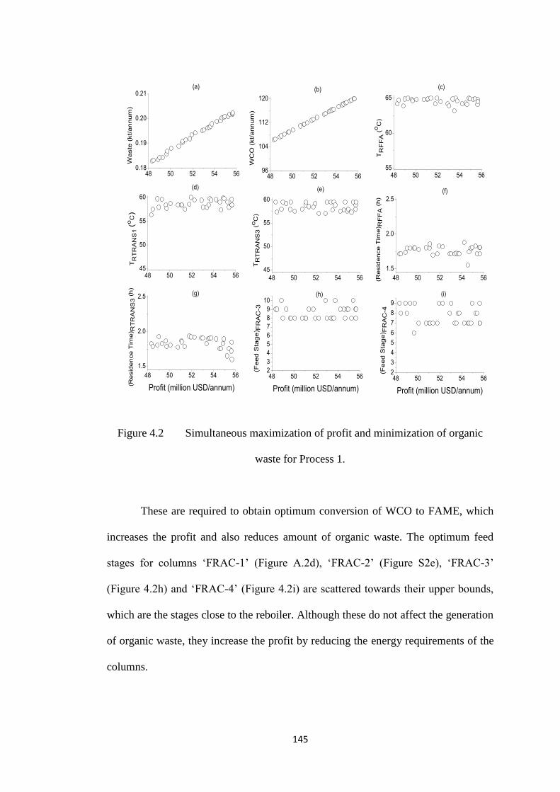
145
48 50 52 54 560.18
0.19
0.20
0.21(a)
Waste
(kt/annum
)
48 50 52 54 5655
60
65
(c)
TR
FF
A (
oC
)
48 50 52 54 5645
50
55
60
(d)
TR
TR
AN
S1
(oC
)
48 50 52 54 5696
104
112
120
(b)
WC
O (
kt/annum
)
48 50 52 54 56
45
50
55
60
(e)
TR
TR
AN
S3
(oC
)
48 50 52 54 56
1.5
2.0
2.5(f)
(Resid
ence T
ime) R
FF
A (
h)
48 50 52 54 56
1.5
2.0
2.5 (g)
(Resid
ence T
ime) R
TR
AN
S3 (
h)
Profit (million USD/annum)
48 50 52 54 562
3
4
5
6
7
8
9
10(h)
(Feed S
tage) F
RA
C-3
Profit (million USD/annum)
48 50 52 54 562
3
4
5
6
7
8
9
(i)
(Feed S
tage) F
RA
C-4
Profit (million USD/annum)
Figure 4.2 Simultaneous maximization of profit and minimization of organic
waste for Process 1.
These are required to obtain optimum conversion of WCO to FAME, which
increases the profit and also reduces amount of organic waste. The optimum feed
stages for columns ‘FRAC-1’ (Figure A.2d), ‘FRAC-2’ (Figure S2e), ‘FRAC-3’
(Figure 4.2h) and ‘FRAC-4’ (Figure 4.2i) are scattered towards their upper bounds,
which are the stages close to the reboiler. Although these do not affect the generation
of organic waste, they increase the profit by reducing the energy requirements of the
columns.
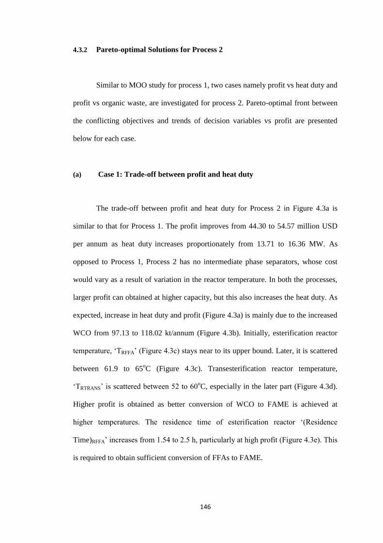
146
4.3.2 Pareto-optimal Solutions for Process 2
Similar to MOO study for process 1, two cases namely profit vs heat duty and
profit vs organic waste, are investigated for process 2. Pareto-optimal front between
the conflicting objectives and trends of decision variables vs profit are presented
below for each case.
(a) Case 1: Trade-off between profit and heat duty
The trade-off between profit and heat duty for Process 2 in Figure 4.3a is
similar to that for Process 1. The profit improves from 44.30 to 54.57 million USD
per annum as heat duty increases proportionately from 13.71 to 16.36 MW. As
opposed to Process 1, Process 2 has no intermediate phase separators, whose cost
would vary as a result of variation in the reactor temperature. In both the processes,
larger profit can obtained at higher capacity, but this also increases the heat duty. As
expected, increase in heat duty and profit (Figure 4.3a) is mainly due to the increased
WCO from 97.13 to 118.02 kt/annum (Figure 4.3b). Initially, esterification reactor
temperature, ‘TRFFA’ (Figure 4.3c) stays near to its upper bound. Later, it is scattered
between 61.9 to 65oC (Figure 4.3c). Transesterification reactor temperature,
‘TRTRANS’ is scattered between 52 to 60oC, especially in the later part (Figure 4.3d).
Higher profit is obtained as better conversion of WCO to FAME is achieved at
higher temperatures. The residence time of esterification reactor ‘(Residence
Time)RFFA’ increases from 1.54 to 2.5 h, particularly at high profit (Figure 4.3e). This
is required to obtain sufficient conversion of FFAs to FAME.
147
42 44 46 48 50 52 54 5613
14
15
16
17(a)
Heat D
uty
(M
W) +
42 44 46 48 50 52 54 5655
60
65
(c)
TR
FF
A (
oC
)
42 44 46 48 50 52 54 5645
50
55
60
(d)
TR
TR
AN
S (
oC
)
42 44 46 48 50 52 54 561.5
2.0
2.5(e)
(Resid
ence T
ime) R
FF
A (
h)
42 44 46 48 50 52 54 561.5
2.0
2.5
(f)
(Resid
ence T
ime) R
TR
AN
S (
h)
42 44 46 48 50 52 54 5696
104
112
120(b)
WC
O (
kt/
annum
)
42 44 46 48 50 52 54 562
34
56
78
9(g)
(Feed S
tage) F
RA
C-2
Profit (million USD/annum)
42 44 46 48 50 52 54 562
4
6
8
10
12
14 (h)
(Feed S
tage) F
RA
C-3
Profit (million USD/annum)
42 44 46 48 50 52 54 562
3
4
5
6
7
8
9
10(i)
(Feed S
tage) F
RA
C-4
Profit (million USD/annum)
Figure 4.3 Simultaneous maximization of profit and minimization of heat duty
for Process 2.
Optimal residence time of transesterification reactor ‘(Residence
Time)RTRANS’ (Figure 4.3f) is scattered between 2.24 to 2.5 h. Capital cost increases
with reactor size, but large reactor is required to obtain optimum conversion of
WCO. Transesterification reactor design is very critical as this process has only one
reactor unlike in Process 1, which has three transesterification reactors in series. In
general, optimum feed stages for columns ‘FRAC-1’ (Figure A.3 in the Appendix
A), ‘FRAC-2’ (Figure 4.3g), ‘FRAC-3’ (Figure 4.3h) and ‘FRAC-4’ (Figure 4.3i) are
scattered towards their upper bounds, which increase the profit by reducing the
148
utility cost in reboilers and condensers. The optimal solution, shown as + in Figure
4.3a, is taken for further analysis in section 4.3.3. Table A.4 in the Appendix A
presents the key data of selected streams corresponding to this optimal solution.
(b) Case 2: Trade-off between profit and organic waste
Figure 4.4a presents the Pareto-optimal solutions obtained for simultaneous
maximization of profit and minimization of organic waste for Process 2. Organic
waste increases from 0.253 to 0.295 kt/annum for the improvement in profit from
44.15 to 54.50 million USD per annum. These increases are mainly due to the
increased WCO from 98.98 to 118.35 kt/annum (Figure 4.4b). Note that only
methanol in streams: ‘ME-WAT-1’, ‘ME-WAT-2’ and ‘ME-WAT-3’ in Figure 3.4,
is the organic waste in Process 2, which does not affect profit much. Optimal values
of TRFFA and TRTRANS are near to their upper bounds of 65 and 60oC, respectively
(Figures 4.4c and 4.4d), which improve the profit by maximizing the product
formation. Optimal (Residence Time)RFFA increases from 1.55 to 2.23 h, which is
required to convert FFAs into FAME (Figure 4.4e). Optimal (Residence Time)RTRANS
is near to its upper bound (scattered between 2.32 to 2.5 h), for converting most of
the oil into FAME (Figure 4.4e); this has favorable impact on the profit without
affecting the organic waste. Optimum feed stages for columns ‘FRAC-1’ (Figure A.4
in the Appendix), ‘FRAC-2’ (Figure 4.4g), ‘FRAC-3’ (Figure 4.4h) and ‘FRAC-4’
(Figure 4.4i) are scattered towards their upper bounds, which increase the profit by
reducing the utility cost in reboilers and condensers of different columns. Similar to
Process 1, they do not affect the generation of organic waste but improve the profit
by reducing COM.
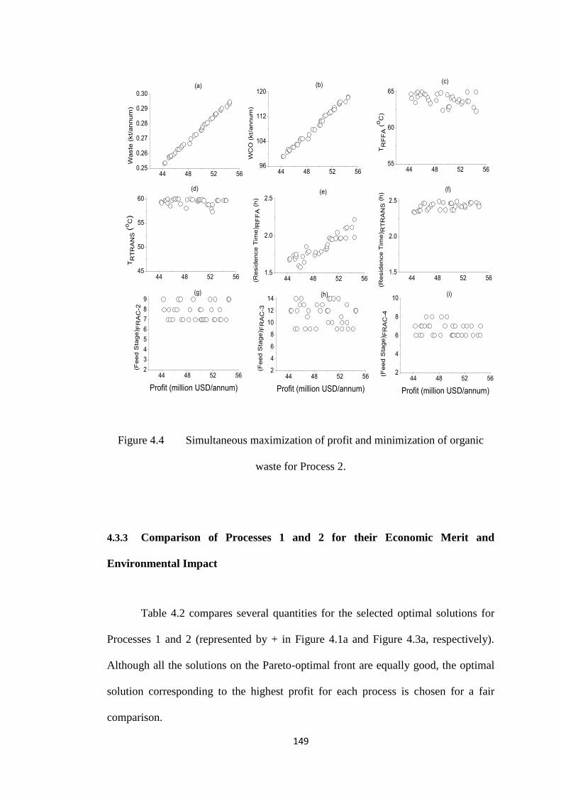
149
44 48 52 560.25
0.26
0.27
0.28
0.29
0.30(a)
Waste
(kt/annum
)
44 48 52 5655
60
65
(c)
TR
FF
A (
oC
)
44 48 52 5645
50
55
60
(d)
TR
TR
AN
S (
oC
)
44 48 52 561.5
2.0
2.5(e)
(Resid
ence T
ime) R
FF
A (
h)
44 48 52 561.5
2.0
2.5
(f)
(Resid
ence T
ime) R
TR
AN
S (
h)
44 48 52 5696
104
112
120(b)
WC
O (
kt/
annum
)
44 48 52 562
3
4
5
6
7
8
9(g)
(Feed S
tage) F
RA
C-2
Profit (million USD/annum)
44 48 52 562
4
6
8
10
12
14(h)
(Feed S
tage) F
RA
C-3
Profit (million USD/annum)
44 48 52 562
4
6
8
10(i)
(Feed S
tage) F
RA
C-4
Profit (million USD/annum)
Figure 4.4 Simultaneous maximization of profit and minimization of organic
waste for Process 2.
4.3.3 Comparison of Processes 1 and 2 for their Economic Merit and
Environmental Impact
Table 4.2 compares several quantities for the selected optimal solutions for
Processes 1 and 2 (represented by + in Figure 4.1a and Figure 4.3a, respectively).
Although all the solutions on the Pareto-optimal front are equally good, the optimal
solution corresponding to the highest profit for each process is chosen for a fair
comparison.
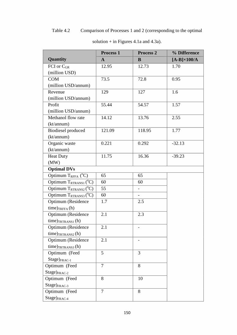
150
Table 4.2 Comparison of Processes 1 and 2 (corresponding to the optimal
solution + in Figures 4.1a and 4.3a).
Quantity
Process 1 Process 2 % Difference
A B [A-B]×100/A
FCI or CGR
(million USD)
12.95 12.73 1.70
COM
(million USD/annum)
73.5 72.8 0.95
Revenue
(million USD/annum)
129 127 1.6
Profit
(million USD/annum)
55.44 54.57 1.57
Methanol flow rate
(kt/annum)
14.12 13.76 2.55
Biodiesel produced
(kt/annum)
121.09 118.95 1.77
Organic waste
(kt/annum)
0.221 0.292 -32.13
Heat Duty
(MW)
11.75 16.36 -39.23
Optimal DVs
Optimum TRFFA (oC) 65 65
Optimum TRTRANS1 (oC) 60 60
Optimum TRTRANS2 (oC) 55 -
Optimum TRTRANS3 (oC) 60 -
Optimum (Residence
time)TRFFA (h)
1.7 2.5
Optimum (Residence
time)TRTRANS1 (h)
2.1 2.3
Optimum (Residence
time)TRTRANS2 (h)
2.1 -
Optimum (Residence
time)TRTRANS3 (h)
2.1 -
Optimum (Feed
Stage)FRAC-1
5 3
Optimum (Feed
Stage)FRAC-2
7 8
Optimum (Feed
Stage)FRAC-3
8 10
Optimum (Feed
Stage)FRAC-4
7 8
151
West et al. (2008) reported CTM of 1.1 million USD (when CEPCI = 394) for
a biodiesel plant of capacity 8 kt/annum with WCO as the feedstock. Further,
Sharma and Rangaiah (2013b) reported CTM of 2.88 million USD (for CPECI = 600)
for a biodiesel plant of capacity 20 kt/annum with WCO as the feedstock.
Projected CTM for a plant capacity of 120 kt/annum, using the six-tenths rule
(Sieder et al., 2010), and CEPCI of 600, is 8.44 million USD (based on Sharma and
Rangaiah, 2013b) and 8.5 million USD (based on West et al., 2008). In the present
study, CTM of 9.31 million USD for Process 1 and 9.30 million USD for Process 2
are obtained, and these are consistent with the previous studies. The small increase in
CTM is mainly due to the increased number of processing steps in both the processes
(see Figures 3.1 and 3.2 in Chapter 3).
From Table 4.2, it can be noticed that FCI for Process 1 is slightly higher
than that for Process 2, mainly due to the more number of equipments e.g. 3
transesterification reactors) involved in the former process. Amount of methanol
required in Process 1 is slightly higher than that of Process 2, mainly due to slightly
larger WCO and more methanol to oil ratio (required to maintain 6:1 methanol to oil
ratio in each transesterification reactor) in Process 1 as some methanol is removed
from the intermediate phase separators. As water wash column is placed after
methanol recovery column in Process 1, recovered methanol is almost free from
water. This leads to less energy-intensive methanol recovery. COM for Process 1 is
marginally higher than that of Process 2, mainly due to higher FCI, labor cost and
cost of chemicals in Process 1. Amount of organic waste generated in Process 1 is
significantly lower (32%) than that in Process 2.
152
Also, heat duty of Process 1 is significantly lower (39%) than that of Process 2.
Lower heat duty and lower organic waste suggest that Process 1 has lower
environmental impact compared to Process 2. Lower heat duty indicates the lower
energy demand, and lower environmental impact such as water pollution arising
from disposal of organic waste in the water bodies. The menace due to such disposal
include the threat to the animal kind, especially aquatic life due to the depletion of
dissolved oxygen (DO). DO depletion can occur due to the increased biological
oxygen demand and prevention of sunlight from entering into the water bodies
because of the formation of the thin film of oily liquid on top of the water surface.
Further, the present study reveals that, despite more number of equipments
involved, Process 1 is slightly more profitable than Process 2. This is mainly due to
reduced utility cost and increased revenue resulting from the increased product
formation (Table 4.2); these in turn are attributed to the processing sequence with
three CSTRs in series, where intermediate phase separators are used to remove heavy
phase and prevent backward reactions. Moreover, in Process 1, biodiesel and
glycerol are separated first followed by methanol separation and washing of
biodiesel. The advantages of this scheme include: (1) it prevents backward reactions
as methanol is not removed until separation between biodiesel and glycerol is
complete, and (2) as water washing is carried out after methanol removal, the
recovered methanol contains very small fraction of water, which avoids energy
intensive methanol-water separation and enables methanol re-use in the process.
Comparative results in Table 4.2 for the optimized process alternatives are consistent
with Myint and El-Halwagi (2009). Myint and El-Halwagi (2009) concluded that the
153
best flow-sheet is with the biodiesel and glycerol separation first, followed by
methanol recovery and finally water washing.
4.3.4 Effect of detailed versus lumped components and quality
Properties of biodiesel obtained from Aspen Plus simulation, are analyzed to
evaluate the quality of biodiesel, and then it is compared against EN standards
(European Norms: European standards that describe the requirements and test
methods for biodiesel). The results presented in Table 4.3 show that the quality of the
produced biodiesel meets the minimum required standards. To investigate the effect
of using detailed composition of oil versus lumped component, optimized Process 1
was simulated with all triglycerides lumped into triolein and all FFAs lumped into
oleic acid.
Total heating load (QH), which is the sum of heating required in reboilers,
reactors and heaters, is compared for these two cases. It is found to be 5.61 MW
when detailed oil components are used, compared to QH of 5.71 MW when the oil
components are lumped together. The quality of biodiesel is also analyzed for these
two cases. As expected, the constituent methyl esters considering detailed and
lumped oil components are different; consequently, quality of the biodiesel is
different (Table 4.3). This difference arises due to the different properties (critical
temperature, accentric factor, boiling point etc.) of different glycerides that are not
considered when using the a single lumped component. The differences in the results
indicate that more details, as used in this study, should be considered for more
realistic simulation and optimization.
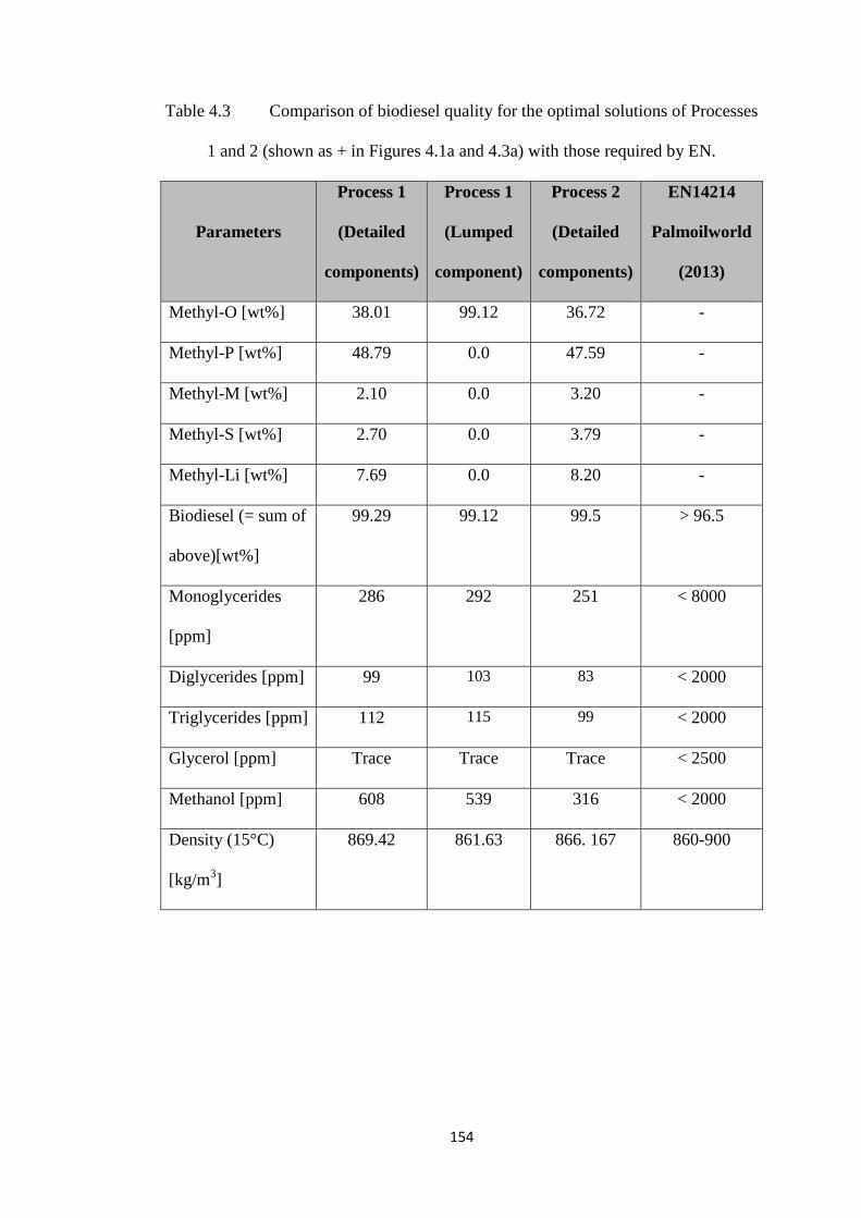
154
Table 4.3 Comparison of biodiesel quality for the optimal solutions of Processes
1 and 2 (shown as + in Figures 4.1a and 4.3a) with those required by EN.
Parameters
Process 1
(Detailed
components)
Process 1
(Lumped
component)
Process 2
(Detailed
components)
EN14214
Palmoilworld
(2013)
Methyl-O [wt%] 38.01 99.12 36.72 -
Methyl-P [wt%] 48.79 0.0 47.59 -
Methyl-M [wt%] 2.10 0.0 3.20 -
Methyl-S [wt%] 2.70 0.0 3.79 -
Methyl-Li [wt%] 7.69 0.0 8.20 -
Biodiesel (= sum of
above)[wt%]
99.29 99.12 99.5 > 96.5
Monoglycerides
[ppm]
286 292 251 < 8000
Diglycerides [ppm] 99 103 83 < 2000
Triglycerides [ppm] 112 115 99 < 2000
Glycerol [ppm] Trace Trace Trace < 2500
Methanol [ppm] 608 539 316 < 2000
Density (15°C)
[kg/m3]
869.42 861.63 866. 167 860-900
155
4.4 Performance Assessment of the Plantwide Control (PWC) System for
Process 1
In the previous section, two processes are optimized and compared
considering profit, heat duty and organic waste as the objectives. The better process
is then identified based on several criteria such as FCI, methanol requirement,
biodiesel produced, COM, organic waste formation, heat duty and profit. Later, a
suitable PWC system is developed for the chosen process i.e. process 1. The final
control system for the complete biodiesel plant consists of 52 control loops (Figure
3.9 in Chapter 3). The details of CV-MV pairings, reasons for pairings and tuning
parameters are presented in Table 3.4 of Chapter 3. This control structure cannot be
compared directly with the previous studies (Shen et al., 2011; Cheng et al., 2014) on
control of biodiesel process as they use different production processes. However, the
main difference in the control structure besides inventory loops is quality controllers,
i.e. FFA and triglyceride impurity, which decide remote set point to the ratio
controllers ‘RC100’ & ‘RC200’ respectively, and methanol impurity in biodiesel
product by manipulating the water flow rate.
Previous studies (Shen et al., 2011; Zhang et al., 2012) on PWC of biodiesel
production use pure vegetable oil, which does not require the esterification section,
needed when using WCO as feedstock, to convert FFAs into biodiesel. Therefore, the
resulted control structure in the present work is different (i.e., controllers in
top/esterification section, and temperature controllers for RTRANS1, RTRANS2,
RTRANS3 and H-4, in Figure 3.9). In this work, we included temperature controllers
for CSTRs as the temperature is found to be varying. Other control loops in the
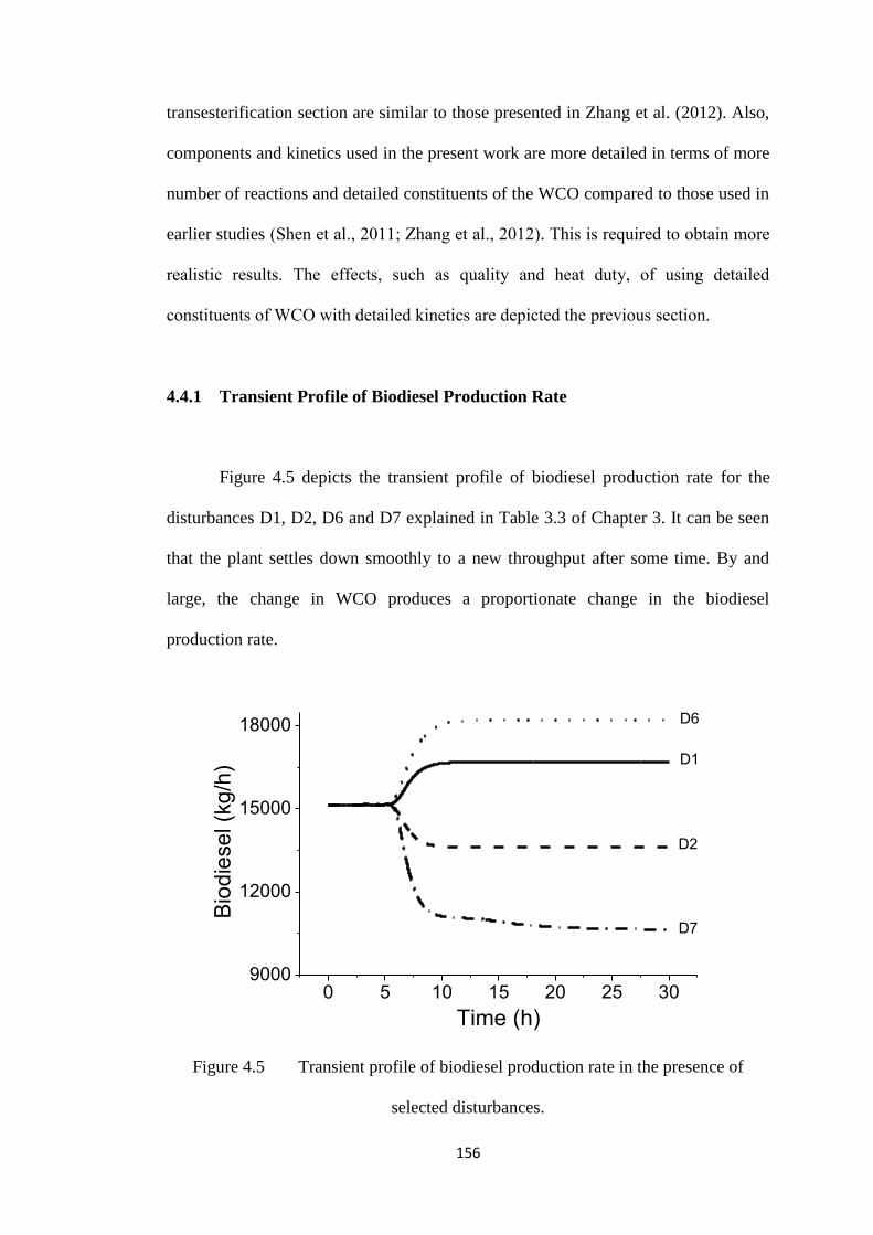
156
transesterification section are similar to those presented in Zhang et al. (2012). Also,
components and kinetics used in the present work are more detailed in terms of more
number of reactions and detailed constituents of the WCO compared to those used in
earlier studies (Shen et al., 2011; Zhang et al., 2012). This is required to obtain more
realistic results. The effects, such as quality and heat duty, of using detailed
constituents of WCO with detailed kinetics are depicted the previous section.
4.4.1 Transient Profile of Biodiesel Production Rate
Figure 4.5 depicts the transient profile of biodiesel production rate for the
disturbances D1, D2, D6 and D7 explained in Table 3.3 of Chapter 3. It can be seen
that the plant settles down smoothly to a new throughput after some time. By and
large, the change in WCO produces a proportionate change in the biodiesel
production rate.
0 5 10 15 20 25 309000
12000
15000
18000
D7
D2
D1
Time (h)
Bio
die
sel (k
g/h
)
D6
Figure 4.5 Transient profile of biodiesel production rate in the presence of
selected disturbances.
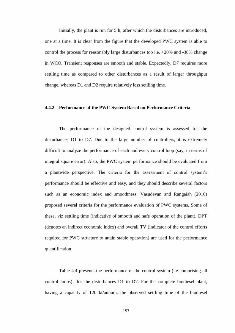
157
Initially, the plant is run for 5 h, after which the disturbances are introduced,
one at a time. It is clear from the figure that the developed PWC system is able to
control the process for reasonably large disturbances too i.e. +20% and -30% change
in WCO. Transient responses are smooth and stable. Expectedly, D7 requires more
settling time as compared to other disturbances as a result of larger throughput
change, whereas D1 and D2 require relatively less setlling time.
4.4.2 Performance of the PWC System Based on Performance Criteria
The performance of the designed control system is assessed for the
disturbances D1 to D7. Due to the large number of controllers, it is extremely
difficult to analyze the performance of each and every control loop (say, in terms of
integral square error). Also, the PWC system performance should be evaluated from
a plantwide perspective. The criteria for the assessment of control system’s
performance should be effective and easy, and they should describe several factors
such as an economic index and smoothness. Vasudevan and Rangaiah (2010)
proposed several criteria for the performance evaluation of PWC systems. Some of
these, viz settling time (indicative of smooth and safe operation of the plant), DPT
(denotes an indirect economic index) and overall TV (indicator of the control efforts
required for PWC structure to attain stable operation) are used for the performance
quantification.
Table 4.4 presents the performance of the control system (i.e comprising all
control loops) for the disturbances D1 to D7. For the complete biodiesel plant,
having a capacity of 120 kt/annum, the observed settling time of the biodiesel
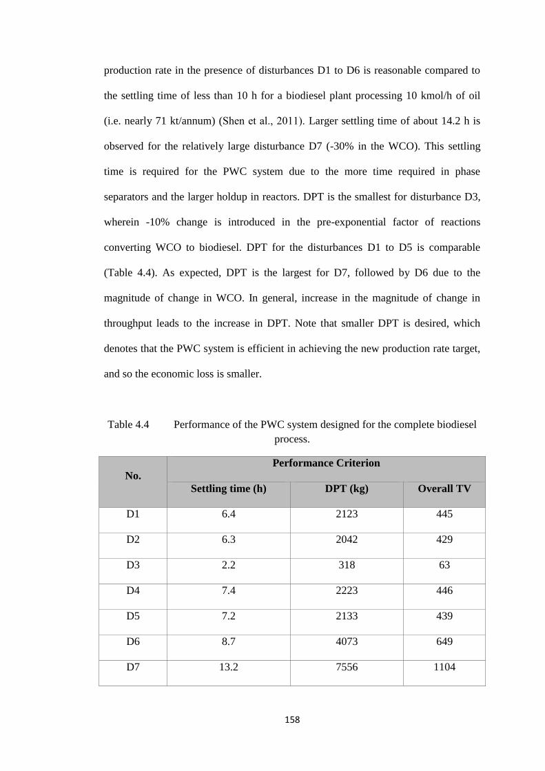
158
production rate in the presence of disturbances D1 to D6 is reasonable compared to
the settling time of less than 10 h for a biodiesel plant processing 10 kmol/h of oil
(i.e. nearly 71 kt/annum) (Shen et al., 2011). Larger settling time of about 14.2 h is
observed for the relatively large disturbance D7 (-30% in the WCO). This settling
time is required for the PWC system due to the more time required in phase
separators and the larger holdup in reactors. DPT is the smallest for disturbance D3,
wherein -10% change is introduced in the pre-exponential factor of reactions
converting WCO to biodiesel. DPT for the disturbances D1 to D5 is comparable
(Table 4.4). As expected, DPT is the largest for D7, followed by D6 due to the
magnitude of change in WCO. In general, increase in the magnitude of change in
throughput leads to the increase in DPT. Note that smaller DPT is desired, which
denotes that the PWC system is efficient in achieving the new production rate target,
and so the economic loss is smaller.
Table 4.4 Performance of the PWC system designed for the complete biodiesel
process.
No.
Performance Criterion
Settling time (h) DPT (kg) Overall TV
D1 6.4 2123 445
D2 6.3 2042 429
D3 2.2 318 63
D4 7.4 2223 446
D5 7.2 2133 439
D6 8.7 4073 649
D7 13.2 7556 1104
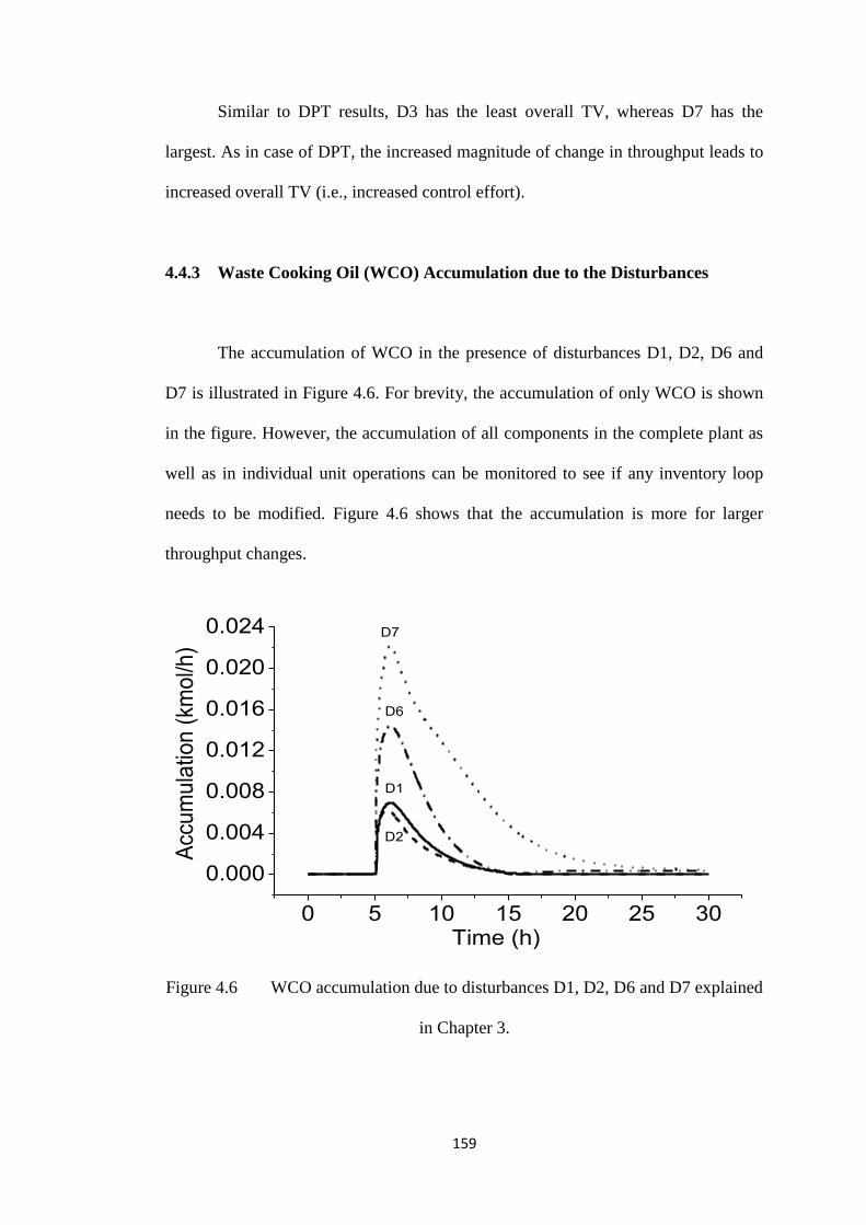
159
Similar to DPT results, D3 has the least overall TV, whereas D7 has the
largest. As in case of DPT, the increased magnitude of change in throughput leads to
increased overall TV (i.e., increased control effort).
4.4.3 Waste Cooking Oil (WCO) Accumulation due to the Disturbances
The accumulation of WCO in the presence of disturbances D1, D2, D6 and
D7 is illustrated in Figure 4.6. For brevity, the accumulation of only WCO is shown
in the figure. However, the accumulation of all components in the complete plant as
well as in individual unit operations can be monitored to see if any inventory loop
needs to be modified. Figure 4.6 shows that the accumulation is more for larger
throughput changes.
0 5 10 15 20 25 30
0.000
0.004
0.008
0.012
0.016
0.020
0.024
D2
D1
D6
D7
Acc
um
ula
tion
(km
ol/h
)
Time (h)
Figure 4.6 WCO accumulation due to disturbances D1, D2, D6 and D7 explained
in Chapter 3.
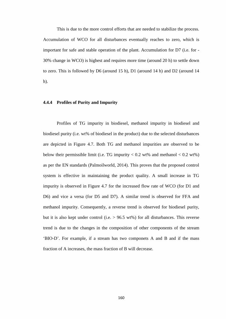
160
This is due to the more control efforts that are needed to stabilize the process.
Accumulation of WCO for all disturbances eventually reaches to zero, which is
important for safe and stable operation of the plant. Accumulation for D7 (i.e. for -
30% change in WCO) is highest and requires more time (around 20 h) to settle down
to zero. This is followed by D6 (around 15 h), D1 (around 14 h) and D2 (around 14
h).
4.4.4 Profiles of Purity and Impurity
Profiles of TG impurity in biodiesel, methanol impurity in biodiesel and
biodiesel purity (i.e. wt% of biodiesel in the product) due to the selected disturbances
are depicted in Figure 4.7. Both TG and methanol impurities are observed to be
below their permissible limit (i.e. TG impurity < 0.2 wt% and methanol < 0.2 wt%)
as per the EN standards (Palmoilworld, 2014). This proves that the proposed control
system is effective in maintaining the product quality. A small increase in TG
impurity is observed in Figure 4.7 for the increased flow rate of WCO (for D1 and
D6) and vice a versa (for D5 and D7). A similar trend is observed for FFA and
methanol impurity. Consequently, a reverse trend is observed for biodiesel purity,
but it is also kept under control (i.e. > 96.5 wt%) for all disturbances. This reverse
trend is due to the changes in the composition of other components of the stream
‘BIO-D’. For example, if a stream has two componets A and B and if the mass
fraction of A increases, the mass fraction of B will decrease.
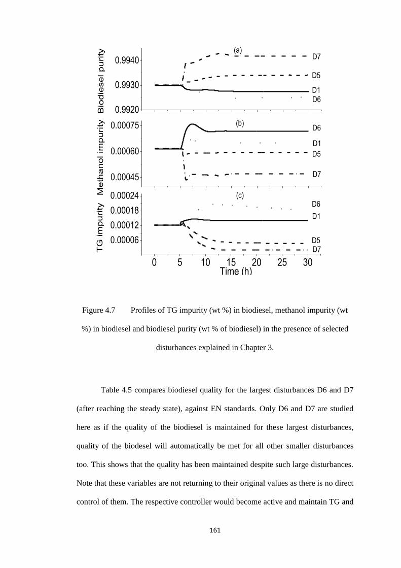
161
0.9920
0.9930
0.9940
0 5 10 15 20 25 30
0.00006
0.00012
0.00018
0.00024
0.00045
0.00060
0.00075
Bio
die
se
l p
uri
ty (a)
D6
D1
D5D7
D6
D6D1
D5
D7
TG
im
pu
rity
Time (h)
D7
D5
D1
(c)
(b)
Meth
an
ol im
pu
rity
Figure 4.7 Profiles of TG impurity (wt %) in biodiesel, methanol impurity (wt
%) in biodiesel and biodiesel purity (wt % of biodiesel) in the presence of selected
disturbances explained in Chapter 3.
Table 4.5 compares biodiesel quality for the largest disturbances D6 and D7
(after reaching the steady state), against EN standards. Only D6 and D7 are studied
here as if the quality of the biodiesel is maintained for these largest disturbances,
quality of the biodesel will automatically be met for all other smaller disturbances
too. This shows that the quality has been maintained despite such large disturbances.
Note that these variables are not returning to their original values as there is no direct
control of them. The respective controller would become active and maintain TG and
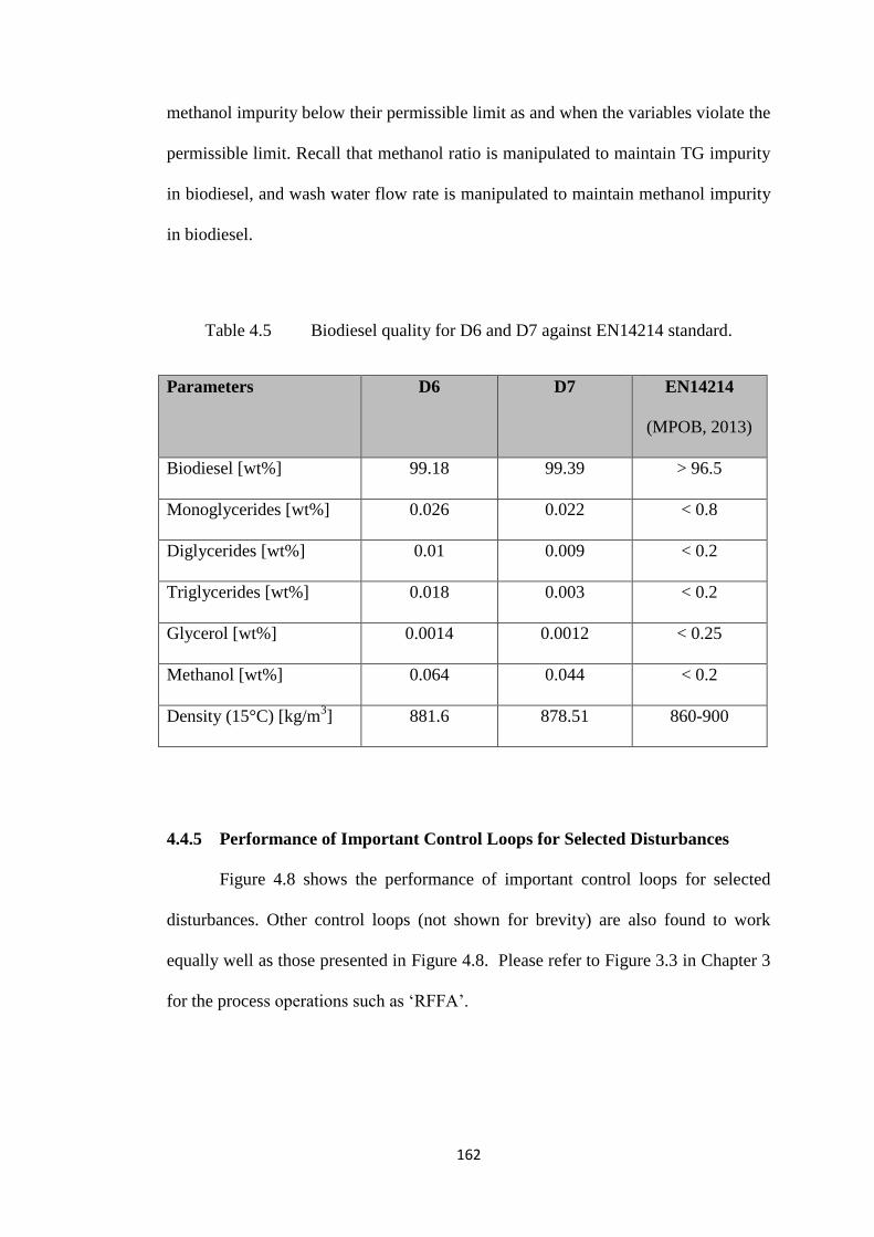
162
methanol impurity below their permissible limit as and when the variables violate the
permissible limit. Recall that methanol ratio is manipulated to maintain TG impurity
in biodiesel, and wash water flow rate is manipulated to maintain methanol impurity
in biodiesel.
Table 4.5 Biodiesel quality for D6 and D7 against EN14214 standard.
Parameters D6 D7 EN14214
(MPOB, 2013)
Biodiesel [wt%] 99.18 99.39 > 96.5
Monoglycerides [wt%] 0.026 0.022 < 0.8
Diglycerides [wt%] 0.01 0.009 < 0.2
Triglycerides [wt%] 0.018 0.003 < 0.2
Glycerol [wt%] 0.0014 0.0012 < 0.25
Methanol [wt%] 0.064 0.044 < 0.2
Density (15°C) [kg/m3] 881.6 878.51 860-900
4.4.5 Performance of Important Control Loops for Selected Disturbances
Figure 4.8 shows the performance of important control loops for selected
disturbances. Other control loops (not shown for brevity) are also found to work
equally well as those presented in Figure 4.8. Please refer to Figure 3.3 in Chapter 3
for the process operations such as ‘RFFA’.
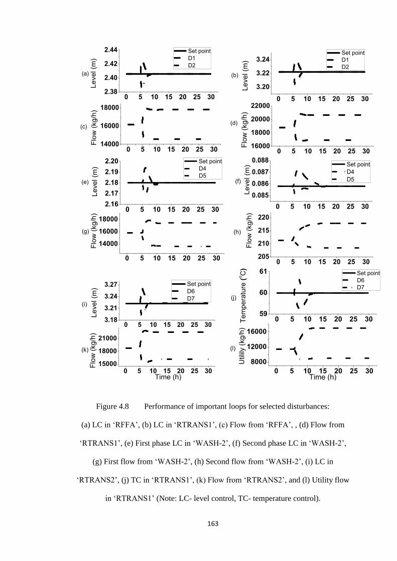
163
0 5 10 15 20 25 302.38
2.40
2.42
2.44
0 5 10 15 20 25 3014000
16000
18000
(c)
Set point
D1
D2
Le
ve
l (m
)
(a)
Flo
w (
kg
/h)
0 5 10 15 20 25 30
3.20
3.22
3.24
0 5 10 15 20 25 3016000
18000
20000
22000
(d)
Set point
D1
D2
Le
vel (m
)
(b)
Flo
w (
kg/h
)
0 5 10 15 20 25 302.16
2.17
2.18
2.19
2.20
0 5 10 15 20 25 30
14000
16000
18000
(g)
Le
ve
l (m
)
Set point
D4
D5(e)
Flo
w (
kg
/h)
0 5 10 15 20 25 30
0.085
0.086
0.087
0.088
0 5 10 15 20 25 30205
210
215
220
(h)
Le
ve
l (m
) Set point
D4
D5(f)
Flo
w (
kg
/h)
0 5 10 15 20 25 303.18
3.21
3.24
3.27
0 5 10 15 20 25 3015000
18000
21000
(k)
Set point
D6
D7
Le
ve
l (m
)
(i)
Time (h)
Flo
w (
kg/h
)
0 5 10 15 20 25 3059
60
61
0 5 10 15 20 25 30
8000
12000
16000
(l)
Te
mp
era
ture
(oC)
Set point
D6
D7
(j)
Utilil
y (
kg
/h)
Time (h)
Figure 4.8 Performance of important loops for selected disturbances:
(a) LC in ‘RFFA’, (b) LC in ‘RTRANS1’, (c) Flow from ‘RFFA’, , (d) Flow from
‘RTRANS1’, (e) First phase LC in ‘WASH-2’, (f) Second phase LC in ‘WASH-2’,
(g) First flow from ‘WASH-2’, (h) Second flow from ‘WASH-2’, (i) LC in
‘RTRANS2’, (j) TC in ‘RTRANS1’, (k) Flow from ‘RTRANS2’, and (l) Utility flow
in ‘RTRANS1’ (Note: LC- level control, TC- temperature control).
164
Due to the large number of control loops present in this PWC scheme,
individual control loops are not assessed in terms of conventional time domain
performance specification such as overshoot, rise time and integral error indices.
Instead, as discussed above, comprehensive PWC performance assessment criteria
are used. In any case, performance of important control loops in terms of overshoot
and rise time can be seen in Figure 4.8. As the control loops are able to maintain the
controlled variables at their respective set points for the disturbances tested, it can be
inferred that the control loops are properly paired and tuned. Settling time of the
control loops shown in Figure 4.8, including the level controllers in phase separators
and reactor, justifies the overall settling time of biodiesel product given in Table 4.4.
The observed settling time in the reactors is due to the larger holdup. Overall, control
loops in the developed PWC system are performing satisfactorily in the presence of
several disturbances.
4.5 Operator Training Simulator (OTS) for Process 1
The industrial processes are becoming extremely complex as a result of
intense energy and material integrations. Ayral and De Jonge (2013) estimated the
total annualized benefits from an OTS for a 100,000 bpd refinery to be 4.9 million
dollars. These show the importance of OTS in the process industry. Several scenarios
such as startup, interlock, equipment malfunctions, fire, pressure safety valve and
bursting disk in the biodiesel plant, are studied using the developed OTS in APD and
Aspen OTS Framework. Seborg et al. (2010) reported the typical failure rates of
selected process components in the year 1986. Failure frequency in a year of control
165
valve, valve positioner, transducer, pressure measurement, orifice plate and D/P
transmitter, magnetic flowmeter, thermocouple, mercury in a steel bulb, controller,
pressure switch, and gas-liquid chromatography is reported to be 0.6, 0.44, 0.49,
1.14, 1.73, 2.18, 0.52, 0.027, 0.29, 0.14 and 30.6, respectively. Therefore, scenarios
depicting the failure of process components should also be studied by operators as
such failure/malfunctions can cause the process operation to enter an unacceptable
region. These are presented and discussed from the perspective of operator training,
in the following sub-sections. In addition to above scenarios, OTS lets trainees tune
various PID controllers in real-time and increased time. It lets trainees try different
setpoints, change auto/manual modes, drive the PIDs unstable with aggressive/robust
tuning, and hence it lets trainees achieve proficiency in controller tuning thereby.
Typically, OTS consists of two major components i.e. dynamic simulation of the
process and control architecture. The focus of this work is on the development of the
former.
4.5.1 Startup of Distillation Column ‘FRAC-3’
Startup of unit operations is of vital importance for a quick, safe, smooth and
economical operation. Figure 4.9 presents the startup of FRAC3 (i.e., the distillation
column separating biodiesel from methanol in the transesterification section). To
illustrate the effect of different startup schemes that could be adopted by trainee
operators, two startup approaches, namely scheme ‘P1’ and ‘P2’ are tested. Table 4.6
shows the steps involved in these approaches, implemented by writing the task in
APD (see Appendix C for sample task for scheme P1).
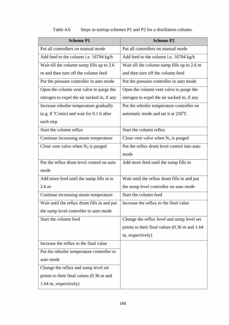
166
Table 4.6 Steps in startup schemes P1 and P2 for a distillation column.
Scheme P1 Scheme P2
Put all controllers on manual mode Put all controllers on manual mode
Add feed to the column i.e. 16794 kg/h Add feed to the column i.e. 16794 kg/h
Wait till the column sump fills up to 2.6
m and then turn off the column feed
Wait till the column sump fills up to 2.6 m
and then turn off the column feed
Put the pressure controller in auto mode Put the pressure controller in auto mode
Open the column vent valve to purge the
nitrogen to expel the air sucked in, if any
Open the column vent valve to purge the
nitrogen to expel the air sucked in, if any
Increase reboiler temperature gradually
(e.g. 8 oC/min) and wait for 0.1 h after
each step
Put the reboiler temperature controller on
automatic mode and set it at 250oC
Start the column reflux Start the column reflux
Continue increasing steam temperature Close vent valve when N2 is purged
Close vent valve when N2 is purged Put the reflux drum level control into auto
mode
Put the reflux drum level control on auto
mode
Add more feed until the sump fills in
Add more feed until the sump fills in to
2.6 m
Wait until the reflux drum fills in and put
the sump level controller on auto mode
Continue increasing steam temperature Start the column feed
Wait until the reflux drum fills in and put
the sump level controller to auto mode
Increase the reflux to the final value
Start the column feed Change the reflux level and sump level set
points to their final values (0.36 m and 1.64
m, respectively)
Increase the reflux to the final value
Put the reboiler temperature controller to
auto mode
Change the reflux and sump level set
points to their final values (0.36 m and
1.64 m, respectively)
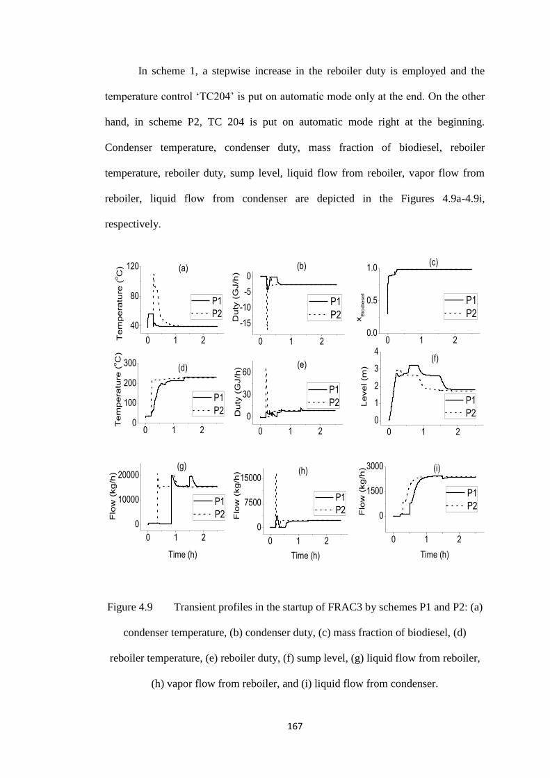
167
In scheme 1, a stepwise increase in the reboiler duty is employed and the
temperature control ‘TC204’ is put on automatic mode only at the end. On the other
hand, in scheme P2, TC 204 is put on automatic mode right at the beginning.
Condenser temperature, condenser duty, mass fraction of biodiesel, reboiler
temperature, reboiler duty, sump level, liquid flow from reboiler, vapor flow from
reboiler, liquid flow from condenser are depicted in the Figures 4.9a-4.9i,
respectively.
0 1 2
40
80
120
0 1 2
-15
-10
-5
0
0 1 20
100
200
300
0 1 2
0
30
60
0 1 2
0
10000
20000
0 1 2
0
7500
15000
0 1 20.0
0.5
1.0
0 1 2
0
1
2
3
4
0 1 2
0
1500
3000
Tem
pera
ture
(oC
)
P1
P2
(a)
Duty
(G
J/h
)
P1
P2
(b)
Tem
pera
ture
(oC
)
P1
P2
(d)
Duty
(G
J/h
)
P1
P2
(e)
Flo
w (
kg/h
)
Time (h)
P1
P2
(g)
Flo
w (
kg/h
)
Time (h)
P1
P2
(h) (i)
(f)x
Bio
die
sel
P1
P2
(c)
Level (m
)
P1
P2
Flo
w (
kg/h
)
Time (h)
P1
P2
Figure 4.9 Transient profiles in the startup of FRAC3 by schemes P1 and P2: (a)
condenser temperature, (b) condenser duty, (c) mass fraction of biodiesel, (d)
reboiler temperature, (e) reboiler duty, (f) sump level, (g) liquid flow from reboiler,
(h) vapor flow from reboiler, and (i) liquid flow from condenser.
168
As it can be noticed from the plots, P1 shows a smooth and gradual variation
in these variables as opposed to that for P2, where spikes are observed in condenser
temperature (Figure 4.9a), condenser duty (Figure 4.9b), reboiler duty (Figure 4.9e)
and vapor flow from reboiler (Figure 4.9h). Behaviour of some of the variables in P2
may be unachievable and potentially dangerous in real practice due to the sudden
increase in temperature and vapor flow in the column arising from putting TC 204 on
automatic mode right at the beginning when error between process variable and set
point is large. This also leads to large bumps in the process variables, as depicted in
Figure 4.9. However, the settling time observed for P2 (for example, close to 1 h for
sump level) is lesser that that found for P1 (close to 1.8 h for sump level). Note that
the startup time also depends on the time a trainee waits after each step. It is clear
from the figure that a stepwise increase is desirable. However, to optimize the step
size, more scenarios can be tested. This is only feasible on an OTS as doing it in a
real plant will be very expensive and hence unfavourable.
4.5.2 Interlock in Distillation Column FRAC-3
Interlock is a mechanism that is used to help prevent any harm to the operator
or any damage to the system itleft by taking the action (e.g. stopping the equipement
or utility flow) when tripped. Typically, a chemical plant has several interlocks (i.e.
safety interlock or process interlock) in place. One such interlock has been simulated
for FRAC3, where the utility trips when the reboiler temperature breaches 250oC as
biodiesel decomposes above 250oC. The feed flow drops to 25% (from 16794 kg/h to
4198.5 kg/h) at 2 h. Reboiler temperature shoots up to 250oC from 230
oC.
Consequently, the utility trips and temperature falls. This is simulated by writing the
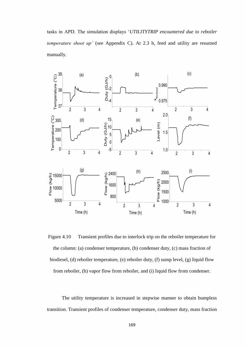
169
tasks in APD. The simulation displays ‘UTILITYTRIP encountered due to reboiler
temperature shoot up’ (see Appendix C). At 2.3 h, feed and utility are resumed
manually.
2 3 437
38
39
2 3 4
-4
-2
0
2 3 40
100
200
300
2 3 4-5
0
5
10
15
2 3 45000
10000
15000
2 3 4
800
1600
2400
2 3 4
0.975
0.990
2 3 41.0
1.5
2.0
2 3 41000
1500
2000
2500
Tem
pera
ture
(oC
) (a)
Duty
(G
J/h
)
(b)
Tem
pera
ture
(oC
)
(d)
Duty
(G
J/h
)
(e)
Flo
w (
kg/h
)
Time (h)
(g)
Flo
w (
kg/h
)
Time (h)
(h) (i)
(f)
xB
iodie
sel
(c)
Level (m
)F
low
(kg/h
)
Time (h)
Figure 4.10 Transient profiles due to interlock trip on the reboiler temperature for
the column: (a) condenser temperature, (b) condenser duty, (c) mass fraction of
biodiesel, (d) reboiler temperature, (e) reboiler duty, (f) sump level, (g) liquid flow
from reboiler, (h) vapor flow from reboiler, and (i) liquid flow from condenser.
The utility temperature is increased in stepwise manner to obtain bumpless
transition. Transient profiles of condenser temperature, condenser duty, mass fraction
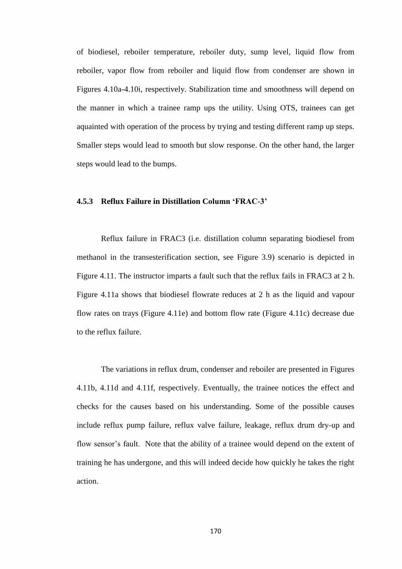
170
of biodiesel, reboiler temperature, reboiler duty, sump level, liquid flow from
reboiler, vapor flow from reboiler and liquid flow from condenser are shown in
Figures 4.10a-4.10i, respectively. Stabilization time and smoothness will depend on
the manner in which a trainee ramp ups the utility. Using OTS, trainees can get
aquainted with operation of the process by trying and testing different ramp up steps.
Smaller steps would lead to smooth but slow response. On the other hand, the larger
steps would lead to the bumps.
4.5.3 Reflux Failure in Distillation Column ‘FRAC-3’
Reflux failure in FRAC3 (i.e. distillation column separating biodiesel from
methanol in the transesterification section, see Figure 3.9) scenario is depicted in
Figure 4.11. The instructor imparts a fault such that the reflux fails in FRAC3 at 2 h.
Figure 4.11a shows that biodiesel flowrate reduces at 2 h as the liquid and vapour
flow rates on trays (Figure 4.11e) and bottom flow rate (Figure 4.11c) decrease due
to the reflux failure.
The variations in reflux drum, condenser and reboiler are presented in Figures
4.11b, 4.11d and 4.11f, respectively. Eventually, the trainee notices the effect and
checks for the causes based on his understanding. Some of the possible causes
include reflux pump failure, reflux valve failure, leakage, reflux drum dry-up and
flow sensor’s fault. Note that the ability of a trainee would depend on the extent of
training he has undergone, and this will indeed decide how quickly he takes the right
action.
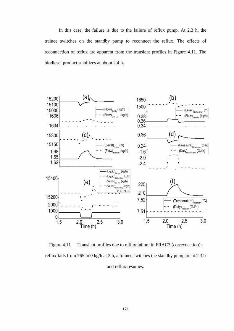
171
In this case, the failure is due to the failure of reflux pump. At 2.3 h, the
trainee switches on the standby pump to reconnect the reflux. The effects of
reconnection of reflux are apparent from the transient profiles in Figure 4.11. The
biodiesel product stabilizes at about 2.4 h.
1634
1636150001510015200
1.621.651.68
15150
15300
-2.4
-2.0
-1.60.24
0.36
1.5 2.0 2.5 3.00
1000
2000
15200
15400
1.5 2.0 2.5 3.0
7.51
7.52
210
225
0.340.360.38
1500
1650 (b)(a)
(Flow)BIO-D
(kg/h)
(Flow)GLY-OUT
(kg/h)
(d)(c)
(Level)Sump
(m)
(Flow)Bottoms
(kg/h)
(Pressure)Condenser
(bar)
(Duty)Condenser
(GJ/h)
Time (h)
(Liquid)top tray
(kg/h)
(Liquid)bottom tray
(kg/h)
(Vapor)top tray
(kg/h)
(Vapor)bottom tray
(kg/h)
in FRAC-3
(f)(e)
Time (h)
(Temperature)Reboiler
(oC)
(Duty)Reboiler
(GJ/h)
(Level)Reflux drum
(m)
(Flow)Distillate
(kg/h)
Figure 4.11 Transient profiles due to reflux failure in FRAC3 (correct action):
reflux fails from 765 to 0 kg/h at 2 h, a trainee switches the standby pump on at 2.3 h
and reflux resumes.
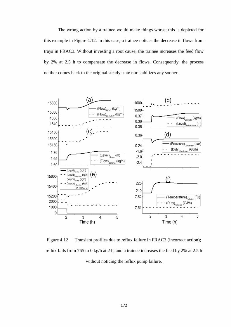
172
The wrong action by a trainee would make things worse; this is depicted for
this example in Figure 4.12. In this case, a trainee notices the decrease in flows from
trays in FRAC3. Without investing a root cause, the trainee increases the feed flow
by 2% at 2.5 h to compensate the decrease in flows. Consequently, the process
neither comes back to the original steady state nor stabilizes any sooner.
1640
1660
15000
15300
1.60
1.65
1.70
15150
15300
15450
-2.4
-2.0
-1.6
0.24
0.36
2 3 4 50
1000
2000
15200
15400
15600
2 3 4 5
7.51
7.52
210
225
0.35
0.36
0.37
1500
1600(b)(a)
(Flow)BIO-D
(kg/h)
(Flow)GLY-OUT
(kg/h)
(d)(c)
(Level)Sump
(m)
(Flow)Bottoms
(kg/h)
(Pressure)Condenser
(bar)
(Duty)Condenser
(GJ/h)
Time (h)
(Liquid)top tray
(kg/h)
(Liquid)bottom tray
(kg/h)
(Vapor)top tray
(kg/h)
(Vapor)bottom tray
(kg/h)
in FRAC-3
(f)(e)
Time (h)
(Temperature)Reboiler
(oC)
(Duty)Reboiler
(GJ/h)
(Flow)Distillate
(kg/h)
(Level)Reflux drum
(m)
Figure 4.12 Transient profiles due to reflux failure in FRAC3 (incorrect action);
reflux fails from 765 to 0 kg/h at 2 h, and a trainee increases the feed by 2% at 2.5 h
without noticing the reflux pump failure.
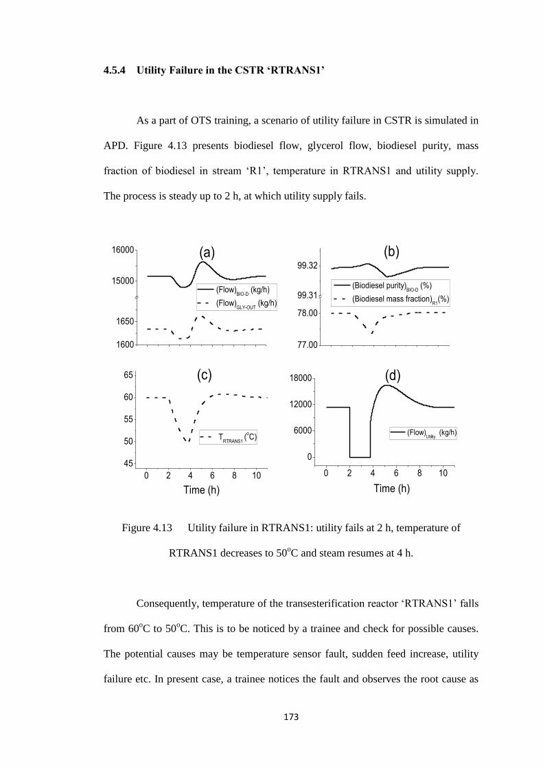
173
4.5.4 Utility Failure in the CSTR ‘RTRANS1’
As a part of OTS training, a scenario of utility failure in CSTR is simulated in
APD. Figure 4.13 presents biodiesel flow, glycerol flow, biodiesel purity, mass
fraction of biodiesel in stream ‘R1’, temperature in RTRANS1 and utility supply.
The process is steady up to 2 h, at which utility supply fails.
1600
1650
15000
16000
77.00
78.00
99.31
99.32
0 2 4 6 8 10
45
50
55
60
65
0 2 4 6 8 10
0
6000
12000
18000 (d)
(b)
(c)
(Flow)BIO-D
(kg/h)
(Flow)GLY-OUT
(kg/h)
(Biodiesel purity)BIO-D
(%)
(Biodiesel mass fraction)R1
(%)
(a)
Time (h)
TRTRANS1
(oC)
Time (h)
(Flow)Utility
(kg/h)
Figure 4.13 Utility failure in RTRANS1: utility fails at 2 h, temperature of
RTRANS1 decreases to 50oC and steam resumes at 4 h.
Consequently, temperature of the transesterification reactor ‘RTRANS1’ falls
from 60oC to 50
oC. This is to be noticed by a trainee and check for possible causes.
The potential causes may be temperature sensor fault, sudden feed increase, utility
failure etc. In present case, a trainee notices the fault and observes the root cause as
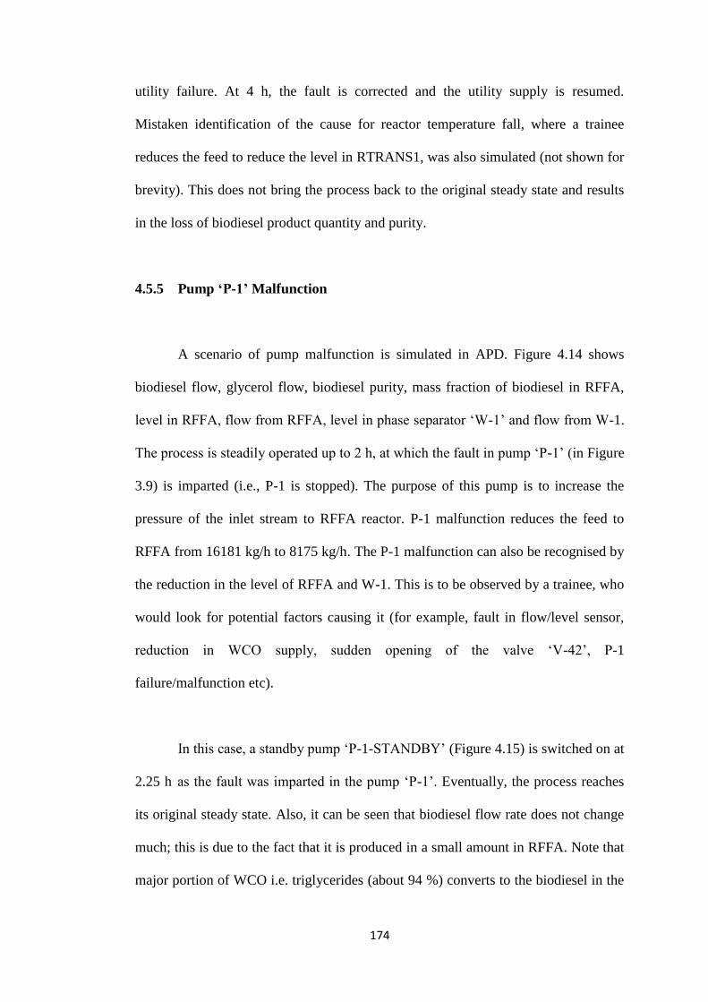
174
utility failure. At 4 h, the fault is corrected and the utility supply is resumed.
Mistaken identification of the cause for reactor temperature fall, where a trainee
reduces the feed to reduce the level in RTRANS1, was also simulated (not shown for
brevity). This does not bring the process back to the original steady state and results
in the loss of biodiesel product quantity and purity.
4.5.5 Pump ‘P-1’ Malfunction
A scenario of pump malfunction is simulated in APD. Figure 4.14 shows
biodiesel flow, glycerol flow, biodiesel purity, mass fraction of biodiesel in RFFA,
level in RFFA, flow from RFFA, level in phase separator ‘W-1’ and flow from W-1.
The process is steadily operated up to 2 h, at which the fault in pump ‘P-1’ (in Figure
3.9) is imparted (i.e., P-1 is stopped). The purpose of this pump is to increase the
pressure of the inlet stream to RFFA reactor. P-1 malfunction reduces the feed to
RFFA from 16181 kg/h to 8175 kg/h. The P-1 malfunction can also be recognised by
the reduction in the level of RFFA and W-1. This is to be observed by a trainee, who
would look for potential factors causing it (for example, fault in flow/level sensor,
reduction in WCO supply, sudden opening of the valve ‘V-42’, P-1
failure/malfunction etc).
In this case, a standby pump ‘P-1-STANDBY’ (Figure 4.15) is switched on at
2.25 h as the fault was imparted in the pump ‘P-1’. Eventually, the process reaches
its original steady state. Also, it can be seen that biodiesel flow rate does not change
much; this is due to the fact that it is produced in a small amount in RFFA. Note that
major portion of WCO i.e. triglycerides (about 94 %) converts to the biodiesel in the
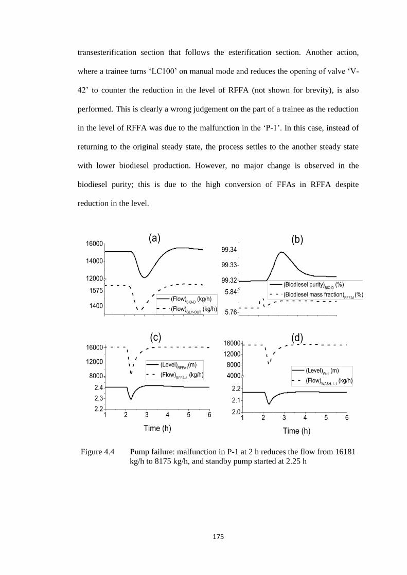
175
transesterification section that follows the esterification section. Another action,
where a trainee turns ‘LC100’ on manual mode and reduces the opening of valve ‘V-
42’ to counter the reduction in the level of RFFA (not shown for brevity), is also
performed. This is clearly a wrong judgement on the part of a trainee as the reduction
in the level of RFFA was due to the malfunction in the ‘P-1’. In this case, instead of
returning to the original steady state, the process settles to the another steady state
with lower biodiesel production. However, no major change is observed in the
biodiesel purity; this is due to the high conversion of FFAs in RFFA despite
reduction in the level.
1400
1575
12000
14000
16000
5.76
5.84
99.32
99.33
99.34
1 2 3 4 5 62.0
2.1
2.2
4000
8000
12000
16000
1 2 3 4 5 62.2
2.3
2.4
8000
12000
16000
(d)
(b)
(c)
(Flow)BIO-D
(kg/h)
(Flow)GLY-OUT
(kg/h)
(Biodiesel purity)BIO-D
(%)
(Biodiesel mass fraction)RFFA1
(%)
(a)
Time (h)
(Level)W-1
(m)
(Flow)WASH-1-1
(kg/h)
Time (h)
(Level)RFFA1
(m)
(Flow)RFFA-1
(kg/h)
Figure 4.4 Pump failure: malfunction in P-1 at 2 h reduces the flow from 16181
kg/h to 8175 kg/h, and standby pump started at 2.25 h
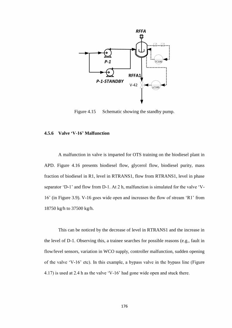
176
Figure 4.15 Schematic showing the standby pump.
4.5.6 Valve ‘V-16’ Malfunction
A malfunction in valve is imparted for OTS training on the biodiesel plant in
APD. Figure 4.16 presents biodiesel flow, glycerol flow, biodiesel purity, mass
fraction of biodiesel in R1, level in RTRANS1, flow from RTRANS1, level in phase
separator ‘D-1’ and flow from D-1. At 2 h, malfunction is simulated for the valve ‘V-
16’ (in Figure 3.9). V-16 goes wide open and increases the flow of stream ‘R1’ from
18750 kg/h to 37500 kg/h.
This can be noticed by the decrease of level in RTRANS1 and the increase in
the level of D-1. Observing this, a trainee searches for possible reasons (e.g., fault in
flow/level sensors, variation in WCO supply, controller malfunction, sudden opening
of the valve ‘V-16’ etc). In this example, a bypass valve in the bypass line (Figure
4.17) is used at 2.4 h as the valve ‘V-16’ had gone wide open and stuck there.
TC100
LC100
P-1
RFFA
V-42
RFFA1P-1-STANDBY
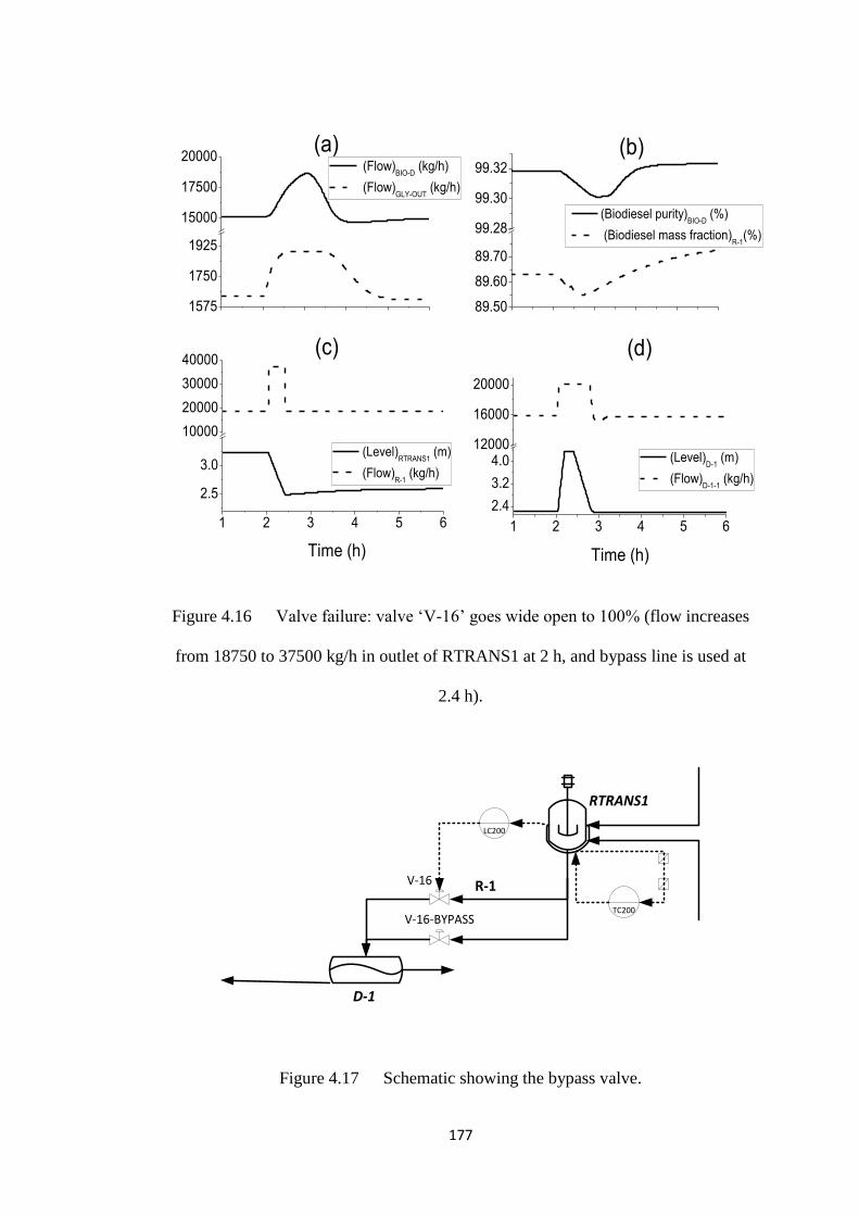
177
1575
1750
1925
15000
17500
20000
89.50
89.60
89.70
99.28
99.30
99.32
1 2 3 4 5 6
2.5
3.0
10000
20000
30000
40000
1 2 3 4 5 6
2.4
3.2
4.012000
16000
20000
(d)
(b)
(c)
(Flow)BIO-D
(kg/h)
(Flow)GLY-OUT
(kg/h)
(Biodiesel purity)BIO-D
(%)
(Biodiesel mass fraction)R-1
(%)
(a)
Time (h)
(Level)RTRANS1
(m)
(Flow)R-1
(kg/h)
Time (h)
(Level)D-1
(m)
(Flow)D-1-1
(kg/h)
Figure 4.16 Valve failure: valve ‘V-16’ goes wide open to 100% (flow increases
from 18750 to 37500 kg/h in outlet of RTRANS1 at 2 h, and bypass line is used at
2.4 h).
Figure 4.17 Schematic showing the bypass valve.
LC200
TC200
RTRANS1
D-1
R-1V-16
V-16-BYPASS
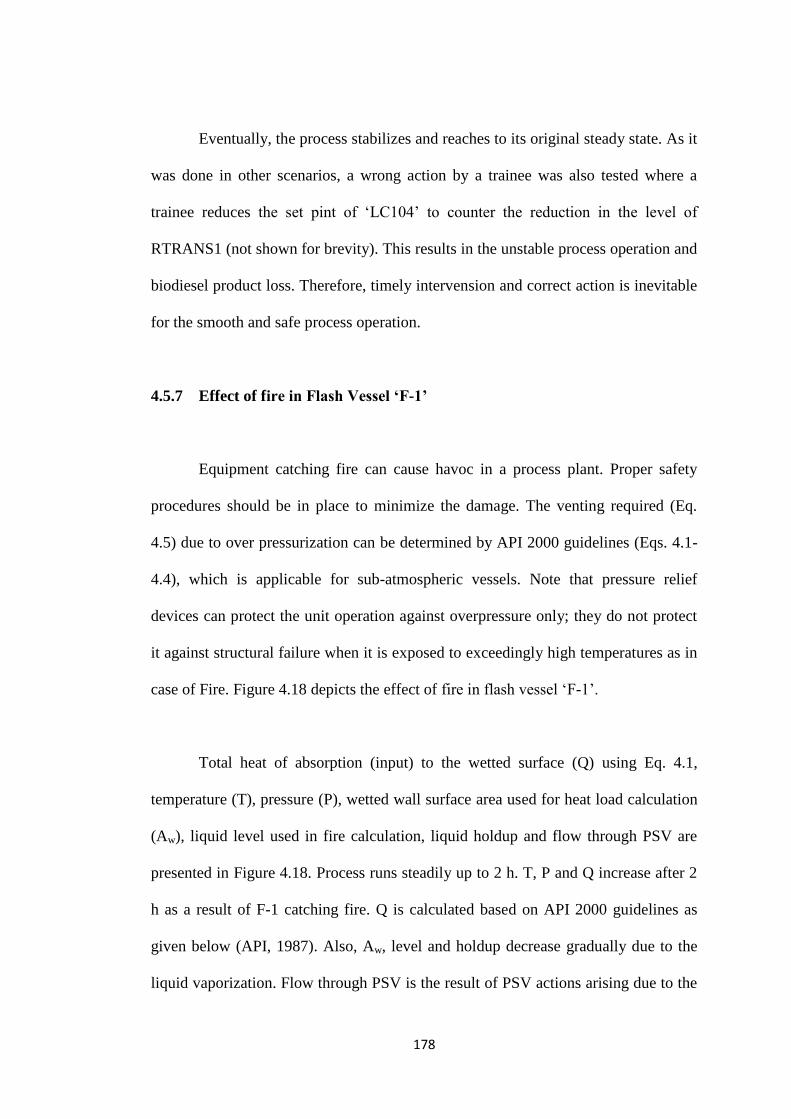
178
Eventually, the process stabilizes and reaches to its original steady state. As it
was done in other scenarios, a wrong action by a trainee was also tested where a
trainee reduces the set pint of ‘LC104’ to counter the reduction in the level of
RTRANS1 (not shown for brevity). This results in the unstable process operation and
biodiesel product loss. Therefore, timely intervension and correct action is inevitable
for the smooth and safe process operation.
4.5.7 Effect of fire in Flash Vessel ‘F-1’
Equipment catching fire can cause havoc in a process plant. Proper safety
procedures should be in place to minimize the damage. The venting required (Eq.
4.5) due to over pressurization can be determined by API 2000 guidelines (Eqs. 4.1-
4.4), which is applicable for sub-atmospheric vessels. Note that pressure relief
devices can protect the unit operation against overpressure only; they do not protect
it against structural failure when it is exposed to exceedingly high temperatures as in
case of Fire. Figure 4.18 depicts the effect of fire in flash vessel ‘F-1’.
Total heat of absorption (input) to the wetted surface (Q) using Eq. 4.1,
temperature (T), pressure (P), wetted wall surface area used for heat load calculation
(Aw), liquid level used in fire calculation, liquid holdup and flow through PSV are
presented in Figure 4.18. Process runs steadily up to 2 h. T, P and Q increase after 2
h as a result of F-1 catching fire. Q is calculated based on API 2000 guidelines as
given below (API, 1987). Also, Aw, level and holdup decrease gradually due to the
liquid vaporization. Flow through PSV is the result of PSV actions arising due to the
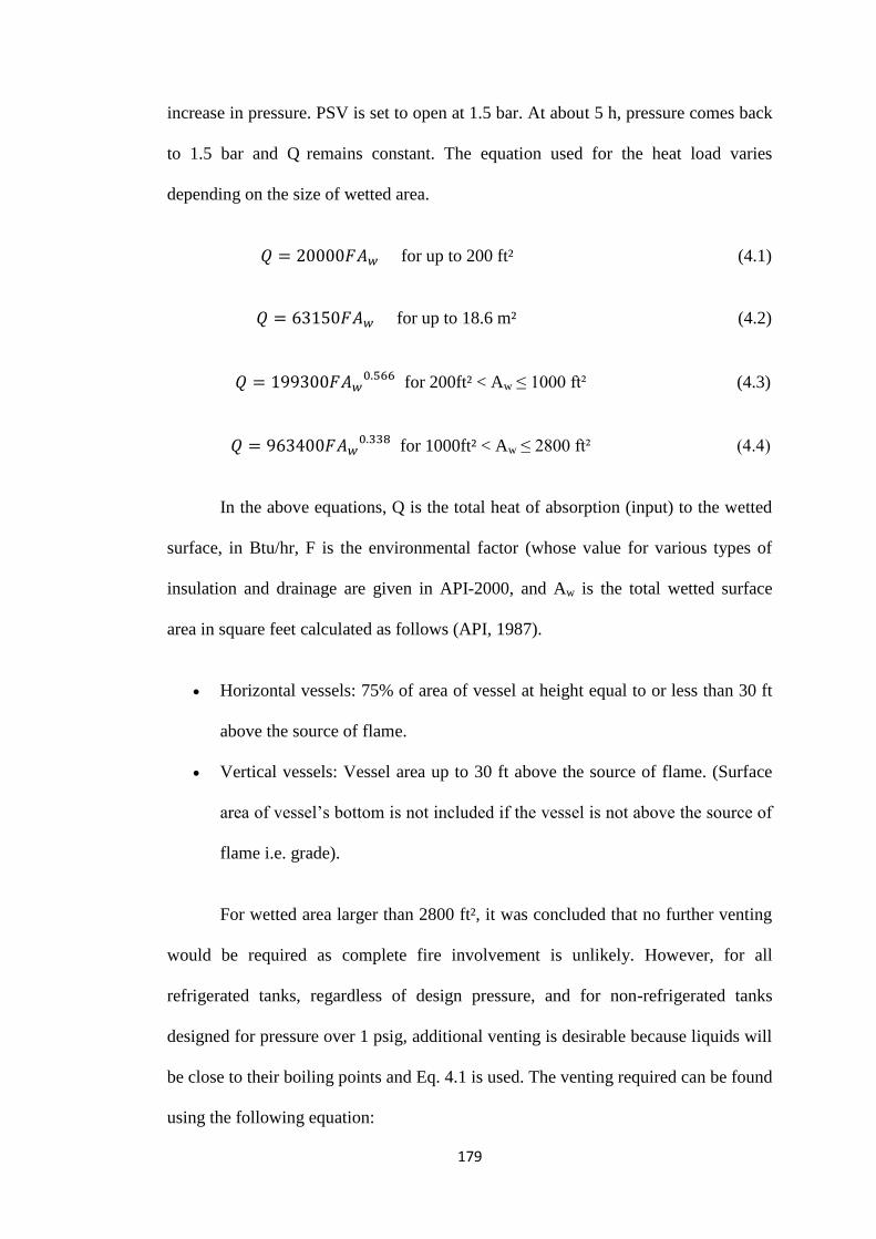
179
increase in pressure. PSV is set to open at 1.5 bar. At about 5 h, pressure comes back
to 1.5 bar and Q remains constant. The equation used for the heat load varies
depending on the size of wetted area.
𝑄 = 20000𝐹𝐴𝑤 for up to 200 ft² (4.1)
𝑄 = 63150𝐹𝐴𝑤 for up to 18.6 m² (4.2)
𝑄 = 199300𝐹𝐴𝑤0.566
for 200ft² < Aw ≤ 1000 ft² (4.3)
𝑄 = 963400𝐹𝐴𝑤0.338
for 1000ft² < Aw ≤ 2800 ft² (4.4)
In the above equations, Q is the total heat of absorption (input) to the wetted
surface, in Btu/hr, F is the environmental factor (whose value for various types of
insulation and drainage are given in API-2000, and Aw is the total wetted surface
area in square feet calculated as follows (API, 1987).
Horizontal vessels: 75% of area of vessel at height equal to or less than 30 ft
above the source of flame.
Vertical vessels: Vessel area up to 30 ft above the source of flame. (Surface
area of vessel’s bottom is not included if the vessel is not above the source of
flame i.e. grade).
For wetted area larger than 2800 ft², it was concluded that no further venting
would be required as complete fire involvement is unlikely. However, for all
refrigerated tanks, regardless of design pressure, and for non-refrigerated tanks
designed for pressure over 1 psig, additional venting is desirable because liquids will
be close to their boiling points and Eq. 4.1 is used. The venting required can be found
using the following equation:
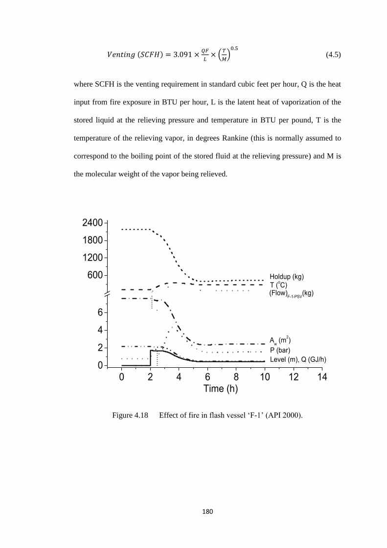
180
𝑉𝑒𝑛𝑡𝑖𝑛𝑔 (𝑆𝐶𝐹𝐻) = 3.091 ×𝑄𝐹
𝐿× (
𝑇
𝑀)
0.5
(4.5)
where SCFH is the venting requirement in standard cubic feet per hour, Q is the heat
input from fire exposure in BTU per hour, L is the latent heat of vaporization of the
stored liquid at the relieving pressure and temperature in BTU per pound, T is the
temperature of the relieving vapor, in degrees Rankine (this is normally assumed to
correspond to the boiling point of the stored fluid at the relieving pressure) and M is
the molecular weight of the vapor being relieved.
0 2 4 6 8 10 12 140
2
4
6
600
1200
1800
2400
Holdup (kg)
T (oC)
(Flow)F-1-PSV
(kg)
Aw (m
2)
P (bar)
Level (m), Q (GJ/h)
Time (h)
Figure 4.18 Effect of fire in flash vessel ‘F-1’ (API 2000).
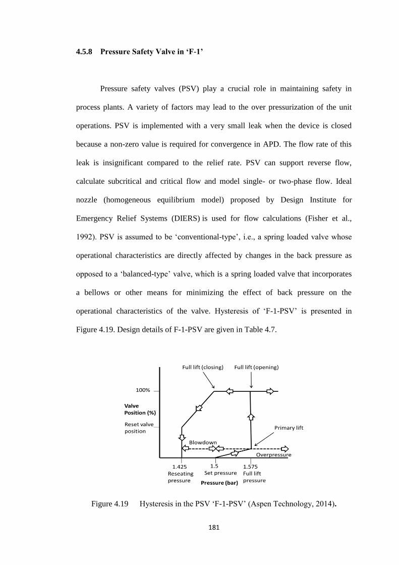
181
4.5.8 Pressure Safety Valve in ‘F-1’
Pressure safety valves (PSV) play a crucial role in maintaining safety in
process plants. A variety of factors may lead to the over pressurization of the unit
operations. PSV is implemented with a very small leak when the device is closed
because a non-zero value is required for convergence in APD. The flow rate of this
leak is insignificant compared to the relief rate. PSV can support reverse flow,
calculate subcritical and critical flow and model single- or two-phase flow. Ideal
nozzle (homogeneous equilibrium model) proposed by Design Institute for
Emergency Relief Systems (DIERS) is used for flow calculations (Fisher et al.,
1992). PSV is assumed to be ‘conventional-type’, i.e., a spring loaded valve whose
operational characteristics are directly affected by changes in the back pressure as
opposed to a ‘balanced-type’ valve, which is a spring loaded valve that incorporates
a bellows or other means for minimizing the effect of back pressure on the
operational characteristics of the valve. Hysteresis of ‘F-1-PSV’ is presented in
Figure 4.19. Design details of F-1-PSV are given in Table 4.7.
Figure 4.19 Hysteresis in the PSV ‘F-1-PSV’ (Aspen Technology, 2014).
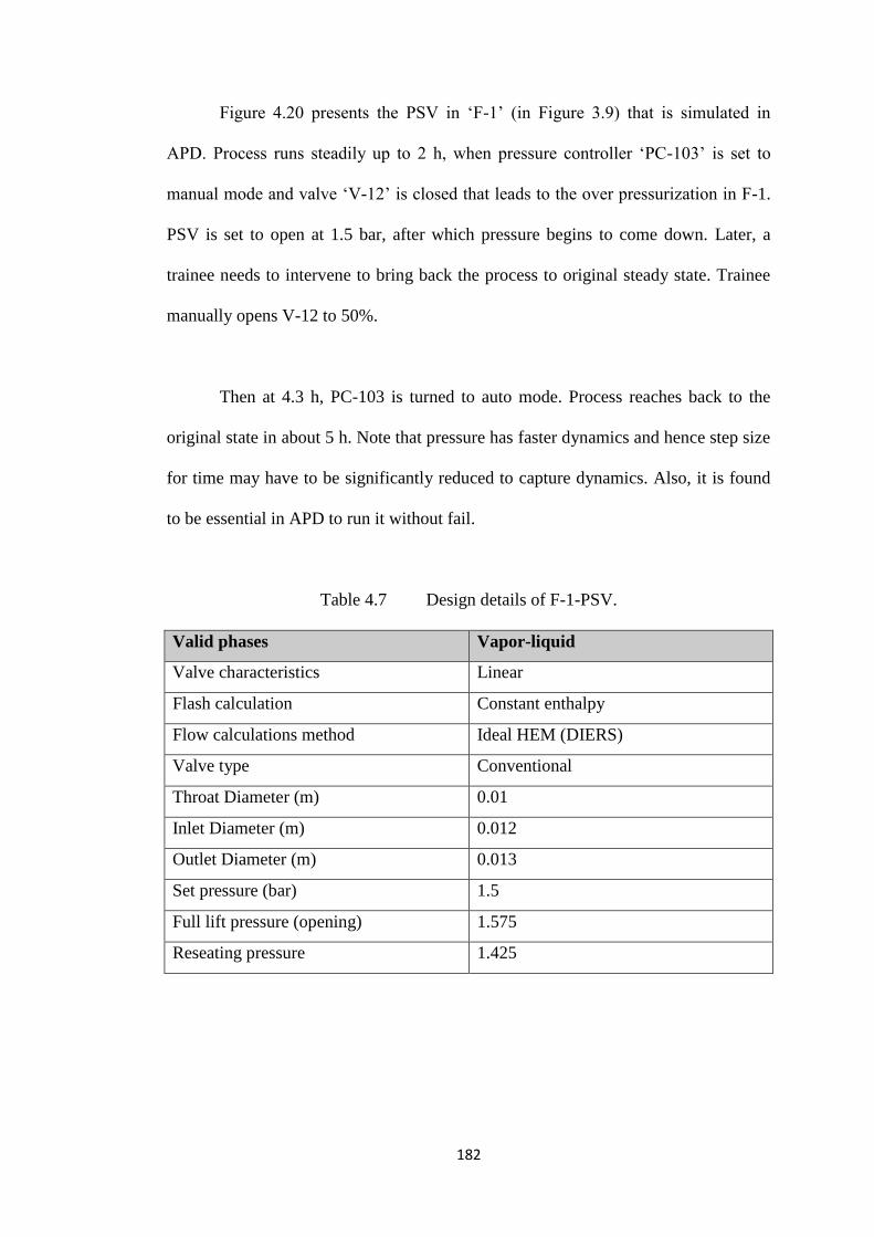
182
Figure 4.20 presents the PSV in ‘F-1’ (in Figure 3.9) that is simulated in
APD. Process runs steadily up to 2 h, when pressure controller ‘PC-103’ is set to
manual mode and valve ‘V-12’ is closed that leads to the over pressurization in F-1.
PSV is set to open at 1.5 bar, after which pressure begins to come down. Later, a
trainee needs to intervene to bring back the process to original steady state. Trainee
manually opens V-12 to 50%.
Then at 4.3 h, PC-103 is turned to auto mode. Process reaches back to the
original state in about 5 h. Note that pressure has faster dynamics and hence step size
for time may have to be significantly reduced to capture dynamics. Also, it is found
to be essential in APD to run it without fail.
Table 4.7 Design details of F-1-PSV.
Valid phases Vapor-liquid
Valve characteristics Linear
Flash calculation Constant enthalpy
Flow calculations method Ideal HEM (DIERS)
Valve type Conventional
Throat Diameter (m) 0.01
Inlet Diameter (m) 0.012
Outlet Diameter (m) 0.013
Set pressure (bar) 1.5
Full lift pressure (opening) 1.575
Reseating pressure 1.425
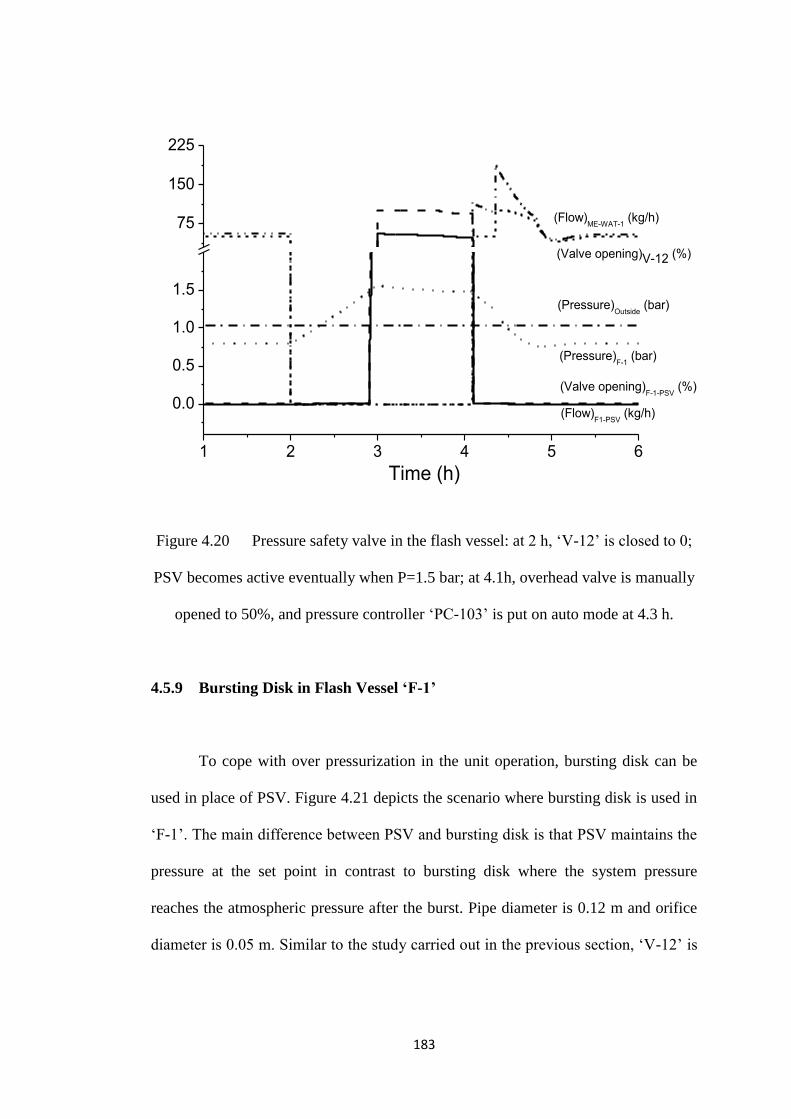
183
1 2 3 4 5 6
0.0
0.5
1.0
1.5
75
150
225
(Flow)F1-PSV
(kg/h)
(Valve opening)F-1-PSV
(%)
(Pressure)F-1
(bar)
(Pressure)Outside
(bar)
(Valve opening)V-12 (%)
(Flow)ME-WAT-1
(kg/h)
Time (h)
Figure 4.20 Pressure safety valve in the flash vessel: at 2 h, ‘V-12’ is closed to 0;
PSV becomes active eventually when P=1.5 bar; at 4.1h, overhead valve is manually
opened to 50%, and pressure controller ‘PC-103’ is put on auto mode at 4.3 h.
4.5.9 Bursting Disk in Flash Vessel ‘F-1’
To cope with over pressurization in the unit operation, bursting disk can be
used in place of PSV. Figure 4.21 depicts the scenario where bursting disk is used in
‘F-1’. The main difference between PSV and bursting disk is that PSV maintains the
pressure at the set point in contrast to bursting disk where the system pressure
reaches the atmospheric pressure after the burst. Pipe diameter is 0.12 m and orifice
diameter is 0.05 m. Similar to the study carried out in the previous section, ‘V-12’ is
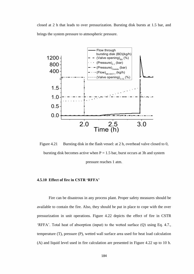
184
closed at 2 h that leads to over pressurization. Bursting disk bursts at 1.5 bar, and
brings the system pressure to atmospheric pressure.
2.0 2.5 3.0
0.0
0.5
1.0
1.5
400
800
1200
Time (h)
Flow through
bursting disk (BD)(kg/h)
(Valve opening)BD
(%)
(Pressure)F-1
(bar)
(Pressure)Outside
(bar)
(Flow)ME-WAT-1
(kg/h)
(Valve opening)V-12
(%)
Figure 4.21 Bursting disk in the flash vessel: at 2 h, overhead valve closed to 0,
bursting disk becomes active when P = 1.5 bar, burst occurs at 3h and system
pressure reaches 1 atm.
4.5.10 Effect of fire in CSTR ‘RFFA’
Fire can be disastrous in any process plant. Proper safety measures should be
available to contain the fire. Also, they should be put in place to cope with the over
pressurization in unit operations. Figure 4.22 depicts the effect of fire in CSTR
‘RFFA’. Total heat of absorption (input) to the wetted surface (Q) using Eq. 4.7.,
temperature (T), pressure (P), wetted wall surface area used for heat load calculation
(A) and liquid level used in fire calculation are presented in Figure 4.22 up to 10 h.
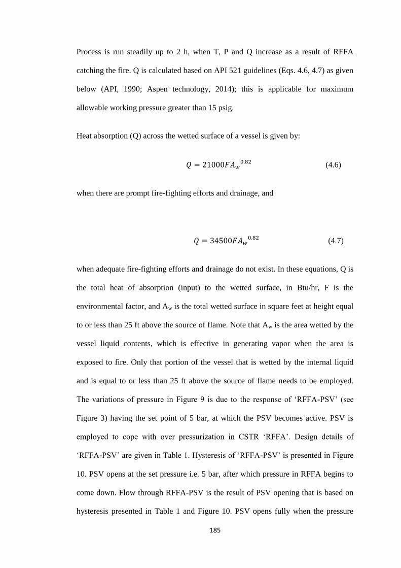
185
Process is run steadily up to 2 h, when T, P and Q increase as a result of RFFA
catching the fire. Q is calculated based on API 521 guidelines (Eqs. 4.6, 4.7) as given
below (API, 1990; Aspen technology, 2014); this is applicable for maximum
allowable working pressure greater than 15 psig.
Heat absorption (Q) across the wetted surface of a vessel is given by:
𝑄 = 21000𝐹𝐴𝑤0.82
(4.6)
when there are prompt fire-fighting efforts and drainage, and
𝑄 = 34500𝐹𝐴𝑤0.82
(4.7)
when adequate fire-fighting efforts and drainage do not exist. In these equations, Q is
the total heat of absorption (input) to the wetted surface, in Btu/hr, F is the
environmental factor, and Aw is the total wetted surface in square feet at height equal
to or less than 25 ft above the source of flame. Note that Aw is the area wetted by the
vessel liquid contents, which is effective in generating vapor when the area is
exposed to fire. Only that portion of the vessel that is wetted by the internal liquid
and is equal to or less than 25 ft above the source of flame needs to be employed.
The variations of pressure in Figure 9 is due to the response of ‘RFFA-PSV’ (see
Figure 3) having the set point of 5 bar, at which the PSV becomes active. PSV is
employed to cope with over pressurization in CSTR ‘RFFA’. Design details of
‘RFFA-PSV’ are given in Table 1. Hysteresis of ‘RFFA-PSV’ is presented in Figure
10. PSV opens at the set pressure i.e. 5 bar, after which pressure in RFFA begins to
come down. Flow through RFFA-PSV is the result of PSV opening that is based on
hysteresis presented in Table 1 and Figure 10. PSV opens fully when the pressure
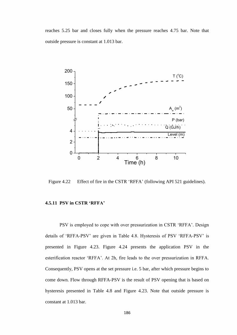
186
reaches 5.25 bar and closes fully when the pressure reaches 4.75 bar. Note that
outside pressure is constant at 1.013 bar.
0 2 4 6 8 100
2
4
50
100
150
200
Level (m)
Q (GJ/h)
P (bar)
Aw (m
2)
T (oC)
Time (h)
Figure 4.22 Effect of fire in the CSTR ‘RFFA’ (following API 521 guidelines).
4.5.11 PSV in CSTR ‘RFFA’
PSV is employed to cope with over pressurization in CSTR ‘RFFA’. Design
details of ‘RFFA-PSV’ are given in Table 4.8. Hysteresis of PSV ‘RFFA-PSV’ is
presented in Figure 4.23. Figure 4.24 presents the application PSV in the
esterification reactor ‘RFFA’. At 2h, fire leads to the over pressurization in RFFA.
Consequently, PSV opens at the set pressure i.e. 5 bar, after which pressure begins to
come down. Flow through RFFA-PSV is the result of PSV opening that is based on
hysteresis presented in Table 4.8 and Figure 4.23. Note that outside pressure is
constant at 1.013 bar.
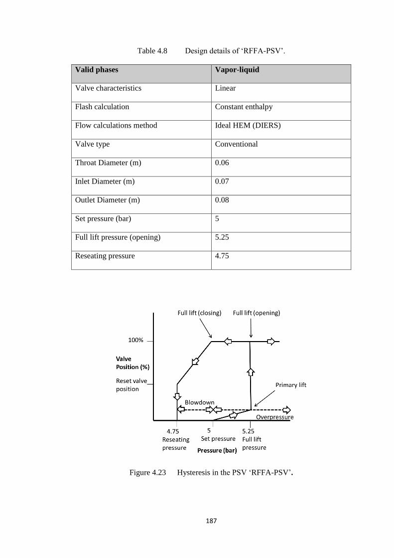
187
Table 4.8 Design details of ‘RFFA-PSV’.
Valid phases Vapor-liquid
Valve characteristics Linear
Flash calculation Constant enthalpy
Flow calculations method Ideal HEM (DIERS)
Valve type Conventional
Throat Diameter (m) 0.06
Inlet Diameter (m) 0.07
Outlet Diameter (m) 0.08
Set pressure (bar) 5
Full lift pressure (opening) 5.25
Reseating pressure 4.75
Figure 4.23 Hysteresis in the PSV ‘RFFA-PSV’.
188
0 2 4 6 8 100
2
4
6
8
2000400060008000
(Valve opening)RFFA-PSV
(%)
(Flow)RFFA-PSV
(kg/h)
(Pressure)RFFA
(bar)
(Pressure)Outside
(bar)
Time (h)
Figure 4.24 PSV in the CSTR ‘RFFA’: at 2 h, pressure increases due to fire, and
PSV becomes active when P=5 bar.
4.6 Summary
In summary, this chapter presents and explains the outcome of the
methodology followed in chapter 3. Firstly, two alternative processes are developed
and compared against respective literature. Then, the camparison is carried out for
the extended capacity. Trade-offs between multiple objectives, such as profit, heat
duty and organic waste resulted from the constrained MOO of biodiesel process are
then discussed. Pareto-optimal fronts between objectives and trends of decision
variables with respect to profit are presented. Based on this, a comparison is carried
out between two processes meticulously and better process alternative is determined.
189
Later, the results of PWC for the chosen process are discussed and performance is
evaluated based on settling time, DPT and TV. For several disturbances, the PWC
system is able to maintain biodiesel purity under control as per EN standards, and is
found to provide smooth, stable and robust control. Transient profiles for several
process variables are also presented for differernt disturbances. In the end, results of
OTS for several scenarios are discussed. The scenarios studied are: equipment
malfunctions, fire, pressure safety valve, bursting disk, interlock and startup. The
developed OTS is found to be able to replicate the process behaviour for these
scenarios. To show the capability of developed OTS in APD, one correct and one
wrong action that would be taken by trainees, are simulated. Effect of such actions
on process operation and biodiesel product are then discussed. In essence, these
scenarios present the in-depth understanding of the process under startup and
emergency events. In addition, HAZOP analysis is carried out as presented in the
Appendix D. Next chapter lists the conclusions arrived from this study and
recommendations for future work in this field.
190
CHAPTER 5
CONCLUSIONS AND RECOMMENDATIONS
5.1 Conclusions
This section presents the findings of this research. This study concludes with
the following conclusions:
This study develops an OTS for the homogeneously catalyzed two-step
biodiesel process. Firstly, two alternative alkali-catalyzed biodiesel production
processes are simulated in Aspen Plus considering detailed reaction kinetics and
detailed constituents of oil. Both processes use waste cooking palm oil as the feed,
which is favourable from the point of both economic feasibility and environmental
impact. Steady state simulation results have been validated against literature dat and
found to be reasonable. Two bi-objective problems are solved using EMOO program
incorporating NSGA-II, to investigate the performance of both the process
alternatives. Trade-offs between profit and heat duty, and profit and organic waste
are analyzed, which examine profitability and environmental impact of biodiesel
processes. Improvement in the profit is accompanied by increase in heat duty, and
also with increased formation of organic waste. The main contributor to these
increases is WCO flow rate.
Process 1 having three transesterification reactors produces significantly
lower organic waste (by 32%), requires lower heat duty (by 39%) and slightly more
profitable (by 1.6%) compared to Process 2 having a single transesterification reactor
191
and also a different separation sequence. Overall, the obtained quantitative trade-offs
between objectives enable better decision making about the process design for
biodiesel production from waste cooking oil. Also, the effect of using detailed
components of oil versus lumped components is analyzed and found to have some
impact. Hence, considering detailed composition of oil with detailed reaction kinetics
is recommended for biodiesel process simulation, for obtaining more realistic results.
Better process in terms of higher profit and lower environmental impact is
determined. Main features of the selected process are: (1) one reactor for
esterification, (2) three reactors for transesterification with intermediate phase
separators, and (3) biodiesel and glycerol are separated first followed by methanol
separation and washing of biodiesel. This scheme prevents backward reactions as
methanol is present until biodiesel and glycerol are separated, and the recovered
methanol contains a very small amount of water, which avoids energy intensive
methanol-water separation and facilitates methanol re-use in the process. Also, the
chosen process is close to that used in the industry.
Later, a suitable PWC structure using IFSH methodology, and an OTS using
APD are developed for the concerned process. Next, a dynamic simulator is
developed for the chosen process. Dynamics of the process has been studied for
several disturbances. This is important for the development of the PWC structure
development. Subsequently, a suitable PWC system is developed and evaluated for
the chosen complex multiunit biodiesel process using WCO as the feedstock. The
IFSH methodology is used to design a PWC system for the biodiesel process; in this,
control loops are decided based on heuristics, simulations and ERGA analysis as this
is a critical factor in the successful implementation of PWC. The main merits of
192
IFSH methodology are effective use of rigorous process simulators and heuristics in
developing a PWC system, and simplicity of application. The performance of the
designed control system is investigated in terms of settling time of biodiesel
production rate, deviation from the production target (that affects economics) and
total variation in manipulated variables (that depicts the control effort needed to
stabilize the process), for a number of disturbances. For these disturbances, the PWC
system is able to maintain biodiesel purity under control as per EN standards, and is
found to provide smooth, stable and robust control.
Finally, an OTS is developed for biodiesel production from WCO. Aspen
OTS Framework is used on top of APD simulation of biodiesel process. Several
emergency situations were developed which can be inserted by the instructor at any
point in time to train the operators. Several scenarios such as equipment
malfunctions, fire, pressure safety valves, burst disk, interlock and startup are studied
using the developed OTS. These process scenarios can be loaded and utilized at any
point in time to train the new and existing operators. This is the first study to
investigate the application of the commonly used Aspen Plus Dynamics in the OTS
development for biodiesel production from WCO. Experience from this is useful for
development of OTS for other processes and consequently increased operator
training for safer plants.
In summary, the novelty of the present study are: 1) development and detailed
simulation of a two-step homogeneously catalyzed biodiesel production from WCO,
2) MOO using NSGA-II, which is implemented in Excel and interlinked with Aspen
Plus, 3) development and evaluation of a PWC system for the complex
193
homogeneously catalyzed two-step biodiesel production from WCO, and 4) OTS
development for the concerned process using APD and Aspen OTS Framework. This
is the first study to develop a complete PWC structure and OTS for a homogeneously
catalyzed two-step biodiesel production from WCO.
5.2 Recommendations for Further Work
There are several recommendations for future research related to this thesis topic,
and they are as follows.
(i) Thus far, biodiesel production using homogeneous catalyst is widely used.
However, this process has some intrinsic drawbacks, namely, 3 phase (V-L-L)
system formation, need of neutralization of acid and alkali catalyst, thus more
number of process equipment, use of excess of methanol and hence its separation etc.
Therefore, efforts should be directed to develop suitable processes which overcome
these drawbacks.
(ii) MOO continues to be the major thrust area in chemical engineering. Stricter
environmental regulations and economic competition drive companies to look for
efficient design and operation of process. Although NSGA-II used in this study
worked successfully to determine the optimal solutions for conflicting objectives,
other evolutionary algorithms such as differential algorithm can be explored.
(iii) Numerous PWC methodologies and applications have been developed in
recent years. As process industry is constantly evolving and facing new challenges
everyday, PWC remains an active research area. Some promising areas of study in

194
the PWC domain are: Improvement of heuristics-based PWC methodologies and
Integrated design and control.
(iv) In continuation of this study, a networked based training should be explored.
Possibility of interlinking this simulator with real DCS/PLC should also be explored.
195
REFERENCES
Al-Arfaj, M. A., & Luyben, W. L. (2004). Plantwide control for TAME production
using reactive distillation. AIChE Journal, 50, 1462-1473.
AlliedMarketResearch. (2014) [Online]. [Accessed December 2014]. Available from
World Wide Web: http://www.alliedmarketresearch.com
Amani, H., Ahmad, Z., & Hameed, B. H. (2014a). Highly active alumina-supported
Cs–Zr mixed oxide catalysts for low-temperature transesterification of waste
cooking oil. Applied Catalysis A: General, 487, 16-25.
Amani, H., Ahmad, Z., & Hameed, B. H. (2014b). Synthesis of fatty acid methyl
esters via the methanolysis of palm oil over Ca3.5xZr0.5yAlxO3 mixed oxide
catalyst. Renewable Energy, 66, 680-685.
API. Guide for Pressure-Relieving and Depressuring Systems”, API Recommended
Practice 521, third edition, November 1990.
API. Venting Atmospheric and Low-Pressure Storage Tanks (Nonrefrigerated and
Refrigerated)”, API Standard 2000, third edition, January 1982, Reaffirmed,
December 1987.
Apostolakou, A. A., Kookos, I. K., Marazioti, C., & Angelopoulos, K. C. (2009).
Techno-economic analysis of a biodiesel production process from vegetable
oils. Fuel Processing Technology, 90, 1023-1031.
Araújo, A. C. B. d., Govatsmark, M., & Skogestad, S. (2007). Application of
plantwide control to the HDA process. I—steady-state optimization and self-
optimizing control. Control Engineering Practice, 15, 1222-1237.
AspenTechnology. (2013) [Online]. [Accessed April 2013]. Available from World
Wide Web:
http://www.aspentech.com/uploadedFiles/Products/Templates/aspen_ots.pdf
AspenTechnology. (2012). Aspen Plus - Aspen Plus Biodiesel Model (Examples).
AspenTechnology. (2014). Aspen Plus Dynamics- Help.
Ayral, T., De Jonge, P. . (2013). Operator training simulators for brownfield process
units offer many benefits. In Hydrocarbon Processing, Vol. 92, pp. 45-47.
Balaton, M. G., Nagy, L., & Szeifert, F. (2013). Operator training simulator process
model implementation of a batch processing unit in a packaged simulation
software. Computers & Chemical Engineering, 48, 335-344.
Behzadi, S., & Farid, M. M. (2009). Production of biodiesel using a continuous gas-
liquid reactor. Bioresource Technology, 100, 683-689.
196
Berrios, M., Siles, J., Martín, M. A., & Martín, A. (2007). A kinetic study of the
esterification of free fatty acids (FFA) in sunflower oil. Fuel, 86, 2383-2388.
Bessiris, Y., Kyriakopoulou, D., Ghajar, F., & Steuckrath, C. (2011). Long Distance
Operator Training. In E. N. Pistikopoulos, M. C. Georgiadis & A. C.
Kokossis (Eds.), Computer Aided Chemical Engineering, Vol. 29, pp. 1115-
1119: Elsevier.
Besuijen, R., Young, R., & Guaraldo, M. (2012). Operator training simulators - Nova
chemicals' experience for training, certification and other applications.
AIChE Spring Meeting and 8th Global Congress on Process Safety,
Conference Proceedings.
Bhaskar, V., Gupta, S. K., & Ray, A. K. (2000). Applications of multi-objective
optimization in chemical engineering. Reviews in Chemical Engineering, 16,
1-54.
Biegler, L. T., Grossmann, I. E., & Westerberg, A. W. (1997). Systemetic methods of
chemical process design, PHI press.
Box, G. E. P. (1979). Robustness in Scientific Model Building. In R. L. Launer & G.
N. Wilkinson (Eds.), Robustness in statistics (pp. 201-236). New York:
Academic Press.
Brambilla, S., & Manca, D. (2011). Recommended features of an industrial accident
simulator for the training of operators. Journal of Loss Prevention in the
Process Industries, 24, 344-355.
Buckley, P. S. (1964). Techniques of Process Control. New York: Wiley.
Cameron, D., Clausen, C., & Morton, W. (2002). Software Architectures and Tools
for Computer Aided Process Engineering In B. Braunschweig & R. Gani
(Eds.), Dynamic Simulators for Operator Training), Elsevier Science, Vol.
11, pp. 393-431: Elsevier Science.
Canakci, M., & Van Gerpen, J. (2001). Biodiesel production from oils and fats with
high free fatty acids. Transactions of the ASAE, 44, 1429-1436.
Chen, M. L., & Wang, F. S. (2010). Optimal trade-off design of integrated
fermentation processesfor ethanol production using genetically engineered
yeast. Chemical Engineering Journal, 158, 271-280.
Chen, Y. H., Huang, Y. H., Lin, R. H., & Shang, N. C. (2010). A continuous-flow
biodiesel production process using a rotating packed bed. Bioresource
Technology, 101, 668-673.
Cheng, J. K., Chao, C. C., Ward, J. D., & Chien, I. L. (2014). Design and control of a
biodiesel production process using sugar catalyst for oil feedstock with
different free fatty acid concentrations. Journal of the Taiwan Institute of
Chemical Engineers, 45, 76-84.
197
Chua, C., Lee, H., & Low, J. (2010). Life cycle emissions and energy study of
biodiesel derived from waste cooking oil and diesel in Singapore. The
International Journal of Life Cycle Assessment, 15, 417-423.
Cox, R. K., Smith, J. F., & Dimitratos, Y. (2006). Can simulation technology enable
a paradigm shift in process control?: Modeling for the rest of us. Computers
& Chemical Engineering, 30, 1542-1552.
Cucek, L., Klemes, J. J., Varbanov, P. S., & Kravanja, Z. (2011). Life cycle
assessment and multi-criteria optimization of regional biomass and bio-
energy supply chains. Chemical Engineering Transactions, 25, 575-580.
Datta, A. (2008), Process engineering & design using visual basic. CRC press.
Dasgupta, S. (1998) Use Operator Training Simulators for FCC Units. Fuel
Technology and Management [Online]. [Accessed MJune 2013]. Available
from World Wide Web:
http://www.kbr.com/Newsroom/Publications/Whitepapers/Use-Operator-
Training-Simulators-for-FCC-Units.pdf
Deb, K., Pratap, A., Agarwal, S., & Meyarivan, T. (2002). A Fast and Elitist
Multiobjective Genetic Algorithm: NSGA-II. IEEE Transactions on
Evolutionary Computation, 6, 182-197.
Drozdowicz, B., Quirós, R., Schiliuk, A., & Cerro, R. (1987). The structure of a real
time dynamic simulator for training (siden). Computers in Industry, 8, 49-63.
Dubé, M. A., Tremblay, A. Y., & Liu, J. (2007). Biodiesel production using a
membrane reactor. Bioresource Technology, 98, 639-647.
Duca, M., & Tamas, L. (2012). Development of an operation training system - A
case study. IFAC Proceedings Volumes (IFAC-PapersOnline), 14, 1622-
1627.
Dudley, T., de Villiers, P., Bouwer, W., & Luh, R. (2008). The Operator Training
Simulator System for the Pebble Bed Modular Reactor (PBMR) Plant.
Nuclear Engineering and Design, 238, 2908-2915.
Fauzi, A., & Amin, N. (2013). Optimization of oleic acid esterification catalyzed by
ionic liquid for green biodiesel synthesis. Energy Conversion and
Management, 76, 818-827.
Fewtrell, P., & Hirst, I. L. (1974). A Review of High-Cost Chemical/Petrochemical
Accidents Since Flixborough 1974. IChemE Loss Prevention Bulletin, 140,
1-12.
Fisher, H., Forrest, H., Grossel, S., Huff, J., Muller, A., Noronha, J., Shaw, S., &
Tilly, B. (1992). Emergency Relief System Design Using DIERS
Technology. American Institute of Chemical Engineers, 71-73.
198
Freedman, B., Pryde, E. H., & Mounts, T. L. (1984). Variables affecting the yields of
fatty esters from transesterified vegetable oils. J Am Oil Chem Soc, 61, 1638-
1643.
Fürcht, Á., Kovács, T., & Rabi, I. (2008). Implementation of Operator Training
System in the MOL Danube Refinery. In MOL Scientific Magazine. 2, 50-
55.
García, M., Gonzalo, A., Sánchez, J. L., Arauzo, J., & Peña, J. Á. (2010). Prediction
of normalized biodiesel properties by simulation of multiple feedstock
blends. Bioresource Technology, 101, 4431-4439.
Gerlach, I., Brüning, S., Gustavsson, R., Mandenius, C.-F., & Hass, V. C. (2014).
Operator training in recombinant protein production using a structured
simulator model. Journal of Biotechnology, 177, 53-59.
Gerlach, I., Hass, V. C., Brüning, S., & Mandenius, C.-F. (2013). Virtual bioreactor
cultivation for operator training and simulation: Application to ethanol and
protein production. Journal of Chemical Technology & Biotechnology, 88,
2159-2168.
Gerpen, J. V. (2005). Biodiesel processing and production. Fuel Processing
Technology, 86, 1097-1107.
Glaser, D. C. (2011). A systematic approach to implementing operator training
simulators. AIChE Spring Meeting and 7th Global Congress on Process
Safety, Conference Proceedings.
Glasscock, D. A., & Dale, J. C. (1994). Process modeling: the art and science of
modeling. Chemical Engineering, 101, 82-89.
HAZOP Guidelines, Hazardous Industry Planning, Department of planning, NSW
Government, Advisory Paper No 8, Consultation Draft, July 2008 (2008)
[Online]. [Accessed March 2014]. Available from World Wide
Web:http://www.planning.nsw.gov.au/plansforaction/pdf/hazards/haz_hipap8
_rev2008.pdf
Haas, M. J., McAloon, A. J., Yee, W. C., & Foglia, T. A. (2006). A process model to
estimate biodiesel production costs. Bioresource Technology, 97, 671-678.
Hass, V. C., Kuhnen, F., & Schoop, K. M. (2005). An Environment for the
Development of Operator Training Systems (OTS) from Chemical
Engineering Models. In L. Puigjaner & A. Espufta (Eds.), European
Symposium on Computer Aided Process Engineering, Vol. 15, pp. 289-293:
Elsevier.
Herrmann, G., Spurgeon, S. K., & Edwards, C. (2003). A model-based sliding mode
control methodology applied to the HDA-plant. Journal of Process Control,
13, 129-138.
199
Huerga, I. R., Zanuttini, M. S., Gross, M. S., & Querini, C. A. (2014). Biodiesel
production from Jatropha curcas: Integrated process optimization. Energy
Conversion and Management, 80, 1-9.
Hyllseth, M., & Cameron, D. (2003). Operator Training and Operator Support using
Multiphase Pipeline Models and Dynamic Process Simulation: Sub-Sea
Production and On-Shore Processing. European Symposium on Computer
Aided Process Engineering, Elsevier, 13, 425-430.
Jagtap, R., Kaistha, N., & Skogestad, S. (2011). Plantwide control for economic
optimum operation of a recycle process with side reaction. Industrial &
Engineering Chemistry Research, 50, 8571-8584.
Jain, S., & Sharma, M. P. (2010). Kinetics of Acid Base Catalyzed
Transesterification of Jatropha Curcas Oil. Bioresource Technology, 101,
7701-7706.
Jayanthi, T., Seetha, H., Narayanan, K. R. S., Jasmine, N., Nawlakha, R., Sankar, B.,
Chakraborty, J., SatyaMurty, S. A. V., & Swaminathan, P. (2011). Simulation
and Integrated Testing of Process Models of PFBR Operator Training
Simulator. Energy Procedia, 7, 653-659.
Joo, E., Lee, K., Lee, M., & Park, S. (2000). CRACKER - a PC based simulator for
industrial cracking furnaces. Computers and Chemical Engineering, 24, 1523-
1578.
Kiss, A. A. (2009). Biodiesel by Reactive Absorption – Towards Green
Technologies. In J. Jacek & T. Jan (Eds.), Computer Aided Chemical
Engineering, Vol. 26, pp. 847-852: Elsevier.
Kiss, A. A., Segovia-Hernández, J. G., Bildea, C. S., Miranda-Galindo, E. Y., &
Hernández, S. (2012). Reactive DWC leading the way to FAME and fortune.
Fuel, 95, 352-359.
Kluge, A., Nazir, S., & Manca, D. (2014). Advanced Applications in Process Control
and Training Needs of Field and Control Room Operators. IIE Transactions
on Occupational Ergonomics and Human Factors (DOI:
10.1080/21577323.2014.920437).
Komulainen, T. M., Enemark-Rasmussen, R., Sin, G., Fletcher, J. P., & Cameron, D.
(2012). Experiences on dynamic simulation software in chemical engineering
education. Education for Chemical Engineers, 7, e153-e162.
KPPK. (2014) [Online]. [Accessed November 2014]. Available from World Wide
Web: http://www.kppk.gov.my/index.php/our-commodities/biofuel/biofuel-
programmes.html
Kusdiana, D., & Saka, S. (2001). Kinetics of Transesterification in Rapeseed Oil to
Biodiesel Fuel as Treated in Supercritical Methanol. Fuel, 80, 693-698.
200
Kwon, H., Lee, J., & Moon, I. (2012). Development of a safety education system for
SMB operation. In I. D. L. Bogle & M. Fairweather (Eds.), Computer Aided
Chemical Engineering, Vol. 30, pp. 1417-1421: Elsevier.
Laganier, F. (1996). Dynamic process simulation trends and perspectives in an
industrial context. Computers & Chemical Engineering, 20, Supplement 2,
S1595-S1600.
Lee, S., Jeong, I., & Il, M. (2000). Development of evaluation algorithms for
operator training system. Computers & Chemical Engineering, 24, 1517-
1522.
Lurgi. (2013) [Online]. [Accessed September 2013]. Available from World Wide
Web: http://www.lurgi.com/website/Biodiesel.57.0.html?&L=1
Luyben, M. L., Tyreus, B. D., & Luyben, W. L. (1997). Plantwide control design
procedure. AIChE Journal, 43, 3161-3174.
Luyben, W. L. (2002). Plant-Wide Dynamic Simulators in Chemical Processing and
Control (ch. 3): New York: Marcel Dekker.
Luyben, W. L. (2009). Design and Control of an Autorefrigerated Alkylation
Process. Industrial & Engineering Chemistry Research, 48, 11081-11093.
Luyben, W. L., & Luyben, M. L. (1997). Essentials of Process Control. New York:
McGraw-Hill. New York: McGraw-Hill.
Luyben, W. L., Tyreus, B. D., & Luyben, W. L. (1998). Plant-wide Process Control.
New York: McGraw-Hill.
Ma, F., Clements, L. D., & Hanna, M. (1998). The effects of catalyst, free fatty acids
and water on transesterification of beef tallow. Transactions of the ASAE, 41,
1261-1264.
Man, Y. B. C., Haryati, T., Ghazali, H. M., & Asbi, B. A. (1999). Composition and
Thermal Profile of Crude Palm Oil and Its Products. J Am Oil Chem Soc, 76,
237-242.
Manca, D., Brambilla, S., & Colombo, S. (2013). Bridging between Virtual Reality
and accident simulation for training of process-industry operators. Advances
in Engineering Software, 55, 1-9.
Manca, D., Totaro, R., Nazir, S., Brambilla, S., & Colombo, S. (2012). Virtual and
Augmented Reality as Viable Tools to Train Industrial Operators. In A. K.
Iftekhar & S. Rajagopalan (Eds.), Computer Aided Chemical Engineering,
Vol. 31, pp. 825-829: Elsevier.
Manenti, F. (2012). Natural gas operations: Considerations on process transients,
design, and control. ISA Transactions, 51, 317-324.
201
Martín, M., & Grossmann, I. E. (2012). Simultaneous Optimization and Heat
Integration for Biodiesel Production from Cooking Oil and Algae. Industrial
& Engineering Chemistry Research, 51, 7998-8014.
Masuduzzaman, & Rangaiah, G. P. (2009). Multi-Objective Optimization
Applications in Chemical Engineering, In G. P. Rangaiah (Ed.), Multi-
objective Optimization: Techniques and Applications in Chemical
Engineering. World Scientific.
Mele, F. D., Kostin, A. M., Guillen-Gosalbez, G., & Jimenez, L. (2011). Multi-
objective model for more sustainable fuel supply chains. a case study of the
sugar cane industry in Argentina. Industrial & Engineering Chemistry
Research, 50, 4939-4958.
Mendoza, L.-F. M., Boix, M., Azzaro-Pantel, C., Montastruc, L., & Domenech, S.
(2014). Biodiesel Production from Waste Vegetable Oils: Combining Process
Modelling, Multiobjective Optimization and Life Cycle Assessment (LCA).
Computer Aided Chemical Engineering, 33, 235-240.
Morais, S., Mata, T. M., Martins, A. A., Pinto, G. A., & Costa, C. A. V. (2010).
Simulation and life cycle assessment of process design alternatives for
biodiesel production from waste vegetable oils. Journal of Cleaner
Production, 18, 1251-1259.
Moaveni, B., Khakisedigh, A, (2008). Input-output pairing analysis for uncertain
multivariable processes. Journal of Process Control, 18, 527-532.
MPOB. (2013) [Online]. [Accessed May 2013]. Available from World Wide Web:
http://www.palmoilworld.org/biodiesel.html
Munn, L., Williams, J., & Glaser, D. C. (2012). Using simulators to teach process
safety and operations at petroplus coryton.
Murthy Konda, N. V. S. N., Rangaiah, G. P., & Krishnaswamy, P. R. (2005).
Plantwide Control of Industrial Processes: An Integrated Framework of
Simulation and Heuristics. Industrial & Engineering Chemistry Research, 44,
8300-8313.
Murthy Konda, N. V. S. N., Rangaiah, G. P., & Krishnaswamy, P. R. (2006a). A
simple and effective procedure for control degrees of freedom. Chemical
Engineering Science, 61, 1184-1194.
Murthy Konda, N. V. S. N., Rangaiah, G. P., & Lim, D. K. H. (2006b). Optimal
Process Design and Effective Plantwide Control of Industrial Processes by a
Simulation-Based Heuristic Approach. Industrial & Engineering Chemistry
Research, 45, 5955-5970.
Myint, L., & El-Halwagi, M. (2009). Process analysis and optimization of biodiesel
production from soybean oil. Clean Technologies and Environmental Policy,
11, 263-276.
202
Narvaez, P. C., Rincon, S. M., & Sanchez, F. J. (2007). Kinetics of Palm Oil
Methanolysis. J Am Oil Chem Soc, 84, 971-977.
Nazir, N., Ramli, N., Mangunwidjaja, D., Hambali, E., Setyaningsih, D., Yuliani, S.,
Yarmo, M. A., & Salimon, J. (2009). Extraction, transesterification and
process control in biodiesel production from Jatropha curcas. European
Journal of Lipid Science and Technology, 111, 1185-1200.
Nazir, S., & Manca, D. (2014). How a plant simulator can improve industrial safety
(DOI: 10.1002/prs.11714).
Nazir, S., Totaro, R., Brambilla, S., Colombo, S., & Manca, D. (2012). Virtual
Reality and Augmented-Virtual Reality as Tools to Train Industrial
Operators. In B. Ian David Lockhart & F. Michael (Eds.), Computer Aided
Chemical Engineering, Vol. 30, pp. 1397-1401: Elsevier.
Nicola, G. D., Moglie, M., Pacetti, M., & Santori, G. (2010). Bioenergy II: modeling
and multiobjective optimization of different bio-diesel production processes.
International Journal Of Chemical Reactor Engineering, 8, 12-18.
Normand, X. (1993). Compact Training Simulators on Workstations. Simulators X,
25, 552-556.
Noureddini, H., & Zhu, D. (1997). Kinetics of Transesterification of Soybean Oil.
Biocatal Articles, 74, 1457–1463.
Pantelides, C. C., & Renfro, J. G. (2013). The online use of first-principles models in
process operations: Review, current status and future needs. Computers &
Chemical Engineering, 51, 136-148.
Park, J., Jung, W., Ha, J., & Shin, Y. (2004). Analysis of operators' performance
under emergencies using a training simulator of the nuclear power plant.
Reliability Engineering & System Safety, 83, 179-186.
Park, S., Lee, S., & Moon, I. F. (2001). Superstructure of yOTS-The Network-Based
Chemical Process Operator Training System for Multiple Trainees. Korean
Chemical Engineering, 18, 788-795.
Pereira, A. C., Riera, A., Padilla, G., Musulin, E., & Nakamura, N. J. (2009).
Operator Trainer System for the Petrobras P-26 Semi-Submersible Oil and
Gas Production Unit. In R. M. d. B. Alves, C. A. O. d. Nascimento & B.
Evaristo Chalbaud (Eds.), Computer Aided Chemical Engineering, Vol.
Volume 27, pp. 1959-1964: Elsevier.
Peters, M., & Peterhaus, K. (2002). Process design and economic for chemical
engineering. 4th
edition, Mc Graw Hill.
Plantbiofuels. (2013) [Online]. [Accessed July 2013]. Available from World Wide
Web:http://www.plantbiofuels.com/html/biodieselplant.htm
Platinumgroup. (2013) [Online]. [Accessed September 2013]. Available from World
Wide Web:http://www.platinumgroup.com.my
203
Platts. (2013) [Online]. [Accessed March 2013]. Available from World Wide Web:
http://www.platts.com
Potts, A. S., Massaro, L. C., & Garcia, C. (2015). Detection of decoupled
input/output pairs in multivariable systems. ISA Transactions, 55, 195-207.
Purcell, P. (1996). Simulation software cuts testing time and expense. Control, 9, 72-
76.
Qiu, Q. F., Rangaiah, G. P., & Krishnaswamy, P. R. (2003). Application of a plant-
wide control design to the HDA process. Computers & Chemical
Engineering, 27, 73-94.
Rahimi, M., Aghel, B., Alitabar, M., Sepahvand, A., & Ghasempour, H. R. (2014).
Optimization of biodiesel production from soybean oil in a microreactor.
Energy Conversion and Management, 79, 599-605.
Ramadhas, A. S., Jayaraj, S., & Muraleedharan, C. (2010). Performance and
emission studies on biodiesel-liquefied petroleum gas dual fuel engine with
exhaust gas recirculation. Journal of Renewable and Sustainable Energy, 2.
(DOI:10.1063/1.3302019)
Rao, M., Wen, J., & Zhang, Y. (2003). Incident prevention training simulator. In B.
Chen & A. W. Westerberg (Eds.), Computer Aided Chemical Engineering,
Vol. 15, pp. 1472-1477: Elsevier.
Ray, M. S., & Sneesby, M. S. (1998). Chemical engineering design project- A case
study approach, 2nd
edition, Gordon and Breach Science Publishers.
Rey, F., Thiabaud, P., & Tourdjman, J. . (2008). Operator Training Simulator:
Payback and Risk Mitigation. Gastech 2008, Bangkok, Thailand.
Rincón, L. E., Valencia, M. J., Hernández, V., Matallana, L. G., & Cardona, C. A.
(2015). Optimization of the Colombian biodiesel supply chain from oil palm
crop based on techno-economical and environmental criteria. Energy
Economics, 47, 154-167.
Santana, G. C. S., Martins, P. F., de Lima da Silva, N., Batistella, C. B., Maciel
Filho, R., & Wolf Maciel, M. R. (2010). Simulation and Cost Estimate for
Biodiesel Production using Castor Oil. Chemical Engineering Research and
Design, 88, 626- 632.
Santos, R. A., Normey-Rico, J. E., Gómez, A. M., Arconada, L. F. A., & Moraga, C.
d. P. (2008). Distributed continuous process simulation: An industrial case
study. Computers & Chemical Engineering, 32, 1195-1205.
Seborg, D. E., Mellichamp, D. A., Edgar, T. F., & Doyle, F. J. (2010). Process
Dynamics and Control (3 ed.). USA: John Wiley & Sons.
Sebzalli, Y. M., Li, R. F., Chen, F. Z., & Wang, X. Z. (2000). Knowledge discovery
from process operational data for assessment and monitoring of operator's
performance. Computers & Chemical Engineering, 24, 409-414.
204
Seider, W. D., Seader, J. D., & Lewin, D. R. (2004). Product & Process Design
Principles-synthesis analysis and evaluation. In: Wliley.
Sharma, S., & Rangaiah, G. P. (2012). Modeling and optimization of a fermentation
process integrated with cell recycling and pervaporation for multiple
objectives. Industrial & Engineering Chemistry Research, 51, 5542-5551.
Sharma, S., & Rangaiah, G. P. (2013a). Multi-objective Optimization Applications in
Chemical Engineering. In G. P. Rangaiah & A. Bonilla-Petriciolet (Eds.),
Multi-Objective Optimization in Chemical Engineering: Developments and
Applications (pp. 35-104): Wiley.
Sharma, S., & Rangaiah, G. P. (2013b). Multi-objective optimization of a bio-diesel
production process. Fuel, 103, 269-277.
Sharma, S., Rangaiah, G. P., & Cheah, K. S. (2012). Multi-objective optimization
using MS Excel with an application to design of a falling-film evaporator
system. Food and Bioproducts Processing, 90, 123-134.
Sharma, Y. C., Singh, B., & Korstad, J. (2011). Latest Developments on Application
of Heterogenous Basic Catalysts for an Efficient and Eco-friendly Synthesis
of Biodiesel: A review. Fuel (in press).
Shen, Y. H., Cheng, J. K., Ward, J. D., & Yu, C. C. (2011). Design and control of
biodiesel production processes with phase split and recycle in the reactor
system. Journal of the Taiwan Institute of Chemical Engineers, 42, 741-750.
Shepherd, A. (1986). Issues in the training of process operators. International Journal
of Industrial Ergonomics, 1, 49-64.
Shewchuk, C. F. (1993). Operator Training Simulators State-of-the-Art and Future-
Directions. Simulators X, 25, 659-666.
Sinnott, R. K., & Towler, G. (2008). Chemical engineering design, Elsevier.
Sivasothy, K., & Lim, N. B. H. (1985). Automation of Palm Oil Mills. Journal of the
American Oil Chemists' Society, 62, 267-273.
Skogestad, S. (2004). Control structure design for complete chemical plants.
Computers and Chemical Engineering, 28, 219-234.
Skogestad, S. (2012). Economic plantwide control. In G. P. Rangaiah & V. Kariwala
(Eds.), Plantwide control-recent developments and applications (pp. 229-
251): Wiley.
Spanel, U., Krost, G., & Rumpel, D. (2001). Simulator for inter-company operator
training. Control Engineering Practice, 9, 777-783.
Smith, R. (2005). Chemical Process: Design and Integration. USA: Wiley.
205
Srinivas, N., & Deb, K. (1995). Multi-objective Function Optimization Using Non-
dominated Sorting Genetic Algorithms. Evolutionary Computation, 2, 221-
248.
Stawarz, A. C., & Sowerby, B. (1995). Cost effective operator training. Computers &
Chemical Engineering, 19, Supplement 1, 459-464.
Sterky, M. (1993). The General-Purpose Simulator. Simulators X, 25, 563-567.
Suryaputra, W., Winata, I., Indraswati, N., & Ismadji, S. (2013). Waste capiz
(Amusium cristatum) shell as a new heterogeneous catalyst for biodiesel
production. Renewable Energy, 50, 795-799.
Timo, R., ani, K., & Pertti, L. (2011). Training Simulator for Flotation Process
Operators. In Preprints of the 18th IFAC World Congress. Milano, Italy.
Turton, R., Bailie, R. C., Whiting, W. B., & Shaeiwitz, J. A. (2009). Analysis
synthesis and design of chemical processes (3rd ed ed.): Prentice Hall.
UKHSE. (2014) [Online]. [Accessed November 2014]. Available from World Wide
Web: http://www.hse.gov.uk/press/2002/e02211.htm
USDA. (2013) [Online]. [Accessed April 2013]. Available from World Wide
Web:http://gain.fas.usda.gov/Pages/Default.aspx
Hass, V.C., Kuntzsch, S., Schoop, K.-M., & Winterhalter, M. (2014). Resource
efficiency studies using a new operator training simulator for a bioethanol
plant. Chemical Engineering Transactions, 39, 541-546
Vasconcelos, C. J. G., Filho, R. M., Spandri, R., & Wolf- Macief, M. R. (2005).
Dynamic Models Towards Operator and Engineer Training: Virtual
Environment. In L. Puigjaner & A. Espufla (Eds.), European Symposium on
Computer Aided Process Engineering, Vol. 15: Elsevier.
Vasudevan, S., Konda, N. V. S. N. M., & Rangaiah, G. P. (2009a). Plant-Wide
Control: Methodologies and Applications. Reviews in Chemical Engineering,
25, 297-338.
Vasudevan, S., & Rangaiah, G. P. (2010). Criteria for Performance Assessment of
Plantwide Control Systems. Industrial & Engineering Chemistry Research,
49, 9209-9221.
Vasudevan, S., & Rangaiah, G. P. (2011). Integrated Framework Incorporating
Optimization for Plant-Wide Control of Industrial Processes. Industrial &
Engineering Chemistry Research, 50, 8122-8137.
Vasudevan, S., Rangaiah, G. P., Konda, N. V. S. N. M., & Tay, W. H. (2009b).
Application and Evaluation of Three Methodologies for Plantwide Control of
the Styrene Monomer Plant. Industrial & Engineering Chemistry Research,
48, 10941-10961.
206
Vlysidis, A., Binns, M., Webb, C., & Theodoropoulos, C. (2011). A techno-
economic analysis of bio-diesel bio-refineries: assessment of integrated
designs for the co-production of fuels and chemicals. Energy & Fuels, 36,
4671-4683.
Wang, F. S., & Lin, H. T. (2010). Fuzzy optimization of continuous fermentations
with cell recycling for ethanol production. Industrial & Engineering
Chemistry Research, 49, 2306-2311.
West, A. H., Posarac, D., & Ellis, N. (2007). Simulation, Case Studies and
Optimization of a Biodiesel Process with a Solid Acid Catalyst. International
Journal Of Chemical Reactor Engineering, 5, Article A37.
West, A. H., Posarac, D., & Ellis, N. (2008). Assessment of four biodiesel production
processes using HYSYS.Plant. Bioresource Technology, 99, 6587-6601.
Woinaroschy, A. (2014). Multiobjective optimal design for biodiesel sustainable
production. Fuel, 135, 393–405.
Worm, G. I. M., Van der Helm, A. W. C., Lapikas, T., Van Schagen, K. M., &
Rietveld, L. C. (2010). Integration of models, data management, interfaces
and training support in a drinking water treatment plant simulator.
Environmental Modelling & Software, 25, 677–683.
Worm, G. I. M., Van der Wees, M., De Winter, J. C. F., De Graaf, L., Wieringa, P.
A., & Rietveld, L. C. (2012). Training and assessment with a faster than real-
time simulation of a drinking water treatment plant. Simulation Modelling
Practice and Theory, 21, 52-64.
Wu, W., & Wang, C.-Y. (2013). Design and Control of Stand-Alone Hydrogen
Production Systems with Maximum Waste Heat Recovery. Industrial &
Engineering Chemistry Research, 52, 14601-14612.
Xiong, Q., Cai, W. J., & He, M. J. (2005). A practical loop pairing criterion for
multivariable processes. Journal of Process Control, 15, 741-747.
Yang, S. H., Yang, L., & He, C. H. (2001). Improve Safety of Industrial Processes
Using Dynamic Operator Training Simulators. Process Safety and
Environmental Protection, 79, 329-338.
Ye, N., Valluri, S., Barker, M., & Yu, P.-Y. (2000). Integration of advanced process
control and full-scale dynamic simulation. ISA Transactions, 39, 273-280.
Yingling, B., Li, C., Honglin, W., Xiwen, Y., & Zongcheng, Y. (2011). Multi-
objective optimization of bio-ethanol production during cold enzyme starch
hydrolysis in very high gravity cassava mash. Bioresource Technology, 102,
8077-8084.
You, Y.-D., Shie, J.-L., Chang, C.-Y., Huang, S.-H., Pai, C.-Y., Yu, Y.-H., & Chang,
C. H. (2007). Economic cost analysis of biodiesel production: case in
soybean oil†. Energy & Fuels, 22, 182-189.
207
Zamboni, A., Shah, N., & Bezzo, F. (2009). Spatially explicit static model for the
strategic design of future bio-ethanol production systems. 2. multi-objective
environmental optimization. Energy and Fuels, 23, 5134–5143.
Zhang, C. (2011). Studies on design and plant-wide control of chemical processes.
ME Thesis. National University of Singapore, Singapore.
Zhang, C., Rangaiah, G. P., & Kariwala, V. (2012). Design and plantwide control of
a biodiesel plant. In G. P. Rangaiah & V. Kariwala (Eds.), Plantwide control-
recent developments and applications (pp. 293-317): Wiley.
Zhang, Y., Dubé, M. A., McLean, D. D., & Kates, M. (2003a). Bio-diesel production
from waste cooking oil-1: Process design and technological assessment.
Bioresour Technol, 89, 1–16.
Zhang, Y., Dubé, M. A., McLean, D. D., & Kates, M. (2003b). Biodiesel production
from waste cooking oil: 2. Economic assessment and sensitivity analysis.
Bioresource Technology, 90, 229-240.
Zhu, G.-Y., & Henson, M. A. (2002). Model predictive control of interconnected
linear and nonlinear processes. Industrial & Engineering Chemistry Research,
41, 801-816.
Ziolkowska, J. R. (2014). Optimizing biofuels production in an uncertain decision
environment: Conventional vs. advanced technologies. Applied Energy, 114,
366-376.
Zong, L., Ramanathan, S., & Chen, C.-C. (2010a). Fragment-based approach for
estimating thermophysical properties of fats and vegetable oils for modeling
biodiesel production processes. Industrial & Engineering Chemistry
Research, 49, 3022-3023.
Zong, L., Ramanathan, S., & Chen, C.-C. (2010b). Fragment-based approach for
estimating thermophysical properties of fats and vegetable oils for modeling
biodiesel production processes. Industrial & Engineering Chemistry
Research, 49, 876-886.
Zong, L., Ramanathan, S., & Chen, C.-C. (2010c). Predicting thermophysical
properties of mono- and diglycerides with the chemical constituent fragment
approach. Industrial & Engineering Chemistry Research, 49, 5479-5484.
Zou, Z., Cao, B., Gui, X., & Chao, C. (2003). The development of a novel type
chemical process operator-training simulator. In B. Chen & A. W.
Westerberg (Eds.), Computer Aided Chemical Engineering, Vol. 15, pp.
1447-1452: Elsevier.
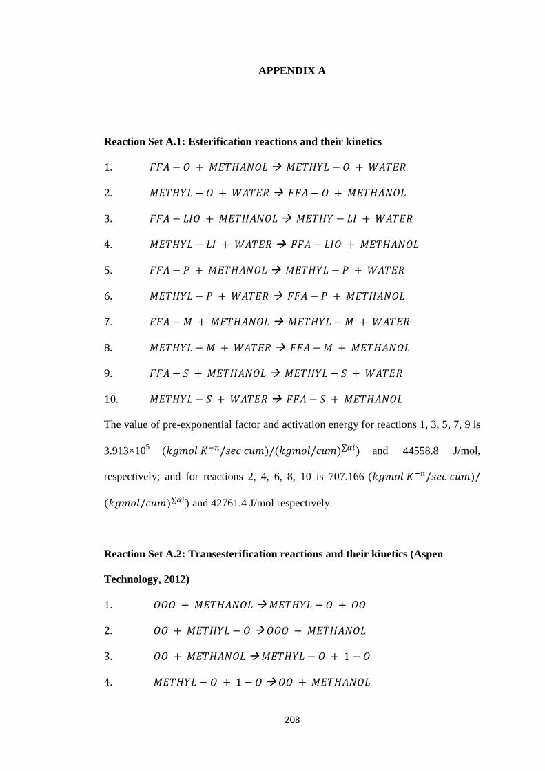
208
APPENDIX A
Reaction Set A.1: Esterification reactions and their kinetics
1. 𝐹𝐹𝐴 − 𝑂 + 𝑀𝐸𝑇𝐻𝐴𝑁𝑂𝐿 𝑀𝐸𝑇𝐻𝑌𝐿 − 𝑂 + 𝑊𝐴𝑇𝐸𝑅
2. 𝑀𝐸𝑇𝐻𝑌𝐿 − 𝑂 + 𝑊𝐴𝑇𝐸𝑅 𝐹𝐹𝐴 − 𝑂 + 𝑀𝐸𝑇𝐻𝐴𝑁𝑂𝐿
3. 𝐹𝐹𝐴 − 𝐿𝐼𝑂 + 𝑀𝐸𝑇𝐻𝐴𝑁𝑂𝐿 𝑀𝐸𝑇𝐻𝑌 − 𝐿𝐼 + 𝑊𝐴𝑇𝐸𝑅
4. 𝑀𝐸𝑇𝐻𝑌𝐿 − 𝐿𝐼 + 𝑊𝐴𝑇𝐸𝑅 𝐹𝐹𝐴 − 𝐿𝐼𝑂 + 𝑀𝐸𝑇𝐻𝐴𝑁𝑂𝐿
5. 𝐹𝐹𝐴 − 𝑃 + 𝑀𝐸𝑇𝐻𝐴𝑁𝑂𝐿 𝑀𝐸𝑇𝐻𝑌𝐿 − 𝑃 + 𝑊𝐴𝑇𝐸𝑅
6. 𝑀𝐸𝑇𝐻𝑌𝐿 − 𝑃 + 𝑊𝐴𝑇𝐸𝑅 𝐹𝐹𝐴 − 𝑃 + 𝑀𝐸𝑇𝐻𝐴𝑁𝑂𝐿
7. 𝐹𝐹𝐴 − 𝑀 + 𝑀𝐸𝑇𝐻𝐴𝑁𝑂𝐿 𝑀𝐸𝑇𝐻𝑌𝐿 − 𝑀 + 𝑊𝐴𝑇𝐸𝑅
8. 𝑀𝐸𝑇𝐻𝑌𝐿 − 𝑀 + 𝑊𝐴𝑇𝐸𝑅 𝐹𝐹𝐴 − 𝑀 + 𝑀𝐸𝑇𝐻𝐴𝑁𝑂𝐿
9. 𝐹𝐹𝐴 − 𝑆 + 𝑀𝐸𝑇𝐻𝐴𝑁𝑂𝐿 𝑀𝐸𝑇𝐻𝑌𝐿 − 𝑆 + 𝑊𝐴𝑇𝐸𝑅
10. 𝑀𝐸𝑇𝐻𝑌𝐿 − 𝑆 + 𝑊𝐴𝑇𝐸𝑅 𝐹𝐹𝐴 − 𝑆 + 𝑀𝐸𝑇𝐻𝐴𝑁𝑂𝐿
The value of pre-exponential factor and activation energy for reactions 1, 3, 5, 7, 9 is
3.913×10⁵ (𝑘𝑔𝑚𝑜𝑙 𝐾−𝑛/𝑠𝑒𝑐 𝑐𝑢𝑚)/(𝑘𝑔𝑚𝑜𝑙/𝑐𝑢𝑚)∑𝛼𝑖)
and 44558.8 J/mol,
respectively; and for reactions 2, 4, 6, 8, 10 is 707.166 (𝑘𝑔𝑚𝑜𝑙 𝐾−𝑛/𝑠𝑒𝑐 𝑐𝑢𝑚)/
(𝑘𝑔𝑚𝑜𝑙/𝑐𝑢𝑚)∑𝛼𝑖) and 42761.4 J/mol respectively.
Reaction Set A.2: Transesterification reactions and their kinetics (Aspen
Technology, 2012)
1. 𝑂𝑂𝑂 + 𝑀𝐸𝑇𝐻𝐴𝑁𝑂𝐿 𝑀𝐸𝑇𝐻𝑌𝐿 − 𝑂 + 𝑂𝑂
2. 𝑂𝑂 + 𝑀𝐸𝑇𝐻𝑌𝐿 − 𝑂 𝑂𝑂𝑂 + 𝑀𝐸𝑇𝐻𝐴𝑁𝑂𝐿
3. 𝑂𝑂 + 𝑀𝐸𝑇𝐻𝐴𝑁𝑂𝐿 𝑀𝐸𝑇𝐻𝑌𝐿 − 𝑂 + 1 − 𝑂
4. 𝑀𝐸𝑇𝐻𝑌𝐿 − 𝑂 + 1 − 𝑂 𝑂𝑂 + 𝑀𝐸𝑇𝐻𝐴𝑁𝑂𝐿
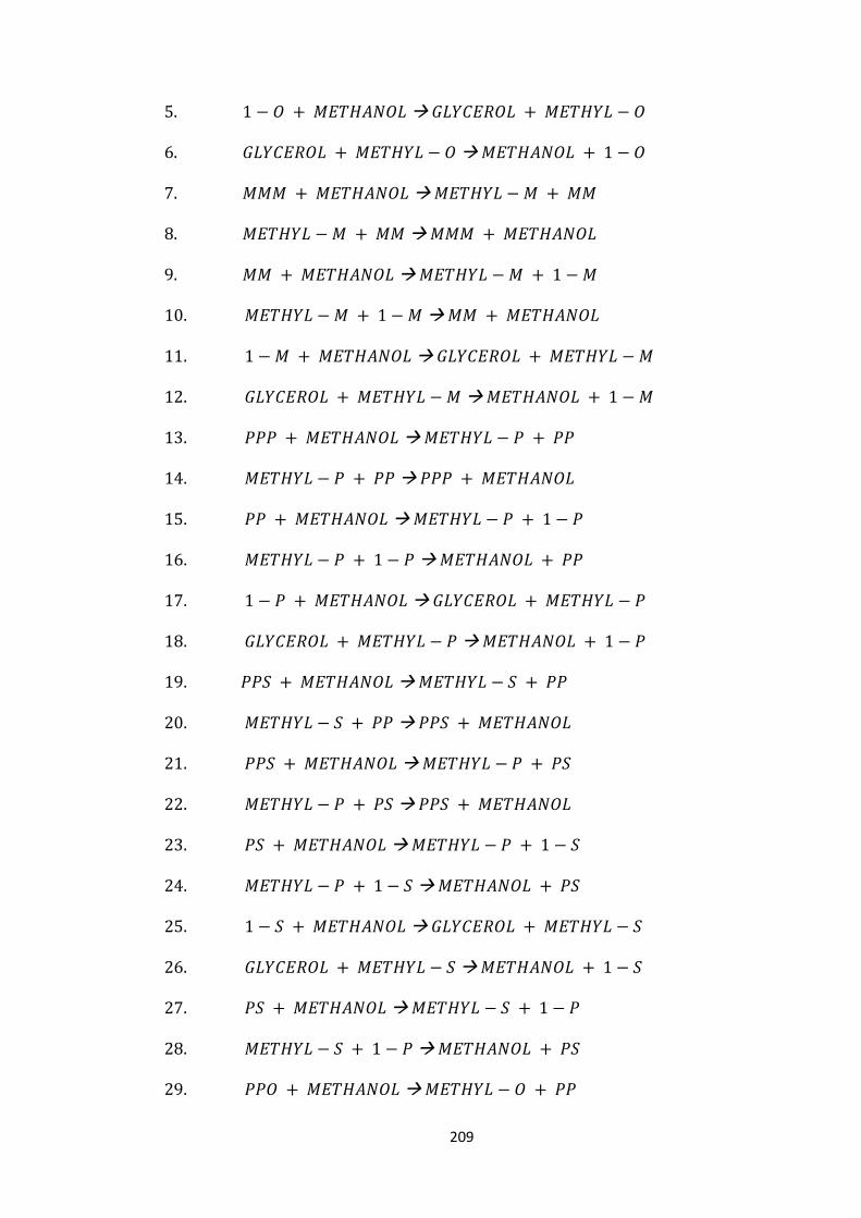
209
5. 1 − 𝑂 + 𝑀𝐸𝑇𝐻𝐴𝑁𝑂𝐿 𝐺𝐿𝑌𝐶𝐸𝑅𝑂𝐿 + 𝑀𝐸𝑇𝐻𝑌𝐿 − 𝑂
6. 𝐺𝐿𝑌𝐶𝐸𝑅𝑂𝐿 + 𝑀𝐸𝑇𝐻𝑌𝐿 − 𝑂 𝑀𝐸𝑇𝐻𝐴𝑁𝑂𝐿 + 1 − 𝑂
7. 𝑀𝑀𝑀 + 𝑀𝐸𝑇𝐻𝐴𝑁𝑂𝐿 𝑀𝐸𝑇𝐻𝑌𝐿 − 𝑀 + 𝑀𝑀
8. 𝑀𝐸𝑇𝐻𝑌𝐿 − 𝑀 + 𝑀𝑀 𝑀𝑀𝑀 + 𝑀𝐸𝑇𝐻𝐴𝑁𝑂𝐿
9. 𝑀𝑀 + 𝑀𝐸𝑇𝐻𝐴𝑁𝑂𝐿 𝑀𝐸𝑇𝐻𝑌𝐿 − 𝑀 + 1 − 𝑀
10. 𝑀𝐸𝑇𝐻𝑌𝐿 − 𝑀 + 1 − 𝑀 𝑀𝑀 + 𝑀𝐸𝑇𝐻𝐴𝑁𝑂𝐿
11. 1 − 𝑀 + 𝑀𝐸𝑇𝐻𝐴𝑁𝑂𝐿 𝐺𝐿𝑌𝐶𝐸𝑅𝑂𝐿 + 𝑀𝐸𝑇𝐻𝑌𝐿 − 𝑀
12. 𝐺𝐿𝑌𝐶𝐸𝑅𝑂𝐿 + 𝑀𝐸𝑇𝐻𝑌𝐿 − 𝑀 𝑀𝐸𝑇𝐻𝐴𝑁𝑂𝐿 + 1 − 𝑀
13. 𝑃𝑃𝑃 + 𝑀𝐸𝑇𝐻𝐴𝑁𝑂𝐿 𝑀𝐸𝑇𝐻𝑌𝐿 − 𝑃 + 𝑃𝑃
14. 𝑀𝐸𝑇𝐻𝑌𝐿 − 𝑃 + 𝑃𝑃 𝑃𝑃𝑃 + 𝑀𝐸𝑇𝐻𝐴𝑁𝑂𝐿
15. 𝑃𝑃 + 𝑀𝐸𝑇𝐻𝐴𝑁𝑂𝐿 𝑀𝐸𝑇𝐻𝑌𝐿 − 𝑃 + 1 − 𝑃
16. 𝑀𝐸𝑇𝐻𝑌𝐿 − 𝑃 + 1 − 𝑃 𝑀𝐸𝑇𝐻𝐴𝑁𝑂𝐿 + 𝑃𝑃
17. 1 − 𝑃 + 𝑀𝐸𝑇𝐻𝐴𝑁𝑂𝐿 𝐺𝐿𝑌𝐶𝐸𝑅𝑂𝐿 + 𝑀𝐸𝑇𝐻𝑌𝐿 − 𝑃
18. 𝐺𝐿𝑌𝐶𝐸𝑅𝑂𝐿 + 𝑀𝐸𝑇𝐻𝑌𝐿 − 𝑃 𝑀𝐸𝑇𝐻𝐴𝑁𝑂𝐿 + 1 − 𝑃
19. 𝑃𝑃𝑆 + 𝑀𝐸𝑇𝐻𝐴𝑁𝑂𝐿 𝑀𝐸𝑇𝐻𝑌𝐿 − 𝑆 + 𝑃𝑃
20. 𝑀𝐸𝑇𝐻𝑌𝐿 − 𝑆 + 𝑃𝑃 𝑃𝑃𝑆 + 𝑀𝐸𝑇𝐻𝐴𝑁𝑂𝐿
21. 𝑃𝑃𝑆 + 𝑀𝐸𝑇𝐻𝐴𝑁𝑂𝐿 𝑀𝐸𝑇𝐻𝑌𝐿 − 𝑃 + 𝑃𝑆
22. 𝑀𝐸𝑇𝐻𝑌𝐿 − 𝑃 + 𝑃𝑆 𝑃𝑃𝑆 + 𝑀𝐸𝑇𝐻𝐴𝑁𝑂𝐿
23. 𝑃𝑆 + 𝑀𝐸𝑇𝐻𝐴𝑁𝑂𝐿 𝑀𝐸𝑇𝐻𝑌𝐿 − 𝑃 + 1 − 𝑆
24. 𝑀𝐸𝑇𝐻𝑌𝐿 − 𝑃 + 1 − 𝑆 𝑀𝐸𝑇𝐻𝐴𝑁𝑂𝐿 + 𝑃𝑆
25. 1 − 𝑆 + 𝑀𝐸𝑇𝐻𝐴𝑁𝑂𝐿 𝐺𝐿𝑌𝐶𝐸𝑅𝑂𝐿 + 𝑀𝐸𝑇𝐻𝑌𝐿 − 𝑆
26. 𝐺𝐿𝑌𝐶𝐸𝑅𝑂𝐿 + 𝑀𝐸𝑇𝐻𝑌𝐿 − 𝑆 𝑀𝐸𝑇𝐻𝐴𝑁𝑂𝐿 + 1 − 𝑆
27. 𝑃𝑆 + 𝑀𝐸𝑇𝐻𝐴𝑁𝑂𝐿 𝑀𝐸𝑇𝐻𝑌𝐿 − 𝑆 + 1 − 𝑃
28. 𝑀𝐸𝑇𝐻𝑌𝐿 − 𝑆 + 1 − 𝑃 𝑀𝐸𝑇𝐻𝐴𝑁𝑂𝐿 + 𝑃𝑆
29. 𝑃𝑃𝑂 + 𝑀𝐸𝑇𝐻𝐴𝑁𝑂𝐿 𝑀𝐸𝑇𝐻𝑌𝐿 − 𝑂 + 𝑃𝑃
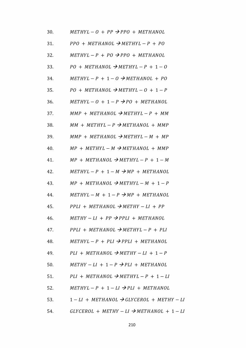
210
30. 𝑀𝐸𝑇𝐻𝑌𝐿 − 𝑂 + 𝑃𝑃 𝑃𝑃𝑂 + 𝑀𝐸𝑇𝐻𝐴𝑁𝑂𝐿
31. 𝑃𝑃𝑂 + 𝑀𝐸𝑇𝐻𝐴𝑁𝑂𝐿 𝑀𝐸𝑇𝐻𝑌𝐿 − 𝑃 + 𝑃𝑂
32. 𝑀𝐸𝑇𝐻𝑌𝐿 − 𝑃 + 𝑃𝑂 𝑃𝑃𝑂 + 𝑀𝐸𝑇𝐻𝐴𝑁𝑂𝐿
33. 𝑃𝑂 + 𝑀𝐸𝑇𝐻𝐴𝑁𝑂𝐿 𝑀𝐸𝑇𝐻𝑌𝐿 − 𝑃 + 1 − 𝑂
34. 𝑀𝐸𝑇𝐻𝑌𝐿 − 𝑃 + 1 − 𝑂 𝑀𝐸𝑇𝐻𝐴𝑁𝑂𝐿 + 𝑃𝑂
35. 𝑃𝑂 + 𝑀𝐸𝑇𝐻𝐴𝑁𝑂𝐿 𝑀𝐸𝑇𝐻𝑌𝐿 − 𝑂 + 1 − 𝑃
36. 𝑀𝐸𝑇𝐻𝑌𝐿 − 𝑂 + 1 − 𝑃 𝑃𝑂 + 𝑀𝐸𝑇𝐻𝐴𝑁𝑂𝐿
37. 𝑀𝑀𝑃 + 𝑀𝐸𝑇𝐻𝐴𝑁𝑂𝐿 𝑀𝐸𝑇𝐻𝑌𝐿 − 𝑃 + 𝑀𝑀
38. 𝑀𝑀 + 𝑀𝐸𝑇𝐻𝑌𝐿 − 𝑃 𝑀𝐸𝑇𝐻𝐴𝑁𝑂𝐿 + 𝑀𝑀𝑃
39. 𝑀𝑀𝑃 + 𝑀𝐸𝑇𝐻𝐴𝑁𝑂𝐿 𝑀𝐸𝑇𝐻𝑌𝐿 − 𝑀 + 𝑀𝑃
40. 𝑀𝑃 + 𝑀𝐸𝑇𝐻𝑌𝐿 − 𝑀 𝑀𝐸𝑇𝐻𝐴𝑁𝑂𝐿 + 𝑀𝑀𝑃
41. 𝑀𝑃 + 𝑀𝐸𝑇𝐻𝐴𝑁𝑂𝐿 𝑀𝐸𝑇𝐻𝑌𝐿 − 𝑃 + 1 − 𝑀
42. 𝑀𝐸𝑇𝐻𝑌𝐿 − 𝑃 + 1 − 𝑀 𝑀𝑃 + 𝑀𝐸𝑇𝐻𝐴𝑁𝑂𝐿
43. 𝑀𝑃 + 𝑀𝐸𝑇𝐻𝐴𝑁𝑂𝐿 𝑀𝐸𝑇𝐻𝑌𝐿 − 𝑀 + 1 − 𝑃
44. 𝑀𝐸𝑇𝐻𝑌𝐿 − 𝑀 + 1 − 𝑃 𝑀𝑃 + 𝑀𝐸𝑇𝐻𝐴𝑁𝑂𝐿
45. 𝑃𝑃𝐿𝐼 + 𝑀𝐸𝑇𝐻𝐴𝑁𝑂𝐿 𝑀𝐸𝑇𝐻𝑌 − 𝐿𝐼 + 𝑃𝑃
46. 𝑀𝐸𝑇𝐻𝑌 − 𝐿𝐼 + 𝑃𝑃 𝑃𝑃𝐿𝐼 + 𝑀𝐸𝑇𝐻𝐴𝑁𝑂𝐿
47. 𝑃𝑃𝐿𝐼 + 𝑀𝐸𝑇𝐻𝐴𝑁𝑂𝐿 𝑀𝐸𝑇𝐻𝑌𝐿 − 𝑃 + 𝑃𝐿𝐼
48. 𝑀𝐸𝑇𝐻𝑌𝐿 − 𝑃 + 𝑃𝐿𝐼 𝑃𝑃𝐿𝐼 + 𝑀𝐸𝑇𝐻𝐴𝑁𝑂𝐿
49. 𝑃𝐿𝐼 + 𝑀𝐸𝑇𝐻𝐴𝑁𝑂𝐿 𝑀𝐸𝑇𝐻𝑌 − 𝐿𝐼 + 1 − 𝑃
50. 𝑀𝐸𝑇𝐻𝑌 − 𝐿𝐼 + 1 − 𝑃 𝑃𝐿𝐼 + 𝑀𝐸𝑇𝐻𝐴𝑁𝑂𝐿
51. 𝑃𝐿𝐼 + 𝑀𝐸𝑇𝐻𝐴𝑁𝑂𝐿 𝑀𝐸𝑇𝐻𝑌𝐿 − 𝑃 + 1 − 𝐿𝐼
52. 𝑀𝐸𝑇𝐻𝑌𝐿 − 𝑃 + 1 − 𝐿𝐼 𝑃𝐿𝐼 + 𝑀𝐸𝑇𝐻𝐴𝑁𝑂𝐿
53. 1 − 𝐿𝐼 + 𝑀𝐸𝑇𝐻𝐴𝑁𝑂𝐿 𝐺𝐿𝑌𝐶𝐸𝑅𝑂𝐿 + 𝑀𝐸𝑇𝐻𝑌 − 𝐿𝐼
54. 𝐺𝐿𝑌𝐶𝐸𝑅𝑂𝐿 + 𝑀𝐸𝑇𝐻𝑌 − 𝐿𝐼 𝑀𝐸𝑇𝐻𝐴𝑁𝑂𝐿 + 1 − 𝐿𝐼
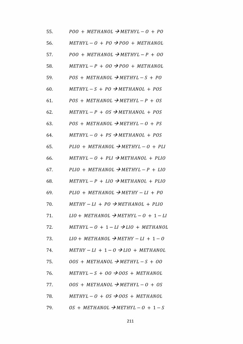
211
55. 𝑃𝑂𝑂 + 𝑀𝐸𝑇𝐻𝐴𝑁𝑂𝐿 𝑀𝐸𝑇𝐻𝑌𝐿 − 𝑂 + 𝑃𝑂
56. 𝑀𝐸𝑇𝐻𝑌𝐿 − 𝑂 + 𝑃𝑂 𝑃𝑂𝑂 + 𝑀𝐸𝑇𝐻𝐴𝑁𝑂𝐿
57. 𝑃𝑂𝑂 + 𝑀𝐸𝑇𝐻𝐴𝑁𝑂𝐿 𝑀𝐸𝑇𝐻𝑌𝐿 − 𝑃 + 𝑂𝑂
58. 𝑀𝐸𝑇𝐻𝑌𝐿 − 𝑃 + 𝑂𝑂 𝑃𝑂𝑂 + 𝑀𝐸𝑇𝐻𝐴𝑁𝑂𝐿
59. 𝑃𝑂𝑆 + 𝑀𝐸𝑇𝐻𝐴𝑁𝑂𝐿 𝑀𝐸𝑇𝐻𝑌𝐿 − 𝑆 + 𝑃𝑂
60. 𝑀𝐸𝑇𝐻𝑌𝐿 − 𝑆 + 𝑃𝑂 𝑀𝐸𝑇𝐻𝐴𝑁𝑂𝐿 + 𝑃𝑂𝑆
61. 𝑃𝑂𝑆 + 𝑀𝐸𝑇𝐻𝐴𝑁𝑂𝐿 𝑀𝐸𝑇𝐻𝑌𝐿 − 𝑃 + 𝑂𝑆
62. 𝑀𝐸𝑇𝐻𝑌𝐿 − 𝑃 + 𝑂𝑆 𝑀𝐸𝑇𝐻𝐴𝑁𝑂𝐿 + 𝑃𝑂𝑆
63. 𝑃𝑂𝑆 + 𝑀𝐸𝑇𝐻𝐴𝑁𝑂𝐿 𝑀𝐸𝑇𝐻𝑌𝐿 − 𝑂 + 𝑃𝑆
64. 𝑀𝐸𝑇𝐻𝑌𝐿 − 𝑂 + 𝑃𝑆 𝑀𝐸𝑇𝐻𝐴𝑁𝑂𝐿 + 𝑃𝑂𝑆
65. 𝑃𝐿𝐼𝑂 + 𝑀𝐸𝑇𝐻𝐴𝑁𝑂𝐿 𝑀𝐸𝑇𝐻𝑌𝐿 − 𝑂 + 𝑃𝐿𝐼
66. 𝑀𝐸𝑇𝐻𝑌𝐿 − 𝑂 + 𝑃𝐿𝐼 𝑀𝐸𝑇𝐻𝐴𝑁𝑂𝐿 + 𝑃𝐿𝐼𝑂
67. 𝑃𝐿𝐼𝑂 + 𝑀𝐸𝑇𝐻𝐴𝑁𝑂𝐿 𝑀𝐸𝑇𝐻𝑌𝐿 − 𝑃 + 𝐿𝐼𝑂
68. 𝑀𝐸𝑇𝐻𝑌𝐿 − 𝑃 + 𝐿𝐼𝑂 𝑀𝐸𝑇𝐻𝐴𝑁𝑂𝐿 + 𝑃𝐿𝐼𝑂
69. 𝑃𝐿𝐼𝑂 + 𝑀𝐸𝑇𝐻𝐴𝑁𝑂𝐿 𝑀𝐸𝑇𝐻𝑌 − 𝐿𝐼 + 𝑃𝑂
70. 𝑀𝐸𝑇𝐻𝑌 − 𝐿𝐼 + 𝑃𝑂 𝑀𝐸𝑇𝐻𝐴𝑁𝑂𝐿 + 𝑃𝐿𝐼𝑂
71. 𝐿𝐼𝑂 + 𝑀𝐸𝑇𝐻𝐴𝑁𝑂𝐿 𝑀𝐸𝑇𝐻𝑌𝐿 − 𝑂 + 1 − 𝐿𝐼
72. 𝑀𝐸𝑇𝐻𝑌𝐿 − 𝑂 + 1 − 𝐿𝐼 𝐿𝐼𝑂 + 𝑀𝐸𝑇𝐻𝐴𝑁𝑂𝐿
73. 𝐿𝐼𝑂 + 𝑀𝐸𝑇𝐻𝐴𝑁𝑂𝐿 𝑀𝐸𝑇𝐻𝑌 − 𝐿𝐼 + 1 − 𝑂
74. 𝑀𝐸𝑇𝐻𝑌 − 𝐿𝐼 + 1 − 𝑂 𝐿𝐼𝑂 + 𝑀𝐸𝑇𝐻𝐴𝑁𝑂𝐿
75. 𝑂𝑂𝑆 + 𝑀𝐸𝑇𝐻𝐴𝑁𝑂𝐿 𝑀𝐸𝑇𝐻𝑌𝐿 − 𝑆 + 𝑂𝑂
76. 𝑀𝐸𝑇𝐻𝑌𝐿 − 𝑆 + 𝑂𝑂 𝑂𝑂𝑆 + 𝑀𝐸𝑇𝐻𝐴𝑁𝑂𝐿
77. 𝑂𝑂𝑆 + 𝑀𝐸𝑇𝐻𝐴𝑁𝑂𝐿 𝑀𝐸𝑇𝐻𝑌𝐿 − 𝑂 + 𝑂𝑆
78. 𝑀𝐸𝑇𝐻𝑌𝐿 − 𝑂 + 𝑂𝑆 𝑂𝑂𝑆 + 𝑀𝐸𝑇𝐻𝐴𝑁𝑂𝐿
79. 𝑂𝑆 + 𝑀𝐸𝑇𝐻𝐴𝑁𝑂𝐿 𝑀𝐸𝑇𝐻𝑌𝐿 − 𝑂 + 1 − 𝑆
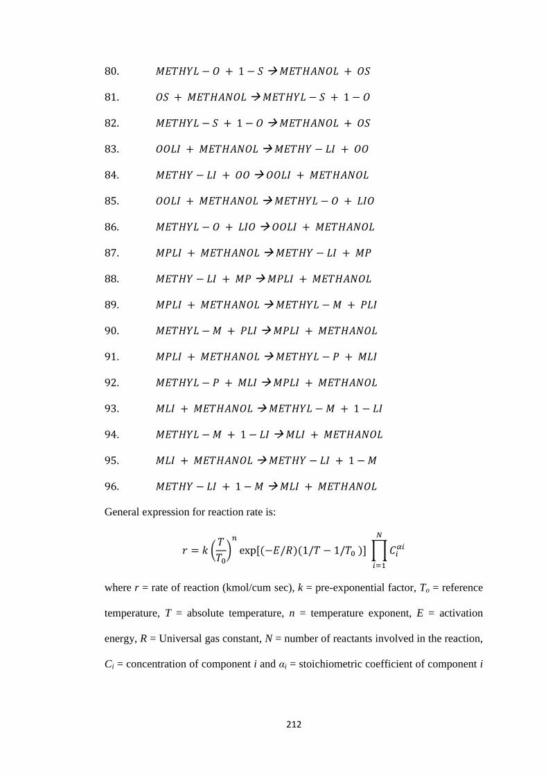
212
80. 𝑀𝐸𝑇𝐻𝑌𝐿 − 𝑂 + 1 − 𝑆 𝑀𝐸𝑇𝐻𝐴𝑁𝑂𝐿 + 𝑂𝑆
81. 𝑂𝑆 + 𝑀𝐸𝑇𝐻𝐴𝑁𝑂𝐿 𝑀𝐸𝑇𝐻𝑌𝐿 − 𝑆 + 1 − 𝑂
82. 𝑀𝐸𝑇𝐻𝑌𝐿 − 𝑆 + 1 − 𝑂 𝑀𝐸𝑇𝐻𝐴𝑁𝑂𝐿 + 𝑂𝑆
83. 𝑂𝑂𝐿𝐼 + 𝑀𝐸𝑇𝐻𝐴𝑁𝑂𝐿 𝑀𝐸𝑇𝐻𝑌 − 𝐿𝐼 + 𝑂𝑂
84. 𝑀𝐸𝑇𝐻𝑌 − 𝐿𝐼 + 𝑂𝑂 𝑂𝑂𝐿𝐼 + 𝑀𝐸𝑇𝐻𝐴𝑁𝑂𝐿
85. 𝑂𝑂𝐿𝐼 + 𝑀𝐸𝑇𝐻𝐴𝑁𝑂𝐿 𝑀𝐸𝑇𝐻𝑌𝐿 − 𝑂 + 𝐿𝐼𝑂
86. 𝑀𝐸𝑇𝐻𝑌𝐿 − 𝑂 + 𝐿𝐼𝑂 𝑂𝑂𝐿𝐼 + 𝑀𝐸𝑇𝐻𝐴𝑁𝑂𝐿
87. 𝑀𝑃𝐿𝐼 + 𝑀𝐸𝑇𝐻𝐴𝑁𝑂𝐿 𝑀𝐸𝑇𝐻𝑌 − 𝐿𝐼 + 𝑀𝑃
88. 𝑀𝐸𝑇𝐻𝑌 − 𝐿𝐼 + 𝑀𝑃 𝑀𝑃𝐿𝐼 + 𝑀𝐸𝑇𝐻𝐴𝑁𝑂𝐿
89. 𝑀𝑃𝐿𝐼 + 𝑀𝐸𝑇𝐻𝐴𝑁𝑂𝐿 𝑀𝐸𝑇𝐻𝑌𝐿 − 𝑀 + 𝑃𝐿𝐼
90. 𝑀𝐸𝑇𝐻𝑌𝐿 − 𝑀 + 𝑃𝐿𝐼 𝑀𝑃𝐿𝐼 + 𝑀𝐸𝑇𝐻𝐴𝑁𝑂𝐿
91. 𝑀𝑃𝐿𝐼 + 𝑀𝐸𝑇𝐻𝐴𝑁𝑂𝐿 𝑀𝐸𝑇𝐻𝑌𝐿 − 𝑃 + 𝑀𝐿𝐼
92. 𝑀𝐸𝑇𝐻𝑌𝐿 − 𝑃 + 𝑀𝐿𝐼 𝑀𝑃𝐿𝐼 + 𝑀𝐸𝑇𝐻𝐴𝑁𝑂𝐿
93. 𝑀𝐿𝐼 + 𝑀𝐸𝑇𝐻𝐴𝑁𝑂𝐿 𝑀𝐸𝑇𝐻𝑌𝐿 − 𝑀 + 1 − 𝐿𝐼
94. 𝑀𝐸𝑇𝐻𝑌𝐿 − 𝑀 + 1 − 𝐿𝐼 𝑀𝐿𝐼 + 𝑀𝐸𝑇𝐻𝐴𝑁𝑂𝐿
95. 𝑀𝐿𝐼 + 𝑀𝐸𝑇𝐻𝐴𝑁𝑂𝐿 𝑀𝐸𝑇𝐻𝑌 − 𝐿𝐼 + 1 − 𝑀
96. 𝑀𝐸𝑇𝐻𝑌 − 𝐿𝐼 + 1 − 𝑀 𝑀𝐿𝐼 + 𝑀𝐸𝑇𝐻𝐴𝑁𝑂𝐿
General expression for reaction rate is:
𝑟 = 𝑘 (𝑇
𝑇0)
𝑛
exp[(−𝐸/𝑅)(1/𝑇 − 1/𝑇0 )] ∏ 𝐶𝑖𝛼𝑖
𝑁
𝑖=1
where r = rate of reaction (kmol/cum sec), k = pre-exponential factor, To = reference
temperature, T = absolute temperature, n = temperature exponent, E = activation
energy, R = Universal gas constant, N = number of reactants involved in the reaction,
Ci = concentration of component i and αi = stoichiometric coefficient of component i
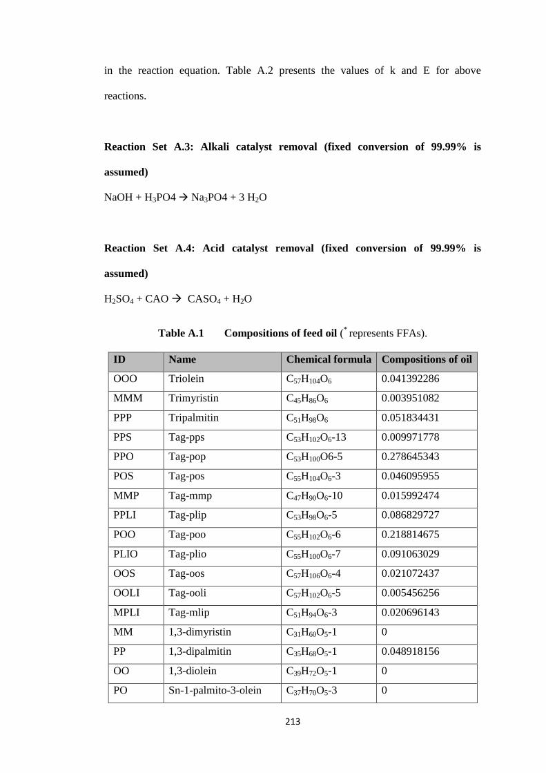
213
in the reaction equation. Table A.2 presents the values of k and E for above
reactions.
Reaction Set A.3: Alkali catalyst removal (fixed conversion of 99.99% is
assumed)
NaOH + H3PO4 Na3PO4 + 3 H2O
Reaction Set A.4: Acid catalyst removal (fixed conversion of 99.99% is
assumed)
H2SO4 + CAO CASO4 + H2O
Table A.1 Compositions of feed oil (* represents FFAs).
ID Name Chemical formula Compositions of oil
OOO Triolein C57H104O6 0.041392286
MMM Trimyristin C45H86O6 0.003951082
PPP Tripalmitin C51H98O6 0.051834431
PPS Tag-pps C53H102O6-13 0.009971778
PPO Tag-pop C53H100O6-5 0.278645343
POS Tag-pos C55H104O6-3 0.046095955
MMP Tag-mmp C47H90O6-10 0.015992474
PPLI Tag-plip C53H98O6-5 0.086829727
POO Tag-poo C55H102O6-6 0.218814675
PLIO Tag-plio C55H100O6-7 0.091063029
OOS Tag-oos C57H106O6-4 0.021072437
OOLI Tag-ooli C57H102O6-5 0.005456256
MPLI Tag-mlip C51H94O6-3 0.020696143
MM 1,3-dimyristin C31H60O5-1 0
PP 1,3-dipalmitin C35H68O5-1 0.048918156
OO 1,3-diolein C39H72O5-1 0
PO Sn-1-palmito-3-olein C37H70O5-3 0
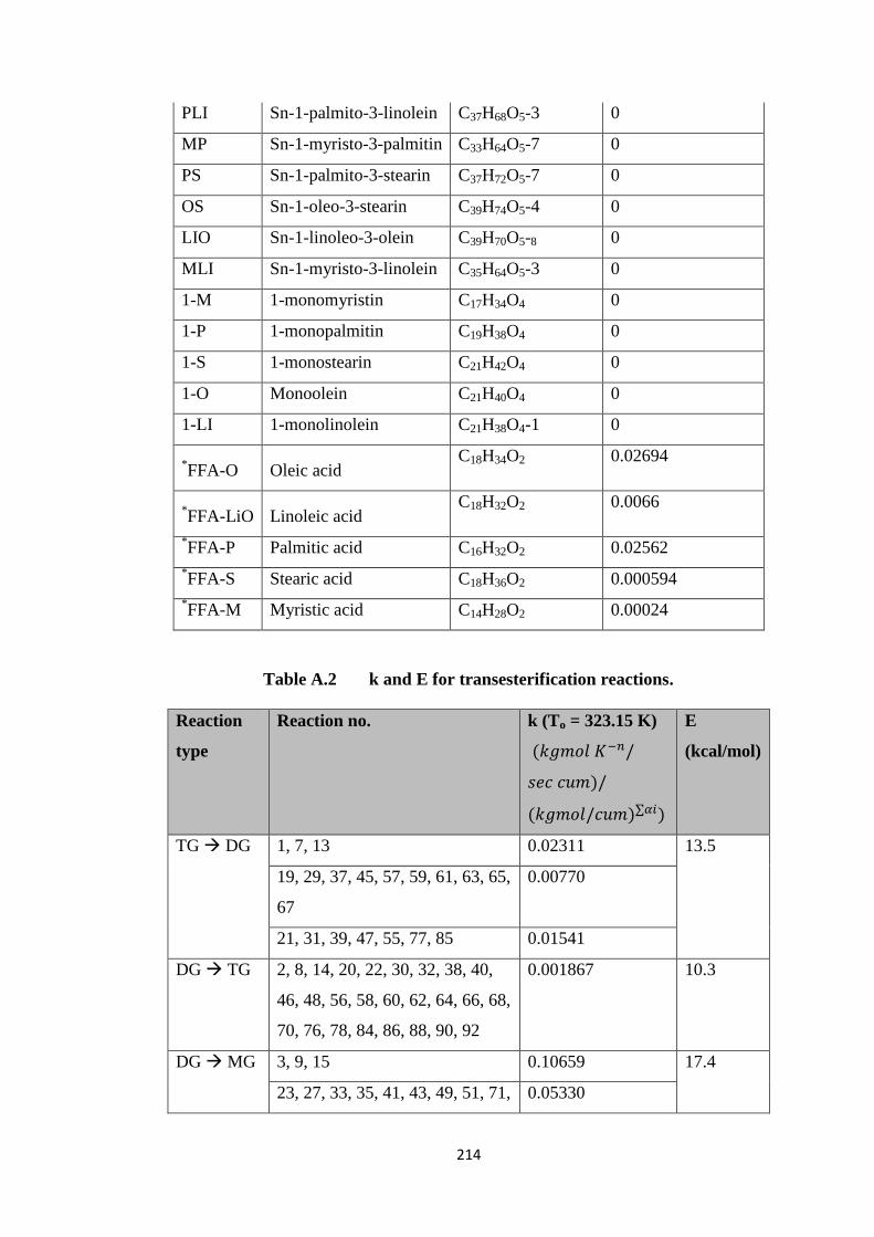
214
PLI Sn-1-palmito-3-linolein C37H68O5-3 0
MP Sn-1-myristo-3-palmitin C33H64O5-7 0
PS Sn-1-palmito-3-stearin C37H72O5-7 0
OS Sn-1-oleo-3-stearin C39H74O5-4 0
LIO Sn-1-linoleo-3-olein C39H70O5-8 0
MLI Sn-1-myristo-3-linolein C35H64O5-3 0
1-M 1-monomyristin C17H34O4 0
1-P 1-monopalmitin C19H38O4 0
1-S 1-monostearin C21H42O4 0
1-O Monoolein C21H40O4 0
1-LI 1-monolinolein C21H38O4-1 0
*FFA-O Oleic acid
C18H34O2 0.02694
*FFA-LiO Linoleic acid
C18H32O2 0.0066
*FFA-P Palmitic acid C16H32O2 0.02562
*FFA-S Stearic acid C18H36O2 0.000594
*FFA-M Myristic acid C14H28O2 0.00024
Table A.2 k and E for transesterification reactions.
Reaction
type
Reaction no. k (To = 323.15 K)
(𝑘𝑔𝑚𝑜𝑙 𝐾−𝑛/
𝑠𝑒𝑐 𝑐𝑢𝑚)/
(𝑘𝑔𝑚𝑜𝑙/𝑐𝑢𝑚)∑𝛼𝑖)
E
(kcal/mol)
TG DG 1, 7, 13 0.02311 13.5
19, 29, 37, 45, 57, 59, 61, 63, 65,
67
0.00770
21, 31, 39, 47, 55, 77, 85 0.01541
DG TG 2, 8, 14, 20, 22, 30, 32, 38, 40,
46, 48, 56, 58, 60, 62, 64, 66, 68,
70, 76, 78, 84, 86, 88, 90, 92
0.001867 10.3
DG MG 3, 9, 15 0.10659 17.4
23, 27, 33, 35, 41, 43, 49, 51, 71, 0.05330
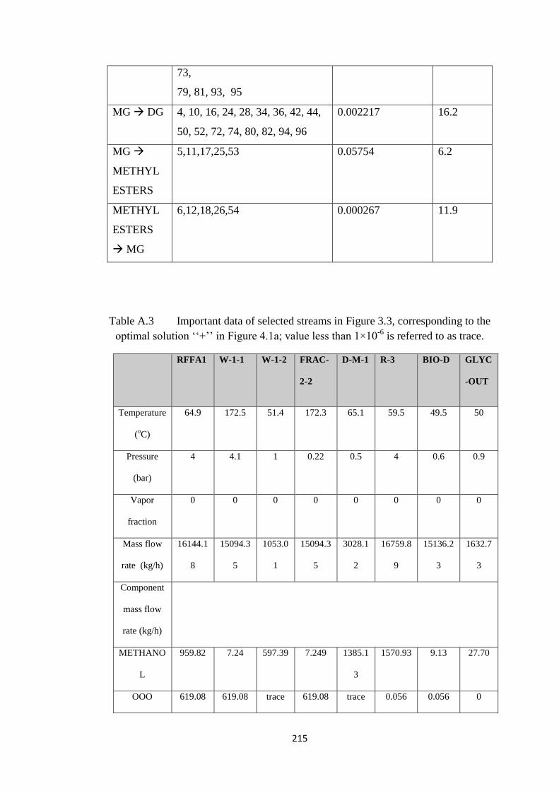
215
73,
79, 81, 93, 95
MG DG 4, 10, 16, 24, 28, 34, 36, 42, 44,
50, 52, 72, 74, 80, 82, 94, 96
0.002217 16.2
MG
METHYL
ESTERS
5,11,17,25,53 0.05754 6.2
METHYL
ESTERS
MG
6,12,18,26,54 0.000267 11.9
Table A.3 Important data of selected streams in Figure 3.3, corresponding to the
optimal solution ‘‘+’’ in Figure 4.1a; value less than 1×10⁻⁶
is referred to as trace.
RFFA1 W-1-1 W-1-2 FRAC-
2-2
D-M-1 R-3 BIO-D GLYC
-OUT
Temperature
(oC)
64.9 172.5 51.4 172.3 65.1 59.5 49.5 50
Pressure
(bar)
4 4.1 1 0.22 0.5 4 0.6 0.9
Vapor
fraction
0 0 0 0 0 0 0 0
Mass flow
rate (kg/h)
16144.1
8
15094.3
5
1053.0
1
15094.3
5
3028.1
2
16759.8
9
15136.2
3
1632.7
3
Component
mass flow
rate (kg/h)
METHANO
L
959.82 7.24 597.39 7.249 1385.1
3
1570.93 9.13 27.70
OOO 619.08 619.08 trace 619.08 trace 0.056 0.056 0
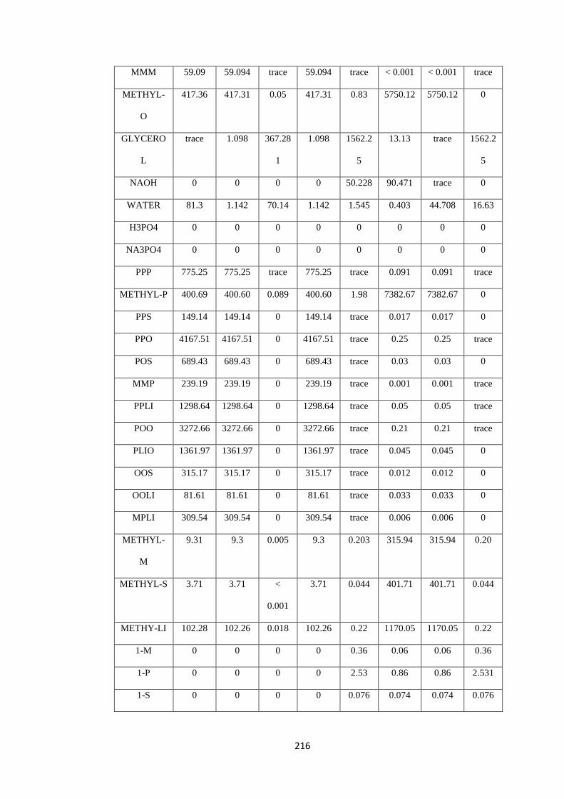
216
MMM 59.09 59.094 trace 59.094 trace < 0.001 < 0.001 trace
METHYL-
O
417.36 417.31 0.05 417.31 0.83 5750.12 5750.12 0
GLYCERO
L
trace 1.098 367.28
1
1.098 1562.2
5
13.13 trace 1562.2
5
NAOH 0 0 0 0 50.228 90.471 trace 0
WATER 81.3 1.142 70.14 1.142 1.545 0.403 44.708 16.63
H3PO4 0 0 0 0 0 0 0 0
NA3PO4 0 0 0 0 0 0 0 0
PPP 775.25 775.25 trace 775.25 trace 0.091 0.091 trace
METHYL-P 400.69 400.60 0.089 400.60 1.98 7382.67 7382.67 0
PPS 149.14 149.14 0 149.14 trace 0.017 0.017 0
PPO 4167.51 4167.51 0 4167.51 trace 0.25 0.25 trace
POS 689.43 689.43 0 689.43 trace 0.03 0.03 0
MMP 239.19 239.19 0 239.19 trace 0.001 0.001 trace
PPLI 1298.64 1298.64 0 1298.64 trace 0.05 0.05 trace
POO 3272.66 3272.66 0 3272.66 trace 0.21 0.21 trace
PLIO 1361.97 1361.97 0 1361.97 trace 0.045 0.045 0
OOS 315.17 315.17 0 315.17 trace 0.012 0.012 0
OOLI 81.61 81.61 0 81.61 trace 0.033 0.033 0
MPLI 309.54 309.54 0 309.54 trace 0.006 0.006 0
METHYL-
M
9.31 9.3 0.005 9.3 0.203 315.94 315.94 0.20
METHYL-S 3.71 3.71 <
0.001
3.71 0.044 401.71 401.71 0.044
METHY-LI 102.28 102.26 0.018 102.26 0.22 1170.05 1170.05 0.22
1-M 0 0 0 0 0.36 0.06 0.06 0.36
1-P 0 0 0 0 2.53 0.86 0.86 2.531
1-S 0 0 0 0 0.076 0.074 0.074 0.076
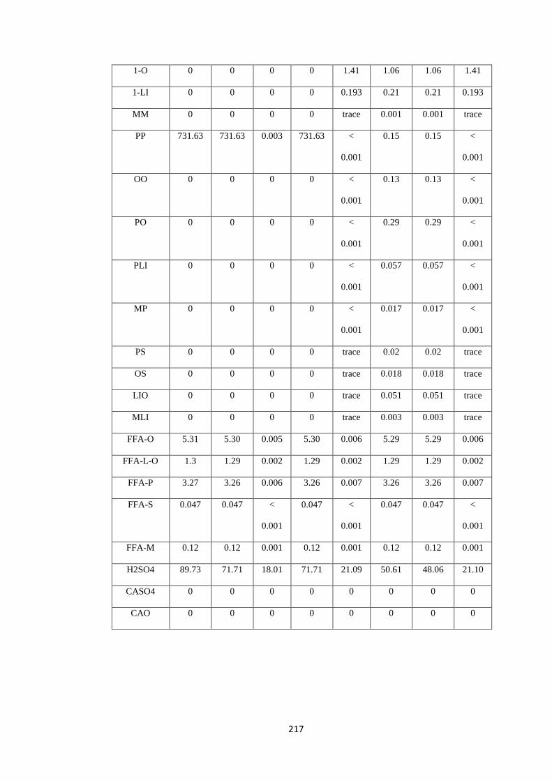
217
1-O 0 0 0 0 1.41 1.06 1.06 1.41
1-LI 0 0 0 0 0.193 0.21 0.21 0.193
MM 0 0 0 0 trace 0.001 0.001 trace
PP 731.63 731.63 0.003 731.63 <
0.001
0.15 0.15 <
0.001
OO 0 0 0 0 <
0.001
0.13 0.13 <
0.001
PO 0 0 0 0 <
0.001
0.29 0.29 <
0.001
PLI 0 0 0 0 <
0.001
0.057 0.057 <
0.001
MP 0 0 0 0 <
0.001
0.017 0.017 <
0.001
PS 0 0 0 0 trace 0.02 0.02 trace
OS 0 0 0 0 trace 0.018 0.018 trace
LIO 0 0 0 0 trace 0.051 0.051 trace
MLI 0 0 0 0 trace 0.003 0.003 trace
FFA-O 5.31 5.30 0.005 5.30 0.006 5.29 5.29 0.006
FFA-L-O 1.3 1.29 0.002 1.29 0.002 1.29 1.29 0.002
FFA-P 3.27 3.26 0.006 3.26 0.007 3.26 3.26 0.007
FFA-S 0.047 0.047 <
0.001
0.047 <
0.001
0.047 0.047 <
0.001
FFA-M 0.12 0.12 0.001 0.12 0.001 0.12 0.12 0.001
H2SO4 89.73 71.71 18.01 71.71 21.09 50.61 48.06 21.10
CASO4 0 0 0 0 0 0 0 0
CAO 0 0 0 0 0 0 0 0
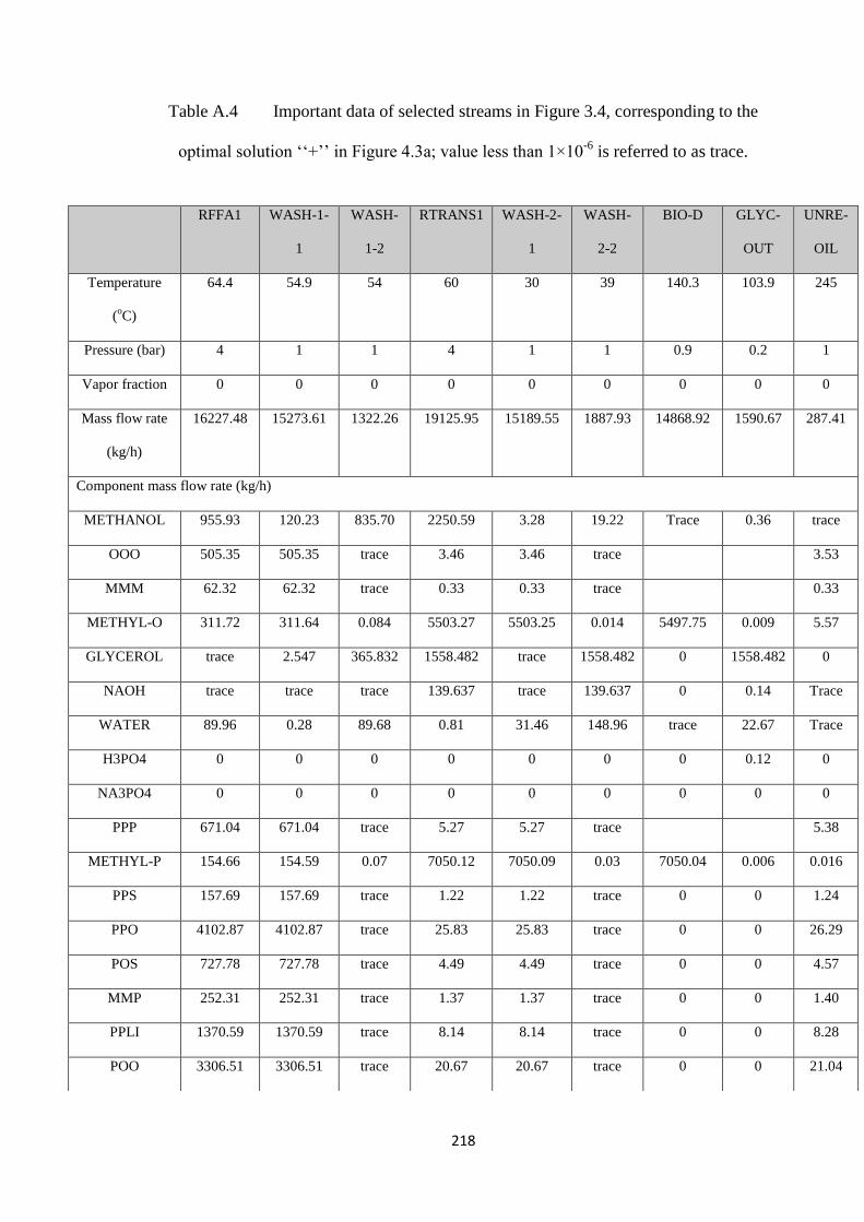
218
Table A.4 Important data of selected streams in Figure 3.4, corresponding to the
optimal solution ‘‘+’’ in Figure 4.3a; value less than 1×10⁻⁶
is referred to as trace.
RFFA1 WASH-1-
1
WASH-
1-2
RTRANS1 WASH-2-
1
WASH-
2-2
BIO-D GLYC-
OUT
UNRE-
OIL
Temperature
(oC)
64.4 54.9 54 60 30 39 140.3 103.9 245
Pressure (bar) 4 1 1 4 1 1 0.9 0.2 1
Vapor fraction 0 0 0 0 0 0 0 0 0
Mass flow rate
(kg/h)
16227.48 15273.61 1322.26 19125.95 15189.55 1887.93 14868.92 1590.67 287.41
Component mass flow rate (kg/h)
METHANOL 955.93 120.23 835.70 2250.59 3.28 19.22 Trace 0.36 trace
OOO 505.35 505.35 trace 3.46 3.46 trace 3.53
MMM 62.32 62.32 trace 0.33 0.33 trace 0.33
METHYL-O 311.72 311.64 0.084 5503.27 5503.25 0.014 5497.75 0.009 5.57
GLYCEROL trace 2.547 365.832 1558.482 trace 1558.482 0 1558.482 0
NAOH trace trace trace 139.637 trace 139.637 0 0.14 Trace
WATER 89.96 0.28 89.68 0.81 31.46 148.96 trace 22.67 Trace
H3PO4 0 0 0 0 0 0 0 0.12 0
NA3PO4 0 0 0 0 0 0 0 0 0
PPP 671.04 671.04 trace 5.27 5.27 trace 5.38
METHYL-P 154.66 154.59 0.07 7050.12 7050.09 0.03 7050.04 0.006 0.016
PPS 157.69 157.69 trace 1.22 1.22 trace 0 0 1.24
PPO 4102.87 4102.87 trace 25.83 25.83 trace 0 0 26.29
POS 727.78 727.78 trace 4.49 4.49 trace 0 0 4.57
MMP 252.31 252.31 trace 1.37 1.37 trace 0 0 1.40
PPLI 1370.59 1370.59 trace 8.14 8.14 trace 0 0 8.28
POO 3306.51 3306.51 trace 20.67 20.67 trace 0 0 21.04
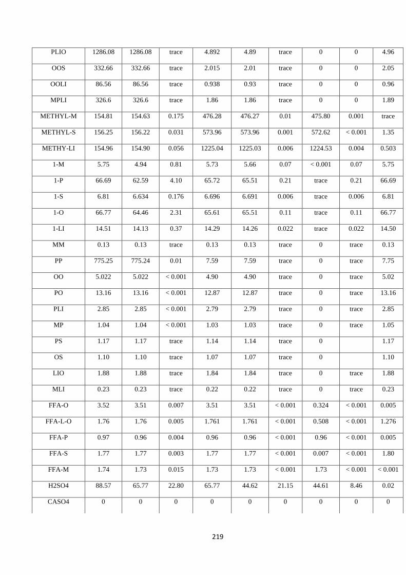
219
PLIO 1286.08 1286.08 trace 4.892 4.89 trace 0 0 4.96
OOS 332.66 332.66 trace 2.015 2.01 trace 0 0 2.05
OOLI 86.56 86.56 trace 0.938 0.93 trace 0 0 0.96
MPLI 326.6 326.6 trace 1.86 1.86 trace 0 0 1.89
METHYL-M 154.81 154.63 0.175 476.28 476.27 0.01 475.80 0.001 trace
METHYL-S 156.25 156.22 0.031 573.96 573.96 0.001 572.62 < 0.001 1.35
METHY-LI 154.96 154.90 0.056 1225.04 1225.03 0.006 1224.53 0.004 0.503
1-M 5.75 4.94 0.81 5.73 5.66 0.07 < 0.001 0.07 5.75
1-P 66.69 62.59 4.10 65.72 65.51 0.21 trace 0.21 66.69
1-S 6.81 6.634 0.176 6.696 6.691 0.006 trace 0.006 6.81
1-O 66.77 64.46 2.31 65.61 65.51 0.11 trace 0.11 66.77
1-LI 14.51 14.13 0.37 14.29 14.26 0.022 trace 0.022 14.50
MM 0.13 0.13 trace 0.13 0.13 trace 0 trace 0.13
PP 775.25 775.24 0.01 7.59 7.59 trace 0 trace 7.75
OO 5.022 5.022 < 0.001 4.90 4.90 trace 0 trace 5.02
PO 13.16 13.16 < 0.001 12.87 12.87 trace 0 trace 13.16
PLI 2.85 2.85 < 0.001 2.79 2.79 trace 0 trace 2.85
MP 1.04 1.04 < 0.001 1.03 1.03 trace 0 trace 1.05
PS 1.17 1.17 trace 1.14 1.14 trace 0 1.17
OS 1.10 1.10 trace 1.07 1.07 trace 0 1.10
LIO 1.88 1.88 trace 1.84 1.84 trace 0 trace 1.88
MLI 0.23 0.23 trace 0.22 0.22 trace 0 trace 0.23
FFA-O 3.52 3.51 0.007 3.51 3.51 < 0.001 0.324 < 0.001 0.005
FFA-L-O 1.76 1.76 0.005 1.761 1.761 < 0.001 0.508 < 0.001 1.276
FFA-P 0.97 0.96 0.004 0.96 0.96 < 0.001 0.96 < 0.001 0.005
FFA-S 1.77 1.77 0.003 1.77 1.77 < 0.001 0.007 < 0.001 1.80
FFA-M 1.74 1.73 0.015 1.73 1.73 < 0.001 1.73 < 0.001 < 0.001
H2SO4 88.57 65.77 22.80 65.77 44.62 21.15 44.61 8.46 0.02
CASO4 0 0 0 0 0 0 0 0 0
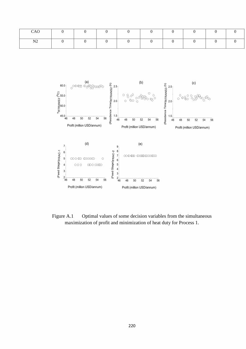
220
46 48 50 52 54 5645.0
50.0
55.0
60.0
(a)
TR
TR
AN
S3
(oC
)
46 48 50 52 54 56
1.5
2.0
2.5
(b)
(Resid
ence T
ime) R
TR
AN
S2 (
h)
46 48 50 52 54 56
1.5
2.0
2.5
(c)
(Resid
ence T
ime) R
TR
AN
S3 (
h)
46 48 50 52 54 562
3
4
5
6
7
Profit (million USD/annum)
Profit (million USD/annum)Profit (million USD/annum)
(d)
(Fe
ed
Sta
ge
) FR
AC
-1
46 48 50 52 54 562
3
4
5
6
7
8
9
Profit (million USD/annum)Profit (million USD/annum)
(e)
(Fe
ed
Sta
ge
) FR
AC
-2
Figure A.1 Optimal values of some decision variables from the simultaneous
maximization of profit and minimization of heat duty for Process 1.
CAO 0 0 0 0 0 0 0 0 0
N2 0 0 0 0 0 0 0 0 0
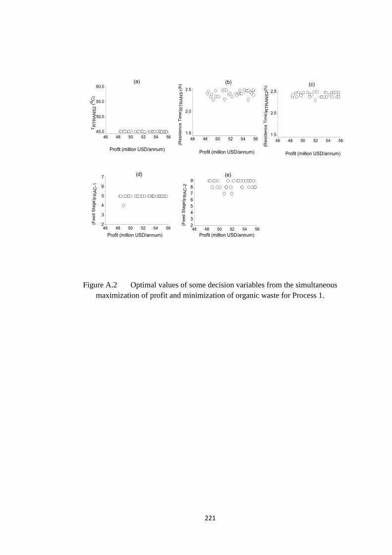
221
46 48 50 52 54 56
45.0
50.0
55.0
60.0(a)
TR
TR
AN
S2
(oC
)
46 48 50 52 54 56
1.5
2.0
2.5
(b)
(Resid
ence T
ime) R
TR
AN
S1
(h)
46 48 50 52 54 56
1.5
2.0
2.5
(c)
(Resid
ence T
ime) R
TR
AN
S2
(h)
46 48 50 52 54 562
3
4
5
6
7
Profit (million USD/annum)
Profit (million USD/annum)
(d)
(Feed S
tage) F
RA
C-1
46 48 50 52 54 562
3
4
5
6
7
8
9
Profit (million USD/annum)
Profit (million USD/annum)Profit (million USD/annum)
(e)
(Feed S
tage) F
RA
C-2
Figure A.2 Optimal values of some decision variables from the simultaneous
maximization of profit and minimization of organic waste for Process 1.
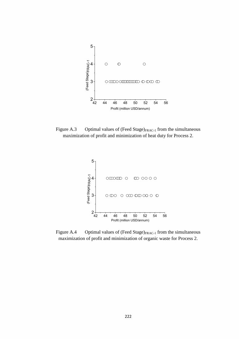
222
42 44 46 48 50 52 54 562
3
4
5
(Feed S
tage) F
RA
C-1
Profit (million USD/annum)
Figure A.3 Optimal values of (Feed Stage)FRAC-1 from the simultaneous
maximization of profit and minimization of heat duty for Process 2.
42 44 46 48 50 52 54 562
3
4
5
(Feed S
tage) F
RA
C-1
Profit (million USD/annum)
Figure A.4 Optimal values of (Feed Stage)FRAC-1 from the simultaneous
maximization of profit and minimization of organic waste for Process 2.
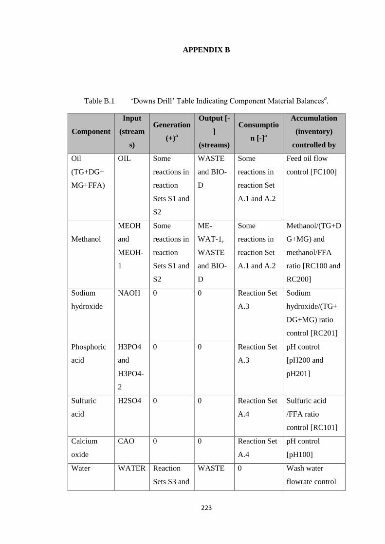
223
APPENDIX B
Table B.1 ‘Downs Drill’ Table Indicating Component Material Balancesa.
Component
Input
(stream
s)
Generation
(+)a
Output [-
]
(streams)
Consumptio
n [-]a
Accumulation
(inventory)
controlled by
Oil
(TG+DG+
MG+FFA)
OIL Some
reactions in
reaction
Sets S1 and
S2
WASTE
and BIO-
D
Some
reactions in
reaction Set
A.1 and A.2
Feed oil flow
control [FC100]
Methanol
MEOH
and
MEOH-
1
Some
reactions in
reaction
Sets S1 and
S2
ME-
WAT-1,
WASTE
and BIO-
D
Some
reactions in
reaction Set
A.1 and A.2
Methanol/(TG+D
G+MG) and
methanol/FFA
ratio [RC100 and
RC200]
Sodium
hydroxide
NAOH 0 0 Reaction Set
A.3
Sodium
hydroxide/(TG+
DG+MG) ratio
control [RC201]
Phosphoric
acid
H3PO4
and
H3PO4-
2
0 0 Reaction Set
A.3
pH control
[pH200 and
pH201]
Sulfuric
acid
H2SO4 0 0 Reaction Set
A.4
Sulfuric acid
/FFA ratio
control [RC101]
Calcium
oxide
CAO 0 0 Reaction Set
A.4
pH control
[pH100]
Water WATER Reaction
Sets S3 and
WASTE 0 Wash water
flowrate control
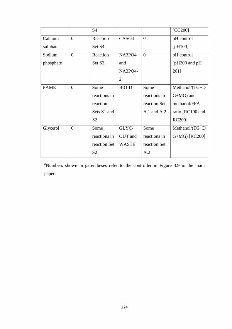
224
S4 [CC200]
Calcium
sulphate
0 Reaction
Set S4
CASO4 0 pH control
[pH100]
Sodium
phosphate
0 Reaction
Set S3
NA3PO4
and
NA3PO4-
2
0 pH control
[pH200 and pH
201]
FAME 0 Some
reactions in
reaction
Sets S1 and
S2
BIO-D Some
reactions in
reaction Set
A.1 and A.2
Methanol/(TG+D
G+MG) and
methanol/FFA
ratio [RC100 and
RC200]
Glycerol 0 Some
reactions in
reaction Set
S2
GLYC-
OUT and
WASTE
Some
reactions in
reaction Set
A.2
Methanol/(TG+D
G+MG) [RC200]
aNumbers shown in parentheses refer to the controller in Figure 3.9 in the main
paper.
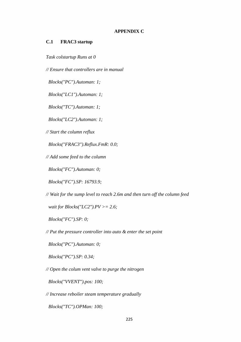
225
APPENDIX C
C.1 FRAC3 startup
Task colstartup Runs at 0
// Ensure that controllers are in manual
Blocks("PC").Automan: 1;
Blocks("LC1").Automan: 1;
Blocks("TC").Automan: 1;
Blocks("LC2").Automan: 1;
// Start the column reflux
Blocks("FRAC3").Reflux.FmR: 0.0;
// Add some feed to the column
Blocks("FC").Automan: 0;
Blocks("FC").SP: 16793.9;
// Wait for the sump level to reach 2.6m and then turn off the column feed
wait for Blocks("LC2").PV >= 2.6;
Blocks("FC").SP: 0;
// Put the pressure controller into auto & enter the set point
Blocks("PC").Automan: 0;
Blocks("PC").SP: 0.34;
// Open the colum vent valve to purge the nitrogen
Blocks("VVENT").pos: 100;
// Increase reboiler steam temperature gradually
Blocks("TC").OPMan: 100;
226
Wait 0.1;
Blocks("TC").OPMan: 150;
Wait 0.1;
Blocks("TC").OPMan: 200;
Wait 0.1;
// Start the column reflux
Blocks("FRAC3").Reflux.FmR: 770;
Wait 0.05;
// Continue increasing steam temperature
Blocks("TC").OPMan: 230;
// Close vent valve when N2 is purged
Blocks("VVENT").pos: 0;
// Put the reflux drum level control into auto & enter the set point
Blocks("LC1").Automan: 0;
Blocks("LC1").SP: 0.33;
// Add some more feed until the sump level reaches 2.6m
Blocks("FC").SP: 16793.9;
wait for Blocks("LC2").PV >= 2.6;
Blocks("FC").SP: 0;
// Increase reboiler steam temp
Blocks("TC").OPMan: 250;
wait 0.15;
Blocks("TC").OPMan: 280;
227
wait 0.15;
// Wait until the level in the reflux drum rises to 0.3
wait for Blocks("LC1").PV >= 0.3;
// ... put the sump level controller to automatic
Blocks("LC2").Automan: 0;
Blocks("LC2").SP: 2.4;
// and increase the reflux rate to the final value
Blocks("FRAC3").Reflux.FmR: 777.621;
// start the column feed - put the feed valve to 50% open
Blocks("FC").SP: 16793.9;
wait 0.5;
// Ramp up the steam temperature
Blocks("TC").OPMan: 320;
// Wait until bottom temperature reaches 230 OC and put the temperature controller
to Auto mode
wait for Blocks("TC").PV >= 230;
Blocks("TC").Automan: 0;
wait 0.1;
// Change the reflux level & sump level set points to the final value
Blocks("LC1").SP: 0.36;
Blocks("LC2").SP: 1.64;
// Wait for 1 more hour and pause the simulation
wait 1.0;
228
Pause;
End
C.2 Utility trip in FRAC3
Task utilitytrip
Runs When Blocks("FRAC3").TReb >= 250;
Blocks("TC").OPMan: 100;
Print "UTILITYTRIP encountered due to reboiler temperature shoot up";
pause;
End
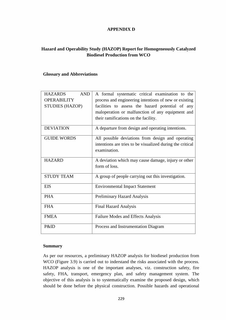
229
APPENDIX D
Hazard and Operability Study (HAZOP) Report for Homogeneously Catalyzed
Biodiesel Production from WCO
Glossary and Abbreviations
HAZARDS AND
OPERABILITY
STUDIES (HAZOP)
A formal systematic critical examination to the
process and engineering intentions of new or existing
facilities to assess the hazard potential of any
maloperation or malfunction of any equipment and
their ramifications on the facility.
DEVIATION A departure from design and operating intentions.
GUIDE WORDS All possible deviations from design and operating
intentions are tries to be visualized during the critical
examination.
HAZARD A deviation which may cause damage, injury or other
form of loss.
STUDY TEAM A group of people carrying out this investigation.
EIS Environmental Impact Statement
PHA Preliminary Hazard Analysis
FHA Final Hazard Analysis
FMEA Failure Modes and Effects Analysis
P&ID Process and Instrumentation Diagram
Summary
As per our resources, a preliminary HAZOP analysis for biodiesel production from
WCO (Figure 3.9) is carried out to inderstand the risks associated with the process.
HAZOP analysis is one of the important analyses, viz. construction safety, fire
safety, FHA, transport, emergency plan, and safety management system. The
objective of this analysis is to systematically examine the proposed design, which
should be done before the physical construction. Possible hazards and operational
230
problems can be prevented or reduced by redesign of suitable operating procedures.
Plant items in the process flowsheet are evaluated by applying appropriate guide
words. Potentially hazardous situations and their ramifications are then estimated.
Preventing measures to avoid or reduce the undesirable situations are also
recommended. The findings of the step by step procedure and the recommendations
are organized in the HAZOP minute sheet. Figure 3.17 presents HAZOPed process
diagram for biodiesel production from WCO. The important recommendations from
this analysis are:
The vital recommendations from this analysis are:
Rec #1
Install high flow alarm on feed line.
Rec #10, #24, #52 & #60
Install high level alarms on the column to ensure that the operating efficiency is
maintained by avoiding the flooding of reboiler outlet.
Rec #8, #16, #22, #30, #34, #42, #50, #56, #58, #64, #66
Install high pressure and high temperature alarms on columns and reactors to prevent
overheating.
Rec #15, #29, #57 & #65
Investigate the need for protection against such back into the column on cooling.
231
Hazop Study
Technical description of the plant and the guide words and any other important
details are explained briefly to enable reader to follow the minute sheets.
1.1 Description of the facility
The main plant items consist of distillation columns (FRAC-1, FRAC-2, FRAC-3,
FRAC-4), Four CSTRs (RFFA, RTRANS1, RTRANS2, RTRANS3). Heat
exchangers (H-1, H-3), Coolers (H-2, H-4, H-5), phase separators (W-1, D-1, D-2,
WASH-2) and pumps and control instruments. A process description has been given
in the earlier section (see Figure 3.9). The control structure obtained by applying a
systematic integrated framework approach is discussed in the previous section.
1.2 HAZOP team members
Normally, a team should consist of experts from all relevant fields from design
through commissioning to operation (design engineer, operation engineer,
maintenance supervisor, HAZOP chairman and instrument engineer. However in this
study, a preliminary analysis is carried out by us.
1.3 HAZOP methodology
All important unit operations in the plant are HAZOPed. Guide words such as HIGH
FLOW, as described below, are used in the minute sheet. For each guide word, the
potential causes were analyzed and mentioned in the second column. Their
ramifications are mentioned in the third column. The fourth column is to record any
existing design or operational safeguards. The recommendations, for the causes
which may lead to several hazardous situation or loss in terms of product and time,
are then entered in the sixth column against the recommendation number (Rec #).
These recommendations include possible changes to the system to eliminate or
reduce the consequences. Further evaluation is considered necessary as required and
the recommendations are minuted accordingly.
1.4 Guide words
The guide words used in this analysis are:
Flow: HIGH LOW ZERO REVERSE
Level: HIGH LOW
Pressure: HIGH LOW
Temperature: HIGH LOW
232
1.5 Plant overview
In this analysis, only the operating mode is covered. However, in a complete HAZOP
study including start-up/shutdown procedures, more changes may be recommended.
The issue to be analysed further prior to changing the design are:
Rec #17, #25, #65 & #73
Consider nitrogen gas purging in the distillation columns (and in condensers) before
start-up, to expel air sucked in on cooling during shut down.
Rec #16, #24, #64 & #72
Recommendations minuted (regarding backup cooling water system) to be adopted
or not; further investigations may be needed.
1.5 Analysis of main findings
The HAZOP results are described in the minute sheet (Table D.1). The results of
each deviation are examined to verify if the ramification would cause a hazardous
condition to the plant. All critical unit operations are analysed. If the hazard or loss is
found to be credible, the safeguard should be developed to eliminate or reduce the
possibility. Additionally, the alarms and trip systems are recommended wherever the
possibilities of hazard are anticipated. Please refer to the minute sheet.
1.6 Action arising from HAZOP study
The recommendations outlined from the HAZOP analysis that are to be included in
the design are as shown in Figure 3.18 (Drawing no. BD 001 REV2). Note the
changes and the additional instruments and alarms.
The implementation of the changes as a result of HAZOP should not lead to any
potential hazard to plant personnel, public or environment.
The pre-commissioning and commissioning checklists and the test procedures should
be modified to ensure that the final recommendations of HAZOP are verified at
every appropriate stage.
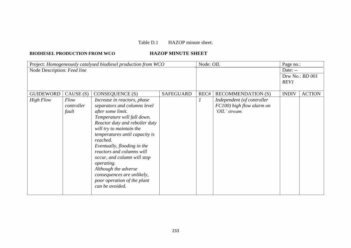
233
Table D.1 HAZOP minute sheet.
BIODIESEL PRODUCTION FROM WCO HAZOP MINUTE SHEET
Project: Homogeneously catalysed biodiesel production from WCO Node: OIL Page no.:
Date: -- Node Description: Feed line
Drw No.: BD 001
REV1
GUIDEWORD CAUSE (S) CONSEQUENCE (S) SAFEGUARD REC# RECOMMENDATION (S) INDIV ACTION
High Flow Flow
controller
fault
Increase in reactors, phase
separators and columns level
after some limit.
Temperature will fall down.
Reactor duty and reboiler duty
will try to maintain the
temperatures until capacity is
reached.
Eventually, flooding in the
reactors and columns will
occur, and column will stop
operating.
Although the adverse
consequences are unlikely,
poor operation of the plant
can be avoided.
1 Independent (of controller
FC100) high flow alarm on
‘OIL’ stream.
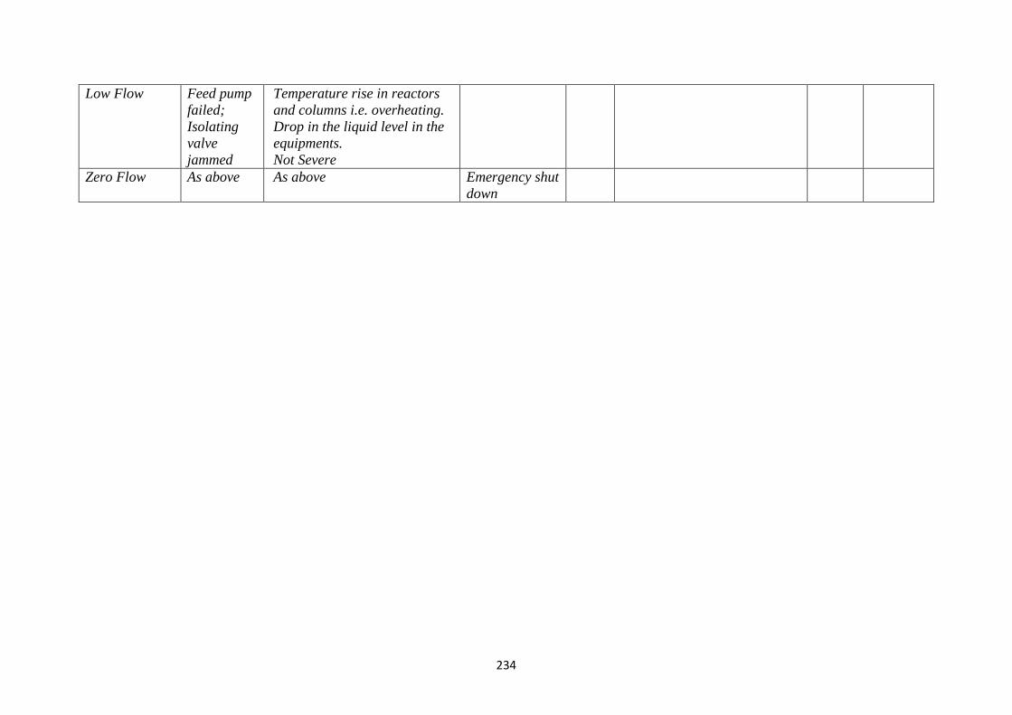
234
Low Flow Feed pump
failed;
Isolating
valve
jammed
Temperature rise in reactors
and columns i.e. overheating.
Drop in the liquid level in the
equipments.
Not Severe
Zero Flow As above As above Emergency shut
down
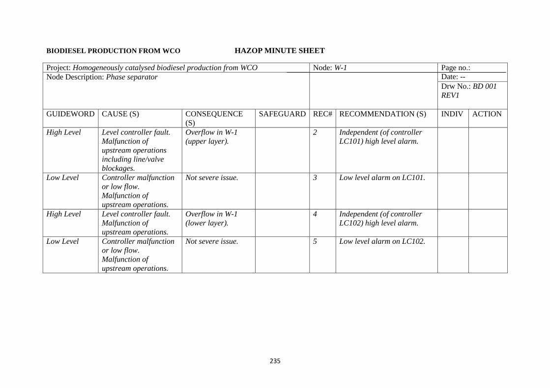
235
BIODIESEL PRODUCTION FROM WCO HAZOP MINUTE SHEET
Project: Homogeneously catalysed biodiesel production from WCO Node: W-1 Page no.:
Date: -- Node Description: Phase separator
Drw No.: BD 001
REV1
GUIDEWORD CAUSE (S) CONSEQUENCE
(S)
SAFEGUARD REC# RECOMMENDATION (S) INDIV ACTION
High Level Level controller fault.
Malfunction of
upstream operations
including line/valve
blockages.
Overflow in W-1
(upper layer).
2 Independent (of controller
LC101) high level alarm.
Low Level Controller malfunction
or low flow.
Malfunction of
upstream operations.
Not severe issue. 3 Low level alarm on LC101.
High Level Level controller fault.
Malfunction of
upstream operations.
Overflow in W-1
(lower layer).
4 Independent (of controller
LC102) high level alarm.
Low Level Controller malfunction
or low flow.
Malfunction of
upstream operations.
Not severe issue. 5 Low level alarm on LC102.
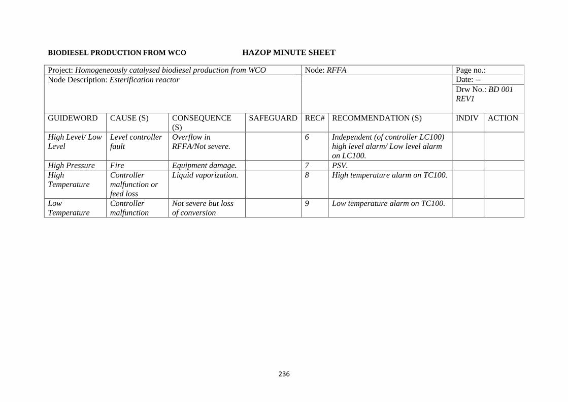
236
BIODIESEL PRODUCTION FROM WCO HAZOP MINUTE SHEET
Project: Homogeneously catalysed biodiesel production from WCO Node: RFFA Page no.:
Date: -- Node Description: Esterification reactor
Drw No.: BD 001
REV1
GUIDEWORD CAUSE (S) CONSEQUENCE
(S)
SAFEGUARD REC# RECOMMENDATION (S) INDIV ACTION
High Level/ Low
Level
Level controller
fault
Overflow in
RFFA/Not severe.
6 Independent (of controller LC100)
high level alarm/ Low level alarm
on LC100.
High Pressure Fire Equipment damage. 7 PSV.
High
Temperature
Controller
malfunction or
feed loss
Liquid vaporization. 8 High temperature alarm on TC100.
Low
Temperature
Controller
malfunction
Not severe but loss
of conversion
9 Low temperature alarm on TC100.
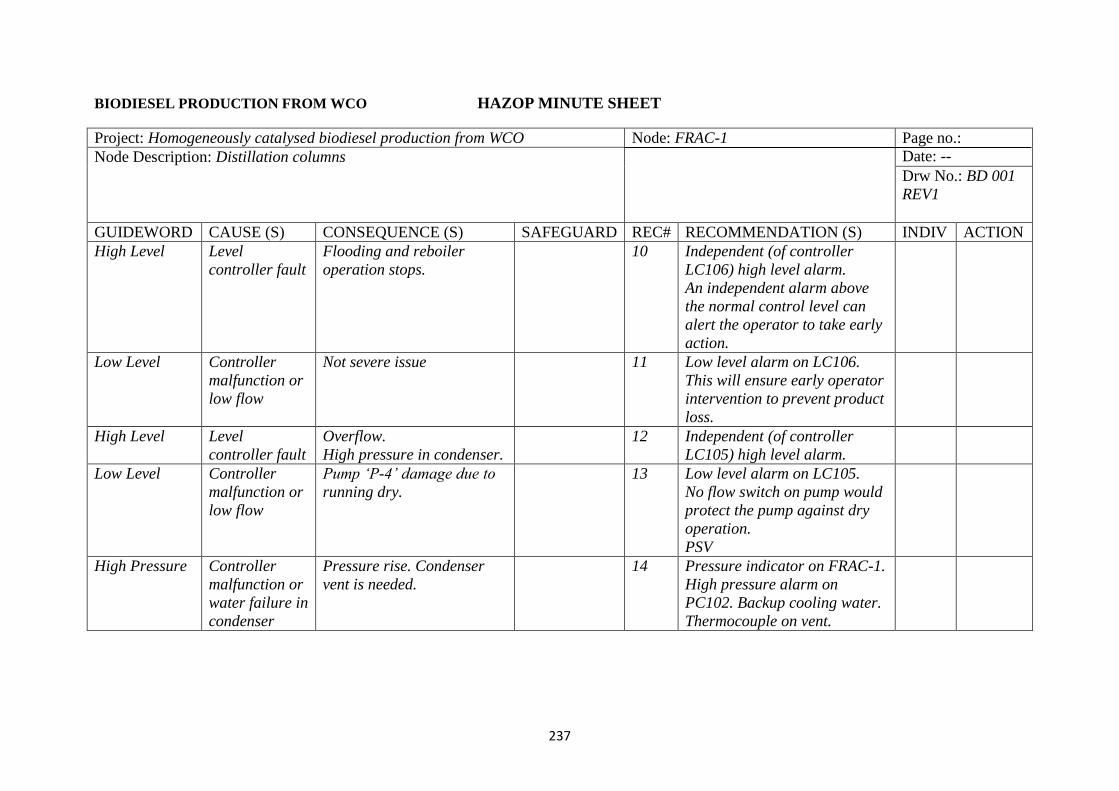
237
BIODIESEL PRODUCTION FROM WCO HAZOP MINUTE SHEET
Project: Homogeneously catalysed biodiesel production from WCO Node: FRAC-1 Page no.:
Date: -- Node Description: Distillation columns
Drw No.: BD 001
REV1
GUIDEWORD CAUSE (S) CONSEQUENCE (S) SAFEGUARD REC# RECOMMENDATION (S) INDIV ACTION
High Level Level
controller fault
Flooding and reboiler
operation stops.
10 Independent (of controller
LC106) high level alarm.
An independent alarm above
the normal control level can
alert the operator to take early
action.
Low Level Controller
malfunction or
low flow
Not severe issue 11 Low level alarm on LC106.
This will ensure early operator
intervention to prevent product
loss.
High Level Level
controller fault
Overflow.
High pressure in condenser.
12 Independent (of controller
LC105) high level alarm.
Low Level Controller
malfunction or
low flow
Pump ‘P-4’ damage due to
running dry.
13 Low level alarm on LC105.
No flow switch on pump would
protect the pump against dry
operation.
PSV
High Pressure Controller
malfunction or
water failure in
condenser
Pressure rise. Condenser
vent is needed.
14 Pressure indicator on FRAC-1.
High pressure alarm on
PC102. Backup cooling water.
Thermocouple on vent.
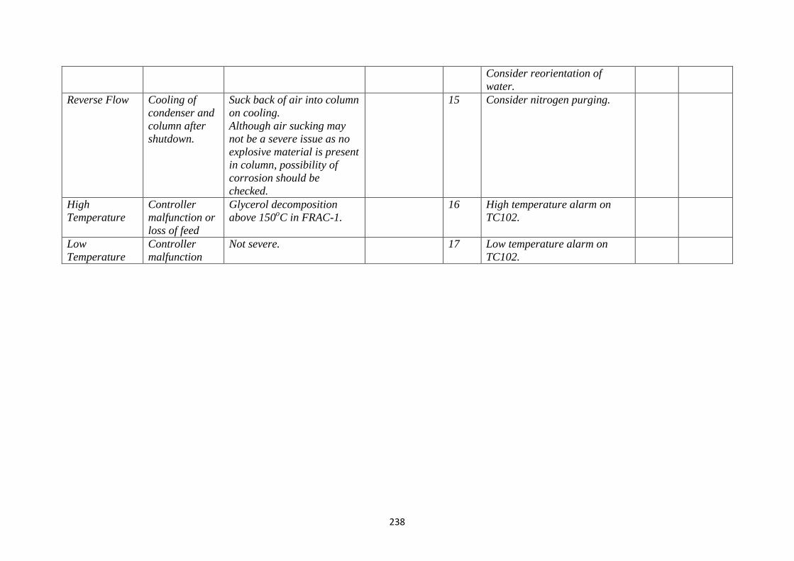
238
Consider reorientation of
water.
Reverse Flow Cooling of
condenser and
column after
shutdown.
Suck back of air into column
on cooling.
Although air sucking may
not be a severe issue as no
explosive material is present
in column, possibility of
corrosion should be
checked.
15 Consider nitrogen purging.
High
Temperature
Controller
malfunction or
loss of feed
Glycerol decomposition
above 150oC in FRAC-1.
16 High temperature alarm on
TC102.
Low
Temperature
Controller
malfunction
Not severe. 17 Low temperature alarm on
TC102.
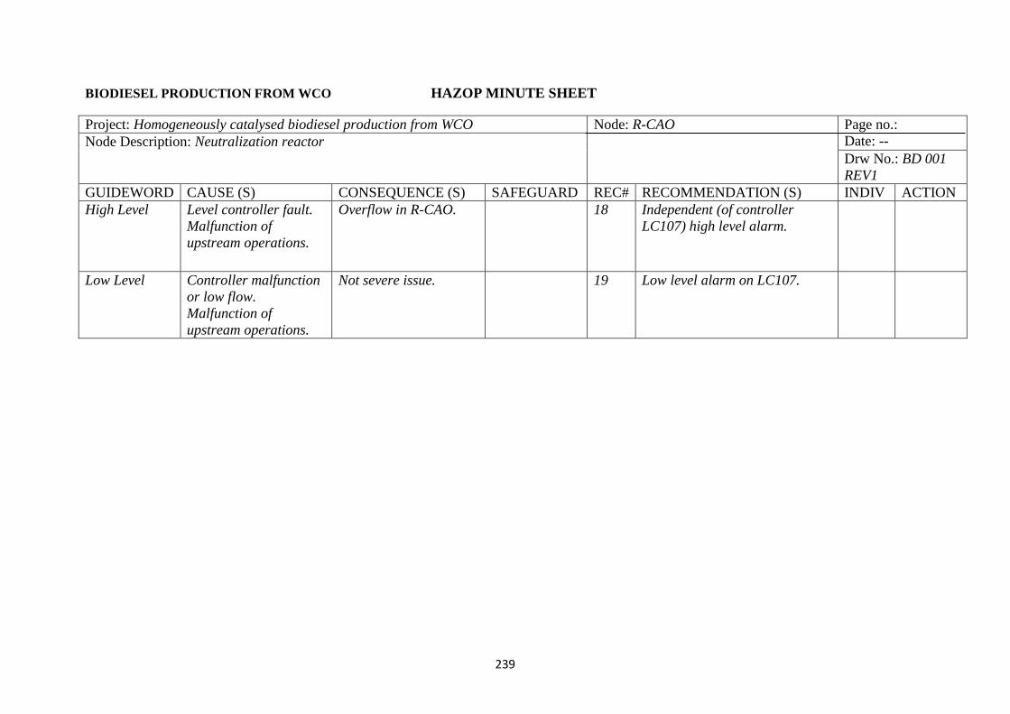
239
BIODIESEL PRODUCTION FROM WCO HAZOP MINUTE SHEET
Project: Homogeneously catalysed biodiesel production from WCO Node: R-CAO Page no.:
Date: -- Node Description: Neutralization reactor
Drw No.: BD 001
REV1
GUIDEWORD CAUSE (S) CONSEQUENCE (S) SAFEGUARD REC# RECOMMENDATION (S) INDIV ACTION
High Level Level controller fault.
Malfunction of
upstream operations.
Overflow in R-CAO. 18 Independent (of controller
LC107) high level alarm.
Low Level Controller malfunction
or low flow.
Malfunction of
upstream operations.
Not severe issue. 19 Low level alarm on LC107.
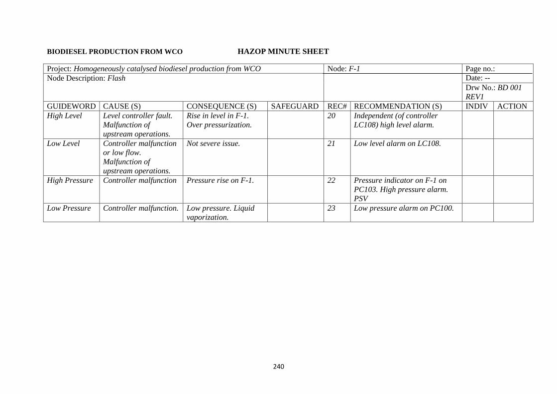
240
BIODIESEL PRODUCTION FROM WCO HAZOP MINUTE SHEET
Project: Homogeneously catalysed biodiesel production from WCO Node: F-1 Page no.:
Date: -- Node Description: Flash
Drw No.: BD 001
REV1
GUIDEWORD CAUSE (S) CONSEQUENCE (S) SAFEGUARD REC# RECOMMENDATION (S) INDIV ACTION
High Level Level controller fault.
Malfunction of
upstream operations.
Rise in level in F-1.
Over pressurization.
20 Independent (of controller
LC108) high level alarm.
Low Level Controller malfunction
or low flow.
Malfunction of
upstream operations.
Not severe issue. 21 Low level alarm on LC108.
High Pressure Controller malfunction Pressure rise on F-1. 22 Pressure indicator on F-1 on
PC103. High pressure alarm.
PSV
Low Pressure Controller malfunction. Low pressure. Liquid
vaporization.
23 Low pressure alarm on PC100.

241
BIODIESEL PRODUCTION FROM WCO HAZOP MINUTE SHEET
Project: Homogeneously catalysed biodiesel production from WCO Node: FRAC-2 Page no.:
Date: -- Node Description: Distillation column
Drw No.: BD 001
REV1
GUIDEWORD CAUSE (S) CONSEQUENCE (S) SAFEGUARD REC# RECOMMENDATION (S) INDIV ACTION
High Level Level
controller fault
Flooding and reboiler
operation stops.
24 Independent (of controller
LC104) high level alarm.
An independent alarm above
the normal control level can
alert the operator to take early
action.
Low Level Controller
malfunction or
low flow
Not severe issue 25 Low level alarm on LC104.
This will ensure early operator
intervention to prevent product
loss.
High Level Level
controller fault
Overflow.
High pressure in condenser.
26 Independent (of controller
LC103) high level alarm.
Low Level Controller
malfunction or
low flow
Pump ‘P-3 damage due to
running dry.
27 Low level alarm on LC105 &
LC103.
No flow switch on pump would
protect the pump against dry
operation.
High Pressure Controller
malfunction or
water failure in
condenser
Pressure rise. Condenser
vent is needed.
28 Pressure indicator on FRAC-2.
High pressure alarm on
PC101. Backup cooling water.
Thermocouple on vent.
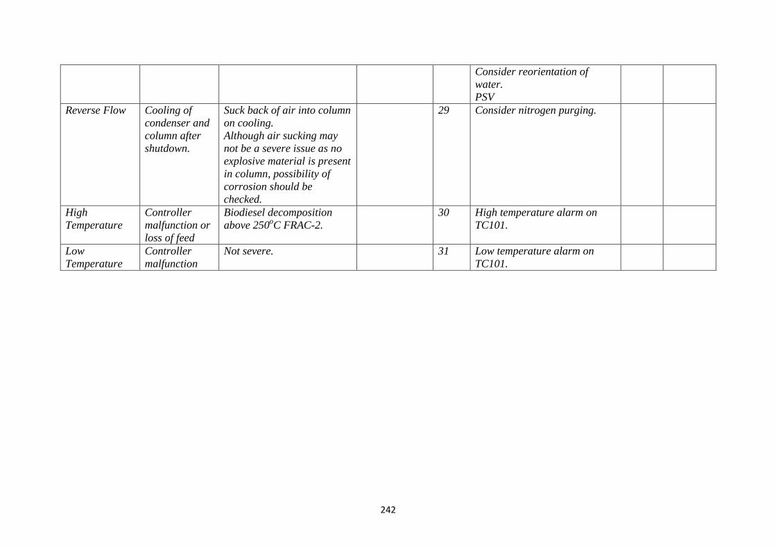
242
Consider reorientation of
water.
PSV
Reverse Flow Cooling of
condenser and
column after
shutdown.
Suck back of air into column
on cooling.
Although air sucking may
not be a severe issue as no
explosive material is present
in column, possibility of
corrosion should be
checked.
29 Consider nitrogen purging.
High
Temperature
Controller
malfunction or
loss of feed
Biodiesel decomposition
above 250oC FRAC-2.
30 High temperature alarm on
TC101.
Low
Temperature
Controller
malfunction
Not severe. 31 Low temperature alarm on
TC101.
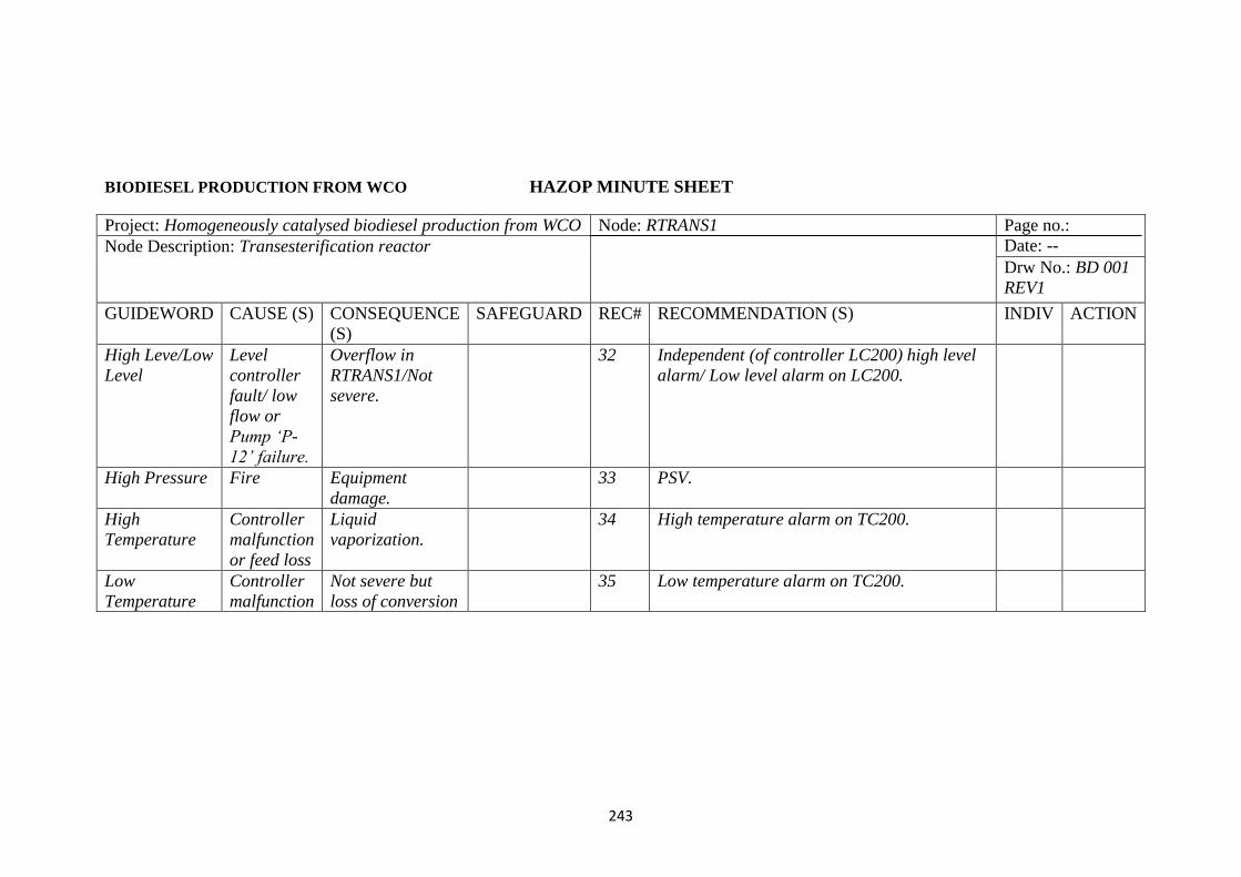
243
BIODIESEL PRODUCTION FROM WCO HAZOP MINUTE SHEET
Project: Homogeneously catalysed biodiesel production from WCO Node: RTRANS1 Page no.:
Date: -- Node Description: Transesterification reactor
Drw No.: BD 001
REV1
GUIDEWORD CAUSE (S) CONSEQUENCE
(S)
SAFEGUARD REC# RECOMMENDATION (S) INDIV ACTION
High Leve/Low
Level
Level
controller
fault/ low
flow or
Pump ‘P-
12’ failure.
Overflow in
RTRANS1/Not
severe.
32 Independent (of controller LC200) high level
alarm/ Low level alarm on LC200.
High Pressure Fire Equipment
damage.
33 PSV.
High
Temperature
Controller
malfunction
or feed loss
Liquid
vaporization.
34 High temperature alarm on TC200.
Low
Temperature
Controller
malfunction
Not severe but
loss of conversion
35 Low temperature alarm on TC200.

244
BIODIESEL PRODUCTION FROM WCO HAZOP MINUTE SHEET
Project: Homogeneously catalysed biodiesel production from WCO Node: D-1 Page no.:
Date: -- Node Description: Phase separator
Drw No.: BD 001
REV1
GUIDEWORD CAUSE (S) CONSEQUENCE (S) SAFEGUARD REC# RECOMMENDATION (S) INDIV ACTION
High Level Level controller
fault.
Malfunction of
upstream
operations.
Overflow in D-1
(upper layer).
36 Independent (of controller
LC201) high level alarm.
Low Level Controller
malfunction or low
flow.
Malfunction of
upstream
operations.
Not severe issue. 37 Low level alarm on LC201.
High Level Level controller
fault.
Malfunction of
upstream
operations.
Overflow in D-1
(lower layer).
38 Independent (of controller
LC202) high level alarm.
Low Level Controller
malfunction or low
flow.
Malfunction of
upstream
Not severe issue. 39 Low level alarm on LC202.
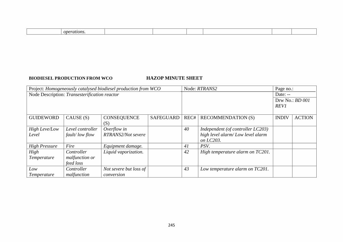
245
operations.
BIODIESEL PRODUCTION FROM WCO HAZOP MINUTE SHEET
Project: Homogeneously catalysed biodiesel production from WCO Node: RTRANS2 Page no.:
Date: -- Node Description: Transesterification reactor
Drw No.: BD 001
REV1
GUIDEWORD CAUSE (S) CONSEQUENCE
(S)
SAFEGUARD REC# RECOMMENDATION (S) INDIV ACTION
High Leve/Low
Level
Level controller
fault/ low flow
Overflow in
RTRANS2/Not severe
40 Independent (of controller LC203)
high level alarm/ Low level alarm
on LC203.
High Pressure Fire Equipment damage. 41 PSV.
High
Temperature
Controller
malfunction or
feed loss
Liquid vaporization. 42 High temperature alarm on TC201.
Low
Temperature
Controller
malfunction
Not severe but loss of
conversion
43 Low temperature alarm on TC201.
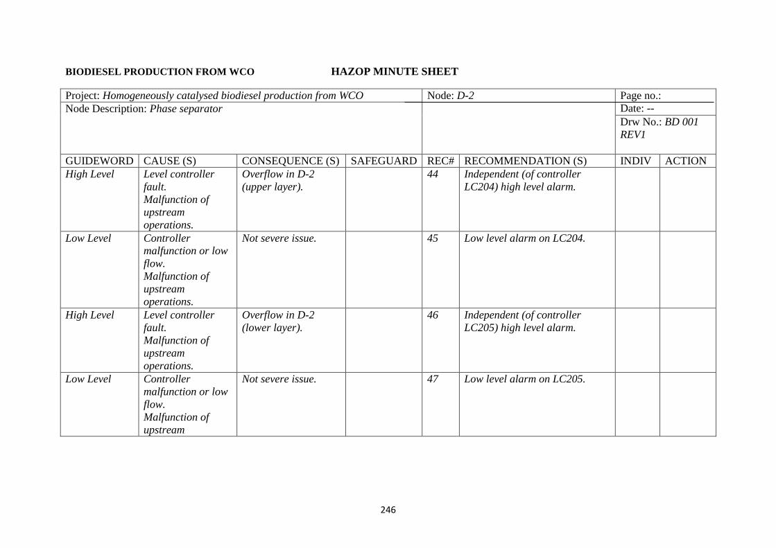
246
BIODIESEL PRODUCTION FROM WCO HAZOP MINUTE SHEET
Project: Homogeneously catalysed biodiesel production from WCO Node: D-2 Page no.:
Date: -- Node Description: Phase separator
Drw No.: BD 001
REV1
GUIDEWORD CAUSE (S) CONSEQUENCE (S) SAFEGUARD REC# RECOMMENDATION (S) INDIV ACTION
High Level Level controller
fault.
Malfunction of
upstream
operations.
Overflow in D-2
(upper layer).
44 Independent (of controller
LC204) high level alarm.
Low Level Controller
malfunction or low
flow.
Malfunction of
upstream
operations.
Not severe issue. 45 Low level alarm on LC204.
High Level Level controller
fault.
Malfunction of
upstream
operations.
Overflow in D-2
(lower layer).
46 Independent (of controller
LC205) high level alarm.
Low Level Controller
malfunction or low
flow.
Malfunction of
upstream
Not severe issue. 47 Low level alarm on LC205.
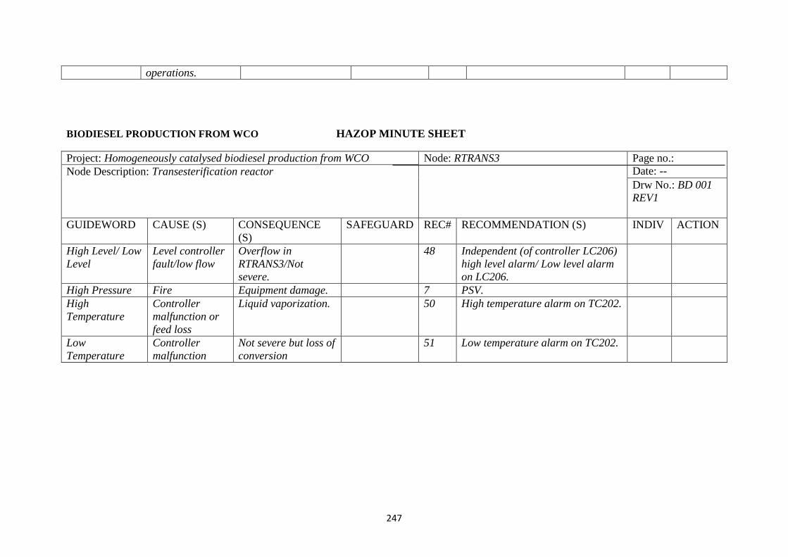
247
operations.
BIODIESEL PRODUCTION FROM WCO HAZOP MINUTE SHEET
Project: Homogeneously catalysed biodiesel production from WCO Node: RTRANS3 Page no.:
Date: -- Node Description: Transesterification reactor
Drw No.: BD 001
REV1
GUIDEWORD CAUSE (S) CONSEQUENCE
(S)
SAFEGUARD REC# RECOMMENDATION (S) INDIV ACTION
High Level/ Low
Level
Level controller
fault/low flow
Overflow in
RTRANS3/Not
severe.
48 Independent (of controller LC206)
high level alarm/ Low level alarm
on LC206.
High Pressure Fire Equipment damage. 7 PSV.
High
Temperature
Controller
malfunction or
feed loss
Liquid vaporization. 50 High temperature alarm on TC202.
Low
Temperature
Controller
malfunction
Not severe but loss of
conversion
51 Low temperature alarm on TC202.
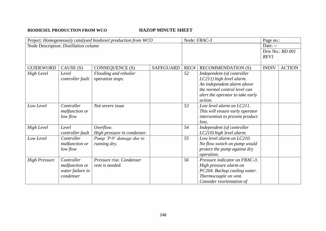
248
BIODIESEL PRODUCTION FROM WCO HAZOP MINUTE SHEET
Project: Homogeneously catalysed biodiesel production from WCO Node: FRAC-3 Page no.:
Date: -- Node Description: Distillation column
Drw No.: BD 001
REV1
GUIDEWORD CAUSE (S) CONSEQUENCE (S) SAFEGUARD REC# RECOMMENDATION (S) INDIV ACTION
High Level Level
controller fault
Flooding and reboiler
operation stops.
52 Independent (of controller
LC211) high level alarm.
An independent alarm above
the normal control level can
alert the operator to take early
action.
Low Level Controller
malfunction or
low flow
Not severe issue 53 Low level alarm on LC211.
This will ensure early operator
intervention to prevent product
loss.
High Level Level
controller fault
Overflow.
High pressure in condenser.
54 Independent (of controller
LC210) high level alarm.
Low Level Controller
malfunction or
low flow
Pump ‘P-9’ damage due to
running dry.
55 Low level alarm on LC210.
No flow switch on pump would
protect the pump against dry
operation.
High Pressure Controller
malfunction or
water failure in
condenser
Pressure rise. Condenser
vent is needed.
56 Pressure indicator on FRAC-3.
High pressure alarm on
PC204. Backup cooling water.
Thermocouple on vent.
Consider reorientation of
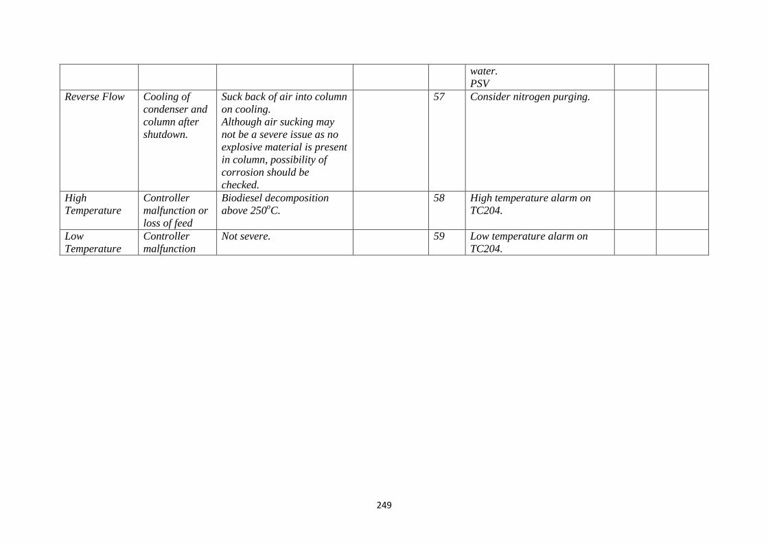
249
water.
PSV
Reverse Flow Cooling of
condenser and
column after
shutdown.
Suck back of air into column
on cooling.
Although air sucking may
not be a severe issue as no
explosive material is present
in column, possibility of
corrosion should be
checked.
57 Consider nitrogen purging.
High
Temperature
Controller
malfunction or
loss of feed
Biodiesel decomposition
above 250oC.
58 High temperature alarm on
TC204.
Low
Temperature
Controller
malfunction
Not severe. 59 Low temperature alarm on
TC204.

250
BIODIESEL PRODUCTION FROM WCO HAZOP MINUTE SHEET
Project: Homogeneously catalysed biodiesel production from WCO Node: FRAC-4 Page no.:
Date: -- Node Description: Distillation column
Drw No.: BD 001
REV1
GUIDEWORD CAUSE (S) CONSEQUENCE (S) SAFEGUARD REC# RECOMMENDATION (S) INDIV ACTION
High Level Level
controller fault
Flooding and reboiler
operation stops.
60 Independent (of controller
LC208) high level alarm.
An independent alarm above
the normal control level can
alert the operator to take early
action.
Low Level Controller
malfunction or
low flow
Not severe issue. 61 Low level alarm on LC208.
This will ensure early operator
intervention to prevent product
loss.
High Level Level
controller fault
Overflow.
High pressure in condenser.
62 Independent (of controller
LC207) high level alarm.
Low Level Controller
malfunction or
low flow
Pump ‘P-8’ damage due to
running dry.
63 Low level alarm on LC207.
No flow switch on pump would
protect the pump against dry
operation.
High Pressure Controller
malfunction or
water failure in
condenser
Pressure rise. Condenser
vent is needed.
64 Pressure indicator on FRAC-4.
High pressure alarm on
PC203. Backup cooling water.
Thermocouple on vent.
Consider reorientation of
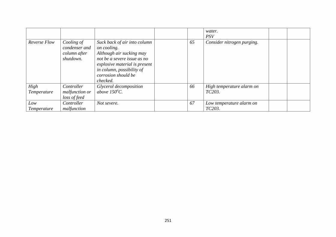
251
water.
PSV
Reverse Flow Cooling of
condenser and
column after
shutdown.
Suck back of air into column
on cooling.
Although air sucking may
not be a severe issue as no
explosive material is present
in column, possibility of
corrosion should be
checked.
65 Consider nitrogen purging.
High
Temperature
Controller
malfunction or
loss of feed
Glycerol decomposition
above 150oC.
66 High temperature alarm on
TC203.
Low
Temperature
Controller
malfunction
Not severe. 67 Low temperature alarm on
TC203.

252
BIODIESEL PRODUCTION FROM WCO HAZOP MINUTE SHEET
Project: Homogeneously catalysed biodiesel production from WCO Node: R-CAT2 Page no.:
Date: -- Node Description: Neutralization reactor
Drw No.: BD 001
REV1
GUIDEWORD CAUSE (S) CONSEQUENCE
(S)
SAFEGUARD REC# RECOMMENDATION (S) INDIV ACTION
High Level Level controller
fault.
Malfunction of
upstream
operations.
Overflow in R-
CAT2.
68 Independent (of controller
LC209) high level alarm.
Low Level Controller
malfunction or low
flow.
Malfunction of
upstream
operations.
Not severe issue. 69 Low level alarm on LC209.
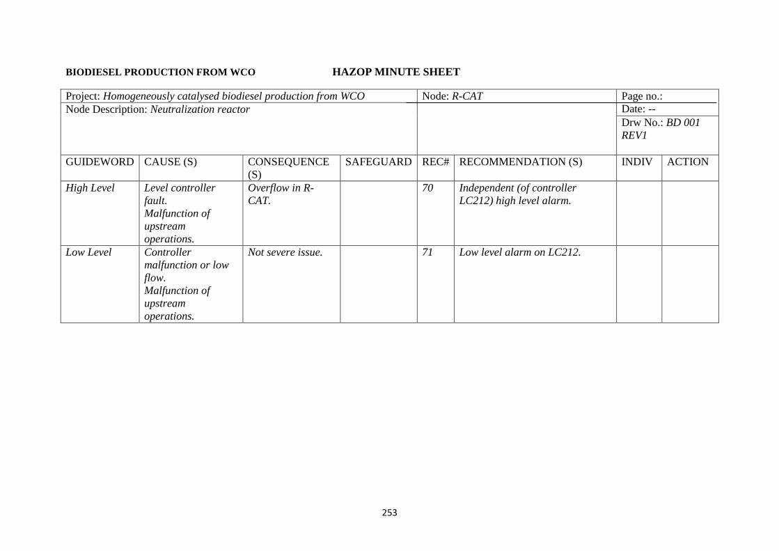
253
BIODIESEL PRODUCTION FROM WCO HAZOP MINUTE SHEET
Project: Homogeneously catalysed biodiesel production from WCO Node: R-CAT Page no.:
Date: -- Node Description: Neutralization reactor
Drw No.: BD 001
REV1
GUIDEWORD CAUSE (S) CONSEQUENCE
(S)
SAFEGUARD REC# RECOMMENDATION (S) INDIV ACTION
High Level Level controller
fault.
Malfunction of
upstream
operations.
Overflow in R-
CAT.
70 Independent (of controller
LC212) high level alarm.
Low Level Controller
malfunction or low
flow.
Malfunction of
upstream
operations.
Not severe issue. 71 Low level alarm on LC212.
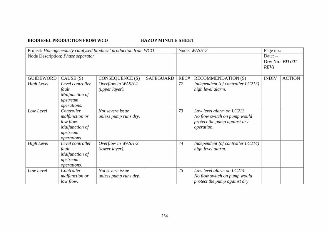
254
BIODIESEL PRODUCTION FROM WCO HAZOP MINUTE SHEET
Project: Homogeneously catalysed biodiesel production from WCO Node: WASH-2 Page no.:
Date: -- Node Description: Phase separator
Drw No.: BD 001
REV1
GUIDEWORD CAUSE (S) CONSEQUENCE (S) SAFEGUARD REC# RECOMMENDATION (S) INDIV ACTION
High Level Level controller
fault.
Malfunction of
upstream
operations.
Overflow in WASH-2
(upper layer).
72 Independent (of controller LC213)
high level alarm.
Low Level Controller
malfunction or
low flow.
Malfunction of
upstream
operations.
Not severe issue
unless pump runs dry.
73 Low level alarm on LC213.
No flow switch on pump would
protect the pump against dry
operation.
High Level Level controller
fault.
Malfunction of
upstream
operations.
Overflow in WASH-2
(lower layer).
74 Independent (of controller LC214)
high level alarm.
Low Level Controller
malfunction or
low flow.
Not severe issue
unless pump runs dry.
75 Low level alarm on LC214.
No flow switch on pump would
protect the pump against dry

255
Malfunction of
upstream
operations.
operation.
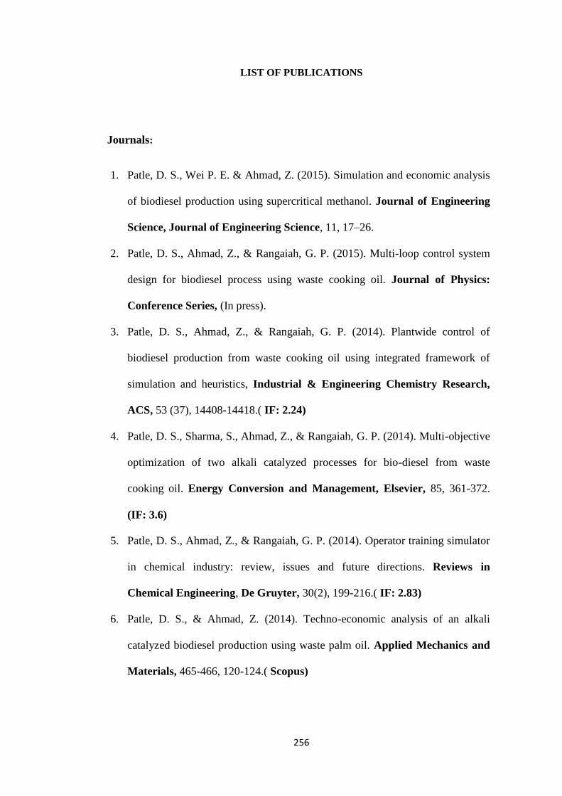
256
LIST OF PUBLICATIONS
Journals:
1. Patle, D. S., Wei P. E. & Ahmad, Z. (2015). Simulation and economic analysis
of biodiesel production using supercritical methanol. Journal of Engineering
Science, Journal of Engineering Science, 11, 17–26.
2. Patle, D. S., Ahmad, Z., & Rangaiah, G. P. (2015). Multi-loop control system
design for biodiesel process using waste cooking oil. Journal of Physics:
Conference Series, (In press).
3. Patle, D. S., Ahmad, Z., & Rangaiah, G. P. (2014). Plantwide control of
biodiesel production from waste cooking oil using integrated framework of
simulation and heuristics, Industrial & Engineering Chemistry Research,
ACS, 53 (37), 14408-14418.( IF: 2.24)
4. Patle, D. S., Sharma, S., Ahmad, Z., & Rangaiah, G. P. (2014). Multi-objective
optimization of two alkali catalyzed processes for bio-diesel from waste
cooking oil. Energy Conversion and Management, Elsevier, 85, 361-372.
(IF: 3.6)
5. Patle, D. S., Ahmad, Z., & Rangaiah, G. P. (2014). Operator training simulator
in chemical industry: review, issues and future directions. Reviews in
Chemical Engineering, De Gruyter, 30(2), 199-216.( IF: 2.83)
6. Patle, D. S., & Ahmad, Z. (2014). Techno-economic analysis of an alkali
catalyzed biodiesel production using waste palm oil. Applied Mechanics and
Materials, 465-466, 120-124.( Scopus)
257
Manuscripts under Preparation:
1. Patle, D. S., Ahmad, Z., Rangaiah, G. P., Operator training simulator for a
homogeniously alkali catalyzed biodiesel production from waste cooking oil.
(under review).
Conference Proceedings:
1. Patle, D. S., Ahmad, Z., & Rangaiah, G. P. (2014). Biodiesel production from
waste cooking oil: plant-wide control system design using integrated
framework approach, 5th
International Symposium on Advanced Control of
Industrial Processes, Hiroshima, Japan, May 28-30, 2014.
2. Patle, D. S., & Ahmad, Z. (2013). Training simulator development for palm oil
based biodiesel production plant, Proceedings of the 6th International
Conference on Process Systems Engineering (PSE ASIA), Kuala Lumpur, June
25-27, 2013.
3. Patle, D. S., & Ahmad, Z. (2012). Simulation, cost and energy analysis of eco-
friendly biodiesel production plant, International Conference on Environment
2012 (ICENV 2012), Penang, Malaysia, December 11-13, 2012.