PHYSICAL REVIEW A 89, 022341 (2014)

Optimal arbitrarily accurate composite pulse sequences

Guang Hao Low, Theodore J. Yoder, and Isaac L. ChuangMassachusetts Institute of Technology, Cambridge, Massachusetts 02139, USA

(Received 5 July 2013; revised manuscript received 15 January 2014; published 28 February 2014)

Implementing a single-qubit unitary is often hampered by imperfect control. Systematic amplitude errorsε, caused by incorrect duration or strength of a pulse, are an especially common problem. But a sequence ofimperfect pulses can provide a better implementation of a desired operation, as compared to a single primitivepulse. We find optimal pulse sequences consisting of L primitive π or 2π rotations that suppress such errorsto arbitrary order O(εn) on arbitrary initial states. Optimality is demonstrated by proving an L = O(n) lowerbound and saturating it with L = 2n solutions. Closed-form solutions for arbitrary rotation angles are given forn = 1,2,3,4. Perturbative solutions for any n are proven for small angles, while arbitrary angle solutions areobtained by analytic continuation up to n = 12. The derivation proceeds by a novel algebraic and nonrecursiveapproach, in which finding amplitude error correcting sequences can be reduced to solving polynomial equations.

DOI: 10.1103/PhysRevA.89.022341 PACS number(s): 03.67.Pp, 82.56.Jn

I. INTRODUCTION

Quantum computers are poised to solve a class of techno-logically relevant problems intractable on classical machines[1], but scalable implementations managing a useful numberof qubits are directly impeded by two general classes oferrors [2]. On one hand, unwanted system-bath interactionsin open quantum systems lead to decoherence, and on theother, imperfect controls for addressing and manipulating qubitstates result in cumulative errors that eventually render largecomputations useless.

Systematic amplitude errors, the consistent over- or under-rotation of a single-qubit unitary operation by a small factor ε,are one common control fault. The discovery of a protocolfor the complete and efficient suppression of these errorswould greatly advance the field of quantum control, withapplications as far ranging as implementing fault-tolerantquantum computation and improving nuclear magnetic reso-nance spectra acquisition. Due to the broad scope of systematicamplitude errors, this problem has been attacked repeatedlyby a variety of methods with varying degrees of success[3–8]. A concept common to most approaches is the compositepulse sequence, in which some number of L carefully chosenerroneous primitive unitary operations, or pulses, are appliedsuccessively such that a target ideal rotation is approximatedto some order n with an exponentially reduced error O(εn+1).

In the realm of quantum computation, the criteria for usefulpulse sequences are stringent: (1) For each order n, a procedurefor constructing a pulse sequence correcting to that order isgiven. (2) This construction gives sequence lengths L thatscale efficiently with n, that is, L = O(nk), with k as smallas possible. (3) Sequences should be “fully compensating” or“class A” [4], meaning they operate successfully on arbitraryand unknown states (in contrast to “class B” sequences thatoperate successfully only on select initial states). (4) Althoughfinite sets of universal quantum gates exist [1], ideally se-quences should be capable of implementing arbitrary rotationsso that quantum algorithms can be simplified conceptually andpractically.

One finds that there are currently no sequences satisfyingall four of these criteria and suppressing systematic amplitudeerrors. In the literature, SCROFULOUS [9], PB1, BB1 [10] satisfy

criteria (3) and (4) but offer corrections only up to order n = 2.Unfortunately, generalizations of these to arbitrary n comewith prohibitively long sequence lengths, so that criterion (2)ends up unsatisfied. Typically, a sequence correct to ordern + 1 is recursively constructed from those at order n, resultingin an inefficient sequence length L = 2O(n) [5], althoughnumerical studies suggest that efficient sequences with L =O(n3.09) exist [5]. To date, other classes of systematic controlerrors [11–13] do not fare better.

There are some provable successes in efficient pulsesequences, though. However, to find them one must relaxcriterion (4), which requires arbitrary rotations. For example, ifone restricts attention to correcting π rotations in the presenceof amplitude errors, Jones proved the impressive resultthat sequences with L = O(n1.47) [3,7] are possible. Uhrigefficiently implements the identity operator in the presenceof dephasing errors with L = O(n) [14]. If we also relax thecriterion (3) and settle for specialized class B sequences thattake |0〉 to |1〉 (those we call inverting sequences), Vitanovhas found efficient narrow-band sequences for amplitudeerrors also with L = O(n) [15]. Notably, both Uhrig’s andVitanov’s results were achieved via algebraic, nonrecursiveprocesses. In fact, as we show, a more generalized algebraicapproach in the amplitude error case can reinstate the crucialcriteria (3) and (4) while maintaining Vitanov’s efficient lengthscaling.

Our main result is exactly such an algebraic generalization,a nonrecursive formalism for systematic amplitude errors.With this, we prove a lower bound of L = O(n) for classA sequences comprised of either primitive π or 2π rotations,then constructively saturate this bound to a constant factor withL = 2n (plus a single initializing rotation). The improvementof these new sequences over prior state of the art is illustratedin Table I. We derive optimal closed-form solutions up ton = 4 for arbitrary target angles and perturbative solutionsfor any n, valid for small target angles. We then analyticallycontinue these perturbative solutions to arbitrary angles up ton = 12. Since any random or uncorrected systematic errors inthe primitive pulses accumulate linearly with sequence length,optimally short sequences such as ours minimize the effect ofsuch errors.

1050-2947/2014/89(2)/022341(14) 022341-1 ©2014 American Physical Society

GUANG HAO LOW, THEODORE J. YODER, AND ISAAC L. CHUANG PHYSICAL REVIEW A 89, 022341 (2014)

TABLE I. Comparison of known pulse sequences operating onarbitrary initial states that suppress systematic amplitude errorsto order n for arbitrary target rotation angles. Arbitrary accuracygeneralizations are known or conjectured for all with the exceptionof SCROFULOUS. The sequences APn, PDn, and ToPn are presented inthis work. Of interest is the subset of APn sequences labeled ToPn, forwhich arbitrary accuracy is provable perturbatively for small targetangles.

Name Length notes

SCROFULOUS 3 n = 1, nonuniform θj [9]Pn, Bn O(en2

) Closed form [5]SKn O(n3) n � 30, Numerical [5]

n > 30, ConjecturedAPn (PDn) 2n n � 3(4), Closed form

n � 12, Analytic continuationn > 12, Conjectured

ToPn 2n Arbitrary n, perturbative

We define the problem statement for amplitude-errorcorrecting pulse sequences mathematically in Sec. II, leading,in Sec. III, to a set of constraint equations that such pulsesequences must satisfy, which is then solved in Sec. IVby three approaches: analytical, perturbative, and numerical.The analytical method is interesting as it gives closed-formsolutions for low order sequences in a systematic fashion. Theperturbative method relies on the invertibility of the Jacobianof the constraints and is used for proving the existence ofsolutions for select target angles. The numerical method is themost straightforward and practical for higher orders, givingoptimally short pulse sequences for correction orders up ton = 12. Section V then presents several generalizations ofour results, including discussions on narrow-band toggling,nonlinear amplitude errors, random errors, and simultaneouscorrection of off-resonance errors. Finally, we point out dif-ferences and similarities between our sequences and existingart in Sec. VI and conclude in Sec. VII.

II. PULSE SEQUENCES

A single-qubit rotation of target angle θT about the axis�n is the unitary R�n[θT ] = exp[−iθT (�n · �σ )/2], where �σ =(X,Y ,Z) is the vector of Pauli operators. Without affectingthe asymptotic efficiency of our sequences, Euler angles allowus to choose nz = 0, and consequently, we define Rϕ[θT ] =exp(−iθT σϕ/2) for σϕ = X cos ϕ + Y sin ϕ. However, we onlyhave access to imperfect rotations Mϕ[θ ] = Rϕ[(1 + ε)θ ] thatovershoot a desired angle θ by εθ , |ε| � 1. With theseprimitive elements, we construct a pulse sequenceS consistingof L faulty pulses:

S = Mϕ1 [θ1]Mϕ2 [θ2] . . . MϕL[θL]. (1)

Denote by �ϕ the vector of phase angles (ϕ1,ϕ2, . . . ,ϕL), whichare our free parameters. Leaving each amplitude θj as a freeparameter (e.g., SCROFULOUS [9]) may help reduce sequencelength, but we find that a fixed value θj = θ0 leads to the mostcompelling results.

The goal is to implement a target rotation Rϕ0 [θT ] (or,without loss of generality, R0 [θT ] by the replacement ϕj →

ϕj − ϕ0), including the correct global phase, with a small error.The trace distance [1]

D(U ,V ) = ‖U − V ‖ = 12 Tr

√(U − V )†(U − V ) (2)

is a natural metric for defining errors between two operatorsU , V [5]. We demand that the pulse sequence implements

S = R0[−εθT ] + O(εn+1), (3)

so that the corrected rotation UT = SM0 [θT ] = R0 [θT ] +O(εn+1) has trace distance with the same small leading errorD(UT ,R0 [θT ]) = O(εn+1). Thus constructed, UT implementsR0 [θT ] over a very wide range of ε due to its first n derivativesvanishing and so has broadband characteristics [2].

For completeness, we mention other error quantifiers.First is the fidelity F (U ,V ) = ‖U V †‖, which is not truly adistance metric but can be easier to compute, and bounds 1 −F (U ,V ) � D(U ,V ) �

√1 − F (U ,V )2 [1]. The infidelity of

UT is then 1 − F (UT ,R0 [θT ]) = O(ε2n+2), which is a com-monly used quantifier [2,7]. Finally, for the specialized class Bsequences called inverting sequences, the transition probability|〈1|U |0〉|2 is a viable quantity for comparison [15].

III. CONSTRAINT EQUATIONS

We now proceed to derive a set of equations, or constraints,on the phase angles �ϕ that will yield broadband correction.We begin very generally in the first section by assumingjust θj = θ0 as mentioned before, but then we specialize inthe subsequent two sections to the case θ0 = 2π and thecase of symmetric sequences, both of which greatly enhancetractability of the problem.

A. Equal amplitude base pulses

To begin, we obtain an algebraic expression forS by a directexpansion of a length L sequence. Defining θ ′

0 = (1 + ε)θ0/2,

S =L∏

j=1

Mϕj[θ0] = cosL(θ ′

0)L∏

j=1

[1 − i tan(θ ′

0)σϕj

]

=L∑

j=0

Aj

L(θ ′0)�j

L( �ϕ), (4)

where indices in the matrix product ascend from left to right,A

j

L(s) = (−i)j sinj (s) cosL−j (s), and �j

L are noncommutativeelementary symmetric functions generated by

∏Lj=1(1 +

t σϕj) = ∑L

j=0 t j �j

L [16]. The �j

L are hard to work with, so byapplying the Pauli matrix identity,

σϕ1σϕ2 · · · σϕj= exp

(iZ

j∑k=1

(−1)kϕk

)Xj , (5)

we obtain a more useful expression as functions of the phaseangles ϕj :

�j

L( �ϕ) = (Re

[�

j

L( �ϕ)]I − i Im

[�

j

L( �ϕ)]Z

)Xj , (6)

�j

L( �ϕ) =∑

1�h1<h2<···<hj �L

exp

(−i

j∑k=1

(−1)kϕhk

). (7)

022341-2

OPTIMAL ARBITRARILY ACCURATE COMPOSITE PULSE . . . PHYSICAL REVIEW A 89, 022341 (2014)

By defining the terminal case �0L( �ϕ) ≡ 1, the phase sums �

j

L

are efficiently computable at numeric values of the phasesby the recursion �

j

L = �j

L−1 + �j−1L−1e

i(−1)j+1ϕL using dynamicprogramming (i.e., start from the terminal case and fill in thetable �

j

L for all desired j and L).Combining the expansion of S with Eq. (3) then imposes

a set Bn,L of real constraints on �ϕ to be satisfied by anyorder n, length L sequence. Bn,L is obtained by first matchingcoefficients of the trace orthogonal Pauli operators on eitherside of Eq. (3). We then obtain, in terms of normalizederror x = 1

2εθ0 and normalized target angle γ = θT /θ0, thenecessary and sufficient conditions

∑j∈

{evenodd

Aj

L(θ0/2 + x)�j

L( �ϕ) ={

cos(xγ )i sin(xγ ) + O(xn+1). (8)

Second, the complex coefficients of x0,x1, . . . ,xn are matched,giving 2(n + 1) complex equations linear in the phase sums�

j

L( �ϕ), or, letting |·| denote the size of a set, |Bn,L| = 4(n + 1)real constraints.

However, these constraints Bn,L are intractable to directsolution, and a simplifying assumption is necessary. It shouldbe reasonable to suspect that the small rotation R0 [−εθT ]can be generated by small pure error terms Rϕ [εθ0]. We willtherefore set θ0 = 2π [5]. Note that θ0 = π is also a tractablecase but is related to the 2π -pulse case by phase toggling andso need not be considered separately. We give more detail ontoggling in Sec. V.

B. Assuming base pulses of θ0 = 2π

We now enumerate several key results, due simply toimposing θ0 = 2π , that apply to all order n, length L, 2π -pulse

sequences. First, Eq. (8) reduces to

(−1)LL∑

j=0

Aj

L(x)�j

L( �ϕ) = eixγ + O(xn+1) (9)

by summing its even and odd parts, justified by notingA

j

L(θ0/2 + x) → (−1)LAj

L(x); hence x occurs only in even(odd) powers for j even (odd). By matching coefficients ofpowers of x, this represents 2(n + 1) real constraints. Second,the x0 terms in Eq. (9) match if and only if L is even.Assuming this, 2n constraints remain. Third, we arrive atour most important result by transforming Eq. (9) with thesubstitution x → i tanh−1(y). This eliminates trigonometricand exponential functions from Eq. (9), and (assuming L iseven) leaves

[(1 − y)(1 + y)]−L/2L∑

j=1

yj�j

L( �ϕ) =[

1 − y

1 + y

]γ /2

. (10)

Upon rearrangement, this is a generating function for equationsthat the phase sums �

j

L( �ϕ) must satisfy. The functions fj

L (γ )generated by

∑∞j=0 f

j

L (γ )yj = (1 + y)(L−γ )/2(1 − y)(L+γ )/2

are, in fact, real polynomials in γ of degree j which generalizethose of Mittag-Leffler [17]. We can now write

�j

L( �ϕ) = fj

L (γ ), 0 < j � n, (11)

fj

L (γ ) =j∑

k=0

(−1)k(

T

k

)(L − T

j − k

), T ≡ 1

2(γ + L). (12)

Equation (11) is, in our opinion, the simplest and most usefulrepresentation of the nonlinear (in �ϕ) constraints that form thebasis for our solutions. We provide in Table II their explicitexpansions for L = 2,4,6 as examples.

TABLE II. Shown are explicit examples of the phase sums �Lj ( �ϕ) defined in Eq. (7) and the polynomials f L

j (γ ) defined in Eq. (12). Fromthe definitions, we see �L

0 ( �ϕ) = f L0 = 1, not shown in the table. For L = 2,4, when the expressions are still relatively short, we show �L

j ( �ϕ)and f L

j (γ ) for all j for completeness, although only those with j � L/2 are used in solving for our pulse sequences. Note that �Lj ( �ϕ) is a sum

of ( L

j) complex unit vectors and f L

j (γ ) is a j -degree polynomial with either even or odd symmetry.

L j �Lj ( �ϕ) f L

j (γ )

2 1 eiϕ1 + eiϕ2 −γ

2 ei(ϕ1−ϕ2) 12 γ 2 − 1

4 1 eiϕ1 + eiϕ2 + eiϕ3 + eiϕ4 −γ

2 ei(ϕ1−ϕ2) + ei(ϕ1−ϕ3) + ei(ϕ1−ϕ4) + ei(ϕ2−ϕ3) + ei(ϕ2−ϕ4) + ei(ϕ3−ϕ4) 12 γ 2 − 2

3 ei(ϕ1−ϕ2+ϕ3) + ei(ϕ1−ϕ2+ϕ4) + ei(ϕ1−ϕ3+ϕ4) + ei(ϕ2−ϕ3+ϕ4) − 16 γ 3 + 5

3 γ

4 ei(ϕ1−ϕ2+ϕ3−ϕ4) 124 γ 4 − 2

3 γ 2 + 1

6 1 eiϕ1 + eiϕ2 + eiϕ3 + eiϕ4 + eiϕ5 + eiϕ6 −γ

2 ei(ϕ1−ϕ2) + ei(ϕ1−ϕ3) + ei(ϕ1−ϕ4) + ei(ϕ1−ϕ5) + ei(ϕ1−ϕ6)

+ ei(ϕ2−ϕ3) + ei(ϕ2−ϕ4) + ei(ϕ2−ϕ5) + ei(ϕ2−ϕ6) + ei(ϕ3−ϕ4)

+ ei(ϕ3−ϕ5) + ei(ϕ3−ϕ6) + ei(ϕ4−ϕ5) + ei(ϕ4−ϕ6) + ei(ϕ5−ϕ6)

12 γ 2 − 3

3 ei(ϕ1−ϕ2+ϕ3) + ei(ϕ1−ϕ2+ϕ4) + ei(ϕ1−ϕ2+ϕ5) + ei(ϕ1−ϕ2+ϕ6) + ei(ϕ1−ϕ3+ϕ4)

+ ei(ϕ1−ϕ3+ϕ5) + ei(ϕ1−ϕ3+ϕ6) + ei(ϕ1−ϕ4+ϕ5) + ei(ϕ1−ϕ4+ϕ6) + ei(ϕ1−ϕ5+ϕ6)

+ ei(ϕ2−ϕ3+ϕ4) + ei(ϕ2−ϕ3+ϕ5) + ei(ϕ2−ϕ3+ϕ6) + ei(ϕ2−ϕ4+ϕ5) + ei(ϕ2−ϕ4+ϕ6)

+ ei(ϕ2−ϕ5+ϕ6) + ei(ϕ3−ϕ4+ϕ5) + ei(ϕ3−ϕ4+ϕ6) + ei(ϕ3−ϕ5+ϕ6) + ei(ϕ4−ϕ5+ϕ6)

− 16 γ 3 − 8

3 γ

022341-3

GUANG HAO LOW, THEODORE J. YODER, AND ISAAC L. CHUANG PHYSICAL REVIEW A 89, 022341 (2014)

In our notation the leading error of an order n, even L,2π -pulse sequence S2π has a simple form,

S2πR0[2xγ ] = I − (f n+1

L (γ )Xn+1 − �n+1L ( �ϕ)

)(−ix)n+1.

(13)

Now, we recognize the operator on the right of Eq. (13) must beunitary. Thus, if a set �ϕ satisfies Eq. (11) for 0 < j < k for anyeven integer k, Re[�k

L( �ϕ)] = f kL(γ ) follows automatically. So

we define B2πn,L, the set of constraints resulting from applying

θ0 = 2π to Bn,L, to consist of the n complex equations fromEq. (11), ignoring the real parts for even j .

B2πn,L =

{Re �

j

L( �ϕ) = fj

L (γ ), j odd

Im �j

L( �ϕ) = 0, for all j

}j=1,2,...,n

(14)

Thus, |B2πn,L| = �3n/2 .

In fact, it is not difficult to place a lower bound on thepulse length L for a sequence correcting to order n using theframework we have so far. This is the first bound of its kind,and, given our solutions of the constraints to come in Sec. IV, itmust be tight to a constant factor. Begin the argument by wayof contradiction, letting n > L. In examining B2π

n,L, observe

�j

L( �ϕ) = 0 for L < j � n, but f j

L (γ ) is a real polynomial in γ

of degree j . Hence 0 = �nL( �ϕ) = f n

L (γ ) cannot be satisfied forarbitrary γ . Likewise, if L = n, then 1 = |�n

L( �ϕ)| = |f nL (γ )|

cannot be satisfied for arbitrary γ . Thus L > n is necessary.

C. Assuming phase angle symmetries

Some constraints in B2πn,L can be automatically sat-

isfied if appropriate symmetries on the phase angleare imposed. A symmetry property of the phase sums,�

j

L( �ϕ) = [�j

L((−1)j �ϕR)]∗ with reversed phase angles �ϕR =(ϕL,ϕL−1, . . . ,ϕ1), motivates us to impose a palindromic(antipalindromic) symmetry on the phases, �ϕ = +�ϕR ( �ϕ =−�ϕR), so that Im[�j

L( �ϕ)] = 0 for even (odd) j . Removingthese equations from B2π

n,L, we are left with the subset BPDn,L

(BAPn,L). By definition, ϕAP

k = −ϕAPL−k+1 and ϕPD

k = ϕPDL−k+1. In

both cases, we have |BPDn,L| = |BAP

n,L| = n real constraints tobe satisfied by �L/2 real variables �ϕAP or �ϕPD. With whatminimum L is this possible.

IV. SOLVING THE CONSTRAINTS

We now satisfy the constraints BPDn,L and BAP

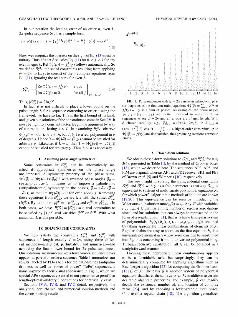
n,L withsequences of length exactly L = 2n, using three differ-ent methods—analytical, perturbative, and numerical—andachieving the linear lower bound for 2π -pulse sequences.Our solutions are nonrecursive; a lower-order sequence neverappears as part of an order n sequence. Table I summarizes ourresults labeled by PDn (APn) for the palindromes (antipalin-dromes), as well as “tower of power” (ToPn) sequences, aname inspired by their visual appearance in Fig. 1, which arespecial APn sequences essential to our perturbative proof thatlength-optimal arbitrary n corrections for nontrivial γ exist.

Sections IV A, IV B, and IV C detail, respectively, theanalytical, perturbative, and numerical solution methods andthe corresponding results.

n: 1 2 3 4 5 6 7 8 9 10 11 12 13 14 15 16

Re L1

Im L1

FIG. 1. Pulse sequences with θ0 = 2π can be visualized with pha-sor diagrams as the first constraint equation; �1

L( �ϕ) = ∑L

k=1 eiϕk =f 1

L(γ ) = −γ is a sum of phases. As examples, the phase angles�ϕL|γ=1 = (ϕ1, . . . ,ϕL) are plotted tip-to-tail to scale for ToPn

sequences where L = 2n and all arrows are of unit length. With�ϕ chosen carefully, e.g., �ϕ2|γ=1 = (2π/3,−2π/3) or �ϕ4|γ=1 =( cos−1(

√10−64 ), cos−1(1 −

√58 ), . . . ), higher-order constraints up to

�nL( �ϕ) = f n

L (γ ) are also satisfied, thus producing rotations correct toO(εn).

A. Closed-form solutions

We obtain closed-form solutions to BAPn,2n and BPD

n,2n for n �3(4), presented in Table III, by the method of Grobner bases[18], which we describe here. The sequences AP2, AP3, andPD4 are original, whereas AP1 and PD2 recover SK1 and PB1

of Brown et al. [5] and Wimperis [10], respectively.The key insight in solving the transcendental constraints

BAPn,L and BPD

n,L with γ as a free parameter is that any Bn,L isequivalent to systems of multivariate polynomial equations F ,for which powerful algorithmic methods of solution are known[19,20]. This equivalence can be seen by introducing theWeierstrass substitution tan(ϕk/2) = tk . Any F with variablest1, . . . ,tn ∈ C that has a finite number of zeros is zero dimen-sional and has solutions that can always be represented in theform of a regular chain [21], that is, a finite triangular systemof polynomials {h1(t1),h2(t1,t2), . . . ,hn(t1, . . . ,tn)} obtainedby taking appropriate linear combinations of elements of F .Regular chains are easy to solve, as the first equation h1 is aunivariate polynomial in t1 whose zeros can then be substitutedinto h2, thus converting it into a univariate polynomial in t2.Through recursive substitution, all tk can be obtained in astraightforward manner.

Divining these appropriate linear combinations appearsto be a formidable task, but surprisingly, they can bedeterministically computed by applying algorithms such asBuchberger’s algorithm [22] for computing the Grobner basis[18] G of F . The basis G is another system of polynomialequations that shares the same zeros asF , in addition to certaindesirable algebraic properties. For example, G can readilydecide the existence, number of, and location of complexzeros [23], and by choosing a lexicographic term order,G is itself a regular chain [18]. The algorithm generalizes

022341-4

OPTIMAL ARBITRARILY ACCURATE COMPOSITE PULSE . . . PHYSICAL REVIEW A 89, 022341 (2014)

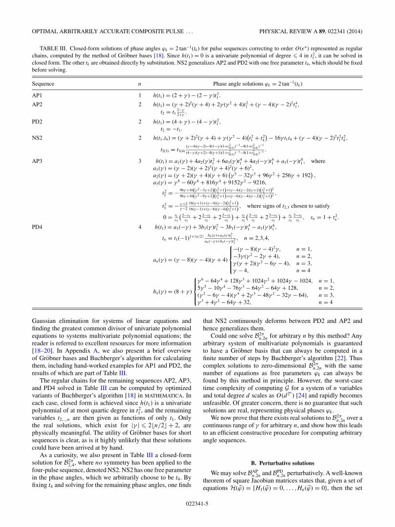
TABLE III. Closed-form solutions of phase angles ϕk = 2 tan−1(tk) for pulse sequences correcting to order O(εn) represented as regularchains, computed by the method of Grobner bases [18]. Since h(t1) = 0 is a univariate polynomial of degree � 4 in t2

1 , it can be solved inclosed form. The other tk are obtained directly by substitution. NS2 generalizes AP2 and PD2 with one free parameter t4, which should be fixedbefore solving.

Sequence n Phase angle solutions ϕk = 2 tan−1(tk)

AP1 1 h(t1) = (2 + γ ) − (2 − γ )t21 .

AP2 2 h(t1) = (γ + 2)2(γ + 4) + 2γ (γ 2 + 4)t21 + (γ − 4)(γ − 2)2t4

1 ,

t2 = t12−γ

2+γ.

PD2 2 h(t1) = (4 + γ ) − (4 − γ )t21 ,

t2 = −t1.

NS2 2 h(t1,t4) = (γ + 2)2(γ + 4) + γ (γ 2 − 4)(t21 + t2

4

) − 16γ t1t4 + (γ − 4)(γ − 2)2t21 t2

4 ,

t2(3) = t1(4)(γ−4)(γ−2)−8(1−γ )(1+t2

4(1))−1−8(1+t21(4))

−1

(4−γ )(γ+2)−8(γ+1)(1+t24(1))−1−8(1+t2

1(4))−1 .

AP3 3 h(t1) = a1(γ ) + 4a2(γ )t21 + 6a3(γ )t4

1 + 4a2(−γ )t61 + a1(−γ )t8

1 , wherea1(γ ) = (γ − 2)(γ + 2)3(γ + 4)2(γ + 6)2,

a2(γ ) = (γ + 2)(γ + 4)(γ + 6)(γ 5 − 32γ 3 + 96γ 2 + 256γ + 192

),

a3(γ ) = γ 8 − 60γ 6 + 816γ 4 + 9152γ 2 − 9216,

t22 = − 96γ+16(γ 2−3γ+2)(t2

1 +1)+(γ−4)(γ−2)(γ+2)(t21 +1)2

96γ+16(γ 2−9γ+2)(t21 +1)+(γ−6)(γ−4)(γ−2)(t2

1 +1)2 ,

t23 = − γ+2

γ−2

16(γ+1)+(γ−4)(γ−2)(t21 +1)

16(γ−1)+(γ−6)(γ−4)(t21 +1) , where signs of t2,3 chosen to satisfy

0 = t1s1

( 2−s1s1

+ 2 2−s2s2

+ 2 2−s3s3

) + t2s2

( 2−s2s2

+ 2 2−s3s3

) + t3s3

2−s3s3

, sn = 1 + t2n .

PD4 4 h(t1) = a1(−γ ) + 3b1(γ )t21 − 3b1(−γ )t4

1 − a1(γ )t61 ,

tn = t1(−1)1+�n/2 bn(γ )+an(γ )t21

an(−γ )+bn(−γ )t21, n = 2,3,4,

an(γ ) = (γ − 8)(γ − 4)(γ + 4)

⎧⎪⎪⎨⎪⎪⎩

−(γ − 8)(γ − 4)2γ, n = 1,

−3γ (γ 2 − 2γ + 4), n = 2,

γ (γ + 2)(γ 2 − 6γ − 4), n = 3,

γ − 4, n = 4

bn(γ ) = (8 + γ )

⎧⎪⎪⎨⎪⎪⎩

γ 6 − 64γ 4 + 128γ 3 + 1024γ 2 + 1024γ − 1024, n = 1,

5γ 5 − 10γ 4 − 76γ 3 − 64γ 2 − 64γ + 128, n = 2,

(γ 2 − 6γ − 4)(γ 4 + 2γ 3 − 48γ 2 − 32γ − 64), n = 3,

γ 3 + 4γ 2 − 64γ + 32, n = 4

Gaussian elimination for systems of linear equations andfinding the greatest common divisor of univariate polynomialequations to systems multivariate polynomial equations; thereader is referred to excellent resources for more information[18–20]. In Appendix A, we also present a brief overviewof Grobner bases and Buchberger’s algorithm for calculatingthem, including hand-worked examples for AP1 and PD2, theresults of which are part of Table III.

The regular chains for the remaining sequences AP2, AP3,and PD4 solved in Table III can be computed by optimizedvariants of Buchberger’s algorithm [18] in MATHEMATICA. Ineach case, closed form is achieved since h(t1) is a univariatepolynomial of at most quartic degree in t2

1 , and the remainingvariables t2,..,n are then given as functions of only t1. Onlythe real solutions, which exist for |γ | � 2�n/2� + 2, arephysically meaningful. The utility of Grobner bases for shortsequences is clear, as is it highly unlikely that these solutionscould have been arrived at by hand.

As a curiosity, we also present in Table III a closed-formsolution for B2π

2,4, where no symmetry has been applied to thefour-pulse sequence, denoted NS2. NS2 has one free parameterin the phase angles, which we arbitrarily choose to be t4. Byfixing t4 and solving for the remaining phase angles, one finds

that NS2 continuously deforms between PD2 and AP2 andhence generalizes them.

Could one solve B2πn,2n for arbitrary n by this method? Any

arbitrary system of multivariate polynomials is guaranteedto have a Grobner basis that can always be computed in afinite number of steps by Buchberger’s algorithm [22]. Thuscomplex solutions to zero-dimensional B2π

n,2n with the samenumber of equations as free parameters ϕk can always befound by this method in principle. However, the worst-casetime complexity of computing G for a system of n variablesand total degree d scales as O(d2n

) [24] and rapidly becomesunfeasible. Of greater concern, there is no guarantee that suchsolutions are real, representing physical phases ϕk .

We now prove that there exists real solutions to B2πn,2n over a

continuous range of γ for arbitrary n, and show how this leadsto an efficient constructive procedure for computing arbitraryangle sequences.

B. Perturbative solutions

We may solve BAPn,2n and BPD

n,2n perturbatively. A well-knowntheorem of square Jacobian matrices states that, given a set ofequations H( �ϕ) = {H1( �ϕ) = 0, . . . ,Hn( �ϕ) = 0}, then the set

022341-5

GUANG HAO LOW, THEODORE J. YODER, AND ISAAC L. CHUANG PHYSICAL REVIEW A 89, 022341 (2014)

H( �ϕ) is locally invertible, or analytical, in the neighborhoodabout some root �ϕ0 if and only if the determinant det (J ) ofits Jacobian matrix Jjk = ∂ϕk

Hj ( �ϕ)| �ϕ=�ϕ0 is nonzero. The setof interest for us is Bn,L, for which this theorem says thatone may always construct a perturbative expansion for �ϕ overa continuous range γ about γ0 given a valid starting point( �ϕ0,γ0) satisfying Bn,L if and only if det(J ) �= 0. So long asthe Jacobian remains nonzero, one may extend such a solutionbeyond its neighborhood by analytic continuation.

However, for arbitrary n, what are these valid initial points( �ϕ0,γ0)? As we do not a priori know of solutions to Bn,L forarbitrary γ , such points must be found at some γ where theproblem simplifies. Even then, the problem is nontrivial: forexample, imposing phase angle symmetries forces ϕk = mπ

2 ,

m ∈ Z at γ = 0, but one can readily verify that many suchsolutions of this form to Eq. (11) suffer from det(J ) = 0.Using the closed-form solutions in Table III, one finds atγ = 0 that while the Jacobian of the PD2,4 sequences is zero,the AP1,3 sequences each have a solution with a nonzeroJacobian wherein ϕk = π/2, for k � n. We now prove thatthis generalizes to arbitrary n, resulting in the special class ofToPn antipalindrome sequences with initial values,

�ϕToPn

∣∣γ=2b

={π, 1 � k � b

π/2, b < k � n,(15)

for b = 0,1, . . . �n/2�. Hence nontrivial real solutions to B2πn,2n

exist for arbitrary n.

1. ToPn is analytical at γ = 0 ∀n

We first transform the function mapping for ToPn:H( �ϕ)j ={Re �

j

2n( �ϕ), j oddIm �

j

2n( �ϕ), j even ,→ { �

j

2n( �ϕ), j odd−i�

j

2n( �ϕ), j even .This does not affect the

magnitude of its Jacobian J as Re �j

L( �ϕ) = �j

L( �ϕ) for oddj due to antipalindromic symmetry, while for even j the realpart of Eq. (11) is automatically satisfied due to unitarity [seeEq. (13)].

The γ = 0 solution to ToPn has a simple form ϕToPk = π/2,

for k � n. With this solution, a straightforward, if tedious,manipulation of the phase sums shows that elements of the n ×n Jacobian matrix satisfy the recurrence Jj+1,k+1 = Jj+1,k +Jj,k+1 + Jjk . The solution to this recurrence is best seen froma combinatorial standpoint. Consider the related puzzle—youbegin at the northwest corner (1,1) of an h × k checkerboardand would like to reach the position (h,k), the southeast corner.You may move only south, southeast, or east at any given time,enforcing the recursion. If, additionally, your first move cannotbe south, how many paths exist that achieve your goal? Thesolution is

Whk =h−1∑r=0

(k − 1

h − r − 1

)(k + r − 2

r

), (16)

since you may take any number of southerly steps r . If yourfirst move is not restricted, the number of paths is Dhk =∑h

p=1 Wpk = ∑h−1r=0 ( k−1

h−r−1 )( k+r−1r

). For later use, define ann × n matrix D with the elements Djk .

We will now express Jjk in terms of the leftmost columnJj1. This is an extension of the path counting problem, in which

we may begin our walk to (j,k) from any leftmost location.Therefore,

Jjk =j∑

h=1

Jj−h+1,1Whk. (17)

Now notice that the determinant of J does not depend uponthe leftmost column. Since Jjk = Jj1W0k + · · · + J11Wjk andJ11 = −2 �= 0, we can always subtract multiples of rows of J

to obtain −2D. Thus, det(J ) = (−2)n det(D).We have reduced the problem to finding the determinant of

D. We claim that D has LU decomposition,

Djk =n∑

h=1

(j − 1

h − 1

)Uhk, Uhk ≡ 2h−1

(k − 1

h − 1

). (18)

This means that Djk is the binomial transform of theChebyshev triangle Uhk . This is proved by looking at thegenerating functions of D and U , namely,

D(y,z) =∞∑

j,k=1

Djkyj−1zk−1 = 1

1 − (y + yz + z), (19)

U(y,z) =∞∑

j,k=1

Ujkyj−1zk−1 = 1

1 − (1 + 2y)z. (20)

These are related by D(y,z) = 11−y

U( y

1−y,z), which implies

the binomial transform in Eq. (18). With the LU decom-position, one can immediately see that det(D) = det(U ) =2n(n−1)/2, and we have det(J ) = (−1)n2n(n+1)/2 �= 0. Thisconcludes the proof that ToPn sequences exist for a continuousrange of small target angles γ within the neighborhood of γ0

all n.

C. Numerical solutions

Our demonstrations of real, arbitrary angle (γ ) solutionsfor small order (n) and real, arbitrary order solutions for acontinuous range of small angles inspires confidence that realsolutions for larger γ at arbitrary n can always be found.Although proving this notion is difficult, the zeroth-orderanalytically continuable solutions provide, in principle, ameans of obtaining arbitrary γ , arbitrary n sequences thatare exponentially more efficient than a brute force search forsolutions to Eq. (11). As long as a sequence for some γ hasa nonzero Jacobian, its phase angles may be continuouslydeformed into another solution to Eq. (11) in the neighborhoodof γ .

We detail this procedure for ToPn and PDn to obtain realoptimal-length solutions over γ ∈ [0,2] in Secs. IV C 1 andIV C 2. In Sec. IV C 3 and Appendix B, we provide for theconvenience of the reader the solutions derived in this mannerat common values of γ = {1, 1

2 , 14 } up to n = 12.

1. Analytic continuation of ToPn

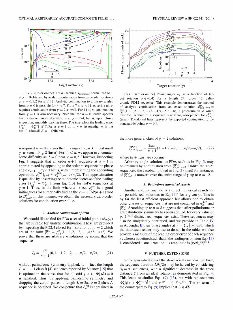
We plot the Jacobian of ToPn solutions obtained by analyticcontinuation as a function of target angle γ in Fig. 2. Thezeroth-order ToPn solutions in Eq. (15) can be continued fromγ = 0 to arbitrary γ , up to n = 7, as J is nonzero over the rangeγ ∈ [0,2]. For 8 � n � 10, analytic continuation from γ = 2

022341-6

OPTIMAL ARBITRARILY ACCURATE COMPOSITE PULSE . . . PHYSICAL REVIEW A 89, 022341 (2014)

n 1n 3 n 2

n 5n 4

n 7n 6

n 9n 8

n 10n 11

n 12

0 1 2 1 3 2 210 6

10 4

10 2

1

Target rotation Γ

J normalized

n1 4 16

0.50.9E

FIG. 2. (Color online) ToPn Jacobian Jnormalized normalized to 1at γ = 0 obtained by analytic continuation from zero-order solutionsat γ = 0,1,2 for n � 12. Analytic continuation to arbitrary anglesfrom γ = 0 is possible for n < 7. From 7 � n < 11, covering all γ

requires continuation from γ = 2 as well. For 11 � n, continuationfrom γ = 1 is also necessary. Note that the n = 10 curve appearshave a discontinuous derivative near γ = 7/4, but is, upon closerinspection, smoothly varying there. The inset plots the leading error|f n+1

2n − �n+12n | of ToPn at γ = 1 up to n = 16 together with the

best-fit (dotted) E = −O(ln(n)).

is required as well to cover the full range of γ , as J = 0 at smallγ , as seen in Fig. 2 (inset). For 11 � n, we appear to encountersome difficulty as J = 0 near γ = 0,2. However, inspectingFig. 1 suggests that an order n + 1 sequence at γ = 1 isapproximated by appending to the order n sequence the phaseangle ϕn+1 = π/2. That is, with ◦ representing the appendingoperation, �ϕToP

n+1|γ=1 ≈ �ϕToPn |γ=1 ◦ (π/2). This approximation

is qualified by observing the monotonic decrease of the leadingerror |f n+1

2n − �n+12n | from Eq. (13) for ToPn sequences at

γ = 1. Thus, in the limit where n → ∞, ϕToPn is a good

initial guess for numerically finding the γ = 1 ToP(n + 1) rootto BAP

n,2n. In this manner, we obtain the necessary zero-ordersolutions for continuation over all γ .

2. Analytic continuation of PDn

We would like to find for PDn a set of initial points ( �ϕ0,γ0)that are suitable for analytic continuation. These are providedby inspecting the PD2,4 closed-form solutions at γ = 2 whichare of the form �ϕPD

n = 2πn+1 (1,−1,2,−2, . . . ,n/2,−n/2). We

prove that these are arbitrary n solutions by noting that thesequence

Vn = 2π

n + 1(0,1,−1,2,−2, . . . ,n/2,−n/2), (21)

without palindrome symmetry applied, is in fact the lengthL = n + 1 class B [4] sequence reported by Vitanov [15] thatis optimal in the sense that for all odd j < L, �

j

L( �ϕ) = 0is satisfied. Thus, by applying palindrome symmetry anddropping the zeroth pulses, a length L = 2n, γ = 2 class Asequence is obtained. We conjecture that �ϕPD

n is contained in

1

2

34

5

6

7

89

1011

12

0 1 2 3 4

0

Π

2 Π

3 Π

Target rotation Γ

Phas

e an

gle

units

of ra

d.

n 12

n 2

Γ0 1 2 3 410 3

103

109

Jacobian

FIG. 3. (Color online) Phase angles ϕk as a function of tar-get rotation γ ∈ (0,4) for a length 24, order 12 palin-dromic PD12 sequence. This example demonstrates the methodof analytic continuation from an exact solution �ϕPD

12,6|γ=2 =12π

13 (1,−1,2,−2,3,−3,4,−4,5,−5,6,−6), a procedure valid wher-ever the Jacobian of a sequence is nonzero, also plotted for �ϕPD

n,n/2

(inset). The dotted lines represent the expected continuation to thenonanalytic points γ = 0,4.

the more general class of γ = 2 solutions:

�ϕPDn,m

∣∣γ=2 = 2mπ

n + 1(1,−1,2,−2, . . . ,n/2,−n/2), (22)

where (n + 1,m) are coprime.Arbitrary angle solutions to PDn, such as in Fig. 3, may

be obtained by continuation from �ϕPDn,m|γ=2. Unlike the ToPn

sequences, the Jacobian plotted in Fig. 3 (inset) for instancesof �ϕPD

n,n/2 is nonzero over the entire range of γ up to n = 12.

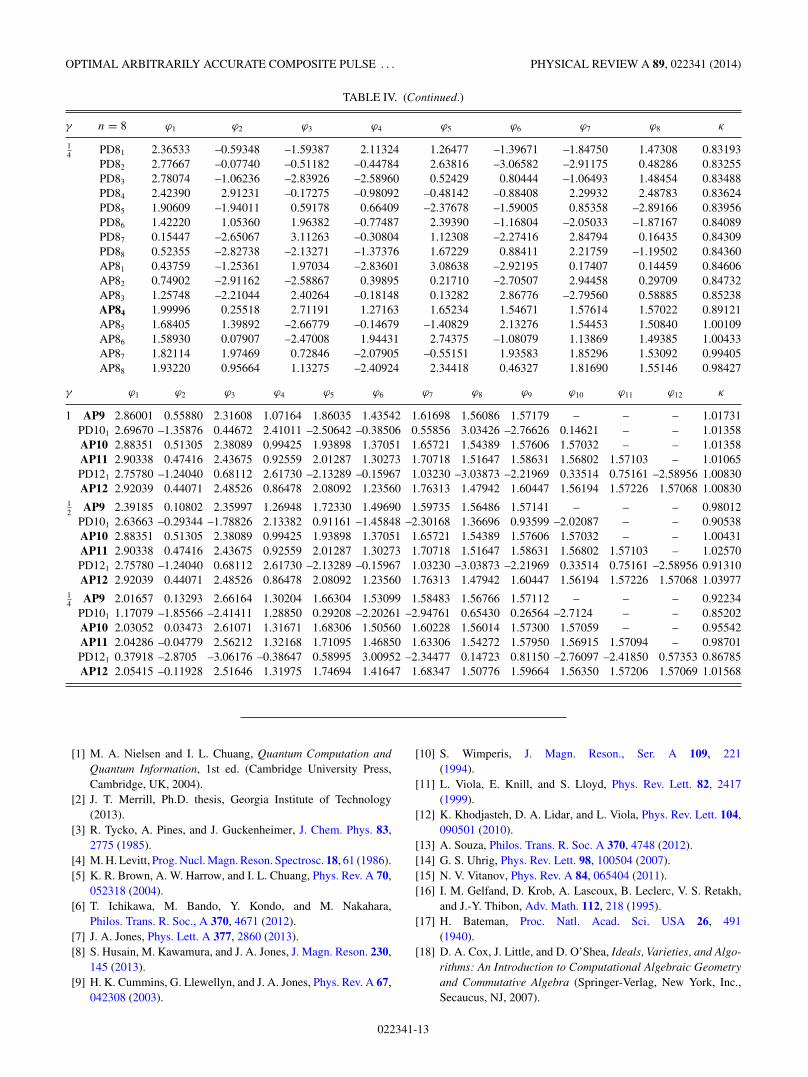
3. Brute-force numerical search

Another solution method is a direct numerical search forall possible real solutions to Eq. (11) for a given γ . This isby far the least efficient approach but allows one to obtainother classes of sequences that are not contained in �ϕToP

n and�ϕPDn,m. Searching up to n = 8 suggests that, after palindrome or

antipalindrome symmetry has been applied, for every value ofγ , 2�n/2 distinct real sequences exist. These sequences mayalso be analytically continued, and we provide in Table IVin Appendix B their phase angles at γ = {1, 1

2 , 14 } with which

the interested reader may use to do so. In the table, we alsoprovide a measure of the leading order error of each sequenceκ , where κ is defined such that if the leading error from Eq. (13)is considered a small rotation, its amplitude is (κεθ0/2)n+1.

V. FURTHER EXTENSIONS

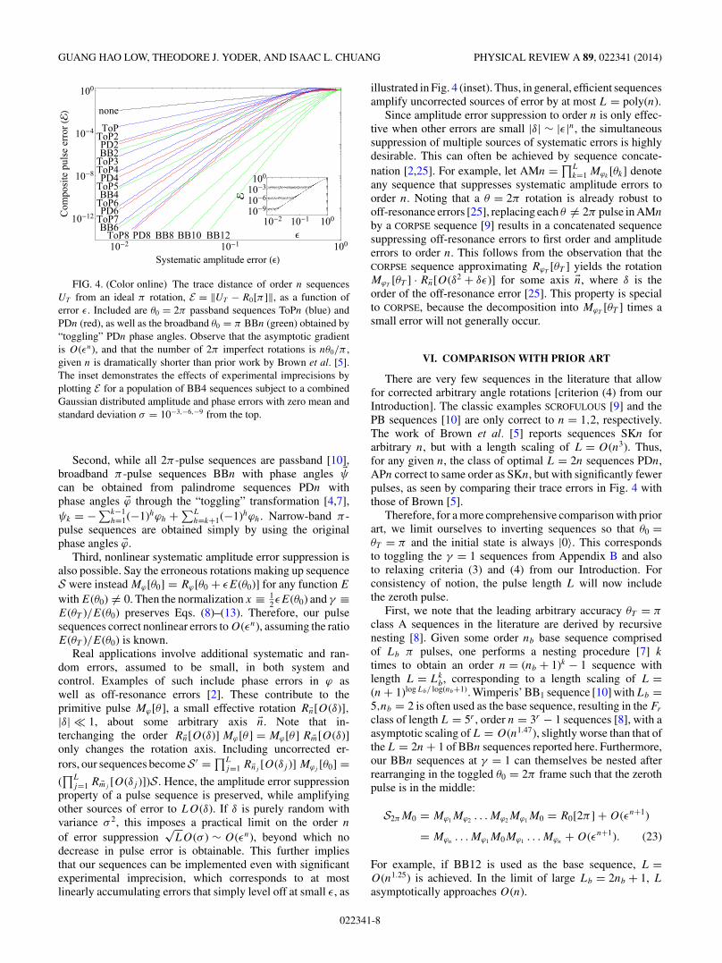
Some generalizations of the above results are possible. First,the sequence duration Lθ0/2π may be halved by consideringθ0 = π sequences, with a significant decrease in the tracedistance E from an ideal rotation as demonstrated in Fig. 4.This leads to similar Eqs. (9)–(13), but with replacements�

j

L( �ϕ) → �L−j

L ( �ψ) and eixγ → (−i)Leixγ . The x0 term ofthe counterpart to Eq. (9) implies that L ∈ 4Z.

022341-7

GUANG HAO LOW, THEODORE J. YODER, AND ISAAC L. CHUANG PHYSICAL REVIEW A 89, 022341 (2014)

none

ToPToP2PD2BB2ToP3ToP4PD4ToP5BB4ToP6PD6ToP7BB6ToP8 PD8 BB8 BB10 BB1210 2 10 1 100

10 12

10 8

10 4

100

Systematic amplitude error Ε

Compositepulseerror

10 2 10 1 10010 910 610 3100

Ε

FIG. 4. (Color online) The trace distance of order n sequencesUT from an ideal π rotation, E = ‖UT − R0[π ]‖, as a function oferror ε. Included are θ0 = 2π passband sequences ToPn (blue) andPDn (red), as well as the broadband θ0 = π BBn (green) obtained by“toggling” PDn phase angles. Observe that the asymptotic gradientis O(εn), and that the number of 2π imperfect rotations is nθ0/π ,given n is dramatically shorter than prior work by Brown et al. [5].The inset demonstrates the effects of experimental imprecisions byplotting E for a population of BB4 sequences subject to a combinedGaussian distributed amplitude and phase errors with zero mean andstandard deviation σ = 10−3,−6,−9 from the top.

Second, while all 2π -pulse sequences are passband [10],broadband π -pulse sequences BBn with phase angles �ψcan be obtained from palindrome sequences PDn withphase angles �ϕ through the “toggling” transformation [4,7],ψk = −∑k−1

h=1(−1)hϕh + ∑Lh=k+1(−1)hϕh. Narrow-band π -

pulse sequences are obtained simply by using the originalphase angles �ϕ.

Third, nonlinear systematic amplitude error suppression isalso possible. Say the erroneous rotations making up sequenceS were instead Mϕ[θ0] = Rϕ[θ0 + εE(θ0)] for any function E

with E(θ0) �= 0. Then the normalization x ≡ 12εE(θ0) and γ ≡

E(θT )/E(θ0) preserves Eqs. (8)–(13). Therefore, our pulsesequences correct nonlinear errors to O(εn), assuming the ratioE(θT )/E(θ0) is known.

Real applications involve additional systematic and ran-dom errors, assumed to be small, in both system andcontrol. Examples of such include phase errors in ϕ aswell as off-resonance errors [2]. These contribute to theprimitive pulse Mϕ[θ ], a small effective rotation R�n[O(δ)],|δ| � 1, about some arbitrary axis �n. Note that in-terchanging the order R�n[O(δ)] Mϕ[θ ] = Mϕ[θ ] R �m[O(δ)]only changes the rotation axis. Including uncorrected er-rors, our sequences becomeS ′ = ∏L

j=1 R�nj[O(δj )] Mϕj

[θ0] =(∏L

j=1 R �mj[O(δj )])S. Hence, the amplitude error suppression

property of a pulse sequence is preserved, while amplifyingother sources of error to LO(δ). If δ is purely random withvariance σ 2, this imposes a practical limit on the order n

of error suppression√

LO(σ ) ∼ O(εn), beyond which nodecrease in pulse error is obtainable. This further impliesthat our sequences can be implemented even with significantexperimental imprecision, which corresponds to at mostlinearly accumulating errors that simply level off at small ε, as

illustrated in Fig. 4 (inset). Thus, in general, efficient sequencesamplify uncorrected sources of error by at most L = poly(n).

Since amplitude error suppression to order n is only effec-tive when other errors are small |δ| ∼ |ε|n, the simultaneoussuppression of multiple sources of systematic errors is highlydesirable. This can often be achieved by sequence concate-nation [2,25]. For example, let AMn = ∏L

k=1 Mϕk[θk] denote

any sequence that suppresses systematic amplitude errors toorder n. Noting that a θ = 2π rotation is already robust tooff-resonance errors [25], replacing each θ �= 2π pulse in AMn

by a CORPSE sequence [9] results in a concatenated sequencesuppressing off-resonance errors to first order and amplitudeerrors to order n. This follows from the observation that theCORPSE sequence approximating RϕT

[θT ] yields the rotationMϕT

[θT ] · R�n[O(δ2 + δε)] for some axis �n, where δ is theorder of the off-resonance error [25]. This property is specialto CORPSE, because the decomposition into MϕT

[θT ] times asmall error will not generally occur.

VI. COMPARISON WITH PRIOR ART

There are very few sequences in the literature that allowfor corrected arbitrary angle rotations [criterion (4) from ourIntroduction]. The classic examples SCROFULOUS [9] and thePB sequences [10] are only correct to n = 1,2, respectively.The work of Brown et al. [5] reports sequences SKn forarbitrary n, but with a length scaling of L = O(n3). Thus,for any given n, the class of optimal L = 2n sequences PDn,APn correct to same order as SKn, but with significantly fewerpulses, as seen by comparing their trace errors in Fig. 4 withthose of Brown [5].

Therefore, for a more comprehensive comparison with priorart, we limit ourselves to inverting sequences so that θ0 =θT = π and the initial state is always |0〉. This correspondsto toggling the γ = 1 sequences from Appendix B and alsoto relaxing criteria (3) and (4) from our Introduction. Forconsistency of notion, the pulse length L will now includethe zeroth pulse.

First, we note that the leading arbitrary accuracy θT = π

class A sequences in the literature are derived by recursivenesting [8]. Given some order nb base sequence comprisedof Lb π pulses, one performs a nesting procedure [7] k

times to obtain an order n = (nb + 1)k − 1 sequence withlength L = Lk

b, corresponding to a length scaling of L =(n + 1)log Lb/ log(nb+1). Wimperis’ BB1 sequence [10] with Lb =5,nb = 2 is often used as the base sequence, resulting in the Fr

class of length L = 5r , order n = 3r − 1 sequences [8], with aasymptotic scaling of L = O(n1.47), slightly worse than that ofthe L = 2n + 1 of BBn sequences reported here. Furthermore,our BBn sequences at γ = 1 can themselves be nested afterrearranging in the toggled θ0 = 2π frame such that the zerothpulse is in the middle:

S2πM0 = Mϕ1Mϕ2 . . .Mϕ2Mϕ1M0 = R0[2π ] + O(εn+1)

= Mϕn. . .Mϕ1M0Mϕ1 . . . Mϕn

+ O(εn+1). (23)

For example, if BB12 is used as the base sequence, L =O(n1.25) is achieved. In the limit of large Lb = 2nb + 1, L

asymptotically approaches O(n).

022341-8

OPTIMAL ARBITRARILY ACCURATE COMPOSITE PULSE . . . PHYSICAL REVIEW A 89, 022341 (2014)

BB12V24 F2

S2BB4 2V8C9Π

1.0 0.5 0 0.5 1.00

0.2

0.4

0.6

0.8

1.0

Systematic amplitude error Ε

Transitionprobability

1 0 110 4

10 2

1

Ε

1p

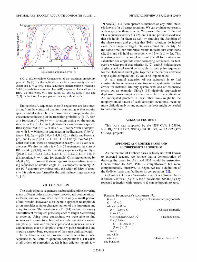
FIG. 5. (Color online) Comparison of the transition probabilityp = | 〈1| UT |0〉 |2 with amplitude error ε between a variety of L = 9(blue) and L = 25 (red) pulse sequences implementing π rotations.Solid (dashed) lines represent class A(B) sequences. Included are theBB4,12 of this work, V8,24 [Eq. (21)], 2 [26], C9 [27], F2 [8], andS2[3]. In the inset, 1 − p is plotted on a logarithmic scale.

Unlike class A sequences, class B sequences are less inter-esting from the context of quantum computing as they requirespecific initial states. The trace error metric is inapplicable, butone can nevertheless plot the transition probability |〈1|UT |0〉|2as a function of ε for θT = π rotations acting on the groundstate as in Fig. 5. As our highest-order closed-form sequenceBB4 specialized to θT = π has L = 9, we perform a compari-son with L = 9 inverting sequences in the literature: V8 by Vi-tanov [15], 2 = π

6 (0,3,0,4,7,4,0,3,0) by Shaka and Freeman[26], and C9 = π

12 (0,1,12,11,18,11,12,1,0) by Cho et al. [27].Other than ours, there do not appear to be any L = 9 class A se-quences. We also include a few L = 25 sequences: the class ABB12 and F2 [8,10], and the inverting sequences V24 and S2 =π3 (0,0,2,1,2,0,0,2,1,2,2,2,4,3,4,1,1,3,2,3,2,2,4,3,4) [3]. Inthis notation, θ0 = π and, for example, C9 is implemented byM0M π

12Mπ . . . . We see that even against the specialized invert-

ing sequences of similar length, BBn compares favorably. Atthe 10−4 quantum error threshold, the width of BBn of aboutε = 0 is only outperformed by the optimal inverting sequencesVn [15].

VII. CONCLUSION

The study of pulse sequences is a broad discipline, coveringmany different pulse shapes, error models, and computationalmethods, and we have dealt here with only a small portionof this breadth. However, our algebraic approach to amplitudeerrors provides a major characterization of this important andubiquitous case. The constraints in Eq. (14) are both necessaryand sufficient for any 2π -pulse sequence of length L correctingto order n. Using these constraints, we were able to findsequences in closed form beyond any order previously knownanalytically. From our 2π -pulse passband sequences, we alsodemonstrated that it is simple to obtain π -pulse broadband andπ -pulse narrow-band sequences of the same optimal length.

In the Introduction, we proposed four criteria for a pulsesequence to be useful to quantum computation: (1) It existsat all orders of correction n. (2) It has efficient length L =

O( poly(n)). (3) It can operate as intended on any initial state.(4) It exists for all target rotations. We can evaluate our resultswith respect to these criteria. We proved that our ToPn andPDn sequences satisfy (1), (2), and (3) and provided evidencethat (4) holds for them as well by studying the Jacobian ofthe phase sums and proving that ToPn solutions do indeedexist for a range of target rotations around the identity. Atthe same time, our numerical results indicate that conditions(2), (3), and (4) hold up to order n = 12 with L = 2n. Thisis a strong start to a complete proof that all four criteria aresatisfiable for amplitude error correcting sequences. In fact,even a weaker proof that criteria (1), (2), and (3) hold at targetangles π and π/4 would be valuable, as then pulse sequencesfor the Hadamard and T gate, together sufficient for universalsingle-qubit computation [1], could be implemented.

A very natural extension of our approach is to findconstraints for sequences correcting other systematic controlerrors, for instance, arbitrary system drifts and off-resonanceerrors. As an example, Uhrig’s [14] algebraic approach todephasing errors might also be amenable to generalization.An anticipated problem in these other cases might be thenonpolynomial nature of such constraint equations, meaningmore difficult analytic and numeric methods might be neededto find solutions.

ACKNOWLEDGMENT

This work was supported by the NSF CUA 1125846,NSF RQCC 1111337, NSF iQuISE IGERT, and IARPA QCSORAQL projects.

APPENDIX A: GROBNER BASES ANDBUCHBERGER’S ALGORITHM

As the method of Grobner bases is likely not well knownto expected readers, we believe that a demonstration ofderiving the bases for AP1 and PD2 would be instructive.Generalization to AP3, PD4 is straightforward but morecomputationally intensive. To begin, we use a definition ofthe Grobner basis that facilitates its computation [22]:

Definition 1: Given a term order, a set G is a Grobner basisif and only if for all f,g ∈ G the S-polynomial SPOL(f,g) byrepeated reduction with respect to G can be brought to zero.

Function: BUCHBERGER’S ALGORITHM (F).G ← F �System of multivariate polynomialsC ← G × Gwhile C �= ∅ do

p ← (a,b) ∈ C �Chosen arbitrarilyC ← C\{p}h = RED(SPOL(a,b),G) �Defined belowif h �= 0 then

C ← C ∪ (G × {h})G ← G ∪ {h}

end ifend whilereturn G �Grobner basis of F

end Function

022341-9

GUANG HAO LOW, THEODORE J. YODER, AND ISAAC L. CHUANG PHYSICAL REVIEW A 89, 022341 (2014)

This definition follows from Buchberger’s theorem andleads to his famous algorithm for computing a Grobner basisof F [22]:where

RED(a,G)=Remainder of a upon division by G (reduction),

SPOL(a,b)= lcm(LPP(a),LPP (b))(

a

LM(a)− b

LM(b)

),

lcm(a,b)= least common multiple of a,b,

LM(a)= leading monomial of a

with respect to some term order,

LPP(a)=LM(a) with coefficients dropped.

In what follows, we apply the Weierstrass substitutiontan(ϕk/2) = tk to Bn,L, rearrange to obtain a polynomialsystem Wn,L, and use the lexicographic monomial orderingt1 ≺lex t2 ≺lex · · · ≺lex tn [18] in computing a Grobner basis.

1. Example: AP1 from BAP1,2

BAP1,2 ⇒ WAP

1,2 = {t21 (1 + γ

2 ) − (1 − γ

2 )}. This example istrivial, as WAP

1,2 is automatically a Grobner basis G followingfrom Definition 1 as the S polynomial of an arbitrarypolynomial with itself is 0. As G generatesWAP

1,2 , they share the

same simultaneous roots. Solving G, we obtain t1 = ±√

2−γ

2+γ.

Solving for ϕ1 = cos−1 ( γ

2 ), we see that AP1 is the sequenceSK1 [5].

2. Example: PD2 from BPD2,4

BPD2,4 ⇒ WPD

2,4 = {t21 t2

2 (γ−4)+ t21 γ + t2

2 γ + (4 + γ ),t21 t2 +

t1t22 + t1 + t2}. In rearranging, we have introduced the

complex roots 1 + t2k = 0, which we shall have to remove

later. One could solve WPD2,4 by inspection, but we apply

Buchberger’s algorithm to demonstrate the algorithmicmanner in which solutions may be derived. We perform thefirst iteration in detail and only state the computed basiselement hi,j of succeeding iterations for brevity:

Input: WPD2,4 .

G = WPD2,4, C = {(g1,g2)},

Take the pair g1,g2.

LM(g1) = t22 t2

1 (γ − 4) = (γ − 4)LPP(g1),

LM(g2) = t22 t1 = LPP(g2),

LCM(LPP(g1),LPP(g2)) = t22 t2

1 ,

SPOL(g1,g2) = γ t22

γ − 4− t3

1 t2 − t1t2 + 4t21

γ − 4+ γ + 4

γ − 4,

h1,2 = RED(SPOL(g1,g2),G) = SPOL(g1,g2),

G = G ∪ {h1,2}, C = {(g1,g3),(g2,g3)},· · ·Output: G = WPD

2,4 ∪ {h1,2,h2,3,h1,4,h4,5,h1,6},

h2,3 = (γ − 4)t2t41 + 2(γ − 2)t2t2

1 + γ t2 − 4t31 − 4t1

γ,

h1,4 = 4t31 t2 + 4t1t2 + γ t4

1 + 2(γ + 2)t21 + γ + 4

γ − 4,

h4,5 = 4γ t2t21 + 4γ t2 − (γ − 4)γ t5

1 − 2(γ − 2)γ t31 − γ 2t1

4(4 − γ ),

h1,6 = (γ − 4)t61 + (3γ − 4)t4

1 + (3γ + 4)t21 + γ + 4

4,

all other hi,j = 0. (A1)

Note that the last term h1,6 is univariate in t1, as expected froma regular chain. We have chosen pairs from C so as to minimizethe output, but any arbitrary choice will eventually terminate.However, G from Eq. (A1) still contains more elements than isnecessary to generate WPD

2,4 . We can deterministically computefrom G a unique minimal, or reduced, Grobner basis GR up toconstant factors by repeating G ← (G − {g}) ∪ {RED(g,G −{g})} ∀g ∈ G until the process converges [18]:

GR = {(t21 + 1

)2[4 + γ − (4 − γ )t2

1

],(

t21 + 1

)[(γ − 4)t3

1 + γ t1 − 4t2],

4 + γ + (γ − 4)t41 + 2(γ − 2)t2

1 + 4t22

}. (A2)

The nonphysical zeros M = {1 + t21 ,1 + t2

2 } that wereintroduced earlier are now apparent and can be removed. Wecan deterministically compute from GR another Grobner basisGQ with the same zeros sans M by repeatedly computing theGrobner basis of the ideal quotient GQ → 〈GQ〉 : 〈M〉 untilconvergence, or saturation [18]. Finally, we obtain the simpletriangular system

GQ = {4 + γ − (4 − γ )t2

1 ,t1 + t2}. (A3)

Solving for ϕ1 = cos−1(

γ

4

), ϕ2 = −ϕ1, we see that PD2 is the

sequence PB1 [10].

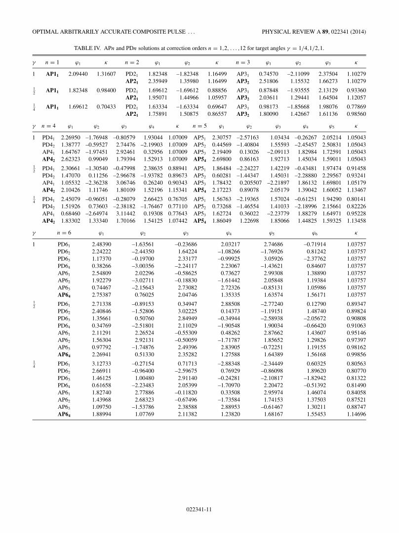
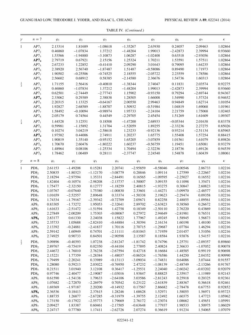
APPENDIX B: NUMERICAL SOLUTIONS

Here in Table IV, we provide phase angles for APn andPDn sequences at some common values of γ ∈ {1, 1

2 , 14 }

up to n = 12. Up to n = 8, we provide the phase anglesfor all existing symmetric solutions at the selected valuesof γ . Sequences with the same subscript are related byanalytic continuation and are sorted by their leading errorκ at γ = 1

2 . Recall from Sec. IV C 3 that κ is defined sothat (κεθ0/2)n+1 is the rotation angle of the leading error inEq. (13) when it is considered as a small rotation. In the table,the bolded APn are ToPn sequences, and all PDn1 sequencesare obtained by analytic continuation from �ϕPD

n,n/2|γ=2. Notethat ϕAP

k = −ϕAPL−k+1 and ϕPD

k = ϕPDL−k+1. Also, for each se-

quence �ϕ listed here, there is a sequence −�ϕ with the sameleading error.

022341-10

OPTIMAL ARBITRARILY ACCURATE COMPOSITE PULSE . . . PHYSICAL REVIEW A 89, 022341 (2014)

TABLE IV. APn and PDn solutions at correction orders n = 1,2, . . . ,12 for target angles γ = 1/4,1/2,1.

γ n = 1 ϕ1 κ n = 2 ϕ1 ϕ2 κ n = 3 ϕ1 ϕ2 ϕ3 κ

1 AP11 2.09440 1.31607 PD21 1.82348 –1.82348 1.16499 AP31 0.74570 –2.11099 2.37504 1.10279AP21 2.35949 1.35980 1.16499 AP32 2.51806 1.15532 1.66273 1.10279

12 AP11 1.82348 0.98400 PD21 1.69612 –1.69612 0.88856 AP31 0.87848 –1.93555 2.13129 0.93360

AP21 1.95071 1.44966 1.05957 AP32 2.03611 1.29441 1.64504 1.1205714 AP11 1.69612 0.70433 PD21 1.63334 –1.63334 0.69647 AP31 0.98173 –1.85668 1.98076 0.77869

AP21 1.75891 1.50875 0.86557 AP32 1.80090 1.42667 1.61136 0.98560

γ n = 4 ϕ1 ϕ2 ϕ3 ϕ4 κ n = 5 ϕ1 ϕ2 ϕ3 ϕ4 ϕ5 κ

1 PD41 2.26950 –1.76948 –0.80579 1.93044 1.07009 AP51 2.30757 –2.57163 1.03434 –0.26267 2.05214 1.05043PD42 1.38777 –0.59527 2.74476 –2.19903 1.07009 AP52 0.44569 –1.40804 1.55593 –2.45457 2.50831 1.05043AP41 1.64767 –1.97451 2.92461 0.32956 1.07009 AP53 2.19409 0.13026 –2.09113 1.82984 1.72591 1.05043AP42 2.62323 0.99049 1.79394 1.52913 1.07009 AP54 2.69800 0.86163 1.92713 1.45034 1.59011 1.05043

12 PD41 2.30661 –1.30540 –0.47998 2.38635 0.88941 AP51 1.86484 –2.24227 1.42219 –0.43481 1.97474 0.91458

PD42 1.47070 0.11256 –2.96678 –1.93782 0.89673 AP52 0.60281 –1.44347 1.45031 –2.28880 2.29567 0.93241AP41 1.05532 –2.36238 3.06746 0.26240 0.90343 AP53 1.78432 0.205507 –2.21897 1.86132 1.69801 1.05179AP42 2.10426 1.11746 1.80109 1.52196 1.15341 AP54 2.17223 0.89078 2.05179 1.39042 1.60052 1.13467

14 PD41 2.45079 –0.96051 –0.28079 2.66423 0.76705 AP51 1.56763 –2.19365 1.57024 –0.61251 1.94290 0.80141

PD42 1.51926 0.73603 –2.38182 –1.76467 0.77110 AP52 0.73268 –1.46554 1.41033 –2.18996 2.15661 0.82226AP41 0.68460 –2.64974 3.11442 0.19308 0.77643 AP53 1.62724 0.36022 –2.23779 1.88279 1.64971 0.95228AP42 1.83302 1.33340 1.70166 1.54125 1.07442 AP54 1.86049 1.22698 1.85066 1.44825 1.59325 1.13458

γ n = 6 ϕ1 ϕ2 ϕ3 ϕ4 ϕ5 ϕ6 κ

1 PD61 2.48390 –1.63561 –0.23686 2.03217 2.74686 –0.71914 1.03757PD62 2.24222 –2.44350 1.64224 –1.08266 –1.76926 0.81242 1.03757PD63 1.17370 –0.19700 2.33177 –0.99925 3.05926 –2.37762 1.03757PD64 0.38266 –3.00356 –2.24117 2.23067 –1.43621 0.84607 1.03757AP61 2.54809 2.02296 –0.58625 0.73627 2.99308 1.38890 1.03757AP62 1.92279 –3.02711 –0.18830 –1.61442 2.05848 1.19384 1.03757AP63 0.74467 –2.15643 2.73082 2.72326 –0.85131 1.05986 1.03757AP64 2.75387 0.76025 2.04746 1.35335 1.63574 1.56171 1.03757

12 PD61 2.71338 –0.89153 0.34947 2.88508 –2.77240 0.12790 0.89347

PD62 2.40846 –1.52806 3.02225 0.14373 –1.19151 1.48740 0.89824PD63 1.35661 0.50760 2.84949 –0.34944 –2.58938 –2.05672 0.90808PD64 0.34769 –2.51801 2.11029 –1.90548 1.90034 –0.66420 0.91063AP61 2.11291 2.26524 –0.55309 0.48262 2.87662 1.43607 0.95146AP62 1.56304 2.92131 –0.50059 –1.71787 1.85652 1.29826 0.97397AP63 0.97792 –1.74876 2.49396 2.83905 –0.72251 1.19155 0.98162AP64 2.26941 0.51330 2.35282 1.27588 1.64389 1.56168 0.99856

14 PD61 3.12733 –0.27154 0.71713 –2.88348 –2.34449 0.60325 0.80563

PD62 2.66911 –0.96400 –2.59675 0.76929 –0.86098 1.89620 0.80770PD63 1.46125 1.00480 2.91140 –0.24281 –2.10817 –1.82942 0.81322PD64 0.61658 –2.23483 2.05399 –1.70970 2.20472 –0.51392 0.81490AP61 1.82740 2.77886 –0.11820 0.33508 2.95974 1.46074 0.84058AP62 1.43968 2.68323 –0.67496 –1.73584 1.74153 1.37503 0.87521AP63 1.09750 –1.53786 2.38588 2.88953 –0.61467 1.30211 0.88747AP64 1.88994 1.07769 2.11382 1.23820 1.68167 1.55453 1.14696

022341-11

GUANG HAO LOW, THEODORE J. YODER, AND ISAAC L. CHUANG PHYSICAL REVIEW A 89, 022341 (2014)

TABLE IV. (Continued.)

γ n = 7 ϕ1 ϕ2 ϕ3 ϕ4 ϕ5 ϕ6 ϕ7 κ

1 AP71 2.13314 1.81689 –1.08618 –1.35267 2.63930 0.24057 2.09463 1.02864AP72 0.46860 –1.07834 1.37212 –1.48204 1.99013 –2.42873 2.39994 0.93660AP73 1.53566 –1.94880 –3.10873 1.06287 –1.02408 0.63518 –2.93056 1.02864AP74 2.79719 0.67921 2.15156 1.25324 1.70211 1.53591 1.57511 1.02864AP75 2.67233 1.22852 –0.41410 2.09290 3.01643 0.79095 1.64235 1.02864AP76 2.38920 2.56740 –1.87487 1.51487 –0.58086 0.89490 1.71973 1.02864AP77 1.90502 –0.25506 –0.74525 2.18555 –2.05722 2.23559 1.78586 1.02864AP78 2.56602 0.68912 0.58385 –2.14580 2.36676 1.54736 1.60313 1.02864

12 AP71 1.71155 2.56416 –0.40810 –1.38344 2.74047 0.11831 2.03574 0.92275

AP72 0.46860 –1.07834 1.37212 –1.48204 1.99013 –2.42873 2.39994 0.93660AP73 0.62501 –2.74449 –2.77743 1.15902 –0.93150 0.79294 –2.69744 0.94367AP74 2.33062 0.29389 2.38838 1.28505 1.66008 1.54990 1.57324 0.94652AP75 2.20315 1.13325 –0.64167 2.00550 2.99463 0.94849 1.62714 1.01054AP76 1.92827 2.68589 –1.88707 1.50932 –0.51984 1.04819 1.69068 1.01961AP77 1.58492 –0.10094 –0.98974 1.95733 –2.24104 2.21759 1.75068 1.02465AP78 2.05179 0.74564 0.44549 –2.29705 2.45454 1.51269 1.61609 1.09307

14 AP71 1.44528 3.12551 0.18508 –1.47200 2.68933 –0.05344 2.01638 0.83378

AP72 0.59981 –1.15892 1.31704 –1.52059 1.89255 –2.33236 2.27275 0.85026AP73 0.10274 3.04219 –2.58618 1.23233 –0.92136 0.93214 –2.51134 0.85965AP74 1.97582 0.44006 2.74911 1.20237 1.65775 1.55408 1.57254 0.88415AP75 1.90819 1.35140 –0.95152 1.65205 –3.07859 1.01561 1.61079 0.89826AP76 1.70670 2.60476 –1.80222 1.60237 –0.56759 1.19451 1.65081 0.93279AP77 1.48964 0.08106 –1.25334 1.70494 –2.32236 2.18736 1.69126 0.94539AP78 1.78462 1.06489 0.28111 –2.37747 2.24540 1.54878 1.60439 1.08061

γ n = 8 ϕ1 ϕ2 ϕ3 ϕ4 ϕ5 ϕ6 ϕ7 ϕ8 κ

1 PD81 2.61153 –1.49208 0.15281 2.20741 –2.95859 –0.58046 –0.00546 2.86733 1.02216PD82 2.50835 –1.80323 –1.12170 –3.08779 0.28846 1.09114 1.27599 –2.22667 1.02216PD83 2.18294 –2.97594 1.35331 –2.84491 0.16565 –1.09595 –2.25027 0.16552 1.02216PD84 1.82404 –0.10574 –2.98208 –2.13737 –1.50007 3.09155 0.11098 1.35471 1.02216PD85 1.75477 –2.32150 0.12777 –1.18259 2.40815 –1.93275 0.30847 2.60823 1.02216PD86 1.03767 –0.07640 1.75380 –1.00830 2.33601 –1.44271 –3.09970 –2.48577 1.02216PD87 1.01659 –2.52557 2.89648 0.33374 –1.50338 2.19623 –2.29474 0.09358 1.02216PD88 1.74334 –1.79167 –2.39342 –0.72709 2.05671 0.82258 2.48855 –1.09561 1.02216AP81 0.83305 –1.73272 1.95053 –2.32641 2.89702 –2.63823 0.38560 0.26672 1.02216AP82 1.61633 –2.51472 –1.51594 1.42758 0.18349 –2.50110 2.76220 0.43869 1.02216AP83 2.27849 –2.00209 1.75303 –0.08067 0.27972 2.94649 –2.81981 0.76531 1.02216AP84 2.83177 0.61330 2.24038 1.15822 1.77967 1.49245 1.58945 1.56873 1.02216AP85 2.35733 1.05688 –2.82410 –0.44884 –1.30394 2.16134 1.60198 1.48100 1.02216AP86 2.13392 –0.24881 –2.41837 1.70116 2.70715 –1.29687 1.07784 1.46294 1.02216AP87 2.59142 1.60949 0.74701 –2.11111 –0.81043 1.71959 2.01457 1.51056 1.02216AP88 2.74925 0.90733 0.84501 –2.90598 2.13587 0.18584 1.93876 1.54157 1.02216

12 PD81 3.09896 –0.40393 1.07238 –2.81247 –1.81742 0.74796 1.25751 –2.09357 0.89860

PD82 2.89767 –0.75419 0.02350 –0.44104 2.77895 2.40824 2.36633 –1.07052 0.90078PD83 2.44672 –1.76010 2.76238 –2.67594 0.42718 0.16684 –1.48585 0.99119 0.90698PD84 2.15221 1.77359 –1.28384 –1.48037 –0.86524 –1.76586 1.44250 2.04352 0.90990PD85 1.79499 –2.20241 0.33989 –0.13113 –3.09034 –1.74831 0.64086 3.07444 0.91557PD86 1.28080 0.59213 2.03022 –0.76950 2.47232 –1.08139 –2.48749 –2.13266 0.91767PD87 0.21511 3.01940 3.12108 0.36417 –1.25531 2.24040 –2.60242 –0.03202 0.92079PD88 0.97746 –2.40477 –2.19087 –1.03016 1.93847 0.88825 2.35917 –1.11989 0.92143AP81 0.61590 –1.54138 1.79633 –2.64106 3.03586 –2.81243 0.25918 0.20325 0.92361AP82 1.07682 –2.72870 –2.26979 0.70542 0.23122 –2.61839 2.88367 0.36618 0.92461AP83 1.69369 –1.97187 2.20200 –0.14932 0.17567 2.86682 –2.78478 0.67753 0.92852AP84 2.36536 0.18413 2.37615 1.28246 1.68628 1.52971 1.58055 1.56971 0.95723AP85 1.88735 1.26877 –2.67285 –0.31979 –1.39755 2.12492 1.60375 1.47723 1.05962AP86 1.73150 –0.17922 –2.55773 1.79669 2.76172 –1.23074 1.08662 1.45651 1.05991AP87 2.09427 1.83387 0.60461 –2.17505 –0.63648 1.77937 1.98533 1.50975 1.06029AP88 2.24717 0.77780 1.17411 –2.62726 2.07274 0.36619 1.91234 1.54065 1.07079

022341-12

OPTIMAL ARBITRARILY ACCURATE COMPOSITE PULSE . . . PHYSICAL REVIEW A 89, 022341 (2014)

TABLE IV. (Continued.)

γ n = 8 ϕ1 ϕ2 ϕ3 ϕ4 ϕ5 ϕ6 ϕ7 ϕ8 κ

14 PD81 2.36533 –0.59348 –1.59387 2.11324 1.26477 –1.39671 –1.84750 1.47308 0.83193

PD82 2.77667 –0.07740 –0.51182 –0.44784 2.63816 –3.06582 –2.91175 0.48286 0.83255PD83 2.78074 –1.06236 –2.83926 –2.58960 0.52429 0.80444 –1.06493 1.48454 0.83488PD84 2.42390 2.91231 –0.17275 –0.98092 –0.48142 –0.88408 2.29932 2.48783 0.83624PD85 1.90609 –1.94011 0.59178 0.66409 –2.37678 –1.59005 0.85358 –2.89166 0.83956PD86 1.42220 1.05360 1.96382 –0.77487 2.39390 –1.16804 –2.05033 –1.87167 0.84089PD87 0.15447 –2.65067 3.11263 –0.30804 1.12308 –2.27416 2.84794 0.16435 0.84309PD88 0.52355 –2.82738 –2.13271 –1.37376 1.67229 0.88411 2.21759 –1.19502 0.84360AP81 0.43759 –1.25361 1.97034 –2.83601 3.08638 –2.92195 0.17407 0.14459 0.84606AP82 0.74902 –2.91162 –2.58867 0.39895 0.21710 –2.70507 2.94458 0.29709 0.84732AP83 1.25748 –2.21044 2.40264 –0.18148 0.13282 2.86776 –2.79560 0.58885 0.85238AP84 1.99996 0.25518 2.71191 1.27163 1.65234 1.54671 1.57614 1.57022 0.89121AP85 1.68405 1.39892 –2.66779 –0.14679 –1.40829 2.13276 1.54453 1.50840 1.00109AP86 1.58930 0.07907 –2.47008 1.94431 2.74375 –1.08079 1.13869 1.49385 1.00433AP87 1.82114 1.97469 0.72846 –2.07905 –0.55151 1.93583 1.85296 1.53092 0.99405AP88 1.93220 0.95664 1.13275 –2.40924 2.34418 0.46327 1.81690 1.55146 0.98427

γ ϕ1 ϕ2 ϕ3 ϕ4 ϕ5 ϕ6 ϕ7 ϕ8 ϕ9 ϕ10 ϕ11 ϕ12 κ

1 AP9 2.86001 0.55880 2.31608 1.07164 1.86035 1.43542 1.61698 1.56086 1.57179 – – – 1.01731PD101 2.69670 –1.35876 0.44672 2.41011 –2.50642 –0.38506 0.55856 3.03426 –2.76626 0.14621 – – 1.01358AP10 2.88351 0.51305 2.38089 0.99425 1.93898 1.37051 1.65721 1.54389 1.57606 1.57032 – – 1.01358AP11 2.90338 0.47416 2.43675 0.92559 2.01287 1.30273 1.70718 1.51647 1.58631 1.56802 1.57103 – 1.01065PD121 2.75780 –1.24040 0.68112 2.61730 –2.13289 –0.15967 1.03230 –3.03873 –2.21969 0.33514 0.75161 –2.58956 1.00830AP12 2.92039 0.44071 2.48526 0.86478 2.08092 1.23560 1.76313 1.47942 1.60447 1.56194 1.57226 1.57068 1.00830

12 AP9 2.39185 0.10802 2.35997 1.26948 1.72330 1.49690 1.59735 1.56486 1.57141 – – – 0.98012

PD101 2.63663 –0.29344 –1.78826 2.13382 0.91161 –1.45848 –2.30168 1.36696 0.93599 –2.02087 – – 0.90538AP10 2.88351 0.51305 2.38089 0.99425 1.93898 1.37051 1.65721 1.54389 1.57606 1.57032 – – 1.00431AP11 2.90338 0.47416 2.43675 0.92559 2.01287 1.30273 1.70718 1.51647 1.58631 1.56802 1.57103 – 1.02570PD121 2.75780 –1.24040 0.68112 2.61730 –2.13289 –0.15967 1.03230 –3.03873 –2.21969 0.33514 0.75161 –2.58956 0.91310AP12 2.92039 0.44071 2.48526 0.86478 2.08092 1.23560 1.76313 1.47942 1.60447 1.56194 1.57226 1.57068 1.03977

14 AP9 2.01657 0.13293 2.66164 1.30204 1.66304 1.53099 1.58483 1.56766 1.57112 – – – 0.92234

PD101 1.17079 –1.85566 –2.41411 1.28850 0.29208 –2.20261 –2.94761 0.65430 0.26564 –2.7124 – – 0.85202AP10 2.03052 0.03473 2.61071 1.31671 1.68306 1.50560 1.60228 1.56014 1.57300 1.57059 – – 0.95542AP11 2.04286 –0.04779 2.56212 1.32168 1.71095 1.46850 1.63306 1.54272 1.57950 1.56915 1.57094 – 0.98701PD121 0.37918 –2.8705 –3.06176 –0.38647 0.58995 3.00952 –2.34477 0.14723 0.81150 –2.76097 –2.41850 0.57353 0.86785AP12 2.05415 –0.11928 2.51646 1.31975 1.74694 1.41647 1.68347 1.50776 1.59664 1.56350 1.57206 1.57069 1.01568

[1] M. A. Nielsen and I. L. Chuang, Quantum Computation andQuantum Information, 1st ed. (Cambridge University Press,Cambridge, UK, 2004).

[2] J. T. Merrill, Ph.D. thesis, Georgia Institute of Technology(2013).

[3] R. Tycko, A. Pines, and J. Guckenheimer, J. Chem. Phys. 83,2775 (1985).

[4] M. H. Levitt, Prog. Nucl. Magn. Reson. Spectrosc. 18, 61 (1986).[5] K. R. Brown, A. W. Harrow, and I. L. Chuang, Phys. Rev. A 70,

052318 (2004).[6] T. Ichikawa, M. Bando, Y. Kondo, and M. Nakahara,

Philos. Trans. R. Soc., A 370, 4671 (2012).[7] J. A. Jones, Phys. Lett. A 377, 2860 (2013).[8] S. Husain, M. Kawamura, and J. A. Jones, J. Magn. Reson. 230,

145 (2013).[9] H. K. Cummins, G. Llewellyn, and J. A. Jones, Phys. Rev. A 67,

042308 (2003).

[10] S. Wimperis, J. Magn. Reson., Ser. A 109, 221(1994).

[11] L. Viola, E. Knill, and S. Lloyd, Phys. Rev. Lett. 82, 2417(1999).

[12] K. Khodjasteh, D. A. Lidar, and L. Viola, Phys. Rev. Lett. 104,090501 (2010).

[13] A. Souza, Philos. Trans. R. Soc. A 370, 4748 (2012).[14] G. S. Uhrig, Phys. Rev. Lett. 98, 100504 (2007).[15] N. V. Vitanov, Phys. Rev. A 84, 065404 (2011).[16] I. M. Gelfand, D. Krob, A. Lascoux, B. Leclerc, V. S. Retakh,

and J.-Y. Thibon, Adv. Math. 112, 218 (1995).[17] H. Bateman, Proc. Natl. Acad. Sci. USA 26, 491

(1940).[18] D. A. Cox, J. Little, and D. O’Shea, Ideals, Varieties, and Algo-

rithms: An Introduction to Computational Algebraic Geometryand Commutative Algebra (Springer-Verlag, New York, Inc.,Secaucus, NJ, 2007).

022341-13

GUANG HAO LOW, THEODORE J. YODER, AND ISAAC L. CHUANG PHYSICAL REVIEW A 89, 022341 (2014)

[19] B. Sturmfels, Solving Systems of Polynomial Equations(CBMS Regional Conference Series in Mathematics) (AmericanMathematical Society, Providence, RI, 2002).

[20] B. Sturmfels, Notices AMS 52, 2 (2005).[21] M. Kalkbrener, J. Symbolic Computation 15, 143

(1993).[22] B. Buchberger, J. Symbolic Computation 41, 475

(2006).

[23] B. Buchberger, London Mathematical Society Lecture NoteSeries 251, 535 (1998).

[24] T. W. Dube, SIAM J. Comput. 19, 750 (1990).[25] M. Bando, T. Ichikawa, Y. Kondo, and M. Nakahara, J. Phys.

Soc. Jpn. 82, 014004 (2013).[26] A. J. Shaka and R. Freeman, J. Magn. Reson. 59, 169 (1984).[27] H. M. Cho, R. Tycko, A. Pines, and J. Guckenheimer, Phys. Rev.

Lett. 56, 1905 (1986).

022341-14