Embed Size (px)
Citation preview

ORI GIN AL PA PER
Outbreeding causes developmental instabilityin Drosophila subobscura
Zorana Kurbalija • Marina Stamenkovic-Radak •
Cino Pertoldi • Marko Andjelkovic
Received: 25 June 2009 / Accepted: 29 November 2009� Springer Science+Business Media B.V. 2010
Abstract A possible effect of interpopulation hybridization is either outbreeding
depression, as a consequence of breakdown of coadapted gene complexes which can
increase developmental instability (DI) of the traits, or increased heterozygosity, which can
reduce DI. One of the principal methods commonly used to estimate DI is the variability of
fluctuating asymmetry (FA). We analysed the effect of interpopulation hybridization in
Drosophila subobscura through the variability in the wing size and the FA of wing length
and width for both sexes in parental, F1 and F2 generations. The results of the wing size
per se in intra- and interpopulation hybrids of D. subobscura do not explicitly reveal the
significance of either of the two hypotheses. However, the results of the FA of the wing
traits give a different insight. The FA of wing length and width generally increases in
interpopulation crosses in F1 with respect to the FA in the parental generation, which
suggests the possibility that outbreeding depression occurred in the first generation after
the hybridization event. We generally observed that the FA values for the wing length and
width of interpopulation hybrids were higher in F1 and F2 generations, compared to
intrapopulation hybrids in same generations. These results suggest that the association
between coadaptive genes with the same evolutionary history are the most probable
mechanism that maintains the developmental homeostasis in Drosophila subobscurapopulations.
Keywords Coadapted genome � Fluctuating asymmetry � Outbreeding depression �Wing size
Z. Kurbalija (&) � M. Stamenkovic-Radak � M. AndjelkovicInstitute of Biological Research, University of Belgrade, Despot Stefan Blvd. 142,11000 Belgrade, Serbiae-mail: [email protected]
M. Stamenkovic-Radak � M. AndjelkovicFaculty of Biology, University of Belgrade, Studentski trg 3, 11000 Belgrade, Serbia
C. PertoldiDepartment of Ecology and Genetics, Institute of Biological Science, University of Aarhus,Ny Munkegade, Building 540, 8000 Arhus C, Denmark
123
Evol EcolDOI 10.1007/s10682-009-9342-0

Introduction
The anthropogenic activities on natural ecosystems increase the risk of stochastic fluctu-
ations in population size and cause changes in the population genetic structure, which
potentially result in inbreeding or outbreeding depressions (Edmands and Timmerman
2003; Frankham 2005). In disturbed habitats, previously isolated populations may come in
contact and, if individuals from two such populations mate, hybridization of the two
different gene pools will occur (Ross and Robertson 1990; Edmands 1999). Mating
between individuals from genetically different populations which are not taxonomically
distinguishable is called intraspecific or interpopulation hybridization (Barton and Hewitt
1985). Hybridization between different populations can lead to heterosis in the first gen-
eration, followed by outbreeding depression in the consecutive generation (Dobzhansky
1950; Andersen et al. 2002; Edmands 2007).
Hybridization can cause outbreeding depression within the affected population due to
breakdown of coadaptive gene complexes (Dobzhansky 1950). A breakdown of coadap-
tation might be displayed by an individual as a decreased ability to develop an optimal
phenotype due to an increased DI (Leary and Allendorf 1989). Developmental instability is
the product of developmental noise or stress, which affects on individuals capacity to
buffer the processes that otherwise result in the development of the specific phenotype
(Zakharov 1981; Palmer 1996). This can be reflected in decreasing fitness components and
an increase in phenotypic variability (Barton and Hewitt 1985). This effect might be
displayed after hybridization in the F1 generation if the hybridization event occurs between
very distinct genomes (Markow and Ricker 1991). In other cases, disruption of coadaptive
gene complexes might not be observed before the F2 generation. The disruption of coa-
dapted gene complexes in F2 is a result of a recombination of the F1 genomes (Graham
1992; Goldberg et al. 2004). Therefore, F2 genomes consist of genes which have evolved
under different selection pressures (Felley 1980).
There is growing evidence that environmental and genomic stress can induce sig-
nificant levels of developmental instability (DI) (Palmer and Strobeck 1986; Palmer
1994, 1996; Møller and Swaddle 1997; Pertoldi et al. 2006a). Two principal methods are
commonly used to estimate DI. Some studies used phenotypic variance of different
morphological traits, where estimate can be blurred by the presence of genetic and/or
environmental variability (Andersen et al. 2002; Pertoldi et al. 2006a, b). Other studies
used fluctuating asymmetry (FA), defined as small deviations from the perfect bilateral
symmetry in morphological traits. This dissimilarity in expression of a given character
on the left and right side cannot be explained by either genotypic or environmental
differences, since the development of bilateral characters in an individual is ensured by
the same genotype under identical environmental conditions (Palmer and Strobeck
1986).
The increase or decrease of DI as a consequence of the genomic stress has been
explained by two hypotheses: heterozigosity (Lerner 1954) and the genomic coadaptation
(Dobzhansky 1950). The heterozygosity theory predicts that levels of heterozygosity will
be inversely correlated with the level of DI (Lerner 1954; Livshits and Kobyliansky 1985;
Pertoldi et al. 2006a). It has been suggested that heterozygosity has a buffering role
through increased biochemical diversity, which enables a dynamic and stable develop-
mental pathway in changing conditions (Livshits and Smouse 1993). Lerner (1954) sug-
gested that heterozygosity in complex multi-genetics systems provides a mechanism for
maintaining potential plasticity and promoting canalization.
Evol Ecol
123

The genomic coadaptation hypothesis predicts that more balanced coadapted gene
complexes, established over the evolutionary history of the populations via natural
selection, will show higher stability in development over time (Markow 1995).
Whether genomic coadaptation or heterozygosity have influence on DI is still unclear.
Although no clear patterns have been found, several trends emerged. Available data
indicate a tendency of FA to increase with inbreeding and population hybridization (Pal-
mer and Strobeck 1986; Waldmann 1999; Lens et al. 2000; Garnier et al. 2006; Andersen
et al. 2008). There is evidence which suggests a positive correlation between FA and
genomic stress (Leary and Allendorf 1989). However, there are several studies that report
exceptions to these patterns (Clarke et al. 1992; Sheridan and Pomiankowski 1997; Pel-
abon et al. 2005). On the other hand, the relationships of DI (measured by FA) with a
breakdown of coadapted gene complexes and heterozygosity are still unclear (Vøllestad
et al. 1999; Alibert and Auffray 2003).
Inversion polymorphism of Drosophila was used as a model system for studying pro-
cesses involved in adaptation and genetic diversity. As crossing-over is suppressed within
the inversion loops of heterokaryotypes, all genes within the inverted segments segregate
as a linked group, representing one physical and functional unit, called the ‘supergene’, so
the different arrangements can be regarded as ‘allelic’ complexes (Krimbas 1993).
Assuming a relatively long-time of selection on the linked genes within inverted regions,
Dobzhansky (1948) developed the coadaptation hypothesis, which proposed that the
selective value of inversions depends on the combinations of alleles, genes and their
interaction. The important aspect of this hypothesis is the effects of heterosis and fitness
epistasis, causing the evolution of the genes evolve after their origin (Hoffmann et al.
2004). The coadaptation hypothesis presumes that different alleles of genes will be pre-
sented in different gene arrangements, and that interpopulation differences exist for the
allelic combinations of the same arrangement (Hoffmann et al. 2004).
Drosophila subobscura is a Palearctic species which displays rich inversion polymor-
phism on all five acrocentric chromosomes of the set (Krimbas and Loukas 1980; Krimbas
1993) which makes that species a good candidate for studying the above mentioned
hypotheses.
In the present paper we focused on coadaptive aspect of inversion polymorphism in
Drosophila subobscura populations from three ecologically and topologically distinct hab-
itats, knowing that they possess a certain degree of genetic differentiation due to their
different evolutionary histories. The aim of this study is to detect variability of the wing size
and FA of wing length and wing width between inter-population and intra-population hybrids
of D. subobscura. The analysis performed over two generations after hybridization was
aimed at comparing the level of fluctuating asymmetry as measure of DI between intra-
population and interpopulation hybrids through generations. However, the most important
aim of the study was to discover if there was association of coadaptive gene complexes and/or
higher heterozygosity maintaining developmental homeostasis in populations.
Materials and methods
For the present study, D. subobscura flies were sampled in Serbia simultaneously at the end
of June 2006 using fermented fruit traps. The flies were collected from three localities
(beech-B, oak-O and Botanical Garden-BG).
The beech (B) and the oak (O) woods are situated in different expositions on mountain
Goc in central Serbia. These two woods have distinct microclimates. Beech wood features
Evol Ecol
123

higher humidity with dense vegetation coverage, whereas the oak has sparser trees and is
slightly warmer. The third locality is the Botanical Garden (BG) situated in the central,
urban part of Belgrade, with a specific microclimate and surrounded by high anthropogenic
activity.
The flies collected in these three localities were used to obtain isofemale lines (IF) and
they were reared on the common cornmeal-sugar-yeast-agar medium for Drosophila. All
cultures were maintained and all experiments performed under constant laboratory condi-
tions, at 19�C, approx. 60% relative humidity, light of 300 lux and 12/12 h light/dark cycles.
We used 63 IF lines from oak, 38 IF lines from beech and 64 IF lines from the Botanical
Garden population. The progeny of these IF lines formed from the field samples were used
as the parental (P) generation in the experiment. Virgin males and females were separated
within each IF line upon emerging and intra- and interpopulation crosses were made 4 days
after eclosion.
The intra- (B 9 B, O 9 O and BG 9 BG) and interpopulation crosses (B 9 O,
BG 9 O and BG 9 B) were made among IF lines of the three D. subobscura populations.
Both direct and reciprocal crosses were made in order to take into account the potential
maternal effect (i.e., direct cross: male from IF line No1 with female from IF No2, and
reciprocal cross: male from IF No2 crossed with female from IF No1 etc.) (Table 1). The
progeny (6 males and 6 females) from each cross was transferred to fresh vials to obtain F1
and F2 generation, respectively.
The flies from P, F1, and F2 generations, from intra- and interpopulation crosses
(B 9 B, O 9 O, BG 9 BG, B 9 O, BG 9 O, BG 9 B) were frozen (-20�C) and used
for further wing measurements.
Wing length and width analyses
The left and right wings from each fly were cut and mounted on a microscope slide using
double sided scotch (12.7–22.8 mm) and cover slip was placed over them. Each wing was
photographed with a Canon Power Shot camera attached to a Leica stereomicroscope
under 409 magnification. The measurements were performed on photographs, with Image
Tool Software 3.0 (Wilcox et al. 2002). (http://ddsdx.uthscsa.edu/dig/download.html). The
wing length (L) was taken as the distance from the intersection of the third longitudinal
vein (L3) with the anterior cross vein (A1) to the wing tip where the third vein ends.
Table 1 Number and type ofcrosses for direct and reciprocalcrosses
O Oak population, B Beechpopulation, BG botanical gardenpopulation
Type of cross Direct cross Reciprocalcross
No. ofcrosses
Intrapopulation Inter line crosses
O 9 O (63 IF lines) O$ 9 O# O# 9 O$ 63
B 9 B (38 IF lines) B$ 9 B# B# 9 B$ 71
BG 9 BG (64 IF lines) BG$ 9 BG# BG# 9 BG$ 89
Interpopulation
B 9 O B$ 9 O# B# 9 O$ 82
BG 9 O BG$ 9 O# BG# 9 O$ 81
BG 9 B BG$ 9 B# BG# 9 B$ 73
Evol Ecol
123
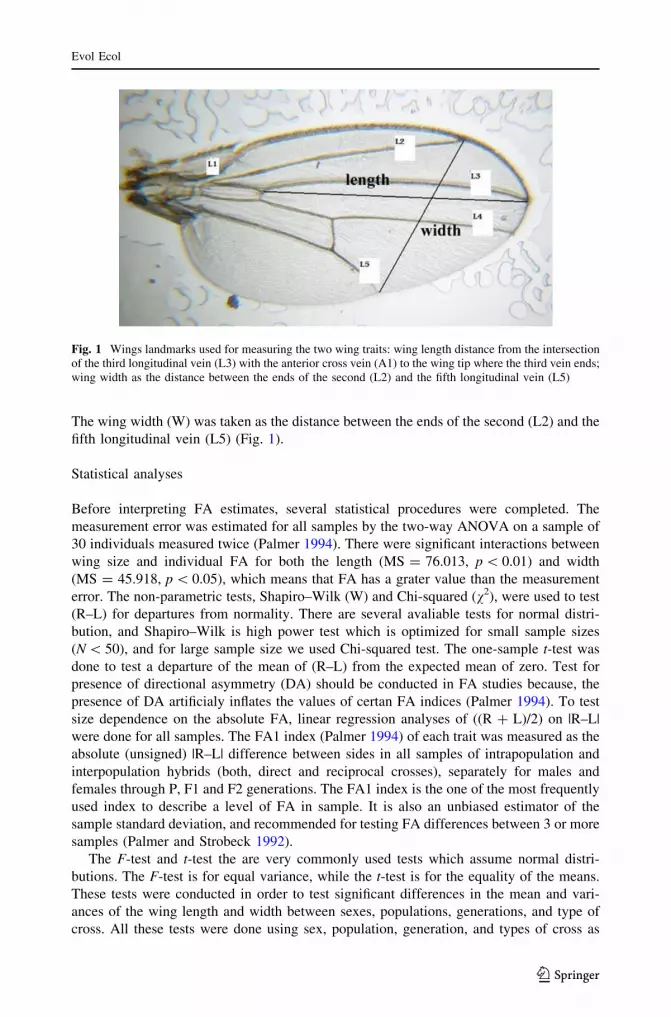
The wing width (W) was taken as the distance between the ends of the second (L2) and the
fifth longitudinal vein (L5) (Fig. 1).
Statistical analyses
Before interpreting FA estimates, several statistical procedures were completed. The
measurement error was estimated for all samples by the two-way ANOVA on a sample of
30 individuals measured twice (Palmer 1994). There were significant interactions between
wing size and individual FA for both the length (MS = 76.013, p \ 0.01) and width
(MS = 45.918, p \ 0.05), which means that FA has a grater value than the measurement
error. The non-parametric tests, Shapiro–Wilk (W) and Chi-squared (v2), were used to test
(R–L) for departures from normality. There are several avaliable tests for normal distri-
bution, and Shapiro–Wilk is high power test which is optimized for small sample sizes
(N \ 50), and for large sample size we used Chi-squared test. The one-sample t-test was
done to test a departure of the mean of (R–L) from the expected mean of zero. Test for
presence of directional asymmetry (DA) should be conducted in FA studies because, the
presence of DA artificialy inflates the values of certan FA indices (Palmer 1994). To test
size dependence on the absolute FA, linear regression analyses of ((R ? L)/2) on |R–L|
were done for all samples. The FA1 index (Palmer 1994) of each trait was measured as the
absolute (unsigned) |R–L| difference between sides in all samples of intrapopulation and
interpopulation hybrids (both, direct and reciprocal crosses), separately for males and
females through P, F1 and F2 generations. The FA1 index is the one of the most frequently
used index to describe a level of FA in sample. It is also an unbiased estimator of the
sample standard deviation, and recommended for testing FA differences between 3 or more
samples (Palmer and Strobeck 1992).
The F-test and t-test the are very commonly used tests which assume normal distri-
butions. The F-test is for equal variance, while the t-test is for the equality of the means.
These tests were conducted in order to test significant differences in the mean and vari-
ances of the wing length and width between sexes, populations, generations, and type of
cross. All these tests were done using sex, population, generation, and types of cross as
Fig. 1 Wings landmarks used for measuring the two wing traits: wing length distance from the intersectionof the third longitudinal vein (L3) with the anterior cross vein (A1) to the wing tip where the third vein ends;wing width as the distance between the ends of the second (L2) and the fifth longitudinal vein (L5)
Evol Ecol
123

separate variables. The conservative F-test and t-test were used to reduce the possibility of
a Type 1 error. Type 1 error is typically associated with investigations dealing with a large
amount of data, as in the present study. All the statistical analyses were performed using
PAST software (Hammer et al. 2001). Corrections for multiple comparisons were per-
formed using overall Bonferroni correction (Rice 1989).
Results
None of the samples manifest significant deviations from normality (Tables 2, 3) and the
signed right-left (R–L) size analysis show that directional asymmetry (DA) is absent in all
samples. In less than 1% of the samples a positive correlation between |R–L| and the
(R ? L)/2 is found. After sequential Bonferroni correction none of the regressions were
significant, indicating that FA is not correlated with the trait size.
Intrapopulation hybridization
Changes of the mean and variance across generations in males
Analysis of the difference in the mean and variance of the wing length in males is given in
Table 4a. Generally, a significant decrease of the mean is observed in males from P to F2
in all direct and reciprocal crosses. The variance, in general, significantly decreases from P
to F1, and increases in F2, both in direct and reciprocal crosses.
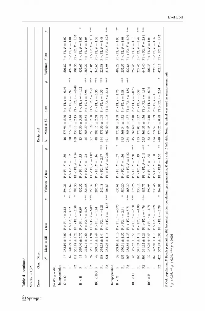
Analysis of the difference in the mean and variance of the wing width is given in
Table 4b. Significant decrease of the mean is obtained in all crosses (both direct and
reciprocal), except in the BG 9 BG direct cross, where different trends through genera-
tions (P [ F1 \ F2) were found. The variance significantly decreases from P to F1, and
towards F2, except in the B 9 B reciprocal cross.
Changes of the mean and variance across generations in females
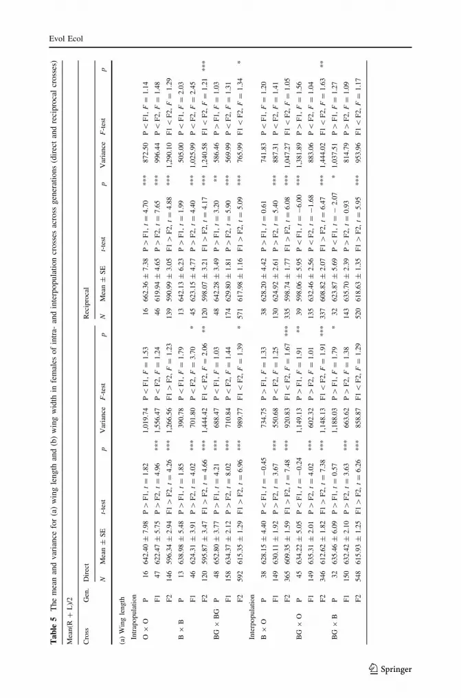
Analysis of the difference in the mean and variance of the wing length in females is given
in Table 5a. A significant decrease of the mean is observed from P toward F2 in all direct
and reciprocal crosses. The variance generally increases through generations
(P \ F1 \ F2) in both direct and reciprocal crosses.
Analyses of the difference in the mean and variance of the wing width are shown in
Table 5b. A significant decrease of the mean toward F2 is observed both in direct and
reciprocal crosses. The variance change shows no general trend, with a significant dif-
ference between generations, found only in direct crosses.
Changes of the FA across generations in males
Analysis of the FA1 index between generations for wing length in males shows no sig-
nificant differences between generations either in the direct and reciprocal crosses
(Table 6a).
Analysis of FA1 between generations for wing width, shows no significant difference
between generations, except in the hybrids from BG 9 BG reciprocal cross (tP,F1 = -2.17,
p \ 0.05; tP,F2 = -2.30, p \ 0.05) (Table 6b).
Evol Ecol
123

Ta
ble
2R
esult
so
fS
hap
iro
–W
ilk
(W)
and
Ch
i-sq
uar
e(v
2)
test
sfo
rn
orm
ald
istr
ibu
tio
no
fw
ing
len
gth
insa
mple
so
fin
tra-
and
inte
rpo
pu
lati
on
cro
sses
inP
,F
1an
dF
2g
ener
atio
ns
inm
ales
and
fem
ales
(dir
ect
and
reci
pro
cal
cro
sses
)
Cro
ssG
en.
Mal
esF
emal
es
Dir
ect
Rec
ipro
cal
Dir
ect
Rec
ipro
cal
NS
hap
iro
–W
ilk
Ch
i-sq
uar
eN
Sh
apir
o–W
ilk
Ch
i-sq
uar
eN
Sh
apir
o–W
ilk
Ch
i-sq
uar
eN
Sh
apir
o–W
ilk
Chi-
squar
e
Intr
apo
pu
lati
on
O9
OP
16
W=
0.9
6,
p=
0.6
5v2
=2
.00,
p=
0.6
51
6W
=0
.96,
p=
0.7
1v2
=0
.50,
p=
0.7
01
6W
=0
.88,
p=
0.0
5v2
=1
.50,
p=
0.0
51
6W
=0
.92,
p=
0.2
4v2
=8
.5,
p=
0.2
4
F1
62
W=
0.9
8,
p=
0.6
1v2
=1
.35,
p=
0.6
15
0W
=0
.98,
p=
0.7
8v2
=0
.88,
p=
0.7
84
7W
=0
.97,
p=
0.2
9v2
=0
.23,
p=
0.2
84
6W
=0
.97,
p=
0.4
5v2
=1
.82,
p=
0.4
5
F2
11
7W
=0
.96,
p=
0.0
6v2
=1
.13,
p=
0.6
11
10
W=
0.9
9,
p=
0.9
0v2
=1
.78,
p=
0.9
01
46
W=
0.9
9,
p=
0.4
9v2
=1
.78,
p=
0.4
91
05
W=
0.9
7,
p=
0.0
6v2
=1
.62,
p=
0.6
0
B9
BP
13
W=
0.9
3,
p=
0.4
4v2
=0
.84,
p=
0.4
41
3W
=0
.90,
p=
0.1
6v2
=2
.69,
p=
0.1
61
3W
=0
.91,
p=
0.2
0v2
=0
.84,
p=
0.2
01
3W
=0
.82,
p=
0.0
5v2
=2
.69,
p=
0.0
5
F1
45
W=
0.9
7,
p=
0.5
8v2
=2
.34,
p=
0.5
84
5W
=0
.97,
p=
0.4
2v2
=2
.55,
p=
0.4
24
6W
=0
.97,
p=
0.2
8v2
=3
.04,
p=
0.2
94
4W
=0
.96,
p=
0.1
8v2
=4
.54,
p=
0.1
8
F2
97
W=
0.9
8,
p=
0.5
9v2
=0
.36,
p=
0.6
09
8W
=0
.96,
p=
0.0
9v2
=2
.00,
p=
0.0
91
20
W=
0.9
7,
p=
0.0
5v2
=2
.20,
p=
0.0
61
20
W=
2.6
0,
p=
0.0
6v2
=2
.60,
p=
0.0
6
BG
9B
GP
48
W=
0.9
7,
p=
0.1
9v2
=1
.16,
p=
0.1
94
8W
=0
.99,
p=
0.9
6v2
=0
.17,
p=
0.9
64
8W
=0
.98,
p=
0.8
3v2
=1
.16,
p=
0.8
34
8W
=0
.98,
p=
0.8
6v2
=0
.83,
p=
0.8
6
F1
18
8W
=0
.99,
p=
0.6
7v2
=0
.85,
p=
0.6
71
48
W=
0.9
8,
p=
0.0
8v2
=5
.13,
p=
0.0
81
58
W=
0.9
9,
p=
0.9
7v2
=0
.28,
p=
0.9
71
84
W=
0.9
9,
p=
0.8
8v2
=2
.04,
p=
0.8
8
F2
46
4W
=0
.98,
p=
0.0
8v2
=1
.27,
p=
0.0
84
91
W=
0.9
8,
p=
0.6
0v2
=1
.26,
p=
0.0
65
93
W=
0.9
8,
p=
0.1
7v2
=4
.17,
p=
0.1
75
72
W=
0.9
9,
p=
0.0
6v2
=1
.46,
p=
0.0
7
Evol Ecol
123

Ta
ble
2co
nti
nu
ed
Cro
ssG
en.
Mal
esF
emal
es
Dir
ect
Rec
ipro
cal
Dir
ect
Rec
ipro
cal
NS
hap
iro
–W
ilk
Chi-
squar
eN
Sh
apir
o–
Wil
kC
hi-
squar
eN
Sh
apir
o–W
ilk
Ch
i-sq
uar
eN
Shap
iro–W
ilk
Chi-
squar
e
Inte
rpo
pu
lati
on
B9
OP
38
W=
0.9
9,
p=
0.9
7v2
=0
.10,
p=
0.9
73
8W
=0
.98,
p=
0.7
9v2
=1
.78,
p=
0.7
93
8W
=0
.98,
p=
0.9
1v2
=0
.52,
p=
0.9
13
8W
=0
.97,
p=
0.4
9v2
=0
.52
,p
=0
.49
F1
15
5W
=0
.95
,p
=0
.05
v2=
1.4
2,
p=
0.0
91
45
W=
0.9
8,
p=
0.1
1v2
=3
.05,
p=
0.1
11
49
W=
0.9
4,
p=
0.0
5v2
=1
.69,
p=
0.0
81
32
W=
0.9
7,
p=
0.0
5v2
=1
.51
,p
=0
.05
F2
26
3W
=0
.98
,p
=0
.06
v2=
1.7
8,
p=
0.4
92
85
W=
0.9
3,
p=
0.0
5v2
=1
.15,
p=
0.5
13
65
W=
0.9
6,
p=
0.0
6v2
=2
.30,
p=
0.0
52
86
W=
0.9
4,
p=
0.0
5v2
=1
.16
,p
=0
.60
BG
9O
P4
5W
=0
.96
,p
=0
.17
v2=
4.3
3,
p=
0.1
74
5W
=0
.98,
p=
0.7
4v2
=4
.33,
p=
0.7
54
5W
=0
.97,
p=
0.3
5v2
=1
.67,
p=
0.3
54
5W
=0
.97,
p=
0.3
7v2
=0
.95
,p
=0
.37
F1
16
9W
=0
.97
,p
=0
.05
v2=
2.9
1,
p=
0.0
71
35
W=
0.9
8,
p=
0.1
0v2
=3
.47,
p=
0.1
01
69
W=
0.9
8,
p=
0.0
5v2
=1
.62,
p=
0.0
51
35
W=
0.9
8,
p=
0.1
6v2
=1
.14
,p
=0
.16
F2
30
6W
=0
.99
,p
=0
.42
v2=
2.0
5,
p=
0.4
22
65
W=
0.9
8,
p=
0.0
5v2
=6
.09,
p=
0.0
63
64
W=
0.9
9,
p=
0.0
5v2
=6
.34,
p=
0.0
53
37
W=
0.9
8,
p=
0.0
5v2
=8
.64
,p
=0
.05
BG
9B
P3
2W
=0
.96
,p
=0
.06
v2=
2.7
5,
p=
0.0
63
2W
=0
.98,
p=
0.9
6v2
=0
.25,
p=
0.7
63
2W
=0
.97,
p=
0.5
1v2
=0
.25,
p=
0.5
13
2W
=0
.95,
p=
0.1
9v2
=3
.00
,p
=0
.19
F1
16
9W
=0
.98
,p
=0
.05
v2=
1.6
2,
p=
0.0
51
54
W=
0.9
7,
p=
0.0
5v2
=4
.83,
p=
0.7
51
50
W=
0.9
9,
p=
0.4
9v2
=1
.62,
p=
0.4
91
43
W=
0.9
8,
p=
0.0
9v2
=4
.15
,p
=0
.06
F2
42
6W
=0
.98
,p
=0
.05
v2=
4.6
9,
p=
0.0
84
40
W=
0.9
7,
p=
0.0
7v2
=2
.41,
p=
0.1
05
48
W=
0.9
8,
p=
0.0
6v2
=5
.78,
p=
0.0
73
65
W=
0.9
8,
p=
0.0
6v2
=1
.70
,p
=0
.06
OO
akp
op
ula
tio
n,
BB
eech
po
pu
lati
on
,B
Gb
ota
nic
alg
ard
enp
op
ula
tio
n,
gen
gen
erat
ion
,R
rig
ht
sid
e,L
left
side.
No
te:
the
pix
elw
asu
sed
asm
easu
rem
ent
un
it
*p\
0.0
5,
**
p\
0.0
1,
**
*p\
0.0
01
Evol Ecol
123

Tab
le3
Res
ult
so
fS
hap
iro
–W
ilk
(W)
and
Ch
i-sq
uar
e(v
2)
test
sfo
rn
orm
ald
istr
ibu
tio
no
fw
ing
wid
thin
sam
ple
so
fin
tra-
and
inte
rpo
pu
lati
on
cross
esin
P,
F1
and
F2
gen
erat
ion
sin
mal
esan
dfe
mal
es(d
irec
tan
dre
cip
roca
lcr
oss
es)
Cro
ssG
en.
Mal
esF
emal
es
Dir
ect
Rec
ipro
cal
Dir
ect
Rec
ipro
cal
NS
hap
iro
–W
ilk
Ch
i-sq
uar
eN
Sh
apir
o–
Wil
kC
hi-
squar
eN
Sh
apir
o–
Wil
kC
hi-
squar
eN
Sh
apir
o–
Wil
kC
hi-
squar
e
Intr
apop
ula
tio
n
O9
OP
16
W=
0.9
3,
p=
0.3
4v2
=2
.00,
p=
0.3
41
6W
=0
.94,
p=
0.4
3v2
=2
.50,
p=
0.4
31
6W
=0
.96,
p=
0.7
5v2
=0
.5,
p=
0.7
51
6W
=0
.87,
p=
0.0
5v2
=2
.50,
p=
0.0
5
F1
62
W=
0.9
8,
p=
0.7
4v2
=0
.58,
p=
0.7
45
0W
=0
.97,
p=
0.3
9v2
=2
.32,
p=
0.3
94
7W
=0
.97,
p=
0.3
5v2
=1
.77,
p=
0.3
64
6W
=0
.97,
p=
0.3
8v2
=3
.56,
p=
0.3
8
F2
16
0W
=0
.99
,p
=0
.64
v2=
2.1
4,
p=
0.6
41
10
W=
0.9
9,
p=
0.6
8v2
=0
.98,
p=
0.6
81
46
W=
0.9
9,
p=
0.9
4v2
=0
.03,
p=
0.9
41
39
W=
0.9
9,
p=
0.8
3v2
=1
.80,
p=
0.8
3
B9
BP
13
W=
0.9
1,
p=
0.2
0v2
=8
.23,
p=
0.2
01
3W
=0
.93,
p=
0.3
4v2
=4
.53,
p=
0.3
41
3W
=0
.96,
p=
0.8
7v2
=0
.23,
p=
0.8
71
3W
=0
.87,
p=
0.0
6v2
=0
.84,
p=
0.0
6
F1
46
W=
0.9
4,
p=
0.0
6v2
=1
.13,
p=
0.0
64
5W
=0
.98,
p=
0.7
8v2
=0
.24,
p=
0.7
84
6W
=0
.95,
p=
0.0
8v2
=0
.95,
p=
0.0
84
4W
=0
.97,
p=
0.3
2v2
=0
.73,
p=
0.3
2
F2
97
W=
0.9
9,
p=
0.9
6v2
=0
.36,
p=
0.9
69
7W
=0
.99,
p=
0.9
0v2
=1
.10,
p=
0.9
01
20
W=
0.9
8,
p=
0.4
6v2
=4
.00,
p=
0.4
51
20
W=
0.9
9,
p=
0.3
2v2
=8
.46,
p=
0.3
2
BG
9B
GP
48
W=
0.9
6,
p=
0.1
4v2
=2
.83,
p=
0.1
44
8W
=0
.96,
p=
0.2
0v2
=0
.83,
p=
0.2
04
8W
=0
.97,
p=
0.1
5v2
=1
.67,
p=
0.1
54
8W
=0
.98,
p=
0.7
5v2
=2
,50,
p=
0.7
5
F1
15
0W
=0
.99
,p
=0
.71
v2=
0.5
1,
p=
0.7
11
49
W=
0.9
8,
p=
0.1
2v2
=3
.15,
p=
0.1
31
58
W=
0.9
8,
p=
0.0
7v2
=3
.87,
p=
0.4
71
74
W=
0.9
8,
p=
0.1
2v2
=1
.17,
p=
0.1
2
F2
44
7W
=0
.99
,p
=0
.81
v2=
0.8
8,
p=
0.8
14
85
W=
0.9
9,
p=
0.6
4v2
=1
.01,
p=
0.6
35
64
W=
0.9
9,
p=
0.3
9v2
=0
.42,
p=
0.3
95
57
W=
0.9
9,
p=
0.3
8v2
=0
.43,
p=
0.3
8
Evol Ecol
123

Tab
le3
con
tin
ued
Cro
ssG
en.
Mal
esF
emal
es
Dir
ect
Rec
ipro
cal
Dir
ect
Rec
ipro
cal
NS
hap
iro
–W
ilk
Ch
i-sq
uar
eN
Sh
apir
o–
Wil
kC
hi-
squ
are
NS
hap
iro
–W
ilk
Ch
i-sq
uar
eN
Sh
apir
o–
Wil
kC
hi-
squ
are
Inte
rpop
ula
tio
n
B9
OP
38
W=
0.9
8,
p=
0.6
6v2
=0
.52,
p=
0.6
53
8W
=0
.98
,p
=0
.82
v2=
0.5
2,
p=
0.8
33
8W
=0
.97,
p=
0.4
1v2
=2
.00,
p=
0.4
13
8W
=0
.98
,p
=0
.61
v2=
1.1
6,
p=
0.6
1
F1
15
5W
=0
.98,
p=
0.0
6v2
=5
.23,
p=
0.0
71
55
W=
0.9
8,
p=
0.6
6v2
=5
.23
,p
=0
.06
14
9W
=0
.98,
p=
0.1
4v2
=1
.34,
p=
0.1
41
49
W=
0.9
8,
p=
0.1
4v2
=1
.74
,p
=0
.14
F2
25
0W
=0
.99,
p=
0.6
0v2
=2
.48,
p=
0.6
02
84
W=
0.9
9,
p=
0.3
7v2
=0
.31
,p
=0
.37
34
4W
=0
.99,
p=
0.4
4v2
=2
.77,
p=
0.4
43
21
W=
0.9
9,
p=
0.7
7v2
=0
.27
,p
=0
.77
BG
9O
P4
5W
=0
.96,
p=
0.8
7v2
=0
.23,
p=
0.8
74
5W
=0
.97
,p
=0
.54
v2=
1.4
9,
p=
0.5
44
5W
=0
.97,
p=
0.3
1v2
=0
.24,
p=
0.8
64
5W
=0
.98
,p
=0
.65
v2=
2.0
2,
p=
0.6
5
F1
16
5W
=0
.98,
p=
0.1
3v2
=1
.71,
p=
0.1
31
42
W=
0.9
8,
p=
0.0
6v2
=6
.22
,p
=0
.05
14
9W
=0
.99,
p=
0.1
3v2
=1
.04,
p=
0.1
41
35
W=
0.9
8,
p=
0.3
4v2
=1
.94
,p
=0
.08
F2
29
8W
=0
.99,
p=
0.8
1v2
=3
.61,
p=
0.8
02
61
W=
0.9
9,
p=
0.4
8v2
=0
.99
,p
=0
.08
34
6W
=0
.99,
p=
0.0
6v2
=6
.34,
p=
0.0
53
32
W=
0.9
9,
p=
0.9
0v2
=1
.80
,p
=0
.91
BG
9B
P3
2W
=0
.96,
p=
0.2
9v2
=0
.05,
p=
0.2
94
5W
=0
.96
,p
=0
.51
v2=
2.9
3,
p=
0.5
13
2W
=0
.96,
p=
0.2
8v2
=0
.50,
p=
0.2
83
1W
=0
.98
,p
=0
.84
v2=
0.3
8,
p=
0.8
4
F1
16
0W
=0
.98,
p=
0.2
5v2
=4
.85,
p=
0.2
51
42
W=
0.9
8,
p=
0.0
8v2
=1
.94
,p
=0
.08
15
0W
=0
.98,
p=
0.2
2v2
=1
.94,
p=
0.3
21
42
W=
0.9
9,
p=
0.7
9v2
=1
.15
,p
=0
.79
F2
42
6W
=0
.99,
p=
0.0
6v2
=6
.34,
p=
0.0
64
31
W=
0.9
9,
p=
0.5
3v2
=2
.05
,p
=0
.53
54
8W
=0
.99,
p=
0.1
0v2
=5
.45,
p=
0.1
15
11
W=
0.9
9,
p=
0.1
8v2
=2
.73
,p
=0
.18
OO
akp
op
ula
tio
n,
BB
eech
po
pula
tio
n,
BG
Bo
tan
ical
gar
den
po
pula
tio
n,
gen
gen
erat
ion
,R
rig
ht
sid
e,L
left
side.
No
te:
the
pix
elw
asu
sed
asm
easu
rem
ent
un
it
*p\
0.0
5,
**
p\
0.0
1,
**
*p\
0.0
01
Evol Ecol
123

Ta
ble
4T
he
mea
nan
dv
aria
nce
for
(a)
win
gle
ngth
and
(b)
win
gw
idth
inm
ales
of
intr
a-an
din
terp
op
ula
tio
ncr
oss
esac
ross
gen
erat
ion
s(d
irec
tan
dre
cip
roca
lcr
oss
es)
Mea
n(R
?L
)/2
Cro
ssG
en.
Dir
ect
Rec
ipro
cal
NM
ean
±S
Et-
test
pV
aria
nce
F-t
est
pN
Mea
n±
SE
t-te
stp
Var
iance
F-t
est
p
(a)
Win
gle
ngth
Intr
apopula
tion
O9
OP
16
603.9
8±
10.8
8P
[F
1,
t=
2.2
7*
1,8
94.4
6P
[F
1,
F=
2.7
1**
16
590.3
0±
9.0
7P
[F
1,
t=
0.3
21,3
15.6
0P
[F
1,
F=
1.2
6
F1
59
584.2
8±
3.4
4P
[F
2,
t=
4.1
6***
697.6
0P
[F
2,
F=
1.3
150
587.1
5±
4.5
8P
[F
2,
t=
4.7
8***
1,0
47.4
5P
\F
2,
F=
1.0
3
F2
117
561.0
6±
3.5
2F
1[
F2,
t=
4.2
0***
1,4
50.0
1F
1\
F2,
F=
2.0
8**
109
543.1
6±
3.5
3F
1[
F2,
t=
7.2
5***
1,3
57.1
9F
1\
F2,
F=
1.2
9
B9
BP
13
598.2
1±
7.7
6P
[F
1,
t=
2.1
4*
783.6
2P
[F
1,
F=
1.5
713
595.9
8±
7.9
4P
[F
1,
t=
0.1
2820.5
0P
\F
1,
F=
1.2
6
F1
46
582.3
4±
3.3
0P
[F
2,
t=
6.4
2***
499.9
9P
\F
1,
F=
1.1
445
594.8
0±
4.7
8P
[F
2,
t=
4.6
4***
1,0
30.4
5P
\F
2,
F=
1.4
2
F2
97
541.9
3±
3.0
3F
1[
F2,
t=
8.1
5***
892.3
1F
1\
F2,
F=
1.7
8*
97
549.9
3±
3.4
7F
1[
F2,
t=
7.4
2***
1,1
68.3
9F
1\
F2,
F=
1.1
4
BG
9B
GP
48
598.2
1±
3.3
7P
[F
1,
t=
2.7
4**
544.1
9P
[F
1,
F=
1.0
048
602.4
7±
3.5
2P
[F
1,
t=
4.9
2***
596.5
6P
[F
1,
F=
1.3
4
F1
188
587.8
5±
1.7
0P
[F
2,
t=
5.6
0***
543.5
3P
\F
2,
F=
2.1
6**
194
585.2
2±
1.5
1P
[F
2,
t=
6.6
2***
443.3
5P
\F
2,
F=
1.7
2*
F2
463
569.8
1±
1.5
9F
1[
F2,
t=
6.6
2***
1,1
76.2
0P
\F
2,
F=
2.1
7***
490
571.0
0±
1.4
5F
1[
F2,
t=
5.7
1***
1,0
27.0
9F
1\
F2,
F=
2.3
2***
Inte
rpopula
tion
B9
OP
38
586.3
0±
5.2
9P
[F
1,
t=
1.0
71,0
64.1
4P
[F
1,
F=
1.3
638
590.3
0±
4.9
9P
[F
1,
t=
2.1
1*
944.9
0P
[F
1,
F=
1.4
1
F1
155
580.7
1±
2.2
4P
[F
2,
t=
4.4
4***
781.4
1P
[F
2,
F=
1.1
2145
579.9
4±
2.1
5P
[F
2,
t=
4.9
7***
669.4
0P
\F
2,
F=
1.2
6
F2
263
562.3
7±
1.9
0F
1[
F2,
t=
6.0
8***
949.0
7F
1\
F2,
F=
1.2
1284
561.0
1±
2.0
5F
1[
F2,
t=
5.9
2***
1,1
91.2
8F
1\
F2,
F=
1.7
8***
BG
9O
P45
562.1
0±
5.6
2P
\F
1,
t=
-5.5
2***
1,4
22.0
6P
[F
1,
F=
3.2
8***
45
578.0
0±
3.6
0P
\F
1,
t=
-1.6
9581.8
6P
[F
1,
F=
1.0
1
F1
165
585.6
2±
1.6
2P
\F
2,
t=
-0.9
9432.7
8P
[F
2,
F=
1.4
4153
584.8
7±
1.9
4P
[F
2,
t=
0.3
7574.4
7P
\F
2,
F=
2.6
5***
F2
306
567.2
1±
1.8
0F
1[
F2,
t=
6.7
6***
987.9
7F
1\
F2,
F=
2.2
8***
265
575.7
8±
2.4
1F
1[
F2,
t=
0.3
71,5
40.9
5F
1\
F2,
F=
2.6
5***
BG
9B
P32
580.9
6±
4.6
0P
[F
1,
t=
0.0
4677.1
3P
[F
1,
F=
1.4
745
578.0
0±
3.6
0P
\F
1,
t=
-2.6
6***
587.4
4P
\F
1,
F=
2.3
6**
F1
169
580.7
7±
1.6
5P
[F
2,
t=
1.8
6458.8
5P
\F
2,
F=
1.3
6141
604.2
9±
3.1
2P
[F
2,
t=
1.8
8***
1,3
72.2
6P
\F
2,
F=
1.6
3
F2
426
570.6
6±
1.4
7F
1[
F2,
t=
3.9
5***
922.8
6F
1\
F2,
F=
2.0
1***
440
575.4
2±
1.4
7F
1[
F2,
t=
9.1
6***
959.6
7F
1[
F2,
F=
1.4
3**
Evol Ecol
123
Ta
ble
4co
nti
nu
ed
Mea
n(R
?L
)/2
Cro
ssG
en.
Dir
ect
Rec
ipro
cal
NM
ean
±S
Et-
test
pV
aria
nce
F-t
est
pN
Mea
n±
SE
t-te
stp
Var
iance
F-t
est
p
(b)
Win
gw
idth
Inta
rpopula
tion
O9
OP
16
383.1
9±
6.0
9P
[F
1,
t=
2.1
2*
594.2
1P
[F
1,
F=
1.5
616
373.9
6±
5.6
0P
[F
1,
t=
-0.4
9501.8
2P
[F
1,
F=
1.0
2
F1
62
370.9
9±
2.4
7P
[F
2,
t=
3.3
2**
379.6
2P
[F
2,
F=
1.0
250
377.1
0±
3.1
4P
[F
2,
t=
3.9
7***
492.3
4P
\F
2,
F=
1.0
1
F2
117
361.7
8±
2.2
3F
1[
F2,
t=
2.5
8*
583.3
0F
1\
F2,
F=
1.5
4109
350.1
3±
2.1
5F
1\
F2,
t=
-0.4
9502.3
6F
1\
F2,
F=
1.0
2
B9
BP
13
379.4
0±
5.7
7P
[F
1,
t=
0.8
9432.5
2P
[F
1,
F=
1.3
313
377.3
0±
5.9
0P
\F
1,
t=
-1.0
2452.6
7P
\F
1,
F=
3.0
5*
F1
46
374.2
1±
2.6
6P
[F
2,
t=
4.9
9***
324.5
8P
[F
2,
F=
1.2
245
388.3
9±
5.5
4P
[F
2,
t=
3.9
8***
1,3
83.2
7P
[F
2,
F=
1.0
8
F2
97
351.3
1±
1.9
1F
1[
F2,
t=
6.8
9***
353.3
7F
1\
F2,
F=
1.0
997
353.1
6±
2.0
8F
1[
F2,
t=
7.2
7***
418.0
5F
1[
F2,
F=
3.3
1***
BG
9B
GP
48
379.0
5±
2.4
4P
[F
1,
t=
1.7
4285.7
6P
[F
1,
F=
1.1
648
382.1
5±
2.6
8P
[F
1,
t=
3.3
6***
345.6
5P
[F
1,
F=
1.5
2
F1
188
374.5
5±
1.4
4P
\F
2,
t=
-1.2
1246.1
8P
\F
2,
F=
2.4
7***
194
373.5
6±
1.0
8P
[F
2,
t=
4.3
5***
227.8
8P
\F
2,
F=
1.4
8
F2
521
383.7
6±
1.1
6F
1\
F2,
t=
-4.4
8***
704.8
3F
1\
F2,
F=
2.8
6***
491
367.4
9±
1.0
2F
1[
F2,
t=
3.4
4***
511.9
5F
1\
F2,
F=
2.2
5***
Inte
rpopula
tion
B9
OP
38
368.1
0±
4.1
0P
\F
1,
t=
-0.7
5635.6
1P
[F
1,
F=
1.6
7*
38
373.9
1±
3.5
8P
[F
1,
t=
1.7
6488.2
8P
[F
1,
F=
1.9
3**
F1
155
370.9
1±
1.5
7P
[F
2,
t=
2.4
1*
380.2
0P
[F
2,
F=
1.3
6145
368.3
4±
1.3
2P
[F
2,
t=
3.8
8***
252.5
7P
\F
2,
F=
1.0
8
F2
263
358.8
6±
1.3
3F
1[
F2,
t=
5.7
1***
465.3
9F
1\
F2,
F=
1.2
2284
358.5
5±
1.3
7F
1[
F2,
t=
4.5
9***
529.8
6F
1\
F2,
F=
2.0
9***
BG
9O
P45
355.5
2±
3.5
8P
\F
1,
t=
-5.3
1***
576.2
6P
[F
1,
F=
2.5
0***
45
368.6
0±
2.4
0P
\F
1,
t=
-0.5
5259.4
5P
[F
1,
F=
1.1
3
F1
165
371.0
7±
1.1
8P
\F
2,
t=
-1.8
0230.1
2P
[F
2,
F=
1.1
9153
370.0
3±
1.2
2P
[F
2,
t=
0.5
8229.4
5P
\F
2,
F=
2.4
9***
F2
306
361.9
2±
1.2
6F
1[
F2,
t=
4.7
6***
485.7
5F
1\
F2,
F=
2.1
1***
265
366.3
3±
1.5
6F
1[
F2,
t=
1.6
4645.4
0F
1\
F2,
F=
2.8
1***
BG
9B
P32
367.2
6±
3.5
3P
\F
1,
t=
-1.7
1399.9
5P
[F
1,
F=
1.6
8*
32
374.3
5±
3.1
0P
\F
1,
t=
-0.0
6307.3
3P
[F
1,
F=
1.0
4
F1
169
372.6
0±
1.1
9P
[F
2,
t=
-0.2
1238.4
6P
[F
2,
F=
1.0
8154
374.5
7±
1.3
9P
[F
2,
t=
1.1
296.1
6P
\F
2,
F=
1.3
7
F2
426
367.9
9±
0.9
3F
1[
F2,
t=
2.7
9*
368.9
1F
1\
F2,F
=1.5
5**
440
370.2
5±
0.9
8F
1[
F2,
t=
2.3
4*
422.1
2F
1\
F2,
F=
1.4
2
OO
akpopula
tion,
BB
eech
popula
tion,
BG
bota
nic
algar
den
popula
tion,
gen
gen
erat
ion,
Rri
ght
side,
Lle
ftsi
de.
Note
:th
epix
elw
asuse
das
mea
sure
men
tunit
*p
\0.0
5,
**
p\
0.0
1,
***
p\
0.0
01
Evol Ecol
123
Ta
ble
5T
he
mea
nan
dv
aria
nce
for
(a)
win
gle
ngth
and
(b)
win
gw
idth
infe
mal
eso
fin
tra-
and
inte
rpo
pu
lati
on
cro
sses
acro
ssg
ener
atio
ns
(dir
ect
and
reci
pro
cal
cross
es)
Mea
n(R
?L
)/2
Cro
ssG
en.
Dir
ect
Rec
ipro
cal
NM
ean
±S
Et-
test
pV
aria
nce
F-t
est
pN
Mea
n±
SE
t-te
stp
Var
iance
F-t
est
p
(a)
Win
gle
ngth
Intr
apopula
tion
O9
OP
16
642.4
0±
7.9
8P
[F
1,
t=
1.8
21,0
19.7
4P
\F
1,
F=
1.5
316
662.3
6±
7.3
8P
[F
1,
t=
4.7
0***
872.5
0P
\F
1,
F=
1.1
4
F1
47
622.4
7±
5.7
5P
[F
2,
t=
4.9
6***
1,5
56.4
7P
\F
2,
F=
1.2
446
619.9
4±
4.6
5P
[F
2,
t=
7.6
5***
996.4
4P
\F
2,
F=
1.4
8
F2
146
596.3
4±
2.9
4F
1[
F2,
t=
4.2
6***
1,2
66.5
6F
1[
F2,
F=
1.2
3139
590.9
9±
3.0
5F
1[
F2,
t=
4.8
8***
1,2
90.1
0F
1\
F2,
F=
1.2
9
B9
BP
13
638.9
8±
5.4
8P
[F
1,
t=
1.8
5390.7
8P
\F
1,
F=
1.7
913
642.1
3±
6.2
3P
[F
1,
t=
1.9
9505.0
0P
\F
1,
F=
2.0
3
F1
46
624.3
1±
3.9
1P
[F
2,
t=
4.0
2***
701.8
0P
\F
2,
F=
3.7
0*
45
623.1
5±
4.7
7P
[F
2,
t=
4.4
0***
1,0
25.9
9P
\F
2,
F=
2.4
5
F2
120
595.8
7±
3.4
7F
1[
F2,
t=
4.6
6***
1,4
44.4
2F
1\
F2,
F=
2.0
6**
120
598.0
7±
3.2
1F
1[
F2,
t=
4.1
7***
1,2
40.5
8F
1\
F2,
F=
1.2
1***
BG
9B
GP
48
652.8
0±
3.7
7P
[F
1,
t=
4.2
1***
688.4
7P
\F
1,
F=
1.0
348
642.2
8±
3.4
9P
[F
1,
t=
3.2
0**
586.4
6P
[F
1,
F=
1.0
3
F1
158
634.3
7±
2.1
2P
[F
2,
t=
8.0
2***
710.8
4P
\F
2,
F=
1.4
4174
629.8
0±
1.8
1P
[F
2,
t=
5.9
0***
569.9
9P
\F
2,
F=
1.3
1
F2
592
615.3
5±
1.2
9F
1[
F2,
t=
6.9
6***
989.7
7F
1\
F2,
F=
1.3
9*
571
617.9
8±
1.1
6F
1[
F2,
t=
5.0
9***
765.9
9F
1\
F2,
F=
1.3
4*
Inte
rpopula
tion
B9
OP
38
628.1
5±
4.4
0P
\F
1,
t=
-0.4
5734.7
5P
[F
1,
F=
1.3
338
628.2
0±
4.4
2P
[F
1,
t=
0.6
1741.8
3P
\F
1,
F=
1.2
0
F1
149
630.1
1±
1.9
2P
[F
2,
t=
3.6
7***
550.6
8P
\F
2,
F=
1.2
5130
624.9
2±
2.6
1P
[F
2,
t=
5.4
0***
887.3
1P
\F
2,
F=
1.4
1
F2
365
609.3
5±
1.5
9F
1[
F2,
t=
7.4
8***
920.8
3F
1\
F2,
F=
1.6
7***
335
598.7
4±
1.7
7F
1[
F2,
t=
6.0
8***
1,0
47.2
7F
1\
F2,
F=
1.0
5
BG
9O
P45
634.2
2±
5.0
5P
\F
1,
t=
-0.2
41,1
49.1
3P
[F
1,
F=
1.9
1**
39
598.0
6±
5.9
5P
\F
1,
t=
-6.0
0***
1,3
81.8
9P
[F
1,
F=
1.5
6
F1
149
635.3
1±
2.0
1P
[F
2,
t=
4.0
2***
602.3
2P
[F
2,
F=
1.0
1135
632.4
6±
2.5
6P
\F
2,
t=
-1.6
8883.0
6P
\F
2,
F=
1.0
4
F2
346
612.6
2±
1.8
2F
1[
F2,
t=
7.3
8***
1,1
48.1
3F
1\
F2,
F=
1.9
1***
337
608.8
2±
2.0
7F
1[
F2,
t=
6.4
7***
1,4
44.0
2F
1\
F2,
F=
1.6
3**
BG
9B
P32
635.4
6±
6.0
9P
[F
1,
t=
0.5
71,1
88.0
3P
[F
1,
F=
1.7
9*
32
623.8
7±
5.6
9P
\F
1,
t=
-2.0
7*
1,0
37.5
1P
[F
1,
F=
1.2
7
F1
150
632.4
2±
2.1
0P
[F
2,
t=
3.6
3***
663.6
2P
[F
2,
F=
1.3
8143
635.7
0±
2.3
9P
[F
2,
t=
0.9
3814.7
9P
[F
2,
F=
1.0
9
F2
548
615.9
3±
1.2
5F
1[
F2,
t=
6.2
6***
858.8
7F
1\
F2,
F=
1.2
9520
618.6
3±
1.3
5F
1[
F2,
t=
5.9
5***
953.9
6F
1\
F2,
F=
1.1
7
Evol Ecol
123

Ta
ble
5co
nti
nu
ed
Mea
n(R
?L
)/2
Cro
ssG
en.
Dir
ect
Rec
ipro
cal
NM
ean
±S
Et-
test
pV
aria
nce
F-t
est
pN
Mea
n±
SE
t-te
stp
Var
iance
F-t
est
p
(b)
Win
gw
idth
Intr
apopula
tion
O9
OP
16
412.6
6±
5.9
4P
[F
1,
t=
1.7
5565.3
4P
\F
1,
F=
1.3
816
421.9
4±
4.6
1P
[F
1,
t=
4.2
5***
340.4
6P
\F
1,
F=
1.2
4
F1
47
398.9
7±
4.0
8P
[F
2,
t=
4.7
1***
781.2
4P
[F
2,
F=
1.2
646
397.2
2±
3.0
3P
[F
2,
t=
7.3
2***
421.9
0P
\F
2,
F=
1.3
7
F2
146
386.0
8±
1.7
5F
1[
F2,
t=
3.3
4***
447.9
3F
1[
F2,
F=
1.7
4*
139
380.6
8±
1.8
3F
1[
F2,
t=
4.5
5***
468.3
1F
1\
F2,
F=
1.1
1
B9
BP
13
406.5
7±
4.6
1P
[F
1,
t=
1.0
8276.1
8P
\F
1,
F=
1.2
913
403.6
4±
7.0
5P
[F
1,
t=
0.3
8647.0
2P
[F
1,
F=
1.6
4
F1
46
400.3
2±
2.7
8P
[F
2,
t=
2.3
8*
356.2
3P
\F
2,
F=
2.8
6*
44
401.0
8±
2.9
9P
[F
2,
t=
2.5
2*
394.4
5P
[F
2,
F=
1.1
7
F2
120
387.6
4±
2.5
6F
1[
F2,
t=
2.8
2**
789.6
3F
1\
F2,
F=
2.2
2**
120
386.2
0±
2.1
4F
1[
F2,
t=
3.7
4***
552.2
6F
1\
F2,
F=
1.4
0
BG
9B
GP
48
414.3
1±
3.1
8P
[F
1,
t=
2.5
7*
490.8
1P
[F
1,
F=
1.3
348
409.8
5±
2.3
4P
[F
1,
t=
2.5
7*
262.2
6P
\F
1,
F=
1.2
7
F1
158
405.8
5±
1.5
3P
[F
2,
t=
4.9
7***
369.6
1P
\F
2,
F=
1.0
0174
402.3
8±
1.3
8P
[F
2,
t=
3.5
2***
333.0
6P
\F
2,
F=
1.5
0
F2
592
397.7
5±
0.9
1F
1[
F2,
t=
4.1
9***
492.0
0F
1\
F2,
F=
1.3
3*
572
399.4
8±
0.8
3F
1[
F2,
t=
1.7
2393.8
8F
1\
F2,
F=
1.1
8
Inte
rpopula
tion
B9
OP
38
396.5
4±
4.5
3P
\F
1,
t=
-2.6
2**
780.5
6P
[F
1,
F=
2.5
3***
38
401.1
4±
2.7
8P
[F
1,
t=
0.9
2293.5
1P
\F
1,
F=
1.4
5
F1
149
406.0
9±
1.4
4P
[F
2,
t=
1.4
8308.6
2P
[F
2,
F=
1.8
5**
130
397.7
6±
1.8
1P
[F
2,
t=
4.6
5***
425.8
6P
\F
2,
F=
1.5
3
F2
346
391.1
4±
1.1
0F
1[
F2,
t=
7.7
5***
421.7
4F
1\
F2,
F=
1.3
7*
335
384.5
3±
1.1
6F
1[
F2,
t=
6.0
8***
449.5
9F
1\
F2,
F=
1.0
5
BG
9O
P45
399.9
1±
3.7
2P
\F
1,
t=
-0.7
5622.5
0P
[F
1,
F=
1.9
2**
45
379.0
2±
3.6
6P
\F
1,
t=
-5.0
8***
602.0
9P
[F
1,
F=
1.3
6
F1
149
402.4
4±
1.4
8P
[F
2,
t=
2.0
0*
324.6
7P
[F
2,
F=
1.2
1135
398.2
1±
1.8
1P
\F
2,
t=
-2.8
5**
441.9
5P
\F
2,
F=
1.0
9
F2
346
392.6
3±
1.2
2F
1[
F2,
t=
4.6
8***
515.1
4F
1\
F2,
F=
1.5
9**
337
390.5
6±
1.4
0F
1[
F2,
t=
3.0
7**
657.8
8F
1\
F2,
F=
1.4
9**
BG
9B
P32
407.2
2±
3.6
8P
[F
1,
t=
4.6
1***
434.2
7P
\F
1,
F=
1.1
332
397.7
7±
3.2
9P
\F
1,
t=
-2.2
2*
346.4
5P
\F
1,
F=
1.1
3
OO
akpopula
tion,
BB
eech
popula
tion,
BG
bota
nic
algar
den
popula
tion,
gen
gen
erat
ion,
Rri
ght
side,
Lle
ftsi
de.
Note
:th
epix
elw
asuse
das
mea
sure
men
tunit
*p
\0.0
5,
**
p\
0.0
1,
***
p\
0.0
01
Evol Ecol
123

Ta
ble
6T
he
FA
1in
dex
dif
fere
nce
sb
etw
een
gen
erat
ion
san
dty
pe
of
cross
esfo
r(a
)w
ing
len
gth
and
(b)
win
gw
idth
inm
ales
and
fem
ales
ind
irec
tan
dre
cip
roca
lcr
oss
es
FA
1=
|R-
L|
win
gle
ng
th
Cro
ssG
en.
Mal
esF
emal
es
Dir
ect
Rec
ipro
cal
Dir
ect
Rec
ipro
cal
NM
ean
±S
Et-
test
pN
Mea
n±
SE
t-te
stp
NM
ean
±S
Et-
test
pN
Mea
n±
SE
t-te
stp
(a)
Win
gle
ng
th
Intr
apop
ula
tio
n
O9
OP
16
3.5
1±
0.5
9P
[F
1,
t=
0.0
51
63
.90
±0
.75
P[
F1
,t
=1
.35
16
3.4
2±
0.6
3P
[F
1,
t=
1.0
31
62
.86
±0
.40
P\
F1
,t
=-
0.1
4
F1
59
3.4
8±
0.3
9P
[F
2,
t=
0.5
75
02
.99
±0
.30
P[
F2
,t
=2
.17
*4
72
.73
±0
.33
P[
F2
,t
=0
.91
46
2.9
6±
0.3
8P
[F
2,
t=
0.6
1
F2
11
73
.12
±0
.24
F1[
F2
,t
=0
.80
10
92
.71
±0
.18
F1[
F2
,t
=0
.84
14
62
.89
±0
.18
F1\
F2
,t
=-
0.4
41
39
2.5
6±
0.1
6F
1[
F2
,t
=1
.13
B9
BP
13
2.2
6±
0.3
3P
\F
1,
t=
-1
.46
13
2.7
3±
0.4
8P
\F
1,
t=
-0
.77
13
3.1
4±
0.5
5P
[F
1,
t=
0.3
01
33
.11
±0
.36
P\
F1
,t
=-
0.2
4
F1
46
3.3
8±
0.3
9P
\F
2,
t=
-1
.78
45
3.2
2±
0.3
1P
\F
2,
t=
-1
.00
46
2.9
5±
0.3
1P
\F
2,
t=
-0
.19
45
3.2
8±
0.3
8P
\F
2,
t=
-0
.56
F2
97
3.5
2±
0.2
5F
1\
F2
,t
=-
0.3
19
73
.50
±0
.27
F1\
F2
,t
=-
0.6
21
20
3.3
0±
0.2
6F
1\
F2
,t
=-
0.7
51
20
3.4
8±
0,2
1F
1\
F2
,t
=-
0.4
6
BG
9B
GP
48
4.4
2±
0.4
2P
[F
1,
t=
0.1
64
84
.73
±0
.48
P[
F1
,t
=0
.36
48
3.5
5±
0.3
8P
\F
1,
t=
-1
.20
*4
83
.68
±0
.42
P\
F1
,t
=-
1.1
3
F1
18
84
.34
±0
.23
P\
F2
,t
=-
0.0
91
94
4.5
3±
0.2
5P
[F
2,
t=
0.2
01
58
4.5
8±
0.2
6P
\F
2,
t=
-2
.38
**
17
44
.22
±0
.22
P\
F2
,t
=-
1.7
8
F2
46
34
.47
±0
.15
F1\
F2
,t
=-
0.4
54
90
4.6
2±
0.1
6F
1\
F2
,t
=-
0.3
15
92
4.7
5±
0.1
4F
1\
F2
,t
=-
0.5
75
71
4.6
7±
0.1
6F
1\
F2
,t
=-
1.4
4
Evol Ecol
123

Ta
ble
6co
nti
nu
ed
FA
1=
|R-
L|
win
gle
ng
th
Cro
ssG
en.
Mal
esF
emal
es
Dir
ect
Rec
ipro
cal
Dir
ect
Rec
ipro
cal
NM
ean
±S
Et-
test
pN
Mea
n±
SE
t-te
stp
NM
ean
±S
Et-
test
pN
Mea
n±
SE
t-te
stp
Inte
rpop
ula
tio
n
B9
OP
38
4.4
2±
0.8
1P
\F
1,
t=
-1
.71
38
4.1
0±
0.4
7P
\F
1,
t=
-0
.99
38
4.3
3±
0.5
5P
\F
1,
t=
-0
.85
38
5.0
7±
0.6
3P
[F
1,
t=
1.3
3
F1
15
55
.94
±0
.39
P[
F2
,t
=0
.12
14
54
.66
±0
.26
P\
F2
,t
=-
0.2
41
49
4.8
8±
0.2
9P
\F
2,
t=
-0
.54
13
04
.32
±0
.42
P\
F2
,t
=-
0.1
2
F2
26
34
.35
±0
.18
F1[
F2
,t
=4
.17
**
*2
84
4.2
1±
0.1
5F
1[
F2
,t
=1
.56
36
54
.60
±0
.15
F1[
F2
,t
=0
.91
33
55
.17
±0
.26
F1\
F2
,t
=-
1.9
3
BG
9O
P4
54
.10
±0
.37
P\
F1
,t
=-
1.2
94
53
.78
±0
.39
P\
F1
,t
=-
2.1
*4
54
.00
±0
.39
P\
F1
,t
=-
1.4
23
93
.74
±0
.42
P\
F1
,t
=-
1.7
5
F1
16
54
.79
±0
.26
P\
F2
,t
=-
1.2
51
53
5.2
4±
0.3
6P
\F
2,
t=
-1
.03
14
94
.84
±0
.32
P\
F2
,t
=-
2.0
7*
13
54
.89
±0
.33
P\
F2
,t
=-
1.9
7*
F2
30
64
.78
±0
.20
F1[
F2
,t
=0
.03
26
54
.31
±0
.18
F1[
F2
,t
=2
.49
**
34
65
.22
±0
.21
F1\
F2
,t
=-
1.0
23
37
4.9
0±
0.1
9F
1\
F2
,t
=-
0.0
2
BG
9B
P3
23
.73
±0
.33
P\
F1
,t
=-
0.9
53
24
.29
±0
.49
P\
F1
,t
=-
1.2
33
13
.69
±0
.48
P\
F1
,t
=-
1.8
44
83
.68
±0
.43
P\
F1
,t
=-
1.8
2
F1
16
94
.33
±0
.29
P\
F1
,t
=-
2.1
2*
14
15
.17
±0
.32
P\
F2
,t
=-
1.5
01
50
5.1
1±
0.3
3P
\F
2,
t=
-2
.45
**
14
35
.23
±0
.47
P\
F2
,t
=-
2.8
8*
*
F2
42
65
.25
±0
.19
F1\
F2
,t
=-
2.4
5*
*4
40
5.4
1±
0.2
0F
1\
F2
,t
=-
0.6
05
48
5.7
0±
0.1
9F
1\
F2
,t
=-
1.4
55
20
5.4
2±
0.1
8F
1\
F2
,t
=-
0.4
3
Evol Ecol
123

Ta
ble
6co
nti
nu
ed
FA
1=
|R-
L|
win
gle
ng
th
Cro
ssG
en.
Mal
esF
emal
es
Dir
ect
Rec
ipro
cal
Dir
ect
Rec
ipro
cal
NM
ean
±S
Et-
test
pN
Mea
n±
SE
t-te
stp
NM
ean
±S
Et-
test
pN
Mea
n±
SE
t-te
stp
(b)
Win
gw
idth
Intr
apop
ula
tio
n
O9
OP
16
1.8
7±
0.4
7P
\F
1,
t=
-1
.98
16
2.9
0±
0.5
9P
[F
1,
t=
0.6
41
62
.46
±0
.51
P\
F1
,t
=-
1.4
71
62
.15
±0
.63
P\
F1
,t
=-
0.4
5
F1
62
3.1
7±
0.3
1P
\F
2,
t=
-1
.92
50
2.5
2±
0.2
7P
[F
2,
t=
1.2
34
73
.53
±0
.39
P\
F2
,t
=-
0.3
84
62
.41
±0
.27
P\
F2
,t
=-
1.2
1
F2
11
73
.03
±0
.21
F1[
F2
,t
=0
.38
10
92
.27
±0
.17
F1[
F2
,t
=0
.80
14
62
.65
±0
.16
F1[
F2
,t
=2
.46
*1
39
2.8
2±
0.1
7F
1\
F2
,t
=-
1.1
9
B9
BP
13
2.0
1±
0.3
3P
\F
1,
t=
-1
.44
13
2.3
7±
0.2
9P
[F
1,
t=
-0
.18
13
2.4
4±
0.4
7P
[F
1,
t=
0.1
51
32
.94
±0
.67
P[
F1
,t
=0
.33
F1
46
2.7
6±
0.2
6P
[F
2,
t=
0.8
44
52
.47
±0
.29
P[
F2
,t
=-
0.8
24
62
.34
±0
.32
P\
F2
,t
=-
0.3
04
42
.73
±0
.30
P\
F2
,t
=-
0.3
6
F2
97
3.1
0±
0.2
5F
1[
F2
,t
=-
0.8
49
72
.91
±0
.24
F1\
F2
,t
=-
1.0
91
20
2.6
3±
0.2
0F
1\
F2
,t
=-
0.7
71
20
3.1
8±
0.2
0F
1\
F2
,t
=-
1.1
8
BG
9B
GP
48
3.1
0±
0.4
0P
\F
1,
t=
-2
.17
*4
84
.22
±0
.44
P\
F1
,t
=-
0.1
74
84
.35
±0
.46
P\
F1
,t
=-
0.8
94
83
.43
±0
.35
P\
F1
,t
=-
2.4
6*
F1
18
84
.15
±0
.22
P\
F2
,t
=-
2.3
0*
19
44
.32
±0
.25
P\
F2
,t
=-
0.5
91
58
4.8
2±
0.2
6P
[F
2,
t=
0.0
51
74
4.6
5±
0.2
4P
\F
2,
t=
-2
.00
*
F2
52
14
.37
±0
.16
F1\
F2
,t
=-
0.7
14
91
4.5
3±
0.1
6F
1\
F2
,t
=-
0.7
35
92
4.3
2±
0.1
5F
1[
F2
,t
=1
.54
57
24
.64
±0
.17
F1[
F2
,t
=0
.04
Evol Ecol
123

Ta
ble
6co
nti
nu
ed
FA
1=
|R-
L|
win
gle
ng
th
Cro
ssG
en.
Mal
esF
emal
es
Dir
ect
Rec
ipro
cal
Dir
ect
Rec
ipro
cal
NM
ean
±S
Et-
test
pN
Mea
n±
SE
t-te
stp
NM
ean
±S
Et-
test
pN
Mea
n±
SE
t-te
stp
Inte
rpop
ula
tio
n
B9
OP
38
2.8
0±
0.4
2P
\F
1,
t=
-3
.22
**
38
3.6
5±
0.4
3P
\F
1,
t=
-1
.32
38
4.0
8±
0.4
0P
\F
1,
t=
-1
.69
38
3.8
8±
0.4
7P
\F
1,
t=
-1
.58
F1
15
55
.28
±0
.37
P\
F2
,t
=-
2.6
1*
*1
45
4.4
8±
0.3
0P
\F
2,
t=
-2
.14
*1
49
5.2
9±
0.3
5P
\F
2,
t=
-1
.13
13
05
.19
±0
.43
P\
F2
,t
=-
2.0
5*
F2
26
34
.67
±0
.26
F1[
F2
,t
=1
.37
28
45
.08
±0
.24
F1\
F2
,t
=-
1.5
03
46
4.8
2±
0.2
1F
1[
F2
,t
=1
.17
33
55
.54
±0
.27
F1\
F2
,t
=-
0.7
0
BG
9O
P4
53
.32
±0
.38
P\
F1
,t
=-
2.5
3*
45
4.2
1±
0.4
7P
\F
1,
t=
-1
.06
45
3.8
7±
0.5
1P
\F
1,
t=
-1
.61
45
3.8
8±
0.4
0P
\F
1,
t=
-2
.71
**
F1
16
54
.67
±0
.26
P\
F2
,t
=-
2.1
9*
15
34
.86
±0
.30
P\
F2
,t
=-
0.3
01
49
5.1
9±
0.4
2P
\F
2,
t=
-1
.57
13
55
.46
±0
.31
P\
F2
,t
=-
0.8
7
F2
30
64
.55
±0
.21
F1[
F2
,t
=0
.34
26
54
.38
±0
.22
F1[
F2
,t
=1
.29
34
64
.72
±0
.18
F1[
F2
,t
=1
.18
33
74
.35
±0
.19
F1[
F2
,t
=3
.09
**
BG
9B
P3
23
.40
±0
.66
P\
F1
,t
=-
1.1
43
23
.94
±0
.59
P\
F1
,t
=-
1.0
53
24
.20
±0
.42
P\
F1
,t
=-
0.6
73
25
.98
±1
.51
P[
F1
,t
=0
.75
F1
16
95
.07
±0
.39
P\
F2
,t
=-
0.5
31
54
4.7
7±
0.3
4P
\F
2,
t=
-1
.21
15
74
.73
±0
.35
P\
F2
,t
=-
0.5
61
43
5.2
7±
0.3
7P
[F
2,
t=
1.5
4
F2
42
64
.34
±0
.17
F1[
F2
,t
=2
.00
*4
40
4.8
5±
0.2
0F
1\
F2
,t
=-
0.2
15
48
4.5
8±
0.1
6F
1[
F2
,t
=0
.41
52
04
.79
±0
.18
F1[
F2
,t
=1
.22
OO
akp
op
ula
tio
n,
BB
eech
po
pula
tio
n,
BG
bo
tan
ical
gar
den
po
pula
tio
n,
gen
gen
erat
ion
,R
rig
ht
sid
e,L
left
side.
No
te:
the
pix
elw
asu
sed
asm
easu
rem
ent
un
it
*p\
0.0
5,
**p\
0.0
1,
**
*p\
0.0
01
Evol Ecol
123

Changes of the FA across generations in females
Analysis of FA1 between generations for wing length in females shows a significant
increase of FA through generations (P \ F1 \ F2) only in direct cross BG 9 BG
(tP,F1 = -1.20, p \ 0.05; tP,F2 = -2.38, p \ 0.001) (Table 6a).
The FA1 analysis between generations for wing width shows no significant differences
between generations (Table 6b), except in the hybrids from the direct cross O 9 O
(tF1,F2 = 2.46, p \ 0.05). In the hybrids of the reciprocal crosses within the BG population,
a significant difference is obtained between generations (tP,F1 = -2.46, p \ 0.05;
tP,F2 = -2.00, p \ 0.05).
Interpopulation hybridization
Changes of the mean and variance across generations in males
The analysis of the mean and variance of the wing length in males is given in Table 4a. A
significant decrease of the mean (as the one observed for intrapopulation hybrids) is found
in the hybrids from B 9 O, both in direct and reciprocal crosses. But, in the hybrids from
BG 9 O and BG 9 B, a different general pattern is obtained. In direct crosses, the mean
significantly increases in F1 and significantly decreases in the F2 generation
(P \ F1 [ F2). The same tendency is found in hybrids of the BG 9 B reciprocal crosses.
The variance, in general, significantly decreases in F1 and increases in F2, except in the
hybrids of BG 9 B, where the opposite was obtained in the reciprocal crosses.
Analysis of the mean and variance of the wing width in males is given in Table 4b. The
same general pattern as for the wing length is obtained, with a significant decrease of the
mean through generations, in B 9 O, both in direct and reciprocal crosses. In hybrids from
direct crosses of BG 9 O and BG 9 B a significant increase of the mean in F1 is followed
by a significant decrease in F2.
The variance, in general, significantly decreases in F1 and an increase in F2, both in
direct and reciprocal crosses (Table 4b.).
Changes of the mean and variance across generations in females
Analysis of the mean and variance of the wing length in females is shown in Table 5a. The
mean significantly decreases in hybrids from both direct and reciprocal B 9 O crosses. In
the hybrids from the BG 9 O cross, the mean increases in F1 and significantly decreases in
the F2 generation. A similar response is found in the reciprocal crosses of BG 9 O.
However, in the hybrids from BG 9 B, the mean significantly increases in consecutive
generations of direct crosses, and a different trend is obtained in hybrids from the reci-
procal crosses (P \ F1 [ F2). The variance, in general, significantly decreases in F1 and
increases in F2, in both direct and reciprocal crosses.
Analysis of the mean and variance of the wing width in females shows a significant
increase of the mean in F1 and a significant decrease in the F2 generation in B 9 O hybrids
from direct crosses (Table 5b). The mean significantly decreases through generations in
reciprocal crosses (P [ F1 [ F2). In BG 9 O hybrids the mean increases in the F1 gen-
eration and significantly decreases in F2, in both direct and reciprocal crosses. However, in
the hybrids from the BG 9 B direct cross, a significant decrease of the mean in F1 and a
significant increase in F2 is found. In the reciprocal crosses, a different result is obtained
(P \ F1 [ F2).
Evol Ecol
123

The variance, in general, significantly decreases in F1 and increases in F2 in the hybrids
from both direct and reciprocal crosses, with the exception of BG 9 B (P \ F1 [ F2) in
direct crosses (Table 5b).
Changes of FA across generations in males
Analysis of the FA1 between generations for wing length in males is shown in Table 6a. A
significant increase of FA in F1 and its significant decrease in F2 is observed for B 9 O
hybrids both from direct and reciprocal crosses. In the hybrids from the BG 9 B direct
cross, FA1 increases across generations (P \ F1 \ F2).
The FA1 index analysis between generations for wing width in males is shown in
Table 6b. In the hybrids from B 9 O (direct crosses) FA significantly increases in F1 and
decreases in F2. However, a different trend (P \ F1 \ F2) is found in the reciprocal
crosses. In direct crosses, BG 9 O and BG 9 B, a trend (P \ F1 [ F2) is obtained,
without significant differences in reciprocal crosses.
Changes of the FA across generations in females
The results of the FA1 analysis between generations for wing length in females are shown
in Table 6a. The FA1 significantly increases across generations in the hybrids both from
direct and reciprocal BG 9 O crosses. Also, in the hybrids from BG 9 B direct crosses,
FA1 increases through generations (P \ F1 \ F2) and the same significant trend is found
in the hybrids from the reciprocal crosses.
Analysis of FA1 between generations for wing width in females is shown in Table 6b.
No significant difference between generations in the hybrids from the B 9 O direct crosses
is obtained, but in the reciprocal crosses, a significant increase of FA between generations
(P \ F1 \ F2) is observed. In the hybrids from the BG 9 O reciprocal crosses, FA sig-
nificantly increases in F1 and decreases in F2. No significant difference of FA is obtained
between generations of BG 9 B both in direct and reciprocal crosses.
Discussion
In the present paper we focused on the coadaptive aspect of genetic variability at popu-
lation level, and its relation to genomic stress, such as interpopulation hybridization.
Populations of D. subobscura from three ecologically and topologically distinct habitats
were analyzed, presuming that they possess a certain degree of genetic differences due to
their different evolutionary histories. Previous analyses of the inversion polymorphism
show that these populations differ in the frequencies of some gene arrangements (Andj-
elkovic et al. 2003; Stamenkovic-Radak et al. 2008; Jelic et al. 2009). The different gene
arrangements are carriers of various alleles that are differently favoured in diverse envi-
ronmental conditions and prove in most cases to be the major factor determining the gene
arrangement frequencies in natural populations of D. subobscura (Andjelkovic et al. 2003).
Assuming that all genes within inversion segregate as a linked group, and that they have
existed together for relatively long-time under selection, we could considered each
inversion as a coadapted gene complex (Krimbas 1993). The coadaptation hypothesis
presumes that different alleles of genes will be presented in different gene arrangements,
and that interpopulation differences exist for the allelic combinations of the same
Evol Ecol
123

arrangement (Hoffmann et al. 2004), which makes these three populations suitable for
testing the coadaptation versus heterozygosity hypothesis.
In most studies with different Drosophila species and with various traits (Anderson
1968; David 1979), heterosis is found in F1 hybrids, and lost in F2, as a consequence of
disruption of the balanced polygene complexes. This supports the coadaptation hypothesis.
Our results show that the means of the wing length and width for intrapopulation hybrids
significantly decrease in F1 and F2 generations with respect to parental values in both
sexes, in direct and reciprocal crosses. As opposed to that, hybridization between eco-
logically different and distant populations causes an increase of the wing size in F1 and a
decrease in F2. This confirms that distance is important in hybridization between the
closely situated beech and oak populations. Their hybrids show a similar decrease of the
mean wing size through generations as hybrids from intrapopulation crosses of each
population, suggesting that a higher gene flow is probably involved between these two
populations. Some studies showed evidence of coadaptation in this species when different
experimental design, populations, and traits were considered (Orengo and Prevosti 1996;
Banerjee and Singh 1998).
The results concerning wing size and variance per se obtained in intra- and interpop-
ulation hybrids of D. subobscura in our paper cannot explicitly reveal the significance of
either of the two hypotheses. However, the observed results of the FA of the wing traits,
give a different insight.
It is generally believed that the degree of DI in hybrids is related to the genetic distance
between hybridizing populations, as a result of the balance between the stabilizing effect
due to the increased heterozygosity and the disruption caused by the breakdown of the
coadapted gene complexes (Markow and Ricker 1991). Investigations of the genetic basis
of the DI, using several approaches, gave inconclusive results, for several reasons. Both
genomic coadaptation theory and the heterozygosity theory lead to similar predictions of
the DI decrease in hybrids with respect to their parental strains (Andersen et al. 2002). A
problem associated with the hybrid approach is that parental strains are not completely
homozygous, especially in the lines from the field. Furthermore, the negative correlation
between heterozygosity and DI may only become apparent in certain ecological and
population contexts, possibly because DI is related to various exogenic and endogenic
factors (Pertoldi et al. 2006b). Also, to obtain the highest fitness level, sexual reproducing
individuals have to aim for optimal outbreeding. Optimal outbreeding is where the crosses
between two individuals can raise offspring with highest fitness (fitness optimum) without
expression of any detrimental effects. The optimal outbreeding can be described as a
continuous variable that is under influence by other variables like population size and is
flanked by the two extremes of inbreeding and outbreeding (Sagvik et al. 2005).
In the interpopulation hybrids we generally observed an increase of the FA in F1, which
suggests that outbreeding depression occurred in the first generation after hybridization.
Theoretically, outbreeding depression occurs as a consequence of disruption of the coa-
dapted genome phenomenon which can occur after the second generation upon hybrid-
ization (Graham 1992). The Dobzhansky-Muller model (Orr and Turelli 2001) suggested
that outbreeding depression is considered to be more likely expressed in the F2, because
different populations can accumulate genetic incompatibilities more easily (i.e., alleles
with negative epistatic interactions). It has become widely accepted that the evolution of
epistatic incompatibility is explained by the observation that isolated populations gradually
accumulate neutral or advantageous mutations over time. Furthermore, selection for
positive epistasis may result in development of unique coadapted gene complexes within
each isolated population (Whitlock et al. 1995; Fenster et al. 1997).
Evol Ecol
123

The occurrence of significant outbreeding depression in F1 generation of populations
which are not too distant from each other is more surprising. Outbreeding depression is
usually considered an important issue when divergent populations, often recognized as
distinct subspecies, are brought into contact, rather than two demes in a local metapopu-
lation. But, there is some evidence that outbreeding depression may also occur in the F1,
due to factors such as underdominance, epistatic interactions (heterozygote-heterozygote
interactions or interaction involving sex chromosomes) or disruption of local adaptations
(i.e., extrinsic isolation) (Edmands 2007; Escobar et al. 2008). Furthermore, if an indi-
vidual have parents originating from different populations its fitness depends on the type of
selection acting on the parental populations. For example, if recessive deleterious alleles
are present in the parental populations in high frequency, hybridization will mask such
recessive variation and heterosis is expected. In contrast, under some scenarios of over-
dominant selection, outbreeding depression might be expected, particularly if different
pairs of alleles are most fit in different populations or if only one of the populations is
subject to overdominant selection at the locus (Charlesworth and Hughes 1999; Garnier
et al. 2006; Andersen et al. 2008).
We generally observed that the FA value for wing length and width, of interpopulation
hybrids is higher in F2 generation compared to the FA value in intrapopulation hybrids, for
both sexes. This was expected if we take into account that the intrapopulation crosses, in
fact represents the simulation of random mating in parental natural populations. In each
parental population, new mutations may arise and in increase of FA but, if these mutations
are either neutral or advantageous for the populations they are predicted to accumulate and
become fixed in the genome. Here they may be incorporate in specific gene complexes on
which selection for local adaptation may invoke. In the other words, they become coa-
dapted and increase the fitness of populations which suggest that the specific association of
coadaptive gene complexes are the most probable mechanism that maintains the devel-
opmental homeostasis in populations. In the case of hybridisation between two different
populations (interpopulation crosses), coadaptive gene complexes were disrupted because
the new recombination due to divergence in selection for local adaptation between the two
populations So, the new gene complexes will be expected to decrease overall fitness and
individuals and populations will experience outbreeding depression (Dobzhansky 1936;
Orr 1995; Burke et al. 1998; Andersen et al. 2002, 2008; Edmands 2007). The impact of
outbreeding depression on populations differs and depends on the amount of genes
involved in the coadapted gene complexes. If only few genes are involved a coadapted
gene complex, outbreeding depression may be temporary, because selection may effi-
ciently re-establish fitness. But, if the most genes within genome are involved in coad-
aptation the chances of re-establish fitness are very low.
We expected the breakdown of coadapted gene complexes to be equal for males and
females in interpopulation crosses. However, our results show that effects of the break-
down differ between sexes which are in accordance to previous studies (see Andersen et al.
2002 and references therein). The results of the FA of wing length and width in inter-
population hybrids, suggest a different response in males and a general increase of FA in
F1, followed by a reduction of FA in the F2 generation. We found a different response in
females, which was a constant increase of FA through the generations. The results show a
greater trend of FA change in males than in females both for wing length and width.
The observed difference in FA between direct and reciprocal crosses suggests the
presence of the maternal effect. A large part of FA variation is non-additive and is
influenced by cytoplasimic maternal effect, reflecting unpredictable interactions between
genetic backgrounds that have diverged to stochastic processes. Its importance is not
Evol Ecol
123
questionable in literature, and there are experiments indicating that a maternal effect can
account for the variation of the individual size in offspring, survival and behavioural
differences and may have a huge impact on the fitness (Cheverud and Moore 1994;
McAdam et al. 2002; Andersen et al. 2005). Maternal effects arise due to a lot of different
causes, both intrinsic and extrinsic. There are investigations showing that extrinsic changes
in parental environment, such as temperature (Gilchrist and Huey 2001), pollution,
nutrition (Gliwich and Guisande 1992; Rossiter 1996) and oviposition site (Mousseau and
Fox 1998) can influence the offspring. Similarly, various more direct intrinsic effects as
maternal size (Emlet and Hoegh-Guldberg 1997; Hunt and Simmons 2000), parental care
(Rauter and Moore 2002) and maternal age (Kern et al. 2001) influence offspring across
one or more generations. There is also growing evidence that some maternal effects are not
simply the accidental transmission of environmental information from one generation to
the next. Rather, type and function of maternal effects appear often to have been shaped by
natural selection (Hunter 2002).
The results of our study suggest that D. subobscura populations are genetically diverse
even at small geographic scale with frequently strong and unpredictable consequences of
outbreeding. That pattern is likely to become increasingly pronounced as a result of
ongoing habitat fragmentation and destruction by the increased anthropogenic activity. In
such a situation, it seems that one preventive action to increase survival may be to increase
the gene flow by translocation of individuals between populations, and in that way hinder
inbreeding and loss of genetic variation. Our results indicate that care should be taken with
such translocations because that kind of activity could have strong consequences on the
population fitness, and could potentially increase the risk of outbreeding depression. Cli-
mate change is therefore also altering the immigration-emigration dynamics which in turn
will have profound consequences for the population genetic structure as increased gene-
flow typically increase the genetic variability within of populations simultaneously
reducing their local adaptation (Pertoldi and Topping 2004). In a population, the actual
degree of adaptation is the residual effect of the dynamic interaction between the selective
pressure and gene flow. Hence, the high levels of gene flow can reduce or impede the
capacity of adaptation to a stressor (Roush and McKenzie 1987) or may introduce essential
new genes for future adaptation or increase in tolerance (Slatkin 1995). The importance of
gene flow as a force for the maintenance of genetic diversity and avoidance of inbreeding
depression is therefore quite evident. However, as the results of this study are showing high
levels of gene flow also have the potential to introduce poorly adapted genes (outbreeding
depression) that can reduce viability of the population, even if the consequences of out-
breeding have been shown to not being predictable. Furthermore, different outcomes could
be expected depending on the origin of the populations, microhabitat adaptation and
evolutionary history of each population. Clearly, we know too little about long-term
consequences of outbreeding. Overall, among-population heterogeneity in genetic archi-
tecture makes it difficult to assess short/long time results of different population crossings.
However, our results confirm that the studies dealing with DI seem to provide valuable
insights into the importance of the genetic factors in the long term survival of isolated
populations.
Acknowledgments We are grateful to anonymous reviewers for helpful and valuable suggestions on themanuscript. This work was supported by the Ministry of Science and Technology of the Republic of Serbia,Grant No. 143014.
Evol Ecol
123

References
Alibert P, Auffray JC (2003) Genomic coadaptation, outbreeding depression, and developmental stability.In: Polak M (ed) Developmental instability: causes and consequences. Oxford University Press,Oxford, pp 116–134
Andersen DH, Pertoldi C, Scali V, Loeschcke V (2002) Intraspecific hybridization, developmental stabilityand fitness in Drosophila mercatorum. Evol Ecol Res 4:603–621
Andersen DH, Pertoldi C, Scali V, Loeschcke V (2005) Heat stress and age induced maternal effects onwing size and shape in partenogenetic Drosophila mercatorum. J Evol Biol 18:884–892
Andersen DH, Pertoldi C, Loeschcke V, Cavicchi S, Scali V (2008) The impact of genetic parental distanceon developmental stability and fitness in Drosophila buzzatii. Genetica 134:223–233
Anderson WW (1968) Further evidence for coadaptation in crosses between geographic populations ofDrosophila pseudoobscura. Genet Res Camb 12:317–330
Andjelkovic M, Savkovic V, Kalajdzic P (2003) Inversion polymorphism in Drosophila subobscura fromtwo different habitats from the mountain of Goc. Hereditas 138:241–243
Banerjee R, Singh BN (1998) Evidence for coadaptation in geographic populations of Drosophilabipectinata. J Zool Syst Evol Res 36:1–6
Barton NH, Hewitt GM (1985) Analysis of hybrid zones. Ann Rev Ecol Syst 16:113–148Burke JM, Voss TJ, Arnold ML (1998) Genetic interactions and natural selection in Louisiana iris hybrids.
Evolution 52:1304–1310Charlesworth B, Hughes KA (1999) The maintenance of genetic variation in life-history traits. In: Singh RS,
Krimbas CB (eds) Evolutionary genetics: from molecules to morphology, vol 1. Cambridge UniversityPress, Cambridge, pp 369–392
Cheverud JM, Moore AJ (1994) Quantitative genetics and the role of environment provided by relatives inthe evolution of behaviour. In: Quantitative genetic studies of behavior evolution. University ofChicago Press, Chicago, pp 67–100
Clarke GM, Oldroyd BP, Hunt P (1992) The genetic basis of developmental stability in Apis mellifera:heterozygosity versus genetic balance. Evolution 46:753–762
David JR (1979) Utilization of morphological traits for the analysis of genetic variation of wild populations.Aquilo Ser Zool 20:49–61
Dobzhansky T (1936) Studies on hybrid sterility. II. Localization of sterility factors in Drosophila pseud-oobscura hybrids. Genetics 21:113–135
Dobzhansky T (1948) Chromosomal variation in populations of Drosophila pseudoobscura which inhabitnorthern Mexico. Amer Nat 82:97–106
Dobzhansky T (1950) Genetics of natural populations. XIX. Origin of heterosis through natural selection inpopulations of Drosophila pseudoobscura. Genetics 35:288–302
Edmands S (1999) Heterosis and outbreeding depression in interpopulation crosses spanning a wide range ofdivergence. Evolution 53:1757–1768
Edmands S (2007) Between a rock and a hard place: evaluating the relative risks of inbreeding andoutbreeding for conservation and management. Mol Ecol 16:463–475
Edmands S, Timmerman CC (2003) Modelling factors affecting the severity of outbreeding depression.Conserv Biol 17:883–892
Emlet RB, Hoegh-Guldberg O (1997) Effects of egg size on postlarval performance: experimental evidenceform a sea urchin. Evolution 51:141–152
Escobar JS, Nicot A, David P (2008) The different sources of variation in inbreeding depression, heterosis,and outbreeding depression in a metapopulation of Phisa acuta. Genetics 180:1593–1608
Felley J (1980) Analysis of morphology and asymmetry in Bluegill Sunfish Lepomis macrochirus in theSoutheastern United States. Copeia 1:18–29
Fenster CB, Galoway LG, Chao L (1997) Epistasis and its consequences for the evolution of naturalpopulations. Trends Eco Evol 12:282–286
Frankham R (2005) Genetics and extinction. Biol Conserv 126:131–140Garnier S, Gidaszewski N, Charlot M, Rasplus JY, Alibert P (2006) Hibridization, developmental stability,
and functionality of morphological traits in the ground beetle Carabus soliery (Coleoptera, Carabidae).Biol J Linn Soc 89:151–158
Gilchrist GW, Huey RB (2001) Parental and developmental temperature effects on the thermal dependenceof fitness in Drosophila melanogaster. Evolution 55:209–214
Gliwich ZM, Guisande C (1992) Family planning in Daphnia: resistance to starvation in offspring born tomothers grown at different food levels. Oecologia 91:463–467
Goldberg TL, Grant EC, Inendino KR, Kassler TW, Claussen JE, David PP (2004) Increased infectiousdisease susceptibility resulting from outbreeding depression. Conserv Biol 19:455–462
Evol Ecol
123

Graham JH (1992) Genomic coadaptation and developmental stability in hybrid zones. Acta Zool Fenn191:121–131
Graham JH, Felley J (1985) Genomic coadaptation and developmental stability within introgresed popu-lations of Enneachantus gloriosus and E. obesus (Pisces, Centrarchidae). Evolution 39:283–289
Hammer Ø, Harper D, Ryan PD (2001) PAST: Paleontological statistics software package for education anddata analysis. Paleontol Electron 4:9
Hoffmann AA, Sgro CM, Weeks A (2004) Chromosomal inversion polymorphism and adaptation. TrendsEcol Evol 9:482–488
Hunt J, Simmons LW (2000) Maternal and paternal effects on offspring phenotype in the dung beetleOnthophagus taurus. Evolution 54:936–941
Hunter MD (2002) Maternal effects and the population dynamics of insects on plants. Agric For Entomol4:1–9
Jelic M, Kenig B, Kurbalija Z, Stamenkovic-Radak M, Andjelkovic M (2009) Intra-species differentiationamong Drosophila subobscura from different habitats in Serbia. Arch Biol Sci 61:513–521
Kern S, Ackermann M, Stearns SC, Kawecki TJ (2001) Decline in offspring viability as a manifestation ofaging in Drosophila melanogaster. Evolution 55:1822–1831
Krimbas CB (1993) Drosophila subobscura: biology, genetics, and inversion polymorphism. VerlagDr. Kovac, Hamburg
Krimbas CB, Loukas M (1980) The inversion polymorphism of Drosophila subobscura. Evol Biol 12:163–234
Leary RF, Allendorf FW (1989) Fluctuating asymmetry as an indicator of stress: implication for conser-vation biology. Trends Ecol Evol 4:214–217
Lens L, Van Dongen S, Galbusera P (2000) Developmental instability and inbreeding natural bird popu-lations exposed to different levels of habitat disturbance. J Evol Biol 13:889–896
Lerner IM (1954) Genetic homeostasis. Wiley, New YorkLivshits G, Kobyliansky E (1985) Lerners concept of developmental homeostasis and the problem of
heterozygosity level in natural populations. Heredity 55:341–353Livshits G, Smouse PE (1993) Relationship between fluctuating asymmetry, morofological modality and
heterozygosity in elderly Israely populations. Genetica 89:155–166Markow TA (1995) Evolutionary ecology and developmental instability. Ann Rev Entomol 40:105–120Markow TA, Ricker P (1991) Developmental stability in hybrids between the sibiling species pair,
Drosophila melanogaster and Drosophila simulans. Genetica 84:115–121McAdam AG, Boutin S, Reale D, Berteaux D (2002) Maternal effects and the potential for evolution in
natural populations of animals. Evolution 56:846–851Møller AP, Swaddle JP (1997) Asymmetry, developmental stability, and evolution. Oxford University Press,
OxfordMousseau TA, Fox CW (1998) Maternal effects as adaptations. Oxford University Press, New YorkOrengo DJ, Prevosti A (1996) Temporal changes in chromosomal polymorphism of Drosophila subobscura
related to climatic changes. Evolution 50:1346–1350Orr HA (1995) The population-genetics of speciation—the evolution of hybrid incompatibilities. Genetics
139:1805–1813Orr HA, Turelli M (2001) The evolution of postzygotic isolation: accumulating Dobzhansky–Muller
incompatibilities. Evolution 55:1085–1094Palmer AR (1994) Fluctuating asymmetry analyses: a primer. In: Developmental instability: its origins and
evolutionary implications, pp 335–364Palmer AR (1996) Waltzing with asymmetry: is fluctuating asymmetry a powerful new tool for biologists or
just an alluring new dance step? Bio Sci 46:518–532Palmer AR, Strobeck C (1986) Fluctuating asymmetry: measurement, analysis, patterns. Ann Rev Ecol Syst
17:391–421Palmer AR, Strobeck C (1992) Fluctuating asymmetry as a measure of developmental stability: implications
of non-normal distributions and power of statistical tests. Acta Zool Fenn 191:55–70Pelabon C, Carlson ML, Hansen TF, Armbruster WS (2005) Effect of crossing distance of offspring fitness
and developmental stability in Dalechampia scadens (Euphorbiaceae). Am J Bot 92:842–851Pertoldi C, Topping C (2004) Impact assessment predicted by means of genetic agent-based modelling. Crit
Rev Toxicol 34:487–498Pertoldi C, Kristensen TN, Andersen DN, Loeschcke V (2006a) Developmental instability as an estimator of
genetic stress. Heredity 96:122–127Pertoldi C, Sørensen JG, David JR, Loeschcke V (2006b) Lerner’s theory on the genetic relationship
between heterozigosity, genomic co-adaptations, and developmental instability revised. Evol Ecol Res8:1487–1498
Evol Ecol
123

Rauter CM, Moore AJ (2002) Evolutionary importance of parental care performance, food resources, anddirect and indirect genetic effects in a burying beetle. J Evol Biol 15:407–417
Rice WR (1989) Analysing tables of statistical tests. Evolution 43:223–225Ross KG, Robertson JL (1990) Developmental stability, heterozigosity, and fitness in two introduced fire
ants (Solenopsis invicta and S. richteri) and their hybrids. Heredity 64:93–103Rossiter MC (1996) Incidence and consequence of inherited environmental effects. Ann Rev Ecol Syst
27:451–476Roush RT, McKenzie JA (1987) Ecological genetics of insecticide and arcaricide resistance. Ann Rev
Entomol 32:361–380Sagvik J, Uller T, Olsson M (2005) Outbreeding depression in the common frog, Rana temporaria. Conserv
Genet 6:205–211Sheridan L, Pomiankowski A (1997) Fluctuating asymmetry, spot asymmetry and inbreeding depression in
the sexual coloration of male guppy fish. Heredity 79:515–523Slatkin M (1995) A measure of population subdivision based on microsatellite allele frequencies. Genetics
139:457–462Stamenkovic-Radak M, Rasic G, Savic T, Kalajdzic P, Kurbalija Z, Kenig B, Andjelkovic M (2008)
Monitoring of the genetic structure of natural populations: change of the effective population size andinversion polymorphism in Drosophila subobscura. Genetica 133:57–63
Vøllestad LA, Hindar K, Møller AP (1999) A meta-analysis of fluctuating asymmetry in relation to het-erozigosity. Heredity 83:138–144
Waldmann P (1999) The effect of inbreeding and population hybridization on developmental instability inpetals and leaves of the rare plant Silene diclinis (Caryophyllaceae). Heredity 83:138–144
Whitlock MC, Phillips PC, Moore FBG, Tonsor S (1995) Multiple fitness peaks and epistasis. Ann Rev EcolSyst 26:601–629
Wilcox DC, Brent SD, McDavid WD, Greer DB (2002). ImageTool 3.0. Department of Dental DiagnosticScience at the University of Texas Health Science Center, San Antonio, (http://ddsdx.uthscsa.edu/dig/download.html)
Zakharov VM (1981) Fluctuating asymmetry as an index of developmental homeostasis. Genetica 13:241–256
Evol Ecol
123


