Embed Size (px)
Citation preview
Performance Evaluation of a ZigBee-based Wireless Sensor
Network for Wide Area Network Micro-grid Applications
by
Gift Owhuo
B.Sc.E., University of New Brunswick, 2014
A THESIS SUBMITTED IN PARTIAL FULFILLMENT OF THE
REQUIREMENTS FOR THE DEGREE OF
Masters of Science in Engineering
In the Graduate Academic Unit of Electrical and Computer Engineering
Supervisors: Julian Meng, Ph.D., Electrical and Comp. Eng
Eduardo Castillo Guerra, Ph.D., Electrical and Comp. Eng
Examining Board: Dawn MacIsaac, Ph.D., Electrical and Comp. Eng (Chair)
Brent Petersen, Ph.D., Electrical and Comp. Eng
Saleh Saleh, Ph.D., Electrical and Comp. Eng
David Bremner, Ph.D., Faculty of Computer Science
This thesis is accepted by the
Dean of Graduate Studies
THE UNIVERSITY OF NEW BRUNSWICK
April, 2016
© Gift Owhuo, 2016
ii
Abstract
With low cost and power consumption attributes, plus large-scale wireless
networking capabilities, the ZigBee platform is a strong candidate for Wireless Sensor
Network (WSN) applications. However, due to low transmit power, ZigBee sensors
have a limited Wide Area Network (WAN) capability where long-range data
transmission is required. Extending the ZigBee-based WSN coverage increases the
overall deployment flexibility including that needed for micro-grid applications where
localized monitoring of energy devices and centralized energy management are needed.
In order to meet this requirement, a ZigBee controller node (ZCN) was developed with
long-range communications capabilities giving ZigBee sensors an access point to the
Internet or a centralized data server. To facilitate the real-time processing of
information, the WSN latency was managed by the Earliest Deadline First and First
Come First Serve prioritization algorithms implemented in the ZCN. The performance
of the prioritization mechanisms was investigated and the reliability of the ZCN with its
network performance was evaluated in terms of transmission latency, packet drop and
retry rates, and processing time. A ZigBee-based WSN was simulated in OMNeT++ to
verify the network behavior of the ZCN. Also, a mathematical model of the transmission
latency from the sensor nodes in a ZigBee-based network to a data storage facility was
derived from identified latency sources.
iii
I dedicate this thesis to my twin brother, Promise Owhuo.

iv
Acknowledgements
First of all, I give glory to God Almighty for a successful completion of my
master‟s degree program.
I would like to acknowledge the tremendous efforts of my supervisors Dr. Julian
Meng and Dr. Eduardo Castillo Guerra towards my research work and thesis writing. I
appreciate their professional advice on public presentation and report writing.
I deeply appreciate Dr. Julian Cardenas Barrera for his guidance and his precious
time spent during the course of my research. He helped me in understanding the latency
in wireless networks.
I would like to thank Shelley Cormier for her motherly care and kindness. I
would like to extend my gratitude to Denise Burke and Karen Annett for their kindness
and support during my stay at University of New Brunswick.
I would like to thank the ECE department technicians Bruce Miller, Kevin
Hanscom, Michael Morton, Ryan Jennings, and Dayton Coburn for their helps during
the development of the ZCN hardware. Thank you so much Kevin Hanscom for the
leisure time of fishing, skiing and Bible studies you provided to me.
My thanks also go out to my best friend Monica Mrawira for her friendly support
during the measurement of the latency in the ZigBee-based WSN.
Finally, I would like to give special thanks to my parents Mr. Emmanuel Owhuo
and Mrs. Celine Owhuo for their prayers and parental advice.
v
Table of Contents
Abstract ii
Dedication iii
Acknowledgements iv
Table of Contents v
List of Tables x
List of Figures xi
List of Symbols and Abbreviations xiv
1 Introduction 1
1.1 Problem Statement…………………………………………………………………………………………………... 1
1.2 Background……………………………………………………………………………………………………………….4
1.3 Research Objectives.......................................................................................................5
1.4 Thesis Contributions………………………………………………………………………………………………….6
1.5 Organization of Thesis………………………………………………………………………………………………7
2 Overview of ZigBee-based WSN 9
vi
2.1 The Architecture of ZigBee-based WSN……………………………………………………………………9
2.1.1 ZigBee Protocol Stack……………………………………………………………………………………..10
2.1.2 Networking Layer…………………………………………………………………………………………….12
2.1.2.1 Network Creation and Joining Process ............................................................ 13
2.2 Enhancement of ZigBee-based WSN……………………………………………………………………….13
2.2.1 WAN: Long-range Data Transmission……………………………………………..………………14
2.2.2 Prioritization of ZigBee-based WSN………………………………………………………………..15
2.3 Performance and Reliability Metrics for the WSN……………………………………………………17
2.3.1 Average Latency………………………………………………………………………………………………18
2.3.2 ZigBee Throughput………………………………………………………………………………………….18
2.3.3 Packet Drop or Loss…………………………………………………………………………………………18
2.3.4 Packet Retries………………………………………………………………………………………………….19
2.3.5 Average Packet Delivery Ratio………………………………………………………………………..19
2.4 ZigBee-based WSN Simulation Platforms……………………………………………………………….19
2.4.1 The Network Simulation Software……………………………………………………………………20
2.4.2 OMNeT++ Simulation Software…………..………………………………………………………….20
2.4.3 MiXiM Simulation Framework………………………………………………………………………..21
3 ZigBee Controller Node Hardware Design and Prioritization
Schemes 22
3.1 ZCN Architecture…………………………………………………………………………………………………….22
vii
3.1.1 ZigBee Coordinator Hardware…………………………………………………………………………24
3.1.2 The ZigBee Coordinator Codes Descriptions……………………………………………………28
3.1.2.1 Service Discovering Event ............................................................................... 28
3.1.2.2 Sensor Query Event ......................................................................................... 30
3.1.2.3 Transfer Event .................................................................................................. 31
3.1.3 Microcontroller………………………………………………………………………………………………..31
3.1.3.1 Serial Communication and Ethernet Configuration of the 3BM ...................... 32
3.1.3.2 Data Collection and Storage Process of the 3BM ............................................ 33
3.1.3.3 ZigBee Coordinator Code Compilation and Debugging .................................. 33
3.1.4 Cellular Communication Module……………………………………………………………………..34
3.1.5 Web Server Design and Database…………………………………………………………………….35
3.2 Implementation of the Two-Valve Water Tap Flow Model……………………………………..35
3.2.1 Data Queue Size and Over-flow………………………………………………………………….……37
3.3 One-way Transmission Latency Models…………………………………………………………………..38
3.3.1 Transmission Time from a Sensor Node to the ZCN………………………………..………38
3.3.2 Wait Time at the ZCN (TZCN)………………………………………………………………….……….42
3.3.3 Transmission Time from the ZCN to the Server……………………………………………….44
4 Performance Tests and Result Analysis 47
4.1 Test Environments…………………………………………………………………………………………..………48
4.2 Test Scenarios and Set-Ups……………………………………………………………………………………..49
viii
4.2.1 Test Scenario 1…………………………………………………………………………………………………49
4.2.2 Test Scenario 2…………………………………………………………………………………………………51
4.2.3 Test Scenario 3…………………………………………………………………………………………………51
4.2.4 Test Scenario 4…………………………………………………………………………………………………51
4.3 Test Results and Analysis………………………………………………………………………………………..53
4.3.1 Processing Time in a ZigBee Sensor Application…………………………………………….54
4.3.2 Transmission Latency in a ZigBee-based WSN………………………………………………..54
4.3.3 Prioritized and Non-prioritized ZCN Process Time………………………………………….59
4.3.4 Latency with Ethernet and Cellular Connectivity……………………………………………..60
4.4 OMNeT++ Simulation Result………………………………………………………………………………...65
5 Conclusion and Future Work 68
5.1 Conclusion………………………………………………………………………………………………………………68
5.2 Future Work…………………………………………………………………………………………………………….70
Bibliography 71
Appendices 77
A More Test Scenarios’ Results 77
B PCB Design of the UNB ZigBee Coordinator Node and
Cellular Module Configurations 85
B.1 The PCB Design of the ZigBee Coordinator Hardware……………………………………………85
ix
B.1.1 Serial Communication Configuration of the Zigbee Coordinator Node
with the 3BM………………………………………………………………………………………….……….89
B.2 SM5100B Cellular Module Configuration for TCP/IP Connection……………………..……90
B.2.1 GPRS Configuration……………………………………………………………………………………...91
C Relevant Source Codes 93
C.1 OMNeT++ Simulation Code……………………………………………………………………………………93
C.2 MATLAB® Codes for the Results‟ Graphs…..…………………………………………………………98
Vita
x
List of Tables
3.1 The 3BM UART Pin Assignment [29]. ................................................................... 33
4.1 Test Scenario 1 Results ............................................................................................ 53
4.2 The Simulation Parameters used for estimating Latency in ZigBee Network. ........ 65
A.1 The Statistical Information of the Latency in Cellular and Ethernet Networks…...82
xi
List of Figures
2.1 ZigBee Protocol Stack [6] ........................................................................................ 10
2.2 ZigBee-based WSN with enhanced long-range transmission capabilities using
the ZCN. ................................................................................................................... 15
3.1 Wireless Sensor Network Architecture Diagram including the ZCN. ..................... 23
3.2 UNB ZigBee Controller Node (ZCN). ..................................................................... 24
3.3 UNB ZigBee Coordinator Hardware. ...................................................................... 25
3.4 The Three Events in the Coordinator Application Code. ......................................... 28
3.5 The Flow Chart of the Instructions executed during Service Discovering Event. ... 29
3.6 The Flow Chart of the Instructions executed during Sensor Query Event. ............. 30
3.7 The 3BM Microcontroller. ....................................................................................... 32
3.8 The SM5100B Cellular circuit Board. ..................................................................... 34
3.9 Two-Valve Water Tap Flow Model. ........................................................................ 36
3.10 The Graphical Description of the Two-Valve Water Tap Flow Algorithm. ........... 37
3.11 Mac Retries and Acknowledgement Process [6] .................................................... 40
4.1 The Picture of the Gym Environment where the Experiments were conducted. ..... 49
4.2 MAC Drops and Retries against Change in Distance .............................................. 56
4.3 TX Latency in ZigBee Network with Change in Channel Power Level.................. 56
4.4 Transmission Latency in ZigBee Network with Change in Distance from a
xii
Sensor Node to the ZCN. ........................................................................................ 57
4.5 Transmission Latency in ZigBee Network with increase in the number of
Network Nodes........................................................................................................ 58
4.6 Wait Time comparison of highest priority data in Prioritized and Non-prioritized
WSN ......................................................................................................................... 59
4.7 Distribution of the data transmitted at the ZCN in a Prioritized and Non-
prioritized WSN at the same experiment Run Time. ............................................... 60
4.8 A Snapshot of the Latency and Hops in the Ethernet Network using Traceroute. .. 62
4.9 One-way TX Time from the ZCN to the Server at 4.7 km using Ethernet. ............. 63
4.10 One-way TX Time from the ZCN to the Server at 4.7 km using Cellular. ............. 64
4.11 Transmission Latency with Change in Distance ..................................................... 66
4.12 Plot of BER and Packet Success Rate as a function of Distance. ........................... 66
A.1 The graphs of MAC Drops and Retries against Change in Channel Power Level..77
A.2 Wait Time of Sensor Data for a Non-prioritized ZigBee WSN at 60 s run time. ... 78
A.3 The Transmission Sequence of different Priority Data in a Non-prioritized ZCN. 79
A.4 A Ping Result showing the TX Latencies during transmission of 64 bytes of
Data Packets transmitted from the Controller to a Remote Server of different
LAN and 4.7 km away from ZCN. ......................................................................... 80
A.5 Snapshot of MAC and APS Retry Process for 321 Unicast Message by the ZCN
at TX Power of -22 dBm. ........................................................................................ 81
A.6 Snapshot of MAC and APS Retry Process for 311 Unicast Message by the ZCN
at Distance of 40 m from a Sensor Node. ............................................................... 83
A.7 A Ping Result showing the TX Latencies during Transmission of 64 bytes of
Data packets transmitted from the controller to a remote server in the same LAN. 84
xiii
A.8 A Trace Route Result showing the TX Latencies and numbers of Hops during
transmission of 64 bytes of Data Packets transmitted from the Controller to a
Remote Server in the same LAN. ........................................................................... 84
B.1 Schematic Diagram of the Power Unit for the ZigBee Coordinator Hardware…...86
B.2 Schematic Diagram of the UART circuit for the ZigBee Coordinator Hardware. .. 86
B.3 Schematic Diagram of the Processor Unit for the ZigBee Coordinator Hardware. 87
B.4 PCB Board of the UNB ZigBee Coordinator Hardware. ........................................ 89
xiv
List of Symbols and Abbreviations
6LOWPAN IPv6 Over Low power Wireless Personal Area Network
A Ampere
AC Alternating Current
ADC Analog Digital Converter
AES Advanced Encryption Standard
APN Access Point Name
APS Application Support Sublayer
ARM Advanced RISC Machine
3BM BeagleBone Black Microcontroller
BOM Bill of Material
CCA Clear Channel Assessment
CSMA/CA Carrier Sense Multiple Access/Collision Avoidance
CTS Clear to Send
dBm Decibel relative to 1 mW
DC Direct Current
DCS Digital Cross-connect System
DGND Digital Ground
DPH Data Processing Hardware
EDF Earliest Deadline First
EGSM Extended Global System for Mobile Communications
xv
eMMC Embedded Multi-Media Controller
etc Etcetera
FCFS First Come First Serve
FFD Full Function Device
FIBRE-OP Fiber Optic
GB Gigabyte
GHz Gigahertz
GND Ground
GPRS General Packet Radio System
GPS General Positioning System
GSM Global System for Mobile Communications
GTS Guaranteed Time Slot
HDMI High Definition Multimedia Interface
HF High Frequency
HTTP Hypertext Transport Protocol
IEEE Institute of Electrical and Electronic Engineers
IP Internet Protocol
kB Kilobyte
km Kilometer
LAN Local Area Network
LED Light Emitting Diode
Li-Ion Lithium Ion
LTE Long Term Evolution
m Meter
MAC Medium Access Control
MHz Mega Hertz
NCP Netware Core Protocol
xvi
NED Network Topology Description Language
NS2 Network Simulation 2
NS3 Network Simulation 3
NWK Network
OMNeT++ Objective Modular Network Test bed in C++
OPNET Optimized Network Engineering Tool
P2P Point to Point
PA Power Amplifier
PAN ID Personal Area Network Identifier
PC Personal Computer
PCB Printed Circuit Board
PCS Personal Communications Service
PDP Packet Data Protocol
PHY Physical
PING Packet InterNet Groper
QoS Quality of Service
RAM Random Access Memory
RF Radio Frequency
RFD Reduced Function Device
RJ45 Registered Jack-45
RN Random Number
RTS Request to Send
RX Receiver
SIM Subscriber Identity Module
SMS Short Message Service
SoC System on Chip
SPI Serial Protocol Interface
xvii
SSH Secure Shell
TCP Transmission Communication Protocol
TLS Transport Layer Security
TTL Time to Leave
TWI Two Wire Interface
TX Transmitter/Transmission
UART Universal Asynchronous Receiver Transmitter
UNB University of New Brunswick
Us Microsecond
USB Universal Serial Bus
V Voltage
VCC Common Collector Voltage
VDC DC Voltage
VDD Drain Voltage
VLSI Very Large Scale Integration
WAN Wireless Area Network
WLAN Wireless Local Area Network
WSN Wireless Sensor Network
XON/XOFF Transmission OFF and ON flow control
ZDO ZigBee Device Object
ZED ZigBee End Device
ZCN ZigBee Controller Node

1
Chapter 1
Introduction
1.1 Problem Statement
A Wireless Sensor Network (WSN) is the wireless interconnection of individual
sensor nodes that sense, collect, process and transmit data to a central unit for further
processing and storage. WSNs are useful in everyday life especially in the areas of
resource monitoring, industrial automation and control, health care monitoring, and
home automation. The monitoring of a micro-grid using WSN is important; it provides
information on the operational status and performance of localized power generation
(usually in the form of renewable energy), energy storage devices, load requirements,
islanding status and protection. Also, non-critical physical and environmental conditions
of industrial assets can be observed. The penetration of such distributed technologies
will require stringent monitoring by large utilities, which is currently the dominant entity
for power distribution and management. Real-time data and emergency applications
require low end-to-end communication latencies and reliable transmission of data to a
2
base station which could be hundreds of miles away from the WSN deployment
location. Other key challenges for WSN deployments include low sensor node energy
consumption, sensitivity to external RF noise, integration on a large networking scale
and a self-healing network capability.
A ZigBee-based WSN is a short-range wireless communication technology that
utilizes the IEEE 802.15.4 standard. This standard focuses on low cost, low power
consumption and low data rate communication between devices. The ZigBee protocol
provides additional mesh networking capability. The mesh networking capability of
ZigBee-based WSN provides the ability to re-route data path for an unreachable sensor
node providing the means for reliable data transfer. However, the use of ZigBee-based
WSN as a Wide Area Network (WAN) is limited by its short distance communication
capacity. The WAN feature is necessary in most power system applications given
distances between the WSN and the central office. Also, the low power output of ZigBee
sensor node results in low data rates and channel access delays that can constitute
significant drawbacks for real-time data delivery. Consequently, part of this research
work focuses on alleviating some of these weaknesses of ZigBee WSN by prioritizing
the data collection and adding a long-range data transmission capability. This will
provide a ZigBee-based WSN greater flexibility for real-time long distance monitoring
and control.
In this context, a real-time operation is an event or process that has to be
performed within a finite and specific period of time. Real-time operation depends on
the system application and the time between events in a system. For instance, the
processing and delivering data to a remote station in a period of time equal or less than
3
the sample time of data collection can be considered real-time. In this case, the real-time
processing can be in the range of seconds to minutes depending on the sensor
application. In this research, these time frames are considered given the low data rate,
cost and limited processing power of the ZigBee sensors. Ideally, for a micro-grid
system critical measures like current faults (short circuit, current spikes), frequency
synchronization, voltage variation, and power variation can be reported to the control
system in real-time for appropriate action while equipment condition monitoring like
temperature and vibration measurements can be considered non-critical and can be
reported periodically. Other power system applications such as distributed generation
islanding that require fast response times measured in fractions of the 50 or 60 AC cycle
may not allow for real-time data exchange with a database when using a ZigBee WSN.
In summary, this research work investigates the operation, reliability and
performance of a WAN solution for a ZigBee-based WSN with the monitoring of a
micro-grid as the main target application. The research also focuses on prioritization
schemes for the ZigBee WSN for real-time data delivery. The research is beneficial for
understanding the performance levels and to manage expectations of a practical
deployment of a ZigBee-based WSN for WAN deployments. To facilitate this
requirement, a special ZigBee controller node (ZCN) enabled with cellular and Ethernet
communications was developed to allow for WAN data transmission. Also, a
prioritization protocol was developed to enable various sensor nodes to exchange high
priority status data and control commands in real-time to a central processor.
4
1.2 Background
Data-prioritized WSNs integrated with long distance communication
technologies should be well suited for data collection and monitoring of real-time and
non-real-time events occurring in micro-grid substations and other remote industrial
facility sites that are located off-site from a central data processing center. Short-range
wireless communication technologies such as Bluetooth and Wi-Fi standards are
commonly used in WLANs, but their main disadvantages include high cost, large power
dissipation, and small scale networking in a close proximity. These make them less
appropriate for micro-grid applications where range and power consumption could be
paramount. As described earlier, a ZigBee-based WSN is a short-range communication
network that satisfies the demand of low cost, low power consumption, less complexity,
and large networking scales using mesh topologies [5]. This type of WSN, like other
short-range wireless communication networks has a major issue with long distance
communications. ZigBee WSNs have a typical communication range of up to 100 m [5],
and thus enhancing ZigBee WSN with a long distance communication capability can
make a ZigBee-based network a possible choice for applications requiring WAN
capabilities.
Alternatively, there are several long-range communication technologies that can
transfer data over 100 m. 6LoWPAN is an Internet Protocol (IP) based technology that
uses Transport Layer Security (TLS) for network security, which requires high
processing power and memory. This is disadvantageous in terms of battery power
consumption and long field operation deployments. Also, it is not cost effective when
compared to ZigBee since the stack and IP addresses are not licensed for free. Another
5
WSN technology is Digimesh. Digimesh uses a proprietary network stack and lacks
some of the important features of ZigBee such as over-the-air firmware update.
As discussed earlier, ZigBee is not ideal for WSNs with real-time data
requirements since access to the communication channel may experience delays due to
low processing rates enforced to conserve energy. This drawback can be compensated
by developing an efficient data prioritization scheme that enables better real-time
performance. ZigBee‟s Medium Access Control (MAC) Layer controls the channel
where data is transferred and allows network nodes to access the channel without packet
collisions. Since the MAC layer configuration cannot be modified, prioritization of the
ZigBee node data must be performed in the application layer of the ZigBee stack. There
are several prioritization algorithms that can be implemented, but the combination of the
Earliest Deadline First (EDF) and First Come First Serve (FCFS) algorithms is the
preferred choice for our target applications because of efficiency and fairness to low
priority data. Detailed descriptions and comparisons of the prioritization algorithms are
discussed in Chapter 2 and Chapter 3 of this thesis.
1.3 Research Objectives
The main objective of this research is to develop and evaluate the performance of
a WAN capable prioritized ZigBee WSN for real-time micro-grid operations. This
research investigates the design, implementation, and prioritization of a ZigBee-based
WSN with cellular and Ethernet communication capabilities through a custom ZCN. As
discussed earlier, the ZCN is used to integrate the ZigBee WSN with an IP network
infrastructure for WAN coverage. The purpose of offering two communication
6
modalities is to improve the coverage and flexibility of the network. The Ethernet data
communication protocol is the primary data transmission link provided that a wired
network access point is available. Cellular data communication can be used where there
is no Ethernet network service.
A test bed was developed in this research to collect data from individual sensor
nodes in a ZigBee network using a ZCN, and send the data to a remote database server
according to its priority class through a cellular or Ethernet communication protocol at
scheduled times. Some transmission metrics such as latency, packet drop rates, and
packet retry rates were measured and compared with simulated metrics. A mathematical
expression was developed to estimate the one-way transmission latency of data in a
prioritized ZigBee network. The performance of the overall ZigBee-based WSN on
power conservation was not considered in this thesis because the ZCN is not self-
powered due to the high peak current requirement of the cellular hardware.
1.4 Thesis Contributions
The contributions of this thesis are as follows:
1) The hardware design and development of a ZCN with Ethernet and cellular
capabilities.
2) Creation of a database from an Apache web server which served as the network
storage center.
3) Development of a node access algorithm for prioritizing ZigBee sensor node‟s data
sent through the ZCN.
4) Network simulation of an IEEE 802.15.4 based WSN.
7
5) Practical deployment of a test bed to determine the latency in transmission of data
from the prioritized ZigBee End Devices (ZEDs) to a remote web server through the
developed access ZCN.
6) Practical estimation/calculations of data transmission time in a prioritized ZigBee
WSN for real-time data transmission.
7) Experimental comparison of data transmission delay in a ZigBee WSN using the two
communication modalities of the ZCN: wired Ethernet and cellular.
1.5 Organization of Thesis
This thesis was organized as follows:
Chapter 1 introduces the research problem: developing a WAN capable ZigBee
WSNs for micro-grid applications, the means of solving the problems, comparisons
between the proposed solution and other solutions, the benefits and contributions of the
research work.
Chapter 2 presents the architecture of the ZigBee sensor node with a description
of the network layer of the ZigBee stack. It outlines the various enhancements of a
ZigBee-based WSN with respect to data prioritization and long-range data
communication. The chapter also describes the various performance and reliability
metrics and simulation platforms.
Chapter 3 discusses the hardware design of the ZCN and the implementation of
the data prioritization algorithm used in the research. It also discusses the mathematical
expressions to estimate the wait time or latency in the ZCN.
8
Chapter 4 presents the experimental WSN set-up, and shows the performance
results recorded in different test deployment scenarios. The chapter explains the results
and highlights the benefits/drawbacks of the proposed solution for micro-grid
applications.
Chapter 5 summarizes this thesis‟ contributions. It describes the challenges encountered
while performing research for this thesis, and also describes the recommended future
work.
9
Chapter 2
Overview of ZigBee-based WSN
This chapter introduces different prioritization algorithms and long distance
communication technologies that address limitations of the ZigBee MAC layer and
limited output power and range. The transmission metrics and simulation platforms for
determining the performance of our solution are elaborated in this chapter.
2.1 The Architecture of ZigBee-based WSN
ZigBee is a low cost, low power, wireless mesh network standard used by high
level communication protocols to create wireless personal area networks. ZigBee‟s
Physical layer (PHY) and Media Access layer (MAC) are based on IEEE 802.15.4
standard, which satisfy a low data rate and power consumption functional requirement
[5]. ZigBee technology is embedded into nodes that can represent various functionalities
including sensors, routers, and coordinators.
10
2.1.1 ZigBee Protocol Stack
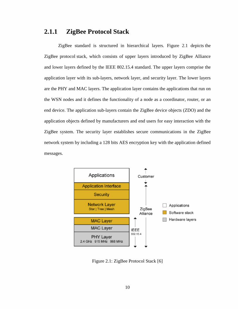
ZigBee standard is structured in hierarchical layers. Figure 2.1 depicts the
ZigBee protocol stack, which consists of upper layers introduced by ZigBee Alliance
and lower layers defined by the IEEE 802.15.4 standard. The upper layers comprise the
application layer with its sub-layers, network layer, and security layer. The lower layers
are the PHY and MAC layers. The application layer contains the applications that run on
the WSN nodes and it defines the functionality of a node as a coordinator, router, or an
end device. The application sub-layers contain the ZigBee device objects (ZDO) and the
application objects defined by manufacturers and end users for easy interaction with the
ZigBee system. The security layer establishes secure communications in the ZigBee
network system by including a 128 bits AES encryption key with the application defined
messages.
Figure 2.1: ZigBee Protocol Stack [6]
11
The PHY layer specified by IEEE 802.15.4 protocol requires ZigBee technology
to operate at 2.4 GHz with data transfer rate of 250 kb/s making it a good candidate for
Low Rate Wireless Personal Area Networks (LoWPANs). The low data rate feature of
ZigBee results in low power consumption and this makes it useful for WSNs where long
battery life devices are needed for sensing and communication. The MAC layer is
responsible for network channel access control, data packet retransmission, frame
validation, and reception acknowledgement [6]. The MAC layer provides link support
between layers as it validates each layer message frame and content prior to
transmission. The channel access techniques used in IEEE 802.15.4 MAC layer are
Carrier Sense, Multiple Access/Collision Avoidance (CSMA/CA), and Guaranteed Time
Slots (GTS). The CSMA/CA technique allows sensor nodes to check if the channel is
free for use before transmission. This technique helps prevent collision of packets from
different sensor nodes. The GTS technique, if available, allocates time slots for packets
with high priority to access the channel with a high level of urgency.
The ZigBee protocol stack provided by the Ember Corporation (a member of the
ZigBee Alliance) was used in this thesis work and its MAC layer uses only CSMA/CA
access mode in order to save code space in the software [6]. The lower layers of ZigBee
architecture cannot be modified or overwritten because they are defined IEEE standards.
So, prioritization of the network sensor nodes can only be done in the application layer
of the architecture. The network layer is broadly elaborated in Section 2.1.2 because it is
the part of the architecture that gives better understanding of this thesis.
12
2.1.2 Networking Layer
The network (NWK) layer is the medium link between the application layer and
the MAC layer. It handles network addressing and routing actions that are executed in
the MAC layer. The NWK layer supports multiple network structures, which include
star, tree, and mesh network. A ZigBee network constitutes a coordinator, routers, and
end devices. A coordinator node controls the network and uses the NWK layer to initiate
a network, assign network addresses, add or remove devices from the network, and
discovers reliable routing. Router nodes and end devices execute the functions of the
sensor application with the router nodes also relaying messages intended for other nodes.
The coordinator and the router are full-function (FFD) devices while the end device
could be either a full-function device (FFD) or a reduced-function device (RFD) [6].
FFD nodes are network nodes that have full functionalities which include route
discovery, route maintenance, network data acquiring, and storing network information.
RFD nodes are responsible for data transmission but lack the functionalities of network
building and management.
The network topology implemented in this thesis is the star network because of
the small numbers of nodes that were available for testing. Other topologies such as
mesh network can also be used since network topology has no significant effect on the
network performance metrics used in this thesis. A star network is a network that
consists of a coordinator and end devices whereby the end device(s) only communicates
with the coordinator. On the other hand, a mesh network is a network that consists of a
coordinator, routers, and multiple end devices whereby an end device communicates
with a parent node which can be a router, a coordinator, or an end device. Overall, the
13
network of either topology is controlled by a single coordinator. The process by which
the coordinator node initiates and manages the network is described in Section 2.1.2.1.
2.1.2.1 Network Creation and Joining Process
A ZigBee coordinator initiates the ZigBee network formation. After forming a
network, the coordinator can accept requests from other devices (nodes) that wish to join
the network. Depending on the stack and application profile used, the coordinator might
also perform additional duties after network formation. An application profile describes
the messages and network settings for a particular application, such as smart energy
saving by the node.
A ZigBee node finds a network by scanning channels and using a personal area
network identifier (PAN ID) to identify a network. When a node finds a network with
the correct profile that is open to joining, it can request to join that network. A node can
send a join request to the network‟s coordinator or one of its router nodes if it is an end
device node. If the application is using a trust center, the trust center can further specify
security conditions under which join requests are accepted or denied. All nodes that
communicate on a network transmit and receive on the same frequency channel.
2.2 Enhancement of ZigBee-based WSN
A ZigBee-based WSN that is connected to the Internet through cellular or
Ethernet connectivity becomes WAN capable. Also, inherent ZigBee channel delays
need to be managed by prioritization mechanisms in the application layer for the WSN
to be used in real-time systems, e.g., micro-grid device protection and possibly islanding
detection.
14
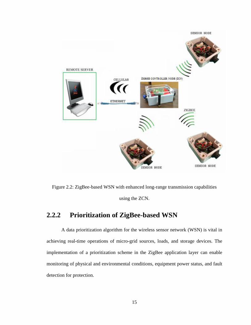
2.2.1 WAN: Long-Range Data Transmission
The low power consumption specification of ZigBee limits the effective
transmission range of individual sensor nodes. ZigBee can transmit data over a distance
of approximately 100 meters depending on the environmental characteristics of the
WSN location. Although the ZigBee network structure can increase local area coverage
through a mesh network deployment, this requires intermediate router devices to reach
more distant devices. For WAN applications, the ZigBee‟s mesh network structure
cannot solve the connectivity problem between remote micro-grid stations and distant
data processing facilities. For this scenario, a ZCN with cellular and Ethernet
connections for Internet access is needed.
Fiber-optic, Ethernet, satellite (GPS), HF radio, and cellular communication
technologies are possible technologies for transferring data over a long distance. For this
work, a ZigBee controller node (ZCN) with cellular and Ethernet communication
capabilities was selected and developed given the low cost of the cellular module and
perhaps any legacy wired networks previously installed near the micro-grid deployment.
As expected, the cellular module requires a network data service for data transmission
over private or public network in order to reach the main processing center. In remote
areas where Ethernet connectivity is not available, the cellular connection offers
deployment flexibility since costly wiring and infrastructure setup are not required. Data
transmission costs can be managed by the prioritization and compression schemes
utilized by the WSN and the ZCN.
15
Figure 2.2: ZigBee-based WSN with enhanced long-range transmission capabilities
using the ZCN.
2.2.2 Prioritization of ZigBee-based WSN
A data prioritization algorithm for the wireless sensor network (WSN) is vital in
achieving real-time operations of micro-grid sources, loads, and storage devices. The
implementation of a prioritization scheme in the ZigBee application layer can enable
monitoring of physical and environmental conditions, equipment power status, and fault
detection for protection.
16
Outlining the pros and cons of known prioritization mechanisms; in pre-emptive
priority scheduling, when high priority data packet arrive during the management of low
priority data packet, the contents of the low priority packets are saved for the high
priority data packet to be executed first. A large amount of high priority data packets
would effectively suppress transmission of low priority packets for a long duration,
thereby limiting overall packet queuing fairness. In non-pre-emptive priority scheduling,
when a high priority packet arrives during the start of execution of a low priority packet,
the execution continues even though the newly arrived packet is of high priority, thus
limiting the effectiveness of prioritizing packets. In order to balance priority throughput
and queuing fairness, the Earliest Deadline First (EDF) and First Come First Serve
(FCFS) scheduling algorithms [37] were implemented for this thesis work. The Earliest
Deadline First (EDF) and First Come First Serve (FCFS) scheduling algorithms [37] are
the prioritization mechanisms used in this thesis. EDF is a dynamic prioritization
algorithm where data packets are assigned deadlines (time to leave) according to their
priority class, and the data packet with the lowest deadline is first processed. The EDF
mechanism is a time-dependent mechanism that provides a strict way of allocating time
slots to data packets and requires another mechanism to resolve conflicts that occur
when two packets of the same priority class arrive successively. The FCFS prioritization
method is a mechanism that processes or transmits data according to their arrival time.
With FCFS, a high priority packet that arrives after a low priority packet has to wait in
the queue for the low priority packet to be transmitted. Although FCFS neglects the
priority of a packet, it can be used to resolve the conflict that might occur when data
packets of the same priority arrive at the same time. FCFS scheduling provides fairness
17
irrespective of the data packet priority. The combination of EDF and FCFS scheduling is
efficient in terms of average packet waiting time and end-to-end delay.
In this thesis, the sensor measurements are prioritized into 3 distinct priority
classes. The highest priority class is designated as real-time data used for fast response
applications such as fault detection and device protection. The aforementioned micro-
grid real-time applications are assumed to have processing times that is up to one second
in order to accommodate the WSN‟s low data rate and processing delays through the
Internet. The second and the third priority classes are non-real-time packets classified
according to their data size such as data used to determine the environmental conditions
of an area and the power status of micro-grid devices. The applied prioritization
mechanism is implemented so that a sensor node provides the priority identity of each of
its measurement parameters at the point of joining a network. When a data packet from
the sensor node becomes available at a ready-to-go queue in the ZCN, the packet will be
assigned a deadline to move to the remote server. High priority data packets are given a
lower deadline than low priority data packets. When two packets of the same priority
class arrive at the ZCN, the first packet to arrive is inserted in the ready-to-go queue
before the other. The combined EDF and FCFS algorithm were implemented in the ZCN
with the concept of a two-valve water tap flow process which is described in Chapter 3.
2.3 Performance and Reliability Metrics for
the WSN
Performance metrics assessed in this thesis include packet loss, latency, and
throughput. Packet loss is an indication of reliability or the assurance that information
18
will reach its destination on time without losing its data or becoming corrupted, while
latency and throughput are channel performance measures. Other performance metrics
include packet retries and average packet delivery ratio.
2.3.1 Average Latency
The average latency is the average total time required for a data packet to be
transmitted from the sensor node to a remote server and vice versa. This metric
determines the end-to-end delay of a WSN system for various packet prioritization
levels, and the average latency will vary for packets of different priority classes. The
highest priority data packets are expected to have the lowest average latency.
2.3.2 ZigBee Throughput
ZigBee throughput is the rate of successful message (data packet) delivering to
the ZCN from the sensor node. The unit for packet throughput is packets/second.
2.3.3 Packet Drop or Loss
Packet drop or loss is the number of packets dropped during the data
transmission in the ZigBee network. Packet drops occur when the receiver fails to
acknowledge the reception of a packet either as a result of errors in packet bit sequence
or a corrupted packet due to external RF interference such as Wi-Fi network.
19
2.3.4 Packet Retries
Packet retries is the number of times a packet retry is initiated by the
ZigBee‟s MAC layer whenever a packet is lost and continues until a success packet
reception acknowledgement is received or a retry timeout occurs.
2.3.5 Average Packet Delivery Ratio
Average Packet Delivery Ratio is the ratio of the average number of packets
received successfully and the total average number of packets transmitted.
2.4 ZigBee-based WSN Simulation Platforms
A network simulation platform is computer software with network device
libraries and protocols that can be used to predict the performance and reliability of a
particular information network. The simulation platform can be used to study how a
network works in various operational scenarios, predict the financial cost, compute the
execution time, determine level of design difficulty, and assess the impact of various
protocol and prioritization algorithms on system performance. In our case, the
performance of a simulated WSN can be evaluated under various deployment schemes
such as number of sensor nodes used, sensor node type (end device, router, access
point), network type (e,g, mesh, star, tree), deployment configuration, prioritization
algorithms etc., to predict the behavior of the WSN. The increased complexity of
information networks has resulted in the development of several simulation platforms
that can be used for WSN behavioral studies. Network simulation platforms are
relatively simple to use, flexible, and accurate provided network protocols, information
20
sources, and sinks are correctly modeled. The simulation results in this thesis are
considered to be the best case scenario when compared to experimental results since
physical layer impairments such as channel interference are not considered for the WSN
simulation. In this thesis, the performance metrics from simulation are compared with
the experimental metrics to confirm reasonable expectations from the ZigBee-based
WSN.
2.4.1 The Network Simulation Software
There are several network simulation software or platforms used by researchers
to predict network system performance. Widely used network simulation software
includes Network Simulation 2 (NS2), Network Simulation 3 (NS3), OMNeT++, and
OPNET. The addition of MiXiM framework to the OMNeT++ platform makes
OMNeT++ suitable for the performance analysis of a ZigBee-based WSN given
ZigBee‟s CSMA/CA medium access specification, plus it is open-source and free to use
by researchers.
2.4.2 OMNeT++ Simulation Software
Objective Modular Network Test bed in C++ (abbreviated as OMNeT++) is an
open source, component-based, modular communication network simulation platform
popularly used for research purposes. OMNeT++ is also an event-driven simulator tool
that uses modules programmed in C++ and network topology description language
(NED) to simulate events for wireless communication networks. The simulated events
are defined based on the network topology, scheduling method, energy consumption,
and Quality of Service (QoS) requirements. OMNeT++ has a graphical interface for
21
displaying the simulated network and performance results. Results such as packet drop
against an increase in sensor nodes in the network, system throughput, and energy
consumption can be displayed as line graphs or bar charts.
OMNeT++ is just a skeleton that has a backbone on which networks are built. It
is not a simulator in itself, and requires frameworks that contain the models or
application codes of the network. Simulation frameworks such as ALOHA, INET, and
MiXiM are network models that have already been implemented for OMNeT++, the
platform used in this thesis.
2.4.3 MiXiM Simulation Framework
MiXiM is an OMNeT++ framework that supports mobile and fixed wireless
network simulations. It provides wireless connectivity and mobility models such as radio
wave propagation, interference estimation, and radio transceiver power consumption,
which are written in object oriented C++ and NED. The models are graphically
displayed during simulation and give the user an idea of the performance of the network.
MiXiM contains a basic example of sensor application wireless network that has IEEE
506.15.4 PHY and MAC layers. This example was modified in this thesis to serve as a
ZigBee WSN since ZigBee is an IEEE 506.15.4 based protocol. The performance
analysis features were added to the MiXiM example and its simulation results were
assessed. To manage the complexity of the network simulation model used in this thesis,
only the performance metrics of the ZigBee network were observed.
22
Chapter 3
ZigBee Controller Node Hardware
Design and Prioritization Schemes
This chapter discusses the hardware design of the ZigBee controller node (ZCN)
and the implementation of the prioritization algorithms used in this thesis. The chapter
describes the various components of the ZCN and highlights the pseudo-code for
initiating and managing a ZigBee network and providing Internet access. A
mathematical model for estimating the latency of a data packet from a sensor node to a
remote server is also derived in this chapter.
3.1 ZCN Architecture
The developed ZCN is a customized hardware node that has embedded ZigBee
coordinator hardware as the foundation, data processing hardware with Ethernet
communication, and cellular communication hardware, as shown in Figure 3.1.
23
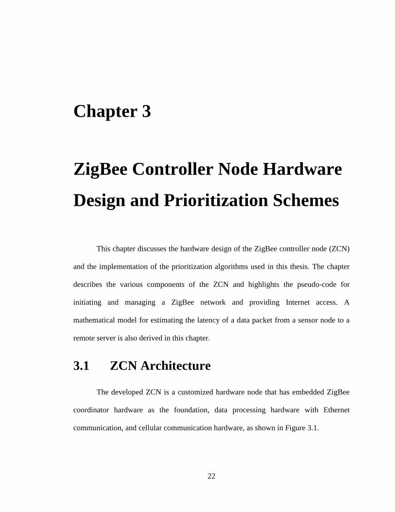
Figure 3.1: Wireless Sensor Network Architecture Diagram including the ZCN.
The ZCN sends and receives messages from the ZigBee end devices and router
nodes through the ZigBee coordinator hardware to a web application server by means of
either cellular communication or Ethernet communication network. The microcontroller
in the ZCN has on-board data storage for messages received from either the ZigBee
coordinator hardware or the remote server. The ZCN is constructed with an off-the-shelf
BeagleBone Black microcontroller (3BM), an off-the-shelf cellular module (SparkFun
SM5100B cellular module) and in-house designed ZigBee coordinator hardware. The
UNB coordinator hardware and the SparkFun SM5100B cellular module are serially
connected to the 3BM. The ZCN components are coupled and packaged in a weather
resistant case as shown in Figure 3.2. The ZCN has a water-proof mini USB connector
for debugging, configuring, and powering of the 3BM. It also has a water-proof 5 V
24
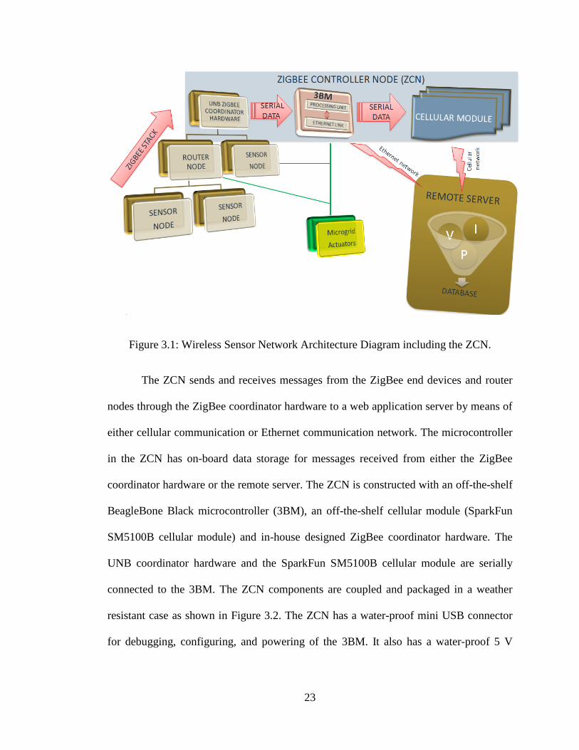
power connector for power and a water-proof RJ45 Ethernet connector that connects the
3BM to an Ethernet network.
Figure 3.2: UNB ZigBee Controller Node (ZCN).
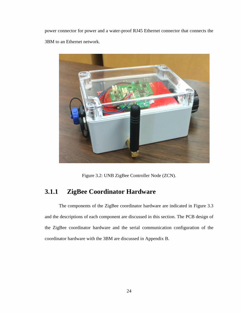
3.1.1 ZigBee Coordinator Hardware
The components of the ZigBee coordinator hardware are indicated in Figure 3.3
and the descriptions of each component are discussed in this section. The PCB design of
the ZigBee coordinator hardware and the serial communication configuration of the
coordinator hardware with the 3BM are discussed in Appendix B.
25
Figure 3.3: UNB ZigBee Coordinator Hardware.
The coordinator hardware consists of nine major components:
1. 2.4 GHz radio transceiver: The transceiver is circuitry that boosts the radio
strength of the ZigBee EM357 chip. The transceiver consists of a 2.4 GHz ceramic
chip antenna, signal power amplifiers, and a crystal oscillator. The radio transceiver
is compliant with IEEE 802.15.4 standard. It limits ZigBee channels to be within the
standard 2.4 GHz with each channel bandwidth of 2 MHz.
2. Ember EM357 System-on-chip (SoC): EM347 SoC is a member of Ember EM35x
family, integrated with EmberZNET PRO stack, which is the software that supports

26
the connection between the chip and any external processor. The stack also provides
a platform for writing the application code to the chip. The SoC chip has a 32-bit
ARM Cortex-M3 processor with 128 kB flash and 12 kB RAM memory. The
EM357 SoC has an in-built 2.4 GHz IEEE 802.15.4-2003 transceiver and also allows
connection of an external Power Amplifier (PA). It has flexible ADC,
UART/SPI/TWI serial communications, and general purpose timers for external
peripheral connections. The chip also has AES 128 bits encryption engine that
generates random numbers to encrypt the message for security purposes.
3. Ember In-sight serial port: This is a programming and debugging header that
connects the coordinator hardware to a computer through an Ember Debug Adapter.
Application code and firmware are uploaded to the EM357 chip through the Ember
in-sight serial port. The serial port is also use for powering the hardware, debugging,
and printing the data from the sensor nodes on a computer. It is a 10-pin male
connector with 3.3 V VCC.
4. 4 MB Data Flash: The flash is used to store and boot load the application code,
supplementing the 128 kB flash memory of the EM357. The flash is not deleted
when the node is shut down so the node resumes the running of the application in the
flash whenever the node is powered.
5. Battery Connector: A Li-Ion Poly power battery or solar cell with a voltage source
that ranges from 3.3 to 6 VDC and a maximum current rating of 500 mA can be
connected to the coordinator board through the battery connector. It regulates source
voltage to 3.3 V. The EM357 chip requires a VCC of 2.1 V to 3.6 V for system
operation. The entire system may be damaged if the supplied voltage to the power
connector is more than 6 VDC. The LED beside the battery connector labeled
27
„charge‟ on the coordinator board shows the charging states of the connected battery.
When the power LED is solid, it means the battery is charging, and when the LED
light is off, it means the battery is fully charged or there is no battery connected.
6. Li-Ion Battery charging Circuit: This circuit charges only Li-Ion Poly batteries
with supply voltage less than 6 VDC. The circuit monitors the power level of the Li-
Ion battery and the charging level can be programmed in the application code. The
circuit was programmed to charge the connected battery when the voltage level is
less than 3.35 V.
7. Serial Connector: The 4-pin serial connector links the coordinator hardware serially
to a microcontroller. The ZigBee EM357 SoC is configured to serially communicate
to an external processor. The UART serial communication system was programmed
to have XON/XOFF instead of RTS/CTS control so that the application code can
handle the communication lines and also to minimize wire connections. The serial
configuration firmware has to be uploaded once before uploading an application
code to the 4MB flash memory. The ZCN is also powered through the serial
connector with VCC of 3.3 V. The RX and TX connector pins are connected to the
UART pin of the EM357 chip.
8. Push Buttons: There are two push buttons on the coordinator board: the Leave
button and the Join button. The Leave button allows the user to manually force the
ZCN to leave the network and the Join button allows the user to manually force the
ZCN to join an existing network that was created and left by the ZCN.
9. Network Status LEDs: The status LEDs indicate the network states of the ZCNs in
terms of the network creation and data transmission. The LED labeled „Act‟ on the
coordinator board indicates the presence of a network. When the Act LED is solid, it
28
means a network is created by the ZCN. The LED labeled „Heart‟ on the coordinator
board indicates the flow of data from the sensor nodes to the ZCN. When the Heart
LED is blinking, it means there is data flow and also indicates the presence of a
sensor node in the network. These status LEDs were programmed in the application
code to behave in such manners. They can be reprogrammed by the user.
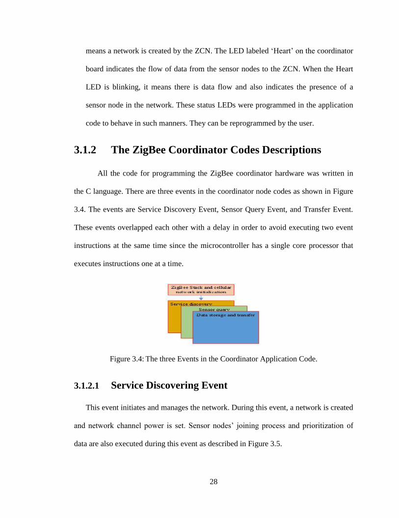
3.1.2 The ZigBee Coordinator Codes Descriptions
All the code for programming the ZigBee coordinator hardware was written in
the C language. There are three events in the coordinator node codes as shown in Figure
3.4. The events are Service Discovery Event, Sensor Query Event, and Transfer Event.
These events overlapped each other with a delay in order to avoid executing two event
instructions at the same time since the microcontroller has a single core processor that
executes instructions one at a time.
Figure 3.4: The three Events in the Coordinator Application Code.
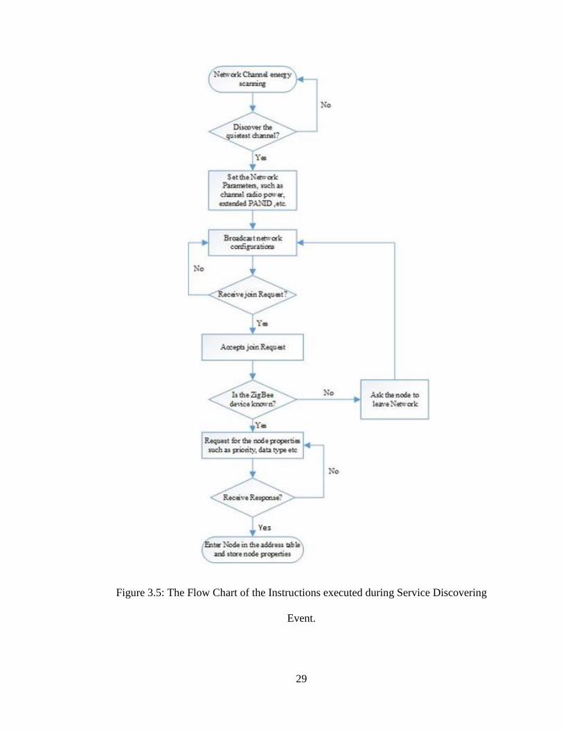
3.1.2.1 Service Discovering Event
This event initiates and manages the network. During this event, a network is created
and network channel power is set. Sensor nodes‟ joining process and prioritization of
data are also executed during this event as described in Figure 3.5.
29
Figure 3.5: The Flow Chart of the Instructions executed during Service Discovering
Event.
30
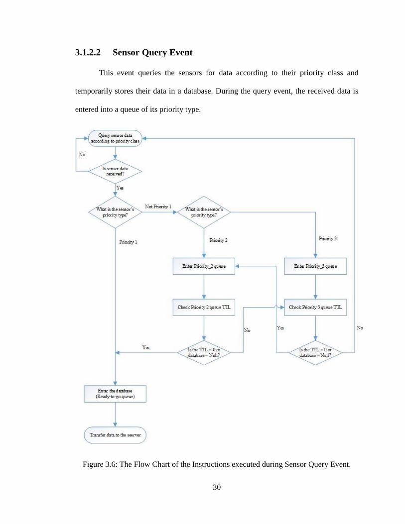
3.1.2.2 Sensor Query Event
This event queries the sensors for data according to their priority class and
temporarily stores their data in a database. During the query event, the received data is
entered into a queue of its priority type.
Figure 3.6: The Flow Chart of the Instructions executed during Sensor Query Event.
31
3.1.2.3 Transfer Event
The transfer event moves data from the ready-to-go queue (database) to the
remote server through a communication channel selected by the user. Data from the
lowest row of the database table is sent to the server and moves to the next in row after a
successful transmission. The database in the ZCN is overwritten when it runs out of
storage capacity. The database can hold up to 2 GB of data. The information transmitted
to the server is less than 64 bytes of data and consists of the sensor‟s node number,
priority type, data value, and data arrival time at the ZCN.
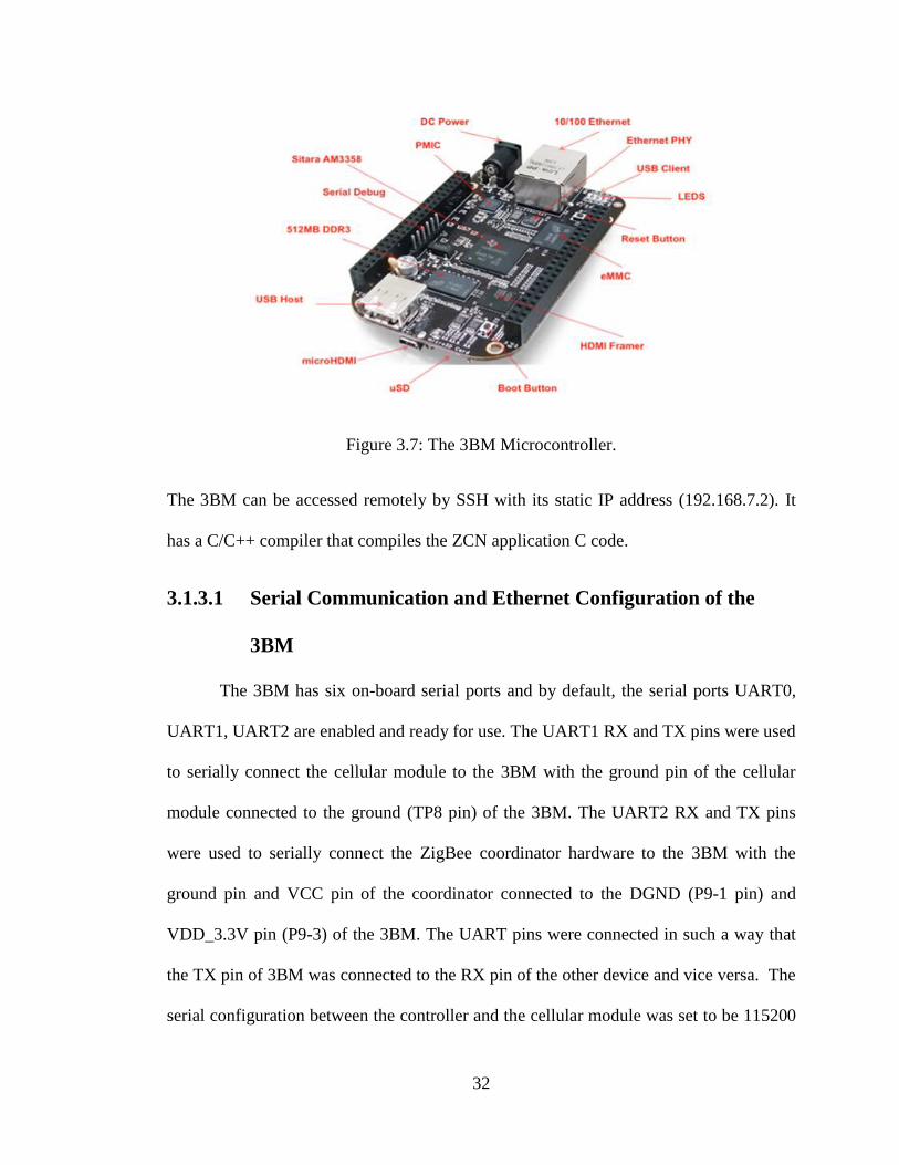
3.1.3 Microcontroller
The microcontroller used in the ZCN is the BeagleBone Black (3BM), which has
a data processing unit that analyzes, sorts, and temporarily stores the data collected from
the ZigBee coordinator hardware before sending it to the web server through the cellular
or Ethernet connection. The 3BM is a low cost, low power, community-supported
microcontroller that runs on Linux operating system. The 3BM has all the functionality
of a basic computer. It is a 32 bit AM335x 1GHz ARM® Cortex-A8 processor with a
512MB DDR3 RAM and 4GB 8 bit eMMC on board flash [29]. 3BM is compatible with
the Ångström, Debian, Android, and Ubuntu Linux operating systems. The 3BM has
many connectivity features such as HDMI, Ethernet, 92 IO pins, USB host, and USB
client for power and communications.
32
Figure 3.7: The 3BM Microcontroller.
The 3BM can be accessed remotely by SSH with its static IP address (192.168.7.2). It
has a C/C++ compiler that compiles the ZCN application C code.
3.1.3.1 Serial Communication and Ethernet Configuration of the
3BM
The 3BM has six on-board serial ports and by default, the serial ports UART0,
UART1, UART2 are enabled and ready for use. The UART1 RX and TX pins were used
to serially connect the cellular module to the 3BM with the ground pin of the cellular
module connected to the ground (TP8 pin) of the 3BM. The UART2 RX and TX pins
were used to serially connect the ZigBee coordinator hardware to the 3BM with the
ground pin and VCC pin of the coordinator connected to the DGND (P9-1 pin) and
VDD_3.3V pin (P9-3) of the 3BM. The UART pins were connected in such a way that
the TX pin of 3BM was connected to the RX pin of the other device and vice versa. The
serial configuration between the controller and the cellular module was set to be 115200
33
bauds, 8 data bits, no parity bit, and 1 stop bit. The 3BM is powered by the cellular
module through the module VCC pin which was connected to TP6 of the 3BM.
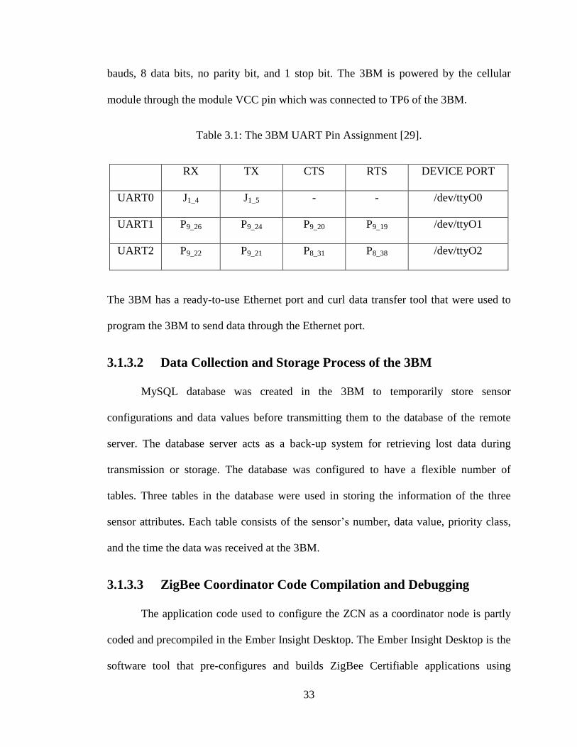
Table 3.1: The 3BM UART Pin Assignment [29].
RX TX CTS RTS DEVICE PORT
UART0 J1_4 J1_5 - - /dev/ttyO0
UART1 P9_26 P9_24 P9_20 P9_19 /dev/ttyO1
UART2 P9_22 P9_21 P8_31 P8_38 /dev/ttyO2
The 3BM has a ready-to-use Ethernet port and curl data transfer tool that were used to
program the 3BM to send data through the Ethernet port.
3.1.3.2 Data Collection and Storage Process of the 3BM
MySQL database was created in the 3BM to temporarily store sensor
configurations and data values before transmitting them to the database of the remote
server. The database server acts as a back-up system for retrieving lost data during
transmission or storage. The database was configured to have a flexible number of
tables. Three tables in the database were used in storing the information of the three
sensor attributes. Each table consists of the sensor‟s number, data value, priority class,
and the time the data was received at the 3BM.
3.1.3.3 ZigBee Coordinator Code Compilation and Debugging
The application code used to configure the ZCN as a coordinator node is partly
coded and precompiled in the Ember Insight Desktop. The Ember Insight Desktop is the
software tool that pre-configures and builds ZigBee Certifiable applications using
34
ZigBee public or custom application profiles. The software generates objects files and
callback files which are saved in the path to the application framework and EmberZNET
PRO stack libraries files. The coordinator application code was saved in the application
callback file. The generated callback files of the coordinator application were compiled
with the built-in C compiler in the 3BM.
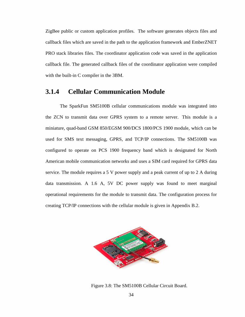
3.1.4 Cellular Communication Module
The SparkFun SM5100B cellular communications module was integrated into
the ZCN to transmit data over GPRS system to a remote server. This module is a
miniature, quad-band GSM 850/EGSM 900/DCS 1800/PCS 1900 module, which can be
used for SMS text messaging, GPRS, and TCP/IP connections. The SM5100B was
configured to operate on PCS 1900 frequency band which is designated for North
American mobile communication networks and uses a SIM card required for GPRS data
service. The module requires a 5 V power supply and a peak current of up to 2 A during
data transmission. A 1.6 A, 5V DC power supply was found to meet marginal
operational requirements for the module to transmit data. The configuration process for
creating TCP/IP connections with the cellular module is given in Appendix B.2.
Figure 3.8: The SM5100B Cellular Circuit Board.
35
3.1.5 Web Server Design and Database
Apache 3.1.3 is the HTTP webserver used during the research. The server was
installed and configured in a personal computer (PC) located in a remote location that is
away from the ZigBee WSN deployment area. The PC was configured to allow traffic
from an external computer that is not in the local network, by turning off the firewall and
setting the local IP address of the PC to static. The web server listens to Port 8080 to
make a TCP connection through this port of the local network router. Port 8080 was port
forwarded in the network router to allow Port 8080 to be accessed by an external PC
when appended with the local network external address of the webserver in the URL.
The webpages that receive and display data information were scripted in PHP and
HTML. MySQL database was configured in the webserver to store data received from
the ZCN. The database has three tables, each of which consists of the sensor number,
data value, priority class, and the arrival time of the data at the ZCN. The database only
removes data at the request of the user.
3.2 Implementation of the Two-Valve Water
Tap Flow Model
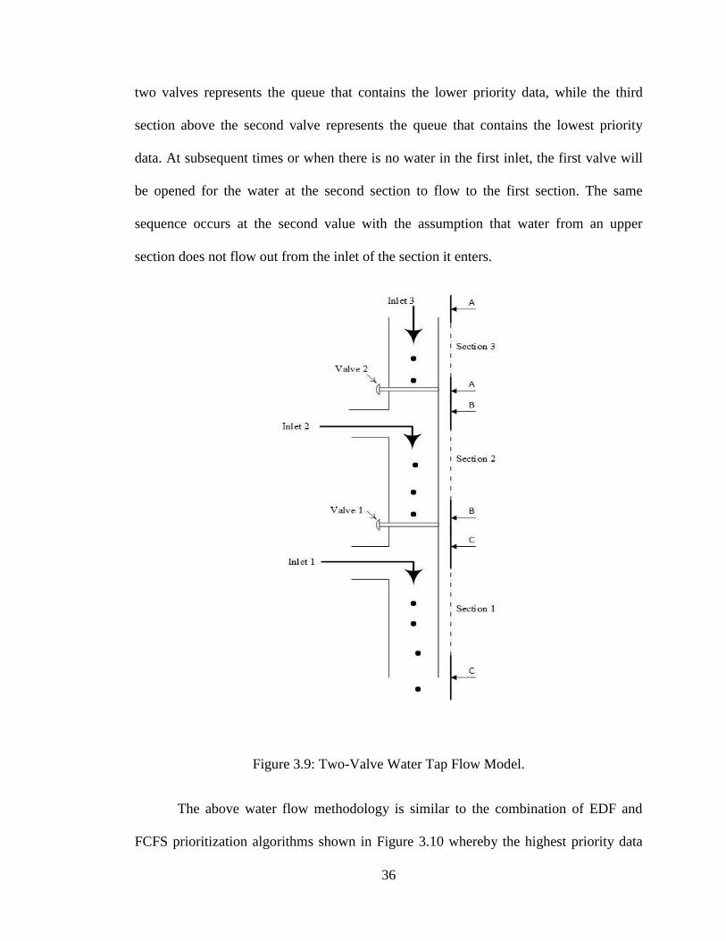
The concept of the combination of EDF and FCFS prioritization mechanisms
implemented in the ZCN was based on the two-valve water tap flow model shown in
Figure 3.9. The two-valve water tap flow model is based on a water tap with three water
flow sections and two control valves. The first flow section represents the highest
priority data queue which is also the ready-to-go queue. The flow section between the
36
two valves represents the queue that contains the lower priority data, while the third
section above the second valve represents the queue that contains the lowest priority
data. At subsequent times or when there is no water in the first inlet, the first valve will
be opened for the water at the second section to flow to the first section. The same
sequence occurs at the second value with the assumption that water from an upper
section does not flow out from the inlet of the section it enters.
Figure 3.9: Two-Valve Water Tap Flow Model.
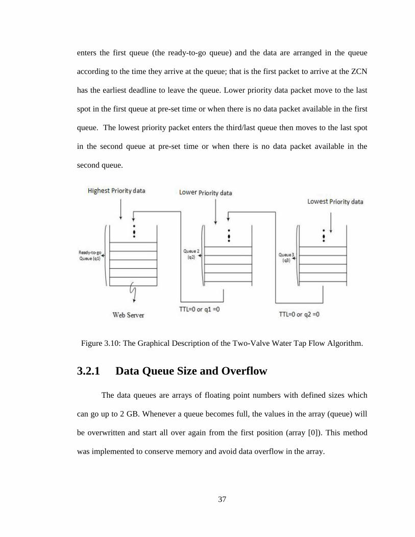
The above water flow methodology is similar to the combination of EDF and
FCFS prioritization algorithms shown in Figure 3.10 whereby the highest priority data
37
enters the first queue (the ready-to-go queue) and the data are arranged in the queue
according to the time they arrive at the queue; that is the first packet to arrive at the ZCN
has the earliest deadline to leave the queue. Lower priority data packet move to the last
spot in the first queue at pre-set time or when there is no data packet available in the first
queue. The lowest priority packet enters the third/last queue then moves to the last spot
in the second queue at pre-set time or when there is no data packet available in the
second queue.
Figure 3.10: The Graphical Description of the Two-Valve Water Tap Flow Algorithm.
3.2.1 Data Queue Size and Overflow
The data queues are arrays of floating point numbers with defined sizes which
can go up to 2 GB. Whenever a queue becomes full, the values in the array (queue) will
be overwritten and start all over again from the first position (array [0]). This method
was implemented to conserve memory and avoid data overflow in the array.
38
3.3 One-way Transmission Latency Models
In a prioritized ZigBee-based WSN, the total transmission delay/latency depends
on several factors such as the deployment environment, the ZigBee network bandwidth,
priority class, communication network type, and network traffic. The communication
network traffic through the Internet depends on the time of the day. Therefore, the total
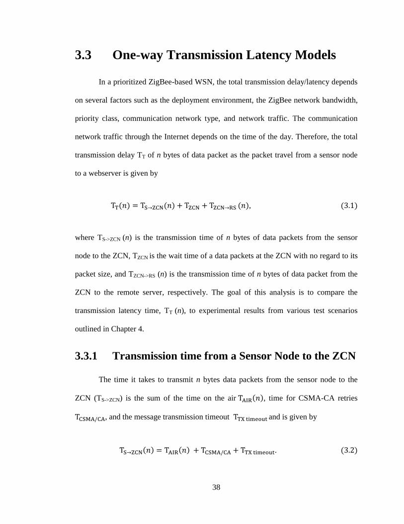
transmission delay TT of n bytes of data packet as the packet travel from a sensor node
to a webserver is given by
,
where TS->ZCN (n) is the transmission time of n bytes of data packets from the sensor
node to the ZCN, TZCN is the wait time of a data packets at the ZCN with no regard to its
packet size, and TZCN->RS (n) is the transmission time of n bytes of data packet from the
ZCN to the remote server, respectively. The goal of this analysis is to compare the
transmission latency time, TT (n), to experimental results from various test scenarios
outlined in Chapter 4.
3.3.1 Transmission time from a Sensor Node to the ZCN
The time it takes to transmit n bytes data packets from the sensor node to the
ZCN (TS->ZCN) is the sum of the time on the air , time for CSMA-CA retries
, and the message transmission timeout and is given by
.
39
The time on the air, TAIR (n), is the actual time taken to send n payload bytes plus header
bytes of data over the air. So,
.
At 2.4 GHz, the ZigBee (802.15.4) PHY layer specifies an RF baud rate of 250 kbits/s
which is a 0.032 ms byte time. The EM357 ZigBee firmware uses 64 bits for addressing
and a 25 byte header. Thus, equation (3.3) becomes
Equation (3.4) is further simplified as
(3.4)
The time for CSMA-CA retries does not depends on the packet size.
It depends on the outcome of channel assessment. Prior to transmission, the MAC
layer senses the carrier channel to make sure the air waves are clear. This process is
called CCA (Clear Channel Assessment). If this process senses a busy channel, it will
perform a random delay and then try again with another CCA. The message
sent by the sensor node to the ZCN is a unicast message and requires a transmission
timeout that could take up to an upper bound of 0.864 ms [6]. This timeout
40
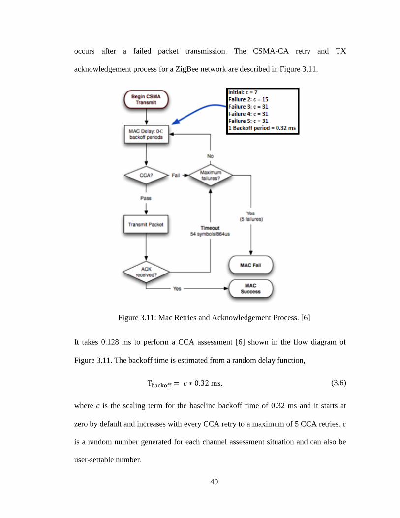
occurs after a failed packet transmission. The CSMA-CA retry and TX
acknowledgement process for a ZigBee network are described in Figure 3.11.
Figure 3.11: Mac Retries and Acknowledgement Process. [6]
It takes 0.128 ms to perform a CCA assessment [6] shown in the flow diagram of
Figure 3.11. The backoff time is estimated from a random delay function,
(3.6)
where c is the scaling term for the baseline backoff time of 0.32 ms and it starts at
zero by default and increases with every CCA retry to a maximum of 5 CCA retries. c
is a random number generated for each channel assessment situation and can also be
user-settable number.
41
Hence, the time for CSMA-CA retries is expressed as the sum of the total
time taken to perform CCA and the total backoff periods. That is,
, (3.7)
where y is the number of times CCA was performed.
In a best case scenario there is no transmission timeout and the backoff time,
, is 0.128ms. Using this latency term and Equations (3.2) and (3.5), the best
case scenario transmit time for n payload data packets to be sent from the sensor node
to the ZCN can be estimated as
.
In a worst case scenario, where there is no clear channel and a maximum number (i.e.
5) of CCA retries is needed to send data. Also in this case, c is limited to a maximum
of 7,15,31,31, and 31 in this sequence. Thus, using equation (3.7) the for
worst scenario is approximately,
The first term shows that CCA was performed six times which
consists of the first CCA and 5 CCA retries. The calculated value with
Equations (3.2) and (3.5) can be used to estimate the worst scenario with
three maximum packet retries, thus,
(3.9)
42
The first term of Equations (3.9) shows that packet transmission was performed four
times which is the accumulation of the first transmission and the three packet retries.
The last transmission has no message failure acknowledgement. In chapter 4, Equations
(3.8) and (3.9) will be used to validate transmission times of data over an actual ZigBee
WSN.
3.3.2 Wait Time at the ZCN (TZCN)
The wait time term, TZCN, given in Equation (3.1) depends on the data priority
class and number of waiting packets in the queues. The instantaneous waiting time TZCNi
can be expressed as
∑
where, N is the priority type value, xk is the total number of packets in queue k, t is the
wait/process time of a data packet in a queue and Wk is the pre-set time for a packet to
move to the next queue depending on the availability of a packet in the queue k,
respectively. For the EDF/FCFS priority mechanism, N = 1 represents the highest
priority class, N = 2 represents the lower priority class, and N = 3 represents the lowest
priority class.
In a prioritization system such as the implemented EDF/FCFS mechanism where
three queues are used, the possible wait times TZCN at the ZCN can be expressed as
follows. For the first (ready-to-go) queue,
43
and for the second queue which contains the lower priority data,
∑
Finally, for the third queue which contains the lowest priority data,
∑
∑
These equations are used to estimate the waiting times at the ZCN using the
implemented priority algorithm. These wait times will impact the overall data
44
transmission times over the WAN and are validated using experimental measurements as
discussed in Chapter 4.
3.3.3 Transmission Time from the ZCN to the Server
The mathematical model for estimating the transmission latency over the cellular
network is difficult to derive since it depends on an inconsistent network behavioral
model, the network service provider, and the data routing utilized by the data packet.
Given the complexities of this transmission model, the cellular latency model was not
attempted in this research work. However, the author of [25] considered the transmission
factors that might introduce latency in the cellular network and estimated the latency in a
3G cellular network to be 100 – 500 ms. The author argued that the real performance of
every cellular network will vary by the network service provider, the network
configuration, the number of active users in a given cell, the radio environment in a
specific location, the device in use, and other factors that can affect the wireless channel.
With Ethernet protocol, the latency during data transmission depends
significantly on the physical medium links and forwarding routers, queuing time in the
router nodes, network traffic loads from other connections, cable properties, and
transmission distance [26]. The transmission latency via Ethernet protocol can be
modelled from individual latency sources [26] as
where Rrouters is the number of routers along the transmission path of the data, Lforwarding is
the time it takes to forward data to the next router, Lqueuing is the delay that occurs in
45
sorting of data packet in an Ethernet network, Lwire is the time taken for a packet to
propagate over a specific medium and Lroutertype is the delay introduced by the fabric
material of the router during sorting and data forwarding, respectively.
The delays can be summarized as follows:
,
where Mloads in Equation (3.20) is the number of network loads present during
transmission. For Lroutertype, most of the routers are made with sophisticated silicon and
have common fabric delay of 5.2 µs [26]. Correspondingly, the transmission latency in
Ethernet network becomes
.
Assuming an ideal telecommunication network, the transmission latency will simply be
the time taken for a packet at a given bit rate to travel over a medium from its source to
its destination. That is,
46
Assuming an Ethernet 100 BASE-TX connection with a bit rate of 100Mbits/s, a packet
size of 1460 bytes, a link speed of about ⅔ of the speed of light ( m/s) [25] and a
distance of approximately 4.7 km for our test WAN, the transmission delay is estimated
from Equation (3.23) to be approximately 0.14 ms. As expected, in a real environment
this value is highly depends on the level of Internet traffic and the number of routers
along the travelling path of the data. In any event, the best case scenario (ideal network)
serves as a baseline to gauge measured transmission times.
47
Chapter 4
Performance Tests and Result
Analysis
This chapter describes the system performance analysis of the ZigBee controller
node (ZCN) when deployed in an open space and the likelihood of RF interference being
present due to open UNB Wi-Fi connectivity. The performance measurements were
done in three environments: a school gymnasium with a maximum of 45 meters line of
sight (LOS), a VLSI lab room and a private home. The latency, packet drops, and retries
in the prioritized and non-prioritized ZigBee-based WSN created by the ZCN were
observed and these metrics were compared with the results from a simulated WSN.
Also, the reliability of the ZCN to transmit data over a long distance was investigated by
running the ZCN for more than 24 hours and observing the status telemetry.
48
4.1 Test Environments
A test bed was deployed at UNB‟s RICHARD CURRIE CENTER Recgym
which has an open space of 45 meters line of sight. The gymnasium room is an enclosed
area that has some sports equipment such as indoor soccer nets, badminton poles, and
basketball hoops and also Wi-Fi availability. The gymnasium room was preferred
because of its enclosed wide space without object interference and the presence of
Ethernet network drops. The measurement of a sensor‟s wait time data packet at the
ZCN in a prioritized and non-prioritized ZigBee-based network were performed in the
gymnasium, along with assessing the effects of varying link distances. The other
experiment performed was the total time taken to transfer sensor data through cellular or
Ethernet communication networks to a server located at the private home mentioned
above. For comparison, latency times of a private Ethernet network were also measured
using the private home‟s Internet network. The technical specifications and performance
of the ZCN in an open space were obtained from the aforementioned observations.
The rest of the experiments were performed in the VLSI lab room (D119) located
at the D-level of Head Hall, University of New Brunswick. The VLSI lab has equipment
which can generate and attenuate RF waves and also obstruct the line of sight between
sensor nodes. Some experiments were performed in the VLSI lab to mimic a possible
real micro-grid environment where LOS RF interference objects are present.
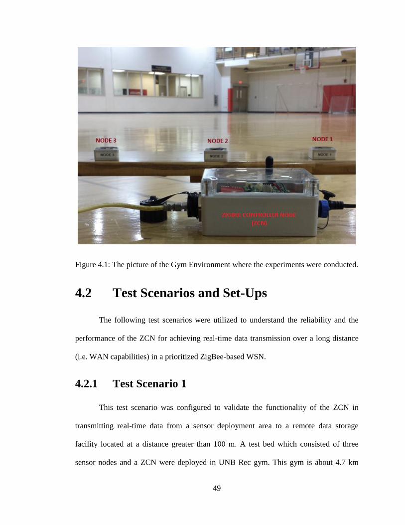
49
Figure 4.1: The picture of the Gym Environment where the experiments were conducted.
4.2 Test Scenarios and Set-Ups
The following test scenarios were utilized to understand the reliability and the
performance of the ZCN for achieving real-time data transmission over a long distance
(i.e. WAN capabilities) in a prioritized ZigBee-based WSN.
4.2.1 Test Scenario 1
This test scenario was configured to validate the functionality of the ZCN in
transmitting real-time data from a sensor deployment area to a remote data storage
facility located at a distance greater than 100 m. A test bed which consisted of three
sensor nodes and a ZCN were deployed in UNB Rec gym. This gym is about 4.7 km
50
away from 240 Wetmore Road Fredericton where the server was located. Three sensor
nodes were configured to measure data of different priority classes. The sensor node
labelled “Node 1” in Figure 4.1 was configured to measure electric current which was
assigned as the highest priority data. Sensor Node 2 measured temperature which was
regarded as lower priority data while Node 3 which measured vibrations was set as the
lowest priority data. The sensors were placed 10 meters in LOS from the ZCN. The ZCN
was configured to broadcast data requests to the sensor nodes at one second intervals
and receive their data according to their priority class before sending them to the remote
server. The total average time for data transmission in this scenario using Ethernet and
cellular networks were measured, the results are recorded in Table 4.1.
The performance of the EDF-FCFS prioritization algorithm was also observed in
this scenario. The node prioritization code was uploaded to the ZCN and the wait or
processing time of the sensor‟s data in the ZCN were measured for 1 minute of run time
and repeated four times. The time-to-leave (TTL) from queue 3 to queue 2 by the
priority 3 data was set to be 1 second while TTL from queue 2 to queue 1 was set to be
500 ms to accommodate fairness. The experiment was repeated for the non-prioritized
ZCN which has a no-wait queue and the sensor nodes having no-priority type. The
Ethernet communication network was used for transferring the data from the ZCN to the
remote server in both test cases. The results of the test cases are analyzed in Section
4.3.3.
51
4.2.2 Test Scenario 2
This test scenario describes the experimental procedure to determine the effect of
distance changes between the sensor nodes and the ZCN on the data transmission times
in a prioritized ZigBee network. This test configuration is similar to that described for
Test Scenario 1. Three ZigBee sensors were placed in increments of 5 meters away from
the ZCN and packet loss, errors, and retries were collected for 1 minute for each sensor.
This was repeated four times yielding 200 samples of each desired metric per sensor.
Transmission latency was measured by subtracting the processing time at the sensor
node from the round trip time and dividing by 2 and was measured at each sensor
distance. Section 4.3.2 discusses the results from this test scenario.
4.2.3 Test Scenario 3
The effects of increasing the number of sensor nodes in a ZigBee network were
verified in this test scenario. The test was performed in UNB‟s VLSI lab and the
distance between an individual sensor and the ZCN was 2.5 meters. The ZCN was
allowed to collect the sensor‟s data for 1 minute of run time and the packet loss, errors,
and retries that occurred in the ZigBee network were collected. The experiment was
repeated, increasing the number of sensors until the number of sensor nodes reached 14.
The transmission latency that occurred as a result of change in the distance of the sensor
nodes and ZCN was also measured. Section 4.3.2 discusses the outcome of the tests.
4.2.4 Test Scenario 4
This test scenario determines the reliability of ZCN to operate for a long period
of time and to assess the overall connection stability and reliability. Three nodes were
52
prioritized by the ZCN and the ZCN was configured to send their data from the VLSI
lab room to the server at 1 minute intervals for 24 hours through the two different
WANs: the Ethernet and cellular. The Ethernet experiment started at 1.30pm October
21th, 2015 and ended at 1:30pm October 22th, 2015. The Ethernet connection was made
over the UNB WAN to a Bell Aliant WLAN. There were 20 routers in the transmission
path which were identified by the „traceroute‟ command entered on the ZCN at 1:30 pm
October 21th, 2015. The experiment for mobile cellular experiment started at 1:36 pm
October 22th, 2015 and ended at 1:36 pm October 23th, 2015. The transmission latency
times during the transmission data from the ZCN to the home server over cellular at the
different times of the day were collected. The 3G Rogers network service was used and
the cellular module has transmission power of 1 W and a measured signal strength of -66
dB during the tests. A cellular module is considered to have a high quality connection
when the signal strength is greater than -55 dB [25]. The reduced amount in the cellular
signal strength of the module might be as a result of the presence of RF equipment at the
test environment and possible reflection of signal from the room glass windows. These
factors contributed to the amount of instability in the cellular connection as seen in
Figure 4.10.
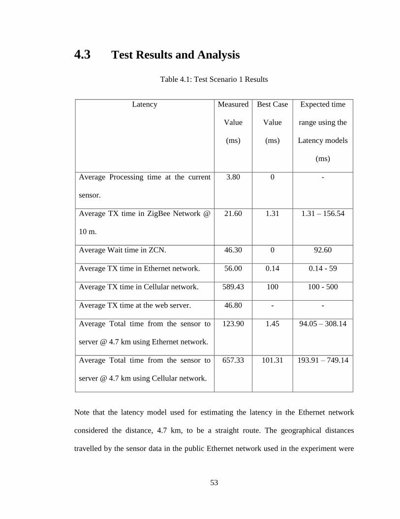
53
4.3 Test Results and Analysis
Table 4.1: Test Scenario 1 Results
Latency Measured
Value
(ms)
Best Case
Value
(ms)
Expected time
range using the
Latency models
(ms)
Average Processing time at the current
sensor.
3.80 0 -
Average TX time in ZigBee Network @
10 m.
21.60 1.31 1.31 – 156.54
Average Wait time in ZCN. 46.30 0 92.60
Average TX time in Ethernet network. 56.00 0.14 0.14 - 59
Average TX time in Cellular network. 589.43 100 100 - 500
Average TX time at the web server. 46.80 - -
Average Total time from the sensor to
server @ 4.7 km using Ethernet network.
123.90 1.45 94.05 – 308.14
Average Total time from the sensor to
server @ 4.7 km using Cellular network.
657.33 101.31 193.91 – 749.14
Note that the latency model used for estimating the latency in the Ethernet network
considered the distance, 4.7 km, to be a straight route. The geographical distances
travelled by the sensor data in the public Ethernet network used in the experiment were
54
not accounted in the latency model. These geographical distances may have marginal
impact on the transmission latency in the Ethernet network.
4.3.1 Processing Time in a ZigBee Sensor Application
All sensors used in this research have an Ember EM357 SoC chip which has a
32-bit ARM® Cortex-M3 processor operating at a clock speed up to 24 MHz. The
average processing time exhibited for the three different sensor applications developed
by the UNB team were found to be: current sensor 3.8 ms, temperature sensor 1.1 ms,
and vibration sensor 5.2 ms. These values meet expectations given typical
microprocessor overhead such as cluster initialization, data sampling, and data transfer.
The average delay for each sensor application was determined from the mean of 200
measured samples from each sensor. The variations in the processing time of the three
applications were a result of the application implementation. The current sensor required
both ADC processing and buffer sampling while the temperature sensor required only
the buffer sampling. The vibration measurement required coordinator axes cluster event,
and data sampling. In general, localized real-time management of micro-grid devices or
other devices using our sensors can be done if the processing time of the data in the
sensor node is less than the required operational time.
4.3.2 Transmission Latency in a ZigBee-based WSN
The transmission latency in the ZigBee network created by the ZCN was
investigated from Test Scenario 2 and Test Scenario 3. The calculated latency from the
latency estimation model in Chapter 3 was compared to measured latency from the test
scenarios. The message sent by the sensor node has a payload size of 12 bytes. From
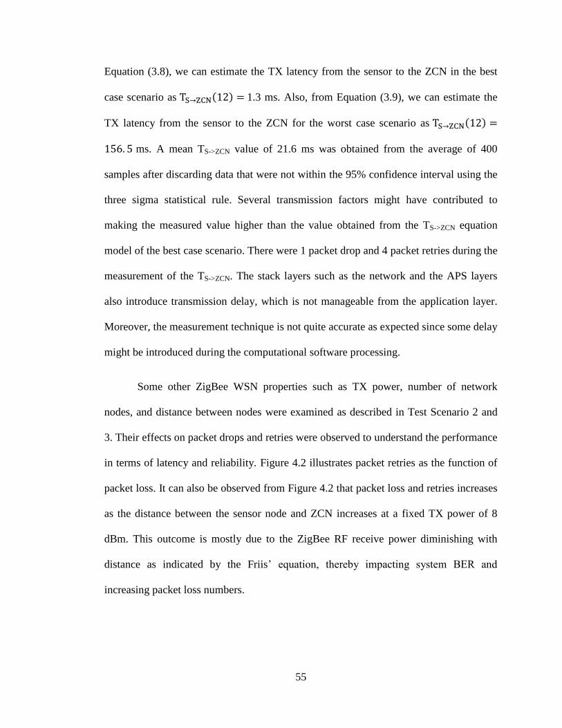
55
Equation (3.8), we can estimate the TX latency from the sensor to the ZCN in the best
case scenario as 1.3 ms. Also, from Equation (3.9), we can estimate the
TX latency from the sensor to the ZCN for the worst case scenario as
ms. A mean TS->ZCN value of 21.6 ms was obtained from the average of 400
samples after discarding data that were not within the 95% confidence interval using the
three sigma statistical rule. Several transmission factors might have contributed to
making the measured value higher than the value obtained from the TS->ZCN equation
model of the best case scenario. There were 1 packet drop and 4 packet retries during the
measurement of the TS->ZCN. The stack layers such as the network and the APS layers
also introduce transmission delay, which is not manageable from the application layer.
Moreover, the measurement technique is not quite accurate as expected since some delay
might be introduced during the computational software processing.
Some other ZigBee WSN properties such as TX power, number of network
nodes, and distance between nodes were examined as described in Test Scenario 2 and
3. Their effects on packet drops and retries were observed to understand the performance
in terms of latency and reliability. Figure 4.2 illustrates packet retries as the function of
packet loss. It can also be observed from Figure 4.2 that packet loss and retries increases
as the distance between the sensor node and ZCN increases at a fixed TX power of 8
dBm. This outcome is mostly due to the ZigBee RF receive power diminishing with
distance as indicated by the Friis‟ equation, thereby impacting system BER and
increasing packet loss numbers.
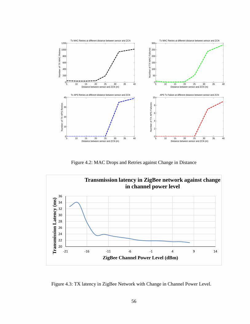
56
Figure 4.2: MAC Drops and Retries against Change in Distance
Figure 4.3: TX latency in ZigBee Network with Change in Channel Power Level.
5 10 15 20 25 30 35 400
200
400
600
800
1000
1200
Distance between sensor and ZCN (m)
Tx MAC Retries at different distance between sensor and ZCN
Num
ber
of T
X M
AC
Retr
ies
5 10 15 20 25 30 35 400
50
100
150
200
250
300
Distance between sensor and ZCN (m)
Tx MAC Retries at different distance between sensor and ZCN
Num
ber
of T
X M
AC
Failure
s
5 10 15 20 25 30 35 400
10
20
30
40
Distance between sensor and ZCN (m)
Tx APS Retries at different distance between sensor and ZCN
Num
ber
of T
X A
PS
Retr
ies
5 10 15 20 25 30 35 400
2
4
6
8
10
Distance between sensor and ZCN (m)
APS Tx Failure at different distance between sensor and ZCN
Num
ber
of T
X A
PS
Failure
s
20
22
24
26
28
30
32
34
36
-21 -16 -11 -6 -1 4 9 14Tra
nsm
issi
on
Late
ncy
(m
s)
ZigBee Channel Power Level (dBm)
Transmission latency in ZigBee network against change
in channel power level
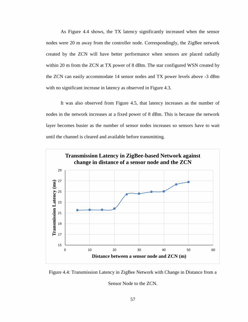
57
As Figure 4.4 shows, the TX latency significantly increased when the sensor
nodes were 20 m away from the controller node. Correspondingly, the ZigBee network
created by the ZCN will have better performance when sensors are placed radially
within 20 m from the ZCN at TX power of 8 dBm. The star configured WSN created by
the ZCN can easily accommodate 14 sensor nodes and TX power levels above -3 dBm
with no significant increase in latency as observed in Figure 4.3.
It was also observed from Figure 4.5, that latency increases as the number of
nodes in the network increases at a fixed power of 8 dBm. This is because the network
layer becomes busier as the number of sensor nodes increases so sensors have to wait
until the channel is cleared and available before transmitting.
Figure 4.4: Transmission Latency in ZigBee Network with Change in Distance from a
Sensor Node to the ZCN.
15
17
19
21
23
25
27
29
0 10 20 30 40 50 60
Tra
nsm
issi
on
Late
ncy
(m
s)
Distance between a sensor node and ZCN (m)
Transmission Latency in ZigBee-based Network against
change in distance of a sensor node and the ZCN
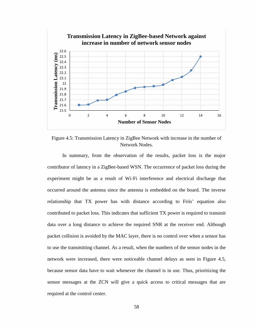
58
Figure 4.5: Transmission Latency in ZigBee Network with increase in the number of
Network Nodes.
In summary, from the observation of the results, packet loss is the major
contributor of latency in a ZigBee-based WSN. The occurrence of packet loss during the
experiment might be as a result of Wi-Fi interference and electrical discharge that
occurred around the antenna since the antenna is embedded on the board. The inverse
relationship that TX power has with distance according to Friis‟ equation also
contributed to packet loss. This indicates that sufficient TX power is required to transmit
data over a long distance to achieve the required SNR at the receiver end. Although
packet collision is avoided by the MAC layer, there is no control over when a sensor has
to use the transmitting channel. As a result, when the numbers of the sensor nodes in the
network were increased, there were noticeable channel delays as seen in Figure 4.5,
because sensor data have to wait whenever the channel is in use. Thus, prioritizing the
sensor messages at the ZCN will give a quick access to critical messages that are
required at the control center.
21.5
21.6
21.7
21.8
21.9
22
22.1
22.2
22.3
22.4
22.5
22.6
0 2 4 6 8 10 12 14 16
Tra
nsm
issi
on
Late
ncy
(m
s)
Number of Sensor Nodes
Transmission Latency in ZigBee-based Network against
increase in number of network sensor nodes
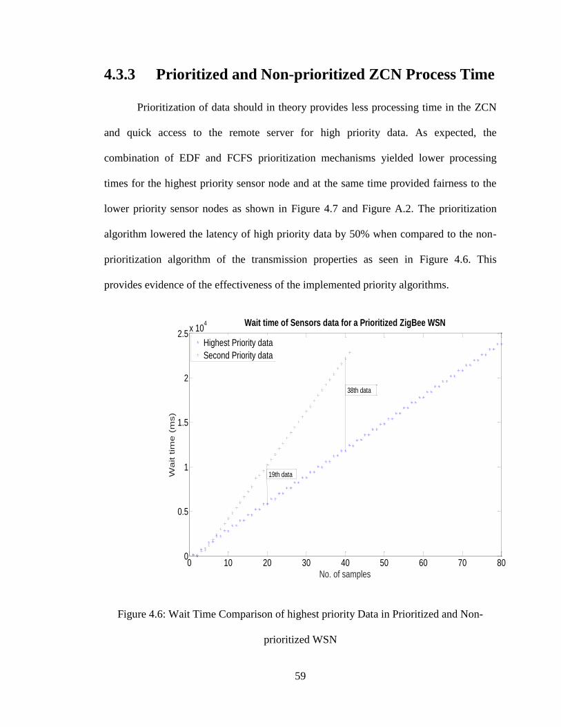
59
4.3.3 Prioritized and Non-prioritized ZCN Process Time
Prioritization of data should in theory provides less processing time in the ZCN
and quick access to the remote server for high priority data. As expected, the
combination of EDF and FCFS prioritization mechanisms yielded lower processing
times for the highest priority sensor node and at the same time provided fairness to the
lower priority sensor nodes as shown in Figure 4.7 and Figure A.2. The prioritization
algorithm lowered the latency of high priority data by 50% when compared to the non-
prioritization algorithm of the transmission properties as seen in Figure 4.6. This
provides evidence of the effectiveness of the implemented priority algorithms.
Figure 4.6: Wait Time Comparison of highest priority Data in Prioritized and Non-
prioritized WSN
0 10 20 30 40 50 60 70 800
0.5
1
1.5
2
2.5x 10
4
No. of samples
Wa
it t
ime
(m
s)
Wait time of Sensors data for a Prioritized ZigBee WSN
Highest Priority data
Second Priority data
38th data
19th data
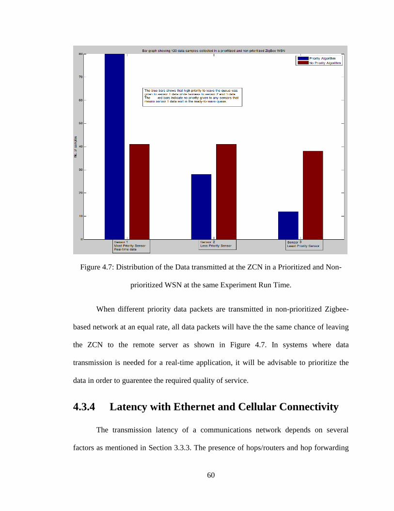
60
Figure 4.7: Distribution of the Data transmitted at the ZCN in a Prioritized and Non-
prioritized WSN at the same Experiment Run Time.
When different priority data packets are transmitted in non-prioritized Zigbee-
based network at an equal rate, all data packets will have the the same chance of leaving
the ZCN to the remote server as shown in Figure 4.7. In systems where data
transmission is needed for a real-time application, it will be advisable to prioritize the
data in order to guarentee the required quality of service.
4.3.4 Latency with Ethernet and Cellular Connectivity
The transmission latency of a communications network depends on several
factors as mentioned in Section 3.3.3. The presence of hops/routers and hop forwarding
r
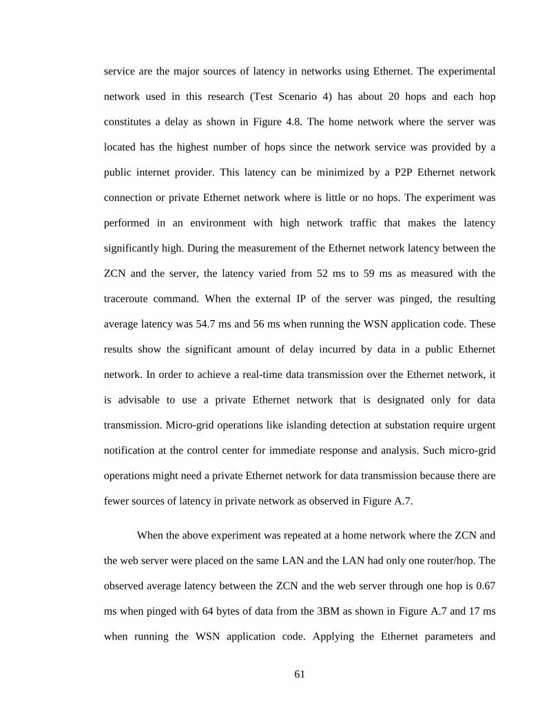
61
service are the major sources of latency in networks using Ethernet. The experimental
network used in this research (Test Scenario 4) has about 20 hops and each hop
constitutes a delay as shown in Figure 4.8. The home network where the server was
located has the highest number of hops since the network service was provided by a
public internet provider. This latency can be minimized by a P2P Ethernet network
connection or private Ethernet network where is little or no hops. The experiment was
performed in an environment with high network traffic that makes the latency
significantly high. During the measurement of the Ethernet network latency between the
ZCN and the server, the latency varied from 52 ms to 59 ms as measured with the
traceroute command. When the external IP of the server was pinged, the resulting
average latency was 54.7 ms and 56 ms when running the WSN application code. These
results show the significant amount of delay incurred by data in a public Ethernet
network. In order to achieve a real-time data transmission over the Ethernet network, it
is advisable to use a private Ethernet network that is designated only for data
transmission. Micro-grid operations like islanding detection at substation require urgent
notification at the control center for immediate response and analysis. Such micro-grid
operations might need a private Ethernet network for data transmission because there are
fewer sources of latency in private network as observed in Figure A.7.
When the above experiment was repeated at a home network where the ZCN and
the web server were placed on the same LAN and the LAN had only one router/hop. The
observed average latency between the ZCN and the web server through one hop is 0.67
ms when pinged with 64 bytes of data from the 3BM as shown in Figure A.7 and 17 ms
when running the WSN application code. Applying the Ethernet parameters and
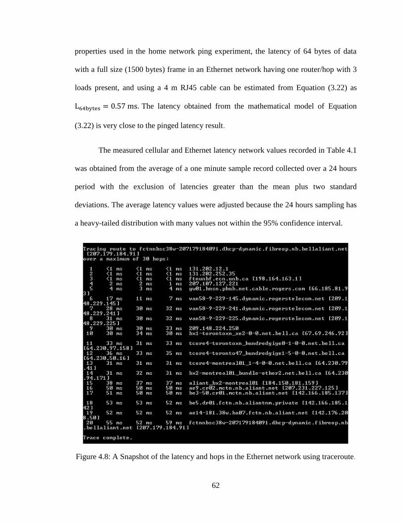
62
properties used in the home network ping experiment, the latency of 64 bytes of data
with a full size (1500 bytes) frame in an Ethernet network having one router/hop with 3
loads present, and using a 4 m RJ45 cable can be estimated from Equation (3.22) as
The latency obtained from the mathematical model of Equation
(3.22) is very close to the pinged latency result.
The measured cellular and Ethernet latency network values recorded in Table 4.1
was obtained from the average of a one minute sample record collected over a 24 hours
period with the exclusion of latencies greater than the mean plus two standard
deviations. The average latency values were adjusted because the 24 hours sampling has
a heavy-tailed distribution with many values not within the 95% confidence interval.
Figure 4.8: A Snapshot of the latency and hops in the Ethernet network using traceroute.
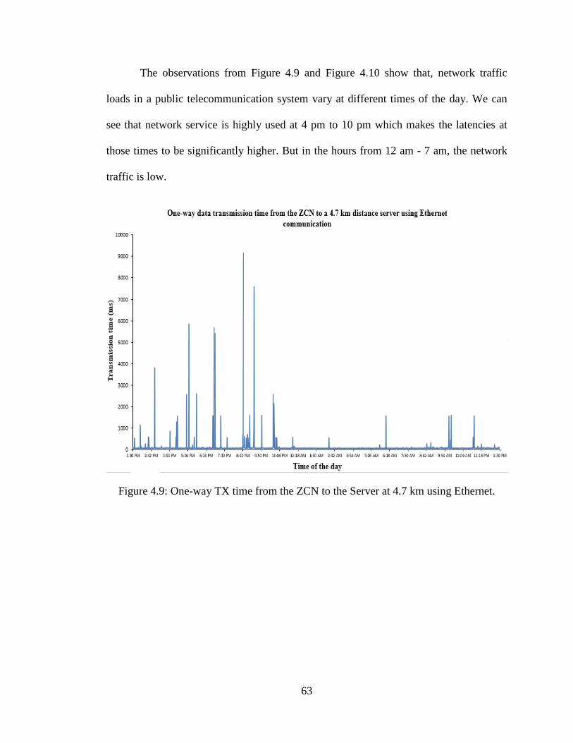
63
The observations from Figure 4.9 and Figure 4.10 show that, network traffic
loads in a public telecommunication system vary at different times of the day. We can
see that network service is highly used at 4 pm to 10 pm which makes the latencies at
those times to be significantly higher. But in the hours from 12 am - 7 am, the network
traffic is low.
Figure 4.9: One-way TX time from the ZCN to the Server at 4.7 km using Ethernet.
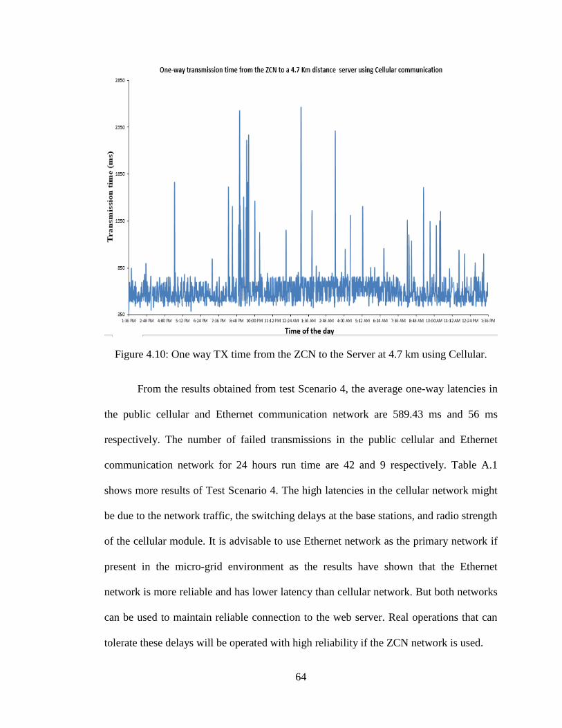
64
Figure 4.10: One way TX time from the ZCN to the Server at 4.7 km using Cellular.
From the results obtained from test Scenario 4, the average one-way latencies in
the public cellular and Ethernet communication network are 589.43 ms and 56 ms
respectively. The number of failed transmissions in the public cellular and Ethernet
communication network for 24 hours run time are 42 and 9 respectively. Table A.1
shows more results of Test Scenario 4. The high latencies in the cellular network might
be due to the network traffic, the switching delays at the base stations, and radio strength
of the cellular module. It is advisable to use Ethernet network as the primary network if
present in the micro-grid environment as the results have shown that the Ethernet
network is more reliable and has lower latency than cellular network. But both networks
can be used to maintain reliable connection to the web server. Real operations that can
tolerate these delays will be operated with high reliability if the ZCN network is used.
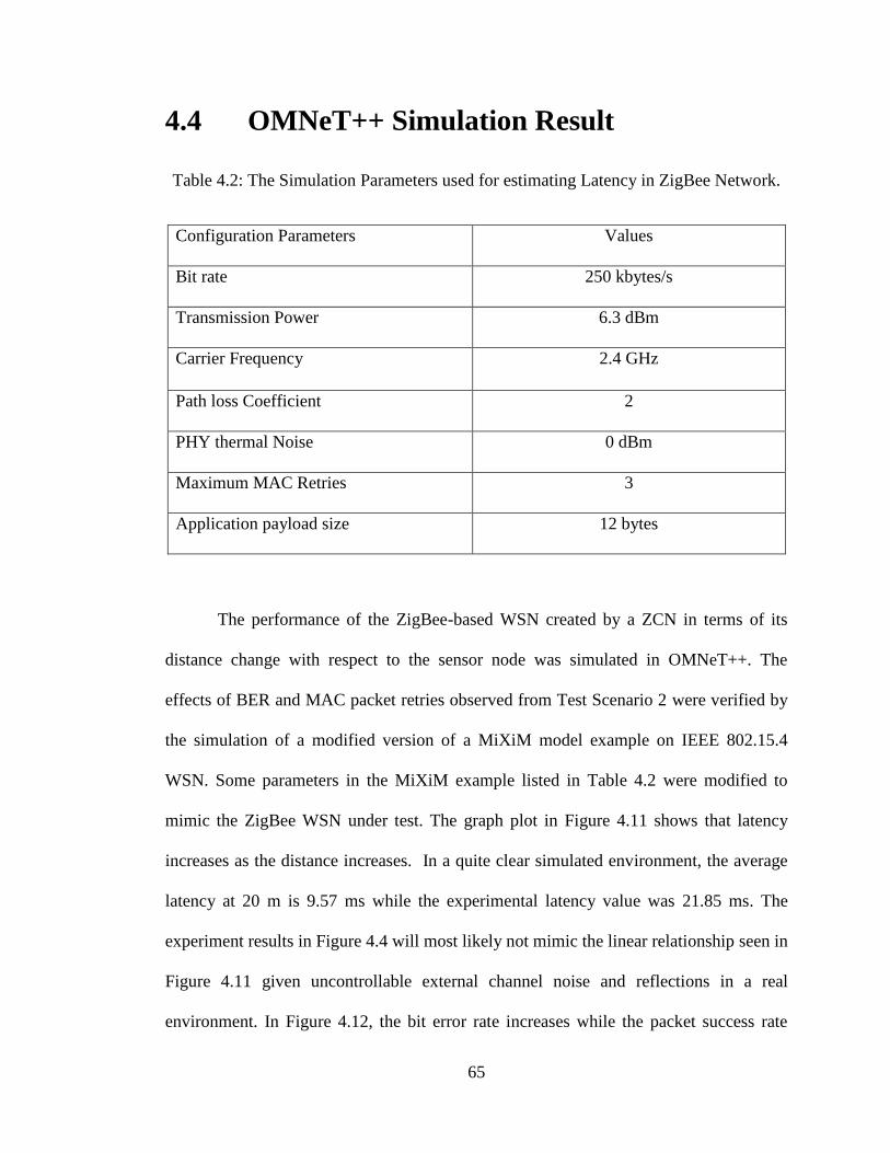
65
4.4 OMNeT++ Simulation Result
Table 4.2: The Simulation Parameters used for estimating Latency in ZigBee Network.
Configuration Parameters Values
Bit rate 250 kbytes/s
Transmission Power 6.3 dBm
Carrier Frequency 2.4 GHz
Path loss Coefficient 2
PHY thermal Noise 0 dBm
Maximum MAC Retries 3
Application payload size 12 bytes
The performance of the ZigBee-based WSN created by a ZCN in terms of its
distance change with respect to the sensor node was simulated in OMNeT++. The
effects of BER and MAC packet retries observed from Test Scenario 2 were verified by
the simulation of a modified version of a MiXiM model example on IEEE 802.15.4
WSN. Some parameters in the MiXiM example listed in Table 4.2 were modified to
mimic the ZigBee WSN under test. The graph plot in Figure 4.11 shows that latency
increases as the distance increases. In a quite clear simulated environment, the average
latency at 20 m is 9.57 ms while the experimental latency value was 21.85 ms. The
experiment results in Figure 4.4 will most likely not mimic the linear relationship seen in
Figure 4.11 given uncontrollable external channel noise and reflections in a real
environment. In Figure 4.12, the bit error rate increases while the packet success rate
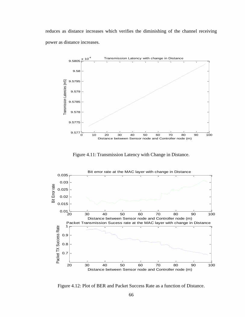
66
reduces as distance increases which verifies the diminishing of the channel receiving
power as distance increases.
Figure 4.11: Transmission Latency with Change in Distance.
Figure 4.12: Plot of BER and Packet Success Rate as a function of Distance.
0 10 20 30 40 50 60 70 80 90 1009.577
9.5775
9.578
9.5785
9.579
9.5795
9.58
9.5805x 10
-4
Distance between Sensor node and Controller node (m)
Transmission Latency with change in Distance
Tran
smis
sion
Lat
enci
es (m
S)
20 30 40 50 60 70 80 90 1000.01
0.015
0.02
0.025
0.03
0.035
Distance between Sensor node and Controller node (m)
Bit error rate at the MAC layer with change in Distance
Bit
Err
or r
ate
20 30 40 50 60 70 80 90 100
0.7
0.8
0.9
1
Distance between Sensor node and Controller node (m)
Packet Transmission Sucess rate at the MAC layer with change in Distance
Pac
ket
TX
Suc
cess
Rat
e
67
In summary, the results obtained from Test Scenario 2 and the simulated WSN
verified packet loss as a product of environmental conditions and diminishing of the
receiving power of the ZCN with distance. Considering the TX latency at the different
points of data transmission from the sensor nodes to the webserver, it is advisable that
fast response actuation of something like a line protection circuit should be done locally
at the sensor nodes.
68
Chapter 5
Conclusion and Future Work
This thesis evaluated the performance of a WAN capable ZigBee WSN for
possible real-time applications to monitor and control devices in micro-grid power
systems. The main goal was the design and development of a novel ZCN with Ethernet
and cellular communication capabilities providing the necessary WAN requirement.
Performance evaluations were based on metrics (outlined in Section 2.3) experimentally
obtained from various test scenarios highlighted in Chapter 4. Recommended future
work is outlined in Section 5.2 and focuses on optimizing the performance of the ZCN
and actual field deployments of the WAN ZigBee WSN.
5.1 Conclusion
A prioritized ZCN was designed and developed to improve the WAN coverage
of ZigBee and reduce delays in transmission of high priority data. The main goal was to
develop a real-time capable WSN monitoring system for micro-grid applications. In
priority mode, the ZCN can transmit data over a distance of 4.7 km with an average
69
latency of 56 ms and 589 ms when a busy public Ethernet and cellular network are used,
respectively (see Table 4.1). With telemetry processing and transmit intervals shorter in
duration than these time frames, real-time applications are possible. The implementation
of a priority mode algorithm shows higher priority data having shorter TX latencies and
thus will yield tighter tolerances for real-time applications. Correspondingly, a ZigBee
WSN using the prioritized mode ZCN can be targeted for faster real-time micro-grid
applications such as device protection and fault detection, as well as the collection of
slower telemetric data such as those related to environmental conditions.
It was also verified that packet drops and retries due to low TX (channel) power
and environmental conditions have an effect on transmission latency for the ZigBee
WSN. In Section 4.3.2, we observed that an increase in channel power lowers the packet
drops and retries which led to a reduction in the overall transmission latency. We also
observed the rate of packet losses and retries as a function of TX distance also impacted
transmission latency. Simulation results confirmed the effects that TX distance and
environmental conditions have on transmission latency for a ZigBee WSN.
Experimentally, Figure 4.4 and Figure 4.11, show that increases in distance between the
sensor nodes and the ZCN reduces the receive power, and hence expectedly results a
high packet losses and retries due to an unsuccessful packet reception by the ZCN. The
mathematical model to determine the TX latency for a WAN ZigBee WSN under
different scenarios was developed in Chapter 3. Also in this chapter, the measured TX
latency from the ZCN was compared to latency given by the mathematical model in the
best case scenario. Results compared favorably within the worst case bounds predicted.
70
5.2 Future Work
Some future work should focus on improving the performance and reliability of the
ZCN. The recommended improvements are as follows:
The cellular hardware used in this thesis has a GSM service that operated on a 3G
network. Improving the network service to LTE network will impact the latency
results. LTE has faster data speed than 3G, hence the latency of the cellular network
will significantly reduce if LTE network service is used. The SM5100B cellular
hardware requires a peak current up to 2 A during data transmission which is quite
high for a portable lithium battery to supply. Therefore, a power supply was
provided from a 1.6 A 5 VDC adapter connected to an AC main socket. Although
not quite meeting the peak current requirements, this adapter was used because it
was in surplus and deemed acceptable for prototype development. Replacing the
cellular hardware with a low current cellular transceiver will improve the reliability
of the ZCN and also make long term battery operation viable.
Basic OMNET++ simulation metrics were obtained from the examples in the
software package and were modified to observe the performance metrics of an actual
ZigBee WSN. Adding more frameworks to OMNET++ and further exploring the
capabilities of OMNET++ would help in the development of more realistic WAN
network models that use ZigBee technology.
The more ubiquitous presence of RF disturbance and field transients in micro-grid
substations will likely have a greater impact on the ZigBee WSN performance. This
needs to be assessed using an actual deployment of the WAN ZigBee WSN
developed in this research.
71
Bibliography
[1] S. Ghildiya, A. K. Mishra, and N. Garg, “An Overview of Wireless Sensor
Networks Using ZigBee Technology,” International Journal of Advanced
Research in Computer Science and Software Engineering, vol. 4, issue 2, pp. 114
– 116, February 2014.
[2] S. Basha and K. Krisha, “The Design of network Coordinator between ZigBee and
GPRS for Remote Monitoring Applications,” International Journal of
Engineering Science and Technology, vol. 3, No. 4, pp. 628- 632, August 2013.
[3] P. Zhang, F. Li, and N. Bhatt, “Next-Generation Monitoring, Analysis and Control
for the Future Smart Control Center,” IEEE Transactions on Smart Grid, vol. 1,
No. 2, pp. 186 – 192, Septmeber 2010.
[4] T. Zwavashe and R. Duri, “Integrating GSM and ZigBee Wireless Networks for
Smart A2 farming Enterprise in Zimbabwe,” International Journal of Science and
Research (IJSR), vol. 3, issue 6, pp. 75 – 80, June 2014.
[5] Z. Alliance, “Zigbee specification,” January 2008. Available online:
https://www.silabs.com/Support%20Documents/TechnicalDocs/EM35x.pdf, 2015.
[6] Silicon Labs, “Ember Application Development Fundamentals: ZigBee,”
http://www.silabs.com/Support%20Documents/TechnicalDocs/UG103.2.pdf
{accessed on January 2015}
72
[7] Z.Y. Guan, “A Reliability Evaluation of Wireless Sensor Network Simulator:
Simulation vs. Testbed,” M.Sc. Thesis, UNITEC New Zealand, 2011.
[8] W. Stalling, Wireless Communication and Networks 4th Edition. Pearson
Publication Limited, 2004, pp. 39-118.
[9] J. Byun, I. Hong, and S. Park, “Design and Implementation of a Smart Home
Energy Management System with Hybrid Sensor Network in Smart Grid
Environments,” The Eight International Conference on Wireless and Mobile
Communications. 2012, pp 159 – 165.
[10] D. Kong, T. Li, X. You, X. Sun, B. Wang, and Q. Liu, “The Research of Long-
Distance Data Transmission Based on Meterological Sensor Network,”
International Journal of Future Generation Communication and Networking,
vol.7, issue No.1, (2014), pp 59 – 70.
[11] A. Shaikh and S. Pathan, “Reasearch on Wireless Sensor Network Technology,”
International of Information and Education Technology, vol. 2, No. 5, pp. 476 –
479, October 2012.
[12] M.J. Yang, F. Zhuo, X.W. Wang, H.P. Guo,Y.J. Zhou, “Research of Seamless
Transfer Control Strategy of Microgrid System,” Power Electronics and ECCE
Asia (ICPE & ECCE), 2011 IEEE 8th International Conference. pp. 2059‐2066,
June 2011.
[13] A.S.K. Pathan, L. Hyunh‐Woo and H. Choong‐Seon, “Security in wireless sensor
networks: issues and challenges,” Advanced Communication Technology, 2006.
ICACT 2006. The 8th International Conference, vol. 2, p. 6, February 2006.
73
[14] A. Usman and S. H. Shami, “Evolution of Communication Technologies for Smart
Grid applications,” Renewable and Sustainable Energy Reviews, vol. 19, pp. 191–
199, Mar. 2013.
[15] IEEE 802. 15. 4, Wireless Medium Access Control (MAC), and Physical Layer
(PHY), “Specifications for Low-Rate Wireless Personal Area Networks (LR-
WPANs),” IEEE, New York, NY, USA, 2006.
[16] J.S. Lee and Y.C. Huang, “ITRI ZBnode: a ZigBee/IEEE 802.15.4 platform for
wireless sensor networks,” in Proceedings of the IEEE International Conference
on Systems, Man and Cybernetics, pp. 1462–1467, Taipei, Taiwan, October 2006.
[17] B. Meenakshi and P. Anandhakumar, “Cluster Based Time Division Multiple
Access Scheduling Scheme for ZigBee Wireless Sensor Network,” Journal of
Computer Science 2012, pp. 1979 – 1986, vol. 8(12), 2012.
[18] M. Petrova, J. Riihijärvi, P. Mähönen, and S. Labella, “Performance study of IEEE
802.15.4 using measurements and simulations,” in Proceedings of the IEEE
Wireless Communications and Networking Conference, pp. 487–492, Las Vegas,
Nev., USA, April 2006.
[19] F. Chen, N. Wang, R. German, and F. Dressler, “Simulation study of IEEE
802.15.4 LR-WPAN for industrial applications,” Wireless Communications and
Mobile Computing, vol. 10, no. 5, pp. 609–621, 2010.
[20] K. Shuaib, M. Alnuaimi, M. Boulmaif, I. Jawhar, F. Sallabi, and A. lakas,
“Performance Evaluation of IEEE 802.15.4: Experimental and Simulation
Results,” Journal of Communications, pp. 29 – 37, Vol. 2, No. 4, June 2007.
[21] M. Laner, P. Svoboda, and M. Rupp, “Latency Analysis of 3G Network
Components” European Wireless 2012, April 18-20, 2012, Poznan, Poland.
74
[22] W.L. Tan, F. Lam, and W.C. Lau, “An Empirical Study on the capacity and
performance of 3G Networks,” IEEE transactions on Mobile Computing, pp. 737
– 750, Vol. 7, No. 6, June 2008.
[23] T. Blajić and D. Nogulić, and Mružijanić, “Latency Improvements in 3G Long
Term Evolution,” Mobile Solutions, Ericsson Nikola Tesla d.d., Zagreb Croatia.
[24] M. Laner, P. Svoboda, P.R. Maierhofer, N. Nikaein, F. Ricciato, and M. Rupp, “A
comparison Between One-way Delays in Operating HSPA and LTE Networks,”
8th International Workshop on Wireless Network Measurements, 14-18 May 2012.
pp. 286 - 292
[25] Grigorik, L. (2013). Mobile Network. In L. Grigorik (Ed.), “High Performance
Browser Networking” [E-reader Version], Published by O‟Reilly Media.
Retrieved from http://chimera.labs.oreilly.com/books/1230000000545/ch08.html.
[26] Siemens, “Application note 8: Latency on a Switched Ethernet Network” accessed
on 15 October, 2015 at https://w3.siemens.com/mcms/industrial-
communication/en/rugged-communication/Documents/AN8.pdf.
[27] SparkFun, “SM5100B-D AT Command,” Accessed on September, 2014 at
https://www.sparkfun.com/datasheets/CellularShield/SM5100B%20AT%20Comm
and%20Set.pdf.
[28] SparkFun, “Using AT commands to control TCP/IP stack on SM5100B-D
modules,” https://www.sparkfun.com/datasheets/Cellular%20Modules/CEL-
09533-TCPIP-APPNOTES-V1.1.pdf {accessed on September, 2014}
[29] Official 3BM Wiki. http://elinux.org/Beagleboard:BeagleBoneBlack {accessed on
August, 2014}
75
[30] A. Varga and R. Hornig, “An overview of the OMNeT++ simulation
environment” in Proceedings of the 1st International Conference on Simulation
Tools and techniques for Communications, Networks and Systems & Workshops,
Article No. 60, ICST Brussels, Belgium 2008.
[31] OMNeT++ Home Page. http://www.omnetpp.org {accessed on April, 2015}
[32] MiXiM home page. http://sourceforge.net/projects/mixim/ {accessed on April,
2015}
[33] A. Kopke, M. Swigulski, K. Wessel, D. Willkomm, P.T.K. Haneveld, T.E.V.
Parker, O.W. Visser, H.S. Lichte, and S. Valentin,Simulating “Wireless and
Mobile Networks in OMNeT++, The MiXiM Vision,” OMNeT++ Workshop ‟08
Marseille, France 2008.
[34] X. Xian, W. Shi, and H. Huang, “Comparison of OMNeT++ and other simulator
for wsn simulation,” in Industrial Electronics and Applications, 2008. ICIEA
2008. 3rd IEEE Conference, pp. 1439–1443.
[35] H.R. Shaukat and F. Hashim, “MWSN Modeling Using OMNeT++ Simulator,”
2014 Fifth International Conference on Intelligent Systems, Modelling and
Simulation, pp. 597 – 602.
[36] H. Ahmed and M. Khurram, “Performance Analysis of MAC layer Protocols in
Wireless Sensor Network,” I.J. Information Engineering and Electronic Business,
pp. 44 – 52, No. 5, 2014.
[37] Z. Azmi, K. Abu Bakar, A. Abdullah, M. Shamsir, W. Manan, “Performance
Comparison of Priority Rule Scheduling Algorithms Using Different Inter Arrival
Time Jobs in Grid Environment,” International Journal of Grid and Distributed
Computing, Vol. 4, No. 3, 2011.
76
[38] E. Acha, V.G. Agelidis, O. Anaya, T. J. E. Miller, Power Electronics Control in
Electrical Systems: (1st Ed.). Oxford, UK: Newnes Power Engineering Series,
2002, pp. 31-81 online.
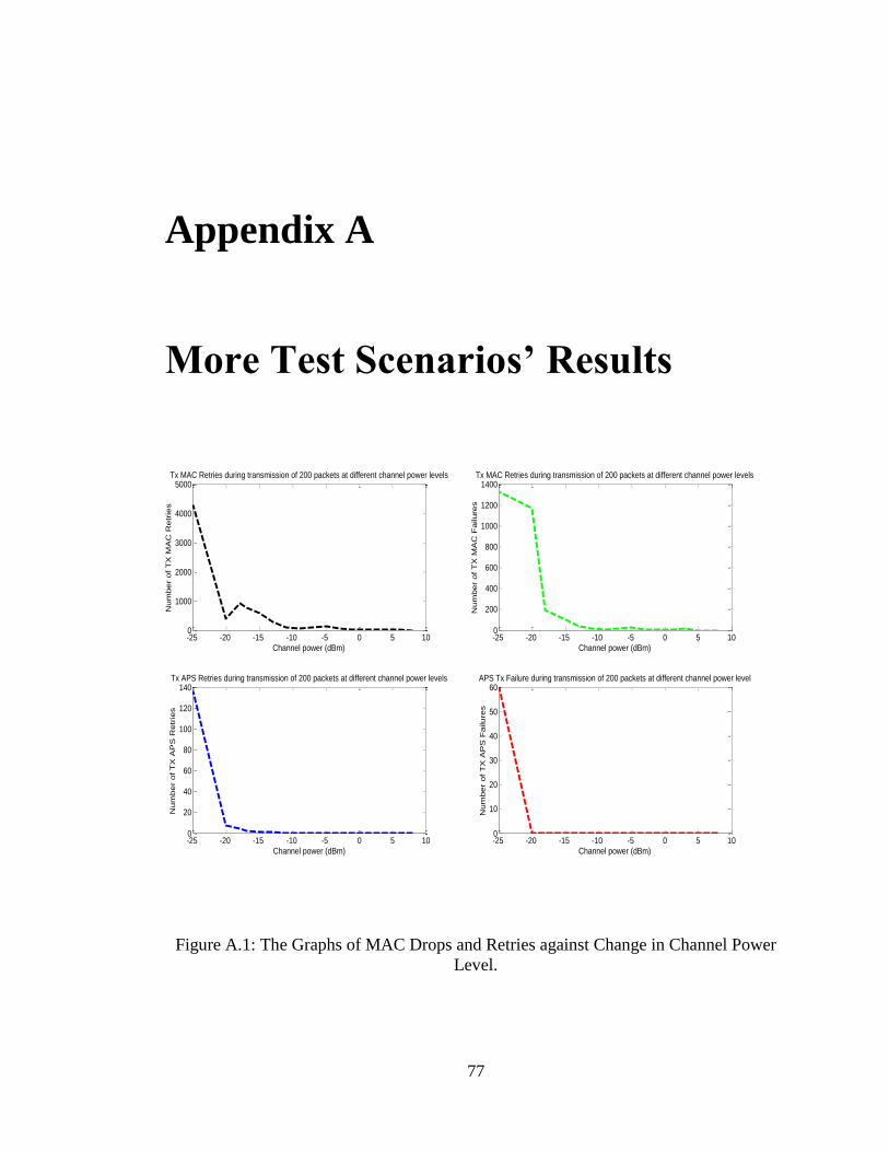
77
Appendix A
More Test Scenarios’ Results
Figure A.1: The Graphs of MAC Drops and Retries against Change in Channel Power
Level.
-25 -20 -15 -10 -5 0 5 100
1000
2000
3000
4000
5000
Channel power (dBm)
Tx MAC Retries during transmission of 200 packets at different channel power levels
Num
ber
of T
X M
AC
Retr
ies
-25 -20 -15 -10 -5 0 5 100
200
400
600
800
1000
1200
1400
Channel power (dBm)
Tx MAC Retries during transmission of 200 packets at different channel power levelsN
um
ber
of T
X M
AC
Failure
s
-25 -20 -15 -10 -5 0 5 100
20
40
60
80
100
120
140
Channel power (dBm)
Tx APS Retries during transmission of 200 packets at different channel power levels
Num
ber
of T
X A
PS
Retr
ies
-25 -20 -15 -10 -5 0 5 100
10
20
30
40
50
60
Channel power (dBm)
APS Tx Failure during transmission of 200 packets at different channel power level
Num
ber
of T
X A
PS
Failure
s
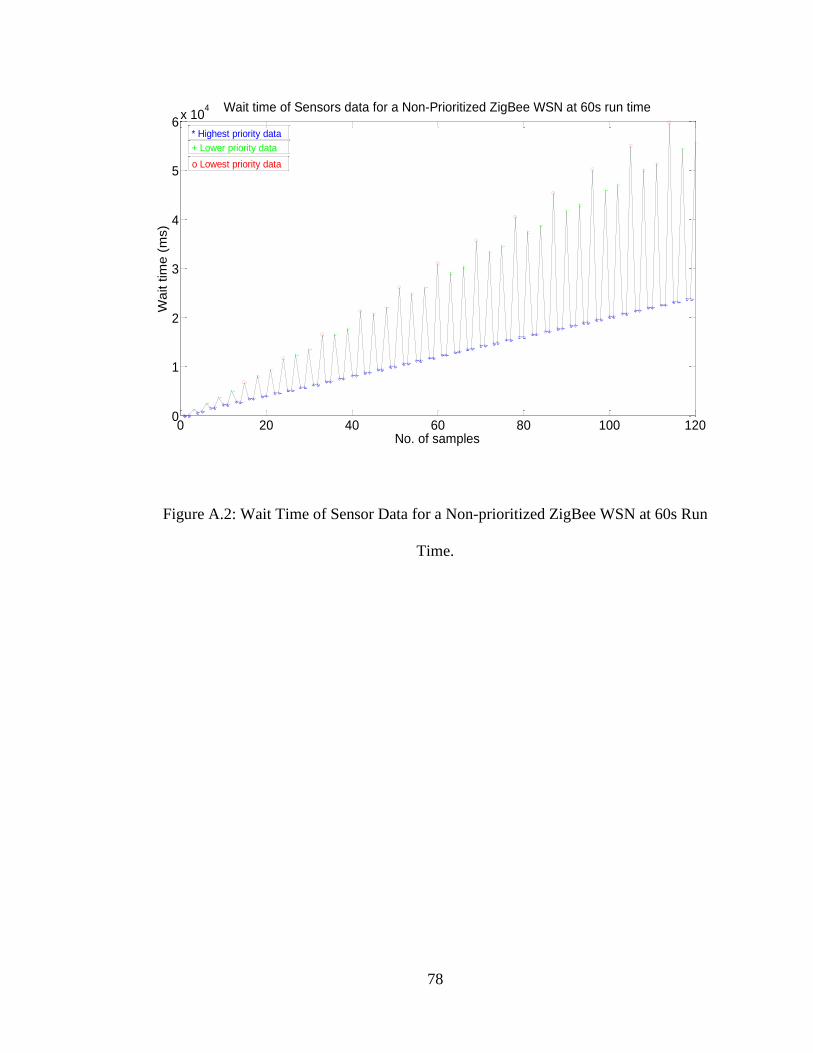
78
Figure A.2: Wait Time of Sensor Data for a Non-prioritized ZigBee WSN at 60s Run
Time.
0 20 40 60 80 100 1200
1
2
3
4
5
6x 10
4
No. of samples
Wa
it t
ime
(m
s)
Wait time of Sensors data for a Non-Prioritized ZigBee WSN at 60s run time
+ Lower priority data
o Lowest priority data
* Highest priority data
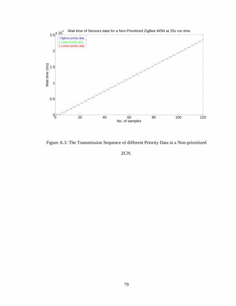
79
Figure A.3: The Transmission Sequence of different Priority Data in a Non-prioritized
ZCN.
0 20 40 60 80 100 1200
0.5
1
1.5
2
2.5x 10
4
No. of samples
Wait time of Sensors data for a Non-Prioritized ZigBee WSN at 25s run time
Wa
it t
ime
(m
s)
* Highest priority data
+ Lower priority data
o Lowest priority data
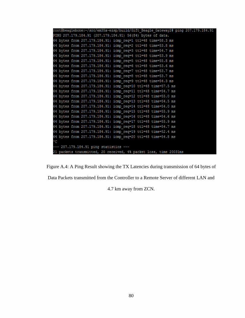
80
Figure A.4: A Ping Result showing the TX Latencies during transmission of 64 bytes of
Data Packets transmitted from the Controller to a Remote Server of different LAN and
4.7 km away from ZCN.
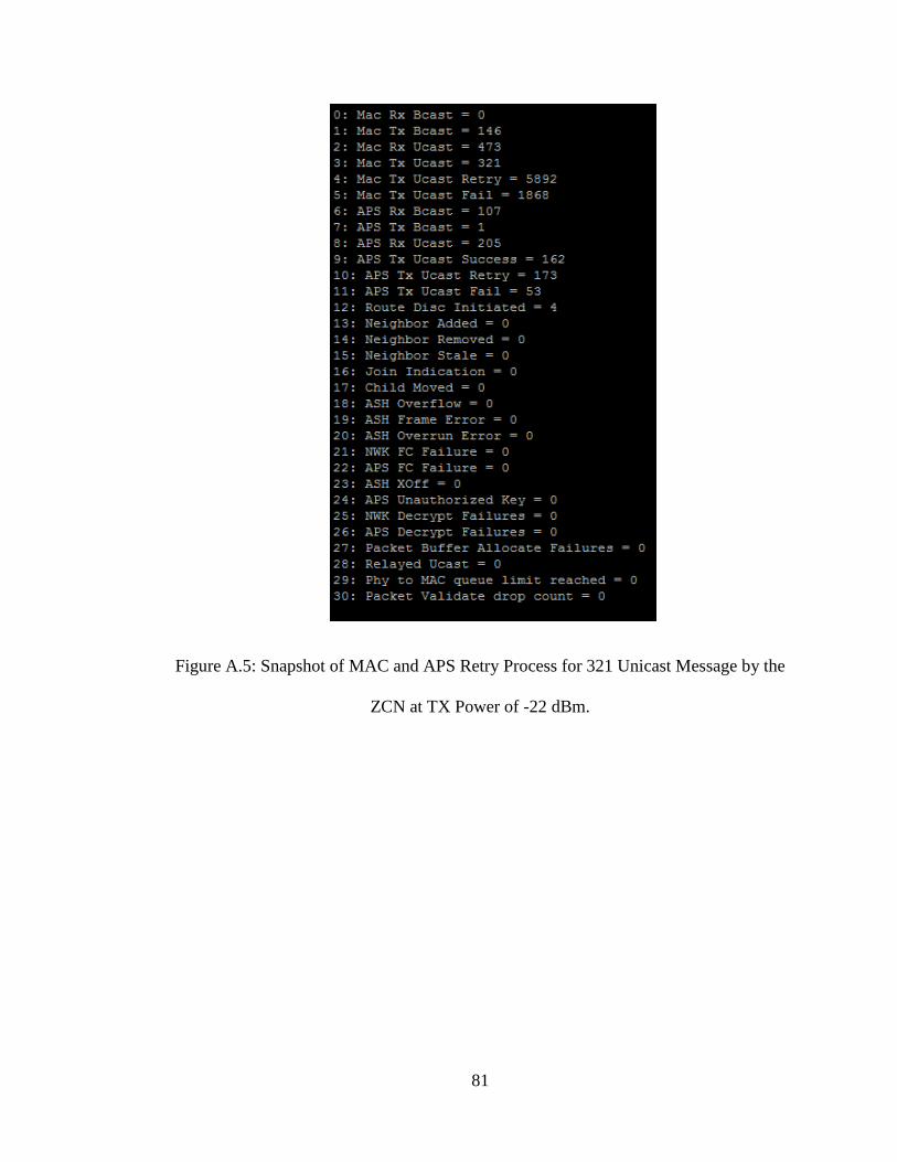
81
Figure A.5: Snapshot of MAC and APS Retry Process for 321 Unicast Message by the
ZCN at TX Power of -22 dBm.
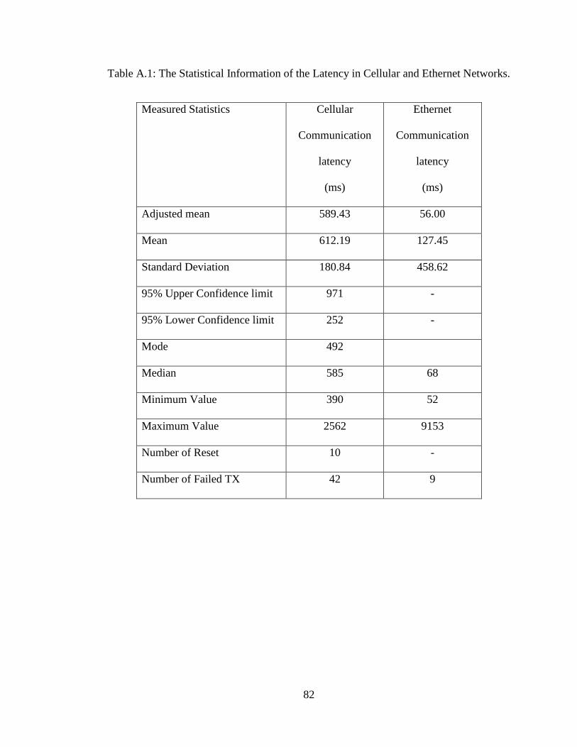
82
Table A.1: The Statistical Information of the Latency in Cellular and Ethernet Networks.
Measured Statistics Cellular
Communication
latency
(ms)
Ethernet
Communication
latency
(ms)
Adjusted mean 589.43 56.00
Mean 612.19 127.45
Standard Deviation 180.84 458.62
95% Upper Confidence limit 971 -
95% Lower Confidence limit 252 -
Mode 492
Median 585 68
Minimum Value 390 52
Maximum Value 2562 9153
Number of Reset 10 -
Number of Failed TX 42 9
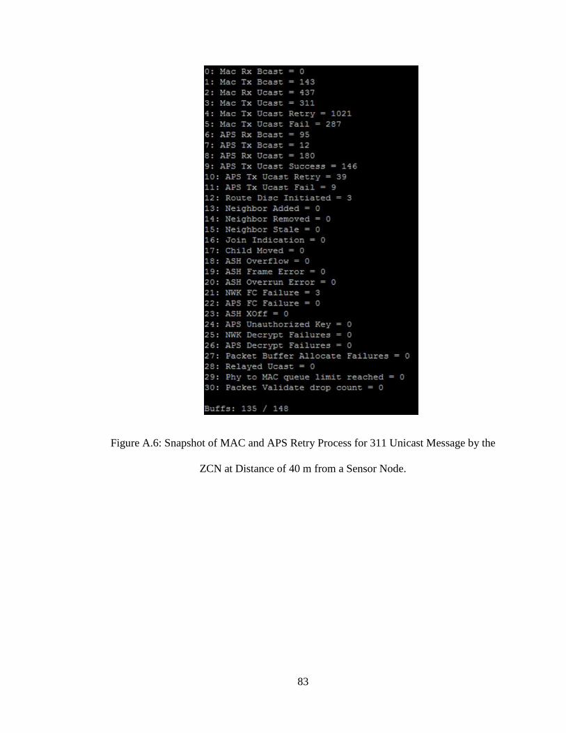
83
Figure A.6: Snapshot of MAC and APS Retry Process for 311 Unicast Message by the
ZCN at Distance of 40 m from a Sensor Node.
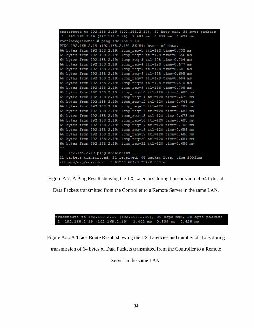
84
Figure A.7: A Ping Result showing the TX Latencies during transmission of 64 bytes of
Data Packets transmitted from the Controller to a Remote Server in the same LAN.
Figure A.8: A Trace Route Result showing the TX Latencies and number of Hops during
transmission of 64 bytes of Data Packets transmitted from the Controller to a Remote
Server in the same LAN.
85
Appendix B
The PCB Design of the UNB
ZigBee Coordinator Node and
Cellular Module Configurations
B.1 PCB Design of the ZigBee Coordinator
Hardware
The Printed Circuit Board (PCB) of the UNB ZigBee coordinator hardware was
designed in Altium designer software. Altium designer software is a computer design
platform for building, verifying, and validating a PCB design. It has an easy user
interface and synchronizes the PCB board with its schematic diagram. The first
procedure of designing the coordinator hardware PCB in Altium software was to draw
the schematic diagram of the coordinator circuit. The schematic circuit diagram of the
ZigBee coordinator hardware was divided into three sections which are the power
supply circuit, the ZigBee module circuit, and the UART serial connector circuit.
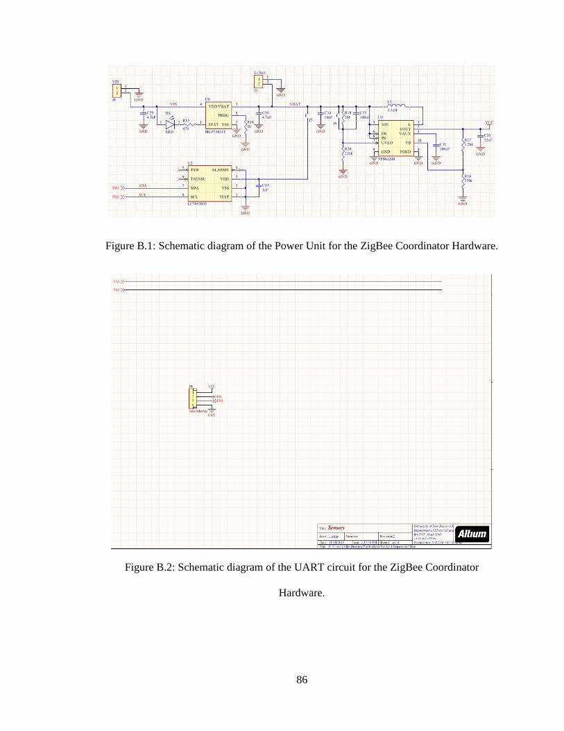
86
Figure B.1: Schematic diagram of the Power Unit for the ZigBee Coordinator Hardware.
Figure B.2: Schematic diagram of the UART circuit for the ZigBee Coordinator
Hardware.
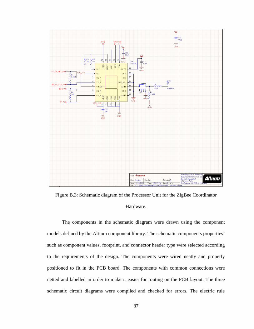
87
Figure B.3: Schematic diagram of the Processor Unit for the ZigBee Coordinator
Hardware.
The components in the schematic diagram were drawn using the component
models defined by the Altium component library. The schematic components properties‟
such as component values, footprint, and connector header type were selected according
to the requirements of the design. The components were wired neatly and properly
positioned to fit in the PCB board. The components with common connections were
netted and labelled in order to make it easier for routing on the PCB layout. The three
schematic circuit diagrams were compiled and checked for errors. The electric rule
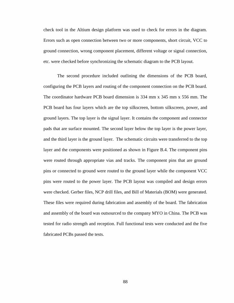
88
check tool in the Altium design platform was used to check for errors in the diagram.
Errors such as open connection between two or more components, short circuit, VCC to
ground connection, wrong component placement, different voltage or signal connection,
etc. were checked before synchronizing the schematic diagram to the PCB layout.
The second procedure included outlining the dimensions of the PCB board,
configuring the PCB layers and routing of the component connection on the PCB board.
The coordinator hardware PCB board dimension is 334 mm x 345 mm x 556 mm. The
PCB board has four layers which are the top silkscreen, bottom silkscreen, power, and
ground layers. The top layer is the signal layer. It contains the component and connector
pads that are surface mounted. The second layer below the top layer is the power layer,
and the third layer is the ground layer. The schematic circuits were transferred to the top
layer and the components were positioned as shown in Figure B.4. The component pins
were routed through appropriate vias and tracks. The component pins that are ground
pins or connected to ground were routed to the ground layer while the component VCC
pins were routed to the power layer. The PCB layout was compiled and design errors
were checked. Gerber files, NCP drill files, and Bill of Materials (BOM) were generated.
These files were required during fabrication and assembly of the board. The fabrication
and assembly of the board was outsourced to the company MYO in China. The PCB was
tested for radio strength and reception. Full functional tests were conducted and the five
fabricated PCBs passed the tests.
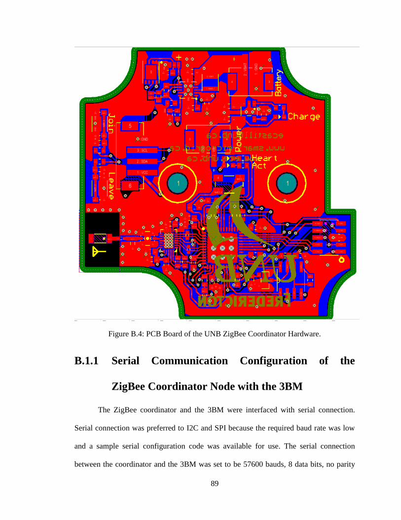
89
Figure B.4: PCB Board of the UNB ZigBee Coordinator Hardware.
B.1.1 Serial Communication Configuration of the
ZigBee Coordinator Node with the 3BM
The ZigBee coordinator and the 3BM were interfaced with serial connection.
Serial connection was preferred to I2C and SPI because the required baud rate was low
and a sample serial configuration code was available for use. The serial connection
between the coordinator and the 3BM was set to be 57600 bauds, 8 data bits, no parity
90
bit, and 1 stop bit. The serial configuration firmware has to be uploaded once before
uploading any application in the ZCN.
B.2 SM5100B Cellular Module Configuration
for TCP/IP Connection
The following steps were performed in order to set-up the SM5100B cellular device
for TCP/IP connection:
1. An active SIM card with no pin lock was inserted into the SIM card slot on the
cellular module.
2. The TX0 pin on the module was connected to the RX pin of the 3BM UART2.
3. The RX0 pin on the module was connected to the TX pin of the 3BM UART2.
4. The GND pin on the module was connected to the GND (TP8 pin) of the 3BM.
5. The ZCN was powered on and the ZCN application code was run using a Putty
terminal window.
6. During the initialization process of the cellular module, the following was displayed
which indicated correct and complete module setup for GPRS configuration.
+SIND: 1
+SIND: 10,”SM”,1,”FD”,1,”LD”,1,”MC”,1,”RC”,1,”ME”,1
+SIND: 11
+SIND: 3
91
+SIND: 4
+SIND: 1 means the SIM card has been inserted properly.
+SIND: 10, line shows the status of the SIM card, all ones mean the SIM card is
ready.
+SIND: 11 means the module has registered with the cellular network.
+SIND: 3 means the module is partially ready to communicate.
+SIND: 4 means the module is registered on the network, and ready to communicate.
If a value different from the above statements appears on the screen, then the module is
not ready to be configured for GPRS service.
B.2.1 GPRS Configuration
The GPRS configuration for TCP/IP connection was performed during the
initialization of the cellular module in the running ZCN application code. The following
AT commands were used to configure the GPRS data service of the cellular module.
//Attach GPRS data service
AT+CGATT =1
//set up PDP context using APN - access point name, internet.com is Rogers APN.
AT+CGDCONT=1,"IP","internet.com"
// The user and password for the rogers GPRS APN.
AT+CGPCO=0,”wap”,”wap1”, 1
// Activate PDP context
92
AT+CGACT=1,1
// Configure TCP connection to the remote web server.
AT+SDATACONF=1,"TCP","www.giftoplazer.ddns.net",8080
AT+SDATASTART=1,1
// Start TCP connection,
//check socket status – SOCKSTATUS: 1,1,102,0,0 means connected.
AT+SDATASTATUS=1
// The below command is used to send data to the web server, if module responds with
// "+STCPD:1" that means data transmission is successful. Data are sent to the server by
// including the data information in the URL address of the webserver.
AT+SSTRSEND=1,”GET / HTTP/1.0”
// Information received from the cellular can be read using the below command:
AT+SDATAREAD=1
//The TCP connection with the command below:
AT+SDATASTART=1,0
93
Appendix C
Relevant Source Codes
C.1 OMNeT++ Simulation Code
// This code is implemented in MiXiM. The code is a modified version of a MiXiM
// example that illustrates the use of the IEEE 802.15.4A UWB-IR simulation model
// provided by the National Competence Center in Research on Mobile Information and
// Communication Systems NCCR-MICS, a center supported by the Swiss National
// Science Foundation under grant number 5005-67322.
// This code was modified by Gift Owhuo on September 24, 2015 to measure the
// latencies, BER and Packet success rate of an IEEE 802.15.4 (ZigBee) WSN.
// Disclaimer: The author of this thesis is not liable for damage that might occur from
// the use of this code.
# declaring the network configuration parameters.
[General]
network = ieee802154a # Using an ieee 802.15.4 standard for the WSN
94
# Enable the WSN events recording
record-eventlog = true
# Define network metrics as vector quantities and disable scalar form.
**.scalar-recording = false
**.vector-recording = true
# Include the path for the module functions and images.
num-rngs = 88
tkenv-image-path = ../../images;
cmdenv-express-mode = true
# Because of the battery module, there are always scheduled events
# thus we need a fallback sim-time-limit.
# Otherwise the battery module will eventually lead to a simtime_t overflow
sim-time-limit= 60 s # 60s for 20000 packets
ieee802154a.**.coreDebug = false # Disable debug functions to minimize processing delay.
# The Area of the ieee 802.15. 4 WSN coverage.
ieee802154a.playgroundSizeX = 200 m
ieee802154a.playgroundSizeY = 200 m
ieee802154a.playgroundSizeZ = 200 m
ieee802154a.world.useTorus = false
# Network configurations of the WSN.
ieee802154a.node[*].nic.connectionManagerName = "connectionManager"
ieee802154a.connectionManager.sendDirect = false
ieee802154a.connectionManager.pMax = 6.3 mW
ieee802154a.connectionManager.sat = -100 dBm
ieee802154a.connectionManager.alpha = 2.0
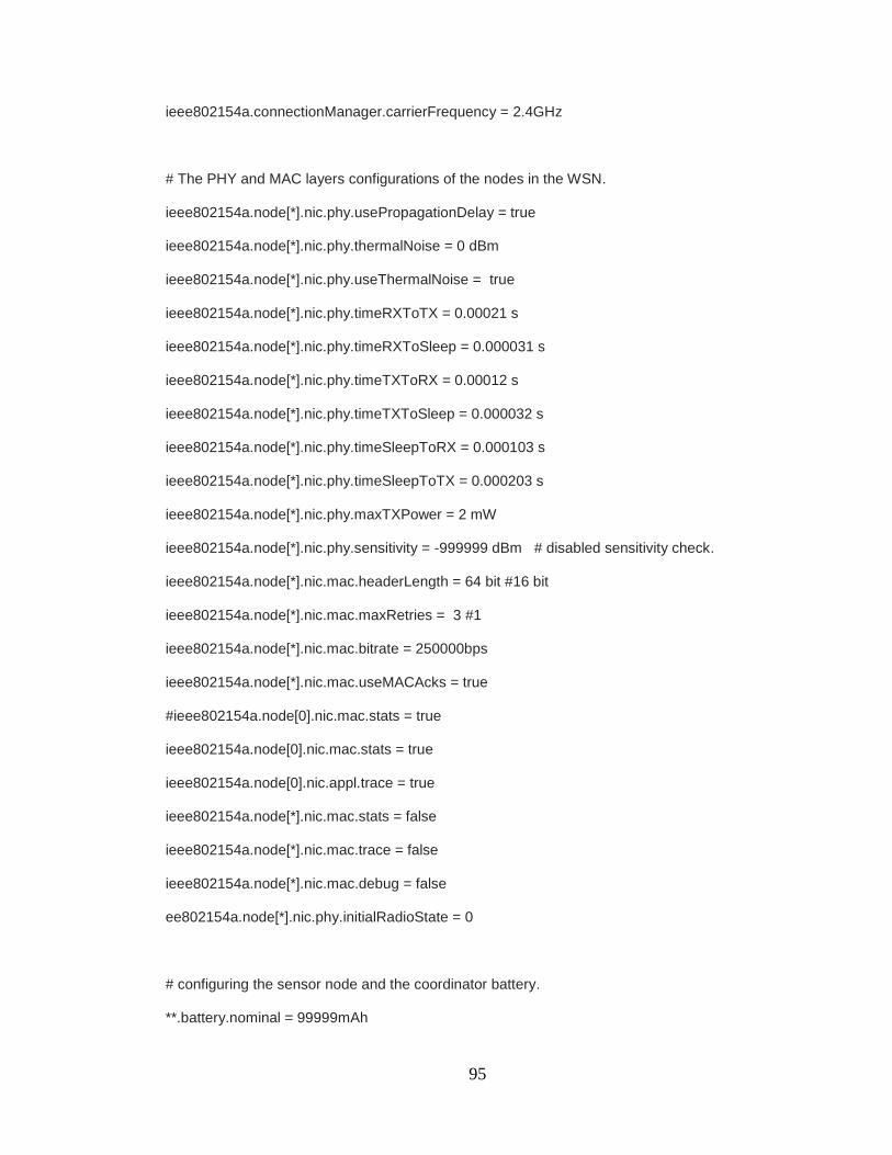
95
ieee802154a.connectionManager.carrierFrequency = 2.4GHz
# The PHY and MAC layers configurations of the nodes in the WSN.
ieee802154a.node[*].nic.phy.usePropagationDelay = true
ieee802154a.node[*].nic.phy.thermalNoise = 0 dBm
ieee802154a.node[*].nic.phy.useThermalNoise = true
ieee802154a.node[*].nic.phy.timeRXToTX = 0.00021 s
ieee802154a.node[*].nic.phy.timeRXToSleep = 0.000031 s
ieee802154a.node[*].nic.phy.timeTXToRX = 0.00012 s
ieee802154a.node[*].nic.phy.timeTXToSleep = 0.000032 s
ieee802154a.node[*].nic.phy.timeSleepToRX = 0.000103 s
ieee802154a.node[*].nic.phy.timeSleepToTX = 0.000203 s
ieee802154a.node[*].nic.phy.maxTXPower = 2 mW
ieee802154a.node[*].nic.phy.sensitivity = -999999 dBm # disabled sensitivity check.
ieee802154a.node[*].nic.mac.headerLength = 64 bit #16 bit
ieee802154a.node[*].nic.mac.maxRetries = 3 #1
ieee802154a.node[*].nic.mac.bitrate = 250000bps
ieee802154a.node[*].nic.mac.useMACAcks = true
#ieee802154a.node[0].nic.mac.stats = true
ieee802154a.node[0].nic.mac.stats = true
ieee802154a.node[0].nic.appl.trace = true
ieee802154a.node[*].nic.mac.stats = false
ieee802154a.node[*].nic.mac.trace = false
ieee802154a.node[*].nic.mac.debug = false
ee802154a.node[*].nic.phy.initialRadioState = 0
# configuring the sensor node and the coordinator battery.
**.battery.nominal = 99999mAh
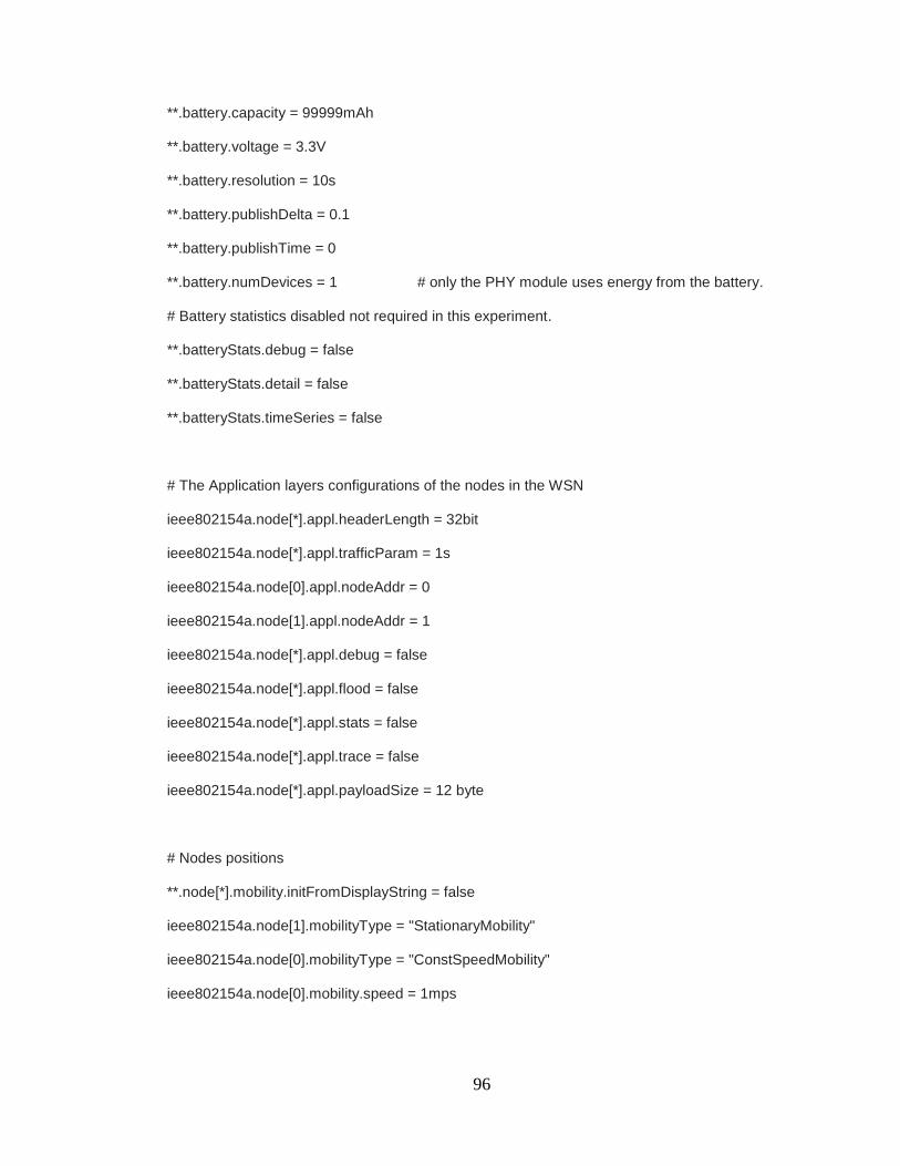
96
**.battery.capacity = 99999mAh
**.battery.voltage = 3.3V
**.battery.resolution = 10s
**.battery.publishDelta = 0.1
**.battery.publishTime = 0
**.battery.numDevices = 1 # only the PHY module uses energy from the battery.
# Battery statistics disabled not required in this experiment.
**.batteryStats.debug = false
**.batteryStats.detail = false
**.batteryStats.timeSeries = false
# The Application layers configurations of the nodes in the WSN
ieee802154a.node[*].appl.headerLength = 32bit
ieee802154a.node[*].appl.trafficParam = 1s
ieee802154a.node[0].appl.nodeAddr = 0
ieee802154a.node[1].appl.nodeAddr = 1
ieee802154a.node[*].appl.debug = false
ieee802154a.node[*].appl.flood = false
ieee802154a.node[*].appl.stats = false
ieee802154a.node[*].appl.trace = false
ieee802154a.node[*].appl.payloadSize = 12 byte
# Nodes positions
**.node[*].mobility.initFromDisplayString = false
ieee802154a.node[1].mobilityType = "StationaryMobility"
ieee802154a.node[0].mobilityType = "ConstSpeedMobility"
ieee802154a.node[0].mobility.speed = 1mps
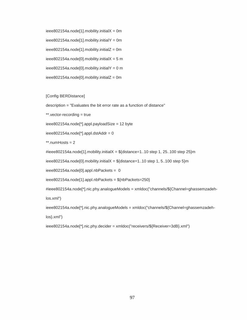
97
ieee802154a.node[1].mobility.initialX = 0m
ieee802154a.node[1].mobility.initialY = 0m
ieee802154a.node[1].mobility.initialZ = 0m
ieee802154a.node[0].mobility.initialX = 5 m
ieee802154a.node[0].mobility.initialY = 0 m
ieee802154a.node[0].mobility.initialZ = 0m
[Config BERDistance]
description = "Evaluates the bit error rate as a function of distance"
**.vector-recording = true
ieee802154a.node[*].appl.payloadSize = 12 byte
ieee802154a.node[*].appl.dstAddr = 0
**.numHosts = 2
#ieee802154a.node[1].mobility.initialX = ${distance=1..10 step 1, 25..100 step 25}m
ieee802154a.node[0].mobility.initialX = ${distance=1..10 step 1, 5..100 step 5}m
ieee802154a.node[0].appl.nbPackets = 0
ieee802154a.node[1].appl.nbPackets = ${nbPackets=250}
#ieee802154a.node[*].nic.phy.analogueModels = xmldoc("channels/${Channel=ghassemzadeh-
los.xml")
ieee802154a.node[*].nic.phy.analogueModels = xmldoc("channels/${Channel=ghassemzadeh-
los}.xml")
ieee802154a.node[*].nic.phy.decider = xmldoc("receivers/${Receiver=3dB}.xml")
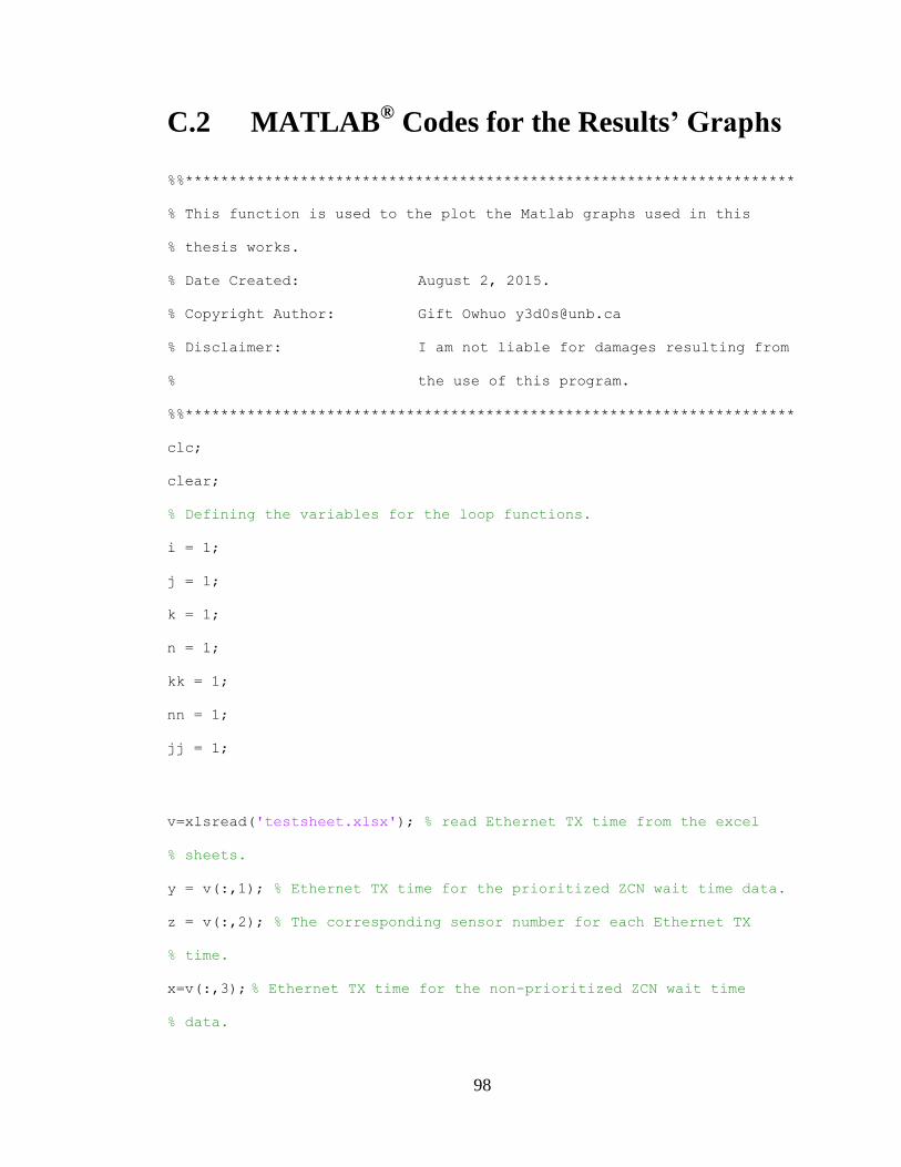
98
C.2 MATLAB® Codes for the Results’ Graphs
%%*********************************************************************
% This function is used to the plot the Matlab graphs used in this
% thesis works.
% Date Created: August 2, 2015.
% Copyright Author: Gift Owhuo [email protected]
% Disclaimer: I am not liable for damages resulting from
% the use of this program.
%%*********************************************************************
clc;
clear;
% Defining the variables for the loop functions.
i = 1;
j = 1;
k = 1;
n = 1;
kk = 1;
nn = 1;
jj = 1;
v=xlsread('testsheet.xlsx'); % read Ethernet TX time from the excel
% sheets.
y = v(:,1); % Ethernet TX time for the prioritized ZCN wait time data.
z = v(:,2); % The corresponding sensor number for each Ethernet TX
% time.
x=v(:,3); % Ethernet TX time for the non-prioritized ZCN wait time
% data.
99
w=v(:,4); % The corresponding sensor number for each Ethernet TX time.
% matching each sensor number with its corresponding Ethernet TX time
% for prioritized and non-prioritized WSN.
Figure (1)
for i = 1:120 % Ethernet TX time for prioritized WSN
% Sensor No.1 (Most Priority sensor Ethernet TX time).
if w(i) == 1
waittime1a(jj) = x(i);
plot(i,x(i),'. b')
hold on
jj = jj+1;
end % end of if statement.
% Sensor No.2 (Less Priority sensor Ethernet TX time).
if w(i) == 2
waittime2b(kk) = x(i);
kk = kk+1;
plot(i,x(i), '. g')
hold on
end % end of if statement.
% Sensor No.2 (Less Priority sensor Ethernet TX time).
if w(i) == 3
waittime3c(nn) = x(i);
plot(i,x(i), ' . r')
hold on
nn = nn+1;
end % end of if statement.
100
end % end of for statement.
% Plotting the Wait time of the Sensors data at the ZCN in a Non-
% Prioritized ZigBee WSN at 25s run time.
k = k-1;
j = j-1;
n = n-1;
kk = kk-1;
jj = jj-1;
nn = nn-1;
plot(x, 'K --')
hold off
xlabel('No. of samples')
title('Wait time of Sensors data for a Non-Prioritized ZigBee WSN at
25s run time')
ylabel('Wait time (ms)')
% Plotting the bar graph that shows 120 data samples collected in a
% prioritized and non-prioritized ZigBee WSN.
Figure (2)
seeme = [j jj; k kk;n nn];
bar(seeme)
ylabel('No. of samples')
title('Bar graph showing 120 data samples collected in a prioritized
and non-prioritized ZigBee WSN')
% xlabel('Sensor')
legend('Priority Algorithm','No Priority
Algorithm','Location','NorthEast')

Vita
Candidate’s full name: Gift Obuokam Owhuo
University attended: University of New Brunswick, B.Sc.E., 2014
Conference Presentations:
[1] 2015 Smart Grid Canada Conference, Markham, Ontario, Canada, October 2015.
[2] 2014 NSERC Smart Microgrid Network Annual General Meeting, McGill
University, Montreal, Quebec, Canada, August 2014.


