Embed Size (px)
Citation preview
POLITECNICO DI MILANODEPARTMENT OF AEROSPACE SCIENCE AND TECHNOLOGY
DOCTORAL PROGRAMME IN AEROSPACE ENGINEERING
MOMENT METHODS FOR NON-EQUILIBRIUM
LOW-TEMPERATURE PLASMAS WITH
APPLICATION TO ELECTRIC PROPULSION
Doctoral Dissertation of:Stefano Boccelli
Supervisor:Prof. Aldo Frezzotti
External Supervisor:Prof. Thierry E. Magin
Tutor:Prof. Luigi Vigevano
The Chair of the Doctoral Program:Prof. Pierangelo Masarati

Year 2021 – Cycle XXXIII
2

“If you can’t solve a problem,then there is an easier problem you can’t solve: find it.”
G. Pólya.
I

Acknowledgements
First, I would like to thank Prof. Aldo Frezzotti. Under your supervision, Icould enjoy all the freedom that I wanted, yet you have been always avail-able for discussing with me, and, if needed, for bringing me back on trackfrom my constant wandering among various unrelated engineering topics.What I perhaps appreciated most of your supervision is your ability to X-ray any problem, and identify the ultimate issues. Thank you for all thetime that you dedicated to teaching me, and for the patience of sometimesrepeating over and over the same concepts (be they complex or trivial) untilI could finally get a grasp of them.
The first idea for this thesis work comes from Prof. Thierry E. Magin,who originally proposed me to model Hall thruster discharges using mo-ment methods. Since I first came to VKI for working at my MSc thesis,back in the spring of 2016, I have learned so much from you, virtually aboutany side of research. I am also very grateful for the numerous research andcollaboration opportunities that you have offered to me, over the years. Theresearch group and the expertise that you have built are truly amazing, andmade all the time spent at VKI absolutely unique and a constant learningexperience.
At the beginning of this PhD, Hall thrusters were quite a new topic forme. I would like to thank Dr. Anne Bourdon, for all the precious insightsinto Hall thrusters and plasma physics in general, and for the very interest-ing meetings with her research group at the Laboratoire de Physique desPlasmas (LPP). I am also very grateful to Prof. James G. McDonald, at theUniversity of Ottawa, for hosting me to learn about maximum-entropy mo-ment methods. The experience in your research group was a turning pointinto my PhD research. Also, I would like to thank all members of my PhDcommittee for their helpful feedback.
III
I have learned so much from all professors, and probably equally asmuch from so many colleagues and friends. Federico and Bruno, althoughour research interests somehow diverged after the end of the Research Mas-ter, your friendship and scientific input was like a fixed-point inside thenonlinearity of a PhD. You guys set the standard that I try hard to follow inmy work. Thank you.
To all VKI colleagues, friends, professors and staff members goes myprofound gratitude. Every single one of you contributes making VKI sucha special place. My PhD was characterized by a good amount of roamingaround, spending time here and there. But despite this, VKI always felt likehome. Thanks Isa for all the nice times in the CC office, and all our talks infront of a nice cup of coffee. Thanks to Maria, Claudia, Anabel, who alsohelped so much in organizing the 3rd PLS, Bogdan, Yunus, George, andthanks to all the office mates that I met over these years (and that I probablyunintentionally annoyed by constantly chewing my pen). Pietro, Giuseppe,Lorenzo and Alfonso, I was so lucky to have the chance of mentoring yourRM or MSc thesis work. I have learned a lot from you. The energy andamazing ingenuity that you put into research gave me the extra fuel forkeeping working at the PhD, when the simulations were not convergingor when my moment code was running even slower than the full kineticsimulations (now it is faster, I promise!)
Sahadeo, Mahdieh, I am very happy that we had the chance to collab-orate on blackout and steering needles. A big shout-out to all PoliMi col-leagues, sharing the office / open space / ex-library / aquarium / whatever itis. I could meet a lot of talent in that room, and wish to all you folks the verybest. Karthik, I had a lot of fun working together at the EP-trajectory opti-mization coupling. I wish to address my special thanks also to Luca Zioni,the best secretary that a department could ever hope for, and to Prof. Mau-rizio Boffadossi, for the many stimulating conversations about aerodynam-ics, experimentation and various other topics. You made the department avery lively place.
Moving to the Paris area, I would like to thank all people from the low-temperature plasmas group, at LPP, in particular Alejandro, Thomas andProf. Pascal Chabert. Your insights into plasma physics were so precious,and I am glad that we are keeping the collaboration active. I met so manypassionated and dedicated researchers in my short time in Paris. Among all,I would like to thank particularly Bo, Hanen and Pedro for the interestingdiscussions and for the fun time besides work.
IV
During the winter of 2019, I had the opportunity to spend some monthsat the University of Ottawa. I wish to thank the whole research group ofProf. McDonald, in particular Fabien and Willem, with whom I had thechance to collaborate more directly. Thanks for all the knowledge thatyou have shared with me about the maximum-entropy method. Also, Iwould like to thank my office mates, Ramki, Farzane, Kevin, Aliou. AndHongxia: your dedication to research is amazing and is a great source ofmotivation for all who stand beside you. Keep up the great work! Thankyou also to Prof. Clinton P. T. Groth, at the University of Toronto Insti-tute for Aerospace Studies, and to his team. Finally, besides the research,thanks a lot James and Lani for your amazing hospitality. The kindness ofyour family made my stay unforgettable.
Un ringraziamento speciale va alla mia famiglia. Grazie a mamma epapà, per essere sempre presenti, da vicino o da lontano, alla nonna ed a miofratello Riccardo per le stimolanti discussioni sui neutroni, la meccanicaquantistica e tutte le cose a me incomprensibili che studi tu. Inoltre, unringraziamento ingegneristico va a papà per aver accolto il mio disordinato“laboratorio”, dopo il trasloco. Ho imparato tanto sui plasmi “giocando” ingarage, quanto in vari mesi di simulazioni. Grazie a tutti gli amici, nuovio di lunga data, Gale, Marti, Sara, Luca, Chiara, Kamila... ed ai colleghidella PLS Milan Penguins Division: Darione, i “Davidi” DB e DDCB, edil grande Maik.
L’ultimo ringraziamento va ad Elena. Grazie per la tua vicinanza incon-dizionata, per la tua pazienza nei momenti più bui e per la tua allegria inquelli felici. La tua presenza è stata un regalo meraviglioso, che non possoadeguatamente esprimere in poche righe.
Finally, this PhD thesis would undoubtly be much much worse had Alexan-dra Elbakyan never created Sci-Hub.
V

Summary
LOW-TEMPERATURE plasmas frequently show non-equilibrium fea-tures, due to the low collisionality and to the effect of the electricand magnetic fields. An accurate modeling of such situations re-
quires to employ kinetic descriptions (such as the Boltzmann or Vlasovequations), that describe the evolution in phase space of the particle ve-locity distribution function (VDF). This is the case, for example, for Hallthruster electric propulsion devices, where non-equilibrium characterizesboth neutrals and charged species. Fluid methods (such as the Euler or theNavier-Stokes-Fourier hydrodynamic approaches) cannot reproduce suchsituations accurately, and often mispredict transport processes. Moreover,such methods cannot reproduce kinetic instabilities, commonly observedin Hall thruster devices. Nonetheless, such methods are widely employed,due to their favorable computational cost, if compared to the much moreexpensive kinetic simulations.
A promising strategy for extending fluid descriptions towards non-equi-librium is offered by moment methods. Such methods solve for an enlargedset of equations, including higher-order moments with respect to the com-monly employed mass, momentum and energy balances. This work aimsat investigating the accuracy of moment and fluid methods for modelingkinetic plasmas. Particular emphasis is put on a selection of the kineticfeatures appearing in Hall thrusters. Among the possible moment meth-ods, order-4 maximum-entropy methods will be considered, as they showa superior robustness and the ability to represent strongly non-Maxwelliandistribution functions. In particular, the 5 and 14-moment systems willbe studied. These formulations are able to retrieve important VDFs, com-monly appearing in plasma physics, such as the Druyvesteyn distribution,as well as ring-like and anisotropic VDFs, and reproduce the Maxwellianas a limiting case.
VII
This work starts with an analysis of the maximum-entropy methods inlow-collisional situations, that are often encountered in low-temperatureplasmas and particularly in Hall thrusters. Then, the methods are extendedto the simulation of plasmas, by formulating electromagnetic source termsand investigating the dispersion relation of electrostatic plasma waves.
The 5 and 14-moment systems are then applied to the simulation of theaxial and azimuthal ion dynamics in a Hall thruster channel, and to thedynamics of electrons. The latter are magnetized and drift in the E × Bdirection, and their distribution function is known to settle to non-equilib-rium steady states, also due to the presence of a weak collisionality withbackground neutrals. For all cases, a kinetic reference solution is obtained,either numerically (with the use of particle or deterministic solvers) or ana-lytically, and the accuracy of the maximum-entropy systems is investigated,and additionally compared to the solution of the Euler equations of gas dy-namics. The maximum-entropy systems demonstrate strong improvementsfor all the considered conditions, and often reach the same accuracy as ki-netic methods, in terms of the tracked moments. This comes at the priceof a higher computational cost with respect to the Euler equations, but stilllower than kinetic methods. Finally, the last chapter of this work is devotedto the study of the propellant dynamics, and an alternative gas feed configu-ration is proposed, aimed at increasing the mass utilization efficiency of thethruster through a maximisation of the residence time of neutral particles inthe ionization region.
From the analysis performed in this work, the order-4 maximum-entropymethods appear completely suitable for the task of describing a number ofkinetic features in Hall thruster plasmas. The computational cost is clearlyhigher than for the Euler equations, but still advantageous with respect tofully kinetic formulations. Additional developments of this method, build-ing upon this work and suggested as future work activities, will pave theway to further applications of the methods to different plasma applications.
VIII
Sommario
IPLASMI a bassa temperatura sono spesso caratterizzati da non-equilib-rio termodinamico, per effetto della bassa collisionalità e dei campielettrici e magnetici. Una modellazione accurata di tale situazione
richiede l’uso di descrizioni cinetiche (quali per esempio le equazioni diBoltzmann o Vlasov), che descrivono l’evoluzione della funzione di dis-tribuzione delle velocità nello spazio delle fasi. I propulsori spaziali di tipoHall sono un esempio di tale non-equilibrio, che caratterizza sia le speciecariche che le specie neutrali presenti nel plasma. La descrizione del prob-lema tramite un approccio di tipo “fluido” (quali le equazioni inviscide diEulero o l’approccio idrodinamico di Navier-Stokes-Fourier) non perme-tte di riprodurre accuratamente le situazioni di non-equilibrio menzionate,e spesso predice in modo fallimentare i processi di trasporto. Inoltre, imetodi fluidi non permettono di predirre le instabilità di natura cineticaspesso osservate nei propulsori di tipo Hall. Malgrado tali limitazioni, imetodi di tipo fluido sono frequentemente utilizzati per via del loro bassocosto computazionale, che li rende favorevoli rispetto alle molto più impeg-native simulazioni cinetiche.
Una strategia promettente per estendere le descrizioni fluide verso situ-azioni di non-equilibrio consiste nei “metodi dei momenti”. Tali metodirisolvono un sistema allargato di equazioni, che include momenti di ordinesuperiore rispetto ai soli bilanci di massa, momento ed energia. L’obiettivodi questo lavoro consiste nell’investigare l’accuratezza di metodi dei mo-menti e di metodi fluidi, per l’applicazione a plasmi cinetici. Tra i pos-sibili metodi dei momenti, saranno considerati metodi della massima en-tropia, che mostrano un ottimo grado di robustezza e la capacità di rap-presentare funzioni di distribuzione fortemente non-Maxwelliane. In par-ticolare, saranno studiati sistemi di 5 e 14 momenti, membri di ordine 4della famiglia dei metodi della massima entropia. Tali formulazioni perme-
IX
ttono di riprodurre importanti funzioni di distribuzione, comuni nella fisicadei plasmi, quali la distribuzione di Druyvesteyn, funzioni di distribuzione“ad anello” ed anisotrope, ed includono la distribuzione Maxwelliana comecaso limite.
Questo lavoro parte dall’analisi dei sistemi della massima entropia incondizioni scarsamente collisionali, caratteristiche dei plasmi a bassa tem-peratura, e dei propulsori di tipo Hall. I metodi sono poi applicati alla sim-ulazione di plasmi, tramite la formulazione dei termini di sorgente elettro-magnetici, e l’analisi della relazione di dispersione per onde elettrostatiche.I sistemi di 5 e 14 momenti sono poi applicati allo studio dell’evoluzioneassiale ed azimutale degli ioni nel canale di un propulsore di tipo Hall,e successivamente allo studio della dinamica degli elettroni. Gli elettroniin particolare sono magnetizzati, ed hanno una componente di velocità didrift nella direzione E × B. La loro funzione di distribuzione è nota es-sere fuori equilibrio anche nello stato stazionario, per l’effetto dei campielettromagnetici e della collisionalità con gli atomi neutrali. Per tutti icasi considerati, una soluzione cinetica è ottenuta numericalmente (tramitemetodi alle particelle o solutori deterministici) oppure analiticamente, edè successivamente confrontata con i metodi della massima entropia e conla soluzione delle equazioni di Eulero. I metodi della massima entropiamostrano forti miglioramenti rispetto ai classici approcci fluidi, ed in molticasi mostrano un’accuratezza analoga ai metodi cinetici. Infine, l’ultimocapitolo di questo lavoro è dedicato allo studio della dinamica del propel-lente neutrale, dall’iniezione all’espansione fuori dal canale, ed una config-urazione alternativa di iniezione viene proposta ed investigata. Tale con-figurazione ha l’obiettivo di migliorare l’efficienza del propulsore, tramitela massimizzazione del tempo di residenza delle particelle neutrali nellaregione di ionizzazione.
Dalle analisi eseguite in questo lavoro, il metodo della massima entropiadi ordine 4 (sistemi di 5 e 14 momenti) appare completamente applica-bile all’obiettivo di modellare il non-equilibrio nei propulsori di tipo Hall.Il costo computazionale di questi metodi appare notevolmente superioread una soluzione delle equazioni di Eulero, ma in ogni caso vantaggiosorispetto a formulazioni completamente cinetiche. Ulteriori sviluppi delmetodo sono suggeriti come lavoro futuro, e permetteranno l’applicazionedei metodi della massima entropia a differenti tipologie di plasmi.
X
Contents
Summary VII
Sommario IX
1 Introduction 11.1 Plasmas for space propulsion: the Hall thruster . . . . . . . 11.2 Modeling of low-temperature plasmas . . . . . . . . . . . . 41.3 Objectives and structure of the thesis . . . . . . . . . . . . . 7
1.3.1 Motivation . . . . . . . . . . . . . . . . . . . . . . . 71.3.2 Aims of this work . . . . . . . . . . . . . . . . . . . 81.3.3 Structure of this manuscript . . . . . . . . . . . . . . 9
2 Kinetic and fluid modeling of gases and plasmas 112.1 Kinetic theory . . . . . . . . . . . . . . . . . . . . . . . . . 132.2 The dimensionless kinetic equation:
operating regime for electrons, ions and neutrals . . . . . . 152.3 Fluid formulations: moments of the kinetic equation . . . . 20
2.3.1 Moments of the distribution function . . . . . . . . . 202.3.2 The generalized moment equation . . . . . . . . . . . 232.3.3 Pressureless gas, Euler equations and moment methods 24
2.4 The maximum-entropy closure . . . . . . . . . . . . . . . . 282.4.1 Order-4 maximum-entropy method: 14-moment system 302.4.2 Order-4 maximum-entropy method: 5-moment system 33
2.5 Conclusions . . . . . . . . . . . . . . . . . . . . . . . . . . 34
XI
Contents
3 Overview of the numerical methods 373.1 Particle-based solutions of the kinetic equation . . . . . . . 373.2 The finite volume method . . . . . . . . . . . . . . . . . . 39
3.2.1 Formulation . . . . . . . . . . . . . . . . . . . . . . 393.2.2 Numerical fluxes for fluid and moment systems . . . 413.2.3 Time integration . . . . . . . . . . . . . . . . . . . . 433.2.4 Boundary conditions . . . . . . . . . . . . . . . . . . 443.2.5 Finite volume solution of the kinetic equation . . . . 45
3.3 Units for low-density numerical simulations . . . . . . . . . 47
4 Application of the maximum-entropy closure to rarefied gases andplasmas 494.1 The rarefied Sod shock tube problem . . . . . . . . . . . . . 50
4.1.1 Kinetic solution . . . . . . . . . . . . . . . . . . . . 524.1.2 Solution of the 5-moment system . . . . . . . . . . . 544.1.3 Comparison of the HLL and Rusanov fluxes . . . . . 57
4.2 Approximated wave speeds . . . . . . . . . . . . . . . . . . 604.2.1 Approximated wave speeds for the 5-moment system 614.2.2 Extending the approximation to the 6-moment system 634.2.3 Extending the approximation to the 14-moment system 66
4.3 Computational efficiency and minimum allowed σ . . . . . 704.4 2-dimensional test case: rarefied crossing jets . . . . . . . . 73
4.4.1 Kinetic solution . . . . . . . . . . . . . . . . . . . . 744.4.2 14-moment and Euler solutions . . . . . . . . . . . . 77
4.5 Electromagnetic source terms . . . . . . . . . . . . . . . . 814.6 Plasma dispersion relations . . . . . . . . . . . . . . . . . . 85
4.6.1 Electron waves . . . . . . . . . . . . . . . . . . . . . 874.6.2 Ion acoustic waves . . . . . . . . . . . . . . . . . . . 90
4.7 Conclusions . . . . . . . . . . . . . . . . . . . . . . . . . . 94
5 Collisionless ions in Hall thrusters:an analytical axial model and a simple fluid closure 955.1 Genesis of the axial VDF . . . . . . . . . . . . . . . . . . . 965.2 Analytical axial VDF . . . . . . . . . . . . . . . . . . . . . 98
5.2.1 Moments of the analytical VDF . . . . . . . . . . . . 1015.2.2 Comparison with 2D PIC simulations . . . . . . . . . 1025.2.3 Comparison with experimental results . . . . . . . . 1055.2.4 Notes: beyond monoenergetic ion birth . . . . . . . . 107
5.3 A fluid model with ad hoc heat flux closure . . . . . . . . . 1095.3.1 Derivation of the fluid equations . . . . . . . . . . . 109
XII
Contents
5.3.2 Heat flux closure . . . . . . . . . . . . . . . . . . . . 1105.3.3 Comparison with PIC simulations . . . . . . . . . . . 115
5.4 Conclusions . . . . . . . . . . . . . . . . . . . . . . . . . . 117
6 Maximum-entropy modeling of ions 1196.1 Order-4 maximum-entropy systems for collisionless and un-
magnetized ions . . . . . . . . . . . . . . . . . . . . . . . . 1206.1.1 Governing equations for ions: 5-moment system . . . 1206.1.2 Governing equations for ions: 14-moment system . . 122
6.2 Axial ion acceleration in a Hall thruster channel . . . . . . . 1226.3 Tonks-Langmuir sheath . . . . . . . . . . . . . . . . . . . . 124
6.3.1 Description of the case . . . . . . . . . . . . . . . . 1246.3.2 Kinetic solution . . . . . . . . . . . . . . . . . . . . 1256.3.3 5-moment maximum-entropy solution . . . . . . . . 1266.3.4 Euler system solution . . . . . . . . . . . . . . . . . 127
6.4 Ions in a stationary wave . . . . . . . . . . . . . . . . . . . 1286.4.1 Description of the case . . . . . . . . . . . . . . . . 1296.4.2 Kinetic solution . . . . . . . . . . . . . . . . . . . . 1296.4.3 5-moment and Euler solutions . . . . . . . . . . . . . 132
6.5 Ions in a travelling wave . . . . . . . . . . . . . . . . . . . 1376.6 Ions in axial-azimuthal 2D plane . . . . . . . . . . . . . . . 141
6.6.1 Description of the case . . . . . . . . . . . . . . . . 1416.6.2 Kinetic solution . . . . . . . . . . . . . . . . . . . . 1436.6.3 Fluid simulations . . . . . . . . . . . . . . . . . . . 1446.6.4 Comparison of the results . . . . . . . . . . . . . . . 145
6.7 Conclusions . . . . . . . . . . . . . . . . . . . . . . . . . . 146
7 Maximum-entropy modeling of electrons 1497.1 Overview of non-equilibrium effects for electrons in Hall
thrusters . . . . . . . . . . . . . . . . . . . . . . . . . . . . 1507.2 14-moment formulation against analytical VDFs . . . . . . 151
7.2.1 Preliminary considerations . . . . . . . . . . . . . . 1517.2.2 Analytical and maximum-entropy VDFs . . . . . . . 152
7.3 BGK-like source terms for electron-neutral collisions . . . . 1567.3.1 A simple Maxwellian-relaxation collision model . . . 1587.3.2 Collision model for large mass disparity . . . . . . . 1597.3.3 Elastic collisions with energy loss . . . . . . . . . . . 1617.3.4 Excitation and ionization reactions . . . . . . . . . . 1637.3.5 Collision frequency and non-equilibrium . . . . . . . 163
7.4 Application: homogeneous relaxation towards non-equilibrium 165
XIII
Contents
7.5 Application: a one-dimensional test case . . . . . . . . . . . 1687.6 Conclusions . . . . . . . . . . . . . . . . . . . . . . . . . . 171
8 DSMC and TPMC analysis of the neutral gas injection:an alternative gas feed configuration 1758.1 Preliminary considerations . . . . . . . . . . . . . . . . . . 1768.2 Direct and reversed injection: a simplified analysis . . . . . 1778.3 DSMC simulations . . . . . . . . . . . . . . . . . . . . . . 1788.4 Test-particle Monte Carlo simulations: the method . . . . . 1828.5 Test-particle Monte Carlo simulations: results . . . . . . . . 187
8.5.1 Preliminary analysis in the free-molecular limit . . . 1878.5.2 Collisional case and residence time in the ionization
region . . . . . . . . . . . . . . . . . . . . . . . . . 1898.5.3 Estimation of the mass utilization efficiency . . . . . 190
8.6 Conclusions . . . . . . . . . . . . . . . . . . . . . . . . . . 192
Conclusions and future work 195
A Notes on the GPU implementation 201
B Time integration error for accelerated gases 207
C Wave speeds approximation via Artificial Neural Networks 211
D Implementation of the 14-moment wave speeds 223
Bibliography 225
List of publications 239
XIV
CHAPTER1Introduction
Starting at the beginning of the last century, with the development of thevacuum tube diode [1], which marked the dawn of electronics, plasmashave quickly become a fundamental branch of human technology. Nowa-days, plasmas are employed in a huge variety of industrial and medicalapplications, and in a large number of research fields. We shall cite, for ex-ample, the surface processing of semiconductors [2], X-rays generation [3],novel compact particle accelerator designs [4], nuclear fusion research [5],Solar physics and space weather prediction [6].
This work focuses on low-temperature plasmas, where the heavy species(background neutrals and ions) are typically at a much lower temperaturethan electrons. Particular emphasis will be put to the plasma conditionsencountered in Hall thruster electric propulsion devices.
1.1 Plasmas for space propulsion: the Hall thruster
Since the early days of rocket propulsion research, it was recognized thatelectric fields have the potential to accelerate ions to very high velocities,drastically increasing the specific impulse Isp of classical chemical rockets[7, 8]. As the power input is typically limited by solar cells, this form of
1
Chapter 1. Introduction
space propulsion is characterized by low thrust, often in the sub-Newtonsrange, depending on the size of the thruster. Therefore, these devices arenot able to lift a spacecraft from the ground to orbit, but still require aninitial kick to orbital speed by use of traditional chemical boosters.
However, electrical propulsion has a number of important advantages.To start off, the low thrust happens to be finely tunable through a selectionof the mass flow rate and the power input, making electric thrusters veryaccurate devices for tasks such as satellite maneuvering and station keeping,and the high specific impulse additionally reduces the amount of requiredfuel, increasing the possible mission time or the payload [9, 10].
The latter point happens to be crucial for what concerns Solar Systemexploration. Indeed, considering the Tsiolkovskii equation [11], one caneasily see that the low specific impulse of chemical rockets implies theneed for extremely high amounts of fuel [12]. For example, it can be es-timated that a mission to Mars could easily require that 85% of the space-craft mass is composed by fuel, and the situation drastically worsens forother planets (for instance, the percentage is roughly 90% for Venus, 98%for Mercury etc.) [13], making gravity assist absolutely necessary. Fromthis perspective, the high specific impulse of electric propulsion is a gamechanger. Also, in terms of trajectory design, the possibility to keep thethrusters active for long amounts of time introduces new degrees of free-dom, and combinations of the classical ballistic trajectory and thrust arcscan be employed, optimizing the fuel efficiency or the travel time [14, 15].
A large number of different electric thruster designs have been proposedover the years [16, 17]. As a quick review, we shall cite, among others,the pulsed plasma thruster (PPT) [18], the pulsed inductive thruster [19],the magnetoplasmadynamic thruster (MPD) [20] and the helicon thruster[21]. More advanced concepts have also been presented in the past andare currently being investigated, such as fusion-based propulsion (see forexample [22, 23]). Finally, we shall cite the two most widely studied (andemployed) designs: the gridded ion thruster and the Hall thruster [24]. Eachconfiguration comes with its own advantages in terms of reliability, specificimpulse and attainable thrust levels.
In this work, particular attention is put on plasma modeling for the con-ditions encountered in Hall thrusters. However, a number of the resultscould be easily extended to different configurations.
The Hall thruster
In Hall thrusters, the potential drop that accelerates ions is obtained bylimiting the longitudinal electron mobility by effect of a radial magnetic
2
1.1. Plasmas for space propulsion: the Hall thruster
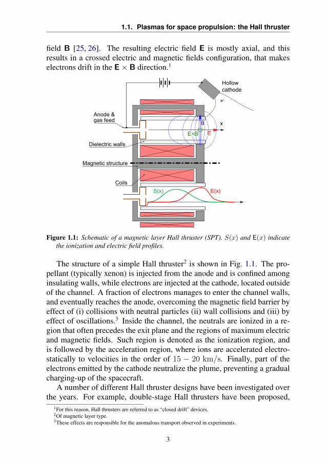
field B [25, 26]. The resulting electric field E is mostly axial, and thisresults in a crossed electric and magnetic fields configuration, that makeselectrons drift in the E× B direction.1
Figure 1.1: Schematic of a magnetic layer Hall thruster (SPT). S(x) and E(x) indicatethe ionization and electric field profiles.
The structure of a simple Hall thruster2 is shown in Fig. 1.1. The pro-pellant (typically xenon) is injected from the anode and is confined amonginsulating walls, while electrons are injected at the cathode, located outsideof the channel. A fraction of electrons manages to enter the channel walls,and eventually reaches the anode, overcoming the magnetic field barrier byeffect of (i) collisions with neutral particles (ii) wall collisions and (iii) byeffect of oscillations.3 Inside the channel, the neutrals are ionized in a re-gion that often precedes the exit plane and the regions of maximum electricand magnetic fields. Such region is denoted as the ionization region, andis followed by the acceleration region, where ions are accelerated electro-statically to velocities in the order of 15 − 20 km/s. Finally, part of theelectrons emitted by the cathode neutralize the plume, preventing a gradualcharging-up of the spacecraft.
A number of different Hall thruster designs have been investigated overthe years. For example, double-stage Hall thrusters have been proposed,
1For this reason, Hall thrusters are referred to as “closed drift” devices.2Of magnetic layer type.3These effects are responsible for the anomalous transport observed in experiments.
3
Chapter 1. Introduction
allowing for a separate control between thrust and specific impulse by sep-arating the ionization and acceleration stages [27]. Various magnetic con-figurations have also been proposed, with the aim of optimizing the plasmaprofile, or reducing wall erosion4 (see the magnetically shielded thrusters,[29, 30]).
The choice of the walls material proves to be crucial in a Hall thruster,as it dictates the temperature of wall-emitted electrons, and thus their dif-fusion across the magnetic field lines [25, 31]. An important variation ofthe insulating-walls design is obtained by employing conductive walls [32]instead of the frequently used boron nitride ceramic walls. In such con-ducting-wall thrusters, a part of the channel becomes electrically equipo-tential, and most of the acceleration happens in a thin region near the anode(thruster with anode layer, TAL). Wall-less configurations have also beeninvestigated [33], aiming at directly solving the problem of wall erosion.
In this work, we will only consider the simple configuration of Fig. 1.1,often referred to as “magnetic layer Hall thruster”, or “Stationary PlasmaThruster” (SPT). Unless otherwise specified, all mentions to “Hall thrusters”in this work will refer to such configuration.
1.2 Modeling of low-temperature plasmas
The modeling of low-temperature plasmas encountered in electric propul-sion devices can be tackled at different levels of accuracy. In the following,we shall give a brief introduction to some of the possible models, and high-light their range of validity and computational complexity. Most of theattention will be put on transport modeling, while a number of importanttopics (such as the detailed treatment of collisions, instabilities and particle-wall interactions [34, 35]) will not be discussed in detail, as to reflect theaim and focus of the present work.
At the simplest level, when collisions dominate the dynamics of eachspecies, one can consider drift-diffusion models, that have proven effectivefor a range of problems for Torr-level discharges [36]. Such models solvefor the density equations of the different charged species, assuming a simplediffusion-type relation between the drift velocity and the applied fields. Thedrift-diffusion model typically has a low computational effort, although theequations are parabolic, due to the presence of diffusion terms.5
For situations of lower collisionality, the diffusion laws become ques-
4See for example [28].5This requires to satisfy the von Neumann condition on finite grids (see [37]), which is sub-optimal with
respect to hyperbolic equations, that only need to respect the CFL conditions.
4
1.2. Modeling of low-temperature plasmas
tionable, and drift-diffusion models can be replaced by multi-fluid formula-tions, where a larger set of equations is solved for each species [38], and thecoupling happens through the electromagnetic fields and the inter-speciescollisional sources.6 The choice for the set of equations to be solved de-pends on the considered species and the operating conditions, a commonchoice being the set of mass, momentum and energy equations. This resultsin the so-called “fluid models”, typically consisting in the Euler equationsof gas dynamics (one set of equations for each species) if the conductionand viscous terms are neglected, or the Navier-Stokes-Fourier (NSF) equa-tions in the “hydrodynamic approach”.
Multi-fluid models based on the Euler/NSF equations are valid when theassumption of local thermodynamic equilibrium is satisfied, namely whenthe considered species have a (quasi-) Maxwellian distribution of particlevelocities [39]. A first extension of such methods, commonly employed inplasma physics whenever magnetic fields are present, consists in includ-ing temperature anisotropy between the parallel and perpendicular direc-tions [40]. However, as will also be discussed in this work, Hall thrustershappen to show further deviations from equilibrium [41]. Indeed, ions ap-pear to be low-collisional, and strongly affected by the electric field. On theother hand, electrons are both magnetized and collisional [42, 43], result-ing in skewed and asymmetric velocity distribution functions (VDF) [44].7
Non-equilibrium directly affects transport quantities, as the Euler/NSF con-vective fluxes may no longer be accurate due to the breaking apart of theclosure assumptions. Moreover, Hall thrusters are known to show a widerange of plasma instabilities, whose origin and and characteristics are ki-netic in nature (see for example [47, 48]), and are known to heavily influ-ence the electron cross-field transport [49].
In principle, all such kinetic effects could be described by solving theBoltzmann, Fokker-Planck or Vlasov kinetic equations, but at the price ofa very high computational cost [50]. This ultimately reflects the high di-mensionality of the kinetic equation (in case of a deterministic numericalsolution [51, 52]), or the need to keep the statistical noise to an acceptablelevel (for Particle-in-Cell (PIC) methods [53]). Additionally, such methodsare often time-explicit, and thus need to resolve the plasma frequency, forc-ing a rather small time step, and the Debye length, imposing tiny cell sizes.Various strategies have been proposed for reducing the computational costof kinetic methods, such as scaling the thruster geometry [54, 55] or arti-
6Other possible coupling phenomena such as radiation will not be considered in this work.7In this regard, Hall thrusters share a number of similarities with magnetron sputtering devices [45,46], except
that they typically operate at a much lower background pressure.
5
Chapter 1. Introduction
ficially modifying the vacuum permittivity [56], while preserving certaincrucial plasma properties. However, such models in general do not guaran-tee that all kinetic features are properly preserved. Despite the high com-putational cost, kinetic methods are often employed for obtaining a deepunderstanding of selected features, often in reduced dimensionalities, as toreduce the computational complexity [57–59].
The hybrid fluid-PIC method is a commonly employed approach forspeeding-up the calculations, while retaining some kinetic information [60,61]. This approach is based on the observation that the electron dynamicsis so fast that a quasi-steady state is reached at the ion time scales. In thesemodels, one simulates ions (slow and low-collisional) as particles, whilethe electron population (more collisional due to the higher temperature andlower mass, and faster) is described by the Euler or NSF equations. Theseapproaches simplify significantly the fast electron dynamics, still retaininga kinetic description for ions. However, of course, such methods assumethat electrons have reached conditions close to local thermodynamic equi-librium, which is not necessarily the case in low-collisional E × B config-urations.
Non-equilibrium fluid-like models: moment methods
In order to extend the validity of fluid models towards non-equilibrium, anoption consists in enlarging the set of governing equations, as to include ad-ditional thermodynamic fields such as the heat flux vector, up to the desiredorder [40, 62]. Such formulations are commonly referred to as “momentmethods”, and promise to increase the range of validity of fluid systems,while retaining affordable computational costs.
Among all possible formulations, we shall cite the Grad [63] and max-imum-entropy [64, 65] families of moment methods. In both cases, onestarts by assuming a shape for the distribution function, that can reproducenon-Maxwellian shapes. An equation is then written for each parameter ap-pearing in the assumed distribution function, resulting in a set of momentequations, that include but extend the mass-momentum-energy description.
The Grad method has the strong advantage of providing a direct linkbetween the shape of the VDF and its moments, but also has a series ofdrawbacks. For example, it does not guarantee that the VDF is positive.On the other hand, the maximum-entropy formulation is typically more ro-bust, guarantees a positive VDF by construction, and is hyperbolic. Amongits drawbacks, it should be mentioned that such formulation was shownunable to reproduce some states that would otherwise be physically realiz-
6
1.3. Objectives and structure of the thesis
able [66]. Moreover, in this formulation, the link between the moments andthe distribution function is not known analytically, and would require anentropy-maximisation problem to be solved at every occurrence during thesimulations. The latter problem can however be mitigated through the useof approximated solutions [67], which make the maximum-entropy meth-ods much more computationally affordable. For this reason, and in view ofits robustness (even in non-equilibrium conditions), the maximum-entropymethod will be the method of choice for this work. More details about itsformulation and on the mentioned issues will be given in Chapter 2.
1.3 Objectives and structure of the thesis
1.3.1 Motivation
As discussed, moment methods are obtained by extending the fluid formu-lation, including additional equations for the higher order moments. Theseadditional governing equations allow us to reproduce accurately a range ofnon-equilibrium states. Moreover, this is done at a computational cost thatcan be comparable to fluid methods, and is often much lower than the costof a kinetic solution. Also, being based on PDEs, moment methods arenot subject to the statistical noise that affects particle-based kinetic meth-ods, and are suitable for the application of a broad range of optimizationstrategies.8 Methods that are at the same time computationally efficient andaccurate in non-equilibrium situations will provide in the next future a use-ful tool for the design of Hall thrusters and low-temperature plasma devicesin general.
Besides this specific application, one should consider that non-equilib-rium situations are virtually ubiquitous in plasma physics. Many differentmoment formulations for plasma applications are actively being investi-gated [68–71] and are likely to become a broadly employed approach forthe study of many plasma problems and for obtaining engineering predic-tions. Among all possibilities, we choose to investigate the maximum-en-tropy family of moment methods. Such methods have been studied in arange of conditions and for different problems, but their systematic appli-cation to plasmas is still missing in the literature. The accuracy of thesemethods, as well as their computational advantage over full kinetic ap-proaches, are still to be investigated for most plasma problems, includingHall thrusters.
8Such as, for instance, adjoint optimization methods.
7
Chapter 1. Introduction
1.3.2 Aims of this work
This thesis aims at investigating the applicability of moment methods tothe accurate description of the non-equilibrium conditions that characterizeHall thrusters. Particular emphasis will be put on the order-4 maximum-entropy moment methods. The thesis is centered around two tasks:
• After a theoretical introduction, the first part deals with developing theorder-4 maximum-entropy moment method, that has been previouslyapplied to rarefied and multiphase flows, but never to completely colli-sionless and charged gases, and in presence of electrical and magneticfields;
• The second part is then devoted to the applications to Hall thrusters-like conditions. Different test cases are investigated, and the accu-racy and computational cost of the maximum-entropy method are dis-cussed, comparing it to kinetic solutions and to simpler moment meth-ods.
Throughout the work, a number of heavy simplifications have been made.For instance, the collision operator will be often simplified with a BGK ap-proximation, if not completely neglected. Even more drastically, all anal-ysis of this work consider individual species and never couple them. Ionsare studied independently from electrons, and the electric field (the onlycoupling element, if we neglect charge-charge collisions) is externally im-posed. Of course, the coupling is a crucial feature of any real plasma.
However, in terms of the present work, the coupling constitutes an un-necessary complexity. Keeping in mind our goal of describing the problemusing moment methods, aiming at retrieving as many kinetic features aspossible, one can identify three sources of error: (i) the higher order clos-ing moments appearing in the fluxes (ii) electro-magnetic source terms and(iii) the computation of collisional sources.9 The first two points reflecthow accurately the moment method can represent the streaming of the dis-tribution function in physical space (Point i) and velocity (Point ii). Point(iii) on the other hand reflects the collision operator and chemical produc-tion. Prior to considering full and coupled systems, it is here reputed thatinvestigating the accuracy of the said points, individually, has priority. Forthis reason, rather than providing a full description of the plasma, the aimof the work is instead to give an accurate comparison of the methods invery controlled conditions.
9These points will be discussed in detail in the next sections.
8
1.3. Objectives and structure of the thesis
Clearly, a number of further issues may arise when the coupling will beenabled, and additional careful studies will thus be required. Among othertopics, this will be indeed one of the suggested future work activities.
1.3.3 Structure of this manuscript
This manuscript is structured as follows.The Chapters 2 and 3 are introductory, and outline the theoretical fun-
dations and numerical methods upon which this work is built. In partic-ular, Chapter 2 discusses some of the theoretical models that allow us todescribe rarefied gases and plasmas. The chapter starts from kinetic the-ory and describes all sets of moment equations that will be employed inthis work, including the Euler equations and the 5-moment and 14-moment(order-4) maximum-entropy systems. Chapter 3 briefly discusses how thegoverning equations can be solved numerically.
The kinetic equation and the Euler equations are readily applied to rar-efied gases and plasmas, and have been discussed in a broad literature boththeoretically and numerically. On the other hand, the maximum-entropysystems have been covered only partially. Chapter 4 discusses the fur-ther ingredients required in order to solve the maximum-entropy system inthe required conditions, in terms of numerical solution (approximating theeigenvalues, identifying the proper numerical schemes) and modeling ofthe electromagnetic terms and their resulting dispersion relation.
All other chapters discuss applications to Hall thruster-like configura-tions. First, ions are considered: Chapter 5 constitutes a first attempt at an-alyzing the problem. By considering the thruster channel as 1-dimensional,some analytical results are obtained for the axial velocity distribution func-tion, and a simple moment method is developed. These results are com-pared to 2-dimensional kinetic simulations and experiments, and give bothqualitative and quantitative information over the kinetic features to be ex-pected.
Then, the ion description using the maximum-entropy systems is inves-tigated in Chapter 6. The same test cases of the previous chapter is con-sidered, together with other cases relevant for plasma physics and to Hallthrusters. In particular, a Tonks-Langmuir sheath is studied, together withions in stationary and moving waves, in one and two dimensions. All along,a comparison between kinetic results, moments and the Euler equations isgiven.
Chapter 7 then tackles electrons modeling. As mentioned, electronsare magnetized, and this includes additional complexity to the problem.
9
Chapter 1. Introduction
The maximum-entropy description is first compared to analytical solutionsfrom the literature, for 0-dimensional test cases. This is followed by the for-mulation of electron-neutral collisional terms, and the study of space homo-geneous relaxation problems, and finally by the analysis of 1-dimensionalproblems, where electrons evolve along a thruster-like channel, in presenceof a magnetic field barrier. This chapter completes the work on momentmethods.
Chapter 8 considers a quite different problem, and discusses the neutralspecies injection and expansion into the Hall thruster channel. The analysisfocuses on the residence time of neutral particles inside an imposed ioniza-tion region, and the corresponding ionization probability, resulting in theengine efficiency, is studied. An alternative injection configuration is thenproposed: the propellant is injected from a slit located on the inner wall,close to the exit plane, and is directed towards the anode. The numericalanalysis suggest that this configuration is associated to an increased massutilization efficiency.
Finally, a concluding chapter is devoted to summarize the work, high-lighting the main achievements and weaknesses, and some possible futuredevelopments are suggested.
10
CHAPTER2Kinetic and fluid modeling of gases and
plasmas
This chapter introduces the governing equations for the description of rar-efied gases and low-temperature plasmas. The numerical solution of suchequations and the application to Hall thrusters configurations will be dis-cussed in the next chapters.
The starting point for studying the behavior of a rarefied gas or plasmaconsists in analyzing the individual behavior of its particles. Only elec-trons and monoatomic species will be considered, since most often electricpropulsion operates on noble gases.1 In most electric propulsion applica-tions, the particle energy is rather low (the electron energy is in the rangeof 1 − 100 eV, while heavy particles are slower and have a temperatureroughly in the 1000 K range) and a non-relativistic description can be prof-itably employed. In this work, the internal (electronic) structure of atomicspecies will not be considered, hence all particles are considered as classi-
1A notable exception consists in iodine-fed thrusters, currently being tested both in the lab and in orbit [72].
11
Chapter 2. Kinetic and fluid modeling of gases and plasmas
cal points evolving following the Newton’s equations:
dxidt
= vi ,
dvidt
=Fimi
,
(2.1)
where xi and vi are the position and velocity of the i–th particle, mi itsmass and Fi all forces acting on it, including inter-particle interactions andexternal forces of electromagnetic nature. Inter-particle interactions dependon the considered species and divide in three categories: neutral-neutral,neutral-charged and charged-charged (Coulomb) interactions.
For macroscopic systems, one does not solve these equations directly,due to the large number of particles involved. Instead, a statistical for-mulation is introduced. Different strategies are possible at this point: onepossibility consists in writing the equations using the Hamiltonian formal-ism, deriving the Liouville equation for the N-particles distribution func-tion, and then expanding it in the BBGKY hierarchy and neglecting corre-lations [39,73,74]. This is the preferred approach in gas dynamics. Anotherstrategy, common in plasma physics, consists in deriving the Klimontovichequation for the microscopic distribution function, and then applying anaverage operator to it [75–77]. In either case, one ends up with an equationfor the one-particle distribution function f , discussed in the following.
This chapter is structured as follows. Section 2.1 introduces the kineticequation (Boltzmann/Vlasov/BGK), that governs the evolution of the dis-tribution function f . A non-dimensionalization of such equations allowsone to extract dimensionless parameters, that can be profitably employedfor understanding the operating regimes. This is done in Section 2.2, wherethe operating conditions of typical Hall thrusters are analyzed for electri-ons, ions an neutrals. In Section 2.3, the statistical microscopic formulationis connected to macroscopic thermodynamics through the definition of themoments of the distribution function. A generalized moment equation forthe evolution of a given moment is discussed, and is employed to derive thepressureless gas approximation and the Euler equations of gas dynamics.Moment methods are also introduced as a generalization of the said sys-tems. Section 2.4 then considers the maximum-entropy moment method,that will be employed in this work, discussing the governing equations andspecifying the shape of the closing moments.
12
2.1. Kinetic theory
2.1 Kinetic theory
By “kinetic equation” we refer to an evolution equation for the one-particlevelocity distribution function (VDF) fa(x,v, t):
∂fa∂t
+ v · ∂fa∂x
+Fama
· ∂fa∂v
= Ca , (2.2)
where the subscript a specifies which species is being described, eitherelectrons, ions or neutrals. The vector Fa introduces external forces,2 thataccelerate the VDF along the velocity axes. The only forces consideredhere have electromagnetic nature and are described by the Lorentz force,Fa = qa(E+v×B), with E and B the electric and magnetic fields.3 Thesefields include the externally imposed fields and the self-consistent ones aris-ing from space-charge distributions (Coulomb long-range interactions) andcurrents. These fields may be obtained through the Maxwell equations, orsimply the Poisson equation in the electrostatic case.
In the general case, the VDF is defined in three physical space and threevelocity dimensions, constituting the 6-dimensional phase space. This casewill be denoted in the following chapters by 3D3V. Analogously, 1D1Vrefers to a 1-dimensional approximation both in space and velocity andcorresponds to a gas of particles with only one velocity component, thatevolves in one physical direction only.
The collision operator Ca lumps the effect of all collisions, that are short-range interactions in the case of neutral-neutral and charged-neutral inter-actions, and only include the effect of short-range charged interactions.
The Boltzmann equation
Boltzmann derived the homonymous equation in the assumptions that
• Only binary collisions are accounted for (the gas is dilute);
• Correlations vanish in time and can be neglected (this is the “molecu-lar chaos” assumption, that introduces irreversibility and leads to theH-theorem);
• Spatial variations of the distribution function are neglected for the sakeof collisions (the problem must be sufficiently uniform).
2In Eq. (2.2), the forcing term was written out of the velocity gradient: this is correct for the Lorenz force,and whenever the forces do not depend on the particle velocity.
3Note that the velocity v that multiplies the magnetic field B is the velocity coordinate in the phase space, asdifferent points in the phase space experience a different magnetic force.
13
Chapter 2. Kinetic and fluid modeling of gases and plasmas
In such cases, and for multi-species mixtures, the collision operator canbe written as a sum of the contributions for each species in the mixture,denoted by c subscript in the following [39, 78]
Ca =∑c
Cac =
ˆ(f ′af
′c − fafc) |v − vc| b db dε dvc , (2.3)
where f ′a and f ′c are evaluated using the inverse collision, b is the impactparameter and ε the angle of the collision cylinder. The collision operatorcan be rewritten as to let the collision cross-section emerge. In case ofCoulomb collisions, the long-range nature of the forces introduces eitherthe need to crop the integral at the Debye length, or to rewrite it as to obtainthe Landau collision operator [79]. This will not be discussed further, ascharge-charge collisions turn out to be unimportant for the conditions ofthis work (see Section 2.2).
A major consequence of the Boltzmann equation is the H-theorem, show-ing that a colliding gas eventually settles to the Maxwellian equilibriumdistribution function,
Ma = na
(ma
2πkBTa
)3/2
exp
[−ma(v − ua)2
2kBTa
], (2.4)
with na the gas number density, ma the particle mass, kB the Boltzmannconstant, Ta the gas temperature, and ua the average velocity. Note that forparticles having a single translational degree of freedom (such as in the caseof a 1D1V description), the equilibrium Maxwellian takes an exponent of1/2 in place of 3/2,
M(1V)a = na
(ma
2πkBTa
)1/2
exp
[−ma(v − ua)2
2kBTa
], (2.5)
The Boltzmann operator results in an integro-differential kinetic equa-tion, whose analytical solution is known only in a limited set of cases. Anumber of further simplifications are possible. We shall mention only a fewhere.
The BGK kinetic equation
A simplified form of the collision operator was proposed by Bhatnagar,Gross and Krook [80], where the VDF is assumed to relax towards a localMaxwellian. For a simple gas, the relaxation happens at a given rate, equalto the inverse of the collision frequency, τ = 1/ν, and we have:
Ca = −fa −Ma
τ. (2.6)
14
2.2. The dimensionless kinetic equation:operating regime for electrons, ions and neutrals
This results in the BGK kinetic equation.4 This model automatically re-trieves the H-theorem and is simple enough to allow for obtaining analyticalsolutions. However, its simplicity also brings a number of drawbacks. Forexample, besides resulting in the same relaxation rate for all moments ofthe distribution function, this model is known to reproduce a wrong Prandltnumber of 1, in place of the value 2/3 that one may expect for monatomicgases (see for example [81, 82]).
Nonetheless, in view of its great simplicity, the BGK model has beenapplied to multiple different conditions, including multi-species gases withinternal degrees of freedom [83–85]. Moreover, while the original modeluses a macroscopic collision frequency, the model has been extended toinclude the dependence of the particles velocity [86, 87].
The Vlasov equation
Finally, plasmas (especially when fully ionized) may be substantially col-lisionless, when the density is low enough and the electric and magneticfields dominate the dynamics. In such case, the collision operator is Ca = 0and one obtains the Vlasov equation,
∂fa∂t
+ v · ∂fa∂x
+Fama
· ∂fa∂v
= 0 . (2.7)
2.2 The dimensionless kinetic equation:operating regime for electrons, ions and neutrals
In this section, we introduce a non-dimensionalization of the kinetic equa-tion (2.2), and apply it to Hall thruster plasmas. This will allow us to com-pute the dimensionless numbers for electrons, ions and neutrals, and willthus give an insight on the operating regimes. This analysis is preliminaryto the formulation of a simplified model, and allows us to understand whatterms can be safely neglected.
Non-dimensionalisation is performed by first introducing a characteris-tic quantity for all variables, and then collecting them as to form dimen-sionless groups [73], resulting in the dimensionless kinetic equation,
4This choice for the collision operator leads to the “relaxation time approximation”, commonly employed inplasma physics
15
Chapter 2. Kinetic and fluid modeling of gases and plasmas
(L0
Vat0
)∂fa
∂t+ v · ∂fa
∂x+
(qaE0
maV 2a /L0
)E · ∂fa
∂v
+
(qaB0VamaV 2
a /L0
)(v × B
)· ∂fa∂v
=
(νa
Va/L0
)Ja +
(νa,rVa/L0
)Ra (2.8)
where dimensionless quantities are denoted by •, the subscript 0 is a charac-teristic quantity common to all species (such as the thruster geometry) andcharacteristic quantities with subscript a are species-specific. The collisionoperator at the right hand side was splitted into non-reactive (Ja) and reac-tive (Ra) collisions. For the sake of the present simplified analysis, we willnot detail further the effect of different inelastic collisional processes, andwe will neglect recombination reactions.5 The terms inside the parenthesesare respectively, from left to right:
• The Strouhal number, expressing the time scale for the consideredspecies, with respect to the reference time t0;
• The inverse of the Froude numbers for the electric and magnetic fields,ratio of the inertia and the electromagnetic forces;
• At the right hand side, the inverse of the Knudsen number, where1/Kn→ 0 gives collisionless conditions.
The relative importance of these terms gives an estimation of the regimeof the various species. An accurate value for the reference dimensions andfields is not needed, and an estimate correct within an order of magnitudeis sufficient. The values employed here are based on the SPT-100 thruster[88–90], L0 = 0.025 m, E0 = 50 000 V/m, B0 = 0.02 T. Other referencequantities are species-specific. The plasma density is taken as ne = ni =1018 m−3, and the neutral density is nn = 5 × 10¹⁹ m−3. For electrons,we assume a temperature of Te = 80 eV. Electrons are typically subsonic,therefore we take their characteristic velocity equal to the thermal velocity:Ve ≈ 6× 10⁶ m/s. Xenon singly charged ions are considered, whose massis mi = 2.18×10⁻²⁵ kg, and with a temperature Ti = 10 000 K. Since ionsare typically supersonic, their characteristic velocity is taken as the bulkvelocity, Vi = 15 000 m/s. Neutrals are colder and slower. We assumeTn = 500 K and Vn = 300 m/s.
5Gas-phase recombination, being a three-body reaction, can be expected to be less important than ionizationin the considered low-pressure and high temperature regimes.
16
2.2. The dimensionless kinetic equation:operating regime for electrons, ions and neutrals
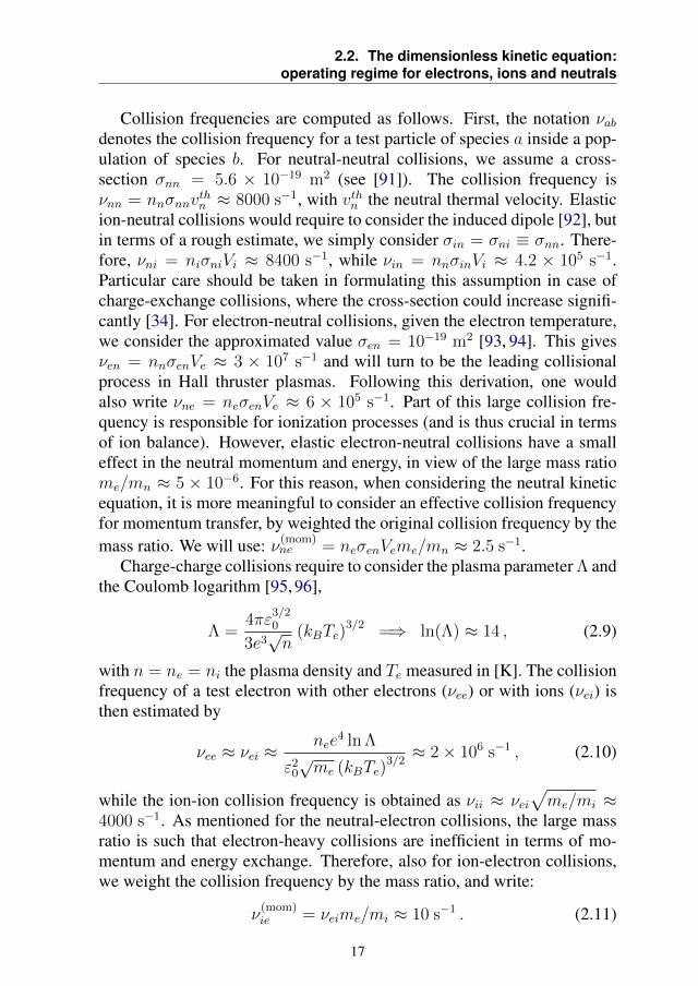
Collision frequencies are computed as follows. First, the notation νabdenotes the collision frequency for a test particle of species a inside a pop-ulation of species b. For neutral-neutral collisions, we assume a cross-section σnn = 5.6 × 10⁻¹⁹ m2 (see [91]). The collision frequency isνnn = nnσnnv
thn ≈ 8000 s−1, with vthn the neutral thermal velocity. Elastic
ion-neutral collisions would require to consider the induced dipole [92], butin terms of a rough estimate, we simply consider σin = σni ≡ σnn. There-fore, νni = niσniVi ≈ 8400 s−1, while νin = nnσinVi ≈ 4.2 × 10⁵ s−1.Particular care should be taken in formulating this assumption in case ofcharge-exchange collisions, where the cross-section could increase signifi-cantly [34]. For electron-neutral collisions, given the electron temperature,we consider the approximated value σen = 10−19 m2 [93, 94]. This givesνen = nnσenVe ≈ 3 × 10⁷ s−1 and will turn to be the leading collisionalprocess in Hall thruster plasmas. Following this derivation, one wouldalso write νne = neσenVe ≈ 6 × 10⁵ s−1. Part of this large collision fre-quency is responsible for ionization processes (and is thus crucial in termsof ion balance). However, elastic electron-neutral collisions have a smalleffect in the neutral momentum and energy, in view of the large mass ratiome/mn ≈ 5 × 10⁻⁶. For this reason, when considering the neutral kineticequation, it is more meaningful to consider an effective collision frequencyfor momentum transfer, by weighted the original collision frequency by themass ratio. We will use: ν(mom)
ne = neσenVeme/mn ≈ 2.5 s−1.Charge-charge collisions require to consider the plasma parameter Λ and
the Coulomb logarithm [95, 96],
Λ =4πε
3/20
3e3√n
(kBTe)3/2 =⇒ ln(Λ) ≈ 14 , (2.9)
with n = ne = ni the plasma density and Te measured in [K]. The collisionfrequency of a test electron with other electrons (νee) or with ions (νei) isthen estimated by
νee ≈ νei ≈nee
4 ln Λ
ε20
√me (kBTe)
3/2≈ 2× 10⁶ s−1 , (2.10)
while the ion-ion collision frequency is obtained as νii ≈ νei√me/mi ≈
4000 s−1. As mentioned for the neutral-electron collisions, the large massratio is such that electron-heavy collisions are inefficient in terms of mo-mentum and energy exchange. Therefore, also for ion-electron collisions,we weight the collision frequency by the mass ratio, and write:
ν(mom)ie = νeime/mi ≈ 10 s−1 . (2.11)
17
Chapter 2. Kinetic and fluid modeling of gases and plasmas
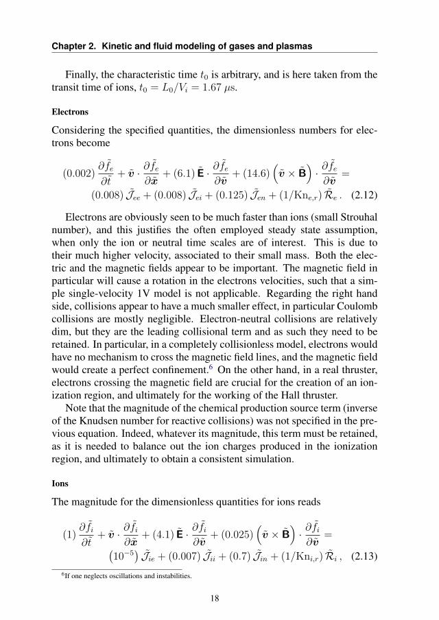
Finally, the characteristic time t0 is arbitrary, and is here taken from thetransit time of ions, t0 = L0/Vi = 1.67 µs.
Electrons
Considering the specified quantities, the dimensionless numbers for elec-trons become
(0.002)∂fe
∂t+ v · ∂fe
∂x+ (6.1) E · ∂fe
∂v+ (14.6)
(v × B
)· ∂fe∂v
=
(0.008) Jee + (0.008) Jei + (0.125) Jen + (1/Kne,r) Re . (2.12)
Electrons are obviously seen to be much faster than ions (small Strouhalnumber), and this justifies the often employed steady state assumption,when only the ion or neutral time scales are of interest. This is due totheir much higher velocity, associated to their small mass. Both the elec-tric and the magnetic fields appear to be important. The magnetic field inparticular will cause a rotation in the electrons velocities, such that a sim-ple single-velocity 1V model is not applicable. Regarding the right handside, collisions appear to have a much smaller effect, in particular Coulombcollisions are mostly negligible. Electron-neutral collisions are relativelydim, but they are the leading collisional term and as such they need to beretained. In particular, in a completely collisionless model, electrons wouldhave no mechanism to cross the magnetic field lines, and the magnetic fieldwould create a perfect confinement.6 On the other hand, in a real thruster,electrons crossing the magnetic field are crucial for the creation of an ion-ization region, and ultimately for the working of the Hall thruster.
Note that the magnitude of the chemical production source term (inverseof the Knudsen number for reactive collisions) was not specified in the pre-vious equation. Indeed, whatever its magnitude, this term must be retained,as it is needed to balance out the ion charges produced in the ionizationregion, and ultimately to obtain a consistent simulation.
Ions
The magnitude for the dimensionless quantities for ions reads
(1)∂fi
∂t+ v · ∂fi
∂x+ (4.1) E · ∂fi
∂v+ (0.025)
(v × B
)· ∂fi∂v
=(10−5
)Jie + (0.007) Jii + (0.7) Jin + (1/Kni,r) Ri , (2.13)
6If one neglects oscillations and instabilities.
18
2.2. The dimensionless kinetic equation:operating regime for electrons, ions and neutrals
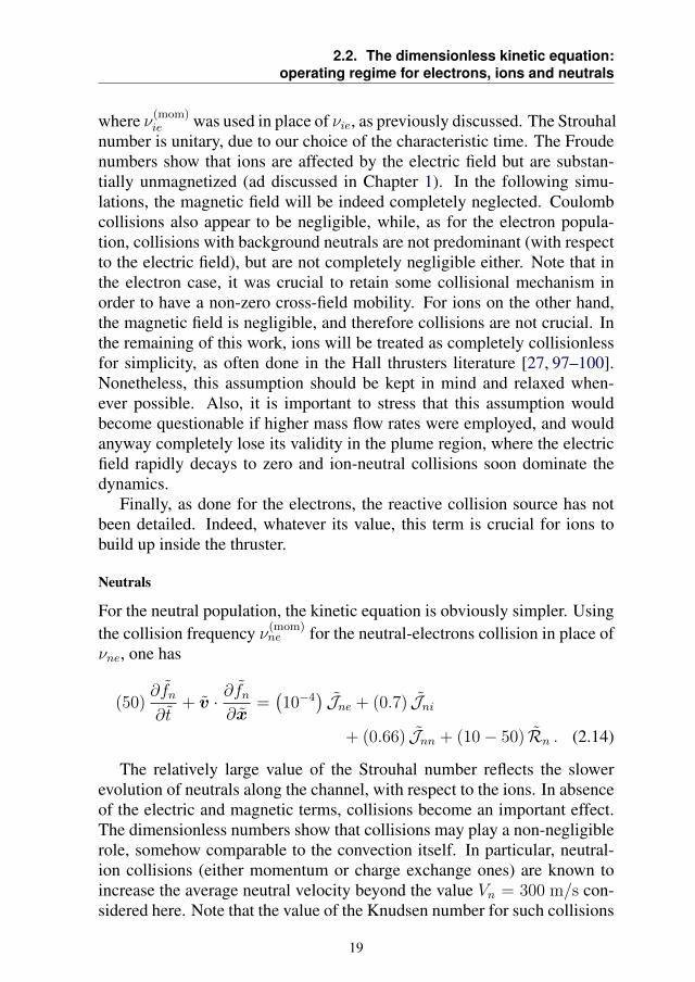
where ν(mom)ie was used in place of νie, as previously discussed. The Strouhal
number is unitary, due to our choice of the characteristic time. The Froudenumbers show that ions are affected by the electric field but are substan-tially unmagnetized (ad discussed in Chapter 1). In the following simu-lations, the magnetic field will be indeed completely neglected. Coulombcollisions also appear to be negligible, while, as for the electron popula-tion, collisions with background neutrals are not predominant (with respectto the electric field), but are not completely negligible either. Note that inthe electron case, it was crucial to retain some collisional mechanism inorder to have a non-zero cross-field mobility. For ions on the other hand,the magnetic field is negligible, and therefore collisions are not crucial. Inthe remaining of this work, ions will be treated as completely collisionlessfor simplicity, as often done in the Hall thrusters literature [27, 97–100].Nonetheless, this assumption should be kept in mind and relaxed when-ever possible. Also, it is important to stress that this assumption wouldbecome questionable if higher mass flow rates were employed, and wouldanyway completely lose its validity in the plume region, where the electricfield rapidly decays to zero and ion-neutral collisions soon dominate thedynamics.
Finally, as done for the electrons, the reactive collision source has notbeen detailed. Indeed, whatever its value, this term is crucial for ions tobuild up inside the thruster.
Neutrals
For the neutral population, the kinetic equation is obviously simpler. Usingthe collision frequency ν(mom)
ne for the neutral-electrons collision in place ofνne, one has
(50)∂fn
∂t+ v · ∂fn
∂x=(10−4
)Jne + (0.7) Jni
+ (0.66) Jnn + (10− 50) Rn . (2.14)
The relatively large value of the Strouhal number reflects the slowerevolution of neutrals along the channel, with respect to the ions. In absenceof the electric and magnetic terms, collisions become an important effect.The dimensionless numbers show that collisions may play a non-negligiblerole, somehow comparable to the convection itself. In particular, neutral-ion collisions (either momentum or charge exchange ones) are known toincrease the average neutral velocity beyond the value Vn = 300 m/s con-sidered here. Note that the value of the Knudsen number for such collisions
19
Chapter 2. Kinetic and fluid modeling of gases and plasmas
is slightly larger than one, meaning that the flow is significantly rarefied. Insuch conditions, gas-surface interactions are likely to play an equally im-portant role, depending on the surface-to-volume ratio.7
Differently than for electrons and ions, the value of the Knudsen numberfor neutral ionization has been also given in the previous equation, basedon the ionization frequency νiz = neσizVe ≈ 6× 10⁵ s−1. Using the wholechannel length results in an inverse Knudsen number of 50, while a morereasonable estimate would consider that ionization happens mostly insidethe ionization region, whose length is approximately 5 mm [90]. This givesa somewhat lower estimate of 10. These high values are expected, as theyconfirm that the thruster is indeed effectively ionizing the propellant.
2.3 Fluid formulations: moments of the kinetic equation
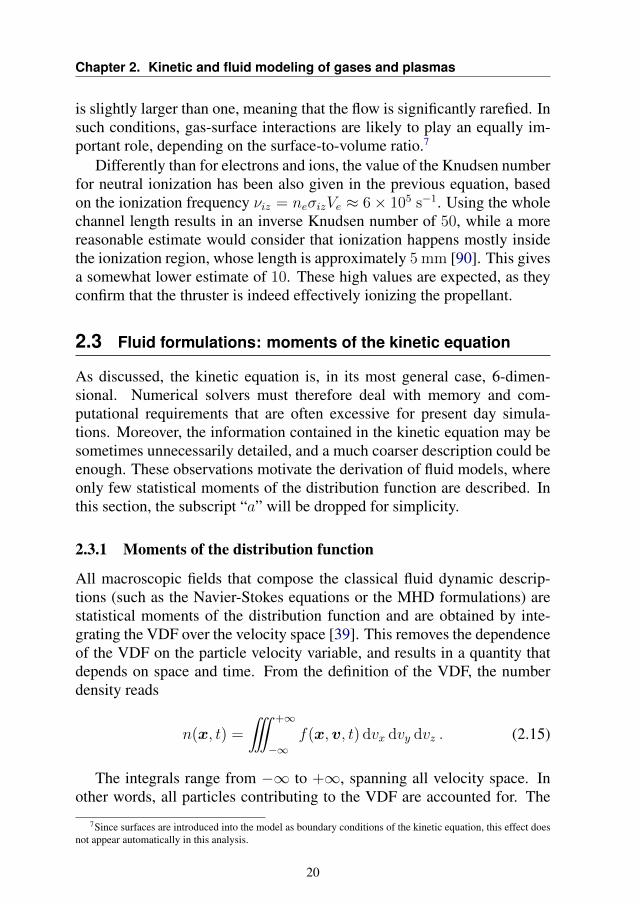
As discussed, the kinetic equation is, in its most general case, 6-dimen-sional. Numerical solvers must therefore deal with memory and com-putational requirements that are often excessive for present day simula-tions. Moreover, the information contained in the kinetic equation may besometimes unnecessarily detailed, and a much coarser description could beenough. These observations motivate the derivation of fluid models, whereonly few statistical moments of the distribution function are described. Inthis section, the subscript “a” will be dropped for simplicity.
2.3.1 Moments of the distribution function
All macroscopic fields that compose the classical fluid dynamic descrip-tions (such as the Navier-Stokes equations or the MHD formulations) arestatistical moments of the distribution function and are obtained by inte-grating the VDF over the velocity space [39]. This removes the dependenceof the VDF on the particle velocity variable, and results in a quantity thatdepends on space and time. From the definition of the VDF, the numberdensity reads
n(x, t) =
˚ +∞
−∞f(x,v, t) dvx dvy dvz . (2.15)
The integrals range from −∞ to +∞, spanning all velocity space. Inother words, all particles contributing to the VDF are accounted for. The
7Since surfaces are introduced into the model as boundary conditions of the kinetic equation, this effect doesnot appear automatically in this analysis.
20
2.3. Fluid formulations: moments of the kinetic equation
mass density is ρ = mn. The (average) momentum is obtained by weight-ing the VDF by the particle momentum,
ρ(x, t)ui(x, t) =
˚ +∞
−∞mvif(x,v, t) dvx dvy dvz . (2.16)
By computing moments of the distribution function about the average ve-locity ui, one obtains central moments. These moments do not depend any-more on the velocity, but instead describe the purely thermodynamic stateof the gas, and allow us to identify non-equilibrium. The pressure tensorcomponents are second order central moments, defined as
Pij(x, t) =
˚ +∞
−∞m(vi − ui)(vj − uj)f(x,v, t) dvx dvy dvz . (2.17)
Where the hydrostatic pressure is P = (Pxx+Pyy+Pzz)/3. In this work,we will consider perfect gases, such that P = nkBT . Note that a separatetemperature can be defined for each axis, such that Pxx ≡ Px = nkBTx,and the same for the y and z components. From the kinetic definition, it isclear that the temperatures give an indication of the width of the distributionfunction along the three velocity axes. Using the same notation, the energyof a particle with three translational degrees of freedom would read
ρ(x, t)E(x, t) =ρu2
2+
3
2nkBT =
˚ +∞
−∞
mv2
2f(x,v, t) dvx dvy dvz .
(2.18)The heat flux vector is an order-3 central moment and is here defined as
qi(x, t) =
˚ +∞
−∞mc2 ci f(x,v, t) dvx dvy dvz . (2.19)
where the peculiar velocity ci = vi − ui was defined. Note that in muchof the literature, the heat flux definition embeds a factor 1/2. Unless spec-ified otherwise, in this work we employ the definition of Eq. (2.19) to beconsistent with the definitions that will follow. Being an odd-order centralmoment, the heat flux indicates the skewness of the VDF, and being pro-portional to the cube of the peculiar velocity, it is particularly sensitive tothe tails of the VDF. The mentioned moments are employed in most fluiddynamic descriptions. However, there is no limit in the number of mo-ments that can be computed. In particular, in the present work we will needmoments up to an order 5 of the velocity, that we define in the following.
21
Chapter 2. Kinetic and fluid modeling of gases and plasmas
After having defined the heat flux vector, a heat flux tensor can also beintroduced,
Qijk(x, t) =
˚ +∞
−∞mci cj ck f(x,v, t) dvx dvy dvz . (2.20)
Clearly, qi can be obtained from the contractions of Qijk. Denoting a sum-mation by repeated indices, we use the notation:
qi = Qi ≡ Qijj . (2.21)
A rank 2 tensor is then defined for the order-4 moment, Rijkk,
Rijkk(x, t) =
˚ +∞
−∞mci cj c
2 f(x,v, t) dvx dvy dvz , (2.22)
and its contraction Riijj = Rxxkk +Ryykk +Rzzkk,
Riijj(x, t) =
˚ +∞
−∞mc4 f(x,v, t) dvx dvy dvz , (2.23)
At equilibrium, when the VDF is Maxwellian, this moment can be shownto take the valueRiijj = 15P 2/ρ. This moment is connected to the kurtosisof the VDF. Finally, a vector containing order-5 moments is also defined as
Sijjkk(x, t) =
˚ +∞
−∞mcic
4 f(x,v, t) dvx dvy dvz . (2.24)
The moments described in the previous equations are a total of 29 inde-pendent scalar quantities: the density, 3 velocity components, 6 entries forthe pressure tensor, 10 for Qijk, 6 for Rijkk and 3 for Sijjkk. No further mo-ments will be needed in the present work, except for their contractions. Itshould be noted that all odd-order central moments are zero for symmetricVDFs.
Moments of the 1V distribution function
In case the kinetic equation is formulated as to describe one only compo-nent of the particle velocity (“1-dimensional physics”), the moments of the1V VDF are obtained as a single integral. The 29 independent momentsreduce to a small set of 5 moments, defined as
ρ =´ +∞−∞ mf(v) dv , (2.25a)
ρu =´ +∞−∞ mv f(v) dv , (2.25b)
22
2.3. Fluid formulations: moments of the kinetic equation
P =´ +∞−∞ m (v − u)2 f(v) dv , (2.25c)
Q =´ +∞−∞ m (v − u)3 f(v) dv , (2.25d)
r =´ +∞−∞ m (v − u)4 f(v) dv , (2.25e)
s =´ +∞−∞ m (v − u)5 f(v) dv . (2.25f)
Dimensionless moments
As seen, all moments are proportional to the particle mass and to an in-creasing power of the velocity. An effective adimensionalization can thusbe performed by dividing the moments by ρ and by a power of the quantity√P/ρ, that is fundamentally a thermal velocity. By doing this non-dimen-
sionalization on the density, momentum and hydrostatic pressure, we find
ρ? = 1 , u?i = ui/√P/ρ , P ? = 1 , (2.26)
while the dimensionless central moments read
P ?ij = Pij/
[ρ (P/ρ)2/2
], (2.27a)
Q?ijk = Qijk/
[ρ (P/ρ)3/2
], (2.27b)
R?ijkk = Rijkk/
[ρ (P/ρ)4/2
], (2.27c)
S?ijjkk = Siijkk/[ρ (P/ρ)5/2
], (2.27d)
The contractions q?i and R?iijj are obtained in the same way.
2.3.2 The generalized moment equation
The moments definition can be generalized by denoting the particle quanti-ties by ψ, and computing the moment of the VDF weighted by ψ as
Mψ =
˚ +∞
−∞ψ(v)f(x,v, t) dv ≡ 〈ψ(v)〉 . (2.28)
Considering that f(x,v, t) = n g(x,v, t), with n the number density and gthe normalized distribution function, the moment Mψ represents the aver-aged value of ψ(v) over the normalized distribution of particle velocities,further scaled by the number density. For example, the choice ψ = mwould result in the mass density, while ψ = mvx would result in the aver-age momentum along x. By multiplying by ψ the whole kinetic equation
23
Chapter 2. Kinetic and fluid modeling of gases and plasmas
and then applying the average operator, one obtains a governing equationfor the moment Mψ, reading [39]
∂ 〈ψ〉∂t
+∂
∂x· 〈v ψ〉 =
q
m
⟨(E + v × B) · ∂ψ
∂v
⟩+
˚ψ C dv . (2.29)
This equation has an important characteristic: while writing it for a mo-ment Mψ = 〈ψ〉 of a given order n, the convective fluxes 〈vψ〉 introducea moment of order n + 1 in the velocity. This requires that one also writesan equation for the moment n + 1, that in turn will require the moment oforder n + 2. The resulting system is not closed, and an infinite number ofmoment equations would be required to recover the kinetic equation. Prac-tically speaking, one truncates the series at a certain point, or followingcertain assumptions. The set of equations resulting from such choice willbe denoted by “moment method” and in conservative form are written as
∂U
∂t+
∂
∂x· [Fx,Fy,Fz] = GEB +Gc , (2.30)
where U is the vector of moments, Fi are the vectors of convective fluxes,with i = x, y, z andGEB andGc the electromagnetic and collisional sourceterms respectively.
2.3.3 Pressureless gas, Euler equations and moment methods
As seen in the previous section, the choice of a set of particle quantities ψresults in a set of governing equations for the respective moments, that canbe closed by formulating some assumption. We shall illustrate here twonoteworthy examples, namely the pressureless gas system and the Eulerequations. More general strategies will be then introduced.
The pressureless gas formulation
The simplest formulation can be obtained by writing a governing equationfor the particle mass, choosing ψ = m, and three equations for the particlemomentum, obtained from ψ = mvi. The higher order moments (thatrequire a closure) are the pressure terms Pij . In the limiting case of a gaswhere the convective fluxes are much larger than the thermal ones, one maydecide to neglect these contributions.8 The resulting system is known as thepressureless gas formulation (sometimes called “cold gas”), and correspondto prescribing that the VDF is a Dirac delta in velocity space, centered on
8This can be an effective choice in some situations, but results in discontinuities known as δ-shocks.
24
2.3. Fluid formulations: moments of the kinetic equation
the bulk velocity. The set of equations (2.30) is defined by
U =
ρ
ρux
ρuy
ρuz
, Fi =
ρui
ρuiux
ρuiuy
ρuiuz
, GEB =ρ q
m
0
Ex + uyBz − uzByEy + uzBx − uxBzEz + uxBy − uyBx
,
(2.31)
where the x,y and z convective fluxes are obtained by choosing i = x, y, z.The formulation of the collisional source term Gc depends on the specificcase and the type of collisions to be considered. The pressureless gas sys-tem will be employed for the description of ions in Section 6.6.
The Euler equations of gas dynamics
The choice ψ = m(1, vi, v2/2) extends the previous description, by also
considering the energy of the particle. This results in the Euler equationsof gas dynamics, where the chosen closure consists in assuming that higherorder moments are zero (the heat flux qi in this case) and that the pressuretensor is isotropic. The equations read
U =
ρ
ρux
ρuy
ρuz12ρu2 + 1
γ−1P
, Fi =
ρui
ρuiux + Pδxi
ρuiuy + Pδyi
ρuiuz + Pδzi12ρu2ui + γ
γ−1Pui
, (2.32)
where δij is the Kronecker delta, and γ is the specific heats ratio (adiabaticconstant), with N/2 = 1/(γ − 1), where N is the number of degrees offreedom (DOF) for the considered species. Particles that show only threeDOFs (no internal energy) have N = 3, and therefore γ = 5/3. In thecase of a gas described by one single degree of freedom, only a singlecomponent of velocity should be retained (say, vx) and the other momentsare to be discarded. The adiabatic constant is then obtained from the choiceN = 1, resulting in γ = 3.
The electromagnetic source term for the Euler equations is easily ob-
25
Chapter 2. Kinetic and fluid modeling of gases and plasmas
tained as
GEB =ρ q
m
0
Ex + uyBz − uzByEy + uzBx − uxBzEz + uxBy − uyBxExux + Eyuy + Ezuz
. (2.33)
Also in this case, the collision termsGc depend on the process and speciesto be considered and will not be detailed here.
At a kinetic level, the aforementioned closure assumptions correspondto prescribing that the VDF is symmetric. The Maxwellian is a particularcase of a symmetric VDF, that further results in a zero collisional sourceterm, for what concerns collisions between particles of the same species.Other collisions terms may still be non-zero.9
Moment methods, the Chapman-Enskog expansion and the Grad closure
Strictly speaking, the term “moment methods” refers to modeling the prob-lem by a system of moment equations, closed by some assumption.10 Thepressureless gas system and the Euler systems are two simple examples of(rather low order) moment methods, and they were obtained by an intuitivechoice of the particle quantities ψ. A number of general formulations havebeen proposed in the years, with varying degree of success and generality,and we shall discuss here some of them.
The Chapman-Enskog expansion [101] is a common strategy to find aclosure to the moment equations, and consists in expanding the VDF inpowers of a small parameter ε (proportional to the inverse of the Knudsennumber),
f = f (0) + εf (1) + ε2f (2) + · · · , (2.34)
where f (0) is the local Maxwellian and the other terms are corrections ofprogressively higher order. The choice of the maximum order of ε to beretained results in a set of governing equations of increasing complexity.For a Maximum order ε0, one retrieves the Euler equations. At the order ε1
on the other hand, the Navier-Stokes-Fourier equations are retrieved. At ahigher order, one obtains the Burnett [102] and super-Burnett systems, thatare however unstable to certain wavelengths [62] and are not well behavedin terms of entropy production [103]. Various corrections to these prob-lems have been proposed through the years (see for example [104]). Also,
9For example, electron collisions with background neutrals.10Traditionally, in the fluid dynamic community, moment methods are refer to systems at least one order higher
than the Euler/NSF equations, thus writing governing equations for moments of higher order than the energy.
26
2.3. Fluid formulations: moments of the kinetic equation
detailed studies have been performed on the Chapman-Enskog method,extending it towards multi-component plasmas, and including multiscaleanalyses of the streaming and collision terms [105]. However, the behaviorof the Burnett and super-Burnett systems shows that the Chapman-Enskogclosure works well only for moderate deviations from equilibrium, and adifferent formulation is in order if one wishes to reach higher orders.
Another general approach towards obtaining a closed set of momentequations is the Grad method [63], that consists in expanding the VDFin a series of N-dimensional Hermite polynomials of the velocity H(n)(v),weighted by a set of coefficients a(n),
f = f0
(1 + a
(1)i H
(1)i +
1
2a
(2)ij H
(2)ij + ...+
1
N !a
(N)ij...qH
(N)ij...q
)(2.35)
where f0 is again the local Maxwellian. The moment equations are closedby truncating such series, putting all coefficients a(n) above a certain or-der equal to zero. This formulation has been broadly employed in plasmaphysics, see for example the classical works of Zhdanov [40], Balescu [106]and Braginskii [107], where the 13, 21 and 29-moment approximations arediscussed. The Grad formulation has an important advantage, namely themoments of the distribution function f are directly mapped to the coeffi-cients a(n). In terms of its drawbacks, it is important to notice that in orderto retrieve strong non-equilibrium conditions, it has been shown that thenumber of required moments may be rather large [108, 109], with a signif-icant increase in the computational complexity. Also, the Grad closure isknown to suffer from a limited region of hyperbolicity [110], such that theeigenvalues of the fluxes Jacobian may develop an imaginary part. Finally,for strong non-equilibrium situations, the Grad method does not guaran-tee that the VDF remain positive, and the method may generate unphysicalsubshocks beyond a certain Mach number [62], thus requiring a regulariza-tion [111, 112].
A number of other formulations have been developed in the years (seefor example the Quadrature Moments [113, 114] or the Pearson Distribu-tion [68,115] formulations). Among all possible formulations, we shall fo-cus on the “maximum-entropy” family of moment methods, whose order-4member will be investigated in this work.
27
Chapter 2. Kinetic and fluid modeling of gases and plasmas
2.4 The maximum-entropy closure
This section introduces the maximum-entropy family of moment methods,that will be central in this work. For a complete introduction to the method,the reader is referred to [64, 65, 116], and for an application to differentproblems including microfluidics and radiation transport, [117–122].
The idea behind the maximum-entropy method is the following: for agiven state of the gas, described by a finite set of moments U , an infinitenumber of possible distribution functions exist; among these, the maxi-mum-entropy method considers the distribution that maximises the entropyof the system, σ = f log f . In a statistical sense, this corresponds to select-ing the most probable distribution, given the limited amount of informationabout its moments U . The resulting VDF takes the form of an exponentialof a polynomial of the particle velocity,
f = exp[αTΨ(v)
], (2.36)
where Ψ is a vector of monomials of the particle velocity v (where themaximum power of v defines the order of the approximation), while α isthe vector of the corresponding weights. Provided that the order of thehighest-power velocity monomial inside Ψ is even, and that the respectivecoefficient is negative, the maximum-entropy VDF is bounded. Also, it isalways positive (since the exponential of a real number is positive), which isa strong advantage over the Grad system, especially if strong non-equilib-rium conditions are targeted. Moreover, the resulting system of governingequations for the moments can be shown to be hyperbolic whenever theunderlying entropy maximisation problem is solvable.
In order to ensure that the moments of the distribution function f areequal to U , one writes the condition:
U −˚ +∞
−∞Ψ exp
[αTΨ
]dv = 0 . (2.37)
Since the maximum-entropy distribution has been employed, this is knownas the “entropy-maximisation problem”, where one aims at finding the vec-tor of coefficients α that realize such condition. Practically speaking, oneoften solves a slightly different problem: after the vector Ψ has been de-fined, the functional J is maximised for a set of target moments U , whereJ is defined as
J =
˚ +∞
−∞exp
[αTΨ
]dv −αTU , (2.38)
28
2.4. The maximum-entropy closure
where the condition of zero gradient ∂J/∂α = 0 retrieves Eq. (2.37). Afterthis problem is solved, the maximum-entropy distribution f is fully de-fined, and the closing moments appearing in the moment equations can beobtained by integration.
Besides the mentioned advantages, this method also has a number ofdrawbacks. In particular, the entropy maximisation problem proves to benon-trivial for the methods above order 2. This requires to employ com-putationally expensive numerical solutions. Also, for orders above 2, themaximum-entropy method happens to embed a region of non-realizabilityin the moment space, referred to as the Junk subspace [66, 123], such thatsome states that would be physically realizable (as defined from the solu-tion to the Hamburger problem [124]) cannot be properly reproduced by aVDF in the form of Eq. (2.36). This region, associated to a singularity in thefluxes, reaches the equilibrium point. As will be discussed in Section 4.2,the wave speeds may grow unbounded as the singularity is approached, andsome additional care is required in the numerical solution.
Order-2 maximum-entropy method: the Euler equations
As a first example, we shall analyze the choice Ψ = (1, vi, v2), with i =
x, y, z. This gives an order-2 method, from the maximum power appear-ing in Ψ. The corresponding maximum-entropy VDF happens to be aMaxwellian, that is thus a particular case of this formulation,
f = exp(α0 + αivi + α2v2) ≡ A exp
[B(vi − ui)2
]. (2.39)
For this system, the entropy maximisation problem of Eq. (2.37) is triv-ial. Indeed the coefficients α0, αi, α2 are easily mapped to the momentsof the Maxwellian VDF, observing that A = n(m/2πkBT )3/2 and B =−m/2kBT , and the α coefficients are therefore obtained. All closing mo-ments will be zero, since this VDF is symmetric, and one finally obtainsthe Euler equations of gas dynamics.
Order-2 maximum-entropy method: the anisotropic Euler equations
The Maxwellian case is not the only order-2 member of the family of max-imum-entropy methods. A more general choice would be Ψ = (1, vi, vivj),that has 10 independent entries. The resulting maximum-entropy VDF is
f = exp(α0 + αivi + αijvivj) ≡ A exp
[∑i
Bi(vi − ui)2
], (2.40)
29
Chapter 2. Kinetic and fluid modeling of gases and plasmas
that is an anisotropic Gaussian. Also for this system, the vector of coeffi-cients α is easily mapped to the moments of the VDF. This choice resultsin a system composed by 10 governing equations, that can represent tem-perature anisotropy, but still assume a symmetric VDF, thus resulting in azero heat flux.
2.4.1 Order-4 maximum-entropy method: 14-moment system
The next level after the order-2 methods, are the order-4 maximum-entropysystems.11 A number of different choices are possible for the vector Ψ, butthe simplest is [64]
Ψ =(1, vi, vivj, viv
2, v4), (2.41)
that has 14 different entries and will result in a 14-moment system. Themaximum-entropy VDF reads
f14 = exp(α0 + αivi + αijvivj + αi,3viv2 + α4v
4) . (2.42)
Despite being the simplest member of the order-4 maximum-entropy meth-ods, this VDF is very flexible. For example, this VDF includes as limingcases the Maxwellian and the Gaussian distributions. Moreover, if all co-efficients except α4 are zero, it can be seen to retrieve the Druyvestein dis-tribution [2, 125]. This VDF can be both asymmetrical (thus allowing foran heat flux) and anisotropic, and by effect of α4 it can reproduce ring-likedistributions. The resulting system of moment equations reads, in indexform,
∂∂tρ+ ∂
∂xi(ρui) = G1 , (2.43a)
∂∂t
(ρui) + ∂∂xj
(ρuiuj + Pij) = G2,3,4 , (2.43b)
∂∂t
(ρuiuj + Pij) + ∂∂xk
(ρuiujuk + uiPjk + ujPik
+ukPij +Qijk) = G5−10 , (2.43c)
∂∂t
(ρuiujuj + uiPjj + 2ujPij +Qijj)
+ ∂∂xk
(ρuiukujuj + uiukPjj + 2uiujPjk + 2ujukPij + ujujPik
+uiQkjj + ukQijj + 2ujQijk +Rikjj) = G11,12,13 , (2.43d)11As mentioned, no order-3 closure exist, as this would generate an unbounded maximum-entropy VDF.
30
2.4. The maximum-entropy closure
∂∂t
(ρuiuiujuj + 2uiuiPjj + 4uiujPij + 4uiQijj +Riijj)
+ ∂∂xk
(ρukuiuiujuj + 2ukuiuiPjj + 4uiuiujPjk + 4uiujukPij + 2uiuiQkjj
+4uiukQijj + 4uiujQijk + 4uiRikjj + ukRiijj + Skiijj) = G14 , (2.43e)
where the heat flux vector is denoted by Qijj , and represents the contrac-tion over Qijk terms. The source terms G at the right hand side includeboth electromagnetic and collisional contributions. The collisional sourcesdepend on the considered species (for a single species BGK collision oper-ator, the reader is referred to [67, 126]). The electromagnetic sources willbe developed in Section 4.5.
A solution of this system requires to specify the closing moments Qijk,Rijkk and Sijjkk. These moments could be computed from the VDF, thatin turn is obtained by solving the entropy-maximisation problem. Unfor-tunately, this problem happens to be rather complex for the 14-momentformulation, and no algebraic solution is known. Therefore, in order to findthe f14 VDF from a set of target moments (and therefore, to compute theclosing terms of the moment system), one has to solve the problem numer-ically, often done by employing iterative methods. During a simulation,such procedure needs to be done at each time step and for each cell in thedomain, dramatically increasing the computational time, up to the pointthat the method may be no longer convenient with respect to a fully kineticmethod.
Luckily, some interpolative approximations to the entropy maximisationproblem have been developed for the 14-moment system, allowing for af-fordable CFD computations [67]. These formulations bypass the entropymaximisation problem and directly give the closing moments as a functionof the moments U . For all details, the reader is referred to the originalpaper, and only the main ingredients will be illustrated here. The closurestarts from the definition of a parabolic mapping of moment space, intro-ducing a parameter σ that assumes a value σ → 0 in correspondence ofthe Junk subspace (and thus, also the equilibrium point) and σ = 1 at thephysical realizability boundary:
σ =1
4PijPji
[2PijPji + PiiPjj − ρRiijj
+
√(2PijPji + PiiPjj − ρRiijj)
2 + 8ρPmnPnmQkii (P−1)klQljj
].
(2.44)
31
Chapter 2. Kinetic and fluid modeling of gases and plasmas
The closing moments are then written as
Rijkk =1
σQijl
(P−1
)lmQmkk +
2(1− σ)PikPkj + PijPkkρ
, (2.45)
with the elements of the heat flux tensor defined by
Qijk = KijkmQmnn , (2.46)
where the matrix Kijkm is defined as
Kijkm =[2Pil(P
2)jk + 2Pkl(P2)ij + 2Pjl(P
2)ik]B−1lm , (2.47)
and with the matrix Blm defined as
Blm = 2Plm(P 2)αα + 4(P 3)lm . (2.48)
The remaining moments Sijjkk read
Sijjkk =1
σ2P−1kn P
−1lm QnppQmjjQikl+2σ1/2PjjQikk
ρ+(1−σ1/2)WimQmnn ,
(2.49)Note that in this expression a power of σ equal to 1/2 is used, differentlyfrom the original paper where a coefficient 3/5 was employed, as it hasbeen later shown to provide better results. The matrixWim appearing in theexpression is defined as
Wim =1
ρ
[2Pil(Pαα)3 + 12Pil(P
3)αα + 14(P 2)αα(P 2)il + 20Pαα(P 3)il
+20(P 4)il − 2(P 2)ααPββPil − 6(Pαα)2(P 2)il]B−1lm . (2.50)
It is important to notice that the presented interpolative closure is notentirely hyperbolic, and the eigenvalues may show some slight imaginarypart in some regions of the moment space (see Appendix C). This does notbring particular issues into the computation. Also, it should be noted thatdifferent interpolative closures have been developed in other references (see[127]), providing an interpolation of increased accuracy in certain regionsof the moment space. These will not be considered in the present work.
Finally, we shall report here the expressions of the physical realizabilityboundary and of the Junk subspace. The former is obtained by the solutionof the Hamburger problem and reads
Riijj ≥(Qkii
(P−1
)klQljj + PiiPjj
)/ρ , (2.51)
32
2.4. The maximum-entropy closure
and this is retrieved by σ = 1 in the parabolic mapping. On the other hand,for σ → 0 the mapping retrieves the Junk subspace, whose moments cannotbe described by the assumed shape of the VDF. The Junk subspace reads
Qi = 0 and Riijj > (2PjiPij + PiiPjj) /ρ . (2.52)
In the discussion of the 5-moment system, these boundaries will simplify,and a graphical interpretation will be shown. Since the Junk subspace isassociated to a singularity, where the wave speeds grow unbounded, a lowerlimiting value is imposed to σ in numerical calculations. This value isoften in the range of σmin ≈ 10−3 − 10−5, and will be discussed further inSection 4.3.
2.4.2 Order-4 maximum-entropy method: 5-moment system
A special case of the 14-moment system can be obtained in the limit of“1D thermodynamics”, where the particle motion is constrained along onesingle axis. This corresponds to the 1V kinetics considered in Section 2.1.Considering that particles have a single translational degree of freedom,the 14-moment formulation simplifies to a system of 5 equations. Denotingby v the only nonzero velocity component, the 5-moment description isobtained by the choice Ψ = m(1, v, v2, v3, v4). Notice that this descriptionis still of order 4. The resulting 1V distribution function is
f5 = exp(α0 + α1v + α2v2 + α3v
3 + α4v4) . (2.53)
Also in this case, the VDF is seen to be always positive, and is boundedprovided that α4 < 0. The resulting moment system reads
∂ρ
∂t+
∂
∂x(ρu) = G1 , (2.54a)
∂
∂t(ρu) +
∂
∂x
(ρu2 + P
)= G2 , (2.54b)
∂
∂t
(ρu2 + P
)+
∂
∂x
(ρu3 + 3uP +Q
)= G3 , (2.54c)
∂
∂t
(ρu3 + 3uP +Q
)+
∂
∂x
(ρu4 + 6u2P + 4uQ+ r
)= G4 , (2.54d)
∂
∂t
(ρu4 + 6u2P + 4uQ+ r
)+
∂
∂x
(ρu5 + 10u3P + 10u2Q
+5ur + s) = G5 . (2.54e)
33
Chapter 2. Kinetic and fluid modeling of gases and plasmas
As for the 14-moment case, the collisional source terms depend on thespecies considered and will be covered in the relevant sections, while theelectromagnetic sources will be developed in Section 4.5. Note that the 5-moment formulation could also be obtained from the 14-moment system,in the limit of a zero temperature and zero bulk velocity in two out of thethree space directions.
The 5-moment system has the same issues of the 14-moment systemin terms of absence of an algebraic solution to the entropy maximisationproblem. Clearly, as the system is much smaller, a numerical solution willbe much less demanding. Nonetheless, in this work we will employ theinterpolative closure developed in [67]. The first step consists in non-di-mensionalizing the variables, scaling them by ρ and a power of the thermalvelocity
√P/ρ, as done in Section 2.3.1 (subscript ?). The parameter σ is
then defined as
σ =3− r? +
√(3− r?)2 + 8Q2
?
4. (2.55)
and the only required closing moment is
s? =Q3?
σ2+ (10− 8σ1/2)Q? . (2.56)
The expression for the physical realizability boundary and the Junk sub-space are much simpler for the 5-moment problem. Physical realizabilityis satisfied by
r? ≥ Q2? + 1 (2.57)
while the Junk subspace corresponds to the line
Q? = 0 and r? > 3 , (2.58)
where (q?, r?) = (0, 3) represents equilibrium, that happens to be located atone extreme of the Junk line. These boundaries are represented in Fig. 2.1.In this work, the solution to the 5-moment system will often be representedin the (Q?, r?) plane, that will simply be referred to as “moment space”.This is indeed a convenient way to graphically represent how the solutionevolves with respect to equilibrium.
2.5 Conclusions
This chapter has introduced some common governing equations that al-lows to model rarefied gases and plasmas from the kinetic to the contin-uum regime, together with the assumptions upon which they are built. The
34
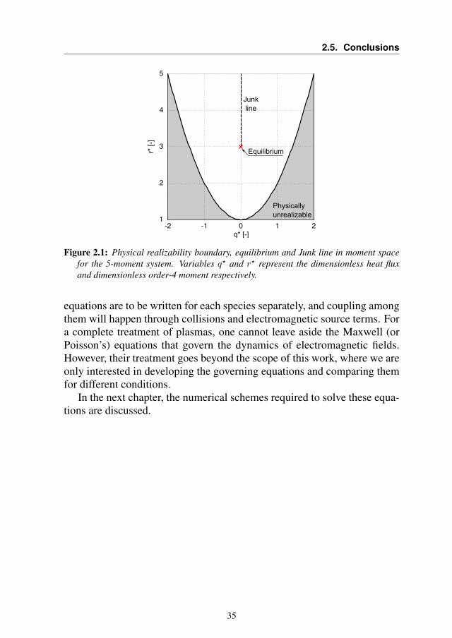
2.5. Conclusions
Figure 2.1: Physical realizability boundary, equilibrium and Junk line in moment spacefor the 5-moment system. Variables q? and r? represent the dimensionless heat fluxand dimensionless order-4 moment respectively.
equations are to be written for each species separately, and coupling amongthem will happen through collisions and electromagnetic source terms. Fora complete treatment of plasmas, one cannot leave aside the Maxwell (orPoisson’s) equations that govern the dynamics of electromagnetic fields.However, their treatment goes beyond the scope of this work, where we areonly interested in developing the governing equations and comparing themfor different conditions.
In the next chapter, the numerical schemes required to solve these equa-tions are discussed.
35

CHAPTER3Overview of the numerical methods
This chapter introduces the numerical methods used for solving the gov-erning equations discussed in Chapter 2. Section 3.1 considers a particle-based solution of the kinetic equations, discussing the PIC and DSMC ap-proaches. Section 3.2 then introduces the finite volume method (FV), thatallows one to efficiently integrate a system of PDEs. Besides the classicalapplication to the solution of the fluid and moment equations, the finite vol-ume method is applied to the direct solution of the 1D1V kinetic equation,in Section 3.2.5. Finally, Section 3.3 discusses a set of scaled units, thatwill improve the numerical conditioning for situations of low density.
3.1 Particle-based solutions of the kinetic equation
As seen in Chapter 2, the kinetic equation is 6-dimensional in its most gen-eral form.1 This high dimensionality, with respect to standard 3-dimensionalfluid dynamic simulations, causes large memory requirements, that oftenhappen to be overwhelming if the required cell size is small. For exam-ple, in plasma physics the cell size is frequently governed by the Debyelength, often much smaller than the characteristic size of the problem. For
1Considering electrons or atomic species without internal degrees of freedom.
37
Chapter 3. Overview of the numerical methods
this reason, one often gives up with the hope of discretizing directly the6-dimensional kinetic equation with standard numerical methods (such asfinite differences/volumes/elements), and uses Monte Carlo-type methodsinstead, based on simulating a limited set of particles [128]. For a compre-hensive description of particle methods for gases and plasmas, the reader isreferred to the following classical references: for the simulation of chargedparticles using the Particle-in-Cell (PIC) method, Birdsall & Langdon [53];for the simulation of neutral gases, Bird [129]; and for a treatment of ad-ditional problems, Hockney & Eastwood [130]. Only a succinct review ofthe key concepts is given in the following.
The idea underlying particle methods consists in approximating the dis-tribution function in phase space by a finite set of macro-particles (justdenoted as “particles” in the following), each describing a (usually large)amount of real particles. The ratio of real-to-simulated particles plays animportant role and is defined as W = Nreal/Nsim. An operator splitting isthen applied to the kinetic equation under the assumptions that the gas is di-lute, separating the particle advection from the gas-phase collisions, and thetwo steps are performed successively. In case a charged gas is considered,an additional step is included, where electromagnetic fields are computedfrom the charges density and velocity.
For classical particles, the advection operation is performed by integrat-ing Newton’s equations, and common integrators include the Leapfrog andBoris particle pushers [131] when electric and magnetic fields are present,or a simpler first order Euler ballistic advection for neutral particles. Thevalue of the electric and magnetic fields at the particle location are oftenfound by linear interpolation [132].
After particles are advected in space and velocity, collisions are per-formed. Different formulations are possible, according to the type of colli-sions and the considered problem. A common strategy in the simulation oflow-temperature plasmas consists in Monte Carlo Collisions (MCC) [133],where the tracked species collide with a prescribed background gas. Var-ious strategies have been formulated for describing the Boltzmann colli-sion operator, such as the Direct Simulation Monte Carlo (DSMC) method[129,134]. Such strategy groups particles within a spatial cell and lets themcollide, sampling the collision pairs according to the Boltzmann collisionrate probability density. A number of phenomenological models have beenformulated for describing the interaction potential, the most commonlyused being the hard-sphere (HS), the variable hard-sphere (VHS) and thevariable-soft-sphere (VSS) models (see [129, 135]). The collision step typ-ically imposes strong limitations to explicit particle simulations, limiting
38
3.2. The finite volume method
the time step to a fraction of the mean collision time, and for the DSMCmethod an additional limitation is imposed to the grid size, that shouldproperly resolve the mean free path.
Particle-surface collisions are often performed with the Maxwell model[136], assuming a partial or full accommodation of the particle to the walltemperature, described by an accommodation coefficient α, but more de-tailed approaches are possible [137–139].
For simulating charged particles, the external and self-consistent elec-tromagnetic fields need to be computed. This is done by assigning theparticles charge and velocity to grid points, employing some uniform, lin-ear or bell-shaped weighting based on the distance between the particle andthe grid point [132]. After the charges and velocities are deposited, theMaxwell equations (or simply the Poisson’s equation in case of an electro-static simulation) are solved. An important requirement to avoid numericalheating is that the grid size in PIC simulation needs to properly resolve thelocal Debye length.
3.2 The finite volume method
The finite volume method allows us to solve a set of PDEs in a determin-istic fashion, and is particularly suited to hyperbolic systems of governingequations. In this work, the finite volume method will be used to solve thefluid equations and in some occasions the Boltzmann equation.2 For a thor-ough discussion of the method, the reader can refer to [37, 140, 141]. Onlya brief recap will be given in the following.
3.2.1 Formulation
We consider a system described by the state vector U , and write a systemof governing equations in conservative form,
∂U
∂t+∂Fk∂xk
= G , (3.1)
where Fk are the fluxes vectors along direction k and G is a vector ofsource terms. The domain is divided into a set of cells, that are separatedfrom the other cells via interfaces, as shown in Fig. 3.1 for a 1-dimensionaldomain, where xmin and xmax are the borders of the domain and the celli has interfaces denoted by i ± 1/2. One or more ghost cells are placedoutside the domain, allowing us to apply the boundary conditions.
2No solution of the Poisson’s equation will be discussed, as it is beyond the scope of this work.
39
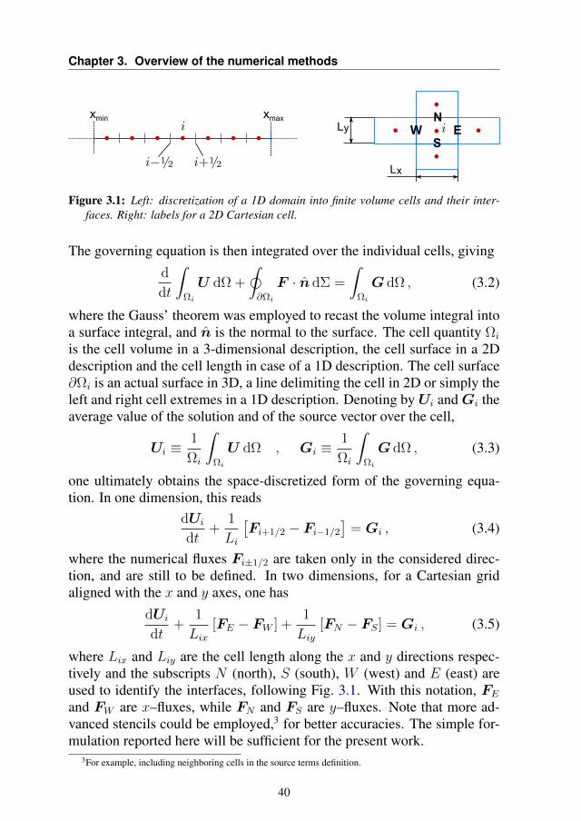
Chapter 3. Overview of the numerical methods
Figure 3.1: Left: discretization of a 1D domain into finite volume cells and their inter-faces. Right: labels for a 2D Cartesian cell.
The governing equation is then integrated over the individual cells, giving
d
dt
ˆΩi
U dΩ +
˛∂Ωi
F · n dΣ =
ˆΩi
G dΩ , (3.2)
where the Gauss’ theorem was employed to recast the volume integral intoa surface integral, and n is the normal to the surface. The cell quantity Ωi
is the cell volume in a 3-dimensional description, the cell surface in a 2Ddescription and the cell length in case of a 1D description. The cell surface∂Ωi is an actual surface in 3D, a line delimiting the cell in 2D or simply theleft and right cell extremes in a 1D description. Denoting byUi andGi theaverage value of the solution and of the source vector over the cell,
Ui ≡1
Ωi
ˆΩi
U dΩ , Gi ≡1
Ωi
ˆΩi
G dΩ , (3.3)
one ultimately obtains the space-discretized form of the governing equa-tion. In one dimension, this reads
dUi
dt+
1
Li
[Fi+1/2 − Fi−1/2
]= Gi , (3.4)
where the numerical fluxes Fi±1/2 are taken only in the considered direc-tion, and are still to be defined. In two dimensions, for a Cartesian gridaligned with the x and y axes, one has
dUi
dt+
1
Lix[FE − FW ] +
1
Liy[FN − FS] = Gi , (3.5)
where Lix and Liy are the cell length along the x and y directions respec-tively and the subscripts N (north), S (south), W (west) and E (east) areused to identify the interfaces, following Fig. 3.1. With this notation, FEand FW are x–fluxes, while FN and FS are y–fluxes. Note that more ad-vanced stencils could be employed,3 for better accuracies. The simple for-mulation reported here will be sufficient for the present work.
3For example, including neighboring cells in the source terms definition.
40
3.2. The finite volume method
3.2.2 Numerical fluxes for fluid and moment systems
The choice for the numerical fluxes proves to be crucial for the performanceof a finite volume method. A number of different formulations have beendeveloped in the years (for a review of the main methods, see Toro [142]).Rather than being completely general, a number of such methods have beendeveloped with a specific target system in mind. This is the case for theRoe scheme [143], the AUSM family of schemes [144] and the kineticschemes [145,146] to cite a few, that specifically target the Euler or Navier-Stokes equations. This is an issue for certain moment methods, as theseschemes would need either a very detailed knowledge of the eigenstructureof the system [119], or at least to be reformulated and extended.
Central schemes such as Lax-Friedrichs’ are general enough to be di-rectly applied to the moment equations, but are known to be very diffusive.This happens to be a major issue for moment methods, where the wavespeeds may exceed by orders of magnitude the wave speeds of the Eulersystem for some non-equilibrium conditions, as will be discussed in Sec-tion 4.2. This magnifies the undesirable numerical diffusion of the Lax-Friedrichs scheme. Higher order central schemes that mitigate such issuehave also been developed, as in the case of the Nessyahu-Tadmor [147] andthe Kurganov-Tadmor schemes [148], the latter requiring as an additionalinformation the maximum wave speed of the system.
When the maximum and minimum wave speeds of the system are known,a classical and robust choice consists in the HLL (Harten, Lax & van Leer)scheme [149]. Although not optimal for low-velocity flows such as bound-ary layers or contact discontinuities (its HLLC extension would improvethe situation), the scheme has been proficiently employed in the solution ofmoment systems due to its simplicity. However, it will be shown in Sec-tion 4.1.3 that, despite working well for moderate departures from equi-librium, the method shows some oscillations in the higher moments, whenapplied to strong non-equilibrium conditions. This may be due to numericalreasons, or may be caused by the scheme generating a non-realizable flux.For additional discussion on possible methods for the maximum-entropysystem, the reader can refer to [150]. Finally, in case the full entropy max-imisation problem is being solved at every iteration (as opposed to employ-ing the interpolative closure), another option consists in employing kineticfluxes [151].
The preferred scheme of the present work will be the Rusanov scheme(also known as “local Lax-Friedrichs”) [142]. Such scheme is slightly more
41
Chapter 3. Overview of the numerical methods
diffusive than the HLL scheme,4 but this is easily fixed by going second or-der in space, as discussed in the following. With the Rusanov scheme, theinterface flux Fint is obtained from the left and right states and fluxes (sub-scripts L and R) and the maximum wave speed Smax (maximum absolutevalue among the left and right cells),
Fint =1
2(FR + FL)− Smax
2(UR −UL) . (3.6)
MUSCL scheme for second order spatial accuracy
If the left and right states of Eq. (3.6) are taken directly from the left andright cells, the resulting spatial discretization is first order in space. Thevan Leer’s MUSCL scheme [152] allows us to retrieve a second order so-lution in space, by employing a linear reconstruction of the solution, wherethe slope is limited to achieve TVD properties. With marginal modifica-tions, one could also reach third order in space [153], however this was notinvestigated in the present work.
For systems of conservation equations, reconstruction is convenientlyperformed in primitive variables, that we define by Q. Using primitivevariables appears to be crucial for maximum-entropy simulations in pres-ence of strong non-equilibrium.5 The left and right states of the interfacei+ 1/2 are obtained as
QLi+1/2 = Qi +
xi+1/2 − xixi − xi−1
(Qi −Qi−1) Φ(θi) , (3.7a)
QRi+1/2 = Qi+1 −
xi+1 − xi+1/2
xi+2 − xi+1
(Qi+2 −Qi+1) Φ(1/θi+1) , (3.7b)
where θi = (Qi+1 −Qi)/(Qi −Qi−1) is the ratio of consecutive gradients,and Φ is a slope limiter function. The symmetric van Albada’s limiter isselected in this work, Φ(θ) = (θ2 + θ)/(θ2 + 1).
The MUSCL approach, together with van Albada’s slope limiter and Ru-sanov fluxes, has been seen to work smoothly for both the 5 and 14-momentsimulations for most conditions. However, for some test cases (such as thecrossing jets cases of Section 4.4), second order appears to stall the simu-lation at certain simulated times. Employing different TVD slope limitersdid not appear to improve the situation significantly. On the other hand,simply disabling the possibility to employ a linear reconstruction based on
4This may be the reason why the mentioned oscillations do not appear.5Reconstruction in conserved variables may create large inconsistencies unless a dimensionless formulation
is employed. Indeed, conserved moments include increasing powers of the velocity: and a linear reconstructionfor the momentum ρu would be inconsistent with a linear reconstruction of, say, the order-4 moment ρu4 + · · · .
42
3.2. The finite volume method
a large stencil would result in an overly diffusing simulation and the needto use a very large number of cells to reach spatial convergence. Therefore,an intermediate approach was applied in such cases, artificially limiting theslope by a further factor β = 0.5 or β = 0.75. For a uniform grid, thismodification reads
QLi+1/2 = Qi + β Φ(θi)
Qi −Qi−1
2, (3.8a)
QRi+1/2 = Qi+1 − β Φ(1/θi+1)
Qi+2 −Qi+1
2. (3.8b)
This further limiting causes the approach to depart from the second-orderTVD region (as defined in [140]). Nonetheless, it allows us to significantlyreduce the numerical diffusion of the Rusanov scheme, while still retaininga robust method.
3.2.3 Time integration
Once the equations are discretized in space, a time integrator is selected.The simplest choice consists in the explicit forward Euler scheme,
Un+1i = Un
i −∆t
Lix[F n
E − F nW ]− ∆t
Liy[F n
N − F nS ] + ∆tGn
i , (3.9)
where the superscript n denotes the current time and ∆t the time step. Thescheme has first order accuracy, and is only stable for Courant numberslower than one. More importantly, for charged gas simulations, the forwardEuler scheme may produce excessive numerical cooling (or heating) andmay numerically drive the temperature to zero, when conserved variablesare employed. This effect is important mostly in the study of the long-timebehavior of closed systems (see for example the test cases of Sections 6.4and 6.5), when the external input of work in the system is negligible andthe self-consistent fields dominate. On the other hand, for open systems,where the fluid is constantly being refreshed, this issue may very well benegligible.
The reason for this to occur is that the Euler method does not integrateexactly both the momentum and the total energy. Employing higher orderschemes (such as the ubiquitous order-4 Runge-Kutta method) surely im-proves the situation, but does not solve it. The problem will be consideredin more detail in Appendix B, where it will be shown that the MidpointEuler method, a simple 2nd order Runge-Kutta formulation, allows one tointegrate exactly both the momentum and the total energy for simple test
43
Chapter 3. Overview of the numerical methods
cases and uniform forces, thus solving the issue. For this reason, the Mid-point Euler scheme is the reference method for the present work.
First, the method performs a half-step, and computes an intermediatesolution as:
Un+1/2i = Un
i −∆t
2Lix[F n
E − F nW ]− ∆t
2Liy[F n
N − F nS ] +
∆t
2Gni , (3.10)
this solution is then used to compute both the fluxes and the source termsat the step n+ 1/2, denoted as F n+1/2 = F (Un+1/2) and the same for thesources. The actual step is then performed from n to n + 1, but using onlythe fluxes and sources at the intermediate step:
Un+1i = Un
i −∆t
Lix
[Fn+1/2E − F n+1/2
W
]− ∆t
Liy
[Fn+1/2N − F n+1/2
S
]+ ∆tG
n+1/2i , (3.11)
In this work, collisions or fields were never so strong as to cause anoverwhelming stiffness, and thus to require an implicit formulation, andthe explicit Midpoint Euler method proved to work just fine. In the case ofstiffer problems, point-implicit formulations could be employed.
3.2.4 Boundary conditions
In the presence of solid walls, the choice of a proper set of boundary con-ditions (BCs) may not be trivial in the case of moment equations. In par-ticular, for wall-bounded gases, one may expect Knudsen layers to form(see [119,154] for an implementation of the BCs for such conditions). Thesimulation of plasmas shares analogous issues, as one may need to considerfor example secondary electron emission at walls, due to electron impact,or the emission of electrons by ion impact at the electrodes. These problemsare respectively important for instance for modeling the near wall conduc-tivity [31] and for DC gas discharges [36].
In the present work, we do not need to consider such problems in greatdetail, and simple BCs are sufficient. All simulations will be either peri-odic or will have open-boundaries, and BCs are implemented through ghostcells. In the periodic case, the value at the ghost cells is updated in time asto match the corresponding periodic neighbor cell. In open-boundary simu-lations, the ghost cells are assigned a large velocity and small density, suchthat all characteristic waves will leave the domain. This is rigorous for su-
44
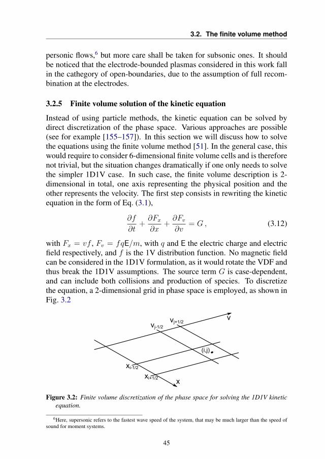
3.2. The finite volume method
personic flows,6 but more care shall be taken for subsonic ones. It shouldbe noticed that the electrode-bounded plasmas considered in this work fallin the cathegory of open-boundaries, due to the assumption of full recom-bination at the electrodes.
3.2.5 Finite volume solution of the kinetic equation
Instead of using particle methods, the kinetic equation can be solved bydirect discretization of the phase space. Various approaches are possible(see for example [155–157]). In this section we will discuss how to solvethe equations using the finite volume method [51]. In the general case, thiswould require to consider 6-dimensional finite volume cells and is thereforenot trivial, but the situation changes dramatically if one only needs to solvethe simpler 1D1V case. In such case, the finite volume description is 2-dimensional in total, one axis representing the physical position and theother represents the velocity. The first step consists in rewriting the kineticequation in the form of Eq. (3.1),
∂f
∂t+∂Fx∂x
+∂Fv∂v
= G , (3.12)
with Fx = vf , Fv = fqE/m, with q and E the electric charge and electricfield respectively, and f is the 1V distribution function. No magnetic fieldcan be considered in the 1D1V formulation, as it would rotate the VDF andthus break the 1D1V assumptions. The source term G is case-dependent,and can include both collisions and production of species. To discretizethe equation, a 2-dimensional grid in phase space is employed, as shown inFig. 3.2
Figure 3.2: Finite volume discretization of the phase space for solving the 1D1V kineticequation.
6Here, supersonic refers to the fastest wave speed of the system, that may be much larger than the speed ofsound for moment systems.
45
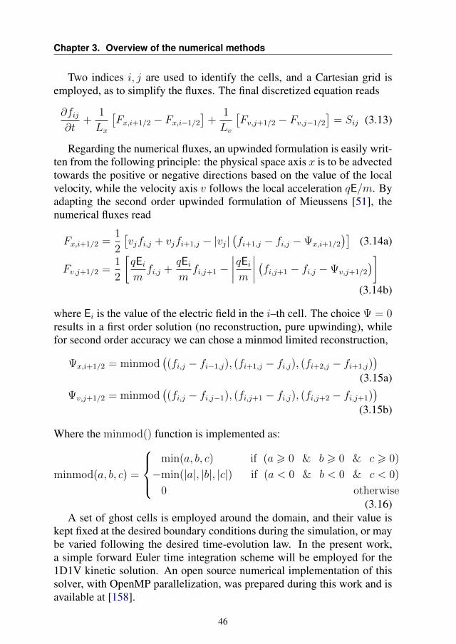
Chapter 3. Overview of the numerical methods
Two indices i, j are used to identify the cells, and a Cartesian grid isemployed, as to simplify the fluxes. The final discretized equation reads
∂fij∂t
+1
Lx
[Fx,i+1/2 − Fx,i−1/2
]+
1
Lv
[Fv,j+1/2 − Fv,j−1/2
]= Sij (3.13)
Regarding the numerical fluxes, an upwinded formulation is easily writ-ten from the following principle: the physical space axis x is to be advectedtowards the positive or negative directions based on the value of the localvelocity, while the velocity axis v follows the local acceleration qE/m. Byadapting the second order upwinded formulation of Mieussens [51], thenumerical fluxes read
Fx,i+1/2 =1
2
[vjfi,j + vjfi+1,j − |vj|
(fi+1,j − fi,j −Ψx,i+1/2
)](3.14a)
Fv,j+1/2 =1
2
[qEimfi,j +
qEimfi,j+1 −
∣∣∣∣qEim∣∣∣∣ (fi,j+1 − fi,j −Ψv,j+1/2
)](3.14b)
where Ei is the value of the electric field in the i–th cell. The choice Ψ = 0results in a first order solution (no reconstruction, pure upwinding), whilefor second order accuracy we can chose a minmod limited reconstruction,
Ψx,i+1/2 = minmod((fi,j − fi−1,j), (fi+1,j − fi,j), (fi+2,j − fi+1,j)
)(3.15a)
Ψv,j+1/2 = minmod((fi,j − fi,j−1), (fi,j+1 − fi,j), (fi,j+2 − fi,j+1)
)(3.15b)
Where the minmod() function is implemented as:
minmod(a, b, c) =
min(a, b, c) if (a > 0 & b > 0 & c > 0)
−min(|a|, |b|, |c|) if (a < 0 & b < 0 & c < 0)
0 otherwise(3.16)
A set of ghost cells is employed around the domain, and their value iskept fixed at the desired boundary conditions during the simulation, or maybe varied following the desired time-evolution law. In the present work,a simple forward Euler time integration scheme will be employed for the1D1V kinetic solution. An open source numerical implementation of thissolver, with OpenMP parallelization, was prepared during this work and isavailable at [158].
46
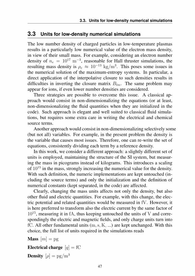
3.3. Units for low-density numerical simulations
3.3 Units for low-density numerical simulations
The low number density of charged particles in low-temperature plasmasresults in a particularly low numerical value of the electron mass density,in view of their small mass. For example, considering an electron numberdensity of ne = 1017 m−3, reasonable for Hall thruster simulations, theresulting mass density is ρe ≈ 10−13 kg/m3. This poses some issues inthe numerical solution of the maximum-entropy systems. In particular, adirect application of the interpolative closure to such densities results indifficulties in inverting the closure matrix Blm. The same problem mayappear for ions, if even lower number densities are considered.
Three strategies are possible to overcome this issue. A classical ap-proach would consist in non-dimensionalizing the equations (or at least,non-dimensionalizing the fluid quantities when they are initialized in thecode). Such approach is elegant and well suited to classical fluid simula-tions, but requires some extra care in writing the electrical and chemicalsource terms.
Another approach would consist in non-dimensionalizing selectively some(but not all) variables. For example, in the present problem the density isthe variable that causes most issues. Therefore, one can re-write the set ofequations, consistently dividing each term by a reference density.
In this work, we consider a different approach: a slightly different set ofunits is employed, maintaining the structure of the SI system, but measur-ing the mass in picograms instead of kilograms. This introduces a scalingof 1015 in the mass, strongly increasing the numerical value for the density.With such definition, the numeric implementations are kept untouched (in-cluding the source terms) and only the initialization and the definition ofnumerical constants (kept separated, in the code) are affected.
Clearly, changing the mass units affects not only the density, but alsoother fluid and electric quantities. For example, with this change, the elec-tric potential and related quantities would be measured in fV. However, itis here preferred to transform also the electric current by the same factor of1015, measuring it in fA, thus keeping untouched the units of V and corre-spondingly the electric and magnetic fields, and only charge units turn intofC. All other fundamental units (m, s,K, ...) are kept unchanged. With thischoice, the full list of units required in the simulations reads
Mass [m] = pg
Electrical charge [q] = fC
Density [ρ] = pg/m3
47
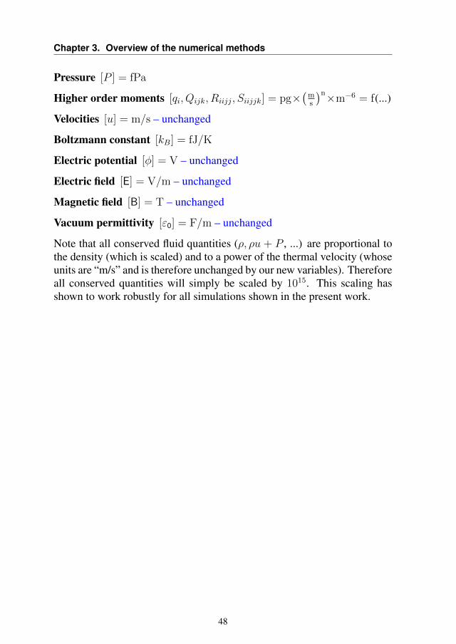
Chapter 3. Overview of the numerical methods
Pressure [P ] = fPa
Higher order moments [qi, Qijk, Riijj, Siijjk] = pg×(
ms
)n×m−6 = f(...)
Velocities [u] = m/s – unchanged
Boltzmann constant [kB] = fJ/K
Electric potential [φ] = V – unchanged
Electric field [E] = V/m – unchanged
Magnetic field [B] = T – unchanged
Vacuum permittivity [ε0] = F/m – unchanged
Note that all conserved fluid quantities (ρ, ρu + P , ...) are proportional tothe density (which is scaled) and to a power of the thermal velocity (whoseunits are “m/s” and is therefore unchanged by our new variables). Thereforeall conserved quantities will simply be scaled by 1015. This scaling hasshown to work robustly for all simulations shown in the present work.
48
CHAPTER4Application of the maximum-entropy
closure to rarefied gases and plasmas
In order to apply the maximum-entropy method to the low-temperatureplasma conditions considered in this work, some further analysis and de-velopments are necessary.
The first part of this chapter will focus on investigating the method inlow-collisional situations. First, in Section 4.1 we introduce the Sod shocktest case, and consider free-molecular, transitional and continuum condi-tions, solving both the kinetic equation and the 1D1V 5-moment system.This test case will offer a first verification of the 5-moment system forvarying degrees of non-equilibrium, and will serve as a basis for the furthersections. For this problem, Section 4.1.3 compares the HLL and Rusanovnumerical fluxes and identifies the most suitable one.
As can be seen from an analysis of the Sod shock tube problem, thewave speeds of the maximum-entropy system differ greatly from the speedof sound, when non-equilibrium situations are considered. Their analyti-cal expression is not known, and computing them numerically during CFDsimulations is very expensive. In this regard, Section 4.2 is devoted tothe development of approximated wave speeds for the 14-moment system.
49
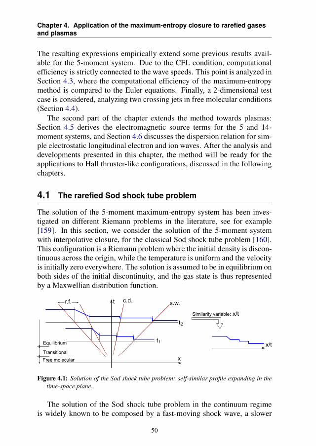
Chapter 4. Application of the maximum-entropy closure to rarefied gasesand plasmas
The resulting expressions empirically extend some previous results avail-able for the 5-moment system. Due to the CFL condition, computationalefficiency is strictly connected to the wave speeds. This point is analyzed inSection 4.3, where the computational efficiency of the maximum-entropymethod is compared to the Euler equations. Finally, a 2-dimensional testcase is considered, analyzing two crossing jets in free molecular conditions(Section 4.4).
The second part of the chapter extends the method towards plasmas:Section 4.5 derives the electromagnetic source terms for the 5 and 14-moment systems, and Section 4.6 discusses the dispersion relation for sim-ple electrostatic longitudinal electron and ion waves. After the analysis anddevelopments presented in this chapter, the method will be ready for theapplications to Hall thruster-like configurations, discussed in the followingchapters.
4.1 The rarefied Sod shock tube problem
The solution of the 5-moment maximum-entropy system has been inves-tigated on different Riemann problems in the literature, see for example[159]. In this section, we consider the solution of the 5-moment systemwith interpolative closure, for the classical Sod shock tube problem [160].This configuration is a Riemann problem where the initial density is discon-tinuous across the origin, while the temperature is uniform and the velocityis initially zero everywhere. The solution is assumed to be in equilibrium onboth sides of the initial discontinuity, and the gas state is thus representedby a Maxwellian distribution function.
Figure 4.1: Solution of the Sod shock tube problem: self-similar profile expanding in thetime-space plane.
The solution of the Sod shock tube problem in the continuum regimeis widely known to be composed by a fast-moving shock wave, a slower
50
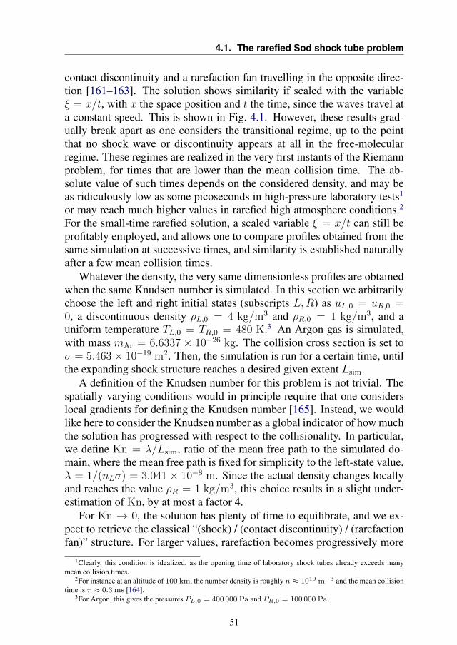
4.1. The rarefied Sod shock tube problem
contact discontinuity and a rarefaction fan travelling in the opposite direc-tion [161–163]. The solution shows similarity if scaled with the variableξ = x/t, with x the space position and t the time, since the waves travel ata constant speed. This is shown in Fig. 4.1. However, these results grad-ually break apart as one considers the transitional regime, up to the pointthat no shock wave or discontinuity appears at all in the free-molecularregime. These regimes are realized in the very first instants of the Riemannproblem, for times that are lower than the mean collision time. The ab-solute value of such times depends on the considered density, and may beas ridiculously low as some picoseconds in high-pressure laboratory tests1
or may reach much higher values in rarefied high atmosphere conditions.2
For the small-time rarefied solution, a scaled variable ξ = x/t can still beprofitably employed, and allows one to compare profiles obtained from thesame simulation at successive times, and similarity is established naturallyafter a few mean collision times.
Whatever the density, the very same dimensionless profiles are obtainedwhen the same Knudsen number is simulated. In this section we arbitrarilychoose the left and right initial states (subscripts L,R) as uL,0 = uR,0 =0, a discontinuous density ρL,0 = 4 kg/m3 and ρR,0 = 1 kg/m3, and auniform temperature TL,0 = TR,0 = 480 K.3 An Argon gas is simulated,with mass mAr = 6.6337 × 10⁻²⁶ kg. The collision cross section is set toσ = 5.463× 10⁻¹⁹ m2. Then, the simulation is run for a certain time, untilthe expanding shock structure reaches a desired given extent Lsim.
A definition of the Knudsen number for this problem is not trivial. Thespatially varying conditions would in principle require that one considerslocal gradients for defining the Knudsen number [165]. Instead, we wouldlike here to consider the Knudsen number as a global indicator of how muchthe solution has progressed with respect to the collisionality. In particular,we define Kn = λ/Lsim, ratio of the mean free path to the simulated do-main, where the mean free path is fixed for simplicity to the left-state value,λ = 1/(nLσ) = 3.041 × 10⁻⁸ m. Since the actual density changes locallyand reaches the value ρR = 1 kg/m3, this choice results in a slight under-estimation of Kn, by at most a factor 4.
For Kn → 0, the solution has plenty of time to equilibrate, and we ex-pect to retrieve the classical “(shock) / (contact discontinuity) / (rarefactionfan)” structure. For larger values, rarefaction becomes progressively more
1Clearly, this condition is idealized, as the opening time of laboratory shock tubes already exceeds manymean collision times.
2For instance at an altitude of 100 km, the number density is roughly n ≈ 1019 m−3 and the mean collisiontime is τ ≈ 0.3 ms [164].
3For Argon, this gives the pressures PL,0 = 400 000 Pa and PR,0 = 100 000 Pa.
51
Chapter 4. Application of the maximum-entropy closure to rarefied gasesand plasmas
important, until for Kn → ∞, we expect the solution to be composed bya smooth profile that connects the left and right states. Considering theintermediate case of Kn = 0.1, the mean free path is 1/10 of the simu-lated domain Lsim. Practically speaking, all solutions for Kn ≥ 1 appearalmost identical in terms of the lower order moments (density, velocity andpressure), and differ only when higher order moments are considered.
We consider here a 1D1V problem, where particles are assumed to haveonly one translational degree of freedom. This may appear to be an exces-sive simplification, since the physical realm of a 1V shock is debatable atbest. However, this allows us to keep the difficulty at a minimum, and toemploy the simple deterministic solver developed in Chapter 3 in place ofthe particle-based solver, allowing us to obtain noise-free estimations forthe higher order moments. The kinetic equation describing the 1D1V BGKgas is
∂f
∂t+ v
∂f
∂x= −ν(f −M) , (4.1)
whereM is the 1V Maxwellian at the local conditions (see Eq. (2.5)) andthe velocity independent collision frequency ν is computed in every cellfrom the local values,
ν = nvthσ = σρ
m
√8P
πρ. (4.2)
The 5-moment system corresponding to this case is reported in Eq. 2.54,and its BGK collision sources read [67]
G(5) =
0
0
0
−νQ−ν (4uQ+R− 3P 2/ρ)
. (4.3)
These terms do not affect the density, momentum and total energy, and onlydrive the heat flux Q towards zero, and the order-4 moment R towards theequilibrium value 3P 2/ρ.
4.1.1 Kinetic solution
A solution to the kinetic equation was computed for the three mentionedconditions with the deterministic solver outlined in Section 3.2.5, using agrid composed by 1000 × 1000 cells in physical space and velocity. A
52
4.1. The rarefied Sod shock tube problem
number of 15 000 time steps proved sufficiently fine for reproducing theresults with negligible numerical diffusion. The value of the time step ischosen as to reach the required simulation time. The kinetic solution isshown in Fig. 4.2. The effect of collisions is clearly dim at these conditions,and the resulting distribution function is a combination of the left and rightfamilies of particles (two Maxwellian at different densities).
Figure 4.2: Kinetic solution in phase space for a time comparable to the mean collisiontime (Kn = 1). Test case a).
Solutions at lower values of the Knudsen number are qualitatively simi-lar, except that the distribution is smoother in velocity, but obviously startsto show discontinuities in space as the continuum regime is approached[166–168]. The moments of the kinetic solution are shown in Fig. 4.3. Theconsidered cases correspond to the following conditions:
a) Kn = 1, Tsim = 10−11 s;
b) Kn = 0.1, Tsim = 10−10 s;
c) Kn = 0.01, Tsim = 10−9 s;
d) Kn = 0.001, Tsim = 10−8 s;
e) Kn = 0.0001, Tsim = 10−7 s;
For increasing simulated times, the solution is progressively more spreadin space: the different profiles are superimposed by rescaling the spatialcoordinate by the simulated time. As to allow for a comparison with themaximum-entropy system, a plot of the solution in moment space is alsoshown, together with the Junk subspace of the 5-moment system4 and thephysical realizability boundary. In Fig. 4.3, equilibrium is represented by(q?, r?) = (0, 3).
4Clearly, the kinetic solution can cross freely the Junk subspace.
53
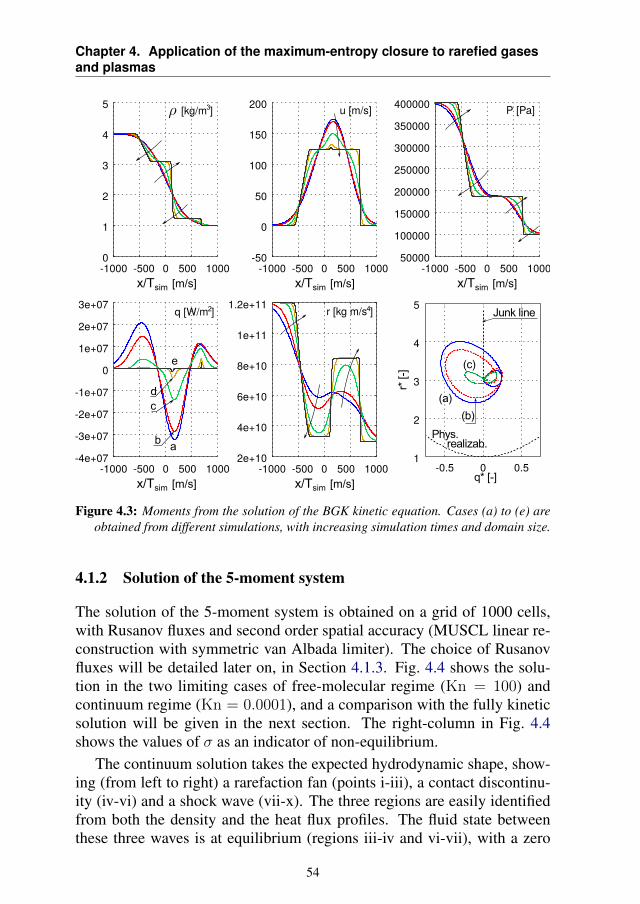
Chapter 4. Application of the maximum-entropy closure to rarefied gasesand plasmas
Figure 4.3: Moments from the solution of the BGK kinetic equation. Cases (a) to (e) areobtained from different simulations, with increasing simulation times and domain size.
4.1.2 Solution of the 5-moment system
The solution of the 5-moment system is obtained on a grid of 1000 cells,with Rusanov fluxes and second order spatial accuracy (MUSCL linear re-construction with symmetric van Albada limiter). The choice of Rusanovfluxes will be detailed later on, in Section 4.1.3. Fig. 4.4 shows the solu-tion in the two limiting cases of free-molecular regime (Kn = 100) andcontinuum regime (Kn = 0.0001), and a comparison with the fully kineticsolution will be given in the next section. The right-column in Fig. 4.4shows the values of σ as an indicator of non-equilibrium.
The continuum solution takes the expected hydrodynamic shape, show-ing (from left to right) a rarefaction fan (points i-iii), a contact discontinu-ity (iv-vi) and a shock wave (vii-x). The three regions are easily identifiedfrom both the density and the heat flux profiles. The fluid state betweenthese three waves is at equilibrium (regions iii-iv and vi-vii), with a zero
54
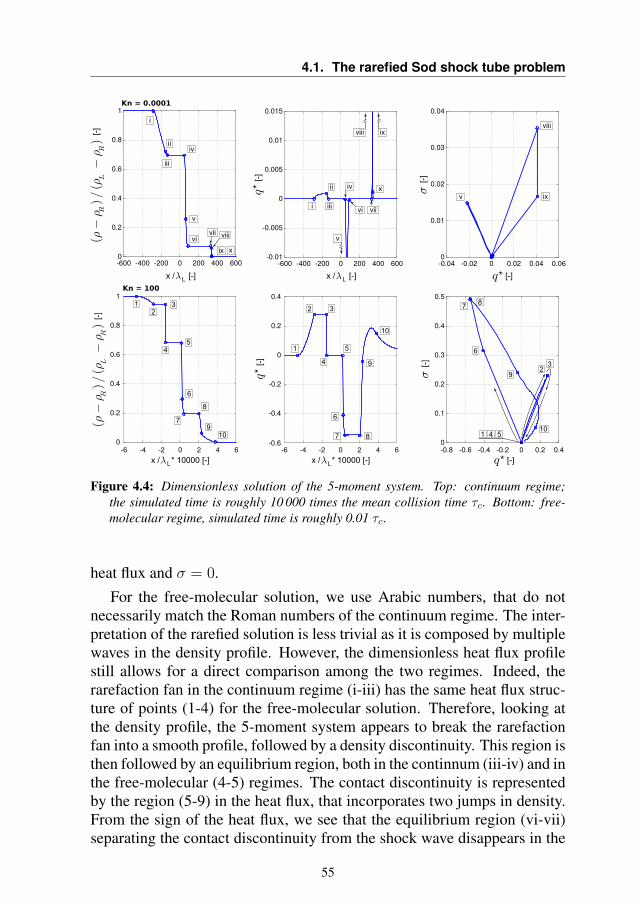
4.1. The rarefied Sod shock tube problem
Figure 4.4: Dimensionless solution of the 5-moment system. Top: continuum regime;the simulated time is roughly 10 000 times the mean collision time τc. Bottom: free-molecular regime, simulated time is roughly 0.01 τc.
heat flux and σ = 0.
For the free-molecular solution, we use Arabic numbers, that do notnecessarily match the Roman numbers of the continuum regime. The inter-pretation of the rarefied solution is less trivial as it is composed by multiplewaves in the density profile. However, the dimensionless heat flux profilestill allows for a direct comparison among the two regimes. Indeed, therarefaction fan in the continuum regime (i-iii) has the same heat flux struc-ture of points (1-4) for the free-molecular solution. Therefore, looking atthe density profile, the 5-moment system appears to break the rarefactionfan into a smooth profile, followed by a density discontinuity. This region isthen followed by an equilibrium region, both in the continnum (iii-iv) and inthe free-molecular (4-5) regimes. The contact discontinuity is representedby the region (5-9) in the heat flux, that incorporates two jumps in density.From the sign of the heat flux, we see that the equilibrium region (vi-vii)separating the contact discontinuity from the shock wave disappears in the
55
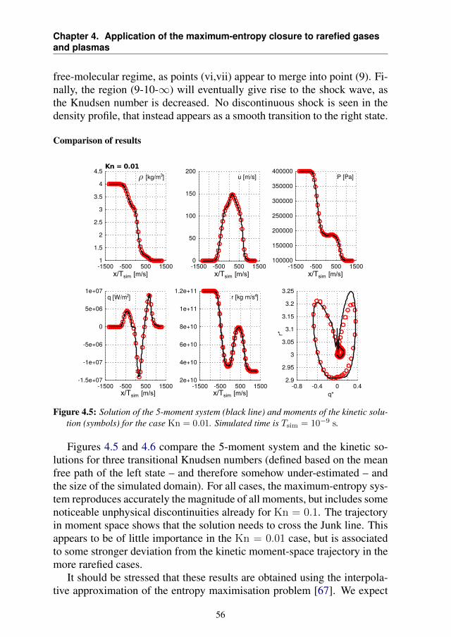
Chapter 4. Application of the maximum-entropy closure to rarefied gasesand plasmas
free-molecular regime, as points (vi,vii) appear to merge into point (9). Fi-nally, the region (9-10-∞) will eventually give rise to the shock wave, asthe Knudsen number is decreased. No discontinuous shock is seen in thedensity profile, that instead appears as a smooth transition to the right state.
Comparison of results
Figure 4.5: Solution of the 5-moment system (black line) and moments of the kinetic solu-tion (symbols) for the case Kn = 0.01. Simulated time is Tsim = 10−9 s.
Figures 4.5 and 4.6 compare the 5-moment system and the kinetic so-lutions for three transitional Knudsen numbers (defined based on the meanfree path of the left state – and therefore somehow under-estimated – andthe size of the simulated domain). For all cases, the maximum-entropy sys-tem reproduces accurately the magnitude of all moments, but includes somenoticeable unphysical discontinuities already for Kn = 0.1. The trajectoryin moment space shows that the solution needs to cross the Junk line. Thisappears to be of little importance in the Kn = 0.01 case, but is associatedto some stronger deviation from the kinetic moment-space trajectory in themore rarefied cases.
It should be stressed that these results are obtained using the interpola-tive approximation of the entropy maximisation problem [67]. We expect
56
4.1. The rarefied Sod shock tube problem
the global shape of the solution to be unchanged, however the details ofthe trajectory in moment space appear to be very sensitive to the employedgrid, and are therefore likely to be affected by the details of the closureapproximations.
4.1.3 Comparison of the HLL and Rusanov fluxes
As discussed in Section 3.2.2, few schemes are directly applicable to themaximum-entropy systems. In this section, we compare the often employedHLL scheme to the simpler Rusanov fluxes, for rarefied and continuumconditions. Lax-Friedrichs fluxes were also considered, but provided anoverwhelmingly high numerical diffusion in the free-molecular regime, dueto the high value of the wave speeds in non-equilibrium, such that no shockstructure could be identified for the considered grids. A comparison of theHLL and Rusanov fluxes is shown in Fig. 4.7, using 500 grid cells and firstorder accuracy. A second order solution is also computed, using Rusanovfluxes on 5000 cells, as to show a reference shock profile.
The two methods appear roughly equivalent in continuum conditions,the Rusanov scheme showing only a very slight additional diffusion. Onthe other hand, in rarefied conditions, the HLL fluxes are significantly lessdiffusive than the Rusanov ones, but induce strong oscillations in the higherorder moments. As previously mentioned, such oscillations may be con-nected by the prediction of non-realizable numerical fluxes, or states veryclose to the Junk line singularity, but this is to be investigated further. Inany case, the oscillations are a major problem, as they prevent to obtainsecond order via piecewise limited reconstruction.
By employing Rusanov fluxes, we have no significant oscillations, andsecond order can be reached, thus offering a remedy to Rusanov’s addi-tional diffusion. Therefore, this will be the method of choice for most sim-ulations in this work. The investigation and formulation of less diffusivefluxes is suggested as a future work activity (see the Conclusions chapter).
57
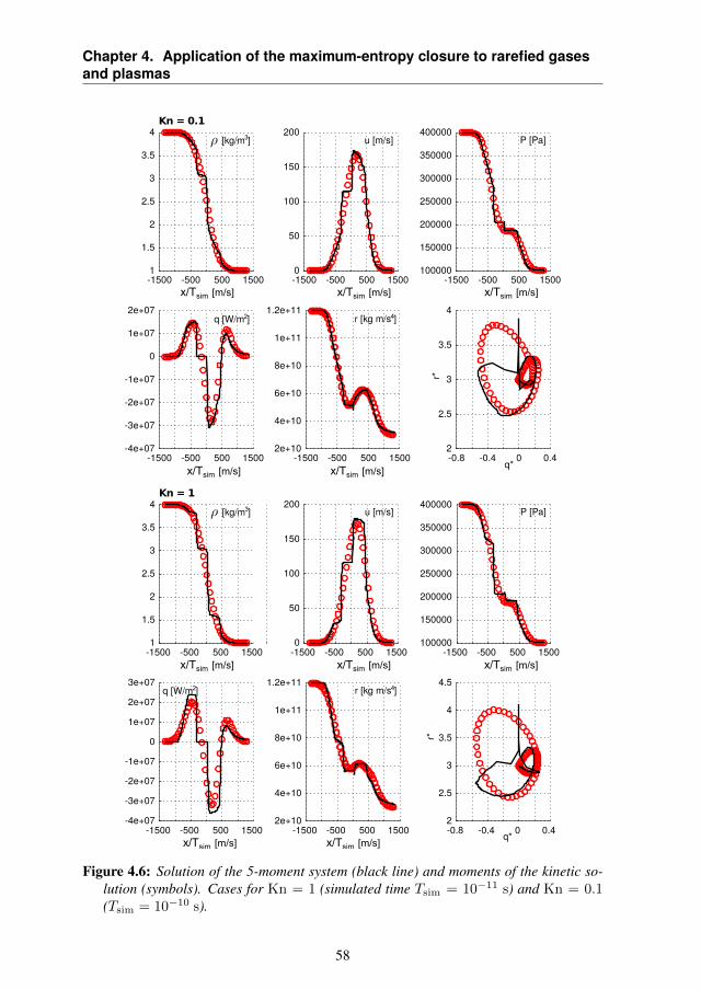
Chapter 4. Application of the maximum-entropy closure to rarefied gasesand plasmas
Figure 4.6: Solution of the 5-moment system (black line) and moments of the kinetic so-lution (symbols). Cases for Kn = 1 (simulated time Tsim = 10−11 s) and Kn = 0.1(Tsim = 10−10 s).
58
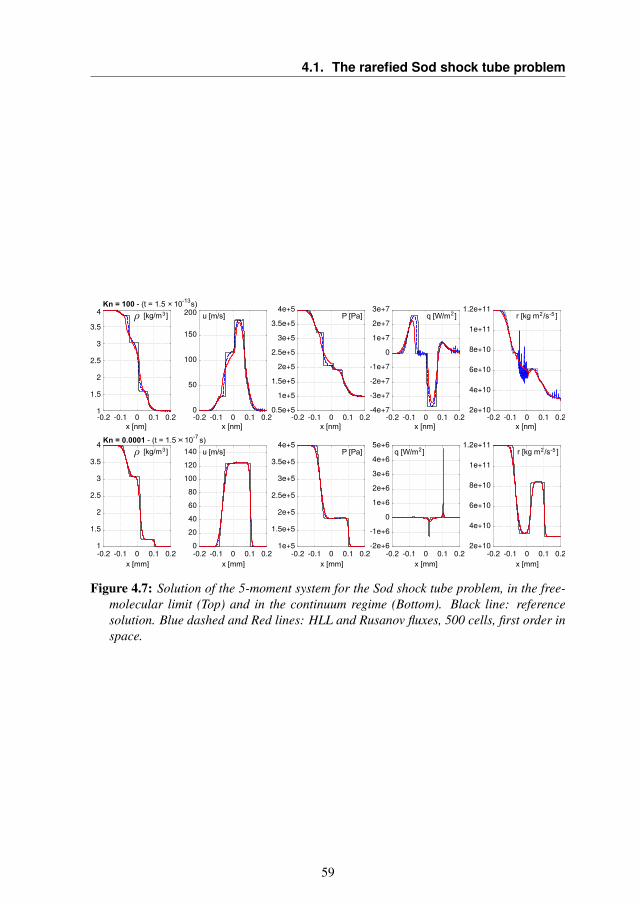
4.1. The rarefied Sod shock tube problem
Figure 4.7: Solution of the 5-moment system for the Sod shock tube problem, in the free-molecular limit (Top) and in the continuum regime (Bottom). Black line: referencesolution. Blue dashed and Red lines: HLL and Rusanov fluxes, 500 cells, first order inspace.
59
Chapter 4. Application of the maximum-entropy closure to rarefied gasesand plasmas
4.2 Approximated wave speeds
The eigenvalues of a system (or at least the maximum and minimum wavespeeds) play an important role in its numerical solution. As discussed inChapter 3, explicit time integration schemes are stable for given values ofthe Courant number, that depends on the system wave speeds. A numberof implicit formulations also require a knowledge of the Courant number(among others, we shall cite implicit dual-time stepping strategies [169–171] where a CFL evolution law is introduced). Also, many numericalfluxes formulations (such as the HLL, Rusanov or Kurganov-Tadmor tocite a few) also require the wave speeds, and their accuracy influences thenumerical diffusion properties of such methods.
For the Euler system, the maximum and minimum wave speeds are eas-ily obtained analytically and result in u ± a, u being the bulk velocity anda the speed of sound. However, maximum-entropy systems have muchmore complex convective fluxes, that include singular closing terms. Theanalytical expression of such closing moments is either unknown (in thegeneral maximum-entropy formulation) or at least rather complex (in theinterpolative closure approximations). As a result, an analytical expressionfor the eigenvalues of the fluxes Jacobian is often not available. Numeri-cally, this means that one has to (i) build a Jacobian5 and (ii) compute itsnumerical eigenvalues in each cell and at every time step. This dramati-cally reduces the efficiency of numerical computations, and may becomeunbearable if one considers multi-dimensional cases and non-equilibriumconditions, where the computational cost of maximum-entropy methods isalready much higher than the Euler system (as will be discussed in Sec-tion 4.3). Therefore, some approximation of the wave speeds is required.
The simplest strategy, consists in assuming that the maximum and min-imum wave speeds of a maximum-entropy system have the same form ofthe Euler wave speeds, but include a multiplying constant k:
wmaxmin = u± ka . (4.4)
An arbitrary value k > 1 is chosen, large enough to reproduce the wavespeeds of the actual system, or anyway to introduce enough diffusion toallow for a solution. This strategy has been profitably employed in thetransitional regime, see for example [154]. In that reference, it was howevershown that the maximum-entropy wave speeds can be larger than the Eulerequations by orders of magnitude, in non-equilibrium conditions.
5That is a 14 by 14 matrix for the 14-moment system.
60
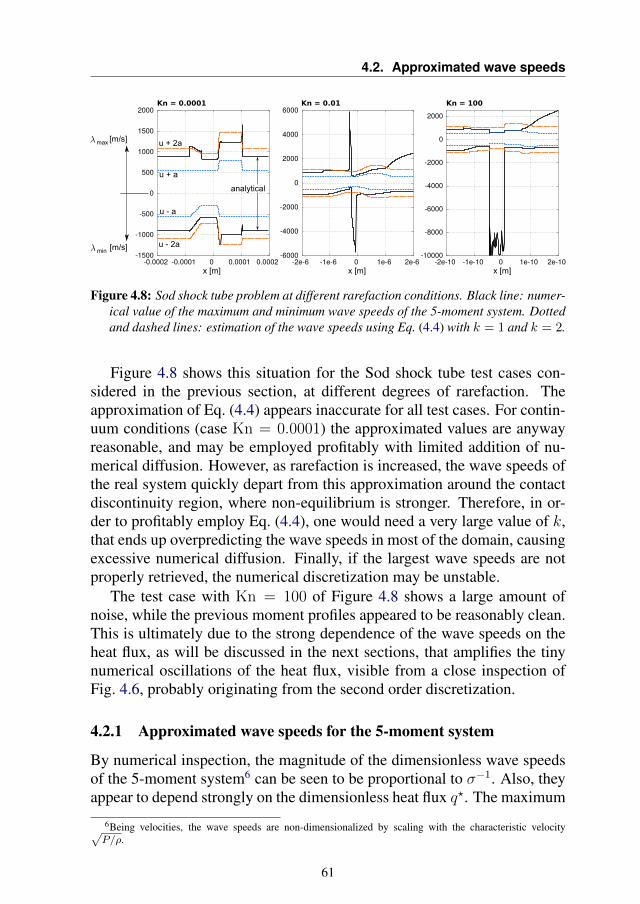
4.2. Approximated wave speeds
Figure 4.8: Sod shock tube problem at different rarefaction conditions. Black line: numer-ical value of the maximum and minimum wave speeds of the 5-moment system. Dottedand dashed lines: estimation of the wave speeds using Eq. (4.4) with k = 1 and k = 2.
Figure 4.8 shows this situation for the Sod shock tube test cases con-sidered in the previous section, at different degrees of rarefaction. Theapproximation of Eq. (4.4) appears inaccurate for all test cases. For contin-uum conditions (case Kn = 0.0001) the approximated values are anywayreasonable, and may be employed profitably with limited addition of nu-merical diffusion. However, as rarefaction is increased, the wave speeds ofthe real system quickly depart from this approximation around the contactdiscontinuity region, where non-equilibrium is stronger. Therefore, in or-der to profitably employ Eq. (4.4), one would need a very large value of k,that ends up overpredicting the wave speeds in most of the domain, causingexcessive numerical diffusion. Finally, if the largest wave speeds are notproperly retrieved, the numerical discretization may be unstable.
The test case with Kn = 100 of Figure 4.8 shows a large amount ofnoise, while the previous moment profiles appeared to be reasonably clean.This is ultimately due to the strong dependence of the wave speeds on theheat flux, as will be discussed in the next sections, that amplifies the tinynumerical oscillations of the heat flux, visible from a close inspection ofFig. 4.6, probably originating from the second order discretization.
4.2.1 Approximated wave speeds for the 5-moment system
By numerical inspection, the magnitude of the dimensionless wave speedsof the 5-moment system6 can be seen to be proportional to σ−1. Also, theyappear to depend strongly on the dimensionless heat flux q?. The maximum
6Being velocities, the wave speeds are non-dimensionalized by scaling with the characteristic velocity√P/ρ.
61
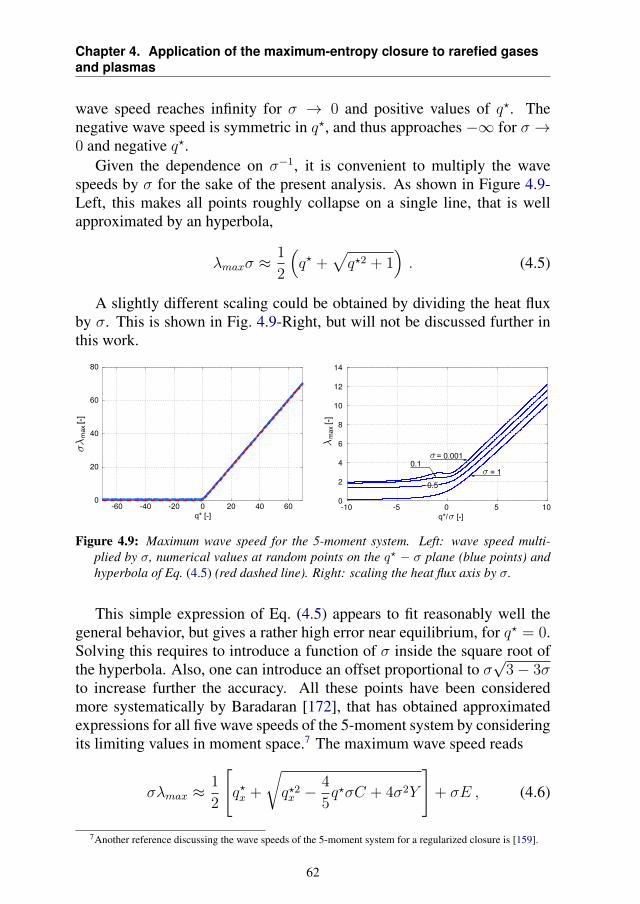
Chapter 4. Application of the maximum-entropy closure to rarefied gasesand plasmas
wave speed reaches infinity for σ → 0 and positive values of q?. Thenegative wave speed is symmetric in q?, and thus approaches −∞ for σ →0 and negative q?.
Given the dependence on σ−1, it is convenient to multiply the wavespeeds by σ for the sake of the present analysis. As shown in Figure 4.9-Left, this makes all points roughly collapse on a single line, that is wellapproximated by an hyperbola,
λmaxσ ≈1
2
(q? +
√q?2 + 1
). (4.5)
A slightly different scaling could be obtained by dividing the heat fluxby σ. This is shown in Fig. 4.9-Right, but will not be discussed further inthis work.
Figure 4.9: Maximum wave speed for the 5-moment system. Left: wave speed multi-plied by σ, numerical values at random points on the q? − σ plane (blue points) andhyperbola of Eq. (4.5) (red dashed line). Right: scaling the heat flux axis by σ.
This simple expression of Eq. (4.5) appears to fit reasonably well thegeneral behavior, but gives a rather high error near equilibrium, for q? = 0.Solving this requires to introduce a function of σ inside the square root ofthe hyperbola. Also, one can introduce an offset proportional to σ
√3− 3σ
to increase further the accuracy. All these points have been consideredmore systematically by Baradaran [172], that has obtained approximatedexpressions for all five wave speeds of the 5-moment system by consideringits limiting values in moment space.7 The maximum wave speed reads
σλmax ≈1
2
[q?x +
√q?2x −
4
5q?σC + 4σ2Y
]+ σE , (4.6)
7Another reference discussing the wave speeds of the 5-moment system for a regularized closure is [159].
62
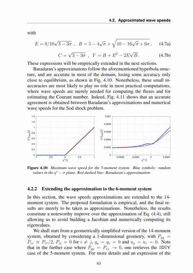
4.2. Approximated wave speeds
with
E = 8/10√
3− 3σ , B = 5− 4√σ +
√10− 16
√σ + 6σ , (4.7a)
C =√
3− 3σ , Y = B + E2 − 2E√B . (4.7b)
These expressions will be empirically extended in the next sections.Baradaran’s approximations follow the aforementioned hyperbola struc-
ture, and are accurate in most of the domain, losing some accuracy onlyclose to equilibrium, as shown in Fig. 4.10. Nonetheless, these small in-accuracies are most likely to play no role in most practical computations,where wave speeds are merely needed for computing the fluxes and forestimating the Courant number. Indeed, Fig. 4.11 shows that an accurateagreement is obtained between Baradaran’s approximations and numericalwave speeds for the Sod shock problem.
Figure 4.10: Maximum wave speed for the 5-moment system. Blue symbols: randomvalues in the q? − σ plane. Red dashed line: Baradaran’s approximation.
4.2.2 Extending the approximation to the 6-moment system
In this section, the wave speeds approximations are extended to the 14-moment system. The proposed formulation is empirical, and the final re-sults are merely to be taken as approximations. Nonetheless, the resultsconstitute a noteworthy improve over the approximation of Eq. (4.4), stillallowing us to avoid building a Jacobian and numerically computing itseigenvalues.
We shall start from a geometrically simplified version of the 14-momentsystem, obtained by considering a 1-dimensional geometry, with Pyy =Pzz ≡ Prr/2, Pij = 0 for i 6= j, qy = qz = 0 and uy = uz = 0. Notethat in the further case where Pyy = Pzz → 0, one retrieves the 1D1Vcase of the 5-moment system. For more details and an expression of the
63
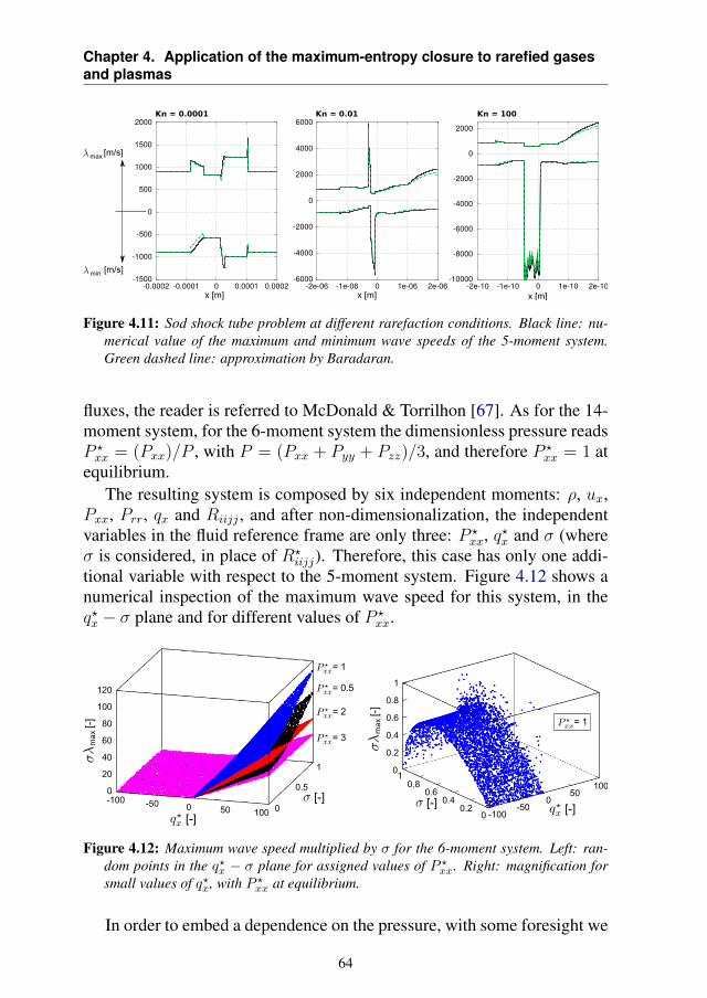
Chapter 4. Application of the maximum-entropy closure to rarefied gasesand plasmas
Figure 4.11: Sod shock tube problem at different rarefaction conditions. Black line: nu-merical value of the maximum and minimum wave speeds of the 5-moment system.Green dashed line: approximation by Baradaran.
fluxes, the reader is referred to McDonald & Torrilhon [67]. As for the 14-moment system, for the 6-moment system the dimensionless pressure readsP ?xx = (Pxx)/P , with P = (Pxx + Pyy + Pzz)/3, and therefore P ?
xx = 1 atequilibrium.
The resulting system is composed by six independent moments: ρ, ux,Pxx, Prr, qx and Riijj , and after non-dimensionalization, the independentvariables in the fluid reference frame are only three: P ?
xx, q?x and σ (whereσ is considered, in place of R?
iijj). Therefore, this case has only one addi-tional variable with respect to the 5-moment system. Figure 4.12 shows anumerical inspection of the maximum wave speed for this system, in theq?x − σ plane and for different values of P ?
xx.
Figure 4.12: Maximum wave speed multiplied by σ for the 6-moment system. Left: ran-dom points in the q?x − σ plane for assigned values of P ?xx. Right: magnification forsmall values of q?x, with P ?xx at equilibrium.
In order to embed a dependence on the pressure, with some foresight we
64
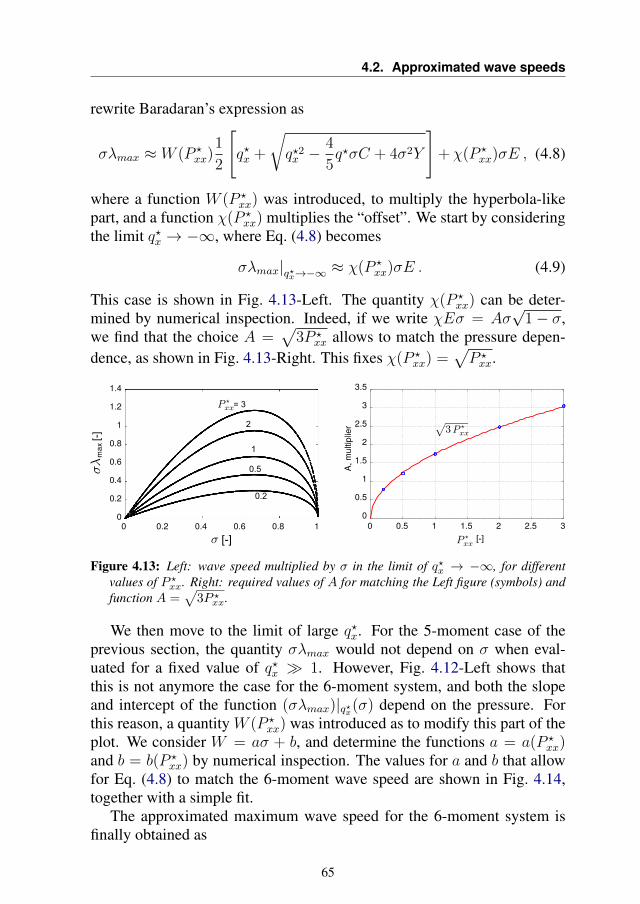
4.2. Approximated wave speeds
rewrite Baradaran’s expression as
σλmax ≈ W (P ?xx)
1
2
[q?x +
√q?2x −
4
5q?σC + 4σ2Y
]+ χ(P ?
xx)σE , (4.8)
where a function W (P ?xx) was introduced, to multiply the hyperbola-like
part, and a function χ(P ?xx) multiplies the “offset”. We start by considering
the limit q?x → −∞, where Eq. (4.8) becomes
σλmax|q?x→−∞ ≈ χ(P ?xx)σE . (4.9)
This case is shown in Fig. 4.13-Left. The quantity χ(P ?xx) can be deter-
mined by numerical inspection. Indeed, if we write χEσ = Aσ√
1− σ,we find that the choice A =
√3P ?
xx allows to match the pressure depen-dence, as shown in Fig. 4.13-Right. This fixes χ(P ?
xx) =√P ?xx.
Figure 4.13: Left: wave speed multiplied by σ in the limit of q?x → −∞, for differentvalues of P ?xx. Right: required values of A for matching the Left figure (symbols) andfunction A =
√3P ?xx.
We then move to the limit of large q?x. For the 5-moment case of theprevious section, the quantity σλmax would not depend on σ when eval-uated for a fixed value of q?x 1. However, Fig. 4.12-Left shows thatthis is not anymore the case for the 6-moment system, and both the slopeand intercept of the function (σλmax)|q?x(σ) depend on the pressure. Forthis reason, a quantity W (P ?
xx) was introduced as to modify this part of theplot. We consider W = aσ + b, and determine the functions a = a(P ?
xx)and b = b(P ?
xx) by numerical inspection. The values for a and b that allowfor Eq. (4.8) to match the 6-moment wave speed are shown in Fig. 4.14,together with a simple fit.
The approximated maximum wave speed for the 6-moment system isfinally obtained as
65
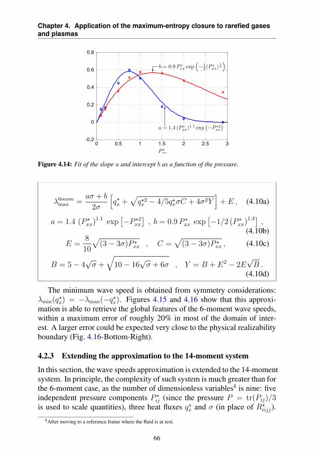
Chapter 4. Application of the maximum-entropy closure to rarefied gasesand plasmas
Figure 4.14: Fit of the slope a and intercept b as a function of the pressure.
λ6mommax =
aσ + b
2σ
[q?x +
√q?2x − 4/5q?xσC + 4σ2Y
]+ E , (4.10a)
a = 1.4 (P ?xx)
1.1 exp[−P ?2
xx
], b = 0.9P ?
xx exp[−1/2 (P ?
xx)1.4] ,(4.10b)
E =8
10
√(3− 3σ)P ?
xx , C =√
(3− 3σ)P ?xx , (4.10c)
B = 5− 4√σ +
√10− 16
√σ + 6σ , Y = B + E2 − 2E
√B .
(4.10d)
The minimum wave speed is obtained from symmetry considerations:λmin(q?x) = −λmax(−q?x). Figures 4.15 and 4.16 show that this approxi-mation is able to retrieve the global features of the 6-moment wave speeds,within a maximum error of roughly 20% in most of the domain of inter-est. A larger error could be expected very close to the physical realizabilityboundary (Fig. 4.16-Bottom-Right).
4.2.3 Extending the approximation to the 14-moment system
In this section, the wave speeds approximation is extended to the 14-momentsystem. In principle, the complexity of such system is much greater than forthe 6-moment case, as the number of dimensionless variables8 is nine: fiveindependent pressure components P ?
ij (since the pressure P = tr(Pij)/3is used to scale quantities), three heat fluxes q?x and σ (in place of R?
iijj).
8After moving to a reference frame where the fluid is at rest.
66
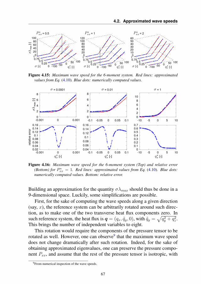
4.2. Approximated wave speeds
Figure 4.15: Maximum wave speed for the 6-moment system. Red lines: approximatedvalues from Eq. (4.10). Blue dots: numerically computed values.
Figure 4.16: Maximum wave speed for the 6-moment system (Top) and relative error(Bottom) for P ?xx = 1. Red lines: approximated values from Eq. (4.10). Blue dots:numerically computed values. Bottom: relative error.
Building an approximation for the quantity σλmax should thus be done in a9-dimensional space. Luckily, some simplifications are possible.
First, for the sake of computing the wave speeds along a given direction(say, x), the reference system can be arbitrarily rotated around such direc-tion, as to make one of the two transverse heat flux components zero. Insuch reference system, the heat flux is q = (qx, qy, 0), with qy =
√q2y + q2
z .This brings the number of independent variables to eight.
This rotation would require the components of the pressure tensor to berotated as well. However, one can observe9 that the maximum wave speeddoes not change dramatically after such rotation. Indeed, for the sake ofobtaining approximated eigenvalues, one can preserve the pressure compo-nent Pxx, and assume that the rest of the pressure tensor is isotropic, with
9From numerical inspection of the wave speeds.
67
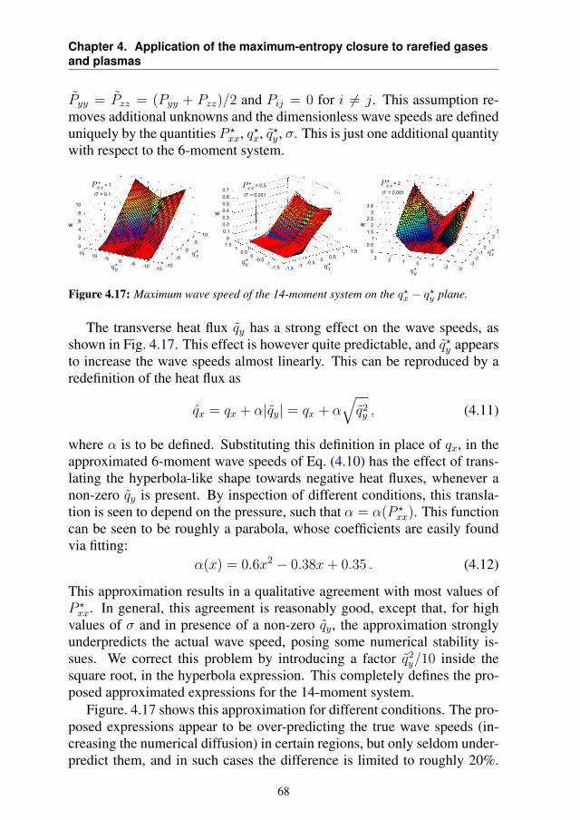
Chapter 4. Application of the maximum-entropy closure to rarefied gasesand plasmas
Pyy = Pzz = (Pyy + Pzz)/2 and Pij = 0 for i 6= j. This assumption re-moves additional unknowns and the dimensionless wave speeds are defineduniquely by the quantities P ?
xx, q?x, q?y , σ. This is just one additional quantitywith respect to the 6-moment system.
Figure 4.17: Maximum wave speed of the 14-moment system on the q?x − q?y plane.
The transverse heat flux qy has a strong effect on the wave speeds, asshown in Fig. 4.17. This effect is however quite predictable, and q?y appearsto increase the wave speeds almost linearly. This can be reproduced by aredefinition of the heat flux as
qx = qx + α|qy| = qx + α√q2y , (4.11)
where α is to be defined. Substituting this definition in place of qx, in theapproximated 6-moment wave speeds of Eq. (4.10) has the effect of trans-lating the hyperbola-like shape towards negative heat fluxes, whenever anon-zero qy is present. By inspection of different conditions, this transla-tion is seen to depend on the pressure, such that α = α(P ?
xx). This functioncan be seen to be roughly a parabola, whose coefficients are easily foundvia fitting:
α(x) = 0.6x2 − 0.38x+ 0.35 . (4.12)
This approximation results in a qualitative agreement with most values ofP ?xx. In general, this agreement is reasonably good, except that, for high
values of σ and in presence of a non-zero qy, the approximation stronglyunderpredicts the actual wave speed, posing some numerical stability is-sues. We correct this problem by introducing a factor q2
y/10 inside thesquare root, in the hyperbola expression. This completely defines the pro-posed approximated expressions for the 14-moment system.
Figure. 4.17 shows this approximation for different conditions. The pro-posed expressions appear to be over-predicting the true wave speeds (in-creasing the numerical diffusion) in certain regions, but only seldom under-predict them, and in such cases the difference is limited to roughly 20%.
68
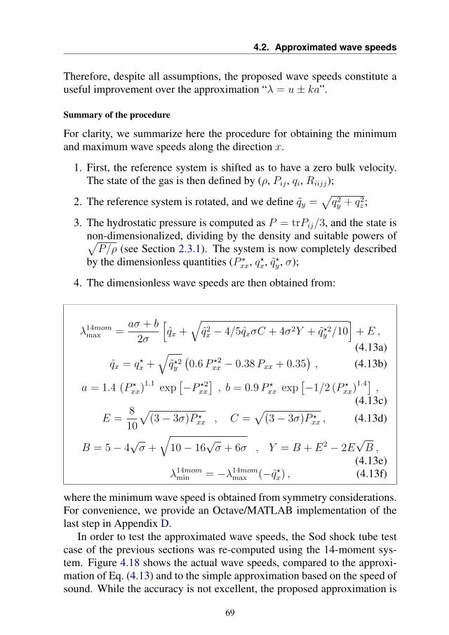
4.2. Approximated wave speeds
Therefore, despite all assumptions, the proposed wave speeds constitute auseful improvement over the approximation “λ = u± ka”.
Summary of the procedure
For clarity, we summarize here the procedure for obtaining the minimumand maximum wave speeds along the direction x.
1. First, the reference system is shifted as to have a zero bulk velocity.The state of the gas is then defined by (ρ, Pij , qi, Riijj);
2. The reference system is rotated, and we define qy =√q2y + q2
z ;
3. The hydrostatic pressure is computed as P = trPij/3, and the state isnon-dimensionalized, dividing by the density and suitable powers of√P/ρ (see Section 2.3.1). The system is now completely described
by the dimensionless quantities (P ?xx, q?x, q?y , σ);
4. The dimensionless wave speeds are then obtained from:
λ14mommax =
aσ + b
2σ
[qx +
√q2x − 4/5qxσC + 4σ2Y + q?2y /10
]+ E ,
(4.13a)qx = q?x +
√q?2y(0.6P ?2
xx − 0.38Pxx + 0.35), (4.13b)
a = 1.4 (P ?xx)
1.1 exp[−P ?2
xx
], b = 0.9P ?
xx exp[−1/2 (P ?
xx)1.4] ,(4.13c)
E =8
10
√(3− 3σ)P ?
xx , C =√
(3− 3σ)P ?xx , (4.13d)
B = 5− 4√σ +
√10− 16
√σ + 6σ , Y = B + E2 − 2E
√B ,
(4.13e)λ14mom
min = −λ14mommax (−q?x) , (4.13f)
where the minimum wave speed is obtained from symmetry considerations.For convenience, we provide an Octave/MATLAB implementation of thelast step in Appendix D.
In order to test the approximated wave speeds, the Sod shock tube testcase of the previous sections was re-computed using the 14-moment sys-tem. Figure 4.18 shows the actual wave speeds, compared to the approxi-mation of Eq. (4.13) and to the simple approximation based on the speed ofsound. While the accuracy is not excellent, the proposed approximation is
69
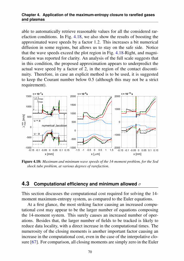
Chapter 4. Application of the maximum-entropy closure to rarefied gasesand plasmas
able to automatically retrieve reasonable values for all the considered rar-efaction conditions. In Fig. 4.18, we also show the results of boosting theapproximated wave speeds by a factor 1.2. This increases a bit numericaldiffusion in some regions, but allows us to stay on the safe side. Noticethat the wave speeds exceed the plot region in Fig. 4.18-Right, and magni-fication was reported for clarity. An analysis of the full scale suggests thatin this condition, the proposed approximation appears to underpredict theactual wave speed by a factor of 2, in the region of the contact disconti-nuity. Therefore, in case an explicit method is to be used, it is suggestedto keep the Courant number below 0.5 (although this may not be a strictrequirement).
Figure 4.18: Maximum and minimum wave speeds of the 14-moment problem, for the Sodshock tube problem, at various degrees of rarefaction.
4.3 Computational efficiency and minimum allowed σ
This section discusses the computational cost required for solving the 14-moment maximum-entropy system, as compared to the Euler equations.
At a first glance, the most striking factor causing an increased compu-tational cost may appear to be the larger number of equations composingthe 14-moment system. This surely causes an increased number of oper-ations. Besides that, the larger number of fields to be tracked is likely toreduce data locality, with a direct increase in the computational times. Thenumerosity of the closing moments is another important factor causing anincrease in the computational cost, even in the case of the interpolative clo-sure [67]. For comparison, all closing moments are simply zero in the Euler
70
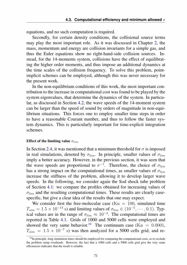
4.3. Computational efficiency and minimum allowed σ
equations, and no such computation is required.Secondly, for certain density conditions, the collisional source terms
may play the most important role. As it was discussed in Chapter 2, themass, momentum and energy are collision invariants for a simple gas, andthus the Euler equations show no right-hand-side collision sources. In-stead, for the 14-moments system, collisions have the effect of equilibrat-ing the higher order moments, and thus impose an additional dynamics atthe time scales of the collision frequency. To solve this problem, point-implicit schemes can be employed, although this was never necessary forthe present work.
In the non-equilibrium conditions of this work, the most important con-tribution to the increase in computational cost was found to be played by thesystem eigenvalues, that determine the dynamics of the system. In particu-lar, as discussed in Section 4.2, the wave speeds of the 14-moment systemcan be larger than the speed of sound by orders of magnitude in non-equi-librium situations. This forces one to employ smaller time steps in orderto have a reasonable Courant number, and thus to follow the faster sys-tem dynamics. This is particularly important for time-explicit integrationschemes.
Effect of the limiting value σlim
In Section 2.4, it was mentioned that a minimum threshold for σ is imposedin real simulations, denoted by σlim. In principle, smaller values of σlimimply a better accuracy. However, in the previous section, it was seen thatthe wave speeds are proportional to σ−1. Therefore, the choice of σlimhas a strong impact on the computational times, as smaller values of σlimincrease the stiffness of the problem, allowing it to develop larger wavespeeds. In the following, we consider again the Sod shock tube problemof Section 4.1: we compare the profiles obtained for increasing values ofσlim and the resulting computational times. These results are clearly case-specific, but give a clear idea of the results that one may expect.
We consider first the free-molecular case (Kn = 100, simulated timeTsim = 1.5× 10⁻¹³ s) and limiting values of σlim ∈ (10−5, · · · , 0.1). Typ-ical values are in the range of σlim ≈ 10−4. The computational times arereported in Table 4.1. Grids of 1000 and 5000 cells were employed andshowed the very same behavior.10 The continuum case (Kn = 0.0001,Tsim = 1.5 × 10⁻⁷ s) was then analyzed for a 5000 cells grid, and re-
10In principle, long simulation times should be employed for comparing the computational costs, as to excludethe problem setup overheads. However, the fact that a 1000 cells and a 5000 cells grid give the very sameefficiencies indicates that the result is reliable.
71
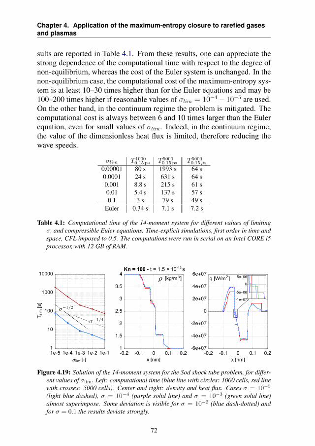
Chapter 4. Application of the maximum-entropy closure to rarefied gasesand plasmas
sults are reported in Table 4.1. From these results, one can appreciate thestrong dependence of the computational time with respect to the degree ofnon-equilibrium, whereas the cost of the Euler system is unchanged. In thenon-equilibrium case, the computational cost of the maximum-entropy sys-tem is at least 10–30 times higher than for the Euler equations and may be100–200 times higher if reasonable values of σlim = 10−4− 10−5 are used.On the other hand, in the continuum regime the problem is mitigated. Thecomputational cost is always between 6 and 10 times larger than the Eulerequation, even for small values of σlim. Indeed, in the continuum regime,the value of the dimensionless heat flux is limited, therefore reducing thewave speeds.
σlim T 10000.15 ps T 5000
0.15 ps T 50000.15µs
0.00001 80 s 1993 s 64 s0.0001 24 s 631 s 64 s0.001 8.8 s 215 s 61 s0.01 5.4 s 137 s 57 s0.1 3 s 79 s 49 s
Euler 0.34 s 7.1 s 7.2 s
Table 4.1: Computational time of the 14-moment system for different values of limitingσ, and compressible Euler equations. Time-explicit simulations, first order in time andspace, CFL imposed to 0.5. The computations were run in serial on an Intel CORE i5processor, with 12 GB of RAM.
Figure 4.19: Solution of the 14-moment system for the Sod shock tube problem, for differ-ent values of σlim. Left: computational time (blue line with circles: 1000 cells, red linewith crosses: 5000 cells). Center and right: density and heat flux. Cases σ = 10−5
(light blue dashed), σ = 10−4 (purple solid line) and σ = 10−3 (green solid line)almost superimpose. Some deviation is visible for σ = 10−2 (blue dash-dotted) andfor σ = 0.1 the results deviate strongly.
72
4.4. 2-dimensional test case: rarefied crossing jets
The effects of the value of σlim are shown in Fig. 4.19 for the free-molecular case, together with the computational times. Obviously, whilevery large value of σlim are appealing in terms of computational efficiency,they introduce progressively larger errors in the closing fluxes. All choicesof σlim ≤ 10−3 in Fig. 4.19 result roughly in the same profile, and onlysome details on the (unphysical) jumps differ. The final effect is howeverstrongly case-sensitive, and ultimately depends on the importance of theclosing moments. For the simulations performed in this work, values ofσlim = 10−3 − 10−5 are employed, and never larger.
Finally, it should be stressed that the present analysis considers a sim-ple explicit time marching scheme. Different figures of merit are expectedfor implicit schemes, and one may employ preconditioning to improve thesituation [172]. These points are however beyond the scope in this work.
4.4 2-dimensional test case: rarefied crossing jets
We conclude this first part of the chapter by considering a 2-dimensionaltest case. Two rarefied supersonic jets are simulated, injected from the sidesof a square domain as to cross in the middle, forming an angle of 90. Thedensity of the jets is taken to be low enough to be in the free-molecularregime. On physical grounds, one would expect that the two jets do notinteract, and eventually re-separate. The state in the crossing region is ki-netically out of equilibrium, and is the superposition of the drifted VDFs ofthe two individual jets. A moment closure does not necessarily reproducethis non-equilibrium correctly, hence the motivation for this test case.
This test case is apparently not related to electric propulsion. However,one can consider a number of similarities, for example in the modeling ofthe thruster plume, where the ions created in the thruster channels cross atthe axis and create a toroidal VDF [173]. In general, as we will be con-sidering ions as collisionless, it is important to study the behavior of the14-moment system for completely collisionless conditions, and a neutralfluid is a good starting point. A similar version of this problem was consid-ered in [120].
A square domain of length Lx = Ly = 1 m is considered, and the twojets are centered on the left and on the bottom sides, with a size ∆x = ∆y =Lx/7 m. Argon neutral gas is simulated. The initial solution inside thedomain is taken at a density n0 = 1010 m−3 and T0 = 300 K. To simulatethe jets, the ghost cells of the domain are set at a density nj = 1015 m−3,temperature Tj = 300 K and the velocity is set to give a Mach numberM = 5. Both the initial state and the jets injection points are described by
73
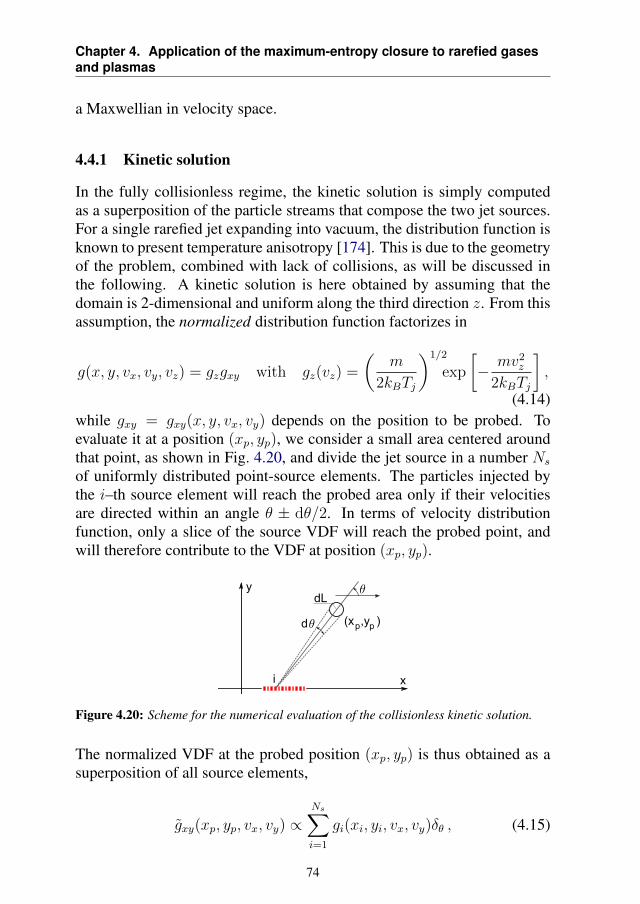
Chapter 4. Application of the maximum-entropy closure to rarefied gasesand plasmas
a Maxwellian in velocity space.
4.4.1 Kinetic solution
In the fully collisionless regime, the kinetic solution is simply computedas a superposition of the particle streams that compose the two jet sources.For a single rarefied jet expanding into vacuum, the distribution function isknown to present temperature anisotropy [174]. This is due to the geometryof the problem, combined with lack of collisions, as will be discussed inthe following. A kinetic solution is here obtained by assuming that thedomain is 2-dimensional and uniform along the third direction z. From thisassumption, the normalized distribution function factorizes in
g(x, y, vx, vy, vz) = gzgxy with gz(vz) =
(m
2kBTj
)1/2
exp
[− mv2
z
2kBTj
],
(4.14)while gxy = gxy(x, y, vx, vy) depends on the position to be probed. Toevaluate it at a position (xp, yp), we consider a small area centered aroundthat point, as shown in Fig. 4.20, and divide the jet source in a number Ns
of uniformly distributed point-source elements. The particles injected bythe i–th source element will reach the probed area only if their velocitiesare directed within an angle θ ± dθ/2. In terms of velocity distributionfunction, only a slice of the source VDF will reach the probed point, andwill therefore contribute to the VDF at position (xp, yp).
Figure 4.20: Scheme for the numerical evaluation of the collisionless kinetic solution.
The normalized VDF at the probed position (xp, yp) is thus obtained as asuperposition of all source elements,
gxy(xp, yp, vx, vy) ∝Ns∑i=1
gi(xi, yi, vx, vy)δθ , (4.15)
74
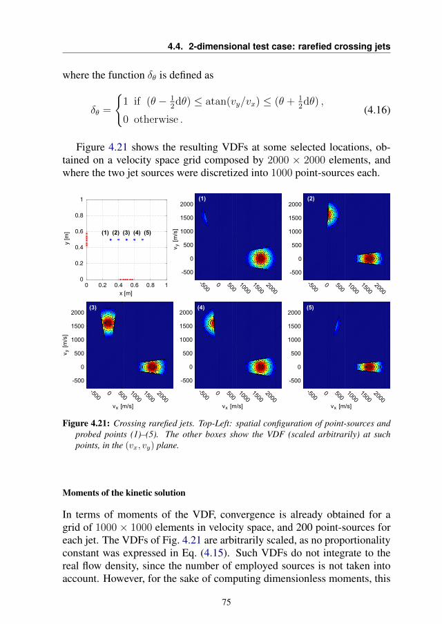
4.4. 2-dimensional test case: rarefied crossing jets
where the function δθ is defined as
δθ =
1 if (θ − 1
2dθ) ≤ atan(vy/vx) ≤ (θ + 1
2dθ) ,
0 otherwise .(4.16)
Figure 4.21 shows the resulting VDFs at some selected locations, ob-tained on a velocity space grid composed by 2000 × 2000 elements, andwhere the two jet sources were discretized into 1000 point-sources each.
Figure 4.21: Crossing rarefied jets. Top-Left: spatial configuration of point-sources andprobed points (1)–(5). The other boxes show the VDF (scaled arbitrarily) at suchpoints, in the (vx, vy) plane.
Moments of the kinetic solution
In terms of moments of the VDF, convergence is already obtained for agrid of 1000 × 1000 elements in velocity space, and 200 point-sources foreach jet. The VDFs of Fig. 4.21 are arbitrarily scaled, as no proportionalityconstant was expressed in Eq. (4.15). Such VDFs do not integrate to thereal flow density, since the number of employed sources is not taken intoaccount. However, for the sake of computing dimensionless moments, this
75
Chapter 4. Application of the maximum-entropy closure to rarefied gasesand plasmas
is not an issue. Instead, we first compute a “numerical density” n′ as
n′ =
ˆ +∞
−∞gz(vz) dvz
ˆˆ +∞
−∞gxy(vx, vy) dvxdvy (4.17)
where the “prime” superscript recalls that this does not necessarily matchthe physical density. The integral over vz was separated since g factorizes.From the definition of gz (Eq. (4.14)) this integral givesˆ +∞
−∞gz(vz) dvz = 1 . (4.18)
The average velocities ux and uy are obtained as averages of the numeri-cally constructed gxy,
ui =1
n′
ˆ +∞
−∞gz(vz) dvz
ˆˆ +∞
−∞vigxy(vx, vy) dvxdvy . (4.19)
Analogously, the temperatures in the x and y directions read
Ti =m
n′kB
ˆ +∞
−∞gz(vz) dvz
ˆˆ +∞
−∞(vi − ui)2gxy(vx, vy) dvxdvy . (4.20)
The dimensionless heat fluxes are obtained by dividing the heat flux bythe factor ρ(P/ρ)3/2 = mn(kBT/m)3/2, with T = (Tx + Ty + Tz)/3 andTz = 300 K,
q?i =1
mn′(kBT/m)3/2
ˆˆˆ +∞
−∞mcic
2gxy(vx, vy)gz(vz) dvxdvydvz
=1
n′(kBT/m)3/2
1׈ˆ +∞
−∞ci[(vx − ux)2 + (vy − uy)2
]gxy dvxdvy
+
ˆ +∞
−∞v2zgz(vz) dvz
ˆˆ +∞
−∞cigxy(vx, vy) dvxdvy
, (4.21)
with ci = vi − ui and i either x or y. Notice that this time the velocity vzappears in the integral (through the peculiar velocity term c2). We have thatˆ +∞
−∞v2zgz(vz) dvz =
kBT
m, (4.22)
finally giving
q?i =1
n′(kBT/m)3/2
ˆˆ +∞
−∞ci
(c2x + c2
y +kBT
m
)gxy(vx, vy) dvxdvy .
(4.23)These moments will be compared to the 14-moment solution in the nextsection.
76
4.4. 2-dimensional test case: rarefied crossing jets
4.4.2 14-moment and Euler solutions
In the free-molecular regime, the two rarefied jets should not interact. How-ever, a general moment system does not necessarily reproduce correctlysuch behavior. To start off, we compute the solution of the 14-moment sys-tem for a single jet. This solution is then rotated by 90 and superimposedto itself, as to give artificially the expected result of two crossing jets thatdo not interact. This artificial solution is then compared to a full solutionof two jets simulated simultaneously.
The problem is solved on a Cartesian grid of 1280 × 1280 cells. Atime-marching approach is employed, with Courant number fixed to 0.5and explicit Midpoint Euler time integrator. The steady state is reachedafter roughly 1.5 ms of simulation time. The same numerical settings areemployed for both the single-jet and the two-jets simulations: in such way,both simulations show an analogous degree of numerical diffusion, andresults can be compared.
The numerical solution of the full problem proceeds reasonably fast un-til the two jets cross. At such point, non-equilibrium increases (as the VDFdeviates from the Maxwellian), and correspondingly the wave speeds alsoincrease, and a smaller time step is needed in order to respect the CFL con-dition. In particular, the situation happens to be so strong that, when thesecond order MUSCL approach is enabled, the wave speeds become ex-tremely large and the simulation becomes impractical. This problem couldbe solved by implicit time stepping, or by preconditioning the system. Inthis work, we simply give up with second order accuracy, but in order toreduce the high numerical diffusion of the Rusanov scheme, we adopt thepartial MUSCL reconstruction of Eq 3.8, with β = 0.75.
Figure 4.22 shows the resulting density field from the 14-moment sys-tem, and compares the full solution of the two-jets to the artificially su-perimposed jets. From such solution, the values were extracted along theaxis of one jet, on the line with y = 0.5 m, for x ∈ (0, 1) m, and dimen-sionless moments were computed. These moments were also computedfrom the kinetic results, and are compared in Fig. 4.23. All these resultsconfirm the quality of the 14-moment solution. It is useful to recall herereference [127], where various shapes of the attainable VDFs are shownfor the 5-moment systems in moment space. The order-4 maximum-en-tropy system shows capable of representing a number of situations such asthe bump-on-tail and bi-Maxwellians. Analogously, the 14-moment systemis a reasonable choice for representing the VDFs of the present case, thatare roughly the superposition of two drifted Maxwellians. We expect the
77
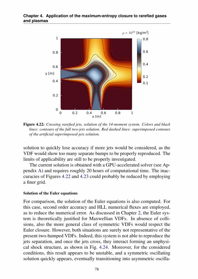
Chapter 4. Application of the maximum-entropy closure to rarefied gasesand plasmas
Figure 4.22: Crossing rarefied jets, solution of the 14-moment system. Colors and blacklines: contours of the full two-jets solution. Red dashed lines: superimposed contoursof the artificial superimposed-jets solution.
solution to quickly lose accuracy if more jets would be considered, as theVDF would show too many separate bumps to be properly reproduced. Thelimits of applicability are still to be properly investigated.
The current solution is obtained with a GPU-accelerated solver (see Ap-pendix A) and requires roughly 20 hours of computational time. The inac-curacies of Figures 4.22 and 4.23 could probably be reduced by employinga finer grid.
Solution of the Euler equations
For comparison, the solution of the Euler equations is also computed. Forthis case, second order accuracy and HLL numerical fluxes are employed,as to reduce the numerical error. As discussed in Chapter 2, the Euler sys-tem is theoretically justified for Maxwellian VDFs. In absence of colli-sions, also the more general class of symmetric VDFs would respect theEuler closure. However, both situations are surely not representative of thepresent two-humped VDFs. Indeed, this system is not able to reproduce thejets separation, and once the jets cross, they interact forming an unphysi-cal shock structure, as shown in Fig. 4.24. Moreover, for the consideredconditions, this result appears to be unstable, and a symmetric oscillatingsolution quickly appears, eventually transitioning into asymmetric oscilla-
78
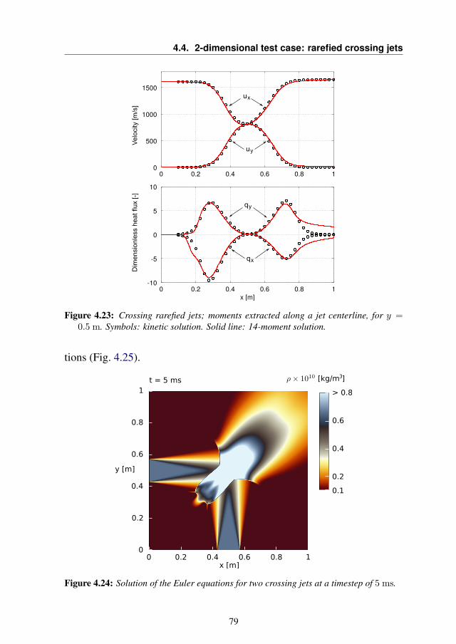
4.4. 2-dimensional test case: rarefied crossing jets
Figure 4.23: Crossing rarefied jets; moments extracted along a jet centerline, for y =0.5 m. Symbols: kinetic solution. Solid line: 14-moment solution.
tions (Fig. 4.25).
Figure 4.24: Solution of the Euler equations for two crossing jets at a timestep of 5 ms.
79
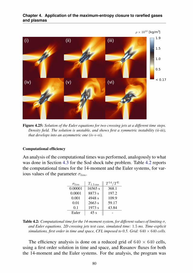
Chapter 4. Application of the maximum-entropy closure to rarefied gasesand plasmas
Figure 4.25: Solution of the Euler equations for two crossing jets at a different time steps.Density field. The solution is unstable, and shows first a symmetric instability (ii-iii),that develops into an asymmetric one (iv-v-vi).
Computational efficiency
An analysis of the computational times was performed, analogously to whatwas done in Section 4.3 for the Sod shock tube problem. Table 4.2 reportsthe computational times for the 14-moment and the Euler systems, for var-ious values of the parameter σlim.
σlim T1.5ms T 14/TE
0.00001 16565 s 368.10.0001 8873 s 197.20.001 4948 s 109.90.01 2663 s 59.170.1 1973 s 43.84
Euler 45 s -
Table 4.2: Computational time for the 14-moment system, for different values of limiting σ,and Euler equations. 2D crossing jets test case, simulated time: 1.5 ms. Time-explicitsimulations, first order in time and space, CFL imposed to 0.5. Grid: 640× 640 cells.
The efficiency analysis is done on a reduced grid of 640 × 640 cells,using a first order solution in time and space, and Rusanov fluxes for boththe 14-moment and the Euler systems. For the analysis, the program was
80
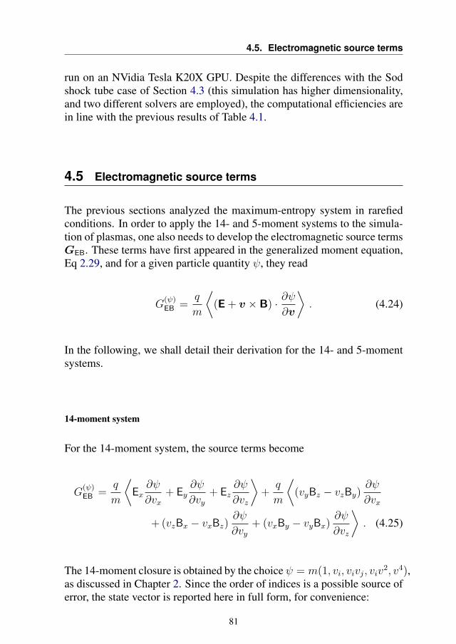
4.5. Electromagnetic source terms
run on an NVidia Tesla K20X GPU. Despite the differences with the Sodshock tube case of Section 4.3 (this simulation has higher dimensionality,and two different solvers are employed), the computational efficiencies arein line with the previous results of Table 4.1.
4.5 Electromagnetic source terms
The previous sections analyzed the maximum-entropy system in rarefiedconditions. In order to apply the 14- and 5-moment systems to the simula-tion of plasmas, one also needs to develop the electromagnetic source termsGEB. These terms have first appeared in the generalized moment equation,Eq 2.29, and for a given particle quantity ψ, they read
G(ψ)EB =
q
m
⟨(E + v × B) · ∂ψ
∂v
⟩. (4.24)
In the following, we shall detail their derivation for the 14- and 5-momentsystems.
14-moment system
For the 14-moment system, the source terms become
G(ψ)EB =
q
m
⟨Ex∂ψ
∂vx+ Ey
∂ψ
∂vy+ Ez
∂ψ
∂vz
⟩+
q
m
⟨(vyBz − vzBy)
∂ψ
∂vx
+ (vzBx − vxBz)∂ψ
∂vy+ (vxBy − vyBx)
∂ψ
∂vz
⟩. (4.25)
The 14-moment closure is obtained by the choiceψ = m(1, vi, vivj, viv2, v4),
as discussed in Chapter 2. Since the order of indices is a possible source oferror, the state vector is reported here in full form, for convenience:
81
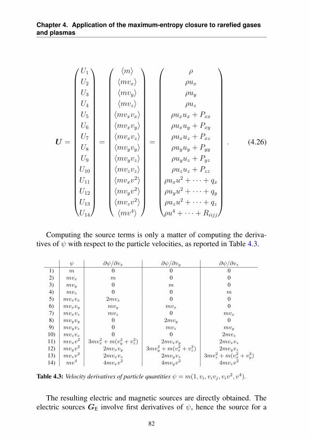
Chapter 4. Application of the maximum-entropy closure to rarefied gasesand plasmas
U =
U1
U2
U3
U4
U5
U6
U7
U8
U9
U10
U11
U12
U13
U14
=
〈m〉〈mvx〉〈mvy〉〈mvz〉〈mvxvx〉〈mvxvy〉〈mvxvz〉〈mvyvy〉〈mvyvz〉〈mvzvz〉〈mvxv2〉〈mvyv2〉〈mvzv2〉〈mv4〉
=
ρ
ρux
ρuy
ρuz
ρuxux + Pxx
ρuxuy + Pxy
ρuxuz + Pxz
ρuyuy + Pyy
ρuyuz + Pyz
ρuzuz + Pzz
ρuxu2 + · · ·+ qx
ρuyu2 + · · ·+ qy
ρuzu2 + · · ·+ qz
ρu4 + · · ·+Riijj
. (4.26)
Computing the source terms is only a matter of computing the deriva-tives of ψ with respect to the particle velocities, as reported in Table 4.3.
ψ ∂ψ/∂vx ∂ψ/∂vy ∂ψ/∂vz1) m 0 0 02) mvx m 0 03) mvy 0 m 04) mvz 0 0 m5) mvxvx 2mvx 0 06) mvxvy mvy mvx 07) mvxvz mvz 0 mvx8) mvyvy 0 2mvy 09) mvyvz 0 mvz mvy
10) mvzvz 0 0 2mvz11) mvxv
2 3mv2x +m(v2y + v2z) 2mvxvy 2mvxvz12) mvyv
2 2mvxvy 3mv2y +m(v2x + v2z) 2mvyvz13) mvzv
2 2mvxvz 2mvyvz 3mv2z +m(v2x + v2y)14) mv4 4mvxv
2 4mvyv2 4mvzv
2
Table 4.3: Velocity derivatives of particle quantities ψ = m(1, vi, vivj , viv2, v4).
The resulting electric and magnetic sources are directly obtained. Theelectric sources GE involve first derivatives of ψ, hence the source for a
82
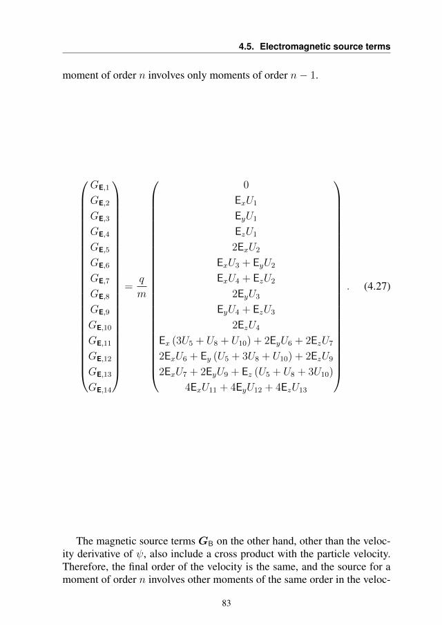
4.5. Electromagnetic source terms
moment of order n involves only moments of order n− 1.
GE,1
GE,2
GE,3
GE,4
GE,5
GE,6
GE,7
GE,8
GE,9
GE,10
GE,11
GE,12
GE,13
GE,14
=q
m
0
ExU1
EyU1
EzU1
2ExU2
ExU3 + EyU2
ExU4 + EzU2
2EyU3
EyU4 + EzU3
2EzU4
Ex (3U5 + U8 + U10) + 2EyU6 + 2EzU7
2ExU6 + Ey (U5 + 3U8 + U10) + 2EzU9
2ExU7 + 2EyU9 + Ez (U5 + U8 + 3U10)
4ExU11 + 4EyU12 + 4EzU13
. (4.27)
The magnetic source terms GB on the other hand, other than the veloc-ity derivative of ψ, also include a cross product with the particle velocity.Therefore, the final order of the velocity is the same, and the source for amoment of order n involves other moments of the same order in the veloc-
83
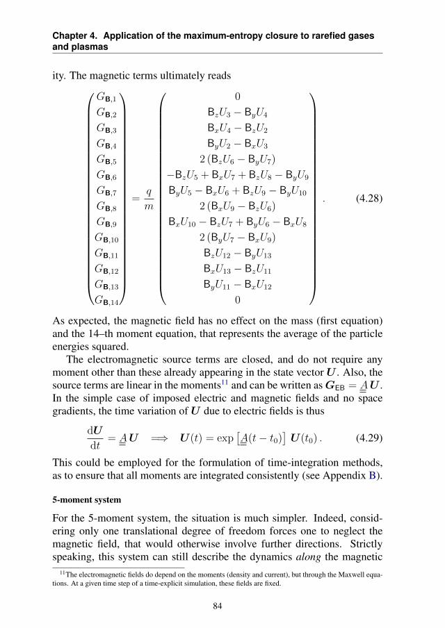
Chapter 4. Application of the maximum-entropy closure to rarefied gasesand plasmas
ity. The magnetic terms ultimately reads
GB,1
GB,2
GB,3
GB,4
GB,5
GB,6
GB,7
GB,8
GB,9
GB,10
GB,11
GB,12
GB,13
GB,14
=q
m
0
BzU3 − ByU4
BxU4 − BzU2
ByU2 − BxU3
2 (BzU6 − ByU7)
−BzU5 + BxU7 + BzU8 − ByU9
ByU5 − BxU6 + BzU9 − ByU10
2 (BxU9 − BzU6)
BxU10 − BzU7 + ByU6 − BxU8
2 (ByU7 − BxU9)
BzU12 − ByU13
BxU13 − BzU11
ByU11 − BxU12
0
. (4.28)
As expected, the magnetic field has no effect on the mass (first equation)and the 14–th moment equation, that represents the average of the particleenergies squared.
The electromagnetic source terms are closed, and do not require anymoment other than these already appearing in the state vector U . Also, thesource terms are linear in the moments11 and can be written asGEB = AU .In the simple case of imposed electric and magnetic fields and no spacegradients, the time variation of U due to electric fields is thus
dU
dt= AU =⇒ U(t) = exp
[A(t− t0)
]U (t0) . (4.29)
This could be employed for the formulation of time-integration methods,as to ensure that all moments are integrated consistently (see Appendix B).
5-moment system
For the 5-moment system, the situation is much simpler. Indeed, consid-ering only one translational degree of freedom forces one to neglect themagnetic field, that would otherwise involve further directions. Strictlyspeaking, this system can still describe the dynamics along the magnetic
11The electromagnetic fields do depend on the moments (density and current), but through the Maxwell equa-tions. At a given time step of a time-explicit simulation, these fields are fixed.
84
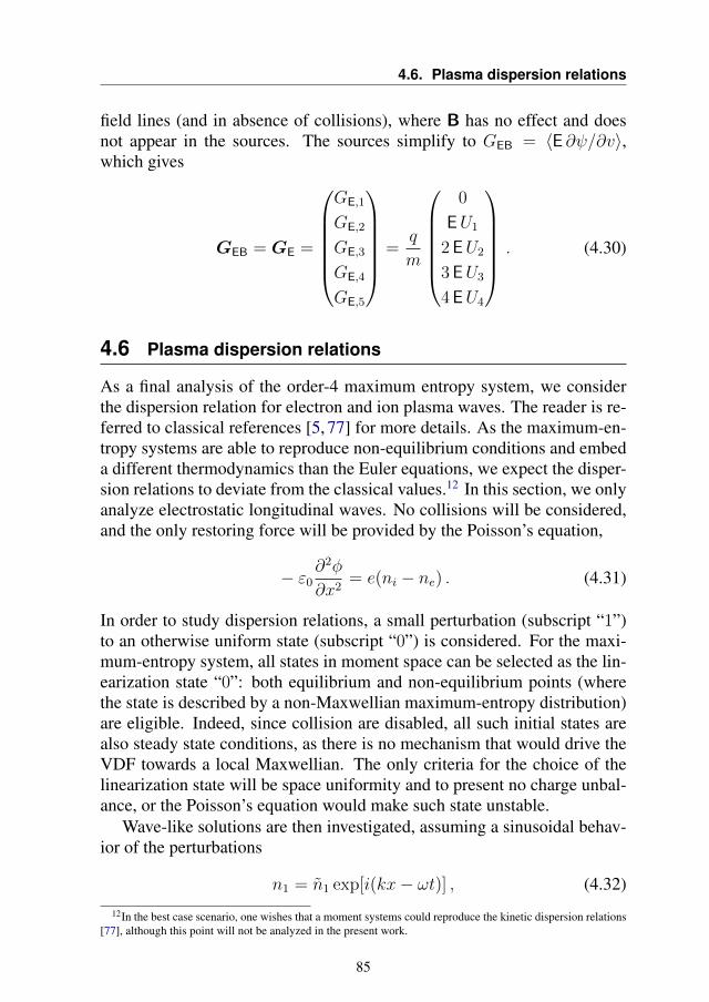
4.6. Plasma dispersion relations
field lines (and in absence of collisions), where B has no effect and doesnot appear in the sources. The sources simplify to GEB = 〈E ∂ψ/∂v〉,which gives
GEB = GE =
GE,1
GE,2
GE,3
GE,4
GE,5
=q
m
0
EU1
2EU2
3EU3
4EU4
. (4.30)
4.6 Plasma dispersion relations
As a final analysis of the order-4 maximum entropy system, we considerthe dispersion relation for electron and ion plasma waves. The reader is re-ferred to classical references [5, 77] for more details. As the maximum-en-tropy systems are able to reproduce non-equilibrium conditions and embeda different thermodynamics than the Euler equations, we expect the disper-sion relations to deviate from the classical values.12 In this section, we onlyanalyze electrostatic longitudinal waves. No collisions will be considered,and the only restoring force will be provided by the Poisson’s equation,
− ε0∂2φ
∂x2= e(ni − ne) . (4.31)
In order to study dispersion relations, a small perturbation (subscript “1”)to an otherwise uniform state (subscript “0”) is considered. For the maxi-mum-entropy system, all states in moment space can be selected as the lin-earization state “0”: both equilibrium and non-equilibrium points (wherethe state is described by a non-Maxwellian maximum-entropy distribution)are eligible. Indeed, since collision are disabled, all such initial states arealso steady state conditions, as there is no mechanism that would drive theVDF towards a local Maxwellian. The only criteria for the choice of thelinearization state will be space uniformity and to present no charge unbal-ance, or the Poisson’s equation would make such state unstable.
Wave-like solutions are then investigated, assuming a sinusoidal behav-ior of the perturbations
n1 = n1 exp[i(kx− ωt)] , (4.32)
12In the best case scenario, one wishes that a moment systems could reproduce the kinetic dispersion relations[77], although this point will not be analyzed in the present work.
85
Chapter 4. Application of the maximum-entropy closure to rarefied gasesand plasmas
and the same for all other variables. In the following, the symbol “ ˜ ” willbe dropped for simplicity. The stability in time of a perturbation of wavenumber k can be analyzed by checking the real and imaginary parts of theangular frequency ω(k) (see for example [62]). Writing ω = ωR+iωI gives
n1 = n1 exp(ωIt) exp[i(kx− ωRt)] , (4.33)
hence, with this formulation, positive values of ωI imply amplification ofthe perturbation, while negative values represent damping.
For wave-like solutions, the derivatives transform as ∂t → −iω, and∂x → ik. Since the uniform state is taken as uniform, we obtain φ0 = 0,and the Poisson’s equation transforms to
− ε0∂2φ1
∂x2= e(ni − ne) =⇒ φ1 =
e(ni1 − ne1)
k2ε0
. (4.34)
At this point, the charges dynamics is described by introducing a fluidmodel. We consider here the Euler equations and the 5-moment system.The 14-moment system is not considered: indeed, in absence of a mag-netic field, electrostatic waves are purely longitudinal and involve a singletranslational degree of freedom. Without collisions, this degree of freedomdoes not exchange energy with the other translational modes. For this samereason, in treating plasma waves, the authors typically set the adiabaticconstant to γ = 3 (see [5, 53]). The Euler system is written in primitivevariables and reads
∂tρ+ u ∂xρ+ ρ ∂xu = 0 ,
∂tu+ u ∂xu+ 1/ρ ∂xP = − qm∂xφ ,
∂tP + γP ∂xu+ u ∂xP = 0 ,
(4.35)
and after linearization, it is easily written in matrix form as
− iω
ρ1
u1
P1
+ ik
u0 ρ0 0
0 u0 1/ρ0
0 γP0 u0
ρ1
u1
P1
= −ik qm
0
φ1
0
. (4.36)
The same can be done for the 5-moment system, that in primitive variables
86
4.6. Plasma dispersion relations
reads
∂tρ+ u ∂xρ+ ρ ∂xu = 0 ,
∂tu+ u ∂xu+ 1/ρ ∂xP = − qm∂xφ ,
∂tP + 3P ∂xu+ u ∂xP + ∂xQ = 0 ,
∂tQ+ 4Q∂xu− 3P/ρ ∂xP + u∂xQ+ ∂xR = 0 ,
∂tR + 5R∂xu− 4Q/ρ ∂xP + u∂xR + ∂xS = 0 .
(4.37)
and the very same linearization can be done. Note that in both systems theelectric field appears only in the velocity equation, since all other equationsare those of the central moments, that are not affected by it. The furthersteps depend on the type of oscillations to be considered.
4.6.1 Electron waves
Let us start by analyzing longitudinal electron oscillations and waves. Allmoments n, ρ, u, P,Q,R are referred to the electron population. Given thelarge mass disparity, electron waves have a much higher frequency thanion waves, hence ions can be treated as a background of fixed neutralizingcharges, with number density ni = ne0 = n0, and thus ni1 = 0. The lin-earized Poisson’s equation gives φ1 = −en1/(k
2ε0), with n1 the perturbedelectrons number density. The Euler system thus becomesk
u0 ρ0 0
0 u0 1/ρ0
0 γP0 u0
+1
k
q2
m2ε0
0 0 0
1 0 0
0 0 0
− ω1 0 0
0 1 0
0 0 1
ρ1u1
P1
=
0
0
0
, (4.38)
that is an eigenvalue problem. We write it ask [J0] +
1
k
q2
m2ε0
[Mφ]− ω [I]
U1 = 0 (4.39)
with [J0] the Jacobian of the convective fluxes, evaluated at the linearizationstate, [I] the identity matrix, and [Mφ] a matrix filled with zeros with a soleunitary entry in the first element (density) of the second row (momentumequation). The eigenvalues of such system can be easily obtained both an-alytically and numerically, and result in the classical (fluid) warm electronsdispersion relation
ω2 = ω2p + 3
2k2 (2kBT/m) (4.40)
where kB is the Boltzmann constant, T and m are the electron temperatureand mass and ωp =
√n0e2/(mε0) the electron plasma frequency.
87
Chapter 4. Application of the maximum-entropy closure to rarefied gasesand plasmas
The same calculations can be done on the 5-moment system and thisalso results in Eq. (4.39), with
[J0] =
u ρ 0 0 0
0 u 1/ρ 0 0
0 3P u 1 0
0 4Q −3P/ρ u 1∂S∂ρ
5R −4Q/ρ+ ∂S∂P
∂S∂Q
u+ ∂S∂R
0
, (4.41)
and where the matrix [Mφ] reads
[Mφ] =
0 0 0 0 0
1 0 0 0 0
0 0 0 0 0
0 0 0 0 0
0 0 0 0 0
. (4.42)
The dispersion relation is less trivial for this case, due to the higherdimensionality and the more complex structure of the fluxes Jacobian (at-tributed to the closing moment S). However, by numerical computationone can easily evaluate the dispersion relation at different points in momentspace.
Dispersion relation at different points in moment space
The linearization condition for the numerical computation of the dispersionrelation is taken as n0 = 1010 m−3, T0 = 1000 K and u0 = 0 m/s. Theonly ion property that matters for electron waves is the density, ni0 = n0.
The 5-moment system without source terms is hyperbolic. Therefore,its eigenvalues are in the form ω(k) = kλi, with λi the i–th (real) wavespeed.13 The dispersion relation for the electrically neutral 5-moment sys-tem is thus composed by a straight line, with constant phase and groupvelocities for each fluid mode. When introducing the self-consistent elec-tric field as a source term, we observe the very same feature in the limitingcase of a very large wave number, kλDe 1 (with λDe the Debye length forthe considered n0 and T0). This is shown in Fig. 4.26 for equilibrium condi-tions (Q? = 0, R? = 3), where the numerical dispersion relation is seen toasymptote to the neutral-fluid dispersion relation. For lower wave numbers,the dispersion relation settles on the plasma frequency, as expected.
13This is evident if one considers the eigenvalue problem of Eq. (4.39), without electric fields, where theeigenvalues of the system are seen to be equal to ω/k.
88
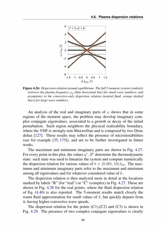
4.6. Plasma dispersion relations
Figure 4.26: Dispersion relation around equilibrium. The full 5-moment system (symbols)retrieves the plasma frequency ωp (blue horizontal line) for small wave numbers, andasymptotes to the convective-only dispersion relation (neutral fluid, orange dashedlines) for large wave numbers.
An analysis of the real and imaginary parts of ω shows that in someregions of the moment space, the problem may develop imaginary com-plex conjugate eigenvalues, associated to a growth or decay of the initialperturbation. Such region neighbors the physical realizability boundary,where the VDF is strongly non-Maxwellian and is composed by two Diracdeltas [127]. These results may reflect the presence of microinstabilities(see for example [35, 175]), and are to be further investigated in futureworks.
The maximum and minimum imaginary parts are shown in Fig. 4.27.For every point in this plot, the values q?, R? determine the thermodynamicstate: such state was used to linearize the system and compute numericallythe dispersion relation for various values of k ∈ (0.001, 10)λDe. The max-imum and minimum imaginary parts refer to the maximum and minimumamong all eigenvalues and for whatever considered value of k.
The dispersion relation is then analyzed more in detail at the locationsmarked by labels “R” (for “real”) or “C” (complex) in Fig. 4.27. These areshown in Fig. 4.28 for the real points, where the fluid dispersion relationof Eq. (4.40) is also reported. The 5-moment results match closely thewarm fluid approximation for small values of k, but quickly departs fromit, having higher convective wave speeds.
The dispersion relation for the points (C1),(C2) and (C3) is shown inFig. 4.29. The presence of two complex conjugate eigenvalues is clearly
89
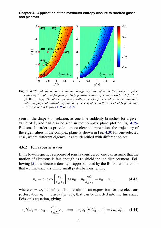
Chapter 4. Application of the maximum-entropy closure to rarefied gasesand plasmas
Figure 4.27: Maximum and minimum imaginary part of ω in the moment space,scaled by the plasma frequency. Only positive values of k are considered, for k ∈(0.001, 10)λDe. The plot is symmetric with respect to q?. The white dashed line indi-cates the physical realizability boundary. The symbols in the plot identify points thatare inspected in Figures 4.28 and 4.29.
seen in the dispersion relation, as one line suddenly branches for a givenvalue of k, and can also be seen in the complex plane plot of Fig. 4.29-Bottom. In order to provide a more clear interpretation, the trajectory ofthe eigenvalues in the complex plane is shown in Fig. 4.30 for one selectedcase, where different eigenvalues are identified with different colors.
4.6.2 Ion acoustic waves
If the low-frequency response of ions is considered, one can assume that themotion of electrons is fast enough as to shield the ion displacement. Fol-lowing [5], the electron density is approximated by the Boltzmann relation,that we linearize assuming small perturbations, giving
ne = n0 exp
[eφ
kBTe
]≈ n0 + n0
eφ
kBTe= n0 + ne1 , (4.43)
where φ = φ1 as before. This results in an expression for the electronsperturbation ne1 = n0eφ1/(kBTe), that can be inserted into the linearizedPoisson’s equation, giving
ε0k2φ1 = eni1 −
e2n0
kBTeφ1 =⇒ ε0φ1
(k2λ2
De + 1)
= eni1λ2De , (4.44)
90
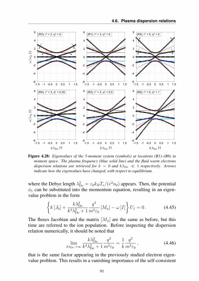
4.6. Plasma dispersion relations
Figure 4.28: Eigenvalues of the 5-moment system (symbols) at locations (R1)–(R6) inmoment space. The plasma frequency (blue solid line) and the fluid warm electronsdispersion relations are retrieved for k = 0 and kλDe 1 respectively. Arrowsindicate how the eigenvalues have changed, with respect to equilibrium.
where the Debye length λ2De = ε0kBTe/(e
2n0) appears. Then, the potentialφ1 can be substituted into the momentum equation, resulting in an eigen-value problem in the form
k [J0] +kλ2
De
k2λ2De + 1
q2
m2ε0
[Mφ]− ω [I]
U1 = 0 . (4.45)
The fluxes Jacobian and the matrix [Mφ] are the same as before, but thistime are referred to the ion population. Before inspecting the dispersionrelation numerically, it should be noted that
limkλDe→∞
kλ2De
k2λ2De + 1
q2
m2ε0
=1
k
q2
m2ε0
, (4.46)
that is the same factor appearing in the previously studied electron eigen-value problem. This results in a vanishing importance of the self-consistent
91
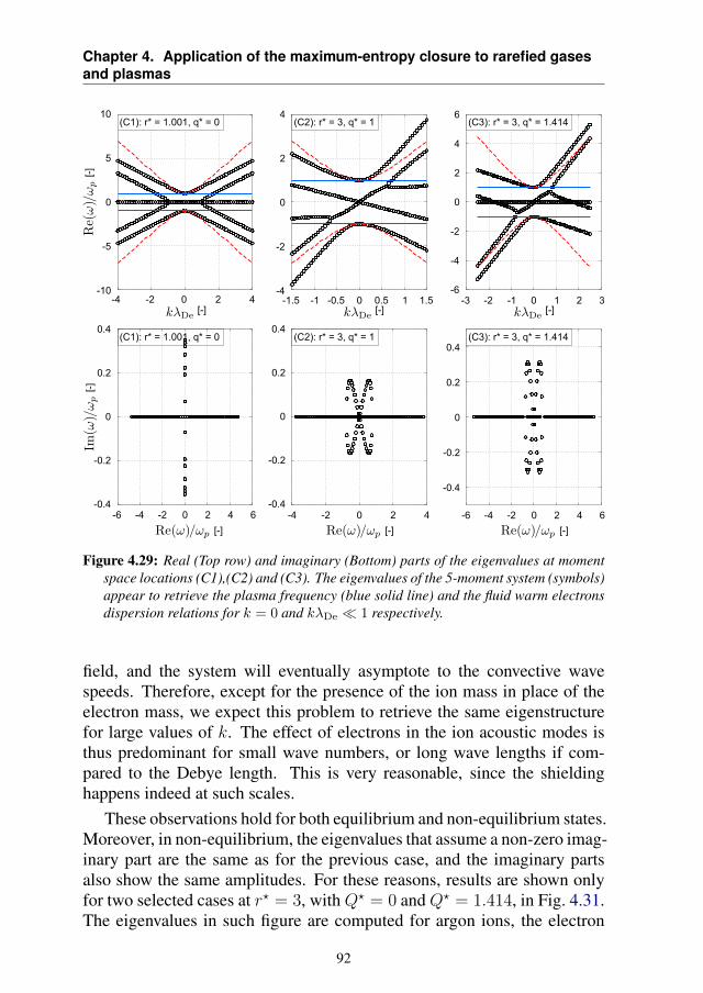
Chapter 4. Application of the maximum-entropy closure to rarefied gasesand plasmas
Figure 4.29: Real (Top row) and imaginary (Bottom) parts of the eigenvalues at momentspace locations (C1),(C2) and (C3). The eigenvalues of the 5-moment system (symbols)appear to retrieve the plasma frequency (blue solid line) and the fluid warm electronsdispersion relations for k = 0 and kλDe 1 respectively.
field, and the system will eventually asymptote to the convective wavespeeds. Therefore, except for the presence of the ion mass in place of theelectron mass, we expect this problem to retrieve the same eigenstructurefor large values of k. The effect of electrons in the ion acoustic modes isthus predominant for small wave numbers, or long wave lengths if com-pared to the Debye length. This is very reasonable, since the shieldinghappens indeed at such scales.
These observations hold for both equilibrium and non-equilibrium states.Moreover, in non-equilibrium, the eigenvalues that assume a non-zero imag-inary part are the same as for the previous case, and the imaginary partsalso show the same amplitudes. For these reasons, results are shown onlyfor two selected cases at r? = 3, with Q? = 0 and Q? = 1.414, in Fig. 4.31.The eigenvalues in such figure are computed for argon ions, the electron
92
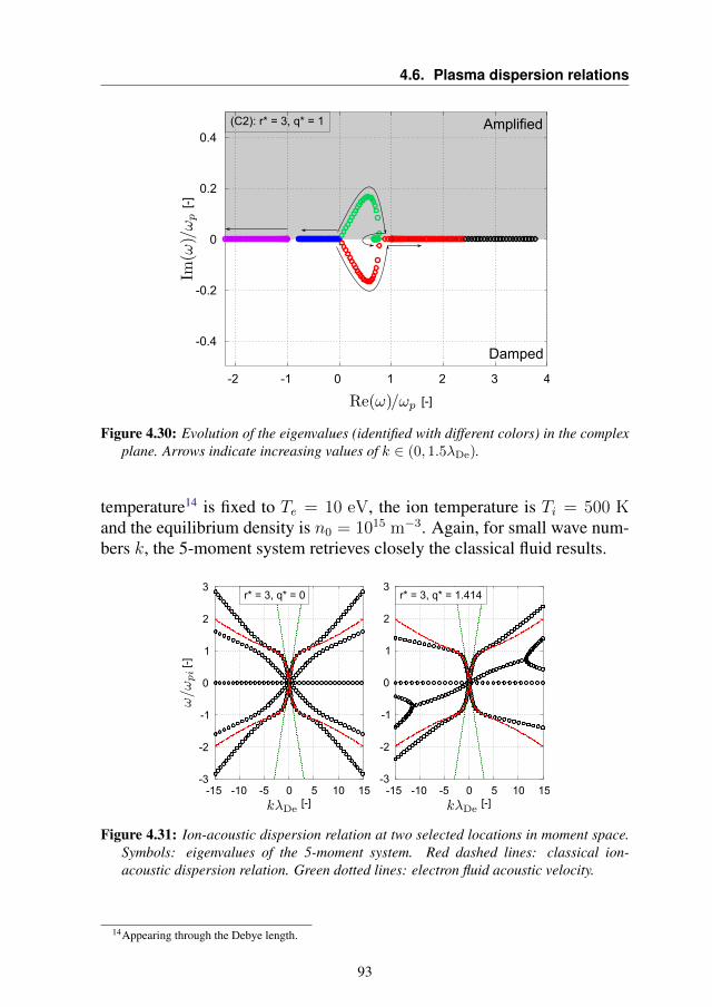
4.6. Plasma dispersion relations
Figure 4.30: Evolution of the eigenvalues (identified with different colors) in the complexplane. Arrows indicate increasing values of k ∈ (0, 1.5λDe).
temperature14 is fixed to Te = 10 eV, the ion temperature is Ti = 500 Kand the equilibrium density is n0 = 1015 m−3. Again, for small wave num-bers k, the 5-moment system retrieves closely the classical fluid results.
Figure 4.31: Ion-acoustic dispersion relation at two selected locations in moment space.Symbols: eigenvalues of the 5-moment system. Red dashed lines: classical ion-acoustic dispersion relation. Green dotted lines: electron fluid acoustic velocity.
14Appearing through the Debye length.
93
Chapter 4. Application of the maximum-entropy closure to rarefied gasesand plasmas
4.7 Conclusions
This chapter has introduced some developments and analysis preliminaryto the practical application of the order-4 maximum-entropy systems to rar-efied gases and plasmas.
First part of the chapter: rarefied gases
First, a rarefied test case was defined as a reference: the Sod shock tubeproblem was studied numerically from the free-molecular to the continuumregime. This allowed us to compare the accuracy of the maximum-entropysolution to the kinetic solution. The structure of the 5-moment solution,composed by five waves in the rarefied regime, was also analyzed. TheRusanov scheme was identified as the scheme of choice for this work, as itdoes not need a detailed knowledge of the system eigenstructure (but onlythe maximum wave speed) and appears to be more robust than the HLLscheme.
This test case was then employed as a benchmark to analyze the wavespeeds of the maximum-entropy system. It was observed that these can ex-ceed the speed of sound by orders of magnitude, and some approximationswere developed for the 6-moment and 14-moment systems. These approxi-mations allow for more stable and much less diffusive numerical solutions.
A further test case was then defined, in two dimensions, to study the be-havior of the 14-moment system, test the formulated wave speeds approx-imation and to test second order accuracy in space. With these develop-ments, the methods is ready and tested for tackling collisionless situations.
Second part of the chapter: plasmas
Then, attention was put to develop and characterize the plasma capabili-ties of the method. In particular, the electromagnetic source terms weredeveloped for the 5 and 14-moment equations, and then plasma dispersionrelations were analyzed, for electrostatic waves.
Based on these developments and analysis, the next chapters will dealwith an application of the method to Hall thruster conditions.
94
CHAPTER5Collisionless ions in Hall thrusters:
an analytical axial model and a simple fluidclosure
The content of this chapter was published in [176]: Boccelli, S., Charoi,T., Alvarez Laguna, A., Chabert, P., Bourdon, A., Magin, T.E., Colli-sionless ion modeling in Hall thrusters: analytical axial velocity dis-tribution function and heat flux closures, Physics of Plasmas 27 (7),073506.
In the previous chapters, the theoretical basis for the description of rar-efied gases and plasmas were introduced, and the order-4 maximum-en-tropy systems were adapted to tackling plasma simulations. In this chapter,we start the analysis of Hall thruster-like problems. However, before apply-ing the maximum-entropy system, some preliminary study of the problemis in order. In particular, in this chapter we start by considering the axialevolution of ions in a Hall thruster channel, with the aims of:
• Obtaining an understanding of the problem, from both the kinetic andfluid perspectives;
95
Chapter 5. Collisionless ions in Hall thrusters:an analytical axial model and a simple fluid closure
• Developing reference solutions to be further analyzed, in the laterchapters, by the maximum-entropy system.
The preliminary analysis of Section 2.2 indicated that ions are, to a firstapproximation, collisionless, unmagnetized and strongly affected by theelectric field. This causes the axial VDF to deviate from a Maxwellian, asshown by both experiments and kinetic simulations [177–179].
Outside of the thruster channel, as the plume develops and the electricfield weakens, the effect of charge exchange (CEX) and momentum ex-change (MEX) collisions eventually becomes dominant [180, 181]. Thepresent analysis focuses on the interior or near-plume of the thruster, ne-glecting all collisions. Only ions will be considered in this chapter: elec-trons and neutrals will not be accounted for, and their interaction with ionsis introduced by assigning a given electric field and ionization profile. Insuch way, it is possible to compare different ion models without introducingany error or assumptions related to the electrons model.
In Section 5.1, we consider the axial ion VDF, and describe its featuresbased on the structure of the ionization and electric field profiles. An ana-lytical solution of the kinetic equation is then obtained in Section 5.2 andis compared to PIC simulations (Section 5.2.2) and to experimental mea-surements (Section 5.2.3). Then, a 3-equations fluid model is developedin Section 5.3. The mass, momentum and energy equations are derived,and an ad hoc non-Fourier closure for the heat flux is formulated in Sec-tion 5.3.2. This formulation is then compared to the PIC simulations inSection 5.3.3.
5.1 Genesis of the axial VDF
We start by a qualitative description of the ion axial VDF.The shape of the ion VDF is conveniently explained by assuming steady
state conditions. Steady state is not necessarily realized in real situations:this assumption could however be interpreted as a quasi-steady state in caseof low-frequency oscillations (such that the characteristic time is longerthan the transit time of ions into the channel) or as a time average for fastermodes.
In this section, we import the spatial profiles of the electric field (as-sumed purely axial) and ionization source from [182]. The fields wereslightly adapted as to remove the negative electric field region, and areshown in Fig. 5.1-Left. The maximum electric field for such case is Emax ≈20 kV/m and the ionization source Smax ≈ 2.5× 10²³ ions/(m3s). In Hallthruster channels, the ionization source peak often precedes the peak in the
96
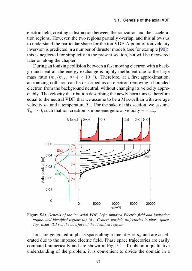
5.1. Genesis of the axial VDF
electric field, creating a distinction between the ionization and the accelera-tion regions. However, the two regions partially overlap, and this allows usto understand the particular shape for the ion VDF. A point of ion velocityinversion is predicted in a number of thruster models (see for example [90]):this is neglected for simplicity in the present section, but will be recoveredlater on along the chapter.
During an ionizing collision between a fast moving electron with a back-ground neutral, the energy exchange is highly inefficient due to the largemass ratio (me/mXe ≈ 4 × 10⁻⁶). Therefore, at a first approximation,an ionizing collision can be described as an electron removing a boundedelectron from the background neutral, without changing its velocity appre-ciably. The velocity distribution describing the newly born ions is thereforeequal to the neutral VDF, that we assume to be a Maxwellian with averagevelocity un and a temperature Tn. For the sake of this section, we assumeTn → 0, such that ion creation is monoenergetic at velocity v = un.
Figure 5.1: Genesis of the ion axial VDF. Left: imposed Electric field and ionizationprofile, and identified regions (a)–(d). Center: particle trajectories in phase space.Top: axial VDFs at the interface of the identified regions.
Ions are generated in phase space along a line at v = un and are accel-erated due to the imposed electric field. Phase space trajectories are easilycomputed numerically and are shown in Fig. 5.1. To obtain a qualitativeunderstanding of the problem, it is convenient to divide the domain in a
97
Chapter 5. Collisionless ions in Hall thrusters:an analytical axial model and a simple fluid closure
series of regions. At the beginning of the ionization region (Region (a) inFig. 5.1), the electric field is low, such that all the created ions cumulate,with negligible acceleration. This will create a sharp peak in the axial VDF.Such ions travel towards the channel exit at low velocity, until they reachthe ionization region and start to accelerate. At first (Region (b)), the ion-ization source is still dominant, and despite ions being accelerated towardsa higher average velocity, low-velocity ions are still being produced at eachlocation. This will generate a plateau in the ion VDF. Then (Region (c)), theionization term vanishes, while the electric field is in most cases still non-negligible. Only few new ions are created in such region, and this region isthus responsible for a translation of the VDF towards higher velocities. Atthis point ions have typically entered the plume. Further on in the trail (Re-gion (d)) both electric field and the ionization term are small, and collisionsplay a major role in the evolution of the VDF.
The steady state axial VDF at the interface between the said regions isshown in Fig. 5.1-Top, obtained as discussed in the following section.
5.2 Analytical axial VDF
For collisionless unmagnetized ions, the kinetic equation reads
∂f
∂t+ v · ∂f
∂x+qE
m· ∂f∂v
= S(x,v) , (5.1)
where q and m are the ion charge and mass respectively, and f = f(x,v, t)is the velocity distribution function. Under the assumptions of (i) monoen-ergetic ion creation, (ii) 1-dimensional electric field and (iii) steady stateconditions, it is possible to obtain an analytical expression for the ion ax-ial VDF. Steady state conditions imply ∂tf ≡ 0. The monoenergetic ioncreation assumption simplifies the ionization source term as
S(x,v) = S(x)δ(vx − vn)δ(vy)δ(vz) , (5.2)
with vn the (monoenergetic) velocity of neutral particles, correspondingto their average velocity, vn = un for Tn → 0. Note that S(x) repre-sents the number of ions created per unit time per unit physical volume:[S] = s−1m−3 and its profile is imposed. Finally, the problem is simplifiedby restricting the analysis to the centerline of the thruster channel. By as-suming a purely axial electric field E = Ex, neglecting all azimuthal and ra-dial variations, then ∂y = ∂z = 0. Moreover, the VDF loses its dependenceon the y and z coordinates: f(x,v) = f(x,v). All such assumptions arequestionable in real Hall thruster geometries, due to the presence of walls.
98
5.2. Analytical axial VDF
Nonetheless, the present model allows to gain a noteworthy insight in theproblem, and may still be reasonable close to the channel centerline.
In the said simplifying assumptions, the three components of particlevelocities are decoupled. The (steady state) kinetic equation for f can berecast into an equation for the marginal distribution function fx by integrat-ing over the vy and vz velocity components,
vx∂fx∂x
+qE
m
∂fx∂vx
= S(x)δ(vx − vn) , (5.3)
with the marginal distribution function fx = fx(x, vx) defined as
fx(x, vx) ≡¨ +∞
−∞f(x, vx, vy, vz) dvy dvz . (5.4)
A solution to Eq. (5.3) is easily found by following the characteristic lines,that correspond to ion trajectories in the 1D1V phase space. The solutiondiscussed in the following is an adaptation of a classical solution to theTonks-Langmuir sheath [183–185]. To our knowledge, it is the first timethat such solution is applied to a Hall thruster channel.
In the collisionless regime, ions fall freely along the electrostatic poten-tial φ. Therefore, an ion injected at position x0 with velocity v0 = vn willreach at position x a velocity
vx(x0;x) =
[2q
m(φ(x0)− φ(x)) + v2
0
]1/2
. (5.5)
With reference to Fig. 5.1, one can see that particles being injected betweenthe positions x0 and x0 + dx will have, at position x, a velocity betweenvx(x0, x) and vx(x0, x) + dv. One can thus write the balance
vxfx(vx) dvx = −S(x0) dx0 , (5.6)
with the minus sign accounting for the inverse relation between an increasein x0 and the final corresponding velocity. From Eq. (5.5), one computes
dvxdx0
=d
dx0
[2q
m(φ(x0)− φ(x)) + v2
n
]1/2
= − q
m
E(x0)
vx(x0;x), (5.7)
that can be inserted into Eq. (5.6), giving f(x, vx) = −S(x0)vx
dx0dvx
, and thus
fx(x, vx) =m
q
S(x0)
E(x0). (5.8)
99
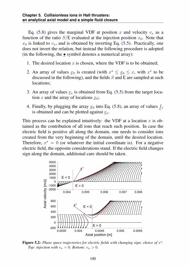
Chapter 5. Collisionless ions in Hall thrusters:an analytical axial model and a simple fluid closure
Eq. (5.8) gives the marginal VDF at position x and velocity vx as afunction of the ratio S/E evaluated at the injection position x0. Note thatx0 is linked to vx, and is obtained by inverting Eq. (5.5). Practically, onedoes not invert the relation, but instead the following procedure is adopted(in the following, the • symbol denotes a numerical array):
1. The desired location x is chosen, where the VDF is to be obtained;
2. An array of values x0 is created (with x? ≤ x0 ≤ x, with x? to bediscussed in the following), and the fields S and E are sampled at suchlocations;
3. An array of values vx is obtained from Eq. (5.5) from the target loca-tion x and the array of locations x0;
4. Finally, by plugging the array x0 into Eq. (5.8), an array of values fxis obtained and can be plotted against vx.
This process can be explained intuitively: the VDF at a location x is ob-tained as the contribution of all ions that reach such position. In case theelectric field is positive all along the domain, one needs to consider ionscreated from the very beginning of the domain, until the desired location.Therefore, x? = 0 (or whatever the initial coordinate is). For a negativeelectric field, the opposite considerations stand. If the electric field changessign along the domain, additional care should be taken.
Figure 5.2: Phase space trajectories for electric fields with changing sign; choice of x?.Top: injection with vn = 0. Bottom: vn > 0.
100
5.2. Analytical axial VDF
Let us consider first the case of zero injection velocity, vn = 0. The sit-uation is depicted in Fig. 5.2-Top. In such case, for a given probed positionx located downstream of the point where the electric field reverses, all ionscreated in the region of E > 0 will eventually reach x. On the other hand,all ions produced in the region of E < 0 will never reach x. In this case, thechoice of x? simply coincides with the point where E = 0.
In case ions have a non-zero birth velocity vn 6= 0, some energy is avail-able to overcome the adverse field, as depicted in Fig. 5.2-Bottom. For agiven position x located in the positive–E region, an additional contribu-tion is to be considered, and x? is to be taken upstream of the nodal pointfor E. One can easily find x? by equating the birth kinetic energy to theelectrostatic potential energy. Another possibility consists in locating x?
graphically, after a numerical computation of some particle trajectories.Finally, note that this analysis does not account for closed islands of
electric field lines, that would trap particles indefinitely.
5.2.1 Moments of the analytical VDF
The moments of the analytical VDF (superscript “a” in the following) areeasily obtained from the kinetic definition (see Section 2.3.1). As we arehere interested in axial quantities only, the integral over the velocity spacecan be performed selectively on the vy and vz components, leaving the de-pendence of vx. The moments definition is recast into an integral over themarginal VDF, fx dvx. This integral is transformed into an integral over theaxial coordinate through Eq. (5.6), and involves the ionization profile. Theanalytical moments read:
na(x) =
ˆ +∞
−∞fx(vx) dvx =
ˆ x
x?
S(x0)
v(x0;x)dx0 , (5.9a)
ua(x) =1
na(x)
ˆ +∞
−∞vxfx(vx) dvx =
ˆ x
x?S(x0) dx0 , (5.9b)
P ax (x) =
ˆ x
x?m
S(x0)
v(x0;x)[v(x0;x)− vax(x)]2 dx0 , (5.9c)
Qax(x) =
ˆ x
x?
m
2
S(x0)
v(x0;x)[v(x0;x)− vax(x)]3 dx0 , (5.9d)
Nax (x) =
ˆ x
x?m
S(x0)
v(x0;x)[v(x0;x)− vax(x)]n dx0 , (5.9e)
where Nax (x) denotes all further central moments of order n > 3. Notice
that, differently from the previous definitions, in this section a factor 1/2
101
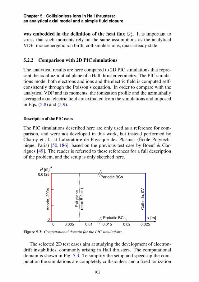
Chapter 5. Collisionless ions in Hall thrusters:an analytical axial model and a simple fluid closure
was embedded in the definition of the heat flux Qax. It is important to
stress that such moments rely on the same assumptions as the analyticalVDF: monoenergetic ion birth, collisionless ions, quasi-steady state.
5.2.2 Comparison with 2D PIC simulations
The analytical results are here compared to 2D PIC simulations that repre-sent the axial-azimuthal plane of a Hall thruster geometry. The PIC simula-tions model both electrons and ions and the electric field is computed self-consistently through the Poisson’s equation. In order to compare with theanalytical VDF and its moments, the ionization profile and the azimuthallyaveraged axial electric field are extracted from the simulations and imposedin Eqs. (5.8) and (5.9).
Description of the PIC cases
The PIC simulations described here are only used as a reference for com-parison, and were not developed in this work, but instead performed byCharoy et al., at Laboratoire de Physique des Plasmas (École Polytech-nique, Paris) [50, 186], based on the previous test case by Boeuf & Gar-rigues [49]. The reader is referred to these references for a full descriptionof the problem, and the setup is only sketched here.
Figure 5.3: Computational domain for the PIC simulations.
The selected 2D test cases aim at studying the development of electron-drift instabilities, commonly arising in Hall thrusters. The computationaldomain is shown in Fig. 5.3. To simplify the setup and speed-up the com-putation the simulations are completely collisionless and a fixed ionization
102
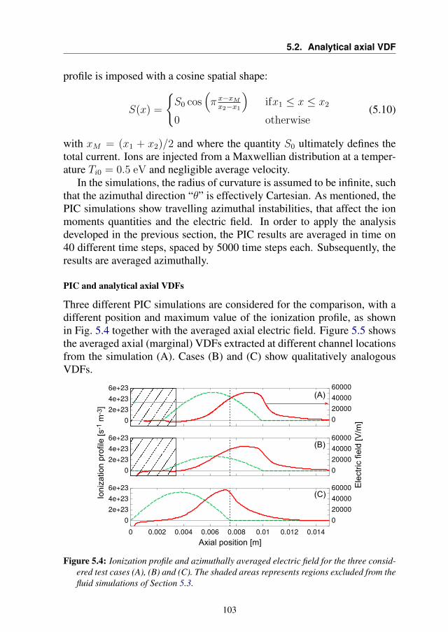
5.2. Analytical axial VDF
profile is imposed with a cosine spatial shape:
S(x) =
S0 cos
(π x−xMx2−x1
)ifx1 ≤ x ≤ x2
0 otherwise(5.10)
with xM = (x1 + x2)/2 and where the quantity S0 ultimately defines thetotal current. Ions are injected from a Maxwellian distribution at a temper-ature Ti0 = 0.5 eV and negligible average velocity.
In the simulations, the radius of curvature is assumed to be infinite, suchthat the azimuthal direction “θ” is effectively Cartesian. As mentioned, thePIC simulations show travelling azimuthal instabilities, that affect the ionmoments quantities and the electric field. In order to apply the analysisdeveloped in the previous section, the PIC results are averaged in time on40 different time steps, spaced by 5000 time steps each. Subsequently, theresults are averaged azimuthally.
PIC and analytical axial VDFs
Three different PIC simulations are considered for the comparison, with adifferent position and maximum value of the ionization profile, as shownin Fig. 5.4 together with the averaged axial electric field. Figure 5.5 showsthe averaged axial (marginal) VDFs extracted at different channel locationsfrom the simulation (A). Cases (B) and (C) show qualitatively analogousVDFs.
Figure 5.4: Ionization profile and azimuthally averaged electric field for the three consid-ered test cases (A), (B) and (C). The shaded areas represents regions excluded from thefluid simulations of Section 5.3.
103
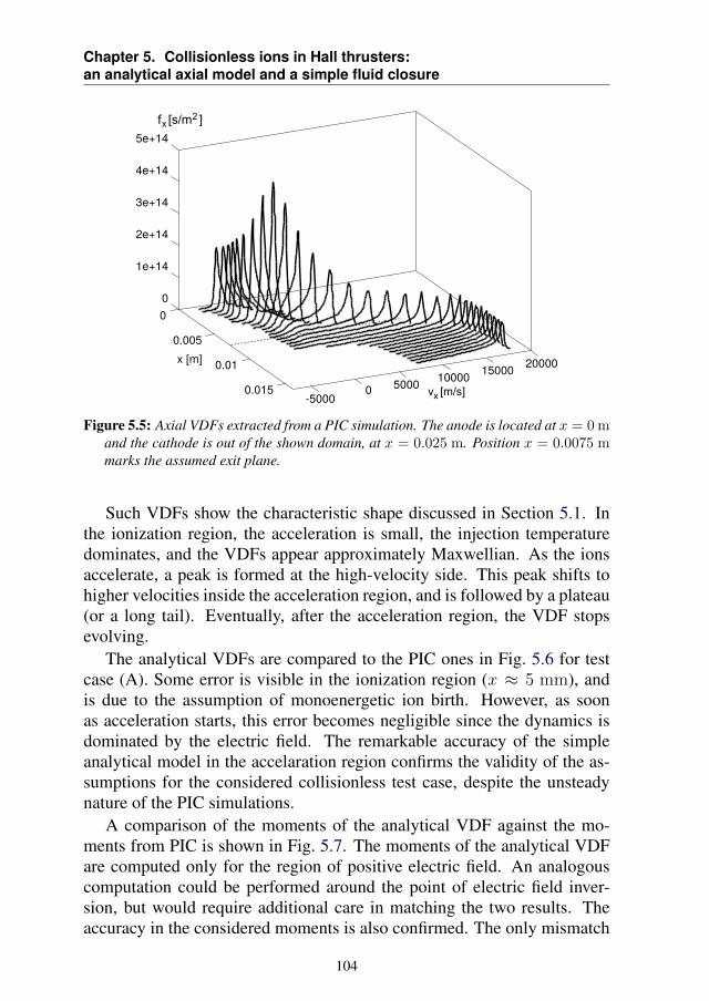
Chapter 5. Collisionless ions in Hall thrusters:an analytical axial model and a simple fluid closure
Figure 5.5: Axial VDFs extracted from a PIC simulation. The anode is located at x = 0 mand the cathode is out of the shown domain, at x = 0.025 m. Position x = 0.0075 mmarks the assumed exit plane.
Such VDFs show the characteristic shape discussed in Section 5.1. Inthe ionization region, the acceleration is small, the injection temperaturedominates, and the VDFs appear approximately Maxwellian. As the ionsaccelerate, a peak is formed at the high-velocity side. This peak shifts tohigher velocities inside the acceleration region, and is followed by a plateau(or a long tail). Eventually, after the acceleration region, the VDF stopsevolving.
The analytical VDFs are compared to the PIC ones in Fig. 5.6 for testcase (A). Some error is visible in the ionization region (x ≈ 5 mm), andis due to the assumption of monoenergetic ion birth. However, as soonas acceleration starts, this error becomes negligible since the dynamics isdominated by the electric field. The remarkable accuracy of the simpleanalytical model in the accelaration region confirms the validity of the as-sumptions for the considered collisionless test case, despite the unsteadynature of the PIC simulations.
A comparison of the moments of the analytical VDF against the mo-ments from PIC is shown in Fig. 5.7. The moments of the analytical VDFare computed only for the region of positive electric field. An analogouscomputation could be performed around the point of electric field inver-sion, but would require additional care in matching the two results. Theaccuracy in the considered moments is also confirmed. The only mismatch
104
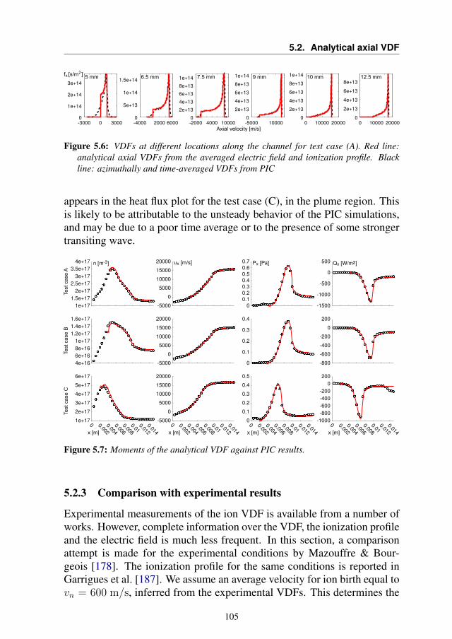
5.2. Analytical axial VDF
Figure 5.6: VDFs at different locations along the channel for test case (A). Red line:analytical axial VDFs from the averaged electric field and ionization profile. Blackline: azimuthally and time-averaged VDFs from PIC
appears in the heat flux plot for the test case (C), in the plume region. Thisis likely to be attributable to the unsteady behavior of the PIC simulations,and may be due to a poor time average or to the presence of some strongertransiting wave.
Figure 5.7: Moments of the analytical VDF against PIC results.
5.2.3 Comparison with experimental results
Experimental measurements of the ion VDF is available from a number ofworks. However, complete information over the VDF, the ionization profileand the electric field is much less frequent. In this section, a comparisonattempt is made for the experimental conditions by Mazouffre & Bour-geois [178]. The ionization profile for the same conditions is reported inGarrigues et al. [187]. We assume an average velocity for ion birth equal tovn = 600 m/s, inferred from the experimental VDFs. This determines the
105
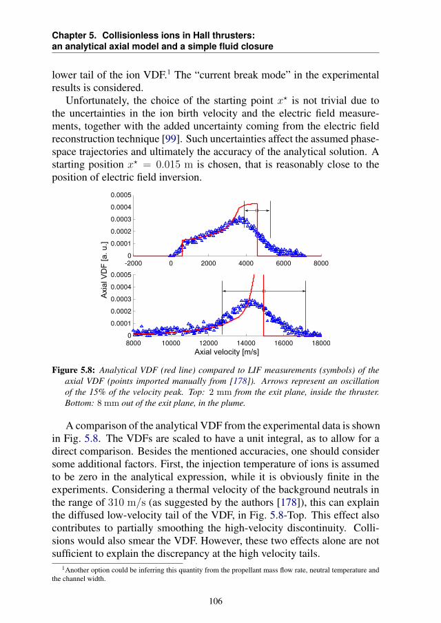
Chapter 5. Collisionless ions in Hall thrusters:an analytical axial model and a simple fluid closure
lower tail of the ion VDF.1 The “current break mode” in the experimentalresults is considered.
Unfortunately, the choice of the starting point x? is not trivial due tothe uncertainties in the ion birth velocity and the electric field measure-ments, together with the added uncertainty coming from the electric fieldreconstruction technique [99]. Such uncertainties affect the assumed phase-space trajectories and ultimately the accuracy of the analytical solution. Astarting position x? = 0.015 m is chosen, that is reasonably close to theposition of electric field inversion.
Figure 5.8: Analytical VDF (red line) compared to LIF measurements (symbols) of theaxial VDF (points imported manually from [178]). Arrows represent an oscillationof the 15% of the velocity peak. Top: 2 mm from the exit plane, inside the thruster.Bottom: 8 mm out of the exit plane, in the plume.
A comparison of the analytical VDF from the experimental data is shownin Fig. 5.8. The VDFs are scaled to have a unit integral, as to allow for adirect comparison. Besides the mentioned accuracies, one should considersome additional factors. First, the injection temperature of ions is assumedto be zero in the analytical expression, while it is obviously finite in theexperiments. Considering a thermal velocity of the background neutrals inthe range of 310 m/s (as suggested by the authors [178]), this can explainthe diffused low-velocity tail of the VDF, in Fig. 5.8-Top. This effect alsocontributes to partially smoothing the high-velocity discontinuity. Colli-sions would also smear the VDF. However, these two effects alone are notsufficient to explain the discrepancy at the high velocity tails.
1Another option could be inferring this quantity from the propellant mass flow rate, neutral temperature andthe channel width.
106
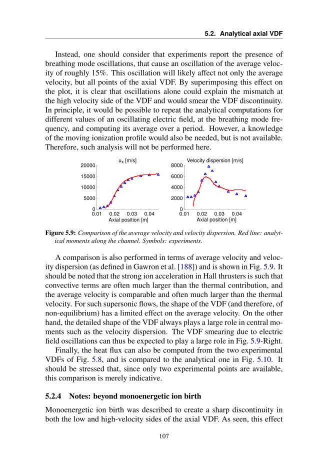
5.2. Analytical axial VDF
Instead, one should consider that experiments report the presence ofbreathing mode oscillations, that cause an oscillation of the average veloc-ity of roughly 15%. This oscillation will likely affect not only the averagevelocity, but all points of the axial VDF. By superimposing this effect onthe plot, it is clear that oscillations alone could explain the mismatch atthe high velocity side of the VDF and would smear the VDF discontinuity.In principle, it would be possible to repeat the analytical computations fordifferent values of an oscillating electric field, at the breathing mode fre-quency, and computing its average over a period. However, a knowledgeof the moving ionization profile would also be needed, but is not available.Therefore, such analysis will not be performed here.
Figure 5.9: Comparison of the average velocity and velocity dispersion. Red line: analyt-ical moments along the channel. Symbols: experiments.
A comparison is also performed in terms of average velocity and veloc-ity dispersion (as defined in Gawron et al. [188]) and is shown in Fig. 5.9. Itshould be noted that the strong ion acceleration in Hall thrusters is such thatconvective terms are often much larger than the thermal contribution, andthe average velocity is comparable and often much larger than the thermalvelocity. For such supersonic flows, the shape of the VDF (and therefore, ofnon-equilibrium) has a limited effect on the average velocity. On the otherhand, the detailed shape of the VDF always plays a large role in central mo-ments such as the velocity dispersion. The VDF smearing due to electricfield oscillations can thus be expected to play a large role in Fig. 5.9-Right.
Finally, the heat flux can also be computed from the two experimentalVDFs of Fig. 5.8, and is compared to the analytical one in Fig. 5.10. Itshould be stressed that, since only two experimental points are available,this comparison is merely indicative.
5.2.4 Notes: beyond monoenergetic ion birth
Monoenergetic ion birth was described to create a sharp discontinuity inboth the low and high-velocity sides of the axial VDF. As seen, this effect
107
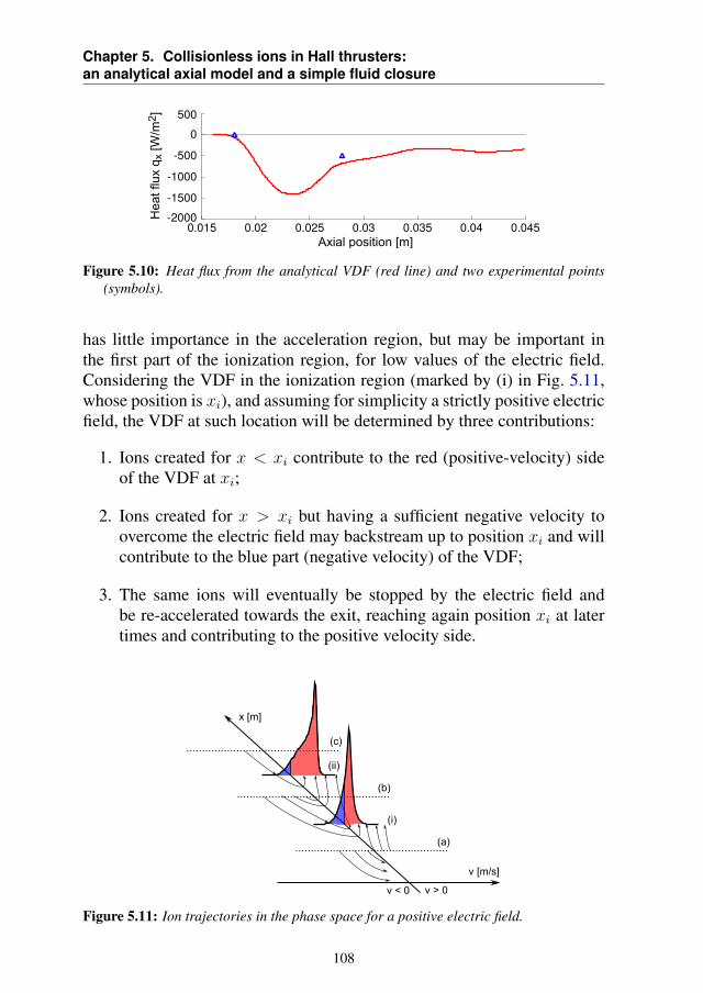
Chapter 5. Collisionless ions in Hall thrusters:an analytical axial model and a simple fluid closure
Figure 5.10: Heat flux from the analytical VDF (red line) and two experimental points(symbols).
has little importance in the acceleration region, but may be important inthe first part of the ionization region, for low values of the electric field.Considering the VDF in the ionization region (marked by (i) in Fig. 5.11,whose position is xi), and assuming for simplicity a strictly positive electricfield, the VDF at such location will be determined by three contributions:
1. Ions created for x < xi contribute to the red (positive-velocity) sideof the VDF at xi;
2. Ions created for x > xi but having a sufficient negative velocity toovercome the electric field may backstream up to position xi and willcontribute to the blue part (negative velocity) of the VDF;
3. The same ions will eventually be stopped by the electric field andbe re-accelerated towards the exit, reaching again position xi at latertimes and contributing to the positive velocity side.
Figure 5.11: Ion trajectories in the phase space for a positive electric field.
108
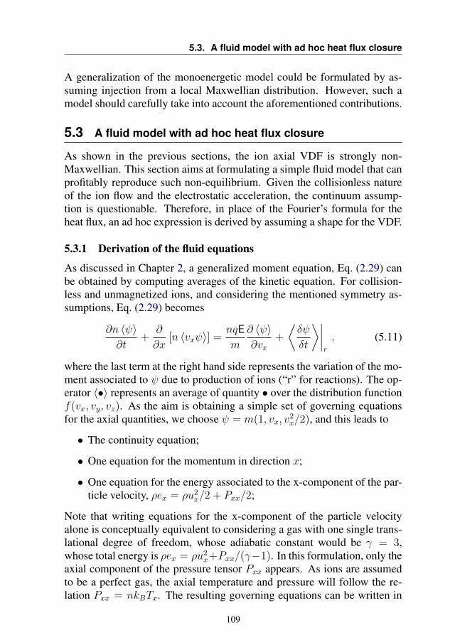
5.3. A fluid model with ad hoc heat flux closure
A generalization of the monoenergetic model could be formulated by as-suming injection from a local Maxwellian distribution. However, such amodel should carefully take into account the aforementioned contributions.
5.3 A fluid model with ad hoc heat flux closure
As shown in the previous sections, the ion axial VDF is strongly non-Maxwellian. This section aims at formulating a simple fluid model that canprofitably reproduce such non-equilibrium. Given the collisionless natureof the ion flow and the electrostatic acceleration, the continuum assump-tion is questionable. Therefore, in place of the Fourier’s formula for theheat flux, an ad hoc expression is derived by assuming a shape for the VDF.
5.3.1 Derivation of the fluid equations
As discussed in Chapter 2, a generalized moment equation, Eq. (2.29) canbe obtained by computing averages of the kinetic equation. For collision-less and unmagnetized ions, and considering the mentioned symmetry as-sumptions, Eq. (2.29) becomes
∂n 〈ψ〉∂t
+∂
∂x[n 〈vxψ〉] =
nqE
m
∂ 〈ψ〉∂vx
+
⟨δψ
δt
⟩∣∣∣∣r
, (5.11)
where the last term at the right hand side represents the variation of the mo-ment associated to ψ due to production of ions (“r” for reactions). The op-erator 〈•〉 represents an average of quantity • over the distribution functionf(vx, vy, vz). As the aim is obtaining a simple set of governing equationsfor the axial quantities, we choose ψ = m(1, vx, v
2x/2), and this leads to
• The continuity equation;
• One equation for the momentum in direction x;
• One equation for the energy associated to the x-component of the par-ticle velocity, ρex = ρu2
x/2 + Pxx/2;
Note that writing equations for the x-component of the particle velocityalone is conceptually equivalent to considering a gas with one single trans-lational degree of freedom, whose adiabatic constant would be γ = 3,whose total energy is ρex = ρu2
x+Pxx/(γ−1). In this formulation, only theaxial component of the pressure tensor Pxx appears. As ions are assumedto be a perfect gas, the axial temperature and pressure will follow the re-lation Pxx = nkBTx. The resulting governing equations can be written in
109
Chapter 5. Collisionless ions in Hall thrusters:an analytical axial model and a simple fluid closure
conservative form, defining a vector of conserved variables U , the fluxesF and the source termG,
∂U
∂t+∂F
∂x= G , (5.12)
with
U =
ρ
ρux12ρu2
x + 12Pxx
, F =
ρux
ρu2x + Pxx
12ρu3
x + 32Pxxux +Qx
. (5.13)
The only closing moment in such problem is the scalar quantityQx, definedas
Qx(x) =
˚ +∞
−∞
m
2v3xf(x, vx, vy, vz) d3v =
ˆ +∞
−∞
m
2v3xfx(x, vx) dvx .
(5.14)It should be noted that a factor 1/2 was embedded in the definition of
Qx, differently from the definition employed in Chapter 2. Also note that,differently from the usual definition of the heat flux vector, the quantity Qx
considered here only includes contributions from the axial velocity vx. Thesource terms G are also obtained as simple averages from Eq. (5.11), andare composed by a contribution from the electric field and a contributiondue to the chemical source. Ions are created from the neutrals population,with an average momentummun and an average energymnu
2n/2+kBTn/2.
G =
0
nqE
nquxE
+
mS
mSun
S(
12mnu
2n + 1
2kBTn
) , (5.15)
with S = S(x) the assigned ionization profile measured in [m−3s−1] and nthe ion number density.
5.3.2 Heat flux closure
The system of equations needs a closure for the heat flux Qx, as a functionof the lower moments. As the heat flux measures the skewness of the distri-bution function, it is unlikely that the Euler adiabatic closure Qx = 0 coulddescribe the strongly asymmetric ion VDFs. Instead, this section proposesan ad hoc closure that accounts for this skewness.
The simplest geometrical shapes that approximate the asymmetry of theions VDFs are polynomials of order p of the velocity, limited between two
110
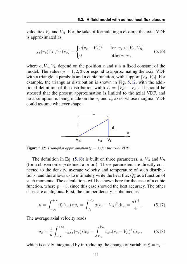
5.3. A fluid model with ad hoc heat flux closure
velocities VA and VB. For the sake of formulating a closure, the axial VDFis approximated as
fx(vx) ≈ f (p)(vx) =
a(vx − VA)p for vx ∈ [VA, VB]
0 otherwise ,(5.16)
where a, VA, VB depend on the position x and p is a fixed constant of themodel. The values p = 1, 2, 3 correspond to approximating the axial VDFwith a triangle, a parabola and a cubic function, with support [VA, VB]. Forexample, the triangular distribution is shown in Fig. 5.12, with the addi-tional definition of the distribution width L = |VB − VA|. It should bestressed that the present approximation is limited to the axial VDF, andno assumption is being made on the vy and vz axes, whose marginal VDFcould assume whatever shape.
Figure 5.12: Triangular approximation (p = 1) for the axial VDF.
The definition in Eq. (5.16) is built on three parameters, a, VA and VB(for a chosen order p defined a priori). These parameters are directly con-nected to the density, average velocity and temperature of such distribu-tions, and this allows us to ultimately write the heat fluxQp
x as a function ofsuch moments. The calculations will be shown here for the case of a cubicfunction, where p = 3, since this case showed the best accuracy. The othercases are analogous. First, the number density is obtained as
n =
ˆ +∞
−∞fx(vx) dvx =
ˆ VB
VA
a(vx − VA)3 dvx =aL4
4. (5.17)
The average axial velocity reads
ux =1
n
ˆ +∞
−∞vxfx(vx) dvx =
ˆ VB
VA
vxa(vx − VA)3 dvx , (5.18)
which is easily integrated by introducing the change of variables ξ = vx −
111
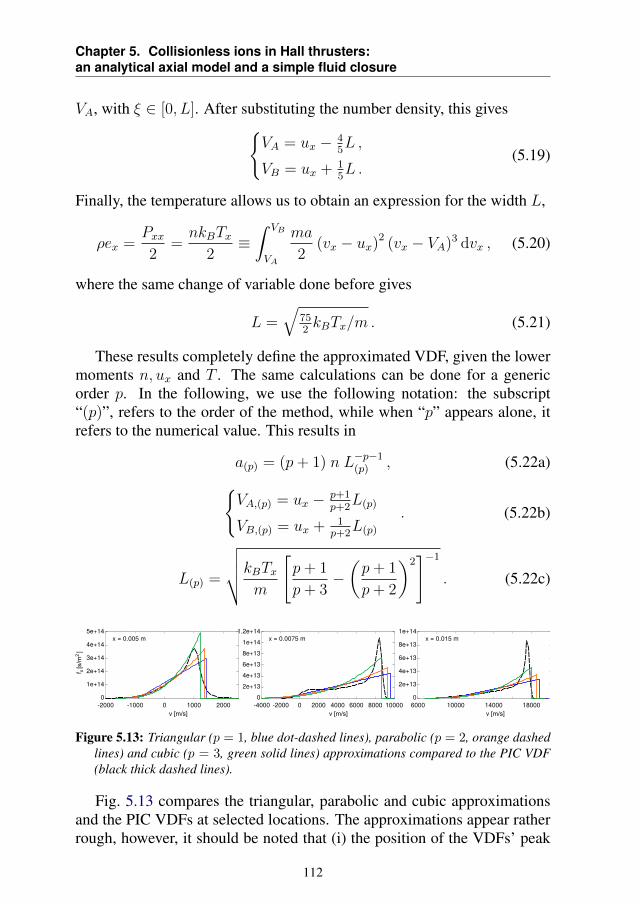
Chapter 5. Collisionless ions in Hall thrusters:an analytical axial model and a simple fluid closure
VA, with ξ ∈ [0, L]. After substituting the number density, this givesVA = ux − 4
5L ,
VB = ux + 15L .
(5.19)
Finally, the temperature allows us to obtain an expression for the width L,
ρex =Pxx2
=nkBTx
2≡ˆ VB
VA
ma
2(vx − ux)2 (vx − VA)3 dvx , (5.20)
where the same change of variable done before gives
L =√
752kBTx/m . (5.21)
These results completely define the approximated VDF, given the lowermoments n, ux and T . The same calculations can be done for a genericorder p. In the following, we use the following notation: the subscript“(p)”, refers to the order of the method, while when “p” appears alone, itrefers to the numerical value. This results in
a(p) = (p+ 1) n L−p−1(p) , (5.22a)
VA,(p) = ux − p+1p+2
L(p)
VB,(p) = ux + 1p+2
L(p)
. (5.22b)
L(p) =
√√√√kBTxm
[p+ 1
p+ 3−(p+ 1
p+ 2
)2]−1
. (5.22c)
Figure 5.13: Triangular (p = 1, blue dot-dashed lines), parabolic (p = 2, orange dashedlines) and cubic (p = 3, green solid lines) approximations compared to the PIC VDF(black thick dashed lines).
Fig. 5.13 compares the triangular, parabolic and cubic approximationsand the PIC VDFs at selected locations. The approximations appear ratherrough, however, it should be noted that (i) the position of the VDFs’ peak
112
5.3. A fluid model with ad hoc heat flux closure
is reasonably well captured by the position VB, especially for the cubicclosure; (ii) what really matters in terms of the closure is the heat flux Qx,not the VDF per se.
As done for the lower moments, the heat flux for a polynomial VDF isobtained from the kinetic definition,
Qx,(3) =
ˆ VB
VA
ma
2(vx − ux)3(vx − VA)3 dvx = − 2ρ
875
(75 kBTx
2m
)3/2
.
(5.23)This gives the required closure Qx,(3)(ρ, Tx). As expected, since the heatflux is a central moment, it does not depend on the average velocity ux. Fora generic p,
Qx,(p) =ρL3
(p)
2
[p+ 1
p+ 4− 3
(p+ 1)2
(p+ 2)(p+ 3)+ 2
(p+ 1
p+ 2
)3]. (5.24)
Note that, whatever the value of p, the heat flux is proportional to the VDFwidth L to the power of 3. Since L ∝
√T , one has that Qx ∝ T 3/2, as
physically expected.A preliminary verification of such closures can be obtained even without
running a full fluid simulation. Indeed, it is possible to extract the momentsρ, Tx from the PIC simulation and plug them into the closures for Qx, com-paring the approximated heat flux to the PIC heat flux. This is shown inFig. 5.14 for the conditions of test case (A) (see Section 5.2.2). The tri-angular closure (p = 1) reproduces a qualitatively correct heat flux, butmisses the peak by roughly a factor 2. The parabolic (p = 2) and cubic(p = 3) closures improve the accuracy further. We now focus on the caseof p = 3. Higher orders will not be investigated.2
The developed approximations appear to work well in the accelerationregion, but their validity is questionable inside the ionization region or nearthe anode. The next section will address these issues.
Correction for negative and low velocities
The formulated closures implicitly assume that the ion velocity ux is pos-itive. In order to describe regions of negative ion velocity (as may be thecase in certain regions of Hall thruster channels [90]) one would need tomirror the polynomial distributions, such as to make them face the nega-tive axis. This is done by simply including a sign(ux) function in the heat
2Indeed, it is likely that the accuracy is strongly dependent on the considered test case, and it makes littlesense to be excessively specific at this stage.
113
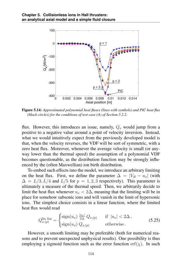
Chapter 5. Collisionless ions in Hall thrusters:an analytical axial model and a simple fluid closure
Figure 5.14: Approximated polynomial heat fluxes (lines with symbols) and PIC heat flux(black circles) for the conditions of test case (A) of Section 5.2.2.
flux. However, this introduces an issue, namely, Qx would jump from apositive to a negative value around a point of velocity inversion. Instead,what we would intuitively expect from the previously developed model isthat, when the velocity reverses, the VDF will be sort of symmetric, with azero heat flux. Moreover, whenever the average velocity is small (or any-way lower than the thermal speed) the assumption of a polynomial VDFbecomes questionable, as the distribution function may be strongly influ-enced by the (often Maxwellian) ion birth distribution.
To embed such effects into the model, we introduce an arbitrary limitingon the heat flux. First, we define the parameter ∆ = |VB − ux| (with∆ = L/3, L/4 and L/5 for p = 1, 2, 3 respectively). This parameter isultimately a measure of the thermal speed. Then, we arbitrarily decide tolimit the heat flux whenever ux < 2∆, meaning that the limiting will be inplace for somehow subsonic ions and will vanish in the limit of hypersonicions. The simplest choice consists in a linear function, where the limitedheat flux would read
Qlin. limx,(p) =
sign(ux)
|ux|2∆
Qx,(p) if |ux| < 2∆ ,
sign(ux) Qx,(p) otherwise .(5.25)
However, a smooth limiting may be preferable (both for numerical rea-sons and to prevent unexpected unphysical results). One possibility is thusemploying a sigmoid function such as the error function erf(χ). In such
114
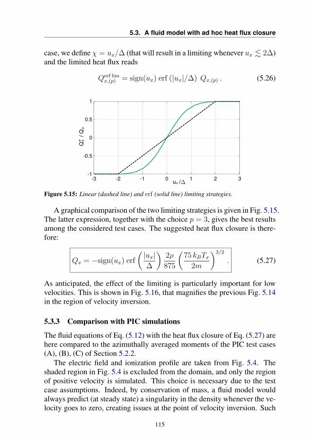
5.3. A fluid model with ad hoc heat flux closure
case, we define χ = ux/∆ (that will result in a limiting whenever ux . 2∆)and the limited heat flux reads
Qerf limx,(p) = sign(ux) erf (|ux|/∆) Qx,(p) . (5.26)
Figure 5.15: Linear (dashed line) and erf (solid line) limiting strategies.
A graphical comparison of the two limiting strategies is given in Fig. 5.15.The latter expression, together with the choice p = 3, gives the best resultsamong the considered test cases. The suggested heat flux closure is there-fore:
Qx = −sign(ux) erf
(|ux|∆
)2ρ
875
(75 kBTx
2m
)3/2
. (5.27)
As anticipated, the effect of the limiting is particularly important for lowvelocities. This is shown in Fig. 5.16, that magnifies the previous Fig. 5.14in the region of velocity inversion.
5.3.3 Comparison with PIC simulations
The fluid equations of Eq. (5.12) with the heat flux closure of Eq. (5.27) arehere compared to the azimuthally averaged moments of the PIC test cases(A), (B), (C) of Section 5.2.2.
The electric field and ionization profile are taken from Fig. 5.4. Theshaded region in Fig. 5.4 is excluded from the domain, and only the regionof positive velocity is simulated. This choice is necessary due to the testcase assumptions. Indeed, by conservation of mass, a fluid model wouldalways predict (at steady state) a singularity in the density whenever the ve-locity goes to zero, creating issues at the point of velocity inversion. Such
115
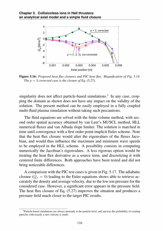
Chapter 5. Collisionless ions in Hall thrusters:an analytical axial model and a simple fluid closure
Figure 5.16: Proposed heat flux closures and PIC heat flux. Magnification of Fig. 5.14.The p = 3 corrected case is the closure of Eq. (5.27).
singularity does not affect particle-based simulations.3 In any case, crop-ping the domain as shown does not have any impact on the validity of thesolution. The present method can be easily employed in a fully coupledmulti-fluid plasma simulation without taking such precautions.
The fluid equations are solved with the finite volume method, with sec-ond order spatial accuracy obtained by van Leer’s MUSCL method, HLLnumerical fluxes and van Albada slope limiter. The solution is marched intime until convergence with a first order point-implicit Euler scheme. Notethat the heat flux closure would alter the eigenvalues of the fluxes Jaco-bian, and would thus influence the maximum and minimum wave speedsto be employed in the HLL scheme. A possibility consists in computingnumerically the Jacobian’s eigenvalues. A less rigorous option would betreating the heat flux derivative as a source term, and discretizing it withcentered finite differences. Both approaches have been tested and did notbring noticeable differences.
A comparison with the PIC test cases is given in Fig. 5.17. The adiabaticclosure (Qx = 0) leading to the Euler equations shows able to retrieve ac-curately the density and average velocity, due to the low ion pressure for theconsidered case. However, a significant error appears in the pressure field.The heat flux closure of Eq. (5.27) improves the situation and produces apressure field much closer to the target PIC results.
3Particle-based simulations are always unsteady at the particle level, and anyway the probability of creatingparticles with exactly a zero velocity is small.
116
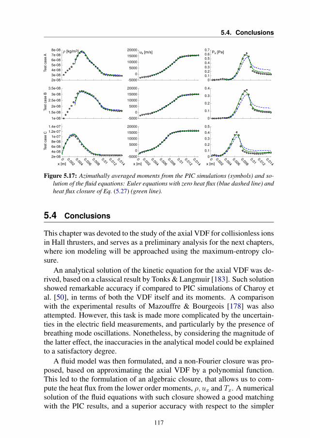
5.4. Conclusions
Figure 5.17: Azimuthally averaged moments from the PIC simulations (symbols) and so-lution of the fluid equations: Euler equations with zero heat flux (blue dashed line) andheat flux closure of Eq. (5.27) (green line).
5.4 Conclusions
This chapter was devoted to the study of the axial VDF for collisionless ionsin Hall thrusters, and serves as a preliminary analysis for the next chapters,where ion modeling will be approached using the maximum-entropy clo-sure.
An analytical solution of the kinetic equation for the axial VDF was de-rived, based on a classical result by Tonks & Langmuir [183]. Such solutionshowed remarkable accuracy if compared to PIC simulations of Charoy etal. [50], in terms of both the VDF itself and its moments. A comparisonwith the experimental results of Mazouffre & Bourgeois [178] was alsoattempted. However, this task is made more complicated by the uncertain-ties in the electric field measurements, and particularly by the presence ofbreathing mode oscillations. Nonetheless, by considering the magnitude ofthe latter effect, the inaccuracies in the analytical model could be explainedto a satisfactory degree.
A fluid model was then formulated, and a non-Fourier closure was pro-posed, based on approximating the axial VDF by a polynomial function.This led to the formulation of an algebraic closure, that allows us to com-pute the heat flux from the lower order moments, ρ, ux and Tx. A numericalsolution of the fluid equations with such closure showed a good matchingwith the PIC results, and a superior accuracy with respect to the simpler
117
Chapter 5. Collisionless ions in Hall thrusters:an analytical axial model and a simple fluid closure
Euler adiabatic closure. As a final note, we shall stress that while a “coldions” formulation is often sufficient for retrieving the ion velocity profile insimple 1D cases, an accurate reproduction of the pressure profile may playan important role in a number of circumstances, such as in determining thesaturation of instabilities, due to ion trapping (see for example [48, 58]).
118
CHAPTER6Maximum-entropy modeling of ions
As discussed in the previous chapter, the low collisionality of ions insideHall thrusters, together with a strong accelerating field, causes the VDFsto deviate from the equilibrium Maxwellian. A phenomenological fluidformulation was derived in Chapter 5 to describe the evolution of axialquantities, even out of equilibrium. However, such formulation is veryspecific and a generalization to different kinetic phenomena characterizingHall thrusters (such as wave-trapping, happening in the azimuthal directionin presence of instabilities [58,59]) would require further ad hoc modeling.
The advantage of employing a general formulation, such as a momentmethod, is to provide a unified framework, that automatically adapts todifferent types of non-equilibrium. The aim of this chapter is to investigatehow well the order-4 maximum-entropy method (in its one-dimensional 5-moment version or in the full 14-moment form) can reproduce differentnon-equilibrium situations, commonly arising in low-temperature plasmas.
As did in Chapter 5, all cases discussed in this chapter consider ionsonly. Electrons are not explicitly simulated, but instead an electric field andan ionization profile are imposed in space. Besides simplifying the analy-sis, this allows for a direct comparison between kinetic and fluid methods,where additional sources of error may be introduced due to different elec-
119
Chapter 6. Maximum-entropy modeling of ions
trons modeling.Due to the low-pressure conditions, the numerical simulations presented
in this chapter are performed using scaled units, where picograms are usedin place of kilograms, and the remaining units are chosen accordingly, asdiscussed in Section 3.3.
First, in Section 6.1, the maximum-entropy equations describing colli-sionless ions are recapped. The equations are then applied, in Section 6.2,to the very same case of Chapter 5, describing the axial ion evolution in aHall thruster channel. Section 6.3 then investigates the classical problem ofa Tonks-Langmuir sheath, describing a wall-bounded plasma. Sections 6.4and 6.5 consider charged particles inside a stationary or moving electricfield wave, showing ion wave trapping. This case is then extended to two-dimensions in Section 6.6, that aims at investigating traveling azimuthalwaves in a 2D Hall thruster-like geometry, in presence of an assigned axialfield.
6.1 Order-4 maximum-entropy systems for collisionless andunmagnetized ions
The general theory regarding maximum-entropy moment methods was dis-cussed in Section 2.4. This section describes the application of such systemto collisionless and unmagnetized ions.
6.1.1 Governing equations for ions: 5-moment system
For collisionless and unmagnetized particles in 1D geometries, the threevelocity components are often decoupled, and one may write governingequations for a single degree of freedom. In such case, the order-4 max-imum-entropy system is composed by 5 equations. In conservative form,we write
∂U5
∂t+∂F5
∂x= G5 , (6.1)
where the vector of conserved variables U5 and the fluxes F5 were definedin Section 2.4.2. For collisionless and unmagnetized ions, the source termG5 only includes the (x-component of the) electric field and chemical pro-duction terms due to ionization: G5 = GE
5 + Giz5 . The electric field GE
5
term was developed in Section 4.5.The ionization termGiz
5 depends on the considered reactions and is dis-cussed in the following. We consider that ions are created from a back-ground of neutral particles only due to electron-neutral collisions. Ioniza-tion due to neutral-neutral collisions are neglected due to the low tempera-
120
6.1. Order-4 maximum-entropy systems for collisionless andunmagnetized ions
ture of the background gas. Neutrals are assumed to be Maxwellian, char-acterized by an average velocity un, temperature Tn and density nn. Suchquantities may depend on the position x, but will be assumed uniform inthe present chapter.
We define by gMn = gMn (v;un, Tn) the normalized Maxwellian distri-bution of neutrals, that integrates to unity. When an ionizing electron-neutral collision happens, we assume that the neutral loses one electronwithout changing its velocity, due to the small electron-to-neutral mass ra-tio.1 Therefore, the distribution of ion birth is characterized by the verysame normalized distribution gMn . The 1D1V kinetic equation for ions thusreads
∂fi∂t
+ v∂fi∂x
+qiE
mi
∂fi∂v
= Siz gMn (6.2)
with Siz = Siz(x) the ionization profile expressed in [ions/s/m3]. The ion-ization source term for the moment 〈ψi〉 of the microscopic ion quantity ψi(as defined in Chapter 2) reads:
∂ 〈ψi〉∂t
∣∣∣∣iz
= Siz
ˆ +∞
−∞ψi g
Mn dv =
Siz
nn
ˆ +∞
−∞ψi fn dv , (6.3)
where the neutral distribution function fn = nngMn was introduced. The
5-moment system is obtained by the choice ψi = mi(1, v, v2, v3, v4). Since
we assume that a neutral turns into an ion by a simple loss of an electron,without changing its velocity, we have ψi = ψnmi/mn (with mi/mn ≈ 1),and the source terms thus become
∂ 〈ψi〉∂t
∣∣∣∣iz
= · · · = Siz
nn
mi
mn
ˆ +∞
−∞ψn fn dv = Siz
mi
mn
〈ψn〉nn
. (6.4)
In other words, the source for the moment 〈ψi〉 of the ion population is thevalue of the same moment for the neutral population, 〈ψn〉, normalized withrespect to the neutral number density and corrected by the ratio mi/mn.The ionization source terms for ions finally read
Giz5 =
∂U5
∂t
∣∣∣∣iz
= Siz(x)mi
mnnn
ρn
ρnun
ρnu2n + Pn
ρnu3n + 3unPn +qn
ρnu4n + 6u2
nPn + 4uqn + rn
, (6.5)
1For a kinetic analysis of the problem, the reader can refer to [189], where an analysis of the scaling is alsoperformed.
121
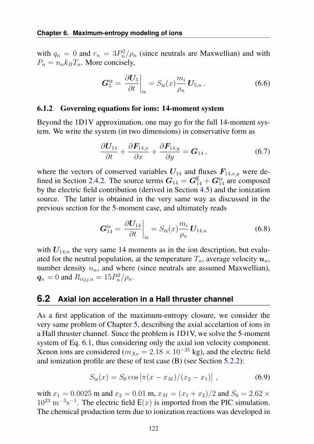
Chapter 6. Maximum-entropy modeling of ions
with qn = 0 and rn = 3P 2n/ρn (since neutrals are Maxwellian) and with
Pn = nnkBTn. More concisely,
Giz5 =
∂U5
∂t
∣∣∣∣iz
= Siz(x)mi
ρnU5,n . (6.6)
6.1.2 Governing equations for ions: 14-moment system
Beyond the 1D1V approximation, one may go for the full 14-moment sys-tem. We write the system (in two dimensions) in conservative form as
∂U14
∂t+∂F14,x
∂x+∂F14,y
∂y= G14 , (6.7)
where the vectors of conserved variables U14 and fluxes F14,x,y were de-fined in Section 2.4.2. The source terms G14 = GE
14 +Giz14 are composed
by the electric field contribution (derived in Section 4.5) and the ionizationsource. The latter is obtained in the very same way as discussed in theprevious section for the 5-moment case, and ultimately reads
Giz14 =
∂U14
∂t
∣∣∣∣iz
= Siz(x)mi
ρnU14,n (6.8)
with U14,n the very same 14 moments as in the ion description, but evalu-ated for the neutral population, at the temperature Tn, average velocity un,number density nn, and where (since neutrals are assumed Maxwellian),qn = 0 and Riijj,n = 15P 2
n/ρn.
6.2 Axial ion acceleration in a Hall thruster channel
As a first application of the maximum-entropy closure, we consider thevery same problem of Chapter 5, describing the axial accelartion of ions ina Hall thruster channel. Since the problem is 1D1V, we solve the 5-momentsystem of Eq. 6.1, thus considering only the axial ion velocity component.Xenon ions are considered (mXe = 2.18× 10⁻²⁵ kg), and the electric fieldand ionization profile are these of test case (B) (see Section 5.2.2):
Siz(x) = S0 cos [π(x− xM)/(x2 − x1)] , (6.9)
with x1 = 0.0025 m and x2 = 0.01 m, xM = (x1 + x2)/2 and S0 = 2.62×10²³ m−3s−1. The electric field E(x) is imported from the PIC simulation.The chemical production term due to ionization reactions was developed in
122
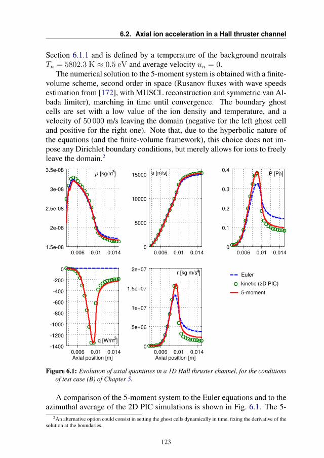
6.2. Axial ion acceleration in a Hall thruster channel
Section 6.1.1 and is defined by a temperature of the background neutralsTn = 5802.3 K ≈ 0.5 eV and average velocity un = 0.
The numerical solution to the 5-moment system is obtained with a finite-volume scheme, second order in space (Rusanov fluxes with wave speedsestimation from [172], with MUSCL reconstruction and symmetric van Al-bada limiter), marching in time until convergence. The boundary ghostcells are set with a low value of the ion density and temperature, and avelocity of 50 000 m/s leaving the domain (negative for the left ghost celland positive for the right one). Note that, due to the hyperbolic nature ofthe equations (and the finite-volume framework), this choice does not im-pose any Dirichlet boundary conditions, but merely allows for ions to freelyleave the domain.2
Figure 6.1: Evolution of axial quantities in a 1D Hall thruster channel, for the conditionsof test case (B) of Chapter 5.
A comparison of the 5-moment system to the Euler equations and to theazimuthal average of the 2D PIC simulations is shown in Fig. 6.1. The 5-
2An alternative option could consist in setting the ghost cells dynamically in time, fixing the derivative of thesolution at the boundaries.
123
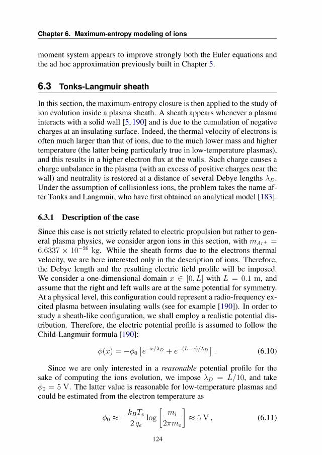
Chapter 6. Maximum-entropy modeling of ions
moment system appears to improve strongly both the Euler equations andthe ad hoc approximation previously built in Chapter 5.
6.3 Tonks-Langmuir sheath
In this section, the maximum-entropy closure is then applied to the study ofion evolution inside a plasma sheath. A sheath appears whenever a plasmainteracts with a solid wall [5, 190] and is due to the cumulation of negativecharges at an insulating surface. Indeed, the thermal velocity of electrons isoften much larger than that of ions, due to the much lower mass and highertemperature (the latter being particularly true in low-temperature plasmas),and this results in a higher electron flux at the walls. Such charge causes acharge unbalance in the plasma (with an excess of positive charges near thewall) and neutrality is restored at a distance of several Debye lengths λD.Under the assumption of collisionless ions, the problem takes the name af-ter Tonks and Langmuir, who have first obtained an analytical model [183].
6.3.1 Description of the case
Since this case is not strictly related to electric propulsion but rather to gen-eral plasma physics, we consider argon ions in this section, with mAr+ =6.6337 × 10⁻²⁶ kg. While the sheath forms due to the electrons thermalvelocity, we are here interested only in the description of ions. Therefore,the Debye length and the resulting electric field profile will be imposed.We consider a one-dimensional domain x ∈ [0, L] with L = 0.1 m, andassume that the right and left walls are at the same potential for symmetry.At a physical level, this configuration could represent a radio-frequency ex-cited plasma between insulating walls (see for example [190]). In order tostudy a sheath-like configuration, we shall employ a realistic potential dis-tribution. Therefore, the electric potential profile is assumed to follow theChild-Langmuir formula [190]:
φ(x) = −φ0
[e−x/λD + e−(L−x)/λD
]. (6.10)
Since we are only interested in a reasonable potential profile for thesake of computing the ions evolution, we impose λD = L/10, and takeφ0 = 5 V. The latter value is reasonable for low-temperature plasmas andcould be estimated from the electron temperature as
φ0 ≈ −kBTe2 qe
log
[mi
2πme
]≈ 5 V , (6.11)
124
6.3. Tonks-Langmuir sheath
where the electron temperature was taken as Te = 11604 K (thus corre-sponding to 1 eV). In the present formulation, φ0 is assumed to representthe potential difference between the walls and the plasma bulk, the latterbeing taken as zero in Eq. (6.10). In any case, any shift in the potentialdoes not change the electric field, that is obtained by differentiation andonly the difference φ0 matters. The electric field thus reads
E(x) = − φ0
λD
[e−x/λD − e(x−L)/λD
]. (6.12)
The electric field and the potential are shown in Fig. 6.2.
Figure 6.2: Imposed potential and electric field for the Tonks-Langmuir plasma test case.Note that the electric field is zero at the symmetry plane.
A production term for ions is imposed, uniform along the domain. Itsvalues is arbitrarily fixed to Siz = 5 × 10²⁰ [particles/m3s]. This value isreasonable, as can be seen from the following check. First, the resultingplasma density will be in the order of n ≈ 1016 m−3. Therefore, assum-ing an electrons temperature, one can estimate the density of backgroundneutrals that would guarantee such ionization term. Considering then theion-neutral cross section and such neutral density, one can confirm that ionsare indeed rather rarefied in this condition.
Ions are assumed to be created from a cold and slow neutral background,such that the kinetic equation reads
∂fi∂t
+ v∂fi∂x
+qiE
mi
∂fi∂v
= Siz δ(v) , (6.13)
with δ(v) the Dirac delta function.
6.3.2 Kinetic solution
As mentioned, an analytical solution is available for Eq. (6.13), as also dis-cussed in Chapter 5. Nonetheless, a numerical solution is here employed,
125
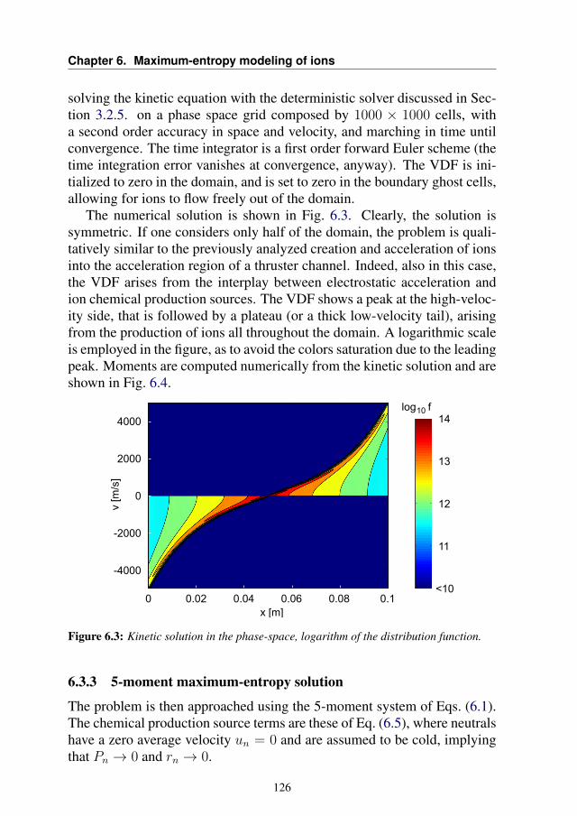
Chapter 6. Maximum-entropy modeling of ions
solving the kinetic equation with the deterministic solver discussed in Sec-tion 3.2.5. on a phase space grid composed by 1000 × 1000 cells, witha second order accuracy in space and velocity, and marching in time untilconvergence. The time integrator is a first order forward Euler scheme (thetime integration error vanishes at convergence, anyway). The VDF is ini-tialized to zero in the domain, and is set to zero in the boundary ghost cells,allowing for ions to flow freely out of the domain.
The numerical solution is shown in Fig. 6.3. Clearly, the solution issymmetric. If one considers only half of the domain, the problem is quali-tatively similar to the previously analyzed creation and acceleration of ionsinto the acceleration region of a thruster channel. Indeed, also in this case,the VDF arises from the interplay between electrostatic acceleration andion chemical production sources. The VDF shows a peak at the high-veloc-ity side, that is followed by a plateau (or a thick low-velocity tail), arisingfrom the production of ions all throughout the domain. A logarithmic scaleis employed in the figure, as to avoid the colors saturation due to the leadingpeak. Moments are computed numerically from the kinetic solution and areshown in Fig. 6.4.
Figure 6.3: Kinetic solution in the phase-space, logarithm of the distribution function.
6.3.3 5-moment maximum-entropy solution
The problem is then approached using the 5-moment system of Eqs. (6.1).The chemical production source terms are these of Eq. (6.5), where neutralshave a zero average velocity un = 0 and are assumed to be cold, implyingthat Pn → 0 and rn → 0.
126
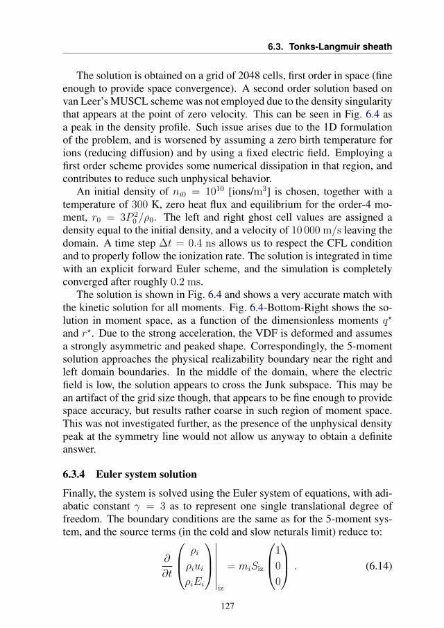
6.3. Tonks-Langmuir sheath
The solution is obtained on a grid of 2048 cells, first order in space (fineenough to provide space convergence). A second order solution based onvan Leer’s MUSCL scheme was not employed due to the density singularitythat appears at the point of zero velocity. This can be seen in Fig. 6.4 asa peak in the density profile. Such issue arises due to the 1D formulationof the problem, and is worsened by assuming a zero birth temperature forions (reducing diffusion) and by using a fixed electric field. Employing afirst order scheme provides some numerical dissipation in that region, andcontributes to reduce such unphysical behavior.
An initial density of ni0 = 1010 [ions/m3] is chosen, together with atemperature of 300 K, zero heat flux and equilibrium for the order-4 mo-ment, r0 = 3P 2
0 /ρ0. The left and right ghost cell values are assigned adensity equal to the initial density, and a velocity of 10 000 m/s leaving thedomain. A time step ∆t = 0.4 ns allows us to respect the CFL conditionand to properly follow the ionization rate. The solution is integrated in timewith an explicit forward Euler scheme, and the simulation is completelyconverged after roughly 0.2 ms.
The solution is shown in Fig. 6.4 and shows a very accurate match withthe kinetic solution for all moments. Fig. 6.4-Bottom-Right shows the so-lution in moment space, as a function of the dimensionless moments q?
and r?. Due to the strong acceleration, the VDF is deformed and assumesa strongly asymmetric and peaked shape. Correspondingly, the 5-momentsolution approaches the physical realizability boundary near the right andleft domain boundaries. In the middle of the domain, where the electricfield is low, the solution appears to cross the Junk subspace. This may bean artifact of the grid size though, that appears to be fine enough to providespace accuracy, but results rather coarse in such region of moment space.This was not investigated further, as the presence of the unphysical densitypeak at the symmetry line would not allow us anyway to obtain a definiteanswer.
6.3.4 Euler system solution
Finally, the system is solved using the Euler system of equations, with adi-abatic constant γ = 3 as to represent one single translational degree offreedom. The boundary conditions are the same as for the 5-moment sys-tem, and the source terms (in the cold and slow neturals limit) reduce to:
∂
∂t
ρi
ρiui
ρiEi
∣∣∣∣∣∣∣iz
= miSiz
1
0
0
. (6.14)
127
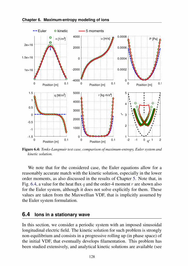
Chapter 6. Maximum-entropy modeling of ions
Figure 6.4: Tonks-Langmuir test case, comparison of maximum-entropy, Euler system andkinetic solution.
We note that for the considered case, the Euler equations allow for areasonably accurate match with the kinetic solution, especially in the lowerorder moments, as also discussed in the results of Chapter 5. Note that, inFig. 6.4, a value for the heat flux q and the order-4 moment r are shown alsofor the Euler system, although it does not solve explicitly for them. Thesevalues are taken from the Maxwellian VDF, that is implicitly assumed bythe Euler system formulation.
6.4 Ions in a stationary wave
In this section, we consider a periodic system with an imposed sinusoidallongitudinal electric field. The kinetic solution for such problem is stronglynon-equilibrium and consists in a progressive rolling up (in phase space) ofthe initial VDF, that eventually develops filamentation. This problem hasbeen studied extensively, and analytical kinetic solutions are available (see
128
6.4. Ions in a stationary wave
for example [191, 192]). Not only this test case is interesting per se, butis also propaedeutic to the study of travelling waves that mimic azimuthalinstabilities in Hall thrusters.
6.4.1 Description of the case
Xenon ions are simulated, in a periodic one-dimensional domain with x ∈[0, 0.01] m. Ions are initialized uniformly in the domain, following a 1D1VMaxwellian VDF with zero average velocity and a temperature of 10 eV.Since the domain is periodic, no ionization source term is used. An electricpotential is imposed, and reads
V = V0 cos(kx) . (6.15)
The wave number k is chosen as to have four peaks in the simulated do-main, k = 2Nπ/L, with N = 4. The electric field is simply obtained bydifferentiating the potential,
E = kV0 sin(kx) . (6.16)
Since the ion temperature was assigned, the electric potential amplitudeV0 determines the dynamics of the problem. Indeed, on a particle perspec-tive, all ions with an initial energy εi < V0 (with εi expressed in [eV]) willbe trapped inside the electric field profile and will oscillate back and forth.On the other hand, ions with energy εi > V0 will manage to overcomethe electric field barrier, but will be perturbed by it. Finally, the ions forwhich εi V0 will travel almost unperturbed by the electric field. Differ-ent regimes are thus obtained for different values of the ratio of the initialion thermal energy over the electrostatic energy. We consider the two cases:
• Case 1) V0 = Ti [eV];
• Case 2) V0 = 5Ti [eV].
6.4.2 Kinetic solution
As mentioned, no chemical production source term is considered. There-fore, the kinetic equation corresponds to the 1D1V Vlasov equation withimposed electric field. The kinetic solution is obtained with the determin-istic solver, with 2048×2048 grid cells in physical space and velocity, sec-ond order in phase space and first order in time. The computations wereperformed with different time steps and phase space grids as to ensure con-vergence. The phase space grid needs to be rather refined, especially due tothe appearance of filamentation and therefore strong gradients.
129
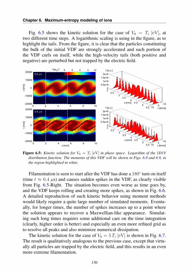
Chapter 6. Maximum-entropy modeling of ions
Fig. 6.5 shows the kinetic solution for the case of V0 = Ti [eV], attwo different time steps. A logarithmic scaling is using in the figure, as tohighlight the tails. From the figure, it is clear that the particles constitutingthe bulk of the initial VDF are strongly accelerated and such portion ofthe VDF curls on itself, while the high-velocity tails (both positive andnegative) are perturbed but not trapped by the electric field.
Figure 6.5: Kinetic solution for V0 = Ti [eV] in phase space. Logarithm of the 1D1Vdistribution function. The moments of this VDF will be shown in Figs. 6.8 and 6.9, inthe region highlighted in white.
Filamentation is seen to start after the VDF has done a 180 turn on itself(time t ≈ 0.4 µs) and causes sudden spikes in the VDF, as clearly visiblefrom Fig. 6.5-Right. The situation becomes even worse as time goes by,and the VDF keeps rolling and creating more spikes, as shown in Fig. 6.6.A detailed reproduction of such kinetic behavior using moment methodswould likely require a quite large number of simulated moments. Eventu-ally, for longer times, the number of spikes increases up to a point wherethe solution appears to recover a Maxwellian-like appearance. Simulat-ing such long times requires some additional care on the time integration(clearly, higher order is better) and especially an even more refined grid asto resolve all peaks and also minimize numerical dissipation.
The kinetic solution for the case of V0 = 5Ti [eV] is shown in Fig. 6.7.The result is qualitatively analogous to the previous case, except that virtu-ally all particles are trapped by the electric field, and this results in an evenmore extreme filamentation.
130
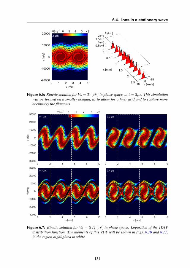
6.4. Ions in a stationary wave
Figure 6.6: Kinetic solution for V0 = Ti [eV] in phase space, at t = 2µs. This simulationwas performed on a smaller domain, as to allow for a finer grid and to capture moreaccurately the filaments.
Figure 6.7: Kinetic solution for V0 = 5Ti [eV] in phase space. Logarithm of the 1D1Vdistribution function. The moments of this VDF will be shown in Figs. 6.10 and 6.11,in the region highlighted in white.
131
Chapter 6. Maximum-entropy modeling of ions
6.4.3 5-moment and Euler solutions
The solution to the 5-moment and Euler systems are obtained on a spacegrid of 2048 cells, second order both in space and time. The ionizationsource terms are put to zero for this test case. The results are compared tothe kinetic solution in Figs. 6.8 and 6.9 for the V0 = Ti [eV] case and inFigs. 6.10 and 6.11 for the case of V0 = 5Ti [eV]. Since the solution isperiodic, only a portion of the domain is shown in such figures, as to makethe results more clear.
The lower moments appear well reproduced by both the Euler and 5-moment systems at early times (t ≈ 0.1 µs), while the Euler system al-ready shows some inaccuracy in the higher moments. As time passes, fort = 0.2 µs, the accuracy of the 5-moment system is still high, while theEuler solution starts to show some artifacts and shock waves. Eventually,as non-equilibrium keeps increasing, even the 5-moment solution starts todeviate from the kinetic solution, especially in terms of the lower moments.Remarkably, though, the higher moments maintain a higher accuracy evenfor relatively long times. This behavior can be observed for both test cases.
As may be expected, the plot in moment space q? − r? shows that thesecond case (V0 = 5Ti [eV]) is much farther from equilibrium than the pre-vious one. Indeed, in the second case, the moment space trajectory reachesboth higher values for q? and r?, and also gets much closer to the physicalrealizability boundary. The Junk subspace appears to be crossed already atearly times. In terms of the interpolative maximum-entropy closure, we canexpect the parameter σ to assume very small values even far from equilib-rium, and correspondingly we expect wave speeds to deviate strongly fromthe equilibrium values. This makes a time-explicit numerical solution ofthe 5-moment system much more stiff than its Euler counterpart.
In terms of long-time solution, the kinetic equation would predict anincreasing number of filaments, with an increasingly small thickness, upto the point where the VDF could appear macroscopically analogous to aMaxwellian. Therefore, as a future work activity, we suggest the study ofthe asymptotic behavior of the 5-moment system for this problem.
132
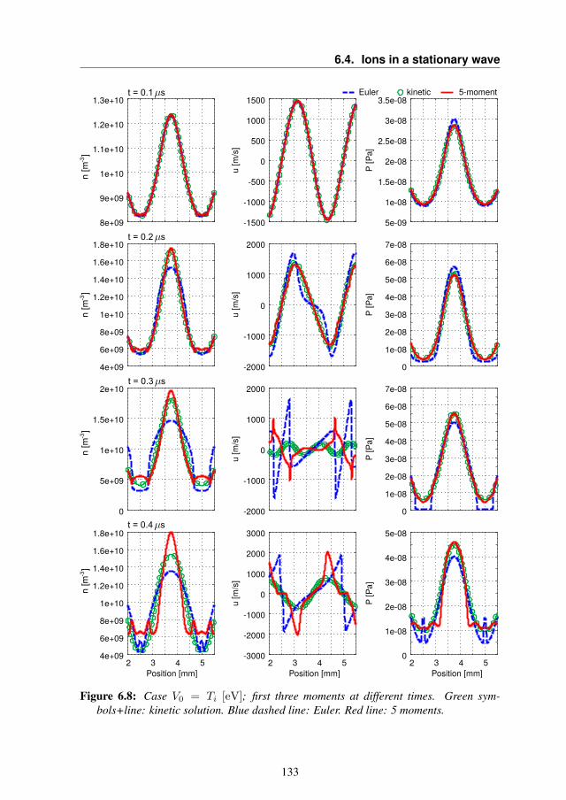
6.4. Ions in a stationary wave
Figure 6.8: Case V0 = Ti [eV]; first three moments at different times. Green sym-bols+line: kinetic solution. Blue dashed line: Euler. Red line: 5 moments.
133
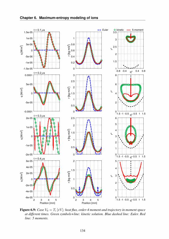
Chapter 6. Maximum-entropy modeling of ions
Figure 6.9: Case V0 = Ti [eV]; heat flux, order-4 moment and trajectory in moment spaceat different times. Green symbols+line: kinetic solution. Blue dashed line: Euler. Redline: 5 moments.
134
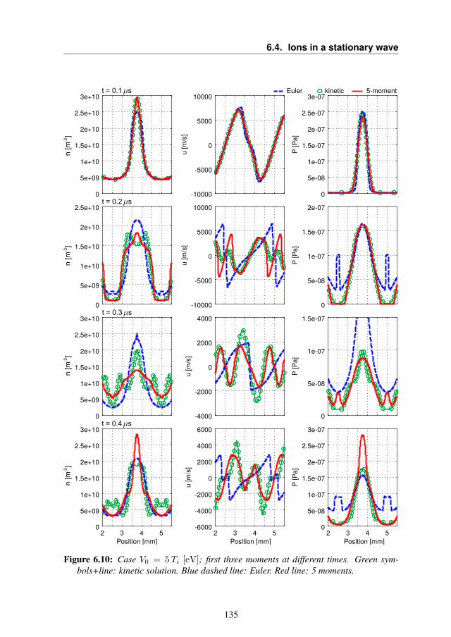
6.4. Ions in a stationary wave
Figure 6.10: Case V0 = 5Ti [eV]; first three moments at different times. Green sym-bols+line: kinetic solution. Blue dashed line: Euler. Red line: 5 moments.
135
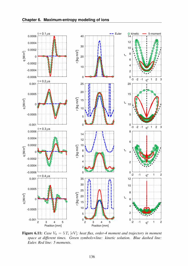
Chapter 6. Maximum-entropy modeling of ions
Figure 6.11: Case V0 = 5Ti [eV]; heat flux, order-4 moment and trajectory in momentspace at different times. Green symbols+line: kinetic solution. Blue dashed line:Euler. Red line: 5 moments.
136
6.5. Ions in a travelling wave
6.5 Ions in a travelling wave
In this section, we investigate the behavior of ions inside a travelling elec-tric field wave. The test case setup is identical to the one described in theprevious section, except that a non-zero phase velocity is added into the si-nusoidal electric field profile. The same phenomenology as for the previoustest case will be observed, but this time acting on a tail of the VDF ratherthan on its bulk, and thus showing ion-trapping. The latter has been iden-tified as one possible mechanism for the saturation of azimuthal electrondrift instabilities in Hall thruster discharges [58], making the present testcase particularly interesting in view of further more complete applications.
As for the previous test case, the potential profile is in the form
V (x, t) = V0 cos (ωt+ kx) , (6.17)
where x could represent the azimuthal direction in a Hall thruster geometry.By differentiation, the electric field reads
E(x, t) = V0k sin (ωt+ kx) , (6.18)
A domain x ∈ [0, L] is employed, with L = 0.01 m. To simulate fourelectric field peaks in the domain, we consider N = 4 and
k = N2π/L ≈ 2513.27 m−1 (6.19)
These choices allow us to select a regime that somehow resembles theoscillations observed in the numerical simulations of Boeuf & Garrigues[49], at least for their lower current test cases. An analogous test case isperformed by Charoy et al. [50]: by estimating the value of V0 from thisreference, we see that V0 ≈ Ti [eV]. Therefore, after having arbitrarilychosen T eV
i = 10 eV, we select V0 consistently as V0 = 10 V.From the numerical dispersion relation reported in [50], the wave ap-
pears to be traveling at roughly twice of the ion thermal speed. The phasevelocity is thus set to
vp =ω
k= 2
√8kBTiπm
, (6.20)
resulting in ω ≈ 21.745 MHz. The choice of these values is highly approx-imated, but gives anyway a reasonable starting point.
Kinetic, 5-moment and Euler simulations
The setup for the kinetic, 5-moment and Euler system simulations are thesame as described in the previous section.
137
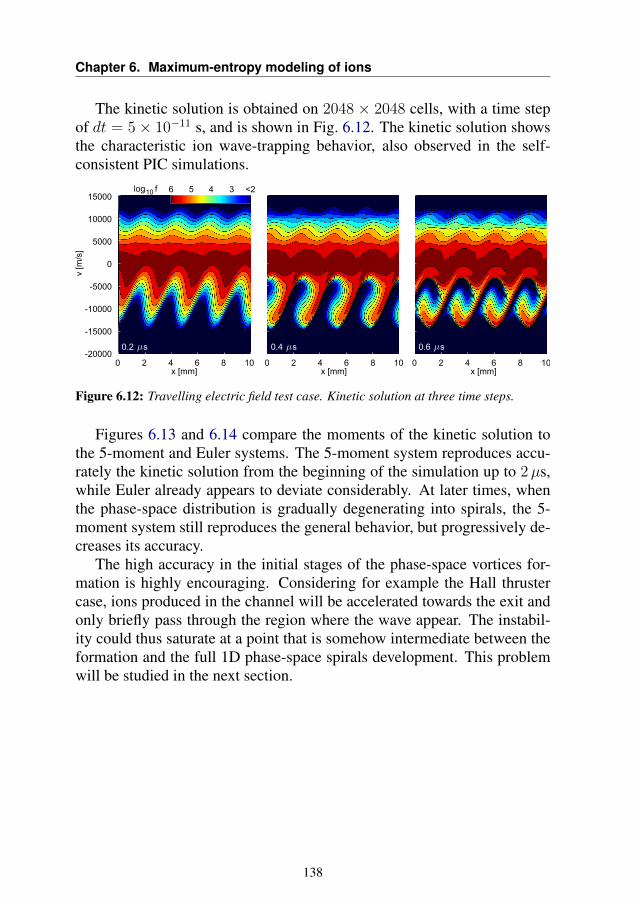
Chapter 6. Maximum-entropy modeling of ions
The kinetic solution is obtained on 2048 × 2048 cells, with a time stepof dt = 5× 10⁻¹¹ s, and is shown in Fig. 6.12. The kinetic solution showsthe characteristic ion wave-trapping behavior, also observed in the self-consistent PIC simulations.
Figure 6.12: Travelling electric field test case. Kinetic solution at three time steps.
Figures 6.13 and 6.14 compare the moments of the kinetic solution tothe 5-moment and Euler systems. The 5-moment system reproduces accu-rately the kinetic solution from the beginning of the simulation up to 2µs,while Euler already appears to deviate considerably. At later times, whenthe phase-space distribution is gradually degenerating into spirals, the 5-moment system still reproduces the general behavior, but progressively de-creases its accuracy.
The high accuracy in the initial stages of the phase-space vortices for-mation is highly encouraging. Considering for example the Hall thrustercase, ions produced in the channel will be accelerated towards the exit andonly briefly pass through the region where the wave appear. The instabil-ity could thus saturate at a point that is somehow intermediate between theformation and the full 1D phase-space spirals development. This problemwill be studied in the next section.
138
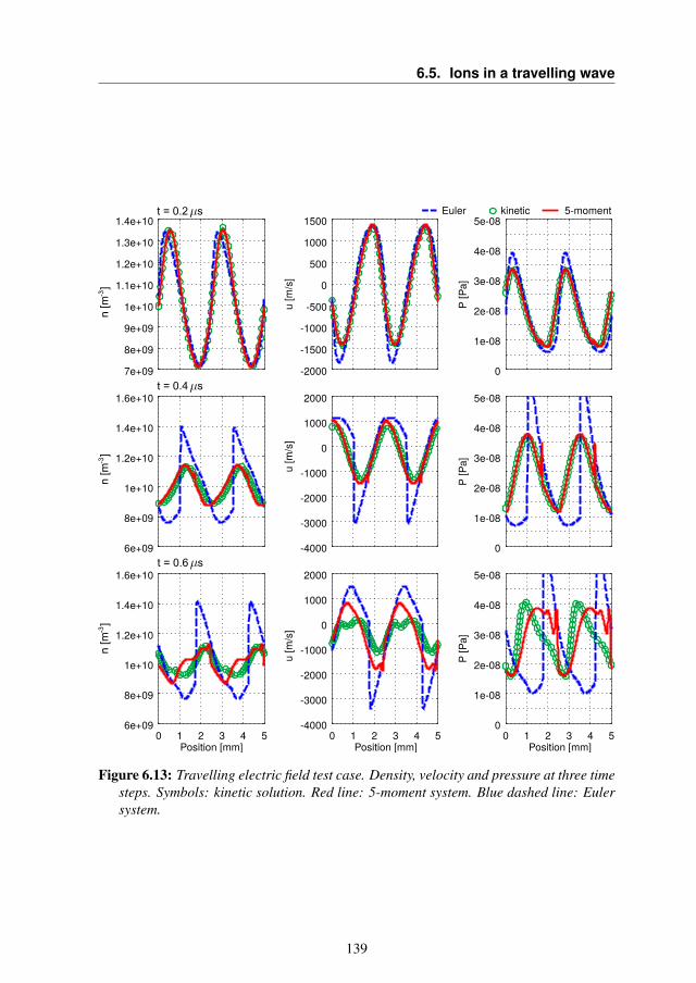
6.5. Ions in a travelling wave
Figure 6.13: Travelling electric field test case. Density, velocity and pressure at three timesteps. Symbols: kinetic solution. Red line: 5-moment system. Blue dashed line: Eulersystem.
139
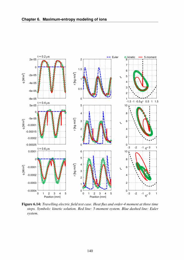
Chapter 6. Maximum-entropy modeling of ions
Figure 6.14: Travelling electric field test case. Heat flux and order-4 moment at three timesteps. Symbols: kinetic solution. Red line: 5-moment system. Blue dashed line: Eulersystem.
140
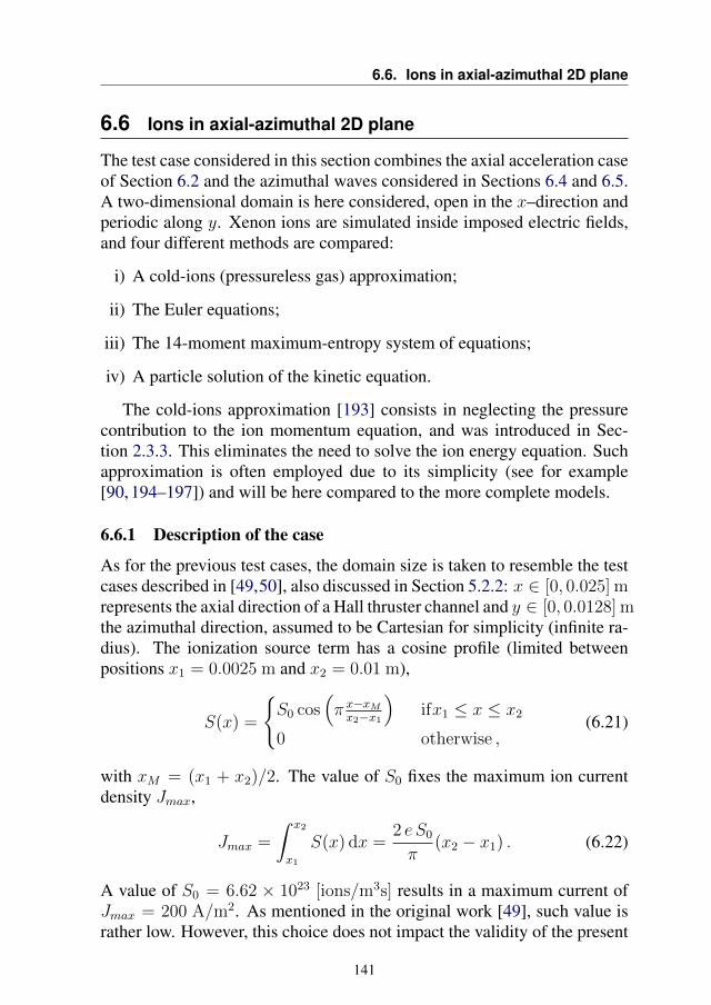
6.6. Ions in axial-azimuthal 2D plane
6.6 Ions in axial-azimuthal 2D plane
The test case considered in this section combines the axial acceleration caseof Section 6.2 and the azimuthal waves considered in Sections 6.4 and 6.5.A two-dimensional domain is here considered, open in the x–direction andperiodic along y. Xenon ions are simulated inside imposed electric fields,and four different methods are compared:
i) A cold-ions (pressureless gas) approximation;
ii) The Euler equations;
iii) The 14-moment maximum-entropy system of equations;
iv) A particle solution of the kinetic equation.
The cold-ions approximation [193] consists in neglecting the pressurecontribution to the ion momentum equation, and was introduced in Sec-tion 2.3.3. This eliminates the need to solve the ion energy equation. Suchapproximation is often employed due to its simplicity (see for example[90, 194–197]) and will be here compared to the more complete models.
6.6.1 Description of the case
As for the previous test cases, the domain size is taken to resemble the testcases described in [49,50], also discussed in Section 5.2.2: x ∈ [0, 0.025] mrepresents the axial direction of a Hall thruster channel and y ∈ [0, 0.0128] mthe azimuthal direction, assumed to be Cartesian for simplicity (infinite ra-dius). The ionization source term has a cosine profile (limited betweenpositions x1 = 0.0025 m and x2 = 0.01 m),
S(x) =
S0 cos
(π x−xMx2−x1
)ifx1 ≤ x ≤ x2
0 otherwise ,(6.21)
with xM = (x1 + x2)/2. The value of S0 fixes the maximum ion currentdensity Jmax,
Jmax =
ˆ x2
x1
S(x) dx =2 e S0
π(x2 − x1) . (6.22)
A value of S0 = 6.62 × 10²³ [ions/m3s] results in a maximum current ofJmax = 200 A/m2. As mentioned in the original work [49], such value israther low. However, this choice does not impact the validity of the present
141
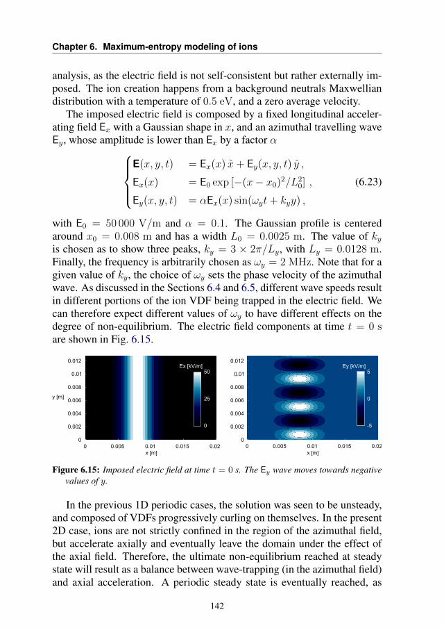
Chapter 6. Maximum-entropy modeling of ions
analysis, as the electric field is not self-consistent but rather externally im-posed. The ion creation happens from a background neutrals Maxwelliandistribution with a temperature of 0.5 eV, and a zero average velocity.
The imposed electric field is composed by a fixed longitudinal acceler-ating field Ex with a Gaussian shape in x, and an azimuthal travelling waveEy, whose amplitude is lower than Ex by a factor α
E(x, y, t) = Ex(x) x+ Ey(x, y, t) y ,
Ex(x) = E0 exp [−(x− x0)2/L20] ,
Ey(x, y, t) = αEx(x) sin(ωyt+ kyy) ,
(6.23)
with E0 = 50 000 V/m and α = 0.1. The Gaussian profile is centeredaround x0 = 0.008 m and has a width L0 = 0.0025 m. The value of kyis chosen as to show three peaks, ky = 3 × 2π/Ly, with Ly = 0.0128 m.Finally, the frequency is arbitrarily chosen as ωy = 2 MHz. Note that for agiven value of ky, the choice of ωy sets the phase velocity of the azimuthalwave. As discussed in the Sections 6.4 and 6.5, different wave speeds resultin different portions of the ion VDF being trapped in the electric field. Wecan therefore expect different values of ωy to have different effects on thedegree of non-equilibrium. The electric field components at time t = 0 sare shown in Fig. 6.15.
Figure 6.15: Imposed electric field at time t = 0 s. The Ey wave moves towards negativevalues of y.
In the previous 1D periodic cases, the solution was seen to be unsteady,and composed of VDFs progressively curling on themselves. In the present2D case, ions are not strictly confined in the region of the azimuthal field,but accelerate axially and eventually leave the domain under the effect ofthe axial field. Therefore, the ultimate non-equilibrium reached at steadystate will result as a balance between wave-trapping (in the azimuthal field)and axial acceleration. A periodic steady state is eventually reached, as
142
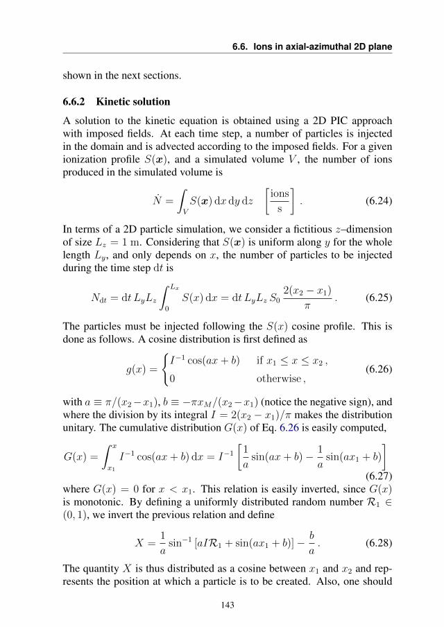
6.6. Ions in axial-azimuthal 2D plane
shown in the next sections.
6.6.2 Kinetic solution
A solution to the kinetic equation is obtained using a 2D PIC approachwith imposed fields. At each time step, a number of particles is injectedin the domain and is advected according to the imposed fields. For a givenionization profile S(x), and a simulated volume V , the number of ionsproduced in the simulated volume is
N =
ˆV
S(x) dx dy dz
[ions
s
]. (6.24)
In terms of a 2D particle simulation, we consider a fictitious z–dimensionof size Lz = 1 m. Considering that S(x) is uniform along y for the wholelength Ly, and only depends on x, the number of particles to be injectedduring the time step dt is
Ndt = dt LyLz
ˆ Lx
0
S(x) dx = dt LyLz S02(x2 − x1)
π. (6.25)
The particles must be injected following the S(x) cosine profile. This isdone as follows. A cosine distribution is first defined as
g(x) =
I−1 cos(ax+ b) if x1 ≤ x ≤ x2 ,
0 otherwise ,(6.26)
with a ≡ π/(x2−x1), b ≡ −πxM/(x2−x1) (notice the negative sign), andwhere the division by its integral I = 2(x2 − x1)/π makes the distributionunitary. The cumulative distribution G(x) of Eq. 6.26 is easily computed,
G(x) =
ˆ x
x1
I−1 cos(ax+ b) dx = I−1
[1
asin(ax+ b)− 1
asin(ax1 + b)
](6.27)
where G(x) = 0 for x < x1. This relation is easily inverted, since G(x)is monotonic. By defining a uniformly distributed random number R1 ∈(0, 1), we invert the previous relation and define
X =1
asin−1 [aIR1 + sin(ax1 + b)]− b
a. (6.28)
The quantity X is thus distributed as a cosine between x1 and x2 and rep-resents the position at which a particle is to be created. Also, one should
143
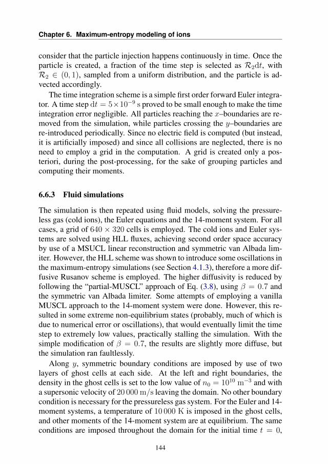
Chapter 6. Maximum-entropy modeling of ions
consider that the particle injection happens continuously in time. Once theparticle is created, a fraction of the time step is selected as R2dt, withR2 ∈ (0, 1), sampled from a uniform distribution, and the particle is ad-vected accordingly.
The time integration scheme is a simple first order forward Euler integra-tor. A time step dt = 5×10⁻⁹ s proved to be small enough to make the timeintegration error negligible. All particles reaching the x–boundaries are re-moved from the simulation, while particles crossing the y–boundaries arere-introduced periodically. Since no electric field is computed (but instead,it is artificially imposed) and since all collisions are neglected, there is noneed to employ a grid in the computation. A grid is created only a pos-teriori, during the post-processing, for the sake of grouping particles andcomputing their moments.
6.6.3 Fluid simulations
The simulation is then repeated using fluid models, solving the pressure-less gas (cold ions), the Euler equations and the 14-moment system. For allcases, a grid of 640 × 320 cells is employed. The cold ions and Euler sys-tems are solved using HLL fluxes, achieving second order space accuracyby use of a MSUCL linear reconstruction and symmetric van Albada lim-iter. However, the HLL scheme was shown to introduce some oscillations inthe maximum-entropy simulations (see Section 4.1.3), therefore a more dif-fusive Rusanov scheme is employed. The higher diffusivity is reduced byfollowing the “partial-MUSCL” approach of Eq. (3.8), using β = 0.7 andthe symmetric van Albada limiter. Some attempts of employing a vanillaMUSCL approach to the 14-moment system were done. However, this re-sulted in some extreme non-equilibrium states (probably, much of which isdue to numerical error or oscillations), that would eventually limit the timestep to extremely low values, practically stalling the simulation. With thesimple modification of β = 0.7, the results are slightly more diffuse, butthe simulation ran faultlessly.
Along y, symmetric boundary conditions are imposed by use of twolayers of ghost cells at each side. At the left and right boundaries, thedensity in the ghost cells is set to the low value of n0 = 1010 m−3 and witha supersonic velocity of 20 000 m/s leaving the domain. No other boundarycondition is necessary for the pressureless gas system. For the Euler and 14-moment systems, a temperature of 10 000 K is imposed in the ghost cells,and other moments of the 14-moment system are at equilibrium. The sameconditions are imposed throughout the domain for the initial time t = 0,
144
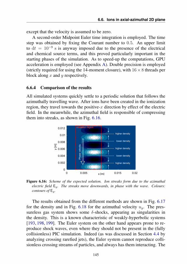
6.6. Ions in axial-azimuthal 2D plane
except that the velocity is assumed to be zero.A second-order Midpoint Euler time integration is employed. The time
step was obtained by fixing the Courant number to 0.5. An upper limitto dt = 10−9 s is anyway imposed due to the presence of the electricaland chemical source terms, and this proved particularly important in thestarting phases of the simulation. As to speed-up the computations, GPUacceleration is employed (see Appendix A). Double precision is employed(strictly required for using the 14-moment closure), with 16× 8 threads perblock along x and y respectively.
6.6.4 Comparison of the results
All simulated systems quickly settle to a periodic solution that follows theazimuthally travelling wave. After ions have been created in the ionizationregion, they travel towards the positive-x direction by effect of the electricfield. In the meanwhile, the azimuthal field is responsible of compressingthem into streaks, as shown in Fig. 6.16.
Figure 6.16: Scheme of the expected solution. Ion streaks form due to the azimuthalelectric field Ey . The streaks move downwards, in phase with the wave. Colours:contours of Ey .
The results obtained from the different methods are shown in Fig. 6.17for the density and in Fig. 6.18 for the azimuthal velocity uy. The pres-sureless gas system shows some δ-shocks, appearing as singularities inthe density. This is a known characteristic of weakly-hyperbolic systems[193, 198, 199]. The Euler system on the other hand appears prone to re-produce shock waves, even where they should not be present in the (fullycollisionless) PIC simulation. Indeed (as was discussed in Section 4.4 byanalyzing crossing rarefied jets), the Euler system cannot reproduce colli-sionless crossing streams of particles, and always has them interacting. The
145
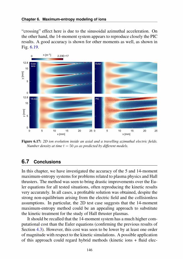
Chapter 6. Maximum-entropy modeling of ions
“crossing” effect here is due to the sinusoidal azimuthal acceleration. Onthe other hand, the 14-moment system appears to reproduce closely the PICresults. A good accuracy is shown for other moments as well, as shown inFig. 6.19.
Figure 6.17: 2D ion evolution inside an axial and a travelling azimuthal electric fields.Number density at time t = 50 µs as predicted by different models.
6.7 Conclusions
In this chapter, we have investigated the accuracy of the 5 and 14-momentmaximum-entropy systems for problems related to plasma physics and Hallthrusters. The method was seen to bring drastic improvements over the Eu-ler equations for all tested situations, often reproducing the kinetic resultsvery accurately. In all cases, a profitable solution was obtained, despite thestrong non-equilibrium arising from the electric field and the collisionlessassumptions. In particular, the 2D test case suggests that the 14-momentmaximum-entropy method could be an appealing approach to substitutethe kinetic treatment for the study of Hall thruster plasmas.
It should be recalled that the 14-moment system has a much higher com-putational cost than the Euler equations (confirming the previous results ofSection 4.3). However, this cost was seen to be lower by at least one orderof magnitude with respect to the kinetic simulations. A possible applicationof this approach could regard hybrid methods (kinetic ions + fluid elec-
146
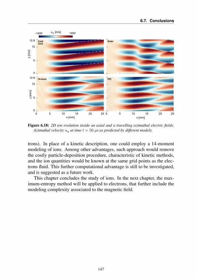
6.7. Conclusions
Figure 6.18: 2D ion evolution inside an axial and a travelling azimuthal electric fields.Azimuthal velocity uy at time t = 50 µs as predicted by different models.
trons). In place of a kinetic description, one could employ a 14-momentmodeling of ions. Among other advantages, such approach would removethe costly particle-deposition procedure, characteristic of kinetic methods,and the ion quantities would be known at the same grid points as the elec-trons fluid. This further computational advantage is still to be investigated,and is suggested as a future work.
This chapter concludes the study of ions. In the next chapter, the max-imum-entropy method will be applied to electrons, that further include themodeling complexity associated to the magnetic field.
147
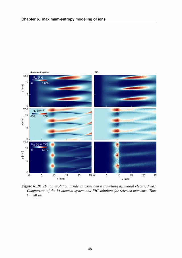
Chapter 6. Maximum-entropy modeling of ions
Figure 6.19: 2D ion evolution inside an axial and a travelling azimuthal electric fields.Comparison of the 14-moment system and PIC solutions for selected moments. Timet = 50 µs.
148
CHAPTER7Maximum-entropy modeling of electrons
The content of this chapter was partly published in [200]: Boccelli, S.,Giroux, F., Magin, T.E., Groth, C.P.T., McDonald, J.G., A 14-momentmaximum-entropy description of electrons in crossed electric and mag-netic fields, Physics of Plasmas 27 (12), 123506;and partly presented at the 73rd Gaseous Electronics Conference [201].
While ions in Hall thrusters are fundamentally unmagnetized, a compu-tation of the Larmor radius reveals that electrons are strongly affected bythe magnetic field, due to their small mass. Together with the axial electricfield, electrons are subject to a drift in the E × B direction. Also, whileions were assumed to be collisionless, electrons collisions are much morefrequently, mostly with background neutrals, and such collisions are im-portant in terms of cross-field electron transport, but not strong enough tokeep electrons close at thermodynamic equilibrium. Indeed, we will seethat electrons can be expected to develop strongly non-Maxwellian VDFs.This chapter is aimed at investigating the maximum-entropy closure in suchconditions.
Due to the low plasma density, Coulomb collisions will be neglectedand only collisions with background neutrals will be accounted for. Only
149
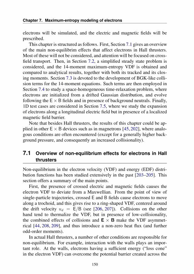
Chapter 7. Maximum-entropy modeling of electrons
electrons will be simulated, and the electric and magnetic fields will beprescribed.
This chapter is structured as follows. First, Section 7.1 gives an overviewof the main non-equilibrim effects that affect electrons in Hall thrusters.Most of these will not be considered, and attention will be focused on cross-field transport. Then, in Section 7.2, a simplified steady state problem isconsidered, and the 14-moment maximum-entropy VDF is obtained andcompared to analytical results, together with both its tracked and its clos-ing moments. Section 7.3 is devoted to the development of BGK-like colli-sion terms for the 14-moment equations. Such terms are then employed inSection 7.4 to study a space-homogeneous time-relaxation problem, whereelectrons are initialized from a drifted Gaussian distribution, and evolvefollowing the E× B fields and in presence of background neutrals. Finally,1D test cases are considered in Section 7.5, where we study the expansionof electrons along a longitudinal electric field but in presence of a localizedmagnetic field barrier.
Note that besides Hall thrusters, the results of this chapter could be ap-plied in other E× B devices such as in magnetrons [45, 202], where analo-gous conditions are often encountered (except for a generally higher back-ground pressure, and consequently an increased collisionality).
7.1 Overview of non-equilibrium effects for electrons in Hallthrusters
Non-equilibrium in the electron velocity (VDF) and energy (EDF) distri-bution functions has been studied extensively in the past [203–205]. Thissection offers a summary of the main points.
First, the presence of crossed electric and magnetic fields causes theelectron VDF to deviate from a Maxwellian. From the point of view ofsingle-particle trajectories, crossed E and B fields cause electrons to movealong a trochoid, and this gives rise to a ring-shaped VDF, centered aroundthe drift velocity ud = E/B (see [206, 207]). Collisions on the otherhand tend to thermalize the VDF, but in presence of low-collisionality,the combined effects of collisions and E × B make the VDF asymmet-rical [44, 208, 209], and thus introduce a non-zero heat flux (and furtherodd-order moments).
In actual Hall thrusters, a number of other conditions are responsible fornon-equilibrium. For example, interaction with the walls plays an impor-tant role. At the walls, electrons having a sufficient energy (“loss cone”in the electron VDF) can overcome the potential barrier created across the
150
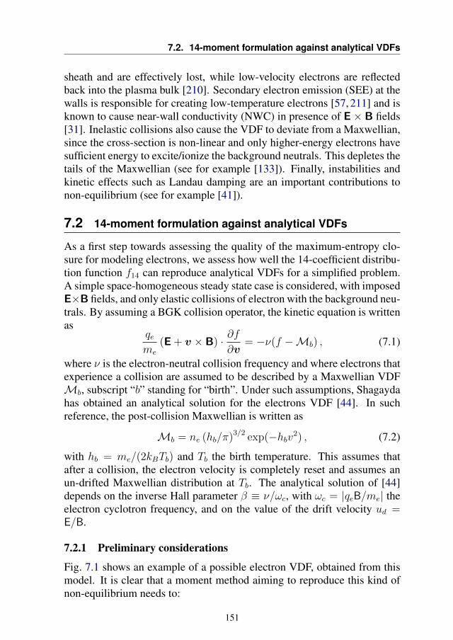
7.2. 14-moment formulation against analytical VDFs
sheath and are effectively lost, while low-velocity electrons are reflectedback into the plasma bulk [210]. Secondary electron emission (SEE) at thewalls is responsible for creating low-temperature electrons [57, 211] and isknown to cause near-wall conductivity (NWC) in presence of E× B fields[31]. Inelastic collisions also cause the VDF to deviate from a Maxwellian,since the cross-section is non-linear and only higher-energy electrons havesufficient energy to excite/ionize the background neutrals. This depletes thetails of the Maxwellian (see for example [133]). Finally, instabilities andkinetic effects such as Landau damping are an important contributions tonon-equilibrium (see for example [41]).
7.2 14-moment formulation against analytical VDFs
As a first step towards assessing the quality of the maximum-entropy clo-sure for modeling electrons, we assess how well the 14-coefficient distribu-tion function f14 can reproduce analytical VDFs for a simplified problem.A simple space-homogeneous steady state case is considered, with imposedE×B fields, and only elastic collisions of electron with the background neu-trals. By assuming a BGK collision operator, the kinetic equation is writtenas
qeme
(E + v × B) · ∂f∂v
= −ν(f −Mb) , (7.1)
where ν is the electron-neutral collision frequency and where electrons thatexperience a collision are assumed to be described by a Maxwellian VDFMb, subscript “b” standing for “birth”. Under such assumptions, Shagaydahas obtained an analytical solution for the electrons VDF [44]. In suchreference, the post-collision Maxwellian is written as
Mb = ne (hb/π)3/2 exp(−hbv2) , (7.2)
with hb = me/(2kBTb) and Tb the birth temperature. This assumes thatafter a collision, the electron velocity is completely reset and assumes anun-drifted Maxwellian distribution at Tb. The analytical solution of [44]depends on the inverse Hall parameter β ≡ ν/ωc, with ωc = |qeB/me| theelectron cyclotron frequency, and on the value of the drift velocity ud =E/B.
7.2.1 Preliminary considerations
Fig. 7.1 shows an example of a possible electron VDF, obtained from thismodel. It is clear that a moment method aiming to reproduce this kind ofnon-equilibrium needs to:
151
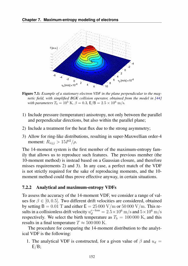
Chapter 7. Maximum-entropy modeling of electrons
Figure 7.1: Example of a stationary electron VDF in the plane perpendicular to the mag-netic field, with simplified BGK collision operator, obtained from the model in [44]with parameters Tb = 105 K, β = 0.3, E/B = 2.5× 10⁶ m/s.
1) Include pressure (temperature) anisotropy, not only between the paralleland perpendicular directions, but also within the parallel plane;
2) Include a treatment for the heat flux due to the strong asymmetry;
3) Allow for ring-like distributions, resulting in super-Maxwellian order-4moment: Riijj > 15P 2/ρ.
The 14-moment system is the first member of the maximum-entropy fam-ily that allows us to reproduce such features. The previous member (the10-moment method) is instead based on a Gaussian closure, and thereforemisses requirements 2) and 3). In any case, a perfect match of the VDFis not strictly required for the sake of reproducing moments, and the 10-moment method could thus prove effective anyway, in certain situations.
7.2.2 Analytical and maximum-entropy VDFs
To assess the accuracy of the 14-moment VDF, we consider a range of val-ues for β ∈ [0, 0.5]. Two different drift velocities are considered, obtainedby setting B = 0.01 T and either E = 25 000 V/m or 50 000 V/m. This re-sults in a collisionless drift velocity uc−less
d = 2.5×10⁶ m/s and 5×10⁶ m/srespectively. We select the birth temperature as Tb = 100 000 K, and thisresults in a final temperature T ≈ 500 000 K.
The procedure for comparing the 14-moment distribution to the analyt-ical VDF is the following:
1. The analytical VDF is constructed, for a given value of β and ud =E/B;
152
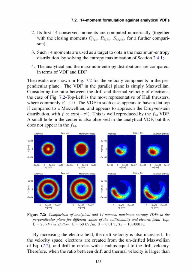
7.2. 14-moment formulation against analytical VDFs
2. Its first 14 conserved moments are computed numerically (togetherwith the closing moments Qijk, Rijkk, Sijjkk, for a further compari-son);
3. Such 14 moments are used as a target to obtain the maximum-entropydistribution, by solving the entropy maximisation of Section 2.4.1;
4. The analytical and the maximum-entropy distributions are compared,in terms of VDF and EDF.
The results are shown in Fig. 7.2 for the velocity components in the per-pendicular plane. The VDF in the parallel plane is simply Maxwellian.Considering the ratio between the drift and thermal velocity of electrons,the case of Fig. 7.2-Top-Left is the most representative of Hall thrusters,where commonly β → 0. The VDF in such case appears to have a flat topif compared to a Maxwellian, and appears to approach the Druyvensteindistribution, with f ∝ exp(−v4). This is well reproduced by the f14 VDF.A small hole in the center is also observed in the analytical VDF, but thisdoes not appear in the f14.
Figure 7.2: Comparison of analytical and 14-moment maximum-entropy VDFs in theperpendicular plane for different values of the collisionality and electric field. Top:E = 25 kV/m. Bottom: E = 50 kV/m. B = 0.01 T, Tb = 100 000 K.
By increasing the electric field, the drift velocity is also increased. Inthe velocity space, electrons are created from the un-drifted Maxwellianof Eq. (7.2), and drift in circles with a radius equal to the drift velocity.Therefore, when the ratio between drift and thermal velocity is larger than
153
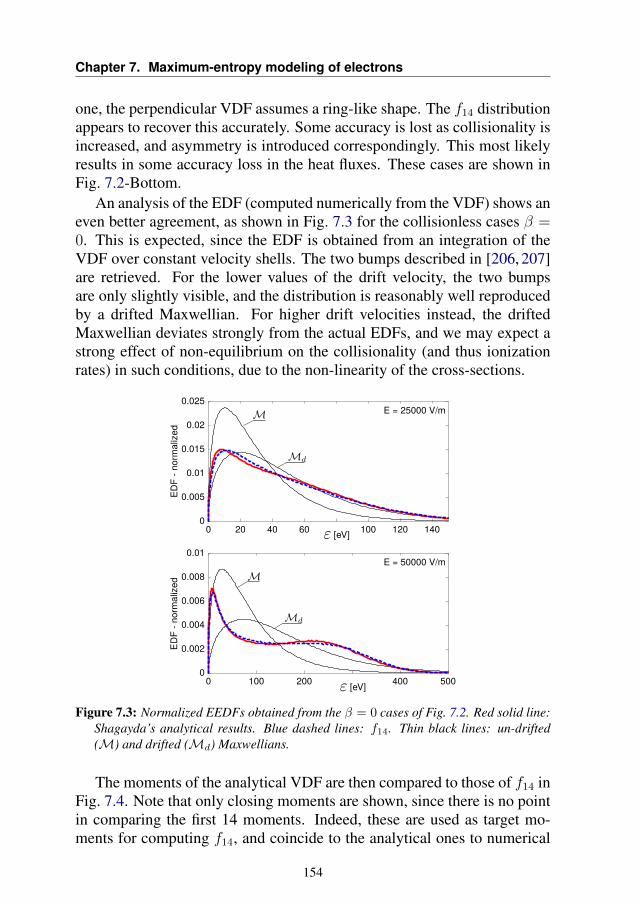
Chapter 7. Maximum-entropy modeling of electrons
one, the perpendicular VDF assumes a ring-like shape. The f14 distributionappears to recover this accurately. Some accuracy is lost as collisionality isincreased, and asymmetry is introduced correspondingly. This most likelyresults in some accuracy loss in the heat fluxes. These cases are shown inFig. 7.2-Bottom.
An analysis of the EDF (computed numerically from the VDF) shows aneven better agreement, as shown in Fig. 7.3 for the collisionless cases β =0. This is expected, since the EDF is obtained from an integration of theVDF over constant velocity shells. The two bumps described in [206, 207]are retrieved. For the lower values of the drift velocity, the two bumpsare only slightly visible, and the distribution is reasonably well reproducedby a drifted Maxwellian. For higher drift velocities instead, the driftedMaxwellian deviates strongly from the actual EDFs, and we may expect astrong effect of non-equilibrium on the collisionality (and thus ionizationrates) in such conditions, due to the non-linearity of the cross-sections.
Figure 7.3: Normalized EEDFs obtained from the β = 0 cases of Fig. 7.2. Red solid line:Shagayda’s analytical results. Blue dashed lines: f14. Thin black lines: un-drifted(M) and drifted (Md) Maxwellians.
The moments of the analytical VDF are then compared to those of f14 inFig. 7.4. Note that only closing moments are shown, since there is no pointin comparing the first 14 moments. Indeed, these are used as target mo-ments for computing f14, and coincide to the analytical ones to numerical
154
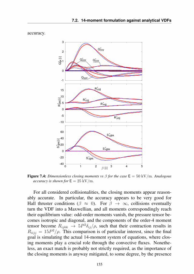
7.2. 14-moment formulation against analytical VDFs
accuracy.
Figure 7.4: Dimensionless closing moments vs β for the case E = 50 kV/m. Analogousaccuracy is shown for E = 25 kV/m.
For all considered collisionalities, the closing moments appear reason-ably accurate. In particular, the accuracy appears to be very good forHall thruster conditions (β ≈ 0). For β → ∞, collisions eventuallyturn the VDF into a Maxwellian, and all moments correspondingly reachtheir equilibrium value: odd-order moments vanish, the pressure tensor be-comes isotropic and diagonal, and the components of the order-4 momenttensor become Rijkk → 5P 2δij/ρ, such that their contraction results inRiijj = 15P 2/ρ. This comparison is of particular interest, since the finalgoal is simulating the actual 14-moment system of equations, where clos-ing moments play a crucial role through the convective fluxes. Nonethe-less, an exact match is probably not strictly required, as the importance ofthe closing moments is anyway mitigated, to some degree, by the presence
155
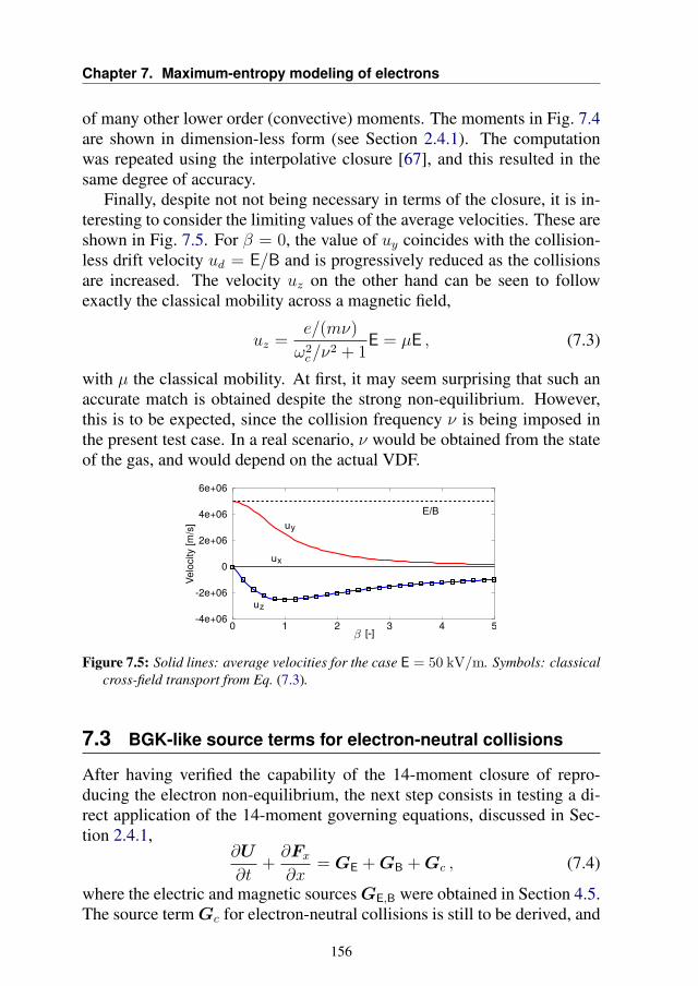
Chapter 7. Maximum-entropy modeling of electrons
of many other lower order (convective) moments. The moments in Fig. 7.4are shown in dimension-less form (see Section 2.4.1). The computationwas repeated using the interpolative closure [67], and this resulted in thesame degree of accuracy.
Finally, despite not not being necessary in terms of the closure, it is in-teresting to consider the limiting values of the average velocities. These areshown in Fig. 7.5. For β = 0, the value of uy coincides with the collision-less drift velocity ud = E/B and is progressively reduced as the collisionsare increased. The velocity uz on the other hand can be seen to followexactly the classical mobility across a magnetic field,
uz =e/(mν)
ω2c/ν
2 + 1E = µE , (7.3)
with µ the classical mobility. At first, it may seem surprising that such anaccurate match is obtained despite the strong non-equilibrium. However,this is to be expected, since the collision frequency ν is being imposed inthe present test case. In a real scenario, ν would be obtained from the stateof the gas, and would depend on the actual VDF.
Figure 7.5: Solid lines: average velocities for the case E = 50 kV/m. Symbols: classicalcross-field transport from Eq. (7.3).
7.3 BGK-like source terms for electron-neutral collisions
After having verified the capability of the 14-moment closure of repro-ducing the electron non-equilibrium, the next step consists in testing a di-rect application of the 14-moment governing equations, discussed in Sec-tion 2.4.1,
∂U
∂t+∂Fx∂x
= GE +GB +Gc , (7.4)
where the electric and magnetic sourcesGE,B were obtained in Section 4.5.The source termGc for electron-neutral collisions is still to be derived, and
156
7.3. BGK-like source terms for electron-neutral collisions
this is the aim of the present section. In this work, we are mostly inter-ested in the study of the streaming part of the system, therefore a simplifiedtreatment of collisions will be sufficient. The BGK collision operator [80]is a convenient choice, as it allows for a simple derivation of the sourceterms for the moment equations. Moreover, the BGK operator automati-cally recovers the Boltzmann’s H-theorem, as relaxation happens towardsa Maxwellian. Such operator has been employed in a number of scenar-ios, including multi-temperature monatomic/polyatomic gases and reactingmixtures [83–85].
In the following, we develop a BGK-like collision operator for electroncollisions with background neutrals, in the conditions of low-temperaturenon-thermal plasmas, where the electron temperature is much higher thanthe neutral temperature. First, we write
C =
(δf
δt
)c
= −ν (f − fp) , (7.5)
where fp is the distribution that characterizes the post-collision state ofelectrons and where the collision frequency ν only depends on the macro-scopic parameters. The latter choice implies that all moments relax at thesame rate, which is unphysical, or at least inaccurate. An improvementcould be obtained by taking ν as a function of the particle velocity (andthus not only depending on the macroscopic quantities), at the price of in-creasing the model complexity [62, 86].
In the work of Shagayda [44], the post-collision distribution fp is as-sumed Maxwellian. However, from a physical standpoint, this it is notnecessarily the case. As mentioned, such choice allows us to retrieve theH-theorem, which is surely desired for ordinary gases in absence of externalfields, but is not necessarily representative of low-temperature plasmas. In-deed, while in an ordinary gas all species relax towards a common tempera-ture (consider for example the relaxation behind a strong shock wave), low-temperature plasmas typically settle to a multi-temperature steady state:electrons are typically in the [eV] range (being excited by external fields),neutrals have a temperature often comparable to the walls temperature andions are somewhere in the middle. Therefore, the collision operator mustbe formulated as to represent such steady state non-thermal conditions.
A second important aspect to be considered is mass disparity: as elec-trons have a much lower mass than neutrals, the energy exchange becomesextremely ineffective. In particular, considering the binary collision be-tween a lightweight particle of mass m and a heavy particle of mass M , the
157
Chapter 7. Maximum-entropy modeling of electrons
exchange of energy ∆ε/ε results, in the limiting gase of mM [212],
∆ε
ε= 2
m
M(1− cosχ) , (7.6)
where χ is the deflection angle. Considering collisions of electrons withxenon atoms, me/MXe ≈ 4 × 10⁻⁶, such that the initial energy of a hotelectron will be transfered to the neutrals, in average, after some 105–106
elastic collisions.In the following, we will consider isotropic scattering, that is a reason-
able approximation for low collision energies [133, 213].
7.3.1 A simple Maxwellian-relaxation collision model
The simplest choice for the post-collision distribution consists in assumingthat fp = M, with M the local Maxwellian, as also done in [44]. Thisresembles a classical single-species BGK formulation, but differs in that:
• Neutrals are cold and slow with respect to the colliding electrons;
• The energy exchange ∆ε/ε is here neglected, and the energy of theelectrons population is conserved;
• Scattering is assumed isotropic in the center of mass frame, that ap-proximately coincides with the center of mass of the heavy neutralparticle.
From these assumptions, the post-collision Maxwellian is characterized bya zero average velocity, and collisions have the effect of transforming thewhole initial energy (kinetic + thermal) into thermal energy. Therefore, thepost-collision electron temperature is obtained from
3
2kBTp =
3
2kBT +
1
2meu
2 , (7.7)
with T and u the temperature and average velocity of electrons. The post-collision pressure simply reads Pp = nkBTp, where the local density n isunchanged by the collision process, since only elastic collisions are beingconsidered.
The source terms for the 14-moment equations are then obtained as av-erages over this collision term (see Chapter 2). After having defined thevector of generating functions Ψ = m(1, vi, vivj, viv
2, v4), composed by14 entries, the collisional sources are obtained as
GMc = −〈Ψ ν (f −M)〉 = −ν [〈Ψf〉 − 〈ΨM〉] . (7.8)
158

7.3. BGK-like source terms for electron-neutral collisions
In other words, the source terms for the 14-moment equations are the differ-ence between the moments themselves (the term 〈Ψf〉) and their value fora non-drifted Maxwellian at temperature Tp, weighted by the collision fre-quency ν. From symmetry considerations, all odd-order central momentsof the Maxwellian are zero, and the source terms are easily evaluated byconsidering that
• All odd-order moments (ui, qi, Qijk, Sijjkk) relax to zero;
• Even-order moments relax to their Maxwellian value (Pij → Pδij ,Riijj → 15P 2/ρ).
This is easily verified by a direct calculation from Eq. (7.8), and ultimatelygives
GMc =
(δU
δt
)c
= −ν
0
U2
U3
U4
(U5 − Pp)U6
U7
(U8 − Pp)U9
(U10 − Pp)U11
U12
U13
(U14 − 15P 2p /ρ)
. (7.9)
7.3.2 Collision model for large mass disparity
In the previous section, the post-collision distribution was assumed to beMaxwellian. Such assumption is not physically justified for electron-neutralcollisions, and was only based on simplicity. Indeed, during a single electron-neutral collision, not only energy is (to a first approximation) conserved atthe population level, but also the energy of the single electron is conserved.Therefore, the distribution that characterizes the post-collision state is not aMaxwellian, but rather a distribution that has the very same energy contentas the initial distribution f . Therefore, when plotted in the energy variable,
159
Chapter 7. Maximum-entropy modeling of electrons
we havefp(ε) = f(ε) =⇒ fp(v
2) = f(v2) . (7.10)
For simplicity, we further assume that collisions are isotropic, and there-fore fp is symmetric, and we denote it by f iso
p for clarity. As before, thesource terms are obtained from
Gisoc = −
⟨Ψ ν
(f − f iso
p
)⟩= −ν
[〈Ψf〉 −
⟨Ψf iso
p
⟩]. (7.11)
For the sake of obtaining the source terms, an explicit knowledge of theshape of f iso
p is not necessary, and the following considerations are suffi-cient:
• Since f isop is isotropic, its odd-order central moments are zero;
• The average velocity of f isop is also zero, as we consider isotropic scat-
tering around a fixed target heavy particle;
• The temperature of f isop is also obtained from Eq. (7.7).
Some more considerations are required regarding the order-4 moment,U14 = 〈mv4〉. Intuitively, one can realize that, since the electron energy isconserved in each collision, its square will also be conserved. Therefore,the moment 〈mv4〉 will be a conserved quantity, being the average of in-dividually conserved quantities. This is easily shown at a formal level bywriting the definition of the order-4 moment in spherical coordinates, forthe post-collision isotropic distribution:⟨
mv4⟩iso
p=
ˆmv4f iso
p (v2)v2 sin θ dv dψ dθ , (7.12)
where the dependence on the velocity modulus is highlighted in the distri-bution function by writing v2. From Eq. (7.10), since f iso
p (v2) = f(v2), wesimply obtain that
U14,p =⟨mv4
⟩iso
p=⟨mv4
⟩= U14 . (7.13)
Therefore, energy preserving collisions do make the distribution isotropic,but have no effect on the contracted order-4 moment, and the energy spec-trum of the VDF is preserved. Ultimately, the collisional sources from thismodel are equal to the the previous Maxwellian-relaxation sources, differ-ing only in the 14–th element:
Gisoc (1, · · · , 13) = GMc (1, · · · , 13) and Giso
c (14) = 0 . (7.14)
160
7.3. BGK-like source terms for electron-neutral collisions
7.3.3 Elastic collisions with energy loss
In the previous sections, the energy exchanged by electrons via collisionswith neutrals was neglected in view of the large mass disparity. We discusshere how to include such effect.
Eq. (7.6) gives the energy transfered from a given electron to a targetneutral, ∆ε/ε = 2m/M(1− cosχ), as a function of the deflection angle χand the mass ratio. In general, the deflection angle is a function of the im-pact parameter b and of the collision energy, through the differential crosssection. We assume isotropic scattering for simplicity, hence, the deflec-tion angle only depends on the impact parameter b. In the assumption thatthe position of the electron and the location of the target neutral are un-correlated, the impact parameter b is linearly distributed (fewer electronshave a head-on collision, and more electrons experience a grazing colli-sion). From this observation, we can obtain the distribution of angles χ,that is sinusoidal. The average deflection angle is π/2, and by definitionχ ∈ [0, π]. The quantity (1 − cosχ), appearing in the expression for theenergy loss, can be seen to be uniformly distributed (see [212]) over theinterval [0, 2], and averages to 1. Therefore, given all possible impact pa-rameters, and consequent deflection angles χ, the electron in average losesan amount of energy 〈∆ε/ε〉χ = 2m/M .
Let us now consider the whole population of electrons. In the previouscase, in the limit of an infinitely large mass disparity, the total energy of theelectron population was conserved. In the present case, the post-collisionenergy should be investigated by averaging the energy loss over the electronenergy distribution function. An accurate analysis would also consider thatmore energetic electrons collide more frequently than slow-moving ones.However, such effects are neglected in a BGK-like approach, and we thuslimit ourselves to the following observation: if the energy lost by an elec-tron, whatever the deflection angle, is 2m/M times the initial energy, thenthe post-collision energy of the whole population shall be reduced by thesame factor. Therefore, we modify Eq. (7.7) into
3
2kBTp =
(3
2kBT +
1
2meu
2
)(1− 2m
M
). (7.15)
Notice that the post-collision distribution is still symmetric, due to isotropicscattering, and its odd-order central moments and the average velocity arestill zero. The pressure tensor relaxes to Pij = nkBTpδij , as for the previouscases, with Tp from Eq. (7.15). This completely extends the Maxwellianmodel of Section 7.3.1 to include energy losses.
161
Chapter 7. Maximum-entropy modeling of electrons
Regarding the general isotropic-collision model of Section 7.3.2, thefourth-order moment still needs to be investigated. We recall that the order-4 moment is defined as 〈mv4〉, that is proportional to the average of thesquared particle energies.1 By squaring Eq. (7.6), one can obtain the post-collision quantity (mv′2)2 of an electron i deflected by the angle χ,
m2v′4i = m2v4i
(1− 2m
M(1− cosχ)
)2
= m2v4i
(1 +
4m2
M2(1− cosχ)2 − 4m
M(1− cosχ)
). (7.16)
This eventually allows us to estimate the post-collision value for the order-4 moment. At first, we shall average this term over all possible deflectionangles. Following the previous discussion, by considering that the impactparameter is linearly distributed, the quantity (1 − cosχ) is found to beuniformly distributed for isotropic collisions. The probability distributionof (1 − cosχ)2 is thus also known, and can be seen to have an averagevalue of 4/3 (see [214]). Therefore, averaging Eq. (7.16) over χ, one ulti-mately finds the (average over the possible deflection angles) post-collisionvelocity as
v′4i = v4i
(1 +
16
3
m2
M2− 4m
M
). (7.17)
Notice that the quantity inside the parenthesis is smaller than 1, such thatv′4i < v4
i . As done for the post-collision temperature, we write the post-col-lision order-4 moment as the pre-collision moment reduced by the quantityappearing in the parenthesis:⟨
mv4⟩iso
p=
(1 +
16
3
m2
M2− 4m
M
)⟨mv4
⟩. (7.18)
With this definition, the isotropic-collision model is also completely de-fined. In particular, the isotropic-collision source terms are thus equal totheir Maxwellian counterpart for moments 1 to 13, and differ only for thelast moment:
Gisoc (14) = νU14
(16
3
m2
M2− 4m
M
). (7.19)
This term is in general small (being proportional to m/M ) and negative,slowly reducing the Riijj moment in time. For t → ∞, if no energy is ex-ternally supplied to the system, this collision operator would result in a pro-
1Except for a multiplying coefficient proportional to the mass.
162
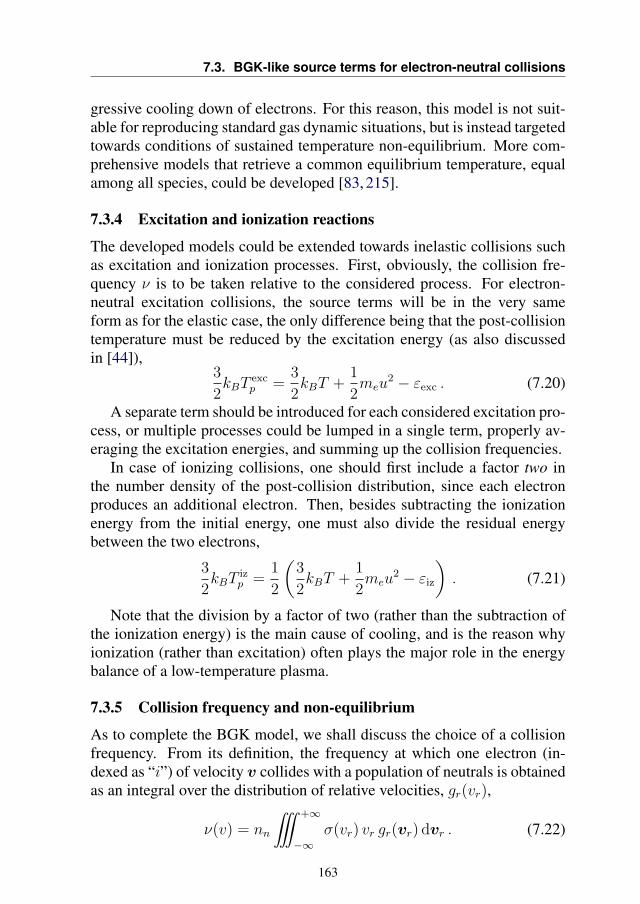
7.3. BGK-like source terms for electron-neutral collisions
gressive cooling down of electrons. For this reason, this model is not suit-able for reproducing standard gas dynamic situations, but is instead targetedtowards conditions of sustained temperature non-equilibrium. More com-prehensive models that retrieve a common equilibrium temperature, equalamong all species, could be developed [83, 215].
7.3.4 Excitation and ionization reactions
The developed models could be extended towards inelastic collisions suchas excitation and ionization processes. First, obviously, the collision fre-quency ν is to be taken relative to the considered process. For electron-neutral excitation collisions, the source terms will be in the very sameform as for the elastic case, the only difference being that the post-collisiontemperature must be reduced by the excitation energy (as also discussedin [44]),
3
2kBT
excp =
3
2kBT +
1
2meu
2 − εexc . (7.20)
A separate term should be introduced for each considered excitation pro-cess, or multiple processes could be lumped in a single term, properly av-eraging the excitation energies, and summing up the collision frequencies.
In case of ionizing collisions, one should first include a factor two inthe number density of the post-collision distribution, since each electronproduces an additional electron. Then, besides subtracting the ionizationenergy from the initial energy, one must also divide the residual energybetween the two electrons,
3
2kBT
izp =
1
2
(3
2kBT +
1
2meu
2 − εiz
). (7.21)
Note that the division by a factor of two (rather than the subtraction ofthe ionization energy) is the main cause of cooling, and is the reason whyionization (rather than excitation) often plays the major role in the energybalance of a low-temperature plasma.
7.3.5 Collision frequency and non-equilibrium
As to complete the BGK model, we shall discuss the choice of a collisionfrequency. From its definition, the frequency at which one electron (in-dexed as “i”) of velocity v collides with a population of neutrals is obtainedas an integral over the distribution of relative velocities, gr(vr),
ν(v) = nn
˚ +∞
−∞σ(vr) vr gr(vr) dvr . (7.22)
163
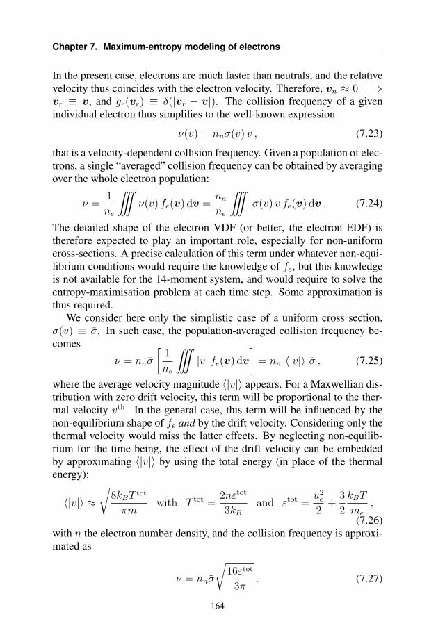
Chapter 7. Maximum-entropy modeling of electrons
In the present case, electrons are much faster than neutrals, and the relativevelocity thus coincides with the electron velocity. Therefore, vn ≈ 0 =⇒vr ≡ v, and gr(vr) ≡ δ(|vr − v|). The collision frequency of a givenindividual electron thus simplifies to the well-known expression
ν(v) = nnσ(v) v , (7.23)
that is a velocity-dependent collision frequency. Given a population of elec-trons, a single “averaged” collision frequency can be obtained by averagingover the whole electron population:
ν =1
ne
˚ν(v) fe(v) dv =
nnne
˚σ(v) v fe(v) dv . (7.24)
The detailed shape of the electron VDF (or better, the electron EDF) istherefore expected to play an important role, especially for non-uniformcross-sections. A precise calculation of this term under whatever non-equi-librium conditions would require the knowledge of fe, but this knowledgeis not available for the 14-moment system, and would require to solve theentropy-maximisation problem at each time step. Some approximation isthus required.
We consider here only the simplistic case of a uniform cross section,σ(v) ≡ σ. In such case, the population-averaged collision frequency be-comes
ν = nnσ
[1
ne
˚|v| fe(v) dv
]= nn 〈|v|〉 σ , (7.25)
where the average velocity magnitude 〈|v|〉 appears. For a Maxwellian dis-tribution with zero drift velocity, this term will be proportional to the ther-mal velocity vth. In the general case, this term will be influenced by thenon-equilibrium shape of fe and by the drift velocity. Considering only thethermal velocity would miss the latter effects. By neglecting non-equilib-rium for the time being, the effect of the drift velocity can be embeddedby approximating 〈|v|〉 by using the total energy (in place of the thermalenergy):
〈|v|〉 ≈√
8kBT tot
πmwith T tot =
2nεtot
3kBand εtot =
u2e
2+
3
2
kBT
me
,
(7.26)with n the electron number density, and the collision frequency is approxi-mated as
ν = nnσ
√16εtot
3π. (7.27)
164
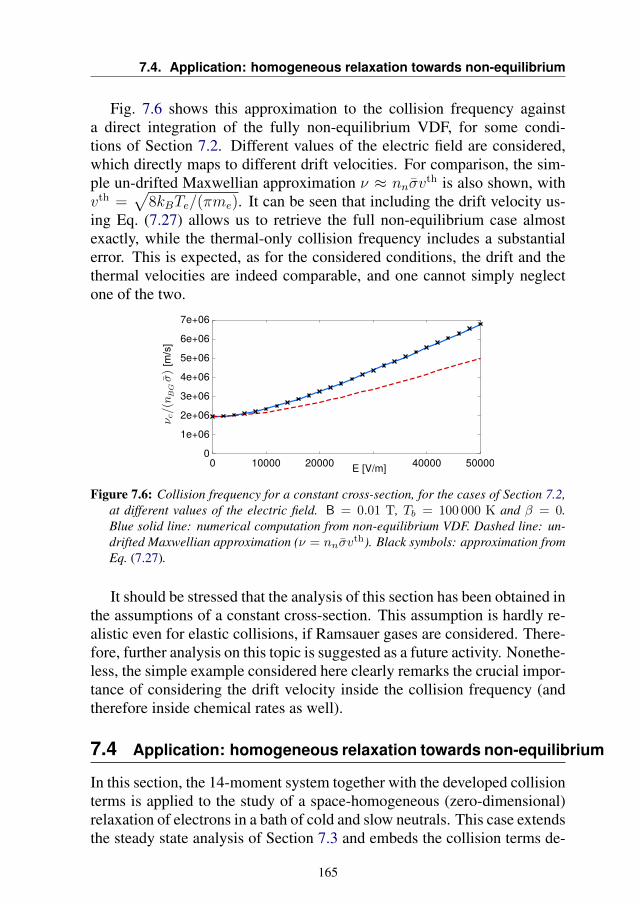
7.4. Application: homogeneous relaxation towards non-equilibrium
Fig. 7.6 shows this approximation to the collision frequency againsta direct integration of the fully non-equilibrium VDF, for some condi-tions of Section 7.2. Different values of the electric field are considered,which directly maps to different drift velocities. For comparison, the sim-ple un-drifted Maxwellian approximation ν ≈ nnσv
th is also shown, withvth =
√8kBTe/(πme). It can be seen that including the drift velocity us-
ing Eq. (7.27) allows us to retrieve the full non-equilibrium case almostexactly, while the thermal-only collision frequency includes a substantialerror. This is expected, as for the considered conditions, the drift and thethermal velocities are indeed comparable, and one cannot simply neglectone of the two.
Figure 7.6: Collision frequency for a constant cross-section, for the cases of Section 7.2,at different values of the electric field. B = 0.01 T, Tb = 100 000 K and β = 0.Blue solid line: numerical computation from non-equilibrium VDF. Dashed line: un-drifted Maxwellian approximation (ν = nnσv
th). Black symbols: approximation fromEq. (7.27).
It should be stressed that the analysis of this section has been obtained inthe assumptions of a constant cross-section. This assumption is hardly re-alistic even for elastic collisions, if Ramsauer gases are considered. There-fore, further analysis on this topic is suggested as a future activity. Nonethe-less, the simple example considered here clearly remarks the crucial impor-tance of considering the drift velocity inside the collision frequency (andtherefore inside chemical rates as well).
7.4 Application: homogeneous relaxation towards non-equilibrium
In this section, the 14-moment system together with the developed collisionterms is applied to the study of a space-homogeneous (zero-dimensional)relaxation of electrons in a bath of cold and slow neutrals. This case extendsthe steady state analysis of Section 7.3 and embeds the collision terms de-
165
Chapter 7. Maximum-entropy modeling of electrons
veloped in the previous section. The results of this section are propaedeuticto 1-dimensional applications, that will be considered in the next section.
Electrons are initialized from a drifted Gaussian distribution (anisotropicMaxwellian),fe,0 = A exp
[− m
2kB
(v2xT0x
+ (vy−u0y)2
T0y+ v2z
T0z
)],
A = n0
(m
2πkB
)3/2 (1
T0xT0yT0z
)1/2
,(7.28)
with initial density n0 = 1017 m−3, initial velocity u0y = 30 000 m/s andtemperatures T0x = 10 000, T0y = 20 000 and T0z = 5000 K. Electric andmagnetic field are enabled at time t = 0 s and have a constant value ofE = 20 000 z V/m and B = 0.02 x T. Electric quantities are chosen tobe somehow representative of Hall thrusters, and thermodynamic quantitiesare initialized as to present some degree of anisotropy, in order to stress themodel. On a physical standpoint, this problem is characterized by at leastthree time scales:
1. At the time scales of the cyclotron frequency, electrons spiral alongmagnetic field lines. This will be associated to oscillations in the mo-ments, as the initial anisotropy is transferred between the directionsperpendicular to the magnetic field;
2. At the collision frequency, the VDF tends to relax toward a somehowisotropic distribution and the electron average velocity adapts to thevelocity of the neutral background (zero in this case);
3. At a time scale that depends on both the collision frequency and themass ratio, the temperature of electrons tends to equilibrate with thebackground temperature.
Notice that a number of other scales are typically present in low-temperatureplasmas. The plasma oscillations for example have not been accounted for(since the electric field is being imposed), as well as all time scales asso-ciated to inelastic collision processes. Given the large mass disparity, theenergy relaxation time scale (the third one in the list) happens to be almostdecoupled from the first two. Moreover, if the ultimate equilibrium tem-perature is required, including ionization and excitation reactions becomenecessary. Neglecting them would result in an unphysically large heatingdue to the lack of energy absorption mechanisms.
In this section, we consider a simpler toy model: the collision operator isapproximated by the BGK-like model of Section 7.3, and the post-collision
166
7.4. Application: homogeneous relaxation towards non-equilibrium
temperature is not taken from the electron energy during the simulation,but is instead imposed to the value Tp = 10 000 K. The collision frequencyis also imposed, equal to a fraction of the cyclotron frequency, such thatβ = ν/ωc = 0.3. These two assumptions are a strong simplification, butallow us to get rid of the longer time scale associated to energy relaxation.Using the simple Maxwellian relaxation model, the kinetic equation reads
∂f
∂t+qE
m
∂f
∂vz+qB
m
[vz∂f
∂vy− vy
∂f
∂vz
]= −β ωc [f −M(Tp)] . (7.29)
This problem is solved using a PIC method, to obtain a reference kineticsolution. The time step for such simulation was taken as ∆t = 1/(100ν)and 107 particles were simulated. BGK collisions are implemented in asimple stochastic way: for every simulated particle, the collision probabil-ity is computed as Pc = 1− exp(−ν ∆t); a random numberR is computedat every time step for each particle, and if R < Pc, a collision is per-formed by resetting the particle velocities to random values sampled froma Maxwellian at Tp. Note that the same procedure could be followed forimplementing the isotropic BGK-like collision operator of Section 7.3.2,the only difference being that in place of sampling the new velocity from aMaxwellian, one should rotate randomly the velocity vector without chang-ing its magnitude. With the considered time step and number of particles,the kinetic solution requires a few hours on a 32 cores machine. As ex-pected, an analysis of the VDF shows a complete overlap to the analyticalVDFs of Shagayda [44], once steady state is reached.
The solution of the 14-moment system is then computed by solving theset of Eqs. (7.4) with source terms from Eq. (7.9), using the same initialconditions. Being zero-dimensional, the 14-moment system reduces to asystem of ODEs, and is conveniently integrated using an adaptive Runge-Kutta algorithm for instance. The computation takes only a few seconds ofwall time.
A comparison of the two methods is shown in Fig. 7.7. The left col-umn shows some of the moments that are present in the state vector of the14-moment closure. After an initial oscillation at the time scale of the cy-clotron frequency, the solution appears to settle to an equilibrium after acomparable (actually, slightly longer) time has passed. This was expected,given the choice of β = 0.3. Also, the average velocity component uz (par-allel to the electric field) is seen to settle on the value given by the classicalmobility of Eq. (7.3), uz ≈ 2.7 × 10⁵ m/s. The uy velocity (in the E × Bdirection) is essentially equal to the value E/B = 106 m/s.
It is important to notice that, since the problem is zero-dimensional,
167
Chapter 7. Maximum-entropy modeling of electrons
no space fluxes are present, and the solution is totally independent fromclosing fluxes. Therefore, for zero-dimensional problems, the 14-momentsolution is exact. This is indeed seen in Fig. 7.7-Left, where all momentsmatch the kinetic solution to numerical precision.
Anyway, the closing moments have also been calculated alongside therelaxation, for the sake of a comparison with the kinetic scheme. Closingmoments are obtained using the iterative solution to the entropy-maximisationproblem. The interpolative closure of McDonald & Torrilhon [67] resultedin analogous closing moments. These moments are shown in Fig. 7.7-Right. Closing moments from the maximum-entropy approximation appearto reproduce very closely the kinetic moments, and some discrepancies areobserved mainly for the heat flux tensor Qijk terms. This could result fromthe fact that bothRijkk and Sijjkk contain some contractions over the veloc-ity components, that could mitigate some error. However, it is important toremark that an analysis of the closing moments in dimensionless form (su-perscript ?) shows that R?
ijkk and S?ijjkk roughly have the same importance,while the Q?
ijk terms are about 10 times smaller (and thus less important).The test case thus confirms the quality of the 14-moment description, forthe conditions considered here.
7.5 Application: a one-dimensional test case
As a final application for the 14-moment system, we consider a 1D simu-lation of electrons flowing along a longitudinal electric field and through aperpendicular magnetic field. An electron-emitting cathode at a potentialφc = 0 V is located at the right extreme of the domain, and the left bound-ary is assumed to be an anode at φa = 300 V. The distance between anodeand cathode is L = 0.1 m and such axis is denoted by x. Axes y and z arenot simulated, and we thus assume symmetry in such directions. Still, theof having a non-zero velocity in such directions (driven by the magneticfield) is retained, as the equations for the respective quantities are solvedanyway.
The electron density is assumed small enough as to give negligible space-charge effects. The potential distribution is therefore linear, and the electricfield is constant. In particular, in the simulations we do not solve the Pois-son equation, but instead impose an electric field E = (φa − φc)/L =3000 V/m along x. This quantity is lower than the typical values found inHall thrusters by roughly a factor 10. This comes from having neglectedspace-charge, that cumulate due to the magnetic confinement. As to re-store a partial similarity with Hall thrusters, the amplitude of the imposed
168
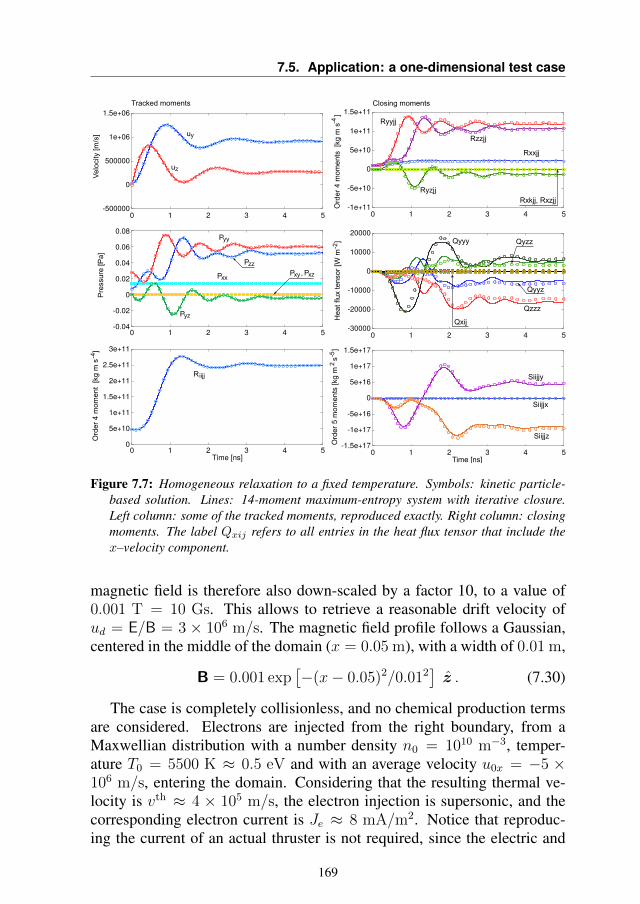
7.5. Application: a one-dimensional test case
Figure 7.7: Homogeneous relaxation to a fixed temperature. Symbols: kinetic particle-based solution. Lines: 14-moment maximum-entropy system with iterative closure.Left column: some of the tracked moments, reproduced exactly. Right column: closingmoments. The label Qxij refers to all entries in the heat flux tensor that include thex–velocity component.
magnetic field is therefore also down-scaled by a factor 10, to a value of0.001 T = 10 Gs. This allows to retrieve a reasonable drift velocity ofud = E/B = 3 × 10⁶ m/s. The magnetic field profile follows a Gaussian,centered in the middle of the domain (x = 0.05 m), with a width of 0.01 m,
B = 0.001 exp[−(x− 0.05)2/0.012
]z . (7.30)
The case is completely collisionless, and no chemical production termsare considered. Electrons are injected from the right boundary, from aMaxwellian distribution with a number density n0 = 1010 m−3, temper-ature T0 = 5500 K ≈ 0.5 eV and with an average velocity u0x = −5 ×10⁶ m/s, entering the domain. Considering that the resulting thermal ve-locity is vth ≈ 4 × 10⁵ m/s, the electron injection is supersonic, and thecorresponding electron current is Je ≈ 8 mA/m2. Notice that reproduc-ing the current of an actual thruster is not required, since the electric and
169
Chapter 7. Maximum-entropy modeling of electrons
magnetic fields are here imposed.
Numerical solution
This problem is solved by (i) a kinetic PIC scheme, (ii) the 14-momentmaximum-entropy and (iii) the Euler systems. In the kinetic simulation,all particles crossing both the left and right boundaries are removed fromthe domain, and particles are injected from the right boundary by sam-pling a drifted Maxwellian. To reproduce the same conditions in the fluidsimulation, the state in the left ghost cell consists in a low density of nL =105 m−3, and negative velocity of uLx = −5×10⁷ m/s, as to induce a super-sonic flux towards the left. The remaining conditions are uLy = uLz = 0 m/s
and equilibrium conditions at a temperature TL = 5500 K, PLij = Pδij ,
qLi = 0, and RLiijj = 15P 2/ρ. The conditions in the right ghost cells are at
equilibrium, with the aforementioned values for the cathode injection. Forthe initial condition, an empty domain is used for the kinetic simulation. Inthe fluid simulations, a small density n0 = 105 m−3 is employed, with azero average velocity ux0 = uy0 = 0 m/s and T0 = 5500 K.
A Boris time integration scheme is used in the particle simulations. Thefluid systems are solved using a second order Midpoint Euler explicit timeintegration scheme, marching until convergence. A space discretizationof 1000 cells is employed, with Rusanov fluxes and second order spaceaccuracy is achieved with van Leer’s MUSCL scheme, with symmetric vanAlbada limiter.
The computational cost of the Euler simulation was approximately 2minutes on a single-core machine, while the 14-moment approximation re-quired roughly 10 minutes. The kinetic solution on the other hand requiredaround 1 hour on a 16-cores machine, as to converge the simulation andreduce the statistical error to an acceptable value.
Results
The results of the numerical simulations are shown in Fig.7.8.Once injected from the cathode with initial velocity ux0 = 5× 10⁶ m/s,
electrons are accelerated by the electric field towards the anode, at x = 0 m.The magnetic field acts as a barrier and converts part of the momentum intothe y direction, generating a drift velocity uy ≈ 3× 10⁶ m/s, as mentionedpreviously. After the electrons have passed the magnetic field region, thereis no mechanism to restore the value of uy, that therefore remains constant.The density profile is affected by the magnetic field, that concentrate some
170
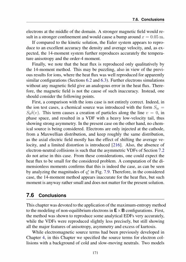
7.6. Conclusions
electrons at the middle of the domain. A stronger magnetic field would re-sult in a stronger confinement and would cause a bump around x = 0.05 m.
If compared to the kinetic solution, the Euler system appears to repro-duce to an excellent accuracy the density and average velocity, and, as ex-pected, the 14-moment system further reproduces accurately the tempera-ture anisotropy and the order-4 moment.
Finally, we note that the heat flux is reproduced only qualitatively bythe 14-moment method. This may be puzzling, also in view of the previ-ous results for ions, where the heat flux was well reproduced for apparentlysimilar configurations (Sections 6.2 and 6.3). Further electrons simulationswithout any magnetic field give an analogous error in the heat flux. There-fore, the magnetic field is not the cause of such inaccuracy. Instead, oneshould consider the following points.
First, a comparison with the ions case is not entirely correct. Indeed, inthe ion test cases, a chemical source was introduced with the form Siz =S0δ(v). This term causes a creation of particles along the line v = 0, inphase space, and resulted in a VDF with a heavy low-velocity tail, thusshowing strong asymmetry. In the present case on the other hand, no chem-ical source is being considered. Electrons are only injected at the cathode,from a Maxwellian distribution, and keep roughly the same distribution,as the axial electric field mostly has the effect of shifting the average ve-locity, and a limited distortion is introduced [216]. Also, the absence ofelectron-neutral collisions is such that the asymmetric VDFs of Section 7.2do not arise in this case. From these considerations, one could expect theheat flux to be small for the considered problem. A computation of the di-mensionless moments confirms that this is indeed the case, as can be seenby analyzing the magnitudes of q?i in Fig. 7.9. Therefore, in the consideredcase, the 14-moment method appears inaccurate for the heat flux, but suchmoment is anyway rather small and does not matter for the present solution.
7.6 Conclusions
This chapter was devoted to the application of the maximum-entropy methodto the modeling of non-equilibrium electrons in E×B configurations. First,the method was shown to reproduce some analytical EDFs very accurately,while the VDFs were reproduced slightly less precisely, but still showingall the major features of anisotropy, asymmetry and excess of kurtosis.
While electromagnetic source terms had been previously developed inChapter 4, in this Chapter we specified the source terms for electron col-lisions with a background of cold and slow-moving neutrals. Two models
171
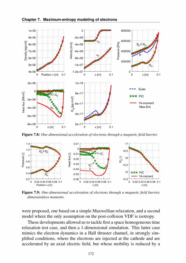
Chapter 7. Maximum-entropy modeling of electrons
Figure 7.8: One-dimensional acceleration of electrons through a magnetic field barrier.
Figure 7.9: One-dimensional acceleration of electrons through a magnetic field barrier,dimensionless moments.
were proposed, one based on a simple Maxwellian relaxation, and a secondmodel where the only assumption on the post-collision VDF is isotropy.
These developments allowed us to tackle first a space homogeneous timerelaxation test case, and then a 1-dimensional simulation. This latter casemimics the electron dynamics in a Hall thruster channel, in strongly sim-plified conditions, where the electrons are injected at the cathode and areaccelerated by an axial electric field, but whose mobility is reduced by a
172

7.6. Conclusions
perpendicular magnetic field.With this chapter, we conclude the part of this work related to maximum-
entropy modeling. Among the future developments, together with attempt-ing a coupling with ions (and thus solving the full self-consistent problem),it will be necessary to develop chemical source terms for electron-neutralcollisions, that take into account non-equilibrium conditions without re-quiring to solve the entropy-maximisation problem at each time step.
173

CHAPTER8DSMC and TPMC analysis of the neutral
gas injection:an alternative gas feed configuration
The content of this chapter is also discussed in [217]: Boccelli, S.,Magin, T.E., Frezzotti, A., Numerical investigation of reversed gas feedconfigurations for Hall thrusters, under review.
In the previous chapters, we have investigated the non-equilibrium regimethat characterizes ions and electrons. So far, neutrals were always treatedas a fixed background of cold and slow-moving particles.
In this chapter, we shift the attention on the neutral population, and in-vestigate their dynamics from the injection to their expansion into the vac-uum. The rarefaction degree will be seen to be high enough to require akinetic modeling, as the Knudsen numbers approach unity. No fluid mod-eling will be attempted in this chapter, but we will focus instead on thediscussion of the effect of different injection configurations. The typical in-jection strategy consists in placing the gas feed at the anode, located at theclosed end of the thruster channel. This setup will be here analyzed numer-ically, and an alternative feed configuration will then be proposed, where
175
Chapter 8. DSMC and TPMC analysis of the neutral gas injection:an alternative gas feed configuration
the propellant is injected backwards from a slit located near the exit plane.As will be discussed, different injection configurations are likely to result inquite different thruster efficiencies. In particular, the ionization efficiencycan be estimated from the distribution of (and the average) residence timesof neutral particles, inside the ionization region. The proposed reversedinjection strategy causes an increased residence time, and this ultimatelyaffects the thruster mass utilization efficiency.
This chapter is structured as follows. After some preliminary consid-erations about the degree of rarefaction and the mass utilization efficiency,drawn in Section 8.1, a simplified analysis is proposed in Section 8.2, wherethe ionization probabilities and an estimate of the thruster efficiency areconsidered for a simplistic case that neglects all gas-phase collisions, andemploys a specular wall scattering kernel. All simplifying assumptions arethen relaxed in Section 8.3, where DSMC simulations are performed forthe SPT-100 thruster geometry, including gas-phase collisions and assum-ing diffusive wall interactions. A test-particle Monte Carlo algorithm isthen introduced in Section 8.4, and is employed in Section 8.5 to obtain thedistribution of residence times of neutral particles inside the thruster chan-nel and inside a region that we arbitrarily identify as the ionization region.From such results, the efficiency of the reversed injection is analyzed andcompared to the direct injection strategy in Section 8.5.3, and maps of theimproved efficiency are given.
Only neutrals are considered in this chapter, and the interaction withelectrons and ions is completely disregarded, apart from an increased tem-perature of the anode: two cases are considered, a cold anode at 300 K anda warm anode at 1000 K.
8.1 Preliminary considerations
The neutral flow is characterized by rather large Knudsen numbers, Kn =λ/Ltc, where λ is the mean free path and Ltc is a characteristic dimensionof the thruster channel, such as its width or length. The propellant flowmay be initially transitional at the injection point, but soon increases toKn ≈ 1 during the expansion into the channel, and eventually reaches thefree molecular regime Kn 1 in the plume. In this work, we will considerthe SPT-100 geometry [89], where “100” stands for the diameter of theouter wall in millimeters, and the inner diameter is 70 mm. As will beseen in the next sections, Kn roughly ranges between Kn ≈ 0.1 − 1 forsuch configuration. The neutrals analysis should therefore be tackled withkinetic methods, such as the Direct Simulation Monte Carlo (DSMC) and
176
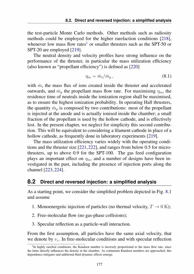
8.2. Direct and reversed injection: a simplified analysis
the test-particle Monte Carlo methods. Other methods such as radiositymethods could be employed for the higher rarefaction conditions [218],whenever low mass flow rates1 or smaller thrusters such as the SPT-50 orSPT-20 are employed [219].
The neutral density and velocity profiles have strong influence on theperformance of the thruster, in particular the mass utilization efficiency(also known as “propellant efficiency”) is defined as [220]
ηm = mi/mp , (8.1)
with mi the mass flux of ions created inside the thruster and acceleratedoutwards, and mp the propellant mass flow rate. For maximising ηm, theresidence time of neutrals inside the ionization region shall be maximised,as to ensure the highest ionization probability. In operating Hall thrusters,the quantity mp is composed by two contributions: most of the propellantis injected at the anode and is actually ionised inside the chamber; a smallfraction of the propellant is used by the hollow cathode, and is effectivelylost. In the present chapter, we neglect for simplicity this second contribu-tion. This will be equivalent to considering a filament cathode in place of ahollow cathode, as frequently done in laboratory experiments [219].
The mass utilization efficiency varies widely with the operating condi-tions and the thruster size [221,222], and ranges from below 0.5 for micro-thrusters, up to above 0.9 for the SPT-100. The gas feed configurationplays an important effect on ηm, and a number of designs have been in-vestigated in the past, including the presence of injection ports along thechannel [223, 224].
8.2 Direct and reversed injection: a simplified analysis
As a starting point, we consider the simplified problem depicted in Fig. 8.1and assume
1. Monoenergetic injection of particles (no thermal velocity, T → 0 K);
2. Free-molecular flow (no gas-phase collisions);
3. Specular reflection as a particle-wall interaction.
From the first assumption, all particles have the same axial velocity, thatwe denote by vz. In free-molecular conditions and with specular reflection
1In highly rarefied conditions, the Knudsen number is inversely proportional to the mass flow rate, sincethe latter directly influences the density in the chamber. As continuum Knudsen numbers are approached, thisdependence mitigates and additional fluid dynamic effects emerge.
177
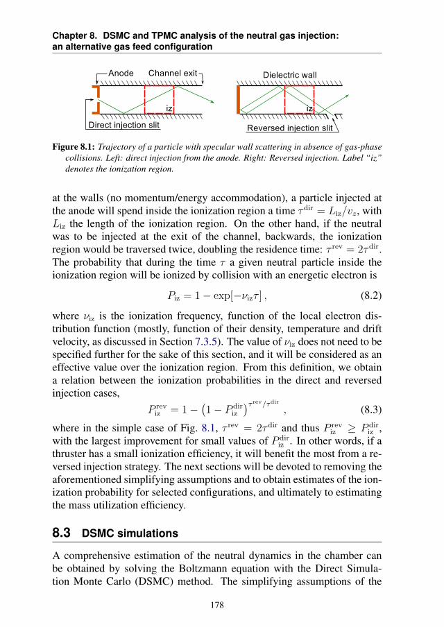
Chapter 8. DSMC and TPMC analysis of the neutral gas injection:an alternative gas feed configuration
Figure 8.1: Trajectory of a particle with specular wall scattering in absence of gas-phasecollisions. Left: direct injection from the anode. Right: Reversed injection. Label “iz”denotes the ionization region.
at the walls (no momentum/energy accommodation), a particle injected atthe anode will spend inside the ionization region a time τdir = Liz/vz, withLiz the length of the ionization region. On the other hand, if the neutralwas to be injected at the exit of the channel, backwards, the ionizationregion would be traversed twice, doubling the residence time: τ rev = 2τdir.The probability that during the time τ a given neutral particle inside theionization region will be ionized by collision with an energetic electron is
Piz = 1− exp[−νizτ ] , (8.2)
where νiz is the ionization frequency, function of the local electron dis-tribution function (mostly, function of their density, temperature and driftvelocity, as discussed in Section 7.3.5). The value of νiz does not need to bespecified further for the sake of this section, and it will be considered as aneffective value over the ionization region. From this definition, we obtaina relation between the ionization probabilities in the direct and reversedinjection cases,
P reviz = 1−
(1− P dir
iz
)τ rev/τdir, (8.3)
where in the simple case of Fig. 8.1, τ rev = 2τdir and thus P reviz ≥ P dir
iz ,with the largest improvement for small values of P dir
iz . In other words, if athruster has a small ionization efficiency, it will benefit the most from a re-versed injection strategy. The next sections will be devoted to removing theaforementioned simplifying assumptions and to obtain estimates of the ion-ization probability for selected configurations, and ultimately to estimatingthe mass utilization efficiency.
8.3 DSMC simulations
A comprehensive estimation of the neutral dynamics in the chamber canbe obtained by solving the Boltzmann equation with the Direct Simula-tion Monte Carlo (DSMC) method. The simplifying assumptions of the
178
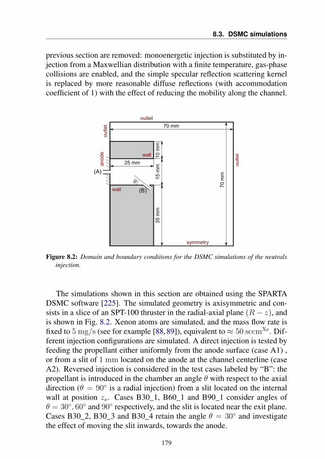
8.3. DSMC simulations
previous section are removed: monoenergetic injection is substituted by in-jection from a Maxwellian distribution with a finite temperature, gas-phasecollisions are enabled, and the simple specular reflection scattering kernelis replaced by more reasonable diffuse reflections (with accommodationcoefficient of 1) with the effect of reducing the mobility along the channel.
Figure 8.2: Domain and boundary conditions for the DSMC simulations of the neutralsinjection.
The simulations shown in this section are obtained using the SPARTADSMC software [225]. The simulated geometry is axisymmetric and con-sists in a slice of an SPT-100 thruster in the radial-axial plane (R− z), andis shown in Fig. 8.2. Xenon atoms are simulated, and the mass flow rate isfixed to 5 mg/s (see for example [88,89]), equivalent to≈ 50 sccmXe. Dif-ferent injection configurations are simulated. A direct injection is tested byfeeding the propellant either uniformly from the anode surface (case A1) ,or from a slit of 1 mm located on the anode at the channel centerline (caseA2). Reversed injection is considered in the test cases labeled by “B”: thepropellant is introduced in the chamber an angle θ with respect to the axialdirection (θ = 90 is a radial injection) from a slit located on the internalwall at position zs. Cases B30_1, B60_1 and B90_1 consider angles ofθ = 30, 60 and 90 respectively, and the slit is located near the exit plane.Cases B30_2, B30_3 and B30_4 retain the angle θ = 30 and investigatethe effect of moving the slit inwards, towards the anode.
179
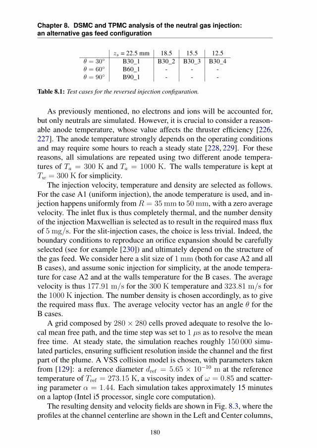
Chapter 8. DSMC and TPMC analysis of the neutral gas injection:an alternative gas feed configuration
zs = 22.5 mm 18.5 15.5 12.5θ = 30 B30_1 B30_2 B30_3 B30_4θ = 60 B60_1 - - -θ = 90 B90_1 - - -
Table 8.1: Test cases for the reversed injection configuration.
As previously mentioned, no electrons and ions will be accounted for,but only neutrals are simulated. However, it is crucial to consider a reason-able anode temperature, whose value affects the thruster efficiency [226,227]. The anode temperature strongly depends on the operating conditionsand may require some hours to reach a steady state [228, 229]. For thesereasons, all simulations are repeated using two different anode tempera-tures of Ta = 300 K and Ta = 1000 K. The walls temperature is kept atTw = 300 K for simplicity.
The injection velocity, temperature and density are selected as follows.For the case A1 (uniform injection), the anode temperature is used, and in-jection happens uniformly fromR = 35 mm to 50 mm, with a zero averagevelocity. The inlet flux is thus completely thermal, and the number densityof the injection Maxwellian is selected as to result in the required mass fluxof 5 mg/s. For the slit-injection cases, the choice is less trivial. Indeed, theboundary conditions to reproduce an orifice expansion should be carefullyselected (see for example [230]) and ultimately depend on the structure ofthe gas feed. We consider here a slit size of 1 mm (both for case A2 and allB cases), and assume sonic injection for simplicity, at the anode tempera-ture for case A2 and at the walls temperature for the B cases. The averagevelocity is thus 177.91 m/s for the 300 K temperature and 323.81 m/s forthe 1000 K injection. The number density is chosen accordingly, as to givethe required mass flux. The average velocity vector has an angle θ for theB cases.
A grid composed by 280 × 280 cells proved adequate to resolve the lo-cal mean free path, and the time step was set to 1 µs as to resolve the meanfree time. At steady state, the simulation reaches roughly 150 000 simu-lated particles, ensuring sufficient resolution inside the channel and the firstpart of the plume. A VSS collision model is chosen, with parameters takenfrom [129]: a reference diameter dref = 5.65 × 10⁻¹⁰ m at the referencetemperature of Tref = 273.15 K, a viscosity index of ω = 0.85 and scatter-ing parameter α = 1.44. Each simulation takes approximately 15 minuteson a laptop (Intel i5 processor, single core computation).
The resulting density and velocity fields are shown in Fig. 8.3, where theprofiles at the channel centerline are shown in the Left and Center columns,
180
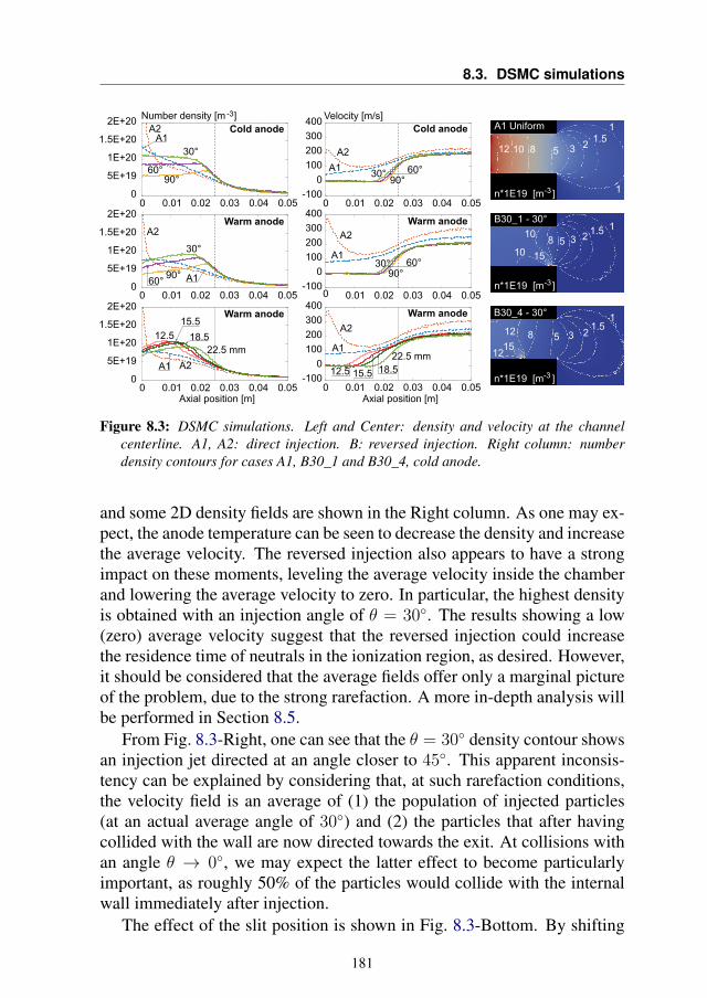
8.3. DSMC simulations
Figure 8.3: DSMC simulations. Left and Center: density and velocity at the channelcenterline. A1, A2: direct injection. B: reversed injection. Right column: numberdensity contours for cases A1, B30_1 and B30_4, cold anode.
and some 2D density fields are shown in the Right column. As one may ex-pect, the anode temperature can be seen to decrease the density and increasethe average velocity. The reversed injection also appears to have a strongimpact on these moments, leveling the average velocity inside the chamberand lowering the average velocity to zero. In particular, the highest densityis obtained with an injection angle of θ = 30. The results showing a low(zero) average velocity suggest that the reversed injection could increasethe residence time of neutrals in the ionization region, as desired. However,it should be considered that the average fields offer only a marginal pictureof the problem, due to the strong rarefaction. A more in-depth analysis willbe performed in Section 8.5.
From Fig. 8.3-Right, one can see that the θ = 30 density contour showsan injection jet directed at an angle closer to 45. This apparent inconsis-tency can be explained by considering that, at such rarefaction conditions,the velocity field is an average of (1) the population of injected particles(at an actual average angle of 30) and (2) the particles that after havingcollided with the wall are now directed towards the exit. At collisions withan angle θ → 0, we may expect the latter effect to become particularlyimportant, as roughly 50% of the particles would collide with the internalwall immediately after injection.
The effect of the slit position is shown in Fig. 8.3-Bottom. By shifting
181
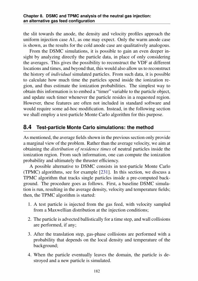
Chapter 8. DSMC and TPMC analysis of the neutral gas injection:an alternative gas feed configuration
the slit towards the anode, the density and velocity profiles approach theuniform injection case A1, as one may expect. Only the warm anode caseis shown, as the results for the cold anode case are qualitatively analogous.
From the DSMC simulations, it is possible to gain an even deeper in-sight by analyzing directly the particle data, in place of only consideringthe averages. This gives the possibility to reconstruct the VDF at differentlocations and times, and beyond that, this would also allow us to reconstructthe history of individual simulated particles. From such data, it is possibleto calculate how much time the particles spend inside the ionization re-gion, and thus estimate the ionization probabilities. The simplest way toobtain this information is to embed a “timer” variable to the particle object,and update such timer whenever the particle resides in a requested region.However, these features are often not included in standard software andwould require some ad-hoc modification. Instead, in the following sectionwe shall employ a test-particle Monte Carlo algorithm for this purpose.
8.4 Test-particle Monte Carlo simulations: the method
As mentioned, the average fields shown in the previous section only providea marginal view of the problem. Rather than the average velocity, we aim atobtaining the distribution of residence times of neutral particles inside theionization region. From such information, one can compute the ionizationprobability and ultimately the thruster efficiency.
A possible alternative to DSMC consists in test-particle Monte Carlo(TPMC) algorithms, see for example [231]. In this section, we discuss aTPMC algorithm that tracks single particles inside a pre-computed back-ground. The procedure goes as follows. First, a baseline DSMC simula-tion is run, resulting in the average density, velocity and temperature fields;then, the TPMC algorithm is started:
1. A test particle is injected from the gas feed, with velocity sampledfrom a Maxwellian distribution at the injection conditions;
2. The particle is advected ballistically for a time step, and wall collisionsare performed, if any;
3. After the translation step, gas-phase collisions are performed with aprobability that depends on the local density and temperature of thebackground;
4. When the particle eventually leaves the domain, the particle is de-stroyed and a new particle is simulated.
182
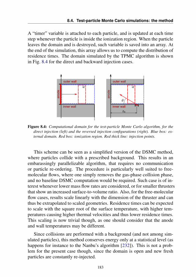
8.4. Test-particle Monte Carlo simulations: the method
A “timer” variable is attached to each particle, and is updated at each timestep whenever the particle is inside the ionization region. When the particleleaves the domain and is destroyed, such variable is saved into an array. Atthe end of the simulation, this array allows us to compute the distribution ofresidence times. The domain simulated by the TPMC algorithm is shownin Fig. 8.4 for the direct and backward injection cases.
Figure 8.4: Computational domain for the test-particle Monte Carlo algorithm, for thedirect injection (left) and the reversed injection configurations (right). Blue box: ex-ternal domain. Red box: ionization region. Red thick line: injection points.
This scheme can be seen as a simplified version of the DSMC method,where particles collide with a prescribed background. This results in anembarassingly parallelizable algorithm, that requires no communicationor particle re-ordering. The procedure is particularly well suited to free-molecular flows, where one simply removes the gas-phase collision phase,and no baseline DSMC computation would be required. Such case is of in-terest whenever lower mass flow rates are considered, or for smaller thrustersthat show an increased surface-to-volume ratio. Also, for the free-molecularflow cases, results scale linearly with the dimension of the thruster and canthus be extrapolated to scaled geometries. Residence times can be expectedto scale with the square root of the surface temperature, with higher tem-peratures causing higher thermal velocities and thus lower residence times.This scaling is now trivial though, as one should consider that the anodeand wall temperatures may be different.
Since collisions are performed with a background (and not among sim-ulated particles), this method conserves energy only at a statistical level (ashappens for instance to the Nanbu’s algorithm [232]). This is not a prob-lem for the present case though, since the domain is open and new freshparticles are constantly re-injected.
183
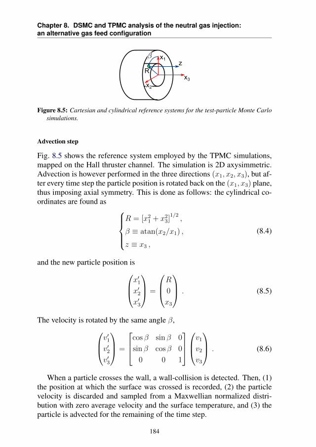
Chapter 8. DSMC and TPMC analysis of the neutral gas injection:an alternative gas feed configuration
Figure 8.5: Cartesian and cylindrical reference systems for the test-particle Monte Carlosimulations.
Advection step
Fig. 8.5 shows the reference system employed by the TPMC simulations,mapped on the Hall thruster channel. The simulation is 2D axysimmetric.Advection is however performed in the three directions (x1, x2, x3), but af-ter every time step the particle position is rotated back on the (x1, x3) plane,thus imposing axial symmetry. This is done as follows: the cylindrical co-ordinates are found as
R = [x21 + x2
3]1/2,
β ≡ atan(x2/x1) ,
z ≡ x3 ,
(8.4)
and the new particle position isx′1
x′2x′3
=
R0x3
. (8.5)
The velocity is rotated by the same angle β,v′1
v′2v′3
=
cos β sin β 0
sin β cos β 0
0 0 1
v1
v2
v3
. (8.6)
When a particle crosses the wall, a wall-collision is detected. Then, (1)the position at which the surface was crossed is recorded, (2) the particlevelocity is discarded and sampled from a Maxwellian normalized distri-bution with zero average velocity and the surface temperature, and (3) theparticle is advected for the remaining of the time step.
184
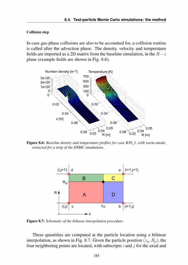
8.4. Test-particle Monte Carlo simulations: the method
Collision step
In case gas-phase collisions are also to be accounted for, a collision routineis called after the advection phase. The density, velocity and temperaturefields are imported as a 2D matrix from the baseline simulation, in theR−zplane (example fields are shown in Fig. 8.6).
Figure 8.6: Baseline density and temperature profiles for case B30_1, with warm anode,extracted for a strip of the DSMC simulations.
Figure 8.7: Schematic of the bilinear interpolation procedure.
These quantities are computed at the particle location using a bilinearinterpolation, as shown in Fig. 8.7. Given the particle position (zp, Rp), thefour neighboring points are located, with subscripts i and j for the axial and
185
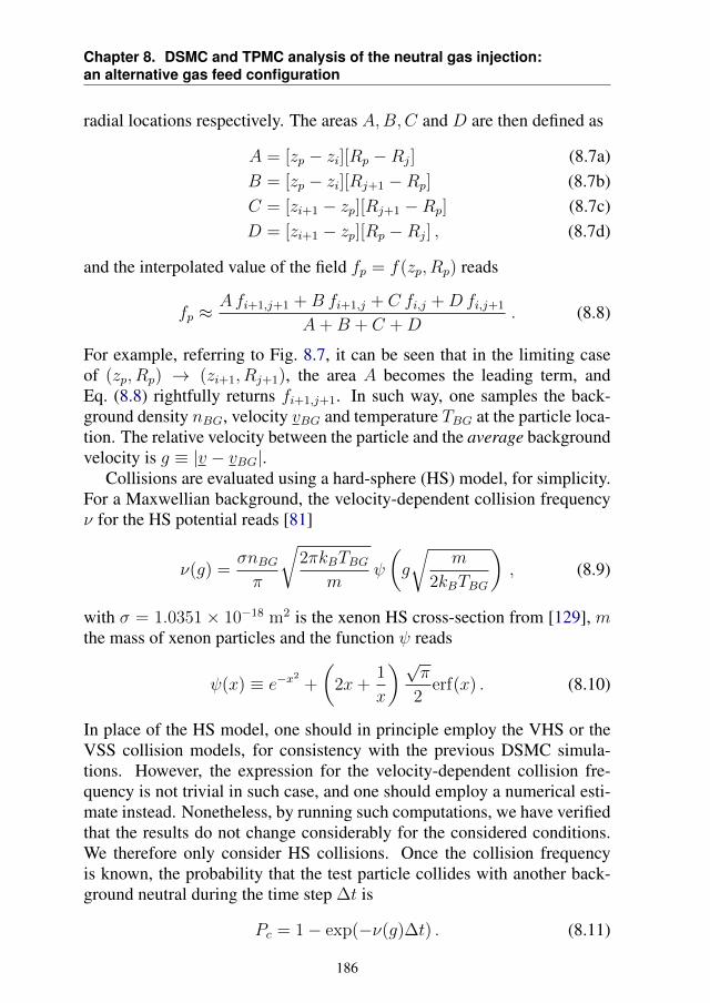
Chapter 8. DSMC and TPMC analysis of the neutral gas injection:an alternative gas feed configuration
radial locations respectively. The areas A,B,C and D are then defined as
A = [zp − zi][Rp −Rj] (8.7a)B = [zp − zi][Rj+1 −Rp] (8.7b)C = [zi+1 − zp][Rj+1 −Rp] (8.7c)D = [zi+1 − zp][Rp −Rj] , (8.7d)
and the interpolated value of the field fp = f(zp, Rp) reads
fp ≈Afi+1,j+1 +B fi+1,j + C fi,j +Dfi,j+1
A+B + C +D. (8.8)
For example, referring to Fig. 8.7, it can be seen that in the limiting caseof (zp, Rp) → (zi+1, Rj+1), the area A becomes the leading term, andEq. (8.8) rightfully returns fi+1,j+1. In such way, one samples the back-ground density nBG, velocity vBG and temperature TBG at the particle loca-tion. The relative velocity between the particle and the average backgroundvelocity is g ≡ |v − vBG|.
Collisions are evaluated using a hard-sphere (HS) model, for simplicity.For a Maxwellian background, the velocity-dependent collision frequencyν for the HS potential reads [81]
ν(g) =σnBGπ
√2πkBTBG
mψ
(g
√m
2kBTBG
), (8.9)
with σ = 1.0351× 10⁻¹⁸ m2 is the xenon HS cross-section from [129], mthe mass of xenon particles and the function ψ reads
ψ(x) ≡ e−x2
+
(2x+
1
x
) √π
2erf(x) . (8.10)
In place of the HS model, one should in principle employ the VHS or theVSS collision models, for consistency with the previous DSMC simula-tions. However, the expression for the velocity-dependent collision fre-quency is not trivial in such case, and one should employ a numerical esti-mate instead. Nonetheless, by running such computations, we have verifiedthat the results do not change considerably for the considered conditions.We therefore only consider HS collisions. Once the collision frequencyis known, the probability that the test particle collides with another back-ground neutral during the time step ∆t is
Pc = 1− exp(−ν(g)∆t) . (8.11)
186
8.5. Test-particle Monte Carlo simulations: results
Notice that the time step must ensure that Pc 1. Not respectingsuch conditions would result in a practical under-estimation of the collisionfrequency. Since ν = ν(g) depends on the velocity of the test particle andalso on the local collisions, one should ensure this condition all along thesimulation. In order to perform a collision, a random number R ∈ (0, 1)is sampled, and the collision is performed if R < Pc. If this is the case, acolliding pair is created by sampling from a Maxwellian distribution at thelocal conditions, and the collision is performed by random rotation of therelative velocity vector [233]. After the collision, the colliding pair particleis discarded.
Numerical implementation
As to exploit the embarrassingly parallelizable nature of the algorithm, aGPGPU version of the TPMC algorithm was implemented in CUDA For-tran and is available at [234] (also see Appendix A). Since all particles areindependent, the parallel implementation allows for an optimal speed-up.Speed-ups of 1600 times were obtained while simulating 106 particles onan NVidia GTX 760 GPU (compute capability 3.0), with respect to a se-rial implementation running on an Intel CORE i5 processor with 12 GB ofRAM. The parallel simulations for 106 particles require just a few seconds.
8.5 Test-particle Monte Carlo simulations: results
The algorithm introduced in the previous section is here applied to the anal-ysis of residence times inside the ionization region. In this section, we as-sume the ionization region is a square block located at x ∈ [13, 18] mm(see [90]), as depicted in Fig. 8.4.
8.5.1 Preliminary analysis in the free-molecular limit
To start, we consider in this section a simplified case that allows us to gainan insight on the dynamics of neutral particles. We assume free-molecularconditions and neglect all gas-phase collisions. The cases A1, A2 and allB cases of Table 8.1 are simulated, for both the cold and warm anode case.In such simulations, the residence time of each neutral particle in the wholechannel is tracked.
The results are shown in Fig. 8.8, where the distribution of logarithmsof residence times is shown, for clarity. The distribution appears rathersimple for the uniform injection case A1. On the other hand, the directinjection from a slit (case A2) shows a bimodal distribution: the low-times
187
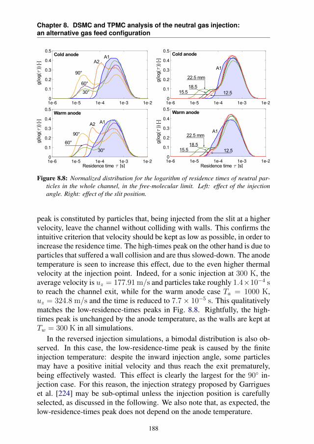
Chapter 8. DSMC and TPMC analysis of the neutral gas injection:an alternative gas feed configuration
Figure 8.8: Normalized distribution for the logarithm of residence times of neutral par-ticles in the whole channel, in the free-molecular limit. Left: effect of the injectionangle. Right: effect of the slit position.
peak is constituted by particles that, being injected from the slit at a highervelocity, leave the channel without colliding with walls. This confirms theintuitive criterion that velocity should be kept as low as possible, in order toincrease the residence time. The high-times peak on the other hand is due toparticles that suffered a wall collision and are thus slowed-down. The anodetemperature is seen to increase this effect, due to the even higher thermalvelocity at the injection point. Indeed, for a sonic injection at 300 K, theaverage velocity is uz = 177.91 m/s and particles take roughly 1.4×10⁻⁴ sto reach the channel exit, while for the warm anode case Ta = 1000 K,uz = 324.8 m/s and the time is reduced to 7.7× 10⁻⁵ s. This qualitativelymatches the low-residence-times peaks in Fig. 8.8. Rightfully, the high-times peak is unchanged by the anode temperature, as the walls are kept atTw = 300 K in all simulations.
In the reversed injection simulations, a bimodal distribution is also ob-served. In this case, the low-residence-time peak is caused by the finiteinjection temperature: despite the inward injection angle, some particlesmay have a positive initial velocity and thus reach the exit prematurely,being effectively wasted. This effect is clearly the largest for the 90 in-jection case. For this reason, the injection strategy proposed by Garrigueset al. [224] may be sub-optimal unless the injection position is carefullyselected, as discussed in the following. We also note that, as expected, thelow-residence-times peak does not depend on the anode temperature.
188
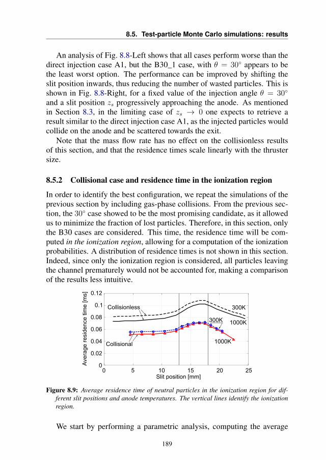
8.5. Test-particle Monte Carlo simulations: results
An analysis of Fig. 8.8-Left shows that all cases perform worse than thedirect injection case A1, but the B30_1 case, with θ = 30 appears to bethe least worst option. The performance can be improved by shifting theslit position inwards, thus reducing the number of wasted particles. This isshown in Fig. 8.8-Right, for a fixed value of the injection angle θ = 30
and a slit position zs progressively approaching the anode. As mentionedin Section 8.3, in the limiting case of zs → 0 one expects to retrieve aresult similar to the direct injection case A1, as the injected particles wouldcollide on the anode and be scattered towards the exit.
Note that the mass flow rate has no effect on the collisionless resultsof this section, and that the residence times scale linearly with the thrustersize.
8.5.2 Collisional case and residence time in the ionization region
In order to identify the best configuration, we repeat the simulations of theprevious section by including gas-phase collisions. From the previous sec-tion, the 30 case showed to be the most promising candidate, as it allowedus to minimize the fraction of lost particles. Therefore, in this section, onlythe B30 cases are considered. This time, the residence time will be com-puted in the ionization region, allowing for a computation of the ionizationprobabilities. A distribution of residence times is not shown in this section.Indeed, since only the ionization region is considered, all particles leavingthe channel prematurely would not be accounted for, making a comparisonof the results less intuitive.
Figure 8.9: Average residence time of neutral particles in the ionization region for dif-ferent slit positions and anode temperatures. The vertical lines identify the ionizationregion.
We start by performing a parametric analysis, computing the average
189
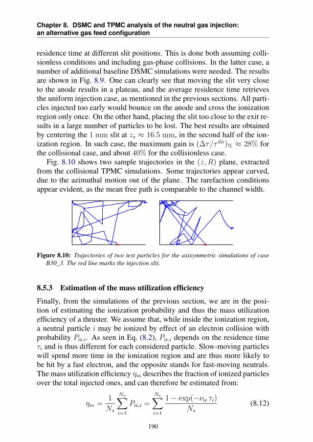
Chapter 8. DSMC and TPMC analysis of the neutral gas injection:an alternative gas feed configuration
residence time at different slit positions. This is done both assuming colli-sionless conditions and including gas-phase collisions. In the latter case, anumber of additional baseline DSMC simulations were needed. The resultsare shown in Fig. 8.9. One can clearly see that moving the slit very closeto the anode results in a plateau, and the average residence time retrievesthe uniform injection case, as mentioned in the previous sections. All parti-cles injected too early would bounce on the anode and cross the ionizationregion only once. On the other hand, placing the slit too close to the exit re-sults in a large number of particles to be lost. The best results are obtainedby centering the 1 mm slit at zs ≈ 16.5 mm, in the second half of the ion-ization region. In such case, the maximum gain is (∆τ/τdir)% ≈ 28% forthe collisional case, and about 40% for the collisionless case.
Fig. 8.10 shows two sample trajectories in the (z,R) plane, extractedfrom the collisional TPMC simulations. Some trajectories appear curved,due to the azimuthal motion out of the plane. The rarefaction conditionsappear evident, as the mean free path is comparable to the channel width.
Figure 8.10: Trajectories of two test particles for the axisymmetric simulations of caseB30_3. The red line marks the injection slit.
8.5.3 Estimation of the mass utilization efficiency
Finally, from the simulations of the previous section, we are in the posi-tion of estimating the ionization probability and thus the mass utilizationefficiency of a thruster. We assume that, while inside the ionization region,a neutral particle i may be ionized by effect of an electron collision withprobability Piz,i. As seen in Eq. (8.2), Piz,i depends on the residence timeτi and is thus different for each considered particle. Slow-moving particleswill spend more time in the ionization region and are thus more likely tobe hit by a fast electron, and the opposite stands for fast-moving neutrals.The mass utilization efficiency ηm describes the fraction of ionized particlesover the total injected ones, and can therefore be estimated from:
ηm =1
Ns
Ns∑i=1
Piz,i =Ns∑i=1
1− exp(−νiz τi)
Ns
(8.12)
190
8.5. Test-particle Monte Carlo simulations: results
whereNs is the total number of simulated particles and∑
i=1,NsPiz,i = Niz,
the number of ionized particles. In the present chapter, electrons are notbeing simulated, and a value of νiz is a priori unknown. However, our aimis not to determine the efficiency of the reversed injection per se, but insteadto determine the efficiency increase with respect to a direct injection case.We therefore employ the following strategy:
1. First, a standard-injection configuration is considered for a given thruster,with direct efficiency ηdir
m . This may be for example ηdirm = 0.95 for
the SPT-100, or lower for smaller thrusters;
2. After running the TPMC algorithm on such configuration, we obtainan array of simulated values τi;
3. We then plug τi and ηdirm into Eq. (8.12) and invert it numerically, re-
sulting into an estimate for νiz. This value represents an average, oranyway an effective value over the ionization region;
4. Finally, a reversed injection configuration is considered: a TPMC sim-ulation is run, and a value of ηrev
m is computed, using the previouslyfound value of νiz.
This strategy allows us to find the efficiency of the reversed configurationas a function of the initial direct-injection efficiency. Note that in the mostgeneral scenario, νdir
iz 6= νreviz , since different neutral profiles have a differ-
ent influence on the electron mobility and thus on their space profile. Also,if the reversed injection would increase the ionization efficiency, more ionswould be produced, resulting in some additional ion-neutral collisionality.Our simplified analysis completely neglects all these phenomena. Nonethe-less, this assumption allows for a simple analysis of the problem and per-mits to easily compute maps of the effectiveness of the reversed injection,without the need of a full (and much more expensive) PIC model of theproblem. Given the tightly coupled nature of the plasma problem and thelarge number of uncertainties involved in the determination of the electronsmobility in Hall thruster channels (such as the wall conductivity and vari-ous types of instabilities), we believe that the present analysis is a valuablepreliminary investigation tool.
Fig. 8.11 shows the maps of the mass utilization efficiency, computedas 100(ηrev
m − ηdirm )/ηdir
m , for an injection at 30 and different slit positions,in the cold and warm anode cases (left and right columns). The collisionalcases (bottom) are obtained for a mass flow rate of m = 5 mg/s. The col-lisionless cases on the other hand are completely independent on the mass
191
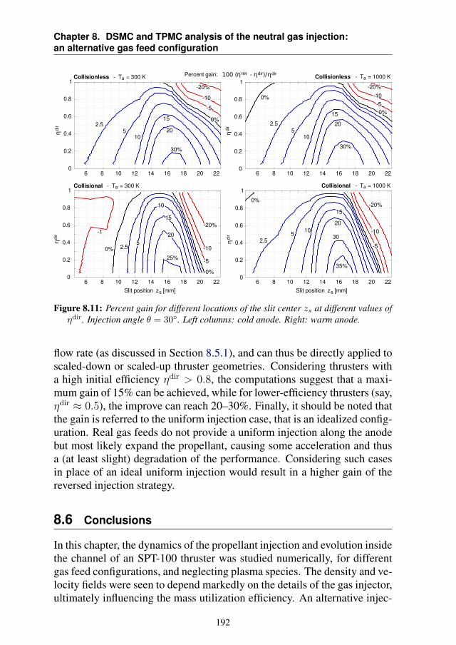
Chapter 8. DSMC and TPMC analysis of the neutral gas injection:an alternative gas feed configuration
Figure 8.11: Percent gain for different locations of the slit center zs at different values ofηdir. Injection angle θ = 30. Left columns: cold anode. Right: warm anode.
flow rate (as discussed in Section 8.5.1), and can thus be directly applied toscaled-down or scaled-up thruster geometries. Considering thrusters witha high initial efficiency ηdir > 0.8, the computations suggest that a maxi-mum gain of 15% can be achieved, while for lower-efficiency thrusters (say,ηdir ≈ 0.5), the improve can reach 20–30%. Finally, it should be noted thatthe gain is referred to the uniform injection case, that is an idealized config-uration. Real gas feeds do not provide a uniform injection along the anodebut most likely expand the propellant, causing some acceleration and thusa (at least slight) degradation of the performance. Considering such casesin place of an ideal uniform injection would result in a higher gain of thereversed injection strategy.
8.6 Conclusions
In this chapter, the dynamics of the propellant injection and evolution insidethe channel of an SPT-100 thruster was studied numerically, for differentgas feed configurations, and neglecting plasma species. The density and ve-locity fields were seen to depend markedly on the details of the gas injector,ultimately influencing the mass utilization efficiency. An alternative injec-
192
8.6. Conclusions
tion strategy was then proposed, where the propellant is injected backwards,from a slit located near the exit plane, and is directed towards the anode.A comparison of the distribution of residence times of neutrals in the ion-ization region, obtained from DSMC and TPMC simulations, showed thatthe proposed reversed-injection configuration could improve the mass uti-lization efficiency from 5–10% up to 20–30%, according to the efficiencyof the baseline thruster.
A number of simplifying assumptions were introduced in this section.Most notably, the analyses are run for a switched-off thruster, neglectingall interaction between neutrals and electrons or ions. The only consideredplasma effect was an increased temperature of the anode. A suggested fu-ture work activity would consist in repeating the simulations including atleast neutral-ion momentum exchange and charge exchange interactions.After verifying the influence of such effects on the final efficiency maps,a next step would be performing a fully coupled simulation, as to retrieveself-consistently the ionization region and electron transport.
193

Conclusions and future work
This work aimed at investigating the modeling of low-temperature plasmasusing moment methods. In particular, Hall thruster plasmas were consid-ered. In such device, ions are collisionless, to a first approximation. Theacceleration is achieved by creating a region of higher electron density,trapping them via a radial magnetic field. The axial electric field, combinedwith the radial magnetic field, makes electrons drift in the E×B direction.Together with the low pressure, all such effects are strong sources of non-equilibrium.
This work investigated kinetic and fluid strategies for modeling these sit-uations, through a selection of simple test cases. In particular, the order-4maximum-entropy moment methods showed an excellent potential for de-scribing the mentioned non-equilibrium, often offering a solution as accu-rate as the kinetic method, but at a lower computational cost, as discussedin the following. The maximum-entropy methods employed in this workare the 14-moment system, together with the 5-moment system, describinga particle with a single translational degree of freedom.
Developing the maximum-entropy method
Applying the maximum-entropy methods required first of all to developsuch systems for profitably dealing with the conditions of ions and elec-trons. In particular, the following results were needed:
• Achieving an affordable computational cost;
• Ensuring a profitable treatment of collisionless conditions;
195
Chapter 8. DSMC and TPMC analysis of the neutral gas injection:an alternative gas feed configuration
• Developing electromagnetic source terms;
• Developing sources for the collisions of warm electrons with cold andslow neutrals.
An affordable computational cost is particularly important in plasmas, wherethe tiny time scales associated to plasma waves, and the refined grids aris-ing from the need to resolve the Debye length, often make the system par-ticularly stiff. In the current state-of-the-art, the 14-moment system is al-ready much more affordable than traditional maximum-entropy formula-tions, thanks to the development of approximated solutions of the entropy-maximisation problem. However, a significant part of the remaining com-putational cost was seen to be the approximation of the system eigenvalues.From the analysis that we performed, traditional approximations for themaximum and minimum wave speeds of the 14-moment system appearedto bring an excessive degree of diffusion when strong non-equilibrium situ-ations are considered. For this reason, part of this work was devoted to thedevelopment of approximated formulas, that allow us to retrieve an accu-rate estimate of the system wave speeds, without the need of numericallycomputing the fluxes Jacobian2 and its eigenvalues at each iteration.
Among the drawbacks of the method, we should certainly cite the com-putational cost. Through the rarefied test cases, it was seen that the methodcan be somewhere between 7 and 100 times more expensive than the Eulerequations (less for continuum conditions, more when strong non-equilib-rium appears). However, these figures of merit were obtained with simpleexplicit time integration strategies, that make the solution completely de-pendent on the system eigenvalues, through the CFL conditions. Amongthe strategies to mitigate this problem, we shall cite for example precondi-tioning [235].
The crossing of the Junk line, in some test cases, requires a carefulselection of the numerical schemes. For continuum conditions, the fre-quently employed HLL fluxes work faultlessly, but in rarefied simulations,they showed to cause strong oscillations, especially in the higher order mo-ments. The Rusanov fluxes appear to introduce sufficient diffusion to solvethe issue, and thus allow us to apply reconstructions (such as in van Leer’sMUSCL scheme) that allow us to reach higher orders in space.
Electric and magnetic source terms were developed for the 5-momentand the 14-moment systems, starting from the generalized moment equa-tion, and were employed for the study of plasma waves. The dispersionrelations showed to retrieve the expected fluid behavior for small values
2It should be recalled that, for the 14-moment system, the Jacobian is a 14× 14 matrix.
196
8.6. Conclusions
of the wave number k, and asymptote to the convective eigenvalues whenkλDe 1. Also, it was noted that some regions of the moment space areassociated so unstable eigenvalues, which may be associated to the pres-ence of micro-instabilities, and will be suggested as a future work activity.
Regarding collisional source terms, only simplified formulations wereattempted, and merely for electron-neutral interactions, being the most im-portant collisional phenomena in Hall thrusters. The formulations werebased on the BGK collision operator, where the effect of a large electron-neutral mass disparity was embedded.
Applying the maximum-entropy method to plasma systems
The aforementioned developments allowed us to apply the 14 and 5-momentsystems to the modeling of ions and electrons. A set of test cases was iden-tified, describing individual non-equilibrium effects arising in Hall thrusterplasmas. The aim of such test cases was to compare the accuracy at whichthe fluid and moment methods can reproduce the kinetic features. For thisreason, in all test cases, an individual species was studied. The effect of theother species was embedded by prescribing the electric field. The investi-gated problems are therefore not self-consistent from the plasma point ofview. However, this allows to perform a detailed comparison of the resultsfrom each method, overruling all inaccuracies associated to the modelingof the other species. A coupling of the models for the different species willbe suggested as a future work activity.
Ions
Regarding ions, the first problem considered consists in the 1-dimensionalcollisionless acceleration in a Hall thruster-like channel. For this problem,we have investigated an analytical solution of the kinetic equation, and thendeveloped an ad-hoc fluid model that includes only the lower three mo-ments of the distribution function, but retrieves non-equilibrium through anon-Fourier closure for the heat flux. These models appeared very accurateif compared to fully kinetic simulations, and at least reasonable when com-pared to experimental results. Further test cases were then developed forinvestigating the accuracy of the maximum-entropy closure in such con-dition. In most test cases, the maximum-entropy method allowed us toreproduce the kinetic results to a very good accuracy.
The most notable exception consists in the study of charged particles ina closed system, and in presence of an imposed sinusoidal electric field.Such test case results in a progressively increasing non-equilibrium, show-
197
Chapter 8. DSMC and TPMC analysis of the neutral gas injection:an alternative gas feed configuration
ing filamentation in phase space. The maximum-entropy method appearedto reproduce very closely the first instants of the simulation (much betterthan the simpler Euler system) but eventually breaks apart for long times.Such test case was chosen as to reproduce the ion wave trapping, appearingin Hall thrusters due to the presence of azimuthal instabilities.
In terms of application to Hall thrusters however, the situation is lessdramatic: once this case was extended in two dimension, the axial accel-eration showed to be a crucial factor, limiting the permanence of ions inthe region of azimuthal travelling waves. The resulting non-equilibriumconditions appear to be reproduced with high accuracy by the 14-momentsystem, confirming the quality of such approximation.
Electrons
Finally, regarding electrons, the presence of a magnetic field introduces fur-ther non-equilibrium features, where ring-like, asymmetric and anisotropicdistribution functions appear. For this problem, the 14-moment approxi-mation appeared to be an ideal approach, as the 14-parameter maximum-entropy distribution function is able to naturally reproduce such features.A comparison of the analytical and maximum-entropy velocity distributionfunctions showed very promising results (yet not exact), while the energydistribution function appeared to reproduce the analytical results extremelyclosely. Analogously, space-homogeneous time relaxation problems, aswell as the study of a 1-dimensional test case confirmed the quality of themaximum-entropy formulation for this problem.
For what concerns electron modeling, the main disadvantage of the max-imum-entropy formulation consists in source terms. Indeed, unless onesolves the full costly entropy-maximisation problem, the shape of the dis-tribution function is not known from its moments. Such knowledge wouldbe needed if one is to formulate accurate non-equilibrium (both elastic andinelastic) collision terms that embed non-linear cross-sections. At the mo-ment, this is an open problem that will be suggested as a future researchactivity.
Other results
To conclude, we should mention a couple of further activities performed inthe framework of this thesis.
First, a study of the dynamics of neutral particles was conducted withDirect Simulation Monte Carlo and test-particle Monte Carlo methods. Inthis study, we have proposed an alternative gas feed strategy, that could
198
8.6. Conclusions
allow one to increase significantly the residence time of neutral particlesin the ionization region. The expected gains in mass utilization efficiencyrange from 5–10% to 20–30% for the less efficient thrusters. Such analysisis however approximated, as it neglects all interactions between neutralsand the charged species. This is equivalent to considering the efficiency ofa switched-off thruster, except that different anode temperatures have beenconsidered.
Finally, we should cite a further activity, uncorrelated to neutrals, butaimed instead at approximating the maximum and minimum wave speedsof the maximum-entropy systems by use of artificial neural networks. Thiswork is preliminary, and is thus confined to an appendix. Nonetheless, thisstrategy is quite interesting, as it could be easily generalized to whateversystem.
Future work
Based on this work, a number of future research activities are suggested.
Numerical solution of the 14-moment method
A number of developments will be in order for increasing the accessibilityand effectiveness of the 14-moment solution. In particular,
• Developing higher-accuracy numerical fluxes, extending existing for-mulations based on the Euler/Navier-Stokes equations (such as theAUSM family of schemes), or investigating kinetic fluxes;
• Improving the empirical wave speeds approximation formulated inthis work, embedding more physical considerations and removing thequestionable assumptions;
• Investigating pre-conditioners and implicit methods, in order to lowerthe spread in computational cost if compared to fluid simulations.
Maximum-entropy system for plasma modeling
The most compelling developments for what concerns running plasma sim-ulations are
• Developing non-equilibrium collisional source terms for the 14-momentequations, especially regarding electron-neutral collisions, but alsocharge and momentum exchange ion-neutral collisions. In particular,we suggest a comparison of such collision models agains PIC-MCC
199
Chapter 8. DSMC and TPMC analysis of the neutral gas injection:an alternative gas feed configuration
algorithms and other moment methods, starting from 0-dimensionalreactor configurations;
• Investigating fully coupled problems, employing a multi-fluid formu-lation and the Poisson’s equation for the description of the electricfield.
Moreover, a number of further analyses are possible. We shall cite forexample:
• Extending the study of the dispersion relation for plasma waves, andinvestigating how the maximum-entropy systems can develop micro-instabilities;
• Extending the affordable interpolative closure to higher order maxi-mum-entropy systems, that could reproduce even stronger non-equi-librium situations;
• Comparing hybrid methods (kinetic ions and fluid electrons) to a mo-ment – fluid approach, where ions are modeled with the 14-momentsystem and electrons are fluid. For Hall thruster problems, this couldgive analogous accuracies to the hybrid method, but at a lower com-putational cost, and with a simpler data structure, since electron andion quantities will be known at the same grid points.
The methods developed in this thesis may find a direct application to a num-ber of other plasma configurations, such as the study of the Hall thrusterplume. Besides the important problem of the plume-spacecraft interaction,an electric propulsion device can be used as a particle flow generator for theground simulaton of satellites in low Earth orbit conditions, and for inves-tigating air-breathing electric propulsion configurations [236–238]. Cur-rently, a new rarefied facility is being built at the von Karman Institute forFluid Dynamics, targeted to such problems, and numerical tools are be-ing developed for the characterization of the facility. Together with suchtools, the developments of this thesis may prove useful, for example, forthe simulation of the chamber operating conditions and of the plume non-equilibrium, allowing us to ensure that the required testing specificationsare met.
200
APPENDIXANotes on the GPU implementation
In this work, graphics cards were used to accelerate the 2-dimensional fi-nite volume computations of crossing rarefied jets (Section 4.4), ions intravelling electric fields (Section 6.6), as well as the test-particle MonteCarlo computations of the neutral injection, in Chapter 8. This appendixbriefly reviews the caveats of such GPU implementation, and is based onthe NVidia GTX760 (compute capability 3.0) and the Tesla K20X (com-pute capability 3.5). The implementations are based on CUDA Fortran (seefor example [239]).
At a simplistic level, the GPU is composed by a large number of pro-cessors that can be run in parallel. All processes have direct access to theGPU memory, that is composed by a global memory (typically the largest),and various levels of smaller (but faster) memories, as shown in Fig. A.1.For storing the physical constants, one can employ the constant memory,that has a fast access but cannot be modified during the execution. Thetexture memory has some peculiar interpolation features, but was not em-ployed in this work. Since the memory is dedicated, the access via CPUis a rather slow operation, showing an important latency. For this reason,provided that the GPU memory is sufficient to hold all necessary data forthe simulation, one typically tries to follow the strategy:
201
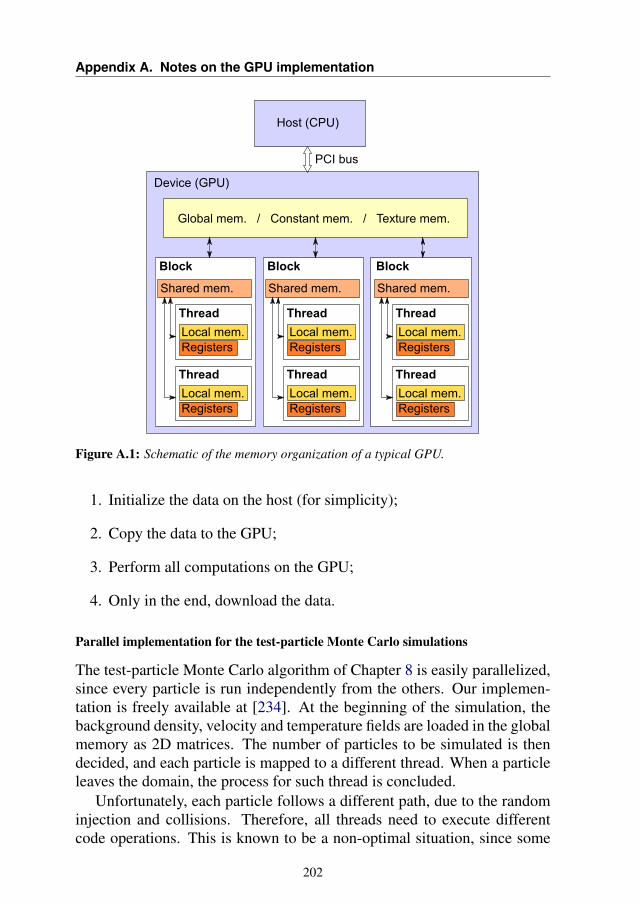
Appendix A. Notes on the GPU implementation
Figure A.1: Schematic of the memory organization of a typical GPU.
1. Initialize the data on the host (for simplicity);
2. Copy the data to the GPU;
3. Perform all computations on the GPU;
4. Only in the end, download the data.
Parallel implementation for the test-particle Monte Carlo simulations
The test-particle Monte Carlo algorithm of Chapter 8 is easily parallelized,since every particle is run independently from the others. Our implemen-tation is freely available at [234]. At the beginning of the simulation, thebackground density, velocity and temperature fields are loaded in the globalmemory as 2D matrices. The number of particles to be simulated is thendecided, and each particle is mapped to a different thread. When a particleleaves the domain, the process for such thread is concluded.
Unfortunately, each particle follows a different path, due to the randominjection and collisions. Therefore, all threads need to execute differentcode operations. This is known to be a non-optimal situation, since some
202
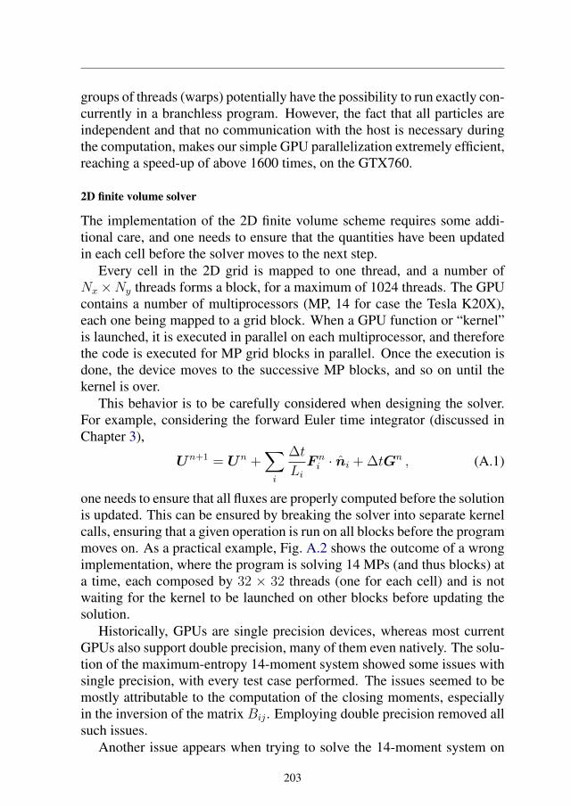
groups of threads (warps) potentially have the possibility to run exactly con-currently in a branchless program. However, the fact that all particles areindependent and that no communication with the host is necessary duringthe computation, makes our simple GPU parallelization extremely efficient,reaching a speed-up of above 1600 times, on the GTX760.
2D finite volume solver
The implementation of the 2D finite volume scheme requires some addi-tional care, and one needs to ensure that the quantities have been updatedin each cell before the solver moves to the next step.
Every cell in the 2D grid is mapped to one thread, and a number ofNx×Ny threads forms a block, for a maximum of 1024 threads. The GPUcontains a number of multiprocessors (MP, 14 for case the Tesla K20X),each one being mapped to a grid block. When a GPU function or “kernel”is launched, it is executed in parallel on each multiprocessor, and thereforethe code is executed for MP grid blocks in parallel. Once the execution isdone, the device moves to the successive MP blocks, and so on until thekernel is over.
This behavior is to be carefully considered when designing the solver.For example, considering the forward Euler time integrator (discussed inChapter 3),
Un+1 = Un +∑i
∆t
LiF ni · ni + ∆tGn , (A.1)
one needs to ensure that all fluxes are properly computed before the solutionis updated. This can be ensured by breaking the solver into separate kernelcalls, ensuring that a given operation is run on all blocks before the programmoves on. As a practical example, Fig. A.2 shows the outcome of a wrongimplementation, where the program is solving 14 MPs (and thus blocks) ata time, each composed by 32 × 32 threads (one for each cell) and is notwaiting for the kernel to be launched on other blocks before updating thesolution.
Historically, GPUs are single precision devices, whereas most currentGPUs also support double precision, many of them even natively. The solu-tion of the maximum-entropy 14-moment system showed some issues withsingle precision, with every test case performed. The issues seemed to bemostly attributable to the computation of the closing moments, especiallyin the inversion of the matrix Bij . Employing double precision removed allsuch issues.
Another issue appears when trying to solve the 14-moment system on
203
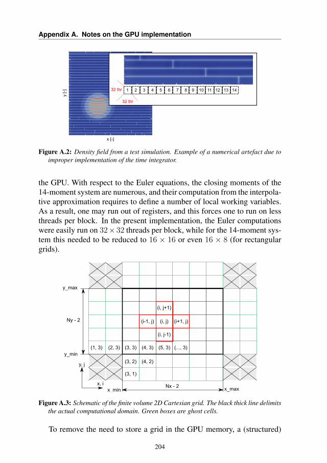
Appendix A. Notes on the GPU implementation
Figure A.2: Density field from a test simulation. Example of a numerical artefact due toimproper implementation of the time integrator.
the GPU. With respect to the Euler equations, the closing moments of the14-moment system are numerous, and their computation from the interpola-tive approximation requires to define a number of local working variables.As a result, one may run out of registers, and this forces one to run on lessthreads per block. In the present implementation, the Euler computationswere easily run on 32× 32 threads per block, while for the 14-moment sys-tem this needed to be reduced to 16 × 16 or even 16 × 8 (for rectangulargrids).
Figure A.3: Schematic of the finite volume 2D Cartesian grid. The black thick line delimitsthe actual computational domain. Green boxes are ghost cells.
To remove the need to store a grid in the GPU memory, a (structured)
204
Cartesian grid is employed, as shown in Fig A.3, where cells numberingstarts from 1 as custom in Fortran implementations. Two layers of ghostcells are employed at each side of the domain, simplifying the numericalimplementation of second order accuracy at the boundaries. Four “deadcells” are present in each corner: these are kept in the arrays for simplicity,but are not taken into account during the actual computations.
The present implementation is based on a single GPU and is rathersimplistic. More advanced strategies could be employed, exploiting var-ious features of the GPU (for example, leveraging on shared memory) andmultiple-GPU configurations (see for example [240, 241]).
205

APPENDIXBTime integration error for accelerated gases
The discretization error intrinsic to time integration methods may play animportant role in numerical simulations, when closed systems are to bedescribed or the long-time behavior is of interest. This appendix is basedon the conservative form of the governing equations. When the equationsare written in primitive variables, this analysis does not hold anymore assome errors disappear.
Considering a uniform slab of gas subject to a uniform and constantforce F , the mass, momentum and energy equations give
dρ
dt= 0 ,
d
dt(ρu) = F ,
d
dt(ρE) = Fu . (B.1)
The density is therefore constant, while the velocity grows linearly in time:
u(t) = u(0) + F t/ρ , (B.2)
and the energy changes quadratically:
(ρE)(t) = (ρE)(0)+
ˆ t
0
Fu(t)dt = (ρE)(0)+
ˆ t
0
F (u(0) + F t/ρ) dt ,
= (ρE)(0) + Fu(0)t+ F 2t2ρ . (B.3)
207
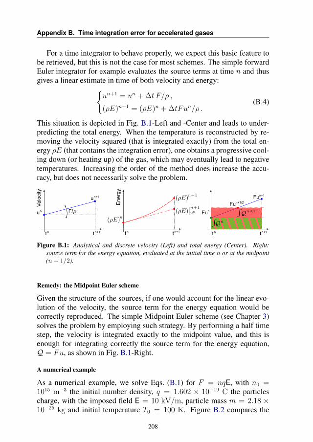
Appendix B. Time integration error for accelerated gases
For a time integrator to behave properly, we expect this basic feature tobe retrieved, but this is not the case for most schemes. The simple forwardEuler integrator for example evaluates the source terms at time n and thusgives a linear estimate in time of both velocity and energy:
un+1 = un + ∆t F/ρ ,
(ρE)n+1 = (ρE)n + ∆tFun/ρ .(B.4)
This situation is depicted in Fig. B.1-Left and -Center and leads to under-predicting the total energy. When the temperature is reconstructed by re-moving the velocity squared (that is integrated exactly) from the total en-ergy ρE (that contains the integration error), one obtains a progressive cool-ing down (or heating up) of the gas, which may eventually lead to negativetemperatures. Increasing the order of the method does increase the accu-racy, but does not necessarily solve the problem.
Figure B.1: Analytical and discrete velocity (Left) and total energy (Center). Right:source term for the energy equation, evaluated at the initial time n or at the midpoint(n+ 1/2).
Remedy: the Midpoint Euler scheme
Given the structure of the sources, if one would account for the linear evo-lution of the velocity, the source term for the energy equation would becorrectly reproduced. The simple Midpoint Euler scheme (see Chapter 3)solves the problem by employing such strategy. By performing a half timestep, the velocity is integrated exactly to the midpoint value, and this isenough for integrating correctly the source term for the energy equation,Q = Fu, as shown in Fig. B.1-Right.
A numerical example
As a numerical example, we solve Eqs. (B.1) for F = nqE, with n0 =1015 m−3 the initial number density, q = 1.602 × 10⁻¹⁹ C the particlescharge, with the imposed field E = 10 kV/m, particle mass m = 2.18 ×10⁻²⁵ kg and initial temperature T0 = 100 K. Figure B.2 compares the
208
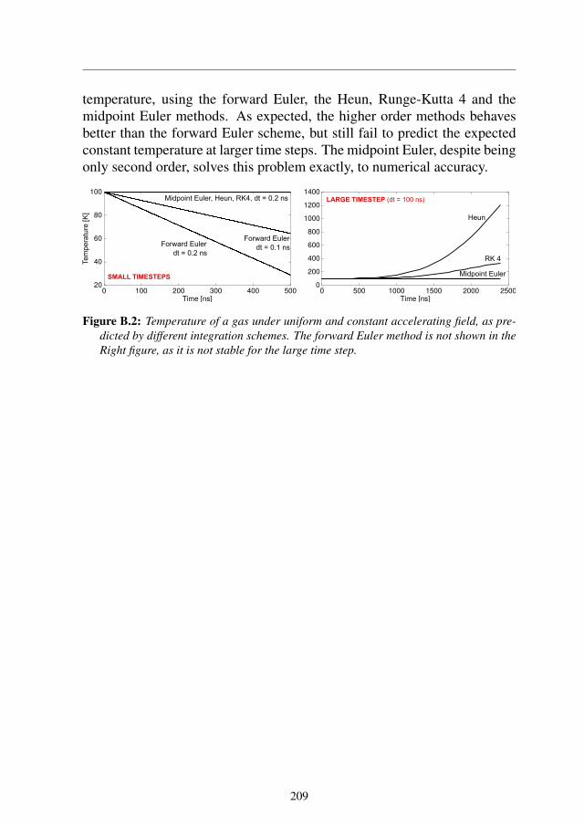
temperature, using the forward Euler, the Heun, Runge-Kutta 4 and themidpoint Euler methods. As expected, the higher order methods behavesbetter than the forward Euler scheme, but still fail to predict the expectedconstant temperature at larger time steps. The midpoint Euler, despite beingonly second order, solves this problem exactly, to numerical accuracy.
Figure B.2: Temperature of a gas under uniform and constant accelerating field, as pre-dicted by different integration schemes. The forward Euler method is not shown in theRight figure, as it is not stable for the large time step.
209

APPENDIXCWave speeds approximation via Artificial
Neural Networks
In Section 4.2, approximated expressions for the wave speeds of the 6 and14-moment maximum-entropy systems were formulated. Before findingthese approximations, an alternative approach based on Artificial NeuralNetworks was initially attempted. Such approach will be discussed in thisappendix. Many important observations of Section 4.2, such as the depen-dence of the wave speeds on σ−1, were not initially accounted for. Doingso would surely improve the quality of the present appendix. Nonetheless,the approach outlined here is useful as it outlines the procedure and theaccuracy that can be expected.
In this work, we are interested in obtaining the wave speedsw by feedingthe gas state U to the artificial neural network (ANN). Roughly speaking:
(wmin, wmax) = ANN(U) . (C.1)
To do that, the actual procedure is as follows:
1) From the gas state U , move in the reference frame with zero velocityand compute dimensionless variables;
211
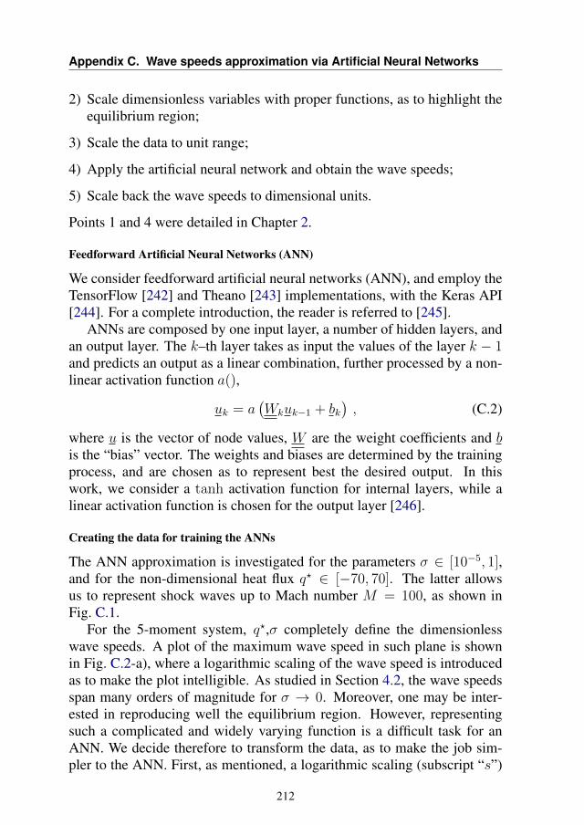
Appendix C. Wave speeds approximation via Artificial Neural Networks
2) Scale dimensionless variables with proper functions, as to highlight theequilibrium region;
3) Scale the data to unit range;
4) Apply the artificial neural network and obtain the wave speeds;
5) Scale back the wave speeds to dimensional units.
Points 1 and 4 were detailed in Chapter 2.
Feedforward Artificial Neural Networks (ANN)
We consider feedforward artificial neural networks (ANN), and employ theTensorFlow [242] and Theano [243] implementations, with the Keras API[244]. For a complete introduction, the reader is referred to [245].
ANNs are composed by one input layer, a number of hidden layers, andan output layer. The k–th layer takes as input the values of the layer k − 1and predicts an output as a linear combination, further processed by a non-linear activation function a(),
uk = a(Wkuk−1 + bk
), (C.2)
where u is the vector of node values, W are the weight coefficients and bis the “bias” vector. The weights and biases are determined by the trainingprocess, and are chosen as to represent best the desired output. In thiswork, we consider a tanh activation function for internal layers, while alinear activation function is chosen for the output layer [246].
Creating the data for training the ANNs
The ANN approximation is investigated for the parameters σ ∈ [10−5, 1],and for the non-dimensional heat flux q? ∈ [−70, 70]. The latter allowsus to represent shock waves up to Mach number M = 100, as shown inFig. C.1.
For the 5-moment system, q?,σ completely define the dimensionlesswave speeds. A plot of the maximum wave speed in such plane is shownin Fig. C.2-a), where a logarithmic scaling of the wave speed is introducedas to make the plot intelligible. As studied in Section 4.2, the wave speedsspan many orders of magnitude for σ → 0. Moreover, one may be inter-ested in reproducing well the equilibrium region. However, representingsuch a complicated and widely varying function is a difficult task for anANN. We decide therefore to transform the data, as to make the job sim-pler to the ANN. First, as mentioned, a logarithmic scaling (subscript “s”)
212
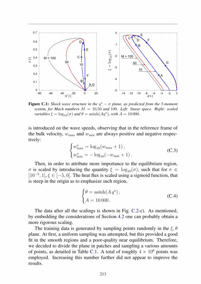
Figure C.1: Shock wave structure in the q? − σ plane, as predicted from the 5-momentsystem, for Mach numbers M = 10,50 and 100. Left: linear space. Right: scaledvariables ξ = log10(σ) and θ = asinh(Aq?), with A = 10 000.
is introduced on the wave speeds, observing that in the reference frame ofthe bulk velocity, wmax and wmin are always positive and negative respec-tively:
wsmax = log10(wmax + 1) ,
wsmin = − log10(−wmin + 1) .(C.3)
Then, in order to attribute more importance to the equilibrium region,σ is scaled by introducing the quantity ξ = log10(σ), such that for σ ∈[10−5, 1], ξ ∈ [−5, 0]. The heat flux is scaled using a sigmoid function, thatis steep in the origin as to emphasize such region,
θ = asinh(Aq?) ,
A = 10 000 .(C.4)
The data after all the scalings is shown in Fig. C.2-c). As mentioned,by embedding the considerations of Section 4.2 one can probably obtain amore rigorous scaling.
The training data is generated by sampling points randomly in the ξ, θplane. At first, a uniform sampling was attempted, but this provided a goodfit in the smooth regions and a poor-quality near equilibrium. Therefore,we decided to divide the plane in patches and sampling a various amountsof points, as detailed in Table C.1. A total of roughly 4 × 10⁶ points wasemployed. Increasing this number further did not appear to improve theresults.
213
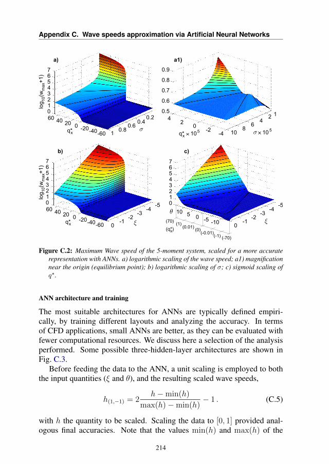
Appendix C. Wave speeds approximation via Artificial Neural Networks
Figure C.2: Maximum Wave speed of the 5-moment system, scaled for a more accuraterepresentation with ANNs. a) logarithmic scaling of the wave speed; a1) magnificationnear the origin (equilibrium point); b) logarithmic scaling of σ; c) sigmoid scaling ofq?.
ANN architecture and training
The most suitable architectures for ANNs are typically defined empiri-cally, by training different layouts and analyzing the accuracy. In termsof CFD applications, small ANNs are better, as they can be evaluated withfewer computational resources. We discuss here a selection of the analysisperformed. Some possible three-hidden-layer architectures are shown inFig. C.3.
Before feeding the data to the ANN, a unit scaling is employed to boththe input quantities (ξ and θ), and the resulting scaled wave speeds,
h(1,−1) = 2h−min(h)
max(h)−min(h)− 1 . (C.5)
with h the quantity to be scaled. Scaling the data to [0, 1] provided anal-ogous final accuracies. Note that the values min(h) and max(h) of the
214
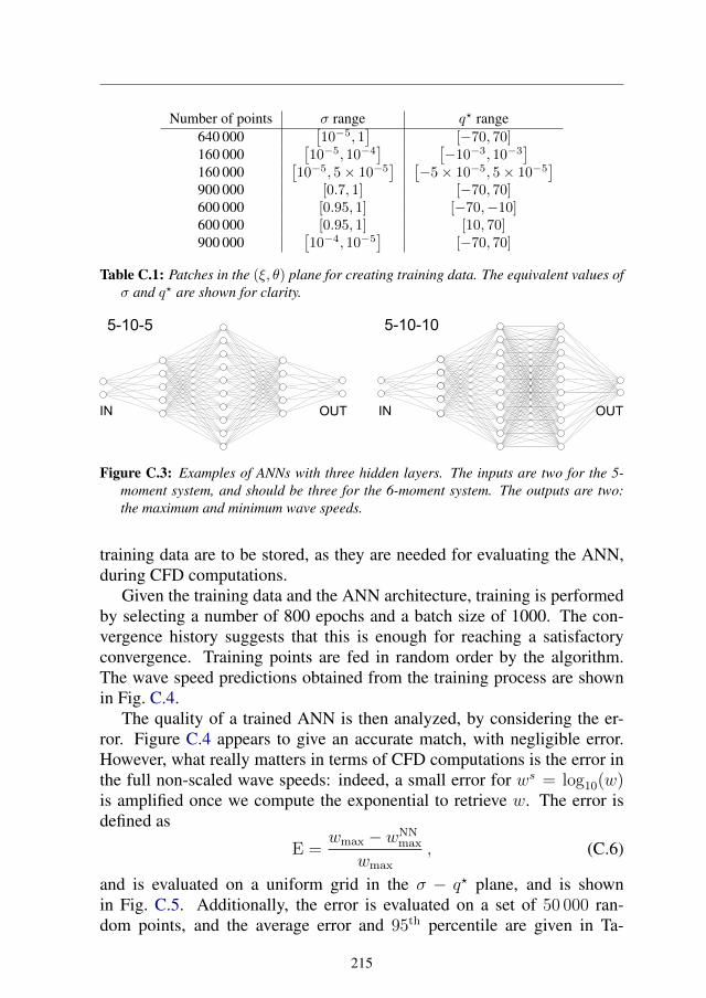
Number of points σ range q? range640 000
[10−5, 1
][−70, 70]
160 000[10−5, 10−4
] [−10−3, 10−3
]160 000
[10−5, 5× 10⁻⁵
] [−5× 10⁻⁵, 5× 10⁻⁵
]900 000 [0.7, 1] [−70, 70]600 000 [0.95, 1] [−70,−10]600 000 [0.95, 1] [10, 70]900 000
[10−4, 10−5
][−70, 70]
Table C.1: Patches in the (ξ, θ) plane for creating training data. The equivalent values ofσ and q? are shown for clarity.
Figure C.3: Examples of ANNs with three hidden layers. The inputs are two for the 5-moment system, and should be three for the 6-moment system. The outputs are two:the maximum and minimum wave speeds.
training data are to be stored, as they are needed for evaluating the ANN,during CFD computations.
Given the training data and the ANN architecture, training is performedby selecting a number of 800 epochs and a batch size of 1000. The con-vergence history suggests that this is enough for reaching a satisfactoryconvergence. Training points are fed in random order by the algorithm.The wave speed predictions obtained from the training process are shownin Fig. C.4.
The quality of a trained ANN is then analyzed, by considering the er-ror. Figure C.4 appears to give an accurate match, with negligible error.However, what really matters in terms of CFD computations is the error inthe full non-scaled wave speeds: indeed, a small error for ws = log10(w)is amplified once we compute the exponential to retrieve w. The error isdefined as
E =wmax − wNN
max
wmax
, (C.6)
and is evaluated on a uniform grid in the σ − q? plane, and is shownin Fig. C.5. Additionally, the error is evaluated on a set of 50 000 ran-dom points, and the average error and 95th percentile are given in Ta-
215
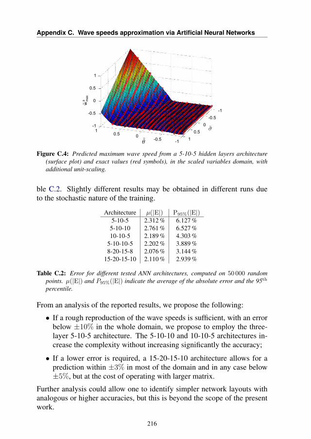
Appendix C. Wave speeds approximation via Artificial Neural Networks
Figure C.4: Predicted maximum wave speed from a 5-10-5 hidden layers architecture(surface plot) and exact values (red symbols), in the scaled variables domain, withadditional unit-scaling.
ble C.2. Slightly different results may be obtained in different runs dueto the stochastic nature of the training.
Architecture µ(|E|) P95%(|E|)5-10-5 2.312 % 6.127 %5-10-10 2.761 % 6.527 %10-10-5 2.189 % 4.303 %
5-10-10-5 2.202 % 3.889 %8-20-15-8 2.076 % 3.144 %
15-20-15-10 2.110 % 2.939 %
Table C.2: Error for different tested ANN architectures, computed on 50 000 randompoints. µ(|E|) and P95%(|E|) indicate the average of the absolute error and the 95th
percentile.
From an analysis of the reported results, we propose the following:
• If a rough reproduction of the wave speeds is sufficient, with an errorbelow ±10% in the whole domain, we propose to employ the three-layer 5-10-5 architecture. The 5-10-10 and 10-10-5 architectures in-crease the complexity without increasing significantly the accuracy;
• If a lower error is required, a 15-20-15-10 architecture allows for aprediction within ±3% in most of the domain and in any case below±5%, but at the cost of operating with larger matrix.
Further analysis could allow one to identify simpler network layouts withanalogous or higher accuracies, but this is beyond the scope of the presentwork.
216
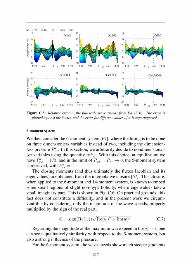
Figure C.5: Relative error in the full-scale wave speeds from Eq. (C.6). The error isplotted against the θ axis, and the error for different values of σ is superimposed.
6-moment system
We then consider the 6-moment system [67], where the fitting is to be doneon three dimensionless variables instead of two, including the dimension-less pressure P ?
xx. In this section, we arbitrarily decide to nondimensional-ize variables using the quantity trPij . With this choice, at equilibrium wehave P ?
xx = 1/3, and in the limit of Pyy = Pzz → 0, the 5-moment systemis retrieved, with P ?
xx = 1.The closing moments (and thus ultimately the fluxes Jacobian and its
eigenvalues) are obtained from the interpolative closure [67]. This closure,when applied to the 6-moment and 14-moment system, is known to embedsome small regions of slight non-hyperbolicity, where eigenvalues take asmall imaginary part. This is shown in Fig. C.6. On practical grounds, thisfact does not constitute a difficulty, and in the present work we circum-vent this by considering only the magnitude of the wave speeds, properlymultiplied by the sign of the real part,
w = sign(Re(w))√
Re(w)2 + Im(w)2 , (C.7)
Regarding the magnitude of the maximum wave speed in the qσx−σ, onecan see a qualitatively similarity with respect to the 5-moment system, butalso a strong influence of the pressure.
For the 6-moment system, the wave speeds show much steeper gradients
217
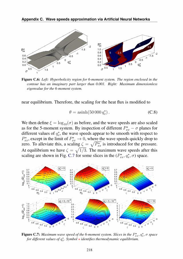
Appendix C. Wave speeds approximation via Artificial Neural Networks
Figure C.6: Left: Hyperbolicity region for 6-moment system. The region enclosed in thecontour has an imaginary part larger than 0.001. Right: Maximum dimensionlesseigenvalue for the 6-moment system.
near equilibrium. Therefore, the scaling for the heat flux is modified to
θ = asinh(50 000 q?x) . (C.8)
We then define ξ = log10(σ) as before, and the wave speeds are also scaledas for the 5-moment system. By inspection of different P ?
xx − σ planes fordifferent values of q?x, the wave speeds appear to be smooth with respect toP ?xx, except in the limit of P ?
xx → 0, where the wave speeds quickly drop tozero. To alleviate this, a scaling ζ =
√P ?xx is introduced for the pressure.
At equilibrium we have ζ =√
1/3. The maximum wave speeds after thisscaling are shown in Fig. C.7 for some slices in the (P ?
xx, q?x, σ) space.
Figure C.7: Maximum wave speed of the 6-moment system. Slices in the P ?xx, q?x, σ space
for different values of q?x. Symbol ? identifies thermodynamic equilibrium.
218
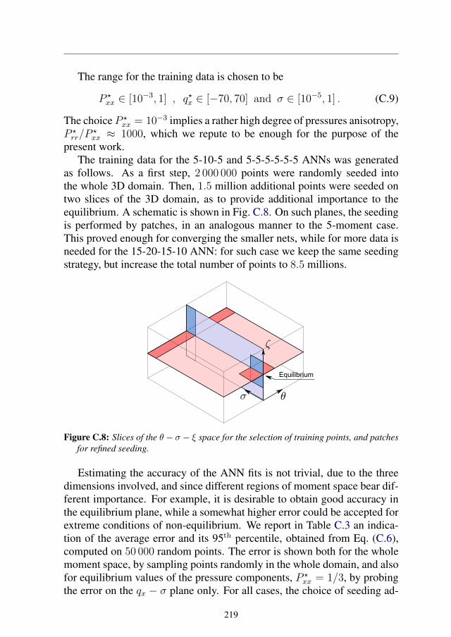
The range for the training data is chosen to be
P ?xx ∈ [10−3, 1] , q?x ∈ [−70, 70] and σ ∈ [10−5, 1] . (C.9)
The choice P ?xx = 10−3 implies a rather high degree of pressures anisotropy,
P ?rr/P
?xx ≈ 1000, which we repute to be enough for the purpose of the
present work.The training data for the 5-10-5 and 5-5-5-5-5-5 ANNs was generated
as follows. As a first step, 2 000 000 points were randomly seeded intothe whole 3D domain. Then, 1.5 million additional points were seeded ontwo slices of the 3D domain, as to provide additional importance to theequilibrium. A schematic is shown in Fig. C.8. On such planes, the seedingis performed by patches, in an analogous manner to the 5-moment case.This proved enough for converging the smaller nets, while for more data isneeded for the 15-20-15-10 ANN: for such case we keep the same seedingstrategy, but increase the total number of points to 8.5 millions.
Figure C.8: Slices of the θ− σ − ξ space for the selection of training points, and patchesfor refined seeding.
Estimating the accuracy of the ANN fits is not trivial, due to the threedimensions involved, and since different regions of moment space bear dif-ferent importance. For example, it is desirable to obtain good accuracy inthe equilibrium plane, while a somewhat higher error could be accepted forextreme conditions of non-equilibrium. We report in Table C.3 an indica-tion of the average error and its 95th percentile, obtained from Eq. (C.6),computed on 50 000 random points. The error is shown both for the wholemoment space, by sampling points randomly in the whole domain, and alsofor equilibrium values of the pressure components, P ?
xx = 1/3, by probingthe error on the qx − σ plane only. For all cases, the choice of seeding ad-
219
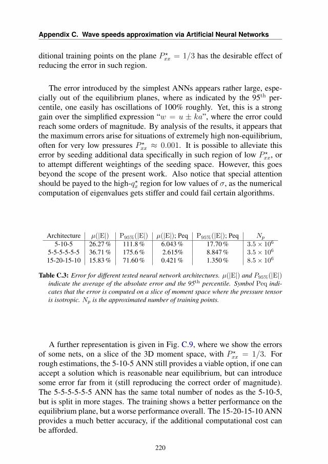
Appendix C. Wave speeds approximation via Artificial Neural Networks
ditional training points on the plane P ?xx = 1/3 has the desirable effect of
reducing the error in such region.
The error introduced by the simplest ANNs appears rather large, espe-cially out of the equilibrium planes, where as indicated by the 95th per-centile, one easily has oscillations of 100% roughly. Yet, this is a stronggain over the simplified expression “w = u ± ka”, where the error couldreach some orders of magnitude. By analysis of the results, it appears thatthe maximum errors arise for situations of extremely high non-equilibrium,often for very low pressures P ?
xx ≈ 0.001. It is possible to alleviate thiserror by seeding additional data specifically in such region of low P ?
xx, orto attempt different weightings of the seeding space. However, this goesbeyond the scope of the present work. Also notice that special attentionshould be payed to the high-q?x region for low values of σ, as the numericalcomputation of eigenvalues gets stiffer and could fail certain algorithms.
Architecture µ(|E|) P95%(|E|) µ(|E|); Peq P95%(|E|); Peq Np5-10-5 26.27 % 111.8 % 6.043 % 17.70 % 3.5× 10⁶
5-5-5-5-5-5 36.71 % 175.6 % 2.615% 8.847 % 3.5× 10⁶
15-20-15-10 15.83 % 71.60 % 0.421 % 1.350 % 8.5× 10⁶
Table C.3: Error for different tested neural network architectures. µ(|E|) and P95%(|E|)indicate the average of the absolute error and the 95th percentile. Symbol Peq indi-cates that the error is computed on a slice of moment space where the pressure tensoris isotropic. Np is the approximated number of training points.
A further representation is given in Fig. C.9, where we show the errorsof some nets, on a slice of the 3D moment space, with P ?
xx = 1/3. Forrough estimations, the 5-10-5 ANN still provides a viable option, if one canaccept a solution which is reasonable near equilibrium, but can introducesome error far from it (still reproducing the correct order of magnitude).The 5-5-5-5-5-5 ANN has the same total number of nodes as the 5-10-5,but is split in more stages. The training shows a better performance on theequilibrium plane, but a worse performance overall. The 15-20-15-10 ANNprovides a much better accuracy, if the additional computational cost canbe afforded.
220
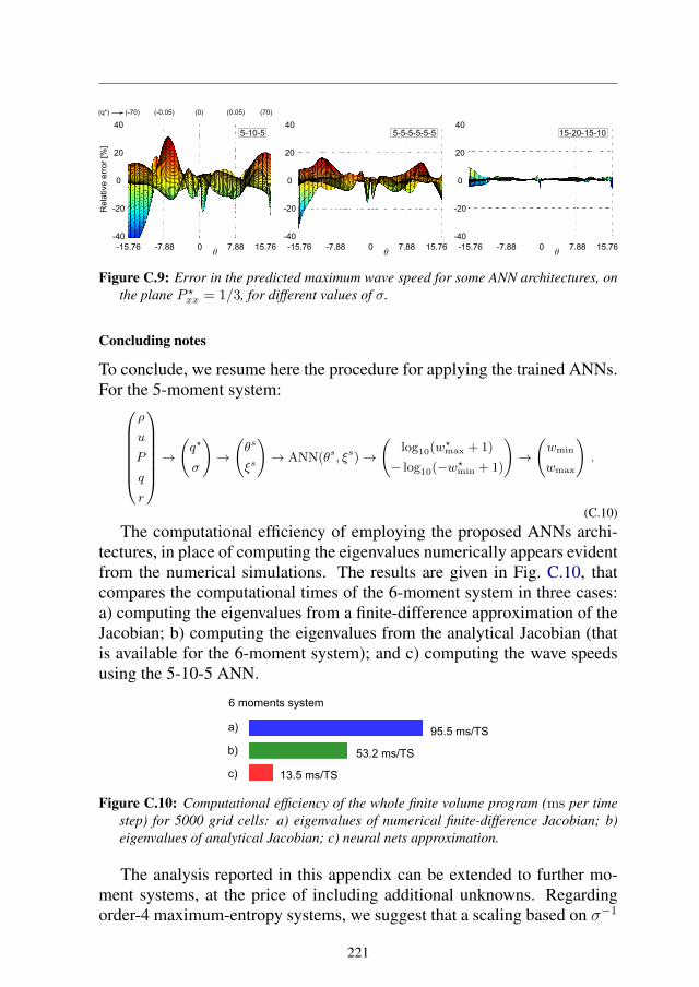
Figure C.9: Error in the predicted maximum wave speed for some ANN architectures, onthe plane P ?xx = 1/3, for different values of σ.
Concluding notes
To conclude, we resume here the procedure for applying the trained ANNs.For the 5-moment system:
ρ
u
P
q
r
→(q?
σ
)→
(θs
ξs
)→ ANN(θs, ξs)→
(log10(w
?max + 1)
− log10(−w?min + 1)
)→
(wmin
wmax
).
(C.10)
The computational efficiency of employing the proposed ANNs archi-tectures, in place of computing the eigenvalues numerically appears evidentfrom the numerical simulations. The results are given in Fig. C.10, thatcompares the computational times of the 6-moment system in three cases:a) computing the eigenvalues from a finite-difference approximation of theJacobian; b) computing the eigenvalues from the analytical Jacobian (thatis available for the 6-moment system); and c) computing the wave speedsusing the 5-10-5 ANN.
Figure C.10: Computational efficiency of the whole finite volume program (ms per timestep) for 5000 grid cells: a) eigenvalues of numerical finite-difference Jacobian; b)eigenvalues of analytical Jacobian; c) neural nets approximation.
The analysis reported in this appendix can be extended to further mo-ment systems, at the price of including additional unknowns. Regardingorder-4 maximum-entropy systems, we suggest that a scaling based on σ−1
221

Appendix C. Wave speeds approximation via Artificial Neural Networks
is employed in further simulations, as this would most likely improve theaccuracy of the ANN training.
222
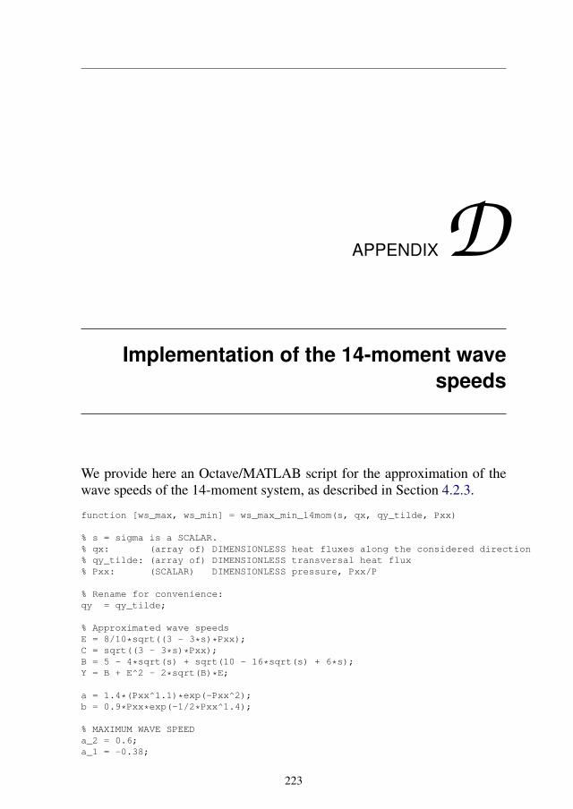
APPENDIXDImplementation of the 14-moment wave
speeds
We provide here an Octave/MATLAB script for the approximation of thewave speeds of the 14-moment system, as described in Section 4.2.3.
function [ws_max, ws_min] = ws_max_min_14mom(s, qx, qy_tilde, Pxx)
% s = sigma is a SCALAR.% qx: (array of) DIMENSIONLESS heat fluxes along the considered direction% qy_tilde: (array of) DIMENSIONLESS transversal heat flux% Pxx: (SCALAR) DIMENSIONLESS pressure, Pxx/P
% Rename for convenience:qy = qy_tilde;
% Approximated wave speedsE = 8/10*sqrt((3 - 3*s)*Pxx);C = sqrt((3 - 3*s)*Pxx);B = 5 - 4*sqrt(s) + sqrt(10 - 16*sqrt(s) + 6*s);Y = B + E^2 - 2*sqrt(B)*E;
a = 1.4*(Pxx^1.1)*exp(-Pxx^2);b = 0.9*Pxx*exp(-1/2*Pxx^1.4);
% MAXIMUM WAVE SPEEDa_2 = 0.6;a_1 = -0.38;
223
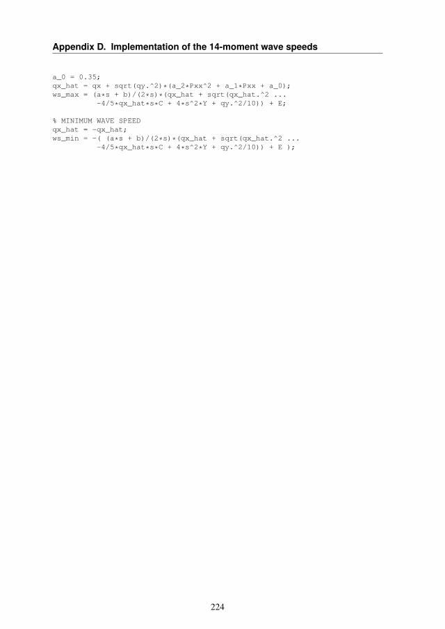
Appendix D. Implementation of the 14-moment wave speeds
a_0 = 0.35;qx_hat = qx + sqrt(qy.^2)*(a_2*Pxx^2 + a_1*Pxx + a_0);ws_max = (a*s + b)/(2*s)*(qx_hat + sqrt(qx_hat.^2 ...
-4/5*qx_hat*s*C + 4*s^2*Y + qy.^2/10)) + E;
% MINIMUM WAVE SPEEDqx_hat = -qx_hat;ws_min = -( (a*s + b)/(2*s)*(qx_hat + sqrt(qx_hat.^2 ...
-4/5*qx_hat*s*C + 4*s^2*Y + qy.^2/10)) + E );
224
Bibliography
[1] Hendrik Johannes Van der Bijl. The thermionic vacuum tube and its applications. McGraw-Hill book Company, Incorporated, 1920.
[2] Michael A Lieberman and Alan J Lichtenberg. Principles of plasma discharges and materialsprocessing. John Wiley & Sons, 2005.
[3] A Haga, S Senda, Y Sakai, Y Mizuta, S Kita, and F Okuyama. A miniature x-ray tube.Applied physics letters, 84(12):2208–2210, 2004.
[4] Victor Malka, S Fritzler, E Lefebvre, M-M Aleonard, F Burgy, J-P Chambaret, J-F Chemin,K Krushelnick, G Malka, SPD Mangles, et al. Electron acceleration by a wake field forcedby an intense ultrashort laser pulse. Science, 298(5598):1596–1600, 2002.
[5] Francis F Chen et al. Introduction to plasma physics and controlled fusion, volume 1.Springer, 1984.
[6] Rudolf A Treumann and Wolfgang Baumjohann. Advanced space plasma physics, volume 30.Imperial College Press London, 1997.
[7] Ernst Stuhlinger. Ion propulsion for space flight. McGraw-Hill New York, 1964.
[8] Edgar Y Choueiri. A critical history of electric propulsion: The first 50 years (1906-1956).Journal of Propulsion and Power, 20(2):193–203, 2004.
[9] Harold R Kaufman and Raymond S Robinson. Electric thruster performance for orbit raisingand maneuvering. Journal of Spacecraft and Rockets, 21(2):180–186, 1984.
[10] Robert J Vondra and Keith I Thomassen. Flight qualified pulsed electric thruster for satellitecontrol. Journal of Spacecraft and Rockets, 11(9):613–617, 1974.
[11] George P Sutton and Oscar Biblarz. Rocket propulsion elements. John Wiley & Sons, 2016.
[12] Yves Langevin. Chemical and solar electric propulsion options for a cornerstone mission tomercury. acta astronautica, 47(2-9):443–452, 2000.
[13] Giuseppe D Racca. Capability of solar electric propulsion for planetary missions. Planetaryand Space Science, 49(14-15):1437–1444, 2001.
[14] Kybeom Kwon, Gregory Lantoine, Ryan P Russell, and Dimitri N Mavris. A study on si-multaneous design of a Hall Effect Thruster and its low-thrust trajectory. Acta Astronautica,119:34–47, 2016.
225
Bibliography
[15] K Mani, Stefano Boccelli, Francesco Topputo, Angelo Cervone, et al. Electric propulsioncharacterization for a stand-alone Mars CubeSat. In 36th International Electric PropulsionConference, pages 1–15, 2019.
[16] Robert G Jahn. Physics of electric propulsion. Courier Corporation, 2006.
[17] Eduardo Ahedo. Plasmas for space propulsion. Plasma Physics and Controlled Fusion,53(12):124037, 2011.
[18] Rodney L Burton. Pulsed plasma thrusters. Encyclopedia of Aerospace Engineering, 2010.
[19] Derrek Russell, C Dailey, Wayne Goldstein, Ralph Lovberg, James Poylio, and Bernard Jack-son. The PIT mark VI pulsed inductive thruster. In Space 2004 Conference and Exhibit, page6054, 2004.
[20] ROGER MYERS, MICHAEL LAPOINTE, and MARIS MANTENIEKS. MPD thruster tech-nology. In Conference on Advanced SEI Technologies, page 3568, 1991.
[21] Timothy Ziemba, John Carscadden, John Slough, James Prager, and Robert Winglee. Highpower helicon thruster. In 41st AIAA/ASME/SAE/ASEE Joint Propulsion Conference & Ex-hibit, page 4119, 2005.
[22] Edward Teller, Alexander J Glass, T Kenneth Fowler, Akira Hasegawa, and John F Santarius.Space propulsion by fusion in a magnetic dipole. Fusion Technology, 22(1):82–97, 1992.
[23] Yosef S Razin, Gary Pajer, Mary Breton, Eric Ham, Joseph Mueller, Michael Paluszek,Alan H Glasser, and Samuel A Cohen. A direct fusion drive for rocket propulsion. ActaAstronautica, 105(1):145–155, 2014.
[24] Dan M Goebel and Ira Katz. Fundamentals of electric propulsion: ion and Hall thrusters,volume 1. John Wiley & Sons, 2008.
[25] AI Morozov and VV Savelyev. Fundamentals of stationary plasma thruster theory. Reviewsof plasma physics, pages 203–391, 2000.
[26] Viacheslav V Zhurin, Harold R Kaufman, and Raymond S Robinson. Physics of closed driftthrusters. Plasma Sources Science and Technology, 8(1):R1, 1999.
[27] C Boniface, GJM Hagelaar, L Garrigues, JP Boeuf, and M Prioul. Modeling of double stageHall effect thruster. IEEE Transactions on Plasma Science, 33(2):522–523, 2005.
[28] D Pérez-Grande, P Fajardo, and E Ahedo. Evaluation of erosion reduction mechanisms inHall effect thrusters. In International Electric Propulsion Conference, Hyogo-Kobe, 2015.
[29] Ryan W Conversano, Dan M Goebel, Ioannis G Mikellides, Richard R Hofer, and Richard EWirz. Performance analysis of a low-power magnetically shielded Hall thruster: computa-tional modeling. Journal of Propulsion and Power, 33(4):992–1001, 2017.
[30] Lou Grimaud and Stéphane Mazouffre. Conducting wall Hall thrusters in magnetic shieldingand standard configurations. Journal of Applied Physics, 122(3):033305, 2017.
[31] AI Morozov and VV Savel’Ev. Theory of the near-wall conductivity. Plasma Physics Reports,27(7):570–575, 2001.
[32] Dan M Goebel, Richard R Hofer, Ioannis G Mikellides, Ira Katz, James E Polk, and Bran-don N Dotson. Conducting wall Hall thrusters. IEEE Transactions on Plasma Science,43(1):118–126, 2014.
[33] S Mazouffre, J Vaudolon, S Tsikata, C Henaux, D Harribey, and A Rossi. Optimization ofthe design of a wall-less Hall thruster. Joint 30th ISTS, 34th IEPC and 6th, 2703, 2015.
[34] Mario Capitelli, Gianpiero Colonna, and Antonio D’Angola. Fundamental aspects of plasmachemical physics, volume 66. Springer, 2012.
226
Bibliography
[35] Donald B Melrose. Instabilities in space and laboratory plasmas. 1986.
[36] Sergey T Surzhikov. Computational physics of electric discharges in gas flows, volume 7.Walter de Gruyter, 2012.
[37] Charles Hirsch. Numerical computation of internal and external flows. Wiley, 1997.
[38] Nicolaas G van Kampen and Barend Ubbo Felderhof. Theoretical methods in plasma physics.Amsterdam: North Holland Publication Co, 1967.
[39] JH Ferziger and HG Kaper. Mathematical theory of transport processes in gases. AmericanJournal of Physics, 41(4):601–603, 1973.
[40] Viktor Mikhaı Zhdanov. Transport processes in multicomponent plasma.
[41] Francesco Taccogna and Giorgio Dilecce. Non-equilibrium in low-temperature plasmas. TheEuropean Physical Journal D, 70(11):1–37, 2016.
[42] Jean-Pierre Boeuf. Tutorial: Physics and modeling of Hall thrusters. Journal of AppliedPhysics, 121(1):011101, 2017.
[43] JC Adam, JP Boeuf, N Dubuit, M Dudeck, L Garrigues, D Gresillon, A Heron, GJM Hagelaar,V Kulaev, N Lemoine, et al. Physics, simulation and diagnostics of Hall effect thrusters.Plasma Physics and Controlled Fusion, 50(12):124041, 2008.
[44] Andrey Shagayda. Stationary electron velocity distribution function in crossed electric andmagnetic fields with collisions. Physics of Plasmas, 19(8):083503, 2012.
[45] CH Shon and JK Lee. Modeling of magnetron sputtering plasmas. Applied Surface Science,192(1-4):258–269, 2002.
[46] Igor D Kaganovich, Andrei Smolyakov, Yevgeny Raitses, Eduardo Ahedo, Ioannis G Mikel-lides, Benjamin Jorns, Francesco Taccogna, Renaud Gueroult, Sedina Tsikata, Anne Bour-don, et al. Physics of E×B discharges relevant to plasma propulsion and similar technologies.Physics of Plasmas, 27(12):120601, 2020.
[47] Kentaro Hara and Sedina Tsikata. Cross-field electron diffusion due to the coupling of drift-driven microinstabilities. Physical Review E, 102(2):023202, 2020.
[48] Trevor Lafleur, SD Baalrud, and Pascal Chabert. Theory for the anomalous electron transportin Hall effect thrusters. II. kinetic model. Physics of Plasmas, 23(5):053503, 2016.
[49] Jean-Pierre Boeuf and Laurent Garrigues. E×B electron drift instability in Hall thrusters:Particle-in-cell simulations vs. theory. Physics of Plasmas, 25(6):061204, 2018.
[50] Thomas Charoy, Jean-Pierre Boeuf, Anne Bourdon, Johan A Carlsson, Pascal Chabert,B Cuenot, Denis Eremin, Laurent Garrigues, Kentaro Hara, Igor D Kaganovich, et al. 2Daxial-azimuthal particle-in-cell benchmark for low-temperature partially magnetized plasmas.Plasma Sources Science and Technology, 28(10):105010, 2019.
[51] Luc Mieussens. Discrete velocity model and implicit scheme for the BGK equation of rarefiedgas dynamics. Mathematical Models and Methods in Applied Sciences, 10(08):1121–1149,2000.
[52] RJ Kingham and AR Bell. An implicit vlasov–fokker–planck code to model non-local elec-tron transport in 2-d with magnetic fields. Journal of Computational Physics, 194(1):1–34,2004.
[53] Charles K Birdsall and A Bruce Langdon. Plasma physics via computer simulation. CRCpress, 2004.
[54] Francesco Taccogna, Savino Longo, Mario Capitelli, and Ralf Schneider. Self-similarity inHall plasma discharges: Applications to particle models. Physics of Plasmas, 12(5):053502,2005.
227
Bibliography
[55] K Matyash, R Schneider, S Mazouffre, S Tsikata, Y Raitses, and A Diallo. 3D simulationof the rotating spoke in a Hall thruster. In Proceedings of the 33rd International ElectricPropulsion Conference, volume 32, 2013.
[56] James Joseph Szabo. Fully kinetic numerical modeling of a plasma thruster. PhD thesis,Massachusetts Institute of Technology, 2001.
[57] D Sydorenko, A Smolyakov, I Kaganovich, and Y Raitses. Kinetic simulation of secondaryelectron emission effects in Hall thrusters. Physics of Plasmas, 13(1):014501, 2006.
[58] Trevor Lafleur, SD Baalrud, and Pascal Chabert. Theory for the anomalous electron transportin Hall effect thrusters. I. insights from particle-in-cell simulations. Physics of Plasmas,23(5):053502, 2016.
[59] Zahra Asadi, Francesco Taccogna, and Mehdi Sharifian. Numerical study of electron cy-clotron drift instability: Application to Hall thruster. Frontiers in Physics, 7:140, 2019.
[60] FI Parra, E Ahedo, JM Fife, and M Martinez-Sanchez. A two-dimensional hybrid model ofthe Hall thruster discharge. Journal of Applied Physics, 100(2):023304, 2006.
[61] Andrey Shashkov, Alexander Lovtsov, and Dmitry Tomilin. A one-dimensional with three-dimensional velocity space hybrid-PIC model of the discharge plasma in a Hall thruster.Physics of Plasmas, 24(4):043501, 2017.
[62] Henning Struchtrup. Macroscopic transport equations for rarefied gas flows. In Macroscopictransport equations for rarefied gas flows, pages 145–160. Springer, 2005.
[63] Harold Grad. On the kinetic theory of rarefied gases. Communications on pure and appliedmathematics, 2(4):331–407, 1949.
[64] C David Levermore. Moment closure hierarchies for kinetic theories. Journal of statisticalPhysics, 83(5):1021–1065, 1996.
[65] Ingo Müller and Tommaso Ruggeri. Rational extended thermodynamics, volume 37. SpringerScience & Business Media, 2013.
[66] Michael Junk. Domain of definition of Levermore’s five-moment system. Journal of Statisti-cal Physics, 93(5):1143–1167, 1998.
[67] James McDonald and Manuel Torrilhon. Affordable robust moment closures for CFD basedon the maximum-entropy hierarchy. Journal of Computational Physics, 251:500–523, 2013.
[68] Sean T Miller and Uri Shumlak. A multi-species 13-moment model for moderately collisionalplasmas. Physics of Plasmas, 23(8):082303, 2016.
[69] Shaun Gilliam. A 13-moment two-fluid plasma physics model based on a Pearson type-IVdistribution function. PhD thesis, University of Washington, 2011.
[70] Andrew Ho, Iman Anwar Michael Datta, and Uri Shumlak. Physics-based-adaptive plasmamodel for high-fidelity numerical simulations. Frontiers in Physics, 6:105, 2018.
[71] David J Larson. Kinetic plasma simulation using a quadrature-based moment method. Bul-letin of the American Physical Society, 53, 2008.
[72] Javier Martines Martinez, Dmytro Rafalskyi, and Ane Aanesland. Development and testingof the NPT30-I2 iodine ion thruster. In 36th International Electric Propulsion Conference,number 15-20, 2019.
[73] Mikhail Naumovich Kogan. Rarefied Gas Dynamics. Plenum Press, New York, 1969.
[74] Richard L Liboff. Kinetic theory: classical, quantum, and relativistic descriptions. SpringerScience & Business Media, 2003.
228
Bibliography
[75] Yu L Klimontovich. The statistical theory of non-equilibrium processes in a plasma. Journalof Plasma Physics, 3:148, 1969.
[76] Iu I Klimontovich. Kinetic theory of nonideal gas and nonideal plasma. Moscow IzdatelNauka, 1975.
[77] Dwight Roy Nicholson and Dwight R Nicholson. Introduction to plasma theory. Wiley NewYork, 1983.
[78] Vincent Giovangigli. Multicomponent flow modeling. Science China Mathematics,55(2):285–308, 2012.
[79] Yuri N Dnestrovskii and Dimitri P Kostomarov. Numerical simulation of plasmas. SpringerScience & Business Media, 2012.
[80] Prabhu Lal Bhatnagar, Eugene P Gross, and Max Krook. A model for collision processes ingases. I. small amplitude processes in charged and neutral one-component systems. Physicalreview, 94(3):511, 1954.
[81] Carlo Cercignani. The Boltzmann equation and its applications. pages 40–103. Springer,1988.
[82] Luc Mieussens and Henning Struchtrup. Numerical comparison of Bhatnagar–Gross–Krookmodels with proper prandtl number. Physics of Fluids, 16(8):2797–2813, 2004.
[83] Johannes Martinus Burgers. Flow equations for composite gases. Maryland University Col-lege Park Institute for Fluid Dynamics and Applied Mathematics, 1969.
[84] Marzia Bisi and Maria José Cáceres. A BGK relaxation model for polyatomic gas mixtures.Communications in Mathematical Sciences, 14(2):297–325, 2016.
[85] Florian Bernard, Angelo Iollo, and Gabriella Puppo. BGK polyatomic model for rarefiedflows. Journal of Scientific Computing, 78(3):1893–1916, 2019.
[86] Henning Struchtrup. The BGK-model with velocity-dependent collision frequency. Contin-uum Mechanics and Thermodynamics, 9(1):23–31, 1997.
[87] François Bouchut and Benoít Perthame. A BGK model for small Prandtl number in theNavier-Stokes approximation. Journal of statistical physics, 71(1):191–207, 1993.
[88] John M Sankovic, John A Hamley, and Thomas W Haag. Performance evaluation of therussian SPT-100 thruster at NASA LeRC. 1993.
[89] OA Mitrofanova, R Yu Gnizdor, VM Murashko, AI Koryakin, and AN Nesterenko. Newgeneration of SPT-100. In 32nd International Electric Propulsion Conference, pages 2011–041, 2011.
[90] E Ahedo, P Martınez-Cerezo, and M Martınez-Sánchez. One-dimensional model of theplasma flow in a Hall thruster. Physics of Plasmas, 8(6):3058–3068, 2001.
[91] Vanessa Vial, A Lazurenko, D Pagnon, and A Bouchoule. Measurement of absolute xenondensity and gas injection impact in Hall thrusters. In 4th International Spacecraft PropulsionConference, volume 555, 2004.
[92] John David Jackson. Classical electrodynamics, 1999.
[93] Biagi database. www.lxcat.net. retrieved on February 22, 2021.
[94] Leanne C Pitchford, Luis L Alves, Klaus Bartschat, Stephen F Biagi, Marie-Claude Bordage,Igor Bray, Chris E Brion, Michael J Brunger, Laurence Campbell, Alise Chachereau, et al.Lxcat: An open-access, web-based platform for data needed for modeling low temperatureplasmas. Plasma Processes and Polymers, 14(1-2):1600098, 2017.
229
Bibliography
[95] Richard Fitzpatrick. Introduction to plasma physics. The University of Texas at Austin: sn,page 242, 2008.
[96] RJ Goldston, PH Rutherford, and J Wesson. Introduction to plasma physics. Plasma Physicsand Controlled Fusion, 38(1):103, 1996.
[97] S Barral, N Gascon, K Makowski, Z Peradzynski, and M Dudeck. Numerical study of thecurrent-voltage characteristic of Hall thrusters. In 27th International Electric PropulsionConference, IEPC, pages 01–27, 2001.
[98] Serge Barral, Karol Makowski, Zbigniew Peradzynski, and Michel Dudeck. Transit-timeinstability in Hall thrusters. Physics of Plasmas, 12(7):073504, 2005.
[99] J Pérez-Luna, GJM Hagelaar, L Garrigues, and JP Boeuf. Method to obtain the electric fieldand the ionization frequency from laser induced fluorescence measurements. Plasma SourcesScience and Technology, 18(3):034008, 2009.
[100] GJM Hagelaar, J Bareilles, LBJP Garrigues, and J-P Boeuf. Two-dimensional model of astationary plasma thruster. Journal of Applied Physics, 91(9):5592–5598, 2002.
[101] Sydney Chapman, Thomas George Cowling, and David Burnett. The mathematical theoryof non-uniform gases: an account of the kinetic theory of viscosity, thermal conduction anddiffusion in gases. Cambridge university press, 1990.
[102] David Burnett. The distribution of velocities in a slightly non-uniform gas. Proceedings ofthe London Mathematical Society, 2(1):385–430, 1935.
[103] Keith Comeaux, Dean Chapman, Ma, and Robert Cormack. An analysis of the burnett equa-tions based on the second law of thermodynamics. In 33rd Aerospace sciences meeting andexhibit, page 415, 1995.
[104] Xiaolin Zhong. Development and computation of continuum higher order constitutive rela-tions for high-altitude hypersonic flow. 1992.
[105] Benjamin Graille, Thierry E Magin, and Marc Massot. Kinetic theory of plasmas: trans-lational energy. Mathematical Models and Methods in Applied Sciences, 19(04):527–599,2009.
[106] Radu Balescu. Transport processes in plasmas. 1988.
[107] SI Braginskii. Transport processes in a plasma. Reviews of Plasma Physics, 1:205, 1963.
[108] Manuel Torrilhon. Convergence study of moment approximations for boundary valueproblems of the Boltzmann-BGK equation. Communications in Computational Physics,18(3):529–557, 2015.
[109] George V Khazanov. Kinetic theory of the inner magnetospheric plasma, volume 372.Springer Science & Business Media, 2010.
[110] M Torrilhon. Characteristic waves and dissipation in the 13-moment-case. Continuum Me-chanics and Thermodynamics, 12(5):289–301, 2000.
[111] Henning Struchtrup and Manuel Torrilhon. Regularization of Grad’s 13 moment equations:Derivation and linear analysis. Physics of Fluids, 15(9):2668–2680, 2003.
[112] M Torrilhon and Henning Struchtrup. Regularized 13-moment equations: shock structurecalculations and comparison to Burnett models. Journal of Fluid Mechanics, 513:171, 2004.
[113] Olivier Desjardins, Rodney O Fox, and Philippe Villedieu. A quadrature-based momentmethod for dilute fluid-particle flows. Journal of Computational Physics, 227(4):2514–2539,2008.
[114] Rodney O Fox. Higher-order quadrature-based moment methods for kinetic equations. Jour-nal of Computational Physics, 228(20):7771–7791, 2009.
230
Bibliography
[115] Manuel Torrilhon. Hyperbolic moment equations in kinetic gas theory based on multi-variatePearson-IV-distributions. Communications in Computational Physics, 7(4):639, 2010.
[116] GM8807460618 Kremer. Extended thermodynamics of ideal gases with 14 fields. In Annalesde l’IHP Physique théorique, volume 45, pages 419–440, 1986.
[117] Boone R Tensuda, James G McDonald, and Clinton PT Groth. Multi-dimensional validationof a maximum-entropy-based interpolative moment closure. In AIP Conference Proceedings,volume 1786, page 140008. AIP Publishing LLC, 2016.
[118] JG McDonald, JS Sachdev, and CPT Groth. Use of the gaussian moment closure for themodelling of continuum and micron-scale flows with moving boundaries. In ComputationalFluid Dynamics 2006, pages 783–788. Springer, 2009.
[119] James G McDonald. Extended fluid-dynamic modelling for numerical solution of micro-scaleflows. University of Toronto, 2011.
[120] François Forgues and James G McDonald. Higher-order moment models for laminar multi-phase flows with accurate particle-stream crossing. International Journal of Multiphase Flow,114:28–38, 2019.
[121] Joachim AR Sarr and Clinton PT Groth. A second-order maximum-entropy inspired inter-polative closure for radiative heat transfer in gray participating media. Journal of QuantitativeSpectroscopy and Radiative Transfer, 255:107238, 2020.
[122] Vittorio Romano. 2D simulation of a silicon MESFET with a nonparabolic hydrodynam-ical model based on the maximum entropy principle. Journal of Computational Physics,176(1):70–92, 2002.
[123] Michael Junk and Andreas Unterreiter. Maximum entropy moment systems and Galileaninvariance. Continuum Mechanics and Thermodynamics, 14(6):563–576, 2002.
[124] Hans Ludwig Hamburger. Hermitian transformations of deficiency-index (1, 1), Jacobi matri-ces and undetermined moment problems. American Journal of Mathematics, 66(4):489–522,1944.
[125] MJ Druyvesteyn and Fi M Penning. The mechanism of electrical discharges in gases of lowpressure. Reviews of Modern Physics, 12(2):87, 1940.
[126] James G McDonald and Clinton PT Groth. Towards realizable hyperbolic moment closuresfor viscous heat-conducting gas flows based on a maximum-entropy distribution. ContinuumMechanics and Thermodynamics, 25(5):573–603, 2013.
[127] James G McDonald. Approximate maximum-entropy moment closures for gas dynamics. InAIP Conference Proceedings, volume 1786, page 140001. AIP Publishing LLC, 2016.
[128] Reinhard Illner and Helmut Neunzert. On simulation methods for the Boltzmann equation.Transport Theory and Statistical Physics, 16(2-3):141–154, 1987.
[129] Graeme A Bird. Molecular gas dynamics and the direct simulation of gas flows. Moleculargas dynamics and the direct simulation of gas flows, 1994.
[130] Roger W Hockney and James W Eastwood. Computer simulation using particles. crc Press,1988.
[131] Jay P Boris. Acceleration calculation from a scalar potential. Technical report, PrincetonUniv., NJ Plasma Physics Lab., 1970.
[132] Giovanni Lapenta. Particle in cell methods. In With Application to Simulations in Space.Weather. Citeseer, 2016.
[133] Vahid Vahedi and Maheswaran Surendra. A Monte Carlo collision model for the particle-in-cell method: applications to argon and oxygen discharges. Computer Physics Communica-tions, 87(1-2):179–198, 1995.
231
Bibliography
[134] GA Bird. Approach to translational equilibrium in a rigid sphere gas. The Physics of Fluids,6(10):1518–1519, 1963.
[135] Iain D Boyd and Thomas E Schwartzentruber. Nonequilibrium Gas Dynamics and MolecularSimulation, volume 42. Cambridge University Press, 2017.
[136] Felix Sharipov. Rarefied gas dynamics: fundamentals for research and practice. John Wiley& Sons, 2015.
[137] Carlo Cercignani and Maria Lampis. Kinetic models for gas-surface interactions. transporttheory and statistical physics, 1(2):101–114, 1971.
[138] RG Lord. Some extensions to the Cercignani–Lampis gas–surface scattering kernel. Physicsof Fluids A: Fluid Dynamics, 3(4):706–710, 1991.
[139] RG Lord. Some further extensions of the Cercignani–Lampis gas–surface interaction model.Physics of Fluids, 7(5):1159–1161, 1995.
[140] Randall J LeVeque and Randall J Leveque. Numerical methods for conservation laws, volume132. Springer, 1992.
[141] Randall J LeVeque et al. Finite volume methods for hyperbolic problems, volume 31. Cam-bridge university press, 2002.
[142] Eleuterio F Toro. Riemann solvers and numerical methods for fluid dynamics: a practicalintroduction. Springer Science & Business Media, 2013.
[143] Philip L Roe. Characteristic-based schemes for the Euler equations. Annual review of fluidmechanics, 18(1):337–365, 1986.
[144] Meng-Sing Liou. The evolution of AUSM schemes. Defence Science Journal, 60(6), 2010.
[145] DI Pullin. Direct simulation methods for compressible inviscid ideal-gas flow. Journal ofComputational Physics, 34(2):231–244, 1980.
[146] Benoıt Perthame. Second-order Boltzmann schemes for compressible Euler equations in oneand two space dimensions. SIAM Journal on Numerical Analysis, 29(1):1–19, 1992.
[147] Haim Nessyahu and Eitan Tadmor. Non-oscillatory central differencing for hyperbolic con-servation laws. Journal of computational physics, 87(2):408–463, 1990.
[148] Alexander Kurganov and Eitan Tadmor. New high-resolution central schemes for nonlinearconservation laws and convection–diffusion equations. Journal of Computational Physics,160(1):241–282, 2000.
[149] Amiram Harten, Peter D Lax, and Bram van Leer. On upstream differencing and Godunov-type schemes for hyperbolic conservation laws. SIAM review, 25(1):35–61, 1983.
[150] Roman Pascal Schaerer, Pratyuksh Bansal, and Manuel Torrilhon. Efficient algorithms andimplementations of entropy-based moment closures for rarefied gases. Journal of Computa-tional Physics, 340:138–159, 2017.
[151] C Kristopher Garrett, Cory Hauck, and Judith Hill. Optimization and large scale computationof an entropy-based moment closure. Journal of Computational Physics, 302:573–590, 2015.
[152] Bram Van Leer. Towards the ultimate conservative difference scheme. II. monotonicityand conservation combined in a second-order scheme. Journal of computational physics,14(4):361–370, 1974.
[153] Miroslav Cada and Manuel Torrilhon. Compact third-order limiter functions for finite volumemethods. Journal of Computational Physics, 228(11):4118–4145, 2009.
[154] Boone R Tensuda, James McDonald, and Clinton P Groth. Application of a maximum-entropy-based 14-moment closure for multi-dimensional non-equilibrium flows. In 22ndAIAA Computational Fluid Dynamics Conference, page 3420, 2015.
232
Bibliography
[155] Alessandro Munafò, Jeffrey R Haack, Irene M Gamba, and Thierry E Magin. A spectral-Lagrangian Boltzmann solver for a multi-energy level gas. Journal of Computational Physics,264:152–176, 2014.
[156] José A Morales Escalante, Irene M Gamba, Eirik Endeve, and Cory Hauck. Positivity preserv-ing DG schemes for a Boltzmann-Poisson model of electrons in semiconductors in curvilinearmomentum coordinates. arXiv preprint arXiv:1711.03949, 2017.
[157] Aldo Frezzotti, Gian Pietro Ghiroldi, and Livio Gibelli. Solving the Boltzmann equation onGPUs. Computer Physics Communications, 182(12):2445–2453, 2011.
[158] Stefano Boccelli. FVkin. https://github.com/sbocce/fvkin, 2019.
[159] Roman Pascal Schaerer and Manuel Torrilhon. On singular closures for the 5-moment systemin kinetic gas theory. Communications in Computational Physics, 17(2):371–400, 2015.
[160] Gary A Sod. A survey of several finite difference methods for systems of nonlinear hyperbolicconservation laws. Journal of computational physics, 27(1):1–31, 1978.
[161] Ya B Zeldovich, Yuri Petrovich Raizer, WD Hayes, and RF Probstein. Physics of shock wavesand high-temperature hydrodynamic phenomena. Vol. 2. Academic Press New York, 1967.
[162] Hans Wolfgang Liepmann and Anatol Roshko. Elements of gasdynamics. Courier Corpora-tion, 2001.
[163] Joe D Hoffman and Maurice Joseph Zucrow. Gas dynamics. Wiley, 1976.
[164] JM Picone, AE Hedin, D Pj Drob, and AC Aikin. NRLMSISE-00 empirical model of theatmosphere: Statistical comparisons and scientific issues. Journal of Geophysical Research:Space Physics, 107(A12):SIA–15, 2002.
[165] Eswar Josyula and Jonathan Burt. Review of rarefied gas effects in hypersonic applications.Technical report, AIR FORCE RESEARCH LAB WRIGHT-PATTERSON AFB OH, 2011.
[166] Harold Meade Mott-Smith. The solution of the Boltzmann equation for a shock wave. Phys-ical Review, 82(6):885, 1951.
[167] Aldo Frezzotti, Gian Pietro Ghiroldi, and Livio Gibelli. Solving model kinetic equations onGPUs. Computers & fluids, 50(1):136–146, 2011.
[168] Alessandro Munafo. Multi-Scale models and computational methods for aerothermodynam-ics. PhD thesis, Ecole Centrale Paris, 2014.
[169] S Venkateswaran and Charles Merkle. Dual time-stepping and preconditioning for unsteadycomputations. In 33rd Aerospace Sciences Meeting and Exhibit, page 78, 1995.
[170] H Martin Bücker, Bernhard Pollul, and Arno Rasch. On CFL evolution strategies for implicitupwind methods in linearized Euler equations. International journal for numerical methodsin fluids, 59(1):1–18, 2009.
[171] Ken Miura. Development of a Multifluid Magnetohydrodynamic Model for Anisotropic, Par-tially Ionized Plasmas. PhD thesis, 2019.
[172] Amir R Baradaran. Development and implementation of a preconditioner for a five-momentone-dimensional moment closure. PhD thesis, Université d’Ottawa/University of Ottawa,2015.
[173] PQ Elias, J Jarrige, E Cucchetti, F Cannat, and D Packan. 3D ion velocity distribution functionmeasurement in an electric thruster using laser induced fluorescence tomography. Review ofScientific Instruments, 88(9):093511, 2017.
[174] Bernard B Hamel and D Roger Willis. Kinetic theory of source flow expansion with applica-tion to the free jet. The physics of Fluids, 9(5):829–841, 1966.
233
Bibliography
[175] Susmita Sarkar, Samit Paul, and Raicharan Denra. Bump-on-tail instability in space plasmas.Physics of Plasmas, 22(10):102109, 2015.
[176] Stefano Boccelli, T Charoy, Alejandro Alvarez Laguna, Pascal Chabert, Anne Bourdon, andThierry E Magin. Collisionless ion modeling in Hall thrusters: Analytical axial velocitydistribution function and heat flux closures. Physics of Plasmas, 27(7):073506, 2020.
[177] Vernon H Chaplin, Benjamin A Jorns, Alejandro Lopez Ortega, Ioannis G Mikellides,Ryan W Conversano, Robert B Lobbia, and Richard R Hofer. Laser-induced fluorescencemeasurements of acceleration zone scaling in the 12.5 kW HERMeS Hall thruster. Journal ofApplied Physics, 124(18):183302, 2018.
[178] S Mazouffre and G Bourgeois. Spatio-temporal characteristics of ion velocity in a Hallthruster discharge. Plasma Sources Science and Technology, 19(6):065018, 2010.
[179] Kentaro Hara, Iain D Boyd, and Vladimir I Kolobov. One-dimensional hybrid-direct kineticsimulation of the discharge plasma in a Hall thruster. Physics of Plasmas, 19(11):113508,2012.
[180] Lyon B King and Alec D Gallimore. Ion-energy diagnostics in an SPT-100 plume from thrustaxis to backflow. Journal of propulsion and power, 20(2):228–242, 2004.
[181] Ioannis G Mikellides, Ira Katz, Robert A Kuharski, and Myron J Mandell. Elastic scatteringof ions in electrostatic thruster plumes. Journal of propulsion and power, 21(1):111–118,2005.
[182] JP Boeuf and L Garrigues. Low frequency oscillations in a stationary plasma thruster. Journalof Applied Physics, 84(7):3541–3554, 1998.
[183] Lewi Tonks and Irving Langmuir. A general theory of the plasma of an arc. Physical review,34(6):876, 1929.
[184] ER Harrison and WB Thompson. The low pressure plane symmetric discharge. Proceedingsof the Physical Society (1958-1967), 74(2):145, 1959.
[185] SG Ingram and N St J Braithwaite. Ion and electron energy analysis at a surface in an RFdischarge. Journal of Physics D: Applied Physics, 21(10):1496, 1988.
[186] Thomas Charoy. Numerical study of electron transport in Hall thrusters. PhD thesis, InstitutPolytechnique de Paris, 2020.
[187] L Garrigues, S Mazouffre, and G Bourgeois. Computed versus measured ion velocity distri-bution functions in a Hall effect thruster. Journal of Applied Physics, 111(11):113301, 2012.
[188] D Gawron, S Mazouffre, N Sadeghi, and A Héron. Influence of magnetic field and dischargevoltage on the acceleration layer features in a Hall effect thruster. Plasma Sources Scienceand Technology, 17(2):025001, 2008.
[189] B Graille, TE Magin, and M Massot. Modeling of reactive plasmas for atmospheric entryflows based on kinetic theory. In Proceedings of the Summer Program, page 17, 2008.
[190] Pascal Chabert and Nicholas Braithwaite. Physics of radio-frequency plasmas. CambridgeUniversity Press, 2011.
[191] MV Berry and DHJ O’Dell. Ergodicity in wave-wave diffraction. Journal of Physics A:Mathematical and General, 32(19):3571, 1999.
[192] Denis A Silantyev, Pavel M Lushnikov, and Harvey A Rose. Langmuir wave filamentation inthe kinetic regime. I. filamentation instability of Bernstein-Greene-Kruskal modes in multidi-mensional Vlasov simulations. Physics of Plasmas, 24(4):042104, 2017.
[193] Gui-Qiang Chen and Hailiang Liu. Formation of δ-shocks and vacuum states in the vanishingpressure limit of solutions to the Euler equations for isentropic fluids. SIAM journal onmathematical analysis, 34(4):925–938, 2003.
234
Bibliography
[194] E Ahedo, JM Gallardo, and M Martınez-Sánchez. Model of the plasma discharge in a Hallthruster with heat conduction. Physics of Plasmas, 9(9):4061–4070, 2002.
[195] John Tamin Yim. Computational Modeling of Hall Thruster Channel Wall Erosion. PhDthesis, 2008.
[196] Yongjun Choi. Modeling an Anode Layer Hall Thruster and its Plume. PhD thesis, 2008.
[197] A De Marco Enrico and Andrenucci Mariano. 3D transient modeling of Hall thrusters: a fullyfluid approach. 2009.
[198] François Bouchut, Shi Jin, and Xiantao Li. Numerical approximations of pressureless andisothermal gas dynamics. SIAM Journal on Numerical Analysis, 41(1):135–158, 2003.
[199] Naveen Kumar Garg, Michael Junk, SV Rao, and M Sekhar. An upwind method for genuineweakly hyperbolic systems. arXiv preprint arXiv:1703.08751, 2017.
[200] S Boccelli, F Giroux, TE Magin, CPT Groth, and JG McDonald. A 14-moment maximum-entropy description of electrons in crossed electric and magnetic fields. Physics of Plasmas,27(12):123506, 2020.
[201] Stefano Boccelli, Pietro Parodi, Lorenzo Vallisa, Willem Kaufmann, Paolo Barbante, James GMcDonald, and Thierry E Magin. Maximum-entropy 14 moments description of non-equilibrium electrons in crossed electric and magnetic fields. Bulletin of the American Physi-cal Society, 2020.
[202] TE Sheridan, MJ Goeckner, and J Goree. Electron velocity distribution functions in a sput-tering magnetron discharge for the E×B direction. Journal of Vacuum Science & TechnologyA: Vacuum, Surfaces, and Films, 16(4):2173–2176, 1998.
[203] G Guerrini, C Michaut, M Dudeck, AN Vesselovzorov, and M Bacal. Characterization ofplasma inside the SPT-50 channel by electrostatic probes. In 25th International ElectricPropulsion Conference, pages 97–053, 1997.
[204] V Lago, M de Graaf, and M Dudeck. Electron energy distribution function in a stationaryplasma thruster plume. AIAA Paper, (97-3049), 1997.
[205] Naohiko Shimura and Toshiaki Makabe. Electron velocity distribution function in a gas inE×B fields. Applied physics letters, 62(7):678–680, 1993.
[206] V Yu Fedotov, AA Ivanov, G Guerrini, AN Vesselovzorov, and M Bacal. On the electronenergy distribution function in a Hall-type thruster. Physics of Plasmas, 6(11):4360–4365,1999.
[207] S Barral, Z Peradzynski, K Makowski, and M Dudeck. About the double-humped elec-tron distribution function in Hall thrusters. In Proceedings of the 27th International ElectricPropulsion Conference, 2000.
[208] AA Shagayda, SA Stepin, and AG Tarasov. Electron velocity distribution moments for col-lisional inhomogeneous plasma in crossed electric and magnetic fields. Russian Journal ofMathematical Physics, 22(4):532–545, 2015.
[209] Andrey Shagayda, Aleksey Tarasov, and Dmitry Tomilin. Analytical and numerical study ofelectron velocity distribution function in a Hall discharge. In The 35th International ElectricPropulsion Conference, 2017.
[210] ID Kaganovich, Yevgeny Raitses, Dmytro Sydorenko, and Andrei Smolyakov. Kinetic effectsin a Hall thruster discharge. Physics of Plasmas, 14(5):057104, 2007.
[211] Yevgeny Raitses, Igor D Kaganovich, Alexander Khrabrov, Dmytro Sydorenko, Nathaniel JFisch, and Andrei Smolyakov. Effect of secondary electron emission on electron cross-fieldcurrent in ExB discharges. IEEE Transactions on Plasma Science, 39(4):995–1006, 2011.
235
Bibliography
[212] John R Lamarsh. Introduction to nuclear reactor theory. Addison-Wesley, 1966.
[213] M Surendra, DB Graves, and GM Jellum. Self-consistent model of a direct-current glowdischarge: Treatment of fast electrons. Physical Review A, 41(2):1112, 1990.
[214] David Stirzaker. Elementary probability. Cambridge University Press, 2003.
[215] Pierre Andries, Kazuo Aoki, and Benoit Perthame. A consistent BGK-type model for gasmixtures. Journal of Statistical Physics, 106(5):993–1018, 2002.
[216] George W Sutton and Arthur Sherman. Engineering magnetohydrodynamics. Courier DoverPublications, 2006.
[217] Stefano Boccelli, Thierry E Magin, and Aldo Frezzotti. Numerical investigation of reversedgas feed configurations for Hall thrusters. Under Review.
[218] Samuel J Araki. Radiosity view factor model for sources with general distribution. Journalof Computational Physics, 406:109146, 2020.
[219] G Guerrini, C Michaut, M Dudeck, and M Bacal. Parameter analysis of three ion thrusters(SPT-20, SPT-50 and A-3). In European Spacecraft Propulsion Conference, volume 398,page 441, 1997.
[220] Daniel L Brown, C William Larson, Brian E Beal, and Alec D Gallimore. Methodology andhistorical perspective of a Hall thruster efficiency analysis. Journal of Propulsion and Power,25(6):1163–1177, 2009.
[221] Y Raitses, J Ashkenazy, and M Guelman. Propellant utilization in Hall thrusters. Journal ofPropulsion and Power, 14(2):247–253, 1998.
[222] Kimiya Komurasaki and Yoshihiro Arakawa. Performance calculation of Hall thrusters. Actaastronautica, 38(3):185–192, 1996.
[223] Bryan M Reid and Alec D Gallimore. Review of Hall thruster neutral flow dynamics. In 30thInternational Electric Propulsion Conference, pages 2007–038, 2007.
[224] L Garrigues, GJM Hagelaar, C Boniface, and JP Boeuf. Optimized atom injection in a Halleffect thruster. Applied physics letters, 85(22):5460–5462, 2004.
[225] SJ Plimpton, SG Moore, A Borner, AK Stagg, TP Koehler, JR Torczynski, and MA Gallis.Direct simulation Monte Carlo on petaflop supercomputers and beyond. Physics of Fluids,31(8):086101, 2019.
[226] Carl F Book and Mitchell LR Walker. Effect of anode temperature on Hall thruster perfor-mance. Journal of Propulsion and Power, 26(5):1036–1044, 2010.
[227] Rafael A Martinez and Mitchell LR Walker. Propellant thermal management effect on neutralresidence time in low-voltage Hall thrusters. Journal of Propulsion and Power, 29(3):528–539, 2013.
[228] Wensheng Huang, Alec D Gallimore, and Richard R Hofer. Neutral flow evolution in a six-kilowatt Hall thruster. Journal of Propulsion and Power, 27(3):553–563, 2011.
[229] S Mazouffre, P Echegut, and M Dudeck. A calibrated infrared imaging study on the steadystate thermal behaviour of Hall effect thrusters. Plasma Sources Science and Technology,16(1):13, 2006.
[230] Felix Sharipov. Numerical simulation of rarefied gas flow through a thin orifice. Journal ofFluid Mechanics, 518:35, 2004.
[231] Thomas W Tuer and George S Springer. A test particle Monte Carlo method. Computers &Fluids, 1(4):399–417, 1973.
236
Bibliography
[232] Kenichi Nanbu. Direct simulation scheme derived from the Boltzmann equation. I. mono-component gases. Journal of the Physical Society of Japan, 49(5):2042–2049, 1980.
[233] Alejandro L Garcia. Numerical methods for physics. Prentice Hall Englewood Cliffs, NJ,2000.
[234] Stefano Boccelli. Tpmc-2d. https://github.com/sbocce/TPMC_2D, 2020.
[235] S Venkateswaran and L Merkle. Analysis of preconditioning methods for the Euler andNavier-Stokes equations. Lecture series-van Kareman Institute for fluid dynamics, 3:B1–B155, 1999.
[236] Tommaso Andreussi, Eugenio Ferrato, Vittorio Giannetti, Antonio Piragino, Christopher APaissoni, Gianluca Cifali, and Mariano Andrenucci. Development status and way forwardof SITAEL’s air-breathing electric propulsion engine. In AIAA Propulsion and Energy 2019Forum, page 3995, 2019.
[237] Francesco Romano, Y-A Chan, Georg Herdrich, C Traub, S Fasoulas, PCE Roberts, K Smith,S Edmondson, S Haigh, NH Crisp, et al. Rf helicon-based inductive plasma thruster (IPT)design for an atmosphere-breathing electric propulsion system (ABEP). Acta Astronautica,176:476–483, 2020.
[238] Pietro Parodi, Damien Le Quang, Federico Bariselli, Stefano Boccelli, Zuheyr Alsalihi, andThierry Magin. Study of a collector-intake system for VLEO air-breathing platforms. In FAR- International Conference on Flight Vehicles, Aerothermodynamics and Re-entry Missionsand Engineering, 2019.
[239] Gregory Ruetsch and Massimiliano Fatica. CUDA Fortran for scientists and engineers: bestpractices for efficient CUDA Fortran programming. Elsevier, 2013.
[240] M Aissa. GPU-accelerated CFD simulations for turbomachinery design optimization. PhDthesis, Doctoral thesis, Delft University of Technology, 2017.
[241] Daniel Molinero, Sergio Galván, Jesús Pacheco, and Nicolás Herrera. Multi GPU imple-mentation to accelerate the CFD simulation of a 3D turbo-machinery benchmark using theRapidCFD library. In International Conference on Supercomputing in Mexico, pages 173–187. Springer, 2019.
[242] Martín Abadi, Ashish Agarwal, Paul Barham, Eugene Brevdo, Zhifeng Chen, Craig Citro,Greg S. Corrado, Andy Davis, Jeffrey Dean, Matthieu Devin, Sanjay Ghemawat, Ian Good-fellow, Andrew Harp, Geoffrey Irving, Michael Isard, Yangqing Jia, Rafal Jozefowicz, LukaszKaiser, Manjunath Kudlur, Josh Levenberg, Dandelion Mané, Rajat Monga, Sherry Moore,Derek Murray, Chris Olah, Mike Schuster, Jonathon Shlens, Benoit Steiner, Ilya Sutskever,Kunal Talwar, Paul Tucker, Vincent Vanhoucke, Vijay Vasudevan, Fernanda Viégas, OriolVinyals, Pete Warden, Martin Wattenberg, Martin Wicke, Yuan Yu, and Xiaoqiang Zheng.TensorFlow: Large-scale machine learning on heterogeneous systems, 2015. Software avail-able from tensorflow.org.
[243] Rami Al-Rfou, Guillaume Alain, Amjad Almahairi, Christof Angermueller, Dzmitry Bah-danau, Nicolas Ballas, Frédéric Bastien, Justin Bayer, Anatoly Belikov, Alexander Belopol-sky, et al. Theano: A Python framework for fast computation of mathematical expressions.arXiv, pages arXiv–1605, 2016.
[244] François Chollet et al. Keras. https://keras.io, 2015.
[245] Ian Goodfellow, Yoshua Bengio, and Aaron Courville. Deep Learning. MIT Press, 2016.http://www.deeplearningbook.org.
[246] Hessam Mirgolbabaei and Tarek Echekki. Nonlinear reduction of combustion compositionspace with kernel principal component analysis. Combustion and flame, 161(1):118–126,2014.
237

List of publications
This section collects the author’s scientific contributions, prepared while carrying out the researchpresented in this work.
Journal articles
1. S. Boccelli, T.E. Magin, A. Frezzotti, Numerical investigation of reversed gas feed configu-rations for Hall thrusters, Under Review.
2. S. Boccelli, F. Giroux, T.E. Magin, C.P.T. Groth, J.G. McDonald, A 14-moment maximum-entropy description of electrons in crossed electric and magnetic fields, Physics of Plasmas27 (12), 123506, 2020.
3. S. Boccelli, T. Charoi, A. Alvarez Laguna, P. Chabert, A. Bourdon, T.E. Magin, Collisionlession modeling in Hall thrusters: analytical axial velocity distribution function and heat fluxclosures, Physics of Plasmas 27 (7), 073506, 2020.
4. S. Ramjatan, A. Lani, S. Boccelli, B. Van Hove, Ö. Karatekin, T. Magin, J. Thoemel, Blackoutanalysis of Mars entry missions, Journal of Fluid Mechanics 904, 2020.
5. F. Bariselli, S. Boccelli, B. Dias, A. Hubin, T.E. Magin, A self-consistent method for the simu-lation of meteor trails with an application to radio observations, Astronomy & Astrophysics641, A100, 2020.
6. M. Babaiasl, S. Boccelli, Y. Chen, F. Yang, J.L. Ding, J.P. Swensen, Predictive mechanics-based model for depth of cut (DOC) of waterjet in soft tissue for waterjet-assisted medicalapplications, Medical & Biological Engineering & Computing 58, 1845-1872, 2020.
7. S. Boccelli, F. Bariselli, B. Dias, T.E. Magin, Lagrangian diffusive reactor for detailed ther-mochemical computations of plasma flows, Plasma Sources Science and Technology 28 (6),065002, 2019.
Conference proceedings and presentations
1. S. Boccelli, P. Parodi, L. Vallisa, W. Kaufmann, P. Barbante, J.G. McDonald, T.E. Magin,Maximum-entropy 14 moments description of non-equilibrium electrons in crossed electricand magnetic fields, 73rd Gaseous Electronics Conference, 2020.
239
Bibliography
2. M. Babaiasl, F. Yang, S. Boccelli, J.P. Swensen, Fracture-directed waterjet needle steering:design, modeling, and path planning, 2020 8th IEEE RAS/EMBS International Conferencefor Biomedical Robotics and Biomechatronics (BioRob), 2020.
3. K. Mani, S. Boccelli, F. Topputo, A. Cervone, Electric propulsion characterization for astand-alone Mars CubeSat, 36th International Electric Propulsion Conference, 1-15, 2019.
4. F. Bariselli, S. Boccelli, B. Dias, A. Hubin, T.E. Magin. Detailed Simulations of Meteor Trailswith Application to Radio Observations, FAR - International Conference on Flight vehicles,Aerothermodynamics and Re-entry Missions and Engineering, 2019.
5. P. Parodi, D. Le Quang, F. Bariselli, S. Boccelli, Z. Alsalihi, T.E. Magin, Study of a Collector-Intake System for VLEO Air-Breathing Platforms, FAR - International Conference on Flightvehicles, Aerothermodynamics and Re-entry Missions and Engineering, 2019.
6. J. Amorosetti, A. Bultel, S. Boccelli, T.E. Magin, J. Annaloro, Simulation of electronic exci-tation in transitional atmospheric entry flows, Radiation of High Temperature Gas - RHTGWorkshop, 2019.
7. S. Boccelli, F. Bariselli, B. Dias, T.E. Magin, Lagrangian diffusive reactor for detailed ther-mochemical computations of plasma flows, Radiation of High Temperature Gas - RHTGWorkshop, 2019 (presented by T. Magin).
8. F. Bariselli, S. Boccelli, T. Magin, A. Frezzotti, A. Hubin, Aerothermodynamic modellingof meteor entry flows in the rarefied regime, 2018 Joint Thermophysics and Heat TransferConference, 4180, 2018.
240


![[09] The Inflectional Morphology of the Synodal Church Slavonic Verb [PhD dissertation] (1972)](https://img.pdfslide.net/doc/110x75/631a5885d5372c006e03740b/09-the-inflectional-morphology-of-the-synodal-church-slavonic-verb-phd-dissertation.jpg)