Embed Size (px)
Citation preview
Dissertation
submitted to the
Combined Faculties for the Natural Sciences and for Mathematics
of the Ruperto-Carola University of Heidelberg, Germany
for the degree of
Doctor of Natural Sciences
Put forward by
Dipl.-Phys. Julian Stürmer
Born in Aschaenburg
Oral examination: 29.01.2015

Technologies for improving the precision of radial
velocity measurements with high-resolution,
bre-fed échelle spectrographs
Referees:
Prof. Dr. Andreas Quirrenbach
Apl. Prof. Dr. Reinhard Mundt

Abstract
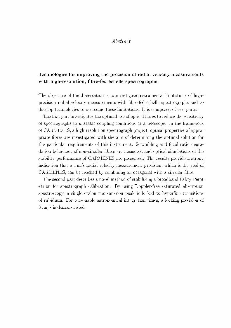
Technologies for improving the precision of radial velocity measurements
with high-resolution, bre-fed échelle spectrographs
The objective of the dissertation is to investigate instrumental limitations of high-
precision radial velocity measurements with bre-fed échelle spectrographs and to
develop technologies to overcome these limitations. It is composed of two parts:
The rst part investigates the optimal use of optical bres to reduce the sensitivity
of spectrographs to unstable coupling conditions at a telescope. In the framework
of CARMENES, a high-resolution spectrograph project, optical properties of appro-
priate bres are investigated with the aim of determining the optimal solution for
the particular requirements of this instrument. Scrambling and focal ratio degra-
dation behaviour of non-circular bres are measured and optical simulations of the
stability performance of CARMENES are presented. The results provide a strong
indication that a 1m/s radial velocity measurement precision, which is the goal of
CARMENES, can be reached by combining an octagonal with a circular bre.
The second part describes a novel method of stabilizing a broadband Fabry-Pérot
etalon for spectrograph calibration. By using Doppler-free saturated absorption
spectroscopy, a single etalon transmission peak is locked to hyperne transitions
of rubidium. For reasonable astronomical integration times, a locking precision of
3 cm/s is demonstrated.

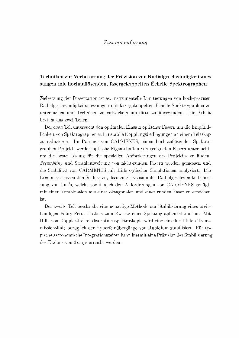
Zusammenfassung
Techniken zur Verbesserung der Präzision von Radialgeschwindigkeitsmes-
sungen mit hochauösenden, fasergekoppelten Échelle Spektrographen
Zielsetzung der Dissertation ist es, instrumentelle Limitierungen von hoch-präzisen
Radialgeschwindigkeitsmessungen mit fasergekoppelten Échelle Spektrographen zu
untersuchen und Techniken zu entwickeln um diese zu überwinden. Die Arbeit
besteht aus zwei Teilen:
Der erste Teil untersucht den optimalen Einsatz optischer Fasern um die Empnd-
lichkeit von Spektrographen auf unstabile Kopplungsbedingungen an einem Teleskop
zu reduzieren. Im Rahmen von CARMENES, einem hoch-auösenden Spektro-
graphen Projekt, werden optische Eigenschaften von geeigneten Fasern untersucht,
um die beste Lösung für die speziellen Anforderungen des Projektes zu nden.
Scrambling und Strahlaufweitung von nicht-runden Fasern werden gemessen und
die Stabilität von CARMENES mit Hilfe optischer Simulationen analysiert. Die
Ergebnisse lassen den Schluss zu, dass eine Präzision der Radialgeschwindkeitsmes-
sung von 1m/s, welche somit auch den Anforderungen von CARMENES genügt,
mit einer Kombination aus einer oktagonalen und einer runden Faser zu erreichen
ist.
Der zweite Teil beschreibt eine neuartige Methode zur Stabilisierung eines breit-
bandigen Fabry-Pérot Etalons zum Zwecke einer Spektrographenkalibration. Mit
Hilfe von Doppler-freier Absorptionsspektroskopie wird eine einzelne Etalon Trans-
missionslinie bezüglich der Hyperfeinübergänge von Rubidium stabilisiert. Für ty-
pische astronomische Integrationszeiten kann hiermit eine Präzision der Stabilisierung
des Etalons von 3 cm/s erreicht werden.

Acronyms
ADEV Allan deviationAPC angled physical contact
CFP confocal Fabry-PérotCTE coecient of thermal expan-
sionCU calibration unit
ECDL external cavity diode laserEE encircled energy
FE front-endFF far eldFFP bre Fabry-PérotFoV eld of viewFPE Fabry-Pérot etalonFRD focal ratio degradationFSR free spectral rangeFWHM full width half maximum
GIF gradient index bre
HCL hollow-cathode lamp
LFC laser frequency comb
MHF mode-hop freeMM multi-mode
NA numerical apertureNF near eld
PD photo diodePID proportional-integral-derivativePM polarisation maintainingPSF point spread function
RV radial velocity
SG scrambling gainSMF single-mode breSNR signal to noise ratio
ThAr thorium argon

Contents
1 Introduction 3
1.1 Exoplanet Detection Methods . . . . . . . . . . . . . . . . . . . . . . 41.2 Radial Velocities . . . . . . . . . . . . . . . . . . . . . . . . . . . . . 71.3 Échelle Spectrographs . . . . . . . . . . . . . . . . . . . . . . . . . . 91.4 CARMENES . . . . . . . . . . . . . . . . . . . . . . . . . . . . . . . 121.5 Objective and Outline . . . . . . . . . . . . . . . . . . . . . . . . . . 15
2 Optical Fibres in High-Resolution Spectroscopy 19
2.1 Theoretical Background . . . . . . . . . . . . . . . . . . . . . . . . . 192.2 Optical Properties of Fibres . . . . . . . . . . . . . . . . . . . . . . . 26
2.2.1 Scrambling . . . . . . . . . . . . . . . . . . . . . . . . . . . . 262.2.2 Focal Ratio Degradation . . . . . . . . . . . . . . . . . . . . . 29
2.3 Requirements for CARMENES . . . . . . . . . . . . . . . . . . . . . 302.4 Experiments . . . . . . . . . . . . . . . . . . . . . . . . . . . . . . . . 32
2.4.1 Optical Test Setup . . . . . . . . . . . . . . . . . . . . . . . . 322.4.2 Neareld Measurement Procedure . . . . . . . . . . . . . . . . 342.4.3 Fareld Measurement Procedure . . . . . . . . . . . . . . . . . 362.4.4 Results . . . . . . . . . . . . . . . . . . . . . . . . . . . . . . . 39
2.5 Numerical Simulations . . . . . . . . . . . . . . . . . . . . . . . . . . 482.5.1 Fibre Simulations . . . . . . . . . . . . . . . . . . . . . . . . . 482.5.2 Impact of Fibre Illumination Eects on RV Precision . . . . . 542.5.3 Pupil vs. Image Coupling . . . . . . . . . . . . . . . . . . . . 64
2.6 Modal Noise . . . . . . . . . . . . . . . . . . . . . . . . . . . . . . . . 662.6.1 Background . . . . . . . . . . . . . . . . . . . . . . . . . . . . 662.6.2 Experiments . . . . . . . . . . . . . . . . . . . . . . . . . . . . 68
2.7 Dynamical Billiard . . . . . . . . . . . . . . . . . . . . . . . . . . . . 722.7.1 Billiard Systems . . . . . . . . . . . . . . . . . . . . . . . . . . 722.7.2 Circular, Elliptical and Oval Boundaries . . . . . . . . . . . . 762.7.3 Polygonal Boundaries . . . . . . . . . . . . . . . . . . . . . . . 772.7.4 Boundaries with Chaotic Dynamics . . . . . . . . . . . . . . . 78
2.8 Fibres for CARMENES . . . . . . . . . . . . . . . . . . . . . . . . . . 812.8.1 Mechanical Considerations . . . . . . . . . . . . . . . . . . . . 832.8.2 Fibre Preparation . . . . . . . . . . . . . . . . . . . . . . . . . 84
2.9 Conclusion and Future Work . . . . . . . . . . . . . . . . . . . . . . . 87
1
Contents
3 Stabilized Fabry-Pérot Etalon for High-Resolution Spectrographs 91
3.1 Introduction to Wavelength Calibration . . . . . . . . . . . . . . . . . 913.1.1 Emission Lamps . . . . . . . . . . . . . . . . . . . . . . . . . . 913.1.2 Gas Absorption Cell . . . . . . . . . . . . . . . . . . . . . . . 943.1.3 Laser Frequency Combs . . . . . . . . . . . . . . . . . . . . . 953.1.4 Etalons . . . . . . . . . . . . . . . . . . . . . . . . . . . . . . 96
3.2 Fabry-Pérot Etalon . . . . . . . . . . . . . . . . . . . . . . . . . . . . 973.2.1 Theory . . . . . . . . . . . . . . . . . . . . . . . . . . . . . . . 973.2.2 Types of Etalons . . . . . . . . . . . . . . . . . . . . . . . . . 1023.2.3 Etalon Mirror Coatings . . . . . . . . . . . . . . . . . . . . . . 1083.2.4 Etalon Tuning . . . . . . . . . . . . . . . . . . . . . . . . . . . 112
3.3 Laser Locked Etalon Concept . . . . . . . . . . . . . . . . . . . . . . 1143.4 Experiments . . . . . . . . . . . . . . . . . . . . . . . . . . . . . . . . 116
3.4.1 Laser . . . . . . . . . . . . . . . . . . . . . . . . . . . . . . . . 1163.4.2 Rubidium Doppler Free Spectroscopy . . . . . . . . . . . . . . 1183.4.3 Etalons . . . . . . . . . . . . . . . . . . . . . . . . . . . . . . 1213.4.4 Data Acquisition and Software . . . . . . . . . . . . . . . . . . 1233.4.5 Locking Stability . . . . . . . . . . . . . . . . . . . . . . . . . 128
3.5 Reliability and Systematics . . . . . . . . . . . . . . . . . . . . . . . . 1343.6 Échelle Measurements . . . . . . . . . . . . . . . . . . . . . . . . . . 1373.7 Conclusion and Future Work . . . . . . . . . . . . . . . . . . . . . . . 139
Bibliography 143
2
1 Introduction
Two possibilities exist: either we
are alone in the universe or we are
not. Both are equally terrifying.
Arthur C. Clarke
Are we alone in the universe? Is our solar system unique? Is our Earth and life
unique? For the rst time in the history of mankind, these fundamental questions
can be scientically investigated. One of the crowning achievements of modern as-
tronomy is the discovery of the rst planet around a Sun-like star by Mayor and
Queloz (1995). Together with the earlier discovery of a planetary system around
a pulsar by Wolszczan and Frail (1992), these studies initiated an entirely new re-
search eld in astronomy. In particular, the exploration of planetary companions
around other stars, called extra solar planets or exoplanets, has become a rapidly
expanding research area of modern astronomy.
As of today, more than 1500 conrmed exoplanets have been detected and the num-
ber of exoplanets has been steadily increasing over the last decades, thus allowing
scientists to improve their statistics on the existence of planets.1 Recent publica-
tions suggest that there is at least one planet per star in our galaxy (Cassan et al.,
2012). In addressing the question of the uniqueness of our Earth, planets around
stars within their habitable zone (HZ) are of particular interest. Usually, the HZ is
dened as the region around a star in which the surface temperature of a potential
planet is such that water would be in liquid form. Current estimates indicate that
about one in ve Sun-like stars hosts an Earth-sized planet within its HZ (Petigura
et al., 2013). Occurrence rates of planets around low mass stars, the most abun-
dant type of stars in our universe, are possibly even higher (Tuomi et al., 2014).
Considering the 100 to 300 billion stars in our galaxy, these estimates put into new
perspective the unanswered question of whether our Earth is unique.
However, an actual Earth twin, i.e. a planet with environmental conditions com-
parable to the ones on our planet, has not been detected so far. It still remains
1Source: http://exoplanets.org/
3
1 Introduction
technically extremely challenging, since such a discovery requires the exploration of
the composition of an exoplanet including its atmosphere. Even so, there exist some
candidates such as Kepler-22b, which is a planet with 2.4 times the radius of Earth
orbiting within the HZ of a solar type star (Borucki et al., 2012). Up to now, little
is known about its mass, its composition, and its potential atmosphere. However,
some ongoing studies already probe the atmospheres of individual exoplanets and
rst claims of detection of water in atmospheres have been made, see e.g. Fraine
et al. (2014).
The enormous progress in exoplanetary research over the last decades has only
been possible due to advances in technology that allowed for suitable high-precision
measurements. This development is likely to even accelerate in the foreseeable fu-
ture, considering the numerous facilities that are either currently being built or
planned, such as ground based spectrograph projects (see Section 1.3 and Table 1.1
in particular) as well as space missions like PLATO and the James Webb Space
Telescope. These projects concentrate on further rening the statistics on exoplanet
occurrence rates, learning about planet formation and evolution, as well as actually
probing physical and chemical properties of individual planets.
1.1 Exoplanet Detection Methods
In the following, I summarize the most successful methods that are currently be-
ing used for exoplanet detection. A more detailed overview of instrumentation for
exoplanetary research can be found in Pepe et al. (2014a).
Direct Detection
Imaging, or direct detection, is the only technique that collects light from the exo-
planets themselves. This is hindered by the extreme contrast in apparent brightness
of host star and planet and their physical closeness. Only a few planets have been
directly observed and all of them are massive planets located at a great distance
from the host star. Such images are obtained in the infrared, because the contrast
ratio between the star and the planet is smaller at longer wavelength. One example
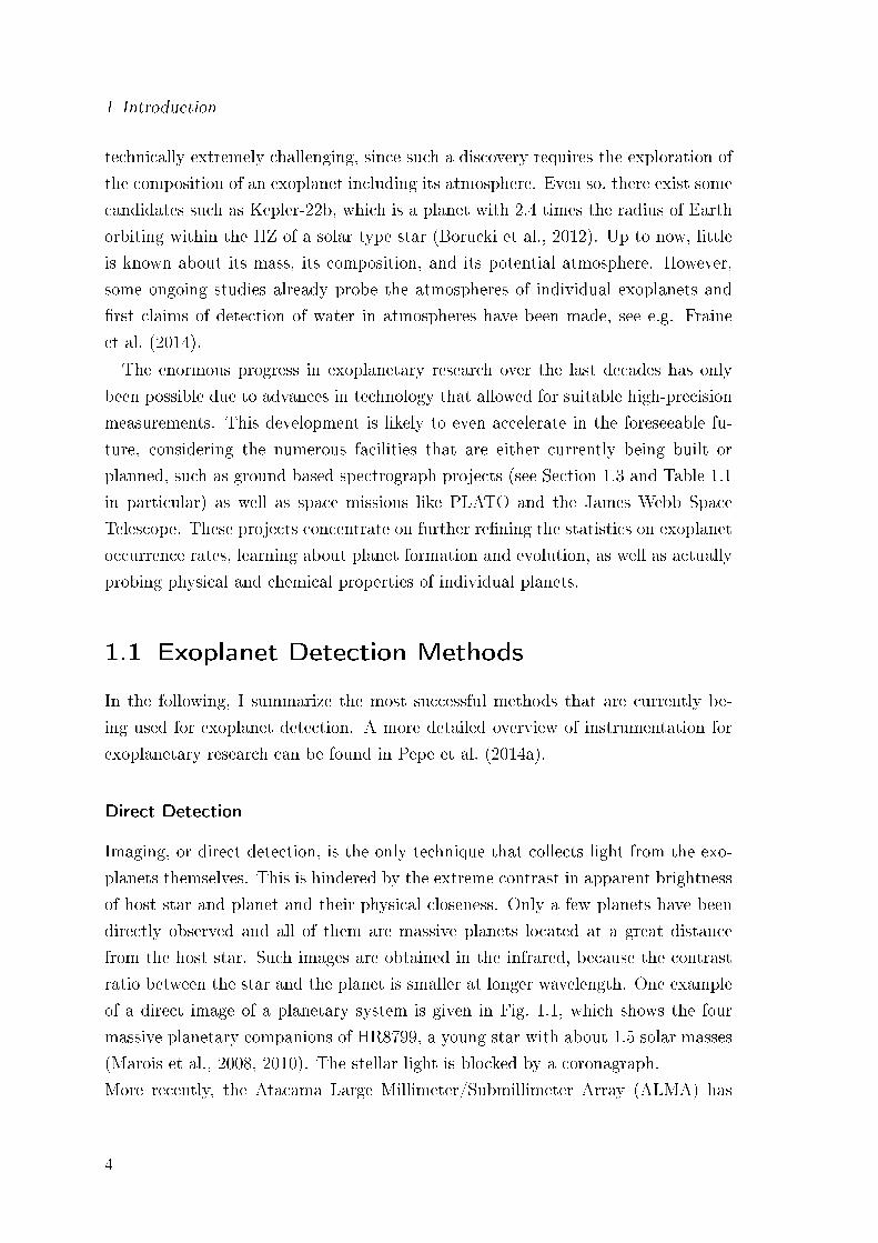
of a direct image of a planetary system is given in Fig. 1.1, which shows the four
massive planetary companions of HR8799, a young star with about 1.5 solar masses
(Marois et al., 2008, 2010). The stellar light is blocked by a coronagraph.
More recently, the Atacama Large Millimeter/Submillimeter Array (ALMA) has
4
1.1 Exoplanet Detection Methods
taken an image of a planet-forming disc around the star HL Tauri (Fig. 1.1). The
image reveals structures in the accretion disc around the young star, indicating the
ongoing formation process of planets within a system. However, only very few sys-
tems can be imaged directly and most detections of exoplanets have been made by
indirect methods.
Figure 1.1 Left: Direct image of HR8799 and its four companions (b-e). Source:Marois et al. (2010). Right: The protoplanetary disc around HL Tauri, a young starlocated approximately 450 light years from earth. Source: http://www.eso.org/public/news/eso1436/
Transiting
The transit technique monitors stars for periodic dips in their light curves that result
from partial eclipses of the stellar disc while a planetary body is transiting. These
dips can only be detected when the planetary system is observed edge-on from the
Earth. Assuming a random orientation of planetary orbits around other stars, the
probability of an edge-on orientation for a planet around a Sun-sized star is below
1%. The drop in brightness of a star due to a transiting planet is, depending on the
size of both the planet and the star, on the order of a few percent or below. The rst
planet that has been detected by transiting was HD 209458b (Charbonneau et al.,
2000), and follow-up observations allowed for a precise determination of its mass, its
density, and even of its actual atmospheric composition. By far the most successful
5
1 Introduction
project using the transit method for detecting exoplanets was the Kepler mission,
that looked for planets around 190000 stars in the constellations Cygnus, Lyra, and
Draco. Kepler discovered over 3000 planet candidates and most of them are waiting
for their conrmation by follow-up observations. It is expected that around 90% of
these candidates will be conrmed as planets.
Dynamical Methods and Microlensing
All other indirect methods rely on the impact of the planets' gravity.
The radial velocity (RV) method measures the line of sight velocity of a star to
infer the existence of any planets. It will be described in more detail in the next
section.
Astrometry can be used to map the orbit of a host star when circling the common
barycentre with its planetary companion. The astrometric precision required lies
beyond what ground-based telescopes can deliver. Benedict et al. (2002) published
the conrmation of a planet, which had been discovered with the radial velocity
method, by astrometric measurements using the Hubble Space Telescope. This was
the rst time, the astrometric signal of a planet could be detected. It is expected that
the currently launched GAIA satellite will deliver astrometric data of unprecedented
precision of about one billion stars and will discover thousands of planets via their
astrometric signal.
Microlensing also detects the planets' gravity eld, but in a very dierent way.
When two stars are almost perfectly aligned with respect to the line of sight from an
observer on Earth, the foreground star acts as a lens that magnies the light of the
background star. This eect is called gravitational lensing. During a microlensing
event, which may last days or weeks, the apparent brightness of the foreground
star is changing in a very characteristic fashion. In case the foreground star has
a planetary companion, the light curve is disturbed and by comparing models to
the observed shape of the light curve, one can deduce physical parameters of the
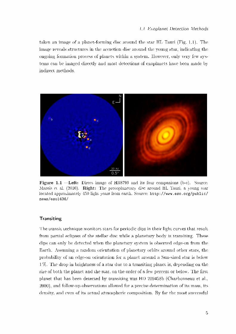
companion such as its mass and orbital distance. As an example, Fig. 1.2 shows
the light curve of a microlensing event that led to the discovery of a 5.5 Earth-mass
planet, which was the lowest mass of any exoplanet around a regular star that had
been discovered at that time (Beaulieu et al., 2006). Compared to other methods,
microlensing is quite sensitive to low-mass planets. However, one major drawback
of the method is that it is not repeatable: The lensing event occurs just once, since
Earth, the foreground and the background star are moving.
6
1.2 Radial Velocities
Figure 1.2 Observed light curve of a microlensing event that led to the discovery of alow mass planet around OGLE-2005-BLG-390. Source: Beaulieu et al. (2006)
Of the detection methods discussed, the transit and RV methods have detected
the bulk of currently known planetary systems. As a matter of fact, they may com-
plement each other in the case where both methods can be used for the same target.
The transit method gives insight into the orbital period, inclination (as a require-
ment), and ratio of radii between the host star and its companion. The RV method
allows to determine period, eccentricity, and mass ratio modulo the inclination an-
gle. Together, both methods yield extra information such as the average density
of the planet, initiating further theoretical work on the formation mechanisms and
inner composition of exoplanets, which are still mainly unexplored.
1.2 Radial Velocities
The radial velocity (RV) of an astronomical object is dened as its velocity projected
onto the line of sight of an observer. Variations of this velocity can be measured
by the use of Doppler spectroscopy: as an object moves towards the observer, its
spectrum gets blue shifted and red shifted when the object recedes. When a planet
moves around a host star, both objects circle the common barycentre. This in-
teraction leads depending on the inclination angle of the planet's orbit to a
characteristic and periodic variation of the radial velocity (RV) of the host star. By
observing the stellar spectrum and comparing it to some reference, the RV variations
can be measured and parameters of the planetary orbit can be deduced.
However, the RV variations induced by a planet can be rather small. More precisely,
7
1 Introduction
−0.2 0.0 0.2 0.4 0.6 0.8 1.0 1.2Phase
−150
−100
−50
0
50
100
150
Rad
ial V
eloc
ity (
m/s
)
51 Peg b, trend removed
P = 4.2 d
exoplanets.org2000 2001 2002 2003 2004 2005 2006
Year
−400
−200
0
200
400
Rad
ial V
eloc
ity (
m/s
)
ι Dra b, trend removed
exoplanets.org
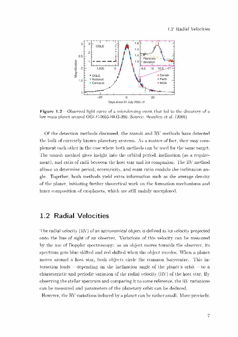
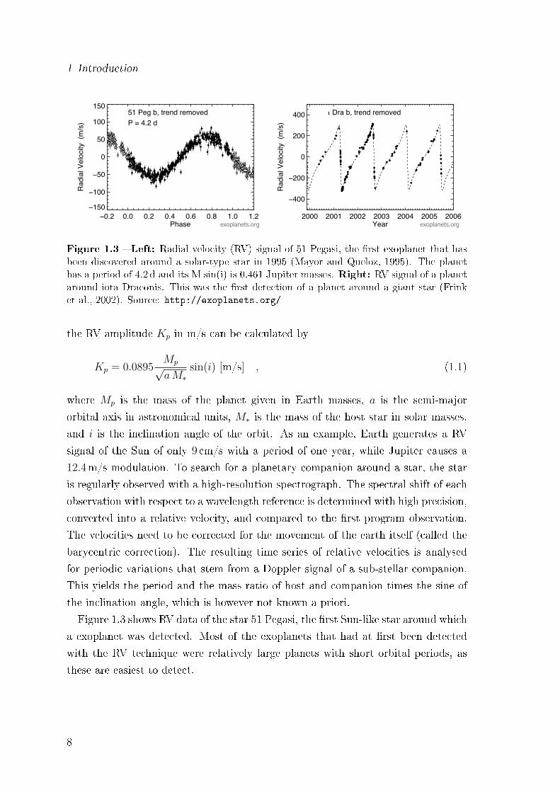
Figure 1.3 Left: Radial velocity (RV) signal of 51 Pegasi, the rst exoplanet that hasbeen discovered around a solar-type star in 1995 (Mayor and Queloz, 1995). The planethas a period of 4.2 d and its M sin(i) is 0.461 Jupiter masses. Right: RV signal of a planetaround iota Draconis. This was the rst detection of a planet around a giant star (Frinket al., 2002). Source: http://exoplanets.org/
the RV amplitude Kp in m/s can be calculated by
Kp = 0.0895Mp√aM∗
sin(i) [m/s] , (1.1)
where Mp is the mass of the planet given in Earth masses, a is the semi-major
orbital axis in astronomical units, M∗ is the mass of the host star in solar masses,
and i is the inclination angle of the orbit. As an example, Earth generates a RV
signal of the Sun of only 9 cm/s with a period of one year, while Jupiter causes a
12.4m/s modulation. To search for a planetary companion around a star, the star
is regularly observed with a high-resolution spectrograph. The spectral shift of each
observation with respect to a wavelength reference is determined with high precision,
converted into a relative velocity, and compared to the rst program observation.
The velocities need to be corrected for the movement of the earth itself (called the
barycentric correction). The resulting time series of relative velocities is analysed
for periodic variations that stem from a Doppler signal of a sub-stellar companion.
This yields the period and the mass ratio of host and companion times the sine of
the inclination angle, which is however not known a priori.
Figure 1.3 shows RV data of the star 51 Pegasi, the rst Sun-like star around which
a exoplanet was detected. Most of the exoplanets that had at rst been detected
with the RV technique were relatively large planets with short orbital periods, as
these are easiest to detect.
8

1.3 Échelle Spectrographs
The fractional shift in wavelength of a spectral line due to the Doppler shift is
given by
∆λ/λ0 = RV/c , (1.2)
where λ0 is the wavelength if the star did not move relative to Earth, and c is the
speed of light. In order to measure RV shifts in the meter per second regime or even
below, fractional wavelength shifts on the order of 1× 10⁻⁹ have to be detected.
This requires extraordinarily stable and precise spectrographs.
1.3 Échelle Spectrographs
Figure 1.4 A true colour image of an échelle spectrum recorded using a commercialDSLR camera with the laboratory échelle spectrograph at the Landessternwarte Heidel-berg. Each order covers only a few nanometres wavelength range, but due to the two-dimensional format of an échelle spectrum, a large bandwidth can be recorded at once.
The key component for any high-resolution spectroscopic measurements in astron-
omy is a so called échelle spectrograph. The term échelle is derived from the French
word for ladder, and is also used to name the diraction grating, which is the char-
acteristic element of an échelle spectrograph. Échelle gratings are characterized by
a very large groove spacing and the groove prole is shaped for the use at large blaze
angles and thus high diraction orders. Because of the high order of diraction, the
9
1 Introduction
theoretical resolving power R is also high:
R =λ
∆λ= mN , (1.3)
where m is the diraction order and N is the total number of illuminated grooves.
However, the above formula is only true in case of diraction limited optics. When
observing stars from the ground with large telescopes, the turbulence of the earth's
atmosphere leads to a blurring of the objects. Their angular size on the sky, φ, does
not decrease for larger telescope mirrors. For this so called seeing-limited case, the
resolution of a spectrograph scales as
R ∝ W
φD, (1.4)
where W is the width of the grating, and D is the diameter of the telescope
(Schroeder, 1999). This relation is the reason, why large telescopes require large
spectrograph optics, including large échelle gratings for high-resolution spectroscopy.
Throughout the thesis, I will use the terms resolving power and resolution inter-
changeable, following common nomenclature in the astronomical literature.
Échelles provide dispersion comparable to the highest line density holographic
gratings, but as they operate in high orders, the free spectral range (FSR) for each
order, i.e. the largest wavelength range that does not overlap with the same range
of an adjacent order, is small:
FSR = λ/m . (1.5)
For m of the order 100 and for wide spectral bandpass often spanning the whole
visible wavelength range, this means that the spectrum is divided into several ten or-
ders. All orders of an échelle overlap, and one needs a secondary dispersive element,
called the cross disperser, which is oriented perpendicular to the échelle's dispersion
direction. Essentially, the cross disperser slightly shifts the orders apart so that
they become disentangled and can be recorded simultaneously on a rectangular de-
tector array. This matching of the spectrum's spatial distribution to commercially
available detectors enables the wide simultaneous bandwidth desired in stellar spec-
troscopy, and is the prime advantage of the cross dispersed échelle conguration.
A typical échelle spectrum is shown in Fig. 1.4. Échelle spectrographs used for
Doppler studies operate with resolution of the order 100000. However, as stated
10
1.3 Échelle Spectrographs
above a fractional precision of 1× 10⁻⁹ four orders of magnitude below the native
resolution of a spectrograph is needed to detect RV signals of small planets. This
corresponds to a shift of only several nanometres on the detector. To be able to
measure shifts of the whole spectrum by this small fraction of a resolution element,
and in addition over periods of many months or years, one needs an extraordinarily
stable and well-calibrated instrument. Imperceptibly small movements of the optics
or the spectrograph bench can move the spectrum well beyond the desired amount.
Likewise, temperature changes in the mounts, optical elements or the detector may
shift the spectrum. Finally, pressure changes in the refractive index of the medium
surrounding the dispersive elements translate the spectrum on short time-scales To
counteract these eects, the leading instruments are mounted inside a vacuum vessel
and their temperature is very tightly regulated. The opto-mechanical engineering
aims to reduce the sensitivity to temperature changes as much as possible by using
low CTE materials. Lastly, very precise wavelength calibration techniques are used
to monitor instrumental drifts, often during the science exposure, and to calibrate
out any remaining shifts of the spectrum that can mask a RV signal.
However, all these measures only concern the inherent stability of the spectro-
graph. The spectrum is also sensitive to the coupling conditions, namely the input
illumination. This is because an échelle spectrograph images its input slit, which is
in case of a bre-fed instrument an image of the bre itself. Illumination changes
in the spatial and angular distribution of the light will lead to a misinterpretation of
the spectral content of the light. Additionally to detection limitations, there are also
intrinsic eects arising from the stars' activity that hinder precise RV measurements.
Sun-spots, stellar pulsation, ares and also rotation all eect the RV measured and
it depends on the particular target star, which is what kind of noise is dominant.
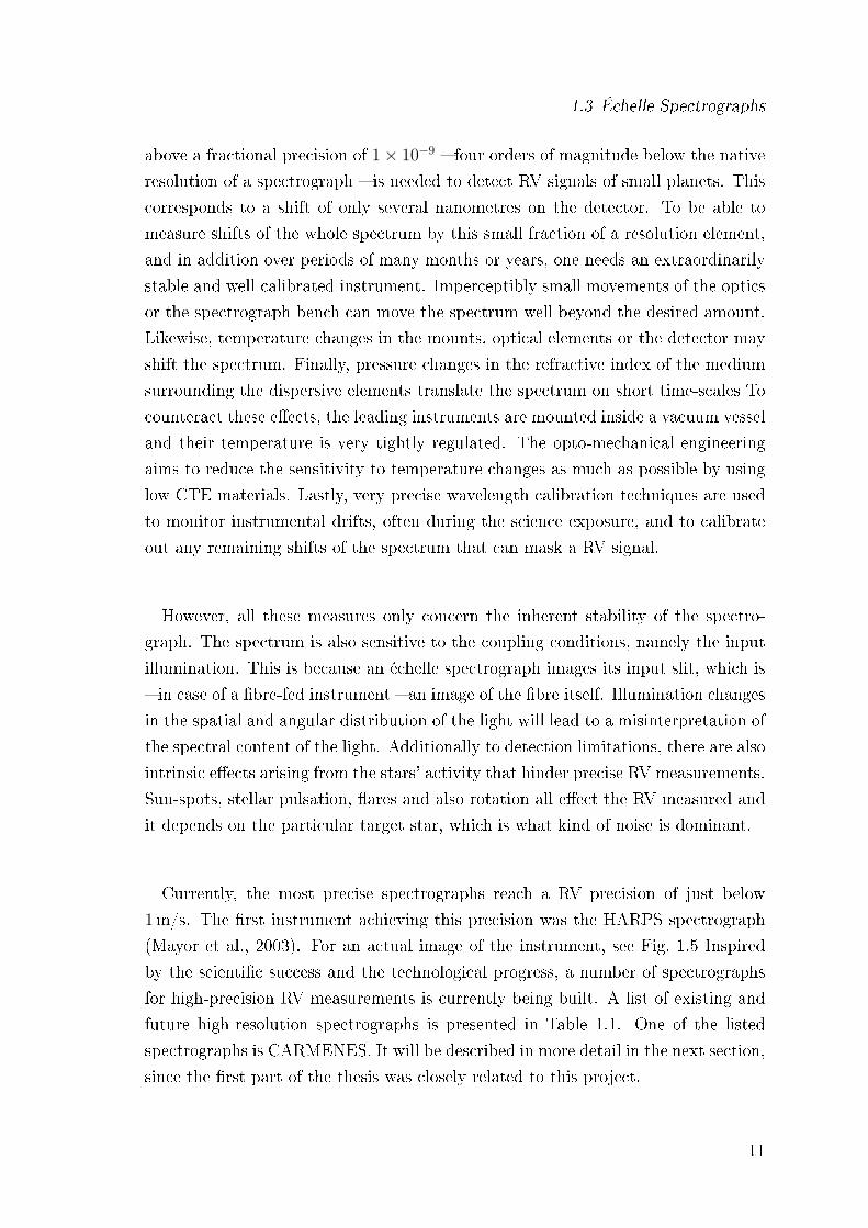
Currently, the most precise spectrographs reach a RV precision of just below
1m/s. The rst instrument achieving this precision was the HARPS spectrograph
(Mayor et al., 2003). For an actual image of the instrument, see Fig. 1.5 Inspired
by the scientic success and the technological progress, a number of spectrographs
for high-precision RV measurements is currently being built. A list of existing and
future high-resolution spectrographs is presented in Table 1.1. One of the listed
spectrographs is CARMENES. It will be described in more detail in the next section,
since the rst part of the thesis was closely related to this project.
11
1 Introduction
Figure 1.5 The optical bench of the HARPS spectrograph is enclosed in a vacuum tank.At the centre, the large optical échelle grating can be seen. Source: http://www.eso.org
1.4 CARMENES
CARMENES is a high-resolution spectroscopy facility for the 3.5m telescope at the
Calar Alto Observatory in Granada (Spain), consisting of two R ∼ 82000 échelle
spectrographs, one for the visual range from 550nm to 950nm (VIS) and one for
the near infrared range from 950nm to 1700nm (NIR) (Quirrenbach et al., 2012).
The main scientic goal of CARMENES is to search for planets within the HZs
of 300 low-mass stars. This is also suggested by the ocial logo of CARMENES
(Fig. 1.6): the red circle represents the M-dwarf (also called red dwarf due to its
typical apparent colour), the smaller black circle a potential planet.
Figure 1.6 CARMENES [kár-men-es] stands for: Calar Alto high-resolution search forM dwarfs with exoearths with near-infrared and optical échelle spectrographs
12
1.4 CARMENES
There are several reasons why a study of exoplanets around M-dwarfs is a logical
next step in the exoplanet research. As stated before, an Earth-like planet around
a Sun-like star produces a RV signal of about 10 cm/s. However, such precision
cannot be reached with today's astronomical spectrographs and next generation
instruments like ESPRESSO (Pepe et al., 2014b) have yet to prove that it is tech-
nically feasible. When looking for Earth-like planets around low-mass stars at the
same orbital distance, the RV signature is considerably higher, because the ampli-
tude of the signal increases with decreasing stellar mass. In addition, the HZ lies
closer to M-dwarfs than to solar-type stars, which also implies an increased RV am-
plitude for planets within this zone according to Eq. (1.1). Stellar luminosity is a
steep function of stellar mass that ultimately denes the actual location of the HZ.
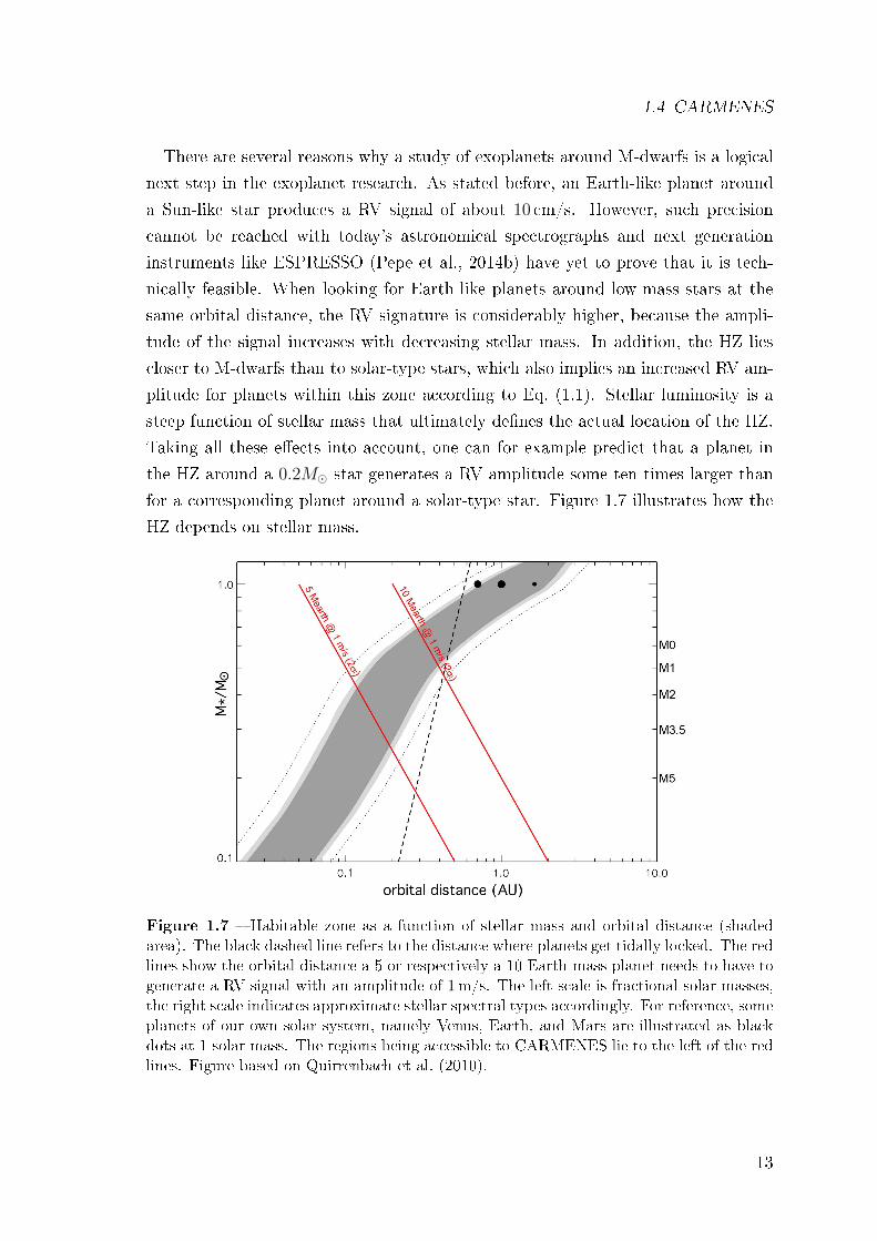
Taking all these eects into account, one can for example predict that a planet in
the HZ around a 0.2M star generates a RV amplitude some ten times larger than
for a corresponding planet around a solar-type star. Figure 1.7 illustrates how the
HZ depends on stellar mass.
Figure 1.7 Habitable zone as a function of stellar mass and orbital distance (shadedarea). The black dashed line refers to the distance where planets get tidally locked. The redlines show the orbital distance a 5 or respectively a 10 Earth-mass planet needs to have togenerate a RV signal with an amplitude of 1m/s. The left scale is fractional solar masses,the right scale indicates approximate stellar spectral types accordingly. For reference, someplanets of our own solar system, namely Venus, Earth, and Mars are illustrated as blackdots at 1 solar mass. The regions being accessible to CARMENES lie to the left of the redlines. Figure based on Quirrenbach et al. (2010).
13
1 Introduction
M-dwarfs are by far the most abundant stars in our milky way (∼ 75%) and
obtaining statistics on planet abundance around these stars is therefore pivotal to
understanding planet formation and evolution. However, the number of planets
that have been found around low-mass stars is low compared to those around solar-
type stars. The main reason for this is that the stars are relatively faint in the
visible wavelength range and that their intrinsic stellar jitter hinders the detection
of planets with current high-resolution spectrographs.
Camera
Échelle grating Collimator
Cross disperserCCD
Image slicer
Fold mirror
Fibre exit
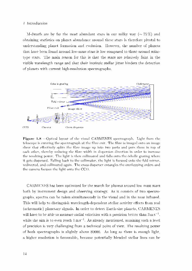
Figure 1.8 Optical layout of the visual CARMENES spectrograph. Light from thetelescope is entering the spectrograph at the bre exit. The bre is imaged onto an imageslicer that eectively splits the bre image up into two parts and puts them in top ofeach other, thereby reducing the bre width in dispersion direction in order to increasethe resolving power. The light is then collimated and falls onto the échelle grating whereit gets dispersed. Falling back to the collimator, the light is focused onto the fold mirror,redirected, and collimated again. The cross disperser entangles the overlapping orders andthe camera focuses the light onto the CCD.
CARMENES has been optimised for the search for planets around low mass stars
both by instrument design and observing strategy. As it consists of two spectro-
graphs, spectra can be taken simultaneously in the visual and in the near infrared.
This will help to distinguish wavelength-dependent stellar activity eects from real
(achromatic) planetary signals. In order to detect Earth-size planets, CARMENES
will have to be able to measure radial velocities with a precision better than 3ms−1,
while the aim is to even reach 1ms−1. As already mentioned, attaining such a level
of precision is very challenging from a technical point of view. The resolving power
of both spectrographs is slightly above 80000. As long as there is enough light,
a higher resolution is favourable, because potentially blended stellar lines can be
14
1.5 Objective and Outline
resolved, thus allowing for more precise RV determination (Bouchy et al., 2001).
However, above ∼80000 the gain in RV precision with increasing resolution is small
in case of typical M-dwarf spectra. According to Eq. (1.4), a higher resolving power
also needs either larger optics, or the eld of view (and therefore the number of
available photons) has to be reduced. There is another possibility to increase the
resolving power: In the optical design of CARMENES (see Fig. 1.8), an image slicer
is used to cut the bre image in half in dispersion direction and reassemble it such
that the two halves are on top of each other, roughly doubling the image size in
cross dispersion direction but reducing it by the same factor in dispersion direction,
eectively doubling the resolution (see also Section 2.5.2). Due to its non-linear
nature, the usage of an image slicer is delicate and it comes at the price of higher
cross dispersion needed to entangle the échelle orders and more detector pixels to
cover the same bandwidth.
According to the current schedule of CARMENES, the VIS spectrograph will be
delivered to Calar Alto in April 2015 and the NIR spectrograph in September 2015.
First scientic results are expected to be obtained by December 2015.
1.5 Objective and Outline
The objective of this thesis is to investigate instrumental limitations of high precision
RV measurements with bre coupled échelle spectrographs. The thesis is split into
two parts that can be read independently. The rst part investigates the optimal
use of optical bres to reduce the sensitivity of spectrographs to unstable coupling
conditions at a telescope. The second part of the thesis describes a novel method to
generate an extremely stable and precise wavelength calibrator.
Chapter 2 deals with the properties of optical bres and their optimal use for spec-
troscopy in the framework of the CARMENES project. After a general introduction
to the optical properties of bres in Section 2.1, I discuss the most important proper-
ties in the context of high-resolution spectroscopy in Section 2.2. The requirements
regarding the CARMENES project are introduced in Section 2.3.
I present experimental data in Section 2.4 and numerical simulations on illumination
eects in bres and their corresponding impact on spectrum stability are discussed
in Section 2.5. In Section 2.6, I investigate methods to mitigate the consequences of
the limited number of modes in an optical bre. Section 2.7 provides a theoretical
foundation based on dynamical billiard systems to explain the diering scrambling
performances of various types of bres. In Section 2.8, I present an overview of
15
1 Introduction
the CARMENES bre link with an emphasis on its actual manufacturing. Finally,
Section 2.9 concludes the rst part of the thesis.
Chapter 3 describes a novel precise wavelength calibration method. After an
introduction on current wavelength calibration methods in Section 3.1, I discuss
in detail the theory of Fabry-Pérot etalons and present own simulations on etalon
mirror coatings in Section 3.2. Section 3.3 presents an active locking concept based
on laser spectroscopy that enables the usage of an etalon as a stable and precise
wavelength calibrator. Section 3.4 describes the conducted experiments and analyses
the obtained locking stability. In Section 3.5, the reliability of the setup is discussed.
I present basic échelle measurements of the transmission spectrum of etalons in
Section 3.6. Finally, Section 3.7 concludes the second part of the thesis and provides
an outlook on future work.
16
1.5 Objective and Outline
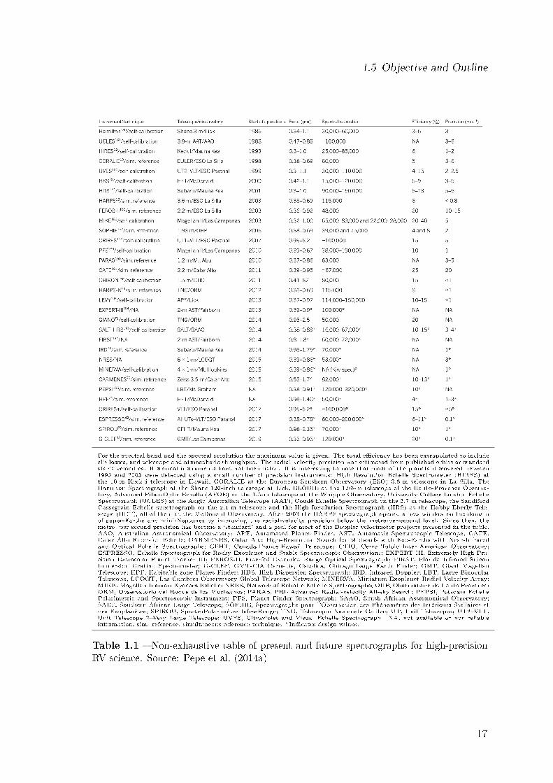
For the spectral band and the spectral resolution the maximum value is given. The total eciency has been extrapolated to includeslit losses, and telescope and atmospheric throughput. The radial-velocity precision was estimated from published orbits or standardstar's velocities. Historical instruments have not been listed. It is interesting to note that most of the planets discovered between1995 and 2003 were detected using a small number of precision instruments: High Resolution Echelle Spectrometer (HIRES) atthe 10-m Keck i telescope in Hawaii, CORALIE at the European Southern Observatory (ESO) 3.6-m telescope in La Silla, TheHamilton Spectrograph at the Shane 120-inch telescope at Lick, ELODIE at the 1.93-m telescope of the Haute-Provence Observa-tory, Advanced Fiber-Optic Echelle (AFOE) on the 1.5-m telescope at the Whipple Observatory, University College London ÉchelleSpectrograph (UCLES) at the Anglo-Australian Telescope (AAT), Coudé Echelle Spectrograph on the 2.7-m telescope, the SandifordCassegrain Echelle spectrograph on the 2.1-m telescope and the High-Resolution Spectrograph (HRS) at the Hobby-Eberly Tele-scope (HET), all of them at the McDonald Observatory. After 2003 the HARPS spectrograph opened a new window on the domainof super-Earths and mini-Neptunes by improving the radial-velocity precision below the metre-per-second level. Since then, themetre- per-second precision has become a `standard' and a goal for most of the Doppler-velocimeter projects presented in the table.AAO, Australian Astronomical Observatory; APF, Automated Planet Finder; AST, Automatic Spectroscopic Telescope; CAFE,Calar Alto Fiber-fed Echelle; CARMENES, Calar Alto High-Resolution Search for M dwarfs with Exo-Earths with Near-Infraredand Optical Echelle Spectrographs; CFHT, Canada-France-Hawaii Telescope; CTIO, Cerro Tololo Inter-American Observatory;ESPRESSO, Echelle Spectrograph for Rocky Exoplanet and Stable Spectroscopic Observations; EXPERT-III, Extremely High Pre-cision Extrasolar Planet Tracker III; FEROS-II, Fiberfed Extended Range Optical Spectrograph; FIRST, Florida Infrared SiliconImmersion Grating Spectrometer; G-CLEF, GMT-CfA Carnegie, Catolica, Chicago Large Earth Finder; GMT, Giant MagellanTelescope; HPF, Habitable-zone Planet Finder; HDS, High Dispersion Spectrograph; IRD, Infrared Doppler; LBT, Large BinocularTelescope; LCOGT, Las Cumbres Observatory Global Telescope Network; MINERVA, Miniature Exoplanet Radial Velocity Array;MIKE, Magellan Inamori Kyocera Echelle; NRES, Network of Robotic Echelle Spectrographs; OHP, Observatoire de Haute Provence;ORM, Observatorio del Roque de los Muchachos; PARAS, PRL Advanced Radial-velocity All-sky Search; PEPSI, Potsdam EchellePolarimetric and Spectroscopic Instrument; PFS, Planet Finder Spectrograph; SAAO, South African Astronomical Observatory;SALT, Southern African Large Telescope; SOPHIE, Spectrographe pour l'Observation des Phénomènes des Intérieurs Stellaires etdes Exoplanètes; SPIROU, SpectroPolarimètre Infra-Rouge; TNG, Telescopio Nazionale Galileo; UT, Unit Telescopes; UT2VLT,Unit Telescope 2Very Large Telescope; UVES, Ultraviolet and Visual Echelle Spectrograph. NA, not available or non-reliableinformation; sim. reference, simultaneous reference technique. *Indicates design values.
Table 1.1 Non-exhaustive table of present and future spectrographs for high-precisionRV science. Source: Pepe et al. (2014a)
17

2 Optical Fibres in High-Resolution
Spectroscopy
The results presented in this chapter have partly been published in Stürmer et al.
(2014). Unless stated otherwise, all gures presented are based on own calculations
or measurements.
2.1 Theoretical Background
The optical properties of bres are usually described by the means of ray or wave
optics. For bres with a large core size, the ray optical treatment is a good ap-
proximation but becomes more and more inaccurate when the core size of the bre
decreases towards diameters that are only a few times larger than the wavelength.
Following the more descriptive approach, we will introduce the basic properties of
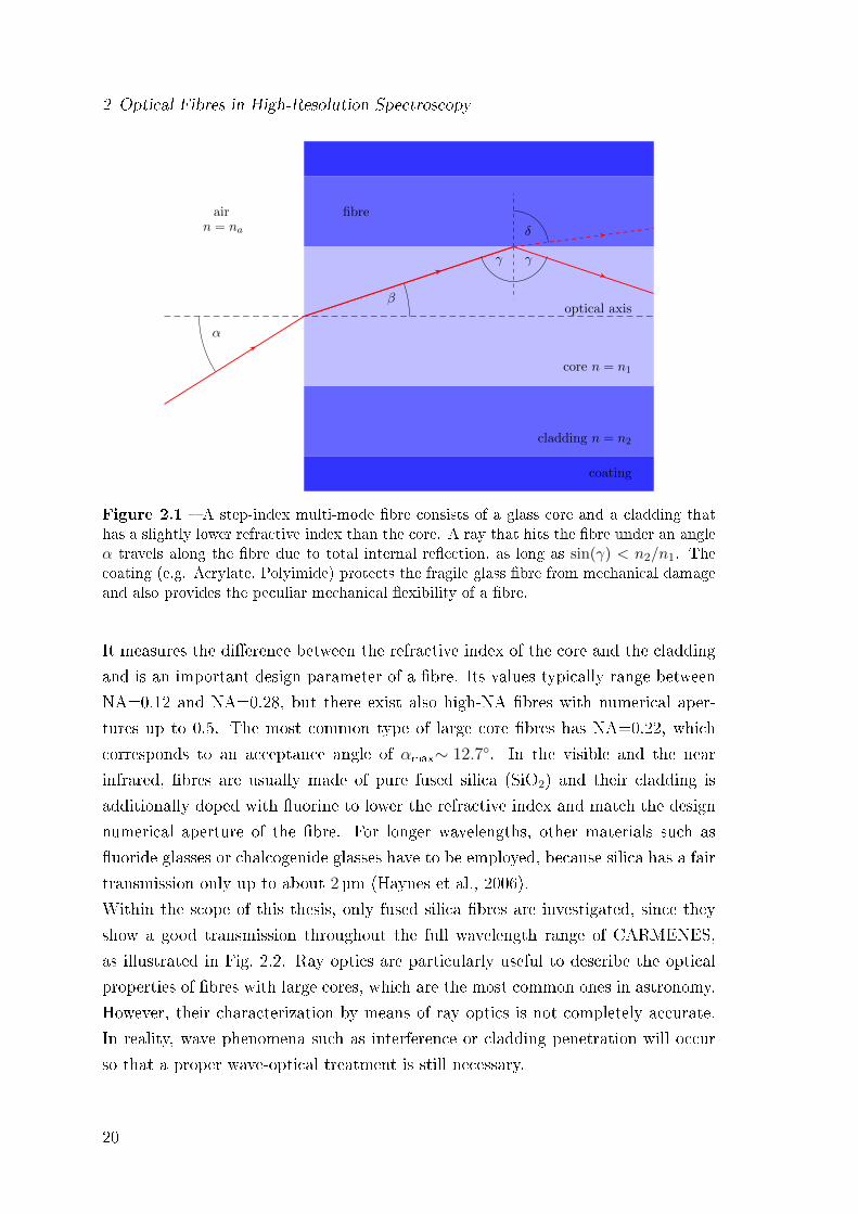
optical bres by ray optics. Figure 2.1 illustrates the ray propagation inside a step-
index bre, which is the most commonly used type of optical bre in astronomy.
This bre consists of a core with a refractive index n1 and a cladding with a slightly
lower index n2. When light is coupled into the bre from an ambient medium with
index na, its angle with respect to the optical axis of the bre is refracted according
to Snell's law to sin(β) = na/n1 sin(α). The ray is propagating inside the core and
eventually hits the cladding, where it gets reected by total internal refection as long
as the incidence angle γ is smaller than sin(γmax) = n2/n1. This can be translated
into the maximum acceptance angle of the bre
αmax = arcsin
(√n2
1 − n22
). (2.1)
The argument of the arcsin is called numerical aperture (NA):
NA =√n2
1 − n22 . (2.2)
19
2 Optical Fibres in High-Resolution Spectroscopy
core n = n1
fibreairn = na
coating
cladding n = n2
α
β
γ γ
δ
optical axis
Figure 2.1 A step-index multi-mode bre consists of a glass core and a cladding thathas a slightly lower refractive index than the core. A ray that hits the bre under an angleα travels along the bre due to total internal reection, as long as sin(γ) < n2/n1. Thecoating (e.g. Acrylate, Polyimide) protects the fragile glass bre from mechanical damageand also provides the peculiar mechanical exibility of a bre.
It measures the dierence between the refractive index of the core and the cladding
and is an important design parameter of a bre. Its values typically range between
NA=0.12 and NA=0.28, but there exist also high-NA bres with numerical aper-
tures up to 0.5. The most common type of large core bres has NA=0.22, which
corresponds to an acceptance angle of αmax∼ 12.7. In the visible and the near
infrared, bres are usually made of pure fused silica (SiO2) and their cladding is
additionally doped with uorine to lower the refractive index and match the design
numerical aperture of the bre. For longer wavelengths, other materials such as
uoride glasses or chalcogenide glasses have to be employed, because silica has a fair
transmission only up to about 2 µm (Haynes et al., 2006).
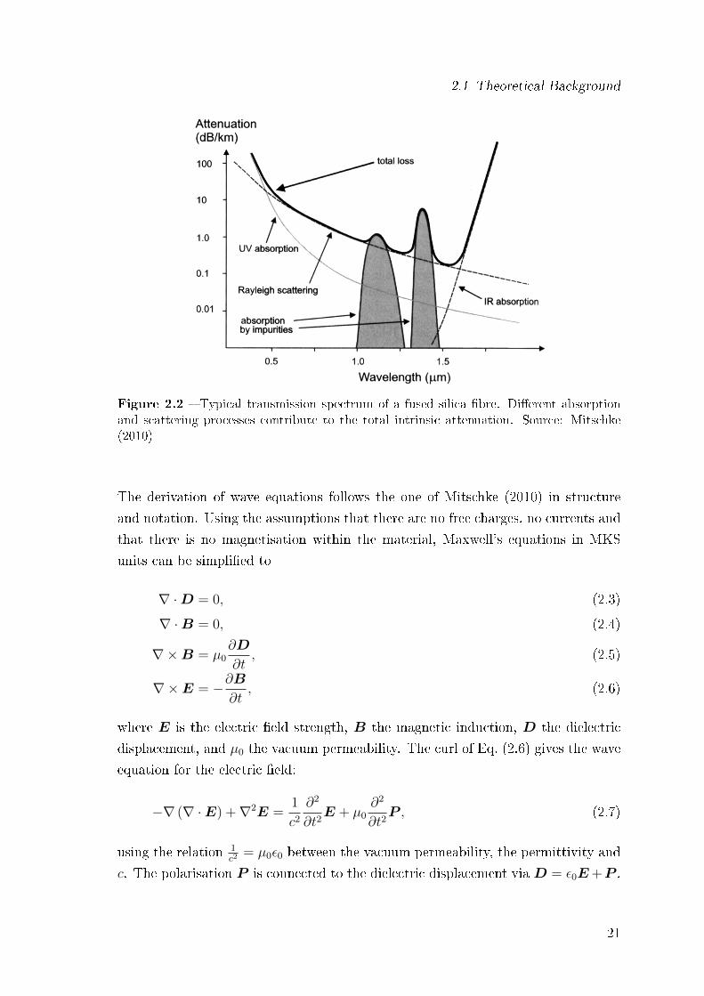
Within the scope of this thesis, only fused silica bres are investigated, since they
show a good transmission throughout the full wavelength range of CARMENES,
as illustrated in Fig. 2.2. Ray optics are particularly useful to describe the optical
properties of bres with large cores, which are the most common ones in astronomy.
However, their characterization by means of ray optics is not completely accurate.
In reality, wave phenomena such as interference or cladding penetration will occur
so that a proper wave-optical treatment is still necessary.
20
2.1 Theoretical Background
Figure 2.2 Typical transmission spectrum of a fused silica bre. Dierent absorptionand scattering processes contribute to the total intrinsic attenuation. Source: Mitschke(2010)
The derivation of wave equations follows the one of Mitschke (2010) in structure
and notation. Using the assumptions that there are no free charges, no currents and
that there is no magnetisation within the material, Maxwell's equations in MKS
units can be simplied to
∇ ·D = 0, (2.3)
∇ ·B = 0, (2.4)
∇×B = µ0∂D
∂t, (2.5)
∇×E = −∂B∂t
, (2.6)
where E is the electric eld strength, B the magnetic induction, D the dielectric
displacement, and µ0 the vacuum permeability. The curl of Eq. (2.6) gives the wave
equation for the electric eld:
−∇ (∇ ·E) +∇2E =1
c2
∂2
∂t2E + µ0
∂2
∂t2P , (2.7)
using the relation 1c2
= µ0ε0 between the vacuum permeability, the permittivity and
c. The polarisation P is connected to the dielectric displacement via D = ε0E +P .
21
2 Optical Fibres in High-Resolution Spectroscopy
Equation (2.7) can be derived for the magnetic eld in an analogous way.
An optical bre made of ultra-pure fused silica can well be approximated by a
homogeneous medium, which means one can assume that the polarisation is always
parallel to the eld strength. Therefore, the dielectrics are isotropic: ε = ε0εr with
εr being a scalar. Additionally, light intensities are always low in astronomical
spectroscopy, which implies a linear relationship between P and E. The wave
equation can therefore be further simplied to
∇2E =n2
c2
∂2
∂t2E, (2.8)
with n2 = ε being the refractive index and respectively for the magnetic component
of the wave
∇2H =n2
c2
∂2
∂t2H . (2.9)
In case of a step index bre in the linear regime (low light intensities), the ansatz
E = E0NZT (2.10)
allows to separate the wave function into its eld distribution in the plane normal
to the z-axis N = N (x, y), along the z-axis Z = Z(z), and a monochromatic wave
with angular frequency ω: T (t) = eıωt.
Finally, the wave equation can be simplied to the Helmholtz equation:
∇2NZ + n2k20NZ = 0 . (2.11)
The solution to this equations can be derived analytically only in few cases when
symmetries of the underlying geometry can be used to simplify the problem. For a
bre, Z takes the form e−ıβz with wave number β.
In a circular step index bre, the equation can be solved by using a cylindrical
coordinate system and the solutions take the general form:
N (r, φ) = c1Jm(ur/a) cos(mφ+ φ0) : r ≤ a (2.12)
N (r, φ) = c2Km(wr/a) cos(mφ+ φ0) : r > a, (2.13)
where a is the core radius and c1, c2 are normalization constants, which account for
the smoothness of the solution at the core cladding transition at r = a. The integer
22
2.1 Theoretical Background
m is derived from the azimuthal part of Eq. (2.11). Jm is the Bessel function of rst
kind and Km is the modied Bessel function of second kind.
The dimensionless quantities u and w depend on the refractive indices of the bre,
its diameter, and the wavelength. The constant√u2 + w2 is called normalized
frequency or V-number, and is dened as
V =√u2 + w2 = k0 aNA =
2π
λ0
a√
(n21 − n2
2) . (2.14)
The V-number is of great importance, since it determines all relevant information
about the bre as well as the wavelength.
The conditions for smooth transition at r = a and recursion relations between Bessel
functions allow to derive the characteristic equations:
Jm(u)
uJm+1(u)=
Km(w)
wKm+1(w)and w =
√V2 − u2 . (2.15)
Obviously, only certain combinations of arguments yield valid solutions of these
equations. The discrete set of solutions is called (guided) modes and is denoted
by LPmp, where the index m species the number of pairs of azimuthal maxima
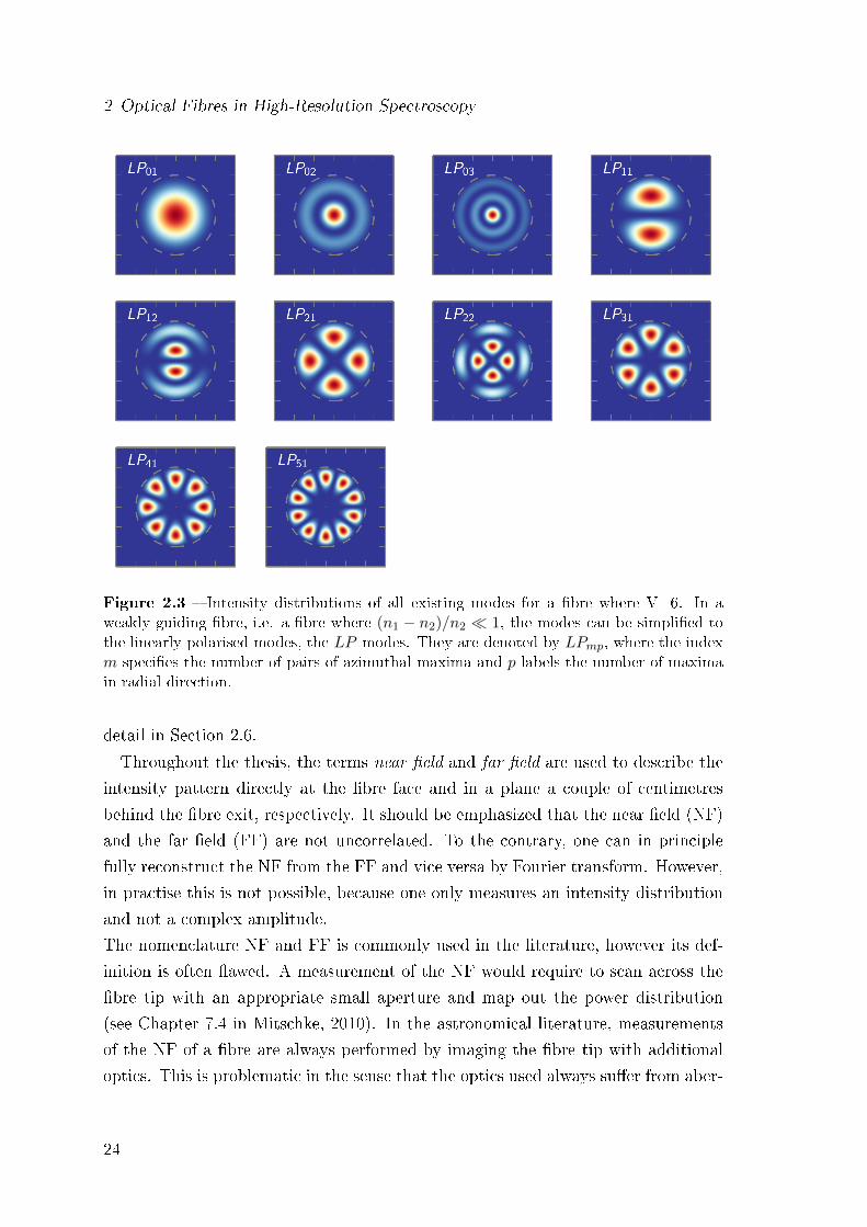
and p labels the number of maxima in radial direction. As an example, Fig. 2.3
shows the intensity patterns of all existing modes in a circular bre where V=6. As
noted above, the V-number contains information about the particular experimental
conditions (wavelength) and the bre. V also denes the number of guided modes
inside a bre. For V∼ 2.405, there exists only one mode, the LP01, and the bre is
called a single-mode bre (SMF). In practice, this means that assuming a standard
NA the core radius is suciently small, i.e. a few microns for visible light.
As it is impossible to couple light from a telescope into a SMF eciently (at least
for large telescopes without the use of adaptive optics), bres with core radii from
50µm to 400µm are commonly used in astronomy. In case of a step index bre, the
number of supported modes for large V-numbers can be approximated by
Nmodes ≈4
π2V2 ≈ V2/2 . (2.16)
For a 100µm diameter bre, the number of modes available in the visible is on the
order of a few thousands and when coupling light into it, a superposition of these
modes will get excited. The limited number of modes within a bre will lead to an
additional noise contribution in a bre-fed spectrograph as will be described in more
23
2 Optical Fibres in High-Resolution Spectroscopy
Figure 2.3 Intensity distributions of all existing modes for a bre where V=6. In aweakly guiding bre, i.e. a bre where (n1 − n2)/n2 1, the modes can be simplied tothe linearly polarised modes, the LP modes. They are denoted by LPmp, where the indexm species the number of pairs of azimuthal maxima and p labels the number of maximain radial direction.
detail in Section 2.6.
Throughout the thesis, the terms near eld and far eld are used to describe the
intensity pattern directly at the bre face and in a plane a couple of centimetres
behind the bre exit, respectively. It should be emphasized that the near eld (NF)
and the far eld (FF) are not uncorrelated. To the contrary, one can in principle
fully reconstruct the NF from the FF and vice versa by Fourier transform. However,
in practise this is not possible, because one only measures an intensity distribution
and not a complex amplitude.
The nomenclature NF and FF is commonly used in the literature, however its def-
inition is often awed. A measurement of the NF would require to scan across the
bre tip with an appropriate small aperture and map out the power distribution
(see Chapter 7.4 in Mitschke, 2010). In the astronomical literature, measurements
of the NF of a bre are always performed by imaging the bre tip with additional
optics. This is problematic in the sense that the optics used always suer from aber-
24
2.1 Theoretical Background
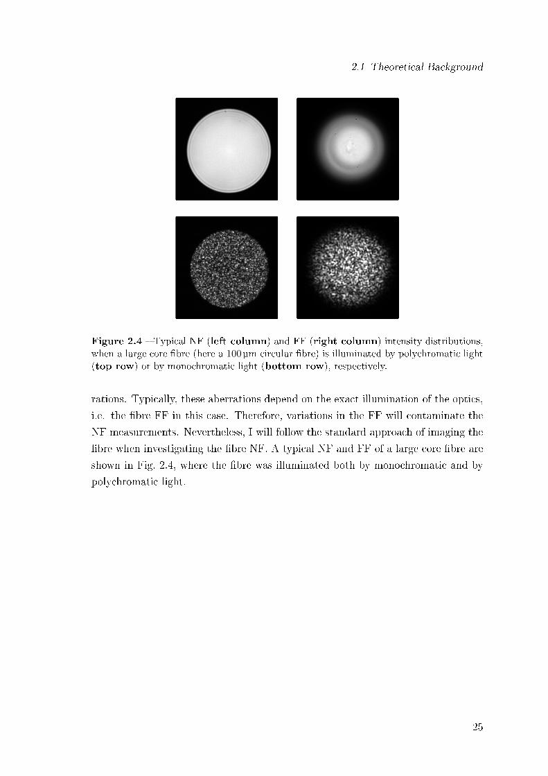
Figure 2.4 Typical NF (left column) and FF (right column) intensity distributions,when a large core bre (here a 100 µm circular bre) is illuminated by polychromatic light(top row) or by monochromatic light (bottom row), respectively.
rations. Typically, these aberrations depend on the exact illumination of the optics,
i.e. the bre FF in this case. Therefore, variations in the FF will contaminate the
NF measurements. Nevertheless, I will follow the standard approach of imaging the
bre when investigating the bre NF. A typical NF and FF of a large core bre are
shown in Fig. 2.4, where the bre was illuminated both by monochromatic and by
polychromatic light.
25
2 Optical Fibres in High-Resolution Spectroscopy
2.2 Optical Properties of Fibres
Fibres are a key optical element of a bre-fed spectrograph. Not only do they al-
low to separate the spectrograph from the highly variable environmental conditions
the telescope is exposed to. They also stabilize the input illumination of the spec-
trograph, which is an important factor for high-precision spectroscopy in terms of
attainable RV precision. However, one major drawback is that they do not conserve
the étendue.1 The main optical properties of bres that are of particular inter-
est for astronomical spectrographs will be discussed in more detail in the next two
subsections.
2.2.1 Scrambling
During the late 1970s and early 1980s, astronomers realized that optical bres could
signicantly reduce systematic wavelength errors in spectroscopic measurements
compared to slit spectrographs, due to their incomplete transfer of spatial image
content (Serkowski et al., 1979; Heacox, 1988). In case of a slit spectrograph, errors
of the guiding of the telescope, dierent focus positions and seeing variations all
lead to a direct change of the illumination of the spectrograph. These illumination
eects cause systematic wavelength shifts that limit the RV precision attainable
for Doppler spectroscopic measurements. However, in case of a bre-coupled spec-
trograph, guiding errors and other environmental parameters such as temperature
entail a change of the particular coupling conditions of the bre. Luckily, while
the light is travelling along the bre, this spatial information is partly lost. This
benecial property of a bre is called scrambling. It is one of the greatest benets
of a bre-fed spectrograph compared to a slit spectrograph. Yet, the output of a
bre is not fully independent of its input. As a consequence, changes in the bre
illumination may cause a varying bre output. In case of an échelle spectrograph,
this can easily be misinterpreted as a change of the spectral content of the light.
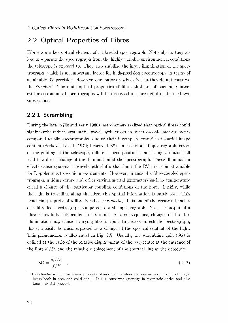
This phenomenon is illustrated in Fig. 2.5. Usually, the scrambling gain (SG) is
dened as the ratio of the relative displacement of the barycentre at the entrance of
the bre di/Di and the relative displacement of the spectral line at the detector:
SG =di/Di
f/F, (2.17)
1The étendue is a characteristic property of an optical system and measures the extent of a lightbeam both in area and solid angle. It is a conserved quantity in geometric optics and alsoknown as AΩ product.
26
2.2 Optical Properties of Fibres
D
d
Fibre input
Scrambler
Spectrograph
Spectral line
f
F
SG = d/Df/F
Scrambling gain:
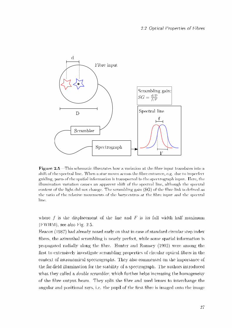
Figure 2.5 This schematic illustrates how a variation at the bre input translates into ashift of the spectral line. When a star moves across the bre entrance, e.g. due to imperfectguiding, parts of the spatial information is transported to the spectrograph input. Here, theillumination variation causes an apparent shift of the spectral line, although the spectralcontent of the light did not change. The scrambling gain (SG) of the bre link is dened asthe ratio of the relative movements of the barycentres at the bre input and the spectralline.
where f is the displacement of the line and F is its full width half maximum
(FWHM), see also Fig. 2.5.
Heacox (1987) had already noted early on that in case of standard circular step index
bres, the azimuthal scrambling is nearly perfect, while some spatial information is
propagated radially along the bre. Hunter and Ramsey (1992) were among the
rst to extensively investigate scrambling properties of circular optical bres in the
context of astronomical spectrographs. They also commented on the importance of
the far-eld illumination for the stability of a spectrograph. The authors introduced
what they called a double scrambler, which further helps increasing the homogeneity
of the bre output beam. They split the bre and used lenses to interchange the
angular and positional rays, i.e. the pupil of the rst bre is imaged onto the image
27
2 Optical Fibres in High-Resolution Spectroscopy
plane of the second bre and vice versa. By doing so, they increased the poor radial
scrambling of the circular bre and at the same time stabilized the far-eld of the
entire bre link. Their device had a throughput of only 20%, but the principle
of exchanging near eld and far eld became the standard solution for many high
stability spectrographs. Examples are the HERMES spectrograph (Raskin et al.,
2011), the HR+ mode of the SOPHIE+ spectrograph (Perruchot et al., 2008) or
HARPS (Pepe et al., 2000). By optimisation of the design, the throughput could
further be increased and lies between 70% to 85% for more recent devices (Barnes
and MacQueen, 2010).
Avila et al. (2006) and Avila and Singh (2008) investigated alternative scrambling so-
lutions, such as solid light pipes, mechanical squeezing and bre agitating, single lens
scramblers, and beam homogenizers. A promising candidate with good scrambling
eciencies is the mechanical squeezing of bres. Hereby, the bres are slightly bent
at small radii, which increases the mode-to-mode coupling and results in a more
homogeneous near eld and far eld pattern. However, stress on bres is known
to increase focal ratio degradation (FRD) (see next section) and the experiments
mentioned above showed indeed a reduced FRD performance. Avila et al. (2010)
and Chazelas et al. (2010) presented rst results for the scrambling performance
of bres with a non-circular core geometry. Square, rectangular, and octagonal ge-
ometries were shown to have very promising scrambling properties. These results
have been conrmed by subsequent work, see Avila (2012),Chazelas et al. (2012),
and Spronck et al. (2012). In particular, octagonal bres are nowadays used on-sky
in several high-resolution spectrographs with excellent results, e.g. at CHIRON,
HAPRS-North or SOPHIE+ (Tokovinin et al., 2013; Cosentino et al., 2012; Perru-
chot et al., 2011), where in case of the latter they are used in combination with an
optical double scrambler.
28
2.2 Optical Properties of Fibres
2.2.2 Focal Ratio Degradation
Optical axis
Input coneFibre
Output cone with FRD
Output cone of ideal bre
θin θin θout
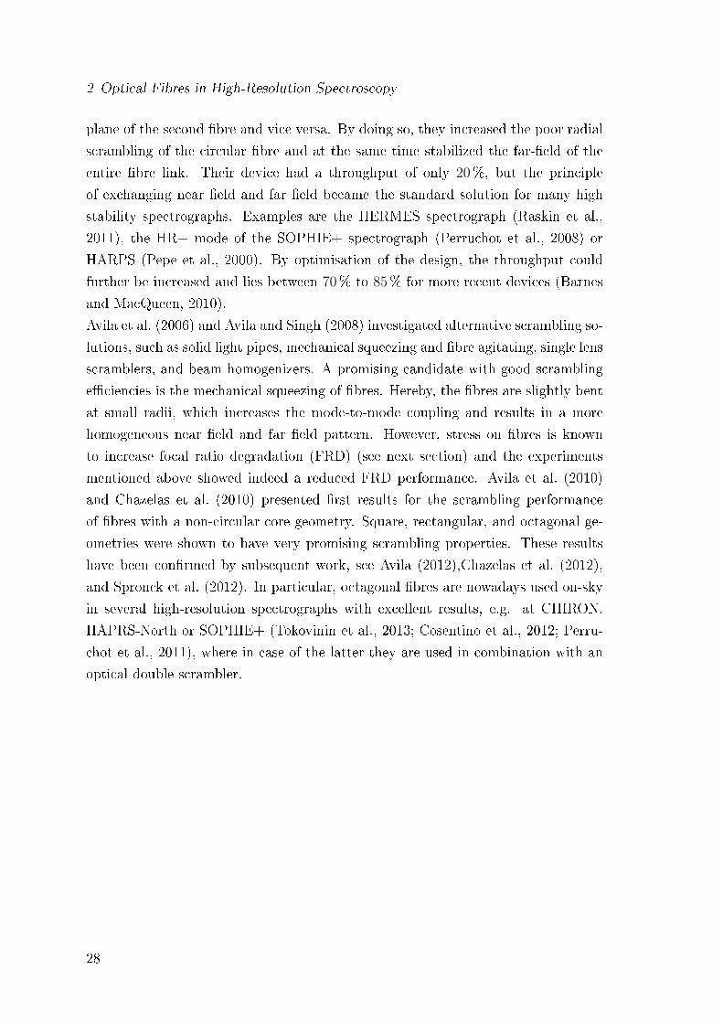
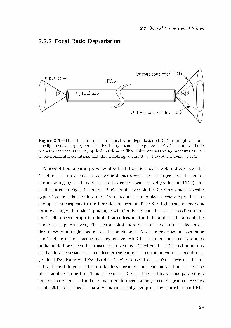
Figure 2.6 The schematic illustrates focal ratio degradation (FRD) in an optical bre:The light cone emerging from the bre is larger than the input cone. FRD is an unavoidableproperty that occurs in any optical multi-mode bre. Dierent scattering processes as wellas environmental conditions and bre handling contribute to the total amount of FRD.
A second fundamental property of optical bres is that they do not conserve the
étendue, i.e. bres tend to scatter light into a cone that is larger than the one of
the incoming light. This eect is often called focal ratio degradation (FRD) and
is illustrated in Fig. 2.6. Parry (1998) emphasized that FRD represents a specic
type of loss and is therefore undesirable for an astronomical spectrograph. In case
the optics subsequent to the bre do not account for FRD, light that emerges at
an angle larger than the input angle will simply be lost. In case the collimator of
an échelle spectrograph is adapted to collect all the light and the F-ratio of the
camera is kept constant, FRD entails that more detector pixels are needed in or-
der to record a single spectral resolution element. Also, larger optics, in particular
the échelle grating, become more expensive. FRD has been encountered ever since
multi-mode bres have been used in astronomy (Angel et al., 1977) and numerous
studies have investigated this eect in the context of astronomical instrumentation
(Avila, 1988; Ramsey, 1988; Barden, 1998; Crause et al., 2008). However, the re-
sults of the dierent studies are far less consistent and conclusive than in the case
of scrambling properties. This is because FRD is inuenced by various parameters
and measurement methods are not standardized among research groups. Haynes
et al. (2011) described in detail what kind of physical processes contribute to FRD:
29
2 Optical Fibres in High-Resolution Spectroscopy
scattering, diraction, and modal diusion. Material impurities, micro- and mac-
robending, mechanical stress, and bre end-face quality all aect FRD. As these
processes have dierent wavelength dependencies, there is yet no consensus in the
literature on the overall wavelength dependency of FRD. Rather, it is determined
by the dominant FRD source of the particular bre under test. There is also no
agreement on whether FRD has a dependency on bre length. If so, it is a small one,
at least for the relatively short bre lengths that typically astronomical bres have
(compared to e.g. telecommunication). Furthermore, precise FRD measurements
are challenging, as for example already slight misalignments of the optical axis of
the bre and the rest of the optical system lead to an additional articial FRD (see
Avila, 1998). One aspect that all research groups agree on is that FRD losses are
generally more prominent when a bre is fed by a beam that is slow compared to the
NA of the bre. As a consequence, the light from the telescope is usually coupled
into bres at F-ratios faster than ≈ F/5 to limit FRD losses.
2.3 Requirements for CARMENES
Scrambling and FRD are important quantities for high-resolution spectrographs that
need to be understood and carefully tested when designing a bre link. This part
of the thesis deals with the following aspects of designing a suitable bre link for
CARMENES: understanding the particularities of optical bres, determining the
relevant parameters for an elaborate bre link and eventually providing such bres.
In doing so, nancial constraints had to be taken into account, since the costs of a
custom bre draw can easily reach a few ten thousand Euro, which is beyond the
project's budget.
The design parameters for the CARMENES bre link were determined by the spe-
cic conditions at the Calar Alto observatory and scientic top level requirements.
According to internal CARMENES documents, the 80 percentile seeing at Calar
Alto is measured to be ∼ 1.05′′ in the V-band and scaled to ∼ 0.9′′ at 1 µm. The
3.5m telescope has a focal ratio of F/10, which corresponds to a plate scale of
169.78µm/′′. In order to collect ∼ 90% of the light of a star for these given seeing
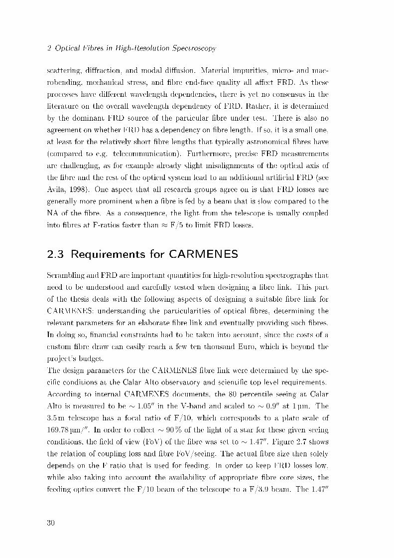
conditions, the eld of view (FoV) of the bre was set to ∼ 1.47′′. Figure 2.7 shows
the relation of coupling loss and bre FoV/seeing. The actual bre size then solely
depends on the F-ratio that is used for feeding. In order to keep FRD losses low,
while also taking into account the availability of appropriate bre core sizes, the
feeding optics convert the F/10 beam of the telescope to a F/3.9 beam. The 1.47′′
30
2.3 Requirements for CARMENES
are then covered by a 100µm bre. As the spectrograph optics accept a F/3.5 beam
emerging from the bre, the design accounts for quite some FRD of the bre link.
The project's minimum requirement on total throughput of both the VIS and NIR
spectrograph including atmosphere and telescope is 5%, while the project's goal is
7%. This translates into a throughput of the bre of 70%, including all types of
losses, such as coupling, FRD, intrinsic absorption. The same factor of 70% is used
for a potential scrambler, since this eciency is typical for a double scrambler as
noted earlier. Therefore, the bre link that includes the scrambler is required to
have a throughput of at least 49%.
The requirement for the scrambling gain is derived from the scientic goal of keep-
ing the total error budget within 1m/s RMS. The guiding accuracy of the 3.5m
telescope is reported to be 0.12′′ RMS, which translates to a shift of about 8.2 µm at
the bre entrance. A resolution element in CARMENES has a width of 3.75 km s−1,
and therefore the scrambling gain has to be SG = 0.12′′/1.47′′
0.5ms−1/3.75 km s−1 ≈ 600 to keep
the systematic shifts below 0.5m/s. In order not to let the guiding errors be the
dominant noise source of the spectrograph, the goal for the scrambling factor was
set to 1000.
Regarding FRD, there is no specic requirement, as FRD losses are already included
by their contribution to the total throughput losses.
0.0 0.5 1.0 1.5 2.0 2.5
Fibre FoV / seeing
0
20
40
60
80
100
cou
plin
glo
ss[%
]
CA
RM
EN
ES
@1
µm
−3 −2 −1 0 1 2 3
x [′′]
−3
−2
−1
0
1
2
3
y[′′
]
Fibre FoV
Figure 2.7 Left: Coupling loss versus bre eld of view/seeing. Right: Gaussiandisk with a typical FWHM according to seeing measurements on Calar Alto and theCARMENES FoV of the bre.
31
2 Optical Fibres in High-Resolution Spectroscopy
2.4 Experiments
This section describes the experiments that I performed to investigate possible so-
lutions for the CARMENES bre link. The optimal solution needs to maximize the
throughput while fullling the project's requirements stated in the previous section.
2.4.1 Optical Test Setup
First, I describe my optical setup of the bre test-bench. I do so in detail, as reliable
and reproducible results strongly dependent on a correct setup. The whole setup is
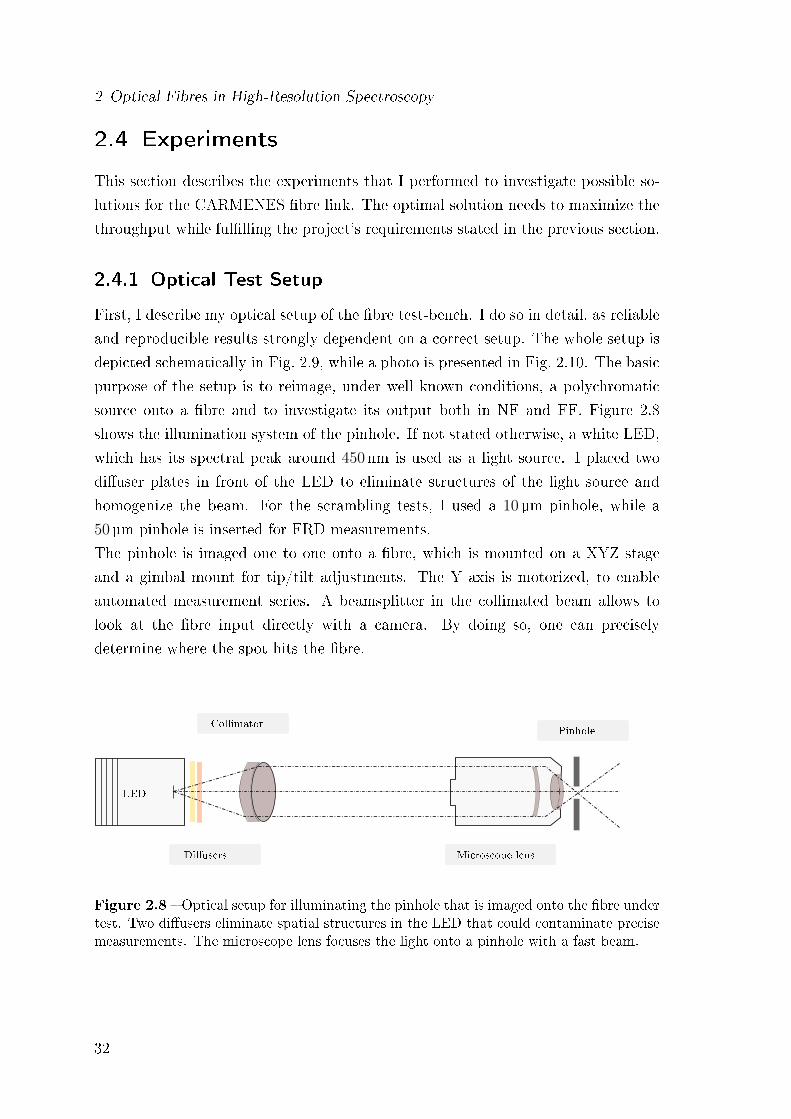
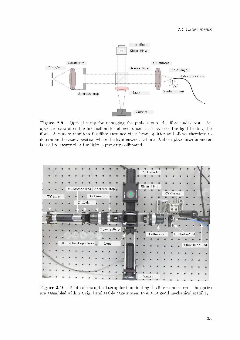
depicted schematically in Fig. 2.9, while a photo is presented in Fig. 2.10. The basic
purpose of the setup is to reimage, under well known conditions, a polychromatic
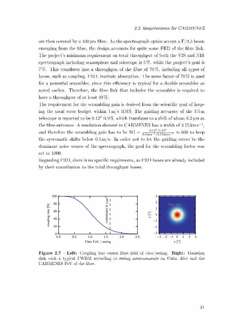
source onto a bre and to investigate its output both in NF and FF. Figure 2.8
shows the illumination system of the pinhole. If not stated otherwise, a white LED,
which has its spectral peak around 450nm is used as a light source. I placed two
diuser plates in front of the LED to eliminate structures of the light source and
homogenize the beam. For the scrambling tests, I used a 10µm pinhole, while a
50µm pinhole is inserted for FRD measurements.
The pinhole is imaged one to one onto a bre, which is mounted on a XYZ stage
and a gimbal mount for tip/tilt adjustments. The Y axis is motorized, to enable
automated measurement series. A beamsplitter in the collimated beam allows to
look at the bre input directly with a camera. By doing so, one can precisely
determine where the spot hits the bre.
PinholeCollimator
Microscope lensDiusers
LED
Figure 2.8 Optical setup for illuminating the pinhole that is imaged onto the bre undertest. Two diusers eliminate spatial structures in the LED that could contaminate precisemeasurements. The microscope lens focuses the light onto a pinhole with a fast beam.
32
2.4 Experiments
Camera
Photodiode
Shear-Plate
Pinhole
Aperture stop
Collimator
Gimbal mount
Fibre under test
XYZ stage
Collimator
Beam splitter
Lens
Figure 2.9 Optical setup for reimaging the pinhole onto the bre under test. Anaperture stop after the rst collimator allows to set the F-ratio of the light feeding thebre. A camera monitors the bre entrance via a beam splitter and allows therefore todetermine the exact position where the light enters the bre. A shear plate interferometeris used to ensure that the light is properly collimated.
Camera
Photodiode
Shear-Plate
Pinhole
Aperture stop
Collimator
Gimbal mount
Fibre under test
XYZ stage
Collimator
Beam splitter
LensSet of xed apertures
XY stage
Microscope lens
Figure 2.10 Photo of the optical setup for illuminating the bres under test. The opticsare assembled within a rigid and stable cage system to ensure good mechanical stability.
33
2 Optical Fibres in High-Resolution Spectroscopy
2.4.2 Neareld Measurement Procedure
In order to measure the scrambling gain, I took a series of images of the NF for
varying positions of the spot on the entrance of the bre. The spot is displaced
across the bre entrance by the motorised axis of the XYZ-stage. According to the
denition of the scrambling gain (SG), see Eq. (2.17), one would need to measure
the SG directly with the spectrograph, which is often not possible. Instead, the SG
is derived by measuring
SG =di/Di
do/Do
, (2.18)
where do/Do is the relative displacement of the barycentre directly at the bre
output (i.e. the shift of the barycentre of the NF).
However, this denition is somewhat problematic due to several reasons. First,
the SG generally varies for dierent spatial displacements di. Thus, it is always
more conclusive to look at a series of displacements rather than presenting just
a single measured SG. Second, the denition only accounts for movements of the
barycentre of the bre output, which is not the only possible source of line distortion
or line shift in a spectrograph. In fact, simulations show that even for circular
bres (which are known to have relatively poor scrambling gain), the contribution
of imperfect scrambling on the barycentre shift is negligible (Allington-Smith et al.,
2012). In reality, barycentric shifts are still measured, due to inhomogeneities of
the bre surface, due to illumination dependent aberrations of the optics used for
investigating the NF, and due to an inhomogeneous sensitivity of the detector. All
these eects are also present in a spectrograph. As a consequence, if one only looks
at the barycentric shift of the bre output, the eect of imperfect scrambling can be
underestimated. On the other hand, the barycentric shift can easily be converted
to a radial velocity error, whereas other measurements of the inhomogeneity of the
NF, such as RMS values or higher image moments, do not have a direct relation to
the RV error. They are therefore only useful for relative comparisons of dierent
bres or scrambling methods.
For precise scrambling gain measurements, the setup needs to be mechanically
very stable. Any movement of the bre that is imaged by the microscope objective
contributes to the overall measured barycentric shift and contaminates precise SG
measurements. Avila et al. (2006) suggested to mount a reference bre next to the
bre under test and to measure only dierential shifts. In case of connectorized
34
2.4 Experiments
bres, this was not possible, because the eld of view of the camera was too small to
image two bres at the same time. Instead, I developed an alternative procedure that
identies bre movements and allows to reject contaminated measurements, or in
some cases, to correct for the movements: After dark subtraction for each NF image,
a mask is created by blurring and thresholding the image. The mask covers the bre
NF plus a small margin around it. All remaining pixel values are ignored for further
processing. By analysing the mask position of the image series, one has a good
indicator of how stable the setup was during the measurement. Ideally, the mask
would not move at all, but only the illumination within it would change. In reality,
the image of the NF will not stay at the exact same position, due to mechanical
instabilities of the setup. In principle, one could correct for these movements of
the bre by subtracting the mask position from the measured barycentres, but non-
linearities and inhomogeneities might lead to ambiguous results. Therefore, I only
used the mask position as an indicator for the setup stability. This method has
another advantage over a simple weighted mean of the whole detector: It eciently
suppresses noise from outside the region of interest that could otherwise massively
distort the results, especially when calculating higher image moments. Figure 2.11
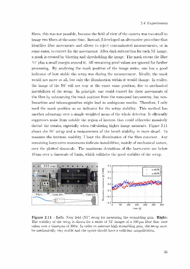
shows the NF setup and a measurement of the bench stability in more detail. To
measure the intrinsic stability, I kept the illumination of the bre constant. Any
remaining barycentre movements indicate instabilities, mainly of mechanical nature,
over the plotted timescale. The maximum deviations of the barycentre are below
10nm over a timescale of 5min, which validates the good stability of the setup.
Fibre
XYZ stage
Lens 20x Camera
Figure 2.11 Left: Near eld (NF) setup for measuring the scrambling gain. Right:
The stability of the setup is shown for a series of NF images of a 100µm bre that weretaken over a timespan of 300 s. In order to measure high scrambling gain, the setup mustbe mechanically very stable and the optics should have a sucient magnication.
35
2 Optical Fibres in High-Resolution Spectroscopy
2.4.3 Fareld Measurement Procedure
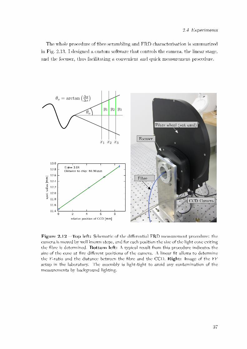
I measured the FF of the bre to check both FRD and the inuence of a moving
spot on the FF structure. For measuring the FRD, the angle of the cone of light
exiting the bre has to be determined. Since the exact distance between the CCD
(FLI ProLine 16803) and the bre is unknown at the beginning of a measurement,
I used a dierential method. I calculated the angle of the outgoing beam θo using a
linear t to the sizes of the FF at dierent distances between the detector and the
bre (Fig. 2.12). The F-ratio of the beam is then dened by
F/# =1
2 tan(θ0). (2.19)
The CCD is mounted with a motorized focuser (FLI Atlas) that allows to control
very precisely the relative distance between the bre and the CCD, as the resolution
of a single step is only 8 nm. After dark subtraction, the size of the light cone is
determined by calculating its radius of 95% encircled energy (EE95). As mentioned
above, FRD measurements can easily be contaminated by a misalignment of the
optical axis of the bre with respect to the illumination system. In order to avoid
this eect, I adjusted the tip/tilt angle at the beginning of the procedure until the
diameter of the cone recorded on the CCD was minimised at a xed distance of the
bre to the CCD, as suggested by Murphy et al. (2008). Other error contributions to
FRDmeasurements are non-perfect collimation, errors in the aperture stop diameter,
and deviations from a top-hat prole of the pupil illumination. To check for correct
collimation of the beam, I used a shearing interferometer. As aperture stops, I used
a set of xed apertures to ensure repeatability in setting the input F-ratio. It should
further be noted that the calculated FRD value also depends on the encircled energy
level used for the determination of the spot size. Choosing EE99 or EE90 will lead to
slightly dierent results (see Wang et al., 2013). This makes the comparison between
the absolute values I measured and the ones proposed in the literature very dicult.
Additionally to the FRD images, I took another set of images in similar fashion as
for the scrambling gain measurements in the NF: while moving the spot across the
bre entrance, I recorded a series of FF images. As mentioned before, there exists
no simple relation between variations in the FF and the RV shifts they entail. I
link RV shifts to FF variations via numerical simulations that will be presented in
Section 2.5.2.
36
2.4 Experiments
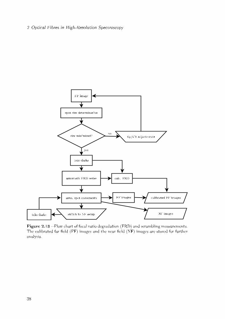
The whole procedure of bre scrambling and FRD characterisation is summarized
in Fig. 2.13. I designed a custom software that controls the camera, the linear stage,
and the focuser, thus facilitating a convenient and quick measurement procedure.
θo
x1 x2 x3
y1 y2 y3
θo = arctan(
∆y∆x
)
Filter wheel (not used)
Focuser
CCD Camera
Fibre
Figure 2.12 Top left: Schematic of the dierential FRD measurement procedure: thecamera is moved by well known steps, and for each position the size of the light cone exitingthe bre is determined. Bottom left: A typical result from this procedure indicates thesize of the cone at ve dierent positions of the camera. A linear t allows to determinethe F-ratio and the distance between the bre and the CCD. Right: Image of the FFsetup in the laboratory. The assembly is light-tight to avoid any contamination of themeasurements by background lighting.
37
2 Optical Fibres in High-Resolution Spectroscopy
FF image
spot size determination
tip/tilt adjustmentssize minimized?
take darks
automatic FRD series
auto. spot movements
switch to NF setuptake darks
calc. FRD
FF images calibrated FF images
no
yes
NF images
Figure 2.13 Flow chart of focal ratio degradation (FRD) and scrambling measurements.The calibrated far eld (FF) images and the near eld (NF) images are stored for furtheranalysis.
38
2.4 Experiments
2.4.4 Results
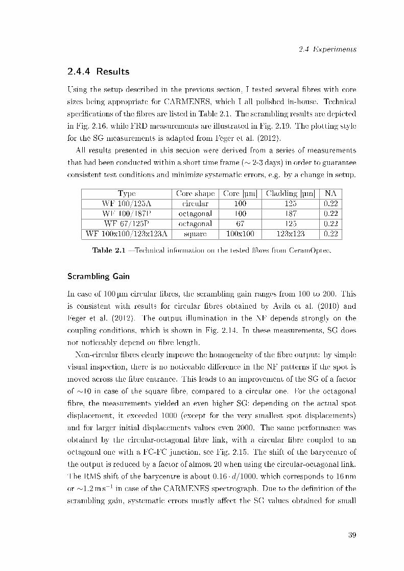
Using the setup described in the previous section, I tested several bres with core
sizes being appropriate for CARMENES, which I all polished in-house. Technical
specications of the bres are listed in Table 2.1. The scrambling results are depicted
in Fig. 2.16, while FRD measurements are illustrated in Fig. 2.19. The plotting style
for the SG measurements is adapted from Feger et al. (2012).
All results presented in this section were derived from a series of measurements
that had been conducted within a short time frame (∼ 2-3 days) in order to guarantee
consistent test conditions and minimize systematic errors, e.g. by a change in setup.
Type Core shape Core [µm] Cladding [µm] NAWF 100/125A circular 100 125 0.22WF 100/187P octagonal 100 187 0.22WF 67/125P octagonal 67 125 0.22
WF 100x100/123x123A square 100x100 123x123 0.22
Table 2.1 Technical information on the tested bres from CeramOptec.
Scrambling Gain
In case of 100µm circular bres, the scrambling gain ranges from 100 to 200. This
is consistent with results for circular bres obtained by Avila et al. (2010) and
Feger et al. (2012). The output illumination in the NF depends strongly on the
coupling conditions, which is shown in Fig. 2.14. In these measurements, SG does
not noticeably depend on bre length.
Non-circular bres clearly improve the homogeneity of the bre output: by simple
visual inspection, there is no noticeable dierence in the NF patterns if the spot is
moved across the bre entrance. This leads to an improvement of the SG of a factor
of ∼10 in case of the square bre, compared to a circular one. For the octagonal
bre, the measurements yielded an even higher SG: depending on the actual spot
displacement, it exceeded 1000 (except for the very smallest spot displacements)
and for larger initial displacements values even 2000. The same performance was
obtained by the circular-octagonal bre link, with a circular bre coupled to an
octagonal one with a FC-FC junction, see Fig. 2.15. The shift of the barycentre of
the output is reduced by a factor of almost 20 when using the circular-octagonal link.
The RMS shift of the barycentre is about 0.16 · d/1000, which corresponds to 16nm
or ∼1.2ms−1 in case of the CARMENES spectrograph. Due to the denition of the
scrambling gain, systematic errors mostly aect the SG values obtained for small
39
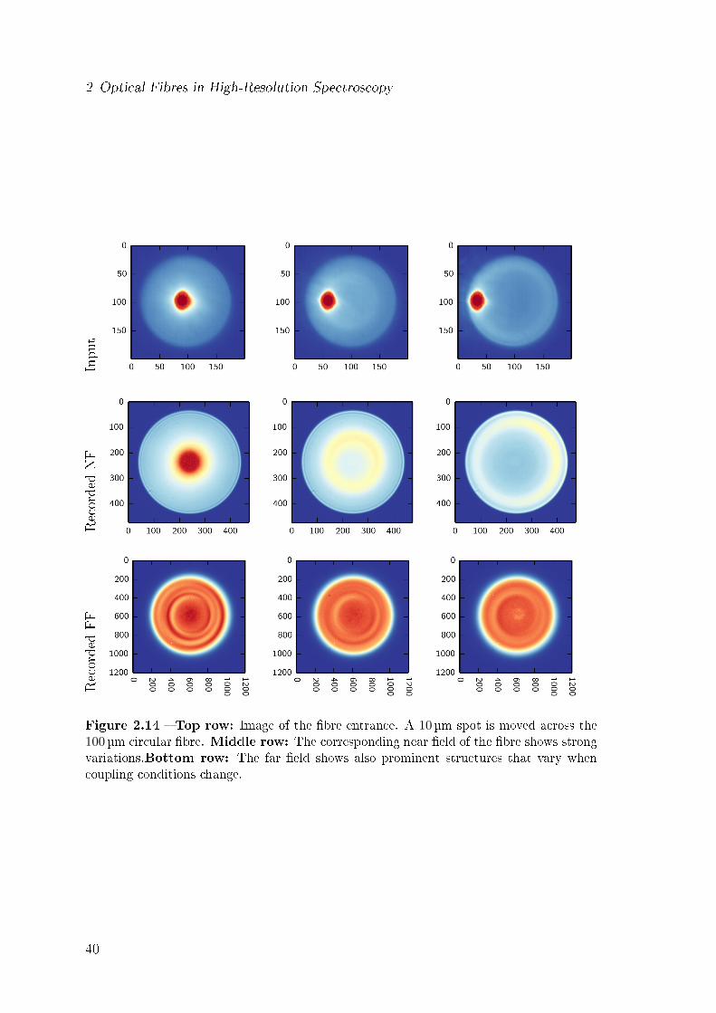
2 Optical Fibres in High-Resolution SpectroscopyInpu
tRecordedNF
RecordedFF
Figure 2.14 Top row: Image of the bre entrance. A 10 µm spot is moved across the100 µm circular bre. Middle row: The corresponding near eld of the bre shows strongvariations.Bottom row: The far eld shows also prominent structures that vary whencoupling conditions change.
40
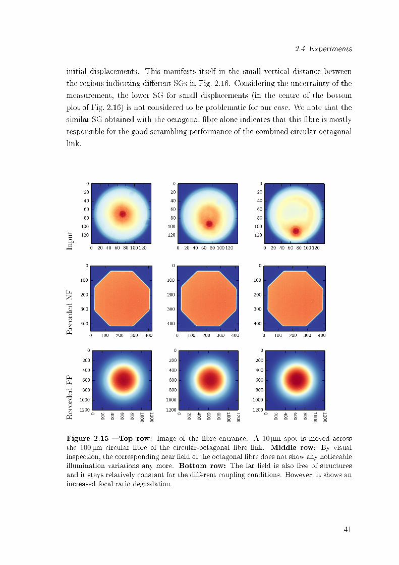
2.4 Experiments
initial displacements. This manifests itself in the small vertical distance between
the regions indicating dierent SGs in Fig. 2.16. Considering the uncertainty of the
measurement, the lower SG for small displacements (in the centre of the bottom
plot of Fig. 2.16) is not considered to be problematic for our case. We note that the
similar SG obtained with the octagonal bre alone indicates that this bre is mostly
responsible for the good scrambling performance of the combined circular-octagonal
link.
Inpu
tRecordedNF
RecordedFF
Figure 2.15 Top row: Image of the bre entrance. A 10 µm spot is moved acrossthe 100 µm circular bre of the circular-octagonal bre link. Middle row: By visualinspection, the corresponding near eld of the octagonal bre does not show any noticeableillumination variations any more. Bottom row: The far eld is also free of structuresand it stays relatively constant for the dierent coupling conditions. However, it shows anincreased focal ratio degradation.
41
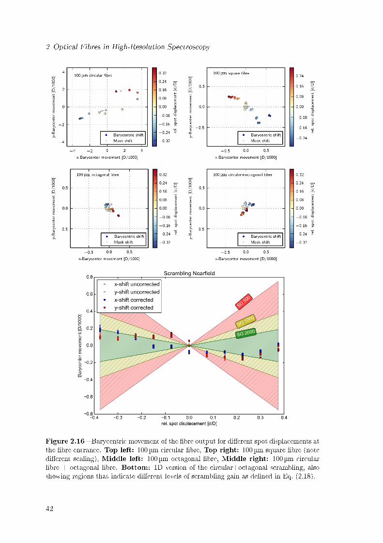
2 Optical Fibres in High-Resolution Spectroscopy
Figure 2.16 Barycentric movement of the bre output for dierent spot displacements atthe bre entrance. Top left: 100 µm circular bre, Top right: 100 µm square bre (notedierent scaling), Middle left: 100 µm octagonal bre, Middle right: 100 µm circularbre + octagonal bre. Bottom: 1D version of the circular+octagonal scrambling, alsoshowing regions that indicate dierent levels of scrambling gain as dened in Eq. (2.18).
42
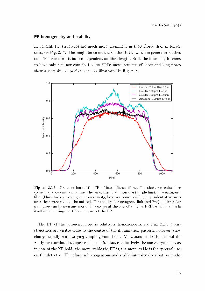
2.4 Experiments
FF homogeneity and stability
In general, FF structures are much more prominent in short bres than in longer
ones, see Fig. 2.17. This might be an indication that FRD, which in general smoothes
out FF structures, is indeed dependent on bre length. Still, the bre length seems
to have only a minor contribution to FRD: measurements of short and long bres
show a very similar performance, as illustrated in Fig. 2.19.
0 200 400 600 800 1000
Pixel
0.0
0.2
0.4
0.6
0.8
1.0
Rel
ati
vein
ten
sity
Circ-oct-2 L=50 m / 5 mCircular 100 µm L=3 mCircular 100 µm L=50 mOctagonal 100 µm L=5 m
Figure 2.17 Cross sections of the FFs of four dierent bres. The shorter circular bre(blue line) shows more prominent features than the longer one (purple line). The octagonalbre (black line) shows a good homogeneity, however, some coupling dependent structuresnear the centre can still be noticed. For the circular-octagonal link (red line), no irregularstructures can be seen any more. This comes at the cost of a higher FRD, which manifestsitself in faint wings on the outer part of the FF.
The FF of the octagonal bre is relatively homogeneous, see Fig. 2.17. Some
structures are visible close to the centre of the illumination pattern, however, they
change rapidly with varying coupling conditions. Variations in the FF cannot di-
rectly be translated to spectral line shifts, but qualitatively the same arguments as
in case of the NF hold: the more stable the FF is, the more stable is the spectral line
on the detector. Therefore, a homogeneous and stable intensity distribution in the
43
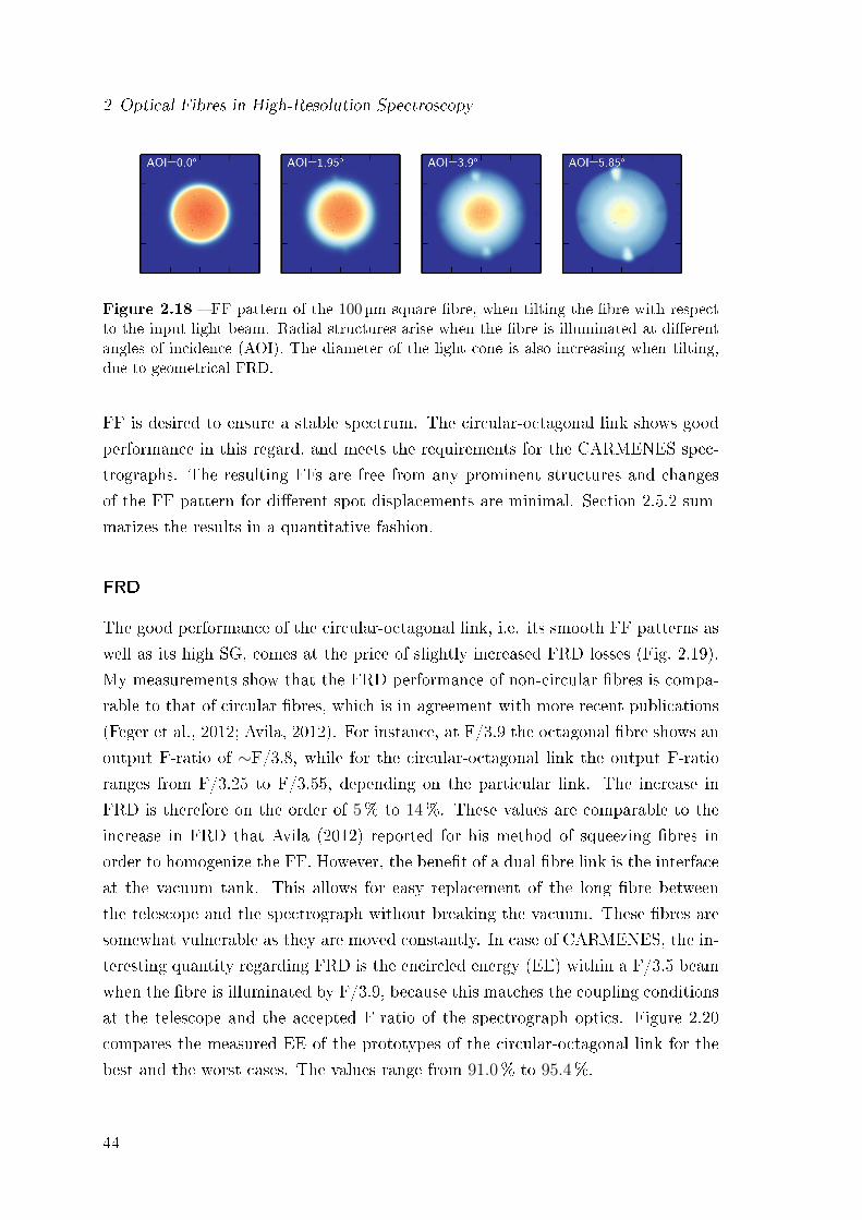
2 Optical Fibres in High-Resolution Spectroscopy
Figure 2.18 FF pattern of the 100 µm square bre, when tilting the bre with respectto the input light beam. Radial structures arise when the bre is illuminated at dierentangles of incidence (AOI). The diameter of the light cone is also increasing when tilting,due to geometrical FRD.
FF is desired to ensure a stable spectrum. The circular-octagonal link shows good
performance in this regard, and meets the requirements for the CARMENES spec-
trographs. The resulting FFs are free from any prominent structures and changes
of the FF pattern for dierent spot displacements are minimal. Section 2.5.2 sum-
marizes the results in a quantitative fashion.
FRD
The good performance of the circular-octagonal link, i.e. its smooth FF patterns as
well as its high SG, comes at the price of slightly increased FRD losses (Fig. 2.19).
My measurements show that the FRD performance of non-circular bres is compa-
rable to that of circular bres, which is in agreement with more recent publications
(Feger et al., 2012; Avila, 2012). For instance, at F/3.9 the octagonal bre shows an
output F-ratio of ∼F/3.8, while for the circular-octagonal link the output F-ratio
ranges from F/3.25 to F/3.55, depending on the particular link. The increase in
FRD is therefore on the order of 5% to 14%. These values are comparable to the
increase in FRD that Avila (2012) reported for his method of squeezing bres in
order to homogenize the FF. However, the benet of a dual bre link is the interface
at the vacuum tank. This allows for easy replacement of the long bre between
the telescope and the spectrograph without breaking the vacuum. These bres are
somewhat vulnerable as they are moved constantly. In case of CARMENES, the in-
teresting quantity regarding FRD is the encircled energy (EE) within a F/3.5 beam
when the bre is illuminated by F/3.9, because this matches the coupling conditions
at the telescope and the accepted F-ratio of the spectrograph optics. Figure 2.20
compares the measured EE of the prototypes of the circular-octagonal link for the
best and the worst cases. The values range from 91.0% to 95.4%.
44
2.4 Experiments
One particular result that requires further comment is the seemingly inferior per-
formance of the square bre. In the course of the FRD measurement, prominent
patterns in the FF of the square bre appeared. This prompted further investiga-
tion of the bre after the end of the test. During a visual inspection of the bre
with a microscope to check for defects, the bre broke, most probably due to a bre
crack located near the connector. The high FRD values are not in agreement with
older measurements that clearly showed that the FRD is comparable to that of the
octagonal or the circular bre. Also, Chazelas et al. (2010) reported that in their
tests the square bres, obtained from the same vendor as our samples, suered from
strange patterns in the FF, whose origin was not clear. In previous measurements,
no irregularities in the FF of our square bre under test were detected. However,
prominent radial features were visible in the FF when I tilted the bre with respect
to the incoming beam (Fig. 2.18). The patterns I recorded for the damaged square
bre looked very similar to the ones for a high angle of incidence.
In conclusion, my measurements show that non-circular bres have a similar FRD
performance compared to circular ones, while their scrambling is at least ten times
better. In order to eliminate FF structures, which are most prominent in short
bres, one has to induce some FRD. This can be done by squeezing in the spirit
of Avila (2012) or by linking bres of dierent cross sections. A circular-octagonal
link is a good solution for two reasons: First, circular geometries match the geom-
etry of optical components, which are also mostly circular symmetric. In case of
CARMENES, the eld of view of the bre is circular, because in the focal plane the
light has to pass a small hole in a mirror that is used for telescope guiding. In case
an octagonal bre would be used directly at the telescope, one would either have
to underll the bre or drill up the hole in the mirror to fully cover the octagon.
The latter would reduce the light available for guiding of the telescope, while not all
of the light, which now passes the circular hole, is coupled into the bre. Second,
coupling two octagonal bres requires either more advanced bre couplers that allow
to rotate the bres with respect to each other, or one has to accept higher coupling
losses due to a larger geometrical mismatch (see also Section 2.8.1).
45
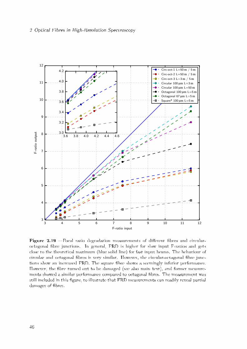
2 Optical Fibres in High-Resolution Spectroscopy
3 4 5 6 7 8 9 10 11 12
F-ratio input
3
4
5
6
7
8
9
10
11
12
F-r
ati
oo
utp
ut
Circ-oct-1 L=50 m / 5 mCirc-oct-2 L=50 m / 5 mCirc-oct-3 L=3 m / 5 mCircular 100 µm L=3 mCircular 100 µm L=50 mOctagonal 100 µm L=5 mOctagonal 67 µm L=5 mSquare* 100 µm L=5 m
3.6 3.8 4.0 4.2 4.4 4.63.0
3.2
3.4
3.6
3.8
4.0
4.2
Figure 2.19 Focal ratio degradation measurements of dierent bres and circular-octagonal bre junctions. In general, FRD is higher for slow input F-ratios and getsclose to the theoretical maximum (blue solid line) for fast input beams. The behaviour ofcircular and octagonal bres is very similar. However, the circular-octagonal bre junc-tions show an increased FRD. The square bre shows a seemingly inferior performance.However, the bre turned out to be damaged (see also main text), and former measure-ments showed a similar performance compared to octagonal bres. The measurement wasstill included in this gure, to illustrate that FRD measurements can readily reveal partialdamages of bres.
46
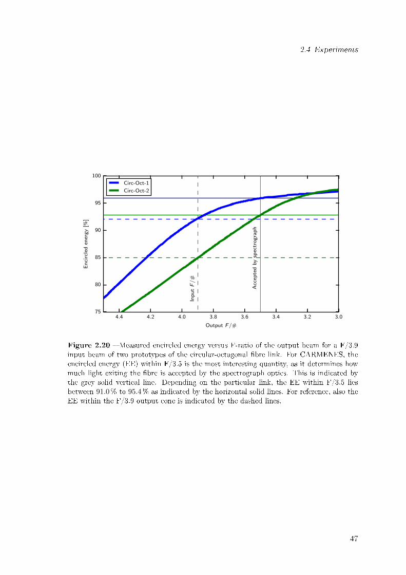
2.4 Experiments
3.03.23.43.63.84.04.24.4
Output F/#
75
80
85
90
95
100
En
circ
led
ener
gy
[%]
Inp
ut
F/
#
Acc
epte
db
ysp
ectr
og
rap
h
Circ-Oct-1
Circ-Oct-2
Figure 2.20 Measured encircled energy versus F-ratio of the output beam for a F/3.9input beam of two prototypes of the circular-octagonal bre link. For CARMENES, theencircled energy (EE) within F/3.5 is the most interesting quantity, as it determines howmuch light exiting the bre is accepted by the spectrograph optics. This is indicated bythe grey solid vertical line. Depending on the particular link, the EE within F/3.5 liesbetween 91.0% to 95.4% as indicated by the horizontal solid lines. For reference, also theEE within the F/3.9 output cone is indicated by the dashed lines.
47
2 Optical Fibres in High-Resolution Spectroscopy
2.5 Numerical Simulations
In this section, I present a couple of numerical simulations that I ran in order to
better understand the optical properties of bres and to translate the measured
illumination variations in NF and FF into RV errors.
2.5.1 Fibre Simulations
Precise measurements of scrambling gain and FRD are rather involved and time-
consuming. Moreover, non-circular bres are not available with arbitrary core shapes
and diameters and customized bre manufacturing is very costly. Simulations are
therefore a convenient way of predicting and analysing the potential performance of
new bre types. In the context of circular optical bres, an early analytical approach
of image transfer was presented by Heacox (1987). He theoretically derived the poor
radial scrambling of circular bres, which was conrmed experimentally at about
the same time. More recently, Allington-Smith et al. (2012) performed raytracing
simulations for bres with various core shapes with the aim of providing an insight
into their scrambling and FRD behaviour. The authors wrote their own raytrace
method to account for FRD. They limited the region where FRD happens to a small
section of the bre, because the authors argued in former studies that FRD does
not depend on bre length (Poppett and Allington-Smith, 2010).
For the simulations presented here, I used the commercial software ZEMAX to in-
vestigate some basic scrambling behaviour of various bres.2 My simulations mimic
the experiments for scrambling measurements as presented in Section 2.4.4. In the
non-sequential mode of ZEMAX, a light spot is imaged onto a bre and moved
across the bre surface.3 At the bre output, both NF and FF are recorded. The
bre is modelled by a solid silica tube surrounded by another silica tube, while the
dierence in their refractive indices was manually set to match a standard NA 0.22
bre. The bre is assumed to be straight, i.e. without bends and non-uniformities
of the bre cross-section.
In a rst test to validate this simulation approach, a spot with 5µm diameter and
wavelength λ = 550 nm is moved across a 100µm circular bre and the NF is com-
pared to actual measurements. Indeed, the simulated and the measured NF show
2https://www.zemax.com3In the sequential mode of ZEMAX, rays travel from surface to surface in a predened order.In the non-sequential mode, ZEMAX allows for tracing rays when there are multiple opticalpaths. This is useful for the implementation of e.g. scattering or extended light sources.
48
2.5 Numerical Simulations
a qualitative match (see second and third row of Fig. 2.21). However, a closer look
at the cross section in the middle of the bre reveals that the simulations gen-
erally show more pronounced features in the NF compared to the measurements
(Fig. 2.22). This is not surprising, as by default no scattering or other FRD eects
are simulated. The resulting NF pattern is thus purely dependent on the geometry
of the boundary. In principle, ZEMAX can handle both bulk and surface scattering
and it even allows for user dened scattering functions. Any scattering will eect
the NF as well as the FF, and it is a valid assumption that scattering processes will
happen within a bre. As an example, I turned on Mie bulk scattering. As depicted
in Fig. 2.22, a persuasive match between the simulation and experiment could be
reached by appropriately adapting the scattering parameters such as mean free path
and the size of the particles. This points towards the possibility of providing full
quantitative models in ZEMAX if the scattering properties of the bres are investi-
gated empirically, and accounted for accordingly.
It is clear that when turning on bulk scattering, eects such as FRD become de-
pendent on bre length. As stated in Section 2.2.2, the literature does not agree
as to whether FRD shows a length dependence or not. It seems to be a reasonable
assumption that FRD is mainly determined by bre end eects and stress from the
adhesive that is used to hold the bre. This could easily be implemented in ZEMAX
by restricting the scattering processes to small sections of the bre in the spirit of
Allington-Smith et al. (2012). However, I did not attempt to trace the sources of
FRD to their actual physical processes, such as dierent scattering processes within
the bre. Figure 2.22 should therefore only be seen as a strong indication that realis-
tic NF patterns can be simulated when taking scattering into account. Nevertheless,
even without considering scattering eects, I was able to verify with my simulation
that ray tracing is a feasible way to describe multi mode bres, and in particular
that circular bres are poor radial scramblers.
The same is true for bres with an elliptical core, see Fig. 2.23. In general, the
illumination is far from homogeneous and strongly dependent on the input param-
eters. The results indicate, that in case a homogeneous illumination is desired, it
is not sucient to remove circular symmetry from the core shape. A theoretical
explanation will be given in Section 2.7.
49
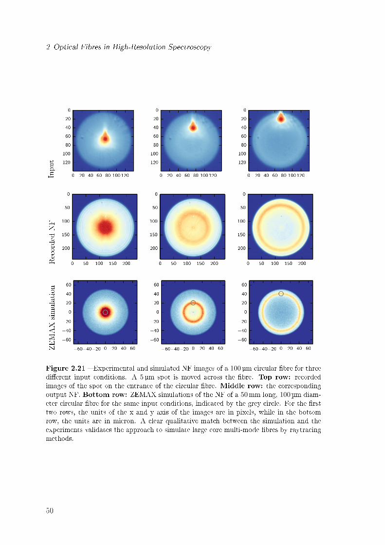
2 Optical Fibres in High-Resolution SpectroscopyInpu
tRecordedNF
ZEMAXsimulation
Figure 2.21 Experimental and simulated NF images of a 100 µm circular bre for threedierent input conditions. A 5 µm spot is moved across the bre. Top row: recordedimages of the spot on the entrance of the circular bre. Middle row: the correspondingoutput NF. Bottom row: ZEMAX simulations of the NF of a 50mm long, 100 µm diam-eter circular bre for the same input conditions, indicated by the grey circle. For the rsttwo rows, the units of the x and y axis of the images are in pixels, while in the bottomrow, the units are in micron. A clear qualitative match between the simulation and theexperiments validates the approach to simulate large core multi-mode bres by raytracingmethods.
50
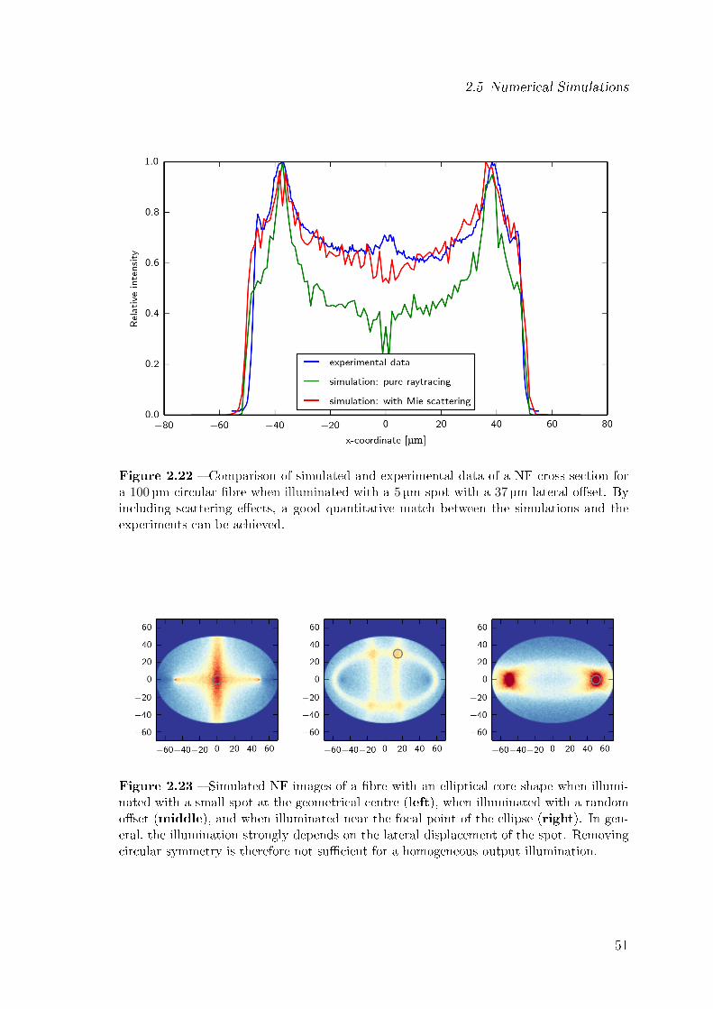
2.5 Numerical Simulations
Figure 2.22 Comparison of simulated and experimental data of a NF cross section fora 100 µm circular bre when illuminated with a 5 µm spot with a 37 µm lateral oset. Byincluding scattering eects, a good quantitative match between the simulations and theexperiments can be achieved.
Figure 2.23 Simulated NF images of a bre with an elliptical core shape when illumi-nated with a small spot at the geometrical centre (left), when illuminated with a randomoset (middle), and when illuminated near the focal point of the ellipse (right). In gen-eral, the illumination strongly depends on the lateral displacement of the spot. Removingcircular symmetry is therefore not sucient for a homogeneous output illumination.
51
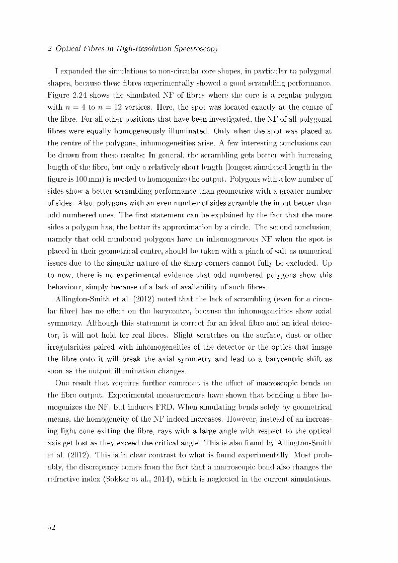
2 Optical Fibres in High-Resolution Spectroscopy
I expanded the simulations to non-circular core shapes, in particular to polygonal
shapes, because these bres experimentally showed a good scrambling performance.
Figure 2.24 shows the simulated NF of bres where the core is a regular polygon
with n = 4 to n = 12 vertices. Here, the spot was located exactly at the centre of
the bre. For all other positions that have been investigated, the NF of all polygonal
bres were equally homogeneously illuminated. Only when the spot was placed at
the centre of the polygons, inhomogeneities arise. A few interesting conclusions can
be drawn from these results: In general, the scrambling gets better with increasing
length of the bre, but only a relatively short length (longest simulated length in the
gure is 100mm) is needed to homogenize the output. Polygons with a low number of
sides show a better scrambling performance than geometries with a greater number
of sides. Also, polygons with an even number of sides scramble the input better than
odd numbered ones. The rst statement can be explained by the fact that the more
sides a polygon has, the better its approximation by a circle. The second conclusion,
namely that odd numbered polygons have an inhomogeneous NF when the spot is
placed in their geometrical centre, should be taken with a pinch of salt as numerical
issues due to the singular nature of the sharp corners cannot fully be excluded. Up
to now, there is no experimental evidence that odd numbered polygons show this
behaviour, simply because of a lack of availability of such bres.
Allington-Smith et al. (2012) noted that the lack of scrambling (even for a circu-
lar bre) has no eect on the barycentre, because the inhomogeneities show axial
symmetry. Although this statement is correct for an ideal bre and an ideal detec-
tor, it will not hold for real bres. Slight scratches on the surface, dust or other
irregularities paired with inhomogeneities of the detector or the optics that image
the bre onto it will break the axial symmetry and lead to a barycentric shift as
soon as the output illumination changes.
One result that requires further comment is the eect of macroscopic bends on
the bre output. Experimental measurements have shown that bending a bre ho-
mogenizes the NF, but induces FRD. When simulating bends solely by geometrical
means, the homogeneity of the NF indeed increases. However, instead of an increas-
ing light cone exiting the bre, rays with a large angle with respect to the optical
axis get lost as they exceed the critical angle. This is also found by Allington-Smith
et al. (2012). This is in clear contrast to what is found experimentally. Most prob-
ably, the discrepancy comes from the fact that a macroscopic bend also changes the
refractive index (Sokkar et al., 2014), which is neglected in the current simulations.
52
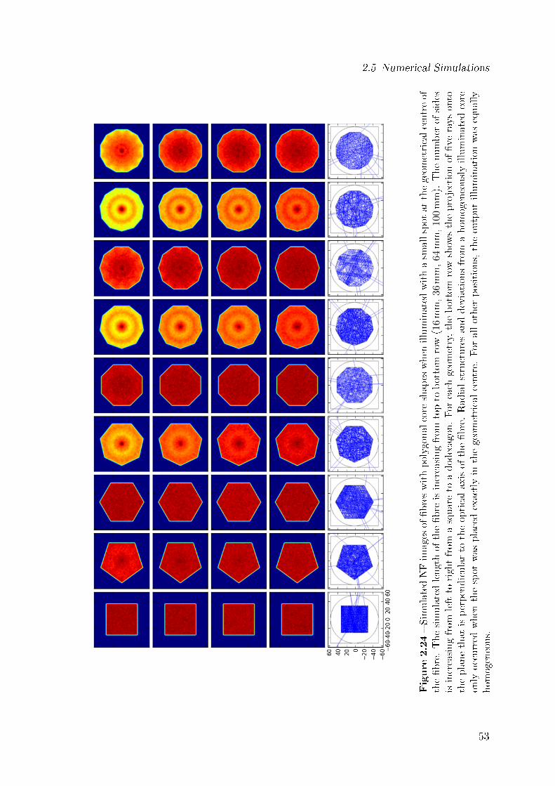
2.5 Numerical Simulations
Figure
2.24SimulatedNFim
ages
ofbreswithpolygonalcore
shapes
when
illuminated
withasm
allspot
atthegeom
etricalcentreof
thebre.Thesimulatedlengthof
thebre
isincreasingfrom
topto
bottom
row(1
6mm,
36mm,
64mm,
100mm).Thenumber
ofsides
isincreasingfrom
leftto
rightfrom
asquareto
adodecagon.For
each
geom
etry,thebottom
rowshow
stheprojectionof
ve
raysonto
theplanethat
isperpendicularto
theopticalaxisof
thebre.Radialstructuresanddeviationsfrom
ahom
ogeneouslyilluminated
core
only
occurred
when
thespot
was
placedexactlyin
thegeom
etricalcentre.
For
allother
positions,theoutputilluminationwas
equally
hom
ogeneous.
53
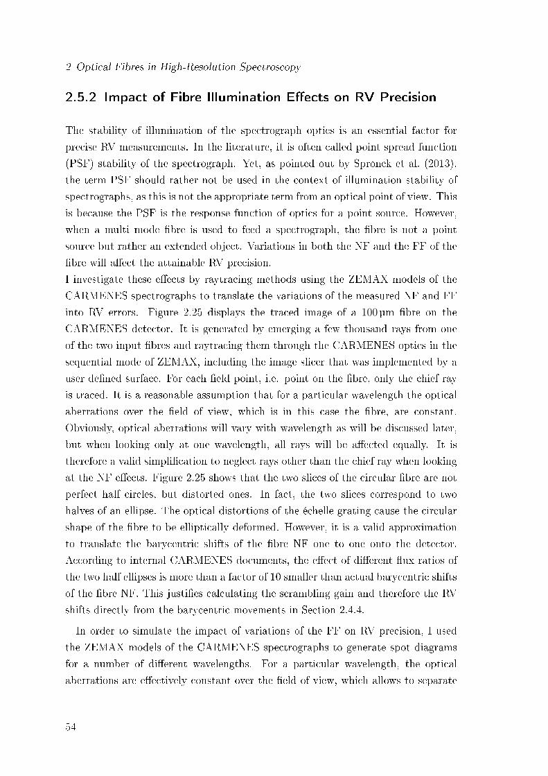
2 Optical Fibres in High-Resolution Spectroscopy
2.5.2 Impact of Fibre Illumination Eects on RV Precision
The stability of illumination of the spectrograph optics is an essential factor for
precise RV measurements. In the literature, it is often called point spread function
(PSF) stability of the spectrograph. Yet, as pointed out by Spronck et al. (2013),
the term PSF should rather not be used in the context of illumination stability of
spectrographs, as this is not the appropriate term from an optical point of view. This
is because the PSF is the response function of optics for a point source. However,
when a multi mode bre is used to feed a spectrograph, the bre is not a point
source but rather an extended object. Variations in both the NF and the FF of the
bre will aect the attainable RV precision.
I investigate these eects by raytracing methods using the ZEMAX models of the
CARMENES spectrographs to translate the variations of the measured NF and FF
into RV errors. Figure 2.25 displays the traced image of a 100µm bre on the
CARMENES detector. It is generated by emerging a few thousand rays from one
of the two input bres and raytracing them through the CARMENES optics in the
sequential mode of ZEMAX, including the image slicer that was implemented by a
user dened surface. For each eld point, i.e. point on the bre, only the chief ray
is traced. It is a reasonable assumption that for a particular wavelength the optical
aberrations over the eld of view, which is in this case the bre, are constant.
Obviously, optical aberrations will vary with wavelength as will be discussed later,
but when looking only at one wavelength, all rays will be aected equally. It is
therefore a valid simplication to neglect rays other than the chief ray when looking
at the NF eects. Figure 2.25 shows that the two slices of the circular bre are not
perfect half circles, but distorted ones. In fact, the two slices correspond to two
halves of an ellipse. The optical distortions of the échelle grating cause the circular
shape of the bre to be elliptically deformed. However, it is a valid approximation
to translate the barycentric shifts of the bre NF one to one onto the detector.
According to internal CARMENES documents, the eect of dierent ux ratios of
the two half ellipses is more than a factor of 10 smaller than actual barycentric shifts
of the bre NF. This justies calculating the scrambling gain and therefore the RV
shifts directly from the barycentric movements in Section 2.4.4.
In order to simulate the impact of variations of the FF on RV precision, I used
the ZEMAX models of the CARMENES spectrographs to generate spot diagrams
for a number of dierent wavelengths. For a particular wavelength, the optical
aberrations are eectively constant over the eld of view, which allows to separate
54
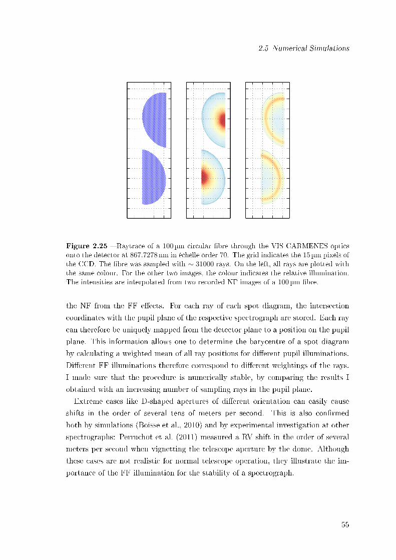
2.5 Numerical Simulations
Figure 2.25 Raytrace of a 100µm circular bre through the VIS CARMENES opticsonto the detector at 867.7278 nm in échelle order 70. The grid indicates the 15 µm pixels ofthe CCD. The bre was sampled with ∼ 31000 rays. On the left, all rays are plotted withthe same colour. For the other two images, the colour indicates the relative illumination.The intensities are interpolated from two recorded NF images of a 100 µm bre.
the NF from the FF eects. For each ray of each spot diagram, the intersection
coordinates with the pupil plane of the respective spectrograph are stored. Each ray
can therefore be uniquely mapped from the detector plane to a position on the pupil
plane. This information allows one to determine the barycentre of a spot diagram
by calculating a weighted mean of all ray positions for dierent pupil illuminations.
Dierent FF illuminations therefore correspond to dierent weightings of the rays.
I made sure that the procedure is numerically stable, by comparing the results I
obtained with an increasing number of sampling rays in the pupil plane.
Extreme cases like D-shaped apertures of dierent orientation can easily cause
shifts in the order of several tens of meters per second. This is also conrmed
both by simulations (Boisse et al., 2010) and by experimental investigation at other
spectrographs: Perruchot et al. (2011) measured a RV shift in the order of several
meters per second when vignetting the telescope aperture by the dome. Although
these cases are not realistic for normal telescope operation, they illustrate the im-
portance of the FF illumination for the stability of a spectrograph.
55
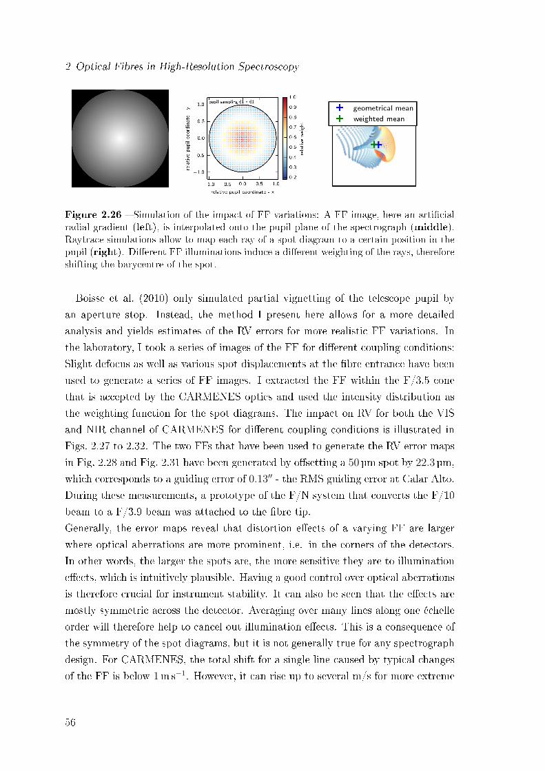
2 Optical Fibres in High-Resolution Spectroscopy
Figure 2.26 Simulation of the impact of FF variations: A FF image, here an articialradial gradient (left), is interpolated onto the pupil plane of the spectrograph (middle).Raytrace simulations allow to map each ray of a spot diagram to a certain position in thepupil (right). Dierent FF illuminations induce a dierent weighting of the rays, thereforeshifting the barycentre of the spot.
Boisse et al. (2010) only simulated partial vignetting of the telescope pupil by
an aperture stop. Instead, the method I present here allows for a more detailed
analysis and yields estimates of the RV errors for more realistic FF variations. In
the laboratory, I took a series of images of the FF for dierent coupling conditions:
Slight defocus as well as various spot displacements at the bre entrance have been
used to generate a series of FF images. I extracted the FF within the F/3.5 cone
that is accepted by the CARMENES optics and used the intensity distribution as
the weighting function for the spot diagrams. The impact on RV for both the VIS
and NIR channel of CARMENES for dierent coupling conditions is illustrated in
Figs. 2.27 to 2.32. The two FFs that have been used to generate the RV error maps
in Fig. 2.28 and Fig. 2.31 have been generated by osetting a 50µm spot by 22.3 µm,
which corresponds to a guiding error of 0.13′′ - the RMS guiding error at Calar Alto.
During these measurements, a prototype of the F/N system that converts the F/10
beam to a F/3.9 beam was attached to the bre tip.
Generally, the error maps reveal that distortion eects of a varying FF are larger
where optical aberrations are more prominent, i.e. in the corners of the detectors.
In other words, the larger the spots are, the more sensitive they are to illumination
eects, which is intuitively plausible. Having a good control over optical aberrations
is therefore crucial for instrument stability. It can also be seen that the eects are
mostly symmetric across the detector. Averaging over many lines along one échelle
order will therefore help to cancel out illumination eects. This is a consequence of
the symmetry of the spot diagrams, but it is not generally true for any spectrograph
design. For CARMENES, the total shift for a single line caused by typical changes
of the FF is below 1ms−1. However, it can rise up to several m/s for more extreme
56
2.5 Numerical Simulations
lateral displacements as illustrated in Fig. 2.29 for the VIS channel, and in Fig. 2.32
for the NIR, respectively.
However, it is dicult to predict how the FF varies on a real telescope over a longer
period of time. Guiding, focussing, and seeing have an impact on the exact shape
of the FF. It is still very instructive to perform these simulations to get a better
understanding of the impact of illumination variations on spectrograph stability and
to possibly incorporate these results for new spectrograph designs. In this spirit,
F¶rész et al. (2014) explicitly included a term in the merit function during the G-
CLEF (GMT-CfA, Carnegie, Catolica, Chicago Large Earth Finder) spectrograph
design that minimizes shifts caused by pupil illumination variations.
One limitation of the presented raytrace approach is that it neglects diraction
eects. Also, it is assumed that the FF variations, which are measured with the bre
being illuminated with white light, are on average the same for dierent wavelengths.
Still, the method provides insight into the complex relation of optical aberrations,
FF illumination, and radial velocity stability.
57
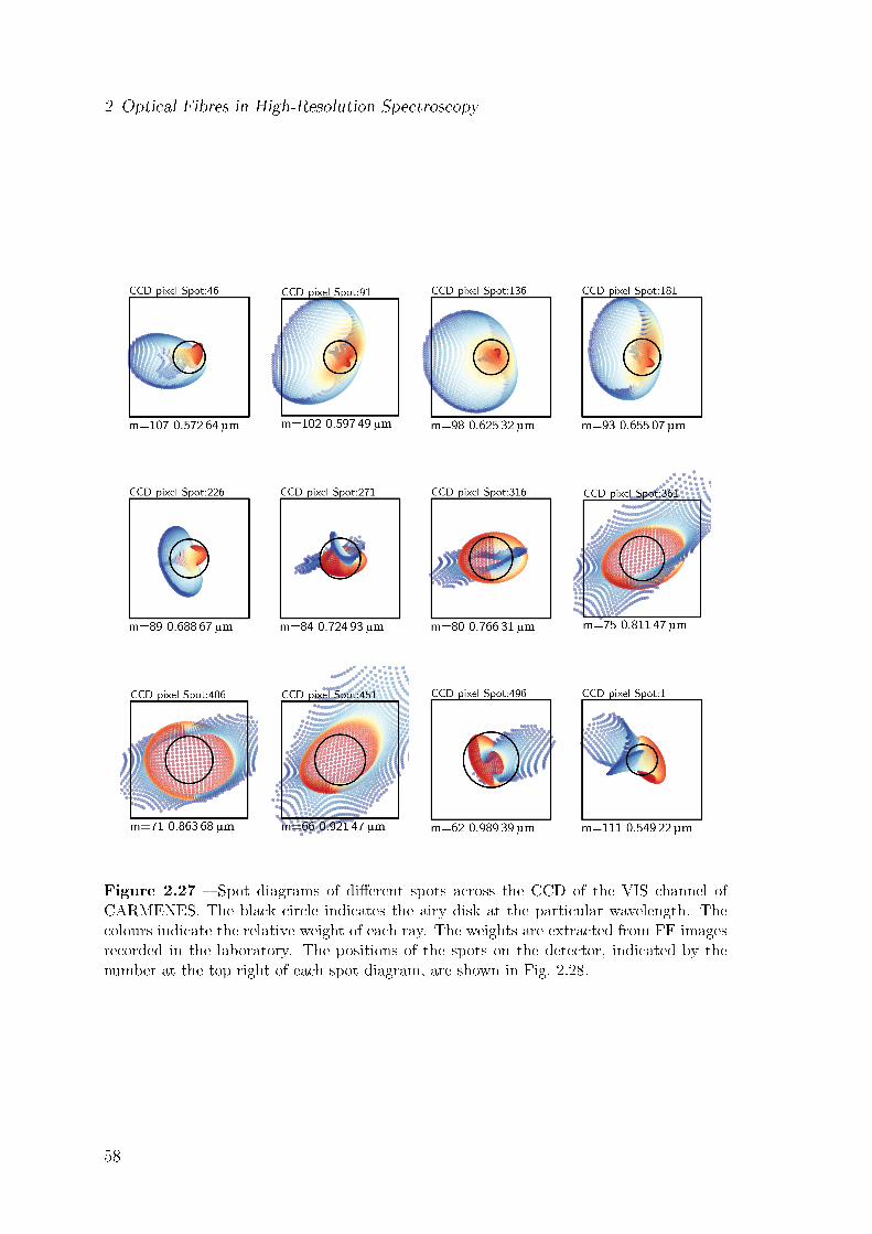
2 Optical Fibres in High-Resolution Spectroscopy
Figure 2.27 Spot diagrams of dierent spots across the CCD of the VIS channel ofCARMENES. The black circle indicates the airy disk at the particular wavelength. Thecolours indicate the relative weight of each ray. The weights are extracted from FF imagesrecorded in the laboratory. The positions of the spots on the detector, indicated by thenumber at the top right of each spot diagram, are shown in Fig. 2.28.
58
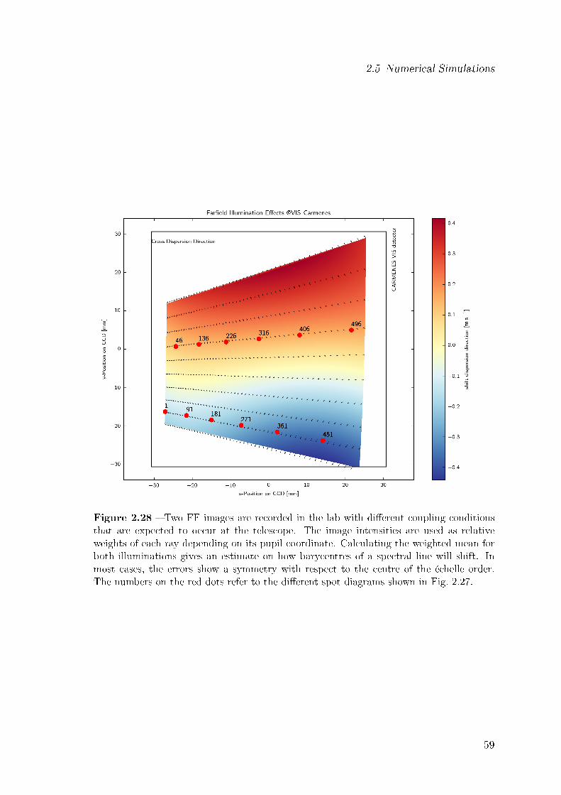
2.5 Numerical Simulations
Figure 2.28 Two FF images are recorded in the lab with dierent coupling conditionsthat are expected to occur at the telescope. The image intensities are used as relativeweights of each ray depending on its pupil coordinate. Calculating the weighted mean forboth illuminations gives an estimate on how barycentres of a spectral line will shift. Inmost cases, the errors show a symmetry with respect to the centre of the échelle order.The numbers on the red dots refer to the dierent spot diagrams shown in Fig. 2.27.
59
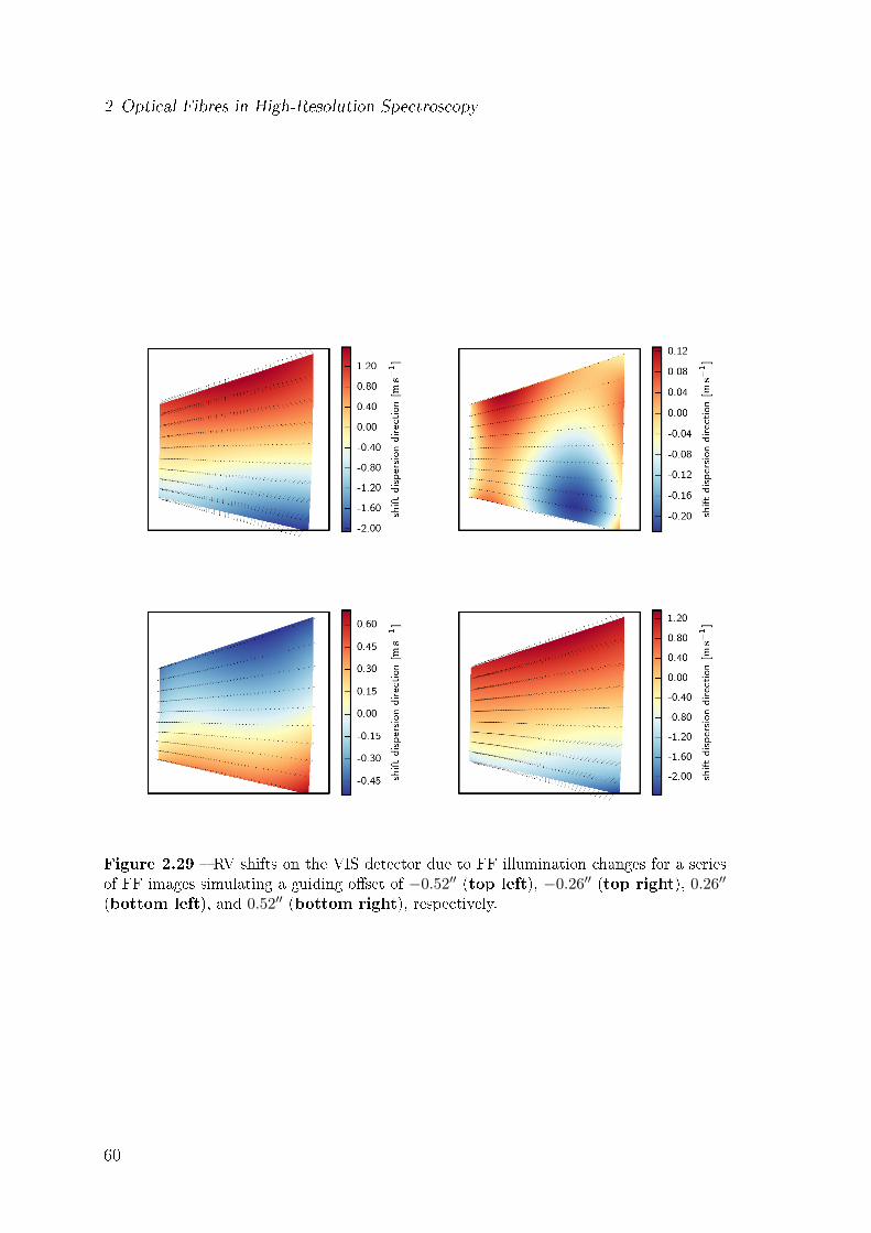
2 Optical Fibres in High-Resolution Spectroscopy
Figure 2.29 RV shifts on the VIS detector due to FF illumination changes for a seriesof FF images simulating a guiding oset of −0.52′′ (top left), −0.26′′ (top right), 0.26′′
(bottom left), and 0.52′′ (bottom right), respectively.
60
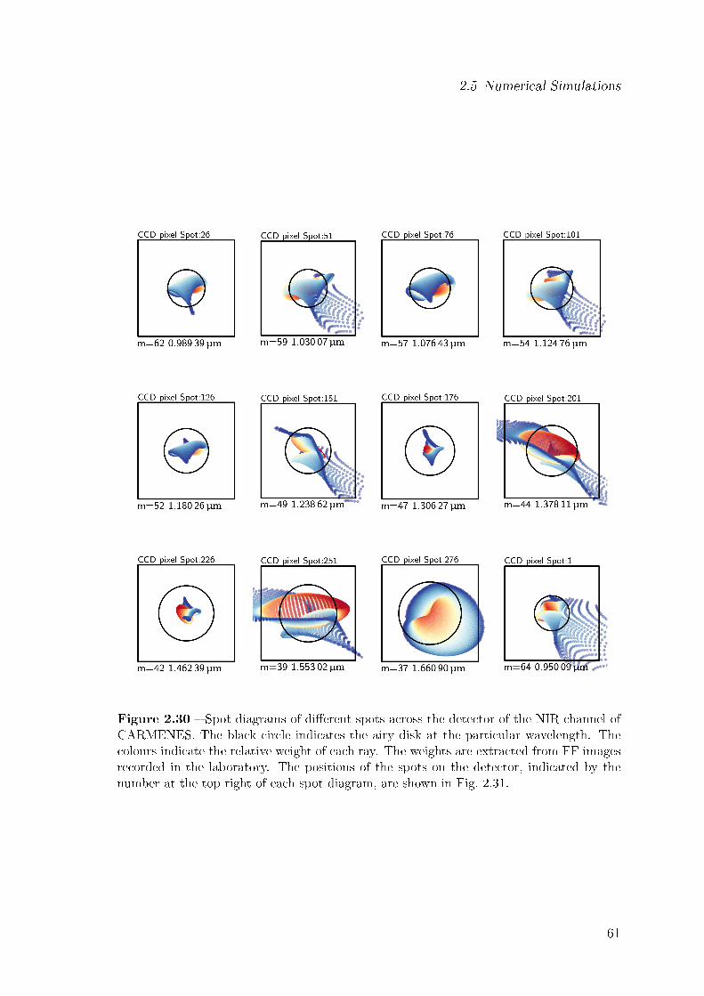
2.5 Numerical Simulations
Figure 2.30 Spot diagrams of dierent spots across the detector of the NIR channel ofCARMENES. The black circle indicates the airy disk at the particular wavelength. Thecolours indicate the relative weight of each ray. The weights are extracted from FF imagesrecorded in the laboratory. The positions of the spots on the detector, indicated by thenumber at the top right of each spot diagram, are shown in Fig. 2.31.
61
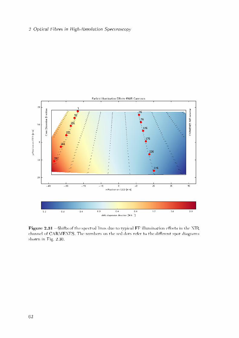
2 Optical Fibres in High-Resolution Spectroscopy
Figure 2.31 Shifts of the spectral lines due to typical FF illumination eects in the NIRchannel of CARMENES. The numbers on the red dots refer to the dierent spot diagramsshown in Fig. 2.30.
62
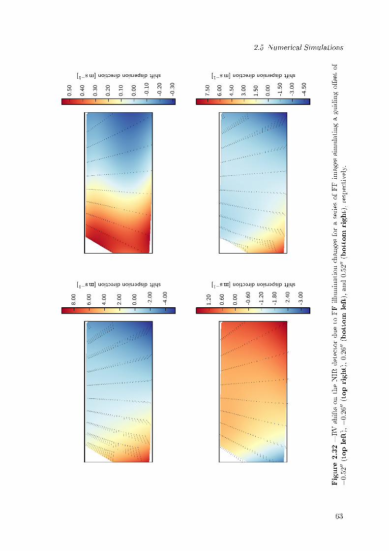
2.5 Numerical Simulations
Figure
2.32RV
shifts
ontheNIR
detectordueto
FFilluminationchangesforaseries
ofFFim
ages
simulatingaguidingosetof
−0.
52′′(topleft),−
0.26′′(topright),
0.2
6′′(bottom
left),and
0.52′′(bottom
right),respectively.
63
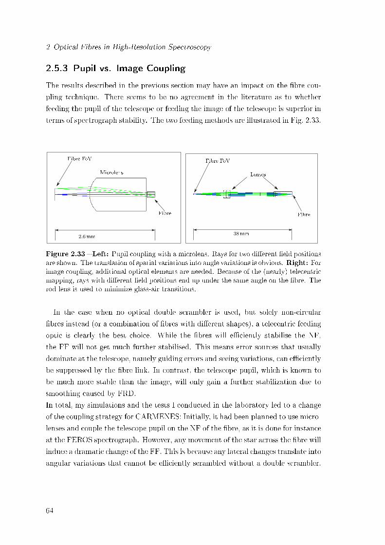
2 Optical Fibres in High-Resolution Spectroscopy
2.5.3 Pupil vs. Image Coupling
The results described in the previous section may have an impact on the bre cou-
pling technique. There seems to be no agreement in the literature as to whether
feeding the pupil of the telescope or feeding the image of the telescope is superior in
terms of spectrograph stability. The two feeding methods are illustrated in Fig. 2.33.
Microlens
Fibre
2.6mm
Fibre FoV
Lenses
Fibre
38mm
Fibre FoV
Figure 2.33 Left: Pupil coupling with a microlens. Rays for two dierent eld positionsare shown. The translation of spatial variations into angle variations is obvious. Right: Forimage coupling, additional optical elements are needed. Because of the (nearly) telecentricmapping, rays with dierent eld positions end up under the same angle on the bre. Therod lens is used to minimize glass-air transitions.
In the case when no optical double scrambler is used, but solely non-circular
bres instead (or a combination of bres with dierent shapes), a telecentric feeding
optic is clearly the best choice. While the bres will eciently stabilise the NF,
the FF will not get much further stabilised. This means error sources that usually
dominate at the telescope, namely guiding errors and seeing variations, can eciently
be suppressed by the bre link. In contrast, the telescope pupil, which is known to
be much more stable than the image, will only gain a further stabilization due to
smoothing caused by FRD.
In total, my simulations and the tests I conducted in the laboratory led to a change
of the coupling strategy for CARMENES: Initially, it had been planned to use micro-
lenses and couple the telescope pupil on the NF of the bre, as it is done for instance
at the FEROS spectrograph. However, any movement of the star across the bre will
induce a dramatic change of the FF. This is because any lateral changes translate into
angular variations that cannot be eciently scrambled without a double scrambler.
64
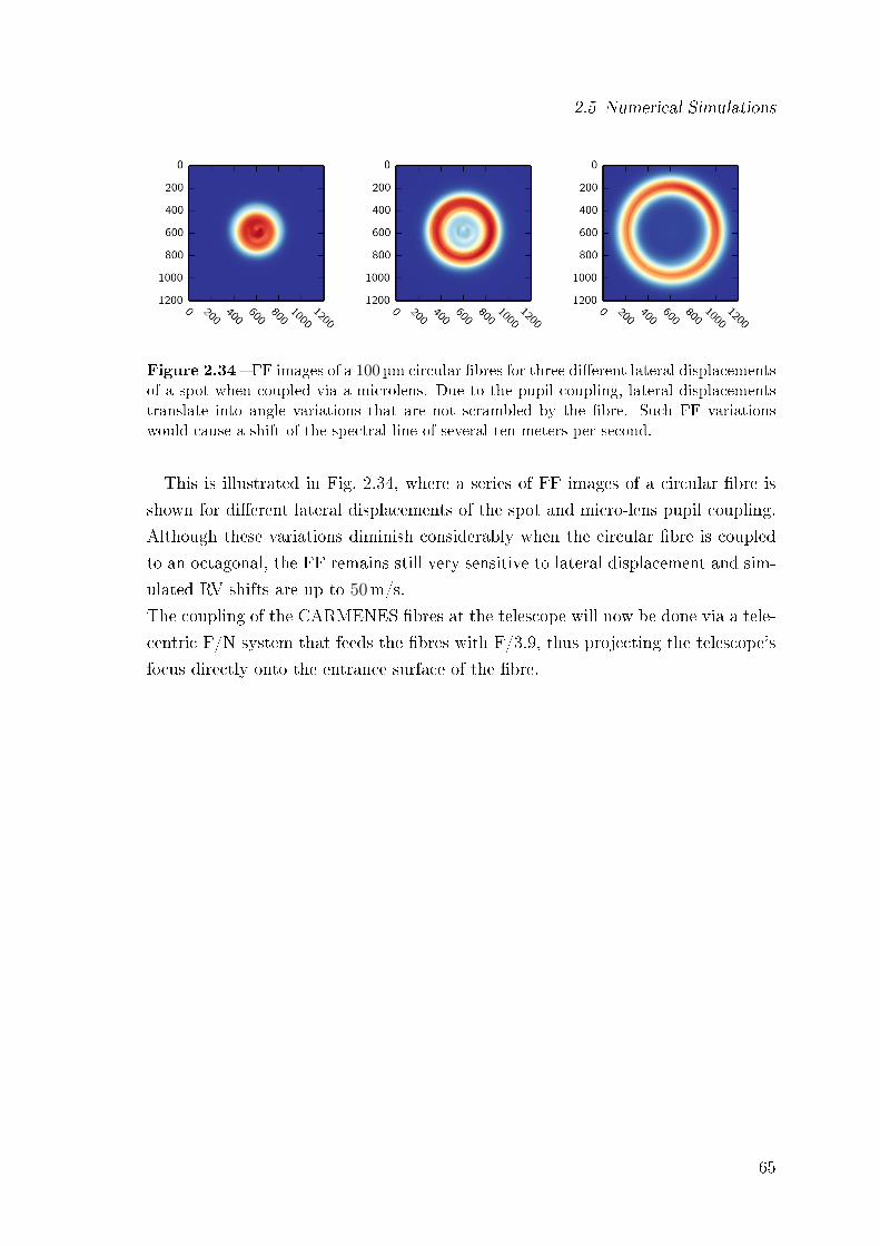
2.5 Numerical Simulations
Figure 2.34 FF images of a 100 µm circular bres for three dierent lateral displacementsof a spot when coupled via a microlens. Due to the pupil coupling, lateral displacementstranslate into angle variations that are not scrambled by the bre. Such FF variationswould cause a shift of the spectral line of several ten meters per second.
This is illustrated in Fig. 2.34, where a series of FF images of a circular bre is
shown for dierent lateral displacements of the spot and micro-lens pupil coupling.
Although these variations diminish considerably when the circular bre is coupled
to an octagonal, the FF remains still very sensitive to lateral displacement and sim-
ulated RV shifts are up to 50m/s.
The coupling of the CARMENES bres at the telescope will now be done via a tele-
centric F/N system that feeds the bres with F/3.9, thus projecting the telescope's
focus directly onto the entrance surface of the bre.
65
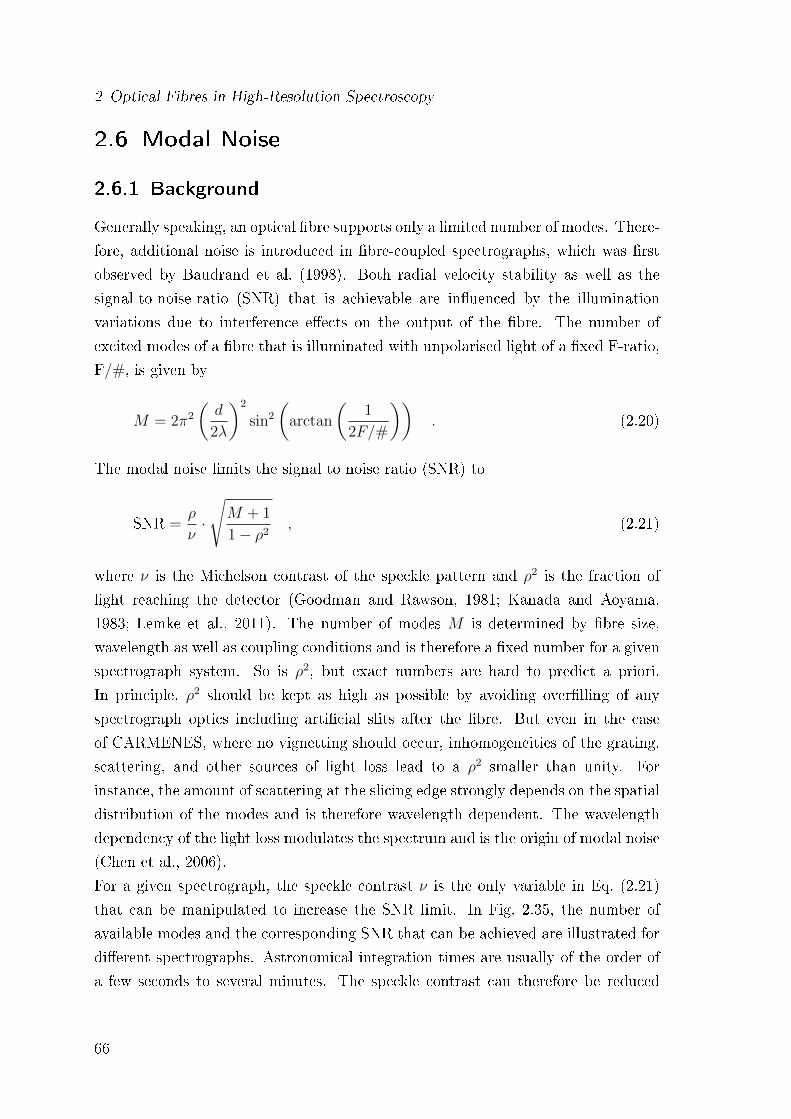
2 Optical Fibres in High-Resolution Spectroscopy
2.6 Modal Noise
2.6.1 Background
Generally speaking, an optical bre supports only a limited number of modes. There-
fore, additional noise is introduced in bre-coupled spectrographs, which was rst
observed by Baudrand et al. (1998). Both radial velocity stability as well as the
signal-to-noise-ratio (SNR) that is achievable are inuenced by the illumination
variations due to interference eects on the output of the bre. The number of
excited modes of a bre that is illuminated with unpolarised light of a xed F-ratio,
F/#, is given by
M = 2π2
(d
2λ
)2
sin2
(arctan
(1
2F/#
)). (2.20)
The modal noise limits the signal to noise ratio (SNR) to
SNR =ρ
ν·√M + 1
1− ρ2, (2.21)
where ν is the Michelson contrast of the speckle pattern and ρ2 is the fraction of
light reaching the detector (Goodman and Rawson, 1981; Kanada and Aoyama,
1983; Lemke et al., 2011). The number of modes M is determined by bre size,
wavelength as well as coupling conditions and is therefore a xed number for a given
spectrograph system. So is ρ2, but exact numbers are hard to predict a priori.
In principle, ρ2 should be kept as high as possible by avoiding overlling of any
spectrograph optics including articial slits after the bre. But even in the case
of CARMENES, where no vignetting should occur, inhomogeneities of the grating,
scattering, and other sources of light loss lead to a ρ2 smaller than unity. For
instance, the amount of scattering at the slicing edge strongly depends on the spatial
distribution of the modes and is therefore wavelength dependent. The wavelength
dependency of the light loss modulates the spectrum and is the origin of modal noise
(Chen et al., 2006).
For a given spectrograph, the speckle contrast ν is the only variable in Eq. (2.21)
that can be manipulated to increase the SNR limit. In Fig. 2.35, the number of
available modes and the corresponding SNR that can be achieved are illustrated for
dierent spectrographs. Astronomical integration times are usually of the order of
a few seconds to several minutes. The speckle contrast can therefore be reduced
66
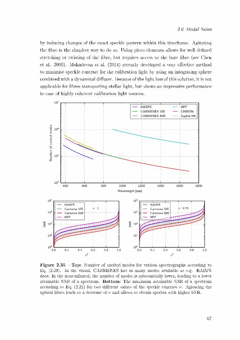
2.6 Modal Noise
by inducing changes of the exact speckle pattern within this timeframe. Agitating
the bre is the simplest way to do so. Using piezo elements allows for well dened
stretching or twisting of the bre, but requires access to the bare bre (see Chen
et al., 2006). Mahadevan et al. (2014) recently developed a very eective method
to minimise speckle contrast for the calibration light by using an integrating sphere
combined with a dynamical diuser. Because of the light loss of this solution, it is not
applicable for bres transporting stellar light, but shows an impressive performance
in case of highly coherent calibration light sources.
Figure 2.35 Top: Number of excited modes for various spectrographs according toEq. (2.20). In the visual, CARMENES has as many modes available as e.g. HARPSdoes. In the near-infrared, the number of modes is substantially lower, leading to a lowerattainable SNR of a spectrum. Bottom: The maximum attainable SNR of a spectrumaccording to Eq. (2.21) for two dierent values of the speckle contrast ν. Agitating theoptical bres leads to a decrease of ν and allows to obtain spectra with higher SNR.
67
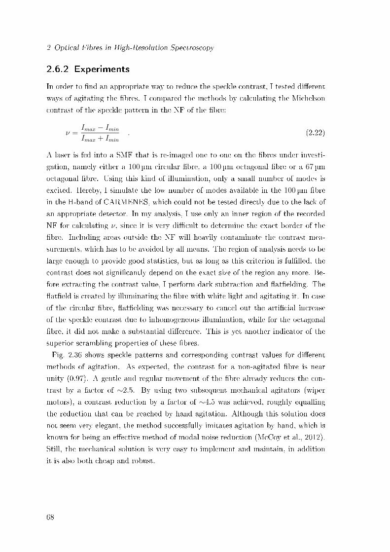
2 Optical Fibres in High-Resolution Spectroscopy
2.6.2 Experiments
In order to nd an appropriate way to reduce the speckle contrast, I tested dierent
ways of agitating the bres. I compared the methods by calculating the Michelson
contrast of the speckle pattern in the NF of the bre:
ν =Imax − IminImax + Imin
. (2.22)
A laser is fed into a SMF that is re-imaged one to one on the bres under investi-
gation, namely either a 100µm circular bre, a 100µm octagonal bre or a 67µm
octagonal bre. Using this kind of illumination, only a small number of modes is
excited. Hereby, I simulate the low number of modes available in the 100µm bre
in the H-band of CARMENES, which could not be tested directly due to the lack of
an appropriate detector. In my analysis, I use only an inner region of the recorded
NF for calculating ν, since it is very dicult to determine the exact border of the
bre. Including areas outside the NF will heavily contaminate the contrast mea-
surements, which has to be avoided by all means. The region of analysis needs to be
large enough to provide good statistics, but as long as this criterion is fullled, the
contrast does not signicantly depend on the exact size of the region any more. Be-
fore extracting the contrast value, I perform dark subtraction and atelding. The
ateld is created by illuminating the bre with white light and agitating it. In case
of the circular bre, atelding was necessary to cancel out the articial increase
of the speckle contrast due to inhomogeneous illumination, while for the octagonal
bre, it did not make a substantial dierence. This is yet another indicator of the
superior scrambling properties of these bres.
Fig. 2.36 shows speckle patterns and corresponding contrast values for dierent
methods of agitation. As expected, the contrast for a non-agitated bre is near
unity (0.97). A gentle and regular movement of the bre already reduces the con-
trast by a factor of ∼2.5. By using two subsequent mechanical agitators (wiper
motors), a contrast reduction by a factor of ∼4.5 was achieved, roughly equalling
the reduction that can be reached by hand agitation. Although this solution does
not seem very elegant, the method successfully imitates agitation by hand, which is
known for being an eective method of modal noise reduction (McCoy et al., 2012).
Still, the mechanical solution is very easy to implement and maintain, in addition
it is also both cheap and robust.
68
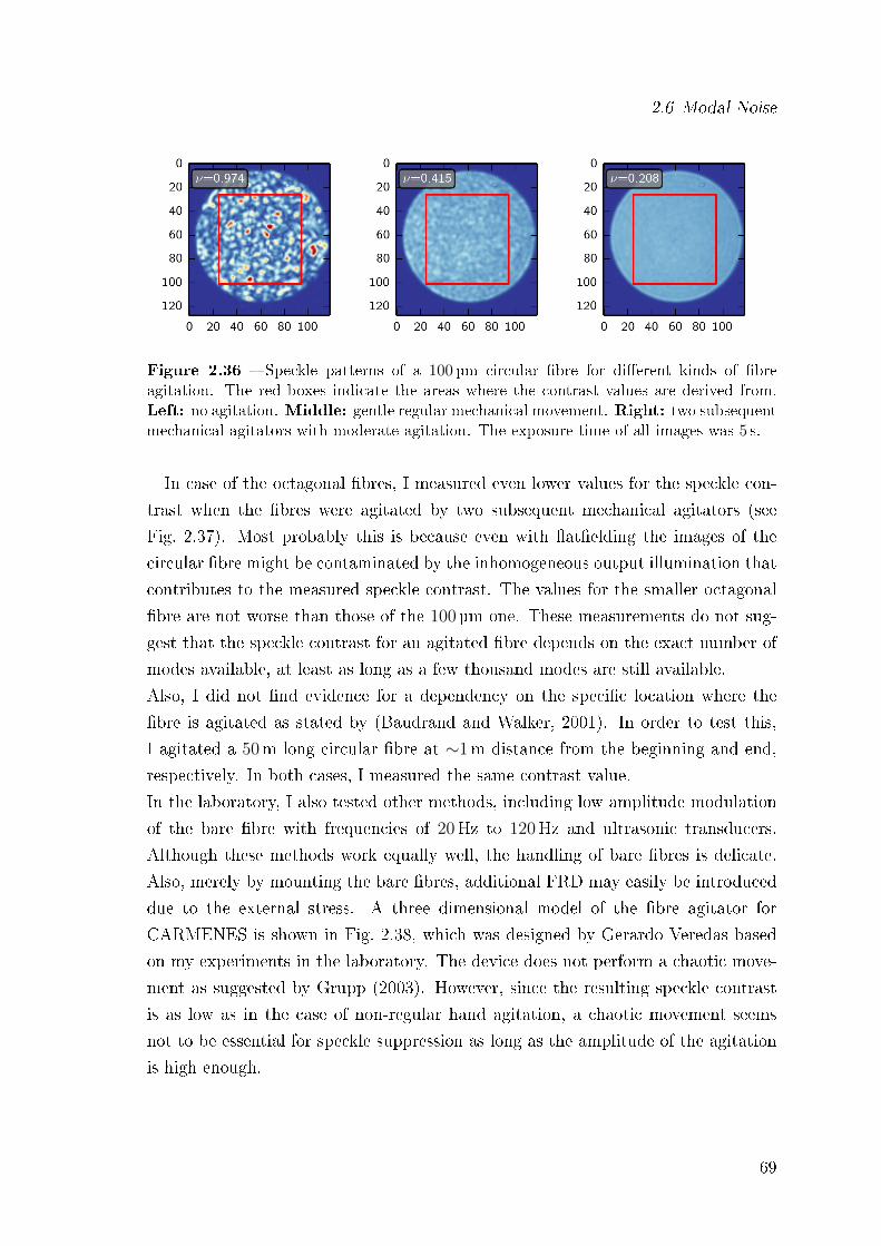
2.6 Modal Noise
Figure 2.36 Speckle patterns of a 100µm circular bre for dierent kinds of breagitation. The red boxes indicate the areas where the contrast values are derived from.Left: no agitation. Middle: gentle regular mechanical movement. Right: two subsequentmechanical agitators with moderate agitation. The exposure time of all images was 5 s.
In case of the octagonal bres, I measured even lower values for the speckle con-
trast when the bres were agitated by two subsequent mechanical agitators (see
Fig. 2.37). Most probably this is because even with atelding the images of the
circular bre might be contaminated by the inhomogeneous output illumination that
contributes to the measured speckle contrast. The values for the smaller octagonal
bre are not worse than those of the 100µm one. These measurements do not sug-
gest that the speckle contrast for an agitated bre depends on the exact number of
modes available, at least as long as a few thousand modes are still available.
Also, I did not nd evidence for a dependency on the specic location where the
bre is agitated as stated by (Baudrand and Walker, 2001). In order to test this,
I agitated a 50m long circular bre at ∼1m distance from the beginning and end,
respectively. In both cases, I measured the same contrast value.
In the laboratory, I also tested other methods, including low amplitude modulation
of the bare bre with frequencies of 20Hz to 120Hz and ultrasonic transducers.
Although these methods work equally well, the handling of bare bres is delicate.
Also, merely by mounting the bare bres, additional FRD may easily be introduced
due to the external stress. A three dimensional model of the bre agitator for
CARMENES is shown in Fig. 2.38, which was designed by Gerardo Veredas based
on my experiments in the laboratory. The device does not perform a chaotic move-
ment as suggested by Grupp (2003). However, since the resulting speckle contrast
is as low as in the case of non-regular hand agitation, a chaotic movement seems
not to be essential for speckle suppression as long as the amplitude of the agitation
is high enough.
69
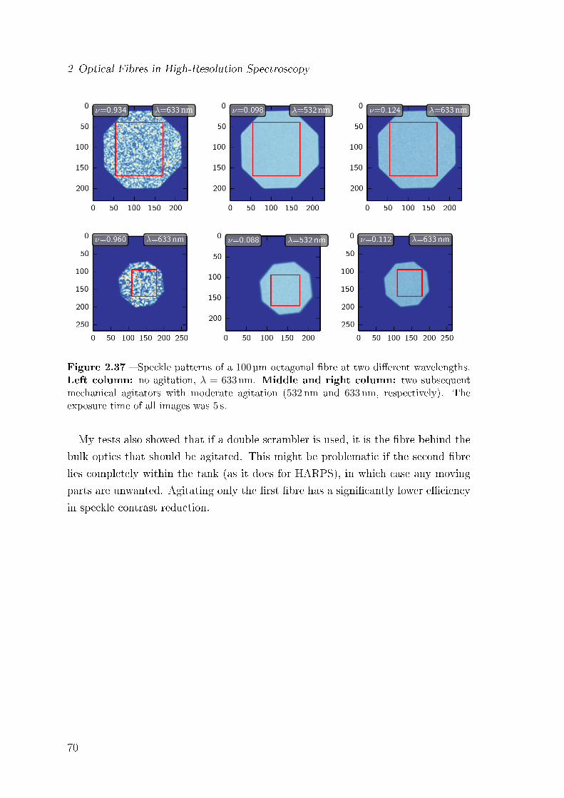
2 Optical Fibres in High-Resolution Spectroscopy
Figure 2.37 Speckle patterns of a 100µm octagonal bre at two dierent wavelengths.Left column: no agitation, λ = 633 nm. Middle and right column: two subsequentmechanical agitators with moderate agitation (532 nm and 633 nm, respectively). Theexposure time of all images was 5 s.
My tests also showed that if a double scrambler is used, it is the bre behind the
bulk optics that should be agitated. This might be problematic if the second bre
lies completely within the tank (as it does for HARPS), in which case any moving
parts are unwanted. Agitating only the rst bre has a signicantly lower eciency
in speckle contrast reduction.
70
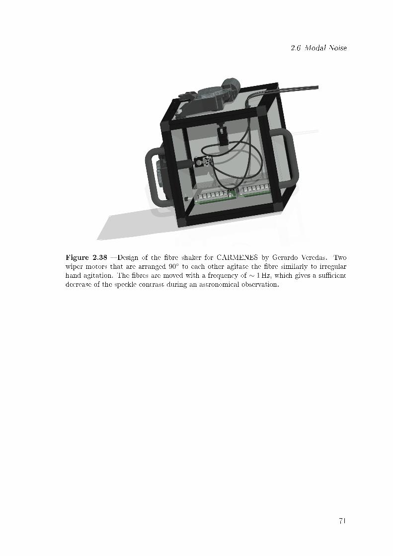
2.6 Modal Noise
Figure 2.38 Design of the bre shaker for CARMENES by Gerardo Veredas. Twowiper motors that are arranged 90 to each other agitate the bre similarly to irregularhand agitation. The bres are moved with a frequency of ∼ 1Hz, which gives a sucientdecrease of the speckle contrast during an astronomical observation.
71
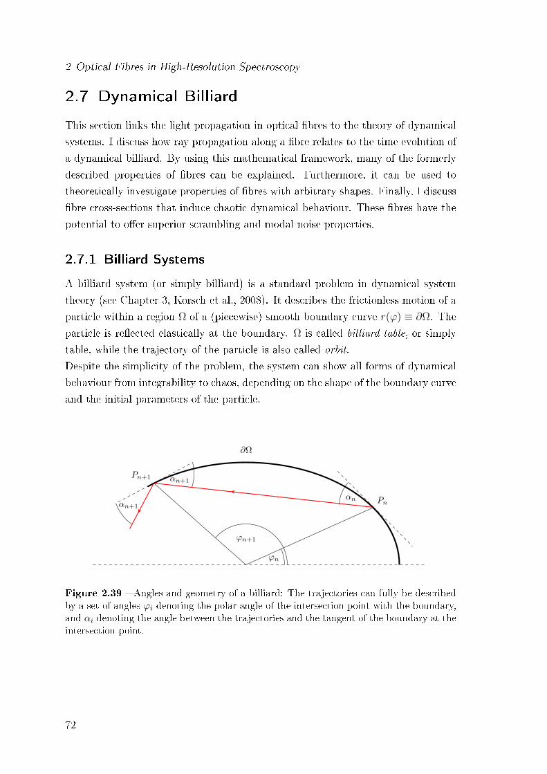
2 Optical Fibres in High-Resolution Spectroscopy
2.7 Dynamical Billiard
This section links the light propagation in optical bres to the theory of dynamical
systems. I discuss how ray propagation along a bre relates to the time evolution of
a dynamical billiard. By using this mathematical framework, many of the formerly
described properties of bres can be explained. Furthermore, it can be used to
theoretically investigate properties of bres with arbitrary shapes. Finally, I discuss
bre cross-sections that induce chaotic dynamical behaviour. These bres have the
potential to oer superior scrambling and modal noise properties.
2.7.1 Billiard Systems
A billiard system (or simply billiard) is a standard problem in dynamical system
theory (see Chapter 3, Korsch et al., 2008). It describes the frictionless motion of a
particle within a region Ω of a (piecewise) smooth boundary curve r(ϕ) ≡ ∂Ω. The
particle is reected elastically at the boundary. Ω is called billiard table, or simply
table, while the trajectory of the particle is also called orbit.
Despite the simplicity of the problem, the system can show all forms of dynamical
behaviour from integrability to chaos, depending on the shape of the boundary curve
and the initial parameters of the particle.
∂Ω
Pn
Pn+1
ϕn
ϕn+1
αn
αn+1
αn+1
Figure 2.39 Angles and geometry of a billiard: The trajectories can fully be describedby a set of angles ϕi denoting the polar angle of the intersection point with the boundary,and αi denoting the angle between the trajectories and the tangent of the boundary at theintersection point.
72
2.7 Dynamical Billiard
The geometry and relevant angles of a billiard system are shown in Fig. 2.39.
A billiard can be described by a Hamiltonian system:
H(px, py, x, y) =1
2m
(p2x + p2
y
)+ V (x, y) , (2.23)
with
V (x, y) =
0 (x, y) ∈ Ω
∞ (x, y) /∈ Ω. (2.24)
In classical mechanics, the systems treated are almost always integrable. This means
that for a system withN degrees of freedom, there existN constants of motion which
are in involution. By denition, the energy is always conserved in a billiard system.
Therefore, the time evolution of the particle in the four-dimensional phase space
(x, y, px, py) can be restricted to a three-dimensional sub-manifold, often called the
energy surface. In case a second constant of motion exists (e.g. constant angular
momentum for rotationally symmetric boundary curves), the trajectory of the par-
ticle usually lies on a torus. Exceptions from this rule will be discussed later. If
we follow the trajectories for a typical billiard in a Cartesian coordinate system,
the resulting orbits show a complicated form. It is therefore very useful to switch
to a dierent coordinate system, the Poincaré-Birkho coordinate system. These
coordinates describe a Poincaré section that naturally emerges from the geometry
of a billiard system. The rst coordinate corresponds to the length of the perimeter
at the point of impact at angle ϕ
S(ϕ) = 1/L
∫ ϕ
0
√r2(ϕ′) + (dr/dϕ′)2dϕ′ , (2.25)
where L is the total length of the boundary curve. The second coordinate is
p = cos(α), where α denotes the angle between the trajectory after reection and the
boundary (see Fig. 2.39). It can therefore be interpreted as the parallel momentum
of the point-mass. As the total momentum is constant and is usually set to unity,
the four-dimensional phase space can be reduced to two dimensions. The underlying
geometry allows to construct a mapping T that relates each point in the Poincaré
section to the succeeding point of impact:
(Sn, pn)T−−→ (Sn+1, pn+1) . (2.26)
73
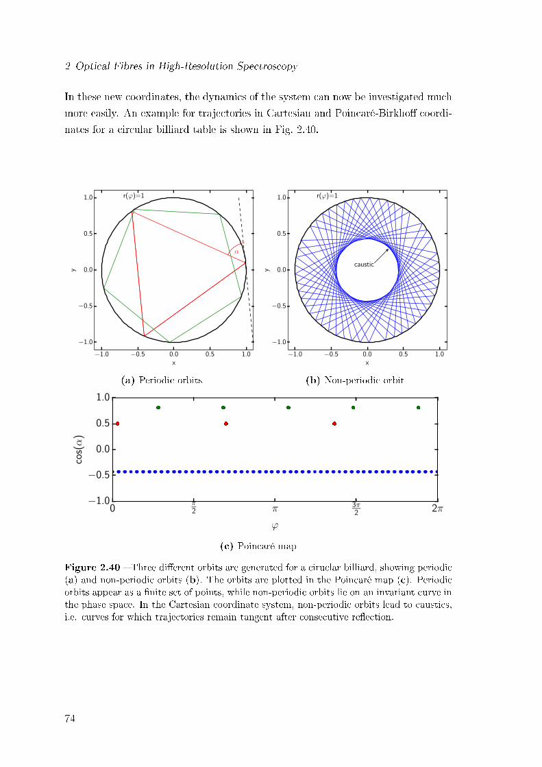
2 Optical Fibres in High-Resolution Spectroscopy
In these new coordinates, the dynamics of the system can now be investigated much
more easily. An example for trajectories in Cartesian and Poincaré-Birkho coordi-
nates for a circular billiard table is shown in Fig. 2.40.
−1.0 −0.5 0.0 0.5 1.0x
−1.0
−0.5
0.0
0.5
1.0
y
r(ϕ)=1
α
(a) Periodic orbits
−1.0 −0.5 0.0 0.5 1.0x
−1.0
−0.5
0.0
0.5
1.0
y
r(ϕ)=1
caustic
(b) Non-periodic orbit
0π2 π 3π
2 2π
ϕ
−1.0
−0.5
0.0
0.5
1.0
cos(α
)
(c) Poincaré map
Figure 2.40 Three dierent orbits are generated for a ciruclar billiard, showing periodic(a) and non-periodic orbits (b). The orbits are plotted in the Poincaré map (c). Periodicorbits appear as a nite set of points, while non-periodic orbits lie on an invariant curve inthe phase space. In the Cartesian coordinate system, non-periodic orbits lead to caustics,i.e. curves for which trajectories remain tangent after consecutive reection.
74
2.7 Dynamical Billiard
One can derive the equivalence of a dynamical billiard to the ray propagation in
an optical multi-mode bre in two ways. The intuitive way is to further simplify
ray-tracing methods by assuming the bre to be ideal along the z-direction. In fact,
this is an appropriate assumption, as modern bres do have very tight tolerances on
the diameter deviations in the order of 1%. It should also be noted that in principle,
billiard systems could account for such variations by adding a time dependence to
the potential V = V (x, y, t). For simplicity, we will however not include a time
dependent potential for the following considerations. Total internal reection at the
core-cladding transition turns into specular reection at the billiard boundary.
A second way to show the equivalence of ray propagation in a weakly guiding multi-
mode bre and a billiard system is given in Doya et al. (2002).4 The authors showed
that the Helmholtz equation (Eq. (2.11)) corresponds to the pseudo time-dependent
Schrödinger equation, where instead of a dependency on time t the equation depends
on the coordinate z. By deriving the eikonal equation in paraxial approximation,
i.e. for small angles between the optical axis of the bre and the incoming light,
they showed that the wave propagation of light within the bre can be reduced to
the dynamics of a billiard.
In order to investigate the dynamical properties of a billiard system, it is useful to
follow the time evolution of a set of initial points. Usually, a small region in the
phase space is selected as an initial set. The behaviour of this region under the
mapping T is used to reveal the underlying dynamics and to distinguish between
regular and chaotic systems. Here, we pick our initial values in a slightly dierent
way, in order to make the simulations similar to the experiments in Section 2.5.1.
We pick a location r0 within the region Ω and create initial values by choosing
random vectors in a small disk around r0 with random directions. Both location
and direction are chosen from uniform distributions over the following intervals:
φinitial ∈ [0, 2π[ , rinitial ∈ Dd/2(r0) , (2.27)
where D is the disk with radius d/2 around r0. For a large number of initial values,
this is equivalent to imaging a small spot with diameter d onto the bre with a
homogeneous far eld, as it was done in the raytracing simulations and experiments
in Section 2.5.1.
4Amulti-mode bre is called weakly guiding if (n1−n2)/n2 1, where n1 and n2 are the refractiveindices of the core and the cladding, respectively. All standard silica bres are weakly guidingbres.
75
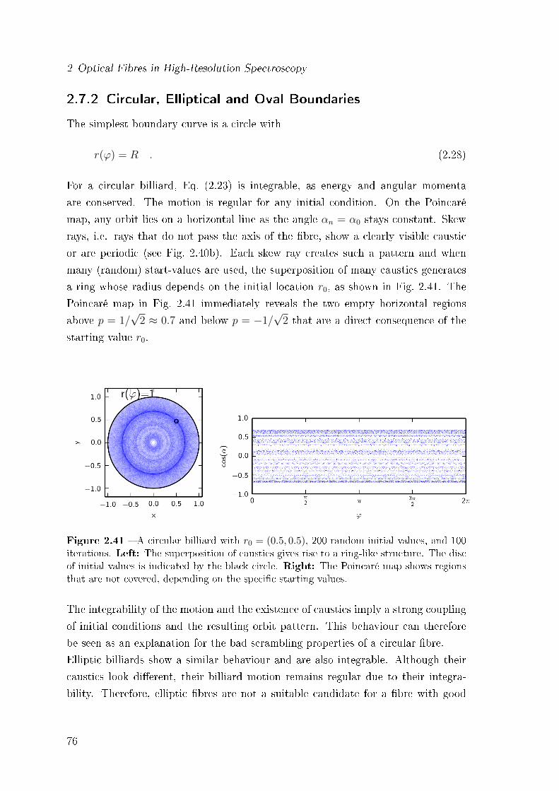
2 Optical Fibres in High-Resolution Spectroscopy
2.7.2 Circular, Elliptical and Oval Boundaries
The simplest boundary curve is a circle with
r(ϕ) = R . (2.28)
For a circular billiard, Eq. (2.23) is integrable, as energy and angular momenta
are conserved. The motion is regular for any initial condition. On the Poincaré
map, any orbit lies on a horizontal line as the angle αn = α0 stays constant. Skew
rays, i.e. rays that do not pass the axis of the bre, show a clearly visible caustic
or are periodic (see Fig. 2.40b). Each skew ray creates such a pattern and when
many (random) start-values are used, the superposition of many caustics generates
a ring whose radius depends on the initial location r0, as shown in Fig. 2.41. The
Poincaré map in Fig. 2.41 immediately reveals the two empty horizontal regions
above p = 1/√
2 ≈ 0.7 and below p = −1/√
2 that are a direct consequence of the
starting value r0.
Figure 2.41 A circular billiard with r0 = (0.5, 0.5), 200 random initial values, and 100iterations. Left: The superposition of caustics gives rise to a ring-like structure. The discof initial values is indicated by the black circle. Right: The Poincaré map shows regionsthat are not covered, depending on the specic starting values.
The integrability of the motion and the existence of caustics imply a strong coupling
of initial conditions and the resulting orbit pattern. This behaviour can therefore
be seen as an explanation for the bad scrambling properties of a circular bre.
Elliptic billiards show a similar behaviour and are also integrable. Although their
caustics look dierent, their billiard motion remains regular due to their integra-
bility. Therefore, elliptic bres are not a suitable candidate for a bre with good
76
2.7 Dynamical Billiard
scrambling properties. This observation puts into perspective the suggestion of us-
ing elliptical bres in astronomy by Allington-Smith et al. (2012). However, the
elliptical form is benecial in other applications: bres with a small elliptical core
are commonly used for polarisation maintaining bres.
Elliptical and circular boundaries are the only twice dierentiable boundaries known
to be integrable.5 In general, oval forms show a mixture of chaotic and regular mo-
tion that depends on the initial condition (Lopac et al., 2002).
In summary, neither elliptical nor oval billiards seem to be a good choice if a homo-
geneous and stable output illumination is desired.
2.7.3 Polygonal Boundaries
Billiards with polygonal boundaries are somewhat special, because their boundaries
are not a smooth function that is twice dierentiable. We will restrict our view to
rational polygons, where each angle is a rational fraction of π. In such billiards,
each trajectory has only a nite number of directions. Therefore, the phase space is
at most two-dimensional (Richens and Berry, 1981). Zemlyakov and Katok (1975)
showed that unlike the case of integrable systems, rational polygons possess an
invariant surface whose topology diers from a torus. A few exceptions exist, such
as rectangles and special triangles, which are integrable systems. For all other regular
polygons, no unique action-angle variables can be dened.6 This is the reason why
regular polygonal systems are called pseudointegrable (Richens and Berry, 1981).
The dynamics in a regular polygon are non chaotic in the sense that the Lyapunov
exponent is zero (Chernov and Troubetzkoy, 1998), i.e. neighbouring trajectories do
not exponentially diverge.7 By looking at Fig. 2.42, one sees that Ω is homogeneously
lled and that there are no visible caustics as in the case of a circular boundary.
In fact, one property of rational polygons is that they are dynamically optimal.
This means that any trajectory is either periodic or it uniformly covers the table
(DeMarco, 2011).
5This statement is referred to as the Birkho-Poritsky conjecture. As of today, it has not formallybeen proven yet.
6Action-angle variables are a set of coordinates that provide a convenient way to describe inte-grable systems in classical mechanics.
7The Lyapunov exponent measures how fast two orbits starting with slightly dierent initialconditions diverge. In a chaotic system, the distance of orbits increases exponentially.
77
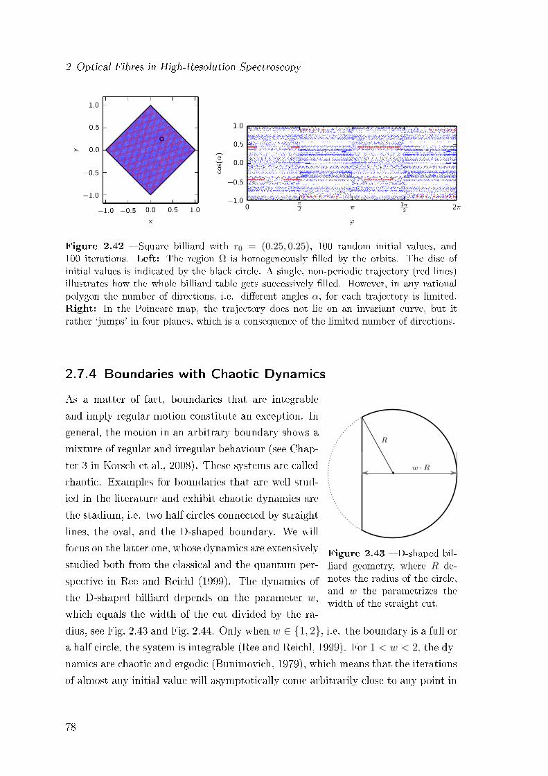
2 Optical Fibres in High-Resolution Spectroscopy
Figure 2.42 Square billiard with r0 = (0.25, 0.25), 100 random initial values, and100 iterations. Left: The region Ω is homogeneously lled by the orbits. The disc ofinitial values is indicated by the black circle. A single, non-periodic trajectory (red lines)illustrates how the whole billiard table gets successively lled. However, in any rationalpolygon the number of directions, i.e. dierent angles α, for each trajectory is limited.Right: In the Poincaré map, the trajectory does not lie on an invariant curve, but itrather `jumps' in four planes, which is a consequence of the limited number of directions.
2.7.4 Boundaries with Chaotic Dynamics
w ·R
R
Figure 2.43 D-shaped bil-liard geometry, where R de-notes the radius of the circle,and w the parametrizes thewidth of the straight cut.
As a matter of fact, boundaries that are integrable
and imply regular motion constitute an exception. In
general, the motion in an arbitrary boundary shows a
mixture of regular and irregular behaviour (see Chap-
ter 3 in Korsch et al., 2008). These systems are called
chaotic. Examples for boundaries that are well stud-
ied in the literature and exhibit chaotic dynamics are
the stadium, i.e. two half circles connected by straight
lines, the oval, and the D-shaped boundary. We will
focus on the latter one, whose dynamics are extensively
studied both from the classical and the quantum per-
spective in Ree and Reichl (1999). The dynamics of
the D-shaped billiard depends on the parameter w,
which equals the width of the cut divided by the ra-
dius, see Fig. 2.43 and Fig. 2.44. Only when w ∈ 1, 2, i.e. the boundary is a full ora half circle, the system is integrable (Ree and Reichl, 1999). For 1 < w < 2, the dy-
namics are chaotic and ergodic (Bunimovich, 1979), which means that the iterations
of almost any initial value will asymptotically come arbitrarily close to any point in
78
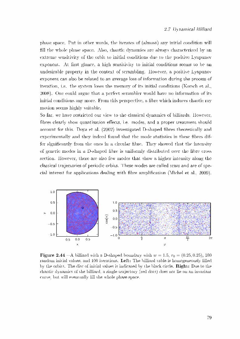
2.7 Dynamical Billiard
phase space. Put in other words, the iterates of (almost) any initial condition will
ll the whole phase space. Also, chaotic dynamics are always characterized by an
extreme sensitivity of the orbit to initial conditions due to the positive Lyapunov
exponent. At rst glance, a high sensitivity to initial conditions seems to be an
undesirable property in the context of scrambling. However, a positive Lyapunov
exponent can also be related to an average loss of information during the process of
iteration, i.e. the system loses the memory of its initial conditions (Korsch et al.,
2008). One could argue that a perfect scrambler would have no information of its
initial conditions any more. From this perspective, a bre which induces chaotic ray
motion seems highly suitable.
So far, we have restricted our view to the classical dynamics of billiards. However,
bres clearly show quantisation eects, i.e. modes, and a proper treatment should
account for this. Doya et al. (2002) investigated D-shaped bres theoretically and
experimentally and they indeed found that the mode statistics in these bres dif-
fer signicantly from the ones in a circular bre. They showed that the intensity
of generic modes in a D-shaped bre is uniformly distributed over the bre cross
section. However, there are also few modes that show a higher intensity along the
classical trajectories of periodic orbits. These modes are called scars and are of spe-
cial interest for applications dealing with bre amplication (Michel et al., 2009).
Figure 2.44 A billiard with a D-shaped boundary with w = 1.5, r0 = (0.25, 0.25), 100random initial values, and 100 iterations. Left: The billiard table is homogeneously lledby the orbits. The disc of initial values is indicated by the black circle. Right: Due to thechaotic dynamics of the billiard, a single trajectory (red dots) does not lie on an invariantcurve, but will eventually ll the whole phase space.
79
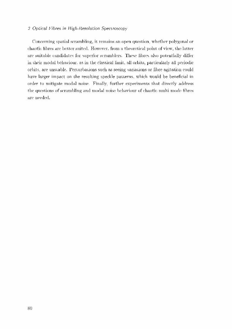
2 Optical Fibres in High-Resolution Spectroscopy
Concerning spatial scrambling, it remains an open question, whether polygonal or
chaotic bres are better suited. However, from a theoretical point of view, the latter
are suitable candidates for superior scramblers. These bres also potentially dier
in their modal behaviour, as in the classical limit, all orbits, particularly all periodic
orbits, are unstable. Perturbations such as seeing variations or bre agitation could
have larger impact on the resulting speckle patterns, which would be benecial in
order to mitigate modal noise. Finally, further experiments that directly address
the questions of scrambling and modal noise behaviour of chaotic multi mode bres
are needed.
80
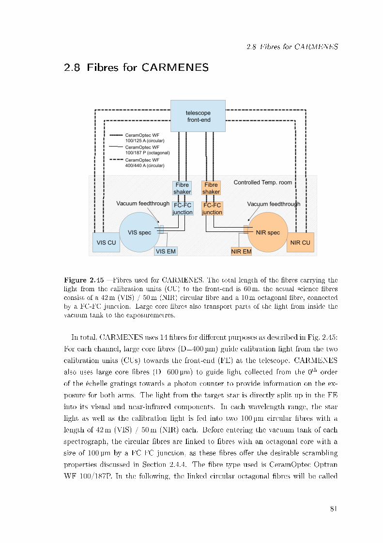
2.8 Fibres for CARMENES
2.8 Fibres for CARMENES
VIS CU NIR CU
VIS spec NIR spec
Controlled Temp. roomFibreshaker
Fibreshaker
FC-FCjunction
FC-FCjunction
Vacuum feedthrough
CeramOptec WF 100/125 A (circular)
CeramOptec WF 100/187 P (octagonal)
CeramOptec WF400/440 A (circular)
VIS EM NIR EM
Vacuum feedthrough
telescope front-end
Figure 2.45 Fibres used for CARMENES. The total length of the bres carrying thelight from the calibration units (CU) to the front-end is 60m, the actual science bresconsist of a 42m (VIS) / 50m (NIR) circular bre and a 10m octagonal bre, connectedby a FC-FC junction. Large core bres also transport parts of the light from inside thevacuum tank to the exposuremetres.
In total, CARMENES uses 14 bres for dierent purposes as described in Fig. 2.45:
For each channel, large core bres (D=400µm) guide calibration light from the two
calibration units (CUs) towards the front-end (FE) at the telescope. CARMENES
also uses large core bres (D=600µm) to guide light collected from the 0th order
of the échelle gratings towards a photon counter to provide information on the ex-
posure for both arms. The light from the target star is directly split up in the FE
into its visual and near-infrared components. In each wavelength range, the star
light as well as the calibration light is fed into two 100µm circular bres with a
length of 42m (VIS) / 50m (NIR) each. Before entering the vacuum tank of each
spectrograph, the circular bres are linked to bres with an octagonal core with a
size of 100µm by a FC-FC junction, as these bres oer the desirable scrambling
properties discussed in Section 2.4.4. The bre type used is CeramOptec Optran
WF 100/187P. In the following, the linked circular octagonal bres will be called
81
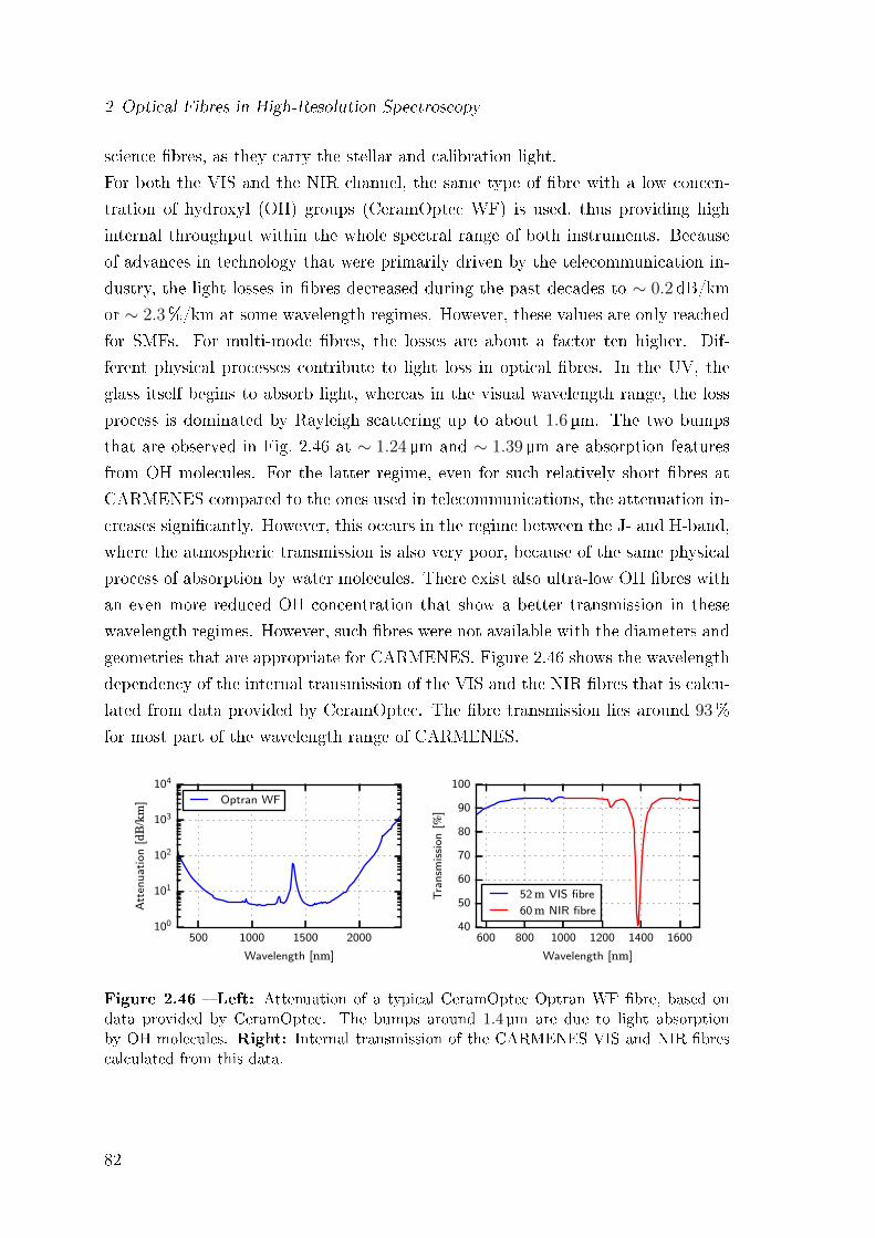
2 Optical Fibres in High-Resolution Spectroscopy
science bres, as they carry the stellar and calibration light.
For both the VIS and the NIR channel, the same type of bre with a low concen-
tration of hydroxyl (OH) groups (CeramOptec WF) is used, thus providing high
internal throughput within the whole spectral range of both instruments. Because
of advances in technology that were primarily driven by the telecommunication in-
dustry, the light losses in bres decreased during the past decades to ∼ 0.2 dB/km
or ∼ 2.3%/km at some wavelength regimes. However, these values are only reached
for SMFs. For multi-mode bres, the losses are about a factor ten higher. Dif-
ferent physical processes contribute to light loss in optical bres. In the UV, the
glass itself begins to absorb light, whereas in the visual wavelength range, the loss
process is dominated by Rayleigh scattering up to about 1.6 µm. The two bumps
that are observed in Fig. 2.46 at ∼ 1.24µm and ∼ 1.39µm are absorption features
from OH molecules. For the latter regime, even for such relatively short bres at
CARMENES compared to the ones used in telecommunications, the attenuation in-
creases signicantly. However, this occurs in the regime between the J- and H-band,
where the atmospheric transmission is also very poor, because of the same physical
process of absorption by water molecules. There exist also ultra-low OH bres with
an even more reduced OH concentration that show a better transmission in these
wavelength regimes. However, such bres were not available with the diameters and
geometries that are appropriate for CARMENES. Figure 2.46 shows the wavelength
dependency of the internal transmission of the VIS and the NIR bres that is calcu-
lated from data provided by CeramOptec. The bre transmission lies around 93%
for most part of the wavelength range of CARMENES.
500 1000 1500 2000
Wavelength [nm]
100
101
102
103
104
Att
enu
ati
on
[dB
/km
] Optran WF
600 800 1000 1200 1400 1600
Wavelength [nm]
40
50
60
70
80
90
100
Tra
nsm
issi
on
[%]
52 m VIS fibre
60 m NIR fibre
Figure 2.46 Left: Attenuation of a typical CeramOptec Optran WF bre, based ondata provided by CeramOptec. The bumps around 1.4 µm are due to light absorptionby OH molecules. Right: Internal transmission of the CARMENES VIS and NIR brescalculated from this data.
82
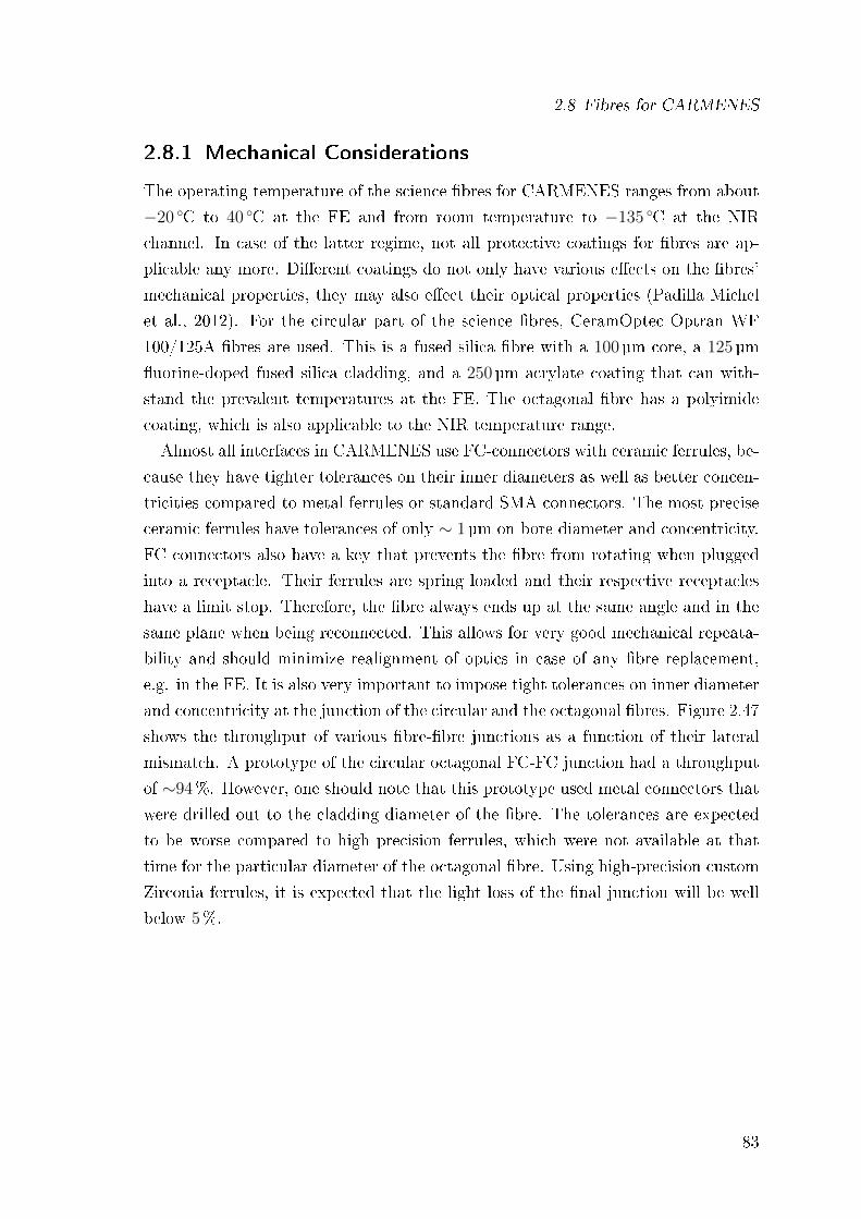
2.8 Fibres for CARMENES
2.8.1 Mechanical Considerations
The operating temperature of the science bres for CARMENES ranges from about
−20 C to 40 C at the FE and from room temperature to −135 C at the NIR
channel. In case of the latter regime, not all protective coatings for bres are ap-
plicable any more. Dierent coatings do not only have various eects on the bres'
mechanical properties, they may also eect their optical properties (Padilla Michel
et al., 2012). For the circular part of the science bres, CeramOptec Optran WF
100/125A bres are used. This is a fused silica bre with a 100µm core, a 125µm
uorine-doped fused silica cladding, and a 250µm acrylate coating that can with-
stand the prevalent temperatures at the FE. The octagonal bre has a polyimide
coating, which is also applicable to the NIR temperature range.
Almost all interfaces in CARMENES use FC-connectors with ceramic ferrules, be-
cause they have tighter tolerances on their inner diameters as well as better concen-
tricities compared to metal ferrules or standard SMA connectors. The most precise
ceramic ferrules have tolerances of only ∼ 1 µm on bore diameter and concentricity.
FC connectors also have a key that prevents the bre from rotating when plugged
into a receptacle. Their ferrules are spring loaded and their respective receptacles
have a limit stop. Therefore, the bre always ends up at the same angle and in the
same plane when being reconnected. This allows for very good mechanical repeata-
bility and should minimize realignment of optics in case of any bre replacement,
e.g. in the FE. It is also very important to impose tight tolerances on inner diameter
and concentricity at the junction of the circular and the octagonal bres. Figure 2.47
shows the throughput of various bre-bre junctions as a function of their lateral
mismatch. A prototype of the circular octagonal FC-FC junction had a throughput
of ∼94%. However, one should note that this prototype used metal connectors that
were drilled out to the cladding diameter of the bre. The tolerances are expected
to be worse compared to high precision ferrules, which were not available at that
time for the particular diameter of the octagonal bre. Using high-precision custom
Zirconia ferrules, it is expected that the light loss of the nal junction will be well
below 5%.
83
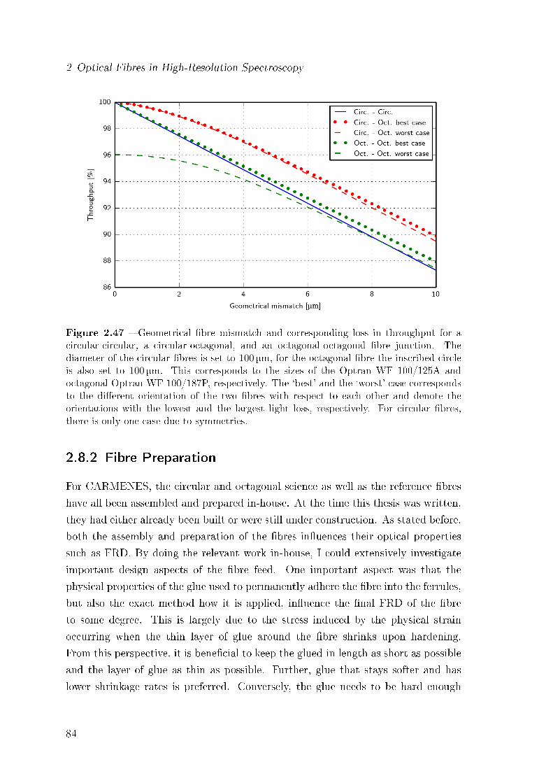
2 Optical Fibres in High-Resolution Spectroscopy
Figure 2.47 Geometrical bre mismatch and corresponding loss in throughput for acircular-circular, a circular-octagonal, and an octagonal-octagonal bre junction. Thediameter of the circular bres is set to 100 µm, for the octagonal bre the inscribed circleis also set to 100 µm. This corresponds to the sizes of the Optran WF 100/125A andoctagonal Optran WF 100/187P, respectively. The `best' and the `worst' case correspondsto the dierent orientation of the two bres with respect to each other and denote theorientations with the lowest and the largest light loss, respectively. For circular bres,there is only one case due to symmetries.
2.8.2 Fibre Preparation
For CARMENES, the circular and octagonal science as well as the reference bres
have all been assembled and prepared in-house. At the time this thesis was written,
they had either already been built or were still under construction. As stated before,
both the assembly and preparation of the bres inuences their optical properties
such as FRD. By doing the relevant work in-house, I could extensively investigate
important design aspects of the bre feed. One important aspect was that the
physical properties of the glue used to permanently adhere the bre into the ferrules,
but also the exact method how it is applied, inuence the nal FRD of the bre
to some degree. This is largely due to the stress induced by the physical strain
occurring when the thin layer of glue around the bre shrinks upon hardening.
From this perspective, it is benecial to keep the glued-in length as short as possible
and the layer of glue as thin as possible. Further, glue that stays softer and has
lower shrinkage rates is preferred. Conversely, the glue needs to be hard enough
84
2.8 Fibres for CARMENES
after curing to enable polishing the bre without `smearing' its surface. In practice,
the lower limit for glue lm thickness is about 1 µm to 2 µm for the gap between bre
and ferrule. Below this range, it becomes hard to insert the bre into the ferrule, as
the tolerances on the diameter of the bre as well as the bore of the ferrule are in
the same regime.
Two methods for bre end-face preparation exist: Polishing and cleaving.8 The
rst technique applies a set of successively ner grades of lapping sheets to polish
the bre, which is glued into a ferrule or a connector, to the surface roughness be-
ing requested. This method is rather time consuming, because after each polishing
step, an inspection of the surface is highly recommended in order to guarantee good
optical quality. The polishing process causes sub-surface damages that can propa-
gate from the surface down the bre. It is believed that these damages propagate
to a depth that is roughly three times the depth of the biggest defect on the bre
surface. This makes it inevitable to remove sucient material after each polishing
step. Figure 2.48 illustrates the polishing steps of one of the CARMENES circular
science bres that I prepared. Care was taken to produce surfaces with low surface
roughness. However, in case of the circular science bres of CARMENES, this is not
particularly critical. Both ends of the bres are immersed to the other components,
i.e. to a rod lens in the FE and to the octagonal bre at the other end, by applying
an index matching gel that reduces irregularities on the bre surface. The second
method that is used for bre end face preparation is cleaving. Hereby, the bre is put
under axial tension and is slightly scratched from the side. Depending on the exact
tension and bre parameters, the glass cracks in a plane that is perpendicular to the
optical axis of the bre. In principle, cleaving is easier and faster than polishing,
and when utilising sophisticated cleavers, the repeatability of high-quality end faces
is also very good. For CARMENES, cleaving can only be used for the end faces of
the octagonal bres at the spectrograph side, because all other bres are in physical
contact with other optical components. However, cleaving of non-standard bres
such as the octagonal bre used for CARMENES is not straight-forward, because
the cleaving parameters are not known a priori. Using wrong parameters may lead
to a bad cleave with chips or lips on the edges of the bre. In addition, the end
face may show zones with high surface roughness, called mist, or with even larger
irregularities, called hackle. Even when the right cleaving parameters are applied,
these problems might still occur, for instance when there is intrinsic stress from the
manufacturing process frozen within the bre.
8Both are equally terrifying.
85
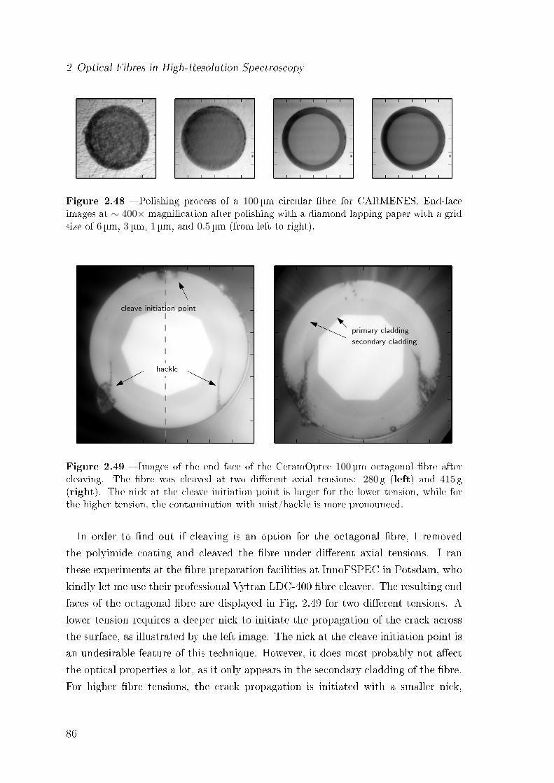
2 Optical Fibres in High-Resolution Spectroscopy
Figure 2.48 Polishing process of a 100 µm circular bre for CARMENES. End-faceimages at ∼ 400× magnication after polishing with a diamond lapping paper with a gridsize of 6µm, 3 µm, 1 µm, and 0.5 µm (from left to right).
Figure 2.49 Images of the end face of the CeramOptec 100 µm octagonal bre aftercleaving. The bre was cleaved at two dierent axial tensions: 280 g (left) and 415 g(right). The nick at the cleave initiation point is larger for the lower tension, while forthe higher tension, the contamination with mist/hackle is more pronounced.
In order to nd out if cleaving is an option for the octagonal bre, I removed
the polyimide coating and cleaved the bre under dierent axial tensions. I ran
these experiments at the bre preparation facilities at InnoFSPEC in Potsdam, who
kindly let me use their professional Vytran LDC-400 bre cleaver. The resulting end
faces of the octagonal bre are displayed in Fig. 2.49 for two dierent tensions. A
lower tension requires a deeper nick to initiate the propagation of the crack across
the surface, as illustrated by the left image. The nick at the cleave initiation point is
an undesirable feature of this technique. However, it does most probably not aect
the optical properties a lot, as it only appears in the secondary cladding of the bre.
For higher bre tensions, the crack propagation is initiated with a smaller nick,
86
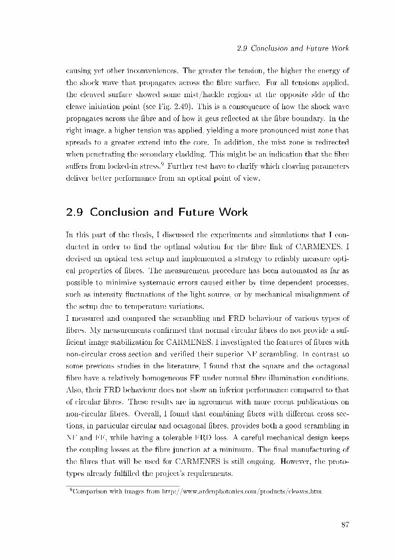
2.9 Conclusion and Future Work
causing yet other inconveniences. The greater the tension, the higher the energy of
the shock wave that propagates across the bre surface. For all tensions applied,
the cleaved surface showed some mist/hackle regions at the opposite side of the
cleave initiation point (see Fig. 2.49). This is a consequence of how the shock wave
propagates across the bre and of how it gets reected at the bre boundary. In the
right image, a higher tension was applied, yielding a more pronounced mist zone that
spreads to a greater extend into the core. In addition, the mist zone is redirected
when penetrating the secondary cladding. This might be an indication that the bre
suers from locked-in stress.9 Further test have to clarify which cleaving parameters
deliver better performance from an optical point of view.
2.9 Conclusion and Future Work
In this part of the thesis, I discussed the experiments and simulations that I con-
ducted in order to nd the optimal solution for the bre link of CARMENES. I
devised an optical test setup and implemented a strategy to reliably measure opti-
cal properties of bres. The measurement procedure has been automated as far as
possible to minimize systematic errors caused either by time dependent processes,
such as intensity uctuations of the light source, or by mechanical misalignment of
the setup due to temperature variations.
I measured and compared the scrambling and FRD behaviour of various types of
bres. My measurements conrmed that normal circular bres do not provide a suf-
cient image stabilization for CARMENES. I investigated the features of bres with
non-circular cross section and veried their superior NF scrambling. In contrast to
some previous studies in the literature, I found that the square and the octagonal
bre have a relatively homogeneous FF under normal bre illumination conditions.
Also, their FRD behaviour does not show an inferior performance compared to that
of circular bres. These results are in agreement with more recent publications on
non-circular bres. Overall, I found that combining bres with dierent cross sec-
tions, in particular circular and octagonal bres, provides both a good scrambling in
NF and FF, while having a tolerable FRD loss. A careful mechanical design keeps
the coupling losses at the bre junction at a minimum. The nal manufacturing of
the bres that will be used for CARMENES is still ongoing. However, the proto-
types already fullled the project's requirements.
9Comparison with images from http://www.ardenphotonics.com/products/cleaves.htm
87
2 Optical Fibres in High-Resolution Spectroscopy
In addition, I simulated the scrambling behaviour of bres using the commercial
raytracing software ZEMAX in order to theoretically investigate bres with cross
sections that have not been available for testing. My simulations of circular bres
show a clear qualitative agreement with my measurements, which justies the ap-
proach to simulate multi mode bres by raytracing. The results for polygonal shaped
bres indicate that the lower the number of their sides, the better their scrambling.
Finally, I analysed the impact of variations in the FF of a bre on RV precision by
raytracing simulations. For both CARMENES spectrographs, I estimated the sen-
sitivity of the position of a spectral line due to illumination changes by calculating
the barycentric shifts of the spot diagrams when the pupil illumination is changing.
The simulations showed that for FF variations that are expected to be typical at a
telescope, the shifts for single lines are smaller than 1m/s to 2m/s. The barycentric
shifts strongly depend on the optical aberrations and therefore also on wavelength.
In case of the CARMENES spectrographs, the shifts along an échelle order typically
show a reection symmetry with respect to the centre of the order. Therefore, av-
eraging over many spectral lines along an order will further reduce the systematic
shifts that are caused by these FF variations.
Although a fair number of publications in the last few years investigated the scram-
bling properties of bres with various cross sections, there is, up to my best knowl-
edge, no such study that gives a satisfying theoretical explanation for the dierent
scrambling performances of these bres. I suggested that the theory of dynamical
billiards provides a suitable theoretical framework to explain and further investigate
the scrambling and modal noise properties of multi mode bres. I concluded that
bres whose underlying geometry induce chaotic ray motion will potentially help
to further reduce the impact of insucient scrambling and modal noise on radial
velocity precision.
88


3 Stabilized Fabry-Pérot Etalon for
High-Resolution Spectrographs
This chapter presents the work on an actively stabilized Fabry-Pérot etalon for
spectrograph calibration. Many of the results are published either in Schwab et al.
(2014) or Gurevich et al. (2014). In collaboration with my co-authors, I developed a
novel etalon locking concept. I was the main responsible for the experimental setup
in the optical laboratory at the Landessternwarte Heidelberg. I implemented all of
the relevant software for locking and performed the data analysis.
3.1 Introduction to Wavelength Calibration
3.1.1 Emission Lamps
Wavelength reference spectra are typically generated by using a hollow-cathode lamp
(HCL). This lamp consists of an anode and a cathode made of a specic material
that is enclosed by a glass tube lled with a buer gas. By applying a high voltage
between the anode and the cathode, the buer gas is ionized, resulting in gas atoms
being accelerated onto the cathode sputtering o atoms. Both gas and cathode
atoms get excited by collision with each other. When decaying into lower states,
they emit light in a rich spectrum of emission lines, whose absolute wavelengths can
be measured with high precision in the laboratory.
In astronomy, two methods for calibrating spectrographs with HCLs are in use. One
is to take an emission lamp spectrum before and after an observation and compare it
to the intermediate science spectrum. In most cases, the short term stability of the
spectrograph ensures suciently small drifts between the calibration and the science
image. However, a major drawback of this method is the overhead generated by the
consecutive recording of calibration and science spectra that reduces the number
of possible targets per time unit. To overcome this problem, Baranne et al. (1996)
introduced a second bre that allows for simultaneous measurement of science and
calibration light. The bre is placed such that each order of the calibration spectrum
91
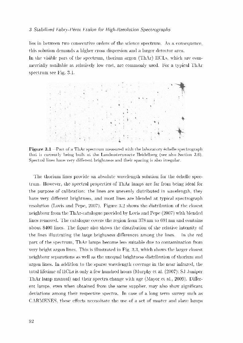
3 Stabilized Fabry-Pérot Etalon for High-Resolution Spectrographs
lies in between two consecutive orders of the science spectrum. As a consequence,
this solution demands a higher cross dispersion and a larger detector area.
In the visible part of the spectrum, thorium argon (ThAr) HCLs, which are com-
mercially available at relatively low cost, are commonly used. For a typical ThAr
spectrum see Fig. 3.1.
Figure 3.1 Part of a ThAr spectrum measured with the laboratory échelle spectrographthat is currently being built at the Landessternwarte Heidelberg (see also Section 3.6).Spectral lines have very dierent brightness and their spacing is also irregular.
The thorium lines provide an absolute wavelength solution for the échelle spec-
trum. However, the spectral properties of ThAr lamps are far from being ideal for
the purpose of calibration: the lines are unevenly distributed in wavelength, they
have very dierent brightness, and most lines are blended at typical spectrograph
resolution (Lovis and Pepe, 2007). Figure 3.2 shows the distribution of the closest
neighbour from the ThAr-catalogue provided by Lovis and Pepe (2007) with blended
lines removed. The catalogue covers the region from 378nm to 691nm and contains
about 8400 lines. The gure also shows the distribution of the relative intensity of
the lines illustrating the large brightness dierences among the lines. In the red
part of the spectrum, ThAr lamps become less suitable due to contamination from
very bright argon lines. This is illustrated in Fig. 3.3, which shows the larger closest
neighbour separations as well as the unequal brightness distribution of thorium and
argon lines. In addition to the sparse wavelength coverage in the near infrared, the
total lifetime of HCLs is only a few hundred hours (Murphy et al. (2007); SJ Juniper
ThAr lamp manual) and their spectra change with age (Mayor et al., 2009). Dier-
ent lamps, even when obtained from the same supplier, may also show signicant
deviations among their respective spectra. In case of a long term survey such as
CARMENES, these eects necessitate the use of a set of master and slave lamps
92
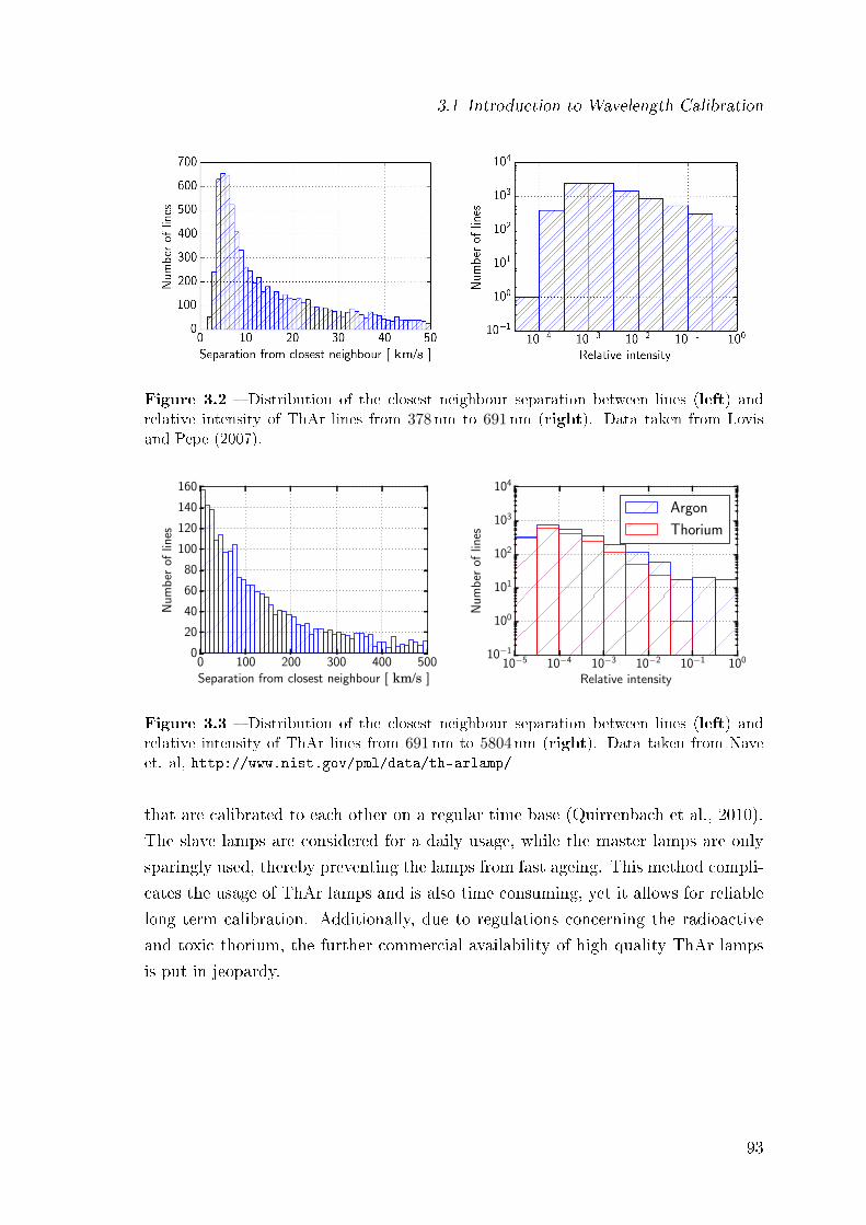
3.1 Introduction to Wavelength Calibration
Figure 3.2 Distribution of the closest neighbour separation between lines (left) andrelative intensity of ThAr lines from 378 nm to 691 nm (right). Data taken from Lovisand Pepe (2007).
0 100 200 300 400 500Separation from closest neighbour [ km/s ]
0
20
40
60
80
100
120
140
160
Num
ber
oflin
es
10−5 10−4 10−3 10−2 10−1 100
Relative intensity
10−1
100
101
102
103
104N
umb
erof
lines
Argon
Thorium
Figure 3.3 Distribution of the closest neighbour separation between lines (left) andrelative intensity of ThAr lines from 691 nm to 5804 nm (right). Data taken from Naveet. al, http://www.nist.gov/pml/data/th-arlamp/
that are calibrated to each other on a regular time base (Quirrenbach et al., 2010).
The slave lamps are considered for a daily usage, while the master lamps are only
sparingly used, thereby preventing the lamps from fast ageing. This method compli-
cates the usage of ThAr lamps and is also time consuming, yet it allows for reliable
long term calibration. Additionally, due to regulations concerning the radioactive
and toxic thorium, the further commercial availability of high quality ThAr lamps
is put in jeopardy.
93
3 Stabilized Fabry-Pérot Etalon for High-Resolution Spectrographs
Nevertheless, ThAr lamps are the primary calibration source for the HARPS
spectrograph and Lovis and Pepe (2007) report a calibration precision with the
simultaneous calibration method of 20 cm/s. They are not a good option for the
near infrared though, where more recently other emission lamps have been used for
calibration. Here, uranium-neon lamps are good candidates (Ramsey et al., 2010),
since they provide a larger number of lines from 900nm to 1300nm. However, these
lamps suer from similar problems regarding line spacing and brightness, limited
lifetime, and changing spectral properties over time.
Boesch et al. (2014) are investigating electrodeless microwave discharge lamps, where
CN molecules produce a feature rich spectrum with many lines between 1000nm
and 2000nm. Yet, the practicability of these lamps for astronomical spectrograph
calibration and their durability still needs to be further studied.
3.1.2 Gas Absorption Cell
The second well established method of calibrating a spectrograph is to pass the
starlight through a gas cell that acts as a transmission lter. The cell imprints
known, stable, and sharp absorption lines onto the stellar spectrum. Therefore, any
illumination-dependent eects are eliminated, since the starlight and the calibration
light always use the same optical path. For slit-fed spectrographs, a radial velocity
(RV) precision in the meter per second regime is possible, as this method relaxes the
stability requirements for the spectrograph and its guiding system. As no interleaved
orders for the calibration light are used, gas cells also save detector area. However,
by introducing a gas cell in the light path of the telescope, the throughput is reduced
by around 15% 1.
Campbell and Walker (1979) used heated cells lled with hydrogen uoride (HF).
They have deep, but few lines for calibrating. Due to its toxic and corrosive nature,
HF has to be handled very carefully. As an alternative, iodine cells can be used,
as they provide a very large number of sharp lines in the range 500nm to 600nm
(Butler et al., 1996; Marcy and Butler, 1992). The narrow bandwidth of the iodine
cell limits its applicability to bright targets that are rich in spectral features in the
visible part of their spectrum. In order to reach the same RV precision, the signal to
noise ratio (SNR) of the obtained spectra must be at least twice as large as the one
needed for simultaneous ThAr calibration (Bouchy et al., 2001). Still, RV precisions
1This values is taken from the CHIRON eciency test document http://www.ctio.noao.edu/~atokovin/echelle/efficiency_jun2011.pdf
94
3.1 Introduction to Wavelength Calibration
better than 2m/s has been reported (Tokovinin et al., 2013).
Mahadevan and Ge (2009) suggested to use gas cells in a similar way as emission
lamps, i.e. by illuminating them with broadband white light. This would eliminate
the SNR problem and increase the throughput of the system. However, now one
loses the benet that the calibration light follows the same optical path as the
stellar light. New gas mixtures for absorption cells that provide lines in a wide
range in the NIR are also extensively being investigated (Mahadevan and Ge, 2009;
Redman et al., 2012; Plavchan et al., 2013; Seemann et al., 2014). In some cases,
it is not even necessary to put another gas mixture in the line of sight between the
observer and the star, but one can rather use what is already out there: the Earth's
atmosphere. Rotational-vibrational transitions from molecules such as CO2 provide
a set of known ducial marks that can be used for calibration. The width of the
lines, their exact position, and their depth depend on weather conditions. Pressure,
temperature, and most importantly wind limit the precision of this method to a few
meters per second (Figueira et al., 2010).
3.1.3 Laser Frequency Combs
A laser frequency comb (LFC) is a coherent light source that generates a comb like
spectrum of very narrow lines, whose frequencies are stabilized to an atomic clock.
This extreme accuracy allows for atomic and molecular transition measurements
with unprecedented precision. For their contribution to this eld of research, T. W.
Hänsch and J. L. Hall were awarded the 2005 Nobel Prize in Physics. During the last
few years, LFCs have been adapted to the needs of RV measurements (Steinmetz
et al., 2008; Li et al., 2008; Stark et al., 2011). Usually, LFCs have a narrow line
spacing around 1GHz that remains unresolved in astronomical spectrographs. In
order to block out most of these narrow lines, Fabry-Pérot etalons have to be used
as lter cavities. The design of these cavities is challenging, because they suer from
dispersion eects and need a high nesse value over a large bandwidth. The comb
itself also has a limited bandwidth of about one octave and its lines vary substan-
tially in brightness over the wavelength range, which demands additional attening
techniques (Ycas et al., 2012; Probst et al., 2013). Wilken et al. (2010) reported a
2.5 cm/s calibration precision at HARPS, which demonstrates the outstanding per-
formance of a LFC for calibration. Still, the intrinsic precision of a LFC cannot fully
be translated into RV precision. This is due to several sources of noise that occur in
an astronomical spectrograph, most noticeable modal noise when multi-mode bres
95
3 Stabilized Fabry-Pérot Etalon for High-Resolution Spectrographs
are used (Wilken et al., 2012). LFCs oer the most precise calibration source, their
accuracy and long-term stability far surpassing the requirements of RV observations.
However, the costs and the high complexity of the systems, which require a signif-
icant operational maintenance, limit their applicability to the largest observational
facilities.
3.1.4 Etalons
A Fabry-Pérot etalon is an optical resonator that acts as a wavelength lter with
a comb-like transmission spectrum. The theory of Fabry-Pérot etalons (FPEs) is
discussed in detail in the next section. Wildi et al. (2010, 2011, 2012) developed a
FPE for the wavelength calibration of the HARPS spectrograph. They use plane,
dielectric coated mirrors with a compensated zerodur spacer in between and control
the temperature and pressure of the assembly within tight limits. During one night,
they achieved a system stability of 10 cm/s. However, the repeatability over a longer
timespan remains challenging, mainly because of illumination eects.
Halverson et al. (2012, 2014) are developing a bre Fabry-Pérot (FFP) that is in-
sensitive to illumination eects, at the cost of a much larger temperature sensitivity.
Still, a short term stability of about 80 cm/s has been demonstrated at the APOGEE
spectrograph and their experiments indicated that the internal precision of the etalon
is even better.
96
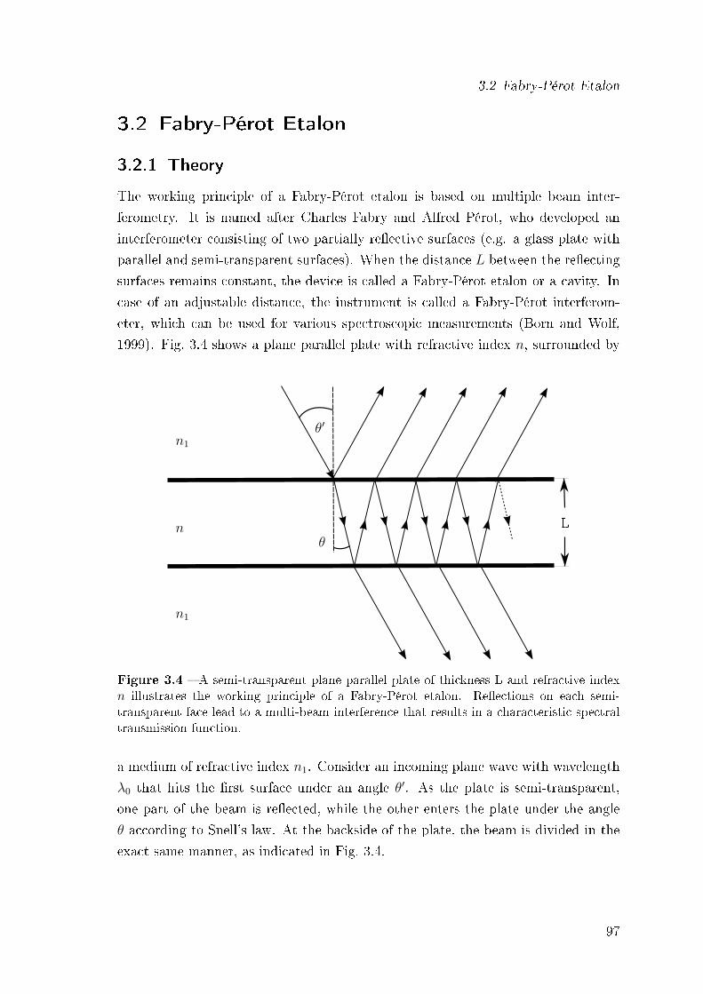
3.2 Fabry-Pérot Etalon
3.2 Fabry-Pérot Etalon
3.2.1 Theory
The working principle of a Fabry-Pérot etalon is based on multiple beam inter-
ferometry. It is named after Charles Fabry and Alfred Pérot, who developed an
interferometer consisting of two partially reective surfaces (e.g. a glass plate with
parallel and semi-transparent surfaces). When the distance L between the reecting
surfaces remains constant, the device is called a Fabry-Pérot etalon or a cavity. In
case of an adjustable distance, the instrument is called a Fabry-Pérot interferom-
eter, which can be used for various spectroscopic measurements (Born and Wolf,
1999). Fig. 3.4 shows a plane parallel plate with refractive index n, surrounded by
n
n1
n1
L
θ′
θ
Figure 3.4 A semi-transparent plane parallel plate of thickness L and refractive indexn illustrates the working principle of a Fabry-Pérot etalon. Reections on each semi-transparent face lead to a multi-beam interference that results in a characteristic spectraltransmission function.
a medium of refractive index n1. Consider an incoming plane wave with wavelength
λ0 that hits the rst surface under an angle θ′. As the plate is semi-transparent,
one part of the beam is reected, while the other enters the plate under the angle
θ according to Snell's law. At the backside of the plate, the beam is divided in the
exact same manner, as indicated in Fig. 3.4.
97
3 Stabilized Fabry-Pérot Etalon for High-Resolution Spectrographs
The optical path dierence between two consecutive reections is 2Ln cos(θ) and
hence the phase dierence can be calculated as
δ =4π
λ0
Ln cos(θ) . (3.1)
Following the notation in Born and Wolf (1999), the complex amplitude of the elec-
tric eld of the incident wave is denoted by A(i). Let r be the reection coecient
and t the transmission coecient at the rst surface and let r′ and t′ be the corre-
sponding coecients at the backside of the plate. Then, the complex amplitudes of
the reected waves are obtained as
rA(i), tt′rA(i)e(ıδ), tt′r3A(i)e(2ıδ), ... , tt′r2p−3A(i)eı(p−1)δ, (3.2)
and in the same way, the transmitted waves are given by
tt′A(i), tt′r2A(i)e(ıδ), tt′r4A(i)e(2ıδ), ... , tt′r2(p−1)A(i)eı(p−1)δ. (3.3)
The reection and transmission coecients can be calculated by the Fresnel formu-
lae, but here only the following relations are needed:
tt′ = T , r2 = r′2 = R, T +R = 1, (3.4)
where T and R denote the transmissivity and reectivity of the plate surface.
The resulting electric eld of all p superposed waves of Eq. (3.2) and Eq. (3.3) is given
by the sum of all complex amplitudes. This sum takes the form of a geometrical
series and can for p→∞ be reduced to:
A(r) =
(1− eıδ
)√R
1−Reıδ A(i), A(t) =T
1−ReıδA(i). (3.5)
The intensity of the reected light is now given by
Ir = A(r)A(r) = I04R sin2 (δ/2)
(1−R)2 + 4R sin2 (δ/2). (3.6)
Similarly, the transmitted light is determined by
It = A(t)A(t) = I01
1 + 4R(1−R2)
sin2 (δ/2)= I0
1
1 + F sin2 (δ/2), (3.7)
98
3.2 Fabry-Pérot Etalon
where the parameter F is called the coecient of nesse. It solely depends on the
reectivity R and is given by
F =4R
(1−R2). (3.8)
The transmission function of an etalon is of special interest. It has its maxima when
the phase shift δ is an integer multiple m of 2π:
δ = 2πm =4π
λ0
nL cos(θ) . (3.9)
An important characteristic of a FPE is its free spectral range (FSR). It is dened
as the distance in wavelength between two adjacent maxima of the transmission
function. The free spectral range (FSR) can be derived from Eq. (3.9) as
FSRλ =λ2
0
2nL cos(θ), (3.10)
or when expressed in terms of frequency:
FSRν =c
2nL cos(θ). (3.11)
The FSR is inversely proportional to the distance of the two reective surfaces.
Aside from the FSR, the so-called nesse F is the second characteristic quantity
describing an etalon. It is dened as the ratio of the FSR to the full width half
maximum (FWHM) of a peak:
F =FSRλ
FWHMλ
=FSRν
FWHMν
. (3.12)
The transmission functions for etalons with dierent nesses and FSRs are plotted
in Fig. 3.5. For a suciently high reectivity of the mirrors, the nesse can be
calculated as
F =π√F
2=
π√R
(1−R). (3.13)
This close relation between F and F is the reason why the distinction between
both quantities is often awed in the literature. The wavelength dependency of the
FSR, see Eq. (3.10), has two interesting consequences for the use of etalons in échelle
99
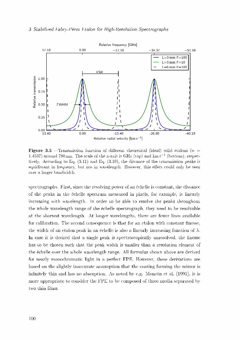
3 Stabilized Fabry-Pérot Etalon for High-Resolution Spectrographs
Figure 3.5 Transmission function of dierent theoretical (ideal) solid etalons (n =1.4537) around 780nm. The scale of the x-axis is GHz (top) and km s−1 (bottom), respec-tively. According to Eq. (3.11) and Eq. (3.10), the distance of the transmission peaks isequidistant in frequency, but not in wavelength. However, this eect could only be seenover a larger bandwidth.
spectrographs. First, since the resolving power of an échelle is constant, the distance
of the peaks in the échelle spectrum measured in pixels, for example, is linearly
increasing with wavelength. In order to be able to resolve the peaks throughout
the whole wavelength range of the échelle spectrograph, they need to be resolvable
at the shortest wavelength. At longer wavelengths, there are fewer lines available
for calibration. The second consequence is that for an etalon with constant nesse,
the width of an etalon peak in an échelle is also a linearly increasing function of λ.
In case it is desired that a single peak is spectroscopically unresolved, the nesse
has to be chosen such that the peak width is smaller than a resolution element of
the échelle over the whole wavelength range. All formulas shown above are derived
for nearly monochromatic light in a perfect FPE. However, these derivations are
based on the slightly inaccurate assumption that the coating forming the mirror is
innitely thin and has no absorption. As noted by e.g. Monzón et al. (1991), it is
more appropriate to consider the FPE to be composed of three media separated by
two thin lms.
100
3.2 Fabry-Pérot Etalon
By using transfer matrix methods, the authors showed that the above formulae
hold when δ is replaced by
δ =4π
λ0
Ln cos(θ) + 2Φ , (3.14)
where Φ is the phase change on internal reection. Additionally, R should be inter-
preted as the reectivity for internal reection, yielding
R+ T +A = 1 , (3.15)
where A is the amount of light absorbed by the thin lm. This is of particular
importance in case the mirror is formed by a semi-transparent metal layer, where
absorption can be signicant compared to the transmission. Finally,
It = I0
( T1−R
)21
1 + F sin2 (δ/2)(3.16)
= I0
(1−R−A
1−R
)21
1 + F sin2 (δ/2). (3.17)
The eect of absorptive layers is thus reected by a reduction of the peak transmis-
sion by a factor of
Tpeak =
(1−R−A
1−R
)2
. (3.18)
It is worth noting that this simple result does not hold for the intensity prole of the
reected part of the light introduced in Eq. (3.6). Here, the nite thickness and the
absorption lead to an asymmetry in the resulting function. Due to scattering eects,
the transmission function is found to be of the form as in Eq. (3.16) even in case
of absorption-free dielectric coatings (Born and Wolf, 1999). Section 3.2.3 presents
some simulations of metal coatings for FPEs that are of interest for astronomy.
A second simplication was made by assuming nearly monochromatic light, which
neglects all dispersion eects. Yet, for real etalons, n1, n as well as the additional
phase shift Φ in Eq. (3.14) depend on wavelength. Dispersion eects lead to a
varying line spacing, which prevents the easy use of FPEs as absolute wavelength
references. A priori, the exact position of a transmission line is not known. It could
still be measured though, by comparing it with known lines from an emission lamp
or a laser frequency comb, or by using a Fourier transform spectrometer.
101
3 Stabilized Fabry-Pérot Etalon for High-Resolution Spectrographs
3.2.2 Types of Etalons
There are various types of FPEs with dierent optical properties. This subsection
briey describes the dierences between the two most commonly used etalon types:
the confocal and the plane-parallel FP. As many of the results presented later are
obtained with bre Fabry-Pérots, these devices will be described in more detail.
Confocal Etalons
A confocal Fabry-Pérots (CFPs) consists of two spherical mirrors with equal radii
of curvature r that are separated by L = r. The transmission function is also of the
form in Eq. (3.16), but the phase dierence δ for light of normal incidence is
δ =2π
λ0
(4L+ ρ4/r3
), (3.19)
where ρ is the o-axis distance of the incoming light, see Hercher (1968). The FSR,
i.e. the distance between the interference maxima, is given by
FSRCFPν = c/(4L+ ρ4/r3) , (3.20)
which diers from that of a plane etalon, see Eq. (3.11). CFPs are commonly used
in laser physics, as they have several advantages over plane etalons. In general,
they are much less sensitive to a tilt of the mirrors, as the optical path dierence
does not change for spherical mirrors in rst approximation. Usually, higher Finesse
values can be achieved with CFPs compared to plane-parallel ones, because spherical
mirrors can be polished to higher precision than plane mirrors (Demtröder, 2008).
Astronomical etalons on the other hand, demand a FSR of several GHz in order
to yield resolvable lines in an échelle spectrograph. According to Eq. (3.20), this
requires small radii of curvature for the mirrors. The optical path dierence for a ray
increases with distance ρ from the optical axis of the CFP by ρ4/(4r3). For large
beams, this causes an asymmetric line broadening, which is clearly undesirable.
If one requires that the optical path dierence is smaller than λ/100 in order to
guarantee sharp, symmetric lines, the beam size for an astronomical etalon becomes
very small (on the order of a few hundred micron). Also, to achieve the confocal
condition, the mirror separation must match their radii within tight tolerances (a
few tenth of microns). All in all, the assembly and alignment of a CFP with a large
FSR is challenging.
102
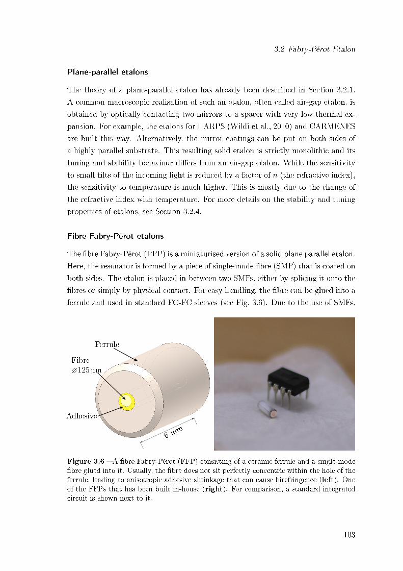
3.2 Fabry-Pérot Etalon
Plane-parallel etalons
The theory of a plane-parallel etalon has already been described in Section 3.2.1.
A common macroscopic realisation of such an etalon, often called air-gap etalon, is
obtained by optically contacting two mirrors to a spacer with very low thermal ex-
pansion. For example, the etalons for HARPS (Wildi et al., 2010) and CARMENES
are built this way. Alternatively, the mirror coatings can be put on both sides of
a highly parallel substrate. This resulting solid etalon is strictly monolithic and its
tuning and stability behaviour diers from an air-gap etalon. While the sensitivity
to small tilts of the incoming light is reduced by a factor of n (the refractive index),
the sensitivity to temperature is much higher. This is mostly due to the change of
the refractive index with temperature. For more details on the stability and tuning
properties of etalons, see Section 3.2.4.
Fibre Fabry-Pérot etalons
The bre Fabry-Pérot (FFP) is a miniaturised version of a solid plane parallel etalon.
Here, the resonator is formed by a piece of single-mode bre (SMF) that is coated on
both sides. The etalon is placed in between two SMFs, either by splicing it onto the
bres or simply by physical contact. For easy handling, the bre can be glued into a
ferrule and used in standard FC-FC sleeves (see Fig. 3.6). Due to the use of SMFs,
Ferrule
Adhesive
6 mm
Fibre125 µm
Figure 3.6 A bre Fabry-Pérot (FFP) consisting of a ceramic ferrule and a single-modebre glued into it. Usually, the bre does not sit perfectly concentric within the hole of theferrule, leading to anisotropic adhesive shrinkage that can cause birefringence (left). Oneof the FFPs that has been built in-house (right). For comparison, a standard integratedcircuit is shown next to it.
103
3 Stabilized Fabry-Pérot Etalon for High-Resolution Spectrographs
any alignment sensitivity is mitigated from the system, which allows building very
compact and robust etalons. However, FFPs suer from birefringent eects within
the bre as noted by Halverson et al. (2014). For a birefringent etalon, the optical
path length depends on the polarisation state of the incoming light: nxL 6= nyL,
where nx and ny denote the refractive index of the fast and the slow axis of the bre
etalon respectively. As a consequence, each transmission peak of the etalon is split
into two peaks, with their relative intensities being dependent on the polarisation
state of the incoming light. A priori, it is not clear whether a broad band source
used for illuminating the etalon has a long term stable polarisation behaviour, as for
example the bre used for feeding the etalon can introduce polarisation that might
depend on environmental conditions. For a long term stable FFP, it is therefore
crucial to control the polarisation of the light by placing polarising lters either in
front or behind the FFP or both.
Birefringence within the etalon can be caused either by residual internal stress of the
bre that results from the manufacturing process or by external forces. By gluing the
bre into a ferrule, asymmetric stress can occur, leading to a polarisation dependent
change of the refractive index. Tateda et al. (2007b) derived a model to explain
and quantify the birefringence caused by the shrinkage of the adhesive. The authors
found a proportional relation between the amount of birefringence B = ∆n/n and
the product of the dierence in the coecient of linear expansion of the bre and
the ferrule material, temperature change, Young's modulus of the adhesive, and
the anisotropy of the adhesive layer width. The authors also measured B for three
dierent adhesives with dierent viscosities and shrinkage properties, nding that
B ranges from 3 to 18× 10−6, and a temperature dependence ∂B/∂T of about
5× 10⁻⁸ K−1. For these values, the separation of the two polarisation peaks lies in
the order of a few GHz and might be unresolved by an astronomical spectrograph.
However, the line barycentre as well as its shape will change if the polarisation state
of the incoming light varies over time.
Beside the stress induced by adhesives, other forms of external forces can cause
stress. Let
σ = F/A (3.21)
denote extrinsic stress, where F is the force and A the cross section of the etalon.
This stress is for instance induced by mounting the bre in between two SMFs using
physical contact. In order to determine its impact on the refractive indices and
104
3.2 Fabry-Pérot Etalon
the cavity length, one has to distinguish between axial and radial stress. Follow-
ing Tateda et al. (2007a), we obtain the relative change of the peak transmission
frequency by dierentiating Eq. (3.11)
dν/ν = −(dn/n+ dL/L) . (3.22)
In case the force is purely axial, we get
dL/L = εz = σz/E , (3.23)
where εz is the strain in z-direction, σz is the stress and E is Young's modulus. For
the change of the refractive index, Tateda et al. (2007a) derived
dnx/nx = dny/ny = (n2σz/2E)(−p11µ+ p12 − p12µ) . (3.24)
Here, p11 and p12 denote the photo-elastic (or opto-elastic) constants of the bre
material, µ is its Poisson's ratio and E is Young's modulus of the ferrule. This leads
to a total relative shift of
dν/ν = (σz/E)[(n2/2)(−p11µ+ p12 − p12µ)− 1
]. (3.25)
Dixon (1967) measured p11 = 0.12 and p12 = 0.27 for fused silica, while µ = 0.16.
Usually, standard ferrules are made of zirconia, where E = 1.9× 10¹¹ Nm−2. These
ferrules typically have a 2.0mm tip diameter, resulting in a peak shift caused by
axial pressure (at 780nm) of
dν = 494MHz/N , (3.26)
or, when expressed in terms of RV:
∆RV ≈ 385ms−1 N−1 . (3.27)
To keep the lines of the etalon stable close to 3 cm/s, the force onto the FFP may
change no more than ∼ 0.08mN, which is comparable to the weight of a large
snowake (on Earth). It is important to note that dν/ν - hence also dλ/λ - remains
constant in rst order, which means that all etalon peaks move by the same amount
on the échelle spectrum.
105
3 Stabilized Fabry-Pérot Etalon for High-Resolution Spectrographs
Pure axial stress causes only a shift of the transmission peak frequency, whereas
radial stress actually inuences the birefringence properties of the etalon. Tateda
et al. (2007a) found
B = σy(n2/2E)(p11 − p12)(1 + µ) (3.28)
for unidirectional side pressure σy. In case of fused silica bres and zirconium fer-
rules, the birefringence is
B = −1× 10⁻¹²σy . (3.29)
I built a 6mm FFP in-house (see Section 3.4.3) and measured its birefringence,
which is shown in Fig. 3.7. The distance of the two etalon transmission peaks is
about 2.09GHz, which corresponds to B = 5× 10⁻⁶. This is a minimal value if the
order of interference of both peaks is the same. The value is in agreement with the
B = 3 − 18× 10−6 measured by Tateda et al. (2007a), which is an indication that
both peaks are indeed of the same order of interference. In order to measure the
dependency of the peak structure on the polarisation state of the light, I placed the
FFP in between a polarisation maintaining (PM) bre and a standard SMF. I fed
laser light through a polariser and a subsequent half-wave plate into the PM bre,
thus allowing for a manipulation of the polarisation direction of the light. Figure 3.7
shows how the intensities of the two transmission peaks vary with changing incoming
polarisation. However, I could not fully suppress the double peak structure, which
is most probably due to some polarisation cross-talk in the PM bre. In order to
completely get rid of one peak, a high contrast polariser should be inserted directly
in front (or after) the FFP (see Halverson et al., 2014).
The applicability of a single mode FFPs is limited to the bandwidth where the bre
operates in the single mode regime. In a SMF, light with shorter wavelengths excites
several modes, each of which having a dierent propagation constant, leading to sim-
ilar problems like birefringence, while for longer wavelengths the throughput quickly
drops. In the visual regime for example, a typical single mode bre has a bandwidth
ranging from 400nm to 680nm (Thorlabs S405-XP). In the near-infrared, a larger
absolute bandwidth can be achieved as the relative wavelength change determines
the type of guidance, e.g. 970nm to 1650nm (Thorlabs SM980-5.8-125).
106
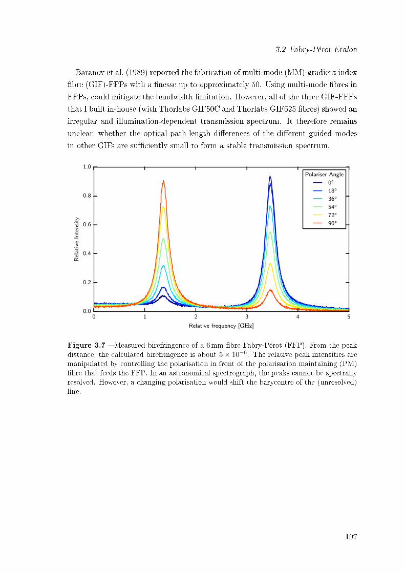
3.2 Fabry-Pérot Etalon
Baranov et al. (1989) reported the fabrication of multi-mode (MM)-gradient index
bre (GIF)-FFPs with a nesse up to approximately 50. Using multi-mode bres in
FFPs, could mitigate the bandwidth limitation. However, all of the three GIF-FFPs
that I built in-house (with Thorlabs GIF50C and Thorlabs GIF625 bres) showed an
irregular and illumination-dependent transmission spectrum. It therefore remains
unclear, whether the optical path-length dierences of the dierent guided modes
in other GIFs are suciently small to form a stable transmission spectrum.
0 1 2 3 4 5
Relative frequency [GHz]
0.0
0.2
0.4
0.6
0.8
1.0
Rel
ati
veIn
ten
sity
Polariser Angle
0°18°36°54°72°90°
Figure 3.7 Measured birefringence of a 6mm bre Fabry-Pérot (FFP). From the peakdistance, the calculated birefringence is about 5× 10⁻⁶. The relative peak intensities aremanipulated by controlling the polarisation in front of the polarisation maintaining (PM)bre that feeds the FFP. In an astronomical spectrograph, the peaks cannot be spectrallyresolved. However, a changing polarisation would shift the barycentre of the (unresolved)line.
107
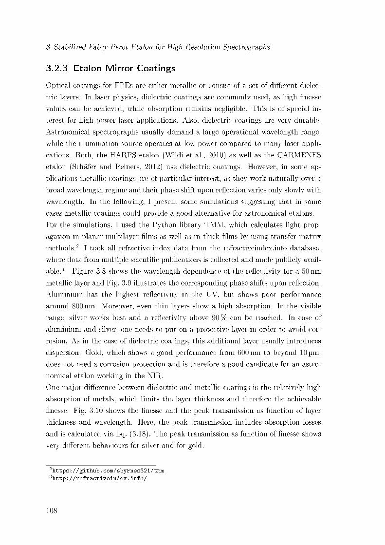
3 Stabilized Fabry-Pérot Etalon for High-Resolution Spectrographs
3.2.3 Etalon Mirror Coatings
Optical coatings for FPEs are either metallic or consist of a set of dierent dielec-
tric layers. In laser physics, dielectric coatings are commonly used, as high nesse
values can be achieved, while absorption remains negligible. This is of special in-
terest for high power laser applications. Also, dielectric coatings are very durable.
Astronomical spectrographs usually demand a large operational wavelength range,
while the illumination source operates at low power compared to many laser appli-
cations. Both, the HARPS etalon (Wildi et al., 2010) as well as the CARMENES
etalon (Schäfer and Reiners, 2012) use dielectric coatings. However, in some ap-
plications metallic coatings are of particular interest, as they work naturally over a
broad wavelength regime and their phase shift upon reection varies only slowly with
wavelength. In the following, I present some simulations suggesting that in some
cases metallic coatings could provide a good alternative for astronomical etalons.
For the simulations, I used the Python library TMM, which calculates light prop-
agation in planar multilayer lms as well as in thick lms by using transfer matrix
methods.2 I took all refractive index data from the refractiveindex.info database,
where data from multiple scientic publications is collected and made publicly avail-
able.3 Figure 3.8 shows the wavelength dependence of the reectivity for a 50nm
metallic layer and Fig. 3.9 illustrates the corresponding phase shifts upon reection.
Aluminium has the highest reectivity in the UV, but shows poor performance
around 800nm. Moreover, even thin layers show a high absorption. In the visible
range, silver works best and a reectivity above 90% can be reached. In case of
aluminium and silver, one needs to put on a protective layer in order to avoid cor-
rosion. As in the case of dielectric coatings, this additional layer usually introduces
dispersion. Gold, which shows a good performance from 600nm to beyond 10µm,
does not need a corrosion protection and is therefore a good candidate for an astro-
nomical etalon working in the NIR.
One major dierence between dielectric and metallic coatings is the relatively high
absorption of metals, which limits the layer thickness and therefore the achievable
nesse. Fig. 3.10 shows the nesse and the peak transmission as function of layer
thickness and wavelength. Here, the peak transmission includes absorption losses
and is calculated via Eq. (3.18). The peak transmission as function of nesse shows
very dierent behaviours for silver and for gold.
2https://github.com/sbyrnes321/tmm3http://refractiveindex.info/
108
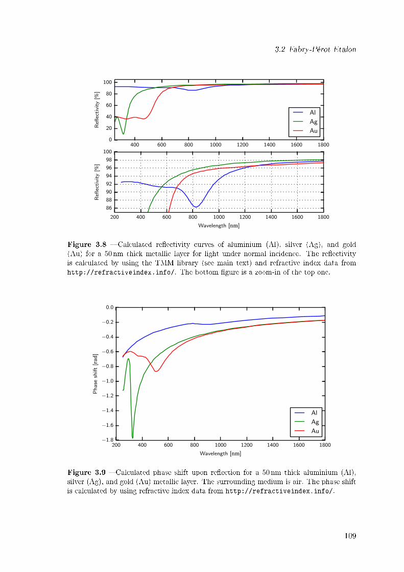
3.2 Fabry-Pérot Etalon
400 600 800 1000 1200 1400 1600 18000
20
40
60
80
100
Refl
ecti
vity
[%]
Al
Ag
Au
200 400 600 800 1000 1200 1400 1600 1800
Wavelength [nm]
86
88
90
92
94
96
98
100
Refl
ecti
vity
[%]
Figure 3.8 Calculated reectivity curves of aluminium (Al), silver (Ag), and gold(Au) for a 50 nm thick metallic layer for light under normal incidence. The reectivityis calculated by using the TMM library (see main text) and refractive index data fromhttp://refractiveindex.info/. The bottom gure is a zoom-in of the top one.
200 400 600 800 1000 1200 1400 1600 1800
Wavelength [nm]
−1.8
−1.6
−1.4
−1.2
−1.0
−0.8
−0.6
−0.4
−0.2
0.0
Ph
ase
shif
t[r
ad]
Al
Ag
Au
Figure 3.9 Calculated phase shift upon reection for a 50 nm thick aluminium (Al),silver (Ag), and gold (Au) metallic layer. The surrounding medium is air. The phase shiftis calculated by using refractive index data from http://refractiveindex.info/.
109
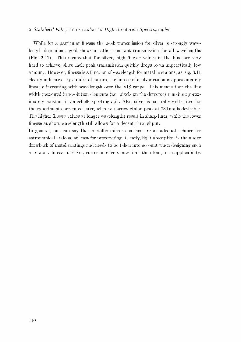
3 Stabilized Fabry-Pérot Etalon for High-Resolution Spectrographs
While for a particular nesse the peak transmission for silver is strongly wave-
length dependent, gold shows a rather constant transmission for all wavelengths
(Fig. 3.11). This means that for silver, high nesse values in the blue are very
hard to achieve, since their peak transmission quickly drops to an impractically low
amount. However, nesse is a function of wavelength for metallic etalons, as Fig. 3.11
clearly indicates. By a quirk of nature, the nesse of a silver etalon is approximately
linearly increasing with wavelength over the VIS range. This means that the line
width measured in resolution elements (i.e. pixels on the detector) remains approx-
imately constant in an échelle spectrograph. Also, silver is naturally well suited for
the experiments presented later, where a narrow etalon peak at 780nm is desirable.
The higher nesse values at longer wavelengths result in sharp lines, while the lower
nesse at short wavelength still allows for a decent throughput.
In general, one can say that metallic mirror coatings are an adequate choice for
astronomical etalons, at least for prototyping. Clearly, light absorption is the major
drawback of metal coatings and needs to be taken into account when designing such
an etalon. In case of silver, corrosion eects may limit their long-term applicability.
110
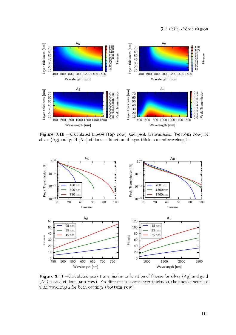
3.2 Fabry-Pérot Etalon
400 600 800 1000 1200 1400 1600
Wavelength [nm]
10203040506070
Lay
erth
ick
nes
s[n
m] Ag
20406080100120140160180
Fin
esse
400 600 800 1000 1200 1400 1600
Wavelength [nm]
10203040506070
Lay
erth
ick
nes
s[n
m] Au
153045607590105120
Fin
esse
400 600 800 1000 1200 1400 1600
Wavelength [nm]
10203040506070
Lay
erth
ick
nes
s[n
m] Ag
0.00.10.20.30.40.50.60.70.8
Pea
kT
ran
smis
sio
n400 600 800 1000 1200 1400 1600
Wavelength [nm]
10203040506070
Lay
erth
ick
nes
s[n
m] Au
0.00.10.20.30.40.50.60.70.8
Pea
kT
ran
smis
sio
n
Figure 3.10 Calculated nesse (top row) and peak transmission (bottom row) ofsilver (Ag) and gold (Au) etalons as function of layer thickness and wavelength.
0 20 40 60 80 100
Finesse
10−3
10−2
10−1
100
Pea
kT
ran
smis
sio
n[%
]
Ag
450 nm600 nm780 nm
0 20 40 60 80 100
Finesse
10−3
10−2
10−1
100
Pea
kT
ran
smis
sio
n[%
]
Au
780 nm1300 nm1700 nm
450 500 550 600 650 700 750
Wavelength [nm]
0
10
20
30
40
50
60
Fin
esse
Ag
25 nm35 nm45 nm
1000 1500 2000 2500
Wavelength [nm]
0
20
40
60
80
100
120
Fin
esse
Au
15 nm25 nm35 nm
Figure 3.11 Calculated peak transmission as function of nesse for silver (Ag) and gold(Au) coated etalons (top row). For dierent constant layer thickness, the nesse increaseswith wavelength for both coatings (bottom row).
111

3 Stabilized Fabry-Pérot Etalon for High-Resolution Spectrographs
3.2.4 Etalon Tuning
Rewriting Eq. (3.9) gives the wavelength of the etalon peaks:
λpeak =2πLn cos(θ)
πm− Φ. (3.30)
For illumination angles around θ ∼ 0, the variation of the peak position that is
due to external parameters can be expressed in terms of a radial velocity error as
follows:
∆RV = c
(dλpeakλpeak
)= c
(dL
L+dn
n− dθ2
2
). (3.31)
All terms on the right hand side can either be seen as possible control parameters
for an actively controlled etalon or as error sources which have to be kept constant
to the level of ∼ 10−10 for a sub m/s stability. It depends strongly on the etalon
design, which constitutes the dominant term in Eq. (3.31).
For a FFP with a SMF, the illumination angle dependence is zero, leaving a temper-
ature and a pressure dependence of the length and the refractive index as follows:(dλ
λ
)FFP
=
(1
L
∂L
∂T+
1
n
∂n
∂T
)dT +
(1
L
∂L
∂σz+
1
n
∂n
∂σz
)dσz
=
(α +
1
n
∂n
∂T
)dT +
(σzE
+1
n
∂n
∂σz
)dσz
≈(α +
1
n
∂n
∂T
)dT . (3.32)
Here, α is the coecient of thermal expansion (CTE) of the bre and ∂n∂T
is often
referred to as the thermo-optic coecient. In the last step of Eq. (3.32), it is
assumed that the pressure onto the FFP is constant. Variation in pressure will lead
to birefringence and signicant peak shifts as described in Section 3.2.2. The setup of
the FFP has to be mechanically stable for these eects to be negligible. For a fused
silica bre one has αSiO2 = 0.55× 10⁻⁶ K−1 and ∂n∂T
= 8.72× 10⁻⁶ K−1 (Leviton and
Frey, 2006), which means that for a solid etalon the major contribution to the peak
shift is due to the change of the refractive index. In total, the peak shift in RV is
given by
d
dTRV =
d
dT
(dλ
λ
)FFP
c = 1.96 km s−1 K−1 = 1.96ms−1 mK−1 . (3.33)
112
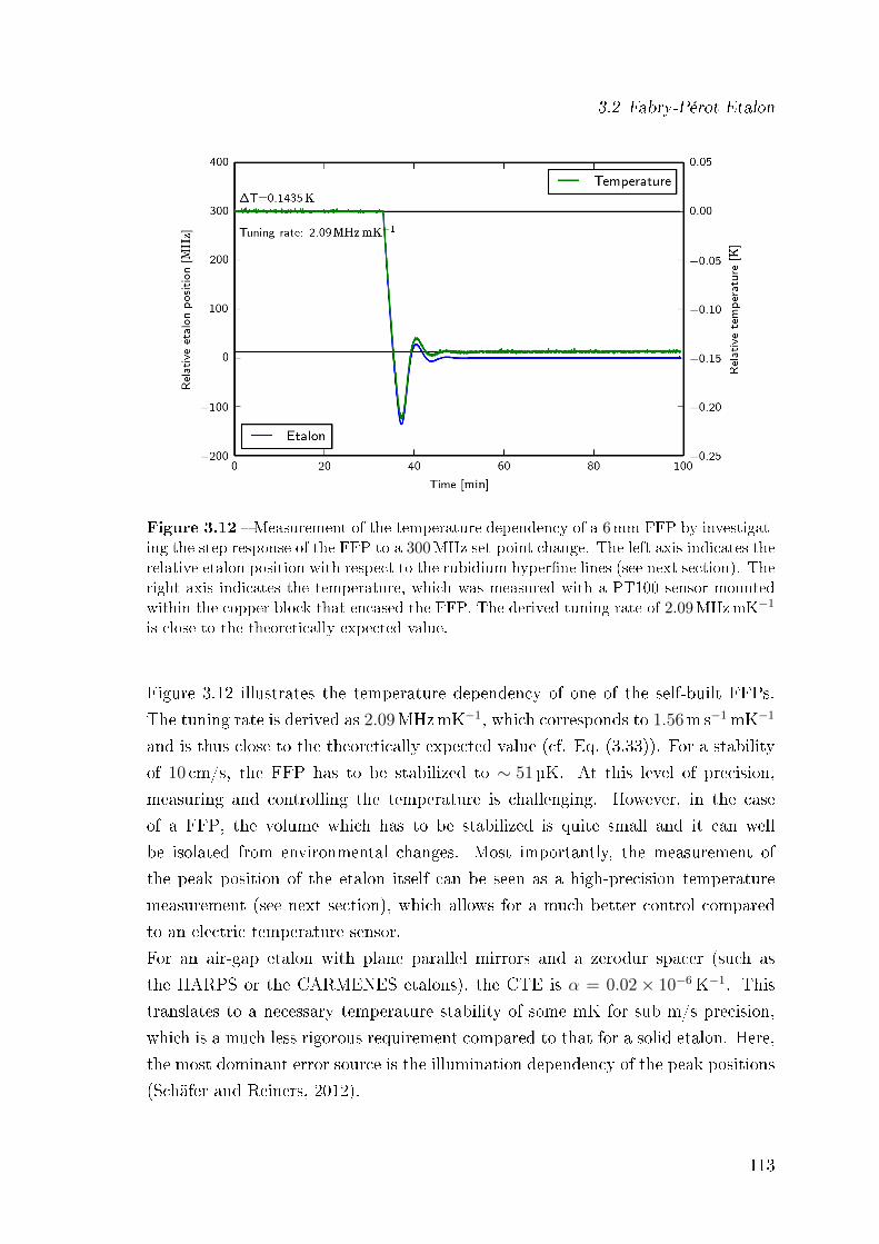
3.2 Fabry-Pérot Etalon
Figure 3.12 Measurement of the temperature dependency of a 6mm FFP by investigat-ing the step response of the FFP to a 300MHz set-point change. The left axis indicates therelative etalon position with respect to the rubidium hyperne lines (see next section). Theright axis indicates the temperature, which was measured with a PT100 sensor mountedwithin the copper block that encased the FFP. The derived tuning rate of 2.09MHzmK−1
is close to the theoretically expected value.
Figure 3.12 illustrates the temperature dependency of one of the self-built FFPs.
The tuning rate is derived as 2.09MHzmK−1, which corresponds to 1.56ms−1 mK−1
and is thus close to the theoretically expected value (cf. Eq. (3.33)). For a stability
of 10 cm/s, the FFP has to be stabilized to ∼ 51µK. At this level of precision,
measuring and controlling the temperature is challenging. However, in the case
of a FFP, the volume which has to be stabilized is quite small and it can well
be isolated from environmental changes. Most importantly, the measurement of
the peak position of the etalon itself can be seen as a high-precision temperature
measurement (see next section), which allows for a much better control compared
to an electric temperature sensor.
For an air-gap etalon with plane parallel mirrors and a zerodur spacer (such as
the HARPS or the CARMENES etalons), the CTE is α = 0.02× 10⁻⁶ K−1. This
translates to a necessary temperature stability of some mK for sub m/s precision,
which is a much less rigorous requirement compared to that for a solid etalon. Here,
the most dominant error source is the illumination dependency of the peak positions
(Schäfer and Reiners, 2012).
113
3 Stabilized Fabry-Pérot Etalon for High-Resolution Spectrographs
3.3 Laser Locked Etalon Concept
The impressive results of Wildi et al. (2010, 2011, 2012) demonstrated the feasibility
of using FPEs for calibration of astronomical spectrographs. However, as noted
before, the long term stability of these devices remains problematic, since the authors
monitored only secondary parameters, such as temperature and pressure, to ensure
the transmission spectrum being stable. It is known that illumination eects can
easily change the line positions on the order of several meters per second (Schäfer and
Reiners, 2012). Additionally, the spacer material can age over time (as for example
zerodur does), and so can coatings. These eects cannot be tracked by a passive
stabilisation of a FPE and therefore it is still necessary to recalibrate the etalon
spectrum against a known absolute spectrum (e.g. ThAr) on a regular timebase for
stable long-term usage.
To overcome the intrinsic limitations of a passive stabilization, we developed a more
direct approach in order to provide a long-term stable etalon spectrum. The basic
idea is to directly measure parts of the etalon spectrum with very high precision
in real time and to compare them to a known absolute wavelength reference. This
can be accomplished by using a tunable laser that simultaneously scans both the
etalon and a reference. As an absolute reference, we use the D2 hyperne transition
of rubidium (Rb) at 780nm. By continuously comparing the position of one single
etalon peak to the Rb spectrum, the oset between the peaks can be determined
with very high precision. This information can then be used to lock the etalon to
any frequency oset to the Rb transitions. Ideally, the oset would be around zero
to avoid problems arising from non-linearities of the scan. The control mechanism
of the etalon peak position depends on the actual etalon design as described in the
previous section. Even in the absence of an active control parameter for the etalon,
this new concept is useful. It allows for a precise determination of the oset of
the etalon during an astronomical observation, which makes recalibration against
an emission lamp redundant. A schematic and an actual photo of the experimental
setup are presented in Fig. 3.13.
Compared to other locking techniques that are typically used in laser physics, such
as the lock-in technique (Wallard, 1972) or the Pound-Drever-Hall method (Drever
et al., 1983), the concept presented here requires less sophisticated hardware and
is less complex. It has been optimised with the aim of serving the needs of RV
observations, while keeping the setup as simple as possible, thus providing a device
that is well suited for an observatory environment. More advanced locking setups
114
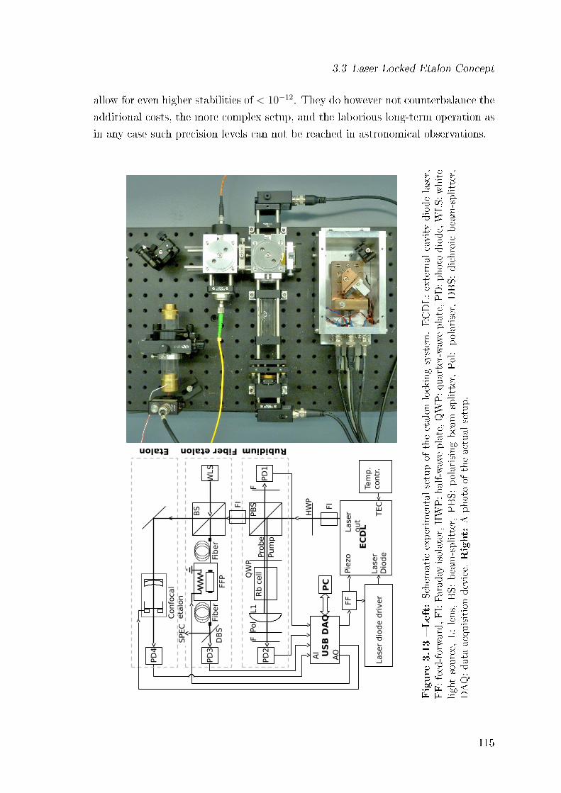
3.3 Laser Locked Etalon Concept
allow for even higher stabilities of < 10−12. They do however not counterbalance the
additional costs, the more complex setup, and the laborious long-term operation as
in any case such precision levels can not be reached in astronomical observations.
FFP
HW
P
PD
2PD
1
Pol
L1R
b c
ellQW
PPB
SF
F Tem
p.
contr
.La
ser
dio
de d
river
US
B D
AQ
FI
EC
DL
Piezo
Lase
r D
iode
TEC
Lase
r ou
tFF
AOAI
BS
PD
3W
LSD
BS
SPEC
Rubidium Fiber etalon
PC
Probe
Pum
p
Confo
cal
eta
lon
PD
4
Etalon
Fiber
Fiber
FI
Figure
3.13Left:Schem
aticexperim
entalsetupof
theetalon
lockingsystem
.ECDL:external
cavitydiodelaser,
FF:feed-forward,FI:Faraday
isolator,HWP:half-waveplate,QWP:quarter-waveplate,PD:photodiode,WLS:white
lightsource,
L:lens,
BS:beam-splitter,PBS:polarisingbeam
splitter,Pol:polariser,DBS:dichroic
beam-splitter,
DAQ:dataacquisitiondevice.Right:
Aphotoof
theactual
setup.
115
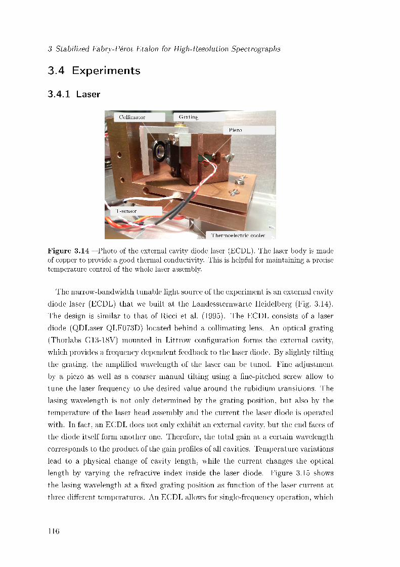
3 Stabilized Fabry-Pérot Etalon for High-Resolution Spectrographs
3.4 Experiments
3.4.1 Laser
Collimator Grating
Piezo
T-sensor
Thermoelectric cooler
Figure 3.14 Photo of the external cavity diode laser (ECDL). The laser body is madeof copper to provide a good thermal conductivity. This is helpful for maintaining a precisetemperature control of the whole laser assembly.
The narrow-bandwidth tunable light source of the experiment is an external cavity
diode laser (ECDL) that we built at the Landessternwarte Heidelberg (Fig. 3.14).
The design is similar to that of Ricci et al. (1995). The ECDL consists of a laser
diode (QDLaser QLF073D) located behind a collimating lens. An optical grating
(Thorlabs G13-18V) mounted in Littrow conguration forms the external cavity,
which provides a frequency dependent feedback to the laser diode. By slightly tilting
the grating, the amplied wavelength of the laser can be tuned. Fine adjustment
by a piezo as well as a coarser manual tilting using a ne-pitched screw allow to
tune the laser frequency to the desired value around the rubidium transitions. The
lasing wavelength is not only determined by the grating position, but also by the
temperature of the laser head assembly and the current the laser diode is operated
with. In fact, an ECDL does not only exhibit an external cavity, but the end faces of
the diode itself form another one. Therefore, the total gain at a certain wavelength
corresponds to the product of the gain proles of all cavities. Temperature variations
lead to a physical change of cavity length, while the current changes the optical
length by varying the refractive index inside the laser diode. Figure 3.15 shows
the lasing wavelength at a xed grating position as function of the laser current at
three dierent temperatures. An ECDL allows for single-frequency operation, which
116
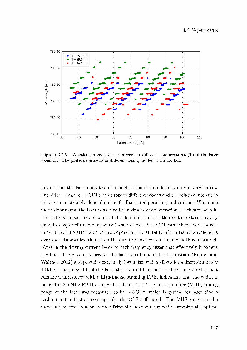
3.4 Experiments
Figure 3.15 Wavelength versus laser current at dierent temperatures (T) of the laserassembly. The plateaus arise from dierent lasing modes of the ECDL.
means that the laser operates on a single resonator mode providing a very narrow
linewidth. However, ECDLs can support dierent modes and the relative intensities
among them strongly depend on the feedback, temperature, and current. When one
mode dominates, the laser is said to be in single-mode operation. Each step seen in
Fig. 3.15 is caused by a change of the dominant mode either of the external cavity
(small steps) or of the diode cavity (larger steps). An ECDL can achieve very narrow
linewidths. The attainable values depend on the stability of the lasing wavelengths
over short timescales, that is, on the duration over which the linewidth is measured.
Noise in the driving current leads to high frequency jitter that eectively broadens
the line. The current source of the laser was built at TU Darmstadt (Führer and
Walther, 2012) and provides extremely low noise, which allows for a linewidth below
10 kHz. The linewidth of the laser that is used here has not been measured, but it
remained unresolved with a high-nesse scanning FPE, indicating that the width is
below the 2.5MHz FWHM linewidth of the FPE. The mode-hop free (MHF) tuning
range of the laser was measured to be ∼ 3GHz, which is typical for laser diodes
without anti-reection coatings like the QLF073D used. The MHF range can be
increased by simultaneously modifying the laser current while sweeping the optical
117
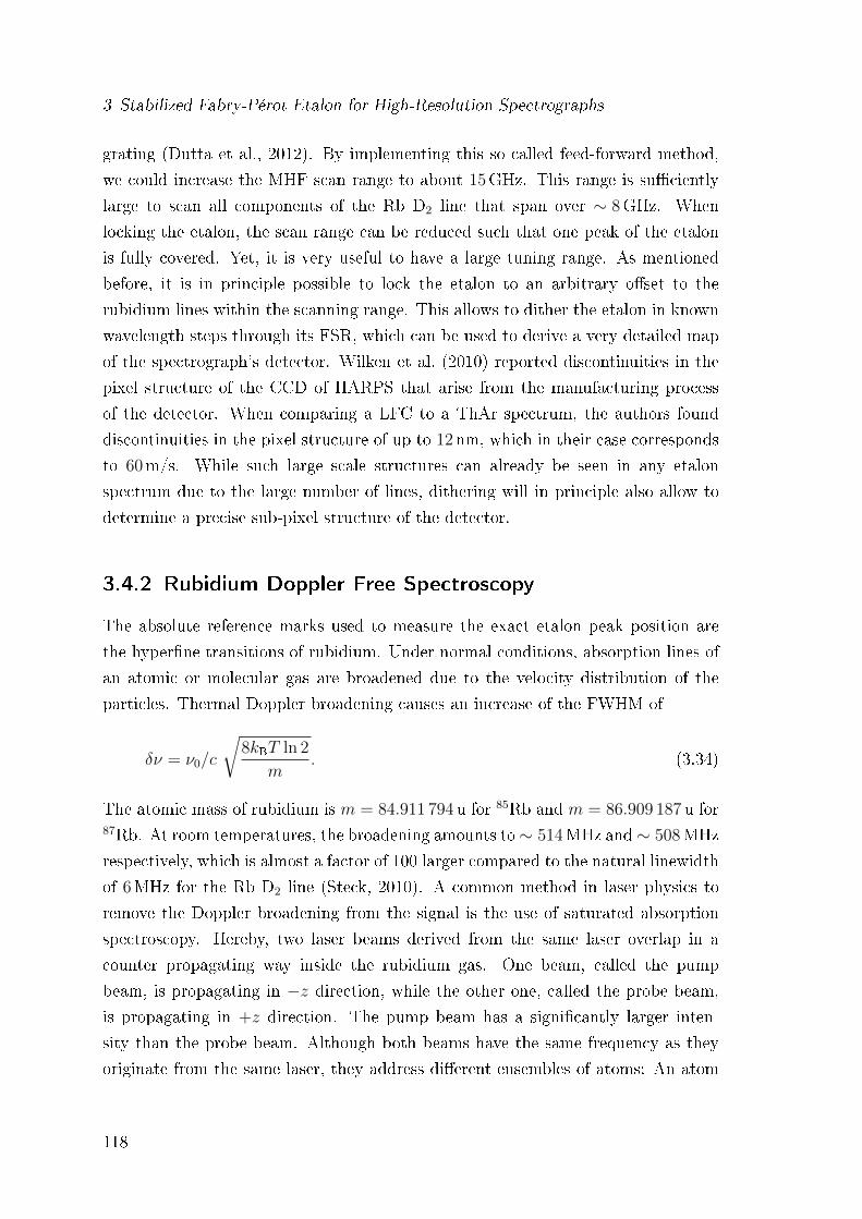
3 Stabilized Fabry-Pérot Etalon for High-Resolution Spectrographs
grating (Dutta et al., 2012). By implementing this so called feed-forward method,
we could increase the MHF scan range to about 15GHz. This range is suciently
large to scan all components of the Rb D2 line that span over ∼ 8GHz. When
locking the etalon, the scan range can be reduced such that one peak of the etalon
is fully covered. Yet, it is very useful to have a large tuning range. As mentioned
before, it is in principle possible to lock the etalon to an arbitrary oset to the
rubidium lines within the scanning range. This allows to dither the etalon in known
wavelength steps through its FSR, which can be used to derive a very detailed map
of the spectrograph's detector. Wilken et al. (2010) reported discontinuities in the
pixel structure of the CCD of HARPS that arise from the manufacturing process
of the detector. When comparing a LFC to a ThAr spectrum, the authors found
discontinuities in the pixel structure of up to 12nm, which in their case corresponds
to 60m/s. While such large scale structures can already be seen in any etalon
spectrum due to the large number of lines, dithering will in principle also allow to
determine a precise sub-pixel structure of the detector.
3.4.2 Rubidium Doppler Free Spectroscopy
The absolute reference marks used to measure the exact etalon peak position are
the hyperne transitions of rubidium. Under normal conditions, absorption lines of
an atomic or molecular gas are broadened due to the velocity distribution of the
particles. Thermal Doppler broadening causes an increase of the FWHM of
δν = ν0/c
√8kBT ln 2
m. (3.34)
The atomic mass of rubidium is m = 84.911 794 u for 85Rb and m = 86.909 187 u for87Rb. At room temperatures, the broadening amounts to∼ 514MHz and∼ 508MHz
respectively, which is almost a factor of 100 larger compared to the natural linewidth
of 6MHz for the Rb D2 line (Steck, 2010). A common method in laser physics to
remove the Doppler broadening from the signal is the use of saturated absorption
spectroscopy. Hereby, two laser beams derived from the same laser overlap in a
counter propagating way inside the rubidium gas. One beam, called the pump
beam, is propagating in −z direction, while the other one, called the probe beam,
is propagating in +z direction. The pump beam has a signicantly larger inten-
sity than the probe beam. Although both beams have the same frequency as they
originate from the same laser, they address dierent ensembles of atoms: An atom
118

3.4 Experiments
with velocity vz in +z direction will see the pump beam frequency being shifted
to ν ′pump = νL(1 + vz/c) due to the Doppler shift, while it will see the probe beam
at frequency ν ′probe = νL(1 − vz/c). In general, when νL 6= ν0, the pump and the
probe beam are resonant for atoms with dierent velocities vpump = c(ν0/νL)−1 and
vprobe = c(1−ν0/νL), respectively. If νL = ν0, both beams interact with the ensemble
of atoms with zero velocity in z-direction. As the pump beam has a stronger inten-
sity, a large portion of the atoms is excited, thereby reducing the absorption of the
probe beam near the atomic resonance. Within the Doppler-broadened, Gaussian-
shaped absorption line small dips (often called Lamb-dips) appear when the transi-
tion frequency of the atoms in the vapour is probed by the laser. Figure 3.16 shows
the full rubidium spectrum of the Rb D2 line measured with the setup. In total,
one can see four nearly Gaussian-shaped absorption features, which are all showing
some ner substructure. The natural abundance of rubidium is 72.2% for 85Rb and
27.8% for 87Rb. Thus, a common gas cell always shows absorption for both isotopes.
Figure 3.17 is a zoom-in of the 87Rb F2 transition, whose lines will later be used as
an absolute reference and whose frequencies are listed in Table 3.1.
Transition Frequency ν0 = 384.229 141 484 483 7THz
F2F1 ν0 − 229.8518MHzF2F2 ν0 − 72.9112MHzF2F3 ν0 + 193.7407MHz
Table 3.1 87Rb F2 transition frequencies for the three dierent hyperne transitions.Data taken from Steck (2010).
Although there are only three hyperne levels, in total six peaks appear in the
spectrum. Three of them are so called crossover peaks. Their frequency lies exactly
in between two transition frequencies ν1 and ν2. They occur because moving atoms
see the counter-propagating pump and probe beam being resonant with the two
separate transitions due to the Doppler shift. The depopulation of the common
ground state by the pump beam causes the probe beam to see a lower absorption
at (ν1 + ν2)/2. It is common in Rb saturated absorption spectroscopy experiments
that the cross-over peaks are more pronounced than the actual transitions, which
can also be seen in the measurements in Fig. 3.17.
119
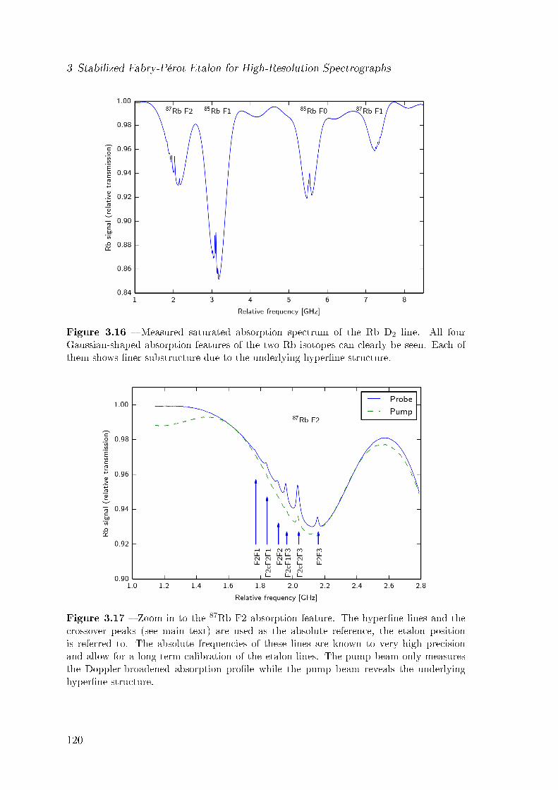
3 Stabilized Fabry-Pérot Etalon for High-Resolution Spectrographs
Figure 3.16 Measured saturated absorption spectrum of the Rb D2 line. All fourGaussian-shaped absorption features of the two Rb isotopes can clearly be seen. Each ofthem shows ner substructure due to the underlying hyperne structure.
Figure 3.17 Zoom-in to the 87Rb F2 absorption feature. The hyperne lines and thecrossover peaks (see main text) are used as the absolute reference, the etalon positionis referred to. The absolute frequencies of these lines are known to very high precisionand allow for a long-term calibration of the etalon lines. The pump beam only measuresthe Doppler-broadened absorption prole while the pump beam reveals the underlyinghyperne structure.
120
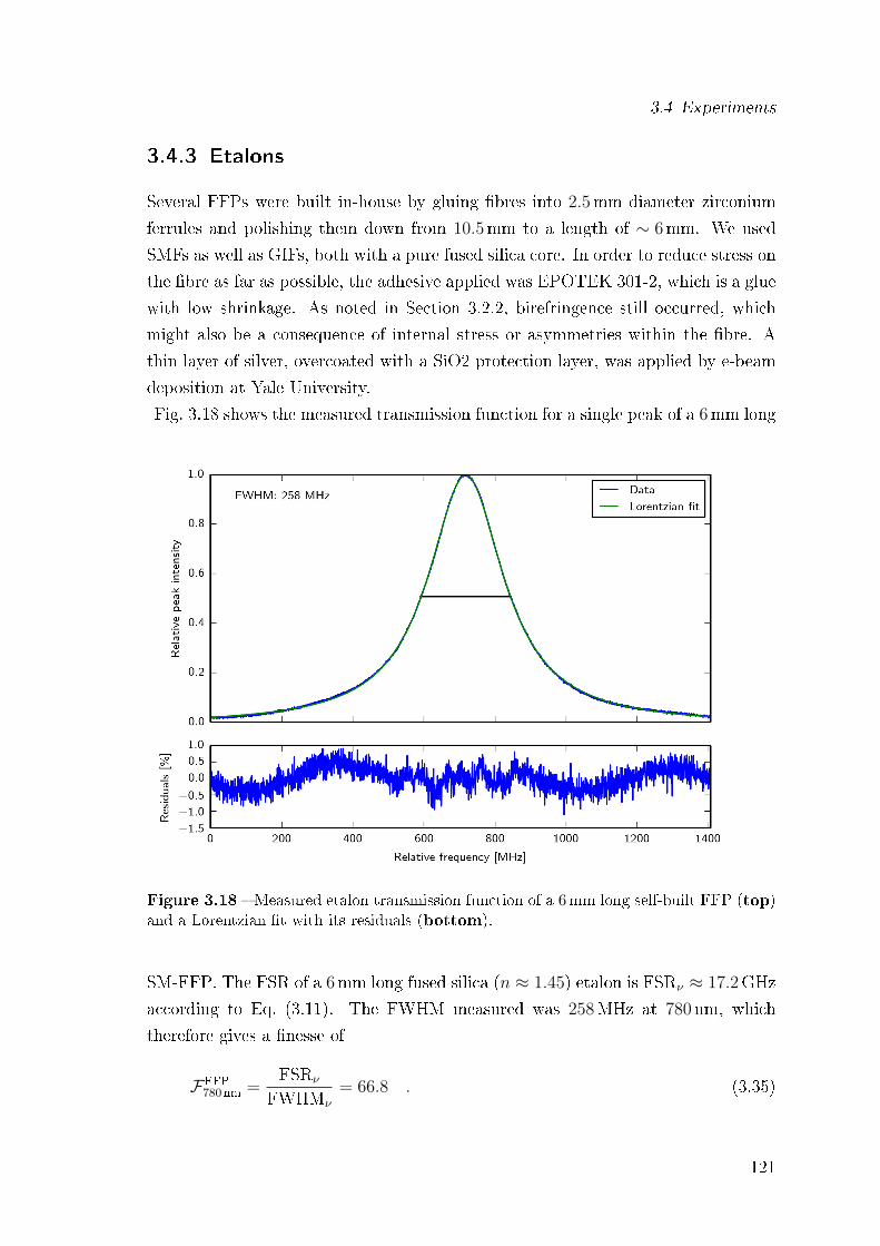
3.4 Experiments
3.4.3 Etalons
Several FFPs were built in-house by gluing bres into 2.5mm diameter zirconium
ferrules and polishing them down from 10.5mm to a length of ∼ 6mm. We used
SMFs as well as GIFs, both with a pure fused silica core. In order to reduce stress on
the bre as far as possible, the adhesive applied was EPOTEK 301-2, which is a glue
with low shrinkage. As noted in Section 3.2.2, birefringence still occurred, which
might also be a consequence of internal stress or asymmetries within the bre. A
thin layer of silver, overcoated with a SiO2 protection layer, was applied by e-beam
deposition at Yale University.
Fig. 3.18 shows the measured transmission function for a single peak of a 6mm long
Figure 3.18 Measured etalon transmission function of a 6mm long self-built FFP (top)and a Lorentzian t with its residuals (bottom).
SM-FFP. The FSR of a 6mm long fused silica (n ≈ 1.45) etalon is FSRν ≈ 17.2GHz
according to Eq. (3.11). The FWHM measured was 258MHz at 780nm, which
therefore gives a nesse of
FFFP780nm =
FSRν
FWHMν
= 66.8 . (3.35)
121
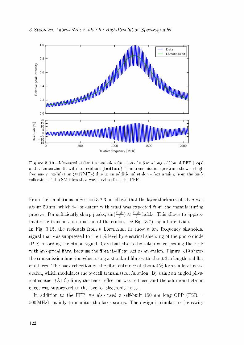
3 Stabilized Fabry-Pérot Etalon for High-Resolution Spectrographs
0.0
0.2
0.4
0.6
0.8
1.0
Rel
ati
vep
eak
inte
nsi
ty
Data
Lorentzian fit
0 500 1000 1500 2000
Relative frequency [MHz]
−15−10−5
05
101520
Res
idu
als
[%]
Figure 3.19 Measured etalon transmission function of a 6mm long self-build FFP (top)and a Lorentzian t with its residuals (bottom). The transmission spectrum shows a highfrequency modulation (≈17MHz) due to an additional etalon eect arising from the backreection of the SM bre that was used to feed the FFP.
From the simulations in Section 3.2.3, it follows that the layer thickness of silver was
about 50nm, which is consistent with what was expected from the manufacturing
process. For suciently sharp peaks, sin( δ−δ02
) ≈ δ−δ02
holds. This allows to approx-
imate the transmission function of the etalon, see Eq. (3.7), by a Lorentzian.
In Fig. 3.18, the residuals from a Lorentzian t show a low frequency sinusoidal
signal that was suppressed to the 1% level by electrical shielding of the photo diode
(PD) recording the etalon signal. Care had also to be taken when feeding the FFP
with an optical bre, because the bre itself can act as an etalon. Figure 3.19 shows
the transmission function when using a standard bre with about 3m length and at
end faces. The back reection on the bre entrance of about 4% forms a low nesse
etalon, which modulates the overall transmission function. By using an angled phys-
ical contact (APC) bre, the back reection was reduced and the additional etalon
eect was suppressed to the level of electronic noise.
In addition to the FFP, we also used a self-built 150mm long CFP (FSR =
500MHz), mainly to monitor the laser status. The design is similar to the cavity
122
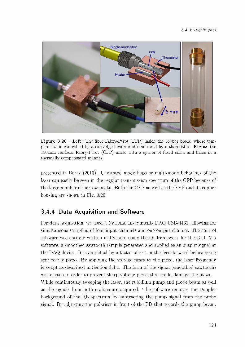
3.4 Experiments
Figure 3.20 Left: The bre Fabry-Pérot (FFP) inside the copper block, whose tem-perature is controlled by a cartridge heater and monitored by a thermistor. Right: the150mm confocal Fabry-Pérot (CFP) made with a spacer of fused silica and brass in athermally compensated manner.
presented in Barry (2013). Unwanted mode hops or multi-mode behaviour of the
laser can easily be seen in the regular transmission spectrum of the CFP because of
the large number of narrow peaks. Both the CFP as well as the FFP and its copper
housing are shown in Fig. 3.20.
3.4.4 Data Acquisition and Software
For data acquisition, we used a National Instruments DAQ USB-4431, allowing for
simultaneous sampling of four input channels and one output channel. The control
software was entirely written in Python, using the Qt framework for the GUI. Via
software, a smoothed sawtooth ramp is generated and applied as an output signal at
the DAQ device. It is amplied by a factor of ∼ 4 in the feed forward before being
sent to the piezo. By applying the voltage ramp to the piezo, the laser frequency
is swept as described in Section 3.4.1. The form of the signal (smoothed sawtooth)
was chosen in order to prevent sharp voltage peaks that could damage the piezo.
While continuously sweeping the laser, the rubidium pump and probe beam as well
as the signals from both etalons are acquired. The software removes the Doppler
background of the Rb spectrum by subtracting the pump signal from the probe
signal. By adjusting the polariser in front of the PD that records the pump beam,
123
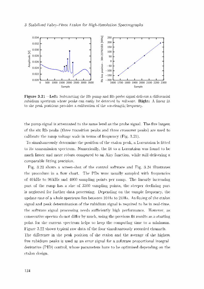
3 Stabilized Fabry-Pérot Etalon for High-Resolution Spectrographs
0 500 1000 1500 2000 2500 3000 3500
Sample
0.020
0.022
0.024
0.026
0.028
0.030
0.032
0.034
Am
pli
tud
e[V
]
1600 1700 1800 1900 2000 2100 2200 2300
Sample
−200
−150
−100
−50
0
50
100
150
200
250
Rb
lin
ep
osi
tio
n-
38
4.2
27
92
1E
6[M
Hz]
Figure 3.21 Left: Subtracting the Rb pump and Rb probe signal delivers a dierentialrubidium spectrum whose peaks can easily be detected by software. Right: A linear tto the peak positions provides a calibration of the wavelength/frequency.
the pump signal is attenuated to the same level as the probe signal. The ve largest
of the six Rb peaks (three transition peaks and three crossover peaks) are used to
calibrate the ramp voltage scale in terms of frequency (Fig. 3.21).
To simultaneously determine the position of the etalon peak, a Lorentzian is tted
to its transmission spectrum. Numerically, the t to a Lorentzian was found to be
much faster and more robust compared to an Airy function, while still delivering a
comparable tting precision.
Fig. 3.23 shows a screen-shot of the control software and Fig. 3.24 illustrates
the procedure in a ow chart. The PDs were usually sampled with frequencies
of 40 kHz to 96 kHz and 4000 sampling points per ramp. The linearly increasing
part of the ramp has a size of 3500 sampling points, the steeper declining part
is neglected for further data processing. Depending on the sample frequency, the
update rate of a whole spectrum lies between 10Hz to 24Hz. As tting of the etalon
signal and peak determination of the rubidium signal is required to be in real-time,
the software signal processing needs suciently high performance. However, as
consecutive spectra do not dier by much, using the previous t results as a starting
point for the current spectrum helps to keep the computing time to a minimum.
Figure 3.22 shows typical raw data of the four simultaneously recorded channels.
The dierence in the peak position of the etalon and the average of the highest
ve rubidium peaks is used as an error signal for a software proportional-integral-
derivative (PID) control, whose parameters have to be optimised depending on the
etalon design.
124
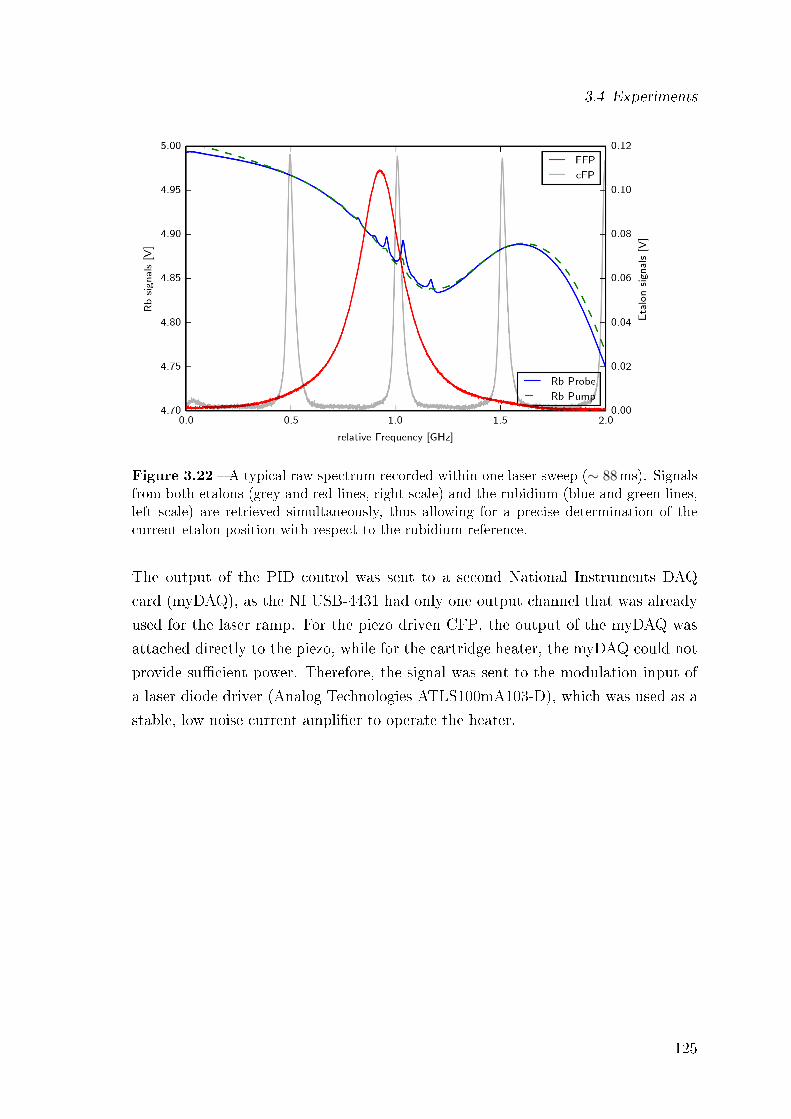
3.4 Experiments
Figure 3.22 A typical raw spectrum recorded within one laser sweep (∼ 88ms). Signalsfrom both etalons (grey and red lines, right scale) and the rubidium (blue and green lines,left scale) are retrieved simultaneously, thus allowing for a precise determination of thecurrent etalon position with respect to the rubidium reference.
The output of the PID control was sent to a second National Instruments DAQ
card (myDAQ), as the NI USB-4431 had only one output channel that was already
used for the laser ramp. For the piezo driven CFP, the output of the myDAQ was
attached directly to the piezo, while for the cartridge heater, the myDAQ could not
provide sucient power. Therefore, the signal was sent to the modulation input of
a laser diode driver (Analog Technologies ATLS100mA103-D), which was used as a
stable, low noise current amplier to operate the heater.
125
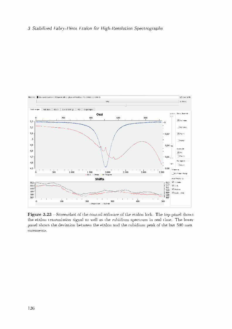
3 Stabilized Fabry-Pérot Etalon for High-Resolution Spectrographs
Figure 3.23 Screenshot of the control software of the etalon lock. The top panel showsthe etalon transmission signal as well as the rubidium spectrum in real time. The lowerpanel shows the deviation between the etalon and the rubidium peak of the last 500 mea-surements.
126
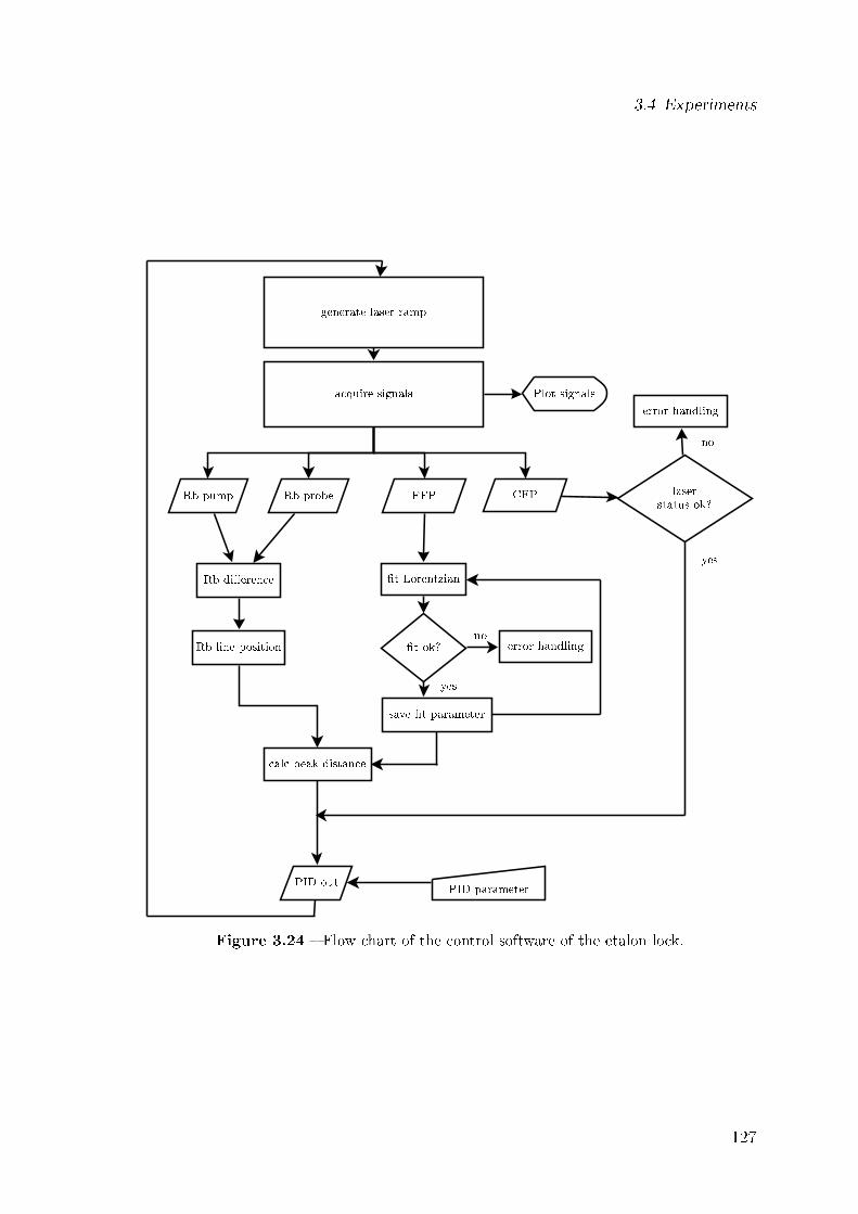
3.4 Experiments
generate laser ramp
acquire signals
Rb dierence
Rb pump Rb probe FFP CFP
t Lorentzian
laserstatus ok?
calc peak distance
t ok?
save t parameter
yes
PID out
error handling
yes
error handling
no
noRb line position
PID parameter
Plot signals
Figure 3.24 Flow chart of the control software of the etalon lock.
127
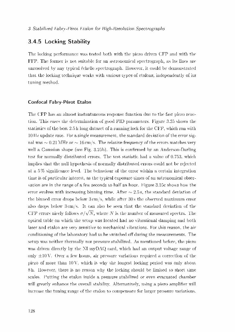
3 Stabilized Fabry-Pérot Etalon for High-Resolution Spectrographs
3.4.5 Locking Stability
The locking performance was tested both with the piezo driven CFP and with the
FFP. The former is not suitable for an astronomical spectrograph, as its lines are
unresolved by any typical échelle spectrograph. However, it could be demonstrated
that the locking technique works with various types of etalons, independently of its
tuning method.
Confocal Fabry-Pérot Etalon
The CFP has an almost instantaneous response function due to the fast piezo reac-
tion. This eases the determination of good PID parameters. Figure 3.25 shows the
statistics of the best 2.5 h long dataset of a running lock for the CFP, which ran with
10Hz update rate. For a single measurement, the standard deviation of the error sig-
nal was ∼ 0.21MHz or ∼ 16 cm/s. The relative frequency of the errors matches very
well a Gaussian shape (see Fig. 3.25b). This is conrmed by an Anderson-Darling
test for normally distributed errors. The test statistic had a value of 0.753, which
implies that the null hypothesis of normally distributed errors could not be rejected
at a 5% signicance level. The behaviour of the error within a certain integration
time is of particular interest, as the typical exposure times of an astronomical obser-
vation are in the range of a few seconds to half an hour. Figure 3.25c shows how the
error evolves with increasing binning time. After ∼ 2.5 s, the standard deviation of
the binned error drops below 3 cm/s, while after 30 s the observed maximum error
also drops below 3 cm/s. It can also be seen that the standard deviation of the
CFP errors nicely follows σ/√N , where N is the number of measured spectra. The
optical table on which the setup was located had no vibrational damping and both
laser and etalon are very sensitive to mechanical vibrations. For this reason, the air
conditioning of the laboratory had to be switched o during the measurements. The
setup was neither thermally nor pressure stabilized. As mentioned before, the piezo
was driven directly by the NI myDAQ card, which had an output voltage range of
only ±10V. Over a few hours, air pressure variations required a correction of the
piezo of more than 10V, which is why the longest locking period was only about
8 h. However, there is no reason why the locking should be limited to short time
scales. Putting the etalon inside a pressure stabilized or even evacuated chamber
will greatly enhance the overall stability. Alternatively, using a piezo amplier will
increase the tuning range of the etalon to compensate for larger pressure variations.
128
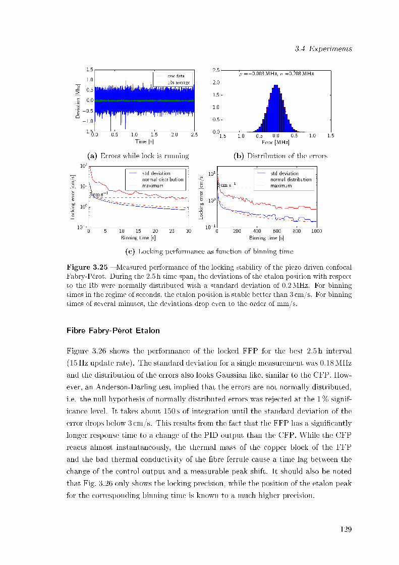
3.4 Experiments
(a) Errors while lock is running (b) Distribution of the errors
(c) Locking performance as function of binning time
Figure 3.25 Measured performance of the locking stability of the piezo driven confocalFabry-Pérot. During the 2.5 h time span, the deviations of the etalon position with respectto the Rb were normally distributed with a standard deviation of 0.2MHz. For binningtimes in the regime of seconds, the etalon position is stable better than 3 cm/s. For binningtimes of several minutes, the deviations drop even to the order of mm/s.
Fibre Fabry-Pérot Etalon
Figure 3.26 shows the performance of the locked FFP for the best 2.5 h interval
(15Hz update rate). The standard deviation for a single measurement was 0.18MHz
and the distribution of the errors also looks Gaussian like, similar to the CFP. How-
ever, an Anderson-Darling test implied that the errors are not normally distributed,
i.e. the null hypothesis of normally distributed errors was rejected at the 1% signif-
icance level. It takes about 150 s of integration until the standard deviation of the
error drops below 3 cm/s. This results from the fact that the FFP has a signicantly
longer response time to a change of the PID output than the CFP. While the CFP
reacts almost instantaneously, the thermal mass of the copper block of the FFP
and the bad thermal conductivity of the bre ferrule cause a time lag between the
change of the control output and a measurable peak shift. It should also be noted
that Fig. 3.26 only shows the locking precision, while the position of the etalon peak
for the corresponding binning time is known to a much higher precision.
129
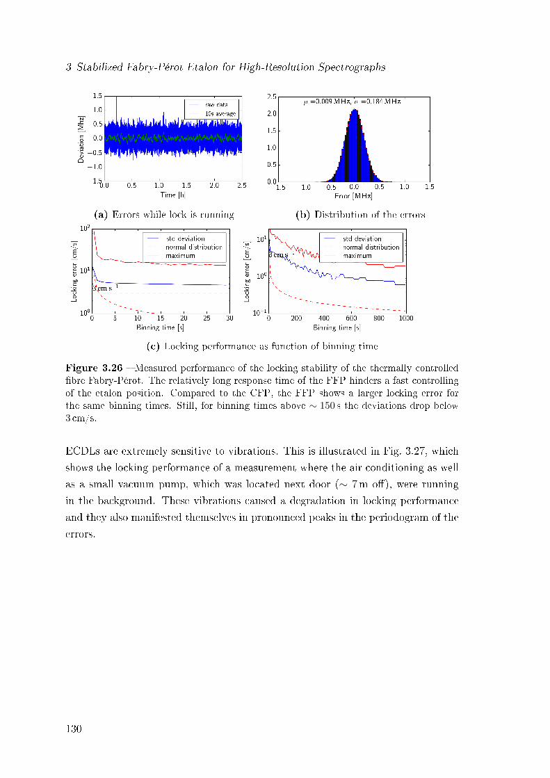
3 Stabilized Fabry-Pérot Etalon for High-Resolution Spectrographs
(a) Errors while lock is running (b) Distribution of the errors
(c) Locking performance as function of binning time
Figure 3.26 Measured performance of the locking stability of the thermally controlledbre Fabry-Pérot. The relatively long response time of the FFP hinders a fast controllingof the etalon position. Compared to the CFP, the FFP shows a larger locking error forthe same binning times. Still, for binning times above ∼ 150 s the deviations drop below3 cm/s.
ECDLs are extremely sensitive to vibrations. This is illustrated in Fig. 3.27, which
shows the locking performance of a measurement where the air conditioning as well
as a small vacuum pump, which was located next door (∼ 7m o), were running
in the background. These vibrations caused a degradation in locking performance
and they also manifested themselves in pronounced peaks in the periodogram of the
errors.
130
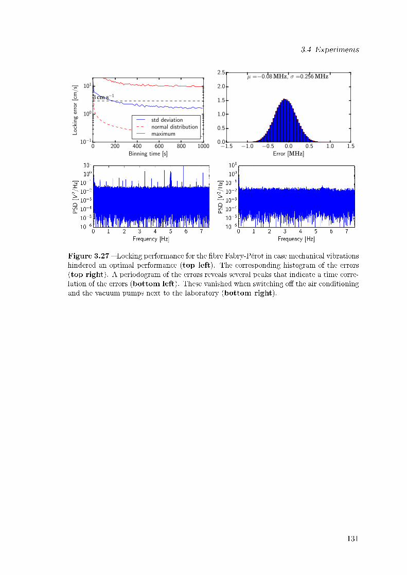
3.4 Experiments
0 200 400 600 800 1000Binning time [s]
10−1
100
101
Lo
ckin
ger
ror
[cm
/s]
3 cm s−1
std deviationnormal distributionmaximum
−1.5 −1.0 −0.5 0.0 0.5 1.0 1.5Error [MHz]
0.0
0.5
1.0
1.5
2.0
2.5µ =−0.08 MHz, σ =0.256 MHz
Figure 3.27 Locking performance for the bre Fabry-Pérot in case mechanical vibrationshindered an optimal performance (top left). The corresponding histogram of the errors(top right). A periodogram of the errors reveals several peaks that indicate a time corre-lation of the errors (bottom left). These vanished when switching o the air conditioningand the vacuum pumps next to the laboratory (bottom right).
131
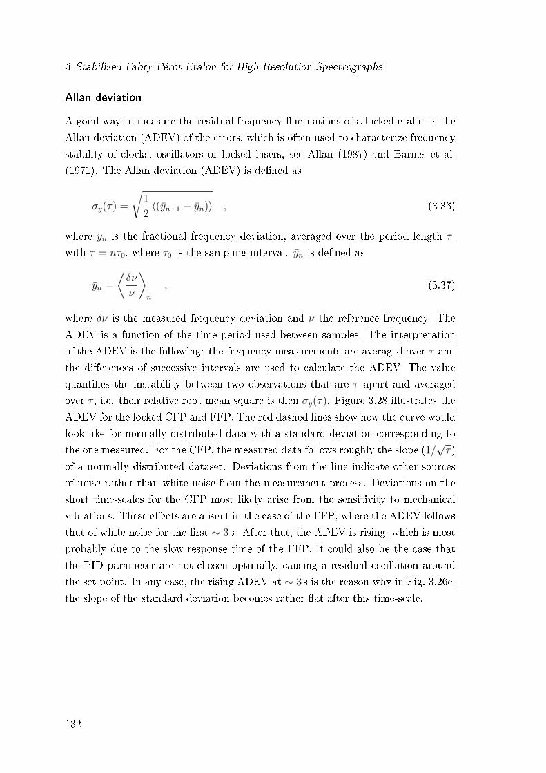
3 Stabilized Fabry-Pérot Etalon for High-Resolution Spectrographs
Allan deviation
A good way to measure the residual frequency uctuations of a locked etalon is the
Allan deviation (ADEV) of the errors, which is often used to characterize frequency
stability of clocks, oscillators or locked lasers, see Allan (1987) and Barnes et al.
(1971). The Allan deviation (ADEV) is dened as
σy(τ) =
√1
2〈(yn+1 − yn)〉 , (3.36)
where yn is the fractional frequency deviation, averaged over the period length τ ,
with τ = nτ0, where τ0 is the sampling interval. yn is dened as
yn =
⟨δν
ν
⟩n
, (3.37)
where δν is the measured frequency deviation and ν the reference frequency. The
ADEV is a function of the time period used between samples. The interpretation
of the ADEV is the following: the frequency measurements are averaged over τ and
the dierences of successive intervals are used to calculate the ADEV. The value
quanties the instability between two observations that are τ apart and averaged
over τ , i.e. their relative root mean square is then σy(τ). Figure 3.28 illustrates the
ADEV for the locked CFP and FFP. The red dashed lines show how the curve would
look like for normally distributed data with a standard deviation corresponding to
the one measured. For the CFP, the measured data follows roughly the slope (1/√τ)
of a normally distributed dataset. Deviations from the line indicate other sources
of noise rather than white noise from the measurement process. Deviations on the
short time-scales for the CFP most likely arise from the sensitivity to mechanical
vibrations. These eects are absent in the case of the FFP, where the ADEV follows
that of white noise for the rst ∼ 3 s. After that, the ADEV is rising, which is most
probably due to the slow response time of the FFP. It could also be the case that
the PID parameter are not chosen optimally, causing a residual oscillation around
the set point. In any case, the rising ADEV at ∼ 3 s is the reason why in Fig. 3.26c,
the slope of the standard deviation becomes rather at after this time-scale.
132
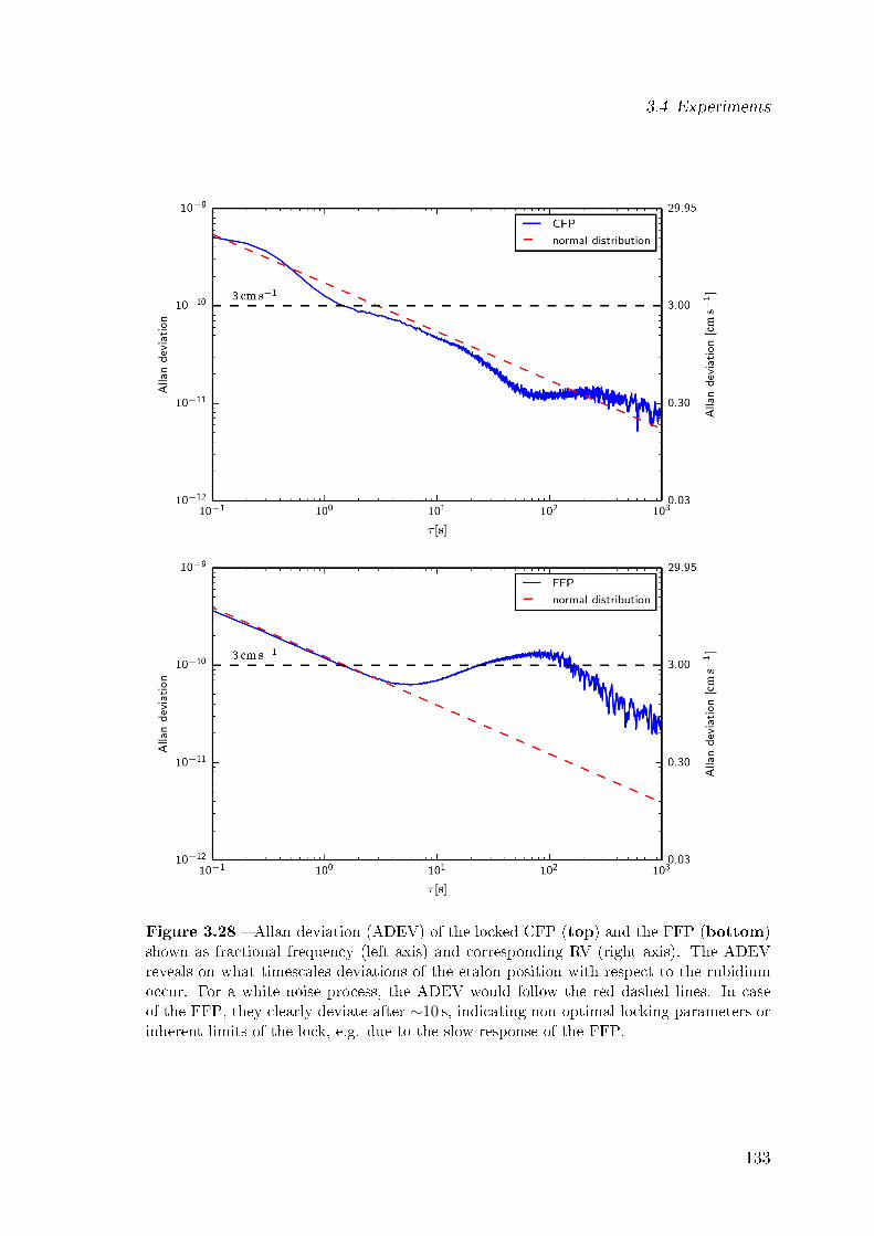
3.4 Experiments
Figure 3.28 Allan deviation (ADEV) of the locked CFP (top) and the FFP (bottom)shown as fractional frequency (left axis) and corresponding RV (right axis). The ADEVreveals on what timescales deviations of the etalon position with respect to the rubidiumoccur. For a white noise process, the ADEV would follow the red dashed lines. In caseof the FFP, they clearly deviate after ∼10 s, indicating non-optimal locking parameters orinherent limits of the lock, e.g. due to the slow response of the FFP.
133
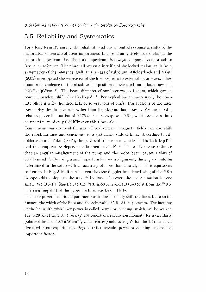
3 Stabilized Fabry-Pérot Etalon for High-Resolution Spectrographs
3.5 Reliability and Systematics
For a long term RV survey, the reliability and any potential systematic shifts of the
calibration source are of great importance. In case of an actively locked etalon, the
calibration spectrum, i.e. the etalon spectrum, is always compared to an absolute
frequency reference. Therefore, all systematic shifts of the locked etalon result from
systematics of the reference itself. In the case of rubidium, Aolderbach and Mileti
(2005) investigated the sensitivity of the line positions to external parameters. They
found a dependence on the absolute line position on the used pump laser power of
0.2 kHz/(µWcm−2). The beam diameter of our laser was ∼ 1.4mm, which gives a
power dependent shift of ∼ 13 kHz µW−1. For typical laser powers used, the abso-
lute oset is a few hundred kHz or several tens of cm/s. Fluctuations of the laser
power play the decisive role rather than the absolute laser power. We measured a
relative power uctuation of 0.175% in our setup over 9.6 h, which translates into
an uncertainty of only 0.59 kHz over this timescale.
Temperature variations of the gas cell and external magnetic elds can also shift
the rubidium lines and contribute to a systematic shift of lines. According to Af-
folderbach and Mileti (2005), the peak shift due to a magnetic eld is 1.2 kHz µT−1
and the temperature dependence is about 4 kHzK−1. The authors also estimate
that an angular misalignment of the pump and the probe beam causes a shift of
80 kHzmrad−1. By using a small aperture for beam alignment, the angle should be
determined in the setup with an accuracy of more than 1mrad, which is equivalent
to 6 cm/s. In Fig. 3.16, it can be seen that the doppler broadened wing of the 85Rb
isotope adds a slope to the used 87Rb lines. However, the contamination is very
small. We tted a Gaussian to the 85Rb spectrum and subtracted it from the 87Rb.
The resulting shift of the hyperne lines was below 1 kHz.
The laser power is a critical parameter as it does not only shift the lines, but also in-
uences the width of the lines and the achievable SNR of the spectrum. The increase
of the linewidth with laser power is called power broadening, which can be seen in
Fig. 3.29 and Fig. 3.30. Steck (2013) reported a saturation intensity for a circularly
polarised laser of 1.67mWcm−2, which corresponds to 26µW for the 1.4mm beam
size used in our experiments. Beyond this threshold, power broadening becomes an
important factor.
134
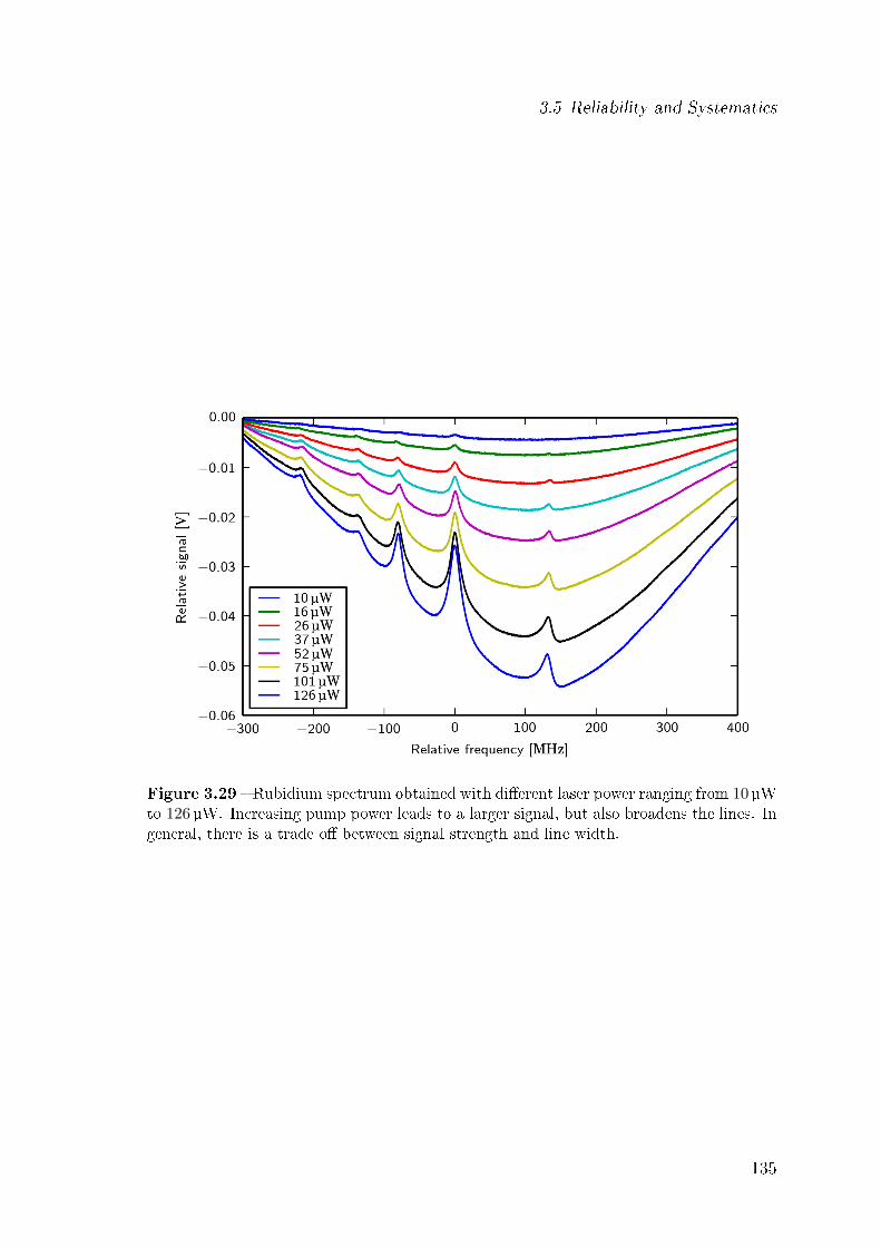
3.5 Reliability and Systematics
Figure 3.29 Rubidium spectrum obtained with dierent laser power ranging from 10 µWto 126 µW. Increasing pump power leads to a larger signal, but also broadens the lines. Ingeneral, there is a trade o between signal strength and line width.
135
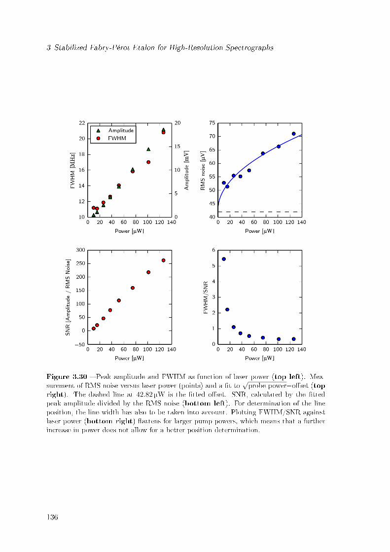
3 Stabilized Fabry-Pérot Etalon for High-Resolution Spectrographs
Figure 3.30 Peak amplitude and FWHM as function of laser power (top left). Mea-surement of RMS noise versus laser power (points) and a t to
√probe power+oset (top
right). The dashed line at 42.82 µW is the tted oset. SNR, calculated by the ttedpeak amplitude divided by the RMS noise (bottom left). For determination of the lineposition, the line width has also to be taken into account. Plotting FWHM/SNR againstlaser power (bottom right) attens for larger pump powers, which means that a furtherincrease in power does not allow for a better position determination.
136
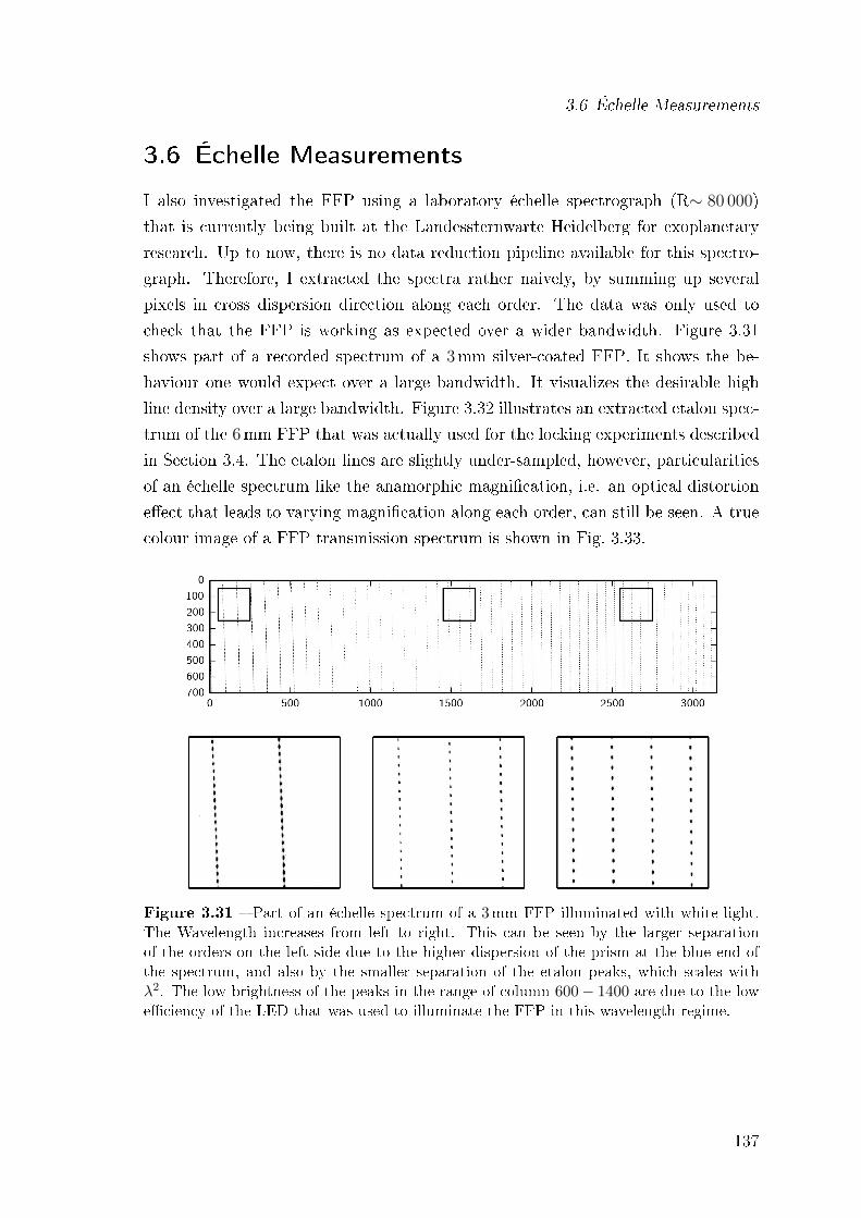
3.6 Échelle Measurements
3.6 Échelle Measurements
I also investigated the FFP using a laboratory échelle spectrograph (R∼ 80 000)
that is currently being built at the Landessternwarte Heidelberg for exoplanetary
research. Up to now, there is no data reduction pipeline available for this spectro-
graph. Therefore, I extracted the spectra rather naively, by summing up several
pixels in cross dispersion direction along each order. The data was only used to
check that the FFP is working as expected over a wider bandwidth. Figure 3.31
shows part of a recorded spectrum of a 3mm silver-coated FFP. It shows the be-
haviour one would expect over a large bandwidth. It visualizes the desirable high
line density over a large bandwidth. Figure 3.32 illustrates an extracted etalon spec-
trum of the 6mm FFP that was actually used for the locking experiments described
in Section 3.4. The etalon lines are slightly under-sampled, however, particularities
of an échelle spectrum like the anamorphic magnication, i.e. an optical distortion
eect that leads to varying magnication along each order, can still be seen. A true
colour image of a FFP transmission spectrum is shown in Fig. 3.33.
Figure 3.31 Part of an échelle spectrum of a 3mm FFP illuminated with white light.The Wavelength increases from left to right. This can be seen by the larger separationof the orders on the left side due to the higher dispersion of the prism at the blue end ofthe spectrum, and also by the smaller separation of the etalon peaks, which scales withλ2. The low brightness of the peaks in the range of column 600− 1400 are due to the loweciency of the LED that was used to illuminate the FFP in this wavelength regime.
137
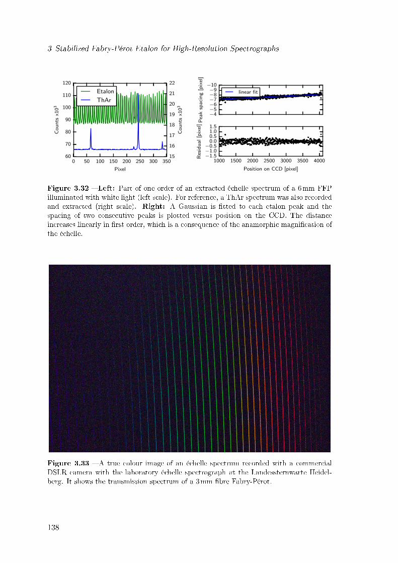
3 Stabilized Fabry-Pérot Etalon for High-Resolution Spectrographs
0 50 100 150 200 250 300 350
Pixel
60
70
80
90
100
110
120
Co
un
tsx1
03
15
16
17
18
19
20
21
22
Co
un
tsx1
03
Etalon
ThAr
−10−9−8−7−6−5−4
Pea
ksp
aci
ng
[pix
el]
linear fit
1000 1500 2000 2500 3000 3500 4000
Position on CCD [pixel]
−1.5−1.0−0.5
0.00.51.01.5
Res
idu
al
[pix
el]
Figure 3.32 Left: Part of one order of an extracted échelle spectrum of a 6mm FFPilluminated with white light (left scale). For reference, a ThAr spectrum was also recordedand extracted (right scale). Right: A Gaussian is tted to each etalon peak and thespacing of two consecutive peaks is plotted versus position on the CCD. The distanceincreases linearly in rst order, which is a consequence of the anamorphic magnication ofthe échelle.
Figure 3.33 A true colour image of an échelle spectrum recorded with a commercialDSLR camera with the laboratory échelle spectrograph at the Landessternwarte Heidel-berg. It shows the transmission spectrum of a 3mm bre Fabry-Pérot.
138
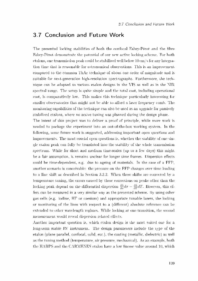
3.7 Conclusion and Future Work
3.7 Conclusion and Future Work
The presented locking stabilities of both the confocal Fabry-Pérot and the bre
Fabry-Pérot demonstrate the potential of our new active locking scheme. For both
etalons, one transmission peak could be stabilized well below 10 cm/s for any integra-
tion time that is reasonable for astronomical observations. This is an improvement
compared to the common ThAr technique of about one order of magnitude and is
suitable for next-generation high-resolution spectrographs. Furthermore, the tech-
nique can be adapted to various etalon designs in the VIS as well as in the NIR
spectral range. The setup is quite simple and the total cost, including operational
cost, is comparatively low. This makes this technique particularly interesting for
smaller observatories that might not be able to aord a laser frequency comb. The
monitoring capabilities of the technique can also be used as an upgrade for passively
stabilized etalons, where no active tuning was planned during the design phase.
The intent of this project was to deliver a proof of principle, while more work is
needed to package the experiment into an out-of-the-box working system. In the
following, some future work is suggested, addressing important open questions and
improvements. The most crucial open questions is, whether the stability of one sin-
gle etalon peak can fully be translated into the stability of the whole transmission
spectrum. While for short and medium time-scales (up to a few days) this might
be a fair assumption, it remains unclear for longer time frames. Dispersion eects
could be time-dependent, e.g. due to ageing of materials. In the case of a FFP,
another scenario is conceivable: the pressure on the FFP changes over time leading
to a line shift as described in Section 3.2.2. When these shifts are corrected by a
temperature tuning, the errors caused by these corrections on peaks other than the
locking peak depend on the dierential dispersion ∂λ∂σdσ − ∂λ
∂TdT . However, this ef-
fect can be measured in a very similar way as the presented scheme. By using other
gas cells (e.g. iodine, HF or caesium) and appropriate tunable lasers, the locking
or monitoring of the lines with respect to a (dierent) absolute reference can be
extended to other wavelength regimes. While locking at one transition, the second
measurement would reveal dispersion related eects.
Another important question is, which etalon design is the most suited one for a
long-term stable RV instrument. The design parameters include the type of the
etalon (plane-parallel, confocal, solid, etc.), the coating (metallic, dielectric) as well
as the tuning method (temperature, air pressure, mechanical). As an example, both
the HARPS and the CARMENES etalon have a low nesse value around 10, which
139
3 Stabilized Fabry-Pérot Etalon for High-Resolution Spectrographs
is roughly constant with wavelength. A detailed study that takes into account the
peculiarities of an échelle such as its constant resolution and incorporates them to
current extraction schemes is needed.
This goes hand in hand with the question whether an etalon that is locked to an
absolute reference could also be used as an absolute wavelength meter. This should
in principle be possible, as the Fabry-Pérot can once be characterized against a LFC
or a ThAr spectrum. Especially in the case of metallic mirrors, when the phase
shifts are a low-order function of wavelength, it should be possible to determine
the wavelength of each single transmission peak with good accuracy. Using two
or three saturated absorption spectroscopic measurements at dierent wavelengths
would deliver good constraints on the slope of the dispersion function.
More concretely, a couple of improvements to the presented setup would further
enhance the precision and stability: As mentioned, the ECDL is very sensitive
to vibrations and uctuations of environmental conditions. An active stabilization
scheme based on polarisation spectroscopy would reduce the sensitivity of the ECDL
at the cost of adding only slightly more hardware complexity (Führer et al., 2011).
One major contribution to the noise of a single measurement is the determination of
the rubidium peak position, which is currently only implemented as a simple peak
detection of the ve largest peak in the rubidium spectrum. Himsworth and Free-
garde (2010) compared measured Rb spectra to theoretical predictions and showed
that their model based t, not using any free parameters, has a residual dierence
of less than 1% over a large range of pump powers. Fitting an analytic function
to the rubidium, would decrease the uncertainty of the peak position and would
also allow for an easy monitoring of the status of the rubidium setup. For example,
if spectral lines get dimmer or broader over time, it could indicate a gradual mis-
alignment of the probe and pump beam or ageing of the cell. An analytic tting
would require more computational power, as it has to be done in real time. With
a fully multi-threaded approach, such requirements should easily be fullled for a
standard computer. So far, no optimisation of the sampling rate, the sampling size
and the locking rate was performed. Investigating and optimising these parameters
will most likely further improve the performance of the instrument.
Even in its current state, the laser locked etalon has signicant benets over other
calibrators and could become an important asset for exoplanet spectrographs in the
near future.
140


Bibliography
Aolderbach, C. and Mileti, G. (2005). A compact laser head with high-frequencystability for Rb atomic clocks and optical instrumentation. Review of ScienticInstruments, 76(7):073108.
Allan, D. W. (1987). Should the classical variance be used as a basic measurein standards metrology? IEEE Transactions on Instrumentation Measurement,36:646654.
Allington-Smith, J., Murray, G., and Lemke, U. (2012). Simulation of complexphenomena in optical bres. Monthly Notices of the Royal Astronomical Society,427(2):919933.
Angel, J. R. P., Adams, M. T., Boroson, T. A., and Moore, R. L. (1977). A verylarge optical telescope array linked with fused silica bers. Astrophysical Journal,218:776782.
Avila, G. (1988). Tests of optical bres for astronomical instrumentation at ESO.In Barden, S. C., editor, Fiber Optics in Astronomy, volume 3 of AstronomicalSociety of the Pacic Conference Series, pages 6373.
Avila, G. (1998). Results on Fiber Characterization at ESO. In Arribas, S., Medi-avilla, E., and Watson, F., editors, Fiber Optics in Astronomy III, volume 152 ofAstronomical Society of the Pacic Conference Series.
Avila, G. (2012). FRD and scrambling properties of recent non-circular bres. InSociety of Photo-Optical Instrumentation Engineers (SPIE) Conference Series,volume 8446, pages 84469L84469L7.
Avila, G. and Singh, P. (2008). Optical ber scrambling and light pipes for high accu-racy radial velocities measurements. In Society of Photo-Optical InstrumentationEngineers (SPIE) Conference Series, volume 7018, pages 70184W70184W7.
Avila, G., Singh, P., and Albertsen, M. (2006). Photometrical scrambling gain andfocal ratio degradation in bers for astronomical instruments. In Society of Photo-Optical Instrumentation Engineers (SPIE) Conference Series, volume 6269, pages62695O62695O9.
Avila, G., Singh, P., and Chazelas, B. (2010). Results on bre scrambling for high ac-curacy radial velocity measurements. In Society of Photo-Optical InstrumentationEngineers (SPIE) Conference Series, volume 7735, pages 7735887735889.
143
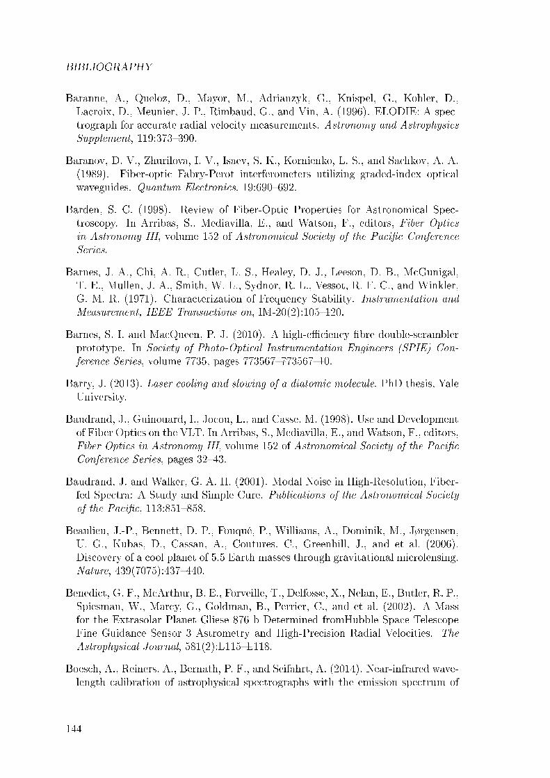
BIBLIOGRAPHY
Baranne, A., Queloz, D., Mayor, M., Adrianzyk, G., Knispel, G., Kohler, D.,Lacroix, D., Meunier, J.-P., Rimbaud, G., and Vin, A. (1996). ELODIE: A spec-trograph for accurate radial velocity measurements. Astronomy and AstrophysicsSupplement, 119:373390.
Baranov, D. V., Zhurilova, I. V., Isaev, S. K., Kornienko, L. S., and Sachkov, A. A.(1989). Fiber-optic Fabry-Perot interferometers utilizing graded-index opticalwaveguides. Quantum Electronics, 19:690692.
Barden, S. C. (1998). Review of Fiber-Optic Properties for Astronomical Spec-troscopy. In Arribas, S., Mediavilla, E., and Watson, F., editors, Fiber Opticsin Astronomy III, volume 152 of Astronomical Society of the Pacic ConferenceSeries.
Barnes, J. A., Chi, A. R., Cutler, L. S., Healey, D. J., Leeson, D. B., McGunigal,T. E., Mullen, J. A., Smith, W. L., Sydnor, R. L., Vessot, R. F. C., and Winkler,G. M. R. (1971). Characterization of Frequency Stability. Instrumentation andMeasurement, IEEE Transactions on, IM-20(2):105120.
Barnes, S. I. and MacQueen, P. J. (2010). A high-eciency bre double-scramblerprototype. In Society of Photo-Optical Instrumentation Engineers (SPIE) Con-ference Series, volume 7735, pages 77356777356710.
Barry, J. (2013). Laser cooling and slowing of a diatomic molecule. PhD thesis, YaleUniversity.
Baudrand, J., Guinouard, I., Jocou, L., and Casse, M. (1998). Use and Developmentof Fiber Optics on the VLT. In Arribas, S., Mediavilla, E., andWatson, F., editors,Fiber Optics in Astronomy III, volume 152 of Astronomical Society of the PacicConference Series, pages 3243.
Baudrand, J. and Walker, G. A. H. (2001). Modal Noise in High-Resolution, Fiber-fed Spectra: A Study and Simple Cure. Publications of the Astronomical Societyof the Pacic, 113:851858.
Beaulieu, J.-P., Bennett, D. P., Fouqué, P., Williams, A., Dominik, M., Jørgensen,U. G., Kubas, D., Cassan, A., Coutures, C., Greenhill, J., and et al. (2006).Discovery of a cool planet of 5.5 Earth masses through gravitational microlensing.Nature, 439(7075):437440.
Benedict, G. F., McArthur, B. E., Forveille, T., Delfosse, X., Nelan, E., Butler, R. P.,Spiesman, W., Marcy, G., Goldman, B., Perrier, C., and et al. (2002). A Massfor the Extrasolar Planet Gliese 876 b Determined fromHubble Space TelescopeFine Guidance Sensor 3 Astrometry and High-Precision Radial Velocities. TheAstrophysical Journal, 581(2):L115L118.
Boesch, A., Reiners, A., Bernath, P. F., and Seifahrt, A. (2014). Near-infrared wave-length calibration of astrophysical spectrographs with the emission spectrum of
144
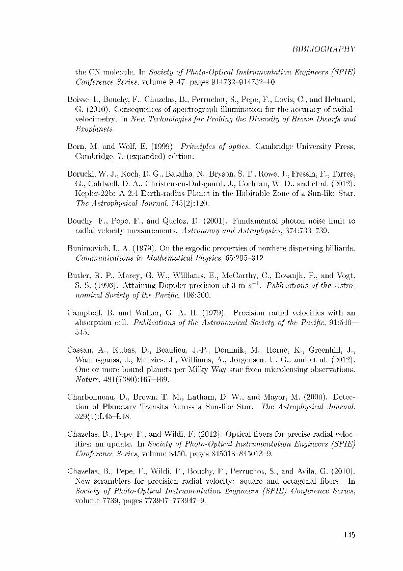
BIBLIOGRAPHY
the CN molecule. In Society of Photo-Optical Instrumentation Engineers (SPIE)Conference Series, volume 9147, pages 91473291473210.
Boisse, I., Bouchy, F., Chazelas, B., Perruchot, S., Pepe, F., Lovis, C., and Hebrard,G. (2010). Consequences of spectrograph illumination for the accuracy of radial-velocimetry. In New Technologies for Probing the Diversity of Brown Dwarfs andExoplanets.
Born, M. and Wolf, E. (1999). Principles of optics. Cambridge University Press,Cambridge, 7. (expanded) edition.
Borucki, W. J., Koch, D. G., Batalha, N., Bryson, S. T., Rowe, J., Fressin, F., Torres,G., Caldwell, D. A., Christensen-Dalsgaard, J., Cochran, W. D., and et al. (2012).Kepler-22b: A 2.4 Earth-radius Planet in the Habitable Zone of a Sun-like Star.The Astrophysical Journal, 745(2):120.
Bouchy, F., Pepe, F., and Queloz, D. (2001). Fundamental photon noise limit toradial velocity measurements. Astronomy and Astrophysics, 374:733739.
Bunimovich, L. A. (1979). On the ergodic properties of nowhere dispersing billiards.Communications in Mathematical Physics, 65:295312.
Butler, R. P., Marcy, G. W., Williams, E., McCarthy, C., Dosanjh, P., and Vogt,S. S. (1996). Attaining Doppler precision of 3 m s−1. Publications of the Astro-nomical Society of the Pacic, 108:500.
Campbell, B. and Walker, G. A. H. (1979). Precision radial velocities with anabsorption cell. Publications of the Astronomical Society of the Pacic, 91:540545.
Cassan, A., Kubas, D., Beaulieu, J.-P., Dominik, M., Horne, K., Greenhill, J.,Wambsganss, J., Menzies, J., Williams, A., Jørgensen, U. G., and et al. (2012).One or more bound planets per Milky Way star from microlensing observations.Nature, 481(7380):167169.
Charbonneau, D., Brown, T. M., Latham, D. W., and Mayor, M. (2000). Detec-tion of Planetary Transits Across a Sun-like Star. The Astrophysical Journal,529(1):L45L48.
Chazelas, B., Pepe, F., and Wildi, F. (2012). Optical bers for precise radial veloc-ities: an update. In Society of Photo-Optical Instrumentation Engineers (SPIE)Conference Series, volume 8450, pages 8450138450139.
Chazelas, B., Pepe, F., Wildi, F., Bouchy, F., Perruchot, S., and Avila, G. (2010).New scramblers for precision radial velocity: square and octagonal bers. InSociety of Photo-Optical Instrumentation Engineers (SPIE) Conference Series,volume 7739, pages 7739477739479.
145
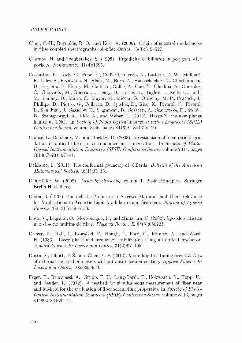
BIBLIOGRAPHY
Chen, C.-H., Reynolds, R. O., and Kost, A. (2006). Origin of spectral modal noisein ber-coupled spectrographs. Applied Optics, 45(3):519527.
Chernov, N. and Troubetzkoy, S. (1998). Ergodicity of billiards in polygons withpockets. Nonlinearity, 11(4):1095.
Cosentino, R., Lovis, C., Pepe, F., Collier Cameron, A., Latham, D. W., Molinari,E., Udry, S., Bezawada, N., Black, M., Born, A., Buchschacher, N., Charbonneau,D., Figueira, P., Fleury, M., Galli, A., Gallie, A., Gao, X., Ghedina, A., Gonzalez,C., G onzalez, M., Guerra, J., Henry, D., Horne, K., Hughes, I., Kelly, D., Lodi,M., Lunney, D., Maire, C., Mayor, M., Micela, G., Ordw ay, M. P., Peacock, J.,Phillips, D., Piotto, G., Pollacco, D., Queloz, D., Rice, K., Riverol, C., Riverol,L., San Juan, J., Sasselov, D., Segransan, D., Sozzetti, A., Sosnowska, D., Stobie,B., Szentgyorgyi, A., Vick, A., and Weber, L. (2012). Harps-N: the new planethunter at TNG. In Society of Photo-Optical Instrumentation Engineers (SPIE)Conference Series, volume 8446, pages 84461V84461V20.
Crause, L., Bershady, M., and Buckley, D. (2008). Investigation of focal ratio degra-dation in optical bres for astronomical instrumentation. In Society of Photo-Optical Instrumentation Engineers (SPIE) Conference Series, volume 7014, pages70146C70146C11.
DeMarco, L. (2011). The conformal geometry of billiards. Bulletin of the AmericanMathematical Society, 48(1):3333.
Demtröder, W. (2008). Laser Spectroscopy, volume 1. Basic Principles. SpringerBerlin Heidelberg.
Dixon, R. (1967). Photoelastic Properties of Selected Materials and Their Relevancefor Applications to Acoustic Light Modulators and Scanners. Journal of AppliedPhysics, 38(13):51495153.
Doya, V., Legrand, O., Mortessagne, F., and Miniatura, C. (2002). Speckle statisticsin a chaotic multimode ber. Physical Review E, 65(5):056223.
Drever, R., Hall, J., Kowalski, F., Hough, J., Ford, G., Munley, A., and Ward,H. (1983). Laser phase and frequency stabilization using an optical resonator.Applied Physics B: Lasers and Optics, 31(2):97105.
Dutta, S., Elliott, D. S., and Chen, Y. P. (2012). Mode-hop-free tuning over 135 GHzof external cavity diode lasers without antireection coating. Applied Physics B:Lasers and Optics, 106:629633.
Feger, T., Brucalassi, A., Grupp, F. U., Lang-Bardl, F., Holzwarth, R., Hopp, U.,and Bender, R. (2012). A testbed for simultaneous measurement of ber nearand far-eld for the evaluation of ber scrambling properties. In Society of Photo-Optical Instrumentation Engineers (SPIE) Conference Series, volume 8446, pages84469284469214.
146
BIBLIOGRAPHY
Figueira, P., Pepe, F., Melo, C. H. F., Santos, N. C., Lovis, C., Mayor, M., Queloz,D., Smette, A., and Udry, S. (2010). Radial velocities with CRIRES. Pushingprecision down to 5-10 m/s. Astronomy and Astrophysics, 511:A55.
Fraine, J., Deming, D., Benneke, B., Knutson, H., Jordán, A., Espinoza, N., Mad-husudhan, N., Wilkins, A., and Todorov, K. (2014). Water vapour absorption inthe clear atmosphere of a Neptune-sized exoplanet. Nature, 513(7519):526529.
Frink, S., Mitchell, D. S., Quirrenbach, A., Fischer, D. A., Marcy, G. W., and Butler,R. P. (2002). Discovery of a Substellar Companion to the K2 III Giant ι Draconis.Astrophysical Journal, 576:478484.
Führer, T., Euler, S., and Walther, T. (2011). Model for tuning an external-cavitydiode laser by polarization locking. Journal of the Optical Society of America B,28(3):508514.
Führer, T. and Walther, T. (2012). Control and active stabilization of the linewidthof an ECDL. Applied Physics B: Lasers and Optics, 108:249253.
F¶rész, G., Epps, H., Barnes, S., Podgorski, W., Szentgyorgyi, A., Mueller, M.,Baldwin, D., Bean, J., Bergner, H., Chun, M.-Y., Crane, J., Evans, J., Evans,I., Foster, J., Gauron, T., Guzman, D., Hertz, E., Jordán, A., Kim, K.-M., Mc-Cracken, K., Norton, T., Ordway, M., Park, C., Park, S., Plummer, D., Uomoto,A., and Yuk, I.-S. (2014). The G-CLEF spectrograph optical design. In Societyof Photo-Optical Instrumentation Engineers (SPIE) Conference Series, volume9147, pages 91479G91479G9.
Goodman, J. W. and Rawson, E. G. (1981). Statistics of modal noise in bers: acase of constrained speckle. Optics Letters, 6(7):324326.
Grupp, F. (2003). The nature of the ber noise with the FOCES spectrograph.Nature, modeling and a way to achieve S/N > 400. Astronomy and Astrophysics,412:897902.
Gurevich, Y. V., Stürmer, J., Schwab, C., Führer, T., Lamoreaux, S. K., Quirren-bach, A., and Walther, T. (2014). A laser locked Fabry-Perot etalon with 3 cm/sstability for spectrograph calibration. In Society of Photo-Optical InstrumentationEngineers (SPIE) Conference Series, volume 9147, pages 91477M91477M17.
Halverson, S., Mahadevan, S., Ramsey, L., Hearty, F., Wilson, J., Holtzman, J.,Redman, S., Nave, G., Nidever, D., Nelson, M., and et al. (2014). Developmentof Fiber Fabry-Perot Interferometers as Stable Near-infrared Calibration Sourcesfor High Resolution Spectrographs. Publications of the Astronomical Society ofthe Pacic, 126(939):445458.
Halverson, S., Mahadevan, S., Ramsey, L. W., Redman, S., Nave, G., Wilson, J. C.,Hearty, F., and Holtzman, J. (2012). Development of a new, precise near-infrared
147
BIBLIOGRAPHY
Doppler wavelength reference: a ber Fabry-Perot interferometer. Ground-basedand Airborne Instrumentation for Astronomy IV.
Haynes, D. M., Withford, M. J., Dawes, J. M., Lawrence, J. S., and Haynes, R.(2011). Relative contributions of scattering, diraction and modal diusion to fo-cal ratio degradation in optical bres. Monthly Notices of the Royal AstronomicalSociety, 414(1):253263.
Haynes, R., McNamara, P., Marcel, J., and Jovanovic, N. (2006). Advances ininfrared and imaging bres for astronomical instrumentation. In Society of Photo-Optical Instrumentation Engineers (SPIE) Conference Series, volume 6273, pages62733U62733U11.
Heacox, W. D. (1987). Radial image transfer by cylindrical, step-index opticalwaveguides. Journal of the Optical Society of America A, 4(3):488493.
Heacox, W. D. (1988). Wavelength-precise slit spectroscopy with optical ber imagescramblers. In Barden, S. C., editor, Fiber Optics in Astronomy, volume 3 ofAstronomical Society of the Pacic Conference Series, pages 204235.
Hercher, M. (1968). The spherical mirror Fabry-Perot interferometer. Applied Op-tics, 7(5):951966.
Himsworth, M. and Freegarde, T. (2010). Rubidium pump-probe spectroscopy:Comparison between ab initio theory and experiment. Physical Review A: GeneralPhysics, 81(2):023423.
Hunter, T. R. and Ramsey, L. W. (1992). Scrambling properties of optical bers andthe performance of a double scrambler. Publications of the Astronomical Societyof the Pacic, 104:12441251.
Kanada, T. and Aoyama, K. (1983). Modal-noise evaluation in multimode-bertransmission. Optics Letters, 8(6):339341.
Korsch, H. J., Jodl, H.-J., and Hartmann, T. (2008). Chaos: A Program Collectionfor the PC (3 rd. edition). Springer Berlin Heidelberg.
Lemke, U., Corbett, J., Allington-Smith, J., and Murray, G. (2011). Modal noiseprediction in bre spectroscopy I. Visibility and the coherent model. MonthlyNotices of the Royal Astronomical Society, 417(1):689697.
Leviton, D. B. and Frey, B. J. (2006). Temperature-dependent absolute refractiveindex measurements of synthetic fused silica. In Society of Photo-Optical Instru-mentation Engineers (SPIE) Conference Series, volume 6273.
Li, C.-H., Benedick, A. J., Fendel, P., Glenday, A. G., Kärtner, F. X., Phillips, D. F.,Sasselov, D., Szentgyorgyi, A., and Walsworth, R. L. (2008). A laser frequencycomb that enables radial velocity measurements with a precision of 1 cm s−1.Nature, 610-612:452.
148
BIBLIOGRAPHY
Lopac, V., Mrkonji¢, I., and Radi¢, D. (2002). Chaotic dynamics and orbit stabilityin the parabolic oval billiard. Physical Review E, 66:036202.
Lovis, C. and Pepe, F. (2007). A new list of thorium and argon spectral lines in thevisible. Astronomy and Astrophysics, 468:11151121.
Mahadevan, S. and Ge, J. (2009). The Use of Absorption Cells as a WavelengthReference for Precision Radial Velocity Measurements in the Near-Infrared. As-trophysical Journal, 692:15901596.
Mahadevan, S., Halverson, S., Ramsey, L., and Venditti, N. (2014). Suppressionof Fiber Modal Noise Induced Radial Velocity Errors for Bright Emission-lineCalibration Sources. Astrophysical Journal, 786:18.
Marcy, G. W. and Butler, R. P. (1992). Precision radial velocities with an iodineabsorption cell. Publications of the Astronomical Society of the Pacic, 104:270277.
Marois, C., Macintosh, B., Barman, T., Zuckerman, B., Song, I., Patience, J., Lafre-niere, D., and Doyon, R. (2008). Direct Imaging of Multiple Planets Orbiting theStar HR 8799. Science, 322(5906):13481352.
Marois, C., Zuckerman, B., Konopacky, Q. M., Macintosh, B., and Barman, T.(2010). Images of a fourth planet orbiting HR 8799. Nature, 468(7327):10801083.
Mayor, M., Pepe, F., Queloz, D., Bouchy, F., Rupprecht, G., Lo Curto, G., Avila, G.,Benz, W., Bertaux, J.-L., Bonls, X., Dall, T., Dekker, H., Delabre, B., Eckert,W., Fleury, M., Gilliotte, A., Gojak, D., Guzman, J. C., Kohler, D., Lizon, J.-L.,Longinotti, A., Lovis, C., Megevand, D., Pasquini, L., Reyes, J., Sivan, J.-P.,Sosnowska, D., Soto, R., Udry, S., van Kesteren, A., Weber, L., and Weilenmann,U. (2003). Setting New Standards with HARPS. The Messenger, 114:2024.
Mayor, M. and Queloz, D. (1995). A Jupiter-mass companion to a solar-type star.Nature, 378:355359.
Mayor, M., Udry, S., Lovis, C., Pepe, F., Queloz, D., Benz, W., Bertaux, J.-L.,Bouchy, F., Mordasini, C., and Segransan, D. (2009). The HARPS search forsouthern extra-solar planets. XIII. A planetary system with 3 super-Earths (4.2,6.9, and 9.2 M). Astronomy and Astrophysics, 493:639644.
McCoy, K. S., Ramsey, L., Mahadevan, S., Halverson, S., and Redman, S. L. (2012).Optical ber modal noise in the 0.8 to 1.5 micron region and implications for nearinfrared precision radial velocity measurements. In Society of Photo-Optical In-strumentation Engineers (SPIE) Conference Series, volume 8446, pages 84468J84468J8.
Michel, C., Tascu, S., Doya, V., Legrand, O., and Mortessagne, F. (2009). Gain-controlled wave chaos in a chaotic optical bre. Journal of the European OpticalSociety - Rapid publications, 4(0).
149
BIBLIOGRAPHY
Mitschke, F. (2010). Fiber Optics. Springer Berlin Heidelberg.
Monzón, J. J., Sánchez-Soto, L. L., and Bernabeu, E. (1991). Inuence of coatingthickness on the performance of a FabryPerot interferometer. Applied Optics,30(28):41264132.
Murphy, J. D., MacQueen, P. J., Hill, G. J., Grupp, F., Kelz, A., Palunas, P., Roth,M., and Fry, A. (2008). Focal ratio degradation and transmission in VIRUS-P optical bers. In Society of Photo-Optical Instrumentation Engineers (SPIE)Conference Series, volume 7018, pages 70182T70182T12.
Murphy, M. T., Tzanavaris, P., Webb, J. K., and Lovis, C. (2007). Selection of ThArlines for wavelength calibration of echelle spectra and implications for variationsin the ne-structure constant. Monthly Notices of the Royal Astronomical Society,378:221230.
Padilla Michel, Y., Zoheidi, M., Roth, M. M., Haynes, R., and Olaya, J.-C. (2012).Applied stress on coated multimode optical bres: a dierent point of view tobending losses. In Society of Photo-Optical Instrumentation Engineers (SPIE)Conference Series, volume 8450, pages 84503F84503F14.
Parry, I. (1998). The Astronomical Uses of Optical Fibers. In Arribas, S., Medi-avilla, E., and Watson, F., editors, Fiber Optics in Astronomy III, volume 152 ofAstronomical Society of the Pacic Conference Series.
Pepe, F., Ehrenreich, D., and Meyer, M. R. (2014a). Instrumentation for the detec-tion and characterization of exoplanets. Nature, 513:358366.
Pepe, F., Mayor, M., Delabre, B., Kohler, D., Lacroix, D., Queloz, D., Udry, S.,Benz, W., Bertaux, J.-L., and Sivan, J.-P. (2000). HARPS: a new high-resolutionspectrograph for the search of extrasolar planets. In Society of Photo-OpticalInstrumentation Engineers (SPIE) Conference Series, volume 4008, pages 582592.
Pepe, F., Molaro, P., Cristiani, S., Rebolo, R., Santos, N. C., Dekker, H., Mégevand,D., Zerbi, F. M., Cabral, A., Di Marcantonio, P., Abreu, M., Aolter, M., Aliverti,M., Allende Prieto, C., Amate, M., Avila, G., Baldini, V., Bristow, P., Broeg,C., Cirami, R., Coelho, J., Conconi, P., Coretti, I., Cupani, G., D'Odorico, V.,De Caprio, V., Delabre, B., Dorn, R., Figueira, P., Fragoso, A., Galeotta, S.,Genolet, L., Gomes, R., González Hernández, J. I., Hughes, I., Iwert, O., Kerber,F., Landoni, M., Lizon, J.-L., Lovis, C., Maire, C., Mannetta, M., Martins, C.,Monteiro, M., Oliveira, A., Poretti, E., Rasilla, J. L., Riva, M., Santana Tschudi,S., Santos, P., Sosnowska, D., Sousa, S., Spanó, P., Tenegi, F., Toso, G., Vanzella,E., Viel, M., and Zapatero Osorio, M. R. (2014b). ESPRESSO: The next Europeanexoplanet hunter. Astronomische Nachrichten, 335:8.
150
BIBLIOGRAPHY
Perruchot, S., Bouchy, F., Chazelas, B., Díaz, R. F., Hébrard, G., Arnaud, K.,Arnold, L., Avila, G., Delfosse, X., Boisse, I., Moreaux, G., Pepe, F., Richaud, Y.,Santerne, A., Sottile, R., and Tézier, D. (2011). Higher-precision radial velocitymeasurements with the SOPHIE spectrograph using octagonal-section bers. InSociety of Photo-Optical Instrumentation Engineers (SPIE) Conference Series,volume 8151, pages 81511581511512.
Perruchot, S., Kohler, D., Bouchy, F., Richaud, Y., Richaud, P., Moreaux, G., Mer-zougui, M., Sottile, R., Hill, L., Knispel, G., Regal, X., Meunier, J.-P., Ilovaisky,S., Le Coroller, H., Gillet, D., Schmitt, J., Pepe, F., Fleury, M., Sosnowska, D.,Vors, P., Mégevand, D., Blanc, P. E., Carol, C., Point, A., Laloge, A., and Brunel,J.-C. (2008). The SOPHIE spectrograph: design and technical key-points for highthroughput and high stability. In Society of Photo-Optical Instrumentation Engi-neers (SPIE) Conference Series, volume 7014.
Petigura, E. A., Howard, A. W., and Marcy, G. W. (2013). Prevalence of Earth-sizeplanets orbiting Sun-like stars. Proceedings of the National Academy of Sciences,110(48):1927319278.
Plavchan, P. P., Anglada-Escude, G., White, R., Gao, P., Davison, C., Mills, S.,Beichman, C., Brinkworth, C., Johnson, J., Bottom, M., Ciardi, D., Wallace, K.,Mennesson, B., von Braun, K., Vasisht, G., Prato, L., Kane, S., Tanner, A., Walp,B., Crawford, S., and Lin, S. (2013). Precision near-infrared radial velocity in-strumentation I: absorption gas cells. In Society of Photo-Optical InstrumentationEngineers (SPIE) Conference Series, volume 8864.
Poppett, C. L. and Allington-Smith, J. R. (2010). The dependence of the propertiesof optical bres on length. Monthly Notices of the Royal Astronomical Society,404:13491354.
Probst, R. A., Steinmetz, T., Wilken, T., Wong, G. K. L., Hundertmark, H., Stark,S. P., Russell, P. S. J., Hänsch, T. W., Holzwarth, R., and Udem, T. (2013).Spectral attening of supercontinua with a spatial light modulator. In Societyof Photo-Optical Instrumentation Engineers (SPIE) Conference Series, volume8864, pages 88641Z88641Z8.
Quirrenbach, A., Amado, P. J., Mandel, H., Caballero, J. A., Mundt, R., Ribas, I.,Reiners, A., Abril, M., Aceituno, J., Afonso, C., Barrado y Navascues, D., Bean,J. L., Béjar, V. J. S., Becerril, S., Böhm, A., Cárdenas, M. C., Claret, A., Colomé,J., Costillo, L. P., Dreizler, S., Fernández, M., Francisco, X., Galadí, D., Garrido,R., González Hernández, J. I., Guàrdia, J., Guenther, E. W., Gutiérrez-Soto, F.,Joergens, V., Hatzes, A. P., Helmling, J., Henning, T., Herrero, E., Kürster, M.,Laun, W., Lenzen, R., Mall, U., Martin, E. L., Martín-Ruiz, S., Mirabet, E.,Montes, D., Morales, J. C., Morales Muñoz, R., Moya, A., Naranjo, V., Rabaza,O., Ramón, A., Rebolo, R., Reert, S., Rodler, F., Rodríguez, E., RodríguezTrinidad, A., Rohlo, R. R., Sánchez Carrasco, M. A., Schmidt, C., Seifert, W.,
151
BIBLIOGRAPHY
Setiawan, J., Solano, E., Stahl, O., Storz, C., Suárez, J. C., Thiele, U., Wagner,K., Wiedemann, G., Zapatero Osorio, M. R., del Burgo, C., Sánchez-Blanco, E.,and Xu, W. (2010). CARMENES: Calar Alto high-resolution search for M dwarfswith exo-earths with a near-infrared Echelle spectrograph. In Society of Photo-Optical Instrumentation Engineers (SPIE) Conference Series, volume 7735.
Quirrenbach, A., Amado, P. J., Seifert, W., Sánchez Carrasco, M. A., Mandel,H., Caballero, J. A., Mundt, R., Ribas, I., Reiners, A., Abril, M., Aceituno, J.,Alonso-Floriano, J., Ammler-von Ei, M., Anglada-Escude, G., Antona Jiménez,R., Anwand-Heerwart, H., Barrado y Navascués, D., Becerril, S., Bejar, V., Ben-itez, D., Cardenas, C., Claret, A., Colome, J., Cortés-Contreras, M., Czesla,S., del Burgo, C., Doellinger, M., Dorda, R., Dreizler, S., Feiz, C., Fernandez,M., Galadi, D., Garrido, R., González Hernández, J., Guardia, J., Guenther, E.,de Guindos, E., Gutiérrez-Soto, J., Hagen, H. J., Hatzes, A., Hauschildt, P., Helm-ling, J., Henning, T., Herrero, E., Huber, A., Huber, K., Jeers, S., Joergens, V.,de Juan, E., Kehr, M., Klutsch, A., Kürster, M., Lalitha, S., Laun, W., Lemke,U., Lenzen, R., Lizon, J.-L., López del Fresno, M., López-Morales, M., López-Santiago, J., Mall, U., Martin, E., Martín-Ruiz, S., Mirabet, E., Montes, D.,Morales, J. C., Morales Muñoz, R., Moya, A., Naranjo, V., Oreiro, R., Pérez Me-dialdea, D., Pluto, M., Rabaza, O., Ramon, A., Rebolo, R., Reert, S., Rhode,P., Rix, H.-W., Rodler, F., Rodríguez, E., Rodríguez López, C., Rodríguez Pérez,E., Rodriguez Trinidad, A., Rohlo, R.-R., Sánchez-Blanco, E., Sanz-Forcada, J.,Schäfer, S., Schiller, J., Schmidt, C., Schmitt, J., Solano, E., Stahl, O., Storz, C.,Stürmer, J., Suarez, J. C., Thiele, U., Ulbrich, R., Vidal-Dasilva, M., Wagner,K., Winkler, J., Xu, W., Zapatero Osorio, M. R., and Zechmeister, M. (2012).CARMENES. I: instrument and survey overview. In Society of Photo-Optical In-strumentation Engineers (SPIE) Conference Series, volume 8446, pages 84460R84460R13.
Ramsey, L. W. (1988). Focal ratio degradation in optical bers of astronomicalinterest. In Barden, S. C., editor, Fiber Optics in Astronomy, volume 3 of Astro-nomical Society of the Pacic Conference Series, pages 2639.
Ramsey, L. W., Mahadevan, S., Redman, S., Bender, C., Roy, A., Zonak, S., Sig-urdsson, S., and Wolszczan, A. (2010). The Pathnder testbed: exploring tech-niques for achieving precision radial velocities in the near infrared. In Societyof Photo-Optical Instrumentation Engineers (SPIE) Conference Series, volume7735.
Raskin, G., van Winckel, H., Hensberge, H., Jorissen, A., Lehmann, H., Waelkens,C., Avila, G., de Cuyper, J.-P., Degroote, P., Dubosson, R., Dumortier, L., Fré-mat, Y., Laux, U., Michaud, B., Morren, J., Perez Padilla, J., Pessemier, W.,Prins, S., Smolders, K., van Eck, S., and Winkler, J. (2011). HERMES: a high-resolution bre-fed spectrograph for the Mercator telescope. Astronomy and As-trophysics, 526:A69.
152
BIBLIOGRAPHY
Redman, S. L., Kerber, F., Nave, G., Mahadevan, S., Ramsey, L. W., Smoker, J.,Käu, H.-U., and Figueira, P. R. L. (2012). Near-infrared calibration systems forprecise radial-velocity measurements. In Society of Photo-Optical InstrumentationEngineers (SPIE) Conference Series, volume 8446.
Ree, S. and Reichl, L. E. (1999). Classical and quantum chaos in a circular billiardwith a straight cut. Physical Review E, 60:16071615.
Ricci, L., Weidemüller, M., Esslinger, T., Hemmerich, A., Zimmermann, C., Vuletic,V., König, W., and Hänsch, T. W. (1995). A compact grating-stabilized diodelaser system for atomic physics. Optics Communications, 117:541549.
Richens, P. J. and Berry, M. V. (1981). Pseudointegrable systems in classical andquantum mechanics. Physica D Nonlinear Phenomena, 2:495512.
Schäfer, S. and Reiners, A. (2012). Two Fabry-Perot interferometers for high preci-sion wavelength calibration in the near-infrared. In Society of Photo-Optical In-strumentation Engineers (SPIE) Conference Series, volume 8446, pages 8446948446948.
Schroeder, D. J. (1999). Astronomical Optics. Academic Press, second edition.
Schwab, C., Stürmer, J., Gurevich, Y. V., Führer, T., Lamoreaux, S. K., Walther,T., and Quirrenbach, A. (2014). Stabilizing a Fabry-Perot etalon to 3 cm/s forspectrograph calibration. arXiv:1404.0004.
Seemann, U., Anglada-Escude, G., Baade, D., Bristow, P., Dorn, R. J., Follert, R.,Gojak, D., Grunhut, J., Hatzes, A. P., Heiter, U., Ives, D. J., Jeep, P., Jung,Y., Käu, H.-U., Kerber, F., Klein, B., Lizon, J.-L., Lockhart, M., Löwinger,T., Marquart, T., Oliva, E., Pauque, J., Piskunov, N., Pozna, E., Reiners, A.,Smette, A., Smoker, J., Stempels, E., and Valenti, E. (2014). Wavelength cali-bration from 1-5µm for the CRIRES+ high-resolution spectrograph at the VLT.In Society of Photo-Optical Instrumentation Engineers (SPIE) Conference Series,volume 9147, pages 91475G91475G13.
Serkowski, K., Frecker, J. E., Heacox, w. D., and Roland, E. H. (1979). Fabry-Perot Radial Velocity Spectrometer. In Society of Photo-Optical InstrumentationEngineers (SPIE) Conference Series, volume 0172, pages 130133.
Sokkar, T. Z. N., Ramadan, W. A., Shams El-Din, M. A., Wahba, H. H., andAboleneen, S. S. (2014). Bent induced refractive index prole variation and modeeld distribution of step-index multimode optical ber. Optics and Lasers inEngineering, 53:133141.
Spronck, J. F. P., Fischer, D. A., Kaplan, Z. A., Schwab, C., and Szymkowiak, A.(2013). Fiber Scrambling for High-Resolution Spectrographs. I. Lick Observatory.Publications of the Astronomical Society of the Pacic, 125:511521.
153
BIBLIOGRAPHY
Spronck, J. F. P., Kaplan, Z. A., Fischer, D. A., Schwab, C., and Szymkowiak, A. E.(2012). Extreme Doppler precision with octagonal ber scramblers. In Societyof Photo-Optical Instrumentation Engineers (SPIE) Conference Series, volume8446, pages 84468T84468T10.
Stark, S. P., Steinmetz, T., Probst, R. A., Hundertmark, H., Wilken, T., Hänsch,T. W., Udem, T., Russell, P. S. J., and Holzwarth, R. (2011). 14 GHz visiblesupercontinuum generation: calibration sources for astronomical spectrographs.Optic Express, 19(17):1569015695.
Steck, D. A. (2010). Rubidium 87 D line data. http://steck.us/alkalidata/,revision 2.1.4, 23 December 2010.
Steck, D. A. (2013). Rubidium 85 D line data. http://steck.us/alkalidata/ ,revision 2.1.6, 20 September 2013.
Steinmetz, T., Wilken, T., Araujo-Hauck, C., Holzwarth, R., Hänsch, T. W.,Pasquini, L., Manescau, A., D'Odorico, S., Murphy, M. T., Kentischer, T.,Schmidt, W., and Udem, T. (2008). Laser Frequency Combs for AstronomicalObservations. Science, 321(5894):13351337.
Stürmer, J., Stahl, O., Schwab, C., Seifert, W., Quirrenbach, A., Amado, P. J.,Ribas, I., Reiners, A., and Caballero, J. A. (2014). CARMENES in SPIE 2014.Building a bre link for CARMENES. In Society of Photo-Optical InstrumentationEngineers (SPIE) Conference Series, volume 9151, pages 91515291515212.
Tateda, M., Komaki, K., and Yamaguchi, Y. (2007a). Stress dependence of transmis-sion frequency of a ber Fabry-Perot etalon buried in a ber ferrule. Electronicsand Communications in Japan (Part I: Communications), 90(7):18.
Tateda, M., Otake, S., Shintaku, T., and Omatsu, T. (2007b). Birefringence genera-tion mechanism in a ber Fabry-Perot etalon buried in a ber connector housing.Electronics and Communications in Japan (Part I: Communications), 90(5):5662.
Tokovinin, A., Fischer, D. A., Bonati, M., Giguere, M. J., Moore, P., Schwab, C.,Spronck, J. F. P., and Szymkowiak, A. (2013). CHIRON - A Fiber Fed Spectrom-eter for Precise Radial Velocities. Publications of the Astronomical Society of thePacic, 125:13361347.
Tuomi, M., Jones, H. R. A., Barnes, J. R., Anglada-Escude, G., and Jenkins, J. S.(2014). Bayesian search for low-mass planets around nearby m dwarfs - estimatesfor occurrence rate based on global detectability statistics. Monthly Notices of theRoyal Astronomical Society, 441(2):15451569.
Wallard, A. J. (1972). Frequency stabilization of the helium-neon laser by satu-rated absorption in iodine vapour. Journal of Physics E: Scientic Instruments,5(9):926.
154
BIBLIOGRAPHY
Wang, R., Yan, Y., Liu, Y., Zhang, H., and Sun, W. (2013). The inuence on FRDwith dierent encircled energy. In Optoelectronics and Microelectronics (ICOM),2013 International Conference on, pages 180182.
Wildi, F., Chazelas, B., and Pepe, F. (2012). A passive cost-eective solution for thehigh accuracy wavelength calibration of radial velocity spectrographs. In Societyof Photo-Optical Instrumentation Engineers (SPIE) Conference Series, volume8446.
Wildi, F., Pepe, F., Chazelas, B., Lo Curto, G., and Lovis, C. (2010). A Fabry-Perot calibrator of the HARPS radial velocity spectrograph: performance report.In Society of Photo-Optical Instrumentation Engineers (SPIE) Conference Series,volume 7735.
Wildi, F., Pepe, F., Chazelas, B., Lo Curto, G., and Lovis, C. (2011). The per-formance of the new Fabry-Perot calibration system of the radial velocity spec-trograph HARPS. In Society of Photo-Optical Instrumentation Engineers (SPIE)Conference Series, volume 8151.
Wilken, T., Lo Curto, G., Probst, R. A., Steinmetz, T., Manescau, A., Pasquini,L., Hernández, J. I. G., Rebolo, R., Hänsch, T. W., Udem, T., and Holzwarth, R.(2012). A spectrograph for exoplanet observations calibrated at the centimetre-per-second level. Nature, 485:611614.
Wilken, T., Lovis, C., Manescau, A., Steinmetz, T., Pasquini, L., Lo Curto, G.,Hänsch, T. W., Holzwarth, R., and Udem, T. (2010). High-precision calibrationof spectrographs. Monthly Notices of the Royal Astronomical Society, 405:L16L20.
Wolszczan, A. and Frail, D. A. (1992). A planetary system around the millisecondpulsar PSR1257 + 12. Nature, 355:145147.
Ycas, G. G., Quinlan, F., Diddams, S. A., Osterman, S., Mahadevan, S., Redman,S., Terrien, R., Ramsey, L., Bender, C. F., Botzer, B., and Sigurdsson, S. (2012).Demonstration of on-sky calibration of astronomical spectra using a 25 GHz near-IR laser frequency comb. Optic Express, 20(6):66316643.
Zemlyakov, A. and Katok, A. (1975). Topological transitivity of billiards in polygons.Mathematical notes of the Academy of Sciences of the USSR, 18(2):760764.
155

Acknowledgement
I would like to take the opportunity to thank all the people, who supported meduring my PhD studies.First, I would like to thank my supervisor Prof. Andreas Quirrenbach for giving
me the opportunity to work on these interesting topics. I appreciated his helpfulcomments, his guidance, but also the freedom he granted me to focus on my ownresearch interests. Thanks go to my second supervisor Otmar Stahl, who was alwayswilling to listen to my problems and helping me. I also thank Prof. Reinhard Mundtfor being the second referee for this thesis.I acknowledge the support of the Studienstiftung des Deutschen Volkes, both
nancial and otherwise.This work would not have been possible without the support of Christian Schwab.
For the many fruitful (and sometimes exhausting) discussions, your great scienticguidance and your willingness to listen to my problems (and for keeping me busy inthe rare moments I would have had some free time) around the clock from aroundthe world: Thank you!A big thank you goes to my co-authors, especially Yulia Gurevich and Thorsten
Führer, for sharing their knowledge with me.I would also like to thank Christoph Koke, who patiently helped me whenever I
ran into programming issues. He, Stephan Meister and Jens-Malte Gottfried, werealso great company during 'the good old days' in Heidelberg. A special thank yougoes to Tim-Oliver Müller. Not only for your useful comments on the manuscript,but for all your support in the last years. It is good to know to have such friends.I want to thank my colleagues at LSW, Lutz Geuer and Ludwig Schäner for
their competent help whenever I needed something 'special' from the mechanicalworkshop and also my oce colleagues during the last years, Andre, Kirsten, David,Markus and especially Christoph for keeping up with the chaos that tend to spreadfrom my desk.I am grateful for Uli Grötzinger's help and his patience with trying to improve
my knowledge of electronics.To the people in Potsdam, Dionne and Roger Haynes and Andreas Kelz: thank
you for letting me use your fancy bre facilities and sharing your knowledge withme. This was extraordinary helpful.None of this would have happened without the unconditional support of my family,
especially my parents. Thank you for your trust in my abilities and your advice.All I have achieved is your credit as well.To Karin: thank you for scrutinising the manuscript, for your constant encour-
agement and for your understanding for the long evenings this work took up. I amso grateful that I met you.
157


