Embed Size (px)
Citation preview
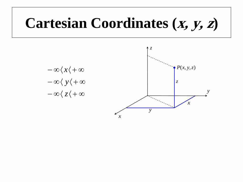
Cartesian Coordinates (x, y, z)
z
y
x
z
x
y
),,( zyxP
z
y
x
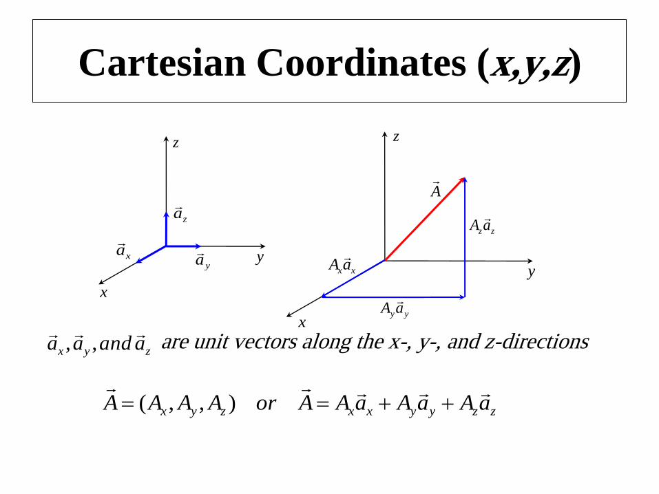
Cartesian Coordinates (x,y,z)
x
y
z z
y
x
A
xa
ya
za
xxaA
yyaA
zzaA
zzyyxxzyx aAaAaAAorAAAA
),,(
are unit vectors along the x-, y-, and z-directions zyx aandaa
,,
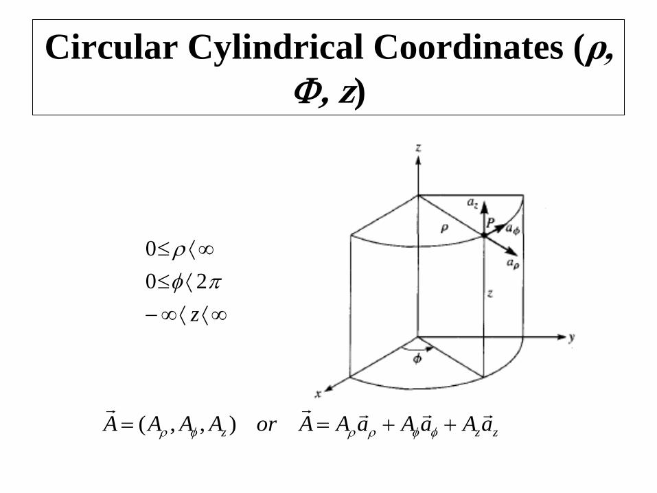
Circular Cylindrical Coordinates (ρ,
, z)
z
20
0
zzz aAaAaAAorAAAA
),,(
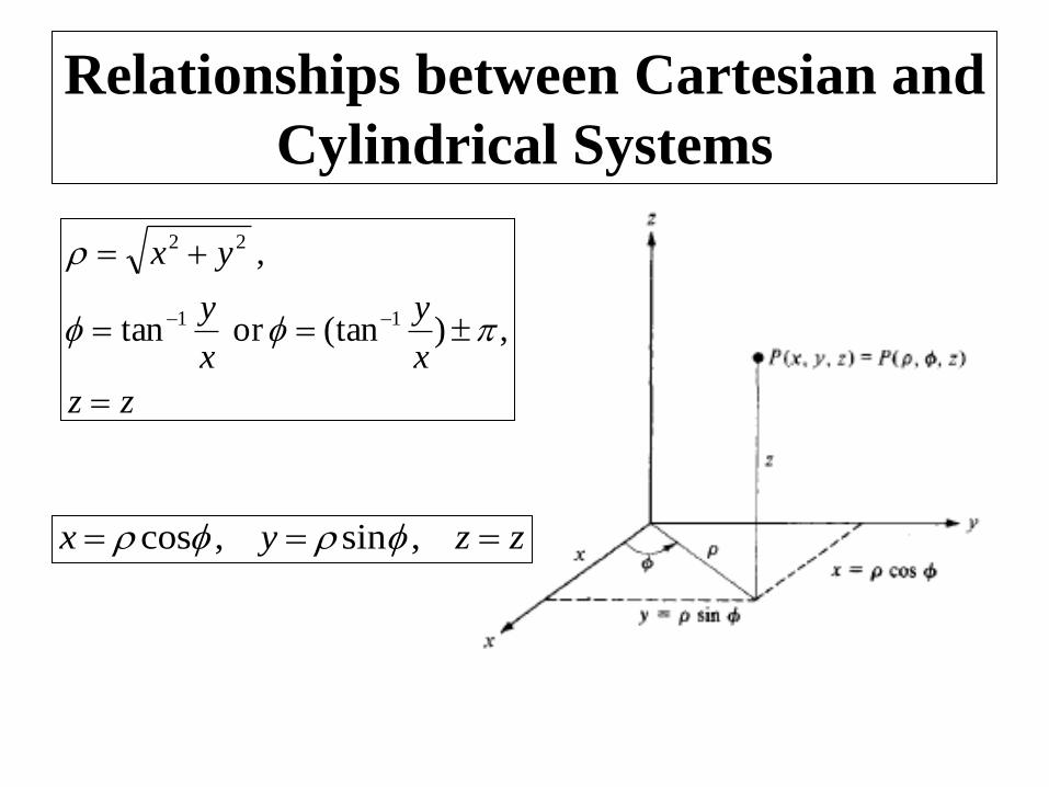
Relationships between Cartesian and
Cylindrical Systems
zz
x
y
x
y
yx
,)(tanor tan
,
11
22
zzyx ,sin,cos
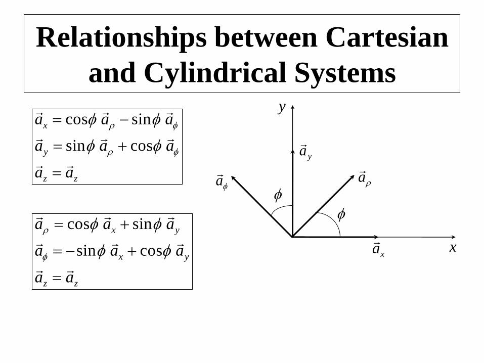
Relationships between Cartesian
and Cylindrical Systems
x
y
ya
a
a
xa
zz
y
x
aa
aaa
aaa
cossin
sincos
zz
yx
yx
aa
aaa
aaa
cossin
sincos
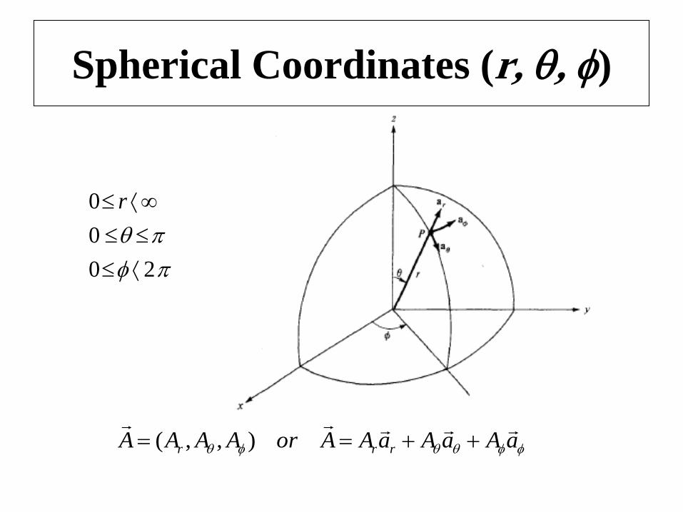
Spherical Coordinates (r, , )
20
0
0
r
aAaAaAAorAAAA rrr
),,(
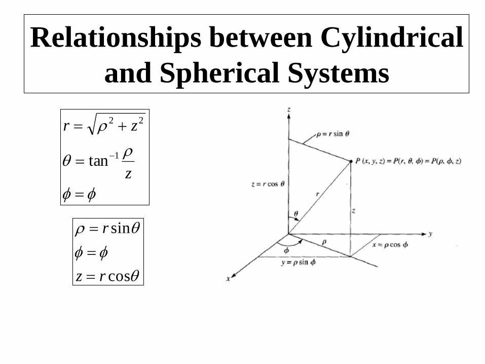
Relationships between Cylindrical
and Spherical Systems
z
zr
1
22
tan
cos
sin
rz
r
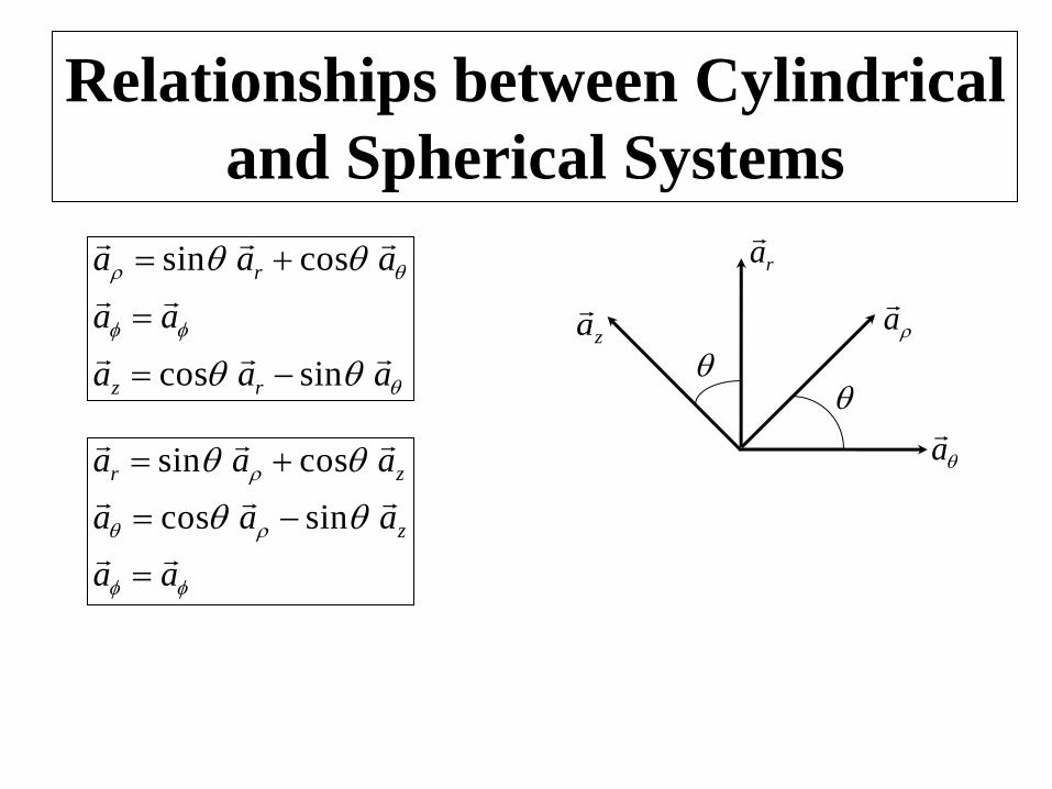
Relationships between Cylindrical
and Spherical Systems
ra
a
a
za
aaa
aa
aaa
rz
r
sincos
cossin
aa
aaa
aaa
z
zr
sincos
cossin
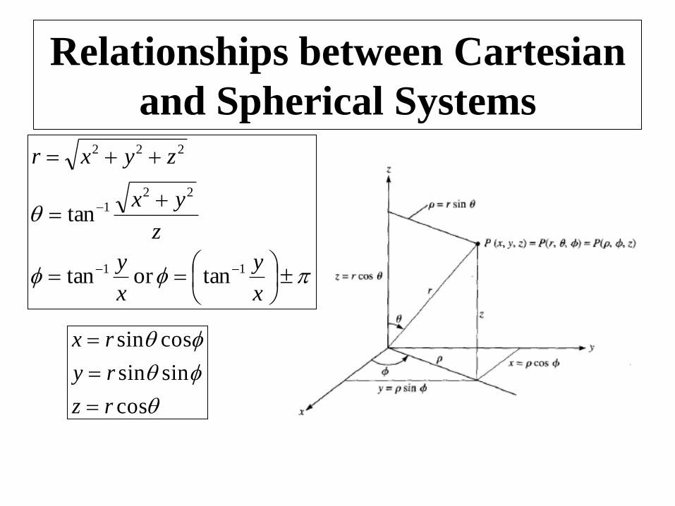
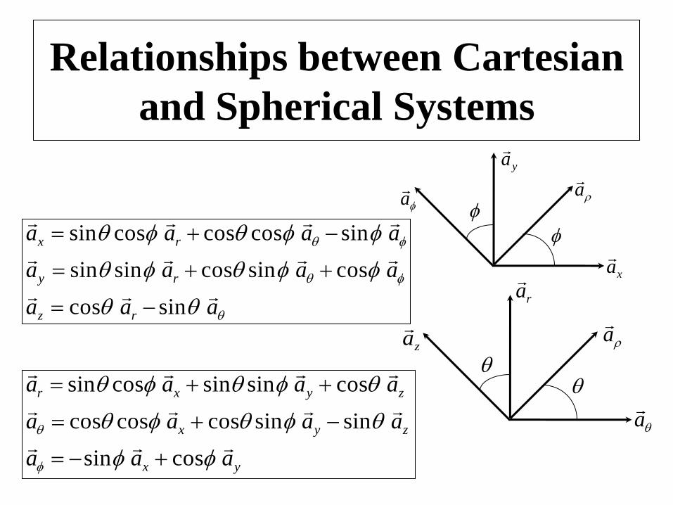
Relationships between Cartesian
and Spherical Systems
x
y
x
y
z
yx
zyxr
11
221
222
tanor tan
tan
cos
sinsin
cossin
rz
ry
rx
Relationships between Cartesian
and Spherical Systems
ya
a
xa
a
ra
a
a
za
aaa
aaaa
aaaa
rz
ry
rx
sincos
cossincossinsin
sincoscoscossin
yx
zyx
zyxr
aaa
aaaa
aaaa
cossin
sinsincoscoscos
cossinsincossin
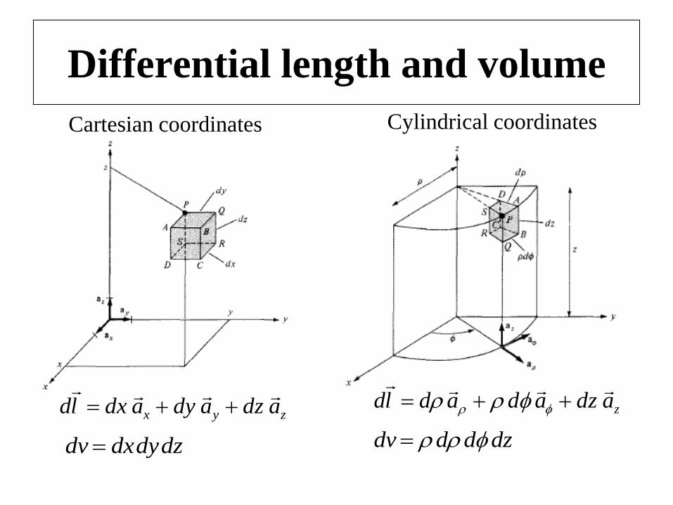
Differential length and volume
dzdddv
Cylindrical coordinates Cartesian coordinates
zyx adzadyadxld
dzdydxdv
zadzadadld
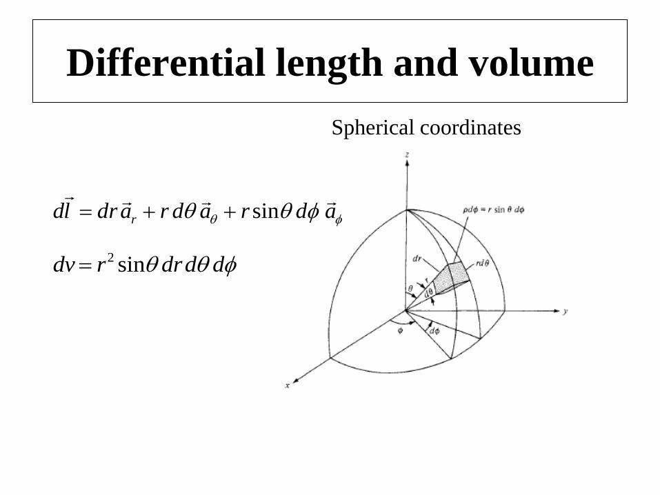
Differential length and volume
Spherical coordinates
adradradrld r
sin
dddrrdv sin2
Exercise 1-1
Given point P(-2, 6, 3) and vector
a) Express P and A in cylindrical and spherical coordinates.
b) Evaluate A at P in the Cartesian, cylindrical, and spherical systems.
yx azxayA
Chapter 2
Some Methods in the
Calculus of Variations
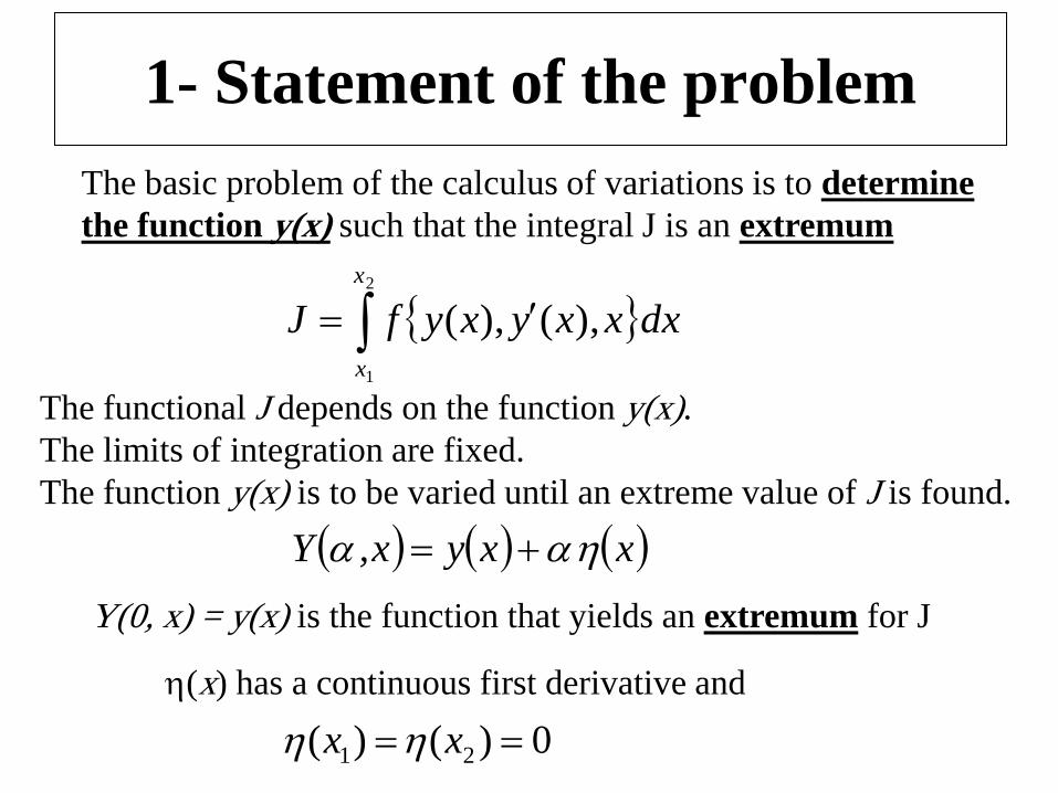
1- Statement of the problem
The basic problem of the calculus of variations is to determine
the function y(x) such that the integral J is an extremum
2
1
),(),(
x
x
dxxxyxyfJ
The functional J depends on the function y(x).
The limits of integration are fixed.
The function y(x) is to be varied until an extreme value of J is found.
xxyx,Y
Y(0, x) = y(x) is the function that yields an extremum for J
(x) has a continuous first derivative and
0)()( 21 xx
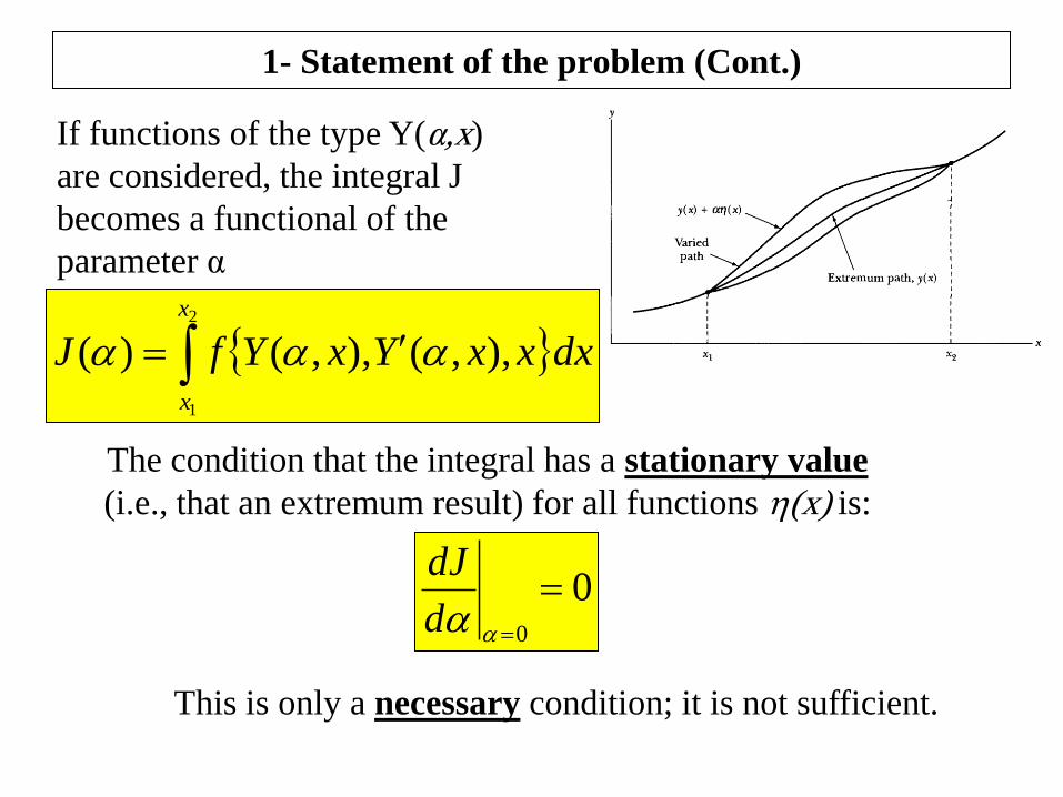
1- Statement of the problem (Cont.)
2
1
),,(),,()(
x
x
dxxxYxYfJ
If functions of the type Y(α,x)
are considered, the integral J
becomes a functional of the
parameter α
The condition that the integral has a stationary value
(i.e., that an extremum result) for all functions (x) is:
00
d
dJ
This is only a necessary condition; it is not sufficient.
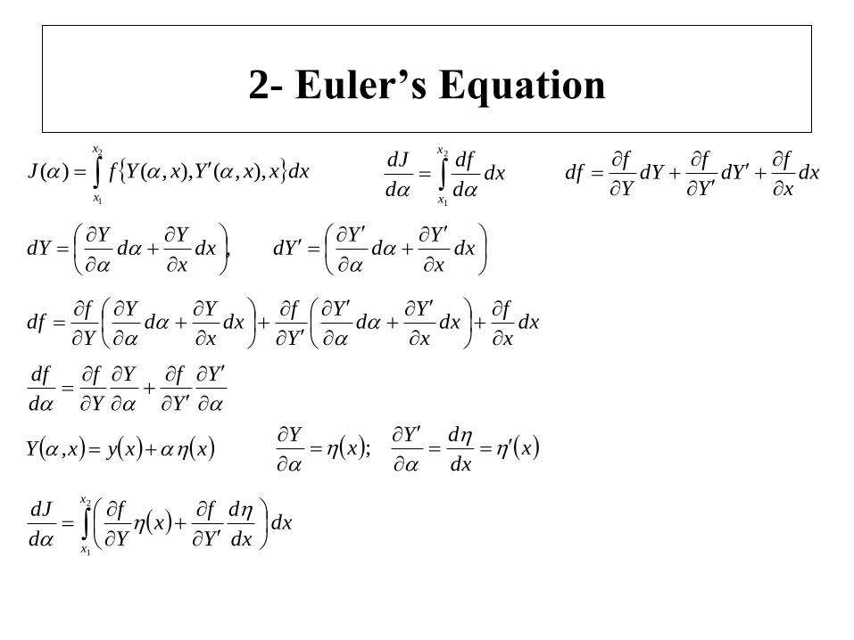
2- Euler’s Equation
2
1
),,(),,()(
x
x
dxxxYxYfJ 2
1
x
x
dxd
df
d
dJ
dx
x
fYd
Y
fdY
Y
fdf
dx
x
Yd
YYddx
x
Yd
YdY
,
dxx
fdx
x
Yd
Y
Y
fdx
x
Yd
Y
Y
fdf
Y
Y
fY
Y
f
d
df
xdx
dYx
Y
; xxyx,Y
dxdx
d
Y
fx
Y
f
d
dJx
x
2
1
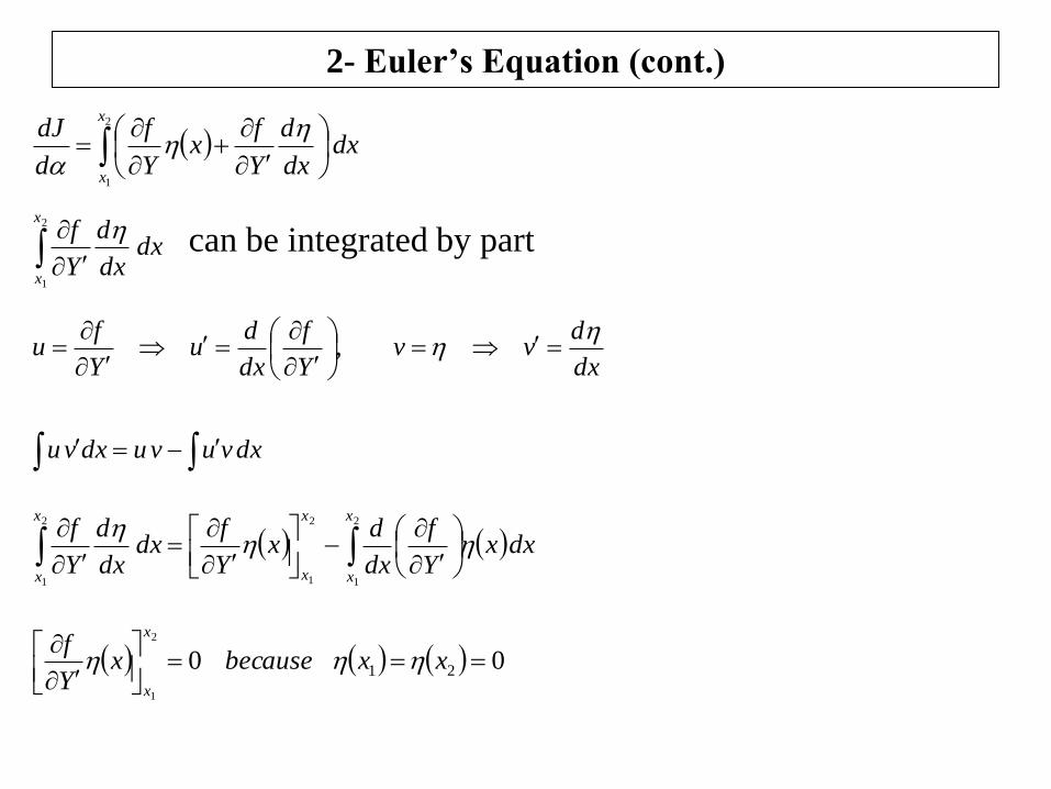
2- Euler’s Equation (cont.)
dxdx
d
Y
fx
x
2
1
can be integrated by part
dxdx
d
Y
fx
Y
f
d
dJx
x
2
1
dx
dvv
Y
f
dx
du
Y
fu
,
dxvuvudxvu
dxxY
f
dx
dx
Y
fdx
dx
d
Y
fx
x
x
x
x
x
2
1
2
1
2
1
00 21
2
1
xxbecausex
Y
fx
x
2- Euler’s Equation (cont.)
dxxY
f
dx
d
Y
fdxx
Y
f
dx
dx
Y
f
d
dJx
x
x
x
2
1
2
1
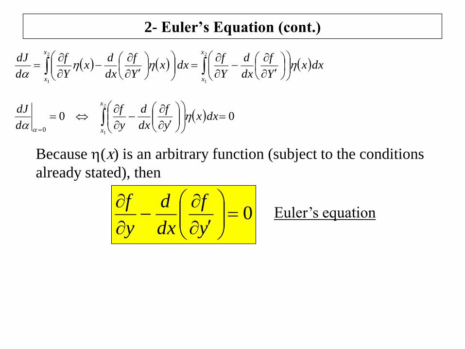
002
10
dxxy
f
dx
d
y
f
d
dJx
x
Because (x) is an arbitrary function (subject to the conditions
already stated), then
0
y
f
dx
d
y
fEuler’s equation
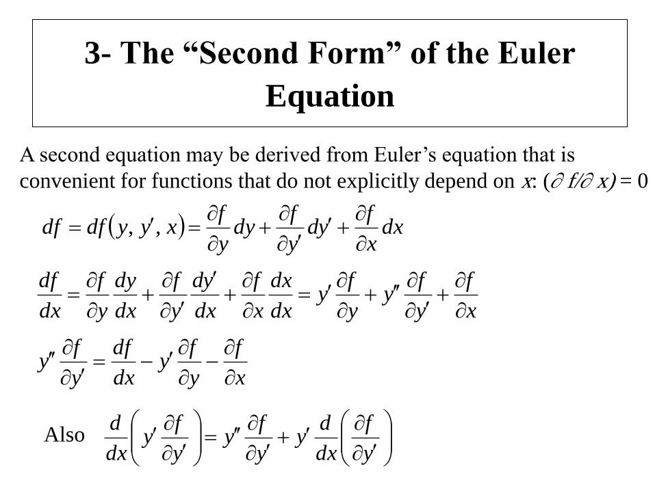
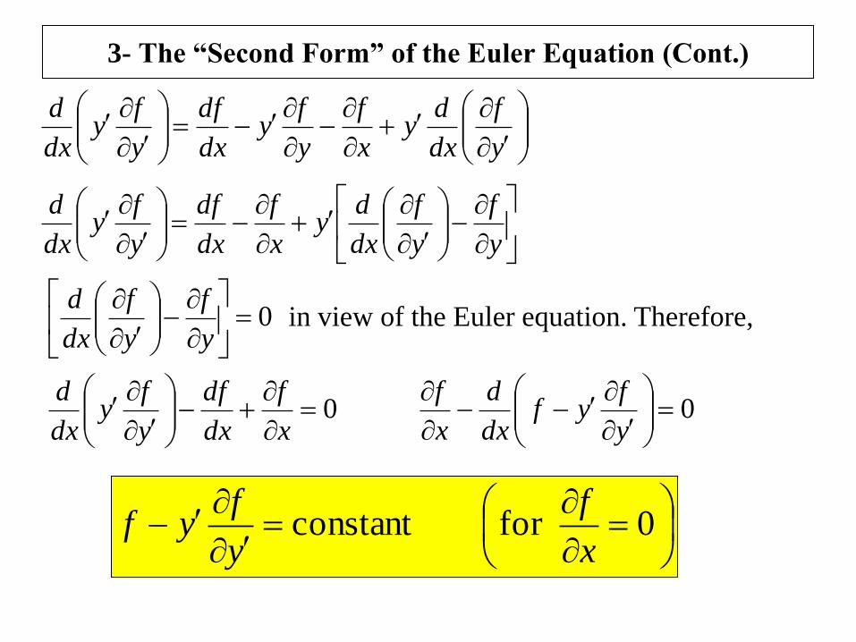
3- The “Second Form” of the Euler
Equation
A second equation may be derived from Euler’s equation that is
convenient for functions that do not explicitly depend on x: ( f/ x) = 0
dxx
fyd
y
fdy
y
fxyydfdf
,,
x
f
y
fy
y
fy
dx
dx
x
f
dx
yd
y
f
dx
dy
y
f
dx
df
x
f
y
fy
dx
df
y
fy
y
f
dx
dy
y
fy
y
fy
dx
dAlso
3- The “Second Form” of the Euler Equation (Cont.)
y
f
dx
dy
x
f
y
fy
dx
df
y
fy
dx
d
y
f
y
f
dx
dy
x
f
dx
df
y
fy
dx
d
0
y
f
y
f
dx
din view of the Euler equation. Therefore,
0
x
f
dx
df
y
fy
dx
d0
y
fyf
dx
d
x
f
0for constant
x
f
y
fyf
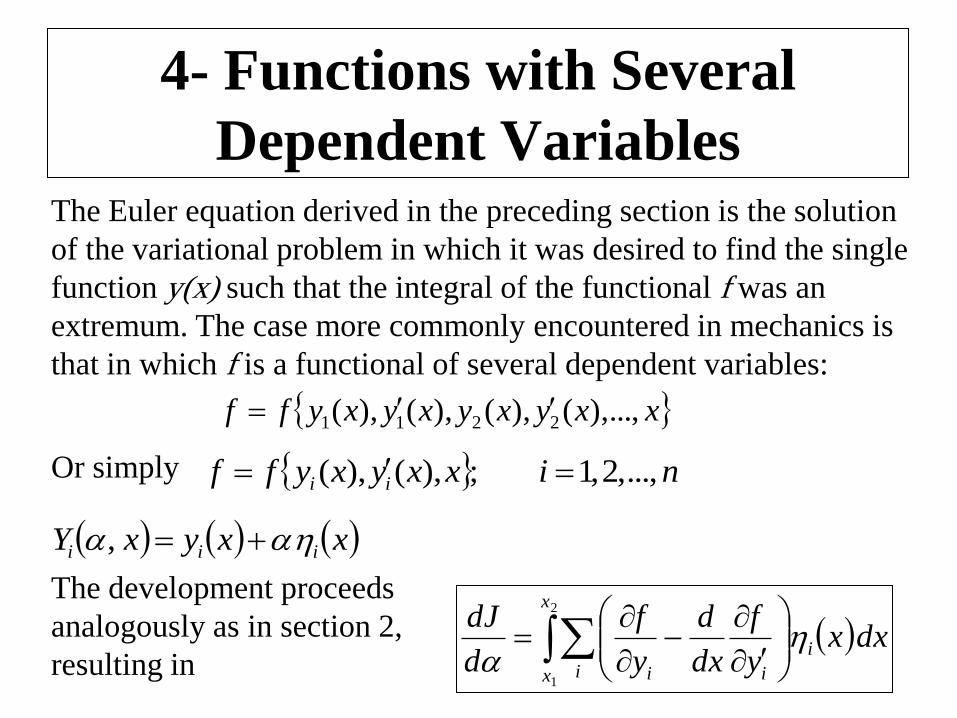
4- Functions with Several
Dependent Variables The Euler equation derived in the preceding section is the solution
of the variational problem in which it was desired to find the single
function y(x) such that the integral of the functional f was an
extremum. The case more commonly encountered in mechanics is
that in which f is a functional of several dependent variables:
xxyxyxyxyff ...,),(),(),(),( 2211
nixxyxyff ii ...,,2,1;),(),( Or simply
xxyxY iii ,
dxxy
f
dx
d
y
f
d
dJi
x
x i ii
2
1
The development proceeds
analogously as in section 2,
resulting in
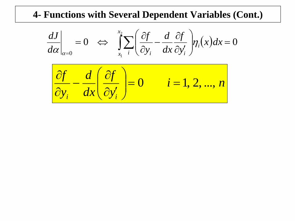
4- Functions with Several Dependent Variables (Cont.)
002
10
dxxy
f
dx
d
y
f
d
dJi
x
x i ii
niy
f
dx
d
y
f
ii
...,,2,10
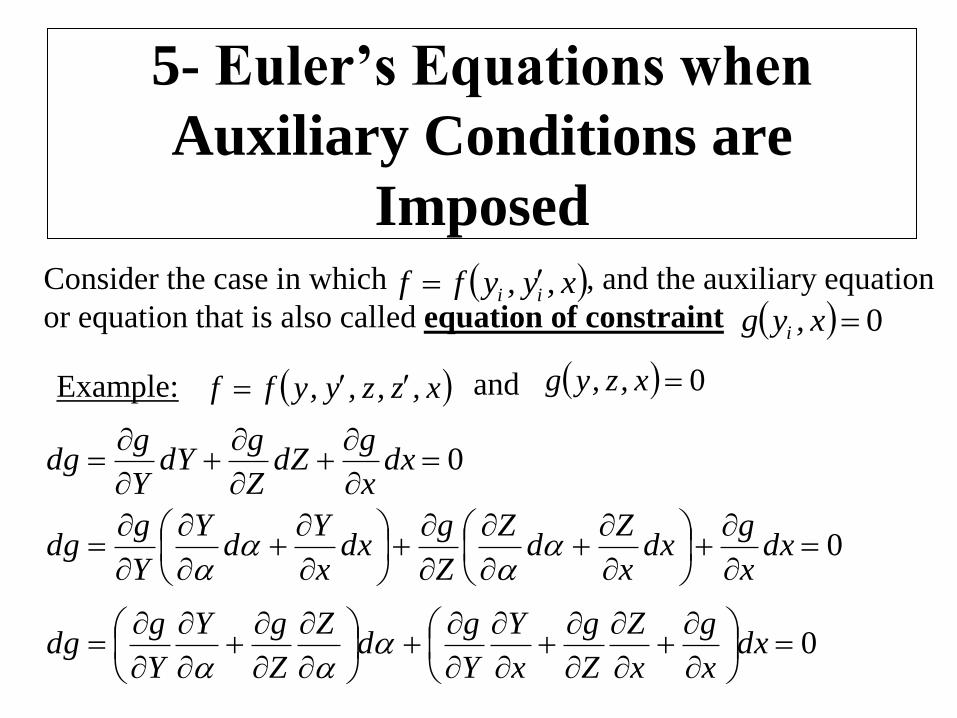
5- Euler’s Equations when
Auxiliary Conditions are
Imposed
Consider the case in which , and the auxiliary equation
or equation that is also called equation of constraint x,y,yff ii
0x,yg i
Example: x,z,z,y,yff 0x,z,ygand
0
dx
x
gdZ
Z
gdY
Y
gdg
0
dx
x
gdx
x
Zd
Z
Z
gdx
x
Yd
Y
Y
gdg
0
dx
x
g
x
Z
Z
g
x
Y
Y
gd
Z
Z
gY
Y
gdg
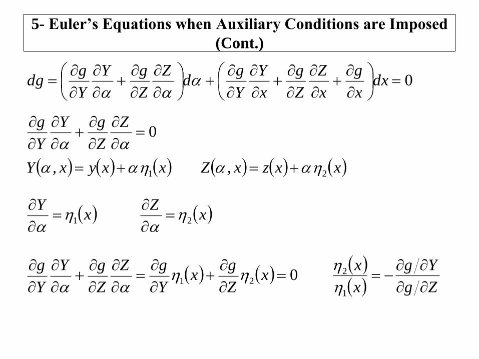
5- Euler’s Equations when Auxiliary Conditions are Imposed
(Cont.)
0
dx
x
g
x
Z
Z
g
x
Y
Y
gd
Z
Z
gY
Y
gdg
0
Z
Z
gY
Y
g
xxyx,Y 1 xxzx,Z 2
xY
1
x
Z2
021
x
Z
gx
Y
gZ
Z
gY
Y
g
Zg
Yg
x
x
1
2
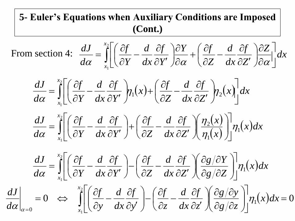
5- Euler’s Equations when Auxiliary Conditions are Imposed
(Cont.)
From section 4:
2
1
x
x
dxZ
Z
f
dx
d
Z
fY
Y
f
dx
d
Y
f
d
dJ
2
1
21
x
x
dxxZ
f
dx
d
Z
fx
Y
f
dx
d
Y
f
d
dJ
2
1
1
1
2
x
x
dxxx
x
Z
f
dx
d
Z
f
Y
f
dx
d
Y
f
d
dJ
2
1
1
x
x
dxxZg
Yg
Z
f
dx
d
Z
f
Y
f
dx
d
Y
f
d
dJ
002
1
1
0
x
x
dxxzg
yg
z
f
dx
d
z
f
y
f
dx
d
y
f
d
dJ
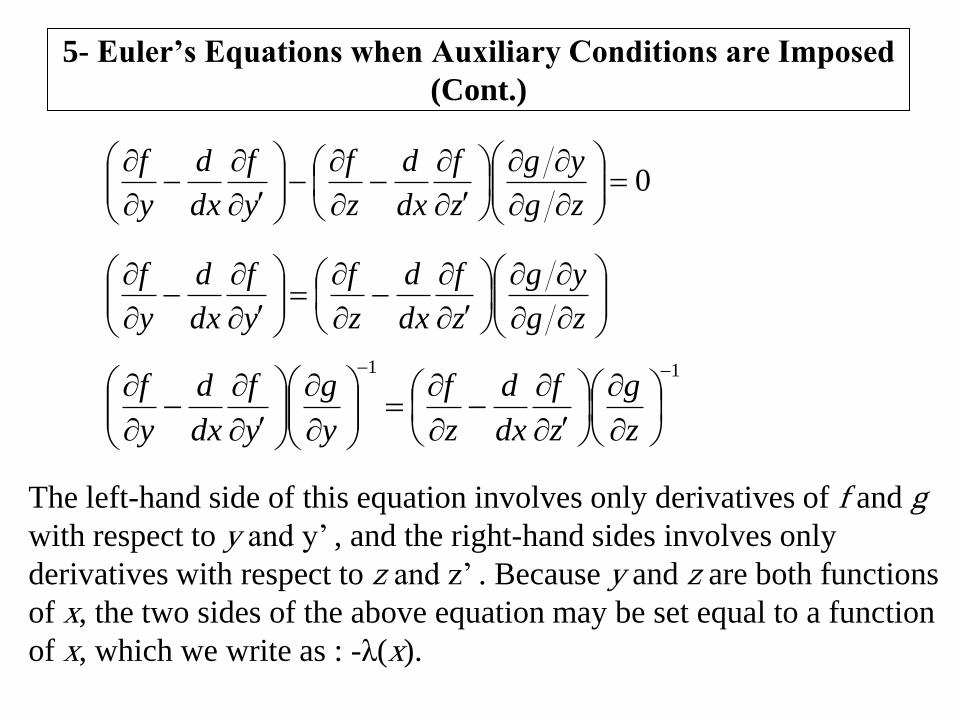
5- Euler’s Equations when Auxiliary Conditions are Imposed
(Cont.)
0
zg
yg
z
f
dx
d
z
f
y
f
dx
d
y
f
zg
yg
z
f
dx
d
z
f
y
f
dx
d
y
f
11
z
g
z
f
dx
d
z
f
y
g
y
f
dx
d
y
f
The left-hand side of this equation involves only derivatives of f and g
with respect to y and y’ , and the right-hand sides involves only
derivatives with respect to z and z’ . Because y and z are both functions
of x, the two sides of the above equation may be set equal to a function
of x, which we write as : -λ(x).
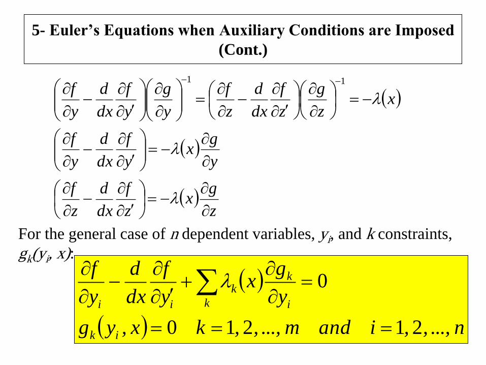
5- Euler’s Equations when Auxiliary Conditions are Imposed
(Cont.)
xz
g
z
f
dx
d
z
f
y
g
y
f
dx
d
y
f
11
z
gx
z
f
dx
d
z
f
y
gx
y
f
dx
d
y
f
For the general case of n dependent variables, yi, and k constraints,
gk(yi, x):
n...,,,iandm...,,,kx,yg
y
gx
y
f
dx
d
y
f
ik
k i
kk
ii
21210
0
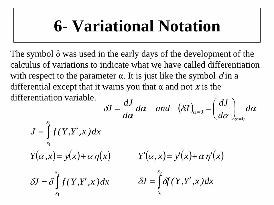
6- Variational Notation
dd
dJJandd
d
dJJ
0
0
dx)x,Y,Y(fJ
x
x
2
1
xxyx,Y xxyxY ,
dx)x,Y,Y(fJ
x
x
2
1
dx)x,Y,Y(fJ
x
x
2
1
The symbol δ was used in the early days of the development of the
calculus of variations to indicate what we have called differentiation
with respect to the parameter α. It is just like the symbol d in a
differential except that it warns you that α and not x is the
differentiation variable.
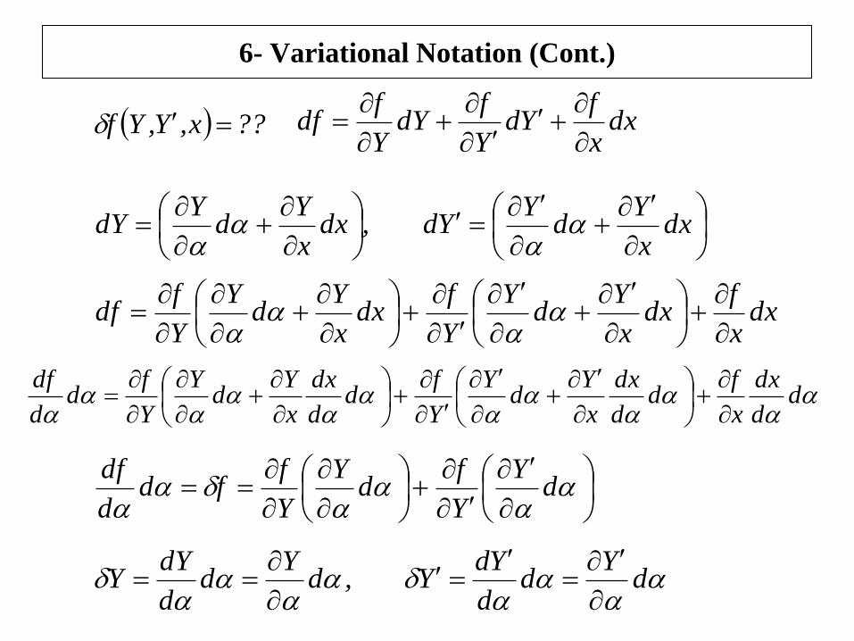
6- Variational Notation (Cont.)
??x,Y,Yf dxx
fYd
Y
fdY
Y
fdf
dx
x
Yd
YYd,dx
x
Yd
YdY
dxx
fdx
x
Yd
Y
Y
fdx
x
Yd
Y
Y
fdf
dd
dx
x
fd
d
dx
x
Yd
Y
Y
fd
d
dx
x
Yd
Y
Y
fd
d
df
d
Y
Y
fd
Y
Y
ffd
d
df
dY
dd
YdY,d
Yd
d
dYY
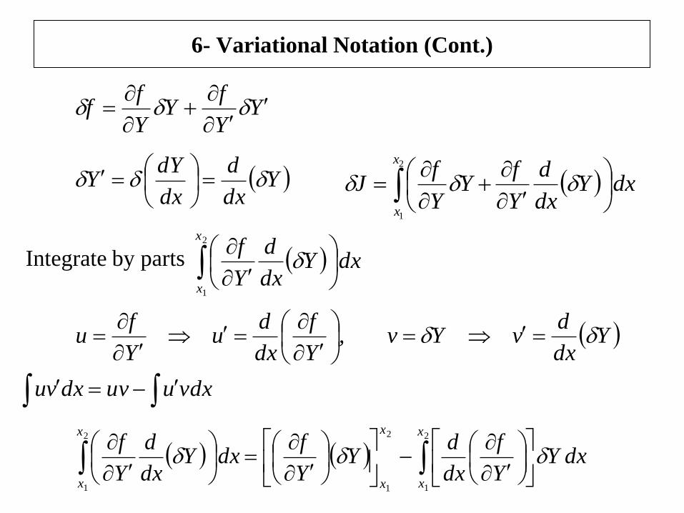
6- Variational Notation (Cont.)
YY
fY
Y
ff
Ydx
d
dx
dYY
dxY
dx
d
Y
fY
Y
fJ
x
x
2
1
Integrate by parts dxYdx
d
Y
fx
x
2
1
Ydx
dvYv,
Y
f
dx
du
Y
fu
vdxuuvdxvu
dxYY
f
dx
dY
Y
fdxY
dx
d
Y
fx
x
x
x
x
x
2
1
2
1
2
1
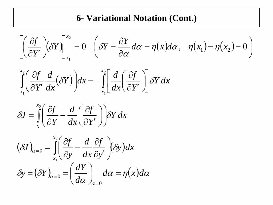
6- Variational Notation (Cont.)
00 21
2
1
xx,dxdY
YYY
fx
x
dxYY
f
dx
ddxY
dx
d
Y
fx
x
x
x
2
1
2
1
dxYY
f
dx
d
Y
fJ
x
x
2
1
2
1
0
x
x
dxyy
f
dx
d
y
fJ
dxdd
dYYy
0
0
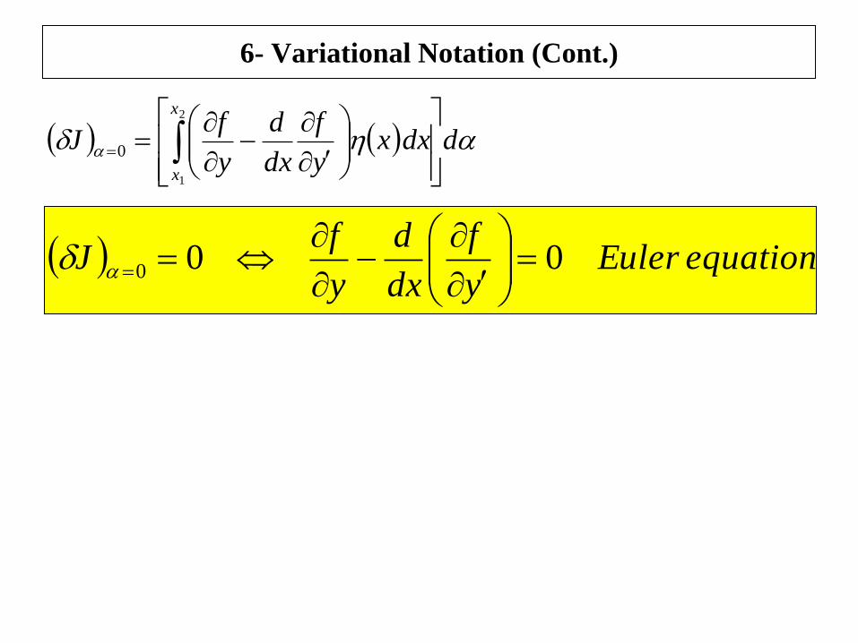
6- Variational Notation (Cont.)
ddxxy
f
dx
d
y
fJ
x
x
2
1
0
equation Eulery
f
dx
d
y
fJ 000
Chapter 3
Hamilton’s Principle
Lagrangian and Hamiltonian
Dynamics
Dr. Abdelaziz Sabik
Physics Department – College of Sciences
Al-Imam Muhammad Ibn Saud Islamic University
1- Introduction
A particle’s motion in an inertial reference frame is correctly
described by the Newtonian second law equation:
amF
where F is the total force acting on the body.
In particular complicated problems, this equation can become
difficult to manipulate.
An alternate method of dealing with complicated problems is
contained in Hamilton’s Principle, and the equations of motion
resulting from the application of this principle are called
Lagrange’s equations.
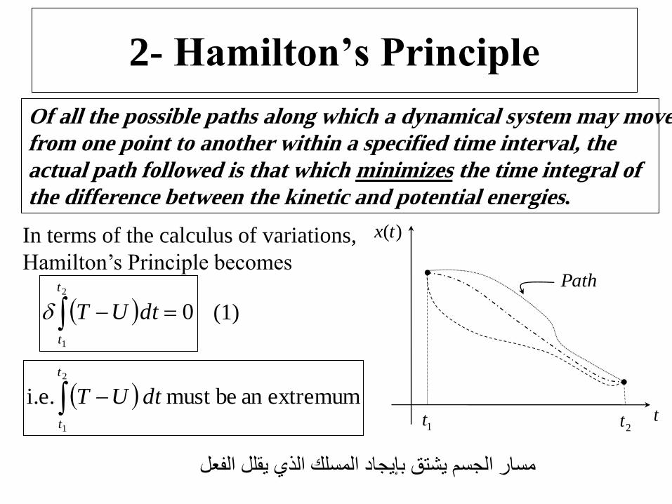
2- Hamilton’s Principle
Of all the possible paths along which a dynamical system may move
from one point to another within a specified time interval, the
actual path followed is that which minimizes the time integral of
the difference between the kinetic and potential energies.
In terms of the calculus of variations,
Hamilton’s Principle becomes
2
1
0
t
t
dtUT
extremuman bemust i.e.2
1
t
t
dtUT
(1)
1t 2tt
)(tx
Path
مسار الجسم يشتق بإيجاد المسلك الذي يقلل الفعل
2- Hamilton’s Principle
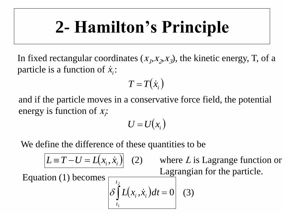
In fixed rectangular coordinates (x1,x2,x3), the kinetic energy, T, of a
particle is a function of :
ixTT
and if the particle moves in a conservative force field, the potential
energy is function of xi:
ix
ixUU
We define the difference of these quantities to be
ii xxLUTL , (2) where L is Lagrange function or
Lagrangian for the particle. Equation (1) becomes
2
1
0
t
t
ii dtx,xL (3)
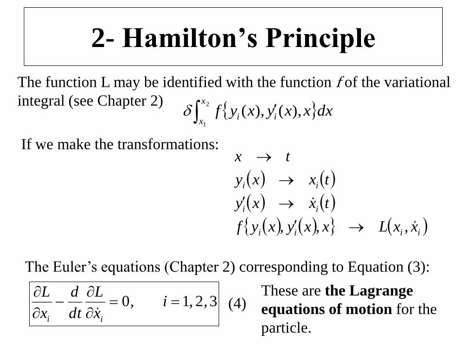
2- Hamilton’s Principle
The function L may be identified with the function f of the variational
integral (see Chapter 2) dxxxyxyf
x
xii
2
1
),(),(
If we make the transformations:
iiii
ii
ii
xxLxxyxyf
txxy
txxy
tx
,,,
The Euler’s equations (Chapter 2) corresponding to Equation (3):
3210 ,,i,x
L
dt
d
x
L
ii
(4)
These are the Lagrange
equations of motion for the
particle.
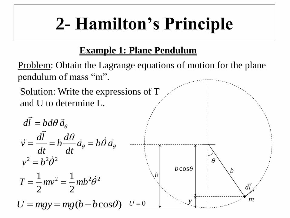
2- Hamilton’s Principle
Example 1: Plane Pendulum
Problem: Obtain the Lagrange equations of motion for the plane
pendulum of mass “m”.
b
m0U
b
y
cosb
ld
abdld
Solution: Write the expressions of T
and U to determine L.
abadt
db
dt
ldv
222 bv
222
2
1
2
1mbmvT
)cos( bbmgmgyU
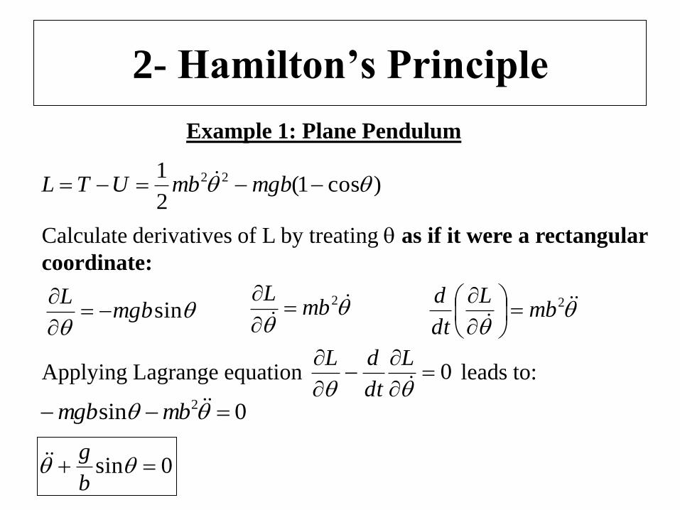
2- Hamilton’s Principle
Example 1: Plane Pendulum
)cos1(2
1 22 mgbmbUTL
sinmgbL
2mb
L
2mb
L
dt
d
0
L
dt
dLApplying Lagrange equation leads to:
Calculate derivatives of L by treating as if it were a rectangular
coordinate:
0sin 2 mbmgb
0sin b
g
b
m
T
gm
x
y
xa
ya
2- Hamilton’s Principle
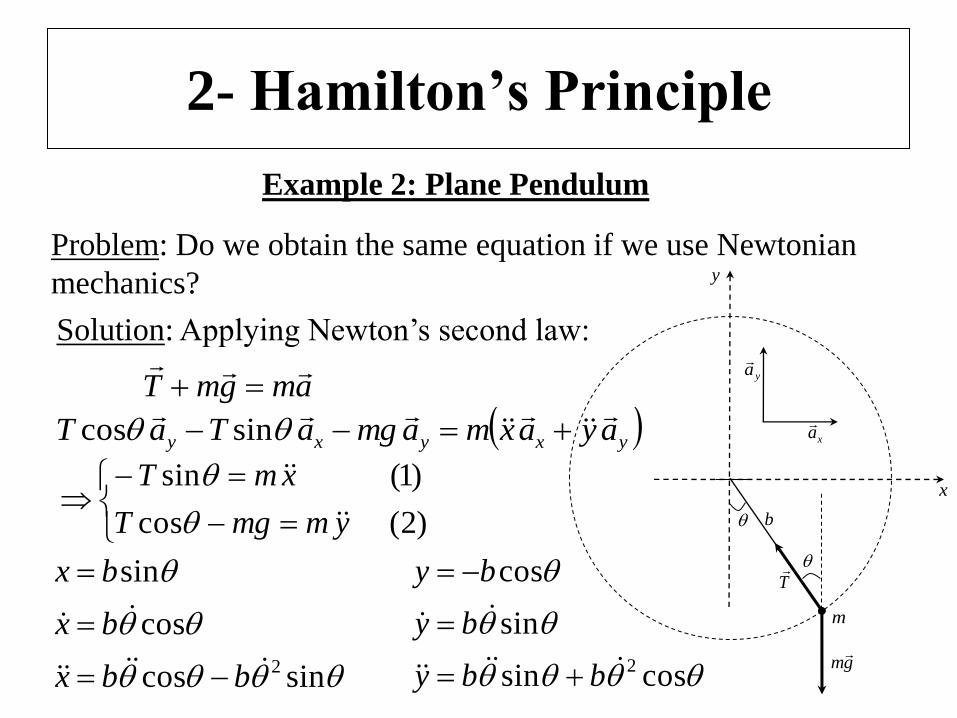
Example 2: Plane Pendulum
Problem: Do we obtain the same equation if we use Newtonian
mechanics?
Solution: Applying Newton’s second law:
amgmT
yxyxy ayaxmamgaTaT
sincos
)2(cos
)1(sin
ymmgT
xmT
sincos
cos
sin
2
bbx
bx
bx
cossin
sin
cos
2
bby
by
by
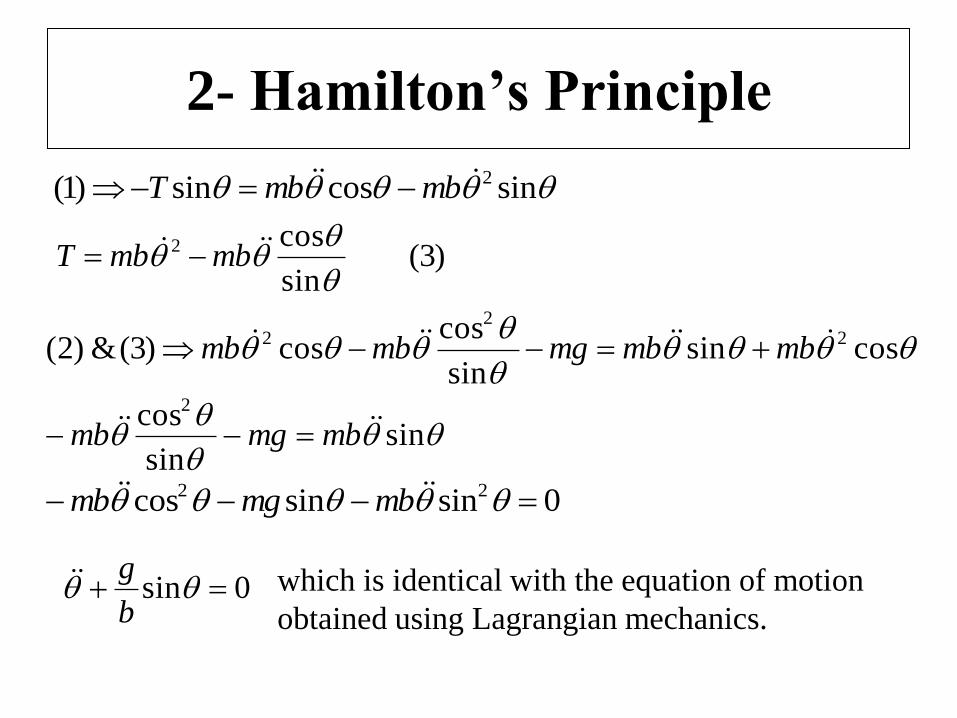
2- Hamilton’s Principle
sincossin)1( 2 mbmbT
)3(sin
cos2
mbmbT
cossin
sin
coscos)3(&)2( 2
22 mbmbmgmbmb
sin
sin
cos2
mbmgmb
0sinsincos 22 mbmgmb
0sin b
g which is identical with the equation of motion
obtained using Lagrangian mechanics.
2- Hamilton’s Principle
Remarks regarding Example 1 (Lagrangian mechanics)
1- Example 1 has been solved by calculating the kinetic and
potential energies in terms of rather than x and then applying a set of
operations designed for use with rectangular rather than angular
coordinates.
2- No-where in calculations did there any statement regarding force.
3- Hamilton’s Principle allows us to calculate the equations of motion
of a body completely without recourse to Newtonian theory.
3- Generalized Coordinates
• Consider mechanical systems consisting of a collection of n
discrete point particles.
• We need n position vectors, i.e. 3n quantities must be specified
to describe the positions of all the particles.
• If there are m constraint equations that limit the motion of particle
by for instance relating some of coordinates, then the number of
independent coordinates is limited to 3n-m.
• One then describes the system as having s = 3n-m degrees of
freedom.
3- Generalized Coordinates
• If s=3n-m coordinates are required to describe a system, it is NOT
necessary these s coordinates be rectangular or curvilinear coordinates.
• One can choose any combination of independent coordinates as long
as they completely specify the system.
• These coordinates need not even have the dimension of length
(e.g. θ in our previous example).
• We use the term generalized coordinates to describe any set of
coordinates that completely specify the state of a system.
• Generalized coordinates will be noted: q1, q2, …, or simply as the qj.
3- Generalized Coordinates
• In some cases, it may be useful to use generalized coordinates
whose number exceeds the number of degrees of freedom, and
to explicitly take into account the constraint relations through the
use of the Lagrange Undetermined multipliers. Such would be the
case, for example, if we desired to calculate the forces of constraint.
• The choice of a set of generalized coordinates is obviously not
unique. We choose the set that gives the simplest equations of
motion.
• In addition to the generalized coordinates, we may define a set of
quantities consisting of the time derivatives of or
simply . We call generalized velocities. jq...,,,: 21 qqq j
jq
3- Generalized Coordinates
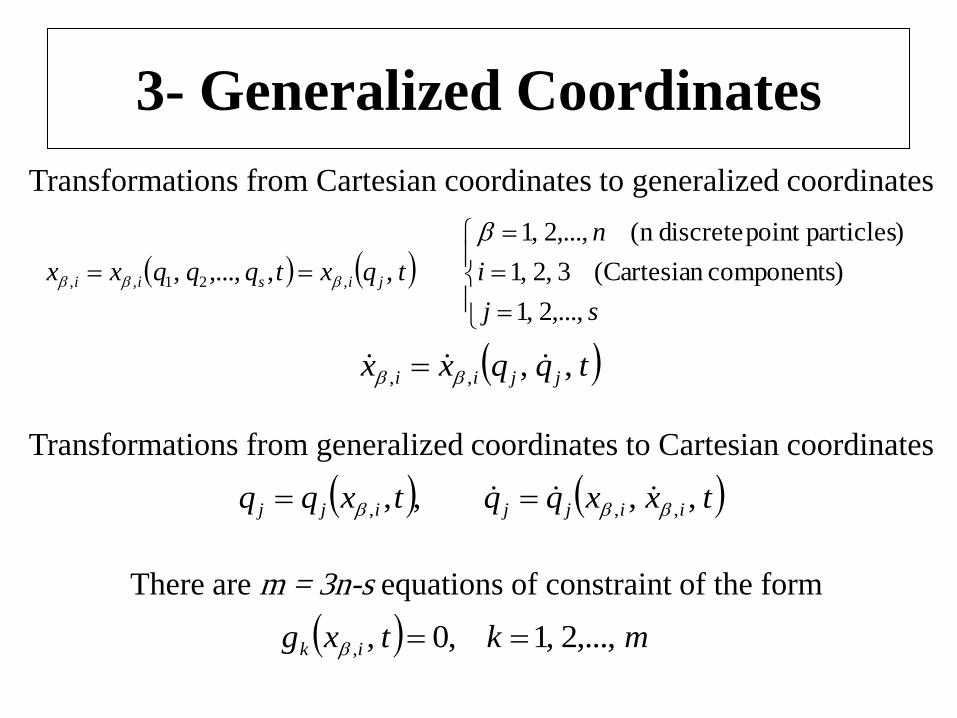
Transformations from Cartesian coordinates to generalized coordinates
sj
i
n
tqxtqqqxx jisii
,...,2,1
)components (Cartesian3,2,1
)particlespoint discreten (,...,2,1
,,,...,, ,21,,
tqqxx jjii ,,,,
Transformations from generalized coordinates to Cartesian coordinates
txxqqtxqq iijjijj ,,,, ,,,
There are m = 3n-s equations of constraint of the form
mktxg ik ,...,2,1,0,,
4- Lagrange’s Equations of Motion in
Generalized Coordinates
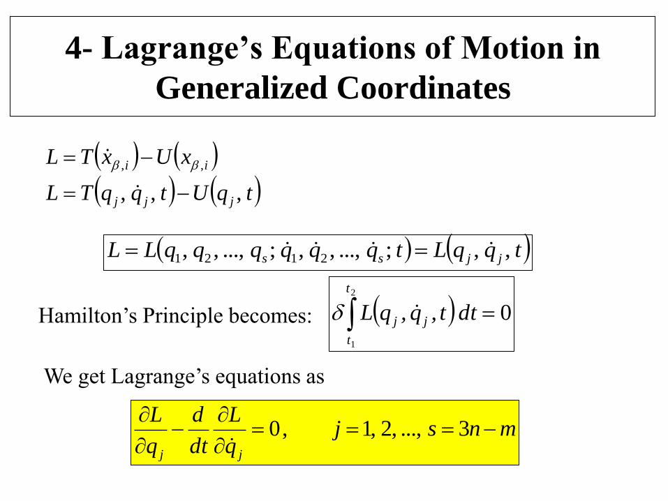
tqUtqqTL
xUxTL
jjj
ii
,,,
,,
tqqLtqqqqqqLL jjss ,,;...,,,;...,,, 2121
Hamilton’s Principle becomes: 02
1
dtt,q,qL
t
t
jj
We get Lagrange’s equations as
mnsjq
L
dt
d
q
L
jj
3...,,2,1,0
4- Lagrange’s Equations of Motion
in Generalized Coordinates
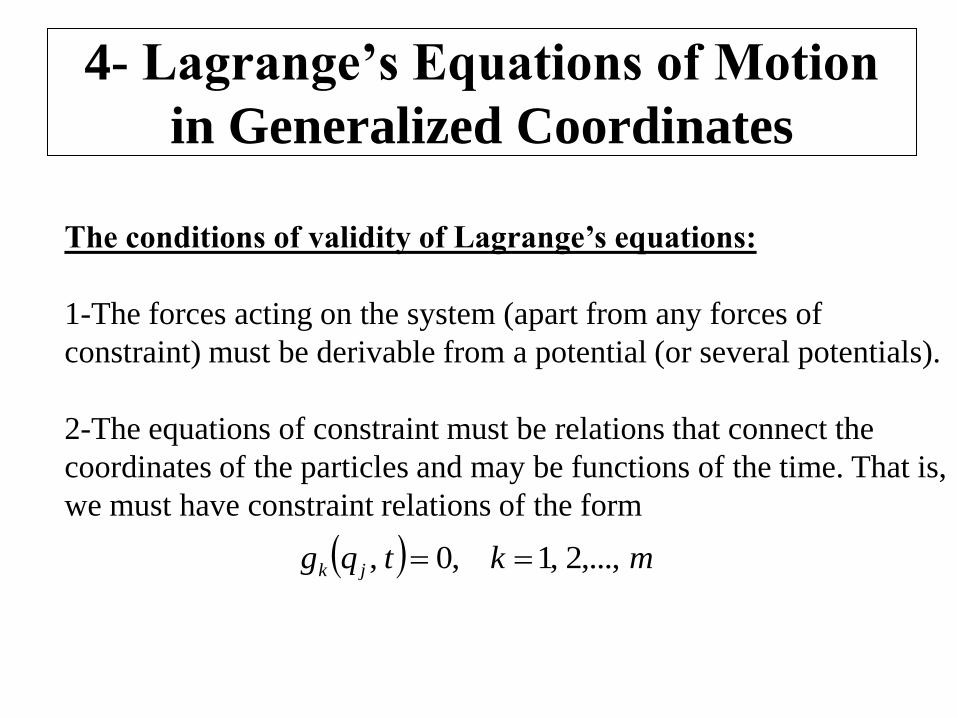
The conditions of validity of Lagrange’s equations:
1-The forces acting on the system (apart from any forces of
constraint) must be derivable from a potential (or several potentials).
2-The equations of constraint must be relations that connect the
coordinates of the particles and may be functions of the time. That is,
we must have constraint relations of the form
mktqg jk ,...,2,1,0,
4- Lagrange’s Equations of Motion in
Generalized Coordinates – Example 2
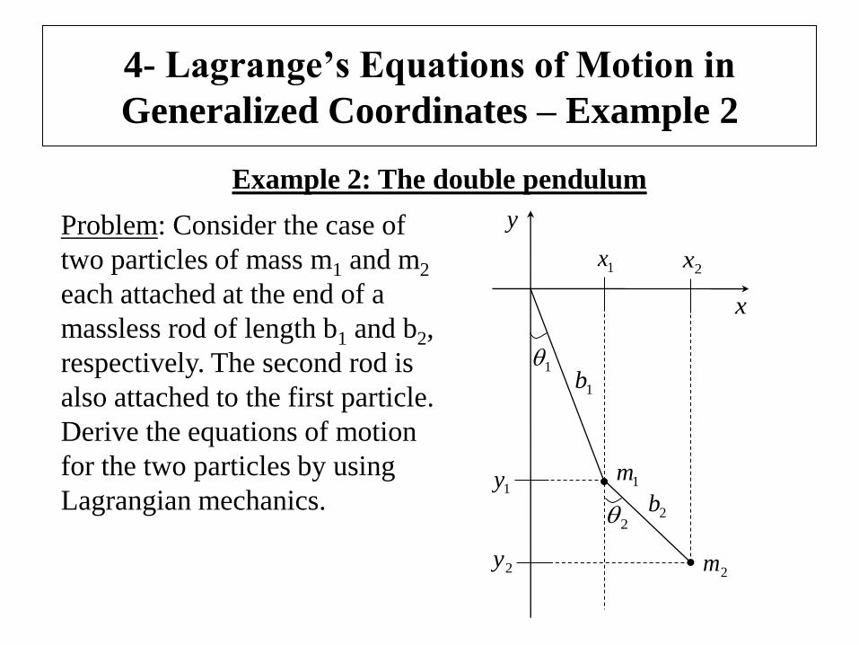
Example 2: The double pendulum
Problem: Consider the case of
two particles of mass m1 and m2
each attached at the end of a
massless rod of length b1 and b2,
respectively. The second rod is
also attached to the first particle.
Derive the equations of motion
for the two particles by using
Lagrangian mechanics.
1
2
1b
2b1m
2m
1x2x
1y
2y
x
y
4- Lagrange’s Equations of Motion in
Generalized Coordinates – Example 2
1
2
1b
2b1m
2m
1x2x
1y
2y
x
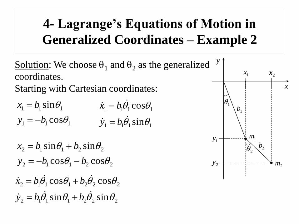
ySolution: We choose 1 and 2 as the generalized
coordinates.
Starting with Cartesian coordinates:
111
111
cos
sin
by
bx
22112
22112
coscos
sinsin
bby
bbx
1111
1111
sin
cos
by
bx
2221112
2221112
sinsin
coscos
bby
bbx
4- Lagrange’s Equations of Motion in
Generalized Coordinates – Example 2
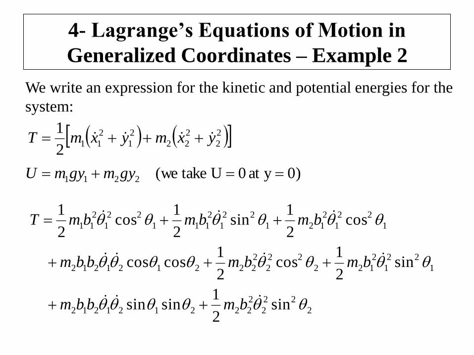
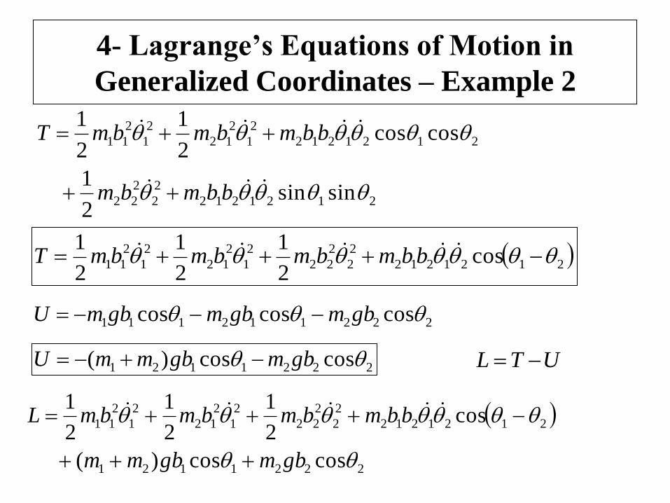
We write an expression for the kinetic and potential energies for the
system:
2
2
2
22
2
1
2
112
1yxmyxmT
0)yat 0 U take(we2211 gymgymU
2
22
2
2
222121212
1
22
1
2
122
22
2
2
222121212
1
22
1
2
121
22
1
2
111
22
1
2
11
sin2
1sinsin
sin2
1cos
2
1coscos
cos2
1sin
2
1cos
2
1
bmbbm
bmbmbbm
bmbmbmT
4- Lagrange’s Equations of Motion in
Generalized Coordinates – Example 2
2121212
2
2
2
22
2121212
2
1
2
12
2
1
2
11
sinsin2
1
coscos2
1
2
1
bbmbm
bbmbmbmT
2121212
2
2
2
22
2
1
2
12
2
1
2
11 cos2
1
2
1
2
1 bbmbmbmbmT
222112111 coscoscos gbmgbmgbmU
2221121 coscos)( gbmgbmmU UTL
2221121
2121212
2
2
2
22
2
1
2
12
2
1
2
11
coscos)(
cos2
1
2
1
2
1
gbmgbmm
bbmbmbmbmL
4- Lagrange’s Equations of Motion in
Generalized Coordinates – Example 2
2221121
2121212
2
2
2
22
2
1
2
12
2
1
2
11
coscos)(
cos2
1
2
1
2
1
gbmgbmm
bbmbmbmbmL
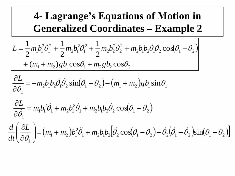
11212121212
1
sinsin
gbmmbbmL
2122121
2
121
2
11
1
cos
bbmbmbmL
212122122121
2
121
1
sincos
bbmbmmL
dt
d
4- Lagrange’s Equations of Motion in
Generalized Coordinates – Example 2
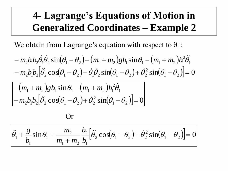
0sinsincos
sinsin
21
2
22121212212
1
2
12111212121212
bbm
bmmgbmmbbm
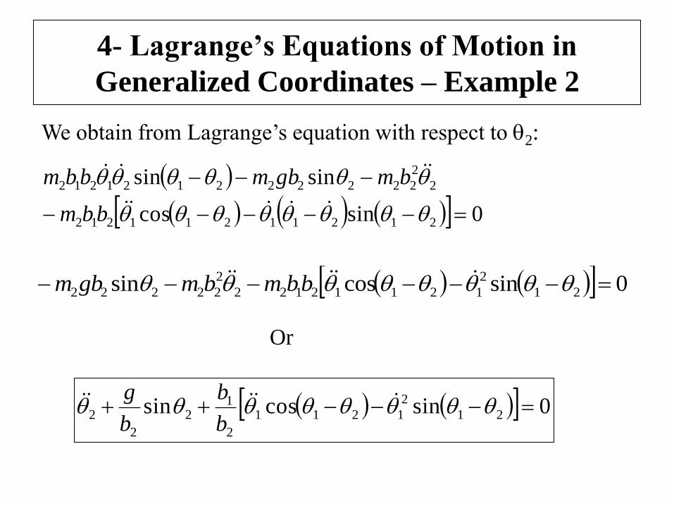
We obtain from Lagrange’s equation with respect to 1:
0sincos
sin
21
2
2212212
1
2
1211121
bbm
bmmgbmm
0sincossin 21
2
2212
1
2
21
21
1
1
b
b
mm
m
b
g
Or
4- Lagrange’s Equations of Motion in
Generalized Coordinates – Example 2
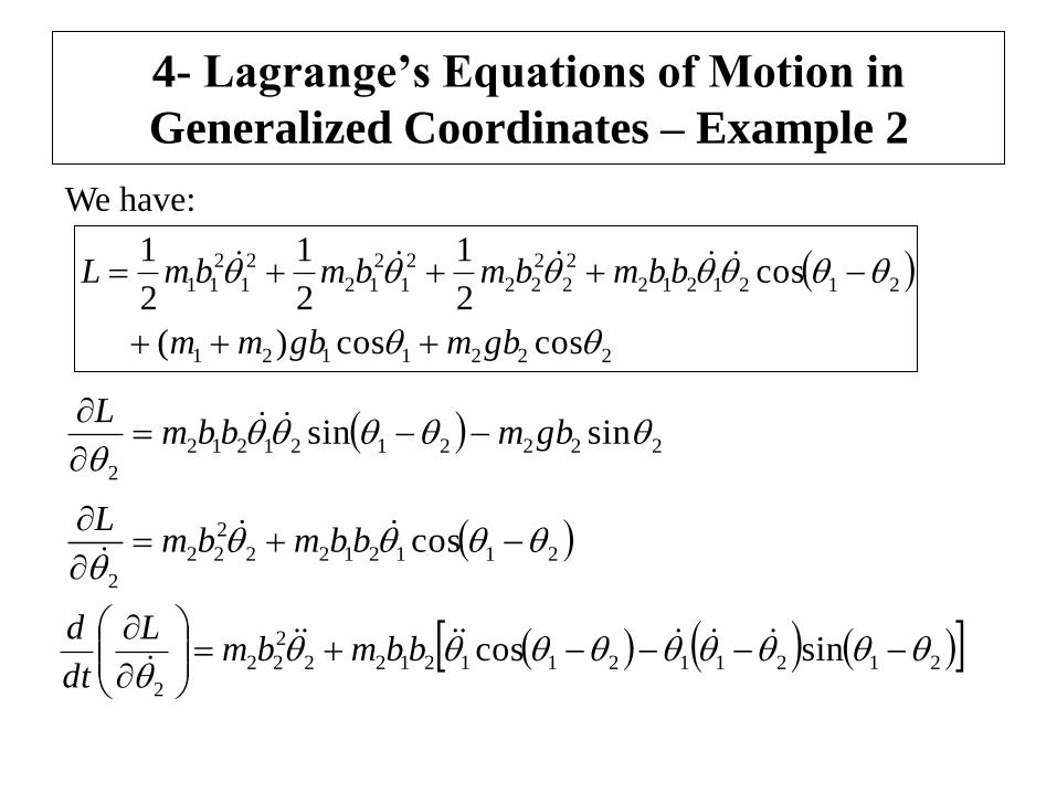
We have:
2221121
2121212
2
2
2
22
2
1
2
12
2
1
2
11
coscos)(
cos2
1
2
1
2
1
gbmgbmm
bbmbmbmbmL
2222121212
2
sinsin
gbmbbmL
2112122
2
22
2
cos
bbmbmL
212112112122
2
22
2
sincos
bbmbmL
dt
d
4- Lagrange’s Equations of Motion in
Generalized Coordinates – Example 2
We obtain from Lagrange’s equation with respect to 2:
0sincos
sinsin
21211211212
2
2
222222121212
bbm
bmgbmbbm
0sincossin 21
2
12112122
2
22222 bbmbmgbm
0sincossin 21
2
1211
2
12
2
2 b
b
b
g
Or
4- Lagrange’s Equations of Motion in
Generalized Coordinates – Example 3
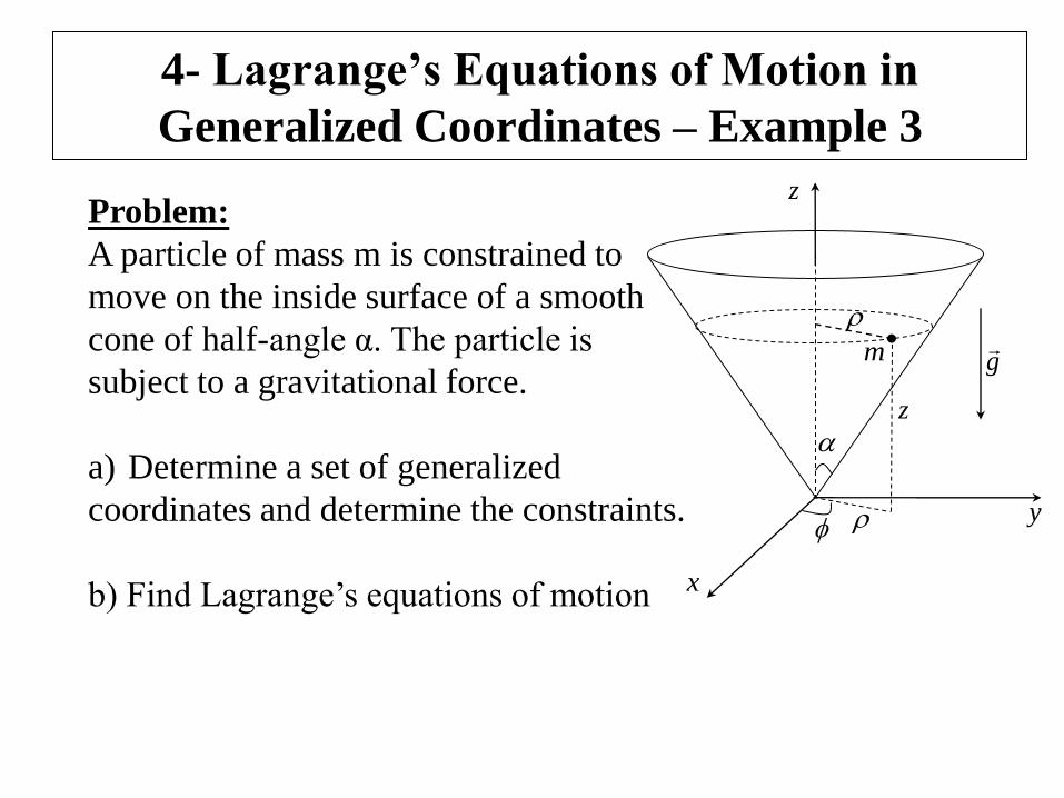
Problem:
A particle of mass m is constrained to
move on the inside surface of a smooth
cone of half-angle α. The particle is
subject to a gravitational force.
a) Determine a set of generalized
coordinates and determine the constraints.
b) Find Lagrange’s equations of motion
x
y
z
z
m g
4- Lagrange’s Equations of Motion in
Generalized Coordinates – Example 3
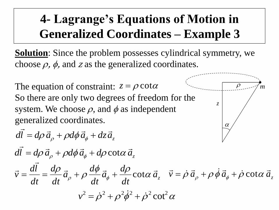
Solution: Since the problem possesses cylindrical symmetry, we
choose , , and z as the generalized coordinates.
The equation of constraint:
So there are only two degrees of freedom for the
system. We choose , and as independent
generalized coordinates.
cotz
z
m
zadzadadld
zadadadld
cot
zadt
da
dt
da
dt
d
dt
ldv
cot zaaav
cot
222222 cot v
4- Lagrange’s Equations of Motion in
Generalized Coordinates – Example 3
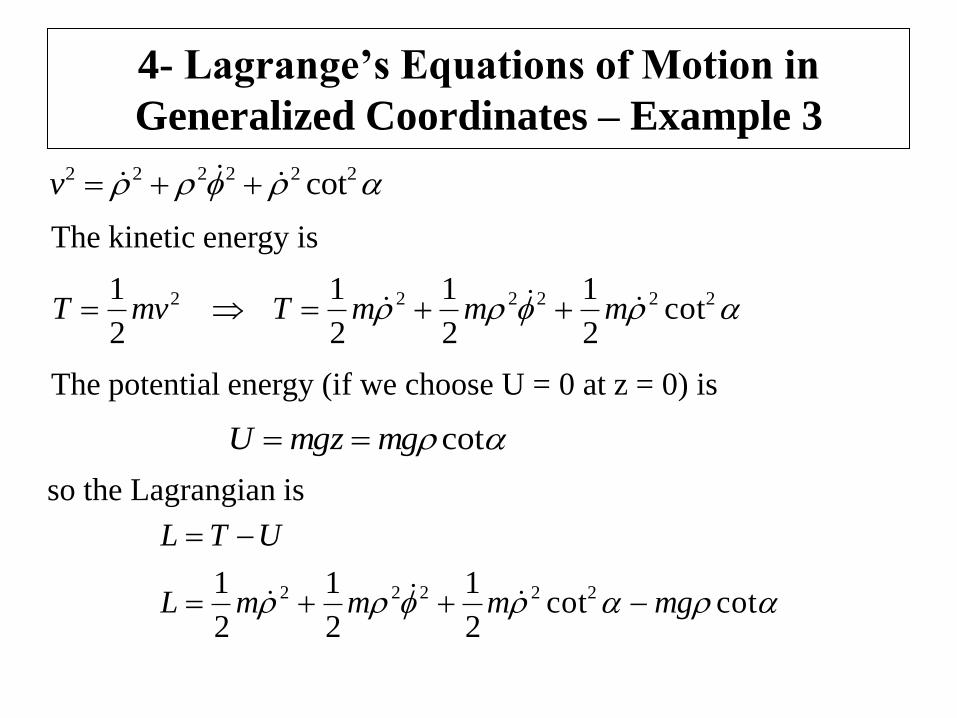
222222 cot v
222222 cot2
1
2
1
2
1
2
1 mmmTmvT
The kinetic energy is
The potential energy (if we choose U = 0 at z = 0) is
cotmgmgzU
so the Lagrangian is
cotcot2
1
2
1
2
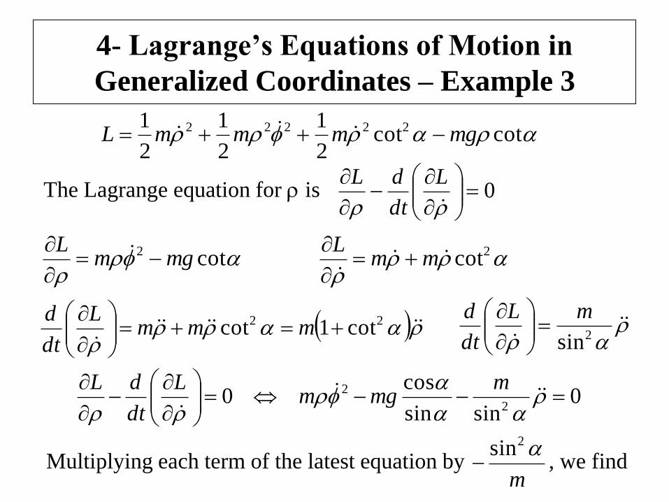
1 22222 mgmmmL
UTL
4- Lagrange’s Equations of Motion in
Generalized Coordinates – Example 3
cotcot2
1
2
1
2
1 22222 mgmmmL
The Lagrange equation for is 0
L
dt
dL
cot2 mgmL
2cot
mmL
22 cot1cot
mmm
L
dt
d
2sin
mL
dt
d
0sinsin
cos0
2
2
mmgm
L
dt
dL
Multiplying each term of the latest equation by , we find m
2sin
4- Lagrange’s Equations of Motion in
Generalized Coordinates – Example 3
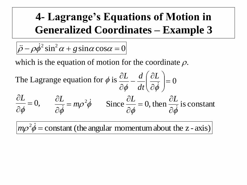
0cossinsin22 g
which is the equation of motion for the coordinate .
The Lagrange equation for is 0
L
dt
dL
,0
L
2m
L
constant is then ,0 Since
LL
axis)-z about the momentumangular (theconstant 2 m
4- Lagrange’s Equations of Motion in
Generalized Coordinates – Example 4
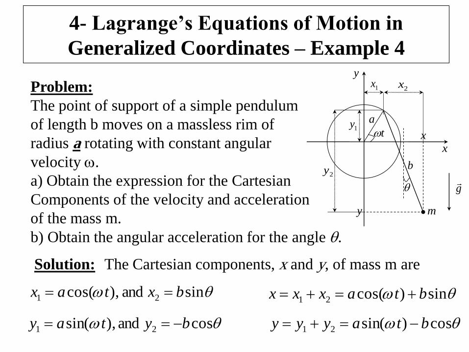
Problem:
The point of support of a simple pendulum
of length b moves on a massless rim of
radius a rotating with constant angular
velocity .
a) Obtain the expression for the Cartesian
Components of the velocity and acceleration
of the mass m.
b) Obtain the angular acceleration for the angle .
a
t
b
x
y
y
x
1x2x
1y
2y
g
m
Solution: The Cartesian components, x and y, of mass m are
sin)cos(21 btaxxx sin and),cos( 21 bxtax
cos and ),sin( 21 bytay cos)sin(21 btayyy
4- Lagrange’s Equations of Motion in
Generalized Coordinates – Example 4
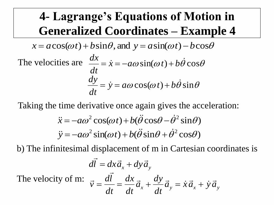
cos)sin( and ,sin)cos( btaybtax
The velocities are cos)sin( btaxdt
dx
sin)cos( btaydt
dy
Taking the time derivative once again gives the acceleration:
)sincos()cos( 22 btax
)cossin()sin( 22 btay
b) The infinitesimal displacement of m in Cartesian coordinates is
yx adyadxld
The velocity of m: yxyx ayaxa
dt
dya
dt
dx
dt
ldv
4- Lagrange’s Equations of Motion in
Generalized Coordinates – Example 4
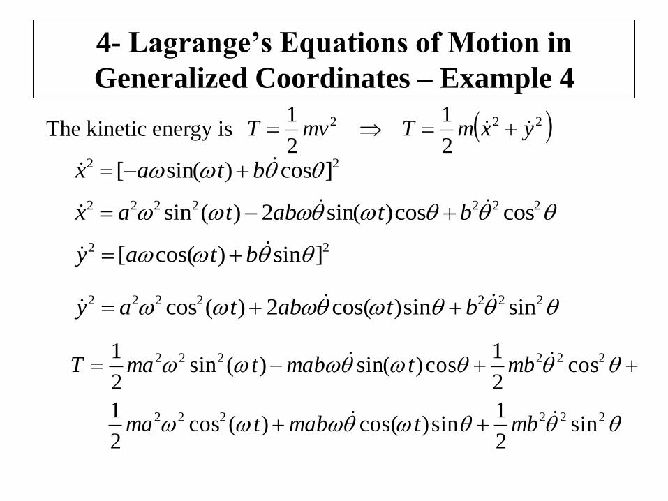
The kinetic energy is 222
2
1
2
1yxmTmvT
22 ]cos)sin([ btax
2222222 coscos)sin(2)(sin btabtax
22 ]sin)cos([ btay
2222222 sinsin)cos(2)(cos btabtay
222222
222222
sin2
1sin)cos()(cos
2
1
cos2
1cos)sin()(sin
2
1
mbtmabtma
mbtmabtmaT
4- Lagrange’s Equations of Motion in
Generalized Coordinates – Example 4
]sin[cos2
1]cos)sin(sin)[cos(
)](cos)([sin2
1
2222
2222
mbttmab
ttmaT
2222
2
1]cos)sin(sin)[cos(
2
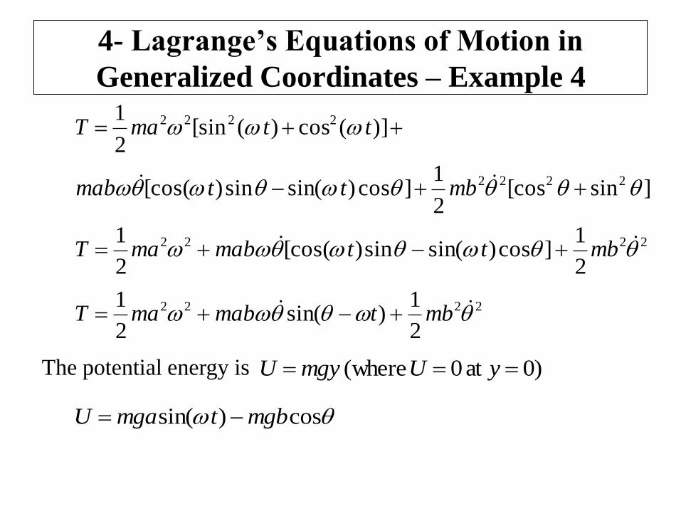
1 mbttmabmaT
2222
2
1)sin(
2
1 mbtmabmaT
The potential energy is )0at 0 (where yUmgyU
cos)sin( mgbtmgaU
4- Lagrange’s Equations of Motion in
Generalized Coordinates – Example 4
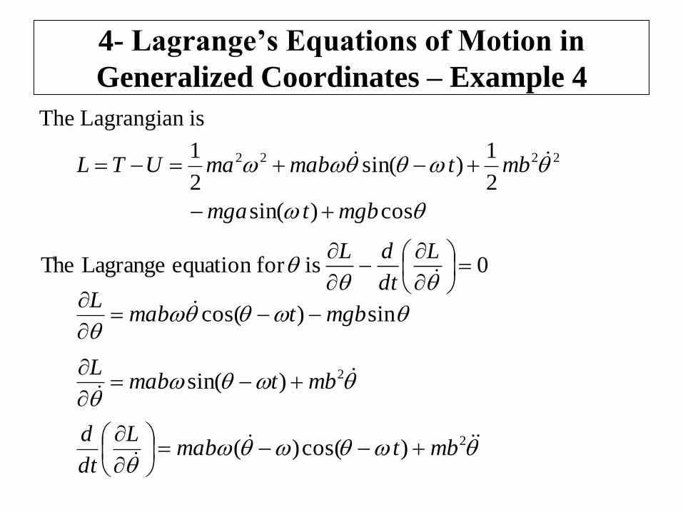
The Lagrangian is
cos)sin(
2
1)sin(
2
1 2222
mgbtmga
mbtmabmaUTL
0 is for equation Lagrange The
L
dt
dL
sin)cos( mgbtmabL
2)sin( mbtmabL
2)cos()( mbtmabL
dt
d
4- Lagrange’s Equations of Motion in
Generalized Coordinates – Example 4
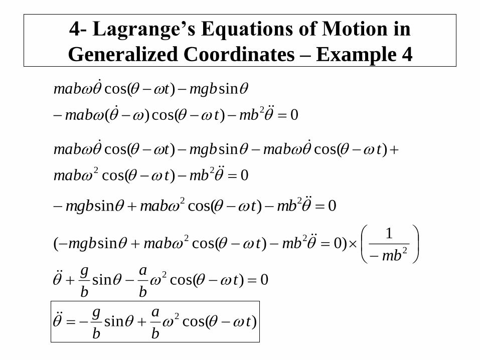
0)cos()(
sin)cos(
2
mbtmab
mgbtmab
0)cos(
)cos(sin)cos(
22
mbtmab
tmabmgbtmab
0)cos(sin 22 mbtmabmgb
2
22 1)0)cos(sin(
mbmbtmabmgb
0)cos(sin 2 tb
a
b
g
)cos(sin 2 tb
a
b
g
Lagrange’s Equations of Motion in
Generalized Coordinates – Example 5
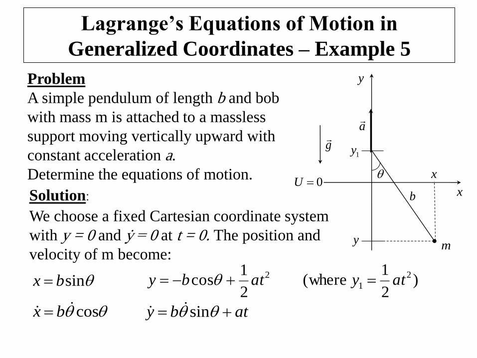
Problem
A simple pendulum of length b and bob
with mass m is attached to a massless
support moving vertically upward with
constant acceleration a.
Determine the equations of motion.
Solution:
b
m
0Ux
x
y
a
1y
y
g
sinbx )2
1 where( 2
1 aty 2
2
1cos atby
We choose a fixed Cartesian coordinate system
with y = 0 and ẏ = 0 at t = 0. The position and
velocity of m become:
cos bx atby sin
Lagrange’s Equations of Motion in
Generalized Coordinates – Example 5
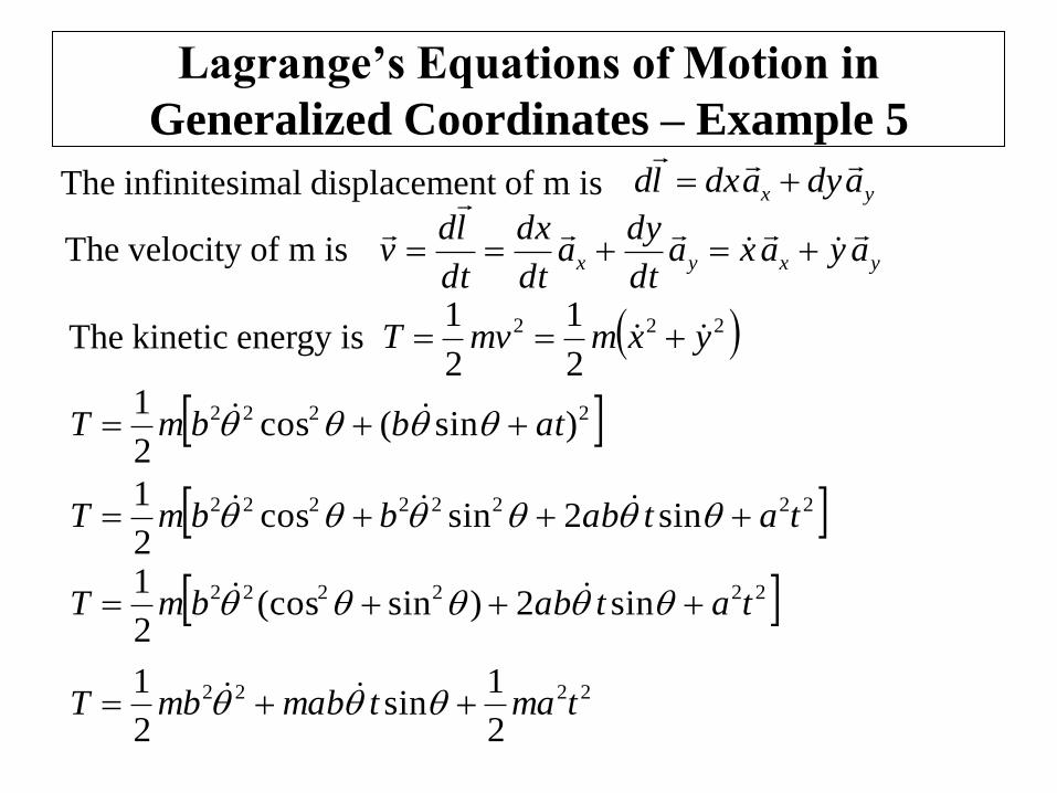
The kinetic energy is
The infinitesimal displacement of m is yx adyadxld
The velocity of m is yxyx ayaxadt
dya
dt
dx
dt
ldv
222
2
1
2
1yxmmvT
2222 )sin(cos2
1atbbmT
22222222 sin2sincos2
1tatabbbmT
222222 sin2)sin(cos2
1tatabbmT
2222
2
1sin
2
1tmatmabmbT
Lagrange’s Equations of Motion in
Generalized Coordinates – Example 5
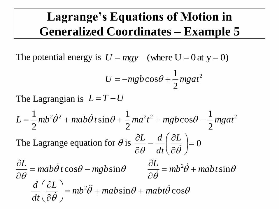
The potential energy is 0)yat 0 U(where mgyU
2
2
1cos mgatmgbU
The Lagrangian is UTL
22222
2
1cos
2
1sin
2
1mgatmgbtmatmabmbL
The Lagrange equation for is 0
L
dt
dL
sincos mgbtmabL
sin2 tmabmbL
cossin2 mabtmabmb
L
dt
d
Lagrange’s Equations of Motion in
Generalized Coordinates – Example 5
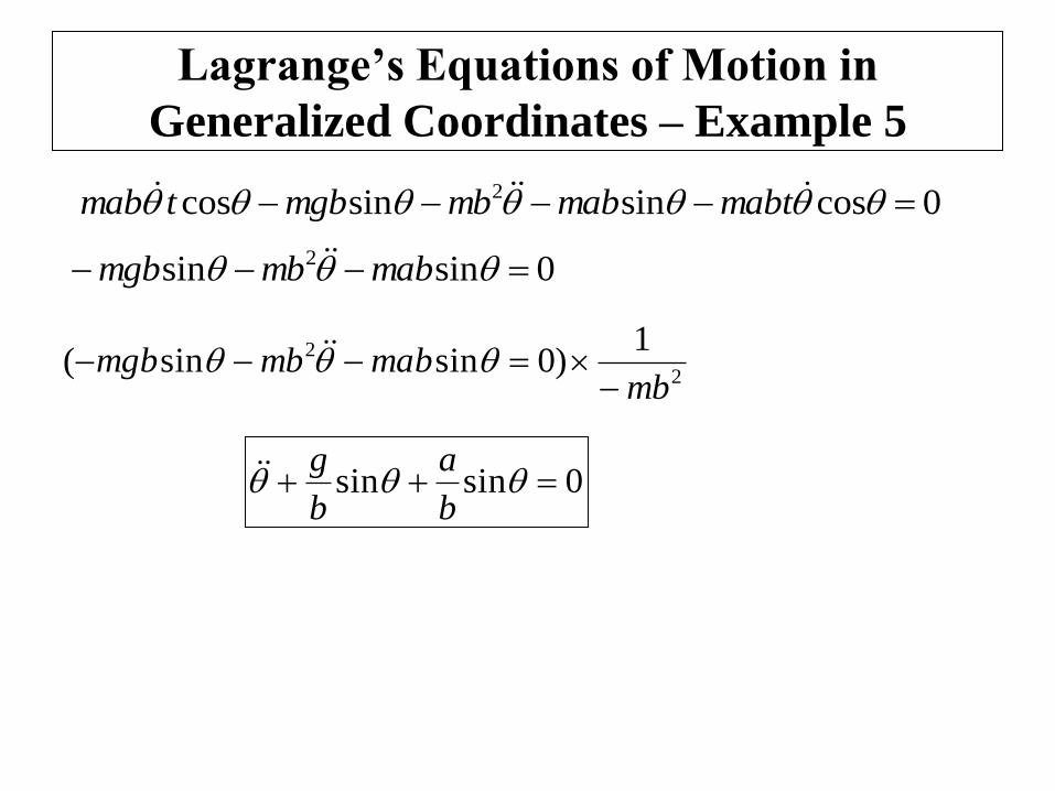
0cossinsincos 2 mabtmabmbmgbtmab
0sinsin 2 mabmbmgb
2
2 1)0sinsin(
mbmabmbmgb
0sinsin b
a
b
g
5- Lagrange’s Equations with Undetermined
Multipliers
Chapter 2 – Section 5
n...,,,iandm...,,,kx,yg
y
gx
y
f
dx
d
y
f
ik
k i
kk
ii
21210
0
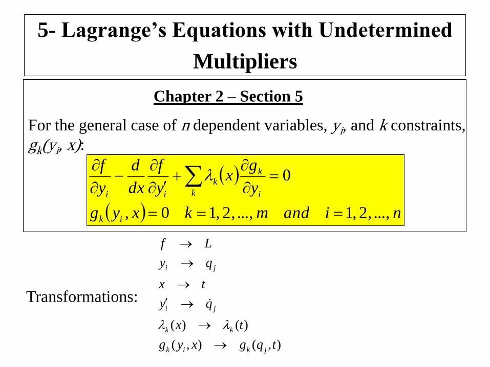
For the general case of n dependent variables, yi, and k constraints,
gk(yi, x):
),(),(
)()(
tqgxyg
tx
qy
tx
qy
Lf
jkik
kk
ji
ji
Transformations:
5- Lagrange’s Equations with Undetermined
Multipliers
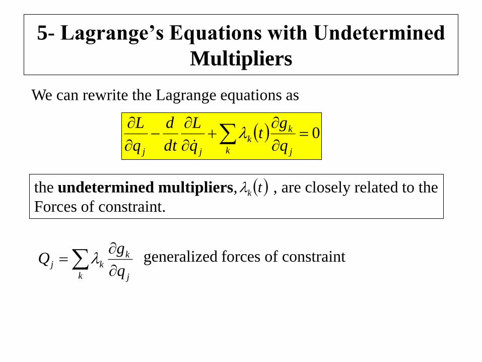
We can rewrite the Lagrange equations as
k j
kk
jj q
gt
q
L
dt
d
q
L0
k j
kkj
q
gQ
the undetermined multipliers, , are closely related to the
Forces of constraint.
tk
generalized forces of constraint
5- Lagrange’s Equations with Undetermined
Multipliers – Example 6
ra
x
y
x
y
0U
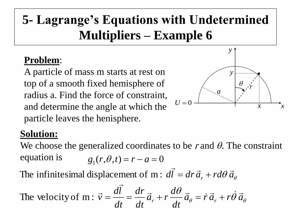
Problem:
A particle of mass m starts at rest on
top of a smooth fixed hemisphere of
radius a. Find the force of constraint,
and determine the angle at which the
particle leaves the henisphere.
Solution:
We choose the generalized coordinates to be r and . The constraint
equation is 0),,(1 artrg
ardadrld r
:m ofnt displaceme malinfinitesi The
araradt
dra
dt
dr
dt
ldv rr
:m of velocity The
5- Lagrange’s Equations with Undetermined
Multipliers – Example 6
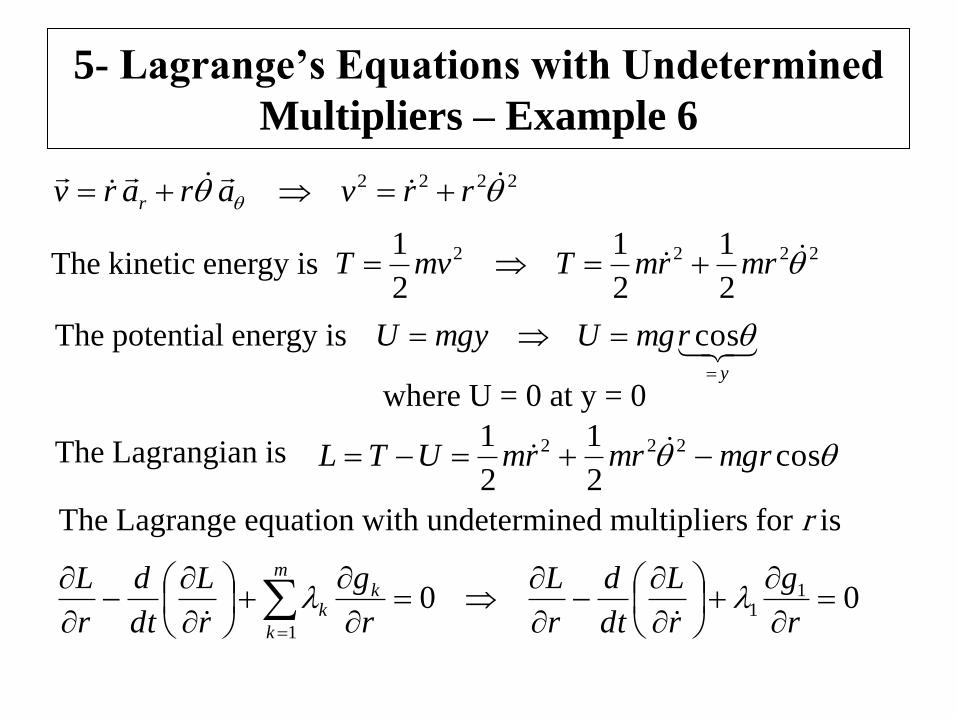
2222
rrvararv r
2222
2
1
2
1
2
1 mrrmTmvT
y
rmgUmgyU
cos
The kinetic energy is
The potential energy is
where U = 0 at y = 0
The Lagrangian is cos2
1
2
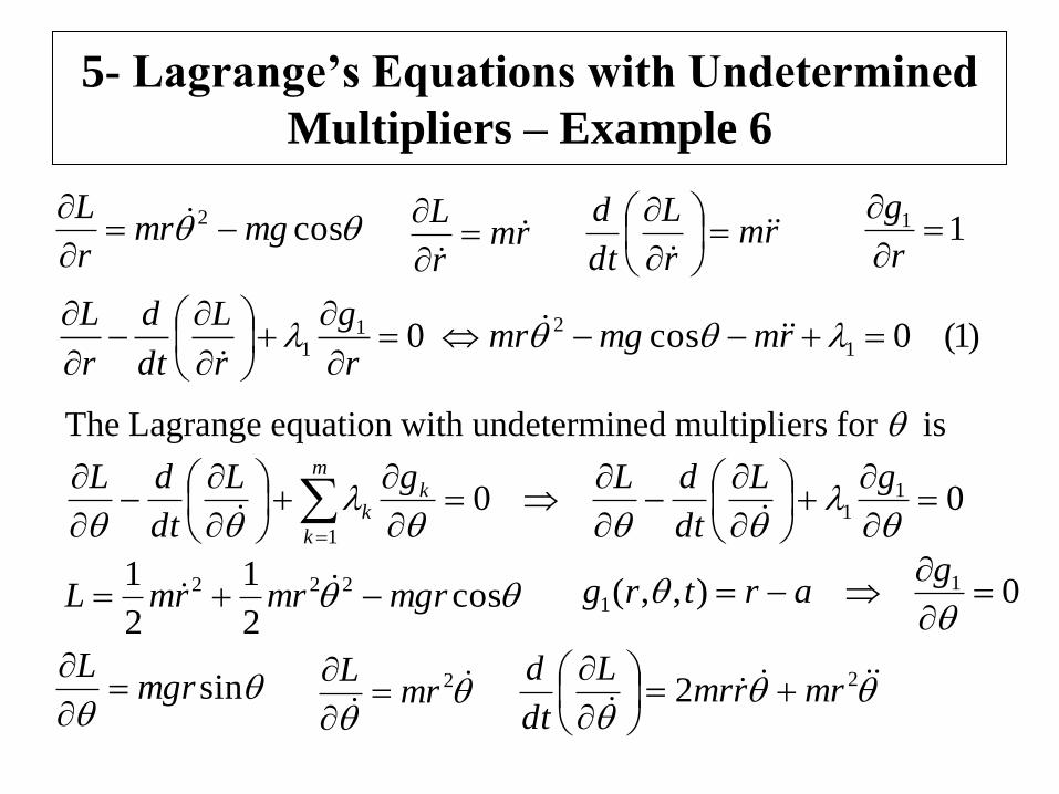
1 222 mgrmrrmUTL
The Lagrange equation with undetermined multipliers for r is
00 11
1
r
g
r
L
dt
d
r
L
r
g
r
L
dt
d
r
L m
k
kk
5- Lagrange’s Equations with Undetermined
Multipliers – Example 6
cos2 mgmrr
L
rmr
L
rm
r
L
dt
d
11
r
g
)1(0cos0 1
211
rmmgmr
r
g
r
L
dt
d
r
L
The Lagrange equation with undetermined multipliers for is
00 11
1
gL
dt
dLgL
dt
dL m
k
kk
cos2
1
2
1 222 mgrmrrmL
sinmgrL
2mr
L
22 mrrmr
L
dt
d
0),,( 11
gartrg
5- Lagrange’s Equations with Undetermined
Multipliers – Example 6
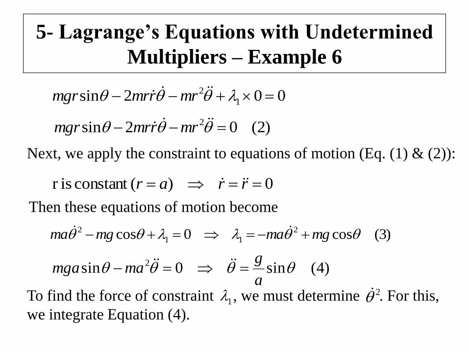
0)(constant isr rrar
Next, we apply the constraint to equations of motion (Eq. (1) & (2)):
)3(cos0cos 2
11
2 mgmamgma
Then these equations of motion become
002sin 1
2 mrrmrmgr
)2(02sin 2 mrrmrmgr
)4(sin0sin 2 a
gmamga
To find the force of constraint , we must determine . For this,
we integrate Equation (4). 1
2
5- Lagrange’s Equations with Undetermined
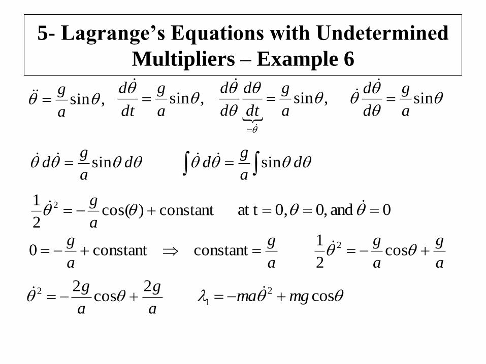
Multipliers – Example 6
,sina
g ,sin
a
g
dt
d
,sin
a
g
dt
d
d
d
sin
a
g
d
d
da
gd sin d
a
gd sin
constant)cos(2
1 2 a
g 0 and ,0 0,at t
a
g
a
g constantconstant0
a
g
a
g cos
2
1 2
a
g
a
g 2cos
22 cos2
1 mgma
5- Lagrange’s Equations with Undetermined
Multipliers – Example 6
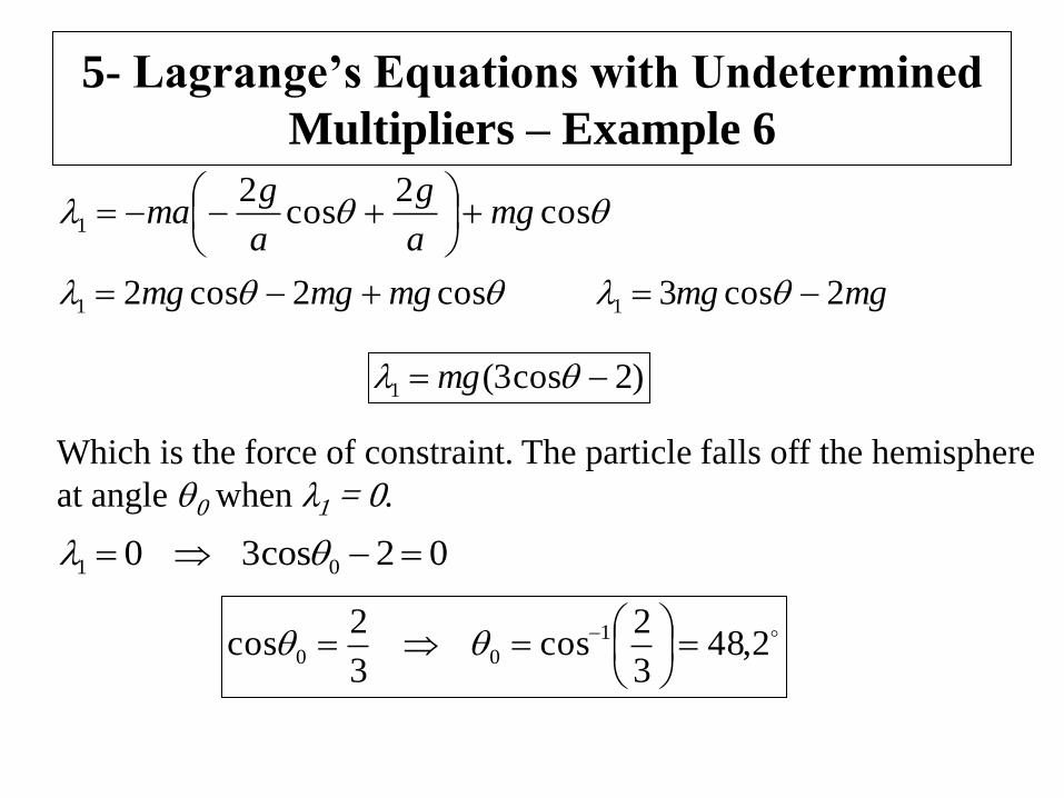
cos2
cos2
1 mga
g
a
gma
cos2cos21 mgmgmg mgmg 2cos31
)2cos3(1 mg
Which is the force of constraint. The particle falls off the hemisphere
at angle 0 when λ1 = 0.
02cos30 01
2,483
2cos
3
2cos 1
00
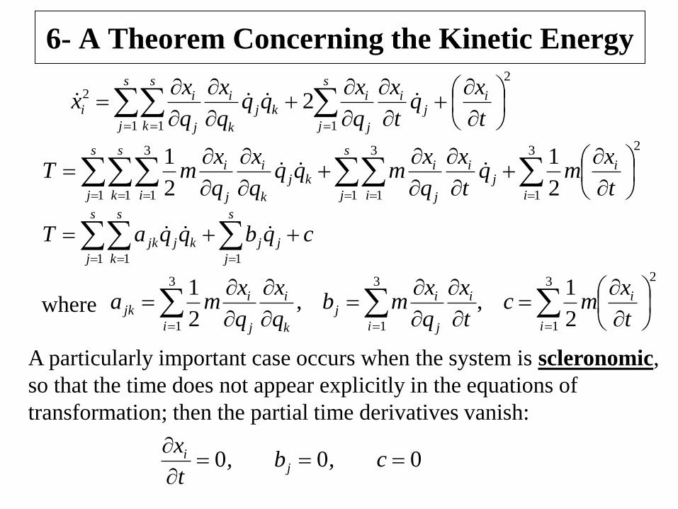
6- A Theorem Concerning the Kinetic Energy
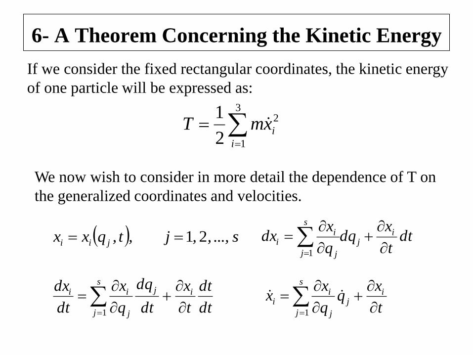
If we consider the fixed rectangular coordinates, the kinetic energy
of one particle will be expressed as:
We now wish to consider in more detail the dependence of T on
the generalized coordinates and velocities.
s...,,,j,t,qxx jii 21 dtt
xdq
q
xdx i
j
s
j j
ii
1
dt
dt
t
x
dt
dq
q
x
dt
dx ijs
j j
ii
1
s
j
ij
j
ii
t
xq
q
xx
1
3
1
2
2
1
i
ixmT
6- A Theorem Concerning the Kinetic Energy
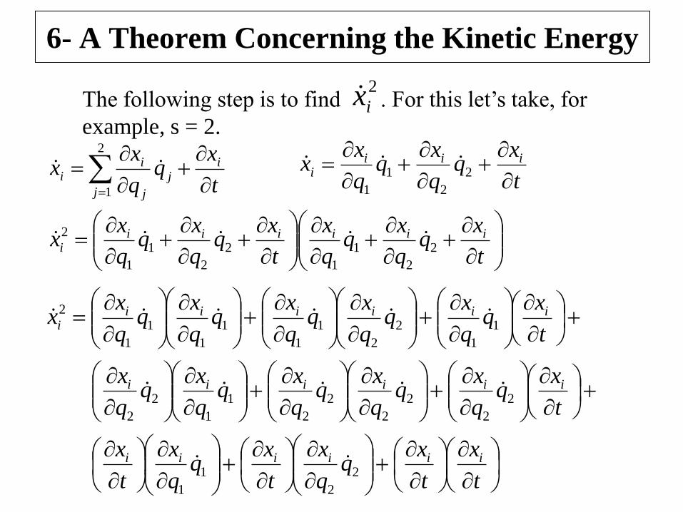
The following step is to find . For this let’s take, for
example, s = 2.
2
ix
2
1j
ij
j
ii
t
xq
q
xx
t
xq
q
xq
q
xx iii
i
2
2
1
1
t
xq
q
xq
q
x
t
xq
q
xq
q
xx iiiiii
i 2
2
1
1
2
2
1
1
2
t
x
t
xq
q
x
t
xq
q
x
t
x
t
xq
q
xq
q
xq
q
xq
q
xq
q
x
t
xq
q
xq
q
xq
q
xq
q
xq
q
xx
iiiiii
iiiiii
iiiiiii
2
2
1
1
2
2
2
2
2
2
1
1
2
2
1
1
2
2
1
1
1
1
1
1
2
6- A Theorem Concerning the Kinetic Energy
t
x
t
xq
q
x
t
xq
q
x
t
x
t
xq
q
xq
q
xq
q
xq
q
xq
q
x
t
xq
q
xq
q
xq
q
xq
q
xq
q
xx
iiiiii
iiiiii
iiiiiii
2
2
1
1
2
2
2
2
2
2
1
1
2
2
1
1
2
2
1
1
1
1
1
1
2
2
2
2
1
1
2
2
22
22
12
12
1
1
21
21
11
11
2
t
xq
t
x
q
xq
t
x
q
x
qt
x
q
xqq
q
x
q
xqq
q
x
q
x
qt
x
q
xqq
q
x
q
xqq
q
x
q
xx
iiiii
iiiiii
iiiiiii
6- A Theorem Concerning the Kinetic Energy
2
2
2
1
1
2
2
22
22
12
12
1
1
21
21
11
11
2
t
xq
t
x
q
xq
t
x
q
x
qt
x
q
xqq
q
x
q
xqq
q
x
q
x
qt
x
q
xqq
q
x
q
xqq
q
x
q
xx
iiiii
iiiiii
iiiiiii
22
1
2
1
2
1
2 2
j k j
ij
i
j
ikj
k
i
j
ii
t
xq
t
x
q
xqq
q
x
q
xx
2
11 1
2 2
t
xq
t
x
q
xqq
q
x
q
xx i
ji
s
j j
ikj
k
is
j
s
k j
ii
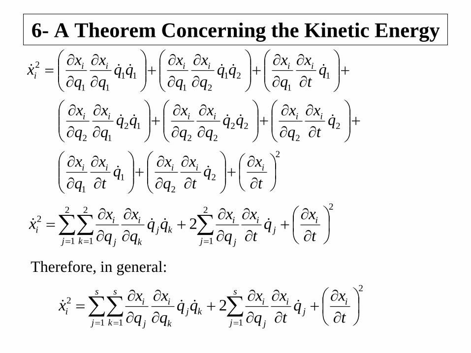
Therefore, in general:
6- A Theorem Concerning the Kinetic Energy 2
11 1
2 2
t
xq
t
x
q
xqq
q
x
q
xx i
ji
s
j j
ikj
k
is
j
s
k j
ii
23
11
3
11 1
3
1 2
1
2
1
t
xmq
t
x
q
xmqq
q
x
q
xmT i
i
ji
s
j j
i
i
kj
k
is
j
s
k j
i
i
cqbqqaT j
s
j
jkj
s
j
s
k
jk
11 1
A particularly important case occurs when the system is scleronomic,
so that the time does not appear explicitly in the equations of
transformation; then the partial time derivatives vanish:
000
c,b,
t
xj
i
23
1
3
1
3
1 2
1,,
2
1
i
i
i
i
j
ij
k
i
j
i
i
jkt
xmc
t
x
q
xmb
q
x
q
xmawhere
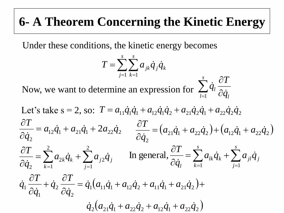
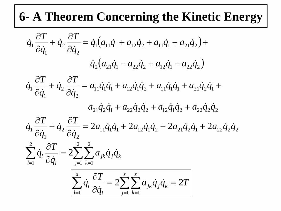
6- A Theorem Concerning the Kinetic Energy
kj
s
j
s
k
jk qqaT
1 1
s
k
s
j
jjlklk
l
qaqaq
T
1 1
general,In
Under these conditions, the kinetic energy becomes
Now, we want to determine an expression for
s
l l
lq
Tq
1
Let’s take s = 2, so: 2222122121121111 qqaqqaqqaqqaT
222121112
2
2 qaqaqaq
T
222112222121
2
qaqaqaqaq
T
2
1
2
1
22
2 k j
jjkk qaqaq
T
2221122221212
2211112121111
2
2
1
1
qaqaqaqaq
qaqaqaqaqq
Tq
q
Tq
6- A Theorem Concerning the Kinetic Energy
2221122221212
2211112121111
2
2
1
1
qaqaqaqaq
qaqaqaqaqq
Tq
q
Tq
2222211222221221
1221111121121111
2
2
1
1
qqaqqaqqaqqa
qqaqqaqqaqqaq
Tq
q
Tq
2222122121121111
2
2
1
1 2222 qqaqqaqqaqqaq
Tq
q
Tq
2
1
2
1
2
1
2l j k
kjjk
l
l qqaq
Tq
Tqqaq
Tq
s
l
s
j
s
k
kjjk
l
l 221 1 1
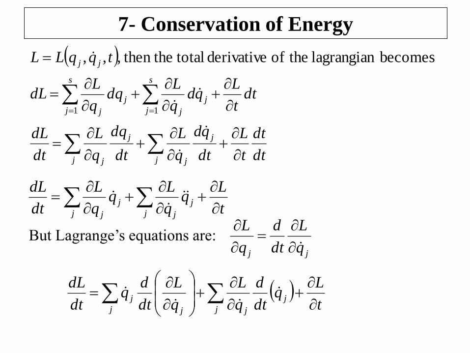
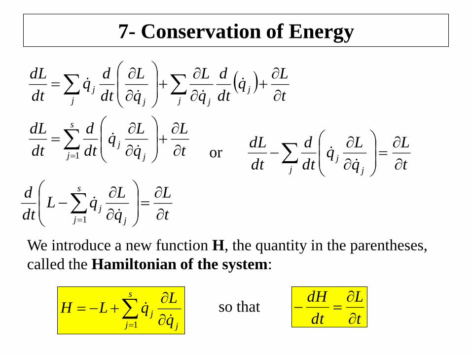
7- Conservation of Energy
j j
j
j
j
j
s
j
s
j
j
j
j
j
jj
dt
dt
t
L
dt
qd
q
L
dt
dq
q
L
dt
dL
dtt
Lqd
q
Ldq
q
LdL
tqqLL
1 1
becomes lagrangian theof derivative total then the,,,
But Lagrange’s equations are: jj q
L
dt
d
q
L
t
Lq
q
Lq
q
L
dt
dL
j j
j
j
j
j
t
Lq
dt
d
q
L
q
L
dt
dq
dt
dL
j j
j
jj
j
7- Conservation of Energy
t
L
q
Lq
dt
d
dt
dL
t
Lq
dt
d
q
L
q
L
dt
dq
dt
dL
s
j j
j
j j
j
jj
j
1
t
L
q
Lq
dt
d
dt
dL
j j
j
or
t
L
q
LqL
dt
d s
j j
j
1
s
j j
jq
LqLH
1
We introduce a new function H, the quantity in the parentheses,
called the Hamiltonian of the system:
t
L
dt
dH
so that
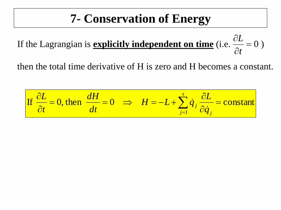
7- Conservation of Energy
If the Lagrangian is explicitly independent on time (i.e. )
then the total time derivative of H is zero and H becomes a constant.
0
t
L
constant0 then ,0 If1
s
j j
jq
LqLH
dt
dH
t
L
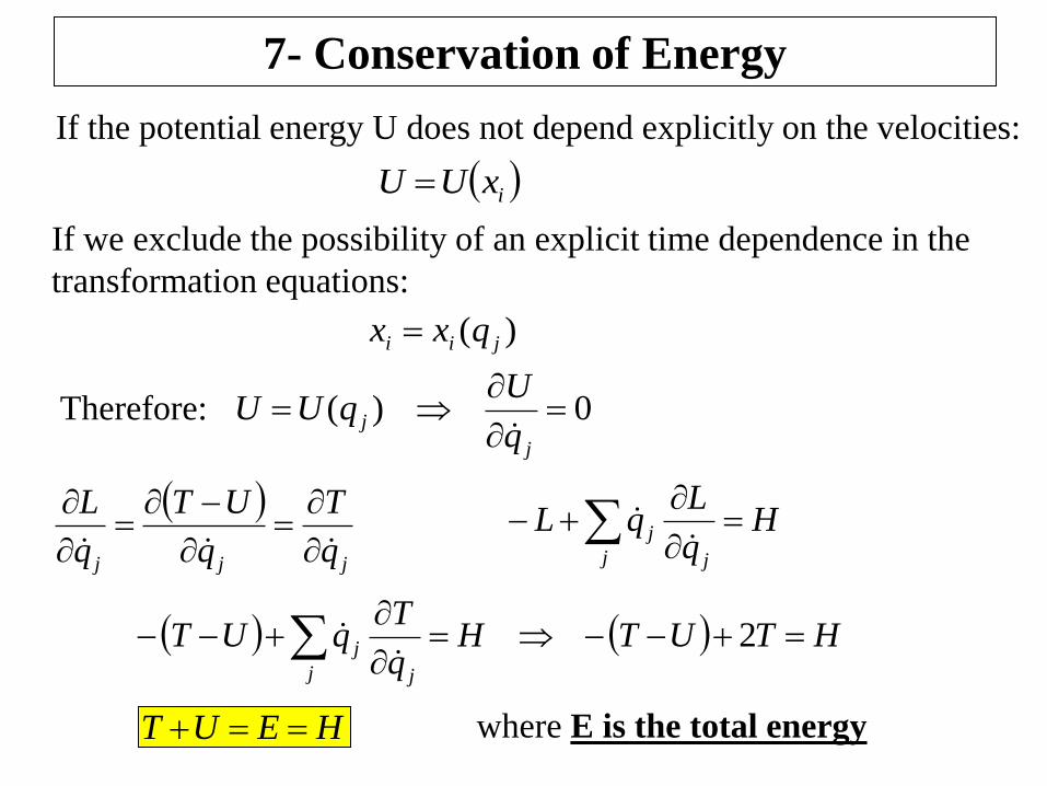
7- Conservation of Energy
If the potential energy U does not depend explicitly on the velocities:
ixUU
If we exclude the possibility of an explicit time dependence in the
transformation equations:
)( jii qxx
Therefore: 0)(
j
jq
UqUU
jjj q
T
q
UT
q
L
H
q
LqL
j j
j
HTUTHq
TqUT
j j
j
2
HEUT where E is the total energy
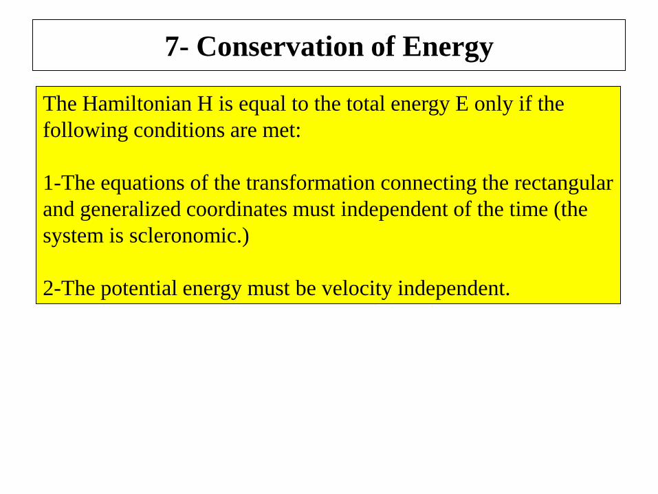
7- Conservation of Energy
The Hamiltonian H is equal to the total energy E only if the
following conditions are met:
1-The equations of the transformation connecting the rectangular
and generalized coordinates must independent of the time (the
system is scleronomic.)
2-The potential energy must be velocity independent.
8- Canonical Equations of Motion –
Hamiltonian Dynamics
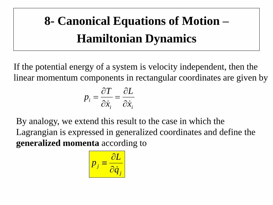
If the potential energy of a system is velocity independent, then the
linear momentum components in rectangular coordinates are given by
ii
ix
L
x
Tp
By analogy, we extend this result to the case in which the
Lagrangian is expressed in generalized coordinates and define the
generalized momenta according to
j
jq
Lp
8- Canonical Equations of Motion –
Hamiltonian Dynamics
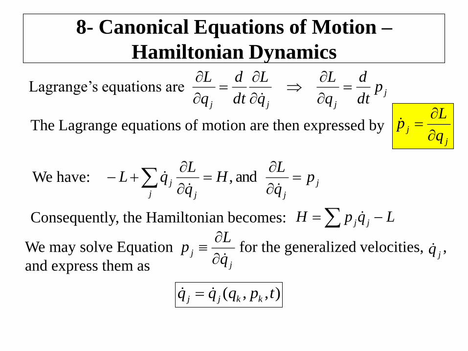
Lagrange’s equations are j
jjj
pdt
d
q
L
q
L
dt
d
q
L
The Lagrange equations of motion are then expressed by j
jq
Lp
j
jj j
j pq
LH
q
LqL
and ,We have:
LqpH jj Consequently, the Hamiltonian becomes:
We may solve Equation for the generalized velocities, ,
and express them as j
jq
Lp
jq
),,( tpqqq kkjj
8- Canonical Equations of Motion –
Hamiltonian Dynamics
tqqLLtpqHH kkkk ,,,,,
k
k
k
k
k
dtt
Hdp
p
Hdq
q
HdH
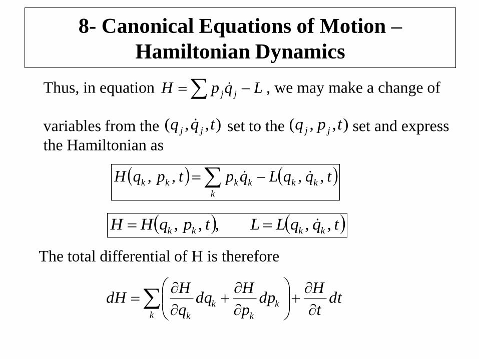
Thus, in equation , we may make a change of
variables from the set to the set and express
the Hamiltonian as
LqpH jj
),,( tqq jj ),,( tpq jj
k
kkkkkk tqqLqptpqH ,,,,
The total differential of H is therefore
8- Canonical Equations of Motion –
Hamiltonian Dynamics
k
k
k
k
k
kkkk dtt
Lqd
q
Ldq
q
LqdpdpqdH
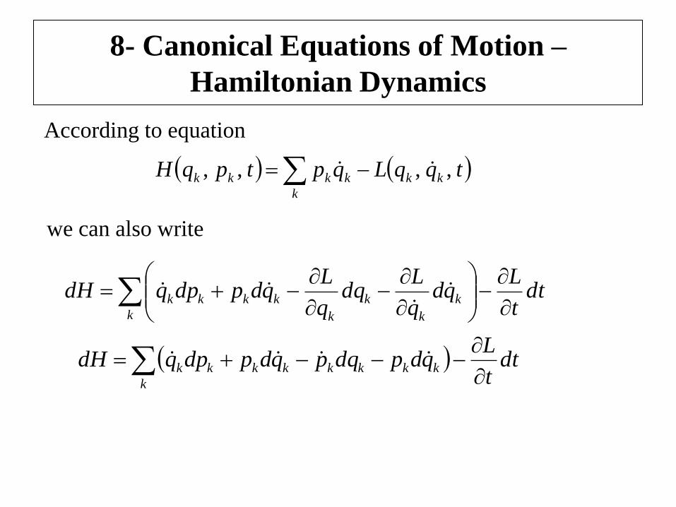
we can also write
k
kkkkkkkk dtt
LqdpdqpqdpdpqdH
According to equation
k
kkkkkk tqqLqptpqH ,,,,
8- Canonical Equations of Motion –
Hamiltonian Dynamics
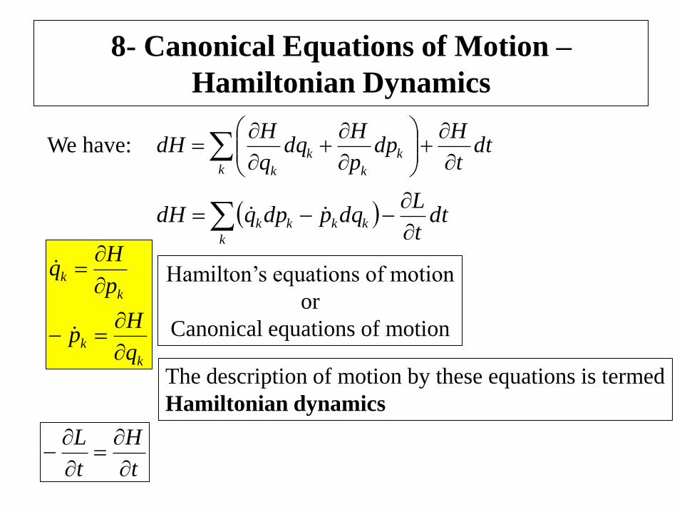
We have:
k
k
k
k
k
dtt
Hdp
p
Hdq
q
HdH
k
kkkk dtt
LdqpdpqdH
k
k
k
k
q
Hp
p
Hq
Hamilton’s equations of motion
or
Canonical equations of motion
t
H
t
L
The description of motion by these equations is termed
Hamiltonian dynamics
8- Canonical Equations of Motion –
Hamiltonian Dynamics
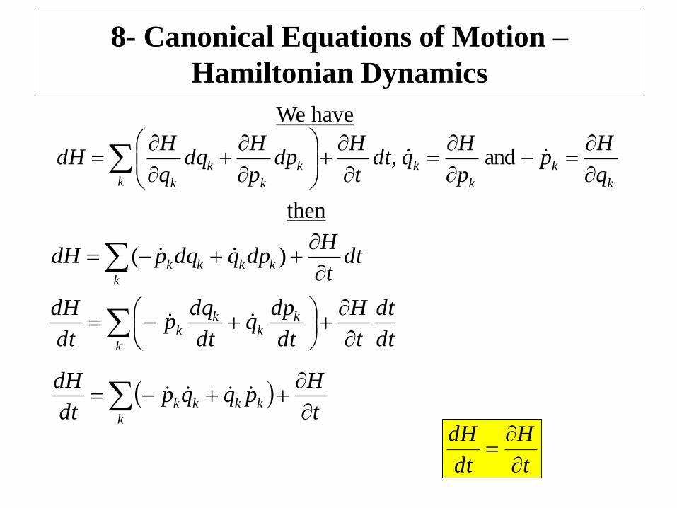
k
k
k
k
k
k
k
k
k q
Hp
p
Hqdt
t
Hdp
p
Hdq
q
HdH
and,
We have
t
H
dt
dH
then
k
kkkk dtt
HdpqdqpdH )(
dt
dt
t
H
dt
dpq
dt
dqp
dt
dH
k
kk
kk
t
Hpqqp
dt
dH
k
kkkk
8- Canonical Equations of Motion –
Hamiltonian Dynamics
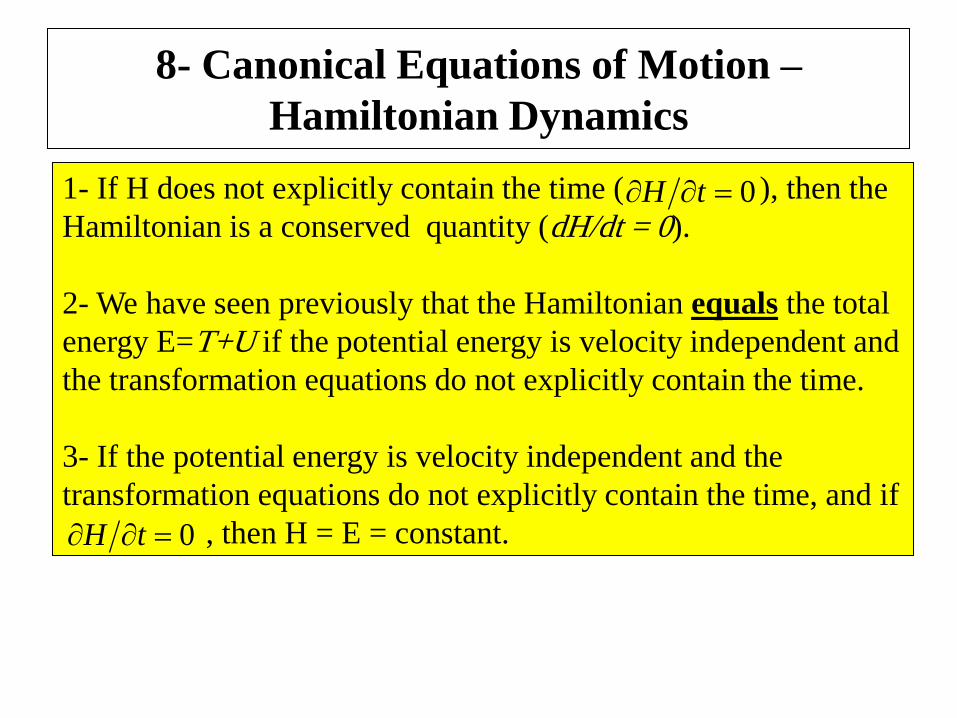
1- If H does not explicitly contain the time ( ), then the
Hamiltonian is a conserved quantity (dH/dt = 0).
2- We have seen previously that the Hamiltonian equals the total
energy E=T+U if the potential energy is velocity independent and
the transformation equations do not explicitly contain the time.
3- If the potential energy is velocity independent and the
transformation equations do not explicitly contain the time, and if
, then H = E = constant.
0 tH
0 tH
8- Canonical Equations of Motion –
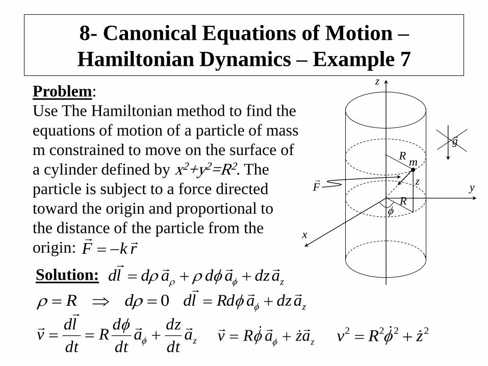
Hamiltonian Dynamics – Example 7
Problem:
Use The Hamiltonian method to find the
equations of motion of a particle of mass
m constrained to move on the surface of
a cylinder defined by x2+y2=R2. The
particle is subject to a force directed
toward the origin and proportional to
the distance of the particle from the
origin: rkF
Solution: zadzadadld
0 dR zadzaRdld
zadt
dza
dt
dR
dt
ldv
zazaRv
2222 zRv
z
R
R
z
x
yF
g
m
8- Canonical Equations of Motion –
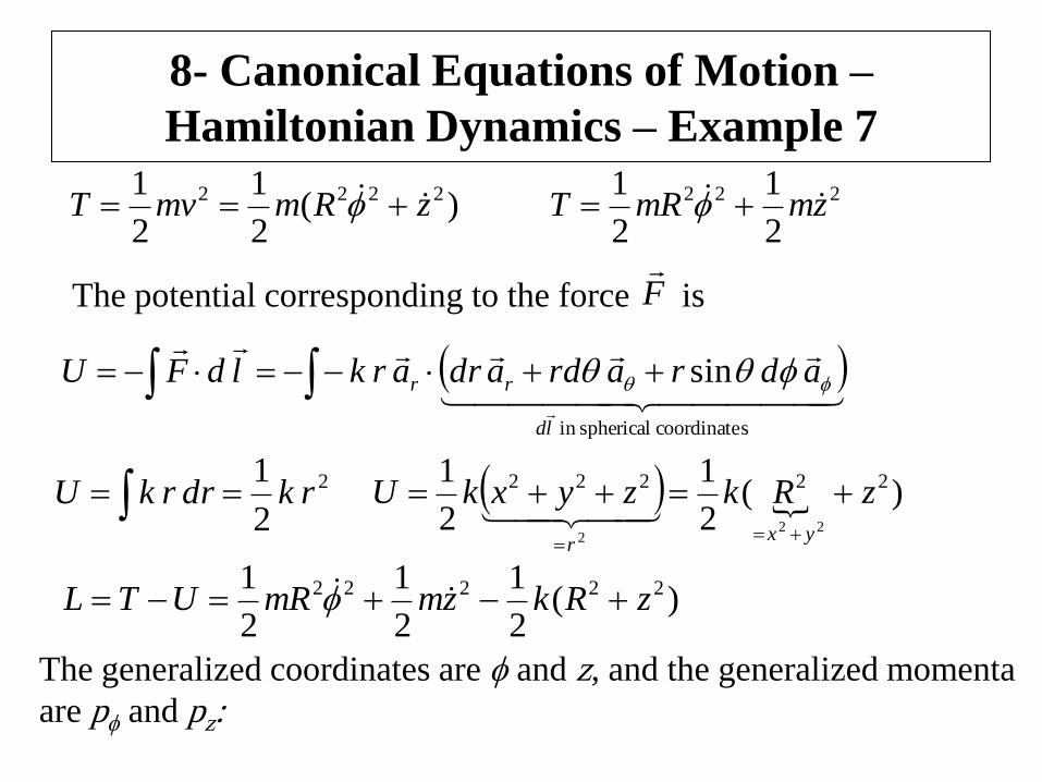
Hamiltonian Dynamics – Example 7
)(2
1
2
1 2222 zRmmvT 222
2
1
2
1zmmRT
scoordinate sphericalin
sin
ld
rr adrardadrarkldFU
The potential corresponding to the force is F
2
2
1rkdrrkU )(
2
1
2
1 22222
222
zRkzyxkUyx
r
)(2
1
2
1
2
1 22222 zRkzmmRUTL
The generalized coordinates are and z, and the generalized momenta
are p and pz:
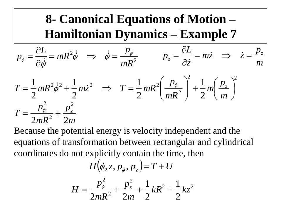
8- Canonical Equations of Motion –
Hamiltonian Dynamics – Example 7
2
2
mR
pmR
Lp
m
pzzm
z
Lp z
z
22
2
2222
2
1
2
1
2
1
2
1
m
pm
mR
pmRTzmmRT z
m
p
mR
pT z
22
2
2
2
Because the potential energy is velocity independent and the
equations of transformation between rectangular and cylindrical
coordinates do not explicitly contain the time, then
UTppzH z ,,,
222
2
2
2
1
2
1
22kzkR
m
p
mR
pH z
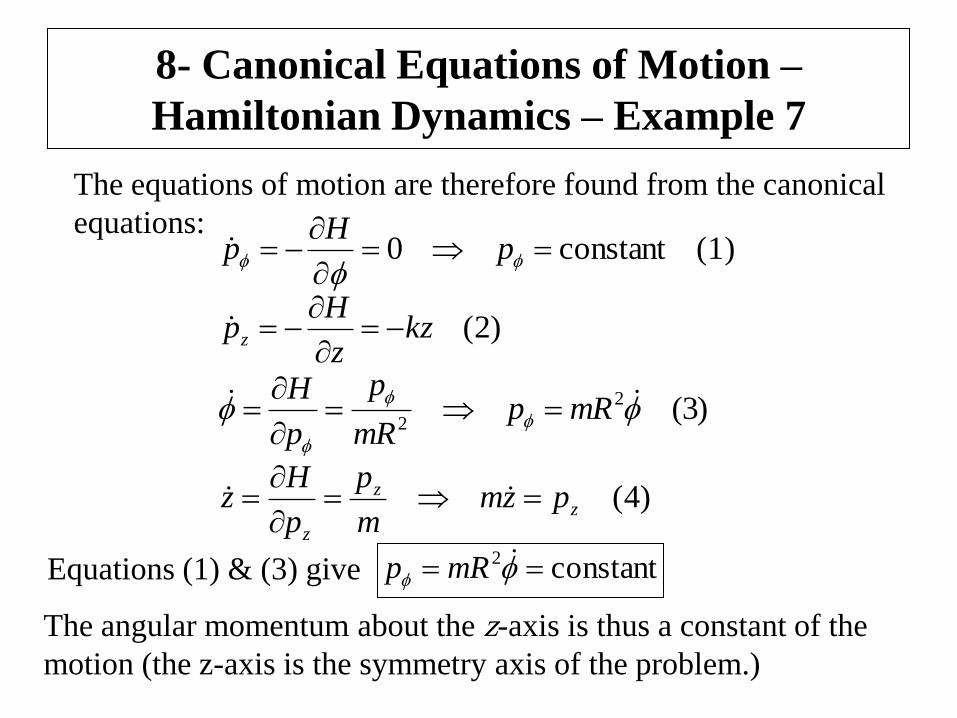
8- Canonical Equations of Motion –
Hamiltonian Dynamics – Example 7
The equations of motion are therefore found from the canonical
equations: (1)constant0
p
Hp
)2(kzz
Hpz
)3(2
2
mRpmR
p
p
H
)4(zz
z
pzmm
p
p
Hz
constant2 mRpEquations (1) & (3) give
The angular momentum about the z-axis is thus a constant of the
motion (the z-axis is the symmetry axis of the problem.)
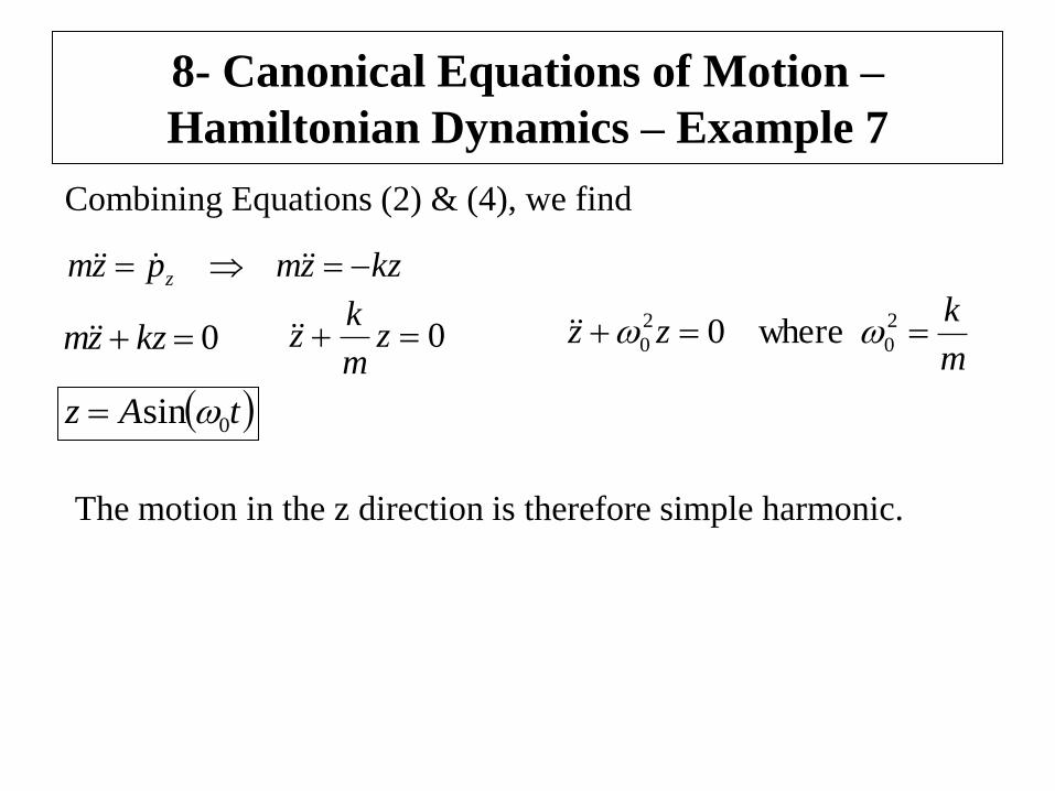
8- Canonical Equations of Motion –
Hamiltonian Dynamics – Example 7
Combining Equations (2) & (4), we find
kzzmpzm z
0 kzzm 0 zm
kz
m
kzz 2
0
2
0 where0
tAz 0sin
The motion in the z direction is therefore simple harmonic.
8- Canonical Equations of Motion –
Hamiltonian Dynamics – Example 8
x
yx
y
b
0U
g
m
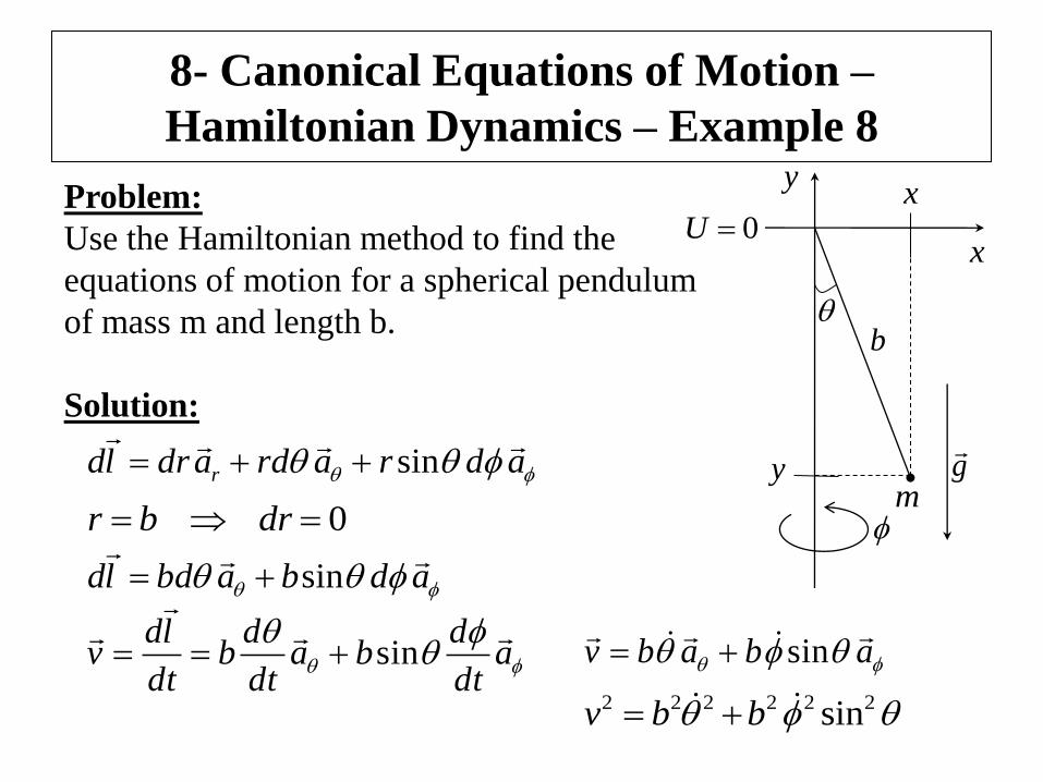
Problem:
Use the Hamiltonian method to find the
equations of motion for a spherical pendulum
of mass m and length b.
Solution:
adrardadrld r
sin
0 drbr
adbabdld
sin
a
dt
dba
dt
db
dt
ldv
sin ababv
sin
222222 sin bbv
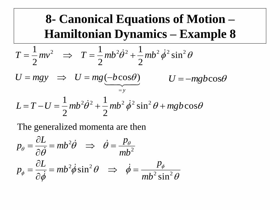
8- Canonical Equations of Motion –
Hamiltonian Dynamics – Example 8
222222 sin2
1
2
1
2
1 mbmbTmvT
y
bmgUmgyU
)cos( cosmgbU
cossin2
1
2
1 22222 mgbmbmbUTL
The generalized momenta are then
2
2
mb
pmb
Lp
22
22
sinsin
mb
pmb
Lp
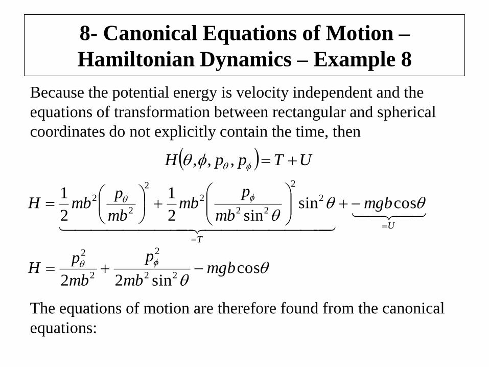
8- Canonical Equations of Motion –
Hamiltonian Dynamics – Example 8
Because the potential energy is velocity independent and the
equations of transformation between rectangular and spherical
coordinates do not explicitly contain the time, then
UTppH ,,,
U
T
mgbmb
pmb
mb
pmbH
cossinsin2
1
2
1 2
2
22
2
2
2
2
cossin22 22
2
2
2
mgbmb
p
mb
pH
The equations of motion are therefore found from the canonical
equations:
8- Canonical Equations of Motion –
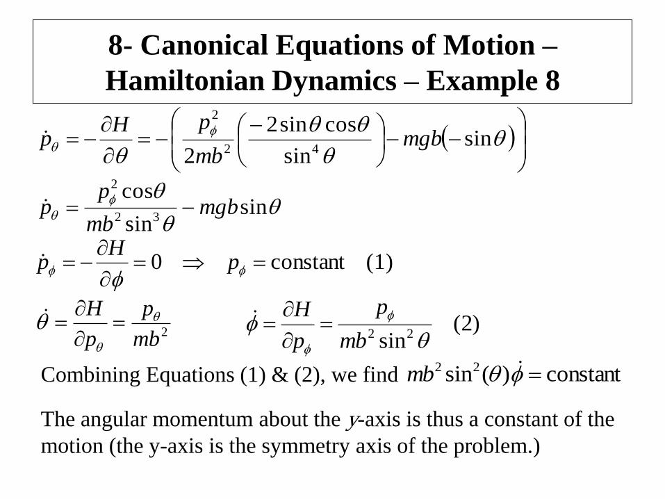
Hamiltonian Dynamics – Example 8
sinsin
cossin2
2 42
2
mgbmb
pHp
sinsin
cos32
2
mgbmb
pp
(1)constant0
p
Hp
2mb
p
p
H
)2(
sin22
mb
p
p
H
Combining Equations (1) & (2), we find constant)(sin22 mb
The angular momentum about the y-axis is thus a constant of the
motion (the y-axis is the symmetry axis of the problem.)
8- Canonical Equations of Motion –
Hamiltonian Dynamics – Example 9
constant dt
dr
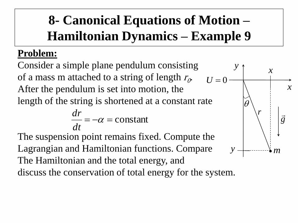
Problem:
Consider a simple plane pendulum consisting
of a mass m attached to a string of length r0.
After the pendulum is set into motion, the
length of the string is shortened at a constant rate
The suspension point remains fixed. Compute the
Lagrangian and Hamiltonian functions. Compare
The Hamiltonian and the total energy, and
discuss the conservation of total energy for the system.
x
yx
y
0U
g
m
r
8- Canonical Equations of Motion –
Hamiltonian Dynamics – Example 9
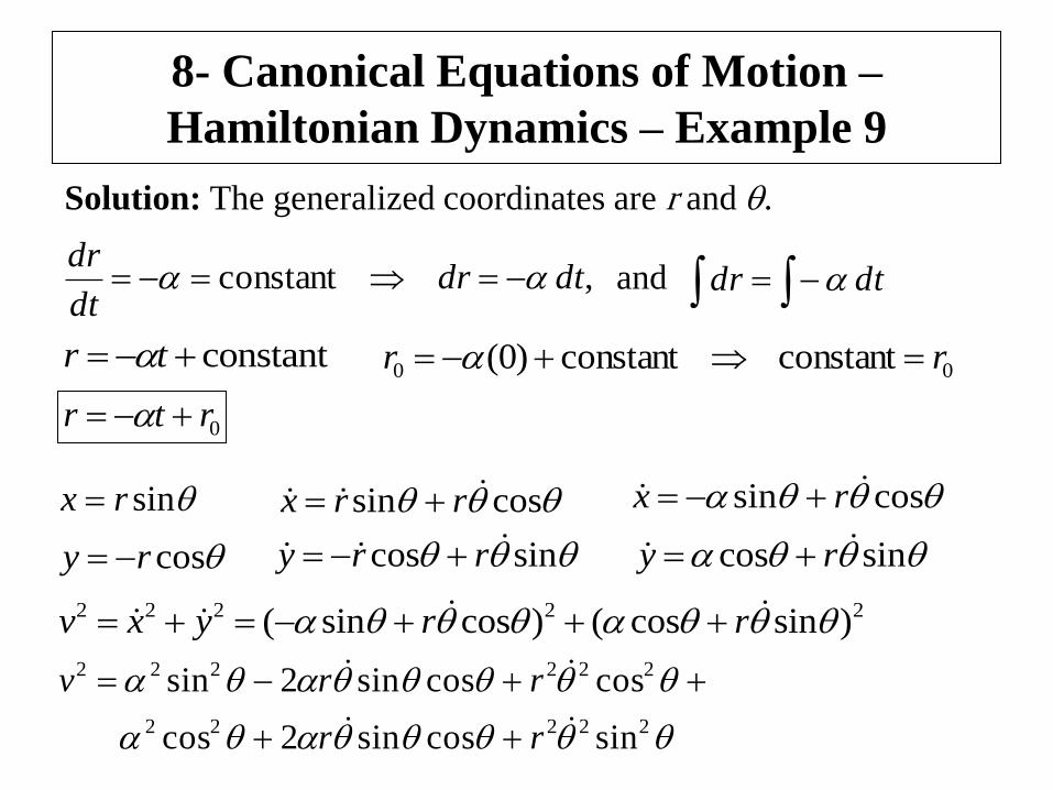
Solution: The generalized coordinates are r and .
,constant dtdrdt
dr dtdr and
constant tr 00 constantconstant)0( rr
0rtr
sinrx cossin rrx cossin rx
cosry sincos rry sincos ry
22222 )sincos()cossin( rryxv
22222
222222
sincossin2cos
coscossin2sin
rr
rrv
8- Canonical Equations of Motion –
Hamiltonian Dynamics – Example 9
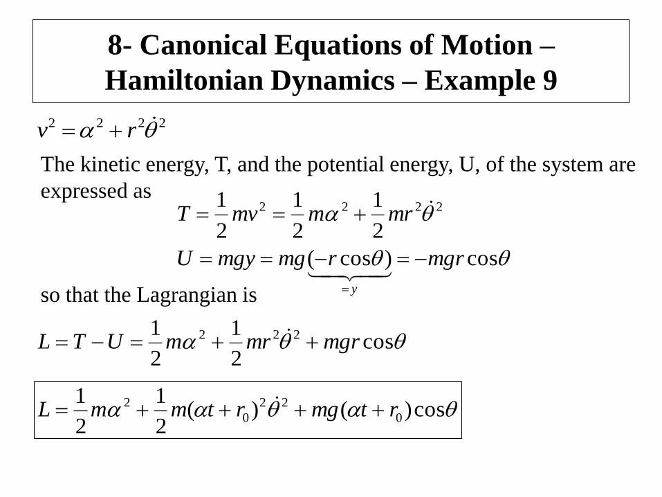
2222 rv
2222
2
1
2
1
2
1 mrmmvT
cos)cos( mgrrmgmgyU
y
cos2
1
2
1 222 mgrmrmUTL
The kinetic energy, T, and the potential energy, U, of the system are
expressed as
so that the Lagrangian is
cos)()(2
1
2
10
22
0
2 rtmgrtmmL
8- Canonical Equations of Motion –
Hamiltonian Dynamics – Example 9
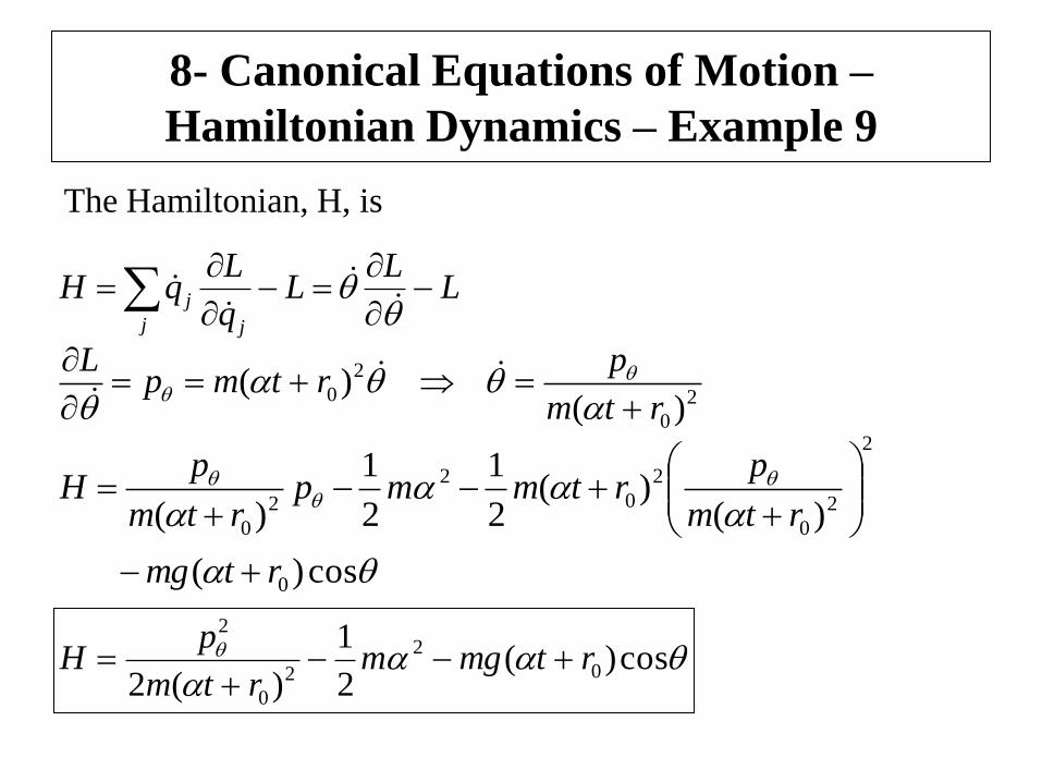
LL
Lq
LqH
j j
j
2
0
2
0)(
)(rtm
prtmp
L
cos)(
)()(
2
1
2
1
)(
0
2
2
0
2
0
2
2
0
rtmg
rtm
prtmmp
rtm
pH
cos)(2
1
)(20
2
2
0
2
rtmgmrtm
pH
The Hamiltonian, H, is
8- Canonical Equations of Motion –
Hamiltonian Dynamics – Example 9
cos)()(2
1
2
10
22
0
2 rtmgrtmmUT
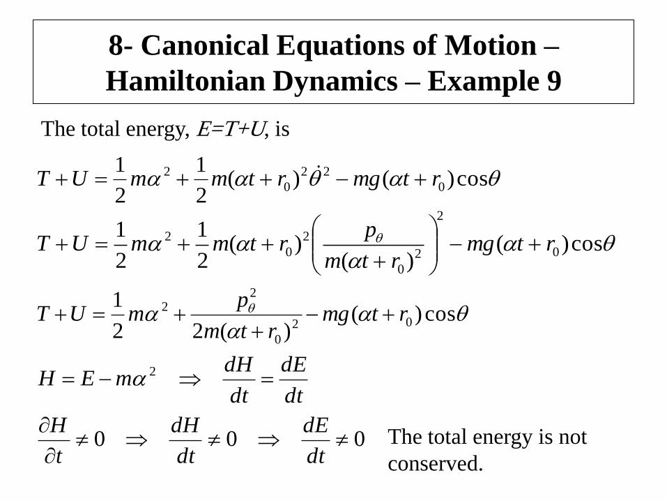
The total energy, E=T+U, is
cos)()(
)(2
1
2
10
2
2
0
2
0
2 rtmgrtm
prtmmUT
cos)()(22
102
0
22 rtmg
rtm
pmUT
dt
dE
dt
dHmEH 2
000
dt
dE
dt
dH
t
HThe total energy is not
conserved.
Chapter 4
Central-Force Motion
Dr. Abdelaziz Sabik
Physics Department – College of Science
Al-Imam Muhammad Ibn Saud Islamic University
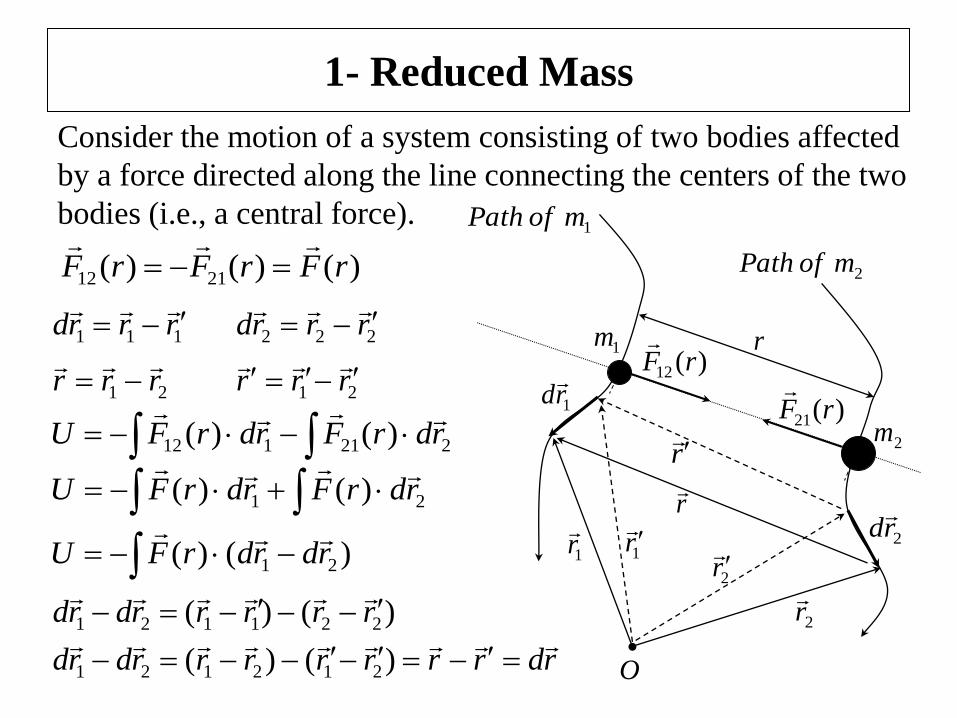
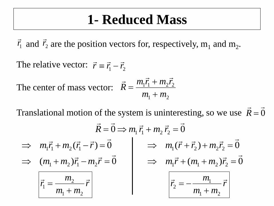
1- Reduced Mass
Consider the motion of a system consisting of two bodies affected
by a force directed along the line connecting the centers of the two
bodies (i.e., a central force).
21 )()( rdrFrdrFU
1m
2m
r
)(21 rF
)(12 rF
O
1r
2r
r
r
1r
2r
1rd
2rd
1mofPath
2mofPath)()()( 2112 rFrFrF
111 rrrd
222 rrrd
21 rrr
21 rrr
221112 )()( rdrFrdrFU
)()( 21 rdrdrFU
)()( 221121 rrrrrdrd
rdrrrrrrrdrd
)()( 212121
1- Reduced Mass
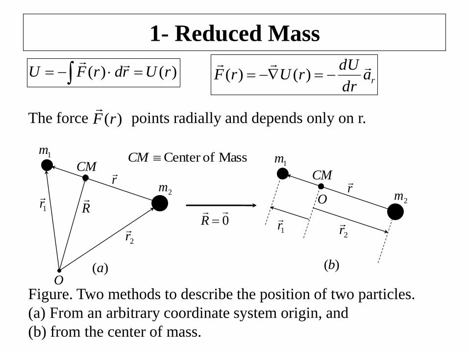
)()( rUrdrFU
radr
dUrUrF
)()(
1m
2m
1r
2r
R
CM
O
r
1m
2m
1r
2r
CM
Or
0
R
Mass ofCenter CM
)(a )(b
Figure. Two methods to describe the position of two particles.
(a) From an arbitrary coordinate system origin, and
(b) from the center of mass.
The force points radially and depends only on r. )(rF
1- Reduced Mass
The relative vector:
1r
2r
and are the position vectors for, respectively, m1 and m2.
21 rrr
The center of mass vector: 21
2211
mm
rmrmR
Translational motion of the system is uninteresting, so we use 0
R
00 2211
rmrmR
0)( 1211
rrmrm
0)( 2121
rmrmm
rmm
mr
21
21
0)( 2221
rmrrm
0)( 2211
rmmrm
rmm
mr
21
12
1- Reduced Mass
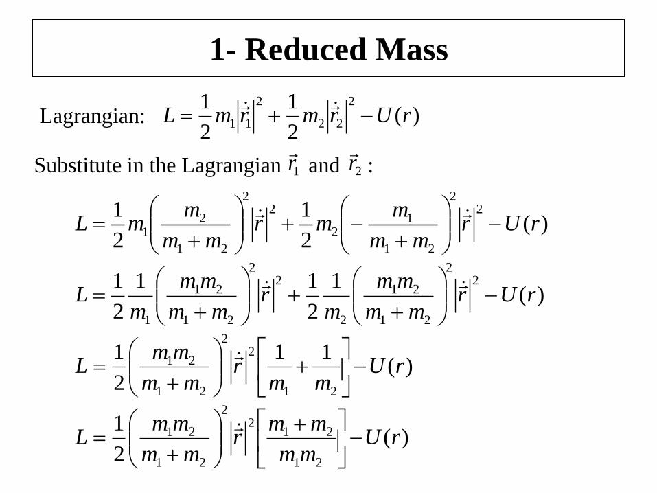
Lagrangian: )(2
1
2
1 2
22
2
11 rUrmrmL
Substitute in the Lagrangian and : 1r
2r
)(2
1
2
1 22
21
12
22
21
21 rUr
mm
mmr
mm
mmL
)(1
2
11
2
1 22
21
21
2
22
21
21
1
rUrmm
mm
mr
mm
mm
mL
)(11
2
1
21
22
21
21 rUmm
rmm
mmL
)(2
1
21
212
2
21
21 rUmm
mmr
mm
mmL
1- Reduced Mass
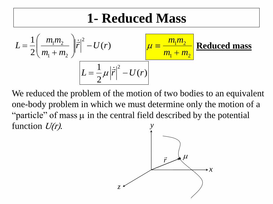
)(2
1 2
21
21 rUrmm
mmL
21
21
mm
mm
Reduced mass
)(2
1 2
rUrL
We reduced the problem of the motion of two bodies to an equivalent
one-body problem in which we must determine only the motion of a
“particle” of mass in the central field described by the potential
function U(r).
x
y
z
r
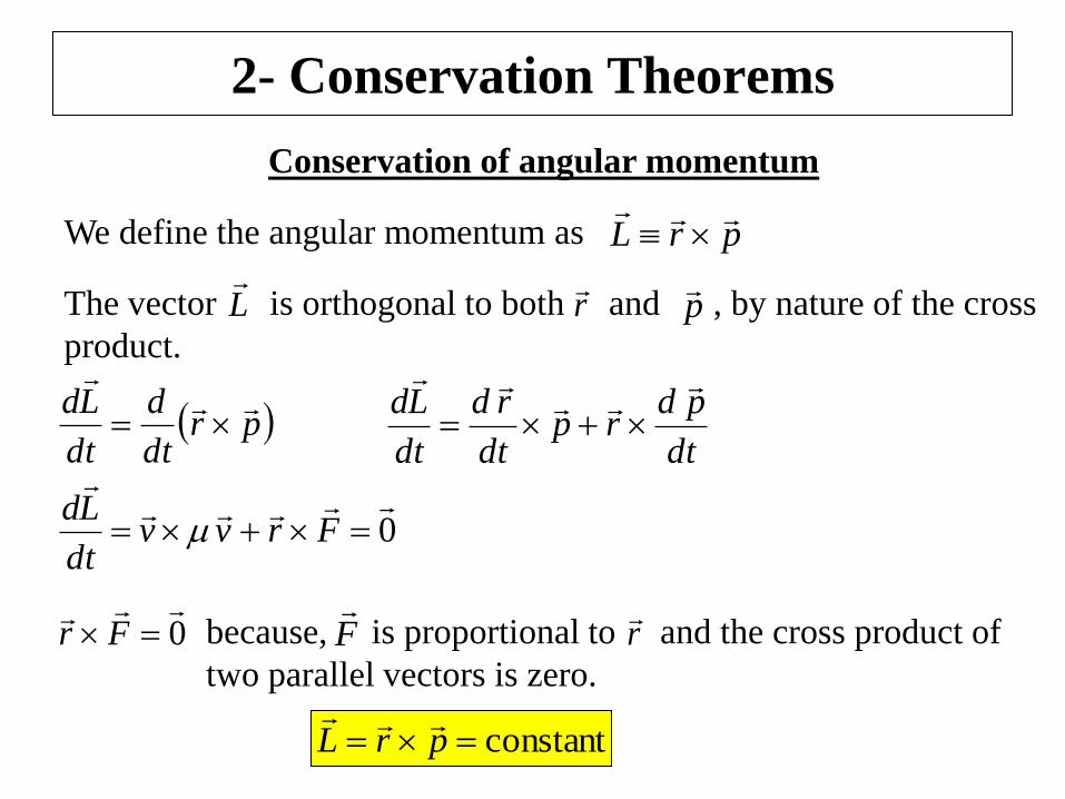
2- Conservation Theorems
Conservation of angular momentum
We define the angular momentum as prL
The vector is orthogonal to both and , by nature of the cross
product.
L
r
p
prdt
d
dt
Ld
dt
pdrp
dt
rd
dt
Ld
0
Frvvdt
Ld
0
Fr because, is proportional to and the cross product of
two parallel vectors is zero.
F
r
constant prL
2- Conservation Theorems
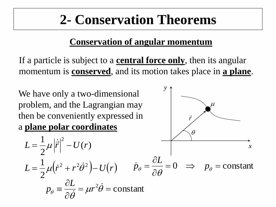
Conservation of angular momentum
If a particle is subject to a central force only, then its angular
momentum is conserved, and its motion takes place in a plane.
r
x
y
We have only a two-dimensional
problem, and the Lagrangian may
then be conveniently expressed in
a plane polar coordinates
rUrrL 222
2
1
)(2
1 2
rUrL
constant0
p
Lp
constant2
r
Lp
2- Conservation Theorems
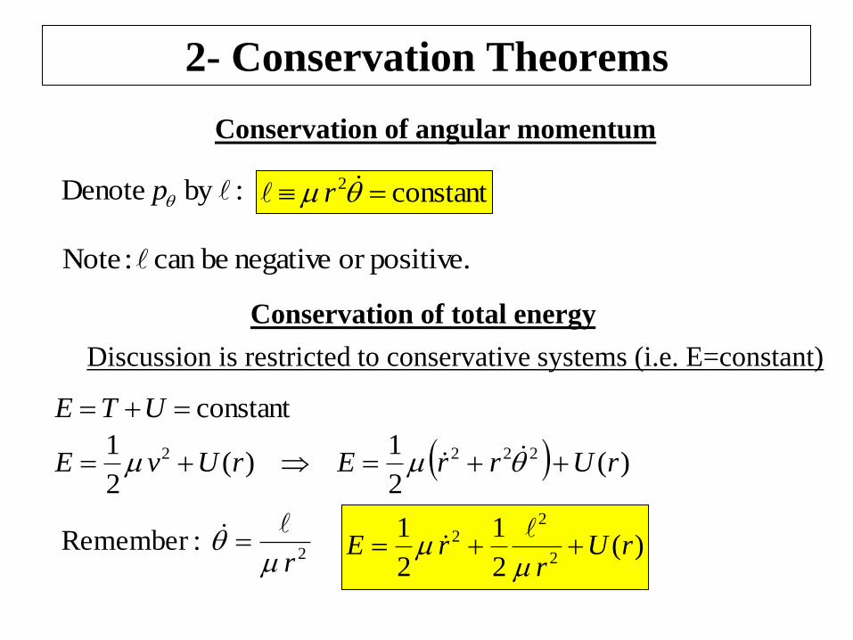
Conservation of angular momentum
constant2 r
positive.or negative becan :Note
:by Denote p
Conservation of total energy
Discussion is restricted to conservative systems (i.e. E=constant)
constant UTE
)(2
1)(
2
1 2222 rUrrErUvE
)(2
1
2
12
22 rU
rrE
2
:Rememberr
3- Equations of Motion
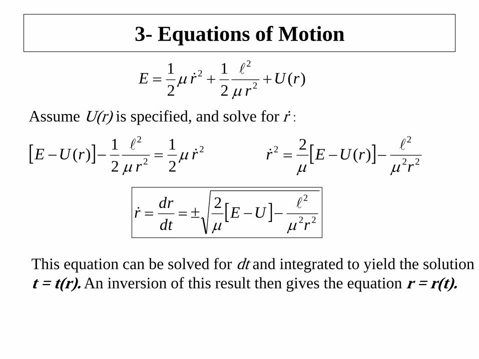
)(2
1
2
12
22 rU
rrE
Assume U(r) is specified, and solve for ṙ :
2
2
2
2
1
2
1)( r
rrUE
22
22 )(
2
rrUEr
22
22
rUE
dt
drr
This equation can be solved for dt and integrated to yield the solution
t = t(r). An inversion of this result then gives the equation r = r(t).
3- Equations of Motion
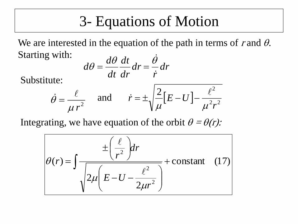
We are interested in the equation of the path in terms of r and .
Starting with:
drr
drdr
dt
dt
dd
Substitute:
2r
22
22
rUEr
and
Integrating, we have equation of the orbit = (r):
)17(constant
22
)(
2
2
2
rUE
drr
r
3- Equations of Motion
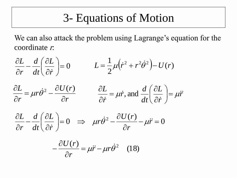
We can also attack the problem using Lagrange’s equation for the
coordinate r:
0
r
L
dt
d
r
L
)(
2
1 222 rUrrL
r
rUr
r
L
)(2 rr
L
dt
dr
r
L
and ,
0)(
0 2
r
r
rUr
r
L
dt
d
r
L
)18()( 2 rr
r
rU
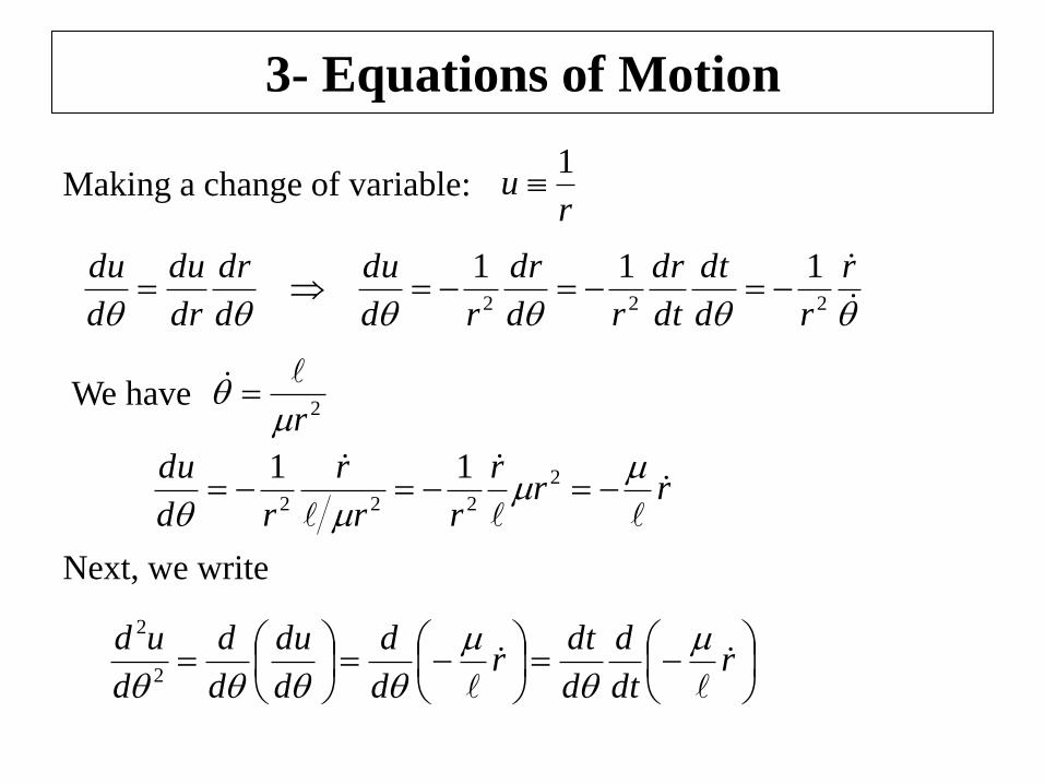
3- Equations of Motion
Making a change of variable: r
u1
r
rd
dt
dt
dr
rd
dr
rd
du
d
dr
dr
du
d
du222
111
2r
We have
rrr
rr
r
rd
du
2
222
11
Next, we write
r
dt
d
d
dtr
d
d
d
du
d
d
d
ud
2
2
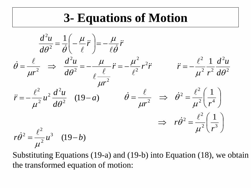
3- Equations of Motion
rrd
ud
12
2
rrr
r
d
ud
r
2
2
2
2
2
2
2
2
2
22
2 1
d
ud
rr
)19(2
22
2
2
ad
udur
32
22
42
22
2
1
1
rr
rr
)19(3
2
22 bur
Substituting Equations (19-a) and (19-b) into Equation (18), we obtain
the transformed equation of motion:
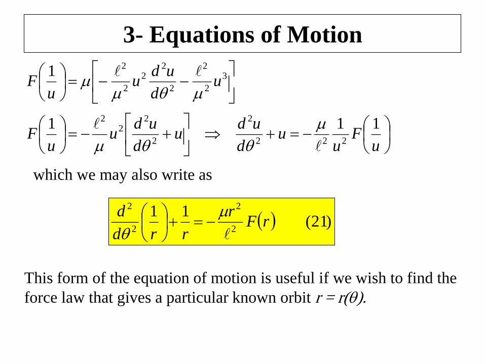
3- Equations of Motion
3
2
2
2
22
2
21u
d
udu
uF
uF
uu
d
udu
d
udu
uF
111222
2
2
22
2
which we may also write as
)21(11
2
2
2
2
rFr
rrd
d
This form of the equation of motion is useful if we wish to find the
force law that gives a particular known orbit r = r().
3- Equations of Motion – Example 1
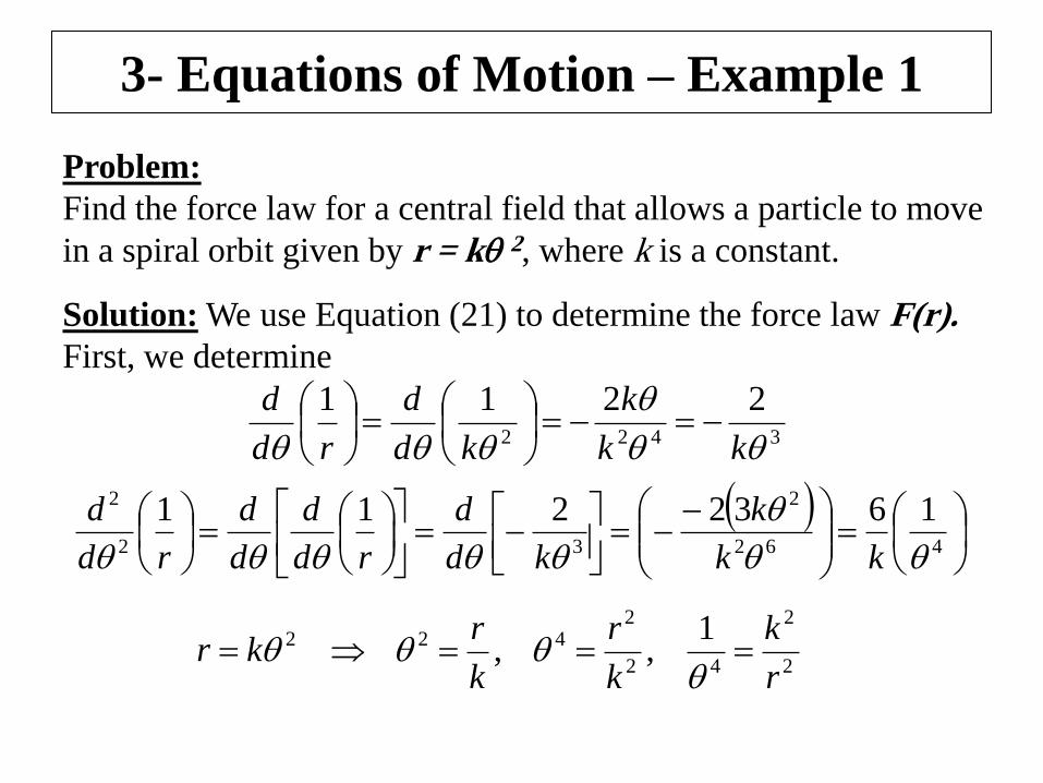
Problem:
Find the force law for a central field that allows a particle to move
in a spiral orbit given by r = k 2, where k is a constant.
Solution: We use Equation (21) to determine the force law F(r).
First, we determine
3422
2211
kk
k
kd
d
rd
d
462
2
32
2 1632211
kk
k
kd
d
rd
d
d
d
rd
d
2
2
42
2422 1
,,r
k
k
r
k
rkr
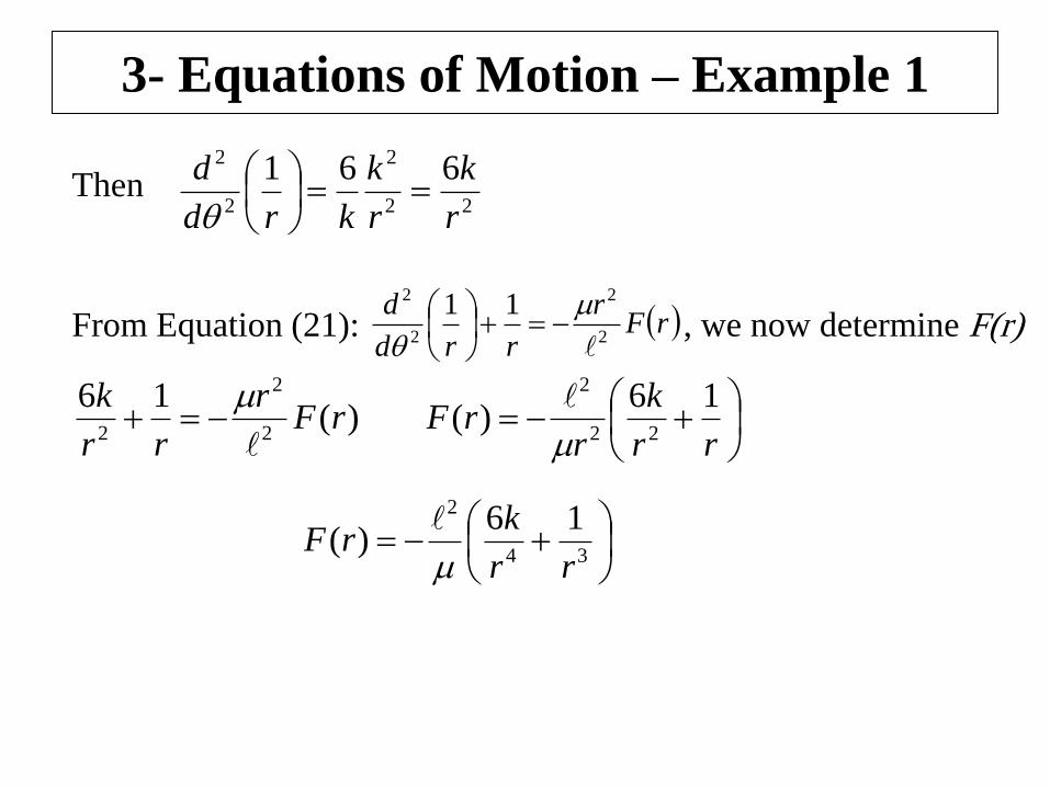
3- Equations of Motion – Example 1
22
2
2
2 661
r
k
r
k
krd
d
Then
rFr
rrd
d2
2
2
2 11
From Equation (21): , we now determine F(r)
)(16
2
2
2rF
r
rr
k
rr
k
rrF
16)(
22
2
34
2 16)(
rr
krF
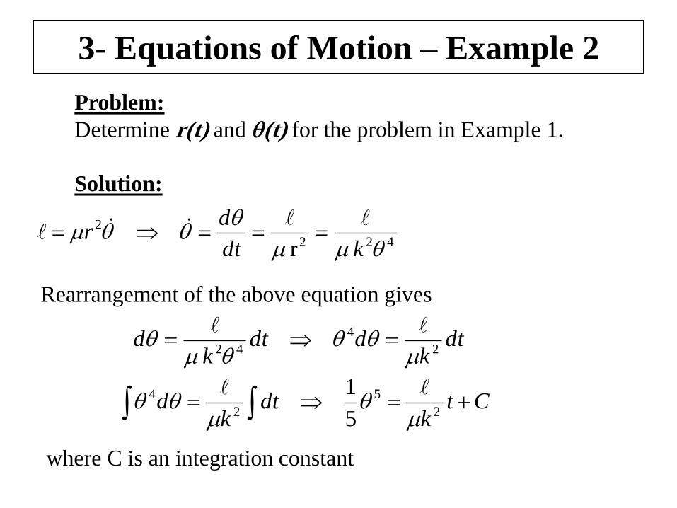
3- Equations of Motion – Example 2
Problem:
Determine r(t) and (t) for the problem in Example 1.
Solution:
422
2
r
kdt
dr
dtk
ddtk
d2
4
42
Rearrangement of the above equation gives
Ctk
dtk
d2
5
2
4
5
1
where C is an integration constant
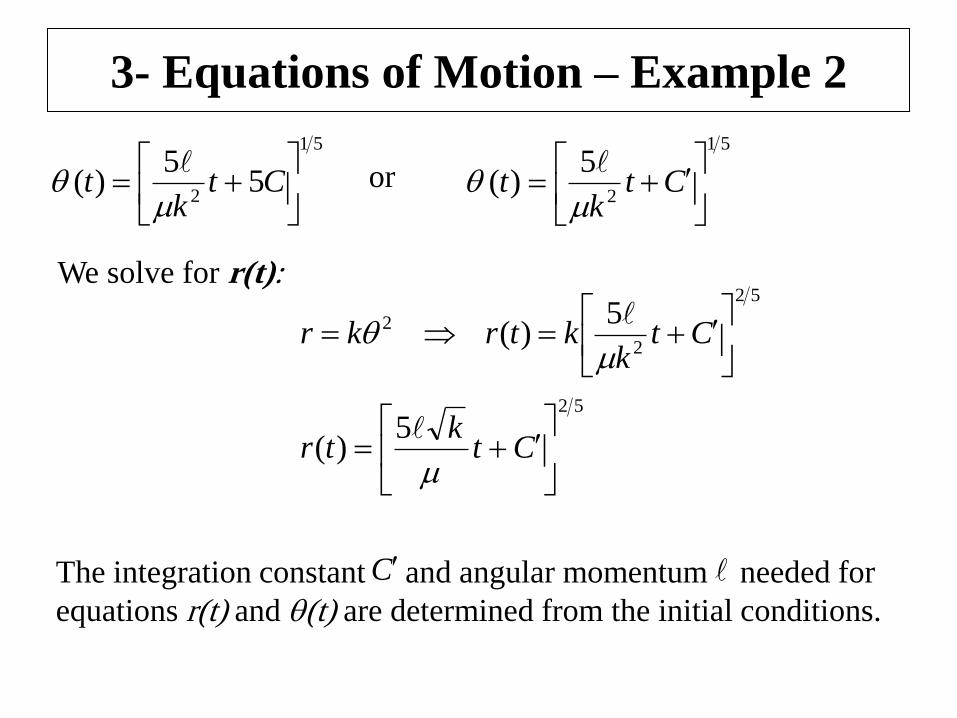
3- Equations of Motion – Example 2
51
25
5)(
Ct
kt
or
51
2
5)(
Ct
kt
We solve for r(t): 52
2
2 5)(
Ct
kktrkr
52
5)(
Ct
ktr
The integration constant and angular momentum needed for
equations r(t) and (t) are determined from the initial conditions.
C
3- Equations of Motion – Example 3
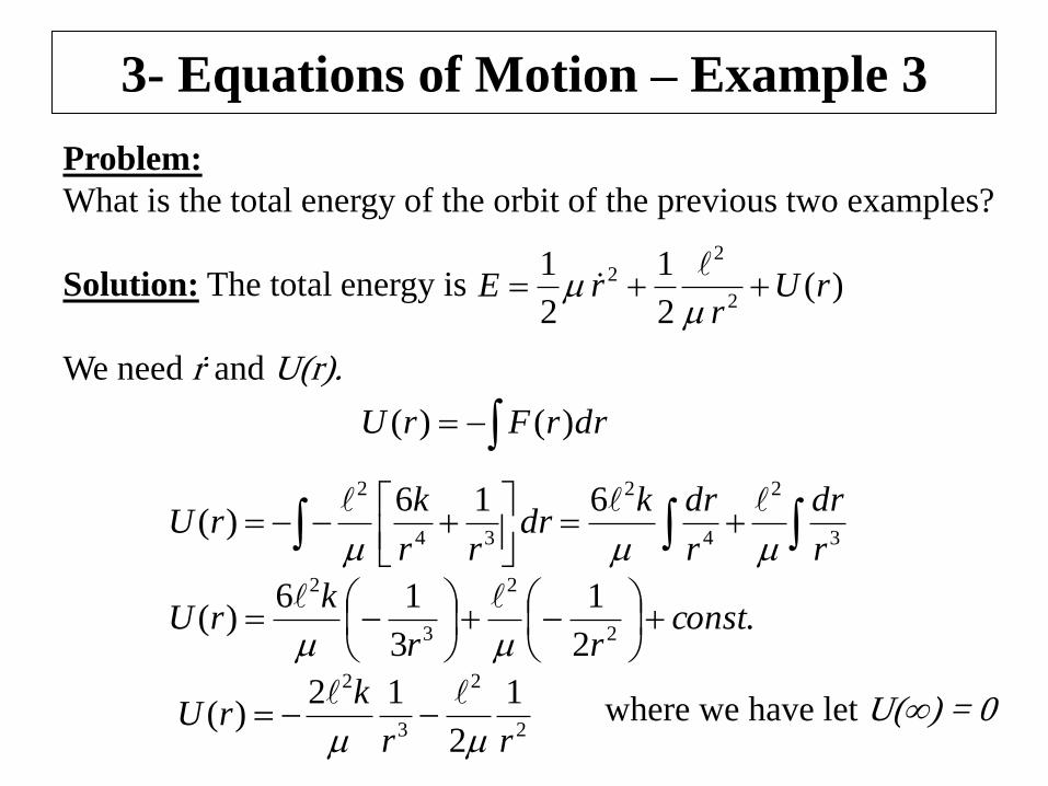
Problem:
What is the total energy of the orbit of the previous two examples?
Solution: The total energy is
We need ṙ and U(r).
)(2
1
2
12
22 rU
rrE
3
2
4
2
34
2 616)(
r
dr
r
drkdr
rr
krU
drrFrU )()(
.2
1
3
16)(
2
2
3
2
constrr
krU
2
2
3
2 1
2
12)(
rr
krU
where we have let U() = 0
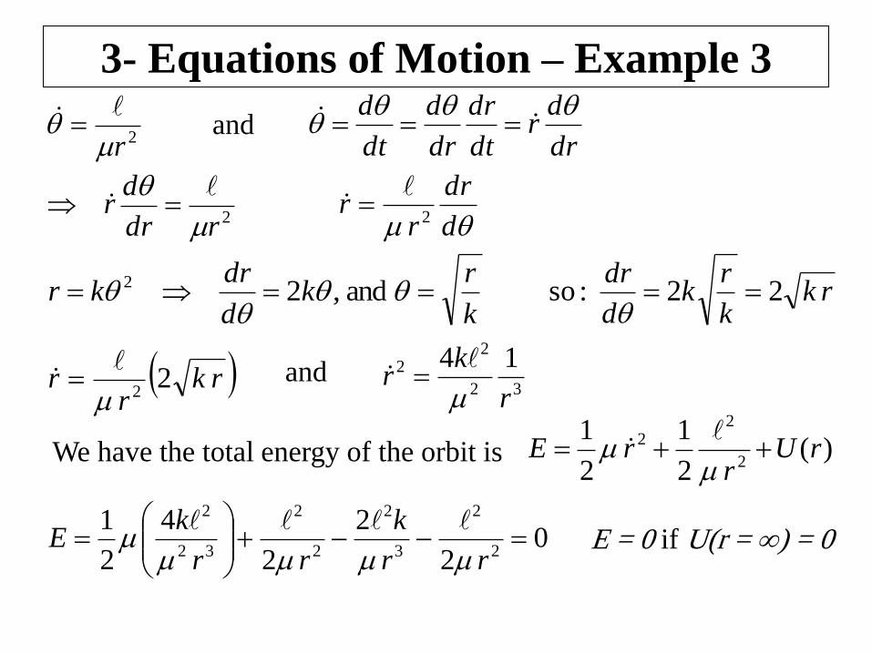
3- Equations of Motion – Example 3
2r
dr
dr
dt
dr
dr
d
dt
d
2rdr
dr
and
d
dr
rr
2
k
rk
d
drkr
and,22 rk
k
rk
d
dr22 :so
rkr
r 22
32
22 14
r
kr
and
We have the total energy of the orbit is )(2
1
2
12
22 rU
rrE
02
2
2
4
2
12
2
3
2
2
2
32
2
rr
k
rr
kE
E = 0 if U(r = ) = 0
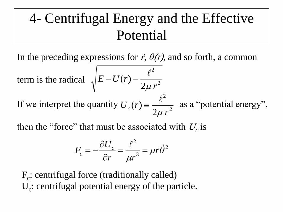
4- Centrifugal Energy and the Effective
Potential
In the preceding expressions for ṙ, (r), and so forth, a common
term is the radical 2
2
2)(
rrUE
2
2
2)(
rrU c
If we interpret the quantity as a “potential energy”,
then the “force” that must be associated with Uc is
2
3
2
r
rr
UF c
c
Fc: centrifugal force (traditionally called)
Uc: centrifugal potential energy of the particle.
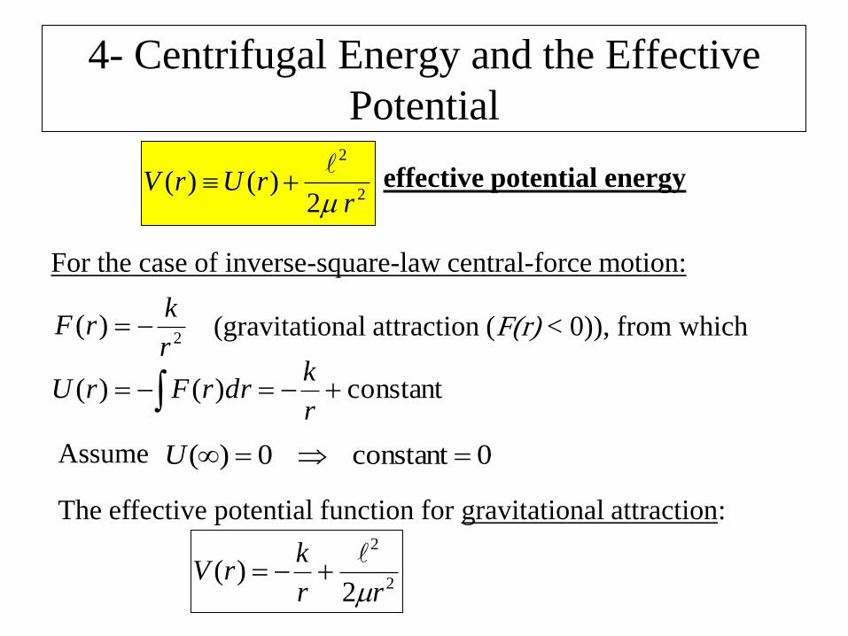
4- Centrifugal Energy and the Effective
Potential
2
2
2)()(
rrUrV
effective potential energy
For the case of inverse-square-law central-force motion:
2)(
r
krF (gravitational attraction (F(r) < 0)), from which
constant)()(r
kdrrFrU
0constant0)( UAssume
The effective potential function for gravitational attraction:
2
2
2)(
rr
krV
4- Centrifugal Energy and the Effective
Potential
r
1E
2E
3E
2
2
1r
4r3r2r
1r
2
2
2)(
rr
krV
)(
2
1 2 rVrE
)(02
1 2 rVEr
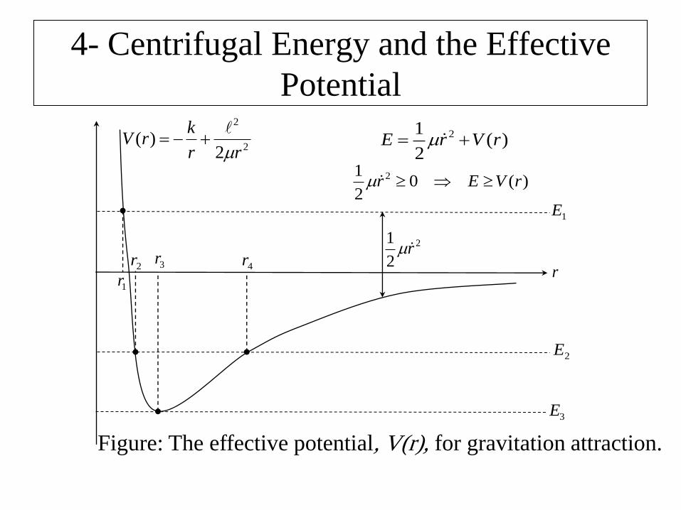
Figure: The effective potential, V(r), for gravitation attraction.
4- Centrifugal Energy and the Effective
Potential
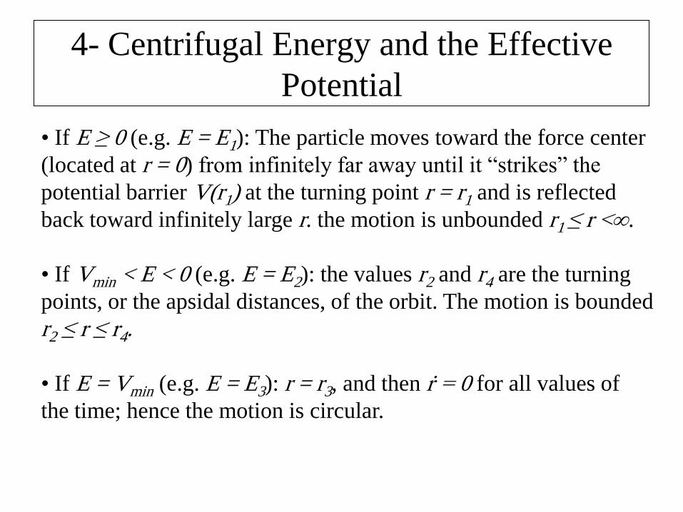
• If E ≥ 0 (e.g. E = E1): The particle moves toward the force center
(located at r = 0) from infinitely far away until it “strikes” the
potential barrier V(r1) at the turning point r = r1 and is reflected
back toward infinitely large r. the motion is unbounded r1 ≤ r <.
• If Vmin < E < 0 (e.g. E = E2): the values r2 and r4 are the turning
points, or the apsidal distances, of the orbit. The motion is bounded
r2 ≤ r ≤ r4.
• If E = Vmin (e.g. E = E3): r = r3, and then ṙ = 0 for all values of
the time; hence the motion is circular.
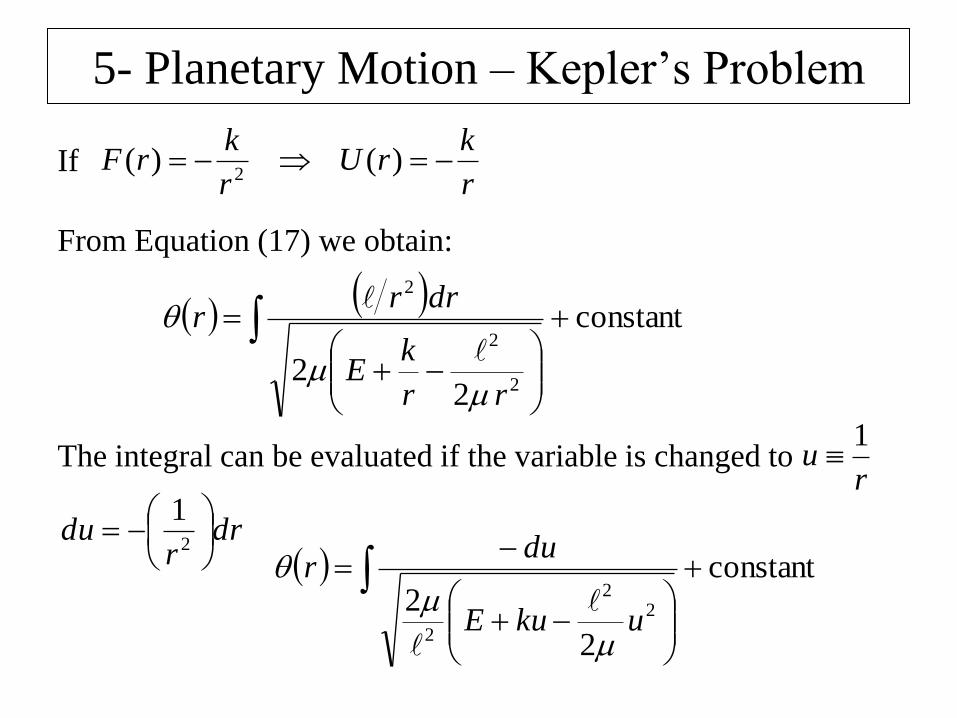
5- Planetary Motion – Kepler’s Problem
r
krU
r
krF )()(
2If
From Equation (17) we obtain:
constant
22
2
2
2
rr
kE
drrr
The integral can be evaluated if the variable is changed to r
u1
drr
du
2
1
constant
2
2 22
2
ukuE
dur
5- Planetary Motion – Kepler’s Problem
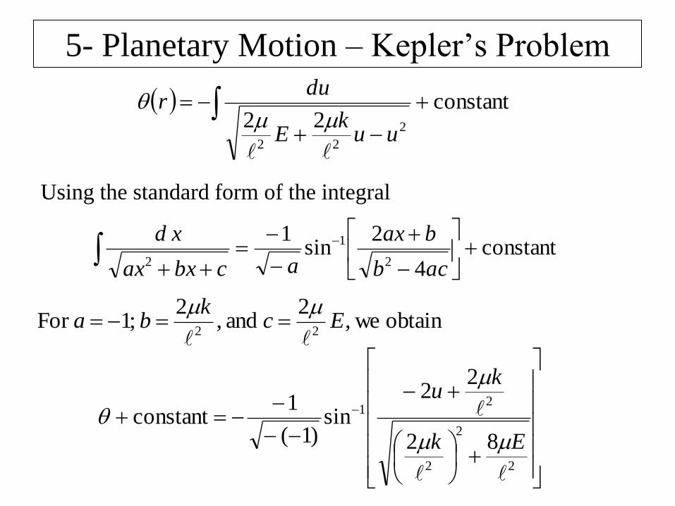
constant22 2
22
uu
kE
dur
Using the standard form of the integral
constant4
2sin
12
1
2
acb
bax
acbxax
xd
obtain we,2
and ,2
;1For 22
Eck
ba
2
2
2
21
82
22
sin)1(
1constant
Ek
ku
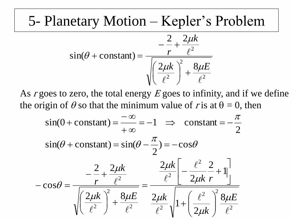
5- Planetary Motion – Kepler’s Problem
2
2
2
2
82
22
constant)sin(
Ek
k
r
As r goes to zero, the total energy E goes to infinity, and if we define
the origin of so that the minimum value of r is at = 0, then
2constant1)constant0sin(
cos)2
sin()constantsin(
2
22
2
2
2
2
2
2
2
8
21
2
12
2
2
82
22
cos
E
k
k
rk
k
Ek
k
r
5- Planetary Motion – Kepler’s Problem
2
2
2
21
11
cos
k
E
rk
2
2
2
21
11
cos
k
E
rk
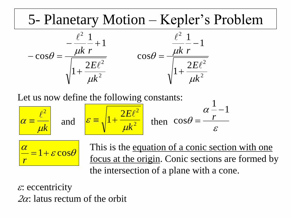
Let us now define the following constants:
k
2 2
221
k
E
and
11
cos
rthen
cos1r
This is the equation of a conic section with one
focus at the origin. Conic sections are formed by
the intersection of a plane with a cone.
: eccentricity
2: latus rectum of the orbit
5- Planetary Motion – Kepler’s Problem
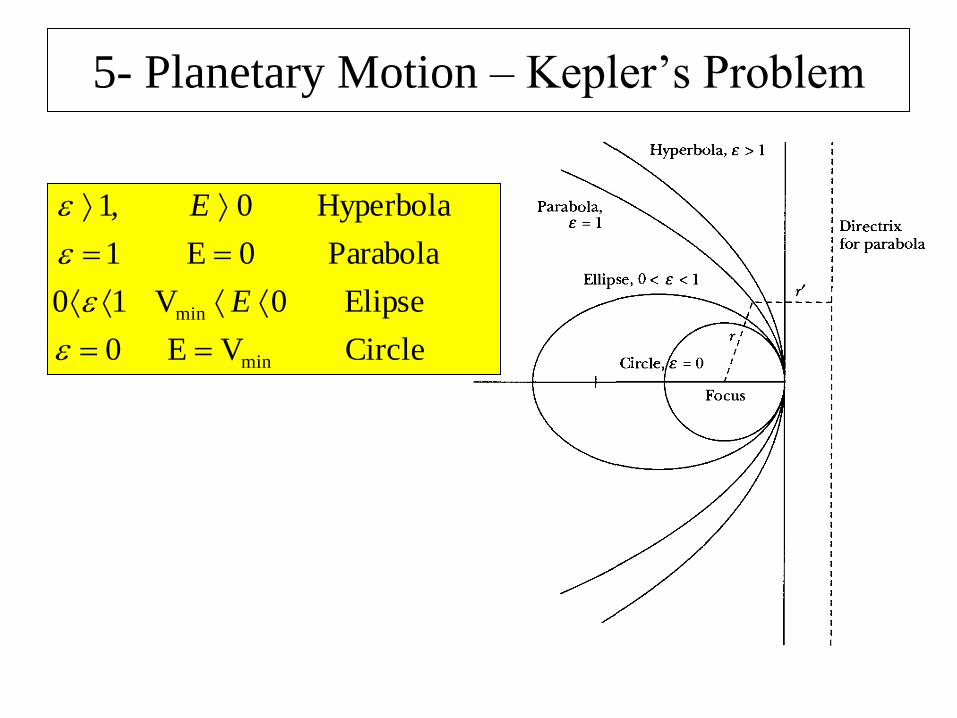
CircleVE0
Elipse0V10
Parabola0E1
Hyperbola0,1
min
min
E
E
5- Planetary Motion – Kepler’s Problem
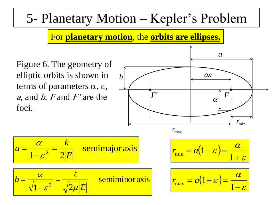
axissemimajor 21 2 E
ka
For planetary motion, the orbits are ellipses.
axissemiminor 21 2 E
b
FF
a
a
b
minr
maxr
Figure 6. The geometry of
elliptic orbits is shown in
terms of parameters , ,
a, and b. F and F’ are the
foci.
11min ar
11max ar
5- Planetary Motion – Kepler’s Problem
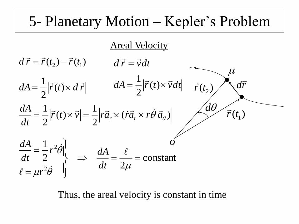
Areal Velocity
d
)( 2tr
)( 1tr
rd
o
)()( 12 trtrrd
dtvrd
rdtrdA
)(2
1 dtvtrdA
)(2
1
)(2
1)(
2
1 arararvtr
dt
dArr
constant2
2
1
2
2
dt
dA
r
rdt
dA
Thus, the areal velocity is constant in time
5- Planetary Motion – Kepler’s Problem
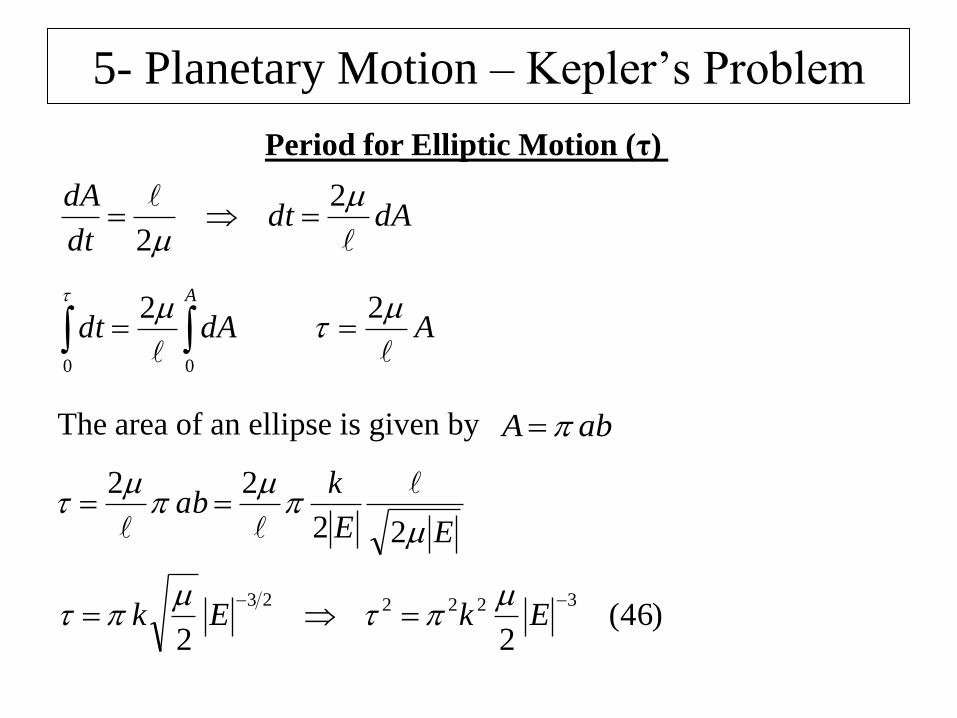
Period for Elliptic Motion (τ)
dAdtdt
dA
2
2
A
dAdt00
2
A
2
The area of an ellipse is given by abA
EE
kab
22
22
)46(22
322223 EkEk
5- Planetary Motion – Kepler’s Problem
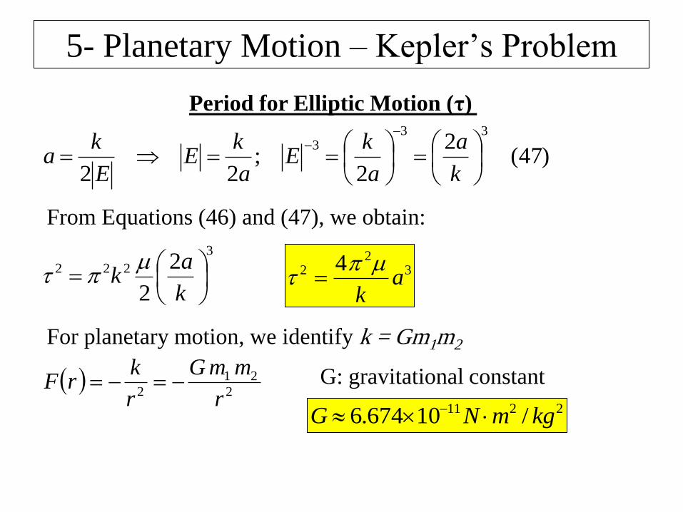
Period for Elliptic Motion (τ)
)47(2
2;
22
333
k
a
a
kE
a
kE
E
ka
From Equations (46) and (47), we obtain:
3
222 2
2
k
ak
3
22 4
ak
For planetary motion, we identify k = Gm1m2
2
21
2 r
mmG
r
krF
2211 /10674.6 kgmNG
G: gravitational constant
5- Planetary Motion – Kepler’s Problem
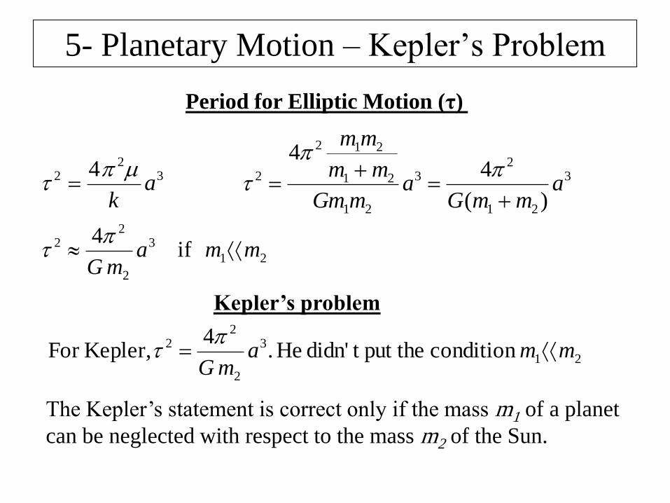
3
21
23
21
21
212
2
)(
44
ammG
amGm
mm
mm
Period for Elliptic Motion (τ)
32
2 4a
k
21
3
2
22 if
4mma
mG
Kepler’s problem
21
3
2
22 condition put thet didn' He .
4 Kepler,For mma
mG
The Kepler’s statement is correct only if the mass m1 of a planet
can be neglected with respect to the mass m2 of the Sun.
5- Planetary Motion – Kepler’s Problem
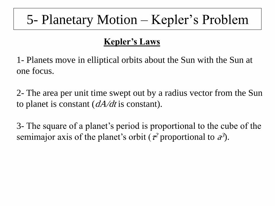
1- Planets move in elliptical orbits about the Sun with the Sun at
one focus.
2- The area per unit time swept out by a radius vector from the Sun
to planet is constant (dA/dt is constant).
3- The square of a planet’s period is proportional to the cube of the
semimajor axis of the planet’s orbit (τ2 proportional to a3).
Kepler’s Laws
Chapter 5
Motion in a Noninertial
Reference Frame
Dr. Abdelaziz Sabik
Physics Department – College of Science
Al-Imam Muhammad Ibn Saud Islamic University
1- Reference Frame
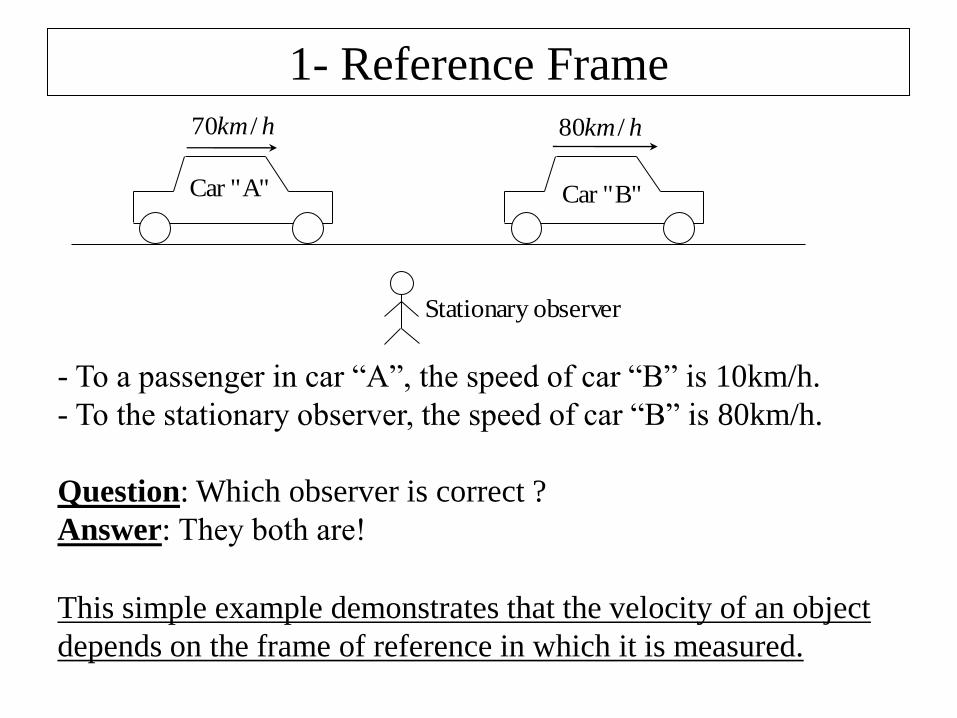
hkm /70 hkm /80
observer Stationary
A""Car B""Car
- To a passenger in car “A”, the speed of car “B” is 10km/h.
- To the stationary observer, the speed of car “B” is 80km/h.
Question: Which observer is correct ?
Answer: They both areǃ
This simple example demonstrates that the velocity of an object
depends on the frame of reference in which it is measured.
1- Reference Frame
Conclusion:
For the laws of motion to have meaning, the motion of bodies must
be measured relative to some reference frame.
Inertial Reference Frame
A reference frame is called an inertial frame if Newton’s laws are
valid in that frame.
For example, if a body subject to no force moves with constant
velocity in a certain coordinate system, that system is, by definition,
an inertial frame.
Consequence:
An inertial reference frame is one that is not accelerating.
1- Reference Frame
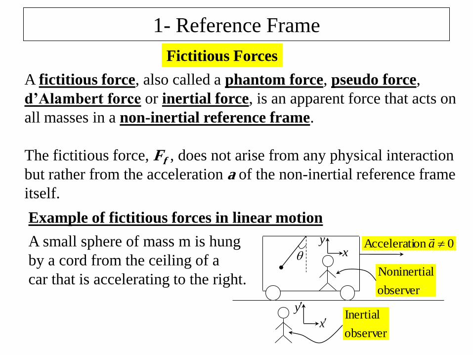
Fictitious Forces
A fictitious force, also called a phantom force, pseudo force,
d’Alambert force or inertial force, is an apparent force that acts on
all masses in a non-inertial reference frame.
The fictitious force, Ff , does not arise from any physical interaction
but rather from the acceleration a of the non-inertial reference frame
itself.
Example of fictitious forces in linear motion
0on Accelerati a
xy
x
y
observer
Inertial
observer
lNoninertia
A small sphere of mass m is hung
by a cord from the ceiling of a
car that is accelerating to the right.
1- Reference Frame
gm
T
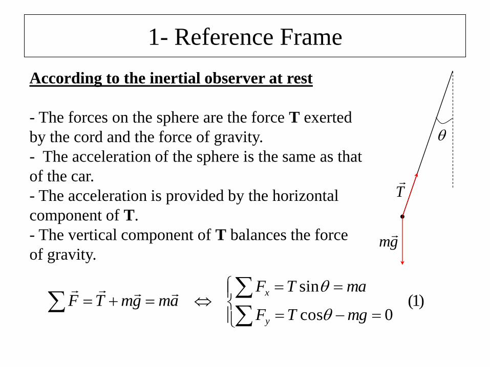
According to the inertial observer at rest
- The forces on the sphere are the force T exerted
by the cord and the force of gravity.
- The acceleration of the sphere is the same as that
of the car.
- The acceleration is provided by the horizontal
component of T.
- The vertical component of T balances the force
of gravity.
)1(0cos
sin
mgTF
maTFamgmTF
y
x
1- Reference Frame
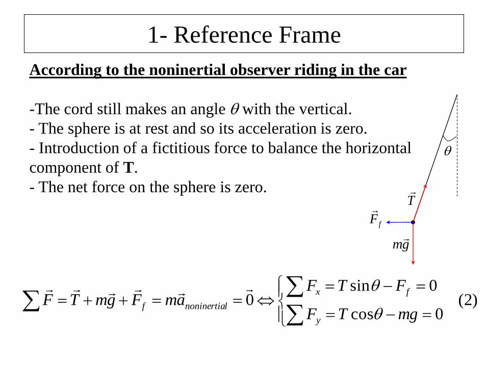
According to the noninertial observer riding in the car
-The cord still makes an angle with the vertical.
- The sphere is at rest and so its acceleration is zero.
- Introduction of a fictitious force to balance the horizontal
component of T.
- The net force on the sphere is zero.
gm
T
fF
)2(0cos
0sin0
mgTF
FTFamFgmTF
y
fx
lnoninertiaf
1- Reference Frame
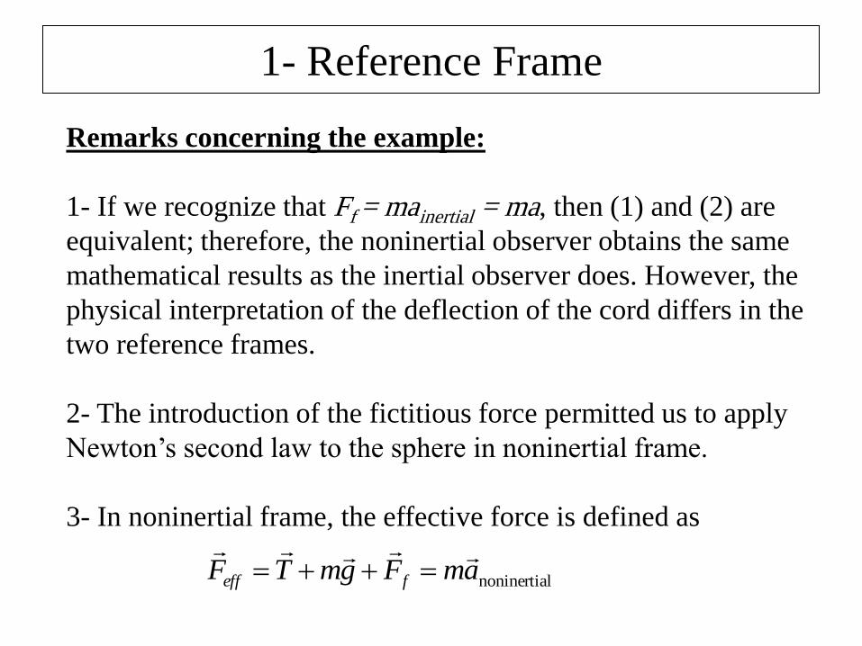
Remarks concerning the example:
1- If we recognize that Ff = mainertial = ma, then (1) and (2) are
equivalent; therefore, the noninertial observer obtains the same
mathematical results as the inertial observer does. However, the
physical interpretation of the deflection of the cord differs in the
two reference frames.
2- The introduction of the fictitious force permitted us to apply
Newton’s second law to the sphere in noninertial frame.
3- In noninertial frame, the effective force is defined as
lnoninertiaamFgmTF feff
2- Rotating Coordinate Systems
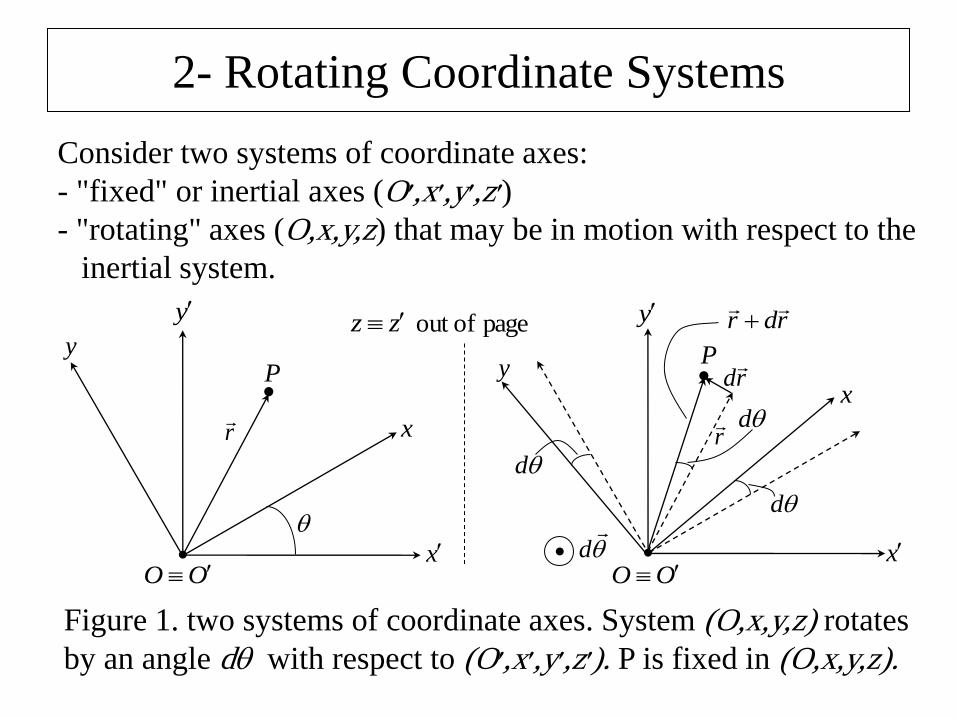
Consider two systems of coordinate axes:
- "fixed" or inertial axes (O׳,x׳,y׳,z׳)
- "rotating" axes (O,x,y,z) that may be in motion with respect to the
inertial system.
r
PP
r
d
d
d
d
rd
rdr
x
y
x
y
x
x
y
y
OO OO
zz page ofout
Figure 1. two systems of coordinate axes. System (O,x,y,z) rotates
by an angle d with respect to (O׳,x׳,y׳,z׳). P is fixed in (O,x,y,z).
2- Rotating Coordinate Systems
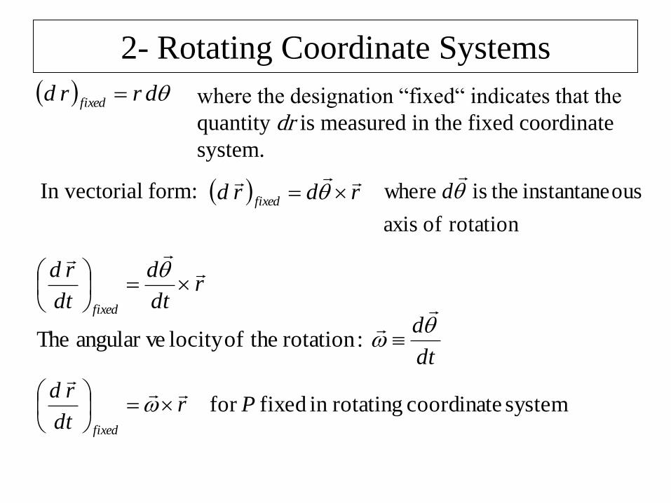
drrdfixed
In vectorial form: rdrdfixed
rotation of axis
ousinstantane theis where
d
rdt
d
dt
rd
fixed
dt
d
:rotation theoflocity angular ve The
systemcoordinate rotatingin fixed for Prdt
rd
fixed
where the designation “fixed“ indicates that the
quantity dr is measured in the fixed coordinate
system.
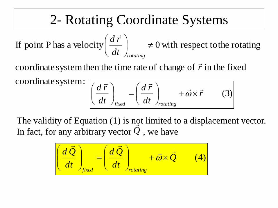
2- Rotating Coordinate Systems
:system coordinate
fixed in the of change of rate time then thesystem coordinate
rotating therespect to with 0 velocity a has Ppoint If
r
dt
rd
rotating
)3(rdt
rd
dt
rd
rotatingfixed
The validity of Equation (1) is not limited to a displacement vector.
In fact, for any arbitrary vector , we have
)4(Qdt
Qd
dt
Qd
rotatingfixed
Q
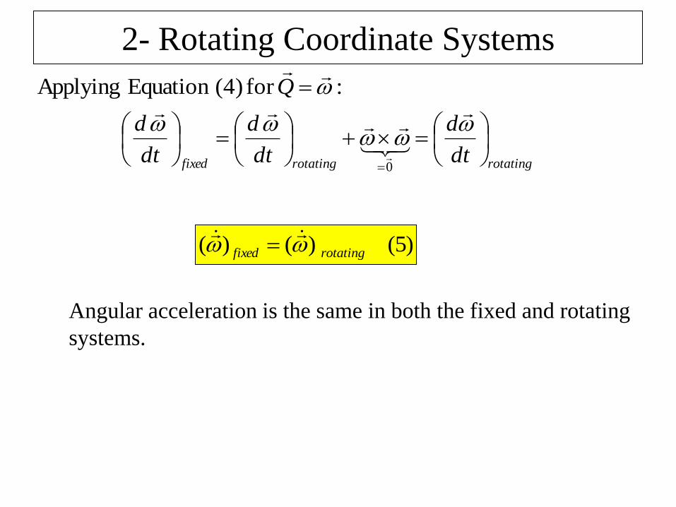
2- Rotating Coordinate Systems
:for (4)Equation Applying
Q
Angular acceleration is the same in both the fixed and rotating
systems.
rotatingrotatingfixed dt
d
dt
d
dt
d
0
)5()()( rotatingfixed
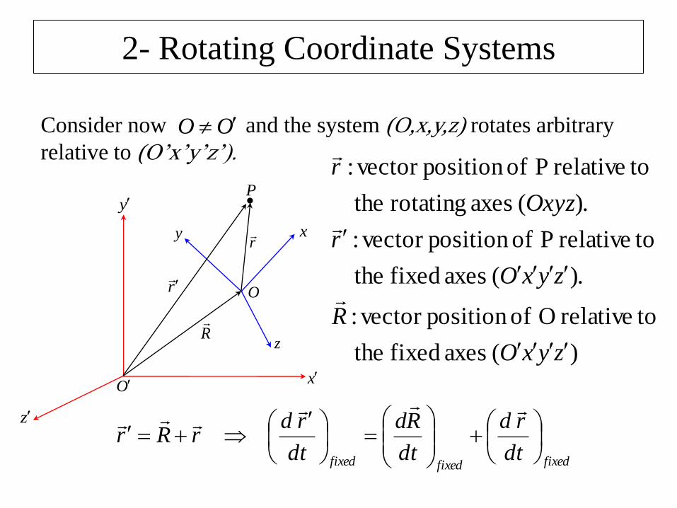
2- Rotating Coordinate Systems
R
r
r
Ox
y
z
O
xy
z
P
)( axes fixed the
torelative O ofposition vector :
.)( axes fixed the
torelative P ofposition vector :
.)( axes rotating the
torelative P ofposition vector :
zyxO
R
zyxO
r
Oxyz
r
Consider now and the system (O,x,y,z) rotates arbitrary
relative to (O’x’y’z’). OO
fixedfixedfixed dt
rd
dt
Rd
dt
rdrRr
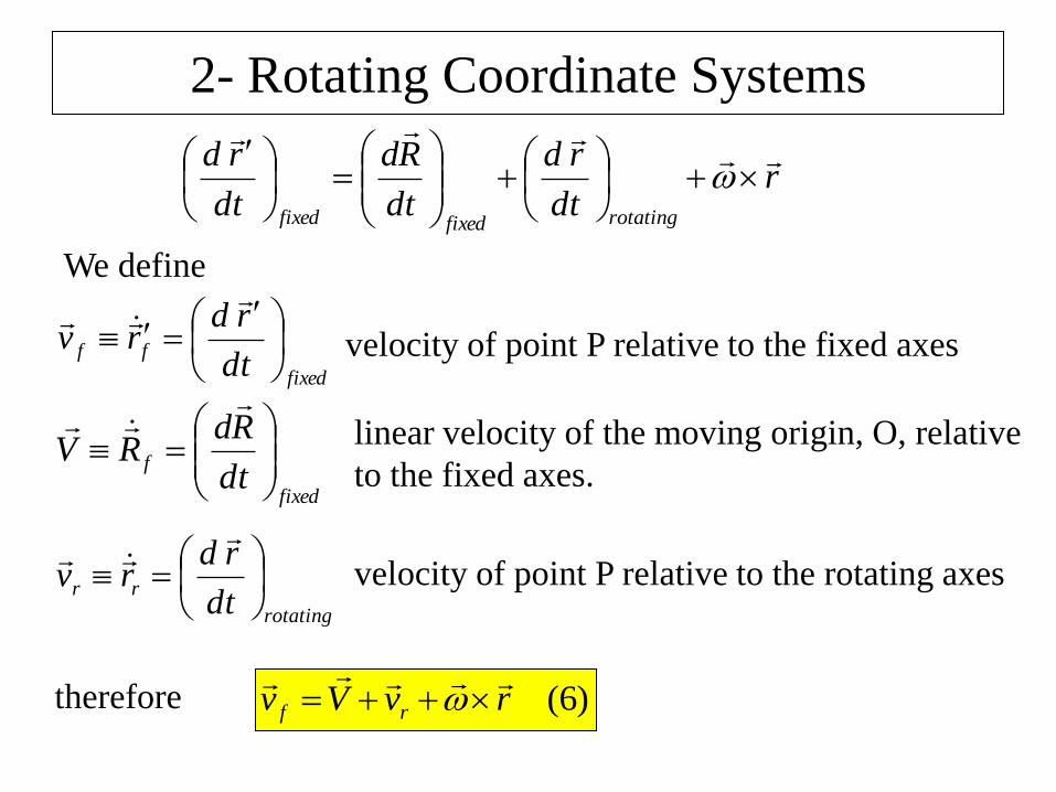
2- Rotating Coordinate Systems
rdt
rd
dt
Rd
dt
rd
rotatingfixedfixed
fixed
ffdt
rdrv
fixed
fdt
RdRV
We define
velocity of point P relative to the fixed axes
linear velocity of the moving origin, O, relative
to the fixed axes.
rotating
rrdt
rdrv
velocity of point P relative to the rotating axes
)6(rvVv rf
therefore
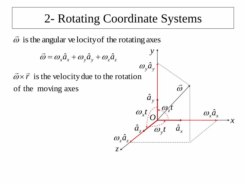
2- Rotating Coordinate Systems
x
y
z
O
xa
ya
za
tx
ty
tzxxa
yya
zza
zzyyxx aaa ˆˆˆ
axes rotating theoflocity angular ve theis
axes moving theof
rotation the todue velocity theis r
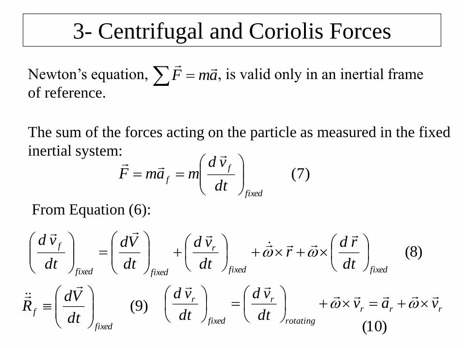
3- Centrifugal and Coriolis Forces
Newton’s equation, , is valid only in an inertial frame
of reference. amF
The sum of the forces acting on the particle as measured in the fixed
inertial system:
(7)
fixed
f
fdt
vdmamF
)8(fixedfixed
r
fixedfixed
f
dt
rdr
dt
vd
dt
Vd
dt
vd
From Equation (6):
)9(
fixed
fdt
VdR
rrr
rotating
r
fixed
r vavdt
vd
dt
vd
)10(
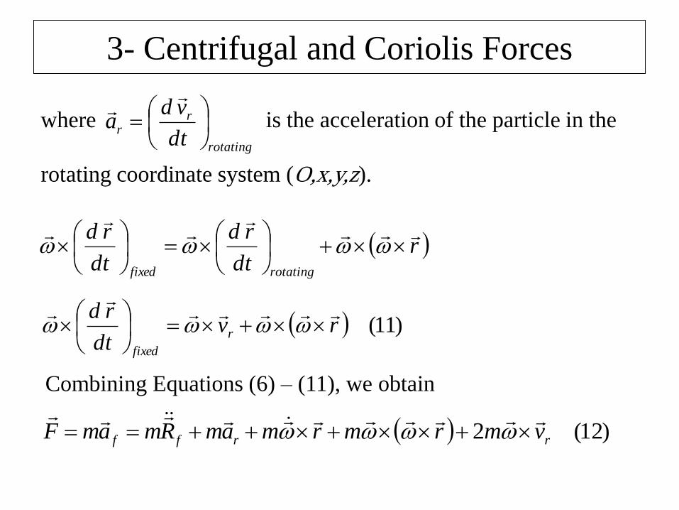
3- Centrifugal and Coriolis Forces
rotating
rr
dt
vda
where is the acceleration of the particle in the
rotating coordinate system (O,x,y,z).
rdt
rd
dt
rd
rotatingfixed
)11(rvdt
rdr
fixed
Combining Equations (6) – (11), we obtain
)12(2 rrff vmrmrmamRmamF
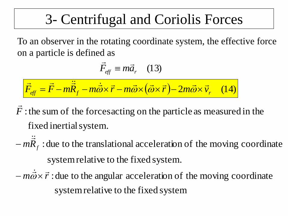
3- Centrifugal and Coriolis Forces
To an observer in the rotating coordinate system, the effective force
on a particle is defined as
)13(reff amF
)14(2 rfeff vmrmrmRmFF
system fixed the torelative system
coordinate moving theofon acceleratiangular the todue :
system. fixed the torelative system
coordinate moving theofon accelerati onal translati the todue :
system. inertial fixed
in the measured as particle on the acting forces theof sum the:
rm
Rm
F
f
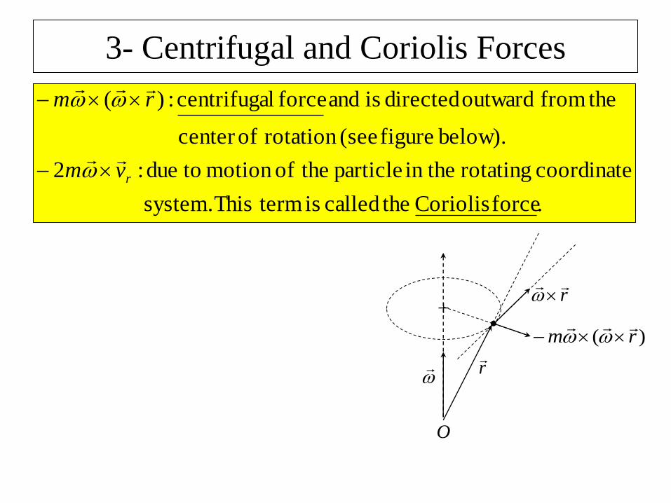
3- Centrifugal and Coriolis Forces
.force Coriolis thecalled is termThis system.
coordinate rotating in the particle theofmotion todue :2
below). figure (seerotation ofcenter
thefrom outward directed is and force lcentrifuga :)(
rvm
rm
r
r
O
)( rm
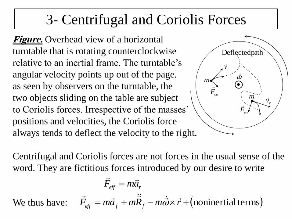
3- Centrifugal and Coriolis Forces
Centrifugal and Coriolis forces are not forces in the usual sense of the
word. They are fictitious forces introduced by our desire to write
reff amF
We thus have: termslnoninertia rmRmamF ffeff
rv
rvcoF
coF
m
m
path Deflected
Figure. Overhead view of a horizontal
turntable that is rotating counterclockwise
relative to an inertial frame. The turntable’s
angular velocity points up out of the page.
as seen by observers on the turntable, the
two objects sliding on the table are subject
to Coriolis forces. Irrespective of the masses’
positions and velocities, the Coriolis force
always tends to deflect the velocity to the right.
4- Motion Relative to the Earth
The Earth is not really an inertial frame for the following reasons:
1- its orbital motion around the Sun experiences a centripetal
acceleration of about 4.4×10⁻³m/s2 directed toward the Sun.
2- its rotational motion about its own axis once every 24 hours, a
point on the equator experiences an additional acceleration of
33.710-3m/s2 directed toward the center of the Earth.
3- the motion of the solar system with respect to the local galaxy…etc
4- Motion Relative to the Earth
The motion of Earth with respect to an inertial reference frame is
dominated by Earth’s rotation about its own axis. The effects of
the other motions are small by comparison.
Therefore let’s explicitly take the Earth’s surface as the rotating
frame and the center of Earth as the fixed frame.
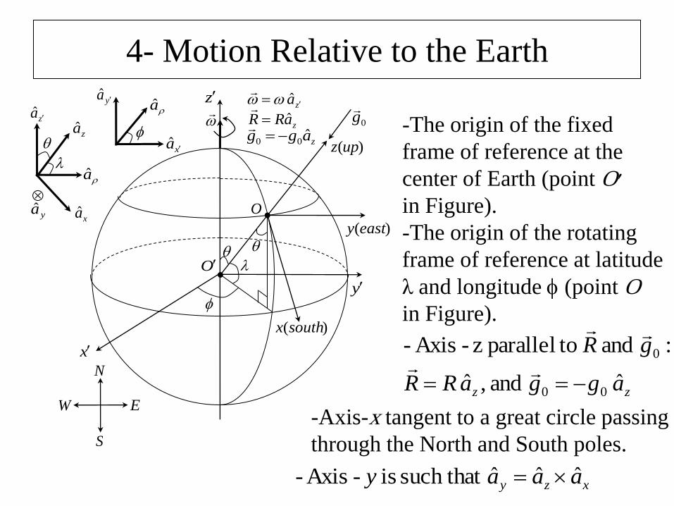
4- Motion Relative to the Earth
-The origin of the fixed
frame of reference at the
center of Earth (point O׳
in Figure).
-The origin of the rotating
frame of reference at latitude
λ and longitude (point O in Figure).
zz aggaRR
gR
ˆ and ,ˆ
: and toparallel z-Axis -
00
0
-Axis-x tangent to a great circle passing
through the North and South poles.
xzy aaay ˆˆˆsuch that is -Axis-
xa
za
x
y
z
N
S
EW
O
O
za ˆ
xa ˆ
ya ˆ
a
a
zaRR ˆ
0g
ya
zagg ˆ00
za ˆ
)(upz
)(easty
)(southx
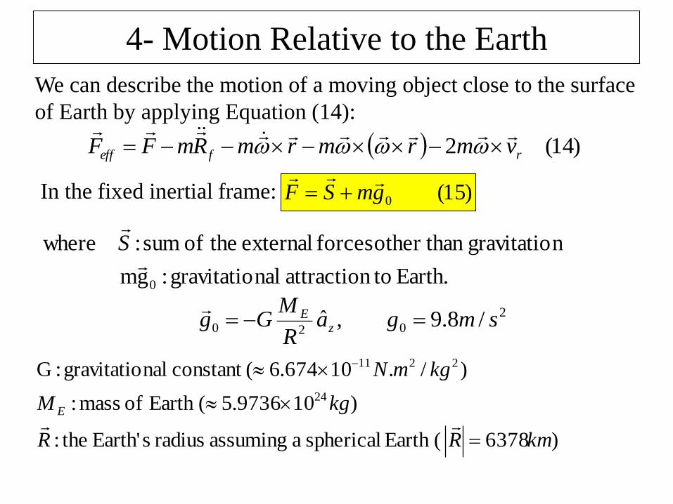
4- Motion Relative to the Earth
)14(2 rfeff vmrmrmRmFF
We can describe the motion of a moving object close to the surface
of Earth by applying Equation (14):
In the fixed inertial frame: )15(0gmSF
Earth. toattraction nalgravitatio :gm
ngravitatio other than forces external theof sum :where
0
S
2
020 /8.9,ˆ smgaR
MGg z
E
)6378 (Earth spherical a assuming radius sEarth' the:
)109736.5(Earth of mass :
)/.10674.6(constant nalgravitatio :G
24
2211
kmRR
kgM
kgmN
E
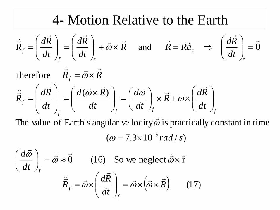
4- Motion Relative to the Earth
Rdt
Rd
dt
RdR
rf
f
0ˆ
r
zdt
RdaRR
RR f
and
therefore
ffff
fdt
RdR
dt
d
dt
Rd
dt
RdR
)(
)/103.7(
in timeconstant y practicall is locity angular ve sEarth' of valueThe
5 srad
rneglect weSo)16(0
fdt
d
)17(Rdt
RdR
f
f
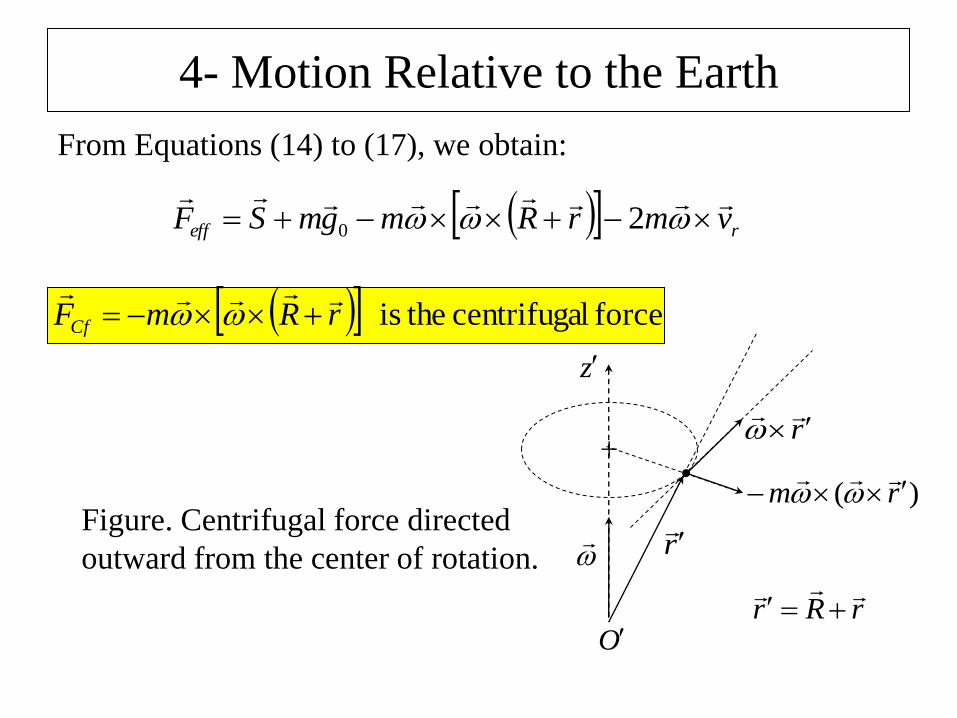
4- Motion Relative to the Earth
From Equations (14) to (17), we obtain:
reff vmrRmgmSF
20
force lcentrifuga theis rRmFCf
r
r
O
)( rm
z
rRr
Figure. Centrifugal force directed
outward from the center of rotation.
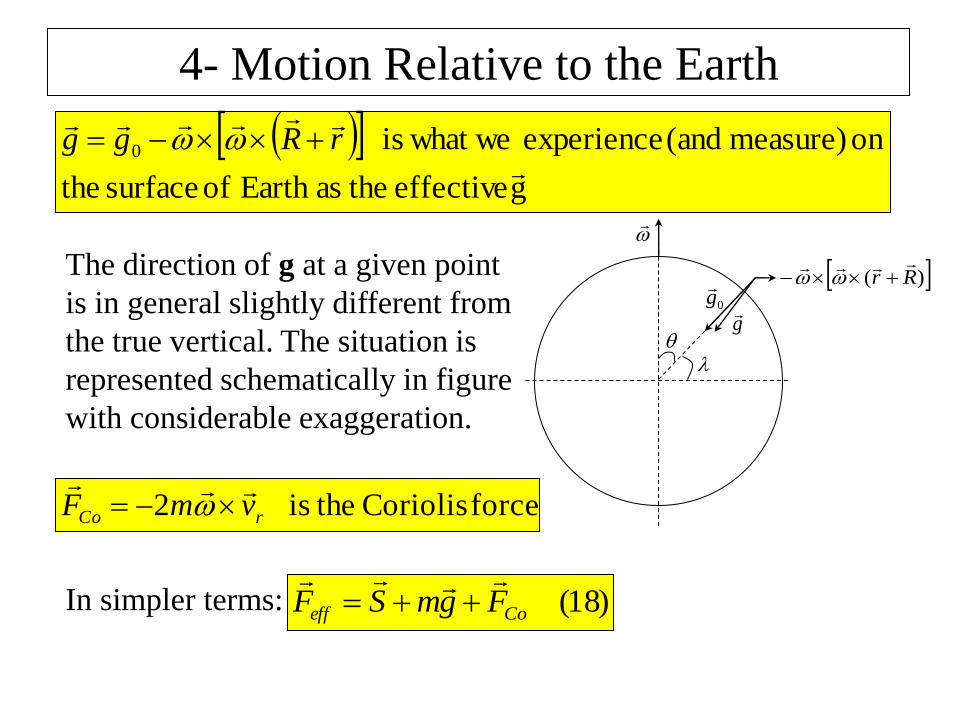
4- Motion Relative to the Earth
g effective theasEarth of surface the
on measure) (and experience what weis 0
rRgg
The direction of g at a given point
is in general slightly different from
the true vertical. The situation is
represented schematically in figure
with considerable exaggeration.
0g
g
)( Rr
force Coriolis theis 2 rCo vmF
In simpler terms: )18(Coeff FgmSF
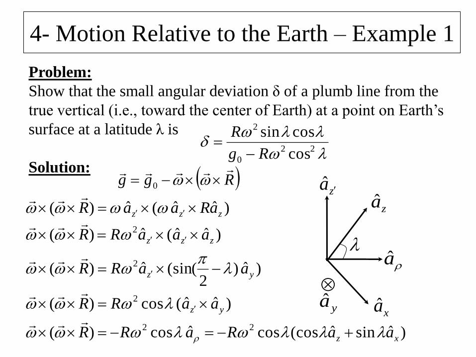
4- Motion Relative to the Earth – Example 1
)ˆsinˆ(coscosˆcos)(
)ˆˆ(cos)(
)ˆ)2
(sin(ˆ)(
)ˆˆ(ˆ )(
)ˆˆ(ˆ)(
22
2
2
2
xz
yz
yz
zzz
zzz
aaRaRR
aaRR
aaRR
aaaRR
aRaaR
Problem:
Show that the small angular deviation δ of a plumb line from the
true vertical (i.e., toward the center of Earth) at a point on Earth’s
surface at a latitude λ is
Solution:
22
0
2
cos
cossin
Rg
R
Rgg
0
xa
zaza ˆ
a
ya
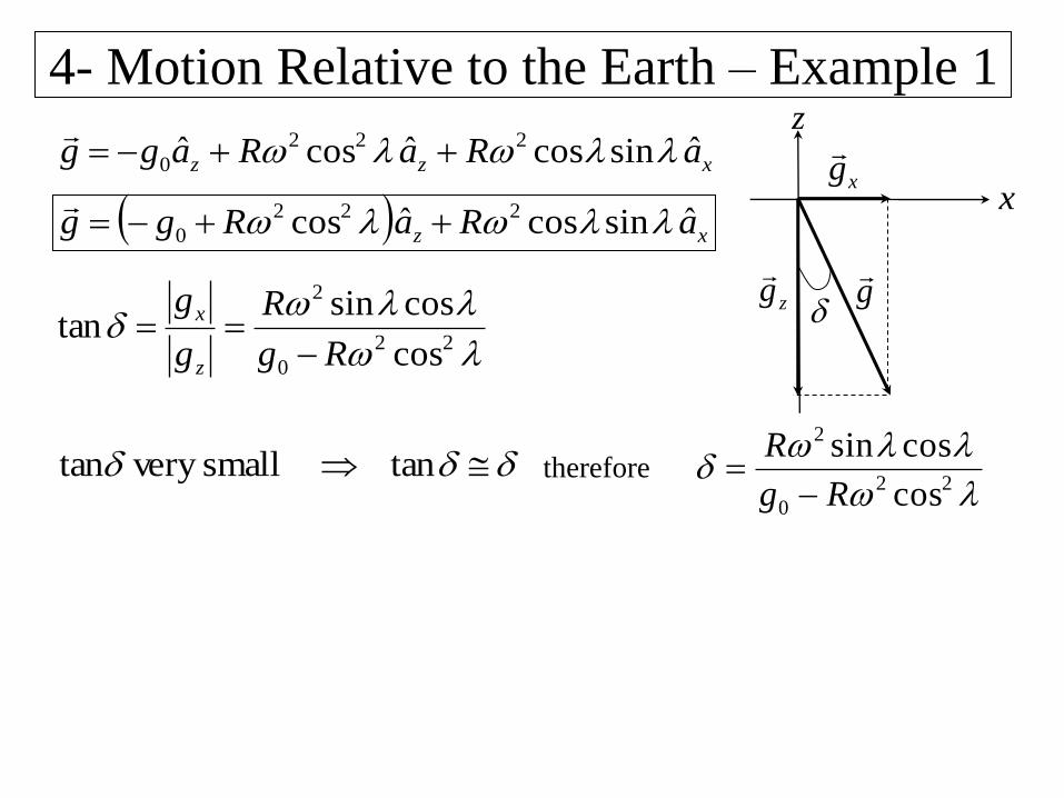
4- Motion Relative to the Earth – Example 1
xzz aRaRagg ˆsincosˆcosˆ 222
0
xz aRaRgg ˆsincosˆcos 222
0
22
0
2
cos
cossintan
Rg
R
g
g
z
x
tan small very tan
22
0
2
cos
cossin
Rg
R
therefore
g
x
z
zg
xg
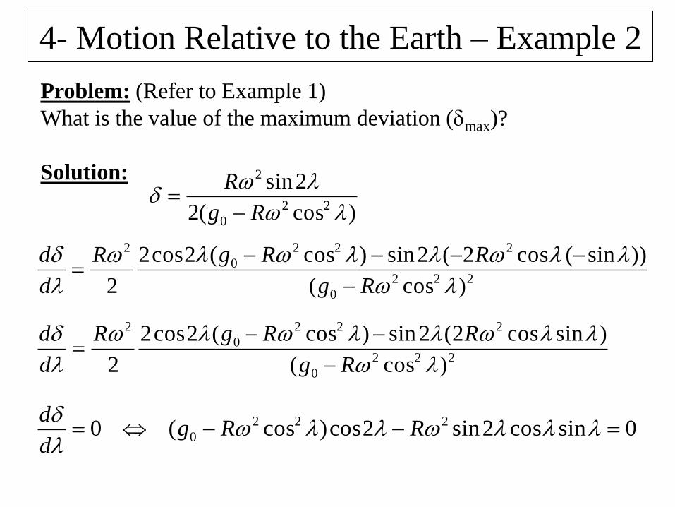
4- Motion Relative to the Earth – Example 2
Problem: (Refer to Example 1)
What is the value of the maximum deviation (max)?
Solution:
)cos(2
2sin22
0
2
Rg
R
222
0
222
0
2
)cos(
))sin(cos2(2sin)cos(2cos2
2
Rg
RRgR
d
d
222
0
222
0
2
)cos(
)sincos2(2sin)cos(2cos2
2
Rg
RRgR
d
d
0sincos2sin2cos)cos(0 222
0
RRg
d
d
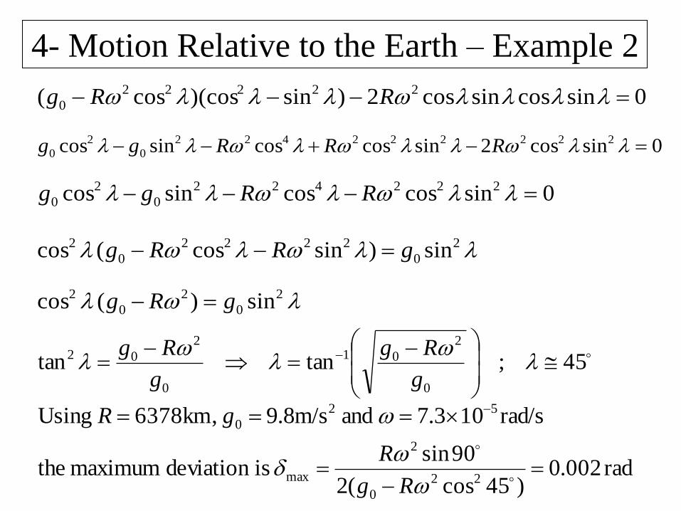
4- Motion Relative to the Earth – Example 2
0sincossincos2)sin)(coscos( 22222
0 RRg
0sincos2sincoscossincos 222222422
0
2
0 RRRgg
0sincoscossincos 222422
0
2
0 RRgg
2
0
2222
0
2 sin)sincos(cos gRRg
2
0
2
0
2 sin)(cos gRg
45;tantan0
2
01
0
2
02
g
Rg
g
Rg
rad 002.0)45cos(2
90sin isdeviation maximum the
rad/s103.7 and m/s8.9 ,km6378 Using
22
0
2
max
52
0
Rg
R
gR
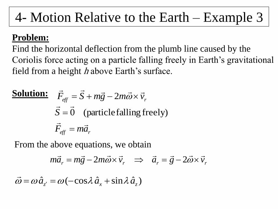
4- Motion Relative to the Earth – Example 3
Problem:
Find the horizontal deflection from the plumb line caused by the
Coriolis force acting on a particle falling freely in Earth’s gravitational
field from a height h above Earth’s surface.
Solution: reff vmgmSF
2
freely) falling (particle0
S
reff amF
rrrr vgavmgmam
22
From the above equations, we obtain
)ˆsinˆcos(ˆzxz aaa
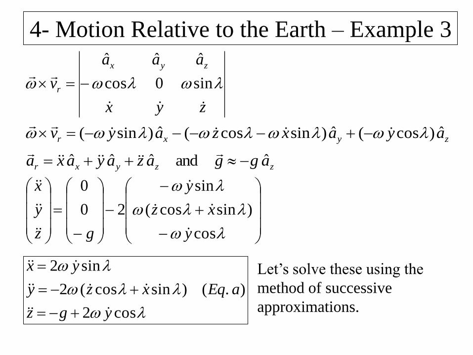
4- Motion Relative to the Earth – Example 3
zyx
aaa
v
zyx
r
sin0cos
ˆˆˆ
zyxr ayaxzayv ˆ)cos(ˆ)sincos(ˆ)sin(
zzyxr aggazayaxa ˆandˆˆˆ
cos
)sincos(
sin
20
0
y
xz
y
gz
y
x
cos2
).()sincos(2
sin2
ygz
aEqxzy
yx
Let’s solve these using the
method of successive
approximations.
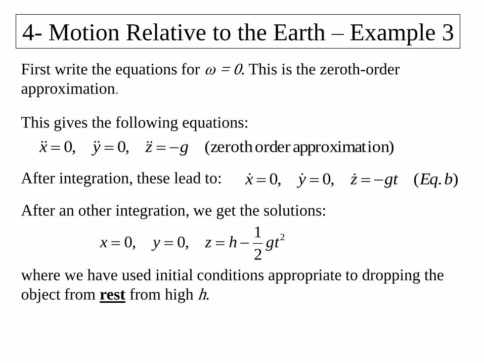
4- Motion Relative to the Earth – Example 3
First write the equations for ω = 0. This is the zeroth-order
approximation.
This gives the following equations:
ion)approximatorder zeroth (,0,0 gzyx
After integration, these lead to: ).(,0,0 bEqgtzyx
After an other integration, we get the solutions:
2
2
1,0,0 gthzyx
where we have used initial conditions appropriate to dropping the
object from rest from high h.
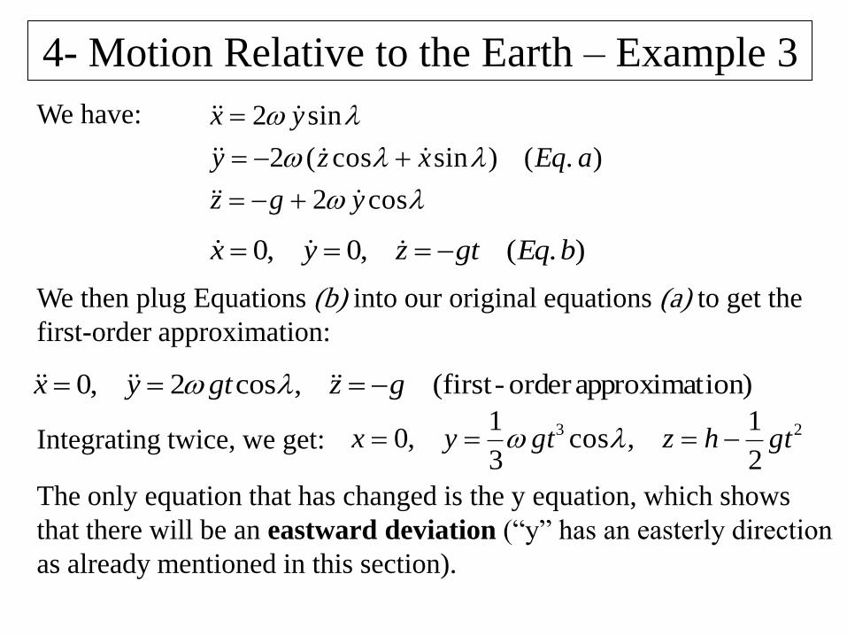
4- Motion Relative to the Earth – Example 3
cos2
).()sincos(2
sin2
ygz
aEqxzy
yx
).(,0,0 bEqgtzyx
We have:
We then plug Equations (b) into our original equations (a) to get the
first-order approximation:
ion)approximatorder -(first,cos2,0 gzgtyx
Integrating twice, we get: 23
2
1,cos
3
1,0 gthzgtyx
The only equation that has changed is the y equation, which shows
that there will be an eastward deviation (“y” has an easterly direction
as already mentioned in this section).
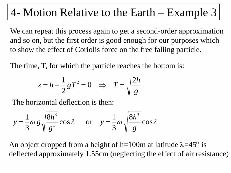
4- Motion Relative to the Earth – Example 3
We can repeat this process again to get a second-order approximation
and so on, but the first order is good enough for our purposes which
to show the effect of Coriolis force on the free falling particle.
The time, T, for which the particle reaches the bottom is:
g
hTgThz
20
2
1 2
The horizontal deflection is then:
cos8
3
13
3
g
hgy cos
8
3
1or
3
g
hy
An object dropped from a height of h=100m at latitude =45 is
deflected approximately 1.55cm (neglecting the effect of air resistance)


