Draft Accepted for Publication in Color Research and Applications-Wiley-2015

1

Physics-Based Spectral Sharpening through Filter-Chart

Calibration

Mohamed Abdellatif

Faculty of Engineering and Technology,

Future University in Egypt, Cairo, Egypt

Abstract: The spectral overlap of color-sampling filters increases errors when using a

Diagonal Matrix Transform, DMT, for color correction and reduces color distinction.

Spectral sharpening is a transformation of colors that was introduced to reduce color-

constancy errors when the colors are collected through spectrally overlapping filters. The

earlier color constancy methods improved color precision when the illuminant color is

changed, but they overlooked the color distinction. In this paper, we introduce a new spectral

sharpening technique that has a good compromise of color precision and distinction, based on

real physical constraints. The spectral overlap is measured through observing a gray reference

chart with a set of real and spectrally disjoint filters selected by the user. The new sharpening

method enables to sharpen colors obtained by a sensor without knowing the camera response

functions. Experiments with real images showed that the colors sharpened by the new method

have good levels of color precision and distinction as well. The color-constancy performance

is compared with the data-based sharpening method in terms of both precision and

distinction.

Keywords: Spectral sharpening, filter-chart spectral sharpening, data-based sharpening,

accuracy–precision evaluation, color distinction, decorrelation stretch, color constancy.

INTRODUCTION

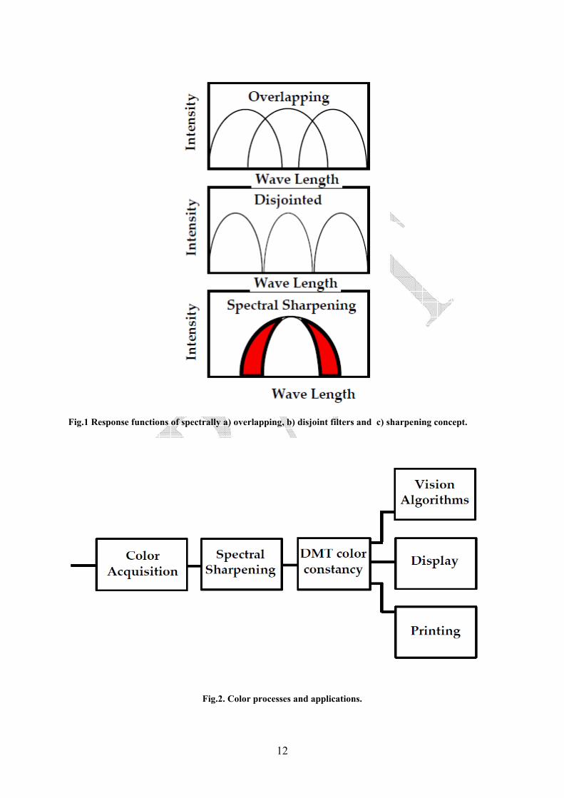
Color responses in an image captured by a camera are strongly affected by the spectral

response functions of the camera sensors [1, 2]. When camera sensors are spectrally

overlapping, as shown in Fig.1, the produced colors have less distinction, and are near to gray

color. Moreover, overlapping filters increase errors for color constancy algorithms when

using DMT for color correction. Spectral sharpening is a linear transformation for the color

responses made to reduce errors when using DMT color-constancy algorithms as proposed in

[1]. Spectral sharpening can also produce enhanced colors for vision algorithms (requiring

color-constancy preprocessing) or enhanced colors for display or printing. Figure 2 shows

color processes involving spectral sharpening. Fig.1 Response functions of spectrally a) overlapping, b) disjoint filters, and c) sharpening concept.

Fig.2. Color processes and applications.

Fig.3. Definition of color accuracy and precision.

Precision and accuracy are two important color constancy evaluation metrics as reported in

[4] and illustrated in Fig.3, where accuracy expresses the proximity of measurement to the

true value, while precision is the repeatability of the measurement. Precision describes the

color vector variance against changes of the illumination color, while accuracy cares about

the quality of the stabilized color and measures its closeness to a canonical interpretation of

the color. Color constancy is classically evaluated through color precision when illumination

color is changed in the scene. This paper introduces the term “Precision” to describe the

commonly used metric to evaluate color constancy. In fact most color constancy work use

precision metric without naming it explicitly as “precision” [1]. It was shown in [4] that while

colors can be mapped to a very precise but wrong color, this is surely not the objective of

color constancy. We argue that color constancy evaluation should consider both precision and

2

distinction as well. Distinction is defined here as the variance of color vector responses from

the mean (not through illumination color variation) normalized by the color vector length.

Distinction here will be used instead of accuracy, since it is the needed visual function from

accurate colors. Therefore, we will evaluate color constancy through both “precision and

distinction,” rather than the current wisdom of considering “precision” only.

Using spectral sharpening had been reported in the literature [5, 6] to improve the image

segmentation by up to 7% [5]. Other applications include display enhancement, using color

for detecting objects such as the human face [5].

The objective of increasing color distinction will be defined as to increase the color vector

variance and hence color differences in the image to the extent that can be related to real

color physics, or in other words, that can be obtained by another set of real filters. The need

for spectral sharpening is strong, in particular for ubiquitous CMOS cameras, where the

potential of spectral sharpening can be well exploited, since their sensors have significant

spectral overlap.

Several spectral sharpening methods were presented in the literature using various constraints

to derive the spectral sharpening matrix [1, 3, 7, and 8]. Finlayson [1] proposed three

methods for computing the sharpening matrix, namely, Sensor-Based, SB, Data-Based, DB,

and an optimal method. The SB technique requires knowledge of the camera sensor response

functions to derive the new filters, while the DB technique requires knowledge of the color

observations for a set of surface colors subject to two different illumination colors. The data-

based sharpening is based on minimizing the color-constancy errors when colors are mapped

to a canonical appearance through the DMT method. Further constraints on the dimensional

representation of surface and illuminant colors were used to reach an optimal solution. In

Finlayson’s work, color constancy was mainly evaluated through the precision metric. The

sharpening methods presented in [1] were reported to deliver negative color responses for

some image colors and were modified later to enforce positivity [3].

Spherical sampling was proposed as a tool to design the sharpened filters based on the human

cone characteristics [9]. Sharpening was also used to derive an invariant image in [10].

Another approach uses chromagenic cameras, where an extra filter is used to obtain a new

image, which gives illumination color clues when compared to the basic color image. The

camera was used to develop the chromagenic algorithm for illumination detection and to

solve for color constancy [11].

Decorrelation Stretching, DS, is widely used for multispectral image processing [12,13], and

considering it as a spectral sharpening technique, it is the only approach that considers color

distinction. In this method, principal component analysis is used to reduce the correlation

between color channels. The DS method improves color distinction, but the sharpening

transformation is not fixed, and varies depending on the image contents [13]. DS also

amplifies the color noise in the image severely. These problems are manifestations of the fact

that DS is purely mathematical and does not employ real physical constraints. The DS

method may be suitable for display enhancement, but not as a physical measurement tool,

since it goes far beyond the physical limits for spectral sharpening to increase visibility of

color differences, even though such differences do not exist in reality.

In this paper, we are inspired by the following argument: Suppose you wanted the camera

that behaved as though it had physical sensors inspired by filters that you have. This requires

constructing a mapping from images of a real camera to images that are like ones taken with

the filter inspired sensors. Then, we need to measure the effectiveness of sharpened sensors

which should tell us that the filter inspired sensors are good, and that the mapping is good.

3

In this article, we are going to introduce an experimental method to achieve this target. The

spectral overlap will be directly measured by using a set of user-selected and spectrally

disjoint filters, together with a gray reference multi-patch chart to obtain the spectral

sharpening transformation. We call this the “Filter-Chart“ method.

The new method is related to SB-sharpening [1] in the core idea, but differs in two aspects.

First, the new method does not require explicit knowledge of the camera sensor functions,

since this knowledge is implicitly exploited through the calibration process. Second, the new

sensor functions are selected by the user and are not virtual.

The work is also related to DB-sharpening; the difference is that DB method finds a

sharpening transformation that is optimized for better color mapping among illuminants and

hence improves precision, while the new method have a good compromise of both precision

and distinction through employing physical constraints.

The paper is arranged as follows: The next section presents briefly the problem formulation.

The new filter-chart (FC) sharpening method is then described in detail. Experiments on real

images and comparison to the DB method are then presented. The performance of the new

method working on real color images is then discussed and concluded.

PROBLEM FORMULATION

The color vector at a pixel can be modeled as (Boldface indicates vector quantities):

( ) ( ) ( )∫= λλλλ dFSEii

...op , (1)

where ( )λE is the incident radiation to the surface, ( )λS is the surface reflectance function,

( )λiF is the spectral response function of the ith sampling filters, λ is the wavelength of light,

superscript o refers to original,

op is the measured color vector with three entries each

corresponding to one filter. The colors are usually corrected in color-constancy algorithms

using a diagonal matrix D, as follows: o

pp .Dc = , (2)

where D is the diagonal matrix whose elements are the correction coefficients for

independent color channels, and the superscript c refers to the corrected colors.

The concept of spectral sharpening aims to perform a linear transformation of colors prior to

correction, so that the diagonal correction works better using the formula o

pp ..TDsc = , (3)

where T is the sharpening matrix, and the superscript sc

refers to sharpened and then corrected

colors.

FC SPECTRAL SHARPENING CALIBRATION

The camera calibration setup consists of the chart of 11 reference patches. Kodak Wratten

filters No. 25 (red), 58 (green), and 47 (blue) are inserted in front of the camera during

calibration. These filters are selected as reference, since they have little spectral overlap and

are responsive only to the visible spectrum. It should be noted that the new filters should be

selected to cover the whole visible spectrum without gaps to be able to represent as many

colors as possible. Fig.4. Concept of measuring the overlap response.

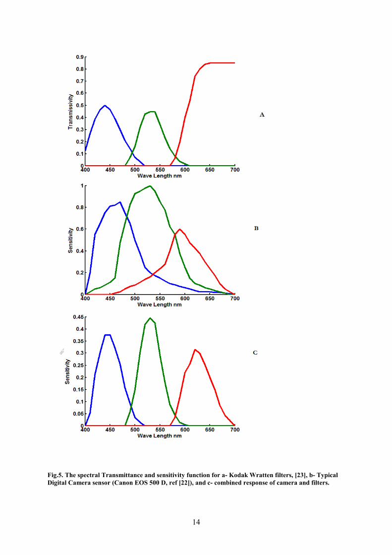
Fig.5. The spectral Transmittance and sensitivity function for A- Kodak Wratten filters, [23], B- Typical

Digital Camera sensor (Canon EOS 500 D, ref [22]), and C- combined response of camera and filters.

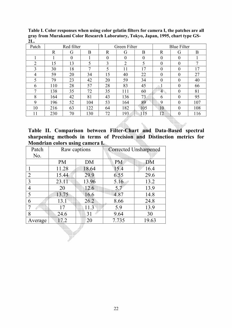
Table I. Sample color responses when using color filters

4

The concept of measuring the spectral overlap can be explained through considering two

simple overlapping filters (only two filters just for explanation, but they are really three) as

shown in Fig.4.

When observing a gray patch, the spectrum input to both sensors is spectrally flat as shown in

Fig.4.a. To separate them spectrally means that we need to assign a spectral range for each,

such that they do not overlap (imagine this is to be done by adding a vertical line between

them). When they are overlapping, each one responds to a region of the other and collects

response from it. Then, to remove the overlap, we will overlay a real filter, which responds,

for example, to the spectral range of the left sensor. This incoming reflection is filtered by

Gelatin filter as in Fig.4.b, which only let go spectrum according to its response function. The

input spectrum is then sampled through the camera filters shown in Fig.4.c. This spectrum

will be sampled into different responses in the main filter colors as shown in Fig.4.d, and will

also have responses in other color channels. Then, we measure the response from both

sensors: the left one’s response is within the limits. The response from the right sensor in this

case represents its overlap with the main filter, and the response should exactly be discounted

from the right sensor response to obtain its response in its own spectral range only. The

response from the other channel in this case represents its overlap with the main filter, and

their response should exactly be discounted from the right sensor response to obtain its

response in its own spectral range only. It is assumed that color channels are not saturated,

and therefore, the imaging model is valid.

In Fig.5A, the transmittance of the selected Kodak Wratten filters are shown, and the spectral

sensitivity of a typical Digital camera (Canon EOS 500 D, ref [22]), where we can observe

significant filter spectral overlap, and C- the combined response of the camera and filters. It

is clear that adding the filters forces filter to be spectrally disjoint. In fact we wish to see

image colors as if captured by sensors with sensitivity functions as that of Fig.5.C.

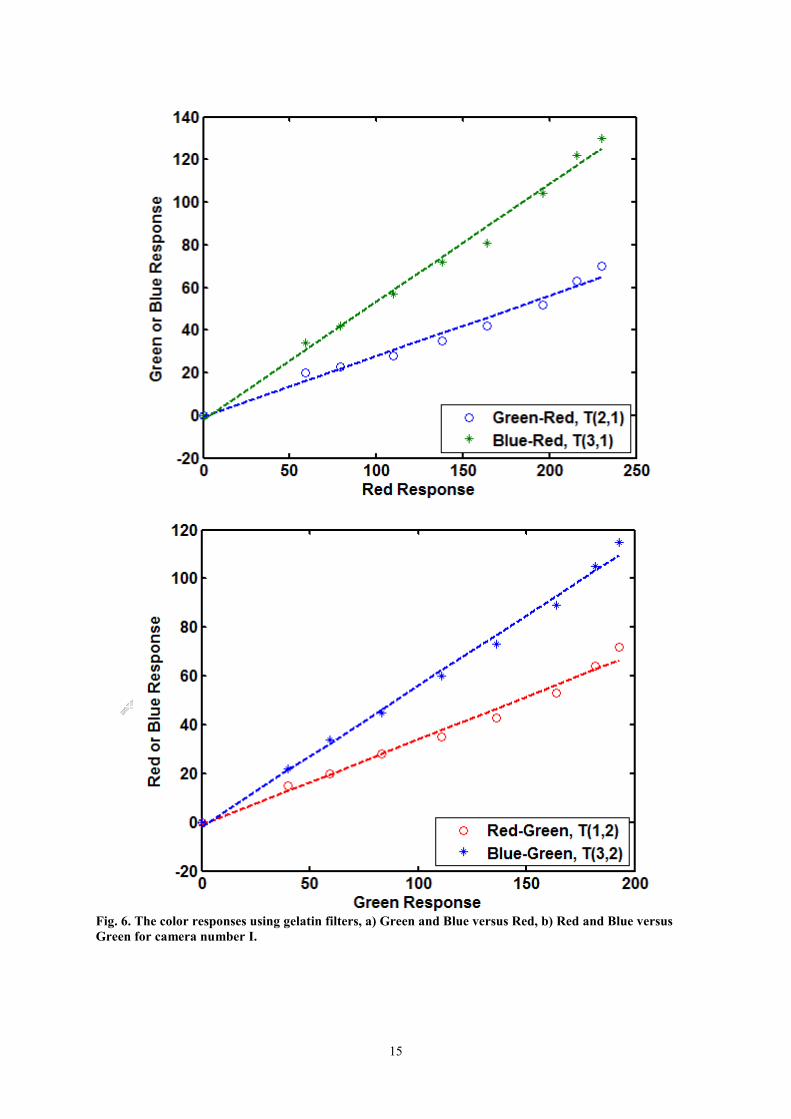
We observe several gray patches with different intensities in a chart containing reference gray

patches of different intensities supplied by Murakami Color Research Laboratory, Tokyo,

Japan, 1995, chart type GS-2L [24]. The responses of each two colors, R–G, R–B, and G–B,

are plotted in Fig.6, and then the slopes of the lines are computed. The three darkest gray

patches were excluded because of noisy response and camera nonlinearity in this region of

the curve. The overlap is the color response itself in Fig.6. This overlap is quantified, relative

to the main color response to compute the entries of the sharpening matrix.

Table I shows the responses of the reference patches when viewed through the filters for

camera number I (Toshiba Satellite M645-S4110 laptop computer camera). A disjoint camera

sensor is expected to respond only in one color channel and should not respond in other

channels. This case is observed for the blue filter case, where there are almost no responses in

the red and green channels. This clearly means that both red and green sensors never gain

response from the band of the blue filter.

For the green color, it can be observed that the blue channel has significant response, which

means that the blue channel receives input in the green filter band. If we can discount this

blue filter response, then we are sure that the blue response comes only from its blue band

and contains no input from the green. This is our basic physical concept for spectral

sharpening.

It can also be observed that both the green and the blue channels respond in the red filter

case. These responses weaken the main color saturation, and it is required to reduce the color

responses other than the main. In the new method, this response will be quantified relative to

the main color response and discounted from the color channels. Fig. 6. Color responses using gelatin filters, the sensor responses are registered while gelatin filter is held

in front of the camera, a) Green and Blue versus Red, b) Red and Blue versus Green for camera I.

We will now describe the method of computing the entries of the spectral sharpening matrix.

5

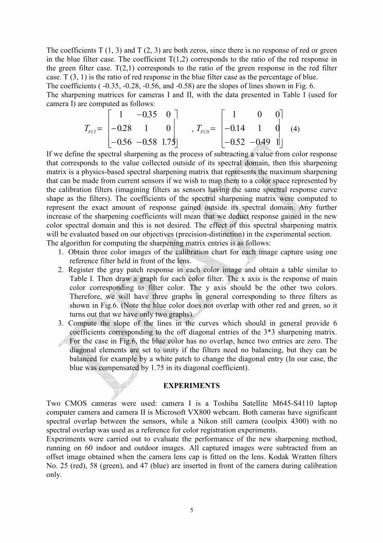
The coefficients T (1, 3) and T (2, 3) are both zeros, since there is no response of red or green

in the blue filter case. The coefficient T(1,2) corresponds to the ratio of the red response in

the green filter case. T(2,1) corresponds to the ratio of the green response in the red filter

case. T (3, 1) is the ratio of red response in the blue filter case as the percentage of blue.

The coefficients ( -0.35, -0.28, -0.56, and -0.58) are the slopes of lines shown in Fig. 6.

The sharpening matrices for cameras I and II, with the data presented in Table I (used for

camera I) are computed as follows:

−−

−

−

=

75.158.056.0

0128.0

035.01

FCIT ,

−−

−=

149.052.0

0114.0

001

FCIIT (4)

If we define the spectral sharpening as the process of subtracting a value from color response

that corresponds to the value collected outside of its spectral domain, then this sharpening

matrix is a physics-based spectral sharpening matrix that represents the maximum sharpening

that can be made from current sensors if we wish to map them to a color space represented by

the calibration filters (imagining filters as sensors having the same spectral response curve

shape as the filters). The coefficients of the spectral sharpening matrix were computed to

represent the exact amount of response gained outside its spectral domain. Any further

increase of the sharpening coefficients will mean that we deduct response gained in the new

color spectral domain and this is not desired. The effect of this spectral sharpening matrix

will be evaluated based on our objectives (precision-distinction) in the experimental section.

The algorithm for computing the sharpening matrix entries is as follows:

1. Obtain three color images of the calibration chart for each image capture using one

reference filter held in front of the lens.

2. Register the gray patch response in each color image and obtain a table similar to

Table I. Then draw a graph for each color filter. The x axis is the response of main

color corresponding to filter color. The y axis should be the other two colors.

Therefore, we will have three graphs in general corresponding to three filters as

shown in Fig.6. (Note the blue color does not overlap with other red and green, so it

turns out that we have only two graphs).

3. Compute the slope of the lines in the curves which should in general provide 6

coefficients corresponding to the off diagonal entries of the 3*3 sharpening matrix.

For the case in Fig.6, the blue color has no overlap, hence two entries are zero. The

diagonal elements are set to unity if the filters need no balancing, but they can be

balanced for example by a white patch to change the diagonal entry (In our case, the

blue was compensated by 1.75 in its diagonal coefficient).

EXPERIMENTS

Two CMOS cameras were used: camera I is a Toshiba Satellite M645-S4110 laptop

computer camera and camera II is Microsoft VX800 webcam. Both cameras have significant

spectral overlap between the sensors, while a Nikon still camera (coolpix 4300) with no

spectral overlap was used as a reference for color registration experiments.

Experiments were carried out to evaluate the performance of the new sharpening method,

running on 60 indoor and outdoor images. All captured images were subtracted from an

offset image obtained when the camera lens cap is fitted on the lens. Kodak Wratten filters

No. 25 (red), 58 (green), and 47 (blue) are inserted in front of the camera during calibration

only.

6

The cameras were controlled during all experiments, so that the automatic white balance is

not activated. For outdoor captions, the blue color was saturated, and this complicated the

sharpening process, since it violates the assumption mentioned earlier. Therefore, the images

were balanced by changing the color temperature setting of manual white balance from 3000

K used for indoor to 6000 K to keep the original image colors within the sensor range.

Calibration was repeated after this change, and a new sharpening matrix was computed, but it

did not change significantly. It should be noted that the camera color should be linear and the

color vector should pass through the origin of RGB color space at (0,0,0) without offset,

which introduces serious errors when using diagonal transformations. Our cameras can be

approximated to be linear if we exclude the low-intensity region below 50. Therefore, the

regions were excluded, and the calibration was fitted to a line passing through the origin.

Evaluation

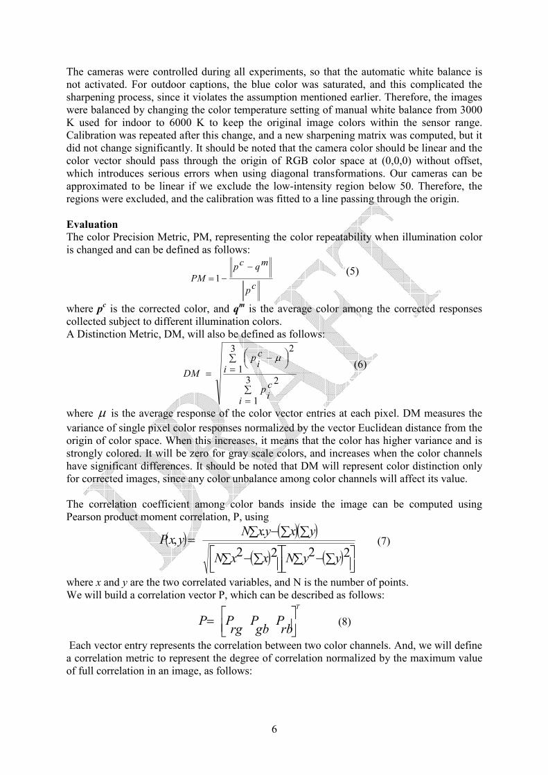
The color Precision Metric, PM, representing the color repeatability when illumination color

is changed and can be defined as follows:

cp

mqcp

PM

−−=1

(5)

where pc is the corrected color, and q

m is the average color among the corrected responses

collected subject to different illumination colors.

A Distinction Metric, DM, will also be defined as follows:

∑=

∑=

−

=3

1

2

3

1

2

i

ci

p

i

ci

p

DM

µ (6)

where µ is the average response of the color vector entries at each pixel. DM measures the

variance of single pixel color responses normalized by the vector Euclidean distance from the

origin of color space. When this increases, it means that the color has higher variance and is

strongly colored. It will be zero for gray scale colors, and increases when the color channels

have significant differences. It should be noted that DM will represent color distinction only

for corrected images, since any color unbalance among color channels will affect its value.

The correlation coefficient among color bands inside the image can be computed using

Pearson product moment correlation, P, using

( ) ( )( )

( ) ( )

∑ ∑−

∑ ∑−

∑ ∑∑−=

2222

.,

yyNxxN

yxyxNyxP (7)

where x and y are the two correlated variables, and N is the number of points.

We will build a correlation vector P, which can be described as follows: T

rbP

gbP

rgPP

= (8)

Each vector entry represents the correlation between two color channels. And, we will define

a correlation metric to represent the degree of correlation normalized by the maximum value

of full correlation in an image, as follows:

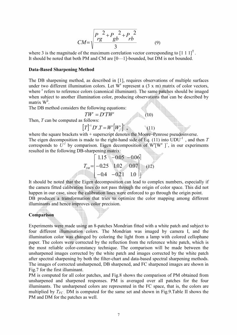
7

3

222rb

Pgb

Prg

P

CM

++= (9)

where 3 is the magnitude of the maximum correlation vector corresponding to [1 1 1]T

.

It should be noted that both PM and CM are [0—1]-bounded, but DM is not bounded.

Data-Based Sharpening Method

The DB sharpening method, as described in [1], requires observations of multiple surfaces

under two different illumination colors. Let Wr represent a (3 x m) matrix of color vectors,

where r refers to reference colors (canonical illuminant). The same patches should be imaged

when subject to another illumination color, producing observations that can be described by

matrix We.

The DB method considers the following equations: eer TWDTW = (10)

Then, T can be computed as follows:

[ ] [ ]+− = ere WWTDT .1

, (11)

where the square brackets with + superscript denotes the Moore–Penrose pseudoinverse.

The eigen decomposition is made to the right-hand side of Eq. (11) into UDU-1

, and then T

corresponds to U-1

by comparison. Eigen decomposition of Wr[W

e ]

+, in our experiments

resulted in the following DB-sharpening matrix:

−−

−

−−

=

0.121.04.0

07.002.125.0

06.005.015.1

DBT (12)

It should be noted that the Eigen decomposition can lead to complex numbers, especially if

the camera fitted calibration lines do not pass through the origin of color space. This did not

happen in our case, since the calibration lines were enforced to go through the origin point.

DB produces a transformation that tries to optimize the color mapping among different

illuminants and hence improves color precision.

Comparison

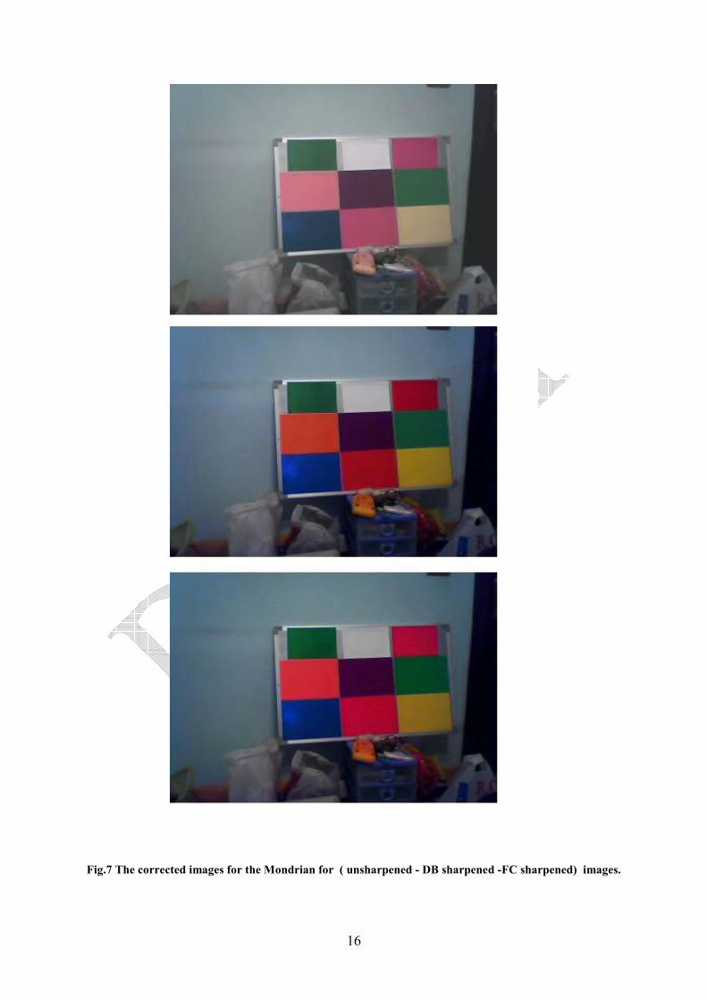
Experiments were made using an 8-patches Mondrian fitted with a white patch and subject to

four different illumination colors. The Mondrian was imaged by camera I, and the

illumination color was changed by coloring the light from a lamp with colored cellophane

paper. The colors were corrected by the reflection from the reference white patch, which is

the most reliable color-constancy technique. The comparison will be made between the

unsharpened images corrected by the white patch and images corrected by the white patch

after spectral sharpening by both the filter-chart and data-based spectral sharpening methods.

The images of corrected unsharpened, DB sharpened, and FC sharpened images are shown in

Fig.7 for the first illuminant.

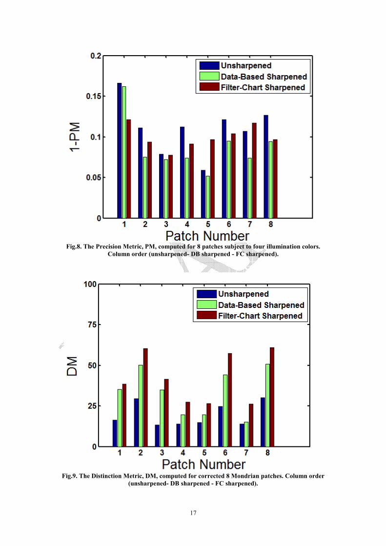
PM is computed for all color patches, and Fig.8 shows the comparison of PM obtained from

unsharpened and sharpened responses. PM is averaged over all patches for the four

illuminants. The unsharpened colors are represented in the FC space, that is, the colors are

multiplied by TFC . DM is computed for the same set and shown in Fig.9.Table II shows the

PM and DM for the patches as well.

8

We can observe that spectral sharpening decreases the precision errors, PM whether done by

the DB or FC methods. The precision errors are on the average of 11 % when represented in

the FC space, but it is 7.735 when represented in the original color space. This is surprising,

because the precision errors are increased by spectral sharpening if each is represented in its

own color space. The results reported in [1] were compared in the unsharpened sensors space.

In our own view, the comparison should be made with reference to new sharpened colors,

since they are the colors we will deal with in further applications. The second reason is that

using real images colors, some colors provide low response, which is a nonlinear region in

most cameras, and this will be the prevailing case, since sharpening will make some color

responses to decrease, while others increase. We also observe that the average PM is almost

the same for both the DB and FC methods. FC results have higher DM, which is a result of

stronger sharpening.

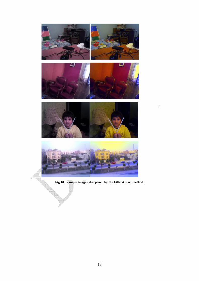
Several experiments were made to apply the FC sharpening method to real indoor and

outdoor images. Sample sharpened images are shown in Fig.10, captured by camera II, where

the left side shows original images and the right shows sharpened images. The first three

images show indoor scene, while the third shows an outdoor scene. The sharpened colors are

consistent with what was realized by human observers as color names. For example, the

orange patch in the first image, the red and orange wall colors in the second image; the shirt

and the skin color of the third image is more saturated and is consistent with the perceived

colors in reality. The outdoor image also shows original building color and strong red car

color.

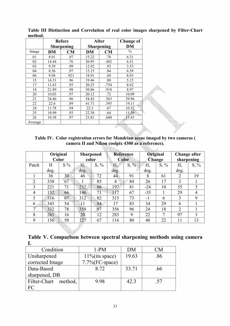
DM and CM were measured for unsharpened and FC-sharpened images, and the results are

summarized in Table III. It can be observed that sharpened color images have higher DM and

lower CM. The highest distinction metric is produced by the FC method.

Fig.7 The corrected images for the Mondrian ( unsharpened–DB-sharpened–FC-sharpened) images.

Fig.8. The Precision Metric, PM, computed for 8 patches subject to four illumination colors.

Column order (unsharpened–DB-sharpened–FC-sharpened).

Fig.9. The Distinction Metric, DM, computed for corrected 8 Mondrian patches. Column order

(unsharpened–DB-sharpened–FC-sharpened).

Table II. Comparison between spectral sharpening methods in terms of PM and DM.

Fig.10. Sample images sharpened by the FC method.

Table III Distinction and Correlation of real color images sharpened by FC method.

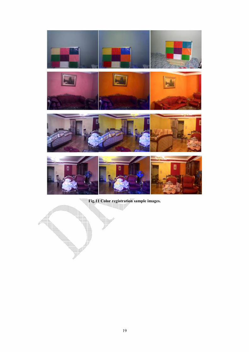
Registration

One interesting application for color spectral sharpening is color registration among different

cameras. We conducted experiments to compare colors captured by camera II and Nikon

coolpix 4300 camera as a reference. Figure 11 shows sample indoor images arranged

horizontally as original, FC-sharpened, and reference colors. It is clear that both sharpened

and reference colors are close to each other, compared to the original colors. Table IV

summarizes the registration errors for the color patches shown in the Mondrian image of

Fig.11.a. The table shows the hue and saturation for each color patch as measured by camera

II in the original, sharpened colors, and the colors from the reference camera. The HIS system

is used in this comparison, since it is perceptually uniform and convenient for human users.

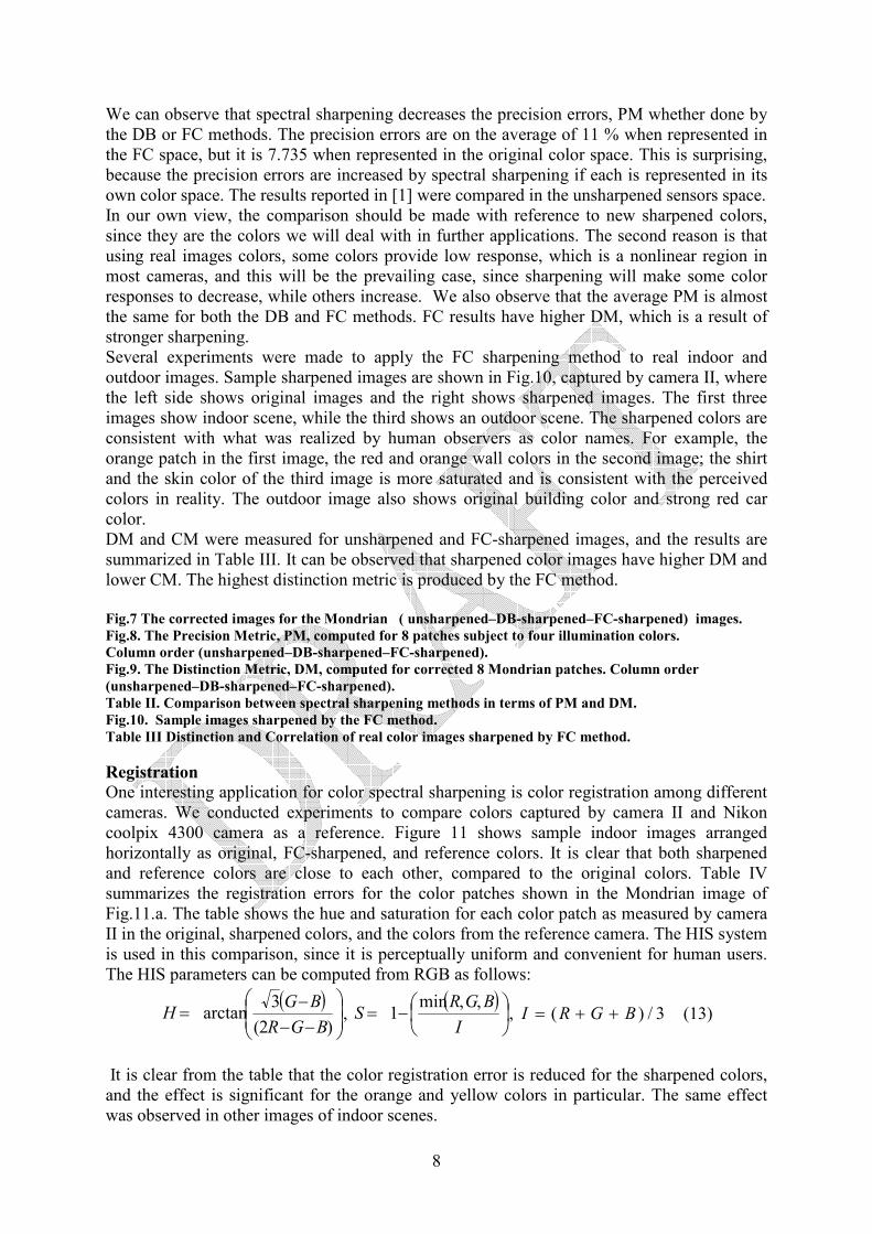
The HIS parameters can be computed from RGB as follows:

( )

−−

−=

)2(

3arctan

BGR

BGH ,

( )

−=I

BGRS

,,min1 , 3/)( BGRI ++= (13)

It is clear from the table that the color registration error is reduced for the sharpened colors,

and the effect is significant for the orange and yellow colors in particular. The same effect

was observed in other images of indoor scenes.

9

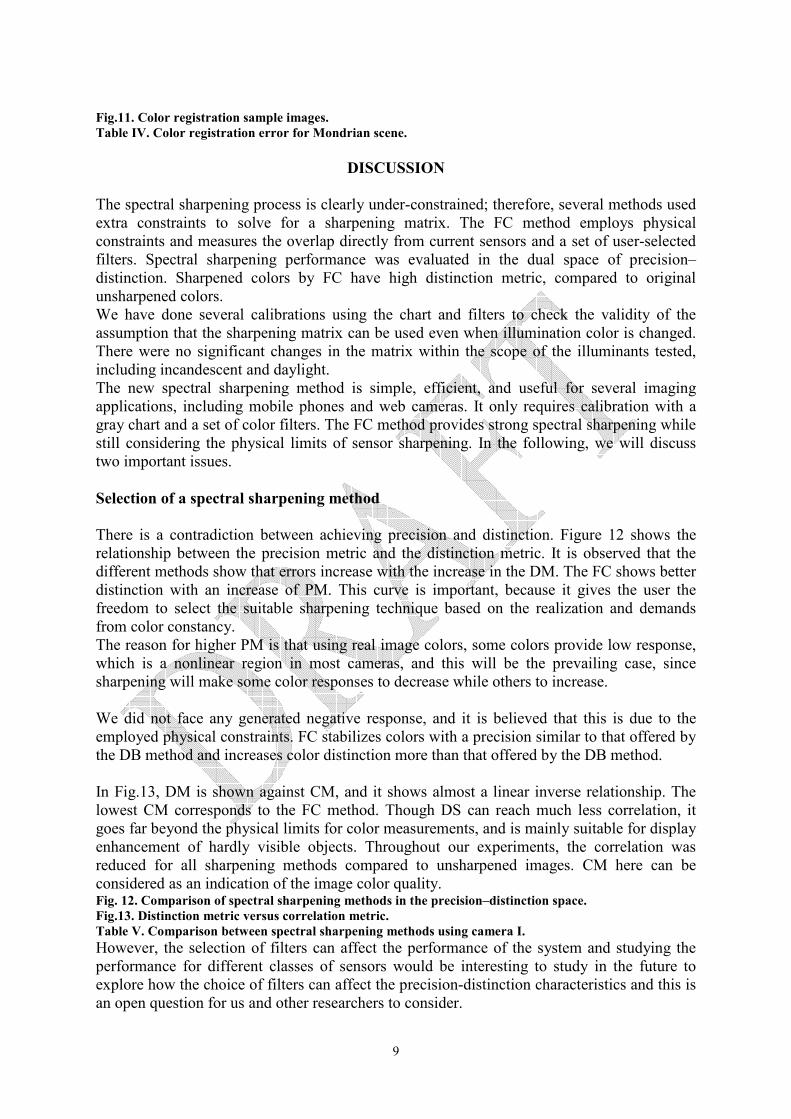
Fig.11. Color registration sample images.

Table IV. Color registration error for Mondrian scene.

DISCUSSION

The spectral sharpening process is clearly under-constrained; therefore, several methods used

extra constraints to solve for a sharpening matrix. The FC method employs physical

constraints and measures the overlap directly from current sensors and a set of user-selected

filters. Spectral sharpening performance was evaluated in the dual space of precision–

distinction. Sharpened colors by FC have high distinction metric, compared to original

unsharpened colors.

We have done several calibrations using the chart and filters to check the validity of the

assumption that the sharpening matrix can be used even when illumination color is changed.

There were no significant changes in the matrix within the scope of the illuminants tested,

including incandescent and daylight.

The new spectral sharpening method is simple, efficient, and useful for several imaging

applications, including mobile phones and web cameras. It only requires calibration with a

gray chart and a set of color filters. The FC method provides strong spectral sharpening while

still considering the physical limits of sensor sharpening. In the following, we will discuss

two important issues.

Selection of a spectral sharpening method

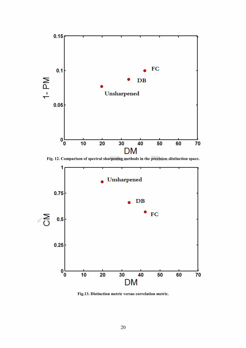
There is a contradiction between achieving precision and distinction. Figure 12 shows the

relationship between the precision metric and the distinction metric. It is observed that the

different methods show that errors increase with the increase in the DM. The FC shows better

distinction with an increase of PM. This curve is important, because it gives the user the

freedom to select the suitable sharpening technique based on the realization and demands

from color constancy.

The reason for higher PM is that using real image colors, some colors provide low response,

which is a nonlinear region in most cameras, and this will be the prevailing case, since

sharpening will make some color responses to decrease while others to increase.

We did not face any generated negative response, and it is believed that this is due to the

employed physical constraints. FC stabilizes colors with a precision similar to that offered by

the DB method and increases color distinction more than that offered by the DB method.

In Fig.13, DM is shown against CM, and it shows almost a linear inverse relationship. The

lowest CM corresponds to the FC method. Though DS can reach much less correlation, it

goes far beyond the physical limits for color measurements, and is mainly suitable for display

enhancement of hardly visible objects. Throughout our experiments, the correlation was

reduced for all sharpening methods compared to unsharpened images. CM here can be

considered as an indication of the image color quality. Fig. 12. Comparison of spectral sharpening methods in the precision–distinction space.

Fig.13. Distinction metric versus correlation metric.

Table V. Comparison between spectral sharpening methods using camera I.

However, the selection of filters can affect the performance of the system and studying the

performance for different classes of sensors would be interesting to study in the future to

explore how the choice of filters can affect the precision-distinction characteristics and this is

an open question for us and other researchers to consider.

10

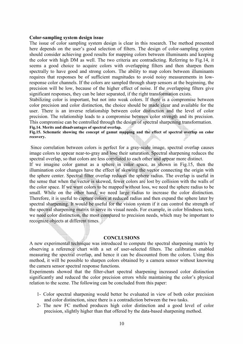
Color-sampling system design issue

The issue of color sampling system design is clear in this research. The method presented

here depends on the user’s good selection of filters. The design of color-sampling system

should consider achieving good results for mapping colors between illuminants and keeping

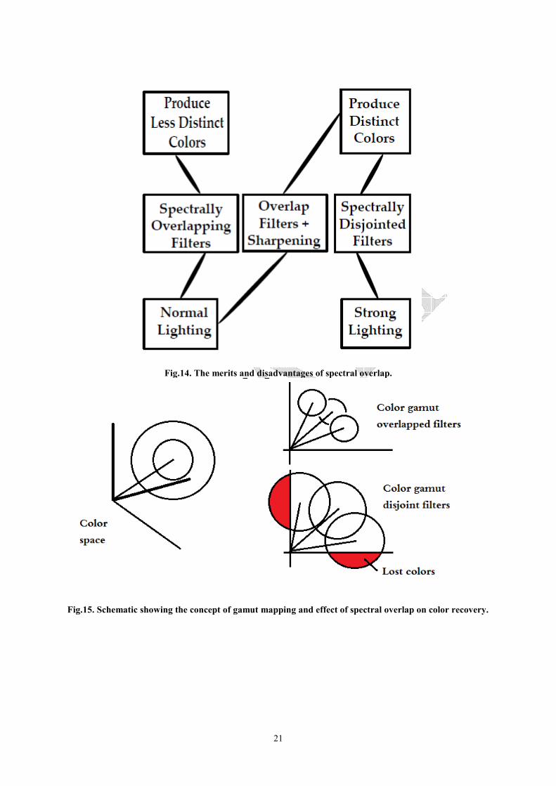
the color with high DM as well. The two criteria are contradicting. Referring to Fig.14, it

seems a good choice to acquire colors with overlapping filters and then sharpen them

spectrally to have good and strong colors. The ability to map colors between illuminants

requires that responses be of sufficient magnitudes to avoid noisy measurements in low-

response color channels. If the colors are sampled through sharp sensors at the beginning, the

precision will be low, because of the higher effect of noise. If the overlapping filters give

significant responses, they can be later separated, if the right transformation exists.

Stabilizing color is important, but not into weak colors. If there is a compromise between

color precision and color distinction, the choice should be made clear and available for the

user. There is an inverse relationship between color distinction and the level of color

precision. The relationship leads to a compromise between color strength and its precision.

This compromise can be controlled through the design of spectral sharpening transformation. Fig.14. Merits and disadvantages of spectral overlap.

Fig.15. Schematic showing the concept of gamut mapping and the effect of spectral overlap on color

recovery.

Since correlation between colors is perfect for a gray-scale image, spectral overlap causes

image colors to appear near-to-gray and lose their saturation. Spectral sharpening reduces the

spectral overlap, so that colors are less correlated to each other and appear more distinct.

If we imagine color gamut as a sphere in color space, as shown in Fig.15, then the

illumination color changes have the effect of skewing the vector connecting the origin with

the sphere center. Spectral filter overlap reduces the sphere radius. The overlap is useful in

the sense that when the vector is skewed, fewer colors are lost by collision with the walls of

the color space. If we want colors to be mapped without loss, we need the sphere radius to be

small. While on the other hand, we need large radius to increase the color distinction.

Therefore, it is useful to capture colors at reduced radius and then expand the sphere later by

spectral sharpening. It would be useful for the vision system if it can control the strength of

the spectral sharpening matrix to serve its visual needs. For example, in color blindness tests,

we need color distinction, the most compared to precision needs, which may be important to

recognize objects at different times.

CONCLUSIONS

A new experimental technique was introduced to compute the spectral sharpening matrix by

observing a reference chart with a set of user-selected filters. The calibration enabled

measuring the spectral overlap, and hence it can be discounted from the colors. Using this

method, it will be possible to sharpen colors obtained by a camera sensor without knowing

the camera sensor spectral response functions.

Experiments showed that the filter-chart spectral sharpening increased color distinction

significantly and reduced the color precision errors while maintaining the color’s physical

relation to the scene. The following can be concluded from this paper:

1- Color spectral sharpening would better be evaluated in view of both color precision

and color distinction, since there is a contradiction between the two tasks.

2- The new FC method produces high color distinction and a good level of color

precision, slightly higher than that offered by the data-based sharpening method.

11

The new method has a strong potential for application in popular CMOS cameras in

particular.

REFERENCES

[1] Finlayson G.D, Drew M.S. and Funt B.V., Spectral sharpening: Sensor transformations for improved color

constancy. Journal of the Optical Society of America, Vol. 11, 1994;5:1553-1563.

[2] Forsyth D., A novel algorithm for color constancy, International Journal of Computer Vision, 1990;5:5-36.

[3] Drew M.S. and Finlayson G.D., Spectral sharpening with positivity, Journal of the Optical Society of

America, Vol. 17, 2000;8:1361-1370.

[4] Abdellatif, M., Tanaka, Y., Gofuku A. and Nagai, I., Color constancy using the inter-reflection from a

reference nose. The International Journal of Computer Vision. Vol.39, 2000;3:171-194.

[5] Mircea C. I and Peter C., Benefits of using decorrelated color information for face segmentation/tracking,

Advances in Optical Technologies, 2008;1-8.

[6] Kalfon, M. and Porat, M., A new approach to texture recognition using decorrelation

stretching, International Journal of Future Computer and Communication Vol. 2, 2013;1: 49-53.

[7] Finlayson GD, Funt BV. Coefficient Channels: Derivation and Relationship to other Theoretical Studies,

Color Research and Applications, Vol.21, 1996;2:87-96.

[8] Vazquez-Corral,J. and Bertalmio, M., Spectral Sharpening of Color Sensors: Diagonal Color Constancy and

Beyond, Sensors, 2014;14(3):3965-3985.

[9] Finlayson G.D., Vazquez-Corral,J., Susstrunk, S. and Varnella, M., Spectral Sharpening by Spherical

Sampling, Journal of the optical Society of America, A, (JOSA A), 2012;29(7):1199-1210.

[10] Finlayson GD. Drew MS. Lu C. Invariant Image Improvement by sRGB colour space sharpening. In: 10th

Congress of the International Colour Association AIC Colour 05, Granada.

[11] Finlayson G.D., Hordley S. D. and Morovic P., Chromagenic filter design, in Proceedings of 10th

Congress

of the International Colour Association, 2005.

[12] Gillespie A.R., Kahle AB. And Walker R.E., Color enhancement of highly correlated images. I. De-

correlation and HSI Contrast Stretches. Remote Sensing of Environment, 1986:209-235.

[13] Liu J.G. and Moore J.M., Direct de-correlation stretch technique for RGB color composition, International

Journal of Remote Sensing, Vol.17, 1996;5:1005–1018.

[14] Barnard K., Ciurea F. and Funt B.V. Sensor sharpening for computational color constancy, Journal of the

Optical Society of America, Vol.18, 2001;11:2728-2743.

[15] Drew M.S. and Bergner, S., Analysis of spatio-chromatic decorrelation for colour image reconstruction,

Color Imaging Conference 2012.

[16] Drew M.S., Chen C., Hordley S.D. and Finlayson G.D., Sensor transforms for invariant image

enhancement, 10th Color Imaging Conference, 2002;325-329.

[17] Hamilton Y. Chong, Steven J.Gurtler and Todd Zickler, The von Kries Hypothesis and a Basis for Color

Constancy, The International Conference on Computer Vision, 2007.

[18] Novak CL. Shafer SA. Supervised color constancy, Physics-Based vision, Color, Jones and Bartlett,

1992;284-299.

[19] Van Trigt, C., Illuminant-dependence of Von Kries type quotients, International Journal of Computer

Vision, Vol. 61, 2005;1:5-30.

[20] Abdellatif M. Al-Salem NH. Illumination-Invariant Color Recognition for Mobile Robot Navigation, In

Proc. of the International Conference on Instrumentation, Control and Information Technology,

2005:3311-3316, SICE, Okayama, Japan.

[21] Abdellatif M., Effect of Color Pre-Processing on Color-Based Object Detection, In Proc. of the

International Conference on Instrumentation, Control and Information Technology, SICE,2008: 1124-

1129, Tokyo, Japan.

[22] http://publiclab.org/wiki/ndvi-plots-ir-kit (accessed 23 August 2014).

[23] http://motion.kodak.com/motion/Products/Lab_And_Post_Production/Kodak_filters/wrattten2.htm

(accessed 23 August 2014).

[24] http://www.mcrl.co.jp/english/products.html (accessed 27 Sept. 2014).

12

Fig.1 Response functions of spectrally a) overlapping, b) disjoint filters and c) sharpening concept.

Fig.2. Color processes and applications.

13

Fig.3. The definition of color accuracy and precision.

Fig.4. The concept of measuring the overlap response.

14

Fig.5. The spectral Transmittance and sensitivity function for a- Kodak Wratten filters, [23], b- Typical

Digital Camera sensor (Canon EOS 500 D, ref [22]), and c- combined response of camera and filters.

15

Fig. 6. The color responses using gelatin filters, a) Green and Blue versus Red, b) Red and Blue versus

Green for camera number I.

16

Fig.7 The corrected images for the Mondrian for ( unsharpened - DB sharpened -FC sharpened) images.

17

Fig.8. The Precision Metric, PM, computed for 8 patches subject to four illumination colors.

Column order (unsharpened- DB sharpened - FC sharpened).

Fig.9. The Distinction Metric, DM, computed for corrected 8 Mondrian patches. Column order

(unsharpened- DB sharpened - FC sharpened).

18

Fig.10. Sample images sharpened by the Filter-Chart method.

19

Fig.11 Color registration sample images.

20

Fig. 12. Comparison of spectral sharpening methods in the precision–distinction space.

Fig.13. Distinction metric versus correlation metric.

21

Fig.14. The merits and disadvantages of spectral overlap.

Fig.15. Schematic showing the concept of gamut mapping and effect of spectral overlap on color recovery.

22

Table I. Color responses when using color gelatin filters for camera I, the patches are all

gray from Murakami Color Research Laboratory, Tokyo, Japan, 1995, chart type GS-

2L.

Patch Red filter Green Filter Blue Filter

R G B R G B R G B

1 1 0 1 0 0 0 0 0 1

2 15 13 5 3 2 5 0 0 7

3 30 18 7 5 11 17 0 0 17

4 59 20 34 15 40 22 0 0 27

5 79 23 42 20 59 34 0 0 40

6 110 28 57 28 83 45 1 0 66

7 138 35 72 35 111 60 4 0 81

8 164 42 81 43 136 73 6 0 95

9 196 52 104 53 164 89 9 0 107

10 216 63 122 64 182 105 10 0 108

11 230 70 130 72 193 115 12 0 116

Table II. Comparison between Filter-Chart and Data-Based spectral

sharpening methods in terms of Precision and Distinction metrics for

Mondrian colors using camera I.

Patch

No.

Raw captions Corrected Unsharpened

PM DM PM DM

1 11.28 18.64 15.4 16.4

2 15.44 29.9 6.55 29.6

3 23.11 13.96 5.16 13.2

4 20 12.6 5.7 13.9

5 13.75 16.6 4.87 14.8

6 13.1 26.2 8.66 24.8

7 17 11.3 5.9 13.9

8 24.6 31 9.64 30

Average 17.2 20 7.735 19.63

23

Table III Distinction and Correlation of real color images sharpened by Filter-Chart

method.

Before

Sharpening

After

Sharpening

Change of

DM Image DM CM DM CM %

01 8.91 .97 15.22 .78 6.31

02 14.44 .76 20.95 .482 6.51

03 9.39 .99 12.92 .93 3.53

04 8.56 .97 15.15 .84 6.59

06 9.98 .921 18.91 .69 8.93

15 14.31 .96 19.46 .80 5.15

17 11.63 .95 20.25 .754 8.62

18 21.89 .98 30.86 .918 8.97

20 10.03 .97 20.12 .72 10.09

21 24.46 .96 54.42 .563 29.96

22 22.6 .89 41.71 .593 19.11

24 11.78 .94 22.3 .67 10.52

25 10.99 .93 22.38 .64 11.39

26 10.38 .97 25.81 .608 15.43

Average

Table IV. Color registration errors for Mondrian scene imaged by two cameras (

camera II and Nikon coolpix 4300 as a reference).

Original

Color

Sharpened

color

Reference

Color

Original

Change

Change after

sharpening

Patch H

deg.

S % H,

deg.

S, % H,

deg.

S, % H,

deg.

S, % H,

deg.

S, %

1 36 30 46 72 44 91 8 61 2 19

2 338 67 1 85 4 84 26 17 3 1

3 221 71 232 86 197 81 -24 10 35 5

4 152 66 146 71 117 67 -35 1 29 4

5 316 67 312 82 315 73 -1 6 3 9

6 343 54 11 84 17 83 34 29 6 1

7 332 78 358 97 356 96 24 18 2 1

8 261 16 20 12 283 9 22 7 97 3

9 156 58 127 67 116 80 40 22 11 13

Table V. Comparison between spectral sharpening methods using camera

I.

Condition 1-PM DM CM

Unsharpened

corrected Image

11%(its space)

7.7%(FC-space)

19.63 .86

Data-Based

sharpened, DB

8.72 33.71 .66

Filter-Chart method,

FC

9.98 42.3 .57