Arnold Schwarzenegger

Governor

PULSED FLOW EFFECTS ON THE FOOTHILL YELLOW-LEGGED FROG

(RANA BOYLII): POPULATION MODELING

PIE

R F

INA

L P

RO

JE

CT

RE

PO

RT

Prepared For:

California Energy Commission

Public Interest Energy Research Program

Prepared By:

Kupferberg, Lind, and Palen

August/2009

CEC-500-XXXX-XXX

Prepared By:

Kupferberg, Lind, and Palen

Contract No. 500-01-044

Project No. PFP-03

Prepared For:

California Energy Commission

Public Interest Energy Research (PIER) Program

Joseph O’Hagan

Contract Manager

Kelly Birkinshaw

Program Area Team Lead

Martha Krebs, Ph. D.

Deputy Director

ENERGY RESEARCH AND DEVELOPMENT DIVISION

B.B. Blevins

Executive Director

DISCLAIMER

This report was prepared as the result of work sponsored by the California Energy Commission. It does not necessarily represent the views of the Energy Commission, its employees or the State of California. The Energy Commission, the State of California, its employees, contractors and subcontractors make no warrant, express or implied, and assume no legal liability for the information in this report; nor does any party represent that the uses of this information will not infringe upon privately owned rights. This report has not been approved or disapproved by the California Energy Commission nor has the California Energy Commission passed upon the accuracy or adequacy of the information in this report.

Pulsed Flow Effects on the Foothill Yellow-Legged Frog (Rana boylii): Population Modeling

FINAL REPORT

Submitted to:

Douglas Conklin, Pulsed Flow Program Director

Department of Animal Science

University of California, Davis

One Shields Avenue

Room 2201, Meyer Hall

Davis, California 95616

Authored by:

Sarah J. Kupferberg

Questa Engineering

P.O. Box 70356, 1220 Brickyard Cove Rd. Suite 206

Pt. Richmond, CA 94807

skupferberg@pacbell.net

Amy J. Lind

USFS, Sierra Nevada Research Center

1731 Research Park Drive

Davis, CA 95618

alind@fs.fed.us

Wendy J. Palen

Department of Biological Sciences

Simon Fraser University

Burnaby, BC V5A 1S6, Canada

wpalen@sfu.ca

PFP-funded Agreement No. 03

Publication Number: TBD

Publication Date:

i

Legal Notice

This report was prepared as a result of work sponsored by the California Energy Commission

(Energy Commission). It does not necessarily represent the views of the Energy Commission, its

employees, or the State of California. The Commission, the State of California, its employees,

contractors and subcontractors make no warranty, express or implied, and assume no legal

liability for the information in this report; nor does any party represent that the use of this

information will not infringe upon privately owned rights. This report has not been approved

or disapproved by the Commission nor has the Commission passed upon the accuracy of this

information in this report.

Acknowledgments

The authors would like to thank Joe Drennan and other staff at Garcia and Associates, and Clara

Wheeler, of the USDA Forest Service, for graciously sharing their capture-recapture data for

Rana boylii. Antonia D’Amore provided survival rate estimates for juvenile Rana draytonii based

on data from Norm Scott and Galen Rathbun. We would also like to thank Steve Bobzien, Earl

Gonsolin, Rob Grasso, Levi Gray, Karla Marlow, Ryan Peek, Bob Thompson, Kevin Wiseman,

and Sarah Yarnell who helped with egg counting and frog catching. Alessandro Catenazzi

shared unpublished data regarding thermal effects on tadpole survival. We appreciate the use

of the Angelo Reserve of the University of California Natural Reserve System and thank Peter

Steele, Mary Power, and Collin Bode for maintaining the long term hydrologic monitoring of

the South Fork Eel River. This research was supported and funded by the Public Interest Energy

Research Program of the California Energy Commission and the Division of Water Rights of the

State Water Resources Control Board through the Pulsed Flow Program of the Center of

Aquatic Biology and Aquaculture of the University of California, Davis.

Please cite this report as follows:

Kupferberg, S., Lind, A.J., and Palen, W. J. 2009. Pulsed flow effects on the Foothill Yellow-

Legged frog (Rana boylii): Population Modeling. Final Report. California Energy Commission,

PIER. Publication number TBD.

ii

Preface

The Public Interest Energy Research (PIER) Program supports public interest energy research

and development that will help improve the quality of life in California by bringing

environmentally safe, affordable, and reliable energy services and products to the marketplace.

The PIER Program, managed by the California Energy Commission (Energy Commission),

annually awards up to $62 million to conduct the most promising public interest energy

research by partnering with Research, Development, and Demonstration (RD&D)

organizations, including individuals, businesses, utilities, and public or private research

institutions.

PIER funding efforts are focused on the following RD&D program areas:

• Buildings End-Use Energy Efficiency

• Energy-Related Environmental Research

• Energy Systems Integration Environmentally Preferred Advanced Generation

• Industrial/Agricultural/Water End-Use Energy Efficiency

• Renewable Energy Technologies

What follows is a final report detailing results for the hydropower pulsed flow program

(contract number PFP-03) conducted by the University of California, Davis and its affiliates. The

report is entitled Pulsed flow effects on the Foothill Yellow-Legged Frog (Rana boylii): population

modeling approaches. Final Report. The information from this project contributes to PIER’s Energy-

Related Environmental Research program.

For more information on the PIER Program, please visit the Energy Commission’s website

www.energy.ca.gov/pier/reports.html or contact the Energy Commission at (916) 654-4628.

iii

Table of Contents

Legal Notice ................................................................................................................................................. i

Acknowledgments ...................................................................................................................................... i

Preface .......................................................................................................................................................... ii

Abstract....................................................................................................................................................... ix

Executive Summary ................................................................................................................................... 1

1.0 Research Problem Statement ....................................................................................................... 1

1.1. Hydrologic Alteration, Rana boylii Conservation, and the Need for Population Projection

Models ......................................................................................................................................................... 4

1.2. Rana boylii Life Cycle and Demographic transitions ................................................................ 5

1.3. Focal Watersheds (Alameda Creek, South Fork Eel River, North Fork Feather River,

Hurdygurdy Creek) ................................................................................................................................... 6

1.4. Project Objectives and Report Organization ........................................................................... 11

2.0 Methods: Model Construction, Estimation of Survival Rates, and Population Viability

Scenarios .................................................................................................................................................... 13

2.1. Life Table Construction .............................................................................................................. 13

2.2. Model Statement ......................................................................................................................... 14

2.3. Vital Rate Estimation for Each Life Stage ................................................................................ 22

2.3.1. Long-term censuses of Rana boylii egg masses ........................................................... 22

2.3.2. Adult Female Fecundity and Background Embryo Survival ....................................... 23

2.3.3. Survival of Stranding or Scouring events .................................................................... 26

2.3.4. Survival of Tadpoles to Metamorphosis ....................................................................... 28

2.3.5. First Year Over-Winter Survival ................................................................................. 31

2.3.6. Survival from Age 1 to Age 2 ....................................................................................... 32

2.3.7. Survival from Age 2 to Age 3 ....................................................................................... 33

2.3.8. Adult Survival Estimates ............................................................................................. 33

2.4. Central Coastal California Populations Reference Model ..................................................... 36

2.5. Typical Study Reach Lengths, Starting Population Size, and Quasi-Extinction Thresholds

36

2.5.1. Application to Population Model – Reference Values ......................................................... 37

2.5.2 Model Scenarios ................................................................................................................... 40

2.6. Combined Effects Scenarios ...................................................................................................... 40

iv

2.6.1. Simulation of Rana boylii decline history ................................................................... 41

2.6.2. Worst-Case Modern Scenarios – Small Populations and Hydrologic Stressors .......... 41

2.6.3. Central Coast Population Combination Models .......................................................... 41

2.7. Sensitivity Analysis Methods .................................................................................................... 41

3.0 Population Modeling Results and Discussion ........................................................................ 43

3.1. Reference Model .......................................................................................................................... 44

3.2. Manipulations of Starting Population Size and Quasi-Extinction Threshold .................... 46

3.3. Modified Vital Rate Scenarios ................................................................................................... 47

3.3.1. Spring Flow Conditions .............................................................................................. 47

3.3.2. Summer Flow Conditions ............................................................................................ 48

3.4. Combined Scenarios ................................................................................................................... 50

3.4.1. Spring and Summer Hydrologic Stressors ................................................................... 50

3.4.2. Central Coast Population Scenarios ............................................................................. 52

3.5. Sensitivity Analyses .................................................................................................................... 53

4.0 Conclusions and Recommendations ........................................................................................ 55

4.1. Conclusions .................................................................................................................................. 55

4.2. Commercialization Potential ..................................................................................................... 57

4.3. Recommendations....................................................................................................................... 57

4.3.1. Management Recommendations Indicated by Model Outputs and Sensitivity

Analyses 57

4.3.2. Research Priorities Indicated By Information Gaps ..................................................... 61

4.4. Benefits to California .................................................................................................................. 61

5.0 References .................................................................................................................................... 63

6.0 Glossary ........................................................................................................................................ 70

APPENDIX A. Detailed Descriptions of Study Areas ........................................................................ 72

APPENDIX B. Detailed Young of the Year Data Collection and Population and Survival Rate

Estimates ................................................................................................................................................... 76

v

List of Tables

Table 1.1. Overview of potential and documented impacts to Rana boylii in regulated rivers. ...... 4

Table 1.2. General characteristics of the focal river systems’ topography, hydrology,

geomorphology, and vegetation. ............................................................................................................. 9

Table 2.1. Guidelines for minimum data requirements to perform population viability analyses

(adapted from Morris and Doak 2002). The shaded boxes represent the types of data used here

for the R. boylii population modeling scenarios. .................................................................................. 14

Table 2.2. A life table for Rana boylii with a description of Reference Model transition

probabilities and component vital rates. .............................................................................................. 20

Table 2.3. Modeled scenarios for Rana boylii populations. The scenarios are grouped into five

categories: reference models, models addressing starting conditions and evaluation criteria (e.g.,

starting population size), models where vital rates are modified, combination models for 3 year

maturity populations and combination models for the Central Coast, 2 year maturity,

populations. Each scenario is named and the specific parameter values used for that scenario

are presented............................................................................................................................................. 21

Table 2.4. Fecundity and survival to hatching of Rana boylii in the study watersheds. To

represent the number of female embryos, the total number of embryos was divided by two;

assuming a 50:50 sex ratio in each egg mass. ....................................................................................... 24

Table 2.5. Analysis of covariance of embryo number, n=55 clutches. One NF Feather clutch was

excluded due to its advanced Gosner stage when first measured compared to other clutches.

Multiple R = 0.66, multiple R2= 0.44. ...................................................................................................... 25

Table 2.6. Hydrologic effects on persistence of egg masses observed in four regulated rivers (5

river reaches). ........................................................................................................................................... 27

Table 2.7. Steps to determine Rana boylii tadpole to YOY Survival based on 2006 and 2007 field

data. ............................................................................................................................................................ 29

Table 2.8. Rana boylii tadpole survival to metamorphosis values used in overall estimate of this

vital rate. .................................................................................................................................................... 30

Table 2.9. Location, sampling approach, and researcher contacts for the two study sites where

adult Rana boylii survival rates were developed. ................................................................................. 35

Table 2.10. Annual survival rate and capture probability estimates for adult Rana boylii at two

study sites. ................................................................................................................................................. 35

Table 2.11. Reach lengths in a sample of Sierra Nevada regulated rivers with known

populations of Rana boylii. ...................................................................................................................... 37

vi

Table 2.12. A summary of recent egg mass census data from California populations of Rana

boylii............................................................................................................................................................ 38

Table 3.1. Rana boylii population modeling results. The scenarios are grouped into five

categories: reference models, models addressing starting conditions and evaluation criteria (e.g.,

starting population size), models where vital rates are modified, combination models for 3 year

maturity populations and combination models for the Central Coast, 2 year maturity,

populations. .............................................................................................................................................. 43

Table 3.2. Range and variation of λ, the annual proportional rate of change in Rana boylii

populations from rivers with long term population monitoring programs (>5 years). ................. 45

Table 3.3. Reference model sensitivity analysis. .................................................................................. 54

Table 3.4. Central Coast populations reference model sensitivity analysis. .................................... 54

Table 4.1. Overview of potential mitigation and restoration options for Rana boylii in regulated

rivers. ......................................................................................................................................................... 59

Table B.1. Fall 2006 population estimates for young of the year Rana boylii at the South Fork Eel

River and Alameda Creek study sites. Estimates were generated by Program CAPTURE. ......... 78

Table B.2. Spring 2007 capture-recapture results and Lincoln-Peterson population estimates for

one year old Rana boylii at the South Fork Eel River and Alameda Creek study sites. For Days 1-

3, individuals were given day-appropriate color marks as described in the methods. For Days 4

and 5 at Alameda Creek, individuals were not marked. .................................................................... 79

vii

List of Figures

Figure 1.1. Location of the study watersheds in northern and central California. The number of

regulated or unregulated river reaches is listed for each watershed. Populations south of the

dashed purple line are hypothesized to reach maturity in 2 years; populations north and east of

the line reach maturity in 3 years. ........................................................................................................... 7

Figure 1.2. Mean daily discharge (m3sec-1) for water years 2005-2007 in one regulated and one

unregulated reach of Alameda Creek (bottom), the unregulated SF Eel (middle) and two

regulated reaches of the NF Feather (top). Circled regions of hydrographs indicate periods and

events important to the survival of early life stages of Rana boylii. Small arrows along the x-axes

indicate dates when the oviposition and tadpole rearing seasons began in each river system.... 10

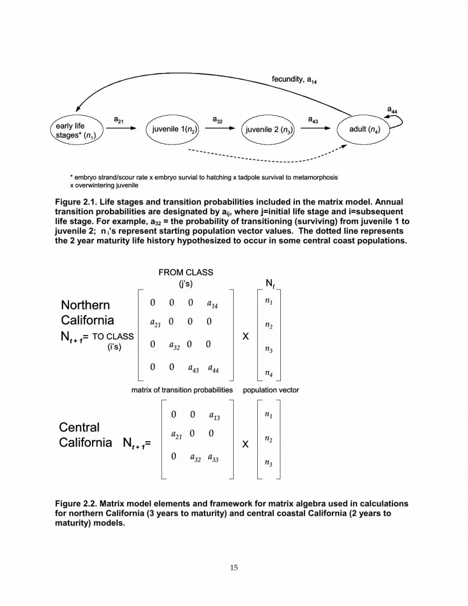
Figure 2.1. Life stages and transition probabilities included in the matrix model. Annual

transition probabilities are designated by aij, where j=initial life stage and i=subsequent life

stage. For example, a32 = the probability of transitioning (surviving) from juvenile 1 to juvenile 2;

n i’s represent starting population vector values. The dotted line represents the 2 year maturity

life history hypothesized to occur in some central coast populations. ............................................. 15

Figure 2.2. Matrix model elements and framework for matrix algebra used in calculations for

northern California (3 years to maturity) and central coastal California (2 years to maturity)

models. ....................................................................................................................................................... 15

Figure 2.3. Tadpole mortality (A) in mesocosm experiments conducted at the SF Eel

(Kupferberg 1997) indicates that survival is not density dependent for single species groups of

Rana boylii (Rb) tadpoles (Hr = Hyla regilla, Pacific treefrog Rc = Rana catesbeiana, Bullfrog).

Experimental densities in enclosures (two or four tadpoles) equivalent to 28 and 56 individuals

per m2 are higher than the large majority of quadrat samples (B) measuring ambient tadpole

density during the summers of 1992-1994. Tadpole densities are only that high early in the

rearing season, when tadpoles are young and small, as indicated by Gosner stage. .................... 18

Figure 2.4. Larval density, as indicated by the number of clutches laid at breeding sites in the

South Fork Eel River during spring 2008 was not correlated with the size (Snout Urostyle

Length) of recently metamorphosed frogs (n=159) captured at the same sites in late August. .... 19

Figure 2.5. Embryo number as a function of clutch volume, calculated using the median axis of

the clutch as the diameter of a sphere. .................................................................................................. 24

Figure 2.6. Earliest laid clutches are larger than those laid later in the spring. Sample size of

clutches observed at Gosner stage 13 or below on particular dates in parentheses (Gosner 1960).

.................................................................................................................................................................... 25

Figure 2.7. Distribution of survival rates of R. boylii egg masses in relation to hydrologic

stressors, i.e. stranding or scouring, over 16 years at the SF Eel River. ............................................ 26

Figure 2.8. Summary of breeding population sizes of Rana boylii compiled from several

researchers in California (see Table 2.11).............................................................................................. 40

viii

Figure 3.1. Reference Model (1) distribution of population growth rates (stochastic λ) over

10,000 simulations of 30-year trajectories of R. boylii populations (left). Cumulative extinction

probability over 30 years (right) generated from 10,000 random simulations drawing from

Reference Model values and distributions of vital rates. ................................................................... 45

Figure 3.2. Extinction risk in relation to starting population size. From left to right the models

are (5), (3), (1), and (4). ............................................................................................................................ 46

Figure 3.3. Extinction risk in relation to extinction threshold, models (6), (1), and (7). ................. 47

Figure 3.4. Multiplicative effects of stranding and scouring of egg masses combined with

decreased fecundity of females breeding after flow fluctuations cease. .......................................... 48

Figure 3.5. Low tadpole survival (0.46) pulsed flow scenarios, models (15) and (17-19),

simulating 1 to 4 pulses per summer. ................................................................................................... 49

Figure 3.6. High tadpole survival (0.61) pulsed flow scenarios, models (20) and (22-24),

simulating one to four pulses per summer. ......................................................................................... 49

Figure 3.7. Single summer pulsed flow effects accounting for effects of algal scour, models (16)

and (21). ..................................................................................................................................................... 50

Figure 3.8. Scenarios combining the effects of spring and summer hydrologic stressors on

embryonic survival, fecundity, and tadpole survival. ........................................................................ 51

Figure 3.9. Modern regulated worst-case model (29). Distribution of population growth rates

(stochastic λ) over 10,000 simulations of 30-year trajectories of R. boylii populations (left),

including small starting population size, regulated egg mass stranding and scouring, and two

summer pulsed flows. Note that the cumulative probability of extinction plateaus at 10 years

(right), rather than 30 in the Reference Model (Figure 3.1). ............................................................... 52

Figure 3.10. Effects of reduced starting population size combined with two levels of egg mass

stranding and scouring in Central Coastal California populations of R. boylii . ............................. 53

Figure A.1 Location of Hurdygurdy Creek study area (from Wheeler 2007) ............................... 73

Figure A.2 Alameda Ck study systems. Down stream regulated reaches include sections

upstream and downstream of the confluence with Calaveras Ck (red box). The unregulated

Camp Ohlone reach is upstream of the Alameda Diversion Tunnel, in the direction of the red

arrow but is off this map. Source of map SFPUC 2007, available online

http://www.sfgov.org/site/uploadedfiles/planning/vol3_sec5-4_wsip-dpeir.pdf accessed July 28,

2007. ........................................................................................................................................................... 74

ix

Abstract

The decline of the river breeding foothill yellow-legged frog (Rana boylii) has been attributed to

the altered flow regimes and habitat fragmentation associated with water storage and

hydropower dams. Recent research has provided insight into potential mechanisms for these

declines, confirming that early life history stages (embryos and tadpoles) are negatively affected

by altered hydrology, especially pulses in water flows during spring and summer which change

water velocities and depths in oviposition and rearing habitats. To evaluate whether such early

life stage impacts could ultimately affect R. boylii population dynamics, we developed a 30-year

stochastic matrix population model (Reference model) and explored a range of possible

hydrologic and demographic perturbations to these virtual populations. While most female R.

boylii appear to reach maturity at age 3, there is evidence that some Central Coast populations

may reach maturity at age 2. To account for this potential regional life-history difference, we

also developed a “two year to maturity” reference model, and explored a subset of relevant

hydrologic scenarios. For each reference model, R. boylii life-stage specific survival rates were

collected by new field efforts and assembled from existing data provided by other researchers

and the literature for populations in hydrologically un-regulated rivers. To incorporate

variability and uncertainty in these rates, distributions of possible values for each vital rate were

described based on multiple data sources, and these distributions served as the basis for

stochastic projections. Thirty different perturbations to the reference models were evaluated,

with each scenario based on expected effects of altered hydrology for single or multiple life

stages. The 30-year probability of extinction increased substantially (relative to the reference

models) with small starting population sizes and in scenarios with high levels of stranding

and/or scouring of egg masses or tadpoles. Multivariate sensitivity analysis confirms that egg

mass scouring, and tadpole, juvenile, and adult survival are key factors influencing overall

population dynamics. Modeled populations were unable to persist with multiple artificial

pulsed summer flows or combinations of hydrologic stressors suggesting that the fate of early

life stages can be critical to R. boylii population persistence in hydrologically altered rivers. A

key observation stemming from this modeling effort is the need for better demographic data

collection for R. boylii, especially annual tadpole and juvenile survival, and a functional

understanding of how specific changes in hydrology affect particular life stage survival rates.

Until such data are collected and incorporated into a similar modeling effort, the results

reported here should be interpreted as preliminary and predictions made about real R. boylii

populations under altered hydrologies will remain highly uncertain.

Key Words: matrix population model, hydrologic scenarios, sensitivity analyses

1

Executive Summary

Project Objective and Problem Statement

Hydrologic alteration of many California rivers has resulted in population declines and local

extinctions of native species. Rana boylii, the Foothill Yellow-legged Frog, exemplifies this

phenomenon, having declined dramatically over the last half century, especially in Southern

California and the Southern Sierra Nevada mountains. It is a California Species of Special

Concern and has disappeared from over 50% of known historic sites, with absences being more

common in close proximity to large dams. During California’s era of hydroelectric dam

construction 30-40 years ago, habitats were destroyed and fragmented as river channels were

converted to reservoirs. The persisting populations are small relative to those in unregulated

rivers and are being adversely affected by aseasonal pulsed releases of water. The altered

hydrologic regimes do not match a key adaptation of R. boylii to avoid flood induced mortality –

synchrony of reproductive timing with the predictable seasonality of discharge.

A conservation challenge for R. boylii is to predict how negative effects on specific life stages

from altered flow regimes will influence a population as a whole. Population viability analysis

using life stage specific demographic rates offers a method to assess the probability that a

population will persist when the survival of one or more stages is changed. Such a

mathematical model requires compiling the probabilities of surviving from one life stage to the

next in a life table. Outcomes are then forecast by using the life table values in combination with

a defined starting population size and extinction threshold. The aim of this study is to construct

the model and develop it as a tool to address a focal question; how are the population dynamics

of R. boylii influenced by the frequency, timing, and magnitude of pulsed flow induced

mortality of early life stages?

Methods: Model Construction and Population Viability Analysis

Life table values were estimated using: (1) breeding censuses conducted at three focal

watersheds to determine starting population sizes; (2) analyses of existing capture-recapture

data on adult frogs to estimate the time to reproductive maturity and annual survival; (3) field

enclosures of egg masses to quantify the number of offspring per female and embryo survival;

(4) field experiments on tadpole survival; and (5) mark-recapture of young of the year frogs in

the fall and following spring to assess the survival of tadpoles to metamorphosis and survival

through the first winter. Missing rates were derived from the literature or data on related

species. Once vital rates were compiled into a reference (unregulated river) model, scenarios

were developed to assess the effects of hydrologic stressors on one or more life stages, and the

population as a whole. The population was projected 30 years into the future and 10,000

simulations were done for the reference models and each scenario. Results were evaluated

based on the probability of extinction and the average population growth rate.

Thirty scenarios of altered hydrology were explored. Each was a virtual manipulation of

population or hydrologic factors: starting population size, the definition of ‘virtual’ extinction,

spring and summer flow effects on egg mass and tadpole survival, thermal effects on tadpole

2

survival, and combinations of factors. The impact of each scenario was compared to the

dynamics of hypothetical unregulated populations of R. boylii in Northern or Central California

(3 and 2 years to maturity, respectively). To assess the relative influence of each life stage on

overall population outcomes, a multivariate sensitivity analysis was conducted.

Population Modeling Results and Discussion

We found that Rana boylii populations in regulated rivers were at greater risk of extinction by

virtue of their low abundance, even before the effects of hydrologic stressors were considered.

Compared to the Reference Model which assumed a starting population of 32 breeding female

frogs / km (unregulated average), regulated river populations (with an average of 4.6 females /

km, or at the low end 2.1 / km) had a four to thirteen-fold increase in the 30-year risk of

extinction. Simulated populations experiencing rapid flow fluctuation causing egg mass

stranding and scouring led to 2.2-4.6 fold increases in extinction risk. The compounding effects

of rapid flow fluctuation on egg survival were explored based on the observation that large

females, which produce larger egg masses, breed earlier. Clutches laid later in the spring,

which escape stranding and scouring, contain many fewer offspring. When this difference was

accounted for, extinction risk was 17 times greater than in the reference model. Similarly, the

joint effects of summer hydrologic stressors were greater than the sum of the component

impacts. Extinction risk more than doubled with the tadpole mortality caused by annually

recurring summer pulsed flows. Notably, extinction risk increased ten-fold when considering

the food scarcity caused by the export of algal food during a pulsed flow. Multiple pulsed flows

increased extinction risk twenty fold.

When the effects of spring and summer hydrologic alteration on R. boylii populations were

considered, the relative increases in extinction above the Reference Model were very large. A

hypothetical decline history for R. boylii was modeled by subjecting a robust starting population

size to worst case scenario levels of stranding and scouring in the spring and then an annual

summer pulsed flow as might have occurred historically due to scheduled maintenance of

hydropower projects. The results indicated that a population would have very small chances of

surviving these joint effects. When the seasonal trends in numbers of offspring produced were

taken into account, extinction risk was >19 times greater than the Reference Model. The

potential for recovery of small populations in regulated rivers, was explored by combining

small starting population size with a background rate of stranding and scouring typical of

regulated rivers as the sole hydrologic stressor. The resulting fifteen fold increase in extinction

risk relative to the Reference Model indicated that recovery potential of such populations is low.

Conclusions and Recommendations

Conservation of R. boylii in regulated rivers will depend on management that minimizes altered

flows during the spring breeding and summer tadpole rearing seasons. In unregulated rivers, R.

boylii populations appear to be self-sustaining under natural levels of hydrologic variation.

When spring pulses that represent spill events and recreational boating flows were simulated,

the 30-year risk of extinction was doubled. Similarly for the tadpole life stage, summer pulsed

flows increased the risk of extinction three to five fold over the reference model. Combinations

3

of hydrologic stressors that reflect real-world situations resulted in compounded increases in

extinction risk.

These model results confirm the importance of the synchrony between the R. boylii life cycle and

the seasonality of low flows typical of Mediterranean climates in spring and summer. When

flow regimes deviate from this natural seasonal timing of flow fluctuation, locally adapted

communities of organisms, including R. boylii, are likely to be threatened. Although model

simulations were not intended to predict the actual dynamics of any one R. boylii population,

the results correspond to trends in time series data collected at the SF Eel River, Alameda Creek,

and NF Feather River.

While the overall results generated from the reference model and scenarios are well-supported,

several uncertainties remain. The top priorities for follow-up investigation are to improve

estimates of tadpole survival, over winter survival, and juvenile survival. As more detailed

demographic data become available, these results and modeling scenarios may need to be

revised. With that caveat, management recommendations are:

• Eliminate manufactured pulsed flows once frog breeding begins in the spring and

suspend such flows through the early fall when metamorphosis occurs.

• Recognize synergisms and indirect effects among various hydrologic changes.

• Gather data on key birth and death rates during dam relicensing and use this model

as a starting point for Population Viability Analyses of specific R. boylii populations.

• Improve long-term monitoring programs for R. boylii in both regulated and

unregulated (reference) river systems, especially in the Sierra Nevada.

• Appropriate State and/or Federal agencies should elevate the protection status of R.

boylii under the California or Federal Endangered Species Act.

Benefits to California

During adaptive management of dam operations and the relicensing of hydropower projects,

there are often discussions of the possible ecological effects of alternative base flows, pulsed

flows, and other hydrologic conditions. If early life-stages of R. boylii are likely to be affected by

the flow regime attribute under consideration, our results provide support that these actions

may directly affect the status of adult populations. This connection between the dynamics of

early life-stages and the adult population provide an important biological context for evaluating

competing flow proposals. Future applications of these models may also aid in the assessment

of risk for other sensitive species with similar reproductive timing and ecological niches.

4

1.0 Research Problem Statement

1.1. Hydrologic Alteration, Rana boylii Conservation, and the Need for Population Projection Models

Hydrologic alteration has reduced the abundance and imperiled the status of a wide array of

riverine species (Richter et al 1997; Rosenberg et al. 2000; Bunn and Arthington 2002). Rana

boylii, the foothill yellow-legged frog, exemplifies this phenomenon, having declined

dramatically over the last half century, especially in Southern California and the Southern Sierra

Nevada mountains. It is absent from over 50% of known historic sites (Davidson et al. 2002,

Lind 2005) and is a California Species of Special Concern (Jennings and Hayes 1994; Jennings

1996; California Department of Fish and Game 2008). Absences from historic localities are more

common in close proximity to large dams (Lind 2005). During California’s era of hydroelectric

dam construction 30-40 years ago, habitats were destroyed and fragmented as river channels

were converted to reservoirs. The populations that persist are small relative to those in

unregulated rivers and are being adversely affected by aseasonal pulsed releases of water

(Kupferberg et al. 2008).

For R. boylii, the general problem in regulated rivers is that the altered timing, duration, and

magnitude of discharge do not match its key adaptation for evading mortality from flow

fluctuation, synchronizing reproductive timing and life stage transitions with the seasonality of

discharge (Table 1.1). A thorny challenge for conserving a riverine species with a complex life

cycle is predicting how flow regime effects on a particular life stage will influence the

population as a whole. As regulators and utilities negotiate new license conditions for

hydropower projects, there is an urgent need for tools that can link a specific change in

discharge timing or magnitude to a desired conservation outcome. Population viability analysis

(PVA) using life-stage specific demographic rates offers a method to assess the likelihood that a

population will persist for a given period of time, when changes are made to the survival of one

stage. The first step in conducting such a PVA is to define the relevant stages and transitions

among stages.

Table 1.1. Overview of potential and documented impacts to Rana boylii in regulated rivers.

Project Operations

Short-term impacts Long-term impacts

Intentional aseasonal flows

(power generation, recreation,

outmigration of salmonid

smolts); Unintentional spill of

water over dam

- scour and/or desiccation of egg

masses1,2

/ tadpoles3

- export spring and summer algal

productivity4,5

, reduced resources

for tadpoles, reduced insect

abundance5, food web

repercussions

- discharge decoupled from

environmental cues (e.g. rainfall,

air temperature) triggering

inappropriate behavioral

responses by adults, juveniles,

delayed onset of breeding1,6

- smaller population sizes1,2

Intentional de-watering of

stream channels for rescue

operations

- desiccation of egg masses /

tadpoles

Unknown

5

Project Operations

Short-term impacts Long-term impacts

Unintentional powerhouse

outages resulting in rapid

increase in flows in bypass

reaches, followed by rapid

decrease in flows

- changes to margin water

temperature, depth, and velocity,

- scouring/desiccation of

eggs/tadpoles, depending on

ramping rate, magnitude of

change, channel shape

Unknown

Reduced winter/spring flows

- absence of scouring/depositional

flows that prevent riparian

encroachment

- reduced breeding habitat, greater

distances between breeding sites3

- vegetation encroachment,

altered channel morphology,

reduced breeding habitat

- population loss/fragmentation3,

reduced gene flow, altered

metapopulation dynamics

Altered summer baseflows - lower water temperatures

- change in available habitat

(channel shape)

- promotes habitats that support

non-native predatory fish,

amphibians, and invertebrates,

increased predation on eggs,

tadpoles

Movement of water among river

basins

- potential for increased disease

and parasite transmission

Unknown

References: 1. Garcia and Associates (GANDA) 2008; 2. Kupferberg et al. 2008; 3. Lind et al. 1996;

4. Spring Rivers 2002; 5. GANDA 2006; 6. Borque 2008

1.2. Rana boylii Life Cycle and Demographic transitions

For the purposes of building the population model, the following demographic rates, or

transition probabilities are designated during Rana boylii’s life cycle. (1) Fecundity

(eggs/female). Fecundity is the number of eggs produced by each female when the breeding

adults move out of tributaries (unaffected by flow regulation) to spawning sites on main-stem

channels (which are subject to dam related flow fluctuation). Frogs spawn at the margins of

relatively wide and shallow channel sections, in habitats that protect their immobile progeny

from moderate flow variation. Females attach their single clutch of eggs in low velocity

locations behind, and sometimes under, rocks which provide relatively stable depth and

velocity conditions across a range of discharge volumes (Kupferberg 1996; Yarnell 2005; Lind

2005). (2) Embryo scour rate. Under a natural flow regime, there are low recurrence-interval

wet springs with spates, in which some egg masses are lost due to scour. (3) Embryo stranding

rate. In dry springs, rapidly receding shorelines can strand egg masses (Kupferberg 1996, see

Figure 9, Kupferberg et al. 2008). In most years however, spawning occurs in synchrony with

the receding limb of the spring hydrograph such that embryos and recently hatched larvae

avoid flood or desiccation mortality. (4) Embryo survival rate. For those eggs that remain

wetted and attached to substrate, not all hatch. Some may not have been fertilized, and some

die prior to hatching into tadpoles. (5) Tadpole survival to metamorphosis. In addition to

being prey for numerous consumers in stream food webs, tadpoles are susceptible to hydrologic

sources of mortality. The larvae do not have morphological flow adaptations such as a ventral

6

suctorial disc used for adhesion, as occurs in anurans whose larvae inhabit turbulent habitats or

endure unpredictable flooding (Altig and Johnston 1989; Richards 2002). (6) First over winter

juvenile (young of the year) survival. There is scant information about autumn movements of

young of the year frogs (the young of the year life stage extends from metamorphosis through

the first winter). They may move upland away from main stem channels (Twitty et al. 1967;

Palen pers. obs. at SF Eel), to off-channel seeps (Rombough 2006), and caves (Peek and

Kupferberg pers. obs. at SF American), or may over-winter in tributaries. (7) Juvenile survival

and (8) juvenile to adult survival. Frogs must continue to survive for one or two more years

(depending on location specific growth rates) before reaching the transition to reproductive

maturity. The juvenile life-history stage is largely a mystery, and how these transition

probabilities may relate to flow regime, either directly or via carry-over effects related to larval

growth history are topics requiring additional research. (9) Adult survival. Adult numbers do

not appear to be influenced by main-stem winter peak discharges (Kupferberg et al. 2008) and

radio-telemetry data indicate that adults over-winter in tributaries and are able to cross wide

channels to access breeding sites even at high flows (GANDA 2008). Given this multi-staged

natural history, the basic question addressed in this study is: What are the consequences of

changes to a particular life-stage’s vital rate to the persistence of the whole frog population

through time?

1.3. Focal Watersheds (Alameda Creek, South Fork Eel River, North Fork Feather River, Hurdygurdy Creek)

For estimation of demographic rates and time to maturity, data were collected within several

different California watersheds (Figure 1.1. The three primary study areas where new data were

collected are: the unregulated South Fork Eel River (SF Eel) in the University of California

Angelo Reserve (Mendocino Co.); two regulated reaches (Poe and Cresta) of the North Fork

Feather River (NFFR) on the Plumas National Forest (Butte Co.); an unregulated reach of

Alameda Creek (Alameda) in the Sunol-Ohlone Regional Wilderness of the East Bay Regional

Park District (Alameda Co.). Alameda Creek flows into the San Francisco Bay. A pre-existing

data set for a population of R. boylii at Hurdygurdy Creek, a tributary of the South Fork Smith

River (Del Norte Co.), was provided by Clara Wheeler. Each watershed has hydrologic,

geomorphic and habitat characteristics typical of R. boylii localities in its respective region, the

north coast, the Sierra Nevada, and the central coast (Table 1.2). For detailed habitat

descriptions see Appendix A. These study sites correspond with three genetically distinct

clades, or branches, in the evolutionary tree developed for R. boylii (Lind 2005). However, it is

not known if these genetic differences translate to phenotypic differences in timing of breeding

or other life history traits that may be differentially influenced by hydrologic variation. These

locations were chosen because they have ongoing monitoring of frog populations and good

hydrologic records.

7

Figure 1.1. Location of the study watersheds in northern and central California. The number of regulated or unregulated river reaches is listed for each watershed. Populations south of the dashed purple line are hypothesized to reach maturity in 2 years; populations north and east of the line reach maturity in 3 years.

The character of the pulse flows in the three focal watersheds with stream gaging is distinct

(Figure 1.2). Annual hydrographs for the SF Eel illustrate natural seasonal runoff, with peak

discharges in winter and occasional spring spates caused by rainfall. The regulated reaches have

periodic late spring and summer pulsed flows that are aseasonal. The NF Feather reaches have

large magnitude peak flows during winter and spring in wet years when the dams spill at the

8

peak of snowmelt and when rain on snow events occur. The hydrograph is flat during the

summer and fall, unless pulsed flows are manufactured as they were in the Cresta reach for

whitewater boating (2002-2005, once per month June-Oct). The Alameda Creek regulated reach

has a hydrograph that, while somewhat natural in shape, has reduced magnitude base flows,

with occasional disproportionately high-magnitude peaks associated with flood spills and

plateaus associated with continued releases. Since 2001, due to seismic safety concerns about

Calaveras Dam, the maximum allowable reservoir height is 40% of capacity. Water is released

to maintain that level (SFPUC 2007). By comparison, the unregulated Camp Ohlone reach on

Alameda Creek has pulse magnitudes and durations directly coupled to rainfall. The

magnitude of peak flows there is expected to decline under climate change scenarios

(Klausmeyer 2005).

The frog population trends in rivers where these different types of hydrologic regimes

predominate motivate the scenarios presented in this report. Generally populations are sparse

and / or in decline in regulated rivers, while they are more abundant, stable, or increasing in

free-flowing locations (Table 2.12, Figure 2.8). Specifically, at the SF Eel time series data indicate

stable and increasing populations respectively (Kupferberg et al. 2008). In the NF Feather, frog

population trends between the Poe and Cresta reaches are divergent, with Poe increasing and

Cresta decreasing after new license conditions were instituted for Cresta Dam (increased base

flow and summer white water boating flows). In Alameda Creek, populations are increasing in

the Camp Ohlone reach, under natural hydrologic conditions, whereas downstream of the

confluence with Calaveras Creek, R.boylii populations have decreased after consecutive years

with high discharge conditions in the spring. This more southern population may be governed

by different biological processes, such as faster growth rates and earlier age at reproductive

maturity. The hydrologic stressors faced may be determined more by drinking water and

irrigation needs than by power generation and recreational demands, and have different

seasonal timing.

9

Table 1.2. General characteristics of the focal river systems’ topography, hydrology, geomorphology, and vegetation.

River / Creek

Reach and Nearest

USGS Gage #

Regulation

Drainage Area1

(km

2)

Mean±1 s.d.

Annual Discharge2

(cms)

Elevation (m)

Dominant Channel

Morphology

Upland Vegetation

Riparian

Vegetation

Dominant

Substrate

NF Feather

Cresta

11404330

Cresta Dam

4976

22.5±25.6

488-424

Riffle-pool

Chaparral

and Mixed Conifer Forest

Willow, Alder,

blackberry, sedge

Bedrock overlain

by boulders

and cobbles

Poe

11404500

Poe Dam

5078

25.9±27.4

424-287

Riffle-pool

Hurdygurdy

Not currently

gaged

none

~ 80

~ 1

(summer) 100-140 (winter)

5

760

Riffle-pool

Hardwood / Douglas Fir Forest

Alder, willow

Bedrock, overlain

by boulders

and cobbles

SF Eel

Branscomb

3

11475500

none

114

4.88±1.70

427-365

Riffle-pool

Douglas

Fir Forest

Alder, sedge

Bedrock overlain

by boulders

and cobbles

Alameda

Camp Ohlone

11172945

none

88

0.77±0.42

380-365

Riffle-run

Oak

Woodland, Grassland

Sycamore,

Mulefat, Alder, sedge

Bedrock, Cobble, gravel

Sunol4

11173510 11173575

Calaver-as Dam

273

1.17±1.07

134-122

Riffle-run

1. Area upstream of the gaging station, data from USGS for all but Hurdygurdy. Hurdygurdy data is the

area above the creek mouth.

2. Based on the following years of record: NF Feather Poe, 1980–2006, Cresta, 1986-2006; SF Eel, 1946-1970

and 1991–2006, synthetic record derived from Leggett data; Alameda, above diversion 1995–2006, below

confluence with Calaveras 1999-2006

3. Branscomb gage USGS 1946-1970, re-established by Dietrich and Power 4/1990, USFS 2004

4. Alameda Creek, high flow discharges from gage near Welch Ck., approximately 5 km downstream of

survey reach, gage below Calaveras confluence is a low-flow only gaging station

5. Estimated from previous gage data, no current active gage.

10

0.0

0.1

1.0

10.0

100.0

1000.0

Dec-04 Feb-05 May-05 Jul-05 Oct-05 Dec-05 Feb-06 May-06 Jul-06 Oct-06 Dec-06 Feb-07 May-07 Jul-07 Oct-07

Cresta ReachPoe Reach

NF Feather

0.01

0.1

1

10

100

1000

Dec-04 Feb-05 May-05 Jul-05 Oct-05 Dec-05 Feb-06 May-06 Jul-06 Oct-06 Dec-06 Feb-07 May-07 Jul-07 Oct-07

SF Eel

0.001

0.01

0.1

1

10

100

1000

Oct-04 Dec-04 Feb-05 May-05 Jul-05 Oct-05 Dec-05 Feb-06 May-06 Jul-06 Oct-06 Dec-06 Feb-07 May-07 Jul-07 Oct-07

Sunol Reach

Camp Ohlone ReachAlameda Ck

tadpole season

pulsed flows Embryo

stranding

when

spill

ends

embryo scour

from rain

28% survival

benign

conditions

prolonged spill

no breeding

early clutches

(2%) scoured;

benign conditions

for tadpoles

embryo

season

pulsed flow

Dis

ch

arg

e (

m3se

c-1

)

benign

conditions

0.0

0.1

1.0

10.0

100.0

1000.0

Dec-04 Feb-05 May-05 Jul-05 Oct-05 Dec-05 Feb-06 May-06 Jul-06 Oct-06 Dec-06 Feb-07 May-07 Jul-07 Oct-07

Cresta ReachPoe Reach

NF Feather

0.01

0.1

1

10

100

1000

Dec-04 Feb-05 May-05 Jul-05 Oct-05 Dec-05 Feb-06 May-06 Jul-06 Oct-06 Dec-06 Feb-07 May-07 Jul-07 Oct-07

SF Eel

0.001

0.01

0.1

1

10

100

1000

Oct-04 Dec-04 Feb-05 May-05 Jul-05 Oct-05 Dec-05 Feb-06 May-06 Jul-06 Oct-06 Dec-06 Feb-07 May-07 Jul-07 Oct-07

Sunol Reach

Camp Ohlone ReachAlameda Ck

0.0

0.1

1.0

10.0

100.0

1000.0

Dec-04 Feb-05 May-05 Jul-05 Oct-05 Dec-05 Feb-06 May-06 Jul-06 Oct-06 Dec-06 Feb-07 May-07 Jul-07 Oct-07

Cresta ReachPoe Reach

NF Feather

0.01

0.1

1

10

100

1000

Dec-04 Feb-05 May-05 Jul-05 Oct-05 Dec-05 Feb-06 May-06 Jul-06 Oct-06 Dec-06 Feb-07 May-07 Jul-07 Oct-07

SF Eel

0.001

0.01

0.1

1

10

100

1000

Oct-04 Dec-04 Feb-05 May-05 Jul-05 Oct-05 Dec-05 Feb-06 May-06 Jul-06 Oct-06 Dec-06 Feb-07 May-07 Jul-07 Oct-07

Sunol Reach

Camp Ohlone ReachAlameda Ck

tadpole season

pulsed flows Embryo

stranding

when

spill

ends

embryo scour

from rain

28% survival

benign

conditions

prolonged spill

no breeding

early clutches

(2%) scoured;

benign conditions

for tadpoles

embryo

season

pulsed flow

Dis

ch

arg

e (

m3se

c-1

)

benign

conditions

Figure 1.2. Mean daily discharge (m3sec-1) for water years 2005-2007 in one regulated and one unregulated reach of Alameda Creek (bottom), the unregulated SF Eel (middle) and two regulated reaches of the NF Feather (top). Circled regions of hydrographs indicate periods and events important to the survival of early life stages of Rana boylii. Small arrows along the x-axes indicate dates when the oviposition and tadpole rearing seasons began in each river system.

11

1.4. Project Objectives and Report Organization

The purpose of this project is to investigate the demographic processes contributing to patterns

of frog decline associated with river regulation during the times of year when early life stages

are vulnerable to flow induced mortality. The population level consequences of extreme

fluctuation in water discharge volume during atypical times of the year are evaluated using a

stochastic projection matrix model that relies on estimation of demographic rates for early

multiple life stages.

R. boylii demography and populations dynamics were examined by combining: (1) count data

from breeding censuses conducted at three focal watersheds; (2) analyses of existing mark-

recapture data on adult frogs to assess time to reproductive maturity and yearly survival rates;

(3) field enclosures of egg masses to quantify fecundity and embryo survival; and (4) mark-

recapture of young of the year frogs in the fall and following spring to assess tadpole survival to

metamorphosis and first winter survival. This report has six sections and two appendices.

Section 2 presents the methods, section 3 the results, and section 4 the discussion and synthesis.

Sections 5 and 6 contain references and a glossary. Specific objectives are:

Section 2: Model Statement, Life Table Construction, Estimation of Survival Rates,

Development of Population Model, and Descriptions of Modeled Scenarios

• Construct a generalized life table (life stage based summary of fecundity, longevity,

survival, and mortality factors) for R. boylii by compiling data from several northern and

central California populations.

• Define the relationships between hydrologic disturbance and probability of transitioning

from one life stage to the next.

• Conduct field enclosure studies to assess fecundity and embryo survival.

• Compile data on egg mass scouring and stranding rates during natural and artificial flow

fluctuations during the spring and summer breeding and rearing periods.

• Conduct capture-recapture study on young of the year frogs in fall and then again in the

following spring to develop young of the year frog population estimates and determine first

year over-winter survival rate.

• Develop a matrix population projection model that will allow prediction of population and

life stage effects under a variety of hydrologic regimes (both human-controlled and natural).

Section 3: Results and Discussion of Model Runs and Sensitivity Analyses

• Evaluate risk of extinction under different scenarios of starting population size and

hydrologically driven mortality events

• Conduct sensitivity analyses to determine which life stages are critical for conservation.

12

Section 4: Conclusions and Recommendations

• Provide an overall synthesis and conclusions based on sections 2 and 3.

• Recommend future research and direction for FERC studies with the aim of collecting data

to fill gaps in knowledge of the vital rates of stages that have large influence on population

persistence

• Address commercialization potential

• Assess benefits to California

13

2.0 Methods: Model Construction, Estimation of Survival Rates, and Population Viability Scenarios

2.1. Life Table Construction

A demographic population projection model begins with a life table. A life table is a book-

keeping tool that compiles the probabilities of transitioning from one life stage to the next for a

cohort of individuals. Traditionally these transition probabilities are single estimates, which

results in a relatively simple form of matrix population model, a deterministic model. While

informative, this approach limits a model’s utility for evaluating how fluctuations in transition

probabilities (due to natural or anthropogenic causes) influence the population growth rate. In

this project, the goals are to estimate distributions, rather than single values, of life-stage

transition probabilities that are functions of hydrologic variables as well as estimate background

variation not visibly attributable to a mechanistic cause (stochastic modeling). For most life

stages, pre-existing data collected by the authors’ own surveys and experiments were used and

supplemented with data from other researchers. There were no available data on female

fecundity, embryo survival, the transition from metamorphosis to first year juvenile, and the

transition from juvenile to adult. Thus, new data were collected on female fecundity and

embryo survival using field enclosures of egg masses and on metamorphosis to first year

juvenile survival using capture-recapture techniques on newly metamorphosed frogs. For the

first year juvenile to adult transition, data were too sparse for parameter estimation. In this case,

literature estimates for related species of frogs and professional judgment extrapolating from

estimates derived for other life stages were used. These baseline transition probabilities are

presented here in Section 2 (see subsections titled “Application to Population – Reference

Values” for each life stage).

Section 2 also describes model scenarios for each life stage transition. In the scenarios, the

transition probabilities and/or their variances are manipulated to represent effects of pulsed

fluctuations in discharge and other hydrologic effects on vital rates (see subsections titled

“Model Scenarios” for each life stage). Reference transition probabilities and particular

scenarios are simulated over multiple generations of frogs. For example, the effects of spring

run-off events that cause occasional spills are compared to the effects of annual summer

recreational boating flows. The results for the mathematical modeling of R. boylii population

dynamics are presented in Section 3.

A composite approach, utilizing information from several different watersheds, is employed

because different amounts and types of data are available for each individual population. By

combining data from several populations, the recommended minimum criteria for conducting

Population Viability Analyses (PVA’s) are met (Table 2.1 and Morris and Doak 2002). Morris et al.

(1999) admonish researchers and managers that the value of population viability analysis does

not lie in the exact predictions of a single analysis (e.g. that a frog population will have a 50%

chance of persisting for 30 years, a typical FERC license term). Rather “a better use of PVA in a

world of uncertainty, is to gain insight into the range of likely fates of a single population based

14

upon two or more different analyses (if possible), or the relative viability of two or more

populations to which the same type of analysis has been applied.” Despite the limitations of the

techniques, PVA applied to 21 different time series from long-term ecological studies has shown

a high degree of predictive accuracy. When parameters were estimated from the first half of

each data set, and the second half was used to test the predictions of the models, the probability

of population decline corresponded well with the observed outcomes (Brook et al. 2000).

Table 2.1. Guidelines for minimum data requirements to perform population viability analyses (adapted from Morris and Doak 2002). The shaded boxes represent the types of data used here for the R. boylii population modeling scenarios.

Type of PVA Data Needed Applications

deterministic count-based >10 years of

census/count data

qualitative representation of population

status – i.e. declining, growing, relative

viability of one population vs. another

stochastic demographic > 4 years of vital rate

data (= 3 annual

transitions)

provides enough information to develop

means, variances, covariances of vital

rates for a fully parameterized

demographic model

sensitivity analyses for

deterministic models

< 4 years vital rate

data

allows evaluation of management actions

and threats

multi-site PVA

* stochastic with

migration among

subpopulations

2 years presence /

absence surveys at

20+ sites

* 4 years

allows evaluation of population status

across a landscape

2.2. Model Statement

A simple 4-stage annual matrix model (At) of female R. boylii life history including three

juvenile stages and one adult stage was created (Figures 2.1 and 2.2). Composite annual

transition probabilities between stages (aij) often incorporate the survival rates of several distinct

life history stages (Table 2.2). For example, the transition from birth to the end of the first year

(a21) encompasses survival through egg mass stranding and scouring, embryonic and larval

development, metamorphosis, and the first winter as a newly transformed juvenile frog. For

each component of these composite annual transitions, a distribution of survival rates from the

mean and variance of multiple data sources were estimated (Table 2.2), drawing primarily on

data collected from populations in hydrologically unregulated California rivers (Appendix A).

The distributions of survival values for each component life-stage transition (signified as sstage in

Table 2.2) were modeled as beta distributions, except for fecundity, which was modeled as a

lognormal distribution (Morris and Doak 2002). This matrix population model was initially

15

Figure 2.1. Life stages and transition probabilities included in the matrix model. Annual transition probabilities are designated by aij, where j=initial life stage and i=subsequent life stage. For example, a32 = the probability of transitioning (surviving) from juvenile 1 to juvenile 2; n i’s represent starting population vector values. The dotted line represents the 2 year maturity life history hypothesized to occur in some central coast populations.

0 0 0 a14

a21 0 0 0

0 a32 0 0

0 0 a43 a44

FROM CLASS

(j’s)

TO CLASS

(i’s)

XNt + 1=

Nt

matrix of transition probabilities population vector

n1

n2

n3

n4

0 0 a13

a21 0 0

0 a32 a33

X

n1

n2

n3

Central

California Nt + 1=

Northern

California

0 0 0 a14

a21 0 0 0

0 a32 0 0

0 0 a43 a44

FROM CLASS

(j’s)

TO CLASS

(i’s)

XNt + 1=

Nt

matrix of transition probabilities population vector

n1

n2

n3

n4

0 0 a13

a21 0 0

0 a32 a33

X

n1

n2

n3

Central

California Nt + 1=

Northern

California

Figure 2.2. Matrix model elements and framework for matrix algebra used in calculations for northern California (3 years to maturity) and central coastal California (2 years to maturity) models.

early life

stages* (n1)juvenile 1(n2) juvenile 2 (n3) adult (n4)

* embryo strand/scour rate x embryo survial to hatching x tadpole survival to metamorphosis

x overwintering juvenile

fecundity, a14

a21 a43a32

a44

early life

stages* (n1)juvenile 1(n2) juvenile 2 (n3) adult (n4)

* embryo strand/scour rate x embryo survial to hatching x tadpole survival to metamorphosis

x overwintering juvenile

fecundity, a14fecundity, a14

a21a21 a43a43a32a32

a44a44

16

used to simulate the dynamics of a generic R. boylii population in a 10 km reach of an

unregulated environment (referred to as the “Reference Model”) by drawing transition

probabilities at random from the beta or log-normal distribution of each component life-stage,

each year for 30 years, following the population size of adult females through time, and

calculating the average 30 year population growth rate (lambda, λs). A 10 km reach was chosen

to represent a typical R. boylii population based on recent genetic (mtDNA, RAPD) evidence

demonstrating significant isolation by distance between individuals greater than 10 km apart

(Dever 2007). Ten km is also close to typical reach lengths between dams (see Table 2.11). A 30

year simulation window was chosen to represent the typical length of a U.S. Federal Energy

Regulatory Commission (FERC) hydroelectric dam license.

As with most amphibians, there are only sparse demographic data for R. boylii, primarily from

several short-term studies of different populations, and existing studies have not estimated

more than one or two demographic rates simultaneously. The choice to pursue stochastic

demographic modeling was favored despite this shortcoming for the opportunity to evaluate

scenarios of how hydrologic regulation may specifically affect individual life stages and

component vital rates. As a result, this modeling effort is constrained to relatively simple

stochastic simulations, and is subject to a high level of uncertainty in the estimates of individual

vital rates, their distributions, and the resulting population dynamics. A strong cautionary

perspective is required when interpreting these modeling results and should be restricted to the

relative performance of individual models compared to the reference condition, for which there

are the most extensive (but still limited) demographic data. In general, each scenario we explore

beyond the reference model is based on quantitative data (when possible) of likely impacts of

hydrologic regulation to different life stages (or combinations), but none the less should be

considered exploratory and not a representation of any particular ‘real’ R. boylii population.

The Reference Model was initiated (year 1) with a starting population vector (Nt) defined as the

number of individuals in each life stage, determined from the combination of a starting number

of 320 adult females (n4) and the average vital rates (i.e. births and deaths) for each life stage.

The starting population vector therefore represents a population beginning at a stable age

distribution of individuals across life stages. The starting number of adult females for the

reference model is estimated from the average number of egg masses found in unregulated

rivers (see compilation of unpublished and published data in Table 2.12; average 32 clutches/km

x 10 km hypothetical reach). As such, the starting number of adult females is a parameter with

multiple long-term (>5 yrs.) estimates from both un-regulated (reference) and regulated

conditions. Because of the range of values that each life stage transition encompasses, the results

of any one run of this model (with only 30 random draws of each life-stage transition) are not

expected to be broadly representative. To incorporate the uncertainty and variability within and

among life-stage transitions, the 30-year model was simulated 10,000 times, and the average

stochastic population growth rate (λs) and the probability that the R. boylii population drops

below a quasi-extinction threshold are reported (Morris and Doak 2002). Quasi-extinction

thresholds are often used in population dynamics models to represent a minimum viable

population size, below which populations may be exceedingly vulnerable to stochastic genetic

and demographic (Allee) effects and also below which accurate forecasting of population

17

dynamics becomes extremely questionable (e.g. that at very low densities populations are likely

to be governed by very different demographic rates and processes). Morris and Doak (2002)

suggest applying quasi-extinction thresholds of at least 20 breeding individuals, but a more

conservative approach for populations of conservation concern would be to set the threshold at

the lowest density of a known stable population (based on long-term time series data). For the

Reference Model, the quasi-extinction threshold was set to two adult females per river km, or 20

adult females in the simulated population occurring within a hypothetical 10 km reach. This

quasi-extinction value generally falls at the low end of the range of observed females (or egg

mass proxies) in populations that appear stable or even increasing (SF Eel, 107 females/km, Ten

Mile Cr., 13 females/km, Alameda Creek, Camp Ohlone reach 20 females/km), and those that

are likely to be more vulnerable demographically (NF Feather, Cresta reach, 2 females/km,

Alameda Creek below Calaveras dam, 3 females/km).

Because of the paucity of demographic data for R. boylii, neither correlation among vital rates

nor density dependent functions were incorporated into the model structure, as is otherwise

suggested by many authors. Ignoring the potential for correlation among variables implies that

the vital rates for each life-stage (s) are independent of one another. For example, such

independence implies that a ‘good’ year for embryonic survival is not necessarily a ‘good’ year

for larval, juvenile, or adult survival. Without more extensive demographic data collected

across a number of years for each life stage simultaneously, the consequences of this simplifying

assumption cannot be completely evaluated. However, based on first principles, some level of

both positive and negative correlation is expected to exist among at least some of the vital rates,

though we have not detected any significant auto-correlation in lambda from existing time-

series data as might be expected if correlations among vital rates were particularly strong. We

tested for auto-correlations among lambda values at lag times of 1-4 years for five R. boylii

populations with 5 or more continuous years of egg mass censuses (SF Eel, TenMile Ck,

Alameda Creek-Camp Ohlone reach, NF Feather-Poe reach, and NF Feather-Cresta reach,

Kupferberg et al. unpublished data) and none were significant. Similarly, the assumption of

density-independent survival for each life stage may also be expected to potentially affect the

resulting population dynamics simulated by the reference model. Empirical evidence suggests

that most amphibians experience strong density dependent growth and survival primarily

during aquatic larval stages (Brockelman 1969, Wilbur 1976, 1977). However, for R. boylii in

particular, there is very little evidence to suggest the prevalence of a larval density-dependent

bottleneck (Kupferberg 1997, Kupferberg unpublished). Kupferberg (1997) experimentally

manipulated R. boylii larvae as part of a competition experiment with Pacific treefrogs

(Pseudacris regilla) and Bullfrogs (R. catesbeiana), and found no change in R. boylii survival when

reared alone at two densities at the high end of naturally observed densities, 28/m2 and 56/m2

(Figure 2.3). Additionally, empirical evidence also indicates that there can be carry-over effects

in Ranid frogs such that larval growth history has a strong influence on survival in subsequent

stages (Altwegg 2003, Altwegg and Reyer 2003). However, we find no relationship between the

number of clutches laid at individual breeding sites, a potential proxy for larval density, and the

size of metamorphic frogs in August at the SF Eel river (Kupferberg unpublished, Figure 2.4),

suggesting that carry-over effects due to larval density may be uncommon.

18

The remainder of this section provides the methods for estimating each vital rate included in

the Reference Model, along with details of the particular demographic scenarios explored with

this model to evaluate the potential consequences of hydrologic modification on the overall

dynamics of R. boylii populations. The scenarios are grouped into three categories: (1)

modifications of starting conditions and evaluation criteria, (2) modifications to vital rates, and

(3) combination models (Table 2.3).

Figure 2.3. Tadpole mortality (A) in mesocosm experiments conducted at the SF Eel (Kupferberg 1997) indicates that survival is not density dependent for single species groups of Rana boylii (Rb) tadpoles (Hr = Hyla regilla, Pacific treefrog Rc = Rana catesbeiana, Bullfrog). Experimental densities in enclosures (two or four tadpoles) equivalent to 28 and 56 individuals per m2 are higher than the large majority of quadrat samples (B) measuring ambient tadpole density during the summers of 1992-1994. Tadpole densities are only that high early in the rearing season, when tadpoles are young and small, as indicated by Gosner stage.

19

Figure 2.4. Larval density, as indicated by the number of clutches laid at breeding sites in the South Fork Eel River during spring 2008 was not correlated with the size (Snout Urostyle Length) of recently metamorphosed frogs (n=159) captured at the same sites in late August.

clutches at breeding site

metamorphSUL (mm)

10

15

20

25

30

35

0 20 40 60

clutches at breeding site

metamorphSUL (mm)

10

15

20

25

30

35

0 20 40 60

10

15

20

25

30

35

0 20 40 60

20

Table 2.2. A life table for Rana boylii with a description of Reference Model transition probabilities and component vital rates.

Annual

transition

probability

(aij)

Parameter

estimation

equation

Component life stage transitions

Mean (Var)

Data Source

early life

stage

survival,

a21

a21= sembryo1

x sembryo2 x

sembryo3 x

stadpole x syoy

sembryo1= stranding survival 0.96 (0.002) SF Eel 1992-2007

sembryo2 = scouring survival 0.80 (0.089) SF Eel 1992-2007

sembryo3 = hatching of embryos into

tadpoles

0.83 (0.04) baskets in SF Eel,

Alameda, NFFR

stadpole0 = background tadpole to

metamorphosis

0.15 (0.03) SF Eel 1992, 2006,

2008; Alameda 2006

stadpole1 = tadpole survival through

1 pulse

11

stadpole2 = tadpole survival through

2 pulses

11

stadpole3 = tadpole survival through

3 pulses

11

stadpole4 = tadpole survival through

4 pulses

11

syoy= metamorphosis and over-

wintering of young of the year

frogs

0.37 (0.020) Funk et al. 2005;

Berven 1990; Boone

2005; Altwegg 2003;

Altwegg and Reyer

2003; Harper and

Semlitsch 2007

juvenile1

survival,

a32

a32 = sjuv1 sjuv1 = juvenile1 to juvenile2 0.26 (0.038) Scott, Rathburn, and

D’Amore

(unpublished data: R.

draytonii in San

Simeon, Pico Crks.)

juvenile2

survival,

a43

a43 = sjuv2 sjuv2 = juvenile2 to adult 2 0.54 (0.055) Wheeler, Hurdygurdy

Creek 2002-06

adult

survival,

a44

a44 = sadult sadult = adult to adult 0.54 (0.055) Wheeler, Hurdygurdy

Creek 2002-06

female

embryos,

a14

a14 = sadult x

fecundity

fecundity = egg mass size x sex

ratio

871 (98,412) counts (SF Eel,

Alameda, NFFR)

1. Tadpole survival with 1,2,3, and 4 pulses is set to 1 (100%) because there are no summer pulses in the

Reference Model.

2. This lifestage was eliminated for scenarios modeling a 2 year to maturity life history.

21

Table 2.3. Modeled scenarios for Rana boylii populations. The scenarios are grouped into five categories: reference models, models addressing starting conditions and evaluation criteria (e.g., starting population size), models where vital rates are modified, combination models for 3 year maturity populations and combination models for the Central Coast, 2 year maturity, populations. Each scenario is named and the specific parameter values used for that scenario are presented.

Model

Number

Scenario Components Manipulated

Reference Models

1 Reference Model None

2 Central Coast populations reference None

Modified Starting Conditions and Evaluation Criteria

Starting population vector (Nt) (N0 = [n1, n2, n3, n4] )

3 Regulated starting population N0 = [1130 297 160 46]

4 Eel River starting population N0 = [32098 8440 4558 1050]

5 North Fork Feather River (Cresta reach) starting

population

N0 = [642 169 91 21]

Extinction threshold

6 Low quasi-extinction threshold q.e. = 10 (1 adult female / km)

7 High quasi-extinction threshold q.e. = 40 (4 adult females / km)

Modified Vital Rates Scenarios

Spring flow

8 Regulated embryonic strand & scour sembryo1= 0.90 (0.04), sembryo2= 0.77 (0.14)

9 Worst case embryonic strand & scour sembryo1= 0.52 (0.002), sembryo2= 0.43 (0.155)

10 Reduced fecundity (11%) f = 778 (59181)

11 Reduced fecundity (20%) f= 700 (69462)

12 Combine 9 & 10 semb1= 0.52 (0.002), semb2= 0.43 (0.155), f =

778 (59181)

13 Combine 9 & 11 semb1= 0.52 (0.002), semb2= 0.43 (0.155), f=

700 (69462)

Summer flow

14 Increase base flow, lower temperatures stadpole0 = 0.13 (0.03)

15 High mortality summer pulse (.46) x1 stadpole1 = 0.46 (0.03)

16 High mortality summer pulse (.46) x1, scour algae stadpole0 = 0.11 (0.03), stadpole1 = 0.46 (0.03)

17 High mortality summer pulse (.46) x2 stadpole1-2 = 0.46 (0.03)

18 High mortality summer pulse (.46) x3 stadpole1-3 = 0.46 (0.03)

19 High mortality summer pulse (.46) x4 stadpole1-4 = 0.46 (0.03)

20 Low mortality summer pulse (.61) x1 stadpole1 = 0.61 (0.03)

21 Low mortality summer pulse (.61) x1, scour algae stadpole0 = 0.11 (0.03), stadpole1 = 0.61 (0.03)

22 Low mortality summer pulse (.61) x2 stadpole1-2 = 0.61 (0.03)

23 Low mortality summer pulse (.61) x3 stadpole1-3 = 0.61 (0.03)

24

Low mortality summer pulse (.61) x4 stadpole1-4 = 0.61 (0.03)

22

Model

Number

Scenario Components Manipulated

Combination Models

25 R. boylii decline history (9, 15) -

26 R. boylii decline history (9, 10, 15) -

27 R. boylii modern regulated (5,8) -

28 R. boylii modern regulated (5,8,15) -

29 R. boylii modern regulated (5,8,17) -

Central Coast Populations Combination Models

30 Regulated starting population N0 = [1406 370 46]

31 Regulated embryonic strand & scour (30) sembryo1= 0.90 (0.04), sembryo2= 0.77 (0.14)

32 Worst case embryonic strand & scour (30) sembryo1= 0.52 (0.002), sembryo2= 0.43 (0.155)

2.3. Vital Rate Estimation for Each Life Stage

This section provides a detailed description of how vital rates were determined for each life

stage including: adult female fecundity, embryo background hatching rate, embryo (egg mass)

scour and stranding rates, tadpole survival to metamorphosis, first over winter survival,

juvenile survival, and adult survival. First, several long-term data sets for R. boylii that were

used in the derivation of several vital rates are described. Following that, each major subsection

covers a particular vital rate and includes: (1) information on how data for that rate was

obtained (e.g., field study or literature search), (2) the manner in which data were applied to the

Reference population model, and (3) a description of any model scenarios that were run by

altering the reference value for that vital rate.

2.3.1. Long-term censuses of Rana boylii egg masses

Rana boylii population monitoring was conducted in three watersheds, in the form of annual egg

mass surveys. These egg mass surveys were used in the estimation of several parameters and

vital rates including; starting population size, embryonic survival, and adult fecundity. Each of

these parameter and rates are detailed in subsequent sections below. In Alameda Creek

censuses were supervised by Steve Bobzein, Ecological Services Coordinator, East Bay Regional

Parks District, beginning 1997 in the Camp Ohlone Reach and in 2003 for the reach in proximity

to the Calaveras Creek confluence (Bobzein and DiDonato 2007). In the NF Feather, censuses

began in 2001 for the Poe reach and 2002 for the Cresta reach. Censuses were conducted by

Garcia & Associates for PG&E and for the California Energy Commission Pulsed Flow Program.

NF Feather data compiled here are from several reports (GANDA 2003; 2004a; 2004b; 2004c;

2004d; 2006; 2007). At the SF Eel, Kupferberg began annual censuses in 1992 and continued

through 2007. Similar search techniques were used in all three systems, with multiple visits per

season, at intervals ≤ two weeks. View boxes or mask and snorkel were used and egg masses

were marked to prevent double counting.

23

The number of egg masses found each year was used as an index of the number of breeding

females. Using the number of egg masses as an estimator of population size is an accepted

method for Ranid frogs (Crouch and Patton 2000; Loman and Andersson 2007; Petranka et al.

2007), which produce single discrete egg masses and spawn once in a year. Drift fence studies

for pond breeding Ranids show very close correspondence between the number of egg masses

and the number of female frogs (Couch and Patton 2000). Capture-recapture estimates for adult

female population size for R. boylii in one small Sierran creek, Clear Ck., are in close

correspondence to numbers of egg masses found (Van Wagner 1996).

2.3.2. Adult Female Fecundity and Background Embryo Survival

Two vital rate distributions, the proportion of embryos successfully hatching into tadpoles and

the number of eggs laid by a female frog, were derived empirically by in situ rearing egg masses

at the SF Eel, Alameda Creek, and NF Feather. To understand trends of egg mass size in relation

to oviposition date and to relate egg mass volume to number of individual eggs, sets of egg

masses were placed in flow through enclosures at each successive site visit. So as to disturb a

minimum number of egg masses, yet obtain as much information as possible on temporal

variation in fecundity, the dimensions of all recently laid egg masses were measured to

calculate egg mass volume. The information on temporal variation in fecundity was used to

develop model scenarios concerned with the timing of egg mass loss when pulsed flows occur.

The basic method of embryo data collection, conducted during the spring of 2007, involved

placing recently laid egg masses in flow through enclosures (one per enclosure), rearing to

hatching, counting all tadpoles and unhatched embryos, and then releasing the tadpoles.

Enclosures were plastic laundry baskets, or buckets with windows cut out, with 1mm fiberglass

mesh glued over the openings. After hatching, individuals were transferred in batches (up to a

few hundred at a time) to white plastic trays and enumerated using tally counters and released

to their natal environment. Un-hatched embryos were returned to the enclosures to continue

developing. If they did not develop after several visits the embryos were considered not viable,

and counted as mortality. To quantify the relationship between egg mass volume and egg

number, the dimensions (length, width, and depth) of recently laid egg masses were measured

to the nearest 0.5 cm using a ruler. Egg mass volume was calculated using the formula for a

sphere using the median axis of the egg mass as a radius (volume = (4/3)*∏*((0.5*median

axis)3)). Analysis of covariance was used to assess differences in fecundity among populations.

A total of 56 egg masses were successfully reared to hatching and counted (Table 2.4).

Generally, larger volume egg masses have more embryos (Figure 2.5), and analysis of

covariance indicates that egg mass size differences among the populations are statistically

significant (Table 2.5). Alameda Creek frogs produce more embryos than SF Eel and NF Feather

individuals. The significant interaction between site and egg mass volume suggests that there

may be variation in individual egg size from different populations, where more small eggs

occur in the same volume as fewer large eggs. Further, this site by volume interaction may also

be explained if egg masses were systematically found closer to the time of laying in some

24

populations than others, which would result in a different relationship between volume and

egg number due to the swelling that occurs after initial deposition (Rombough and Hayes 2005).

2.3.2.1. Application to the Population Model – Reference Values

The Reference Model accounts for the dynamics of only female individuals. Assuming a 50:50

sex ratio, the number of eggs in each egg mass was divided by two, and the mean and variance

calculated from the resulting number of embryos in "half egg masses" is 871, var= 98,413 (Table

2.4). Background embryonic survival, not including egg mass stranding or scouring (see 2.3.3

below), was estimated from mean survival to hatching inside the flow-through enclosures

across all three populations (0.83, var = 0.04, Table 2.4).

Table 2.4. Fecundity and survival to hatching of Rana boylii in the study watersheds. To represent the number of female embryos, the total number of embryos was divided by two; assuming a 50:50 sex ratio in each egg mass.

Alameda SF Eel NF Feather 3 Site Mean

Mean # of embryos / 2 1078 763 745 871

Variance of embryos / 2 76989 94596 44369 98413

Sample size 20 23 13 56

Mean (proportion) survival

to hatching

0.83

0.82

0.84

0.83

Variance of survival to

hatching

0.05

0.04

0.03

0.04

500

1500

2500

3500

4500

0 100 200 300 400 500 600

volume (cm3)

Alameda Ck.

SF Eel River

NF Feather

number of embryos

500

1500

2500

3500

4500

0 100 200 300 400 500 600

volume (cm3)

Alameda Ck.

SF Eel River

NF Feather

number of embryos

Figure 2.5. Embryo number as a function of clutch volume, calculated using the median axis of the clutch as the diameter of a sphere.

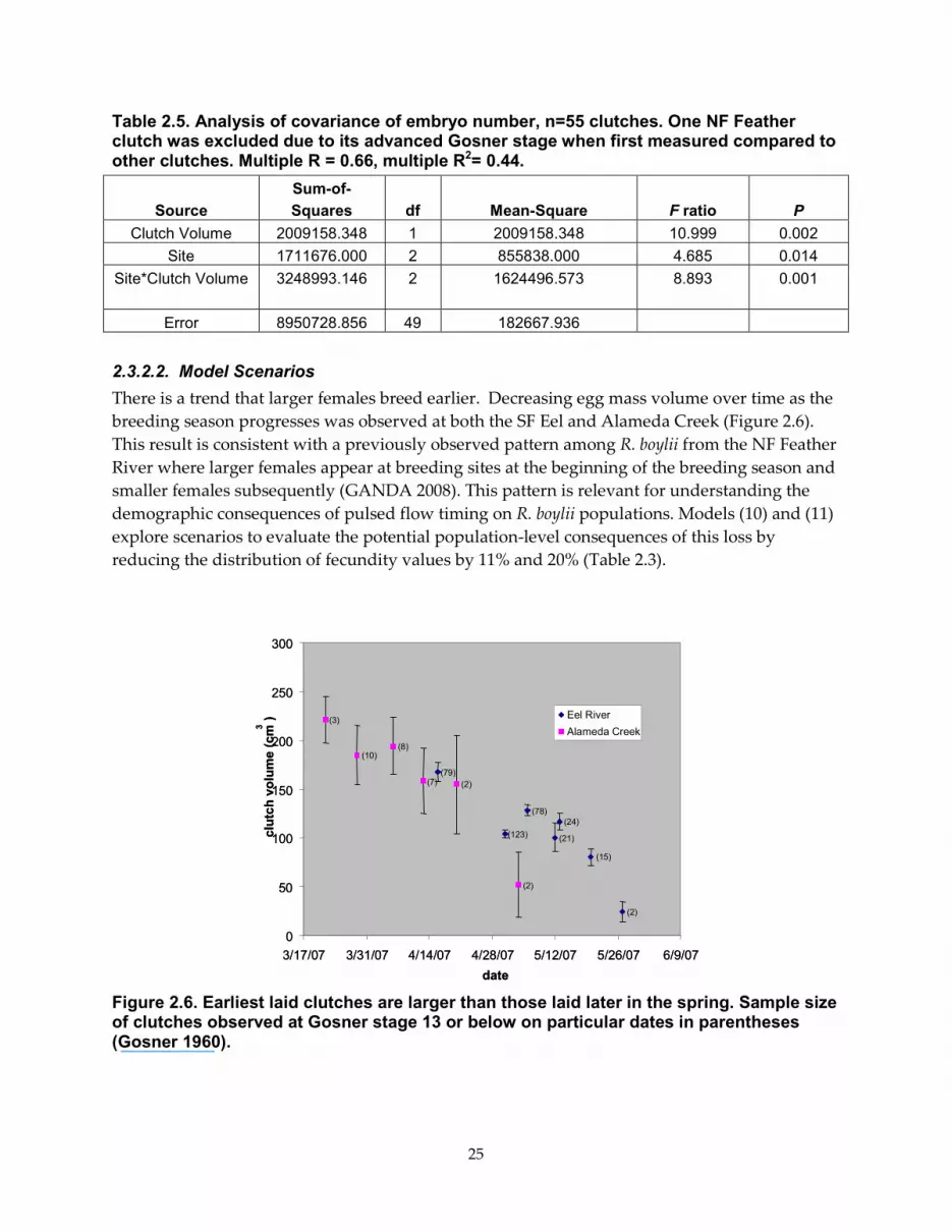
25

Table 2.5. Analysis of covariance of embryo number, n=55 clutches. One NF Feather clutch was excluded due to its advanced Gosner stage when first measured compared to other clutches. Multiple R = 0.66, multiple R2= 0.44.

Source

Sum-of-

Squares

df

Mean-Square

F ratio

P

Clutch Volume 2009158.348 1 2009158.348 10.999 0.002

Site 1711676.000 2 855838.000 4.685 0.014

Site*Clutch Volume

3248993.146 2 1624496.573 8.893 0.001

Error 8950728.856 49 182667.936

2.3.2.2. Model Scenarios

There is a trend that larger females breed earlier. Decreasing egg mass volume over time as the

breeding season progresses was observed at both the SF Eel and Alameda Creek (Figure 2.6).

This result is consistent with a previously observed pattern among R. boylii from the NF Feather

River where larger females appear at breeding sites at the beginning of the breeding season and

smaller females subsequently (GANDA 2008). This pattern is relevant for understanding the

demographic consequences of pulsed flow timing on R. boylii populations. Models (10) and (11)

explore scenarios to evaluate the potential population-level consequences of this loss by

reducing the distribution of fecundity values by 11% and 20% (Table 2.3).

0

50

100

150

200

250

300

3/17/07 3/31/07 4/14/07 4/28/07 5/12/07 5/26/07 6/9/07

clutch volume (cm3

) Eel River

Alameda Creek

(79)

(123)

(78)

(24)

(15)

(2)

(2)

(21)

(3)

(10)(8)

(7) (2)

date

0

50

100

150

200

250

300

3/17/07 3/31/07 4/14/07 4/28/07 5/12/07 5/26/07 6/9/07

clutch volume (cm3

) Eel River

Alameda Creek

(79)

(123)

(78)

(24)

(15)

(2)

(2)

(21)

(3)

(10)(8)

(7) (2)

date

Figure 2.6. Earliest laid clutches are larger than those laid later in the spring. Sample size of clutches observed at Gosner stage 13 or below on particular dates in parentheses (Gosner 1960).

26

2.3.3. Survival of Stranding or Scouring events

In addition to the background rate of survival to hatching, the fate of whole egg masses was

modeled to capture a potentially important source of hydrologically-induced mortality. Such

mortality in unregulated rivers represents natural variation in hydrologic conditions during

embryonic incubation. In regulated rivers, this variation is determined primarily by water

release schedules and hydropower management. Based on observations from both the long-

term SF Eel data set and more recent egg mass surveys in regulated rivers, distributions of

mean annual egg mass scouring rates (due to flow increase) and stranding (due to flow

decrease), semb1 and semb2, respectively were developed.

2.3.3.1. Application to the Population Model – Reference Values

Reference rates of egg mass scour due to flooding during spring spates and stranding

(dessication) due to rapidly falling water stage was quantified for the SF Eel (1992-2007). In

some years, direct observations of the fate of each marked egg mass was followed (1992,

1994-1996, 2003, 2005-2007) and the proportion of total egg masses surviving scouring and

stranding was calculated. For the other eight years, stranding and scouring survival were

estimated by matching the hydrologic conditions (as determined from hydrographs, rainfall

records, and lay dates) to the most similar year among those with data on individual egg

mass fates and assigning the same survival rates. Across the entire time series from the SF

Eel, the 16 year mean (var) annual survival of egg masses through stranding conditions was

0.956 (0.0024), and survival through scouring conditions was 0.802 (0.089). The distribution

of annual survival rates (Figure 2.7) emphasizes that most years have little stranding or

scouring (survival near 1) punctuated with occasional years of late spring spates (scouring

>60% of egg masses) or dry spring conditions leading to rapidly falling stage. Annual

survival due to stranding or scouring was modeled as two component vital rates (semb1 semb2)

which can then be manipulated in the altered hydrologic scenarios below in section 2.3.3.2.

0.0 0.2 0.4 0.6 0.8 1.0

Proportion of clutches

surviving stranding

0

5

10

15

Number of years

0.0 0.2 0.4 0.6 0.8 1.00

5

10

15

Proportion of clutches

surviving scouring

0.0 0.2 0.4 0.6 0.8 1.0

Proportion of clutches

surviving stranding

0

5

10

15

Number of years

0.0 0.2 0.4 0.6 0.8 1.00

5

10

15

Proportion of clutches

surviving scouring

Figure 2.7. Distribution of survival rates of R. boylii egg masses in relation to hydrologic stressors, i.e. stranding or scouring, over 16 years at the SF Eel River.

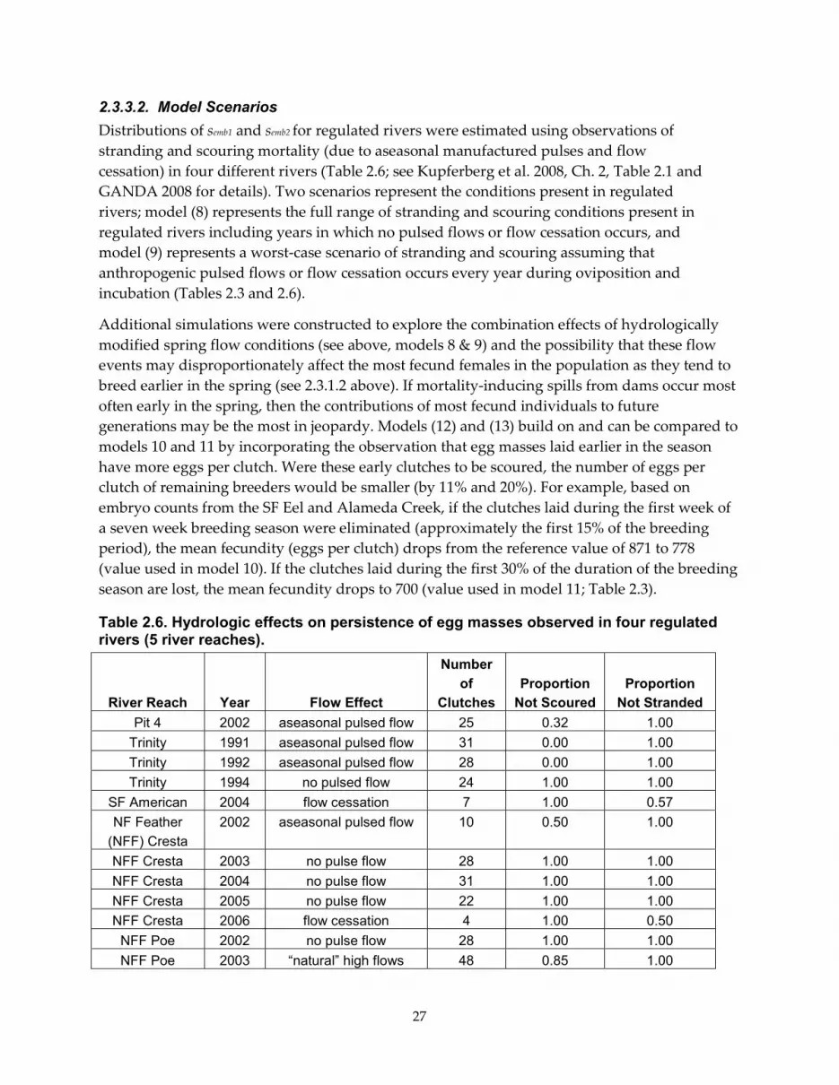
27

2.3.3.2. Model Scenarios

Distributions of semb1 and semb2 for regulated rivers were estimated using observations of

stranding and scouring mortality (due to aseasonal manufactured pulses and flow

cessation) in four different rivers (Table 2.6; see Kupferberg et al. 2008, Ch. 2, Table 2.1 and

GANDA 2008 for details). Two scenarios represent the conditions present in regulated

rivers; model (8) represents the full range of stranding and scouring conditions present in

regulated rivers including years in which no pulsed flows or flow cessation occurs, and

model (9) represents a worst-case scenario of stranding and scouring assuming that

anthropogenic pulsed flows or flow cessation occurs every year during oviposition and

incubation (Tables 2.3 and 2.6).

Additional simulations were constructed to explore the combination effects of hydrologically

modified spring flow conditions (see above, models 8 & 9) and the possibility that these flow

events may disproportionately affect the most fecund females in the population as they tend to

breed earlier in the spring (see 2.3.1.2 above). If mortality-inducing spills from dams occur most

often early in the spring, then the contributions of most fecund individuals to future

generations may be the most in jeopardy. Models (12) and (13) build on and can be compared to

models 10 and 11 by incorporating the observation that egg masses laid earlier in the season

have more eggs per clutch. Were these early clutches to be scoured, the number of eggs per

clutch of remaining breeders would be smaller (by 11% and 20%). For example, based on

embryo counts from the SF Eel and Alameda Creek, if the clutches laid during the first week of

a seven week breeding season were eliminated (approximately the first 15% of the breeding

period), the mean fecundity (eggs per clutch) drops from the reference value of 871 to 778

(value used in model 10). If the clutches laid during the first 30% of the duration of the breeding

season are lost, the mean fecundity drops to 700 (value used in model 11; Table 2.3).

Table 2.6. Hydrologic effects on persistence of egg masses observed in four regulated rivers (5 river reaches).

River Reach

Year

Flow Effect

Number

of

Clutches

Proportion

Not Scoured

Proportion

Not Stranded

Pit 4 2002 aseasonal pulsed flow 25 0.32 1.00

Trinity 1991 aseasonal pulsed flow 31 0.00 1.00

Trinity 1992 aseasonal pulsed flow 28 0.00 1.00

Trinity 1994 no pulsed flow 24 1.00 1.00

SF American 2004 flow cessation 7 1.00 0.57

NF Feather

(NFF) Cresta

2002 aseasonal pulsed flow 10 0.50 1.00

NFF Cresta 2003 no pulse flow 28 1.00 1.00

NFF Cresta 2004 no pulse flow 31 1.00 1.00

NFF Cresta 2005 no pulse flow 22 1.00 1.00

NFF Cresta 2006 flow cessation 4 1.00 0.50

NFF Poe 2002 no pulse flow 28 1.00 1.00

NFF Poe 2003 “natural” high flows 48 0.85 1.00

28

River Reach

Year

Flow Effect

Number

of

Clutches

Proportion

Not Scoured

Proportion

Not Stranded

NFF Poe 2004 no pulse flow 47 1.00 1.00

NFF Poe 2005 “natural” high flows 63 0.89 1.00

NFF Poe 2006 flow cessation 88 1.00 0.48

Model (8)

mean (var) all years

0.771 (0.140)

0.903 (0.040)

Model (9)

mean (var) for pulse / flow cessation years only

0.427 (0.155)

0.517 (0.002)

2.3.4. Survival of Tadpoles to Metamorphosis

To derive the mean value and distribution of tadpole to metamorphosis survival (stadpole0), two

contrasting approaches were employed. The first approach relies on estimating R. boylii

survival to metamorphosis using data collected from rearing experiments conducted in

enclosures (Kupferberg 1997; Kupferberg et al. 2008; Catenazzi and Kupferberg unpublished

data). Due to the confined nature of these enclosure experiments (no opportunity for

dispersal, reduced vulnerability to predators, etc.), estimates derived from these experiments

are likely at the high end of the range of survival rates. The experiments included trials with

invertebrate predators present (Kupferberg 1997; Kupferberg et al. 2008, section 4), as well

experiments in which predators were excluded (Catenazzi and Kupferberg unpublished

data).

The second approach combines mark-recapture data sets from the SF Eel and Alameda Creek

to estimate survival to metamorphosis of a cohort of wild individuals laid as eggs in a given

river reach. This approach may underestimate survival to metamorphosis because of

dispersal away from the natal stream reach. The data sets are: (1) egg mass sampling in

spring 2006 (see Section 2.3.1), (2) fecundity and embryo survival estimates from 2007 (see

Section 2.3.2), and (3) population size and daily survival rates of newly metamorphosed R.

boylii collected in fall of 2006 (Appendix B).

Seven steps of calculations were used for the second approach. In step (1), the starting

number of eggs was calculated (= total # egg masses observed * average #/mass). For step (2)

the initial number of tadpoles was estimated (= total eggs x background survival x

stranding/scouring). In step (3) the population size of newly metamorphic (young of the

year) R. boylii was estimated from the 3-day capture-recapture efforts and was based on the

“best” population estimate model from Program CAPTURE (Otis et al. 1978; White et al.

1982; see Appendix B for detailed methods). Because the population sizes of young of the

year frogs was conducted several weeks after the bulk of metamorphosis occurred (i.e. only a

few tadpoles were remaining in the river), the population estimate needed to be adjusted to

account for those individuals that did not survive the first several weeks of life as frogs. For

step (4) the median date of metamorphosis was estimated and for step (5) the days elapsed

between that date and the first date of capture-recapture work in fall determined. At

29

Alameda Creek, that date was determined by the median date of metamorphosis observed

among individuals in a rearing experiment (see Kupferberg et al. 2008, Section 4). At the SF

Eel the median date was determined based on the ratio of tadpoles to young of the year frogs

located during field sampling conducted mid-August. In step (6) the population estimate for

young of the year frogs (from step 3) was adjusted to the population size at metamorphosis

by back-calculation using the highest daily survival rate generated by Program MARK

(White and Burnham 1999; Cooch and White 2007) for the capture recapture data (see

Appendix B for details). For step (7), to get the final tadpole survival rate to metamorphosis,

the adjusted population size generated in the previous step (5) was divided by the starting

number of hatchlings derived in step (2). Table 2.7 shows the step by step calculations for

each study area.

Table 2.7. Steps to determine Rana boylii tadpole to YOY Survival based on 2006 and 2007 field data.

Steps SF Eel River Alameda Creek

1. number of eggs = # egg masses * average #/mass) 210546.6 109986.600

2. Background survival to hatching rate 0.819 0.828

3. Initial # tadpoles 172437.7 91068.9

4. YOY population size estimate (+ S.E.) 622 ± 24.3 1717 ± 889.2

5. Median date of metamorphosis

1st date of cap-recap:

Days elapsed

25 Aug 2006

16 Sept 2006

22

17 Aug 2006

4 Oct 2006

47

6. Adjusted YOY population estimate 2603 3664

7. Tadpole to YOY survival rate 0.0151 0.0402

2.3.4.1. Application to the Population Model - Reference Values

Combining all available R. boylii data for the two study areas (Table 2.8), the average survival to

metamorphosis was 0.15, with a variance of 0.03 (Table 2.2). The values of tadpole survival rate

included in this calculation are comparable to the range of estimates made for other Ranid

species (Calef 1973, Licht 1974).

30

Table 2.8. Rana boylii tadpole survival to metamorphosis values used in overall estimate of this vital rate.

Approach Survival to Metamorphosis Data Source

Rearing experiments

0.045

SF Eel 2m2 enclosures of

natural substrate, with

competitors and predators

(Kupferberg 1997)

0.33

Alameda basket enclosures,

with predators

(Kupferberg et al. 2008)

0.32

SF Eel basket enclosures,

without predators

(Catenazzi and Kupferberg,

unpublished data)

Capture - recapture 0.0151 SF Eel 2006

0.0402 Alameda 2006

2.3.4.2. Model Scenarios

To simulate the direct effects of elevated velocity on tadpole survival occurring during summer

whitewater boating flows, short-term power generation, or emergency shut-downs, scenarios

including 1, 2, 3, and 4 pulsed flows during tadpole rearing were created. Models (15-19) use an

average tadpole loss rate of 53.7% (mean stadpole1-4 = 0.463 , var = 0.03) for each pulse, and as such

each pulse was modeled as an additional vital rate, e.g. another sub-component of the first year

transition probability. The vital rate stadpole1-4 and its variance were calculated based on the mean

survival of tadpoles from five different studies of tadpole vulnerability to increased flows

including experiments using a Brett chamber (@ 30 cm/sec), a large artificial flume (16-22

cm/sec), an in-stream flume (0-30 cm/sec), and an in-stream drift fence (0-70 cm/sec)

(Kupferberg et al. 2008). Velocities used in these laboratory and field experiments were

comparable to those seen in actual field pulse flows. For example, at the Pit River in 2002, test

flows ranging from 5.25 cubic meters per second (cms; 150 cfs) base flow up to 33.98 cms

(1200cfs) produced a range of velocities up to ~50cm/sec (most ~ 30cm/sec) (SpringRivers

Ecological Sciences LLC 2002; Kupferberg et al. 2008). At the NF Feather in 2008, test flows from

7.08 to 16.99 cms (250 to 600cfs) produced a range up to ~55cm/sec (most measurements 18-37

cm/s, GANDA 2008). Given the level of uncertainty in estimating the form of the relationship

between flow fluctuations and tadpole survival and the possibility that pulsed flows may be

more and less severe, the above model scenarios were compared to a parallel set of models

using the highest survival rate observed in the tadpole vulnerability studies listed above.

Models (20-24) incorporate only the data from the large artificial flume experiments (stadpole1-4 =

0.61, var = 0.03; Table 2.3), where velocities ranged from 16-22 cm/s and on average 61% of

tadpoles were able to maintain position.

The direct effects of flow velocity on tadpoles alone fail to consider two potentially important

aspects of ecological complexity when discharge is increased in a regulated river; flow effects on

31

algal resources, and flow effects on developmental temperatures. First, increases in current

velocities are likely to negatively affect algal food resources as floating mats of algae and

detritus are dislodged and transported to downstream reservoirs, and as attached algae can be

scoured off of rock surfaces. To model the potential combined effects of both direct tadpole

mortality with a single summer pulse and indirect mortality that may result from reduced food

availability following the pulse, the background tadpole survival to metamorphosis rate (stadpole0)

in models (16, high direct mortality) and (21, low direct mortality) was manipulated. These

scenarios were guided by the results of tadpole rearing field experiments with contrasting food

levels; either with only epilithic periphyton (i.e. low food quality and quantity) or with a

combination of epilithic periphyton and abundant macroalgae and diatoms (Catenazzi and

Kupferberg unpublished data). Epiphytic diatoms, especially taxa which contain cyanobacterial

endosymbionts, represent a much higher quality diet for tadpoles (higher fat and protein)

which is known to enhance survival, growth, and development (Kupferberg et al. 1994). When

tadpoles were reared in flow through enclosures under identical conditions other than food

level, there was a 27.8% decrease in survival from hatching to metamorphosis when loose algae

with epiphytes was not present. Accordingly, the Reference Model value of stadpole0 was decreased

by 27.8% to 0.108 in models (16) and (21) (Table 2.3).

A second potential indirect consequence of elevated discharge during the summer is lower

instream temperatures which may affect tadpole growth, development, and survival. For

example, if discharge/baseflow levels are increased to dampen effects of peaking or recreational

boating pulse flows, water temperature is expected to decrease (releases are most often drawn

from the hypolimnion of the upstream reservoir). While little data collection on thermal

consequences of different base flow scenarios has been collected, the potential population

consequences of colder summer water temperatures on tadpole survival were bounded using

data from the recent tadpole rearing experiment described above. Tadpole experiments

compare the survival of individuals raised at summer mean temperature of 18.8 C to those

raised at 16.4 C using a natural gradient of stream water temperatures present in tributaries and

the mainstem of the SF Eel R, which results in a 15% decrease in survival at cooler temperatures.

Accordingly, model (14) uses a value of stadpole0 of 0.128 (15% lower than that used for the

Reference Model, 0.15; Tables 2.2 and 2.3). While the results of this rearing experiment provide

some guidance to the potential magnitude of temperature effects of higher base flows, the exact

relationship between temperature and survival is likely to be complex and site-specific.

2.3.5. First Year Over-Winter Survival

This lifestage covers the time period from metamorphosis in late summer/early fall through

winter and ends when frogs are essentially one year old.

2.3.5.1. Application to Population Model – Reference Values

Initial plans were to derive first year over-winter survival rates from field-based capture-

recapture of newly metamorphic R. boylii marked in the fall and recaptured the following

spring. While the capture-recapture field work was successful in fall 2006, capture rates the

32

following spring (2007) were very low, leading to large uncertainties in estimates of over-winter

survival. Appendix B describes the capture-recapture field methods and the steps for deriving

over-winter estimates with the data collected. However, these estimates were not used in the

Reference Model or any subsequent scenarios due to the large uncertainties and low capture-

recapture rates in spring 2007. Alternatively, rates derived from a literature search on over-

winter survival rates of newly metamorphosed Ranid frog species were used. A variety of

studies provided estimates for various time periods starting from immediately post-

metamorphosis to a maximum of one year later. Only those studies that covered the entire over-

winter time period were used, and an average survival estimate was calculated from the

following species and references: Rana blairi, R. clamitans, R. lessonae, R. luteiventris, R.

sphenocephala, and R. sylvatica (Altwegg 2003; Altwegg and Reyer 2003; Berven 1990; Boone

2005; Funk et al. 2005; Harper and Semlitsch 2007). This provided a Reference Model estimate of

sYOY of 0.3674, with a variance of 0.02 (Table 2.2).

2.3.5.2 Model Scenarios

All models draw from the same distribution for first over-winter survival (sYOY = 0.37, var =0.02)

because no specific predictions of the possible direct hydrologic effects of river regulation for

the first over-winter period of newly metamorphosed frogs were developed. However, the lack

of hydrologic simulations for this vital rate does not preclude the possibility that carryover or

other higher-order interactions may affect the survival of metamorphic frogs over the first

winter, but rather the lack of currently available data to estimate such effects. Previous

experiments do show that R. boylii tadpoles subjected to pulsed elevations of velocity have

reduced growth rates (Kupferberg et al. 2008) and pen studies with other Ranid species show

that size at metamorphosis can often be an important determinant of surviving the first winter

(Altwegg and Reyer 2003).

2.3.6. Survival from Age 1 to Age 2

This is the first year that frogs are defined as juveniles and covers the time period from one year

of age to two years of age.

2.3.6.1. Application to Population Model – Reference Values

The survival of R. boylii during the juvenile terrestrial period (estimated to be from age 1 to 3)

has not been studied, and as a result there is a lack of either empirical or published data for R.

boylii in particular or other Ranid frogs in general. However, unpublished data for a stream-

dwelling population of California red-legged frogs (Rana draytonii) was available (Scott,

Rathbun, and D’Amore pers. comm.). Population studies on R. draytonii were conducted at Pico

Creek and San Simeon Creeks in the central coast mountains of California (San Luis Obispo

County) from 1991 to 1994. Approximately 800 m of Pico Creek and 1km of San Simeon Creek

were surveyed on several occasions each year. Frogs were individually marked and juveniles

were defined by the field researchers as ranging from 35 to 69mm snout-vent length (Scott,

Rathbun, D’Amore pers. comm.). Program MARK was used to estimate juvenile survival rates

33

for each of the two study populations (see analogous methods below in section 2.3.9; D’Amore

pers. comm.). For the R. boylii Reference Model, a mean and variance of the two juvenile

survival estimates (Pico and San Simeon) was calculated to represent survival from age 1 to age

2 (sjuv1 = 0.26, var =0.04; Table 2.2).

2.3.6.2. Model Scenarios

All model scenarios draw values from the same distribution for survival from age one to two as

in the Reference Model.

2.3.7. Survival from Age 2 to Age 3

This is the second year that frogs are defined as juveniles and covers the time period from two

years of age to three years of age, when female frogs are likely to reproduce for the first time in

northern locales (GANDA, unpublished growth data).

2.3.7.1. Application to Population Model – Reference Values

In the absence of any empirical or literature values for juvenile survival from age 2 to age 3, the

simplifying assumption was made that this vital rate would be similar to the adult female

survival rate estimated from relatively robust empirical data (0.54 with variance 0.055, see

Section 2.3.9 below and Table 2.2). The underlying assumptions for using this rate were: (1) the

survival rate should improve (i.e., be higher than that for age 1 to age 2) as individuals get

older, and (2) juveniles should actually have a relatively high survival rate because they are not

yet reproducing or migrating and thus exposure to predators should be reduced and energy

reserves would not be devoted to reproduction.

2.3.7.2. Model Scenarios

All model scenarios draw values from the same distribution for survival from age 2 to 3 as in

the Reference Model except for models (2) and (30-32) which represent a shortened (2 years to

maturity instead of three; Table 2.3). Rana boylii growth that has been observed for marked

individuals in Central California populations informs this supposition (Gonsolin, unpublished

data). In these scenarios, this vital rate was eliminated from the life-history (see Section 2.4 for

more details).

2.3.8. Adult Survival Estimates

Adult (sexually mature individuals) survival rates were derived from capture-recapture data

collected by researchers at two study areas: Hurdygurdy Creek in the South Fork Smith River

drainage, and an unnamed tributary in the Poe Reach of the North Fork Feather River.

Frogs were marked and identified in the field using Passive Integrated Transponder (PIT) tags

and/or chin pattern recognition (e.g., GANDA 2006; Wheeler et al. 2005; Wheeler 2007), all of

which provide individual identification. Data were summarized to represent annual capture-

34

recapture periods (Table 2.9). Multiple captures of a given individual within a capture-

recapture period was counted as one capture. Based on information provided by researchers at

each study area, data were pared down to adults only. At Hurdygurdy Creek adult males were

defined as individuals 40mm and larger (snout-urostyle length, SUL) and adult females were

50mm SUL and larger (Wheeler 2007; C. Wheeler pers. comm.). At the NF Feather, adults (both

sexes) had previously been defined as 40mm or larger SUL (J. Drennan, pers. comm.). However,

there is no evidence to suggest that individuals mature or ultimately grow to smaller sizes at the

NF Feather than at Hurdygurdy Creek, so adults males were defined at 40mm SUL and larger

and adult females at 50mm SUL and larger for the purposes of developing survival rate

estimates (Table 2.9).

Program MARK (White and Burnham 1999; Cooch and White 2007) was used to derive annual

survival rate estimates for adult frogs at each study area. Separate estimates were derived for

males and females. Program MARK offers four “pre-defined” models which allow two

parameters to vary over time (in this case year): survival (Phi) and capture probability (p).

These four models were evaluated for each sex at each study area and the “best” model was

chosen based on the lowest Akaike Information Criterion (AIC) value. This information-

theoretic criterion provides a balance between model fit (based on likelihood theory) and

precision (enforced by a penalty for the number of parameters) (Burnham and Anderson 2002).

Survival rate estimates, and associated standard errors and variances, were then selected from

that best model and are presented in Table 2.10, below. In all analyses the sin link function and

2nd part variance estimator were used (Cooch and White 2007).

2.3.8.1. Application to Population Model – Reference Values

For the matrix population model, the adult female survival rate and associated variance from

the unregulated Hurdygurdy Creek (0.54, var = 0.055) was used (Table 2.2). The estimate for

adult female survival from the regulated NF Feather River was similar, though slightly lower,

and was used as corroboration of the estimate from Hurdygurdy Creek (Table 2.10).

35

Table 2.9. Location, sampling approach, and researcher contacts for the two study sites where adult Rana boylii survival rates were developed.

Study area

County,

State

Sampling

Approach

Years

of

Surveys

SUL

Range By

Sex (mm)

Observers / Researcher Contact

Hurdygurdy

Creek

Del

Norte,

CA

PIT tagging of

individuals at a

large breeding

site

2002-

2006

Females:

52-76

Males:

40-62

Clara Wheeler, USDA Forest

Service, Redwood Sciences Lab,

Arcata, CA

cawheeler@fs.fed.us

(Wheeler 2007)

Unnamed

tributary to

North Fork

Feather River

Plumas,

CA

Chin pattern

recognition of

individuals in

tributary and at

associated river

breeding site

2004-

2007

Females:

50-76

Males:

40-59

Joe Drennan

GANDA Environmental

Consultants, San Francisco, CA

jed@garciaandassociates.com

Table 2.10. Annual survival rate and capture probability estimates for adult Rana boylii at two study sites.

Study Site

Sex (n)

“Best”

Model1

Survival Rate (Phi) + s.e.

(variance) Overall Or By Year

(depending on model)

Capture Probability

(p) + s.e.

Hurdygurdy Creek

2002-2006

F (39)

Phi(.), p(t)

0.54 + 0.23 (0.055)

2003: 0.78 + 0.46

2004: na

2005: 0.21 + 0.19

2006: 0.30 + 0.33

M (144)

Phi(t), p(.)

2002-03: 0.34 + 0.09 (0.008)

2003-04: 0.51 + 0.11 (0.01)

2004-05: 0.14 + 0.06 (0.004)

2005-06: 0.36 + 0.10 (0.011)

0.08 + 0.12

Unnamed tributary to North Fork Feather River 2004-2007

F (179)

Phi(.), p(t)

0.50 + 0.08 (0.007)

2005: 0.80 + 0.14

2006: 0.29 + 0.09

2007: 0.66 + 0.22

M (95) Phi(.), p(.)

0.11 + 0.04 (0.001) 1.0000 + 0.000 note: this estimate is not reliable

1. Notation: (.) = parameter does not vary over time, (t) = parameter varies over time.

36

2.3.8.2. Model Scenarios

All model scenarios draw values from the same distribution of adult survival a44=0.54

(0.055).

2.4. Central Coastal California Populations Reference Model

There is evidence from Central Coastal California R. boylii populations (e.g. Alameda Creek - S.

Bobzien unpublished data and Coyote Creek - E. Gonsolin unpublished data) that individual

females reach reproductive maturity after two years of age rather than the three years of age

assumed by the Reference Model (see Section 2.2). To address whether this shorter life-history

predisposes Central Coast populations to be more or less sensitive to anthropogenic changes in

hydrology an exploratory Central Coast populations Reference Model (2) was constructed. This

model assumes the same mean vital rates and distributions as the Reference Model (1) except

for the elimination of second juvenile stage (sjuv2). Results from this model should be viewed as

exploratory, as there are key simplifying assumptions that can not currently be evaluated

including: (1) the frequency of 2-year maturity within and among Central Coast populations is

dominant, and (2) populations reaching maturity at age 2 are governed by the same

demographic parameters (vital rates) as populations reaching maturity at age 3. For the latter

assumption, basic life-history theory would suggest that populations reaching maturity earlier

would have different demographic rates to achieve the same contribution to the next

generation. For example, earlier maturing species would be expected to have higher fecundities

per reproductive bout if the number of reproductive opportunities are fewer. Although

Alameda Creek clutches were observed to contain more embryos than the other populations,

very little other demographic data was available from Central Coast populations (only limited

fecundity, embryo and tadpole survival from Alameda Creek), so the generality of these

assumptions cannot currently be evaluated.

With this 3-stage matrix model the following scenarios were simulated: model (30) adjusts the

starting population size the mean number of egg masses per/km in regulated rivers (4.6/km),

model (31) combines regulated river embryonic strand and scour rates (semb1, semb2) with the

reduced starting population size in (30), and model (32) which combines the most extreme

reductions in embryonic survival due to stranding and scouring (similar to model (9)) with the

reduced starting population size in (30).

2.5. Typical Study Reach Lengths, Starting Population Size, and Quasi-Extinction Thresholds

To initiate model runs, it was necessary to define a starting population size (a vector of the

number of individuals in each life stage) and an extinction threshold. These values were also

manipulated to evaluate their affects on viability outcomes in several scenarios.

37

2.5.1. Application to Population Model – Reference Values

All models (Reference Models and scenarios) define a population as the total number of

breeding females occurring in a hypothetical 10km reach, and are intended to represent the way

in which R. boylii populations are often studied (e.g. river reach bounded by dams/reservoirs up

and downstream that are often assumed to represent barriers to dispersal). It was also assumed

that this reach length represents a biologically functional local population. However it does

exclude the potential influence of long-distance emigrants and immigrants. The starting

population vector (N0) was estimated to be the stable age distribution that would result from

knowing the average number of breeding adult females multiplied by the average transition

probability (aij) for each life-history stage. The average number of breeding females was

estimated from the average of the number of breeding females/km observed in a series of

unregulated study populations multiplied by the average regulated reach length (Kupferberg

unpublished data). The reach length chosen for modeling, 10 km, was based on the mean of a

sample of regulated Sierran river reaches where R. boylii populations have been studied (Table

2.11) and is generally supported by a recent genetic study of R. boylii (Dever 2007). A

compilation of egg mass census data from several researchers in California served as the basis

for the estimate of the average number of breeding females (32/km x 10 km = 320 adult females,

Table 2.12, Figure 2.8).

Table 2.11. Reach lengths in a sample of Sierra Nevada regulated rivers with known populations of Rana boylii.

Project River Reach length (km)

Spring Gap Stanislaus Middle Fk. Stanislaus 19.8

Poe North Fk. Feather, Poe 12.1

Rock Creek - Cresta North Fk. Feather, Cresta 10.46

Pit 3,4,5 Pit 4 7.0

DeSabla Butte Creek 16.41

DeSabla West Branch Feather 23.01

UARP Silver Creek 9.65

UARP South Fork American 4.5

UARP Slab Creek Reach, S. Fk. American 12.9

mean (± s.e.) 12.87 ± 1.99

38

Table 2.12. A summary of recent egg mass census data from California populations of Rana boylii.

River

system

Site Name

Location

Reach

Length

(km)

%

Sampled

#/km

se

Years

Sampled

Data Source

Middle Fork

Stanislaus

Sand Bar

Dam Reach

Central

Sierra

19.8 5.2 6.2 3.6 2001-2003 ECORP Consulting, Inc. for PG&E, 2004

Trinity Mainstem

Trinity

N. Coast 22.5,

33.3

100 0.45 0.17 1991-1994,

2004-2006

Lind 2005; Ashton, Bettaso, and Welsh

unpublished data

NF Feather Poe N. Sierra 12.07 66.3 7.27 1.65 2001-2008 Garcia and Associates for PG&E

NF Feather Cresta N. Sierra 10.46 76.5 2.24 0.50 2002-2008 Garcia and Associates for PG&E

Pit Pit4 N.Sierra 7 100 8 2.7 2002-2005 Maria Ellis, Spring Rivers, PG&E

Alameda Downstream

Calaveras

Ck

SF Bay Area 3.2 100 3.3 3.3 2003-2008 Bobzein and DiDonato 2007,

Kupferberg unpublished data

Regulated River Mean Egg Mass Density 4.6 1.15

Stanislaus Rose Ck. Central

Sierra

0.65 100 29 2001 Lind et al. 2003

Tuolumne NF

Tuolumne

Central

Sierra

0.3 100 9 2001 Lind et al. 2003

San Joaquin Jose Ck Central

Sierra

1.2 ? 4.6 1995, 2002 Lind et al. 2003

Smith Hurdygurdy

Ck

N. Coast 4.75,

1.65

100 34.6 4.5 1991-1992,

1998-2000,

2002-2007

Lind 2005, Clara Wheeler pers. comm.

Eel S. Fk. Eel N. Coast 5.2 100 106.9 7.5 1992-2008 Kupferberg 1996, and unpublished data

Eel Ten Mile Ck N. Coast 4 100 12.92 2.96 1993-2003,

2008

Kupferberg 1996, and unpublished data

Trinity SF Trinity N. Coast 15.6 100 1992-1994,

2004-2006?

Lind 2005

Trinity SF Trinity N. Coast 5.9 100 69.9 22.5 2004-2006 Ashton, Bettaso, Welsh unpub. data

Yuba Clear Ck. N. Sierra 0.82 100 29 9.5 1992-1994 Van Wagner 1996

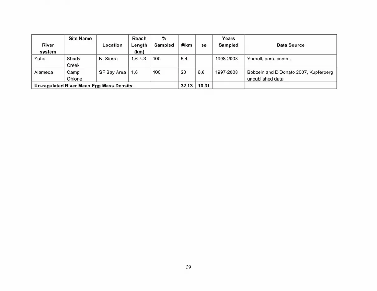
39

River

system

Site Name

Location

Reach

Length

(km)

%

Sampled

#/km

se

Years

Sampled

Data Source

Yuba Shady

Creek

N. Sierra 1.6-4.3 100 5.4 1998-2003 Yarnell, pers. comm.

Alameda Camp

Ohlone

SF Bay Area 1.6 100 20 6.6 1997-2008 Bobzein and DiDonato 2007, Kupferberg

unpublished data

Un-regulated River Mean Egg Mass Density 32.13 10.31

40

Figure 2.8. Summary of breeding population sizes of Rana boylii compiled from several researchers in California (see Table 2.11).

2.5.2 Model Scenarios

The outcome of the Reference Model (32 females/km = 320 adult females in the population), was

compared to models which begin with more robust (model 4), smaller (model 3), and much

smaller (model 5) starting population vectors (Table 2.3). In model (3), the mean regulated

average of 46 adult females in a 10km reach was used (Table 2.11). Model (4) begins with a

robust population, mirroring the mean for the SF Eel, the system for which there is the longest

continuous record of population dynamics. Checking that the extinction probability of this

scenario is indeed low, provides an opportunity to validate that the predictions of the Reference

Model were within the realm of biological reason for a robust R. boylii population, and to give

confidence in its general predictions. In model (5) a starting value only slightly above the

previously defined quasi-extinction threshold was used, based on the actual population size in

the NF Feather Cresta reach of 2.1 females/km. There is substantial uncertainty in defining a

quasi-extinction level, so one scenario explores the consequences of setting this level at half the

Reference Model value (model 6), 1 female/km, and another sets it at double the Reference

Model value (model 7), 4 females/km (Table 2.3).

2.6. Combined Effects Scenarios

Several scenarios were developed to examine the interactions and compounding effects of

multiple effects. These scenarios were intended to be biologically realistic representations to the

0

10

20

30

40

50

60

70

Coastal Sierran

unregulatedregulated

clu

tches p

er

river

km

0

10

20

30

40

50

60

70

Coastal Sierran

unregulatedregulatedunregulatedregulated

clu

tches p

er

river

km

41

extent that populations often experience compounded factors such as small population sizes

combined with local stressors that may negatively affect one or more vital rate(s). In particular,

these scenarios examine the fate of R. boylii during the time period of its observed decline

(approx. the last 50 years) and also assess combined effects on current populations.

2.6.1. Simulation of Rana boylii decline history

Model (25) explores the population consequences of beginning with a robust population and

subjecting it to the effects of spring spills and rapid flow cessation, and a single high-mortality

(stadpole1= 0.46) pulsed flow per summer as might have historically occurred for project

maintenance. Model (26) adds the effect of reduced fecundity, assuming that there is less

control of dams earlier in the season, and that first 15% of eggs are scoured away, thus

eliminating the early large female contribution to the population (Table 2.3).

2.6.2. Worst-Case Modern Scenarios – Small Populations and Hydrologic Stressors

In models (27- 29), the NF Feather Cresta reach starting population size estimate was applied

(based on average count of egg masses from 2002-2007, 21 females or ~2/km were estimated

Table 2.12), combined with the distribution of strand and scour rates measured for regulated

rivers. Model (27) assesses the potential for recovery of a small population in a hydrologically

regulated system, assuming there are no summer pulsed flows. Models (28) and (29) include the

effects of one (28) or two (29) high-mortality (stadpole1-2=0.46) summer pulsed flows combined with

the diminished starting population size and hydrologically regulated spring strand and scour

conditions.

2.6.3. Central Coast Population Combination Models

The potential population-level consequences of smaller population size (model 30) and two

levels hydrologic stress for the faster maturing Central Coast populations were estimated.

Model (31) adds the distribution of both potentially beneficial and detrimental effects of

regulation on stranding and scouring, while model (32) incorporates the worst case rates of

embryonic stranding and scouring in regulated rivers along with the small starting population.

In some instances, regulated river populations might experience less stranding relative to an

unregulated river if stage height were maintained at a constant level, rather than declining over

time.

2.7. Sensitivity Analysis Methods

Sensitivity analyses are traditionally used to evaluate the importance of individual vital rates

(or components of composite vital rates) to overall model outcomes (Caswell 2001; Morris and

Doak 2002). Sensitivity results can inform decisions about which particular life-history stages to

be targeted for future research (to further constrain uncertainties in demographic estimates) or

for direct conservation action in the case of recovery programs for declining species or

42

eradication efforts for invasive species (Crouse et al. 1987; Kareiva et al. 2000). For matrix

population models in particular, traditional sensitivity and elasticity analyses vary single vital

rates over a narrow range of values while holding all other vital rates at their ‘best’ estimates

(Reference Model conditions in this case). By systematically varying individual vital rates over

small ranges and comparing the resulting proportional changes in deterministic lambda (λ)

values, the relative importance of individual vital rates can be assessed. However, many

populations of conservation concern experience wide variation in multiple vital rates

simultaneously, and the resulting changes in the population dynamics are often assumed to be

synergistic. For example, decreasing both embryonic survival and fecundity due to scouring

spring spates may disproportionately affect future reproduction. As a result, these real-world

populations violate several of the critical assumptions of traditional sensitivity and elasticity

analysis: that changes in vital rates are small and result in only linear changes to lambda, and

that changes in multiple rates will be additive combinations of their individual sensitivities or

elasticities. To account for these possible non-linearities among vital rates across biologically

relevant ranges, while still maintaining the power to infer the relative importance of individual

vital rates, we chose to favor a new simulation-based multivariate approach to traditional

sensitivity analysis (Morris and Doak 2002, Wisdom and Mills 1997). Briefly, this method

requires establishing upper and lower bounds for each vital rate that are driven by the observed

variation in each rate (Wisdom et al. 2000, Wisdom and Mills 1997), generating a large number

(5000) of matricies by drawing at random from within these ranges for each vital rate (to create

a uniform distribution), and then calculating the deterministic lambda for each matrix. The

resulting dataset of deterministic lambda values and associated vital rate values can then be

evaluated for the strength of correlations between each vital rate, or combinations of vital rates,

and variation in lambda (Morris and Doak 2002). We used this multivariate approach to

evaluate the importance of individual vital rates for overall R. boylii population dynamics for

the two different reference (un-regluated) models; three years to maturity (Model 1) and two

years to maturity (Model 2). To bound the possible values of each vital rate for this multivariate

sensitivity analysis in a biologically comparable way (Wisdom and Mills 1999), we used the

output of the 10,000 runs of each reference model (Models 1 & 2) to calculate the 95% confidence

interval of vital rate values (Wisdom et al. 2000). These values were then used as the upper and

lower bounds of the uniform distributions for each vital rate in the multivariate sensitivity

analysis. As suggested by other authors, we report several metrics from these analyses; the

maximum potential value of lambda generated by increasing each vital rate to its maximum

value (holding all other rates at their best estimates), the percent of variation in lambda

explained by each vital rate (squared correlation coefficients), and the total percent of variation

in lambda explained by all of the one-way correlations.

43

3.0 Population Modeling Results and Discussion

The results of all model simulations are summarized in Table 3.1. The three main response

variables are: (1) the cumulative probability of the R. boylii population reaching the quasi-

extinction threshold within thirty years, (2) the difference in extinction probability between the

Reference Model and each scenario, and (3) the mean stochastic population growth rate (λs).

The IUCN has developed threshold criteria for assigning species to its Red List categories (for

details, see IUCN 2001) when quantitative predictions of extinction risk are produced by

population viability analyses. A 50% or higher risk of extinction in 10 years or three generations

is considered “Critically Endangered”, ≥ 20% risk in 20 years or five generations is

“Endangered”, and ≥ 10% risk in 100 years is considered vulnerable. While these thresholds

were developed for a species as a whole rather than single populations, they are presented here

as potentially useful benchmarks for categorizing the future outlook for R. boylii populations in

the modeled scenarios.

Table 3.1. Rana boylii population modeling results. The scenarios are grouped into five categories: reference models, models addressing starting conditions and evaluation criteria (e.g., starting population size), models where vital rates are modified, combination models for 3 year maturity populations and combination models for the Central Coast, 2 year maturity, populations.

Model

Scenario

30-yr

extinction

probability

Multiplicative

change in

probability of

extinction1

λs

Reference Models

1 Reference Model 0.05 - 1.21

2 Central Coast reference populations 0.02 -2.5 1.46

Modified Starting Conditions and Evaluation Criteria

Starting population size

3 Regulated starting population 0.2 4.0 1.17

4 Eel River starting population 0.01 -5.0 1.21

5 North Fork Feather River (Cresta reach)

starting population

0.67 13.4 1.21

Extinction threshold

6 Low quasi-extinction threshold 0.02 -2.5 1.21

7 High quasi-extinction threshold 0.11 2.2 1.21

Modified Vital Rate Scenarios

Spring flow

8 Regulated embryonic strand & scour 0.11 2.2 1.16

9 Worst case embryonic strand & scour 0.23 4.6 1.09

10 Reduced fecundity (1st 15% egg masses

removed)

0.07 1.4 1.18

11 Reduced fecundity (1st 30% egg masses

removed)

0.09 1.8 1.16

44

Model

Scenario

30-yr

extinction

probability

Multiplicative

change in

probability of

extinction1

λs

12 Combine 9 & 10 0.85 17.0 0.87

13 Combine 9 & 11 0.88 17.6 0.86

Summer flow

14 Increase base flow, lower temperatures 0.12 2.4 1.14

15 High mortality summer pulse (.46) x1 0.27 5.4 1.03

16 High mortality summer pulse (.46)x1, scoured

algae

0.64 12.8 0.94

17 High mortality summer pulse (.46) x2 0.73 14.6 0.90

18 High mortality summer pulse (.46) x3 0.97 19.4 0.80

19 High mortality summer pulse (.46) x4 1 20.0 0.75

20 Low mortality summer pulse (.61) x1 0.16 3.2 1.09

21 Low mortality summer pulse (.61) x1, scoured

algae

0.50 10 0.98

22 Low mortality summer pulse (.61) x2 0.39 7.8 1.00

23 Low mortality summer pulse (.61) x3 0.68 13.6 0.91

24 Low mortality summer pulse (.61) x4 0.81 16.2 0.88

Combination Models

25 R. boylii decline history (9, 15) 0.91 18.2 0.84

26 R. boylii decline history (9, 10, 15) 0.96 19.2 0.79

27 R. boylii modern regulated (5,8) 0.77 15.4 1.16

28 R. boylii modern regulated (5,8,15) 0.92 18.4 1.00

29 R. boylii modern regulated (5,8,17) 0.99 19.8 0.87

Central Coast Populations Combination Models

30 Regulated starting population 0.25 12.5 1.45

31 Regulated embryonic strand & scour (30) 0.35 17.5 1.37

32 Worst case embryonic strand & scour (30) 0.9 45.0 0.98

1. Values in this column represent the multiplicative increase or decrease in the probability of extinction

relative to the appropriate reference model. For example, Model (3) represents a population that is four

times more likely to go extinct than the Model (1) population and Model (6) represents a population that

is two and one half times less likely to go extinct than the Model (1) population. Model (1) is the

appropriate reference model for all models except 30, 31, and 32; for these, Model (2) is the appropriate

reference model.

3.1. Reference Model

Simulations of Reference Model parameter values (Table 2.2) result in an average 30-year

extinction probability of 5% and an average stochastic population growth rate of 1.21, leading

on average to robust population sizes within 30 years (Figure 3.1). These key response values,

while within the realm of expectations for a population occurring over a 10 km unregulated

45

reach, should not be interpreted strictly as representing the population dynamics of any

particular R. boylii population, but rather the standard against which each of the various

scenarios explored were compared. In this way, the relative impact of each scenario can be

compared against a hypothetical unregulated population (Table 3.1) and observed values of λ in

populations with more than five years of continuous monitoring (Table 3.2).

0.8 0.9 1 1.1 1.2 1.3 1.4 1.5 1.6 1.7 1.8

500

1000

1500

2000

2500

3000

stochastic λ

0 5 10 15 20 25 30

0.01

0.02

0.03

0.04

0.05

0.06

years

probability of extinction

Number of sim

ulations

0.8 0.9 1 1.1 1.2 1.3 1.4 1.5 1.6 1.7 1.8

500

1000

1500

2000

2500

3000

stochastic λ

0 5 10 15 20 25 30

0.01

0.02

0.03

0.04

0.05

0.06

years

probability of extinction

Number of sim

ulations

Figure 3.1. Reference Model (1) distribution of population growth rates (stochastic λ) over 10,000 simulations of 30-year trajectories of R. boylii populations (left). Cumulative extinction probability over 30 years (right) generated from 10,000 random simulations drawing from Reference Model values and distributions of vital rates.

Table 3.2. Range and variation of λ, the annual proportional rate of change in Rana boylii populations from rivers with long term population monitoring programs (>5 years).

Location

Flow status

period of

continuous

record

n

λmin

λmax

λgeo

mean

Coefficent

of

variation

(%)

SF Eel unregulated 1992-2008 16 0.63 2.1 0.99 36.5

Ten Mile Creek

unregulated,

bullfrogs 1993-2003 10 0.35 3.125 1.16 104.7

Alameda Ck.,

Camp Ohlone unregulated 1997-2008 11 0.38 2. 9 1.11 67.9

NF Feather, Poe regulated 2001-2008 7 0.98 1.61 1.25 16.1

NF Feather,

Cresta

regulated,

aseasonal

pulsed flows 2002-2008 6 0.18 2.8 1.03 89.2

46

3.2. Manipulations of Starting Population Size and Quasi-Extinction Threshold

Under natural hydrologic conditions, the size of the population at the beginning of each

simulation has a strong effect on the cumulative risk of extinction, where by chance alone, the

expectation is that smaller populations will have an elevated risk of dropping below the quasi-

extinction threshold. The results of models (3) and (5) illustrate the degree to which R. boylii

populations in regulated rivers are at greater risk of extirpation by virtue of their low

abundance, even before the effects of hydrologic stressors are considered in models (8-24).

There is only a 1% chance of extinction when populations start with 105 breeding females/km,

compared to a 20% chance of extinction when starting with 4.6 females/km, the regulated river

mean (models 3 and 4 in Table 3.1; Figure 3.2). If initial adult population size is close to the

extinction threshold, as with model (5) mimicking the NF Feather Cresta population size, the

risk of extinction is 67%, more than 13 times the extinction risk of the reference population

(Table 3.1).

0.0

0.2

0.4

0.6

0.8

1.0

Starting population size

30 yr. probability of extinction

SF Eel. (1050)

Average un-regulated (320)

(46)

NF Feather, Cresta Reach (21)

0.0

0.2

0.4

0.6

0.8

1.0

Starting population size

30 yr. probability of extinction

SF Eel. (1050)

Average un-regulated (320)

NF Feather, Cresta Reach

SF Eel. (1050)

Average un-regulated (320)

NF Feather, Cresta Reach

Average regulated

0.0

0.2

0.4

0.6

0.8

1.0

Starting population size

30 yr. probability of extinction

SF Eel. (1050)

Average un-regulated (320)

(46)

NF Feather, Cresta Reach (21)

0.0

0.2

0.4

0.6

0.8

1.0

Starting population size

30 yr. probability of extinction

SF Eel. (1050)

Average un-regulated (320)

NF Feather, Cresta Reach

SF Eel. (1050)

Average un-regulated (320)

NF Feather, Cresta Reach

Average regulated

Figure 3.2. Extinction risk in relation to starting population size. From left to right the models are (5), (3), (1), and (4).

The quasi-extinction threshold was varied to evaluate its relative contribution to overall

population extinction risk (Figure 3.3). When the quasi-extinction threshold is set at 40 adult

females (double the Reference Model level), populations persist at a lower rate (extinction risk

more than doubles compared to the Reference Model). As expected when the threshold is set

lower, to 10 adult females, or just 1/km as in model (6), the extinction risk decreases by more

than half relative to the Reference Model (Table 3.1). Closer scrutiny of existing R. boylii

population trends suggest that the quasi-extinction threshold of 20 individuals in a hypothetical

10 km reach may in fact be too low, as some populations with mean adult female densities

above this level (2/km) appear to be in strong demographic decline (see NF Feather River Cresta

reach and Alameda Creek below Calaveras Dam data in Table 2.12 in this report and section 3

47

of Kupferberg et al. 2008). Model (7) raises the quasi-extinction threshold to 40 total adult

females, and while the results are more precautionary from a conservation perspective and

potentially represent a more biologically realistic estimate of quasi-extinction for R. boylii, this

may still be too low. An empirically derived quasi-extinction threshold could be developed by

examining the least dense, yet stable, populations; such a threshold might lie in a range between

54 and 129 total individuals. For example, among coastal populations, R. boylii at Ten Mile Ck.

appear stable over 18 years at a mean adult female density of 12.9/km. In the Sierra Nevada, the

potentially stable Shady Creek population has a density of 5.4 females/km, based on six years of

data (S. Yarnell, pers. comm.). The uncertainty surrounding the estimates of this model feature

highlights the need for a long-term monitoring program in an unregulated Sierran River and

the importance of the current and future monitoring conducted for FERC hydroelectric license

compliance.

0.0

0.2

0.4

0.6

0.8

1.0

Quasi-extinction level

30 yr. probability

of extinction

10 20 400.0

0.2

0.4

0.6

0.8

1.0

Quasi-extinction level

30 yr. probability

of extinction

10 20 40

Figure 3.3. Extinction risk in relation to extinction threshold, models (6), (1), and (7).

3.3. Modified Vital Rate Scenarios

3.3.1. Spring Flow Conditions

A primary hydrologic stressor of interest to be assessed with models (8-13) is rapid flow

fluctuation in the spring. Losses of whole (or partial) egg masses have been observed due to

fluctuations in spring hydrographs due to a wide range of causes including dams being

overtopped during spill events, power houses experiencing emergency shut downs, planned

recreational flows, or stage height dropping rapidly after control of the river flow is regained.

Two modeled scenarios (‘regulated’ and ‘worst-case regulated’) represent gradations in

frequency of spring flow fluctuation. The regulated scenario, model (8), which draws from a

broad distribution of conditions including years when there are no spills and years with

regulated hydrologic effects, results in a doubling of extinction risk relative to the reference

population (Table 3.1). The worst-case scenario, drawing from a distribution in which there are

48

losses due to flow fluctuation occurring every spring, leads to a four-fold increase in extinction

risk (Table 3.1, Figure 3.4).

Models (12) and (13) simulate the potential second order effects of flow fluctuation during the

spring R. boylii breeding season that relate to differences in fecundity between early and late

breeding females. The results of these simulations illustrate the important contribution that

early breeding large-bodied females make to future generations, though the expectation is that

such effects would co-occur with altered spring flow conditions and not alone as was modeled

in (10) and (11) but rather combined with increased strand and scour conditions as in models

(12) and (13) (Table 3.1, Figure 3.4). Declines in fecundity alone, models (10 & 11), do not cause

major changes in population extinction probability, with less than a doubling of extinction risk

compared to the Reference Model (Table 3.1). However, when reduced fecundity distributions

are combined with the worst-case regulated rates of stranding and scouring (9), the effects are

multiplicative. The probability of population extinction increases dramatically to 17 times (12)

and nearly 18 times (13) the background extinction risk in the Reference Model (Table 3.1,

Figure 3.4).

-0.6

-0.4

-0.2

0.0

0.2

0.4

0.6

Spring flow conditions

Sto

chastic lambda

Regulated strand-scour

-Worst case regulated strand

scourReduced fecundity 15%

Reduced fecundity 30%

v

0.0

0.1

0.2

0.3

0.4

0.5

0.6

0.7

0.8

0.9

1.0

Spring flow conditions

30 yr. pro

bability of extinction

Regulated strand-scour

Worst case regulated strand-scour

Reduced fecundity 15%

Reduced fecundity 30%

Combination 9,10

Combination 9,11

v

0.4

0.6

0.8

1.0

1.2

1.4

1.6

-0.6

-0.4

-0.2

0.0

0.2

0.4

0.6

Spring flow conditions

Sto

chastic lambda

Regulated strand-scour

-Worst case regulated strand

scourReduced fecundity 15%

Reduced fecundity 30%

v

0.0

0.1

0.2

0.3

0.4

0.5

0.6

0.7

0.8

0.9

1.0

Spring flow conditions

30 yr. pro

bability of extinction

Regulated strand-scour

Worst case regulated strand-scour

Reduced fecundity 15%

Reduced fecundity 30%

Combination 9,10

Combination 9,11

v

0.4

0.6

0.8

1.0

1.2

1.4

1.6

-0.6

-0.4

-0.2

0.0

0.2

0.4

0.6

Spring flow conditions

Sto

chastic lambda

Regulated strand-scour

-Worst case regulated strand

scourReduced fecundity 15%

Reduced fecundity 30%

v

0.0

0.1

0.2

0.3

0.4

0.5

0.6

0.7

0.8

0.9

1.0

Spring flow conditions

30 yr. pro

bability of extinction

Regulated strand-scour

Worst case regulated strand-scour

Reduced fecundity 15%

Reduced fecundity 30%

Combination 9,10

Combination 9,11

v

0.4

0.6

0.8

1.0

1.2

1.4

1.6

-0.6

-0.4

-0.2

0.0

0.2

0.4

0.6

Spring flow conditions

Sto

chastic lambda

Regulated strand-scour

-Worst case regulated strand

scourReduced fecundity 15%

Reduced fecundity 30%

v

0.0

0.1

0.2

0.3

0.4

0.5

0.6

0.7

0.8

0.9

1.0

Spring flow conditions

30 yr. pro

bability of extinction

Regulated strand-scour

Worst case regulated strand-scour

Reduced fecundity 15%

Reduced fecundity 30%

Combination 9,10

Combination 9,11

v

-0.6

-0.4

-0.2

0.0

0.2

0.4

0.6

Spring flow conditions

Sto

chastic lambda

Regulated strand-scour

-Worst case regulated strand

scourReduced fecundity 15%

Reduced fecundity 30%

v

0.0

0.1

0.2

0.3

0.4

0.5

0.6

0.7

0.8

0.9

1.0

Spring flow conditions

30 yr. pro

bability of extinction

Regulated strand-scour

Worst case regulated strand-scour

Reduced fecundity 15%

Reduced fecundity 30%

Combination 9,10

Combination 9,11

v

-0.6

-0.4

-0.2

0.0

0.2

0.4

0.6

Spring flow conditions

Sto

chastic lambda

Regulated strand-scour

-Worst case regulated strand

scourReduced fecundity 15%

Reduced fecundity 30%

v

-0.6

-0.4

-0.2

0.0

0.2

0.4

0.6

Spring flow conditions

Sto

chastic lambda

Regulated strand-scour

-Worst case regulated strand

scourReduced fecundity 15%

Reduced fecundity 30%

v

0.0

0.1

0.2

0.3

0.4

0.5

0.6

0.7

0.8

0.9

1.0

Spring flow conditions

30 yr. pro

bability of extinction

Regulated strand-scour

Worst case regulated strand-scour

Reduced fecundity 15%

Reduced fecundity 30%

Combination 9,10

Combination 9,11

v

0.4

0.6

0.8

1.0

1.2

1.4

1.6

0.4

0.6

0.8

1.0

1.2

1.4

1.6

Figure 3.4. Multiplicative effects of stranding and scouring of egg masses combined with decreased fecundity of females breeding after flow fluctuations cease.

3.3.2. Summer Flow Conditions

Anthropogenic changes to flow conditions during the summer were simulated by varying the

survival of tadpoles to metamorphosis under scenarios of continuously elevated base flow or

pulsed increases in discharge. The expectation that cooler water associated with increases in

base flow results in decreased tadpole survival (with very large uncertainties around the

magnitude of these impacts) was modeled. Results suggest that the probability of extinction for

this model (14) would increase 2.4 times above the Reference Model (Table 3.1). For pulsed

flows that would elevate velocities sufficient to cause 54% tadpoles to die in each pulse (stadpole1-4

49

= 0.46), only at a frequency of one pulse per summer (model 15) does the mean stochastic

lambda remain above a value of one(Figure 3.5). With four pulsed flows per summer with

elevated tadpole mortality (model 19), extinction becomes almost a certainty, with a probability

= 0.97 (Figure 3.5). Even if tadpole survival through a pulse is higher (stadpole1-4 = 0.61), as might

be expected if less severe velocity fluctuations occurred, the probability of extinction remains

three times higher than the Reference Model (model 20). With multiple pulses the risks fall in

the endangered and critically endangered categories with near certainty of population

extinction when subject to four pulses per summer (Table 3.1, Figure 3.6).

1 2 3 40.0

0.2

0.4

0.6

0.8

1.0

Summer pulses (0.46)

30 yr. probability of extinction

v

1 2 3 40.4

0.6

0.8

1.0

1.2

1.4

1.6

Summer pulses (0.46)

Sto

chastic lambda

1 2 3 40.0

0.2

0.4

0.6

0.8

1.0

Summer pulses (0.46)

30 yr. probability of extinction

v

1 2 3 40.4

0.6

0.8

1.0

1.2

1.4

1.6

Summer pulses (0.46)

Sto

chastic lambda

Figure 3.5. Low tadpole survival (0.46) pulsed flow scenarios, models (15) and (17-19), simulating 1 to 4 pulses per summer.

0.0

0.2

0.4

0.6

0.8

1.0

Summer pulses (0.61)

30 yr. probability of extinction

v

0.4

0.6

0.8

1.0

1.2

1.4

1.6

Summer pulses (0.61)

Sto

chastic lambda

1 2 3 41 2 3 41 2 3 40.0

0.2

0.4

0.6

0.8

1.0

Summer pulses (0.61)

30 yr. probability of extinction

v

0.4

0.6

0.8

1.0

1.2

1.4

1.6

Summer pulses (0.61)

Sto

chastic lambda

1 2 3 41 2 3 41 2 3 4

Figure 3.6. High tadpole survival (0.61) pulsed flow scenarios, models (20) and (22-24), simulating one to four pulses per summer.

50

The previous summer flow scenarios take into consideration the direct, short-term effects of

tadpoles being swept downstream when current velocity increases during a pulse, and do not

incorporate longer-term or indirect effects, which are also expected to be important. When the

background rate of tadpole survival is adjusted to account for the export of algal and detrital

food resources, even the single summer pulse models (16) and (21) become unsustainable with

mean population growth rates below 1, and elevates the risks of extinction to extreme levels at

both the high and low estimates of direct mortality (Table 3.1, Figure 3.7). This response

illustrates that small changes in background tadpole survival rate (from stadpole0 = 0.15 to stadpole0 =

0.108) combined with other effects can have dramatic synergistic negative consequences for

population persistence.

0.0

0.2

0.4

0.6

0.8

1.0

Summer flow conditions

30 yr. probability of extinction

0.8

0.6

0.8

1.0

1.2

1.4

1.6

1

Summer flow conditions

Sto

chastic lambda

pulse

+ algal scourpulse

+ algal scour

low survival

pulse

high survival pulse

pulse+ algal scour

pulse+ algal scour

low survival pulse

high survival pulse

0.0

0.2

0.4

0.6

0.8

1.0

Summer flow conditions

30 yr. probability of extinction

0.8

0.6

0.8

1.0

1.2

1.4

1.6

1

Summer flow conditions

Sto

chastic lambda

pulse

+ algal scourpulse

+ algal scour

low survival

pulse

high survival pulse

pulse

+ algal scourpulse

+ algal scour

low survival

pulse

high survival pulse

pulse+ algal scour

pulse+ algal scour

low survival pulse

high survival pulse

pulse+ algal scour

pulse+ algal scour

low survival pulse

high survival pulse

Figure 3.7. Single summer pulsed flow effects accounting for effects of algal scour, models (16) and (21).

3.4. Combined Scenarios

3.4.1. Spring and Summer Hydrologic Stressors

When the effects of both spring and summer hydrologic alteration are considered to act in

concert in R. boylii populations, the relative increases in extinction above the Reference Model

were very large (Table 3.1). Models (25) and (26) simulate a hypothetical decline history for R.

boylii, in which a robust average unregulated river population is subjected first to worst case

scenario stranding and scouring in the spring and then an annual summer pulsed flow that

might have occurred due to scheduled maintenance. The results of model (25) indicate that a

population would have very small chances of surviving the joint hydrologic effects relative to

the reference condition, and when decreased fecundity is taken into account, as in model (26),

51

the extinction risk increases more than 19 times (Table 3.1, Figure 3.8). Models (27-29) begin

with a population equal to the mean abundance of frogs in the NF Feather Cresta reach, with 2.1

adult females/km. Model (27) combines the small starting population size with only the

background rate of stranding and scouring typical of regulated rivers as a hydrologic stressor,

and thus simulates the potential for recovery of an R. boylii population approaching the quasi-

extinction threshold, were all other hydrologic stressors eliminated. This potential is relatively

low, as indicated by the large increase in extinction risk between model (27) and (1). When the

Cresta-specific small starting population size is combined with spring project stranding and

scouring effects, and then exposed to white water boating or other pulsed flows once (28) or

twice per summer (29), the probability of extinction approaches one (Table 3.1, Figures 3.8 and

3.9).

0.4

0.6

0.8

1.0

1.2

1.4

1.6

Sto

chastic lambda

0.0

0.2

0.4

0.6

0.8

1.0

30 yr. probability of extinction

[25] [26] [27] [28] [29][25] [26] [27] [28] [29]

start pop = 320 start pop = 21

model numbermodel number

0.4

0.6

0.8

1.0

1.2

1.4

1.6

Sto

chastic lambda

0.0

0.2

0.4

0.6

0.8

1.0

30 yr. probability of extinction

[25] [26] [27] [28] [29][25] [26] [27] [28] [29]

start pop = 320 start pop = 21

model numbermodel number

Figure 3.8. Scenarios combining the effects of spring and summer hydrologic stressors on embryonic survival, fecundity, and tadpole survival.

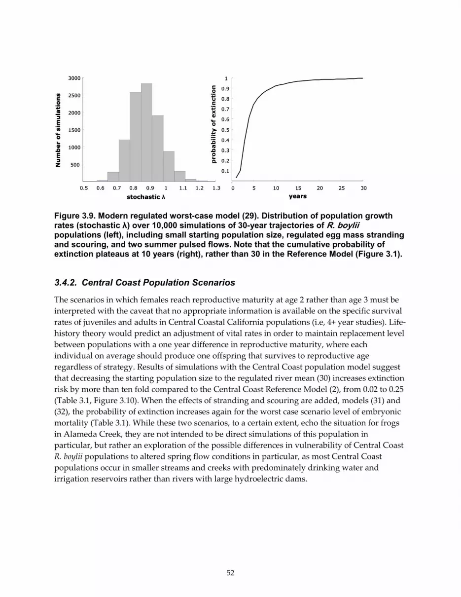
52

05 10 15 20 25 30

0

0.1

0.2

0.3

0.4

0.5

0.6

0.7

0.8

0.9

1

500

1000

1500

2000

2500

3000

0.5 0.6 0.7 0.8 0.9 1 1.1 1.2 1.3 0

stochastic λ years

probability of extinction

Number of sim

ulations

05 10 15 20 25 30

0

0.1

0.2

0.3

0.4

0.5

0.6

0.7

0.8

0.9

1

500

1000

1500

2000

2500

3000

0.5 0.6 0.7 0.8 0.9 1 1.1 1.2 1.3 0

stochastic λ years

probability of extinction

Number of sim

ulations

Figure 3.9. Modern regulated worst-case model (29). Distribution of population growth rates (stochastic λ) over 10,000 simulations of 30-year trajectories of R. boylii populations (left), including small starting population size, regulated egg mass stranding and scouring, and two summer pulsed flows. Note that the cumulative probability of extinction plateaus at 10 years (right), rather than 30 in the Reference Model (Figure 3.1).

3.4.2. Central Coast Population Scenarios

The scenarios in which females reach reproductive maturity at age 2 rather than age 3 must be

interpreted with the caveat that no appropriate information is available on the specific survival

rates of juveniles and adults in Central Coastal California populations (i.e, 4+ year studies). Life-

history theory would predict an adjustment of vital rates in order to maintain replacement level

between populations with a one year difference in reproductive maturity, where each

individual on average should produce one offspring that survives to reproductive age

regardless of strategy. Results of simulations with the Central Coast population model suggest

that decreasing the starting population size to the regulated river mean (30) increases extinction

risk by more than ten fold compared to the Central Coast Reference Model (2), from 0.02 to 0.25

(Table 3.1, Figure 3.10). When the effects of stranding and scouring are added, models (31) and

(32), the probability of extinction increases again for the worst case scenario level of embryonic

mortality (Table 3.1). While these two scenarios, to a certain extent, echo the situation for frogs

in Alameda Creek, they are not intended to be direct simulations of this population in

particular, but rather an exploration of the possible differences in vulnerability of Central Coast

R. boylii populations to altered spring flow conditions in particular, as most Central Coast

populations occur in smaller streams and creeks with predominately drinking water and

irrigation reservoirs rather than rivers with large hydroelectric dams.

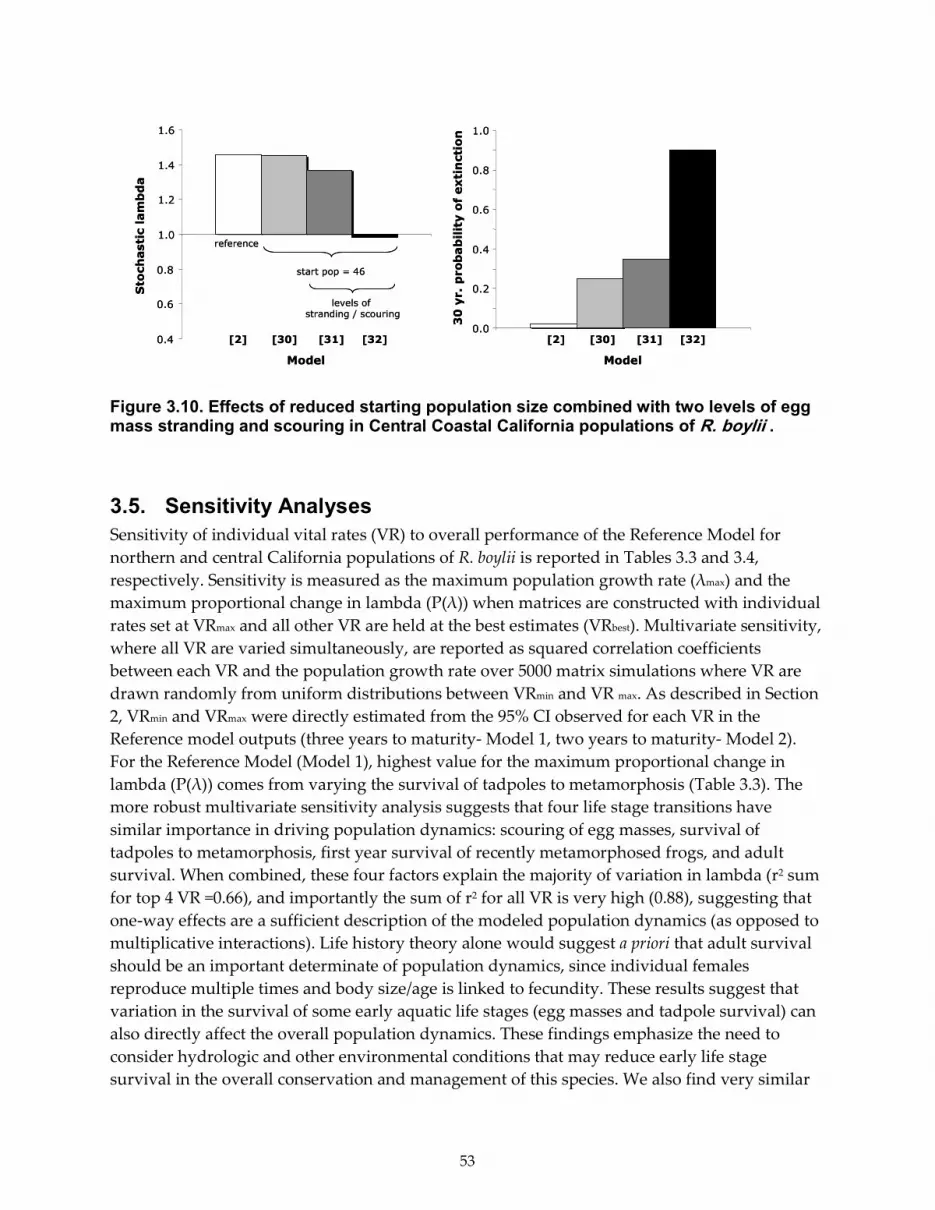
53

0.0

0.2

0.4

0.6

0.8

1.0

Model

30 yr. probability of extinction

0.4

0.6

0.8

1.0

1.2

1.4

1.6

Model

Sto

chastic lambda

[2] [30] [31] [32] [2] [30] [31] [32]

reference

start pop = 46

levels of stranding / scouring

0.0

0.2

0.4

0.6

0.8

1.0

Model

30 yr. probability of extinction

0.4

0.6

0.8

1.0

1.2

1.4

1.6

Model

Sto

chastic lambda

[2] [30] [31] [32] [2] [30] [31] [32]

reference

start pop = 46

levels of stranding / scouring

Figure 3.10. Effects of reduced starting population size combined with two levels of egg mass stranding and scouring in Central Coastal California populations of R. boylii .

3.5. Sensitivity Analyses

Sensitivity of individual vital rates (VR) to overall performance of the Reference Model for

northern and central California populations of R. boylii is reported in Tables 3.3 and 3.4,

respectively. Sensitivity is measured as the maximum population growth rate (λmax) and the

maximum proportional change in lambda (P(λ)) when matrices are constructed with individual

rates set at VRmax and all other VR are held at the best estimates (VRbest). Multivariate sensitivity,

where all VR are varied simultaneously, are reported as squared correlation coefficients

between each VR and the population growth rate over 5000 matrix simulations where VR are

drawn randomly from uniform distributions between VRmin and VR max. As described in Section

2, VRmin and VRmax were directly estimated from the 95% CI observed for each VR in the

Reference model outputs (three years to maturity- Model 1, two years to maturity- Model 2).

For the Reference Model (Model 1), highest value for the maximum proportional change in

lambda (P(λ)) comes from varying the survival of tadpoles to metamorphosis (Table 3.3). The

more robust multivariate sensitivity analysis suggests that four life stage transitions have

similar importance in driving population dynamics: scouring of egg masses, survival of

tadpoles to metamorphosis, first year survival of recently metamorphosed frogs, and adult

survival. When combined, these four factors explain the majority of variation in lambda (r2 sum

for top 4 VR =0.66), and importantly the sum of r2 for all VR is very high (0.88), suggesting that

one-way effects are a sufficient description of the modeled population dynamics (as opposed to

multiplicative interactions). Life history theory alone would suggest a priori that adult survival

should be an important determinate of population dynamics, since individual females

reproduce multiple times and body size/age is linked to fecundity. These results suggest that

variation in the survival of some early aquatic life stages (egg masses and tadpole survival) can

also directly affect the overall population dynamics. These findings emphasize the need to

consider hydrologic and other environmental conditions that may reduce early life stage

survival in the overall conservation and management of this species. We also find very similar

54

patterns in the multivariate sensitivity analysis for the two years to maturity Reference model

(Model 2), with the same four life stages explaining 79% of the variation in lambda (compared

to 0.91 for all VR’s).

While this multivariate sensitivity analysis is among the most appropriate and informative

methods for evaluating the relative importance of different life stages of this particular species,

it is not without caveats and limitations. Foremost is the need to define the maximum and

minimum values for each VR in a way that accurately reflects the biological differences among

VR values (e.g. annual tadpole survival may be inherently lower and more variable than adult

survival), because the ranges over which VR values are varied can substantially alter the

outcome of the sensitivity analysis. While the best available data for R. boylii were used to

calculate VR values and distributions (from which the 95% CI were estimated), there remains a

high degree of uncertainty in all of the estimates. In particular, due to the varied data sources

and populations from which the VR estimates were derived, in most cases corrections for

observation error were not possible. Lack of correction may artificially inflate the variance

estimates and parameter distributions. Thus, as more data are collected and the estimates of

individual vital rates become more precise, the conclusions about which life stages are key

drivers of population dynamics are also expected to be more accurate.

Table 3.3. Reference model sensitivity analysis.

Vital Rate (VR) VRmin VRmax VRbest λmax P(λmax) r2

Semb1 0.84 1.00 0.96 1.41 0.01 0.00

Semb2 0.03 1.00 0.80 1.47 0.05 0.18

Semb3 0.29 1.00 0.83 1.46 0.04 0.02

Stadpole 0.00 0.62 0.15 1.92 0.37 0.15

Smeta 0.12 0.66 0.37 1.59 0.14 0.06

Sjuv1 0.01 0.71 0.26 1.74 0.24 0.17

Sjuv2 0.10 0.94 0.54 1.58 0.13 0.11

adult 0.10 0.94 0.54 1.73 0.24 0.16

F 413 1627 871 1.60 0.15 0.03

Table 3.4. Central Coast populations reference model sensitivity analysis.

Vital Rate (VR) VRmin VRmax VRbest λmax P(λmax) r2

Semb1 0.84 1.00 0.96 1.86 0.01 0.00

Semb2 0.03 1.00 0.80 1.95 0.07 0.15

Semb3 0.29 1.00 0.83 1.93 0.06 0.01

Stadpole 0 0.62 0.15 2.81 0.53 0.21

Smeta 0.12 0.66 0.37 2.18 0.19 0.06

Sjuv1 0.01 0.71 0.26 2.47 0.35 0.17

Sadult 0.10 0.94 0.54 2.33 0.27 0.26

F 413 1625 871 2.20 0.20 0.05

55

4.0 Conclusions and Recommendations

4.1. Conclusions

Overall, the conclusions from this modeling exercise are well supported by first principles

arising from the seasonally synchronized life cycle of R. boylii, where the most vulnerable life

stages are present in rivers during the lowest and most consistent flows of the year in

Mediterranean climates. Spawning occurs in spring or early summer as flood waters recede,

and larvae metamorphose in late summer or early fall prior to the onset of rain-driven floods.

Artificial flow regimes deviating from this natural pattern of flow fluctuation are expected to

threaten locally-adapted communities of organisms, including R. boylii. Although summer and

fall pulsed flows in regulated rivers may not be of greater magnitude than historic base flow

discharges, the model illustrates that when the timing and frequency of pulses are de-coupled

from the timing of R. boylii’s natural life cycle, the effects can be projected forward from stage to

stage, and ultimately influence population persistence. Empirically, negative effects of altered

hydrology for R. boylii such as egg mass scouring, have long been documented (Lind et al.

1996). Population viability analysis provides a tool with which such impacts can be evaluated in

a long-term population context, and also provides a quantitative framework to define priorities

for future data collection.

The conservation of R. boylii in regulated rivers depends on management that minimizes

atypical flow fluctuations during the breeding and tadpole rearing seasons. The results

indicate that the direct effects of anthropogenic hydrologic stressors on individual vital rates,

such as embryonic and larval survival, can result in a several fold higher risk of population

extinction above populations in hydrologically natural environments. Model simulations

mimicking spring flow fluctuations and common hydroelectric project effects on egg masses,

such as spring spills and rapid flow cessation, double the risk of extinction, from 5% in the

Reference Model to 11% in Model (8). Similarly, these recommendations extend beyond spring

flows to include summer flows, since multivariate sensitivity analysis also indicates that tadpole

survival to metamorphosis is among the most important vital rates for overall population

dynamics. For example, even single extreme flow events (with an annual recurrence interval),

such as a summer recreational boating flow or discharge manipulation to conduct studies of fish

habitat for a FERC license application, are predicted to result in a three to five fold increase in

the 30-year extinction risk, from 5% to 16% (Models 1 & 20), or from 5% to 27% (Models 1 & 15),

depending on the level of tadpole mortality. Because one of the major differences between R.

boylii populations in regulated and unregulated rivers is the increased frequency of hydrologic

mass mortality events (e.g. stranding and/or scouring), our model results support the

hypothesis that conditions for R. boylii populations downstream of dams could be much

improved by reducing these events with alternative dam management (e.g. reducing atypical

flows and mimicking natural hydrographs).

Combinations of hydrologic effects often result in disproportionate (e.g. non-additive)

changes to R. boylii population dynamics. Such effects are likely to occur in natural R. boylii

populations, but are often overlooked when single factors are studied or modeled in isolation of

56

one another. For example, the synergy between egg mass scouring and decreased fecundity

simulated in Model (12) produced disproportionate increases in the 30-year risk of extinction

compared to each effect alone (Models 8 & 10). The 30-year extinction risk is 85% for Model (12),

which is 17 times higher than the Reference model, and almost 5 times greater than the sum of

the first order effects (11% and 7%, Models 8 & 10). Similarly, when tadpole mortality during a

single pulsed flow is combined with high rates of egg mass stranding and scouring (Model 25),

the resulting increase in extinction risk is also multiplicative (Model 25 = 91%, Model 9 + 15 =

50%). These results emphasize that attempts to estimate the effect of any one anthropogenic

hydrologic impact (e.g. summer recreational flows, extended spring spills, reduced available

breeding habitat) without consideration for the myriad other impacts occurring simultaneously

will likely underestimate the potential population-level consequences. By extension, we

recommend that studies of hydrologic impacts consider the suite of stressors potentially

affecting R. boylii populations as a whole rather than focusing on any one in isolation.

There is good congruence between observed R. boylii breeding trends in three focal

watersheds; SF Eel, Alameda Creek, and NF Feather, and the results of model scenarios

combining similar differences in starting population sizes and the frequency of spring and

summer hydrologic stressors (see Section 3 Kupferberg et al. 2008). The results of this modeling

exercise are not intended to mimic the dynamics of any one population, but rather explore the

potential for different hydrologic stressors to affect population dynamics. That being said, the

rough similarity between some of the most well-studied R. boylii populations (both regulated

and un-regulated) and model results provides support that the model structure generally

captures R. boylii population dynamics. For example, SF Eel and Alameda Creek (Camp Ohlone

reach) populations are stable or increasing in the presence of naturally-occurring low frequency

spring pulsed flows that cause scouring mortality and low levels of stranding mortality (analog

to Models 1 & 2). Alameda Creek populations below the Calaveras Creek confluence, where

water releases from Calaveras Reservoir decrease stream temperatures and elevate velocities

during the breeding season, are exhibiting declines in breeding (analog to Models 30, 31, & 32).

In the case of the NF Feather, the decline of the Cresta reach R. boylii population began three

years after pulsed flows for whitewater boating were instituted during the egg (2002) and

tadpole (2002-2005) rearing seasons (analog to Models 28 & 29). By comparison, R. boylii

populations in the NF Feather (Poe reach) exhibited increases in breeding over the same time

period (analog to Models 3, 8, & 27). While we are reassured by this general congruence, we

emphasize that this model framework is not intended to be predictive of any one R. boylii

population. Given the large uncertainties surrounding estimates of individual vital rates and

their distributions (uncorrected for observation and other errors), the utility of this modeling

exercise lies in the comparison of hypothetical model scenarios relative to our best estimate of

population dynamics in hydrologically un-regluated environments. Individual scenarios should

be viewed as hypotheses awaiting confrontation with future data collection. As such, this

modeling effort highlights an urgent need to gather field data targeting key R. boylii vital rates

(tadpole, 1st juvenile year, and adult survival), and impacts to them. In the absence of such data,

the results from the Reference Models as compared to the set of hydrologic scenarios provide an

additional tool for water resource managers to assess potential risks of various flow regimes for

R. boylii populations.

57

4.2. Commercialization Potential

Commercialization is not applicable to this study, as prescriptive applications of this model to

particular R. boylii populations are not recommended.

4.3. Recommendations

This section is divided into two parts with the intent to clarify and emphasize particular sets of

recommendations. High priority recommendations that derive directly from the modeling work

and comparative hydrologic scenarios are outlined. The next section identifies critical

information gaps and priorities for future research.

4.3.1. Management Recommendations Indicated by Model Outputs and Sensitivity Analyses

A central tenet of the natural flow regime paradigm is that regulated flows should mimic

natural patterns of temporal variation in hydrology to sustain fluvial geomorphic processes,

functional food webs (Power et al. 1996; Poff et al. 1997; Richter et al. 2003), and match the

adaptations of organisms to the conditions in which they evolved (Lytle and Poff 2004). The

management recommendations stemming from this modeling exercise support the general

ecological principles of this approach. Under natural (un-regulated) levels of hydrologic

variation, R. boylii populations are expected to be self-sustaining over a thirty year time period

with a low probability of extinction. Simulations mimicking different hypotheses about life

stage impacts (and combinations) due to hydrologic regulation all suggest higher extinction risk

and more vulnerable population demography (lambda near or below 1). While large

uncertainties exist in the estimation of many of the vital rate parameters (Section 2, Appendix

B), in every instance where decisions were made during model development the goal was to

incorporate the most rigorous, un-biased quantitative data available. Only when no rigorous

data were available for R. boylii did we resort to the inclusion of quantitative data from sister

taxa (in the case of Stadpole and Sjuv1). As a result, the outcome of this modeling exercise should be

interpreted as preliminary, and results are expected to be refined with the inclusion of

additional demographic data. With these caveats, the following recommendations are made:

• Eliminate manufactured pulsed flows once frog breeding begins in the spring through

the early fall when metamorphosis occurs.

• Adopt water management strategies that anticipate the potential for synergistic and

indirect effects among multiple hydrologic and environmental changes. Some changes to

flow regimes may be positive for one species but have unintended negative

consequences for another. For example, tradeoffs are likely to exist between increasing

base flows to buffer the effects of pulsed flows or to aid out-migrating anadromous fish

pass potential barriers, resulting decreases in stream temperature. Because decreases in

58

water temperature can affect growth and survival rates of tadpoles, such tradeoffs need

to be evaluated and anticipated. Similarly loss of algal food resources from summer

pulse flows can have negative effects on tadpole survival. Additionally, the importance

of the most fecund, early breeding females for overall population dynamics needs to be

evaluated, as the contributions of these individuals to recruitment may be the most

vulnerable to early season hydrologic impacts.

• Gather data simultaneously on key demographic parameters during FERC relicensing

studies (egg mass, tadpole, adult survival at a minimum), and incorporate new

demographic estimates to future PVA’s for R. boylii populations.

• Improve long-term monitoring programs for R. boylii in both regulated and unregulated

(reference) river systems. In particular, a reference (un-regulated) Sierra Nevada

population urgently needs to be identified and studied. Ideally, this site will be the focus

of both monitoring and research on demographic parameters. For science-based

management to be a viable option, attempts to link flow changes to population

responses need to coincide with long-term biological monitoring of an appropriate

sentinel species (Souchon et al. 2008). In order to apply this modeling approach of

comparing scenarios, reliable data on population trends are needed for populations

spanning the broad range of environments where R. boylii occurs.

• Appropriate State and/or Federal agencies should elevate the protection status of R.

boylii (e.g., listing under the California or Federal Endangered Species Act). Evidence has

accumulated over the last five years documenting the range-wide decline of R. boylii and

has identified genetically unique populations in the Southern Sierra Nevada and Central

Coast Ranges of California (Lind 2005) where declines are more pronounced. Likely

mechanisms for R. boylii population declines are well documented and populations that

are extant in regulated streams continue to show evidence of declines (Kupferberg et al.

2008, this report).

Mitigation and adaptive management of the flow regime effects on R. boylii populations

identified Table 1.1 may be achieved by applying the above recommendations. These

approaches for improving early life stage survival are summarized in Table 4.1. A key element

to the success of applying the natural flow regime paradigm is knowledge of the highly site

specific relationship between discharge, water surface elevation, and current velocity in the

edgewater habitats used by R. boylii. This report has focused on R. boylii, however, it should be

noted that a number of species, more commonly thought of as pond breeders, also breed along

the margins of California’s rivers. The species whose egg masses and larvae may be similarly

susceptible to the direct and indirect effects of flow fluctuation include California Red-legged

frogs (Rana aurora draytonii), Pacific Chorus frogs (Pseudacris regilla), Western toads (Bufo boreas),

and newts (Taricha torosa, T. granulosa, T. rivularis, T. sierrae). It is thus imperative that

conservation actions and river restoration efforts intended to improve conditions in the main

part of the channel for a target organism be implemented in concert with an appropriate

monitoring program of the species whose early life stages inhabit edgewaters.

59

Table 4.1. Overview of potential mitigation and restoration options for Rana boylii in regulated rivers.

Project Operations

Short-term impacts

Long-term impacts

Mitigation/Restoration

Intentional aseasonal flows

(power generation, recreation,

out-migration of salmonid

smolts); Unintentional spill of

water over dam

- scouring or desiccation of egg

masses1,2

/ tadpoles3

- export spring and summer algal

productivity4,5

, reduced resources

for tadpoles, reduced insect

abundance5, food web

repercussions

- discharge decoupled from

environmental cues (e.g. rainfall,

air temperature) triggering

inappropriate behavioral

responses by adults, juveniles,

delayed onset of breeding1,6

- smaller population sizes1,2

- mimic natural hydrograph to

degree possible

- flow regimes and ramping rates

to minimize impacts during

breeding and rearing periods

- change management of water

elevation in upstream reservoir

Intentional de-watering of

stream channels for rescue

operations

- desiccation of egg masses /

tadpoles

Unknown - observe minimum instream flow

requirements

- post-event ramping rates that

minimize disturbance

Unintentional powerhouse

outages resulting in rapid

increase in flows in bypass

reaches, followed by rapid

decrease in flows

- changes to margin water

temperature, depth, and velocity,

- scouring/desiccation of

eggs/tadpoles, depending on

ramping rate, magnitude of

change, channel shape

Unknown - change timing of planned

outages (for repairs, etc.) to

outside of breeding and rearing

season

Reduced winter/spring flows

- absence of scouring/depositional

flows that prevent riparian

encroachment

- reduced breeding habitat, greater

distances between breeding sites3

- vegetation encroachment,

altered channel morphology,

reduced breeding habitat

- population loss/fragmentation3,

reduced gene flow, altered

metapopulation dynamics

- mimic natural hydrograph to

degree possible

- restore some components of

spring snow-melt hydrograph7

Altered summer baseflows - lower water temperatures

- change in available habitat

(channel shape)

- promotes habitats that support

non-native predatory fish,

amphibians, and invertebrates,

increased predation on eggs,

tadpoles

- adjust water release

temperatures (mix of depths)

- develop basin-scale plans for

fish stocking relative to frog

needs

60

Project Operations

Short-term impacts

Long-term impacts

Mitigation/Restoration

Movement of water among river

basins

- potential for increased disease

and parasite transmission

Unknown - reassess water redistribution to

eliminate, or shift timing to

decrease disease (fall, winter)

References: 1. GANDA 2008; 2. Kupferberg et al. 2008; 3. Lind et al. 1996; 4. Spring Rivers 2002; 5. GANDA 2006; 6. Borque 2008; McBain and

Trush, Inc. 2009.

61

4.3.2. Research Priorities Indicated By Information Gaps

The best available data and newly collected field data were used to define vital rates for each R.

boylii lifestage in this model. However, several of the vital rate values used in this exercise were

based on related species or incorporated several, currently untested, assumptions. The main

demographic parameters that require immediate follow-up investigation are tadpole, first year

overwinter, and juvenile survival (Table 2.2). Additionally, the demographic impact of different

hydrologic scenarios is only well-described for egg mass survival (stranding and scouring

patterns). For example, predicting the actual survival consequences for tadpoles reared under

different hydrologic conditions is prevented by substantial data gaps. While there are data from

field enclosure and laboratory studies estimating survival and critical swimming velocities

(section 4, Kupferberg et al. 2008) and anecdotal observations from the field of tadpole mortality

after pulsed summer flows (Section 2 of Kupferberg et al. 2008), the critical challenge is to

develop a functional understanding of how particular changes in flow management directly

affect annual tadpole (or other life stage) survival. Such data are critically needed to improve

our ability to accurately forecast the consequences of altered hydrologies for R. boylii

populations, and could be collected as part of the FERC relicenscing process.

The result that R. boylii populations are very sensitive to early life stage survival is consistent

with findings for trout in which the timing of floods which scour redds are known to be limiting

factors (Strange et al 1993), but contrasts with other amphibian population projection models

(Biek et al. 2002; Vonesh and De la Cruz 2002; Govindarajulu et al. 2005). Those models suggest

that the most sensitive vital rates are post-metamorphic juvenile survival, the life stage for

which there are no direct observations in R. boylii.

There are other anthropogenic stressors on R. boylii in regulated rivers that were not explored in

this model, but which deserve further study. For example, predation pressure likely increases

when invasive species (e.g. bullfrogs Rana catesbeiana, crayfish, and non-native fish) flourish in

waterways subject to flow diversion and regulation (Hayes and Jennings 1988; Moyle and Light

1996; Marchetti et al. 2004). There may also be stressors originating outside a population’s

watershed, such as downwind drift of organophosphate pesticides (Davidson 2004; Sparling

and Fellers 2007), that influence early life stage vital rates and could act in synergy with the

hydrologic stressors. Thermal regime effects both directly related to hydrologic regulation and

indirectly due to watershed-scale land-use change (e.g., logging) also require further

investigation.

4.4. Benefits to California

This research will be valuable to the adaptive management of regulated rivers in terms of

evaluating the relative merits of competing flow proposals. By assessing whether early stages of

the R. boylii life cycle are likely to be affected by the flow regime attribute under consideration,

managers can determine if their actions may put populations further at risk or aid in their

restoration. During FERC relicensing of hydropower projects, there are often discussions of the

effects of proposed base flows, pulsed flows, and other conditions on a native aquatic species.

The hydrologic scenarios modeled in this study cover a range of potential flow regimes and

62

their influences on different life stages of R. boylii. These models can aid in the assessment of

risk for this particular sensitive species and others with similar ecological niches, ultimately

providing an additional tool for both hydropower licensees and regulatory agencies to evaluate

and compare relative risks among species.

63

5.0 References

Altig, R. and G. F. Johnston. 1989. Guilds of anuran larvae: relationships among developmental

modes, morphologies, and habitats. Herpetological Monographs 3:81-109.

Altwegg, R. 2003. Multi-stage density dependence in an amphibian. Oecologia 86:140–143.

Altwegg, R. and H. Reyer. 2003. Patterns of natural selection on size at metamorphosis in water

frogs. Evolution 57:872-882.

Berven, K. A. 1990. Factors affecting population fluctuations in larval and adult stages of the

Wood Frog (Rana sylvatica). Ecology 71:1599-1608.

Biek, R., W. C. Funk, B. A. Maxwell, and L. S. Mills. 2002. What is missing in amphibian decline

research? Insights from ecological sensitivity analysis. Conservation Biology 16:728-734.

Bobzien, S. and J. E. DiDonato. 2007. The status of the California Tiger Salamander (Ambystoma

californiense), California red-legged frog (Rana aurora draytonii), Foothill yellow-legged

frog (Rana boylii) and other aquatic herpetofauna in the East Bay Regional Park District,

California. (67pp.)

Boone, M. D. 2005. Juvenile frogs compensate for small metamorph size with terrestrial growth:

overcoming the effects of larval density and insecticide exposure. Journal of Herpetology

39:416-423.

Bourque, R. M. 2008. Yellow-legged frog (Rana boylii) in Tehama Co, CA. M.S. thesis, California

State University, Humboldt (Dec.) 93pp.

Brockelman, W. Y. 1969. An analysis of density dependent effects and predation in Bufo

americanus tadpoles. Ecology 50:632-644.

Brook, B. W., J. J. O’Grady, A. P. Chapman, M. A. Burgman, H. Resit Akcakaya, and R.

Frankham. 2000. Predictive accuracy of population viability analysis in conservation

biology. Nature 404:385-387.

Bunn, S. E. and A. H. Arthington. 2002. Basic principles and ecological consequences of altered

flow regimes for aquatic biodiversity. Environmental Management 30:492-507.

Burnham, K.P. and D.R. Anderson. 2002. Model Selection and Multimodel Inference: A

Practical Information-Theoretic Approach. Springer, New York.

Calef, G. W. 1973. Natural mortality of tadpoles in a population of Rana aurora. Ecology 54:741-

758.

California Department of Fish and Game. 2008. California Natural Diversity Database Special

Animals. Accessed on 27 July 2008.

http://www.dfg.ca.gov/biogeodata/cnddb/pdfs/SPAnimals.pdf (February).

Caswell, H. 2001. Matrix Population Models. 2nd ed. Sinauer, Sunderland, MA.

64

Cooch, E. and G. White (eds.) 2007. Program MARK: A Gentle Introduction, 6th Edition.

Available online at: http://www.phidot.org/software/mark/docs/book/.

Crouch, W.B., and Paton, P.W.C. 2000. Using egg-mass counts to monitor wood frog

populations. Wildlife Society Bulletin 28: 895–901.

Crouse, D. L., L. Crowder and H. Caswell. 1987. A stage-based population model for

loggerhead sea turtles and implications for conservation. Ecology 68:1412-1423.

Davidson, C., H.B. Shaffer, and M.R. Jennings. 2002. Spatial test of pesticide drift, habitat

destruction, UV-B, and climate-change hypotheses for California amphibian declines.

Conservation Biology 16:1588-1601.

Davidson, C. 2004. Declining downwind: Amphibian population declines in California and

historical pesticide use. Ecological Applications 14:1892-1902.

ECORP Consulting, Inc. 2004a. Results of the 2003 Foothill Yellow legged Frog (Rana boylii)

and Mountain yellow legged frog (Rana muscosa) studies at the Spring Gap-Stanislaus

project. Prepared for Pacific Gas and Electric Company, San Ramon, California, 115pp.

ECORP Consulting, Inc. 2004b. Results of the 2004 (Year 1) Amphibian Monitoring Program for

Foothill Yellow-legged Frog and Mountain Yellow-Legged Frog. Prepared for El Dorado

Irrigation District, Placerville, California, 71pp.

Funk, W. C., A. E. Greene, P. S. Corn, and F. W. Allendorf. 2005. High dispersal in a frog species

suggests that it is vulnerable to habitat fragmentation. Biology Letters. 1:13-16.

Garcia and Associates. 2003. Results of 2002 study evaluating the availability, extent, and

quality of foothill yellow-legged frog (Rana boylii) habitat within the Poe Reach at the

existing flow level and at four higher flows. Prepared for Pacific Gas and Electric

Company, San Ramon, California, Job 306/4, 48pp.

Garcia and Associates. 2004a. Results of 2003 surveys of foothill yellow-legged frogs (Rana

boylii) within the Poe Project Area, North Fork Feather River. Prepared for Pacific Gas

and Electric Company, San Ramon, California, Job 332/49, 53pp.

Garcia and Associates. 2004b (NFF5). Results of 2004 study evaluating impacts of elevated flows

on foothill yellow-legged frog (Rana boylii) habitat in the Poe Reach, North Fork Feather

River. Prepared for Pacific Gas and Electric Company, San Ramon, California, Job

332/69, 44pp.

Garcia and Associates. (GANDA) 2004c. Results of 2002 surveys and monitoring for foothill

yellow-legged frogs (Rana boylii) within the Rock Creek-Cresta project area, North Fork

Feather River, recreation and pulse flow biological evaluation. Prepared for Pacific Gas

and Electric Company, San Ramon, California, Job 306/3, 45pp.

65

Garcia and Associates. (GANDA) 2004d. Results of 2003 surveys and monitoring for foothill

yellow-legged frogs (Rana boylii) within the Rock Creek-Cresta project area, North Fork

Feather River, recreation and pulse flow biological evaluation. Prepared for Pacific Gas

and Electric Company, San Ramon, California, Job 332/52, 65pp.

Garcia and Associates. (GANDA). 2006. Evaluating the Impacts of Manufactured Recreation Str

eamflows on the Macroinvertebrate Community of a Regulated River. California Energy

Commission, PIER Energy-Related Environmental Research Program. CEC-500-2006-07

8.

Garcia and Associates. (GANDA) 2007. Summary of Results for the 2006 Cresta and Poe Reach

Amphibian Surveys. Draft report prepared for Pacific Gas and Electric Company, San

Ramon, CA.

Garcia and Associates. (GANDA) 2008. Identifying Climatic and Water Flow Triggers

Associated with the Onset of Breeding in a Foothill Yellow-legged Frog (Rana boylii)

Population in the North Fork Feather River, California: Final Report. Prepared for

Pulsed Flow Program, Department of Animal Sciences, University of California, Davis,

California.

Gosner, K. L. 1960. A simplified table for staging anuran embryos and larvae with notes on

identification. Herpetologica 16:183-190.

Govindarajulu, P., R. Altwegg, and B.R. Anholt. 2005. Matrix model investigation of invasive

species control: bullfrogs on Vancouver Island. Ecological Applications 15:2161-2170.

Harper, E. B. and R. D. Semlitsch. 2007. Density dependence in the terrestrial life history stage

of two anurans. Oecologia 153:879-889.

Hayes, M.P., and M.R. Jennings. 1988. Habitat correlates of the distribution of California red

legged frog (Rana aurora draytonii) and Foothill yellow legged frog (Rana boylii):

implications for management. In: R. C. Szaro, K. E. Severson, D. R. Patton, tech. coords.

Management of Amphibians, Reptiles, and Small Mammals in North America. Pp. 144-

158. USDA Forest Service, Rocky Mountain Forest and Range Experiment Station, Gen.

Tech. Rep. RM 166, Fort Collins, Colorado.

IUCN. 2001. IUCN Red List Categories and Criteria: Version 3·1. International Union for the

Conservation of Nature and Natural Resources, Species Survival Commission, Gland,

Switzerland.

Jennings, M.R. and M.P. Hayes. 1994. Amphibian and Reptile Species of Special Concern in

California. A Report to the California Department of Fish and Game, Rancho Cordova,

California. 255pp.

Jennings, M.R. 1996. Status of amphibians. In: D.C. Erman (ed.), Sierra Nevada Ecosystem

Project: Final Report to Congress, vol. II, Assessments and scientific basis for

management options, pp. 921-944. Davis: University of California, Centers for Water and

Wildland Resources.

66

Kareiva, P., M. Marvier, M. McClure. 2000 Recovery and management options for

spring/summer chinook salmon in the Columbia River Basin. Science 290:977-979.

Klausmeyer, K. 2005. Effects of climate change on the hydrology of upper Alameda Creek (May

12, 2005). Water Resources Center Archives. Hydrology. Paper klausmeyer. Available

URL “ http://repositories.cdlib.org/wrca/hydrology/klausmeyer ” [Accessed Aug. 10,

2007]

Kupferberg, S. J., J.C. Marks, and M. E. Power. 1994. Variation in natural algal and detrital diets

affects larval anuran life history traits. Copeia 1994: 446-457.

Kupferberg, S.J. 1996. Hydrologic and geomorphic factors affecting reproduction of the foothill

yellow-legged frog (Rana boylii). Ecological Applications 6:1332-1344.

Kupferberg, S.J. 1997. Bullfrog (Rana catesbeiana) invasion of a California river: the role of larval

competition. Ecology 78:1736-1751.

Kupferberg, S., A. Lind, S. Yarnell, J. Mount. 2008. Pulsed flow effects on the foothill yellow-

legged frog (Rana boylii): Integration of empirical, experimental and hydrodynamic

modeling approaches. Final Report to the California Energy Commission, PIER., 194 pp

(January).

Licht, L.E. 1974. Survival of embryos, tadpoles, and adults of the frogs Rana aurora aurora and

Rana pretiosa pretiosa sympatric in southwestern British Columbia. Canadian Journal of

Zoology, 52:613-627.

Lind, A.J. 2005. Reintroduction of a declining amphibian: determining an ecologically feasible

approach for the foothill yellow-legged frog (Rana boylii) through analysis of decline

factors, genetic structure, and habitat associations. Ph.D. Dissertation, University of

California, Davis. (March) 169 pp.

Lind, A.J., L. Conway, H. Sanders, P. Strand, and T. Tharalson. 2003. Distribution, relative

abundance, and habitat of foothill yellow-legged frogs (Rana boylii) on National Forests

in the Southern Sierra Nevada Mountains of California. Unpublished report to the Fish

Habitat Relationships (FHR) Program, USDA Forest Service, Region 5 (California).

October. 30pp.

Lind, A.J., and H.H. Welsh, Jr. In revision. Multi-scale oviposition site choice by the foothill

yellow-legged frog (Rana boylii) in California, U.S.A.: Responses to a stochastic

environment. Journal of Herpetology.

Lind, A.J., H.H. Welsh, Jr., and R.A. Wilson. 1996. The effects of a dam on breeding habitat and

egg survival of the foothill yellow legged frog (Rana boylii) in northwestern California.

Herpetological Review 27:62 67.

Loman, J., and G. Andersson. 2007. Monitoring brown frogs Rana arvalis and Rana temporaria in

120 south Swedish ponds 1989–2005. Mixed trends in different habitats. Biological

Conservation 135:46-56.

67

Lytle, D. A. and N. L. Poff. 2004. Adaptation to natural flow regimes. Trends in Ecology and

Evolution. 19:94-100.

Marchetti, M.P., P.B. Moyle, and R. Levine. 2004. Alien fishes in California watersheds:

Characteristics of successful and failed invaders. Ecological Applications 14:587-596.

McBain and Trush, Inc. 2009. Pulse Flow Guidelines: Managing the Annual Snowmelt

Hydrograph and Winter Floods in Regulated Boulder-Bedrock Sierra Nevada Rivers.

Final Report to the California Energy Commission, PIER., 162pp (+ appendices).

Morris,W., D. Doak, M. Groom, P. Kareiva, J. Fieberg, L. Gerber, P. Murphy, D. Thomson. 1999.

A Practical Handbook for Population Viability Analysis. The Nature Conservancy. 79

pp.

Morris, W.F. and D.F. Doak. 2002. Quantitative Conservation Biology: Theory and Practice of

Population Viability Analysis. Sinauer and Associates, Inc. Publishers, Sunderland, MA.

Moyle, P.B., and T. Light. 1996. Fish invasions in California: do abiotic factors determine

success? Ecology 77:1666-1670.

Otis, D.L., K. P. Burnham, G. C. White, and D. R. Anderson. 1978. Statistical-inference from

capture data on closed animal populations. Wildlife Monographs 62:7-135

Petranka, J. W., E. M. Harp, C. T. Holbrook, and J. A. Hamel. 2007. Long term persistence of

amphibian populations in a restored wetland complex. Biological Conservation 138:371-

380.

Poff, N. L., J. D. Allan, M. B. Bain, J. R. Karr, K. L. Prestergaard, B. D. Richter, R. E. Sparks, and J.

C. Stromberg. 1997. The natural flow regime: a paradigm for river conservation and

restoration. BioScience 47:769-784.

Power, M.E., W.E. Dietrich, and J.C. Finlay. 1996. Dams and downstream aquatic biodiversity:

potential foodweb consequences of hydrologic disturbance and geomorphic change.

Environmental Management 20:887-895.

Richards, S. J. 2002. Influence of flow regime on habitat selection by tadpoles in an Australian

forest stream. J. Zoology 257:273-279.

Richter, B. D., R. Matthews, D. L. Harrison, and R. Wigington. 2003. Ecologically sustainable

water management: managing river flows for river integrity. Ecological Applications

13:206-224.

Richter, B. D., D. P. Braun, M. A. Mendelson, and L. L. Master. 1997. Threats to imperiled

freshwater fauna. Conservation Biology 11:1081-1093.

Rombough, Christopher J. 2006. Winter habitat use by juvenile Foothill Yellow-Legged frogs

(Rana boylii): The importance of seeps. Northwestern Naturalist. 87 (2): 159.

68

Rombough, C. J. and M. P. Hayes. 2005. Novel aspects of oviposition site preparation by foothill

yellow-legged frogs (Rana boylii). Northwestern Naturalist 86:157-160.

Rosenberg, D. M., P. McCully, and C. M. Pringle. 2000. Global scale environmental effects of

hydrological alterations: Introduction. Bioscience 50:746-752.

San Francisco Public Utilities Commission. 2007. Water System Improvement Program

Environmental Impact Report, Case No. 2005.0159E. Section 5.4 Alameda Creek

Watershed Streams and Reservoirs. 124 pp. Available URL

http://www.sfgov.org/site/uploadedfiles/planning/vol3_sec5-4_wsip-dpeir.pdf

[Accessed July 28, 2007]

Souchon, Y., C. Sabaton, R. Deibel, D. Reiser, J. Kershner, M. Gard, C. Katopodis, P. Leonard, N.

L. Poff, W. J. Miller, and B.L. Lamb. 2008. Detecting biological responses to flow

management: missed opportunities; future directions. River Research and Applications

24:506-518.

Sparling, D. W. and G. Fellers. 2007. Comparative toxicity of chloropyrifos, diazinon, malathion

and their oxon derivatives to larval Rana boylii. Environmental Pollution 147:535-539.

Spring Rivers Ecological Sciences, LLC. 2002. Foothill yellow-legged frog (Rana boylii) studies in

2002 for PG&E's Pit 3, 4, and 5 Hydroelectric Project (FERC No. 233). Prepared for

Pacific Gas and Electric Company, San Ramon, California, 62pp.

Strange, E. M., P. B. Moyle, and T. C. Foin. 1993. Interactions between stochastic and

deterministic processes in stream fish community assembly. Environmental Biology of

Fishes. 36:1-15.

Twitty, V., D. Grant, and O. Anderson. 1967. Amphibian orientation: an unexpected

observation. Science 155:352-353.

Van Wagner, T. 1996. Selected life history and ecological aspects of a population of foothill

yellow-legged frogs (Rana boylii) from Clear Creek, Nevada City, California. Unpubl.

Master’s Thesis, California State University, Chico.

Vonesh, J. R. and O. De la Cruz. 2002. Complex life cycles and density dependence: assessing

the contribution of egg mortality to amphibian declines. Oecologia 133:325-333.

Wheeler, C.A. 2007. Temporal breeding patterns and mating strategy of the foothill yellow-

legged frog (Rana boylii). Master's Thesis. Department of Wildlife. Humboldt State

University, Arcata, California.

Wheeler, C. A., J. M. Garwood, and H. H. Welsh, Jr. 2005. Rana boylii (Foothill Yellow-legged

Frog). Physiological skin color transformation. Herpetological Review 36: 164-165.

White, G.C., D.R. Anderson, K.P. Burnham, and D.L. Otis. 1982. Capture-Recapture and

Removal Methods for Sampling Closed Populations. Report #LA087-87-NERP. Los

Alamos National Laboratory, Los Alamos, New Mexico. 235pp.

69

White, G. C., and K. P. Burnham. 1999. Program MARK: survival estimation from populations

of marked animals. Bird Study 46(Supplement):120–138.

Wilbur, H. M. 1976. Density-dependent aspects of metamorphosis in Ambystoma and Rana

sylvatica. Ecology 57:1289-1296.

Wilbur, H. M. 1977. Density-dependent aspects of growth and metamorphosis in Bufo

americanus. Ecology 58:196-200.

Wisdom, M. J. and L. S. Mills. 1997. Sensitivity analysis to guide population recovery: prairie

chickens as an example. Journal of Wildlife Management 61:302-312.

Wisdom, M. J., L. S. Mills, and D. F. Doak. 2000. Life stage simulation analysis: estimating vital-

rate effects on population growth for conservation. Ecology 81:628-641.

Yarnell, S.M. 2005. Spatial heterogeneity of Rana boylii habitat: Physical processes,

quantification, and ecological meaningfulness. Ph.D. Dissertation, Hydrology.

University of California, Davis.

70

6.0 Glossary

Allee Effect The point when the spatial distribution and density

of a population inhibit the ability of individuals to

find mates and reproductive rates decline rapidly.

Analysis of Covariance A statistical method for analyzing the differences in

the means of two or more groups of data, while

accounting for variation in one interval-ratio

variable.

Epilithic Periphyton/Diatoms Algae that grows on the surface of rocks in a

waterbody.

Fecundity The number, rate, or capacity of production of

offspring.

FERC Federal Energy Regulatory Commission; the

government body that licenses hydroelectric

projects

F Ratio A statistical ratio in analysis of variance (ANOVA) ;

the variation explained by a set of treatments or

factors in relation to the unexplained (error)

variation

Lambda (λ) and Population Growth Rate Annual proportional change in population, such

that λ = 1 indicates stability, values > 1 indicate

growth, and values < 1 indicate decline

Matrix Population Model A type of population model that uses matrix

algebra and pre-defined parameter values for

different age classes or life stages to project

population growth rate (λ) and extinction

probabilities into the future.

Oviposition Egg laying

Population Viability Analysis The process of defining vital rates and potential

threats for a species or population and

incorporating these into an analysis of the

likelihood of persistence of that species/population

over a given time period into the future.

71

PIT (tag) Abbreviation for “Passive Integrated Transponder”

tags, which are injectable, internal, radio-type tags

that when scanned with the appropriate reader,

provide a unique identification number for

individual animals.

Ranid Frog Any frog species that is a member of the amphibian

genus Rana and family Ranidae.

Recruitment The amount by which a population changes in size

during one stage or over one interval in time, such

as recently metamorphosed young of the year frogs

growing to become adults of reproductive size.

Scouring Removal of frog egg masses from stream

substrates, usually by high water flows.

Stable Age Distribution The proportion and/or number of individuals in

age class or life stage under the assumption that the

population is at equilibrium.

Stochastic Processes and variables that are random, non-

constant, and unpredictable.

Stranding Dessication of frog egg masses due to rapidly

dropping water flow levels.

Vector (of starting population sizes) A definition of the number of individual in each life

stage to be used in subsequent matrix algebra

computations of a population model. The entire

vector is determined based on defining the number

of individuals in one lifestage and carrying that

through mathematically to define all the others

based on the concept of a stable age distribution (see

above). In matrix algebra terms, a vector is a matrix

which has one of its dimensions equal to one.

72

APPENDIX A. Detailed Descriptions of Study Areas

South Fork Eel River

The SF Eel has relatively pristine habitat. It has moderate bank slopes, moderately confined

valleys with bedrock outcrops, small but continuous riparian zones, coarse substrates, and

moderately steep gradient features including steps, riffles, and pools. The study reach

encompasses confluences with five perennial tributaries and other ephemeral drainages

inhabited by R. boylii but not used for breeding. Substrates are sandstone and mudstone-shale

bedrock and boulders. The river has riffle pool morphology with cobble, pebble, and gravel

point bars. One riffle pool sequence is ≈ 5-7 times the bank full channel width (≈35 m). The river

runs through mixed coniferous forest and the common riparian species are similar to the NF

Feather, alder (Alnus latifolia) and sedge (Carex nudata). Detailed geomorphic descriptions are in

Seidl and Dietrich (1992). The algal based food web has been extensively studied by Power

(1990) and Power et al. (2008). R. boylii breeding behavior in relation to channel morphology at

the site is described in Kupferberg (1996).

Hurdygurdy Creek

The Hurdygurdy Creek study area was located in the lower section of the creek within 2km of

the confluence with the South Fork of the Smith River, Del Norte County, California (Figure

A.1). Hurdygurdy is a fifth order tributary (to the Smith River) with cool wet winters and warm

dry summers. General vegetation type is mixed hardwood/Douglas-fir (Pseudotsuga menziesii)

forest in the uplands with alder (Alnus sp.) and willow (Salix sp.) in the riparian zone. Average

annual rainfall is 280 cm (range 152-330 cm) (Gasquet Ranger Station, Smith River National

Recreation Area, eleven air miles north). During the study, ambient water and air temperatures

ranged from 6 to 18° C and 6 to 30° C, respectively. Hydrologic and geomorphologic events in

Hurdygurdy Creek are reflective of high winter/spring run-off events and include debris flows,

flooding, and braided channel migration. Even with this relatively active geomorpohology,

stream mesohabitats (e.g. low gradient riffles, main channel pools) have maintained sizes and

positions over many years. Discharge averages 100 m3sec-1 in winter with 10-year flood events

reaching as high as 140 m3sec-1 (D. Fuller, Bureau of Land Management, personal

communication). Summer discharge can be as low as 1 m3sec-1 (M. McCain, USFS Gasquet

Ranger District, personal communication). Capture-recapture surveys of adult frogs was

conducted at a large breeding area approximately 877m upstream from the river confluence; at

this site, the stream is braided and approximately 40m wide (Wheeler 2007).

73

Figure A.1 Location of Hurdygurdy Creek study area (from Wheeler 2007)

North Fork Feather River

The NF Feather, on the western slope of the Sierra Nevada, has numerous geologic formations

and volcanic features, incised canyons, and steep forested slopes. The canyon shape provides

conditions for a series of dams along the river, each capturing flow for hydropower generation

before sending it downstream to the next in-stream reservoir. Typical of R. boylii breeding

habitat in the Sierra Nevada, the breeding sites throughout the Poe and Cresta reaches of the NF

Feather, are in close proximity to creek confluences, contain shallow coarse cobble bars, and are

vegetated by sedges and willows (Salix spp). The shallow rocky margins provide appropriate

depth and velocity conditions for oviposition and larval rearing, while the rocks and sedges

provide cover for newly metamorphosed frogs. Tributaries provide adult habitat.

Alameda Creek

Similar in area to the SF Eel watershed but receiving less precipitation, the Alameda Ck

watershed provides a portion of San Francisco’s drinking water. The unregulated study reach is

hereafter referred to as the Camp Ohlone reach and is upstream of the dam and tunnel which

divert water to Calaveras Reservoir (Figure A.2). Calaveras Reservoir captures runoff from

Calaveras Ck. and Arroyo Hondo, and then flows back into Alameda Ck. The downstream

regulated egg survey reaches, are a section in the steep gradient bedrock “Little Yosemite”

canyon, which experiences water diversion, and an alluvial section below the confluence with

Calaveras Ck, referred to as the Sunol reach. The topography and vegetation of the Alameda Ck

reaches are typical of Central Coast Range oak woodlands and grasslands. Riparian vegetation

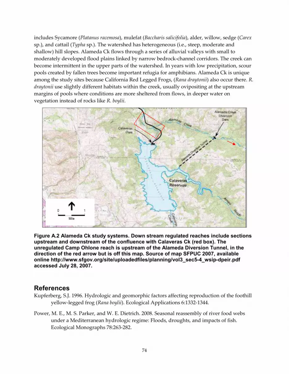
74

includes Sycamore (Platanus racemosa), mulefat (Baccharis salicifolia), alder, willow, sedge (Carex

sp.), and cattail (Typha sp.). The watershed has heterogeneous (i.e., steep, moderate and

shallow) hill slopes. Alameda Ck flows through a series of alluvial valleys with small to

moderately developed flood plains linked by narrow bedrock-channel corridors. The creek can

become intermittent in the upper parts of the watershed. In years with low precipitation, scour

pools created by fallen trees become important refugia for amphibians. Alameda Ck is unique

among the study sites because California Red Legged Frogs, (Rana draytonii) also occur there. R.

draytonii use slightly different habitats within the creek, usually ovipositing at the upstream

margins of pools where conditions are more sheltered from flows, in deeper water on

vegetation instead of rocks like R. boylii.

Figure A.2 Alameda Ck study systems. Down stream regulated reaches include sections upstream and downstream of the confluence with Calaveras Ck (red box). The unregulated Camp Ohlone reach is upstream of the Alameda Diversion Tunnel, in the direction of the red arrow but is off this map. Source of map SFPUC 2007, available online http://www.sfgov.org/site/uploadedfiles/planning/vol3_sec5-4_wsip-dpeir.pdf accessed July 28, 2007.

References Kupferberg, S.J. 1996. Hydrologic and geomorphic factors affecting reproduction of the foothill

yellow-legged frog (Rana boylii). Ecological Applications 6:1332-1344.

Power, M. E., M. S. Parker, and W. E. Dietrich. 2008. Seasonal reassembly of river food webs

under a Mediterranean hydrologic regime: Floods, droughts, and impacts of fish.

Ecological Monographs 78:263-282.

75

Seidl, M. A., and W. E. Dietrich. 1992. The problem of channel erosion into bedrock. Catena

Supplement 23:101-124.

Wheeler, C.A. 2007. Temporal breeding patterns and mating strategy of the foothill yellow-

legged frog (Rana boylii). Master's Thesis. Department of Wildlife. Humboldt State

University, Arcata, California.

76

APPENDIX B. Detailed Young of the Year Data Collection and Population and Survival Rate Estimates

Capture-Recapture Field Methods

Over the course of three days in the fall of 2006 at each of two study areas, young of the year

foothill yellow-legged frogs were marked. Surveys on the South Fork Eel River (SF Eel)

occurred on September 16, 17, and 21, 2006 along a 650m length of river. Surveys on Alameda

Creek occurred on October 4, 5, and 6, 2006 along a 379 m length of stream (see Kupferberg et

al. 2008 for details on each study area). Additional visits to these sites were made in spring of

2007 in an attempt to develop overwinter survival estimates. The SF Eel was visited on June 27-

29, 2007. Alameda Creek was visited on March 29 and 30, and due to low capture numbers,

again on June 13-15, 2007. On all visits, frogs were marked subdermally with Visible Implant

Elastomer (VIE; from Northwest Marine TechnologyTM) which is a silicone-based biocompatible

compound that cures to a pliable state. Though initially visible with the naked eye (a few days),

the elastomer eventually fades, thus, marks are not likely to affect the vulnerability of frogs to

predators. Most of the available elastomer colors will fluoresce under a deep violet (405 nm)

light. Research on a variety amphibian and other aquatic species has found that, if used

properly, this marking technique does not typically cause injury or mortality to the study

species (e.g. Anholt et al. 1998, Vasconcelos and Calhoun 2004).

Frogs were marked using an insulin syringe and 29-gauge needle to inject a small amount (2-3

mm) of elastomer subdermally on the ventral side of their rear legs. Each day a different color

and alternate rear leg was used. For Fall 2006, on the first day at each location, frogs were

marked with orange elastomer on their right rear leg, on the second day frogs were marked

with pink elastomer on the left rear leg, and on the third day, frogs were marked with blue

elastomer on their right rear leg next to the orange mark if a recapture from Day 1. For Spring

2007 visits, the following color/leg combinations were used: first day – yellow on left rear,

second day - green on right rear, and third day - red on left rear.

To increase detection of marked individuals, each captured frog was scanned with a deep violet

light flashlight while the observer was sitting partially covered in a large, thick, black plastic

garbage bag. For each individual captured, the following information was recorded: date, life

stage (though all marked individuals were young of the year), capture/recapture status, colors

on capture, colors on release, snout-urostyle length (mm), weight (g), and location along the

study reach.

Population Estimates and Daily Survival Rates

Individual capture histories were generated from batch mark data using a SAS program

developed by the authors and a USDA Forest Service statistician (J. Baldwin, pers. com.). For

population estimates, Program CAPTURE was used; this program was developed by J. Hines of

the U.S. Geological Survey available at http://www.mbr-pwrc.usgs.gov/software/ and

77

downloaded on 10 January 2007. Previous versions of this software were developed by G.

White, D. Anderson, K. Burnham, and D. Otis (Otis et al. 1978 and White et al. 1982). The

appropriate population estimation model was chosen using the testing options available in this

software. If a particular model was selected as the best fit to the data, but no estimator was

available for that model, estimates from the next most appropriate model(s) were used.

For daily survival rate estimates, Program MARK (White and Burnham 1999, Cooch and White

2007) was used to derive estimates for young of the year frogs at each study area. Program

MARK offers four “pre-defined” models which allow two parameters to vary over time (in this

case day): survival (Phi) and capture probability (p). These four models were evaluated for

each study area. Survival rates from Day 1 to Day 2, Day 2 to Day 3, and overall were evaluated.

In all analyses the sin link function and 2nd part variance estimator were used.

At the SF Eel, 337 individuals were captured over the course of the three days. Six individuals

died during capture and holding or were found dead under stream-side rocks and were not

used in the population estimates. The most appropriate model was one in which capture

probabilities varied by time, behavioral response (e.g., “trap-shy” response), and by individual

characteristics (e.g., due to gender or home range, etc.). However, no estimator existed for this

model, so estimates are presented for the next two best-fitting models: (1) the heterogeneity

model – capture probabilities vary by individual and (2) the null model – constant capture

probabilities. Population estimates from these two models were quite different (Table B.1).

At Alameda Ck, 447 individuals were captured over the course of three days. Ten of these died

during capture and holding or were found dead under stream-side rocks and were not used in

the population estimates. The most appropriate model was one in which capture probabilities

varied by behavioral response (e.g., “trap-shy” response). The estimator for this model yielded

an estimate with an extremely high standard error, so the estimate based on the null model is

also presented (Table B.1).

The highest estimated daily survival rate for each study area was used in subsequent

analyses. For the SF Eel the highest daily survival rate was 0.937 and for Alameda Creek it

was 0.984. The rationale for using these high values was that these estimates were based on

very short recapture intervals (i.e. days) for which survival rates are expected to be high.

Also these values were only used to aid in the derivation of other transition probabilities;

they are not presented on their own as a true survival rate for this life stage (e.g., see Section

2.3.4 Survival of Tadpoles to Metamorphosis).

78

Table B.1. Fall 2006 population estimates for young of the year Rana boylii at the South Fork Eel River and Alameda Creek study sites. Estimates were generated by Program CAPTURE.

Site

Model Type

Model

Selection

Criterion1

Population

Estimate

Standard

Error

95%

Confidence

Interval

SF Eel Heterogeneity 0.82 622 24.28 579-673

Null 0.75 1199 172.83 922-1608

Alameda Ck Behavior 1.00 1717 889.23 812-4816

Null 0.20 834 56.82 738-961

1. Values closest to 1 are most appropriate model(s).

Though initially the plan was to generate over-winter survival estimates by recapturing frogs

marked in Fall 2006 in Spring 2007, VIE marks were not reliable over this extended period of

time. Because the marks were reliable over the short term, is was possible to derive new

population estimates for Spring 2007, for the approximately one year old frogs using the least

biased Chapman (1951) version of the Lincoln-Peterson estimator. From those estimates,

overwinter survival rates were extrapolated based on the logic that the difference between the

fall and spring population size estimates roughly equated to overwinter losses.

Captures and recaptures were low during spring visits at both study sites. At the SF Eel site, a

total of 23 individual frogs were captured and marked over the three day period in June. Using

Day 2 and Day 3 captures and one recapture, the population was estimated to be 47 (+ 21.91)

with 95% confidence intervals of 4 to 90. Only one individual was found with a mark from the

previous fall (Table B.2). The difference between the fall population estimate of 622 (Table B.1)

and the spring population estimate of 47 gives a loss rate of 92.4 %, and thus a survival rate of

7.6%, or as a proportion, 0.076.

At the Alameda Creek site, two capture-recapture surveys were done; a two-day visit in March

and a three-day visit in June. The population estimate for the March visit was 19 (+ 3.98) with

95% confidence intervals of 11-27. In June, only four individuals were captured and four others

escaped so no estimates were done. For all spring Alameda Creek visits, a total of four

individuals were found with marks from the previous fall (Table B.2). The difference between

the fall population estimate of 1717 (Table B.1) and the spring estimate of 19 gives a loss rate of

98.9%, and thus a survival rate of 1.1% or as a proportion, 0.011.

79

Table B.2. Spring 2007 capture-recapture results and Lincoln-Peterson population estimates for one year old Rana boylii at the South Fork Eel River and Alameda Creek study sites. For Days 1-3, individuals were given day-appropriate color marks as described in the methods. For Days 4 and 5 at Alameda Creek, individuals were not marked.

Site

Day 1

Day 2

Day 3

Day 4

Day 5

Population

Estimate

Approach

Population

Estimate

Standard

Error, and

95% C.I.

SF Eel 7 total, all

unmarked;

4 escapes

11 total, 1 fall06

recap; 9

escapes

7 total, 1 recap from

previous day; 4

escapes

na na L-P estimate from

Day 2 and Day 3

captures only

47 21.91,

4 - 90

Alameda

Creek

8 total, 1

recap from

fall06

10 total, 4

recaps from

previous day, 2

from fall 06, 1

from both

1 unmarked, 1

recap with marks

from fall06 and

spring 07 (day 1)

1

escape

1 unmarked, 1

recap with

marks from

spring 07 (day

1); 3 escapes

L-P estimate from

Day 1 and Day 2

captures only

19 3.98,

11 - 27

80

References

Anholt, B. R., S. Negovetic, and C. Som. 1998. Methods for anaesthetizing and marking larval

anurans. Herpetological Review 29(3):153-154.

Chapman, D. G. 1951. Some properties of the hypergeometric distribution with applications to

zoological censuses.University of California Publications in Statistics 1:131–160

Cooch, E. and G. White (eds.) 2007. Program MARK: A Gentle Introduction, 6th Edition.

Available online at: http://www.phidot.org/software/mark/docs/book/.

Kupferberg, S., A. Lind, S. Yarnell, J. Mount. 2008. Pulsed flow effects on the foothill yellow-

legged frog (Rana boylii): Integration of empirical, experimental and hydrodynamic

modeling approaches. Final Report to the California Energy Commission, PIER., 194 pp

(January).

Otis, D.L., K. P. Burnham, G. C. White, and D. R. Anderson. 1978. Statistical-inference from

capture data on closed animal populations. Wildlife Monographs 62:7-135.

Vasconcelos, D. and A. J. K. Calhoun. 2004. Movement patterns of adult and juvenile Rana

sylvatica (LeConte) and Ambystoma maculatum (Shaw) in three restored seasonal pools in

Maine. Journal of Herpetology 38:551-561.

White, G.C., D.R. Anderson, K.P. Burnham, and D.L. Otis. 1982. Capture-Recapture and

Removal Methods for Sampling Closed Populations. Report #LA087-87-NERP. Los

Alamos National Laboratory, Los Alamos, New Mexico. 235pp.

White, G. C., and K. P. Burnham. 1999. Program MARK: survival estimation from populations

of marked animals. Bird Study 46(Supplement):120–138.