Approved for public release.

Distribution unlimited.

Power-Aware Acoustic Processing

April 25, 2003

Ronald Riley, Brian Schott, Joseph Czarnaski, and* University of Southern California Information Sciences Institute

3811 N. Fairfax Dr., Suite 200, Arlington VA 22203-1707

Sohil B. Thakkar University of Maryland, College Park

ABSTRACT

We investigated the tradeoffs between accuracy and battery-energy longevity of acoustic beamforming on disposable sensor nodes subject to varying key parameters: 1) number of microphones, 2) duration of sampling, 3) number of search angles, and 4) CPU clock speed. Beyond finding the most energy efficient implementation of the beamforming algorithm at a specified accuracy, we seek to enable application-level selection of accuracy based on the energy required to achieve this accuracy. Our energy measurements were taken on the HiDRA node, provided by Rockwell Science Center, employing a 133-MHz StrongARM processor. We compared the accuracy and energy of our time-domain beamformer to a Fourier-domain algorithm provided by the Army Research Laboratory (ARL). With statistically identical accuracy, we measured a 300x improvement in energy efficiency of the CPU relative to this baseline. We also present other algorithms under development that combine results from multiple nodes to provide more accurate line-of-bearing estimates despite wind and target elevation.

1. Introduction Our objective is to develop software and hardware that support dynamic control of the use of energy and computational resources at various levels according to the need for precision and the readiness to expend

* This work was sponsored by the Defense Advanced Research Projects Agency (DARPA) and Air Force Research Laboratory, Air Force Materiel Command, USAF, under agreement number F30602-99-1-0529. The U.S. Government is authorized to reproduce and distribute reprints for Governmental purposes notwithstanding any copyright annotation thereon. The views and conclusions contained herein are those of the authors and should not be interpreted as necessarily representing the official policies or endorsements, either expressed or implied, of the Defense Advanced Research Projects Agency (DARPA), the Air Force Research Laboratory, or the U.S. Government.

2

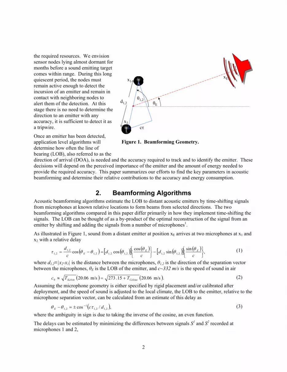
the required resources. We envision sensor nodes lying almost dormant for months before a sound emitting target comes within range. During this long quiescent period, the nodes must remain active enough to detect the incursion of an emitter and remain in contact with neighboring nodes to alert them of the detection. At this stage there is no need to determine the direction to an emitter with any accuracy, it is sufficient to detect it as a tripwire.

Once an emitter has been detected, application level algorithms will determine how often the line of bearing (LOB), also referred to as the direction of arrival (DOA), is needed and the accuracy required to track and to identify the emitter. These decisions will depend on the perceived importance of the emitter and the amount of energy needed to provide the required accuracy. This paper summarizes our efforts to find the key parameters in acoustic beamforming and determine their relative contributions to the accuracy and energy consumption.

2. Beamforming Algorithms Acoustic beamforming algorithms estimate the LOB to distant acoustic emitters by time-shifting signals from microphones at known relative locations to form beams from selected directions. The two beamforming algorithms compared in this paper differ primarily in how they implement time-shifting the signals. The LOB can be thought of as a by-product of the optimal reconstruction of the signal from an emitter by shifting and adding the signals from a number of microphones1.

As illustrated in Figure 1, sound from a distant emitter at position xE arrives at two microphones at x1 and x2 with a relative delay

( ) ( )[ ] ( ) ( )[ ] ( ),

sinsin

coscoscos 2,12,12,12,12,1

2,12,1

−

=−=

cd

cd

cd EE

Eθ

θθ

θθθτ (1)

where d1,2≡|x2-x1| is the distance between the microphones, θ1,2 is the direction of the separation vector between the microphones, θE is the LOB of the emitter, and c~332 m/s is the speed of sound in air

( ) ( ).m/s 20.0615.273m/s 20.060 CelsiusKelvin TTc +=≈ (2) Assuming the microphone geometry is either specified by rigid placement and/or calibrated after deployment, and the speed of sound is adjusted to the local climate, the LOB to the emitter, relative to the microphone separation vector, can be calculated from an estimate of this delay as

( ),/cos 2,12,11

2,1 dcE τθθ −±=− (3) where the ambiguity in sign is due to taking the inverse of the cosine, an even function.

The delays can be estimated by minimizing the differences between signals S1 and S2 recorded at microphones 1 and 2,

θE

θ1,2

x2

xE

cτ

x1

d1,2

Figure 1. Beamforming Geometry.

3

( ) ( ),2,121 τα −= tStS (4)

where α is the relative gain between the two signals. The search for the best delay is limited by (1) to |τ1,2| < d1,2/c. Once the shift has been determined, the signals from the microphones can be shifted and added to provide an enhanced estimate of the signal from the emitter. The background noise and sounds from other emitters will be reduced in proportion to the number of microphones.

Methods for determining the LOB based on reconstructing the emitted signal, as in (4), from an acoustic array with M microphones can distinguish at most M-1 emitters. The additional uncertainty of the position of the emitters results in an underdetermined system of linear equations if we try to resolve M emitters. Resolving more emitters would require additional constraints such as knowing the power-spectrum of the emitters. Algorithms, such as MUSIC2 and ESPRIT3, which do not attempt to reconstruct the emitted signals can resolve, at most, M emitters from an array of M microphones. These algorithms perform eigenvector decomposition of the MxM covariance matrix of the signals from the M microphones and so do not lend themselves to efficient implementation in integer-math oriented processors in sensor nodes.

Beamforming is accomplished by time-shifting the signals from an array of microphones to a common position with time delays prescribed by (1), for an assumed LOB. Beams are formed for a number of LOB search angles. As the search angle approaches the correct LOB of the emitter, the signals constructively interfere as in (4). As shown in Figure 2, the search angle with the maximum power in the delay-summed signal is selected as the estimated LOB. This LOB estimate is refined by parabolic interpolation of the power over the adjacent search angles.

The two algorithms compared in this paper differ primarily in how they shift the signals. The baseline algorithm from ARL performs a floating-point FFT on each signal then shifts, sums, and computes the beam power in the Fourier domain. Our beamformer performs all of these operations in the time domain in integer math.

Our beamformer assumes a single target and employs common integer code to report the LOB as the direction with the delay-summed combined signal of loudest total acoustic energy. These results do not include code for false alarm rejection such as ARL’s Harmonic Line Analysis. We plan to incorporate these capabilities into future implementations.

Our algorithm is roughly 300x more efficient in the consumption of energy by the CPU than the baseline. The largest contribution to this efficiency (~20x) is due to floating-point emulation on the StrongARM processor. The next most significant contribution (~10x) is our ability to use fewer samples to achieve similar accuracy. Fast Fourier transforms operate on vectors containing integer powers of 2 samples (S=2n). We did not modify the baseline algorithm to vary the number of samples from its hard-coded value of S=1024. Operating in the time domain provided the final contribution of (~3/2x,) by not Fourier transforming the signals.

Figure 2. Power of delay-summed at 18 search angles.

4

3. LOB Beyond Beamforming

The algorithms discussed in this section are under development and optimization for sensor nodes. We anticipate that these will lead to significant improvements over beamforming in accuracy/noise insensitivity, false-alarm rejection, and an extended range in tradeoffs between accuracy and energy.

Beamforming makes a number of limiting assumptions 1) that the microphones are fixed on a rigid plane, 2) that the emitter lies on the same plane, and 3) that there is little or no wind. While beamforming uses (1) to construct a set of delays corresponding to various search angles and selects the “best” angle, the LOB can also be estimated directly from (1) based on estimates of the time shifts between pairs of microphones. Given a set of M>2 microphones with synchronized sampling, we can select up to M! / [2 (M-2)!] pairs. For example, three microphones provide three pairs. Assuming that the geometry of the M microphones has been calibrated, (1) provides a system of M! / [2 (M-2)!] equations in two unknowns, the sine and cosine of the LOB divided by the speed of sound. For more than two pairs, the over-determined system of equations can be solved by standard weighted least-squares methods. Increasing the number of microphones and pairs should improve the accuracy.

The LOB and the speed of sound can be extracted from the results in integer math with the CORDIC4 as

( ) ( ),

sin,

costan 1

= −

ccEE

Eθθ

θ (5)

and

( ) ( ).

sincos

122

+

=

cc

cEE θθ

(6)

Although, it may appear that the speed of sound should be constrained to the constant predicted in (2) there are cases in which the apparent speed of sound can vary. When noise results in nonphysical estimates of the apparent speed of sound, the LOB estimated in (5) can be iteratively refined based on small angle corrections with the speed of sound held to the predicted constant in (1) as

( ){ } ( ){ }.cossin 2,12,12,12,12,1 θθτδθθθ −−=− EEE dcd (7) The RMS error of the system of equations defined by (7), or (1), provides a measure of the angular uncertainty of the LOB estimate. If some pairs of microphones produce multiple delays due to multiple targets, this error and the apparent speed of sound provided by (6) could be used to select delays into sets for each target.

Figure 3 shows a plot of this uncertainty for a tracked vehicle driving around an oval track. The vehicle is about 600 meters from the sensor node at an LOB of 280° counterclockwise from east (roughly south). This is based on acoustic data collected by USC-ISI at ARL’s Aberdeen Proving grounds with HiDRA nodes, described in section 5, using with three microphones deployed on an equilateral triangle with 7-foot separation.

0

0.5

1

1.5

2

2.5

3

0 60 120 180 240 300 360LOB (degrees) counterclockwise from east

LOB

Unce

rtant

y (d

egre

es)

Figure 3. Uncertainty in LOB of tracked vehicle.

5

3.1. Emitter Elevation If the emitter is elevated above the plane on which the microphones are distributed, as shown in Figure 4, this decreases the delays between signals and increases the apparent speed of sound estimated by (6) as

( ) ,cos

0

E

ccφ

= (8)

where φE is the elevation angle of the emitter. As the emitter moves directly above the microphones, the apparent speed would tend toward infinity as all of the time shifts approach zero. The elevation angle of the emitter could be estimated by generalizing our analysis to 3D and elevating one or more microphones above a plane containing three or more microphones5. If we can segregate the contribution due to elevation from other effects, such as wind, by collaboration between sensor nodes, each with three or more microphones, we could estimate the elevation angle from (8).

3.2. Wind-Speed Vector Effects As illustrated in Figure 5, the average wind speed W between the emitter and the microphones will add as a vector to the sound radiating from the emitter at speed c0 resulting in an apparent speed of sound of

( ) ( ),sincos 2220 WEWE WWcc θθθθ −+−+= (9)

where θW is the direction that the wind is coming from. The estimated LOB would also be shifted by

( ) ( )[ ].sin,costan 01

WEWEE WWc θθθθδθ −−+= − (10) Assuming that the wind speed is small compared to that of sound (W<<c0,) we can approximate

( ) ( ) ( ) ( ){ } ( ) ( ){ } ,sinsincoscoscos~0 WEWEWE WWWcc θθθθθθ +=−− (11) and

( ) ( ).tan~ 0WEE c

ccθθδθ −

− (12)

A wind speed of 14 mph orthogonal to the LOB would result in an LOB error of about 1 degree.

The difference of apparent from expected sound speed is plotted in Figure 6 for a tracked vehicle driven on an oval track around the sensor node for a number of orbits. These preliminary estimates of the apparent sound speed are based on delays of maximum correlation (15), described in the next section.

φE

c0

Figure 4. Elevation angle of emitter.

W

c

c0

Figure 5. Wind speed geometry.

6

These estimates are compared to the expected deviation based on (11) for a wind speed of 30 mph. This is somewhat larger than the 10-mph average wind speed measured during data collection. The wind direction, taken from the ground truth, agrees well with the estimated deviations in sound speed.

Given an estimate of the wind direction, we can estimate and correct the offset in the LOB from (12) based on the apparent speed of sound, if we can assume that there are no other contributions such as elevation of the emitter above the sensor plane.

If we combine the apparent sound speed and estimated LOB from two or more sensor nodes with enough separation transverse to the LOB of the emitter such that they provide significantly different estimated LOBs, and assume that the wind is roughly the same for all sensor nodes, we can solve the resulting system of linear equations given by (11) for the wind vector components. The wind direction can be computed using the CORDIC algorithm as

( ) ( )[ ],sin,costan 1WWW WW θθθ −= (13)

and the result can be used in (12) to infer the offset of the LOB’s due to the wind.

The LOB and apparent speed of sound from three or more nodes can be combined to solve for the wind and elevation simultaneously by combining (8) and (11) as

( ) ( ) ( ){ } ( ) ( ){ }.sinsincoscoscos

~ 0WEWE

E

WWc

c θθθθϕ

++

(14)

This assumes that all of the nodes have the same emitter elevation, which could be satisfied if all of the nodes are at the same elevation and roughly the same distance from the emitter. We would have to constrain the added unknown such that the inferred cosine is in the assumed range (0, 1) and would interpret the elevation angle to be positive, forcing the object to lie above the sensor plane.

3.3. Signal-Pair Delay Estimation All of this analysis is based on the ability to estimate the delay between signals collected by a pair of microphones. One estimate of the delays can be obtained by finding the shift between the signals that produces a peak in correlation between the signals from microphone 1 (S1) and 2 (S2)

( ) ( ) ( )∑ −=t

tStSC .2,121

2,12,1 ττ (15)

This estimate is best suited to emissions of short duration, such as gunfire or explosions, and is sufficient for cases with high signal to noise and broad band signals.

0 32 64 96 128 160 192 224 256Freq (Hz)

Figure 7. Power spectrum of tracked vehicle.

-100-80-60-40-20

020406080

100

0 60 120 180 240 300 360LOB (degrees)

Air S

peed

- So

und

(mph

)

Figure 6. Deviation of sound speed vs. angle.

7

Much of the recent work in noise-tolerant LOB estimates are based on the fact that many targets of interest, such as ground and air vehicles, emit sound in a number of narrow acoustic bands6, as shown by the acoustic power spectrum of a tracked vehicle shown in Figure 7. If multiple targets emit primarily in different narrow frequency ranges, their LOBs could be determined by a single sensor node with as few as three microphones.

The LOB of frequencies from 32 to 128 Hz is plotted in Figure 8 for a sensor node with three microphones and two tracked vehicles. The average power spectrum of the three microphones is also plotted. The LOBs cluster around 240° and 77° corresponding to the two vehicles. The LOB is plotted as zero for frequencies where it is undefined. Once the LOBs of the two vehicles are estimated, it is straight forward to separate their line-spectra as a basis for target classification.

For each spectral component, the LOB of is based on time shifts of microphone pairs estimated as

( ) ( )[ ] ( )[ ]{ } ,221

2,1 ωπωϕωϕωτ nSS +−

= (16)

where the phase of the Fourier component of the signal φ[S1(ω)] can be computed with the CORDIC algorithm and the time shift is limited to the range [-d1,2/c, d1,2/c]. For higher frequencies (f>c/(2d1,2)), there can be more than one solution to (16). This degeneracy can be resolved by selecting the solution that is most consistent with lower frequency components or is most consistent with the expected speed of sound and error of fit based on the solution to (1). This ambiguity can be avoided by restricting microphone separations to d<c/(2f), where f is the highest frequency of interest in the emitters spectrum.

Our current implementation of the acoustic beamformer operates in the time rather than the frequency domain in order to provide a marginal (3/2x) increase in power efficiency. By using an integer FFT we could achieve comparable efficiency and add an adjustable parameter corresponding to the sampling rate of the acoustic data. Although the sampling rate of the digitizer will probably be fixed at ~1024 Hz, the captured signal can be downsampled to provide significant reductions in energy requirements with little effect on the accuracy of the LOB.

4. Algorithmic “Knobs” The accuracy and energy requirements of acoustic beamforming depend on a number of parameters, as suggested by Figure 9. Some are largely dictated by the application. We have chosen as our set of independent variables: 1) number of microphones M, 2) number of acoustic samples S, 3) number of beams B, and 4) CPU clock speed fCPU.

4.1. Number of Microphones (M) The number and placement of microphones is principally a hardware design parameter but can also be used as an algorithmic parameter by selecting a subset of the signals collected. We will show that the

0

60

120

180

240

300

360

32 48 64 80 96 112 128Freq (Hz)

LOB

(deg

rees

)

0

Pow

er S

pect

rum

Figure 8. LOB of spectral components.

8

system energy required for beamforming is proportional to the number of microphones, but there are negligible improvements in accuracy due to adding more microphones at the same radius.

We limit our analysis to nodes supporting at least two microphones. Although single-microphone nodes could collaborate to determine the direction to an emitter, we exclude this case due to the requirements of a large amount of energy to move raw data between nodes, of 10-us synchronization between nodes, and of 5-mm accuracy in relative positioning of microphones. Although the ambiguities resulting from two-microphone beamforming would require collaboration, only a trivial amount of data need be exchanged. Synchronization to a fraction of a second is sufficient, and the required accuracy of relative positioning is similarly relaxed.

4.2. Number of Acoustic Samples (S) For a fixed sampling rate, in our case 1024 Hz, the system energy required for beamforming is proportional to the number of samples simultaneously collected from each microphone. The number of samples collected per second for each microphone is typically selected to be 1 kHz for acoustic tracking of vehicles to facilitate beamforming with the spectrum above 250 Hz attenuated to filter out wind noise. We implemented this as analog anti-aliasing filtering.

4.3. Number of Beams (B) The beam power is computed at a number of evenly spaced search angles, and interpolated by a parabolic fit to estimate the angle with maximum power. The number of beams only affects the execution speed of the algorithm, not data acquisition. The system energy for beamforming is linear with, not proportional to, the number of beams searched.

4.4. CPU Clock Speed (fCPU) The Highly Deployable Remote Access Network Sensors & Systems (HiDRA) provided by Rockwell Science Center (RSC)7,8,9, supports software-control of the clock speed of the StrongARM CPU over the range 59-133 MHz. Unfortunately, voltage scaling is not supported in this hardware. Without voltage scaling, clock scaling may appear to only change how long the algorithms run without changing the energy requirements. However, the power consumed by other components in the system during execution of the algorithm and the power consumed by the CPU during data collection give this parameter utility in reducing system energy required for beamforming.

5. System Power Equation The energy consumed by the HiDRA node to capture data and compute the LOB is modeled by

,133

lg133

+

++= CPU

CPUOvrA

CPUSAD

S

Pff

PTff

fSP

fSE (17)

B E A M F O R M I N G

Line of Bearing360

180

Num. Mikes

Num. Samples

76

2

4 5M

8

12

18 90

1024

512

32

64

128 256

Search Angles

SEW

N

LOB Confidence

3 B2° 3° 4° 5°

PA/DTA/D+(TA/D+TAlg)(PCPU+POverhead)=0.724Joules

S

Figure 9. Beamforming Algorithmic Knobs.

9

where fCPU is the clock rate of the StrongARM CPU and f133 = 133 MHz is the maximum clock rate.

This equation reflects that the power required by the A/D board, PAD, is only consumed during the data acquisition time which is the number of samples acquired, S, divided by the sampling rate fS=1024 Hz. Also implicit in this equation is that, for the HiDRA node, the CPU and memory consume power, PCPU, while the samples are acquired, but the algorithm does not begin to run, for a period TAlg, until after data collection is complete. There is also a significant overhead power, POvr, consumed by other supporting components such as the radio.

The CPU power and execution time of the algorithm are proportional and inversely proportional, respectively, to the CPU clock rate, fCPU. The clock rate resulting in the minimal energy consumption can be found by setting the derivative of (17) with respect to fCPU to zero, resulting in

,/lg133 CPUADAOvrCPU PTTPff = (18)

where TAlg is the execution time of the algorithm and PCPU is the CPU power at the CPU clock rate of 133 MHz.

When the CPU and overhead power components are roughly equal and the execution time of the algorithm at 133 MHz is a small fraction of the sampling window, as with our algorithm, the minimum available CPU clock rate of 59 MHz provides the best energy efficiency. When the algorithm runs longer than the sampling window, as with the ARL algorithm, the maximum available CPU clock rate of 133 MHz gives the best results.

6. Power Measurements on the HiDRA Node The power measurement test setup consisted of the HiDRA sensor node and a current sensing resistor placed inline with the input voltage connector. The voltage drop across this resistor was measured using a National Instruments PCI-MIO-16E-1 data acquisition card and triggered from GPIO lines on the node's processor module. The HiDRA node, as shown in Figure 10, contains the following modules:

1) Processor/Memory: SA1100 processor board running eCos at 59-133 MHz., with 4 MB of ROM (flash memory), 1 MB RAM, input voltage 3.3V I/O, and 1.5V core.

2) DC/DC: input voltage from 2 9-V batteries or DC adapter. Our test measurements were taken with a 12-V DC input. This module supplies voltages 3.3V and 1.5V for the I/O lines and processor core respectively and separate analog voltage lines for the A/D and Radio modules.

3) Radio: A 900 MHz Rockwell proprietary radio.

4) A/D: 5 channels, 3 Multiplexed with variable gains of 1x, 2x, 5.02x, 10.09x, 20.12x and 2 individual inputs with variable gains of 10x, 43.32x, 30x, 36.68x, 49.98x. The selectable gains are tuned to specific sensors that RSC uses for this platform. The acoustic data was captured using only the multiplexed sensor input to keep the gains equivalent across all channels. Low-pass anti-aliasing filters with a cutoff

Figure 10. RSC HiDRA sensor node stack.

10

frequency of 3 kHz were also added to the inputs of each of these channels to eliminate cross talk between the respective channels.

The current measurements were taken at the full clock rate of 133 MHz, which is the optimal operating frequency for the HiDRA node, and at various increments down to 59 MHz. Other power measurements were taken for the different operating modes required to form a single LOB. These modes include acquiring the data from the input microphones, executing the algorithms, and putting the processor in sleep mode. The individual power consumption of each module was measured by removing boards from the stack and calculating the difference in current through the sensing resistor.

7. Results We evaluated the two algorithms on a test set of acoustic data collected by ARL collected at their Aberdeen Proving Grounds. The data was synchronously collected from six microphones uniformly distributed on a 4-foot radius circle, and a seventh microphone in the center. A single military vehicle was driven by this acoustic array with GPS to provide ground-truth position at 1-second intervals. The signals were collected continuously on a seven-channel digitizer at 12-bits per channel at 1024 samples per second.

For our tests, we broke the acoustic data up into 1-second records associated with the available position ground truth. For each 1-second record, we computed the LOB with both algorithms and measured their errors relative to the ground truth. The results presented are of the Root-Mean-Square of these errors over all of the records in the set.

In addition to validating that our algorithm provided results statistically identical to those of the baseline, we investigated the effect of the various knobs on the accuracy of both algorithms.

As illustrated in Figure 11, increasing the number of microphones on a circle above the minimum of three provides little, if any, improvement in the accuracy of the LOB estimate. Doubling the number of microphones from 3 to 6 reduces the RMS error only by 12% for this single emitter.From the errors plotted in Figure 12, we can see that 32 is the minimum number of samples for which the algorithms can

Figure 11. Beamforming errors of algorithms for 1024 samples, 20 beams, and selected subsets of the seven microphones.

1

1.2

1.4

1.6

1.8

2

2.2

3 4 5 6 7Number of Microphones

RM

S E

rr (d

egre

es)

ARL

ISI

1

2

3

32 64 96 128 160 192 224 256Number of Samples

RM

S Er

ror (

degr

ees)

ISI

ARL

Figure 12. Beamforming errors of algorithms for seven microphones and 20 beams vs. number of samples used.

11

provide a useful result. However, using more than 128 samples provides only modest improvements in accuracy.

As shown in Figure 13, the error grows rapidly for fewer than eight beams, but improves only slightly for more than sixteen beams. These results depend on the dominant frequency of the acoustic spectra emitted by the target and the “knee” of the curve is likely to shift for other vehicles.

We optimized the execution time of our code using the web-based JouleTrack10 emulator before porting it to the HiDRA. Although

JouleTrack did not provide identical results to what we measured directly from the hardware, it was useful guide in modifying the code to reduce execution time and energy use.

We electronically measured the power consumed by each component of the node during various modes of operation and we measured the execution time of the two algorithms at the maximum and minimum clock rates, as shown in Figure 14. The results of these measurements are summarized in Table 1.

Assuming three microphones (M=3), twelve beams (B=12), and a full second of data (S=1024), applying the values in this table to (17) results in a total system energy of 1614 mJ for the baseline algorithm and 746 mJ for the ISI algorithm, as shown in Figure 15. Despite a 250x reduction in execution time for the same clock rate, our algorithm results in a modest 2x reduction in overall system energy required to acquire the data and process it to produce a single LOB.

Under similar conditions, but with only 0.125 sec sampling window (S=128), the system energy for the baseline would be 816 mJ and the system energy for the ISI algorithm

2

3

4

5

6 10 14 18 22Number of Beams

RM

S Er

r (de

gree

s)

ISI

ARL

0

500

1000

1500

2000

2500

ARL -133MHz

ISI - 133MHz

ARL - 59MHz

ISI - 59MHz

Beamforming Algorithms

Tota

l Sys

tem

Ene

rgy

(mJ)

Algorithm Energy (mJ):Processor/Memory On, A/D On, Radio On

Data Acquisition (1024Samples/Sec) Energy (mJ):Processor/Memory On, A/D On, Radio On

Figure 15. Acquisition/Proc. Energy to Compute a LOB.

Figure 13. Beamforming errors for 64 samples and seven microphones vs. number of beams.

0

200

400

600

800

1000

ARL - 133MHz

ISI - 133MHz

ARL - 59MHz

ISI - 59MHz

Beamforming Algorithms

Pow

er (m

W)

Data Acquisition:Processor Active/ADPower On, AcquiringData/Radio Power On(mW)Compute Bearing:Processor On/AD PowerOn/Radio Power On (mW)

Compute Bearing:Processor On/ADRemoved/Radio Removed(mW)

Processor Sleep/ADPower On/Radio Power On (mW)

Processor Sleep/ADPower On/Radio Removed(mW)

Figure 14. Power Consumption of Various Node Modes.

12

would be 93 mJ. Our algorithm would provide a 9x reduction in system energy over the baseline algorithm under these conditions.

Table 1. Power Measurements for the HiDRA node.

POvr mW PAD mW fCPU MHz PCPU fCPU/f133 mW TAlg f133/fCPU µs ISI 274 252 59 132 M B S 0.0555

ARL 358 252 133 302 M B 14300

8. Conclusions We have demonstrated the ability to perform acoustic beamforming over a range of accuracy requiring a corresponding range of energy by introducing a number of “knobs” into the basic algorithm. This analysis led us to develop an algorithm that is roughly 300x more efficient than the baseline in CPU energy. More importantly, our algorithm provides 9x overall system energy savings when LOB estimates of lower accuracy are sufficient.

We found that adjusting the number of microphones M offered the largest improvements to energy efficiency with the least impact on accuracy of the LOB. However, this parameter can only be effectively adjusted during the design of the sensor node. It is difficult to construct a board capable of collecting a large number of synchronized signals but only capture a selected subset without paying much of the power penalty of sampling all of the signals. We determined that three microphones are the minimum required to perform beamforming without collaboration with other nodes.

The number of samples collected, S, for each microphone offers comparable improvements to system energy efficiency with slightly larger impact on accuracy. However, this parameter can be adjusted over a wide range, 32-1024, resulting in a 16x range of system energy requirements. The memory requirements of future nodes could be reduced by reducing the sampling window and by using our integer algorithm rather than the floating-point baseline.

The number of beams formed in the software, B, only modulates the algorithm execution time which is only a fraction of the sampling window. So this parameter has only a minor effect on the energy efficiency of the whole system.

The clock speed of a CPU, fCPU, typically has a limited range of values, in the case of the HiDRA node 59-133 MHz. We have shown that a faster than real-time algorithm will be most efficient at the lowest available clock speed. This will be even more the case for more power-aware sensor nodes being designed that will be capable of voltage scaling and of computing the algorithm during data collection.

9. Future Work We plan to apply what we have learned from the HiDRA node to developing a more power-aware sensor node under the PASTA contract at USC-ISI funded by DARPA. The PASTA architecture will represent a different approach to a sensor node design. Instead of a processor-centric design, where the main CPU controls all functionality of each module in the stack, the modules will act as independent units in a microcontroller network. Each module will have a low power 8051 based microcontroller operating over an I2C control network operating at 100 kbs. This controller will provide the main communication between modules for power control and module to module communication. There will also be a higher speed data channel between modules for transmissions that require higher data rates. This network will allow each module to perform its required task and, when it is not needed, it will either shutdown or go into a low power sleep condition. Modules that have a higher quiescent-current consumption in their idle

13

modes can be removed from the overall power budget if they are not need to perform a required task. An example would be performing data acquisition and computation on a low-power DSP and then sending the results to a radio module over the microcontroller network. The main processor will not be used in this mode and thus will either be turned off or put in a sleep cycle.

Each micro-sensor will have interchangeable hardware with mission specific processing modules, distributed power monitoring, voltage scaling, and sleep management. It will also incorporate techniques and technologies developed under the PAC/C Phase I program (PADS) to include deep-submicron techniques to reduce idle-mode power leakage in digital circuits with minimal or no degradation in performance.

We have collected three-channel raw acoustic data with the HiDRA nodes and we have ported the beamforming codes to these and a variety of sensor nodes. During our next data collect, we plan to have the beamforming code providing realtime LOB results on sensor nodes in the field. The sensor nodes fielded with live acoustic beamforming may include HiDRA, PASTA, and the prototype fabric beamformer11 shown in Figure 16, developed by USC-ISI and Virginia Tech. under the STRETCH e-textile effort funded by DARPA.

10. References 1 D. K. Campbell, Adaptive Beamforming Using a Microphone Array for Hands-Free Telephony. Masters Thesis, Virginia Polytechnic Institute and State University, 1999. Available: http://scholar.lib.vt.edu/theses/available/etd-022099-122645/ 2 R. Schmidt, “Multiple emitter location and signal parameter estimation,” IEEE Trans. Antennas Propagat., vol. AP-34, pp. 276–280, 1986. 3 R. Roy and T. Kailath: “ESPRIT—Estimation of Signal Parameters via Rotational Invariance Techniques,” IEEE Trans. Accoust. Speech and Signal Proc., vol. 37, no. 7, pp.984–995, July 1989. 4 Ray Andraka, “A survey of CORDIC algorithms for FPGAs (121K),”FPGA '98. Proceedings of the 1998 ACM/SIGDA sixth international symposium on Field programmable gate arrays, Feb. 22-24, 1998, Monterey, CA. pp191-200. Available: http://www.fpga-guru.com/cordic.htm 5 M. Walworth and A. Mahajan, “3D Position Sensing Using The Difference In The Time-Of-Flights From A Wave Source To Various Receivers,” ICAR ’97, Monterey, Ca, July 1997. 6 Tien Pham; Sadler, B.M., “Adaptive wideband aeroacoustic array processing,” Statistical Signal and Array Processing, 1996. Proceedings., 8th IEEE Signal Processing Workshop on (Cat. No.96TB10004 , 1996 Page(s): 295 -298. Available: http://eewww.eng.ohio-state.edu/~randy/Microphone_Reading_List/index.html

Figure 16. Fabric Beamformer.

14

7 J. Agre, L. Clare, G. Pottie and N. Romanov, "Development Platform for Self-Organizing Wireless Sensor Networks," Proceedings of the SPIE Conference on Unattended Ground Sensor Technologies and Applications, Orlando, FL, April, 1999, SPIE Vol. 3713, pp. 257-268. 8 “Highly Deployable Remote Access Network Sensors & Systems”, Rockwell Science Center. Available: http://www.rsc.rockwell.com/hidra 9 J. Montague and Control Engineering staff, “Progressive Innovations”, Control Engineering, March 1, 2002. Available: http://www.controleng.com/ 10 A. Sinha and A. Chandrakasan. “JouleTrack - A Web Based Tool For Software Energy Profiling.” Proc. 38th Design Automation Conference, June 2001. Available: http://dry-martini.mit.edu/JouleTrack/ 11 Edmison, J., Jones, M., Nakad, Z., and Martin, T. “Using Piezoelectric Materials for Wearable Electronic Textiles,” Proceedings of the Sixth International Symposium on Wearable Computers, Oct. 2002, to appear.