Pre-conditioned backward Monte Carlo solutions to radiative

A&A 573, A72 (2015)DOI: 10.1051/0004-6361/201424042c© ESO 2014

Astronomy&

Astrophysics

Pre-conditioned backward Monte Carlo solutions to radiativetransport in planetary atmospheres

Fundamentals: Sampling of propagation directions in polarising media�

A. García Muñoz1 and F. P. Mills2,3

1 ESA Fellow, ESA/RSSD, ESTEC, 2201 AZ Noordwijk, The Netherlandse-mail: [email protected]

2 Research School of Physics and Engineering and Fenner School of Environment and Society, Australian National University,ACT 0200 Canberra, Australiae-mail: [email protected]

3 Space Science Institute, Boulder, CO 80301, USA

Received 21 April 2014 / Accepted 15 August 2014

ABSTRACT

Context. The interpretation of polarised radiation emerging from a planetary atmosphere must rely on solutions to the vector radiativetransport equation (VRTE). Monte Carlo integration of the VRTE is a valuable approach for its flexible treatment of complex viewingand/or illumination geometries, and it can intuitively incorporate elaborate physics.Aims. We present a novel pre-conditioned backward Monte Carlo (PBMC) algorithm for solving the VRTE and apply it to planetaryatmospheres irradiated from above. As classical BMC methods, our PBMC algorithm builds the solution by simulating the photontrajectories from the detector towards the radiation source, i.e. in the reverse order of the actual photon displacements.Methods. We show that the neglect of polarisation in the sampling of photon propagation directions in classical BMC algorithmsleads to unstable and biased solutions for conservative, optically-thick, strongly polarising media such as Rayleigh atmospheres. Thenumerical difficulty is avoided by pre-conditioning the scattering matrix with information from the scattering matrices of prior (in theBMC integration order) photon collisions. Pre-conditioning introduces a sense of history in the photon polarisation states through thesimulated trajectories.Results. The PBMC algorithm is robust, and its accuracy is extensively demonstrated via comparisons with examples drawn from theliterature for scattering in diverse media. Since the convergence rate for MC integration is independent of the integral’s dimension, thescheme is a valuable option for estimating the disk-integrated signal of stellar radiation reflected from planets. Such a tool is relevantin the prospective investigation of exoplanetary phase curves. We lay out two frameworks for disk integration and, as an application,explore the impact of atmospheric stratification on planetary phase curves for large star-planet-observer phase angles. By construction,backward integration provides a better control than forward integration over the planet region contributing to the solution, and thispresents a clear advantage when estimating the disk-integrated signal at moderate and large phase angles.

Key words. polarization – radiative transfer

1. Introduction

The gases and aerosols that make up a planetary atmosphereleave characteristic signatures on the radiation emitted and/orreflected from the planet. The technique of polarimetry utilisesthe polarisation state of emergent radiation to investigate theplanet’s atmospheric optical properties. Polarimetry is rele-vant in the remote sensing of planetary atmospheres both as astand-alone technique and in combination with photometry. Inthe solar system, polarimetric observations made from space-borne and ground-based telescopes have yielded insight into thegas and aerosol envelopes of Earth (Dollfus 1957; Hansen &Travis 1974), Venus (Coffeen 1969; Hansen & Hovenier 1974),Mars (Santer et al. 1985), Jupiter and Saturn (Morozhenko &Yanovitskii 1973; Schmid et al. 2011; West et al. 1983), Titan(Veverka 1973; West & Smith 1991), and Neptune and Uranus

� A one-slab, plane-parallel version of the PBMC algorithm isavailable at the CDS via anonymous ftp to cdsarc.u-strasbg.fr(130.79.128.5) or viahttp://cdsarc.u-strasbg.fr/viz-bin/qcat?J/A+A/573/A72

(Joos & Schmid 2007; Michalsky & Stokes 1977; Schmid et al.2006).

Various spacecraft for Earth (ADEOS I and II, PARASOL)and solar system exploration (e.g. Voyager, Galileo, Cassini)carried instrumentation with (limited) polarimetric capabilities.Most modern ground-based observatories are equipped with po-larimeters for either spectroscopy or imaging. Ground-basedobservations of the outer planets, however, only have partialcoverage of the Sun-target-Earth phase angle, which limits thepossible physical insight from polarimetric investigations. Forthe above reasons, it is generally agreed that polarimetry’s po-tential for characterising the atmospheres of Earth and the rest ofthe solar system planets remains underexploited. Interestingly,the discovery of planets orbiting stars other than our Sun hascaused a renewed interest in polarimetry both as a detection anda characterisation technique. The key idea behind this new in-terest is that stars are typically unpolarised or weakly polarised,whereas planets may be partially polarised, which presents anadvantage for separating the planet from the glare of its host star(e.g. Seager et al. 2000; Stam et al. 2004).

Article published by EDP Sciences A72, page 1 of 20

http://dx.doi.org/10.1051/0004-6361/201424042

http://www.aanda.org

http://cdsarc.u-strasbg.fr

ftp://130.79.128.5

http://cdsarc.u-strasbg.fr/viz-bin/qcat?J/A+A/573/A72

http://www.edpsciences.org

A&A 573, A72 (2015)

The new born field of exoplanet research is promptingsignificant effort in the development of polarimetric facilities,as demonstrated by proposed space missions such as ESA’sSPICES (Boccaletti et al. 2012), dedicated instrumentation forGemini (Macintosh et al. 2006), or ESO’s Very Large Telescopeand European-Extremely Large Telescope (Beuzit et al. 2008;Kasper et al. 2008). Correspondingly, on the theoretical front,there has been work to investigate polarimetry’s potential foridentifying planets’ orbital parameters, as well as for character-ising their main atmospheric and surface features (e.g. Bailey2007; Fluri & Berdyugina 2010; Seager et al. 2000; Stamand collaborators 2004, 2008, but also Karalidi & Stam 2012,Karalidi et al., 2011, 2012, 2013; Williams & Gaidos 2008;Zugger et al. 2010, 2011). Since the number of exoplanets al-ready surpasses the number of solar system planets, theoreti-cal investigations that explore gas, cloud, and surface properties,possibly in the framework of a new generation of general circu-lation models, will continue to play a key role in the predictionand prospective characterisation of exoplanetary observables.

This paper is devoted to numerical modelling of radiationscattered by planetary atmospheres. Our approach relies onbackward Monte Carlo (BMC) integration of the vector radiativetransport equation (VRTE). Special attention is paid to the sam-pling of propagation directions in polarising media. We showthat in classical BMC integration, failing to account for polari-sation in the sampling of propagation directions may destabiliseand bias the numerical solution in conservative, optically thick,strongly polarising media. We propose a pre-conditioned BMC(PBMC) algorithm and show that pre-conditioning the scatter-ing matrix with information from prior collisions (in the order ofbackward integration) eliminates the numerical difficulties. Pre-conditioning is equivalent to providing information about thehistory and polarisation state of photons through their simulatedtrajectories. We describe in detail the algorithm and its perfor-mance. Because it consistently delivers precisions of 10−4 whencompared to solutions that are accurate to at least that level,the algorithm may be considered “exact” (in the de Haan et al.1987 sense) or nearly so. This paper is part of an ongoing effortto build a tool for efficiently simulating the radiation emergingfrom both disk-resolved and disk-integrated realistic planetaryatmospheres. In its scalar form, the algorithm has already beenused without description (García Muñoz & Pallé 2011; GarcíaMuñoz & Mills 2012; García Muñoz et al. 2011, 2012, 2014).The cases investigated here focus on Rayleigh and Mie scatter-ing, for which the scattering matrix is easy to obtain. The theoryis more general than that and should also apply to scattering par-ticles with different scattering matrices.

The paper is structured as follows. In Sect. 2, we note someof the differences between forward and backward integration.BMC algorithms are very selective with the planet regions thatthey probe, and this is a clear advantage, for instance, when pro-ducing the disk-integrated signal from a planet at a specifiedphase angle. We review the fundamentals of BMC algorithmsand discuss the sampling of photon propagation directions inclassical BMC algorithms and in our PBMC approach. We alsopresent two different schemes for integrating the net radiationreflected from a spherical-shell planet. In Sect. 3, we assessthe performance of the classical and pre-conditioned algorithmswith test cases for plane parallel configurations. In Sect. 4, wepredict a number of planetary phase curves. The extensive suiteof test cases considered will hopefully help guide the decisionof potential users of the PBMC algorithm. Finally, in Sect. 5we summarise the main conclusions and comment on follow-upwork.

2. The BMC algorithm

MC algorithms for radiative transport fall within the generalclass of Markov chain methods for the statistical simulation ofphoton collisions in scattering media (Cashwell & Everett 1959;Marchuk et al. 1980). By using appropriate statistical estimators,MC algorithms can estimate the radiation within and emergingfrom a medium.

MC algorithms are classified as forward or backward (FMCand BMC, respectively), depending on whether the solution isbuilt by simulating the photon trajectories from the radiationsource towards the observer or vice versa. FMC algorithms eas-ily account for the photon’s polarisation state in the samplingof the photon propagation direction following a collision (e.g.Bartel & Hielscher 2000; Bianchi et al. 1996; Cornet et al. 2010;Fischer et al. 1994; Hopcraft et al. 2000; Kastner 1966; Schmid1992; Whitney 2011). That is not immediately possible in BMCalgorithms because the scattering events are treated in the re-verse order that they actually occur. BMC algorithms generallytreat the sampling of propagation directions by omitting the radi-ation’s polarisation state and correcting subsequently for the biasintroduced (Collins et al. 1972 and works thereafter; e.g. Emdeet al. 2010; Gay et al. 2010; Oikarinen 2001). As shown below,that approach may fail to render accurate solutions in conditionsfor which the scattering directions of the photons are stronglyinfluenced by their polarisation states.

MC algorithms are exact in the sense (de Haan et al. 1987)that their accuracy is in principle only limited by the numberof photon trajectory simulations. Thus, MC algorithms are oftenused as standards in the validation of other methods, particularlyin cases that involve complex viewing and/or illumination ge-ometries (Loughman et al. 2004; Postylyakov 2004).

BMC algorithms are better suited for problems with smalldetectors and large radiation sources, and the opposite is truefor FMC algorithms (Modest 2003). This important distinctionmeans that BMC integration turns out to be the appropriatechoice for numerous applications in investigating planetary at-mospheres. By tracing the photon trajectories from the detectortowards the planet (or towards a part of the planet that is knownto be illuminated), BMC algorithms offer a more efficient ap-proach to achieving the desired accuracy. This is not directlypossible in the FMC framework because there is no previousknowledge about the directions the photons will take to exit themedium. In FMC algorithms, moreover, estimating the emergentradiation typically requires averaging over a range of exiting di-rections. (Alternatively, variance reduction techniques such asthe next-event point-estimator can be utilised, e.g. Kaplan et al.2001 and Lux & Koblinger 1985; their efficiency however isstrongly dependent on the detector’s acceptance angle.) Thesecharacteristics penalise the computational efficiency of FMC al-gorithms, especially when only a specified number of viewinggeometries with narrow acceptance angles are of interest.

Additional properties that make FMC/BMC algorithms ap-pealing in their application to planetary atmospheres include:

– They are easy to implement and debug. Their descriptioncan indeed be accomplished in less than one page (seeAppendix A).

– Implementing the scattering matrix does not require a seriesexpansion of the matrix elements.

– Curvature and twilight effects are naturally accountedfor. Limb-viewing geometries do not require any specialtreatment.

A72, page 2 of 20

A. García Muñoz and F. P. Mills: Backward Monte Carlo modelling of planet polarisation

– It is easy to separate the contributions from the atmosphereand surface, from different atmospheric layers, or from vari-ous orders of scattering.

– Scattering by large particles, which lead to highly asymmet-ric scattering phase functions, can be treated without signifi-cant computational penalty.

– The computational cost for solving the VRTE and its scalarcounterpart are comparable.

– The accuracy of the solution depends on the number of pho-ton trajectory simulations. Moderately accurate solutions canbe obtained at low computational costs.

– In BMC algorithms, each photon collision can be utilised toestimate the contribution to the detector from various inci-dent directions of the illuminating source.

Our implementation of the algorithm follows the basic layout byO’Brien (1992, 1998), which we have extended to include po-larisation. The implementation makes use of variance reductiontechniques, which logically arise from the mathematical elabo-ration of the integrals that occur in the formal solution to theVRTE. O’Brien (1992, 1998) provides an excellent introductionto these ideas, and we follow the nomenclature in those works toa large extent.

2.1. Fundamentals

Our interest lies in the VRTE for a scattering and absorbingmedium without volume or surface emission sources:

s ·∇I(x, s) = −γ(x)I(x, s)+β(x)∫Ω

dΩ(s′)P(x, s, s′)I(x, s′), (1)

where x and s are vectors of position and direction, β(x) and γ(x)are the scattering and extinction coefficients of the medium (in-dependent of direction), and dΩ(s′) is the differential solid angleabout direction s′. The ratio �(x) = β(x)/γ(x) is the local singlescattering albedo of the medium. In terms of the θ and φ anglesat the top of Fig. 1, dΩ(s′) = sin θdθdφ. I(x, s) = [I,Q,U,V]T

is the Stokes vector that describes the polarisation state of ra-diation, and P(x, s, s′) is a 4 × 4 matrix for deflection of radia-tion from the incident direction s′ to the emergent direction s.P(x, s, s′) = L(π − i) M(x, s, s′) L(−i′), and L(π − i) and L(−i′)are rotation matrices for the conversion of the Stokes vector fromthe meridional plane (the plane formed by the z axis of a user-defined rest reference frame and the direction of photon propaga-tion) to the scattering plane and vice versa. The rotation matrix is

L(κ) =

⎛⎜⎜⎜⎜⎜⎜⎜⎜⎜⎜⎜⎝1 0 0 00 cos 2κ sin 2κ 00 − sin 2κ cos 2κ 00 0 0 1

⎞⎟⎟⎟⎟⎟⎟⎟⎟⎟⎟⎟⎠ (2)

with κ either π − i or −i′, angles i′ and i defined as sketched in(Fig. 1, top), and M(x, s, s′) is the scattering matrix, for whichwe assumeM(x, s, s′) = M(x, s · s′) = M(x, cos θ). The normal-isation ofM(x, s · s′) verifies∫Ω

dΩ(s′)M1,1(x, s · s′) = 1. (3)

In Mie scattering theory for spherical particles, the matrix isfully prescribed by means of four elements (Mishchenko et al.2002):

M(x, cos θ) =1

4π

⎛⎜⎜⎜⎜⎜⎜⎜⎜⎜⎜⎜⎝a1(x, θ) b1(x, θ) 0 0b1(x, θ) a1(x, θ) 0 0

0 0 a3(x, θ) b2(x, θ)0 0 −b2(x, θ) a3(x, θ)

⎞⎟⎟⎟⎟⎟⎟⎟⎟⎟⎟⎟⎠ . (4)

θ

i

s’

z

x

y

=e’3

e’1

=e3

e 1 i’

φs

^

x

y

s

n

z

^

^

φ

θ

s’

Fig. 1. Top: definition of the incident, s′, and emergent, s, photon di-rections at a scattering event within the atmosphere. The xyz axes forma rest reference frame fixed to the planet. The differential solid angledΩ(s′) = sin θdθdφ is defined with s serving as polar axis. Anglesθ ∈ [0, π] and φ ∈[0, 2π]. In the backtracing of photons of BMC al-gorithms, s is known at each collision and s′ must be sampled fromthe relevant scattering phase function. Angles i′ and i, both ∈[0, π], areneeded for consistent referencing of the Stokes vector throughout thescattering process. Vectors {e′

1, e′

2and e′

3} and {e1, e2 and e3} define

right-handed coordinate systems at the meridional planes of the inci-dent and emergent photon directions, respectively. Bottom: definition ofthe incident, s′, and emergent, s, photon directions at a reflection eventat the local surface (plane xy). Here, n is the inward-pointing normalvector at the surface, and z is oriented along −n. The differential solidangle dΩ(s′) = sin θdθdφ is defined with z serving as polar axis.

In the Rayleigh limit for particle sizes that are much smaller thanthe radiation wavelength, the four elements take on analyticalexpressions that, neglecting anisotropy effects, are a1 = 3(1 +cos2 θ)/4, b1 = 3(−1 + cos2 θ)/4, a3 = 3 cos θ/2, and b2 = 0.

Equation (1) admits the formal solution for the Stokes vectorat {xk, sk}:

I(xk, sk) = t(xk, xkb)I(xkb, sk) +∫ xk

xkb

dkat(xk, xka)β(xka)

×∫Ω

dΩ(ska)P(xka, sk, ska)I(xka, ska). (5)

On the right-hand side, the first term stands for radiation re-flected from a point xkb at the boundary of the integrationdomain into direction sk, whereas the second term representsthe radiation scattered within the medium from {xka, ska} to{xk, sk}. Each term may include both diffuse and unscattered

A72, page 3 of 20

http://dexter.edpsciences.org/applet.php?DOI=10.1051/0004-6361/201424042&pdf_id=1

A&A 573, A72 (2015)

radiation components, defined as the contributions from photonsthat have undergone at least one and zero prior scattering colli-sions, respectively, and dka stands for the arc-length along thepath joining xkb and xk. The transmittance between xka and xk is

t(xk, xka) = exp

[−

∫ xk

xka

d′γ(x′)], (6)

and t(xk, xkb) is defined analogously.It is useful to introduce the dimensionless variables

εka =t(xk, xka) − t(xk, xkb)

1 − t(xk, xkb), (7)

a(xk, xkb) = 1 − t(xk, xkb), and �(xka) = β(xka)/γ(xka), that, byconstruction, range from 0 to 1, so that the formal solution toEq. (1) becomes

I(xk, sk) = (1 − a(xk, xkb))I(xkb, sk) + a(xk, xkb)∫ 1

0dεka�(xka)

×∫Ω


To evaluate Eq. (8), boundary conditions at the top and bot-tom of the atmosphere are needed. We consider here that theonly source of illumination is stellar radiation from direc-tion s�, for which the unimpeded, unpolarised irradiance is F� =π[1, 0, 0, 0]Tδ(s′ − s�), with

∫dΩ(s′)δ(s′ − s�) ≡ 1. Tacitly, the

given F� assumes that the stellar size subtended from the planetis small so that the radiation incident on the planet is oriented ina single direction s�. We furthermore assume Lambert reflectionwith albedo rg at the atmospheric bottom (the planet’s surface)and a transparent atmospheric top for outgoing radiation.

The surface reflectance properties relate I(xkb, sk) to the in-cident Stokes vector at the boundary I(xkb, skb). For Lambert re-flection at the atmospheric bottom,

I(xkb, sk) =rg(xkb)

π

∫Ω,skb � s�

dΩ(skb)n(xkb) · skbDI(xkb, skb)

+rg(xkb)

πn(xkb) · s�t(xkb, x�)F�. (9)

Here, n(xkb) is the inwards-pointing normal vector at the sur-face, D is the four-by-four depolarizing matrix with D1,1 = 1 asthe only non-zero entry, and I(xkb, skb) is the Stokes vector fordiffuse radiation reaching the surface. The lower panel of Fig. 1sketches the relevant geometrical parameters for photon colli-sions at the surface. The two terms of Eq. (9) are the separatecontributions to I(xkb, sk) from both diffuse radiation and fromunscattered stellar radiation reaching the surface. From the def-inition of the transparent atmospheric top, I(xkb, sk) ≡ 0 for xkbat the top of the atmosphere.

Similarly, it is convenient to separate the diffuse and unscat-tered radiation within the atmospheric medium:∫Ω

dΩ(ska)P(xka, sk, ska)I(xka, ska)→∫Ω,ska � s�

dΩ(ska)

× P(xka, sk, ska)I(xka, ska) + P(xka, sk, s�)t(xka, x�)F�.(10)

In both Eqs. (9) and (10), x� is the intersection at the top bound-ary of the rays traced in the −s� direction from xkb and xka, re-spectively. Clearly, t(xkb, x�) and t(xka, x�) ≡ 0 if the stellar diskis not visible from either xkb and xka, respectively.

With the above considerations, Eq. (8) is now expressed as

I(xk, sk) = (1 − a(xk, xkb))(LB(xk, sk) + BI(xkb, skb)) (11)

+ a(xk, xkb)(LA(xk, sk) +AI(xka, ska))

where

LB(xk, sk) =r(xkb)π

n(xkb) · s�t(xkb, x�)F� (12)

LA(xk, sk) =∫ 1

0dεka�(xka)t(xka, x�)P(xka, sk, s�)F� (13)

and

BI(xkb, skb) =rg(xkb)

π

×∫Ω,skb�s�

dΩ(skb)n(xkb) · skbDI(xkb, skb), (14)

AI(xka, ska) =∫ 1

0dεka�(xka)

×∫Ω,ska�s�


In Eq. (11), only the term preceded by a(xk, xkb) occurs for xkbat the atmospheric top, but for generality, we retain both of them.Both theLB andLA terms can be evaluated based on the opticalproperties of the medium, whereas the B and A terms need ad-ditional information in the form of the diffuse radiation vectorsI(xkb, skb) and I(xka, ska).

Starting from {x0, s0}, which determines the position of andentry direction into the detector, recurrent use of Eq. (11), com-plemented by Eqs. (12)–(15), leads to an expression for I(x0, s0)as an infinite summation series of integrals of increasinglyhigher dimensions (O’Brien 1992, 1998). Physically, higher di-mension integrals account for additional orders of scattering ofthe simulated photons. Figure 2 shows the definition of the pairs{x0a, s0a}, {x0b, s0b}, {x0aa, s0aa}, {x0ab, s0ab}, {x0ba, s0ba}, andso forth, which appear in the recurrence law. The series is con-vergent (and thus amenable to truncation) provided that the op-tical thickness of the medium is finite and/or the medium is notfully conservative (i.e. either � or rg ≤ 1). The recurrence lawbuilds the solution for I(x0, s0) by splitting each summation intoa double summation involving new B and A integrals at eachstep.

Appendix A spells out the first few terms in the summa-tion series and summarises the practical implementation in thePBMC algorithm. Rewriting the integrals that appear in the sum-mation in terms of appropriately normalised variables leads toimproved convergence rates, an approach that is equivalent toso-called variance reduction techniques (O’Brien 1992). In whatfollows, we address the integration in solid angle and the sig-nificance of polarisation in the sampling of photon propagationdirections, which is the feature unique to our PBMC algorithmwith respect to other BMC schemes.

2.2. Monte Carlo integration

The essence of MC integration is to estimate multi-dimensionalintegrals through evaluation of the integrand at properly selectedvalues of the integration variables:∫ 1

0

∫ 1

0...

∫ 1

0f (u1, u2, ..., ud)du1du2...dud ≈

1N

N∑j=1

f (u[ j]1 , u

[ j]2 , ..., u

[ j]d ) + O

(1√N

)· (16)

A72, page 4 of 20


Fig. 2. In black, sketch demonstrating the construction of the {xk, sk}pairs starting from {x0, s0} as the photon is traced back from the de-tector through the medium. Vectors are pointed in the direction of pho-ton propagation, which is the reverse of the direction of integration inthe BMC algorithm. In principle, a {xk, sk} pair can lead to two new{xka, ska} and {xkb, skb} pairs. In the MC implementation of the algo-rithm, a scheme based on the coefficients of the LB+B and LA+A op-erators, Eq. (11), determines whether the photon’s next move occurswithin the atmospheric medium or whether the photon moves onto theplanet’s surface. In blue, one specific photon trajectory within the fam-ily of possible trajectories. For this specific trajectory, the red arrowsdenote the direction of the unscattered stellar photons.

Here, each j represents a random draw from the uniform dis-tribution functions uk∈[0, 1]. Importantly, MC integration con-verges to the exact value at a rate that depends on the number ofrealisations, N, but not on the dimension of the integral, d.

In a BMC framework, the evaluation of the summation seriesfor I(x0, s0) is interpretable in terms of photons whose trajecto-ries are simulated in the backwards direction, i.e. from the de-tector through the medium, finally reaching the radiation source.Thus, we regularly refer to the determination of the {xk, sk} pairsas simulated photon trajectories made up of collision events atx0a, x0b, x0aa, x0ab, x0ba, etc. Ultimately, the solution to the VRTEis built by simulating a number nph (=N in Eq. (16)) of photontrajectories.

2.3. Integration in solid angle

The summation series for I(x0, s0) obtained from recurrent useof Eq. (11) contains multi-dimensional integrals in solid angles:∫ ∫ ∫ ∫

dΩ(s0a)P(s0, s0a){dΩ(s0aa)P(s0a, s0aa)

×{dΩ(s0aaa)P(s0aa, s0aaa)

{dΩ(s0aaaa)P(s0aaa, s0aaaa)...

}}}, (17)

for collisions within the atmospheric medium. For simplicity inthe notation, we removed all references to x0k within the Pmatri-ces. The treatment of collisions at the bottom boundary is anal-ogous. In a BMC framework, dΩ(s′) integration at a particu-lar collision event entails selecting an incident s′ direction for agiven emergent s direction (see Fig. 1), according to an appro-priate probability density function.

2.3.1. The classical sampling scheme

In classical BMC algorithms (Collins et al. 1972, and thereafter),evaluation of Eq. (17) proceeds by separating it into{ ∫

dΩ(s0a)P(s0, s0a)}{ ∫

dΩ(s0aa)P(s0a, s0aa)}{... (18)

and, subsequently, sampling the θ and φ angles in each integralfrom the local M1,1 function and from a uniform distributionbetween 0 and 2π, respectively. Tacitly, the sampling schemeassumes that the relative orientations between s and s′ mustdepend on the local properties of the medium but not on thepropagation history of the photons, or that any bias introducedby proceeding that way can be subsequently corrected for bydividing by the sampled M1,1. The assumption is exact in thetreatment of the scalar RTE, but is fundamentally erroneous inpolarising media. We refer to the simplified approach based onEq. (18) as the classical sampling scheme for photon propaga-tion directions.

2.3.2. The pre-conditioned sampling scheme

A more appropriate approach to the evaluation of Eq. (17) is tosample

s0a from [P(s0, s0a)]1,1dΩ(s0a)

s0aa from [P(s0, s0a)P(s0a, s0aa)]1,1dΩ(s0aa) (19)

s0aaa from [P(s0, s0a)P(s0a, s0aa)P(s0aa, s0aaa)]1,1dΩ(s0aaa),

and so on.

By proceeding sequentially, at each step all the involved photonpropagation directions but the one being sampled are known.The scheme derives directly from Eq. (17), and preserves thehistory of the simulated photon trajectories through the orderedarrangement of the products of P matrices. At each collisionevent, the matricesH(s0, s0a) = U (≡unity matrix),H(s0a, s0aa) =P(s0, s0a), H(s0aa, s0aaa) = P(s0, s0a)P(s0a, s0aa), ..., effectivelypre-condition the local P matrix, and in turn, the probability thatscattering occurs in any of the possible s0a, s0aa, s0aaa, ..., incidentdirections. The pre-conditioning matrix evolves as the photontrajectory is being backtraced, and in this way, the photon his-tory is preserved throughout the simulation. Hereafter, we termthis approach the pre-conditioned sampling scheme for photonpropagation directions. This scheme is at the core of our PBMCalgorithm.

Expanding Eq. (19) yields insight into the pre-conditionedsampling scheme. For an arbitrary HP(s, s′)dΩ(s′) = HL(π −i)M(x, θ)L(−i′) dΩ(θ, φ), the (1, 1) entry leads to an expressionproportional to f (θ, φ)dθdφ=

(a1(θ) + b1(θ)

[q cos (2φ) − u sin (2φ)

]) sin (θ)dθdφ4π

, (20)

where we defined q = H1,2/H1,1 and u = H1,3/H1,1. In the deriva-tion of Eq. (20), we used the geometrical relation between iand φ, for φ locally defined with respect to the meridian plane(see Fig. 1, Top). Angle i′ is evaluated once both θ and φ aredetermined.

Two important properties apply to f (θ, φ), namely: [1] itis ≥0 for θ∈[0, π] and φ∈[0, 2π]; and [2] its integral over theθ–φ domain is equal to one, which is straightforward for con-firming from the normalisation of Eq. (3). Since a1(θ) ≥ 0and |b1| ≤ |a1| (Mishchenko et al. 2002), property [1] requiresthat |q cos (2φ) − u sin (2φ)| ≤ 1. To prove that condition, it

A72, page 5 of 20


A&A 573, A72 (2015)

suffices to show that the first row of H, [H1,1,H1,2,H1,3,H1,4](=H1,1[1, q, u, v] in our own notation), forms from

[1, 0, 0, 0]P(s0, s0a)P(s0a, s0aa)P(s0aa, s0aaa)... (21)

The vector resulting from Eq. (21) is indeed the transpose of

...PT(−s0aaa,−s0aa)PT(−s0aa,−s0a)TP

T(−s0a,−s0)[1, 0, 0, 0]T,

(22)

which is the Stokes vector for an associated direct problem ofphotons propagating onwards from the detector. In this directproblem, the relevant scattering matrix is MT. For Mie scatter-ing, Eq. (4), the matrix satisfies MT(b2) = M(−b2), which sug-gests a connection with the adjoint formulation based on vectorGreen’s functions proposed by Carter et al. (1978). From theassociation of the backward problem with its direct counterpartof scattering matrix MT, it becomes apparent that q and u arerelative linear polarisations and v is the corresponding relativecircular polarisation. As a result, |q cos (2φ) − u sin (2φ)| ≤ 1.

Thus, f (θ, φ) is a bivariate probability density function thatcan be used to sample the propagation directions in the backtrac-ing of photons. Our pre-conditioned scheme of Eq. (19) is indeedsimilar in structure to the schemes utilised in some FMC algo-rithms (e.g. Bartel & Hielscher 2000; Bianchi et al. 1996; Cornetet al. 2010; Fischer et al. 1994; Hopcraft et al. 2000; Kastner1966; Schmid 1992; Whitney 2011).

In practice, the sampling is facilitated by separating f (θ, φ)=fθ(θ) fφ|θ(φ|θ), with

fθ = a1(θ)sin (θ)/2, and (23)

fφ|θ(φ|θ) = (1 + b1(θ)/a1(θ)

[q cos (2φ) − u sin (2φ)

])/2π. (24)

Here, fθ is the conventional θ-sampling function implementedin most FMC and BMC algorithms, whether treating the scalaror vector RTE. Function fφ|θ(φ|θ) conveys that sampling in φ isconstrained by θ and, through q and u, also by the photon po-larisation state and history. Figure 3 explores f (θ, φ) for a fewcombinations of q and u ≡ 0 in the specific case of a Rayleighmedium. The classical sampling scheme is equivalent to drawingthe θ and φ from the probability density function f (θ, φ; q ≡ 0).Doing so appears inappropriate in strongly polarising mediawhere b1(θ)/a1(θ), q and u may take absolute values close toone through the photon simulations. The consequences of thisare investigated below.

2.4. Disk-integration schemes

We are interested in the radiation emerging from both disk-resolved and disk-integrated planetary atmospheres. We derivetwo disk-integration schemes here and describe their incorpora-tion into the PBMC algorithm.

2.4.1. Integration over the “visible” disk

Horak (1950) laid out the expressions for evaluating the disk-integrated radiation scattered from a planet over its “visible”disk. In this context, “visible” refers to the disk portion that ap-pears illuminated by single-scattered photons as viewed from theobserver’s vantage point. We refer to the sketch of Fig. 4, whichpresents the relevant geometrical parameters. Provided that boththe observer and the star are sufficiently far from the planet,Horak (1950) arrives at the expression:

F =(ρ

Δ

)2∫ π

0dηd sin2(ηd)

∫ π/2

α−π/2dζd cos(ζd)I(ζd, ηd), (25)

Fig. 3. Probability density function f (θ, φ)= fθ(θ) fφ|θ(φ|θ) in thepre-condioned sampling scheme of photon propagation directions,Eqs. (23)–(24), for a Rayleigh-scattering medium. Note the changesin f (θ, φ) with q, especially near the maximum of |b1(θ)/a1(θ)| forθ = 90◦. By ignoring polarisation, the classical sampling scheme de-termines the θ and φ values of the incident propagation direction fromf (θ, φ; q ≡ 0). It is apparent that the classical sampling scheme is morelikely to fail in strongly polarising media that involve high q values dur-ing the backtracing of photons.

which we adapt to the vector case by using the Stokes vector I, inwhich case F (=[FI , FQ, FU , FV]T) is the irradiance Stokes vec-tor. Here, ρ (=Rp+hTOA for planets with a solid core of radius Rp

A72, page 6 of 20



z

d

α

ζ d

Observer

Planet

Star

.N

x

y

η

Fig. 4. Geometrical parameters relevant to the integration over theplanet’s “visible” disk. For a pair of ui and vi values, N is the locationon the disk where the observer’s line of sight intercepts the atmosphere.N is equivalent to x0 in our implementation of the PBMC algorithm.

and an atmosphere extending up to altitudes of hTOA) and Δare the radius of the planet’s scattering disk and the observer-to-planet distance, respectively. We normalise F by eliminatingthe (ρ/Δ)2 factor from Eq. (25).

Rather than working with longitudes, ζd, and co-latitudes, ηd,it is convenient to introduce the two auxiliary variables:

u =1π

(ηd − 12

sin(2ηd)) (26)

v =1

1 + cos(α)(sin(ζd) + cos(α)), (27)

such that, after some manipulations, Eq. (25) transforms into

F =π

2(1 + cos (α))

∫ 1

0

∫ 1

0dudv I(u, v). (28)

The pre-multiplying factor before the double integral is the pro-jected size of the planet’s “visible” disk. The double integral maybe seen as an average radiance Stokes vector over that domain.

In the form of Eq. (28), it is straightforward to insert theevaluation of F into the PBMC algorithm as the sum

F =π

2(1 + cos (α))

1nph

nph∑i=1

〈I(ui, vi)〉, (29)

where ui and vi are picked from the random uniform distribu-tions u, v ∈ [0, 1]. Each ui, vi yields the location on the planet’sdisk where the observer’s line of sight intercepts the planet’s at-mosphere or, equivalently, x0 in the implementation of the algo-rithm of Appendix A. For a sufficiently remote observer, s0 is,according to Fig. 4, permanently oriented along the x axis. Theapplication of Eq. (29) requires the inversion of Eqs. (26), (27).For u → ηd, we interpolate from pre-calculated tabulations ofu = u(ηd;α). For v → ζd, the inversion is done analytically.Since in our formulation I is by default referenced to the merid-ian plane containing the z axis and s0, and s0 is fixed in space,there is no need to rotate the emergent 〈I(ui, vi)〉 Stokes vectors,which can be added directly into Eq. (29). In our normalisation,the first of the F elements is AgΦ(α), with Ag being the planet’sgeometric albedo and Φ(0) ≡ 1.

IlluminationSolar polar

AzimuthObserver polar angle

Observer

angle

Fig. 5. Illumination and viewing angles for the plane-parallel atmo-sphere test cases discussed in Sect. 3.

2.4.2. Integration over the entire disk

Alternatively to the integration over the “visible” disk, one canproceed by integrating over the entire disk. Introducing r and Θas the polar coordinates that determine the projection of N inFig. 4 on the yz plane, and the normalised variables u′ = Θ/2πand v′ = (r/ρ)2, integration over the projected surface elementrdrdΘ leads to

F =1Δ2

∫ ρ

0rdr

∫ 2π

0dΘI(r,Θ) =

( ρΔ

)2π

∫ 1

0

∫ 1

0du′dv′I(u′, v′),

(30)

which, after eliminating the (ρ/Δ)2 factor, translates into

F =π

nph

nph∑i=1

〈I(u′i , v′i)〉 (31)

in the PBMC algorithm. Again, u′i , v′i are picked from uniform

distributions u′, v′∈[0, 1].Some of the advantages of the latter implementation with

respect to the one in Sect. 2.4.1 include [1] it makes no as-sumption on the extent of the effectively-scattering disk and,therefore, properly handles the full range of phase angles fromsuperior to inferior conjunctions; [2] each photon trajectory sim-ulation can simultaneously contribute to various specified phaseangles. A drawback of the latter implementation (shared withFMC algorithms) is that for a given number of photon realisa-tions nph, the solution statistics becomes poorer for the largerphase angles because fewer of the simulated photon trajectoriesactually connect the observer and the direction of illumination.We explore in Sect. 4 some of these issues in application of thetwo disk-integration schemes to both Rayleigh and Venus-likeatmospheres.

3. Comparison of the PBMC algorithm againstsolutions from other methods

We assessed the performance of our PBMC algorithm against asuite of test cases for which reliable solutions are either avail-able in the literature or can be produced with existing models.The suite includes solutions to both the scalar and vector RTE,different viewing/illumination geometries, and a variety of op-tical properties for the scattering particles. Here in Sect. 3, wefocus on scattering in plane-parallel atmospheres.

Figure 5 sketches the relevant angles. In particular, an az-imuth of 0 corresponds to the observer facing the Sun, and 180◦to the observer looking away from the Sun. In the scalar RTE cal-culations, polarisation is omitted by zeroeing all entries butM1,1in theM scattering matrix.

A72, page 7 of 20



A&A 573, A72 (2015)

Table 1. Parameters in the investigation of conservative Rayleigh scat-tering in plane-parallel atmospheres.

Optical thickness, τ:0.02, 0.05, 0.1, 0.15, 0.25, 0.5, 1, 2, 4, 8, 16, 32

Lambert surface albedo, rg:0, 0.25, 0.8

Cosine of solar polar angle (SPA):0.1, 0.2, 0.4, 0.6, 0.8, 0.92, 1

Cosine of observer polar angle (OPA):0.02, 0.06, 0.1, 0.2, 0.4, 0.64, 0.84, 0.92, 1

Azimuth between solar and observer planes, Δφ:0, 30, 60, 90, 120, 150, 180◦

Notes. The total number of test cases amounts to 12 × 3 × 7 × 9 × 7 =15 876. Throughout the exercises of Sects. 3.1 and 3.2, we assumed anatmospheric single scattering albedo � ≡ 1.

3.1. Non-polarised Rayleigh scattering

In a first assessment, we compared our PBMC algorithm in itsscalar mode against DISORT (Stamnes et al. 1988) solutionsin Rayleigh scattering media. The exercise includes 15 876 testcases that explore both optically thin and thick atmospheres withviewing/illumination angles from zenith inclination to nearlyhorizontal pointing (see Table 1). The comparison, the detailsof which are given in the appendices, shows an excellent matchbetween the two approaches.

3.2. Polarised Rayleigh scattering

Coulson et al. (1960) tabulated solutions for the elements of theStokes vector in conservative, polarising, Rayleigh-scattering at-mospheres above Lambert reflecting surfaces. More recently,Natraj and collaborators (2009, 2012) have extended the calcu-lations to arbitrarily large optical thicknesses. The newly tab-ulated Stokes vectors (that we adopt as reference) are claimedto be accurate to within one unit in the eighth decimal place.We computed the 15 876 cases summarised in Table 1 for nph upto 107 with our PBMC algorithm in its VRTE mode. For compar-ison, we utilised both the classical and pre-conditioned samplingschemes introduced in Sect. 2.3.

Figure 6 shows δI (=(IBMC−Iref)/Iref × 100) for the pre-conditioned (top) and classical sampling schemes (bottom). Forthe latter, Fig. 7 shows δP (=(PBMC−Pref)/Pref × 100), whereP =

√Q2 + U2.

The δI graphs reveal that the two sampling schemes gener-ally perform well for optical thicknesses≤4, but that the classicalscheme destabilises and/or biases the solutions for larger thick-nesses. A similar behaviour also occurs for δP. Median valuesfor |δI| as calculated with the pre-conditioned scheme are listedin Table C.1. For the PBMC solutions, the convergence rate iscomparable to that for the solution of the scalar RTE.

Figure 8 offers some insight into the stability issue with theclassical sampling scheme. It shows the convergence history forthe I Stokes element for a cos(OPA) = cos(SPA) = 1 view-ing/illumination geometry and varying optical thicknesses abovea black surface. (OPA/SPA stands for observer/solar polar angle,Table 1.) The most striking feature of Fig. 8 is that the classicalsampling scheme produces abrupt changes in the solution witheffects that may not go away even after many photon simula-tions. The instabilities become more frequent and noticeable forthe larger optical thicknesses. Referring to Eq. (24) and Fig. 3,the neglect of polarisation in the classical sampling scheme is

Fig. 6. Differences in intensity, δI, for the solution of the VRTE in con-servative, Rayleigh-scattering atmospheres. The algorithm uses the pre-conditioned (top) and classical (bottom) sampling schemes for photonpropagation directions.

likely to favour some propagation directions rather than othersand, in turn, erroneously bias the solution. Inspection of someof the abrupt changes indicates that they are associated with asequence of photon collision events each with scattering angle θnear 90◦ and therefore likely to be misrepresented by the classi-cal sampling scheme. The disturbance becomes more apparent inoptically thick, conservative media because they allow for manymore collisions before the photon is lost. Further evidence for

A72, page 8 of 20



Fig. 7. Differences in polarisation, δP, for the solution of the VRTE inconservative, Rayleigh-scattering atmospheres. The algorithm uses thepre-conditioned sampling scheme for photon propagation directions.

Fig. 8. Convergence history of the I Stokes element for a conser-vative Rayleigh atmosphere over a black surface with cos(SPA) =cos(OPA) = 1 and two different optical thicknesses. Thin and thickcurves represent the solutions obtained with the pre-conditioned andclassical sampling schemes, respectively. Abrupt changes in the solu-tion with the classical sampling scheme for optical thickness of 4 occur,but they are not discernible on the scale of the graph.

the latter comes from the fact that Rayleigh calculations with� ∼ 0.95 or less (not shown) show no stability issues for anyoptical thickness in the range tested. The bottom line is that theprimary assumption of the classical sampling scheme, i.e. thatthe multi-dimensional integral of Eq. (17) can be approximatedby separate integrals as given by Eq. (18) plus a subsequent cor-rection, becomes inappropriate for specific configurations.

The idea is confirmed by investigating the solution to theVRTE in other polarising media. For this purpose, we producedscattering matrices at λ = 0.63 μm for monodisperse droplets ofreal refractive index equal to 1.53 and a few radii from 1.2× 10−1

to 1.7×10−1 μm. Figure 9 shows the corresponding−b1(θ)/a1(θ)ratios, which are properties of the media but also the correspond-ing degrees of polarisation for photons scattered one single time.

Fig. 9. Polarisation in single scattering for monodisperse droplets ofvarious radii and real refractive index equal to 1.53 at λ = 0.63 μm.

Fig. 10. Convergence history for scattering by the monodispersedroplets of Fig. 9. Thin and thick curves represent the solutions obtainedwith the pre-conditioned and classical sampling schemes, respectively.The classical scheme produces inconsistent solutions for strongly polar-ising conditions. The calculations assumed optical thickness equal to 16and cos(OPA) = cos(SPA) = 1.

When referring to the structure of Eqs. (23), (24), it is appar-ent that lower |b1(θ)/a1(θ)| ratios distort the probability densityfunction f (θ, φ; q � 0) less with respect to the case for q = 0.The convergence history for the solutions to the multiple scat-tering problem in a medium of optical thickness equal to 16 andcos(OPA) = cos(SPA) = 1 are shown in Fig. 10. They revealthat the classical scheme performs poorly in the more stronglypolarising media, but performs similarly to the pre-conditionedsampling algorithm in less polarising conditions.

To the best of our knowledge, there have been no previousreports of difficulties using BMC algorithms with classical sam-pling, probably because benchmarking solutions for opticallythick Rayleigh atmospheres had not been readily available. Thisexample serves to highlight the importance of benchmarking so-lutions in the literature.

3.3. Polarised Mie scattering

We tested our PBMC algorithm against a number of VRTE so-lutions in Mie-scattering media. The Stokes vectors for radia-tion emerging from a conservative atmosphere with so-calledhaze-L scattering particles have been tabulated by de Haan et al.(1987) from calculations based on the doubling-adding method.Tables 2 and B.1 show some of their solutions and the corre-sponding PBMC calculations. The I Stokes element from bothcalculation methods generally agrees to the fourth decimal placefor nph = 109. Typically, solutions accurate to within one per cent

A72, page 9 of 20





A&A 573, A72 (2015)

Table 2. Solutions to the Stokes vector in a conservative, haze-L atmosphere of optical thickness equal to 1 and cos(SPA) = 0.5.

{cos(OPA); de Haan et al. PBMC, nph=

Azimuth} (1987) 105 106 107 108 109

{0.1; 0.}

⎛⎜⎜⎜⎜⎜⎜⎜⎜⎜⎜⎜⎝+1.10269+0.004604+0.+0.

⎞⎟⎟⎟⎟⎟⎟⎟⎟⎟⎟⎟⎠

⎛⎜⎜⎜⎜⎜⎜⎜⎜⎜⎜⎜⎝+1.101852+0.004629+0.000002+0.000002

⎞⎟⎟⎟⎟⎟⎟⎟⎟⎟⎟⎟⎠

⎛⎜⎜⎜⎜⎜⎜⎜⎜⎜⎜⎜⎝+1.103338+0.004588+0.000000+0.000000

⎞⎟⎟⎟⎟⎟⎟⎟⎟⎟⎟⎟⎠

⎛⎜⎜⎜⎜⎜⎜⎜⎜⎜⎜⎜⎝+1.102915+0.004601+0.000004−0.000002

⎞⎟⎟⎟⎟⎟⎟⎟⎟⎟⎟⎟⎠

⎛⎜⎜⎜⎜⎜⎜⎜⎜⎜⎜⎜⎝+1.102821+0.004603−0.000001−0.000001

⎞⎟⎟⎟⎟⎟⎟⎟⎟⎟⎟⎟⎠

⎛⎜⎜⎜⎜⎜⎜⎜⎜⎜⎜⎜⎝+1.102866+0.004605+0.000000+0.000000

⎞⎟⎟⎟⎟⎟⎟⎟⎟⎟⎟⎟⎠

{0.5; 0.}

⎛⎜⎜⎜⎜⎜⎜⎜⎜⎜⎜⎜⎝+0.31943−0.002881+0.+0.

⎞⎟⎟⎟⎟⎟⎟⎟⎟⎟⎟⎟⎠

⎛⎜⎜⎜⎜⎜⎜⎜⎜⎜⎜⎜⎝+0.319251−0.002927+0.000001+0.000006

⎞⎟⎟⎟⎟⎟⎟⎟⎟⎟⎟⎟⎠

⎛⎜⎜⎜⎜⎜⎜⎜⎜⎜⎜⎜⎝+0.320067−0.002894−0.000005+0.000002

⎞⎟⎟⎟⎟⎟⎟⎟⎟⎟⎟⎟⎠

⎛⎜⎜⎜⎜⎜⎜⎜⎜⎜⎜⎜⎝+0.319427−0.002871−0.000001+0.000001

⎞⎟⎟⎟⎟⎟⎟⎟⎟⎟⎟⎟⎠

⎛⎜⎜⎜⎜⎜⎜⎜⎜⎜⎜⎜⎝+0.319394−0.002877−0.000001+0.000000

⎞⎟⎟⎟⎟⎟⎟⎟⎟⎟⎟⎟⎠

⎛⎜⎜⎜⎜⎜⎜⎜⎜⎜⎜⎜⎝+0.319410−0.002880−0.000001+0.000000

⎞⎟⎟⎟⎟⎟⎟⎟⎟⎟⎟⎟⎠

{1.0; 0.}

⎛⎜⎜⎜⎜⎜⎜⎜⎜⎜⎜⎜⎝+0.033033−0.002979+0.+0.

⎞⎟⎟⎟⎟⎟⎟⎟⎟⎟⎟⎟⎠

⎛⎜⎜⎜⎜⎜⎜⎜⎜⎜⎜⎜⎝+0.032659−0.002955+0.000040+0.000006

⎞⎟⎟⎟⎟⎟⎟⎟⎟⎟⎟⎟⎠

⎛⎜⎜⎜⎜⎜⎜⎜⎜⎜⎜⎜⎝+0.032963−0.002976−0.000005+0.000002

⎞⎟⎟⎟⎟⎟⎟⎟⎟⎟⎟⎟⎠

⎛⎜⎜⎜⎜⎜⎜⎜⎜⎜⎜⎜⎝+0.033024−0.002977+0.000001+0.000000

⎞⎟⎟⎟⎟⎟⎟⎟⎟⎟⎟⎟⎠

⎛⎜⎜⎜⎜⎜⎜⎜⎜⎜⎜⎜⎝+0.033019−0.002977−0.000001+0.000000

⎞⎟⎟⎟⎟⎟⎟⎟⎟⎟⎟⎟⎠

⎛⎜⎜⎜⎜⎜⎜⎜⎜⎜⎜⎜⎝+0.033034−0.002979−0.000001+0.000000

⎞⎟⎟⎟⎟⎟⎟⎟⎟⎟⎟⎟⎠

{0.1; 30.}

⎛⎜⎜⎜⎜⎜⎜⎜⎜⎜⎜⎜⎝+0.66414+0.000303−0.002770+0.000038

⎞⎟⎟⎟⎟⎟⎟⎟⎟⎟⎟⎟⎠

⎛⎜⎜⎜⎜⎜⎜⎜⎜⎜⎜⎜⎝+0.662924+0.000390−0.002766+0.000054

⎞⎟⎟⎟⎟⎟⎟⎟⎟⎟⎟⎟⎠

⎛⎜⎜⎜⎜⎜⎜⎜⎜⎜⎜⎜⎝+0.663431+0.000301−0.002736+0.000039

⎞⎟⎟⎟⎟⎟⎟⎟⎟⎟⎟⎟⎠

⎛⎜⎜⎜⎜⎜⎜⎜⎜⎜⎜⎜⎝+0.664643+0.000310−0.002769+0.000038

⎞⎟⎟⎟⎟⎟⎟⎟⎟⎟⎟⎟⎠

⎛⎜⎜⎜⎜⎜⎜⎜⎜⎜⎜⎜⎝+0.664342+0.000302−0.002770+0.000038

⎞⎟⎟⎟⎟⎟⎟⎟⎟⎟⎟⎟⎠

⎛⎜⎜⎜⎜⎜⎜⎜⎜⎜⎜⎜⎝+0.664298+0.000302−0.002770+0.000038

⎞⎟⎟⎟⎟⎟⎟⎟⎟⎟⎟⎟⎠

{0.5; 30.}

⎛⎜⎜⎜⎜⎜⎜⎜⎜⎜⎜⎜⎝+0.25209−0.001444−0.004141+0.000017

⎞⎟⎟⎟⎟⎟⎟⎟⎟⎟⎟⎟⎠

⎛⎜⎜⎜⎜⎜⎜⎜⎜⎜⎜⎜⎝+0.253527−0.001471−0.004180−0.000003

⎞⎟⎟⎟⎟⎟⎟⎟⎟⎟⎟⎟⎠

⎛⎜⎜⎜⎜⎜⎜⎜⎜⎜⎜⎜⎝+0.252656−0.001428−0.004139+0.000012

⎞⎟⎟⎟⎟⎟⎟⎟⎟⎟⎟⎟⎠

⎛⎜⎜⎜⎜⎜⎜⎜⎜⎜⎜⎜⎝+0.252107−0.001445−0.004135+0.000017

⎞⎟⎟⎟⎟⎟⎟⎟⎟⎟⎟⎟⎠

⎛⎜⎜⎜⎜⎜⎜⎜⎜⎜⎜⎜⎝+0.252055−0.001444−0.004137+0.000018

⎞⎟⎟⎟⎟⎟⎟⎟⎟⎟⎟⎟⎠

⎛⎜⎜⎜⎜⎜⎜⎜⎜⎜⎜⎜⎝+0.252060−0.001444−0.004140+0.000018

⎞⎟⎟⎟⎟⎟⎟⎟⎟⎟⎟⎟⎠

{1.0; 30.}

⎛⎜⎜⎜⎜⎜⎜⎜⎜⎜⎜⎜⎝+0.033033−0.001489−0.002580+0.

⎞⎟⎟⎟⎟⎟⎟⎟⎟⎟⎟⎟⎠

⎛⎜⎜⎜⎜⎜⎜⎜⎜⎜⎜⎜⎝+0.032689−0.001472−0.002629−0.000002

⎞⎟⎟⎟⎟⎟⎟⎟⎟⎟⎟⎟⎠

⎛⎜⎜⎜⎜⎜⎜⎜⎜⎜⎜⎜⎝+0.032989−0.001506−0.002578+0.000001

⎞⎟⎟⎟⎟⎟⎟⎟⎟⎟⎟⎟⎠

⎛⎜⎜⎜⎜⎜⎜⎜⎜⎜⎜⎜⎝+0.033071−0.001492−0.002580+0.000000

⎞⎟⎟⎟⎟⎟⎟⎟⎟⎟⎟⎟⎠

⎛⎜⎜⎜⎜⎜⎜⎜⎜⎜⎜⎜⎝+0.033041−0.001488−0.002580+0.000000

⎞⎟⎟⎟⎟⎟⎟⎟⎟⎟⎟⎟⎠

⎛⎜⎜⎜⎜⎜⎜⎜⎜⎜⎜⎜⎝+0.033050−0.001490−0.002581+0.000000

⎞⎟⎟⎟⎟⎟⎟⎟⎟⎟⎟⎟⎠Notes. The de Haan et al. (1987) solutions are extracted from their Table 5.

in I are obtained for nph = 105. Polarisation is low in all casesinvestigated in Table 2. As a consequence, the convergence ofthe Q, U and V elements is slower than for I. In the appendices,we extend the comparison by considering the results publishedby Garcia & Siewert (1986) for scattering within a Venus-likeatmosphere. The good match of our PBMC results attests to thecapacity of our algorithm to produce accurate solutions to elab-orate scattering problems.

4. Planetary phase curves

That the convergence rate of MC integration is independent ofthe dimension of the integral, Eq. (16), can be used to effi-ciently estimate the net radiation scattered from the planet. Inthe solar system, Venus represents a unique demonstration ofhow disk-integrated polarisation can be used to infer a planet’scloud composition (Coffeen 1969; Hansen & Hovenier 1974).At remote distances from Earth, exoplanets will not be spatiallyresolvable in the near future and, thus, their investigation mustrely on disk-integrated measurements. Initial attempts to investi-gate the optical properties of exoplanet atmospheres in reflectedlight by means of polarisation have been made (Berdyugina et al.2008, 2011; Wiktorowicz 2009). Foreseeably, a new generationof telescopes and instruments will provide the technical capacityto detect and characterise a variety of exoplanets.

To explore the disk-integration schemes of Sect. 2.4,we utilised a few configurations relevant to both Rayleighand Venus-like atmospheres. Essentially, the disk-integrationscheme selects the entry point of the photon into the atmosphere.The three-dimensional photon trajectory is then traced throughthe medium. The PBMC algorithm is implemented over a spheri-cal shell description of the planet’s atmosphere, which allows usto investigate phenomena related to atmospheric curvature andstratification at large star-planet-observer phase angles.

Table 3. Parameters in the investigation of disk integration for bothconservative and non-conservative Rayleigh atmospheres.

Optical thickness:0.01, 0.05, 0.1, 0.2, 0.3, 0.4, 0.6, 0.8, 1, 2, 5, 10, 30Single scattering albedo:0.1, 0.2, 0.4, 0.6, 0.8, 0.9, 0.95, 0.99, 1Surface albedo:0, 0.3, 1

Notes. The total number of cases amounts to 13 × 9 × 3 = 351.

4.1. Rayleigh phase curves

Buenzli & Schmid (2009) have investigated with an FMC al-gorithm the phase curves of Rayleigh-scattering planets. Theirstudy expands on earlier work (e.g. Kattawar & Adams 1971)by systematically exploring the parameter space (optical thick-ness, atmospheric single scattering albedo, and Lambert surfacealbedo). Madhusudhan & Burrows (2012) have also producedRayleigh phase curves on the basis of analytical solutions to theplane-parallel problem. Rayleigh scattering may provide a firstapproximation to the interpretation of a planet’s phase curve. Itis, however, of limited usefulness in the general understandingof possibly occurring atmospheres. In such cases, more flexibletreatments including Mie and other non-Rayleigh forms of scat-tering are needed. Thus, Stam et al. (2006) have devised an ef-ficient technique for disk integration based on the plane-parallelapproximation that can deal with arbitrary scattering particlesfor planets with horizontally uniform atmospheres.

We produced Rayleigh phase curves for the configurationslisted in Table 3 with the visible-disk integration scheme ofSect. 2.4.1 and compared them to those published by Buenzli& Schmid (2009). Specific properties of the curves such as the

A72, page 10 of 20


Fig. 11. Computational time per phase curve point for nph=104 andRayleigh-scattering calculations. For a full phase curve with, for in-stance, 34 evenly separated points from 7.5 to 172.5◦ (as for Fig. E.1),the computational time is 34 times what is indicated in the plot. Thecurves correspond to different values of the single scattering albedo ofthe medium, �, and the Lambert surface albedo, rg.

geometric or spherical albedo, or the value and position of thepolarisation peak have been discussed in that work, and are notdiscussed here any further. With the PBMC algorithm all prop-erties are evaluated at the specified phase angles without havingto bin (and possibly extrapolate) in phase angle.

The agreement between Buenzli & Schmid (2009) and ourPBMC calculations is very good. For nph = 106, the median ofthe absolute differences in FI between the two approaches overthe α = 7.5–132.5◦ range is about 0.1%, which is consistentwith the accuracy targeted by Buenzli & Schmid (2009). Sincethe computational time is dictated by the number of photon real-isations, it turns out that the computational cost is comparable inboth the spatially resolved problems of Sect. 3.2 and in the spa-tially unresolved problems discussed here. In other words, inte-grating over the disk involves a computational time comparableto obtaining the solution over a localised region of the planet.With the visible-disk integration scheme, moreover, the conver-gence properties of the algorithm become independent of phaseangle.

Figure E.1 shows phase curves for FI and FQ/FI with� = 1,rg = 1; and τ = 0.1, 0.4, 1, 2, 5, and 10; and nph = 104.Because we use the xz meridional plane for referencing theStokes vector I, the ratio FQ/FI is consistent with positive po-larisation in the xz plane perpendicular to the scattering plane.Figure 11 shows the computational times on a 2.6 GHz desktopcomputer for an average point of a phase curve and nph = 104.Computational times depend on the platform, and are not oftenpublished in the literature, which prevents a comparison with theperformance of other algorithms.

4.2. Venus phase curves

Venus is a well-known example that demonstrates the poten-tial of disk-integrated polarimetry in the remote investigationof clouds (Coffeen 1969; Hansen & Hovenier 1974). The disk-integrated polarisation of Venus is low but sensitive to wave-length and phase angle, facts that were exploited by Hansen &Hovenier (1974) to characterise the droplets that make up the

Fig. 12. Polarisation phase curves for Venus. Black diamonds are themeasurements used in Hansen & Hovenier (1974). Colour symbols andcurves are our PBMC calculations for nph=104 and 105, respectively.This figure can be compared to Figs. 4, 8, 9, and 11, 12 in Hansen &Hovenier (1974).

Venus upper clouds. Venus sets a valuable precedent for eventu-ally investigating exoplanetary clouds with polarimetry.

As a further assessment of our PBMC algorithm, we lookedinto the Venus polarisation phase curves. This analysis has theadded value of allowing comparison with real planetary mea-surements. From the visible through the near-infrared, the Venusclouds are optically thick and close to fully conservative. Theanalysis, thus, provides insight into the performance of thePBMC algorithm in conditions that require many photon col-lisions per simulation.

Figure 12 shows the digitised data points for the degreeof linear polarisation utilised by Hansen & Hovenier (1974)at 0.365, 0.445, 0.55, 0.655, and 0.99 μm. The colour symbolsare our PBMC calculations for nph = 104, and the underlyingsolid curves are the calculations for nph = 105. For the mod-elling, we use the prescriptions for particle size distributions(gamma-distribution, effective radius reff = 1.05, effective vari-ance veff = 0.07), refractive indices, and atmospheric single scat-tering albedo inferred by Hansen & Hovenier (1974). We as-sume that the atmosphere is made up of a single slab of opticalthickness equal to 30 overlaying a fully reflective Lambert sur-face. The legends in the panel give additional information aboutthe Rayleigh-scattering component, fR (see Hansen & Hovenier1974), which becomes important at UV wavelengths, and var-ious reff values. For nph = 104 and the visible-disk scheme ofSect. 2.4.1, the computational time per point in the phase curveis about 8 secs. For the curves of Fig. 12, we took 2◦-incrementsin α, which leads to the full phase curve for nph = 104 be-ing produced in about 12 min. The statistical dispersion of thePBMC calculations is smaller than the dispersion associated

A72, page 11 of 20



A&A 573, A72 (2015)

Fig. 13. Polarisation phase curves for Venus calculated with our PBMCalgorithm with n=105 at near-infrared wavelengths for a H2SO4/H2Odilution at 75%. We adopted a single scattering albedo of 1 in all cases.nr is the refractive index in each case.

with the measurements, and from a practical viewpoint, it seemsappropriate to truncate to nph = 104. The phase curves of Fig. 12can be directly compared to the model calculations of Figs. 4,8, 9, and 11, 12 in Hansen & Hovenier (1974), which confirmsthe good agreement between both approaches.

In addition, we produced polarisation phase curves at wave-lengths from 1.2 to 2.4 μm for the droplets’ size distribu-tion given above and real-only refractive indices based ona 75% H2SO4/H2O solution by mass (Hansen & Hovenier 1974).They are shown in Fig. 13, which further illustrates the sensitiv-ity of polarisation to wavelength.

As a final exercise, we explored the appropriateness of inte-grating over the visible disk, Sect. 2.4.1, against the more com-prehensive approach of Sect. 2.4.2. For this, we took the Venusatmosphere at 0.55 μm described above as a basis. Differencesare expected to arise when the atmosphere is vertically ex-tended. Thus, we stratified the total optical thickness of the at-mosphere (=30) with scale heights H (the e-folding length forchanges in the γ extinction coefficient in the vertical) of 4, 8, 16,and 32 km. Both disk-integration schemes produce nearly iden-tical results (not shown) for the FQ/FI ratio. In contrast, the dif-ferences in FI , Fig. 14, can become significant when the planetapproaches inferior conjunction, especially for the larger scaleheights. Figure 14 provides valuable clues for choosing the ap-propriate disk-integration scheme for specific applications. Thefigure also shows that stratification and curvature effects becomeimportant for sufficiently large phase angles and H/Rp ratios.

5. Summary and future work

We have presented a novel pre-conditioned backward MonteCarlo (PBMC) algorithm to solve the vector radiative transportequation (VRTE) in planetary atmospheres. A unique featureof our PBMC algorithm is that it pre-conditions the scatter-ing matrix before sampling the incident propagation directionat a photon collision. Pre-conditioning retains some of the in-formation associated with the polarisation state of photons, afeature shown to be critical for correct treatment of conserva-tive, optically thick, strongly polarising media. This is, to the

Fig. 14. Phase curves FI in the optical for Venus-like planets with at-mospheres stratified according to the given scale heights.

best of our knowledge, the first investigation to report the nu-merical difficulties that may occur in BMC algorithms (and pos-sibly FMC as well) when polarisation is ignored in samplingpropagation directions. We give extensive evidence that our pro-posed pre-conditioned sampling scheme ensures the stability ofthe PBMC algorithm.

We explored the performance of the PBMC algorithm, show-ing that it consistently produces solutions accurate to better than0.01% in the Stokes element I when compared to publishedbenchmarks provided that enough photon trajectories are sim-ulated. Our extensive assessment exercise, that includes accura-cies and computational times, should help potential users assessthe advantages and disadvantages of the method. We believe thatsimilar exercises should become common place in the investiga-tion of VRTE solvers.

In its spherical shell version, our PBMC algorithm is wellsuited to evaluating the net radiation scattered by a spatially un-resolved planet. This feature is particularly interesting in any in-vestigation of the phase curves of solar system planets and exo-planets. We proposed two disk-integration schemes and showedthat integration over the “visible” disk incurs a computationalcost comparable to solving the VRTE over a localised regionof the planet, provided that the spatial details of the emergingradiation can be overlooked. Thus far, we have focused on plan-etary atmospheres that may be vertically stratified but are oth-erwise homogeneous in the horizontal direction. Future workwill extend the disk-integration scheme to horizontally inhomo-geneous planets, thus accounting for a full three-dimensionaldescription of the planet. Similar ideas will also be exploredfor disk-integrated thermal emission and for the simultaneousspectral-and-disk integration of both scattered and thermally-emitted radiation.

A one-slab, plane-parallel version of our PBMC algorithmis available upon request. Making the algorithm publicly avail-able will hopefully encourage comparative investigations ofVRTE solvers.

Acknowledgements. We gratefully acknowledge N. I. Ignatiev for confirmingthe definition of angles in DISORT, Richard Turner for assistance with the com-puter cluster “The Grid” at ESA/ESTEC, and the Grupo de Ciencias Planetariasat UPV/EHU, Spain, for access to their computational resources.

A72, page 12 of 20




Appendix A: PBMC algorithm implementation

The implementation of our PBMC algorithm follows the formu-lation by O’Brien (1992, 1998), which we extend to include po-larisation. Other BMC formulations exist, that differ mainly intheir definition of the statistical estimator’s kernel (e.g. Collinset al. 1972; Marchuk et al. 1980; Postylyakov 2004). For com-pleteness, we sketch the practical details of the algorithm here.

Starting from {x0, s0}, recurrent use of Eq. (11) for the firstfew pairs {xk,sk} leads to:

I(x0, s0) = (1 − a(x0, x0b))(LB(x0, s0) + BI(x0b, s0b))

+ a(x0, x0b)(LA(x0, s0) +AI(x0a, s0a))

I(x0b, s0b) = (1 − a(x0b, x0bb))(LB(x0b, s0b) + BI(x0bb, s0bb))

+ a(x0b, x0bb)(LA(x0b, s0b) +AI(x0ba, s0ba))

I(x0a, s0a) = (1 − a(x0a, x0ab))(LB(x0a, s0a) + BI(x0ab, sab))

+ a(x0a, x0ab)(LA(x0a, s0a) +AI(x0aa, s0aa))

I(x0bb, s0bb)= (1−a(x0bb,x0bbb))(LB(x0bb,s0bb)+BI(x0bbb, s0bbb))

+ a(x0bb, x0bbb)(LA(x0bb, s0bb) +AI(x0bba, s0bba))

I(x0ba, s0ba)= (1−a(x0ba, x0bab))(LB(x0ba, s0ba)+BI(x0bab, s0bab))

+ a(x0ba, x0bab)(LA(x0ba, s0ba) +AI(x0baa, s0baa))

I(x0ab, s0ab)= (1−a(x0ab, x0abb))(LB(x0ab, s0ab)+BI(x0abb, s0abb))

+ a(x0ab, x0abb)(LA(x0ab, s0ab) +AI(x0aba, s0aba))

I(x0aa, s0aa)= (1−a(x0aa, x0aab))(LB(x0aa, s0aa)+BI(x0aab, s0aab))

+ a(x0aa, x0aab)(LA(x0aa, s0aa) +AI(x0aaa, s0aaa)).

A summation series for I(x0, s0) is obtained by sequentiallyinserting the I(xkb, skb) and I(xka, ska) into the correspond-ing I(xk, sk). In doing so, each I(xk, sk) turns into a dou-ble summation of increasingly higher dimension integrals. Inthe PBMC framework, each of those integrals is estimated bytheir integrands at properly selected values of the integrationvariables.

The overall process, however, is greatly simplified if at eachstep only one of the two summations is pursued. The structure ofEq. (11), with coefficients 1−a(xk, xkb) and a(xk, xkb), suggeststhe way to proceed. In the more general case, it is convenient todraw a random number �∈[0, 1] and follow theA summation ifa(xk, xkb) ≥ � > 0 and the B summation if a(xk, xkb) < � < 1.

The ultimate goal of the PBMC algorithm is to estimate theStokes vector at the detector from a number nph of single photonexperiments. For a fixed {x0, s0}, this is done by evaluating

I(x0, s0) =1

nph

nph∑iph=1

〈Iiph (x0, s0)〉, (A.1)

where each 〈Iiph (x0, s0)〉 is an estimate based on a single photonsimulation. The estimate becomes statistically meaningful by re-peating the process nph of times. When the integration is over theplanetary disk, Eq. (A.1) is replaced by Eqs. (29) or (31), and theposition x0 of entry of the simulated photon into the atmosphereis determined with the corresponding sampling scheme.

The process that yields 〈I(x0, s0)〉 (index iph omitted) startsby tracing the ray from x0 in the −s0 direction, following theinstructions below:

1. Initialise 〈I(x0, s0)〉 = 0, xk = x0, sk = s0, Hk = H0 (≡unitymatrix) and wk = 1.

2. Determine xkb and a(xk, xkb). Then,(a) If rg(xkb) = 0 or if vector −sk does not intersect the

planet’s surface:– g = a(xk, xkb).– Go for A at step 3.

(b) Otherwise,– g = 1.– Draw a random number � ∈ [0, 1]. Then,

– If a(xk, xkb) ≥ � > 0, go for A at step 3.– If a(xk, xkb) < � < 1, go for B at step 4.

3. Going for A: Collision in between boundaries.

– Draw a random number εka ∈ [0, 1] and displace the pho-ton from xk to xka along −sk according to Eq. (7).

– At xka, draw a random number ζka ∈ [0, 1] and find θkafrom the probability distribution function of Eq. (23).This is done by tabulation and subsequent inversion of∫

fθ(θ)dθ ∈ [0, 1].– At xka, find φka from the probability distribution func-

tion of Eq. (24). This is done by means of the rejectionmethod and the fact that by construction 2π fφ|θ(φ|θ) ≤ 2.

– Update:– 〈I(x0, s0)〉 ← 〈I(x0, s0)〉 + wkg�(xka)t(xka, x�)HkP(xka, sk, s�)F�

– wk ← wkg�(xka)– Hk ← HkP(xka, sk, ska)/(HkP(xka, sk, ska))1,1.– xk ← xka and sk ← ska.

– If wk ≥ εph, go to step 2. Otherwise, go to step 5.

4. Going for B: Collision at the bottom boundary. Draw randomnumbers ζkb, ηkb∈[0, 1].

– Displace the photon from xk to xkb along −sk.– At xkb, evaluate φkb = ζkb*2π and cos(θkb) =

√ηkb.

– Update:

– 〈I(x0, s0)〉 ← 〈I(x0, s0)〉+wkgrg(xkb) (n(xkb) · s�)/π t(xkb, x�)HkF�

– wk ← wkgrg(xkb)– Hk ← HkP(xkb, sk, skb)/(HkP(xkb, sk, skb))1,1.– xk ← xkb and sk ← skb.

– If wk ≥ εph, go to step 2. Otherwise, go to step 5.5. End of 〈I(x0, s0)〉 loop.

The loop ends when the weight wk reaches a user-defined thresh-old εph that truncates the summation series. The value of εph hasan impact on both the solution’s accuracy and execution time.Values in the range 10−4–10−5 are adequate for required accura-cies of about 0.1% in the I Stokes element.

BMC algorithms with classical sampling schemes for photonpropagation directions have a structure similar to the above. Inthe classical sampling scheme, the incident photon directions s′are sampled from the local f (θ, φ) for q ≡ 0 (Fig. 3, top panel)rather than from the full f (θ, φ) of Eqs. (23)–(24) (Fig. 3, panelsfor |q| > 0). The classical BMC algorithm can be seen as a vari-ation to the above algorithm, with the main difference being thedefinition of Hk.

A72, page 13 of 20

A&A 573, A72 (2015)

Appendix B: Comparison with de Haan et al. (1987)

Table B.1. Solutions to the Stokes vector in a conservative, haze-L atmosphere of optical thickness equal to 1 and cos(SPA) = 0.1.

{cos(OPA); de Haan et al. PBMC, nph=

Azimuth} (1987) 105 106 107 108 109

{0.1; 0.}

⎛⎜⎜⎜⎜⎜⎜⎜⎜⎜⎜⎜⎝+2.93214+0.009900+0.+0.

⎞⎟⎟⎟⎟⎟⎟⎟⎟⎟⎟⎟⎠

⎛⎜⎜⎜⎜⎜⎜⎜⎜⎜⎜⎜⎝+2.927667+0.009888+0.000015+0.000007

⎞⎟⎟⎟⎟⎟⎟⎟⎟⎟⎟⎟⎠

⎛⎜⎜⎜⎜⎜⎜⎜⎜⎜⎜⎜⎝+2.929702+0.009908+0.000008+0.000000

⎞⎟⎟⎟⎟⎟⎟⎟⎟⎟⎟⎟⎠

⎛⎜⎜⎜⎜⎜⎜⎜⎜⎜⎜⎜⎝+2.932289+0.009902+0.000001+0.000000

⎞⎟⎟⎟⎟⎟⎟⎟⎟⎟⎟⎟⎠

⎛⎜⎜⎜⎜⎜⎜⎜⎜⎜⎜⎜⎝+2.932468+0.009899−0.000001+0.000000

⎞⎟⎟⎟⎟⎟⎟⎟⎟⎟⎟⎟⎠

⎛⎜⎜⎜⎜⎜⎜⎜⎜⎜⎜⎜⎝+2.932400+0.009899+0.000000+0.000000

⎞⎟⎟⎟⎟⎟⎟⎟⎟⎟⎟⎟⎠

{0.5; 0.}

⎛⎜⎜⎜⎜⎜⎜⎜⎜⎜⎜⎜⎝+0.22054+0.000976+0.+0.

⎞⎟⎟⎟⎟⎟⎟⎟⎟⎟⎟⎟⎠

⎛⎜⎜⎜⎜⎜⎜⎜⎜⎜⎜⎜⎝+0.222888+0.000974+0.000015+0.000001

⎞⎟⎟⎟⎟⎟⎟⎟⎟⎟⎟⎟⎠

⎛⎜⎜⎜⎜⎜⎜⎜⎜⎜⎜⎜⎝+0.220427+0.000975+0.000006+0.000000

⎞⎟⎟⎟⎟⎟⎟⎟⎟⎟⎟⎟⎠

⎛⎜⎜⎜⎜⎜⎜⎜⎜⎜⎜⎜⎝+0.220107+0.000975−0.000002+0.000000

⎞⎟⎟⎟⎟⎟⎟⎟⎟⎟⎟⎟⎠

⎛⎜⎜⎜⎜⎜⎜⎜⎜⎜⎜⎜⎝+0.220366+0.000976+0.000001+0.000000

⎞⎟⎟⎟⎟⎟⎟⎟⎟⎟⎟⎟⎠

⎛⎜⎜⎜⎜⎜⎜⎜⎜⎜⎜⎜⎝+0.220391+0.000976+0.000000+0.000000

⎞⎟⎟⎟⎟⎟⎟⎟⎟⎟⎟⎟⎠

{1.0; 0.}

⎛⎜⎜⎜⎜⎜⎜⎜⎜⎜⎜⎜⎝+0.009287−0.000815+0.+0.

⎞⎟⎟⎟⎟⎟⎟⎟⎟⎟⎟⎟⎠

⎛⎜⎜⎜⎜⎜⎜⎜⎜⎜⎜⎜⎝+0.009324−0.000809+0.000010+0.000004

⎞⎟⎟⎟⎟⎟⎟⎟⎟⎟⎟⎟⎠

⎛⎜⎜⎜⎜⎜⎜⎜⎜⎜⎜⎜⎝+0.009345−0.000816−0.000012+0.000001

⎞⎟⎟⎟⎟⎟⎟⎟⎟⎟⎟⎟⎠

⎛⎜⎜⎜⎜⎜⎜⎜⎜⎜⎜⎜⎝+0.009328−0.000817−0.000001+0.000000

⎞⎟⎟⎟⎟⎟⎟⎟⎟⎟⎟⎟⎠

⎛⎜⎜⎜⎜⎜⎜⎜⎜⎜⎜⎜⎝+0.009292−0.000815+0.000000+0.000000

⎞⎟⎟⎟⎟⎟⎟⎟⎟⎟⎟⎟⎠

⎛⎜⎜⎜⎜⎜⎜⎜⎜⎜⎜⎜⎝+0.009287−0.000815+0.000000+0.000000

⎞⎟⎟⎟⎟⎟⎟⎟⎟⎟⎟⎟⎠

{0.1; 30.}

⎛⎜⎜⎜⎜⎜⎜⎜⎜⎜⎜⎜⎝+0.76910−0.003758+0.003124+0.000012

⎞⎟⎟⎟⎟⎟⎟⎟⎟⎟⎟⎟⎠

⎛⎜⎜⎜⎜⎜⎜⎜⎜⎜⎜⎜⎝+0.766669−0.003721+0.003114+0.000011

⎞⎟⎟⎟⎟⎟⎟⎟⎟⎟⎟⎟⎠

⎛⎜⎜⎜⎜⎜⎜⎜⎜⎜⎜⎜⎝+0.767652−0.003747+0.003125+0.000012

⎞⎟⎟⎟⎟⎟⎟⎟⎟⎟⎟⎟⎠

⎛⎜⎜⎜⎜⎜⎜⎜⎜⎜⎜⎜⎝+0.768724−0.003750+0.003124+0.000012

⎞⎟⎟⎟⎟⎟⎟⎟⎟⎟⎟⎟⎠

⎛⎜⎜⎜⎜⎜⎜⎜⎜⎜⎜⎜⎝+0.769202−0.003757+0.003124+0.000012

⎞⎟⎟⎟⎟⎟⎟⎟⎟⎟⎟⎟⎠

⎛⎜⎜⎜⎜⎜⎜⎜⎜⎜⎜⎜⎝+0.769190−0.003759+0.003124+0.000012

⎞⎟⎟⎟⎟⎟⎟⎟⎟⎟⎟⎟⎠

{0.5; 30.}

⎛⎜⎜⎜⎜⎜⎜⎜⎜⎜⎜⎜⎝+0.132828+0.000220−0.000525+0.000007

⎞⎟⎟⎟⎟⎟⎟⎟⎟⎟⎟⎟⎠

⎛⎜⎜⎜⎜⎜⎜⎜⎜⎜⎜⎜⎝+0.131144+0.000180−0.000512+0.000002

⎞⎟⎟⎟⎟⎟⎟⎟⎟⎟⎟⎟⎠

⎛⎜⎜⎜⎜⎜⎜⎜⎜⎜⎜⎜⎝+0.132665+0.000218−0.000523+0.000007

⎞⎟⎟⎟⎟⎟⎟⎟⎟⎟⎟⎟⎠

⎛⎜⎜⎜⎜⎜⎜⎜⎜⎜⎜⎜⎝+0.132663+0.000221−0.000528+0.000007

⎞⎟⎟⎟⎟⎟⎟⎟⎟⎟⎟⎟⎠

⎛⎜⎜⎜⎜⎜⎜⎜⎜⎜⎜⎜⎝+0.132708+0.000220−0.000526+0.000007

⎞⎟⎟⎟⎟⎟⎟⎟⎟⎟⎟⎟⎠

⎛⎜⎜⎜⎜⎜⎜⎜⎜⎜⎜⎜⎝+0.132740+0.000220−0.000525+0.000007

⎞⎟⎟⎟⎟⎟⎟⎟⎟⎟⎟⎟⎠

{1.0; 30.}

⎛⎜⎜⎜⎜⎜⎜⎜⎜⎜⎜⎜⎝+0.009287−0.000408−0.000706+0.

⎞⎟⎟⎟⎟⎟⎟⎟⎟⎟⎟⎟⎠

⎛⎜⎜⎜⎜⎜⎜⎜⎜⎜⎜⎜⎝+0.009749−0.000429−0.000718+0.000002

⎞⎟⎟⎟⎟⎟⎟⎟⎟⎟⎟⎟⎠

⎛⎜⎜⎜⎜⎜⎜⎜⎜⎜⎜⎜⎝+0.009306−0.000412−0.000702+0.000000

⎞⎟⎟⎟⎟⎟⎟⎟⎟⎟⎟⎟⎠

⎛⎜⎜⎜⎜⎜⎜⎜⎜⎜⎜⎜⎝+0.009283−0.000407−0.000706+0.000000

⎞⎟⎟⎟⎟⎟⎟⎟⎟⎟⎟⎟⎠

⎛⎜⎜⎜⎜⎜⎜⎜⎜⎜⎜⎜⎝+0.009279−0.000407−0.000706+0.000000

⎞⎟⎟⎟⎟⎟⎟⎟⎟⎟⎟⎟⎠

⎛⎜⎜⎜⎜⎜⎜⎜⎜⎜⎜⎜⎝+0.009286−0.000408−0.000706+0.000000

⎞⎟⎟⎟⎟⎟⎟⎟⎟⎟⎟⎟⎠Notes. The de Haan et al. (1987) solutions are extracted from their Table 6.

Appendix C: Comparison with DISORT

For an assessment of the PBMC algorithm against the prob-lem of radiation emerging from a conservative, non-polarisingRayleigh atmosphere above a Lambert reflecting surface, webuilt a battery of solutions with DISORT (Stamnes et al. 1988).DISORT is a well-documented and thoroughly tested solverof the scalar RTE for monochromatic radiation in multiple-scattering media based on the discrete-ordinate method.

Table 1 summarises the model parameters and their rangesfor the comparison exercise. They include the atmospheric op-tical thickness, surface albedo, and the three angles of Fig. 5.The atmospheric single scattering albedo is taken to be one ascorresponds to conservative scattering. In total, the battery com-prises 15 876 test cases that explore both optically thin andthick atmospheres with viewing/illumination angles from zenithinclination to nearly horizontal pointing. The PBMC calcula-tions were carried out with nph=104, 105, 106, and 107 photonrealisations. Figure C.1 shows the relative differences, definedas δI=(IPBMC−Iref )/Iref×100, between the computations withDISORT (reference model) and our PBMC algorithm. Median

Table C.1. Median values for |δI| in the PBMC test cases of Sects. 3.1(scalar RTE) and 3.2 (VRTE, pre-conditioned sampling scheme) corre-sponding to conservative Rayleigh atmospheres.

nph Scalar [%] Vector [%]104 0.2835 0.2820105 0.0859 0.0894106 0.0302 0.0291107 0.0087 0.0093

Fig. C.1. Relative differences in intensity, δI, between DISORT andour PBMC algorithm for conservative, non-polarising, Rayleigh atmo-spheres. The full set of cases is summarised in Table 1 of the main text.Dashed vertical lines separate cases run with different atmospheric op-tical thickness (τ, in the graph). The PBMC algorithm simultaneouslyruns 7 × 7 = 49 configurations for the illumination geometry.

values for |δI| are listed in Table C.1. The convergence rate isconsistent with the expected n−1/2

ph law for MC integration.

A72, page 14 of 20



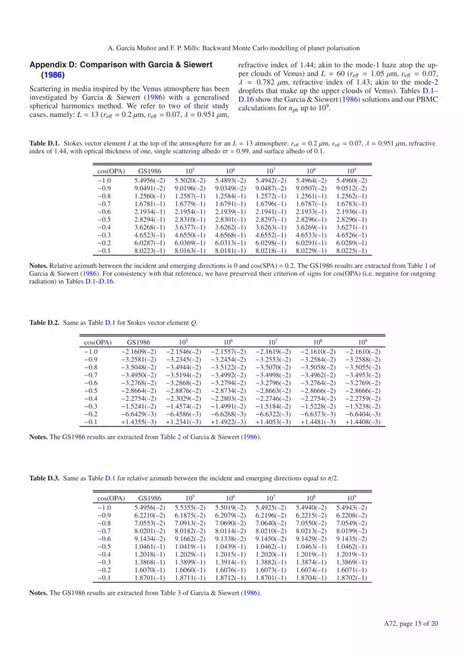
Appendix D: Comparison with Garcia & Siewert(1986)

Scattering in media inspired by the Venus atmosphere has beeninvestigated by Garcia & Siewert (1986) with a generalisedspherical harmonics method. We refer to two of their studycases, namely: L = 13 (reff = 0.2 μm, veff = 0.07, λ = 0.951 μm,

refractive index of 1.44; akin to the mode-1 haze atop the up-per clouds of Venus) and L = 60 (reff = 1.05 μm, veff = 0.07,λ = 0.782 μm, refractive index of 1.43; akin to the mode-2droplets that make up the upper clouds of Venus). Tables D.1–D.16 show the Garcia & Siewert (1986) solutions and our PBMCcalculations for nph up to 109.

Table D.1. Stokes vector element I at the top of the atmosphere for an L = 13 atmosphere: reff = 0.2 μm, veff = 0.07, λ = 0.951 μm, refractiveindex of 1.44, with optical thickness of one, single scattering albedo � = 0.99, and surface albedo of 0.1.

cos(OPA) GS1986 105 106 107 108 109

−1.0 5.4956(–2) 5.5020(–2) 5.4893(–2) 5.4942(–2) 5.4964(–2) 5.4960(–2)−0.9 9.0491(–2) 9.0196(–2) 9.0349(–2) 9.0487(–2) 9.0507(–2) 9.0512(–2)−0.8 1.2560(–1) 1.2587(–1) 1.2584(–1) 1.2572(–1) 1.2561(–1) 1.2562(–1)−0.7 1.6781(–1) 1.6779(–1) 1.6791(–1) 1.6796(–1) 1.6787(–1) 1.6783(–1)−0.6 2.1934(–1) 2.1954(–1) 2.1939(–1) 2.1941(–1) 2.1933(–1) 2.1936(–1)−0.5 2.8294(–1) 2.8310(–1) 2.8301(–1) 2.8297(–1) 2.8296(–1) 2.8296(–1)−0.4 3.6268(–1) 3.6377(–1) 3.6262(–1) 3.6263(–1) 3.6269(–1) 3.6271(–1)−0.3 4.6523(–1) 4.6550(–1) 4.6568(–1) 4.6552(–1) 4.6533(–1) 4.6526(–1)−0.2 6.0287(–1) 6.0369(–1) 6.0313(–1) 6.0298(–1) 6.0291(–1) 6.0289(–1)−0.1 8.0223(–1) 8.0163(–1) 8.0181(–1) 8.0218(–1) 8.0229(–1) 8.0225(–1)

Notes. Relative azimuth between the incident and emerging directions is 0 and cos(SPA) = 0.2. The GS1986 results are extracted from Table 1 ofGarcia & Siewert (1986). For consistency with that reference, we have preserved their criterion of signs for cos(OPA) (i.e. negative for outgoingradiation) in Tables D.1–D.16.

Table D.2. Same as Table D.1 for Stokes vector element Q.

cos(OPA) GS1986 105 106 107 108 109

−1.0 −2.1609(–2) −2.1546(–2) −2.1557(–2) −2.1619(–2) −2.1610(–2) −2.1610(–2)−0.9 −3.2581(–2) −3.2345(–2) −3.2454(–2) −3.2553(–2) −3.2584(–2) −3.2588(–2)−0.8 −3.5048(–2) −3.4944(–2) −3.5122(–2) −3.5070(–2) −3.5058(–2) −3.5055(–2)−0.7 −3.4950(–2) −3.5194(–2) −3.4992(–2) −3.4998(–2) −3.4962(–2) −3.4953(–2)−0.6 −3.2768(–2) −3.2868(–2) −3.2794(–2) −3.2796(–2) −3.2764(–2) −3.2769(–2)−0.5 −2.8664(–2) −2.8876(–2) −2.8734(–2) −2.8663(–2) −2.8666(–2) −2.8666(–2)−0.4 −2.2754(–2) −2.3029(–2) −2.2803(–2) −2.2746(–2) −2.2754(–2) −2.2759(–2)−0.3 −1.5241(–2) −1.4574(–2) −1.4991(–2) −1.5184(–2) −1.5228(–2) −1.5238(–2)−0.2 −6.6429(–3) −6.4586(–3) −6.6268(–3) −6.6322(–3) −6.6373(–3) −6.6404(–3)−0.1 +1.4355(–3) +1.2341(–3) +1.4922(–3) +1.4053(–3) +1.4481(–3) +1.4408(–3)

Notes. The GS1986 results are extracted from Table 2 of Garcia & Siewert (1986).

Table D.3. Same as Table D.1 for relative azimuth between the incident and emerging directions equal to π/2.

cos(OPA) GS1986 105 106 107 108 109

−1.0 5.4956(–2) 5.5355(–2) 5.5019(–2) 5.4925(–2) 5.4940(–2) 5.4943(–2)−0.9 6.2210(–2) 6.1875(–2) 6.2079(–2) 6.2196(–2) 6.2215(–2) 6.2208(–2)−0.8 7.0553(–2) 7.0913(–2) 7.0690(–2) 7.0640(–2) 7.0550(–2) 7.0549(–2)−0.7 8.0201(–2) 8.0182(–2) 8.0114(–2) 8.0210(–2) 8.0213(–2) 8.0199(–2)−0.6 9.1434(–2) 9.1662(–2) 9.1338(–2) 9.1450(–2) 9.1429(–2) 9.1435(–2)−0.5 1.0461(–1) 1.0419(–1) 1.0439(–1) 1.0462(–1) 1.0463(–1) 1.0462(–1)−0.4 1.2018(–1) 1.2029(–1) 1.2015(–1) 1.2020(–1) 1.2019(–1) 1.2019(–1)−0.3 1.3868(–1) 1.3899(–1) 1.3914(–1) 1.3882(–1) 1.3874(–1) 1.3869(–1)−0.2 1.6070(–1) 1.6060(–1) 1.6076(–1) 1.6073(–1) 1.6074(–1) 1.6071(–1)−0.1 1.8701(–1) 1.8711(–1) 1.8712(–1) 1.8701(–1) 1.8704(–1) 1.8702(–1)


A72, page 15 of 20

A&A 573, A72 (2015)


cos(OPA) GS1986 105 106 107 108 109

−1.0 2.1609(–2) 2.1860(–2) 2.1643(–2) 2.1590(–2) 2.1604(–2) 2.1608(–2)−0.9 2.5704(–2) 2.5607(–2) 2.5704(–2) 2.5705(–2) 2.5710(–2) 2.5705(–2)−0.8 3.0469(–2) 3.0671(–2) 3.0429(–2) 3.0517(–2) 3.0475(–2) 3.0472(–2)−0.7 3.6046(–2) 3.6093(–2) 3.6023(–2) 3.6054(–2) 3.6054(–2) 3.6049(–2)−0.6 4.2632(–2) 4.2779(–2) 4.2559(–2) 4.2631(–2) 4.2628(–2) 4.2633(–2)−0.5 5.0505(–2) 5.0141(–2) 5.0446(–2) 5.0512(–2) 5.0509(–2) 5.0511(–2)−0.4 6.0066(–2) 6.0063(–2) 6.0026(–2) 6.0067(–2) 6.0065(–2) 6.0068(–2)−0.3 7.1913(–2) 7.2239(–2) 7.2106(–2) 7.1984(–2) 7.1948(–2) 7.1925(–2)−0.2 8.6986(–2) 8.7084(–2) 8.7023(–2) 8.6990(–2) 8.7004(–2) 8.6992(–2)−0.1 1.0690(–1) 1.0681(–1) 1.0688(–1) 1.0687(–1) 1.0691(–1) 1.0691(–1)


Table D.5. Same as Table D.3 for Stokes vector element U.

cos(OPA) GS1986 105 106 107 108 109

−1.0 0.0 +2.9922(–5) +4.1728(–7) −1.6475(–5) −4.7473(–6) −2.6314(–6)−0.9 −5.9894(–3) −5.9741(–3) −6.0376(–3) −5.9877(–3) −5.9862(–3) −5.9921(–3)−0.8 −9.1368(–3) −8.8194(–3) −9.1365(–3) −9.1444(–3) −9.1407(–3) −9.1363(–3)−0.7 −1.2109(–2) −1.1913(–2) −1.2042(–2) −1.2125(–2) −1.2101(–2) −1.2112(–2)−0.6 −1.5187(–2) −1.5355(–2) −1.5094(–2) −1.5189(–2) −1.5180(–2) −1.5186(–2)−0.5 −1.8526(–2) −1.8432(–2) −1.8539(–2) −1.8551(–2) −1.8527(–2) −1.8530(–2)−0.4 −2.2261(–2) −2.2511(–2) −2.2263(–2) −2.2252(–2) −2.2266(–2) −2.2264(–2)−0.3 −2.6534(–2) −2.6487(–2) −2.6515(–2) −2.6531(–2) −2.6532(–2) −2.6538(–2)−0.2 −3.1534(–2) −3.1663(–2) −3.1532(–2) −3.1545(–2) −3.1543(–2) −3.1537(–2)−0.1 −3.7631(–2) −3.7731(–2) −3.7529(–2) −3.7606(–2) −3.7620(–2) −3.7628(–2)


Table D.6. Same as Table D.3 for Stokes vector element V .

cos(OPA) GS1986 105 106 107 108 109

−1.0 0.0 −4.0359(–6) −2.8272(–6) −1.2913(–6) −3.3342(–7) −7.6852(–8)−0.9 −5.6876(–5) −5.8781(–5) −5.8552(–5) −5.6437(–5) −5.7022(–5) −5.6950(–5)−0.8 −6.8062(–5) −5.7527(–5) −6.6774(–5) −6.8001(–5) −6.8242(–5) −6.8138(–5)−0.7 −6.7491(–5) −7.8796(–5) −6.9653(–5) −6.8228(–5) −6.7184(–5) −6.7626(–5)−0.6 −5.8655(–5) −6.6799(–5) −6.0468(–5) −5.8863(–5) −5.8413(–5) −5.8706(–5)−0.5 −4.2700(–5) −3.3163(–5) −4.4207(–5) −4.3677(–5) −4.2733(–5) −4.2723(–5)−0.4 −1.9781(–5) −2.0763(–5) −2.1645(–5) −2.0016(–5) −1.9869(–5) −1.9829(–5)−0.3 +1.0762(–5) +1.5177(–5) +1.3012(–5) +1.1121(–5) +1.0477(–5) +1.0727(–5)−0.2 +5.0591(–5) +5.4362(–5) +4.9086(–5) +5.0666(–5) +5.0576(–5) +5.0594(–5)−0.1 +1.0277(–4) +9.5783(–5) +1.0541(–4) +1.0422(–4) +1.0323(–4) +1.0281(–4)


Table D.7. Same as Table D.3 for relative azimuth between the incident and emerging directions equal to π.

cos(OPA) GS1986 105 106 107 108 109

−1.0 5.4956(–2) 5.5381(–2) 5.4887(–2) 5.4938(–2) 5.4940(–2) 5.4954(–2)−0.9 5.3085(–2) 5.2828(–2) 5.3125(–2) 5.3082(–2) 5.3088(–2) 5.3091(–2)−0.8 5.8688(–2) 5.8651(–2) 5.8711(–2) 5.8702(–2) 5.8683(–2) 5.8687(–2)−0.7 6.5653(–2) 6.5626(–2) 6.5606(–2) 6.5650(–2) 6.5650(–2) 6.5652(–2)−0.6 7.3678(–2) 7.3572(–2) 7.3684(–2) 7.3720(–2) 7.3686(–2) 7.3680(–2)−0.5 8.2754(–2) 8.2726(–2) 8.2727(–2) 8.2719(–2) 8.2742(–2) 8.2755(–2)−0.4 9.2933(–2) 9.2400(–2) 9.2931(–2) 9.2896(–2) 9.2931(–2) 9.2936(–2)−0.3 1.0421(–1) 1.0402(–1) 1.0454(–1) 1.0425(–1) 1.0424(–1) 1.0422(–1)−0.2 1.1641(–1) 1.1681(–1) 1.1645(–1) 1.1640(–1) 1.1643(–1) 1.1641(–1)−0.1 1.2913(–1) 1.2987(–1) 1.2903(–1) 1.2913(–1) 1.2915(–1) 1.2913(–1)


A72, page 16 of 20



cos(OPA) GS1986 105 106 107 108 109

−1.0 −2.1609(–2) −2.1667(–2) −2.1508(–2) −2.1620(–2) −2.1604(–2) −2.1609(–2)−0.9 −8.9018(–3) −8.8077(–3) −8.8265(–3) −8.8926(–3) −8.9011(–3) −8.9020(–3)−0.8 −3.3079(–3) −3.0655(–3) −3.3472(–3) −3.3118(–3) −3.3080(–3) −3.3078(–3)−0.7 +1.2155(–3) +1.2320(–3) +1.2018(–3) +1.2004(–3) +1.2182(–3) +1.2157(–3)−0.6 +5.2168(–3) +5.1933(–3) +5.2157(–3) +5.2033(–3) +5.2184(–3) +5.2183(–3)−0.5 +8.8753(–3) +8.7096(–3) +8.8633(–3) +8.8735(–3) +8.8756(–3) +8.8752(–3)−0.4 +1.2230(–2) +1.1998(–2) +1.2262(–2) +1.2239(–2) +1.2237(–2) +1.2232(–2)−0.3 +1.5202(–2) +1.5458(–2) +1.5417(–2) +1.5247(–2) +1.5219(–2) +1.5206(–2)−0.2 +1.7500(–2) +1.7913(–2) +1.7470(–2) +1.7479(–2) +1.7516(–2) +1.7503(–2)−0.1 +1.8225(–2) +1.8193(–2) +1.8276(–2) +1.8183(–2) +1.8234(–2) +1.8226(–2)


Table D.9. Stokes vector element I at the top of the atmosphere for an L = 60 atmosphere: reff = 1.05 μm, veff = 0.07, λ = 0.782 μm, refractiveindex of 1.43, with optical thickness of one, single scattering albedo � = 0.99, and surface albedo of 0.1.

cos(OPA) GS1986 105 106 107 108 109

−1.0 3.8783(–2) 4.0259(–2) 3.8870(–2) 3.8890(–2) 3.8815(–2) 3.8787(–2)−0.9 6.3881(–2) 6.5155(–2) 6.4312(–2) 6.3962(–2) 6.3903(–2) 6.3911(–2)−0.8 9.3567(–2) 9.3881(–2) 9.3393(–2) 9.3590(–2) 9.3609(–2) 9.3614(–2)−0.7 1.3570(–1) 1.3459(–1) 1.3554(–1) 1.3575(–1) 1.3575(–1) 1.3577(–1)−0.6 1.9652(–1) 1.9709(–1) 1.9670(–1) 1.9659(–1) 1.9655(–1) 1.9660(–1)−0.5 2.8490(–1) 2.8667(–1) 2.8553(–1) 2.8539(–1) 2.8507(–1) 2.8499(–1)−0.4 4.1401(–1) 4.1261(–1) 4.1488(–1) 4.1407(–1) 4.1421(–1) 4.1413(–1)−0.3 6.0620(–1) 6.1091(–1) 6.0618(–1) 6.0609(–1) 6.0630(–1) 6.0639(–1)−0.2 9.3026(–1) 9.2723(–1) 9.2921(–1) 9.2998(–1) 9.3044(–1) 9.3055(–1)−0.1 1.7498 1.7453 1.7480 1.7504 1.7504 1.7503

Notes. Relative azimuth between the incident and emerging directions is 0 and cos(SPA) = 0.2. The GS1986 results are extracted from Table 9 ofGarcia & Siewert (1986).


cos(OPA) GS1986 105 106 107 108 109

−1.0 +3.2087(–3) +3.4480(–3) +3.2325(–3) +3.2196(–3) +3.2120(–3) +3.2096(–3)−0.9 +5.6437(–3) +5.7535(–3) +5.6839(–3) +5.6392(–3) +5.6471(–3) +5.6488(–3)−0.8 +7.8901(–3) +7.9410(–3) +7.8199(–3) +7.8853(–3) +7.8859(–3) +7.8946(–3)−0.7 +9.9943(–3) +9.8596(–3) +9.9632(–3) +9.9880(–3) +1.0001(–2) +9.9992(–3)−0.6 +1.1613(–2) +1.1428(–2) +1.1618(–2) +1.1636(–2) +1.1611(–2) +1.1616(–2)−0.5 +1.2199(–2) +1.2363(–2) +1.2207(–2) +1.2207(–2) +1.2203(–2) +1.2199(–2)−0.4 +1.1091(–2) +1.1064(–2) +1.1108(–2) +1.1073(–2) +1.1094(–2) +1.1093(–2)−0.3 +8.3270(–3) +8.3240(–3) +8.3002(–3) +8.3205(–3) +8.3292(–3) +8.3296(–3)−0.2 +7.3504(–3) +7.5133(–3) +7.4235(–3) +7.3600(–3) +7.3618(–3) +7.3547(–3)−0.1 +1.9182(–2) +1.9353(–2) +1.9177(–2) +1.9211(–2) +1.9189(–2) +1.9188(–2)


Table D.11. Same as Table D.9 for relative azimuth between the incident and emerging directions equal to π/2.

cos(OPA) GS1986 105 106 107 108 109

−1.0 3.8783(–2) 3.8832(–2) 3.8936(–2) 3.8833(–2) 3.8784(–2) 3.8769(–2)−0.9 4.3702(–2) 4.4171(–2) 4.3742(–2) 4.3753(–2) 4.3693(–2) 4.3691(–2)−0.8 4.9701(–2) 5.0634(–2) 4.9657(–2) 4.9693(–2) 4.9695(–2) 4.9677(–2)−0.7 5.7037(–2) 5.7559(–2) 5.7175(–2) 5.6978(–2) 5.7033(–2) 5.7017(–2)−0.6 6.6034(–2) 6.5713(–2) 6.5610(–2) 6.6049(–2) 6.6014(–2) 6.6043(–2)−0.5 7.7098(–2) 7.5906(–2) 7.6959(–2) 7.7383(–2) 7.7145(–2) 7.7099(–2)−0.4 9.0697(–2) 9.0893(–2) 9.0944(–2) 9.0729(–2) 9.0789(–2) 9.0726(–2)−0.3 1.0709(–1) 1.0592(–1) 1.0761(–1) 1.0725(–1) 1.0713(–1) 1.0714(–1)−0.2 1.2517(–1) 1.2588(–1) 1.2570(–1) 1.2517(–1) 1.2524(–1) 1.2522(–1)−0.1 1.3935(–1) 1.4012(–1) 1.3925(–1) 1.3937(–1) 1.3941(–1) 1.3942(–1)


A72, page 17 of 20

A&A 573, A72 (2015)


cos(OPA) GS1986 105 106 107 108 109

−1.0 −3.2087(–3) −3.2246(–3) −3.1961(–3) −3.2089(–3) −3.2079(–3) −3.2085(–3)−0.9 −3.7776(–3) −3.7995(–3) −3.8133(–3) −3.7942(–3) −3.7817(–3) −3.7775(–3)−0.8 −4.5173(–3) −4.6534(–3) −4.5095(–3) −4.5168(–3) −4.5187(–3) −4.5158(–3)−0.7 −5.4695(–3) −5.4574(–3) −5.4403(–3) −5.4509(–3) −5.4674(–3) −5.4675(–3)−0.6 −6.6841(–3) −6.6171(–3) −6.6422(–3) −6.6838(–3) −6.6841(–3) −6.6855(–3)−0.5 −8.2210(–3) −8.0785(–3) −8.2276(–3) −8.2521(–3) −8.2255(–3) −8.2208(–3)−0.4 −1.0153(–2) −1.0132(–2) −1.0199(–2) −1.0163(–2) −1.0166(–2) −1.0157(–2)−0.3 −1.2551(–2) −1.2301(–2) −1.2697(–2) −1.2583(–2) −1.2555(–2) −1.2556(–2)−0.2 −1.5362(–2) −1.5522(–2) −1.5402(–2) −1.5368(–2) −1.5375(–2) −1.5371(–2)−0.1 −1.7919(–2) −1.8065(–2) −1.7879(–2) −1.7918(–2) −1.7922(–2) −1.7929(–2)


Table D.13. Same as Table D.11 for Stokes vector element U.

cos(OPA) GS1986 105 106 107 108 109

−1.0 0.0 4.1956(–5) −1.2981(–5) 6.1562(–6) 1.1299(–6) −4.9001(–7)−0.9 8.2963(–4) 8.3503(–4) 8.0867(–4) 8.3203(–4) 8.2784(–4) 8.2941(–4)−0.8 1.3068(–3) 1.3137(–3) 1.3230(–3) 1.3182(–3) 1.3095(–3) 1.3064(–3)−0.7 1.7878(–3) 1.8250(–3) 1.7629(–3) 1.7827(–3) 1.7880(–3) 1.7876(–3)−0.6 2.3127(–3) 2.3901(–3) 2.2889(–3) 2.3131(–3) 2.3111(–3) 2.3136(–3)−0.5 2.9041(–3) 2.8899(–3) 2.9072(–3) 2.9146(–3) 2.9066(–3) 2.9046(–3)−0.4 3.5776(–3) 3.6875(–3) 3.5900(–3) 3.5616(–3) 3.5790(–3) 3.5787(–3)−0.3 4.3260(–3) 4.2575(–3) 4.3401(–3) 4.3411(–3) 4.3322(–3) 4.3279(–3)−0.2 5.0624(–3) 5.0706(–3) 4.9985(–3) 5.0585(–3) 5.0599(–3) 5.0640(–3)−0.1 5.5033(–3) 5.6343(–3) 5.4692(–3) 5.5019(–3) 5.5060(–3) 5.5049(–3)


Table D.14. Same as Table D.11 for Stokes vector element V .

cos(OPA) GS1986 105 106 107 108 109

−1.0 +0.0 −4.3645(–6) −1.8591(–7) −6.3359(–7) +4.3425(–7) +9.3999(–9)−0.9 −2.3298(–5) −3.8504(–5) −2.3586(–5) −2.4567(–5) −2.3974(–5) −2.3709(–5)−0.8 −3.3159(–5) −1.7557(–5) −2.8954(–5) −2.9475(–5) −3.2471(–5) −3.3215(–5)−0.7 −4.0605(–5) −4.3482(–5) −3.3880(–5) −4.1344(–5) −4.0458(–5) −4.0574(–5)−0.6 −4.6329(–5) −1.7786(–5) −3.7889(–5) −4.5658(–5) −4.5602(–5) −4.6485(–5)−0.5 −5.0166(–5) −9.0685(–5) −5.0612(–5) −4.9531(–5) −4.8829(–5) −4.9981(–5)−0.4 −5.2027(–5) −3.5571(–5) −5.8161(–5) −5.6519(–5) −4.9828(–5) −5.1378(–5)−0.3 −5.3865(–5) −6.7988(–5) −3.6750(–5) −4.8297(–5) −5.3102(–5) −5.4228(–5)−0.2 −6.1686(–5) −4.4539(–5) −6.4015(–5) −6.1808(–5) −6.1938(–5) −6.1856(–5)−0.1 −8.0698(–5) −1.1810(–4) −9.4732(–5) −8.1532(–5) −8.0507(–5) −8.0468(–5)


Table D.15. Same as Table D.9 for relative azimuth between the incident and emerging directions equal to π.

cos(OPA) GS1986 105 106 107 108 109

−1.0 3.8783(–2) 3.8659(–2) 3.8838(–2) 3.8753(–2) 3.8783(–2) 3.8784(–2)−0.9 4.1409(–2) 4.2703(–2) 4.1395(–2) 4.1426(–2) 4.1439(–2) 4.1412(–2)−0.8 5.1943(–2) 5.2001(–2) 5.1773(–2) 5.1933(–2) 5.1942(–2) 5.1937(–2)−0.7 6.8133(–2) 6.9284(–2) 6.8124(–2) 6.8141(–2) 6.8127(–2) 6.8136(–2)−0.6 9.5937(–2) 9.6150(–2) 9.6270(–2) 9.5912(–2) 9.5951(–2) 9.5959(–2)−0.5 1.3265(–1) 1.3250(–1) 1.3319(–1) 1.3305(–1) 1.3273(–1) 1.3267(–1)−0.4 1.3780(–1) 1.3838(–1) 1.3761(–1) 1.3781(–1) 1.3788(–1) 1.3783(–1)−0.3 1.4338(–1) 1.4424(–1) 1.4402(–1) 1.4344(–1) 1.4343(–1) 1.4342(–1)−0.2 1.9176(–1) 1.9157(–1) 1.9172(–1) 1.9181(–1) 1.9182(–1) 1.9182(–1)−0.1 1.9322(–1) 1.9453(–1) 1.9322(–1) 1.9314(–1) 1.9325(–1) 1.9325(–1)


A72, page 18 of 20



cos(OPA) GS1986 105 106 107 108 109

−1.0 3.2087(–3) 3.2612(–3) 3.2480(–3) 3.1974(–3) 3.2063(–3) 3.2083(–3)−0.9 3.4697(–3) 3.6107(–3) 3.4775(–3) 3.4732(–3) 3.4767(–3) 3.4697(–3)−0.8 3.9993(–3) 4.1837(–3) 3.9768(–3) 4.0047(–3) 3.9993(–3) 3.9993(–3)−0.7 3.2661(–3) 3.3228(–3) 3.2461(–3) 3.2540(–3) 3.2657(–3) 3.2671(–3)−0.6 1.0031(–3) 7.4623(–4) 1.0070(–3) 1.0129(–3) 9.9955(–4) 1.0025(–3)−0.5 3.4663(–3) 3.5630(–3) 3.4973(–3) 3.4719(–3) 3.4727(–3) 3.4655(–3)−0.4 1.1649(–2) 1.1922(–2) 1.1758(–2) 1.1639(–2) 1.1641(–2) 1.1652(–2)−0.3 7.3601(–3) 7.6231(–3) 7.5405(–3) 7.3596(–3) 7.3704(–3) 7.3621(–3)−0.2 −3.5796(–3) −3.7610(–3) −3.6178(–3) −3.5574(–3) −3.5784(–3) −3.5792(–3)−0.1 1.2076(–2) 1.2413(–2) 1.2175(–2) 1.2137(–2) 1.2085(–2) 1.2081(–2)


Appendix E: Rayleigh phase curves

Fig. E.1. Disk-integrated phase curves for FI and FQ/FI for aRayleigh-scattering atmosphere with � = 1 and rg = 1 and opticalthicknesses from 0.1 to 10. Our PBMC calculations for nph = 104

(red curves) are compared to the calculations by Buenzli & Schmid(2009) using a forward Monte Carlo algorithm (black curves) and atleast 2 × 106 photons per exit direction bin over the 30–120◦ α-range.Both sets of curves are nearly indistinguishable on the scale of thegraph, even for the relatively small number of photon realisations usedin our PBMC calculations.

ReferencesBailey, J. 2007, Astrobiol., 7, 320Bartel, S., & Hielscher, A. H. 2000, Appl. Optics, 39, 1580

Berdyugina, S. V., Berdyugin, A. V., Fluri, D. M., & Piirola, V. 2008, ApJ, 673,L83

Berdyugina, S. V., Berdyugin, A. V., Fluri, D. M., & Piirola, V. 2011, ApJ, 728,L6

Beuzit, J.-L., Feldt, M., Dohlen, K., et al. 2008, Proc. SPIE, 7014, 18Bianchi, S., Ferrara, A., & Giovanardi, C. 1996, ApJ, 465, 127Boccaletti, A., Schneider, J., Traub, W., et al. 2012, Exp. Astron., 34, 355Buenzli, E., & Schmid, H. M. 2009, A&A, 504, 259Carter, L. L., Horak, H. G., & Sandford II, M. T. 1978, J. Comput. Phys. 26,

119Cashwell, E. D., & Everett, C. J. 1959, A practical manual on the Monte Carlo

method for random walk problems (New York: Pergamon Press)Coffeen, D. A. 1969, AJ, 74, 446Collins, D. G., Blättner, W. G., Wells, M. B., & Horak, H. G. 1972, Appl. Optics,

11, 2684Cornet, C., C-Labonnote, L., & Szczap, F. 2010, J. Quant. Spectr. Rad. Transf.,

111, 174Coulson, K. L., Dave, J. V., & Sekera, Z. 1960, Tables related to radiation

emerging from a planetary atmosphere with Rayleigh scattering (Berkeley,Los Angeles: University of California Press)

de Haan, J. F., Bosma, P. B., & Hovenier, J. W. 1987, A&A, 183, 371Dollfus, A. 1957, Supplements aux Annales d’Astrophysique, 4, 3Emde, C., Buras, R., Mayer, B., & Blumthaler, M. 2010, Atmos. Chem. Phys.,

10, 383Fischer, O., Henning, Th., & Yorke, H. W. 1994, A&A, 284, 187Fluri, D. M., & Berdyugina, S. V. 2010, A&A, 512, A59Ford, E. B., Seager, S., & Turner, E. L. 2001, Nature, 412, 885Garcia, R. D. M., & Siewert, C. E. 1986, J. Quant. Spectr. Rad. Transf., 36, 401García Muñoz, A., & Mills, F. P. 2012, A&A, 547, A22García Muñoz, A., & Pallé, E. 2011, J. Quant. Spectr. Rad. Transf., 112, 1609García Muñoz, A., Pallé, E., Zapatero Osorio, M. R., & Martín, E. L. 2011,

Geophys. Res. Lett., 38, L14805García Muñoz, A., Zapatero Osorio, M. R., Barrena, R., et al. 2012, ApJ, 755,

103García Muñoz, A., Pérez-Hoyos, S., & Sánchez-Lavega, A. 2014, A&A, 566, L1Gay, B., Vaillon, R., & Mengüç, M. P. 2010, J. Quant. Spectr. Rad. Transf., 111,

287Hansen, J. E., & Hovenier, J. W. 1974, J. Atmos. Sci., 31, 1137Hansen, J. E., & Travis, L. D. 1974, Space Sci. Rev., 16, 527Hopcraft, K. I., Chang, P. C. Y., Walker, J. G., & Jakeman, E. 2000, in Light

Scattering from Microstructures, eds. F. Moreno, & F. González, Lect. NotesPhys., 534, 135

Horak, H. G. 1950, ApJ, 112, 445Joos, F., & Schmid, H. M. 1980, A&A, 463, 1201Kaplan, B., Ledanois, G., & Drévillon, B. 2001, Appl. Optics, 40, 2769Karalidi, T., & Stam, D. M. 2012, A&A, 546, A56Karalidi, T., Stam, D. M., & Hovenier, J. W. 2011, A&A, 530, A69Karalidi, T., Stam, D. M., & Hovenier, J. W. 2012, A&A, 548, A90Karalidi, T., Stam, D. M., & Guirado, D. 2013, A&A, 555, A127Kasper, M. E., Beuzit, J.-L., Verinaud, C., et al. 2008, Proc. SPIE, 7015, id.

70151SKastner, S. O. 1966, J. Quant. Spectr. Rad. Transf., 6, 317Kattawar, G. W., & Adams, C. N. 1971, ApJ, 167, 183Loughman, R. P., Griffioen, E., Oikarinen, L., et al. 2004, J. Geophys. Res., 109,

6303

A72, page 19 of 20


A&A 573, A72 (2015)

Lux, I., & Koblinger, L. 1991, Monte Carlo particle transport methods: Neutronand photon calculations (Boca Raton, Florida: CRC Press Inc.)

Macintosh, B., Graham, J., Palmer, D., et al. 2006, Proc. of the SPIE, 6272,62720L

Madhusudhan, N., & Burrows, A. 2012, ApJ, 747, 25Marchuk, G. I., Mikhailov, G. A., Nazaraliev, M. A., et al. 1980, The Monte

Carlo methods in atmospheric optics (Berlin, Heidelberg: Springer-Verlag)Michalsky, J. J., & Stokes, R. A. 1977, ApJ, 213, L135Mishchenko, M. I., Travis, L. D., & Lacis, A. A. 2002, Scattering, absorption

and emission of light by small particles (Cambridge: Cambridge UniversityPress)

Modest, M. F. 2003, J. Heat Transfer, 125, 57Morozhenko, A. V., & Yanovitskii, E. G. 1973, Icarus, 18, 583Natraj, V., & Hovenier, J. W. 2012, ApJ, 748, 28Natraj, V., Li, K.-F., & Yung, Y. L. 2009, ApJ, 691, 1909O’Brien, D. M. 1992, J. Quant. Spectr. Rad. Transf., 48, 41O’Brien, D. M. 1998, J. Quant. Spectr. Rad. Transf., 60, 573Oikarinen, L. 2001, J. Geophys. Res., 106, 1533Postylyakov, O. V. 2004, J. Quant. Spectr. Rad. Transf., 88, 297Santer, R., Deschamps, M., Ksanformaliti, L. V., & Dollfus, A. 1985, A&A, 150,

217

Schmid, H. M. 1992, A&A, 254, 224Schmid, H. M., Joos, F., & Tschan, D. 2006, A&A, 452, 657Schmid, H. M., Joos, F., Buenzli, E., & Gisler, D. 2011, Icarus, 212, 701Seager, S., Whitney, B. A., & Sasselov, D. D. 2000, ApJ, 540, 504Stam, D. M. 2008, A&A, 482, 989Stam, D. M., Hovenier, J. W., & Waters, L. B. F. M. 2004, A&A, 428,

663Stam, D. M., de Rooij, W. A., Cornet, G., & Hovenier, J. W. 2006, A&A, 452,

669Stamnes, K., Tsay, S.-C., Jayaweera, K., & Wiscombe, W. 1988, Appl. Optics,

27, 2502Veverka, J. 1973, Icarus, 18, 657West, R. A., & Smith, P. H. 1991, Icarus, 90, 330West, R. A., Hart, H., Hord, C. W., et al. 1983, J. Geophys. Res., 88, 8679Whitney, B. A. 2011, Bull. Astron. Soc. India, 39, 101Wiktorowicz, S. J. 2009, ApJ, 696, 1116Williams, D. M., & Gaidos, E. 2008, Icarus, 195, 927Zugger, M. E., Kasting, J. F., Williams, D. M., Kane, T. J., & Philbrick, C. R.

2010, ApJ, 723, 1168Zugger, M. E., Kasting, J. F., Williams, D. M., Kane, T. J., & Philbrick, C. R.

2011, ApJ, 739, 12

A72, page 20 of 20

Documents

Pre-conditioned backward Monte Carlo solutions to radiative