PRECISE ANALYSIS OF π-CALCULUS IN CUBICTIME

L.Colussi, G.Filè and A.GriggioDepartment of Pure and Applied MathematicsUniversity of Padova, Italy

Abstract It is known that a static analysis of π-calculus can be done rather simply andalso efficiently, i.e. in O(n3) time. Clearly, a static analysis should be as preciseas possible. We show that it is not only desirable, but also possible to improvethe precision of the analysis without worsening its asymptotic complexity. Weillustrate the main principles of this efficient algorithm, we prove that it is indeedcubic and we also show that it is correct. The technique introduced here appearsto be useful also for other applications, in particular, for the static analysis oflanguages that extend the π-calculus.

Keywords: static analysis, π-calculus, algorithm complexity

IntroductionThe π-calculus [11, 10] is an algebra of processes that models communications

among agents that share a common channel. When an input and an output operationsynchronize on a common channel, then the bound name of the input gets instanti-ated to the name sent by the output operation. The algebra also models mobility byallowing the exchange of channel names among agents.

In a real computation of a π-calculus process, the bound name of an input operationcan be instantiated at most once. However, when one wants to compute staticallyall possible behaviours of the process he/she must take into account the fact that aninput action can in general synchronize with many output actions (in different realcomputations) and therefore, a static analysis generally associates a set of names toeach input bound name. Thus, in general, a static analysis applied to a process P iscorrect if it computes a function ρ that we call name-association such that for eachinput operation B = b(v) of P , ρ(v) contains all the names that may instantiate v as aresult of the synchronization of B with some output operations of P . It is easy to seethat a correct static analysis could be designed according to the following scheme:

First compute all the input/output pairs (A, B) of P that may synchronize;

For each such pair (A, B), where A = a〈u〉 and B = b(v), the pair can com-municate only when ρ(a) ∩ ρ(b) 6= ∅ and when this condition is satisfied, oneaccounts for the communication from A to B by adding ρ(u) to ρ(v).

317

(c) 2004 IFIP

Such an analysis is surely very simple, but it is also bound to be very poor in termsof precision, because in general it considers many synchronizations that cannot takeplace in real computations. Let us consider this example.

Example 1 In this example we want to model the situation of a client that down-loads an applet from a server and when this applet requests a connection to some hostwith a given IP number, accepts the request only if this IP number meets two condi-tions: (i) it is the same as that of the server from which the applet was downloadedand, (ii) it is in a white list that contains the client’s trustworthy servers.

For simplicity we assume that the client C already shares a channel CS with theserver S and a channel CA with the applet A. Channel CW connects C with its whitelist W . OK is a message that client C sends to A to signal that it accepts its request.The applet A sends to C three IP numbers of hosts to which it wishes to connect. Thesystem is the parallel composition of four processes C|W |S|A where:

C = CS(x).CA(y).CW (z).[x = y].[x = z].CA〈OK〉

W = CW 〈IP1〉 + CW 〈IP2〉 S = !CS〈IPS〉

A = (ν M)(CA〈IPS〉.CA(x).[x = OK].IPS〈M〉 + CA〈IP1〉.CA(x).

[x = OK].IP1〈M〉 + CA〈IP2〉.CA(x).[x = OK].IP2〈M〉)

It should be easy to see that, each test of the client C can be satisfied, but that theycannot be satisfied together. Therefore there is no execution of the system in which C

sends OK to the applet A. For a static analysis to discover this fact, it is importantthat the 2 tests are considered together. The analysis presented below does this andtherefore it will statically discover this fact.

In what follows we consider an input/output pair (A, B) and we assume that A is theoutput action a〈u〉 and B the input action b(v). The above example indicates that itis desirable to have static analyses that consider that pair (A, B) can synchronize onlywhen they really can synchronize! More precisely, only when:

(i) there is a real computation in which A and B synchronize and moreover,(ii) if this is the case, then we would like to model this synchronization by adding

to ρ(v) only the name that may instantiate u in the corresponding computation.

These two points cannot be accomplished in general as deciding point (i) is an un-solvable problem. However, during a static analysis, it is possible to use the name-association ρ that is being computed in order to approximate safely these two wishes.

Concerning point (i), we can discover that A and B can never synchronize if theyare preceded by a test [x = y] such that ρ(x) ∩ ρ(y) = ∅. By the correctness of ρ

this fact clearly implies that the test is never satisfied. As a matter of fact, it is easierto reason in the opposite direction, i.e., to conclude that the test may be satisfied insome real computation only when ρ(x) ∩ ρ(y) 6= ∅. Clearly, if together with [x = y]also the test [y = z] precedes A and B, then both tests must be satisfied together andthis is possible only when ρ(x) ∩ ρ(y) ∩ ρ(z) 6= ∅ and so on. The tests that precedeA and B, permit to refine ρ into a more precise ρ′. For instance, ρ′(x) = ρ′(y) =ρ′(z) = ρ(x) ∩ ρ(y) ∩ ρ(z). This refined ρ′ may allow to detect that indeed thecommunication between A and B is impossible in real computations. This happenswhen ρ′(a) ∩ ρ′(b) = ∅ even though ρ(a) ∩ ρ(b) 6= ∅. Similarly using ρ′, we may

318

(c) 2004 IFIP

deduce that certain input actions A = c(w) never synchronize with an output action:in this case ρ′(w) = ∅. The presence of an input action like A is important for theprecision of the analysis because it implies that all actions that follow A will neverexecute. Unfortunately, ρ′ does not carry an analogous information also for the outputactions. In fact, the values that ρ′ associates to the names used in an output action donot reveal whether the action can synchronize or not.

The aim of point(ii) is approximated by adding ρ′(u) to ρ(v), in place of ρ(u),where ρ′ is the refined name-association introduced in the previous point.

The notion of satisfaction of tests and input actions and how they can be used torefine a name-association is illustrated in the following Example 2.

Example 2 Consider process P = [a = r].a(z).[r = z].a〈r〉 and the name-association ρ such that ρ(a) = {c, d}, ρ(r) = {d, e}, ρ(z) = {e, f}. Clearly, ρ

satisfies both [a = r] and [r = z] since ρ(a)∩ ρ(r) = {d} and ρ(r)∩ ρ(z) = {e} andshows that a(z) can synchronize with some output action because ρ(z) 6= ∅. However,ρ does not satisfy the two tests together: ρ(a)∩ρ(r)∩ρ(z) = ∅! From this we can de-duce that a〈r〉 can never be executed and this consideration may be useful to improvethe quality of the static analysis of a process that contains P .

Consider now a process with two concurrent processes, P = Q |R, where Q =[a = r].r(z).[z = k].a〈r〉 and R = [l = a].b(v) with the following name-association:ρ(a) = {c, d}, ρ(r) = {d, e}, ρ(z) = {e, f}, ρ(k) = {f, g}, ρ(l) = {d, e}, ρ(b) ={c, e}, ρ(v) = ∅. If we consider Q and R independently, then we would deducethat the action A = a〈r〉 of Q and the action B = b(v) of R are both possible.However, it is easy to see that these 2 actions cannot synchronize. In fact, in orderfor these two actions to synchronize, ρ must satisfy [a = b] together with all thetests and input actions that precede the 2 actions. Clearly this in not the case here:ρ(a) ∩ ρ(r) ∩ ρ(l) ∩ ρ(b) = ∅. If, on the other hand, ρ(a) = {c, d, e} (with all othervalues of ρ unchanged) then ρ would satisfy the condition and thus we would deducethat a〈r〉 and b(v) may synchronize and then consider this action in our analysis of P .

The above ideas are rather intuitive and can be used to design a precise static analysisfor the π-calculus. We show that this analysis can also be implemented rather effi-ciently, namely, we show that its time complexity is cubic in the size of the processthat is analyzed. Also [4] presents a static analysis of the π-calculus that has beenshown in [14] to be cubic. However, the analysis of [4] checks the tests one by oneinstead of simultaneously as our analysis and therefore, it is in general less precise.For instance, it would not be able to infer that the system of Example 1 behaves safely.

In [5] a static analysis is presented for a language slightly different from that of [4]and of the present article. The main differences of the language considered inS [5]are that the repetition operator is absent and that the role of tests is played by specialinput actions called selective inputs. A selective input, before to accept an input, testsif the input is in a given set of names. This is in some sense equivalent to group to-gether many tests. Thus, one could say that in [5] a complementary approach is takenwith respect to the one we follow: in place of making the analysis more sophisticatedby grouping together tests, the language of [5] allows to directly write protocols withmore complex tests. On these protocols a simple analysis obtains results similar tothose that our analysis obtains on the same protocols described with a simpler lan-

319

(c) 2004 IFIP

guage. However, it is not difficult to show that all results obtainable with the approachof [5] can be obtained with ours, but not vice versa.

The rest of the article is organized as follows. Section 1 contains some standarddefinitions about π-calculus, some new notation, and a static analysis that uses theideas explained in Example 2 for improving the precision of the analysis. This anal-ysis is very abstract in the sense that it does not specify how its sophisticated testsare actually performed. Section 2 is devoted precisely to the illustration of how thisanalysis can be implemented in cubic time. This is done in 2 steps: a pre-processingstep followed by the static analysis part. Subsection 2 illustrates the theoretical foun-dations on which the actual implementation is built. The implementation of the staticanalysis part is described in Subsection 2. The correctness of the efficient implemen-tation is discussed in Section 3 and the complexity of the algorithm is discussed inSection 4. The work ends with Section 5 where we try to link our algorithm withsimilar proposals and we point out some directions for future investigation.

For the sake of brevity, only the proof of the main theorem 2 is reported, the proofsof all technical lemmata are given in [6]. Also the pre-processing phase of the algo-rithm (and the proof that also this phase is O(n3)) is described in [6].

1 PreliminariesIn this section we first recall the syntax of the π-calculus, [10]. The semantics

of the language is explained only intuitively by means of an Example. A completedescription can be found in [10, 15]. After this we introduce some new notation andwe describe a simple static analysis of the π-calculus.

Definition 1 Let N denote an infinite set of names, ranged over by a, b, x, y, . . . .Let also τ be a symbol not in N . Processes of π-calculus are constructed accordingto the following syntax:

P ::= 0

∣

∣ µ.P∣

∣ P + P∣

∣ P |P∣

∣ (νc)P∣

∣ [x = y].P∣

∣ !Pwhere µ is either a silent action indicated with τ , or an output action a〈b〉, or aninput action a(b). In these actions a is called the subject and b the object of theaction. The “ .” operator indicates sequential execution, the “ +” operator indicatesnondeterministic choice and “ | ” denotes parallel execution. The operator “ !” meansreplication and is very important because it replaces recursion. The (νc) operatorintroduces private name c. Process 0 does nothing and thus we shorten P.0 into P .

Example 3 Consider process P = a〈x〉.x(v).[v = x].R | a(w).[w = x].w〈x〉.P consists of two processes that execute concurrently and whose input and outputactions can synchronize. First, a〈x〉 can synchronize with a(w) producing x(v).[v =x].R | [x = x].x〈x〉. Note that as an effect of this synchronization step, the namex has been substituted to w and thus the test [w = x] has become [x = x] whichis satisfied. Thus the output x〈x〉 can execute and synchronize with x(v) producing[x = x].R |0 = R. Clearly, in process P , actions and tests are partially orderedby the execution order induced by the sequencing operator “ .”. For instance, ina〈x〉.x(v).[v = x].R, a〈x〉 is executed first, then x(v), then [v = x] and finally R.

In what follows P is a π-calculus process. In our analysis private names are consideredas free names. So we will just ignore them. This causes no loss of precision because

320

(c) 2004 IFIP

the fact that a name is private is irrelevant to our analysis. We simply study hownames can propagate inside P . Being able to distinguish the private names from thefree ones may become an issue when considering the problem of approximating thecommunications of P with the “outside world”. fn(P ) and bn(P ) are, respectively,the set of free names of P and that of the bound names of P . We always assume,w.l.g., that fn(P ) ∩ bn(P ) = ∅ and we call n(P ) = fn(P ) ∪ bn(P ).

Definition 2 Two actions or tests of P are said to be in concurrent positions wheneither they occur in a same replicated subprocess !Q or they occur in opposite sidesof a parallel composition Q |R.

PAIR(P) is the set of all pairs (A, B) of actions and tests of P that are in concurrentpositions and such that A and B are not both input or both output actions. We willalso assume that (A, B) ∈ PAIR(P ) only when A occurs to the left of B in theprocess P . Thus, if (A, B) ∈ PAIR(P ) then (B, A) 6∈ PAIR(P ).

Example 4 In process P of Example 3, if we call A = a〈x〉, B = x(v), C = a(w)and D = w〈x〉, the pairs in concurrent positions are (A, C) and (B, D). If weconsider the process !P , then we should add also (A, B) and (C, D).

Definition 3 A name-association is a function ρ : N → PS(N ) (where PS

denotes the power set). Let K be a set of tests and actions, such that their variablesare in N . If n(K) is the set of names contained in K, then the tests in K define anequivalence relation on n(K) whose corresponding partition is denoted with Π(K).We say that a name-association ρ satisfies K, when

⋂

x∈W ρ(x) 6= ∅ for all W ∈Π(K). Observe that this condition also implies that for all input and output actions inK, if a is the subject of the action and u the object, then ρ(a) and ρ(u) are both notempty. That ρ satisfies K is denoted with ρ |= K.

The refinement of ρ wrt K is a new name-association ρ′ as follows:

ρ′(z) =

{

ρ(z) if z 6∈ n(K)⋂

x∈W ρ(x) if z ∈ W ∈ Π(K)Observe that if ρ 6|= K, then for some x ∈ n(K), ρ′(x) = ∅. Given any name x,with [x]K we denote the equivalence class in Π(K) that contains x. This operation isobvious when x ∈ n(K). When x 6∈ n(K), conventionally [x]K = {x}.

Example 2 of the Introduction illustrates the above notions. The following technicalfact is a basis for next results.

Fact 1 Let K be a set of tests and W a non singleton equivalence class in Π(K),let also S ∈ K such that n(S) ∩ W 6= ∅ then the following 3 statements hold:

1 n(S) ⊆ W ;2 for any name a ∈ W , [a]K\{S} ∩ n(S) 6= ∅.3 let S′ be another test in K and assume that a is a name of S and a′ one of S′

and finally, let W ′ be the equivalence class in Π(K) that contains n(S ′). Thenit holds that [a]K\{S′} ∩ [a′]K\{S} 6= ∅ iff W = W ′ = [a]K\{S′} ∪ [a′]K\{S}

Definition 4 For any action or test X of P , with PRED(X) we denote theset of actions and tests that precede X in P according to the execution order ex-plained in Example 3 (observe that PRED(X) does not contain X). COND(X) ⊆

321

(c) 2004 IFIP

PRED(X) is the set of all the tests that precede X in P . Recall from Example 3 thatthe tests and actions in PRED(X) are totally ordered according to their executionorder. For any pair (A, B) ∈ PAIR(P ), PRED(A, B) = PRED(A)∪PRED(B)and COND(A, B) = COND(A) ∪ COND(B).

The following Example explains the previous Definition.

Example 5 Let P be the following process,a(x).a(y).a(z).a(w).[x = w].

(

[x = y].b〈x〉 | [x = z].c〈x〉 | [w = z].[w = y].d(k))

then PRED(b〈x〉) = {a(x), a(y), a(z), a(w), [x = w], [x = y]}, COND(b〈x〉) ={[x = w], [x = y]} and the set of actions and tests in PRED(b〈x〉) ∩ PRED(d(k))is {a(x), a(y), a(z), a(w), [x = w]}. These actions and test precede both b〈x〉 andd(k). Observe that all tests and actions in the above sets are listed in execution order.

This Section is concluded with a very simple but powerful static analysis for the π-calculus, that we call in fact the Simple Analysis.

1 Let P be the process to be analyzed and ρ0 be the following name-association:for each free name x in P , ρ0(x) = {x} and for each bound name y in P ,ρ0(y) = ∅. Set i = 1 and proceed to the following step,

2 consider any pair (A, B) ∈ PAIR(P ), such that A is an output action a〈u〉and B an input action b(v). If ρi−1 |= PRED(A, B) ∪ [a = b], let ρ′

i−1 bethe refinement of ρi−1 wrt PRED(A, B) ∪ [a = b] (cf. Definition 3), thenρi(v) = ρi−1(v) ∪ ρ′i−1(u).

3 if ρi = ρi−1 then stop with output ρSA = ρi, otherwise go back to step 2.

Even though the above analysis is very simple to describe, it contains operations thatseem to require a high polynomial number of steps (in particular, the test whetherρi |= PRED(A, B) ∪ [a = b] and the computation of ρ′

i−1 in step (2)). It is in factfairly easy to see how to perform these operations in O(n5) steps. Observe that theoperations of step (2) of the Simple Analysis that seem to be particularly complex areexactly those that perform the improvements mentioned in points (1) and (2) of theIntroduction. Improving this bound was for us not easy, but we succeeded and in thefollowing Sections we report the algorithm we found. This algorithm implements theSimple Analysis and has worst case time complexity O(n3).

The reader may wonder why in the above step (2) we consider PRED(A, B) andnot COND(A, B). Notice that Π(COND(A, B)) ⊆ Π(PRED(A, B)) and in somecases the containment is proper and the difference consists of some singletons. Thismay happen when PRED(A, B) contains some input or output action with namesthat do not appear in any test in COND(A, B). As already observed in the Introduc-tion (cf. Point (1)), the names in these singletons that are objects of input actions, canbe exploited for improving the analysis. This explains the choice in step (2).

2 The Efficient AlgorithmIn this Section we explain how the Simple Analysis of the previous Section can be

implemented efficiently obtaining an algorithm that has cubic worst case time com-plexity. This algorithm will be called in what follows the Efficient Algorithm.

322

(c) 2004 IFIP

The problem is to perform efficiently the tests of point (2) of the Simple Analysisand the computation of a refined name-association (called ρ′

i−1 in the Simple Analy-sis). The key idea is that of computing and maintaining all the necessary refined valuesthroughout the analysis (instead of recomputing them each time they are needed as ina naive implementation of the Simple Analysis). To this end we introduce a set of newnames whose role is to hold the refined values. Roughly this works as follows. Con-sider a pair A = a〈u〉 and B = b(v) that may synchronize. The tests and actions thatprecede A and B, together with [a = b], determine equivalence classes of names, cf.Example 2. Call these classes X1, . . . , Xm. For each Xi, a new name ci is introducedand during the analysis, if ρ is the name-association computed so far, then the value ofρ(ci) will always satisfy the following relation: ρ(ci) =

⋂

y∈Xiρ(y). Thus, ρ(ci) is

the refined value of each name in Xi. Namely, it is the set of names that are assignedto all the names in Xi and that satisfy all the tests and actions in PRED(A, B) thathave formed the class Xi. The above description is necessarily simplified. In particu-lar, the new names that are used in the algorithm are not simply ci. For instance, thenew name that corresponds to the class that contains the subjects a and b is cA,B andthe new name that corresponds to the class that contains the object u of the output iscA↓B . With these new names that hold the refined values of the equivalence classes, itis possible to implement the actions of point (2) of the Simple Analysis as follows :

(a) the synchronization between A and B is considered by the analysis only wheneach ρ(ci) 6= ∅, this guarantees that all actions and tests in PRED(A, B)∪[a =b] can be executed/satisfied; observe that [a = b] is added to check that A andB can actually communicate;

(b) the synchronization of A and B is modelled by adding ρ(cA↓B) to ρ(v). Ob-serve that this is the refined value of u, as requested in point (2) of the SimpleAnalysis.

The number of new names introduced is quadratic. However, maintaining the valueof each of these names (and also of those in n(P ) that in what follows will be calledold) takes linear time. This follows from the fact that each new name c depends ononly 2 other names (new or old), say c′ and c′′. This dependency is as follows: whenx ∈ ρ(c′) ∩ ρ(c′′) then x must be also in ρ(c). Moreover, c′ and c′′ are strictlysmaller than c wrt a partial order and thus there is no circularity in these dependencies.Exploiting this fact, it is possible to maintain the value of each name in linear time.

The test described in point (a) above can also be done very efficiently: a counterReady(cA↓B) is initially set to the number of classes in Π(PRED(A, B) ∪ [a = b])and is decreased by 1 each time the value of ρ(ci) (where ci corresponds to one of theclasses) becomes not empty. When Ready(cA↓B) = 0, the test of point (a) is satisfiedand thus the analysis performs the action of point (b). We have actually implementedthis sophisticated static analysis algorithm. The C++ source is downloadable from thedirectory “www.math.unipd.it/˜colussi/Analizer/”.

theoretical foundationsThis Section is devoted to the construction of the theoretical foundations of the

Efficient Algorithm and of the proof that it is cubic in the size of P (P is always theprocess under analysis). It mainly contains three things:

323

(c) 2004 IFIP

(I) The precise definition of the new names that are needed for the Efficient Algo-rithm together with a partial order on them;

(II) The proof that the value of each new name v depends on that of only two othernames lc(v) and rc(v);

(III) The proof that for each pair (A, B) of input/output action one can compute onceand for all a set X of names, such that the test of point(a) above is performedby checking that for every name x ∈ X , ρ(x) 6= ∅. It is also important that |X |is linear in the size of P .

Points (II) and (III) are fundamental for showing that the Efficient Algorithm is cubicin the size of P . Recall that n(P ) stands for the set of all the names of P , i.e., n(P ) =fn(P ) ∪ bn(P ), where, w.l.g., we assume that fn(P ) ∩ bn(P ) = ∅. In what followsthese names are called old to distinguish them from the new ones that we are goingto introduce. As explained above, each new name v stands for a set of old names thatis indicated with [v]. This notation is extended to old names x, letting [x] = {x}.The set of new names that we create for P is denoted new(P ) and consists of twoparts news(P ) and newp(P ). The first part contains new names that corresponds to asingle test T of P (‘s’ stands for single), whereas the second one contains new namesthat correspond to pairs (’p’ stands for pair) as follows: these names correspond eitherto pairs (A, B) of an input and an output action which are in concurrent position in P

or to pairs (T, T ′) of tests which are in concurrent position in P .

Definition 5 For each test T = [a = b] of P , news(P ) contains a new name cT

that stands for the set of old names [cT ] = [a]COND(T )∪T .

The following is an easy consequence of Fact 1(2) that is useful for the next Lemma.

Fact 2 Let cT be the new name that corresponds to a test T = [a = b], then[cT ] = [a]COND(T ) ∪ [b]COND(T ).

It is useful to define a partial order on the set news(P ) ∪ n(P ).

Definition 6 The relation � on news(P ) ∪ n(P ) is defined as follows.

for each x ∈ news(P ) ∪ n(P ), x � x;the old names in n(P ) are unrelated among each other and for each x ∈ n(P )and y ∈ news(P ), x � y;for any two names cT and cS ∈ news(P ), cT � cS iff T precedes S in theexecution order.

In what follows we will write x ≺ y to denote x � y and x 6= y.

In the following Lemma we show point (II) for the names in news(P ).

Lemma 1 Let cT be a new name in news(P ), where T = [a = b]. There are twonames (either old or in news(P )) lc(cT ) and rc(cT ) such that [cT ] = [lc(cT )] ∪[rc(cT )]. Moreover, lc(cT ) ≺ cT and rc(cT ) ≺ cT .

Names in newp(P ) correspond to pairs (A, B) ∈ PAIR(P ) whose names may in-teract in some way. Interaction may be of two types: either A and B are an output and

324

(c) 2004 IFIP

an input action that may communicate or A and B are tests and there is a name in A

and a name in B that are equated by the tests in COND(A, B).Recall from Definition 2 that pairs (A, B) ∈ PAIR(P ) are such that A is always

to the left of B in P . In this way we avoid the nuisance of having a new name for(A, B) and another for (B, A), while only one of them is enough for the analysis.

Definition 7 newp(P ) contains the following names:

(a) For each test/test pair (T, T ′) ∈ PAIR(P ), where T = [a = c] and T ′ =[b = d], and such that [a]COND(T,T ′)∪T ∩ [b]COND(T,T ′)∪T ′ 6= ∅ a new namecT,T ′ is in newp(P ). This name stands for the set of old names [cT,T ′ ] =[a]COND(T,T ′)∪T∪T ′ .

(b) For each input/output pair (A, B) ∈ PAIR(P ), where a〈u〉 is the output actionand b(w) is the input action, newp(P ) contains two new names cA,B and cA↓B .The name cA,B is intended to stand for the set [cA,B ] = [a]COND(A,B)∪[a=b] ofold names, whereas cA↓B stands for the set [cA↓B ] = [u]COND(A,B)∪[a=b].

Notice that in point (b) of the above Definition no assumption is made on whichone between A and B is input and which is output. Moreover, [a = b] is not a test inP . We add it to COND(A, B) to mimic the fact that the synchronization of A andB is possible only when this condition is satisfied. Observe that this is coherent withstep (2) of the Simple Analysis, cf. Section 1. In what follow with nn(P ) we denoten(P ) ∪ new(P ). The partial order � is easily extended to nn(P ) as follows.

Definition 8 The partial order � is extended to nn(P ) adding the followingpoints to those of Definition 6:

for each name x ∈ newp(P ), x � x;all old names are smaller than all new names of newp(P );a name cT is smaller than every name cX,Y and cX↓Y ;if T1 and T2 are tests and X1 and X2 are either two tests or an input and outputaction, then cT1,T2

� cX1,X2iff for each i ∈ [1, 2] either Ti precedes Xi or

Ti = Xi;for all name x, if x � cA,B ∈ newp(P ), where A and B are an input and anoutput action, then x � cA↓B .

Fact 3 The relation � of Definition 8 is a partial order.

We want now to show point (II) also for the names in newp(P ). To this end wefollow the same strategy that was used in Lemma 1: for any v ∈ newp(P ), we showthat [v] can be split into two parts for which there are corresponding names. Thefollowing simple consequence of Fact 1(c) is useful for this.

Fact 4 Let cT,T ′ be a new name introduced in step (a) of Definition 7 and let T =[a = c] and T ′ = [b = d]. It is true that [a]COND(T,T ′)∪T∪T ′ = [a]COND(T,T ′)∪T ∪[b]COND(T,T ′)∪T ′ .

Lemma 2 Let v ∈ newp(P ), there are names lc(v) and rc(v) in n(P )∪news(P )∪newp(P ) such that [v] = [lc(v)]∪ [rc(v)] and moreover, these names are smaller thanv with respect to the partial order ≺.

325

(c) 2004 IFIP

A boolean array Bound indexed on the set nn(P ). Bound[x] = 1 if there isa name z ∈ n(P ) such that Rho[z, x] = 1.An array Ready of integers such that for each name v = cA↓B , Ready[v] isinitially set to the cardinality of Pred(v). For each name x ∈ Pred(v), thereis a list isPx that contains v and all other names having x in their Pred set.Two arrays Lc and Rc indexed on the set new(P ) (to store lc(v) and rc(v))and for all x ∈ nn(P ) a list isLcx (for “x is Left Component of”) of all namesv such that x = lc(v) and a list isRcx (for “x is Right Component of”) of allthose names v such that x = rc(v).An array Rho of booleans indexed in n(P ) × nn(P ).

Table 1. Main data structures used by the algorithm.

The following Theorem summarizes what we have shown.

Theorem 1 For each name v in new(P ) there exist names lc(v) and rc(v) (pos-sibly equal) that are strictly smaller than v wrt the partial order ≺ defined on nn(P ).

Corollary 1 The relation on nn(P ) defined by the lc(v) and rc(v) functionsamong names is noncircular.

We turn now to point (III). Consider an input/output pair (A, B) and let a and b bethe subjects of the two actions and u the object of the output one. As explained in (III),in order for the Efficient Algorithm to check whether the pair (A, B) can synchronize,all the refined values corresponding to the equivalence classes of Π(PRED(A, B) ∪[a = b]) should be not empty. In order to perform this test for each such class X theremust exist a new or an old name x that corresponds to the class and thus that will holdits refined value. This is shown in the following Lemma.

Lemma 3 Let v = cA↓B and let a and b be the subjects of the actions A and B. Foreach class X ∈ Π(PRED(A, B) ∪ [a = b]) there is a name x ∈ nn(P ) such that[x] = X . Moreover, x ≺ cA↓B .

Let us conclude the Section with a notation that will be useful in the next one: Forany name cA↓B , Pred(cA↓B) denotes the names (that were just shown to exist) thatcorrespond to the equivalence classes of Π(PRED(A, B) ∪ [a = b]).

the implementationThe Efficient Algorithm uses several data structures and is composed of two parts:

a pre-processing part and the static analysis part. For the sake of brevity, we onlydescribe the static analysis part, in Table 2, and the most important data structuresused in that part, in Table 1. The pre-processing part and all other data structures usedby the algorithm are described in [6]. Data structures in Table 1 have the followingpurpose. In the matrix Rho we assume that the first |n(P )| columns correspond to theold names (i.e., those in n(P )). This matrix holds, throughout the execution of thealgorithm, the name-association computed at each moment.

The name-association ρRho on nn(P ) that corresponds to a given matrix Rho is asfollows: ∀x ∈ n(P ) and w ∈ nn(P ), x ∈ ρRho(w) iff Rho[x, w] = 1. The restriction

326

(c) 2004 IFIP

Compute(P )1 Set to 0 all entries of arrays Rho and Bound.2 Call Try(u) for all u ∈ fn(P ) (i.e., those u that do not occur in P as the

object of an input action).

Try(u)1 if Rho[u, u] = 0 then set Rho[u, u] = 1 and call V isitIsC(u, u) .2 if Bound[u] = 0 then set Bound[u] = 1 and call V isitIsP (u).

Filter(u, v)1 set Rho[u, v] = 1 and call V isitIsC(u, v).2 if v = cA↓B , Ready[v] = 0 and Rho[u, w] = 0, where w is the object

of the input action in the input/output pair (A, B) associated to v, then callClose(u, w).

3 if Bound[v] = 0 set Bound[v] = 1 and call V isitIsP (v).

Transmit(v, w)1 call Close(z, w) for all z ∈ n(P ) such that Rho[z, w] = 0 and Rho[z, v] = 1.

Close(u, v)1 set Rho[u, v] = 1 and call V isitIsC(u, v).2 if Bound[v] = 0 then set Bound[v] = 1 and call V isitIsP (v).3 call Close(z, v) for all z ∈ n(P ) such that Rho[z, v] = 0 and Rho[z, u] = 1.4 call Close(u, z) for all z ∈ n(P ) such that Rho[u, z] = 0 and Rho[v, z] = 1.

V isitIsC(u, v)1 call Filter(u, x) for all x ∈ isLcv such that Rho[u, Rc[x]] = 1 and

Rho[u, x] = 0.2 call Filter(u, x) for all x ∈ isRcv such that Rho[u, Lc[x]] = 1 and

Rho[u, x] = 0.

V isitIsP (v)1 for all x ∈ isPv set Ready[x] = Ready[x]− 1 and in case Ready[x] = 0 call

Transmit(x, w) where w is the object of the input action in the input/outputpair (A, B) associated to x (recall that all x ∈ isPv are of type x = cA↓B).

Table 2. The static analysis part of the Efficient Algorithm

of ρRho to the old names in n(P ) is denoted ρ̄Rho. Lc and Rc specify for each newname v the lc(v) and rc(v). Bound is used to signal when a name x is assigned a notempty value, i.e., ρ(x) 6= ∅. Ready is defined only for names of the form cA↓B . Itsinitial value is the cardinality of Pred(cA↓B). Each time a name x in this set becomesbound, then Ready[cA↓B] is decreased by 1. On the other hand, isLcx is used to reachall those names v that have x as lc(v) and similarly for isRcx. isPx lists those namesof the form cA↓B such that x ∈ Pred(cA↓B).

327

(c) 2004 IFIP

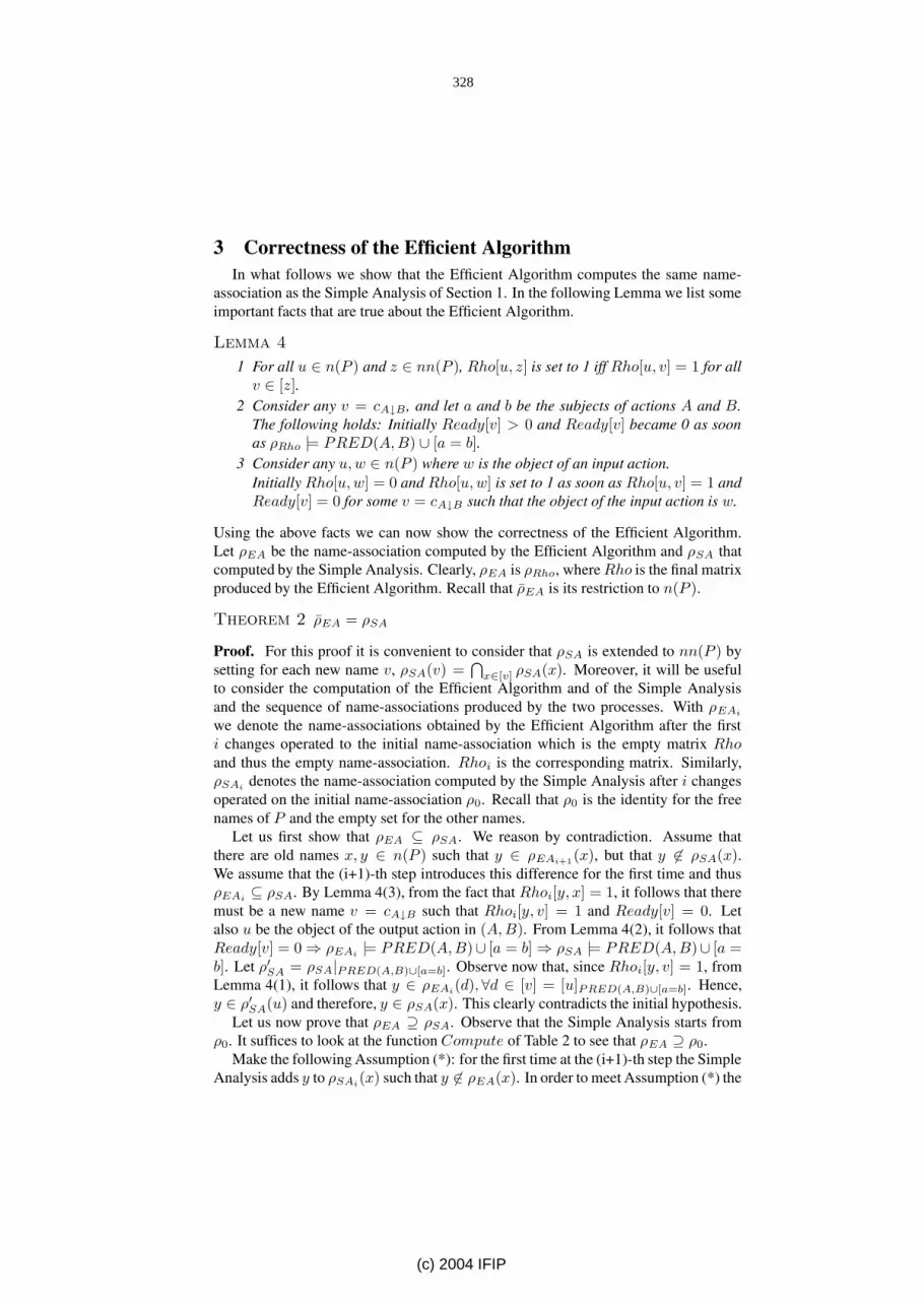
3 Correctness of the Efficient AlgorithmIn what follows we show that the Efficient Algorithm computes the same name-

association as the Simple Analysis of Section 1. In the following Lemma we list someimportant facts that are true about the Efficient Algorithm.

Lemma 4

1 For all u ∈ n(P ) and z ∈ nn(P ), Rho[u, z] is set to 1 iff Rho[u, v] = 1 for allv ∈ [z].

2 Consider any v = cA↓B , and let a and b be the subjects of actions A and B.The following holds: Initially Ready[v] > 0 and Ready[v] became 0 as soonas ρRho |= PRED(A, B) ∪ [a = b].

3 Consider any u, w ∈ n(P ) where w is the object of an input action.Initially Rho[u, w] = 0 and Rho[u, w] is set to 1 as soon as Rho[u, v] = 1 andReady[v] = 0 for some v = cA↓B such that the object of the input action is w.

Using the above facts we can now show the correctness of the Efficient Algorithm.Let ρEA be the name-association computed by the Efficient Algorithm and ρSA thatcomputed by the Simple Analysis. Clearly, ρEA is ρRho, where Rho is the final matrixproduced by the Efficient Algorithm. Recall that ρ̄EA is its restriction to n(P ).

Theorem 2 ρ̄EA = ρSA

Proof. For this proof it is convenient to consider that ρSA is extended to nn(P ) bysetting for each new name v, ρSA(v) =

⋂

x∈[v] ρSA(x). Moreover, it will be usefulto consider the computation of the Efficient Algorithm and of the Simple Analysisand the sequence of name-associations produced by the two processes. With ρEAi

we denote the name-associations obtained by the Efficient Algorithm after the firsti changes operated to the initial name-association which is the empty matrix Rho

and thus the empty name-association. Rhoi is the corresponding matrix. Similarly,ρSAi

denotes the name-association computed by the Simple Analysis after i changesoperated on the initial name-association ρ0. Recall that ρ0 is the identity for the freenames of P and the empty set for the other names.

Let us first show that ρEA ⊆ ρSA. We reason by contradiction. Assume thatthere are old names x, y ∈ n(P ) such that y ∈ ρEAi+1

(x), but that y 6∈ ρSA(x).We assume that the (i+1)-th step introduces this difference for the first time and thusρEAi

⊆ ρSA. By Lemma 4(3), from the fact that Rhoi[y, x] = 1, it follows that theremust be a new name v = cA↓B such that Rhoi[y, v] = 1 and Ready[v] = 0. Letalso u be the object of the output action in (A, B). From Lemma 4(2), it follows thatReady[v] = 0 ⇒ ρEAi

|= PRED(A, B)∪ [a = b] ⇒ ρSA |= PRED(A, B)∪ [a =b]. Let ρ′SA = ρSA|PRED(A,B)∪[a=b]. Observe now that, since Rhoi[y, v] = 1, fromLemma 4(1), it follows that y ∈ ρEAi

(d), ∀d ∈ [v] = [u]PRED(A,B)∪[a=b]. Hence,y ∈ ρ′SA(u) and therefore, y ∈ ρSA(x). This clearly contradicts the initial hypothesis.

Let us now prove that ρEA ⊇ ρSA. Observe that the Simple Analysis starts fromρ0. It suffices to look at the function Compute of Table 2 to see that ρEA ⊇ ρ0.

Make the following Assumption (*): for the first time at the (i+1)-th step the SimpleAnalysis adds y to ρSAi

(x) such that y 6∈ ρEA(x). In order to meet Assumption (*) the

328

(c) 2004 IFIP

Simple Analysis must consider an input/output pair (A, B). Assume that the subjectsof the 2 actions are a and b, whereas the object of the output one is u, whereas thatof the input, from the hypothesis, must be x. Moreover, it must be that (A) ρSAi

|=PRED(A, B)∪[a = b] and if ρ′

SAi= ρSAi

|PRED(A,B)∪[a=b], then (B) y ∈ ρ′SAi

(u).From Assumption (*) and statement (A), it follows that ρEA |= PRED(A, B) ∪

[a = b] and, by Fact 4(2), we derive that (C) Ready[cA↓B] = 0. From (B) andAssumption (*), it follows that ∀d ∈ [cA↓B ] = [u]PRED(A,B)∪[a=b], Rho[y, d] = 1,and thus, by Fact 4(1), that (D) Rho[y, cA↓B] = 1. From (C) and (D), by Fact 4(3),we can conclude that Rho[y, x] = 1 in contradiction with our initial assumption.

4 Complexity of the algorithmIt is quite simple to prove that the Efficient Algorithm requires time O(n3) (where

n is the size of the π-expression P in input): for each function we find a bound for thenumber of times it is called and a bound for the time required to execute the function.The execution time of each function does not include the time required to execute thefunction calls it may contain. At the end it suffices to sum everything up in order toobtain a bound for the total time required by whole Efficient Algorithm.

Observe that there are at most O(n) actions or tests in P and at most O(n) oldnames in n(P ) while the cardinality of nn(P ) can be O(n2). The function Compute

is called only once and requires O(n3) time. This time is needed fundamentally forinitializing matrix Rho. Try is called O(n) times (at most once for each name inn(P )) and its execution requires time O(1). Filter is called O(n3) times (at mostonce for each entry of Rho) and it requires time O(1). Transmit is called O(n2)times (at most once for each name cA↓B) and it requires time O(n). Close is calledO(n2) times (at most once for each pair of names in n(P )) and it requires time O(n).V isitIsC is called at most once for each pair (u, v) and requires time proportional tothe length of lists isLcv and isRcv. Since the sum of the lengths of all lists isLc andisRc is O(n2) the total time required is O(n3). For function V isitIsP the reasoningis more subtle. V isitIsP is called at most once for each name v ∈ nn(P ) and requirestime proportional to the length of the list isPv. Since the sum of the lengths of all listsisPv is O(n3) (because each name in cA↓B can be inserted in at most O(n) such lists),the total time required by this function is O(n3).

Since the above functions use the data structures shown in Table 1, it is importantto consider also the cost of constructing these structures in a pre-processing phase.

The pre-processing can be done in time O(n3). A detailed description of the pre-processing and the proof that it require time O(n3) is given in [6]. Here we explainwhy this is the case on a more intuitive level. The pre-processing consists of a dou-ble visit of the parse tree of the π-expression P in input. For each action or test A

encountered in the first visit we do a second visit to find all action or test B that is inconcurrent position with A. At each step we update a disjoint-set data structure cls

that holds the classes in Π(PRED(A, B)). The data structure cls is augmented bythe name of classes and a list Pred that links names of classes in cls. Since cls andPred can be updated in many different ways, they must be copied before an updatetakes place. Double visiting the parse tree takes time O(n2) and copying the structurescls requires time O(n). Thus the total time used is O(n3).

329

(c) 2004 IFIP

5 Related work and perspectivesBodei et al. in [4] proposed a static analysis of the π-calculus that in [14] was

shown to have a cubic time complexity. This analysis considers that any input/outputpair (A, B) can synchronize only when all tests that precede them are satisfied bythe name-association computed so far, but the tests are considered one at the timeand not together as our analysis does. In [13] the analysis of [4] is extended to thespi−calculus [2] maintaining the same time complexity. This extended version stillhandles the cryptographic primitives one at the time as before.

Also Venet [17] and Feret [8, 9] have proposed static analyses of the π-calculusthat are formulated in the abstract interpretation framework, [7]. They first introducenon standard semantics and then define their analyses as abstractions of these seman-tics. The semantics they propose are expressive enough to encompass non uniformanalyses, that is analyses able to distinguish among the different copies of a samereplicated subprocess and among the names that these copies can define and transmit.In fact, these analyses are useful, for instance, for evaluating the resource usage insidea system. These works are rather different from the present one. They focus on theexpressivity of the analyses rather than on their efficient implementation.

Clearly, many other methods, different from ours and from those mentioned before,have also been used for proving properties of protocols. These methods include modelchecking [12], type systems [2], the use of theorem provers [3, 1]. Often these pro-posals try to establish more sophisticated properties of protocols than what our staticanalysis can compute. However, we believe that any method for inferring propertiesof protocols must lay on a precise knowledge of the name-association the protocolactually produces and this is precisely what our static analysis computes with highprecision and also efficiently.

In the future we intend to substantiate the above statement by extending our analy-sis in various ways. First of all we will further enhance the precision of our analysis byincluding into it the detection of “blocked” output actions, i.e., outputs that cannot syn-chronize with any input and that, therefore, block the successive actions. Our approachimproves precision by considering the global condition COND(A) ∪ COND(B) ∪[a = b] under which transmission of a name can take place from the output actionA = a〈u〉 to the input action B = b(w). It is possible to further improve the precisionof the analysis by considering the transmission of each name through sequences ofsynchronizing pairs of input/output actions, evaluating together all tests that precedethese actions. We obviously expect that the complexity of this improved analysis willgrow with the length of the action sequences considered.

Finally, we will apply our method to the analysis of extensions of the π-calculusthat include various cryptographic primitives.

References

[1] Martìn Abadi and Bruno Blanchet. Computer assisted verification of a protocol for certifiedemail. In Proceedings of 10th SAS, number 2694 in LNCS, pages 316–335, 2003.

[2] Martìn Abadi and Andrew Gordon. A calculus for cryptographic protocols—the spi calcu-lus. Information and Computation, 148(4):1–70, 1999.

330

(c) 2004 IFIP

[3] G. Bella and L.C. Paulson. Kerberos version iv:inductive analysis of the secrecy goals. InProceedings of ESORICS 98, number 1485 in LNCS, pages 361–375, 1998.

[4] Chiara Bodei, Pierpaolo Degano, Flemming Nielson, and Hanne Riis Nielson. Static analy-sis for the π-calculus with applications to security. Information and Computation, 165:68–92, 2001.

[5] C. Priami C.Bodei, P.Degano and N. Zannone. An enhanced cfa for security policies. InProceedings of WITS’03, pp.131-145, Warszawa, 2003.

[6] L. Colussi, G. Filè and A. Griggio. Precise Analysis of π-calculus in cubic time. Preprintn. 20 Dipartimento di Matematica Pura ed Applicata, University of Padova, 2003.

“www.math.unipd.it/˜colussi/DMPA-Preprint20-2003.ps”

[7] Patrick Cousot and Radhia Cousot. Abstract interpretation: a unified lattice model for staticanalysis of programs by construction or approximation of fixpoints. In Proceedings of 4thACM POPL, pages 238–252, 1977.

[8] Jérôme Feret. Confidentiality analysis of mobile systems. In Proceedings of 7th SAS,number 1824 in LNCS, 2000.

[9] Jérôme Feret. Occurrence counting analysis. In Proceedings of GETCO 2000, appearedon ENTCS, number 39, 2001.

[10] Robin Milner. Communicating and mobile systems: the π-calculus. Cambridge UniversityPress, 1999.

[11] Robin Milner, Joachim Parrow, and David Walker. A calculus of mobile processes (i andii). Information and Computation, 100(1):1–77, 1992.

[12] J.C. Mitchell, V. Shmatikov, and U. Stern. Finite state analysis of ssl 3.0. In Proceedingsof 7th USENIX Security Symposium, pages 201–216, 1998.

[13] Flemming Nielson, Hanne Riis Nielson, and Helmut Seidl. Cryptographic analysis incubic time. In ENTCS, number 62 in ?, 2002.

[14] Flemming Nielson and Helmut Seidl. Control flow analysis in cubic time. In Proceedingsof ESOP ’01, number 2028 in LNCS, pages 252–268, 2001.

[15] Davide Sangiorgi and David Walker. The π-calculus: a Theory of Mobile Processes. Cam-bridge University Press, 2001.

[16] R. L. Rivest T. H. Cormen, C. E. Leiserson and C. Stein. Introduction to Algorithms. TheMit Press, 1998.

[17] Arnaud Venet. Automatic determination of communication topologies in mobile systems.In Proceedings of 5th SAS, number 1503 in LNCS, pages 152–167, 1998.

331

(c) 2004 IFIP