Embed Size (px)
Citation preview

PRECISION FORESTRY
PROCEEDINGS OF THE SECOND INTERNATIONALPRECISION FORESTRY SYMPOSIUM
UNIVERSITY OF WASHINGTON COLLEGE OF FOREST RESOURCESFERIC, THE FOREST ENGINEERING RESEARCH INSTITUTE OF CANADA
IUFRO, THE INTERNATIONAL UNION OF FOREST RESEARCH ORGANIZATIONSUSDA FOREST SERVICE, PACIFIC NORTHWEST RESEARCH STATION
SEATTLE, WASHINGTONJUNE 15-17, 2003

PRECISION FORESTRY
PROCEEDINGS OFTHE SECOND INTERNATIONAL
PRECISION FORESTRY SYMPOSIUM

II
Printed in the United States of America
All rights reserved. No part of this publication may be reproduced or transmitted in any form or by any means, electronic or mechanical,including photocopy, recording, or any information storage or retrieval system, without permission in writing from the publisher, theCollege of Forest Resources.
Institute of Forest ResourcesCollege of Forest ResourcesBox 352100University of WashingtonSeattle, WA 98195-2100(206) 685-0887Fax: (206) 685-3091http://www.cfr.washington.edu/Pubs/publist.htm
Proceedings of the Second International Precision Forestry Symposium, sponsored by the University of Washington College of ForestResources, the Precision Forestry Cooperative, Seattle, Washington, FERIC, the Forest Engineering Research Institute, Vancouver, BC,IUFRO, The International Union of Forest Research Organizations, Vienna, Austria, and the USDA Forest Service, Pacific NorthwestResearch Station, Resource Management and Productivity Program, Portland, Oregon.
Additional copies of this book may be purchased from the University of Washington Institute of Forest Resources, Box 352100,Seattle, Washington 98195-2100.
For additional information on the Precision Forestry Cooperative please visit http://www.precisionforestry.org

III
TABLE OF CONTENTS
Acknowledgments VI
Preface VIII
Keynote Speakers
Opening Remarks and Welcome to the First International Precision Forestry Symposium 1B. Bruce Bare
Precision Forestry – The Path to Increased Profitability! 3Bill Dyck
Precision Technologies: Data Availability Past and Future 9Daniel L. Schmoldt and Alan J. Thomson
Plenary Session A: Precision Operations and Equipment -Moderator, Alex Sinclair
Multidata and Opti-Grade: Two Innovative Solutions to Better Manage Forestry Operations 17Pierre Turcotte
A Test of the Applanix POS LS Inertial Positioning System for the Collection of Terrestrial CoordinatesUnder a Heavy Forest Canopy 21
Stephen E. Reutebuch, Ward W. Carson, and Kamal M. AhmedGround Navigation Through the Use of Inertial Measurements, a UXO Survey 29
Mark Blohm and Joel GilletPrecision Forestry Operations and Equipment in Japan 31
Kazuhiro ArugaPrecision Forestry Applications: Use of DGPS Data to Evaluate Aerial Forest Operations 37
Jennie L. Cornell, John Sessions and John Mateski
Plenary Session B: Remote Sensing and Measurement of ForestLands and Vegetation - Moderator, Tom Bobbe
Estimating Forest Structure Parameters on Fort Lewis Military Reservation Using Airborne LaserScanner (LIDAR) Data 45
Hans-Erik Andersen, Jeffrey R. Foster, and Stephen E. ReutebuchDeveloping “COM” Links for Implementing LIDAR Data in Geographic Information System(GIS) to Support Forest Inventory and Analysis 55
Arnab Bhowmick, Peter P. Siska and Ross F. NelsonLarge Scale Photography Meets Rigorous Statistical Design for Monitoring Riparian Buffers and LWD 61
Richard A. Grotefendt and Douglas J. MartinForest Canopy Models Derived from LIDAR and INSAR Data in a Pacific Northwest Conifer Forest 65
Hans-Erik Andersen, Robert J. McGaughey, Ward W. Carson, Stephen E. Reutebuch,Bryan Mercer, and Jeremy Allan

IV
Enhancing Precision in Assessing Forest Acreage Changes with Remotely Sensed Data 67Guofan Shao, Andrei Kirilenko and Brett Martin
Automatic Extraction of Trees from Height Data Using Scale Space and SNAKES 75Bernd-M. Straub
A Tree Tour with Radio Frequency Identification (RFID) and a Personal Digital Assistant (PDA) 85Sean Hoyt, Doug St. John, Denise Wilson and Linda Bushnell
Plenary Session C: Terrestrial Sensing, Measurement and MonitoringModerator, Steve Reutebuch
Value Maximization Software – Extracting the Most from the Forest Resource 87Hamish Marshall and Graham West
Costs and Benefits of Four Procedures for Scanning on Mechanical Processors 89Glen E. Murphy and Hamish Marshall
Evaluation of Small-Diameter Timber for Value-Added Manufacturing – A Stress Wave Approach 91Xiping Wang, Robert J. Ross, John Punches, R. James Barbour, John W. Forsmanand John R. Erickson
Early Experience with Aroma Tagging and Electronic Nose Technology for Log and Forest Products Tracking 97Glen Murphy
Plenary Session D: Design Tools and Decision Support SystemsModerator, Glen Murphy
Modeling Steep Terrain Harvesting Risks Using GIS 99Jeffrey D. Adams, Rien J.M. Visserm and Stephen P. Prisley
Use of the Analytic Hierarchy Process to Compare Disparate Data and Set Priorities 109Elizabeth Coulter and Dr. John Sessions
Use of Spatially Explicit Inventory Data for Forest Level Decisions 115Bruce C. Larson and Alexander Evans
Elements of Hierarchical Planning in Forestry: A Focus on the Mathematical Model 117S. D. Pittman
Update Strategies for Stand-Based Forest Inventories 119Stephen E. Fairweather
A New Precision Forest Road Design and Visualization Tool: PEGGER 127Luke Rogers and Peter Schiess
Harvest Scheduling with Aggregation Adjacent Constraints: A Threshold Acceptance Approach 131Hamish Marshall, Kevin Boston and John Sessions
Preliminary Investigation of Digital Elevation Model Resolution for Transportation Routing in ForestedLandscapes 137
Michael G. Wing, John Sessions and Elizabeth D. CoulterComparison of Techniques for Measuring Forested Areas 143
Derek Solmie, Loren Kellogg, Michael G. Wing and Jim Kiser

V
Posters and AbstractsCan Tracer Help Design Forest Roads? 150
Abdullah E. AkayCPLAN: A Computer Program for Cable Logging Layout Design 150
Woodam Chung and John Sessions
List of Contributors 151
List of Attendees 155
Second International Precision Forestry Symposium Agenda 160

VI
ACKNOWLEDGMENTS
Many individuals and organizations contributed to the success of this symposium and the collection of papers in thisvolume. The conference was sponsored by the University of Washington College of Forest Resources, the Precision ForestryCooperative, the USDA Forest Service, Pacific Northwest Research Station, Resource Management and Productivity Program,Portland, Oregon, FERIC, the Forest Engineering Research Institute of Vancouver, BC, Canada, and IUFRO, the InternationalUnion of Forest Research Organizations of Vienna, Austria.
The program was planned by a committee consisting of:
ChairProfessor David Briggs, College of Forest Resources, University of Washington
Scientific Sub-Committee:Hans-Erik Andrsen, College of Forest Resources, University of WashingtonDavid Briggs, University of WashingtonWard Carson, USDA Forest Service, PNW Research StationMegan O’Shea, University of WashingtonSteve Reutebuch, USDA Forest Service, PNW Research StationProfessor Gerard Schreuder, Acting Director, Precision Forestry Cooperative
This committee developed the program and recruited authors for the topics presented. The lead authors, in turn, workedwith coauthors and consulted with others to make this a truly international effort. The time and effort of all these contributorsresulted in excellent presentations and posters. Papers were reviewed before acceptance for publication, and the input of themany reviewers is much appreciated. The session moderators Alex Sinclair, Vice President, FERIC Western Division, Vancouver,BC, Tom Bobbe, Remote Sensing Applications Center, USDA Forest Service, Salt Lake City, UT, Steve Reutebuch, TeamLeader, Silviculture and Forest Models Team, USDA Forest Service, Pacific Northwest Research Station, Seattle, WA, GlenMurphy, Professor, Forest Engineering, Oregon State University, Corvallis, OR, and B. Bruce Bare, Rachel B. Woods Profes-sor of Forest Management, and Dean, College of Forest Resources, University of Washington provided program linkage andkept the conference on schedule.

VII
We would also like to thank the Precision Forestry Board of Directors for their support in the early planning of the sympo-sium.
Chair, Rex McCullough, Weyerhaeuser CompanyWade Boyd, Longview FibreCraig D. Campbell, Boise Cascade CorporationDavid Crooker, Plum Creek TimberSuzanne Flagor, Seattle Public Utilities Watersheds DivisionSherry Fox, Washington Forest Protection AssociationJohn Gorman, Simpson Investment CompanyPeter Heide, Washington Forest Protection AssociationEdwin Lewis, Bureau of Indian Affairs Yakima AgencyJohn Mankowski, Washington State Department of Fish and WildlifeJohn Olsen, Potlach CorporationCharley Peterson, USDA Forest ServiceMike Renslow, Spencer Gross, Inc.Bryce Stokes, USDA Forest ServiceDavid Warren, The Pacific Forest TrustLaurie Wayburn, The Pacific Forest TrustMaurice Wiliamson, Forestry Consultant
Megan O’Shea of the University of Washington College of Forest Resources was responsible for conference arrangementsand management. Andrew Cooke edited and produced the proceeding CD. Their efforts and those of the registration workers,projectionists, and other volunteers were critical for the smooth operation of the conference and are greatly appreciated.
Production of this volume was coordinated through the Institute of Forest Resources; a special thanks to John Haukaas forhis assistance in editing. Megan O’Shea handled final editing and publication preparation. The capable efforts of this skilledgroup are gratefully acknowledged.
The proceedings are reproductions of papers submitted to the organizing committee after peer review. We wish to acknowl-edge the efforts of all the scientists involved in the peer reviews of these proceedings papers. No attempt has been made toverify results. Specific questions regarding papers should be directed to the authors.
David Briggs, ChairSecond International Precision Forestry Symposium

VIII
PREFACE
The need for precision forestry is no longer a choice in managing forest and producing forest products. Driven by both theever increasing scrutiny over the protection of forest resources, and the economic need to use forest products to the fullest,professional foresters and product managers are demanding quality detailed information about forests they manage and prod-ucts they make. I am confident that the presentations and discussion we have in the next few days will lead to the implemen-tation of technologies that will move forestry to a higher level of information resolution. Please take note of the fine corporateexhibitors featured on the following page. I am grateful for their participation in this symposium. I want to give specialthanks to the College of Forest Resources faculty, staff and students who worked on the Symposium Planning Committee, asvolunteers or scientific reviewers.
Gerard SchreuderActing Director, Precision Forestry Cooperative

1
Opening Remarks and Welcome to the First InternationalPrecision Forestry Symposium
B. BRUCE BARE, DEAN, COLLEGE OF FOREST RESOURCES, UNIVERSITY OF WASHINGTON
WELCOME
The College of Forest Resources, University of Washington is pleased to host this second international symposium dedi-cated to Precision Forestry. We hope your participation and ideas will help focus attention on innovative technologies andapproaches to guide the future of forestry and the forest industries in Washington State and elsewhere. A few words about ourCollege.
HISTORY OF ADVANCED TECHNOLOGY INITIATIVE (ATI)
� The UW�s Precision Forestry Cooperative is one research cluster funded by the State�s Advanced Technology Initia-tive (ATI).
� The ATI is a partnership between the Legislature, private industry, and the research universities of the State ofWashington.
� Washington State Legislature funded six Advanced Technology Initiatives during the 1999/2001 biennium.
HISTORY OF ATI� Each ATI �cluster� is expected to generate new industries or transform existing industries of importance to Washing-
ton State.� And, each �cluster� is a bridge between research, education, and new economic activity. New leaders are being
educated to help transform the industries vital to the State�s economic future.
PRECISION FORESTRY� Employs high technology sensing and analytical tools to support site-specific, economic, environmental, and sustain-
able decision-making for the forest sector.� Provides highly repeatable measurements, actions, and processes to grow and harvest trees, as well as to protect and
enhance riparian areas, wildlife habitat, esthetics, and other environmental resources.� Provides valuable information and linkages between resource managers, the environmental community, manufactur-
ers, and public policy.� Links the practice of sustainable forestry and conversion facilities to produce the best economic returns in an ecologi-
cally and socially acceptable manner.
INNOVATIVE TECHNOLOGIES� GPS, GIS for precise ground measurements� Remote sensing (LIDAR, INSAR)� Wireless systems� Real-time process control scanners� Visualization� Decision support systems (integrated data systems)

2
PRECISION FORESTRY COOPERATIVE FOCUS� Decision Support Systems� Remote Sensing and Geospatial Analysis� Silvicultural and Ecological Engineering� Precision Operations and Terrestrial Sensing
PRECISION FORESTRY COOPERATIVE GOAL� To develop tools and processes that increase the precision of forest data to support better decisions about forests �
their services and products, through a collaborative effort with private landowners, public agencies, manufacturers,and harvesters.
PRECISION FORESTRY SYMPOSIUM� Brings scientists, managers, and developers together to work collaboratively.� Will provide insights into the current �state of the art� and provide a springboard for new ideas and innovations.� We hope you enjoy the symposium, the campus, and the city during your stay with us.

3
INTRODUCTION
The term “precision forestry” means different things todifferent people. To a geneticist it probably means preciselymatching the genetics of a tree species to the site to maximisegrowth. To an industrial forester it might mean preciselymanaging a forest to match what the market needs. But, to aconservationist it probably means being able to precisely man-age a forest to optimise environmental benefits.
What the website for this symposium said was that: “Pre-cision Forestry uses high technology sensing and analyticaltools to support site-specific, economic, environmental, andsustainable decision-making for the forestry sector.
It provides for highly repeatable measurements, actions,and processes to initiate, cultivate, and harvest trees, as wellas enhance riparian zones, wildlife habitat, and other envi-ronmental resources. It provides valuable information link-ages between resource managers and processors.
The Symposium will bring together scientists to presentstate-of-the-art information on topics such as precision sens-ing techniques, operations-sensing techniques and their usefor decision-making.”
What this meant to me was that the audience was goingto be interested in a wide range of topics all designed toimprove the precision by which we manage forests, whetherit is for commercial, environmental, or social benefits.
A keynote paper is supposed to be thought provoking andgenerally delivered at a fairly high level to set the scene forthe rest of the meeting. I’m going to attempt to do that, butwill focus on one side of forestry – “industrial forestry” –i.e., that part of forestry that seeks to make money from trees,and I’ll look at how I think Precision Forestry can improveprofitability.
I have been in the Science & Technology game for over25 years and consider myself to be a sceptical optimist, or
Precision Forestry – The Path to Increased Profitability!
BILL DYCK
Abstract: The market wants good wood and the forest industry wants to see greater profitability. Precision Forestry has a roleto play in both developing tools to find the best wood in existing forests and trees, and also in providing the knowledge to growbetter wood in the first place. New technologies are being developed that can help us evaluate forests at a macro-level, enhanceour ability to estimate stand volumes, and even measure the properties of individual trees and logs. These tools should lead togreater profitability as higher value wood can be allocated to higher value markets. Increased profitability can also be achievedby understanding the interactions of genetics, site and silvicultural management to grow more valuable forests.
perhaps an optimistic sceptic, when it comes to the devel-opment and application of technology for the forest indus-try.
I learned early on that ideas are cheap, there is relativelylittle that is really new patenting is often a costly waste oftime and money, and that implementation is everything.Therefore, I want to start off by making one point with re-gard to Precision Forestry research and technology and itsapplication to industrial forestry:
Get the market to provide the lead. Technology drivenresearch is almost certainly doomed to fail.
The main objective of this presentation is to give you myviews on where precision forestry technology can play a rolein the industrial sector and specifically how it can help theforest industry become more profitable.
HOW PRECISE DOES FORESTRY NEEDTO BE?
When I started out in forestry, and even relatively re-cently, there used to be an expression commonly used byforesters: “close enough for forestry”. What that really meantwas that in forestry you didn’t have to be very precise, afterall, forestry was just cutting down trees and getting them toa sawmill where logs were made into lumber and shippedoff the to market; generally a pretty crude business.
The business has changed, primarily as logs have be-come more valuable and cost cutting puts the squeeze onoperations. But, how precise do we really need to be? A treeis a tree is a tree! At least if it is the same species, the samesize, and the same shape it should be, correct? However,that is not the case. All logs are different even if they are

4
clonal and even if they come from the same tree. In Figure 1several hundred logs from two radiata pine plantation for-ests in New Zealand were selected for similar grade andtested for sound speed, a measure of intrinsic wood stiffnessand other properties. The results were very revealing as therewas wide variability in wood properties, from similar look-ing logs.
The prices paid for the logs were all the same, but thevalue of the structural lumber from the fastest and stiffestlogs was much greater than the industrial grade from theslower logs. Of course it is the forest owner that is missingout on this premium! But it is also the mill owner that iswasting resources processing inferior logs in an attempt tomake premium products.
There is another expression that I’ve heard more recentlyand that is perhaps more relevant. “Forestry isn’t rocket sci-ence, it’s more complicated than that!” I’m not sure whocoined the phrase but I believe it is appropriate. The resultsin Figure 1, and in fact the underlying technology under-pinning what is now a commercial tool, is the work of anex-space physicist Dr Mike Andrews, currently working atIndustrial Research Ltd in New Zealand.
Clearly, a more precise grading system for the radiatapine logs shown in Figure 1 would have seen greater logsegregation based on intrinsic wood properties and greaterprice differential in the market. However, a word of cau-tion, for Precision Forestry technologies to be useful we needto be careful that they don’t over complicate the business offorestry, or the winners will be concrete and steel. But, onthe other hand, new log and wood segregation technologiescan play a big role in protecting wood’s place in the marketby providing better quality control and product assurancefor wood products. There was an example during the SydneyOlympic construction days when a very large laminated beamfailed in use because the manufacturer had used low strengthcomponents, although they looked just as good as previousmaterial he had used. In this case the application of appro-
priate technology would have saved his business.Back to the question “how precise does forestry need to
be?” The answer is “it depends” and it mainly depends onthe market being targeted.
One of the main reasons that forestry is complicated andthere is a need for greater precision is the enormous com-plexity of trees. After decades of research we still fail to un-derstand some of the fundamental principles of tree growthand wood. We can certainly grow big trees and quickly, butwe don’t fully understand the linkages between growing treesand creating high value wood. While this complexity cre-ates problems, it also creates opportunities, at least for thosewho take the time and effort to really understand the natureof trees.
I suggest there are two paths if followed that will makeforestry more precise and lead to greater profitability: (1)know what you’ve got, (2) grow what the market wants.
PATH 1 – KNOW WHAT YOU’VE GOT
Regardless of whether the market is for forests, standingtrees, logs, lumber, or fibre, you need to know what you’vegot and where it is. This path should perhaps therefore read,“Know what you’ve got – in terms the market values”
The forest market wants to know where the forests are,how big they are, and what’s in them. It also wants to knowthe “risk” – how healthy are the forests, what’s their nutri-tional status, and are there potential liabilities associatedwith high value conservation areas, endangered species habi-tat, or cultural sites that need to be protected. We are reason-ably good at valuing forests on a very broad basis, but we’renot all that good at rapidly determining risk values, such asnutritional and health status.
The tree or stumpage market would like to know muchmore precisely then what we are currently able to determineboth the volume that is in the forest and the value. Ideally, itwould also like to know just how variable the quality is inthe stand, both within and between trees.
The log market wants to know volumes by external loggrade (log dimensions, sweep, knot size and spacing) but itis also starting to ask for more than this – hence the crudemeasure of strength in some log markets of “rings per inch”.Ideally we would like to be able to match specific logs tospecific markets, both for lumber, veneer and even chips,but we are only just starting to make progress in this area.
Technologies to tell us what we have:Seeing the Trees from the Sky
Satellite technologies have been very disappointing, atleast for industrial forestry applications, and to my knowl-edge there have been very few examples of satellite technol-ogy improving forest management and helping to increaserevenue flow. Aerial photography from planes and helicop-ters, on the other hand, has been the workhorse of remote
0
40
80
120
2.4
2.6
2.8 3
3.2
3.4
3.6
3.8 4
Speed, Km/s
Freq
uenc
y
Figure 1: The sound speeds (km/s) of a large sample ofsimilar logs from two geographically distinct radiatapine forests in New Zealand demonstrating the large
variability in the intrinsic wood properties of the logs.(Industrial Research Ltd data).

5
sensing. More recently in this area we’ve seen tree countingalgorithms developed that enable automatic determinationof the number of trees per hectare from digital imagery, andalso much better forest boundary identification than whathas been possible in the past.
There have been new developments in remote sensingtechnology that show potential for industrial forestry. I’mparticularly excited about the promise of hyperspectral im-agery for assessing disease infestation and nutrient deficien-cies in production forests. Researchers in CSIRO (NicholasCoops in press), Australia have demonstrated the applica-tion of airborne hyperspectral imagery for the assessment ofDothistroma a needle blight disease of radiata pine (Figure2) and plans are underway to launch this as a commercialservice, thus enabling more rapid and more accurate detec-tion of the disease. As well as showing promise for monitor-ing forest health, it appears that the technology appears toalso have application for determining tree species, the nutri-tional status of forests, and monitoring the spread of weeds.
Seeing the Trees from the Ground
While being able to measure everything remotely is thedream, we still need to measure trees and forests from theground.
Traditional ground-based forest inventories give a rea-sonable estimate of tree volumes by species and to some ex-tent external log grades, but as a rule we tend to be ratherpoor at estimating the true value of stands. New technolo-gies are coming onto the market that will change all this.
Instead of simply estimating log grades, laser tree-profil-ing technology collects digital images of trees that can befed into optimising software to predict values as well as vol-umes per hectare. Currently this is too expensive to be usedas more than just an audit tool but it does point to the future.However, what is really exciting is our increasing ability tosee into trees and quantify some of the more valuable intrin-sic properties such as density, stiffness and specific fibre prop-erties.
Wood is a very complex biomaterial that is poorly under-stood by forest managers and scientists alike, hence the reli-
ance on “seat-of-the-pants forestry”. In the absence of reli-able technology, local knowledge and experience becomesextremely important for estimating the inherent wood prop-erties and hence the value of stands and trees. That relianceis changing as new tools become available to assess standsfor wood properties.
Silvascan-2 developed by Rob Evans and his team atCSIRO in Australia, has proved to be an extremely invalu-able tool for improving our evaluating wood properties. Thistechnology can measure fibre properties from an incrementcore up to 1000 times faster than traditional lab-based meth-ods. The tool is especially useful for measuring microfibrilangle, which in the past has been expensive and somewhatunreliable, as well as for determining other cellular proper-ties that translate into useful market values. Many forestrycompanies are now using Silvascan-2 to improve their in-ventory assessments of wood properties and values by ana-lyzing increment cores from selected trees.
Director (also known as Hitman), a technology devel-oped by IRL in New Zealand and owned and marketed byCHH FibreGen, is being used to determine the structuralproperties and by inference the value of logs (Figure 3a).This technology is based on time-of-flight sonics and hasbeen demonstrated to reliably predict the average stiffnessof lumber produced in logs. Because the MOE of the log issimply equal to density times the speed of sound squared,the technology is basically measuring fibre properties thatinfluence macro properties such as stiffness, strength, andstability. The challenge is to interpret what the log is “say-ing” and translate this information into meaningful values(Figure 3b).
Director is currently being used to identify resource stiff-ness by stand and by forest, and to a lesser extent to segre-gate individual logs for high value structural processing,mainly LVL.
The future is the development of technology to cost-ef-fectively assess the properties of standing trees and therebygreatly improving value estimates of stands and forests, ofparticular interest for the stumpage or forests market. Re-search is currently focused on hand held tools to measurethe density and stiffness of trees.
Figure 3a: Application of Director sonics technology topine logs (IRL photo).
Figure 2. Hyperspectral image of Dothistroma infectionin radiata pine. (N. Coops et al, CSIRO in press).
Healthy Un-healthy

6
Of course, having managed to precisely locate your for-ests and determine what is in the trees, you then need toensure you extract maximum value, which gets into log pro-cessing technology. That is a whole new subject; so insteadof going forward down that path, let us go back to the be-ginning – growing what the market wants.
PATH 2 – GROW WHAT THE MARKETWANTS
The market wants good wood!We now know how to grow big trees quickly, but we have
yet to determine how to reliably produce good wood. Criticsof this statement claim that the definition of “good wood”depends on the end use, and while this is true to a certainextent, we can definitely state what constitutes “bad wood”.If we don’t know what good wood is, or at least understandwhat we don’t want in wood, then we really haven’t gotmuch hope in growing what the market wants.
For decades forest growers have focused on very unso-phisticated markets – the log market and the tree market (orthe market for forests). Consequently we’ve either strivedto grow volume per hectare or volume per stem. Other thanbranch size and straightness, there has been relatively littlefocus on wood quality.
Even worse, in some countries, especially where the for-ests are government owned, there has only been a focus ongetting a new crop started and above the weeds with littleattention to where the final harvest might end up. What weshould really be asking of course is, what does the marketwant and how do we go about growing what the marketwants. We need to put a lot more thinking into growingwood than we have in the past.
I’ve yet to meet a forester who can tell me the formulafor growing good wood.
Geneticists who believe that genetics is the answer toeverything have taken us for a ride down the wrong forestpath. And for the most part we’ve basically ignored the in-fluence of site and management on wood properties. This is
somewhat understandable in that until recently we haven’tbeen able to rapidly measure wood properties, but all that’schanging and we no longer have the lack of tools as anexcuse.
We are now entering what I consider to be the fourthstage of industrial forestry – High Performance Wood (Fig-ure 4). Stage 1 consisted simply of felling old growth natu-ral forest and processing the logs into lumber. Stage 2 wasthe start of plantation forestry in which vast areas of treeswere planted, often to replace dwindling supplies from natu-ral forests. In Stage 3 we started to get more sophisticatedand practiced more intensive silviculture resulting in im-proved genetics, faster growth, and generally fatter trees byan early age, but the focus was simply on what the treeslooked like and had nothing to do with wood quality. Stage4 is what I optimistically refer to as the stage of “high per-formance wood”, and this is where Precision Forestry comesin. Precision Forestry for growing better wood that is.
I do not accept the argument that we cannot predict whatthe market wants 25 years out, or even 100 years out. If welook back at what the market for wood products has wantedfor the last 1000 years it has been for strong and stable ma-terial, and for some applications, attractive wood. Getting abit of durability is a bonus, but if we focus on strong andstable wood then we have to be on the right track. We couldadd to this list with a few other obvious parameters, such asdefect-free (internal checks) and blemish-free wood (resinpockets etc). For some fibre applications we will want strong,coarse fibres, whereas for others we want short fibres andoften fibres that will collapse to give a soft finish. But, let’skeep this simple and focus on solid wood products. Our in-ability to reliably produce strong, stable, and attractive woodat a reasonable cost is at least partially responsible for theintroduction of substitute products, including wood com-posites.
So, where does Precision Forestry come into growing agood crop of trees, or better stated, growing good wood? Itcomes in everywhere, starting with genetics and ending with
Site G11 Stem #4 25.8m
0
0.25
0.5
0.75
1
0 100 200 300 400 500 600 700Frequency, Hz
Am
plitu
de
Figure 3b: Sonics trace from a radiata pine stem.
Figure 4: The four stages of industrial forestry. Timingwill vary by country.
Stage 1 – Old growth forests
Stage 2 – Plantations
Stage 3 – Growing big and straight
Stage 4 – High performance wood
7
harvesting. In fact, it goes back to the molecular level andunderstanding how wood cells respond to site and manage-ment stimulus. The reason that some NZ radiata pine is“trash” and treated as such in some markets, is not becausethere is anything wrong with the species, it’s the way we’vegrown some of our forests.
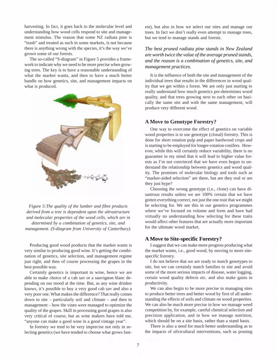
The so-called “S-diagram” in Figure 5 provides a frame-work to indicate why we need to be more precise when grow-ing trees. The key is to have a reasonable understanding ofwhat the market wants, and then to have a much betterhandle on how genetics, site, and management impacts onwhat is produced.
Figure 5:The quality of the lumber and fibre productsderived from a tree is dependent upon the ultrastructureand molecular properties of the wood cells, which are in
determined by a combination of genetics, site, andmanagement. (S-diagram from University of Canterbury).
Producing good wood products that the market wants isvery similar to producing good wine. It’s getting the combi-nation of genetics, site selection, and management regimejust right, and then of course processing the grapes in thebest possible way.
Certainly genetics is important to wine, hence we areable to make choice of a cab sav or a sauvignon blanc de-pending on our mood at the time. But, as any wine drinkerknows, it’s possible to buy a very good cab sav and also avery poor one. What makes the difference? That really comesdown to site – particularly soil and climate – and then tomanagement – how the vines were managed to optimize thequality of the grapes. Skill in processing good grapes is alsovery critical of course, but as wine makers have told me,“anyone can make a good wine in a good vintage year”.
In forestry we tend to be very imprecise not only in se-lecting genetics (we have tended to choose what grows fast-
est), but also in how we select our sites and manage ourtrees. In fact we don’t really even attempt to manage trees,but we tend to manage stands and forests.
The best pruned radiata pine stands in New Zealandare worth twice the value of the average pruned stands,and the reason is a combination of genetics, site, andmanagement practices.
It is the influence of both the site and management of theindividual trees that results in the differences in wood qual-ity that we get within a forest. We are only just starting toreally understand how much genetics pre-determines woodquality, and that trees growing next to each other on basi-cally the same site and with the same management, willproduce very different wood.
A Move to Genotype Forestry?One way to overcome the effect of genetics on variable
wood properties is to use genotype (clonal) forestry. This isdone for short rotation pulp and paper hardwood crops andis starting to be employed for longer-rotation conifers. How-ever, while this will certainly reduce variability, there is noguarantee in my mind that it will lead to higher value for-ests as I’m not convinced that we have even begun to un-derstand the relationship between genetics and wood qual-ity. The promises of molecular biology and tools such as“marker-aided selection” are there, but are they real or arethey just hype?
Choosing the wrong genotype (i.e., clone) can have di-sastrous results unless we are 100% certain that we havegotten everything correct, not just the one trait that we mightbe selecting for. We see this in our genetics programmeswhere we’ve focused on volume and form and have hadvirtually no understanding how selecting for these traitswould affect other features that are actually more importantfor the ultimate wood market.
A Move to Site-specific Forestry?I suggest that we can make more progress producing what
the market wants, i.e., good wood, by moving to more site-specific forestry.
I do not believe that we are ready to match genotypes tosite, but we can certainly match families to site and avoidsome of the more serious impacts of disease, water logging,certain wood quality defects etc. and also make gains inproductivity.
We can also begin to be more precise in managing sitesto produce better trees and better wood by first of all under-standing the effects of soils and climate on wood properties.We can also be much more precise in how we manage weedcompetition by, for example, careful chemical selection andprecision application, and in how we manage nutrition,which should be on a site basis, rather than a stand basis.
There is also a need for much better understanding as tothe impacts of silvicultural interventions, such as pruning

8
and thinning, shelter wood management etc on final woodquality. It appears that thinning may have a detrimental ef-fect on wood quality as it stimulates cell growth producingsteeper microfibril angles in the secondary cell walls lead-ing to reduced stiffness and stability. It also appears to beresponsible for increasing the amount of compression woodin a stem, possibly a response to greater wind movement inthe stand.
The Challenges are There!Forestry needs to focus on genetics, site, and forest man-
agement practices that will produce the best cells, which inturn will lead to the best wood. Sounds difficult? You bet itis! The alternative is “hit and miss forestry” which in manycases will lead to reasonable wood, in some cases be a totaldisaster, and if we are really lucky, will lead to really goodwood that the market can’t get enough of. Ironically, in NewZealand, the best wood that I know of has come from un-tended fire-regenerated stands of radiata pine that were har-vested at age 50.
Clearly there is a role for Precision Forestry to focus onthe underlying mechanisms that influence wood quality, asultimately, the market that we are targeting is not simplydemanding better forests, but it is demanding better wood orit will turn to substitutes.
CONCLUSIONS
This is a keynote paper so I will I wrap up with a coupleof salient lessons for Precision Forestry, and to do this I wantto go back to the point that I made at the start of this presen-tation:
Get the market to provide the lead. Technology drivenresearch is almost certainly doomed to fail.
Forestry research and technology developments have notbeen all that good at really understanding what the marketwants, but it has not necessarily been all our fault. Often weask for input, but we ask the wrong people or we ask thewrong question, and therefore we get the wrong answer. Orwe get the correct answer but we do not know enough toprovide the solution.
There is little doubt in my mind that what the market forindustrial forestry really wants is good wood. We have twoways to produce this good wood (1) find it in our existingforests, and (2) grow it in the first place.
To become more profitable we need to better understandwhat wood is, particularly what good wood is, what key prop-erties we need to measure in all stages of the value chain,and we need to understand what this means to the end user.We then need to develop tools that can help us to make theseassessments, but we have to be able to implement this tech-nology in such a way that the costs do not outweigh thebenefits.
Precision Forestry is required in both enhancing our abil-ity to “know what we’ve got” and also in understandinghow to “grow what the market wants” as we need researchand technology to understand what is in the forest, rightdown to the tree and log level, and we need to be muchmore precise matching genetics with site and silviculturalmanagement.
A greatly improved ability to know what we have got andto grow what the market wants will lead to greater profit-ability, provided we can do all this cost effectively.
ACKNOWLEDGEMENTS
Several people have provided input to this paper and Iparticularly thank Mike Andrews (IRL), Nicholas Coops(CSIRO), Peter Carter (CHH), Rick Walden (Smart Forests),and Brian Rawley.

9
Precision Technologies: Data Availability Past and Future
DANIEL L. SCHMOLDT AND ALAN J. THOMSON
Abstract:Current precision and information technologies portend a future filled with improved capabilities to managenatural resources with greater skill and understanding. Whereas practitioners have historically been data limited in theirmanagement activities, they now have increasing amounts of data and concomitant sophistication in data management, analy-sis, and decision tools. Expanding precision forestry technologies beyond traditional reliance on optics-based tools offers newopportunities for forest resource interrogation. However, as data become more immediate and information rich, traditionalviews of data availability may lose some relevance. Technical constraints are becoming less daunting and social and ethicalresponsibility and sensitivity are gaining prominence. Because data that might be deemed private or protected can be readilymoved and combined with other data, new concerns arise about who uses those data and how they use them. Capabilities builtinto newer analysis and decision support tools add further apprehension about privacy, accuracy, and accessibility. It does notrequire an extraordinary string of suppositions to imagine when regulation and legal decisions will promulgate certain safe-guards for data management and for software that handles data. Such restrictions could likely limit data availability incurrently unforeseen ways�counteracting, to some extent, technology-based advances in data availability. Still, irrespectiveof those possibilities, there are actions that natural resource professionals can take to lessen potential future restrictions on dataavailability. These include defining an �information space� for each precision technology, understanding language and knowl-edge flows, and planning for integrated systems and processes that holistically address information needs and uses.
INTRODUCTION
One of the prominent thrusts in agriculture, food, andnatural resource systems brings increasingly data-rich en-vironments into everyday use. Consumers, for example,might soon be able to scan a package of chicken in the re-frigerator and know exactly where the product was grownand processed, and what its current shelf-life is based onbacterial counts (Pathirana et al. 2000). In other cases, landmanagers might have real-time information about fuel loadsacross large geographic areas and simulate a large numberof hypothetical ignition scenarios based on 24-hour weatherforecasts. For sustainably grown timber, chain-of-custodyverification might rely on programmable identification de-vices (Simula et al. 2002) or chemical markers (q.v., com-panion article in this volume). Significant scientific andtechnical hurdles still remain and modifiers, such as �soon�and �large number,� are as yet undefined, but theoreticallythere is nothing to prevent either scenario from becomingreality, as feasibility is well established in both cases.
These data have the capacity to tell us more about theworld in which we live and work, and also can alter ourprofessional, and emotional, viewpoints of that world andhow we interact with it. In the examples above, we don�tcurrently give much thought to bacterial counts on the foodwe eat, although we wash food, such as chicken, as a matter
of habit. Once bacterial counts become part of our everydayinformation environment, though, we have to alter our con-sciousness to incorporate a more �dirty-aware� reality thataccepts our existence with microbes. Similarly, a fire man-ager, presented with large amounts of real-time data andthe capability to manipulate it, begins to see the landscapein a truly dynamic way. Now, decisions that he or she makescan be continually updated, or tweaked, as conditions change.Dynamic decision making creates increased confidence andcontrol for the manager, and minimizes the likelihood thatfield judgments will be questioned later. In fact, decisionsupport systems can track the decision making process forsubsequent audit.
Not only are more data available more often, but the timebetween measurement and application is shrinking rapidly.Whereas, at one time, field crews collected volumes of in-formation on the ground, recorded data with pencil and pa-per, and entered data into a computer back in the lab foranalysis, it is now possible to collect more spatially densedata much faster without going into the field, in some in-stances. The former process could take many days (or weeks)for relatively low resolution, while current technologies canpotentially reduce the time to just hours. Such just-in-timeinformation promises to bring decision making out frombehind the computer display and into the field (e.g., Clark2001). Here, then, managers and field operators can react

10
more quickly to changing conditions and have a broader,more informed picture of the resource being managed.
The advantages of high spatial and temporal data reso-lution for researchers and practitioners are obvious, so datavolume and rapidity have been primary scientific thrusts.However, we are entering a phase where subtle shifts areoccurring in what �data availability� means. While, thereare still many forest and forest product characteristics thatwe would like to measure and apply effectively, the techni-cal hurdles to doing so are not insurmountable. Those pre-vious science and technology limits to data availability maysoon be supplanted with other availability issues, such asdata-use policy and legal restrictions. Then, the issue be-comes not one of technically capable information technol-ogy (IT), but rather one of human-centric IT (Schmoldt2001). That is, how well these information tools fit withinorganizational and social cultures and how well they reflectthe users� ethical standards and expectations. Just becausephysical hurdles to data generation have been reduced doesnot mean that limitations on data application, based on ethi-cal concerns (Thomson and Schmoldt 2001), won�t beequally problematic.
In the sections that follow, we describe and illustrate thethree phases of precision technologies: basic research; en-gineering and technology development; and application andadoption. While most of the companion papers in this vol-ume deal with the latter two phases, the basic research phasecannot be completely ignored as it provides the scientificbasis for a technology�s capabilities and limitations. Thesecond issue addressed in this paper is the growing impor-tance of ethics in data collection and data use. There needsto be awareness by scientists and practitioners regardingethical standards of conduct and how they may dictate de-velopment and use of precision technologies.
PRECISION TECHNOLOGIES ANDCURRENT DATA AVAILABILITY
Introducing precision technologies into forest environ-ments is difficult for many reasons. First among those arescale issues. Our measurements must be possible at spatialscales in the millimeter range (nitrogen fixation in the soil)and also at the kilometer range (stand health, stand timbervolume). Events occurring over short time periods (e.g.,stomatal aperture) can be equally important to much longer-period phenomena (e.g., tree diameter growth). Second,there is tremendous variability over time and space whenrepeatedly measuring the same phenomenon. While thiscreates problems for taking consistent measurements, ourability to take frequent measurements helps us understandthat variability and better deal with it. Third, most of ourmeasurement modalities to date have relied on optics, whichlimits our observations to line-of-sight interrogation. Fourth,when taking measurements at finer spatial and temporalresolutions, we then often aggregate those data�in ourmodels and decision support systems�to, somewhat arbi-trary, coarser resolutions that suit anthropocentric needs,
which may not necessarily reflect biological realities. Theseand other issues have hindered data availability and appli-cation in the past and continue to present challenges forsome recent technologies. Still, as the papers in this vol-ume and cited works elsewhere demonstrate, forest scienceand management have increased access to data, collectionfrequency, and possess more powerful tools to manipulatethe data.
DefinitionBefore proceeding further, it is important to provide a
definition for the broad area of �precision technologies.�For most intents and purposes inherent in this paper, thefollowing should suffice:
Instrumentation, mechanization, and information tech-nologies that measure, record, process, analyze, man-age, or actuate multi-source data of high spatial and/or temporal resolution to enable information-basedmanagement practices or to support scientific discov-ery
This definition applies equally well to technologies thatmight be employed in agriculture, food, and environmentalsystems. While the definition doesn�t explicitly state so,biophysical, chemical, and engineering sciences provide thebases for these technologies, and information technologies(IT) often provide the application mode�although, in somecases practices are realized through the use of electro-me-chanical devices driven by microprocessors to actuate a re-sponse.
Basic ResearchTechnologies, i.e., tools, processes, and materials, ensue
from scientific discovery. Biophysical and chemical phe-nomena must first be understood before they can be trans-lated into useful devices and products. For example, theoptical properties of the atmosphere and plants, and thephysics of collecting light at great distances, must be knownbefore remote sensing makes sense. Similarly, the math-ematics of optimizing constrained production functions mustbe developed before solution algorithms can be written.These scientific developments provide fundamental knowl-edge for subsequent, possibly unforeseen, technologies.
In some research settings (e.g., a university or federallaboratory), end uses for science endeavors may not alwaysbe immediately apparent; neither are they necessarily of-fered as justification for the research. In other cases, a long-term goal (process, device, product) drives the science, witha proof-of-concept targeted as the immediate research ob-jective. The latter is more common in the private sector. Inrelatively few cases, however, do agriculture and forestryapplications drive research efforts related to precision tech-nologies. Once various precision technologies have beendeveloped, though, they often find ready application to re-

11
search and management of environmental and ecologicalsystems.
Engineering and Technology DevelopmentThe second phase of technology R&D involves applied
engineering, wherein scientific discoveries are turned intonew prototypes. These early stage technologies undergo test-ing and validation (either in the laboratory or in the field) toestablish their capabilities and limitations. It is at this pointwhere theoretical expectations and operational realities of-ten come into conflict, and solutions and compromises mustbe tried, tested, and resolved. Companion IT also needs tobe developed to make the new technologies operationallyeffective. The following paragraphs highlight several emerg-ing technologies�biosensing, micro-electromechanical sys-tems (MEMS), and sensor networks�that offer new andinnovative possibilities for precision forestry, and mitigatesome of the aforementioned difficulties working in forestenvironments.
In agriculture, food, and the environment, there is anever-increasing need to detect and measure minute quanti-ties of chemicals or microbes (e.g., biosecurity) occurringin both indoor and outdoor environments, and to do so al-most instantaneously (just-in-time information). Areas ofparticular interest include: food production and processing,agricultural products, pest management, surface and groundwater, soils, and air. Universities, federal laboratories, andother federal agencies have been developing biosensing tech-nologies to measure trace levels of biological and chemicalmaterials in real-time. Biosensing includes systems thatincorporate a variety of means, including electrical, mechani-cal, and photonic devices; biological materials (e.g., tissue,enzymes, nucleic acids, etc.); and chemical analysis to pro-duce detectable signals for the monitoring or identificationof biological phenomena. In a broader sense, the biosensingincludes any approach to detecting biological elements (ortheir chemical signatures) and the associated software orcomputer identification technologies (e.g., imaging) thatidentify biological characteristics. Because of the scale ofthese biological entities and the masses involved, new ad-vances in nanoscience and nanotechnology are proving use-ful.
MEMS integrate mechanical elements, sensors, actua-tors, and electronics on a common silicon platform. MEMSmake possible the realization of complete systems-on-a-chip.Sensors gather information from the environment by mea-suring mechanical, thermal, biological, chemical, optical,or magnetic phenomena. The electronics then process theinformation derived from the sensors, and through somedecision making capability direct the actuators to respondby moving, positioning, regulating, pumping, or filtering,thereby controlling the environment for some desired out-come or purpose. For many environmental applications,the actuation step will take the form of a wireless transmis-sion of data collected. These devices become particularlyuseful and powerful, however, when combined into networks
of communicating MEMS that can measure ecological vari-ables across an entire watershed, for example.
Convergence of the Internet, communications, and in-formation technologies with techniques for miniaturizationhas placed sensor network technology at the threshold of aperiod of major growth. Emerging technologies can de-crease the size, weight, and cost of sensors and sensor ar-rays by orders of magnitude, and increase their spatial andtemporal resolution and accuracy. Large numbers of sen-sors may be integrated into local- or wide-area systems toimprove performance and lifetime, and decrease life-cyclecosts. Communications networks provide rapid access toinformation and computing, eliminating the barriers of dis-tance and time for tracking endangered species, detectinginsects and pathogens, monitoring engineered structures andair and water quality. The coming years will likely see agrowing reliance on and need for more powerful sensor sys-tems, with increased performance and ecological function-ality.
Application, Adoption, and EconomicsEnabling technologies are converging with fields of ap-
plication, e.g., agriculture and forestry, to provide the mea-surement, storage, analysis, and decision-making needs ofproducers and processors. In many cases, though, innova-tions are frequently adopted in clusters; e.g., geneticallyimproved rice + fertilizer + insecticide. Here, there wouldbe little economic payback for applying costly agronomictreatments to low-yield rice, whereas the same treatmentsapplied to an improved rice strain would be more readilyadopted. The marriage of remote sensing and geographicinformation systems in forestry represents another clusterexample.
In agriculture, for example, techniques are currently be-ing developed to: (1) make precise measurements and con-tinuously monitor field and plant conditions through sen-sors and instruments, (2) organize large volumes of datawith spatially referenced databases, and (3) analyze and in-terpret that information using decision support systems thatmake economically favorable choices. The greatest �tech-nology push� has been in precision agriculture (PA)�whereinformation technologies provide, process, and analyzemultisource data of high spatial and temporal resolution forcrop production operations. Very similar technologies arebeing developed and promoted in the forestry arena for tim-ber production and ecological assessments.
Despite this �push,� the �pull� by the end-user commu-nity has been hesitant and weak, although most producersadmit that they will have to adopt PA technology eventu-ally. Currently, most see initial cost, uncertain economicreturns, and technology complexity as limiting factors. Theseempirical observations are consistent with Rogers�s theoryof innovation diffusion (Rogers 1995). Furthermore, in lightof recent and anticipated regulatory requirements for nutri-ent release and water/air quality, many producers feel thatthe environmental benefits of precision agriculture might

12
be the eventual driving force for technology adoption.Nevertheless, small- and medium-sized producers (both
in agriculture and forestry) have a distinct disadvantageversus large producers. In high-volume food and fiber pro-duction, economies of scale and narrow profit margins pro-vide an economic advantage to large producers. Further-more, large producers tend to have more education and areless technology averse than smaller producers. These char-acteristics of food and fiber production suggest that mosttechnological advances, including precision agriculture/for-estry, are not scale neutral. Furthermore, the factors limit-ing PA adoption, noted above, are also less problematic forlarger producers, giving them an additional competitiveadvantage.
One way for smaller producers to combat these competi-tion trends is to create, or reach into, unique markets wheretheir small size is an advantage. Value-added products ex-pand the profit margin for producers that are positioned toprovide enhanced value to consumers�which is more of-ten the case for small producers that deal with small quanti-ties of raw products and have more direct access to consum-ers. In addition, smaller producers can become more com-petitive in a technology world by mitigating the barriers toadoption. By spreading the initial cost of technology overmany producers and by sharing information about how touse the technology, smaller producers can obtain the adop-tion capabilities held by large producers. One way to ac-complish these tasks�that has been applied successfully bynonindustrial private forest (NIPF) landowners�is by form-ing landowner cooperatives (Stevens et al. 1999). Thesecooperatives are grass-roots activities (as distinct from ex-isting agricultural cooperative enterprises) wherein mem-bers share equipment, information, and market power toachieve some common goals for managing their operations.A nominal fee is usually charged members and the coopera-tive becomes a business entity.
In the eastern U.S., approximately 60% of timberlandresides in NIPF ownerships. Yet, only a small portion ofthat acreage is actively managed. In the past several de-cades, the number of forestland owners has been increas-ing, with more non-farm and absentee owners. This newcohort of owners also has diverse interests. As with agri-culture, precision forestry technologies are more readilyadopted for use on large ownerships (industrial and public),but if economic and educational hurdles can be overcome,smaller ownerships will also participate, either individuallyor in groups.
ETHICS AND FUTURE DATAAVAILABILITY
Ethics is the study of value concepts such as �good,��bad,� �right,� �wrong,� and �ought,� applied to actions inrelation to group norms and rules. Therefore, it deals withmany issues fundamental to practical decision-making. Pre-cision and information technologies lie at the heart of mod-ern decision making, including data/information storage and
manipulation, data availability, and �alternatives� formula-tion and selection. The ethical concerns addressed belowdo not include intentionally malicious behavior, such ascomputer crime, software theft, hacking, viruses, surveil-lance, and deliberate invasions of privacy, but rather ex-plores the subtler, yet important, impacts that data collec-tion and use can have on people and their social, cultural,corporate, and other institutions.
PrivacyImproper access to personal information is the issue that
�privacy� usually brings to mind. Any unauthorized accessto information about an individual or their property can bean invasion of privacy, just as unauthorized access to one�sproperty has traditionally been considered invasive. How-ever, even authorized access may lead to privacy concerns,when access to separate data sources is used to combineinformation (Mason, 1986). For example, one institutionmay record landowners� names and land ownerships, whileanother may be authorized to store land records and timbervalues for tax purposes. Individually, the databases are prop-erly authorized, but if the records are combined by a thirdparty, it may be possible for unauthorized parties to gainfinancial data about individual landowners. As environ-mental databases increase in size, complexity, and connec-tivity, projects that involve adding data fields or combiningdata or knowledge sources must consider the ethical impli-cations of those activities.
In recent years, a new privacy issue has arisen in the areaof geographic information systems (GISs), related to loca-tion protection. For example, many cultural sites on publiclands are protected either by law, policy, or regulation. Yet,entering site locations in a GIS may disclose locations forunethical use. One way around this problem is to define apolygon that contains a site or group of sites, without dis-closing exact point locations. A similar situation exists inrelation to biodiversity and rare species protection. Innova-tive approaches are required to facilitate resource monitor-ing and protection while simultaneously ensuring there isno loss of privacy resulting from location disclosure.
Current remote sensing technologies allow anyone to�look into� someone else�s property�assessing, without theowners knowledge or consent, timber or crop value that canbe used for insurance, bank loan, or taxation purposes. Evenwhen such data have been collected legitimately, there is noguarantee that adequate safeguards have been instituted toprotect unauthorized access and use. Future technologieswill create even greater opportunities for remote intrusion.
As more and more data become available on the Internet,unintended use has become a major problem. Web surferscan borrow data from different source or combine data in-appropriately from many sources either misusing it ormisattributing it. Similar concerns related to re-packagingof information may arise where public funding of govern-ment research places researcher and research informationin the public domain. Enterprising organizations, then, turn

13
that public-domain information into company revenue.While not illegal, it may be unethical if there is minimalvalue added to the publicly available, and public-funded,information.
AccuracyA software developer�s ability to know and predict all
states (especially error states) is low for complex systems.At first sight, it would appear that a software developer wouldbe ethically bound to correct all system errors. However,dealing with errors can raise ethical dilemmas: 15-20% ofattempts to remove program errors introduce one or morenew errors. For programs with more than 100,000 lines ofcode, the chance of introducing a severe error when correct-ing an original error is so large that it may be better to re-tain and work around the original error rather than try tocorrect it (Forester and Morrison, 1994). The frequency ofdisclaimers, software updates and patches, as well as thelack of substance to software warranties, result from soft-ware developers� recognition of this problem. The ultimateeffect is larger and more complex software, whose size isless related to functional capability than it is related to soft-ware age and the battery of �fixes� that it has received overtime. Similar ethical conflicts arise with decision supporttools, where modelers and developers realize that a model�sresults can only be broad approximations in many cases.
Another problem related to accuracy is determining whichspecific information to use. For example, it is often diffi-cult to select appropriate socio-economic or biological indi-cators or to choose among predictive models. An indicatoris something that points to an outcome or condition, andshows how well a system is working in relation to that out-come or condition. For example, in a forest simulationmodel, tree diameter at breast height (dbh) is a key indica-tor of treatment effects. However, there may be a range ofpotential equations available to predict dbh. One equationmay simply predict dbh from tree height, while another equa-tion may predict it from both height and crown width. Theequation selected will have different consequences with re-gard to accuracy, precision, data costs, and suitability forextrapolation. This choice relates, in turn, to precision andbias in the estimators used. Requirements of the intendeduser and usage should guide the choice.
When a social or economic indicator is being used, ethi-cal considerations are even more significant. If the indica-tor misrepresents a value set, then it cannot be consideredaccurate. Indicators have long been used in predictive sys-tems (Holling, 1978): such indicators must be relevant, un-derstandable, reliable, and timely. In natural resource dis-ciplines, with their current emphasis on sustainability, indi-cators must have additional characteristics. Sustainabilityindicators must include community carrying capacity; theymust highlight the links between economic, social and en-vironmental well-being; they must be usable by the peoplein the community; they must focus on a long range view;and they must measure local sustainability that is not at the
expense of global sustainability (Hart, 1999). Scale is a keydeterminant of indicator usefulness: some indicators thatare useful at the household or community level are difficultto measure at the regional level, and some regional indica-tors may have little meaning at the community or house-hold level. Because indicators compress so much ecologi-cal, economic, or social information into a single variableor set of variables, it is especially crucial that they are cho-sen, measured, and interpreted carefully.
Accuracy may also be influenced by the sequence in whichoperations are applied. In theory, error limits of predictionsshould be supplied; however, while error limits of individualequations may be known, it is rare that models actually com-pute the consequences of combining multiple equations.Mowrer (2000) examines error propagation in simulationmodels and presents several approaches (Monte Carlo simu-lation and Taylor series expansion) to project errors. Thishas become an active research topic recently (q.v., Mowrer2000), as several models are typically used in combinationto predict future conditions.
Key language and terminology used to frame a questioncan significantly influence the applicability of data or infor-mation. This is true for any information system in whichthe user is forced to converse using concepts unfamiliar tothem. This cultural mismatch is of special significance instudies of Native peoples, where the interview subject mayhave concepts and values very different from those of thequestioner. For example, the term �forest� is a key conceptfor resource management, but certain Native peoples haveno concept for forest in their culture or any word in theirnative tongue. Instead, they have a more holistic view ofthe land that includes trees, plants, animals, and people(Thomson, 2000). Once such basic cultural differences areidentified, the important challenge becomes one of under-standing the ramifications of those differences, how theyaffect data needs and data use.
Statistics, images, graphs, and maps are all methods ofsummarizing, presenting, or filtering information. Ethicaldecisions behind the selection and transformation of mate-rial can significantly affect the accuracy with which recipi-ents may perceive a situation. When a situation is highlycharged or contentious, objectivity in portraying informa-tion becomes critically important.
Certain decision support software may increase consid-erably the power of users to make or influence decisionsthat were formerly beyond the limits of their knowledge andexperience. For example, upper management may gain di-rect access to lower level data and information summaries.This helps bypass intervening distortions, resulting in moreaccurate perceptions. Greater accuracy is dependent, how-ever, on support software that has itself been developed withappropriate ethical considerations and higher level manag-ers must be willing and able to use the software to achievedistortion-free information sharing. This type of situationhas been a bane of statisticians for years. Very powerfulsoftware packages have allowed users to perform all man-ner of inappropriate statistical tests on data without full

14
knowledge of what they are doing. While current statisticalsoftware manuals contain a great deal of information re-garding model specification and assumptions, they cannotreplace a well-founded understanding of basic statistics bythe experimenter.
AccessibilityAppropriate access to data and software has both techni-
cal and intellectual components. To make use of software, aperson must have access to the required hardware and soft-ware technology, must be able to provide any required in-put, and must be able to comprehend the information pre-sented. For example, for a Web-based system, users musthave reliable connections to the Internet and sufficient band-width. Each end-users must also have a browser compat-ible with the material sent to it (including such things asthe appropriate Java classes for use with applets) and anyhelper applications or browser plug-ins for viewing andhearing content. If an intended audience lives in a develop-ing country, or in a remote area, such technological issuesmay be critical. For this reason, when software or a database is developed, its implementation should be part of anintegrated process that includes the full range of affectedindividuals. This may include specifying duties for a suiteof �actors� such as technology transfer officers or field per-sonnel.
Accessibility is also limited if results are presented inap-propriately. For example, data may be aggregated at a fixedscale that may have limited value for many users. In othercases, language and concepts beyond the end-user�s under-standing or vernacular might render a decision support sys-tem useless for a large audience segment. While it is nei-ther practical nor possible to accommodate all who might�stumble onto� data or software, primary target audiencesneed to be defined and understood.
In a digitally networked age, the ability to connect sys-tems, databases and information-rich environments becomesmore possible but also more problematic. The goal of seam-less, transparent, and �user-friendly� information accessmakes interoperability a required attribute of databases, sys-tems, and vocabularies. This desired attribute requires bothtechnical and human dimensions to enhance interoperabilitywithin regional, national, and global forest information sys-tems. Interoperability ensures that systems, procedures, andcultures of an organization are managed in such a way as tomaximize opportunities for exchange and re-use of infor-mation, whether internally or externally. Because end-us-ers of data are not necessarily local or regional and becauselarge-scale forest assessments are becoming more impor-tant (e.g., carbon management), standards and protocols forforest data are looming on the horizon.
SOME STEPS TO TAKE
Once basic, scientific principles have been demonstrated,the biggest hurdles to realizing an operational technology
lie in the adoption phase. Even though engineering andtechnology development aspects may seem daunting andtime-consuming, it is the economic, cultural, and educa-tional issues that often doom or advance technology use.This suggests that more thought needs to be given to thatfinal phase. Some issues that need to be addressed in thedevelopment phase (or pre-diffusion) are: intended users,intended uses, workflow changes, education and training,economics, associated IT changes or requirements, favor-able or unfavorable regulations, early adopters, commercial-ization entities, and user communities. All these factorscan impact if, and how, a new technology is accepted andused.
Privacy has long been considered an inherent right ofindividuals in a �free� society. Initially, this involved pro-tection of the individual from unwanted or unwarranted in-vasion of their physical space. More recently, privacy hasbeen extended into an individual�s information space, as well.For precision technologies currently under development innatural resource and agricultural domains, more real threatsare likely to arise from unintentional and unforeseen infor-mation breaches than from any intentional conspiracy. Theseoccur when information sources are combined or used inunintended ways. As long as information about individualsexists and is accessible by others, individual privacy canpotentially be compromised. During technology develop-ment, designers need to be cognizant of users, co-develop-ers, publics, cultures, special interest groups, commercialenterprises, governments, and other groups that might beaffected directly or indirectly by their products. Designersmust also consider the information their technology uses orgenerates, and the decision-making landscape that it affectsor creates.
Use of appropriate language is at the heart of many accu-racy issues. Even if an information system does not esti-mate the accuracy of results explicitly, it is important to makeend-users aware of the variability in potential outcomes, andthe assumptions and trade-offs that have contributed to it.Similarly, non-textual rendering of system outputs shouldbe designed to address accuracy concerns in the flow ofknowledge. It is also essential to address the way in whichknowledge flows through organizational hierarchies, and toensure its appropriate use at different organizational levels.
As with accuracy issues, language lies at the heart of manyaccessibility issues. Information delivery must be geared toconcepts appropriate to the intended audience, and infor-mation overload avoided, as knowledge can be inaccessibleif the recipient is swamped with information. Limitationsof technical accessibility by some groups may require devel-oping an integrated range of systems and processes to en-sure access by all stakeholders in a decision environment.
While there will always be some ethical culpability onthe individual�s part, much responsibility still rests with or-ganizations to institute standards of ethical conduct that cre-ate an atmosphere of social morality for their employees andmembers. Self regulation is always more readily acceptedand effective than regulation from governmental institutions,

15
which may not always fully understand the issues involved.By thinking in advance about ethical issues that may even-tually impinge on data availability, organization might al-leviate potential future restrictions or reduce their impacts.
LITERATURE CITED
Clark, N. 2001. Applications of an automated stemmeasurer for precision forestry. Pages 93-98 in D.Briggs (ed.) Proceedings of the First InternationalPrecision Forestry Cooperative Symposium, Collegeof Forest Resource, Univ. of Washington, Seattle WA.
Forester, T., and P. Morrison. 1994. Computer Ethics.MIT Press, Cambridge, Mass.
Hart, M. 1999. Guide to sustainable communityindicators. Hart Environmental Data, North Andover,MA.
Holling, C.S. 1978. Adaptive environmental assessmentand monitoring. John Wiley & Sons, Chichester.
Mason, R.O. 1986. Four ethical issues of the informationage. MIS Quarterly 10(1): 5- 12.
Mowrer, T. 2000. Uncertainty in natural resourcedecision support systems: Sources, interpretation, andimportance. Computers and Electronics inAgriculture 27(1-3): 139-154.
Pathirana, S. T., J. Barbaree, B. A. Chin, M. G. Hartell,W. C. Neely, and V. Vodyanoy. 2000. Rapid and
sensitive biosensor for Salmonella. Biosensors andBioelectroncis 15: 135-141.
Rogers, E. M. 1995. Diffusion of Innovations, FourthEdition. The Free Press, New York.
Schmoldt, D. L. 2001. Precision agriculture andinformation technology. Computers and Electronicsin Agriculture 30(1/3): 5-7.
Simula, M., J. Lounasvuori, J. Löytömäki, M. Rytkönen.2002. Implications of forest certification forinformation management systems of forestryorganizations. Forest information technology 2002international congress and exhibition. 6 pp.www.indufor.fi/documents%26reports/pdf-files/article07.pdf
Stevens, T. H., D. Dennis, D. Kittredge and M.Richenbach. 1999. Attitudes and preferences towardcooperative agreements for management of privateforestlands in the Northeastern United States. Journalof Environmental Management 55:81-90.
Thomson, A.J. 2000. Elicitation and representation ofTraditional Ecological Knowledge, for use in forestmanagement. Computers and Electronics inAgriculture 27(1-3): 155-165.
Thomson, A. J., and D. L. Schmoldt. 2001. Ethics incomputer software design and development.Computers and Electronics in Agriculture 30(1/3): 85-102.

16

17
Multidata and Opti-Grade: Two Innovative Solutions toBetter Manage Forestry Operations
PIERRE TURCOTTE
Abstract: You can�t manage what you don�t measure. Two novel systems recently developed by FERIC address this di-lemma: MultiDAT allows forest contractors to maximize their machine uptime and Opti-Grade provides an integrated pack-age for optimal forest road management.
MultiDAT is a multi-purpose datalogger for forestry managers. MultiDAT can record machine functions, machine move-ment, machine location and collect operator feedback. The associated software can analyze the data and produce reports onwhich optimal decisions can be based. The MultiDAT is designed specifically for heavy equipment operating in areas wherecommunication systems are not existent or very expensive.
Opti-Grade is a road management system to help focus grading or re-profiling activities where they will have the greatestimpact on the road condition for the money invested. Opti-Grade is used to collect important information on the condition ofthe road network on a regular basis, using equipment installed on a log truck. This data is used to schedule maintenanceactivities. This new concept is considerably more efficient than the traditional concept of grading whole road segments.
CONTEXT OF THESE RESEARCHPROJECTS
The two projects described here were done at the ForestEngineering Research Institute of Canada (FERIC) duringthe last 3 years. FERIC is a private research organizationthat has served the Canadian forest industry for more than25 years, and started recruiting new members in the UnitedStates this year. Projects are determined for the most part bythe industrial members and orientations are reviewed on ayearly basis, which accounts for very practical, results-ori-ented research. FERIC programs cover all aspects of forestoperations, from silviculture to harvesting and transporta-tion, but because of the general theme of this symposium,two projects closely related to precision forestry will be pre-sented.
Origin of the MultiDAT development
Foresters have been using paper chart recorders for morethan 30 years to track the utilization of their equipment.They are still in use today in many operations. This crudesystem has many limitations. The precision of the record-ing is usually only about 5 to 10 minutes, the charts geteasily damaged and the operators can falsify the recordings.When members asked FERIC to develop or find a simpleelectronic device, we first tried to adapt a recorder designedfor trucks. We realized that the truck paradigm does not
apply for forest machines, because almost all reporting ontruck systems are based on distance and not on time. Wehad no choice but to develop a complete system.
Why measure machine utilization?
Improving machine utilization has a major impact onthe profits of the contractors who conduct a large portion offorest operations. The documentation of the daily operat-ing hours and the nature of all delays is the first step indetermining the possible avenues of improvement.
To illustrate the importance of machine utilization intoday�s context, let�s analyze the effect of improving the uti-lization of a typical harvester operating in Eastern Canada.
This example is based on the following assumptions (all$ in Canadian funds):
Cost of the harvester: $480,000Useful life: 5 yearsResale value: $144,000Insurance: $24,000 per yearRepairs and maintenance: $96,000 per yearInterest rate: 8%Operation schedule: 4,000 hours per yearCost of operator: $30 per hourCost of fuel: $18.40 per hourProductivity: 40 cubic metres per productive
machine hourRevenue: $3.00 per cubic metre

18
These assumptions do not necessarily represent an aver-age, but are only typical values used to represent the rela-tive importance of the costs. Figure 1 shows the variation ofnet profit that the owner of this harvester would make if theutilization rate would vary from 70% to 85%. It is easy tosee that the owner would make 7 times more profit if themachine is used at 85% instead of 70%.
Figure 1: Profit VS Utilization
DESCRIPTION OF THE MULTIDAT
The MultiDAT has the following characteristics:
- 4 channels programmable as timers, counters, orfrequency meters
- Internal motion sensor sensitive to low frequencyvibrations
- Optional WAAS GPS receiver- Typical autonomy: 2 to 6 weeks
The MultiDAT comes in two versions. The regular unithas an operator interface that allows easy input of operatornumber, work codes and delay codes. The MultiDAT Juniorhas all the characteristics of the regular unit without theoperator interface.
The recordings are downloaded and transferred to a PCusing a PDA, either a Palm OS or Windows CE device. Theaverage size of a MultiDAT download file is 50 Kb for oneweek of recording, which means that a data shuttle can eas-ily download many MultiDATs before being synchronizedwith a PC. The MultiDAT is built for the harsh conditionsin which heavy equipment operates. It is enclosed in a heavyaluminum casing, all components can withstand tempera-tures varying from -40 to 85 deg. C, and the supply voltagecan be from 10 to 28 volts.
Almost everything on the MultiDAT is configurable. Thenumber of sensor channels used, the threshold of the mo-tion sensor, the number of work and delay codes used andtheir meaning. Even the report format is fully configurable.
EXAMPLES OF USE
Weyerhaeuser Company Limited in Dryden, Ontario haveused 20 MultiDAT Junior to support a productivity improve-ment program in partnership with two major contractors.For more than a year, they followed a fleet of harvestingequipment, tracking downtime and finding solutions to re-duce its impact and occurrence. In some cases, the utiliza-tion of skidders improved from 50% to more than 80%. Theyused very simple configurations and connection methods,relying mostly on the motion sensor to determine machineactivity.
In Quebec, Gestion Remabec inc., a large contractor, isusing the MultiDAT on harvesters for two purposes. First,they monitor the utilization using the sensors, but they alsouse the GPS option and record the travel path of the ma-chine. When harvesting is completed in a block, they pro-vide their clients with a map showing the area harvested.This map is used to make sure that the operator was not inviolation when working close to the block boundaries.
The Saskatchewan Department of Transportation is us-ing the MultiDAT exclusively on graders. The MultiDATPC software has a speed analysis function that can be usedto determine approximately the sections of road that weregraded. In general, grader operators drive at a higher speedwhen they are traveling than when they are grading.
In the Atlantic Provinces, J.D.Irving Ltd. is graduallyimplementing the MultiDAT on all their contractors� equip-ment. The company provided the MultiDATs free of chargeto the contractors in exchange for their commitment to usethem and provide utilization reports.
In Windsor, Quebec, Domtar Inc. used a GPS- equippedMultiDAT in 2002 to track site- preparation equipment. Al-though at the time, the MultiDATs were using Garmin25GPS receivers with no WAAS capabilities, the results werevery good; most of the time within 1% of the area measuredby walking the block with a GPS receiver after the workwas completed. In 2003, they are using GPS-equippedMultiDATs on all of their site-preparation equipment. TheseMultiDATs now use the CSI SX-1 WAAS receiver, with sub-metre accuracy.
In 2002, the MultiDAT was also used by FERIC research-ers to evaluate the productivity of new models of Tigercatequipment in a Tembec Industries Inc. harvesting operationin Ontario. The operations were followed in detail for morethan 3 months, and the MultiDAT recordings were down-loaded each week by the supervisors and transferred toFERIC for analysis.
MultiDAT has been used successfully on harvesters, fellerbunchers, skidders, forwarders, bulldozers, excavators, grad-ers, sand trucks, mobile chippers, and loaders.
STRONG AND WEAK POINTS
The strongest point of the MultiDAT is its versatility.The recorder itself and the PC software can be configured

19
in a very simple way to simply record the working hours ofa bulldozer for example. They can also be configured in amore complex way to identify the harvesting time, idle timeand traveling time of a harvester in a given block.
A second strong point is the ease of use for the operator.As shown in Figure 2, the operator interface is very simple,there is no scroll down menus and all the activity and stopcodes are visible at a glance.
Figure 2: Operator interface
The first weak point of the MultiDAT is, paradoxically,its versatility, which sometimes makes the initial configu-ration laborious. Many of the first MultiDAT users neededsupport to configure the recorders and the reports, simplybecause they did not know what was the most effective con-figuration. With later versions of the software, we providedmore configuration templates and we are using the experi-ence of the first users to determine the configurations thatgive the best results. We are thus transforming the MultiDATfrom a simple activity recorder into a methodology to im-prove machine utilization.
The second weak point is the data shuttle. Although sincethe inception of the MultiDAT, users could choose betweena $150 consumer PDA and a $1500 rugged field computer,so far only consumer PDAs have been used as shuttles. Bat-teries have given users the most problems. The average useris not aware that a Palm computer is never turned off, evenwhen the display is switched off, and that it wears out itsbatteries over a period of 3 to 6 weeks even when sitting ina drawer. That is, until users lose their first data files andhave to re-install the shuttle program in the PDA. In 2003,we are introducing shuttles using Windows CE, and thatshould improve the shuttle performance drastically. The dataand shuttle programs can now be backed up in flash memory,and the PC communication is much simpler, using the USBcable that is provided with the PDA. Still, keeping ahead ofproduct development for the shuttle is not an easy task. Wesaw product lives of 9 months with the Palm PDAs and wehope that the Windows CE devices will stay on the marketlonger.
CURRENT DEVELOPMENT PROJECTS
Current projects include the development of geo-fencingfor the MultiDAT. Some analysis software for truckdataloggers give the user the possibility of defining polygonboundaries called geo-fences. The GPS position recordingscan then be analyzed in relation to these geo-fences, andadditional information can be derived such as the time spentin a given region, or the number of times that a truck passeda given location.
With the MultiDAT, the geo-fences are pre-determined,and the recorder can be configured to record only the timeof entry into and exit out of each polygon. This method re-quires much less memory than recording all the GPS posi-tions and does not require intensive computer processingafter the data is downloaded.
The first application that we envision for this develop-ment is the management of wood flow in the mill yard. Bytracking the passage of loaders between zones, we will at-tempt to determine the volume of wood that is moved be-tween various sections of the yard and better balance thetasks assigned to each loader.
Finally, we are working on the development of a bladecontact sensor for graders. This sensor will provide a moreaccurate map of the road sections that were graded.
Since February 2003, the MultiDAT is fabricated anddistributed under license by Geneq (www.geneq.com).
THE OPTI-GRADE SYSTEM
During the last two years, FERIC also worked on thedevelopment of another precision forestry tool, the Opti-Grade system.
Opti-Grade follows two simple principles:
1- Measuring road roughness lets you identifysections that need grading�and those thatdon�t.
2- Using graders efficiently means grading only thesections that need it, and travelling at full speedover sections that don�t.
HOW DOES IT WORK?
Before the Opti-Grade system is used, the road network(all km markers, bridges, intersections, etc.) must be sur-veyed using GPS. Then, the recording equipment is installedin one of the trucks that regularly travel the road beingmonitored.
While a sensor continuously measures the roughness ofthe road, a GPS receiver determines the time and positionof each measurement. A datalogger stores the road rough-ness values, plus the position and recording time of eachvalue.

20
When the truck enters the mill yard, the recordings aretransferred by spread spectrum radio to an office computer.The Opti-Grade software then analyzes the roughness andGPS data to determine which road sections require gradingand calculates the travel speed of the truck on each section.The user can display a map showing the road roughness fordifferent sections as seen in Figure 3. Because the kilometremarkers of the road have been surveyed when the Opti-Gradesystem was set-up, the map can show the correspondencebetween those markers and the sections to be graded.
The software then prepares an optimized grading sched-ule based on three criteria:
1- a roughness level above a trigger threshold2- the minimum length of road to treat3- the minimum distance between sections to be
treated
The next morning, the grader operator uses that sched-ule to determine the sections to grade. Figure 4 shows a
Figure 4: Grading schedule
typical grading schedule. On this example, the operator onlyneeds to grade 22 kilometres out of the total 63 kilometresof the road, thus saving 65% of the normal grading time.
TYPICAL RESULTS
The Opti-Grade system is in use at more than 20 loca-tions in Canada. The users generally attempt to maintainthe same road quality while reducing grading cost. Experi-ence with the system has shown that the grading costs canbe reduced by up to 30% on average. For a company main-taining 400 km of roads, this can represent an annual sav-ing of more than $70,000, or a payback of a few months.
The companies using Opti-Grade are also very interestedwith the speed and time recordings provided by the system.They use this information to establish more precise cycletimes and thus fairer trucking rates.
Finally, analysis of Opti-Grade data helps to identify roadsegments that need constant maintenance. Investments inroad improvements can thus be justified more easily.
Figure 3: Map of road roughness

21
A Test of the Applanix POS LS Inertial Positioning System forthe Collection of Terrestrial Coordinates Under a Heavy
Forest Canopy
STEPHEN E. REUTEBUCH, WARD W. CARSON, AND KAMAL M. AHMED
Abstract: The Applanix POS LS backpack-mounted inertial land positioning/navigation system was used to collect terres-trial coordinates along a previously surveyed closed traverse. A total station surveying instrument was used to establish 26ground-level stakes along a 1 mile traverse under the dense canopy of a 70 year-old conifer forest in the Capitol State Forestnear Olympia, Washington. The Applanix POS LS was initialized at a fixed monument and carried through the forest alongthe traverse 12 times. Coordinate readings were collected continuously both at the survey posts and between posts. Both thesystem�s location accuracy and its potential for developing terrain profiles were evaluated. The system�s average real-timeposition accuracy was 2.3 ft (1.6 ft Stdev., 7.0 ft max.) and average post-processed accuracy was 1.4 ft (0.9 ft Stdev., 4.0 ftmax.), measured at each survey stake. An earlier study provided a 5 by 5-foot, gridded digital terrain model (DEM) derivedfrom high-density LIDAR data. Profiles generated from the LIDAR DEM were compared with profiles measured by the POSLS system. Average post-processed elevation difference along the profiles was 0.7 ft (1.0 ft Stdev., 4.5 ft max.).
INTRODUCTION
Applanix* [a Canadian company that has developed anumber of position and orientation systems (POS) basedupon inertial navigation systems (INS)] has recently pro-duced a system designed for land surveyors (Gillet et al.,2001). The POS LS system combines an INS [with itsembedded inertial measurement unit (IMU)], a roving glo-bal position system (GPS) unit, and a computer dataloggerinto a backpack system weighing about 40 pounds.
When utilizing the internal roving GPS receiver, the POSLS unit is intended to be used with a user-supplied real-time kinematic (RTK) GPS basestation that would providethe necessary carrier-phase ambiguity resolution, therebysupplying frequent, accurate coordinate updates to the INSsystem.
Applanix has established with other products, such asthe airborne POS AV system, that uninterrupted,postprocessed data from such a GPS/INS system can de-liver coordi-nates accurate in the range of inches. How-ever, Applanix anticipates that the land sur-veyor will onoccasion lose the GPS signal�for example, under a forestcanopy. The question then becomes: what accuracy canone expect from the POS LS system under these less thanoptimal GPS conditions?
* Use of trade or firm names in this publication is for reader information and does not imply endorsement by the U.S. Department of Agriculture of any product orservice.
In general, the INS and GPS components of an integratedPOS system complement each other�s strengths or, rather,compensate for weaknesses (Farrel and Barth, 1999). Withan initial coordinate fix and the acceleration vectors sensedby the IMU, an INS can integrate the velocity vectors andcompute the coordinate path as the unit moves; however,positional accuracy is eroded as instrument drift accumu-lates over time.
In contrast, GPS errors are not accumulated over time but,rather, GPS accuracy is maintained by regular, frequent, in-dependent readings. In short, an INS can measure directionand distance in the short run, but benefits greatly by regularcoordinate updates from the GPS to correct drift. The GPSis good over the long run, and benefits greatly from the INSdata acquired between GPS recordings.
As a surveying device operating in the open under a goodconstellation of GPS satellites, the POS LS will deliver coor-dinates accurate in the range of RTK GPS capabilities�ap-proximately 4 inches or better. However, when the GPS sig-nal is blocked, under a forest canopy for example, it revertsto sole dependence upon its INS, and, the error due to driftwill begin to diminish the position accuracy over time.
The effect of INS drift can be mitigated in two ways: 1) byposition updates�the obvious technique of re-initializing thesystem position with either GPS readings or by periodically

22
Figure 1: Applanix POS LS system is held steady inone position during a ZUPT.
re-visiting known points; or, 2) by zero velocity updates(ZUPTs)�a method used to obtain a velocity re-initializa-tion that has been incorporated into the POS LS instrument.If the INS unit is momentarily held still (at zero velocity),
the POS LS software can re-initialize the velocity vector tozero and thereby correct for accumulated velocity drift. InFigure 1, note how the operator uses a blue staff to help holdthe system steady during a ZUPT.
The desired time interval between ZUPTs is user defined;however, longer intervals increase position errors. Whenunder dense canopy (when the position is being updated us-ing only INS data) an audible announcement and text dis-play on the POS LS datalogger informs the user when it istime for either a ZUPT or position fix (acquiring a new GPSlocation in a clearing or moving to a known point). A ZUPTis also automatically initiated when the INS unit senses thatit is stationary. Additionally, the operator can manually ini-tiate a ZUPT at any time.
At the end of a survey, the location of the POS LS unit isaccurately established by either acquiring a high-accuracyGPS position in an opening, or by returning to a known ref-erence point. This allows the traverse data to be post-pro-cessed to derive more accurate, adjusted positions.
OBJECTIVES
It is well established that GPS is not reliable for surveysunder or near a forest canopy due to obstruction of GPS sat-ellite signals or signal multi-path problems (Darche, 1998;
Elosegui et al., 1995; Firth and Brownlie, 1998; Lachapelleand Henriksen, 1995). The POS LS unit offers an alterna-tive method for collecting geographic positions under suchadverse conditions. The accuracy of the POS LS system is afunction of the frequency of coordinate updates�from ei-ther a GPS signal or the input of known coordinates�andthe frequency of ZUPTs.
In this initial study, we only examined POS LS coordi-nate accuracy at a fixed ZUPT interval (nominally 30 sec-onds) under forest canopy. We examined both real-timeaccuracy of the POS LS unit and accuracy obtained by post-processing POS LS positions after each trial run (traverse)was closed on a known point.
It is also important to note that in our test, because ofextremely dense canopy conditions, GPS positions were notcollected with the POS LS unit. Instead, the unit was ini-tialized over previously surveyed reference points for eachtrial run. These reference points were located in a clearcutadjacent to the forested area. In practice, the GPS unit inthe POS LS could have been used in the clearcut to accu-rately establish the initial location of the instrument beforeentering and after emerging from dense forest.
METHODS
On May 21-22, 2002, Applanix technical personnelbrought a POS LS instrument to the Capitol State Forestnear Olympia, Washington for trials under the canopy inour forest test site. The forest is managed by the Washing-ton State Department of Natural Resources. Our test sitehas a mix of forest canopy cover, ranging from 70-year-oldconifer cover to recently clearcut areas. It has been the siteof several other geomatic (Reutebuch et al., 2003) and for-estry (Curtis, et al., in press) research trials.
LIDAR data sets were collected in 1998, 1999, and 2000,and a high resolution, 5x5-ft gridded digital terrain model(DTM) was produced from the 1999 data. Additionally, aclosed traverse, total station survey was performed under afull-canopy segment of the forest and the staked-points wereavailable for use in assessing the accuracy of the POS LSsystem. Our test of the POS LS unit was build primarilyaround re-visiting these surveyed points. A comparison wasalso conducted between POS LS position elevations and el-evations interpolated from the LIDAR-based DTM.
The closed traverse survey loop consisted of 26 points,marked with 2x2-inch wooden pegs driven into the forestfloor down to ground level. Two reference points, markedas 1A and 2A, were established from local HARN pointswith a carrier-phase, survey-grade GPS instrument. Otherpoints, spaced around a roughly circular traverse of approxi-mately 1 mile in length, were established with a TopconITS-1 total station survey instrument. Closure calculationsshowed the horizontal accuracy was 1:2840 and vertical clo-sure was 1.1 inches. After adjustment, the horizontal andvertical accuracy of the ground points were within 6 inchesand 1 inch, respectively.

23
Sets of POS LS coordinate data were collected continu-ously at a once per second rate over the course of the closedtraverse. Most of the readings were collected while in tran-sit between survey stakes; however, specific blocks of re-cordings were noted. These blocks were:
1) Alignment Fix: The operator set the backpackat reference point 1A to establish the initialposition and allow the system to determine truenorth.
2) Point Visitation: After alignment, with the in-strument on his back, the operator located him-self over a survey point (i.e., the 2x2-inch peg)and held himself steady enough to record sev-eral seconds of consistent coordinate readings.(Note: A vertical bias of 3.0 ft was subtractedduring data reduction to account for the heightof the unit�s recording point above the peg inthese standing positions).
3) ZUPTs: When alerted by the unit, the opera-tor stopped with the instrument still on hisback and held steady�at zero velocity�forseveral seconds.
4) Position Fix: The operator took the instrumentoff his back and set it on a survey stake forseveral seconds and commanded the systemto update position. (A survey stake approxi-mately midway through our closed traverse,was used as this intermediate point).
Coordinate and orientation data were collected continu-ously while following the closed traverse through severalloops. We divided this continuous stream of data into runs.Each run was initiated at a Position Fix and terminated laterat another Position Fix with Position Visitations and ZUPTupdates registered in between. Twelve runs were made dur-ing our test.
Data Management and ReductionDuring the two days of POS LS field testing, our opera-
tor (Joel Gillet from Applanix) tramped through our rough,forested terrain for a total of nearly 6 miles while stoppingat 175 known positions to either re-initialize the instrumentor record points as coordinate data. The task took over tenhours and the instrument, recording constantly at the rateof one coordinate set per second, collected nearly 40,000points.
From these data, Applanix delivered to us two types ofcoordinate files: 1) the �real-time� files that held lists of fieldrecorded �time, X, Y, Z� data, and 2) the �post-processed�files of the same data after adjustment. All coordinate datahad been transformed into the State Plane System, Wash-ington South Zone, NAD83, Mean Sea Level Elevation,NAVD88 datum, International Feet.
The �real-time� and �post-processed� data are purposelydistinguished in this report. The �real-time� data are those
that the operator would see on the datalogger coordinate read-out in the field as the POS LS is being carried in the forest.Each real-time data file begins with an initial Position Fix.The data from that initial point forward were computed bydead reckoning based upon the IMU readings and INS pro-jections augmented by the operational ZUPTs.
The �post-processed� data result from the same record-ings, but they depend upon a final Position Fix at the end ofeach run. An algorithm implemented in the ApplanixPOSPac software is designed to adjust to zero the error atthis fixed terminus and to minimize the error over each run.Both these data sets were examined in this study to quantifythe real-time point-by-point accuracy that one can expect inthe field, and the accuracy obtainable from further POSPacrefinements accomplished after data collection in the office.
RESULTS
Both the �real-time� and �post-processed� data from thistest are presented similarly. Tables 1 and 2 summarize thebasic results, including average of coordinate errors at allsurvey stakes, standard deviation, and maximum error asso-ciated with each run. Plots display error accumulation overtime for �real-time� and �post-processed� data and differencesbetween them (fig. 2 and 3).
Run descriptions
A �run� is defined by an initial Position Fix and, with theexception of Run 5, is termi-nated by a final Position Fix.(Run 5 was terminated by an unexpected battery failure and,therefore, did not have a terminal fix and could not be post-processed). Each run took a certain time�recorded andshown in seconds�and covered a certain point-to-point dis-tance�computed as the accumu-lated, straight-line distancebetween the points visited. The count of the actual num-berof points visited is shown in the tables as well. The averagerun time, number of points, and length was 48 minutes, 2,440points, and 2,472 ft, respectively.
Coordinate errors at survey stakes
Tables 1 and 2 present the average coordinate errors (de-fined at each point as the coordinates collected over the sur-vey stake (generally the average of ten readings) minus thesurvey stake coordinates) for each run for the �real-time� andthe �post-processed� data, respectively. The overall errormeans and standard deviations, weighted in proportion tothe number of points visited within each run, are computedand displayed at the bottom of each table.
For the �real-time� runs, the mean horizontal error at thestakes was only 2.3 ft (1.6 ft stdev, 7.0 ft max). The meanreal-time elevation error was 1.4 ft (1.0 ft stdev, 5.4 ft max).
For the �post-processed� runs, the mean horizontal errorat the stakes was only 1.4 ft (0.9 ft stdev, 4.0 ft max). Theaverage post-processed elevation error was a remarkable 0.4ft (0.3 ft stdev, 1.4 ft max).

24
Table 2. Post-processed POS LS system error computed from ground survey stakes.
Stakes Total Horizontal Error Vertical Error Combined Error Time per Stake* Run Run Length Visited Time (ft) (ft) (ft) (sec) No. (ft) (no.) (sec) Avg. Stdev. Max. Avg. Stdev. Max. Avg. Stdev. Max. Avg. Stdev. Max. 1 3732 20 6931 1.9 1.2 3.9 1.4 0.8 2.4 2.4 1.4 4.6 328 397 1912 2 2241 15 2496 1.7 1.2 5.2 1.4 0.9 2.8 2.2 1.4 5.7 162 127 529 3 3799 20 5201 2.4 2.1 5.8 2.6 1.6 5.4 3.7 2.5 7.1 256 198 893 4 2141 12 2553 1.9 1.1 3.7 2.0 1.8 4.6 2.8 1.9 5.4 207 137 522 5 2597 12 3103 3.5 2.2 6.9 1.1 0.4 1.6 3.7 2.2 7.0 259 208 797 6 957 7 1290 4.0 2.5 7.0 0.8 0.4 1.4 4.1 2.5 7.1 177 62 256 7 2237 12 2018 2.7 1.5 4.6 1.2 0.7 2.3 3.0 1.6 5.0 165 101 374 8 253 3 806 1.4 0.7 1.9 0.7 0.4 1.1 1.5 0.8 2.2 254 226 515 9 3486 17 3104 2.7 1.8 5.3 1.6 0.8 3.1 3.1 1.9 5.7 180 98 402 10 2239 13 2245 2.0 1.1 3.6 1.2 0.6 1.8 2.4 1.2 3.9 167 100 351 11 3739 19 3192 1.9 1.5 4.8 0.8 0.7 2.0 2.1 1.5 5.1 165 95 415 12 2239 12 1819 1.6 0.6 2.4 1.3 0.8 2.3 2.2 0.9 3.1 148 87 312
Weighted Avg., Stdev., Max. Error--all runs 2.3 1.6 7.0 1.4 1.0 5.4 2.8 1.8 7.1 *Time spent collecting data at each stake and traveling to next stake.
Table 1. Real-time POS LS system error computed from ground survey stakes.
Stakes Total Horizontal Error Vertical Error Combined Error Time per Stake* Run Run Length Visited Time (ft) (ft) (ft) (sec) No. (ft) (no.) (sec) Avg. Stdev. Max. Avg. Stdev. Max. Avg. Stdev. Max. Avg. Stdev. Max.
1 3732 20 6931 1.1 0.6 2.6 0.3 0.3 0.8 1.2 0.6 2.7 328 397 1912 2 2241 15 2496 2.3 1.1 4.0 0.5 0.3 1.0 2.5 1.1 4.0 162 127 529 3 3799 20 5201 1.5 0.9 3.1 0.5 0.4 1.4 1.7 0.9 3.1 256 198 893 4 2141 12 2553 1.3 0.8 2.4 0.6 0.5 1.3 1.5 0.8 2.7 207 137 522 6 957 7 1290 0.9 0.4 1.4 0.2 0.2 0.5 0.9 0.3 1.4 177 62 256 7 2237 12 2018 1.2 0.9 2.6 0.2 0.2 0.7 1.3 0.9 2.6 165 101 374 8 253 3 806 0.4 0.2 0.6 0.1 0.1 0.3 0.4 0.2 0.6 254 226 515 9 3486 17 3104 1.3 1.2 3.4 0.3 0.3 0.8 1.4 1.2 3.5 180 98 402
10 2239 13 2245 0.9 0.6 1.8 0.3 0.3 0.9 1.0 0.7 2.0 167 100 351 11 3739 19 3192 1.5 1.1 4.0 0.4 0.3 1.2 1.6 1.1 4.0 165 95 415 12 2239 12 1819 1.3 0.8 2.5 0.4 0.3 0.7 1.4 0.8 2.5 148 87 312
Weighted Avg., Stdev., Max. Error--all runs 1.4 0.9 4.0 0.4 0.3 1.4 1.5 0.9 4.0 *Time spent collecting data at each stake and traveling to next stake.
Error Plots at survey stakes versus timeFigures 2 and 3 display the coordinate error as it accu-
mulated over time during each run. The plots distinguisheach run and are organized to contrast error drift in the �real-time� data (fig.2) and the �post-processed� data (fig.3).
Comparisons with a LIDAR DTMAs noted earlier, coordinates were being collected con-
stantly at a one second interval while the operator traveledbetween points. We have distinguished these �between-points� blocks of data by noting the operator movements.By our definition, any point with a coordinate (X, Y) that
differs by a tenth of a foot from the average of coordinatesover a range of plus and minus 5 seconds, is taken as apoint where the operator is in motion and between points.Table 3 summarizes the post-processed data in this �between-points� class. The table shows the total number of pointsrecorded in a run, and the total number of points recordedwhile moving.
There is remarkably little difference between the LIDARDTM elevations and the POS LS elevations (DTM eleva-tion minus the POS LS elevation). The mean, standarddeviation, and root-mean-square difference over all the mov-ing points were 0.7, 1.0, and 1.3 ft, respectively, with dif-ferences ranging from �4.1 to 4.5 ft.

25
Figure 2: Real-time combined (horizontal and vertical) position error over time.
Figure 3: Post-processed combined (horizontal and vertical) position error over time.

26
Elevation Difference Run Total Moving (LIDAR DTM elevation minus the POS LS elevation, ft) (no.) Points Points Avg. Stdev. RMS* Min. Max.
1 4986 3111 0.6 1.0 1.2 -3.0 4.3 2 2324 1628 0.4 0.9 0.9 -2.7 3.9 3 4222 2649 0.8 1.1 1.3 -4.1 4.2 4 2345 1434 1.5 1.0 1.8 -1.8 4.0 6 1065 710 1.1 0.7 1.3 -1.5 3.1 7 1896 1309 0.8 0.9 1.2 -1.0 4.4 8 253 154 0.9 0.4 1.0 -0.1 1.7 9 2982 2113 0.8 1.0 1.3 -2.3 3.9
10 2079 1187 0.4 0.8 0.9 -2.0 3.6 11 3033 2159 0.8 0.9 1.4 -1.5 4.5 12 1660 1181 0.5 0.9 1.0 -1.4 3.3
Weighted Avg., Stdev., RMS, Min., Max. Difference--all runs 0.7 1.0 1.3 -4.1 4.5 *Root-mean-square difference between LIDAR and POS LS elevations
Table 3. Differences between LIDAR DTM and POS LS elevations while unit was in motion (excludes data collectedwhile the POS LS unit was at rest).
DISCUSSION
Our tables and plots were developed to help evaluate theusefulness of the POS LS instrument in a forestry context,particularly in those situations where GPS is unreliable orknown to be inaccurate. Three situations are of interest:
1) How well would the instrument serve as a tool forlocating specific field coordinates�a plot center,for example, or the boundary points of a unit�inreal-time?
2) How well would the instrument serve as a tool forcollecting and post-processing coordinates torecord, for example, an existing plot center orstream bed under a riparian canopy?
3) How well would the instrument serve as a tool forcollecting and post-processing the coordinatesnecessary to define or evaluate a terrain profile ora digital terrain model in areas of dense canopy?
In the first situation, the operator would use the POS LSin a �real-time� mode�out in the forest, using the real-timecoordinate read-out to navigate. With the other situations,the operator would collect data and then post-process in theoffice to prepare an accurate coordinate file.
Both Table 1 and Figure 2 demonstrate typical error pat-terns in runs initiated at a known point and accumulatedover time in the field. The total time lapse varies from 806
seconds (about 13 minutes) in Run 8, to 6931 seconds (al-most 2 hours) in Run 1. The errors are generally dependentupon time, however, as is apparent in both Table 1 and Fig-ure 2, there are exceptions. It does seem safe to expect atotal vector error of less than 3 ft with a maximum error lessthan 8 ft for operations under 30 minutes in length.
Table 2 and Figure 3 show the results when the samedata are post-processed. Generally, as is apparent from theresults, one can expect the error to be cut by half�totalvector errors less than 1.5 ft and maximums under 4 ft for a30 minute operation.
Table 3 presents results in a format that should aid in ourevaluation of the instrument�s potential for collecting datafor a local DTM or linear profiles (stream, roads, trails, etc.).As mentioned above, the elevation difference statistics inTable 3 are based upon POS LS �moving points� (17,635points in total) compared to elevations interpolated fromour LIDAR DTM. The DTM is gridded at 5 by 5 ft. Itsaccuracy was scrutinized closely and reported by Reutebuchet al. (2003). The statistics in this LIDAR DTM evaluationwere based upon the differences between the DTM and theelevations of a larger set of surveyed ground locations.
Using a subset of 121 points under the same portion ofthe forest canopy where this POS LS test was conducted, wecomputed a mean LIDAR DTM error of 1.02 ft, a standarddeviation of 0.95 ft, and minimum, maximum error of �1.97 and 4.30 ft.
Clearly, the weighted means and standard deviations forthe POS LS system (Table 3) are very comparable. AsReutebuch et al. (2003) make clear, the elevation differencesare small and, most likely, can be attributed primarily to the

27
smoothing effect of the DTM, the slight positive bias thatwas noted in the LIDAR DTM, the operator climbing overlarge logs, small random errors in the ground survey, and/or micro-topography of the actual forest floor.
CONCLUSIONS ANDRECOMMENDATIONS
The POS LS does seem to have great potential in for-estry. In an operating mode that is typical for forestry and,unimpeded by heavy canopy cover, the POS LS post-pro-cessed data are considerably better than that of a rovingGPS instrument. This is true for its �real-time� mode aswell. Therefore, whether a forester is navigating to a pointor preparing to record and later post-process coordinate data,the POS LS offers a considerable accuracy improvementover a roving GPS instrument. Currently, the unit is quiteexpensive and heavy compared to conventional GPS units.However, when accurate positions under heavy canopy wereneeded in the past, foresters have been forced to use morelabor-intensive, expensive and heavy ground survey meth-ods and equipment. And, as happened with GPS units, it isexpected that both the cost and weight of the POS LS unitwill decrease as the system is miniaturized in the future.
It is clear that ZUPTs are very important to the accuracyof the POS LS system, as they are the only means of com-pensating for IMU drift when reliable GPS signals are un-available and known points are not nearby. However, ZUPTswill in some circumstances be an operational impediment�requiring the operator to stop too frequently and thus slowdown progress of both navigation and data collection. Theaverage time between ZUPTs in the runs of this test was38.2 seconds, and the average time spent stopped for a ZUPTwas 16.6 seconds. One can expect to erode the accuracy ifthe ZUPTs are less frequent; however, there are many op-erations in forestry where less accuracy would be accept-able. Therefore, we would recommend that a series of testsbe designed to test the positional accuracy versus ZUPT fre-quency relationship. There are certain to be many situa-tions where this relationship will be of interest.
REFERENCES
Curtis, R.O., D.M. Marshall, and D.S. DeBell, (eds.). In press.Silvicultural options for young-growth Douglas-fir forests:The Capitol Forest Study�establishment and first results.U.S. Department of Agriculture, Forest Service, PacificNorthwest Research Station, Portland, Oregon, GeneralTechnical Report PNW-GTR-XXX.
Darche, M. 1998. A comparison of four new GPS systemsunder forestry conditions. Special Report 128. Forest Re-search Institute of Canada, Pointe-Claire, Quebec, Canada.16p.
Elosegui, P., J. Davis, R. Jaldehag, J. Johansson, A. Niell, I.Shapiro. 1995. Geodesy using the Global Positioning Sys-tem: The effects of signal scattering on estimates of site po-sition. J. Geophys. Res.,Vol.100: 9921-9934.
Farrel, J.A. and M. Barth. (1999). The Global Positioning Sys-tem and inertial navigation. McGraw-Hill, New York, NY.
Firth, J. and R. Brownlie. 1998. An efficiency evaluation of theglobal positioning system under forest canopies. NZ For-estry, May 1998: 19-25.
Gillet, J., R. McCuiag, B. Scherzinger, E. Lithopoulos. (2001).Tightly coupled inertial/GPS system for precision forestrysurveys under canopy: test results. First International Pre-cision Forestry Symposium, University of Washington, Col-lege of Forest Resources, Seattle, WA, June 17-20, 2001:131-138.
Lachapelle, G. and J. Henriksen. 1995. GPS under cover: theeffect of foliage on vehicular navigation. GPS World, March1995: 26-35.
Reutebuch, S., R. McGaughey, H. Andersen, and W. Carson. Inpress. Accuracy of a high resolution LIDAR-based terrainmodel under a conifer forest canopy. Canadian Journal ofRemote Sensing, Vol. 29, No. 5, pp. 527-535.
ACKNOWLEDGMENTS
Support for this research was provided by the USDA For-est Service, Pacific Northwest Research Station, and thePrecision Forestry Cooperative within the University ofWashington, College of Forest Resources.
The authors wish to acknowledge the Washington StateDepartment of Natural Resources for their generous contri-butions, by allowing use of the test site and assistance fromthe Resource Mapping Section, that made this study pos-sible. We also acknowledge Brian Johnson and Joel Gilletof Applanix Corporation for all their help with both fieldwork and data processing. Finally, we wish to thank An-drew Cooke, University of Washington student, for allspreadsheet setup and graphics he provided for this paper.

28

29
Ground Navigation Through the Use of InertialMeasurements, a UXO Survey
MARK BLOHM AND JOEL GILLET
Abstract: While portable inertial navigation systems have been successfully developed to facilitate land surveying undertree canopy, and are currently used in the Oil and Gas exploration business, their inherent cost has so far been an hindranceto their acceptance in other markets.
A new generation of inertial survey instruments is being developed to keep the advantages of the previous generation, suchas portability, productivity and low environmental impact, but at a lower cost, more to the level of traditional survey instru-ments and geodetic GPS receivers.
The US army corps of engineers having identified this need after a first phase of demonstration of �Innovative NavigationEquipment and Methodologies to Support Accurate Sensor Tracking in Digital Geophysical Mapping (DGM) Surveys� dur-ing the year 2001, has financed further studies of lower cost portable inertial navigation systems by Applanix Corporation andBlackhawk Geoservices.
This paper presents the joint efforts made by these two companies to define the requirements for a lighter, smaller, lessexpensive inertial Position and Orientation System, that can be directly integrated to existing field instrumentation (such as aGeophysical instrument), for use under canopy. This instrument could be of value to forestry applications.

30
31
Precision Forestry Operations and Equipment in Japan
KAZUHIRO ARUGA
Abstract: A higher level of various forest operational activities will be required to meet the higher demands on forestresources. The Japanese Forestry Agency has been developing equipment required for more efficient and precise operations. Atool consisting of GPS, an electrical compass, a laser range finder, digital calipers, and PDA has been developed to measurebackground information such as topography and forest conditions more easily. In order to access steep terrain of more than 30degrees, monorails equipped with a crane or a grapple will start to be introduced into forestry. Furthermore, an autonomousmonorail for transportation has been developed. According to a harvester and a forwarder, remote controlled or autonomousmachines have been studied to increase forestry productivity as well as to reduce forest environmental impact.
INTRODUCTION
The world�s population is over 6 billion in 2001 and isprojected to be near 9.3 billion by 2050. This increase in theworld population will demand more resources such as fresh-water, energy, food, logs, lumber, pulp, and other forest prod-ucts. Besides providing wood products, the forest has otherimportant functions. Trees and other vegetation on forest-lands remove carbon dioxide from the air and release oxy-gen. Streamside trees provide shade and cool water for fishand other aquatic species during hot summer months; theysupply large woody debris to streams that provide and main-tain fish and wildlife habitat, and they are a critical compo-nent of wetlands and river banks assisting in the protectionof water quality and habitat for fish and wildlife. The forestis also a major source of outdoor recreation where peoplecan fish, hunt and engage in other outdoor activities.
A higher level of various forest operational activities willbe required to meet these higher demands on resources. Anincrease in large and heavy forestry machines and more for-est roads will be needed to increase operational productivitiesto meet the higher demands on resources. However, it isdifficult to use existing forestry machines in mountainousareas. Even if they could be used, their operational cost wouldbecome high. Furthermore, they have had a negative im-pact on forest environments by causing soil disturbance andresidual stand damage even on gentle slopes. Proper plan-ning and implementation of forestry operations minimizethe negative impact. The Japanese Forestry Agency has beendeveloping equipment required for more efficient and pre-cise operations. This paper describes this equipment thatincludes a forest survey tool, a forestry operation simulationtool, and remote controlled or autonomous machines.
SURVEY TOOL AND SIMULATION
Implementation of a more efficient and precise forestryoperation requires more precise and accurate data on topog-raphy and forest conditions. Topography can be measuredaccurately by LIDAR and much research has been conductedto develop a filter to obtain more accurate topography fromraw data of LIDAR. Forest conditions include tree number,location, species, height, diameter, and volume. The Japa-nese Forestry Mechanization Society and the Japanese com-pany, Timbertech, have developed the survey tool, Formas,consisting of a GPS, an electrical compass, a laser rangefinder, digital calipers, and PDA under a Japanese ForestryAgency project. Since these components used in Formasalready exist, this project is aimed at integrating the equip-ment to measure location, height, and diameter and to cal-culate volume more easily. Though automated individualtree measurements with LIDAR were studied (Andersen etal. 2002), this project tries to develop a smaller ground-based laser detector which scans topography and trees inthree dimensions.
More accurate simulation will result with more preciseand accurate data on topography and forest conditions. Manysimulations on forestry operations have been performedthroughout the world. In Japan, Sasaki simulated a mobileyarder with C++ (Sasaki and Kanzaki 1998). Also, Zhousimulated a mobile yarder and processor on steep terrain,and a harvester and forwarder on a gentle slope with GPSS(Zhou and Fujii 1995). In addition, Sakurai simulated amobile yarder, a processor, and a forwarder (Sakurai 2001).However, these simulations are used only for research. Inorder to use these simulations in the forestry industry, it isnecessary to collect data associated with specific sites and

32
equipment. Finally then, verification of simulations on op-erational sites should be conducted.
FOREST ROAD AND MONORAIL
Road density in the forest is 13 m/ha in Japan. Over thecourse of 40 years, the Japanese Forestry Agency is plan-ning to construct roads in the forest up to 18 m/ha. Unfortu-nately, 18 m/ha is not high enough to conduct forestry op-erations with a mobile yarder and small forwarder (usedtypically in Japan). As forest roads must be constructed basedon a forest road standard (the safest means), costs can ex-ceed 100,000 yen/m. A low volume road, called a strip roadis constructed without strict standards in order to comple-ment the forest road. Its width is about 2 m. A small for-warder and small truck can be driven on this road. Its cost isabout 10,000 yen/m. However, a strip road in the mountain-ous area is subject to minor landslides. In fact, strip roadstudies in Japan specifically mentioned that minor landslideswere related to topography, vegetation, soil, climate, androad structure (Cheng et al. 2002, Suzuki and Yamauchi2002, Yoshimura et al. 1996). Though vegetation, soil, andclimate must be measured in the site, topography and roadstructure can be measured with high resolution DEM (e.g.from LIDAR). This is helpful to forecast where minor land-slides occur and to design proper road locations.
It is difficult and expensive to construct even low vol-ume roads at many forest sites in Japan because of the steepslope (in some cases more than 30 degrees). In order to ac-cess the sites, monorails have been introduced to forestry(Nitami 2003). Many industrial monorails for agriculture
and civil engineering are used in Japan. Most notably, agri-culture monorails are used at an orange grove on the steepterrain on Shikoku Island, Japan. Many companies produceindustrial monorails. Maximum load ranges from 200 kg(Figure 1) to 5,000 kg (Figure 2). The construction cost of a
small monorail is about 15,000 yen/m and the cost of a largeone is about 35,000 yen/m including rail material, labor,and cars (if more than 700 m long rails are constructed). Allmonorails can climb more than 40 degrees and their speedis about 40 m a minute. Monorails have rack and piniontraction mechanisms for slip-less movement and a dual brakesystem for safety, especially for downhill. In addition, mono-rails can be equipped with cranes and grapples to load logs(Jinkawa et al. 1998). In the end, it is important that mono-rails cause little disturbance to the overall forest environ-ment. The Japanese Forestry Mechanization Society hasdeveloped autonomous monorails for transportation.
FORESTRY VEHICLE
The Japanese Forestry Agency has developed forestrymachines to be used in mountainous forest regions. Recently,a semi-legged vehicle was introduced and modified for Japa-nese forestry (Aruga et al. 2001). In Europe, a harvesterwith four triangle shaped crawlers was produced by Valmet(Stampfer and Steinmulle 2001). These machines can ma-neuver in steep and rough terrain. Hence, forestry machinescould be widely used on steep and rough terrains. Whenusing a harvester and forwarder system, the forwarding costrepresents approximately 10% of the forest industry’s rawmaterial cost. Forwarders compact soil more than harvest-ers because forwarders move with many loaded logs. Thisoperation’s efficiency can be improved by combining satel-lite navigation (GPS) and radio communication. After theharvester cuts and processes the trees, if the log positionscould be transferred to a forwarder, the forwarder would nothave to move around to find the trees. In this way produc-tivity is improved because moving and judging time areshortened. The environmental impacts are also reduced be-cause the number of vehicle passes decreases and trail areasare restricted. In addition, the use of a transport optimiza-tion algorithm for the forwarding operation would make thisprocess even more efficient.
Figure 1. Monorail with a passenger car.
Figure 2. Monorail with a crane.

33
Though transportation efficiency has been improved withsatellite navigation and radio communication in other in-dustries, it is difficult to use GPS in the forest (Reutebuch etal. 1999). To counter this, a speed sensor, consisting of aGPS, yaw and pitch gyro, and an acceleration meter pro-duced by Datatec Co., Ltd., was tested. The sensor mea-sured vehicle positions in tunnels and on a forest road alonga stream (Figure 3), locations unfavorable to the use of GPS(Figure 4). The sensor could not be used however to mea-sure positions on strip roads where a considerable amountof slippage occurs. (The device was not produced for use onoff-road vehicles.) (Figure 5, 6). As a result, it will be neces-sary to develop a new sensor with a GPS, gyro, an accelera-tion meter, and other meters for off-road vehicles (Imou etal. 2001, Mozuna and Yamaguchi 2003).
As cellular phones are widely used in Japan, they couldbe instrumental in enhancing a vehicle navigation system.
The transfer of GPS data by cellular phone was tested in theTokyo University Forest in Chichibu. A car equipped with aGPS receiver (Trimble AgGPS124) traveled from the TokyoUniversity Forest office along R140 to the end of the IrikawaForest Road. The distance between the office and the end ofthe Irikawa Forest Road is 25 km. GPS data obtained fromthe GPS receiver was downloaded to a computer in the carand transmitted from the computer to a computer in theoffice by cellular phone. It was demonstrated that GPS datacan be transmitted anywhere except for sections with tun-nels and the portion of the test forest road along a stream(Figure 4).
A Japanese construction machinery company has startedto equip construction equipment used as base-machines forforestry equipment with satellite communication systems.This system transfers the machine position obtained fromGPS as well as operational information (such as working
Figure 3. The examination of the speed sensor on national road. (The thick line indicates roads on which the speedsensor could be used.)
Figure 4. The examination of GPS data communication system using cellular phones. (The thick line indicates roads onwhich communication was successful.)

34
Figure 5. The examination of the speed sensor on a forest road.
Figure 6. The examination of the speed sensor on a forest strip road.
35
time and earthwork efficiency) so that a customer in an of-fice decides when the machine needs to be maintained. Thissystem is only used to transmit daily reports. Another Japa-nese forestry equipment company has developed a GPS dataand message transmission system. This system transfers GPSposition data (e.g. forestry workers or vehicles) to other work-ers, vehicles and office locations through satellite communi-cation and Internet applications. Satellite communicationsystems are unique in that they can transfer information any-where. Unfortunately, their continuous use is cost prohibi-tive. For this reason satellite communication systems associ-ated with construction machines transfer information onlyonce a day and the system developed by the Japanese for-estry equipment company transfers only information duringemergency situations. Certainly, if satellite communicationsystem costs go down, we can expect its use will becomewidespread in the forestry industry.
CONCLUSIONS
This paper describes the development of equipment re-quired by more efficient and precise operations. More spe-cifically, this equipment includes the forest survey tool, aforestry operation simulation tool, and remote controlled orautonomous machines. First, we have to gather backgroundinformation such as tree location, property and topographywith survey tools. Second, we must develop criteria for cost,productivity, energy consumption and environmental impact.Third, we have to evaluate equipment and systems based onthese criteria using simulation tools. Once this is done, wecan determine which are technically sound, economicallyefficient and environmentally acceptable. Finally, we mustimplement our decision and monitor its results. If currentsystems and equipment are inadequate, then modifications,improvements, or even new concepts must be investigated.Remote controlled or autonomous machines will be usefulfor forestry operations. However, it is most important thatany forest operational activities protect the forest ecosystem.
LITERATURE CITED
Andersen, H., Reutebuch, S., and Schreuder, G. F. (2002) Auto-mated Individual Tree Measurement Through Morphologi-cal Analysis of a LIDAR-Based Canopy Surface Model. Pro-ceedings of First International Precision Forestry Sympo-sium: University of Washington, College of Forest Resources,June, 2001, pp.11-22.
Aruga, K., Iwaoka, M., Sakai, H., and Kobayashi, H. (2001) TheDynamic Analysis of Soil Deformation Caused by a Semi-legged Vehicle. Proceedings of the Symposium IUFRO Group3.11.00 at the XXI IUFRO World Congress: 1-7.
Cheng, P. F., Gotou, J., and Zhao, W. M. (2002) Assessing thestability of cut slopes by using soil profile pattern classifica-
tion. J. Jpn. For. Eng. Soc. 13(1):3-14. (in Japanese withEnglish summary)
Imou, K., Okamoto, T., Kaizu, Y., and Yoshii, H. (2001) Ultra-sonic Doppler Speed Sensor for Autonomous Vehicles. J.JSAM 63(2): 39-46.
Jinkawa, M., Tsujii, T., Furukawa, K., and Fujii, T. (1998) De-velopment and construction of the tram-car for slopes. J. Jpn.For. Eng. Soc. 13(3):183-192. (in Japanese with Englishsummary)
Mozuna, M. and Yamaguchi, H.(2003) A Study on an Autono-mous Forwarder by Remote Brain Control System. Proceed-ings of Int. Seminar on New Roles of Plantation ForestryRequiring Appropriate Tending and Harvesting Operations:474-479.
Nitami, T. (2003) Network of Roads in the Forest with Com-pound Standards. Proceedings of Int. Seminar on New Rolesof Plantation Forestry Requiring Appropriate Tending andHarvesting Operations: 91-95.
Reutebuch, S. E., Fridley, J. L., and Johnson, L. R. (1999) Inte-grating Realtime Forestry Machine Activity with GPS posi-tional Data. ASAE Annual International Meeting: Paper No.99-5037.
Sakurai, R. (2001) The study on the development of mechanizedlogging operational system*. Ph.D. thesis, The University ofTokyo. 203pp (written in Japanese with a tentative transla-tion by the author).
Sasaki, S., and Kanzaki K. (1998) A computer simulation ofyarding operation using an object-oriented model. J. Jpn. For.Eng. Soc. 13(1):1-8. (in Japanese with English summary)
Stampfer, K., and Steinmulle, T. (2001) A New Approach toDerive a Productivity Model for the Harvester �Valmet 911Snake�. Proceedings of The International Mountain Log-ging and 11th Pacific Northwest Skyline Symposium: 254-262 (http://depts.washington.edu/sky2001/).
Suzuki, Y., and Yamauchi, K. (2000) Practical investigation onaffiliate structures for prevention of disaster and degradationon low-standard forest roads. J. Jpn. For. Eng. Soc. 15(1):113-124. (in Japanese with English summary)
Yoshimura, T., Akabane, G., Miyazaki, H., and Kanzaki, K.(1996) The evaluation of potential slope failure of forest roadsusing the fuzzy integral -Testing the discriminant model. J.Jpn. For. Eng. Soc. 11(3):165-172. (in Japanese with En-glish summary)
Zhou, X. and Fujii, Y. (1995) Simulation of the yarding and log-making operations system with a use of GPSS. J. Jpn. For.Eng. Soc. 10(2):243-252. (in Japanese with English sum-mary)

36

37
Precision Forestry Applications: Use of DGPS Data toEvaluate Aerial Forest Operations
JENNIE L. CORNELL, JOHN SESSIONS AND JOHN MATESKI
Abstract: Aerial operations play an important role in efficient and cost-effective management of forestlands. The focus ofthis paper is on potential uses of precision forestry data for evaluation, planning and implementation of an aerial forestoperation. Helicopters are used for aerial seeding of harvested or burned areas; application of herbicides, insecticides andfungicides; fertilization; timber harvesting; delivery of water and retardant in fire suppression efforts; transportation of crews,equipment and supplies; slash disposal; emergency medical evacuations; cone collection; tree pruning; insect and diseasesurveys; and for general reconnaissance. Planning and implementation of aerial forest operations with helicopters includesthe safest and least-cost approach for personnel and the aircraft.
A helicopter operation involved with the application of experimental minerals on stands of Douglas-fir in the central CoastRange of Oregon was used as a case study. The differential global positioning satellite data collected during application wasused to evaluate empirical estimates for production and costs for one mineral ($/ton applied); to compare the influence ofoperational aspects on cycle time (e.g. heliport approach and departure pathways); and to develop a regression to estimateproduction based on operational parameters. The regression model derived from the differential global positioning satellitedata collected on the operation validated the empirical estimates for helicopter production. This paper summarizes the dataanalyses and discusses some of the potential uses and limitations of differential global positioning satellite data for aerial forestoperations.
INTRODUCTION
Aerial operations play an important role in efficient andcost-effective management of forestlands. Helicopters havehistorically been used in the forested environment for a va-riety of management activities from application and har-vesting operations to fire suppression and reconnaissance.Planning for aerial forest operations has traditionally soughtthe use of the safest and least-cost approach for the helicop-ter, crew and support personnel. The focus of this paper isthe use of precision forestry data collected for a case studyof a mineral application operation. The case study servedas the model for development of a planning approach toconsider the economics of several options for the transpor-tation and aerial application of specialized minerals to standsof Douglas-fir (Pseudotsuga menziesii) in the Coast Rangeof Oregon (Cornell 2003).
CASE STUDY
A forestland manager identified a practical need for anoperations planning approach to minimize costs for trans-portation and aerial application of experimental mineralson private forestland. Stands of Douglas-fir regeneration inthe Coast Range of Oregon have experienced significant
growth reductions in recent years due to the effects of Swissneedle cast disease (Filip et al. 2002). Preliminary resultsindicate application of specialized minerals have potentialto offset growth reductions caused by Swiss needle cast. Tofacilitate incorporation of minerals into the soil with natu-ral precipitation, the minerals were applied aerially duringthe winter and spring season to units in the project (Figure1) (Gourley 2002).
The experimental project covered nine application units.The units varied from 5 acres to 169 acres, with tree agesfrom 2 to 30 years. The minerals were applied from Janu-ary 16, 2002 to February 1, 2002. The operation involvedapplications of up to six minerals at two different times.Dry material (granular and pelletized form) was applied inthe winter using a bucket system and included up to fivedifferent minerals. Then, a two-stage liquid sulfur applica-tion with a spray boom configuration followed in late spring.The total 2002 acreage for the case study (dry material) ap-plication was 302 acres, with a combined amount of appliedminerals of 306 tons. The mineral selected for productionand cost estimates and the flight data analyses was doloprill,a pelletized dolomitic lime with a molasses binder consist-ing primarily of calcium with a 9% magnesium content.The application rate ranged from 1000 – 2273 lbs/acre.
The application of large amounts of minerals during thewinter season potentially increases road improvement and

38
Philomath
LEGEND
Unit # Acres Tons Applied 1 20 10 2 12 20 3 37 41.3 4 12 12 5 169 172.5 6 10 12.2 7 5 3.3 8 15 10 9 22 25
1
2
3
4 5
7
8
6
9
Corvallis
Newport
N
Highway 20
maintenance costs for the landowner and thus can increaseoverall project costs. The increased road costs are a resultof ground transportation of the large quantities of mineralsto heliports. The landowner was interested in evaluatingpotential transportation and application scenarios to mini-mize the total project costs and facilitate future planning ona landscape scale for an aerial operation.
The objective of the research was to develop a planningapproach using mixed-integer linear programming tech-niques to evaluate a combination of heliports, aircraft, andtransportation options to minimize overall project costs un-der the constraints of operational safety while meeting theforest landowner’s objectives. Key cost and production com-ponents for the operation were identified and formulatedfor the mathematical model on a common basis. The ap-proach was suitable for the case study and could be appli-cable to other aerial forest operations involving helicoptersas well.
Empirical production estimates for application were usedto estimate ferry and application costs for the Bell 47G3(B47G3) helicopter in the modeled transportation networkoptions. Data collection in the field application phase ofthe case study supported formulation of the production andcost estimate framework for the project.
EMPIRICAL PRODUCTION MODEL
The empirical production model estimated a total cycletime for the helicopter based on an average forward accel-
eration/deceleration airspeed, a maximum ferry speed, a totalferry distance, a maximum payload and a calibrated appli-cation rate. Calculations for the model were in spreadsheetformat. The cycle elements for the empirical model werethe same for the flight data collection for the delay-freecycles. Details of the empirical model and the cycle compo-nents are discussed in another paper (Cornell 2003).
The production rate for the helicopter was assumed to bethe controlling factor for overall production on the opera-tion. Production rates for the agricultural trucks were basedon the lowest estimated production rate for a helicopter fora given heliport.
DATA COLLECTION
Previous experience with collecting production data inlogging operations has shown it to be challenging due tovariability of the operating environment (Olsen and Kellogg1983). The same is true for aerial forest operations becausethe activity is outdoors and performed under varying weatherconditions and changing geographic locations. The overallobjective for data collection was to obtain production andflight information for the B47G3 helicopter (Figure 2) ap-plying the doloprill and to use that information to verifyempirical production estimates and predict production andcosts of future operations. The helicopter had a maximumhover-out-of-ground-effect1 payload of 1000 pounds for thisoperation.
Detailed flight time data was collected using the Ag-
Figure 1: Vicinity map for case study mineral amendment project.
Scale:1 inch 8 miles

39
1 Hover-out-of-ground-effect (HOGE) payload is the maximum payload the helicopter can lift for a given air temperature, altitude, and wind velocity when thehelicopter is at a vertical distance from the ground greater than one-half the rotor diameter.2 The mention of commercial operators and trade names of commercial products, equipment and software in this paper does not constitute endorsement orrecommendation by the authors or Oregon State University.3 Wide Area Augmentation System
Nav®22 differential globalpositioning satellite(DGPS) system installedon the B47G3 helicopter(Figure 3). The latitude,longitude received fromWide Area AugmentationSystem (WAAS) trans-mitters and used aWGS84 datum for mapcoordinates. The Ag-Nav®2 system recorded aunit map with flight linesand application swathsflown by the helicopter(Figure 4). The flight andapplication data werecross-referenced withnon-productive (non-ap-plication) flight times andactivities recorded withthe shift level informationto identify delay-freecycles.
The cycle data for selected samples from the Ag-Nav®2DGPS system were converted from binary code data files to
a spreadsheet format using the CROP2TXT software fromAg-Nav, Inc. The converted flight data were used to calcu-late total flight path distance per cycle; to estimate a maxi-mum difference in elevation per cycle; to calculate averageacceleration and deceleration; to determine reload time; anddetermine time and distance for the helicopter to transitionand accelerate to ferry speed and decelerate to flare to loadminerals (average airspeed below 25 mph).
Figure 4: Ag-Nav®2 map with flight paths and application swaths for unit 3 of case study.
Heliport
Unit boundary Flight path Application swath
Figure 2: Bell 47G3helicopter reloading the
application bucket from theagricultural truck on the case
study application project.
Figure 3: Ag-Nav®2 display screen and directionallight bar installed in the Bell 47G3 helicopter.
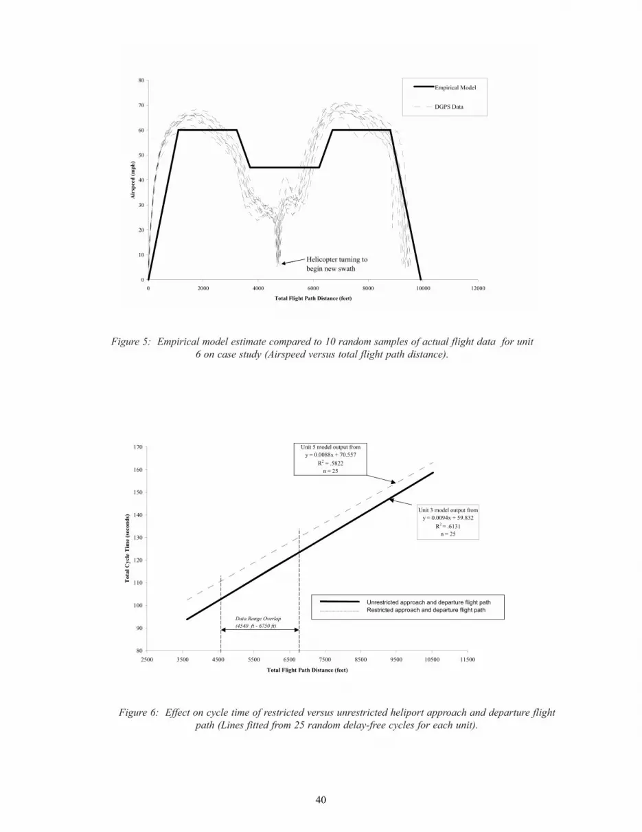
40
Figure 5: Empirical model estimate compared to 10 random samples of actual flight data for unit6 on case study (Airspeed versus total flight path distance).
Figure 6: Effect on cycle time of restricted versus unrestricted heliport approach and departure flightpath (Lines fitted from 25 random delay-free cycles for each unit).
Unit 3 model output fromy = 0.0094x + 59.832
R2 = .6131n = 25
80
90
100
110
120
130
140
150
160
170
2500 3500 4500 5500 6500 7500 8500 9500 10500 11500
Total Flight Path Distance (feet)
Tota
l Cyc
le T
ime
(sec
onds
)
Unit 5 model output from y = 0.0088x + 70.557
R2 = .5822n = 25
Unrestricted approach and departure flight pathRestricted approach and departure flight path
Data Range Overlap(4540 ft - 6750 ft)
0
10
20
30
40
50
60
70
80
0 2000 4000 6000 8000 10000 12000
Total Flight Path Distance (feet)
Air
spee
d (m
ph)
Empirical Model
DGPS Data
Helicopter turning to begin new swath

41
DATA ANALYSES
There were three objectives for the flight data analyses:first, to compare empirical model estimates for delay-freecycle time to actual flight data; second, to compare the ef-fect of a restricted heliport approach and departure path oncycle time; and third, to derive a statistical relationship fromthe flight data to estimate cycle time for project planningand cost estimations.
The first analysis compared empirical model estimatesfor selected field units of helicopter cycle times and produc-tion to actual flight data (Figure 5). The empirical modelappeared to give a reasonable approximation of total cycletime as a function of total flight path distance. The secondanalysis compared the effect of restricted or obstructed heli-copter approach and departure pathways on total cycle timefor two heliports (Figure 6). Restricted heliports with ob-stacles and/or steep approach and departure paths can in-crease operational costs and risk to the pilot, aircraft andsupport personnel. The helicopter has to ascend loaded and/or maneuver around to clear obstacles before accelerationto ferry or application speed, or deceleration to land or load.
The heliport with the obstructed approach and departurepathway had an overall increase in total cycle time for thedata sample. The third analysis developed a simple linearregression from a sample of recorded flight data to predictan average total cycle time for the helicopter (Figure 7). Asecond independent data sample was used to validate theregression. Through the use of an extra-sum-of-squares F-test, the single most significant independent variable was
Regression line equation:Yest = 0.0093Xest + 66.9119
R2 = 0.7686n1 = 50
0
50
100
150
200
250
0 2000 4000 6000 8000 10000 12000 14000 16000
Total Flight Path Distance (feet)
Tot
al C
ycle
Tim
e (s
econ
ds)
Regression Line from Group 1 DGPS Data
95% Prediction Band Using Scheffe's Multiplier
Group 2 DGPS Data
Empirical Model Estimates
Range of Validation (3900 ft - 10,500 ft)
the estimated total flight path distance of the helicopter percycle. The empirical model estimates for helicopter cycletime were within the 95% prediction band for the simplelinear regression. It was assumed the regression could beused as a surrogate for the empirical model to adequatelypredict a total cycle time for a similar operation with simi-lar parameters.
USES OF PRECISION DATA
Data Analysis for Case Study
A comparison of empirical model estimates to actual flightdata illustrated that the model gave a good representation ofthe actual flight pattern of the helicopter during a cycle forthe given operational scenario.
The flight data analysis indicated heliport approach anddeparture flight path access had an effect on the productionand cost of the helicopter. Payload capability is perhaps theperformance characteristic of greatest economic importancefor some operations (Stevens and Clark 1974). In general,reduced payloads from restricted heliports decrease produc-tion and increase cost. Heliport access has a direct effect onrisk management for an operation. Restricted heliports canreduce pilot visibility and increase the performance demandson the helicopter (Stevens and Clark 1974). If the straight-line flight path gradient is greater than 29%, it is not safe tofly and this effect is exaggerated on short distances (O�Brienand Brooks 1996).
The simple linear regression developed from the flight
Figure 7: Simple linear regression to predict a total cycle time as a function of the estimated totalflight path distance with a 95% prediction band and range of validation data (Based on two
random, exclusive, independent 50-cycle samples from entire case study).

42
data predicted a total cycle time in seconds as a function ofthe estimated total flight path distance in feet:
Yest = 0.0093Xest + 66.9119
where:
Yest = prediction estimate for average total cycle time (sec-onds)Xest = estimated average total flight path distance (feet)
and provided a reliable estimation of average total cycletime within the data range indicated. The regression had aR2 = 0.7686, with a residual standard error of 12.64 on 48degrees of freedom. Due to compound uncertainty in esti-mating several means simultaneously, the Scheffe� methodwas used to construct the 95% prediction band (Ramseyand Schafer 1997).
The regression had a good fit within the range of data inthe samples. The estimated cycle time can be used to calcu-late helicopter production for an average payload of doloprillfor a range of flight path distances within the parameterand operational limits of the project.
Application of Regression
If it is assumed that small changes in parameters, suchas payload, do not substantially affect helicopter perfor-mance, the regression may be used to quickly generate gen-eral relationships and trends for helicopter production andcosts over a range of flight path distances. These types ofestimates may be useful to plan projects with similar condi-
Figure 8: Projected production trend for Bell 47G3 helicopter based on the regression model in Figure 7.
tions and materials. Figure 8 illustrates the production trendfor the B47G3 helicopter for two payloads over a range oftotal flight path distances using the regression to estimatetotal cycle time. Figure 9 illustrates the cost trend for thehelicopter for two payloads over a range of total flight pathdistances based on the production estimates from Figure 8.
Other Potential Uses
Aerial operations are well suited to the use of DGPS sys-tems for data collection and analysis of the operation. Un-like most other forestry applications where this technology isused, the aerial operation is above the forest canopy wheresatellite signal reception is unimpeded and the system pro-vides an abundant source of precise positional data through-out the entire operation. Compared to manual methods fortime study data collection, this technology does not requireconstant visual contact with the helicopter.
The maps from the DGPS system can serve as a visualrecord for an application or operation. The real-time heads-up display of the operation can assist pilots with a consistentand even distribution of materials on a field unit, plan opti-mum flight patterns and approaches, and help delineateboundaries and buffers. Unit maps and coordinates can bedownloaded into the navigation system ahead of time, reduc-ing the flight time used to digitize boundaries and helping toidentify the field units and heliports on the ground.
The flight data in conjunction with field tests for applica-tion efficacy could assist in the validation of aerial produc-tivity models previously developed for aerial application op-erations (Ghent 1999; Potter et al. 2002; Ray et al. 1999; Wuet al. 2002). In addition, flight data may be used to evaluate
0
5
10
15
20
25
0 2000 4000 6000 8000 10000 12000
Total Flight Path Distance (feet)
Prod
uctio
n (t
ons/
hour
)
800 pounds
1000 pounds
Payloads
Tons/hour = [(3600 secs/hr)/(Yest)] * [(payload in pounds)/(2000 lbs/ton)]

43
and validate production models for other types of aerial op-erations, such as heli-logging (Giles and Marsh 1994; Lyonset al. 1999; Sessions and Chung 1999).
Flight data analysis may also assist managers and pilotswith evaluation of safe and efficient use of the helicopterfor an operation. Visualizing a similar operation prior toactual field application can help clarify procedures, processesand potential hazards for a pilot and crew unfamiliar with acertain type of operation. This method may also assist theexperienced manager and pilot by providing a slightly dif-ferent perspective to identify approaches for a new opera-tion to improve safety and efficiency.
LIMITATIONS
Case Study DataFor the flight data analysis, additional cycle data are
needed to check the reliability of the regression model be-yond the limits and conditions of the data sets and casestudy. Data parameter limits included: regression data limitswith a total flight path distance range from 1,900 feet to10,500 feet; the second (validation) data set limits with atotal flight path distance range from 3,900 feet to 14,250feet; one type of mineral; the B47G3 helicopter with a skilledpilot; and the weather and operations conditions of the casestudy. An assumption for use of regression is all of the dataset parameters are static as one variable of interest is changedover a projected range of conditions (e.g. equivalent heli-copter performance while varying payload over a range offlight path distances). In a practical application, a pilotmay adjust (increase) production for a reduced payload with
an increase in acceleration capacity. A reduced payloaddecreases the performance demands on the helicopter andcan improve maneuverability of the aircraft, offsetting thepotential production decrease when not flying with a maxi-mum payload.
Although the regression may be useful to help estimateproduction and costs for an operation, a knowledgeable per-son is still needed to evaluate the operation and identifyoperational limitations and hazards (e.g. access, heliports,power lines, pilot experience with an operation, etc.) thatcan influence helicopter productivity and project manage-ment.
Other ConsiderationsAlthough the flight data collected with the DGPS sys-
tem has been determined to be precise, it is the responsi-bility of the user to determine if the data and informationare accurate. Additional record keeping on an operation(such as shift level production information) can be used tocross-reference loads, time, etc. and check for delays orother situations that may impact use of data for analysis orinterpretation. On the case study, for each mineral appliedon the field units and each cycle an observer recorded thetime the bucket was loaded, application time, the payloadand any delays.
The unit map generated by the DGPS system may alsohave discrepancies between what is shown on the map andthe actual application. For example, the bucket may beempty, but if the pilot does not release the switch the DGPSmap will indicate the area that has been flown over whilethe switch is activated had received an application, when ithad not.
Figure 9: Projected cost trend for Bell 47G3 based on production estimates in Figure 8.
0
10
20
30
40
50
60
3000 4000 5000 6000 7000 8000 9000 10000 11000
Total Flight Path Distance (feet)
Hel
icop
ter
Cos
t ($/
ton)
800 pounds
1000 pounds
Payloads
$/ton = [$/hour (direct operating cost)] * [1/(tons/hour)]

44
Another source of discrepancy can arise from boundariesthat are digitized in flight. Although the digitized coordi-nate locations are precise, the mapped boundary consists ofa series of straight lines between digitized points. Caremust be taken to not cut off corners on the unit during thedigitizing phase of the mapping operation.
FUTURE CHALLENGES ANDRESEARCH NEEDS
The equipment used for DGPS data collection on thecase study has proven to be precise and efficient for gather-ing production information. However, initial capital in-vestment in the system is considerable, and requires a sub-stantial commitment by the operator of an additional in-vestment in personnel training. Operation managers needto recognize the potential for added benefits of using thisprecision forestry tool to enhance overall operations safetyand improve project efficiency where possible.
With additional data collection and analysis, other re-gression equations and mathematical models could be de-veloped for different pilots, helicopter types, materials, ap-plications, flight path distances and operational conditionsto estimate production and costs. Automated flight datarecording systems, such as the Ag-Nav®2 DGPS system,could be used to evaluate flight characteristics and perfor-mances under varying circumstances to develop productionrelationships and cost estimates to assist in project plan-ning.
REFERENCES
Ag-Nav®2 by Ag-Nav, Inc. 1999. Newmarket, Ontario, Canada.
Cornell, J. 2003. Aerial forest operations: mineral amendmentproject. M.For. paper, Oregon State University, Forest En-gineering Department, Corvallis, Oregon. 259 p.
Filip, G., A. Kanaskie, K. Kavanagh, G. Johnson, R. Johnson,and D. Maguire. 2000. Silviculture and Swiss Needle Cast:research and recommendations. RC 30. OSU College ofForestry. Corvallis, Oregon.
Ghent, J. 1999. Development of an aerial productivity and effi-ciency model for large-scale aerial treatment programs.USDA Forest Service Research Proposal. R8-2000-02.
Giles, R., F. Marsh.1994. How far can you fly and generatepositive stumpage in helicopter salvage logging? AdvancedTechnology in Forest Operations: Applied Ecology in Ac-tion. Oregon State University. Portland and Corvallis, Or-egon. pp. 231-236.
Gourley, M. 2002. Personal communication. Forester, StarkerForests, Inc., Corvallis, Oregon.
Lyons, K., J. McNeel, J. Nelson, and R. Fight. 1999. Spatialmodeling of helicopter logging in dispersed and aggregatedpartial cutting systems. In proceedings of the InternationalMountain Logging and 10th Pacific Northwest SkylineSymposium. March 28 � April 1. Eds. J. Sessions and W.Chung. Corvallis, Oregon.
O�Brien, S. and E.J. Brooks. 1996. A course filter method fordetermining the economic feasibility of helicopter yarding.Engineering Field Notes � Engineering Technical Informa-tion System. USDA Forest Service. Volume 28. 12 p.
Olsen, E., and L.D. Kellogg. 1983. Comparison of time-studytechniques for evaluating logging production. Transactionsof the ASAE, Vol. 26, No. 6. 1665-1668, 1672.
Potter, W.D., Ramyaa, J. Li, J. Ghent, D. Twardus, and H. Thistle.2002. STP: an aerial spray treatment planning system. Inproceedings IEEE SoutheastCon, 2002. pp. 300-305.
Ramsey, F.L. and D.W. Schafer. 1997. The statistical sleuth, acourse in methods data analysis. Duxbury Press. WadsworthPublishing Company. Belmont, California.
Ray, J.W., B. Richardson, W.C. Schou, M.E. Teske, A.L. Vanner,and G.C. Coker. 1999. Validation of SpraySafe Manager, anaerial herbicide application decision support system. Cana-dian Journal of Forest Research, 29: 875-882.
Reynolds, R.D. 1999. Three GPS-based aerial navigation sys-tems for forestry applications. Forest Engineering Instituteof Canada. Field Note No.: Silviculture-118. October.Vancouver, British Columbia.
Sessions, J. and W. Chung. 1999. Optimizing helicopter land-ing location � a preliminary model. In proceedings of theInternational Mountain Logging and 10th Pacific NorthwestSkyline Symposium. March 28 � April 1. Eds. J. Sessionsand W. Chung. Corvallis, Oregon. pp. 337 � 340.
Stevens, P.M. and E.H. Clarke. 1974. Helicopters for logging,characteristics, operation, and safety considerations. USDAForest Service General Technical Report PNW-20. PacificNorthwest Forest and Range Experiment Station. Portland,Oregon.
Wu, L., W.D. Potter, K. Rasheed, J. Ghent, D. Twardus, H.Thistle, and M. Teske. 2002. Improving the genetic algo-rithm performance in aerial spray deposition management.In proceedings IEEE SoutheastCon, 2002. pp. 306 � 311.

45
Estimating Forest Structure Parameters on Fort LewisMilitary Reservation using Airborne Laser Scanner
(LIDAR) Data
HANS-ERIK ANDERSEN, JEFFREY R. FOSTER, AND STEPHEN E. REUTEBUCH
Abstract: Three-dimensional (3-D) forest structure information is critical to support a variety of ecosystem managementobjectives on the Fort Lewis Military Reservation, including habitat assessment, ecological restoration, fire management, andcommercial timber harvest. In particular, the Forestry Program at Fort Lewis requires measurements of shrub, understory, andoverstory canopy cover to monitor vegetation response to various management approaches. At present, these measurementsare acquired through field-based procedures, which are relatively costly and time-consuming. The use of remotely sensed data,such as airborne laser scanning (LIDAR), has the potential to significantly reduce the cost of acquiring these types of measure-ments over large areas. As an active remote sensing technology, LIDAR provides direct, three-dimensional measurements ofthe forest canopy structure and underlying terrain surface. LIDAR-based cover measurements can be related to forest vegeta-tion cover through a mathematical function based upon the Beer-Lambert law, which accounts for scanning geometry andvertical foliage density. This study was carried out to determine the utility of small-footprint, discrete-return LIDAR forestimation of forest canopy cover at Fort Lewis. LIDAR-based structural measures were compared to spatially-explicit fieldmeasurements acquired from inventory plots in five forest stands representative of the various forest types at Fort Lewis and avariety of terrain. Results indicate that LIDAR-based cover estimates for overstory and understory are generally related tofield-based estimates.
INTRODUCTION
Forests are structured as complex systems in three-di-mensional (3-D) space. The 3-D structural organization offorest canopies is the primary determinant of the understorylight regime, micro-climate, and habitat structure. In thePacific Northwest, the vertical distribution of canopy ele-ments is one of the more important components describingthe spatial structure of a forest stands. For example, theForestry Program at Fort Lewis Military Reservation requiresthis structural information to guide an active silviculturalprogram designed to promote the development of forestswith more diverse structures and composition, and to pro-vide habitat for the northern spotted owl (Strix occidentaliscaurina). Fort Lewis has implemented an inventory pro-gram to document and monitor the spatial structure of theinstallation’s forests. Three-dimensional forest structure isquantified by measuring vegetation cover of the overstory,understory, shrub, and ground layers.
Vegetation cover, expressed as the proportion of the for-est floor covered by the vertical projection of vegetationwithin a layer of the forest canopy, is a conventional mea-sure of forest structure (Jennings et al., 1999). As the inven-tory program currently relies upon ocular, field-based mea-
surements of vegetation cover, inventory costs could be sig-nificantly reduced through the use of remote sensing tech-nology.
In particular, actively-sensed airborne laser scanning(LIDAR) technology has the potential to provide informa-tion relating to spatial structure throughout the depth of theforest canopy and understory. Previous studies have shownthat large-footprint, continuous- waveform LIDAR data canbe used to characterize the vertical distribution of canopyfoliage (Harding et al., 2001; Lefsky et al., 1999; Means etal., 1999). Researchers have related the vertical distribu-tion of small-footprint, first-and multiple-return LIDAR datato empirical- and model-based estimates of leaf area distri-bution within Pacific Northwest forests (Magnussen andBoudewyn, 1998; Andersen, 2003). Other studies haveshown that quantitative measures derived from the verticaldistribution of small-footprint, discrete return LIDAR dataare related to important stand parameters, such as volume,height, and biomass (Means et al., 2000).
While LIDAR-derived measures of canopy cover havebeen used as independent variables in estimation of foreststand parameters (Means et al., 2000), the utility of LIDARfor differential characterization of canopy and subcanopyforest structure components has not been assessed. In thispaper, a methodology for measurement of vegetation cover

46
within discrete canopy layers using first return LIDAR datawill be presented and evaluated.
STUDY AREA AND DATA
Study Sites Within Fort Lewis, WashingtonFive stands considered to be representative of the variety
of forest types present at Fort Lewis were selected as studyareas for the project. The first two stands were located inthe southwestern portion of Fort Lewis on an old recessionalmoraine of the Vashon Glaciation with hummocky topogra-phy and location variation in vertical relief of ca. 10 m.Area 1 was a 65-year-old mixed red alder/Douglas-fir stand,and Area 2 was a 75-year-old Douglas-fir stand. The otherthree stands were located on flat glacial outwash. Area 3,ca. 3 km southeast of Areas 1 and 2, was an 85-year-oldmixed white oak/Douglas-fir stand. Areas 4 and 6 were 95-year-old Douglas-fir stands in the northeastern portion ofFort Lewis. (Area 5 was in a prairie and therefore was notused in this study).
Approximately 35 plots were located within each stand(169 total) to validate the remote sensing estimates (Figure1). These plots were established in a systematic pattern ofclusters to ensure a well-distributed sample within each standtype. Plot coordinates were established by a highly accuratetotal station topographic survey. An additional 300 topo-graphic check points were established in these stands to as-sess the accuracy of the LIDAR digital terrain models.
LIDAR DataLIDAR data were acquired over two 50-km2 areas on Fort
Lewis in August, 2000 (fig. 1). These data were acquiredwith an Earthdata Aeroscan laser scanning system operat-ing from a fixed-wing platform. System specifications andflight parameters are shown in Table 1.
Pulse rate 15,000 per second Ground spacing between pulses
1 meter (nominal)
Laser wavelength 1.064 µm Scan pattern Sinusoidal Pulse length 12 ns Attitude precision 0.004 degrees Range resolution 3 cm Range accuracy 2-4 cm
LIDAR-Based Digital Terrain ModelsA filtering technique coded in IDL (Interactive Data Lan-
guage version 5.5, Research Systems, Inc.) was used to iden-tify the probable ground reflections within the last-returnLIDAR data (Haugerud and Harding, 2001). An interpola-tion algorithm was used to generate a digital terrain model(DTM) on a grid, with a post spacing of 5×5 m, for the twoareas covered by the LIDAR dataset. Figures 2a and 2bshow hill-shade graphics of the DTMs.
A comparison of LIDAR-estimated elevation from theDTMs to the elevations of 225 topographic survey pointsindicated a mean absolute error of -0.14 meters and a rootmean square error (RMSE) of 1.00 meters for the south-western Fort Lewis LIDAR DTM. A similar comparisonfor the northwestern Fort Lewis LIDAR DTM (244 topo-graphic survey points) indicated a mean absolute error of -0.05 meters and an RMSE of 0.72 meters.
Field Cover DataTo compare LIDAR-based measures of vegetation cover
to conventional inventory metrics, field-based observationsof vegetation cover were acquired at each of the 169 plotslocated in the five stands. Following the established fieldprotocol of the Fort Lewis inventory program, ocular esti-mates of vegetation cover within the overstory, understory(1.8 m - base of overstory), and shrub (0.46 m � 1.8 m)were made at each plot (Figure 3). Overstory and under-story cover were estimated for an 809 m2 circular plot, andshrub and ground cover for an 81 m2 circular plot. It shouldbe noted that while the base of the upper and lower bound-aries of the shrub and ground layers are at fixed heights inthe inventory protocol, the height of the base of the over-story layer is a local characteristic of forest structure andwas subjectively estimated at each plot. Cover was definedas the proportion of the total area �filled� by the two-di-mensional (2-D) vertical projection of tree crowns andshrubs onto the ground.
Figure 3. Canopy layers used for cover estimation.
Table 1. System specifications for Earthdata AeroscanLIDAR system.

47
##############################################################
######################### #############
############ #################
########################## ##############
#Area 1
# Area 2
#
Area 3
#
Area 4
#Area 6
Fort Le wis Milita ry Rese rva tion
# ### ###### ########## ### ####
###
# ## #####
#####
## ##
#####
####
####
# #
### ## #####
### #
#### ####
#
##### ## ### #####
##### ##### ## ####
####
### ##
####
####### ### ####
####
#
####
## ####### ## ##
# ###
#
Area 1
#
Area 2
#
Area 3
#
Area 4
#
Area 6
Fort Lewis Military Reservation
Figure 1. LIDAR coverage and study areas within Fort Lewis Military Reservation, Washington.
Figure 2. LIDAR-based DTMs (5-m resolution) within Fort Lewis Military Reservation.
(b) Northeast area (a) Southwest area

48
METHODS
To convert LIDAR coordinate data into vegetation heightdata, the elevation of the underlying terrain (interpolatedfrom the LIDAR DTM) was calculated for each LIDAR re-turn; then, this terrain elevation was subtracted from theLIDAR return elevation to yield vegetation height.
Vertical Point Quadrat SamplingGround-based measures of canopy cover are typically
based upon a sample of measurements acquired with a ver-tical sighting instrument. The percent cover is computed asthe proportion of sample points where the sky is obscuredby vegetation (Jennings et al., 1999). As Jennings noted, alimitation of this approach is that it is highly susceptible tosampling error.
When the vertical heights from the ground to first con-tact with vegetation within each canopy layer are measuredabove each sample point, the canopy cover for a given canopylayer can be estimated as the ratio of the number of mea-sured heights within a layer to the total number of samplepoints. This approach has been used to estimate vertical fo-liage distributions and is termed vertical point quadrat sam-pling (Ford and Newbould, 1971). When an optical rangefinding device, such as a laser, is used to measure the heightto first leaf contact, this sampling technique is termed opti-cal point quadrat sampling (MacArthur and Horn, 1969;Aber, 1979; Radtke and Bolstad, 2001).
LIDAR-Based Cover EstimationIf the geometry of the laser range-finding is inverted, an
estimate of cover within a given layer of the canopy can begenerated from LIDAR data, where cover within each layeris calculated as the ratio of the number of first return LI-DAR reflections within a layer to the total number of LI-DAR pulses entering the layer (Figure 4).
A LIDAR-based cover estimate, based on first return data,was generated for overstory, under-story, and shrub layersfor each of 169 plots Although field cover estimates for theshrub layer were based upon an 81 m2 plot, all LIDAR esti-mates were based upon an 809 m2 plot to maintain an ad-equate sample area. Estimates based upon the larger areawill not bias the results.
A single value for height was used to characterize thebase of the overstory within each stand. A K-means cluster-ing algorithm was applied to the LIDAR data within eachforest stand to estimate the height that separated the under-story and overstory layers (Mardia et al., 1995). This heightwas 10.0 meters for Area 1, 21.4 meters for Area 2, 7.5meters for Area 3, 23.7 meters for Area 4, and 21.3 metersfor Area 6.
Figure 5 is a 3-D representation of a plot within Area 2(75-year-old Douglas-fir stand) created using the Stand Vi-sualization System (McGaughey, 1997). Figure 6 shows a3-D perspective view of the distribution of first return LI-
Figure 4. LIDAR-based cover estimation for overstory,understory, and shrub layers. Vertical lines represent
LIDAR pulses.
DAR data used to generate LIDAR-based cover estimates.If all LIDAR measurements were acquired at nadir, there
is a linear relationship between the LIDAR-based covermeasurement, generated using the theory developed in theprevious section, and the field-based cover estimate for eachlayer. In practice, due to scanning geometry, LIDAR mea-surements are acquired at some off-nadir angle (-25 degreesto +25 degrees in the Aeroscan system used in this study).This off-nadir angle affects the probability of a laser pulsepassing through a given layer of vegetation and influencesthe functional form of the relationship between a LIDAR-based measurement of cover and the cover estimate observedin the field.
Figure 5. Visualization of 809 m2 plot within Douglas-firstand.

49
Simulation of LIDAR Data and Cover EstimatesA simulation approach was used to investigate the effect
of scanning geometry and foliage density on the relation-ship between field-based and LIDAR-based cover estimates.In this simulation, a 3-D array was used to simulate the 3-D�envelope� containing the canopy vegetation within a100×100×60-meter area of forest. The cover within eachlayer of the canopy (i.e. overstory, understory (to 25 meters),
Figure 6. Distribution of first return LIDAR data within809 m2 plot within Douglas-fir stand.
and shrub) was held fixed by randomly assigning a value ofeither 0 or 1 to each layer until the two-dimensional (2-D)projection of the �filled� area for each layer equaled the speci-fied cover percentage. A specified density in the vertical di-mension was also randomly allocated throughout the layer,while keeping the 2-D projection of cover fixed for eachlayer.
The paths of LIDAR pulses traveling at some specifiedoff-nadir angle through the 3-D array were calculated andthe coordinates (x, y, height) for the �first vegetation con-tact� (i.e. first encounter with a cell with code �1�) wererecorded as simulated first return LIDAR measurements. Asimulated LIDAR-based cover estimate was then generatedusing the approach described in the previous section. Thesesimulated LIDAR estimates were then compared to the speci-fied, fixed (�simulated field�) cover values used in fillingthe 3-D array.
Figures 7 and 8 show the influence of the off-nadir angleon simulated LIDAR-based cover estimates. Figure 7 showsthe cover estimates with the off-nadir angle fixed at zero.Perhaps not surprisingly, there is a linear relationship be-tween LIDAR- and field-based cover estimates. Figure 8shows the relationship between LIDAR-based and field-basedcover estimates when the off-nadir angle for each pulse is arandom draw between -25 and +25 degrees and the foliagedensity within each layer is randomly chosen.
Clearly the relationship is no longer linear, and appearsto follow a relatively smooth curve. While this effect is ap-parent in the overstory and understory layers (Figures 8a
(a) Overstory (b) Understory (c) Shrub
Figure 7. Simulated cover estimates with off-nadir of 0 degrees.
(a) Overstory (b) Understory (c) Shrub
Figure 8. Simulated cover estimates with off-nadir angles ranging between -25 and +25 degrees.
0.1 0.3 0.5 0.7 0.9LIDAR-based Overstory Cover
0.0
0.2
0.4
0.6
0.8
1.0
Fiel
d-ba
sed
Ove
rsto
ry C
over
0.1 0.3 0.5 0.7 0.9LIDAR-based Understory Cover
-0.2
0.0
0.2
0.4
0.6
0.8
1.0
Fiel
d-ba
sed
Und
erst
ory
Cov
er
0.1 0.3 0.5 0.7 0.9LIDAR-based Shrub Cover
0.0
0.2
0.4
0.6
0.8
1.0
Fiel
d-ba
sed
Shr
ub C
over
0.1 0.3 0.5 0.7 0.9LIDAR-based Overstory Cover
0.0
0.2
0.4
0.6
0.8
1.0
Fiel
d-ba
sed
Ove
rsto
ry C
over
0.1 0.3 0.5 0.7 0.9LIDAR-based Understory Cover
0.0
0.2
0.4
0.6
0.8
1.0
Fiel
d-ba
sed
Und
erst
ory
Cov
er
0.1 0.3 0.5 0.7 0.9LIDAR-based Shrub Cover
0.0
0.2
0.4
0.6
0.8
1.0
Fiel
d-ba
sed
Shru
b C
over

50
and 8b) it is not evident in the shrub layer (Figure 8c), wherethe relationship exhibits a more linear form.
The form of the mathematical function describing therelationship between LIDAR-based cover and field-basedcover can be obtained from the principles of radiative transfertheory (Martens et al., 1993). Martens and others showedthat the relationship between leaf area index and gap frac-tion, or the ratio of the amount of light beneath a canopylayer to the amount of light above a canopy layer, is givenby the Beer-Lambert law, with the following form:
LAI = (-1/k)ln(gap fraction),
where k is the extinction coefficient governing the attenua-tion of light as it passes through the canopy.
In the context of cover estimation, the relationship be-tween the field-based cover estimate (i.e., 2-D projection ofvegetation onto terrain surface) and LIDAR-based cover canbe estimated by the following function:
Field cover = (a)ln[1/(1 � LIDAR cover)]
where a is the parameter related to the extinction coeffi-cient in Beer-Lambert law shown above, and cover valuesare expressed as fractions.
Density of vegetation in the vertical dimension will alsoinfluence this relationship between field- and LIDAR-basedmeasures of cover. The parameter a in the above functionwill represent the combined effect of off-nadir angle and
vertical foliage density. Figures 9 and 10 show the influ-ence of varying the vertical density of foliage. Figure 9 showsthe relationship between simulated field- and LIDAR-basedestimates of cover with a relatively high density of foliagein the vertical dimension, while Figure 10 shows this rela-tionship for a low density of foliage, with fitted curves su-perimposed.
These graphics indicate that both off-nadir angle and ver-tical foliage density will influence the relationship betweenfield- and LIDAR-based estimates of cover. It also appearsthat the mathematical functional form can be adequatelyrepresented by the logarithmic model based upon the Beer-Lambert law given above, where the parameter of the func-tion will represent the effects of scan angle and foliage den-sity.
RESULTS
LIDAR-based cover estimates obtained using first returnLIDAR data were compared to the field-based cover esti-mates for the 169 plots on Fort Lewis. The relationship be-tween LIDAR- and field-based estimates for each forest typewas quantified using regression analysis, with the resultsshown in Figures 11-14. The coefficient of determination(r2) of each regression model is shown as well.
The results indicate that LIDAR-based cover estimatesfor overstory and understory are generally related to field-based estimates. There does not appear to be a significantrelationship between LIDAR- and field-based estimates ofshrub cover for any forest types.
(a) Overstory (b) Understory (c) Shrub
Figure 9: Simulated cover estimates with high density of foliage in vertical dimension.
(a) Overstory (b) Understory (c) Shrub
Figure 10: Simulated cover estimates with low density of foliage in vertical dimension.
0.2 0.4 0.6 0.8 1.0LIDAR-based Overstory Cover
0.0
0.2
0.4
0.6
0.8
1.0
Fiel
d-ba
sed
Ove
rsto
ry C
over
0.1 0.3 0.5 0.7 0.9LIDAR-based Understory Cover
0.0
0.2
0.4
0.6
0.8
1.0
Fiel
d-ba
sed
Und
erst
ory
Cov
er
0.1 0.3 0.5 0.7 0.9LIDAR-based Shrub Cover
0.0
0.2
0.4
0.6
0.8
1.0
Fiel
d-ba
sed
Shru
b C
over
0.1 0.3 0.5 0.7 0.9LIDAR-based Overstory Cover
0.0
0.2
0.4
0.6
0.8
1.0
Fiel
d-ba
sed
Ove
rsto
ry C
over
0.2 0.4 0.6 0.8 1.0LIDAR-based Understory Cover
0.0
0.4
0.8
1.2
Fiel
d-ba
sed
Und
erst
ory
Cov
er
0.1 0.3 0.5 0.7 0.9LIDAR-based Shrub Cover
0.0
0.2
0.4
0.6
0.8
1.0
1.2
Fiel
d-ba
sed
Shru
b C
over

51
Relationships between LIDAR- and field-based estimatesare strongest in the mature Douglas-fir stand on flat terrain(Figure 11) and the mixed white oak/Douglas-fir prairiestands (Figure 14). It should be noted that the relationshipfor the overstory and understory layers in Area 3 did notexhibit a curvilinear form, so results for this area were basedupon untransformed lidar cover values (Figure 14a and 14b).Relationships are still apparent, although less strong, withinthe Douglas-fir stand with hummocky topography (Figure13). Relationships within the mixed red alder/Douglas-firstand are extremely weak (Figure 12).
DISCUSSION
The graphical and quantitative results indicate that LI-DAR has the potential to provide information relating tovegetation cover in multiple canopy layers within foreststands. The weaker relationship between field- and LIDAR-based cover estimates for the shrub layer is most likely dueto sampling error. Occlusion of subcanopy vegetation byoverstory and understory foliage will reduce the number offirst returns penetrating to the shrub layers, effectively de-
creasing the sample size and increasing the error of coverestimation. Results here indicate that sampling error is theprimary source of variation in the estimation of shrub coveracross all forest types.
The results obtained from simulations and field data sug-gest that the interaction of off-nadir LIDAR scanning ge-ometry and the vertical distribution of canopy foliage intro-duces a significant source of variability in LIDAR-basedcover estimation. The geometry of LIDAR sensing leads tomeasurements of forest struc-ture that are more representa-tive of 3-D canopy density than 2-D (i.e. orthogonal) canopycover. However, if vertical structure is relatively constantover a forest stand, then vertical density can be modeled,allowing for a more accurate mapping of the LIDAR-basedcover estimate to the 2-D vegetation cover.
It should be noted that using a single height for separat-ing overstory from understory layers adds a significant sourceof variability in LIDAR-based cover estimation. Again, er-ror will be decreased when the stand is more structurallyhomogeneous. In stands exhibiting extremely complex ver-tical structure (e.g. the mixed red alder/Douglas-fir standin Area 1), this classification error may lead to gross errorsin cover estimation.
(a) Overstory (r2 = 0.63) (b) Understory (r2 = 0.53) (c) Shrub (r2 = 0.15)
Figure 11: Field-measured vs. predicted cover within 95-year-old Douglas fir stands (Areas 4 and 6). Dashed line shows1:1 relationship.
(a) Overstory (r2 = 0.63) (b) Understory (r2 = 0.53) (c) Shrub (r2 = 0.15)
Figure 12: Field-measured vs. predicted cover within 65-year-old mixed red alder/Douglas-fir stand (Area 1).
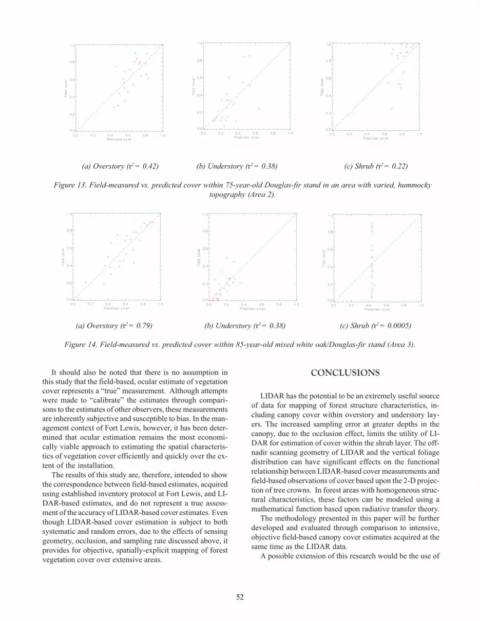
52
It should also be noted that there is no assumption inthis study that the field-based, ocular estimate of vegetationcover represents a �true� measurement. Although attemptswere made to �calibrate� the estimates through compari-sons to the estimates of other observers, these measurementsare inherently subjective and susceptible to bias. In the man-agement context of Fort Lewis, however, it has been deter-mined that ocular estimation remains the most economi-cally viable approach to estimating the spatial characteris-tics of vegetation cover efficiently and quickly over the ex-tent of the installation.
The results of this study are, therefore, intended to showthe correspondence between field-based estimates, acquiredusing established inventory protocol at Fort Lewis, and LI-DAR-based estimates, and do not represent a true assess-ment of the accuracy of LIDAR-based cover estimates. Eventhough LIDAR-based cover estimation is subject to bothsystematic and random errors, due to the effects of sensinggeometry, occlusion, and sampling rate discussed above, itprovides for objective, spatially-explicit mapping of forestvegetation cover over extensive areas.
(a) Overstory (r2 = 0.42) (b) Understory (r2 = 0.38) (c) Shrub (r2 = 0.22)
Figure 13. Field-measured vs. predicted cover within 75-year-old Douglas-fir stand in an area with varied, hummockytopography (Area 2).
CONCLUSIONS
LIDAR has the potential to be an extremely useful sourceof data for mapping of forest structure characteristics, in-cluding canopy cover within overstory and understory lay-ers. The increased sampling error at greater depths in thecanopy, due to the occlusion effect, limits the utility of LI-DAR for estimation of cover within the shrub layer. The off-nadir scanning geometry of LIDAR and the vertical foliagedistribution can have significant effects on the functionalrelationship between LIDAR-based cover measurements andfield-based observations of cover based upon the 2-D projec-tion of tree crowns. In forest areas with homogeneous struc-tural characteristics, these factors can be modeled using amathematical function based upon radiative transfer theory.
The methodology presented in this paper will be furtherdeveloped and evaluated through comparison to intensive,objective field-based canopy cover estimates acquired at thesame time as the LIDAR data.
A possible extension of this research would be the use of
(a) Overstory (r2 = 0.79) (b) Understory (r2 = 0.38) (c) Shrub (r2 = 0.0005)
Figure 14. Field-measured vs. predicted cover within 85-year-old mixed white oak/Douglas-fir stand (Area 3).

53
multiple-return or continuous-waveform (i.e. �single pho-ton�), small footprint LIDAR data. The use of multiple-return data with intensity information may allow for moresophisticated and accurate modeling of foliage density andvegetation cover.
A follow-up project will use these results to model thespatial patchiness of canopy cover within Fort Lewis Mili-tary Reservation to support habitat monitoring and silvicul-tural programs.
LITERATURE CITED
Aber, J. 1979. A method for estimating foliage height profilesin broad leaved forests. Journal of Ecology 67:35-40.
Andersen, H.-E. 2003. Estimation of critical forest structuremetrics through the spatial analysis of airborne laser scan-ner data. Unpublished Ph.D. dissertation, University ofWashington, Seattle, WA.
Ford, D. and P. Newbould. 1971. The leaf canopy of a coppiceddeciduous woodland: I. development and structure. Journalof Ecology 59:843-862.
Harding, D., M. Lefsky, G. Parker, J. Blair. 2001. Laser altim-eter canopy height profiles: Methods and validation forclosed-canopy, broadleaf forests. Remote Sensing of the En-vironment 76:283-297.
Haugerud, R. and D. Harding. 2001. Some algorithms for vir-tual deforestation (VDF) of lidar topographic survey data.International Archives of Photogrammetry and RemoteSensing, XXXIV-3/W4:211-217.
Jennings, S.B., N. Brown, and D. Sheil. 1999. Assessing forestcanopies and understory illumination: canopy closure, canopycover and other measures. Forestry 72(1): 59-73.
Lefsky, M., W. Cohen, S. Acker, G. Parker, T. Spies, and D.Harding. 1999. Lidar remote sensing of the canopy struc-ture and biophysical properties of Douglas-fir western hem-lock forest. Remote Sensing of the Environment 70:339-361.
MacArthur, R. and H. Horn. 1969. Foliage profile by verticalmeasurements. Ecology 50:802-804.
McGaughey, R. 1997. Visualizing forest stand dynamics usingthe stand visualization system. In: Proceedings of the 1997ACSM/ASPRS Annual Convention and Exposition, vol. 4,pages 248-257, Bethesda, MD, April, 1997. American So-ciety for Photogrammetry and Remote Sensing.
Magnussen, S. and P. Boudewyn. 1998. Derivations of standheights from airborne laser scanner data with canopy-basedquantile estimators. Canadian Journal of Forest Research28:1016-1031.
Mardia, K., J. Kent, J. Bibby. 1995. Multivariate Analysis. Aca-demic Press, London.
Martens, S., S. Ustin, and R. Rousseau. 1993. Estimation oftree canopy leaf area index by gap fraction analysis. ForestEcology and Management 61:91-108.
Means, J., S. Acker, D. Harding, J. Blair, M. Lefsky, W. Cohen,M. Harmon, and W. McKee. 1999. Use of large footprintscanning airborne lidar to estimate forest stand characteris-tics in the western Cascades of Oregon. Remote Sensing ofthe Environment 67:298-308.
Means, J., S. Acker, B. Fitt, M. Renslow, L. Emerson, C. Hendrix.2000. Predicting forest stand characteristics with airbornescanning lidar. Photogrammetric Engineering and RemoteSensing 66(1):1367-1371.
Radtke, P. and P. Bolstad. 2001. Laser point-quadrat samplingfor estimating foliage-height profiles in broad-leaved forests.Canadian Journal of Forest Research 31:410-418.
Support for this research was provided by Fort Lewis Mili-tary Reservation, the USDA Forest Service Pacific North-west Research Station, and the Precision Forestry Coopera-tive within the University of Washington College of ForestResources.

54

55
INTRODUCTION
Over the past two decades LIDAR (Light Detection andRanging) data have been extensively used in natural re-sources and engineering. Efforts to determine the depth ofthe ocean floor with high accuracy appeared to be one of thefirst applications involving laser systems (Hoge et al. 1980).Realizing that vegetation canopy �depth,� i.e., height andstructure, might also be measured using this bathymetricLIDAR technology, Link and Collins (1981), Arp et al.(1982), and Hoge et al. (1982) reported some of the firstairborne laser studies of terrestrial targets in the westernhemisphere. Roughly parallel, more theoretically based, ter-restrial LIDAR investigations were ongoing in the UnitedSoviet Socialist Republic at the time (Solodukhin et al.1977a, b; 1979; 1985; Stolyarov and Solodukhin 1987),though the Cold War precluded scientific cooperation.
Over the past 20+ years, numerous researchers have dem-onstrated the capabilities and limitations of a wide varietyof airborne laser systems for forest, rangeland, geologic, andtopographic measurement and mapping. With respect toforestry, airborne LIDAR research has centered on the as-sessment of forest canopy heights, crown closure, internalcanopy structure, and the use of these laser measures to esti-mate stems, basal area, wood volume, forest biomass, and
carbon. The exhaustive and tedious efforts to measure treeheights can be readily enhanced and even replaced by thelaser systems that are capable of determining tree heightswith high precision.
Airborne laser profiling and scanning systems intensivelysample forestlands, and these height and density measurescan, using regression techniques, be used to infer stand char-acteristics (Nelson et al. 1988). The heights of trees andcanopy densities are the first step in estimating more com-plex biometric parameters using the laser data. Hyyppä etal. (2001) estimated stem volume using high pulse rate la-ser scanner data, segmentation method and regression equa-tions with a 10.5% error. Nelson et al. (1988) developedand tested two logarithmic equations in conjunction withsix laser based canopy measurements. The results indicatedthat the mean total tree volume can be predicted with a 2.6%accuracy of the ground value and a mean biomass within a2% accuracy based on 38 ground plots. The Scanning LidarImager of Canopies by Echo Recovery (SLICER) was alsofrequently used to collect data in the deciduous forests onthe North American continent (Lefsky et al. 1999). Thequadratic mean canopy heights explained the 70% varia-tion in the stand basal area and the 80% variation in theabove ground biomass. The crucial segment in estimatingthe above mentioned biometric parameters either with pro-
Developing �COM� Links for Implementing LIDAR Data inGeographic Information System (GIS) to Support Forest
Inventory and Analysis
ARNAB BHOWMICK, PETER P. SISKA AND ROSS F. NELSON
Abstract: In the last decade the computerized technology made significant step forward in the data manipulation, storage,design and analysis. At the same time the acquisition of spatial data experienced significant changes in the natural resources.The field sampling methods, that originally represented the only source of spatial data, have been efficiently enhanced, insome cases even replaced, with modern remote sensing sensors. The airborne laser systems are promising tools for measuringheights of ground objects with high precision. In addition, LIDAR measurements can be linked with field sampling andregression models to provide estimates of ecosystem parameters such as biomass, leaf area index, carbon and other volumetriccharacteristics of vegetation structure. The objective of this project is to develop component object model (COM) for the directtransfer of raw laser measurements to GIS, perform fundamental analysis in a form of close coupling strategy and computestatistics on multiple return LIDAR data. This method allows GIS analyst and LIDAR users to effectively manipulate withlaser data within GIS environment. COM compliant software supports flexible applications using objects and componentsfrom different sources. The close coupling of GIS with geospatial and statistical tools strengthens the role of GIS as aninterdisciplinary science. In this paper coupling strategy involves modules that simultaneously manipulate software compo-nents from the GIS application and the data analysis application. The paper explores the significance of coupling strategies fornatural resource management, engineering and the forest science applications.

56
filing, SLICER, or other imaging laser systems is in de-veloping regression equations that relate measured param-eters on the ground with the airborne laser measurements.The newest results in Delaware (Nelson et al. 2003) indi-cate that biometric estimates of biomass and volume in fourland cover categories (deciduous, mixedwood, conifer, andwetlands) are within 16% of U.S. Forest Service estimatesstatewide.
The geographic information systems (GIS) have provided,until now, limited service to laser based projects. Such ap-plications include data storage and display. More sophisti-cated application are associated with overlay operations. Inparticular, classified vegetation maps can be overlaid in aGIS with scanning laser data or transect lines (profiling la-sers) in order to calculate stratified estimates of biomassand other biometric parameters. Therefore, the spatial dis-tribution of vegetation and its covariation with laser mea-surements across the study area plays a significant role inthe final evaluation of biometric parameters. Additionaloverlays with soil cover can also be useful in relating laserdata to natural resource information.
In this project the close coupling procedure was devel-oped to support the automated transfer of raw laser mea-surements to GIS from the ArcMap module for further analy-sis. The linkage continued back to excel spreadsheet for sta-tistical analysis using moving window strategy and the pro-cess ended again in GIS environment. This task was ac-complished using one of the most recent approaches in com-puterized technology - component object modeling (COM).
PROCEDURES AND RESULTS
A fully integrated computerized system provides dynamiclinks between spatial analysis tools such as GIS and statisti-cal software packages. The newest development in comput-erized technology has introduced object oriented databasemanagement systems and object component models. TheGIS packages such as ArcInfo 8.0 and newer versions andIDRISI have developed their own component object systemthat can be linked with other COM compliant software. Thisintegration increases the flexibility of analysis in spatialanalysis. Linking GIS with other statistical and analyticalpackages via component object modeling can assist in thepursuit of new and creative research ideas.
Database Management SystemsThe integration of GIS and spatial analysis tools is com-
monly known as a coupling strategy. Ungerer and Goodchild(2001) described four levels of coupling: isolated, loose, closeand integrated. The scope of this work falls under a closecoupling strategy whereby the actual task is taken from GIS,and the spatial data is manipulated outside of GIS in anexcel package using a visual basic editor. After the compu-tation of a desired task is completed, the results are auto-matically imported back via established COM links into theGIS environment for further processing and analysis using
GIS tools. The computation of the dissectivity parameter out-side of the GIS environment includes the �moving windows�strategy that was developed in this project. The visual basicmodule is capable of �dropping� a window of selected sizearound each point sample value and computing the statisticalparameter from the samples that falls within the window size.Since LIDAR data represent a highly dense clustered data,the program computed statistics several thousands windows.
The purpose of this project was to develop a module basedon the component object model (COM) for the direct transferof raw laser measurements to GIS, perform statistical analy-sis outside of a GIS environment and then complete surfaceanalysis using the first and last return LIDAR value. Thisclose coupling procedure allows the GIS analyst and LIDAR�susers to manipulate more effectively with laser data directlyfrom the GIS environment. COM compliant software sup-ports flexible applications using objects and components fromdifferent sources. Currently, a number of programs have COMcompatibility and therefore intelligent modules to performsimple or sophisticated analysis on the spatial data can linkthem. All spatial data sets were managed, viewed, queried,and manipulated in an ArcGIS environment. ComponentObject Modules (COM) was developed and embedded in anArcGIS environment using Visual Basic Applications (VBA)to facilitate the automation of input, processing, generation,management and representation of data. The Visual Basic.netversion would also be used for the web interface program-ming. The resultant GIS environment enables multiple usersto access and manipulate digital map and tabular data layersand files. In general, the database handles three generic typesof data � 1) laser and ground transect ASCII files, 2) lasercoverages (i.e., GIS data layers), and 3) satellite-based landcover vector layers and geostatistical vector layers.
Remodeling ArcGIS InterfaceThe raw ACSII LIDAR data (Figure 1) are not easily trans-
ported to analytical packages for viewing, storage and ma-nipulation. Using the COM technology, VBA codes were writ-ten to manipulate simultaneously objects in ArcGIS and MSOffice (Excel). These objects were embedded in a GIS envi-ronment using a visual basic module such as �menu� or�toolbar� items. In addition, the buttons were designed tomake them operational. This technology endows the user toleverage the functionality of statistical calculations, the datamanagement attributes in MS Excel and the spatial functionsof GIS without even leaving the GIS interface. The VBAcodes work in the background to couple the GIS and statisti-cal/database software, perform the destined procedures, andthen import the data back to GIS for further analysis.
As can be seen in Figure 2, this interface converts the rawdata file into a *.csv data format. It also sorts the data accord-ing to laser return numbers. This file can be opened in anydatabase or simple ASCII formats for layer inputs (accordingto return numbers) into GIS and other tools for furthergeospatial analysis.

57
LIDAR COVERAGE FILES
Individual pulse locations from laser instruments alongthe actual flight path are stored as ArcGIS point layers, alongwith GMT time tags. After the data raw laser data are inputto GIS, they are stored as strips of point layers that can bemanipulated individually or merged together in one layer.This, however, requires highly efficient computer power(CRANE) due to the extremely high data density from lasermeasurements.
The processing of all the individual layers in GIS is doneusing the VBA-COM. The Terrain DTM is first developedtaking the lowest return after sufficient filtering of noise (Fig-ure 5). After the digital terrain model (DTM) was gener-ated from the last laser return value using TIN data struc-ture in GIS, the canopy layers were also generated and su-perimposed over the DTM (Figure 6).
Figure 5. Digital elevation models generated usingone strip of laser data (the lowest return) and TIN
method in GIS.
Figure 1. The raw multi-return laser data.
Figure 2. The new ArcGIS Interface.
Figure 3. Output of Raw Data Conversion.
Figure 4. Lidar Data Import in GIS.

58
Spatial AnalysisThe moving window technique and the computation of
basic geo-spatial parameters and surface properties are be-ing programmed in the VBA-COM as another object. Thesame input file can be used to calculate spatial parametersusing 2D and 3D moving windows. The 2D window dealswith surface parameters like dissectivity (Siska and Hung,2003) while the 3D window permits computation of volumebased parameters. Therefore, the 3D window data could belinked with the regression equations to calculate the vol-ume, biomass and carbon content in the forest.
The program is designed to capture surface characteris-tics that will yield to better understanding of the map con-tent. As it was indicated earlier COM system play increas-ingly important role in current technology. This COM mod-ule will be also linked to the GIS platform and integratedwith MS Office products for computations and further analy-sis. The program is designed for a point data file and itcomputes map characteristics.
The output of this program consists of parameters, at-tribute values of the interest that were calculated and tabu-lated by the program. New fields were appended to the da-tabase, which in turn automatically updates the attributetables in the GIS layers.
2D and 3D Moving WindowsThe first step in surface analysis began with developing
a module in VBA-COM for reading *.csv files that repre-sented an output from previously transformed LiDAR rawdata. Surface analysis of ground DTM or tops of the canopyis important for assessing the surface diversity and assess-ing the variability of statistical parameters, including theuncertainty of estimated values. The user defined movingwindows are programmed around each data point and thepreviously mentioned statistical parameters are computedfrom each data value inside the moving window. In the nextparagraph the example of computation of the surfacedissectivity parameter (Di) is discussed. The formula for thissurface parameter is as follows:
Dissectivity (Di) =(z_max- z_min)( )
d *100
Where,z_max = maximum elevation within windowz_min = minimum elevation within windowd = distance between the points
The example of building flexible links between COMcompliant software packages for the purpose of utilizing theadvantages of each package involved and how newly cre-ated parameters can be implemented into these links is thecomputation of surface dissectivity parameter in movingwindows. Di is a simple statistical parameter that capturesthe surface gradient change. Computations of a number ofsimilar statistical parameters are to a large extent performedmanually by using individual statistical packages not linkedwith GIS. This is laborious and extremely time consuming.In this project, the computation of this parameter is fullyembedded in GIS using COM linkages.
Figure 7. Output from the VB based surface analysisprogram.
Figure 8. Ground layer import for surface analysis in2D windows.
Figure 6. Superimposition of Ground and Top ofCanopy DTMs.

59
DISCUSSION
The above-described processes include the integrationof COM compliant software such as Microsoft Office andArcGIS through state-of–the-art technology known as closecoupling. This ensures that the developed software programgives the user-friendly GUI, and the VBA runs the algo-rithms and integrates LiDAR datasets, statistical programsand MSOffice in the background without coming out of theinterface known to the user (GIS). Multiple linear regres-sion procedures will then be used to relate computer simu-lated, top of canopy measurements to estimate volume andbiomass. Forest canopy simulation techniques would beused to develop the regression equations that will predictvolume or biomass as a function of airborne laser measure-ments. Independently, neural networks may also be used topredict volume and biomass as a function of canopy heightor density measures.
Forest Inventory, which has to be regularly monitoredand repetitively measured, is a major application field forthis kind of technology as was presented in this project.The moving windows technique is extremely useful in de-termining the local variation of studied properties that mightbe significantly different from global estimates. This par-ticular 2D-window style that computed the Di parameterindicates the spatial variability of forest canopy as measuredby the imaging laser system. If the dissectivity in a certainwindow at the top of canopy were high, it would mean asharp difference in tree heights in that zone. This findingmay influence a decision making process in managing therenewable resources. The 3D-window system that will beimplemented in a follow-up project will significantly im-prove spatial analysis of the forest inventory parameters suchas biomass, tree volume, carbon estimates, etc. using re-gression parameters that can be programmed as a VBA mod-ule and linked with GIS.
CONCLUSION
The primary goal of this project was to develop a modulecapable of linking GIS and statistical/database platforms in
a close coupling strategy. The results of this work will assistusers of LIDAR data in forestry and natural resource man-agement sciences. The authors plan to continue developingmore sophisticated COM based links that will significantlyenhance the power of spatially oriented projects. For ex-ample, further coupling of this system with the Gradientprogram (Meyer 2001) that computes true surface gradientsfrom irregular data, based on finite difference and the direc-tional derivative method will be a great asset to geospatial,engineering and natural resource management application.The link will combine the strength of the method developedhere with the true gradient approximation at any point ofthe surface that originated from irregularly spaced data setssuch as LIDAR. Application in forest inventory and analy-sis include also developing regression equations for calcu-lating 3D density parameters. Another example of applica-tion includes determining the height of airborne laser andspacing of flight lines for profiling laser in order to developstable, reliable, precise estimates of forest volume and bio-mass at the county and state level. The intention of authorsis to perform statistical sampling tests and developing algo-rithms for optimization of the grid distance in flight paths.This would further economize the cost of repetitive flightsfor forest inventory assessment.
REFERENCES
Arp, H., J.C. Griesbach, and J.P. Burns. 1982. Mapping inTropical Forests: A New Approach Using the Laser APR.Photogrammetric Engineering and Remote Sensing 48(1):91-100.
ESRI. 2002. ArcGIS User’s Guide. ESRI Inc. Redlands, CA.
Goodchild, M.F., R. Haining, and S. Wise. 1992. IntegratingGIS and spatial data analysis: problems and possibilities.International Journal of Geographic Information Systems6(5):407-423.
Hoge, F.E., R.N. Swift, and E.B. Frederick. 1980. Water depthmeasurements using airborne pulsed neon laser system. Ap-plied Optics 19(6):871-883.
Hoge, F.E., R.N. Swift, and J.K. Yungel. 1982. Feasibility ofairborne detection of laser-induced fluorescence emissionsfrom green terrestrial plants. Applied Optics 22(19): 2991-3000.
Hyyppä, J., O. Kelle, M. Lehikoinen, and M. Inkinen. 2001. Asegmentation-based method to retrieve stem volume esti-mates from 3-D tree height models produced by laser scan-ners. Transactions of Geoscience and Remote Sensing39(5):969-925.
Lefsky, M.A., D. Harding, W.B. Cohen, G. Parker, and H.H.Shugart. 1999. Surface Lidar remote sensing of basal areaand biomass in deciduous forests of eastern Maryland. Re-mote Sensing of Environment 67:83-98.
Figure 9. Multiple layer import for density analysis in3D windows.

60
Link, L.E., and J.G. Collins. 1981. Airborne Laser SystemsUse in Terrain Mapping. Proceedings 15th InternationalSymp. on Remote Sensing of Environment, ERIM, Ann Ar-bor, MI., Vol I: 95-110.
Nelson, R.F., W. Krabill, and J. Tonelli. 1988a. Estimating for-est biomass and volume using airborne laser data. RemoteSensing of Environment 24:247-287.
Nelson, R.F., R. Swift, and W. Krabill. 1988b. Using AirborneLasers to Estimate Forest Canopy and Stand Characteris-tics. Journal of Forestry 34:3-38.
Nelson, R.F., M.A. Valenti, A.Short, and C. Keller. 2003. AMultiple Resource Inventory of Delaware Using AirborneLaser Data. BioScience, accepted for publication.
Solodukhin, V.I., A.G. Kulyasov, B.I. Utenkov, A.Ya. Zhukov,I.N. Mazhugin, V.P. Emel�yanov, and I.A. Korolev. 1977a.S�emka profilya krony dereva s pomoshch� yu lazernogodal�nomera (Drawing the crown profile of a tree with the aidof a laser). Lesnoe Khozyaistvo No. 2: 71-73.
Solodukhin, V.I., A.Ya. Zhukov, I.N. Mazhugin, T.K. Bokova, andV.M. Polezhai. 1977b. Vozmozhnosti lazernoi aeros�emkiprofilei lesa (Possibilities of laser aerial photography of forestprofiles). Lesnoe Khozyaistvo No. 10: 53-58.
Solodukhin, V.I., I.N. Mazhugin, A.Ya. Zhukov, V.I. Narkevich,Yu.V. Popov, A.G. Kulyasov, L.E. Marasin, and S.A. Sokolov.1979. Lazernaya aeros�emka profilei lesa (Laser aerial profil-ing of forests). Lesnoe Khozyaistvo No. 10: 43-45.
Solodukhin, V.I., A.V. Zheludov, I.N. Mazhugin, T.K. Bokova, andK.V. Shevchenko. 1985. Lesotaksacionnaya obrabotkalazernykh profilogram (The processing of laser profilogramsfor forest mensuration). Lesnoe Khozyaistvo No.12: 35-37.
Stolyarov, D.P., and V.I. Solodukhin. 1987. O lazernoj taksaciilesa (Laser forest survey). Lesnoi Zhurnal No.5: 8-15.
Ungerer, M.J., and M.F. Goodchild. 2002. Intergrating spatial dataanalysis and GIS a new implementation using ComponentObject Model (COM). International Journal of GeographicInformation Systems 16(1):41-53.

61
Large Scale Photography Meets Rigorous Statistical Designfor Monitoring Riparian Buffers and LWD
RICHARD A. GROTEFENDT AND DOUGLAS J. MARTIN
Abstract: Large scale photography (LSP) proved to be a cost-effective and accurate method for examining the effects ofbuffer zones on timber stand composition and wood recruitment to streams in Southeast Alaska. Rigorous statistical designrequirements were met for the comparison of riparian stand characteristics between a large photo population of logged andunlogged units. The creation of the photo sample population (1,700 photo pairs from 52 km of streams) from 3,700 sq km ofremote terrain was facilitated by a fixed-base camera system that was mounted underneath a helicopter. Large scale photogra-phy was the only medium that could fulfill this design because 3D vision was required to see details as fine as twigs on downtrees. Visual classification of sample units by landform, stream direction, stand type, density, and treatment provided astratified population from which 62 paired, unbiased samples were selected. Photo digitization on an analytical stereoplotterfacilitated accurate measurements of key stand characteristics (tree density, height, and type; down tree density, length, posi-tion relative to stream, and decay class; stream length, area, and average bankfull width; and a stem map) that were evaluatedby the analysis. Large scale photography provided a cost effective means to gather a large sample population and provided themedium for accurate measurement of a wide variety of ecosystem metrics. This study provided the largest known database ofriparian buffer characteristics in Southeast Alaska and the photography allows for future re-measurement and monitoring.
IINTRODUCTION
The Alaska Forest Resources and Practices Act requiresthat 20 m wide buffer zones be retained along streams onprivate timberlands with anadromous salmonids in South-east Alaska (ADNR 1990). A key function of the bufferzones is to supply large woody debris (LWD) that is impor-tant for the formation of fish habitat and influences otherecological processes that support fish production (Bisson etal. 1987). Because buffer zone rules were only implementedin the early 1990s, their effectiveness to provide LWD tostreams has not been evaluated in Southeast Alaska and in-formation from other regions including the Pacific North-west is limited (Murphy 1995). The effects of wind on bufferzone survival and LWD recruitment are a major concern inSoutheast Alaska because wind disturbance is the dominantenvironmental force shaping forest composition and struc-ture in the region (Harris and Farr 1974).
Remote sensing was determined to be the most cost-ef-fective approach to evaluate buffer zone effectiveness. Thestandard transect survey approach (Dunham and Collotzi1975) was simply too costly given the sample intensity andtravel logistics that were needed to accurately characterizebuffer stand composition from remote areas. Transect dataalso give different results from re-sampling in different lo-cations due to the high variability of riparian buffer stands.
Imagery was the optimal remote sensing medium for thisstudy since 3D vision is required to interpret detailed char-
acteristics of the forest stand. Large scale photography (LSP;>1:2,500) must be collected because standard aerial pho-tography (scales of 1:12,000 to 1:62,000) has insufficientimage detail. The most common method of LSP collectionis from a fixed-wing aircraft that collects sequential, over-lapping images that may be viewed in 3D and measured byusing scale derived either from known ground coordinatesor a global positioning system (GPS) / inertial measurementunit (IMU). Interpretation of riparian buffer variables alsorequires the ability to see in between the tree crowns to theforest floor. LSP collected by fixed-wing aircraft have largeinter-photo distances that reduce the forest crown penetra-tion and rugged topography and cloud conditions often pre-vent flights. Because of this a fixed base camera systemwas used to collect the riparian buffer imagery and performa a retrospective study to determine: (1) the effects of thestandard buffer treatment on change in stand density; (2)the post-logging mortality rates; (3) the relationship of standdensity change to location within the buffer; (4) thewindthrow effects compared to other stand mortality pro-cesses; (5) the importance of physical factors; and (6) theeffect of windthrow on wood recruitment to streams. Thismet the statistical design requirements.
STUDY AREA
The study was conducted on Prince of Wales Island andRevillagigedo Island in southern Southeast Alaska (Figure

62
1) and covered approximately 3,700 km2. Conifers domi-nate the temperate rain forest, which are predominantly com-posed of old-growth western hemlock Tsuga heterophyllaand Sitka spruce Picea sitchensis in the uplands, with moun-tain hemlock Tsuga mertensiana, western red cedar Thujaplicata, and Alaska cedar Chamaecyparis nootkatensis onwetlands. Deciduous trees (red alder Alnus rubra and Sitkaalder A. sinuata) are moderately abundant along streams.The buffer zones studied were from lands managed for tim-ber harvest either by Native American corporations or bythe Tongass National Forest.
METHODS
The population of buffer zone sample units was identi-fied from reviews of timber harvest type maps, landownerinformation, and reconnaissance aerial photography. Onlybuffers that were 4 to 11 years old and that met Forest Re-sources and Practices Regulations (ADNR 1993) were in-cluded in the sample population. Data on buffer stand den-sity from a pilot study that used LSP (Martin and Grotefendt,
Figure 1. Location of stream segments photographed and study units sampled by geographic area in southern SoutheastAlaska.
################################################################################################################################################################################################################################################################################################################################################################################################################################################################################################################################################################################################################################################
####################################################################################################################################################################################################################################################################################################################################################################################################################################################################
##########################################################################################################################################################################################################################################################################################################################################################################################################################################################################################################
############################################################################################################################################################################################################################################ #########################################################################################################################################################################################################################################################################################################################################################################
###############################################################################################################################################################################################################################################################################################################################################################################
###################################################################################################################################################################################################################################################################################################################################################################################################################################################################################################################################################################################################################################################################################################################################################################################################################################################################################################################################################################################################################################################################################################################################################################################################################################################################################################################################################################################
#####################################################################################################################################################################################################################################################################################################################################
#############################################################################################################################################################################################################################################################################################################################################################################################################################################################################################################################################################################################################################
##################################################################################################################################################################################################################################################################################################################################################################################################################################################################################################################################################################################################
#############################################################################################################################################################################################################################################################################################################################################################################################################################################################################################################################################################################################################################
#######################################################################################################################################################################################################################################################################################################################################################################################################
#########################################################################################################################################################################################################################################################################################################################################################################################################################################################################################################################################################################################################################################################################################################################################################################################################################################
#############################################################################################################################################################################################################################
#######################################################################################################################################################################################################################################################################################
###################################################################################################################################################################################################################################################################################################################
#######################################################################################################
#############################################################################################
###################################################################################################################################################################################################################
#################################################################################################################################################################################################################################################################################################################################################################################################################################################################################################################################################################################################################################################################################################################################################################################################################################################################################################################################################################################################################################################################################################################################################################################################################
#############################################################################################################################################################################################################################################################################################################################################################################################################################################################################################################################################################################################################################################################################################################################################################################################################################################################################
##########################################################################################################################################################################################################################################################################################################################################################################################################################################################################################################################################################################################################################################################################################################################################################################################################################################################################################################################################################################################################################################################################################################################################################################################################################################################################################################################################################
###############################################################################################################################################################################################################################################################################################################################################################################################################################################################################################################################################################################################################################################################################################
##################################################################################################################################################################
#####################################################################################################################################################################################################################
#################################################################################################################################################################################################################################################################################################################
################################################################################################################################################################################################################################################################################################################################################################################################################################################################################################################################################################################################################################################
####################################################################################################################################################################################################################################################################################################################################################################################################################################################################
##########################################################################################################################################################################################################################################################################################################################################################################################################################################################################################################
############################################################################################################################################################################################################################################ #########################################################################################################################################################################################################################################################################################################################################################################
###############################################################################################################################################################################################################################################################################################################################################################################
###################################################################################################################################################################################################################################################################################################################################################################################################################################################################################################################################################################################################################################################################################################################################################################################################################################################################################################################################################################################################################################################################################################################################################################################################################################################################################################################################################################################
#####################################################################################################################################################################################################################################################################################################################################
###########################################################################################################################################################################################################################################################################################################################################################################################################################################################################################################################################################################################################################################################################################################################################################################################################################################
####################################################################################################################################################################################################################################################################################################################################################################################################################################################
############################################################################################################################################################################################################################################################################################################################################
#####################################################################################################################################################################################################################################################################################################################################################################################################################
########################################################################################################################################
##################################################################################################################################################################################################################################################################################################################################################################################################################################################################################
######################################################################################################################################################################################################################################
###############################################################################################################################################################################################################################################################################################################################
####################################################################################################################################################################################################################
#############################################################################################################################################################################################################################################################################################################################################################################################################################
################################################################################################################################################################################################################################################################################################################################################################
###############################################################################################################################################################
#######################################################################################################################################################################################################
########################################################################################################################################################################################################################################################################################################################################################################
#########################################################################################################################################################################################################################################################################################################################################################################################################################################
############################################################################################################################################################################################
######################################################################################################################################################################
###########################################################################################################################
############################################################################################################################################################################################################(1,0)
(1,12) (2,3)(2,0)
(3,0)(4,0)
(1,0)(4,1)
(1,0)
(0,1)
(0,2)
(0,5)
(2,0)
(1,0)
(1,0)
(4,7)
(2,6)
(4,0)
(3,4)(2,0)
(0,3)
(5,2)
(1,0)
(7,0)
(1,3)
(4,8)
(1,0)
(0,5)
SULZER
SMITHCOVE
TOLSTOIKARTA
KLAWOCK
(0,5)
(1,0)
(4,8)
(1,3)
(7,0)
(1,0)
(5,2)
(0,3)
(2,0)(3,4)
(4,0)
(2,6)
(4,7)
(1,0)
(1,0)
(2,0)
(0,5)
(0,2)
(0,1)
(1,0)
(4,1)(1,0)
(4,0) (3,0)
(2,0)(2,3)(1,12)
(1,0)
#######################################
####################################################################
####################################################################################
#################################################################################################################################
#########################################################################################################################################################################################################
#####
####
Study area
(4,8)
SEGMENTSPHOTOGRAPHED
(N LOGGED, N UNLOGGED)
## ### ##N 2 0 2 4 6 Miles
KETCHIKAN (5,0)
unpublished data) were used to determine the minimumsample size required to achieve an acceptable level of statis-tical power. Based on the range of density changes mea-sured in these data, and the need to attain a statistical powerof 80%, the study required a sample of 62 buffer units.
The challenge of this study was to collect detailed standcompostion data (e.g., density, height, position, mortalityagent, and decay class), as well as associated environmentalvariables (e.g., channel confinement, channel width, length,and aspect). The LSP of the riparian zone and stream chan-nel was taken prior to leaf-out at a scale of 1:1,900 using afixed-base camera system (Grotefendt, et al. 1996) to pro-vide the necessary resolution. Dual 70 mm Rolleiflex 6006metric cameras with 80 mm planar lenses were mounted ona 12 m long boom and carried transversely underneath ahelicopter. Each large scale photo pair covered approxi-mately 1 ha and was taken every 30 m as the helicopter flewat 3 knots along the centerline of the channel. This pro-vided three different stereo views of the same stream loca-tion. To assist in classification of the LSP by physical fac-tors and ensure the unlogged LSP was free of logging re-lated disturbance a flight at 457 m collected smaller scale

63
aerial photos (1:5,712) with a metric camera. A radar al-timeter was used to maintain consistent altitude during allflights and a global positioning system (GPS) recorded photopositions. An analytical stereoplotter with a measurementprecision of 7 to 15 microns (AP190, Carto Instruments,Inc.) was used to measure and interpret riparian stand char-acteristics from the LSP.
Counts of standing trees, stumps, and down trees withinthe buffer zone were used to calculate the proportionalchange in stand density (PCID). Decay class was deter-mined from the presence/absence of conifer needles and ter-minal branches on all down trees. These data were used toidentify recently fallen trees, which indicated post-loggingmortality. The distance of each standing tree, stump, anddown tree from the stream bank was measured from LSPlocal coordinates and was used to evaluate the effect of lo-cation (inner [0-10 m], and outer, [10-20 m]) on the changein stand density within the buffer. The cause of mortality(windthrow, bank erosion, and other) was detected from theLSP to compare windthrow effects to other stand mortalityprocesses.
The buffer units were classified by aspect, confinement,and stand density to detect any effect from physical factors.Initial confinement classification was done with the smallscale photography (1:5,712) and final unit classification wascompleted with the LSP. Aspect was determined for eachphoto pair from GPS position, the small scale photography,LSP, and detailed maps produced from a geographic infor-mation system (GIS). The stand density category (low, me-dium, and high) was visually estimated from the LSP by aforester with extensive timber cruising experience. Thelogged and unlogged buffer units were stratified by geo-graphic area and within those areas matched by aspect, con-finement, and stand density category to reduce variabilityin PCID.
The LSP was used to interpret the down trees� positionsrelative to the stream (in stream, over stream, or away) sothat the proportion of the stand that was recruited to thestream could be computed. Tree heights were measuredfrom the LSP to determine whether the tree could poten-tially supply LWD. A tree needs to be at least 6 m tall toproduce the minimum sized log (10 cm diameter and 2 mlength) to qualify as LWD given the tree taper.
RESULTS
The stand density data (i.e., counts of standing trees,down trees, and stumps) were sufficient to detect a 5% dif-ference in the PCID between logged and unlogged bufferzones with a statistical power of 81%. The quality of thecolor professional film (Kodak Portra) and the scale(1:1,900) of the LSP enabled discernment of details as fineas tiny, western hemlock, drooping leaders. Stumps wereoften similar in color to the dried branches, tree tops, andlogs remaining after timber harvest. In these cases, theimage enlargement provided by the zoom optics of the ana-
lytical stereoplotter, as well as the 3D view, aided in identi-fication. The fixed base camera system facilitated largerstereo views of the ground and down trees through the treecrowns. Three stereo pairs provided three different viewsof each same stream location. When the middle pair wasmeasured, the two neighboring stereo pairs could be exam-ined and this reduced the number of missed down and stand-ing trees and stumps as well as over counting multiple toptrees. Even though the ground was not visible by everytree, visible ground points could be used to develop a digi-tal terrain model that was then used for tree height mea-surement.
The use of decay class to define post-logging stand mor-tality was sufficient to detect a difference in the PCID forrecently down trees in logged and unlogged units. The finegreen branches, twigs, and bark texture and color could beseen on the LSP and enabled the determination of recentversus old windthrow. Also, reddish duff indicative of rot-ten logs was visible. Exposure of the LSP film during over-cast skies increased the contrast and improved interpret-ability. The down tree details were visible even in shad-owed areas when the diapositives were properly illuminated.
The stream bank edge was delineated with the LSP bydirect viewing or by interpolation when overhanging, treecrowns obscured the bank. Bank location was necessaryfor the GIS program to determine the position (i.e., dis-tance from the stream edge) of all standing trees, down trees,and stumps in the buffer zone. This information was usedto stratify the buffer zone into two sub-zones; 0 to 10 m and10 to 20 m from the stream edge. Data analysis by sub-zones showed that the effects of windthrow on stand mor-tality depended on location within the buffer zone. ThePCID was not statistically significant within the inner zone(0-10 m) but was in the outer zone (10-20 m). Although westratified the buffer zone into two sub-zones, the LSP datacould easily be formed into finer categories.
The cause of tree mortality was discernable for most ofthe down trees. We used the presence of upturned root wadsto indicate windthrow and the tipping out of trees on thestream bank to indicate bank erosion. Other forms of mor-tality were lumped together. Mortality as a result of gnaw-ing by beaver was an example of stand mortality processesthat were visible on the LSP.
Channel confinement, aspect, and buffer density catego-ries were reliably determined from interpretation of the LSPby an experienced stream ecologist or forester. This classi-fication enabled us to stratify the sample units, which fa-cilitated a more powerful analysis. For example, we foundthat all three strata influenced the PCID. We also found themeasured stand density (trees/ha) results corroborated thedensity categories that were assigned during the photo strati-fication process.
The position of down trees relative to the streams couldbe seen on the LSP. The analytical stereoplotter enabled usto see the images in high resolution to determine if the downtrees were located in, over, or away from the stream. This

64
information was important for evaluating the effect ofwindthrow on wood recruitment to the stream.
The fixed base method facilitated the collection of 1,700photo pairs (scale 1:1,900) from 42 stream segments (29 kmlength from logged areas and 23 km length from unloggedareas) on 34 different streams. The same section of streamwas usually viewable on 3 separate pairs due to photo pairstaken every 30 m. Ground objects that were obscured onone pair, could thus be viewed on a subsequent pair for in-terpretation and measurement. Over 15,000 trees, down logs,and stumps were measured and located with the analyticalstereoplotter. This instrumentation and the camera systemyielded horizontal errors ranging from 0.20% to 1.76% andvertical errors ranging from 1.16% to 2.61% which is com-parable or better than field methods (Grotefendt, et al. 1996).Although the riparian buffers are highly variable, the large,unbiased sample number and size of each sample unit (0.2ha) enabled us to detect effects that are patchy, such aswindthrow.
CONCLUSION
LSP proved to be a cost effective and accurate method forexamining the effects of buffer zones on timber stand com-position and wood recruitment to streams. LSP facilitateddetailed measurements of stand conditions (e.g, tree height,counts, and down tree lengths) as well as defining the envi-ronmental characteristics of buffer zones. Objects in shad-owed areas could be seen and interpreted with extra illumi-nation of the diapositives. The rigorous statistical designrequirements were met by the LSP. The reliability of theinferences and conclusions were improved because all vis-ible objects were reliably measured rather than subsampled.A larger sample size and increased amount of data per samplewere possible with LSP for less cost than by field samplingmethods. The LSP data are comparable in accuracy to fieldmethods except for obscured objects that are missed. Thefixed base method of LSP collection overcame the limita-tions of other methods by providing scale without the collec-tion of ground control or direct georeferencing, operating inall types of rugged topography and non-optimal weather con-ditions, even rain, and providing stereo vision of the forestfloor through the canopy. Future additional measurement
and analysis of the large population of LSP could occurwithout more fieldwork given additional funding.
REFERENCES
ADNR. 1990. Alaska forest resources and practices act.Alaska Department of Natural Resources, Division of For-estry, Juneau, AK.
ADNR. 1993. Alaska forest resources and practices regula-tions. Alaska Department of Natural Resources, Divisionof Forestry, Juneau, AK.
Bisson, P. A., Bilby, R. E., Bryant, M. D., Dolloff, C. A., Grette,G. B., House, R. A., Murphy, M. L., Koski, K. V., and Sedell,J. R.. 1987. Large woody debris in forested streams in thePacific Northwest past, present, and future. Pages 143-190in E.O. Salo and T.W. Cundy, editors. Streamside manage-ment, forestry and fishery interactions. University of Wash-ington Press, Seattle, WA.
Dunham, D. K. and Collotzi, A. 1975. The transect method ofstream habitat inventory: guidelines and applications.Ogden, Utah. United States Forest Service, IntermountainRegion.
Grotefendt, R.A., B. Wilson, N.P. Peterson, R.L. Fairbanks,D.J. Rugh, D.E. Withrow, S.A. Veress, and D.J. Martin.1996. Fixed-base large scale aerial photography applied toindividual tree dimensions, forest plot volumes, riparianbuffer strips, and marine mammals. Proceedings of theSixth Forest Service Remote Sensing Applications Confer-ence: Remote Sensing; People in Partnership with Tech-nology. April 29-May 3, 1996, ASPRS, Bethesda, MD.
Harris, A. S. and W.A. Farr. 1974. The forest ecosystem ofsoutheast Alaska. USDA Forest Service, Gen.Tech. Rep.PNW-25, Portland, OR.
Murphy, M.L. 1995. Forestry impacts on freshwater habitatof anadromous salmonids in the Pacific Northwest andAlaska�requirements for protection and restoration.NOAA Coastal Ocean Program, Decision Analysis SeriesNo. 7, NOAA Coastal Ocean Office, Silver Spring, MD.
65
Forest Canopy Models Derived from LIDAR and INSARData in a Pacific Northwest Conifer Forest
HANS-ERIK ANDERSEN, ROBERT J. MCGAUGHEY, WARD W. CARSON, STEPHEN E. REUTEBUCH,BRYAN MERCER, AND JEREMY ALLAN
ABSTRACT: Active remote sensing technologies, including interferometric radar (INSAR) and airborne laser scanning(LIDAR) have the potential to provide accurate information relating to three-dimensional forest canopy structure over exten-sive areas of the landscape. In order to assess the capabilities of these alternative systems for characterizing the forest canopydimensions, canopy- and terrain-level elevation models derived from multi-frequency INSAR and high-density LIDAR datawere compared to photogrammetric forest canopy measurements acquired within a Douglas -fir forest near Olympia, WA.Canopy and terrain surface elevations were measured on large scale photographs along two representative profiles within thisforest area, and these elevations were compared to corresponding elevations extracted from canopy models generated from X-band INSAR and high-density LIDAR data. In addition, the elevations derived from INSAR and LIDAR canopy models werecompared to photogrammetric canopy elevations acquired at distinct spot elevations throughout the study area. Results gener-ally indicate that both technologies can provide valuable measurement s of gross canopy dimensions. In general, LIDARelevation models acquired from high-density data more accurately represent the complex morphology of the canopy surface,while INSAR models provide a generalized, less-detailed characterization of canopy structure. The biases observed in theINSAR and LIDAR canopy surface models relative to the photogrammetric measurements are likely due to the differentphysical processes and geometric principles underlying elevation measurement with these active sensing systems.

66
67
Enhancing Precision in Assessing Forest Acreage Changeswith Remotely Sensed Data
GUOFAN SHAO, ANDREI KIRILENKO AND BRETT MARTIN
Abstract: The acreage of forest cover constantly changes over time as a result of natural and/or human-induced changes.Remote sensing technology is an effective tool for detecting these changes over time. A commonly used remote sensingtechnique is the post-classification change detection. In this case, classification accuracy of any individual-date data can affectthe accuracy of the change assessment. Various statistics are available for quantifying classification accuracy but they are notdeveloped for assessing the accuracy of the area of cover types. To assure accurately detect forest cover change, it is essential toaccurately quantify the area of forest cover from individual-date remote sensing data. In this study, we demonstrated how toincrease the precision of forest change detection with a combined accuracy index, which was derived for assessing arealaccuracy of cover classes. It was found that this new approach was effective in improving the accuracy of forest changedetection whereas conventional accuracy statistics normally over-estimate the accuracy of forest change detection. We exam-ined and explained several possible situations with actual remotely sensed data and hypothetical examples. The proposedtechnique has practical significance in decision making that is based on forest acreage changes.
INTRODUCTIONThe study of change usually increases our understanding
about the natural and human-induced processes at work inthe landscape (Jensen 2000). Forest management activitiesgenerally lead to changes in forest area over time. Forestclearing for agriculture, urbanization, and other land usesresults in deficits in forest area; afforestation, on the otherhand, increases forest area. Reliable information on forestchange over time reflects the overall forest management ef-forts and is particularly useful to understand wildlife popu-lations, habitat, forest biodiversity, and forest productivity(Franklin et al. 2000). If a forest is the home of rare andendangered species, its areal change over time indicates howwell the habitat is protected or managed. As can be seen,forest change information can yield many types of usefuldata, and therefore needs to be performed in a precise andaccurate manner.
Remotely sensed data are commonly used for forest coverchange detection (e.g. Hayes and Sader 2001, Rogan et al.2002, Turner et al. 2001). Both pre-classification and post-classification methods can be used to determine thesechanges (Franklin et al. 2000). In the latter approach, twodates of imagery are independently classified and registered.The accuracy of such procedures depends upon the accu-racy of each of the independent classifications used in theanalysis (Lillesand and Kiefer 1999).
Congalton and Green (1999) demonstrated a matrix tech-nique to assess errors in changes between two time periods.However, the errors in changes among land cover types do
not have statistical relations with the errors in areal changesfor individual land cover types. In other words, the errors inareal changes cannot be readily corrected with conventionalaccuracy assessment methods.
Data processing and analysis involve errors, which propa-gate from one stage to the next and up to the end users.Because change detections are made by comparing data be-tween two time periods, the errors associated with informa-tion on changes includes all the accumulated errors fromboth data sets used. On one hand, classification errors froma single time cannot explain the total errors of change de-tections; on the other hand, errors in change detections arehigher than the errors involved in data from each time pe-riod. The overall effects of error propagations determine thatthe detected changes in cover class areas may not reflect theactual changes on the ground. The corrections of areal er-rors prior to change detection can help reduce the errors inareal changes over time. This paper will demonstrate theeffectiveness of areal corrections with a combined accuracyindex developed by Shao et al. (2003) for accurately quanti-fying changes in forest acreage over time.
METHODS
We conducted the study on forest cover change in a for-ested landscape on the eastern Eurasian Continent (128o Eand 42o N) (Fig. 1). The study area was covered mainlywith old-growth broadleaved-coniferous mixed forest

68
(Barnes et al. 1993), one of typical vegetation zones in theeastern Eurasian Continent (Nakashizuka and Iida 1995).Extensive logging in this area did not start until 1970s whenstate owned forestry enterprises were founded throughoutforested regions in China (Shao et al. 1996). Forests werelargely cut with a so-called small-area clear cutting method.The average size of a cutting area or field was about 15 ha(Shao and Zhao 1998). Following forest cutting, cleared fieldswere planted with ginseng, larch or pine seedlings, or leftfor natural regeneration. It took 5-10 years of natural regen-eration for secondary forests to develop into closed canopyforest. The secondary forests were composed mainly of birchand aspen (Shao et al. 1994). It was common that the re-maining forests between cutting fields were damaged by se-lectively cutting valuable trees during logging processes. The
dimension of the study area was defined by a quarter sceneof Landsat Thematic Mapper (TM) imagery. Except for cut-ting areas and roads, there were no other major human dis-turbances within the study areas.
TM data of path 116 and row 31 were acquired from May12, 1985 and September 4, 1997 (Fig. 1). The 1997 datawere rectified into a 30m resolution image in the UTM co-ordinate system by referring to 1:50,000 topographic maps.The 1985 data were rectified against the 1997 data and theRMS errors were controlled within 0.5 pixels. A compositedata set was made by stacking the 1985 and 1997 imagedata. The bi-temporal data contain richer information aboutforest change than a single-temporal data (Wu and Shao2003). The image data classifications were performed byseven student analysts. Each temporal data set was classi-fied with supervised and unsupervised algorithms availablefrom the computer program Erdas Imagine (http://gis.leica-geosystems.com/Products/). After initial classification, spec-tral classes were grouped into two information classes: for-est and clear cut. The classification experiment resulted in
14 pairs of thematic maps. The acreage of forest classes wascomputed for each thematic map. Changes in forest acreagebetween any of 14 1985 thematic maps and any of 14 1997thematic maps were computed, resulting in 196 image pairs.
Manually digitized thematic maps for the two areas, sized7 by 12 km and 4 by 8 km, respectively, were used as refer-ence data for accuracy assessment. We assume that a manualdigitization is correct because the fragmentation of the ho-mogenous forestland has some regular patterns and manualdigitizing is more capable to trace the actual pattern thancomputer-aided classifications. A total of 1,300 points (pix-els) were randomly selected from the two areas and used tobuild an error matrix for assessing classification accuracyof each thematic map (Congalton and Green 1999).Producer�s, user�s, and overall accuracy were computed with
each error matrix. The relative error of area (REA) for theforest class was also computed (Shao and Wu 2003) as fol-lows:
10011×
−=
fff PAUA
REA (1)
where, UAf is user�s accuracy and PAf is producer�s accu-racy for forest class.
The area in percent for forest class from each thematicmap was corrected with the following formula (Shao andWu 2003):
100,, ××−= fff
mfcf REAN
nAA (2)
where, nff is the number of points checked by both referenceand classification in the error matrix, N is the total of points(N = 1,300 in this study), Af,m is forest area in percent de-rived from a thematic map (referred to as �original forest
Fig. 1. The location of study site and a display of the TM image used in the study.

69
area” in this paper), and Af,c is corrected forest area in per-cent.
Changes in forest acreage between one of 14 1985 the-matic maps and one of 14 1997 thematic maps were com-puted as follows:
1001985
19851997 ×−
=∆A
AA3)
where � is forest area change in percent and A1985 and A1997are forest acreage in 1985 and 1997, respectively.
Forest area change is computed with both original andcorrected forest areas. In each case, there are 196 combina-tions.
RESULTS
Classification accuracy for forest class from the 1985 TMdata is consistently higher than that from the 1997 TM data(Fig. 2). The former ranges between 93.4 – 95.9% for over-all accuracy, 92.2 – 97.5% for user’s accuracy, and 94.1 –99.6% for producer’s accuracy; the latter ranges between75.8 – 88.2% for overall accuracy , 71.4 – 90.7% for user’saccuracy, and 70.3 – 94.0% for producer’s accuracy. Thedifferent ranges of the percentages indicate that the 1997maps have much lower classification accuracy but highervariations in classification accuracy than the 1885 maps. Asthe changes are derived from the data of both years, the 1997data limit the accuracy of change detections more than the1985 data in this study.
Similar to the variations in classification accuracy, thevariations in forest acreage from the 1985 data set were muchsmaller than those from the 1997 data set (Fig. 2). The areaof forest is between 304,442 and 360,514 ha in 1985 anddeclined to a range of 206,519 and 289,143 ha in 1997 de-pending on which thematic map was used to compute forestacreage.
The ranges of forest acreage change were between 5 and43 percent when the original forest area data were used (Table1). There were 189 (out of 196) combinations that resultedin forest acreage change between 10 and 40%. Based on theoverall accuracy of the 1997 maps, seven higher-accuracymaps were selected from the 14 maps (Table 1). When thesebetter maps were used, the range of forest acreage changewas between 13 and 40%.
After area correction with Eq. 2, the ranges of forest ar-eas were reduced to between 28,399 and 30,155 ha for the1985 maps and between 20,853 and 22,462 ha for the 1997data (Fig. 2). With the corrected forest areas, the changes inforest acreage were between 21 and 31 percent (Table 2).When only the better maps were used, the range of thechanges dropped slightly to between 22 and 29 percent (Table2).
The major differences in forest acreage change betweenthe original and corrected data sets were the range and varia-tion (Table 3). The mean value of the change was about the
same between the two data sets. Both the corrected and theoriginal data followed normal distributions (Fig. 3).
DISCUSSION AND CONCLUSIONS
The range or variation of forest acreage change is an indi-cation of the uncertainty in forest change detection. Table 3shows that the original data had four times higher uncer-tainty in assessments of deforestation than the corrected data.The correction filter shown in Eq. 2 proved significantlyeffective on increasing the certainty of forest area changeassessment. In contrast, selectively using maps with higheroverall accuracy was not as effective as the filtering processfor reducing the uncertainty of forest acreage change as-sessment. This is because the area of a land cover class hadno close relationships with the overall accuracy (Shao andWu 2003).
The extremely low values of forest area change are foundin the lower right corner of the plot of scattered data of thetwo data sets (Fig. 4). They resulted from combinations ofthe 1997 forest area in map #13, which overestimated forestarea, and the 1985 data from other maps. The algorithmsuccessfully corrected the extremely low values (left part ofthe group being discussed), but over-corrected the valuespreviously closer to average. The extreme variability of rawdata (5 to 20% deforestation) was successfully reduced to26.5 – 31%, and average estimates of forest land reductionfor the sample (12.4% for raw data and 28.6% for correcteddata) have come closer to the overall mean of 24.8%.
It is concluded that the suggested algorithm provides rea-sonably good corrections for assessing forest area change.After the correction, the range and variation were signifi-cantly reduced, the mean value remained the same, and datadistribution stayed normal. Yet there was a notable propen-sity to slightly over-correct the samples that included ex-treme values. This was caused mainly by sampling errorsinvolved in building an error matrix because REA was de-rived under the assumption that the distribution of errors inthe error matrix is representative of the typesmisclassification made in the entire area classified.
The thematic maps used in this study, particularly the1985 maps, have classification accuracy that is acceptablein real remote sensing applications. This does not mean thatthe computations of forest acreage change with these mapsprovide reasonably reliable estimations. If the mean of for-est acreage change, which is 24.8%, is used as standard, theerrors of forest acreage change derived from the originaldata can be between -60% ((10.0-24.8)/24.8*100 = -60%)and 61% ((40.0-24.8)/24.8*100 = 61%). It is obviously toorisky to use uncorrected areas to quantify changes in area. Ifthe 1985 maps had as low classification accuracy as the 1997maps, the estimations of forest acreage change would bemisleading in decision making that is based on forest acre-age changes. The areal correction technique is especiallyeffective to make the estimations of forest acreage changemore reliable and meaningful.

70
Figure 3. Distribution of the raw (a) and corrected (b) estimates of forest area change.
50 60 70 80 90 100
1
2
3
4
5
6
7
8
9
10
11
12
13
14
OverallAccuracy
User'sAccuracy
Producer'sAccuracy
50 60 70 80 90 100
1
2
3
4
5
6
7
8
9
10
11
12
13
14
OverallAccuracy
User'sAccuracy
Producer'sAccuracy
15000 20000 25000 30000 35000
1
2
3
4
5
6
7
8
9
10
11
12
13
14
OriginalArea
CorrectedArea
10000 15000 20000 25000 30000
1
2
3
4
5
6
7
8
9
10
11
12
13
14
OriginalArea
CorrectedArea
Fig. 2. Classification accuracy in percent (left) and area in ha (right) of forest class in 14 thematicmaps derived from the 1985 TM data (above) and 1997 TM data (below).
1985
1997

71
Map# 1 2 3 4 5 6 7 8 9 10 11 12 13 14
1 30.5 32.4 34.8 24.0 19.0 17.6 26.9 34.7 38.1 20.5 29.8 18.1 13.4 19.1
2 29.6 31.5 34.0 23.0 17.9 16.5 26.0 33.9 37.3 19.4 28.9 17.0 12.3 18.0
3 26.6 28.5 31.1 19.7 14.4 12.9 22.8 31.0 34.6 15.9 25.8 13.4 8.5 14.5
4 31.6 33.4 35.8 25.2 20.2 18.9 28.0 35.7 39.1 21.7 30.9 19.3 14.7 20.3
5 32.2 34.0 36.3 25.8 20.9 19.5 28.6 36.3 39.6 22.3 31.5 20.0 15.4 21.0
6 27.6 29.5 32.0 20.8 15.5 14.1 23.8 31.9 35.5 17.1 26.8 14.6 9.7 15.6
7 23.8 25.8 28.5 16.7 11.1 9.6 19.9 28.4 32.2 12.8 23.0 10.2 5.0 11.2
8 29.9 31.7 34.2 23.3 18.2 16.8 26.2 34.1 37.6 19.7 29.1 17.3 12.6 18.3
9 32.8 34.5 36.9 26.4 21.6 20.3 29.3 36.8 40.1 23.0 32.1 20.7 16.2 21.7
10 35.7 37.4 39.6 29.6 25.0 23.7 32.3 39.6 42.7 26.3 35.0 24.2 19.8 25.0
11 30.4 32.3 34.7 23.9 18.9 17.5 26.8 34.6 38.1 20.4 29.7 18.0 13.3 18.9
12 31.6 33.4 35.8 25.2 20.2 18.9 28.0 35.7 39.1 21.7 30.9 19.3 14.7 20.3
13 29.6 31.5 34.0 23.0 17.9 16.6 26.0 33.9 37.4 19.5 28.9 17.1 12.3 18.0
14 24.7 26.7 29.3 17.6 12.1 10.6 20.8 29.2 32.9 13.7 23.9 11.2 6.1 12.2
Note: Bold numbers indicate higher-accuracy maps in 1997.
Table 1: Changes in forest area by percent among 14 maps between 1985 and 1997 using original forest area values.

72
Map# 1 2 3 4 5 6 7 8 9 10 11 12 13 14
1 26.4 25.0 26.8 26.4 23.6 23.5 24.6 25.2 27.7 23.4 25.6 24.3 28.9 25.0
2 26.0 24.6 26.4 26.0 23.2 23.1 24.2 24.8 27.3 23.0 25.2 23.9 28.5 24.6
3 24.7 23.3 25.1 24.8 21.9 21.7 22.9 23.5 26.1 21.7 24.0 22.6 27.3 23.4
4 26.6 25.2 27.0 26.7 23.9 23.7 24.9 25.5 27.9 23.7 25.9 24.6 29.1 25.3
5 27.4 26.0 27.7 27.4 24.7 24.5 25.6 26.2 28.6 24.4 26.6 25.3 29.8 26.0
6 24.8 23.4 25.2 24.8 22.0 21.8 23.0 23.6 26.1 21.7 24.0 22.6 27.3 23.4
7 24.0 22.6 24.4 24.0 21.2 21.0 22.2 22.8 25.3 20.9 23.2 21.8 26.6 22.6
8 26.2 24.8 26.6 26.2 23.5 23.3 24.4 25.0 27.5 23.2 25.4 24.1 28.7 24.9
9 27.2 25.8 27.6 27.2 24.5 24.3 25.4 26.0 28.5 24.2 26.4 25.1 29.6 25.9
10 28.4 27.1 28.8 28.5 25.8 25.6 26.7 27.3 29.7 25.5 27.7 26.4 30.9 27.1
11 27.0 25.6 27.4 27.0 24.3 24.1 25.3 25.8 28.3 24.0 26.3 24.9 29.5 25.7
12 26.6 25.2 27.0 26.7 23.9 23.7 24.9 25.5 27.9 23.7 25.9 24.6 29.1 25.3
13 26.5 25.1 26.9 26.6 23.8 23.6 24.8 25.3 27.8 23.6 25.8 24.4 29.0 25.2
14 24.1 22.7 24.5 24.2 21.3 21.1 22.3 22.9 25.5 21.0 23.4 21.9 26.7 22.7
Table 2: Changes in forest area by percent among 14 maps between 1985 and 1997 using corrected forest area values.
Note: Bold numbers indicate higher-accuracy maps in 1997.
Original Data Corrected Data Minimum 5.03 20.90 Maximum 42.72 30.85 Mean 24.80 25.21 Range 37.69 9.95 Standard Deviation 8.36 2.02 Variance 69.82 4.08 Skewness -.046 .159 Standard Error of Skewness .174 .174 Kurtosis -.935 -.279 Standard Error of Kurtosis .346 .346
Table 3. A comparison of forest area change between the original data and the corrected data.
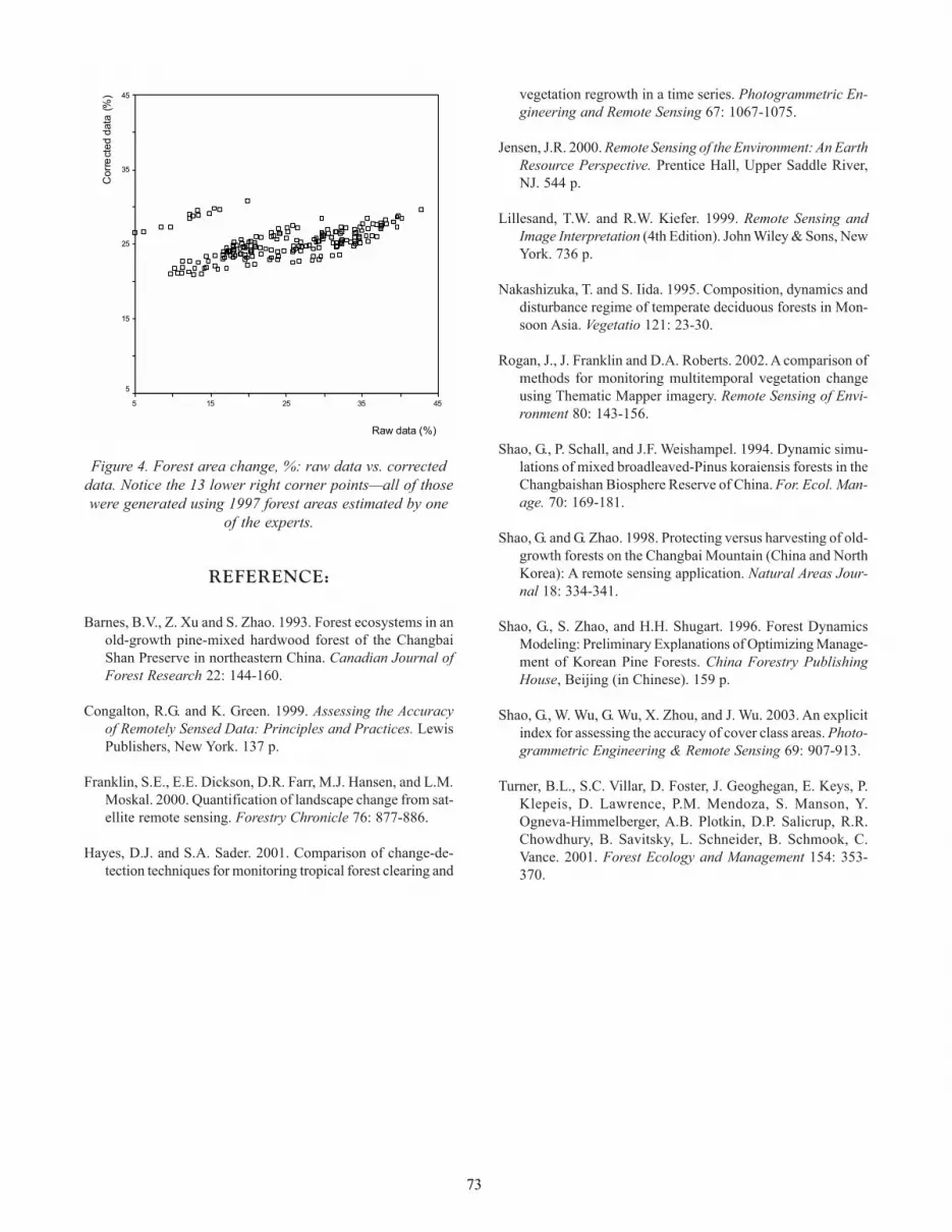
73
REFERENCE:
Barnes, B.V., Z. Xu and S. Zhao. 1993. Forest ecosystems in anold-growth pine-mixed hardwood forest of the ChangbaiShan Preserve in northeastern China. Canadian Journal ofForest Research 22: 144-160.
Congalton, R.G. and K. Green. 1999. Assessing the Accuracyof Remotely Sensed Data: Principles and Practices. LewisPublishers, New York. 137 p.
Franklin, S.E., E.E. Dickson, D.R. Farr, M.J. Hansen, and L.M.Moskal. 2000. Quantification of landscape change from sat-ellite remote sensing. Forestry Chronicle 76: 877-886.
Hayes, D.J. and S.A. Sader. 2001. Comparison of change-de-tection techniques for monitoring tropical forest clearing and
vegetation regrowth in a time series. Photogrammetric En-gineering and Remote Sensing 67: 1067-1075.
Jensen, J.R. 2000. Remote Sensing of the Environment: An EarthResource Perspective. Prentice Hall, Upper Saddle River,NJ. 544 p.
Lillesand, T.W. and R.W. Kiefer. 1999. Remote Sensing andImage Interpretation (4th Edition). John Wiley & Sons, NewYork. 736 p.
Nakashizuka, T. and S. Iida. 1995. Composition, dynamics anddisturbance regime of temperate deciduous forests in Mon-soon Asia. Vegetatio 121: 23-30.
Rogan, J., J. Franklin and D.A. Roberts. 2002. A comparison ofmethods for monitoring multitemporal vegetation changeusing Thematic Mapper imagery. Remote Sensing of Envi-ronment 80: 143-156.
Shao, G., P. Schall, and J.F. Weishampel. 1994. Dynamic simu-lations of mixed broadleaved-Pinus koraiensis forests in theChangbaishan Biosphere Reserve of China. For. Ecol. Man-age. 70: 169-181.
Shao, G. and G. Zhao. 1998. Protecting versus harvesting of old-growth forests on the Changbai Mountain (China and NorthKorea): A remote sensing application. Natural Areas Jour-nal 18: 334-341.
Shao, G., S. Zhao, and H.H. Shugart. 1996. Forest DynamicsModeling: Preliminary Explanations of Optimizing Manage-ment of Korean Pine Forests. China Forestry PublishingHouse, Beijing (in Chinese). 159 p.
Shao, G., W. Wu, G. Wu, X. Zhou, and J. Wu. 2003. An explicitindex for assessing the accuracy of cover class areas. Photo-grammetric Engineering & Remote Sensing 69: 907-913.
Turner, B.L., S.C. Villar, D. Foster, J. Geoghegan, E. Keys, P.Klepeis, D. Lawrence, P.M. Mendoza, S. Manson, Y.Ogneva-Himmelberger, A.B. Plotkin, D.P. Salicrup, R.R.Chowdhury, B. Savitsky, L. Schneider, B. Schmook, C.Vance. 2001. Forest Ecology and Management 154: 353-370.
Raw data (%)
453525155
Cor
rect
ed d
ata
(%) 45
35
25
15
5
Figure 4. Forest area change, %: raw data vs. correcteddata. Notice the 13 lower right corner points�all of thosewere generated using 1997 forest areas estimated by one
of the experts.

74

75
Automatic Extraction of Trees from Height Data Using ScaleSpace and SNAKES
BERND-M. STRAUB
Abstract: An approach is presented for the automatic extraction of trees and the boundaries of treecrowns. It is based on amulti-scale representation of an orthoimage and a surface model in Linear Scale Space. The segmentation of the surface modelis performed using a watershed transformation. Finally the boundary of every crown is measured with Snakes (Active ContourModels). The approach was tested with data from laser scanner (1 m) and image matching (0.25 m).
INTRODUCTION
In this paper we present a new approach for the auto-matic extraction of individual trees using a true orthoimageand a surface model as input data. The surface model isused as main source of information for the extraction ofindividual trees. Additional colour information from theorthoimage is used to differentiate between vegetation andother objects in the scene. The aim of the presented approachis to detect every tree in the observed area of the real worldand to measure the boundary of its crown. Originally, themethod was developed for the automatic extraction of treesin settlement areas using height data from image matching.The type of surface model used has a ground sampling of0.25 m, it was produced by the French company ISTAR us-ing 1:5000 color infrared aerial images. An example of sucha data set, acquired over Grangemouth, Scotland in sum-mer 2000 is depicted in Figure 1, refer (Straub and Heipke2001) for details.
In order to demonstrate the potential of the approach, weapplied it on a test site in a forest in the Austrian alps. Themain species in this test site is spruce (94%). A surface modelwas used in the investigations. The laser scanner flight witha Toposys I Scanner was carried out in August 1999 in Aus-tria, close to Hohentauern. The flying height wasapproximatley 800 m above ground, leading to 4-5 pointsper square meter, refer (Baltsavias 1999) for an overviewabout airborne laser scanner. The data were provided byJoanneum Research in Graz, Austria for this investigation.
In the next section of the paper a short overview is givenon the related work in the field of automatic extraction. Inthe main section of the paper the approach is described indetail, it is divided in two subsections: The first one depictsthe object model for trees and the second one the processing
strategy. In the last section some exemplary results areshown. The paper closes with a short summary and an out-look.
RELATED WORK
The first trial to utilize an aerial image for forest pur-poses was performed in 1897 (Hildebrandt 1987). Since thattime the scientific forest community has worked on meth-ods for the extraction of tree parameters from aerial images.Early work was carried out on the manual interpretation ofimages for forest inventory (Schneider 1974), (Lillesand andKiefer 1994). Pioneering work in the field of the automated,individual tree extraction from images emerged about oneand a half decades ago (Haenel and Eckstein 1986),(Gougeon and Moore 1988), (Pinz 1989). Recent work inthe field was published by Pollock (1996), Brandtberg andWalter (1998), Larsen (1999), Andersen et al. (2002),Persson et al. (2002), Schardt et al. (2002). An excellentstate-of-the-art overview is given by Hill and Leckie (1999).Some of the recent publications are described in detail inthe following section.
A common element of most approaches is the geometricmodel of a tree as it was proposed by Pollock (1994). In thefollowing, this surface description is referred to as the Pol-lock-Model. The geometric part of the Pollock-Model canbe depicted as follows:
The parameter a corresponds to the height, and b to theradius of the crown, n is a shape parameter. Two examplesof surfaces which can be described with Equation 1 are de-
( )2 2 2
1
nn
n n
x yza b
++ = (1)

76
picted in Figure 2. The surface of a real tree is of course verynoisy in comparison to the Pollock-Model. This “noise” isnot caused by the measurement of the surface, it is simply aconsequence of using such a model for a complex shape likethe real crown of a tree. But the main shape of the crown iswell modelled with this surface description.
Another common element in the most approaches is theapplication of the Linear Scale-Space in the early process-ing stages (refer to (Dralle and Rudemo 1996), (Brandtbergand Walter 1998), (Schardt et al. 2002), and (Persson et al.2002)). In (Andersen et al. 2001) a Morphological Scale-Space is used for the extraction of tree positions. A basicidea of the Linear Scale-Space is to construct a multi-scalerepresentation of an image, which only depends on one pa-rameter and has the property of causality: that means it hasto be insured, that features in coarse scale have always areason in fine scale (Koenderink 1984). One can show, thata multi-scale representation based on a Gaussian functionused as a low pass filter fulfils this requirement. In practice,the original signal ( )xf r is convolved with a Gaussian ker-nel with a different scale parameter s; the result of the con-volution operation is assigned as . Small values of σcorrespond to a fine scale level, large values to a coarse scale.An extensive investigation and mathematical reasoning in-cluding technical instructions can be found in (Lindeberg1994).
One of the crucial problems is the estimation of the scaleparameter σ , i.e., the selection of the scale level for theextraction of the low-level features. In (Schardt et al. 2002)it was proposed to use a scale selection mechanism, refer to(Lindeberg 1998) for details, based on the maximum re-sponse after Scale-Space transformation. In our approachthe scale selection is applied on a higher level, i.e. after thesegmentation of the image, and not before, as it was pro-posed in (Schardt et al. 2002). This allows an internal evalu-ation of the segments on a semantic level, which is an im-portant possibility if it is necessary to distinguish betweentrees and other objects.
DESCRIPTION OF THE APPROACH
The idea of our approach is to create a multi-scale repre-sentation of the surface model similar to (Persson et al. 2002).The selection of the scale level is of crucial importance forthe extraction of trees, the reasons are: (1) The correct scalelevel depends mainly on the size of the objects one is look-ing for. In the case of trees this size can neither be assumedto be known nor is it constant for all trees in one image. Thesize of trees depends on the age, the habitat, the species andmany more parameters, which cannot be modelled in ad-vance. (2) The correct scale is of crucial importance for thesegmentation. The small structures of the crown are verydifficult to model and – except for small structures - thecrown has a relatively elementary shape. The image is seg-mented in a wide range of scales, bounded by reasonablevalues for the minimum and maximum diameter of a tree’scrown. In (Gong et al. 2002) the typical range for the diam-eter is proposed to be minimal 2.5 m up to 15 m coveringall species of trees.
This section is subdivided into two parts. In the first partthe model for trees, which constitutes the basis for the strat-
Figure 1: Orthoimage, surface model and 3D vizualization of automatically extracted trees insettlement areas.
Figure 2: 3D visualisation of the Pollock-Model.Left: Surface model of a typical deciduous tree:
a=7, b=3.5, n=1.2.
Right: Coniferous tree: a=20.0; b=5.0; n=1.2,different scales of the horizontal and vertical axis.

77
egy of extraction, is described. The strategy is explained indetail in the second part of the paper.
MODEL FOR TREES
The geometric part of the model of an individual treesimplifies the crown to a 2.5D surface, see the Pollock-Model(Equation 1). The parameter n can be used to define theshape of a broad-leafed tree with a typical range of valuesfrom 1.0 to 1.8, and also for conifers with a typical rangefor n from 1.5 to 2.5. These numerical values are based onan investigation described in (Gong et al. 2002).
Based on the Pollock-Model the following features forthe extraction from the surface model can be derived: theprojection of the model into the xy-plane is a circle with adiameter in given range. Furthermore, the 3D shape of thesurface is always convex. The image processing is based ondifferential geometric properties. A profile is used along fourtree tops to study the geometrical properties of the surface ifthe trees stand close together. In the left part of Figure 3four Pollock-Trees computed with a=6 m, b=2 m, and n=2.0(1 m is equivalent to 10 pixels respectively grey values) aredepicted. The profile is plotted in dark grey in Figure 3.
One can see that the “valley” between the trees decreasesfrom the left to the right. The absolute value of the gradient
(black line in Figure 3) decreases also. Obviouslythis is a consequence of the decreasing distance betweenthe trees, and of the crown shapes.
The surface at the tree tops has a convex shape in bothdirections, along and across the profile. Therefore, the sumof the second partial derivations is always negative for thewhole crown (refer to the light grey line in Figure 3). At apoint on the profile between two trees the partial, secondderivative is smaller than zero along the profile and largerthan zero perpendicular to the profile. Therefore, theLaplacian of the surface model at points like this isnormally higher than at points on the crown, because bothpartial second derivatives are smaller than zero at the treetops. These characteristics lead to local maxima betweenthe crowns in .
In the case of real data this model is only valid in a conve-nient scale level. A height profile from real data is used toexplain the term “convenient” in this context. Two differentScale-Space representations of the surface model with σ val-ues of 0.5 m and 8 m are depicted in Figure 4. One can seethat more and more fine structures disappear and the coarsestructure is enhanced with the increase of the scaleparameter σ.
The height profile along the tree tops is measured alongthe dotted line which is superimposed to the surface modelin Figure 4. The left height profile measured in the originalsurface model is noisy compared to the profile of the syn-thetic trees. As a result of this noise the Laplacian is oscil-lating close to zero. In the “correct” scale level for this smallgroup of trees the assumptions regarding the Laplacian arefulfilled quite well. The Laplacian is negative for trees andpositive for the valleys between them, just like the profile ofthe synthetic Pollock-Trees (Figure 3). The coarse structureof the crown is enhanced, and as a result of this the proper-ties of the Pollock-Model are valid also for the surface modelof real trees in this scale level.
PROCESSING STRATEGY
In general, there are two possibilities to build a strategyfor the automatic extraction of trees from the image data.The first possibility is to model the crown in detail: onecould try to detect and group the fine structures in order toreconstruct the individual crowns. The second possibility isto remove the fine structures from the data with the aim tocreate a surface which has the character of the Pollock-Model. In the literature examples for both strategies can befound: Brandtberg (1999) proposed to use the typical finestructure of deciduous trees in optical images for the detec-tion of individual trees. In (Andersen et al. 2002) the finestructure of the crown is modelled as a stochastic processwith the aim to detect the underlying coarse structure of thecrown. The other strategy, the removal of noise, was pro-posed by Schardt et al. (2002) and by Persson et al. (2002).The main problem of this type of approach is the determi-nation of an optimal low pass filter for every single tree inthe image. This is kind of a chicken-and-egg problem, be-cause the optimal low pass filter depends mainly on the di-ameter of the individual tree one is looking for, which is notknown in advance.
The basis of our approach is the Linear Scale-SpaceTheory. The watershed transformation is used as a segmen-tation technique, Fuzzy Sets for the evaluation of the seg-ments, and Snakes for the refinement of the crowns outline.The basic ideas of the Linear Scale-Space Theory were origi-nally proposed by Koenderink (1984), and were worked outby Lindeberg (1994). The watershed transformation for thesegmentation of images was introduced by Beucher andLantéjoul (1979). Details about the watershed transforma-tion can be found in (Soille 1999). Fuzzy Sets (Zadeh 1965)are used, because they are a “very natural and intuitively
Figure 3: Profile of the surface model of four Pollock-Trees, the location of the profile is depicted in the
upper left corner.
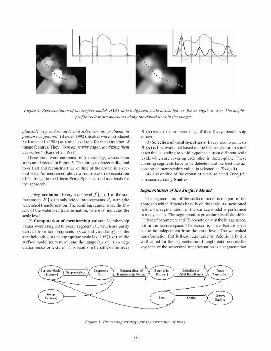
78
plausible way to formulate and solve various problems inpattern recognition.” (Bezdek 1992). Snakes were introducedby Kass et al. (1988) as a mid-level tool for the extraction ofimage features. They “look on nearby edges, localizing themaccurately” (Kass et al. 1988).
These tools were combined into a strategy, whose mainsteps are depicted in Figure 5. The aim is to detect individualtrees first and reconstruct the outline of the crown in a sec-ond step. As mentioned above a multi-scale representationof the image in the Linear Scale-Space is used as a basis forthe approach:
(1) Segmentation: Every scale level of the sur-face model is subdivided into segments using thewatershed transformation. The resulting segments are the Ba-sins of the watershed transformation, where indicates thescale level.
(2) Computation of membership values: Membershipvalues were assigned to every segment , which are partlyderived from both segments (size and circularity), or thearea belonging to the appropriate scale level ( ),H x σ
r of thesurface model (curvature), and the image ( ),I x σ
r ( ⇔ veg-etation index or texture). This results in hypothesis for trees
( )B aσ
r with a feature vector ar of four fuzzy membershipvalues.
(3) Selection of valid hypothesis: Every tree hypothesis( )B aσ
r is first evaluated based on the feature vector. In somecases this is leading to valid hypothesis from different scalelevels which are covering each other in the xy-plane. Thesecovering segments have to be detected and the best one ac-cording its membership value, is selected as ( )Tree aσ
r .(4) The outline of the crown of every selected ( )Tree aσ
r
is measured using Snakes.
Segmentation of the Surface Model
The segmentation of the surface model is the part of theapproach which depends heavily on the scale. As mentionedbefore the segmentation of the surface model is performedin many scales. The segmentation procedure itself should be(1) free of parameters and (2) operate only in the image space,not in the feature space. The reason is that a feature spacehas to be independent from the scale level. The watershedtransformation fulfils these requirements. Additionally it iswell suited for the segmentation of height data because thekey idea of the watershed transformation is a segmentation
Figure 4: Representation of the surface model ( )H xr at two different scale levels, left: σ=0.5 m, right: σ=8 m. The heightprofiles below are measured along the dotted lines in the images.
Figure 5: Processing strategy for the extraction of trees.
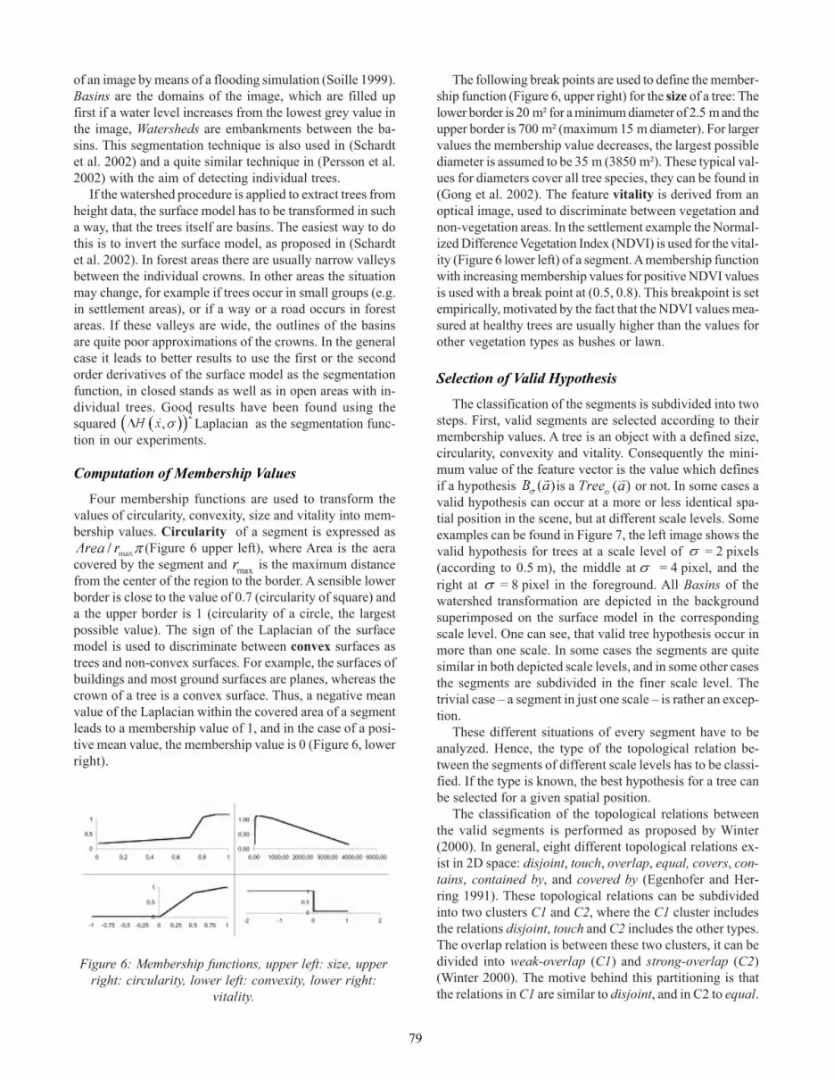
79
of an image by means of a flooding simulation (Soille 1999).Basins are the domains of the image, which are filled upfirst if a water level increases from the lowest grey value inthe image, Watersheds are embankments between the ba-sins. This segmentation technique is also used in (Schardtet al. 2002) and a quite similar technique in (Persson et al.2002) with the aim of detecting individual trees.
If the watershed procedure is applied to extract trees fromheight data, the surface model has to be transformed in sucha way, that the trees itself are basins. The easiest way to dothis is to invert the surface model, as proposed in (Schardtet al. 2002). In forest areas there are usually narrow valleysbetween the individual crowns. In other areas the situationmay change, for example if trees occur in small groups (e.g.in settlement areas), or if a way or a road occurs in forestareas. If these valleys are wide, the outlines of the basinsare quite poor approximations of the crowns. In the generalcase it leads to better results to use the first or the secondorder derivatives of the surface model as the segmentationfunction, in closed stands as well as in open areas with in-dividual trees. Good results have been found using thesquared Laplacian as the segmentation func-tion in our experiments.
Computation of Membership Values
Four membership functions are used to transform thevalues of circularity, convexity, size and vitality into mem-bership values. Circularity of a segment is expressed as
(Figure 6 upper left), where Area is the aeracovered by the segment and is the maximum distancefrom the center of the region to the border. A sensible lowerborder is close to the value of 0.7 (circularity of square) anda the upper border is 1 (circularity of a circle, the largestpossible value). The sign of the Laplacian of the surfacemodel is used to discriminate between convex surfaces astrees and non-convex surfaces. For example, the surfaces ofbuildings and most ground surfaces are planes, whereas thecrown of a tree is a convex surface. Thus, a negative meanvalue of the Laplacian within the covered area of a segmentleads to a membership value of 1, and in the case of a posi-tive mean value, the membership value is 0 (Figure 6, lowerright).
The following break points are used to define the member-ship function (Figure 6, upper right) for the size of a tree: Thelower border is 20 m² for a minimum diameter of 2.5 m and theupper border is 700 m² (maximum 15 m diameter). For largervalues the membership value decreases, the largest possiblediameter is assumed to be 35 m (3850 m²). These typical val-ues for diameters cover all tree species, they can be found in(Gong et al. 2002). The feature vitality is derived from anoptical image, used to discriminate between vegetation andnon-vegetation areas. In the settlement example the Normal-ized Difference Vegetation Index (NDVI) is used for the vital-ity (Figure 6 lower left) of a segment. A membership functionwith increasing membership values for positive NDVI valuesis used with a break point at (0.5, 0.8). This breakpoint is setempirically, motivated by the fact that the NDVI values mea-sured at healthy trees are usually higher than the values forother vegetation types as bushes or lawn.
Selection of Valid Hypothesis
The classification of the segments is subdivided into twosteps. First, valid segments are selected according to theirmembership values. A tree is an object with a defined size,circularity, convexity and vitality. Consequently the mini-mum value of the feature vector is the value which definesif a hypothesis is a or not. In some cases avalid hypothesis can occur at a more or less identical spa-tial position in the scene, but at different scale levels. Someexamples can be found in Figure 7, the left image shows thevalid hypothesis for trees at a scale level of = 2 pixels(according to 0.5 m), the middle at = 4 pixel, and theright at = 8 pixel in the foreground. All Basins of thewatershed transformation are depicted in the backgroundsuperimposed on the surface model in the correspondingscale level. One can see, that valid tree hypothesis occur inmore than one scale. In some cases the segments are quitesimilar in both depicted scale levels, and in some other casesthe segments are subdivided in the finer scale level. Thetrivial case – a segment in just one scale – is rather an excep-tion.
These different situations of every segment have to beanalyzed. Hence, the type of the topological relation be-tween the segments of different scale levels has to be classi-fied. If the type is known, the best hypothesis for a tree canbe selected for a given spatial position.
The classification of the topological relations betweenthe valid segments is performed as proposed by Winter(2000). In general, eight different topological relations ex-ist in 2D space: disjoint, touch, overlap, equal, covers, con-tains, contained by, and covered by (Egenhofer and Her-ring 1991). These topological relations can be subdividedinto two clusters C1 and C2, where the C1 cluster includesthe relations disjoint, touch and C2 includes the other types.The overlap relation is between these two clusters, it can bedivided into weak-overlap (C1) and strong-overlap (C2)(Winter 2000). The motive behind this partitioning is thatthe relations in C1 are similar to disjoint, and in C2 to equal.
Figure 6: Membership functions, upper left: size, upperright: circularity, lower left: convexity, lower right:
vitality.

80
We postulate that all the segments ( )AB ar which have atopological relation in C2 to another segment ( )BB ar , A B≠from another scale level are potential hypothesis of the sametree in the real world. The best hypothesis - the one with thehighest membership value - is selected as a ( )Tree aσ
r in-stance. Accordingly, both investigated hypothesis are as-sumed to be valid, if the relation between the two segmentsis part of C1.
The final selected hypotheses are depicted in Figure 9.But even if the trees in the scene were detected correctly, theboundaries are often poor approximations for the outline ofthe individual crowns. This problem leads to the last pro-cessing step, where the outlines of the crowns will be re-fined with Snakes.
Measurement of the Crown’s Outline
Up to now the geometry of the segments stems from dif-ferent scale levels, as the Basins Bσ were extracted in dif-ferent scales. But the outline of the crown is an object with-out a changing scale, as distinct from the crown itself. Theoutline of the crown is measured in the fine scale with thehelp of Snakes. A Snake is a kind of a virtual rubber cordwhich can be used to detect valleys in a hilly landscape withthe help of gravity. This landscape may be a surface model,
or an image, or the edges of an image.Snakes were originally introduced by Kass et al. (1988)
as mid-level algorithms which combine geometric and/ortopologic constraints with the extraction of low-level fea-tures from images. The principal idea is to define a contourwith the help of mechanic properties like elasticity and ri-gidity, then to initialize this contour close to the boundaryof the object one is looking for, and finally to let the contourmove in the direction of the boundary of the object. In gen-eral, there are two main drawbacks to the application ofSnakes as a measurement tool. The first one is that the Snakehas to be initialized very close to the features one is lookingfor. The second one is the challenging tuning of the param-eters, primarily the weighting between internal and exter-nal forces and the selection of the external force field itself.
In our approach the Snake is used only for fine measure-ment in the last stage, the coarse shape of the crown is moreor less known. Furthermore, the approximation is often toosmall. Based on these constraints one can built a Snake whichis quite stable under these special conditions: the geometryof the Snake is initialized for every ( )Tree aσ
r as circularshaped closed polygon at the gravity center of the appropri-ate Basin Bσ . The snake could also be initialized with theoutline obtained from the watershed transformation. Theidea of using a circle instead of that is to make the Snake
Figure 7: Upper row: Basins of the watershed transformation on three scale levels. Lower row: Hypotheses fortrees in the corresponding scale levels. Left: σ = 2 pixels, middle:σ = 4 pix, right: σ = 8 pixels.

81
optimization a bit more independent from the geometry of thesegment stemming from the watershed transformation. Theradius of the circular closed polygon is computedby ( )( ) /Area B aσ π
r . This initialization stage is depictedin Figure 8 as the black circle in the right image. The pa-rameters for the internal energies were tuned in the follow-ing way: the length of the contour is weighted low, and thecurvature is weighted high. Without external forces, a Snakewhich is tuned in such a way converges to a circle with atrend to decrease its length1. As the approximation is oftentoo small, an additional force is added which makes theSnake behave like a balloon, which is inflated (Cohen 1991).With this additional force the contour moves towards theoutline of the crown if no external forces influence the move-ment. The sum of the gradients over all scale levels is usedas external force.
Finally, the membership values of every ( )Tree aσ
r has tobe computed again because the outlines have changed. Alsothe topological relations between all tree hypothesis are nolonger valid and have to be computed again. A changing ofthe topology occurs, if two or more segments ( )B aσ
r areparts of the same crown in the real world. In these cases, theSnake usually converges to the correct solution, i.e. the to-pological relation changes from the C1 cluster (similar todisjoint) to the C2 cluster (similar to equal). As these up-dated membership values are quite independent from thepre-processing in the different scale levels, these values areused as an internal evaluation of the tree hypothesis.
RESULTS
The described approach was applied to a small subset ofthe Hohentauern dataset as mentioned in the introductionof this paper. The selection of the subset was mainly moti-vated by the fact that ground truth is available for a part ofthis scene. The LIDAR first return data were transformedinto a 0.25 m raster. In order to get an initial idea of theperformance of this approach in forest areas the trees in aslightly smoothed (σ =1.0 pixel) version the surface model
were extracted manually. This is looked upon as the referencedata set for this evaluation (left of Figure 9). It should benoted, that these manually extracted data are a kind of anoptimal result of what the approach should deliver from thedeveloper’s point of view. The relationship between themanually extracted reference trees and the trees in the realworld is not discussed here.
An automatically extracted tree is assigned as a True Posi-tive (TP), if it has a topological relation from the C2 clusterwith a tree in the manually extracted reference data set, oth-erwise it is assigned as a False Positive (FP). Those trees inthe reference data set with a C1 relation to an automaticallyextracted tree are assigned as False Negatives (FP). Basedon these numbers, the Completeness and the Correctness2
of the extraction result can be computed:
In order to characterize the accuracy of the correct auto-matically extracted trees, the mean value and the standarddeviation of the mean value were computed for the distancebetween the centers of gravity and the radii between refer-ence tree and automatically extracted tree. The results aredepicted in Table 1.
One can see that the internal evaluation, which is per-formed after the measurement of the crown’s outline, leadsto a significant degradation for the completeness. As ex-pected the Correctness is enhanced, 97% of the extractedtrees are correct. The accuracy measures are nearly equiva-lent. This is a little bit surprising, because it was expectedthat the outline of the crown would be much more preciselydelineated by the Snake than by the watershed transforma-tion. Similar experiences were made with other datasets.
SUMMARY AND OUTLOOK
In this paper an approach for the automatic extraction oftrees is presented. The object model and the processing strat-egy are illustrated in detail, as well as some exemplary re-sults. The approach is free of assumptions about the scalelevel, because the segmentation is performed in a wide rangeof different scale levels. The classification of the tree hy-pothesis is based only four parameters: size, circularity, con-vexity, and vitality. Of these four parameters only the vital-ity is dependent on using image data, the others are geomet-ric object properties. It should be noted that the values forthe size of the crowns stems from an independent investiga-tion (Gong et al. 2002), and the convexity is always posi-tive. Only the breakpoints in the circularity membershipfunction are empirical values.
The measurement of the crown’s outline is performedwith a Snake algorithm. The adjustment of the parametersfor the Snake is a quite difficult task. But once adjusted, thealgorithm is stable as a measurement tool for this task with-
Figure 8: Example for the measurement of a crownoutline with a Snake, five different optimization steps are
depicted.
TPCompleteness TP FNTPCorrectness TP FP
= +
= +
2

82
Figure 9: Left: Manually extracted trees superimposed to the surface model. Middle: Selected tree hypotheses,different gray values correspond to different scale levels. Right: Results of the approach, final selected trees after
internal evaluation.
out changing these settings for different scenes. Unfortu-nately, the accuracy of the results, namely the position andthe radius of trees, did not increase. This should be investi-gated in detail, to deterime if this applies only for the centerof gravity and the radius or for the whole outline.
The approach was tested with synthetic data (refer Figure3), high resolution data in settlement areas (Completeness68%, Correctness 82%), and a small dataset of a forest (Com-pleteness 70%, Correctness 86%). In the forest case it is nec-essary to evaluate the results with more reliable referencedata. Furthermore, it is planned to use the information aboutthe outline of the individual trees for a detailed classifica-tion. For example, we will investigate how the curvature iscorrelated with the shape parameter of the Pollock-Model,which can be used as a feature for the classification of thespecies. Another idea is the use of the approach in a com-bined strategy for the extraction of the ground surface in for-
est or dense settlement areas. This is possible, because theapproach is free of assumptions about the terrain and theheight of the trees is not used for the detection.
ACKNOWLEDGEMENT
Parts of this work were funded by the European Com-mission under the contract IST-1999-10510. The surfacemodel and the true othoimages were produced by the Frenchcompany ISTAR. All aerial images, digital elevation mod-els, and true orthoimages are copyrighted by ISTAR, SophiaAntipolis, France. Many thanks go to Alix Marc and FrankBignone for their valuable cooperation. The Hohentauerndataset was provided by Joanneum Research in Graz, Aus-tria. Many thanks go to Matthias Schardt and Roland Wackfor their trustful and open discussion in Graz, April 2003.
Step Quality Position Radius
Completeness Correctness
Mean Difference RMS
Mean Difference RMS
Selection of valid hypothesis 70% 86%
4.4 3.6
-3.0 3.6
Measurement of the crowns outline 45% 97%
4.6 3.5
-2.9 3.6
Table 1: Quality measures and accuracy approximations (in pixels) for the Hohentauern dataset (1 pixel = 0.25 m). Thenumbers are given after the step “Selection of the valid hypotheses” in the first row, and after “Measurement of the crownsoutline” in the second row in the table.

83
REFERENCES
Andersen, H., Reutebuch, S.E., and Schreuder, G.F. 2001. Au-tomated Individual Tree Measurement through Morphologi-cal Analysis of a LIDAR-based Canopy Surface Model. P.11-22, in Proceedings of the First International PrecisionForestry Cooperative Symposium, Seattle, USA, June 17-20.
Andersen, H., Reutebuch, S.E., and Schreuder, G.F. 2002. Baye-sian Object Recognition for the Analysis of Complex ForestScenes in Airborne Laser Scanner Data. P. 35-41, in TheInternational Archives of the Photogrammetry, RemoteSensing and Spatial Information Sciences, XXXIV. 3A.ISPRS, Graz, Austria.
Baltsavias, E., 1999. Airborne laser scanning: existing systemsand firms and other resources. ISPRS Journal of Photo-grammetry and Remote Sensing, (1999)54:164-198.
Beucher, S., and Lantéjoul, C. 1979. Use of Watersheds in Con-tour Detection. in International Workshop on Image Pro-cessing, Rennes, France.
Bezdek, J.C., 1992. Computing with Uncertainty. IEEE Com-munications Magazine, (1992)September:24-36.
Brandtberg, T., and Walter, F., 1998. Automated delineation ofindividual tree crowns in high spatial resolution aerial im-ages by multiple scale analysis. Machine Vision and Appli-cations, (1998)11:64-73.
Brandtberg, T. 1999. Structure-based classification of tree spe-cies in high spatial resolution aerial images using a fuzzyclustering technique. P. 165-172, in The 11th ScandinavianConference on Image Analysis, Kangerlussueq, Greenland,June 7-11.
Cohen, L., 1991. On active contour models and balloons.CVGIP: Image Understanding, (53)2:211-218.
Dralle, K., and Rudemo, M., 1996. Stem Number Estimationby Kernel Smoothing of Aerial Photos. Canadian Journalof Forest Research, (1996)26:1228-1236.
Egenhofer, M.J., and Herring, J.R., 1991. Categorizing BinaryTopological Relations Between Regions, Lines, and Pointsin Geographic Databases. University of Maine, NationalCenter for Geographic Information and Analysis, Orono,28p.
Gong, P., Sheng, Y., and Biging, G., 2002. 3D Model BasedTree Measurement from High-Resolution Aerial Imagery.Photogrammetric Engineering and Remote Sensing,(68)11:1203-1212.
Gougeon, F., and Moore, T. 1988. Individual Tree Classifica-tion Using Meis-II Imagery. P. 927 -927, in IGARSS ’88
Geoscience and Remote Sensing Symposium, 2. IEEE.
Haenel, S., and Eckstein, W. 1986. Ein Arbeitsplatz zurautomatischen Luftbildanalyse. P. 38-42, Springer, Berlin,Deutschland.
Hildebrandt, G., 1987. 100 Jahre forstliche Luftbildaufnahme -Zwei Dokumente aus den Anfängen der forstlichenLuftbildinterpretation. Bildmessung und Luftbildwesen,(1987)55:221-224.
Hill, D.A., and Leckie, D.G. (eds.), 1999. International forum:automated interpretation of high spatial resolution digitalimagery for forestry, February 10-12, 1998. Natural Re-sources Canada, Canadian Forest Service, Pacific ForestryCentre, Victoria, British Columbia, 395p.
Kass, M., Witkin, A., and Terzopoulus, D., 1988. Snakes: Ac-tive Contour Models. International Journal of ConputerVision, (1988)1:321-331.
Koenderink, J., 1984. The Structure of Images. Biological Cy-bernetics, (50):363-370.
Larsen, M. 1999. Individual tree top position estimation by tem-plate voting. P. 8, in 21st Canadian Symposium on RemoteSensing, Ottawa, 21-24 June.
Lillesand, T.M., and Kiefer, R.W., 1994. Remote Sensing andImage Interpretation. John Wiley and Sons, Inc., New YorkChichester Brisbane Toronto Singapore, 750p.
Lindeberg, T., 1994. Scale-Space Theory in Computer Vision.Kluwer. Academic Publishers, Boston, USA, 423p.
Lindeberg, T., 1998. Feature Detection with Automatic ScaleSelection. International Journal of Computer Vision,(30)2:79-116.
Persson, A., Holmgren, J., and Söderman, U., 2002. Detectingand Measuring Individual Trees Using an Airborne LaserScanner. Photogrammetric Engineering and Remote Sens-ing, (68)9:925-932.
Pinz, A. 1989. Final Results of the Vision Expert System VES:Finding Trees in Aerial Photographs. P. 90-111, in Proceed-ings ÖAGM 13. Workshop of the Austrian Association forPattern Recognition, Oldenbourg OCG Schriftenreihe.
Pollock, R.J., 1996. The Automatic recognition of Individualtrees in Aerial Images of Forests Based on a Synthetic TreeCrown Image Model. The University of British Columbia,Vancouver, Canada, June 1996.
Pollock, R.J.. 1994. A model-based approach to automaticallylocating tree crowns in high spatial resolution images. P.526-537, in Image and Signal Processing for Remote Sens-ing, 2315. SPIE.

84
Schardt, M., Ziegler, M., Wimmer, A., Wack, R., and Hyyppä,R. 2002. Assessment of Forest Parameter by Means of La-ser Scanning. P. 302-309, in The International Archives ofthe Photogrammetry, Remote Sensing and Spatial Infor-mation Sciences, XXXIV. 3A. ISPRS, Graz, Austria.
Schneider, S., 1974. Luftbild und Luftbildinterpretation. deGruyter, Berlin New York, 530p.
Soille, P., 1999. Morphological Image Analysis: Principles andApplications. Springer, Berlin Heidelberg NewYork, 316p.
Straub, B., and Heipke, C., 2001. Automatic Extraction of Treesfor 3D-City Models from Images and Height Data. P. 267-277. in Automatic Extraction of Man-Made Objects fromAerial and Space Images. Vol. 3. A.A.Balkema Publishers.Lisse/Abingdon/Exton(PA)/Tokio.
Winter, S., 2000. Uncertain Topological Relations between Im-precise Regions. International Journal of Geographic In-formation Science, (14)5:411-430.
Zadeh, L., 1965. Fuzzy Sets. Information Control, (8):338-353.

85
A Tree Tour with Radio Frequency Identification (RFID) anda Personal Digital Assistant (PDA)
SEAN HOYT, DOUG ST. JOHN, DENISE WILSON AND LINDA BUSHNELL
Abstract: A popular tree tour at the University of Washington campus has been automated via RFID and a PDA. Theprevious 81-tree hardcopy tour has also been updated to include more information on each tree, including digital photos. Asurvey conducted demonstrates the updated, electronic tree tour is easier to navigate, full of better visuals, and results in lessfalse identifications.

86

87
Value Maximization Software – Extracting the Most from theForest Resource
HAMISH MARSHALL AND GRAHAM WEST
Abstract: Global competition is encouraging all forest owners to manage their forested lands in more integrated mannerand extract more value from the resource. ATLAS is a new suite of forest management software tools developed by ForestResearch. The goal of the ATLAS concept is to have a suite of fully integrated software applications covering all forestmanagement decisions from planting through to sawmilling. Three major applications have been developed so far: ATLASCruiser – a state-of-the-art forest inventory application, ATLAS GeoMaster – an advanced stand record systems and ATLASMarket Supply – one of the first weekly market supply planning optimization systems. In the future further applicationscovering growth modeling, saw mill optimization, strategic and tactical planning will be developed. This presentation willgive a brief overview of the ATLAS system and highlights its key attributes

88

89
Costs and Benefits of Four Procedures for Scanning onMechanical Processors
GLEN E. MURPHY AND HAMISH MARSHALL
Summary: Four simulated procedures for scanning and bucking Douglas fir, ponderosa pine and radiata pine trees wereevaluated on the basis of productivity, costs, and value recovery. The procedures evaluated were: (a) a conventional operatingprocedure where quality changes and bucking decisions were input by the machine operator, (b) an automated scan of the fullstem prior to optimisation and bucking, (c) a 6 m automated scan with 6.2 m forecast ahead, and (d) a 4.7 m automated scanwith 7.5 m forecast ahead before optimal bucking took place. After subtracting costs, net value recovery for the automatedscanning methods was 4 to 9% higher than for a conventional procedure. Breakeven capital investment costs for new scan-ning and optimisation equipment were dependent on tree species and size, markets and scanning procedure and could rangebetween US$0 and US$1,400,000.

90

91
Evaluation of Small-Diameter Timber for Value-AddedManufacturing � A Stress Wave Approach
XIPING WANG, ROBERT J. ROSS, JOHN PUNCHES, R. JAMES BARBOUR, JOHN W. FORSMAN
AND JOHN R. ERICKSON
Abstract- The objective of this research was to investigate the use of a stress wave technology to evaluate the structuralquality of small-diameter timber before harvest. One hundred and ninety-two Douglas-fir and ponderosa pine trees weresampled from four stands in southwestern Oregon and subjected to stress wave tests in the field. Twelve of the trees, sixDouglas-fir and six ponderosa pine, were harvested and sawn into logs and lumber. The mechanical properties of wood werethen assessed by both stress wave and static bending techniques in the laboratory. Results of this study indicated a significantdifference in stress wave time (SWT) between Douglas-fir and ponderosa pine trees and between two stands of each species.SWT of Douglas-fir trees increased slightly as tree diameter at breast height (DBH) increased; whereas, SWT of ponderosapine trees decreased significantly as DBH increased. The statistical analysis also revealed good relationships between SWT oftrees and modulus of elasticity (MOE) of logs and lumber produced from the trees as the two species were combined. However,the strength of the relationships was reduced within the species because of small sample size and narrow property range.
INTRODUCTION
Throughout the United States, past management prac-tices have created thousands of acres of forest densely stockedwith small-diameter trees. These stands are at increasedrisk of insect and disease attack and have higher catastrophicfire potential. Increased management emphasis on foresthealth and bio-diversity has forced land managers to seekeconomically viable stand treatments such as thinning toimprove the stand condition. Economical and value-addeduses for removed small-diameter timber can help offset for-est management cost, provide economic opportunities formany small, forest-based communities, and avoid future losscaused by catastrophic wildfires. However, the variabilityand lack of predictability of the strength and stiffness ofstanding timber cause problems in engineering applications.It is essential to develop cost-effective technologies for evalu-ating the potential structural quality of such materials.
The traditional log-to-product manufacturing process failsto recognize a tree�s full value. The process occurs in aseries of mostly independent steps (trees, to logs, to lumber,to parts), each optimized for its own outputs. The ultimateend use is rarely a consideration during intermediate pro-cessing stages. By identifying final product potential beforetimber harvest, we hope to 1) enhance resource utilizationefficiency, 2) make it economically viable for secondary woodproducts manufacturers to utilize small-diameter timber, and3) facilitate stand management activities by identifying small-diameter timber value.
This study is part of the project �Evaluation of small-diameter timbers for value-added manufacturing: An inte-grated approach� conducted jointly by Oregon State Uni-versity, USDA Forest Service Forest Products Laboratory,and USDA Forest Service PNW Research Station. The over-all goal of the project was to design, construct, and deliver asystem by which communities and forest industries may ef-ficiently recognize value-added wood products potential insmall diameter trees. The specific objective of this study wasto investigate the use of a stress wave nondestructive evalu-ation technique to assess the potential structural quality ofsmall-diameter timbers before timber harvest.
MATERIAL AND METHODS
A total of one hundred and ninety-two Douglas-fir(Pseudotsuga menziesii) and ponderosa pine (Pinus ponde-rosa) trees were sampled for stress wave evaluation at fourdifferent stands in southwestern Oregon. The stands werelocated in the Applegate Ranger District on the Rogue RiverNational Forest. Stand A (Yale Twin) was a 70 year old even-aged stand consisting primarily of Douglas-fir with somemadrone and a small compliment of ponderosa pine. Thestand had a mean diameter of 6.4 inches (16.3 cm) and aquadratic mean diameter of 7.4 inches (18.8 cm). Stand B(Toe Top) consisted of a sparse stand of 90-year-old trees(primarily ponderosa pine) with a 65 year old under-storyof Douglas-fir, smaller ponderosa pine, madrone, and anoccasional incense cedar. It had a mean diameter of 6.0
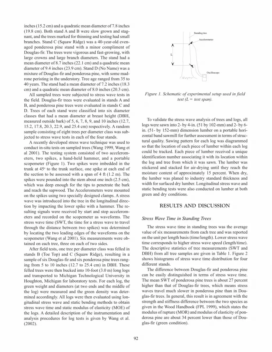
92
Figure 1. Schematic of experimental setup used in fieldtest (L = test span).
Oscilloscope
L
Standing tree
Accelerometer
inches (15.2 cm) and a quadratic mean diameter of 7.8 inches(19.8 cm). Both stand A and B were slow grown and stag-nant, and the trees marked for thinning and testing had smallbranches. Stand C (Squaw Ridge) was a 40-year-old even-aged ponderosa pine stand with a minor compliment ofDouglas-fir. The trees were vigorous and fast-growing, withlarge crowns and large branch diameters. The stand had amean diameter of 8.7 inches (22.1 cm) and a quadratic meandiameter of 9.4 inches (23.9 cm). Stand D (No Name) was amixture of Douglas-fir and ponderosa pine, with some mad-rone peristing in the understory. Tree age ranged from 35 to40 years. The stand had a mean diameter of 7.2 inches (18.3cm) and a quadratic mean diameter of 8.0 inches (20.3 cm).
All sampled trees were subjected to stress wave tests inthe field. Douglas-fir trees were evaluated in stands A andB, and ponderosa pine trees were evaluated in stands C andD. Trees of each stand were classified into six diameterclasses that had a mean diameter at breast height (DBH,measured outside bark) of 5, 6, 7, 8, 9, and 10 inches (12.7,15.2, 17.8, 20.3, 22.9, and 25.4 cm) respectively. A randomsample consisting of eight trees per diameter class was sub-jected to stress wave tests in each of the four stands.
A recently developed stress wave technique was used toconduct in-situ tests on sampled trees (Wang 1999, Wang etal 2001). The testing system consisted of two accelerom-eters, two spikes, a hand-held hammer, and a portablescopemeter (Figure 1). Two spikes were imbedded in thetrunk at 45o to the trunk surface, one spike at each end ofthe section to be assessed with a span of 4 ft (1.2 m). Thespikes were pounded into the stem about one inch (2.5 cm),which was deep enough for the tips to penetrate the barkand reach the sapwood. The Accelerometers were mountedon the spikes using two specially designed clamps. A stresswave was introduced into the tree in the longitudinal direc-tion by impacting the lower spike with a hammer. The re-sulting signals were received by start and stop accelerom-eters and recorded on the scopemeter as waveforms. Thestress wave time (SWT, the time for a stress wave to travelthrough the distance between two spikes) was determinedby locating the two leading edges of the waveforms on thescopemeter (Wang et al 2001). Six measurements were ob-tained on each tree, three on each of two sides.
After field tests, one tree per diameter class was felled instands B (Toe Top) and C (Squaw Ridge), resulting in asample of six Douglas-fir and six ponderosa pine trees rang-ing from 5 to 10 inches (12.7 to 25.4 cm) in DBH. Thesefelled trees were then bucked into 10-foot (3.0 m) long logsand transported to Michigan Technological University inHoughton, Michigan for laboratory tests. For each log, thegreen weight and diameters (at two ends and the middle ofthe log) were measured and the green density was deter-mined accordingly. All logs were then evaluated using lon-gitudinal stress wave and static bending methods to obtainstress wave time and static modulus of elasticity (MOE) ofthe logs. A detailed description of the instrumentation andanalysis procedures for log tests is given by Wang et al.(2002).
To validate the stress wave analysis of trees and logs, alllogs were sawn into 2- by 4-in. (51 by 102-mm) and 2- by 6-in. (51- by 152-mm) dimension lumber on a portable hori-zontal band sawmill for further assessment in terms of struc-tural quality. Sawing pattern for each log was diagrammedso that the location of each piece of lumber within each logcould be tracked. Each piece of lumber received a uniqueidentification number associating it with its location withinthe log and tree from which it was sawn. The lumber wasstickered and stacked for air-drying until they reach themoisture content of approximately 15 percent. When dry,the lumber was planed to industry standard thickness andwidth for surfaced dry lumber. Longitudinal stress wave andstatic bending tests were also conducted on lumber at bothgreen and dry conditions.
RESULTS AND DISCUSSION
Stress Wave Time in Standing Trees
The stress wave time in standing trees was the averagevalue of six measurements from each tree and was reportedon the unit per length basis (time/length). Lower stress wavetime corresponds to higher stress wave speed (length/time).The descriptive statistics of tree measurements (SWT andDBH) from all tree samples are given in Table 1. Figure 2shows histograms of stress wave time distribution for fourdifferent stands.
The difference between Douglas-fir and ponderosa pinecan be easily distinguished in terms of stress wave time.The mean SWT of ponderosa pine trees is about 27 percenthigher than that of Douglas-fir trees, which means stresswaves travel much slower in ponderosa pine than in Dou-glas-fir trees. In general, this result is in agreement with thestrength and stiffness difference between the two species asgiven in the Wood Handbook (FPL 1999), which states themodulus of rupture (MOR) and modulus of elasticity of pon-derosa pine are about 34 percent lower than those of Dou-glas-fir (green condition).

93
Figure 2. Histograms of stress wave time (SWT)distribution for Douglas-fir and ponderosa pine trees.
The SWT of ponderosa pine trees also shows much highervariation than the SWT of Douglas-fir trees. The standarddeviation of SWT is 4.50 ms/ft (14.8 ms/m) for Douglas-fir(stand A and stand B combined), and 16.17 ms/ft (53.0 ms/m) for ponderosa pine (stand C and stand D combined).This might suggest a larger variation in strength and stiff-ness properties of ponderosa pine compared to those of Dou-glas-fir.
The statistical comparison analysis showed significantSWT differences between two stands of each species, whichimply a potential difference in strength and stiffness betweenthe stands. But this could not be substantiated due to thelack of mechanical property data of all tested standing trees.
The relationship between SWT and DBH of standing treesis shown in Figure 3. For better illustration, stress wavetimes in trees were analyzed in terms of diameter classes.The data points are mean values of SWT for eight trees ineach class, and the error bar indicates the standard devia-tions (±1 standard deviation).
The SWT in Douglas-fir trees increased slightly as DBHof the trees increased. The trend is more evident in stand A(Yale Twin) than in stand B (Toe Top). The SWT for standA increased about 12 percent as DBH changed from 5 in. to10 in. (12.7 to 25.4 cm). The SWT-DBH relationship forponderosa pine trees was quite different from Douglas-fir.As shown in Figure 3(b), the SWT in ponderosa pine treesdecreased significantly as DBH of the trees increased, espe-cially in stand C (Squaw Ridge) where the SWT dropped 24percent when the DBH increased from 5 in. to 10 in. (12.7to 25.4 cm). The causes for the different functional relation-ships between SWT and DBH for Douglas fir and ponde-rosa pine trees are not fully understood yet. Huang (2000)reported that, for the same age trees, stress wave time islower for trees with slower growth rate or narrower rings.This might explain the SWT-DBH trend found in Douglas
Table 1. Diameter at breast height and stress wave time of standing trees. a
Sample DBH (in.) SWT (µs/ft)
Species Stand No. Mean Min Max SD Mean Min. Max. SD
Douglas-fir A 48 7.4 4.7 10.3 1.71 75.2 67.3 87.0 4.79
B 48 7.5 4.6 10.2 1.76 72.8 60.8 79.2 3.83
Ponderosa pine C 48 7.6 4.8 10.3 1.76 98.9 77.3 150.0 14.94
D 48 7.6 4.7 10.1 1.77 89.2 71.3 134.3 16.12 a 1 in. = 2.54 cm, 1 µs/ft = 3.28 µs/m. DBH, diameter at breast height. SWT, stress wave time. SD, standard deviation.
0
2
4
6
8
10
12
14
60 70 80 90 100 110 120 130 140 150
Stress w ave time in trees (µs/ft)
Freq
uenc
y (%
)
Stand C: Squaw RidgeStand D: No name
(b) Ponderosa pine
0
2
4
6
8
10
12
14
60 62 64 66 68 70 72 74 76 78 80 82 84 86 88 90
Stress w ave time in trees (µs/ft)
Freq
uenc
y (%
)
Stand A:Yale Tw inStand B: Toe Top
(a) Douglas-f ir

94
40
50
60
70
80
90
100
4 5 6 7 8 9 10 11
DBH of standing trees (in.)
SWT
in tr
ees
(s/
ft)
Stand AStand B
(a) Doudlas f ir
405060708090
100110120130140150160
4 5 6 7 8 9 10 11
DBH of standing trees (in.)
SWT
in tr
ees
(s/
ft)
Stand CStand D
(b) Ponderosa pine
Figure 3. Relationship between stress wave time (SWT)and tree diameter at breast height (DBH).
fir trees. For ponderosa pine trees, the opposite SWT-DBHtrend could be more related to other factors such as the char-acteristics of tree forms (size and frequency of branches),proportion of mature and juvenile wood in the cross sectionas well as moisture content.
Relationship Between Stress Wave Time in Trees andLog Properties
Stress wave time in standing trees was measured in thelower part of the stem, which tracks to the butt log afterharvesting and cutting. In this study, a total of 42 10-ft.(3.0-m) long logs were obtained from 12 harvested trees.The number of the logs produced from each tree varied from3 to 5 for Douglas-fir and from 1 to 4 for ponderosa pine asa result of the difference in tree height. The diameter of thelogs (average value of diameters measured at two ends andthe middle) ranged from 4.3 to 10.0 in. (10.9 to 25.4 cm)for Douglas-fir and from 4.4 to 9.8 in. (11.2 to 24.5 cm) forponderosa pine. The physical and mechanical properties(density, stress wave time, and static MOE) of logs are sum-marized in Table 2. Note that all these properties were de-termined in green and un-debarked logs.
Figure 4 shows the relationship between SWT of treesand SWT of the butt logs cut from the trees. A linear regres-sion analysis indicated a strong correlation (R2 = 0.95) whentwo species were considered as a single population. Thestrength of the relationship was weakened when the twospecies were considered separately (R2 = 0.61 for Douglas-fir, R2 = 0.85 for ponderosa pine). This was presumably dueto the small sample size (n=6) and limited property rangefor samples of each species. It was found that SWT mea-sured in standing trees was about 10 and 22 percent lowerthan SWT of logs for Douglas-fir and ponderosa pine, re-spectively. This could be a systematic difference caused bydifferent stress wave approaches. It has been reported thatthe stress wave speed measured in trees could be dominantlycontrolled by the mature wood (outer wood in the cross-section) since both wave generation and sensing occurredon the surface of the stem (Wang 1999, Huang 2000, Ikeda
Table 2. Physical and mechanical properties of logs. a
Species No. of Density (lb/ft3) Stress wave time (µs/ft) MOE (106 lb/in2)
logs Mean Min. Max. SD Mean Min. Max. SD Mean Min. Max. SD
Douglas-fir 25 41.45 35.17 48.45 3.539 76.1 70.4 84.1 3.68 0.99 0.52 1.33 0.213
Ponderosa pine 17 51.75 43.12 57.55 4.310 116.3 106.0 134.7 8.84 0.57 0.33 0.79 0.149 a 1 lb/ft3 = 16.02 kg/m3, 1 µs/ft = 3.28 ms/m, 1 lb/in2 = 6895 Pa. MOE, modulus of elasticity determined by static bending method. SD, standard deviation

95
et al. 2000, and Wang et al. 2001), whereas in logs the waveswere introduced into the stem from one end and sensed atthe other end (Wang et al. 2002).
The relationships between SWT of trees and the averageMOE of logs are shown in Figures 5. Regression analysisindicated a linear relationship between SWT of trees andMOE of logs as all samples combined. The coefficient ofdetermination (R2) was found to be 0.74. Again, the strengthof the relationships was reduced significantly as two spe-cies were analyzed separately.
Relationship between Stress Wave Time in Trees andLumber MOE
A total of 81 pieces dimension lumber (2 by 4s and 2 by6s), 49 Douglas-fir and 32 ponderosa pine, were obtainedfrom the logs. Stress wave and static bending tests wereperformed on lumber in both rough-cut and dry conditions(air dried and 4-side surfaced). The moisture content (MC)of rough-cut lumber (designated as green lumber) ranged
Table 3. Stress wave and static bending properties of lumber
Rough-cut lumber (MC = 24%) Dry lumber (MC = 9%)
Species Number SWT MOE SWT MOE
of lumber (? s/ft) (106 lb/in2) (? s/ft) (106 lb/in2)
Douglas-fir 49 67.8 (4.0) 2.14 (12.4) 59.1 (4.3) 2.60 (11.8)
Ponderosa pine 32 115.3 (11.1) 1.06 (14.2) 78.1 (11.4) 1.33 (14.5) a 1 ? s/ft = 3.28 ? s/m, 1 lb/in2 = 6895 Pa. SWT, stress wave time. MOE, modulus of elasticity determined by static bending method. COV, coefficient of variation (%). Data in parenthese represents coefficients of variation (%).
50
60
70
80
90
100
110
120
130
140
150
50 60 70 80 90 100 110 120 130 140 150SWT in trees (µs/ft)
SWT
in b
utt l
ogs
(s/
ft)
Douglas-f irPonderosa pine
Figure 4. Relationship between SWT in trees and SWT ofbutt logs.
0
0.5
1
1.5
2
2.5
3
0 20 40 60 80 100 120 140
SWT in trees (µs/ft)
Ave
rage
MO
E s o
f lum
ber (
106 lb
/in2 )
Douglas-fir (Green)Douglas-fir (Dry)Ponderosa pine (Green)Ponderosa pine (Dry)
Figure 6. Relationships between SWT in trees andaverage MOE of lumber produced from the trees.
0
0.2
0.4
0.6
0.8
1
1.2
0 20 40 60 80 100 120 140 160SWT in trees (µs/ft)
MO
E s o
f log
s (M
psi)
Douglas-firPonderosa pine
Figure 5. Relationship between SWT in trees andaverage MOE of logs.
SW
T in
but
t log
s (µ
s/ft)

96
from 19 to 26 percent for Douglas-fir with an average of 24percent and 30 to 42 percent for ponderosa pine with an av-erage of 36 percent. The MC of dry lumber was 8 to 10 per-cent with an average of 9 percent for both species, which wasactually lower than target MC.
The averages and coefficients of variation (COV) for stresswave and static bending properties of lumber are summa-rized in Table 3. The mean comparison results indicated asignificant difference between SWT in trees and SWT in lum-ber. For Douglas-fir, the mean SWT in rough-cut and drylumber decreased about 7 and 17 percent respectively com-pared to the mean SWT in trees. The low SWT in lumber ismainly due to the low moisture content (the MC was belowfiber saturation point for both rough cut and dried lumber).For ponderosa pine, however, the mean SWT in green lum-ber (rough cut) increased about 19 percent compared to thatin trees. This could be caused by the different wave propaga-tion mechanisms associated with the testing approaches usedin tree and lumber measurements. As mentioned earlier, theSWT measured in trees is more controlled by the mature wood(outer wood in the cross-section) compared to the SWT mea-sured in logs. The same interpretation could be reached forlumber. The expectation is that, given the same moisture con-dition, the SWT in trees would be lower than the SWT inlumber. In terms of moisture effect, since the MC of greenponderosa pine lumber was well above the FSP, the moisturehas less effect on the SWT compared to Douglas-fir lumber.Therefore, the high SWT in ponderosa pine green lumbermight be mainly due to the different wave propagation mecha-nism. In the case of dried ponderosa pine lumber (the MCwas far below the FSP), the mean SWT decreased about 19percent compared to that in trees because the moisture effectplayed a more important role compared to wave propagationmechanism.
The relationships between SWT in trees and average MOEof lumber produced from the trees are shown in Figure 6. Inthe case of Douglas-fir, both tree and lumber property rangewas very small, and no statistical relationship was found be-tween SWT of trees and average MOE of lumber. In the caseof ponderosa pine, the data points had a wider property range(tree and lumber) and shown a linear relationship betweenSWT of trees and average lumber MOE (R2 = 0.39 � 0.63).When the two species were combined, the statistical analysisresulted in a good correlation between SWT of trees and av-erage MOE of lumber. The coefficients of determination (R2)were found to be 0.88 for green lumber and 0.86 for dry lum-ber.
CONCLUSIONS
A stress wave technique was used to evaluate the struc-tural potential of small-diameter Douglas-fir and ponderosapine trees. The results of the study indicated a significant
difference in stress wave time between Douglas-fir and pon-derosa pine trees. Stress wave time ranged from 60.8 to 87.0ms/ft (199 to 285 ms/m) for Douglas-fir trees and 71.3 to150 ms/ft (234 to 492 ms/m) for ponderosa pine trees. Sta-tistical comparison analysis between stands suggested a po-tential difference in wood stiffness between the two standsof each species. It was found that stress wave time in Dou-glas-fir trees increased slightly as tree diameter at breastheight increased; whereas, stress wave time in ponderosapine trees decreased significantly as tree diameter at breastheight increased. The statistical analysis resulted in goodrelationships between stress wave time of trees and modu-lus of elasticity of logs and lumber when the two specieswere combined. However, the statistical significance wasreduced as the two species were considered separately be-cause of small sample size and narrow property range withineach species.
The data colleted for this study illustrates the potential ofthe stress wave technique for assessing the structural qual-ity of small-diameter timbers in the field. Further studiesare planned to develop a broader database of SWT-MOErelationship with sufficient samples for each species, andexamine if species has an effect on the relationship.
LITERATURE CITED
Forest Products Laboratory. 1999. Wood Handbook � Wood asan engineering material. Gen. Tech. Rep. FPL-GTR-113.Madison, WI: U.S. Department of Agriculture, Forest Ser-vice, Forest Products Laboratory. 463 p.
.Huang, Chih-lin. 2000. Predicting lumber stiffness of standing
trees. In: Proceedings of the 12th international symposiumon nondestructive testing of wood; 2000 September 13-15;Western Hungary, Sopron, University of Western Hungary,Sopron: 173-180.
Ikeda, K., S. Oomori, and T. Arima. 2000. Quality evaluation ofstanding trees by a stress-wave propagation method and itsapplication III: Application to sugi (Cryptomeria japonica)standing plus trees. Mokuzai Gakkaishi. 46(6): 558-565.
Wang, X. 1999. Stress wave-based nondestructive evaluation(NDE) methods for wood quality of standing trees. Ph.D.diss. Michigan Technological Univ., Houghton, MI.
Wang, X., R. J. Ross, M. McClellan, R. J. Barbour, J. R.Erickson, J. W. Forsman, and G. D. McGinnis. 2001. Non-destructive evaluation of standing trees with a stress wavemethod. Wood and Fiber Science, 33(4): 522-533.
Wang, X., R.J. Ross, J.A. Mattson, J.R. Erickson, J.W. Forsman,E.A. Geske, M.A. Wehr. 2002. Nondestructive evaluationtechniques for assessing modulus of elasticity and stiffnessof small-diameter logs. Forest Prod. J. 52(2): 79-85.

97
Early Experience with Aroma Tagging and Electronic NoseTechnology for Log and Forest Products Tracking
GLEN MURPHY
Abstract: Worldwide the movement of logs from forest to customer can be conservatively estimated at over 5 billion logsper annum. There is increasing interest in being able to track the movement of individual logs from stump to mill or at leastdetermine the chain-of-custody of groups of logs back to individual stands. Some segments of industry would ideally like to beable to track wood products from the standing tree through to the ultimate product – “from seedling to rocking chair”. Bar-coding and radio frequency identification, although not ideal, are the dominant technologies for tagging and tracking of forestproducts. This presentation will cover early experience with a novel technology, aroma-tagging and an electronic nose, fortracking logs from the forest through the mill and out of the drying kilns. Trials indicate that this novel technology is mostlikely to be successful in chain of custody applications from forest to mill door. Development of new tools or further develop-ment of new procedures could eventually result in the ability to track of individual logs.

98

99
Modeling Steep Terrain Harvesting Risks Using GIS
JEFFREY D. ADAMS, RIEN J.M. VISSER, AND STEPHEN P. PRISLEY
Abstract: When preparing to harvest timber on steep terrain, it is necessary to assess a variety of risks, including slopefailure, excessive erosion, residual stand damage, and job-related injury. A number of the risks associated with steep terrainharvesting can be modeled using terrain and soil characteristics such as slope gradient, slope form, soil strength, and soilerodibility. Once assessed, these risks can often be mitigated through detailed harvest planning, an important part of which isthe selection of an appropriate harvesting system. This paper describes the development of a steep terrain harvesting riskassessment model using ArcObjectsä. The model operates within the Visual Basic for Applicationsä (VBA) environmentembedded in ArcMapä, and accepts soil and digital elevation data as inputs into a decision matrix containing key steep terrainharvest system parameters. Model outputs include maps depicting debris slide hazard, soil strength hazard, soil erosionhazard, and harvest system recommendations. The intended use of the model is to serve as a decision support system in thestrategic planning phase of forest management, facilitating the identification of high-risk areas and long-term harvestingsystem requirements. An application of the model is demonstrated on approximately 500 hectares of mountainous terrain insouthwest Virginia.
INTRODUCTIONIn many mountainous regions, planning forest manage-
ment activities can be complicated by a variety of terrainfactors (slope gradient, slope form, topographic complexity,etc.) and host of soil characteristics (strength, erodibility,etc.). This is particularly true in southwest Virginia, wherethe topography is extremely diverse due to the convergenceof the Appalachian Plateau, Ridge and Valley, and Blue Ridgephysiographic provinces. In many locations throughout theregion, it is necessary to assess a number of potential envi-ronmental hazards when planning timber harvesting opera-tions.
The more prominent hazards associated with conductingtimber harvesting operations on mountainous terrain includesoil erosion, soil compaction, and debris slides. Dependingon the severity and extent of the hazard, each can poten-tially lead to significant adverse environmental and economicimpacts if not properly assessed and managed. Soil com-paction can retard the growth of regeneration as well aslead to increased soil erosion (Martin 1988). Soil erosion, acommon byproduct of timber harvesting on steep terrain,can lead to decreases in forest site productivity, water qual-ity, and stream habitat (Rice, et al. 1972). Debris slides canrapidly deliver sediment and woody debris to waterways re-sulting in high turbidity, bank scouring, channel aggrada-tion, and potential damage to roads and other improvementsin their paths (Washington State Forest Practices Board2000). In addition, steep terrain harvesting operations carrya greater risk of equipment damage and personal injury thanoperations conducted on flat terrain. Equipment damage
and personal injury can often lead to significant direct andindirect costs for companies and injured parties.
The factors that contribute to the existence of theabovementioned hazards are often unalterable features ofthe terrain. However, many of the adverse impacts associ-ated with the hazards can be mitigated through informedplanning. To properly assess the severity and extent of thehazards, it is often necessary to conduct detailed field in-vestigations in which site-specific data is collected and ana-lyzed. When properly assessed, one of the more effectiveways to mitigate the identified hazards is to select and ap-ply an appropriate harvesting system. For the purposes ofthis research effort, harvesting system will refer specificallyto the equipment and techniques used to move felled treesfrom the stump to the landing. Harvesting systems com-monly used in mountainous terrain include wheeled skidder,track skidder, cable, and helicopter systems.
The objective of this research was to design a GIS modelthat could serve as a decision-support tool during both thestrategic (long-term) and tactical (short- and medium-term)planning phases of forest management planning. Duringthe strategic phase, when forest-level management concernsare being addressed, the model can be used to assess long-term harvesting system requirements. The model providesestimates of the proportions of a land base that might beappropriate for the different harvesting systems, which canhelp forest managers and planners refine projected harvest-ing costs and determine whether the necessary equipmentor an adequate supply of harvesting contractors is available.Model outputs also include the relative location, severity,and geographic extent of the environmental hazards associ-

100
ated with steep terrain harvesting. During the tactical phaseof management planning, these hazard assessments can beused to prioritize field investigation activities. To maxi-mize the model�s operability and accessibility, data require-ments were limited to widely distributed, publicly availablespatial data. To provide examples of model output, an analy-sis was conducted on approximately 500 hectares of moun-tainous terrain that serves as a teaching and demonstrationforest for Virginia Polytechnic Institute and State Univer-sity.
STEEP TERRAIN HARVESTING RISKS
When conducting timber harvest operations in steep ter-rain, it is necessary to mitigate a number of risks. The sedi-mentation of waterways resulting from increased surface ero-sion is often cited as the primary concern associated withforest management activity in steep terrain. Many of thestreams originating in or flowing through steep forested ter-rain provide important habitat for aquatic species and rep-resent important sources for water supplies, recreation, anda number of other uses. Sedimentation of these streams canhave adverse impacts on water quality and aquatic habitat,as well as lead to increased flood potential (Virginia De-partment of Forestry 2002). As a result, many states haveestablished Best Management Practices (BMP) for forestmanagement activities. BMPs identify forest managementactivities that mitigate increased erosion. Management ac-tivities that are commonly identified as potential contribu-tors to increased surface erosion include logging operations,road construction, grazing, and site preparations associatedwith planting and fire (Toy, et al. 2002, Virginia Depart-ment of Forestry 2002). Of the above listed activities, roadconstruction is widely recognized as the biggest potentialcontributor to increased surface erosion. Although somedegree of increased erosion may be unavoidable, measurescan be taken to minimize the severity and extent of erosion(Rice, et al. 1972).
Another concern associated with steep terrain harvest-ing is the compaction of soil caused by the ground pressureexerted by heavy harvesting equipment. Soil compactionalters the physical properties of a soil by reducing the amountof macropore space and increasing density. While soil com-paction is a hazard that should be assessed for any harvest-ing operation, the amount of ground pressure exerted byharvesting equipment is greater when operating on unevenor sloping terrain (Adams 1998). The physical changesbrought about by compaction can have significant adverseimpacts, including restricted rooting depths for regenera-tion, restricted water and nutrient cycling, increased waterrunoff, and increased surface erosion hazard (Adams 1998,Krag, et al. 1986, Martin 1988, Miller and Sirois 1986, Rice,et al. 1972, Schnepf 2002). Compacted soils can be restoredgiven an adequate period of time and the proper environ-mental conditions. The amount of time required to restorecompacted soils depends on the severity of the disturbance,
and can range from a few years to decades (Martin 1988,Schnepf 2002).
Quite often, debris slides represent the dominant erosionalprocess in steep mountainous terrain (Wu and Sidle 1995).Debris slides are mass failures in which the internal strengthof soil is exceeded by a variety of stressors, including grav-ity, soil pore pressure, and material weight (Dietrich, et al.1986, Shaw and Johnson 1995). They commonly occur inconvergent topography, where water, sediment, and organicdebris become concentrated (Dietrich, et al. 1986). Areasprone to debris slides will infrequently experience recurrentactivity, usually triggered by intense rainfall events. Whiledebris slides are a natural process, certain forest manage-ment activities are believed to increase the frequency andseverity of debris slide activity. As with surface erosion, themanagement features commonly associated with debris slideactivity are poorly located or constructed roads.
In addition to environmental damage, conducting poorlyplanned timber harvest operations in steep terrain can re-sult in equipment damage and worker injury. Logging isone of the most hazardous occupations, with a rate of occu-pational death, illness, or injury approximately 3 timesgreater than the average incident rate for all private indus-tries. As slope gradient increases, so too does the potentialfor injury and accident. Most ground-based harvestingequipment such as wheeled and track skidders possess rela-tively high centers of gravity and can overturn in steep oruneven terrain (Conway 1982). The majority of ground-based and aerial systems (cable and helicopter) requiremanual felling. Falling materials (i.e. trees, snags, andbranches) and poor felling practices are common causes ofinjury and death for tree fellers. This is especially true inlocations characterized by complex stand structures and steepterrain, such as the mixed hardwood stands of the Appala-chians. The high-tension cables used in cable yarding op-erations pose additional threats to workers on the ground.Lastly, helicopter operations can be extremely dangerous,with crashes leading to severe injury or death to both pilotsand loggers (Manwaring and Conway 2001).
HARVESTING SYSTEMS
Harvesting systems commonly used throughout the Ap-palachians and other mountainous regions include wheeledskidders, track skidders, cable yarders, and helicopters.Under a broad range of conditions, the wheeled skidder sys-tem represents the most efficient ground-based alternative.Wheeled skidders are rubber-tired vehicles specially outfit-ted to transport felled timber. They require a relatively lowinitial capital investment, are relatively inexpensive to main-tain, and can move a given quantity of wood from the stumpto the landing up to twice as fast as their tracked counter-parts (Conway 1982). Wheeled skidders travel through har-vested areas on a network of skid roads and skid trails. Skidroads, which are the primary routes from the harvested areato the landing, are often systematically located throughout

101
Figure 1. Screen capture of the user interface, which contains a set of tabbed pages on which the user identifies the modelinput, selects output options, and can adjust model parameters for the different hazards assessed.
the harvested area and experience heavy use during a har-vesting operation. In steep terrain operations, skid roadsare often located on cut-and-fill slopes. Skid trails aresecondary routes established while accessing felled timberand can be somewhat random in location. Skid roads andskid trails can be major sources of erosion in steep terrain(Gibson and Biller 1975, Krag, et al. 1986, Rice, et al. 1972).
Track skidders, often referred to as crawler tractors, arespecially outfitted tracked vehicles used to transport felledtimber. While slower and more expensive than their wheeledcounterparts, track skidders can be much more versatile.They are capable of transporting larger payloads and can beused to construct roads and landings (Conway 1982). Insome situations, soil disturbance impacts can be mitigatedby switching from wheeled to track vehicles (Martin 1988).Track skidders spread their weight over a much larger area,which can significantly reduce the severity of soil compac-tion and rutting. This is particularly true for operationsconducted on wetter sites, where wheeled skidders can alsosuffer significant decreases in pulling power (Conway 1982).
Aerial systems such as cable yarders and helicopters arecommonly used in locations possessing gradients too steepfor the safe and productive implementation of ground-basedsystems. In cable harvesting systems, felled trees are riggedto a suspended cable and pulled to the landing with winchsystems called yarders. Depending upon the configurationof the system being used, felled trees are suspended eitherpartially or fully off the ground. In general, the soil distur-
bance associated with cable systems is less severe and wide-spread than the disturbance caused by ground-based sys-tems, due in most part to the lack of skid roads and trails(Krag, et al. 1986, Miller and Sirois 1986). A necessaryfeature of any cable system configuration is deflection, whichis sag in the suspended skyline cable. In general, a mini-mum deflection of 5% is required for a skyline to possess anacceptable load-carrying capability. Cable operations aretypically conducted on terrain characterized by concaveground profiles, which allow for adequate deflection.
Helicopter systems are the most expensive alternative andapplied when all other systems are deemed inappropriate.For the most part, the use of helicopter systems is relegatedto remote locations that are very sensitive to adverse envi-ronmental impacts. Trees are felled manually and then trans-ported to the landing using a helicopter. The use of heli-copters eliminates skid road construction, soil rutting asso-ciated with skid trails, and corridor damage associated withcable systems. However, large landings with access roadscapable of heavy transport traffic are required, typicallywithin a 3-mile distance of the harvested area (Sloan 2001).
METHODS
In order to provide an automated spatial assessment ofthe risks associated with terrain and soil conditions, a GIS-based model was developed. The model operates within the

102
Visual Basic for Applicationstm (VBA) environment embed-ded in ArcMaptm, and accepts soil and digital elevation dataas inputs into a decision matrix containing key steep terrainharvest system parameters. The interface of the model con-tains a set of tabbed pages on which the user identifies themodel input, selects output options, and can adjust modelparameters for the different hazards assessed (Figure 1).Default parameter values are provided, however, adjustmentscan be made to suit local conditions or knowledge. Modeloutputs include tabular and spatial output depicting soil ero-sion hazard, soil compaction hazard, debris slide hazard,and harvest system allocation.
STUDY AREA
The study area selected to illustrate model operation isthe Fishburn Forest, a teaching and demonstration forestowned by Virginia Polytechnic Institute and State Univer-sity. The forest is situated on an isolated, east-west trendingridge in the Valley and Ridge province of southwest Vir-ginia and is comprised of approximately 500 hectares ofAppalachian hardwood and mixed pine-hardwood covertypes. Elevations range from approximately 550�730 metersabove sea level with a mean and standard deviation of 629and 39, respectively. Slope gradients in the forest rangefrom 0-112%, with a mean and standard deviation of 28 and15, respectively. Within the boundaries of the forest, thefollowing soil series are represented: Berks, Caneyville,Craigsville, Duffield, Groseclose, Jefferson, McGary, andWeaver series.
DATA REQUIREMENTS
The data requirements for the model include elevationand soil data, both of which represent important data sourcesfor GIS applications in a variety of disciplines, includingengineering, ecology, hydrology, natural resource manage-ment and geomorphology. With respect to elevation data,the model is designed to accept grid-based data with either30-meter or 10-meter horizontal resolution. The UnitedStates Geological Survey (USGS) produces both 30-meterand 10-meter grid-based digital elevation models as part ofthe National Mapping Program (U.S. Geological Survey1987). While the availability of 10-meter elevation data isstill somewhat limited, 30-meter data is available to the publicfor a majority of the conterminous United States, Hawaii,and Puerto Rico.
With respect to soil data requirements, the United StatesDepartment of Agriculture�s (USDA) Natural ResourcesConservation Service (NRCS) distributes three spatial soildatabases, including the Soil Survey Geographic (SSURGO),State Soil Geographic (STATSGO), and National Soil Geo-graphic (NATSGO) databases. The databases consist ofmapped soil units (polygons) and a collection of relationaltables containing associated physical properties, chemicalproperties, and interpretations. The databases differ with
respect to the intensity and scale at which the soil units aremapped, with SSURGO being the most detailed. The modelis designed to accept either SSURGO or STATSGO data.The soil units in SSURGO datasets are mapped at scalesranging from 1:12,000 to 1:63,000 and can contain up tothree different soil components. The availability of SSURGOdatasets, while increasing, is currently limited to select lo-cations throughout the conterminous United States, Alaska,Hawaii, and Puerto Rico. STATSGO datasets are availablefor the entire conterminous United States, Alaska, Hawaii,and Puerto Rico. STATSGO soil units can contain up to 27different soil components, and with the exception of Alaska(1:1,000,000), are mapped at a scale of 1:250,000.
SOIL EROSION HAZARD MODELING
Soil erosion hazard is modeled using a combination ofslope gradient classes and Kffact. Kffact is an experimentallydetermined value that quantifies the susceptibility of soilparticles to detachment and movement by water (NaturalResources Conservation Service 1995). Kffact values canrange from 0 to 1, higher values indicating greater erosionpotential. In both SSURGO and STATSGO datasets, eachmap unit can contain multiple soil components and eachcomponent is typically comprised of multiple layers, eachof which is assigned a Kffact value. To characterize soil ero-sion hazard, the model required that each map unit be rep-resented by only one Kffact value. For each soil componentwithin a particular map unit, the relevant Kffact value for themodeling of surface erosion is the Kffact value associated withthe soil layer constituting the thickest mineral horizon inthe upper 15 cm of the component (Natural ResourcesConservation Service 1998). As such, each map unit con-tained multiple soil components represented by the Kffactvalue attributed to the soil layer meeting the above-describedconditions. To provide the most conservative estimate ofsoil erosion hazard, the highest Kffact value from the set ofsoil components contained within the map unit was attrib-uted to the particular map unit. The representative Kffactvalue and slope gradient were then combined to character-ize relative soil erosion hazard.
The default soil erosion hazard classification criteria(Table 1) offered by the model is adapted from interpretive
Table 1. Default slope gradient classes and Kffact valuesused to characterize relative soil erosion hazard.
Soil Erosion Hazard Kffact < 0.35
Kffact ≥ 0.35
Lower 0 - 25% 0 - 17% Moderate 25 - 45% 17 - 35% Higher > 45% > 35%

103
criteria used by the NRCS to rate potential off-road/off-trailerosion hazard (Natural Resources Conservation Service1998).
SOIL COMPACTION HAZARDMODELING
Soil compaction hazard is modeled using a combinationof Unified Classification soil group designations and slopegradient. The Unified Classification System was developedby the Army Corps of Engineers in 1952 and classifies soilsinto groups based on a number of characteristics, includinggrain size, gradation, liquid limit, and plasticity index(Cernica 1995). Unified Classification designations are usedin a number of NRCS interpretive ratings as an indicator ofsoil strength for forestry-related activities.
Up to four different Unified Classification group desig-nations are provided for each soil layer in a soil component.For each soil component, the relevant Unified Classifica-tion designations with respect to the modeling of soil com-paction are the group designations attributed to soil layerslocated in the upper 15 cm of the component that are ≥ 7cmin thickness. For the purposes of modeling protocol, eachmap unit can only be represented by a single Unified Clas-sification designation. As with the soil erosion hazard mod-eling described above, the algorithm used to obtain a mapunit’s representative Unified Classification group designa-tion was designed to provide the most conservative estimateof soil compaction hazard. This was achieved by first se-lecting the most limiting of the multiple designations at-tributed to each layer located in the upper 15 cm of the com-ponent that were ≥ 7 cm in thickness. This designationwas subsequently attributed to the component to which thelayer belonged. The most limiting designation was thenselected from the set of designations corresponding to thesoil components in the map unit. The representative groupdesignation was assigned to the map unit, and used to char-acterize the relative soil compaction hazard. The defaultclassification scheme (Table 2) used by the model is based
on the criteria used by the NRCS to rate log landing suit-ability, natural surface road suitability, and harvest equip-ment operability (Natural Resources Conservation Service1998). Where slope gradient exceeded 20%, lower andmoderate ratings were shifted to moderate and higher rat-ings, respectively.
DEBRIS SLIDE HAZARD MODELING
Debris slide hazard is modeled using slope gradient andslope form. The protocol to produce hazard ratings isadapted from a slope morphology model developed by theWashington Department of Natural Resources (Shaw andJohnson 1995). Slope gradient is calculated from the el-evation data and classified into low, moderate, steep, andvery steep classes (Table 3).
Slope form is captured spatially using planform surfacecurvature, which proved to be very effective in the identifi-cation of the landforms commonly associated with debrisslide occurrences. Planform surface curvature is also cal-culated from the elevation data and classified into convex,planar, and concave classes (Table 4). The combination ofthe slope gradient and slope form classes provide a matrixfrom which debris slide hazard classes are derived. Thedefault matrix used by the model to rate debris slide hazardfrom the slope gradient and slope form classes is providedin Table 5.
Table 2. Default classification scheme used to character-ize relative soil compaction hazard.
Table 3. Slope gradient classification parameters used inthe modeling of debris slide hazard.
Table 4. Slope form classification parameters used in themodeling of debris slide hazard.
Soil Compaction Hazard
Lower1
Moderate1
Higher
UnifiedClassification Group
OtherCL, CH, CL-ML,
ML, MHOL, OH, PT
1hazard ratings shift to one class more limiting on slopes>20%
Slope Gradient ClassLowModerateSteepVery Steep
Slope Gradient (%)0 - 2525 - 4545 - 65
>65
Slope Form ClassConvexPlanarConcave
Planform Curvature1
> -0.1-0.1 - -0.4
< -0.41 the unit of measure in which planform curvature isexpressed is 1 over 100 units

104
Equipment Operability
(Slope Gradient)
Hazard Tolerance System
Min (%)
Max (%)
Soil Erosion
Soil Compaction
Debris Slide
Helicopter 0 150 Higher Higher Higher Cable 15 150 Higher Higher Higher Track
Skidder 0 45 Lower Moderate Moderate
Wheeled Skidder 0 30 Lower Moderate Lower
Table 6. Classification scheme used to allocate harvest systems.
Table 5. Debris slide hazard matrix.
Slope Gradient Class Slope Form Class Low Moderate Steep Very Steep Convex Lower Hazard Lower Hazard Lower Hazard Moderate Hazard Planar Lower Hazard Lower Hazard Moderate Hazard Higher Hazard
Concave Moderate Hazard Higher Hazard Higher Hazard Higher Hazard
Relative Hazard Soil Erosion Soil Compaction Debris Slide Lower 223.2 159.8 436.0 Moderate 211.7 343.5 53.8 Higher 69.5 1.1 14.6
Harvest System Area (ha) Wheeled Skidder 223.1 Track Skidder 173.7 Cable 104.4 Helicopter 3.2
Table 7. Area in hectares by relative hazard category for the Fishburn Forest.
Table 8. Harvest system allocation for the Fishburn Forest.

105
HARVEST SYSTEM ALLOCATION
Harvest system allocation is dictated primarily by slopegradient and tolerance to the aforementioned environmentalhazards. Slope gradient limitations on ground-based equip-ment are imposed based on a combination of production,environmental, and safety reasons (Conway 1982). For theaerial systems, maximum operable slopes are imposed pre-dominantly for the safety of forest workers. Maximum tol-erable ratings for soil erosion, soil compaction, and debrisslide hazards are imposed based on the potential for adverseimpacts associated with the different harvesting systems. Thedefault classification scheme used by the model is containedin Table 6. When two or more systems are deemed appropri-ate, the model defaults to the least expensive alternative. Forthe purposes of this modeling effort, the wheeled skiddersystem is considered the least expensive alternative, followedby the track skidder, cable, then helicopter systems.
In addition to slope gradient and hazard tolerance, yard-ing distance and deflection are also factored into cable sys-tem allocation. While a number of different cable systemconfigurations exist, the model assesses the suitability of asingle span system with a default maximum yarding dis-tance of approximately 450 meters. To ensure adequate load-carrying capacity, the algorithm for cable system suitabilityrequires that a minimum mid-span deflection of at least 5%is attainable given the shape of the terrain and a yarder towerand tailhold of 18 meters and 2 meters, respectively.
RESULTS AND DISCUSSION
The analysis on the Fishburn Forest was conducted usingelevation data obtained from the Blacksburg and RadfordNorth 10-meter USGS 7.5-minute DEMs and soils data fromthe Montgomery County, VA SSURGO dataset. Tables 7and 8 contain tabular results pertaining to the relative haz-ard assessments and harvest system allocation, respectively.Figure 2 contains spatial output depicting soil erosion haz-ard, soil compaction hazard, debris slide hazard, and har-vest system allocation. Even with the conservative approachtaken by the model, only a small portion of the forest wasassigned Kffact values indicative of greater potential erosion.Specifically, 24 hectares were assigned a Kffact > 0.35 andwere subjected to the more restrictive slope gradient rangesdescribed in the erosion hazard assessment protocol outlinedin Table 1. With respect to soil compaction hazard, all but 5hectares were observed to have higher soil strengths as dic-tated by their Unified Soil Group designations.
However, due to the influence of slope gradient, a goodportion of the higher strength soils was assigned a relativesoil compaction hazard of moderate.
Although the model generates relatively precise tabularand spatial information, care must be taken in the interpre-tation and use of output. The purpose of the model is toserve as decision support tool during the strategic and tacti-cal phases of forest management planning, and the algo-
rithms used to compute the relative ratings for the differenthazards and harvesting system allocations are coarse repre-sentations of complex systems. For example, debris slidesand excessive erosion are often initiated by intense or pro-longed rainfall events, which are dynamic, localized fea-tures that are difficult to model spatially. Features such ascanopy cover and time of year can have an impact on the allof hazards assessed. As such, care needs to be taken toavoid overstepping the intended utility of the model output.Appropriate inferences that can be drawn from the outputof the Fishburn analysis include the following:
1. Efforts to mitigate soil erosion and soilcompaction will have to be considered for over50% of the forest.
2. The hazard of debris slide occurrence is lowfor most of the forest; however, a few locationswill require detailed field investigation.
3. A majority of the forest can be harvested usingground-based systems, however, approximately20% will most likely require the use of a cablesystem.
The coarseness of the algorithms is a function ofthe model�s intended use and its reliance on datasetsreadily available to the public. The intended use of themodel output is to supplement the planning of timberharvests at the strategic and tactical levels. The modelis not intended to serve as an operational, site-specificguide for forest management activities. For example, itwould be inappropriate to use the hazard and harvestingsystem allocation maps to delineate harvesting or sitetreatment boundaries without conducting detailed fieldanalyses. With respect to data requirements, the modelwas designed to widely distributed datasets that werereadily available to the public. As such, parameterselection is limited to variables that can be obtainedfrom these readily available datasets. Though limitedto the strategic and tactical phases, the model providesa quick first approximation of harvesting systemrequirements and can assist planners and managers inthe prioritization of detailed hazard inspection.
The value of any model, spatial or nonspatial, isoften assessed through verification and validation.Verification is a subjective assessment of the internallogic used by a model, given its intended purpose (Bradyand Whysong 1999). With respect to verification, theprotocol and default parameter values used by the modelare based primarily on published research. Given theintended use and scale of model application, the protocol,algorithms, and data used by the model are believed tobe more than adequate. Validation is an objective testof model behavior and performance. Because the hazard

106
Figure 2. Model output depicting relative soil erosion hazard, relative soil compaction hazard, relative debris slide hazard,and harvest system allocation for the Fishburn Forest (classification schemes in black-and-white reproductions of model
output are difficult to discern due to the hillshade effect used to convey topographic information).

107
assessments are qualitative (lower, moderate and higherhazard), validation will most likely take the form ofsensitivity analyses, the results of which could varysignificantly depending on the terrain characteristics ofthe study area. The flexibility built into the design ofthe model with respect to the ability to manipulate keyparameter values and select datasets of varying scaleand resolution greatly facilitates the user�s ability toconduct sensitivity analyses. Analyses can easily beconducted to determine the sensitivity of the hazardassessments to perturbations in parameters values andto the use of datasets possessing different scales andresolutions. Similar types of sensitivity analyses couldbe conducted on the harvesting system allocationcomponent of the model.
CONCLUSIONS
Information technologies such as Geographic Informa-tion Systems (GIS) have long been used to assist naturalresources planning and similar models to the one presentedherein have been developed (Bobbe 1987, Davis andReisinger 1990). Existing models, however, do not specifi-cally address the hazards associated with steep terrain, andtheir use is often limited by the need for specialized data.Acquiring the necessary spatial data is one of the biggestlimitations in the modeling of complex natural phenomena.Database development typically constitutes a major expen-diture with respect to both time and financial resources, of-ten consuming up to 80% of a project�s budget (Antenucci,et al. 1991, Green 1999). GIS models designed to utilizepublicly available spatial data, such as the steep terrain har-vesting risk assessment model presented in this research,free up resources that would otherwise be needed for dataacquisition and are accessible to a wide audience of users.
LITERATURE CITED
Adams, P.W. 1998. Soil Compaction on Woodland Properties.Oregon State University Extension Service. 8p.
Antenucci, J.C., K. Brown, P. Croswell, M. Kevany and H. Ar-cher. 1991. Geographic Information Systems: A guide tothe technology. Van Nostrand Reinhold, New York, NY. 301p.
Bobbe, T.J. 1987. An application of a geographic informationsystem to the timber sale planning process on the TongassNational Forest - Ketchikan area. P. 554-562 in Proc. of theGIS �87 - San Francisco: Second International Conference,Exhibits and Workshops on Geographic Information Sys-tems. American Society for Photogrammetry and Remote
Sensing and the American Congress on Surveying and Map-ping. San Francisco, CA.
Brady, W.W. and G.L. Whysong. 1999. Modeling. P. 293-324in GIS solutions in natural resource management: Balanc-ing the technical-political equation. S. Morain (ed.). OnWordPress, Santa Fe, NM.
Cernica, J.N. 1995. Geotechnical engineering: Soil mechan-ics. John Wiley & Sons, Inc, New York, NY. 453 p.
Conway, S. 1982. Logging practices: Principles of timber har-vesting systems. Miller Freeman Publications, Inc., SanFrancisco, CA. 416 p.
Davis, C.J. and T.W. Reisinger. 1990. Evaluating terrain forharvesting equipment selection. Journal of Forest Engi-neering 2(1): 9-16.
Dietrich, W.E., C.J. Wilson and S.L. Reneau. 1986. Hollows,colluvium, and landslides in soil-mantled landscapes. P.361-388 in Hillslope Processes. A. D. Abrahams (ed.). Allenand Unwin, Boston, MA.
Gibson, H.E. and C.J. Biller. 1975. A second look at cable log-ging in the Appalachians. Journal of Forestry 73(10): 649-653.
Green, K. 1999. Development of the spatial domain in resourcemanagement. P. 5-15 in GIS solutions in natural resourcemanagement: Balancing the technical-political equation. S.Morain (ed.). OnWord Press, Santa Fe, NM.
Krag, R., K. Higginbotham and R. Rothwell. 1986. Loggingand soil disturbance in southeast British Columbia. Cana-dian Journal of Forest Research 16(6): 1345-1354.
Manwaring, J.C. and G.A. Conway. 2001. Helicopter loggingin Alaska � surveillance and prevention of crashes. P. 9-20in Proc. of the International Mountain Logging and 11thPacific Northwest Skyline Symposium. P. Schiess and F.Krogstad (eds.). Seattle, WA.
Martin, C.W. 1988. Soil disturbance by logging in New En-gland�review and management recommendations. North-ern Journal of Applied Forestry 5(1): 30-34.
Miller, J.H. and D.L. Sirois. 1986. Soil disturbance by skylineyarding vs. skidding in a loamy hill forest. Soil ScienceSociety of America Journal 50(6): 1579-1583.
Natural Resources Conservation Service. 1995. State Soil Geo-graphic (STATSGO) Data Base Data Use Information.
Natural Resources Conservation Service. 1998. National For-estry Manual.

108
Rice, R.M., J.S. Rothacher and W.F. Megahan. 1972. Erosionalconsequences of timber harvesting: an appraisal. P. 321-329in Proc. of the Watersheds in Transition Symposium. Ameri-can Water Resources Association, Urbana, IL.
Schnepf, C. 2002. Prevent forest soil compaction - designateskid trails. UI Extension Forestry Information Series, For-est Management No. 8. 1 p.
Shaw, S.C. and D.H. Johnson. 1995. Slope morphology modelderived from digital elevation data. in Proc. of the North-west ARC/INFO Users Conference. Coeur d� Alene, ID.
Sloan, H. 2001. Appalachian Hardwood Logging Systems;Managing Change for Effective BMP Implementation. inProc. of the 24th Annual Meeting of the Council on ForestEngineering. J. Wang, M. Wolford and J. McNeel (eds).Snowshoe, WV.
Toy, T.J., G.R. Foster and K.G. Renard. 2002. Soil erosion: Pro-cesses, prediction, measurement and control. John Wileyand Sons, Inc., New York, NY. 338 p.
U.S. Geological Survey. 1987. Digital Elevation Models DataUser�s Guide 5. U.S. Department of the Interior, USGS. 38p
Virginia Department of Forestry. 2002. Virginia�s Forestry BestManagement Practices for Water Quality. 216 p.
Washington State Forest Practices Board. 2000. WashingtonForest Practices Board Manual (Section 16) - Guidelinesfor evaluating potentially unstable slopes and landforms.Washington State Department of Natural Resources, ForestPractices Division, Olympia, WA.
Wu, W. and R.C. Sidle. 1995. A distributed slope stability modelfor steep forested basins. Water Resources Research 31(8):2097-2110.

109
INTRODUCTIONAs the ability to gather more and better data is increased,
the challenge becomes one of determining how to use thisinformation to make better, more informed decisions. Oftenthis data is physical and biological, quantitative and quali-tative, and measured on many different scales. Addition-ally, in many cases science has not determined quantifiablerelationships between cause and effect, leaving the decisionsup to professional judgment. Multi-Criteria Decision Analy-sis (MCDM) is a field of theory that deals with analyzingproblems based on a number of criteria or on a number ofattributes (also called Multi-Attribute Utility Theory, orMAUT).
Many MDCM techniques exist, such as goal program-ming and combinatorial optimization. However, these tech-niques have several drawbacks. For example, the weightsplaced on individual attributes being compared, such as acresharvested, tons of sediment, and dollars of net present value,are required to serve two purposes: first, to make the vari-ables measured on different scales comparables, and secondto adjust the relative importance to the problem of each vari-able.
An alternative MCDM method called the Analytic Hier-archy Process, or AHP, is presented here. AHP is not a newtechnique, but it is a model that has not been widely appliedin natural resource situations and deserves a broader audi-ence as it is well suited to many problems faced in forestryand natural resource management. This paper will discussAHP methodology in general and give examples of its use innatural resource management situations.
Use of the Analytic Hierarchy Process to CompareDisparate Data and Set Priorities
ELIZABETH COULTER AND DR. JOHN SESSIONS
Abstract: Given the promise of more and better data, both physical and biological, the question of how to use it for decisionmaking still remains. The Analytic Hierarchy Process (AHP) may be useful. AHP is a technique that is used to comparealternatives based upon a number of criteria that may not be directly comparable. The AHP involves structuring problems asa hierarchy, completing pairwise comparisons between attributes to determine user preferences, and using these comparisonsto calculate weightings for each of the individual attributes. The major strength of the AHP is that it allows attributes mea-sured on different scales (such as length, area, and categorical variables) to be compared. The utility of AHP will be demon-strated using one or more examples.
ANALYTIC HIERARCHY PROCESS
The Analytic Hierarchy Process (AHP) was originally de-veloped in the mid-1970�s by Thomas L. Saaty (Saaty 1977)and has been used widely in many fields such as businessand operations research. The AHP involves the followingthree basic steps:
� Structuring problems as a hierarchy;
� Completion of pairwise comparisons betweenattributes to determine the user�s preferences;and
� Weighting of attributes and calculation of pri-ority.
Structuring Problems as a HierarchyAHP requires that problems be structured hierarchically
so that the overall goal is represented at the top and theindividual alternatives to be compared form the base of thehierarchy. At the center of the hierarchy is one or morelayers containing the attributes alternatives will be comparedon.
For example, consider a problem where traffic is to berouted through a network based on minimizing total trans-portation costs, represented by monetary costs (distance),and environmental costs related to unstable roads (variousslope stability factors). This problem could be representedwith the hierarchy in Figure 1.

110
Pairwise ComparisonsPairwise comparisons are made between each of the at-
tributes to be compared based on the contribution of eachattribute to the overall goal (the highest level of the hierar-chy). Comparisons use the one to nine scale shown in Fig-ure 2, termed the fundamental scale, where one signifiesequal importance between the attributes and nine is usedwhen one attribute is strongly more important than the otherattribute. Reciprocals are used to express the strength ofthe weaker of the two attributes. For example, if A is 7times more important than B, then B is 1/7 as important asA. The results from pairwise comparisons create a positivereciprocal matrix as shown in Figure 3. AHP does not re-quire that the user be rational or consistent in completingthese pairwise comparisons.
The original version of AHP required that the user alsocomplete pairwise comparisons for each attribute of eachalternative being compared (Saaty 1980), termed relativescaling. Relative scaling is an acceptable method if fewerthan seven alternatives are being compared. If the problembecomes larger than this the comparisons between all pos-sible alternatives become unwieldy. Another approach is touse an absolute scaling method where each alternative isscaled against an �ideal� alternative, often chosen as thelargest alternative available. Depending on the specific na-ture of the problem, this relative value can be assigned lin-early as a proportion of the largest value present or basedon some other non-linear function (Weich 1995).
Weighting of Attributes and Calculation ofPriority
Various methods for calculating attribute weights fromthe pairwise comparison matrix have been proposed. Saaty(1977, 1980) calculates the principle right eigenvector ofthis positive reciprocal matrix while others (Lootsma 1996)have used the normalized geometric mean of the rows ofthe priority matrix. The method involving geometric meansis a simpler method and has not been conclusively shown tobe inferior to the eigenvector method. For our example, thepriority vector would contain the following weights: Dis-tance 0.5876, Upslope Contributing Area 0.2230, MeanHillslope Angle 0.1591, and Surface Type 0.0402. Distancereceived the highest priority value, meaning the user in thiscase feels that distance is the attribute that contributes mostto minimizing overall transportation costs.
The calculation of priority of one route as compared toanother route (Pn) would be the product of the attribute weightand the relative attribute value summed across all attributesfor each route. This can be written for the example here as:
Pn = 0.5876dn + 0.2230an + 0.1591sn + 0.0402tn
Where:Pn = Relative priority of route ndn = relative distance for route nan = relative mean hillslope angle for route ntn = relative surface type value for route n
Minimize total transportation cost (including environmental
costs)
Path Length (m)
Upslope Contributing
Area (m2)
Mean Hillslope
Angle (deg.)
Surface Type (Gravel,
Paved, Dirt)
Path 1 Path 2 Path 3 Path 4 Path 5 Path 6
Figure 1: The example problem presented as a hierarchy.

111
Intensity of Importance
Definition Explanation
1 Equal importance Two activities contribute equally to the objective
2 Weak
3 Moderate importance Experience and judgment slightly favor one activity over another
4 Moderate plus
5 Strong importance Experience and judgment strongly favor one activity over another
6 Strong plus
7 Very strong or demonstrated importance
An activity Is favored very strongly over another; its dominance demonstrated in practice
8 Very, very strong
9 Extreme Importance The evidence favoring one activity over another is of the highest possible order of affirmation
Figure 2: The Fundamental Scale used for pairwise comparisons in AHP.
Distance Upslope Area
Slope Angle
Surface Type
Distance 1 5 3 9 Upslope Area 1/5 1 3 5 Slope Angle 1/3 1/3 1 7 Surface Type 1/9 1/5 1/7 1
Figure 3: Matrix of pairwise comparisons used in the example problem.
Route Distance (m)
Upslope Contributing
Area (m2)
Mean Hillslope Angle (degrees)
Surface Type
1 600 1,000,000 45 Paved 2 1200 3,000,000 20 Gravel 3 800 2,500,000 15 Gravel 4 1500 50,000 50 Dirt 5 2000 100,000 10 Dirt 6 900 150,000 75 Gravel
Figure 4: Example route data.

112
ExampleLet us assume we have the six routes shown in Figure 4
to compare. Because of the widely varying scales used, itwould be difficult to use these values as they are now. In-stead, each of these values needs to be reduced to a relativevalue. For this example, we will assign attribute values foreach route as a percentage of the largest value for each at-tribute overall. This will produce values between zero andone, with larger values being the more �expensive� values,or those that lead to a greater increase in the total transpor-tation cost.
For the Surface Type attribute a different approach mustbe taken. Here, we can either assign values between 0 and 1for each surface type or we can use pairwise comparisonsbetween the surface types to determine weighting values.Figure 5 shows a matrix of pairwise comparisons for Sur-face Type. The last two columns of Figure 5 give the nor-malized geometric mean of the rows as well as the valuethat will be used for attribute values. Either of these valuescould be used, however, to be consistent, all other attributevalues are decimal percentages of the largest attribute valuepresent and therefore this is the value that should be used.It is important to remember the �direction� of the problem.For this example, the higher the value, both for the relative
Dirt Gravel Paved Normalized Geometric
Mean
Attribute Value
Dirt 1 3 9 0.66 1.00 Gravel 1/3 1 7 0.29 0.44 Paved 1/9 1/7 1 0.05 0.08
Route Distance (m)
Upslope Contributing
Area (m2)
Mean Hillslope
Angle (degrees)
Surface Type
Preference Value Rank
1 0.30 0.33 0.60 0.08 0.35 1 2 0.60 1.00 0.27 0.44 0.63 5 3 0.40 0.83 0.20 0.44 0.47 3 4 0.75 0.02 0.67 1.00 0.58 4 5 1.00 0.03 0.13 1.00 0.65 6 6 0.45 0.05 1.00 0.44 0.45 2
Figure 6: Example results using AHP to prioritize transportation routes based on minimizing total transportation costs,both economic and environmental.
Figure 5: Using AHP to determine Surface Type relative attribute values.
attribute values and the attribute weights, the larger the con-tribution to the overall cost of transportation. Therefore,lower values, both of attribute values and later, overall prior-ity values, indicate the least costly, or more preferred op-tions. Problems can be worked in either �direction�, butcare must be taken to be consistent throughout the problemformulation, implementation, and interpretation.
Figure 6 shows relative attribute values for the exampleproblem, the total priority values, and the relative rankedpreference for each route.
CONCLUSION
The major strength of the AHP is that it allows attributesmeasured on different scales to be compared (Saaty 1980).This is especially important to this problem where the com-parison of values such as meters of distance, square metersof upslope contributing area, degrees of hillslope, and a cat-egorical surface type must be undertaken in order to arriveat an overall priority for each proposed route. AHP also forcesthe user to make explicit values used in decision making(Keeney 1988) and is useful in situations where the quantifi-cation of cause and effect relationships is left up to profes-sional judgment.

113
This paper has presented a brief overview of AHP meth-odology and an example demonstrating the technique�s use-fulness in comparing alternatives with multiple criteria mea-sured on different scales in a case where it is left up to pro-fessional judgment to determine the relative contribution ofeach attribute towards the objective.
LITERATURE CITED
Keeney, R.L. 1988. Value-driven expert systems for decisionsupport. Decision Support Systems. 4:405-412.
Lootsma, F. A. 1996. A model for the relative importance of the
criteria in the Multiplicative AHP and SMART. EuropeanJournal of Operational Research. 94:467-476.
Saaty, T.L. 1977. A scaling method for priorities in hierarchicalstructures. Journal of Mathematical Psychology. 15:234-281.
Saaty, T.L. 1980. The Analytic Hierarchy Process: Planning,Priority Setting, Resource Allocation. McGraw-Hill, NewYork. 287 p.
Weich, B.G. 1995. Analytic hierarchy process using MicrosoftExcel. In Engineering. California State University,Northridge, p. 24.

114

115
Use of Spatially Explicit Inventory Data for Forest LevelDecisions
BRUCE C. LARSON AND ALEXANDER EVANS
Abstract: Society is demanding that forest managers produce more spatially complex forests even at the scale of withinforest stand. Harvest techniques for complex even-age management have taken on a variety of names such as partial cutting,green tree retention, and partial overstory removal. Traditional growth models relying on stand averaging techniques are oftenimprecise estimators of timber growth in these situations because many growth processes are non-linear and would require auniform pattern of leave trees. Likewise forest and landscape descriptions are less reliable predictors of non-timber values ifthe forest is viewed as a pattern of discrete polygons (stands) instead of a smaller grain-sized mosaic of different sized trees,especially in mixed species stands.
Most inventory systems now include a GPS location for each plot. These data can be used in a raster-based GIS system togive a finer grain analysis of the forest. Information from each plot can be interpolated to give a smooth interpretation ofvariable values across the forest. Almost any variable or combination of variables can be used. Examples are basal area orvolume either in total or for different species. Crown cover and downed wood volumes are example of other, non-timbervalues, that can be depicted.
Most of our existing forest management quantitative tools were designed when desktop computational power was muchmore limiting. New tools will have to be written such that forests and even stands can be depicted in a much more precisemanner. High precision data management and analysis will be the result of shifting computational paradigms. Much lessaveraging and use of representative stands will result. It is doubtful that new tools will replace the need for existing models;several models will be used in concert to make decisions.
Early indications are, as to be expected, if stand age is the driving variable for all others and the primary disturbance in theforest is clearcutting, then traditional stand polygons are a more accurate representation of the forest. However, in many othersituations, stand averaged polygons will obscure the variation that forest managers are trying to create.

116

117
Elements of Hierarchical Planning in Forestry: A Focus on theMathematical Model
S. D. PITTMAN
Abstract: The hierarchical approach to forest management has been advanced as an integrated method for constructinglarge-scale forest plans. While the planning process functions within a hierarchical construct, the mathematical models de-scribing the plan also have multi-level structure. Two models which consistently appear in multi-level planning, are math-ematical programs with block angular structure, also referred to as a hierarchical production planning problems, and thehierarchical optimization problem. Depending on the conceptual model of the planning venture, each of these mathematicalmodels is a possible realization. The implication of these modeling formulations is discussed within the context of the hierar-chical approach to forest planning.

118

119
Update Strategies for Stand-Based Forest Inventories
STEPHEN E. FAIRWEATHER
Abstract: Stand-based forest inventories are typically kept current with a combination of cruising, growth modeling, andadjustments to represent harvest activity. At any point in time the inventory will have some stands with recent cruise data,some stands which have never been cruised but carry estimates for the stratum they belong to, and some stands which werecruised some time ago and have been grown each year using a growth model.
There are many strategies for keeping the inventory up to date. For example, the entire ownership may be cruised at onepoint in time, and then grown and depleted annually until the ownership is cruised again. Or, cruising may be an ongoingannual activity, such that a different portion of the ownership is cruised each year. Each strategy has advantages and disadvan-tages in terms of costs, how accurately it will portray the true inventory at any point in time, how accurately individual standvolumes will be portrayed, and the degree to which the current inventory estimate will change from one year to the next simplyas an artifact of the updating system.
This paper defines the problem and presents a simulation model for evaluating different update strategies. The modelallows the user to study the impact of update strategy and several sources of estimation error on the accuracy of the inventoryestimates.
DEFINITION OF THE PROBLEM
In a stand-based forest inventory system, the stand is thebasic unit of inventory. As such, the sum of all the indi-vidual stand inventories at one particular point in time con-stitutes the inventory for the entire ownership.
At any point in time the inventory estimate for any par-ticular stand may be established in any of three ways:
� The stand may have an estimate based on acruise of that stand in the current year;
� The stand may have an estimate based on apast cruise that has been grown, with a growthmodel, to the current year;
� The stand may have an estimate which is es-sentially the average for the stratum that thestand belongs to, where the average is basedon the stands in the stratum which have beencruised either in the current year or in thepast.
As the forest-wide inventory is maintained over time, thequestion of an appropriate �update strategy� will eventuallyhave to be considered. For example, should the strategy beto cruise every stand, every year? Or, should the strategybe to cruise all of the stands at one time, grow them aheadeach year with a growth model, and then recruise all of them
ten years later? Or, perhaps it would be better to cruisesome of the stands every year, such that each stand getscruised every ten years, but not all stands are cruised at thesame time. Each of these update strategies has advantagesand disadvantages, and the selection of the proper strategyis not always clear.
GOALS FOR A STAND-BASEDINVENTORY
There are three goals for a stand-based forest inventorythat will help to define criteria for evaluating alternativeupdate strategies. The goals are:
1. Provide an accurate estimate of the total forestinventory at any point in time. This is necessary to facili-tate valuations and appraisals.
2. Provide accurate volume estimates at the standlevel to support on-the-ground operations. It is particu-larly important for the system to provide inventory esti-mates that are close to removal volumes when a stand isactually harvested; the �cutout�, or the ratio of the inven-tory estimate to the harvest volume, should be close to 100%.If the cutout routinely runs much differently than that, theconfidence of the field foresters in the inventory systemwill quickly erode, and their lack of support for the systemwill place it in jeopardy.

120
3. Minimize the frequency and magnitude of year toyear changes in the inventory estimate, both for the owner-ship and for individual stands, where such changes are anartifact of the estimation system being used. For example,inventory foresters recognize the possibility of two well de-signed and well executed cruises in subsequent years in asingle stand suggesting a decrease in stand volume, whenin fact the stand has been growing steadily in volume, sim-ply due to random chance. By the same token, two cruisesmay suggest an increase in volume from one year to thenext that is beyond reasonable expectations of growth, againdue to random chance. At the larger scale, a current inven-tory established by cruising every stand ten years ago andgrowing each stand to the current point in time may showan alarming decrease in total volume when the ownershipis cruised again, perhaps because the growth model was bi-ased high, or perhaps because either cruise was not con-ducted carefully. Inventory foresters may understand howthis could happen, but the folks in timberland accounting,who are used to thinking in terms of changes in the inven-tory due to growth, depletions, and changes in the land base,will be very uncomfortable with changes due to �better in-formation�.
THE SIMULATION MODEL
We have developed an easy to use simulation model inMS Excel to let the user evaluate a range of inventory up-date strategies. The model lets the user do the following:
1. Define a forest of 20 stands in terms of the actual(true) inventory in each stand in each year of an 11-yearperiod, and the acres for each stand. It is helpful to think ofthe 20 stands as constituting a single stratum (cover type, orphoto-interpreted type) in the ownership.
2. Define an actual (true) annual growth rate for eachof the 20 stands.
3. Describe the inventory update strategy to be evalu-ated. In each year of the 11-year period, the inventory esti-mate for a stand will be based either on a cruise of thatstand, a past cruise that has been grown with a growth model,or a stratum average for the other stands which have eitherbeen cruised in that year or grown to that year from a pastcruise. Figure 1 illustrates the characterization of one par-ticular update strategy.
4. Define the number of plots that will be used to cruiseany particular stand. The number of plots is calculated basedon the expected CV (coefficient of variation) for volume,the allowable error, and the confidence level. In small stands,the user can specify a minimum number of acres per plotwhich will override the number of plots from the samplesize calculation. The model uses the number of plots andthe CV to randomly generate errors in the cruise estimate,
where an error is defined as the difference between the cruiseestimate and the true value of the stand inventory at thatpoint in time.
5. Define a bias in the growth model being used togrow stands cruised in the past to the current point in time.
6. Define a cost per cruise plot. The model can thencalculate the total cost of cruising in any year, and the totaldiscounted cost of cruising for the 11-year period. The costof using a growth model or applying a stratum average touncruised stands is assumed to be inconsequential relativeto cruising.
7. Conduct repeated applications of the update strat-egy, and collect the results over all replications.
The simulation model lets the user examine the impactof several sources of error in the inventory update process:
� Non-homogeneous stands within an inven-tory stratum. As the stand-to-stand variationin volume per acre in a stratum increases,the usefulness of applying a stratum averageto individual uncruised stands decreases.
� Sampling error in cruise estimates for indi-vidual stands.
� Growth model prediction error (bias).
SIMULATION RESULTS
We simulated five update strategies for purposes of illus-tration. Our forest consisted of 20 stands ranging in sizefrom 10 to 56 acres, averaging 32 acres. The volume in thestands averaged 3,040 units per acre, and ranged from 2,500to 3,700. The growth rates varied from 2.8 to 4.5%, andaveraged 3.9% overall.
For any stand selected to be cruised, we specified an al-lowable error of +/- 20% at the 90% confidence level. At anassumed coefficient of variation of 50%, the resulting samplesize was 18 plots per stand. We also specified that in anystand there would be no more than 1 plot in 2 acres. There-fore, cruised stands with less than 36 acres ended up with 1plot for every 2 acres, and stands with more than 36 acreswere cruised with 18 plots.
For this set of simulations we assumed the growth modelwas �perfect�, i.e., the true growth percent for each standwas predicted without error.
We assumed a cost per plot of $30, and discounted totalcruising costs each year at a rate of 8%. We assumed thatthe costs of growth modeling and/or using stratum averages(expanding) was negligible compared to the cost of cruis-ing.
We collected results for 100 replications of each of thefollowing update strategies:

121
A. Cruise every stand, every year. This strategyrequired no expanding, and no growth model-ing, so the only source of error would be due tosampling error in the cruising.
B. Cruise every stand at one time, on a 5-year in-terval; use growth modeling to update the standsuntil they are cruised again.
C. Cruise every stand at one time, on a 10-year in-terval; use growth modeling to update the standsuntil they are cruised again.
D. Cruise 10% of the stands each year, such thateach stand is cruised on a 10-year interval; ex-pand the stratum average to uncruised standseach year. No growth modeling is used.
E. Cruise 10% of the stands each year, such thateach stand is cruised on a 10-year interval; ex-pand the stratum average to uncruised stands inthe first year only, and then grow all stands withthe growth model until they are cruised again.This update strategy is illustrated in Figure 1.
The results of the first update strategy are shown in Figure2. The first graph shows the average inventory estimate, overall stands, was equal to the true inventory in each year of thesimulation, as would be expected if our cruising (samplingmethodology) was unbiased. The graph also shows the rangein inventory estimates each year. In 1999, for example, therewas an estimate of the total inventory that was approximately17% less than the true value, which might be surprising giventhat all the stands were cruised in that year, and every year.
The second graph in Figure 2 displays how often the in-ventory estimate, over all stands, decreased from one year tothe next. For example, in 1999, in 30 replications out of 100,the estimate of inventory was less than it was in 1998.
Figures 3 illustrates the results of update strategies B andC. Cruising the entire ownership on either a 5-year or 10-year interval, and using the growth model to update standinventories between cruising, resulted in unbiased estimateswith a range of errors no greater than was experienced whenevery stand was cruised in every year. The rate of decreasinginventory estimates was still between 20 and 30%, but at leastthis would only be experienced only once every 5 or 10 years.
Figure 4 illustrates the results of update strategies D andE. Both strategies cruised 10% of the stands each year, suchthat each stand was cruised every 10 years. In strategy D, the
Stand 1991 1992 1993 1994 1995 1996 1997 1998 1999 2000 2001 A 3 2 2 1 2 2 2 2 2 2 2 B 3 2 2 1 2 2 2 2 2 2 2 C 3 2 2 2 2 2 2 2 1 2 2 D 3 2 2 2 2 2 2 2 1 2 2 E 3 2 2 2 2 1 2 2 2 2 2 F 3 2 2 2 2 1 2 2 2 2 2 G 3 2 2 2 1 2 2 2 2 2 2 H 3 2 2 2 1 2 2 2 2 2 2 I 3 2 2 2 2 2 1 2 2 2 2 J 3 2 2 2 2 2 1 2 2 2 2 K 3 1 2 2 2 2 2 2 2 2 2 L 3 1 2 2 2 2 2 2 2 2 2 M 3 2 2 2 2 2 2 2 2 1 2 N 3 2 2 2 2 2 2 2 2 1 2 O 3 2 2 2 2 2 2 1 2 2 2 P 3 2 2 2 2 2 2 1 2 2 2 Q 1 2 2 2 2 2 2 2 2 2 1 R 1 2 2 2 2 2 2 2 2 2 1 S 3 2 1 2 2 2 2 2 2 2 2 T 3 2 1 2 2 2 2 2 2 2 2
Figure 1. Illustration of how an update strategy is defined in the simulation model. Cells denoted with a �1� indicatecruises in that stand in the given year. Cells denoted with a �2� indicate the estimate of inventory for the stand in thegiven year will based on growing the previous year�s estimate with a growth model. Cells denoted with a �3� indicate
the estimate for the stand in that year is the average (weighted by acres) of the estimates in that year for the otherstands that have either been cruised (�1�) or grown (�2�). This particular update strategy features cruising 10% of the
ownership on a 10-year cycle. In the first year of the inventory, only two stands are actually cruised, and the otherstands are �expanded� to, i.e., they take on the average of the two cruised stands. After the first year, all stands are
either cruised or grown.

122
average of the cruised stands was expanded to the uncruisedstands in each year, resulting in high rates of decreasinginventory estimates. In strategy E, the average of the cruisedstands was expanded to the uncruised stands in only thefirst year of the sequence; after that, each stand was grownwith the growth model until it was cruised. Once a standwas cruised, its inventory was restated, and then grown fromthere. Strategy E appear to be unbiased, and the variabilityin the inventory estimates stabilizes enough by the year 2000(i.e., 10 years into the cycle) to be as precise as any of theother strategies. Strategy E, however, displays a large ad-vantage over strategy D in terms of minimizing the frequencyof decreases in the inventory estimate from one year to thenext.
Figure 5 compares the accuracy of the update strategieson an individual stand basis in the year 2000. The year2000 was selected as the benchmark year because by thattime every stand has been cruised at least once in each strat-
egy. �RMSE� is the root mean squared error, defined as thesquare root of the sum of squared differences between theestimate of volume and the true volume for each stand, over100 replications. A low RMSE would be preferred over ahigh RMSE. The graph shows no clear advantage of anyparticular strategy, but does show the tendency for standswith small areas to have the least accurate inventory esti-mates; the spikes in the RMSE values for stands I, N, and Pcorrespond to the three smallest stands in the model forest.
The average discounted cruising costs for the five strate-gies are shown in Table 1. Given that all the strategies ap-peared to be unbiased, and there was no difference betweenstrategies with regard to the accuracy of individual standestimates (by the year 2000), the low cost for strategies Dand E might make them more attractive than A, B, or C.Strategy E also offers a low rate of decreasing estimates fromyear to year. It might be selected as the preferred strategydepending on the analyst�s willingness to accept the possi-
Cruise Every Stand, Each YearNo Growth Modeling, No Expansion
1000
1500
2000
2500
3000
3500
1990 1992 1994 1996 1998 2000 2002
Year
Tota
l Inv
ento
ry (M
BF)
TRUE
Avg Estimate
Low Estimate
High Estimate
Frequency of Decreases in Estimates of Total Inventory;Cruise Every Stand Each Year
0
10
20
30
40
1992 1993 1994 1995 1996 1997 1998 1999 2000 2001
Year
Freq
/100
Figure 2. Results of 100 replications of update strategy A. In this strategy every stand was cruised in every year.

123
Cruise Every Stand, 5-Year IntervalUse Growth Modeling
1000
1500
2000
2500
3000
3500
1990 1992 1994 1996 1998 2000 2002
Year
Tota
l Inv
ento
ry (M
BF)
TRUE
Avg Estimate
Low Estimate
High Estimate
Frequency of Decreases in Estimates of Total Inventory;Cruise Every Stand, 5-Year Interval
0
10
20
30
40
1992 1993 1994 1995 1996 1997 1998 1999 2000 2001
Year
Freq
/100
Cruise Every Stand, 10-Year IntervalUse Growth Modeling
1000
1500
2000
2500
3000
3500
1990 1992 1994 1996 1998 2000 2002
Year
Tota
l Inv
ento
ry (M
BF)
TRUE
Avg Estimate
Low Estimate
High Estimate
Frequency of Decreases in Estimates of Total Inventory;Cruise Every Stand, 10-Year Interval
0
10
20
30
40
1992 1993 1994 1995 1996 1997 1998 1999 2000 2001
Year
Freq
/100
Figure 3. Results of 100 replications of update strategies B and C.
Figure 4. Results of 100 replications of update strategies D and E.

124
Figure 5. Comparison of update strategies with regard to accuracy of individual stand inventory estimates in the year2000.
RMSE in 2000 by Stand and Update Strategy
300.0
400.0
500.0
600.0
700.0
800.0
900.0
1000.0
1100.0
A B C D E F G H I J K L M N O P Q R S T
Stand
RM
SE (V
olum
e) ABCDE
Strategy Description Cost
A Cruise every stand, every year $64,765
B Cruise every stand on 5-year cycle $18,008
C Cruise every stand on 10-year cycle $12,291
D Cruise 10% of the stands each year; expand each year $6,545
E Cruise 10% of the stands each year; expand in the first year only $6,545
Table 1. Average discounted cruising costs by update strategy.

125
bility of larger errors in the overall inventory estimate whilethe system is being established, i.e., in the early years ofthe process.
A simple variation on strategy E that might mitigatethe range in inventory estimates while the system is beingestablished would be to cruise the larger stands in the be-ginning years of the program. That is, while 10% of thestands may be selected for cruising, they may account for20% or 30% of the area. This idea, and the results of thesimulation, are shown in Figure 6.
In this particular case the results of the simulation inFigure 6 indicate that the largest stands tended to havemore volume per acre, on average, than the rest of thestands in the stratum, resulting in a biased inventory up-date strategy until most of the stands have been cruised.
The lower bound on the inventory estimate was improvedsomewhat over update strategy E, and the average discountedcruising cost for the new strategy only increased to $6,852.But, the slight bias in the strategy underscores the impor-tance of avoiding any relationship between stand size and vol-ume per acre when stands are being assigned to strata.
CONCLUSIONThis simple simulation model will be quite helpful in ex-
ploring different update strategies and the impacts of errorsattributable to cruise design, stratification, variability withinand between stands, and growth modeling. Future applica-tions will use the growth modeling error control to under-stand the importance of calibrating the growth model to beunbiased, i.e., to have 0% error.
Stand 1991 1992 1993 1994 1995 1996 1997 1998 1999 2000 2001 A 3 2 2 1 2 2 2 2 2 2 2 B 3 2 2 1 2 2 2 2 2 2 2 C 1 2 2 2 2 2 2 2 2 2 1 D 3 2 2 2 2 1 2 2 2 2 2 E 1 2 2 2 2 2 2 2 2 2 1 F 3 2 2 2 2 1 2 2 2 2 2 G 3 2 2 2 1 2 2 2 2 2 2 H 3 2 2 2 1 2 2 2 2 2 2 I 3 2 2 2 2 2 1 2 2 2 2 J 3 2 1 2 2 2 2 2 2 2 2 K 3 1 2 2 2 2 2 2 2 2 2 L 3 2 2 2 2 2 2 1 2 2 2 M 3 2 2 2 2 2 2 2 2 1 2 N 3 2 2 2 2 2 2 2 2 1 2 O 3 1 2 2 2 2 2 2 2 2 2 P 3 2 2 2 2 2 2 1 2 2 2 Q 3 2 2 2 2 2 2 2 1 2 2 R 3 2 1 2 2 2 2 2 2 2 2 S 3 2 2 2 2 2 1 2 2 2 2 T 3 2 2 2 2 2 2 2 1 2 2
Figure 6. Simulation results for an update strategy similar to strategy E, but concentrating the cruising on the largeststands in the stratum in the early years. Stands C, E, J, K, O, and R are the largest stands (by area) in the stratum.
Cruise 10% on 10-Year Interval,Use Growth Modeling, Expand in First Year Only, Cruise
Largest Stands First
1000
1500
2000
2500
3000
3500
1990 1992 1994 1996 1998 2000 2002
Year
Tota
l Inv
ento
ry (M
BF)
TRUEAvg EstimateLow EstimateHigh Estimate
Frequency of Decreases in Estimates of Total Inventory;Cruise 10% on 10-Year Interval, Expand in First Year Only, Cruise
Largest Stands First
0
10
20
30
40
1992 1993 1994 1995 1996 1997 1998 1999 2000 2001
Year
Freq
/100

126

127
A New Precision Forest Road Design and Visualization Tool:PEGGER
LUKE ROGERS AND PETER SCHIESS
Abstract: By evaluating alternative routes in the office using a pegging routine, days or even weeks can be saved ofvaluable field time and ultimately, a better design can emerge. Initial road design in forested landscapes often includes peggingroads on large-scale contour maps with dividers and an engineers scale. An automated GIS based road-pegging tool (PEGGER)was developed to assist in initial road planning by automating the road pegging process. PEGGER is an extension for thecommonly available GIS software Arcview®. PEGGER imports topography as digital contours. The user identifies the originof the new road, clicks in the direction they want to go and PEGGER automatically pegs in road at a specified grade. Throughthe use of PEGGER, many alternatives can be quickly analyzed for alignment, slope stability, grades and construction costusing standard GIS functionality. The resulting cuts and fills are then displayed in ROADVIEW, a road visualization packagefor Arcview®.
This paper looks at the algorithm used, evaluates it�s usefulness in an operations planning environment and suggestsadditional methods which might be incorporated into PEGGER to further assist the forest engineer.
INTRODUCTION
A computer program is presented that automates initialforest road location through the use of a Geographic Infor-mation System and digital terrain data. Using PEGGER,forest planners can quickly analyze many road location al-ternatives and, by taking advantage of standard GIS func-tionality, evaluate environmental and economic opportuni-ties.
BACKGROUND
Traditional methods for designing a forest road systemconsisted largely of aerial photo interpretation and field re-connaissance. More recently, forest engineers have usedlarge-scale contour maps to select preliminary routes withdividers, a process known as route projection or �pegging�.According to Pearce (1960), �Route projection is the layingout of a route for a road on a topographic map of aerialphoto. The route defines the narrow strip of land withinwhich the field preliminary survey is made.� This trial anderror method of initial paper based road location has provenitself as a cost effective method for preliminary design andanalysis by avoiding intensive field investigations.
With the overwhelming popularity of Geographic Infor-mation Systems (GIS) in natural resource management itis appropriate to explore opportunities to integrate tradi-
tional road design techniques into the GIS. With the avail-ability of free 10-meter digital elevation data for the UnitedStates and the continually decreasing cost of LIDAR data itis possible to extend the road pegging technique to include amore detailed analysis.
EXISTING MODELS
While many road design packages exist (RoadEng,AutoCAD, F.L.R.D.S�) only one has given the user theability to quickly look at alternative road locations at vary-ing scales, ROUTES (Reutebuch, Stephen E. 1988). Tradi-tional road design software relies on survey data collected inthe field to generate terrain models and very detailed engi-neered road location and construction plans. Others havetaken a more holistic approach and looked at optimizationof road locations for a particular set of topographical, envi-ronmental or economical constraints (Xu 1996, Thompson1988, Wijngaard and Reinders 1985, Cha, Nako and Watahiki1991). All these programs have relied on a high degree oftraining on the part of the user and few of the non-commer-cial packages have matured into an easy to use software pack-age.
ROUTES was developed to automate the road peggingprocess. Using a large-scale contour map (1in = 400ft) and adigitizer, the user could digitize the contours and use the

128
digitizer puck to locate the road. While the user interfacewas primitive consisting of high and low pitch beeps fromthe digitizer puck to signal that the user was “on-grade”,the program worked well and kept track of such things asgrade, road length and stationing. ROUTES reliance on adigitizer, it’s HP 9000 code base and the general lack of agraphical user interface (GUI) left the program withoutmany users.
THE PEGGER PROGRAM
With the growing availability of LIDAR and IFSAR data,locating roads in the office is becoming a more realisticand practical exercise. Within the GIS framework manytools exist to locate geographic features, examine spatialrelationships among natural elements and act as a founda-tion for a decision support system. Watson and Hill (1983)define a decision support system as an “interactive systemthat provides the user with easy access to decision modelsand data in order to support semi structured and unstruc-
tured decision making tasks.” It is with the intention of pro-viding an initial decision support system that PEGGER wasdeveloped.
PEGGER is an Arcview® GIS extension that automatesthe route projection (“road pegging”) process for use by en-gineers and forest planners. PEGGER imports topographyas digital contours much like using a paper contour map.Standard tools available within Arcview GIS allow the userto import the contours from Shapefiles, ESRI coverages,AutoCAD dwg and dxf, and Microstation dgn files. In ad-dition to importing data as digital contours, users can usethe Arcview Spatial Analyst extension or other publicly avail-able tools to convert USGS digital elevation models to con-tours.
One of the goals of the PEGGER project was to make theprogram as usable as possible for as many people as practi-cal. One of the problems with technology is training usersto use the software. Forestry professionals responsible forfieldwork have been slow to adopt new technology into theirwork largely due to the complexity of the software and the
Figure 1 - The simple PEGGER interface in Arcview GIS.
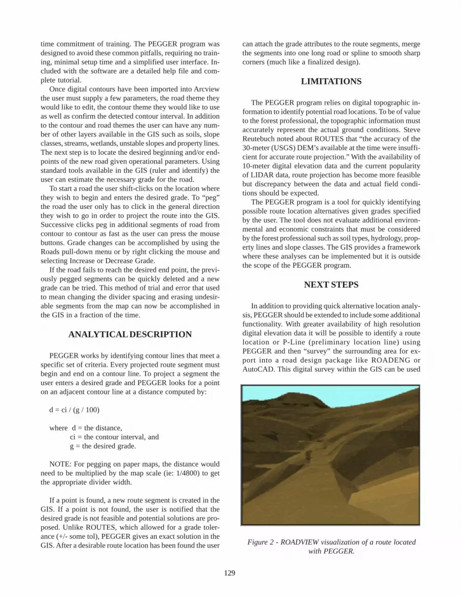
129
time commitment of training. The PEGGER program wasdesigned to avoid these common pitfalls, requiring no train-ing, minimal setup time and a simplified user interface. In-cluded with the software are a detailed help file and com-plete tutorial.
Once digital contours have been imported into Arcviewthe user must supply a few parameters, the road theme theywould like to edit, the contour theme they would like to useas well as confirm the detected contour interval. In additionto the contour and road themes the user can have any num-ber of other layers available in the GIS such as soils, slopeclasses, streams, wetlands, unstable slopes and property lines.The next step is to locate the desired beginning and/or end-points of the new road given operational parameters. Usingstandard tools available in the GIS (ruler and identify) theuser can estimate the necessary grade for the road.
To start a road the user shift-clicks on the location wherethey wish to begin and enters the desired grade. To “peg”the road the user only has to click in the general directionthey wish to go in order to project the route into the GIS.Successive clicks peg in additional segments of road fromcontour to contour as fast as the user can press the mousebuttons. Grade changes can be accomplished by using theRoads pull-down menu or by right clicking the mouse andselecting Increase or Decrease Grade.
If the road fails to reach the desired end point, the previ-ously pegged segments can be quickly deleted and a newgrade can be tried. This method of trial and error that usedto mean changing the divider spacing and erasing undesir-able segments from the map can now be accomplished inthe GIS in a fraction of the time.
ANALYTICAL DESCRIPTION
PEGGER works by identifying contour lines that meet aspecific set of criteria. Every projected route segment mustbegin and end on a contour line. To project a segment theuser enters a desired grade and PEGGER looks for a pointon an adjacent contour line at a distance computed by:
d = ci / (g / 100)
where d = the distance, ci = the contour interval, and g = the desired grade.
NOTE: For pegging on paper maps, the distance wouldneed to be multiplied by the map scale (ie: 1/4800) to getthe appropriate divider width.
If a point is found, a new route segment is created in theGIS. If a point is not found, the user is notified that thedesired grade is not feasible and potential solutions are pro-posed. Unlike ROUTES, which allowed for a grade toler-ance (+/- some tol), PEGGER gives an exact solution in theGIS. After a desirable route location has been found the user
can attach the grade attributes to the route segments, mergethe segments into one long road or spline to smooth sharpcorners (much like a finalized design).
LIMITATIONS
The PEGGER program relies on digital topographic in-formation to identify potential road locations. To be of valueto the forest professional, the topographic information mustaccurately represent the actual ground conditions. SteveReutebuch noted about ROUTES that “the accuracy of the30-meter (USGS) DEM’s available at the time were insuffi-cient for accurate route projection.” With the availability of10-meter digital elevation data and the current popularityof LIDAR data, route projection has become more feasiblebut discrepancy between the data and actual field condi-tions should be expected.
The PEGGER program is a tool for quickly identifyingpossible route location alternatives given grades specifiedby the user. The tool does not evaluate additional environ-mental and economic constraints that must be consideredby the forest professional such as soil types, hydrology, prop-erty lines and slope classes. The GIS provides a frameworkwhere these analyses can be implemented but it is outsidethe scope of the PEGGER program.
NEXT STEPS
In addition to providing quick alternative location analy-sis, PEGGER should be extended to include some additionalfunctionality. With greater availability of high resolutiondigital elevation data it will be possible to identify a routelocation or P-Line (preliminary location line) usingPEGGER and then “survey” the surrounding area for ex-port into a road design package like ROADENG orAutoCAD. This digital survey within the GIS can be used
Figure 2 - ROADVIEW visualization of a route locatedwith PEGGER.

130
to generate the topographic information and field notes nec-essary to do a complete design in the road design package.The final L-Line (location line) and slope staking notes canbe generated using the GIS and the road design package foruse in the field by the forest professional.
Complementing PEGGER is a companion programROADVIEW that takes the preliminary route location gen-erated by PEGGER and creates a 3-dimensional model ofthe road�s cuts, fills and running surface. Using the 3-Dmodel and a visualization program such as EnVision, pro-fessionals can look at the road as it might be constructedand effectively communicate with non-forest professionalsregarding scenic and environmental impacts.
CONCLUSION
While route location has been used by forest profession-als for many years and computerized in the 1980�s with theintroduction of ROUTES, it has never become a widely usedtechnology to evaluate initial road locations. With PEGGER,the forest planner can quickly evaluate route locations withina GIS framework, giving the planner access to additionalGIS functionality. PEGGER was designed with simplicityand minimal investment cost as primary objectives. Throughthe use of a carefully designed user interface and extensive
tutorial, a typical user can be locating roads in a few min-utes on their own PC taking full advantage of forest tech-nology.
LITERATURE CITED
Pearce, J. Kenneth. 1960. Forest engineering handbook. Port-land, OR: U.S. Department of the Interior, Bureau of LandManagement. 220p.
Cha DS, Nako H, Watahiki K. 1991. A computerized arrange-ment of forest roads using a digital terrain model. Journalof the Faculty of Agriculture Kyushu University. 36(1-2):131-142.
Reutebuch, SE. 1988. ROUTES: A Computer Program for Pre-liminary Route Location. Pacific Northwest Research Sta-tion: U.S. Department of Agriculture, Forest Service. Gen-eral Technical Report PNW-GTR-216. 18p.
Watson, H. J. and M. M. Hill. 1983. Decision support systemsor what didn�t happen with MIS. Interface. 13(5):81-88.
Xu, Shenglin. 1996. Preliminary planning of forest roads us-ing ARC GRID. Corvallis, OR: Oregon State University, De-partment of Forest Engineering. 112p.

131
Harvest Scheduling with Aggregation Adjacent Constraints: AThreshold Acceptance Approach.
HAMISH MARSHALL, KEVIN BOSTON, JOHN SESSIONS
Abstract: Three different forest management planning unit sizes were used to compare the results from a tactical planningmodel that included a maximum opening size constraint with aggregation and even-flow goals. The smallest size had a 22-acre average size, the second had an average size of 41-acres, while the largest unit had an average size of 59-acres. There wasa direct correlation between discounted net revenue and unit size as the smallest unit definition produced $45 per acre morethan the second set of units and $225 more than the largest unit size. These results suggest that planners use the latesttechnology when defining individual settings and managing their unit sizes as one method to improve the financial perfor-mance of their assets.
INTRODUCTION
The strategic planner�s goal is to develop a plan that willallow the firm to compete effectively (Porter 1986). Tacti-cal planning aligns the operations to implement that strat-egy. Forestry planning problems, especially considering thelong rotations, are some of the more difficult business plan-ning problems because of economic, biological and opera-tional uncertainty in the data used. As the forest productsindustry is one of the most capital-intensive industries inthe world, a detailed planning and scheduling system is re-quired for competitive share�holder returns (Propper DeCallejon et al. 1998). Strategic plans have traditionally as-sumed the data is continuous and linear; thus allowing theseproblems to be solved using linear programming algorithms.Commercially available products such as FOLPI (Manleyet al. 1991), Magis (MAGIS 2003) and WOODSTOCK(REMSOFT 2003) have been available for approximately20 years to solve the long-term strategic planning problems.Initially, the solutions from these strategic planning solu-tions have been implemented using various ad hoc proce-dures. To improve both the financial and environmentalperformances, optimization routines have been developedto solve tactical scheduling planning problems that incor-porate various spatially explicit constraints. These con-straints have included various forms of green-up restrictionsand unit-fixed cost tactical planning problems. Unfortu-nately, these new tactical planning models quickly exceededthe capacity of commercial solvers and have resulted in theemployment of a variety of heuristics to solve these prob-lems.
A common spatial component found in tactical forest plan-ning involves the harvest of adjacent planning units. One
form of the adjacency constraint limits the maximum open-ing size that can be created. This constraint is found inmany forest practices rules including those of Sweden,Canada, and various western US states (Boston and Bettinger2001, Dahlin and Sallnas 1993). The Sustainable ForestryInitiative (SFI), a voluntary certification scheme that hasbeen adopted by much of US forest products industry, re-stricts the average opening size to less than 120 acres(AFAPA 2002)
Digital surveying equipment, global positioning systems(GPS), and geographical information systems (GIS) tech-nologies allows for smaller settings to be accurately definedand used in forest planning; however, many forest plannersrestrict the solution space of the tactical scheduling modelby aggregating settings into larger units prior to solving thetactical problems. This paper explores the impact of plan-ning unit size on the quality of the solutions produced bythe tactical plan. Three degrees of pre aggregation were used(Table 1) to describe the same 4450-acre planning area withthe identical yields.
The three data sets were used in a tactical planning modelthat had the goal to maximize the discounted net revenuesubject to an area-restriction green-up constraint. The maxi-mum opening allowed is 120 acres as specified in the Or-egon Forest Practices Rules (Oregon Department of For-estry 2003). One potential risk of reducing the planning unitsize is that the model will widely disperse each period�sharvest over the entire landscape, hence increasing harvest-ing and transportation costs. To reduce this possibility, anadditional goal was added to the model to aggregate origi-nal planning settings into larger planning units. The objec-tive of the aggregation was to group settings on oppositesides of valleys into planning units that will be logged inthe same year to improve the logging efficiency. Stumps

132
Aggregation Level Mean Planning Unit Size (acres)
Maximum Planning Unit Size (acres)
1 21.7 39.1 2 40.6 76.8 3 58.9 92.1
Table 1. Description of the planning data sets.
can be used as tailhold anchors for cable logging systemswith less fear of failure than if they were allowed to begin todecompose. A third even volume flow goal was added tothe model to regulate volume flow.
MODEL FORMULATION
Objective Function
The objective function goal was to maximize the netpresent value of the forest over a period of 20 years plus thesum of incentives and penalty values. A discount rate of 5%was applied to revenues at the end of each one-year period.The details of this incentive and penalty values are discussedbelow. The objective function is formulated as:
Even Volume Flow Penalty
Maintaining continuity of supply to customers is a keycomponent in successfully operating a forestry business.operations. We have assumed the goal is to maintain an even-flow of volume throughout the 20 year planning horizon,although we recognize that it can be misapplied to smallareas where the result of an even-flow constraint can sig-nificantly reduce the harvest from an area that cannot sup-port yearly. In this study it was formulated as a goal or “softconstraint” where the objective function was penalized forany deviation of the discounted volume from a target vol-ume in each period. The formulation is given below; thesquared deviation was multiplied by a weighting factor andsubtracted from the objective function.
w = penalty weight, tv = target volume (Mbf), vit = total unitvolume (Mbf)
Aggregation Incentive
The aggregation adjacent constraints have been formu-lated to encourage the harvesting of adjacent planning unitsin the same period. This constraint has also been formu-lated as a goal or “soft constraint”, modeled by increasingthe value of the objective function when aggregation is in-cluded in the model. The amount of the incentive was basedon the sum of the proportion of the perimeter of a planningunit that it shared with other planning units harvested inthe same period, divided by the number of planning units.
(3)
w = penalty weight, pi = proportion of perimeter shared withunits harvested the same period that are either on the otherside of the valley or above or below, Xit = a 0,1 binary vari-able to identify where a unit has been cut.
Maximum Opening Constraint (Oregon State Rules)
The maximum opening constraint or area-restrictionproblem (Murray 1998) was formulated as a hard constraintthat cannot be violated. The area-restriction constraint wasformulated so that a neighborhood of adjacent settings har-vested within 4 years has to have a combined area of lessthan 120 acres to not violate the Oregon State Forest Prac-tices Rules.
(4)
Ai = area, s = a subset of adjacency units all of which areharvested within 4 years of each other.
HEURISTIC ALGORITHM: THRESHOLDACCEPTANCE ALGORITHM
Threshold acceptance (TA) was first developed by Dueckand Scheuer (1990) when they claimed that it appeared tobe superior to simulated annealing (SA). The idea behind
∑=
−n
it
itvtvw1
2))05.1(
(*(
Rit = Gross Revenue, Cit = Costs, i = harvest units, t =planning period, n = number of harvest units, theEven_Flow_Penalty and Aggregation_Incentive formu-lations are described below.
(1)( ) ( )
20 20
1 1 1 1
max( )1.05 1.05
( _ _ ) ( _ )
n nit it
t ti t i t
R C
Even Flow Penalty Aggregation Incentive= = = =
−
− +
∑∑ ∑∑)
))((*( 1
n
pw
n
iiti X∑
=
∑=
<=+s
iitiiti XAXA
1120
(2)

133
Randomly select candidatestand and harvest period
Does the new candidatesolution form an opening less
than 120 acres
No
Yes
Calculate the difference between volumefrom the target volume for each period
raised to the power of two.a
Calculate the net present valuefor each period
b
Calculate the average proportion of theshared perimeter of adjacent units
harvested in the same periodc
CalculateObjective Function
= b - wa + zc
Is proposed objective function less
than best ever objection function
Yes
Make current solution equal best ever solution
Is proposed objective function less
than currentobjective function
No
repetition = repetition + 1
Current solution = proposedsolution
Does repetition = maximumnumber of repetitions ?
Select next threshold level
Any threshold levels left?
Stop and report the bestsolution found during searchand the iterations at which it
first occurred
No
YesYes
Yes
Retain old solution
No
No Yes
Accept solution
Is it within currentthreshold levels
No
Figure 1. Flow Diagram of the Threshold Acceptance Algorithm.
Figure 2. Net Present Value for the Different AggregationModels.
0
500
1000
1500
2000
2500
3000
3500
4000
4500
5000
1 2 3 4 5 6 7 8 9 10 11 12 13 14 15 16 17 18 19 20
Years
Vol
ume
(mbf
)
No AggregationAggregation 1Aggregation 2Aggregation 3
Figure 3. Projected Volumes (Mbf) over the 20 YearPlanning Horizon.
$8.40
$8.60
$8.80
$9.00
$9.20
$9.40
$9.60
$9.80
$10.00
$10.20
$10.40
No Aggregation Aggregation 1 Aggregation 2 Aggregation 3
Model
Net
Pre
sent
Val
ue (m
illion
)

134
the TA algorithm (Figure 1) is similar to SA but much easierto understand and implement. As in SA, the new candidateis selected randomly from the neighborhood of the existingsolution and the objective function for the new solution iscalculated. Bettinger et al. (2002) looked at the perfor-mance of eight heuristic planning techniques to solve threeincreasingly difficult wildlife-planning problems. The re-sults showed that despite the simplistic nature of thresholdacceptance (TA), it performed well compared to some ofthe more complex heuristic techniques.
The threshold acceptance algorithm was implementedusing Microsoft C# programming language. All spatial andyield data was stored in an ESRI geodatabase. Due to thestochastic components in the threshold acceptance algo-rithm, 20 final solutions were generated for each scenariowith each scenario using a new random starting solution.Each solution considered 50,000 iterations at each of theeight threshold levels. The run with the highest objectivefunction for each scenario has been presented in the fol-lowing section of this paper.
RESULTS
As expected, the smaller planning unit size in aggrega-tion 1 produced a higher net present value than the largerunits in aggregation 2 and 3. The result was an increase innet present value of approximately $45 and $225 per acre(Figure 2). These net present values do not include the pen-alties and incentives. An additional cost of increasing plan-ning unit size is a greater variation in the scheduled volumeflow between periods. The smaller planning units allowsfor them to be selected in a manner that will minimize thevolume penalty values (Figure 3). By incorporating the ag-gregation goal, the final harvest unit size has nearly doubledthe average original planning unit size. This suggests thata well designed model can still produce the larger harvestunits, without sacrificing the net present value (Figures 4-7 and Table 2).
Figure 4. No Aggregation
Figure 5. Aggregation 1
Figure 6. Aggregation 2
Figure 7: Aggregation 3
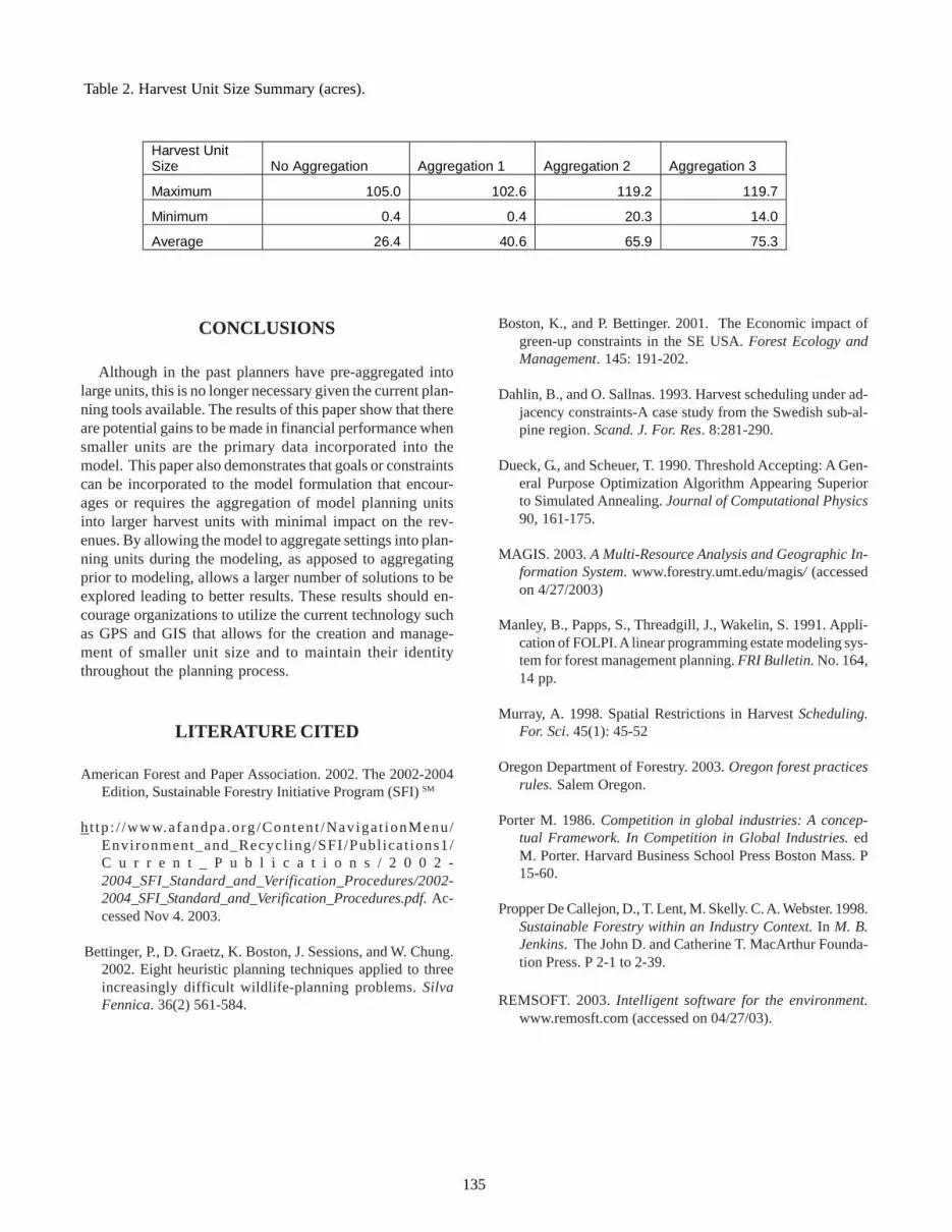
135
Harvest Unit Size No Aggregation Aggregation 1 Aggregation 2 Aggregation 3
Maximum 105.0 102.6 119.2 119.7
Minimum 0.4 0.4 20.3 14.0
Average 26.4 40.6 65.9 75.3
Table 2. Harvest Unit Size Summary (acres).
CONCLUSIONS
Although in the past planners have pre-aggregated intolarge units, this is no longer necessary given the current plan-ning tools available. The results of this paper show that thereare potential gains to be made in financial performance whensmaller units are the primary data incorporated into themodel. This paper also demonstrates that goals or constraintscan be incorporated to the model formulation that encour-ages or requires the aggregation of model planning unitsinto larger harvest units with minimal impact on the rev-enues. By allowing the model to aggregate settings into plan-ning units during the modeling, as apposed to aggregatingprior to modeling, allows a larger number of solutions to beexplored leading to better results. These results should en-courage organizations to utilize the current technology suchas GPS and GIS that allows for the creation and manage-ment of smaller unit size and to maintain their identitythroughout the planning process.
LITERATURE CITED
American Forest and Paper Association. 2002. The 2002-2004Edition, Sustainable Forestry Initiative Program (SFI) SM
ht tp : / /www.afandpa .org /Conten t /Naviga t ionMenu/Environment_and_Recycl ing/SFI/Publ icat ions1/C u r r e n t _ P u b l i c a t i o n s / 2 0 0 2 -2004_SFI_Standard_and_Verification_Procedures/2002-2004_SFI_Standard_and_Verification_Procedures.pdf. Ac-cessed Nov 4. 2003.
Bettinger, P., D. Graetz, K. Boston, J. Sessions, and W. Chung.2002. Eight heuristic planning techniques applied to threeincreasingly difficult wildlife-planning problems. SilvaFennica. 36(2) 561-584.
Boston, K., and P. Bettinger. 2001. The Economic impact ofgreen-up constraints in the SE USA. Forest Ecology andManagement. 145: 191-202.
Dahlin, B., and O. Sallnas. 1993. Harvest scheduling under ad-jacency constraints-A case study from the Swedish sub-al-pine region. Scand. J. For. Res. 8:281-290.
Dueck, G., and Scheuer, T. 1990. Threshold Accepting: A Gen-eral Purpose Optimization Algorithm Appearing Superiorto Simulated Annealing. Journal of Computational Physics90, 161-175.
MAGIS. 2003. A Multi-Resource Analysis and Geographic In-formation System. www.forestry.umt.edu/magis/ (accessedon 4/27/2003)
Manley, B., Papps, S., Threadgill, J., Wakelin, S. 1991. Appli-cation of FOLPI. A linear programming estate modeling sys-tem for forest management planning. FRI Bulletin. No. 164,14 pp.
Murray, A. 1998. Spatial Restrictions in Harvest Scheduling.For. Sci. 45(1): 45-52
Oregon Department of Forestry. 2003. Oregon forest practicesrules. Salem Oregon.
Porter M. 1986. Competition in global industries: A concep-tual Framework. In Competition in Global Industries. edM. Porter. Harvard Business School Press Boston Mass. P15-60.
Propper De Callejon, D., T. Lent, M. Skelly. C. A. Webster. 1998.Sustainable Forestry within an Industry Context. In M. B.Jenkins. The John D. and Catherine T. MacArthur Founda-tion Press. P 2-1 to 2-39.
REMSOFT. 2003. Intelligent software for the environment.www.remosft.com (accessed on 04/27/03).

136

137
Preliminary Investigation of Digital Elevation ModelResolution for Transportation Routing in Forested
Landscapes
MICHAEL G. WING, JOHN SESSIONS AND ELIZABETH D. COULTER
Abstract: Several transportation planning decision support systems utilize geographic information systems (GIS) technol-ogy to plan forest operations. Current decision support systems do not address upslope terrain conditions that may influencethe stability of road networks. This paper describes an on-going research project that uses a GIS and digital elevation model(DEM) to identify transportation route alternatives. Our goal was to develop an algorithm that identified transportationroutes guided by an objective function that weighted road grade and potential drainage area. We used a 9 x 9 meter resolutionDEM. We found that the resolution of the DEM (9 x 9 meter) was unable to provide reliable road grade and landscape slopeestimates. In both road grade and landscape slope results, gradient estimations based on the DEM data appeared to overesti-mate expected values. These results encourage further investigations, including the use of finer resolution DEMs to modeltopographic surfaces for transportation routing purposes.
INTRODUCTION
An important part of forest operations is the develop-ment of an efficient transportation system that incorporateseconomic, environmental, and safety considerations. Sev-eral decision support systems have been developed to assistforest planners with scheduling transportation routes in for-ested terrain (Reutebuch 1988, Liu and Sessions 1993).Previously, forest transportation planners relied on hardcopy maps and other manual techniques for transportationscheduling and were subject to the time and efficiency lim-its imposed by these techniques. Often, this meant that afull range of options may not have been developed and con-sidered. The development of decision support systems hashelped planners with the identification and prioritizationof potential transportation routes, given a set of parametersand accompanying constraints. Decision support systemshave also allowed planners to quickly create a range of trans-portation options with indices or other benchmarks throughwhich to evaluate and choose among alternatives.
While others have used GIS technology as a deci-sion support system for forested route siting and analysis(O�Neill 1991, MacNaughton et al. 1997, Epstein et al.1999, Chung 2002, Akay 2002), accounting for potentiallyunstable or landslide prone sites in the terrain surroundingthe road is not considered. With the increasing availabilityof digital elevation models (DEMs), it is now possible tofind elevation data for most parts of the U.S. at 10 meter, orfiner, resolution. DEMs can be used to create terrain mod-
els for slope and other topographic landscape representa-tions for input into a decision support system. With terraininformation, planners may be able to minimize traffic onforested routes that are potentially less stable than others,and reduce road failures, maintenance needs, sediment de-livery to streams, and other factors related to transportationcosts. Alternately, the identification of problem sites alonga transportation network that is in use may help direct moni-toring and maintenance efforts. Although a few studies havereported progress in this area (Wing et al. 2001), there re-mains a need for further work. We present results in thispaper of efforts to use a DEM to model road grade, slopeconditions, and the amount of upslope contributing area forthe use of transportation route planning. We investigatedthe usefulness of a 9-meter DEM to provide reliable roadgrade and landscape slope estimates for transportation pur-poses.
METHODS
Our study area is the Elliott State Forest, located in theOregon coast range. The Elliott State Forest is an activelymanaged forest of 145 square miles (376 km2) and has rela-tively steep terrain with an approximate average groundslope of 53%. The Elliott has a well-developed transporta-tion network (3.8 miles per square mile) with approximately550 miles (885 km) of roads, both paved and unpaved. Weobtained base GIS data from the Elliott staff for our projectwith layers representing ownership boundaries, roads, and
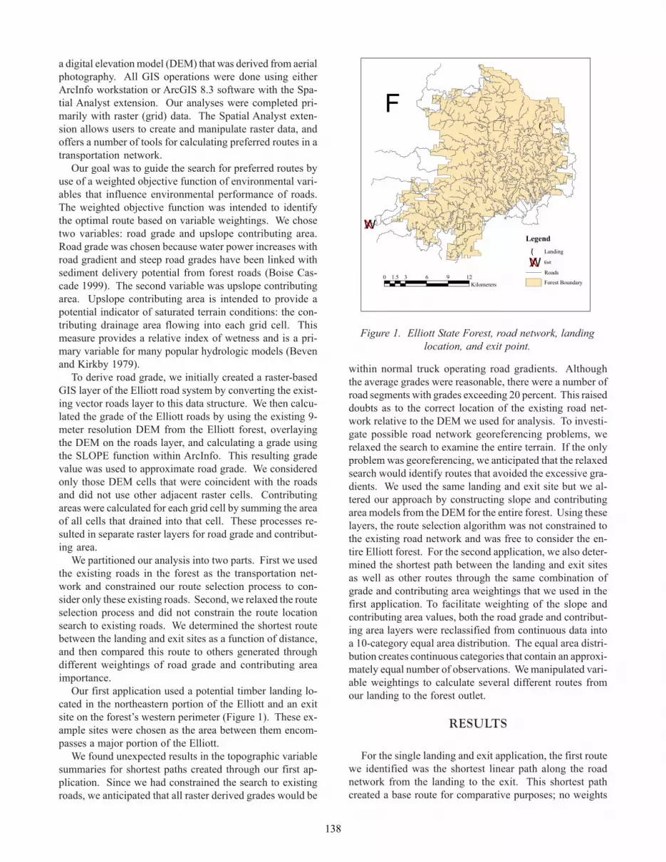
138
Figure 1. Elliott State Forest, road network, landinglocation, and exit point.
!(
XWLegend
!( Landing
XW Exit
Roads
Forest Boundary0 3 6 9 121.5
Kilometers
F
a digital elevation model (DEM) that was derived from aerialphotography. All GIS operations were done using eitherArcInfo workstation or ArcGIS 8.3 software with the Spa-tial Analyst extension. Our analyses were completed pri-marily with raster (grid) data. The Spatial Analyst exten-sion allows users to create and manipulate raster data, andoffers a number of tools for calculating preferred routes in atransportation network.
Our goal was to guide the search for preferred routes byuse of a weighted objective function of environmental vari-ables that influence environmental performance of roads.The weighted objective function was intended to identifythe optimal route based on variable weightings. We chosetwo variables: road grade and upslope contributing area.Road grade was chosen because water power increases withroad gradient and steep road grades have been linked withsediment delivery potential from forest roads (Boise Cas-cade 1999). The second variable was upslope contributingarea. Upslope contributing area is intended to provide apotential indicator of saturated terrain conditions: the con-tributing drainage area flowing into each grid cell. Thismeasure provides a relative index of wetness and is a pri-mary variable for many popular hydrologic models (Bevenand Kirkby 1979).
To derive road grade, we initially created a raster-basedGIS layer of the Elliott road system by converting the exist-ing vector roads layer to this data structure. We then calcu-lated the grade of the Elliott roads by using the existing 9-meter resolution DEM from the Elliott forest, overlayingthe DEM on the roads layer, and calculating a grade usingthe SLOPE function within ArcInfo. This resulting gradevalue was used to approximate road grade. We consideredonly those DEM cells that were coincident with the roadsand did not use other adjacent raster cells. Contributingareas were calculated for each grid cell by summing the areaof all cells that drained into that cell. These processes re-sulted in separate raster layers for road grade and contribut-ing area.
We partitioned our analysis into two parts. First we usedthe existing roads in the forest as the transportation net-work and constrained our route selection process to con-sider only these existing roads. Second, we relaxed the routeselection process and did not constrain the route locationsearch to existing roads. We determined the shortest routebetween the landing and exit sites as a function of distance,and then compared this route to others generated throughdifferent weightings of road grade and contributing areaimportance.
Our first application used a potential timber landing lo-cated in the northeastern portion of the Elliott and an exitsite on the forest�s western perimeter (Figure 1). These ex-ample sites were chosen as the area between them encom-passes a major portion of the Elliott.
We found unexpected results in the topographic variablesummaries for shortest paths created through our first ap-plication. Since we had constrained the search to existingroads, we anticipated that all raster derived grades would be
within normal truck operating road gradients. Althoughthe average grades were reasonable, there were a number ofroad segments with grades exceeding 20 percent. This raiseddoubts as to the correct location of the existing road net-work relative to the DEM we used for analysis. To investi-gate possible road network georeferencing problems, werelaxed the search to examine the entire terrain. If the onlyproblem was georeferencing, we anticipated that the relaxedsearch would identify routes that avoided the excessive gra-dients. We used the same landing and exit site but we al-tered our approach by constructing slope and contributingarea models from the DEM for the entire forest. Using theselayers, the route selection algorithm was not constrained tothe existing road network and was free to consider the en-tire Elliott forest. For the second application, we also deter-mined the shortest path between the landing and exit sitesas well as other routes through the same combination ofgrade and contributing area weightings that we used in thefirst application. To facilitate weighting of the slope andcontributing area values, both the road grade and contribut-ing area layers were reclassified from continuous data intoa 10-category equal area distribution. The equal area distri-bution creates continuous categories that contain an approxi-mately equal number of observations. We manipulated vari-able weightings to calculate several different routes fromour landing to the forest outlet.
RESULTS
For the single landing and exit application, the first routewe identified was the shortest linear path along the roadnetwork from the landing to the exit. This shortest pathcreated a base route for comparative purposes; no weights

139
Grade Contributing Route Mean Route Max Route Mean Contributing Max Contributing Weight (%) Area Weight (%) Distance (miles) Grade (%) Grade (%) Area (acres) Area (acres) 0 0 36.5 9.3 67.2 26.3 12916.9 0 100 38.2 9.5 42.8 12.6 11391.5 10 90 38.1 9.4 42.8 12.7 11391.5 25 75 38.0 9.3 42.8 12.8 11391.5 50 50 37.8 9.2 42.8 12.9 11391.5 75 25 36.8 8.9 67.2 17.0 12916.9 90 10 36.8 8.9 67.2 17.3 12916.9 100 0 36.8 8.9 67.2 27.4 12916.9
were applied in this initial route for road grade or contribut-ing area. We then selected routes based on varying weightsof road grade and contributing area in order to determineoptimal routes given a range of variable importance (Table1). Regardless of the route parameters, the range of result-ing route distances was consistent. The shortest distancebetween these points identified by the base route was about37 miles and, with modifications of the grade and contribut-ing area variables, the range of distances was between 37and 38 miles. The mean grade of all routes was also consis-tent and ranged from 8 to 9%. The maximum grade differedfrom 43 to 67%. These high gradient sections clearly ex-ceed the gradients of the existing road network.
Contributing areas differed markedly with the shortestpath having a mean contributing area of 26 acres and theroutes resulting from considering grade and contributing areahaving a range from 13 to 27 acres. The shortest path androutes that had a grade weight of at least 75% all had thesame maximum contributing area (12,917 acres) whereasall other routes had a maximum of 11,392 acres. Closerinspection of the location of these routes revealed that themaximum contributing areas all occurred along the samesmall section of road. This section of road crossed a majorstream twice and gained the large contributing area valuesassociated with the stream. In general, as the weight of theroad grade increased (and contributing area decreased), the
mean route grade decreased and contributing area increased,although the changes in mean route grade were not pro-nounced.
The high grade values that resulted from our initial analy-ses indicated that the DEM we used was not able to providesufficient information for determining reliable road gradeestimates. Possible sources of error are DEM resolution,incorrect location of the existing road network relative tothe DEM, a processing error, or an inherent bias in the meth-odology that creates the raster elevation values. To test fora road location error, we applied a different approach toroute creation with the shortest path algorithm and differ-ent weightings of topographic variables; we did not con-strain routes to the existing road network. By allowing theshortest path algorithm to navigate freely throughout theElliott’s topography, we believed that the identification ofroutes with less than a 20% grade maximum would confirma road location error.
Results varied more dramatically for the unconstrainedrouting approach. The shortest path had a distance of 19miles, mean grade of 50%, and a mean contributing area of14.63 acres (Table 2). Route distances were dramaticallyshorter for the all of the unconstrained routes when com-pared to the network constrained routes. Distances rangedfrom approximately 23 to 25 miles. Route mean and maxi-mum grades were also very different than the network con-
Table 1. Variable weights and route distance, mean and maximum route grade, and mean and maximum contributing areafor existing road network.
Grade Contributing Route Mean Route Max Route Mean Contributing Max Contributing Weight (%) Area Weight (%) Distance (miles) Grade (%) Grade (%) Area (acres) Area (acres) 0 0 18.8 50.7 137.5 14.6 17337.3 0 100 22.5 35.0 109.8 3.9 18032.9 10 90 23.0 22.7 88.5 7.3 18032.9 25 75 23.0 21.9 171.1 7.3 18032.9 50 50 24.7 18.8 84.0 0.5 1870.2 75 25 24.5 18.6 82.6 9.9 43470.7 0 10 22.7 14.5 88.6 354.9 16000.1 100 0 24.5 11.2 145.1 1026.5 15996.3
Table 2. Variable weights and route distance, mean and maximum route grade, and mean and maximum contributing areafor unconstrained network routing.

140
strained routes; grades were consistently and, in many cases,considerably higher. Contributing area results for the un-constrained routes varied considerably in terms of the mean.With the exception of the 90 and 100% grade weights, meancontributing areas were roughly half, or less, than those ofthe constrained routes. Maximum contributing areas werelarger for all of the unconstrained route results and, withtwo exceptions, ranged from 16,000 to 18,000 acres. Theselarge maximum contributing areas were again the result ofroutes crossing major streams.
DISCUSSION
All of the routes we developed from the existing roadnetwork had average road grades that were well within nor-mal acceptable grade tolerances (16-20%). In addition, allroutes also had maximum grades of more than 42%. Whiletravel distances were significantly lower for the routes wecreated that were not constrained to existing roads, all hadmaximum grades greater than 80% and all had averagegrades that exceeded those that were created using the ex-isting Elliott road network. These results indicated that theDEM values were not providing reliable grade and slopedata.
We wanted to determine whether viable transportationroutes could be determined through the 9 meter DEM. Inorder to create transportation routes that could be used bytypical log hauling vehicles, we adjusted the constraints ofour routing algorithms so that grades in excess of 20% wouldnot be considered in final route creation. We then attemptedto create routes that avoided 20% grades through the con-fines of the existing network and also through the uncon-strained approach, where the entire landscape would be po-tentially available for transportation routes. We found thatthis was not possible; every route possibility included mul-tiple grade values that exceeded 20%. Given that manyparts of the existing route system have been used for loghauling, these results shed doubt on the reliability of theDEM that served as the basis for our topography represen-tations.
We suspected that perhaps a processing error could havecontributed to these results and contacted the Elliott staff toverify the DEM�s history. The base DEM was created fromelevation points derived from aerial photography taken in1996. The points were converted into a triangular irregularnetwork (TIN) data structure and then converted into a ras-ter file. We used the resulting raster file for our analysis.Potential errors could have occurred during operations per-formed on the data prior to our receiving the data, or couldhave resulted from our manipulations during this project.For comparative purposes, we obtained USGS 10 meterDEMs for the Elliott and used these data to create slope andcontributing area models of the Elliott. The average slopeof the USGS DEM was slightly less (50%) than thephotogrametrically derived DEM (53%). We then used thebaseline USGS data to calculate a shortest path and grade
statistics that were not constrained to the existing network.Whereas the average grade (47%) was slightly less thanour previous results (Table 2), the maximum grade wasslightly larger (143%). These similar results led us to be-lieve that it was not a processing error, or necessarily inac-curacy, in our original DEM that contributed to the largegrade values.
Rather, a more likely explanation is that a finer resolu-tion DEM is needed to provide a more reliable approxima-tion of road grade and terrain. The DEMs we used wereunable to accurately capture the lower gradients that shouldexist along the existing road network. In addition, our in-ability to create any route throughout the forest that avoidedgrades above 20% suggests that slopes were systematicallyover estimated throughout the forest. Wilson et al. (2000)detected differences in slope as a function of DEM resolu-tion, and considered resolutions between 30 and 200 meters.One approach to verifying systematic slope exaggerationestimates would be to create or obtain finer resolution (1-5meter) DEM data for the Elliott, calculate slope values, andexamine values to compare differences with our reportedfindings. These could be compared to measured road gradesand cross section data through precision instrumentation,such as total station or digital clinometer, in order to betterunderstand what is being represented in the DEM.
LITERATURE CITED
Akay, A. 2002. Minimizing total cost of construction, mainte-nance, and transportation costs with computer-aided forestroad design. PhD dissertation, Oregon State University,Corvallis. 229 p.
Boise Cascade Corporation. 1999. SEDMODL-Boise Cascaderoad erosion delivery model. Technical documentation.Boise Cascade Corporation, Boise, ID. 19 p.
Beven, K. J. and M.J. Kirkby. 1979. A physically based vari-able contributing area model of basin hydrology. Hydro-logical Sciences Bulletin 24(1):43-69.
Chung, W. 2002. Optimization of cable logging layout using aheuristic algorithm for network programming. Phd disser-tation, Oregon State University, Corvallis. 206 p.
Epstein, R., A. Weintraub, J. Sessions, J. B. Sessions, P. Sapunar,E. Nieto, F. Bustamante, and H. Musante. 1999. PLANEX:an equipment and road location system. In Proceedings ofthe International Mountain Logging and 10th Pacific North-west Skyline Symposium, March 28-April 1, 1999, Dept. ofForest Engineering, Oregon State University, Corvallis. pp.365-368.
Kramer, B. W. 2001. Forest road contracting, construction, andmaintenance for small forest woodland owners. ResearchContribution 35, Forest Research Laboratory, Oregon StateUniversity, Corvallis.

141
Liu, K. and J. Sessions. 1993. Preliminary planning of road sys-tems using digital terrain models. Journal of Forest Engi-neering 4:27-32.
MacNaughton, J., J. Sessions, and S. Xu. 1997. Preliminaryplanning of forest roads using ARC GRID. In: GIS �97 Con-ference Proceedings. Fort Collins: GIS World, Inc. 67-71.
O�Neill, W. A. 1991. Developing optimal traffic analysis zonesusing GIS. ITE Journal 61: 33-36.
Reutebuch, S. 1988. ROUTES: A computer program for pre-liminary route location. USDA General Technical Report.PNW-GTR-216, Portland, OR. 18 p.
Wilson, J. P., P. L. Repetto, and R. D. Snyder. 2000. Effect ofdata source, grid resolution, and flow routing method oncomputed topographic attributes. In: Wilson J P and J CGallant (editors), Terrain Analysis: Principles and Applica-tions. New York, John Wiley and Sons, pp 133-161.
Wing, M. G., E. D. Coulter, and J. Sessions. 2001. Developinga decision support system to improve transportation plan-ning in landslide prone terrain. In Proceedings of the Inter-national Mountain Logging and 11th Pacific Northwest Sky-line Symposium, December 10-11, 2001, College of ForestResources, University of Washington and International Unionof Forestry Research Organizations, Seattle, WA. pp. 56-60.

142

143
Comparison of Techniques for Measuring Forested Areas
DEREK SOLMIE, LOREN KELLOGG , MICHAEL G. WING ANDJIM KISER
Abstract: Operational planning and layout are important steps in determining the feasibility of harvesting operations.Higher-precision technologies may increase measurement accuracy and efficiency while decreasing total planning costs. Al-though a number of trials have been completed on the potential implementation of some of these new technologies, few havequantified the benefits of such devices in an operational setting.
Sixteen (~1 ac) units were identified for an evaluation of different spatial data-collection instruments as well as techniquesfor measuring area. Unit boundaries were measured by three surveying techniques, comprising 1) a string box, manual com-pass, and clinometer; 2) a laser, digital compass, and digital data collector; and 3) a global positioning system. The collecteddata were compared with a series of benchmarks established with a total station. Techniques were statistically analyzed anderror distributions were developed at either a unit or an individual data-point scale. Time studies were conducted to determinethe overall efficiencies of each technique. Our results should assist forest resource managers in their decisions when selectingalternate measurement tools for collecting spatial data.
INTRODUCTIONStudies of conventional methods employed in the Pa-
cific Northwest have analyzed the use of nylon tapes, hand-held compasses, and clinometers for operational measure-ments. Researchers have reported that costs can vary ac-cording to the type of harvesting system (Edwards 1993,Kellogg et al. 1998), unit size and shape (Dunham 2001a),silvicultural treatments (Kellogg et al. 1991, Edwards 1993,Kellogg 1996a, Dunham 2001a, b), and level of crew expe-rience (Kellogg et al. 1996b). However, no studies havebeen published concerning more recent data-capturing tech-nologies available to the forest industry.
Higher-precision technologies may increase measure-ment accuracy and efficiency while decreasing total plan-ning costs. Although a number of trials have been com-pleted on the potential implementation of some of thesenew technologies, few have quantified the benefits of suchdevices in an operational setting. Mixed results have beenreported for the usefulness of electronic distance- and azi-muth-measuring (EDM) devices to traverse forest standboundaries (Liu 1995) and low volume road surveys (Moll1993). The distance- and vertical angle-measuring capa-bilities of the lasers generally met the survey requirements,but the azimuth measurements with the compass did notdue to offsets in the magnetic field.
Several studies have illustrated the potential for digitaldata collectors, compasses, and laser rangefinders in op-erational settings including woodpile volumes (Turcotte1999) and skyline corridor traversing (Wing and Kellogg2001). In operational settings measurements are often dif-ficult to obtain due to understory brush. Further compari-sons between the laser rangefinder and more conventional
methods are needed to fully understand the benefits of thesenewer tools.
Global positioning systems (GPS) have also been usedto collect spatial data in forested environments (Forgues1998). Studies have identified variables that affect its use-fulness, including the amount of canopy closure (Stjernberg1997, Mancebo and Chamberlain 2001), receiver type andgrade (Darche 1998), weather conditions (Forgues 2001),and topography (Liu and Brantigan 1996). Historically, oneof the challenges when using GPS has been the effect ofmulti-path signals caused by the forested canopy (Stjernberg1997, Forgues 2001). However, this effect has largely beenmitigated by manufacturers incorporating ‘multipath’ rec-ognition into their firmware. Signal availability is anotherproblem (Karsky et al. 2000), primarily of the limited vis-ibility of satellites due to forest cover and topography.
Differential GPS (DGPS) has been to be a cost-effectivetechnique for measuring land areas (Liu and Brantigan1996). Both forest canopy and undulating terrain exert adefinite effect on traverse surveys completed by DGPS, withaccuracy being reduced as variations in canopy closure andtopography increase. Nevertheless, kinematic DGPStraverses have proved more capable of achieving a closerforest stand-area approximation than that obtained from atraditional compass-and-chain traverse.
The objectives of this study were to: 1) gather time andcosting information to determine the relative efficiencies ofeach measurement technique; 2) to compare information onprecision and accuracy of each method; and 3) to analyzethe patch-orientation due to discrepancies in angular mea-surements.

144
METHODSStudy Site
This study was located on the McDonald-Dunn CollegeForest, managed by Oregon State University. The site is a55-year-old mixed stand comprised primarily of Douglas-fir (Pseudotsuga menziesii), big leaf maple (Acermacrophyllum), and red alder (Alnus rubrus). The stand alsohad minor shrub vegetation consisting of vine maple (Acercircinatum), salal (Gaultheria shallon), and salmonberry(Rubus spectabilis). Slopes ranged from 0 to 76% (averageof ~25%). Canopy closure was 60 to 95%, with an averagestand density of 280 trees per acre. The average tree was~97 ft tall, with a dbh of 17 in.. Approximate volume peracre was 15 to 24 mbf.
Data Collection
Sixteen study patches (~1 ac each) were selected basedon stand descriptions, topographies, and their location rela-tive to other patches. Boundaries were delineated in the fieldwith surveyor�s flagging and paper tags. Benchmark sta-tions, established along the vertices of each patch, wereflagged and locations measured with a Nikon DT-310 totalstation. Measurement accuracies were reported to within 0.02in. of the horizontal and vertical distances.
Three techniques for determining land area were com-pared against the benchmark measurements. These includedthe use of: 1) a string box with a distance counter, hand-held compass and a Suunto clinometer; 2) electronic dis-tance- and electronic bearing-measurement devices; and 3)a global positioning system. Time required to complete theoperational layout and planning was separated into threecomponents to determine the relative efficiencies of eachmethod as time spent surveying each patch, recording thedata, and either downloading or entering the informationinto a database. Crew sizes depended on the surveyingmethod being employed. All members had at least one yearof experience with the survey equipment and were profi-cient in its operation.
The first method consisted of a single person measur-ing slope distance and slope percent. Data were collectedstation to station, recorded in a field book and manuallyentered into a software program, RoadEng (Softree;Vancouver, BC), in the office. Traverse adjustments weredone using the compass rule (Mikhail and Gracie 1981,Buckner 1983).
The second method employed an electronic distance- andelectronic bearing-measurement device manufactured byLaser Technology Incorporated (LTI). The Impulse 200 EDMwas linked with a MapStar digital compass, which provideddata on slope distance, slope percent, and horizontal angles.This system required a two-person crew, and the collecteddata were logged into a handheld digital data recorder. Thelead traverser maneuvered between stations and held thereflective prism at eye level, directly above the pin flag. Therear traverser aimed the laser at the reflective prism and the
distance, inclination, and azimuth were recorded in the datacollector. Two data recorders, one operating on a WindowsCE and DOS platform (Juniper Allegro), the other on a Win-dows CE platform (Tripod Data Systems (TDS) Ranger),were used in tandem with the laser to determine the mostefficient data recording technique. One advantage in usinga DOS-based application was that the data could be directlydownloaded into the mapping software.
The office work for the Juniper data collector consistedof downloading the information to a desktop computer viaan ActiveSync program. Data Plus software allowed the userto structure the database to match the required input for themapping program. The data were then imported intoRoadEng, using the Terrain Module, and subsequently ana-lyzed. Office work for the TDS data collector involved acomputer spreadsheet program that adjusted the coordinatesto a format that RoadEng could recognize.
The third survey technique incorporated a Trimble ProXR GPS. A one-person crew traversed the perimeter of thepatches, simultaneously logging points and using the areafunction within the TSC1 data collector while moving be-tween stations. This traverse was completed in a kinematicmode, so that no differentiation existed among the stationsbut, rather, the entire boundary was traversed as a singlesegment. Therefore, the GPS portion of this study did notinclude between-station measurements, and comparisonscould be made only at the patch level.
Data were downloaded to Trimble Pathfinder Office ver-sion 2.01 and base station data were used to differentiallycorrect the data and determine patch areas.
The previously described techniques were also comparedwith a benchmark method that could produce the most ac-curate measurements. A Nikon DT-310 total station was usedalong with 2 prisms and a four-person crew. A side shotmethod was used that minimized the number of instrumentset-ups required to traverse the patch (Fig. 1), while collect-ing measurements at each station. Two crew members ma-neuvered prisms between the stations, while another clearedsight-paths between the total station and the survey points.
LEGEND
Total Station
Stations
Measurements
Figure 1. Side shot method for traversing with a total station.

145
Survey data were transformed to determine the x, y, andz coordinates, which were then downloaded as an ASCIIfile into the RoadEng.
RESULTS AND DISCUSSIONTime and Cost Information
Time required to survey a patch and complete the officework varied substantially, depending on the technique (Fig.2). The task was considered complete when all informationwas processed and entered into a common mapping pro-gram.
The method involving the laser, digital compass, andJuniper data collector required the least amount of time perpatch (17 minutes). The second most time-efficient tech-nique was that using the laser, digital compass, and the TDSdata collector. The latter method required approximately twoextra minutes per patch because of the additional step takenby the TDS data collector to arrange the data in an accept-able format for the mapping program.
The string-box method required 19 minutes more perpatch (195% increase) compared with the laser/Juniper datacollector. Contributing factors included the time requiredto manually record the data in the field book and the needto manually transcribe the field notes, whereas the lasermethod included a digital download. Likewise, the GPSmethod took 23 minutes longer (210% increase) than theJuniper data collector, mainly because of intermittent satel-lite reception due to topography, canopy closure, and satel-lite orbits. The GPS data includes time spent on those patchesthat were abandoned after one hour because of poor satel-lite configuration.
Average time difference for the total station was 54 min-utes per patch (370% increase) compared with the laser/Juniper data collector. This was due primarily to requiredinstrument set-up time.
The time, type of equipment, and crew size required tocomplete a traverse were used to calculate the variable costof each survey method (Table 1). Equipment was depreci-ated over an two-year period. Hourly wages, which includedbenefits were obtained from the 2001 Associated OregonLoggers Annual Wage Survey (Salem, OR, USA).
0
20
40
60
80
100
120
140
10 11 12 14 15 16 17 18 19 20 21 22 23 24 25 26
Patch Number
Fiel
d Su
rvey
and
Offi
ce D
ata
Entr
y Ti
me(
Min
)
String Laser GPS Total Station
Figure 2. Time required to complete various forest-area measurement techniques.
Method Crew size
Labor cost ($/hr)
Equipment cost
($/hr)
Total time (hr)
Total cost ($)
Cost per acre ($)
Cost per mbf ($)
String Box 1 18.90 0.05 10.3 195.19 11.67 0.62 Laser (Ranger) 2 37.80 1.18 5.9 229.98 13.22 0.70 Laser (Allegro) 2 37.80 1.31 5.3 207.28 11.92 0.63 GPS 1 18.90 1.88 11.5 238.97 38.86 1.85 Total Station 4 75.60 1.13 19.7 1511.58 86.52 4.59
Table 1. Costs involved in completing land-area survey of 16 forested patches.

146
Hourly labor and initial equipment costs played the mostsignificant role in overall operating costs. The difference be-tween the two digital-data methods could be attributed to theadditional office time the TDS data collector required for for-matting the field data.
PRECISION AND ACCURACY
Precision is the degree of closeness or conformity amongrepeated measurements of the same quantity (Mikhail andGracie 1981). The average patch precision gained from eachof our methods is shown in Table 2.
The mean difference in area compared to the total-stationtechnique appears to be relatively small. Although this was afairly small land area (1742 ft2), one may assume a randomerror effect, for which the percent error would hold fairlyconstant. Therefore, this effect could dramatically impact areacalculations, timber volume estimates, and other operationalconsiderations on larger unit areas.
Because the survey of each patch started and ended at thesame point, the precision or repeatability could be calculatedfrom the difference in coordinates. This difference was thendivided by the total perimeter distance for each patch, result-ing in a percent error term that was averaged for the16 tra-versed patches. The laser and compass method produced theleast amount of precision because the instrument was not
mounted on a staff. Although the manufacturer’s accura-cies had been achieved in trials with the equipmentmounted, this positioning was found to limit the user’smobility in the forested environment. The mean precisionof the string box (1.15%) was good given the perceivedminimal precision of the equipment.
Accuracy is defined as the degree of conformity or close-ness of a measurement to the true value (Buckner 1983).Survey methods were analyzed for significant differencesat the station level (Table 3). Average accuracy was calcu-lated from the difference in measurements between the to-tal station and each of the laser and string box methods.GPS data are station independent and thus were not in-volved.
String box error can be attributed to several factors. Forexample, use of the string box was affected by the amountof brush and branches between stations. The string mayhave gotten caught on the branches, preventing the tra-verser from following a straight path. Likewise, the stringmay have become taut when maneuvering around obstacles,thereby contributing to the error.
Errors for the total station and laser methods were pri-marily brought due to the operator. Both the laser and thetarget had to be positioned vertically above the station. Acommon problem involved the laser operator needing tobend and shift away from the station in order to gain aclear sight path toward the target.
Method Mean patch area (ac)
Mean difference in patch area (ac)
Percent difference (%)
Mean patch precision (%)
String Box 1.03 -0.04 3.7 1.15 Laser 1.06 -0.01 0.93 2.65 GPS 1.03 -0.04 3.7 N/A Total Station 1.07 0 0 0.014
Table 2. Precision of measurements for patch areas, by survey method.
Method Mean slope distance error (ft)
Mean horizontal distance error (ft)
Mean vertical distance error (ft)
String Box 3.02 2.78 2.82 Laser 1.33 1.14 1.81 GPS N/A N/A N/A Total Station 0 0 0
Table 3. Average distance errors produced by each survey method.
Method Total Cost ($) Closing Error (%) n Mean Effectiveness (M.E.) String Box 195.19 1.15 16 1236 Laser (Ranger) 229.98 2.65 16 3247 Laser (Allegro) 207.28 2.65 16 2902 Total Station 1511.58 0 16 94
Table 4. Average mean effectiveness values for each survey method.

147
A multiple range test was used to confirm that all datapoints were from the same population. In addition, t-testswere conducted at the patch level to determine significantdifferences in accuracy. Values from both the laser and thestring-box methods were significantly different (p<0.05)from those obtained with the total-station technique. Like-wise, the t-test used to compare the string box and laserdata also indicated a significant difference between thesetwo methods (p<0.05).
ORIENTATION
Although all traverses closed with adequate precision andapproximately equal areas regardless of the survey techniqueemployed, orientations varied substantially (Fig. 3). Thiseffect on alignment might have major consequences for anumber of tasks completed during operational planning andlayout. For example, such errors could be costly to both par-ties when working with legal boundaries between propertyowners. This difference was most evident when the digital-compass method was implemented because the position atwhich the user held the equipment influenced the reading.Although very good closing precision could be attained, largedeviations from patch alignment occurred. This effect couldhave been minimized by mounting the laser and digital com-pass on a staff.
EFFECTIVENESS
It is difficult to account for practicality when comparingsurvey techniques. Liu (1995) assessed individual methodsthat used different equipment by multiplying the time neededto complete a task by the resulting accuracy, thereby basingeffectiveness on time instead of cost. Because our study in-
volved a combination of techniques for each method, a to-tal-cost variable was calculated. Mean effectiveness (M.E.)for each method (Table 4) was calculated by multiplyingthe total cost by the closing error and dividing this by thenumber of patches (16) to determine a mean effectiveness.Here, the smaller the value, the more effective the survey-ing method.
The total-station technique was the most effective, al-though it was the most time-consuming and expensive ofall the methods, it had a significantly smaller closure er-ror. The large difference between the laser method and thestring-box technique was a result of the higher accuracyand initial costs associated with the former. Effectivenesswith the GPS method was not included because no level ofaccuracy had been calculated.
SUMMARY
Different methods for measuring forest areas may be usedto meet specific land-management objectives. This studycompared four techniques for completing a traverse of par-tial harvests within an uneven-aged management plan. Themethod entailing the string box, manual compass, and cli-nometer was approximately 6% less expensive than the la-ser method. However, although the initial purchase priceand labor rates with the string-box technique were lower,48% more time was spent conducting the traverse of all thepatches. The total-station technique was the most expen-sive because of the larger crew and time required to clearthe sight lines.
Figure 3. Differences in patch orientation generated by survey methods.
Closing Error %((Total Cost)( ))
Closing Error Total Station %M.E.
n =

148
The effectiveness of each survey method also varied sub-stantially. Low (better) values were the result of a combina-tion of small costs and/or high accuracies. The total-stationmethod rated well (value = 94) because of the high amountof precision gained with its use. Although it was the mostexpensive to operate, its resulting precision was magnitudeshigher than that gained by the other methods.
Relative to their specific measurement activities, eachmethod has its strengths (time, cost, and accuracy) and weak-nesses (alignment, repeatability, and cost). Therefore, thepotential benefits must be weighed when allocating resourcesto specific duties for operational planning. In conclusion,this study illustrated that, although time was saved by us-ing the digital instruments, their performances were notalways as effective as those achieved via traditional meth-ods.
LITERATURE CITED
Buckner, R.B., 1983. Surveying Measurements and their Analy-sis. Landmark Enterprises, Rancho Cordova, CA, USA.275 p.
Darche, M.-H., 1998. A Comparison of Four New GPS Sys-tems under Forestry Conditions. Forest Engineering Insti-tute of Canada Special Report 128, Pointe Claire, Quebec,Canada. 16 p.
Dunham, M.T., 2001a. Planning and Layout Costs I: GroupSelection and Clear-cut Prescriptions. Forest EngineeringResearch Institute of Canada, Vancouver, BC, Canada. 2(22):6.
Dunham, M.T., 2001b. Planning and Layout Costs II: TreeMarking Costs for Uniform Shelterwood Prescriptions. For-est Engineering Research Institute of Canada, Vancouver,BC, Canada. 2(34): 4.
Edwards, R.M., 1993. Logging Planning, Felling, and YardingCosts in Five Alternative Skyline Group Selection Harvests.Master of Forestry paper, Department of Forest Engineer-ing, Oregon State University, Corvallis, OR, USA. 213 p.
Forgues, I., 1998. The Current State of Utilization of GPS andGIS Technologies in Forestry. Forest Engineering ResearchInstitute of Canada Field Note, Pointe Claire, Quebec,Canada. 2 p.
Forgues, I., 2001. Trials of the GeoExplorer 3 GPS Receiverunder Forestry Conditions. Forest Engineering ResearchInstitute of Canada, Pointe Claire, Quebec, Canada. 2(8):4.
Karsky, D., Chamberlain, K., Mancebo, S., Patterson, D., andT. Jasumback, 2000. Comparison of GPS Receivers undera Forest Canopy with Selective Availability Off. USDAForest Service Project Report 7100. 21 p.
Kellogg, L.D., Pilkerton, S., and R. Edwards, 1991. LoggingRequirements to Meet New Forestry Prescriptions. P. 43-49 In Proceedings of Council of Forest Engineering An-nual Meeting, Nanaimo, BC, Canada.
Kellogg, L.D., Bettinger, P., and R.M. Edwards, 1996a. A Com-parison of Logging Planning, Felling, and Skyline Costs be-tween Clearcutting and Five Group-Selection HarvestingMethods. Western Journal of Applied Forestry 11(3): 90-96.
Kellogg, L.D., Milota, G.V., and M. Millar Jr., 1996b. A Com-parison of Skyline Harvesting Costs for Alternative Com-mercial Thinning Prescriptions. Journal of Forest Engi-neering 1: 7-23.
Kellogg, L.D., Milota, G.V., and B. Stringham, 1998. LoggingPlanning and Layout Costs for Thinning: Experience fromthe Willamette Young Stand Project. Forestry PublicationsOffice, Oregon State University, Corvallis, OR, USA. 20 p.
Liu, C.J., 1995. Using Portable Laser EDM for Forest TraverseSurveys. Canadian Journal of Forestry Research 25: 753-766.
Liu, C.J., and R. Brantigan, 1996. Using Differential GPS forForest Traverse Surveys. Canadian Journal of Forestry Re-search 25: 1795-1805.
Mancebo, S., and K. Chamberlain, 2001. Performance Test-ing of the Trimble Pathfinder Pro XR Global PositioningSystem Receiver. USDA Forest Service Technical Note 10p.
Mikhail E.M., and G. Gracie, 1981. Analysis and Adjustmentof Survey Measurements. van Nostrand Reinhold Company,New York, USA. 340 p.
Moll, J.E., 1993. Development of an Engineering SurveyMethod for Use with the Laser Technology, Inc. Tree LaserDevice. Master of Science thesis, Department of Civil En-gineering, Oregon State University, Corvallis, OR, USA.74 p.
Stjernberg, E., 1997. A Test of GPS Receivers in Old-growthForest Stands on the Queen Charlotte Islands. Forest En-gineering Institute of Canada Special Report 125, Vancouver,BC, Canada. 26 p.
Turcotte, P., 1999. The Use of a Laser Rangefinder for Mea-suring Wood Piles. Forest Engineering Institute of CanadaField Note 76, Pointe Claire, Quebec, Canada. 2 p.
Wing, M., and L.D. Kellogg, 2001. Using a Laser Range Finderto Assist Harvest Planning. P. 147-150 In Proceedings ofthe First International Precision Forestry Cooperative Sym-posium, Seattle, WA, USA.

149

150
Poster Abstracts
Can Tracer Help Design Forest Roads?
ABDULLAH E. AKAY, GRADUATE RESEARCH ASSISTANT, DEPARTMENT OF FOREST ENGINEERING, COLLEGEOF FORESTRY, OREGON STATE UNIVERSITY, CORVALLIS, OR 97331
JOHN SESSIONS, PROFESSOR, DEPARTMENT OF FOREST ENGINEERING, COLLEGE OF FORESTRY, OREGONSTATE UNIVERSITY, CORVALLIS, OR 97331
CPLAN: A Computer Program for Cable LoggingLayout Design
WOODAM CHUNG, ASSISTANT PROFESSOR, SCHOOL OF FORESTRY, UNIVERSITY OF MONTANA,MISSOULA, MT 59812
JOHN SESSIONS, PROFESSOR, DEPARTMENT OF FOREST ENGINEERING, OREGON STATE UNIVERSITY,CORVALLIS, OR 97331
Abstract: A computerized method for optimizing cable logging layouts using a heuristic network algorithm has beendeveloped. A timber harvest unit layout is formulated as a network problem. Each grid cell containing timber volume to beharvested is identified as an individual entry node of the network. Mill locations or proposed timber exit locations are recog-nized as destinations. Each origin will then be connected to one of the destinations through alternative links representingalternative cable corridors, harvesting equipment, landing locations, and truck road segments. A heuristic algorithm for net-work programming is used to solve the cost minimization network problem. A computerized model has been developed toimplement the method. Logging feasibility and cost analysis modules are included in the model in order to evaluate the loggingfeasibility of alternative cable corridors and estimate yarding and transportation costs.

151
List of ContributorsJeffrey AdamsVirginia Tech775A Sterling DriveCharleston, SC [email protected]
Kamal AhmedUniversity of Washington121C More Hall, Box 352700Seattle, WA [email protected]
Abdullah E. AkayOregon State UniversityCorvallis, OR [email protected]
Jeremy AllanIntermap Technologies Corp.Calgary, Alberta, CANADA T2P 1H4
Hans-Erik AndersenUniversity of WashingtonCollege of Forest ResourcesBox 352100Seattle, WA [email protected]
Kazuhiro ArugaOregon State UniversityPeavy Hall Department of Forest EngineeringCorvallis, OR [email protected]
R. James BarbourUSDA Forest ServicePacific Northwest RegionPO Box 3623,Portland, Oregon [email protected]
B. Bruce BareUniversity of WashingtonCollege of Forest ResourcesBox 352100Seattle, WA [email protected]
Arnab BhowmickUniversity of WashingtonCollege of Forest ResourcesBox 352100Seattle, WA [email protected]
Tom BobbeUSDA Forest ServiceRemote Sensing Applications Center2222 W. 2300 S.Salt Lake City, UT [email protected]
Kevin BostonOregon State UniversityDepartment of Forest Engineering213 Peavy HallCorvallis, OR 97331-5706USAkevin.boston.cof.orst.edu
David BriggsUniversity of WashingtonCollege of Forest ResourcesBox 352100Seattle, WA [email protected]
Ward CarsonUniversity of WashingtonPacific Northwest Research StationBox 352100Seattle, WA [email protected]
Woodam ChungSchool of ForestryUniversity of MontanaMissoula, MT [email protected]
Jennie L. CornellOregon State UniversityForest Engineering OperationsCorvallis, OR [email protected]

152
Elizabeth CoulterOregon State UniversityDepartment of Forest Engineering215 Peavy HallCorvallis, OR [email protected]
Bill Dyck Ltd.PO Box 11236Palm Beach, Papamoa 3003NEW [email protected]
John R. EricksonUSDA Forest ServiceForest Products LaboratoryOne Gifford Pinchot DriveMadison, WI 53726-2398USA
Alexander EvansYale School of Forestry & Environmental Studies205 Prospect StreetNew Haven, CT 06511USA
Stephen E. FairweatherMason, Bruce, & Girard, Inc.707 SW Washington St., Suite 1300Portland, OR [email protected]
John W. ForsmanSchool of Forestry and Wood ProductsMichigan Technological UniversityHoughton, MI 49931USAEmail:[email protected]
Jeffrey R. FosterForestry Branch, Fort Lewis Military ReservationFort Lewis, WAUSA
Joel GilletApplanix Corp85 Leek CrescentRichmond Hill, ON L4B [email protected]
Richard A. GrotefendtUniversity of WashingtonCollege of Forest ResourcesBox 352100Seattle, WA [email protected]
Sean HoytUniversity of WashingtonBox 352500Seattle, WA [email protected]
Loren KelloggOregon State UniversityDepartment of Forest Engineering213 Peavy HallCorvallis, OR 97331-5706USAloren.kellogg.cof.orst.edu
Andrei KirilenkoPurdue UniversityDepartment of Forestry and Natural Resources ForestryBuilding 195 Marsteller St.West Lafayette, IN [email protected]
Jim KiserOregon State UniversityDepartment of Forest Engineering213 Peavy HallCorvallis, OR 97331-5706USAJim.Kiser.cof.orst.edu
Bruce LarsonUniversity of British Columbia2329 West MallVancouver, BC V6T [email protected]
Hamish MarshallOregon State UniversityForest Engineering Department215 Peavy HallCorvallis, OR [email protected]
John MateskiWestern Helicopter Services, INC.PO Box 369Newberg, OR [email protected]
Brett MartinPrudue University2226 Willowbrook Dr. Apt. #192West LaFayette, Indiana [email protected]

153
Douglas J. MartinMartin Environmenta;2103 North 62nd StreetSeattle, WA [email protected]
Glen MurphyOregon State UniversityForest Engineering DepartmentPeavy 271Corvallis, OR [email protected]
Ross F. NelsonNASA Biospheric Sciences BranchCode 923NASA Goddard Space Flight CenterGreenbelt, MD [email protected]
Sam PittmanUniversity of WashingtonBox 352100Seattle, WA [email protected]
Stephen P. PrisleyVirginia Tech229 Cheatham HallBlacksburg, VA [email protected]
John PunchesDouglas Co ExtensionOregon State University1134 SE DouglasRoseburg, OR [email protected]
Steve ReutebuchUniversity of WashingtonPacific Northwest Research StationBox 352100Seattle, WA [email protected]
Luke RogersUniversity of WashingtonRural Technology InitiativeSeattle, WA [email protected]
Rober J. RossUSDA Forest ServiceForest Products LaboratoryOne Gifford Pinchot DriveMadison, WI [email protected]
Peter P. SiskaStephen F. Austin State University1639 North StreetNacogdoches, TX [email protected]
Peter SchiessUniversity of WashingtonCollege of Forest ResourcesBox 352100Seattle, WA [email protected]
Daniel L. SchmoldtUSDA/CSREES/PASInstrumentation & SensorsMail Stop 2220Washington, DC [email protected]
Gerard SchreuderUniversity of WashingtonCollege of Forest ResourcesBox 352100Seattle, WA [email protected]
John SessionsOregon State University213 Peavy HallCorvallis, OR [email protected]
Guofan ShaoPurdue UniversityDepartment of Forestry and Natural Resources ForestryBuilding 195 Marsteller St.West Lafayette, IN [email protected]
Alex SinclairFeric Western Division2601 East MallVancouver, BC V6T [email protected]

Derek SolmieOregon State UniversityDepartment of Forest Engineering215 Peavy HallCorvallis, OR [email protected]
Bernd-M. StraubUniversity of HannoverInstitute for Photogrammetry and GeoInformationNienburger Strasse 1Hannover [email protected]
Pierre TurcotteFERIC580 Boul. St-JeanPointe-Claire, QC H9R [email protected]
Rien VisserVirginia Tech229 Cheatham HallBlacksburg, VA [email protected]
Xiping WangUniversity of Minnesota DuluthC1 Gifford Pinchot DriveMadison, WI [email protected] West
Forest ResearchPrivate Bag 3020Rotorua, NEW [email protected]
Denise WilsonUniversity of WashingtonPO Box 352500Seattle, WA [email protected]
Michael G. WingOregon State UniversityForest Engineering Department213 Peavy HallCorvallis, OR [email protected]
Jianyang ZhengUniversity of WashingtonDepartment of Civil and Environmental EngineeringSeattle, WA 98195-2700USA
David YatesForest Technology Group3950 Faber Place Dr.North Charleston, SC [email protected]

List of AttendeesJeffrey AdamsVirginia Tech775A Sterling DriveCharleston, SC [email protected]
Hans-Erik AndersenUniversity of WashingtonCollege of Forest ResourcesBox 352100Seattle, WA [email protected]
Carolyn AndersonWeyerhaeuser Company361 Schooner Cove, NWCalgary, Alberta [email protected]
Kazuhiro ArugaOregon State UniversityPeavy Hall Dept of Forest EngineeringCorvallis, OR [email protected]
B. Bruce BareUniversity of WashingtonCollege of Forest ResourcesBox 352100Seattle, WA [email protected]
Arnab BhowmickStephen F. Austin State UniversityCollege of Forestry1639 North StreetNacogdoches, TX [email protected]
Earl T. BirdsallWeyerhaeuser Co.PO Box 9777, WWC-IF6Federal Way, WA [email protected]
Tom BobbeUSDA Forest ServiceRemote Sensing Applications Center2222 W. 2300 S.Salt Lake City, UT [email protected]
Andrew BourquePotlatch Corporation - Hybrid Poplar ProgramPO Box 38Boardman, OR [email protected]
David BriggsUniversity of WashingtonCollege of Forest ResourcesBox 352100Seattle, WA [email protected]
Anne G. BriggsPO Box 663Issaquah, WA 98027USA
Ward CarsonUniversity of WashingtonPacific Northwest Research StationBox 352100Seattle ,WA [email protected]
Woodam ChungUniversity of MontanaSchool of Forestry32 Campus DriveMissoula, MT [email protected]
Jennie L. CornellOregon State UniversityForest EngineeringOperationsCorvallis, OR [email protected]

Elizabeth CoulterOregon State UniversityDepartment of Forest Engineering215 Peavy HallCorvallis, OR [email protected]
Christopher DavidsonInternational Paper1201 West Lathrop AvenueSavannah, GA [email protected]
Bill DyckBill Dyck Ltd.PO Box 11236Palm Beach, Papamoa 3003NEW [email protected]
Stephen E. FairweatherMason, Bruce, & Girard, Inc.707 SW Washington St., Suite 1300Portland, OR [email protected]
Dave FurtwanglerCascade Timber Consulting IncPO Box 446Sweet Home, OR [email protected]
Joel GilletApplanix Corp85 Leek CrescentRichmond Hill, ON L4B [email protected]
David GillulyWeyerhaeuser Co.33405 8th Avenue S., WWC 2B2Federal Way, WA 98003USA
Richard A. GrotefendtUniversity of WashingtonCollege of Forest ResourcesBox 352100Seattle, WA [email protected]
Weihe GuanWeyerhaeuser Co.33405 8th Avenue S.Federal Way, WA [email protected]
Andrew HillUniversity of WashingtonBox 352100Seattle, WA [email protected]
Olav Albert HøibøAgricultural University of NorwayDepartment of Forest ScienceP.O. Box 5044N-1432 [email protected]
Sean HoytUniversity of WashingtonBox 352100Seattle, WA [email protected]
Andrew HudakUS Forest ServiceRocky Mountain Research Station1221 S. Main St.Moscow, ID [email protected]
Yan JiangUniversity of WashingtonBox 352100Seattle, WA 98195USA
Dick KarskyUSDA Forest Service5785 Highway 10 WestMissoula, MT [email protected]
Phil LacyWorld Forestry Center4033 SW Canyon RoadPortland, OR [email protected]

Bruce LarsonUniversity of British ColumbiaVancouver, [email protected]
Stephen LewisTimberline Forest Inventory Consultants315-10357-109 StreetEdmonton, Alberta T5J [email protected]
Hamish MarshallOregon State UniversityForest Engineering Department215 Peavy HallCorvallis, OR [email protected]
Brett MartinPrudue University2226 Willowbrook Dr. Apt. #192West LaFayette, Indiana [email protected]
Bob McGaugheyUniversity of WashingtonPacific Northwest Research StationBox 352100Seattle, WA [email protected]
Kurt MullerForest Technology Group16703 SE McGillivray Blvd. Suite 215Vancouver, WA [email protected]
Glen MurphyOregon State UniversityForest Engineering DepartmentPeavy Hall 271Corvallis, OR [email protected]
Megan O’SheaUniversity of WashingtonCollege of Forest ResourcesBox 352100Seattle, WA [email protected]
Ewald PertlikUniversity of Bodenkultur ViennaPeter-Jordan-Strasse 70Vienna [email protected]
Charles PetersonUSDA Forest Service PNW620 SW Main Street Suite 400Portland, OR [email protected]
Lester PowerWeyerhaeuser Co.PO Box 9777Federal Way, WA [email protected]
Steve ReutebuchUniversity of WashingtonPacific Northwest Research StationBox 352100Seattle, WA [email protected]
Luke RogersUniversity of WashingtonRural Technology InitiativeSeattle, WA [email protected]
Peter SchiessrUniversity of WashingtonBox 352100Seattle, WA [email protected]
Daniel L. SchmoldtUSDA/CSREES/PASInstrumentation & Sensors Mail Stop 2220Washington, DC [email protected]
Gerard SchreuderUniversity of WashingtonCollege of Forest ResourcesBox 352100Seattle, WA [email protected]

158
Guofan ShaoPurdue UniversityDepartment of Forestry and Natural Resources ForestryBuilding 195 Marsteller St.West Lafayette, IN [email protected]
Alex SinclairFeric Western Division2601 East MallVancouver, BC V6T [email protected]
Jack A. SjostromDigitShare / Sentry Dynamics, Inc.721 Lochsa St., Suite 16Post Falls, ID [email protected]
Derek SolmieOregon State UniversityDepartment of Forest Engineering215 Peavy HallCorvallis, OR [email protected]
Brant SteigersPotlatch Corporation807 Mill RoadLewiston, ID [email protected]
Bernd-M. StraubUniversity of HannoverInstitute for Photogrammetry and GeoInformationNienburger Strasse 1Hannover [email protected]
Cheryl TalbertWeyerhaeuser Co.PO Box 9777 Mail Stop: CH 2D25Federal Way, WA [email protected]
Pierre TurcotteFERIC580 Boul. St-JeanCanadaPointe-Claire, QC H9R [email protected]
Eric TurnblomUniversity of WashingtonCollege of Forest ResourcesBox 352100Seattle, WA [email protected]
Rien VisserVirginia Tech229 Cheatham HallBlacksburg, VA [email protected]
Matt WalshUniversity of WashingtonBox 352100Seattle, WA 98195USA
Xiping WangUniversity of Minnesota DuluthUSDA Forest Products LaboratoryGifford Pinchot DriveMadison, WI [email protected]
Jack WardTemperate Forest SolutionsPO Box 33Asford, WA [email protected]
Welsey WassonVAP Timberland695 W Satsop RdMontesano, WA [email protected]

159
Denise WilsonUniversity of WashingtonPO Box 352500Seattle, WA [email protected]
Michael G. WingOregon State UniversityForest Engineering Department 213 Peavy HallCorvallis, OR [email protected]
David YatesForest Technology Group3950 Faber Place Dr.North Charleston, SC [email protected]

160
Second International Precision Forestry Symposium AgendaSunday, June 15, 2003
5:00 PM to 7:00 PM
Reception at the UW Waterfront Activities Center
Monday, June 16, 2003
7:00 AM
Registration Desk Opens at Kane Hall room 220
7:00 AM
Continental Breakfast
8:30 AM
Welcome & Introductory Remarks - Dean B. Bruce Bare
8:45 AM
Keynote Speaker -Bill Dyck
Plenary Session A: Precision Operations and Equipment - Moderator, AlexSinclair
9:05 AM
Multidat and Opti-Grade: Two Innovative Solutions to Better Manage Forestry Operations -presented by Pierre Turcotte, FERIC, Canada
9:25 AM
A Test of the Applanix POS LS Positioning System for the Collection of Terrestrial CoordinatesUnder a Closed Forest Canopy - presented by Stephen E. Reutebuch and Ward W. Carson,USDA Forest Service, Pacific Northwest Research Station
9:50 AM
Break & Poster Session
10:20 AM

161
Ground Navigation through the use of Inertial Measurements, a UXO Survey - presented byJoel Gillet, Applanix Corp.
10:45 AM
Precision Forestry Operations and Equipment in Japan - Kazuhiro Aruga, University of Tokyo
11:10 AM
Precision Forestry Applications: Use of DGPS Data to Plan and Implement Aerial Forest Op-erations - presented by Jennie L. Cornell
Plenary Session B: Remote Sensing and Measurement of Forest Lands andVegetation - Moderator, Tom Bobbe
11:35 AM
Estimating Forest Structure Parameters Within Fort Lewis Military Reservation Using AirborneLaser Scanner (LIDAR) Data - presented by Hans-Erik Andersen, University of Washington,College of Forest Resources
12:00 PM
Lunch
1:00 PM
Geo-Spatial Analysis in GIS and LIDAR Remote Sensing using Component Object Modeling ofVisual Basic: Application to Forest Inventory Assessment - presented by Arnab Bhowmick andDr. Peter Siska, College of Forestry, Stephen F. Austin State University
1:25 PM
Large Scale Photography Meets Rigorous Statistical Design for Monitoring Riparian Buffersand LWD - presented by Richard A. Grotefendt, University of Washington
1:50 PM
Forest Canopy Models Derived from LIDAR and INSAR Data in a Pacific Northwest ConiferForest - presented by Hans-Erik Andersen, University of Washington, College of Forest Re-sources
2:15 PM
Fine Tuning Forest Change Detections with a Combined Accuracy Index - presented byGuofan Shao, Department of Forestry and Natural Resources, Purdue University

162
2:40 PM
Break & Poster Session
3:10 PM
Automatic Extraction of Trees From Height Data Using Scale Space and Snakes - presentedby Bernd-M. Straub, Institute for Photogrammetry and GeoInformation, Germany
3:35 PM
RFID Research-presented by Sean Hoyt
4:05 PM
Sean Hoyt Tree Tour
4:30 PM
Adjourn
Tuesday, June 17, 2003
7:00 AM
Registration Desk Opens at Kane Hall room 220
7:00 AM
Continental Breakfast
8:05 AM
Keynote Speaker - Dan Schmoldt
Plenary Session C: Terrestrial Sensing, Measurement and Monitoring -Moderator, Steve Reutebuch
8:30 AM
Value Maximization Software-Extracting the Most from the Forest Rersource - presented byHamish Marshall and Graham West
8:55 AM
Costs and Benefits of Four Procedures for Scanning on Mechanical Processors - presentedby Glen E. Murphy and Hamish Marshall

163
9:20 AM
Evaluation of Small-diameter Timber for Value-added Manufacturing: A Stress WaveApproach - presented by Xiping Wang and Robert J. Ross
9:45 AM
Break & Poster Session
10:15 AM
Aroma Tagging and Electronic Nose Technology for Tracking Log and Wood Products: EarlyExperience - presented by Glen Murphy
Plenary Session D: Design Tools and Decision Support Systems - Moderator,Glen Murphy
10:40 AM
Modeling Steep Terrain Harvesting Risks using GIS - presented by Jeffrey Adams, Rien Visser,and Steve Prisley, Department of Forestry, Virginia Tech
11:05 AM
Use of the Analytic Hierarchy Process to Compare Disparate Data and Set Priorities -
presented by Elizabeth Coulter and John Sessions, Department of Forest Engineering, OregonState University
11:30 AM
Use of Spatially Explicit Inventory Data for Forest Level Decisions - presented by Bruce C.Larson, University of British Columbia, Faculty of Forestry
11:55 AM
Lunch
1:00 PM
Elements of Hierarchical Planning on Forestry: A Focus on the Mathematical Model -presented by Sam Pittman, University of Washington, College of Forest Resources
1:25 PM
Update Strategies for Stand-Based Forest Inventories - presented by Stephen E. Fairweather,

164
Mason, Bruce, & Girard, Inc.1:50 PM
A New Precision Forest Road Design and Visualization Tool: PEGGER - presented by LukeRogers, Geographic Information Scientist; UW Rural Technology Initiative
2:15 PM
Harvest Scheduling with Aggregation Adjacent Constraint: A Threshold Acceptance Approach -presented by Hamish Marshall, Graduate Student, Oregon State University
2:40 PM
Break (Poster Session Breakdown)
3:10 PM
Optimizing Road Network Location in Forested Landscapes - presented by Michael G. Wing,John Sessions, and Elizabeth Coulter, Oregon State University
3:35 PM
Comparing Forest Area Measurement Techniques - presented by Derek Solmie, Department ofForest Engineering, College of Forestry, Oregon State University
4:00 PM
Closing Remarks
4:25 PM
Adjourn
Wednesday, June 18, 2003 - Field trip CANCELED

165


